Polynomial filtration laws for low Reynolds number

flows through porous media

Matthew BalhoffThe University of Texas at Austin

Petroleum and Geosystems Engineering1 University Station C0300

Austin, TX 78712-0228, U.S.A.

Andro Mikelic ∗

Universite de Lyon, Lyon, F-69003, France;Universite Lyon 1, Institut Camille Jordan,

UFR Mathematiques, Site de Gerland, Bat. A,50, avenue Tony Garnier, 69367 Lyon Cedex 07, FRANCE

(mikelic@univ-lyon1.fr), tel: +33 437287412.

Mary F. WheelerThe University of Texas at Austin

Institute for Computational and Engineering Science1 University Station C0200Austin, TX 78712, U.S.A.

February 16, 2009

Abstract: In this work we use the method of homogenization to de-velop a filtration law in porous media that includes the effects of inertia atfinite Reynolds numbers. The result is much different than the empiricallyobserved quadratic Forchheimer equation. First, the correction to Darcy’s

∗The research of A.M. was partially supported by the GDR MOMAS (ModelisationMathematique et Simulations numeriques liees aux problemes de gestion des dechetsnucleaires) (PACEN/CNRS, ANDRA, BRGM, CEA, EDF, IRSN) as a part of the project”Modeles de dispersion efficace pour des problemes de Chimie-Transport: Changementd’echelle dans la modelisation du transport reactif en milieux poreux, en presence desnombres caracteristiques dominants. ” . It was initiated during the stay of A.M. as Visit-ing Researcher at the ICES, University of Austin in May 2007, supported through the J.T. Oden Faculty Fellowship.

1

law is initially cubic (not quadratic) for isotropic media. This is consis-tent with several other authors ([31], [45], [14], [36]) who have solved theNavier-Stokes equations analytically and numerically. Second, the resultingfiltration model is an infinite series polynomial in velocity, instead of a singlecorrective term to Darcy’s law.

Although the model is only valid up to the local Reynolds number atmost of order 1, the findings are important from a fundamental perspectivebecause it shows that the often-used quadratic Forchheimer equation is nota universal law for laminar flow, but rather an empirical one that is usefulin a limited range of velocities. Moreover, as stated by Mei and Auriault in[31] and Barree and Conway in [4], even if the quadratic model were validat moderate Reynolds numbers in the laminar flow regime, the permeabil-ity extrapolated on a Forchheimer plot would not be the intrinsic Darcypermeability.

A major contribution of this work is that the coefficients of the poly-nomial law can be derived a priori, by solving sequential Stokes problems.In each case, the solution to the Stokes problem is used to calculate a co-efficient in the polynomial, and the velocity field is an input of the forcingfunction, F, to subsequent problems. While numerical solutions must beutilized to compute each coefficient in the polynomial, these problems aremuch simpler and robust than solving the full Navier-Stokes equations.

1 Introduction

Darcy’s Law (v = −K

µ∇P ) adequately describes the slow flow of Newto-

nian fluids in porous media and is strictly valid for Stokes flow (Re = 0),but is usually applicable in engineering applications for Re < 1. Whileinitially observed experimentally, Darcy’s law can be recovered analyticallyor numerically by solving the steady-state Stokes equations. It is generallyacceptable to use Darcy’s Law for modeling flow in subsurface applications,such as reservoirs and aquifers, because the low matrix permeability resultsin low velocities. However, higher velocities are often observed in fracturesand near wellbores; a more complicated model is necessary to describe flowin these cases.

Forchheimer’s equation (see [21]) is an empirical extension to Darcy’slaw that is intended to capture nonlinearities that occur due to inertia inthe laminar flow regime.

−∆P

L=

µ

Kv + ρβv2 (1)

2

The quadratic term is small compared to the linear term at low velocities andDarcy’s law is often a good approximation. The constant, β, is referred to asthe non-Darcy coefficient and, like permeability, is an empirical value thatis specific to the porous medium. It is often found experimentally throughdata reduction. While often assumed a scalar, the non-Darcy coefficient islikely a tensor for anisotropic media (see [45] and [31]) since it is dependenton the medium morphology.

Usually Eq. (1) is rearranged to create a Forchheimer plot; relating1

Kapp

versusρv

µresults in a straight line with slope β and an intercept

1K

.

∆P

Lvµ=

1Kapp

=1K

+ β

(ρv

µ

)(2)

Forchheimer’s equation has been found to fit some experimental data verywell by Forchheimer in [21] and [22] and others ([1], [43], [12], [19], [9],[27] and [34]).However, the equation has been shown to be unacceptable formatching other experimental data ([25], [4] and [5])and even Forchheimer(see [22])added additional terms for some data sets.

Recently, Barree and Conway ([4] and [5])conducted experiments andproduced data that did not follow the straight line in (2), suggesting thatForchheimer’s equation is not valid over a large range of velocities. Theirdata is concave downward, which they explain is caused by streamlining andpartitioning in porous media at higher velocities. Batenburg and Milton-Taylor produced in [7] data that disagreed with Barree and Conway andappeared to validate the Forchheimer model. However, Huang and Ayoubargue in [24] that the work of Barree and Conway [4] was partially in a turbu-lent flow regime and Batenburg and Milton-Taylor’s data from [7] entirelyin the turbulent regime. Nonlinearities associated with the Forchheimerequation occur at velocities well before, and not related to, turbulence. Re-gardless, the arguments made by Barree and Conway in [4] and [5] for aminimum-permeability plateau has validity and are supported theoreticallyand numerically by other authors in [18], [42] and [3]. In their paper [4],Barree and Conway have also suggested that the permeability obtained byextrapolation to the intercept in a Forchheimer plot is not the intrinsic,Darcy permeability.

Many attempts have been made to derive the quadratic, Forchheimerequation from first principles using homogenization. Attempts using theformal homogenization go back to 1978 and to the paper [29] by J.L. Lionsand to the book [28], by the same author. Some other non-linear filtration

3

laws could be found in the book [39]. The approach of J.L. Lions and E.Sanchez-Palencia is applicable for Reynolds’ numbers smaller than a thresh-old value and it was observed by Auriault, Levy, Mei and others that theobtained homogenized problem leads to polynomial filtration laws. Thissituation is called the ”weakly non-linear” case and is studied in details inthe papers [45], [31] and [35]. Homogenization derivation of Darcy’s law isthrough a two-scale expansion for the velocity and for the pressure. It is aninfinite series in ε being the ratio between the typical pore size ` and thereservoir size L. In the leading order we obtain the velocity and pressure ap-proximations. Handling them requires an additional term, which is of nextorder and which contains second and higher order derivatives of the effec-tive pressure. As proved in [32], in the absence of the inertia (Re= 0) thisleads to an approximation of the physical quantities which are of order ε. Ifwe want to go further, then we see that the velocity approximation createscompressibility effects. Furthermore there is a force created by the lowerorder terms coming from the zero order approximation. In the fundamentalpaper [31] the local Reynolds number Reloc = ε Re was set to

√ε. As a

consequence, the√

ε-correction to Darcy’s law was quadratic filtration law.For an isotropic porous medium this contribution was proved to be zero.Then the next order correction is of order ε and contains simultaneouslynext order inertia contribution and the compressibility and forcing contri-butions, present in the Stokes flow case. Interaction of all these effects leadsto an effective filtration law which is not polynomial. It is only with addi-tional restrictions to the geometry that Mei and Auriault obtain the cubicfiltration law. In [35] the local Reynolds number Reloc = ε , other effectsappear immediately and the effective filtration law is a nonlinear differentialoperator and not a polynomial. Formal homogenization derivation was rig-orously established in [10], by proving the error estimate for the whole rangeof Reynolds numbers in the weak inertia case. In [30] the general non-localfiltration law for the threshold value of Reynolds’ number was rigorouslyestablished in the homogenization limit when the pore size tends to zero.One of the important observations from [45], [31] and [35] was that for anisotropic porous medium the quadratic terms cancel and one has a cubicfiltration law. This observation is confirmed analytically and numerically inthe paper [20]. In [13] the authors claim that the non-linear filtration lawis quadratic even for isotropic porous media but their conclusions seem tocontradict the theory and numerical experiments.

Derivation using volume averaging was undertaken in [37], [38] and [44].For related approaches we refer to [15] and [23]. In some cases the quadraticcorrection to Darcy’s law is recovered. However, in [37], [38], Ruth and Ma

4

explain that microscopic inertial effects are neglected in volume averagingtechniques and therefore cannot be used to derive a macroscopic law. Theypoint out that the Forchheimer equation is non-unique and any number ofpolynomials could be used to describe non-linear behavior due to inertia inlaminar flow. This is confirmed in [10], where the nonlinear filtration law isobtained as an infinite entire series in powers of the local Reynolds number.

The cubic law has been verified by several authors numerically in simpleporous media by solving the Navier-Stokes equations directly using the Fi-nite Element Method or the Lattice-Boltzman method in [14], [36], [20] and[26]. In most cases, the cubic law is only valid at very low velocities (whereDarcy’s law is approximately valid anyway) and the quadratic Forchheimerequation appears applicable at more moderate velocities. Nonetheless, thesefindings are significant because they suggest that

1. Forchheimer’s equation may not be universal and only valid in a lim-ited range of velocities and

2. Permeability obtained by extrapolation to the intercept on a Forch-heimer plot may not be the intrinsic, Darcy permeability (a point madeby Barree and Conway in [4] as well as by Skjetne and Auriault in [41].

The objectives of this work are to

1. Derive a filtration law via homogenization of the Navier-Stokes equa-tions to account for nonlinearities due to inertia at low local Reynoldsnumber Re (<1),

2. Derive a procedure for determining the constants in the law withoutexperiment or solving the full Navier-Stokes equations,

3. Validate the filtration law through comparison to numerical solutionof the Navier-Stokes equations in simple porous media, and

4. Compare the derived law to existing models, such as the quadraticForchheimer’s equation or cubic law derived in [45], [31] and [35].

The paper is organized as follows. In section §2, homogenization is usedon the steady state Navier Stokes equations to arrive at infinite series poly-nomial filtration law. In difference with the results in the article [31] and[35], we always get a polynomial filtration law, by establishing clearly itsrange of validity in terms of the local Reynolds number Reloc. This agreeswith the result of Wodie and Levy in [45]. Nevertheless, we propose a differ-ent two-scale expansion for the pressure. Our approach is rigorously justified

5

by the error estimates from [10]. Furthermore, our approach permits to goto any order of approximation and the constants in the polynomial can befound a priori, by solving sequential Stokes flow problems. It is importantto note that such systematic approach gave us explicitly the permeability inthe cubic filtration law, which differs from Darcy’s permeability by a con-tribution proportional to local Reynolds number squared. In section §3, anexpansion is used to derive a law specifically valid for periodic, axisymmetricgeometries which is simplification of the model in section §2. Such geome-tries give an isotropic porous medium and for them we were able to derivewithout cumbersome calculations the fifth order filtration law. In section§4 details of numerical techniques used to solve the full Navier-Stokes equa-tions, as well as the Stokes flow problems used to determine the polynomialconstants are discussed. The polynomial law is compared directly the nu-merical solution and good agreement is found. Conclusions of the work aresummarized in Section §5.

2 Homogenization of the stationary Navier-Stokesequations and polynomial non-linear filtrationlaws

We consider the stationary incompressible viscous flow through a porousmedium. The flow regime is assumed to be laminar through the fluid partof porous medium, which is considered as a network of interconnected chan-nels.In order to write the Navier-Stokes system with the viscosity µ and thedensity ρ in non-dimensional form, we introduce the macroscopic character-istic length L, the characteristic velocity V and the characteristic pressureP. Flow is governed by a given pressure drop ∆P in the direction x1. This

pressure drop determines the characteristic volume force∆P

Le1. Then char-

acteristic numbers are defined as follows:

• Re =V Lρ

µis the Reynolds number

• Froude’s number is Fr =ρV 2

|∆P | .

As customary in modeling the filtration using homogenization, we use thefact that the porous medium has a microscopic length scale ` (e.g. a typicalpore size) which is small compared to the characteristic length L.

6

Therefore there is a small parameter ε = `/L in the problem and wesuppose that 2 introduced characteristic numbers behave as powers of ε.

With these conventions, the non-dimensional incompressible Navier-Stokessystem is given by

− 1Re

∇2vε + (vε∇)vε +P

ρV 2∇pε =

sign (−∆P )Fr

e1 in Ωε , (3)

divvε = 0 in Ωε , (4)

where Ωε is the fluid part of the porous medium Ω, vε is the velocity andpε is the pressure.For simplicity, we suppose that Ω is the cube D = (0, L)n, n = 2, 3. Then Ωε

is a bounded domain in Rn, n = 2, 3. For simplicity we suppose it periodicbut our approach would work also for a statistically homogeneous randomporous medium.

Formal description of Ωε goes along the following lines:First we define the geometrical structure inside the unit cell Y = (0, 1)n,

n = 2, 3. Let Ys (the solid part) be a closed subset of Y and YF = Y \Ys (thefluid part). Now we make the periodic repetition of Ys all over Rn and setY k

s = Ys + k, k ∈ Zn. Obviously the obtained set Es =⋃

k∈Zn Y ks is a closed

subset of Rn and EF = Rn\Es in an open set in Rn. Following Allaire [2]we make the following assumptions on YF and EF :

• (i) YF is an open connected set of strictly positive measure, with aLipschitz boundary and Ys has strictly positive measure in Y , as well.

• (ii) EF and the interior of Es are open sets with the boundary of classC0,1, which are locally located on one side of their boundary. MoreoverEF is connected.

Now we see that Ω is covered with a regular mesh of size ε, each cell beinga cube Y ε

i , with 1 ≤ i ≤ N(ε) = |Ω|ε−n[1 + O(1)]. Each cube Y εi is homeo-

morphic to Y , by linear homeomorphism Πεi , being composed of translation

and an homothety of ratio 1/ε.We define

Y εSi

= (Πεi )−1(Ys) and Y ε

Fi= (Πε

i )−1(YF )

For sufficiently small ε > 0 we consider the set

Tε = k ∈ Zn|Y εSk⊂ Ω

7

and define

Oε =⋃

k∈Tε

Y εSk

, Sε = ∂Oε, Ωε = Ω\Oε = Ω ∩ εEF

Obviously, ∂Ωε = ∂Ω ∪ Sε. The domains Oε and Ωε represent, respectively,the solid and fluid parts of a porous medium Ω. For simplicity we supposeL/ε ∈ N.

Then for n = 2, 3 the classical theory gives the existence of at least oneweak solution (vε, pε) ∈ Vper(Ωε)×L2

0(Ωε) for the problem (3), (4) with theboundary conditions

vε = 0 on Sε , (vε, pε) is L− periodic (5)

and

Vper(Ωε) = z ∈ H1(Ωε)n : z = 0 on Sε, z is L−periodic and div z = 0 in Ωε.Let us discuss the influence of the coefficients to the size of the solution:

after testing (3) by vε and integrating over Ωε, we get

||∇vε||2L2(Ωε)n2 ≤ √ϕReFr||vε||L2(Ωε)n , (6)

where ϕ = |Ωε| is the porosity. After recalling that in a periodic porousmedium, with period ε, Poincare’s inequality gives ||vε||L2(Ωε)n ≤ ε√

2||∇vε||L2(Ωε)n2 ,

we find out that (6) yields

||vε||L2(Ωε)n ≤√

ϕ

2ε2Re

Fr=√

ϕ

2ε2 L|∆P |

V µ. (7)

Now we build into the model our dimensional requirements:

• Since the dimensionless velocity should be of order one, the estimate(7) allows to calculate the characteristic velocity and we find V =√

ϕ

2ε2 L|∆P |

µ, which agrees with the Poiseuille profile and with the

corresponding discussion in [20]. The corresponding Reynolds number

is then Re=ε2L2ρ|∆P |

µ2

√ϕ

2.

• In order that the expansion leads to the nontrivial leading term, cor-responding to the non-linear laminar flow, we require that at the porescale the forcing term, caused by the pressure drop, and the viscousterm in the fast variable are of the same order. This condition readsε2 Re = Fr and follows from the above choice of the characteristicvelocity.

8

• Next P = |∆P |√

ϕ

2, assuring the well-posedness of the leading equa-

tion for the zeroth order expansion term.

• Finally, if we want to remain in the stationary non-linear laminar flowregime, then the local Reynolds number Reloc = ε Re should be atmost of order 1. This implies that our analysis applies to the flowssuch that

|∆P | ≤ µ2

ρL2ε3

2√ϕ

and V ≤ µ

ρ`

2√ϕ

. (8)

Consequently we will use the local Reynolds number as expansionparameter.

We expect that being close to the critical value Reloc = ε Re = 1 producesnon-linear effects of a polynomial type. For this reason, we restrict our in-vestigation to the weak nonlinear effects, i.e. we will keep Reloc smaller, butor order one .

Presence of the constant forcing term will oversimplify the result. Inorder to be able to give non-linear filtration laws in the presence of gravity

effects, source terms and wells, we suppose that instead of settingReFr

e1 =

2√ϕ

1ε2

sign (−∆P )e1, we have for the forcing termF(x)ε2

, with |F(x)| ≤ 2√ϕ

.

In the end of the section we will state the results also for F =2√ϕe1, which

corresponds to our model.According to the scaling of data, we seek an asymptotic expansion in powersof the local Reynolds number for vε, pε solution of (3)-(5).If Reloc is sufficiently close to 1 we set the following asymptotic expansion:

(i) vε(x) = v0(x, y) + Relocv1(x, y) + (Reloc)2v2(x, y) + · · ·++εv0,1(x, y) + Relocv1,1(x, y) + · · · + · · ·

(ii) pε(x) = p0(x, y) + Relocp1(x, y) + (Reloc)2p2(x, y) + · · ·+εp0,1(x, y) + Relocp1,1(x, y) + · · · ,

(9)

where y = x/ε.We insert the expansions (9) into the system (3)-(5), now written in the fast

9

and slow variables:

Reloc

((v0(x, y) + Relocv1(x, y) + (Reloc)2v2(x, y) + εv0,1(x, y) + · · · )(∇y+

ε∇x))(

v0(x, y) + Relocv1(x, y) + (Reloc)2v2(x, y) + εv0,1(x, y) + · · · ) =

−1ε(∇y + ε∇x)

(p0(x, y) + Relocp1(x, y) + (Reloc)2p2(x, y) + εp0,1(x, y) + · · ·

)

+(∇2y + 2ε div y∇x + ε2∇2

x)(v0(x, y) + Relocv1(x, y) + (Reloc)2v2(x, y)+

εv0,1(x, y) + · · · ) + F; (10)

( div y + ε div x)(v0(x, y) + Relocv1(x, y) + (Reloc)2v2(x, y)+

εv0,1(x, y) + · · · ) = 0 (11)

After collecting equal powers of ε in (10)-(11), we obtain, as in [32], asequence of the problems in YF × Ω.First we have at the order O(ε−1) (and afterwards at orders O(ε−1(Reloc)k)

∇yp0 = 0 , i.e. p0 = p0(x)

∇yp1 = 0 , i.e. p1 = p1(x) ,

and in fact pk = pk(x) for every k. Then at the order O(1)

−∇2yv

0 +∇yp0,1 = F−∇xp0 in YF × Ω

divyv0 = 0 in YF × Ω, v0 = 0 on S × Ωv0, p0,1 is Y − periodic, divx

∫YF

v0 dy = 0 in Ω∫YF

v0, p0 is Ω− periodic,

(12)

and, at the arbitrary order O((Reloc)k), k ≥ 1,

−∇2yv

k +∇ypk,1 = −

k−1∑

`=0

(v`∇y)vk−1−` −∇xpk in YF × Ω

divyvk = 0 in YF × Ω, vk = 0 on S × Ωvk, pk,1 is Y − periodic, divx

∫YF

vk = 0 in Ω∫YF

vk, pk is Ω− periodic.

(13)

Problems (12)-(13) are standard Stokes problems in YF and the regular-ity of the solutions follows from the regularity of the geometry and of thedata.

10

Using in (12)-(13) the classical separation of scales, as for instance in[39] or in [32], leads to the following formulas for v0 and p0,1.

v0(x, y) =n∑

i=1

wi(y)[Fi − ∂p0

∂xi(x)]; p0,1(x, y) =

n∑

i=1

πi(y)[Fi − ∂p0

∂xi(x)],

where (wi, πi) ∈ C∞(∪k∈Zn(k + YF ))n+1 is the Y -periodic solution of theauxiliary Stokes problem:

−∇2yw

i +∇yπi = ei , divywi = 0 in YF

wi = 0 on S,∫YF

πi = 0 .(14)

In addition (v0F , p0) ∈ C∞

per(Ω)n+1, is the unique solution of :

(i) divxv0

F (x) = 0 in Ω , v0F , p0 is Ω− periodic

(ii) v0F (x) = K(F−∇xp0)(x) in Ω,

∫Ω p0 = 0,

(15)

where K is the permeability tensor, defined by

Kij =∫

YF

wij(y)dy i, j = 1, . . . , n . (16)

and v0F (x) =

∫YF

v0(x, y)dy is Darcy’s velocity.Now we turn to the corrections to Darcy’s law coming from inertiaeffects.

In function of the closeness of Reloc to 1 we could continue with ourapproximations. Once Darcy’s pressure p0 calculated, the scale separationfor the problem (13) gives

vk(x, y) =k−1∑

`=0

n∑

i1,...,i`+1=1

n∑

j1,...,jk−`=1

`+1∏

m=1

[Fim −∂p0

∂xim

(x)]k−∏

r=1

[Fjr−

∂p0

∂xjr

(x)]ui1,...,i`+1,j1,...,ik−`(y)−n∑

i=1

wi(y)∂pk

∂xi(x)

pk,1(x, y) =k−1∑

`=0

n∑

i1,...,i`+1=1

n∑

j1,...,jk−`=1

`+1∏

m=1

[Fim −∂p0

∂xim

(x)]k−∏

r=1

[Fjr−

∂p0

∂xjr

(x)]Λi1,...,i`+1,j1,...,ik−`(y)−n∑

i=1

πi(y)∂pk

∂xi(x)

11

where (ui1,...,i`+1,j1,...,ik−` ,Λi1,...,i`+1,j1,...,ik−`) ∈ C∞(∪k∈Zn(k + YF )) is the Y -periodic solution of the auxiliary Stokes problem:

−∇2yu

i1,...,i`+1,j1,...,ik−` +∇yΛi1,...,i`+1,j1,...,ik−` =−(ui1,...,i`+1∇y)uj1,...,ik−` in YF

divyui1,...,i`+1,j1,...,ik−` = 0 in YF

ui1,...,i`+1,j1,...,ik−` = 0 on S ,∫YF

Λi1,...,i`+1,j1,...,ik−` dy = 0 .

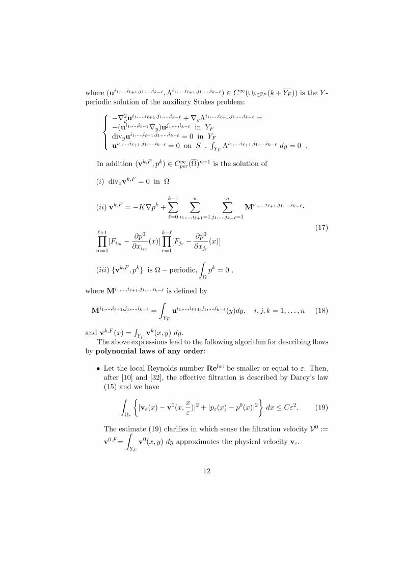
In addition (vk,F , pk) ∈ C∞per(Ω)n+1 is the solution of

(i) divxvk,F = 0 in Ω

(ii) vk,F = −K∇pk +k−1∑

`=0

n∑

i1,...,i`+1=1

n∑

j1,...,jk−`=1

Mi1,...,i`+1,j1,...,ik−` ·

`+1∏

m=1

[Fim −∂p0

∂xim

(x)]k−∏

r=1

[Fjr −∂p0

∂xjr

(x)]

(iii) vk,F , pk is Ω− periodic,∫

Ωpk = 0 ,

(17)

where Mi1,...,i`+1,j1,...,ik−` is defined by

Mi1,...,i`+1,j1,...,ik−` =∫

YF

ui1,...,i`+1,j1,...,ik−`(y)dy, i, j, k = 1, . . . , n (18)

and vk,F (x) =∫YF

vk(x, y) dy.The above expressions lead to the following algorithm for describing flows

by polynomial laws of any order:

• Let the local Reynolds number Reloc be smaller or equal to ε. Then,after [10] and [32], the effective filtration is described by Darcy’s law(15) and we have

∫

Ωε

|vε(x)− v0(x,

x

ε)|2 + |pε(x)− p0(x)|2

dx ≤ Cε2. (19)

The estimate (19) clarifies in which sense the filtration velocity V0 :=

v0,F =∫

YF

v0(x, y) dy approximates the physical velocity vε.

12

• Next let ε <Reloc ≤ √ε. Then we set k = 1 and use (17) to calculate

v1,F , p1. It gives us v1 and auxiliary Stokes problems give us ui,j .Note that for this, knowledge of the solutions to all auxiliary Stokesproblems from previous steps was necessary. Then, after [10] and [32],we have

∫

Ωε

|vε(x)− v0(x,

x

ε)−Relocv1(x,

x

ε))|2+

|pε(x)− p0(x)−Relocp1(x)|2

dx ≤ Cε2. (20)

From this estimate we will obtain in subsection 2.1 the quadratic fil-tration law.

• Next let√

ε <Reloc ≤ ε1/3. Then we set k = 2 and use (17) tocalculate v2,F , p2. It gives us v2 and auxiliary Stokes problemsgive us ui,j,k. Again, knowledge of the solutions to all auxiliary Stokesproblems from previous steps was necessary. Then, after [10] and [32],we have

∫

Ωε

|vε(x)− v0(x,

x

ε)−Relocv1(x,

x

ε))− (Reloc)2v2(x,

x

ε))|2+

|pε(x)− p0(x)−Relocp1(x)− (Reloc)2p2(x)|2

dx ≤ Cε2. (21)

From this estimate we will obtain in subsection 2.2 the cubic filtrationlaw.

• This way we arrive at the range ε1/(k−1) <Reloc ≤ ε1/k. For givenk we use (17) to calculate vk,F , pk. It gives us vk and auxiliaryStokes problems give us ui1,...,ik . Again, knowledge of the solutions toall auxiliary Stokes problems from previous steps was necessary. Then,after [10] and [32], we have

∫

Ωε

|vε(x)−

k−1∑

j=0

vj(x,x

ε)(Reloc)j |2+

|pε(x)−k−1∑

j=0

pj(x)(Reloc)j |2

dx ≤ Cε2. (22)

From this estimate we are able to obtain the kth order polynomialfiltration law, for any k.

13

We define the effective filtration velocity and for the effective pressure bythe following formula

Vk+1 :=k+1∑

`=0

(Reloc)`v`,F , Πk+1 :=k+1∑

`=0

(Reloc)`p` ,

where v`,F =∫

YF

v`(x, y) dy. The estimate (22) clarifies in which sense the

filtration velocity Vk approximates the physical velocity vε. Furthermore,using the two-scale filtration laws (17), we obtain that Vk+1 is a polynomialof order k + 1 in ∇Πk+1. The filtration law of order k + 1 is obtain fromthe law of order k by a recursive procedure. We can write the coefficients asfunctions of the vector M i1,...,il , but it leads to very cumbersome recursionrelations. We prefer to give expressions for several interesting cases.

2.1 The quadratic filtration law

Truncation of the infinite series polynomial to only two terms results in aquadratic correction to Darcy’s law. At first glance, the homogenization mayseem to be in agreement with Forchheimer’s empirically-observed quadraticequation. However, it has been shown (see [31], [45] and [20]) the quadraticterm vanishes for isotropic media and the first correction is cubic. This hasbeen verified both numerically and experimentally. The quadratic behaviorobserved by Forchheimer and others likely occurs at more moderate Re,outside the limits of this homogenization.

Similarly to the Darcy law, by separation of scales, we have v1 and p1,1

given by :

v1(x, y) =n∑

i,j=1

uij(y)[Fi − ∂p0

∂xi(x)] [Fj − ∂p0

∂xj(x)]−

n∑

i=1

wi(y)∂p1

∂xi(x)

p1,1(x, y) =n∑

i,j=1

Λij(y)[Fi − ∂p0

∂xi(x)] [Fj − ∂p0

∂xj(x)]−

n∑

i=1

πi(y)∂p1

∂xi(x),

where (uij ,Λij) ∈ C∞(∪k∈Zn(k + YF ))n+1 is the Y -periodic solution of theauxiliary Stokes problem:

−∇2yu

ij +∇yΛij = −(wi∇y)wj = − Divy (wi ⊗wj) in YF

divyuij = 0 in YF ; uij = 0 on S,∫YF

Λij dy = 0.(23)

14

In addition (v1,F , p1) ∈ C∞per(Ω)n+1 is the solution of

(i) divxv1,F = 0 in Ω; v1,F , p1 is Ω− periodic ,

∫

Ωp1 = 0,

(ii) v1,Fk =

n∑

i,j=1

M ijk Fi − ∂p0

∂xi Fj − ∂p0

∂xj −

n∑

j=1

Kkj∂p1

∂xj

(24)

where Mij is defined by

Mij =∫

YF

uij(y)dy i, j = 1, . . . , n (25)

and v1,F (x) =∫YF

v1(x, y) dy.The above expansions allow us to write the quadratic filtration law.Now we introduce the averaged velocity V1 and the averaged pressure

Π1 byV1 = v0

F + Relocv1,F ; Π1 = p0 + Relocp1 (26)

and with these notations, (15) (ii) and (24) (ii) can be summarized in:

V1 = K(F−∇Π1) + Relocn∑

i,j=1

Mij(Fi − ∂Π1

∂xi)(Fj − ∂Π1

∂xj). (27)

or equivalently, with the error of order O((Reloc)2), as

F−∇Π1 = K−1V1 −RelocK−1n∑

i,j=1

Mij(K−1V1)i(K−1V1)j . (28)

The quadratic expression entering in equation (27) starts to be importantwhen Reloc is close to 1. The filtration law (28) corresponds to the classicalform of non-Darcian filtration law. Nevertheless, the quadratic term is notmonotone. For this reason, we believe that the form (27) is more usefulfor numerical calculations. Formal derivation of the law (27) using homoge-nization was undertaken in [45], [31] and [35]. For the rigorous justification,with correct choice of the pressure field, see the article [10].

2.2 The cubic filtration law

The cubic filtration law is obtained if we calculate the corresponding termsfor k = 2. We note that in all one dimensional cases and in cases when the

15

porous media satisfies some isotropy conditions, the quadratic term van-ishes. For detailed discussion we refer to [20], were this important propertyis established under fairly realistic ”reversibility” condition. This gives im-portance to the cubic filtration law.

Next, let us write explicitly the corresponding terms:

v2(x, y) =n∑

i1=1

n∑

j1,j2=1

[Fi1 −∂p0

∂xi1

(x)][Fj1 −∂p0

∂xj1

(x)][Fj2 −∂p0

∂xj2

(x)]ui1,j1,j2(y)

−n∑

i=1

wi(y)∂p2

∂xi(x)(y)

p2,1(x, y) =n∑

i1=1

n∑

j1,j2=1

[Fi1 −∂p0

∂xi1

(x)][Fj1 −∂p0

∂xj1

(x)][Fj2 −∂p0

∂xj2

(x)]Λi1,j1,j2(y)

−n∑

i=1

πi(y)∂p2

∂xi(x)

where (ui1,j1,j2 , Λi1,j1,j2) ∈ C∞(∪k∈Zn(k + YF )) is the Y -periodic solution ofthe auxiliary Stokes problem:

−∇2

yui1,j1,j2 +∇yΛi1,j1,j2 = −(wi1∇y)uj1,j2 − (uj1,j2∇y)wi1 in YF

divyui1,j1,j2 = 0 in YF

ui1,j1,j2 = 0 on S ,∫YF

Λi1,j1,j2 dy = 0 .

(29)In addition (v2,F , p2) ∈ C∞

per(Ω)n+1 is the solution of

(i) divx v2,F = 0 in Ω; v2,F , p2 is Ω− periodic ,

∫

Ωp2 = 0,

(ii)v2,F =n∑

i1,i2,i3=1

[Fi1 −∂p0

∂xi1

(x)][Fi2 −∂p0

∂xi2

(x)][Fi3

− ∂p0

∂xi3

(x)]Mi1,i2,i3 −K∇p2,

(30)

where Mi1,i2,i3 is defined by

Mi1,i2,i3 =∫

YF

ui1,i2,i3(y)dy i1, i2, i3 = 1, . . . , n (31)

and v2,F (x) =∫YF

v2(x, y) dy.The above expansions allow us to write the cubic filtration law.

16

Now we introduce the averaged velocity V2 and the averaged pressureΠ2 by

V2 = v0F + Relocv1,F + (Reloc)2v2,F ; Π2 = p0 + Relocp1 + (Reloc)2p2

and with these notations, (15) (ii), (24) (ii) and (30) (ii) can be summarized,with the error of order O((Reloc)3), in:

V2 = K(F−∇Π2) + Relocn∑

i,j=1

Mij(Fi − ∂p0

∂xi)(Fj − ∂p0

∂xj)+

(Reloc)2n∑

i1,i2,i3=1

[Fi1 −∂p0

∂xi1

(x)][Fi2 −∂p0

∂xi2

(x)][Fi3 −∂p0

∂xi3

(x)]Mi1,i2,i3 . (32)

This in not yet a filtration law, since it should be expressed in terms ofthe effective pressure Π2. In the case of the quadratic filtration law it wasenough to replace p0 by the effective pressure Π1, but it is not the case anymore. Rewriting (32) in terms of the effective pressure Π2 gives

V2 = K(F−∇Π2) + Relocn∑

i,j=1

Mij(Fi − ∂Π2)∂xi

)(Fj − ∂Π2)∂xj

)+

(Reloc)2 n∑

i1,i2,i3=1

[Fi1 −∂Π2)∂xi1

(x)][Fi2 −∂Π2)∂xi2

(x)][Fi3 −∂Π2)∂xi3

(x)]Mi1,i2,i3+

n∑

i,j=1

(Mij + Mji)∂p1

∂xi(Fj − ∂Π2)

∂xj)

+O((Reloc)3) = (K + (Reloc)2C)(F

−∇Π2) + Relocn∑

i,j=1

Mij(Fi − ∂Π2)∂xi

)(Fj − ∂Π2)∂xj

) + (Reloc)2n∑

i1,i2,i3=1

[Fi1−

∂Π2)∂xi1

(x)][Fi2 −∂Π2)∂xi2

(x)][Fi3 −∂Π2)∂xi3

(x)]Mi1,i2,i3 , (33)

where

Ckj =n∑

i=1

(M ijk + M ji

k )∂p1

∂xi, k, j = 1, . . . n. (34)

We note that the pressure p1, from the quadratic perturbation, is givenby (24) and depends non-locally on the permeability K and the geometry,linearly on Mij and quadratically on ∇p0.

17

Finally, we write the filtration law in the form which generalizes cubicexpressions for Fochheimer’s law:

F−∇Π2 = (K + (Reloc)2C)−1V2 −RelocK−1n∑

i,j=1

Mij(K−1V2)i(K−1V2)j

−(Reloc)2n∑

i1,i2,i3=1

Bi1,i2,i3(K−1V2)i1(K−1V2)i2(K

−1V2)i3 +O((Reloc)3),

(35)

where the vectors Bi1,i2,i3 are given by

Bi1,i2,i3 = K−1Mi1,i2,i3 −n∑

j=1

K−1(Mi1j + Mji1)(K−1Mi2i3

)i1

. (36)

Therefore we arrived at the following conclusions:

• The cubic filtration law (35) describes the effective filtration throughporous media with the precision of order O((Reloc)3). It is differentfrom the effective law obtained by Rasoloarijaona and Auriault in [35],which contains higher order derivatives of the pressure.

• The obtained law (35) is close to the result of Wodie and Levy in [45].Nevertheless, there is a difference in the expansion for the pressure.

• It is interesting to note the change in the permeability due to the highlocal Reynolds number. It was observed before in [41].

• In [10] it is proved that the difference between the physical dimension-less velocity vε and the upscaled velocity, satisfying the cubic filtrationlaw (35), is of order O((Reloc)3) in the energy (L2) norm. This rigor-ously establishes (35) as the correct filtration law.

We conclude section §2 by writing the cubic filtration law (35) in the dimen-sional form. We note that our procedure could be continued to any order ofprecision. But for general media higher order expansions start to be cum-bersome and we prefer giving them for the particular case of the constrictedtubes in section §3.

2.3 Dimensional form of the cubic filtration law for constantpressure drop

Now se consider again the case F = sign (−∆P )2√ϕe1.

18

Then we see immediately that

pk = 0, for every k; v0F = K sign (−∆P )

2√ϕe1; v1,F =

4ϕM11;

v2,F =8

ϕ√

ϕsign (−∆P )M1,1,1.

Now, using that vphys,0 = v0F

√ϕ

2ε2 L|∆P |

µand that physical permeability

Kphys is equal to ε2L2K, we obtain in the zero order Darcy’s law in itsdimensional form:

vphys,0 = −Kphys

µ

∆P

Le1.

Next for V1 = v0F + Relocv1,F = K sign (−∆P )

2√ϕe1 + Reloc 4

ϕM11 we

use the equation (28) and obtain

∆P

Le1 = −µ(Kphys)−1Vphys,1 + ρ(εL)5((Kphys)−1Vphys,1)21(K

phys)−1M11.

We note that

M111 =

∫

YF

u111 dy =

∫

YF

∇yw1∇yu11 dy = −∫

YF

(w1∇y)w1w1 dy = 0.

Hence for scalar permeability there is no quadratic contribution in the di-rection of the flow. In general (Kphys)−1Vphys,1)1 satisfies classical Darcy’slaw. We will see in next section that for constricted tubes the quadraticterms vanishes completely.

Finally, we switch to the cubic filtration law. Now the non-dimensional

velocity is V2 = v0F + Relocv1,F + (Reloc)2v2,F = K sign (−∆P )

2√ϕe1 +

Reloc 4ϕM11 + (Reloc)2

8ϕ√

ϕsign (−∆P )M1,1,1 and using (35) we get

∆P

L= − µ

ε2L2(K−1Vphys,2)1 +

ρ

εL(K−1Vphys,2)21(K

−1M11)1+

ρ2

µ(K−1Vphys,2)31((K

−1M1,1,1)1 − 2(K−1M11)21). (37)

We note that

M1,1,11 =

∫

YF

u1,1,11 (y) dy =

∫

YF

∇yw1∇yu1,1,1 dy = −∫

YF

(w1∇y)u1,1w1 dy

=∫

YF

(w1∇y)w1u1,1 dy = −∫

YF

|∇yu11|2 dy < 0. (38)

19

3 Non-linear filtration laws for flows through con-stricted tubes with axial variations in diameter

In this section we study inertia effects for viscous incompressible flows througha porous medium being a bundle of parallel axially symmetric constrictedtubes. We suppose that the porous medium is periodic, obtained by periodicrepetition of the tubes Ωδ = x1 ∈ (0, L1); 0 < r < δR(x1/δ), where δ > 0is a small parameter, representing the ratio between the pore size and thesize of the domain. The porous medium contains a large number of tubes,proportional to C/δ2. Function R is periodic with the period L. This meansthat the constriction repeats periodically a number of times proportional to1/δ. In order to avoid boundary layer effects, we suppose that number aninteger.

Flow is governed by a given pressure drop ∆P in the direction x1. This

pressure drop determines the characteristic volume force∆P

L1e1 and we sup-

pose the flow periodic in x1 direction, with the period L1.Since we consider the stationary incompressible viscous flow through a

porous medium, it is described by the incompressible Navier-Stokes system

−µ∇2v + ρ(v∇)v +∇p =−∆P

L1e1 in ΩF , (39)

divv = 0 in ΩF , v = 0 on (∂ΩF ) \ (x1 = 0 ∪ x1 = L1) , (40)

where ΩF is the fluid part of the porous medium, i.e. union of the constrictedseparated tubes Ωδ.

Due to the particular periodic geometry and to the constant forcing term,it is obvious that it is sufficient to solve the problem in just one tube. Wechoose the tube with the axis r = 0. Furthermore, the Navier-Stokes system(39)-(40) is invariant to the following change of variables and unknowns:

x = δx; v =vδ; p =

p

δ2, (41)

and it is sufficient to consider the problem

−µ∇2v + ρ(v∇)v +∇p =−∆P

L1δ3 e1 in Ω , (42)

divv = 0 in Ω, v and p are L− periodic in x1, (43)v = 0 on ∂Ω \ (x1 = 0 ∪ x1 = L), (44)

where Ω is the canonic axially symmetric constricted tube Ω = x1 ∈(0, L); 0 < r < R(x1). Without loosing generality we can suppose L = L1.

20

Due to the above proved equivalence the direct numerical simulations in§4 will be performed for a single tube with the pressure drop modified onthe way we saw above.

As we deal with a porous medium, we will apply the results from §2.We note that the fluid part of the porous medium now is not connected.As we will see this leads to many simplifications. Mathematical theory ofthe homogenization process could be generalized to such situation (see [33]).Also pipes could be considered as thin domains and then there is a directanalysis by Bourgeat and Marusic-Paloka in [11].

Our goal is to find an expansion of the velocity and pressure fields interms of the local Reynolds number and to obtain from it polynomial non-Darcian filtration laws, giving a relationship between the pressure drop andthe effective volumetric flow for this simple geometry.

3.1 Darcy permeability and the quadratic correction

Hence we consider a porous medium which is a bundle of capillary tubes.Each tube is obtained by a periodic repetition of the dilated unit tube YF ==y1 ∈ (0, 1) : 0 < r < R(y1) = R(y1)/L, contained in a cell Y = (0, 1)3.YF has as a boundary an axially symmetrical surface of revolution S, givenby

r = R(y1), r2 = y22 + y2

3. (45)

The internal boundary does not intersect the boundary of Y , except aty1 = 0, 1, where we have the inlet and outlet boundaries. In such geometry,our expressions simplify considerably.

First, it is easy to study the problem (14) and get

wi = 0, πi = yi − 1|YF |

∫

YF

yi dy, i = 2, 3; Kij = δ1jδi1K11 > 0, (46)

ϕ =∫ 1

0πR2(y1) dy1 K11 = 2π

∫ R(0)

0w1

1(0, r) rdr, (47)

v0F = K11 sign (−∆P )

2√ϕe1, p0(x) = 0 (48)

We recall that w1 is the 1-periodic in y1 solution for the problem (14) withi = 1

−∇2

yw1 +∇yπ

1 = e1 , divyw1 = 0 in YF

w1 = 0 on S,∫YF

π1 = 0w1, π1 are 1− periodic with respect to y1.

(49)

21

Now, using that vphys,0tube = v0

F

√ϕ

2ε2 L|∆P |

µand that physical permeabil-

ity Kphystube is equal to ε2L2K11, we obtain in the zero order Darcy’s law in

its dimensional form:

vphys,0tube = −Kphys

tube

µ

∆P

Le1.

Next step is to study the problem (23). Clearly, the solution is not zeroonly if i = j = 1. Hence only cell problem to be solved is

−∇2yu

11 +∇yΛ11 = −(w1∇y)w1 in YF

divyu11 = 0 in YF

u11 = 0 on S ,∫YF

Λ11 dy = 0u11,Λ11 are 1− periodic with respect to y1.

(50)

Consequently, only M11 is potentially a non zero vector. Let us calculateits components:

M111 =

∫

YF

u111 (y) dy =

∫

YF

∇yw1∇yu11 dy = −∫

YF

(w1∇y)w1w1 dy = 0.

M11j =

∫

YF

u11j (y) dy = by (14) = 0, j = 2, 3.

Hence there is no quadratic correction in this particular geom-etry. Hence v1,F = 0 and p1 = 0.

For a geometry having the symmetry of mirror with respect to y1 aroundy1 = 1/2, it is easy to see that −(

(w1∇y)w1)1

is uneven with respect tothe plane of symmetry y1 = 1/2. The components −(

(w1∇y)w1)j, j = 2, 3

are even. Consequently, u111 is an uneven function and Λ11, u11

2 and u113 are

even.

3.2 Cubic filtration law

Now we study the problem (29). Clearly, the solution is not zero only ifi1 = j1 = j2 = 1. Hence only cell problem to be solved is

−∇2yu

1,1,1 +∇yΛ1,1,1 = −(w1∇y)u1,1 − (u1,1∇y)w1 in YF

divyu1,1,1 = 0 in YF

u1,1,1 = 0 on S ,∫YF

Λ1,1,1 dy = 0u1,1,1,Λ1,1,1 are 1− periodic with respect to y1.

(51)

22

Consequently, only M1,1,1 is potentially a non zero vector. Let us calcu-late its components:

As before, M1,1,1j = 0, j = 2, 3 and by using (38), we have M1,1,1

1 < 0.For a geometry having the symmetry of mirror with respect to y1 around

y1 = 1/2, it is easy to see that −((w1∇y)u1,1+(u1,1∇y)w1

)1

is even with re-spect to the plane of symmetry y1 = 1/2. The components −(

(w1∇y)u1,1 +(u1,1∇y)w1

)j, j = 2, 3 are uneven. Consequently, u1,1,1

1 is an even function

and Λ1,1,1, u1,1,12 and u1,1,1

3 are uneven.Now v2,F = 2M1,1,1

18

ϕ√

ϕ sign (−∆P )e1, p2 = 0 and the dimensionalfiltration law (37) reads

∆P

L= − µ

ε2L2K11V Cubic +

ρ2

µ

M1111

(K11)4(V Cubic)3. (52)

The law (52) is the cubic non-Darcian law.

3.3 The 5th order filtration law

In order to get higher order filtration laws, we continue with the expansionand take k = 3. Then we have:

−∇2yu

iv +∇yΛiv = −(

(w1∇y)u1,1,1 + (u1,1,1∇y)w1 + (u1,1∇y)u1,1

)in YF

divyuiv = 0 in YF

uiv = 0 on S ,∫YF

Λiv dy = 0uiv,Λiv are 1− periodic with respect to y1.

(53)Concerning the permeability, we have as before M iv

j = 0, j = 2, 3. Ingeneral geometry M iv

1 does not seem to be zero.

Now v3,F = Miv1

16ϕ2 e1 and p3 = 0, where M iv =

∫

YF

uiv(y) dy.

For a geometry having the symmetry of mirror with respect to y1 aroundy1 = 1/2, it is easy to see that−(

(w1∇y)u1,1,1+(u1,1,1∇y)w1+(u1,1∇y)u1,1)1

is uneven with respect to the plane of symmetry y1 = 1/2. The components−(

(w1∇y)u1,1,1 + (u1,1,1∇y)w1 + (u1,1∇y)u1,1)j, j = 2, 3 are even. Conse-

quently, uiv1 is an uneven function and Λiv, uiv

2 and uiv3 are even. For such

geometries M iv1 = 0.

In our numerical exemples we will only consider the constricted tubeshaving the symmetry of mirror with respect to y1 around y1 = 1/2. HenceM iv

1 = 0 and there is no 4th order term in the non-Darcy law.

23

We can switch now to the 5th order contribution.Only auxiliary problem with solution which is not identically zero is the

following:

−∇2yu

v +∇yΛv = −(

(w1∇y)uiv + (u1,1,1∇y)u1,1+

(u1,1∇y)u1,1,1 + (uiv∇y)w1

)in YF

divyuv = 0 in YF

uv = 0 on S ,∫YF

Λv dy = 0uv, Λv are 1− periodic with respect to y1.

(54)

Now v4,F = Mv1 sign (−∆P ) 32

ϕ2√ϕe1 and p4 = 0, where Mv =

∫

YF

uv(y) dy.

As before, Mvj = 0, j = 2, 3.

For a geometry having the symmetry of mirror with respect to y1 aroundy1 = 1/2, it is easy to see that−(

(w1∇y)uiv+(u1,1,1∇y)u1,1+(u1,1∇y)u1,1,1+(uiv∇y)w1

)1

is even with respect to the plane of symmetry y1 = 1/2. Thecomponents−(

(w1∇y)uiv+(u1,1,1∇y)u1,1+(u1,1∇y)u1,1,1+(uiv∇y)w1)j, j =

2, 3 are uneven. Consequently, uv1 is an even function and Λv, uv

2 and uv3 are

uneven.Dimensional velocity is now given by

εV Fifth = −L2K11

µ

∆Pε3

L−L8ρ2M111

1

µ5

(∆Pε3

L

)3−R140 ρ4Mv

1

µ9

(∆Pε3

L

)5 (55)

and we get the following fifth order non-Darcian law:

∆P

L= − µ

ε2L2K11V Fifth +

ρ2

µ

M1111

(K11)4(V Fifth)3−

ρ4ε2L2

µ3

3(M1111 )2 −K11Mv

1

(K11)7(V Fifth)5. (56)

The law (56) is the 5th order non-Darcian law.

4 Numerical simulations

Numerical simulations are performed here in simple porous medium to deter-mine the coefficients of the polynomial; the resulting model is then comparedto the numerical solution of the full Navier-Stokes equations. The sinusoidalgeometry depicted in Figure 1 is periodic, isotropic and symmetric so the ex-pansion solution derived in section §3 is applicable. One advantage of using

24

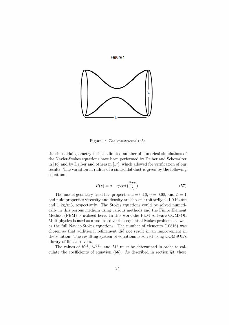
Figure 1: The constricted tube

the sinusoidal geometry is that a limited number of numerical simulations ofthe Navier-Stokes equations have been performed by Deiber and Schowalterin [16] and by Deiber and others in [17], which allowed for verification of ourresults. The variation in radius of a sinusoidal duct is given by the followingequation:

R(z) = a− γ cos(2πz

L

). (57)

The model geometry used has properties a = 0.16, γ = 0.08, and L = 1and fluid properties viscosity and density are chosen arbitrarily as 1.0 Pa-secand 1 kg/m3, respectively. The Stokes equations could be solved numeri-cally in this porous medium using various methods and the Finite ElementMethod (FEM) is utilized here. In this work the FEM software COMSOLMultiphysics is used as a tool to solve the sequential Stokes problems as wellas the full Navier-Stokes equations. The number of elements (10816) waschosen so that additional refinement did not result in an improvement inthe solution. The resulting system of equations is solved using COMSOL’slibrary of linear solvers.

The values of K11, M111, and Mv must be determined in order to cal-culate the coefficients of equation (56). As described in section §3, these

25

parameters may be found from solving Stokes problems of the form:

−∇P + µ∇2v = F; ∇ · v = 0, (58)

with velocity field v = 0 on the lateral boundary S and with v, P beingL−periodic in the axial variable. The forcing function, F, is summarized inTable 1 and each subsequent function is dependent on the previous velocityfields.

Forcing Function, F Output velocity Calculated value of theaveraged quantity

e1 w1 K11 = 3.411E − 4

(w1 · ∇)w1 u11 M111 = 0

(w1 · ∇)u11 + (u11 · ∇)w1 u1,1,1 M1111 = −1.255E − 14

(w1 · ∇)u1,1,1 + (u1,1,1 · ∇)w1

+(u11 · ∇)u11 uiv M iv1 = 0

(w1 · ∇)uiv + (u1,1,1 · ∇)u11

+(u11 · ∇)u1,1,1 + (uiv · ∇)w1 uv Mv1 = 1.314E − 24

Table 1: Forcing functions for Stokes problems and resulting coefficientsobtained numerically

Streamline plots of the velocity field are shown in Figure 2 for the firstfive problems and a few observations can be made from the qualitative flowpatterns.

The velocity field is symmetric for the first, third, and fifth terms andflow is normal at the boundaries. This is consistent with the model de-veloped in section §3, which leads to finite values of K11, M111

1 , and Mv1 .

These values are calculated using equations (49), (50), (51), (53) and (54)respectively. The 2nd order and 4th order terms are antisymmetric and flowdoes not enter or exit the periodic boundaries, resulting in the expectedzero values of M11 (isotropic medium) and Miv (symmetric and isotropicmedium). Plugging in the values from Table 1 into equation (56), gives thefollowing filtration law for this porous medium:

∆P

L= −2931.47V − 0.92705V 3 + 4.57415 · 10−5 · V 5 = PF5(V ). (59)

The model predicts the first correction to Darcy’s law is cubic. Themagnitude of the coefficients diminishes greatly with order and the cubic

26

term (and certainly higher order terms) may be negligible in practice, whichexplains Darcy’s law often being an acceptable approximation at low Re.

Hence the momentum equation is replaced by the polynomial filtrationlaw. Its coefficients are calculated using the auxiliary Stokes’ problems (49),(50), (51), (53) and (54) and then we have a nonlinear scalar PDE forthe pressure, valid in the whole reservoir. Its numerical solution is muchcheaper than solving the full Navier-Stokes system in the complicated poregeometry. The approximation was validated theoretically by estimates (19)-(22), proved in [30]. Here we validate its accuracy by comparison to a directnumerical solution of the Navier-Stokes equations.

We will solve problem (42)-(44), with δ = 1, for different pressure drops∆P . Then we will compute the average of the velocity over the constrictedtube and check whether it satisfies the nonlinear filtration law obtained byhomogenization.

The full Navier-Stokes equations (42)-(44) are solved using the FEM inCOMSOL as was done for the Stokes problems. The equations are solved atvarious applied pressure gradients to compute velocity fields and a macro-scopic average velocity, V. Figure 3 shows streamlines of the velocity field atvarious pressure drops; slight changes can be observed as the Re increaseswhich accounts for corrections to Darcy’s law.

At the Table 2 we give the comparaison between pressure drops ∆P calc =fF5(V ), evaluated using (59), and the given pressure drops:

Figures 4a and 4b compare the analytical model (Equation (59)) to thenumerical results and show excellent agreement.

In Figure 4a a plot of pressure gradient versus velocity appears linearand the cubic behavior is difficult to distinguish.

Figure 4b is similar to a Forchheimer plot (Equation (2)) and the cubiccorrection to Darcy’s law is more apparent. Moreover, the cubic coefficientis verified by the agreement. The fifth order contribution to pressure loss isnot significant, and roundoff error makes it nearly impossible to observe onany plot.

5 Conclusions

Darcy’s law states that velocity is proportional to pressure gradient in porousmedia; it is usually accepted for low velocities in the creeping flow regime(Reloc << 1). Darcy’s law can be found analytically or numerically bysolving the Stokes equations, but for finite Reloc the inertial terms willadd additional resistance in a porous medium and the relationship between

27

pressure gradient and velocity is nonlinear. Experimentally, a quadraticcorrection to Darcy’s law is often observed, but work by several authors ([31],[45], [14] , [36]) has suggested this functionality is not correct, particularlyfor Reloc < 1. In this work homogenization has been used to derive a generalfiltration law in porous media (for Reloc less than unity) and it verifies thatthe first correction to Darcy’s law is cubic for isotropic media. A novelfinding of the homogenization (as well as the expansion for axisymmetric,periodic media) is that the filtration law is an infinite series polynomialand that the coefficients can be determined a priori by solving a series ofsuccessive Stokes flow problems. We note that we establish simultaneouslythe filtration velocity as a polynomial in the pressure gradient (see e.g. (55)and the inverse relationship (see e.g. (56)) where the pressure gradient is apolynomial in the velocity.

The Stokes problems were solved here for a specific medium (an ax-isymmetric, periodic, sinusoidal duct) and the first five coefficients of theinfinite series polynomial were determined. As predicted by the model, thequadratic and 4th order terms are zero because of isotropy and symmetry,respectively. Excellent agreement between the analytical model and a nu-merical solution of the full Navier-Stokes equations is found, verifying thecubic functionality as well as the quantitative value of the cubic coefficient.Fifth (and higher) order terms are not significant and are not observablenumerically. In practice even the cubic term can often be neglected, whichverifies the use of Darcy’s law at low Re.

The infinite series filtration model is only valid for Reloc < 1 and, as pre-viously stated, corrections to Darcy’s law are probably negligible in practice.Additional pressure loss due to inertia is most significant and of most inter-est in subsurface applications at higher Reloc (but still in the laminar flowregime). Nonetheless, the results are important from several fundamentalperspectives. First of all, it further suggests that Forchheimer’s quadraticequation is only empirical and not a universal law valid within the entirelaminar flow regime. Since the quadratic model may not be fundamental,deviations from Forchheimer at high Reloc may also occur (and in fact areobserved). Second, as other authors have observed, even if the quadraticlaw were valid at higher Reloc , extrapolation to the intercept on a Forch-heimer plot (Equation 2) would not result in the intrinsic, Darcy permeabil-ity. Future work will focus on developing a more general model based onhomogenization and/or numerical simulation applicable for Reloc > 1.

Nomenclature

v Physical velocity [L/t]

28

p Pressure [F/L2]

V Characteristic velocity [L/t]

µ Viscosity [F/L2− t]

ρ Density [M/L3]

L Characteristic length M

P Characteristic pressure [F/L2]

∆P Pressure drop

Re Reynolds number

Fr Froude’s number

Ω Reservoir

Y Unit cell

Ys Solid part of the unit cell

YF Pore

Ωε Pore space (the fluid part of Ω)

ε Ratio between the pore size ` and the reservoir size L

ϕ Porosity

F Dimensionless forcing term

vε Dimensionless physical velocity

pε Dimensionless pressure

K Dimensionless permeability

29

References

[1] N. Ahmad: Physical Properties of Porous Medium Affecting Laminarand Turbulent Flow of Water, Ph. D. Thesis, Colorado State University,Fort Collins, Colo., 1967.

[2] Allaire G., Homogenization of the Stokes Flow in Connected PorousMedium, Asymptotic Anal., 3 (1989), 203-222.

[3] M. Balhoff, and M.F. Wheeler: A Predictive Pore-Scale Model for Non-Darcy Flow in Anisotropic Porous Media. SPE 110838, presented at theAnnual Technical Conference and Exhibition, Anaheim (November 11-14, 2007).

[4] R.D. Barree, M.W. Conway: Beyond Beta Factors: A Complete Modelfor Darcy, Forchheimer and Trans-Forccheimer Flow in Porous Media,paper SPE 89325, presented at the SPE Annual Technical Conferenceand Exhibition held in Houston, Texas, U.S.A., 26-29 September 2004.

[5] R.D. Barree, and M.W. Conway: Reply to Discussion of ’BeyondBeta factors: A complete model for Darcy, Forchheimer, and Trans-Forchheimer flow in porous media’. J. Pet. Tech. (2005), p. 73-74.

[6] G.I. Barenblatt, V.M. Entov, V.M. Ryzhik : Theory of Fluid FlowsThrough Natural Rocks, Kluwer, Dordrecht, 1990.

[7] van Batenburg, D. and D. Milton-Taylor: Discussion of SPE 89325,’Beyond Beta factors: A complete model for Darcy, Forchheimer, andTrans-Forchheimer flow in porous media. J. Pet. Tech. (2005), 72-73.

[8] J. Bear: Hydraulics of Groundwater, McGraw-Hill, Jerusalem, 1979.

[9] F.C. Blake: The Resistance of Packing to Fluid Flow, Trans. Am. Inst.Chem. Engrs. Vol. 14 (1922), p. 415-421.

[10] A.Bourgeat, E.Marusic- Paloka, A.Mikelic : Weak Non-Linear Correc-tions for Darcy’s Law, M3 AS : Math. Models Methods Appl. Sci., Vol.6 (no. 8)) (1996), p. 1143–1155.

[11] A. Bourgeat, E. Marusic-Paloka : Nonlinear effects for flow in period-ically constricted channel caused by high injection rate. Math. ModelsMethods Appl. Sci. 8 (1998), no. 3, 379–405.

30

[12] L.E. Brownell, H.S. Dombrowski, C.A. Dickey: Pressure Drop throughPorous Media, Chem. Eng. Prog. , Vol. 43 (1947), p. 537-548.

[13] Z. Chen, S.L. Lyons, and G. Qin: Derivation of the Forchheimer Lawvia Homogenization, Transport in Porous Media, Vol. 44 (2001), p.325-335.

[14] Couland, O., P. Morel, and J.P. Caltagirone: Numerical Modelling ofNonlinear Effects in Laminar Flow through a Porous Medium, J. FluidMech. Vol. 190(1988), p. 393-407.

[15] Cvetkovic, V.D: A continuum approach to high velocity flow in porousmedia, Transport in Porous Media Vol. 1 (1986), p. 63-97.

[16] J. A. Deiber, W. R. Schowalter: Flow through tubes with sinusoidalaxial variations in diameter. AICHE J, Vol 25 (1979), p. 638-645.

[17] J.A. Deiber, M. Peirotti, R. A. Bortolozzi, R.J. Durelli: Flow of New-tonian Fluids Through Sinusoidally Constricted Tubes; Numerical andExperimental Results. Chemical Engineering Communications, Vol. 117(1992), p. 241-262

[18] D.A. Edwards, M. Shapiro, P. Bar-Yoseph, and M. Shapira: The Influ-ence of Reynolds Number upon the Apparent Permeability of SpatiallyPeriodic Arrays of Cylinders, Phys. Fluids A. (1990), 2.

[19] G.H. Fancher, and J.A. Lewis: Flow of Simple Fluids through PorousMaterials, Ind. Eng. Chem. Vol. 25 (1933), 1139-1147.

[20] M. Firdaouss, J.L. Guermond, P. Le Quere : Nonlinear Corrections toDarcy’s Law at Low Reynolds Numbers, J.Fluid Mech., Vol. 343 (1997),331-350.

[21] P. Forchheimer: Wasserbewegung durch Boden, Zeits. V. Deutsch Ing.Vol. 45 (1901), p. 1782-1788.

[22] P. Forchheimer: Hydraulik, 3rd ed., Teubner, Leipzig.

[23] S.M. Hassanizadeh, W.G. Gray : High Velocity Flow in Porous Media,Transport in Porous Media, Vol. 2 (1987), 521-531.

[24] H. Huang, and J. Ayoub: Applicability of the Forchheimer Equationfor Non-Darcy Flow in Porous Media. SPE 102715, presented at the2006 SPE Annual Technical Conference and Exhibition, San Antonio(September 24-27, 2006).

31

[25] B.Y.K. Kim: The Resistance to Flow in Simple and Complex PorousMedia Whose Matrices are Composed of Spheres. M.Sc. Thesis, Uni-versity of Hawaii at Manoa (1985).

[26] D.L. Koch, and A.J.C. Ladd: The First Effects on Fluid Inertia onFlows in Ordered and Random Arrays of Spheres, J. Fluid Mech. Vol.448 (2001), p. 213-241.

[27] E. Lindquist: On the flow of water through porous soils. PremierCongres des Grands Barrages, Stockholm (1933) 5, 81-101.

[28] J.L Lions, Some Methods in the Mathematical Analysis of Systems andTheir Control, Gordon and Breach, New York, 1981.

[29] J.L. Lions: Some problems connected with Navier-Stokes equations,Lectures at the IVth Latin-American School of Mathematics, Lima,1978, in Lions, Jacques-Louis Œuvres choisies de Jacques-Louis Li-ons. Vol. II. (French) [Selected works of Jacques-Louis Lions. Vol. II]Controle. Homogeneisation [Control. Homogenization]. Edited by AlainBensoussan, Philippe G. Ciarlet, Roland Glowinski, Roger Temam,Francois Murat and Jean-Pierre Puel, and with a preface by Bensous-san. EDP Sciences, Les Ulis; Societe de Mathematiques Appliquees etIndustrielles, Paris, 2003. xvi+864 pp.

[30] E.Marusic–Paloka, A.Mikelic : The Derivation of a Non-Linear Filtra-tion Law Including the Inertia Effects Via Homogenization, NonlinearAnalysis, Theory, Methods and Applications, 42 (2000), pp. 97 - 137.

[31] C.C. Mei, J.-L. Auriault : The Effect of Weak Inertia on Flow Througha Porous Medium, J.Fluid Mech., Vol. 222 (1991), 647-663.

[32] A.Mikelic : Homogenization theory and applications to filtrationthrough porous media, chapter in ”Filtration in Porous Media and In-dustrial Applications ” , Lecture Notes Centro Internazionale Matem-atico Estivo (C.I.M.E.) Series, Lecture Notes in Mathematics Vol. 1734,Springer, 2000, p. 127-214.

[33] A. Mikelic: On the justification of the Reynolds equation, describingisentropic compressible flows through a tiny pore, Ann Univ Ferrara,Vol. 53 (2007), p. 95-106.

[34] F. Mobasheri, and D.K. Todd: Investigation of the hydraulics of flownear recharge wells. Water Resources Center Contribution No. 72, Uni-versity of California Berkeley (1963).

32

[35] M. Rasoloarijaona, J.-L. Auriault : Non-linear Seepage Flow Througha Rigid Porous Medium, Eur.J.Mech., B/Fluids , 13, No 2, (1994),177-195.

[36] S. Rojas, J. Koplik: Nonlinear Flow in Porous Media, Physical ReviewE. Vol. 58 (1988), no. 4, p. 4776-4782.

[37] D.W. Ruth, H. Ma, On the Derivation of the Forchheimer Equationby Means of the Averaging Theorem, Transport in Porous Media, Vol.7(1992), p. 255-264.

[38] D.W. Ruth, H. Ma: The Microscopic Analysis of High ForchheimerNumber Flow in Porous Media, Transport in Porous Media Vol.13(1993), p. 139-160.

[39] Sanchez-Palencia E., Non-Homogeneous Media and Vibration Theory,Springer Lecture Notes in Physics 127, Springer-Verlag, Berlin, 1980.

[40] A.E. Scheidegger : Hydrodynamics in Porous Media, in Encyclopediaof Physics, Vol. VIII/2 (Fluid Dynamics II), ed. S. Flugge, Springer-Verlag, Berlin, 1963, 625-663.

[41] E. Skjetne, J.L. Auriault: New insights on steady, non-linear flow inporous media. Eur. J. Mech. B Fluids 18 (1999), no. 1, p. 131–145.

[42] H.E. Stanley, and J.S. Andrade: Physics of the Cigarette Filter: FluidFlow through Structures of Randomly-Packed Obstacles. Physica A,Vol. 295 (2001), p. 17-30.

[43] D.K. Sunada: Laminar and Turbulent Flow of Water through Homo-geneous Porous Media, PhD dissertation, University of California atBerkeley (1965).

[44] S. Whitaker: The Forchheimer Equation: A Theoretical Development,Transport in Porous Media, Vol. 25 (1996), p. 27-61.

[45] Wodie J.-C., Levy T., Correction non lineaire de la loi de Darcy, C.R.Acad. Sci. Paris, t.312, Serie II (1991), p.157-161.

33

34

Figure 2: The streamlines for the Stokes auxiliary problem. Fig. a displaysstreamlines corresponding to the forcing function e1 and so on.

35

Figure 3: The streamlines for the Navier-Stokes equations

36

V = ∆PL ∆P calc |∆P calc−∆P |

|∆P | ∆PD,calc |∆P D,calc−∆P ||∆P |∫

YFv1dx = fF5(V ) = fF5(V )

3,41E-04 1 1,00 6,39E-07 1,00 6,39E-073,41E-01 1000 1000,00 6,88E-07 999,96 3,75E-054,29E-01 1258,925412 1258,92 7,17E-07 1258,85 5,90E-055,41E-01 1584,893192 1584,89 7,63E-07 1584,75 9,32E-056,81E-01 1995,262315 1995,26 8,35E-07 1994,97 1,47E-048,57E-01 2511,886432 2511,88 9,49E-07 2511,30 2,33E-041,08E+00 3162,27766 3162,27 1,13E-06 3161,11 3,69E-041,36E+00 3981,071706 3981,07 1,41E-06 3978,75 5,84E-041,71E+00 5011,872336 5011,86 1,83E-06 5007,24 9,24E-042,15E+00 6309,573445 6309,56 2,48E-06 6300,35 1,46E-032,70E+00 7943,282347 7943,26 3,40E-06 7924,93 2,31E-033,40E+00 10000 9999,95 4,58E-06 9963,53 3,65E-034,27E+00 12589,2541 12589,19 5,4501E-06 12517,0 0,005743085,36E+00 15848,932 15848,87 3,9787E-06 15706,1 0,009012746,71E+00 19952,623 19952,79 8,2538E-06 19672,0 0,014063788,38E+00 25118,864 25120,39 6,086E-05 24572,5 0,021751231,04E+01 31622,777 31630,78 0,00025309 30573,5 0,033182181,16E+01 35481,339 35498,46 0,00048243 34037,6 0,040689671,29E+01 39810,717 39846,28 0,00089323 37836,6 0,049588741,35E+01 41686,938 41734,23 0,0011345 39454,0 0,053564961,43E+01 44668,359 44740,35 0,00161169 41988,6 0,0599931,52E+01 47863,009 47971,60 0,00226881 44656,8 0,0669867

Table 2: Comparison between the starting pressure drops and the pressuredrops recalculated from the 5th order nonlinear filtration law, for velocityobtained by direct solving the stationary Navier-Stokes system

37

Figure 4: Fig. a: Darcy’s filtration law as the fifth order filtration law inthe range of small Reynolds’ numbers 0 ≤ Re ≤ 4; Fig. b: The cubicfiltration law as the fifth order filtration law in the range of more importantReynolds’ numbers

38