Polymer Analysis and Characterization

23 rd International Symposium on Polymer Analysis and Characterization

Short course: Techniques for Polymer

Analysis & Characterization

30 May 2010

Pohang University of Science and Technology Pohang, Republic of Korea

Locations

Pohang Accelerator Laboratory (PAL)

Bus stop

Log Cabin Pub 18:00~02:00

Student Union

Jigok Community Center

POSCO International Center

Main Gate

Dining Facilities on Campus

D’medley (Buffet), 2F POSCO International Center Phoenix (Chinese), 5F POSCO International Center Wisdom (Cafeteria), 2F Jigok Community Center Breakfast 08:30~10:30 / Lunch 11:50~13:20 / Dinner 18:00~19:00 Yeon-Ji (Korean), 1F Jigok Community Center Lunch 13:00~15:00 / Dinner 16:00~20:00 Burger King, 1F Jigok Community Center 10:00~22:00 Oasis (Snack), 1F Student Union Breakfast 08:00~10:00 / Lunch 11:30~ 15:00 / Dinner 16:00~19:30

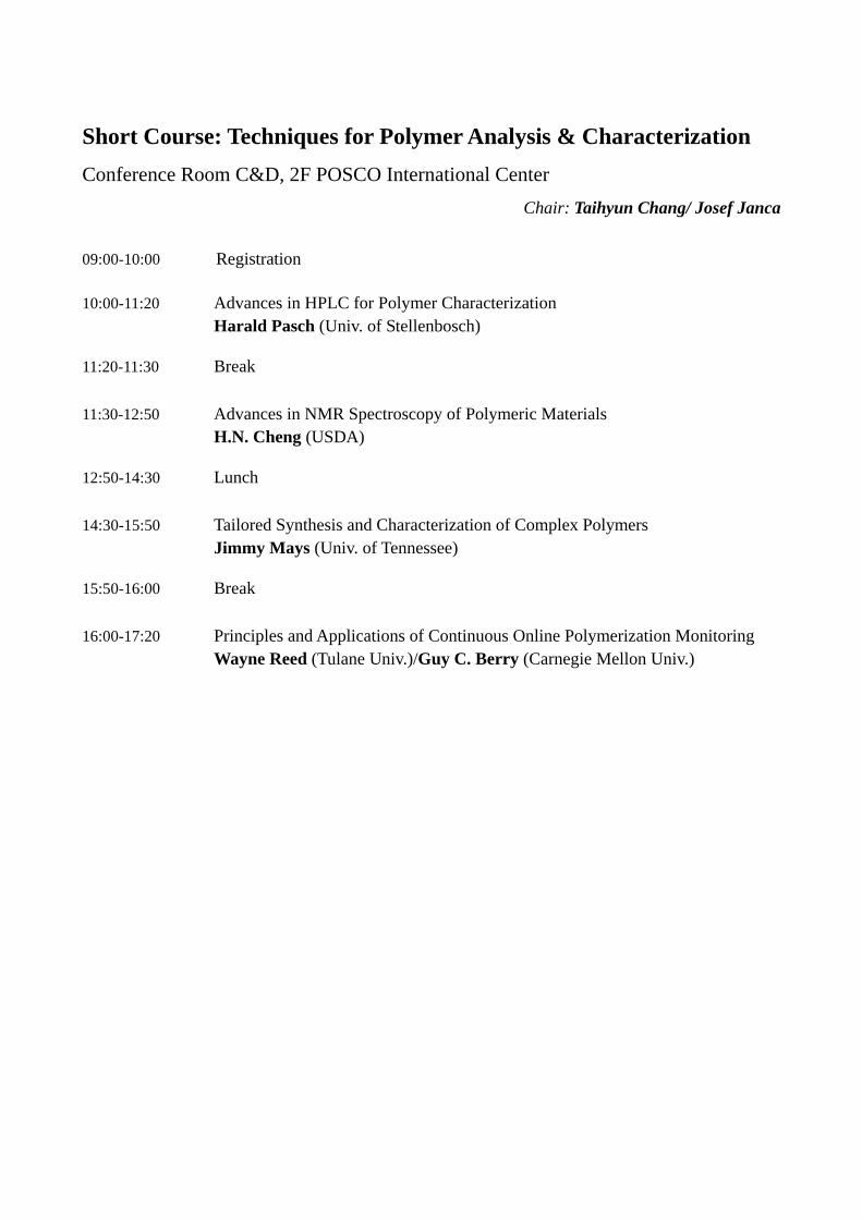
Short Course: Techniques for Polymer Analysis & Characterization Conference Room C&D, 2F POSCO International Center

Chair: Taihyun Chang/ Josef Janca 09:00-10:00 Registration 10:00-11:20 Advances in HPLC for Polymer Characterization

Harald Pasch (Univ. of Stellenbosch)

11:20-11:30 Break

11:30-12:50 Advances in NMR Spectroscopy of Polymeric Materials H.N. Cheng (USDA)

12:50-14:30 Lunch

14:30-15:50 Tailored Synthesis and Characterization of Complex Polymers Jimmy Mays (Univ. of Tennessee)

15:50-16:00 Break

16:00-17:20 Principles and Applications of Continuous Online Polymerization Monitoring Wayne Reed (Tulane Univ.)/Guy C. Berry (Carnegie Mellon Univ.)

ADVANCES IN HPLC FOR

POLYMER CHARACTERIZATION

Harald Pasch

Univ. of Stellenbosch

1

1

Advances in HPLC Advances in HPLC for Polymer Characterizationfor Polymer Characterization

Harald Pasch

SASOL Chair of Analytical Polymer Science

Department of Chemistry and Polymer Science, University of Stellenbosch, South Africa

2

MolecularMolecular HeterogeneityHeterogeneity ofof ComplexComplex PolymersPolymers

Chain Length End Group

Block Length Architecture

Molar Mass

Häu

figke

it Chain Length

Chemical Composition

Functional Groups

Topology

SECbut

direct correlation between Vh and

chain length (molar mass) only for linear

homopolymers

LACbut

effects of molar mass, branching,

functional groups ?

LC-CCbut

only for linear homopolymers with

0,1,2 endgroups

Effects of chemical composition and

branching ?

Topology Type Fractionation ?

size and chemical composition will

contribute !

2

3

Molecular Heterogeneity of a Random Copolymer� distributions in composition and molar mass

3D diagram Contour plot

Molecular Heterogeneity of Complex PolymersMolecular Heterogeneity of Complex Polymers

4

Advantanges of LC techniques

�� simple, reproducible, precise�� adaptable to specific analysis problems�� high flexibility of technical setup

quantitative analysis of distributions

�� molar mass�� chemical heterogeneity�� functionality�� architecture

Analysis of Analysis of DistributionsDistributions byby Liquid ChromatographyLiquid Chromatography

3

5

�� requires separation in more than one direction

One separation step must be strictly in one direction (MMD orCCD/FTD)

�� separation with respect to MMD regardless of CCD/FTD

Complex MMD/CCD distribution is distribution in (at leas t) twodirections

�� separation with respect to CCD/FTD regardless of MMD

�� chromatography at the critical point of adsorption !

WhyWhy HyphenatedHyphenated TechniquesTechniques ??

6

�� optimization of chromatographic separation:

obtaining chemically or functionally homogeneous fractions

Second step �� optimization of detection

�� determination of concentration in the eluate�� determination of structural parameters

First step must be

�� light scattering (M w, molecular shape)

�� FTIR (chemical composition)

�� MALDI-TOF-MS (oligomer distributions, endgroups)

WhyWhy HyphenatedHyphenated TechniquesTechniques ??

4

7

Liquid Chromatography of PolymersLiquid Chromatography of Polymers

8

Size of the spheres: hydrodynamic radiiColor of the spheres: different chemistry

HPLC, LAC: Enthalpy-driven

SEC: Entropy-driven

Separation with regardto chemical composition

Separation with regardto molecular size


5

9

SEC LACCritical point of adsorption

Elution Volume

log

M LC-CC: Compensation of entropic and enthalpic effects

Separation irrespectiveof molar mass


10

Liquid Liquid ChromatographyChromatography of Polymersof Polymers

SS SS

SS

SSSS

SS

SECSEC

Log

M

Elution volume or Kd

LCLC--CCCC LACLACGradientGradient

Example:column: Nucleosil Si 100mobile phase : THF / Hexane 80:20

PSPVAcPMMA

SS injection solvent

6

11

WhyWhy CoupledCoupled TechniquesTechniques ??

SEC: Molar Mass

HP

LC: C

hem

ical

Het

erog

enei

tySEC

HP

LC

SEC

HP

LC

SEC

HP

LC

SEC

HP

LC

12

SchematicSchematic ProtocolProtocol forfor 2D 2D SeparationsSeparations

Vr

1

2

1

2

7

13

„Orthogonal Chromatography“ (Balke, 1980)

2D 2D ChromatographyChromatography-- offlineoffline approachapproach

14

„Chromatographic Cross-Fractionation“ (Glöckner, 1991)

2D 2D ChromatographyChromatography-- offlineoffline approachapproach

8

15

Degasser

Pump

Degasser

Pump

Injector

HPLCColumn

2D 2D Chromatography HPLCChromatography HPLC vs. SECvs. SEC

Detector

DataProcessing

Waste

1. Dimension:HPLC/LCCC

2. Dimension:GPC

SEC Column

16

(b)

2D 2D Chromatography Chromatography –– presentation of resultspresentation of results

a) intensity line diagram

b) contour plot

c) surface plot

discontinuous and continuous

Chemica

l Compo

sition

Molar mass

9

17

Analysis of Analysis of OligomersOligomers

18

FunctionalFunctional PolyethylenePolyethylene OxidesOxides

Alk(Ar) OH +O

Alk(Ar) (OCH2CH2)n OH

secondary reactions additional functionality fractions

H (OCH2CH2)n OH

Alk(Ar) (OCH2CH2)n OAlk(Ar)

(OCH2CH2)n

➘➘➘➘ Molar mass distribution➘➘➘➘ Functionality type distribution➘➘➘➘ Amount of cyclics

10

19

FunctionalityFunctionality separationseparation by LCby LC--CCCC OligomerOligomer Separation Separation byby LACLACstationarystationary phasephase: RP: RP--1818 stationarystationary phasephase: Si : Si mobile mobile phasephase: : MeOHMeOH--waterwater 80:20 80:20 mobile mobile phasephase: : ii--PrOHPrOH--waterwater 88:1288:12


0

20

40

60

80

100

Elution Volume (mL)

1 2 3 4 5 6 7 8

PEG

C10

C12

C13

C14

C15

C16

C18

Nonylphenyl

0

20

40

60

80

100

Elution Volume (mL)

2 3 4 5 6 7 8

Det

ecto

r S

igna

l 16

14 15

11

1213

8

9

10

67

CnH2n+1O(CH2CH2O)xH CnH2n+1O(CH2CH2O)xH

Elution Volume (mL)

20

Endgroup and oligomer separation by 2D-LC (LC-CC x LAC)

C10 C9ΦΦΦΦ C12 C13 C14 C15 C16 C18

Endgroup Length

Oligom

erLength

4-8

9

10

11

12

13

14

15

16


C16H33O(CH2CH2O)14H

11

21

HO OH

Cl

O+ 2

[KOH]O O

OO

BPA

- 2 HCL

O O O OO OOH

k k = 0, 2, 4, 6, ...

O OOO + BPA [KOH]

EpoxyEpoxy Resins Resins -- AdvancementAdvancement ProcessProcess

22

O O O OO OOH

k

OO

O HO OH

HO OHHO OH

HO OHHO OH

O

HO OHHO OH

OO

FTD MAD

MMD

EpoxyEpoxy ResinsResins

12

23

LC of Epoxy Resins

SEC LC-CC(Styragel, THF) (Si, THF-Hexane)

0

10

20

30

40

50

60

70

80

90

100

Elutionsvolumen [ml]

9 10 11 12 13 14 15 16 17 18

0 2 4 6 8 10 12 14 16

P4P3

P2

P1

Retention Volumen [mL]


P 1

P 2

P 3 P 4

Elution Volume (mL)Elution Volume (mL)

24

LC-CC of Epoxy Resins

100

1000

10000

1 1,2 1,4 1,6 1,8 2 2,2 2,4 2,6 2,8 3

Retentionsvolumen [ml]

M [g

/mol

]

95 90 85 80 75 74 72 70 Vol.-% THF

stationarystationary phasephase : Si: Si

eluenteluent : : THFTHF--HexaneHexane


Elution Volume (mL)

13

25

Identification of LC-CC Fractions by MALDI-TOF MS

P1

OO

OO

O

P2 O HO OH

O HO OH

O

P3, P4 HO OHHO OH

HO OHHO OH

O

HO OHHO OH

OO


26

2D Chromatography LC-CC vs. SEC


14

27

Structure Amount M n Mw D1 OO 65 860 1.720 1,99

2 O HO OH

O

O HO OH

4

26

1.690

1.130

2.620

1.840

1,55

1,62

3 HO OHHO OH

OO

HO OHHO OH

O

HO OHHO OH

1

1

3

2.990

1.360

1.100

3.680

1.590

1.990

1,23

1,17

1,81

Total All 100 953 1811 1,90


28


15

29

Analysis of Analysis of CopolymersCopolymers

30

Block Copolymers

-AAAAA -BBBB- -AAAA -BBBBB- AAAAA-

• Total molar mass distribution

• Presence and quantity of homopolymers Poly-A and Poly-B

• Chemical Composition (ratio A/B)

• Molar mass of block A

• Molar mass of block B

16

31

LCLC--CC of CC of DiblockDiblock CopolymersCopolymers AAnnBBmm

∆∆∆∆GAB = ΣΣΣΣ(nA∆∆∆∆GA + mB∆∆∆∆GB)

critical point of homopolymer A ∆GA = 0 ∆GAB = mB∆GB KdAB = KdB

critical point of homopolymer B ∆GB = 0 ∆GAB = nA∆GA KdAB = KdA

32

stationary phase: RP-18

mobile phase: MeOH-water 86:14

HO (CH2CH2O)n (CH2CH(CH3)O)m (CH2CH2O)n H

PEO: chromatographically invisible

PPO: oligomer separation in LAC

EOEO--PO PO TriblockTriblock CopolymersCopolymers

PO block separation by LC-CC

17

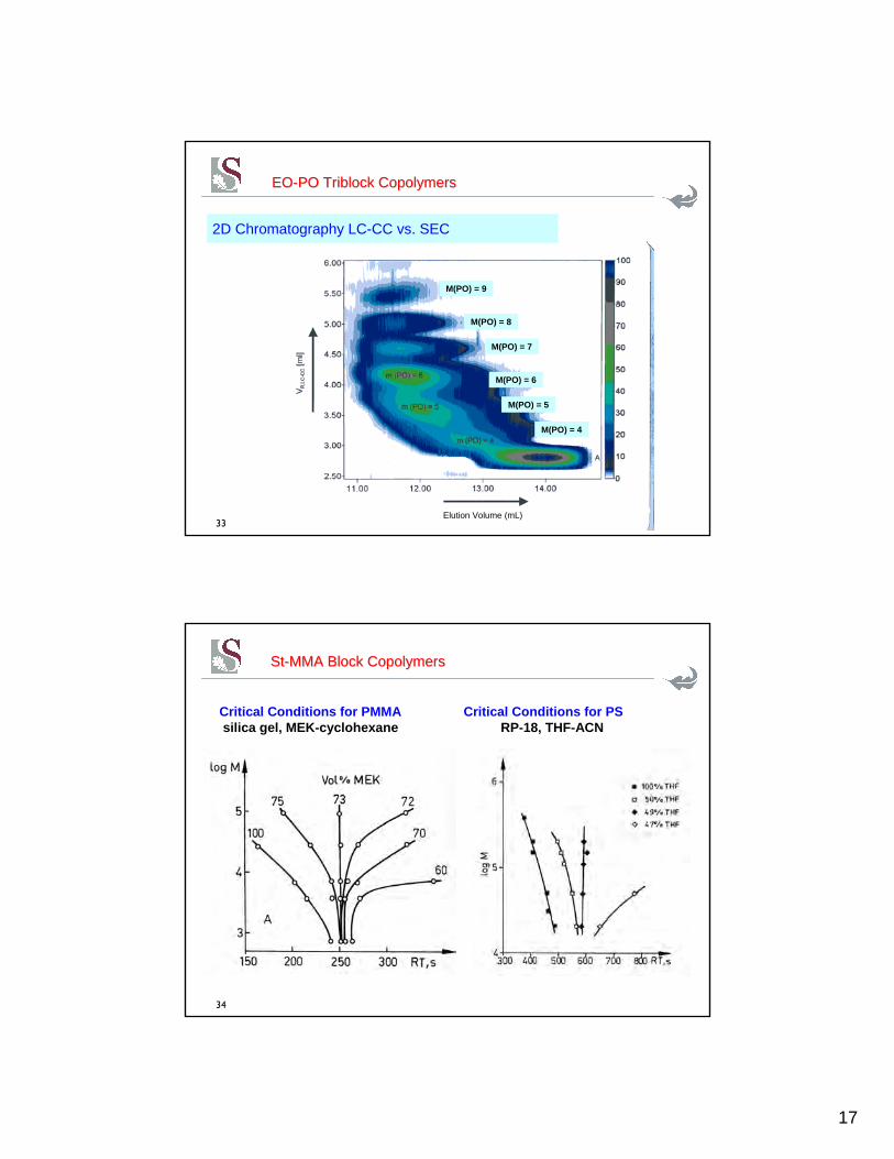
33

2D Chromatography LC-CC vs. SEC

EOEO--PO PO TriblockTriblock CopolymersCopolymers

M(PO) = 9

M(PO) = 8

M(PO) = 7

M(PO) = 6

M(PO) = 5

M(PO) = 4

Elution Volume (mL)

34

Critical Conditions for PMMA Critical Conditions for PSsilica gel, MEK-cyclohexane RP-18, THF-ACN

StSt--MMAMMA Block Block CopolymersCopolymers

18

35

LC-CC Analysis: Critical Conditions for PS

M&N Si-300-C18 + Si-1000-C18, THF - n-hexane 50:50

Elution Volume

[ml]

3.5 4.0 4.5 5.0 5.5 6.0

PS

2

2,5

3

3,5

4

4,5

5

5,5

6

6,5

7

2,00 2,50 3,00 3,50 4,00 4,50 5,00

Vr [ml]

Log

M

PSPMMA


Elution Volume (mL) Elution Volume (mL)

36

2D Chromatography LC-CC (PS) vs. SEC


19

37

SEC and LC-CC of S/MMA Diblock ??? Copolymer

0

10

20

30

40

50

60

70

80

90

100


3.5 4.0 4.5 5.0 5.5 6.0 6.5 7.0 7.5

SMMA 4

0

10

20

30

40

50

60

70

80

90

100


2.0 2.5 3.0 3.5 4.0 4.5 5.0 5.5 6.0

SMMA 4

PS

SEC indicates narrow MMD LC-CC indicates somechemical heterogeneity


Elution Volume (mL) Elution Volume (mL)

38


2D-LC of S/MMA Diblock ??? Copolymer

20

39

GraftingGrafting of of PolybutadienePolybutadiene withwith Methyl Methyl MethacrylateMethacrylate

DBP

Toluol 80°C+

+ MMA

Polybutadien MMA

PB-g-PMMA

PMMA

Abbauprodukte

PB

40

0.000

0.005

0.010

0.015

0.020

0.025

0.030

1 2 3 4 5 6 7 8 9 10 11

0

10

20

30

40

50

60

70

80

90

100

0 2 4 6 8 10 12 14 16 18

Vol

.-%

Chl

orof

orm

Retentionsvolumen [min]

PSS ANIT

Cyclohexane-CHCl 3

PB

PMMA

PB-g-PMMA

Separation of the graft product by Gradient HPLC


Elution Volume (mL)

Elution Volume (mL)

21

41

M (g/mol)

PB

PB-g-PMMA

PMMA

RT (min)

PMMA

PB

PB-g-PMMA

Molar Mass

Chem

icalcom

position


Separation of the graft product by 2D-LC

42


Quantitative analysis of the graft product components

Reaction Component Mw Amount

Time [h] [%]

PB 278.600 52

1 PB-g-PMMA 405.100 44

PMMA 33.400 1

PB 247.400 31

4 PB-g-PMMA 686.600 64

PMMA 32.600 4

22

43

1616--Component Star Block Component Star Block CopolymerCopolymer

PS PB

R

R

R

Butadiene content

17, 39, 63, 78 wt.-%

44

Size Exclusion Chromatography Gradient HPLC

silica gel, i-octane-THF


23

45

1st dimension Gradient-HPLC, 2nd dimension: SEC

3-D view

each trace represents a SEC chromatogram from a

transfer injection


46

1st dimension Gradient-HPLC, 2nd dimension: SEC


24

47

Vr

1

2

1

2

Multidimensional Multidimensional Chromatography: WaysChromatography: Ways to to HyphenationHyphenation

48

CouplingCoupling withwith FTIR FTIR SpectroscopySpectroscopy

25

49

LC-Transform

Universal LCUniversal LC--FTIR FTIR Coupling: LCCoupling: LC TransformTransform InterfaceInterface

0.00

0.05

0.10

0.15

0.20

0.25

0.30

0.35

Ab

s

1.5

2.0

2.5

3.0

Nic

2000

cm-1

FTIR Spectrometer Series of Spectra

Pump +Injector RI Detector

HPLC / GPC

Separation

Identification

50

Universal LCUniversal LC--FTIR FTIR Coupling: LCCoupling: LC TransformTransform InterfaceInterface

26

51

IR-Strahl

IR-Strahl

aufgetrageneFraktion

reflektierende Al-Beschichtung

IR-transparente Germaniumscheibe

Universal LCUniversal LC--FTIR FTIR Coupling: OpticsCoupling: Optics ModuleModule

IR beam

IR beam

reflecting Al layer

Deposited fraction

IR-transparentGermanium disc

52

Waterfall Contour Plot

0,0

0,1

0,2

0,3

0,4

0,5

0,6

Absorbance

1000 2000 3000 Wavenumbers (cm-1)

Universal LCUniversal LC--FTIR FTIR Coupling: PresentationCoupling: Presentation of of resultsresults

27

53

2 0 , 0 2 2 ,0 2 4 ,0 2 6 , 0 2 8 , 0 3 0 , 0

E l u t i o n V o l u m e ( m L )

1

2

3

Analysis of a Polymer Analysis of a Polymer Blend: SECBlend: SEC withwith RI RI DetectionDetection

54

Additive

SAN

PMMA-b-PS

Analysis of a Polymer Analysis of a Polymer Blend: SECBlend: SEC--FTIRFTIR CouplingCoupling

28

55

Analysis of a Polymer Analysis of a Polymer Blend: SECBlend: SEC--FTIRFTIR CouplingCoupling

56

HighHigh--Temperature HPLC CouplingTemperature HPLC Coupling

withwith FTIR FTIR SpectroscopySpectroscopy

29

57

HighHigh--TemperatureTemperature SEC SEC PolymerPolymer Labs Model PL GPC 220Labs Model PL GPC 220

Stationary phase: Cross-linked PS

Mobile phase:Trichlorobenzene

Temperature:140 oC

Calibration: PS, PE

Detectors:RI, ELSD, IR, LS, Vis

58

Separation Separation byby ChemicalChemical HeterogeneityHeterogeneity

• Temperature Rising Elution Fractionation (TREF)• Crystallization Analysis Fractionation (CRYSTAF)

⌦⌦⌦⌦ separation with regard to chemical composition

hydrodynamic volume

chemical composition

fraction

HT-SEC

CRYSTAF

TREF

30

59

Polymer LabsPolymer Labs‘‘ HighHigh--TemperatureTemperatureGradient HPLC SystemGradient HPLC System

High-temperaturegradient HPLC system

quarternary pump

Automatic columnswitching

RI and ELSD detectorsTwo arm roboticsample preparationplatform

two x 96 well autosampler capability

for continuousoperation

60

Separation System for PESeparation System for PE--PP BlendsPP Blends

0 2 4 6 8 10 12

0,0

0,2

0,4

0,6

0,8

1,0 Blend Moplen HP und PE 128.000

ELS

D [V

]

Elutionsvolumen (ml)

column: Nucleosil 500

mobile phase: EGMBE-TCB

T: 140oC

detector: ELSD

sample solvent: TCB

PP PE

0 2 4 6 8 10 12

0,0

0,5

1,0

1,5 BASELL EPM-S1-D 20837-28

Det

ekto

s S

igna

l (V

)

Elutions Volumen (mL)

EP copolymer with 48% ethylene

ethylene-rich

propylene-rich

PP

31

61

HTHT--HPLC Separation of EVA CopolymersHPLC Separation of EVA Copolymers

0 5 10 15 20

0

2

4

6

8

10

12

0

20

40

60

80

100

Det

ekto

rsig

nal E

LSD

[V]


EVA 5% VA EVA 12% VA EVA 14% VA EVA 19% VA EVA 28% VA EVA 45% VA EVA 50% VA EVA 60% VA EVA 70% VA PVAc-St. 164KD PVAc-St. 32KD PE-St. 126KD

% C

yclo

hexa

non

stationary phase: silica gel mobile phase: gradient of decaline-cyclohexanone

PVAc

PE

62

HighHigh--TemperatureTemperature HPLC HPLC CoupledCoupledto LCto LC--Transform InterfaceTransform Interface

LC-Transform

Transfer Line

Chromatograph

ELSD

LC-Transform Series 300, LabConnections

Temperature of the transfer line: 150°C

Temperature of the Germanium disc: 152°C

Temperature of the

nozzle: Gradient

Pressure: 30 mbar

32

63

6 8 10 12 14 16

0

20

40

60

80

100

120

Gram Schmidt EVA 18 % VA EVA 18 % VA EVA 12 % VA

VA content EVA 18 % VA EVA 18 % VA EVA 12 % VA

Elution Volume (mL)

Gra

m S

chm

idt

0,0

0,5

1,0

1,5

2,0

2,5

Relativ C

ontent of Vinyl A

cetate

6 8 10 12 14 16 18 20 22 24 26 280,0

0,5

1,0

1,5

2,0

2,5 Model: Linearequation: y = A + B*x

R2 = 0.99139 A 0.44495 ±0.03758B 0.07217 ±0.00224

VA content (wt. %)

ratio

of p

eak

heig

hts

1736

cm

-1 /1

463

cm-1

HTHT--HPLC/FTIR Analysis of EVA CopolymersHPLC/FTIR Analysis of EVA Copolymers

64

CouplingCoupling withwith 11HH--NMR NMR SpectroscopySpectroscopy

33

65

Analysis of the CCD of Styrene-Acrylate Random Copolymers

Distributed in � Molar Mass � Chemical Composition � Amount of Homopolymers narrow CCD � homogeneous � monophase system broad CCD � heterogeneous � multiphase system broadness of CCD is influenced by monomer reactivity, composition of the monomer feed and conversion

66

0

20

40

60

80

100

0 20 40 60 80 100

styrene content in the monomer mixture [mol-%]

styr

ene

cont

ent i

n th

e po

lym

er [m

ol-%

]

0

20

40

0 10 20 30 40 50 60

Styrene Content in Copolymer [mol-%]

30% Conversion

100% Conversion

60% Conversion

Styrene - Ethyl Acrylate

rS/rEA = 0.80/0.20

CopolymerCopolymer CompositionComposition asas a a FunctionFunction of of ConversionConversion

34

67

y = 11,224x - 89,517

0

10

20

30

40

50

60

70

80

90

100

8 9 10 11 12 13 14 15 16 17 18retention time [min]

styr

ene

cont

ent i

n co

poly

mer

[mol

-%]

0,00

0,05

0,10

0,15

0,20

7 9 11 13 15 17 19

retention time [min]

inte

nsity

[V] PEA

SEA 10/9020mol-% S

SEA 40/6052mol-% S

SEA 50/5059mol-% S

SEA 60/4067mol-% S

SEA 90/1089mol% S

PS

Nucleosil RP-18

ACN/THF 90/10 to 0/100

Gradient HPLC of SEA Gradient HPLC of SEA Copolymers: CalibrationCopolymers: Calibration with standardswith standards

68

0,00

0,10

0,20

8 9 10 11 12 13 14 15 16retention time [min]

inte

nsity

[V]

98% conversion43mol-% S



0,00

0,10

0,20

0 10 20 30 40 50 60 70 80 90styrene content in copolymer[mol-%]

inte

nsity

[V]

SEA 10/90SEA 40/60

SEA 50/50

SEA 60/40

SEA 90/10

Nucleosil RP-18

ACN/THF 90/10 to 0/100

Gradient HPLC of High Gradient HPLC of High Conversion SEAConversion SEA CopolymersCopolymers

35

69

1 2 3 4 5 6 7

SEA 40/60

Solvent mixtureTHF/ACN 50/50 v/v

(δH) 1 2 3 4 5 6 7

(δH)

OffOff--lineline SpectraSpectra of SEA of SEA Copolymer andCopolymer and Mobile PhaseMobile Phase

Copolymer SEA 40/60 in deuterated solvent

Solvent mixtureTHF-acetonitrile 50/50 v/v

70

OnOn--flow Couplingflow Coupling of HPLCof HPLC and and 11HH--NMRNMR

36

71

Instrument: Varian UNITY INOVA TM 500 MHz

HPLC-NMR Probe: 60 µL flow cell, indirect detection probe

with pulsed-field gradients (PFG)

Sample Concentration: 100 µL of 15 mg/mL = 1.5 mg

NMR Sequence: WET sequence of four selective SEDUCE pulses,

four gradient pulses, followed by an additional delay

and a composite read pulse; carbon decoupling during

selective proton pulses using Waltz-16 decoupling

H. Pasch, W. Hiller: Analysis of a Technical Polyethylene Oxide by On-line HPLC-1H-NMR. Macromolecules 29 (1996) 6556

H. Pasch, W. Hiller: Investigation of the Tacticity of Oligostyrenes by On-line HPLC-1H-NMR. Polymer 39 (1998) 1515 I. Krämer, W. Hiller, H. Pasch: On-line Coupling of Gradient-HPLC and 1H-NMR for the Analysis of Random Poly(styrene-co-ethyl acrylate)s. Macromol. Chem. Phys. 201 (2000) 1662

OnOn--LineLine Gradient Gradient HPLCHPLC--11HH--NMR: ExperimentalNMR: Experimental

72

OnOn--LineLine Gradient Gradient HPLCHPLC--11HH--NMR: ContourNMR: Contour plotplot of SEA of SEA 40.9840.98

37

73

O O-CH2-CH3

-C6H5 -O-CH2-

-CH3

OnOn--LineLine Gradient Gradient HPLCHPLC--11HH--NMR: OnNMR: On--lineline spectrumspectrum at at peakpeak maxmax

74

0,00

0,09

0,18

8 9 10 11 12 13 14 15 16 17

Retention time (min)

0

10

20

30

40

50

60

70

80

90

100

SEA 10/90

SEA 40/60

SEA 50/50

SEA 40/60

SEA 90/10

OnOn--lineline Gradient Gradient HPLCHPLC--11HH--NMR: ComparisonNMR: Comparison of of calibrationscalibrations

38

75

ppm1234567

1H-NMR of oligostyrene (500 MHz)⌦ complex and difficult to interpret

HPLCHPLC--NMR of NMR of Polymers: Polymers: 11HH--NMRNMR of of OligostyreneOligostyrene

Degree of polymerization ?

Endgroups ?

Stereochemistry ?

76

UV-Chromatogram in 100% ACN, flow rate gradient 1 - 2mL/minSplitting of chromatographic peaks ????

HPLCHPLC--NMR of NMR of Polymers: HPLCPolymers: HPLC of of OligostyreneOligostyrene

39

77

F2 (ppm)

012345678

t1(sec)

100

200

300

400

500

600

700

800

dimer

trimertetramer

pentamer

hexamer

heptamer

HPLC-NMR on-flow-measurement (100% ACN), no lock signal !

HPLCHPLC--NMR of NMR of Oligostyrene: ContourOligostyrene: Contour plotplot

78

HPLCHPLC--NMR of NMR of Oligostyrene: OnOligostyrene: On--flowflow spectraspectra of of oligomersoligomers

40

79

HPLCHPLC--NMR of NMR of Oligostyrene: spectrumOligostyrene: spectrum of of monomermonomer

80

CH3 CH2 CH

CH3

CH2 CH CH2 CH2

CH3 CH2 CH

CH3

CH2 CH CH2 CH2

HPLCHPLC--NMR of NMR of Oligostyrene: spectrumOligostyrene: spectrum of of dimerdimer

41

81

HPLCHPLC--NMR of NMR of Oligostyrene: spectrumOligostyrene: spectrum of of trimertrimer

82

CH3 CH2 CH CH2 CH

CH3

CH2 CH CH2 CH2

CH3 CH2 CH CH2 CH

CH3

CH2 CH CH2 CH2

CH3 CH2 CH CH2 CH

CH3

CH2 CH CH2 CH2

CH3 CH2 CH CH2 CH

CH3

CH2 CH CH2 CH2

Fraction of trimers:

1 chromatographic peak

2 1H-NMR spectra

4 isomeric structures

HPLCHPLC--NMR of NMR of OligostyreneOligostyrene

42

83

Selected ReferencesSelected References

1. H. Pasch, B. Trathnigg: HPLC of Polymers. Springer-Verlag, Heidelberg, 1997, ISBN: 3-540-61689-6

2. H. Pasch: Hyphenated Techniques in Liquid Chromatography of Polymers. Adv. Polym. Sci. 150 (2000) 1-66

3. P. Kilz, H. Pasch: Coupled Liquid Chromatographic Techniques in Molecular Characterization.

In: Encyclopedia of Analytical Chemistry (Ed. R.A. Meyers), J. Wiley & Sons, Chichester, 2000

4. H. Pasch, W. Schrepp: MALDI-TOF Mass Spectrometry of Synthetic Polymers. Springer-Verlag, 2003, ISBN 3-540-44259-6

5. F. Rittig, H. Pasch: Multidimensional Liquid Chromatography in Industrial Applications. In “Multidimensional Liquid

Chromatography: Theory and Applications in Industrial Chemistry and Life Sciences”.

Eds.: S. Cohen, M. Schure, Wiley, 2008, ISBN: 978-0-471-73847-3,

6. W. Hiller, A. Brüll, D. Argyropoulos, E. Hoffmann, H. Pasch: HPLC-NMR of Fatty Alcohol Ethoxylates.

Magn. Res. Chem. 43 (2005) 729

7. L.-C. Heinz, H. Pasch, High-Temperature Gradient HPLC for the Separation of Polyethylene-Polypropylene Blends.

Polymer 46 (2005) 12040

8. L.-C. Heinz, T. Macko, A. Williams, S. O'Donohue, H. Pasch: A New System for High-Temperature Gradient HPLC of

Polymers. The Column (electronic journal) 2006, Febr., 13-19

9. W. Hiller, H. Pasch, T. Macko, M. Hoffmann, J. Ganz, M. Spraul, U. Braumann, R. Streck, J. Mason, F. van Damme:

On-line Coupling of High Temperature SEC and 1H-NMR for the Analysis of Polymers. J. Magn. Res. 183 (2006) 309

10. A. Albrecht, R. Brüll, T. Macko, H. Pasch: Separation of Ethylene-Vinyl Acetate Copolymers by High-Temperature

Gradient Liquid Chromatography. Macromolecules 40 (2007) 5545

11. H. Pasch, L.-C. Heinz, T. Macko, W. Hiller: High-Temperature Gradient HPLC and LC-NMR for the Analysis of Complex

Polyolefins. Pure & Applied Chem. 80 (2008) 1747

84

Thanks for attending the course !Thanks for attending the course !Thanks for attending the course !Thanks for attending the course !

Questions ?Questions ?Questions ?Questions ?

ADVANCES IN NMR

SPECTROSCOPY OF POLYMERIC

MATERIALS

H.N. Cheng

USDA

Advances in the NMR Spectroscopy of Polymeric Materials

H. N. ChengMay 30, 2010

Presented to ISPAC, Pohang, South Korea

monomers

plants

micro-organisms

polymerization

extraction

fermentation

composition

tacticity

regio-sequence

copolymer sequence

molecularweight and distribution

physicalstructure

physical

chemical

enzymatic

microbial

rheology

Tg / Tm

crystallinity

stiffness

tensile

impact

etc.

fabrication

formulation

specification

regulatoryissues

testing

quality

cost

adhesives

packaging

coating

film

fiber

specialties

etc.

RawMaterials Structure Properties End

UsePossible

ImprovementsApplicationReaction or

DevelopmentProcess

Product Development Scheme

Monomers:• styrene

• VC/VDC

• Sty/BuAc

• Sty/BD

• ethylene

Plant:

Seaweeds

Polymerization

• polystyrene

• copolymer

• copolymer

• SBR

• LDPE

alginate

NMR info:

tacticity

copolymer sequence

branching

mixture

rheology

Tg / Tm

crystallinity

stiffness

tensile

impact

RawMaterials Structure Properties End

UsePossible

ImprovementsApplicationReaction or

DevelopmentProcess

Product Development Scheme

*

*

*Triad YXY; Pentad XYXYX

Triad XXY; Pentad XXXYY

*

*

Other Statistical Models

• 2nd order Markov and Coleman-Fox models

• Markovian/reversible propagation

• Complex participation

• E/Z model

• Bootstrap model

• Dual chain end/catalytic site control

• Consecutive multiple site model (generalized Coleman Fox)

• Multiple catalytic site model

• Perturbed models (compositional heterogeneity)

• Four-component models– Tetrapolymerization (4-component copolymer)

– Regiorregular and stereoirregular homopolymers

For review, Cheng, "Structural Studies of Polymers by Solution NMR," RAPRA Report 125 (2001)

Approaches to study 13C NMR spectrum of polymers

Polymerization Model

“Analytical”Approaches

Spectral Simulationor “Synthetic”Approaches

Cheng, Lee, Int. J. Polym. Anal. Charact., 2, 379 (1996)

Predictedspectrum

Observedspectrum

Presentation Scheme

Analytical

Simulation

IntegratedApproaches

HighConversion

Polymers

ImprovedMethodology

MoreSophisticated

Models

Separation-NMRData

Four-componentCopolymerization

Kinetic Modelling

Mean Deviation 8.8 4.2 0.4

Previous Approaches 1. Ito and Yamashita, J. Appl. Polym. Sci., Appl. Polym. Symp. 8, 245 (1969) NMR data compute low conversion -----> reactivity -----> high conversion copolymers ratios {rij} NMR data 2. Perturbed Models Cheng, Macromolecules, 25, 1351 (1992) Cheng, Macromolecules, 30, 4117 (1997).

Combined Analytical/Synthetic Approach for High Conversion Polymers

Reaction probability model

Inputr1, r2, x

Reactionprobability

model

Revisedr1, r2, x

Calculatedtriads

Observed triads

ObservedNMR

spectrum

Predictedspectrum

synthetic

analytical

i = 1

i = i + 1

polymerization

simulation

assignment

shift

rules

Compare

(simplex algorithm)

Cheng, IJPAC, 4, 71 (1997)

N

P

M

Table I. NMR analysis of whole (unfractionated) alginate samples

Sequence Protonal NaAlginate ManegelIobsd Icalc

a Icalcb Iobsd Icalc

a Icalcb Iobsd Icalc

a Icalcb

MM 19.1 19.1 19.1 32.4 32.4 32.4 20.9 20.9 20.9MG 24.0 24.0 24.0 49.5 49.5 49.5 27.2 27.2 27.2GG 56.9 56.9 56.9 18.1 18.1 18.1 51.9 51.9 51.9MGM 5.9 2.1 8.8 19.9 14.3 19.1 9.1 2.8 9.1GGM 6.4 19.8 6.4 11.3 20.9 11.3 9.0 21.6 9.0GGG 56.4 47.0 53.7 11.7 7.6 12.4 44.2 41.1 47.4

One-component 1st order Markov modelPGM 0.174 0.578 0.208PMG 0.386 0.433 0.394MDc 4.4 3.2 3.7

Two-component 1st order Markov model component 1 PGM 0.004 0.006 0.004

PMG 0.991 0.998 0.984w1 0.533 0.110 0.459

component 2 PGM 0.745 0.774 0.678PMG 0.382 0.432 0.391w2 0.467 0.890 0.541

MDc 0.9 0.3 0.5

Table IV. Contributions of the components to each polymerSample Fr. % polymer w1 w2 % polym.* w1 % polym.* w2

Protonal LFR 1 9.4 0.799 0.201 7.51 1.892 21.9 0.744 0.256 16.29 5.613 46.9 0.570 0.430 26.73 20.174 21.8 0.479 0.521 10.44 11.36

Component weight % from all fractions 60.97 39.03

NaAlginate 1 8.6 0.358 0.642 3.08 5.522 20.0 0.348 0.652 6.96 13.043 42.9 0.263 0.737 11.28 31.624 19.9 0.241 0.759 4.80 15.105 8.6 0.282 0.718 2.43 6.17


Manegel LMW 1 8.6 0.750 0.250 6.45 2.152 20.0 0.718 0.282 14.36 5.643 42.9 0.614 0.386 26.34 16.564 19.9 0.545 0.455 10.85 9.055 8.6 0.462 0.538 3.97 4.63


Neiss, Cheng, ACS Symp. Ser., 834, 382 (2002).

Alginate Results

• All samples can be described by a 2-component M1 model– Component 1 is G homopolymer– Component 2 is M/G copolymer, with a random to alternating tendency

• Correlation of structure with molecular weight– Second component increases as MW decreases– Less pronounced in high M polymer

• Implications for epimerization reaction– At least two separate enzymes that attack the alginate chains.– The first enzyme mostly converts M to blocks of G.– The second enzyme produces single M —> G conversion or favors the

formation of alternating MG units.– The components weights are different for different samples, reflecting

different enzyme actions or different biological origins.

Presentation Scheme

Analytical

Simulation

IntegratedApproaches

HighConversion

Polymers

ImprovedMethodology

MoreSophisticated

Models

Separation-NMRData

Four-componentCopolymerization

Kinetic Modelling

Styrene Butadiene Rubber

Styrene Butadiene Rubber 4-component copolymerization

M1 = cis-BD C = C| |

C C

C|

M2 = trans-BD C = C|

C

M3 = vinyl-BD C - C|

C = C

M4 = styrene C - C |Φ

Statistical equations have been derived earlier:Roland, Cheng, Macromol., 24, 2015 (1991)

Cheng, Polymer News, 25, 114 (2000)

Cheng, Kasehagen, ACS Polymer Preprints, 44(1), 381 (2003).

Program ALDPEZ

Program CALDPE

Observed spectrum of LDPE

Predicted spectrum 1

Observed spectrum of LDPE

Predicted spectrum 2

Solution NMR Summary

• Many solution NMR techniques are being standardized and becomingroutine.

• New approaches have been devised in several areas.

– Analytical and Simulation approaches

– Improved methodologies

• Separation/NMR

• 2D NMR

– More sophisticated probability models

• Multi-component copolymerization models

• Kinetic modeling

– Compositional heterogeneity

• Examples of NMR analysis are given for:

– polystyrene tacticity

– vinyl chloride/vinylidene chloride copolymer

– alginates

– low-density polyethylene

Solid State NMR

• Solution NMR spectra consist of a series of very sharp transitions, due to averaging of anisotropic NMR interactions by rapid random tumbling.

• In contrast, solid-state NMR spectra show broad lines, as the full effects of anisotropic or orientation-dependent interactions are observed in the spectrum.– Wideline NMR can provide a lot of information, e.g.,

% crystallinity, phase transitions, dynamics, etc.

• High-resolution solid NMR spectra can provide the same type of information that is available from corresponding solution NMR spectra, but a number of special techniques/equipment are needed– magic-angle spinning, cross polarization, high-power decoupling

– 2D experiments, enhanced probe electronics, etc.

High Resolution Solid State NMR

• Magic-angle spinning– Rapid sample spinning at the magic angle w.r.t. B0 (7 to 35 kHz)

• Dilution– Occurs naturally for many nuclei (e.g., 13C, 1.108% n.a.), and the

dipolar interactions scales with r-3. However, this only leads to “high-resolution” spectra if there are no heteronuclear dipolar interactions (e.g., with protons, fluorine).

– Anisotropic chemical shielding can still broaden the spectra

• Multiple-Pulse Sequences– Pulse sequences can impose artificial motion on the spin

operators. Good for 1H NMR spectra (e.g., CRAMPS -ombined rotation and multiple pulse spectroscopy), and 2D NMR

• Cross Polarization– Polarization from abundant nuclei (e.g., 1H, 19F and 31P) can be

transferred to rare nuclei (13C, 15N, 29Si) to enhance s/n

Example of Adamantane

A practical example of solid NMR

• Pecan is a major crop in the US, with an annual production of 88,000 metric tons in 2008.

• Pecan shells are waste materials; their disposal is costly and may pose environmental problems.

• Pecan shells can be made into activated carbons– Remove metal ions and organic species in wastewater

– Can potentially be used in sugar refining

– Can potentially be used as a soil fertility agent

• Properties of pecan shell based activated carbon depend on the activation process– Effect of acid, oxygen level, phosphorus incorporation, etc.

– Surface activity, porosity, oxidation, etc.

– Better understanding is needed: Use NMRCheng, H.N. et al., Carbon, in press

NMR techniques used

Techniques Description Information available for activated carbon

CP-MAS cross-polarization –magic angle spinning

chemical composition

SPE-MAS single pulse excitation –magic angle spinning

quantitative 13C composition

DD-MAS dipolar dephasing –magic angle spinning

observation of only aromatic quaternary carbons.

VCT variable contact time (giving TCH and T1ρ

H)relative mobility and homogeneity

Relaxation 1. inversion recovery (T1)2. TD (time domain)

expts for T1 and T2

- mobility of carbon matrix- porosity of sample through water

adsorption

Samples used

Sample Activation air flow rate

Nominal oxygen level (%)

Surface area (m2/g)

A 0 0 N/A

B 100 ml/min 4.0 904

C 400 ml/min 7.6 895

D 2000 ml/min 14.0 915

Pecan shells were activated with phosphoric acid, and carbonized at 450oC for 4 hours with varying amounts of air flow

Solid state CP-MAS and SPE-MAS

Starting pecan shells

Approximate Carbon Structure Type

Begin (ppm)

End(ppm)

Sample A –CP-MAS% intensity

Sample A –SPE-MAS% intensity

Carbonyl C 210 190 2 1

Carboxyl C 190 165 6 6

Phenolic C 165 150 9 9

Substituted Aromatic C

150 140 5 6

Bridgehead+Protonated Aromatic

140 90 26 37

Aliphatic C 90 5 35 aliphatic C-O16 aliphatic C-C

26 aliphatic C-O16 aliphatic C-C

CP-MAS of samples A-D

SPE-MAS of samples A-D

DD-MAS D2-array spectra and Gaussian/Lorentzian fit

For sample B

2-component fit of DD data

M(τ) = M0L.exp(-τ /TL) + M0G .exp(-0.5(τ/TG)2)

Definition Parameter Sample B Sample C Sample D

Weakly Coupled C

M0L 80.5 54.0 59.1

Strongly Coupled C

M0G 48.3 61.2 59.8

Lorentzian Relaxation Time

TL (μs) 599.6 598.2 599.6

Gaussian Relaxation Time

TG (μs) 16.1 15.4 14.7

Fraction of Bridgehead C

M0L/(M0G+M0L) 62 % 47 % 50 %

Carbon type fractions (13C CP-MAS)Parameter Sample B Sample C Sample D Description

FaCO 1.1 2.0 1.3 Fraction of Carbonyl (%)

FaCOO 5.6 8.3 9.2 Fraction of Carboxyl (%)

FaP 6.9 10.5 10.7 Fraction of phenolic carbon (ar-C-OH) (%)

FaS 9.6 10.9 9.9 Fraction of substituted aromatic carbon (%)

FaB + Fa

H 76.2 67.7 68.3 Fraction of combined bridgehead and protonated aromatic C(%)

FaN 64.1 53.2 54.6 Fraction of non-protonated aromatic carbon

(%)

FaC 6.7 10.2 10.5 Fraction of sp2 carbon present as carbonyl

and carboxyl (%)

Fa' 92.7 89.1 88.9 Fraction of aromatic carbon (%)

Fa 99.3 99.3 99.4 Fraction of sp2 carbon (aromatics and carboxyl/carbonyl) (%)

Fal 0.7 0.7 0.6 Fraction of sp3 (aliphatic) carbon (%)

FaB 47.6 31.7 34.0 Fraction of bridgehead aromatic carbon (%)

FaH 28.6 35.9 34.3 Fraction of protonated aromatic carbon (%)

Calculated structural parametersMolecular Parameter

Sample B

Sample C

Sample D

Description

χb 51 36 38 Mole fraction of bridgehead aromatic carbon (%)

C 25.6 17.8 18.9 Number of carbons per aromatic ring system

# Ring Systems per 100 C

3.6 5.0 4.7 Number of aromatic ring systems per 100 carbons

Phenolic C per cluster

1.9 2.1 2.3 Number of phenolic carbons per aromatic ring system

Carboxyls per cluster

1.6 1.7 2.0 Number of carboxyl carbons per aromatic ring system

k/a per cluster

0.3 0.4 0.3 Number of ketone/aldehyde carbons per aromatic ring system

s+1 0.0 0.0 0.0 Average length of aliphatic substitutions on the aromatic ring system

Methodology used follows that of Solum MS, et al., Energy & Fuels 1989, 3, 187.

Effective overall 1H spin-lattice relaxation times (T1)

(from 1H-13C-CP-MAS-prepared inversion recovery experiment)

Sample A B C D

T1 (ms) 33 ± 7 23 ± 1 19 ± 2 16 ± 3

(for sample B)

CP-MAS-VCT –relaxation fit (1-component)

CP-MAS-VCT –relaxation fit (1-component)

Sample Carbon type TCH (μs)

A Carboxyl 294

Phenolic 269

Aromatic 238

Aromatic/Cellulose 185

Cellulose 81

Aliphatic 61

B Aromatic 2530

C Aromatic 4340

D Aromatic 790

31P SPE-MAS spectra

31P SPE-MAS spectra

• Narrow component is most likely due to free phosphoric acid• Broad component is likely to be alkyl (& dialkyl) phosphates• Small peaks at -40 to -60 ppm, perhaps polyphosphates• Phosphonates and phosphonic acid do not appear to be present

Sample Unbound (Narrow) (%P) Bound (Broad) (%P)

A 0 100

B 22.0 78.0

C 30.1 69.9

D 15.0 85.0

1H NMR (TD low-resolution)

• FID signals varies with 1H spins present (mostly water here)• Samples B-D are microporous and contain more water

– Increasing pore volume, more adsorbed water expected

• Trend in porosity from FID intensity: D > B > C >> A

Comparison: Average pore volume and width from gas sorption measurements

sample air flow rate (mL/min)

average pore volume (mL/g)

average pore width (Å)

B 100 0.361 9.26

C 400 0.354 10.07

D 2000 0.368 8.52

•Gas sorption studies were carried out on a Nova® instrument (Quantachrome, Boynton Beach, FL)•Samples were degassed and then brought to 77K when nitrogen was admitted in steps in the evacuated sample chamber•Trend in porosity from gas sorption: D > B > C

ESR absorption spectra

ESR intensities, g factor and radical content

sample g value intensity radical content(1018 spins per gram)

Illinois #6 coal 2.0028 69.3 6.8

A 2.0018 5.8 0.6

B 2.0013 121.2 11.9

C 2.0039 129.3 12.7

D 2.0039 62.2 6.1

•g value increases with the number of heteroatoms present. Here increase in g value may be due to the oxidation of the carbon matrix and the formation of oxidized functional group •Radical content reaches a maximum at C, and then decreases at D,probably due to oxidation and/or reactions involving the radicals during carbonization at a very high oxygen flow rate.

Solid State NMR Summary

• The use of different NMR techniques and ESR gives complementary information on structure and dynamics of the polymeric system.

• For carbons, structural parameters available include mole fraction of bridgehead aromatic carbons, number of carbons per aromatic ring system, and number of phenolic carbons per aromatic ring system

• The relaxation times are indicative of the relative mobility of different structural units.

• 31P NMR indicates the type of phosphorus-containing chemical species present

• 1H NMR data on adsorbed water are shown to be consistent with the trends in the amount of pore volumes for different samples of activated carbons.

• ESR spectra showed the presence of π-type aromatic free radicals in the carbonized samples with a slight shift in g value with increasing oxidation.

Cheng, HN, et al., Carbon, in press

Acknowledgments

• Solution NMR– Leo Kasehagen (now at Arkema)– Michael Roland (ex-Hercules)– Mark Bennett (ex-Hercules)– G. H. Lee (ex-Sunoco)– Thomas G. Neiss (now at GlaxoSmithKline)

• Solid State NMR– John Edwards (Process NMR)– Lynda Wartelle (USDA)– K. Thomas Klasson (USDA)

TAILORED SYNTHESIS AND

CHARACTERIZATION OF

COMPLEX POLYMERS

Jimmy Mays

Univ. of Tennessee

5/5/2010

1

Molecular Characterization of Complex Polymers

Jimmy MaysDepartment of Chemistry, University of Tennessee

Chemical Sciences Division and Center for NanophaseMaterials Sciences, Oak Ridge National Laboratory

552 Buehler Hall

K ill TN 37996Knoxville, TN 37996

[email protected]

Categories of Complex Polymers

• Branched polymers (star, comb, d d i d l b h d)dendrimers, randomly branched)

• Cyclic polymers

• Copolymers (blocky, random, branched)

• End-functionalized or telechelic polymers

• Stiff polymer chains (conformational studies)

5/5/2010

2

For a review on synthesis of various polymer architectures see

Molecular Weight MethodsClassical

Absolute methods

Advanced

Absolute methods• end group analysis• colligative properties• light scattering• ultracentrifugationRelative method

solution viscosity

• MALDI-TOF MS• SEC with light

scattering detectionRelative method • SEC with viscosity

detection• solution viscosityFractionation methods• Solvent/non-solvent

fractionation• SEC (GPC)

detectionFractionation method• TGIC and multi-detector

SEC

5/5/2010

3

Synthesis of Model Star Polymers

This classic approach was first demonstrated using living anionic polymerization and chlorosilane linking chemistry by Morton et al. in 1962• this approach allows the “arms” to be sampled and characterized independently• a small excess of arms is used to force the linking reaction to completion

the star is isolated from excess arm by solvent/non solvent fractionation (no• the star is isolated from excess arm by solvent/non-solvent fractionation (no SEC at the time!)• Absolute molecular weight of the star should be 3x that of the arm for a 3-arm star, etc., i.e. this is proof of the star structure

The Evolution of Size Exclusion Chromatography (SEC)

• Unlike in HPLC (or interaction chromatography) no chemical attraction of the polymeric solute to the column is allowedattraction of the polymeric solute to the column is allowed. • Solvent flow carries molecules from left to right; big ones come out first while small ones get detained in the pores.• Polymer “hydrodynamic volume”, not molecular weight, controls the order of elution.

5/5/2010

4

Simple SEC

og10

M

c

c

og10

MConc sensitive detector only -DRI or UV most typically

d

DRI

Ve

lolo

degas

pump

injector

c

log10M

Definition of molar mass averages

Average Molecular Weights and Polydispersity

Here a is the exponent in the Mark-Houwink equation which relates the intrinsic viscosity to molar mass.

The breadth of the molecular weight distribution (MWD) or polydispersity ratio (PDI) is usually taken as the ratio of Mw/Mn, which would equal unity for a monodisperse polymer.

5/5/2010

5

They were young when SEC was…

Compliments of Professor Paul Russo, Louisiana State University

Early Development of SEC

• Development of the technique: J. Moore, Dow Chemical Company (1962)Chemical Company (1962)

• First paper: J. Moore, J. Polym. Sci., Part A 2835 (1964)

• Universal calibration: Z. Grubisic; P. Rempp; H. Benoit, J. Polym. Sci., Part B 5 753 (1967)

• Theoretical Interpretation: E.F. Casassa, J. Polym. Sci., Part B 5 773 (1967)

5/5/2010

6

Conventional Calibration Requires Standard Samples

• PROBLEM - commercial narrow polydispersity standards are only readily available for polystyrene and a few other polymers and Vhdepends on type of polymer. PS equivalent MWs are often reported.

• Since the hydrodynamic volume of branched polymer is smaller than the linear material having the same mass, the density must be higher yielding a larger SEC retention volume, thus a lower apparent MW.

SEC of Branched Polymers

M

Linear BranchedThe same MW polymers elute at different elution

volume

Elution volume

Log

LinearBranched

True MWMeasured MW

5/5/2010

7

Universal Calibration

Grubisic, Rempp & Benoit, JPS Pt. B, 5, 753

(1967)

One of the most citedi l ipapers in polymer science.

Universal Calibration Equations

[η]A⋅MA = [η]S⋅MS= f (Ve)Universal CalibrationA = analyte; S = standard

[η] = KM a

[η]A MA [η]S MS f (Ve)

11 ++ = SA aSS

aAA MKMK

Mark-Houwink Relation

A = analyte; S = standard

• must know Mark-Houwink parameters for both the standard and the analytefor both the standard and the analyte(very laborious and especially a problem with branched polymers)

• wouldn’t it be great if we could measure intrinsic viscosity online…

11

1 ++

⎟⎟⎠

⎞⎜⎜⎝

⎛=

AS

S

a

A

aS

A KMK

M

5/5/2010

8

MW- and Size-Sensitive Detectors for SEC

• Beginning around 1980, molecular weight and size sensitive detectors for SEC became commercially available

• Detectors include viscosity detectors, which allow facile use of universal calibration and provide insight into branching

Single angle (LALLS) and multi angle light• Single-angle (LALLS) and multi-angle light scattering (MALLS) instruments, which allow measurement of absolute molecular weights and, for MALLS, the radius of gyration Rg

SEC with on-line Viscosity Detection

DRI

ΔP η viscometer

degas

pump

injector

5/5/2010

9

SEC/MALLS

MALLS

DRI

DRI

degas

pump

injector

SEC/MALLS

3D Plot - PBLG

4 5

6

Scattered intensity(gives absolute MW)

6 7

89

1011

1213

1415

16

(gives Rg)

5/5/2010

10

SEC/RALS/VIS

LS90o

ΔP η viscometer

DRI

degas

pump

injector

Evolution of Multi-Detector SEC

By the mid-1990s SEC/MALLS/Vis was as reliable as much more tedious off-line measurements for measuring polymer molecular weights and sizes.

From Jackson, Chen, Mays, J. Appl. Polym. Sci., 61, 865 (1996)

5/5/2010

11

Evolution of Multi-Detector SEC

From Jackson, Chen, Mays, J. Appl. Polym. Sci., 61, 865 (1996)

Radius of Gyration of Branched Polymers

• Long chain branching can have a profound effect on polymer processing and properties even at very low levels that are hard to quantify via spectroscopy• As we saw earlier, branched polymers are smaller than their linear counterparts at a given molecular weight.• A branching parameter g has been defined

g = (Rg2,br /Rg

2,l)M < 1

b l l t d th ti ll f li d b h d• g can be calculated theoretically for linear and branched chains of different architectures and degrees of branching.• Thus, experimentally derived g values can be used to estimate the degree of branching.

5/5/2010

12

Effect of Branching on Hydrodynamic Properties

• Branching also affects hydrodynamic ti i l tiproperties in solution.

• Another commonly used branching parameter is g’:

g’ = ([η]br/[η]lin)M < 1

g’ is easier to measure particularly at lower• g’ is easier to measure, particularly at lower MW, but theory relating g’ to the branched architecture is not so well established

Experimental Data on Randomly Branched Samples

• Randomly branched PMMAs were synthesized by copolymerization of MMA with small amounts of ethylene glycol dimethacrylate.• At low MWs the data merge, suggesting that low MW samples contain little or no branching, as expected.• Larger scatter in data at lower MW reflects larger errors in measuring Rg for smaller macromoleculesRg for smaller macromolecules.

Jackson, Chen, and Mays, J. Appl. Polym. Sci., 59, 179 (1996).

5/5/2010

13


• Data for intrinsic viscosity are very high quality even at low MW.• Clearly the extent of branching increases as MW increases



Limitation: the Zimm-Stockmayertheory that relates g to extent of branches was developed for polymers chains in theta solvents whereas SEC is almost always conducted in thermodynamically

d l


good solvents.

5/5/2010

14

Can we carry out multi-detector SEC in a theta solvent???

• Would allow for simple and rapid studies of dilute solution properties, with better comparison to theory.

We chose trans decalin as the theta sol ent for PS at• We chose trans-decalin as the theta solvent for PS at about 21-22 ˚C. It has a high boiling point so it could be run through the SEC columns at 110 ˚C (good solvent conditions) to prevent adsorption of PS onto the columns.

• Viscosity and two-angle light scattering (TALS, also y g g g (DLS at 90˚) detectors were maintained at 21-22 ˚C.

• Failed with differential viscometer due to adsorption of polymer within viscometer.

Farmer, Terao, Mays, Int. J. Polym. Anal. Charac., 11, 3 (2006)

(a) Comb

CS25-35

100

Mw dependence of Rg for regularly branched PS in THF: open circles = TALS, filled circles = Nakamura et al. via MALLS

50

50GS60-15

GS40-25

Rg

/ nm

CS25 35

(b) Centipedes

105 106 10710

Two-angle light scattering has been shown to yield identical results to MALLS both theoretically and experimentally. Data at left are for linear and branched PS in the good solvent THF.

10

10

105 106 10710

Mw

GS15-3530≈

Terao, Mays, Eur Polym J. 40, 1623 (2004)

5/5/2010

15

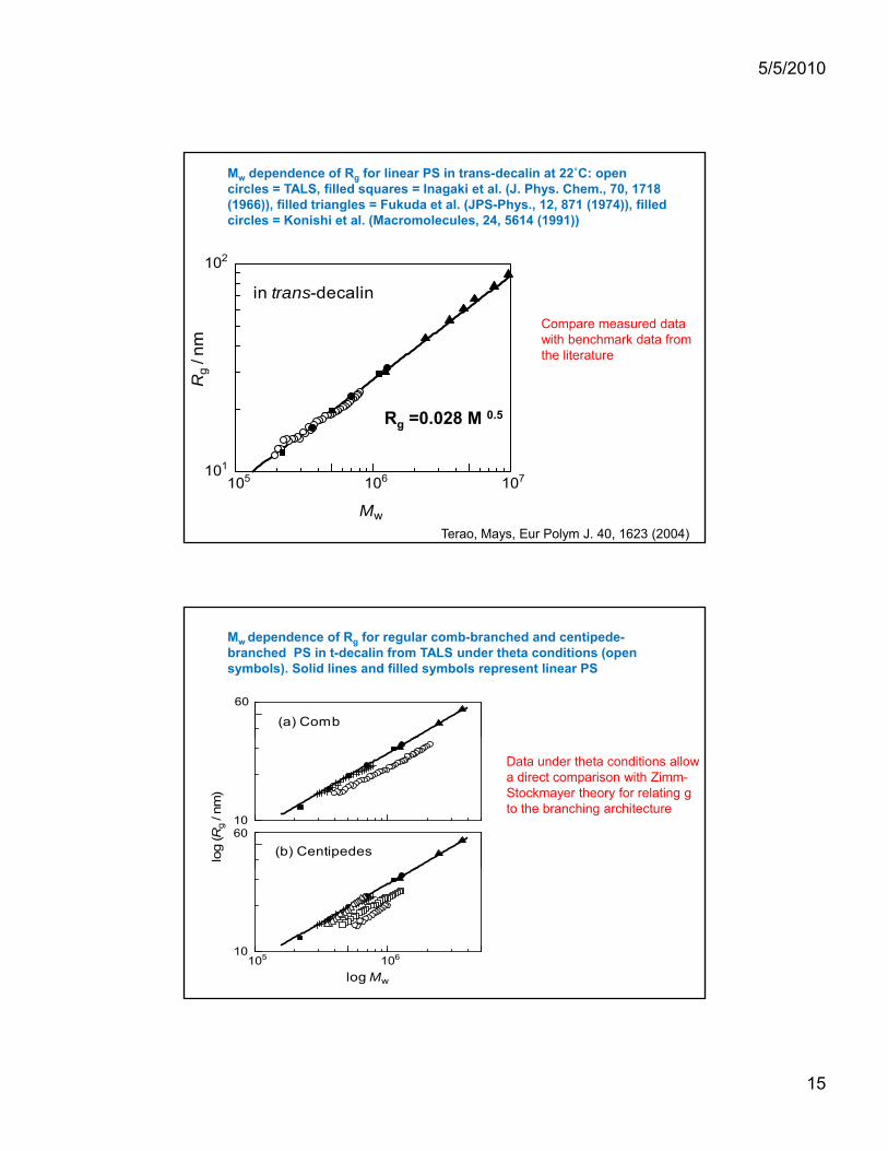
102

Mw dependence of Rg for linear PS in trans-decalin at 22˚C: open circles = TALS, filled squares = Inagaki et al. (J. Phys. Chem., 70, 1718 (1966)), filled triangles = Fukuda et al. (JPS-Phys., 12, 871 (1974)), filled circles = Konishi et al. (Macromolecules, 24, 5614 (1991))

Rg

/ nm

in trans-decalin

R 0 028 M 0 5

Compare measured data with benchmark data from the literature

105 106 107101

Mw

Rg =0.028 M 0.5

Terao, Mays, Eur Polym J. 40, 1623 (2004)

60

(a) Comb

Mw dependence of Rg for regular comb-branched and centipede-branched PS in t-decalin from TALS under theta conditions (open symbols). Solid lines and filled symbols represent linear PS

10

log (R

g / n

m)

(b) Centipedes

60

Data under theta conditions allow a direct comparison with Zimm-Stockmayer theory for relating g to the branching architecture

105 10610

log Mw

5/5/2010

16

Limitations in SEC analysisAAAAAAAAA

Intrinsic Band broadening –particularly serious in SEC

Linear Homopolymer

BBBBBBAAAA

ABABAABBAAAAAB

AAAA, AAAAA, AA AAAA

1. SEC separates polymers by hydrodynamic size only2. Hydrodynamic size decreases with chain branching

Polymer Blend

AAAA

Copolymer

AAAB A AAAAA

Branched Polymer

⎟⎟⎠

⎞⎜⎜⎝

⎛Δ≅⎟⎟

⎠

⎞⎜⎜⎝

⎛ Δ−=

RSexp

RTGexpK SEC

oSEC

o

SEC

SEC vs. IC

Size Exclusion ChromatographySolid phaseInterstitial space

⎠⎝⎠⎝ RRT

1≤=≤i

pSEC c

cKo

⎞⎛⎞⎛

Interaction ChromatographySolid phaseInterstitial space

Pore

⎟⎟⎠

⎞⎜⎜⎝

⎛ Δ−

Δ=⎟⎟

⎠

⎞⎜⎜⎝

⎛ Δ−=

RTH

RSexp

RTGexpK

oIC

oIC

oIC

IC

∞≤=≤m

sIC c

cKo

Stationary phasepp

Pore

5/5/2010

17

Temperature & Solvent Effect on HPLC Retention

Column: Nucleosil C18, 5 μm, 100 Å , 250 x 4.5 mmEluent: CH2Cl2/CH3CN mixture, 0.5 mL/min

Eluent Effect (30.5oC) Temperature Effect (57/43)

1,2,3

2 13

6,5,4 Temperature50oC

45oC

40oC

35oC

30.5oC

28oC

A2

60 (

a.u.

)

6,5,4

3 21

59 %

57.5 %

57 %

62 %

65 %

CH2Cl

2 vol%

A26

0 (a

.u.)

< Samples >

29 0003

12,0002

2,5001

MWPS

0 10 20 30 40

32

1

54 28oC

25oC

20oC

tR (min)

0 10 20 30 40

4

32

1

53 %

55 %

57 %

tR (min)

1,800,0006

502,0005

165,0004

29,0003

Chromatographic Critical Conditionto to

Chang, Adv. Polym. Sci. 163 1 (2003)

Temperature gradient elution chromatography

20

30

40

648k200k15.3k

5.1kdT/dt = 2 oC/min

T ( oC

)2

60(a

.u.)

dT/dt = 8 oC/min

0 5 10 15tR (min)

1098.9k55.2k

30.9kA2

0 5 10 15tR (min)

Column: Nucleosil C18, 3 mm, 100Å, 50 x 4.6 mmEluent: CH2Cl2/CH3CN = 57/43 (v/v), 0.7 mL/min

Ryu et al. J. Chromatogr. A. 1075 145 (2005)

5/5/2010

18

4 DVB columns, 105, 104, 103 Å, mixed,250 x 10 mm, THF

1 C18 silica column, 100 Å, 250 x 4.5 mm, CH2Cl2/CH3CN (57/43)

TGIC separation of polystyrene

IC SEC

Mw/Mn = 1.005

Mw/Mn = 1.05

9 PS standards: 2.0 k,11.6 k, 30.7 k, 53.5 k, 114 k, 208 k, 502 k, 1090 k, 2890 k

Lee & Chang, Polymer 37 5747 (1996)

SEC and TGIC Characterization of Polystyrenes

3226181555

T (oC)

Styrene

oo+-

LiCyclohexane, 45 oC

Take out aliquots and terminate with i-propanol at different polymerization times.

4.0

4.5

5.0

A26

0 (a

.u.)

logM

SECPS1

PS2

PS3

PS4

TGIC

1626s

2296s

888s

6.0x104

8.0x104

1.0x105

M

3226181555

A26

0 (a

.u.)

238s

13 14 15 16 17 18 19 202.5

3.0

3.5

A

tR (min)

M

PS7

PS5

PS6

3098s

4220s

14345s

0.0

2.0x104

4.0x104

0 20 40 60 80 100

A

tR (min)

5/5/2010

19

TGIC Poisson distribution

SEC

MWD of Polystyrenes by SEC and TGIC

SEC: 2 x PL mixed C, THF

TGIC: 1 x Nucleosil C18 (100Å), CH2Cl2/CH3CN 57/43 (v/v)

i i ν1

238s

888s

1626s

2296s

3098s

wi (

a.u

.)

Poissondistribution: ( )( )w i e

ii

i=

+ −

− −νν

ν1

1 1 !

Poly’n time

Mw/Mn (Mw)SEC TGIC Poisson

238s 1.08 (4.3k) 1.06 (4.0k) 1.02888s 1.04 (21.3k) 1.02 (21.0k) 1.003

14345s

4220s

0 200 400 600 800 10000 200 400 600 800 1000

i

1626s 1.05 (35.0k) 1.02 (34.4k) 1.0022296s 1.05 (42.9k) 1.01 (43.4k) 1.0023098s 1.05 (50.3k) 1.008 (50.2k) 1.0024220s 1.05 (56.0 k) 1.006 (55.2k) 1.002

14345s 1.05 (62.0k) 1.005 (62.0k) 1.002

Lee et al. Macromolecules 33 5111 (2000)

Branched PS by linking with divinyl benzene

DVBStyrene

oo+-

Li

+ + + +Higher Branched Species

R

90 &

Δn

(a.u

.)

Light Scattering R.I.SEC

A

260 (a

.u.)

TGIC

12 3 4 5 6

Nucleosil C18 250 × 4.6 mm (500 Å)Eluent : CH2Cl2/CH3CN = 57/43 (v/v)Flow rate: 0.5 mL/min

2 x PL mixed C (300 x 7.5 mm)Eluent: THF at 0.8 mL/min

8 10 12 14 16VR (mL)

0 10 20 30tR (min)

K. Lee, Kumho Petrochemical Ltd.

5/5/2010

20

s-BuLi LiBenzene

RT

Synthesis of Symmetric H-PBd

Si ClCl

CH3

Si

CH3

Butadienes-BuLi

Li

Titration

(CH3)2SiCl2Li

GPCTGIC

99K

125K

86K

74K

11 12 13 14 15 16Elution time (min)

10 15 20 25tR (min)

Mn=98K, PDI=1.03

5/5/2010

21

Si ClCl

CH

SiCH3

ButadieneSec-BuLi

(A)

Synthesis of Asymmetric H-PBd

CH33

SiCH3

Si ClCl

CH3

(B)

(A)

(B)THF, MeOH

26

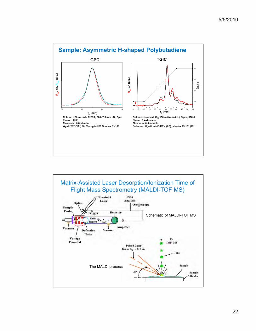
GPC TGIC

Comparison of conventional GPC with TGICSample: Asymmetric H-shaped Polybutadiene

R90

, Δn

(a.u

.) T ( oC)

23

24

25

6

15 16 17 18 19 20 21

Elution time (min)

0 5 10 15 20 25 30 35 40 45

tR (min)

Column: Kromasil C18 150×4.6 mm (i.d.), 5 μm, 300 ÅEluent: 1,4-dioxaneFlow rate: 0.5 mL/minDetector : Wyatt miniDAWN (LS), shodex RI-101 (RI)

Column : PL mixed - B 2EA and PL Mixed DEluent : THF Flow rate : 1 mL/minPrecision detector PD-2040, low angle light Scattering at 15 o..

5/5/2010

22

.u.)

25

26

0 (a.u

.)

Sample: Asymmetric H-shaped PolybutadieneGPC TGIC

0 5 10 15 20 25 30 35 40 45 50 55

tR (min)

R90

, Δn

(a. T ( oC

)

23

24

13 14 15 16

tR (min)

R90

, Δn,

A26

0

Column: Kromasil C18 150×4.6 mm (i.d.), 5 μm, 300 ÅColumn : PL mixed - C 2EA, 300×7.5 mm I.D., 5μmEluent: 1,4-dioxaneFlow rate: 0.5 mL/minDetector : Wyatt miniDAWN (LS), shodex RI-101 (RI)

Eluent : THF Flow rate : 0.8mL/minWyatt TREOS (LS), Younglin UV, Shodex RI-101

Matrix-Assisted Laser Desorption/Ionization Time of Flight Mass Spectrometry (MALDI-TOF MS)

Schematic of MALDI-TOF MS

The MALDI process

5/5/2010

23

• The TOF mass spectrum is a recording of the detector signal as a function of time. • The time of flight for a molecule of mass m and charge z to travel this distance is proportional to (m/z)1/2. • This relationship, t ~ (m/z)1/2, can be used to calculate the ions mass.• Through calculation of the ions mass, conversion of the TOF mass spectrum to a conventional mass spectrum of mass-to-charge axis canspectrum to a conventional mass spectrum of mass to charge axis can be achieved.

Advantages and Limitations of MALDI-TOF MS

• Baseline separation of low MW polymers (<10K)

• Great mass accuracy for low MW polymers allows determination of end groups

• Limited separation at higher MWs

• Underestimates polydispersity especially for samples with PDI>1.2 (sampling issues, detector saturation issues).

• SEC-MALDI-TOF MS is useful with higher PDI samples

5/5/2010

24

Determination of numbers of repeat units and end group masses

The observed mass of a singly charged copolymer chain in MALDI-TOF-MS is described by the following equation:

where mobs is the observed mass of a peak in the MALDI-TOF spectrum, MA is the mass of the repeating unit, nrA is the number of repeat units, mion is the mass of the adduct ion, and mend1 and mend2 are the masses of the end groups.

MALDI spectrum of PS with two different types of end groups, i ldi t i f kyielding two series of peaks

differing by 104.1 in mass

sec-Butyl Li + Styrene

OH end-functional PSSEC: 2 x PL-mixed B

TGIC is also very useful in characterizing end-functionalized polymers

(1) Ethyleneoxide

(2) i-propanoli-propanol

PS,PS-OH 10K

PS,PS-OH 100KA26

0 (a

.u.)

( ) p p

H CH2CH2OH

10 11 12 13 14 15 16

PS,PS-OH 500K

VR (mL)

5/5/2010

25

PS-OH 10k

PS 10k

T( OC

0 (a

.u.)

20

30

40

50

NP-TGIC

Column: Nucleosil bare silica

NP- vs. RP-TGIC: Separation by a single -OH end group

NP-TGIC

0 1 2 3 4 5 6 7

PS-OH 100kPS 100k

C)

A26

0

VR (mL)

0

10

20

30

35

100 Å pore, 250 x 2.1 mmEluent: i-octane/THF = 55/45(v/v)

RP-TGIC

Column: Nucleosil C18 bonded silicaRP-TGIC

0 1 2 3 4 5 6

PS, PS-OH 100k

PS, PS-OH 10k

T( OC

)

A26

0 (a

.u.)

VR (mL)

5

10

15

20

25Column: Nucleosil C18 bonded silica

100 Å pore, 250 x 2.1 mmEluent: CH2Cl2/CH3CN = 57/43(v/v)

Lee et al. J. Chromatogr. A 910 51 (2001)

Synthetic scheme of Ring PS

LCCC separation of Rings from Linear precursors

-CH CH2 (St)n-2 CH2 CH-Na+ Na+

(1) (CH3)2SiCl2

extreme dilution

(2) CH3OHSi(CH3)2(St)nSi(CH3)2(St)n

CH3CH3 CH3CH3 CH3CH3(St) n(St) n

Ring PS

Si OCH3

CH3

(St)nSi

CH3

CH3O Si OCH3

CH3

(St)nSi

CH3

CH3O H(St)n Si OCH3

CH3

H(St)n Si OCH3

CH3

Si(CH3)2(CH3)2Si

(St) m

Si(CH3)2(CH3)2Si

(St) m

+ + +

Possible byproducts

J. Roovers, NRC-Canada

5/5/2010

26

Linear Ring

RingLinear

LCCC for linear PSColumn: Nucleosil C18ABEluent: CH2Cl2/CH3CN=57/43Column temperature: 42 oC

SECColumn: 2 x PL mixed-CEluent: THFColumn temperature: 40 oC

LCCC separation of Rings from Linear precursors

Linearprecursor

Ring

A2

60 (

a.u

.)

187 k

179

83.1

67.6

48.522.0

83.1

179

Ringprecursor

48.5

67.6

187k

Δn (

a.u

.)

3 5 7 9 11 13

tR (min)

22.0

18.1

11.8

4.8

14 16 18 20 22

4.8

11.8

18.1

Δ

tR (min)

Lee et al. Macromolecules, 33 8129 (2000)

SEC

Fractionation results by SEC & MALDI-TOF MS

MALDI-TOF MS

tens

ity (a

.u.)

R17H (Ring PS)As-received

R17P (PS precursor)

: As-received Ring PS : Fractionated Ring PS

R4DB

R8DC

R10DD

Δn

(a.u

.)

2000 3000 4000 5000 6000 7000 8000 9000 100002000 3000 4000 5000 6000 7000 8000 9000 100002000 3000 4000 5000 6000 7000 8000 9000 10000

Int

m/z

R17H (Ring PS) fractionated by LCCC

15 16 17 18 19

R16E

tR (min)

5/5/2010

27

Si

CH3

CH3

Before and After LCCC Fractionation

Before After

DP =38

4244.7

4155.7

4124.4

4124.5

4000 4100 4200 4300

4000 4100 4200 4300

Si

CH3

CH3

Si

CH3

CH3

OCH3H3COSi

CH3

CH3

OCH3H

Cho et al. Macromolecules 34 7570 (2001)

P

Fractionation of individual blocks of BCP

PS block length

PI block length

RPLC

Composition

MW

PS block PI block

PS block lengthNPLC

Composition

5/5/2010

28

100 nm100 nm 100 nm 100 nm 100 nm

SLIHSHIL MotherSMIM

SMIH

16

18

20

22

24 LAM HPL G HEX ODT mean-field

χN

SLIHSMIH SHIH

SLIM SMIM SHIM

PI block leR

PLC

0.60 0.62 0.64 0.66 0.68 0.70 0.72 0.7410

12

14

fPI

SLIL SMILSHIL

engthC

PS block lengthNPLC

Park et al. Macromolecules 36 4662 (2003)

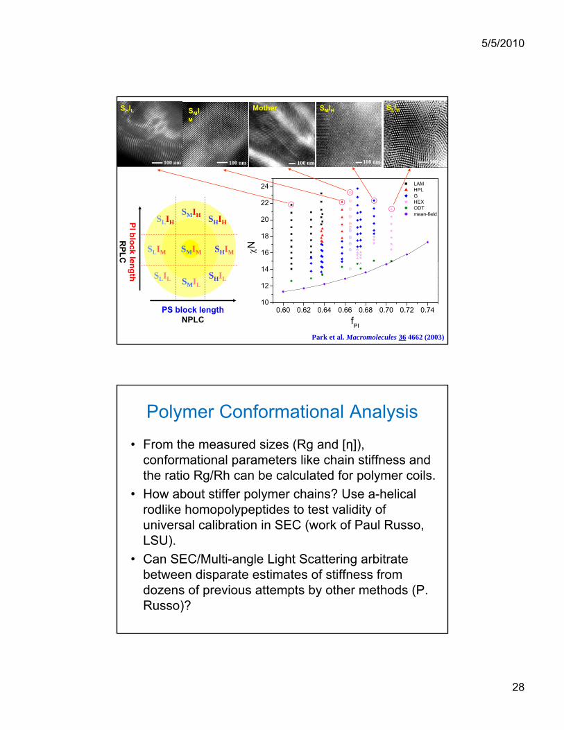
Polymer Conformational Analysis

• From the measured sizes (Rg and [η]), conformational parameters like chain stiffness and the ratio Rg/Rh can be calculated for polymer coils.

• How about stiffer polymer chains? Use a-helical rodlike homopolypeptides to test validity of universal calibration in SEC (work of Paul Russo, LSU).

• Can SEC/Multi-angle Light Scattering arbitrate between disparate estimates of stiffness from dozens of previous attempts by other methods (P. Russo)?

5/5/2010

29

Strategy

Ld

Severe test of universal calibration: d & il

Ld

Hydrodynamic volume

compare rods & coils

Combine Ms from SEC/MALLS with [η] values from literature Mark-Houwink relations.

Polymers Used

[CH2-CH]x Polystyrene (expanded random coil)Solvent: THF = tetrahydrofuran

[NH-CHR-C]x

OR (CH ) COCH

Homopolypeptides (semiflexible rods)

PBLG = poly(benzylglutamate)R = (CH2)2COCH2

R = (CH2)2CO(CH2)CH3

G po y(be y g uta ate)Solvent: DMF=dimethylformamide

PBLG = poly(stearylglutamate)Solvent: THF = tetrahydrofuran

5/5/2010

30

Mark-Houwink Relations

[η] = 0.011·Mw0.725 for PSw

[η] = 1.26·10-5·Mw1.29 for PSLG

[η] = 1.58 10-5·Mw1.35 for PBLG

Universal Calibration Works for These Rods and Coils

10

l-1) PS

PSLG

6

8

log(

[η]M

/m

l-mol PSLG

PBLG PBLG Mixture

12 14 16 18 20 22

4

Ve /ml

5/5/2010

31

Persistence Length ap from Rg

)]1(1[2

3/

322 paLppp

pg e

La

La

aLa

R −−−+−=3 LL

Persistence length is the projection of an infinitely long chain on a tangent line drawn from one end. ap = ∞ for true rod.

Persistence Length of Helical Polypeptides is Very Large

100

a = 240 nmRod

40

60

80

ap = 70 nmap = 120 nm

p

R g / n

m

What the biggest polymers in our

0 100000 200000 300000 400000 5000000

20

M

What the biggest polymers in our sample would look like at this ap

5/5/2010

32

ConclusionsConclusions• Multi-Detector SEC provides an accurate and facile means for characterizing polymer solution properties, such as Mark-Houwink coefficients and chain stiffness, in thermodynamically good solventsthermodynamically good solvents.• Measurements on branched polymers can detect branching and provide insight into the level of branching across the molecular weight distribution.• However, multidetector SEC has limitations in band broadening, resolution, and due to its size-based separation mechanism.• TGIC and MALDI-TOF MS are powerful newer tools that provide deeper insight into polymer structure, particularly for complex polymers.

AcknowledgmentsAcknowledgmentsCo-workers and collaborators:

Taihyun Chang (Postech), C. Jackson (DuPont), K. Terao (Osaka Univ.), Y. Nakamura (Kyoto Univ.), Nikos Hadjichristidis Athens) and many great

Support and funding:

U.S. Army Research Office, National Science F d ti D P t T Ad d M t i l

Nikos Hadjichristidis Athens) and many great students and postdocs over the years.

Paul Russo (LSU)

Foundation, DuPont, Tennessee Advanced Materials Laboratory, U. S. Department of Energy.

PRINCIPLES AND APPLICATIONS

OF CONTINUOUS ONLINE

POLYMERIZATION MONITORING

Wayne Reed

Tulane Univ.

Principles and applications of Automatic Continuous Online Monitoring of

Polymerization reactions (ACOMP)

Wayne F. Reed and Alina M. Alb

Physics Department and PolyRMC Tulane UniversityNew Orleans, Louisiana, USA

http://tulane.edu/sse/polyRMC/

TULANE CENTER FOR POLYMER REACTION MONITORING AND CHARACTERIZATION: PolyRMC

Polymer ‘born characterized’

Polymers with desired properties ‘on-command’

Monitoringand control

•new polymeric materials •drug delivery, other medical applications•nanotechnology, •new high performance materials and coatings,• materials for optical and electronic purposes, etc.

Resins, Paints, Coatings

Focus on industrially relevant R&D and problem solving

Fundamental and applied research

Accelerate R&D of new materials

Advancedcharacterization

Multi-detector SEC analysis:Multi-angle Light Scattering, Viscometer, RI, UV detectors

http://tulane.edu/sse/polyRMC/

Why monitor polymerization reactions?

• Fundamental studies of polymerization kinetics and mechanisms

• Optimization of reactions at bench and pilot plant levels

• Full scale, feedback control of industrial reactors; more efficient use of energy, natural resources, plant and labor; higher quality products.

• The US chemical industry is the 2nd largest industrial consumer of energy.

Energy consumption in the polymer manufacturing sectorsSector NAICS TBtu* Barrels of crude

oil equiv. [*]$ of crude oil

equivalent @$50/barrel

Plastics and Resins

325211

1,821 314 million $15.7 billion

Synthetic Rubber

325212

57 10 million $0.5 billion

Non-cellulosic organic fibers

325222


Petrochemicals*

*32511


Total Polymer sector

2,830 488 million $24.4 billion

Energy consumption in the US polymer industry

The polymer industry is a major consumer of non-renewable resources. It is an ideal target for efficiency gains to reduce overall energy consumption and dependence on foreign oil.

Important characteristics of polymer products

• Molecular weight distributions and averages

• Dimensions, static and hydrodynamic

• Intrinsic viscosity

• Branching/ cross-linking

• Aggregated/microgel fraction of polymer

• Charged polymer linear charge density

• Copolymer composition

• Stimuli responsiveness of polymers

Important processes during polymerization reactions

• Kinetics

• Conversion of monomers

• Evolution of molecular weight distribution

• Evolution of intrinsic viscosity

• Charged polymers

• Composition drift and distribution

• Unexpected problems; premature reaction termination, microgelation, exotherms

• Heterogeneous phase changes; e.g. partitioning

• Onset and evolution of stimuli responsiveness of polymers

Types of polymerization reactions

** Chain growth polymerization- free radical

- controlled radical

- anionic, cationic, etc.

e.g. vinyl monomers, acrylates, acrylamides, styrene

Step-growth polymerization Chain-growth polymerization

Growth throughout matrixGrowth by addition of monomer only

at one end of chain

Rapid loss of monomer early in the reaction

Some monomer remains even at long reaction times

Same mechanism throughoutDifferent mechanisms operate at

different stages of reaction

Average molecular weight increases slowly at low conversion and high

conversion is required to obtain high chain length

Molar mass of backbone chain increases rapidly at early stage and remains ~ the same throughout the

polymerization

Ends remain active (no termination) Chains not active after termination

No initiator necessary Initiator required

** Step growth polymerizatione.g. polyesters, polyurethane, polysulfides, biopolymers (peptide bond)

** Post polymerization modification; hydrolysis, PEGylation, quaternization, sulfonation, carboxylation, etc.

Chain growth reactions

In free radical polymerization individual chains are initiated, propagate and terminate on the order of milliseconds, whereas the reaction that converts all monomer to polymer can last minutes or hours

Initiator

+ MRn+1

Propagation

Termination

Rn

+

Rm

Pn

Pm

Disproportionation

Pm+n

Recombination

Rn

Free radical polymerization kinetics. Chain growth

** Initiationkd

a) Radical decomposition I2 ⎯→ 2I*ki

b) Diffusion controlled production of first monomer radical I* + m ⎯→ R1

** Propagation kp

Rn+ m ⎯→ Rn+1

** Termination kt

Rm + Rn ⎯→ Pm + Pn (disproportionation)

kt

Rm + Rn ⎯→ Pm+n (recombination)

Individual polymer chains are formed by radical initiation, propagation, and termination, usually within milliseconds, whereas the entire reaction may require hours.

A living type chain growth; controlled free radical polymerization (CRP)

Dormant radical

Propagating radical+M

+M

Most radicals are thermoreversibly ‘capped’ and do not propagate (dormant). So actively propagating radical population is low and there is very little termination. When all monomer is used up, more monomer can be added later and the reaction will then resume, hence ‘living’

CRP includesAtom Transfer Radical Polymerization (ATRP)

Reversible Addition Fragmentation Chain Transfer (RAFT)

Nitroxide Mediate Polymerization (NMP)

Step growth polymerization reactions

There are two (or more) monomer units A, B, that can add to each other when in chains of arbitrary length

A+B A-B +A-B-A-B-A-B A-B-A-B-A-B-A-B

This leads to second order reaction kinetics and a continuously evolving mass distribution.

Degree of polymerization, DP as function of conversion

Homogeneous vs. heterogeneous phase polymerization

Homogeneous phase - with solvent - low viscosity and less exothermicity

- in bulk - very high viscosity with maximum use of reactor time since there is no dilution.

Heterogeneous phase;

e.g. emulsion polymerization - low viscosity and high molecular weight polymers, ease of handling, latex particles often used as product, water used instead of organic solvents

Monomer droplet

I•

I•

I•

Other heterogeneous phase reactions include inverse emulsion polymerization, suspension, fluidized bed.

Batch, semi-batch and continuous reactors

Batch reactor - offers very little control over the reaction

Semi-batch reactor - offers more control over MWD, kinetics, copolymer composition, etc.

Continuous reactor - operates at a steady-state, continuously produces polymer

Reactants added at t = 0

Volume ~ constantduring reaction

Some reactants added at t = 0, others flow in during reaction

Volume increases during reaction

Reactantinflows

Reactant inflows Reaction at steady-state

Volume ~ constant

Steady product stream output

Recovery of monomer, volatiles

Polymer architectures

Many types of architectures can be produced

Branched Star

Comb Dendrimer

2/13/1 MMRG −∝

Types of copolymers

Alternating copolymers

A-B-A-B-A-B-A-B-A-B

Random copolymers

A-B-B-B-A-A-B-A-B-A-A-A-A-B-B-A

(free radical polymerization)

Gradient copolymers - composition changes along chain

A-A-A-A-B-B-A-B-A-A-B-B-B-A-B-B-B-B

(living copolymerization)

Diblock copolymers

A-A-A-A-A-A-A-A-B-B-B-B-B-B-B-B-B-B

Let us now look at:

• Methods for measuring polymer characteristics

• Methods to measure polymer characteristics during reactions

• Assessing reaction kinetics

• Applications

Polymer characteristics. Molecular weight

In linear polymers the individual polymer chains rarely have the exact same degree of polymerization and mass, and there is always a distribution around an average value.

The molecular weight distribution (MWD) relates the number of moles of each polymer species and the molar mass of that species.

** Measuring molecular weightDifferent techniques measures different averages of MWD.

E.g. osmometry measures number average molar mass Mn, multi-angle light scattering measures weight average molar mass Mw, viscometry measures Mv, sedimentation offers Mz.

- The most common technique for measuring MWD: size exclusion chromatography (SEC).

Size exclusion chromatography. Setup

Based on separation by size:

- large particles (1) elute first, small particles (2) enter the columns pore gels and elute later (more volume to traverse)

HPLCpump

Detectors

Light Scattering

Viscometer

Refractive index detector

UV detector

Injector + column

Polymer absolute molecular weight based on direct measurements or approximate values based on the relationship between hydrodynamic volume and molecular weight of known species. MWD by light scattering provides an absolute determination of MWD, no calibration required.

Polymer characteristics. MWD

** Averages of the molecular weight distribution (MWD)

∑∑=

ii

in MC

CM

/

∑∑=

i

iiw C

CMM

∑∑=

ii

iiz CM

CMM

2

0

0.05

0.1

0.15

0.2

0.25

0.3

0.35

0.4

0 20 40 60 80 100

Ci

chain length, i

(Most probable distribution, q=0.95)

Mi=i*m, m=monomer mass, also Ci=NiMi, Ni=# of polymers of mass Mi

Polymer characteristics. Dimensions

** Hydrodynamic radius RH and radius of gyration RG

M

dVrRG

∫=2ρ

, (RG = <S2>1/2)

DTk

R BH πη6

=kB = Boltzmann’s constantT = temp. in Kη = solution viscosityD = self-diffusion coefficient (cm2/s)

Hollow sphere of radius R:

R

R=RH=RG

RH and RG of a random coil polymer

(measured from polymer center of mass)

Solid sphere of radius R:

GH RRR 3/5==

RG

2/12 >< h

center of massRH

6

35.12/12 ><

=

==

h

RR HG

R

RG

Measuring polymer characteristics

• Light scattering

• Viscosity

• Size exclusion chromatography (SEC)

• Combined measurements

Measuring monomer characteristics to determine conversion during reactions

• Spectroscopic identification of monomer concentrations; UV/visible/ Near Infra-Red (NIR), mid-IR, Raman scattering

• Refractive index identification of monomer concentrations. dn/dc of monomer vs. dn/dc of polymer in a given solvent

• Conductivity, for monitoring conversion of charged monomers


** Light Scattering Lexicon

Static Light Scattering - single or multiple angle (MALS) measures total intensity of light scattered and can yield molecular weight, virial coefficients, and radius of gyration.

Depending on the type of data collection and analysis MALS can include Rayleigh, Rayleigh-Debye, Zimm, and Mie Scattering.

Dynamic Light Scattering (DLS) - autocorrelates scattered intensity fluctuations, usually to determine polymer and colloid diffusion coefficients, from which equivalent hydrodynamic diameters can be determined.

(Diffusing Wave Spectroscopy uses DLS for concentrated solutions)

Electrophoretic Light Scattering - Can make use of Doppler shifts and other features of light scattering from particles in directed motion under electric fields to obtain electrophoretic mobility and zeta-potential.


** Static and Dynamic Light Scattering

• Static light scattering (e.g. ‘MALS’) measures the average total scattered intensity at any given scattering angle. It typically yields Mw, A2, and Rg.

• Dynamic Light Scattering (DLS) autocorrelates the fluctuations in scattered intensity due to polymer diffusion. It typically measures polymer diffusion constants, which are then related to hydrodynamic size via the Stokes-Einstein equation.

Sca

tter

ed L

igh

t In

tens

ity a

t th

e D

ete

ctor

Time

Average Intensity measured by 'static light scattering'

Intensity fluctuations autocorrelated in Dynamic Light Scattering


** Typical light scattering experimental set-up for MALS and DLS


** Rayleigh-Debye-Zimm Scattering (for vertically polarized incident light)

• The size of such scatterers is typically >10nm

• Light is scattered preferentially in the forward direction

• Interactions are taken account of with the second virial coefficient A2.

cASq

MqcRKc z

w2

22

23

11),(

+⎟⎟⎠

⎞⎜⎜⎝

⎛ ><+=

0

1

2

3

4

5

0 0.5 1 1.5 2 2.5 3 3.5 4

Inve

rse

Fo

rm F

act

or, 1

/P(q

)

q2<S2>1/2

Sphere

Random Coil

Rod

'Zimm regime'

For q<S2>1/2<1, Zimm’s representation is used:

Measuring polymer characteristics. Zimm plot

For q<S2>1/2 < 1, Zimm’s approximation

cASqMqcR

Kc z

w2

22

23

11),(

+⎟⎟⎠

⎞⎜⎜⎝

⎛ ><+=

allows Mw, 2nd order virial coefficient, A2 and radius of gyration ,<S2>z to be determined:

Intercept=1/MwSlope <S2>z

Slope= 2A2

Measuring polymer characteristics. Zimm plot

** Continuous Zimm - Mw, A2, and <S2>z are determined based on Zimmequation (1>>2A2cMw >>3A3c

2Mw and q2<S2> <1):

cASqMqcI

Kc z

wR2

22

23

11),(

+⎟⎟⎠

⎞⎜⎜⎝

⎛ ><+=

wR0q0c M

1IKclim =

→→

w

2

2R

3M

s

dqIKcd

=⎟⎟⎠

⎞⎜⎜⎝

⎛

2R A2

dcIKcd

=⎟⎟⎠

⎞⎜⎜⎝

⎛

at c = 0:

at q = 0:

Solvent: 0.1M NaNO3

Mw=2.2x106g/moleA2=1.7x10-3 cm3 mole/g2

A3=0.09 cm6 mole/g3

E.g.: poly(vinylbenzyl sulfonic acid)

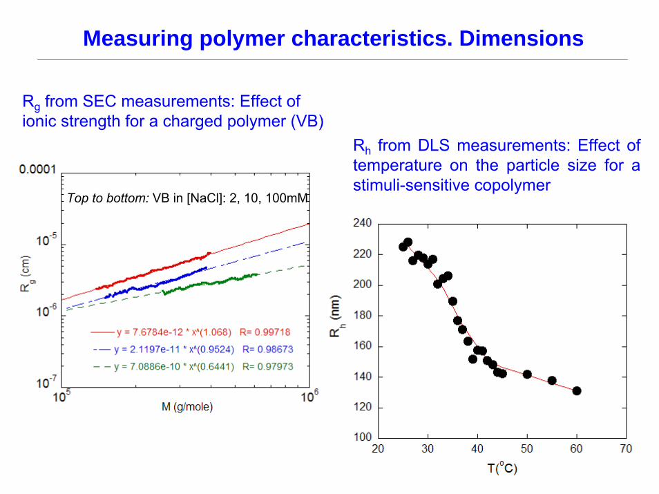
Measuring polymer characteristics. Dimensions

Rg from SEC measurements: Effect of ionic strength for a charged polymer (VB)

Rh from DLS measurements: Effect of temperature on the particle size for a stimuli-sensitive copolymer

Top to bottom: VB in [NaCl]: 2, 10, 100mM

Polymer characteristics. Viscosity

The presence of particles in the solvent creates drag (frictional) forces, which is the origin of viscosity

Total solution viscosity η:

( )22][][1 cc Hs ηκηηη ++= , κH ~0.4 for ideal coils

(Units: 1Poise=1 g/(cm-s))

Intrinsic viscosity of the polymer, [η]:

cc solvent

solvent

ηηη

η−

→=

0lim

][ (Units: cm3/g)

Flory relationship between [η] and RG for ideal coils:

[ ] ( )36 Gv R

MΦ

=η , Φv=2.56x1023

Measuring viscosity

Measurement principle for capillary viscometers: Poisseuille’s law for viscous flow

Poisseuille’s equation: 1 Poise= 1 g/(cm-s)

LQPR

8

4∆=

πη

L, ∆P

R

Q33

8RQ

ave πγ =&Average shear rate:

Single capillary viscometer measures pressure drop ∆P across a capillary of radius R of length L with fluid flowing at rate Q

L

RQ∆P

Differential Pressure Transducer (e.g. Validyne Corp.)

Polymer characteristics. Reduced viscosity

Solvent: 0.1M NaNO3

[η]=403 cm3/g

)(][][ 22

0

0 cOckcr ++=

−≡ ηη

ηηη

η

[ ] red0climηη

→=

(poly(vinylbenzyl sulfonic acid)

Polymer characteristics. Intrinsic viscosity

** Intrinsic viscosity, [η] relationship to M

MNV AH=][η

[η] measures the hydrodynamic volume per mass for a polymer:

This leads to a Mark-Houwink relationship:βη KM=][

For non-free draining coils and other structures:3

GH RV ∝

RG vs. M scaling offers information on the structure (RG RH):

Structure α β

Sphere 1/3 0

Ideal Random Coil 1/2 1/2

Random Coil with excluded volume

3/5 4/5

Rod 1 2

13 −=→= αβαaMRG

Measuring polymer characteristics : SEC

Raw SEC chromatogram: Each detector responds to a different polymer characteristic.

][* ηC∝

MC *∝

C∝

Measuring polymer characteristics : SEC

E.g. Complete multi-detector SEC analysis of a polyacrylamide

0

1 10-5

2 10-5

3 10-5

4 10-5

5 10-5

6 10-5

10

100

1000

104 105 106 107

c (g/cm3)

Rg (A

ng.), [η] (cm3/g)

M (g/Mole)

[η]=0.028M0.69

Rg =0.16M0.56

Mn=83,000 g/Mole

Mw=384,000

Mz=1,030,000

<S2>1/2

w=306 Ang.

<S2>z=386

[η]w=177cm3/g

PolyAcrylamide w/aqueous eluent

From SEC viscosity measurements: Mark - Houwinkcoefficients

E.g. [η] vs. M for copolymer samples in aqueous medium

βη KM=][

Polymer characteristics. Branching

Zimm-Stockmayer branching parameter:

12

2

<=unbranched

branched

S

Sg

- g needs a model in order to be interpreted

2

23nng −

=

e.g. For star molecules with n branches:

e.g. For randomly branched polymers of n branches of functionality f:

( ))2)(1(

6*2)2)(1(2

32/1

−−−

−⎟⎟⎠

⎞⎜⎜⎝

⎛−−

=ffnf

ffng π

0

0.1

0.2

0.3

0.4

0.5

0.6

0.7

0.8

0 20 40 60 80 100

Branching_Zimm_Stockmayer

g, f=3

g, f=4

g, f=8g

n= # of branches

Random branches of functionality f withrandom chain lengths

Polymer characteristics. Branching

- A related branching parameter is g’, obtained from [η]:

unbranched

brancehdg][]['

ηη

= βεε −== 2 ,' gg,

100

1000

104

105

106

107

108

0 5 10 15 20 25 30 35

LinearBranched

M

Elution Volume (ml)

Contrasting elution behavior between a branched polymer and its linear analog

Polymer characteristics - charged polymers

** Electrically charged polymers: Polyelectrolytes

Polyelectrolyte dimensions and electrostatic repulsion diminish with added salt; viscosity decreases, light scattering increases.

Ionic strength increasing

Measuring polyelectrolyte characteristics

E.g.: Sodium hyaluronate (HA). [NaCl] ramp at fixed polymer concentration

Effects of ionic strength on polyelectrolyte interactions and viscosity:

- light scattering increases as ionic strength shields the charges on the HA.

- viscosity drops as the shielding leads to a contraction in the coil size.

Light Scattering

Visc.R

g(A

)

[NaCl] (M)

Sorci, Reed, Macromolecules 2002

Polymer characteristics

Dilute, c<<c* Semi-dilute, c~c*

Concentrated, c>>c*

** Concentration regimes in polymer solutions

The overlap concentration c*, is often approximated by c*~1/[η]

Concentration regimes in polymer solutions. High throughput screening of polymerization reactions

0 100

5 10-5

1 10-4

1.5 10-4

2 10-4

0 1000 2000 3000 4000 5000 6000

I R @

θ=

900 (

cm-1

)

I AAA1

I AAA2

I BCC

I CAA1

I BAA1

I BBB

I BAA2

I CAA2

Signatures from polymerizing solutions in different conditions, with fits to theoretical forms.

Acrylamide polymerization

tDrenski, Mignard, Alb, Reed, J. Comb. Chem 2004

Measuring polymer characteristics during reaction:

Automatic Continuous Online Monitoring of Polymerization

reactions: ACOMP

ACOMP is normally a non-chromatographic method, although in certain applications its performance can be enhanced by addition of SEC

ACOMP configurations

- Continuously extract and dilute viscous reactor liquid producing a stream through the detectors so dilute that detector signals are dominated by the properties of single polymers, not their interactions.

** Principle of ACOMP:

ACOMP ‘front-end’: Extraction/dilution/conditioning

ACOMP ‘back-end’: Detector train

UV detector

Refractive indexdetector

Viscometer

Light scattering

Solvent

Reactor

Optional automatic SEC

Detector train

Auto-Injector/pump

Some complete ACOMP systems

Commercial ACOMP unit previously produced by Varian Inc. under license from Tulane University

A typical, custom built ACOMP at PolyRMC

ACOMP: Rapidly expanding applications

• Free radical homo- and copolymerization

• Step growth

• Controlled radical (co)polymerization (ATRP, NMP, RAFT) and other living types (ROMP)

• Batch, semi-batch, continuous, pressurized reactors

• Solvent, bulk (viscosity up to 106cP)

• Heterogeneous phase polymerization; free and controlled radical routes

• Grafting and cross-linking reactions, multiblock syntheses

• Predictive and feedback control of reactions

• Monitoring the evolution of stimuli responsiveness in tailored polymers

• Post-polymer modifications; e.g. hydrolysis, quaternization

• On the horizon: Extension to slurries, fluidized bed

Kinetics of polymerization and the Quasi-Steady State Approximation (QSSA), followed with ACOMP

Initiator decomposition: [I2]= [I2]o exp (-kdt)

Radical concentration, [R] d[R]/dt = 2Fkd [I2] – kt [R]2

(F = fraction of radicals yielding propagating chains, ‘radical efficiency’)

-For [I2] decomposition rate limited initiation:

d[m]/dt= - 2Fkd [I2]- kp[R][m]~ -kp [R] [m] (long chain approximation)

The quasi-steady state approximation (QSSA): d[R]/dt= 0

k=kp [R](expo-exponential monomer consumption)

If [I2](t) ≈[I2]0 then

Kinetic chain length:

i.e. Mw decreases during the reactions

t

2d

k]I[Fk2

]R[ = ( )⎥⎦

⎤⎢⎣

⎡−= − 1e

kAk2

expm)t(m 2/tk

d

p0

dt0 e]m[]m[ κ−=

]R[k]m[k

t

p=ν )2f1(M)f(M 0ww −≅

,

Typical ACOMP raw data

E.g. RAFT copolymerization of butyl acrylate (BA) and methyl methacrylate(MMA)

Comonomer concentrations

From continuously collected RI and UV signals CFc

dcdnc

dcdnc

dcdnV P

PB

BA

ARI /)( ++=

lcccV PPBBAAUV )( εεε ++=Or, alternately, for charged monomers, from monitoring conductivity in aqueous medium from SEC.

Comonomer concentratons

Monomer conversion

E.g. free radical polymerization of acrylamide . Conversion curves with first-order function fits

0

0.2

0.4

0.6

0.8

1

0 500 1000 1500 2000

Mo

nom

er c

onve

rsio

n

[Persulfate]/[AAm] (M/M)Top to bottom:0.10.0250.01250.0060( )t

cc

ftotal

mon κexp11 −=−=

CFcdc

dncdc

dnV polpol

monmon

RI /)( +=

lccV polpolmonmonUV )( εε +=

polmontotal ccc +=

t0 e]m[]m[ κ−=

Molecular weight in free radical polymerizationE.g. free radical polymerization of acrylamide . Conversion curves with first-order function fits

Kinetic chain length:

0 0.2 0.4 0.6 0.8 1

T=60C[Persulfate]/[AAm] (M/M)Top to bottom: 0.006, 0.025, 0.1

Large circles are GPC data from aliquotswithdrawn during the reaction.

]R[k]m[k

t

p=ν , temm κ−= 0][][

)2

1()( 0

fMfM ww −≅

i.e. Mw decreases during the reactions

Molecular weight in CRP vs. free radical polymerization

Radical transfer reactionsThe radical is transferred to a monomer, another chain, solvent, or other molecule.

Generally, the effect of chain transfer is to shorten the chains.

Transfer of a radical to agent, S: P*SSR 3k +⎯→⎯+

S* bears the transferred radical, P is the dead polymer chain' P left. S* can initiate another propagating chain

SRm*S 4k +⎯→⎯+

No loss of propagating free radical but rate of producing chains increases, since

]R][S[k]R[Ykdt

]P[d3

2t +=

(Y = 1 for recombination dominates, and 2 for disproportionation).

]R[k]m[k

t

pinst =ν

AAmp

3

inst,ninst,n M]m[k]S[k

)0]S([M1

M1

+=

=

Chain transfer in free radical polymerization

increasing ethanol concentration:cAam=0.034g/ml

0-0.743M

[S]k[R]Yk[m]Mk

Mtrt

AAmpinstn, +

=

E.g. Free radical polymerization of acrylamide . Effect of alcohols used as chain transfer agents on the polymer molecular weight

Chain transfer in emulsion polymerization

E.g. Free radical polymerization of methyl methacrylate (MMA) . The effect of the transfer agent on the polymer molecular mass and reduced viscosity

MMA, 15% solid content

n-dodecyl mercaptan added

Chain transfer in living polymerization

E.g. Nitroxide mediated polymerization. Deviations in Mw due to chain transfer

(NMP of butyl acrylate in butyl acetate with MONAMS/SG1)

Pn-X Pn.

X

M

+

kp kt

kact

kdeact

Drenski, Mignard, Reed. Macromolecules, 39, 8213, 2006

[BA]=2.08M, [AIBN]=2.42mMT=70oC

Monitoring the ‘livingness’ of controlled radical polymerization

Monitoring the transition from ‘living’-like behavior in the ‘controlled radical polymerization’ regime, to the non-controlled radical polymerization regime:

[DoPAT]: 0 (top) to 5.69mM (bottom)

E.g. Polymerization of butyl acrylate (BA)

Alb, Serelis, Reed, Macromolecules, 41, 2008

ACOMP and copolymerization: the copolymer is ‘born characterized’

Model independent:

♦ Average Bivariate Mass/Composition distribution

♦ Composition Drift

♦ Average viscosity distribution

♦ Reaction kinetics

♦ ‘Events’; e.g. microgelation due to composition drift

Model dependent:

♦ Reactivity ratios

♦ Average sequence length distributions

Copolymerization: Discrimination of comonomers of similar spectral characteristics

Random copolymer AABABAAABBAB , (40/60 BA/MMA)

total conversion

Inst

anta

neou

s fra

ctio

n of

BA

Average composition drift during MMA/BA free radical copolymerization reactions

c (g/cm3)

λ (nm)

MMA

BA

copol.

t (s)

MMA

BA

t=8,000s (start reaction)

t (s)

Average extinction coefficient basis spectra for MMA, BA and the copolymer); computed comonomer concentrationin detector train.

(Alb, Enohnyaket, Head, Drenski, Reed, Reed, Macromolecules, 39, 2006)

Copolyelectrolytes

UV

@20

6, 2

60nm

, con

duct

ivity

(V)

solv. base.

Aam Aam+VB

Reactionstarts

LS90o

Visc.UV260

Conductivity

UV206

t (s)

Unified understanding of copolyelectrolyte properties via monitoring of their synthesis and subsequent endproduct characterization

t (s)

Mw(g/mole)

conversion

Large composition drift leads to bimodality

'Trivariate distribution': Mass, Composition, linear charge density (ξ)- add conductivity monitoringCounterion condensation: Composition dist. ≠ x dist.

Alb, Paril, Catal-Giz, Giz, Reed, J. Phys. Chem. B, 111, 2007

Diblock copolymers by RAFT

E.g. RAFT copolymerization of MMA/BA

AAAAAAAAAAABBBBBBBBBBB

Alb, Reed, unpublished results

Dilute with solvent and BAand begin BA block

MMA, first block True diblock

If BA onlyhomopolymerizes

Light scattering and UV data agree well with theoretical predictions for a true diblock copolymer

[BA]=0.08M; [MMA]=2.9M, T=70oC

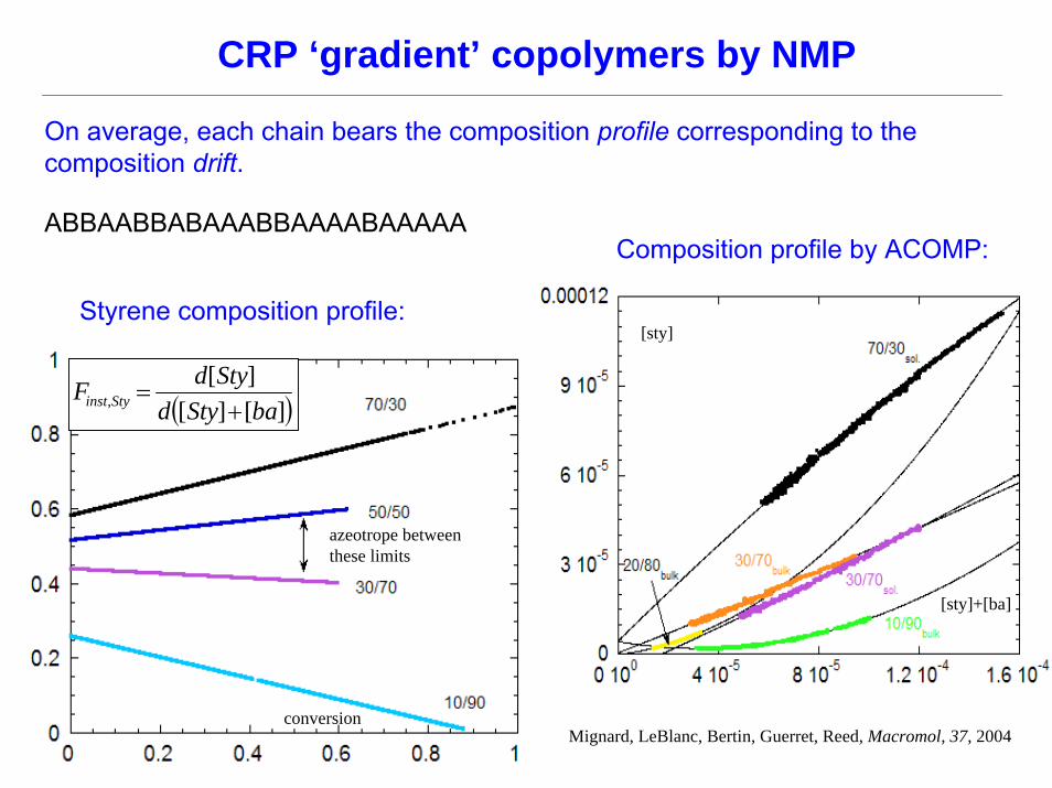
CRP ‘gradient’ copolymers by NMP

On average, each chain bears the composition profile corresponding to the composition drift.

ABBAABBABAAABBAAAABAAAAAComposition profile by ACOMP:

[sty]

[sty]+[ba]

Styrene composition profile:

conversion

azeotrope between these limits

( )][][][

, baStydStydF Styinst +

=

Mignard, LeBlanc, Bertin, Guerret, Reed, Macromol, 37, 2004

Simultaneous continuous non-chromatographic and discrete chromatographic detectionFree radical polymerization of butyl acrylate with an initiator boost

‘front-end’:

dilution/conditioning

SolventReactor

‘back-end’:Light

ScatteringViscometerRefractive

IndexDetector

UV detector

Automatic GPC detector trainLight Scattering

ViscometerRefractive Index Detector

UV detector

SEC data from several detectorsfollow the reaction progress.

ACOMP signals change as the reaction proceeds

ACOMP-SEC system

A M. Alb, M F. Drenski, W F. Reed, J. Appl. Polym. Sci., 13, 2009

Emulsion polymerization- first simultaneous online monitoring of both polymer and particle properties

Left: polymer Mw and ηr vs. conversion; Right: particle size distribution and specific surface area

Raw data and analysis for free radical polymerization of MMA in emulsion at 70C.

A. M Alb, W. F Reed, Macromolecules, 41, 2008

Mw for living vs. free radical polymerization in emulsion

Different trends for Mw as BA is added in one shot or continuously for NMP and for free radical polymerization reactions

Predictive control through programmable reagent flow to the reactor (semi-batch)

- Free radical (co)polymerization

Detailed, quantitative reaction kinetics yielded by ACOMP allow for predictive control

• Control of conversion kinetics

• Control of molecular weight distribution

• Control of copolymer composition

Predictive control for free radical polymerization

Approach to quasi-steady state through monomer feed to the reactor

⎟⎟⎠

⎞⎜⎜⎝

⎛

⎭⎬⎫

⎩⎨⎧

⎟⎟⎠

⎞⎜⎜⎝

⎛ +−−⎟⎟

⎠

⎞⎜⎜⎝

⎛+

+⎭⎬⎫

⎩⎨⎧

⎟⎟⎠

⎞⎜⎜⎝

⎛ +−= t

VV

Vmt

VV

mtm0

0

00

00 exp1]'[exp][)]([

αραρ

ραρ

00

][]'[ mV

m<⎟⎟

⎠

⎞⎜⎜⎝

⎛+ αρ

ρ

‘Starved regime’

00

][]'[ mV

m>⎟⎟

⎠

⎞⎜⎜⎝

⎛+ αρ

ρ

‘Flooded regime’

00

][]'[ mV

m=⎟⎟

⎠

⎞⎜⎜⎝

⎛+ αρ

ρ

‘Isoreactive regime’

( )( )flow

reaction

//

dtdmdtdm

A =

Approach Index, A

Early results on predictive control of polymer Mw

Use detailed knowledge of kinetics from ACOMP to control evolution of Mw

E.g. Acrylamide free radical polymerization

In batch mode, Mw decreases during conversionIn semi-batch mode, Mw is programmed

• for constant Mw

• for increasing Mw

Kreft, Reed, ?

Predictive control for free radical copolymerization

Control of composition drift for high drift comonomers VB and Am

High drift monomer pair

Styrene sulfonate, VB

C

O

CH CH2NH2

Acrylamide, Am

Reactivity ratios

rVB=2.14

rAm=0.18 15% starting VB, 60c, [V50]=0.002M, and [Am]+[VB]=0.360M

Predictive control for free radical polymerization in emulsion

E.g. Semi-batch free radical polymerization of methyl methacrylate in emulsion

The effect of the rate of monomer addition on reaction kinetics

(MMA polymerization at 70C)

Predictive control for free radical polymerization in emulsion

The effect of the rate of monomer addition on Mw

Monitoring postpolymerization modifications

E.g. Postpolymerization production of a polyelectrolyte: NaOH hydrolysis of acrylamide to carboxylate.

Many modifications are possible: e.g.HydrolysisAminationGrafting, cross-linking Huisgen cycloaddition, ‘Click reactions’

Paril, Alb, Reed, Macromolecules, 40,4409, 2007

2nd generation ACOMP for determination of LCST

Measuring the onset of lower critical solution temperature with second generation ACOMP during copolymerization of NIPAM with styrene sulfonate

Conclusions

Light scattering and other physical approaches are one way physicists contribute to interdisciplinary polymer science

Automated, online, multi-detector methods provide massive data streams yielding rich, comprehensive characterization of equilibrium properties and non-equilibrium processes in polymer solutions for both fundamental and applied goals

Polymer Analysis and Characterization

Documents

Transcript of Polymer Analysis and Characterization