The Implicit Cost of Environmental Protection:

Pollution Performance and Chemical Industries

in the European Union

Florian Klein

Ph.D. Thesis, Department of Geography and Environment

London School of Economics and Political Science

University of London

UMI Number: U209734

All rights reserved

INFORMATION TO ALL USERS The quality of this reproduction is dependent upon the quality of the copy submitted.

In the unlikely event that the author did not send a complete manuscript and there are missing pages, these will be noted. Also, if material had to be removed,

a note will indicate the deletion.

Dissertation Publishing

UMI U209734Published by ProQuest LLC 2014. Copyright in the Dissertation held by the Author.

Microform Edition © ProQuest LLC.All rights reserved. This work is protected against

unauthorized copying under Title 17, United States Code.

ProQuest LLC 789 East Eisenhower Parkway

P.O. Box 1346 Ann Arbor, Ml 48106-1346

1 0 f S' 2 0 * )

Abstract

This thesis is about environmental competition. The underlying question is whether or

not countries, or, more specifically, regulators and markets, compete among each other

by the means of trading-off environmental assets such as clean air for economic

performance. On the balance of the empirical results, the preliminary answer is yes -

with some qualifications attached.

After a comprehensive review of the literature on approaches towards the analysis of

environmental performance across various social sciences, this thesis sets out to

construct a proxy indicator for environmental performance, based on the relative

performance across EU countries concerning several air pollutants.

Using that indicator, this thesis classifies 15 EU member states according to their

empirically observed pollution performance during the period 1990 to 1999. The

classification produced four distinct clusters: poor and strong pollution performers, as

well as two transition clusters.

The second part of the thesis evolves around the idea to relate air pollution performance

to a number of chemical industry performance variables using panel data. The main

hypothesis to be tested is whether strong pollution performance has an impact on

chemical industry performance, and if so, what the sign of that relationship would be.

The three performance variables are production value, employment, and value of intra-

EU exports.

The results of the regression analysis show that strong pollution performance has a

negative and significant impact on two of the three chemical industry performance

variables, namely, on production value and intra-EU exports. On the other hand, this

study does not produce evidence that strong pollution performance has an impact on the

employment of the chemical industries in the EU.

2

Acknowledgements

First of all, I would like to thank my two supervisors, Professor Andres Rodriguez-Pose

and Dr Eric Neumayer for their constant help and constructive critique over the last

years. Thank you so much for your effort, patience and rigour.

This investigation would not have been started without the encouragement of my

family. Thank you so much for believing in me, for your advice, and for making it

possible for me to study abroad.

The process of writing this thesis would have been much less pleasant without the many

colleagues I met ‘along the way’ -in London, Corfu, Florence, Munich, and Madrid.

Thank you so much for your ideas, laughs, academic and mental support, and

friendship.

Finally, this thesis would never have been finished without the love, as well as the

valuable expertise, of my wife Paloma. Thank you so very much for the amazing

teamwork, Palo.

This research has been carried out with the financial support of a doctoral scholarship,

which was kindly granted by the German Academic Exchange Service (DAAD).

3

Contents

1 A Comparative Study on Environmental Competition..........................................................10

1.1 A popular myth -challenged........................................................................................................ 10

1.2 Set-up of this thesis...................................................................................................................... 12

2 The Context: three basic concepts............................................................................................18

2.1 Environmental performance......................................................................................................... 18

2.1.1 The subtle art of naming environment-related issues..................................................... 21

2.1.2 Approaches towards the study of environmental performance in social science...........26

2.1.2.1 The political level: Environmental policy analysis.....................................................27

2.1.2.2 The legislative level: Environmental legislation analysis...........................................31

2.1.2.3 The technical level: Environmental regulation and standards analysis..................... 36

2.1.2.4 Pollution performance analysis...................................................................................41

2.2 Links between environmental performance and economic activity............................................ 45

2.2.1 The link between economic development and pollution performance........................... 47

2.2.2 Theories on indirect links between the economy and pollution performance................ 52

2.2.2.1 Environmental regulation and innovation...................................................................52

2.2.2.2 Environmental regulation and barriers to market entry..............................................59

2.2.2.3 Environmental taxes and the economy.......................................................................61

2.3 Environmental competition..........................................................................................................65

2.3.1 The trade-off between pollution performance and industrial production....................... 65

2.3.2 The impact of environmental regulation on trade............................................................66

2.3.3 Competitive advantages in trade through environmental externalities........................... 72

2.3.4 Spatial implications of the environment-economy trade-off: location theory................ 74

2.3.5 Synergies between environmental performance and regional development................... 78

2.4 Concluding remarks..................................................................................................................... 81

2.5 The contribution of this thesis to the literature............................................................................82

4

3 Data: Dependent and Independent Variables.........................................................................84

3.1 The dependent variables: EU chemical industry performance.....................................................84

3.1.1 What do we mean by chemical industry?....................................................................... 84

3.1.2 Importance and performance of the chemical sector...................................................... 95

3.1.2.1 The contribution of chemical industries to GDP........................................................99

3.1.2.2 Chemical industries and labour markets................................................................. 108

3.1.2.3 Chemical industries and trade................................................................................... 114

3.1.3 Restructuring of the chemical sector in the European context......................................118

3.1.3.1 Structural differences among EU member states...................................................... 118

3.1.3.2 Drivers and trends of the restructuring..................................................................... 125

3.1.4 Evidence on the link between chemical industries and pollution performance............. 128

3.1.4.1 The impact of chemical industry activity on pollution performance.......................129

3.1.4.2 The impact of environmental performance on chemical industry activity................132

3.2 The independent variables.......................................................................................................... 137

3.2.1 Air pollution performance............................................................................................. 139

3.2.1.1 Methodology..............................................................................................................139

3.2.1.2 Population-based Pollution Load Index (PLI).........................................................154

3.2.1.3 GDP-based General Pollution Intensity (GPI).......................................................... 157

3.2.1.4 GDP-based Manufacturing Pollution Intensity (MPI).............................................. 161

3.2.1.5 Interpreting air pollution performance patterns....................................................... 164

3.2.1.6 A pollution performance ‘ranking’ of EU member states......................................... 173

3.2.1.7 GPI 3 as lead pollution performance indicator......................................................... 194

3.2.2 Taxes on imports and production.................................................................................. 196

3.2.3 Fuel price........................................................................................................................199

3.2.4 Productivity of the manufacturing sector......................................................................202

3.2.5 GDP............................................................................................................................... 204

4 Regression Analysis.................................................................................................................. 205

4.1 The framework to the regression analysis..................................................................................205

4.1.1 Research hypotheses...................................................................................................... 205

4.1.2 Theoretical model.......................................................................................................... 207

4.1.3 The regression model.................................................................................................... 210

4.2 Regression Results..................................................................................................................... 213

4.2.1 Models on chemical industry production......................................................................214

4.2.2 Models on chemical industry employment....................................................................226

4.2.3 Models on intra-EU chemical industry exports.............................................................230

4.2.4 Summary of the empirical observations........................................................................238

5

5 The scope of environmental competition: some conclusions from this study.....................240

5.1 Summary of the main findings................................................................................................... 240

5.2 Directions for future research.....................................................................................................243

5.3 Cost and benefits of environmental protection: some policy implications from this study 244

Appendices........................... ....................................................................................................................248

Appendix 1: Pollution performance indicators.....................................................................................248

Appendix 2: Regression variables........................................................................................................ 281

Appendix 3: Regression Results........................................................................................................... 290

Bibliography......................................................................................................................................................338

6

TablesTable 1 Comparison of different chemical industry classifications

Table 2 Anthropogenic S 0 2 emissions per capita

Table 3 Air pollution data availability (national level)

Table 4 Anthropogenic S 0 2 emissions / GDP

Table 5 Manufacturing S 0 2 emissions / manufacturing GDP

Table 6 Advantages and disadvantages of the pollution performance indicators

Table 7 Correlation coefficients between pollution performance indicators

Table 8 Pollution performance scenarios

Table 9 Pollution performance indicators: poor pollution performers

Table 10 Pollution performance indicators: countries that catch-up

Table 11 Pollution performance indicators: countries that fall behind

Table 12 Pollution performance indicators: strong pollution performers

Table 13 Empirical pollution performance clusters

Table 14 Tax rates on chemical industry production factors

Table 15 Regression estimates on Cl production value / GDP

Table 16 Regression estimates on Cl production value, absolute terms

Table 17 Actual and predicted changes: Cl production value / GDP

Table 18 Actual and predicted changes: Cl production value, absolute terms

Table 19 Regression estimates on Cl employment / total workforce

Table 20 Regression estimates on Cl employment, absolute terms

Table 21 Regression estimates on Cl intra-EU exports / GDP

Table 22 Regression estimates on Cl intra-EU exports, absolute terms

Table 23 Actual and predicted changes: Cl intra-EU exports / GDP

Table 24 Actual and predicted changes: Cl exports, absolute terms

Table 25 Summary of regression results

Table 26 Anthropogenic emissions per capita

Table 27 Anthropogenic emissions / GDP

Table 28 Manufacturing emissions / manufacturing GDP

Table 29 Pollution load index

Table 30 General pollution intensity

Table 31 Manufacturing pollution intensity

Table 32 Taxes on production and imports

Table 33 Fuel price

Table 34 Labour productivity of the manufacturing Sector

Table 35 Pollution performance

Table 36 Chemical industry production value at 1995 prices

88

145

153

158

162

165

169

176

179

183

188

189

192

196

216

218

220

224

227

228

231

233

234

236

238

248

255

262

265

271

277

281

282

283

283

284

7

Table 37 Chemical industry production value / GDP at 1995 prices 285

Table 38 Chemical industry employees (absolute terms) 286

Table 39 Chemical industry employees / total workforce 287

Table 40 Chemical industry intra-EU exports (absolute) 288

Table 41 Chemical industry intra-EU exports / GDP 289

Table 42 Regression models on Cl production / GDP, Ireland included 290

Table 43 Regression models on Cl production / GDP, Ireland excluded 294

Table 44 Regression models on Cl production in absolute terms, Ireland included 298

Table 45 Regression models on Cl production in absolute terms, Ireland excluded 302

Table 46 Regression models on Cl employees / total workforce, Ireland included 306

Table 47 Regression models on Cl employment / total workforce, Ireland excluded 310

Table 48 Regression models on Cl employment in absolute terms, Ireland included 314

Table 49 Regression models on C l employment in absolute terms, Ireland excluded 318

Table 50 Regression models on C l intra-EU exports / GDP, Ireland included 322

Table 51 Regression models on Cl intra-EU exports / GDP, Ireland excluded 326

Table 52 Regression models on Cl intra-EU export in absolute terms, Ireland included 330

Table 53 Regression models on Cl intra-EU export in absolute terms, Ireland excluded 334

Figures

Figure 1 Spectrum of environment-related concepts in social science 24

Figure 2 An environmental policy circle 25

Figure 3 EU chemical industry production by sector 91

Figure 4 Material input of chemistry in the manufacture of selected consumer goods 97

Figure 5 EU domestic consumption of chemical products by economic sector, 1995 98

Figure 6 Chemical industry production value as percent of total manufacturing production 100

Figure 7 Chemical industry production value (absolute) 101

Figure 8 Chemical industry production value / GDP at 1995 prices 104

Figure 9 Employment in chemical industries as percent of total workforce, 1998 109

Figure 10 Chemical industry employees (absolute) 110

Figure 11 Chemical industry employees / total workforce 113

Figure 12 Chemical industry intra-EU exports (absolute) 115

Figure 13 Chemical industry intra-EU exports / GDP 117

Figure 14 Average number of employees per chemical industry enterprise, 1996 119

Figure 15 Absolute number of chemical industry enterprises, 1996 120

Figure 16 Basic chemicals production as percentage of total chemical production

(basic chemistry and specialities) 121

8

123

124

130

143

146

148

155

159

160

163

168

170

172

177

181

185

190

195

198

199

201

203

207

209

210

Highest education degree of the chemical industry workforce, 1995

Patent applications (organic & inorganic chemicals) /

chemical industry employees, 1995

Major industrial C 0 2 sources, 1996

Anthropogenic sulphur (S 0 2) emissions in EU member states

Anthropogenic sulphur emissions per capita, selected EU member states

Anthropogenic sulphur emissions per capita (EU15):

coefficient of variation and weighted average

Pollution load index (S 0 2 emissions): Finland and Greece

Anthropogenic sulphur emissions / GDP, selected EU member states

General pollution intensity (S 0 2 Emissions): Greece, Netherlands and Spain

Manufacturing S 0 2 emissions / manufacturing GDP, EU member states

Empirical pollution performance indicators, Denmark

Empirical pollution performance indicators, Ireland

GPI 3, Germany and United Kingdom, 1990 to 1999

Pollution trends: poor pollution performers

Pollution trends: countries that catch-up

Pollution trends: countries that fall behind

Pollution trends: strong pollution performers

General pollution intensity indicator (GPI 3)

Taxes on production and imports as % of GDP

EU chemicals producer price vs. crude oil price, U.S.S, Indexed (1990=100)

Price of high sulphur fuel oil for industrial customers, U.S.S at 1995 prices

Labour productivity of the manufacturing sector,

thousands of € at constant prices

Reduced theoretical model

Extended theoretical model

Layout of the regression framework

9

1 A Comparative Study on Environmental Competition

1.1 A popular myth -challenged

The old regulations, let me start o ff by telling you, undermined our goals for protecting the environment and growing the economy. The old regulations on the books made it difficult to either protect the economy o r —protect the environment or grow the economy. Therefore, I wanted to get rid o f them. I'm interested in job creation and clean air, and I believe we can do both.

George W. Bush on his Clear Skies Initiative, speaking at the Detroit Edison Monroe Power Plant in Monroe, Michigan, on 15 September 2003

This thesis is about environmental competition. The underlying question is whether or

not countries, or, more specifically, regulators and markets, compete among each other

by the means of trading-off environmental assets, such as clean air, for economic

performance. There are examples in the social science literature of similar forms of

competition, such as fiscal competition, or competition in the field of social security. As

the above quote illustrates, the notion of environmental competition has long found its

place in governmental agendas.

However, it seems that the relationship between environmental performance and

economic competitiveness remains an issue with many unknowns. For one, we have

considerable difficulties to define what exactly ‘environmental performance’ stands for.

There are plenty of concepts in social science on the issue, but, as the literature review

chapter will illustrate, there seems to be no integrating theory with the power to

combine the approaches distinct academic disciplines.

10

Secondly, scholars have to face severe problems concerning environment-related data.

Most of these problems fall in two broad categories, which, paradoxically, appear to

stand in conflict at first sight. On the one hand, there are too little consistent and

comprehensive environmental indicator data sets. If there are data series, they are often

not comparable between each other. And yet, on the other hand, the amount of

environment-related information that is available is incredibly large, and at times

contradictory. The practical implication of these two constraints is typically that we

study environmental competition selectively, based on the availability and quality of the

data at hand.

Arguably, the notion of environmental competition describes a basic dilemma of our

time: at some point we have to choose between, say, expanding industrial production

and the preservation of the global climate. Given the enormous implications of such a

choice, it seems curious how most people have accepted the alleged trade-off -quietly

and without challenge.

It appears quite evident that both economic growth and environmental protection are in

the interest of most people. The difficulties start when one has to rate them against each

other. What is more important to us, economic welfare or environmental protection?

Of course, such a simplistic argument does not reflect the full complexity of the

dilemma. Hence, there are an infinite number of variations to this theme. One could

rephrase: what is more important to us, short-term economic gain or the preservation of

opportunities for future generations? How about the choice between developing the

means to feed starving children versus the salvation of the black-spotted owl from

distinction?

The answers to this kind of questions have to come from each one of us, or

alternatively, from the representatives that take such decisions in our name. Scientific

analysis plays an important part in this process -by verifying the existence of the

dilemma, by focusing attention on the choices we have as a society, and, if possible, by

providing hints about the size of the implications we would have to expect.

My thesis aims to be a contribution to that end. In this spirit, let us get ready to crunch

some numbers.

11

1.2 Set-up of this thesis

Research problem

This study is a comparative analysis with two main objectives. The first objective is to

provide a workable measure of ‘environmental performance’. To do so, we will resort to

using a proxy, in the form of an air pollution indicator, which will allow us to compare

the relative performance among the countries in our sample and along time. The second

objective is to establish the statistical relationships between that pollution performance

indicator and a number of data series about the performance of national chemical

industries.

The underlying research question is whether environmental competition did take place

among the countries in our sample, and what type of impact such competition had on

national chemical industries. In order to address this problem, the investigation will

focus on the two following questions. First, can pollution performance be shown to

have a statistically significant impact on chemical industry competitiveness? And

secondly, if there is such a relationship, is strong pollution performance beneficial or

detrimental to chemical industry performance?

The analysis covers the 15 EU member states before the European Union’s latest round

of enlargement in 2004, that is, Austria, Belgium, Denmark, Finland, France, Germany

Greece, Ireland, Italy, Luxembourg, the Netherlands, Portugal, Spain, Sweden, and the

United Kingdom. The observations relate to the period between 1980 and 1999.

Aims and objectives o f the research

The following points summarize the objectives of this thesis:

• Provide an example of a workable quantitative comparative analysis in the field

of environmental competition. This objective includes the establishment of an

extensive literature review on the current state of the art in environment-related

social science, a critical justification of the methods used in this study, and the

development of a proxy for environmental performance.

12

• Based on the findings of the comparative analysis, verify the existence and the

sign of the impact of environmental competition. Obviously, the verification or

rejection of the departing hypothesis is a central objective of any scientific

analysis. However, in the case of this study, there is no ‘preconceived’ result:

the issue whether or not environmental performance can be shown to have an

impact on chemical industry competitiveness is very much an open question at

the outset of the study. For this reason, to find the direction and strength of the

statistical relationship has to be considered a crucial step in the investigation.

• A further aim of this study is to develop a deeper and more differentiated

understanding of environmental competition. If the analysis showed that there is

indeed a relationship between environmental performance and industrial

activity, this study will attempt to differentiate the observed link. First, does

environmental performance impact equally across different indicators of

industrial competitiveness? Are there clusters among EU member states with

regard to environmental performance? And if so, did the impact of

environmental performance on industrial activity differ among those clusters?

• Contribute to the empirical literature on environmental competition in the EU.

Given the huge body of literature around the economy-environment trade-off, it

seems surprising how few empirical studies so far have compared EU member

states. As the literature review will illustrate, there are plenty of contributions

with a comparative approach among U.S. states, many case studies on individual

EU member states, and some comparative analyses on a selection of EU member

states.

13

Yet, few empirical analyses look at environmental competition among EU

member states. This appears even more surprising when one considers what an

interesting object of investigation the European Union currently makes: a

common market with an increasingly integrated legal system - but at the same

time an, in many ways, heterogeneous cluster of nation states, each attempting

to guard its national interests. Interestingly, industrial and environmental

policies are two policy fields in which EU member states appear to be especially

reluctant to transfer powers to Brussels. All in all, it seems a rather fascinating

setting for a comparative analysis.

General structure and brief overview on each chapter

There are four main parts to this thesis: a literature review that provides the context to

this analysis, a detailed description on the set-up of the quantitative analysis as well as

on the dependent and independent variables, the presentation of the findings of the

analysis, and finally, a concluding section that discusses the findings and relates them to

the literature context.

First, based on an extensive literature review, chapter 2 will provide the context to this

analysis. There are two central themes which will be at the heart of the literature review.

One of them revolves around the notion of environmental performance. This section

describes how different fields of social science sought to understand and capture the

complex idea of environmental performance. The final objective of this section is to

justify why pollution performance may be considered a valid proxy for environmental

performance at large. The second theme of the literature review aims to highlight

theories that could help to explain the relationship between environmental performance

and economic activity, and how those links can be the subject of environmental

competition among countries.

14

Chapter 3 focuses on the presentation of the data used in the subsequent sections. The

chapter starts off by describing the chemical industry, since it is the dependent variable

of the regression analysis. It addresses four guiding questions: what is the chemical

industry? Why is it so important? What have been the drivers of its recent restructuring?

And finally, what are the links between chemical industry activity and pollution

performance? The second part of chapter three introduces the independent variables.

The main independent variable, air pollution performance, is presented in detail and

used to construct a relative performance indicator. The remainder of the section

discusses the other independent variables.

Chapter 4 is dedicated to the regression analysis. It starts by presenting the framework

to the empirical study. It then reports the empirical estimations of the impact of the

independent variables on chemical industry production, employment, and intra-EU

exports. It also compares the predicted contribution of the explanatory variables to the

actually observed figures.

Finally, chapter 5 concludes; after presenting a summary of the main findings, and

discussing the contribution of the thesis to the literature, it discusses shortly future

fields of research that may be pursued to follow up this study.

Summary and short discussion o f the results

The research problem at the heart of this investigation is whether or not countries

compete among themselves by the means of ‘playing’ with their environmental

performance in order to foster industrial activity. The empirical results presented here

appear to indicate that, on balance, the preliminary answer to that question is yes -with

some qualifications attached.

In order to reach this conclusion, the first step is to construct a proxy indicator for

environmental performance. As the literature review will show, there are several

approaches to deal with environmental performance in social sciences. After a

discussion of the advantages and disadvantages of each approach, this investigation will

rely on a quantitative comparative analysis on air pollution performance patterns.

15

Since the frame of reference for this thesis is a closed system (the 15 EU member

states), the air pollution time series reflect the relative performance of the countries

within the system. The advantage of this approach is that it is comparative in nature -

once the indicator is developed, one can easily work out distinct pollution performance

patterns, rank countries according to their pollution performance, or classify them into

performance clusters.

Using the air pollution indicator, one finding of this thesis will be the classification of

EU 15 member states according to their empirically observed pollution performance

during the period 1990 to 1999. The classification yields four distinct clusters. There

were two “clear-cut” performance clusters with countries that were either clearly poor

pollution performers or strong pollution performers. Furthermore, there are two

‘transitory’ pollution performance clusters. The first of those two clusters comprises

countries in the process of catching-up: its constituents start from relatively poor

pollution performance levels, but show convergence towards the EU average. The last

cluster contains countries that fall behind in terms of pollution performance. These

countries show strong initial pollution performance levels, but converge downwards

towards (and in some cases, beyond) the EU average.

The second part of the thesis builds on the idea to relate the pollution performance

indicator to a number of variables that capture the performance of chemical industries

using panel data of the 15 countries in the sample along 20 years. The main hypothesis

to be tested is whether strong pollution performance had an impact on chemical industry

performance, and if so, what the sign of that relationship was. There will be three

performance variables: production value, employment, and value of intra-EU exports

-in order to stay within the EU as frame of reference.

16

The results of the regression analysis show that, with regard to two of the three

chemical industry performance variables, strong pollution performance has a negative

and significant impact. This is the case with regard to production value and intra-EU

exports. This finding is in line with conventional economic and location theory, which

states that there is a trade-off between economic performance and environmental

performance. The empirical observations of this thesis lend further support to such

theories. Hence, it seems that the countries in the sample actually do compete by means

of environmental performance.

On the other hand, this study does not produce evidence that strong pollution

performance has had an impact on the employment of the chemical industries in the EU.

Hence, employment seems to respond to a different set of factors.

17

2 The Context: three basic concepts

This investigation departs from the notion that countries, or, to be more specific,

regulators and markets, might compete with each other by adjusting their environmental

performance in such a way that economic actors will be triggered to respond.

The idea that environmental performance plays a role in determining the competitive

background of economies is not new, and there are a number of policy fields, such as

fiscal policies (e.g., Bayindir-Upmann 1998; Biswas 2002) or social policies (Brownen

2003), in which regulative competition between countries is well documented.

The purpose of this literature review chapter is to present the current understanding in

three fields of research, which are fundamental to the idea of environmental

competition. The first part will provide an overview on how social scientists understand

and capture the notion of environmental performance. Building on this outline, the

second part will present theories on how environmental performance, and in particular

pollution performance, have an impact on economic activity. Finally, given the

existence of a link between environmental performance and economic activity, the third

part will discuss how countries use environmental performance to acquire a

comparative advantage over other countries.

2.1 Environmental performance

What is environmental performance, and how could we measure it? Judging from the

wealth of different approaches in social science literature, there is more than just one

way to address the issue. As this section will show, most contributions concentrate on

issues like environmental policy, environmental regulation, environmental standards, or

pollution performance.

18

There are many reasons for this variety in approaches towards environmental

performance. Obviously, most scholars depart from ‘their’ set of theories and methods.

For this reason, political scientists might rather look at environmental policies and

compare them between countries, scholars of law may choose environmental regulation

as their reference, and, as one should expect, environmental economists show a clear

propensity towards quantifiable measures of environmental standards.

Choosing the conceptual framework that corresponds to each academic specialisation

appears straightforward, convenient, and efficient. Yet, there is one crucial drawback to

this multitude of approaches. The body of literature on environmental performance, as

well as on the impact of environmental performance on economic performance -which

one could dub the ‘economy-environment trade-off - appears deeply fragmented.

Thus, the broadness in academic approaches of the field of environmental research may

be somewhat of a misperception. Although on the face of it, distinct contributions from

different disciplines focus on the same issue, for instance on environmental regulation,

they may actually refer to rather incompatible concepts and approaches. The subsequent

literature review chapter will highlight a number of examples on this point.

However, there is one common denominator across all approaches. One central

objective of environmental policies is to define the limits to the human use of the

environment. The rationale behind environmental legislation is to codify and implement

those policies. Finally, environmental standards may essentially be understood as the

qualitative or quantitative expression of said limits concerning the human use of the

environment.

19

Many empirical studies on environmental policies typically resort to qualitative

descriptions in the form of case studies rather than using quantitative indicators. This

makes the task of comparing their results rather tricky. To put it bold and simple, there

appears to be no objective way to rate one environmental policy against another, let

alone to score them. Environmental policies are a central and complicated area of

current policies, and they affect many neighbouring policy fields such as industry,

agriculture, or infrastructure. Moreover, every country has its own political culture and

socio-economic background that could determine the shape and efficiency of

environmental policies. With some qualification, the same appears to hold true with

regard to environmental legislation analyses. In fact, the overwhelming majority of

contributions in comparative environmental law are descriptive in nature.

The great advantage of qualitative studies is their flexibility in describing the observed

reality; among the drawbacks of that approach can be the danger of implicit normative

judgements. By contrast, quantitative measures are often focused on some specific

observation; they could therefore be described as one-dimensional and inflexible.

Moreover, quantitative measures can also contain implicit normative judgements,

especially when they are composite indicators. However, one advantage of quantitative

measures appears to be the fact that if there are implicit normative judgements involved,

they should be relatively obvious to spot.

The human use of the environment generally manifests itself, inter alia, in the form of

pollution. Thus, pollution is one important common denominator among the distinct

scientific approaches that study the economy-environment relationship from a

quantitative point of view. Looking at pollution performance provides an opportunity to

compare the outcome from various environment-related theories, irrespective of their

‘disciplinary’ origin.

20

The advantages of focusing on pollution rather than on environmental policies, laws, or

standards have been stressed in the literature before. For instance, Jahn (1998) argued

that pollution was determined by structural, economic and political factors. As a result,

he concluded that environmental policies or specific features of environmental

regulation could only explain the state of the environment up to some point, but not

entirely. In line with Crepaz (1995) and Janicke et al. (1996), Jahn contended that

focussing on the outcomes of environmental policies rather than analysing the policies

themselves could be one way of overcoming this problem by providing an overview on

the state of the environment as well as, indirectly, on the quality of environmental

policies, regulations, and standards.

A considerable number of comparative studies, among them Lundquist (1980), Knopfel

and Weidner (1985), Henderson (1996), and Becker and Henderson (2000), take air

pollution performance as one focal point of environmental policies. In fact, Crepaz

(1995) and Binder (1996) note that the origins of international comparative analysis

could be identified in this area of research.

Another argument in favour of focusing on pollution performance is the fact that

pollution is a straightforward and, at least to some point, objective concept. This

characteristic sets pollution performance indicators apart from measurements on

environmental policies, environmental laws, or environmental regulation.

2.1.1 The subtle art of naming environment-related issues

One apparently trivial but on second thought fundamental problem in discussing the

state of the environment is the rather confusing nomenclature around the issue in the

literature. In economics and political science alone, there are literally dozens of ways to

name environment-related issues.

21

What exactly is the environment?

There could be several reasons for this apparent conceptual vagueness. For a start, there

are a number of views on how exactly one has to define the term environment. At the

very least, the environment includes its basic physical components, or environmental

media, such as water, air and soil (Bimie and Boyle 1992). Some broader definitions

also include the biosphere, that is, all living things like plants or animals, as well as the

interaction between the different components of the environment.

Yet, other contributions focus on some specific component of the environment, such as

the medium air, or on certain environment-related processes, such as pollution. Because

there is such a multitude of possible investigation foci, ranging from comprehensive to

very specific, it may be little surprise that the nomenclature of environment-related

issues consists of a whole range of terms.

Implicit preferences and judgements

A second cause for the wealth of terms on environment-related issues appears to be the

fact that any reflection on the matter almost automatically involves personal preferences

or judgements, which could manifest itself in the semantics of terming. The perception

of environment-related issues and its processing in the way of academic analysis,

political discourse, or every-day behaviour, seems to depend in no small part on the

personal values and experiences of the processor. For this reason, there are at times

several terms for the same environment-related issue. The terms may well describe the

same observation or concept, but express the perception of the person who reflects on

the issue.

Take as example the terms environmental regulation, environmental standards, and

environmental protection. They could be understood to be congruent in describing the

same thing - the setting of rules that define limits to the use of the environment.

However, each of the terms has a distinct ‘flavour’, and may therefore describe a

slightly distinct concept on the issue.

22

The wording environmental regulation appears to be the least specific among the three

options, both with regard to what kind of rules are being taken and to what objective

those rules have. ‘Regulation’ seems to be a generic term for all kinds of laws, decrees,

procedures, policies and the like, and is therefore unspecific with regard to what type of

environmental rule is meant. Moreover, the term does not provide any clue as to the

purpose of said regulation. If the term was chosen with care, this vagueness may be

exactly the intention of the person who uses the term.

The expression ‘environmental standards’, on the other hand, may indeed imply a

statement on those two points. First, the word ‘standard’ appears to be a much more

specific description of environmental rules. This could be a hint that the person who

uses the term has a rather technical understanding of environment-related issues, as one

would expect of engineers or scientists. More likely than not, ‘standards’ could refer to

some measurable, and therefore comparable, category.

It may also be perceivable that the phrase ‘standard’ contained an unspoken judgement

with the quality or purpose of the environmental rule in question, since it is generally

associated to the notion of higher or lower standards. Most people may instinctively feel

that higher standards are preferable to lower ones. That implicit value judgement

becomes even more apparent if the term environmental protection is used to describe

the setting of environment-related rules. One could argue that the phrase ‘protection’

seems to imply that its subject, in other words, the protected, is in need of such action.

Nuances in the wording of environment-related issues do matter not only because they

may explain the vast number of sometimes congruent notions. They appear noteworthy,

especially with regard to the academic literature, because the terming of environment-

related issues can be an expression of concepts or value judgements that formed the

basis of their analysis.

Different levels o f abstraction

The study of environment-related issues in social sciences takes place on several levels

of abstraction, and this may be a third reason for the multitude of environment-related

terms.

23

Figure 1 is an attempt to illustrate this point. The concept o f environmentalism is related

to the public awareness about environmental issues, which in turn may depend on a

variety o f factors, such as the state of the environment as well as the cultural and socio­

economic background o f the society in question. The only direct way to measure

environmentalism is through opinion polls. It may therefore be fair to state that

environmentalism is a rather abstract concept in social science.

The politics o f the environment are related to environmentalism, since the awareness

about environmental issues among a broader public shapes the political setting. One

example for this relationship may be the rise o f the green party movements over the

seventies and eighties across Europe, and the subsequent incorporation o f

environmental considerations into the political programmes o f mainstream parties. No

doubt, environmental politics is a rather abstract concept, but it still appears more

accessible and measurable than environmentalism.

Figure 1 Spectrum o f environment-related concepts in social science

Environmental Performance

Environmental Standards

Environmental Regulation

Environmental Legislation

Environmental Policy

Environmental Politics

Environmentalism

1Concrete

Level of abstraction

The next link in the chain is environmental policies, which may be understood as the

expression o f environmental politics. Again, environmental policies are a somewhat

more concrete and intelligible concept than environmental politics.

i--------Abstract

24

The remaining environment-related concepts mentioned in the graph follow the same

logic: environmental legislation is the expression of environmental policies in legal

terms. Environmental regulation is the institutional expression o f environmental

legislation. Environmental standards are the technical expression o f environmental

regulation. And finally, environmental performance may be understood as the

objectively perceivable, that is: measurable, expression o f environmental standards.

As a last step, consider that environmentalism depends, among other factors, on the

perceived state o f the environment, which in turn is a function o f environmental

performance. One may, therefore, reach the conclusion that the spectrum of

environment-related concepts laid out above is actually a loop, as depicted in figure 2.

Figure 2 An environmental policy circle

Perception of theenvironm ental situation F orm ulation of policies

Environmentalism

EnvironmentalPerformance

EnvironmentalPolitics

EnvironmentalStandards

EnvironmentalPolicy

EnvironmentalRegulation

EnvironmentalLegislation

Im plem entation T ranslation of policiesinto law

25

The underlying principle of this environmental policy circle (for the lack of a better

term) is that societies deal with environmental issues in four stages. The first stage

relates to the formulation of environmental policies: environmental issues are identified

and undergo “the political process”. The second stage covers the translation of

environmental policies into law. The third stage represents the actual implementation of

those laws. Finally, the fourth stage regards the effects of the implemented measures

and their perception and closes the loop, leading back to the first stage.

2.1.2 Approaches towards the study of environmental performance in social

science

As mentioned before, literature contributions related to environmental performance

originate from a range of academic disciplines, most notably from political scientists,

scholars of jurisprudence, economists, and geographers. Given the enormous number of

theories and approaches, and especially considering the at times confusing ambiguity of

the terms they use, the environmental policy circle can be an instrument to put the

pieces of literature contributions into their proper context.

Each academic discipline has developed a distinct ‘toolkit’ of methods to capture

environmental performance, and to put it into relation with, for example, economic

performance. Accordingly, one way to sort the literature is by grouping the

contributions according to their ‘background’, that is by the academic discipline they

stem from.

However, the following outline follows a different structure, which reflects the logic of

the environmental policy circle. There are two advantages to this approach. For one,

organising literature contributions by their focus on the environmental policy circle, and

not by their academic provenience or by the terms they use to describe the environment-

related issue they refer to, may help the reader to keep a better overview on the matter.

Secondly, the study of environment-related issues is, or at least should be, an

interdisciplinary field of social science. Sorting literature not by their academic

background, but by the interdisciplinary contribution they make, may help to appreciate

their ‘added interdisciplinary value’.

26

2.1.2.1 The political level: Environmental policy analysis

One way to capture the environmental performance of countries can be to look at their

environmental policies. Comparisons can then be drawn both over time, as well as

across countries. In the first case, a typical research question could be analogous to the

following: did the subject country strengthen or weaken its environmental policies? In

the latter case, one would ask how does the environmental policy regime of country x

compare to the environmental policies of country y?

Focus

Typically, contributions in the field of environmental policy analysis focus on the

processes which lead to the development, formalisation, and implementation of

environmental policies. The most commonly used means of environmental policy

analysis are socio-economic studies, political-economy analyses, or political science

case studies.

Studies in this research arena often highlight “the genesis” of environmental regulation;

they are therefore more often than not descriptive or analytic, as well as positive, rather

than predominantly normative. It appears that this descriptive research approach is one

of the main distinguishing features of this field of study vis-a-vis other bodies of

environment-related literature, which focus on the outcome of environmental policies as

expressed in environmental legislation, environmental standards, or environmental

performance (for example, Leveque 1996; Leveque and Collier 1997; Leveque and

Hallett 1997).

27

Theories on environmental policy

Approaching the analysis of environmental policies from the perspective of political

economy, Ciocirlan and Yandle (2003) highlight four possible theories to explain the

process and drivers of environmental regulation. First, the so-called normative theory of

environmental regulation is based on an essentially economic understanding of the

objective of environmental protection, that is, as an exercise of maximising social

welfare subject to constraints. The overarching objective of the regulatory authority is

to serve the public interest. Accordingly, politicians following this approach would

choose instruments to maximise the efficiency of environmental regulation. Unswayed

by special interest pleadings, publicly-interested politicians pursue long-term goals

aimed at maximising social welfare. According to economic theory, politicians need to

calculate the implications of their legislation carefully, and intervene up to the point

where the incremental costs of environmental intervention just offset the associated

incremental benefits (Becker 1985; Stavins 1998).

Unfortunately, there is rather little empirical evidence to support this normative theory.

This has led social scientists to look for alternative theories and models that could

explain the environmental policy making process.

Second, the capture theory, which is generally attributed to the economic historian

Gabriel Kolko (1963), states that politicians are sincerely willing to respond to the

needs of the electorate, but lack essential information on how to do so. Therefore, they

may have to rely on information and guidance provided by those who have much of it to

offer, that is, the industry that is to be regulated, or the special interest groups that plead

to regulate it. Because of this information asymmetry, special interest groups are likely

to manipulate politicians towards their own interests.

28

Third, the special interest theory takes the capture theory one step further to explain

which one of a number of competing special interests will be successful in gaining

influence. According to this theory, politicians can be thought of as brokers who auction

their services to the highest bidder. Taking into account organising and other transaction

costs, the theory holds that the group that can bid the most is the group that has the most

to gain or to lose when politicians act (Stigler 1971; Posner 1974; Peltzman 1976;

Ciocirlan and Yandle 2003).

Fourth, the so-called Bootleggers and Baptists theory (Yandle 1989) departs from the

notion that both environmental groups, which Yandle dubs ‘Baptists’, and industry (the

‘bootleggers’), may advocate the pursuit of the same environmental goal. However, the

motivation behind their action may be very different. Yandle argues that, although

bootleggers wear the clothing of a special concern towards the environment, the implicit

goals behind their actions are more related to protecting their market share and

competitiveness.

Literature examples

There is a host of contributions providing case studies on the political process of

environmental policy making. In order to illustrate the variety of research approaches,

consider this small selection of analyses focused on the European Union: The

contribution of Godard (1996) looked at the process of decision making under scientific

controversy and at the limits to the applicability of the precautionary principle in the

political practice. Golub (1996) analysed the process of political bargaining among

national governments during EU policy making. Taking environmental policy making

as example, Collier (1996) pointed out how the subsidiarity principle is exploited by EU

member states in order to protect their national sovereignty.

29

Analysing the example of Britain and Germany, Knill and Lenschow (1997) highlighted

the importance of administrative traditions to the implementation of EU environmental

policies. Pallemaerts (1998) analysed the development and scope of EU policies on the

export of hazardous chemicals. Kramer (2002) compared the development of

environmental policies in the United States and Europe. Departing from a historic

overview on the different political and legislative traditions in the two regions, he

described the distinct periods of environmental policy development, which have led to

fundamental differences in environmental politics today.

Although the majority of environmental policy analyses appear to stem from political

scientists, there are also a number of interesting interdisciplinary contributions. For

example, Damania (1999) investigated the impact of political lobbying on the choice of

environmental policy instrument by means of modelling the rent seeking behaviour of

the involved actors. The analysis shows that rival political parties have an incentive to

set the similar or equal emission standards. Moreover, emission taxes are more likely to

be supported and proposed by parties that represent environmental interest groups.

Scruggs (1999) examined the relationship between national political institutions and

environmental performance in seventeen OECD countries. His study concludes that

neo-corporatist societies may experience much better environmental outcomes than

pluralist systems.

Summary

One of the principal achievements of this field of literature lies in the description of

national environmental policy traditions, and in highlighting a whole range of different

special interests that can shape environmental policies. Even if the existence and the

impact of those special interests could only be captured in a descriptive way, that

information is important to understand the background to the economy-environment

trade-off.

30

The most obvious advantages of analysing environmental performance through the

perspective of environmental policies lie in the flexibility of the descriptive method and

in the fact that no hard quantitative data is needed. However, the complexity of political

analysis, in particular the existence of “black boxes”, appears to limit the ‘predictive

power’ in linking policies to environmental outcomes.

2.1.2.2 The legislative level: Environmental legislation analysis

Another way of understanding environmental performance could be through analysing

the stringency, timing or comprehensiveness of environmental legislation. The research

emphasis of such an approach is the material content of regulation, as well as, in second

place, its genesis.

Focus

Contributions on environmental legislation typically revolve around the layout of

environmental legal and monitoring systems. Theoretical concepts in the environmental

legislation arena may analyse and discuss the type or allocation of competences in

environmental legislation and enforcement, which may rest at local, regional, national,

or supranational level. Empirical studies often investigate and compare different types

of environmental regulation, such as laws, bylaws, voluntary or negotiated agreements

between regulators and private parties, as well as international legal regimes.

National traditions in command-and-control regulation

One classic topic among scholars in this field is the discussion on the advantages and

drawbacks of so-called ‘command and control’ mechanisms. In this tradition, Heritier

(1995) as well as Ltibbe-Wolff (2001) compared two ‘traditional’ European

environmental law making approaches, that is, the technical or emission-oriented

approach, which is sometimes dubbed the German approach, with the quality-oriented

approach of Britain. The differences between these approaches are not merely of

academic interest, but have very real implications both to regulators as well as for the

regulated.

31

In practice, emission-oriented pieces of legislation could bear a higher workload for

monitoring and enforcement agencies, as all emission sources should be monitored on a

regular basis. Once that technical and administrative problem of monitoring is solved,

emission-oriented regulation appears rather straightforward to enforce. By contrast, the

quality-oriented approach to command-and-control legislation does not so much depend

on individual emission measurements, but stresses the importance that polluters, such as

industrial plants, meet overall environmental quality goals. One way to implement this

approach may be through integrated pollution control programmes.

Adding another ‘national’ approach, Gouldson and Murphy (1998) highlight the Dutch

approach to environmental regulation, which is essentially anticipatory and process

focused. It is typically associated with a flexible and hands-on approach to

implementation and with a consultative and consensual enforcement style. One

characteristic policy tool under this approach is the voluntary agreement that is

negotiated between regulators and regulated.

With a view to assess the potential use of such measures at supra-national level,

Khalastchi and Ward (1998) discussed the practicality of voluntary agreements at EU

level. They conclude that there are a number of open issues, such as transparency or

equal implementation procedures across member states, which need to be resolved

before this policy tool could effectively be applied at EU level.

There are many country case studies on environmental legal systems. Among many

others, Nystrom (2000) highlighted the distinguishing features of the Swedish system of

integrated operating permits. Delams and Terlaak (2002) compared the institutional

environment for negotiated environmental agreements in the United States and three

European Union member states.

32

Self-regulation o f industries

Drackrey (1998) added another perspective by highlighting the potential for industrial

self-regulation schemes. Based on a case study about the “Responsible Care” initiative

of the German Chemical Industry Association, Druckrey argues that self-regulation can

be an effective tool to promote ethical conduct among industrial firms. However, she

notes that such behaviour needs to be supported and acknowledged by the “political and

social framework”.

I f customers are prepared to pay back a company’s ethical “investments ” through greater demand, or i f these investments improve the motivation and productivity o f employees, morality can also be a part o f increased competitive strength.

Druckrey (1998: 980)

However, the idea that firms may ‘behave ethically’ appears contended by other

scholars, especially in the economic literature. As a case in point, Altman (2001) stated

that private economic agents could not be expected to adopt ‘green’ economic policy

independent of regulations since there need not be any economic advantage accruing to

the affected firm in becoming greener. Along the same line of argument, Mullin (2002)

pointed at the often considerable scientific uncertainty under which managers have to

take environment-related business decisions. Even if companies were firmly committed

to business ethics, they might not be able to judge the full consequences of their actions

due to incomplete or contradicting information.

Environmental enforcement and monitoring

Dion et al. (1997) investigated whether plant-level pollution monitoring varies due to

local conditions. Their data reveals that plants whose emissions are most likely to

impose high environmental damages are facing a higher probability of being inspected.

33

According to Dion et al., the probability of inspection appears to be positively linked to

the visibility of the plant. Moreover, they note that the inspection probability appeared

to be a decreasing function of the regional unemployment rate. They conclude that

environmental regulators do not blindly enforce uniform standards given their

commonly limited resources, but distribute their resources according to local conditions.

Expanding the results of Deily and Gray (1991), Dion et al. (1997) contend that

regulators appeared to monitor larger plants for visibility of their actions, thus satisfying

one subset of their electorate. At the same time, regulators appeared to avoid enforcing

the regulation for those larger plants, by which they satisfied another subset of their

electorate.

Focusing on the issue of how infringements against pollution rules are sanctioned, Ogus

and Abbot (2002) argued that enforcement policies in England and Wales may best be

described as ‘cautious’, both with regard to seeking conviction in court as well as with

regard to revoking operating licences of the offending firms. They note that such a lax

sanction regime is cause for concern, as potential offenders commonly assume the costs

resulting from punishment to be low, given the small probability of substantial

imposition. In order to correct this, they argue in favour of other enforcement regimes,

like the German system of Ordnungswidrigkeiten, which gives environmental agencies

the power of levying administrative financial charges from offenders, without extended

legal procedures and onus of proof.

Allocation o f legislation and enforcement competences

Another topic that is picked up with some regularity in analyses on environmental

legislation revolves around the question at which level of administration the

responsibility for environmental legislation and enforcement is allocated best. For

example, Millimet and Slottje (2002) assessed the impact of uniform changes in

environmental compliance costs in the United States. They concluded that uniform

increases in federal environmental standards had little impact on the distribution of

environmental hazards. Furthermore, they found that uniform legislation could actually

exacerbate spatial inequalities in this respect. Based on this conclusion, Millimet and

Slottje called for environmental standards that target specific high pollution locations.

34

Gassner and Narodoslawsky (2001) concurred with this finding. They argued that

national and international environmental standards are necessarily blind to the actual

ecological impact of, for example, emissions at the regional level. Because

environmental characteristics, such as climate, soil conditions or vegetation vary from

region to region, there is the need to establish regional environmental quality standards,

which should complement national and international ones. Another reason to call for

regionally adapted standards was the fact that the man-made environment, such as the

agglomeration of industrial sites causing cumulative pollution, is also region-specific.

Based on a model on optimal environmental policy in a federal system with asymmetric

information, Ulph (2000) argued that setting environmental policies at federal level

could be efficient when each state government only knows its local environmental

damages, and if they do not co-operate. However, this effect wears off, as the welfare

loss from harmonising environmental policies across states rises sharply with the

variance in damage costs across states. The cost of setting federal environmental rules

may erode the benefit of setting policies at the federal level to counter environmental

dumping.

Summary

In conclusion, one of the most important contributions of the literature on

environmental legislation is the highlighting of different traditions, approaches, and

philosophies in environmental law making. To this end, most analyses on environmental

law making appear to base their discussion of legal issues mainly on the means of

qualitative analysis and reasoning.

Some contributions from this research arena appear to be highly relevant to our

analysis, especially when they touch on cultural differences with regard to legal culture

and enforcement among EU member states. However, analogous to environmental

policy analyses, studies in the legal field appear to have limited predictive power when

it comes to actual environmental outcomes.

35

2.1.2.3 The technical level: Environmental regulation and standards analysis

There is a broad body of literature that analyses the implementation of environmental

policies and legislation, which generally uses the means of quantitative modelling.

Under this perspective, the notion of environmental performance shifts towards the

question which regulative system could be considered effective, efficient, or in line with

overall welfare.

Focus

Studies in this research arena are typically rooted in environmental economics;

theoretical contributions focus on questions around the design and efficiency of

environmental regulation and standards. Most empirical studies in this field set out to

test the validity of such theories.

By contrast to most scholars of environmental law, most contributions in environmental

economics depart from an economic understanding on what environmental standards

may be. In consequence, environmental economists understand standards not only as

legally binding regulation, but also include economic instruments’ like taxes or

marketable pollution rights (Bruckner et al. 2001; Liibbe-Wolff 2001).

Capturing environmental regulation and standards

Xing and Kolstad (1996; 2002) state that capturing environmental regulation or

standards is no easy task, considering the complexity of a country’s environmental

regulations. For this reason, empirical studies in environmental economics seldom

operate with direct measurements relating to the strictness of regulations. Instead, most

investigations operate with rankings, indexes or other indicators that proxy the number,

stringency, or comprehensiveness of environmental standards.

36

One possible approach to analyse environmental regulation in a quantitative way is to

use survey data. Dasgupta et al. (2001) develop a cross-country index on environmental

regulation stringency, which was compiled on the basis of United Nations Conference

on Environment and Development, UNCED, reports. The index considers the state of

policy and performance in four environmental dimensions: air, water, land, and living

resources. Proxies for the state of environmental policies included environmental

awareness, the scope of environmental legislation, and environmental control

mechanisms. The same index is also applied by Wilson et al. (2002). Van Beers and van

den Berg (1997) base their analysis on a measure of environmental stringency, which

was entirely specified by themselves (Xing and Kolstad 2002: 3). It is no big surprise

that such an approach was criticised by other contributors as “somewhat arbitrary”

(Xing and Kolstad 2002: 3).

A second strategy to obtain a picture on the stringency or quality of environmental

regulation is to use proxies, or to combine a number of proxies. For instance, Bartik

(1988) uses a variety of quantitative measures in order to assess the stringency of

environmental regulation. All measures used in the study were based on pollution

abatement and control costs.

Similarly, List and Co (1999) use four different measures regarding the stringency of

U.S. environmental regulation. The first two measures covered money spent by

different regulatory agencies to control air and water pollution, and money spent to

control solid waste disposal. The third measure used firm-level pollution abatement

expenditures concerning air and water emissions, as well as solid waste disposals. The

fourth measure was an index that combined local, state and federal government

pollution efforts with firm-level abatement expenditures to assign a money-value

ranking for each state in the sample.

37

Other literature contributions propose different proxies. Levinson (1996) includes six

different indexes on the environmental stringency. Two measures on the quality of

environmental regulation were provided by NGOs: one by the Conservation Foundation

(Duerksen 1983), and another by the Fund for Renewable Energy and the Environment.

The other four indicators covered the number of environmental statutes each state had

from a list of 50 common environmental laws; the number of state employees in charge

of pollution monitoring; the aggregate pollution abatement cost per state; and the

industrial pollution abatement cost per state.

Mani et al. (1997) assess the level of environmental regulation by two variables: the

share of government spending for environment and ecology as reflected in its budget,

and the total number of environmental cases brought forward by state regulatory

agencies. Smarzynska and Wei (2001) capture the stringency of a country’s

environmental standards by looking at its participation in international environmental

treaties or regimes like the convention on long-range trans-boundary pollution, the

quality of its ambient air, its water and emission standards, and the observed actual

reduction in various pollutants.

Finally, another proxy for environmental regulation may be the factor time, as for

example in Reitenga (2000). In this study on the cross-sectional variation in market

returns of chemical industry firms following a major environmental accident, there is no

direct measure on environmental regulation. Instead, Reitenga takes the catastrophe at

the chemical plant in Bhopal as an external shock, after which environmental regulation

is assumed to have been tightened. By doing so, he can compare the performance of

chemical industries before and after the event without the need to apply proxies.

38

The pros and cons o f different types o f environmental regulation

The focus of environmental economists on market-based instruments seems strong. A

substantial number of studies compare the utility and efficiency of different

environmental policy instruments. For example, Jung et al. (1996) evaluate the

incentive effects of five environmental regulation instruments to promote the

development and adaptation of advanced pollution abatement technology. They

concluded that the type of policy, which provided the most incentive for heterogeneous

industries, were auctioned permits, followed by emission taxes or subsidies, and

marketable permits. According to their findings, the least incentive policy was to

establish performance standards.

Sandmo (2002) compares the efficiency of environmental taxes and environmental

quotas under conditions of imperfect information about the degree of compliance, that

is, when the regulator cannot be sure whether some firms evade taxes or exceed their

quota. Sandmo concludes that the properties of the two instruments were more alike

than was previously assumed in the economic literature.

Alternatives to environmental regulation

Lanoie et al. (1997), Wheeler (1997), as well as Foulon et al. (2000; 2002) investigate

the impact of public disclosure programmes as a means to enforce environmental

regulation. Their studies show that public disclosure of environmental performance

does indeed create additional and strong incentives for pollution control. Moreover,

Lanoie et al. note that their empirical evidence showed that heavy polluters were more

significantly affected by mandatory disclosure than minor polluters. A survey on the

theoretical literature comparing the economic efficiency of non-mandatory and

mandatory environmental policy instruments can be found in the paper of Khanna

(2001).

Some contributors, such as Abrego and Perroni (2002) go as far as proposing to

substitute environmental policy commitment by investment subsidies. Effectively,

Abrego and Perroni argue that the long-run distortionary effects of subsidies on

investment choices may be sufficiently large to eliminate the need for environmental

policies in this context entirely.

39

Getting the right mixture o f environmental regulation and standards

Afsah et al. (1996) criticise the focus of the conventional policy discussion on pollution

control mechanisms as “too shallow” and “too n a r r o w It is too shallow, because it

devotes inordinate attention to instrument choice while ignoring the preconditions for

applying any instrument effectively; and too narrow because it continues to focus on the

interaction of regulators with firms as the sole determinant of environmental

performance.

Eskeland and Devarajan (1996) argue that choosing a regulation mix of market-based as

well as command-and-control approaches may be the most practicable and promising

approach to environmental regulation. They note that the choice of pollution monitoring

or equipment evaluation should be made in the light of feasibility and cost. They also

note that environmental regulation of private sources, such as cars, was much easier

than of industrial pollution sources, due to their much higher heterogeneity and

complexity. Keene (1999) concurs with this finding. She notes that there are particular

circumstances in which neither strict environmental regulation nor market-based

instruments alone are appropriate or feasible. The challenge to policy makers and

regulators lies in identifying these situations and determining which pollution

management tool, or which combination of tools, regulations and market-based

instruments will be most effective. Keene concludes that, in any case, the success of

environmental regulation relies largely on a strong institutional and regulatory

foundation.

Summary

Studies on environmental regulation and standards have contributed to the analysis of

environmental performance issues in at least two ways: first, environmental economists

have established an entire set of quantitative methods and indicators to analyse

environmental issues. Moreover, they have also highlighted a range of market-based

instruments that could complement or substitute command-and-control environmental

regulation.

40

For these reasons, many contributions from this research arena are important as

‘background information’ for this study. In an ideal world with complete and

comparable data on environmental standards in EU member states, a quantitative

analysis on environmental regulation would have been the method of choice to address

environmental competition. However, it is precisely the issue of data comparability that

poses a seemingly unsurpassable obstacle.

Economies, as well as ecosystems, are extremely complex entities which differ between

each other. The notion that there was one ideal system of environmental standards

seems highly questionable. Therefore, in a comparative analysis of environmental

standards, it may be hard to compare one country’s set of regulations to another in an

objective way. Hence, we are, metaphorically speaking, back to square one -back to

qualitative statements.

2.1.2.4 Pollution performance analysis

The last cluster of literature contributions in this section does not deal with

environmental policies, laws, or standards, but with their actual outcome - that is with

environmental performance in the stricter sense. The basic rationale behind this

approach could be summarised as follows:

The world is too complex to predict the detailed environmental consequences o f technological changes, or o f policy initiative in other areas. Thus it is important to monitor the state o f the environment on a continuous basis, and to develop tools fo r ascertaining causal relationships.

Ayres (2001: 22)

41

There are several reasons why one might choose to look at environmental performance

rather than at regulation itself. One of them is the straightforwardness of pollution data.

As mentioned above, it appears that there is no one-to-one measure of the stringency or

quality of environmental regulation. Instead, one has to resort to proxies, which may be

difficult to justify. For instance, Xing and Kolstad (2002: 3) argue that proxies like

pollution abatement costs were “disquietingly ambiguous and potentially imprecise”.

They argue in favour of using emission data instead, as this information was a more

accurate mirror to the strictness of overall environmental regulation.

Literature examples

This approach is in line with a number of empirical contributions in the environmental

economics literature that use pollution data as a basis for their analyses. Among them

are Lundquist (1980), Crepaz (1995), Janicke et al. (1996; 1997), Henderson (1996),

Jahn (1998), Becker and Henderson (2000), Khanna (2000), and Neumayer (2001).

However, one should not ignore the fact that environmental regulation is probably not

the only determinant of pollution performance. Neumayer (2003) argues that

geographical factors have often been neglected by economic analysis. His analysis on

CO2 emission data across 163 countries over the period from 1960 to 1999 shows that

factors like cold climates, transportation requirements, and the availability of renewable

energy sources can have an impact on emission performance.

Measuring individual environmental indicators, such as water quality or air pollution,

can present a technical challenge, especially if the area or timeframe of the

measurement increases in scale. However, the task of putting together individual

environment-related observations into a coherent overall assessment appears to be a

much larger challenge.

42

The much discussed book “The Skeptical Environmentalist - Measuring the Real State

o f the World’ by Bjom Lomborg (2001) may serve as an indication of the workload

connected to such an exercise. In an effort that one cannot but wonder at, Lomborg lists

scores of statistics about the state of the environment. In over more than 500 pages, the

compilation covers ‘the usual suspects’ like air and water pollution, waste generation,

biodiversity, and climate change, but also less frequently used environmental indicators

like food yields, deforestation, energy reserves, commodity prices, and cancer rates.

Lomborg’s book provoked a heated debate, both on the quality of the data he presents,

on the methods he employs, and on his conclusion that, looking at the big picture, the

environmental situation is improving instead of deteriorating.

However, there is another point to make about Lomborg’s contribution that seems more

relevant in this context: the vast majority of his data is quantitative, yet Lomborg does

not apply it to quantitative analysis. His final assessment of the environmental situation

is essentially descriptive and fragmented into the several sub-issues he deals with.

Lomborg does not attempt to put the pieces of the environmental puzzle together into an

overall picture.

This apparent inability to generate a comprehensive environmental quality score is

reflected in virtually the entire body of literature. The vast majority of contributions

aimed at assessing environmental performance focus on specific aspects of

environmental quality.

One example for this is the article of Plut (2000), which compares a number of

environmental trends among EU member states and accession countries. The study uses

a variety of environmental indicators, such as energy consumption, number of cars,

various air pollutants, defoliation of conifers, municipal waste generation, waste water

treatment plant coverage, and number of organic farms. Plut does not endeavour to

combine these indicators into an overall score, but rather describes and compares each

indicator across his country sample.

43

A different approach is to construct aggregated environmental indexes from a variety of

sub-indicators. The contributions of Montgomery (1999), as well as of van den Berg

and van Veen-Groot (2000), are examples of how this could be put into practice. Both

contributions aim to capture the state of the environment by using several categories of

sub-indicators. For instance, Montgomery (1999) proposes to develop a matrix of 60

environmental indicators, which should be divided into 10 sub-categories: air pollution,

climate change, loss of biodiversity, marine environment and costal zones, ozone layer

depletion, resource depletion, dispersion of toxic substances, urban environmental

problems, waste, as well as water pollution and water resources. As promising as such

an idea may appear one should note that the data for that matrix is not yet completely

available, as its compilation is a currently ongoing project of the EU’s statistical office,

Eurostat.

Summary

Contributions in the field of pollution performance analyses have shown that one can

assess the quality of the environment and countries’ individual performance in that

regard over time, keeping in mind that there are certain important limitations: Due to

the complexity of the matter, no study can capture a comprehensive picture of

environmental performance. Hence, serious research can only process a selection of

pollution performance indicators. Consequently, studies in this field will generally have

to resort to proxies, which focus on some limited aspect of the environment.

Furthermore, although the body of literature in this research arena is extensive, one

recurrent problem of empirical studies appears to be clear, being the lack of comparable

and complete data sets.

Nevertheless, the great advantage of approaching environmental performance through

pollution performance is the straightforwardness and objectivity of the method.

Therefore, in spite of the limitations mentioned above, this thesis will use pollution

performance data to approximate environmental performance.

44

2.2 Links between environmental performance and economic activity

Environmental performance interacts with a country’s economy in a variety of direct

and indirect ways. Beforehand, the environment is the basis of the natural resource

endowment of a country. But below that surface, there is a host of literature

contributions asserting that environmental performance is interacting with, and indeed

has the power to influence, many of the most basic ‘settings’ of an economy, like

production costs, trade patterns, industry locations or gains from trade (Jayadevappa

and Chhatre 2000).

The following section, 2.2, focuses on concepts and theories from environmental

economics. Its objective is to summarise the existing literature on possible economy-

environment trade-offs, and more specifically on the linkages between economic

competitiveness on the one hand, and pollution performance on the other hand. It will

do so by distinguishing between theories that propose direct links between economic

performance and pollution on the one hand, and theories that put forward indirect

interactions between the two factors.

There are a great number of survey articles on the environment-economy nexus, which

formed an important departing point for this overview. The contribution by Dean

(1992), focuses on giving an overview on earlier literature about trade and the

environment without addressing any particular research question. The Organisation for

Economic Co-operation and Development, OECD, issued two survey studies. One

paper published in 1993 (OECD 1993) provides an overview on environmental policies

and regulations in OECD countries, and discusses the evidence about their

repercussions on industrial competitiveness. The second study (OECD 1999) is an

update of the 1993 survey. It focuses on the use of economic instruments for pollution

control and resource management among OECD countries.

45

The contribution by Beghin et al. (1994) highlights the relationship between global

environmental problems, trade liberalisation, growth and competitiveness. Jaffe et al.

(1995) focus their literature review on theories and evidence around the issue of U.S.

manufacturing competitiveness vis-a-vis environmental regulation. Theories and

evidence regarding the problem of monitoring and enforcement of environmental

policies were the emphasis of the economic literature survey by Cohen (1998). The

paper of Jayadevappa and Chhatre (2000) outlines major economic theories around

international trade and environmental quality. Finally, based on an overview on the

related literature contributions, Loschel (2002) discusses the significance of

technological change in economic models of environmental policy.

Although literature surveys are helpful in outlining the main issues in the current

debate, they also show how hard it is to capture the sheer wealth of contributions in

environmental economics and related disciplines. The environment-related strands of

economics are still developing and getting increasingly complex; any catalogue

concerning their principle research questions risks being incomplete or outdated.

Environmental issues have gained significance in various branches of economics since

the 1960s. The recognition of environmental issues as subject of economics took place

gradually in several waves (Jayadevappa and Chhatre 2000). During the early stages in

the development of this field of studies, the industrial pollution in industrialised

countries was at the centre of attention. In the late 1970s, a new wave of contributions

related environmental issues with trade analysis. Triggered by a rising degree of

environmental awareness in Europe and the United States, trans-boundary

environmental issues and the concept of sustainability played an increasingly important

role in the literature around 1980. The notion of differential environmental regulations

and their importance for the competitiveness of countries or industries gained

prominence since the 1990s. Lastly, the notion of technological change induced by

environmental regulation gained in prominence in the second half of the 1990s.

46

2.2.1 The link between economic development and pollution performance

There is a substantial body of literature on growth and the environment, which discusses

the causality between a country’s state of development and the state of its environment.

As Jayadevappa and Chhatre (2000) and Israel and Levinson (2002) point out, one

could distinguish a number of different approaches in this field of research.

Jahn (1998) builds his argument on the hypothesis that the degree of pollution depends

on the physical and industrial structure of a nation. According to this notion, possible

determinants of pollution could include the territorial size of a country, its population

density, its climate, the size of the industrial and service sectors, and the development of

industrial production.

Jahn also mentions that the wealth of a nation or economic growth rates may serve as

explanatory factors for pollution levels. However, he notes that there are two competing

hypotheses about the impact of those factors on pollution levels, and that this may make

it difficult to work out the dominating effect. On the one hand, rich nations with a high

GNP or with high economic growth might have more financial resources to combat

environmental problems. On the other hand, those nations might also have higher levels

of consumption, which could lead to increasing pollution pressure.

The concept of the Environmental Kuznets Curve is one of the most prominent theories

on the development-pollution relationship. It evolves around the notion of an inverse-U-

shaped relationship between the wealth of a nation and the pollution intensity of its

economy (Kuznets 1955). The basic assertion of this concept is that poor economies

pollute very little. As the economies expand and develop, their pollution intensity

grows. With a certain degree of development achieved, however, the pollution level

then decreases again for a variety of possible reasons.

47

Pollution as a function o f development

One strand of literature contributions discusses the theoretical underpinnings of such an

inverse-U-shaped pollution-income path (Thompson and Strom 1996; de Bruyn and

Heintz 1999). A first approach to explain this relationship is to understand it as “the

natural progression o f economic development, from clean agrarian economies to dirty

industrial economies to clean service economies” (Israel and Levinson 2002: 3).

Connected to this argument is the notion that richer countries would become gradually

cleaner by substituting environmentally harmful products, as they would import

products whose manufacture creates the most pollution.

Some scholars produce empirical evidence to support this hypothesis. For example,

relating sulphur dioxide concentrations in urban areas and dissolved oxygen levels in

rivers to national income, Xepapadeas and Amri (1998) conclude that the probability of

having an acceptable environmental quality increases as a country moves to a higher

state of economic development.

Pollution as a function o f individual preferences

An alternative argument rests on the claim that the environmental Kuznets curve exists

because of individual preferences. According to this theory, an inverse-U-shaped

pollution-income path might merely represent a form of non-monotonic income

expansion path, or so-called Engel Curve. According to this concept, individual

preferences with regard to environmental quality may change with distinct levels of

income. In other words, poor people may not have ways to trade the environment for

other goods, middle-income people would trade clean environments for other goods,

and rich people may in turn give preference to the environment over other goods (Israel

and Levinson 2002).

48

Pollution as a function o f institutional capacity

The last broad group of theories on the relation between growth and environmental

quality relies on institutional characteristics of economies. Within this group, one could

distinguish three different conceptual approaches. First, a number of contributions use

the notion of technology constraints to explain the poor environmental performance of

less developed countries. For example, John and Pecchenino (1994) as well as Stokey

(1998) argue that the observed inverse-U shape would represent a Pareto-optimal

response to technological constraints of poor countries in the sense that it would

improve the condition of the observed countries without compromising the position of

other countries.

According to this argument, poor countries would employ the most polluting form of

production, as, from their point of view, they were endowed with an “excess o f

environmental quality” (Israel and Levinson 2002: 6). As their economies expand, these

countries would become both dirtier and richer. Once a country is sufficiently wealthy,

and in consequence more polluted, the marginal cost of abating pollution becomes

worthwhile, and less polluting but more expensive technologies are put in place.

A second line of argument builds on the institutional characteristics of economies with

institutional constraints. This theory asserts that there are obstacles in poor countries

that prevent them from establishing the social or political institutions necessary to

regulate pollution. An example of such obstacles could be political-economic barriers,

as described by Gareth Porter (1999) as well as Jones and Manuelli (2001). Once a

country is sufficiently wealthy, the fixed costs of implementing the said institutions

become worth incurring. At that point, institutions like environmental agencies are

established, and pollution begins to decline with economic growth.

The third group of institutional explanations focuses on returns to scale. This theory

builds on the notion that as economies expand the marginal cost of abating pollution

would become cheaper because of returns to scale. Based on this rationale, authors like

James and Levinson (2001) assert that larger economies abate more than smaller ones.

49

An important factor to consider with regard to institutional capacity is corruption.

Modelling the interaction between the government and a private firm, Lopez and Mitra

(2000) show that corruption is not likely to preclude the existence of an inverted U-

shaped Kuznets curve, but that the pollution levels corresponding to corrupt behaviour

are always above the socially optimal level. Further, under corruption, the turning point

of the Kuznets curve takes place at income and pollution levels above those

corresponding to the social optimum.

Critique from the scientific community

In spite of numerous theoretical and empirical studies on the concept, a number of

contributions contend that the notion of an Environmental Kuznets Curve was

eventually revealed to be deceptive (Beghin et al. 1994; Jayadevappa and Chhatre

2000). Stem et al. (1996) argue that the problems associated with the concept and the

empirical implementation of the EKC are such that its usefulness was limited to the role

of a descriptive statistic.

The ideas that growth per se is good fo r the environment and that developing countries are ‘too poor to be green ’ are incorrect. Further and more sophisticated studies [...] would clearly be more valuable than further additions to the EKC literature.

Stem (2002: 217)

As further examples of economic analyses that question the validity of the EKC

hypothesis, Park and Brat (1995) show that global inequality with regard to the state of

the environment among nations has grown over the period 1960 to 1988, despite an

international trend of rising incomes. Jayadevappa and Chhatre (2000) note that it is not

clear whether every country will follow the sequence of stages implied the EKC

relationship. They go on to argue that, though the concept was intuitively important, it

“offers no information about the actual chemistry o f the interactions between

development and environment that is crucial for policy measures” (Jayadevappa and

Chhatre 2000: 182).

50

Investigating the relationship between economic growth and CO2 emissions in the

European Union over the period from 1981 to 1995, Bengochea-Morancho et al. (2001)

observe that there are differences in the individual emissions of states that cannot be

explained by their level of income alone. The empirical findings of Hill and Magnani

(2002) appear to point in the same direction.

Ansuategi and Escapa (2002) conclude from their data that the inverted U-shaped

relationship between economic growth and emissions does not appear to hold with

regard to greenhouse gas emissions. They provide a number of possible reasons for this

observation: Greenhouse gases may create global, not local disutility. It is therefore

problematic to relate them to the growth of individual economies. More important, they

argue, is the fact that greenhouse gases may have intergenerational effects, as they

accumulate and impact on income over very long periods of time.

Coondoo and Dinda (2002) conduct a Granger causality test to cross-country panel data

on per capita income and the corresponding per-capita CO2 emission data. Their results

indicate that there are three different types of causality relationships holding for

different country groups: For the developed-country groups of North America and

Western Europe, the causality was found to run from emission to income. For the

country groups of Central and South America, Oceania and Japan, causality from

income to emissions is obtained. Finally, for the country groups of Asia and Africa, the

causality appeared bi-directional.

As part of their Granger analysis, Coondoo and Dinda established regression equations,

which indicated that, with regard to the country groups of North America and Western

Europe, the growth rate of emissions has become stationary around a zero mean, and a

shock in the growth rate of emissions tends to generate a corresponding shock in the

growth rate of income. In other words, their results appear to indicate that differences in

emission levels are positively linked to disparities in income levels.

In conclusion, there are a number of theoretical arguments that could support the notion

of an Environmental Kuznets Curve. Empirical evidence for the existence of such a

relationship, however, appears to be - at best - mixed.

51

2.2.2 Theories on indirect links between the economy and pollution performance

The above mentioned literature contributions have pointed out possible direct links

between economic indicators and pollution performance. By contrast, the following

theories and concepts highlight a number of indirect links. Indirect links would exist

when factors that influence pollution performance also had an impact on other

economic indicators.

For example, the theories and concepts presented in section 2.2.2.1 establish that

environmental regulation has certain effects on the competitive position of firms. On the

other hand, there is evidence that stricter environmental regulation leads to decreased

pollution emissions (Xepapadeas and de Zeeuw 1999). Hence, one could argue that

there is a connection between pollution levels and the competitive position of firms in

so far as the change in emissions could be attributed to environmental regulation.

Along the same line of argument, the second set of indirect effects of pollution

performance on economic indicators is based on the notion that environmental taxes

could have an impact on the economy on the one hand, and on pollution performance on

the other hand. Basic economic theory predicts that there is a link between

environmental taxes and pollution performance. As one example, Larsen and

Nesbakken (1997) show that CO2 taxes have had an impact on CO2 emissions in

Norway.

2.2.2.1 Environmental regulation and innovation

There are several important theories in economics and related sciences that elaborate

the possible relationship between environmental performance - or, to be exact, the

related concept of environmental regulation - and the competitive position of firms.

Some theories evolve around the notion that the right type of regulation might stimulate

innovation or facilitate the spreading of innovation. Other theoretical concepts depart

from the idea that environmental regulation could provide competitive advantages to

some firms or industries while disadvantaging others.

52

Innovation offsets: the Porter Hypothesis

In their article “Toward a new conception o f the environment-competitiveness

relations”, Porter and van der Linde (1995) lay out an approach to frame the impact of

environmental regulation on competitiveness. One central argument of the article is that

conventional economic theory inevitably had to conclude that there was a clash between

the ecology and the economy, because they had a static view of environmental

regulation. This was because conventional theories ignored the role of environmental

regulation in the development and dispersion of new technology, the improvement of

processes, the design of new products, and in changing customer preferences. Such a

limited conception had led to the establishment of a “static world\ where firms had

already made their cost-minimising choices, and environmental regulation inevitably

raised costs. It therefore decreased the competitiveness of companies on the market.

Porter argues that one way to establish a more dynamic understanding of

competitiveness was to include the concept of innovation into the equation (Porter

1990; Porter 1991).

Competitiveness at the industry level arises from superior productivity, either in terms o f lower costs than rivals or the ability to offer products with superior value that justify a premium price.

(...)

Competitive advantage, then, rests not on static efficiency nor on optimizing within fixed constraints, but on the capacity fo r innovation and improvements that shift the constraints.

This paradigm o f dynamic competitiveness raises an intriguing possibility: in this paper, we will argue that properly designed environmental standards can trigger innovation that may partially or more than fully offset the costs o f complying with them. Such “innovation offsets, ” as we call them, can not only lower the net cost o f meeting environmental regulations, but can even lead to absolute advantages over firms in foreign countries not subject to similar regulations.

Porter and van der Linde (1995: 97/98)

53

At the centre of this dynamic approach to competitiveness rests the assertion that firms

do not always make optimal choices. According to the argument of Porter and van der

Linde (1995: 99), the actual process of competition among firms is characterised by

changing technological opportunities coupled with highly incomplete information,

organisational inertia and control problems. Taking this point into account,

environmental regulation could have an important influence on the direction of

innovation by a variety of paths.

First, environmental regulation may signal companies about likely resource

inefficiencies and potential technological improvements. Second, regulation with a

focus on information gathering may raise corporate awareness. Third, once

environmental regulation is put into force it reduces the uncertainty whether investment

into environment protection would be valuable in the future. Fourth, regulation may

create pressure that motivates innovation and progress. Fifth, environmental regulation

could ensure that one company cannot opportunistically gain position by avoiding

environmental investments. Finally, if the innovation gains did not offset the cost of

compliance, or were not perceived by companies to do so, environmental regulation

could be used to enforce measures to improve environmental quality.

Porter and van der Linde argue that firms innovate in response to environmental

regulation in two broad forms. First, companies could simply get smarter about how to

deal with pollution once it occurs or how to reduce the amount of toxic or harmful

material generated. This sort of innovation would merely reduce the cost of compliance

with pollution control.

The second form of innovation would address environmental impacts while

simultaneously improving the affected product or the related processes. The benefits of

the resulting innovation offsets could exceed the cost of compliance, and thus increase

industrial competitiveness. Porter and van der Linde divide the potential innovation

offsets into product offsets and process offsets.

54

Accordingly, product offsets could manifest themselves in increased product quality,

safety, resale value or scrap value. Inversely, product offsets could also decrease

production or product disposal costs. Production offsets would occur through higher

resource productivity such as higher process yields, reduced downtime, materials

savings, an improved utilisation of by-products, lower energy consumption, lower

handling costs, and the like.

Many economists met the notion that environmental regulations may benefit firms, over

and above improvements in environmental quality, with considerable scepticism. For

example, Portney (1994: 22) states “7 disagree fundamentally with the message [that]

we can avoid painful choices when setting environmental goals”. Portney, and other

economists like Palmer et al. (1995) or Jaffe et al. (1995), warn policy makers to beware

of a no-cost paradigm, arguing that new regulations do have costs, which normally

would not be outweighed by their benefits.

The empirical evidence on the validity of the Porter hypothesis is mixed. Using a

process analysis framework to consistently account for non-separabilities in pollution

and pollution abatement practices, Smith and Walsh (2000) conclude that apparent

productivity gains could appear to be greater with environmental regulation than

without, even when they are not. Their finding appears to cast doubt on earlier studies

that found supporting evidence for the Porter hypothesis, since they may be the result of

inadequacies in the methods used to decompose the influences of productivity change.

Based on the notion that managers can be myopic, that is, that they can take wrong

investment decisions, Schmutzler (2001) analyses the circumstances under which

environmental regulation might raise the expected profits of firms. He identified several

factors pertaining to the likelihood of innovation offsets. First, the type of regulation is

important. The more flexible regulations are, the more scope they leave for innovation.

Second, technological factors are important, as benefits from innovations arise mainly

in the long-run. Third, the market environment needs to be conductive to innovation. In

other words, there needs to be some market pressure for innovation to overcome

organisational inefficiencies of the firm. And finally, the firm structure appears most

important, as innovation in a firm occurs when there is communication and mutual

learning between different departments and the management.

55

Based on empirical data on Mexican industries, Dasgupta et al. (1998) challenge one of

the basic premises of the Porter hypothesis, arguing that new technology did not appear

to be significantly cleaner than old one. Once their model took account for other factors

that might influence environmental performance, Dasgupta et al. do not find evidence

that plants with newer technology performed better than old ones with regard to

environmental performance. Instead, they highlight the importance of introducing

environmental management systems, such as ISO 14000, regulatory enforcement, duties

to inform the public about environmental performance, employee education, and plant

size.

Xepapadeas and de Zeeuw (1999) tested the standard criticism that economists have

about the Porter hypothesis, which is the idea that if opportunities existed to improve

the competitive position through innovation, firms would not have to be triggered by an

extra cost to take them. Their model confirms this criticism, but also shows that

downsizing and modernisation of firms subject to environmental regulation increases

the average productivity. Another positive effect of downsizing and modernisation is

the marginal decrease of profits and environmental damage.

Rege (2000) introduces a slightly different rationale why environmental regulation may

improve the competitiveness of domestic industries. She departs from the notion that

regulators require domestic firms to produce at the environmental standards at which

they claim to produce, or otherwise impose a penalty on those firms found cheating.

This would improve competitiveness because firms are forced to provide credible

information about the environmental qualities of their products. Because such credible

information will differentiate domestic products from other products on the world

market and consumers could be more willing to buy them.

Based on their empirical analysis on 53 large Spanish companies, Garces and Galve

(2001) report that command-and-control regulation often binds companies to make

environmental investments that are not productive in the conventional economic sense.

They note, however, that their findings do not necessarily disagree with the Porter

hypothesis, as their investigation considered only the effect of command-and-control

regulation in the short term.

56

Mohr (2002) states results which are consistent with Porter’s hypothesis, by employing

a general equilibrium framework with a large number of agents, external economies of

scale in production, and discrete changes in technology. His model shows that

endogenous technical change makes the Porter hypothesis feasible.

Finally, based on their study on the productivity growth patterns of chemical industries

at U.S. state level over the period 1988-1992, Domazlicky and Weber (2004) report that

environmental regulation did show a significant positive correlation with chemical

industry productivity. In that respect, their findings were inconsistent with the Porter

hypothesis. However, they also point out that the lack of a significant negative

relationship suggests that environmental protection measures do not appear to reduce

productivity growth either.

In conclusion, the academic discussion on the validity and implications of the Porter

hypothesis has sparked a lively interdisciplinary exchange of opinions. While many

economists dismiss the idea on the grounds of theoretical considerations, some

empirical contributions have produced supporting evidence.

The timing o f induced technological change

Based on the basic notion of the Porter Hypothesis, which states that environmental

regulation may induce technological change, one strand of economic literature

investigates the issue of how to achieve optimal timing with regard to induced change.

Apparently on the grounds of data availability, many contributions in this research

arena concentrate on CO2 emissions as example. Nordhaus (1980; 1980b) was the first

to obtain analytical expressions for the optimal pollution tax trajectory. Further

contributions include, among others, Ulph and Ulph (1994; 1997), Sinclair (1994),

Farzin and Tahovonnen (1996), Farzin (1996), Peck and Wan (1996), as well as

Goulder and Mathai (2000).

57

One important consideration in this arena concerns the optimal timing to introduce

environmental regulation. For instance, Wigley et al. (1996) argue that the prospect of

technological change justified relatively little current abatement of CO2 emissions. For

this reason, legislators could wait until scientific advances made such abatement less

costly. By contrast, Ha-Doung et al. (1996) maintain that the potential for induced

technological change justifies relatively more abatement in the near term, in light of the

ability of current abatement activities to contribute to leaming-by-doing.

When governments wait for the optimal moment to implement environmental

regulations vis-a-vis their competitors, this may result in what is sometimes called

“leapfrogging” in an international setting (Brezis et al. 1993; Brezis and Krugman

1997). The idea behind this is that nations that benefit the most from adopting a new

technology are typically those nations that currently use the worst technologies.

On the firm level, Colby et al. (1995) confirm the strategic importance of timing. They

argued that the right timing in responding to environmental regulation is critical to the

success of enterprises, as firms have to decide which strategy they want to pursue. On

the one hand, being the first out of the blocks with a new process, product, or

technology may confer an advantage in the form of favourable customer perception or

the chance to shape regulation. On the other hand, being first could also be expensive,

with competitors quickly following along the learning curve. There was also the risk of

governments failing to reward successful innovators, or even putting them at a

disadvantage. For this reason, Colby et al. (1995) argue that it made sense for firms to

be opportunistic by leapfrogging a competitor just after it makes a major capital

commitment into new technologies.

According to the findings of Maglia and Sassoon (1999), strictly economic factors such

as productivity and the cost of labour, go a long way to explaining the lack of

competitiveness of chemical industries. They also assert that lagging chemical

industries cannot afford additional burdens in terms of industry regulation. Hence, they

seem to dismiss the notion of leapfrogging.

58

2.2.2.2 Environmental regulation and barriers to market entry

Conventional economic wisdom implies that the costs connected to environmental

regulation, for example pollution abatement expenditures, reduce polluters’ profits.

However, Stigler (1971) was one of the first to argue that regulation could be sought by

industry because it constituted a barrier to entry. The implication of this hypothesis is

that compliance costs should in some way increase economic rents. In response to this

notion, a number of subsequent studies examine Stigler’s contention, among them

Jordon (1972), Neumann and Nelson (1982), and Bartel and Thomas (1985).

The evidence from these contributions, which were typically event studies of a single

regulation or a subset of regulations, appears inconclusive. Some studies have

concluded that compliance costs resulting from technology regulation could create

barriers to entry and scarcity rents, others have reached the opposite conclusion. In the

case of environmental regulation, Helland and Matsuno (2003) note that even authors

examining the same regulatory event have reached opposite conclusions. For instance,

this was the case with regard to the contributions of Pashigian (1984; 1986) versus

Evans (1986), as well as to the studies of Maloney and McCormick (1982) versus

Hughes et al. (1986).

Dean et al. (2000) estimate the effect of environmental regulations on the formation of

small manufacturing establishments. Their results suggest that a greater intensity of

environmental regulation is associated with fewer small business formations. Since

there are no apparent effects on the formation of large establishments, Dean et al.

conclude that environmental regulations put small entrants at a unit cost disadvantage.

Helland and Matsuno (2003) examine the impact of compliance costs of economic

profits, using data of the U.S. Environmental Protection Agency on environmental

compliance costs at industry level. Their results indicate that compliance expenditures

create or increase rents for larger firms in an industry by increasing the barriers to entry.

Helland and Matsuno note that these results are consistent with the theoretical

prediction that economic profits are created when economies of scale in pollution

abatement are coupled with restrictions on output due to environmental standards.

59

Empirical findings on the competitiveness and environmental behaviour of the pulp and

paper industry in India published by Pradhan and Barik (1999) seem to point in the

same direction. Before the background of lax environmental regulation in India,

Pradhan and Barik observe that the Indian pulp and paper industry shows signs of

weakening competing capacity, as it is characterised by a declining technical change

and diseconomies of scale. This tendency gives an upper hand to rivals in the

international market. Pradhan and Barik argue that, for these reasons, the industry is

facing profitability constraints, which prevent it from switching to cleaner technologies.

In consequence, the industry’s pollution level as well as the use of other material

continues to be high. Overall, this study appears to show that the lack of appropriate

environmental regulation may lower the barriers to market entry, and that this was taken

advantage of by the international competitors of the Indian pulp and paper industry.

Dooley and Fryxell (1999) as well as Hitchens (1999) contribute another view to the

notion that larger firms could be more capable of complying with higher environmental

standards than their competitors. Based on an empirical study about the diversification

of U.S. corporations and the pollution intensity of their subsidiaries, Dooley and Fryxell

(1999) report that chemical plants which were owned by more broadly diversified

parents pollute on average more than facilities that were owned by more focused

companies. This could lead to the conclusion that not only the size of firms plays a role

in determining their capacity to reduce pollution, but also their strategic focus.

It should be noted that a very similar case of establishing entry barriers could also be

made at macroeconomic level. Modelling the linkages between trade and environmental

policies, Copeland (2000) states that countries, which import pollution intensive goods,

may have an incentive to try to link trade agreements with environmental agreements.

By doing so, they could establish barriers to the entry of the other country’s good into

their markets. On the other hand, countries that export pollution-intensive goods have

an incentive to prevent just that - by trying to obtain binding commitments to free trade

prior to negotiations over global pollution.

60

Lastly, Innes and Bial (2002) introduce the notion of rewarding successful innovators

by raising their competitors’ costs. Such “post-innovation benefits” could take the form

of the government adopting the new innovation as the benchmark standard, and to put a

penalty on all competitors that do not comply with it. Innes and Bial argue that such a

strategy would introduce efficient incentives for environmental R&D without directly

taxing or subsidising research.

In conclusion, both theoretical as well as empirical literature seems to point out the

importance of environmental regulation in the creation of market barriers. Most

contributions note that established and larger enterprises would gain from

environmental regulation vis-a-vis their smaller competitors or newcomers on the

market.

2.2.23 Environmental taxes and the economy

One important strand in the economic literature investigates the interactions between

environmental policies and the tax system. Surveys on this strand of literature were

carried out, among others, by Goulder (1995), Oates (1995), Bovenberg and Goulder

(1998), as well as Parry and Oates (1998).

The theoretical basis of environmental taxation was laid by Arthur Cecil Pigou (1920),

who introduced the notion of corrective taxes. The Pigouvian theory of taxation, which

emerges in a discussion on spillover effects that impose costs on non-transacting

parties, stipulates that appropriately designed taxes could limit polluting behaviour

while minimizing social costs. However, Pigou later stated that, although corrective

taxes seemed good in theory, they would not work in practice. He argued that

environmental taxes were not likely to be set according to their environmental logic, but

rather for other reasons (Pigou 1938; 1960). Ciocirlan and Yandle (2003) develop this

notion further and show, based on a political economy model using OECD data, that

policymakers do not commonly set taxes with a specific concern for the environment

but that their primary focus is to generate revenue.

61

One notion that often forms the basis for investigations on environmental taxes is the

so-called “double dividend’ hypothesis, which states that environmental taxes may

simultaneously improve the environment and reduce the economic cost of the tax

system. The latter effect could seem plausible if revenues from environment-related

taxes were used to reduce the rates of pre-existing taxes that distort labour and capital

markets (Parry and Bento 1999; Bye 2002).

Besides the obvious benefit this strategy could bring to labour market, there are some

additional benefits from environmental taxes that are, in some studies, overlooked. For

example, Eskeland (2000b) mentions the benefit of environmental protection to

industrial producers, such as less polluted water sources for brewers, or less congested

roads for trucks. Not surprisingly, policy makers have been quick in picking-up the

notion of a double dividend, as it appears to solve a number of hot political issues, like

unemployment, competitiveness and taxation, at the same time (for example, European

Commission 1997; 2000).

There are a number of studies that have investigated the conditions under which the

double dividend hypothesis could hold. They depart from the notion that the hypothesis,

in its pure form, ignores an important source of interaction between environmental taxes

and the pre-existing taxes. Since environmental taxes cause the costs and prices of

products to rise, they tend to discourage labour supply and investment. By doing so,

environmental taxes exacerbate the efficiency cost associated with tax distortions in

labour and capital markets. Only if the distortions in the pre-existing tax system are

high, the introduction of environmental taxes can be a leverage to improve welfare -

even without considering the improvement in environmental quality (Felder and

Schleininger 2000).

62

Analysing the effect of hazardous waste disposal taxes on employment growth in

industries that generate hazardous waste in the United States, Levinson (2000) shows

that such taxes did not impose large employment losses. He notes that this finding was

in line with most existing literature, but disagrees with the common explanations for

this lack of measurable economic consequences. Typically, contributions put this down

to the fact that (1) measures of environmental stringency were poorly quantified, (2)

compliance costs were modest, (3) variance in compliance costs among jurisdictions

was small, and (4) cross-section data were insufficient to explore the consequences of

increasingly stringent standards. Levinson refutes some of these explanations and

argues that the most compelling explanation left appeared to be that pollution-intensive

industries are also those that are the least geographically footloose. In this case,

environmental authorities would find themselves in the favourable position of being

able to tax the most pollution-intensive industries at the highest rates without worrying

about capital or labour flight to competing jurisdictions (Levinson 2000: 362).

Therefore, aside from this case, the cost from this so-called tax interaction or tax

shifting effect might dominate any efficiency benefits from recycling environmental tax

revenues in other tax reductions. In consequence, an environmental tax reform might

typically increase rather than decrease the efficiency costs of pre-existing tax

distortions. Other contributions that found theoretical or empirical evidence to limit the

applicability of double dividend hypothesis, include Bovenberg and de Mooij (1994),

Kennedy and Laplante (1995; 2000), Bovenberg (1998), de Mooij and Bovenberg

(1998), Ligthart and van der Ploeg (1999), and Eskeland (2000a).

Goodstein (2002) questions the existence of a tax interaction effect altogether.

Moreover, Goodstein (2003) points out that the entire double dividend debate has so far

been held within a relatively small circle of environmental economists, arguing that

their finding are largely uncontested due to a lack of critical mass in the research arena.

63

Highlighting the possibility that environmental tax may do bad rather than good, Oates

and Schwab (1988) consider the joint determination of a tax rate on capital, and the

appropriate level environmental quality. In their model, a tax on capital is used to raise

revenue to finance public goods and as a distortion factor. The nature of the tax

competition in their model is a capital relocation externality; in other words, capital is

assumed to move to untaxed regions. Based on the model, Oates and Schwab predict

too few public goods and too low a level of environmental quality relative to the first-

best optimum.

Using industry-level data regarding four heavily polluting industries, Morgenstem et al.

(2001) show that increased environmental spending did not generally cause a significant

change in employment levels. They concluded that their data did not support the notion

of a jobs-versus-the-environment trade-off.

Parry et al. (2003) compare the importance of environmental taxation to policies that

foster technological innovation by investigating whether welfare gains from

technological innovation that reduce future abatement costs were larger or smaller than

welfare gains from optimal pollution control. Modelling welfare gains from innovation

under a variety of scenarios, Parry et al. argue that such gains depended on three key

factors: the initially optimal level of abatement, the speed at which innovation reduces

future abatement costs, and the discount rate. Their analysis shows that welfare gains

from innovation are in most cases less than the ‘Pigouvian’ welfare gains. Only when

innovation was assumed to reduce abatement costs substantially and quickly, and when

the initially optimal abatement level was fairly modest, welfare gains from innovation

resulted to be greater than from optimal pollution control.

In conclusion, based on the notion of ‘Pigouvian’ taxes, theory holds that some forms of

taxation have the potential to limit pollution. There also seems to be some theoretical

basis for the existence of a double dividend. Empirical studies on those issues have not

produced a coherent picture on the validity of both theories.

64

2.3 Environmental competition

Once we have established that there may be a range of basic relationships between

environmental performance and economic activity, the mental leap towards

environmental competition appears relatively minor. The following section presents a

range of theories that reflect the links between the environment and economy by

‘translating’ them into the logic of competitive advantage analysis.

2.3.1 The trade-off between pollution performance and industrial production

Economic literature highlights the trade-off between economic production and pollution

performance. A first group of contributions in this field establish the theoretical

foundation of this relationship. For example, Ayres and Kneese (1969) show that

pollution is inherent to the production and the consumption of an economy. Their study

points at a trade-off between production and consumption on the one hand, and

pollution on the other hand.

Elaborating on this basic link, a number of studies assessed its implications. If higher

production levels implied increased pollution, environmental regulation that succeeds to

improve the pollution performance of countries should be expected to affect production

values negatively.

The issue has gained considerable prominence, since the expected negative impact of

pollution reduction goals laid down in the Kyoto Protocol was one reason for the U.S.

administration to withdraw from the process. Isolating that effect, literature on

technological change seems to show that the cost of pollution abatement could be quite

significant.

Focussing on the CO2 reduction goals laid down in the Kyoto protocol, Weynant and

Hill (1999) estimate that the potential losses in terms of GDP among industrialised

nations - United States, Canada, Japan, the EU, Australia and New Zealand - add up to

approximately 1 percent. In other words, industrialised countries would have to ‘pay’

one percent of their GDP to meet the CO2 targets Stipulated in the Kyoto Protocol. A

later study by Khanna (2001) estimated considerably higher GDP losses in the region of

approximately 6 percent in average.

65

As one might expect, other studies vehemently contested those findings. Krause et al.

(2002) argue that most studies on the effects of air pollution reduction schemes had

omitted important cost-reducing policy options. As a result of this, the cost estimates

that those studies had produced were far too pessimistic. To reason their point, Krause

et al. put forward the following cost-reducing policy options: emission cap and trading

programmes, productivity-enhancing market reforms, technology programmes, and tax

cuts financed from permit auction revenues. The analysis of Krause et al. concludes that

an integrated least-cost strategy for mitigating greenhouse gas emissions in the United

States would produce an annual net output gain of roughly 0.4 percent of GDP by 2010

and of about 0.9 percent in 2020.

In conclusion, economic theory puts forward the notion of a positive link between

production and pollution levels. The basic notion appears to be widely accepted in the

literature. However, some contributions argue that while the implied trade-off between

production and pollution performance may be right, calculations on the potential

economic loss due to pollution reduction may fall short of covering all economic

implications.

2.3.2 The impact of environmental regulation on trade

Economists have become aware about the importance of environmental issues primarily

since the 1970s when many industrialised countries began introducing significant

environmental control programmes (Bailey 1993). One of the main branches of

economics that have dealt with environmental considerations was the trade arena.

Because disputes about the linkages between trade and the environment have intensified

over the last decades, the relationship between environmental standards and trade has

become an issue at the forefront of policy debate. One example of this were the

profound differences among the participants of the World Trade Organization Meeting

in Seattle in 1999 over the issue whether trade agreements should be linked to

international environmental standard regimes. The dispute could not be resolved, and

could be considered one of the reasons that led to the failure of the meeting (Wilson et

al. 2002).

66

The basic theory

Grubel (1975) modified the Heckscher-Ohlin model, which states that each country has

a comparative advantage in the good which is relatively intense in the use of the

country’s relatively abundant factor. The altered model reveals that if environmental

costs are not reflected in the domestic production of commodities in the trading

countries, it will increase the production of goods, which would normally be imported,

and decrease the production of exports. In other words, by not reflecting environmental

costs one would distort the market and thus impede trade.

Theories of international trade that build on the Ricardian model (cfi, Blanchard 1997;

Jayadevappa and Chhatre 2000) use natural resources or climate as potential

determinants of labour productivity. Such models understand productivity as a function

of production factors. Some models include environmental variables as production

factors, like the factor proportion model, which frequently incorporated natural resource

inputs under the composite heading ‘land’.

One fundamental concept of environmental economics is the notion of an environmental

externality. An externality exists whenever the welfare of some agent depends not only

on his or her activities but also on activities under the control of some other agent for

which he is not monetarily compensated (Tietenberg 2000). The concept applies to

many environment-related issues. For example, some agents such as polluting industries

use environmental resources, which in turn may have impact on the welfare of others.

General equilibrium analysis

Studies which use the general equilibrium framework to investigate the determination

of output take a look at the equilibrium of all three markets, i.e. goods, financial and

labour (Blanchard 1997). From their perspective, one important question regarding

pollution control measures is whether the reduction in potential output induced by them

is symmetrical between trading sectors or not. If the impact of pollution control was

relatively neutral, a country’s comparative advantage would remain unchanged,

although the volume and the gains from trade may decline. In effect, the terms of trade

remain the same while the price of goods increases (Jayadevappa and Chhatre 2000).

67

When the impact of pollution control is asymmetrical, the mix of tradable goods would

be expected to change (Jayadevappa and Chhatre 2000). Capital intensive trade sectors

should be expected to suffer from expensive environmental control measures more than

labour intensive trade sectors. The models predict that the volume and gains of trade

decline more in the capital intensive sectors than in labour intensive branches.

Therefore, resource diversions into environmental control activities may lead to reduced

output and consumption of tradable goods. Besides an overall reduction in trade, this

development would imply a real cost of environmental control to society.

Walter (1974b) shows through a general equilibrium model that environmental costs

could be increased by demand for environmental quality, and that they would draw

resources away from exports and imports. As a result, trade declines while the

production and consumption of environmentally friendlier goods would increase.

Blackhurst (1977) puts forward the notion of environmental assimilative capacity

(EAC), which is defined as the demand for aesthetic and recreational services which

also considers the nature’s capacity to absorb waste and the physical endowment. As a

result, this demand would trigger a flow of environment-related services. The demand

may vary across nations, since the EAC, the natural endowment of countries, and the

value accorded to the environment might differ between them (Siebert 1992). Therefore,

environmental policy of one country could affect the environmental quality in another

country through specialisation and trade. It should be noted, however, that some studies

on the impact of EAC on the pattern of trade could not confirm this line of argument

(Pething 1976).

The impact o f increased trade on the environment

The existing literature provides no conclusive picture regarding the impact of trade on

the environment (Bhagwati 1993; Daly 1993; French 1993; Jayadevappa and Chhatre

2000). On the one hand, proponents of a negative impact of trade on the environment

argue that trade damages natural resources both with regard to stocks as well as to on­

going pollution. Other scholars contend that trade could also have positive effect on the

environment.

68

A standard assertion of trade theory holds that trade enhances economic development.

Applying this notion to the environment, one may argue that through trade-derived

income, environmental technologies and management systems could be disseminated.

Furthermore, trade could provide incentives for more stringent environmental standards,

and may have the potential to enhance environmental harmonisation among countries.

For example, using a three dimensional trade model to analyse the effects of pollution

reduction, Koo (1979) concludes that trade would increase real income, and that some

of these gains may be in the form of cleaner environment.

Copeland and Taylor (1994) look at the linkage between national income, pollution and

trade. They show that income gains from trade do affect pollution levels. Free trade,

they argued, raised real income, but also changed the composition of national output

and therefore alters the incidence and level of pollution. If the pattern of trade-induced

specialisation was driven only by differences in pollution policy, then aggregate world

pollution might rise with trade. If income levels differed between countries, free trade

would increase world pollution (Copeland and Taylor 1995).

In a later study, Copeland and Taylor (1997) contend that under certain circumstances,

free trade would increase pollution while reducing real income. Such an observation,

they argued, would prove their trade-induced environmental degradation hypothesis.

Free trade and the environment

As Jayadevappa and Chhatre (2000) point out, a number of arguments in the literature

have the potential to weaken the argument for free trade, as they appear to show that

suitable tariffs might improve world resource allocation. This notion is of course a

source of controversy.

Some contributions, like the study of d'Arge and Kneese (1972), contend that measures

to control trade in order to protect the environment did not have significant effects on

the long-term comparative advantage or efficiency of trading partners nor on the

balance of payments or domestic incomes in the short term.

69

Others, like Anderson and Blackhurst (1992), point out that trade liberalisation may

have distinct effects on the environmental quality of countries, depending on the size of

the countries and the trade pattern in which pollution intensive goods are imported and

exported. They show that industrial countries’ environmental standards have

implications for poorer countries that engage in trade. If both the production as well as

the consumption of a good causes pollution, appropriate environmental policies could

improve welfare and environmental quality when the small country opens for trade. On

the other hand, Anderson and Blackhurst also argue that in such a situation any trade

intervention to abate pollution would reduce welfare.

However, if industrial countries produce pollution intensive goods for which there are

competing imported goods, unilaterally introduced environmental standards would

improve the terms of trade for poorer countries. As a result, the production of pollution

intensive goods would be moved from richer to poorer economies, provided that capital

is internationally mobile.

Conventional trade models suggest that unilateral environmental regulation, or

harmonisation of environmental regulation, may be damaging to trade performance

(Ulph 1997; 1998). Ulph notes that, in a textbook trade model of a small open economy

with a welfare maximising government and no other distortions, national governments

would wish to pursue free trade and full internalisation of externalities, such as

environmental damages. If countries were different in terms of endowments of natural

resources or in terms of their preferences regarding environmental quality,

harmonisation of environmental policies would be undesirable because it would prevent

the operation of environmental comparative advantages.

70

Ulph (1998) highlights two possible reasons for governments to manipulate their

environmental policies. First, governments may engage in what Ulph calls ‘strategic

trade’. If markets are imperfectly competitive, and governments cannot use trade

instruments, then they will have incentives to alter their environmental policies to gain a

strategic trade advantage. This practice could, but does not necessarily need to, result in

environmental dumping. The second reason is in line with concepts of political

economy, which are based on the notion that governments might not seek to maximise

welfare but rather maximise a utility function which may include social welfare but also

reflect the influence of special interest groups. In the context of the European Union and

based on an endogenous-policy model, Bommer (1996) argues that European

integration and policy harmonisation make downward competition of national

environmental standards unlikely.

Interestingly, Schneider and Wellisch (1997) show that ‘the opposite of ecological

dumping’ may occur as well. Based on a model with international capital mobility and

local pollution, they argue that in some cases local welfare maximising governments

may have an incentive to discriminate against polluting industries. This assertion holds

when the implicit factor reward on pollution, which is the monetary gain from

exploiting the competitive advantage due to ecological dumping, leaves the country

because it accrues to foreign owners of mobile capital.

Harris et al. (2002) note that most empirical studies have concluded that the

contribution of environmental costs to the overall production costs is still very marginal.

In consequence, they argue that environmental policies have hardly any effect on

comparative advantage patterns and thus on foreign trade. Ferrer-i-Carbonell et al.

(2000) estimate the impact of environment-related taxes on prices for energy and

transport. Their study shows that the demand for energy and transport are generally

inelastic. The price elasticity was found to be significantly different from zero but

smaller than 1. That means that a 1 percent increase of prices would lead to a reduction

in demand of less than 1 percent. In the long run, however, the reduction appeared to be

larger because economic agents have a wider range of options available for responding,

such as new techniques, reorganisation, relocation or shifting to other goods or services.

71

The notion of environmental costs being marginal was challenged by Beers and van den

Bergh (1997) who reports that stricter environmental regulation has some negative

impact on bilateral trade flows between OECD countries. Jayadevappa and Chhatre

(2000) reinforce this argument by stating that the trade and environment literature

indicates that when a country eliminates some of its internal pollution, it has to allocate

the required resources. Such measures shift productive capabilities from internationally

tradable goods to goods that cannot be traded. As a result, in the presence of pollution

control, import and export levels are expected to be lower than the level they would

otherwise be.

However, a considerable part of the literature appears not to have found support for

either of the above mentioned approaches. Jaffe et al. (1995), as well as Harris et al.

(2002), argue that only few studies have produced evidence that environmental

regulations or control costs could significantly explain the pattern of trade between

countries. Hence they contend that environmental costs appear to have no real impact,

neither negative nor positive, on foreign trade.

2.3.3 Competitive advantages in trade through environmental externalities

Siebert (1974) shows that a country which is richly endowed with the resource

‘environment’ will export commodities with a high pollution content. His study also

found that the relative abundance or scarcity of environment between countries was a

determinant of price differences between them. Therefore, environmental factors could

define comparative advantage of countries through environmental endowment.

72

In the same spirit, Siebert (1992) analyses the interaction between national

environmental endowment and competitiveness. He argued that a country with fewer

environmental attributes would export less pollution-intensive commodities and vice

versa. His analysis shows that a small country lacking environmental protection

measures would produce more pollution-intensive commodities, and that the state of the

country’s environment would decline as a result. However, if the country put

environmental measures into place, its competitiveness in pollution-intensive

commodities would decline. This would lead to a reduction in exports of pollution

intensive commodities and overall trade.

Interestingly, Siebert also argues that the same set of premises led to different results if

the observed country was large. In this case, after protection measures are implemented

the comparative advantage of the large country would be reduced. This could result in

decreasing exports of high-pollution goods, which in turn may lead to an increase in the

price of the polluting commodity on the world market.

Bommer (1999) investigates the question whether relocation was always caused by

reduced competitiveness at home. Using a signalling approach, Bommer shows that

industrial relocation may happen for purely strategic reasons. Some of the results in the

study were rather surprising, for instance the finding that the probability of strategic

capital flight increased with the amount of capital in question. Even more counter­

intuitive, Bommer concluded that strong environmental interest groups helped to avoid

strategic relocation, as their presence raised the cost of strategic ambitions. This is

because environmental interest group pressure makes ‘dirty’ technology, which

Bommer holds necessary for mimicking, less attractive than other technology available.

73

2.3.4 Spatial implications of the environment-economy trade-off: location theory

A number of literature contributions use partial equilibrium models to assess the short-

and long-run effects of environmental externalities on trade. Taking air pollution as

example, Baumol (1971) and Baumol and Oates (1988) argue that less developed

countries may specialise in pollution intensive products in anticipation of economic

growth. This strategy could increase their exports without adding to their employment

or real earnings.

Through trade, environmentally harmful production may be transferred to countries

with relatively lax environmental standards, so-called pollution haven countries.

Contributions by Pething (1976), Siebert (1977), Yohe (1979) and McGuire (1982), put

forward the theoretical arguments which provide a framework for the so-called

pollution haven hypothesis. This notion states that countries may receive economic

gains in exchange for the degradation or depletion of their natural resources. The

argument therefore implies that trade undercuts existing environmental protection laws.

Furthermore, trade issues would also affect the design and functioning of international

environmental agreements.

By modelling non-cooperative games between regions, Markusen et al. (1993)

demonstrate that environmental policy could determine plant location and market

structure. Ulph (1994) extends the model, and shows that the importance of

environmental policy in terms of its impact on location decisions appeared much greater

than in earlier estimates. Competition between the two governments in the game to

restrict pollution will result in highly restrictive policies and low levels of pollution and

trade. Ulph and Valentini (1997) show that under certain circumstances, environmental

regulation can affect relocation decisions of industries between countries. In a later

article, Ulph and Valentini (2001) note that competition for location could not generally

be presumed to lead to greater environmental dumping than competition for market

share with fixed locations. Thus, competition between non-cooperative governments

can be greater when legislators set environmental policies after firms decide where to

locate.

74

There are two basic approaches to trace the link between the stringency of

environmental standards and industry location. One concept evolves around pollution

havens and the notion of industrial flight from areas with stringent environmental

regulation. The other approach is the industrial specialisation hypothesis, which centres

on investigating whether environmental regulation influences foreign direct investment

decisions (Wilson et al. 2002).

In a theoretical context, Wilson (1996), Ulph (1997), Rauscher (1994; 1997), and List

and Mason (2001), among others, present a number of scenarios under which local

environmental regulations may reasonably race to the bottom. Fundamental to these

theoretical models is the assumption that capital flows respond adversely to more

stringent environmental regulations (Jeppesen et al. 2002). Cumberland (1979; 1981)

considers governmental strategies under the assumption of pure competition to alter

environmental standards, arguing that regions are likely to relax them to attract

industry. He concludes that this competition would result in too low a level of

environmental quality.

In the context of developing countries, Wheeler (2001) challenges the notion of

environmental legislators racing to the bottom for five reasons. First, pollution control

was not a critical cost factor for most private firms. Second, low income communities

penalised dangerous polluters even when formal regulation was weak or absent. Third,

rising income strengthened regulation. Fourth, local businesses controlled pollution

because pollution abatement reduces costs. Fifth, large multinational firms generally

adhered to OECD environmental standards in their developing-country operations.

Markusen et al. (1995) develop a two-region model under conditions of imperfect

competition. They conclude that if the disutility resulting from industry pollution was

high enough, the two regions would compete by increasing their environmental taxes or

standards until the polluting firm was driven from the market. Alternatively, if the

disutility from pollution was not as great, the regions will usually compete by

undercutting each other’s pollution tax rates.

75

However, empirical studies have produced mixed evidence regarding the notion of

pollution havens. Tobey (1990) reports that a qualitative variable describing the

stringency of environmental controls in 23 countries failed to contribute to net exports

of the five most pollution intensive commodities. Low and Yeats (1992) conclude that

on the one hand pollution-intensive industries account for a large and growing share of

exports in the total manufacture of exports in some developing countries between 1965

and 1988. On the other hand, however, they note that this share decreased in developed

countries. The studies of Xu (1999; 2000) focus on bilateral trade and environmental

standards. They find no evidence that a country with stricter environmental standards

had lower exports of pollution-intensive goods.

Walter (1974a) and Leonhard (1988) also find little evidence to support the assertion

that pollution costs have influenced location decisions of multinational firms. Based on

firm-level data on location choice and pollution abatement costs in the United States,

Levinson (1996) indicates that there was limited evidence of industry flight towards

pollution havens. One reason for this appeared to be the fact that firms which had plants

in several U.S. states followed the most stringent environmental regulation in all

locations. Markusen (1997) concludes that stringent environmental regulations would

give multinational companies little incentive either to increase production or to relocate.

In the context of India, Mani et al. (1997) argue against the hypothesis that businesses

might choose locations in response to differences in the stringency of environmental

regulation across jurisdictions. Looking at the investment patterns of multinational

corporations in four developing countries, Eskeland and Harrison (1997) find almost no

evidence that investors in developing countries are fleeing environmental costs at home.

Instead, they noted that their evidence suggests that foreign-owned plants are less

polluting than comparable domestic plants.

By contrast, Henderson (1996; 1997), Gray (1997), Kahn (1997), Keller and Levinson

(1999), as well as Becker and Henderson (2000) report much stronger evidence in

favour of the hypothesis that environmental regulation affects the location of new firms.

Coefficients of the environmental regulation variables were often significant and

negative. For instance, in Henderson (1996), the two measures of environmental

regulation are significant and negative in seven out of nine regression models.

76

Lucas et al. (1990) suggest that the implementation of progressively strict

environmental regulation in OECD countries may have led to significant migration of

pollution intensive industries. In a study that investigated industry location decisions of

new firms in West Virginia, List et al. (1990) show that regulatory expenditures per

manufacturer and location decisions were inversely related. This finding was confirmed

in a later study by List and Co (1999). The investigation of Smarzynska and Wei (2001)

also produces supporting evidence for the industry flight hypothesis using a firm-level

dataset for 25 transition economies.

Finally, some literature contributions provide possible explanations for the inconclusive

empirical picture. Gray (1997) notes that empirical evidence of industrial flight towards

pollution havens was less clear than one might expect. He argued that one reason might

be that firms generally want to locate in large markets, yet polluted areas may exactly

offer the opposite, i.e., shrinking markets. In consequence firms may rather be driven

away from pollution havens than attracted to them.

Grossman and Krueger (1992; 1993) argue that one of the reasons for the difficulties in

finding statistical evidence that supports the notion of pollution havens or industrial

specialisation may lie in the fact that are overshadowed by a number of dominant

determinants. They conclude that endowments like physical and human capital, or

investments are much more powerful factors in determining a country’s trade pattern.

From their meta-analysis of 11 empirical studies, Jeppesen et al. (2002) note that

foreign firms investing in the United States appear to be more influenced by

environmental regulation than their domestic counterparts.

Emphasising the policy implications of the debate in a study about the effects of

environmental regulation in regional and global context, McGuire (1982) concludes that

concerning local environmental damage, relocation of polluting industries was desirable

from an efficiency standpoint. Differential regulations transfer polluting production to

regions of low utility cost. The study also found that for inter-country pollution,

unilateral regulation was inefficient and ineffective.

77

Wilson et al. (2002) show that, if country heterogeneity was accounted for, more

stringent environmental standards may imply lower net exports. They argue that

environmental regulation could therefore affect export competition. Based on their

results, they argue that the so-called industrial specialisation hypothesis appeared to

hold, according to which lax environmental standards could lead to specialisation in

pollution-intensive industries by creating greater accessibility for industries to air and

water resources.

In conclusion, a number of contributions seem to support the theoretical notion of a

direct link between pollution performance and the reduction of competitive advantages

in trade. Further theoretical extensions on this link established that, in consequence,

location decisions of firms could be affected. However, the empirical evidence on the

issue appears mixed and inconclusive.

2.3.5 Synergies between environmental performance and regional development

Regional embeddedness

Golub (1998a) argues that society, governments and private sector actors could

mutually benefit from environmental performance, as strong environmental regulation

would strengthen the competitiveness both of the regions and of the enterprises (Porter

1991; Dooley and Fryxell 1999). By applying the best available techniques for the

environment, firms could both improve the quality as well as the efficiency of their

production, because they would strive to produce their goods by using as few natural

resources as possible. Furthermore, firms could publicly show their commitment to the

welfare of the region. In other words, through their commitment to environmental

performance, private sector actors could demonstrate their regional embeddedness

(Grabher 1993).

78

Regional development agencies should support this creation of environmental

partnerships by explaining and propagating the mutual benefits of environmentally

sensitive ways of doing business to the private sector (Perrons 1992; Gibbs 1998; Swain

and Hardy 1998). If the flow of information was efficient and mutual trust contributed

to the creation of a common agenda between all parties involved, enterprises might be

convinced that regionally responsible action could indeed be beneficial for their

business perspectives. Granovetter (1985) argues that firms could thus be encouraged to

alter their business philosophy in such a way that “economic action must also be seen as

social action”.

Welford and Gouldson (1993) develop this idea further. They claim that the

implementation of integrated environmental management systems could be a means

towards the creation of a comparative regional advantage. Such a management system

could consist of a negotiated and mutually agreed set of policy instruments, such as

environmental taxes, pollution control, and the institutionalised exchange of

environmentally relevant information. It may be based on co-operation and mutual

commitment of both the private and the public actors, who would jointly set up a

regional environmental partnership (Biekart 1998). According Biekart, regions and

firms could both profit from this scheme, since environmental management systems

would contribute to ensure high environmental and product quality standards. This

advantage could also be marketed, through the environmental certification or regional

branding of the goods produced (Taschner 1998; Golub 1998b).

Ecological modernisation

Approaching environmental competition from the perspective of economic and societal

development, the theory of ecological modernisation goes one step further. This concept

is discussed, among others, by Simonis (1989), Spaargaren and Mol (1991), Weale

(1992), Janicke (1992), Gouldson and Murphy (1996), Hajer (1996), and Janicke et al.

(1997).

79

Its basic notion suggests that policies for economic development and environmental

protection can be combined with synergistic effect. Hence ecological modernisation

promotes the application of stringent environmental policies as a positive influence on

economic efficiency and technological innovation. This argument challenges the neo­

classical idea of an ecological market failure.

Economic theory suggests that without government intervention the lack o f a regime o f clear and enforceable property rights leads to the over-exploitation o f common property resources and the under-provision o f public goods. In seeking to prescribe an economically efficient response to market failure, the suitability o f various policy instruments in different situations is continually assessed. However, while neo-classical economics suggests that market failure is at the root o f environmental degradation, many political theorists suggest that it is the combined inability o f the market to allocate environmental resources efficiently and o f the government to respond efficiently that is to blame (see, for example, Panayotou 1992).[...]

Notwithstanding the importance o f market and government failures, modern economies cannot be characterized by such an obvious division between the market economy on the one hand and the regulating state bureaucracy on the other hand. Instead, blame for the impacts o f market and government failure is more accurately ascribed to the failings o f those alliances between the common interests o f industry and government that direct the formulation o f policy (see Janicke 1986). Consequently, it is neither the failure o f the market nor o f government but the failure o f the state (meaning the bureaucracy-industry complex) that is at the root o f the environmental malaise (see Anderson 1994).

Gouldson and Murphy (1996: 12)

Proponents of the ecological modernisation theory argue that it is ultimately the

institutional, technological, and cultural inertia that restricts the ability of the state to

correct this market and government failure, and thus to adopt proactive environmental

policies. To overcome this inertia, they put forward a number of ‘policy themes’. First,

governments should intervene to combine environment and economy for further

economic development. Second, environmental policy goals should be integrated into

other policy areas. Third, alternative and innovative policy measures should be

explored. And finally, the invention, innovation and diffusion of new clean technologies

would be essential.

80

Gouldson and Murphy (1996) note that, in order to achieve these themes, state and

market institutions need a driver causing a wish to address the issue (problem pressure),

the capacity for innovation in both state and market institutions (innovative capacity),

and the ability to strongly institutionalise environmental policy over a long period

(strategic capacity).

There are empirical studies in support of the notion of ecological modernisation. For

example, based on an analysis about the impact of pollution regulation on technological

innovations, Simila (2002) highlights the importance of environmental regulation to

foster the diffusion of innovations, particularly with respect to end-of-pipe technologies.

The literature around ecological modernisation theory appears to provide a basis to

support the claim that economic development may be linked with less pollution.

Considering that the concept of ecological modernisation is based on the notion of

socio-economic development, one might argue that this theory is quite independent

from conventional Environmental Kuznets Curve theories.

In conclusion, there appear to be two distinct theoretical bases that put forward the

notion of a positive link between the economic or socio-economic development state

and the pollution performance of a country. The majority of empirical contributions on

the issue, however, seem to cast some doubt on the validity of this claim.

2.4 Concluding remarks

One of the objectives of chapter 2 was to illustrate that there is no overarching or

unifying theory on the economic or welfare cost of pollution performance. Looking at

the example of climate change politics, Bernard and Vielle note that

Measuring the welfare cost o f climate change policies is a real challenge, raising difficult issues o f micro- and macro-economics: cost benefit analysis on the one hand, foreign trade and international specialisation on the second hand. At the domestic level the possible existence o f distortions, in particular in the fiscal system, may either increase or alleviate the welfare cost o f a climate change policy, as illustrated by the debate on “double dividend”.

Bernard and Vielle (2003: 199)

81

The second goal of this chapter was to present a line of argument that ends with the

insight that environmental competition is theoretically possible, and indeed to be

expected if regulators behave rationally by seeking competitive advantages over each

other.

The following points present a summary of some theoretical predictions which concern

the impact of strong pollution performance on economic performance. In order to see

how well these predictions fit with our empirical findings, we will return to them at the

end of this study.

• Pollution reduction is linked to a fall in production. This prediction is based

on the notion that pollution is inherent to economic production and

consumption.

• Pollution reduction narrows the scope to exploit competitive advantages.

This prediction is based on notions put forward by theories around

environmental externalities and trade.

• Pollution reduction is indirectly associated with the creation of barriers to

market entry. This prediction is based on the idea that rents from

environmental regulation may be unevenly distributed among competing

industries or firms.

• Pollution reduction is indirectly associated with the creation of

employment. This prediction is based on the notion of a double dividend

resulting from pollution taxes, as well as on the possible impact of pollution

performance on industrial production and competitiveness.

2.5 The contribution of this thesis to the literature

This thesis is a contribution to the literature on the trade-off of environmental

performance and economic competitiveness. It will take the form of a quantitative

comparative analysis.

82

To this end, the first objective of this study is to develop a proxy for environmental

performance, which will be a pollution performance indicator. Before the background of

pollution indicators already documented in the literature, this indicator will be

constructed within a relative framework, that is, the European Union. In other words,

the pollution indicator captures the relative performance of one country with respect to

the average of the reference system. Moreover, the quantitative nature of the indicator

allows us to compare the performance of a large number of countries over a long period.

The large majority of literature contributions on the trade-off between environmental

performance and the economy focus on the situation in the United States due to much

better data availability. This study, on the other hand, focuses on the European Union

before the last round of accession, that is, on the EU 15. Few studies have attempted to

do so, in spite of the fact that the EU makes a highly interesting case study for a variety

of reasons. First there is free movement of capital among the EU countries, and hence

ongoing competition among member states. Second, environmental policy is among the

top issues on the European political agenda, which should increase the relevance of

scientific research aimed to understand the consequences of environmental competition.

Third, and maybe most importantly, the EU is an entity which is still under

development in terms of political and economic integration. For this reason, it seems

interesting to capture the development of a policy field that has potentially important

implications on both the political as well as on the economic situation of the EU’s

member states.

Last but not least, the quantitative set-up of our analysis allows to assess the

applicability of two fundamental theories in the area of environmental competition to

the case study at hand: On the one hand, the conventional economic and location theory,

which predicts a negative link between pollution performance and economic

competitiveness, and the Porter hypothesis on the other hand, which is based on the

notion of positive implications of environmental regulation through spill-over effects.

83

3 Data: Dependent and Independent Variables

The following chapter sets the foundation for the subsequent regression analysis, in

which the relation between pollution performance and chemical industry

competitiveness is tested. However, before arriving to that point, the first part of the

chapter, section 3.1, will provide an introduction to the actual subject of the

comparative analysis, that is, the chemical industry in the European Union. After that,

section 3.2 will provide details on a range of indicators which will later be used as

independent variables in the regression analysis. Obviously, since pollution

performance will be the lead explanatory variable of this study, that indicator will be

highlighted in considerable depth.

3.1 The dependent variables: EU chemical industry performance

3.1.1 What do we mean by chemical industry?

In general, the terms ‘chemical industry’ and ‘chemical industries’ are used

synonymously. This may not seem a big issue, but to the author’s best knowledge, the

chemical sector is probably the only industry class which can be addressed both in

singular as well as in plural form. Why is that?

The reason seems obvious: it is not quite clear whether the chemical sector is one

industry or in fact a cluster of more or less similar industries. This ambiguity is rooted

in the historical development of the business. Few other industries have such a long

history of technological progress, which resulted in the development of increasingly

independent sub-sectors (for example, organic and inorganic chemistry), and few

industrial sectors occupy such central function in modem economies.

84

Definition

The smallest common denominator across all firms in the sector is that chemical

industries produce their products exclusively or primarily by the conversion of

substances (Fleischer et al. 2000). The goal of chemistry, in this definition, is the

substitution of natural substances, or the creation of new substances.

This can either be achieved by the conversion of natural substances, or by the synthesis

of organic or inorganic base materials. Practically, chemical industries combine organic

or inorganic materials from the earth with heat, air, and water to make chemicals to be

used by other chemical producers to make other chemicals, or by other industries to

make a broad range of products that are used in everyday life.

Industries whose treatment of substances is done exclusively by (or connected with)

physical processes, such as mixing, emulsifying or extracting, are also often considered

to be part of the chemical industry (Fleischer et al. 2000).

Approaches towards the classification o f chemical sub-sectors

There are several basic approaches to break down the chemical sector into sub-sectors.

First, one could differentiate certain chemical industries by their production volume or

the added value their transformation processes generate. The resulting classification into

bulk chemicals and speciality chemicals is a fundamental criterion with, as we shall see

later, a number of important practical implications.

Bulk chemicals are high quantity and low value-added products characterised by low

differentiation. By contrast, speciality products such as dyes, paints, food additives, and

photographic material are more differentiated and sophisticated products. Closely

related industries, such as the pharmaceutical sector, could also be counted as speciality

chemical industries. Typically, speciality chemicals are produced in lower volumes than

bulk chemicals, and sold for higher prices (Cook and Sharp 1992; European

Commission 1998d; Cesaroni et al. 2001).

85

Second, an alternative way to differentiate chemical industries is by asking whether

they produce intermediary or finished goods, hence the distinction between basic

chemistry and parachemistry. According to the definition of the Federation of the

Belgian Chemical Industries (1999a), basic chemical products are commonly

intermediary goods or simple bulk consumer goods. Petrochemical goods, plastics and

synthetic rubbers make up the class of basic organic chemical goods. By contrast, acids

and alkalis, their derivatives as well as minerals and metallic salts are basic inorganic

products.

Parachemistry, on the other hand, comprises chemical consumer products, industrial

chemicals, and agricultural chemicals. The group of consumer products contains paints,

vanish, inks and colours, wood-protection products, pharmaceuticals, soaps, detergents

and cosmetics. Among the parachemicals for industrial use are gases, glues, oils,

explosives, dyes, biocides and cleaning products. Parachemicals for agricultural use are

compound fertilisers, phytopharmaceutical products, and some biotechnological goods.

Third, one could also differentiate chemical industries by the position they take in the

production chain. Within this system, the chemical production chain covers the

transformation of raw materials via primary industries and chemical industries into

products that meet consumer needs. The most common raw materials for chemical

industries are oil and gas, minerals and agricultural raw products. Following that logic,

there is the group of primary (non-chemical) industries, the cluster of basic chemical

industries, and the class of advanced chemical industries. One proponent of such a

classification is the European Chemical Industry Council (CEFIC 2000a).

Primary industries process raw materials. Thus, refinery of crude oil and gas yields

petrochemical primary products. Crushers and renders turn agricultural raw products

into oleochemical primary products.

86

The chemical industry processes those primary products further through a sequence of

hierarchical production steps. One major production sequence covers the transformation

of oil and gas into petrochemical products, which can then be used as primary material

for plastics and polymers, which may in turn be used as primary products fibre or

transformer production. A second important production sequence involves the

transformation of minerals into inorganic bulk chemicals, such as acids and alkalis.

These are then used as primary material for speciality and fine chemistry (e.g., coatings,

adhesives, photographic products), or pharmaceuticals. Finally, agricultural raw

products are turned into oleochemical products, which are then processed further into

detergents or cosmetics.

Classification o f chemical sub-sectors

At this point it should be apparent that there is no method to differentiate chemical sub­

sectors that is in itself methodologically superior to others. All three approaches

mentioned above appear to suit a certain perspective on the issue well, all are intuitively

useful. However, this situation bears a great disadvantage: in practice, this spells the

lack of a coherent standard to classify chemical industries, both within the chemical

sector (what sub-sectors are there?) as well as vis-a-vis other industrial sectors (are

primary industries, such as refineries, part of the chemical industry?).

Table 1 illustrates that problem. It is a comparison between different chemical industry

classification systems. On the one hand, it represents the chemical sub-sectors as

defined by one of the most widely used industrial classification standards, NACE rev. 1.

On the other hand, it shows how a range of other institutions with considerable

expertise in the area of chemical industries solve the problem. Column ‘a’ follows the

method used by the European Commission (1998d). This approach clusters chemical

industries by product groups. Column ‘b’ corresponds to the above mentioned approach

of the Federation of Belgian Chemical Industries (1999). Finally, column ‘c’ shows the

chemical sub-sectors according to the European Chemical Industry Council (CEFIC

2000a).

87

24 C

hem

ical

s an

d ch

emic

al p

rodu

cts

Classification by other Institutions

NACE Industrial Classification

Industrial g a s e s

I24.12 D yes an d Pigm ents24.13 O ther inorganic basic chem icals

24.1 Basic chemicals 24.14 O ther organic basic chem icals24.15 Fertilizers and nitrogen com pounds24.16 P lastic in prim ary form

Synthetic rubber in prim ary form s24.1724.2 Pesticides and other agro-chemical products24.3 Paints, varnishes, similar coatings, printing inks, mastics

Basic pharm aceutica l products24.4 Pharmaceuticals, medical chemicals, botanical products24.42 P harm aceu tical p repara tions

Soaps & detergents, cleaning & polishing preparations, perfumes S oap , de te rgen ts , cleaning p repara tions& toilet preparations 24.52 P erfum es and toilet p repara tions

Explosives24.62 G lues and gelatines24.63 Essential oils24.6 Other chemical products

P hotographic chem ical materialP rep ared unrecorded m aterial

24.66 O ther chem ical products n .e.c .24.7 Man-made fibres

(a) E uropean C om m ission (1998a)(b) Federation of Belgian Chem ical Industries (1999a)(c) CEFIC (2000a)

Table I

Comparison

of different chem

ical industry classifications

The table illustrates that, especially with regard to the basic chemical sector, there is

little congruence among the classification methods. At the later stages of the chemical

production chain, when the production steps add higher value to the products (and

hence require superior skills), the classification methods seem to converge.

The two faces o f chemical industry: cost leadership vs. specialisation

In summary, all three differentiation methods point at the fact that there is a transition in

the production chain from the rather simple production of bulk chemicals to the

knowledge-intensive small-scale manufacture of specialised chemical goods. Typically,

raw materials are turned into primary products in large-scale facilities that operate on a

relatively low technological level. In each subsequent stage of production, the

knowledge intensity of the operation is increasing, while the scale of the producing

facilities tends to decrease.

Obviously, this implies that the individual chemical industries, which perform those

distinct production stages, operate very differently and hence follow different business

strategies. Arora (1997) states that large-scale low-tech facilities are likely to draw their

profits from economies of scale of their production. They could require a relatively less

skilled work force, as mature production processes are, more or less simply, applied.

Inversely, speciality chemical industries typically run small-scale but high-tech plants,

as well as research-intensive operations. In consequence, their work force needs to meet

higher requirements in terms of skills. Speciality chemical industries have to compete to

stay at the forefront of technological development.

Given the very profound differences between bulk and speciality chemicals production

and their different business approaches, one might wonder why the chemical industry is

commonly perceived as one industrial sector. Probably the most important reason to this

lies in the chemical production chain. Given their strong horizontal and vertical

integration, chemical industries exhibit a marked tendency for organisational and spatial

concentration (Hudson 1997). In other words, due to their dependence on each other,

chemical sub-industries show a tendency to produce within the same firm, or in clusters

of firms.

89

Implications on the competitive strategy o f chemical industries

The chemical sector’s heterogeneity on the one hand, and its tendency to concentrate

different sub-industries in terms of organisation and space on the other hand make it a

complex subject to analyse. Cesaroni et al. (2001) note that the strategies of individual

chemical firms are, inter alia, dependent upon the characteristics of the branch of

industry in which they operate. Product heterogeneity leads chemical firms to follow

two fundamentally distinct business strategies: cost leadership on the one hand, and

specialisation on the other hand. The choice of strategy depends on the product range of

the chemical firm.

Firms that operate in areas characterised by price competition, as it is the case with

regard to basic chemicals, are likely to opt for cost leadership strategies (Porter 1985).

The empirical study by Albach et al. (1996) shows that European firms in commodity

chemicals commonly focus on cost leadership strategies. Firms that pursue cost

leadership typically concentrate on their core business areas. They may also choose to

engage in strategic alliances with other companies in order to generate synergies. By

contrast, firms in the speciality chemicals sector tend to pursue so-called specialisation

strategies. Important features of the specialisation approach is the emphasis on product

differentiation and customisation, and the attempt to establish higher profit margins

(Cesaroni et al. 2001).

Internal structure o f the EU chemical sector

Now that we have some idea about chemical sub-sectors, what is their relative

importance? Figure 3 provides some information on the relative size and the

development of key chemical industries in the EU between 1997 and 2001. According

to data provided by the European Chemical Industry Council (CEFIC 2000a), the

biggest EU chemical sub-sector in terms of production value was the pharmaceutical

industry, which accounted for approximately one quarter of the overall chemical

industry. The graph also reveals that the pharmaceutical sector was growing over the

period. The second biggest sub-sector was specialty chemicals with around 21% of

overall production volume, followed by the plastics and polymer industry with some

15% production share.

90

Figure 3 EU chemical industry production by sector

30.0%

25.0%

20 .0%

15.0%

10 .0%

5.0%

0.0%

Data source: CEFIC (1998b; 1999b; 2000b; 2001c; 2002a)

In terms of sales, if one sticks to the definition o f chemical sub-sectors used by the

European Commission (1998d), speciality chemicals was the most important chemical

sub-sector with sales that accounted for 34% o f overall chemical industry sales. The

next largest sub-sectors were petrochemicals with 31% and life sciences with 26%. All

other chemical sub-sectors (inorganic chemicals, fertilisers, man-made fibres, and

industrial gases) together accounted for the remaining 9%.

Since these three large sub-sectors make up the lion’s share o f the chemical sector

between themselves, let us have a closer look at them. The following characterisation of

the three main chemical sub-sectors is based on findings reported in the European

Commission report (1998d).

■ 1997 ■ 1998 0 1 9 9 9 0 2 0 0 0 0 2 0 0 1

91

Speciality chemicals

The specialities segment consists of those chemical industry firms that take raw material

from the basic chemicals segment, such as petrochemicals or inorganics and convert

them into ‘active’ ingredients for use in consumable products. The segment could be

further split into fine chemicals and performance chemicals. The general characteristic

of fine and performance chemicals is that they tend to be produced in small volumes. As

a result, the capital intensity of this sub-sector is comparatively low.

So-called fine chemicals are active chemical compounds for use in areas such as the

pharmaceutical industry. They are typically produced on the basis of exact chemical

descriptions of the product required by the customer. For this reason, the main value-

added by producers of fine chemistry is their internal technical knowledge to produce

the product. Fine chemical companies mainly compete on the quality of their product

and the cost of their production. As they have little influence on the end use to which

the chemicals are put, there is a tendency for the products to behave like commodity

chemicals. In effect the producers act as an outsourced manufacturing capability for the

customer.

Performance chemicals on the other hand are chemical compounds produced to satisfy

well-defined performance requirements. As the name implies, these chemicals are

critical to the performance of the end products in which they are used. To achieve this

performance the chemicals are often developed for a specific customer, with the

speciality chemical producer having a strong influence in the design of the end product.

Considerable effort needs to be put into technical service to ensure that the customers

keep their competitive advantage, which can be a significant cost item. As the speciality

segment consists of a wide range of different products, it is characterised by having a

larger number of small companies than other segments in the chemical industry. In

many instances companies in the segment are based on a single product line, for which

they have developed a leading technology position.

Increasingly this fragmented market of small companies is rationalising as speciality

conglomerates are created. These conglomerates allow the companies to reduce the cost

of common items in the business process such as branding and management systems.

92

Another important driver has been the reduction in the number of major customer

organisations due to global consolidation. As this occurs the customers instigate world­

wide supply initiatives to cut down the number of suppliers that they use, and as a result

the speciality companies have had to reorganise on the same international basis. The

new speciality companies are then able to develop product development partnerships

with these large customers, where they add value through their ability to innovate new

performance chemicals that enhance the performance of consumable products.

In spite of this consolidation however, the sector still includes a large number of small

producers as the focus on product performance and the relatively small volumes mean

that there are many niche markets.

Petrochemicals

The petrochemicals segment covers the areas of chemical processing that are

downstream of the oil refining industry. The majority of the chemicals produced in this

sector are intermediates, which are then further processed both within the petrochemical

segment and also in others such as specialities.

The petrochemical sector can be characterised by its high capital intensity and large

economies of scale. Petrochemical producers have to carry out very large investments in

their production sites. The competition among petrochemicals takes place at global

level, and is essentially cost-based. There is significant inter-regional trade between the

major trading blocks Europe, North America and South-East Asia. Feedstock costs take

a dominant position in the balance sheets of petrochemical producers. In other words,

relative differences in the price of oil and gas primary products can offer a substantial

competitive advantage.

The R&D expenditures in the petrochemical sector are relatively low in relation to

sales. This seems to indicate that the petrochemical sector is relatively less knowledge-

intensive that the other two major chemical sub-sectors speciality chemistry and

pharmaceuticals.

93

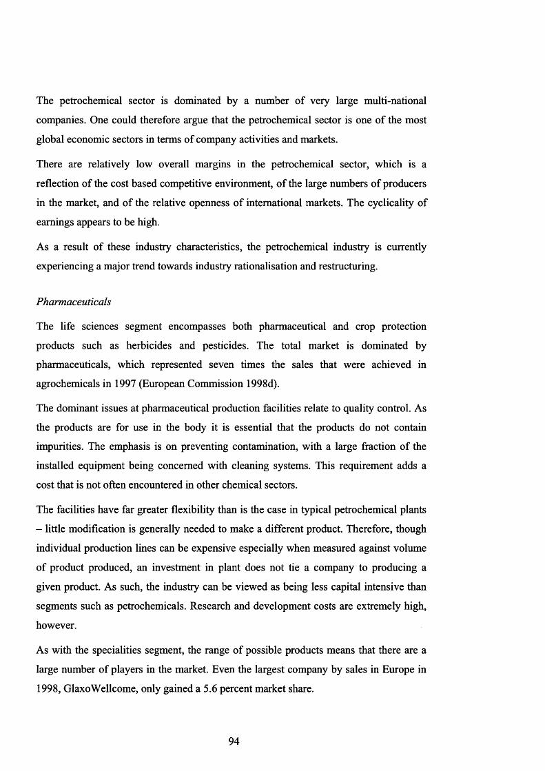
The petrochemical sector is dominated by a number of very large multi-national

companies. One could therefore argue that the petrochemical sector is one of the most

global economic sectors in terms of company activities and markets.

There are relatively low overall margins in the petrochemical sector, which is a

reflection of the cost based competitive environment, of the large numbers of producers

in the market, and of the relative openness of international markets. The cyclicality of

earnings appears to be high.

As a result of these industry characteristics, the petrochemical industry is currently

experiencing a major trend towards industry rationalisation and restructuring.

Pharmaceuticals

The life sciences segment encompasses both pharmaceutical and crop protection

products such as herbicides and pesticides. The total market is dominated by

pharmaceuticals, which represented seven times the sales that were achieved in

agrochemicals in 1997 (European Commission 1998d).

The dominant issues at pharmaceutical production facilities relate to quality control. As

the products are for use in the body it is essential that the products do not contain

impurities. The emphasis is on preventing contamination, with a large fraction of the

installed equipment being concerned with cleaning systems. This requirement adds a

cost that is not often encountered in other chemical sectors.

The facilities have far greater flexibility than is the case in typical petrochemical plants

- little modification is generally needed to make a different product. Therefore, though

individual production lines can be expensive especially when measured against volume

of product produced, an investment in plant does not tie a company to producing a

given product. As such, the industry can be viewed as being less capital intensive than

segments such as petrochemicals. Research and development costs are extremely high,

however.

As with the specialities segment, the range of possible products means that there are a

large number of players in the market. Even the largest company by sales in Europe in

1998, GlaxoWellcome, only gained a 5.6 percent market share.

94

Rationalisation in the pharmaceuticals market is likely to be caused by the cost of new

drug development. A typical new treatment takes up to nine years to develop, with

many potential compounds failing to make it through to successful product. It is the

costs associated with this development that are forcing companies to merge in order to

achieve economies of scale.

3.1.2 Importance and performance of the chemical sector

So far, this chapter aimed to provide some insights on the nature of the chemical sector

by ‘looking inside’ the industry. In contrast, the following pages will present the

performance of the chemical sector as a whole and put it into relation with the overall

economy. The underlying question that this section intends to address is why the

chemical sector makes a worthwhile case study from an economic point of view. Later,

section 3.1.4 will provide reasons why the chemical sector also is a meaningful object

of study from an environmental point of view.

Strategic importance

Historically, the chemical sector has acted both as a focus and a motor for scientific andtli tlitechnological development of industrialising economies. In the late 19 and early 20

century, innovations in the field of chemistry and the subsequent development of

chemical technologies have been regarded crucial national assets. They were therefore

jealously guarded by national governments. For instance, Arora (1997) quotes the

example of the German chemical industries, which were carefully shielded national

scientific-industrial complexes until the end of World War I. This helped the German

economy to outgrow other industrialising nations at the time. Later, as part of

Germany’s World War I compensations, its chemical industries were made to give up

their technological advantage by voiding their patents, such as the rights on Aspirin.

Through this, German chemical industries had lost much of strategic competitive

advantage.

95

Naturally, the role of the sector in catalysing economic development has changed over

the last century. Chemical industries have lost much of their national strategic

importance due to the fact that they, as all other economic sectors, have been subject to

globalisation. Many of the leading chemical enterprises today are huge multinational

corporations that conduct their business as well as their research and development

activities on an international scale (Chapman and Edmond 2000).

Linkages with consumers and other industries

Chemical industries produce intermediate and consumer goods that serve a wide range

of consumer needs. In fact, as figure 4 shows, chemical products can be found in almost

every industrial product that we use on a day-to-day basis. Civilisation, the functioning

of industrialised economies and societies, seems plainly unthinkable without the

amenities provided by chemical industries (Chapman and Edmond 2000).

To name but a few examples of possible applications, chemicals are used for textile

production, packaging, electrical and electronic components, the automotive industry,

the building industry, health care, food products, home care and personal care.

Furthermore, people tend to underestimate the importance of chemicals in modem

agriculture, but according to CEFIC (2001b) data, chemicals account for 30 percent of

all material input in agriculture.

The chemical industry is highly forward linked with other industries both in terms of

economic and technology impact and in terms of environmental issues, such as

production processes or environmental techniques and services. For this reason, the

chemical industry has a crucial and central role within the manufacturing sector (Maglia

and Sassoon 1999).

96

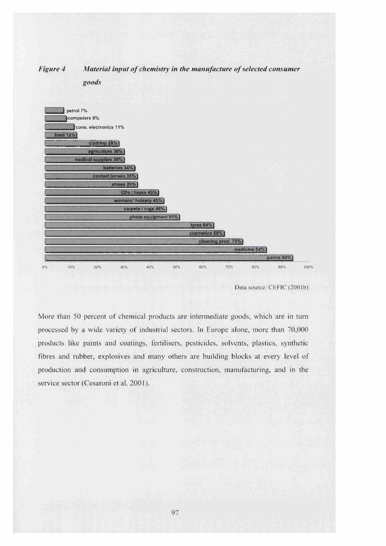
Figure 4 Material input o f chemistry in the manufacture o f selected consumer

goods

I I petrol 7%

com puters 8%

1 I cons, e lectronics 11%

I food 12%1

I clothing 28% I

I agriculture 30% I

I medical supplies 30% |

I batteries 34% |

I contact lenses 35% 1

1 shoes 35% j

I CDs / tapes 43% I1 womens' hoisery 45% |

I carpets I rugs 46%1

photo equipm ent 51% )

i i 11 mmmm| paints 94% |

0% 10% 20% 30% 40% 50% 60% 70% 80% 90% 100%

Data source: CEFIC (2001b)

More than 50 percent o f chemical products are intermediate goods, which are in turn

processed by a wide variety o f industrial sectors. In Europe alone, more than 70,000

products like paints and coatings, fertilisers, pesticides, solvents, plastics, synthetic

fibres and rubber, explosives and many others are building blocks at every level of

production and consumption in agriculture, construction, manufacturing, and in the

service sector (Cesaroni et al. 2001).

97

Figure 5 EU domestic consumption o f chemical products by economic sector,

1995'

paper & prin ting 4.5%

autom otive 5.3%

construction 5.4%

final consum ption 30.3%

textile & cloth ing 6.3%

agricu lture 6.4%

m etals, m echan ical & electrica l engineering

9.0%

other 16.4%

services & adm inistration 16.4%

Source: (CEFIC 2001b)

Figure 5 shows the split o f domestic chemical consumption by EU economic sectors.

While some 30 percent o f the total chemical industry production in 1995 reached the

final consumer, around 70 percent were used by other sectors o f the economy: that is,

agriculture, industries and the service sector.

Accounting for some 16.4 percent o f total chemicals consumption, the biggest non-final

consumer o f chemical goods appears to be service and administration sector. Metal

processing and electrical engineering, agriculture, and the textile industry were also

among the most important customers of chemical industries.

1 Percentage shares were calculated by taking into account the re-allocation of domestic consumption to downstream consumers of chemicals, self-consumption and consumption by the rubber and plastic processing industries.

98

As impressive as these numbers may be, one should not lose sight of another reason for

the importance of chemical industries in modem economies: that is, the role of the

chemical sector in transmitting innovation. Product or process improvements in the

chemical sector may have positive effects in downstream industries. Since the chemical

industry provides goods and engineering services to a host of other industries

simultaneously, innovation in the field of chemical engineering may have the potential

to create multiple spillover effects (Cesaroni and Arduini 2001; Cesaroni et al. 2001).

3.1.2.1 The contribution of chemical industries to GDP

The output of chemical industries makes up a substantial part of the total manufacturing

production in all EU member states. As figure 6 shows, the country with the highest

proportion of chemical industry production value in the manufacturing total in 1997 was

Belgium. In fact, the country’s industrial sector produced goods that valued more than

one third of the entire manufacturing sector. The Dutch and Irish chemical industries

follow with some distance. On the other end of the spectrum appears Austria, where

chemical industry production accounted for little more than five percent of the total

manufacturing production value.

When one considers the evolution in the percentage of chemical industry production

over the observation period, it appears that some countries exhibit significant changes,

while the position of the chemical sector did not change much in others. The country

with the most pointed development is clearly Ireland.

The share of the Irish chemical industry in the total manufacturing production appears

to have doubled between 1990 and 1997. The size of this movement is remarkable and

might cause some suspicion regarding the quality of the underlying data. In response, an

extensive check of various data sources on the indicator was carried out. Its findings, as

well as the overall performance of the Irish economy in general and of its chemical

industry in particular (Murphy 2000), appear to confirm the validity of the observation.

A more detailed discussion on the plausibility of Irish chemical industry production data

follows at the end of this section.

99

Figure 6 Chemical industry production value as percent o f total manufacturing

production

50%

■ 1980

H 1 9 9 5

ino> (/) o> 0)T- Unr a c l

a> in 3 CD ffl cn> rc ro .2 Q.1 8I f

w ^3 cC (0 = 2

25%

Unweighted average 1995

Unweighted average 1980

0%dk fi d e fr uk bea t Pt it nlse e s gr ie

Data Source: 1980-1996 CEFIC ESCIMO database (2001) 1997-1999 CEFIC (1998b, 1999b, 2000b)

Besides Ireland, some other EU member states seemed to exhibit significant changes:

the proportion of chemical industry production decreased in Austria and the

Netherlands, and increased in Greece and Luxembourg. All other EU member states did

not appear to have experienced major changes.

Production value as the first chemical industry performance indicator

The first dependent variable for the subsequent regression analysis in chapter 4.2 will

be the value o f chemical industry production in the EU member states. This data series

is expressed in U.S. Dollars at 1995 prices.

The raw data for the time series was provided by the European Chemical Industry

Council. CEFIC provides a range o f data series on EU chemical industries as part of

their comprehensive chemical industry database ESCIMO, or in the form of annual

figures in their statistical yearbooks.

100

Among the data series provided by that organisation are data points on EU chemical

industry production value; absolute data were available for the years 1997, 1998 and

1999. The figures were taken from CEFIC’s statistical yearbooks (CEFIC 1998b;

1999b; 2000b). Originally, the production value was reported in €; the data was

converted into U.S. Dollars using the annual exchange rates provided by U.S. Federal

Reserve Bank (2000) and deflated to reflect constant prices o f 1995.

Figure 7 Chemical industry production value (absolute)

re 3

> 3 o o>O X-3 O

? § Q - .2

I I3T3C

100,000

■ 1980 □ 1999

75 ,000

50 ,000

Unweighted average 199925 ,000

Unweighted average 1980

fi dk nl be frat it uk d es e e s

Data Source: 1980-1996 CEFIC ESCIMO database (2001) 1997-1999 CEFIC (1998b, 1999b, 2000b)

101

The remaining years 1980 to 1996 were extrapolated from a chemical industry

production index, which was also provided by CEFIC as part of its ESCIMO database.

The base year of the index was re-calculated to 1995. Since both the index data series as

well as the absolute production values in U.S. Dollars provided values for 1997, it was

possible to extrapolate the missing absolute production values in U.S. Dollars (1980 to

1996) by combining the two data series. The result of this operation is recorded as table

36 in the appendix.

Figure 7 represents the production value of EU chemical industries in 1980 and 1999.

The diagram shows that all European chemical sectors have increased their production

volume over the observation period. It also shows that the rate of increase varied

considerably across the EU.

Of the fourteen countries in the sample, the production volumes of thirteen chemical

sectors grew by more or less comparable ratios. The most different evolution in

chemical industry production value among the countries in this ‘mainstream group’ can

be observed in Greece and Denmark. The smallest increase occurred in Greece with 36

percent; Denmark marked the biggest increase in chemical industry production volume

with 160 percent.

Yet, the increase in production volume of the chemical sector in Ireland clearly stands

out from the rest of the EU. Over the observation period, the value of chemical industry

production in Ireland grew by the factor 23. While the Irish chemical sector was the

smallest of all 14 countries in the sample in terms of production value in 1980, the

country ranked eighth in 1999. Indeed, the production value of the Irish chemical

industry in 1999 was bigger than the production of the three following countries -

Sweden, Denmark and Finland- taken together.

2 The index was labeled ‘Production Index, Chemical Industry (kind-of-activity index)’. Further explanations or details on its methodology were not available. The CEFIC statistical yearbooks mention that the definition of chemical industry varies across countries. This may explain why CEFIC had to resort to its particular kind-of-activity definition of the chemical sector.

102

The evolution of the absolute chemical industry production value appears to be an

interesting and telling dependent variable if one wants to investigate the sector’s

competitiveness. The production value provides a clear idea on which national chemical

sector has grown most in terms of absolute output. From this angle, the outstanding

increase of production value in Ireland is a remarkable fact in itself. It poses the

question in what way the background for development of the Irish chemical sector

differs from the rest of the EU. The regression model will test whether Ireland’s

chemical industry production performance is connected to the differences among EU

countries with regard to taxation, fuel prices, productivity, and pollution performance.

Yet, the outstanding development of the Irish chemical industry production value also

appears to hint at the fact that there are additional important aspects that might help in

the interpretation of production values. It is a well documented fact that the Irish

economy and its manufacturing sector in particular have grown much stronger than the

European average over the observation period.

Chemical industry production value / GDP

Before this background, it appears reasonable to compare the increase of chemical

industry production value with the overall growth of the economy (GDP). The

following dependent variable will pick up this line of argument. Therefore, as a

complement to the above data set on production values in absolute terms, the second

dependent variable will be the ratio of chemical industry production to GDP.

Chemical industry production value / GDP provides a distinct take on the

competitiveness of the chemical sector, because it reflects developments in the

production value of the chemical industries in relation to the growth of the rest of the

economy. Hence, the evolution of this indicator over time shows whether the chemical

industry production value has grown faster or slower than the overall economy.

The basic data on chemical industry production values is identical to the dependent

variable introduced above. In addition, the production value is put into relation to

national GDP data drawn from the OECD and the World Bank.

103

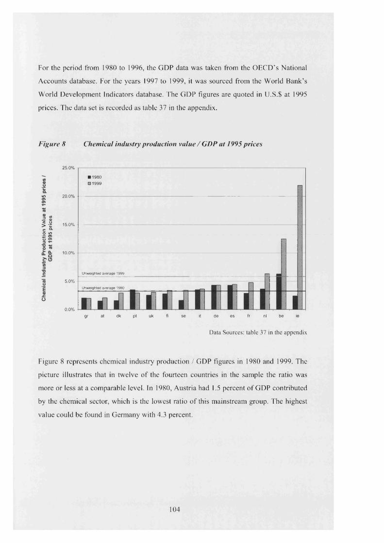
For the period from 1980 to 1996, the GDP data was taken from the OECD’s National

Accounts database. For the years 1997 to 1999, it was sourced from the World Bank’s

World Development Indicators database. The GDP figures are quoted in U.S.$ at 1995

prices. The data set is recorded as table 37 in the appendix.

Figure 8 Chemical industry production value / GDP at 1995 prices

2 5 .0%

■ 1980 □ 1999

20 .0% -------in<T>o>

3 W _ O CD O 15.0% —> -Zc Q- o m zz o> o O)

10 .0%

Unweighted average 1999

5 .0%

Unweighted average 1980

0 .0%

dk uk d e fr nl b ea t Pt its e e sgr

Data Sources: table 37 in the appendix

Figure 8 represents chemical industry production / GDP figures in 1980 and 1999. The

picture illustrates that in twelve o f the fourteen countries in the sample the ratio was

more or less at a comparable level. In 1980, Austria had 1.5 percent of GDP contributed

by the chemical sector, which is the lowest ratio o f this mainstream group. The highest

value could be found in Germany with 4.3 percent.

104

In 1999, the country with the lowest chemical industry production value / GDP ratio

was Greece with 2.0 percent; the Netherlands showed the highest ratio with 6.3 percent.

Most countries in this group showed a moderate increase in their production value /

GDP ratios; two notable exceptions were Greece and Portugal, where the chemical

sector lost some of its importance compared to the overall economy.

There are two countries that do not appear to fit into the EU mainstream. First, Belgium

exhibited a significantly higher share of chemical industry production value in total

GDP both at the beginning and at the end of the observation period. In 1980, the

production value of the chemical sector amounted to 6.3 percent of the GDP; this ratio

almost doubled to 12.5 percent in 1999. The data appears to indicate that the Belgian

chemical industry is much more important in the context of the overall economy than in

most other EU countries.

This observation also holds true for Ireland, which is the second outlier among the EU

member states. The production value / GDP ratio for the Irish chemical sector grew

from 2.4 percent in 1980 to 21.9 percent in 1999.

One should note that this rise, which corresponds roughly to an increase by the factor 9

-as impressive as it may appear-, is well below the observed increase in absolute

chemical industry production value in Ireland, which grew 23-fold. In other words, not

only the chemical sector in Ireland grew considerably, so did the Irish economy as a

whole. Yet, the growth rate of the chemical industry production value exceeded the

growth of the general economy by far. In consequence, according to the data, the Irish

chemical sector accounted for almost 22 percent of the country’s GDP in 1999.

The correlation coefficient between the chemical industry production value in absolute

terms and as a ratio of GDP is 0.15. This low coefficient indicates that the two data

series are to a large degree independent. Based on this observation, the two dependent

variables appear to capture different aspects of chemical industry competitiveness. The

first indicator -the absolute production value- captures the increase or decrease of

chemical industry output. The second indicator -the production value relative to the

GDP- reflects the relative importance of chemical industry production value in the

context of the national economy.

105

On the plausibility o f the Irish production value figures

The ratio of Irish chemical industry production value to GDP appears suspiciously high.

In response to this, the data series that were used for the construction of this variable

have been carefully checked for consistency and plausibility, and were compared to

other data sources. The data was discussed with experts of the statistical office of the

European Commission, Eurostat, as well as with representatives of the Irish Central

Statistics Office. Alternative data series provided by (1) the Irish Development Agency

IDA, (2) the Irish Pharmaceutical & Chemical Manufacturers Federation, (3) the Irish

Business and Employers Confederation IBEC, and (4) the Chemical & Engineering

News, appear to show comparable proportions and evolution over time. Taking the

feedback from various sources into account, there appear to be no grounds to question

the validity of the data.

One possible explanation for the particularly high percentage in Ireland may lie in the

fact that the definition of “chemical industry” by the Irish Central Statistics Office

includes the pharmaceutical industry, a chemical sub-sector that appears to have had

particularly high growth rates in Ireland over the last decades (IBEC 2001). This

practice is, in itself, no reason to suspect that the Irish data is biased, as including

pharmaceutical industries appears to be common practice across most EU member

states. However, one should note that each EU member state’s statistical office has

some degree of liberty in defining its industry definition. For this reason, one needs to

be cautious in comparing that indicator between countries. However, since the primary

focus of this investigation is the evolution over time of the indicator, and since the

regression analysis incorporates country dummy variables, the use of the data series

may be justifiable.

106

According to data obtained from Eurostat and the Central Statistics Office of Ireland,

the manufacturing share of GDP in 1995 stood at 26.9 percent. By virtue of this figure,

the Irish manufacturing sector represented the largest share in GDP of all EU

manufacturing sectors. On the other hand, the production value of the Irish chemical

industries grew almost exponentially in the subsequent years from 1995 to 1999. These

two observations taken together may also support to the notion of such a high chemical

industry production value/GDP ratio.

According to information by the Irish Pharmaceutical & Chemical Manufacturers

Federation (IBEC 2001), there was a massive influx of greenfield inward development

into the Irish chemical sector during the 1980s and early 1990s. 16 of the top 20

pharmaceutical companies in the world opened plants in Ireland. According to IBEC

(2001: 4), the exports by the Irish chemical industry grew between 1974 and 1995 by a

massive 17,974 percent. Since the early 1990s, the growth of the industry was in its

majority organic, based on existing company extensions. Due to the fact that the Irish

chemical industry is dominated by fine chemical and pharmaceutical companies, and

taking into account that most plants were constructed after 1970, Ireland possesses a

very modem high-tech chemical sector that lack some of the negative characteristics of

older EU chemical industries such as massive scale intrusions on local communities and

pollution problems.

3 Note that the data points of Ireland as well as of all other EU member states were extrapolated from an index with regard to the years 1980 to 1996, and taken directly from CEFIC’s Eskimo data base for the years 1997 to 1999. In the case of Ireland, there appears to be a break in the time series from 1996 to 1997. That break is probably due to a change in the definition of chemical industry. In order to assess the impact of this break, the subsequent analysis will present two sets of regression models: one including Ireland, and another one excluding the country. With regard to all other EU countries but Ireland, the extrapolated and the original data points seem to correspond well.

107

Last but not least, the strength and relative importance of the Irish chemical industry has

been highlighted in a number of previous empirical studies. For example, Maglia and

Sassoon (1999) point out the economic strength of the Irish chemical sector relative to

other EU chemical industries, and most notably in relation to the German chemical

sector. For instance, their analysis illustrates that the Irish chemical sector has

outperformed the rest of the EU with regard to profitability, profit growth, and foreign

direct investment. Murphy (2000: 15/16) notes that among the five leading high-tech

industries in Ireland -computers, software, pharmaceuticals, chemicals, and cola

concentrates- the net output per person in the chemical sector clearly surpassed the

other sectors.

In conclusion, although there is no evidence that the data set on the Irish chemical

industry production value is systematically or materially wrong, there may remain some

intuitive doubt about whether ‘they can be true’. For this reason, the subsequent

regression analysis will report two sets of models: one including and another one

excluding Ireland.

3.1.2.2 Chemical industries and labour markets

As figure 9 shows, chemical industries provide a significant source of employment in

the European Union. In 1998, EU chemical industries provided jobs for 0.98 percent of

the total workforce, compared to 0.75 percent in the United States and 0.56 percent in

Japan (CEFIC 2001a).

108

Figure 9 Employment in chemical industries as percent o f total workforce, 1998

2.50%

2 .00%

1.50%

1.00%

0.50%

0 .00%

Note: IE refers to 1997 Data sources: CEFIC (2001)

OECD / Main Industrial Indicators (2001)

One should note that the percentage of employment to the total workforce varies

considerably across EU member states. The two countries with by far the highest

proportion of chemical industry jobs in 1998 were Belgium and Denmark. In both

countries, the chemical sector provided employment for more than two percent o f the

occupied population. Ireland, Germany, Austria, and the Netherlands also exhibited

more jobs in the chemical sector than the EU average. The EU member states with the

lowest proportion o f chemical industry employment in 1999 were Greece and Portugal,

followed by Finland and Spain.

unweighted average

109

Chemical industry workforce as the second performance indicator

Given the importance o f the chemical sector as employer and the socio-economic

importance of job creation over the recent years in the EU, the second chemical industry

performance indicator will be the number o f chemical industry employees. As in the

case o f the first dependent variable, chemical industry employment will be used in

absolute terms as well as in relation to the total employment.

The data for this indicator was obtained from the European Chemical Industry Council

(CEFIC) and Eurostat. Data covering the number o f employees in the national chemical

sectors was provided by CEFIC as part o f its ESCIMO data base. The time series was

obtained through the CEFIC homepage in 2001. It is recorded in the appendix as table

38.

Figure 10 Chemical industry employees (absolute)

600

tAT3Cra(A3O& 400(As0>oaE0)

■ 1980 □ 1999

200 —

Unweighted average 1980

Unweighted average 1999

fi gr ie pt s e a t dk nl b e e s it uk fr de

Data source: CEFIC, ESCIMO Database (2001)

110

The figures, which are represented in figure 10, suggest that in the five countries with

the largest chemical sectors in the EU, i.e. Germany, France, Britain, Italy and Spain,

the absolute number of chemical industry employees has decreased over the observation

period. This process appeared to be especially significant in the UK, where the

workforce of the chemical sector was almost cut in half between 1980 and 1999. On the

other hand, the largest chemical sector in the EU, Germany, seemed to experience a

much less dramatic cut in employment.

Among the fourteen countries in the sample, only three experienced an increase in

chemical industry employment. These three countries were Ireland, Denmark and

Belgium. With regard to Ireland and Belgium, that development appears plausible, since

absolute chemical production as well as production relative to the GDP also increased

significantly over the observation period (cf. figure 11).

It should be noted, however, that the very significant increase in chemical industry

employment in Denmark cannot be fully explained by simultaneous increases in

production volumes. The data shows that Denmark experienced a slow and relatively

constant increase over the observation period, with the exception of 1987/1988 when

the ratio of chemical industry employment to occupied population almost doubled.

The most likely explanation for this sudden shift may be a break in the time series

between 1987 and 1988. Such a break could have been introduced by a re-definition of

the chemical sector. Unfortunately, the ESCIMO data base does not provide further

information that could clarify this point.

I l l

Chemical industry employment / total workforce

The fourth dependent variable in the regression analysis will be the ratio of chemical

industry employment to the total workforce. The corresponding data on the overall

workforce of EU member states4 was provided by Eurostat as part of its Newcronos

data base (2001). The original data set covers the period from 1980 to 1997. The

missing years 1998 and 1999 were extrapolated as a linear projection on the basis of the

available data. The final data set on chemical industry employment / total workforce is

recorded as table 39 in the data appendix.

The chemical industry employment/overall workforce indicator appears useful for the

assessment of chemical industry competitiveness, because it may show whether the

sector has outperformed the overall economy in terms of job creation, or whether the

sector has indeed provided proportionally less jobs than the rest of the economy.

Inversely, in times of economic decline or stagnation, the ratio of chemical industry

employees to the total occupied population could reveal whether the chemical industry

lost proportionally more or less jobs than other sectors of the economy.

Across countries, the ratio could also tell something about the relative importance of the

chemical sectors as employers within the national job markets. As figure 11 illustrates,

national chemical industries had very different shares in the overall workforce. The

highest ratio could be found in Belgium, where approximately 2.5 percent of the

workforce was employed by chemical industry employers. In Belgium, this ratio

increased slightly over the observation period.

4 The data set was originally labelled “total occupied population (paid and unpaid)”.

112

Figure 11 Chemical industry employees / total workforce

3.0%

■ 1980 □ 19990)ot-

£k.

ITOO 2 .0%

(A0)Q)oa£a>

Unweighted average 1980

Unweighted average 1999

(A3-oc1 .0%

rooE0J.cO

0 .0%

gr pt e s it fi s e uk fr ie a t nl d e dk be

Data sources: CEFIC, ESCIMO Database (2001) Eurostat, Newcronos Database (2001)

By contrast, Greece exhibited the lowest percentage o f chemical industry employment

relative to the total occupied population. Approximately 0.5 percent o f the workforce

found jobs in the chemical sector. That ratio decreased by around 0.1 percent over the

observation period.

Eleven o f the fourteen countries in the sample experienced a decrease in chemical

industry employment in relative terms. This appears to indicate that in a majority o f EU

member states, the chemical industry lost some o f its importance on the national labour

markets. Only Ireland, Denmark and Belgium exhibited an increase in chemical

industry employment relative to the total.

113

If one puts the chemical production value/GDP in relation to the percentage of national

workforce employed by chemical industries, one may conclude that the chemical sector

appears highly productive relative to the rest of the economy. For example, in the UK in

1999, the chemical sector produced goods at the value of 3.0 percent of the GDP while

using only 0.82 percent of the UK workforce. This pattern appears to be generally

consistent across all EU member states. However, some countries such as Belgium or

Ireland exhibit an especially large difference in productivity between the chemical

sector and the rest of the economy.

3.1.2.3 Chemical industries and trade

For chemical industry stockholders, one of the most relevant business figures is

probably the market share of their company, as it helps to judge the competitive success

of their products and their marketing. All other factors being equal, the evolution of

market share could serve as a sign whether the company is offering competitive

products at appropriate prices vis-a-vis its competitors. If it decreased, this might be a

hint at strategic or structural problems that the company experiences on the market.

With some qualifications, a similar argument could be applied to entire chemical

sectors. Obviously, one cannot simply argue that aggregate entities such as entire

economic sectors would commit clear-cut strategic mistakes such as over-pricing or the

like. Other factors, such as tax levels, productivity, or market size, which will be

captured by the independent variables in the regression analysis, could play a role in

determining the market share of economic sectors.

As this focus of the comparative analysis lies on the performance of national chemical

industries relative to each other, the EU common market appears to be the most relevant

reference basis. Following that logic, the best suited unit to compare the ‘sales volume’

of chemical sectors would have to be intra-EU exports. Hence, chemical industry intra-

EU exports will serve as the third dependent variable. Again, the variable will be

expressed in absolute terms and as a ratio of intra-EU exports to GDP.

114

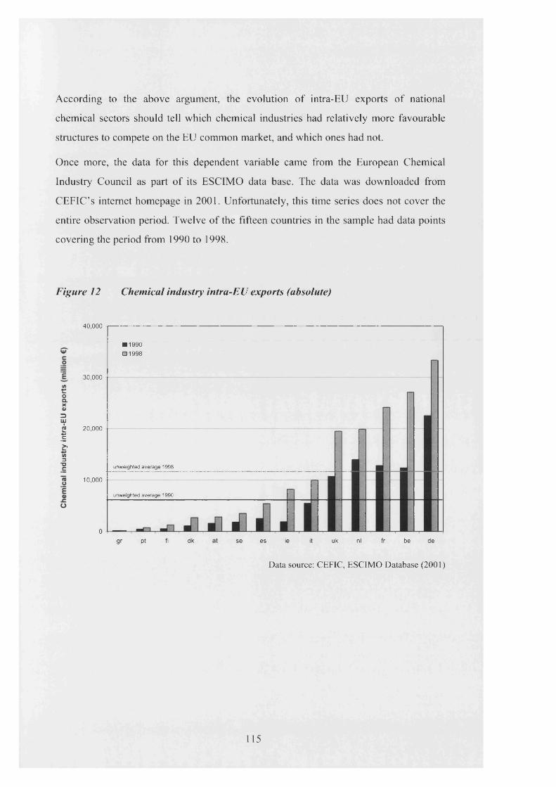
According to the above argument, the evolution o f intra-EU exports o f national

chemical sectors should tell which chemical industries had relatively more favourable

structures to compete on the EU common market, and which ones had not.

Once more, the data for this dependent variable came from the European Chemical

Industry Council as part o f its ESCIMO data base. The data was downloaded from

CEFIC’s internet homepage in 2001. Unfortunately, this time series does not cover the

entire observation period. Twelve o f the fifteen countries in the sample had data points

covering the period from 1990 to 1998.

Figure 12 Chemical industry intra-EU exports (absolute)

int0Q.x0)=)iu1 c'£*on3TJC

40 ,0 0 0

■ 1990 □ 1998

30 ,000

20,000

unweighted average 1998

10,000

unweighted average 1990

0gr pt ft dk s e e s ie it uk nl fr be d e

Data source: CEFIC, ESCIMO Database (2001)

115

The Irish time series relates to 1990 to 1997; the missing data point was projected on

the basis of the available data points using an exponential function, which was the one

fitting best to the existing cloud of observations. The Swedish data set provided

information only for the period 1990 to 1994. Since the evolution of the Swedish intra-

EU exports appeared to follow a linear trend, the missing values were filled in as a

linear projection of the available data points. The data series is recorded as table 40 in

the appendix.

Figure 12 shows that the absolute value of chemical industry intra-EU exports-

measured in € million- has grown in all EU member states. The diagram illustrates that

the highest increase over the observation period 1990 to 1998 took place in Ireland,

where it more than quadrupled in less than a decade. The second highest growth rate

was experienced by Belgium, where intra-EU exports more than doubled. With roughly

25 percent, Greece experienced the lowest augment.

Furthermore, the graph also shows relatively high intra-EU export figures for countries

like Belgium and the Netherlands. In terms of absolute intra-EU export value in 1999,

the two countries rank second and fourth respectively among all EU member states. As

such, their chemical industry intra-EU exports are larger than the ones of Britain, Italy

or Spain.

Intra-EU chemical industry exports / GDP

When one puts the intra-EU export figures in relation to the national GDP,5 this

observation becomes even more evident. As figure 13 illustrates, relative to the size of

their national economies, the intra-EU exports of the Belgian, Irish and Dutch chemical

industries were much higher than in the rest of the European Union member states.

5 The data set regarding national GDP values corresponds to the ones used as independent variable and as normalizing factor in section 3.2.2. Please refer to that chapter for details on the data source and construction of the time series.

116

Figure 13 Chemical industry intra-EU exports / GDP

10%■ 1990 □ 1998

Q.□0 8%

U)roCLX0)3II! 6%

2c

4%i/>3■oC

TOOa)

■C

unweighted average 1998

2%O

unweighted average 1990

0%gr pt it e s ft a t uk s e dk d e fr ni ie be

Data Sources: Table 41 in the appendix

The share o f Belgian chemical industry intra-EU exports in GDP more than doubled

over the observation period from 4.3 percent in 1990 to 8.8 percent in 1998. An even

more significant increase took place in Ireland, where the ratio grew almost threefold.

All EU member states experienced increases in relation to that indicator. The intra-EU

exports o f some chemical sectors, for example in Finland, Denmark, Sweden or Spain,

grew by comparable magnitudes. However, the data also shows clearly that these raises

took place on a much lower level.

117

3.1.3 Restructuring of the chemical sector in the European context

So far, this description of the chemical sector has focussed on two issues. The first

section, 3.1.1, was an attempt to define the sector and discuss its internal structure. The

second section, 3.1.2, presented a number of indicators on the economic performance of

the chemical industry. The following section takes another perspective: its central issue

will be to show the structural differences of the chemical industries across EU member

states, and to discuss the drivers of the current restructuring processes.

3.1.3.1 Structural differences among EU member states

Various indicators draw a vivid picture on the structural differences between the

national chemical industries among the 15 EU member states. These differences could

be summarised into three distinct aspects: the average size of chemical companies, the

share of ‘low-tech’ chemical industries, and the knowledge intensity of chemical

sectors.

Average size o f chemical companies

To begin with, figure 14 reveals one very fundamental difference across national

chemical industries: the average number of employees per chemical industry enterprise.

The country with the, in average, largest chemical enterprises among EU member states

is Germany, where the average enterprise size was around 430 employees in 1996. With

in average more than 300 employees, the Dutch chemical enterprises appeared to be

already significantly smaller in terms of enterprise size. Given the enormous size of

some German and Dutch chemical industry conglomerates, such as Bayer or Royal

Dutch/Shell, these numbers appear plausible. However, the German and Dutch chemical

sectors exhibit a significant difference in average size relative to their counterparts in

the United Kingdom and France - countries that also have a number of major chemical

industry players.

118

Figure 14 Average number o f employees per chemical industry enterprise, 1996

unweighted average

pt e s ft lu ie gr it a t uk fr s e dk nl de

Data source: Eurostat / Newcronos (2001)

At the other extreme of the spectrum appears Portugal with an average chemical

enterprise size o f only 25 employees. The cluster o f EU member states with relatively

small chemical enterprises also includes Spain, Finland, Ireland, and Greece. This

observation appears to hint at the fact that chemical firms in central and more developed

EU economies tend to be bigger than their counterparts in relatively more peripheral

markets. Furthermore, the data also seems to suggest that chemical firms in

Mediterranean countries are relatively smaller than the EU -15 average.

119

Complementing the point before, figure 15 reports the absolute number o f chemical

industry enterprises across EU member states. Obviously, the figures should not be

compared across member states, as they are not normalised. However, looking at the

data, one observation could safely be made: considering the relative size o f the Spanish

and Portuguese economy, the absolute number o f chemical industry enterprises in those

countries appears remarkably high. As a result, judging from the information on the

average size and absolute number o f chemical industry enterprises, the two Iberian

chemical sectors seem to stand out for their large number o f small chemical firms,

whereas the chemical sector in countries like Germany or the UK appears much more

concentrated.

Figure 15 Absolute number o f chemical industry enterprises, 1996

4000

unweighted average

Data source: Eurostat / Newcronos (2001)

120

Share o f basic chemical industry

Figure 16 shows the ratio of the basic chemical industry (cf. chapter 3.1.1) relative to

the fine and performance chemical industries in terms of its production value. The

diagram illustrates that the significance of the basic chemicals vis-a-vis the more

knowledge intensive and value-added speciality chemistry varies greatly across EU

member states.

In 1998, Ireland exhibited the highest share o f basic chemicals, amounting to

approximately 70 percent. The sub-sector also appeared to be relatively more important

in countries like the Netherlands and Finland than in the rest o f the European Union. By

contrast, the basic chemical industry was markedly underrepresented in Denmark and

Italy, where it accounted for approximately 11 and 23 percent o f total chemical

production respectively.

Figure 16 Basic chemicals production as percentage o f total chemical production

(basic chemistry and specialities)

90 t--------------------------------------------------------------------------------------------------------------------------------------------------------------------------------------------------------------------

■ 1988■ 1998

80 -

I

50 -unweighted average 1988

unweighted average 1998

Idk it se gr fr e s uk at pt be de fi nl ie

Note: DK / IE / SE refer to 1990 and 1998; AT refers to 1991 and 1998Data source: Eurostat / Newcronos (2001)

121

Furthermore, the graph shows that, between 1988 and 1998, the share of basic

chemicals in total chemical production shrank in most EU member states. The only

exception to this trend was apparently Ireland, where, starting from an already high

level, the basic chemicals sector increased its relative weight.

Last but not least, one interesting observation may be that the relative importance of the

basic chemicals industry in the Mediterranean EU member states appears to be rather

lower than EU average. This fact is surprising, since one often-heard topic about the

regional distribution of chemical industries states that southern European countries had

a higher share of ‘primitive’ basic chemical industries than northern ones.

Education o f the workforce and R&D intensity

The great importance of innovation on the development and competitiveness of

chemical industries is a common theme among most studies on the sector. For example,

Cesaroni et al. (2001) highlight the chemical industry’s long tradition in innovation and

R&D activities as one key characteristic of the sector. Since its origins in the second

half of the nineteenth century with British and German dyestuff manufacturers, the

chemical sector appears to be science-based and science-driven. Moreover, Cesaroni et

al. note that, more than in other industries, innovation in the chemical industry derives

from the interaction between the academic world, individual firms, government policies,

and historical events.

For this reason, the average education level of the chemical industries’ workforce may

provide an important insight into the competitive position and strategy of national

chemical sectors. As figure 17 shows, there are significant differences across EU

chemical industries with regard to the highest degree of their workforce. Judging by the

percentage of employees with secondary or higher degrees, the chemical sectors in

Denmark, the Netherlands, and Germany appear to have the workforce with the highest

average skills. It may be worth noticing that it is exactly this group of countries that also

have in average the largest chemical industry enterprises. By contrast, the chemical

industry’s workforce in Portugal, Italy, The United Kingdom, and Spain exhibits a

distinctly smaller percentage of secondary or higher education.

122

Figure 17 Highest education degree o f the chemical industry workforce, 1995

100%

dk nl d e fr b e ie g r e s uk it pt

■ R im a ry □ Secondary El H igher

Note: PT refers to 1994 Data source: Eurostat / Newcronos (2001)

As noted above, the production o f bulk chemicals is regarded as less R&D intensive and

sophisticated than the production of speciality chemicals (Cook and Sharp 1992;

Cesaroni et al. 2001). Based on this notion, one might expect that chemical sectors with

a high percentage o f basic chemicals production have a lower-skilled workforce.

However, comparing the information contained in figures 16 and 17, there is no

apparent relation on first sight. In the case o f Denmark, the observed relationship

corresponds to what one might expect: the chemical sector with the lowest percentage

o f basic chemicals production does indeed have the highest-skilled workforce. Yet, with

regard to Italy, the expected relationship does not hold. Italy’s chemical sector exhibits

the second lowest percentage o f basic chemicals production as well as the second

lowest-skilled workforce. An inverse but similarly counter-intuitive relationship appears

to apply to the Dutch chemical sector as well.

123

Figure 18 Patent applications (organic & inorganic chemicals) / chemical

industry employees, 1995

unweighted average

0.0 0.5 1.0 1.5 2.0 2.5

P a te n ts / th o u sa n d chem ica l ind u stry em p lo y ees

Data Sources: patent applications - Eurostat / Newcronos (2001) Chemical industry employees - CEFIC Eskimo database (2001)

Among the possible explanations for this inconclusive relationship could be the fact that

chemical production, irrespective o f whether it regards basic or speciality chemicals,

requires a generally high average level o f skill. Furthermore, mentioned before, due to

the integrated chemical production chain, basic and speciality chemicals production

facilities are commonly found in close neighbourhood to each other. The workforce o f a

chemical plant typically operates both types o f chemical production. Finally, it may be

that the type o f chemical production is not the key determinant to the average skill o f

the chemical industry workforce, but the R&D intensity of the national chemical

sectors, as illustrated in figure 18.

124

3.1.3.2 Drivers and trends of the restructuring

Global market pressures

On a global level, according to the European Commission (1998d), the key challenges

to European chemical industry restructuring lie within the large diversified groups that

have commodity petrochemicals as a significant component of their current portfolio.

These are the main product areas where Europe is under the most global competitive

pressure, and where the legacy of prior government and national influence has created a

structure most disadvantaged compared to the key competitor region of North America.

First, Europe has had too many producers of the main individual petrochemicals and

polymers, a legacy of national focus in prior years. The cost burden that this imposes is

reducing rapidly, as restructuring occurs in response to global competitive pressures.

The European Commission expects this process to continue as the global pressures are

currently still intensifying.

Second, different chemical industries are - appropriately - responding in different ways

to the competitive environment. All are seeking to reduce unit costs and improve

customer focus, but radically different business models are being adopted to achieve

this. These range from a complete shift to different businesses (e.g. ICI), to adherence to

the virtues of integration and a broad portfolio while attacking costs at all levels (e.g.

BASF). In between, many companies are choosing to focus upon the core products and

competencies that they see as representing their strongest competitive position. There is

as yet no compelling financial evidence that one of these models is broadly superior to

others. It is clear however that some form of strong and continuous improvement is

essential by all European producers, in the face of global pressures.

125

Third, European-based companies achieve lower levels of profitability than their US-

based competitors. This reflects the lower margins in their home markets, to which all

producers are heavily linked. Possible reasons for this lower profitability in European

operations include relatively lower plant scales, excessive numbers of producers, less

access to advantaged feedstock situations, higher unit labour costs (and lower labour

flexibility), higher utility costs (particularly electric power and natural gas, due to cost

and competition factors), higher capital costs (mainly due to higher unit labour costs),

less effective integration and logistics, and less homogeneous markets.

Some of the above points are being addressed by industry consolidation and

restructuring; some are being improved by the move to increasingly unified markets and

price transparency; utility and feedstock costs may be addressed by efforts for de­

regulation and more supplier competition. Most of the labour-related (including capital

cost) penalties are due to national legislation, which varies widely between countries,

with Germany normally cited as having the biggest comparative disadvantages.

Fourth, there are efforts among EU chemical sectors to improve their industry structure

and efficiency via “strategic alliances”. However, full mergers among major chemical

companies are still rare in the EU, due to the reluctance of national governments to ‘sell

out’ their strategic economic sectors. This practical constraint prompts chemical

industries to seek “virtual restructurings” as second best solutions in terms of the

desired competitiveness improvements (European Commission 1998d).

The competitiveness gap between American and European chemical industries

Maglia and Sassoon (1999) highlight a number of ‘competitiveness gaps’ between

European and U.S. chemical industries, which causes the profitability of the European

chemical sector to be steadily lower than U.S. levels. First, the capital intensity of EU

and U.S. chemical is different, with EU investment levels being consistently lower. In

the 1990s, capital spending as a ratio of sales increased in the U.S., after a short

decrease during the recession of the early 1990s. By contrast, capital spending levels

remained low and constant among EU chemical industries over that period.

126

Second, Maglia and Sassoon argue that a comparison of the human capital structure

shows that the EU chemical industry is a disadvantageous position: the average skill

level of an employee in the American chemical industry is higher than in Europe. In

addition there is a greater polarization of skills in the U.S. chemical sector: in the U.S.

there seems to be a relatively higher proportion of higher level skills and low skills,

whereas in Europe, employees with intermediate skills represent a greater proportion.

Further reasons for the competitiveness gap may also be found in structural differences

between the two chemical sectors. According to Maglia and Sassoon (1999), the

European chemical industry differs from the American one with regard to a relatively

higher concentration of low-value-added activities, and thus in relatively lower overall

productivity. Furthermore, the production scale of European chemical industries is

relatively smaller and hence their ability to exploit economies of scale.

Finally, Maglia and Sassoon also report that R&D expenditures relative to sales

volumes are higher than in the U.S., but doubt that this indicator is a valid proxy for the

competitiveness of R&D efforts. The findings of Fleischer et al. (2000) appear to lend

support to this suspicion, as they report that EU chemical industries exhibit lower R&D

productivity, lower patent productivity, less polymer patents, and a lower number of

new chemicals notifications than their U.S. and Japanese counterparts.

With a special emphasis on knowledge-related drivers of the current restructuring

processes, Cesaroni et al. (2001) state that knowledge linkages become increasingly

important. First, networks play an ever more important role in the business. Second, the

division of labour at the industry level between chemical companies and technology

suppliers is increasing. Third, the depth of the relationships between chemical producers

and their customers is growing in order to better specify the characteristics of chemical

products. Finally, knowledge and R&D take an ever more important role as a source of

competitive advantage and growth.

127

Competitive pressures within the EU

Obviously, these competitive pressures do not only exist on a global level, but should

also have an impact on the competitive position of national chemical sectors within the

EU. In fact, there is ample literature evidence of an increasing competition between EU

chemical industries (for example, Pintelon and Geeroms 1997; BDI and VCI 1999; VCI

1999). The completion of the EU common market may have played an important role in

this development: the removal of trade barriers and the harmonisation of tax

regulations, labour laws and environmental laws may have levelled the playing field

among national chemical sectors.

As Chapman and Edmond (2000) illustrate, there has been a profound restructuring

process among chemical industries in the European Union since the mid-1980s. In fact,

a significant proportion of the worldwide merger and acquisition activities in the

chemical sector took place within EU, where it was stimulated by economic and

political integration. Moreover, Chapman and Edmond argue that through the

restructuring process in the EU chemical industry, a systematic transfer of corporate

control took place, as companies based in northern Europe acquired a substantial

number of competitors in southern Europe.

3.1.4 Evidence on the link between chemical industries and pollution

performance

Given the variety regarding its constituting sub-sectors, its economic importance, and

the size of its structural differences across EU member states, it should be apparent at

this point why the chemical industry makes a fascinating subject to this comparative

analysis. However, the last, obvious, and maybe crucial question that remains to be

answered concerns the logical link between the activities of the chemical sector and

pollution performance.

128

3.1.4.1 The impact of chemical industry activity on pollution performance

Capturing the impact of chemical industry activity on pollution is not as straight

forward as it may look, and there is only limited ‘hard evidence’ in the form of chemical

industry pollution statistics, especially with regard to the EU. There are two reasons that

may explain this difficulty. First, pollution statistics for EU member states do not

disaggregate pollution sources below the level of the manufacturing sector. Secondly,

even if data on the pollution output of the chemical industry was available, the question

remains whether this information would actually represent its ‘true’ pollution

performance.

The reason for this, at first sight paradoxical, twist lies in the nature of the chemical

industries’ business. Most economic activities produce pollution as a by-product of their

actual products or services. Many of the chemical industries’ products, however, are

pollutants in themselves. One good example for this ‘indirect’ form of pollution is

ammonium nitrate (N H 4N O 3), which is produced by agrochemical firms in great

quantities as a high-nitrogen fertilizer. Once the fertilizer is applied to the soil, a part of

it is decomposed into ammonia (N H 3) -which is an air pollutant. For that reason,

statistics show that by far the biggest source of ammonia pollution in Europe is the

agricultural sector. This observation is certainly correct, but also somewhat superficial.

Depending on the perspective one chooses, both farmers and the agrochemical

companies could be considered producers of ammonia pollution. Moreover, one could

reasonably expect that any change in ammonia pollution performance at macro level

(for example, through tougher environmental standards) would affect both farmers and

agrochemical producers.

However, even its own right (that is, even if one only looks at the pollution that is

generated as a by-product of chemical production), the chemical industry is a significant

polluter. As an example, figure 19 shows the percentage of chemical industry CO2

emissions relative to the total CO2 emissions of the industrial sector.

129

Figure 19 Major industrial CO2 sources, 1996

Other industries

■ Food, drink and tobacco

■ Textile, leather and clothing

■ Paper and printing

■ G lass, pottery and building materials

□ Metal industries

□ Chemical industries

Data: Eurostat / Newcronos data base (2001)

The diagram illustrates how dependent the share o f chemical industry emissions is on a

country’s industrial structure. Notwithstanding, the chemical industry generally appears

to be one among several major industrial polluters - along with the metal industry, the

cement producing industry (which, in the classification used in the graph, forms part of

the glass, pottery, and building materials industry), and the paper and pulp industry.

Literature evidence

Most empirical studies that specify the quantity o f chemical industry pollution focus on

the situation in the United States. The reason for this appears to be rather simple -the

U.S. Environmental Protection Agency compiles a toxic release inventory that is far

more detailed in terms of source location as well as industrial classification than any

reference for the European Union. However, there seems little reason to suspect that the

pollution contribution of American chemical industries may vary greatly from its

European counterpart -a t least not with regard to the order o f magnitude.

100%

130

Using data from the U.S. toxic release inventory (TRI) system, Wilson et al. (2002)

note that the chemical industry emitted 33 percent of all industrial discharges to the air,

water and soil in 1993. They note that this finding is consistent with historical data, as

the chemical industry consistently surpassed other industries in TRI releases.

Also based on data from the U.S. Environmental Protection Agency, Domazlicky and

Weber (2004) report that chemical industries accounted for 36% of all toxic releases

generated by the U.S. manufacturing sector in 1993. Between 1988 and 1993, toxic

releases by the chemical industry declined by 7.1% annually, which is less than the

annual decline of 8 .6 % in the overall manufacturing sector. Over the same period, the

chemical industry share in manufacturing pollution abatement operating costs increased

from 22.9% to 24.8%.

Earlier empirical literature has used various definitions as to which industrial sectors

may be considered pollution-intensive. One approach to this issue is to look at the

amount of money industries have to spend to reduce their pollution, i.e., their pollution

abatement cost. This approach formed the basis for the study by Grossman and Krueger

(1993) who investigate the environmental intensity of industrial sectors by the ratio of

pollution abatement costs to the total amount of value added. Low and Yeats (1992)

follow the same rationale of using abatement costs as a measure for pollution intensity.

They defined pollution-intensive goods as products of industries that incurred

abatement costs of approximately 1 percent or more of the total value of sales. Based on

this definition and using data for 1988, they identified four industries as pollution­

intensive: iron and steel, metal manufacturing, cement, and agricultural chemicals.

Along the same line of argument but using different thresholds, Tobey (1990) considers

industries pollution-intensive when direct and indirect abatement costs were equal or

greater than 1.85 percent of total costs. By this standard, metal mining, primary

nonferrous metals, pulp and paper, primary iron and steel, as well as the chemical

industry were found to be pollution-intensive sectors. In a later study, Wilson et al.

(2 0 0 2 ) also followed this definition.

131

Technological advances in the area o f chemical processes

Cesaroni and Arduini (2001) note that innovation in the chemical sector is especially

relevant to environmental innovation as a whole, as European environmental patents are

mostly developed by the chemical industry. They argue that the European chemical

industry has the leadership role in the development of environmental technologies.

Furthermore, chemical industries and chemical engineering firms are very active in

offering their technologies to provide environmental products and services. In this

sense, the impact of environmental innovation in the chemical sector could be

multiplied through applying them in other industrial sectors.

Over time, the pollution intensity of chemical industries has been shown to decrease due

to technical progress. Chemical engineering is constantly developing new production

processes, especially in the field of new chemical reaction concepts. Such technical

advances could have the potential to create environmentally friendlier processes in the

middle and long term. Pereira (1999) notes that the long-term goal is to develop

chemical processes, which posses a raw material utilisation rate of 100 percent. In other

words, those processed would use the entire material input to produce new goods. With

time, Pereira expects a shift in the focus of chemical production, from mere compliance

with environmental standards to a point where environmentalism, like safety, was fully

integrated into the corporate culture.

3.1.4.2 The impact of environmental performance on chemical industry activity

There are a significant number of literature contributions that report findings about the

impact of pollution performance on the economic performance of chemical industries.

One broad strand of contribution focuses on the cost of pollution reduction, which could

take the form of capital expenditure. A second group of contributions investigates the

impact of environmental regulation on chemical industry innovation and productivity

changes. Finally, there is a branch of investigations on the impact of environmental

performance on various other indicators of chemical industry competitiveness such as

exports or FDI.

132

Pollution abatement expenditures

Based on data provided by the U.S. Department of Commerce (1993), the chemical

sector had the highest pollution abatement capital expenditures {PACE) of all industries

in the sample. Hence, changes in environmental regulation could imply significant

changes in the cost structure of the industry. For example, in 1991, the pollution

abatement costs in the production of chemicals and allied products accounted for 12.9

percent of total capital expenditures. That figure was even higher for related chemical

sectors, such as the production of paper and allied products, where PACE made up 13.7

percent of total capital expenditures, and petroleum and coal production. In that

industry, pollution abatement costs accounted for 24.8 percent of total capital

expenditures. The average PACE of all U.S. industries was 7.5 percent (Jaffe et al.

1995).

Moreover, the United States Department of Commerce (1993; also Jaffe et al. 1995),

also published data on the percentage value of pollution abatement cost (PAC) relative

to the total value of shipments in 1991. The figures appear to vary greatly across

industrial sectors. The mean percentage in the sample was 0.62 percent; in other words,

the U.S. industrial sectors in the sample spent on average 0.62 percent of the value of

their shipments on pollution abatement measures in 1991. However, some industrial

sectors in the sample spent significantly less on pollution abatement than the average.

For example, printing and publishing invested a mere 0.15 percent an PAC, followed by

machinery (0.24 percent), furniture and fixtures (0.32 percent), electrics and electric

equipment (0.42 percent), rubber and plastics (0.44 percent), and fabricated metal

products (0.54 percent).

Among the industries that were found to have high pollution abatement costs were

paper and pulp production (1.27 percent), chemicals (1.38 percent), primary metal

products (1.51 percent), and petroleum and coal products (1.8 percent). In conclusion,

this data seems to indicate that the chemical industry spends more on pollution

abatement than most other industrial sectors.

133

Productivity

Based on their analysis covering various industrial sectors and the period between 1970

and 1980, Barbera and McConnell (1990) show that environmental regulation has had a

modestly adverse impact on chemical industry productivity. According to their results,

the total percentage change in productivity due to environmental regulation amounted to

approximately -10 percent. As a result of this, total factor productivity appeared to

decline due to environmental regulation.

Berman and Bui (1998) examine the effect of air quality regulation on the productivity

of some of the most heavily regulated manufacturing plants in the United States, the oil

refineries of the Los Angeles air basin. They used direct measures of local air pollution

regulation in this region to estimate their effects on abatement investment, and

compared the sample to refineries not subject to local environmental regulations over a

period between 1979 and 1992.

Despite the high costs associated with the environmental regulations, productivity in the

Los Angeles Air Basin refineries rose sharply during 1987-1992, a period of generally

decreasing levels of productivity in the refinery business in other regions. The evidence

appears to show that stringent air quality regulation could increase productivity levels in

petroleum refining. Berman and Bui conclude that abatement investments are

productive, as productivity levels appear to increase due to air quality regulation.

Based on their study on productivity growth among chemical industries at U.S. state-

level over the period 1988-1993, Domazlicky and Weber (2004) state that they found no

evidence that environmental protection measures reduced productivity growth. At the

same time, they conclude that their result is inconsistent with the Porter hypothesis that

tougher regulation foster innovation.

134

Furthermore, according to the estimates of Domazlicky and Weber (2004), the U.S.

chemical industry lost some U.S. $540 million in 1988 from regulatory constraints and

threats of lawsuits which kept it from being able to freely dispose of pollution. This

figure increased over time to U.S. $ 1,112 million in 1993. These numbers appear to

correspond in broad terms with the estimate of Konar and Cohen (2001), who found

pollution-related losses of U.S. $ 989 million in 1989 related to U.S. chemical

industries.

Innovation

As an empirical example of the advantages to the development of innovative

technology, Porter and van der Linde (1995) refer to the Scandinavian pulp and paper

producers. This industry was among the first to introduce new environmentally friendly

production processes. Porter and van der Linde argue that, as a result of this leadership

position, pulp and paper equipment suppliers have made major gains on the world

market for innovative bleaching equipment.

Focussing on quality management and pollution reduction, Sheridan (1992) reports the

example of Dow Chemicals, one of the first global chemical industry producers to

institutionalise the link between quality improvement and environmental performance.

Statistical process control mechanisms were established to serve two purposes. First,

they reduced the variance in production processes. Secondly, they also helped to lower

the amount of waste generated through these processes. After Dow Chemicals

implemented these innovative measures, quality management and pollution control has

become common practice in the chemical sector. Today, it is standard industry practice

to concentrate the responsibility for environmental, safety, health and quality issues in

one joint department.

135

Overall competitiveness

The European Commission (1998a; 1998b; 1998c) issued a major study on the impact

of environmental regulation on the competitiveness of the EU chemical industry. The

study concentrated on six factors of competitiveness: net exports of the EU, the share of

the EU in world chemical production, outward and inward direct investment, gross

fixed capital formation, annual turnover, and labour productivity. The main variables to

proxy the strictness of environmental regulation were pollution abatement costs and

expenditures (PACE), as well as the ratio of PACE to value added by the chemical

sector.

The study asserts that, despite facing stricter environmental regulation, the chemical

industry has performed better than other manufacturing sectors. Based on this finding,

the investigation team concluded that business decisions of the chemical sector are not

based on the strength of environmental regulation.

On the other hand, based on correlation estimations between the six competitiveness

indicators and the proxies for environmental regulation regarding Germany and the

Netherlands, the study found no correlation between the competitiveness of the

chemical industry and the severity of environmental regulation.

Wilson et al. (2002) conducted an empirical study on the impact of environmental

regulation on exports of five pollution-intensive sectors in 6 OECD and 18 non-OECD

countries. The industrial sectors under observation include metal mining, nonferrous

metals, iron, steel and chemicals. Wilson et al. concludes that, if country heterogeneity

is accounted for, more stringent environmental standards imply lower net exports.

An empirical study on the effect of the laxity of environmental regulation on FDI by

Xing and Kolstad (1996; 2002) shows that environmental regulation is a highly

significant determinant of FDI into chemical industry and primary metals. Thus, lower

foreign direct investment seems to be related to the strictness of environmental

regulation. On the other hand, the analysis also concludes that environmental regulation

is insignificant for variations in FDI into less polluting sectors.

136

Concluding remarks

As the evidence from the data and the literature shows, there are numerous sources of

evidence of a two-way relationship between environmental performance and chemical

industry activity. Both observations are important for the theoretical basis of this study.

On the one hand, the link between chemical industry activity and environmental

performance, and in particular pollution performance, is a fundamental assumption to

the following analysis. Unfortunately, the data evidence on this point in the context of

the EU is far from comprehensive. There are, however, two lines of argument that could

make up for the lack of a clear statistical proof. First, and most importantly, there is the

analogy with the situation in the United States, where numerous studies have produced

empirical evidence on the chemical industry-pollution link. Second, chemical industry

products contain or are -by their nature- pollutants which might be released to the

environment by subsequent users. For this reason, statistics that show only the amount

of chemical industry pollution which is generated as a by-product of their production

process, might fall short of the sector’s real contribution anyway.

On the other hand, there is a host of literature evidence on the link between

environmental performance and the different aspects of chemical industry performance.

Since this study is also a contribution to this arena, its results will have to be reflected

with those earlier observations.

3,2 The independent variables

One o f the most important effects o f increased state involvement in environmental affairs will be the new competitive disparities it will produce. There are already significant geographical differences in environmental costs in such industries as petroleum, chemicals, and pulp and paper. [...]

In addition to labor availability, access to raw materials, and energy costs, state environmental regulation is likely to become a key criterion in siting new production facilities in the future.

Christensen (1995: 150)

137

The choice of independent variables is one of the critical steps that determine the

quality of a regression model. The independent variables need to meet a number of

criteria. First, they should have an intuitive and straight forward causal relation to the

dependent variable. Second, they need to be sufficiently independent from each other in

order to minimise the risk of collinearity. Yet, taken together, the explanatory factors

have to account for as much of the evolution of the dependent variable as possible. Last

but not least, the data sets need to be available, consistent and comprehensive.

Given the research question at hand, pollution performance will obviously be one of the

independent variables; the other explanatory factors need to be chosen according to the

requirements mentioned above.

The first question to be answered here is which factors other than pollution performance

may have an impact on the economic performance of EU chemical industries. One of

the most obvious places to look for answers is certainly the chemical industry itself.

The European Chemical Industry Council (CEFIC) has published a series of position

papers, called Barometers o f Competitiveness, in which it highlights and analyses issues

that it believes are of importance to the competitive position of the European chemical

sector. Over the last years, this series included position papers on the following topics:

• the profitability and productivity gap between the U.S. and European chemical

sectors (CEFIC 1998a)

• the tax burden on EU chemical industries (CEFIC 1999a)

• regulation as an inhibitor of innovation (CEFIC 2000c)

• the EU policy towards chemicals’ regulation (CEFIC 2001b)

138

Three of the independent variables introduced below aim to reflect these issues. First,

the variable ‘taxes on import and production’ aims to proxy different taxation systems

or taxation levels. Second, the variable ‘productivity of the manufacturing sector’

should serve as a proxy for differences in labour productivity between national chemical

sectors. Third, ‘fuel price’, reflects one very important cost factor for chemical industry

production. Moreover, the GDP evolution of EU member states will serve as a technical

independent variable to account for the size of the economy in regression estimations

where the dependent variables are expressed in absolute terms.

Finally, and most important in the context of this thesis, the lead independent variable

will be environmental performance. The following sections will provide a

comprehensive overview on each of these independent variables. Let us start by looking

at environmental performance, which will be proxied by relative pollution performance.

3.2.1 Air pollution performance

3.2.1.1 Methodology

Every quantitative analysis on the pollution performance of states or of industries has to

deal with considerable practical and methodological challenges. Most of them may be

summarised by two keywords - availability and suitability.

At first sight, the issue of data availability appears to be the more obvious and

immediate difficulty. The scarceness of consistent, comparable data series that cover

sufficiently large periods of time is a well documented problem in the field of

environmental analysis (Jahn 1998). Yet, in practice data suitability may pose the much

more demanding obstacle to the work of empirical researchers. In particular, questions

on data significance, data comparability, and the selection of a meaningful observation

period need to be addressed.

139

In his book The Sceptical Environmentalist, Bjom Lomborg (2001) argues that many

statistical analyses on environmental status-quo or performance have failed to provide

satisfactory answers to the above mentioned concerns. Lomborg states that the failure

might sometimes have been due to the fact that environmental statistics or their analyses

are ideologically biased. In other instances, data sources might have been inadequate or

statistical techniques flawed.

The heated and at times bitter debate about Lomborg’s contribution illustrates how

difficult it is in practise to overcome the practical and methodological problems

connected to pollution performance analysis. The question still stands whether it may be

even impossible to solve them. Nevertheless, from a more positive angle, this ongoing

battle of arguments and approaches also shows that, despite all criticism, quantitative

environmental analysis is a lively and interesting field for empirical research.

This study will look at air pollution as a proxy for the pollution at large. This approach

is in line with a large number of empirical contributions in the environmental

economics literature, for example, Lundquist (1980), Crepaz (1995), Janicke et al.

(1996; 1997), Henderson (1996), Jahn (1998), Becker and Henderson (2000), and

Khanna (2000).

Data basis

Before this background, the importance of commenting the source and type of data that

will be used in the following analysis is obvious. At the core of this investigation are

three indicators, which aim to reflect the pollution performance of the EU economies.

The indicators are based on air pollution data series, which were provided by two

research centres, EMEP and the Oak Ridge National Laboratory.

140

EMEP, the Co-operative Programme for Monitoring and Evaluation o f Long Range

Transmissions o f Air Pollutants in Europe, is an international research project under the

United Nations Framework Convention on Climate Change (EMEP and CORINAIR

1999; UNECE 1999; cf. Roca et al. 2001). Its principal objective is to compile reliable

and internationally standardised data series on a number of air pollutants. For our

purposes, this data source is especially valuable, since the first international convention

on long range air pollution was adopted in Geneva in 1979 -a t a time when some

European countries did not even have designated environmental ministries. Therefore,

the EMEP database provides a valuable insight into the development of environmental

performance, as some data series provide continuous information from 1980 onwards.

The Carbon Dioxide Information Analysis Centre (CDIAC) of the U.S. Oak Ridge

National Laboratory offers an even more extensive time series. Its database also

contains estimates of historical carbon dioxide emission data. Some national data sets

reach back as far as 1751. However, for the purpose of the present investigation, it is

sufficient to utilize emission data reaching back to 1980.

This investigation will draw on EMEP and CDIAC data regarding anthropogenic

emissions at national level for 15 member states of the European Union -that is,

Austria, Belgium, Denmark, Finland, France, Germany, Greece, Ireland, Italy,

Luxembourg, the Netherlands, Portugal, Spain, Sweden, and the United Kingdom- over

the period from 1980 to 1999.

Analytical framework

One fundamental characteristic about the research approach taken in this study is that it

deals with pollution performance indicators, which are computed within a relative

system. Put differently, the indicators that this study is about to develop are designed to

compare national pollution levels within the framework of all countries in the data set.

Hence, the pollution of each EU member state is compared to the other EU nations.

141

A second basic feature of the subsequent pollution performance indicators is that they

are computed over a period of several years. Hence, one can compare the pollution

intensity within the relative system between several points in time. The development of

the indicators may therefore describe relative changes in a nation’s pollution

performance over the observation period.

Third, one should note that the indicators are composed from up to seven sub­

indicators, each of which represents a particular type of anthropogenic air pollutant:

ammonia (NH3), carbon monoxide (CO), carbon dioxide (CO2), methane (CH4), non­

methane volatile organic compounds (NMVOC), nitrogen dioxide (NO2) and sulphur

dioxide (SO2).

The pollution performance indicators will incorporate some or all of these sub­

indicators. Each sub-indicator contributes to the final pollution performance indicator at

equal weight. Note however that in some cases, indicators will be composed of less than

all seven sub-indicators. This is due to data constraints.

The principle that governs the transformation of the raw pollution data into the sub­

indicators applies equally to all pollutants. For the sake of clarity, the following section

will focus on sulphur emissions as an example.

Figure 20 captures the development of national sulphur emissions in the 15 EU member

states from 1980 to 1999 in absolute values. The data in this chart is not normalised; as

a result, the information it provides cannot be used as a basis for cross-country

comparisons. However, several initial observations are readily apparent. Overall, the

amount of sulphur emissions in the EU has declined over the observation period. This

reduction was especially pointed in Germany and the United Kingdom. 6 After 1989, the

widespread rapid degradation of the East German industrial landscape as well as the

proliferation of other types of domestic heating caused a swift decrease in sulphur

emissions.

6 There appears to be a striking rise of sulphur emissions in Germany between 1989 and 1990. However, this increase was probably a direct result of the German reunification. The German data series refers to West Germany until 1989 and to reunited Germany from 1990 onwards.

142

Figure 20 Anthropogenic sulphur (SO2) emissions in EU member states

6000

5000 -

de

i .(04>>1 4000

c2o<0■oc<0<03

3000 -

eso£ 2000 -

1000 -

in h-coO)CM COs 3 3 inCM so>CO

01 8

Data source: EMEP (2001)

In order to compare pollution values across the countries in the sample, the 'raw'

pollution data will be normalised, i.e., the analysis will account for the size of the

country or its economy.

There is a range of potential normalising factors, among them territory, population or

economic size. From a geographic point of view, territorial size may be the first and

most intuitive choice of normalising factor. However, with regard to the statistical

question at hand, this normalising method appears less appropriate than the latter

factors. By definition, anthropogenic, i.e. man-made, pollution is fundamentally linked

to human presence and its economic activity. By contrast, territorial size is not

dynamically linked to population or economic presence.

143

In the European Union at large, as well as within its member states, population and

economic activity are not equally distributed. Consequently, in large countries with a

relatively low population and economic density like Sweden, the amount of pollution

per area unit would be downward biased. Inversely, in countries with relatively high

population and economic density figures, such as the Netherlands, pollution per area

values would be upward biased.

For this reason, pollution per capita values seem to be the appropriate starting point for

an investigation into pollution performance. It will be used as an example in the

following explanation on the methodological background of the indexes. Sections

3.2.1.2, 3.2.1.3, and 3.2.1.4 will develop these indexes in detail.

Following this, the normalised value of a country's pollution N \AP/t ) could be

calculated as follows:

/ \ A P j(3.1.1) N i i P j ) --------- ---------

populationit

where i indexes the country, t the year and j the pollutant.

In this context, APj stands for the amount of air pollution with regard to country /, year

t and pollutant j . The result of this operation yields the national average value of

pollutant j per capita. In other words, this normalisation function computes the average

annual pollution load, expressed for instance in grams of sulphur emissions per capita.

144

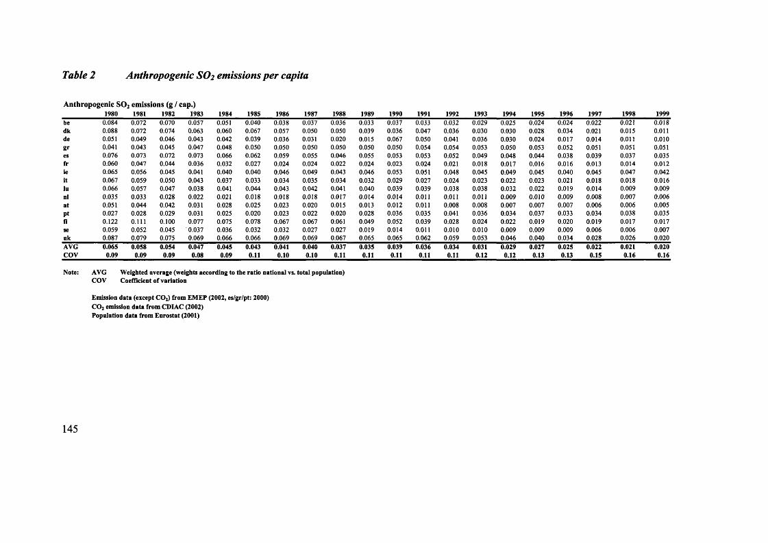
Table 2 Anthropogenic SO2 emissions per capita

Anthropogenic S 0 2 emissions (g / cap.)1980 1981 1982 1983 1984 1985 1986 1987 1988 1989 1990 1991 1992 1993 1994 1995 1996 1997 1998 1999

be 0.084 0.072 0.070 0.057 0.051 0.040 0.038 0.037 0.036 0.033 0.037 0.033 0.032 0.029 0.025 0.024 0.024 0.022 0.021 0.018dk 0.088 0.072 0.074 0.063 0.060 0.067 0.057 0.050 0.050 0.039 0.036 0.047 0.036 0.030 0.030 0.028 0.034 0.021 0.015 0.011de 0.051 0.049 0.046 0.043 0.042 0.039 0.036 0.031 0.020 0.015 0.067 0.050 0.041 0.036 0.030 0.024 0.017 0.014 0.011 0.010gr 0.041 0.043 0.045 0.047 0.048 0.050 0.050 0.050 0.050 0.050 0.050 0.054 0.054 0.053 0.050 0.053 0.052 0.051 0.051 0.051es 0.076 0.073 0.072 0.073 0.066 0.062 0.059 0.055 0.046 0.055 0.053 0.053 0.052 0.049 0.048 0.044 0.038 0.039 0.037 0.035fr 0.060 0.047 0.044 0.036 0.032 0.027 0.024 0.024 0.022 0.024 0.023 0.024 0.021 0.018 0.017 0.016 0.016 0.013 0.014 0.012ie 0.065 0.056 0.045 0.041 0.040 0.040 0.046 0.049 0.043 0.046 0.053 0.051 0.048 0.045 0.049 0.045 0.040 0.045 0.047 0.042it 0.067 0.059 0.050 0.043 0.037 0.033 0.034 0.035 0.034 0.032 0.029 0.027 0.024 0.023 0.022 0.023 0.021 0.018 0.018 0.016lu 0.066 0.057 0.047 0.038 0.041 0.044 0.043 0.042 0.041 0.040 0.039 0.039 0.038 0.038 0.032 0.022 0.019 0.014 0.009 0.009nl 0.035 0.033 0.028 0.022 0.021 0.018 0.018 0.018 0.017 0.014 0.014 0.011 0.011 0.011 0.009 0.010 0.009 0.008 0.007 0.006at 0.051 0.044 0.042 0.031 0.028 0.025 0.023 0.020 0.015 0.013 0.012 0.011 0.008 0.008 0.007 0.007 0.007 0.006 0.006 0.005pt 0.027 0.028 0.029 0.031 0.025 0.020 0.023 0.022 0.020 0.028 0.036 0.035 0.041 0.036 0.034 0.037 0.033 0.034 0.038 0.035fi 0.122 0.111 0.100 0.077 0.075 0.078 0.067 0.067 0.061 0.049 0.052 0.039 0.028 0.024 0.022 0.019 0.020 0.019 0.017 0.017se 0.059 0.052 0.045 0.037 0.036 0.032 0.032 0.027 0.027 0.019 0.014 0.011 0.010 0.010 0.009 0.009 0.009 0.006 0.006 0.007uk 0.087 0.079 0.075 0.069 0.066 0.066 0.069 0.069 0.067 0.065 0.065 0.062 0.059 0.053 0.046 0.040 0.034 0.028 0.026 0.020AVG 0.065 0.058 0.054 0.047 0.045 0.043 0.041 0.040 0.037 0.035 0.039 0.036 0.034 0.031 0.029 0.027 0.025 0.022 0.021 0.020COV 0.09 0.09 0.09 0.08 0.09 0.11 0.10 0.10 0.11 0.11 0.11 0.11 0.11 0.12 0.12 0.13 0.13 0.15 0.16 0.16

Note: AVG Weighted average (weights according to the ratio national vs. total population)COV Coefficient of variation

Emission data (except C 0 2) from EMEP (2002, es/gr/pt: 2000)C 0 2 emission data from CDIAC (2002)Population data from Eurostat (2001)

145

Table 2 shows the empirical results with regard to sulphur emissions; the complete

results for all seven covered air pollutants can be found in the appendix as table 27.

Figure 21 illustrates to which considerable extent the average sulphur pollution load of

EU countries varied. In 1980, Finland had the highest sulphur emission levels with

0.122g per capita. On the other hand, Portugal had the lowest figure with 0.027g per

capita. The average value across all fifteen EU member states, which was composed

from national values that were weighted according to the countries’ population

numbers, amounted to 0 . 6 6 grams of sulphur emissions per capita per annum.

Figure 21 Anthropogenic sulphur emissions per capita, selected EU member

states

0.14

0.12

0.06 - Weighted Average (EU15)

0.04 -

0.02

0.003 o> CO in 00CM io>

Emission data from EMEP (2002) Population data from Eurostat (2001)

146

On the first look, the above graph tells a fairly straight-forward story: over the

observation period, sulphur emission levels have decreased considerably in most of the

15 states that currently constitute the European Union. The weighted average has

declined to 0.035g and 0.020g per capita in 1989 and 1999 respectively. As mentioned

earlier, the rise in the average sulphur pollution level in 1990 may be explained by the

inclusion of Eastern Germany.

The picture also illustrates that some countries have managed to cut their sulphur

emission levels more than others. Both Finland and the United Kingdom exhibit a

significant reduction. Sulphur emission levels in Greece and Portugal have risen

significantly over the observation period. After 1994, Greece had the highest sulphurn

emission level per capita in the sample.

On the basis of this graph, one might be tempted to conclude that a downward

harmonisation of sulphur emission levels took place across the EU15 countries. This

would correspond to the observations that the weighted average has decreased over the

observation period and that the differences between the highest and the lowest sulphur

emission figures per capita have also decreased in absolute terms.

However, such an assessment would tell only half the story. Since the average is

changing over the observation period, the development regarding the differences

between the highest and the lowest sulphur emission figures must be assessed in relative

terms. One way to do this is by calculating the so-called coefficient of variation (COV).

The COV is a statistical tool to compare the variability of data measured across the

observed years (Neumayer 2001). It is computed for a certain year t as follows:

(3.1.2) COV. =N i ZC*i; - X,Y

i = i

7 The reasons behind this observed change in pollution load may differ from country to country; possible explanations could include a shift to cleaner technologies, a shift in industrial structure, or the expansion or contraction of economies. Although this would be interesting background information, highlighting the individual factors for each country in the sample would exceed the scope of this thesis.

147

where N is the number of countries (in this case, the 15 EU member states), jc, is the

sulphur emission load per capita with regard to country i at time t, and x t is the

weighted average at time t.

Figure 22 graphically displays the results of this calculation (cf. table 2). While the

weighted average is decreasing, the COV is increasing over time. This seems to indicate

that the relative differences in sulphur emission between EU member states have

actually increased while the overall level of sulphur emissions has decreased over the

observation period.

Figure 22 Anthropogenic sulphur emissions per capita (EU15): coefficient of

variation and weighted average

0.18 -| r 0.07

0.16 -0.06

Coefficient of Variation (COV) [left-hand scale] v

0.14 -

- 0.050.12 -

- 0.040.10 -

0.08 - 0.03Weighted Average [right-hand scale]0.06 -

- 0.02

0.04 -

- 0.010.02 -

0.00oCO CMCO CO00 m

COCOCO CO COCO O)

GOCOO) o> in COO) O)

ooo> a>O)oo CNO)CO o>

148

This observation corresponds in principle to the findings presented by Neumayer

(2001). Using a different data source and a slightly different calculation method,

Neumayer showed that between 1985 and 1996, sulphur emission levels in the EU have

decreased in average, but diverged within the sample.

This conclusion is important because it represents the rationale behind the theoretical

approach to the further development of the environmental performance indicators:

Looking at the development of emission levels in absolute terms certainly reveals one

specific aspect of statistical reality. Such an approach may well be best suited for

analyses into the pollution performance of particular states or economies on a stand

alone basis. However, if the focus is on the pollution performance within a set of

countries over time, the method of choice must be to look at the relative development of

emission figures.

For this reason, this study will analyse pollution performance indicators which are

computed within a relative system. With regard to the research question at hand, the

pollution performance indicators need to compare the relative development of air

pollutant emission levels across the EU and relate them to chemical industry

performance. Thus, the fifteen European Union member states jointly represent the

relative system that forms the focal point of the study. The scope of analysis is restricted

to the relative differences within the system; the overall or absolute development of EU

pollution levels as well as the EU pollution performance relative to other economies

will not be the object of this analysis.

Note that this set-up inherently implies that the European Union constitutes a valid

relative system. In other words, the study assumes that the EU member states to form a

sufficiently homogeneous group of countries.

149

Air pollution time series

As mentioned before, the pollution performance indicators will be aggregates of up to

seven sub-indicators. The sub-indicators capture the following anthropogenic air

pollutants:8

• Methane (C H 4) is an integral component of the greenhouse effect, second only

to CO2 as a contributor to anthropogenic greenhouse gas emissions. Methane is

mainly produced by anthropogenic sources, such as landfills, natural gas and

petroleum systems, agricultural activities, coal mining, stationary and mobile

combustion, wastewater treatment, and certain industrial processes. In the

chemical industry, methane is a raw material for the manufacture of methanol,

formaldehyde, nitro methane, chloroform, carbon tetrachloride, and Freon.

• Carbon monoxide (CO) is a colourless, odourless, tasteless and toxic gas

produced as a by-product of combustion. Any fuel burning appliance, vehicle,

tool or other device produces carbon monoxide gas. Carbon monoxide inhibits

the blood's ability to carry oxygen to body tissues including vital organs such as

the heart and brain.

• Carbon dioxide (CO2) is one of the gases in our atmosphere, being uniformly

distributed over the earth's surface.

8 Information on air pollutant characteristics in this section was obtained through the several internet sources Columbia University Press (2001). The Columbia Encyclopaedia. 12 May 2002, European Environment Agency (2002). EEA Multilingual Glossary. 12 May 2002;http://glossary.eea.eu.int/EEAGlossary, Ontario Ministry of Environment and Energy (2002). Air Quality Ontario. Pollutants. 12 May 2002, Shakhashiri (2002). Chemical of the week. 12 May 2002; http://scifun.chem.wisc.edu/chemweek, U.S. Environmental Protection Agency (2002). EPA Global Warming Site: National Emissions. 12 May 2002; www.epa.gov/globalwarming/emissions/national/index.html..

150

Energy-related activities account for almost all CO2 emissions. The dominant

contributor is carbon dioxide from fossil fuel combustion. As fossil fuels are

combusted, the carbon stored in them is almost entirely emitted as CO2 . The

amount of carbon in fuels per unit of energy content varies significantly by fuel

type. For example, coal contains the highest amount of carbon per unit of

energy, while petroleum has about 25 percent less carbon than coal, and natural

gas about 45 percent less.

Some CO2 emissions are also produced as by-products of various non-energy-

related activities. Such production processes include cement manufacture, lime

manufacture, limestone and dolomite use, e.g. in iron and steel making, as well

as soda ash manufacture and consumption. Commercially, CO2 finds uses as a

refrigerant as dry ice, in beverage carbonation, and in fire extinguishers.

• Ammonia (NH3) is a colourless gas that is about one half as dense as air at

ordinary temperatures and pressures. It has a characteristic pungent, penetrating

odour. Ammonia forms a minute proportion of the atmosphere. It also takes part

in many chemical reactions.

Ammonia is prepared commercially in vast quantities. The major method of

production is the so-called Haber process, in which nitrogen is combined

directly with hydrogen at high temperatures and pressures in the presence of a

catalyst. It is obtained as a by-product of the destructive distillation of coal.

Ammonia solutions are used to clean, bleach, and deodorize; to etch aluminium;

to saponify (hydrolyze) oils and fats; and in chemical manufacture. The

ammonia sold for household use is a dilute water solution of ammonia in which

ammonium hydroxide is the active cleansing agent. The major use of ammonia

and its compounds is as fertilizers. Ammonia is also used in large amounts in the

Ostwald process for the synthesis of nitric acid; in the Solvay process for the

synthesis of sodium carbonate; in the synthesis of numerous organic compounds

used as dyes, drugs, and in plastics; and in various metallurgical processes.

Ammonia can attack the skin and eyes. The vapours are especially irritating, as

prolonged exposure and inhalation cause serious injury and may be fatal.

151

• Non-methane volatile organic compounds (NMVOC) include such compounds

as propane, butane, and ethane. They are emitted primarily from transportation,

industrial processes, and non-industrial consumption of organic solvents. The

main source of NMVOC is the combustion of fossil fuels.

• Nitrogen dioxide (NO2) results from the combustion of fossil fuels, contributing

to both smog and acid precipitation. NO2 is hazardous to human health and the

environment. It contributes to acid rain, which harms aquatic ecosystems (rivers,

lakes and wetlands) as well as forests and crops.

Nitrogen dioxide is a component of smog and ground level ozone primarily

produced by the combustion of fossil fuels - mainly by vehicles, electricity

generation and industrial processes. The health impacts of exposure to smog

include impaired lung function in the short term as well as accelerated

deterioration in lung function over the long term.

• Sulphur dioxide (SO2) is a colourless gas. It can be oxidized to sulphur trioxide,

which in the presence of water vapour is readily transformed to sulphuric acid

mist. SO2 can be oxidized to form acid aerosols. SO2 is a precursor to sulphates,

which are one of the main components of respirable particles in the atmosphere.

Health effects caused by exposure to high levels of SO2 include breathing

problems, respiratory illness and cardiovascular disease. It also damages trees

and crops. SO2 , along with Nitrogen Oxides, are the main precursors of acid

rain. This contributes to the acidification of lakes and streams, accelerated

corrosion of buildings and reduced visibility. SO2 also causes formation of

microscopic acid aerosols, which have serious health implications as well as

contributing to climate change.

An important source of SO2 emissions are smelters and utilities. Other industrial

sources include iron and steel mills, petroleum refineries, and pulp and paper

mills. Small sources include residential, commercial and industrial space

heating.

152

Besides being greenhouse gases, all seven air pollutants have in common that they are

strongly linked to human economic activity. With the exception of methane and N H 3,

the emission of the listed pollutants is, to varying degrees, the product of fossil fuel

combustion.

Table 3 illustrates the availability of complete data sets regarding the seven air

pollutants. All data sets are complete from 1990 onwards. The data series on CO2 , NO2

and SO2 are complete from 1980 onwards. CO2 values for 1999 have been estimated on

the basis of a linear projection.

Table 3 Air pollution data availability (national level)

O e o 0 00 00 00 00 00 00 00 0 0 © \ © s 0 \ ® 0 s 0 \ ® 0 \ ® Os

cu, ■ ■ ■ ■ ■ ■ ■ ■ ■ ■

co ■ ■ ■ ■ ■ ■ ■ ■ ■ ■

C02 ■ ■ ■ ■ ■ ■ ■ ■ ■ ■ ■ ■ ■ ■ ■ ■ ■ ■ ■ □

n h 3 ■ ■ ■ ■ ■ ■ ■ ■ ■ ■

NMVOC ■ ■ ■ ■ ■ ■ ■ ■ ■ ■

N0 3 ■ ■ ■ ■ ■ ■ ■ ■ ■ ■ ■ ■ ■ ■ ■ ■ ■ ■ ■ ■

S 0 2 ■ ■ ■ ■ ■ ■ ■ ■ ■ ■ ■ ■ ■ ■ ■ ■ ■ ■ ■ ■

■ Complete data set □ Values projected (linear projection)

Because the observation periods vary from pollutant to pollutant, this study will look at

two types of pollution performance indicator time series: One time series will cover the

period between 1990 and 1999 and comprise all seven air pollutants at equal weight.

The second time series will cover an extended observation period (1980 to 1999) at the

trade-off of comprising only three air pollutants (CO2 , NO2 and SO2) at equal weight.

153

3.2.1.2 Population-based Pollution Load Index (PLI)

The first indicator will be called Pollution Load Index (PLI). It compares the

development of national air pollution levels per capita to the development of the

weighted EU average. The weight of country i (w) in year t is derived as a function of

its population size relative to the European Union as a whole:

(3.2.1) Wu=_Popuhtion^ ^ i = b ed k >uk

y population ktk=be

The overall weighted average with regard to pollutant j , W \EU 15)/, is composed as

follows:

v k

(3.2.2) W (Et/15); = Y .A P I • wkt where AP stands for air pollutionk=be

To avoid distorted results, the weighted average will exclude country i when analysing

its pollution performance relative to the average:

uk

(3.2.3) W (El/15 - iX = Y j Api ■ wk< with k „ ik=be

The Pollution Load Index of country i with regard to pollutant j ( PLIJit) is thus

constructed as follows:

(3.2.4) PLIJit = {tv- UPj )/W \EU\5 -/,)]• 10o|- 100

or,

154

A p J / uk' H a P ’ ■ wkl

populationit / £^e•KXU-lOO

with k „ i

where N(AP) stands for normalised per capita air pollution.

In plain words, this operation compares the national air pollution performance per

capita to the weighted EU average. The PLI therefore stands for the difference of

national air pollution levels relative to the EU average in percent.

Figure 23 Pollution load index (SO2 emissions): Finland and Greece

300

200

100

0

-100 O00 COCO CO CO

COo>CO COo> COO) h-o> GOo> ayo)01oo coco co o0 CDCO o>

Emission data from EMEP (2002) Population data from Eurostat (2001)

155

Table 29 in the appendix reports the outcome of this calculation comprehensively, both

with regard to sulphur emissions, as well as with regard to the other air pollutants. The

following graph also illustrates the outcome of this operation. As in the previous

section, sulphur emission figures serve as examples (cf. figure 2 1 ).

As the graph illustrates, the PLI projects national pollution load levels onto a scale that

ranges from [-1 0 0 ,+ 0 0). On this scale, the value -100 would indicate zero emissions.

Index value 0 would indicate that national pollution load levels were equal to the EU

average, whereas positive PLI values point at national pollution load levels being higher

than the average.

Looking at the development of the PLI values regarding the sulphur emissions of

Finland and Greece, the very different sulphur pollution performance of the two

countries becomes apparent. Finland has managed to reduce its sulphur pollution load

from an index value that was roughly twice the EU average in the first years of the

observation period to below-average values from 1991 onwards. 9

Inversely, Greece’s sulphur pollution load indicator has increased almost steadily, with

the exception of the years 1989/1990. Note that this break may well be explained by the

external shock of German reunification due to which the East German states were

incorporated into German sulphur emission figures from 1990 onwards. Since Germany

has the biggest weight in the weighted EU average, this had a significant impact on the

average from 1990 onwards (cf. figure 22). Given that the indicator is constructed in

relation to the EU average, that external shock introduces a break into the indicator time

series.

9 Cf. footnote 7 on page 147.

156

3.2.1.3 GDP-based General Pollution Intensity (GPI)

As mentioned earlier, population is not the only feasible normalising factor for national

air pollution. Hence, the second pollution performance indicator will be GDP-based.

Normalising a country's pollution with its economic size, expressed in GDP, yields how

much pollution per unit of GDP occurs. In other words, this method reveals how much

pollution an economy produces in the process of generating a unit of GDP, for instance

a million Euro worth of GDP. The basic idea of the indicator is comparable to the

approach of Zaim and Taskim (2000).

The General Pollution Intensity (GPI) index builds on this idea. Methodically, the GPI

is constructed much in the same way as the first indicator. The main difference is that

economic size, as expressed by GDPu, replaces population both in the normalising as

well as in the weighting function:

(3.3.1) GPI!, =uk

GDP• 100^-100

it / k =be

GDP.with =it uk

Ik=be

T g d p„,

and k „ i

The following table 4 displies the results of this calculation for sulphur emissions. The

complete results for all pollutants can be found as table 30 in the appendix.

157

Table 4 Anthropogenic SO2 emissions / GDP

A n th ro p o g en ic S 0 2 em issions / G D P (tonnes / m illion €) 1980 1981 1982 1983 1984 1985 1986 1987 1988 1989 1990 1991 1992 1993 1994 1995 1996 1997 1998 1999

be 9.60 8.06 7.91 6.13 5.07 3.75 3.27 2.98 2.71 2.29 2.42 2.05 1.83 1.61 1.28 1.16 1.12 1.01 0.93 0.79dk 9.71 7.43 6.92 5.31 4.60 4.68 3.63 3.03 2.89 2.16 1.87 2.39 1.77 1.38 1.31 1.14 1.31 0.78 0.52 0.36de 5.41 4.91 4.24 3.61 3.27 2.87 2.45 1.97 1.20 0.87 4.46 2.84 2.16 1.80 1.43 1.09 0.77 0.61 0.48 0.43gr 11.07 10.22 9.11 9.62 9.27 9.63 10.54 10.54 9.21 8.31 7.69 7.53 7.22 6.96 6.26 6.15 5.52 4.99 4.98 4.57es 18.64 16.79 15.07 15.75 12.59 10.99 9.43 8.24 6.00 6.02 5.19 4.71 4.50 4.61 4.55 3.94 3.21 3.20 2.89 2.59fr 6.68 4.80 4.28 3.36 2.80 2.15 1.81 1.73 1.50 1.58 1.36 1.44 1.20 1.00 0.89 0.80 0.76 0.63 0.63 0.51ie 16.67 12.22 8.75 7.47 6.98 6.33 6.79 7.12 5.79 5.60 5.84 5.33 4.74 4.38 4.35 3.69 3.01 2.91 2.87 2.30it 11.57 9.16 7.00 5.30 4.07 3.42 3.16 3.11 2.79 2.37 1.94 1.68 1.51 1.61 1.51 1.61 1.28 1.07 1.00 0.85lu 6.05 4.86 3.47 2.58 2.52 2.38 2.16 2.04 1.87 1.63 1.43 1.30 1.23 1.14 0.91 0.59 0.51 0.38 0.23 0.21nl 3.97 3.61 2.84 2.12 1.87 1.52 1.45 1.40 1.29 0.98 0.91 0.74 0.70 0.62 0.52 0.48 0.43 0.37 0.31 0.28at 6.86 5.52 4.58 3.09 2.58 2.18 1.80 1.50 1.08 0.89 0.73 0.61 0.44 0.39 0.35 0.32 0.30 0.28 0.25 0.21Pt 13.20 11.66 11.52 12.20 9.70 6.79 7.09 6.17 5.02 5.90 6.68 5.51 5.62 5.05 4.59 4.58 3.83 3.86 3.97 3.42fi 16.06 12.06 9.56 6.92 5.84 5.52 4.74 4.39 3.50 2.42 2.52 2.05 1.79 1.79 1.44 1.03 1.10 0.96 0.83 0.76se 5.47 4.23 3.69 2.99 2.48 2.05 2.05 1.66 1.48 0.94 0.68 0.51 0.48 0.57 0.51 0.47 0.44 0.26 0.25 0.31uk 12.62 9.60 8.47 7.45 6.72 6.19 6.83 6.53 5.60 5.02 4.99 4.43 4.28 3.88 3.12 2.79 2.21 1.44 1.29 0.95AVG 10.24 834 7.16 6.26 536 4.70 4.48 4.16 3.46 3.13 3.25 2.87 2.63 2.45 2.20 1.99 1.72 1.52 1.43 1.24COV 0.11 0.11 0.12 0.15 0.15 0.15 0.16 0.17 0.17 0.19 0.18 0.18 0.20 0.20 0.21 0.23 0.22 0.24 0.26 0.27

Note: AVG Weighted average (weights according to the ratio national vs. total GDP)COV Coefficient of variation

Emission data (except C 0 2) from EM EP (2002, es/gr/pt 2000)C 0 2 emission data from CDIAC (2002)GDP data from Eurostat (2001)

158

Figure 24 graphically displays selected results of the first calculation step, the

normalising operation. The average has been constructed by weighting the 15 EU

member states according to their economic size (GDP), calculated on an annual basis.

The figures reveal that Spain and Greece generated relatively more sulphur emissions

(“used up more clean air”) to produce goods and services than other EU economies had

to. In other words, the Spanish and Greek economies were more pollution intense than

the EU average. Inversely, the data also show that the Netherlands were comparatively

less pollution intense than other EU countries.

Figure 24 Anthropogenic sulphur emissions / GDP, selected EU member states

2 0 .0 0 -i

18.00 -

16.00 -

14.00 - esouioSa.oO

12.00 -

10.00 -

MC0 'm 101 0)<5(/>

8.00 -

weighted average

6.00 -

4.00 -

2.00 -

0.00oCOo> sO) 3 8O) o>

h-00o> 00

00o> g>COO) CM O)£CM

00o o>

Emission data from EMEP (2002) GDP data from Eurostat (2001)

159

Following the operation outlined in equation 4.3.1 above, one can transform the

normalised emission figures into the GPI indicator. Figure 25 graphically represents the

indicators for Greece, Spain and the Netherlands of this operation. With regard to

sulphur emissions in 1980, the GPI was 123 in Spain and 23 in Greece. In 1999, that

index was 256 in Spain and 474 in Greece. Thus, both countries’ pollution intensity

increased dramatically compared to the EU average over the observation period. By

contrast, the general pollution intensity in the Netherlands decreased from -57 in 1980

to - 6 8 in 1999.

Figure 25 General pollution intensity (SO2 Emissions): Greece, Netherlands and

Spain

500

400»01E§103111 300£o«a(AE 200

esc«ocS£Q

100

-100LOCO <0OO CO

COCO 10o>o00 Cs|co COCO CO O)GO

oo> CM0)

CO05 O) (0

050005

050505CO

Emission data from EMEP (2002) GDP data from Eurostat (2001)

160

3.2.1.4 GDP-based Manufacturing Pollution Intensity (MPI)

The third pollution performance indicator is aimed at capturing specifically the

pollution performance of the manufacturing sector. Whereas the GPI indicator is a tool

to capture inefficiency differences on the level of the general economy, the

Manufacturing Pollution Intensity (MPI) indicator looks at the industrial pollution

performance.

This approach is based on the notion that some economic sectors are more

environmentally hazardous than others. In this respect, the manufacturing sector is an

especially interesting case, because it produces a significant amount of pollution. One

might hypothesize that manufacturing sectors are therefore especially sensitive to

changes in pollution performance. The MPI indicator is constructed as follows:

(3.4.1)

MPIjtmanufacturingAPJ ,

--------------------------- / > manufacturingAPI •manufacturingGDPj( /

100M 00

with w;, =manufacturingGDPit

y manufacturingGDPktk=be

and k „ i

Although the basic method of construction of this indicator remains the same as for the

other two indicators, in practice, its calculation is a more difficult task. The raw data for

the computation of the MPI has to be more specific, as the indicator puts the amount of

manufacturing emissions ( manufacturingAPj) in relation to the manufacturing GDP

( manufacturingGDPjt).

The results of this operation applied to the case of sulphur emissions is recorded in table

5. The complete results for all pollutants are appended as table 31.

161

Table 5 Manufacturing SO2 emissions / manufacturing GDP

S 0 2 Emissions by Combustion, Manufacturing Sector (tonnes) / Manufactoring GDP (million €)1980 1981 1982 1983 1984 1985 1986 1987 1988 1989 1990 1991 1992 1993 1994 1995 1996 1997

be 10.73 8.46 7.76 8.45 7.86 4.03 4.14dk 10.57 6.46 5.18 4.29 2.89 2.85 2.88 2.41 2.05 2.02 1.49de 10.12 8.70 7.47 5.56 3.79 2.81 2.12 1.50 1.22gr 31.33 25.33 23.33 21.60 18.41 18.54 16.84 14.33 13.90 12.95 12.84es 53.63 51.75 39.31 33.22 25.66 22.10 20.06 18.68 18.96 15.14 14.72 13.84 12.58 13.24 12.12 10.12fr 3.23 3.28 2.75 2.36 2.27 1.89ie 10.57 8.34 7.31 7.50 7.71 5.52it 45.72 34.63 25.07 20.11 13.14 8.90 7.62 6.24 5.84 5.13 4.41 4.03 3.73 2.96 2.29 2.08lu 23.45 15.68 16.48 15.74 15.30 11.73 6.58nl 7.74 2.86 2.34 2.09 1.95 1.77 1.62at 35.88 29.31 23.64 13.16 7.88 6.27 4.98 4.00 2.80 1.84 1.78 1.16 0.77 0.63 0.50 0.58Pt 17.14 13.38 13.52 12.01 11.15 11.39fi 12.06 6.12 3.40 2.23 2.17 1.42se 1.25 0.99 0.75 0.82 0.64 0.52uk 31.65 24.36 20.31 16.28 12.76 10.57 11.50 9.42 9.34 7.53 5.84 5.49 5.49 5.33 4.32 3.08AVG 8.33 7.11 6.41 6.02 5.14 4.30COV 0.18 0.19 0.20 0.22 0.22 0.24

Note: AVG W eighted average (weights according to the ratio national vs. total manufactoring GDP)COV Coefficient of variation

Emission data from EM EP (2002, es/gr/pt: 2000)GDP data from E urostat (2001)

Data on the GDP share of the m anufactoring sector:All countries except Ireland and Luxembourg: OECD (2000)Ireland— data extrapolated from C entral Statistics Office, Ireland (2001)Luxembourg— Eurostat (2001)

162

As table 5 and the following graph illustrate, data scarcity restricted the compilation of

a comprehensive data set to the period from 1990 to 1995. The average has been

constructed by weighting the 15 EU member states according to the size o f their

manufacturing sector (manufacturing GDP in absolute terms), calculated on an annual

basis. Since the country weights, which are necessary for the calculation o f the

weighted average, require complete data sets for all 15 EU member states, the weighted

average could only be computed for the five years with complete data sets.

Figure 26 Manufacturing SO2 emissions / manufacturing GDP, EU member

states

(/>Q)C ^ c VlP 2 c* | 1 E(Ain 0- E Q£ o6 |£ 1 C

e s

o•213CHJ2

w eighted a v e ra g e20

3c032

CO COh-s s

Data Sources: see table 5

163

The variance of observations appears high, and, as in the case of the other two

indicators, there appears to be a trend towards downward harmonisation across the EU

in absolute values. However, as was the case concerning the normalised sulphur

emission figures mentioned earlier, this impression is misleading. The rising coefficient

of variation (cf. equation 4.1.2) clearly indicates that the internal difference relative to

the average has increased significantly. The empirical COV in the above graph has

increased from 0.18 in 1990 to 0.24 in 1995 (table 5).

3.2.1.5 Interpreting air pollution performance patterns

So far, based on the air pollution data series introduced above, this study has laid the

foundation to the calculation of three different pollution performance indicators. The

first indicator, called PLI (Pollution Load Indicator, cf. section 3.2.1.2) compares

national air pollution levels per capita to the weighted EU average.

The second indicator, called GPI (General Pollution Intensity, cf. section 3.2.1.3)

compares national air pollution levels per unit of GDP to the weighted EU average.

Finally, the MPI (Manufacturing Pollution Intensity, cf. section 3.2.1.4) puts air

pollution generated by the manufacturing sectors of EU member states in relation to the

manufacturing GDP and compares that figure to the weighted EU average.

The following section will introduce and discuss the empirical pollution performance

indicators.

Scope o f the indicators

At first sight, all three indicators may appear rather similar in design and content. This

may well be connected to the fact that the numerator of the three indicators is identical,

i.e., an air pollution time series. Yet, each of the indicators has distinct features, which

are summarised in table 6 .

The table aims to illustrate that each indicator mirrors pollution performance from a

different angle, and that therefore each of them has a significant analytical value.

164

Table 6 Advantages and disadvantages o f the pollution performance indicators

Indicator Advantages / Disadvantages

Pollution Load

(air pollution per capita)

the focus of the indicator is pollution per capita, which is the most intuitive and least economic of the three indicators

population is a relatively static denominator (with the exception of German reunification). Hence changes in the indicator are mainly due differences in pollution.

time series for all seven air pollutants from 1990 to 1999; a long-term time series from 1980 to 1999 covers three pollutants

General Pollution • the indicator reflects pollution performance from theIntensity perspective of the general economy

(air pollution per unit • GDP is a more volatile denominator; economic cyclesGDP) have an impact on the indicator

• time series for all seven air pollutants from 1990 to 1999;a long-term time series from 1980 to 1999 covers threepollutants

Manufacturing Pollution Intensity

(air pollution per unit of manufacturing GDP)

the indicator is specific to the manufacturing sector

reduced data availability and consistency

time series cover only two air pollutants from 1990 to 1995

Nevertheless, for consistency and transparency, the subsequent regression analysis laid

out in chapter six will build on one primary pollution performance indicator. The

overview on the indicator featured in table 6 should provide some answers to the

question, which indicator could be suited best to proxy the impact of pollution

performance on chemical industry performance.

Although the PLI indicator appears to be the most straight-forward index that is easiest

to understand by intuition, the other two GDP-based indicators may be closer to

economic reality. Since the purpose of this study is to compare the economic

performance of an industrial sector to pollution performance, the indicator of choice

should incorporate the concept of economic dynamism.

165

This reasoning would favour GPI or MPI as lead indicator for the subsequent analysis.

Between the two of them, the MPI indicator would obviously be the better-suited

candidate, since it is specifically designed to reflect the pollution performance of the

manufacturing sector of which the chemical industry forms part.

However, there is one very important drawback to the use of the MPI as lead indicator:

complete and consistent pollution data on the manufacturing sector is limited to the

period of 1990 to 1995 and to two pollutants. Given that some GPI time series cover a

period of twenty year from 1980 to 1999, the MPI data constraint is an important

argument. Key parts of the subsequent analysis are based on quantitative methods.

Therefore, the number of observations is an important practical consideration, as it

determines, for example, the reliability of regression estimates.

Long-term and short-term indicators

At this point, the reader should recall once more that the three pollution performance

indicators are aggregate indicators, which are composed of several sub-indicators. As an

example, the ‘global’ GPI indicator is composed of GPI sub-indicators, each of which

covers one specific pollutant. Thus, there are GPI sub-indicators for ammonia (NH3),

carbon monoxide (CO), carbon dioxide (CO2), methane (CH4), non-methane volatile

organic compounds (NMVOC), nitrogen dioxide (NO2) and sulphur dioxide (SO2). The

‘global’ pollution performance indicators are averages of those sub-indicators at equal

weight.

However, some pollution time series were more comprehensive than others. As

mentioned before, manufacturing pollution was complete only between 1990 and 1995.

National pollution time series were complete from 1980 to 1999 for CO2 , NO2 and SO2 .

The other data sets were complete on national level from 1990 to 1999 (cf. table 3).

For this reason, two PLI and GPI indicators series may be constructed. The first set of

indicators would consist of all seven sub-indicators. These PLI 7 and GPI 7 indicators

account for all available pollution data. However, these comprehensive pollution

performance indicators are short-term time series, since they cover only the ten years

1990 to 1999.

166

By contrast, if the indicators were composed only by the CO2 , NO2 and SO2 sub­

indicators, they covered the period from 1980 to 1999. Thus, PLI 3 and GPI 3 indicator

series could serve as long-term indicators.

Indicator correlation

The following section will discuss the empirical pollution performance indicators by

taking Denmark and Spain as examples. Tables 29 to 31 in the appendix provide all

empirical pollution performance indicators for those two countries, both by pollutant as

well as on an aggregate level.

Figure 27 represents the empirical results of Denmark. Because the CO2 , NO2 and SO2

pollution data sets allowed the compilation of a long-term time series covering the

period from 1980 to 1999, there are two PLI and GPI sets. Thus, the PLI 3 and GPI 3

indicators cover the three above mentioned pollutants over a period of twenty years.

Inversely, the PLI 7 and GPI 7 time series are short-term indicators, covering only ten

years from 1990 to 1999 but all seven air pollutants. As mentioned before, air pollution

data on the manufacturing sector was only complete over the period from 1990 to 1995

and with regard to two pollutants, SO2 and NO2 . For this reason, the manufacturing

pollution intensity is marked MPI 2.

Note that the PLI 3 and GPI 3 time series are broken between 1989 and 1990. Again,

this is due to the external shock of German reunification. The indicator values up to

1989 cannot be compared to the figures thereafter, because the relative system on which

the indicators are based has shifted.

167

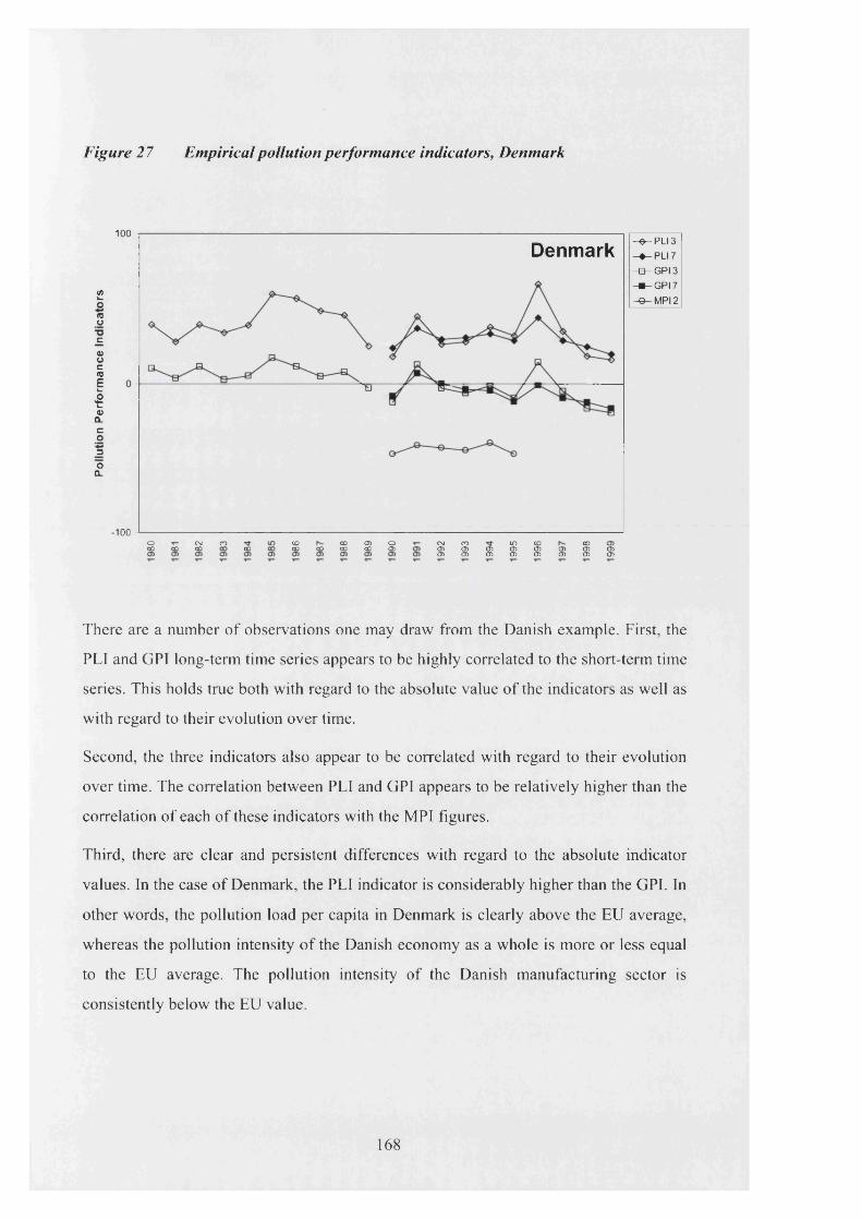
Figure 27 Empirical pollution performance indicators, Denmark

100—0 - P L I 3

—♦ - P L I 7

- B —G P I3

- * - G P I 7

-© - M P I 2

Denmark

</>L-ocooc0>ocCO

Eu-£X-<D

CLCoDO

CL

-100oco cm

00CO

COCOCO oo 00

COCDCO

oa: CN CO CO CO 0 0 __0 5 CD CD 05 CD CD CD CD 0 5 0 5 0 ) 0 5 0 ) 0 5 0 5 0 5

00

There are a number o f observations one may draw from the Danish example. First, the

PLI and GPI long-term time series appears to be highly correlated to the short-term time

series. This holds true both with regard to the absolute value of the indicators as well as

with regard to their evolution over time.

Second, the three indicators also appear to be correlated with regard to their evolution

over time. The correlation between PLI and GPI appears to be relatively higher than the

correlation o f each of these indicators with the MPI figures.

Third, there are clear and persistent differences with regard to the absolute indicator

values. In the case o f Denmark, the PLI indicator is considerably higher than the GPL In

other words, the pollution load per capita in Denmark is clearly above the EU average,

whereas the pollution intensity o f the Danish economy as a whole is more or less equal

to the EU average. The pollution intensity of the Danish manufacturing sector is

consistently below the EU value.

168

A correlation analysis of the long-term and short-term pollution performance indicators

reveals the very high degree of association between the two time series in most EU

member states.

Table 7 Correlation coefficients between pollution performance indicators

PLI3 / PL I7 GPI 3 / GPI 7 PLI 3 / GPI 3 GPI 3 / MPI 2 PLI 3 / MPI 2be 0.98 0.98 0.75 -0.23 0.36dk 0.96 0.88 0.87 0.75 0.69de 0.98 0.99 0.83 0.97 0.91gr 1.00 1.00 0.94 0.92 0.94es 0.99 1.00 0.74 0.98 0.94fr 0.72 0.94 0.86 0.01 0.10ie 0.98 -0.05 0.82 0.39 0.58it 0.62 0.95 0.64 -0.79 -0.59lu 0.98 0.99 0.75 0.63 0.86nl 0.25 0.89 0.42 -0.16 -0.05at 0.80 0.86 0.97 0.75 0.79Pt 0.99 0.99 0.97 0.99 0.93fi 0.95 0.98 0.12 -0.64 0.83se 0.80 0.98 0.80 -0.47 -0.20uk 0.99 1.00 0.88 0.44 -0.08AVG 0.87 0.89 0.76 0.30 0.47

The correlation coefficients between PLI 3 and PLI 7, GPI 3 and GPI 7, as well as

between PLI 3 and GPI 3 appear to be consistently positive except in one instance. The

average coefficients are well above 0.75, which seems to indicate a very high degree of

correlation.

The notable exception is the correlation coefficient between GPI 3 and GPI 7 in Ireland,

which is very close to nil. That observation seems to indicate an almost complete

independence between the two data sets. Figure 28 illustrates how the GPI 3 and GPI 7

indicators appear to converge instead of running more or less parallel. As the

correlation analysis shows, Ireland is the only country in the sample that exhibits this

behaviour.

169

Figure 28 Empirical pollution performance indicators, Ireland

200

Ireland

■5 100

100 O)00

LOCD

OCO

COCO

o-co CDCO

CDCO

ocd

CNCD

COcd 3 CDO) CD

COCF>co o>

GPI 3

GPI 7

MP 2

One reason for this peculiar conduct appears to lie in the development o f the Irish GPI

indicator concerning SO2 emissions. Unlike the other six Irish GPI indicators, which are

generally stable or decreasing between 1990 and 1999, the SO2 pollution intensity

increases significantly from 86 in 1990 to 173 in 1999. Since this SO2 sub-indicator

accounts for one third of the aggregated GPI 3 indicator but only for one seventh o f the

GPI 7 indicator, the GPI 3 is much more sensitive to this distinct behaviour.

The empirical GPI results indicate that this sharp increase o f the SO2 GPI indicator is

not an exclusively Irish phenomenon. One can observe similar patterns with regard to

Greece, Portugal and Spain. However, in contrast to Ireland, the other pollution

indicators also increase in those three countries, which means that the SO2 GPI

development is more accentuated but generally in line with the other pollutants.

170

Lastly, the results represented in table 7 show that the average correlation coefficient

between PLI 3 and MPI 2 is 0.47; the figure is 0.30 with regard to GPI 3 and MPI 2.

This observation indicates that the MPI indicator is positively linked to the other two

pollution performance measures, although its degree of correlation is small. This may

be due to the fact that the PLI and GPI indicators are based on the same emission data

aggregated on national level, whereas the MPI indicator uses a completely different and

less aggregated data set.

One may draw two basic conclusions from the above discussion. First, the three

pollution performance indicators are sufficiently different with regard to their scope and

data basis to stand alone as individual indicators. For this reason, one part of the

subsequent empirical analysis will use all three indicators to categorise EU member

states according to their pollution performance. For this, the fact that the three

indicators address the same issue from different angles should be rather an advantage.

On the other hand, as the correlation analysis has shown, the indicators are clearly

linked to each other. This should improve the efficiency of quantitative analyses, when

one of the indicators could stand as proxy for the two others. Taking all aspects into

consideration, this proxy would best be the long-term general pollution intensity (GPI

3) indicator, as it combines economic focus with the largest available pool of

observations.

Indicator interpretation

Figure 29 provides an example of how pollution performance indicators develop over

time: in this instance, with regard to the GPI 3 indicators in Germany and Britain. The

graph illustrates the point that the interpretation of the indices can be tricky. In both

countries, the GPI 3 indicator decreased over time indicating an improvement in

environmental performance.

With regard to Germany, that indicator decreased by 46 points, from 17 in 1990 to -29

in 1999. In the United Kingdom, the index apparently declined at a higher rate; from 59

to 6 over the same period of time. Thus, the British pollution intensity went down by

53.

171

Figure 29 GPI 3, Germany and United Kingdom, 1990 to 1999

100

GPI 3

&(AC

Cco3O0.

15>_Q)C<1>O

de

-100§ Sityi 3 stn5

However, this observation does not necessarily indicate that Britain has a better

pollution performance than Germany. The reason for this at first sight surprising fact is

that the UK is improving its index from a considerably higher starting level. As Britain

is catching up to approach the EU average, Germany appears to expand its lead over the

EU average from 1992 onwards. Due to the way the pollution performance indicators

are constructed, (-100) is an asymptote, because pollution values cannot be more than

100 percent less than the EU average. Thus, the closer observed indicator values get to

(-100), the slower indicator values are going to continue decreasing.

For this reason, any comparison o f pollution performance indicators between countries

must account for both the indicator development over time as well as for the indicators’

overall position relative to the EU average. The former may be achieved by looking at

the trend o f an index in absolute numbers as compared to the EU average, normalised to

zero. In other words, the first task would be to assess whether the indicator shows a

statistically significant trend over time.

172

A second step needs to calculate the overall position of the indicator compared to the

EU average. Measuring the deviation of the index-average (taken across all years in the

observation period) from zero could achieve this objective.

As a conclusion to the empirical pollution performance chapter, this section will

compare how the European Union member states have presented themselves with

regard to the three pollution performance indicators over the period from 1980 to 1999.

The aim of this empirical study is to develop some sort of categorisation or ranking that

tells which countries exhibited a generally strong pollution performance and which ones

have shown a generally weak one.

In this context a ‘strong pollution performance’ indicates a better-than-EU-average

pollution indicator development, that is, it flags countries where air pollution has gone

down relative to the EU average. Inversely, ‘weak pollution performance’ countries

would show a worse-than-average pollution performance; their pollution figures would

have increased relative to the EU level.

3.2.1.6 A pollution performance ‘ranking’ of EU member states

At this point, the obvious question most people would ask is “so, who is polluting the

most?”, or “how is my country doing?” Let us have a look.

This categorisation exercise will compare the PLI, GPI and MPI indicator of the EU

member states. As mentioned earlier, since the reunification of Germany in 1989/1990

introduced an external shock into the relative system on which the pollution

performance indicators are based, it would be methodically unsound to compare

indicator values before and after this time mark. Therefore, the analysis will only

compare the pollution performance indicators after 1990.

The upside of this time restriction is that the comparative analysis can use the more

comprehensive short-term indicators PLI 7 and GPI 7, as well as the MPI 2 indicator.

This allows comparing national pollution performances on the broadest available range

of air pollutants.

173

As mentioned before, a comparative analysis will need to take into account both the

development as well as the relative position towards the average of the pollution

performance indicators. The categorisation exercise will therefore assess the following

dimensions:

• P LI 7 trend over the observation period 1990 to 1999. The trend values correspond

to the coefficient of the time dummy in a regression where the dependent variable is

PLI 7.

This observation captures the relative evolution over time of the pollution load

indicator compared to the EU average. An upward PLI 7 trend indicates an increase

in the aggregated national pollution load, as measured in pollution per capita, has

grown relative to EU average. Hence, the country's pollution performance has

under-performed the EU average. Inversely, a downward PLI trend would point at

stronger-than-average pollution performance.

• P LI 7 deviation, written Dev (PLI 7), indicates whether the average value of the PLI

indicator across the observation period is above or below the EU average, which is

normalised to zero. This measure mirrors the long-term per capita pollution level of

a country. If Dev(GPI) has a value that is larger than zero, the country has a higher

per capita pollution load over the period than the EU average. The reasons for this

structural difference may be of economic nature, such as the development level of a

country, or due to other factors such as climate. Inversely, if Dev(GPT) shows a

value smaller than zero, it would indicate that the country has structurally less

average per capita pollution over the observation period than the EU as a whole.

• The GPI 7 trend over the observation period captures the relative pollution

performance at the level of the general economy compared to the EU average. An

upward GPI 7 trend would indicate that the economy's pollution intensity has

increased relative to EU average. Hence, the country would have a worse pollution

performance with regard to the general economy than the EU. A downward GPI 7

trend would stand for a stronger-than-average pollution performance.

174

• The GPI 7 deviation, Dev (GPI 7), shows whether pollution intensity of a member

state’s economy has been, in average over the observation period, above or below

the EU level. This figure reflects the overall economic structure and pollution

efficiency. If Dev(GPI 7) has a value larger than zero, the economy is structurally

more pollution intense than the average. In other words, that economy ‘needs

consume in average more clean air’ than other EU economies to produce the same

amount of GDP over the observation period. Inversely, lower than zero Dgv(GPI)

values would indicate that the economy is less pollution intense, and is thus 'greener'

than the average.

• The M PI 2 trend focuses on the pollution intensity of a country’s manufacturing

sector relative to the EU average. It echoes the relative pollution performance of the

relative pollution performance of industries and other production sectors. If the MPI

2 trend is upwards, the pollution intensity of the national manufacturing sector has

grown relative to the EU. Therefore, the manufacturing pollution performance

would be considered worse-than-average. On the other hand, a downward MPI 2

trend value would hint at a better-than-average pollution performance of the

manufacturing sector.

• Lastly, the deviation of a country's M PI 2 average, Dev (MPI 2), indicates whether

a country's manufacturing sector is over the observation period more or less

pollution intense than the EU average. If Dev (MPI 2) is shown to be above zero,

the manufacturing sector is historically over the observation period more pollution

intense, and therefore less efficient, than the EU average. Hence, the manufacturing

sector would structurally under-perform the EU average, because it generally

generates more air pollution than the other EU manufacturing sectors while

producing the same value of goods. Inversely, a Dev (MPI 2) value below zero

would indicate better-than-average pollution intensity structure.

175

Pollution performance scenarios

Before we can go on to classify the European Union member states according to their

pollution performance based on the above mentioned six observations, there needs to be

a definition of performance scenarios. The pollution performance trend and deviation

provides information on two sorts of dimensions: the deviation reveals whether the

country starts from a relatively high or low initial pollution levels, whereas the trend

reveals the evolution of the pollution performance indicator. If these two dimensions are

combined, there are four potential scenarios:

Table 8 Pollution performance scenarios

Poor pollution

performers

Catching-up

countries

Falling-behind

countries

Strong

pollution

performers

DeviationHigh initial

pollution levels

High initial

pollution levels

Low initial

pollution levels

Low initial

pollution levels

TrendLack of

convergenceConvergence Convergence

Lack of

convergence

Poor pollution performers

The first country cluster consists of Greece, Spain and Portugal. The observed data

suggests for these countries a very weak pollution performance over the observation

period. The graphic representation of the pollution performance indicators in figure 30

illustrates that the country cases in this cluster possess a number of common features:

176

First, with regard to all countries and to all pollution performance indicators, the trend

values are upward and, as noted in table 9, highly significant. In other words, the

pollution performance o f the countries in this group clearly deteriorated relative to the

EU average over the observation period. Secondly, in all cases, the deviation o f the

three observed pollution performance indicators was above zero. This indicates that the

said deterioration o f the pollution performance captured by the upward trend values

took actually place in countries that were already doing worse than EU average.

Figure 30 Pollution trends: poor pollution performers

300

Greece-♦ — PLI 7 -■ — GPI 7 -©— MPI 2 PLI 7 T rend— GPI 7 Trend- - - - MPI 2 Trend

200 -----

100 -

-100inCD05

<D05o> 05

0 5

00050 5

CN05 05

0 5

177

300

Spain-PLI 7 -G P I 7 -M PI 2

PLI 7 Trend GPI 7 Trend

■ MPI 2 T rend

200

100

100CD

COcd

CDCD

CMCD

COCD CD

h-CDCD

300

Portugal•— PLI 7 I— GPI 7 >— MPI 2- PLI 7 Trend- * GPI 7 Trend * • MPI 2 Trend

200 -

100

100 inCD

CO COcd

CDCD

CMQ> CD<D

178

Based on these observations, it appears fair to conclude that Greece, Spain and Portugal

showed a poor pollution performance pattern relative to the rest of the European Union

over the period from 1990 to 1999. One should note that this poor pollution

performance was particularly pointed with regard to the manufacturing sector. As the

trend values in table 9 reveal, the manufacturing pollution performance deteriorated

much more rapidly than the other two pollution performance indicators.

Table 9 Pollution performance indicators: poor pollution performers

Greece Spain Portugal

PLI 7 Trend +6 .1 ** +5.3** +5.2**

Dev (PLI 7) + 1 1 + 2 2 + 1 0

Overallperformance

Poor Poor Poor

GPI 7 Trend +7.8** +10.9** +6.3**

Dev (GPI 7) +124 +90 +144

Overallperformance

Poor Poor Poor

MPI 2 Trend +2 1 .6 * +25.2** +18.9**

Dev (MPI 2) +168 +213 +175

Overallperformance

Poor Poor Poor

* Significant at 90% level** Significant at 99% level

Overall, the similarities between Greece, Spain and Portugal with regard to their

pollution performance indicators seem remarkably strong. Besides their particularly

pollution intensive manufacturing sectors, all three countries were more or less EU

average with regard to per capita pollution intensity at the beginning of the 1990s. The

indicators have since deteriorated at roughly the same rate, i.e. at five or six index

points per year. The countries’ GPI indicator also appears to follow this pattern.

179

In conclusion, the empirical figures seem to indicate that Greece, Spain and Portugal

form a remarkably clear cut and homogenous pollution performance cluster. This could

of course be due to rather obvious factors, as those Southern European countries share

to some degree a comparable economic, cultural and geographic setting.

However, the empirical data indicates a much lower degree of similarity with regard to

other pollution performance clusters. As the other results below will show, this holds

true even to groups of countries of which one might expect similar pollution

performance patterns, such as the Nordic states or the Benelux countries.

Countries that catch-up

The second cluster comprises Ireland, Luxembourg and the United Kingdom. The

pollution performance of those countries may be characterised as ‘poor but improving’.

In other words, although the pollution performance of the countries in this cluster was

overall below EU average, at least one of their performance indicators improved over

the observation period.

Just by looking at the graphs represented in figure 31, one probably gets the intuitive

impression that this country cluster is much less homogeneous that the one presented

earlier. The pollution indicators of the UK appear to lie very close to zero, which

represents the EU average. In contrast, both Ireland and Luxembourg exhibit much

greater pollution index deviations. There are, however, also some common trends

among the three countries in this group, as table 1 0 illustrates.

First, the general pollution intensity (GPI 7) indicator is decreasing significantly across

all three countries. In other words, their economies appear to become more pollution

efficient over time.

180

Figure 31 Pollution trends: countries that catch-up

200

Ireland-♦ — PLI 7 -■ — GPI 7 -©— MPI 2 PLI 7 Trend- - ■ GPI 7 T rend MPI 2 T rend

100 -

-100oCT> d> ID

CDCDCD

coCD

o>icoCDCD

500

Luxembourg

400 -

PLI 7 -■ — GPI 7 - e — MPI 2 PLI 7 T rend- - - GPI 7 Trend- - - - MPI 2 T rend

300 ■

200 -

100

-100oCD

coCD

o>■CD

CNCD

COCDCD

181

100

0

-100

United Kingdom— ♦ — PLI 7 —■ — GPI 7 — 0 — MPI 2 PLI 7 T rend GPI 7 T rend MPI 2 T rend

Second, the manufacturing pollution intensity (MPI 2) across all three countries has

been less consistently above the EU average. Furthermore, the fact that all three MPI 2

trend values appear to be insignificant seems to indicate that the Irish, Luxembourgian,

and British manufacturing sectors remain relatively more polluting than the EU average.

Third, the pollution load index (PLI 7) in Luxembourg and the United Kingdom

decreased significantly over the observation period, whereas it appeared to increase

significantly in Ireland. This seems to be a reflection o f Ireland’s extraordinary

economic growth in the 1990s. In other words, although the pollution efficiency of the

Irish economy increased, the overall pollution load actually increased due to the very

high growth rates in economic activity.

182

Table 10 Pollution performance indicators: countries that catch-up

Ireland Luxembourg UK

PLI 7 Trend +5.2** -9.1** -2.1**

Dev (PLI 7) +80 +75 +7

Overallperformance

Poor Catching-up Catching-up

GPI 7 Trend -2.9* -5.0** -4.3**

Dev (GPI 7) +150 -14 +19

Overallperformance

Catching-up Strong Catching-up

MPI 2 Trend +3.8 +0 . 2 +3.0

Dev (MPI 2) +51 +359 +17

Overallperformance

Poor Poor Poor

* Significant at 90% level** Significant at 99% level

In conclusion, the pollution performance patterns of Ireland, Luxembourg and the

United Kingdom seem to convey the overall picture of economies that are on their way

towards increased pollution efficiency. This country group appears much less

homogeneous than other pollution performance clusters, which may be explained by at

least two reasons. First, the cluster includes Luxembourg, which may exhibit some

rather freakish performance indicator behaviour, due to its small size and, in particular,

due to its industrial structure. Second, this cluster also includes Ireland, which

experienced a period of extraordinary economic growth over the observation period.

One might suspect that, once this boom is over, Ireland’s pollution performance should

fall into line with the British performance pattern.

183

Falling-behindpollution performers

The third pollution performance cluster is made up of countries that come from a

position of relatively strong pollution performance, but appear to lose their lead. There

are five countries in this category: Belgium, France, Finland, Italy, and Sweden.

Their performances are graphically represented in figure 32.

The big common denominator among those five EU member states is that all of them

appear to have a general economy that was -in average over the observation period-

more pollution efficient than the EU average, but shows clear signs of deterioration. In

fact, as table 11 shows, the GPI 7 indicators of almost all countries in this cluster

exhibit a significant upward trend, with the only exception being Finland that shows an

upward trend which is below the 90% significance level.

This overall trend towards increasing pollution levels also appears to manifest itself

with regard to the overall pollution load. The PLI 7 indicators of all five countries in the

cluster exhibit upward trends, although this development appears to be statistically

significant only with regard to Belgium and France.

184

Figure 32 Pollution trends: countries that fa ll behind

200 ---------------------------------------------------------------------------------------------------------------

100 -

-100

Belgium— ♦ — PLI 7 — ■ — GPI 7 — ©— MPI 2 PLI 7 T rend GPI 7 T rend MPI 2 T rend

100

France-♦ — PLI 7 -■ — GPI 7 -©— MPI 2 PLI 7 T rend- - - GPI 7 Trend - - - - MPI 2 T rend

-100

185

Finland>— PLI 7 I— GPI 7 ►— MPI 2- PLI 7 T rend- - GPI 7 Trend- - MPI 2 T rend

-100§ CNI05 CO

CD00o> CD

05

100

Italy-PL I 7 -G P I 7 -M PI 2

PLI 7 Trend GPI 7 Trend

■ MPI 2 Trend

100oO) CO

CDinO) CO CO o>o>

186

100

Sweden— ♦ — PLI 7 —■ — GPI 7 — 0 — MPI 2 PLI 7 T rend GPI 7 T rend MPI 2 T rend

One interesting observation may be that the pollution performance o f the manufacturing

sector is not at all homogeneous among the countries in this cluster. The manufacturing

sectors o f Sweden and Finland show a statistically significant trend towards improving

their pollution efficiency. The Italian manufacturing sector is also exhibiting a

downward MPI 2 indicator; however, the trend does not appear to be sufficiently

significant. This behaviour contrasts with the performance of the manufacturing sectors

in Belgium and France, where the MPI 2 indicator appears to be trending upwards.

As seems to be the case with regard to the other ‘transitory’ pollution performance

cluster (that is, with regard to the catching-up countries), the falling-behind-cluster is an

assortment o f countries with rather different characteristics. On the one hand, there are

Belgium and France. Those two countries seem to exhibit a consistent overall

performance pattern which clearly fits the definition o f this cluster.

187

Table 11 Pollution performance indicators: countries that fa ll behind

Finland Belgium France Italy Sweden

PLI 7 Trend +0.4 +1.5** +0.4* +0.7 +0.4

Dev (PLI 7) +5 + 1 +3 - 2 -14

Overallperformance

Poor Poor Poor Fallingbehind

Fallingbehind

GPI 7 Trend +1.7 +0.8* +0.7* +2.6* +2.2*

Dev (GPI 7) - 1 - 1 1 - 1 1 -3 -29

Overallperformance

Fallingbehind

Fallingbehind

Fallingbehind

Fallingbehind

Fallingbehind

MPI 2 Trend -13.0* +4.8 +1.6* -6 . 2 -1.1*

Dev (MPI 2) +14 +82 -40 + 6 - 6 6

Overallperformance

Catching-up

Poor Fallingbehind

Catching-_ up__

Strong

Significant at 90% level Significant at 99% level

On the other hand, there are three countries, Finland, Italy and Sweden, where the

trends of the three pollution performance indicators do not exhibit the same sign. In

other words, the pollution performance trend of the manufacturing sector in those

countries appears downwards, whereas the to the overall pollution trend points upwards.

One possible explanation of this behaviour may be that the major part of the overall

pollution increase in those countries does not originate from the manufacturing sector

but from other sources, such as road traffic or private households.

188

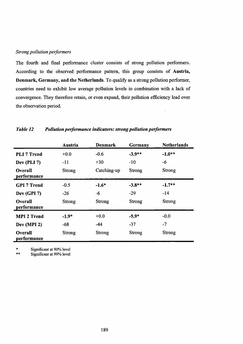
Strong pollution performers

The fourth and final performance cluster consists of strong pollution performers.

According to the observed performance pattern, this group consists of Austria,

Denmark, Germany, and the Netherlands. To qualify as a strong pollution performer,

countries need to exhibit low average pollution levels in combination with a lack of

convergence. They therefore retain, or even expand, their pollution efficiency lead over

the observation period.

Table 12 Pollution performance indicators: strong pollution performers

Austria Denmark Germany Netherlands

PLI 7 Trend +0 . 0 -0 . 6 -3.9** - 1 .0 **

Dev (PLI 7) - 1 1 +30 - 1 0 - 6

Overallperformance

Strong Catching-up Strong Strong

GPI 7 Trend -0.5 - 1 .6 * -3.8** -1.7**

Dev (GPI 7) -26 - 6 -29 -14

Overallperformance

Strong Strong Strong Strong

M PI 2 Trend -1.9* +0 . 0 -5.9* -0 . 0

Dev (MPI 2) - 6 8 -44 -37 -7

Overallperformance

Strong Strong Strong Strong

Significant at 90% level Significant at 99% level

189

Figure 33 Pollution trends: strong pollution performers

100

Austria-♦ — PLI 7 -■ — GPI 7 -©— MPI 2 PLI 7 Trend• - - GPI 7 Trend - - - - MPI 2 Trend

-100oCD CM

cdIT)cd

COCD

00CD

05CDCD

100

Denmark- ♦ — PLI 7 -■ — GPI 7 -©— MPI 2 PLI 7 Trend

GPI 7 Trend MPI 2 Trend

-100

190

100Germany

►— PLI 7 I— GPI 7 >— MPI 2- PLI 7 T rend- - GPI 7 T rend • • MPI 2 T rend

100o05 COa m

cncocn

r -cn

oo<j) a>cn0>

100

Netherlands

-PLI 7 -G P I 7 -M PI 2

PLI 7 T rend GPI 7 Trend

• MPI 2 Trend

-100ocn

egcn

COcn CO 00

cnO)i

191

Figure 33 graphically illustrates this high degree of homogeneity. The only exception to

this rule is Denmark, where the overall pollution load index (PLI 7) shows a positive

deviation and a negative but insignificant trend. One might wonder whether this

observation would make Denmark a candidate for being part of the catching-up country

cluster. However, the development of the other two pollution indicators clearly points in

the direction of Denmark being a strong pollution performer, as the pollution

performance of both the general economy and of the manufacturing sector appear to be

consistently better than EU average. On balance, there seem to be valid reasons why the

country should be considered a part of the strong pollution performer cluster, rather than

of the catching-up cluster.

Conclusion

The overall results of the categorisation exercise are reported in table 13. Looking at the

big picture, the two clusters at the ends of the spectrum appear to be not only rather

homogeneous with regard to the observed pollution performance pattern, but also with

regard to the geographic location.

Table 13 Empirical pollution performance clusters

Pollution Performance

In transitionPoor Strong

Catching up Falling behind

Greece

Spain

Ireland

Luxembourg

Belgium

France

Finland

Austria

Denmark

Germany

NetherlandsPortugal United Kingdom Italy

Sweden

192

With Austria, Denmark, Germany, and the Netherlands, the strong pollution performer

appears to be composed of countries that have a comparable degree of economic

development as well as a similar cultural and technological background. The same

could be said about the poor pollution performance cluster, which consists of three

Mediterranean countries.

It is the two country clusters ‘in the middle’ that seem to have less clear cut, but

arguably more interesting country combinations. On the one hand, there is the group of

countries that catch-up to the EU average in terms of pollution performance, in which

the United Kingdom and Ireland are by far the most important constituents. It seems an

interesting empirical observation that both countries appear to share the same pollution

performance ‘disposition’ in spite of their quite distinct economic development over the

last decades.

On the other hand, the cluster of countries which fall behind in terms of relative

pollution performance seems to be an assembly of two rather different sub-groups. First,

there are France and Belgium which appear to exhibit a quite analogous pollution

performance pattern. Second, there is Sweden and Italy, with Finland apparently in

between. It may seem odd, but Finland appears to share some pollution performance

characteristics with each of the two countries mentioned before.

In terms of overall pollution performance (as expressed by the PLI and GPI indicators),

Finland seems to exhibit a pattern that is by and large comparable to the Swedish one.

Yet, as it is the case with regard to Italian manufacturing sector, the Finnish

manufacturing industry has improved its pollution efficiency by a considerable margin

up to a point at the end of the observation period when it was in line with the EU

average.

193

3.2.1.7 GPI 3 as lead pollution performance indicator

For the subsequent regression analyses, the General Pollution Intensity based on three

air pollutants (GPI 3) will be used as proxy for pollution performance. Among the three

pollution performance indicators developed for the purpose of this investigation, the

GPI 3 indicator appears to represent the best compromise between long-term data

availability and comprehensiveness with regard to different types of air pollutants. A

more extended discussion on the advantages and disadvantages of the three indicators

can be found above in section 3.2.1.5. The complete data set can be found as table 35 in

the appendix.

As figure 34 illustrates, the variation between indicator values has increased over the

observation period. In 1980, pollution indicator extremes were -30 of Sweden and +55

of Finland. The pollution intensity figures of all 15 countries in the sample were

relatively close to the weighted average. The variation amounted to 85 indicator points.

By contrast, at the end of the observation period in 1999, the variation was 281

indicator points. Austria had with -45 the lowest GPI, while Greece’s pollution intensity

indicator stood at +236.

This increase in variation appears to imply that the difference in pollution intensity

between EU member states has gone up significantly over the observation period. In ten

of the 15 countries in the sample, GPI 3 figures have decreased; four countries exhibited

an increase of their pollution intensity indicator. The Netherlands scored the same GPI 3

value in 1980 and 1999.

194

Figure 34 General pollution intensity indicator (GPI 3)

-50

-100 -------------------------------------------------------------------------------------------------------------------------------------------------------------------------a t s e lu d e fr nl dk b e it uk fi ie e s pt gr

Data Sources: N 0 2 / S 0 2 data from EMEP (2002) C 0 2 data from CDIAC (2002)

GDP data from Eurostat (2000)

One should keep in mind that the GPI 3 indicator mirrors the relative difference in

pollution intensity between EU member states on the one hand and the weighted EU

average on the other hand. A majority o f countries in the sample, including the biggest

EU economies, managed to decrease their pollution indicator scores. In other words,

their absolute pollution figures have decreased at a higher rate than the EU average. For

this reason, the increase in GPI 3 figures in Ireland, Spain, Portugal and Greece does not

necessarily mean that these countries have increased their absolute amount o f pollution.

The rising indicator values merely indicate that the national pollution values decreased

at a lower rate than the weighted EU average.

195

3.2.2 Taxes on imports and production

In its position paper on taxation, the European Chemical Industry Council (CEFIC

1999a) argued that the “gloomy tax environment featured by the European Union” was

one of the main competitive disadvantages of chemical industries. According to that

report, in 1997, the total tax revenues in Europe summed up to 41% of the GNP, 10 while

that figure stood at 28% in the United States.

Apart from this gap in tax burden, CEFIC went on to argue that the structure of tax

revenues also distorted the competitive position of EU chemical production. According

to the analysis of CEFIC, social contribution accounted for 39 percent of total tax

revenues in Europe compared to 25 percent in the United States. In turn, the tax level on

labour income and corporate profits were more substantial in the U.S., where it made up

44 percent of total tax revenues in 1997 against 24 percent in the EU.

With regard to tax rates on chemical industry production factors, the CEFIC study

estimated the comparative tax levels as follows.

Table 14 Tax rates on chemical industry production factors

European Chemical ¥T . . . . , .5 , . . U.S. Chemical industriesIndustries

Taxes on corporate profits

Employers’ social security charges

Non-refundable taxes on motor fuels

Non-refundable taxes on heating fuels

^ ^ — ~ S o u r c e : CEFIC (1999a)

10 CEFIC calculated that number on the basis of a weighted average for Germany, France, UK, Italy, the Netherlands and Belgium.

45%

31 %

126%

5%

21 %

23%

37%

3%

196

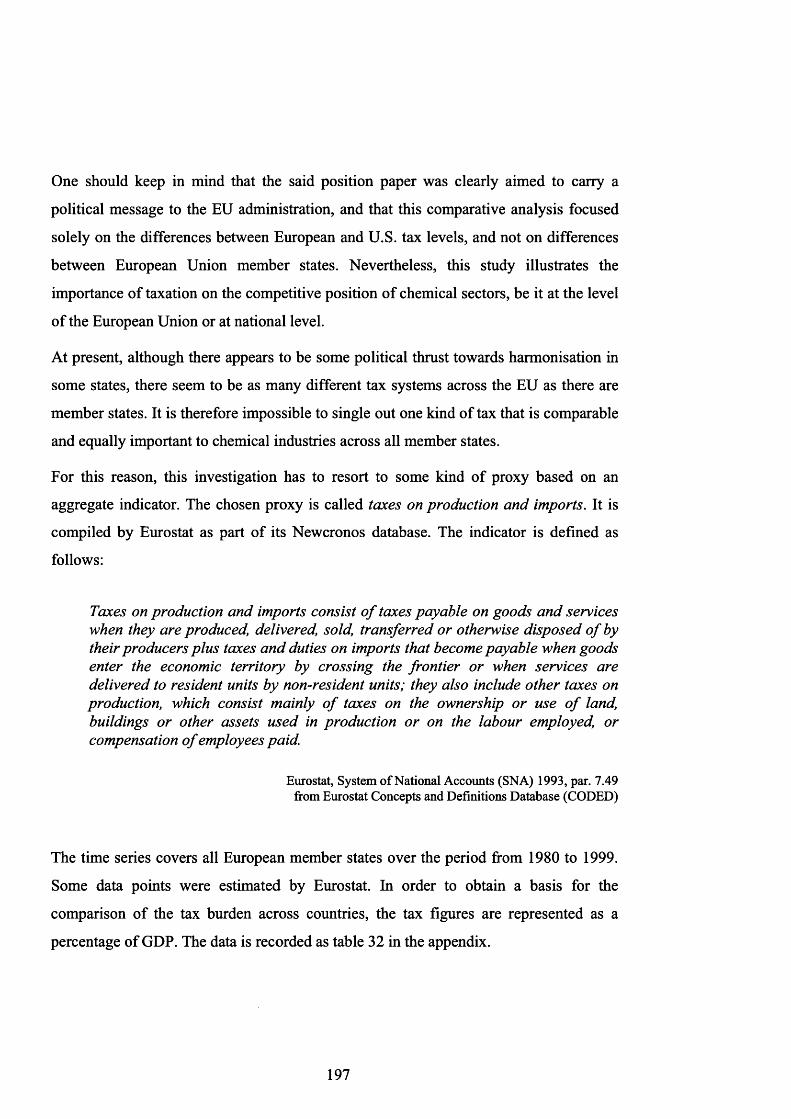
One should keep in mind that the said position paper was clearly aimed to carry a

political message to the EU administration, and that this comparative analysis focused

solely on the differences between European and U.S. tax levels, and not on differences

between European Union member states. Nevertheless, this study illustrates the

importance of taxation on the competitive position of chemical sectors, be it at the level

of the European Union or at national level.

At present, although there appears to be some political thrust towards harmonisation in

some states, there seem to be as many different tax systems across the EU as there are

member states. It is therefore impossible to single out one kind of tax that is comparable

and equally important to chemical industries across all member states.

For this reason, this investigation has to resort to some kind of proxy based on an

aggregate indicator. The chosen proxy is called taxes on production and imports. It is

compiled by Eurostat as part of its Newcronos database. The indicator is defined as

follows:

Taxes on production and imports consist o f taxes payable on goods and services when they are produced, delivered, sold, transferred or otherwise disposed o f by their producers plus taxes and duties on imports that become payable when goods enter the economic territory by crossing the frontier or when services are delivered to resident units by non-resident units; they also include other taxes on production, which consist mainly o f taxes on the ownership or use o f land, buildings or other assets used in production or on the labour employed, or compensation o f employees paid.

Eurostat, System of National Accounts (SNA) 1993, par. 7.49 from Eurostat Concepts and Definitions Database (CODED)

The time series covers all European member states over the period from 1980 to 1999.

Some data points were estimated by Eurostat. In order to obtain a basis for the

comparison of the tax burden across countries, the tax figures are represented as a

percentage of GDP. The data is recorded as table 32 in the appendix.

197

Figure 35 Taxes on production and imports as % o f GDP

Data Source: Eurostat, Newcronos Database (2001)

According to the Eurostat figures, Denmark was the one EU member state with the

highest tax burden on production and imports both at the beginning as well as at the end

o f the observation period. Its tax burden was at 18.6 percent o f the GDP in 1980 and at

18.9 percent in 1999. By contrast, the Spanish taxes on production and imports were the

lowest among EU countries both in 1980 and 1999. Note that the Spanish tax burden

was 6.6 in 1980 and 11.8 in 1999; hence, it has almost doubled over the observation

period.

Overall, the data suggests that the tax levels in EU member states on production and

imports converged significantly over the observation period, as figure 35 illustrates. The

Mediterranean countries generally increased their tax burden. In some cases, such as

Spain and Italy, that tax increase appears to have been quite significant. Inversely,

Britain and Ireland achieved a notable reduction o f their tax burden over the observation

period. One rather surprising aspect contained in the Eurostat data may be that in 1999,

Germany had the second lowest tax burden on production and imports.

198

3.2.3 Fuel price

According to the European Chemical Industry Council, one of the biggest factors in the

cost of chemical production is the price of energy. In 1999, EU chemical industries

spent 9 percent of their sales value on direct energy costs. This percentage was even

higher with regard to the sub-sector of basic chemicals. In that industry branch, energy

costs accounted for no less than 51 percent of the total sales value (CEFIC 2000b).

Figure 36 illustrates the importance of energy cost on the overall chemical producing

cost using crude oil prices as example. The picture shows that, especially with regard to

the period between 1990 and 1995, the price circles of crude oil and chemical producer

price developed in a quite synchronised way. The correlation coefficient between the

two series was 0.51.

Figure 36 EU chemicals producer price vs. crude oil price, U.S.$, Indexed

(1990=100)

150

EU Chemicals Producer Price, US$, Indexed (1990=100)

100

Crude Oil Price, US$, Indexed (1990=100)

1990 1991 1992 1993 1994 1995 1996 1997 1998 1999

Data Source: CEFIC (2000b)

199

One could therefore make the case that relative differences in the cost of fuel should

prove to be an important determinant of competitiveness of chemical industries. The

regression model will take this into account by including the cost of high sulphur fuel

oil for industrial customers as an energy-related independent variable.

This time series was constructed from two data sets that were provided by the

International Energy Agency. The basis for the data set used in this analysis is a time

series on the real (constant) value of oil products for industrial customers. The series is

an index with the base year 1995. It covers all EU member states over the period from

1980 to 1999.

In order to calculate absolute values, the index increments were combined with the

absolute price of high sulphur fuel oil in U.S.$ per tonne (at PPP) for industrial

customers. With regard to nine of the fifteen EU member states, 1995 data was

available. For the rest, 1995 values had to be extrapolated using the index. 11 The index

on prices of oil products was provided by the International Energy Agency Data

Services in April 2001. The absolute prices of high sulphur fuel oil are of July 2002.

Both data series are part of the energy price database of the International Energy

Agency. The time series can be found in the appendix as table 33.

The data represented in figure 37 appears to suggest that over the observation period,

fuel prices for industrial customers have decreased in twelve of the fifteen EU member

states. The reduction in fuel price was particularly significant in Ireland, the UK,

Austria and Germany. By contrast, fuel prices appeared to increase in the Netherlands,

Italy and Spain.

11 Absolute prices for high sulphur fuel were available for Austria, Belgium, France, Ireland, Italy, the Netherlands, Portugal, Spain and the United Kingdom. 1990 prices were available for Finland, Germany, Greece and Luxembourg. The latest data point with regard to Denmark was 1988 and with regard to Sweden 1984.

200

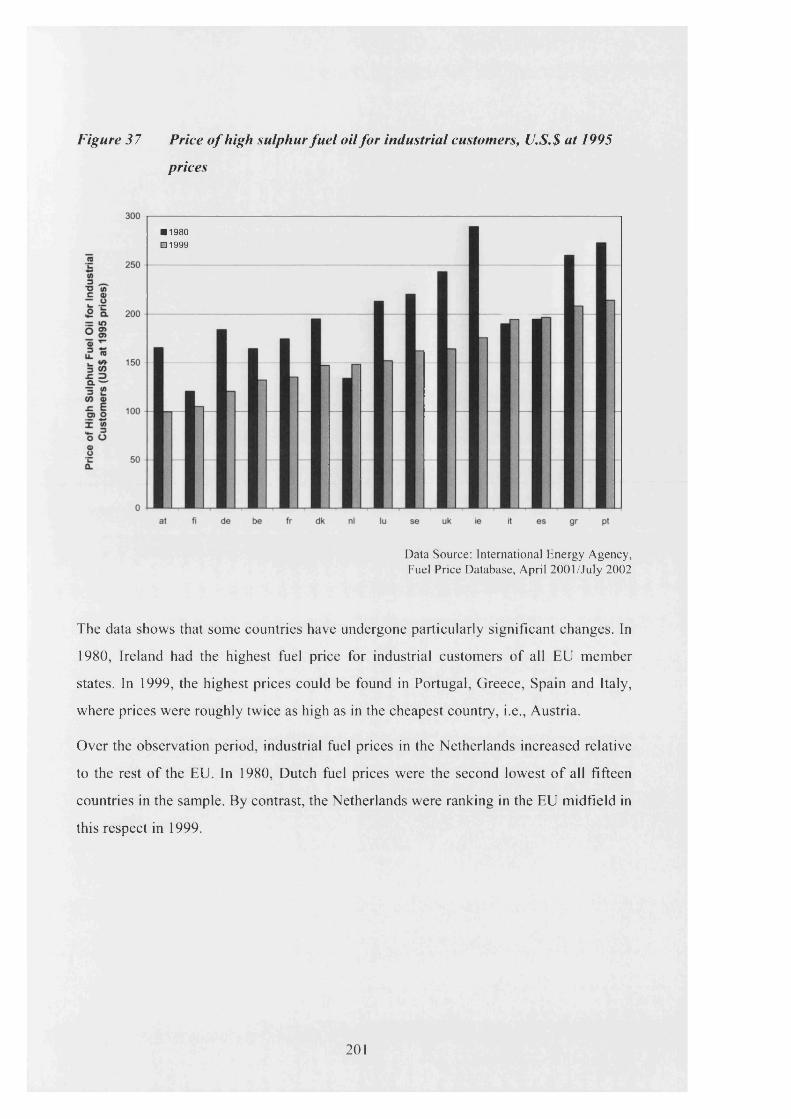
Figure 37 Price o f high sulphur fuel oil for industrial customers, U.S.$ at 1995

prices

■ 1980 □ 1999

Data Source: International Energy Agency, Fuel Price Database, April 2001 /July 2002

The data shows that some countries have undergone particularly significant changes. In

1980, Ireland had the highest fuel price for industrial customers of all EU member

states. In 1999, the highest prices could be found in Portugal, Greece, Spain and Italy,

where prices were roughly twice as high as in the cheapest country, i.e., Austria.

Over the observation period, industrial fuel prices in the Netherlands increased relative

to the rest o f the EU. In 1980, Dutch fuel prices were the second lowest o f all fifteen

countries in the sample. By contrast, the Netherlands were ranking in the EU midfield in

this respect in 1999.

201

3.2.4 Productivity of the manufacturing sector

In one of its annual Barometers o f Competitiveness (CEFIC 1998a), the European

Chemical Industry Council argued that the European Union appeared to be a less

attractive location for the manufacture of chemicals than the U.S. because of the

following vicious circle: Weaker profits in the EU triggered lower investments, which

in turn slowed down progress in labour productivity and energy efficiency. The lower

investment relative to the U.S. with regard to labour productivity and energy efficiency

impaired the cost competitiveness of EU chemical sectors, which closed the vicious

circle.

CEFIC supported this line of argument with data from the OECD-STAN database and

its own analyses, which showed that the hourly labour productivity of EU chemical

industries from1990 to 1994 were 25 percent lower than in the United States.

The data series used in the subsequent regression analysis was provided by Eurostat in

2001 as part of its Newcronos database. The data set is titled labour productivity in the

manufacturing sector. It comprises figures on the labour productivity of national

manufacturing sectors in thousands of € per year at market exchange rates.

The data set is complete for the 15 EU member states over the period from 1985 to

1995. The German data series covers Western Germany only. With regard to seven

countries, that is, Belgium, Germany, Spain, France, Luxembourg, Sweden and the

United Kingdom, there are also data points for the year 1996. For all other countries, as

well as for the years of the observation period 1980 to 1999 that are not covered by the

data series, missing values were computed by linear projection.

202

Figure 38 Labour productivity o f the manufacturing sector,

thousands o f € at constant prices

Data Source: Eurostat, NewCronos Database (2001) Original data description: Labour productivity, level (at market exchange rate)

This appeared appropriate because the available figures seemed to follow a linear

evolution. The regression model was constructed both with the original data set as well

as with the data set including the projections. The regression coefficients were generally

robust and coherent with regard to both data sets. The data set is recorded as table 34 in

the appendix.

The figures represented in figure 38 indicate that the manufacturing sectors o f EU

member states have increased their labour productivity between 1985 and 1995. Over

that observation period, Sweden has experienced the largest rise in labour productivity -

amounting to 88 percent. Inversely, with 16 percent, manufacturing labour productivity

grew least in Greece.

Overall, the differences among EU member states were considerable both in 1985 as

well as in 1995. At both points in time, the highest value in the sample was more than

4.5 times the lowest one.

203

In 1995, the countries with the highest manufacturing labour productivity in the EU

were Finland, Sweden, Ireland and Italy. The last places in that ranking were taken by

Portugal and Greece. Spain has improved its manufacturing labour productivity

considerably between 1985 and 1995. One interesting aspect of the overall productivity

pattern might be the very high figures with regard to Ireland both in 1985 and 1995.

3.2.5 GDP

A time series on the GDP of EU member states will be included in a number of

regression models. This is for technical reasons mainly. The function of this

independent variable will be to account for the size of the national economies in

regressions where the dependent variables are expressed in absolute terms.

The data set was taken from the OECD’s National Accounts database, which contained

data points regarding the period 1980 to 1996. For the years 1997 to 1999, the

information was obtained from the World Bank’s World Development Indicators

database. The composed data set was checked for consistency. There appeared to be no

break in the time series.

204

4 Regression Analysis

4.1 The framework to the regression analysis

4.1.1 Research hypotheses

The purpose of the following regression analysis is to assess whether and in what way

the relative air pollution performance of EU member states - which is used as a proxy

for environmental performance - has actually had an impact on the economic

performance of their chemical industries. More formally expressed, the investigation

will attempt to verify the following principal hypothesis:

Ho: Chemical industry performance does not react to variations in pollution

performance.

Hi: Chemical industry performance reacts to variations in pollution

performance.

If the empirical data showed with a sufficient degree of statistical security that changes

in pollution performance have had a significant impact on the performance of the

chemical sector, Ho could be rejected and Hi could be considered true.

The first hypothesis, however, represents only the initial research question. If Ho was

ruled out, the analysis would then move on to assess a number of follow-up hypotheses:

H u : Chemical industry performance deteriorates in response to strong

pollution performance.

Hu: Chemical industry performance improves in response to strong pollution

performance.

205

Hjj : Chemical industry performance reacts inconclusively to strong pollution

performance.

One underlying rationale behind the secondary hypotheses is to test the applicability of

the conventional economic and location theories (cf. sections 2.3.1 and 2.3.4) and of the

so-called Porter hypothesis (cf. section 2.2.2.1) to the particular case of EU chemical

industries. These two basic approaches have distinct views on how pollution

performance and economic performance interact.

Hypothesis 1.1 corresponds to the expectations of conventional economic and location

theory. It bases on the assumption that rational economic agents that produce substantial

amounts of pollution, such as the chemical sector, seek out regulative environments

where pollution performance is relatively weak. They would tend to avoid pollution

regimes that forced them to internalise pollution reduction costs into their own profit

calculations.

By contrast, hypothesis 1.2 builds on the principal notion of the Porter hypothesis,

which asserts that industries gained competitive advantages from reducing their

emissions through innovation offsets (Porter and van der Linde 1995). In the case at

hand, that approach would suggest that chemical sectors in EU member states with a

strong air pollution performance would gain competitiveness through innovation

offsets. The argument implies that countries with a strong pollution performance might

attract or foster the development of more competitive economic sectors, because their

strong pollution regime would force industries to employ technologies that secured

them an advantage over competitors or newcomers in the market.

Lastly, hypothesis 1.3 implies that some national chemical sectors react more positively

to strong pollution performance than others. If this hypothesis was true, the objective of

the analysis would be to specify distinct reaction patterns and to look for explanations.

206

4.1.2 Theoretical model

The apparent conflict between the two principal concepts may surprise at first, and

could pose the question how this investigation aims to reconcile them. How could a

particular pollution performance pattern be either positive or negative with regard to

chemical industry performance -o r inconclusive, or even both at the same time?

Furthermore, how could the regression analysis unite the two opposite implications of

hypothesis 1.1 and 1.2 under one theoretical framework?

Reduced theoretical model

In order to bring together these two seemingly conflicting notions, one needs to think

about the theoretical connection between pollution performance and chemical industry

performance. The very basic theoretical model represented in figure 39 may serve as a

starting point.

Figure 39 Reduced theoretical model

NegativeImplications

Change in Chemical Industry

Performance

PollutionPerformance

PositiveImplications

The proposed theoretical model asserts that the link between pollution performance and

chemical industry performance is a causal relationship. Hence, it implies that pollution

performance had a significant impact on chemical industry performance, and that

therefore Hi is valid. The rationale behind this assertion is documented in section

3.1.4.1.

Based on this set-up, there are three possible ways in which pollution performance may

be linked with chemical industry competitiveness. First, pollution performance could

carry negative repercussions for chemical industry performance. Second, pollution

performance might have positive implications on the chemical sector competitiveness.

However, it is also conceivable that both effects may take place at the same time. In this

case, the outcome of a particular pollution performance on chemical industry

performance would be a mixture between positive and negative implications.

Obviously, this would be the most complicated of the three constellations, as it would

indicate that both hypothesis 1 . 1 and hypothesis 1 . 2 were true to some degree at the

same time.

Extended theoretical model

The extended theoretical model represented in figure 40 explains further how the causal

relationship between pollution performance and chemical industry performance may

function. Following the broad lines of argument of the principal theories around

pollution and competitiveness, one might therefore find out empirically that strong

pollution performance could indeed bring about both negative as well as positive

implications for chemical industries.

208

Figure 40 Extended theoretical model

StrongPollution

PerformanceCompetitiveAdvantages

HigherPollution

AbatementCost

Weak Chemical Industry

Performance

Inconclusive Chemical Industry

Performance

Strong Chemical Industry

Performance

On the one hand, chemical sectors could suffer in strong pollution performance regimes,

as they would have to spend more money for pollution abatement measures than their

competitors in less strong pollution performance regimes. On the other hand, however,

chemical industries in strong pollution performance regimes might also have a

competitive advantage, due to innovation offsets, e.g. more efficient technologies, or

through consumer preferences.

The regression analysis will have to answer which one o f the two arguments stands in

the case of EU chemical industries. If the negative implications o f strong pollution

performance dominated the equation, one would expect chemical industries to perform

relatively worse than in countries with relatively poorer environmental performance.

This outcome is marked in the picture as alternative 1.

Inversely, if mainly positive implications o f strong pollution performance were true,

one should expect the chemical industry to perform better than in the other countries. In

this case, alternative 2 in the picture was valid.

209

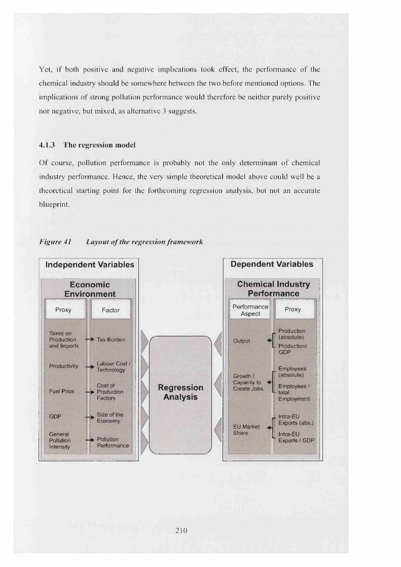
Yet, if both positive and negative implications took effect, the performance of the

chemical industry should be somewhere between the two before mentioned options. The

implications of strong pollution performance would therefore be neither purely positive

nor negative, but mixed, as alternative 3 suggests.

4.1.3 The regression model

O f course, pollution performance is probably not the only determinant o f chemical

industry performance. Hence, the very simple theoretical model above could well be a

theoretical starting point for the forthcoming regression analysis, but not an accurate

blueprint.

Figure 41 Layout o f the regression framework

Independent Variables

Economic Environment

Proxy Factor

Taxes on Production and Imports

► Tax Burden

Productivity - Labour Cost/ Technology

Fuel PriceCost of

► Production Factors

GDP ^ Size of the Economy

GeneralPollutionIntensity

PollutionPerformance

RegressionAnalysis

Dependent Variables

Chemical Industry Performance

PerformanceAspect

.....................

Proxy

Output ■*!

Growth / Capacity to -4 Create Jobs

EU Market J Share

Production I (absolute)

I. Production/ GDP

_ Employees (absolute)

Employees /- total

Employment

Intra-EU Exports (abs.)

| Intra-EU ' Exports / GDP

210

The aim of the regression analysis is to estimate the strength and the direction of the

impact that the independent variables exercise on the dependent variable. With regard to

the research question at hand, the regression analysis should estimate to which degree

and in what way chemical industry performance depends on a number of explanatory

factors. Figure 41 graphically represents that basic layout of the regression analysis.

The picture illustrates that the regression analysis used in this study is based on the

working assumption that four lead independent variables constitute the ‘performance

background’ of EU chemical industries. These four factors are pollution performance,

tax burden, labour cost, and energy cost. Furthermore, GDP will be introduced into

some regressions as a further control variable.

As dependent variables, the regression framework operates with three chemical industry

performance indicators, i.e. production, employment and exports. The three dependent

variables will be expressed in both relative and absolute terms. This aims to estimate the

impact of the independent variables on chemical industry performance in relation to the

rest of the economy as well as in itself.

The regression model

The regression model uses pooled data from fourteen EU member states to account for

changes in chemical industry performance. Note that Luxembourg was excluded from

the analysis, as some of its data sets were incomplete. Therefore, the sample will

comprise 14 country cases; the following investigation will refer to this country cluster

as the EU 14 sample.

The following regression model will be estimated:

CIPit = ct +dt + (TAXES it) + f i2 (FUELPit) + f i PRODUCTIVITYit) + fi4(POLLUit) + eit

211

where CIP„ is the dependent variable (chemical industry production, employment, or

intra-EU exports) for country i at time t. Moreover, c, and d t are country and time1 9dummies respectively to account for unobserved variations across countries and

unobserved shocks over time. Finally, sit is the error term.

The main independent variables are tax burden on industrial production and imports

{TAXES), fuel price (FUELP), productivity of the manufacturing sector

{PRODUCTIVITY), and pollution performance (POLLU). The size of the national

economy {GDP) will be included in the regression estimations only when dependent

variables are used in absolute terms.

The data used in the regression model was monotonically transformed into natural log

form. For this reason, the computed coefficients stand for percentage-changes (Gujarati

1978, 1995). For example, a coefficient of 1.5 would indicate that a one-percent-change

in the independent variable triggers a 1.5 percent change in the dependent variable.

Panel data can be estimated using either a fixed effect model or a random effect model.

The random effects assumption include all the fixed effects assumptions plus the

additional requirement that the unobserved effect is independent of all explanatory

variables in all time periods (Wooldridge 2000: 449). If that assumption is met, random

effect models are preferable to fixed effect models because the estimators they deliver

are more efficient (i.e., with smaller variance).

In order to determine whether random effects can be used to estimate the coefficients

from the expression above, a Hausman specification test has been run for each

dependent variable. As can be seen in the appendix 3, almost all tests confirm that

random effects can be used, the exception being the regression explaining chemical

industry employment in absolute terms (cf. table 48 and table 49). Therefore, random

effects will be used to explain all dependent variables but employment in absolute terms

where fixed effects will be used instead.

12 The country dummies cover all 15 EU member states except Luxembourg and the UK. The UK is used as reference category Dougherty, C. (1992). Introduction to Econometrics. New York and Oxford, Oxford University Press..

212

A subsequent inspection of the residuals confirms the presence of first-order

autocorrelation. Please refer to appendix 3 for a graphical and numerical test of

autocorrelation. Heteroskedasticity, on the other hand, does not seem to be a problem in

all regressions. For a graphical test for heteroskedasticity, please refer to appendix 3.

Consequently, the regression model that will be reported in the main part of this study

will be a random effect GLS (general least squares) model correcting for first-order

autocorrelation. There is one exception to this, namely the regression on absolute

employment, which will use a corrected fixed effects model instead of a random effects

one.

4.2 Regression Results

The purpose of chapter 3 was to set the foundation of the subsequent regression analysis

by introducing and discussing the variables that will be used in the models. The

following chapter highlights the findings of the regression analyses, which produced a

substantial amount of information.

Regression models were estimated for each of the three dependent variables, both in

absolute and relative terms. In addition, since there was some doubt about the reliability

of the chemical industry production value data regarding Ireland (cf. section 3.1.2.1),

two sets of regression models were run: one including Ireland, and another one

excluding the country. By doing so, one should be able to assess the sensitivity of the

regression estimates towards the inclusion of the Irish data set.

213

4.2.1 Models on chemical industry production

Table 15 presents the regression estimations with regard to the first dependent variable,

that is, chemical industry production value. As explained earlier, the variable is

represented both in relative terms (regression models 15.1 and 15.2) as well as in

absolute terms (estimations 16.1 and 16.2). One should therefore remember that the first

two regression estimations do not include ‘GDP’, because the dependent variable

‘production value/GDP’ is already normalised with a measure of the size of the

economy. In contrast, the latter two regressions contain ‘GDP’ as independent variable

in order to account for the size of the economy in the model.

The first set of regression models focus on chemical industry production performance

relative to the rest o f the economy. Therefore, the question to be answered by this set of

estimations is whether the chemical sector reacts to the independent variables in a way

that is distinct from the rest of the economy.

By contrast, regression models 16.1 and 16.2, where production value is expressed in

absolute terms, is aimed at understanding the immediate impact of changes in the

independent variables on production value. In other words, this set of regressions seeks

to shed light on the question whether chemical industry production increases or

decreases in reaction to changes in pollution performance and other independent

variables.

214

Discussion o f the regression results

The discussion of the regression results starts by looking at model 15.1, which reports

the impact of the independent variables on chemical industry production value divided

by GDP. In a first step, this regression was estimated using a fixed effects model. After

that, a random effects GLS model was computed. In order to assess whether the random

effects model could safely be used, the regression coefficients of both models were

tested for systematic differences using the Hausman specification test. Since the

Hausman test showed that there are no systematic differences in the coefficient values,

it seemed reasonable to use the results of the random effects model that delivers more

efficient coefficients, which are presented below in models 15.1. The complete set of

regression estimations including the Hausman test can be found as table 42 in appendix

3.

Two out of the four independent variables show significant regression coefficients.

This, in connection with the fact that the R2 and chi2 values seem to be sufficiently large

to indicate a fair amount of reliability, appears to indicate that the explanatory variables

are well chosen.

One interesting observation is that R2-within is clearly larger than R2-between. This

points out that the development of the independent variables over time has a larger

explanatory power on the evolution of the dependent variable than the differences

between countries with regard to the independent variables.

Moving on to revising the regression coefficients, one could state with a high degree of

confidence that the value of chemical industry production is positively associated with

air pollution. Thus, countries that experienced relatively weak air pollution

performances seemed to exhibit relatively higher chemical industry production. Hence,

if one understands absolute chemical industry production as a measure of the sector’s

competitiveness, national chemical industries appeared to profit from relatively higher

levels in air pollution.

215

Table 15 Regression estimates on Cl production value / GDP

Cl production (15.1) (15.2)value / GDP IE included IE excluded

TAXES -0.4 (0.00) -0.4 (0.01)

FUEL PRICE +0.0 (0.70) +0.1 (0.10)

PRODUCTIVITY +0.1 (0.33) +0.1 (0.13)

GDP — —

POLLUTION +0.2 (0.00) +0.2 (0.00)

(Constant) -3.9 (0.00) -4.5 (0.00)

within 0.47 0.63

R2 between 0.22 0.18

overall 0.26 0.25

Wald chi2 604.71 (0.00) 688.13 (0.00)

N 280 260

Residual DF 243 224

Note: Random effects GLS regression, corrected for first-order autocorrelation.Group variable: country; year dummies included.P-values in brackets.

The regression coefficients estimated by model 15.1 further indicate that ‘taxes’ are

negatively linked to chemical industry production and significant. In contrast, ‘fuel

price’ and the ‘productivity’ of the manufacturing sector appear to be positively linked

to chemical industry production, but were found to be not significantly different from

zero.

All findings seem to correspond well to theoretical expectations. The variable ‘taxes’

aims to reflect differences in the taxation o f production and imports; it seems obvious

that differences in tax levels over time or across countries should have negative

repercussions on chemical industry competitiveness. Furthermore, since the type of

taxes covered by this indicator affects the manufacturing sector - such as the chemical

industry - relatively more than the general economy, the empirically observed negative

impact seems intuitively justifiable.

216

Superior manufacturing productivity may, on the other hand, be a hint at technological

advantages or beneficial structural differences. Countries with relatively higher

productivity seem to have a competitive advantage, which in turn should increase their

chemical industry’s production. For this reason, the observed positive link, although not

statistically significant, also appears in line with theoretical expectations.

Finally, the computed regression coefficients of model 15.1 also show that differences

in the price of fuel have had virtually no perceivable impact on the value of chemical

industry production.

Last but not least, based on these findings, the regression results provide grounds to

refute the null hypothesis stated in section 4.1.1 with regard to relative chemical

industry production as dependent variable and the EU 14 country cluster as reference

framework. The estimations seem to confirm that pollution performance has a

significant and considerably large impact on the development of chemical industry

production value. For this reason, the regression results would verify hypothesis 1.1,

which states that chemical industry performance deteriorates in response to strong

pollution performance.

Regression model 15.2, in which Ireland is excluded from the sample, confirms the

above findings. Again, the result of the Hausman test justifies the reporting of the

random effect model results (cf. table 43 in appendix 3). The coefficients of all

independent variables are almost identical in both estimations. One could, therefore

conclude with some confidence that the regression results are robust towards the

exclusion of Ireland from the sample.

Regression models 16.1 and 16.2 estimate the impact of the independent variables - this

time, including ‘GDP’ - on chemical industry production in absolute terms. Once more,

the two models reported are random effects estimations (cf. table 44 and table 45 in

appendix 3). In broad terms, they appear to confirm once more the direction and size of

the regression coefficients observed before. The only exceptions to this rule are shown

in model 16.2 where Ireland is excluded from the sample. In that regression estimation,

‘productivity’ shows up to be significant at 1 0 % significance level, and ‘pollution’ is

found to be not significantly different from zero.

217

Table 16 Regression estimates on Cl production value, absolute terms

Cl production (16.1) (16.2)value, abs. terms IE included IE excluded

TAXES -0.4 (0.00) -0.4 (0.00)

FUEL PRICE +0.0 (0.95) +0.1 (0.12)

PRODUCTIVITY +0.1 (0.46) +0.1 (0.06)

GDP +0.7 (0.00) +0.6 (0.00)

POLLUTION +0.1 (0.01) +0.1 (0.24)

(Constant) -0.2 (0.84) + 1.6 (0.12)

within 0.65 0.75

R2 between 0.90 0.90

overall 0.88 0.88

Wald chi2 267.47 (0.00) 311.99 (0.00)

N 280 260

Residual DF 242 223

Note: Random effects GLS regression, corrected for first-order autocorrelation.Group variable: country; year dummies included.P-values in brackets.

The newly introduced independent variable ‘GDP’ has the largest coefficient and is

shown to be highly significant. Again, this behaviour seems in line with theoretical

expectations - i t seems obvious that the production volume of chemical industries

depends in no small part on the absolute size o f the economy. This observation and the

observation that the R2-between value in models 16.1 and 16.2 is relatively higher than

in models 15.1 and 15.2 respectively, seems to suggest that differences between

countries concerning the independent variable ‘GDP’ explain a good part o f the

development of the dependent variable.13

13 Obviously, the explanatory variables are held in different units, and, as a result o f this, their coefficients cannot be directly compared. However, since all variables were transformed into natural log form, the results reported here indicate that a change of x percent in the explanatory variable appears to have an impact of y percent in the development of the dependent variable (cf. section 4.1.3).

218

Considering what has been said about, for example, the Irish economic boom and its

impact on the development of the Irish chemical industry, this observation appears

plausible.

Actual versus predicted change

Based on the results of the regression models presented above, it is now possible to

compare the actual development of the dependent variable to the predicted changes by

the model. Using the computed regression coefficients of estimation 15.1, one can

estimate the individual contribution of each independent variable to the overall

predicted change.

To do this, the actual change of each independent variable is multiplied by its estimated

coefficient. In other words, the computed regression model renders an estimation of the

individual impact of each independent variable, which can be compared to the actual,

empirically observed, change. Taken together, the individual impacts of all independent

variables will add up to the overall predicted change of the dependent variable. Table 17

reports the results of this exercise with regard to regression model 15.1, which

established an estimation using the relative chemical industry production value as the

dependent variable.

In order to compare the differences in the impact of the independent variables across the

pollution performance clusters (cf. section 3.2.1.6), the countries are ordered by poor

pollution performers, catching-up countries, falling-behind countries, and strong

pollution performers.

219

Table 17 Actual and predicted changes: Cl production value / GDP

Chemical Industry Production / GDP, 1980-1999

J Poor pollution performers 1 8r es Pt AVGActual Change -3% 4% -16% -5%Predicted Change 61% 38% 62% 54%contribution to the predicted change

TAXES -18% -30% -14% -21%FUEL PRICE -1% 0% -1% -1%PRODUCTIVITY 1% 10% 5% 5%POLLUTION 26% 10% 19% 18%(year) 53% 49% 53% 51%

[Countries that catch" up ie uk AVGActual Change 815% 20% 417%Predicted Change 76% 54% 65%contribution to the predicted change

TAXES 11% 6% 8%FUEL PRICE -2% -1% -2%PRODUCTIVITY 6% 5% 6%POLLUTION 6% -7% -1%(year) 55% 52% 53%

|Countries that fall behind be fr fi it se AVGActual Change 99% 67% 22% 4% 111% 61%Predicted Change 52% 55% 52% 29% 53% 48%contribution to the predicted change

TAXES -2% -1% -5% -25% -14% -10%FUEL PRICE -1% -1% -1% 0% -1% -1%PRODUCTIVITY 7% 7% 12% 9% 19% 11%POLLUTION -3% -1% -6% -2% -2% -3%(year) 51% 52% 51% 47% 51% 50%

|Strong pollution performers 1 ^ dk de nl AVGActual Change 37% 85% 0% 74% 49%Predicted Change 52% 50% 56% 50% 52%contribution to the predicted change

TAXES 0% -1% 1% -7% -2%FUEL PRICE -2% -1% -2% 0% -1%PRODUCTIVITY 12% 10% 9% 6% 9%POLLUTION -9% -8% -4% 0% -5%(year) 51% 51% 52% 51% 51%

Calculations based on regression model 15.1

220

Taking Belgium as an example, regression model 15.1 would predict a proportional

increase in relative chemical industry production of 52 percent. The actual increase,

however, was 99 percent, which indicates that the regression model predicts around half

of the actual increase in chemical industry production.

With regard to the impact of the distinct independent variables on absolute chemical

industry production, table 17 disaggregates the overall predicted change into the

individual contributions of ‘taxes’, ‘fuel price’, ‘productivity’, ‘GDP’, ‘pollution’, and

the time-dummies ‘year’.

According to the regression estimations, and keeping Belgium as an example, the actual

development in ‘taxes’ over the observation period 1980 to 1999 has contributed a

predicted decrease of -2 percent in relative chemical industry production. In other

words, since the tax burden with regard to production and import taxes has gone up in

Belgium over the observation period, and since this variable is negatively associated

with the development of the absolute production value, the evolution of ‘taxes’ in itself

would imply a negative development in the dependent variable. The input to the

predicted change by the independent variable ‘fuel price’ appeared to be - 1 percent.

Last but not least, changes in ‘pollution’ have contributed some -3 percent to the

development of the chemical industry production value / GDP over the observation

period.

These negative contributions of ‘taxes’, ‘fuel price’ and ‘pollution’ were partly set off

by the developments of the other explanatory factors. The increase in ‘productivity’ in

the Belgian manufacturing sector contributed a predicted increase of +7 percent to the

overall development of chemical industry production. However, the biggest projected

contribution clearly comes from the auxiliary independent variable ‘year’, which is a

dummy variable that captures all unidentified time shocks that have hit the EU countries

in the sample.

221

Based on the information contained in the regression model, one could only speculate as

to what unobserved trends or developments hide behind the dummy variable ‘year’.

Possible explanations might include external shocks such as the accession of new EU

member states or the reunification of Germany, or a general increase in European and

world trade activity.

Looking at the bigger pattern of actual and predicted changes across the countries in the

sample, there seem to be considerable differences both among individual countries as

well as among country clusters. To start with, the model predicts very accurately the

actual change in chemical industry production among strong pollution performers and

among countries that fall behind. On the other hand, chemical industry production in

poor pollution performance countries, and in catching-up countries, does not appear to

be comprehensively explained by the independent variables in this model.

With regard to the poor pollution performers’ cluster, one can observe that some

countries experienced a negative actual change. In other words, the production value of

the chemical sector in Greece and Portugal did not grow as much as the general

economy over the course of the observation period. Thus, judging from this

development, the Greek and Portuguese chemical sectors were less competitive than the

rest of the economy.

Turning to the contribution of the independent variables, and focusing first on the

variable of our interest, that is, pollution performance, we observe that across the poor

air pollution performers’ cluster, in average, ‘pollution’ contributed +18 percent to the

predicted increase in relative chemical industry production. In other words, relative

chemical industry production in this cluster has profited very much from the poor

pollution performance among the three Mediterranean countries.

222

Overall, the results of the regression model seem to suggest that the predicted

contribution of ‘pollution’ among poor pollution performers was very considerable,

only second to ‘taxes’ with an average predicted contribution of -21 percent. In Greece

and Portugal, ‘pollution’ appears to be even the single largest independent variable

covered in this analysis. The other two explanatory factors appear to have a much

smaller average impact. However, one should also keep in mind that the average

predicted contribution of the time-dummies was +51 percent.

If one considers the strong air pollution performers Austria, Denmark, Germany and the

Netherlands, ‘pollution’ has had the opposite effect: its average contribution to relative

chemical industry production was -5 percent. In other words, the relatively strong

pollution performance of those countries has had a perceivable negative impact on their

chemical industries, as the sector’s production value relative to the GDP decreased over

the observation period.

Again, pollution performance was the second biggest contributor after ‘productivity’. It

may be worth taking note that the biggest contributing factor varies between poor and

strong pollution performers: productivity is positively associated with the dependent

variables for the strong performance cluster, and much less so with regard to the poor

pollution performers.

Adding up the positive contribution of ‘pollution’ among poor pollution performers

(+18%) to its negative contribution among strong pollution performers (-5%), one

arrives to the conclusion that distinct pollution performance patterns among EU

member states accounted for 23 percent of the difference in the development of their

chemical industry production value / GDP.

223

Table 18 Actual and predicted changes: Cl production value, absolute terms

Absolute Chemical Industry Production, 1980-1999

|Poor pollution performers 1 es Pt AVGActual Change 36% 60% 81% 59%Predicted Change 118% 104% 205% 142%contribution to the predicted change

TAXES -20% -34% -19% -24%FUEL PRICE 0% 0% 0% 0%PRODUCTIVITY 1% 9% 5% 5%GDP 38% 46% 105% 63%POLLUTION 21% 8% 19% 16%(year) 78% 75% 95% 83%

|Countries that catch up ie uk AVGActual Change 2219% 75% 1147%Predicted Change 282% 130% 206%contribution to the predicted change

TAXES 16% 7% 11%FUEL PRICE -1% 0% 0%PRODUCTIVITY 7% 5% 6%GDP 145% 44% 94%POLLUTION 6% -6% 0%(year) 109% 81% 95%

|Countries that fall behind be fr fi it se AVGActual Change 125% 97% 68% 48% 122% 92%Predicted Change 85% 95% 113% 86% 73% 90%contribution to the predicted change

TAXES -2% -1% -6% -29% -14% -10%FUEL PRICE 0% 0% 0% 0% 0% 0%PRODUCTIVITY 6% 6% 11% 8% 15% 9%GDP 13% 17% 35% 37% 5% 21%POLLUTION -2% -1% -4% -2% -1% -2%(year) 72% 74% 77% 72% 69% 73%

jStrong pollution performers at dk de nl AVGActual Change 100% 162% 43% 118% 106%Predicted Change 126% 118% 126% 95%; 116%contribution to the predicted change

TAXES 0% -1% 1% -8% -2%FUEL PRICE 0% 0% 0% 0% 0%PRODUCTIVITY 11% 9% 8% 5% 8%GDP 43% 39% 40% 23%| 36%POLLUTION -7% -7% -3% o%; -4%(year) 80% 78% 80% 73% 78%

Calculations based on regression model 16.1

224

Moving on to table 18, the dependent variable now changes to be expressed in absolute

terms. The figures represented in this table seem to differ from what has been said

before in a number of ways. The actual changes are much bigger in absolute terms than

in relative terms. This could be explained by the fact that the relative production value

captured the chemical industry growth in excess of the (generally positive) growth of

the general economy. Since the absolute production value indicator reports the chemical

sector’s development on a ‘stand-alone’ basis, these figures should be higher. In other

words, an explanation for this difference is the fact that ‘GDP’ is now included as a

separate independent variable.

With regard to the contribution of each independent variable, the predicted impact of

‘GDP’ is the most important contributing factor among all independent variables,

followed by ‘taxes’ and ‘pollution’. Again, this observation could serve as one more

confirmation that the overall evolution of the economy is the major explanatory factor

for the development of the chemical industry production volume.

The importance of the dummy variable ‘year’ has increased across all countries in the

sample. Thus, the importance of unidentified time shocks is bigger with regard to

chemical industry production in absolute terms than with regard to chemical industry

production value in relative terms.

Finally, the contribution of ‘pollution’ to absolute chemical industry production is

smaller than to production in relative terms. This could be an indication that the

production performance of the chemical sector relative to the general economy is more

sensitive to differences in pollution performance than the chemical production in

absolute terms.

Chemical industry production and pollution performance: an interim conclusion

The regression models presented in this section have produced a quite robust picture

about the relationship between chemical industry production and the independent

variables.

225

In general, ‘taxes’ appear to be significant and negatively linked to chemical industry

production. Moreover, they are among the most important contributing factors, along

with ‘productivity’ and ‘pollution’, irrespective of whether the dependent variable is

expressed in absolute or relative terms. The finding that differences in ‘productivity’ are

positively linked to chemical industry production value seems equally robust. Finally,

the regression estimations have consistently shown that ‘pollution’ has a positive impact

on the dependent variable.

Overall, the contribution of ‘pollution’ to the development of chemical industry

production was shown to be considerable vis-a-vis the other explanatory variables. This

observation is in line with the literature, which generally notes that environment-related

factors are typically not the biggest, but one among the most important determinants of

economic competitiveness.

In terms of the overall difference in chemical industry production that is caused by

distinct pollution performance patterns of EU member states, the impact of pollution

performance appears to be very significant. With regard to production value relative to

GDP, the overall impact seemed to make a difference of up to 35 percent, ranging from

+26 percent in the case of Greece, to -9 percent regarding Austria. In absolute terms, the

overall impact appeared to be somewhat smaller with 28 percent.

4.2.2 Models on chemical industry employment

The following set of regression models establishes the relationship between the

independent variables and chemical industry employment. The basic structure of the

regression models and of the tables in which they are presented here is the same as in

the previous section.

Table 19 shows the estimated impact of the independent variables on relative chemical

employment, that is, the percentage of chemical industry employees in the total

workforce of a country. Model 19.1 includes Ireland into the sample, while model 19.2

reports the results of the regression estimation when we exclude the country. Later,

models 2 0 . 1 and 2 0 . 2 will report regression coefficients for absolute chemical industry

employment as the dependent variable.

226

The Hausman specification test failed to confirm that a random effect model could

safely be used with regard to regression estimations 20.1 and 20.2. Therefore, the

results reported in the main part o f this thesis for these two models are first-order

autoregressive fixed effect regressions. The detailed results of the regression analysis

can be found as table 48 and table 49 in appendix 3.

Table 19 Regression estimates on Cl employment / total workforce

C l employment / (19.1) (19.2)total workforce IE included IE excluded

TAXES -0.1 (0.54) -0.0 (0.84)

FUEL PRICE -0.0 (0.75) -0.0 (0.55)

PRODUCTIVITY +0.1 (0.10) +0.1 (0.06)

GDP — —

POLLUTION -0.0 (0.88) -0.0 (0.83)

(Constant) +0.2 (0.68) +0.2 (0.74)

within 0.16 0.22

R2 between 0.42 0.46

overall 0.25 0.30

Wald chi2 24.04 (0.46) 28.57 (0.24)

N 280 260

Residual DF 243 224

Note: Random effects GLS regression corrected for first-order autocorrelation.Group variable: country; year dummies included.P-values in brackets.

The first fundamental observation, which will set the general tone o f the subsequent

discussion o f the regression results on chemical industry employment, must be a word

of caution: the chi2 values o f regression models 19.1 and 19.2, as well as the F values o f

estimations 20.1 and 20.2, are too low to reject the hypothesis that all coefficient are

zero. In other words, the statistical relationships between the explanatory variables and

the development o f chemical industry employment are not strong enough to establish

underlying causalities with a sufficiently high degree o f certainty.

227

Table 20 Regression estimates on Cl employment, absolute terms

Cl employment, (2 0 .1 ) (2 0 .2 )absolute terms IE included IE excluded

TAXES -0.0 (0.79) +0.0 (0.89)

FUEL PRICE +0.0 (0.46) +0.0 (0.76)

PRODUCTIVITY +0.1 (0.12) +0.1 (0.12)

GDP +0.0 (0.59) +0.0 (0.83)

POLLUTION -0.0 (0.68) -0 .0 (0.62)

(Constant) +3.0 (0.00) +3.5 (0.00)

within 0.09 0 .1 0

R2 between 0.56 0.33

overall 0.42 0 .2 2

F 0.97 (0.50) 1.06 (0.40)

N 280 260

Residual DF 229 211

Note: Fixed effects regression corrected for first-order autocorrelation.Country dummies and year dummies included.P-values in brackets.

Therefore, one could only make a couple o f limited observations regarding the

regression results. First o f all, the R2-between values o f all regression models appear to

be higher than the R2-within values. This might be taken as an indication that the

observed differences regarding the independent variables between countries has more

explanatory power than the development of the independent variables over time. In

other words, structural differences between countries seem to have a bigger impact on

the development o f chemical industry employment than changes in the explanatory

variables over the observation period. That observation is consistent with the notion that

employment is caused by institutional factors, which vary greatly across countries but

not so much across time.

228

Second, the only explanatory variable that appears to have some significance with

regard to chemical industry employment is ‘productivity’. In model 19.2, this factor was

shown to be significant at 10 percent significance level. With regard to the three other

models, the P-values appeared to be just below that threshold. Therefore, one could

state with some moderate degree of confidence that differences in the productivity of

the manufacturing sector were positively linked to chemical industry employment

levels, especially when the dependent variable is measured in relative terms. As

mentioned above, such behaviour appears to be in line with theoretical expectations.

Third, and most importantly in the context of this study, the regression coefficient of the

‘pollution’ indicator turns out to be not significantly different from zero in all four

models. Based on this observation, the null hypothesis of this study cannot be rejected.

In other words, the empirical analysis does not provide any evidence that differences in

pollution performance among EU member states have had an impact on the employment

performance of their chemical industries.

Concluding remarks

One could sum up the findings in this section into three points: first, the regression

models do not seem satisfactory in terms of reliability and robustness. Second, they

might show that ‘productivity’ is positively linked to chemical industry employment,

while all other explanatory variables fail to achieve significance. Finally, the regression

results appear to indicate that pollution performance has little impact on the creation or

destruction of jobs in the EU chemical sector, which seems to be more related to the

existing labour market institutions in each country.

These findings correspond to earlier results of Levinson (2000) and Morgenstem et al.

(2 0 0 1 ), which show that increased environmental taxes or spending, respectively, did

not generally cause a significant change in employment levels. Both studies conclude

that their data does not support the notion of a jobs-versus-the-environment trade-off.

229

4.2.3 Models on intra-EU chemical industry exports

The third and final set of regression models tests the impact of the independent

variables on intra-EU chemical industry exports. Again, the system in which the results

are presented here corresponds to the earlier two sections.

Table 21 presents the results of the regression estimations relating to intra-EU chemical

industry exports as a percentage of GDP. Models 21.1, 21.2 and 22.1 were estimated as

random effects models, while model 22.2 - which refers to intra-EU exports in absolute

terms excluding Ireland - failed to pass the Hausman specification test. Therefore, that

estimation was based on a fixed effects regression. Based on the observed R2, chi2 or F

values, all estimations appear to exhibit a high level of significance concerning the

overall set of independent variables. For details on the regression analysis, please refer

to annex 3.

With regard to all four regression models, the R2-within value was the highest observed

indicator among all R2 values. This seems to indicate that the development of the

independent variables over time has had a higher explanatory power than structural

differences between countries.

230

Table 21 Regression estimates on C l intra-EU exports / GDP

Intra-EU exports / (21.1)______________________(2U2)GDP IE included IE excluded

TAXES -0.2 (0.39) -0.1 (0.81)

FUEL PRICE -0.2 (0.29) -0 .3 (0.06)

PRODUCTIVITY +0.4 (0.02) +0.5 (0.00)

GDP — —

POLLUTION +0.3 (0.01) +0.2 (0.03)

(Constant) -6.3 (0.00) -6.2 (0.00)

within 0.79 0.78

R2 between 0.26 0.24

overall 0.23 0.25

Wald chi2 189.47 (0.00) 163.16 (0.00)

N 126 117

Residual DF 100 92

Note: Random effects GLS regression corrected for first-order autocorrelation.Group variable: country; year dummies included.P-values in brackets.

Regression model 21.1 indicates that there are two independent variables with a

statistically significant impact on the development o f intra-EU chemical industry

exports in relative terms. One o f them is ‘productivity’, which is positively linked with

exports. The other one is ‘pollution’, which is also shown to have a positive impact on

chemical industry exports relative to the general economy.

In other words, our lead independent variable appears to have a very sizeable impact on

the export performance of chemical industries, second only to the impact o f

‘productivity’. Considering that productivity differences translate into production costs,

and given the paramount importance of price as a competitive advantage in the global

market, the impact o f ‘productivity’ on export levels may not come as a big surprise.

The empirically observed importance o f ‘pollution’, however, is remarkably large.

231

The coefficients of the two other independent variables, ‘taxes’ and ‘fuel price’, were

not significantly different from zero. Thus, neither differences in taxation nor

differences in the price of fuel appeared to make a difference with regard to the export

performance of chemical industries.

By and large, regression model 21.2, where Ireland is excluded from the sample,

confirms the above conclusions. The only major finding that differs from the earlier

regression model concerns the independent variable ‘fuel price’, which is reported to be

significant and negatively linked to relative chemical industry exports. Given that a

large proportion of chemical industry raw materials are petrochemicals, this finding

appears in line with theoretical expecatations.

Moving to regression models 22.1 and 22.2, which report the impact of the independent

variables on intra-EU exports of chemical industries in absolute terms, the picture

seems to change in a number of ways. First, the R2-between values of the regression

estimations increase. This could be an indication that structural differences across

countries have a larger impact on chemical industry exports in absolute terms than on

exports in relative terms.

232

Table 22 Regression estimates on Cl intra-EU exports, absolute terms

Intra-EU exports, (2 2 .1 ) ( 2 2 .2 )absolute terms IE included(,) IE excluded(2)

TAXES -0.3 (0.32) +0.3 (0.21)

FUEL PRICE -0.1 (0.33) -0.2 (0.13)

PRODUCTIVITY +0.4 (0.01) +0.1 (0.50)

GDP +0.6 (0.00) +0.2 (0.36)

POLLUTION +0.1 (0.32) -0.1 (0.59)

(Constant) -0.9 (0.70) +6,5 (0.00)

within 0.85 0.76

R2 between 0.66 0.68

overall 0.66 0.62

Wald chi2 275.35 (0.00)

F 21.09 (0.00)

N 126 104

Residual DF 99 79

Note: (1) Random effects GLS regression corrected for first-order autocorrelation.Group variable: country; year dummies included.

(2) Fixed effects regression with robust standard errors corrected for first-order autocorrelation.Country dummies and year dummies included.

P-values in brackets.

Second, with regard to model 22.1, ‘productivity’ remains significant and positively

linked to absolute chemical industry production, while ‘pollution’ is not statistically

different from zero. In other words, while productivity is still shown to be a competitive

advantage in terms o f absolute chemical exports to the EU, differences in the pollution

performance of countries appear to lose their importance. However, we have to take this

result with caution, as table 22 casts some doubt on the regression model explaining

absolute exports as a whole. The reason for this is that the estimation results do not

appear to be robust to the exclusion of Ireland.

233

Table 23 Actual and predicted changes: Cl intra-EU exports / GDP

Chemical Industry Intra-EU Exports / GDP, 1980-1999

|Poor pollution performers 1 Kr es P* AVGActual Change 1% 114% 21% 45%Predicted Change 81% 96% 91% 89%contribution to the predicted change

TAXES -1% -4% -3% -2%FUEL PRICE -2% -3% 1% -1%PRODUCTIVITY 9% 21% 17% 16%POLLUTION 15% 20% 13% 16%(year) 60% 63% 62% 62%

|Countries that catch up 1 uk AVGActual Change 174% 51% 112%Predicted Change 83% 48% 65%contribution to the predicted change

TAXES 4% -2% 1%FUEL PRICE 1% -2% 0%PRODUCTIVITY 12% 9% 10%POLLUTION 5% -10% -3%(year) 60% 54% 57%

|Countries that fall behind be fr fi it se AVGActual Change 105% 85% 200% 99% 122% 122%Predicted Change 72% 75% 100% 80% 117% 89%contribution to the predicted change

TAXES -2% -1% 1% -10% 1% -2%FUEL PRICE -1% -2% 3% -2% 7% 1%PRODUCTIVITY 15% 13% 23% 21% 34% 21%POLLUTION 2% 6% 9% 11% 8%' 7%(year) 58% 59% 64% 60% 66% 61%

|Strong pollution performers 1 at dk de nl AVGActual Change 60% 125% 23% 23% 58%Predicted Change 80% 60% 53% 57% 63%contribution to the predicted change

TAXES -1% -2% 0% -3% -2%FUEL PRICE 1% -10% 1% -4% -3%PRODUCTIVITY 19% 18% 16% 11% 16%POLLUTION 1% -2% -18% -3% -5%(year) 60% 56% 55% 56% 57%

Calculations based on regression model 23.1

234

Actual and predicted changes

Table 23 reports the actual and predicted changes with regard to the dependent variable,

intra-EU chemical industry exports expressed in relative terms, while table 24 relates to

absolute export figures. Overall, both the actual as well as the predicted changes are

smaller when the dependent variable is expressed in relative terms. Based on this

observation, one might conclude that the value of chemical industry exports to the

European common market grew at a lesser rate than the respective national economies.

With regard to the lead independent variable, ‘pollution’, table 23 reveals at least two

important findings. First, in Greece (+15%) and the United Kingdom (-9%), pollution

performance is predicted to be the single most important contributing factor to the

development of chemical industry exports, while it shows to be the second most

important factor across all other countries. Second, the importance of ‘pollution’ as

contributor to the predicted development of the dependent variable varies considerably

across countries and across country clusters. Among poor pollution performers,

‘pollution’ contributes with +16 percent in average, which is the same average

contribution as ‘productivity’, while in other country clusters, the relative importance of

‘productivity’ appears more accentuated.

The predicted contribution to the overall development of chemical industry exports in

relative terms ranged from +20 percent in Spain, to -18 percent in Germany. Hence,

pollution performance appeared to make a cumulative difference of 38 percent. This

finding is indeed a strong indicator for the importance of relative pollution performance

to chemical industry competitiveness.

235

Table 24 Actual and predicted changes: C l exports, absolute terms

Chemical Industry Intra-EU Exports, absolute terms, 1990-1998

|Poor pollution performers 1 8r es Pt AVGActual Change 25% 114% 64% 67%Predicted Change 104% 90% 131% 108%contribution to the predicted change

TAXES -1% -4% -3% -3%FUEL PRICE -1% -3% 1% -1%PRODUCTIVITY 9% 20% 20% 16%GDP 19% 0% 30% 17%POLLUTION 7% 8% 6% 7%(year) 71% 69% 76% 72%

|Countries that catch up 1 «e uk AVGActual Change 335% 83% 209%Predicted Change 154% 84% 119%contribution to the predicted change

TAXES 6% -3% 1%FUEL PRICE 1% -2% 0%PRODUCTIVITY 14% 10% 12%GDP 49% 17% 33%POLLUTION 3% -5% -1%(year) 81% 67% 74%

jCountries that fall behind be fr fi it se AVGActual Change 120% 89% 141% 83% 95% 105%Predicted Change 87% 82% 76% 69% 103% 84%contribution to the predicted change

TAXES -2% -1% 1% -11% 1% -2%FUEL PRICE -1% -2% 2% -1% 6% 1%PRODUCTIVITY 15% 14% 22% 20% 34% 21%GDP 6% 2% -19% -7% -12% -6%POLLUTION 1% 3% 4% 4% 3% 3%(year) 68% 67% 66% 64% 71% 67%

[Strong pollution performers 1 - dk de nl AVGActual Change 78% 147% 48% 42% 79%Predicted Change 102% 82% 97% 84% 91%contribution to the predicted change

TAXES -1% -3% 0% -4% -2%FUEL PRICE 1% -9% 1% -4% -3%PRODUCTIVITY 21% 19% 18% 13% 18%GDP 10% 8% 17% 13% 12%POLLUTION 0% -1% -9% -1% -3%(year) 71% 67% 70% 67% 69%

Calculations based on regression model 24.1

236

Based on the coefficients that were estimated by model 21.1, table 24 compares the

actual to the predicted changes with regard to absolute intra-EU chemical industry

exports. As was the case with regard to chemical industry production as well, the

observed actual changes in chemical industry exports were bigger in absolute terms than

in relative terms. Considering that these relative numbers reveal the chemical industry

performance in excess of the general economic performance, this observation seems in

line with what would be expected.

Secondly, the contribution of ‘pollution’ appears, with regard to the development of

chemical industry exports in absolute terms, smaller than in relative terms. This may be,

on the one hand, explained by the before-mentioned “increased sensibility” of relative

chemical industry export figures to environmental performance. Another possible

explanation is the inclusion of the auxiliary independent variable ‘GDP’.

Nevertheless, the importance of pollution performance is considerable, even when one

looks at absolute export figures. Its predicted contribution to the overall development of

chemical industry exports ranged from +8 percent in Spain, to -9 percent in Germany.

Hence, pollution performance appeared to make a cumulative difference of no less than

17 percent.

Interim conclusion

The regression analysis on the link between intra-EU chemical industry exports and the

independent variables clearly shows that pollution performance is one of the main

determining factors. In general, ‘pollution’ is positively linked to chemical industry

exports. For this reason, the results of this regression analysis seem to reject the null

hypothesis and to lend support to hypothesis H u , which states that chemical industry

performance deteriorates in response to strong pollution performance. This is consistent

with the findings of the regression analysis concerning chemical industry production

value.

237

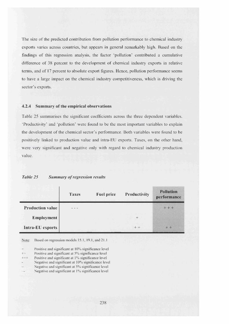
The size o f the predicted contribution from pollution performance to chemical industry

exports varies across countries, but appears in general remarkably high. Based on the

findings o f this regression analysis, the factor ‘pollution’ contributed a cumulative

difference o f 38 percent to the development o f chemical industry exports in relative

terms, and of 17 percent to absolute export figures. Hence, pollution performance seems

to have a large impact on the chemical industry competitiveness, which is driving the

sector’s exports.

4.2.4 Summary of the empirical observations

Table 25 summarises the significant coefficients across the three dependent variables.

‘Productivity’ and ‘pollution’ were found to be the most important variables to explain

the development o f the chemical sector’s performance. Both variables were found to be

positively linked to production value and intra-EU exports. Taxes, on the other hand,

were very significant and negative only with regard to chemical industry production

value.

Table 25 Summary o f regression results

Taxes Fuel price Productivity Pollutionperformance

Production value ----- + + +

Employment +

Intra-EU exports + + + +

Note: Based on regression models 15.1, 19.1, and 21.1

+ Positive and significant at 10% significance level++ Positive and significant at 5% significance level+++ Positive and significant at 1% significance level

Negative and significant at 10% significance level Negative and significant at 5% significance level

— Negative and significant at 1% significance level

238

Looking at the tables that report the predicted contribution of each independent

variable, there are at least two interesting observations. First, the cluster of poor

pollution performers has suffered from increases in taxes over the observation period

1980 to 1999. Looking at the development of this independent variable over time (table

32), it seems reasonable to assume that this increase in taxes was related to the

accession of Greece, Portugal and Spain to the European Community in the 1980s. On

the other hand, the pollution load on these countries also increased over the period, from

below-EU-average levels towards the average (and beyond, as table 29 shows). Hence,

one could talk about a double convergence, in taxes and pollution, among these

accession countries.

The net effect of this double convergence appears to be almost a zero-sum-game, as the

predicted contributions in table 17 and table 18 illustrate.

Secondly, the predicted contribution of ‘productivity’ to all chemical industry

performance variables appears to be larger among countries in the strong pollution

performance cluster and the falling-behind pollution performance cluster (which could

be considered the cluster of formerly strong pollution performers). Hence, the findings

of the regression analysis could lend some support to the Porter hypothesis on

innovation offsets.

239

5 The scope of environmental competition: some conclusions

from this study

5.1 Summary of the main findings

This thesis was about environmental competition. The research problem at the heart of

the analysis was the question whether countries compete among themselves by the

means of ‘playing’ with their environmental performance in order to foster industrial

activity. On the balance of the empirical results, the preliminary answer is yes - with

some qualifications attached.

In order to reach this conclusion, the first step was to construct a proxy indicator for

environmental performance. There are several approaches to deal with environmental

performance in social sciences. Since one of the initial objectives of this research was to

carry out a quantitative comparative analysis, the approach of choice was pollution

performance analysis. Pollution performance is too broad a concept to be workable in

practice, so this study had to narrow the concept of pollution performance to air

pollution performance. Therefore, the basis of the indicator was an average of several

air pollutants.

Since the frame of reference for this thesis was a closed system (the EU 15), the air

pollution time series were transformed into a relative performance indicator across the

countries within the system. The advantage of this approach is that it is comparative in

nature - once the indicator is developed, one can easily work out distinct pollution

performance patterns, rank countries according to their pollution performance, or

classify them into performance clusters.

240

Therefore, using the air pollution indicator, the first contribution of this thesis, is the

classification of EU 15 member states according to their empirically observed pollution

performance during the period 1990 to 1999. The classification produced four distinct

clusters. There were two “clear-cut” performance clusters with countries that were

either clearly poor pollution performers or strong pollution performers. Countries in the

first cluster were Greece, Portugal and Spain. They exhibited poor initial performance

levels with respect to the EU average and a lack of convergence. Inversely, strong

pollution performers, such as Austria, Denmark, Germany and the Netherlands were

characterised by strong initial pollution levels with regard to the other countries, and

also a lack of convergence. Furthermore, there were two ‘transitory’ pollution

performance clusters. The first of those two clusters comprises countries in the process

of catching-up: its constituents start from relatively poor pollution performance levels,

but show convergence towards the EU average. This group is comprised of Ireland,

Luxembourg and the United Kingdom. The last cluster contains countries that fall

behind in terms of pollution performance, such as Belgium, Finland, France, Italy, and

Sweden. These countries show strong initial pollution performance levels, but converge

downwards towards (and in some cases, beyond) the EU average.

The second part of the thesis evolved around the idea to relate the pollution

performance indicator to a number of variables that capture the performance of

chemical industries using panel data of 15 EU countries along 20 years. The main

hypothesis to be tested was whether strong pollution performance had an impact on

chemical industry performance, and if so, what the sign of that relationship was. There

were three performance variables: production value, employment, and value of intra-EU

exports - in order to stay within the EU as frame of reference.

241

The results of the regression analysis show that, with regard to two of the three

chemical industry performance variables, strong pollution performance has a negative

and significant impact. This is the case with regard to production value and intra-EU

exports. This finding is in line with conventional economic and location theory, which

states that there is a trade-off between economic performance and environmental

performance. The empirical observations of this thesis lend further support to such

theories. Hence, it seems that the countries in the sample actually do compete by means

of environmental competition.

On the other hand, this study did not produce evidence that strong pollution

performance has had an impact on the employment of the chemical industries in the EU.

Hence, employment seems to respond to a different set of factors.

Besides the pollution performance indicator, this study produced a number of

interesting results on the effect of other explanatory variables on the evolution of

chemical industries. First, the contribution of manufacturing productivity to both

chemical industry production value and exports was remarkably large within the strong

pollution performance cluster as well as to the falling-behind country cluster. Moreover,

manufacturing productivity was shown to be the only significant and positive

explanatory variable in the employment regression.

Second, taxes on production and imports had a negative impact on chemical industry

production value. The contribution of this explanatory factor was especially significant

within the poor pollution performer cluster, which is comprised of Greece, Portugal and

Spain. It seems that all three countries experienced a “double convergence” during their

accession process to the European Community during the 1980s. On the one hand, the

three countries had to adjust their tax level upwards to meet EC standards, which

harmed their chemical industries’ production. On the other hand, pollution performance

also converged from low initial levels towards European averages (and beyond), which

had a positive impact on chemical industry production levels. According to the results

of the regression analysis, the overall outcome of this double convergence was, more or

less, a zero-sum-game.

242

5.2 Directions for future research

One of the hottest issues in the news concerns the relocation of industries to the newly

acceded EU countries. Given the fact that, due to data constraints, this study only

covered the EU-15 member states, one obvious field for future research would be to

include all EU-26 countries, or to include further transition economies. In particular, it

would be very interesting to see whether these countries also experience what was

called a double convergence. Or, in other words, are these countries currently

attempting to compete - among others - on the basis of their environmental

performance?

Another promising field for future research seems to originate from one of the by­

products of this study, which is the observation that countries in the strong pollution

performer cluster and the falling-behind pollution performance cluster (that is, in a

sense, the cluster of formerly strong pollution performers), benefit consistently from

higher contributions of the ‘productivity’ variable to chemical industry performance.

This could suggest that the returns from investing in strong pollution performance are

achieved and harvested in the long term.

The explanatory variables used in the regression analysis did not explain the

employment performance of chemical industries. Hence, one interesting research

question could be to identify the ‘missing link’, that is the determinants of employment

in such a special industry.

Last but not least, another promising research question could be to expand the frame of

reference beyond the European Union, with the United Sates or Japan as the obvious

candidates for inclusion.

243

5 .5 Cost and benefits o f environmental protection: some policy

implications from this study

To conclude this investigation, let us take a step back and assess its implications ‘in the

big picture’ in terms of policies, business strategies, and further academic research.

Obviously, one needs to be very cautious to point out once more that there are important

constraints that should prevent the reader from taking its results as generally valid. First,

this study was set-up as a case study, which uses the 15 EU member states as a closed

frame of reference. Second, it used air pollution performance as a proxy for

environmental competition. Third, the analysis is limited to the period of 1980 to 1999.

Given the broadness and complexity of the academic arenas that link into the notion of

environmental competition, the narrow scope of this investigation will obviously limit

the degree to which it could be taken as generally applicable.

Fourth, and maybe most importantly, in order to keep the analysis within a manageable

scope, we had to focus on testing one specific set of hypotheses. Although there is a

range of what one might consider interesting ‘collateral’ findings, this thesis can merely

point at the apparent existence of those additional findings and recommend further

investigation. However, if we allow ourselves to relax this strict standard of objectivity

for a moment and permit some degree of ‘educated’ speculation, an intriguing set of

policy implications emerges.

A puzzle o f three pieces

This investigation has produced three sets of observations on how relative air pollution

performance among EU member states may have shaped the competitiveness of their

chemical industries. The first set of insights highlights the correlation between air

pollution performance and chemical industry competitiveness indicators. The second set

of observations highlights the predicted contribution from the factors ‘pollution

performance’ and ‘taxes’ on chemical industry competitiveness, and how the observed

differences vary among the four pollution performance clusters. Finally, the third set of

observations focuses on the differences in the contribution of the independent variable

‘productivity’ among the four pollution performance clusters. Like a puzzle, taken

together these three sets of insights seem to fit into one consistent overall picture.

244

Trading-off air pollution performance fo r chemical industry competitiveness does work

The first insight of this investigation is the notion that there seems to be a trade-off

between chemical industry production value as well as market share on the one hand,

and air pollution performance on the other hand. Furthermore, this investigation showed

no apparent link between pollution performance and chemical industry employment

levels.

The policy implications from this set of observations seem to be straight forward:

governments have certain scope for environmental competition. In other words, there

seems to be the possibility to trade pollution performance for chemical industry

production value and market share. The possibility of trading pollution performance for

jobs in the chemical industry sector seems much less certain. Hence, this investigation

lends some support to the notions of environmental externalities and of the

environmental Kuznets curve.

At this point, one should recall that the regression models did not use time lags between

dependent and independent variables. Hence, the trade-off between pollution

performance and chemical industry competitiveness appears to occur in a relatively

short term. From a policy point of view, this may be an important consideration: the

results of this research seem to point at the opportunity to realize relatively quick

economic gains through the reduction of environmental performance. Therefore, if

governments are pressed to generate economic wealth within a limited period of time,

pursuing a strategy of “selling o ff’ pollution performance, may appear an appealing

option. The medium and long term implications of such a strategy are, however, not

covered by this first set of insights, but rather by the subsequent two.

245

Double convergence: avoid trading-offpollution performance for the adjustment o f tax

levels among accession countries

The second insight of this investigation is related to what has been called the

phenomenon of “double convergence”. Based on the predicted contributions to

chemical industry competitiveness by the factors ‘pollution’ and ‘taxes’, one could

conclude that the chemical industries of Greece, Portugal and Spain have at the same

time profited and suffered from the accession to the EU and its common market. On the

one hand, the three countries appear to have succeeded in trading some of their

pollution performance for chemical industry competitiveness within the European

market. On the other hand, it seems that at the same time, while converging to European

standards, the tax regimes of those countries changed to the disadvantage of chemical

industries. In the end, competitiveness gains due to weak environmental performance

were to a large degree compensated by changes in the tax regime.

This notion could be relevant with regard to how to manage the accession of further

countries to the European Union. If we accept the notion of a “double convergence”,

one might speculate whether limiting the rate of upward adjustment of tax levels in the

accession countries could actually reduce the pressure on national governments to trade­

off pollution performance in order to compensate for the implied loss of chemical

industry competitiveness.

Productivity increases through environmental innovation offsets: the jury is still out

The third insight of this investigation concerns the indirect impact of pollution

performance on productivity levels. Due to the focus of this study, the results do not

present any definite endorsement or negation to the Porter hypothesis, which claims that

strong environmental regulation induces innovation offsets, which, in the medium and

long run would increase productivity levels. Yet, at the least, our empirical data seems

to show circumstantial evidence that the Porter Hypothesis could hold. If so, policy

implications would be important.

246

First of all, it would open the possibility for governments to justify a policy of pollution

performance leadership by pointing at the long term economic benefits. The biggest

advantage of such a policy would be its sustainability, not only in the environmental

sense but more importantly in the economic sense, as higher levels of innovation and

productivity are genuine competitive advantages, which are difficult for competitors to

match. In comparison, although selling-off pollution performance for short-term

increases in wealth is possible in the short-run, such policies do not create genuine

competitive advantages, since relaxing pollution performance levels is a strategy that

can be matched by any competitor.

The second important policy implication concerns the design of environmental

regulation. If innovation offsets originate from pollution policies, governments need to

design regulations that enable the creation and spread of innovations across industrial

sectors. In this context, policies aimed at the chemical industry would be key, as this

sector is generally seen as a generator and multiplier of environmental innovation across

a range of connected industries. Therefore, governments should seek to design policies

that encourage the development of pollution-reducing technologies within the chemical

industry, as well as the multiplication of such technologies across connected industrial

sectors. For this reason, environmental policies that aim to enable the Porter Hypothesis

to hold should not only consist of setting strict pollution standards, but also of

supporting measures such as subsidising R&D, protecting intellectual property, as well

as facilitating the exchange of knowledge across industry networks or local knowledge

clusters.

247

Appendices

Appendix 1: Pollution performance indicators Table 26 Anthropogenic emissions per capita

A nthropogenic C H 4 em issions (g / cap.)1980 1981 1982 1983 1984 1985 1986 1987 1988 1989 1990 1991 1992 1993 1994 1995 1996 1997 1998 1999

be 0.059 0.059 0.059 0.059 0.059 0.059 0.059 0.058 0.058 0.057dk 0.064 0.065 0.065 0.064 0.064 0.062 0.061 0.059 0.058 0.059 0.054 0.055 0.054 0.055 0.054 0.054 0.053 0.051 0.054 0.051de 0.080 0.078 0.076 0.075 0.074 0.076 0.075 0.073 0.071 0.070 0.070 0.063 0.058 0.053 0.049 0.048 0.044 0.042 0.041 0.040gr 0.043 0.043 0.043 0.042 0.043 0.044 0.043 0.044 0.044 0.044es 0.030 0.030 0.033 0.033 0.034 0.034 0.037 0.039 0.039 0.042 0.042 0.042 0.043 0.044 0.045 0.046 0.048 0.049 0.050 0.051fr 0.052 0.053 0.052 0.053 0.053 0.053 0.052 0.048 0.047 0.045ie 0.172 0.172 0.172 0.172 0.173 0.174 0.174 0.175 0.172 0.170it 0.039 0.038 0.038 0.039 0.039 0.039 0.040 0.040 0.041 0.040 0.041 0.041 0.041 0.042 0.044 0.044 0.033 0.033 0.033 0.033lu 0.063 0.059 0.059 0.063 0.054 0.056 0.058 0.057 0.054 0.055nl 0.069 0.061 0.061 0.070 0.072 0.081 0.072 0.071 0.069 0.070 0.087 0.086 0.083 0.080 0.078 0.076 0.079 0.071 0.068 0.065at 0.070 0.070 0.070 0.071 0.071 0.071 0.071 0.071 0.070 0.070 0.070 0.067 0.065 0.064 0.062 0.061 0.060 0.058 0.057 0.056Pt 0.064 0.065 0.064 0.063 0.064 0.064 0.064 0.064 0.064 0.063fi 0.060 0.056 0.050 0.045 0.044 0.044 0.042 0.040 0.038 0.037se 0.038 0.038 0.037 0.037 0.035 0.034 0.034 0.029 0.029 0.034uk 0.069 0.069 0.070 0.070 0.057 0.066 0.069 0.068 0.067 0.065 0.064 0.063 0.061 0.055 0.050 0.050 0.049 0.047 0.045 0.047AVG 0.065 0.064 0.063 0.062 0.060 0.060 0.059 0.058 0.057 0.057COV 0.12 0.13 0.13 0.13 0.14 0.14 0.14 0.15 0.15 0.14

Note: AVG Weighted average (weights according to the ratio national vs. total population)COV Coefficient of variation

Emission data (except C 0 2) from EMEP (2002, es/gr/pt: 2000) COz emission data from CDIAC (2002)Population data from Eurostat (2001)

248

A nthropogenic C 0 2 em issions (g / cap.)1980 1981 1982 1983 1984 1985 1986 1987 1988 1989 1990 1991 1992 1993 1994 1995 1996 1997 1998 1999

be 3.64 3.36 3.20 2.76 2.83 2.82 2.72 2.70 2.47 2.65 2.75 2.87 2.82 2.70 2.79 2.85 2.90 2.79 2.71 2.80dk 3.35 2.90 2.98 2.79 2.83 3.37 3.29 3.26 2.92 2.53 2.69 3.33 2.87 2.99 3.20 2.91 3.76 3.04 2.75 3.15de 3.38 3.15 3.00 2.99 3.06 3.04 3.03 2.97 2.97 2.89 2.32 3.04 2.92 2.85 2.93 2.77 2.87 2.77 2.74 2.88gr 1.46 1.42 1.45 1.54 1.57 1.65 1.61 1.71 1.81 1.97 1.94 1.78 1.95 1.94 2.01 2.02 2.15 2.14 2.21 2.23es 1.46 1.44 1.44 1.40 1.30 1.35 1.23 1.26 1.29 1.47 1.49 1.51 1.57 1.44 1.51 1.62 1.62 1.70 1.71 1.72fr 2.44 2.19 2.09 1.98 1.90 1.86 1.77 1.68 1.65 1.72 1.72 1.84 1.73 1.68 1.55 1.64 1.74 1.60 1.72 1.85ie 2.02 2.00 1.97 1.93 1.93 1.98 2.21 2.31 2.34 2.22 2.32 2.58 2.42 2.43 2.53 2.53 2.64 2.72 2.81 2.76it 1.80 1.76 1.71 1.64 1.68 1.71 1.66 1.73 1.76 1.85 1.89 1.90 1.92 1.84 1.82 1.92 1.88 1.90 1.93 1.90lu 7.91 6.74 6.34 5.93 6.36 6.48 6.36 6.11 6.31 6.69 7.07 7.47 7.48 7.40 6.89 5.54 5.53 5.12 4.91 4.66nl 2.95 2.76 2.14 2.22 2.39 2.55 2.43 2.48 2.39 2.72 2.74 2.73 2.67 2.77 2.55 2.69 2.98 2.84 2.85 2.87at 1.89 2.03 1.94 1.87 1.94 1.95 1.92 1.94 1.86 1.89 2.03 2.11 1.95 1.92 1.94 1.96 2.01 2.06 2.16 2.08P* 0.75 0.70 0.80 0.82 0.78 0.83 0.81 0.87 0.89 1.12 1.17 1.17 1.30 1.26 1.29 1.39 1.32 1.38 1.50 1.48fi 3.25 2.84 2.59 2.35 2.26 2.67 3.05 3.00 2.80 2.91 2.90 2.84 2.60 2.67 2.89 2.80 3.25 3.10 2.82 3.04se 2.34 2.24 1.99 1.85 1.80 1.97 1.94 1.87 1.85 1.76 1.55 1.60 1.62 1.50 1.56 1.44 1.67 1.47 1.50 1.51uk 2.81 2.67 2.66 2.65 2.51 2.65 2.69 2.71 2.69 2.72 2.70 2.75 2.59 2.56 2.54 2.52 2.63 2.49 2.50 2.46AVG 2.76 2.55 2.42 2.31 2.34 2.46 2.45 2.44 2.40 2.47 2.49 2.63 2.56 2.53 2.53 2.44 2.60 2.47 2.45 2.49COV 0.15 0.13 0.13 0.13 0.13 0.13 0.13 0.13 0.13 0.13 0.14 0.14 0.14 0.14 0.13 0.10 0.10 0.09 0.09 0.08

Note: AVG Weighted average (weights according to the ratio national vs. total population)COV Coefficient of variation

Emission data (except C 0 2) from EMEP (2002, es/gr/pt: 2000)C 0 2 emission data from CDIAC (2002)Population data from Eurostat (2001)

249

A n thropogen ic S 0 2 em issions (g / cap .)1980 1981 1982 1983 1984 1985 1986 1987 1988 1989 1990 1991 1992 1993 1994 1995 1996 1997 1998 1999

be 0.084 0.072 0.070 0.057 0.051 0.040 0.038 0.037 0.036 0.033 0.037 0.033 0.032 0.029 0.025 0.024 0.024 0.022 0.021 0.018dk 0.088 0.072 0.074 0.063 0.060 0.067 0.057 0.050 0.050 0.039 0.036 0.047 0.036 0.030 0.030 0.028 0.034 0.021 0.015 0.011de 0.051 0.049 0.046 0.043 0.042 0.039 0.036 0.031 0.020 0.015 0.067 0.050 0.041 0.036 0.030 0.024 0.017 0.014 0.011 0.010

gr 0.041 0.043 0.045 0.047 0.048 0.050 0.050 0.050 0.050 0.050 0.050 0.054 0.054 0.053 0.050 0.053 0.052 0.051 0.051 0.051es 0.076 0.073 0.072 0.073 0.066 0.062 0.059 0.055 0.046 0.055 0.053 0.053 0.052 0.049 0.048 0.044 0.038 0.039 0.037 0.035fr 0.060 0.047 0.044 0.036 0.032 0.027 0.024 0.024 0.022 0.024 0.023 0.024 0.021 0.018 0.017 0.016 0.016 0.013 0.014 0.012ie 0.065 0.056 0.045 0.041 0.040 0.040 0.046 0.049 0.043 0.046 0.053 0.051 0.048 0.045 0.049 0.045 0.040 0.045 0.047 0.042it 0.067 0.059 0.050 0.043 0.037 0.033 0.034 0.035 0.034 0.032 0.029 0.027 0.024 0.023 0.022 0.023 0.021 0.018 0.018 0.016In 0.066 0.057 0.047 0.038 0.041 0.044 0.043 0.042 0.041 0.040 0.039 0.039 0.038 0.038 0.032 0.022 0.019 0.014 0.009 0.009nl 0.035 0.033 0.028 0.022 0.021 0.018 0.018 0.018 0.017 0.014 0.014 0.011 0.011 0.011 0.009 0.010 0.009 0.008 0.007 0.006at 0.051 0.044 0.042 0.031 0.028 0.025 0.023 0.020 0.015 0.013 0.012 0.011 0.008 0.008 0.007 0.007 0.007 0.006 0.006 0.005P* 0.027 0.028 0.029 0.031 0.025 0.020 0.023 0.022 0.020 0.028 0.036 0.035 0.041 0.036 0.034 0.037 0.033 0.034 0.038 0.035fi 0.122 0.111 0.100 0.077 0.075 0.078 0.067 0.067 0.061 0.049 0.052 0.039 0.028 0.024 0.022 0.019 0.020 0.019 0.017 0.017se 0.059 0.052 0.045 0.037 0.036 0.032 0.032 0.027 0.027 0.019 0.014 0.011 0.010 0.010 0.009 0.009 0.009 0.006 0.006 0.007uk 0.087 0.079 0.075 0.069 0.066 0.066 0.069 0.069 0.067 0.065 0.065 0.062 0.059 0.053 0.046 0.040 0.034 0.028 0.026 0.020AVG 0.065 0.058 0.054 0.047 0.045 0.043 0.041 0.040 0.037 0.035 0.039 0.036 0.034 0.031 0.029 0.027 0.025 0.022 0.021 0.020COV 0.09 0.09 0.09 0.08 0.09 0.11 0.10 0.10 0.11 0.11 0.11 0.11 0.11 0.12 0.12 0.13 0.13 0.15 0.16 0.16

Note: AVG Weighted average (weights according to the ratio national vs. total population)COV Coefficient of variation

Emission data (except C 0 2) from EMEP (2002, es/gr/pt: 2000)C 0 2 emission data from CDIAC (2002)Population data from Eurostat (2001)

250

A n thropogen ic N 0 2 em issions (g / cap .)1980 1981 1982 1983 1984 1985 1986 1987 1988 1989 1990 1991 1992 1993 1994 1995 1996 1997 1998 1999

be 0.045 0.043 0.040 0.038 0.035 0.033 0.032 0.034 0.035 0.036 0.034 0.033 0.034 0.034 0.034 0.033 0.031 0.030 0.031 0.029dk 0.053 0.047 0.052 0.050 0.053 0.057 0.063 0.059 0.058 0.054 0.053 0.061 0.052 0.051 0.052 0.048 0.055 0.047 0.044 0.040de 0.043 0.041 0.041 0.042 0.042 0.042 0.042 0.040 0.038 0.035 0.034 0.031 0.029 0.027 0.025 0.024 0.023 0.022 0.021 0.020gr 0.030 0.030 0.030 0.030 0.031 0.031 0.031 0.032 0.033 0.033 0.032 0.032 0.032 0.032 0.033 0.033 0.036 0.034 0.036 0.036es 0.027 0.025 0.025 0.025 0.025 0.024 0.025 0.026 0.027 0.029 0.030 0.031 0.032 0.031 0.031 0.031 0.030 0.032 0.033 0.033fr 0.037 0.035 0.034 0.034 0.033 0.033 0.032 0.032 0.032 0.033 0.033 0.034 0.033 0.031 0.030 0.029 0.029 0.028 0.027 0.026ie 0.021 0.025 0.025 0.024 0.024 0.026 0.028 0.032 0.035 0.036 0.034 0.034 0.037 0.033 0.032 0.032 0.033 0.032 0.033 0.032it 0.029 0.028 0.028 0.028 0.028 0.028 0.030 0.032 0.032 0.033 0.034 0.034 0.035 0.034 0.031 0.030 0.030 0.028 0.027 0.025lu 0.063 0.062 0.060 0.057 0.057 0.057 0.058 0.059 0.060 0.061 0.060 0.061 0.063 0.063 0.057 0.051 0.053 0.043 0.040 0.037nl 0.041 0.040 0.039 0.039 0.040 0.041 0.040 0.041 0.041 0.039 0.039 0.038 0.037 0.035 0.033 0.032 0.032 0.029 0.027 0.026at 0.030 0.029 0.029 0.028 0.028 0.029 0.028 0.028 0.027 0.025 0.025 0.025 0.024 0.022 0.023 0.021 0.021 0.021 0.021 0.021Pt 0.017 0.017 0.018 0.019 0.014 0.010 0.011 0.012 0.012 0.013 0.032 0.034 0.036 0.035 0.035 0.036 0.036 0.036 0.037 0.038fi 0.062 0.058 0.056 0.054 0.053 0.056 0.056 0.058 0.059 0.061 0.060 0.058 0.056 0.056 0.055 0.051 0.052 0.051 0.049 0.048se 0.049 0.050 0.049 0.048 0.049 0.051 0.052 0.052 0.051 0.049 0.039 0.039 0.038 0.037 0.038 0.034 0.034 0.031 0.029 0.029uk 0.046 0.044 0.044 0.044 0.043 0.045 0.046 0.048 0.049 0.049 0.048 0.046 0.044 0.041 0.039 0.036 0.034 0.031 0.029 0.027AVG 0.040 0.038 0.038 0.037 0.037 0.037 0.038 0.039 0.039 0.039 0.039 0.039 0.039 0.037 0.036 0.035 0.035 0.033 0.032 0.031COV 0.09 0.08 0.08 0.08 0.08 0.09 0.09 0.09 0.09 0.08 0.07 0.07 0.07 0.07 0.07 0.06 0.07 0.06 0.06 0.06

Note: AVG Weighted average (weights according to the ratio national vs. total population)COV Coefficient of variation

Emission data (except C 0 2) from EMEP (2002, es/gr/pt: 2000)C 0 2 emission data from CDIAC (2002)Population data from Eurostat (2001)

251

A nthropogenic N M V O C em issions (g / cap.)1980 1981 1982 1983 1984 1985 1986 1987 1988 1989 1990 1991 1992 1993 1994 1995 1996 1997 1998 1999

be 0.070 0.060 0.054 0.048 0.041 0.036 0.031 0.031 0.031 0.030 0.029 0.027 0.027 0.027 0.027dk 0.040 0.039 0.039 0.039 0.040 0.038 0.039 0.039 0.038 0.038 0.033 0.032 0.031 0.031 0.029 0.028 0.028 0.026 0.025 0.024de 0.041 0.040 0.040 0.040 0.040 0.040 0.040 0.040 0.039 0.037 0.041 0.035 0.032 0.029 0.027 0.025 0.023 0.022 0.021 0.020gr 0.062 0.057 0.052 0.047 0.042 0.033 0.033 0.033 0.034 0.034 0.035 0.036 0.037 0.038 0.038es 0.069 0.067 0.066 0.067 0.067 0.068 0.068 0.069 0.070 0.071 0.072 0.070 0.068 0.064 0.069 0.067 0.064 0.068 0.068 0.068fr 0.043 0.043 0.042 0.039 0.037 0.035 0.034 0.033 0.032 0.030ie 0.031 0.031 0.032 0.030 0.030 0.029 0.030 0.031 0.031 0.025it 0.039 0.037 0.037 0.036 0.035 0.035 0.035 0.036 0.037 0.038 0.038 0.040 0.040 0.040 0.040 0.041 0.033 0.032 0.030 0.028lu 0.041 0.043 0.045 0.047 0.048 0.050 0.048 0.047 0.045 0.045 0.039 0.038 0.036 0.030 0.035nl 0.035 0.034 0.033 0.036 0.032 0.034 0.031 0.029 0.026 0.025 0.024 0.023 0.020 0.019 0.018at 0.047 0.047 0.046 0.047 0.048 0.047 0.049 0.049 0.050 0.048 0.045 0.040 0.035 0.034 0.032 0.032 0.031 0.030 0.029 0.029Pt 0.020 0.023 0.027 0.031 0.035 0.038 0.041 0.044 0.045 0.045 0.047 0.044 0.050 0.049 0.050fi 0.043 0.043 0.044 0.042 0.041 0.040 0.038 0.037 0.036 0.034 0.034 0.033 0.032se 0.066 0.064 0.061 0.060 0.056 0.055 0.054 0.052 0.052 0.047 0.047 0.047uk 0.042 0.042 0.042 0.043 0.044 0.044 0.045 0.046 0.047 0.047 0.046 0.045 0.043 0.041 0.040 0.038 0.037 0.035 0.032 0.029AVG 0.043 0.041 0.040 0.039 0.038 0.037 0.036 0.035 0.034 0.033COV 0.07 0.07 0.07 0.07 0.08 0.08 0.08 0.09 0.09 0.10

Note: AVG Weighted average (weights according to the ratio national vs. total population)COV Coefficient of variation

Emission data (except C 0 2) from EMEP (2002, es/gr/pt: 2000)COz emission data from CDIAC (2002)Population data from Eurostat (2001)

252

A nthropogenic C O em issions (g / cap.)1980 1981 1982 1983 1984 1985 1986 1987 1988 1989 1990 1991 1992 1993 1994 1995 1996 1997 1998 1999

be 0.112 0.112 0.113 0.109 0.104 0.102 0.099 0.093 0.095 0.092dk 0.187 0.210 0.219 0.186 0.207 0.194 0.195 0.199 0.183 0.195 0.137 0.139 0.133 0.128 0.119 0.116 0.119 0.107 0.113 0.102de 0.179 0.163 0.154 0.149 0.151 0.147 0.146 0.141 0.135 0.127 0.142 0.119 0.104 0.095 0.087 0.082 0.076 0.071 0.065 0.060gr 0.131 0.134 0.128 0.127 0.126 0.128 0.132 0.134 0.142 0.136es 0.098 0.094 0.092 0.093 0.092 0.090 0.091 0.094 0.099 0.103 0.100 0.103 0.105 0.099 0.099 0.088 0.093 0.099 0.099 0.100fr 0.292 0.276 0.266 0.257 0.257 0.252 0.243 0.238 0.229 0.218 0.190 0.187 0.178 0.167 0.155 0.152 0.142 0.134 0.129 0.121ie 0.114 0.112 0.111 0.098 0.092 0.085 0.084 0.085 0.086 0.076it 0.134 0.132 0.133 0.131 0.133 0.135 0.133 0.134 0.132 0.134 0.136 0.138 0.138 0.133 0.130 0.133 0.119 0.114 0.108 0.103lu 0.458 0.587 0.520 0.550 0.359 0.261 0.248 0.190 0.120 0.115nl 0.095 0.086 0.081 0.080 0.076 0.076 0.068 0.065 0.063 0.059 0.058 0.058 0.048 0.046 0.043at 0.227 0.217 0.209 0.205 0.212 0.204 0.217 0.211 0.204 0.194 0.169 0.165 0.152 0.147 0.143 0.130 0.127 0.127 0.120 0.107Pt 0.113 0.120 0.130 0.128 0.125 0.121 0.119 0.115 0.110 0.115fi 0.112 0.110 0.095 0.090 0.087 0.085 0.090 0.092 0.088 0.106se 0.141 0.141 0.136 0.132 0.130 0.123 0.122 0.109 0.113 0.104uk 0.136 0.135 0.135 0.131 0.131 0.127 0.127 0.127 0.128 0.131 0.124 0.120 0.114 0.106 0.100 0.094 0.093 0.088 0.084 0.080AVG 0.150 0.157 0.148 0.145 0.128 0.117 0.115 0.107 0.101 0.097COV 0.15 0.19 0.18 0.20 0.13 0.10 0.09 0.08 0.06 0.06

Note: AVG Weighted average (weights according to the ratio national vs. total population)COV Coefficient of variation

Emission data (except C 0 2) from EMEP (2002, es/gr/pt: 2000)C 0 2 emission data from CDIAC (2002)Population data from Eurostat (2001)

253

A n thropogen ic N H 3 em issions (g / cap .)1980 1981 1982 1983 1984 1985 1986 1987 1988 1989 1990 1991 1992 1993 1994 1995 1996 1997 1998 1999

be 0.0090 0.0094 0.0097 0.0101 0.0104 0.0107 0.0093 0.0092 0.0096 0.0095 0.0096 0.0097 0.0097 0.0100 0.0101dk 0.0244 0.0240 0.0234 0.0233 0.0225 0.0264 0.0264 0.0256 0.0249 0.0250 0.0249 0.0240 0.0233 0.0225 0.0216 0.0201 0.0191 0.0189 0.0190 0.0181de 0.0093 0.0090 0.0092 0.0094 0.0096 0.0096 0.0095 0.0094 0.0091 0.0090 0.0097 0.0084 0.0081 0.0079 0.0078 0.0078 0.0078 0.0076 0.0077 0.0076g r 0.0078 0.0076 0.0073 0.0072 0.0070 0.0081 0.0070 0.0068 0.0070 0.0069es 0.0106 0.0101 0.0108 0.0108 0.0109 0.0109 0.0113 0.0123 0.0123 0.0126 0.0121 0.0120 0.0120 0.0115 0.0120 0.0119 0.0132 0.0128 0.0130 0.0131fr 0.0139 0.0138 0.0135 0.0133 0.0134 0.0134 0.0136 0.0137 0.0137 0.0136ie 0.0319 0.0326 0.0330 0.0328 0.0333 0.0335 0.0336 0.0335 0.0342 0.0338it 0.0085 0.0084 0.0082 0.0089 0.0084 0.0085 0.0086 0.0087 0.0087 0.0084 0.0081 0.0078 0.0076 0.0077 0.0079 0.0079 0.0074 0.0076 0.0075 0.0076lu 0.0183 0.0181 0.0178 0.0176 0.0173 0.0171 0.0168 0.0166 0.0164 0.0169nl 0.0165 0.0168 0.0170 0.0170 0.0171 0.0171 0.0177 0.0176 0.0161 0.0156 0.0151 0.0151 0.0119 0.0125 0.0108 0.0094 0.0094 0.0120 0.0108 0.0111at 0.0104 0.0105 0.0105 0.0107 0.0108 0.0107 0.0107 0.0106 0.0104 0.0104 0.0103 0.0101 0.0097 0.0095 0.0095 0.0092 0.0090 0.0089 0.0089 0.0087P* 0.0106 0.0101 0.0108 0.0100 0.0094 0.0103 0.0100 0.0101 0.0103 0.0100fi 0.0076 0.0079 0.0081 0.0077 0.0073 0.0069 0.0068 0.0074 0.0073 0.0068se 0.0064 0.0062 0.0060 0.0059 0.0070 0.0070 0.0069 0.0069 0.0069 0.0067 0.0067 0.0062uk 0.0063 0.0062 0.0059 0.0059 0.0059 0.0058 0.0057 0.0058 0.0059 0.0059AVG 0.0129 0.0126 0.0123 0.0122 0.0120 0.0119 0.0117 0.0119 0.0119 0.0118COV 0.14 0.15 0.15 0.15 0.15 0.15 0.15 0.15 0.15 0.15

Note: AVG Weighted average (weights according to the ratio national vs. total population)COV Coefficient of variation

Emission data (except C 0 2) from EMEP (2002, es/gr/pt: 2000)C 0 2 emission data from CDIAC (2002)Population data from Eurostat (2001)

254

Table 27 A nthropogenic emissions / GDP

A nthropogenic C H 4 em issions / G D P (tonnes / m illion €) 1980 1981 1982 1983 1984 1985 1986 1987 1988 1989 1990 1991 1992 1993 1994 1995 1996 1997 1998 1999

be 3.839 3.652 3.413 3.248 3.023 2.815 2.783 2.712 2.609 2.480dk 7.050 6.673 6.085 5.423 4.931 4.341 3.903 3.559 3.405 3.300 2.854 2.782 2.640 2.560 2.352 2.153 2.041 1.922 1.935 1.729de 8.408 7.841 7.010 6.230 5.759 5.592 5.034 4.603 4.272 3.989 4.669 3.567 3.035 2.607 2.331 2.129 1.949 1.897 1.772 1.677gr 6.659 6.032 5.716 5.567 5.309 5.093 4.630 4.292 4.291 3.918es 7.290 6.937 6.816 7.231 6.438 6.021 5.912 5.804 5.108 4.573 4.114 3.789 3.721 4.105 4.257 4.114 4.055 4.050 3.944 3.810fr 3.145 3.106 2.974 2.891 2.758 2.664 2.544 2.296 2.179 2.027ie 18.907 18.017 16.823 16.659 15.306 14.295 12.996 11.276 10.370 9.325it 6.699 5.977 5.287 4.806 4.244 4.015 3.731 3.542 3.329 2.979 2.756 2.607 2.553 2.974 3.041 3.117 2.037 1.959 1.893 1.817lu 2.291 1.977 1.889 1.897 1.536 1.518 1.542 1.513 1.349 1.321nl 7.875 6.815 6.157 6.616 6.488 6.946 5.761 5.558 5.274 5.014 5.818 5.553 5.076 4.597 4.251 3.860 3.933 3.435 3.119 2.891at 9.427 8.769 7.697 6.959 6.592 6.189 5.661 5.270 5.018 4.692 4.298 3.936 3.572 3.273 3.037 2.780 2.686 2.585 2.421 2.291P‘ 11.844 10.195 8.734 8.736 8.594 7.933 7.498 7.199 6.705 6.227fi 2.885 2.942 3.202 3.340 2.808 2.398 2.265 2.025 1.812 1.644se 1.847 1.729 1.741 2.110 1.886 1.750 1.566 1.346 1.311 1.489uk 10.113 8.478 7.897 7.596 5.842 6.202 6.879 6.493 5.567 5.058 4.884 4.505 4.389 3.972 3.447 3.464 3.139 2.424 2.164 2.239AVG 5.387 4.959 4.632 4.569 4.262 4.006 3.711 3.395 3.192 2.992COV 0.21 0.21 0.20 0.20 0.21 0.20 0.20 0.19 0.19 0.18

Note: AVG Weighted average (weights according to the ratio national vs. total GDP)COV Coefficient of variation

Emission data (except C 0 2) from EMEP (2002, es/gr/pt 2000)C 0 2 emission data from CD1AC (2002)GDP data from Eurostat (2001)

255

A nthropogenic C 0 2 em issions / G D P (tonnes / m illion €) 1980 1981 1982 1983 1984 1985 1986 1987 1988 1989 1990 1991 1992 1993 1994 1995 1996 1997 1998 1999

be 415.3 374.7 359.3 298.3 283.3 261.3 233.3 217.4 187.6 185.1 178.6 176.5 163.5 147.9 142.9 136.5 137.3 130.7 121.7 121.2dk 368.8 297.6 278.9 235.0 218.0 234.7 209.5 196.3 169.9 141.8 141.8 169.7 139.5 139.3 139.1 116.8 144.8 113.6 98.4 107.6de 355.8 317.0 275.9 249.0 237.5 224.9 203.4 187.3 179.8 165.4 154.3 172.9 153.7 141.2 138.1 123.9 128.2 124.2 119.0 121.3gr 390.9 336.8 295.4 318.5 301.8 316.9 338.2 359.0 333.6 327.2 299.7 249.9 261.5 253.9 250.0 236.1 230.1 210.4 214.6 199.2es 358.8 329.7 298.8 303.2 248.5 237.8 196.5 187.1 167.8 161.2 146.4 135.4 135.4 135.0 143.9 145.7 136.4 140.4 134.9 128.0fi­ 274.1 225.9 202.2 183.7 165.3 149.7 132.6 122.4 113.8 110.9 104.2 108.9 97.9 92.0 81.2 81.9 84.4 76.8 79.0 82.5le 515.8 437.6 378.8 356.5 335.5 316.4 328.6 334.1 314.9 269.8 255.3 269.2 236.5 235.7 224.3 207.8 196.4 175.0 170.0 151.7it 312.5 274.2 237.7 201.1 183.9 175.5 155.7 151.9 143.9 136.2 128.2 119.7 120.1 129.2 125.7 136.4 116.7 111.3 109.3 103.7lu 727.0 570.5 472.9 399.2 391.4 353.7 320.1 296.6 285.8 271.0 257.9 250.7 241.0 223.6 194.3 149.7 147.8 135.8 122.9 112.0nl 338.6 306.1 214.8 209.4 215.5 218.1 194.1 193.0 181.8 194.6 184.2 175.6 164.3 159.1 138.7 136.9 147.6 136.9 131.6 127.0at 255.0 253.6 213.5 183.4 179.5 169.6 152.5 145.0 132.5 126.6 125.5 122.9 106.9 98.7 94.6 89.6 90.4 91.5 91.9 84.9Pt 366.6 290.8 314.3 325.4 301.0 286.4 245.3 246.4 217.2 234.8 214.8 184.4 176.9 175.2 172.6 172.6 155.0 154.7 157.7 145.2fi 426.8 308.2 247.0 212.6 175.5 189.0 215.2 197.7 160.5 143.3 139.8 150.1 166.7 196.9 185.8 153.7 174.6 155.3 133.9 136.8se 216.9 183.1 164.5 150.6 125.8 126.5 122.1 113.9 103.2 88.2 75.5 73.2 76.2 85.8 85.5 74.9 77.7 67.4 68.0 66.4uk 409.6 326.0 301.1 287.3 256.6 248.2 266.8 258.0 224.2 210.6 206.4 197.4 186.2 186.4 173.4 175.4 169.8 129.0 121.5 117.6AVG 382.2 322.1 283.7 260.9 2413 233.9 220.9 213.7 194.4 184.5 174.2 170.4 161.7 160.0 152.7 142.5 142.5 130.2 125.0 120.3COV 0.08 0.07 0.07 0.07 0.07 0.07 0.08 0.09 0.09 0.09 0.09 0.08 0.08 0.08 0.08 0.08 0.07 0.07 0.07 0.07

Note: AVG Weighted average (weights according to the ratio national vs. total GDP)COV Coefficient of variation

Emission data (except C 0 2) from EMEP (2002, es/gr/pt 2000)C 0 2 emission data from CDIAC (2002)GDP data from Eurostat (2001)

256

A nthropogenic S 0 2 em issions / G D P (tonnes / m illion €) 1980 1981 1982 1983 1984 1985 1986 1987 1988 1989 1990 1991 1992 1993 1994 1995 1996 1997 1998 1999

be 9.60 8.06 7.91 6.13 5.07 3.75 3.27 2.98 2.71 2.29 2.42 2.05 1.83 1.61 1.28 1.16 1.12 1.01 0.93 0.79dk 9.71 7.43 6.92 5.31 4.60 4.68 3.63 3.03 2.89 2.16 1.87 2.39 1.77 1.38 1.31 1.14 1.31 0.78 0.52 0.36de 5.41 4.91 4.24 3.61 3.27 2.87 2.45 1.97 1.20 0.87 4.46 2.84 2.16 1.80 1.43 1.09 0.77 0.61 0.48 0.43gr 11.07 10.22 9.11 9.62 9.27 9.63 10.54 10.54 9.21 8.31 7.69 7.53 7.22 6.96 6.26 6.15 5.52 4.99 4.98 4.57es 18.64 16.79 15.07 15.75 12.59 10.99 9.43 8.24 6.00 6.02 5.19 4.71 4.50 4.61 4.55 3.94 3.21 3.20 2.89 2.59fr 6.68 4.80 4.28 3.36 2.80 2.15 1.81 1.73 1.50 1.58 1.36 1.44 1.20 1.00 0.89 0.80 0.76 0.63 0.63 0.51ie 16.67 12.22 8.75 7.47 6.98 6.33 6.79 7.12 5.79 5.60 5.84 5.33 4.74 4.38 4.35 3.69 3.01 2.91 2.87 2.30it 11.57 9.16 7.00 5.30 4.07 3.42 3.16 3.11 2.79 2.37 1.94 1.68 1.51 1.61 1.51 1.61 1.28 1.07 1.00 0.85lu 6.05 4.86 3.47 2.58 2.52 2.38 2.16 2.04 1.87 1.63 1.43 1.30 1.23 1.14 0.91 0.59 0.51 0.38 0.23 0.21nl 3.97 3.61 2.84 2.12 1.87 1.52 1.45 1.40 1.29 0.98 0.91 0.74 0.70 0.62 0.52 0.48 0.43 0.37 0.31 0.28at 6.86 5.52 4.58 3.09 2.58 2.18 1.80 1.50 1.08 0.89 0.73 0.61 0.44 0.39 0.35 0.32 0.30 0.28 0.25 0.21Pt 13.20 11.66 11.52 12.20 9.70 6.79 7.09 6.17 5.02 5.90 6.68 5.51 5.62 5.05 4.59 4.58 3.83 3.86 3.97 3.42fi 16.06 12.06 9.56 6.92 5.84 5.52 4.74 4.39 3.50 2.42 2.52 2.05 1.79 1.79 1.44 1.03 1.10 0.96 0.83 0.76se 5.47 4.23 3.69 2.99 2.48 2.05 2.05 1.66 1.48 0.94 0.68 0.51 0.48 0.57 0.51 0.47 0.44 0.26 0.25 0.31uk 12.62 9.60 8.47 7.45 6.72 6.19 6.83 6.53 5.60 5.02 4.99 4.43 4.28 3.88 3.12 2.79 2.21 1.44 1.29 0.95AVG 10.24 8.34 7.16 6.26 5.36 4.70 4.48 4.16 3.46 3.13 3.25 2.87 2.63 2.45 2.20 1.99 1.72 1.52 1.43 1.24COV 0.11 0.11 0.12 0.15 0.15 0.15 0.16 0.17 0.17 0.19 0.18 0.18 0.20 0.20 0.21 0.23 0.22 0.24 0.26 0.27

Note: AVG Weighted average (weights according to the ratio national vs. total GDP)COV Coefficient of variation

Emission data (except C 0 2) from EMEP (2002, es/gr/pt 2000)C 0 2 emission data from CDIAC (2002)GDP data from Eurostat (2001)

257

A n thropogen ic N 0 2 em issions / G D P (ton n es / m illion €) 1980 1981 1982 1983 1984 1985 1986 1987 1988 1989 1990 1991 1992 1993 1994 1995 1996 1997 1998 1999

be 5.124 4.744 4.511 4.082 3.552 3.051 2.748 2.745 2.642 2.516 2.206 2.059 1.978 1.849 1.729 1.584 1.473 1.407 1.373 1.238dk 5.867 4.877 4.823 4.230 4.067 3.976 3.996 3.573 3.350 3.025 2.782 3.114 2.522 2.395 2.260 1.929 2.135 1.769 1.566 1.352de 4.471 4.151 3.772 3.485 3.298 3.083 2.799 2.510 2.269 1.975 2.268 1.774 1.502 1.338 1.181 1.076 1.025 0.972 0.903 0.839gr 7.984 7.119 6.145 6.296 5.893 5.891 6.587 6.716 5.988 5.497 4.956 4.565 4.339 4.179 4.071 3.809 3.863 3.390 3.525 3.212es 6.698 5.732 5.182 5.464 4.771 4.289 3.979 3.863 3.461 3.206 2.928 2.779 2.737 2.886 2.946 2.786 2.561 2.665 2.576 2.470fr 4.190 3.633 3.313 3.129 2.916 2.641 2.390 2.352 2.226 2.124 1.991 2.001 1.865 1.682 1.563 1.463 1.404 1.335 1.247 1.154ie 5.481 5.475 4.762 4.470 4.129 4.113 4.191 4.703 4.650 4.394 3.706 3.556 3.585 3.234 2.857 2.639 2.460 2.069 1.986 1.742it 5.043 4.414 3.945 3.405 3.070 2.904 2.771 2.773 2.633 2.451 2.282 2.164 2.172 2.404 2.126 2.157 1.847 1.662 1.539 1.375lu 5.802 5.212 4.493 3.865 3.529 3.128 2.939 2.881 2.726 2.465 2.196 2.063 2.020 1.897 1.606 1.386 1.414 1.135 0.997 0.894nl 4.728 4.478 3.950 3.639 3.578 3.476 3.224 3.180 3.101 2.818 2.610 2.426 2.252 2.011 1.802 1.639 1.598 1.402 1.245 1.145at 4.062 3.636 3.161 2.800 2.616 2.489 2.230 2.057 1.891 1.698 1.540 1.465 1.296 1.125 1.103 0.968 0.924 0.949 0.901 0.861Pt 8.235 7.243 7.192 7.652 5.236 3.291 3.331 3.281 3.002 2.783 5.893 5.301 4.874 4.792 4.670 4.481 4.201 4.082 3.906 3.682fi 8.110 6.232 5.355 4.859 4.081 3.973 3.970 3.851 3.400 2.987 2.904 3.058 3.609 4.112 3.567 2.774 2.810 2.532 2.318 2.148se 4.500 4.095 4.096 3.928 3.441 3.284 3.255 3.172 2.862 2.465 1.927 1.803 1.785 2.130 2.060 1.773 1.592 1.398 1.316 1.291uk 6.671 5.416 4.995 4.806 4.445 4.188 4.575 4.562 4.057 3.756 3.661 3.267 3.169 2.946 2.646 2.479 2.213 1.617 1.421 1.289AVG 5.798 5.097 4.646 4.407 3.908 3.585 3.532 3.481 3.217 2.944 2.923 2.760 2.647 2.599 2.413 2.196 2.101 1.892 1.788 1.646COV 0.06 0.06 0.06 0.07 0.06 0.06 0.08 0.08 0.08 0.08 0.10 0.10 0.10 0.10 0.11 0.11 0.11 0.12 0.13 0.13

Note: AVG Weighted average (weights according to the ratio national vs. total GDP)COV Coefficient of variation

Emission data (except C 0 2) from EMEP (2002, es/gr/pt 2000)C 0 2 emission data from CDIAC (2002)GDP data from Eurostat (2001)

258

A nthropogenic N M V O C em issions / G D P (tonnes / m illion €)1980 1981 1982 1983 1984 1985 1986 1987 1988 1989 1990 1991 1992 1993 1994 1995 1996 1997 1998 1999

be 6.458 5.175 4.337 3.607 2.868 2.303 1.924 1.805 1.686 1.542 1.386 1.277 1.241 1.219 1.149dk 4.359 3.990 3.634 3.324 3.100 2.678 2.465 2.338 2.219 2.124 1.733 1.656 1.520 1.423 1.260 1.127 1.072 0.967 0.904 0.823de 4.309 4.000 3.675 3.331 3.140 2.970 2.700 2.510 2.334 2.112 2.699 1.989 1.656 1.421 1.251 1.107 1.035 0.985 0.911 0.847gr 11.820 11.911 10.872 8.606 6.946 5.078 4.634 4.417 4.393 4.250 4.043 3.843 3.606 3.663 3.363es 16.907 15.418 13.747 14.501 12.732 11.913 10.902 10.318 9.110 7.822 7.067 6.286 5.847 5.966 6.545 6.036 5.395 5.621 5.356 5.062fr 2.626 2.527 2.362 2.151 1.927 1.768 1.660 1.564 1.456 1.345ie 3.455 3.289 3.144 2.935 2.659 2.386 2.255 1.999 1.872 1.391it 6.708 5.831 5.097 4.399 3.861 3.585 3.310 3.198 3.017 2.832 2.605 2.502 2.527 2.832 2.792 2.889 2.049 1.860 1.703 1.547lu 2.234 2.160 2.174 2.108 1.951 1.814 1.603 1.519 1.366 1.257 1.056 1.028 0.945 0.762 0.829nl 2.962 2.685 2.575 2.771 2.258 2.259 1.974 1.774 1.522 1.375 1.201 1.155 0.981 0.877 0.791at 6.297 5.812 5.076 4.603 4.407 4.132 3.914 3.700 3.543 3.213 2.756 2.346 1.947 1.732 1.574 1.478 1.392 1.352 1.246 1.163Pt 6.822 7.117 7.664 7.554 7.232 7.063 6.511 6.000 6.225 5.994 5.780 5.184 5.642 5.117 4.946fi 2.808 2.472 2.144 2.023 2.173 2.580 2.844 2.378 1.989 1.814 1.685 1.582 1.461se 3.676 3.185 2.999 2.750 2.631 3.175 2.975 2.693 2.415 2.159 2.115 2.083uk 6.136 5.099 4.794 4.631 4.455 4.082 4.419 4.337 3.880 3.631 3.529 3.219 3.093 2.982 2.740 2.629 2.366 1.798 1.573 1.402AVG 3.334 3.026 2.855 2.844 2.701 2.505 2.263 2.160 2.024 1.880COV 0.13 0.13 0.13 0.14 0.16 0.16 0.16 0.18 0.18 0.19

Note: AVG Weighted average (weights according to the ratio national vs. total GDP)COV Coefficient of variation

Emission data (except C 0 2) from EMEP (2002, es/gr/pt 2000)C 0 2 emission data from CDIAC (2002)GDP data from Eurostat (2001)

259

A nthropogenic C O em issions / G D P (tonnes / m illion €)1980 1981 1982 1983 1984 1985 1986 1987 1988 1989 1990 1991 1992 1993 1994 1995 1996 1997 1998 1999

be 7.24 6.89 6.56 5.99 5.33 4.87 4.70 4.36 4.25 4.00dk 20.54 21.56 20.51 15.64 15.95 13.52 12.40 11.95 10.65 10.93 7.21 7.11 6.46 5.94 5.19 4.64 4.57 4.01 4.06 3.48de 18.80 16.38 14.17 12.36 11.72 10.89 9.81 8.91 8.15 7.25 9.40 6.77 5.45 4.71 4.10 3.65 3.40 3.18 2.82 2.54gr 20.19 18.77 17.12 16.63 15.58 14.97 14.16 13.19 13.84 12.15es 24.12 21.44 19.24 20.16 17.53 15.96 14.66 13.99 12.85 11.34 9.87 9.17 9.00 9.33 9.36 7.90 7.86 8.17 7.81 7.41fr 32.74 28.47 25.72 23.85 22.39 20.26 18.20 17.27 15.81 14.05 11.50 11.03 10.11 9.17 8.11 7.63 6.90 6.42 5.96 5.41ie 12.59 11.68 10.89 9.51 8.17 6.98 6.29 5.47 5.18 4.17it 23.36 20.58 18.50 15.99 14.60 13.84 12.47 11.75 10.77 9.89 9.21 8.73 8.60 9.37 8.97 9.46 7.38 6.68 6.10 5.60lu 16.71 19.71 16.75 16.62 10.12 7.06 6.62 5.04 2.99 2.77nl 8.15 6.88 6.33 6.07 5.46 5.14 4.38 3.98 3.61 3.21 2.94 2.88 2.32 2.12 1.91at 30.51 27.14 22.92 20.12 19.53 17.78 17.23 15.76 14.54 12.98 10.45 9.61 8.37 7.58 6.99 5.96 5.72 5.64 5.12 4.36P* 20.71 18.94 17.66 17.79 16.71 15.04 13.96 12.93 11.58 11.31fi 5.41 5.82 6.07 6.66 5.62 4.69 4.83 4.62 4.16 4.76se 6.90 6.45 6.38 7.55 7.11 6.41 5.70 4.98 5.14 4.57uk 19.77 16.51 15.31 14.25 13.42 11.86 12.56 12.09 10.63 10.13 9.50 8.64 8.24 7.67 6.85 6.52 6.01 4.55 4.07 3.83AVGCOV

10.800.11

10.250.12

9.440.12

9.210.12

8.090.12

7.250.12

6.730.12

6.100.13

5.680.14

5.220.14

Note: AVG Weighted average (weights according to the ratio national vs. total GDP)COV Coefficient of variation

Emission data (except C 0 2) from EMEP (2002, es/gr/pt 2000)C 0 2 emission data from CDIAC (2002)GDP data from Eurostat (2001)

260

A n thropogen ic N H 3 em issions / G D P (ton n es / m illion €) 1980 1981 1982 1983 1984 1985 1986 1987 1988 1989 1990 1991 1992 1993 1994 1995 1996 1997 1998 1999

be 0.835 0.806 0.780 0.766 0.726 0.696 0.572 0.530 0.526 0.485 0.457 0.461 0.455 0.449 0.437dk 2.684 2.466 2.191 1.958 1.730 1.837 1.677 1.541 1.451 1.403 1.309 1.224 1.134 1.049 0.937 0.807 0.736 0.707 0.681 0.617de 0.977 0.909 0.843 0.780 0.743 0.714 0.638 0.592 0.551 0.512 0.641 0.479 0.423 0.390 0.370 0.347 0.347 0.341 0.334 0.320gr 1.201 1.069 0.974 0.947 0.869 0.949 0.746 0.667 0.683 0.615es 2.603 2.318 2.243 2.342 2.081 1.929 1.809 1.826 1.596 1.381 1.196 1.075 1.033 1.075 1.141 1.070 1.109 1.060 1.021 0.975fr 0.844 0.816 0.767 0.729 0.699 0.672 0.663 0.656 0.632 0.607ie 3.518 3.408 3.227 3.180 2.957 2.753 2.501 2.157 2.068 1.859it 1.475 1.307 1.140 1.084 0.925 0.876 0.812 0.761 0.709 0.615 0.549 0.492 0.476 0.543 0.546 0.562 0.456 0.443 0.423 0.415iu 0.668 0.607 0.575 0.531 0.489 0.462 0.450 0.441 0.411 0.405nl 1.898 1.869 1.715 1.600 1.536 1.464 1.417 1.370 1.221 1.120 1.017 0.974 0.729 0.718 0.587 0.480 0.466 0.582 0.500 0.491at 1.398 1.309 1.150 1.055 1.000 0.935 0.849 0.789 0.740 0.698 0.639 0.591 0.530 0.491 0.461 0.421 0.405 0.397 0.379 0.354Pt 1.945 1.595 1.466 1.392 1.255 1.274 1.175 1.137 1.090 0.978fi 0.368 0.417 0.521 0.570 0.471 0.378 0.367 0.370 0.348 0.306se 0.358 0.310 0.291 0.271 0.331 0.401 0.380 0.359 0.322 0.306 0.302 0.272uk 0.485 0.447 0.427 0.429 0.404 0.400 0.368 0.299 0.287 0.280AVG 1.024 0.936 0.876 0.865 0.803 0.760 0.705 0.668 0.640 0.595COV 0.20 0.21 0.21 0.20 0.20 0.20 0.20 0.18 0.18 0.17

Note: AVG Weighted average (weights according to the ratio national vs. total GDP)COV Coefficient of variation

Emission data (except C 0 2) from EMEP (2002, es/gr/pt 2000)C 0 2 emission data from CDIAC (2002)GDP data from Eurostat (2001)

261

Table 28 Manufacturing emissions / manufacturing GDP

S 0 2 Emissions by Combustion, Manufacturing Sector (tonnes) / Manufactoring GDP (million €)1980 1981 1982 1983 1984 1985 1986 1987 1988 1989 1990 1991 1992 1993 1994 1995 1996 1997

be 10.73 8.46 7.76 8.45 7.86 4.03 4.14dk 10.57 6.46 5.18 4.29 2.89 2.85 2.88 2.41 2.05 2.02 1.49de 10.12 8.70 7.47 5.56 3.79 2.81 2.12 1.50 1.22

gr 31.33 25.33 23.33 21.60 18.41 18.54 16.84 14.33 13.90 12.95 12.84es 53.63 51.75 39.31 33.22 25.66 22.10 20.06 18.68 18.96 15.14 14.72 13.84 12.58 13.24 12.12 10.12fr 3.23 3.28 2.75 2.36 2.27 1.89ie 10.57 8.34 7.31 7.50 7.71 5.52it 45.72 34.63 25.07 20.11 13.14 8.90 7.62 6.24 5.84 5.13 4.41 4.03 3.73 2.96 2.29 2.08lu 23.45 15.68 16.48 15.74 15.30 11.73 6.58nl 7.74 2.86 2.34 2.09 1.95 1.77 1.62at 35.88 29.31 23.64 13.16 7.88 6.27 4.98 4.00 2.80 1.84 1.78 1.16 0.77 0.63 0.50 0.58Pt 17.14 13.38 13.52 12.01 11.15 11.39fi 12.06 6.12 3.40 2.23 2.17 1.42se 1.25 0.99 0.75 0.82 0.64 0.52uk 31.65 24.36 20.31 16.28 12.76 10.57 11.50 9.42 9.34 7.53 5.84 5.49 5.49 5.33 4.32 3.08AVG 8.33 7.11 6.41 6.02 5.14 4.30COV 0.18 0.19 0.20 0.22 0.22 0.24

Note: AVG W eighted average (weights according to the ratio national vs. total manufactoring GDP)COV Coefficient o f variation

Emission data from EM EP (2002, es/gr/pt: 2000)GDP data from Eurostat (2001)

D ata on the GDP share o f the m anufactoring sector:All countries except Ireland and Luxembourg: OECD (2000)Ireland— data extrapolated from Central Statistics O ffice, Ireland (2001)Luxembourg— Eurostat (2001)

262

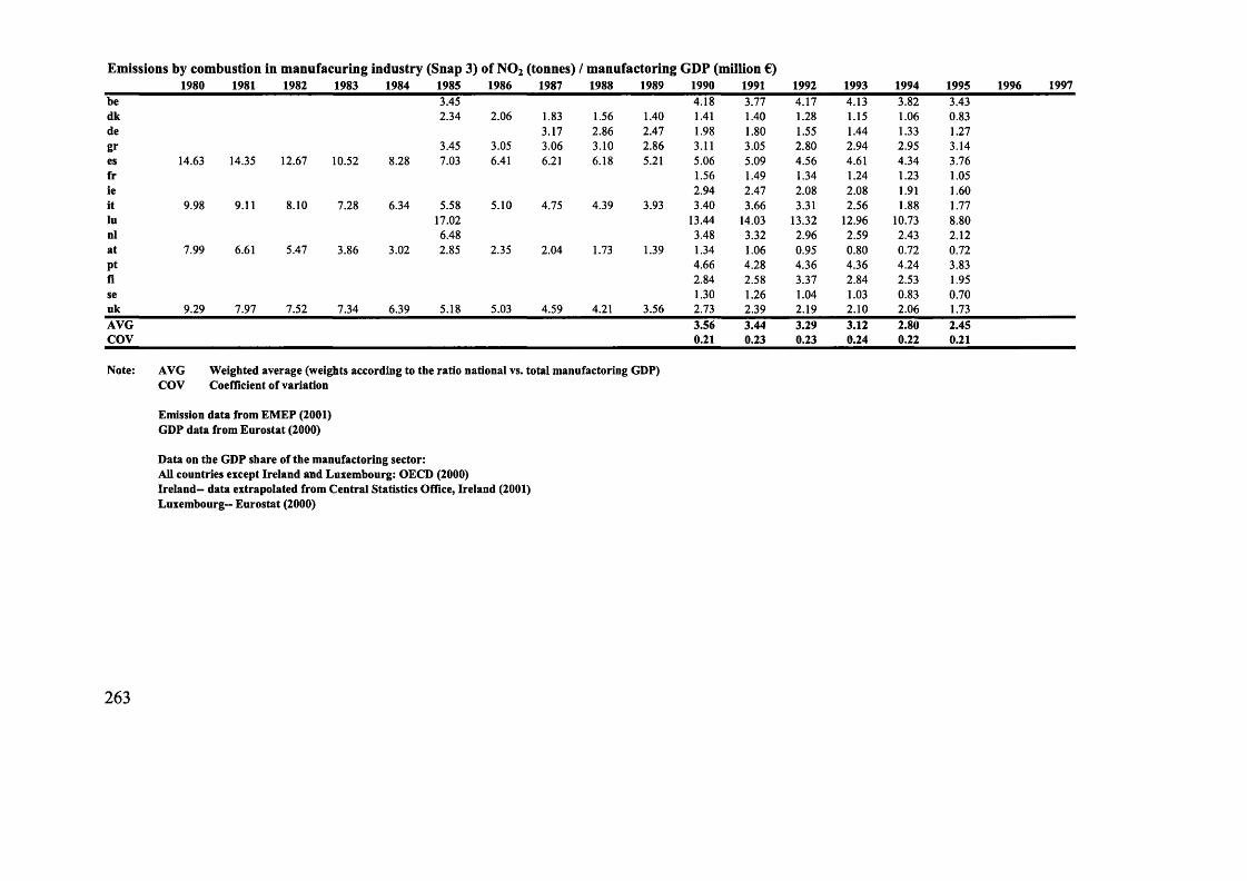
Emissions by combustion in manufacuring industry (Snap 3) of N 02 (tonnes) / manufactoring GDP (million €)1980 1981 1982 1983 1984 1985 1986 1987 1988 1989 1990 1991 1992 1993 1994 1995 1996 1997

be 3.45 4.18 3.77 4.17 4.13 3.82 3.43dk 2.34 2.06 1.83 1.56 1.40 1.41 1.40 1.28 1.15 1.06 0.83de 3.17 2.86 2.47 1.98 1.80 1.55 1.44 1.33 1.27gr 3.45 3.05 3.06 3.10 2.86 3.11 3.05 2.80 2.94 2.95 3.14es 14.63 14.35 12.67 10.52 8.28 7.03 6.41 6.21 6.18 5.21 5.06 5.09 4.56 4.61 4.34 3.76fi­ 1.56 1.49 1.34 1.24 1.23 1.05le 2.94 2.47 2.08 2.08 1.91 1.60it 9.98 9.11 8.10 7.28 6.34 5.58 5.10 4.75 4.39 3.93 3.40 3.66 3.31 2.56 1.88 1.77lu 17.02 13.44 14.03 13.32 12.96 10.73 8.80nl 6.48 3.48 3.32 2.96 2.59 2.43 2.12at 7.99 6.61 5.47 3.86 3.02 2.85 2.35 2.04 1.73 1.39 1.34 1.06 0.95 0.80 0.72 0.72Pt 4.66 4.28 4.36 4.36 4.24 3.83fi 2.84 2.58 3.37 2.84 2.53 1.95se 1.30 1.26 1.04 1.03 0.83 0.70uk 9.29 7.97 7.52 7.34 6.39 5.18 5.03 4.59 4.21 3.56 2.73 2.39 2.19 2.10 2.06 1.73AVG 3.56 3.44 3.29 3.12 2.80 2.45COV 0.21 0.23 0.23 0.24 0.22 0.21

Note: AVG W eighted average (weights according to the ratio national vs. total manufactoring GDP)COV Coefficient o f variation

Emission data from EM EP (2001)GDP data from Eurostat (2000)

Data on the GDP share o f the manufactoring sector:All countries except Ireland and Luxembourg: OECD (2000)Ireland— data extrapolated from Central Statistics O ffice, Ireland (2001)Luxem bourg— Eurostat (2000)

263

Emissions by combustion in manufacuring industry (Snap 3) of NMVOC (tonnes) / manufactoring GDP (million €)1980 1981 1982 1983 1984 1985 1986 1987 1988 1989 1990 1991 1992 1993 1994 1995 1996 1997

be 1.18 0.26 0.17 0.23 0.17 0.16 0.14dk 0.18 0.17 0.19 0.15 0.11 0.12 0.11 0.10 0.09 0.07 0.05de 0.11 0.10 0.08 0.07 0.06 0.05 0.05 0.05 0.04

gr 1.72 1.45 1.39 1.34 1.19 1.25 1.18 1.05 1.06 1.03 1.07es 0.92 0.86 0.78 0.63 0.51 0.47 0.42 0.40 0.39 0.32 0.32 0.33 0.32 0.33 0.28 0.22fr 0.10 0.09 0.08 0.08 0.08 0.07ie 0.08 0.08 0.04 0.04 0.04 0.02it 0.38 0.35 0.31 0.28 0.24 0.21 0.19 0.18 0.17 0.15 0.13 0.12 0.10 0.07 0.09 0.07lu 0.76 0.50 0.90 1.21 1.52 0.33 0.20nl 0.40 0.19 0.19 0.20 0.14 0.11 0.20at 0.30 0.26 0.23 0.17 0.15 0.15 0.12 0.11 0.10 0.09 0.08 0.07 0.07 0.06 0.02 0.03Ptfi

1.71 1.54 1.48 1.46 1.44 1.18iise 0.34 0.33 0.35 0.33 0.26 0.21uk 0.24 0.22 0.20 0.20 0.18 0.15 0.14 0.13 0.12 0.10 0.08 0.07 0.06 0.06 0.06 0.05AVG 0.37 0.37 0.38 0.39 0.29 0.25COV 0.32 0.31 0.31 0.34 0.36 0.36

Note: AVG W eighted average (weights according to the ratio national vs. total manufactoring GDP)COV Coefficient o f variation

Emission data from EM EP (2002, es/gr/pt: 2000)GDP data from Eurostat (2001)

Data on the GDP share o f the m anufactoring sector:All countries except Ireland and Luxembourg: OECD (2000)Ireland— data extrapolated from Central Statistics O ffice, Ireland (2001)Luxem bourg— Eurostat (2001)

264

2524

47

-1726

_ 7

>99

-2134-4

812

16-2911

Pollution load index

980 1981 1982 1983 1984 1985 1986 1987 1988 1989 1990 1991 1992 1993 1994 1995 19962 6 8 13 15 16 22

51 48 47 29 34 30 28 27 17 21 32 25 27 24 29 31 2831 25 30 16 12 -5 -9 -8 0 -7 -17 -17 -14 -12 -17 -11 021 19 13 7 0 -7 -11 -6 -4 -1 -6 -6 -2 2 7 9 4

59 37 21 5 -9 -21 -27 -25 -22 -22 -23 -23-19 -15 -10 -8 -7 -6 -4

-16 -13 -11 -4 0 4 -7 -5 1 0 2 4- 4 - 6 - 3 0 1 2 4

980 1981 1982 1983 1984 1985 1986 1987 1988 1989 1990 1991 1992 1993 1994 1995 1996

0 0 0 0 0 0 0 0 0 0 3 -1 -9 -14 -15 -15 -1333 24 18 9 6 23 43 41 32 33 38 23 16 22 32 28 4391 93 86 57 67 85 63 67 72 41 17 -4 -24 -27 -25 -31 -1367 61 59 53 50 61 59 62 65 69 68 64 64 70 77 67 76

0 0 0 0 0 0 0 -5 -5 -3 -6 -4 -2 -2 -4 -3 -40 0 0 0 0 0 0 0 0 0 -18 -16 -24 -24 -22 -21 -130 0 0 0 0 0 0 0 0 0 -27 -21 -16 -19 -23 -27 -28

11 6 1 1 3 0 7

G e rm a n y1980 1981 1982 1983 1984 1985 1986 1987 1988 1989 1990 1991 1992 1993 1994 1995 1996 1997 1998 1999

c h 4 57 54 49 43 54 45 41 37 34 32 29 15 7 0 -5 -8 -13 -12 -14 -16c o 2 51 49 47 52 59 52 55 51 53 42 13 44 42 42 47 36 35 35 32 37s o 2 -24 -19 -19 -14 -9 -11 -15 -26 -50 -62 74 33 16 12 2 -13 -33 -40 -51 -48n o 2 18 18 19 23 26 23 21 11 4 -6 -7 -16 -21 -22 -25 -25 -28 -29 -30 -30NM VO C -13 -14 -13 -13 -12 -13 -12 -14 -19 -22 -11 -22 -28 -32 -37 -39 -40 -42 -43 -43CO 6 0 -4 -5 -4 -3 -2 -4 -7 -12 5 -12 -21 -24 -27 -29 -31 -33 -37 -39n h 3 -15 -16 -15 -16 -13 -12 -16 -19 -18 -18 -9 -19 -20 -21 -21 -21 -22 -24 -23 -24PLI 7 13 3 -4 -7 -9 -14 -19 -21 -24 -23

G reece1980 1981 1982 1983 1984 1985 1986 1987 1988 1989 1990 1991 1992 1993 1994 1995 1996 1997 1998 1999

c h 4 -26 -24 -22 -20 -17 -15 -11 -7 -4 Ac o 2 -41 -39 -35 -29 -27 -25 -26 -21 -15 -10 -8 -24 -13 -12 -8 -8 -6 -3 -1 -2s o 2 -37 -27 -18 -5 6 19 21 26 41 44 12 35 49 62 72 99 126 153 172 211n o 2 -20 -17 -16 -15 -13 -13 -13 -12 -11 -9 -12 -9 -7 -4 4 7 21 21 32 37NM VO C 40 28 16 3 -7 -27 -23 -20 -15 -12 -8 3 7 14 19CO -4 2 2 8 13 19 29 37 52 52n h 3 -26 -24 -25 -25 -27 -14 -27 -30 -27 -28PLI 7 -13 -10 -5 -1 3 11 19 25 34 41

S p a in1980 1981 1982 1983 1984 1985 1986 1987 1988 1989 1990 1991 1992 1993 1994 1995 1996 1997 1998 1999

c h 4 -54 -52 -47 -47 -43 -45 -41 -37 -35 -31 -30 -27 -23 -19 -14 -11 -1 5 10 13c o 2 -43 -40 -38 -38 -42 -41 -46 -44 -42 -36 -32 -37 -32 -37 -33 -28 -31 -25 -25 -27s o 2 19 30 38 57 54 55 49 45 33 67 20 36 50 56 72 73 74 107 107 126n o 2 -30 -33 -33 -32 -32 -34 -33 -31 -29 -22 -20 -14 -9 -8 -2 2 1 14 20 28NM V O C 68 69 66 67 66 65 67 70 68 74 74 78 79 75 96 98 103 124 134 146CO -46 -46 -45 -43 -45 -43 -41 -39 -34 -30 -29 -24 -18 -17 -13 -20 -11 0 5 11n h 3 3 0 6 3 5 4 7 17 22 27 19 24 28 24 31 31 46 40 42 44PLI 7 0 5 11 11 19 21 26 38 42 49

266

France1980 1981 1982 1983 1984 1985 1986 1987 1988 1989 1990 1991 1992 1993 1994 1995 1996 1997 1998 1999

c h 4 -12 -8 -5 0 3 5 9 3 3 -1c o 2 0 -6 -6 -9 -13 -17 -20 -25 -26 -25 -21 -23 -26 -26 -33 -29 -27 -31 -26 -22s o 2 -10 -23 -22 -30 -33 -41 -46 -45 -44 -34 -54 -43 -47 -49 -47 -45 -38 -41 -34 -38n o 2 0 -2 -4 -6 -6 -8 -12 -13 -13 -11 -11 -6 -6 -8 -6 -5 -5 -3 -3 -3NMVOC -3 0 1 0 -5 -6 -3 -6 -6 -7CO 106 102 99 97 95 98 93 89 85 76 50 54 55 54 49 53 47 45 46 42n h 3 43 49 52 51 53 55 57 57 56 56PLI 7 -1 3 3 3 2 4 6 3 5 4

Ireland1980 1981 1982 1983 1984 1985 1986 1987 1988 1989 1990 1991 1992 1993 1994 1995 1996 1997 1998 1999

c h 4 202 212 221 234 243 249 269 284 283 280c o 2 -18 -13 -11 -10 -9 -10 3 8 10 1 10 12 8 11 16 15 16 23 27 21s o 2 1 -4 -17 -18 -12 -7 10 23 20 32 19 27 33 36 65 66 72 119 143 143n o 2 -43 -31 -31 -32 -33 -27 -21 -11 -5 0 -7 -5 6 1 2 5 10 12 18 19NMVOC -30 -27 -22 -23 -23 -23 -14 -10 -7 -21CO -16 -15 -11 -17 -18 -22 -18 -14 -10 -17n h 3 214 235 251 254 260 265 265 261 268 265PLI 7 56 63 69 71 78 79 86 97 103 99

Italy1980 1981 1982 1983 1984 1985 1986 1987 1988 1989 1990 1991 1992 1993 1994 1995 1996 1997 1998 1999

c h 4 -40 -39 -40 -38 -35 -39 -38 -37 -35 -35 -34 -30 -29 -22 -17 -16 -36 -32 -31 -31c o 2 -30 -27 -26 -27 -25 -25 -26 -22 -20 -18 -12 -21 -17 -18 -20 -15 -20 -16 -15 -19s o 2 3 1 -9 -14 -21 -25 -22 -14 -6 -10 -40 -38 -38 -35 -31 -19 -15 -14 -12 -12n o 2 -26 -24 -24 -25 -24 -23 -20 -15 -13 -10 -8 -4 0 4 -3 -1 -1 -1 -3 -6NMVOC -19 -20 -22 -24 -26 -26 -25 -23 -22 -18 -16 -9 -2 3 5 10 -6 -9 -11 -13CO -25 -23 -20 -19 -18 -12 -12 -10 -10 -6 -1 7 12 16 19 29 19 19 16 16n h 3 -24 -23 -27 -22 -26 -25 -25 -26 -22 -25 -25 -25 -24 -21 -19 -19 -25 -24 -25 -23PLI 7 -20 -17 -14 -10 -9 -4 -12 -11 -12 -12

267

Luxembourg1980 1981 1982 1983 1984 1985 1986 1987 1988 1989 1990 1991 1992 1993 1994 1995 1996 1997 1998 1999

c h 4 8 5 7 19 6 10 19 22 17 20co2 224 193 187 176 199 197 197 185 197 206 236 224 234 239 215 152 143 132 121 105so2 1 -1 -15 -22 -10 3 3 5 15 14 -12 -4 4 13 8 -19 -19 -32 -53 -49n o 2 69 71 69 62 63 63 63 63 66 68 66 72 81 90 80 68 77 49 44 40NMVOC -8 -4 0 2 7 12 12 14 15 15 4 10 4 -8 8CO 236 349 317 367 222 142 140 92 26 27n h 3 77 82 85 85 83 82 79 75 72 78PLI 7 89 106 106 119 90 63 64 49 31 33

The Netherlands1980 1981 1982 1983 1984 1985 1986 1987 1988 1989 1990 1991 1992 1993 1994 1995 1996 1997 1998 1999

c h 4 19 7 7 23 34 44 25 25 23 24 52 57 54 55 55 52 69 55 50 45co2 22 21 -3 3 13 18 14 16 13 25 31 19 20 28 17 24 32 30 29 27so2 -48 -45 -49 -55 -56 -59 -58 -56 -54 -62 -71 -72 -70 -69 -69 -66 -64 -65 -66 -65n o 2 11 13 11 9 13 16 13 13 13 9 7 6 6 6 5 6 8 1 -3 -3NMVOC -23 -26 -27 -21 -31 -25 -29 -31 -33 -35 -38 -34 -42 -44 -45CO -38 -43 -46 -45 -47 -45 -49 -49 -48 -48 -48 -45 -53 -53 -54n h 3 69 76 76 70 72 70 75 71 60 57 49 56 24 33 15 0 0 28 14 17PLI 7 0 -2 -6 -4 -9 -10 -5 -6 -10 -11

Austria1980 1981 1982 1983 1984 1985 1986 1987 1988 1989 1990 1991 1992 1993 1994 1995 1996 1997 1998 1999

c h 4 21 23 23 23 31 24 22 22 24 24 20 20 19 21 21 20 24 25 24 23co2 -23 -12 -12 -14 -9 -11 -11 -10 -13 -14 -4 -9 -14 -13 -12 -11 -12 -7 -3 -9so2 -22 -25 -24 -37 -39 -42 -46 -50 -58 -63 -74 -74 -79 -78 -77 -75 -73 -70 -71 -71n o 2 -19 -19 -20 -20 -20 -19 -22 -25 -27 -30 -32 -30 -32 -34 -29 -31 -32 -26 -24 -21NMVOC 3 5 5 6 7 7 11 11 9 7 0 -6 -14 -14 -17 -14 -12 -12 -12 -11CO 34 34 32 34 37 37 48 46 44 39 24 26 23 25 29 21 24 29 27 18n h 3 1 3 2 2 3 2 0 -3 -1 1 0 2 0 0 0 -2 -5 -6 -7 -9PLI 7 -9 -10 -14 -13 -12 -13 -12 -10 -10 -11

268

40■36.06426028

535

>99

-21

34-481

216

-29

>99

-27-34-60115015

-35-11

1980 1981 1982 1983 1984 1985 1986 1987 1988 1989 1990 1991 1992 1993 1994 1995 1996 199711 16 18 20 25 26 33 38

-70 -70 -64 -63 -64 -62 -63 -60 -59 -50 -45 -50 -43 -43 -42 -37 -43 -38-59 -53 -47 -38 -45 -54 -45 -46 -44 -20 -19 -13 14 10 15 36 39 68-56 -52 -49 -47 -62 -73 -70 -69 -67 -64 -12 -6 4 5 10 19 20 28

-56 -48 -40 -33 -24 -14 -3 8 15 16 25 27 48-18 -8 4 9 12 13 15 17

2 2 13 6 -1 9 6 6-14 -9 2 3 5 13 14 24

980 1981 1982 1983 1984 1985 1986 1987 1988 1989 1990 1991 1992 1993 1994 1995 1996 19973 -1 -9 -14 -15 -15 -13 -14

33 24 18 9 6 23 43 41 32 33 38 23 16 22 32 28 43 4191 93 86 57 67 85 63 67 72 41 17 -4 -24 -27 -25 -31 -13 -867 61 59 53 50 61 59 62 65 69 68 64 64 70 77 67 76 78

-5 -5 -3 -6 -4 -2 -2 -4 -3 -4 -2-18 -16 -24 -24 -22 -21 -13 -7-27 -21 -16 -19 -23 -27 -28 -2311 6 1 1 3 0 7 10

1980 1981 1982 1983 1984 1985 1986 1987 1988 1989 1990 1991 1992 1993 1994 1995 1996 1997

-35 -34 -33 -31 -34 -35 -31 -38-4 -3 -10 -15 -16 -10 -10 -13 -14 -20 -27 -31 -28 -32 -29 -35 -27 -34-9 -11 -19 -26 -22 -26 -22 -33 -26 -47 -69 -73 -73 -70 -69 -68 -61 -7331 41 40 37 41 46 46 45 43 37 9 11 10 13 20 12 14 7

47 43 39 42 37 43 42 40 50 394 7 9 12 17 15 19 10

-40 -41 -43 -41 -27 -27 -27 -27 -27 -30-18 -17 -15 -13 -12 -14 -9 -17

U n ite d K in g d o m 1980 1981 1982 1983 1984 1985 1986 1987 1988 1989 1990 1991 1992 1993 1994 1995 1996 1997 1998 1999

c h 4 26 29 30 29 5 20 25 24 23 20 12 14 14 4 -2 -3 0 0 -4 2c o 2 18 20 26 29 22 27 32 33 33 30 35 23 19 21 19 18 18 16 15 10so2 43 45 48 52 58 75 90 99 126 121 59 71 83 81 69 61 58 42 43 18n o 2 29 29 30 31 29 34 37 40 44 44 41 35 34 28 28 20 17 11 6 1NMVOC -10 -8 -6 -5 -3 -3 0 2 3 5 4 6 5 5 4 1 6 1 -3 -10CO -24 -21 -18 -18 -19 -18 -17 -16 -13 -9 -11 -10 -10 -12 -12 -15 -12 -13 -14 -14n h 3 -43 -41 -43 -42 -42 -43 -44 -43 -42 -42PLI 7 14 14 15 12 9 6 6 2 0 -5

Note: PLI 7 based on all seven pollutants

Em ission data (except C 0 2) from EM EP (2002, es/gr/pt: 2000)

C 0 2 em ission data from C DIAC (2001)Population data from Eurostat (2000)

270

Table 30 General pollution intensity

Belgium1980 1981 1982 1983 1984 1985 1986 1987 1988 1989 1990 1991 1992 1993 1994 1995 1996 1997 1998 1999

c h 4 -7 -1 -1 -2 -3 -6 3 10 12 11c o 2 23 30 41 28 33 28 23 21 13 18 20 18 16 7 8 7 8 12 8 9

s o 2 7 10 25 14 11 -7 -12 -12 -4 -10 -24 -22 -21 -24 -30 -28 -15 -8 -7 -8n o 2 -1 4 9 5 0 -8 -14 -11 -7 -4 -14 -12 -10 -12 -10 -11 -12 -7 -3 -5N M V O C 49 25 10 -1 -14 -28 -32 -31 -33 -35 -37 -35 -32 -28 -27CO -26 -20 -17 -20 -22 -23 -19 -17 -12 -10n h 3 -18 -14 -13 -4 1 -5 -12 -13 -13 -16 -17 -12 -10 -8 -6G P I7 -12 -12 -11 -14 -15 -16 -12 -8 -5 -5G P I3 10 15 25 16 14 4 -1 -1 0 1 -6 -6 -5 -9 -11 -11 -6 -1 -1 -1

Denmark1980 1981 1982 1983 1984 1985 1986 1987 1988 1989 1990 1991 1992 1993 1994 1995 1996 1997 1998 1999

c h 4 -16 -11 -11 -15 -12 -22 -26 -28 -25 -20 -31 -25 -24 -23 -25 -28 -25 -23 -17 -23c o 2 9 2 8 0 1 14 10 8 2 -11 -5 13 -1 1 5 -9 14 -3 -13 -4

s o 2 8 1 9 -1 0 17 -2 -11 3 -15 -41 -9 -24 -35 -28 -29 0 -30 -49 -58n o 2 14 7 16 9 14 20 26 17 18 16 9 34 16 15 19 9 29 17 11 4N M V O C -34 -32 -32 -33 -33 -40 -42 -41 -40 -36 -45 -41 -42 -43 -47 -49 -45 -47 -47 -48CO -12 6 13 -5 4 -1 -3 0 -2 11 -26 -17 -18 -21 -24 -27 -21 -24 -16 -22n h 3 89 89 83 73 67 88 86 79 88 101 81 91 90 77 66 49 42 42 42 34G P I7 -8 7 0 -4 -5 -12 -1 -10 -13 -17G P I3 10 3 11 3 5 17 11 5 7 -3 -13 13 -3 -6 -1 -10 14 -5 -17 -19

271

G e rm a n y1980 1981 1982 1983 1984 1985 1986 1987 1988 1989 1990 1991 1992 1993 1994 1995 1996 1997 1998 1999

c h 4 2 7 5 -3 6 2 -6 -9 -7 -5 19 -4 -15 -28 -32 -36 -35 -29 -30 -31c o 2 6 12 9 8 14 12 9 4 10 6 4 20 12 3 6 -4 1 9 7 12s o 2 -47 -39 -39 -39 -35 -34 -40 -49 -64 -71 61 11 -9 -19 -27 -39 -50 -52 -60 -57n o 2 -17 -11 -12 -13 -10 -9 -15 -23 -25 -30 -14 -29 -38 -44 -46 -48 -46 -43 -43 -43N M VO C -46 -42 -41 -43 -41 -41 -44 -45 -44 -44 -18 -35 -43 -51 -55 -58 -55 -53 -53 -53CO -25 -25 -28 -31 -30 -26 -29 -32 -31 -32 -4 -26 -38 -45 -48 -50 -49 -46 -49 -50n h 3 -48 -46 -45 -47 -43 -41 -44 -46 -41 -39 -16 -32 -37 -43 -43 -45 11 -39 -38 -38GPI 7 5 -14 -24 -32 -35 -40 -39 -36 -38 -37GPI 3 -19 -13 -14 -15 -10 -10 -15 -22 -26 -32 17 1 -11 -20 -22 -30 -32 -29 -32 -29

G reece1980 1981 1982 1983 1984 1985 1986 1987 1988 1989 1990 1991 1992 1993 1994 1995 1996 1997 1998 1999

c h 4 64 65 68 69 72 73 74 75 86 76c o 2 15 16 15 36 41 55 79 100 102 110 103 67 87 86 91 87 83 82 93 81s o 2 23 39 44 81 105 145 192 218 237 237 148 194 222 242 258 304 341 378 428 474n o 2 55 58 49 64 67 79 110 121 113 113 96 98 101 103 116 118 136 128 156 152NM VO C 176 194 183 141 113 62 67 72 79 84 88 100 102 121 119CO 112 122 121 127 135 143 152 158 195 181n h 3 65 66 62 59 53 75 43 33 42 33GPI 7 93 97 105 109 116 127 133 137 160 159GPI 3 31 38 36 60 71 93 127 147 151 153 116 120 137 144 155 169 187 196 225 236

S p a in1980 1981 1982 1983 1984 1985 1986 1987 1988 1989 1990 1991 1992 1993 1994 1995 1996 1997 1998 1999

c h 4 -14 -8 0 15 18 10 14 20 15 12 0 3 9 26 41 42 56 71 78 79c o 2 6 14 17 31 17 17 3 3 0 2 -2 -11 -5 -2 9 15 8 22 21 16s o 2 123 148 160 231 208 208 184 169 132 166 73 92 112 142 182 178 174 237 234 256n o 2 32 28 27 44 37 32 27 28 23 25 16 21 28 42 60 63 60 86 94 103NM V O C 210 219 212 261 241 215 205 206 189 173 150 151 152 170 222 218 219 265 278 288CO 4 6 6 25 15 18 17 19 20 16 2 8 16 27 42 28 40 63 69 75n h 3 99 91 105 129 123 115 120 137 130 119 72 75 81 91 114 110 131 129 129 128GPI 7 44 49 56 71 96 93 98 125 129 135GPI 3 54 64 68 102 87 85 71 67 52 64 29 34 45 61 84 85 81 115 117 125

272

France1980 1981 1982 1983 1984 1985 1986 1987 1988 1989 1990 1991 1992 1993 1994 1995 1996 1997 1998 1999

c h 4 -27 -18 -16 -15 -14 -13 -7 -9 -8 -12c o 2 -23 -26 -25 -26 -27 -32 -35 -37 -37 -34 -35 -32 -35 -38 -43 -41 -38 -39 -34 -30s o 2 -30 -40 -38 -42 -44 -52 -56 -54 -52 -43 -62 -50 -53 -57 -55 -54 -47 -48 -41 -44n o 2 -23 -24 -24 -23 -21 -24 -29 -28 -26 -22 -26 -17 -17 -23 -21 -21 -19 -14 -14 -14NMVOC -20 -11 -11 -16 -21 -22 -17 -16 -16 -16CO 60 59 61 66 67 69 62 64 64 59 24 37 37 29 25 27 25 29 30 27n h 3 19 33 34 27 28 29 34 39 39 39GPI 7 -18 -8 -9 -13 -14 -14 -10 -8 -6 -7GPI 3 -25 -30 -29 -30 -31 -36 -40 -40 -38 -33 -41 -33 -35 -39 -40 -39 -35 -33 -30 -29

Ireland1980 1981 1982 1983 1984 1985 1986 1987 1988 1989 1990 1991 1992 1993 1994 1995 1996 1997 1998 1999

c h 4 372 401 401 414 405 393 396 368 357 327c o 2 52 51 48 52 56 54 73 85 89 71 72 79 68 71 70 63 55 50 51 36s o 2 86 66 38 39 52 58 84 111 107 122 86 105 107 110 143 135 131 168 190 173n o 2 6 20 15 15 16 24 32 53 64 69 45 53 65 56 50 49 48 37 41 34NMVOC 10 18 21 19 14 10 16 10 11 -11CO 31 36 39 28 21 11 9 5 7 -6NH, 391 438 447 444 431 416 390 340 339 311GPI 7 144 162 164 163 162 154 149 140 142 123GPI 3 48 46 33 35 42 46 63 83 87 87 67 79 80 79 88 82 78 85 94 81

Italy1980 1981 1982 1983 1984 1985 1986 1987 1988 1989 1990 1991 1992 1993 1994 1995 1996 1997 1998 1999

c h 4 -23 -24 -26 -29 -28 -32 -34 -34 -31 -33 -37 -33 -29 -12 -3 5 -27 -24 -21 -22c o 2 -9 -7 -9 -17 -17 -17 -21 -19 -16 -16 -17 -24 -17 -7 -6 8 -9 -5 -4 -8s o 2 34 29 12 -2 -13 -17 -17 -10 -1 -8 -43 -40 -39 -26 -19 2 -3 -3 0 0n o 2 -3 -3 -6 -14 -16 -15 -15 -11 -9 -7 -13 -8 -1 18 13 25 13 11 11 6NMVOC 3 0 -5 -13 -19 -23 -25 -23 -21 -18 -20 -12 -3 17 23 39 6 3 1 -1CO 0 2 2 -3 -6 1 -2 -2 -1 0 -6 2 11 31 40 62 35 34 32 31n h 3 1 -4 -10 -9 -17 -17 -17 -19 -14 -19 -29 -28 -25 -11 -5 3 -15 -14 -14 -12GPI 7 -23 -20 -15 1 6 21 0 0 1 -1GPI 3 7 6 -1 -11 -15 -16 -18 -13 -9 -11 -24 -24 -19 -5 -4 11 0 1 2 -1

273

Luxembourg1980 1981 1982 1983 1984 1985 1986 1987 1988 1989 1990 1991 1992 1993 1994 1995 1996 1997 1998 1999

c h 4 -44 -46 -45 -43 -51 -49 -43 -39 -42 -41co2 114 96 84 70 82 72 68 64 71 71 73 66 71 62 47 17 16 16 9 0so2 -33 -34 -46 -52 -45 -41 -42 -40 -34 -36 -55 -51 -47 -46 -50 -63 -61 -66 -77 -75n o 2 12 15 8 0 -1 -6 -8 -6 -4 -6 -14 -11 -8 -9 -16 -22 -15 -25 -29 -31NMVOC -50 -48 -45 -42 -41 -43 -43 ^ 1 -45 -46 -52 -47 -48 -55 -47CO 73 130 113 123 50 12 15 -4 -38 -38n h 3 -9 -7 -5 -12 -15 -16 -14 -12 -15 -13G P I7 -3 6 5 4 -12 -25 -21 -25 -35 -35G P I3 31 26 16 6 12 9 6 6 11 10 1 1 6 2 -6 -23 -20 -25 -32 -35

The Netherlands1980 1981 1982 1983 1984 1985 1986 1987 1988 1989 1990 1991 1992 1993 1994 1995 1996 1997 1998 1999

c h 4 -6 -9 -10 4 18 29 11 14 19 23 45 54 51 41 39 32 49 41 36 30co2 0 5 -17 -12 0 6 2 7 9 24 25 17 17 16 5 7 17 18 17 15so2 -57 -52 -57 -62 -61 -63 -62 -60 -55 -62 -72 -73 -71 -72 -72 -71 -68 -68 -70 -68n o 2 -9 -2 -5 -7 0 5 1 4 9 8 2 4 3 -4 -6 -8 -4 -8 -12 -13NMVOC -35 -37 -36 -25 -33 -29 -30 -33 -40 -42 -46 -42 -47 -49 -51CO -42 -47 -48 -45 -46 -48 -50 -50 -53 -54 -55 -51 -57 -57 -58n h 3 34 45 45 43 51 52 60 62 61 62 41 53 21 21 3 -13 -12 16 3 6GPI 7 -5 -3 -9 -13 -18 -22 -16 -15 -19 -20GPI 3 -22 -16 -26 -27 -20 -17 -20 -17 -12 -10 -15 -17 -17 -20 -24 -24 -19 -19 -21 -22

Austria1980 1981 1982 1983 1984 1985 1986 1987 1988 1989 1990 1991 1992 1993 1994 1995 1996 1997 1998 1999

c h 4 14 18 14 10 19 13 8 7 12 14 5 7 4 -2 -2 -7 0 4 4 2co2 -25 -13 -17 -22 -17 -18 -21 -20 -21 -20 -16 -19 -25 -29 -29 -31 -29 -22 -19 -24so2 -24 -26 -29 -43 -44 -46 -52 -56 -62 -65 -77 -77 -81 -82 -81 -80 -78 -75 -76 -76n o 2 -22 -20 -24 -28 -27 -26 -30 -34 -34 -36 -40 -38 -41 -47 -43 -46 -45 -38 -37 -35NMVOC -4 -1 -5 -7 -3 -7 -7 -6 -3 -3 -13 -16 -25 -31 -33 -33 -29 -26 -26 -26CO 32 35 27 23 28 31 37 33 35 33 8 12 7 2 3 -5 -1 8 6 -2n h 3 -5 -3 -7 -9 -6 -7 -9 -11 -7 -3 -13 -9 -13 -19 -20 -24 -23 -22 -22 -24GPI 7 -21 -20 -25 -30 -29 -32 -29 -24 -24 -26GPI 3 -24 -20 -23 -31 -30 -30 -34 -37 -39 ^10 -45 -45 -49 -53 -51 -52 -51 -45 -44 -45

274

199918431

318189226159113174179

1999-2723

-1266-77

-352

26

1999-34-41-64

-134

3-42-21-35

980 1981 1982 1983 1984 1985 1986 1987 1988 1989 1990 1991 1992 1993 1994 1995 1996 1997 1998195 183 159 168 182 172 185 197 194

8 0 22 39 40 40 29 36 30 49 44 22 26 27 31 35 22 33 4047 59 82 129 113 70 93 83 80 136 114 113 148 145 159 195 199 262 31160 60 74 99 47 -1 5 7 5 6 133 131 127 133 149 157 157 175 184

55 72 96 109 122 127 137 135 156 162 171 172 220 212117 124 128 143 152 143 147 152 144170 150 146 136 122 136 128 129 129129 123 124 130 137 144 144 167 173

38 40 59 89 67 36 42 42 38 64 97 89 100 102 113 129 126 157 178

980 1981 1982 1983 1984 1985 1986 1987 1988 1989 1990 1991 1992 1993 1994 1995 1996 1997 1998-30 -20 -7 0 -10 -20 -16 -19 -23

26 6 -4 -10 -19 -8 13 9 -4 -10 -7 -1 18 43 41 20 38 34 1980 65 51 29 28 39 29 30 25 -5 -21 -22 -23 -15 -20 -35 -16 -13 -1858 38 30 26 15 20 25 26 20 15 14 32 67 99 89 57 70 69 66

-29 -33 -36 -36 -23 -1 15 2 -9 -7 -7 -6-44 -32 -23 -11 -17 -26 -16 -12 -14-50 -36 -14 -5 -18 -31 -30 -27 -28-25 -15 3 18 9 -6 3 4 -1

55 36 26 15 8 17 22 22 14 0 -5 3 21 43 36 14 31 30 22

1980 1981 1982 1983 1984 1985 1986 1987 1988 1989 1990 1991 1992 1993 1994 1995 1996 1997 1998-56 -54 -50 -37 -40 -42 -43 -46 -45

-37 -38 -37 -37 -42 -39 -37 -38 -39 -45 -50 -52 -47 -39 -36 -42 -40 -43 -40-40 -44 -43 -45 -41 -50 -45 -52 -48 -64 -79 -81 -80 -73 -72 -71 -67 -77 -75-14 -10 -1 1 -4 -1 2 3 0 -6 -25 -23 -19 2 8 0 -5 -8 -7

1 -4 -5 -2 2 29 28 24 25 20 27-29 -25 -19 1 5 2 -1 -5 7

-56 -58 -61 -59 -46 -34 -34 -35 -39 -40 -38-44 -42 -37 -21 -20 -23 -24 -28 -25

-30 -31 -27 -27 -31 -30 -27 -29 -29 -38 -52 -52 -49 -37 -33 -38 -37 -42 -41

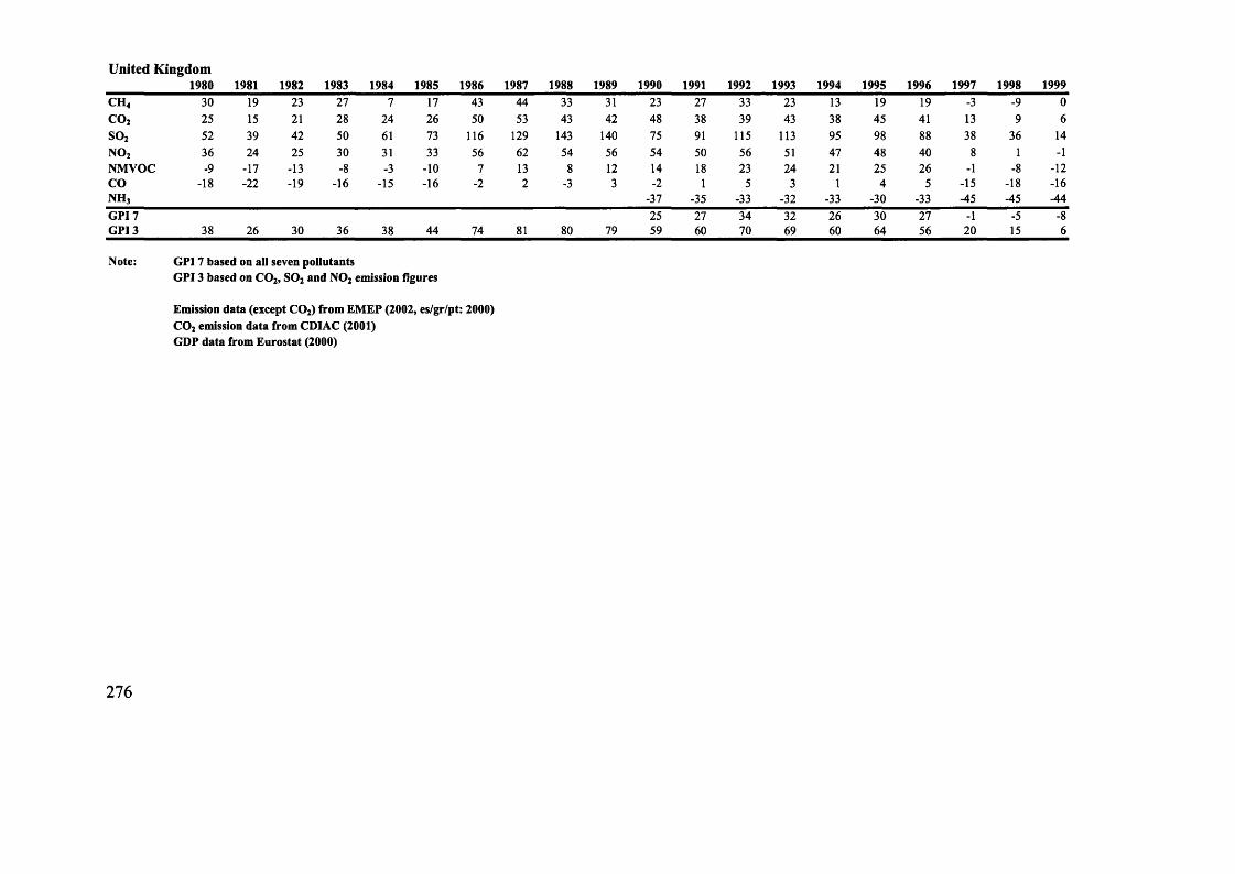
United Kingdom 1980 1981 1982 1983 1984 1985 1986 1987 1988 1989 1990 1991 1992 1993 1994 1995 1996 1997 1998 1999

c h 4 30 19 23 27 7 17 43 44 33 31 23 27 33 23 13 19 19 -3 -9 0c o 2 25 15 21 28 24 26 50 53 43 42 48 38 39 43 38 45 41 13 9 6s o 2 52 39 42 50 61 73 116 129 143 140 75 91 115 113 95 98 88 38 36 14n o 2 36 24 25 30 31 33 56 62 54 56 54 50 56 51 47 48 40 8 1 -1NMVOC -9 -17 -13 -8 -3 -10 7 13 8 12 14 18 23 24 21 25 26 -1 -8 -12CO -18 -22 -19 -16 -15 -16 -2 2 -3 3 -2 1 5 3 1 4 5 -15 -18 -16n h 3 -37 -35 -33 -32 -33 -30 -33 -45 -45 -44GPI 7 25 27 34 32 26 30 27 -1 -5 -8GPI 3 38 26 30 36 38 44 74 81 80 79 59 60 70 69 60 64 56 20 15 6

Note: GPI 7 based on all seven pollutantsG PI 3 based on C 0 2, SO z and N 0 2 em ission figures

Em ission data (except C 0 2) from E M E P (2002, es/gr/pt: 2000)

C 0 2 em ission data from C DIAC (2001)GDP data from Eurostat (2000)

276

Table 31

Belgium

Manufacturing pollution intensity

1980 1981 1982 1983 1984 1985 1986 1987 1988 1989 1990 1991 1992 1993 1994 1995 1996 1997 1998 1999

s o 2 52 65 106 117 29 58n o 2 69 58 92 110 112 113NM VO C 90 24 84 51 43 44M P I 2 60 62 99 113 71 86

Denmark1980 1981 1982 1983 1984 1985 1986 1987 1988 1989 1990 1991 1992 1993 1994 1995 1996 1997 1998 1999

s o 2 -50 -40 -43 -46 -36 -44n o 2 -45 -42 -43 -44 -43 -50NM VO C -16 -17 -23 -23 -38 -51M PI 2 -47 -41 -43 -45 -40 -47

Germany1980 1981 1982 1983 1984 1985 1986 1987 1988 1989 1990 1991 1992 1993 1994 1995 1996 1997 1998 1999

s o 2 -3 -27 -41 -52 -60 -61n o 2 -29 -33 -38 -36 -35 -30NM V O C -62 -65 -67 -68 -63 -64M PI 2 -16 -30 -39 -44 -47 -45

Greece1980 1981 1982 1983 1984 1985 1986 1987 1988 1989 1990 1991 1992 1993 1994 1995 1996 1997 1998 1999

s o 2 235 260 248 282 324 400n o 2 23 26 26 46 60 90NM VO C 838 845 780 899 914 1076M PI 2 129 143 137 164 192 245

277

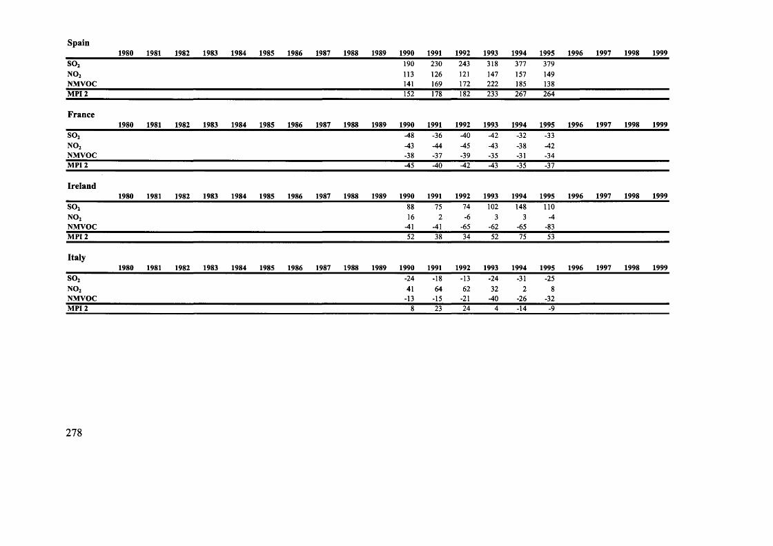
Spain1980 1981 1982 1983 1984 1985 1986 1987 1988 1989 1990 1991 1992 1993 1994 1995 1996 1997 1998 1999

s o 2n o 2N M VO C

190113141

230126169

243121172

318147222

377157185

379149138

M PI 2 152 178 182 233 267 264

France1980 1981 1982 1983 1984 1985 1986 1987 1988 1989 1990 1991 1992 1993 1994 1995 1996 1997 1998 1999

S 0 2 -48 -36 -40 -42 -32 -33n o 2 -43 -44 -45 -43 -38 -42NM VO C -38 -37 -39 -35 -31 -34M PI 2 -45 -40 -42 -43 -35 -37

Ireland1980 1981 1982 1983 1984 1985 1986 1987 1988 1989 1990 1991 1992 1993 1994 1995 1996 1997 1998 1999

s o 2 88 75 74 102 148 110n o 2 16 2 -6 3 3 -4NM VO C -41 -41 -65 -62 -65 -83M PI 2 52 38 34 52 75 53

Italy1980 1981 1982 1983 1984 1985 1986 1987 1988 1989 1990 1991 1992 1993 1994 1995 1996 1997 1998 1999

s o 2 -24 -18 -13 -24 -31 -25n o 2 41 64 62 32 2 8N M VO C -13 -15 -21 -40 -26 -32M PI 2 8 23 24 4 -14 -9

278

Luxembourg1980 1981 1982 1983 1984 1985 1986 1987 1988 1989 1990 1991 1992 1993 1994 1995 1996 1997 1998 1999

s o 2n o 2NM VO C

178434249

245482573

274504851

310545

1233

274483200

148433104

M PI 2 306 364 389 427 378 290

The Netherlands 1980 1981 1982 1983 1984 1985 1986 1987 1988 1989 1990 1991 1992 1993 1994 1995 1996 1997 1998 1999

s o 2n o 2NM VO C

-504037

-523944

-523562

-492918

-4533-2

-4029

109M PI 2 -5 -7 -8 -10 -6 -6

Austria1980 1981 1982 1983 1984 1985 1986 1987 1988 1989 1990 1991 1992 1993 1994 1995 1996 1997 1998 1999

s o 2n o 2N M VO C

-69-48-44

-76-57-49

-82-58-49

-84-61-48

-85-62-79

-78-57-75

M PI 2 -58 -67 -70 -73 -73 -68

Portugal1980 1981 1982 1983 1984 1985 1986 1987 1988 1989 1990 1991 1992 1993 1994 1995 1996 1997 1998 1999

s o 2n o 2N M VO C

20986

1227

18478

1180

22798

1182

227118

1316

263132

1367

343133

1225M PI 2 147 131 163 173 197 238

279

Finland1980 1981 1982 1983 1984 1985 1986 1987 1988 1989 1990 1991 1992 1993 1994 1995 1996 1997 1998 1999

s o 2n o 2N M V O C

11612

287

-2053

-4141

-3137

-4718

M PI 2 64 17 17 0 3 -15

Sweden1980 1981 1982 1983 1984 1985 1986 1987 1988 1989 1990 1991 1992 1993 1994 1995 1996 1997 1998 1999

s o 2n o 2NM VO C

-79-49148

-80-49156

-83-54185

-79-50198

-80-56143

-81-59120

M PI 2 -64 -64 -68 -64 -68 -70

United Kingdom 1980 1981 1982 1983 1984 1985 1986 1987 1988 1989 1990 1991 1992 1993 1994 1995 1996 1997 1998 1999

s o 2n o 2NM VO C

49

-50

17-2

-54

37-2

-56

544

-53

4714

-50

195

-49M PI 2 6 8 18 29 30 12

Note: M PI 2 based on SOz and N 0 2 em issions by com bustion in m anufacturing sector

Em ission data from E M E P (2002, es/gr/pt: 2000)G DP data from Eurostat (2001)

D ata on the G D P share o f the m anufactoring sector:All countries except Ireland and Luxem bourg: O ECD (2000)Ireland— C entral Statistics O ffice, Ireland (2001)Luxem bourg— Eurostat (2001)

280

Appendix 2: Regression variablesTable 32 Taxes on production and imports

T axes on P roduction and Im p orts /

1980 1981 1982

G D P

1983 1984 1985 1986 1987 1988 1989be 12.36 12.45 12.68 12.83 12.45 12.20 11.87 12.30 12.12 12.15dk 18.62 18.41 17.66 17.84 18.08 18.36 19.64 19.43 19.26 18.29de 13.17 12.94 12.72 12.87 12.94 12.66 12.29 12.36 12.29 12.51gr 10.27 10.73 11.82 12.57 12.63 12.77 13.98 14.57 13.68 12.37es 6.56 7.19 7.61 8.29 8.77 9.38 10.47 10.50 10.63 10.59fr 15.26 15.17 15.44 15.47 15.78 15.80 15.50 15.67 15.57 15.18ie 16.78 17.44 18.11 18.91 18.98 18.38 17.81 17.43 17.32 17.12it 9.30 8.97 9.26 9.83 9.98 9.58 9.92 10.29 10.81 11.11lu 14.31 14.53 15.19 17.25 16.85 13.65 13.14 13.16 13.07 12.90nl 12.06 11.61 11.74 11.82 12.15 12.13 12.64 13.30 13.23 12.44at 16.02 16.12 15.93 15.93 16.64 16.50 16.26 16.41 16.28 16.19P* 11.89 12.12 12.63 13.23 13.13 12.81 14.94 14.56 15.21 14.41fi 13.37 13.65 13.59 13.57 14.24 14.37 14.74 14.83 15.35 15.52se 13.45 14.23 14.03 15.20 15.77 16.45 16.78 17.28 16.40 16.21uk 15.48 16.44 16.40 15.96 15.88 15.52 16.02 16.05 13.41 12.92

Data Source: Eurostat, New Cronos Database, 2001

281

1990 1991 1992 1993 1994 1995 1996 1997 1998 199912.23 12.13 12.13 12.41 12.73 12.30 12.68 12.81 12.86 12.9117.60 17.27 17.14 17.44 17.96 17.79 18.09 18.43 18.92 18.9012.46 12.56 12.66 12.95 13.34 13.00 12.76 12.69 12.61 12.9014.04 14.76 15.53 14.90 14.46 14.34 14.56 14.52 14.51 14.2410.39 10.43 10.96 10.26 10.66 10.46 10.57 10.91 11.57 11.8015.13 14.72 14.56 14.70 15.00 15.16 15.61 15.78 15.60 15.5116.15 15.72 15.53 14.70 15.34 14.81 14.75 14.65 14.17 13.9611.36 11.95 11.90 12.78 12.46 12.49 12.47 12.74 15.51 15.5813.10 13.06 13.86 14.18 14.30 13.94 14.26 14.26 13.92 14.0212.35 12.40 12.75 12.92 12.92 12.85 13.23 13.48 13.65 13.7815.87 15.72 15.84 16.00 15.93 15.78 16.04 16.37 16.19 16.0514.37 14.35 15.21 14.38 15.08 14.95 15.02 14.95 15.49 15.2915.14 15.22 15.03 14.83 14.52 13.95 14.50 14.64 14.53 14.7017.16 17.74 16.31 15.62 14.94 14.37 16.54 16.31 16.67 17.5212.82 13.54 13.36 13.22 13.23 13.54 13.59 13.68 13.89 13.90

Table 33 Fuel price

Price of High Sulphur Fuel Oil for Industrial Customers, US$ at 1995 prices

1980 1981 1982 1983 1984 1985 1986 1987 1988 1989be 164.6 186.6 194.3 181.5 193.0 179.3 109.6 110.1 92.4 105.8dk 195.1 231.1 217.0 201.2 199.9 174.7 103.1 96.4 84.0 84.3de 184.2 215.6 202.6 188.8 193.8 193.1 116.7 109.2 96.4 107.3gr 260.0 292.5 269.1 268.6 279.3 291.8 263.0 224.5 197.3 177.5es 194.8 274.4 261.4 280.0 266.9 264.3 194.5 162.6 154.4 150.9fr 174.6 201.1 204.2 208.5 209.9 201.3 138.1 129.7 109.6 112.3ie 289.4 316.1 307.0 304.6 302.1 302.6 209.2 209.8 173.5 179.1it 190.0 218.0 205.6 205.3 211.8 200.9 120.9 129.9 123.5 137.6lu 213.2 201.9 194.3 195.8 202.8 196.5 117.7 125.1 100.9 107.5nl 134.1 146.1 157.1 140.8 148.7 139.0 94.6 101.3 91.5 95.6at 165.4 202.6 189.4 174.4 181.2 179.3 136.5 108.4 102.5 97.5Pt 272.8 309.0 361.2 380.3 394.2 396.2 298.7 251.5 246.1 232.7fi 120.7 133.7 129.1 128.2 128.9 128.8 87.2 88.3 87.1 93.2se 220.4 254.1 278.7 277.8 295.6 292.6 184.0 194.8 168.7 188.3uk 243.2 257.7 251.7 241.2 244.3 232.7 157.3 147.8 126.1 128.8

Data Source: International Energy Agency, Fuel Prices Database, April 2001 / July 2002

282

1990 1991 1992 1993 1994 1995 1996 1997 1998 1999115.7 118.9 121.6 130.2 130.6 125.4 136.3 137.4 123.9 132.382.9 101.4 102.8 116.6 111.6 111.1 125.3 133.6 134.3 147.3

110.7 117.2 110.0 108.6 111.8 108.0 118.6 119.8 107.3 120.7179.5 203.3 221.2 215.1 210.5 209.1 223.6 219.9 193.1 208.4159.5 173.3 173.7 184.3 182.6 178.5 194.4 198.4 183.6 196.6113.1 111.6 107.4 114.9 118.6 112.1 127.2 132.1 124.3 135.4180.8 180.4 169.1 168.1 170.3 168.3 238.4 207.3 172.6 175.8165.1 180.4 176.1 184.3 180.9 183.0 190.9 188.6 177.7 194.6110.0 111.4 120.8 132.3 136.9 133.9 151.7 154.4 138.7 152.1112.6 116.6 115.1 153.5 157.3 152.7 164.3 142.4 139.3 148.3101.8 101.3 96.2 96.6 90.5 99.6 105.2 106.9 99.1 99.5228.1 234.6 235.5 235.9 227.4 217.3 215.5 218.5 216.1 214.2107.4 106.8 102.9 109.0 92.8 88.5 95.9 97.3 94.5 105.0207.7 209.6 191.0 157.3 160.3 147.0 159.4 166.1 152.5 162.3135.6 132.4 126.9 131.1 133.2 136.5 144.5 151.6 150.3 164.3

Table 34 Labour productivity o f the manufacturing Sector

Labour Productivity, Manufacturing Sector (Thousand € at current prices)

1980 1981 1982 1983 1984 1985 1986 1987 1988be 29.1 30.5 31.8 33.1 34.5 35.0 37.4 39.2 39.6dk 24.7 26.5 28.3 30.2 32.0 32.9 34.9 37.3 41.9de 23.8 25.2 26.6 28.1 29.5 31.9 32.8 34.3 35.9g r 13.9 14.0 14.1 14.1 14.2 14.8 17.7 13.7 14.7es 16.1 17.4 18.6 19.9 21.2 22.0 24.1 26.0 26.4f r 28.2 29.5 30.8 32.1 33.4 33.4 35.7 38.2 40.4ie 40.2 41.6 42.9 44.3 45.6 45.0 47.1 53.1 54.7it 27.0 29.0 31.0 32.9 34.9 36.4 39.6 43.1 46.2lu 31.2 33.0 34.8 36.6 38.4 37.3 41.6 42.2 48.0nl 31.7 32.9 34.1 35.3 36.5 36.5 38.8 40.5 43.9at 17.6 19.3 21.1 22.8 24.5 27.8 27.8 28.3 30.9P* 9.3 9.5 9 .8 10.0 10.3 9.8 10.7 11.9 12.7<1 25.1 27.7 30.2 32.7 35.2 37.8 40.7 46.3 46.2se 13.4 16.6 19.7 22.8 25.9 34.4 34.9 36.5 37.6uk 25.1 25.9 26.7 27.5 28.3 27.2 29.2 31.4 33.5

Note: Data in grey cells was extrapolated by linear projectionO riginal da ta label "L abour productivity, level (at m arket exchange rate)"

D ata Source: E urostat, New C ronos D atabase, 2001

Table 35 Pollution performance

Refer to GPI 3 indicator (table 30)

283

1989 1990 1991 1992 1993 199443.6 41.5 42.7 44.6 45.8 48.142.2 42.1 44.2 47.1 47.6 49.536.2 37.0 38.1 38.7 40.1 44.413.5 13.5 10.9 14.7 15.5 16.527.6 28.1 29.3 30.6 31.7 33.940.9 41.3 41.6 42.4 43.0 46.954.0 53.1 50.1 53.2 57.3 60.244.3 44.4 46.2 47.1 49.5 55.753.1 51.1 47.6 51.1 55.8 60.544.4 43.8 43.4 44.0 45.4 50.933.1 35.2 36.8 37.8 38.6 41.312.4 10.6 11.4 12.0 12.6 12.749.0 49.2 44.8 51.2 59.8 64.737.0 41.6 42.5 44.5 54.0 59.934.2 33.8 32.4 33.9 35.5 37.0

1995 1996 1997 1998 199949.3 51.2 51.9 53.2 54.552.7 I g 5 3 .9 55.7 57.5 59.446.5 48.5 47.9 49.4 50.817.3 15.3 15.4 15.5 15.636.6 36.3 37.6 38.9 40.148.1 49.6 50.2 51.5 52.863.1 61.8 63.2 64.5 65.962.5 58.7 60.7 62.6 64.657.2 57.5 62.1 63.9 65.750.9 51.2 52.4 53.6 54.845.2 45.1 46.8 48.6 50.313.9 13.4 13.7 14.0 14.264.9 65.6 68.1 70.6 73.164.6 66.7 66.5 69.6 72.736.9 37.5 38.8 39.6 40.4

Table 36 Chemical industry production value at 1995prices

Chemical Industry Production Value at 1995 prices, millions of 1995 US$

________________ 1980 1981 1982 1983 1984 1985 1986 1987 1988be 12957 13080 13345 13897dk 1849 2012 2090 2071de 59869 59505 56959 61106gr 1705 1668 1670 1797es 15694 16021 15294 15421fr 32708 33316 34001 35903ie 828 952 911 1089it 27125 26252 26217 27125lunl 10742 11495 11145 12932at 2041 2058 1983 2161Pt 1730 1698 1891 1823fi 2460 2529 2430 2612se 3508 3534 3570 3845uk 23447 23419 23587 25349

14878 15389 15737 17004 184962237 2367 2516 2367 2533

64379 65325 64816 66416 700531942 2074 1970 1984 2134

16203 16585 16857 17130 1742137728 38962 39282 40515 42845

1205 1376 1374 1487 170728801 29918 30441 31628 33653

14106 15210 15140 15420 165242504 2400 2631 2455 27341936 3295 3403 3617 36412744 2830 2817 2992 32203960 4001 3873 4303 4582

26972 27979 28467 30839 32432

Data source: 1980-1996: extrapolated from an production index (CEFIC, ESCIMO Database 2001)1997-1999: CEFIC Facts &Figures 1998,1999,2000

284

1989 1990 1991 1992 1993 1994 1995 1996 1997 1998 199919211 20437 20682 22930 22011 21949 23646 24463 27888 27418 291202604 2625 2649 2814 2861 3203 3523 3649 4169 4269 4846

70926 72739 73763 74927 72236 76455 76528 77692 81983 80760 855262258 2307 2191 2113 2201 2231 2475 2662 2781 2137 2321

18185 18185 18203 18130 17858 20385 20913 20967 22497 23036 2505145129 45677 46408 48829 49377 52665 53305 54812 58797 59116 64413

1992 2050 2497 2929 3214 3843 4456 5284 10208 12587 1920634281 34910 34107 34805 33932 35084 36167 36935 38351 37714 40197

17120 17521 16978 17080 17256 19107 20474 20382 21945 22131 233672835 2878 3022 2915 2818 3036 3278 3514 3628 3702 40833778 4032 3565 3307 2964 3004 2948 2992 3087 2977 31363402 3306 3134 3180 3266 3584 3683 3706 3824 3786 41324551 4467 5075 5611 5933 5875 6085 6531 6994 7143 7776

33957 33889 34838 35922 36736 38633 39616 40463 40236 39648 41138

Table 3 7 Chemical industry production value / GDP at 1995prices

Chemical Industry Production Value at 1995 prices / GDP at 1995 prices

1980 1981 1982 1983 1984 198S 1986 1987 1988 1989 1990be 6.3% 8.4% 10.4% 11.9% 13.9% 14.2% 10.6% 9.4% 9.8% 10.4% 9.2%dk 1.6% 2.2% 2.5% 2.5% 2.9% 3.0% 2.3% 1.8% 1.9% 2.0% 1.7%de 4.3% 5.6% 5.9% 6.6% 7.6% 7.9% 5.6% 4.7% 4.8% 5.1% 4.3%gr 2.0% 2.4% 2.4% 3.0% 3.5% 3.8% 3.2% 2.8% 2.7% 2.9% 2.5%es 4.3% 5.5% 5.7% 6.8% 7.4% 7.5% 5.6% 4.6% 4.1% 4.1% 3.3%fi­ 2.9% 3.6% 4.2% 4.8% 5.5% 5.6% 4.1% 3.6% 3.6% 4.0% 3.4%le 2.4% 3.2% 3.1% 4.0% 4.7% 5.3% 4.0% 3.8% 4.0% 4.7% 4.0%it 3.5% 4.1% 4.4% 4.6% 5.1% 5.3% 3.9% 3.3% 3.3% 3.3% 2.8%1U

nl 3.6% 5.1% 5.4% 6.7% 8.1% 8.9% 6.5% 5.6% 5.8% 6.4% 5.4%at 1.5% 1.9% 2.0% 2.2% 2.8% 2.7% 2.1% 1.6% 1.8% 1.9% 1.6%Pt 3.5% 3.9% 4.8% 5.4% 6.4% 10.4% 7.7% 6.8% 6.0% 6.0% 5.1%fl 2.8% 3.2% 3.2% 3.8% 3.9% 4.0% 3.1% 2.7% 2.5% 2.5% 2.2%se 1.6% 2.0% 2.4% 2.9% 3.0% 3.0% 2.2% 2.1% 2.1% 2.0% 1.7%uk 2.5% 2.9% 3.3% 3.9% 4.5% 4.6% 3.9% 3.5% 3.2% 3.4% 3.1%

Data Sources: Production 1980-1996: extrapolated from an production index (CEFIC, ESCIMO Database 2001)1997-1999: CEFIC Facts &Figures 1998,1999,2000

GDP 1980-1996: OECD National Accounts/main aggregates 1960-1997 (1999)1997-1999: W orld Bank, W ord Development Indicators (2002)

285

1991 1992 1993 1994 1995 1996 1997 1998 19999.4% 9.5% 9.9% 9.2% 8.6% 9.3% 11.9% 11.5% 12.5%1.8% 1.8% 2.0% 2.1% 1.9% 2.0% 2.6% 2.6% 2.9%3.9% 3.6% 3.6% 3.6% 3.2% 3.4% 4.0% 3.9% 4.3%2.2% 2.0% 2.3% 2.2% 2.1% 2.2% 2.4% 1.8% 2.0%3.1% 2.9% 3.6% 4.1% 3.7% 3.7% 4.2% 4.1% 4.5%3.5% 3.5% 3.8% 3.9% 3.5% 3.6% 4.3% 4.3% 4.8%4.9% 5.2% 6.3% 6.9% 6.8% 7.5% 13.2% 15.3% 21.9%2.7% 2.7% 3.3% 3.4% 3.3% 3.1% 3.4% 3.3% 3.6%

5.3% 5.0% 5.3% 5.5% 5.1% 5.2% 6.0% 5.9% 6.3%1.7% 1.5% 1.5% 1.5% 1.4% 1.6% 1.8% 1.8% 2.1%4.2% 3.3% 3.4% 3.3% 2.8% 2.8% 3.0% 2.8% 2.9%2.4% 2.8% 3.7% 3.6% 2.9% 3.0% 3.2% 3.1% 3.4%1.9% 2.1% 3.1% 2.9% 2.6% 2.6% 3.0% 3.1% 3.4%3.1% 3.2% 3.7% 3.7% 3.6% 3.6% 3.2% 3.0% 3.0%

Table 38 Chemical industry employees (absolute terms)

Chemical Industry Employees (thousands)

1980 1981 1982 1983 1984 1985 1986 1987 1988be 89.9 88.3 87.8 87.6 88.6 89.6 90.6 90.7 92.4dk 22.6 22.6 23.4 22.6 24.2 25.3 25.7 26.2 51.2de S68.0 565.0 559.0 549.0 550.0 557.0 567.1 571.8 575.3gr 19.7 19.8 20.5 19.8 20.3 20.5 20.1 19.6 19.9es 139.1 135.6 132.5 134.1 133.7 130.5 132.7 129.3 129.3fr 297.4 285.1 280.4 275.2 274.0 272.3 269.3 267.6 265.6ie 12.4 12.3 11.5 11.8 11.7 11.7 12.0 12.2 12.2itin

283.0 271.0 263.0 251.0 241.0 233.0 230.0 225.0 222.51U

nl 89.9 90.5 88.5 86.7 86.9 89.7 91.1 91.8 93.5at 62.2 60.0 56.2 56.5 56.5 56.3 55.4 54.8 55.8Pt 36.5 37.0 36.4 35.2 33.6 37.3 36.7 39.1 37.8fi 24.3 24.9 24.5 25.0 24.8 24.6 24.2 25.2 20.3se 45.2 43.8 43.2 43.0 43.6 42.7 43.6 44.0 42.8uk 401.8 365.5 350.3 330.2 329.1 324.4 314.8 308.7 314.4

Data source: Chemical industry employees: CEFIC, ESCIMO Database (2001)

286

1989 1990 1991 1992 1993 1994 1995 1996 1997 1998 199995.3 96.2 98.9 98.5 97.4 94.2 93.1 92.7 93.7 95.0 97.251.7 52.1 52.8 52.9 52.3 51.7 54.2 54.7 57.1 58.9 65.6

582.0 591.9 716.7 654.8 608.7 570.0 535.9 517.5 500.5 484.6 556.420.6 20.6 20.0 18.6 19.1 19.2 19.2 19.0 18.6 17.5 18.6

135.7 133.9 133.3 131.0 124.9 121.8 120.2 120.8 122.5 121.4 120.8264.4 266.4 263.3 259.5 249.7 250.1 246.3 242.9 242.1 236.5 236.0

12.9 13.8 15.0 15.3 15.9 16.5 18.3 19.7 21.0 18.9 19.4220.0 217.0 215.0 207.5 200.0 193.0 191.0 189.7 189.0 188.4 172.7

93.6 94.0 93.5 91.2 84.8 81.8 80.4 78.6 79.0 79.1 81.756.8 56.6 54.1 52.2 49.9 49.1 48.8 45.0 44.0 42.0 44.433.4 30.2 28.3 30.0 27.6 26.4 26.4 25.7 24.5 27.2 24.419.9 19.7 19.0 18.7 18.2 17.7 18.0 18.0 18.1 18.0 16.142.0 41.7 39.7 37.0 31.5 31.9 33.5 35.5 35.5 34.5 32.6

318.5 303.6 278.2 267.8 257.9 250.6 255.6 249.7 242.4 251.6 224.3

Table 39 Chemical industry employees / total workforce

Chemical Industry Employees / Total Workforce

YEAR__________1980 1981 1982 1983be 2.43% 2.43% 2.45% 2.47%dk 0.93% 0.94% 0.97% 0.93%de 2.11% 2.10% 2.10% 2.09%gr 0.57% 0.55% 0.57% 0.55%es 1.19% 1.19% 1.18% 1.20%fl­ 1.36% 1.31% 1.28% 1.26%ic 1.06% 1.07% 1.00% 1.04%it 1.28% 1.23% 1.19% 1.12%lunl 1.83% 1.87% 1.87% 1.87%at 1.90% 1.84% 1.74% 1.77%P‘ 0.82% 0.83% 0.83% 0.81%fi 1.08% 1.09% 1.06% 1.08%se 1.07% 1.03% 1.02% 1.01%uk 1.58% 1.50% 1.46% 1.40%

Data sources: Chemical industry employees:Total occupied population (1980-1997): Total occupied population (1998-1999):

1984 1985 1986 1987 19882.50% 2.52% 2.53% 2.52% 2.53%0.98% 1.00% 0.99% 1.00% 1.94%2.09% 2.10% 2.11% 2.11% 2.11%0.56% 0.56% 0.55% 0.54% 0.54%1.22% 1.17% 1.09% 1.01% 0.98%1.26% 1.26% 1.24% 1.23% 1.21%1.05% 1.08% 1.10% 1.10% 1.10%1.08% 1.03% 1.01% 0.98% 0.96%

1.87% 1.90% 1.89% 1.87% 1.87%1.77% 1.76% 1.73% 1.71% 1.74%0.79% 0.87% 0.88% 0.91% 0.86%1.06% 1.06% 1.04% 1.08% 0.86%1.02% 0.99% 1.00% 1.00% 0.96%1.36% 1.32% 1.28% 1.23% 1.22%

CEFIC, ESCIMO Database (2001) Eurostat, New Cronos Database (2001) Linear projection of Eurostat data

19892.57%1.97%2 . 10%0.56%0.99%1.19%1.16%0.95%

1.84%1.74%0.75%0.84%0.92%1.20%

287

1990 1991 1992 1993 1994 1995 1996 1997 1998 19992.56% 2.62% 2.62% 2.62% 2.56% 2.52% 2.50% 2.51% 2.51% 2.56%2.00% 2.04% 2.06% 2.07% 2.05% 2.12% 2.11% 2.16% 2.18% 2.40%2.08% 1.96% 1.83% 1.73% 1.63% 1.54% 1.50% 1.47% 1.43% t.64%0.55% 0.54% 0.50% 0.51% 0.50% 0.50% 0.49% 0.48% 0.45% 0.47%0.94% 0.92% 0.92% 0.90% 0.88% 0.85% 0.84% 0.83% 0.79% 0.77%1.19% 1.17% 1.16% 1.13% 1.13% 1.11% 1.09% 1.08% 1.04% 1.03%1.19% 1.30% 1.32% 1.35% 1.36% 1.44% 1.48% 1.55% 1.32% 1.29%0.93% 0.91% 0.89% 0.88% 0.87% 0.86% 0.85% 0.85% 0.84% 0.77%

1.81% 1.77% 1.71% 1.59% 1.54% 1.49% 1.43% 1.40% 1.37% 1.40%1.70% 1.60% 1.54% 1.48% 1.45% 1.45% 1.34% 1.31% 1.24% 1.31%0.67% 0.61% 0.65% 0.61% 0.59% 0.59% 0.58% 0.54% 0.58% 0.52%0.84% 0.85% 0.90% 0.94% 0.92% 0.92% 0.92% 0.90% 0.87% 0.77%0.92% 0.89% 0.86% 0.78% 0.79% 0.82% 0.87% 0.88% 0.85% 0.79%1.13% 1.07% 1.05% 1.03% 0.99% 1.00% 0.97% 0.90% 0.93% 0.82%

Table 40 Chemical industry intra-EU exports (absolute)

In tra-E U Chem ical Exports (million €)

1980 1981 1982 1983 1984 1985 i m 1987 1988hedkdegresfr

Data source CEFIC, ESCIMO Database (2001)Note: Projected data points are marked in grey

1989

288

1990 1991 1992 1993 1994 1995 1996 1997 199812338.8 12731.7 13098.5 14401.9 17402.8 20831.5 22086.6 19789.1 27101.1

1081.9 1150.8 1356.9 1330.4 2001.4 2297.0 2231.1 2626.0 2676.122518.5 22625.6 22906.3 21052.9 24809.0 31503.8 30986.6 32954.4 33352.6

173.1 171.7 180.6 171.9 179.2 242.3 209.2 199.2 215.52521.4 2566.2 2547.0 2449.2 3273.0 3880.2 4432.8 4917.6 5383.7

12783.5 13367.5 13897.7 13753.5 15875.0 19701.0 20105.1 22126.7 24147.65453.8 5416.6 5858.4 5769.7 6524.9 7718.5 8474.6 9516.3 9970.61886.1 2203.6 2675.9 2776.5 3739.2 4324.5 5512.0 7597 5 8204.3

13948.2 13565.0 13316.8 12049.0 13998.1 16520.7 18102.4 19565.7 19872.01575.6 1754.4 1747.6 1751.6 1978.3 2426.2 2481.3 2675.1 2804.4462.7 430.0 419.8 399.4 532.2 640.5 618.0 735.4 758.2534.7 546.1 571.7 574.0 718.6 1086.2 1037.2 1179.6 1289.2

1795.2 2069.4 2244.4 2346.8 2707.11 2862.9 3073.0 3283.2 3493.310666.1 11377.0 11501.0 12032.0 13752.8 15645.8 16487.5 18501.2 19494.0

Table 41 Chemical industry intra-EU exports / GDP

Chemical Industry Intra-EU Exports / GDP

1980 1981 1982 1983 1984 1985 1986 1987 1988 1989 1991 1992 1993 1994 1995 1996 1997be 4.28% 4.47% 4.21% 4.98% 5.67% 5.88% 6.49% 6.51% 8.79%dk 0.55% 0.61% 0.67% 0.71% 1.00% 0.98% 0.96% 1.25% 1.24%de 1.02% 0.93% 0.84% 0.81% 0.91% 1.01% 1.04% 1.25% 1.26%gr 0.14% 0.14% 0.13% 0.14% 0.14% 0.16% 0.13% 0.13% 0.14%es 0.35% 0.34% 0.32% 0.38% 0.51% 0.54% 0.60% 0.70% 0.75%fr 0.73% 0.79% 0.76% 0.81% 0.90% 0.99% 1.03% 1.26% 1.35%it 0.34% 0.33% 0.35% 0.43% 0.49% 0.55% 0.55% 0.65% 0.68%ielu

2.82% 3.37% 3.69% 4.18% 5.19% 5.09% 6.03% 7.62% % * m

nl 3.35% 3.30% 2.99% 2.85% 3.14% 3.20% 3.59% 4.17% 4.12%at 0.67% 0.74% 0.67% 0.71% 0.76% 0.81% 0.85% 1.04% 1.08%Pt 0.46% 0.39% 0.32% 0.35% 0.46% 0.47% 0.45% 0.55% 0.55%fi 0.27% 0.32% 0.39% 0.50% 0.56% 0.67% 0.65% 0.77% 0.81%se 0.53% 0.61% 0.66% 0.94% i .03% m 0.96% 0.96% 1.10% -m muk 0.74% 0.79% 0.79% 0.94% 1.02% 1.09% 1.13% 1.13% 1.12%

Data source Exports:GDP:

CEFIC, ESCIMO Database (2001)1980-1996: OECD National Accounts/main aggregates 1960-1997 (1999) 1997-1999: World Bank. Word Development Indicators (2002)

Chemical Industry intra-Eli exports in USS at 1995 exchange rates/GDP at 1995 constant prices, millions of USX Projected data points are marked in grey

1999

289

Appendix 3: Regression ResultsTable 42 Regression models on Cl production / GDP, Ireland included

Fixed effects modelDependent variable: prod_r Dataset Includes Ireland

xtreg prod_r tax fpr m_prod gdp gpl3 year2-year20, fe

Fixed-effects (within) regression Number of obs = 280Group variable (i): country2 Number of groups = 14

R-sq: within = 0.5826 Obs per group: mln = 20between = 0.2576 avg = 20overall = 0.3245 max = 20

corr(u_i, Xb) =F(24,243) = Prob > F =

14.750.0000

prod r Coef. Std. Err. t p*ltl [95% Conf. Int.]tax -1.7294 0.1654 -10.4500 0.0000 -2.0553 -1.4035fpr 0.5818 0.1120 5.2000 0.0000 0.3612 0.8024

m_prod 0.3145 0.1098 2.8600 0.0050 0.0982 0.5308gpl3 0.2567 0.0825 3.1100 0.0020 0.0943 0.4191

year2 0.1470 0.0688 2.1400 0.0330 0.0116 0.2825year3 0.2490 0.0695 3.5800 0.0000 0.1121 0.3858year4 0.4382 0.0703 6.2300 0.0000 0.2998 0.5767year5 0.5776 0.0723 7.9900 0.0000 0.4351 0.7201year6 0.6445 0.0736 8.7500 0.0000 0.4994 0.7895year7 0.6239 0.0838 7.4400 0.0000 0.4588 0.7890years 0.5155 0.0891 5.7900 0.0000 0.3401 0.6910year9 0.5245 0.0963 5.4500 0.0000 0.3348 0.7141

year10 0.5212 0.0938 5.5600 0.0000 0.3364 0.7060yaar11 0.3425 0.0901 3.8000 0.0000 0.1651 0.5199yaar12 0.3356 0.0885 3.7900 0.0000 0.1612 0.5099year 13 0.3031 0.0930 3.2600 0.0010 0.1200 0.4862year14 0.3769 0.0949 3.9700 0.0000 0.1901 0.5638year15 0.3878 0.1005 3.8600 0.0000 0.1899 0.5858year16 0.2769 0.1039 2.6700 0.0080 0.0723 0.4815year17 0.2841 0.1022 2.7800 0.0060 0.0829 0.4854year18 0.4467 0.1040 4.2900 0.0000 0.2417 0.6516year19 0.4860 0.1087 4.4700 0.0000 0.2719 0.7002year20 0.5513 0.1089 5.0600 0.0000 0.3369 0.7658_cons -4.3992 0.8010 -5.4900 0.0000 -5.9770 -2.8214

sigma_u 0.41268slgma_e 0.176188

rho 0.845827 (fraction of variance due to u j)

F test that all u_i=0: F(13, 243) = 88.76 Prob > F = 0.0000

Random effects modelDependent variable: prod_r Dataset Includes Ireland

xtreg prod_r tax fpr m_prod gdp gpi3 year2-year20, re

Random-effects GLS regression Number of obs - 280Group variable (I): country2 Number of groups = 14

R-sq: within = 0.5822 Obs per group: min = 20between = 0.2711 avg = 20overall = 0.338 max = 20

Random effects u j - Gaussian Wald chi2(23) 344.52corr(u_i, X) = 0 (assumed) Prob > chi2 = 0.0000

prod_r Coef. Std. Err. z P>|z| [95% Conf. Int.]tax -1.6833 0.1589 -10.5900 0.0000 -1.9948 -1.3718fpr 0.5439 0.1076 5.0500 0.0000 0.3329 0.7548

m_prod 0.3346 0.1044 3.2100 0.0010 0.1300 0.5391gpl3 0.2443 0.0794 3.0700 0.0020 0.0886 0.4000

year2 0.1504 0.0684 2.2000 0.0280 0.0163 0.2844year3 0.2501 0.0690 3.6200 0.0000 0.1148 0.3854year4 0.4362 0.0698 6.2500 0.0000 0.2994 0.5731yaar5 0.5746 0.0717 8.0100 0.0000 0.4340 0.7151year6 0.6396 0.0729 8.7800 0.0000 0.4968 0.7824year7 0.6018 0.0819 7.3500 0.0000 0.4413 0.7622yearS 0.4899 0.0867 5.6500 0.0000 0.3200 0.6597year9 0.4943 0.0933 5.3000 0.0000 0.3114 0.6771

year10 0.4928 0.0910 5.4200 0.0000 0.3145 0.6712year11 0.3156 0.0874 3.6100 0.0000 0.1442 0.4870y earl 2 0.3104 0.0860 3.6100 0.0000 0.1417 0.4790year13 0.2758 0.0901 3.0600 0.0020 0.0992 0.4525year14 0.3505 0.0919 3.8100 0.0000 0.1704 0.5307year15 0.3592 0.0971 3.7000 0.0000 0.1689 0.5496year16 0.2472 0.1002 2.4700 0.0140 0.0507 0.4436year17 0.2573 0.0987 2.6100 0.0090 0.0637 0.4508year18 0.4190 0.1005 4.1700 0.0000 0.2221 0.6159year19 0.4543 0.1047 4.3400 0.0000 0.2490 0.6596year20 0.5214 0.1049 4.9700 0.0000 0.3157 0.7271

cons -4.3202 0.7853 -5.5000 0.0000 -5.8594 -2.7809sigma_u 0.441206sigma_e 0.176188

rho 0.862465 (fraction of variance due to u j)

Hausman specification test

Ho: difference in coefficients not systematic

chi2( 24) = (b-B)'[SA(-1 )](b-B), S = (S_fe - S_re)= 1.88

Ho cannot be rejected.Random effects model can be used safely.

prod_r FE RE Differencetax -1.7294 -1.6833 -0.0461fpr 0.5818 0.5439 0.0379

m_prod 0.3145 0.3346 -0.0201gpl3 0.2567 0.2443 0.0124

year2 0.1470 0.1504 -0.0033year3 0.2490 0.2501 -0.0012year4 0.4382 0.4362 0.0020year5 0.5776 0.5746 0.0030year6 0.6445 0.6396 0.0049year7 0.6239 0.6018 0.0221yearS 0.5155 0.4899 0.0257years 0.5245 0.4943 0.0302

year10 0.5212 0.4928 0.0284year11 0.3425 0.3156 0.0269year12 0.3356 0.3104 0.0252year13 0.3031 0.2758 0.0273year 14 0.3769 0.3505 0.0264year15 0.3878 0.3592 0.0286year16 0.2769 0.2472 0.0298year17 0.2841 0.2573 0.0268year 18 0.4467 0.4190 0.0277year19 0.4860 0.4543 0.0317year20 0.5513 0.5214 0.0300

290

Auto-correlation: graphical approximation

Production value / GDP: Residuals against lagged residuals

1.23571 H

- .89538 -I

■*-!. 1.23571 iCNI

L_cD Oo

t 1----------1---------- 1---------- r

0+c\T

-.89538 - l 1---------- 1---------- 1---------- r

1.23571 -

cDO o3 - .89538 -

t 1---------- 1---------- 1---------- r

1.23571 H

-.89538 - -.81

t 1----------1---------- 1---------- r

1----------1----------1---------- 1---------- r

uk

-.81 5442

n r

fr

15442

Lresid_prod_r

291

dk

“I------------- T.969684

t 1---------- 1---------- 1---------- r

gr

t 1---------- 1----------1 r.815442 .969684

Breusch and Pagan Lagrangian multiplier testDataset Includes Ireland

prod_r(country2,t] = Xb + u[country2] + e[country2,t]

Test: Var(u) = 0ch i2 (l) = 1726.62Prob > chi2 = 0.0000

Result: Within-unit correlation cannot be ruled out

292

Random effects model corrected for autocorrelationDependent variable: prod_r Dataset includes Ireland

xtregar prod_r tax fpr m_prod gpi3 year2-year20

Random-effects GLS regression Number of obs = 280Group variable (i): country2 Number of groups = 14

R-sq: within = 0.473 Obs per group: min = 20between = 0.217 avg = 20overall = 0.2646 max = 20

Wald chi2(24) = 604.71corr(u_i, X) = 0 (assumed) Prob > chi2 = 0.0000

prod_r Coef. Std. Err. z P>|z| [95% Conf. Int.]tax -0.4314 0.1429 -3.0200 0.0030 -0.7115 -0.1513fpr 0.0304 0.0806 0.3800 0.7060 -0.1275 0.1883

m_prod 0.0893 0.0925 0.9700 0.3340 -0.0920 0.2706gpi3 0.2147 0.0572 3.7500 0.0000 0.1025 0.3269

year2 0.2183 0.0254 8.6100 0.0000 0.1686 0.2679yearS 0.3093 0.0342 9.0300 0.0000 0.2422 0.3764year4 0.4619 0.0415 11.1400 0.0000 0.3806 0.5432yearS 0.6031 0.0482 12.5200 0.0000 0.5086 0.6975year6 0.6665 0.0532 12.5300 0.0000 0.5623 0.7708year7 0.4080 0.0664 6.1500 0.0000 0.2779 0.5381year8 0.2638 0.0733 3.6000 0.0000 0.1201 0.4075year9 0.2439 0.0813 3.0000 0.0030 0.0845 0.4033

year 10 0.2871 0.0814 3.5300 0.0000 0.1275 0.4466yea rll 0.1366 0.0806 1.6900 0.0900 -0.0214 0.2945year12 0.1426 0.0806 1.7700 0.0770 -0.0153 0.3005yearlS 0.1076 0.0857 1.2600 0.2090 -0.0604 0.2756year14 0.2264 0.0886 2.5600 0.0110 0.0528 0.4000year15 0.2351 0.0942 2.5000 0.0130 0.0504 0.4197year16 0.1432 0.0982 1.4600 0.1440 -0.0491 0.3356year17 0.1735 0.0969 1.7900 0.0740 -0.0166 0.3635year18 0.3286 0.0992 3.3100 0.0010 0.1342 0.5230year19 0.3092 0.1038 2.9800 0.0030 0.1058 0.5125year20 0.4115 0.1044 3.9400 0.0000 0.2068 0.6161

cons -3.9102 0.5972 -6.5500 0.0000 -5.0807 -2.7397rho_ar 0.92267 (estimated autocorrelation coefficient)sigma_u 0.33916slgma_e 0.07877rho_fov 0.94882 (fraction of variance due to u j)theta 0.58700

u[co

untry

2] +

e[co

untry

2,t]

Heteroskedasticity: graphical approximation

Production value / GDP: Predicted values against residuals

1.23571 - - -

- - o • -

;

-.89538 - i i i i r es

I I I I I fi

1.23571 - “;

- - -

-.89538 - - —I I I I I'

ie1 1 1 f 1

it

1.23571 - o - -8

" Oo ^ °-

O w-

° V ° o-

-.89538 - - -I I I I I 1 ' LJ "* ]' " 1 ■ ■ r

-4.1se uk

1.23571 - -

- -

- ° W ° o -

- R9SW - _T ”-----1----- 1 1 1

-4.19361 -2.06269l 1 » 1 - L

-4.19361 -2.06269

i— i— i— i— i

Xb

293

dk

o

t i i i r gr

o<%° o

^ P ° O O

®0

-4.19361 ' ' -2.06269

Table 43 Regression models on C l production / GDP, Ireland excluded

Fixed effects modelDependent variable: prod_r D ataset excludes Ireland

xtreg prod_r tax fpr m_prod gdp gpi3 year2-year20, fe

Fixed-effects (within) regression Number of obs = 260Group variable (i): country2 Number of groups = 13

R-sq: within = 0.6863 Obs per group: min = 20between = 0.2604 avg = 20overall = 0.3434 max = 20

F(13,224) = 21.31corr(u_i, Xb) = 0.0241 Prob > F = 0.0000

prod_r Coef. Std. Err. t P>lt| [95% Conf. Int.]tax -0.9804 0.1381 -7.1000 0.0000 -1.2527 -0.7082fpr 0.4990 0.0856 5.8300 0.0000 0.3304 0.6676

m_prod 0.3783 0.0822 4.6000 0.0000 0.2163 0.5402gpl3 0.1256 0.0635 1.9800 0.0490 0.0006 0.2507

year2 0.1328 0.0530 2.5100 0.0130 0.0284 0.2372year3 0.2229 0.0536 4.1600 0.0000 0.1172 0.3286year4 0.3775 0.0543 6.9600 0.0000 0.2706 0.4845year5 0.4996 0.0559 8.9400 0.0000 0.3894 0.6097yearti 0.5620 0.0570 9.8600 0.0000 0.4497 0.6742year7 0.4889 0.0650 7.5200 0.0000 0.3608 0.6170yearS 0.3658 0.0692 5.2900 0.0000 0.2295 0.5021year9 0.3627 0.0743 4.8800 0.0000 0.2163 0.5090

yearlO 0.3673 0.0722 5.0900 0.0000 0.2250 0.5096y ea rll 0.1863 0.0697 2.6700 0.0080 0.0490 0.3236y ea rl 2 0.1642 0.0686 2.3900 0.0170 0.0290 0.2993y ea rl 3 0.1174 0.0719 1.6300 0.1040 -0.0242 0.2590year14 0.1984 0.0731 2.7100 0.0070 0.0544 0.3424year15 0.1915 0.0773 2.4800 0.0140 0.0392 0.3438year16 0.0811 0.0798 1.0200 0.3100 -0.0761 0.2384year17 0.0891 0.0792 1.1300 0.2620 -0.0669 0.2452year! 8 0.2086 0.0804 2.5900 0.0100 0.0502 0.3671y ea rl 9 0.2117 0.0841 2.5200 0.0130 0.0460 0.3775year20 0.2568 0.0842 3.0500 0.0030 0.0908 0.4228

cons -5.4256 0.6006 -9.0300 0.0000 -6.6092 -4.2420slgma_u 0.393214sigma_e 0.130592

rho 0.900657 (fraction of variance due to u_i)

F test that all u_i-0: F(12,224) 164.23 Prob > F = 0.0000

Random effects modelDependent variable: prod_r D ataset excludes Ireland

xtreg prod_r tax fpr m_prod gdp gpi3 year2-year20, re

Random-effects GLS regression Group variable (i): country2

R-sq: within = 0.6863between = 0.2632overall = 0.3456

Random effects u j - Gaussian corr(uJ, X) = 0 (assumed)

Number of obs =

Obs per group:

Wald chi2(23) = Prob > chi2 =

26013

min = 20avg = 20max = 20

498.520.0000

prod_r Coef. Std. Err. z P>lz| [95% Conf. Int.ltax -0.9840 0.1337 -7.3600 0.0000 -1.2460 -0.7219fpr 0.4926 0.0832 5.9200 0.0000 0.3294 0.6557

m_prod 0.3825 0.0801 4.7800 0.0000 0.2255 0.5395gpl3 0.1252 0.0621 2.0200 0.0440 0.0036 0.2468

year2 0.1335 0.0527 2.5300 0.0110 0.0303 0.2368year3 0.2234 0.0533 4.1900 0.0000 0.1189 0.3279year4 0.3777 0.0539 7.0000 0.0000 0.2720 0.4834year5 0.4997 0.0555 9.0000 0.0000 0.3909 0.6086year6 0.5617 0.0565 9.9400 0.0000 0.4509 0.6725year7 0.4861 0.0638 7.6100 0.0000 0.3610 0.6112year8 0.3624 0.0677 5.3500 0.0000 0.2296 0.4952year9 0.3584 0.0726 4.9400 0.0000 0.2161 0.5006

yeaMO 0.3630 0.0706 5.1400 0.0000 0.2246 0.5014year11 0.1825 0.0682 2.6800 0.0070 0.0489 0.3161year12 0.1607 0.0672 2.3900 0.0170 0.0290 0.2924year13 0.1136 0.0703 1.6200 0.1060 -0.0242 0.2514year 14 0.1945 0.0716 2.7200 0.0070 0.0543 0.3348year15 0.1873 0.0756 2.4800 0.0130 0.0391 0.3354year16 0.0765 0.0780 0.9800 0.3260 -0.0763 0.2294y ea rl 7 0.0851 0.0775 1.1000 0.2720 -0.0668 0.2370year18 0.2046 0.0787 2.6000 0.0090 0.0504 0.3588year 19 0.2073 0.0821 2.5200 0.0120 0.0464 0.3682year20 0.2527 0.0824 3.0700 0.0020 0.0913 0.4141

cons -5.3939 0.6054 -8.9100 0.0000 -6.5804 -4.2073sigma_uslgma_e

rho

0.4373980.1305920.918154 (fraction of variance due to u_i)

Hausman specification test

Test: Ho: difference in coefficients not systematic

chi2( 24) = (b-B)'[SA(-1 )](b-B), S = (S_fe - S_re)0.60

Prob>chi2 = 1.0000

Result: Ho cannot be rejected.Random effects model can be used safely.

prod_r FE RE Differencetax -0.9804 -0.9840 0.0035fpr 0.4990 0.4926 0.0064

m_prod 0.3783 0.3825 -0.0042gpl3 0.1256 0.1252 0.0004

year2 0.1328 0.1335 -0.0007year3 0.2229 0.2234 -0.0005year4 0.3775 0.3777 -0.0002year5 0.4996 0.4997 -0.0002year6 0.5620 0.5617 0.0002year7 0.4889 0.4861 0.0029yearS 0.3658 0.3624 0.0034year9 0.3627 0.3584 0.0043

yearlO 0.3673 0.3630 0.0043year11 0.1863 0.1825 0.0038year12 0.1642 0.1607 0.0035year13 0.1174 0.1136 0.0038year 14 0.1984 0.1945 0.0038year15 0.1915 0.1873 0.0042year16 0.0811 0.0765 0.0046y ea rl 7 0.0891 0.0851 0.0040year18 0.2086 0.2046 0.0040y ea rl 9 0.2117 0.2073 0.0044year20 0.2568 0.2527 0.0041

294

u[co

untry

2] +

e[co

untry

2,t]

Auto-correlation: graphical approximation

Production value / GDP: Residuals against lagged residuals

1.06811 H

-.607682 - 1 I I I I

1.06811 1

- .607682 -

1.06811 H

-.607682 Ht 1-------1-------1-------ruk

1.06811 H

607682 V n 1----- 1 r-.607682 1.06811

i 1------ 1-------1-------rfi

'i-------1-------1-------1-------rnl

t 1------ 1-------1------ rfr

n 1 r

Lresid prod r

295

dk

-

i 1--------- 1--------- 1--------- r

gr

o o

n 1--------- 1--------- 1--------- r

se

1.06811

Breusch and Pagan Lagrangian multiplier testDataset excludes Ireland

prod_r[country2,t] = Xb + u[country2] + e[country2,t]

Test: Var(u) = 0ch i2 (l) = 1791.12Prob > chi2 = 0.0000

Result: Within-unit correlation cannot be ruled out

296

Random effects model corrected for autocorrelationDependent variable: prod_r Dataset excludes Ireland

xtregar prod_r tax fpr m_prod gpi3 year2-year20

Random-effects GLS regression Number of obs = 260Group variable (i): country2 Number of groups = 13

R-sq: within = 0.6263 Obs per group: min = 20between = 0.1828 avg = 20overall = 0.2487 max = 20

Wald chi2(24) = 688.13corr(u_i, X) = 0 (assumed) Prob > chl2 = 0.0000

prod r Coef. Std. Err. z P>|z| [95% Conf. Int.]tax -0.3531 0.1289 -2.7400 0.0060 -0.6058 -0.1004fpr 0.1236 0.0751 1.6500 0.1000 -0.0236 0.2708

m_prod 0.1228 0.0810 1.5200 0.1300 -0.0360 0.2816gpi3 0.1809 0.0507 3.5700 0.0000 0.0817 0.2802

year2 0.1954 0.0233 8.3900 0.0000 0.1498 0.2410year3 0.2901 0.0310 9.3500 0.0000 0.2293 0.3509year4 0.4327 0.0371 11.6800 0.0000 0.3600 0.5053year5 0.5667 0.0428 13.2500 0.0000 0.4828 0.6505year6 0.6294 0.0470 13.3900 0.0000 0.5373 0.7216year7 0.4058 0.0591 6.8700 0.0000 0.2899 0.5216yearS 0.2614 0.0651 4.0100 0.0000 0.1338 0.3891year9 0.2440 0.0720 3.3900 0.0010 0.1030 0.3850

yearlO 0.2774 0.0715 3.8800 0.0000 0.1373 0.4175yearH 0.1194 0.0703 1.7000 0.0890 -0.0183 0.2571year12 0.1063 0.0699 1.5200 0.1280 -0.0307 0.2434yearl 3 0.0646 0.0742 0.8700 0.3840 -0.0809 0.2101yean 4 0.1766 0.0763 2.3100 0.0210 0.0270 0.3261yearl 5 0.1774 0.0812 2.1900 0.0290 0.0183 0.3366yean 6 0.0814 0.0845 0.9600 0.3350 -0.0842 0.2470yean 7 0.0994 0.0836 1.1900 0.2350 -0.0645 0.2633yean 8 0.2211 0.0852 2.6000 0.0090 0.0541 0.3880yean 9 0.1931 0.0893 2.1600 0.0310 0.0181 0.3682year20 0.2676 0.0895 2.9900 0.0030 0.0921 0.4430

cons -4.5274 0.5334 -8.4900 0.0000 -5.5729 -3.4820rho_arslgma_uslgma_erho_fovtheta

0.88245 (estimated autocorrelation coefficient)0.348900.068920.96245 (fraction of variance due to u I) 0.72683

u[co

untry

2] +

e[co

untry

2,t]

Heteroskedasticity: graphical approximation

Production value / GDP: Predicted values against residuals

1.06811 -

-.607682 -

1.06811 H

-.607682 H<S& 8

t r

oo

i 1-------1------- 1------- rfl

0 2 ,0 O o ,

t 1------- 1------- 1------- rfr

-i 1------- 1------- r

1.06811 H

-.607682 - i r uk

> o ° o 0

—i------- r

1.06811 H

-.607682 H-3.96781 ' ' -2.45198

T 1-------1------- 1 r-3.96781 -2.45198

o <S ° °° o o

i 1------- 1------- r-2.45198

Xb

297

i 1------- 1------- 1 r-3.96781 -2.45198

Table 44 Regression models on C l production in absolute terms, Ireland included

Fixed effects modelDependent variable: prod_a D ataset includes Ireland

xtreg prod_a tax fpr m_prod gdp gpi3 year2-year20, fe

Fixed-effects (within) regression Number of obs = 280 Random-effects GLS regression Number of obs = 280Group variable (i): country2 Number of groups = 14 Group variable (i): country2 Number of groups = 14

R-sq: within = 0.7166 Obs per group: min = 20 R-sq: within = 0.7151 Obs per group: min = 20between = 0.8757 avg = 20 between = 0.8942 avg = 20overall = 0.8644 max = 20 overall = 0.8833 max = 20

corr(u_i, Xb) = 0.4129F(24,242) = Prob > F =

25.490.0000

prod_a Coef. Std. Err. t p»ltl [95% Conf. Int.]tax -1.6644 0.1673 -9.9500 0.0000 -1.9940 -1.3348fpr 0.5275 0.1143 4.6200 0.0000 0.3024 0.7526

m_prod 0.2300 0.1165 1.9700 0.0490 0.0005 0.4595gdp 0.7558 0.1181 6.4000 0.0000 0.5233 0.9884gpl3 0.2165 0.0842 2.5700 0.0110 0.0507 0.3823

year2 0.1104 0.0706 1.5600 0.1190 -0.0286 0.2494year3 0.1935 0.0740 2.6100 0.0100 0.0476 0.3393year4 0.3640 0.0785 4.6300 0.0000 0.2093 0.5186year5 0.4907 0.0832 5.9000 0.0000 0.3267 0.6546year6 0.5615 0.0834 6.7300 0.0000 0.3972 0.7258year7 0.5942 0.0845 7.0300 0.0000 0.4278 0.7606year8 0.5300 0.0887 5.9700 0.0000 0.3552 0.7048year9 0.5575 0.0970 5.7500 0.0000 0.3665 0.7485

yearl 0 0.5556 0.0947 5.8700 0.0000 0.3691 0.7420y ea rll 0.4211 0.0972 4.3300 0.0000 0.2296 0.6126yearl 2 0.4174 0.0964 4.3300 0.0000 0.2275 0.6073yearl 3 0.4036 0.1043 3.8700 0.0000 0.1980 0.6091yearl 4 0.4533 0.1012 4.4800 0.0000 0.2540 0.6527yearl 5 0.4818 0.1097 4.3900 0.0000 0.2658 0.6978yearl 6 0.4075 0.1210 3.3700 0.0010 0.1692 0.6458yearl 7 0.4217 0.1213 3.4800 0.0010 0.1827 0.6607yearl 8 0.5727 0.1200 4.7700 0.0000 0.3364 0.8091yearl 9 0.6152 0.1247 4.9300 0.0000 0.3695 0.8609year20 0.6848 0.1259 5.4400 0.0000 0.4368 0.9329

cons -0.8167 1.9061 -0.4300 0.6690 -4.5714 2.9381sigma_u 0.4938sigma_e 0.1750

rho 0.8884 (fraction of variance due to u_i)

F test that all u_i=0: F(13, 242) = 88.91 Prob > F = 0.0000

Random effects modelDependent variable: prod_a D ataset Includes Ireland

xtreg prod_a tax fpr m_prod gdp gpi3 year2-year20, re

Random effects u j - Gaussian corr(u_i, X) = 0 (assumed)

Wald chi2(24) = Prob > chi2 =

698.610.0000

prod_a Coef. Std. Err. z P>|Z| [95% Conf. Int.]tax -1.6658 0.1594 -10.4500 0.0000 -1.9782 -1.3533fpr 0.5192 0.1091 4.7600 0.0000 0.3053 0.7330

m_prod 0.2982 0.1068 2.7900 0.0050 0.0888 0.5076gdp 0.8766 0.0816 10.7400 0.0000 0.7166 1.0366gpl3 0.2217 0.0809 2.7400 0.0060 0.0631 0.3802

year2 0.1313 0.0692 1.9000 0.0580 -0.0043 0.2669year3 0.2214 0.0713 3.1100 0.0020 0.0817 0.3611year4 0.3982 0.0740 5.3800 0.0000 0.2532 0.5432year5 0.5300 0.0773 6.8600 0.0000 0.3785 0.6816year6 0.5968 0.0780 7.6500 0.0000 0.4439 0.7497year7 0.5871 0.0824 7.1300 0.0000 0.4256 0.7485yearS 0.4975 0.0865 5.7500 0.0000 0.3280 0.6671year9 0.5110 0.0935 5.4600 0.0000 0.3277 0.6944

yearlO 0.5098 0.0913 5.5800 0.0000 0.3309 0.6887yearl 1 0.3547 0.0905 3.9200 0.0000 0.1773 0.5321yearl 2 0.3511 0.0895 3.9200 0.0000 0.1757 0.5265yearl 3 0.3258 0.0952 3.4200 0.0010 0.1391 0.5124yearl 4 0.3878 0.0946 4.1000 0.0000 0.2024 0.5731yearl 5 0.4051 0.1011 4.0100 0.0000 0.2071 0.6032yearl 6 0.3110 0.1079 2.8800 0.0040 0.0996 0.5225yearl 7 0.3249 0.1075 3.0200 0.0030 0.1141 0.5357yearl 8 0.4808 0.1077 4.4700 0.0000 0.2698 0.6918yearl 9 0.5180 0.1120 4.6200 0.0000 0.2984 0.7375year20 0.5870 0.1127 5.2100 0.0000 0.3661 0.8078

cons -2.4940 1.4449 -1.7300 0.0840 -5.3259 0.3379slgma_u 0.464342slgma_e 0.175012

rho 0.875614 (fraction of variance due to u j )

Hausman specification test

Test: Ho: difference in coefficients not systematic

chi2( 24) = (b-B)'[SA(-1 )](b-B), S = (S_fe - S_re)= 3.89

Prob>chi2 = 1.0000

Result: Ho cannot be rejected.Random effects model can be used safely.

prod_a FE RE Differencetax -1.6644 -1.6658 0.0014fpr 0.5275 0.5192 0.0083

m_prod 0.2300 0.2982 -0.0682gdp 0.7558 0.8766 -0.1208gpl3 0.2165 0.2217 -0.0051

year2 0.1104 0.1313 -0.0209year3 0.1935 0.2214 -0.0280year4 0.3640 0.3982 -0.0342year5 0.4907 0.5300 -0.0393yearS 0.5615 0.5968 -0.0353year7 0.5942 0.5871 0.0071yearS 0.5300 0.4975 0.0325year9 0.5575 0.5110 0.0465

yearlO 0.5556 0.5098 0.0458yearl 1 0.4211 0.3547 0.0665yearl 2 0.4174 0.3511 0.0663yearl 3 0.4036 0.3258 0.0778yearl 4 0.4533 0.3878 0.0656yearl 5 0.4818 0.4051 0.0767yearl 6 0.4075 0.3110 0.0965yearl 7 0.4217 0.3249 0.0968yearl 8 0.5727 0.4808 0.0920yearl 9 0.6152 0.5180 0.0972year20 0.6848 0.5870 0.0979

298

u[co

untry

2] +

e[co

untry

2,t]

Auto-correladon: graphical approximation

Production value in absolute terms: Residuals against lagged residuals

1.09961 H

-1.03031 -I 1---- 1---- 1---- 1---- T

1.09961 H

-1.03031 -

1.09961 H

-1.03031 J ~\----------1---------- 1---------- r

1.09961 -

-1.03031 Hi i i i r -.953133 904574

i 1----------1---------- 1---------- r

fi

i r

uk

-.953133

I I

f r

I I I

9#

nl

l l 1

i t

-.953133

Lresid_prod_a

299

dk

&

S 1---------- 1---------- 1---------- r

gr

1---------- 1---------- 1----------r

f*

-.95^133 ' ' '.904574

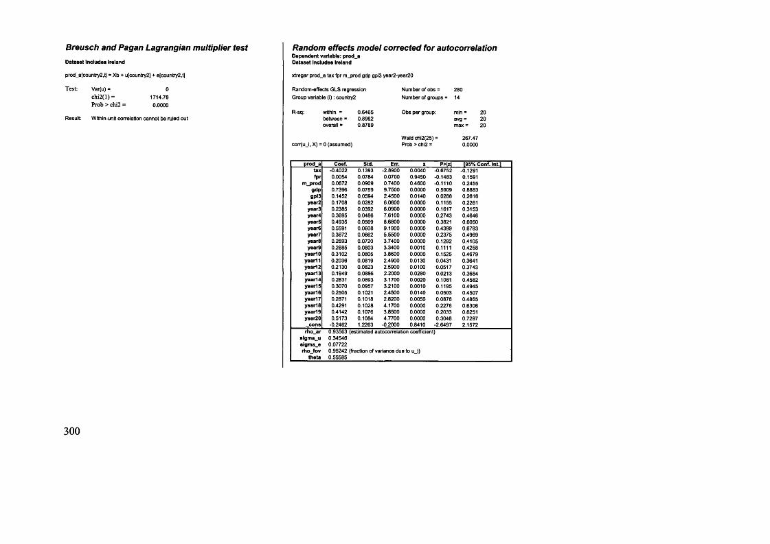
Breusch and Pagan Lagrangian multiplier testDataset Includes Ireland

prod_a[country2,t] = Xb + u[country2] + e[country2,t]

Test: Var(u) = 0ch i2 (l) = 1714.78Prob > chi2 = 0.0000

Result: Wlthin-unit correlation cannot be ruled out

300

Random effects model corrected for autocorrelationDependent variable: prod_a Dataset Includes Ireland

xtregar prod_a tax fpr m prod gdp gpi3 year2-year20

Random-effects GLS regression Group variable (I): country2

R-sq: within = 0.6465between = 0.8992overall = 0.8789

corr(u_i, X) = 0 (assumed)

Number of obs = 280Number of groups = 14

Obs per group: mln = 20avg = 20max = 20

Wald chi2(25) = 267.47Prob > chi2 = 0.0000

prod a Coef. Std. Err. z P>lz| [95% Conf. Int.ltax -0.4022 0.1393 -2.8900 0.0040 -0.6752 -0.1291fpr 0.0054 0.0784 0.0700 0.9450 -0.1483 0.1591

m_prod 0.0672 0.0909 0.7400 0.4600 -0.1110 0.2455gdp 0.7396 0.0759 9.7500 0.0000 0.5909 0.8883gpl3 0.1452 0.0594 2.4500 0.0140 0.0288 0.2616

year2 0.1708 0.0282 6.0600 0.0000 0.1155 0.2261year3 0.2385 0.0392 6.0900 0.0000 0.1617 0.3153year4 0.3695 0.0486 7.6100 0.0000 0.2743 0.4646year5 0.4935 0.0569 8.6800 0.0000 0.3821 0.6050year6 0.5591 0.0608 9.1900 0.0000 0.4399 0.6783year7 0.3672 0.0662 5.5500 0.0000 0.2375 0.4969year8 0.2693 0.0720 3.7400 0.0000 0.1282 0.4105year9 0.2685 0.0803 3.3400 0.0010 0.1111 0.4258

yeartO 0.3102 0.0805 3.8600 0.0000 0.1525 0.4679year11 0.2036 0.0819 2.4900 0.0130 0.0431 0.3641year! 2 0.2130 0.0823 2.5900 0.0100 0.0517 0.3743year13 0.1949 0.0886 2.2000 0.0280 0.0213 0.3684yearM 0.2831 0.0893 3.1700 0.0020 0.1081 0.4582yearl5 0.3070 0.0957 3.2100 0.0010 0.1195 0.4945year16 0.2505 0.1021 2.4500 0.0140 0.0503 0.4507year! 7 0.2871 0.1018 2.8200 0.0050 0.0876 0.4865year18 0.4291 0.1028 4.1700 0.0000 0.2276 0.6306year! 9 0.4142 0.1076 3.8500 0.0000 0.2033 0.6251year20 0.5173 0.1084 4.7700 0.0000 0.3048 0.7297

cons -0.2462 1.2263 -0.2000 0.8410 -2.6497 2.1572rho_ar

sigma_usigma_erho_fov

theta

0.93563 (estimated autocorrelation coefficient)0.345460.077220.95242 (fraction of variance due to u i) 0.55585

u[co

untry

2] +

e[co

untry

2,t]

Heteroskedasticity: graphical approximation

Production value in absolute terms: Predicted values against residuals

1.09961 -

-1.03031 -

at

* * *

1 \ 1 -i1*— t es

1.09961 -

_ V-1.03031 - 1 1 1 1 1

le

1.09961 - 00

_ 0

r #-1.03031 - 1 1 1 1 1

se1.09961 -

-4

-1.03031 -7.10017 1 ' 11.146V 7.10017 1.1467

Xb

301

dk

i 1-------- 1-------- 1-------- r

gr

T 1-------- 1-------- 1-------- r

pt

*

7.i 6o1 7 ' ' 11.1467

Table 45 Regression models on C l production in absolute terms, Ireland excluded

Fixed effects modelDependent variable: prod_a D ataset excludes Ireland

xtreg prod_a tax fpr m_prod gdp gpi3 year2-year20, fe

Fixed-effects (within) regression Number of obs = 260Group variable (i): country2 Number of groups = 13

R-sq: within = 0.8538 Obs per group: min = 20between = 0.7363 avg = 20overall = 0.2149 max = 20

F(24,223) = 54.25corr(u_i, Xb) = -0.6049 Prob > F = 0.0000

p ro d a Coef. Std. Err. t p>ltl [95% Conf. Int.]tax -0.2955 0.0961 -3.0800 0.0020 -0.4849 -0.1062fpr 0.1622 0.0578 2.8100 0.0050 0.0484 0.2761

m_prod -0.0113 0.0568 -0.2000 0.8430 -0.1231 0.1006gdp -0.1841 0.0656 -2.8100 0.0050 -0.3134 -0.0548gpl3 -0.1324 0.0430 -3.0800 0.0020 -0.2172 -0.0477

year2 -0.0435 0.0352 -1.2300 0.2190 -0.1129 0.0260year3 -0.0546 0.0376 -1.4500 0.1470 -0.1287 0.0194year4 -0.0040 0.0406 -0.1000 0.9210 -0.0841 0.0760year5 0.0507 0.0435 1.1700 0.2450 -0.0351 0.1365year6 0.1271 0.0437 2.9100 0.0040 0.0411 0.2132year7 0.2677 0.0433 6.1800 0.0000 0.1824 0.3531year8 0.3455 0.0442 7.8200 0.0000 0.2584 0.4326year9 0.4320 0.0476 9.0700 0.0000 0.3382 0.5258

yearlO 0.4522 0.0464 9.7500 0.0000 0.3608 0.5436y ea rll 0.4848 0.0475 10.2100 0.0000 0.3912 0.5784year12 0.4824 0.0472 10.2100 0.0000 0.3893 0.5755year13 0.5189 0.0510 10.1700 0.0000 0.4184 0.6195y earl 4 0.4838 0.0493 9.8100 0.0000 0.3866 0.5809year15 0.5560 0.0534 10.4200 0.0000 0.4508 0.6611yearl6 0.6217 0.0591 10.5100 0.0000 0.5052 0.7382year) 7 0.6521 0.0594 10.9700 0.0000 0.5350 0.7693year! 8 0.7018 0.0582 12.0600 0.0000 0.5871 0.8165year19 0.7021 0.0602 11.6600 0.0000 0.5834 0.8208year20 0.7664 0.0608 12.6100 0.0000 0.6466 0.8862

cons 11.7761 1.0276 11.4600 0.0000 9.7510 13.8012slgma_u 1.4155slgma_e 0.0834

rbo 0.9965 (fraction of variance due to u_ i)

F test that all u_i=0: F(12, 242) = 429.18 Prob > F = 0.0000

Random effects modelDependent variable: prod_a Dataset excludes Ireland

xtreg prod_a tax fpr m_prod gdp gpi3 year2-year20, re

Random-effects GLS regression Group variable (i): country2

R-sq: within = 0.842between = 0.7825overall = 0.4634

Random effects u j - Gaussian corr(u_i, X) = 0 (assumed)

Number of obs = Number of groups =

Obs per group:

Wald chi2(24) = Prob > chi2 =

26013

min = 20avg = 20max = 20

990.850.0000

prod_a Coef. Std. Err. z P>|z| [95% Conf. Int.]tax -0.4841 0.1065 -4.5400 0.0000 -0.6929 -0.2753fpr 0.2449 0.0648 3.7800 0.0000 0.1179 0.3719

m_prod 0.1061 0.0630 1.6800 0.0920 -0.0174 0.2295gdp 0.0918 0.0661 1.3900 0.1650 -0.0377 0.2214gpl3 -0.0694 0.0483 -1.4400 0.1510 -0.1641 0.0254

year2 -0.0043 0.0401 -0.1100 0.9140 -0.0829 0.0742year3 0.0069 0.0423 0.1600 0.8710 -0.0761 0.0898year4 0.0811 0.0452 1.7900 0.0730 -0.0075 0.1697yearS 0.1506 0.0482 3.1300 0.0020 0.0562 0.2450yearS 0.2226 0.0485 4.5900 0.0000 0.1276 0.3176year7 0.3143 0.0490 6.4100 0.0000 0.2181 0.4104yearS 0.3448 0.0504 6.8400 0.0000 0.2460 0.4436year9 0.4090 0.0542 7.5500 0.0000 0.3028 0.5151

yearlO 0.4245 0.0527 8.0500 0.0000 0.3211 0.5279year11 0.4074 0.0532 7.6500 0.0000 0.3030 0.5118year12 0.4005 0.0529 7.5800 0.0000 0.2969 0.5041year13 0.4161 0.0567 7.3400 0.0000 0.3050 0.5272year14 0.4061 0.0554 7.3400 0.0000 0.2976 0.5146y earl 5 0.4582 0.0596 7.6900 0.0000 0.3415 0.5749year16 0.4813 0.0650 7.4000 0.0000 0.3539 0.6088y earl 7 0.5069 0.0652 7.7700 0.0000 0.3790 0.6347year18 0.5725 0.0643 8.9000 0.0000 0.4465 0.6985year19 0.5737 0.0667 8.6100 0.0000 0.4430 0.7044year20 0.6327 0.0672 9.4200 0.0000 0.5010 0.7643

cons 7.7243 1.0627 7.2700 0.0000 5.6415 9.8072slgma_u 0.468225slgma_e 0.083446

rho 0.969216 (fraction of variance due to u j )

Hausman specification test

Test: Ho: difference in coefficients not systematic

chi2( 24) = (b-B)'[SA(-1 )](b-B), S = (S_fe - S_re)0.00

Prob>chi2 = 1.0000

Result: Ho cannot be rejected.Random effects model can be used safely.

prod_a FE RE Differencetax -0.2955 -0.4841 0.1885fpr 0.1622 0.2449 -0.0827

m_prod -0.0113 0.1061 -0.1174gdp -0.1841 0.0918 -0.2759gpl3 -0.1324 -0.0694 -0.0631

year2 -0.0435 -0.0043 -0.0391year3 -0.0546 0.0069 -0.0615year4 -0.0040 0.0811 -0.0851year5 0.0507 0.1506 -0.0999year6 0.1271 0.2226 -0.0955year7 0.2677 0.3143 -0.0465yearS 0.3455 0.3448 0.0007year9 0.4320 0.4090 0.0230

yearlO 0.4522 0.4245 0.0277year11 0.4848 0.4074 0.0774year12 0.4824 0.4005 0.0819year13 0.5189 0.4161 0.1028year14 0.4838 0.4061 0.0776year15 0.5560 0.4582 0.0978y ea rl 6 0.6217 0.4813 0.1404year17 0.6521 0.5069 0.1453year18 0.7018 0.5725 0.1293year19 0.7021 0.5737 0.1284year20 0.7664 0.6327 0.1338

302

u[co

untry

2] +

e[co

untry

2,t]

Auto-correlation: graphical approximation

Production value in absolute terms: Residuals against lagged residuals

1.88983 -

-1.58916 -

at

*>

be

i ' T “ " r " "T" —“ T es

1 1 1 1 —1 fi

1.88983 - -

_

- - #-1.58916 - _

i i i i i it

i 1 ■ r ■" i1 r nl

1.88983 - -

- 0>

-*

-1.58916 - i i i ■ i r i i i i i

’-----fr

1.91507 -1.5&535

-1.58916 H

Lresid prod a

303

0

gr

i i 1-------- 1-------- r

1.915oV -1.58535 1.91507

Breusch and Pagan Lagrangian multiplier testDataset excludes Ireland

prod_a[country2,t] = Xb + u[country2] + e[country2,t]

Test: Var(u) = 0ch i2 (l) = 1792.88Prob > chi2 = 0.0000

Result: Within-unit correlation cannot be ruled out

304

Random effects model corrected for autocorrelationDependent variable: prod_aDataset excludes Ireland

xtregar prod_a tax fpr m_prod gdp gpi3 year2-year20

Random-effects GLS regression Number of obs = 260Group variable (I): country2 Number of groups = 13

R-sq: within = 0.7527 Obs per group: min = 20between = 0.9025 avg = 20overall = 0.878 max = 20

Wald chi2(25) = 311.99corr(u_i, X) = 0 (assumed) Prob > chi2 = 0.0000

p ro d a Coef. Std. Err. z P>|z| [95% Conf. Int.]tax -0.3629 0.1190 -3.0500 0.0020 -0.5960 -0.1297fpr 0.1108 0.0707 1.5700 0.1170 -0.0278 0.2494

m_prod 0.1361 0.0731 1.8600 0.0630 -0.0072 0.2795gdp 0.5557 0.0668 8.3100 0.0000 0.4247 0.6866gpl3 0.0583 0.0501 1.1600 0.2440 -0.0398 0.1565

year2 0.1060 0.0256 4.1400 0.0000 0.0558 0.1562year3 0.1575 0.0348 4.5200 0.0000 0.0892 0.2257year4 0.2621 0.0423 6.2000 0.0000 0.1792 0.3450year5 0.3643 0.0488 7.4600 0.0000 0.2685 0.4600year6 0.4282 0.0513 8.3400 0.0000 0.3276 0.5289year7 0.3276 0.0543 6.0300 0.0000 0.2211 0.4341yearS 0.2628 0.0582 4.5200 0.0000 0.1488 0.3768year9 0.2775 0.0643 4.3200 0.0000 0.1515 0.4035

yearlO 0.3053 0.0633 4.8200 0.0000 0.1812 0.4293yearH 0.2205 0.0634 3.4800 0.0010 0.0962 0.3449year12 0.2132 0.0630 3.3900 0.0010 0.0899 0.3366year! 3 0.1966 0.0676 2.9100 0.0040 0.0641 0.3291year14 0.2509 0.0671 3.7400 0.0000 0.1194 0.3823year15 0.2737 0.0720 3.8000 0.0000 0.1326 0.4148year! 6 0.2342 0.0771 3.0400 0.0020 0.0831 0.3853year! 7 0.2599 0.0765 3.4000 0.0010 0.1100 0.4099yearlS 0.3538 0.0764 4.6300 0.0000 0.2040 0.5036year19 0.3339 0.0803 4.1600 0.0000 0.1766 0.4912year20 0.4049 0.0802 5.0500 0.0000 0.2476 0.5621

cons 1.6437 1.0516 1.5600 0.1180 -0.4174 3.7048rho_ar 0.81326 (estimated autocorrelation coefficient)

slgma_u 0.34824sigma_e 0.07214rho_fov 0.95885 (fraction of variance due to u j )

theta 0.79727

u[co

untry

2] +

e[co

untry

2,t]

Heteroskedasticity: graphical approximation

Production value in absolute terms: Predicted values against residuals

1.91507-

-1.58916 -

at

00 °o o6)<a*o SOO

be

oo O (uc*>«0oa5»o

de

“fc0 0 to « » o o o o o

I i I I I

es

|i— — -( i '1 1 ■(

fi1 1 1 1 1

fr

1.91507- - -CD oo oaoiS ® o° °

-«ao® ®>«po§tp -

- - “*> 0 0 0 0 0 ® ® 0 0-1.58916 - _ -

*-------■»"------- r -------r - rit

I 1 1 1 1

nl

1 1 i i i

Pt

1.91507 - - -

- <4*0 o oomoBdfc -

- -grpoacooooo COS °

- - -6b o '*^as> o

-1.58916- - -

8.68114 9.74593 8.68114

1.91507 i® 0 0 < p 4fe(DO

-1.58916 4 , , , , r8.68114 9.74593

Xb

305

dk

cP oQ ao< tocfico 0 °

T 1-------- 1-------- 1-------- r

gr

<Stt’0»W*>oOon 1 r 1 rse

W J o o o o 1

7 i I I r 8.68114 9.74593

Table 46 Regression models on C l employees / total workforce, Ireland included

Fixed effects modelDependent variable: empl_r Dataset Includes Ireland

xtreg empl_r tax fpr m_prod gdp gpi3 year2-year20, fe

Fixed-effects (within) regression Number of obs = 280Group variable (i): country2 Number of groups = 14

R-sq: within = 0.2178 Obs per group: min = 20between = 0.0003 avg = 20overall = 0.0085 max = 20

F(23,243) = 2.94corr(u_i, Xb) = -0.202 Prob > F = 0.0000

empl r Coef. Std. Err. t P>|t| [95% Conf. Int.]tax -0.6088 0.1408 -4.3200 0.0000 -0.8861 -0.3315fpr 0.0686 0.0953 0.7200 0.4720 -0.1191 0.2563

m_prod 0.0584 0.0935 0.6200 0.5330 -0.1257 0.2424gpl3 0.0013 0.0702 0.0200 0.9850 -0.1369 0.1395

year2 -0.0173 0.0585 -0.3000 0.7670 -0.1326 0.0979year3 -0.0226 0.0591 -0.3800 0.7030 -0.1390 0.0939year4 -0.0162 0.0598 -0.2700 0.7870 -0.1340 0.1016year5 -0.0101 0.0616 -0.1600 0.8690 -0.1314 0.1111year6 -0.0112 0.0627 -0.1800 0.8580 -0.1347 0.1122year7 0.0198 0.0713 0.2800 0.7820 -0.1207 0.1602yearS 0.0220 0.0758 0.2900 0.7710 -0.1272 0.1713year9 0.0368 0.0819 0.4500 0.6530 -0.1245 0.1982

yearlO 0.0101 0.0798 0.1300 0.9000 -0.1472 0.1673y e a rd -0.0135 0.0767 -0.1800 0.8610 -0.1644 0.1375year12 -0.0277 0.0753 -0.3700 0.7130 -0.1761 0.1206year13 -0.0382 0.0791 -0.4800 0.6300 -0.1940 0.1177year14 -0.0727 0.0807 -0.9000 0.3690 -0.2317 0.0864y earl 5 -0.0889 0.0855 -1.0400 0.2990 -0.2574 0.0795year16 -0.1027 0.0884 -1.1600 0.2460 -0.2768 0.0714year17 -0.1089 0.0869 -1.2500 0.2110 -0.2802 0.0623year18 -0.1184 0.0885 -1.3400 0.1820 -0.2928 0.0560y earl 9 -0.1290 0.0925 -1.3900 0.1640 -0.3112 0.0532year20 -0.1475 0.0926 -1.5900 0.1130 -0.3300 0.0349

cons 1.2490 0.6816 1.8300 0.0680 -0.0936 2.5917slgma_u 0.424877slgma_e 0.149931

rho 0.889265 (fraction of variance due to u_i)

F test that all u 1=0: F(13, 243) = 74.65 Prob > F = 0.0000

Random effects modelDependent variable: empl_r Dataset Includes Ireland

xtreg empl_r tax fpr m_prod gdp gpi3 year2-year20, re

Random-effects GLS regression Group variable (i): country2

R-sq: within = between = overall =

0.21280.11890.1267

Random effects u j - Gaussian corr(u_i, X) = 0 (assumed)

Number of obs =

Obs per group:

Wald chi2(23) = Prob > chi2 =

28014

min = 20avg = 20max = 20

66.60.0000

em pljr Coef. Std. Err. z P>|z| [95% Conf. Int.]tax -0.5258 0.1362 -3.8600 0.0000 -0.7927 -0.2589fpr -0.0084 0.0922 -0.0900 0.9270 -0.1892 0.1723

m_prod 0.1021 0.0892 1.1400 0.2520 -0.0727 0.2769gpl3 -0.0284 0.0681 -0.4200 0.6770 -0.1619 0.1051

year2 -0.0106 0.0591 -0.1800 0.8580 -0.1264 0.1052year3 -0.0202 0.0596 -0.3400 0.7340 -0.1371 0.0967year4 -0.0202 0.0603 -0.3300 0.7380 -0.1384 0.0980year5 -0.0162 0.0619 -0.2600 0.7940 -0.1375 0.1052year6 -0.0212 0.0629 -0.3400 0.7360 -0.1444 0.1021year7 -0.0250 0.0704 -0.3500 0.7230 -0.1630 0.1131year8 -0.0299 0.0745 -0.4000 0.6880 -0.1759 0.1161year9 -0.0247 0.0801 -0.3100 0.7580 -0.1817 0.1323

yearlO -0.0481 0.0782 -0.6200 0.5380 -0.2013 0.1051yearl 1 -0.0687 0.0751 -0.9100 0.3600 -0.2160 0.0785year12 -0.0794 0.0739 -1.0700 0.2830 -0.2243 0.0656yearl 3 -0.0941 0.0774 -1.2200 0.2240 -0.2459 0.0576yearl 4 -0.1270 0.0789 -1.6100 0.1080 -0.2817 0.0277yearl 5 -0.1477 0.0833 -1.7700 0.0760 -0.3111 0.0156yearl 6 -0.1643 0.0860 -1.9100 0.0560 -0.3328 0.0042yearl 7 -0.1641 0.0847 -1.9400 0.0530 -0.3302 0.0020yearl 8 -0.1753 0.0862 -2.0300 0.0420 -0.3442 -0.0063yearl 9 -0.1940 0.0898 -2.1600 0.0310 -0.3700 -0.0179year20 -0.2090 0.0900 -2.3200 0.0200 -0.3854 -0.0326

cons 1.4482 0.6728 2.1500 0.0310 0.1296 2.7668sigma_u 0.33405slgma_e 0.149931

rho 0.832331 (fraction of variance due to u_i)

Hausman specification test

Test: Ho: difference in coefficients not systematic

chi2( 24) = (b-B)'[SA(-1 )](b-B), S = (S_fe - S_re) 10.58

Prob>chi2 =

Result: Ho cannot be rejected.Random effects model can be used safely.

empl_r FE RE Differencetax -0.6088 -0.5258 -0.0830fpr 0.0686 -0.0084 0.0771

m_prod 0.0584 0.1021 -0.0437gpl3 0.0013 -0.0284 0.0297

year2 -0.0173 -0.0106 -0.0067year3 -0.0226 -0.0202 -0.0023year4 -0.0162 -0.0202 0.0040year5 -0.0101 -0.0162 0.0060year6 -0.0112 -0.0212 0.0099year7 0.0198 -0.0250 0.0447year8 0.0220 -0.0299 0.0519year9 0.0368 -0.0247 0.0615

yearlO 0.0101 -0.0481 0.0582yearl 1 -0.0135 -0.0687 0.0553yearl 2 -0.0277 -0.0794 0.0516yearl 3 -0.0382 -0.0941 0.0560yearl 4 -0.0727 -0.1270 0.0543yearl 5 -0.0889 -0.1477 0.0588yearl 6 -0.1027 -0.1643 0.0616yearl 7 -0.1089 -0.1641 0.0552yearl 8 -0.1184 -0.1753 0.0569yearl 9 -0.1290 -0.1940 0.0650year20 -0.1475 -0.2090 0.0614

306

u[co

untry

2] +

e[co

untry

2,t]

Auto-correlation: graphical approximation

Chemical industry employees / total workforce: Residuals against lagged residuals

.932072 H

-.874557 - i 1------- 1------- 1------- r

.932072 i

-.874557 -

1---- 1---- 1---- 1---- T t 1-------- 1---------1-------- rfr

t 1-------- 1-------- 1-------- r

gr

- 8"

.932072 H

-.874557 - l i 1---------1---------r-.874557

i i i i r .874557 .823195

.932072 -

-.874557 -

8o+

-.874557 ' .82319^1 1-------1------- 1 r

.874557 .823195

Lresid errol r

307

Breusch and Pagan Lagrangian multiplier testDataset includes Ireland

empl_rfcountry2,t] = Xb + u[country2] + e[country2,t]

Test: Var(u) = 0ch i2 (l) = 1439.24Prob > chi2 = 0.0000

Result: Withln-unit correlation cannot be ruled out

308

Random effects model corrected for autocorrelationDependent variable: empl_rDataset Includes Ireland

xtregar empl_r tax fpr m_prod gpi3 year2-year20

Random-effects GLS regression Number of obs = 280Group variable (I): country2 Number of groups = 14

R-sq: within = 0.1582 Obs per group: min = 20between = 0.4245 avg = 20overall = 0.2535 max = 20

Wald chi2(24) = 24.04corr(u_i, X) = 0 (assumed) Prob > chi2 0.4596

empl_r Coef. Std. Err. z P>|z| [95% Conf. Int.]tax -0.0656 0.1075 -0.6100 0.5420 -0.2763 0.1451fpr -0.0189 0.0605 -0.3100 0.7540 -0.1374 0.0996

m_prod 0.1151 0.0701 1.6400 0.1010 -0.0223 0.2525gpl3 -0.0065 0.0430 -0.1500 0.8800 -0.0907 0.0777

year2 -0.0176 0.0190 -0.9300 0.3520 -0.0548 0.0195year3 -0.0353 0.0256 -1.3800 0.1690 -0.0855 0.0150year4 -0.0492 0.0311 -1.5800 0.1140 -0.1101 0.0118year5 -0.0531 0.0362 -1.4700 0.1420 -0.1240 0.0178year6 -0.0581 0.0400 -1.4500 0.1460 -0.1366 0.0203year7 -0.0819 0.0501 -1.6400 0.1020 -0.1801 0.0163year8 -0.0939 0.0554 -1.7000 0.0900 -0.2024 0.0146year9 -0.0835 0.0615 -1.3600 0.1740 -0.2039 0.0370

yearlO -0.0965 0.0616 -1.5700 0.1170 -0.2171 0.0241yearl 1 -0.1161 0.0610 -1.9000 0.0570 -0.2357 0.0034yearl 2 -0.1306 0.0610 -2.1400 0.0320 -0.2501 -0.0111yearl 3 -0.1486 0.0649 -2.2900 0.0220 -0.2759 -0.0213yearl 4 -0.1784 0.0671 -2.6600 0.0080 -0.3100 -0.0468yearl 5 -0.2041 0.0714 -2.8600 0.0040 -0.3441 -0.0640yearl 6 -0.2147 0.0745 -2.8800 0.0040 -0.3607 -0.0687yearl 7 -0.2244 0.0736 -3.0500 0.0020 -0.3687 -0.0802yearl 8 -0.2397 0.0753 -3.1800 0.0010 -0.3873 -0.0921yearl 9 -0.2694 0.0788 -3.4200 0.0010 -0.4239 -0.1149year20 -0.2860 0.0793 -3.6000 0.0000 -0.4415 -0.1305

cons 0.1883 0.4491 0.4200 0.6750 -0.6918 1.0684rho_arslgma_uslgma_erho_fovtheta

0.92779 (estimated autocorrelation coefficient)0.280970.059700.95680 (fraction of variance due to u i) 0.60087

u[co

untry

2] +

e[co

untry

2,t]

Heteroskedasticity: graphical approximation

Chemical industry employees / total workforce: Predicted values against residuals

.932072 -

-.874557 -

at be

I I I '! I es

i i i " i in

.932072 -

-c o o a o j 0<b° o 0

-.874557 - _| | 'I "" I I

ie

1 1 1 1 1 It

.932072 - -

& -- & a® &OQ

-.874557 - _i — — r r .- i -s;se

1 1 1 1 1 uk

.932072 - -

”

_g&s*><9

-.874557 - _

-.128859 ' ' '.55592b -.128859 . 555929

de dk

-8 *8 8° ^n 1--------- 1--------- 1 r 1--------- 1--------- 1--------- 1 r

-.128869 555929 -.128859 . 555929

Xb

309

Table 47 Regression models on C l employment / total workforce, Ireland excluded

Fixed effects modelDependent variable: empl_r Dataset excludes Ireland

xtreg empl_r tax fpr m_prod gdp gpi3 year2-year20, fe

Fixed-effects (within) regression Number of obs = 260Group variable (i): country2 Number of groups = 13

R-sq: within = 0.241 Obs per group: min = 20between = 0.1723 avg = 20overall = 0.1459 max = 20

F(23,224) = 3.09corr(u_i, Xb) = 0.1732 Prob > F = 0.0000

e m p lr Coef. Std. Err. t P>|t| [95% Conf. Int.]tax -0.3443 0.1588 -2.1700 0.0310 -0.6572 -0.0315fpr 0.0247 0.0983 0.2500 0.8020 -0.1691 0.2185

m_prod 0.0779 0.0944 0.8200 0.4100 -0.1082 0.2640gpl3 -0.0513 0.0729 -0.7000 0.4820 -0.1951 0.0924

year2 -0.0187 0.0609 -0.3100 0.7590 -0.1387 0.1013year3 -0.0258 0.0616 -0.4200 0.6760 -0.1473 0.0957year4 -0.0333 0.0624 -0.5300 0.5940 -0.1562 0.0896year5 -0.0327 0.0642 -0.5100 0.6110 -0.1593 0.0939year6 -0.0366 0.0655 -0.5600 0.5770 -0.1656 0.0925year7 -0.0326 0.0747 -0.4400 0.6630 -0.1798 0.1146yearS -0.0367 0.0795 -0.4600 0.6450 -0.1933 0.1200year9 -0.0230 0.0854 -0.2700 0.7880 -0.1912 0.1452

yearl 0 -0.0488 0.0830 -0.5900 0.5570 -0.2123 0.1148y ea rll -0.0749 0.0801 -0.9400 0.3510 -0.2327 0.0829yearl 2 -0.0955 0.0788 -1.2100 0.2270 -0.2509 0.0598yearl 3 -0.1102 0.0826 -1.3300 0.1830 -0.2730 0.0525yearl 4 -0.1431 0.0840 -1.7000 0.0900 -0.3086 0.0224yearl 5 -0.1657 0.0888 -1.8700 0.0630 -0.3407 0.0094yearl 6 -0.1824 0.0917 -1.9900 0.0480 -0.3632 -0.0017year! 7 -0.1905 0.0910 -2.0900 0.0370 -0.3699 -0.0112yearl 8 -0.2068 0.0924 -2.2400 0.0260 -0.3889 -0.0247yearl 9 -0.2150 0.0967 -2.2200 0.0270 -0.4054 -0.0245year20 -0.2311 0.0968 -2.3900 0.0180 -0.4219 -0.0403

cons 1.0029 0.6903 1.4500 0.1480 -0.3574 2.3632sigma_u 0.404797slgma_e 0.150088

rho 0.879142 (fraction of variance due to u_i)

F test that all u_i=0: F(12,224) 75.93 Prob > F = 0.0000

Random effects modelDependent variable: empl_r Dataset excludes Ireland

xtreg empl_r tax fpr m_prod gdp gpi3 year2-year20, re

Random-effects GLS regression Group variable (i): country2

R-sq: within = 0.2372between = 0.4467overall = 0.3322

Random effects u_i - Gaussian corr(u_i, X) = 0 (assumed)

Number of obs =

Obs per group:

Wald chi2(23) = Prob > chi2 =

26013

min = 20avg = 20max = 20

73.280.0000

empl_r Coef. Std. Err. z P>|z| [95% Conf. Int.]tax -0.2624 0.1509 -1.7400 0.0820 -0.5581 0.0332fpr -0.0459 0.0946 -0.4800 0.6280 -0.2313 0.1395

m_prod 0.1167 0.0911 1.2800 0.2000 -0.0618 0.2952gpi3 -0.0808 0.0708 -1.1400 0.2540 -0.2197 0.0580

year2 -0.0122 0.0614 -0.2000 0.8420 -0.1325 0.1081year3 -0.0230 0.0621 -0.3700 0.7110 -0.1447 0.0987year4 -0.0364 0.0628 -0.5800 0.5620 -0.1595 0.0867year5 -0.0378 0.0646 -0.5900 0.5580 -0.1645 0.0888yearS -0.0458 0.0657 -0.7000 0.4860 -0.1746 0.0830year7 -0.0745 0.0734 -1.0200 0.3100 -0.2183 0.0693year8 -0.0857 0.0776 -1.1000 0.2690 -0.2379 0.0664yeari) -0.0804 0.0829 -0.9700 0.3320 -0.2428 0.0821

yearlO -0.1030 0.0808 -1.2700 0.2020 -0.2613 0.0553yearl 1 -0.1266 0.0780 -1.6200 0.1050 -0.2795 0.0263yearl 2 -0.1442 0.0770 -1.8700 0.0610 -0.2950 0.0067yearl 3 -0.1626 0.0804 -2.0200 0.0430 -0.3202 -0.0050yearl 4 -0.1937 0.0819 -2.3700 0.0180 -0.3543 -0.0332yearl 5 -0.2204 0.0864 -2.5500 0.0110 -0.3897 -0.0510yearl 6 -0.2397 0.0891 -2.6900 0.0070 -0.4143 -0.0652yearl 7 -0.2435 0.0886 -2.7500 0.0060 -0.4173 -0.0698yearl 8 -0.2608 0.0900 -2.9000 0.0040 -0.4371 -0.0845yearl 9 -0.2763 0.0937 -2.9500 0.0030 -0.4599 -0.0927year20 -0.2889 0.0941 -3.0700 0.0020 -0.4733 -0.1045

cons 1.1856 0.6918 1.7100 0.0870 -0.1703 2.5414sigma_u 0.329659sigma_e 0.150088

rho 0.828307 (fraction of variance due to u_i)

Hausman specification test

Test: Ho: difference in coefficients not systematic

chi2( 24) = (b-B)'[SA(-1 )](b-B), S = (S_fe - S_re)6.61

Prob>chi2 = 0.9997

Result: Ho cannot be rejected.Random effects model can be used safely.

empl_r FE RE Differencetax -0.3443 -0.2624 -0.0819fpr 0.0247 -0.0459 0.0706

m_prod 0.0779 0.1167 -0.0388gpi3 -0.0513 -0.0808 0.0295

year2 -0.0187 -0.0122 -0.0065year3 -0.0258 -0.0230 -0.0028year4 -0.0333 -0.0364 0.0031yearS -0.0327 -0.0378 0.0051yearS -0.0366 -0.0458 0.0092year7 -0.0326 -0.0745 0.0419yearS -0.0367 -0.0857 0.0491yeari) -0.0230 -0.0804 0.0574

yearlO -0.0488 -0.1030 0.0542yearl 1 -0.0749 -0.1266 0.0517yearl 2 -0.0955 -0.1442 0.0486yearl 3 -0.1102 -0.1626 0.0524year14 -0.1431 -0.1937 0.0506yearl 5 -0.1657 -0.2204 0.0547yearl 6 -0.1824 -0.2397 0.0573yearl 7 -0.1905 -0.2435 0.0530yearl 8 -0.2068 -0.2608 0.0540yearl 9 -0.2150 -0.2763 0.0613year20 -0.2311 -0.2889 0.0578

310

u[co

untry

2] +

e[co

untry

2,t]

Auto-correlation: graphical approximation

Chemical industry employees / total workforce: Residuals against lagged residuals

.857969 -

-.803108 -

at

✓

I I I I Ies

.857969 -

- &-.803108 - I ' i " i i i

ft

.857969 -

-

-.803108 - i i i i iuk

857969-

-

-.803108 -- 803108 \ t 1 t r-.803108 .811895

be

✓

i 1--------- 1--------- 1--------- r

fi

- 4*1 1--------- 1--------- r

nl

&

i i i i i.803108 .811895

de

n 1---------1-------- 1-------- rfr

S 1---------- 1---------- 1---------- r

pt

i 1----------1---------- 1---------- r-.803108 . 811895

&

i 1---------1-------- 1-------- r

gr

se

- S f

-.803108 .811895

Lresid empl r

311

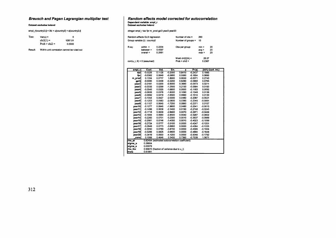
Breusch and Pagan Lagrangian multiplier testDataset excludes Ireland

empl_rfcountry2,t] = Xb + u[country2] + e[country2,t]

Test: Var(u) = 0ch i2 (l) = 1267.51Prob > chi2 = 0.0000

Result: Withln-unit correlation cannot be ruled out

312

Random effects model corrected for autocorrelationDependent variable: empl_rDataset excludes Ireland

xtregar empl_r tax fpr m_prod gpl3 year2-year20

Random-effects GLS regression Number of obs = 260Group variable (1): country2 Number of groups = 13

R-sq: within = 0.2204 Obs per group: min = 20between = 0.4597 avg = 20overall = 0.2961 max = 20

Wald chl2(24) = 28.57corr(uJ, X) = 0 (assumed) Prob > chi2 = 0.2367

empl_r Coef. Std. Err. z P»M [95% Conf. Int.]tax -0.0226 0.1128 -0.2000 0.8410 -0.2437 0.1985fpr -0.0382 0.0649 -0.5900 0.5560 -0.1654 0.0890

m_prod 0.1334 0.0717 1.8600 0.0630 -0.0071 0.2740gpl3 -0.0095 0.0439 -0.2200 0.8290 -0.0955 0.0765

year2 -0.0181 0.0200 -0.9000 0.3660 -0.0573 0.0211year3 -0.0335 0.0269 -1.2500 0.2130 -0.0864 0.0193year4 -0.0545 0.0325 -1.6800 0.0930 -0.1183 0.0092year5 -0.0606 0.0378 -1.6000 0.1090 -0.1348 0.0136year6 -0.0692 0.0419 -1.6500 0.0990 -0.1514 0.0130year7 -0.1054 0.0527 -2.0000 0.0460 -0.2087 -0.0021year8 -0.1203 0.0583 -2.0600 0.0390 -0.2345 -0.0061year9 -0.1107 0.0645 -1.7200 0.0860 -0.2371 0.0157

yearlO -0.1277 0.0645 -1.9800 0.0480 -0.2541 -0.0013yea rll -0.1496 0.0638 -2.3400 0.0190 -0.2748 -0.0245yearl 2 -0.1718 0.0639 -2.6900 0.0070 -0.2971 -0.0464yearl 3 -0.1934 0.0680 -2.8500 0.0040 -0.3267 -0.0602yearl 4 -0.2263 0.0701 -3.2300 0.0010 -0.3637 -0.0889yearl 5 -0.2561 0.0746 -3.4300 0.0010 -0.4023 -0.1099yearl 6 -0.2724 0.0777 -3.5100 0.0000 -0.4247 -0.1201yearl 7 -0.2849 0.0773 -3.6900 0.0000 -0.4364 -0.1335yearl 8 -0.3050 0.0789 -3.8700 0.0000 -0.4595 -0.1504yearl 9 -0.3266 0.0825 -3.9600 0.0000 -0.4884 -0.1648year20 -0.3419 0.0830 -4.1200 0.0000 -0.5046 -0.1792

cons 0.1566 0.4646 0.3400 0.7360 -0.7539 1.0671rho_arslgma_uslgma_erho_fovtheta

0.92454 (estimated autocorrelation coefficient)0.288040.059790.95870 (fraction of variance due to u i) 0.61881

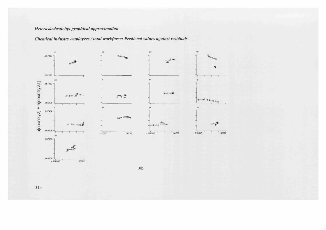
u[co

untry

2] +

e[co

untry

2,t]

Heteroskedasticity: graphical approximation

Chemical industry employees / total workforce: Predicted values against residuals

.857969-

-.803108 -

at be de

° * g m ‘

dk

**

i — | i i 1 I

es

1 1 1 1 1'

fi

1 1 1 1 1

fr

i I i i i

gr

.857969 - - - -

- - - -

_ - oPcocbaatf?CP°<®ooc$> °

-.803108 - 1 - f ? - i Iit

T 'f ® i I 'nl

I i ' i i I

P*

1 1 1 1 1 se

.857969 - - - -

- “

- 8 000 oooo $ - 80t o 88 ^ ’° 00o<£>^C

-.803108 - - - n---------1-------- 1 i-------- r--.210537 .36782 -.210537 .36782 -.210537 .36782

-803108 V 1 1 1 T-.210537 . 36782

Xb

313

Table 48 Regression models on C l employment in absolute terms, Ireland included

Fixed effects modelDependent variable: empl_a Dataset Includes Ireland

xtreg empl_a tax fpr m_prod gdp gpi3 year2-year20, fe

Fixed-effects (within) regression Number of obs = 280Group variable (i): country2 Number of groups = 14

R-sq: within = 0.1463 Obs per group: min = 20between = 0.8893 avg = 20overall = 0.8614 max = 20

F(24,242) = 1.73corr(u_i, Xb) = 0.8745 Prob > F = 0.0215

empl a Coef. Std. Err. t P>|t| [95% Conf. Int.]tax -0.5973 0.1483 -4.0300 0.0000 -0.8894 -0.3052fpr 0.0894 0.1013 0.8800 0.3790 -0.1102 0.2889

m_prod 0.0011 0.1032 0.0100 0.9920 -0.2023 0.2045gdp 0.2553 0.1046 2.4400 0.0150 0.0492 0.4614gpi3 -0.0191 0.0746 -0.2600 0.7980 -0.1661 0.1278

year2 0.0300 0.0625 0.4800 0.6320 -0.0932 0.1532year3 0.0444 0.0656 0.6800 0.4990 -0.0848 0.1737year4 0.0701 0.0696 1.0100 0.3150 -0.0670 0.2072year5 0.0957 0.0738 1.3000 0.1960 -0.0496 0.2410year6 0.1028 0.0739 1.3900 0.1660 -0.0428 0.2485year7 0.0834 0.0749 1.1100 0.2670 -0.0641 0.2308year8 0.0541 0.0787 0.6900 0.4920 -0.1008 0.2090year9 0.0678 0.0859 0.7900 0.4310 -0.1014 0.2371

yearlO 0.0575 0.0839 0.6900 0.4940 -0.1078 0.2227yearl 1 0.0008 0.0862 0.0100 0.9930 -0.1690 0.1705yearl 2 -0.0004 0.0854 0.0000 0.9960 -0.1687 0.1679yearl 3 -0.0349 0.0925 -0.3800 0.7060 -0.2171 0.1472yearM -0.0507 0.0897 -0.5700 0.5720 -0.2274 0.1260year15 -0.0766 0.0972 -0.7900 0.4320 -0.2680 0.1149yearl 6 -0.1108 0.1072 -1.0300 0.3020 -0.3220 0.1004yearl 7 -0.1136 0.1076 -1.0600 0.2920 -0.3255 0.0982yearl 8 -0.0967 0.1063 -0.9100 0.3640 -0.3061 0.1128yearl 9 -0.0926 0.1105 -0.8400 0.4030 -0.3103 0.1252year20 -0.0975 0.1116 -0.8700 0.3830 -0.3173 0.1224

cons 2.3401 1.6894 1.3900 0.1670 -0.9878 5.6680sigma_u 0.8291slgma_e 0.1551

rho 0.9662 (fraction of variance due to u j )

F test that all u_i=0: F(13, 242) = 67.29 Prob > F = 0.0000

Random effects modelDependent variable: empl_a Dataset Includes Ireland

xtreg empl_a tax fpr m_prod gdp gpi3 year2-year20, re

Random-effects GLS regression Group variable (i): country2

R-sq: within = 0.1226between = 0.9248overall = 0.9064

Random effects u j - Gaussian corr(u_i, X) = 0 (assumed)

Number of obs =

Obs per group:

Wald chi2(24) = Prob > chi2 =

28014

min = 20avg = 20max = 20

135.450.0000

empl_a Coef. Std. Err. z P>|z| [95% Conf. Int.]tax -0.6970 0.1455 -4.7900 0.0000 -0.9822 -0.4118fpr 0.1514 0.0996 1.5200 0.1290 -0.0439 0.3466

m_prod 0.1248 0.0967 1.2900 0.1970 -0.0647 0.3143gdp 0.6596 0.0686 9.6100 0.0000 0.5251 0.7941gpl3 0.0145 0.0740 0.2000 0.8440 -0.1304 0.1595

year2 0.0955 0.0639 1.4900 0.1350 -0.0297 0.2206year3 0.1417 0.0656 2.1600 0.0310 0.0132 0.2703year4 0.1988 0.0678 2.9300 0.0030 0.0660 0.3316year5 0.2464 0.0706 3.4900 0.0000 0.1079 0.3848year6 0.2470 0.0713 3.4600 0.0010 0.1072 0.3868year7 0.1298 0.0757 1.7100 0.0870 -0.0186 0.2782year8 0.0268 0.0795 0.3400 0.7360 -0.1290 0.1825yeari) 0.0075 0.0857 0.0900 0.9310 -0.1606 0.1755

yearlO -0.0041 0.0837 -0.0500 0.9600 -0.1681 0.1598yearl 1 -0.1344 0.0825 -1.6300 0.1030 -0.2961 0.0273yearl 2 -0.1390 0.0815 -1.7000 0.0880 -0.2988 0.0208yearl 3 -0.2035 0.0865 -2.3500 0.0190 -0.3729 -0.0340yearl 4 -0.1767 0.0862 -2.0500 0.0400 -0.3457 -0.0078yearl 5 -0.2305 0.0918 -2.5100 0.0120 -0.4105 -0.0506yearl 6 -0.3253 0.0974 -3.3400 0.0010 -0.5163 -0.1344yearl 7 -0.3365 0.0970 -3.4700 0.0010 -0.5266 -0.1463yearl 8 -0.3001 0.0973 -3.0800 0.0020 -0.4909 -0.1093year19 -0.3026 0.1013 -2.9900 0.0030 -0.5010 -0.1041year20 -0.3125 0.1018 -3.0700 0.0020 -0.5120 -0.1129

cons -3.2607 1.2513 -2.6100 0.0090 -5.7132 -0.8081sigma_u 0.344624slgma_e 0.155115

rho 0.831539 (fraction of variance due to u j )

Hausman specification test

Test: Ho: difference in coefficients not systematic

chi2( 24) = (b-B)'[SA(-1 )](b-B), S = (S_fe - S_re) 34.22

Prob>chi2 = 0.0808

Result: Ho cannot be rejected at 10 percent level.Ho rejected at 1 percent level.RE model cannot be used safely.

empl_a FE RE Differencetax -0.5973 -0.6970 0.0997fpr 0.0894 0.1514 -0.0620

m_prod 0.0011 0.1248 -0.1237gdp 0.2553 0.6596 -0.4043gpl3 -0.0191 0.0145 -0.0337

year2 0.0300 0.0955 -0.0655year3 0.0444 0.1417 -0.0973year4 0.0701 0.1988 -0.1287year5 0.0957 0.2464 -0.1507yeariS 0.1028 0.2470 -0.1442year7 0.0834 0.1298 -0.0464yearS 0.0541 0.0268 0.0273year9 0.0678 0.0075 0.0604

yearlO 0.0575 -0.0041 0.0616yearl 1 0.0008 -0.1344 0.1352yearl 2 -0.0004 -0.1390 0.1386yearl 3 -0.0349 -0.2035 0.1685yearl 4 -0.0507 -0.1767 0.1260yearl 5 -0.0766 -0.2305 0.1540yearl 6 -0.1108 -0.3253 0.2146yearl 7 -0.1136 -0.3365 0.2228yearl 8 -0.0967 -0.3001 0.2035yearl 9 -0.0926 -0.3026 0.2100year20 -0.0975 -0.3125 0.2150

314

u[co

untry

2] +

e[co

untry

2,t]

Auto-correlation: graphical approximation

Chemical industry employees in absolute terms: Residuals against lagged residuals

1.71622 -

-1.29021 -

at be de dk

4 ?

I I I I I

esi ------- r --------1-------- rfi

i i i t ifr

i i i i i

gr

1.71622 - - - -

- - - *

- - -

-1.29021 -e * m

i 1 i i i - - r ie

i i i i i

it

i i i i inl

V i l i l

pt

1.71622 - - - -

- - "- - -

_ _ _ -

-1.29021 - _ H-------- r-------- 1-------- 1-------- 1- t ---------1---------1-------- 1-------- r*-.865 .965322 -.865.196 .965322

-1.29021 --.86^196 ' ' '.965322 865196

Lresid empl a

315

Breusch and Pagan Lagrangian multiplier testnot possible, a s this Is a fixed effects regression model

316

Fixed effects model corrected for autocorrelationDependent variable: empl_aDataset Includes Ireland

xtregar empl_a tax fpr m_prod gdp gpi3 year2-year20, fe

Fixed effects (within) regression Number of obs = 266Group variable (i): country2 Number of groups = 14

R-sq: within = 0.0889 Obs per group: min = 19between = 0.5572 avg = 19overall = 0.4182 max = 19

corr(u_i, X) = 0.6196F (23,229) Prob > chi2 =

0.970.5035

empl a Coef. Std. Err. z P>|z| [95% Conf. Int.]tax -0.0298 0.1115 -0.2700 0.7900 -0.2494 0.1899fpr 0.0428 0.0583 0.7400 0.4630 -0.0720 0.1577

m_prod 0.1278 0.0825 1.5500 0.1230 -0.0347 0.2903gdp 0.0476 0.0890 0.5300 0.5940 -0.1278 0.2229gpl3 -0.0198 0.0486 -0.4100 0.6840 -0.1156 0.0760

year2 -0.0032 0.0268 -0.1200 0.9060 -0.0559 0.0496year3 -0.0065 0.0388 -0.1700 0.8680 -0.0829 0.0699year4 -0.0054 0.0491 -0.1100 0.9130 -0.1022 0.0914year5 0.0067 0.0583 0.1100 0.9090 -0.1082 0.1216year6 0.0238 0.0608 0.3900 0.6960 -0.0960 0.1436year7 0.0328 0.0451 0.7300 0.4680 -0.0561 0.1218year8 0.0377 0.0390 0.9700 0.3350 -0.0392 0.1145year9 0.0762 0.0397 1.9200 0.0560 -0.0019 0.1544

yearlO 0.0871 0.0393 2.2100 0.0280 0.0096 0.1646yeartl 0.0793 0.0354 2.2400 0.0260 0.0096 0.1490yearl 2 0.0861 0.0349 2.4700 0.0140 0.0174 0.1548yearl 3 0.0612 0.0338 1.8100 0.0720 -0.0054 0.1277yearl 4 0.0252 0.0334 0.7600 0.4500 -0.0405 0.0910yearl 5 0.0035 0.0308 0.1100 0.9100 -0.0571 0.0641yearl 6 0.0050 0.0288 0.1700 0.8620 -0.0518 0.0618year! 7 0.0029 0.0254 0.1200 0.9080 -0.0470 0.0529year! 8 0.0077 0.0209 0.3700 0.7120 -0.0334 0.0489yearl 9 year20

0.0035(dropped)

0.0157 0.2200 0.8260 -0.0275 0.0345

cons 3.0413 0.0971 31.3100 0.0000 2.8500 3.2327rho_ar

slgma_u sigma_e rho fov

0.929878 (estimated autocorrelation coefficient) 1.07408

0.0564240.997248 (fraction of variance due to u j)

F test that all u_i=0: F(13, 229) = 12.01 Prob > F = 0.0000

u[co

untry

2] +

e[co

untry

2,t]

Heteroskedasticity: graphical approximation

Chemical industry employees in absolute terms: Predicted values against residuals

at be de dk

1.71622 - - - «B

- * -

0

-1.29021 - _ _ _I I ‘ i i i

esI I I I I

fii i i i i

f r

i ' f S r i— - i

gr

1.71622 - - - -

- - -

- ^ C O O - -

-1.29021 -I I I I I

iei i i i I

it

i i i i i

nl

1 1 1 1 1

pt

1.71622 - - - -

- -8 «

-

- - - < * »

_ _ _ _ &-1.29021 - i i i i i i i i i i i i i i

3.684 4.87219 3.I 1 T I I

684 4.87219se uk

1.71622 - -

- - V

-

-1.29021 -_

3 (>84 ' ' :4.872lb 3. <j84 ' ' 4.8721 b

Xb

317

Table 49 Regression models on C l employment in absolute terms, Ireland excluded

Fixed effects modelDependent variable: empl_a Dataset excludes Ireland

xtreg empl_a tax fpr m_prod gdp gpi3 year2-year20, fe

Fixed-effects (within) regression Number of obs = 260 Random-effects GLS regression Number of obs = 260Group variable (i): country2 Number of groups = 13 Group variable (i): country2 Number of groups = 13

R-sq: within = 0.1409 Obs per group: min = 20 R-sq: within = 0.0815 Obs per group: min = 20between = 0.083 avg = 20 between = 0.9105 avg = 20overall = 0.0129 max = 20 overall = 0.8888 max = 20

corr(u_i, Xb) = -0.1787F(24,223) = Prob > F =

1.520.0611

empl_a Coef. Std. Eit. t P»|t| [95% Conf. Int.]tax -0.1354 0.1750 -0.7700 0.4400 -0.4803 0.2096fpr -0.0427 0.1052 -0.4100 0.6850 -0.2501 0.1646

m_prod -0.0726 0.1034 -0.7000 0.4830 -0.2764 0.1312gdp -0.0269 0.1195 -0.2200 0.8220 -0.2624 0.2087gpl3 -0.1334 0.0783 -1.7000 0.0900 -0.2878 0.0210

year2 -0.0112 0.0642 -0.1700 0.8620 -0.1376 0.1153year3 -0.0221 0.0684 -0.3200 0.7470 -0.1570 0.1127year4 -0.0347 0.0740 -0.4700 0.6390 -0.1805 0.1111year5 -0.0297 0.0793 -0.3700 0.7090 -0.1859 0.1266year6 -0.0194 0.0795 -0.2400 0.8080 -0.1761 0.1373year7 -0.0192 0.0789 -0.2400 0.8080 -0.1747 0.1362year8 -0.0091 0.0805 -0.1100 0.9100 -0.1678 0.1496yeari) 0.0254 0.0867 0.2900 0.7700 -0.1455 0.1963

yearlO 0.0219 0.0845 0.2600 0.7960 -0.1446 0.1884yearl 1 0.0118 0.0865 0.1400 0.8920 -0.1587 0.1822yearl 2 0.0099 0.0860 0.1100 0.9090 -0.1597 0.1795yearl 3 -0.0098 0.0929 -0.1100 0.9160 -0.1930 0.1733yearl 4 -0.0530 0.0898 -0.5900 0.5560 -0.2299 0.1240yearl 5 -0.0682 0.0972 -0.7000 0.4830 -0.2598 0.1233yearl 6 -0.0651 0.1077 -0.6000 0.5460 -0.2774 0.1472yearl 7 -0.0660 0.1083 -0.6100 0.5430 -0.2794 0.1474yearl 8 -0.0710 0.1060 -0.6700 0.5040 -0.2799 0.1379yearl 9 -0.0691 0.1097 -0.6300 0.5290 -0.2853 0.1470year20 -0.0680 0.1107 -0.6100 0.5400 -0.2863 0.1502

cons 6.2379 1.8719 3.3300 0.0010 2.5491 9.9268sigma_u 1.0943sigma_e 0.1520

rho 0.9811 (fraction of variance due to u_i)

F test that all u_i=0: F(12,223) = 72.61 Prob > F = 0.0000

Random effects modelDependent variable: empl_a Dataset excludes Ireland

xtreg empl_a tax fpr m_prod gdp gpi3 year2-year20, re

Random effects u_i - Gaussian corr(u_i, X) = 0 (assumed)

Wald chi2(24) = Prob > chi2 =

95.290.0000

empl_a Coef. Std. Err. z P>|z| [95% Conf. Int.]tax -0.5142 0.1660 -3.1000 0.0020 -0.8396 -0.1888fpr 0.1270 0.1040 1.2200 0.2220 -0.0769 0.3309

m_prod 0.1473 0.0994 1.4800 0.1380 -0.0476 0.3422gdp 0.5820 0.0763 7.6300 0.0000 0.4325 0.7315gpl3 -0.0116 0.0782 -0.1500 0.8820 -0.1648 0.1417

year2 0.0791 0.0676 1.1700 0.2420 -0.0534 0.2116year3 0.1194 0.0701 1.7000 0.0880 -0.0179 0.2567year4 0.1599 0.0730 2.1900 0.0290 0.0168 0.3030yeari) 0.1990 0.0767 2.5900 0.0090 0.0487 0.3492yeari) 0.2010 0.0776 2.5900 0.0100 0.0490 0.3531year7 0.0897 0.0810 1.1100 0.2680 -0.0691 0.2485yeari) -0.0041 0.0841 -0.0500 0.9610 -0.1690 0.1607year9 -0.0176 0.0898 -0.2000 0.8440 -0.1936 0.1583

yearlO -0.0300 0.0875 -0.3400 0.7320 -0.2015 0.1415yearl 1 -0.1501 0.0860 -1.7500 0.0810 -0.3187 0.0185yearl 2 -0.1614 0.0852 -1.9000 0.0580 -0.3283 0.0055yearl 3 -0.2249 0.0899 -2.5000 0.0120 -0.4011 -0.0488yearl 4 -0.2092 0.0898 -2.3300 0.0200 -0.3851 -0.0333yearl 5 -0.2664 0.0953 -2.8000 0.0050 -0.4531 -0.0796yearl 6 -0.3553 0.1006 -3.5300 0.0000 -0.5524 -0.1581yearl 7 -0.3664 0.1006 -3.6400 0.0000 -0.5636 -0.1692yearl 8 -0.3356 0.1007 -3.3300 0.0010 -0.5330 -0.1382yearl 9 -0.3324 0.1046 -3.1800 0.0010 -0.5375 -0.1273year20 -0.3413 0.1052 -3.2400 0.0010 -0.5475 -0.1350

cons -2.5304 1.3151 -1.9200 0.0540 -5.1079 0.0471sigma_u 0.333153

01 to 3 C 0.152001rho 0.827702 (fraction of variance due to u j)

Hausman specification test

Test: Ho: difference in coefficients not systematic

chi2( 24) = (b-B)'[SA(-1 )](b-B), S = (S_fe - S_re)43.77

Prob>chi2 = 0.0081

Result: Ho cannot be rejected at 10 percent level.Ho rejected at 1 percent level.RE model cannot be used safely.

empl_a FE RE Differencetax -0.1354 -0.5142 0.3788fpr -0.0427 0.1270 -0.1697

m_prod -0.0726 0.1473 -0.2199gdp -0.0269 0.5820 -0.6088gpl3 -0.1334 -0.0116 -0.1218

year2 -0.0112 0.0791 -0.0902year3 -0.0221 0.1194 -0.1415year4 -0.0347 0.1599 -0.1946year5 -0.0297 0.1990 -0.2286yeari) -0.0194 0.2010 -0.2204year7 -0.0192 0.0897 -0.1089yeari) -0.0091 -0.0041 -0.0049yeari) 0.0254 -0.0176 0.0430

yearlO 0.0219 -0.0300 0.0519yearl 1 0.0118 -0.1501 0.1619yearl 2 0.0099 -0.1614 0.1713yearl 3 -0.0098 -0.2249 0.2151yearl 4 -0.0530 -0.2092 0.1562yearl 5 -0.0682 -0.2664 0.1981yearl 6 -0.0651 -0.3553 0.2902yearl 7 -0.0660 -0.3664 0.3004yearl 8 -0.0710 -0.3356 0.2646yearl 9 -0.0691 -0.3324 0.2632year20 -0.0680 -0.3413 0.2732

318

u[co

untry

2] +

e[co

untry

2,t]

Auto-correlation: graphical approximation

Chemical industry employees in absolute terms: Residuals against lagged residuals

be de

2.14099-

-1.55453-

*

0

# >

o ^

0l I l I I

es

T—— 1--------1 ----- T - - i

fi

1 I i i i

fr

1 1 1 1 1

gr

2.14099 - - - -

- - - 0- 0 - -

_ - - -

-1.55453 -m

i i i i iit

h------ 7 i i inl

i t' r “ i »

pt

1 1 1 1 1 se

2.14099 - - - -

- *- -

- - 0- - -

*-1.55453 - - - h-------- 1-------- 1---------1-------- T h-------- 1-------- 1-------- 1-------- r

-1.55752 2.14099 2.14 2.14099

2.14099 -

-1.55453--1.55752

Lresid empl a

319

Breusch and Pagan Lagrangian multiplier testnot possible, a s this is a fixed effects regression model

320

Fixed effects model corrected for autocorrelationDependent variable: empl_aDataset excludes Ireland

xtregar empl a tax fpr m_prod gdp gpi3 year2-year20, fe

Fixed effects (within) regression Number of obs = 247Group variable (i): country2 Number of groups = 13

R-sq: within = 0.1032 Obs per group: min = 19between = 0.3319 avg = 19overall = 0.2169 max = 19

F (23,211) 1.06corr(u_i, X) = 0.4294 Prob > chl2 = 0.3982

empl. a Coef. Std. Err. z P>lzl [95% Conf. Int.]tax 0.0157 0.1168 0.1300 0.8930 -0.2146 0.2460fpr 0.0192 0.0626 0.3100 0.7590 -0.1042 0.1426

m_prod 0.1321 0.0842 1.5700 0.1180 -0.0338 0.2980gdp 0.0202 0.0928 0.2200 0.8280 -0.1627 0.2030gpl3 -0.0245 0.0495 -0.4900 0.6220 -0.1220 0.0731

year2 -0.0013 0.0283 -0.0500 0.9640 -0.0571 0.0545yearS 0.0009 0.0409 0.0200 0.9830 -0.0798 0.0815year4 -0.0008 0.0515 -0.0200 0.9880 -0.1023 0.1007year5 0.0136 0.0610 0.2200 0.8240 -0.1066 0.1338year6 0.0340 0.0635 0.5400 0.5930 -0.0911 0.1591year7 0.0413 0.0467 0.8800 0.3780 -0.0508 0.1333yearS 0.0516 0.0404 1.2800 0.2030 -0.0280 0.1313yeari) 0.0952 0.0410 2.3200 0.0210 0.0144 0.1760

yearlO 0.1057 0.0406 2.6000 0.0100 0.0256 0.1858yearl 1 0.1003 0.0369 2.7200 0.0070 0.0275 0.1730year! 2 0.1027 0.0363 2.8300 0.0050 0.0312 0.1742yearl 3 0.0768 0.0353 2.1800 0.0310 0.0072 0.1464yearl 4 0.0339 0.0343 0.9900 0.3240 -0.0337 0.1016yearl 5 0.0096 0.0317 0.3000 0.7630 -0.0530 0.0721yearl 6 0.0086 0.0303 0.2800 0.7770 -0.0512 0.0684yearl 7 0.0035 0.0268 0.1300 0.8950 -0.0492 0.0563yearl 8 0.0022 0.0218 0.1000 0.9180 -0.0407 0.0452yearl 9 0.0037 0.0165 0.2300 0.8220 -0.0287 0.0362year20 (dropped)

cons 3.4886 0.1110 31.4200 0.0000 3.2697 3.7075rho_ar 0.922837 (estimated autocorrelation coefficient)

sigma_u 1.038654slgma_e 0.056461rho fov 0.997054 (fraction of variance due to u j)

F test that all uj=0: F(12, 211) = 13.4 Prob > F = 0.0000

u[co

untry

2] +

e[co

untry

2,t]

Heteroskedasticity: graphical approximation

Chemical industry employees in absolute terms: Predicted values against residuals

2.14099-

-1.55752 -

0 <£®t>030 01) (8 a<fc>o

o

°C%3 o <© o ®

I I I I Ies

1 1 i i i

fir i "i ■ "" 1 mi

fr

1 1 1 1 1

gr2.14099 - - - -

- - - m> <o Sxx&doo -

-000 ® o c* oo o o - -

-1.55752 - gDDO <wBO o S o omo o>o JI I I I I

It1 1 1 1 1 nl

i i i i r

pt

i I I I I se

2.14099 - - - -

- 8 ODO O O - -

- — OOO OOflBD —- - - 0CCO O o ° ^ > o °«fcco Ooo< »0 °

-1.55752 - I I I I I i-------- i-------- i-------- i-------- r 1 1 1 1 1 I i I I 14.26383 4.5706 4.5706 4.26383 4.5706

2.14099 H

-1.55752 T l_45706

Xb

321

Table 50 Regression models on Clinira-EUexports/GDP, Ireland included

Fixed effects modelDependent variable: exp_r Dataset includes Ireland

xtreg exp_r_r tax fpr m_prod gdp gp!3 yearl 2-year19, fe

Fixed-effects (within) regression Group variable (i): country2

Number of obs = 126Number of groups = 14

R-sq: within = 0.7985 Obs per group: min = 9between = 0.2202 avg = 9overall = 0.2314 max = 9

F(12,100) = 33.02corr(u_i, Xb) = 0.1842 Prob > F = 0.0000

exp_r Coef. Std. Err. t P>|t| [95% Conf. Int.]tax -0.6433 0.3376 -1.9100 0.0600 -1.3132 0.0266fpr 0.0828 0.1617 0.5100 0.6100 -0.2380 0.4036

m_prod 0.6074 0.2547 2.3800 0.0190 0.1021 1.1126gpl3 0.3278 0.1013 3.2300 0.0020 0.1267 0.5288

yearl 2 0.0313 0.0456 0.6900 0.4940 -0.0592 0.1219yearl 3 -0.0184 0.0479 -0.3800 0.7020 -0.1134 0.0766yearl 4 0.0535 0.0556 0.9600 0.3390 -0.0569 0.1638yearl 5 0.1555 0.0664 2.3400 0.0210 0.0237 0.2872yearl 6 0.1802 0.0751 2.4000 0.0180 0.0312 0.3292yearl 7 0.2054 0.0798 2.5700 0.0120 0.0470 0.3637yearl 8 0.3448 0.0839 4.1100 0.0000 0.1783 0.5114yearl 9 0.3962 0.0873 4.5400 0.0000 0.2231 0.5693

cons -7.3108 1.5355 -4.7600 0.0000 -10.3572 -4.2644sigma_u 0.912755sigma_e 0.119236

rho 0.983221 (fraction of variance due to u j)

F test that all u_i=0: F(13,100) 420.11 Prob > F = 0.0000

Random effects modelDependent variable: exp_r Dataset includes Ireland

xtreg exp_r tax fpr m_prod gdp gpi3 year12-year19, re

Random-effects GLS regression Group variable (i): country2

R-sq: within = between : overall =

0.79780.28530.2948

Random effects u_i - Gaussian corr(u_i, X) = 0 (assumed)

Number of obs =

Obs per group:

Wald chi2(12) = Prob > chi2 =

126

Test: Ho: difference in coefficients not systematic

chi2( 24) = (b-B)'[SA(-1 )](b-B), S = (S fe - S re)14 1.73

min = 9 Prob>chi2 = 0.9997avg = 9max = 9 Result: Ho cannot be rejected.

406.560.0000

aX Coef. Std. Err. z P>|z| [95% Conf. Int.]tax -0.6131 0.3285 -1.8700 0.0620 -1.2569 0.0308fpr 0.0801 0.1580 0.5100 0.6120 -0.2295 0.3897

m_prod 0.7466 0.2305 3.2400 0.0010 0.2948 1.1984gpl3 0.2965 0.0972 3.0500 0.0020 0.1059 0.4871

yearl 2 0.0327 0.0452 0.7200 0.4690 -0.0559 0.1213yearl 3 -0.0255 0.0471 -0.5400 0.5890 -0.1179 0.0669yearl 4 0.0394 0.0540 0.7300 0.4650 -0.0664 0.1453yearl 5 0.1319 0.0633 2.0800 0.0370 0.0078 0.2560yearl 6 0.1497 0.0708 2.1100 0.0350 0.0109 0.2885yearl 7 0.1758 0.0757 2.3200 0.0200 0.0273 0.3242yearl 8 0.3123 0.0794 3.9300 0.0000 0.1567 0.4678yearl 9 0.3591 0.0818 4.3900 0.0000 0.1987 0.5195

cons -7.7228 1.5016 -5.1400 0.0000 -10.6659 -4.7797sigma_usigma_e

rho

0.9772670.1192360.985332 (fraction of variance due to u_i)

Hausman specification test

Random effects model can be used safely.

e x p .r FE RE Differencetax -0.6433 -0.6131 -0.0302fpr 0.0828 0.0801 0.0027

m_prod 0.6074 0.7466 -0.1392gpi3 0.3278 0.2965 0.0313

yearl 2 0.0313 0.0327 -0.0014yearl 3 -0.0184 -0.0255 0.0071yearl 4 0.0535 0.0394 0.0140yearl 5 0.1555 0.1319 0.0236yearl 6 0.1802 0.1497 0.0306yearl 7 0.2054 0.1758 0.0296yearl 8 0.3448 0.3123 0.0326yearl 9 0.3962 0.3591 0.0371

322

Auto-correlation: graphical approximation

Intra-EU exports / GDP: Residuals against lagged residuals

1.78188 H

CM

C=:oo .0

CN>i—c13oo .ZJ

1.78188 H

1.78188 H

-1.74274 - i i i i r

i 1-------- 1---------r

t 1-------- 1-------- r

<#i 1-------- 1-------- 1-------- ruk

i r fr

i r-1.74274

-1.74274 -L

Lresid exp r

323

dk

“i 1 r -|-------- 1-------- r

n 1---- 1---- 1 r-1.74274 1.69176

Breusch and Pagan Lagrangian multiplier testDataset includes Ireland

exp_r[country2,t] = Xb + u[country2] + e[country2,t]

Test: Var(u) = 0c h i2 ( l)= 481.64Prob > chi2 = 0.0000

Result: Within-unit correlation cannot be ruled out

324

Random effects model corrected for autocorrelationDependent variable: exp_rDataset Includes Ireland

xtregar exp_r tax fpr m_prod gpi3 year12-year19

Random-effects GLS regression Number of obs = 126Group variable (I): country2 Number of groups = 14

R-sq: within = 0.7921 Obs per group: min = 9between = 0.2639 avg = 9overall = 0.2324 max = 9

Wald chi2(24) = 189.47corr(u_i, X) = 0 (assumed) Prob > chi2 = 0.0000

exp_r Coef. Std. Err. z P>|z| [95% Conf. Int.]tax -0.2414 0.2788 -0.8700 0.3860 -0.7878 0.3049fpr -0.1554 0.1457 -1.0700 0.2860 -0.4411 0.1302

m_prod 0.4429 0.1859 2.3800 0.0170 0.0786 0.8073gpl3 0.2646 0.1023 2.5900 0.0100 0.0641 0.4651

year12 0.0391 0.0276 1.4100 0.1580 -0.0151 0.0932year13 -0.0063 0.0372 -0.1700 0.8660 -0.0793 0.0667year14 0.0884 0.0469 1.8900 0.0590 -0.0034 0.1803year! 5 0.1961 0.0563 3.4800 0.0000 0.0857 0.3066year16 0.2297 0.0636 3.6100 0.0000 0.1050 0.3544year17 0.2694 0.0675 3.9900 0.0000 0.1372 0.4017year18 0.4086 0.0708 5.7700 0.0000 0.2698 0.5473year19 0.4399 0.0737 5.9700 0.0000 0.2954 0.5844

cons -6.3250 1.2482 -5.0700 0.0000 -8.7714 -3.8786rho_arslgma_usigma_erho_fovtheta

0.73350 (estimated autocorrelation coefficient)0.786730.095920.98535 (fraction of variance due to u I) 0.88073

u[co

untry

2] +

e[co

untry

2,t]

Heteroskedasticity: graphical approximation

Intra-EU exports / GDP: Predicted values against residuals

1.78188 4

a t b e

~ <#><XP 0 °

t* * O ® O o -

1 I I I T

1.78188 H

1.78188 H

-1.74274 4

><#

l 1-------- 1-------- 1---------r

1.78188 -

-1.74274 4-5.59628

'fi

i-------- r - t r

o8> 00

:it

1 1 1 1

oq£>

iuk

i ■ i i 'i

-

-5.596281 -------- 1-------- r

-3.90355

n 1 r

CEO S o oo

?> af> 0}

Xb

325

dk

i 1-------- 1-------- 1-------- r

gr

<*ooi 1------- 1------- r

cPo°°

-5.5^628

Table 51 Regression models on C l intra-EU exports / GDP, Ireland excluded

Fixed effects modelDependent variable: exp_r Dataset excludes Ireland

xtreg exp_r_r tax fpr m_prod gdp gpi3 year12-year19, fe

Fixed-effects (within) regression Number of obs = 117Group variable ( i): country2 Number of groups = 13

R-sq: within = 0.7959 Obs per group: min = 9between = 0.1886 avg = 9overall = 0.2202 max = 9

F(12,92) = 29.9corr(u_i, Xb) = 0.1171 Prob > F = 0.0000

exp_r Coef. Std. Err. t P>|t| [95% Conf. Int.]tax -0.0628 0.3738 -0.1700 0.8670 -0.8052 0.6795fpr -0.0355 0.1699 -0.2100 0.8350 -0.3730 0.3019

m_prod 0.7640 0.2533 3.0200 0.0030 0.2608 1.2671gpl3 0.3120 0.0987 3.1600 0.0020 0.1159 0.5081

year12 0.0201 0.0461 0.4400 0.6640 -0.0716 0.1117year13 -0.0523 0.0490 -1.0700 0.2880 -0.1496 0.0450y earl 4 0.0208 0.0569 0.3700 0.7160 -0.0923 0.1339year15 0.0994 0.0680 1.4600 0.1470 -0.0357 0.2345year16 0.1275 0.0765 1.6700 0.0990 -0.0244 0.2795yaar17 0.1380 0.0808 1.7100 0.0910 -0.0225 0.2985year18 0.2639 0.0860 3.0700 0.0030 0.0932 0.4346year19 0.2947 0.0914 3.2300 0.0020 0.1133 0.4762

cons -8.8049 1.5716 -5.6000 0.0000 -11.9263 -5.6835sigma_u 0.835871slgma_e 0.115921

rho 0.98113 (fraction of variance due to u j )

F test that all u_i=0: F(12,92) = 332.82 Prob > F = 0.0000

Random effects modelDependent variable: exp_r Dataset excludes Ireland

xtreg exp_r tax fpr m_prod gdp gpi3 year12-year19, re

Random-effects GLS regression Group variable (i): country2

within = between = overall =

0.79540.22070.2532

Random effects u j - Gaussian corr(u_i, X) = 0 (assumed)

Number of obs =

Obs per group:

Wald chi2(12) = Prob > chi2 =

11713

min = 9avg = 9max = 9

363.050.0000

e x p r Coef. Std. Err. z P>|z| [95% Conf. Int.]tax -0.0575 0.3611 -0.1600 0.8730 -0.7653 0.6503fpr -0.0495 0.1664 -0.3000 0.7660 -0.3755 0.2766

m_prod 0.8563 0.2264 3.7800 0.0000 0.4125 1.3000gpl3 0.2770 0.0948 2.9200 0.0030 0.0912 0.4627

year12 0.0216 0.0460 0.4700 0.6390 -0.0686 0.1118year13 -0.0564 0.0484 -1.1600 0.2450 -0.1513 0.0386year14 0.0130 0.0555 0.2300 0.8150 -0.0958 0.1218year15 0.0851 0.0649 1.3100 0.1900 -0.0421 0.2123year16 0.1080 0.0720 1.5000 0.1330 -0.0330 0.2491year17 0.1207 0.0766 1.5800 0.1150 -0.0295 0.2710year18 0.2449 0.0812 3.0200 0.0030 0.0858 0.4040year19 0.2722 0.0853 3.1900 0.0010 0.1050 0.4393

cons -8.9116 1.5382 -5.7900 0.0000 -11.9265 -5.8968sigma_usigma_e

rho

0.8396440.1159210.981296 (fraction of variance due to u j)

Hausman specification test

Test: Ho: difference in coefficients not systematic

chi2( 24) = (b-B)’[SA(-1 )](b-B), S = (S_fe - S_re)2.82

Prob>chi2 = 0.9967

Result: Ho cannot be rejected.Random effects model can be used safely.

e x p r FE RE Differencetax -0.0628 -0.0575 -0.0053fpr -0.0355 -0.0495 0.0140

m_prod 0.7640 0.8563 -0.0923gp!3 0.3120 0.2770 0.0350

year12 0.0201 0.0216 -0.0015year13 -0.0523 -0.0564 0.0041year14 0.0208 0.0130 0.0078year15 0.0994 0.0851 0.0143year16 0.1275 0.1080 0.0195year17 0.1380 0.1207 0.0173year18 0.2639 0.2449 0.0190year19 0.2947 0.2722 0.0226

326

Auto-correlation: graphical approximation

Intra-EU exports / GDP: Residuals against lagged residuals

1.91703 H

-1.46323 -

“L 1.91703 HCN

+—•CDO0

CN

£C

oD

-1.46323 -

1.91703 -

-1.46323 -

1.91703 -

-1.46323 - i 1-------1 r-1.46323 1.81853

f e

I I I I I

es

I I i I i

fi

"i t ■ it

1 V t r t nl

- 8 *

< 9

-

-1.46323 1.81853

fr

h r

P»

-1.46323

Lresid exp r

327

dk

~ t 1 r

i 1-------- 1-------- 1-------- r

gr

i 1-------- 1-------- 1-------- r

i i i i r -1.46323 1.81853

Breusch and Pagan Lagrangian multiplier testDataset excludes Ireland

exp_r[country2,t] = Xb + u[country2] + e[country2,t]

Test: Var(u) = 0ch i2 (l) = 401.57Prob > chi2 = 0.0000

Result: Within-unit correlation cannot be ruled out

328

Random effects model corrected for autocorrelationDependent variable: exp_rDataset excludes Ireland

xtregar exp_r tax fpr m_prod gpi3 year12-year19

Random-effects GLS regression Number of obs = 117Group variable (i): country2 Number of groups = 13

R-sq: within = 0.7871 Obs per group: min = 9between = 0.2374 avg = 9overall = 0.2529 max = 9

Wald chi2(24) = 163.16corr(u_i, X) = 0 (assumed) Prob > chi2 = 0.0000

exp r Coef. Std. Err. z P>|z| [95% Conf. Int.]tax -0.0700 0.2955 -0.2400 0.8130 -0.6491 0.5091fpr -0.3076 0.1634 -1.8800 0.0600 -0.6280 0.0127

m_prod 0.5311 0.1809 2.9400 0.0030 0.1766 0.8856gpl3 0.2155 0.1019 2.1200 0.0340 0.0158 0.4151

year12 0.0348 0.0293 1.1900 0.2350 -0.0226 0.0921year13 -0.0265 0.0395 -0.6700 0.5020 -0.1040 0.0509year14 0.0727 0.0496 1.4600 0.1430 -0.0246 0.1699year15 0.1644 0.0589 2.7900 0.0050 0.0489 0.2798year16 0.1980 0.0657 3.0100 0.0030 0.0692 0.3268year17 0.2315 0.0702 3.3000 0.0010 0.0940 0.3690year18 0.3645 0.0741 4.9200 0.0000 0.2193 0.5097year19 0.3859 0.0773 4.9900 0.0000 0.2345 0.5374

cons -6.1975 1.3189 -4.7000 0.0000 -8.7825 -3.6125rho_ar 0.73317 (estimated autocorrelation coefficient)slgma_u 0.68642slgma_e 0.10974rho_fov 0.97508 (fraction of variance due to u j)theta 0.84454

u[co

untry

2] +

e[co

untry

2,t]

Heteroskedasticity: graphical approximation

Intra-EU exports / GDP: Predicted values against residuals

1.91703 -

-1.46323 -

1.91703 H

1.91703 H

-1.46323 H

at

W o o CD

be

oS>a*> o°

I I I I I

es

l I l l l

fi

<teo ° e 00o °

_i i i i i

it nl

-'f i rf> <t>

<J,0 oO o®

<*

i 1 rfr

i 1-------- 1---------1-------- r

pt

< P o ° 0 O o

-4.04196 -5.85269

1.91703 -

%oSkt,

-1.46323 - L , , , r-5.85269 -4.04196

Xb

329

dk

h 1---------1---------1-------- r

gr

h 1---------1---------1 r-5.85269 -4.04196

Table 52 Regression models on C l intra-EU export in absolute terms, Ireland included

Fixed effects modelD ependen t variab le: exp_a D a tase t In clu d es Ireland

xtreg exp_a tax fpr m_prod gdp gpi3 year12-year19, fe

Fixed-effects (within) regression Num ber of obs = 126Group variable ( i) : country2 Num ber of groups = 14

R-sq: within = 0.8618 Obs p e r group: min = 9between 0.5749 avg = 9overall = 0.5489 m ax = 9

F(13,99) = 47.51corr(u_i, Xb) = 0.4815 Prob > F = 0.0000

e x p a Coef. Std . ErT. t P»lt| [95% Conf. Int.]tax -0.8553 0.3239 -2.6400 0.0100 -1.4979 -0.2126fpr 0.1710 0.1545 1.1100 0.2710 -0.1356 0.4775

m _prod 0.2640 0.2581 1.0200 0.3090 -0.2482 0.7761g d p 0.3876 0.1680 2.3100 0.0230 0.0543 0.7208gpl3 0.1618 0.1059 1.5300 0.1300 -0.0484 0.3720

y e a r l 2 0.0338 0.0431 0.7800 0.4340 -0.0517 0.1193year13 0.0462 0.0486 0.9500 0.3430 -0.0501 0.1426y e a r l 4 0.0553 0.0525 1.0500 0.2940 -0.0488 0.1595year15 0.2181 0.0650 3.3600 0.0010 0.0892 0.3470year16 0.3392 0.0832 4.0800 0.0000 0.1741 0.5043year17 0.3709 0.0879 4.2200 0.0000 0.1964 0.5453y e a rlS 0.4881 0.0884 5.5200 0.0000 0.3127 0.6636year19 0.5742 0.0957 6.0000 0.0000 0.3843 0.7642

c o n s 2.7773 3.0607 0.9100 0.3660 -3.2957 8.8504sigm a_uslg m a_ e

rho

1.150480.1125190.990525 (fraction of variance due to u j )

F test that all u i=0: F(13,99) = 421.21 Prob > F = 0.0000

Random effects modelD ep en d en t variab le: exp_a D atase t Inclu d es Ireland

xtreg exp_a tax fpr m_prod gdp gpi3 year12-year19, re

Random-effects GLS regression Group variable ( i) : country2

R-sq: within = between = overall =

0.8590.666

0.6627

Random effects u_i - Gaussian corr(u_i, X) = 0 (assum ed)

Number of obs =

Obs per group:

Wald chi2(24) = Prob > chi2 =

12614

min = 9avg = 9max = 9

621.860.0000

exp a Coef. Std. Err. z P»M [95% Conf. Int.ltax -0.7852 0.3212 -2.4400 0.0140 -1.4146 -0.1557fpr 0.1413 0.1533 0.9200 0.3570 -0.1592 0.4419

m _prod 0.5597 0.2307 2.4300 0.0150 0.1075 1.0119g d p 0.5791 0.1389 4.1700 0.0000 0.3068 0.8514gpl3 0.1668 0.1034 1.6100 0.1070 -0.0359 0.3695

year12 0.0353 0.0434 0.8100 0.4170 -0.0499 0.1204y ea r 13 0.0171 0.0474 0.3600 0.7180 -0.0758 0.1100year14 0.0361 0.0520 0.6900 0.4870 -0.0658 0.1381year15 0.1673 0.0621 2.7000 0.0070 0.0457 0.2889year16 0.2483 0.0754 3.3000 0.0010 0.1006 0.3960y ear 17 0.2801 0.0804 3.4800 0.0000 0.1224 0.4377year18 0.4006 0.0816 4.9100 0.0000 0.2405 0.5606y ea r 19 0.4705 0.0868 5.4200 0.0000 0.3005 0.6406

c o n s -0.7433 2.6406 -0.2800 0.7780 -5.9189 4.4322sigm a_us igm a_e

rho

0.9732290.112519

0.98681 (fraction of variance due to u j )

Hausman specification test

Test: Ho: difference in coefficients not system atic

chi2( 24) = (b-B)'[SA(-1 )](b-B), S = (S_fe - S_re)6.99

Prob>chi2 = 0.9026

Result: Ho cannot be rejected.Random effects model can be used safely.

exp ..a FE RE D ifferencetax -0.8553 -0.7852 -0.0701fpr 0.1710 0.1413 0.0296

m _prod 0.2640 0.5597 -0.2957g d p 0.3876 0.5791 -0.1915gpl3 0.1618 0.1668 -0.0050

y e a r l 2 0.0338 0.0353 -0.0015year13 0.0462 0.0171 0.0292year14 0.0553 0.0361 0.0192year15 0.2181 0.1673 0.0508year16 0.3392 0.2483 0.0909y e a r! 7 0.3709 0.2801 0.0908y e a r l 8 0.4881 0.4006 0.0876year19 0.5742 0.4705 0.1037

330

u[co

untry

2] +

e[co

untry

2,t]

Auto-correlation: graphical approximation

Intra-EU exports in absolute terms: Residuals against lagged residuals

1.64324 i

-2.26213 -I t 1 r

-2.26213 H t i 1-------- 1---------r

1.64324 H

-2.26213 ^ l 1-------- 1-------- 1---------r

1.64324 -I

-2.26213 4 .-2.26213

i 1 rfi

-i 1 r

i ruk

de

1 - | r -----fr

i i i

o

i Inl

1 1 1

<sP

1 i i i i1.57865

.5786^

Lresid exp a

331

dk

i 1-------- 1-------- 1-------- r

gr

pt

<&o

-2.26213 1.57865

Breusch and Pagan Lagrangian multiplier testD atase t includes Ireland

exp_a[country2,t] = Xb + u[country2] + e[country2,t]

T est: Var(u) = 0c h i2 ( l) = 1714.78P rob > chi2 = 0.0000

Result: Wlthln-unlt correlation cannot be ruled out

332

Random effects model corrected for autocorrelationDependent variable: exp_aDataset Includes Ireland

xtregar exp_a tax fpr m_prod gdp gpi3 year12-year19

Random-effects GLS regression Number of obs = 126Group variable ( i) : country2 Number of groups = 14

R-sq: within = 0.8512 Obs per group: min = 9between = 0.6649 avg = 9overall = 0.6641 max = 9

Wald ch!2(25) = 275.35corr(u_l, X) = 0 (assum ed) Prob > chi2 = 0.0000

e x p a Coef. Std. Err. z P>|z| [95% Conf. Int.]tax -0.2701 0.2748 -0.9800 0.3260 -0.8087 0.2685fpr -0.1403 0.1439 -0.9700 0.3300 -0.4223 0.1418

m _prod 0.4481 0.1794 2.5000 0.0130 0.0964 0.7998gdp 0.6429 0.1284 5.0100 0.0000 0.3913 0.8945gpl3 0.1124 0.1125 1.0000 0.3180 -0.1081 0.3329

year12 0.0438 0.0273 1.6100 0.1080 -0.0097 0.0973year13 0.0214 0.0383 0.5600 0.5760 -0.0536 0.0965y ea rl 4 0.0711 0.0467 1.5200 0.1280 -0.0204 0.1626y e a n 5 0.1993 0.0557 3.5800 0.0000 0.0901 0.3086y e a n 6 0.2788 0.0659 4.2300 0.0000 0.1497 0.4079y ea rl 7 0.3260 0.0704 4.6300 0.0000 0.1880 0.4639y e a n s 0.4473 0.0719 6.2200 0.0000 0.3064 0.5882y e a n 9 0.4889 0.0757 6.4600 0.0000 0.3406 0.6373

co n s -0.8741 2.2476 -0.3900 0.6970 -5.2792 3.5310rho_ar

slgm a_usigm a_erho_fov

th e ta

0.75082 (estimated autocorrelation coefficient)0.743420.102630.98130 (fraction of variance due to u I) 0.85851

u[co

untry

2] +

e[co

untry

2,t]

Heteroskedasticity: graphical approximation

Intra-E\J exports in absolute terms: Predicted values against residuals

1.64324 -

-2.26213 -

at

® o octi

be<fcO<g>

de

C&0<«to

I I I I I

es

I I I I I

fi

i i i i i

fr

1.64324 - - -

- - - GDo&O

- CfcO -

- -

-2.26213 - _ _I I I I I

le

i i i i i ’

it

I I t I I

nl

1.64324 - - -% o S b

- -

-

-2.26213 - i r i r | 'fi - - i I — - 4 ■— §-------- %--------ft i i i i 16.6581 9.70007

se uk

1.64324 - -

- - G Office

- ^ ° QBD —

-2.26213 -6.6581 9.7C 6.6581 9.70007

Xb

333

dk

oS°

T 1--------- 1--------- 1--------- r

gr

1 1---------- 1---------- 1---------- r

Pt

°<tf> ecb

1-------- 1-------- 1 r6.6581 9.70007

Table 53 Regression models on C l intra-EU export in absolute terms, Ireland excluded

Fixed effects modelDependent variable: exp_a Dataset excludes Ireland

xtreg exp_a tax fpr m _prod gdp gpi3 year12-year19, fe

Fixed-effects (within) regression Num ber of obs = 117Group variable ( i) : country2 Num ber of groups = 13

R-sq: within = 0.8919 O bs per group: min = 9betw een = 0.3965 avg = 9overall = 0.1229 m ax = 9

corr(u_i, Xb) = -0.5225F(13,91) = Prob > F =

57.770.0000

ex p a Coef. S td . Err. t P>|t| T95% C onf. Int.ltax 0.1137 0.2914 0.3900 0.6970 -0.4651 0.6926fpr 0.0397 0.1324 0.3000 0.7650 -0.2234 0.3027

m _prod 0.2034 0.2095 0.9700 0.3340 -0.2129 0.6196g d p -0.2517 0.1599 -1.5700 0.1190 -0.5694 0.0660gpl3 -0.0410 0.0890 -0.4600 0.6460 -0.2178 0.1358

y e a rl 2 0.0286 0.0359 0.8000 0.4280 -0.0427 0.0999y e a rl 3 0.0655 0.0410 1.6000 0.1130 -0.0158 0.1469y e a rl 4 0.0062 0.0443 0.1400 0.8890 -0.0818 0.0942y e a rl 5 0.1906 0.0542 3.5200 0.0010 0.0831 0.2982y e a rl 6 0.4128 0.0697 5.9200 0.0000 0.2742 0.5513y e a rl 7 0.4309 0.0731 5.8900 0.0000 0.2856 0.5762y e a rl 8 0.4879 0.0727 6.7100 0.0000 0.3436 0.6323y e a rl 9 0.5594 0.0787 7.1100 0.0000 0.4031 0.7157

c o n s 10.1631 2.6845 3.7900 0.0000 4.8307 15.4955slgm a_us lgm a_e

rho

1.7154860.0901070.997249 (fraction of variance due to u _i)

F test that all u_i=0: F(12.91) = 522.79 Prob > F = 0.0000

Random effects modelDependent variable: exp_a Dataset excludes Ireland

xtreg exp_a tax fpr m_prod gdp gpi3 year12-year19, re

Random -effects GLS regression Group variable ( i) : country2

R-sq: within = betw een = overall =

0.88160.66460.5828

Random effects u j - Gaussian corr(u_i, X) = 0 (assum ed)

Number of obs =

O bs per group:

Wald chi2(13) = Prob > chi2 =

11713

min = 9avg = 9m ax = 9

621.90.0000

exp a Coef. Std. ErT. z P>|z| [95% Conf. Int.ltax 0.0084 0.3143 0.0300 0.9790 -0.6076 0.6244fpr 0.0198 0.1444 0.1400 0.8910 -0.2632 0.3028

m _prod 0.5687 0.2078 2.7400 0.0060 0.1614 0.9761gd p 0.1930 0.1437 1.3400 0.1790 -0.0887 0.4747gpi3 0.0409 0.0937 0.4400 0.6620 -0.1428 0.2247

y e a rl 2 0.0269 0.0395 0.6800 0.4970 -0.0506 0.1044y e a rl 3 0.0155 0.0436 0.3600 0.7220 -0.0699 0.1010y e a rl 4 -0.0055 0.0482 -0.1100 0.9100 -0.1000 0.0890y e a rl 5 0.1303 0.0571 2.2800 0.0230 0.0184 0.2422y e a rl 6 0.2742 0.0693 3.9600 0.0000 0.1385 0.4100y e a rl 7 0.2920 0.0733 3.9900 0.0000 0.1484 0.4356y e a rl 8 0.3705 0.0742 4.9900 0.0000 0.2250 0.5160y e a rl 9 0.4244 0.0794 5.3500 0.0000 0.2688 0.5799

c o n s 3.2133 2.5025 1.2800 0.1990 -1.6915 8.1181slgm a_us lgm a_e

rho

0.8590340.0901070.989117 (fraction of variance due to u j )

Hausman specification test

Test: Ho: difference in coefficients not system atic

chi2( 24) = (b-B)'[SA(-1 )](b-B), S = (S_fe - S_re) 40.24

Prob>chi2 = 0.0001

Result: Ho rejected at 99 percent level.RE model cannot be used safely.

ex p a FE RE D ifferencetax 0.1137 0.0084 0.1053fpr 0.0397 0.0198 0.0199

m _prod 0.2034 0.5687 -0.3654g d p -0.2517 0.1930 -0.4447gpl3 -0.0410 0.0409 -0.0819

y e a r l 2 0.0286 0.0269 0.0017y e a r l 3 0.0655 0.0155 0.0500y e a r l 4 0.0062 -0.0055 0.0117y e a r l 5 0.1906 0.1303 0.0603y e a r l 6 0.4128 0.2742 0.1385y e a r l 7 0.4309 0.2920 0.1389y e a r l 8 0.4879 0.3705 0.1174y e a rl 9 0.5594 0.4244 0.1350

334

u[co

untry

2] +

e[co

untry

2,t]

Auto-correlation: graphical approximation

Intra-EU exports in absolute terms: Residuals against lagged residuals

2.44369 -

-3.26123 -

at

•

be

SB

de

0

dk

&

1 1 1 1 1

es

1 1 1 1 1

fi

1 1 1 1 1

fr

1 1 1 1 1

gr

2.44369 - - - -0

*> !- - a® -

-3.26123 - _ _ &1 1 1 1 1

it

i 1 1 1 1

nl

1 1 I I r

pt

1 1 1 1 1

se

2.44369 - - - -

<*><9

- - - 9

- - - •

-3.26123 - _ - -

-3.26123 ' ' ' 2.457V -3.26123 ' ' 2.457^ -3.26123

2.44369 H

-3.26123 H I 1-------- 1-------- 1----- T-3.26123 2.4577

I rpcirl PYn a

335

Breusch and Pagan Lagrangian multiplier testnot possible, as this Is a fixed effects regression model

336

Fixed effects model corrected for autocorrelationDependent variable: empl_aDataset excludes Ireland

xtregar exp_a tax fpr m_prod gdp gpi3 year12-year19, fe

Fixed effects (within) regression Number of obs = 104Group variable ( i) : country2 Number of groups = 13

R-sq: within = 0.7621 Obs per group: min = 8between = 0.6823 avg = 8overall = 0.6167 max = 8

corr(u_i, X) = 0.6745F (12.79) Prob > chi2 =

21.090.0000

exp_a Coef. SE z P»l*l [95% Conf. Int.]tax 0.2926 0.2334 1.2500 0.2140 -0.1720 0.7571fpr -0.2318 0.1517 -1.5300 0.1310 -0.5338 0.0702

m _prod 0.1113 0.1654 0.6700 0.5030 -0.2179 0.4405gdp 0.1839 0.1981 0.9300 0.3560 -0.2105 0.5782gpl3 -0.0627 0.1158 -0.5400 0.5900 -0.2931 0.1678

y e a rl 2 -0.1607 0.0276 -5.8100 0.0000 -0.2157 -0.1057y e a rl 3 -0.2782 0.0309 -9.0000 0.0000 -0.3398 -0.2167y e a rl 4 -0.3473 0.0434 -8.0100 0.0000 -0.4336 -0.2610y e a rl 5 -0.2399 0.0357 -6.7200 0.0000 -0.3109 -0.1689y e a rl 6 -0.1115 0.0315 -3.5400 0.0010 -0.1741 -0.0488y e a rl 7 -0.1043 0.0302 -3.4600 0.0010 -0.1643 -0.0442y e a rl 8 -0.0339 0.0239 -1.4200 0.1600 -0.0815 0.0137year19 (dropped)

c o n s 6.4716 1.0399 6.2200 0.0000 4.4017 8.5414rho_ar 0.659922 (estimated autocorrelation coefficient)

s igm a_u 1.334821s igm a_e 0.065957rho fov 0.997564 (fraction of variance due to u j )

F test that all u_l=0: F(12, 79) = 107.33 Prob > F = 0.0000

u[co

untry

2] +

e[co

untry

2,t]

Heteroskedasticity: graphical approximation

Intra-EU exports in absolute terms: Predicted values against residuals

at be de dk

2.4577 ~ - - • o m o o -

- -aft o a> Oo

- -

- o cn> o o - - -° « ° o

-3.26123 - I I I 1 " T

es

1

fi

1 1 1 1 1 1 I

fr

1 1 I

gr

I ■ r i

2.4577 - ■ -<00 O OD oo

-

o*> o S ° °

- - 00 OD O ® ° ° - -

-3.26123 - _ _ o fiboif - r— f - - - f “p w i * M

It

i

nl

r r i i 1 1 1

pt

1 1 1

se

I I i

2.4577 - - - -

- Q® o ©O O -o (poo

- -

- - - - c5f° ° (p o o

- - - O o o o -

-3.26123 - _ _ _1 I I 1 [

uk7.56439

1 1 1 1 8.92632 7.5^439

1 1 8.92632 7.56439

i i i8.92632

2.4577 Hc3n> o ( S p o

-3.26123 -L____7.56439 1.92632

Xb

337

Bibliography

Abrego, L. and C. Perroni (2002). "Investment subsidies and time-consistent environmental policy." Oxford Economic Papers 54: 617-635.

Afsah, S., B. Laplante and D. Wheeler (1996). Controlling Industrial Pollution: A New Paradigm. Working Paper No. 1672. Policy Research Department. Washington DC, The World Bank.

Albach, H., D. Audretsch, M. Fleischer, R. Greb, E. Hofs, L. Roller and I. Schulz(1996). Innovation in the European Chemical industry. Paper presented at the "International Conference on Innovation Measurement and Policies". 20-21 May 1996. Research Unit Market Processes and Corporate Development. Luxembourg.

Altman, M. (2001). "When green isn't mean: economic theory and the heuristics of the impact of environmental regulations on competitiveness and opportunity cost." Ecological Economics 360 V 31-44.

Anderson, K. and R. Blackhurst, Eds. (1992). The Greening of World Trade Issues. Ann Arbor, The University of Michigan Press.

Anderson, M. (1994). Governance by Green Taxes. Manchester, Manchester University Press.

Ansuategi, A. and M. Escapa (2002). "Economic growth and greenhouse gas emissions." Ecological Economics 40: 23-37.

Arora, A. (1997). "Patents, licensing, and market structure in the chemical industry." Research Policv(26k 391-403.

Ayres, R. U. and A. V. Kneese (1969). "Production, consumption and externalities." American Economic Review LIX: 282-297.

Ayres, R. U. (2001). Resources, scarcity, growth and the environment. Center for Management of Environmental Resources. Fontainbleau, INSEAD.

Bailey, N. A. (1993). Foreign direct investment and environmental protection in the Third World. Trade and the Environment - Law. Economics and Policy. D. Zaelke, P. Orbuch and R. F. Housman. Washington DC, Island Press.

Barbera, A. J. and V. D. McConnell (1990). "The Impact of Environmental Regulations on Industry Productivity: Direct and Indirect Effects." Journal of Environmental Economics and Management 18(1): 50-65.

Bartel, A. P. and L. G. Thomas (1985). "Direct and indirect effects of regulation: a new look at OSHA's impact." Journal of Law and Economics 28(1): 1-25.

Bartik, T. J. (1988). "The Effects of Environmental Regulation on Business Location in the United States." Growth and ChangefSummer): 22-44.

Baumol, w. J. (1971). Environmental Protection, International Spillovers and Trade. Stockholm, Almqvist and Wiksell.

338

Baumol, W. J. and W. E. Oates (1988). The Theory of Environmental Policy. Cambridge, Cambridge University Press.

Bayindir-Upmann, T. (1998). Fiscal policy and environmental welfare: modelling interiurisdictional competition. Northampton, Mass., Edward Elgar.

BDI and VCI (1999). Die Steuerbelastung der Untemehmen in Deutschland. Fakten statt falscher Behauptungen. Bundesverband der Deutschen Industrie and Verband der Chemischen Industrie: 36.

Becker, G. (1985). "Public policies, pressure groups, and dead weight costs." Journal of Public Economics 28: 400-403.

Becker, R. and J. V. Henderson (2000). "Effects of Air Quality Regulation on Polluting Industries." Journal of Political Economy 108: 379-421.

Beers, C. v. and J. v. d. Bergh (1997). "The impact of environmental policies on trade flows. An empirical analysis." Kvklos 50(1): 29-46.

Beghin, J., D. Roland-Holst and D. van der Mensbrugghe (1994). A survey of the trade and environment nexus: global dimensions. OECD Economic Studies No. 23, Winter 1994: 167-192.

Bengochea-Morancho, A., F. Higon-Tamarit and I. Martinez-Zarzoso (2001)."Economic growth and CO2 emissions in the European Union." Environmental and Resource Economics 19: 165-172.

Berg, J. C. v. d. and D. B. v. Veen-Groot (2000). Constructing aggregateenvironmental-economic indicators: a comparison of 12 OECD countries. Free University. Department of Spatial Economics. Amsterdam.

Berman, E. and T. M. Bui (1998). Environmental regulation and productivity: evidence from oil refineries. Working Paper No. 6776. National Bureau of Economic Research. Cambridge, MA.

Bernard, A. L. and M. Vielle (2003). "Measuring the welfare cost of climate changepolicies: a comparative assessment based on the computable general equilibrium model GEMINI-E3." Environmental Modelling and Assessment 8(199-217).

Bhagwati, J. (1993). "The case for free trade." Scientific American 1993(November): 42-49.

Binder, M. (1996). Mogliche Erfolgsbedingungen der Schwefeldioxidminderung im intemationalen Vergleich. Umweltnolitik der Industrielander: Entwicklung - Bilanz - Erfolgsbedingungen. M. Janicke. Berlin, Edition Sigma.

Bimie, P. W. and A. E. Boyle (1992). International law & the environment. Oxford, Clarendon Press.

Biswas, R. (2002). International tax competition: globalisation and fiscal sovereignty. London, Commonwealth Secretariat.

Blackhurst, R. (1977). International trade and domestic environmental policies in agrowing world economy. International Relations in a changing World. Institute Universitaire de Hautes Etudes Internationales. Geneva.

339

Blanchard, O. (1997). Macroeconomics. Upper Saddle River, NJ, Prentice Hall.

Bommer, R. (1996). "Environmental regulation of production processes in theEuropean Union: a political- economy approach." Aussenwirtschaft 51 (IV): 559-582.

Bommer, R. (1999). "Environmental policy and industrial competitiveness: thepollution haven hypothesis reconsidered." Review of International Economics 7(2): 342-355.

Bovenberg, A. L. (1998). "Environmental taxes and the double dividend." Emnirica 25: 15-35.

Bovenberg, A. L. and L. H. Goulder (1998). Environmental taxation. Handbook of Public Economics. A. Auerbach and M. Feldstein. New York, North Holland.

Bovenberg, L. A. and R. A. de Mooij (1994). "Environmental taxes and labour market distortions." European Journal of Political Economy 10: 655-683.

Brezis, E. S., P. R. Krugman and D. Tsiddon (1993). "Leapfrogging in internationalcompetition: a theory of cycles in national technological leadership." American Economic Review 83: 1211-1219.

Brezis, E. S. and P. R. Krugman (1997). "Technology and the life cycle of cities." Journal of Economic Growth 2: 369-384.

Brownen, M. (2003). Social citizenship in the shadow of competition: the bureaucratic politics of regulatory justification. Ashgate, Dartmouth, Aldershot.

Bruckner, L., A. Jordan, R. Wurzel and A. Zito (2001). Policy learning and the transfer of New Environmental Policy Instruments (NEPIs) in the European Union. Paper delivered at the 2001 Annual Meeting, August 31 - September 3. 2001. American Political Science Association. San Francisco.

Bye, B. (2002). "Taxation, unemployment, and growth: dynamic welfare effects of"green" policies." Journal of Environmental Economics and Management 43(1): 1-19.

CEFIC (1998a). Barometer of competitiveness. Vicious circle. November 1998. Brussels, The European Chemical Industry Council: 5.

CEFIC (1998b). Facts & Figures. The European chemical industry in a worldwide perspective. November 1998. Brussels, The European Chemical Industry Council: 113.

CEFIC (1999a). Barometer of competitiveness. Taxation, November 1999. Brussels, The European Chemical Industry Council: 5.

CEFIC (1999b). Facts & Figures. The European chemical industry in a worldwide perspective. November 1999. Brussels, The European Chemical Industry Council: 119.

CEFIC (2000a). The chemical industry: between raw materials and consumer needs, European Chemical Industry Council. 2000.

340

CEFIC (2000b). Facts & Figures 2000. The European chemical industry in a worldwide perspective. November 2000. Brussels, The European Chemical Industry Council: 113.

CEFIC (2000c). Barometer of competitiveness. Innovation and competitiveness. November 2000. Brussels, The European Chemical Industry Council: 5.

CEFIC (2001a). Escimo Database, European Chemical Industry Council. 2001.

CEFIC (2001b). Unlocking € 670 billion of Growth. Seven Priorities for the Chemical Industry in a New Trade Round. Brussels, The European Chemical Industry Council: 26.

CEFIC (2001b). Barometer of Competitiveness. White Paper on Chemicals Policy. Brussels, The European Chemical Industry Council: 5.

CEFIC (2001c). Facts and Figures. The European Chemical Industry in a Worldwide Perspective. 2000. Brussels, The European Chemical Industry Council.

CEFIC (2002a). Facts and Figures. The European Chemical Industry in a Worldwide Perspective. June 2002. Brussels, The European Chemical Industry Council.

Cesaroni, F. and R. Arduini (2001). Environmental technologies in the Europeanchemical industry. Working Paper No. 2001/09. Laboratory of Economics and Management. Pisa, Sant1 Anna School of Advanced Studies.

Cesaroni, F., A. Gambardella, W. Garcia-Fontes and M. Mariani (2001). The chemical sectoral system. Firms, markets, institutions and the processes of knowledge creation and diffusion. Working Paper No. 2001/17. Laboratory of Economics and Management. Pisa, Sant’Anna School of Advanced Studies.

Chapman, K. and H. Edmond (2000). "Mergers/ acquisitions and restructuring in the EU chemical industry: patterns and implications." Regional Studies 34(8): 753- 767.

Christensen, P. D. (1995). "The environment: it’s no time to relax." The McKinsev Quarterly 4: 147-154.

Ciocirlan, C. E. and B. Yandle (2003). "The political economy of green taxation in OECD countries." European Journal of Law and Economics 15: 203-218.

Cohen, M. A. (1998). Monitoring and Enforcement of Environmental Policy. Nashville, TN, Owen Graduate School of Management.

Colby, S. J., T. Kingsley and B. W. Whitehead (1995). "The real green issue: debunking the myths of environmental management." The McKinsev Quarterly 2: 132-143.

Collier, U. (1996). Deregulation, subsidiarity and sustainability: New challenges for EU environmental policy. EUI Working Paper No. 96/60. Robert Schuman Centre. San Domenico, European University Institute.

Columbia University Press (2001). The Columbia Encyclopaedia. 12 May 2002.

Cook, P. L. and M. Sharp (1992). The chemical industry. Technology and the future of Europe. C. Freeman, M. Sharp and W. Walker. London, Pinter.

341

Coondoo, D. and S. Dinda (2002). "Causality between income and emission: a country group specific econometric analysis." Ecological Economics 40: 351-367.

Copeland, B. R. and M. S. Taylor (1994). "North-South trade and the environment." Quarterly Journal of Economics 109(3): 755-787.

Copeland, B. R. and M. S. Taylor (1995). "Trade and the environment: a partial synthesis." American Journal of Agricultural Economics 77: 765-771.

Copeland, B. R. and M. S. Taylor (1997). "The trade-induced degradation hypothesis." Resource and Energy Economics 19: 321-344.

Copeland, B. R. (2000). "Trade and environment: policy linkages." Environment and Development Economics 5: 405-432.

Crepaz, M. M. L. (1995). "Explaining variations in air pollution levels: Politicalinstitutions and their impact on environmental policy-making." Environmental Politics 4(Autumn): 391-414.

Cumberland, J. H. (1979). Interregional Pollution spillovers and Consistency ofEnvironmental Policy. Regional Environmental Policy: the Economic Issues. H. Siebert. New York, New York University Press: 255-281.

Cumberland, J. H. (1981). "Efficiency and Equity in Interregional Environmental Management." Review of Regional Studies 2: 1-9.

Daly, H. (1993). "The perils of free trade." Scientific American 1993(November): 50- 57.

Damania, R. (1999). "Political competition, rent seeking and the choice ofenvironmental policy instruments." Environmental and Resource Economics 13: 415-433.

d'Arge, R. C. and A. V. Kneese (1972). "Environmental quality and international trade." International Organization 26: 419-465.

Dasgupta, S., H. Hettige and D. Wheller (1998). What improves environmental performance? Evidence from Mexican industry. Working Paper No. 1877. Development Research Group. Washington DC, The World Bank.

Dasgupta, S., A. Mody, S. Roy and D. Wheeler (2001). "Environmental Regulation and Development: A Cross-Country Empirical Analysis." Oxford Development Studies 29(2): 173-187.

de Bruyn, S. M. and R. J. Heintz (1999). The Environmental Kuznets CurveHypothesis. Handbook of Environmental and Resource Economics. J. van den Berg. Cheltenham, UK, Edward Elgar Publishing: 656-677.

de Mooij, R. A. and A. L. Bovenberg (1998). "Environmental taxes, international capital mobility and inefficient tax systems: tax burden vs. tax shifting." International Tax and Public Finance 5: 7-39.

Dean, J. M. (1992). Trade and the Environment - A Survey of the Literature. Working Papers - Policy Research: Background Paper for the world Development Report. Washington DC, World Bank.

342

Dean, T. J., R. L. Brown and V. Stango (2000). "Environmental Regulation as a Barrier to the Formation of Small Manufacturing Establishments: A Longitudinal Examination." Journal of Environmental Economics and Management 40: 56- 75.

Deily, M. E. and W. B. Gray (1991). "Enforcement of pollution regulations in adeclining industry." Journal of Environmental Economics and Management 21: 260-274.

Delmas, M. and A. Terlaak (2002). "Regulatory commitment to negotiated agreements: evidence from the United States, Germany, the Netherlands, and France."Journal of Comparative Policy Analysis: Research and Practice 4: 5-29.

Dion, C., P. Lanoie and B. Laplante (1997). Monitoring of Pollution Regulation: Do Local Conditions Matter? Working Paper No. 1701. Policy Research Department. Washington DC, The World Bank.

Domazlicky, B. R. and W. L. Weber (2004). "Does environmental protection lead to slower productivity growth in the chemical industry?" Environmental and Resource Economics 28: 301-324.

Dooley, R. S. and G. E. Fryxell (1999). "Are conglomerates less environmentallyresponsible? An empirical examination of diversification strategy and subsidiary pollution in the U.S. chemical industry." Journal of Business Ethics(21): 1-14.

Dougherty, C. (1992). Introduction to Econometrics. New York and Oxford, Oxford University Press.

Druckrey, F. (1998). "How to make business ethics operational: responsible care - an example of successful self-regulation?" Journal of Business Ethics 17: 979-985.

Duerksen, C. J. (1983). Environmental Regulation of Industrial Plant Siting.Washington DC, The Conservation Foundation.

EMEP and CORINAIR (1999). Atmospheric emission inventory guidebook. Second edition. Copenhagen, European Environment Agency.

Eskeland, G. S. and S. Devarajan (1996). Taxing Bads by Taxing Goods. Pollution Control with Presumptive Charges. Washington DC, The World Bank.

Eskeland, G. S. and A. E. Harrsion (1997). Moving to greener pastures? Multinationals and the pollution-haven hypothesis. Working Paper No. 1744. Policy Research Department. Washington DC, The World Bank.

Eskeland, G. S. (2000a). Environmental protection and optimal taxation. Working Paper No. 2510. D. R. Group. Washington DC, The World Bank.

Eskeland, G. S. (2000b). Public expenditures and environmental protection: when is the cost of funds irrelevant? Working Paper No. 2507. Development Research Group. Washington DC, The World Bank.

European Commission (1997). Communication from the Commission on environment and employment (Building a sustainable Europe). COM (97) 592 final. Brussels.

343

European Commission (1998a). Study on the impact of EU environmental regulation on selected indicators of the competitiveness of the EU chemical industry. Volume 1: Synthesis. Luxembourg, European Communities.

European Commission (1998b). Study on the impact of EU environmental regulation on selected indicators of the competitiveness of the EU chemical industry. Volume 2: Databases. Luxembourg, European Communities.

European Commission (1998c). Study on the impact of EU environmental regulation on selected indicators of the competitiveness of the EU chemical industry. Volume 3: Graphs. Luxembourg, European Communities.

European Commission (1998d). Industrial restructuring in the chemical industry. Brussels, European Commission DGIII-C4. Contract ETD/98/502062.

European Commission (2000). Study on investment and employment related to EU policy on air, water and waste. EC 4739/M/l 1452-0. Directorate General - Environment. Brussels.

European Environment Agency (2002). EEA Multilingual Glossary. 12 May 2002; http://glossarv.eea.eu.int/EEAGlossarv.

Evans, D. S. (1986). "The differential effect of regulation across plant size: comment on Pashigian." Journal of Law and Economics 29: 187-199.

Farzin, Y. H. (1996). "Optimal pricing of environmental and natural resource use with stock externalities." Journal of Public Economics 62: 31-57.

Farzin, Y. H. and O. Tahovonnen (1996). "Global carbon cycle and the optimal time path of a carbon tax." Oxford Economic Papers 48: 515-538.

Federal Reserve Statistical Release (2000). Foreign Exchange Rates (Annual).

Federation of the Belgian Chemical Industries (1999). Facts & Figures of the Chemical Industry in Belgium. Brussels, Fedichem.

Federation of the Belgian Chemical Industries (1999a). The chemical industry in Belgium and its regions. Brussels, Fedichem.

Felder, S. and R. Schleininger (2000). "Optimal differentiation of international environmental taxes in the presence of national labor market distortions." Environmental and Resource Economics 15: 89-102.

Ferrer-i-Carbonell, A., A. C. Muskens, M. J. van Leeuwen and J. W. Velthuijsen (2000). Behavioral Responses to Environmentally-Related Taxes. COM/ENV/EPOC/DAFFE/CFAI99)l 11/FINAL. Organisation for Economic Co-operation and Development. Paris, OECD.

Fleischer, M., S. Kelm and D. Palm (2000). Regulation and innovation in the chemical industry. Seville, European Commission DG Joint Research Centre. Institute for Prospective Technological Studies (IPTS).

Foulon, J., P. Lanoie and B. Laplante (2000). Incentives for pollution control:regulation and public disclosure. Working Paper No. 2291. Development Research Group. Washington DC, The World Bank.

344

Foulon, J., P. Lanoie and B. Laplante (2002). "Incentives for pollution control: regulation or information." Journal of Environmental Economics and Management 44: 169-187.

French, H. F. (1993). Reconciling trade and environment. State of the World. A World Watch Institute Report on Progress Toward a Sustainable Society. W. W. Norton. New York, World Watch Institute.

Garces Ayerbe, C. and C. Galve Gorriz (2001). "The effects of environmentalregulations on the productivity of large companies: an empirical analysis of the Spanish case." Journal of Management and Governance 5: 129-152.

Gassner, J. and M. Narodoslawsky (2001). "International legal instruments and regional environmental protection." Environment. Development and Sustainability 3: 185-198.

Gibbs, D. (1998). "Regional development agencies and sustainable development." Regional Studies 32(4): 365-368.

Godard, O. (1996). Integrating scientific expertise into regulatory decision-making.Social decision-making under conditions of scientific controversy, expertise and the precautionary principle. EUI Working Paper No. 96/6. Robert Schuman Centre. San Domenico, European University Institute.

Golub, J. (1996). Why did they sign? Explaining EC environmental policy bargaining. EUI Working Paper No. 96/52. Robert Schuman Centre. San Domenico, European University Institute.

Golub, J. (1998a). Global competition and EU environmental policy: an overview. EUI Working Papers. European University Institute. San Domenico. RSC 98/1.

Golub, J. (1998b). New instruments for environmental policy in the EU: an overview. EUI Working Papers. E. U. Institute. San Domenico. RSC 98/12.

Goodstein, E. (2002). "Labor supply and the double-dividend." Ecological Economics 42(1): 101-106.

Goodstein, E. (2003). "The death of the Pigovian Tax? Policy implications from the double-dividend debate." Land Economics 79(3): 402-414.

Goulder, L. H. (1995). "Environmental taxation and the 'Double Dividend': A reader's guide." International Tax and Public Finance 2: 157-183.

Goulder, L. H. and K. Mathai (2000). "Optimal CO2 abatement in the presence of induced technological change." Journal of Environmental Economics and Management 39: 1-38.

Gouldson, A. and J. Murphy (1996). "Ecological modernization and the European Union." Geoforum 27(1): 11-21.

Gouldson, A. and J. Murphy (1998). Regulatory Realities: The Implementation and Impact of Industrial Environmental Regulation. London, Earthscan.

Grabher, G., Ed. (1993). The embedded firm: on the socioeconomics of industrial networks. London, Routledge.

345

Granovetter, M. (1985). "Economic action and social structure: The problem of embeddedness." American Journal of Sociology 91(3): 481-510.

Gray, W. (1997). Manufacturing Plant Location: Does State Pollution RegulationMatter? Working Paper 5880. National Bureau of Economic Research (NBER). Boston, MA., NBER.

Grossman, G. and A. Krueger (1992). Environmental impact of a North America free trade agreement. Discussion Paper No. 664. Centre for Economic Policy Research.

Grossman, G. M. and A. B. Krueger (1993). Environmental Impacts of a NorthAmerican Free Trade Agreement. The Mexico-U.S. free trade agreement. P. M. Garber. London and Cambridge, MA, MIT Press: 13-56.

Grubel, H. G. (1975). Some effects of environmental controls on international trade: the Heckscher-Ohlin model. Studies in International Environmental Economics. I. Walter. New York, Wiley-Interscience.

Gujarati, D. N. (1978, 1995). Basic econometrics. New York, McGraw-Hill.

Ha-Duong, M., M. Grubb and J.-C. Hourcade (1996). Optimal Emission Paths Towards CO2 Stabilization and the Cost of Deferring Abatement: The Influence of Inertia and Uncertainty. Working Paper. CIRED. Montrouge.

Hajer, M. (1996). Ecological modernisation as cultural politics. Risk, environment and modernity: towards a new ecology. S. Lash, B. Szerszynski and B. Wynne. London, Sage: 247-266.

Harris, M. N., L. Konya and L. Matyas (2002). "Modelling the impact of environmental regulations on bilateral trade flows: OECD, 1990-1996." The World Economy 25(3): 387-405.

Helland, E. and M. Matsuno (2003). "Pollution abatement as a barrier to entry." Journal of Regulatory Economics 24(2): 243-259.

Henderson, J. V. (1996). "Effects of Air Quality Regulation." American Economic Review 86: 789-813.

Henderson, J. V. (1997). "The Impact of Air Quality Regulation on Industrial Location." Annales D'Economie Et De Statistique 45: 123-137.

Heritier, A. (1995). Die Koordination von Interessenvielfalt im europaischenEntscheidungsprozeB und deren Ergebnis: Regulative Politik als "Patchwork". MPIFG Discussion Paper 95/4. M.-P.-I. f. Gesellschaftsforschung. Cologne.

Hill, R. J. and E. Magnani (2002). "An exploration of the conceptual and empiricalbasis of the Environmental Kuznets Curve." Australian Economic Papers!JuneV 239-254.

Hitchens, D. M. (1999). "The implications for competitiveness of environmentalregulations for peripheral regions in the E.U." Omega. The International Journal of Management Science 27: 101-114.

346

Hudson, R. (1997). Industrial restructuring in Europe: recent tendencies in the organisation and geography of production. Lecture presented at the Geographisches Intsitut Tubingen, Tubingen, Eberhard-Karls Universitat.

Hughes, J. S., W. A. Magat and W. E. Ricks (1986). "The economic consequences ofthe OSHA cotton dust standards: an analysis of stock price behavior." Journal of Law and Economics 29: 29-59.

IBEC (2001). Educating a skilled workforce. Dublin, The Irish Pharmaceutical & Chemical Manufacturers Federation: 24.

Innes, R. and J. J. Bial (2002). "Inducing innovation in the environmental technology of oligopolisitc firms." Journal of Industrial Economics L(3): 265-287.

Israel, D. and A. Levinson (2002). Willingness to Pay for Environmental Quality: Testable Empirical Implications of the Growth and Environment Literature. Draft, December 2002.

Jaffe, A. B., S. R. Peterson, P. R. Portney and R. N. Stavins (1995). "Environmental Regulation and the Competitiveness of U.S. Manufacturing: What Does the Evidence Tell Us?" Journal of Economic Literature 33(March 1995): 132-163.

Jahn, D. (1998). "Environmental performance and policy regimes: explaining variations in 18 OECD-countries." Policy Sciences 31: 107-131.

James, A. and A. Levinson (2001). "The Simple Analytics of the Environmental Kuznets Curve." Journal of Public Economics 80(2): 269-286.

Janicke, M. (1986). State failure: the impotence of politics in industrial society. Cambridge, Polity Press.

Janicke, M. (1992). Conditions for environmental policy success: an international comparison. Environmental policy in Europe: assessment, challenges and perspectives. M. Jachtenfuchs and M. Strubel. Baden-Baden, Nomos: 26-39.

Janicke, M., H. Monch and M. Binder (1996). Umweltinikatoren imIndustrielandervergleich: Wohlstandsniveau und Problemdruck. Umweltpolitik der Industrielander: Entwicklung - Bilanz - Erfolgsbedingungen. M. Janicke. Berlin, Edition Sigma.

Janicke, M., M. Binder and H. Monch (1997). "'Dirty industries': patterns of change in industrial countries." Environmental and Resource Economics 9: 467-491.

Jayadevappa, R. and S. Chhatre (2000). "International trade and environmental quality: a survey." Ecological Economics 32: 175-194.

Jeppesen, T., J. A. List and H. Folmer (2002). "Environmental Regulations and NewPlant Location Decisions: Evidence From a Meta-Analysis." Journal of Regional Science 42(1): 19-49.

John, A. and R. Pecchenino (1994). "An Overlapping Generations Model of Growth and the Environment." The Economic Journal 104: 1393-1410.

Jones, L. E. and R. E. Manuelli (2001). "Endogenous Policy Choice: The Case of Pollution and Growth." Review of Economic Dynamics 4(2): 369-405.

347

Jordon, W. (1972). "Producer protection, prior market structure, and the effect of government regulation." Journal of Law and Economics: 151 -176.

Jung, C., K. Krutilla and R. Boyd (1996). "Incentives for advances pollution abatement technology at the industry level: an evaluation of policy alternatives." Journal of Environmental Economics and Management 30: 95-111.

Kahn, M. E. (1997). "Particulate Pollution Trends in the United States." Regional Science and Urban Economics 27: 87-107.

Keene, M. L. (1999). Developing a culture of industrial environmental compliance: a new approach. Environment Department Papers. Pollution Management Series. Paper No. 70. Washington DC, The World Bank: 31.

Keller, W. and A. Levinson (1999). Environmental Regulations and FDI Inflows to U.S. States: The Potential for a 'Race to the Bottom' of Environmental Stringency. Paper prepared for the ISIT 99 Conference. June 4-5. 1999.

Kennedy, P. W. and B. Laplante (1995). Equilibrium incentives for adopting cleaner technology under emissions pricing. Working Paper No. 1491. Policy Research Deprtment. Washington DC, The World Bank.

Kennedy, P. W. and B. Laplante (2000). Environmental policy, and time consistency: emissions taxes and emissions trading. Working Paper No. 2351. D. R. Group. Washington DC, The World Bank.

Khalastchi, R. and H. Ward (1998). "New instruments for sustainability: an assessment of environmental agreements under community law." Journal of Environmental Law 10(2): 257-290.

Khanna, M. (2001). "Non-mandatory approaches to environmental protection." Journal of Economic Surveys 15(3): 291-324.

Khanna, N. (2000). "Measuring environmental quality: an index of pollution." Ecological Economics 35: 191-202.

Khanna, N. (2001). "Analyzing the economic cost of the Kyoto protocol." Ecological Economics 38: 59-69.

Knill, C. and A. Lenschow (1997). Coping with Europe: The impact of British and German administrations on the implementation of EU environmental policy.EUI Working Paper No. 97/57. Robert Schuman Centre. San Domenico, European University Institute.

Knopfel, P. and H. Weidner (1985). Luftreinhaltepolitik (stationare Ouellen) im intemationalen Vergleich. Berlin, Edition Sigma.

Kolko, G. (1963). The triumph of conservatism. New York, The Free Press.

Konar, S. and M. A. Cohen (2001). "Does the market value environmental performance?" Review of Economics and Statistics 83(2): 281-289.

Koo, A. Y. C. (1979). "Environmental repercussion and trade theory." Rev. Econ. Statist.

348

Kramer, L. (2002). Development of environmental policies in the United States andEurope: convergence or divergence? RSC No. 2002/33. Robert Schuman Centre for Advanced Studies. San Domenico, European University Institute.

Krause, F., S. J. Decanio, A. Hoemer and P. Baer (2002). "Cutting carbon emissions at a profit (part I): opportunities for the United States." Contemporary Economic Policy 20(4): 339-365.

Kuznets, S. (1955). "Economic growth and income inequality." American Economic Review 45(1): 1-28.

Lanoie, P., B. Laplante and M. Roy (1997). Can capital markets create incentives for pollution control? Working Paper No. 1753. Policy Research Department. Washington DC, The World Bank.

Larsen, B. M. and R. Nesbakken (1997). "Norwegian emissions of C02 1987-1994. A study of some effects of the C02 tax." Environmental and Resource Economics 9: 275-290.

Leonhard, H. (1988). Pollution and the Struggle for the World Product. Cambridge, Cambridge University Press.

Leveque, F. (1996). Environmental policy in Europe: industry, competition, and the policy process. Cheltenham, Edward Elgar.

Leveque, F. and U. Collier (1997). "Environmental policy in Europe: industry,competition and the policy process." Environmental politics 6(2): 181-182.

Leveque, F. and G. Hallett (1997). "Environmental policy in Europe: industry, competition and the policy process." Regional Studies 31(4): 437-438.

Levinson, A. (1996). "Environmental Regulations and Manufacturers Location Choices, Evidence from the Census of Manufacturers." Journal of Public Economics 62: 5-29.

Levinson, A. (2000). "The missing pollution haven effect." Environmental and Resource Economics 15: 343-364.

Ligthart, J. E. and F. van der Ploeg (1999). "Environmental policy, tax incidence, and the cost of public funds." Environmental and Resource Economics 13: 187-207.

List, J. A. and C. Y. Co (1990). "The Effects of Environmental Regulations onn Foreign Direct Investment." Journal of Environmental Economics and Management(40): 1- 20 .

List, J. A. and C. Y. Co (1999). "The Effects of Environmental Regulations onn Foreign Direct Investment." Journal of Environmental Economics and Management 40: 1- 20 .

List, J. A. and C. F. Mason (2001). "Optimal Institutional Arrangements for PollutionControl: Evidence from a Differential Game with Asymetric Players." Journal of Environmental Economics and Management.

Lomborg, B. (2001). The skeptical environmentalist. Measuring the real state of the world. Cambridge, Cambridge University Press.

349

Lopez, R. and S. Mitra (2000). "Corruption, pollution, and the Kuznets Environment Curve." Journal of Environmental Economics and Management 40: 137-150.

Loschel, A. (2002). "Technological change in economic models of environmental policy: a survey." Ecological Economics 43: 105-126.

Low, P. and A. Yeats (1992). Do Dirty Industries Migrate? World Bank Discussion Series #159. Washington DC, The World Bank.

Ltibbe-Wolff, G. (2001). "Efficient environmental legislation - on different philosophies of pollution control in Europe." Journal of Environmental Law 13(1): 79-87.

Lucas, R. E. B., D. Wheeler and H. Hettige (1990). Economic Development,Environmental Regulation and the International Migration of Toxic Industrial Pollution. Paper presented at the Symposium on International Trade and the Environment. Washington DC.

Lundquist, L. J. (1980). The Hare and the Tortoise: Clean Air Policies in the United States and Sweden. Ann Arbor, The University of Michigan Press.

Maglia, V. and C. R. Sassoon (1999). Chemical industry and regulation. ResearchProject "Regulatory Reform for the Better Functioning of Market". Final Report. Centro Studi Confmustria.

Maloney, M. T. and McCormick (1982). "A positive theory of environmental quality regulation." Journal of Law and Economics 25: 99-123.

Mani, M., S. Pargal and M. Huq (1997). Does Environmental Regulation Matter?Determinants of the Location of New Manufacturing Plants in India in 1994. Working Paper No. 1718. Washington DC, The World Bank.

Markusen, J. R., E. R. Morey andN. Olewiler (1993). "Environmental policy whenmarket structure and plant locations are endogenous." Journal of Environmental Economics and Management 24: 69-86.

Markusen, J. R., E. R. Morey and N. Olewiler (1995). "Competition in Regional Environmental Policies when Plant Locations are Endogenous." Journal of Public Economics 56: 55-77.

Markusen, J. R. (1997). "Costly pollution abatement, competitiveness and plant location decisions." Resource and Energy Economics 19: 299-320.

McGuire, M. C. (1982). "Regulation, factor rewards, and international trade." Journal of Public Economics 17: 335-354.

Millimet, D. L. and D. Slottje (2002). "Environmental compliance costs and thedistribution of emissions in the U.S." Journal of Regional Science 42(1): 87-105.

Mohr, R. D. (2002). "Technical change, external economies, and the PorterHypothesis." Journal of Environmental Economics and Management 43: 158- 168.

Montgomery, R. (1999). Eurostat's environmental pressure indicators project.Conference of European Statisticians. Jerusalem. 11-14 October 1999. Eurostat.

350

Morgenstem, R. D., W. A. Pizer and J.-S. Shih (2001). "Jobs Versus the Environment: An Industry-Level Perspective." Journal of Environmental Economics and Management 43: 412-436.

Mullin, R. P. (2002). "What can be learned from DuPont and the Freon ban: a case study." Journal of Business Ethics 40: 207-218.

Murphy, A. E. (2000). The 'Celtic Tiger' - an analysis of Ireland's economic growth performance. EUI Working Paper No. 2000/16. Robert Schuman Centre for Advanced Studies. San Domenico, European University Institute.

Neumann, G. and J. Nelson (1982). "Safety regulation and firm size: effects of coal mine health and safety act of 1969." Journal of Law and Economics 25(183- 200).

Neumayer, E. (2001). "Improvement without convergence: Pressure on theEnvironment in the European Union Countries." Journal of Common Market Studies 39(5): 927-937.

Neumayer, E. (2003). National carbon dioxide emissions: geography matters. Research Papers in Environmental and Spatial Analysis No. 83. Department of Geography and Environment. London, London School of Economics.

Nordhaus, W. D. (1980). Thinking about Carbon Dioxide: Theoretical and Empirical Aspects of Optimal Growth Strategies. Discussion Paper No. 565. Cowles Foundation, Yale University.

Nordhaus, W. D. (1980b). "How fast should we graze the global commons?" American Economic Review! 1721: 242-246.

Nystrom, E. (2000). Swedish experience of integrated permit procedures. Swedish Environmental Protection Agency. Industry Section. Implementation and Enforcement Department. Stockholm.

Oates, W. E. and R. M. Schwab (1988). "Economic Competition among Jurisdictions: Efficiency Enhancing or Distortion Inducing?" Journal of Public Economics 35: 333-354.

Oates, W. E. (1995). "Green taxes: can we protect the environment and improve the tax system at the same time?" Southern Economic Journal 61: 914-922.

OECD (1993). Environmental Policies and Industrial Competitiveness. Paris, Organisation for Economic Co-operation and Development.

OECD (1999). Economic instruments for pollution control and natural resourcesmanagement in OECD countries: a survey. Paris, Organisation for Economic Co-operation and Development. ENV/EPOC/GEEI (98)35/REVl/Final.

Ogus, A. and C. Abbot (2002). "Sanctions for pollution: do we have the right regime?" Journal of Environmental Law 14(3): 283-298.

Ontario Ministry of Environment and Energy (2002). Air Quality Ontario. Pollutants.12 May 2002.

351

Pallemaerts, M. (1998). Regulating exports of hazardous chemicals: the EU's external chemical safety policy. EUI Working Paper No. 98/3. Rober Schuman Centre. San Domenico, European University Institute.

Palmer, K., W. E. Oates and P. R. Portney (1995). "Tightening environmental standards: the benefit-cost or no-cost paradigm." Journal of Economic Perspectives 9: 119-132.

Panayotou, T. (1992). The economics of environmental degradation: problems, causes and responses. The Earthscan Reader in Environmental Economics. A. Markandya and J. Richardson. London, Earthscan: 316-360.

Park, W. G. and D. A. Brat (1995). "A global Kuznets curve?" Kyklos 48(1): 105-131.

Parry, I. W. H. and W. E. Oates (1998). Policy analysis in a second best world. Discussion Paper No. 98-48. Resources for the Furture. Washington DC.

Parry, I. W. H. and A. M. Bento (1999). Tax deduction, environmental policy, and the double dividend hypothesis. World Bank Working Paper No. 2119.Development Research Group. Washington DC, The World Bank.

Parry, I. W. H., W. A. Pizer and C. Fischer (2003). "How large are welfare gains from technological innovation induced by environmental policies?" Journal of Regulatory Economics 23(3): 237-255.

Pashigian, B. P. (1984). "The effect of environmental regulation on optimal plant size and factor shares." Journal of Law and Economics 27: 1-26.

Pashigian, B. P. (1986). "Reply to Evans." Journal of Law and Economics 29: 201-209.

Peck, S. C. and Y. S. Wan (1996). Analytical solutions of simple optimal greenhouse gas emission models. Working Paper. Electric Power Research Institute. Palo Alto, CA.

Peltzman, S. (1976). "Towards a more general theory of regulation." Journal of Law and Economics 19: 211-240.

Pereira, C. J. (1999). "Environmentally friendly processes." Chemical Engineering Science 54(13): 1959-1973.

Perrons, D. (1992). The regions and the single market. Cities and regions in the new Europe: the global-local interplay and spatial development strategies. M. Dunford and G. Kafkalas. London, Belhaven Press: 170-194.

Pething, R. (1976). "Pollution, welfare, and environmental policy in the theory ofcomparative advantage." Journal of Environmental Economics and Management 2: 160-169.

Pigou, A. C. (1920). Economics of welfare. London, Macmillan.

Pigou, A. C. (1938). Economics of welfare. London, Macmillan.

Pigou, A. C. (1960). A study in public finance. London, Macmillan.

Pintelon, L. and K. Geeroms (1997). "Computational model for a Belgian chemical engineering plant cost index." Production Economics 49: 101-115.

352

Plut, D. (2000). "Environmental challenges of Europe: the state of environment and environmental trends in the EU (EU15) and the Accession Countries (AC 10)." Geo Journal 52: 149-155.

Porter, G. (1999). "Trade Competition and pollution standards: "race to the bottom" or "stuck at the bottom"?" Journal of Environment and Development 8(2): 133- 151.

Porter, M. (1985). Competitive strategy. New York.

Porter, M. E. (1990). The Competitive Advantage of Nations. New York, Free Press.

Porter, M. E. (1991). "America's Green Strategy." Scientific American 264(April 1991): 168.

Porter, M. E. and C. van der Linde (1995). "Toward a new conception of theenvironment-competitiveness relationship." Journal of Economic Perspectives 9(4): 97-118.

Portney, P. R. (1994). "Does environmental policy conflict with economic growth?" Resources 115: 21-23.

Posner, R. A. (1974). "Theories of Economic Regulation." Bell Journal!Autumn): 335- 358.

Pradhan, G. and K. Barik (1999). "Environment-friendly behaviour andcompetitiveness: a study of pulp and paper industry in India." Environmental and Resource Economics 14: 481-501.

Rauscher, M. (1994). "On Ecological Dumping." Oxford Economic Papers 46: 822-840.

Rauscher, M. (1997). International Trade, Factor Movements and the Environment. Oxford, Oxford University Press.

Rege, M. (2000). "Strategic policy and environmental quality. Helping the domestic industry to provide credible information." Environmental and Resource Economics 15: 279-296.

Reitenga, A. L. (2000). "Environmental regulation, capital intensity, and cross-sectional variation in market returns." Journal of Accounting and Public Policy 19: 189- 198.

Roca, J., E. Padilla, M. Farre and V. Galletto (2001). "Economic growth andatmospheric pollution in Spain: discussing the environmental Kuznets curve hypothesis." Ecological Economics 39: 85-99.

Sandmo, A. (2002). "Efficient environmental policy with imperfect compliance." Environmental and Resource Economics 23: 85-103.

Schmutzler, A. (2001). "Environmental regulations and managerial myopia." Environmental and Resource Economics 18: 87-100.

Schneider, K. and D. Wellisch (1997). "Eco-dumping, capital mobility, andinternational trade." Environmental and Resource Economics 10: 387-404.

Scruggs, L. A. (1999). "Institutions and environmental performance in seventeen western democracies." British Journal of Political Science 29: 1-31.

353

Shakhashiri (2002). Chemical of the week. 12 May 2002; http://scifun.chem.wisc.edu/chemweek.

Sheridan, J. H. (1992). "Attacking Wastes and Saving Money ... Some of the Time." Industry Week 241(4): 43.

Siebert, H. (1974). "Environmental protection and international specialization." Welt. Arch. 110: 494-508.

Siebert, H. (1977). "Environmental Quality and the Gains from Trade." Kvklos 30(4): 657-673.

Siebert, H. (1992). Economics of the Environment. New York, Springer.

Simila, J. (2002). "Pollution regulation and its effects on technological innovation." Journal of Environmental Law 14(2): 143-160.

Simonis, U. (1989). "Ecological modernisation of industrial society: three strategic elements." International Social Science Journal 121: 347-361.

Sinclair, P. J. N. (1994). "On the optimal trend of fossil fuel taxation." Oxford Economic Papers 46: 869-877.

Smarzynska, B. and S. Wei (2001). Pollution Havens and the Location of ForeignDirect Investment: Dirty Secret or Popular Myth? International Trade Team - Development Economics Research Group. Washington DC, The World Bank. Mimeo.

Smith, V. K. and R. Walsh (2000). "Do painless environmental policies exist?" Journal of Risk and Uncertainty 21(1): 73-94.

Spaargaren, G. and A. Mol (1991). Sociology. Environment, and Modernity: Ecological Modernisation as a Theory of Social Change. Wageningen, LUW.

Stavins, R. N. (1998). Environmental protection: Visions of governance for the twenty- first century. Resources for the Future. Cambridge, MA.

Stem, D. I., M. S. Common and E. B. Barbier (1996). "Economic growth andenvironmental degradation: the environmental Kuznets curve and sustainable development." World Development 24(7): 1151-1160.

Stem, D. I. (2002). "Explaining changes in global sulfur emissions: an econometric decomposition approach." Ecological Economics 42: 201-220.

Stigler, G. (1971). "The theory of economic regulation." Bell Journal of Economics and Management Sciences 2: 3-21.

Stokey, N. (1998). "Are There Limits to Growth?" International Economic Review 39(1): 1-31.

Swain, A. and J. Hardy (1998). "Globalization, institutions, foreign investment and the reintegration of East and Central Europe and the Former Soviet Union with the world economy." Regional Studies 32(71: 587-590.

Taschner, K. (1998). Environmental management systems: the European regulation. EUI Working Papers. E. U. Institute. San Domenico. RSC 98/21.

354

Thompson, P. and L. A. Strom (1996). "Trade and environmental quality: a review of the evidence." Journal of Environmental Development 5(4): 363-388.

Tietenberg, T. (2000). Environmental and natural resource economics. Reading, Massachusetts, Addison-Wesley.

Tobey, J. (1990). "The effect of domestic environmental policies on patterns of world trade: an empirical test." Kvklos 50(1): 29-46.

U.S. Department of Commerce (1993). Pollution abatement costs and expenditures,1991. Washington DC, Economics and Statistics Administration, Bureau of the Census.

U.S. Environmental Protection Agency (2002). EPA Global Warming Site: National Emissions. 12 May 2002;www.epa.gov/globalwarming/emissions/national/index.html.

Ulph, A. (1994). Environmental policy, plant location and government protection. Trade. Innovation. Environment. C. Carraro. Dordrecht, Kluwer Academic Publishers.

Ulph, A. and D. Ulph (1994). "The optimal time path of a carbon tax." Oxford Economic Papers 46: 857-868.

Ulph, A. (1997). International Trade and the Environment. The International Yearbook of Environmental and Resource Economics 1997-98. Survey of Current Issues. H. Folmer and T. Tietenberg. Cheltenham, Edward Elgar: 205-242.

Ulph, A. and D. Ulph (1997). "Global warming, irreversibility and learning." Economic Journal 107: 636-650.

Ulph, A. and L. Valentini (1997). "Plant location and strategic environmental policy with inter-sectoral linkages." Resource and Energy Economics 19: 363-383.

Ulph, A. (1998). "Political institutions and the design of environmental policy in afederal system with asymmetric information." European Economic Review 42: 583-592.

Ulph, A. (2000). "Harmonization and optimal environmental policy in a federal system with asymmetric information." Journal of Environmental Economics and Management 39: 224-241.

Ulph, A. and L. Valentini (2001). "Is Environmental Dumping Greater when Plants are Footlose?" Scandinavian Journal of Economics 103(4): 673-688.

UNECE (1999). Strategies and policies for air pollution abatement. New York and Geneva, United Nations Economic Commission for Europe.

VCI (1999). The chemical industry 1999. Facts, analyses, perspectives. Verband der Chemischen Industrie. Frankfurt: 63.

Walter, I. (1974a). "Pollution and protection: US environmental controls as competitive distortions." Welt. Arch. 110(105-115).

Walter, I. (1974b). "International trade and resource diversion: the case of environmental management." Welt. Arch. 110: 482-493.

355

Weale, A. (1992). The new politics of pollution. Manchester, Manchester University Press.

Welford, R. and A. Gouldson (1993). Environmental management & business strategy. London, Pitman.

Weynant, J. P. and J. N. Hill (1999). "Introduction and overview. The costs of theKyoto protocol - a multi-model evaluation." Energy Journal!Special Issue): vii- xliv.

Wheeler, D. (1997). Information in pollution management: the new model. Brazil: managing pollution problems. The brown environmental agenda. Report No. 16513-BR. The World Bank. Washington DC.

Wheeler, D. (2001). Racing to the Bottom? Foreign Investment and Air Pollution inDeveloping Countries. Working Paper No. 2524. Development Research Group. Washington DC, The World Bank.

Wigley, T. M. L., R. Richels and J. Edmonds (1996). "Economic and Environmental Choices in the Stabilization of Atmospheric CO2 Concentrations." Nature 18(January 1996).

Wilson, J. D. (1996). Capital Mobility and Environmental Standards: Is there aTheoretical Basis for a Race to the Bottom. Fair Trade and Harmonization: Prerequisites for Free Trade, Volume 1. J. Bhagwati and R. P. Hudec. Cambridge, MIT Press: 393-427.

Wilson, J. S., T. Otsuki and M. Sewadeh (2002). Dirty Exports and EnvironmentalRegulation: Do Standards Matter to Trade? World Bank Research Paper 2806.D. R. G. The World Bank. Washington DC, The World Bank.

Wooldridge, J. M. (2000). Introductory Econometrics: a Modem Approach. South- Western College Publishing.

Xepapadeas, A. and E. Amri (1998). "Some empirical indications of the relationshipbetween environmental quality and economic development." Environmental and Resource Economics 11: 93-106.

Xepapadeas, A. and A. de Zeeuw (1999). "Environmental Policy and competitiveness: the Porter hypothesis and the composition of capital." Journal of Environmental Economics and Management 37: 165-182.

Xing, Y. and C. D. Kolstad (1996). Do lax environmental regulations attract foreign investment? Workshop on Public Policy and the Environment, Cambridge,Mass.

Xing, Y. and C. D. Kolstad (2002). "Do Lax Environmental Regulations Attract Foreign Investment?" Environmental and Resource Economics 21: 1-22.

Xu, X. (1999). International Trade and Environmental Regulation: A Dynamic Perspective. Huntington, NY, Nova Science Publishers.

Xu, X. (2000). "International trade and environmental regulation: time series evidence and cross-section test." Environmental and Resource Economics 17: 233-257.

356

Yandle, B. (1989). The political limits of environmental regulation. Tracking the unicorn. Westport, CT, Quorum Books.

Yohe, G. (1979). "The Backward Incidence of Pollution Control - Some Comparative Studies in General Equilibrium." Journal of Environmental Economics and Management 6(3): 187-198.

Zaim, O. and F. Taskim (2000). "A Kuznets curve in environmental efficiency: anapplication on OECD countries." Environmental and Resource Economics 17: 21-36.

357