Pneumatic conveying and storage of wet particles to illustrate ...
176
University of South-Eastern Norway Faculty of Technology, Natural Sciences and Maritime Studies — Doctoral dissertation no. 7 2018 Anjana Malagalage
-
Upload
khangminh22 -
Category
Documents
-
view
0 -
download
0
Transcript of Pneumatic conveying and storage of wet particles to illustrate ...

Tittel i fet skrift - Navn
Navn
ese
n
University of South-Eastern Norway Faculty of Technology, Natural Sciences and Maritime Studies
—Doctoral dissertation no. 7
2018
Anjana Malagalage

Anjana Malagalage
A PhD dissertation in Process, Energy and Automation Engineering
Pneumatic conveying and storage of wet particles to illustrate offshore drill cutting handling

© 2018 Anjana Malagalage
Faculty of Technology, Natural Sciences and Maritime Studies University of South-Eastern Norway Porsgrunn, 2018
Doctoral dissertations at the University of South-Eastern Norway no. 7
ISSN: 2535-5244 (print) ISSN: 2535-5252 (online)
ISBN: 978-82-7206-481-4 (print) ISBN: 978-82-7206-482-1 (online)
This publication is, except otherwise stated, licenced under Creative Commons. You may copy and redistribute the material in any medium or format. You must give appropriate credit provide a link to the license, and indicate if changes were made. http://creativecommons.org/licenses/by-nc-sa/4.0/deed.en
Print: University of South-Eastern Norway

Preface
This thesis is submitted as a partial fulfilment of the requirements for the degree ofphilosophiae doctor (PhD) at the University of South-Eastern Norway (USN). I had thepleasure of working as a PhD student at SINTEF Tel-Tek (formerly Tel-Tek) from Au-gust 2014 to December 2017 and my PhD study was funded by the Norwegian ResearchCouncil (NRF) and Aker BP ASA (formerly Det norske oljeselskap ASA ) under thePETROMAKS II project. The PhD study was carried out at SINTEF Tel-Tek with thecollaboration of USN and Aker BP. Apart from them, CUBILITY AS and Powder PowerAS also participated in the project.
The experimental study described in this dissertation would not have become a realitywithout the support of many individuals and organizations. Therefore, I would like totake this opportunity to thank and express my gratitude to,
• Prof.Chandana Rathnayake, my supervisor, and Prof.Arild Saasen at University ofStavenger (formerly at Aker BP), my co-supervisor, for their invaluable guidance,encouragement, support given in obtaining relevant test materials and interestingdiscussions that we had throughout this project amidst their busy schedules.
• Prof.Morten C. Melaaen and Dr.Hiromi Ariyarathna at USN for their many valuablecomments and suggestions on my experimental work.
• Prof.Britt E. Moldestad at USN for providing me with the fluidization test apparatusat USN and also for her valuable comments and suggestions with regarding myexperimental work.
• Prof.Gisle Enstad at Powder Power As for answering my questions and giving mevaluable suggestions with regarding bulk solid shear tests.
• Mr.Richard Gyland at M-I Swaco (Schlumberger) for providing me with the requireddrilling fluids.
• Dr.Frode Brakstad, department manager of the Powder science and technology(POSTEC) at SINTEF Tel-Tek, for all the support given to me in the adminis-trative matters and for the guidance given to me with regarding the application ofprocess analytical technologies (PAT) in my research work. I must also express mysincere gratitude for him as he was always concerned about my well-being duringthis hard working period.
3

• All the colleagues at SINTEF Tel-Tek including Dr.Klaus Schöffel, our managingdirector, Liv Axelsen, administrative manager,Marit Larsen, senior advisor, Eksathde Silva, IT coordinator who supported me in various ways throughout my PhDcareer. I must also thank Dr. Kristian Aas and Ms.Ingrid Haugland who were verycollaborative and helpful in sharing laboratory resources (compressed air) at thePOSTEC hall. The support given to me by Lars Ellingsen with regarding the ITmatters during the final days of thesis writing is also highly appreciated.
• Mr.Franz Hafenbrädl at SINTEF Tel-Tek for his great technical support for myexperimental work. I must also thank him and Ms.Tonje Thomassen at SINTEFTel-Tek for conducting some experimental tests (Jenike shear cell) on behalf of me.
• Mr.Bovinda Ahangama and Mr.Widuramini Sameendranath, my PhD assistants fortheir immense support given to me during the experimental tests.
• Mr.Mahesh Ediriweera at SINTEF Tel-Tek, Mr.Jørgen Vangen at Vangen Weld-ing AS for their immense support in modification and repairing of the pneumaticconveying test rig.
• The staff of the library and the IT department at USN for providing me all thearticles and software that I required for my study.
• The academic staff of the department of chemical and process engineering at theUniversity of Moratuwa, Sri Lanka, specially Dr.P.G.Rathnasiri and Dr.ShanthaAmarasinghe for providing me the opportunity to achieve my higher studies inNorway.
• All the Sri Lankan friends in Norway for their social support that made my stay inNorway a very enjoyable one. I must specially mention Chameera ayya, Manjulaayya, Ajith ayya and their families who were there with me all the time since thevery first day that I came to Norway.
• My beloved parents, my brother and my sister-in-law for standing by me and en-couraging me all the time with love and care.
• My loving wife Jayalanka, for taking care of me and my son with love and care. Shewas very patient, understanding and morally supportive during the difficult timeperiods that I was going through. No words can express my gratitude to her for theburden that she took on behalf of me throughout my PhD career. A big hug to mylittle son Pubud, for being patient with me when I was busy with my work. Loveyou so much!
Porsgrunn, 18th June 2018
Anjana Malagalage
4

Abstract
In this thesis, the pneumatic conveying and storage characteristics of particles mixedwith a drilling fluid are studied based on the pilot scale experiments. The objective ofthis research is to investigate the impact of the presence of a drilling fluid towards thepneumatic conveying and storage properties of a bulk solid, which can be utilized inoffshore drill cuttings handling.
Fluidization tests were conducted for sand samples with different particle size distributionsand for a treated drill cuttings sample. Tests were conducted for both dry and wet(mixed with a drilling fluid) conditions. For this study two drilling fluids were considerednamely, EDC 95/11 (a base oil) and a premix based on EDC 95/11. The comparisonof the results shows that the minimum fluidization velocity of a particular dry particlesystem is significantly increased when a small amount of drilling fluid (1.5% by weight)is introduced to particle mixture. However, there was no significant deviation of thefluidization behaviour when the drilling fluid concentration was increased from 1.5% upto 6.3% but when it was further increased up to 10 %, the minimum fluidization velocitystarted to increase. The phenomenon was observed in both sand and treated drill cuttingssample with both drilling fluids.
The same sand mixtures were used in the pilot scale pneumatic conveying tests in dilutestate both under dry and wet (mixed with the premix) conditions. Horizontal pneumaticconveying pressure drop displayed a similar behaviours as the minimum fluidization velo-city with the drilling fluid concentration. That is, the pressure drop corresponding to thesand-drilling fluid mixture at concentration of 1.5% was significantly low compared to thepressure drop of the same dry sand mixture. It was also observed that the deviation ofthe minimum fluidization velocity of a wet sand mixture with respect to its dry conditionand the the deviation of the horizontal pneumatic pressure drop of the same wet sandmixture with respect to its dry condition are closely correlated.
An empirical model was developed to predict the pressure drop of horizontal pneumaticconveying under dilute conditions. The model can successfully predict the pressure drop ofthe same dry material with different size distributions. It was shown that by incorporatingthe reduction of the minimum fluidization velocity which was obtained by the fluidizationtests, the proposed model can predict the horizontal pneumatic conveying pressure dropof sand-drilling fluid mixtures approximately.
5

Bulk solid flow properties of a sand-drilling fluid mixture with different drilling fluidconcentrations were analysed by using Jenike shear tester. The study shows that theflowability of the bulk solid depends on the fluid concentration, type of the fluid and thetime period which the bulk solid is subjected under stress. With increasing fluid concen-tration, the flowability of the bulk solid reduce and reaches a minimum and beyond thatthe flowability improves as the bulk solid starts to behave as a slurry. Sand sample mixedwith water displayed a lower flowability compared to the sand-drilling fluid mixtures. Asand-soap mixtures displayed a similar behaviour to the sand-drilling fluids approxim-ately. It was also observed that the 7 days time consolidation has reduced the flowabilityof all the sand samples with different fluid types and concentrations.
6

Contents
Preface
Abstract
Contents
List of Figures . . . . . . . . . . . . . . . . . . . . . . . . . . . . . . . . . . . . 14List of Tables . . . . . . . . . . . . . . . . . . . . . . . . . . . . . . . . . . . . . 15
Introduction
1.1 Background . . . . . . . . . . . . . . . . . . . . . . . . . . . . . . . . . . . 211.1.1 Offshore drilling process . . . . . . . . . . . . . . . . . . . . . . . . 211.1.2 Offshore drilling waste handling . . . . . . . . . . . . . . . . . . . . 22
1.2 Problem statement . . . . . . . . . . . . . . . . . . . . . . . . . . . . . . . 251.3 Aim of the project . . . . . . . . . . . . . . . . . . . . . . . . . . . . . . . 261.4 Outline of the thesis . . . . . . . . . . . . . . . . . . . . . . . . . . . . . . 26
Theoretical background and related work
2.1 Particle fluidization . . . . . . . . . . . . . . . . . . . . . . . . . . . . . . . 272.1.1 Phenomenon of fluidization . . . . . . . . . . . . . . . . . . . . . . 272.1.2 Theoretical background . . . . . . . . . . . . . . . . . . . . . . . . 282.1.3 Material properties on fluidization behaviour . . . . . . . . . . . . . 312.1.4 Influence of presence of liquid for fluidization . . . . . . . . . . . . 33
2.2 Pneumatic conveying . . . . . . . . . . . . . . . . . . . . . . . . . . . . . . 342.2.1 Theoretical background . . . . . . . . . . . . . . . . . . . . . . . . 362.2.2 Pneumatic conveying of wet materials . . . . . . . . . . . . . . . . 40
2.3 Flow properties of bulk solid . . . . . . . . . . . . . . . . . . . . . . . . . . 412.3.1 Theoretical background on bulk solid flow . . . . . . . . . . . . . . 422.3.2 Flowability of wet bulk solids . . . . . . . . . . . . . . . . . . . . . 46
Experimental setup, instruments and procedure
3.1 Material selection . . . . . . . . . . . . . . . . . . . . . . . . . . . . . . . . 493.1.1 Alternative material for drill cuttings . . . . . . . . . . . . . . . . . 493.1.2 Drilling fluid . . . . . . . . . . . . . . . . . . . . . . . . . . . . . . 51
3.2 Pneumatic conveying tests . . . . . . . . . . . . . . . . . . . . . . . . . . . 523.2.1 Pneumatic conveying test facilities . . . . . . . . . . . . . . . . . . 53
7

Contents
3.2.2 Pneumatic conveying experimental procedure . . . . . . . . . . . . 553.3 Fluidization tests . . . . . . . . . . . . . . . . . . . . . . . . . . . . . . . . 57
3.3.1 Fluidization test facilities . . . . . . . . . . . . . . . . . . . . . . . 573.3.2 Fluidization experimental procedure . . . . . . . . . . . . . . . . . 58
3.4 Bulk solid shear tests . . . . . . . . . . . . . . . . . . . . . . . . . . . . . . 593.4.1 Shear test apparatus . . . . . . . . . . . . . . . . . . . . . . . . . . 603.4.2 Shear test experimental procedure . . . . . . . . . . . . . . . . . . 61
Fluidization and pneumatic conveying behaviour
4.1 Fluidization . . . . . . . . . . . . . . . . . . . . . . . . . . . . . . . . . . . 674.1.1 Fluidization behaviour of dry particles . . . . . . . . . . . . . . . . 674.1.2 Impact of drilling fluids towards the fluidization behaviour . . . . . 724.1.3 Summary . . . . . . . . . . . . . . . . . . . . . . . . . . . . . . . . 80
4.2 Pneumatic conveying . . . . . . . . . . . . . . . . . . . . . . . . . . . . . . 804.2.1 Pnematic conveying of dry mixtures . . . . . . . . . . . . . . . . . 804.2.2 Impact of drilling fluid towards the pneumatic conveying behaviour 854.2.3 Correlation to predict the pneumatic conveying pressure drop of
the sand-drilling fluid mixtures . . . . . . . . . . . . . . . . . . . . 874.2.4 Summary . . . . . . . . . . . . . . . . . . . . . . . . . . . . . . . . 89
4.3 Discussion . . . . . . . . . . . . . . . . . . . . . . . . . . . . . . . . . . . . 90
Flow properties of sand - drilling fluid mixtures
5.1 Wall friction and the hopper angle . . . . . . . . . . . . . . . . . . . . . . 935.2 Effective angle of internal friction (δ) . . . . . . . . . . . . . . . . . . . . . 955.3 Flow function and the flowability . . . . . . . . . . . . . . . . . . . . . . . 965.4 Size of the hopper opening . . . . . . . . . . . . . . . . . . . . . . . . . . . 985.5 Time consolidation . . . . . . . . . . . . . . . . . . . . . . . . . . . . . . . 995.6 Discussion . . . . . . . . . . . . . . . . . . . . . . . . . . . . . . . . . . . . 100
Conclusion
6.1 Fluidization and pneumatic conveying of wet particles . . . . . . . . . . . 1056.2 Storage of wet particles . . . . . . . . . . . . . . . . . . . . . . . . . . . . . 1066.3 Recommendations . . . . . . . . . . . . . . . . . . . . . . . . . . . . . . . 106
A Powder conveying principles for efficient handling of offshore drill cuttings
B Experiments and simulations for horizontal pneumatic transport of dry drill cuttings
C PSD of sand samples
D Fluidization curves for dry samples
E Fluidization curves for oily samples
8

Contents
F Fluidization curves at different oil concentrations
G Pneumatic conveying state diagrams
H Comparison of pressure drop change and MFV drop
9

10

List of Figures
1.1 Total amount of cuttings generated in Norwegian Continental Shelf [5] . . 221.2 Disposal of cuttings with OBM in Norwegian Continental Shelf [5] . . . . . 231.3 Disposal of cuttings with WBM in Norwegian Continental Shelf [5] . . . . 23
2.1 Pressure drop vs. superficial air velocity diagram for particle fluidization . 282.2 Geldart’s classification of particles [18] . . . . . . . . . . . . . . . . . . . . 322.3 Theoretical pressure gradient curve for packed bed state for different Gel-
dart’s groups [26] . . . . . . . . . . . . . . . . . . . . . . . . . . . . . . . . 332.4 State diagram for horizontal pneumatic conveying . . . . . . . . . . . . . . 352.5 Shear stress - normal stress diagram and the Mohr semi-circle for a bulk
solid element . . . . . . . . . . . . . . . . . . . . . . . . . . . . . . . . . . 432.6 Behaviour of stress at the lower section of the hopper . . . . . . . . . . . . 45
3.1 Particle size distribution of the drill cuttings sample . . . . . . . . . . . . . 503.2 Particle size and solid removal equipment [4] . . . . . . . . . . . . . . . . . 513.3 Particle size distribution of the sand groups . . . . . . . . . . . . . . . . . 523.4 Viscosity of the drilling fluids . . . . . . . . . . . . . . . . . . . . . . . . . 533.5 Schematic diagram of the pneumatic conveying rig . . . . . . . . . . . . . 543.6 Storage and receving tanks of the conveying rig . . . . . . . . . . . . . . . 553.7 Schematic diagram of the fluidization rig . . . . . . . . . . . . . . . . . . . 583.8 Schematic diagram of the Jenike shear cell . . . . . . . . . . . . . . . . . . 603.9 Shear stress - strain diagram . . . . . . . . . . . . . . . . . . . . . . . . . . 623.10 The consolidation bench . . . . . . . . . . . . . . . . . . . . . . . . . . . . 63
4.1 Loadings plot from the PCA of the fluidization and particle size distribu-tion parameters of the dry sand samples . . . . . . . . . . . . . . . . . . . 68
4.2 Minimum fluidization velocity vs. particle diameter of dry sand samples . . 684.3 Geldart’s classification for dry sand mixtures . . . . . . . . . . . . . . . . . 694.4 Fluidization curves for dry sand samples . . . . . . . . . . . . . . . . . . . 704.5 Comparison of the models to predict the minimum fluidization velocities . 714.6 Fluidization curves for C - Premix mixture . . . . . . . . . . . . . . . . . . 724.7 Minimum fluidization velocity vs. Drilling fluid concentration for the
samples of C,CD and D . . . . . . . . . . . . . . . . . . . . . . . . . . . . 734.8 Separation of drilling fluid for the mixture of BCDE-Base oil at air velocity
of 100 SLPM . . . . . . . . . . . . . . . . . . . . . . . . . . . . . . . . . . 74
11

List of Figures
4.9 Minimum fluidization velocity vs. drilling fluid concentrations . . . . . . . 754.10 Minimum fluidization velocity at different drilling fluid concentrations vs.
particle diameter . . . . . . . . . . . . . . . . . . . . . . . . . . . . . . . . 764.11 Increasement of minimum fluidization velocity compared to the dry condi-
tions vs. drilling fluid concentration . . . . . . . . . . . . . . . . . . . . . . 774.12 Increasement of minimum fluidization velocity compared to the dry condi-
tions vs. particle diameter . . . . . . . . . . . . . . . . . . . . . . . . . . . 774.13 Air-particle friction coefficient vs. drilling fluid concentration . . . . . . . . 784.14 Air-particle friction coefficient vs. particle diameter . . . . . . . . . . . . . 794.15 Pressure drop in the horizontal section of PT 8 - PT 9 vs. air velocity for
pneumatic conveying of dry sand mixtures at different solid flow rates . . . 824.16 Experimental vs. calculated pressure pressure drop in the horizontal sec-
tion of PT 8 - PT 9 (calibration) . . . . . . . . . . . . . . . . . . . . . . . 844.17 Experimental vs. calculated pressure pressure drop in the horizontal sec-
tion of PT 8 - PT 9 . . . . . . . . . . . . . . . . . . . . . . . . . . . . . . . 844.18 Pneumatic conveying state diagrams for CD for the section of PT 8 - PT
-9 at different drilling fluid concentrations . . . . . . . . . . . . . . . . . . 864.19 Pressure drop vs. drilling fluid concentration for the mixture CD at air
flow of 400 Nm3hr−1 . . . . . . . . . . . . . . . . . . . . . . . . . . . . . . 874.20 Pressure drop vs. drilling fluid concentration for the mixture BC at air
flow of 250 Nm3hr−1 . . . . . . . . . . . . . . . . . . . . . . . . . . . . . . 884.21 Pressure drop vs. drilling fluid concentration for the mixture BC at air
flow of 250 Nm3hr−1 . . . . . . . . . . . . . . . . . . . . . . . . . . . . . . 89
5.1 Plane and axial symmetric silos [49] . . . . . . . . . . . . . . . . . . . . . . 935.2 Wall friction angle vs. fluid concentration . . . . . . . . . . . . . . . . . . 945.3 Hopper angle vs. fluid concentration . . . . . . . . . . . . . . . . . . . . . 955.4 Effective angle of internal friction vs. fluid concentration . . . . . . . . . . 965.5 Instantaneous flow function vs. fluid concentration . . . . . . . . . . . . . 975.6 Hopper opening dimension [cm] vs. fluid concentration . . . . . . . . . . . 995.7 Instantaneous flow function vs. fluid concentration . . . . . . . . . . . . . 1005.8 Hopper opening dimension [cm] (time consolidation) vs. fluid concentration 101
C.1 Particle size distribution of mixture B . . . . . . . . . . . . . . . . . . . . 137C.2 Particle size distribution of mixture C . . . . . . . . . . . . . . . . . . . . 137C.3 Particle size distribution of mixture D . . . . . . . . . . . . . . . . . . . . 138C.4 Particle size distribution of mixture E . . . . . . . . . . . . . . . . . . . . 138C.5 Particle size distribution of mixture BC . . . . . . . . . . . . . . . . . . . 138C.6 Particle size distribution of mixture CD . . . . . . . . . . . . . . . . . . . 139C.7 Particle size distribution of mixture BCD . . . . . . . . . . . . . . . . . . 139C.8 Particle size distribution of mixture BCDE . . . . . . . . . . . . . . . . . 139C.9 Particle size distribution of mixture BCDEF . . . . . . . . . . . . . . . . 140C.10 Particle size distribution of mixture CDEF . . . . . . . . . . . . . . . . . 140
12

List of Figures
C.11 Particle size distribution of mixture DEF . . . . . . . . . . . . . . . . . . 140C.12 Particle size distribution of mixture EF . . . . . . . . . . . . . . . . . . . 141C.13 Particle size distribution of the treated drill cuttings sample . . . . . . . . 141
E.1 Fluidization curves for the C- base oil mixtures . . . . . . . . . . . . . . . 145E.2 Fluidization curves for the C-premix mixtures . . . . . . . . . . . . . . . . 146E.3 Fluidization curves for the D- base oil mixtures . . . . . . . . . . . . . . . 146E.4 Fluidization curves for the D-premix mixtures . . . . . . . . . . . . . . . . 147E.5 Fluidization curves for the CD- base oil mixtures . . . . . . . . . . . . . . 147E.6 Fluidization curves for the CD- premix mixtures . . . . . . . . . . . . . . 148E.7 Fluidization curves for the BC- base oil mixtures . . . . . . . . . . . . . . 148E.8 Fluidization curves for the BC- premix mixtures . . . . . . . . . . . . . . 149E.9 Fluidization curves for the BCD- base oil mixtures . . . . . . . . . . . . . 149E.10 Fluidization curves for the BCD- base oil mixtures . . . . . . . . . . . . . 150E.11 Fluidization curves for the BCDE- base oil mixtures . . . . . . . . . . . . 150E.12 Fluidization curves for theBCDE- premix mixtures . . . . . . . . . . . . . 151E.13 Fluidization curves for the drill cuttings- base oil mixtures . . . . . . . . . 151E.14 Fluidization curves for the drill cuttings - premix mixtures . . . . . . . . . 152
F.1 Fluidization curves for mixtures with 1.5% of premix . . . . . . . . . . . . 153F.2 Fluidization curves for mixtures with 1.5% of base oil . . . . . . . . . . . . 154F.3 Fluidization curves for mixtures with 6.3% of premix . . . . . . . . . . . . 154F.4 Fluidization curves for mixtures with 6.3% of base oil . . . . . . . . . . . . 155F.5 Fluidization curves for mixtures with 10% of premix . . . . . . . . . . . . 155F.6 Fluidization curves for mixtures with 10% of base oil . . . . . . . . . . . . 156
G.1 Pneumatic conveying state diagram for mixture B (dry) . . . . . . . . . . 157G.2 Pneumatic conveying state diagram for mixture BC (dry) . . . . . . . . . 158G.3 Pneumatic conveying state diagram for mixture C (dry) . . . . . . . . . . 158G.4 Pneumatic conveying state diagram for mixture CD (dry) . . . . . . . . . 159G.5 Pneumatic conveying state diagram for mixture D (dry) . . . . . . . . . . 159G.6 Pneumatic conveying state diagram for mixture BCD (dry) . . . . . . . . 160G.7 Pneumatic conveying state diagram for mixture BCDE (dry) . . . . . . . 160G.8 Pneumatic conveying state diagram for mixture BC- Premix 1.5% . . . . . 161G.9 Pneumatic conveying state diagram for mixture CD- Premix 1.5% . . . . . 161G.10 Pneumatic conveying state diagram for mixture BCD- Premix 1.5% . . . 162G.11 Pneumatic conveying state diagram for mixture BCDE- Premix 1.5% . . . 162G.12 Pneumatic conveying state diagram for mixture CD- Premix 6.3% . . . . . 163G.13 Pneumatic conveying state diagram for mixture BCD- Premix 6.3% . . . 163G.14 Pneumatic conveying state diagram for mixture BCDE- Premix 6.3% . . . 164G.15 Pneumatic conveying state diagram for mixture CD- Premix 10% . . . . . 164
13

List of Figures
H.1 Pressure drop vs. drilling fluid concentration for the mixture BC at airflow of 250 Nm3hr−1 . . . . . . . . . . . . . . . . . . . . . . . . . . . . . . 165
H.2 Pressure drop vs. drilling fluid concentration for the mixture BC at airflow of 300 Nm3hr−1 . . . . . . . . . . . . . . . . . . . . . . . . . . . . . . 166
H.3 Pressure drop vs. drilling fluid concentration for the mixture BC at airflow of 350 Nm3hr−1 . . . . . . . . . . . . . . . . . . . . . . . . . . . . . . 166
H.4 Pressure drop vs. drilling fluid concentration for the mixture BC at airflow of 400 Nm3hr−1 . . . . . . . . . . . . . . . . . . . . . . . . . . . . . . 167
H.5 Pressure drop vs. drilling fluid concentration for the mixture BCD at airflow of 250 Nm3hr−1 . . . . . . . . . . . . . . . . . . . . . . . . . . . . . . 167
H.6 Pressure drop vs. drilling fluid concentration for the mixture BCD at airflow of 300 Nm3hr−1 . . . . . . . . . . . . . . . . . . . . . . . . . . . . . . 168
H.7 Pressure drop vs. drilling fluid concentration for the mixture BCD at airflow of 350 Nm3hr−1 . . . . . . . . . . . . . . . . . . . . . . . . . . . . . . 168
H.8 Pressure drop vs. drilling fluid concentration for the mixture BCD at airflow of 400 Nm3hr−1 . . . . . . . . . . . . . . . . . . . . . . . . . . . . . . 169
H.9 Pressure drop vs. drilling fluid concentration for the mixture BCDE atair flow of 250 Nm3hr−1 . . . . . . . . . . . . . . . . . . . . . . . . . . . . 169
H.10 Pressure drop vs. drilling fluid concentration for the mixture BCDE atair flow of 300 Nm3hr−1 . . . . . . . . . . . . . . . . . . . . . . . . . . . . 170
H.11 Pressure drop vs. drilling fluid concentration for the mixture BCDE atair flow of 350 Nm3hr−1 . . . . . . . . . . . . . . . . . . . . . . . . . . . . 170
H.12 Pressure drop vs. drilling fluid concentration for the mixture BCDE atair flow of 400 Nm3hr−1 . . . . . . . . . . . . . . . . . . . . . . . . . . . . 171
H.13 Pressure drop vs. drilling fluid concentration for the mixture CD at airflow of 250 Nm3hr−1 . . . . . . . . . . . . . . . . . . . . . . . . . . . . . . 171
H.14 Pressure drop vs. drilling fluid concentration for the mixture CD at airflow of 300 Nm3hr−1 . . . . . . . . . . . . . . . . . . . . . . . . . . . . . . 172
H.15 Pressure drop vs. drilling fluid concentration for the mixture CD at airflow of 350 Nm3hr−1 . . . . . . . . . . . . . . . . . . . . . . . . . . . . . . 172
14

List of Tables
2.1 Values for the two constants in Equation 2.9 . . . . . . . . . . . . . . . . 31
3.1 Properties of sand samples . . . . . . . . . . . . . . . . . . . . . . . . . . . 513.2 Pneumatic conveying samples . . . . . . . . . . . . . . . . . . . . . . . . . 573.3 Fluidization test samples . . . . . . . . . . . . . . . . . . . . . . . . . . . . 59
4.1 Parameters of the linear regression correlation between the minimum flu-idization velocity and the particle diameter . . . . . . . . . . . . . . . . . . 76
4.2 Coefficients of the Equation 4.2 . . . . . . . . . . . . . . . . . . . . . . . . 83
15

16

Nomenclature
Symbols
Symbol Explanation Units
A Area [m2]Ar Archimedes number [-]Cd Drag coefficient [-]D Pipe diameter [m]D90 Particle diameter at the 90% of the cumulative distribution [mm]d Particle diameter [m]dm Mean particle diameter [m]Fr Frode number [-]fc Unconfined yield strength [Pa] / [kgm−1s−2]fD Darcy friction factor [-]fp Impact and friction coefficient [-]g Acceleration due to gravity [ms−2]K1,K2 Numerical constants [-]k Permeability [m2]L Distance [m]m Mass flow rate [kgs−1]∆P Pressure drop [Pa] / [kgm−1s−2]Pi Initial pressure [Pa]Re Reynolds number [-]∆T Change in tensile strength [Pa] / [kgm−1s−2]uc Superficial fluid velocity [ms−1]u Velocity [ms−1]ur Relative velocity [ms−1]u−um f Excess gas velocity [ms−1]V Volumetric flow rate [m3s−1]w Weight fraction [-]Wb Weight of the bed [kg]
17

List of Tables
Greek letters
Symbol Explanation Units
βA Fluid particle friction coefficient [Pa.s.m−2] / [kgm−3s−1]δ Effective angle of internal friction [ 0 ]ε Void fraction / voidage [-]η Solid loading ratio [-]θ Hopper angle [ 0 ]λp Additional pressure drop factor [-]λt Global pressure drop factor [-]µ Dynamic viscosity of fluid [Pa.s] / [kgm−1s−1]ρ Density [kgm−3]σ Normal stress [Pa] / [kgm−1s−2]σ1 Major principal stress [Pa] / [kgm−1s−2]σ2 Minor principal stress [Pa] / [kgm−1s−2]σc Unconfined yield strength [Pa] / [kgm−1s−2]σc,crit Critical unconfined yield strength [Pa] / [kgm−1s−2]∆σ Isostatic tensile strength [Pa] / [kgm−1s−2]τ Shear stress [Pa] / [kgm−1s−2]φ Kinematic angle of internal friction [ 0 ]φ ′ Static angle of surface friction [ 0 ]φs Sphericity [-]
Subscripts
Symbol Explanation
b Bulk solidD Based on pipe diameterg Gasm f Minimum fluidizationmp Minimum pressure dropp Particles Solidst Total∞ At terminal velocity conditions
18

List of Tables
Abbrivations
Symbol Explanation
CFD Computational Fluid DynamicsFF Flow functionff Flow factorMFV Minimum Fluidization VelocityOBM Oil Based MudPCA Principle Component AnalysisWBM Water Based Mud
19

20

Introduction
. Background
The statistics published by the U.S. Energy Information Administration [1] show that theoffshore oil production has been contributing for around 30% of the global oil productionduring the last decade.The first reported offshore oil well was drilled in Santa BarbaraChannel at Summerland, California in 1897 and the offshore oil exploration in the Gulfof Mexico commenced in early 1930s. However, the commercial oil production in theGulf of Mexico started in the period of 1960-70. Oil exploration in North Sea initiatedafter 1958 and the first oil reservoir in North Sea was discovered in 1965 in the sector ofUnited Kingdom. The first commercially viable oil reservoir in the Norwegian sector wasdiscovered in 1967 [2]. Currently, Saudi Arabia, Brazil, Mexico, Norway and USA are thefive-major offshore oil producing countries and around 43% of the total offshore oil areproduced by them [1].
. . Offshore drilling process
The first step in drilling an oil well is to conduct proper surveys to explore and locatesuitable oil fields and to identify suitable drilling sites. Once all the technical, legal andenvironmental requirements are being fulfilled the drilling process can be commenced.Depending on the depth of the drilling site, different drilling rigs are used. Jack-up rigsare used in relatively shallow waters while the semi-submersible platforms are used indepths around 80-1800 m. In North Sea both Norway and United Kingdom use bothtypes of these platforms. In deep waters, drill ships are being used and they are quitecommon in USA and Asia [3].
Both onshore and offshore wells are drilled by using a rotating drill bit. The drill bit isconnected to the drill platform through a hollow pipe known as the drill string. The drillstring is rotated by the top drive either by using an electric or hydraulic motor. The drillstring is also used to pump the drilling fluid (drilling mud) to the drill bit. The mainfunctions of a drilling fluid are to maintain the pressure inside the borehole, to lubricatethe drill bit, to function as a cooler to reduce the temperature of the drill bit and to totransport the drill cuttings out from the well (well cleaning). The pumped drilling fluidis returned to the platform through the annulus between the drill string and the casing
21

1 Introduction
or the wall of the drilled hole. Drilling fluids can be categorized as water based drillingfluids which is traditionally known as Water Based Muds (WBM) and oil based drillingfluids which is traditionally known as Oil Based Muds (OBM) depending on the basefluid. As the drill bit rotates and grinds the rock formations, small rock particles knownas cuttings are generated. These cuttings get suspended in the drilling fluid and comes tothe platform through the annulus. Reuse of returned drilling fluid in the drilling processis both economical and environmental friendly. Hence, drill cuttings are separated fromthe returning drilling fluids by using solid control devices such as shale shakers. Separateddrilling fluid are collected in the mud pit. This drilling fluid can be contaminated with fineclay particles and its properties have been altered from its initial values. Hence chemicalsare added to it to correct the properties such as density and viscosity before being reusedin the drilling process. The separated drill cuttings from the solid control devices areconsidered as drilling waste [4].
. . Offshore drilling waste handling
Offshore drilling operations generate significant amount of drilling waste which mainlyconsists of drill cuttings and drilling fluid. Figure 1.1 shows the amount of drill cuttingsgenerated in the Norwegian Continental Shelf (NCS) during the last decade. The amountof OBM associated cuttings generated has been in a steady state at around 100 000 tonnesper year. During the period of 2008-11 the amount of WBM associated cuttings generationhas been increased exponentially and since then it has been reducing gradually.
Figure 1.1: Total amount of cuttings generated in Norwegian Continental Shelf [5]
As mentioned in section 1.1, offshore oil exploration and production developed expo-nentially in the period of 1960-70. The concern over the environmental impact due to
22

1.1 Background
offshore waste also grew simultaneously. Offshore drilling waste management has threeapproaches.
• Offshore discharge
• Re-injection
• Onshore treatment and disposal
Figure 1.2 and Figure 1.3 show the percentage of the disposal methods of the OBM andWBM associated cuttings respectively. It can be clearly seen that no OBM-cuttings havebeen discharged to sea except in 2015 where 2460 tonnes of extensively treated OBM-cuttings have been discharged [5]. On the other hand, around 96% of the WBM-cuttingshave been disposed through offshore discharge.
Figure 1.2: Disposal of cuttings with OBM in Norwegian Continental Shelf [5]
Figure 1.3: Disposal of cuttings with WBM in Norwegian Continental Shelf [5]
23

1 Introduction
Offshore discharge
Prior to 1990, cuttings associated with WBM were allowed to be discharged into marineenvironments under existing environmental regulations. Offshore disposal of cuttings con-taminated with OBM were not allowed in the USA, but in North Sea countries (Norway,Netherland and The United Kingdom) it was allowed [2]. In early 1980s high concentra-tions of hydrocarbons in the sediments closer to several production platforms in NorthSea were discovered. This discovery led the governments to impose controls over offshoredischarge. The usage of diesel based muds were prohibited in 1980s and the permissibleamount of mineral oil associated with cuttings was gradually reduced [6]. According tothe OSPAR decision 2000/3, offshore discharge of cuttings contaminated with organicphase fluids with a concentration above 1% of weight is completely prohibited. Otheroffshore oil producing countries such as USA and Canada have also imposed similar strictcontrol over offshore discharge [2]. Therefore, no cuttings associated with OBM has beenallowed to be discharged into Norwegian continental shelf during the last decade whilearound 96% of the cuttings associated with WBM has been allowed for offshore discharge.Compared to the other oil fields, Norwegian continential shelf has the most strict regu-lations with regarding the discharges. Even though WBMs are environmental friendlyand cuttings associated with them are easy to be discharged, many drilling operators stillprefer to use OBM due to its superior drilling performances such as better shale stability,higher lubricity and higher thermal stability [7].
Re-injection
Re-injection was considered as the most economical and environmental friendly disposalmethod for OBM-cuttings as they are not permitted for offshore discharge. A slurry ismade by mixing finely ground drill cuttings with water. This slurry can be pumped intothe re-injecting wells. The advantage of this method is that the treatment method is closeto the source which reduces the requirement for transportation. The energy consumptionand the emissions associated with re-injection was relatively less [8]. However, in 2009 itwas discovered that certain wells in Norwegian Continental Shelf have lost the integritycausing the fractures to form up to the sea bed [9]. Therefore currently re-injection isallowed to be carried out at dedicated re-injection wells which are drilled at suitablelocations. Drilling of dedicated re-injection wells and transportation of the slurry tothe disposal location has increased the waste handling cost significantly [10]. Therefore,cuttings re-injection has been reduced significantly since 2009 and it can also be clearlyseen in Figure 1.2.
24

1.2 Problem statement
Onshore treatment and disposal
The focus on onshore treatment and disposal of drill cuttings is continuously increasing asthe control over offshore discharge and re-injection are tightened. The most common on-shore disposal methods are burial and land farming. Before the final disposal it is essentialto further treat the drill cuttings to convert them into non-hazardous waste. Stabilizationcombined with solidification, vermiculture, thermal desorption and incineration are suchtreatment methods [11][12]. Once completely treated, cuttings are disposed at burial sitesor seldomly used as road construction material [13].
Drill cuttings storage and transportation
Drill cuttings storage and transportation is one of the major challenges that must beovercome in offshore waste handling. Conventionally skip-and-ship method was used totransfer drill cuttings from the drilling platform to the conveying vessels. This operationis slow, requires large amount of space to store the skips on the drilling platform and isassociated with several health and safety issues [8]. Within the drilling platform gravitycollection methods, screw conveyors and auger belts are used to convey the drill cuttingsfrom the solid control devices to the storage locations. These mechanical conveying sys-tems have low capital cost but higher maintenance cost. Depending on the drilling fluidconcentration of the cuttings screw conveyors tend to get stuck and fail. Mechanical con-veying systems in a drilling platform are associated with higher health and safety risks.A detailed description of the challenges of offshore drill cuttings handling is presented inAppendix A.
. Problem statement
The conventional drill cuttings storage equipment such as skips and the conventionaltransportation systems such as conveyor belts and screw conveyors are unreliable andhave low capacity. Therefore, these conventional systems are being replaced by noveltechniques. Among the new conveying technologies, pneumatic conveying is claimed tobe applied successfully [14][15].
Pneumatic conveying has several advantages such as, flexible routing, closed conveyingsystem (less health and safety issues), potential to collect material from several pick uppoints and the ability to discharge the material at several discharge locations. The disad-vantages of pneumatic conveying are the higher energy consumptions and the sensitivityof the conveying performances to the slight changes in the properties of the material tobe conveyed and/or slight changes in the operating conditions. Pneumatic conveying hasbeen developed and applied mostly for conveying of dry material. Pneumatic conveying
25

1 Introduction
of wet material is itself a challenging task. Therefore, a proper scientific study is requiredto study the conveying characteristics of oil wet material to optimize the pneumatic con-veying of drill cuttings.
. Aim of the project
The main objectives of this study can be listed as,
• Increase the reliability and applicability of wet particle (drill cuttings) transfer
– Identify the influential properties on wet particle (drill cuttings) transfer
– Establish a scientific method to design wet particle (drill cuttings) transfersystem
• Investigate the influence of wet particle (drill cuttings) properties in effective andreliable storage and reclaiming process
– Investigate the influence of characteristic properties in flowability
– Identify the major challenges in storage of drill cuttings
. Outline of the thesis
This thesis is divided into six main chapters. In Chapter 2 the theoretical background andrelated work with regarding particle fluidization, pneumatic conveying and flow propertiesof bulk solids are presented. The experimental setups, instrumentation and procedurescorresponding to fluidization, pneumatic conveying and and bulk solid shear tests aredescribed in Chapter 3. The selection of experimental material is also described in thischapter.
Chapter 4 includes the results and analysis of the fluidization and pneumatic conveyingtests. Based on the results a method to develop a model to predict the pressure dropof horizontal pneumatic conveying is also presented. The results and the finding of thefluidization and pneumatic conveying tests are also discussed in this chapter. Chapter 5presents the results and analysis of the bulk solid shear test. The discussion correspondingto the findings is also included in the same Chapter. The conclusion and the recommend-ation for future work is presented in the Chapter 6. The graphical representation of theexperimental data are given in the Appendix C - Appendix H
26

Theoretical background and related work
The objective of this chapter is to give the reader an overall background knowledge corres-ponding to the experimental work carried out in this research project. The experimentalwork can be categorized into three main fields, that is, pneumatic conveying, particlefluidization and bulk solid flow properties. A brief theoretical background on those fieldsis also provided in this chapter to facilitate the readers who are not familiar with theprinciples of powder handling.
. Particle fluidization
The term particle fluidization is used to describe the process of suspending a bed ofparticles in a fluid to form a fluid-solid mixture that behaves as a fluid-like state [16].
. . Phenomenon of fluidization
When a fluid is flowing upwards through a bed of solids, the pressure drop across the bedis directly proportional to the fluid velocity at relatively low fluid flow rates. Under thiscondition the bed is considered as a packed (fixed) bed. The frictional drag forces exertedon the particles by the fluid flow increase with the fluid flow rate. When the fluid velocityapproaches the minimum fluidization velocity (um f ), the frictional drag forces acting onthe particles get closer to the apparent weight of the particles (actual weight - buoyancyforce). Then the particles tend to rearrange in a manner to reduce the resistance tothe fluid flow. As a result the solid bed expands and the voidage of the bed increases.This phenomenon continues with increasing fluid flow rate until the frictional drag forcesare equal to the apparent weight of the particles. At this point the individual particlesget separated from one another as the vertical compression forces between the particlesdiminish. At this point the fluid bed is considered to be at the minimum fluidizationcondition [17].
Both liquid-solid and gas-solid systems behave similarly until the minimum fluidizationcondition. When the fluid flow rate is increased above the minimum fluidization condi-tions, the liquid-solid systems tend to expand the bed smoothly and continuously. On thecontrary, gas-solid systems tend to behave rather differently at gas flow rates above the
27

2 Theoretical background and related work
minimum fluidization conditions. Gas bubbles and channelling can be observed within thebed and with further increase of gas flow, solid particles start to move vigorously. How-ever, the expansion of the bed is relatively low for gas-solid systems beyond the minimumfluidization condition. When the gas flow rate is increased beyond the terminal velocity(settling velocity) of the solid particles, the particles in the upper boundary of the bedstarts to get entrained with the gas flow. With further increase of gas flow rate, the solidparticles start to get carried away with the gas flow, initiating pneumatic transport ofsolids [16].
In this research project fluidization behaviour of a gas-solid system where the solidparticles are contaminated with drilling fluids is considered. The fluidization behaviour ofthe gas - dry particle systems is well studied relative to the fluidization behaviour of thegas - wet particle systems. Therefore, the well established fundamentals of fluidization ofgas - dry particle systems are presented in the Section 2.1.2. The impact of the presenceof a liquid in the packed bed towards the fluidization behaviour is discussed in the Section2.1.4.
. . Theoretical background
In Figure 2.1 the total pressure drop across the particle bed is plotted against the super-ficial gas velocity (uc). The pressure drop increases with increasing gas velocity until thebed initiates to expand (A-B). With further increase in gas velocity, the pressure droppasses through a maximum (C ) and reaches a constant value. At the maximum pressuredrop, the bed gets fluidized and the voidage of the bed increases, resulting a reductionin the pressure drop across the bed. Therefore, beyond the maximum pressure drop, aslight reduction in the pressure drop is observed and the pressure drop reaches a staticcondition with increasing gas velocity (D-E) [16].
Figure 2.1: Pressure drop vs. superficial air velocity diagram for particle fluidization
28

2.1 Particle fluidization
In the packed (fixed) bed condition where the air velocity is less than the minimumfluidization velocity, the pressure drop across the bed can be obtained by the Ergun’sequation as follows,
∆PL
= 150µuc
d2(1− ε)2
ε3 +1.75ρgu2
c
d(1− ε)
ε3 (2.1)
The first term in the right-hand side of the equation describes the viscous effects towardsthe pressure gradient and the second term describes the kinetic effects towards the pressuregradient in the bed. In the Ergun’s equation the term µ represents the dynamic viscosityof the gas. The voidage in the packed bed (ε) is defined as the fraction of the bed volumeoccupied by the voids (the gas spaces between the particles).
In a fluidized bed, the frictional drag forces acting on the particles due to the gas floware equal to the apparent weight of the particles. Therefore, the pressure drop across thefluidized bed balances the weight of the bed and it can be represented as [16],
∆PLm f
= (1− εm f )(ρp −ρg)g (2.2)
Where Lm f and εm f are the height and the voidage of the bed at the minimum fluidizationcondition respectively.
The pressure drop in A-B region can also be expressed in terms of a friction coefficient(βA) using the Darcy’s law [18]. It is assumed that the effect of wall friction, accelerationand gravity on the momentum balance of gas phase is negligible [18].
dPdL
=−1ε
βAur (2.3)
1βA
=kµ
(2.4)
Where k is the permeability of the solid particle bed. In Equation 2.3, ur is the relativevelocity defined as, ur = ug − up. In the region of A-B, the bed is fixed and the solidparticles are stationary. Hence, up = 0.
Based on the extended version of the Ergun equation for fluidized bed (Equation 2.1) andEquation 2.2, the superficial air velocity at minimum fluidization condition can be foundby solving the equation,
1.75ε3
m f φsRe2
p,m f +150(1− εm f )
ε3m f φ 2
sRep,m f =
d3pρg(ρs −ρg)g
µ2 (2.5)
29

2 Theoretical background and related work
Where Rep,m f is the particle Reynolds number at minimum fluidization conditions andthe Rep is defined as,
Rep =dpucρg
µ(2.6)
The sphericity of a particle (φs) is defined as the ratio of the surface area of a spherewhich has the same volume of the given particle to the surface area of that particle.
The solution of the Equation 2.5 for small particles or low Reynolds value (Rep,m f <20)is given by,
um f ≈d2
p(ρs −ρg)g150µ
ε3m f φ 2
s
1− εm f(2.7)
For larger particles where, Rep,m f > 1000, the solution for the Equation 2.5 is given by,
u2m f ≈
dp(ρs −ρg)g1.75ρg
ε3m f φs (2.8)
For the systems where the voidage at minimum fluidization condition (εm f ) and the spher-icity of the particles (φs) is not known, the Equation 2.5 can be expressed as,
K1 Re2p,m f +K2 Rep,m f = Ar (2.9)
K1 and K2 are numerical constants and Ar is the Archimedes number and they are definedas follows,
K1 =1.75
ε3m f φs
(2.10)
K2 =150(1− εm f )
ε3m f φ 2
s(2.11)
Ar =d3
pρg(ρs −ρg)gµ2 (2.12)
Numerical values for the constants K1 and K2 can be found in literature which havebeen defined empirically. The reported values for K1 and K2 are given in Table 2.1 .These values can be used to simplify Equation 2.7 and Equation 2.8. It must be notedthat this method only gives a rough estimation of the minimum fluidization velocity.
30

2.1 Particle fluidization
For more accurate prediction of the minimum fluidization velocity, the information withregarding the voidage at minimum fluidization state and the sphericity of the particlesare required.
Table 2.1: Values for the two constants in Equation 2.9Investigators K1 K2Wen and Yu (1966) [19] 24.5 1651.3from 284 data points from literatureRichardson (1971) [20] 27.4 1408.4Saxena and Vogel (1977) [21] 17.5 885.5for dolomite at high temperature and pressureBabu et al. (1978) [22] 15.4 779.24for reported data until 1977Grace (1982) [23] 24.5 1332.8Chitester et al. (1982) [24] 20.25 1162.4for coal, char, Ballotini up to 64 bar
. . Material properties on fluidization behaviour
The behaviour of particles in a fluidized bed depends on the particle properties such asdensity, particle size and cohesiveness. Based on those properties, solid particles can beclassified into groups representing different fluidization characteristics.
Geldart’s classification of powders
Powders consisting uniformly sized particles are classified into four groups by Geldartbased on their fluidization behaviour, mean particle size and the density difference betweenthe solid and fluid. This classification has been conducted based on fluidization with airunder ambient conditions and the classification is graphically represented in the Figure 2.2[18].
Group A (Aerated)-Powders with a small mean particle diameter (30 µm - 100µm)and a low particle density (<1400 kgm−3) are classified into this group. These powderscan be fluidized easily and they tend to expand the bed significantly after the minimumfluidization condition. Until the air velocity is increased to a significantly higher valuethan the minimum fluidization velocity, air bubbles will not be formed. The air velocityat which the air bubbles will be formed is denoted as the bubbling velocity (ub).
Group B (Bubbling)-The powders in this group have the mean particle diameter in therange of 40 µm - 500 µm. The particle density lies in the range of 1400 kgm−3 to 4000
31

2 Theoretical background and related work
Figure 2.2: Geldart’s classification of particles [18]
kgm−3. Sand is a typical material that represent the Group B type powders. In thesepowders, bubbling occurs at the minimum fluidization velocity and the bed expansion isnot significant. The boundary between Group A and Group B is given by the followingequation [25].
(ρp −ρg)dp = 225×10−3 (2.13)
Group C (Cohesive)-Cohesive and very fine powders are classified into the Group C.Fluidization of these powders are difficult due to the significant interparticle forces.
Group D (Spoutable)-Group D consists of large and/or dense powders. These are alsodifficult to be fluidized and with increasing air velocity exploding bubbles and spoutingoccurs. The boundary between the Group B and Group D is given by the followingrelation [25].
(ρp −ρg)d2p = 10−3 (2.14)
Based on the Ergun’s equation given in the Equation 2.1 the pressure gradient acrossa packed bed for the different Geldart’s groups has been analysed and it is given byFigure 2.3.
According to the Figure 2.3 the pressure gradient for Group A shows a linear relationshipand for the Group D it shows a parabolic relationship. The pressure gradient curve canbe almost linear or slightly parabolic for different Group B materials [26]. Since Group Cmaterial are difficult to be fluidized, a general form of the pressure gradient for the GroupC materials is not presented by the authors.
32

2.1 Particle fluidization
Figure 2.3: Theoretical pressure gradient curve for packed bed state for different Geldart’s groups [26]
. . Influence of presence of liquid for fluidization
Geldart’s classification of powders is done under the assumption that the interparticleforces are negligible compared to the drag forces and weight of the particles at fluidizedconditions. Generally, this assumption is acceptable but according to Molerus [27] thedifference in the fluidization behaviour in the Geldart’s powder groups can be explainedthrough the relative dominance of inter-particle forces and fluid drag forces. The differencebetween Group A and Group C occurs due to the dominance of cohesive forces in Group Ctype powders which limit the free motion of particles. Group A and Group B is separateddue to the insignificance of interparticle forces in Group B type powders under fluidizedconditions. The main inter-particle forces present in powders are Van der Waals forces,electrostatic forces and liquid bridges (when a liquid is present in powders). A briefdescription of these forces is presented in Section 2.3.1.
Group B powders which demonstrate good fluidization behaviour are transferred to GroupC via Group A with continuous addition of liquid to the fluidized bed. This phenomenonwas observed by Seville and Clift [28], McLaughlin and Rhodes [29] whom studied theinfluence of non-volatile thin liquid layers on fluidization behaviour. However, accordingto the experimental studies it was observed that the impact towards the fluidizationbehaviour of Group B is negligible when only a very little amount of liquid is present.Both these studies support the hypothesis that the boundary of Group A and Group C
33

2 Theoretical background and related work
occurs at a fixed ratio of inter-particle forces to the fluid drag forces. The numericalvalue of this ratio between interparticle forces and fluid drag forces obtained by differentresearchers deviate significantly due to the challenges of estimating the magnitude ofinter-particle forces accurately [29]. Addition of liquid to a fluidized bed can make thebed more compact as the voidage of the fluidized bed is reduced compared to the dryconditions [30].
The minimum fluidization velocity also increases with the addition of liquid to the fluidizedbed. The difference between the fluidization velocities of the wet system and the drysystem can be expressed as, u−um f which represents the excess air velocity that is requiredto overcome the defluidizing impact due to the addition of liquid to the fluidized bed.Hartman et. al. [31] conducted fluidization experiments with sand contaminated with ahigh viscous oil and low viscous oil separately. It was observed that the de-fluidizationeffect of the heavy oil is higher compared to the light oil. They have also proposed twocorrelations for the excess air velocity and oil concentration as follows,
Light oil
u−um f = 17900w
Ar1/2 (2.15)
Heavy oil
u−um f
um f= 9030
wAr1/2 (2.16)
Where w is the oil mass fraction in the fluidized bed and this study has been conductedwith w < 0.02.
. Pneumatic conveying
Pneumatic transportation of solids is commonly used in many industrial applications. Awide range of powders and granular particles can be successfully conveyed pneumatically.According to Molerus [32] pneumatic transportation of solids is a brutal misuse of theprinciple which is basically suitable for transportation of fluids. Therefore, pneumaticconveying has its own advantages, disadvantages and pitfalls. The main advantages ofpneumatic conveying are potential to have flexible routes and to have several pick upand discharge points. Higher power consumption, particle degradation and wearing ofthe conveying line are among the main disadvantages. The main pitfall associated withpneumatic conveying is its high dependability on the conveying system parameters and onthe material properties. A slight variation of these parameters can cause severe problemsin the conveying process and even might cause complete system failure [32][33]. Therefore,
34

2.2 Pneumatic conveying
a pilot scale tests covering the whole range of potential air flow rates and the potential solidmass flow rates are recommended for each conveying material and it will provide requiredinformation of the conveying system within the considered operating region [34].
The experimental data are plotted in the state diagram (pressure drop per unit lengthvs. superficial air velocity). A typical state diagram for horizontal conveying is shown inFigure 2.4. ms0 shows the pressure drop curve corresponding to no solid flow (air only).Other five pressure drop curves denoted by msi represent pressure drop correspondingto different solid mass flow rates. The solid mass flow rate increases from ms1 to ms5.The point c on each curve corresponds to the minimum pressure drop point. The min-imum pressure drop curve can be obtained by connecting these corresponding c points atdifferent solid mass flow rates.
Figure 2.4: State diagram for horizontal pneumatic conveying[35]
The region of a-c represents dilute phase conveying (fully suspended). As the air velocityis decreasing from a to c, the solid loading ratio(η = ms
mg) is increasing. At a particular
point, when the air flow rate is not sufficient to suspend all the solid particles, the particlesbegin to separate from the gas-solid mixture and start forming beds on the bottom of theconveying line. The air velocity at this point is denoted as the saltation velocity. Forfine particles, this occurs before the minimum pressure point and for the coarse particlesthis occurs at the minimum pressure point [35]. Generally, the saltation point has tobe decided by visual observations or by using techniques such as electrical capacitancetomography (ECT).
35

2 Theoretical background and related work
. . Theoretical background
The pressure drop in a pneumatic conveying system represents the amount of powerrequired to convey the gas-solid mixture. The total pressure drop in pneumatic conveyingconsists of the pressure drop due to the air only flow, pressure drop due to the accelerationof solids, pressure drop due to the friction and impact of particles, pressure drop due tothe raising and suspending of particles and the pressure drop due to pipe bends.
The most common approach to study the pressure drop in pneumatic conveying is toconsider the total pressure drop as a linear summation of the pressure drops due to thegas only flow (∆Pg) and pressure drop due to the solid flow (∆Ps) [35].
∆P = ∆Pg +∆Ps (2.17)
Gas phase pressure drop
It is assumed that the pressure drop due to gas flow is independent of the presence ofsolids. Based on Darcy-Weisbach model, the pressure drop due to gas flow is commonlyexpressed as follows[36],
∆Pg =fD
2ρgu2
g∆LD
(2.18)
Where fD is the Darcy friction factor. According to the Blasius equation, the frictionfactor is a function of the Reynolds number (Re) and for smooth pipes it can be expressedas [37],
fD =0.3164Re0.25 (2.19)
The Equation 2.19 is valid for the range of 4000 < Re < 80 000. The friction factor canalso be estimated by using the Moody diagram for both smooth and rough pipes. Thereare other semi-empirical correlations developed by different researchers under differentflow conditions. Klinzing [35] has proposed the following relationship for the compressedair in straight pipes.
∆Pg = 1.6×10³V 1.85 LD5Pi
(2.20)
Where V is the volumetric air flow rate and Pi is the initial pressure.
Another empirical correlation has been present by Wypych and Arnold as follows,
36

2.2 Pneumatic conveying
∆Pg = 0.5[(1012 +0.004567m1.85
g LD−5)0.5 −101]
(2.21)
Solid flow pressure drop in dilute phase
Many research work has been conducted with regarding the pneumatic conveying for morethan a century, but still no universal mathematical model has been developed to expressthe pressure drop in pneumatic conveying. The models acknowledged by professionalbooks deviate from one another as they have been developed for different systems withdifferent operating conditions. The approaches followed by the researchers to model thepressure drop in pneumatic conveying can be classified into two groups as [36],
• Particles’ friction approach- The interactions of particles with the wall in a gas-solid mixture is represented by a friction factor similar to the fluid friction modelfor single phase flow.
• Force balance approach- The presence of particles in a gas flow is considered tobe a disturbance to the motion of the gas. This is represented by an additional gaspressure drop which is obtained through force balance.
Particles’ friction approach
Similar to the Equation 2.18 pressure drop due to the impact and frictional forces in solidflow can be expressed as,
∆Ps = λpηρg
2u2
c∆LD
(2.22)
Where λp is the additional pressure drop factor and η is the solid loading ratio which isdefined as,
η =ms
mg(2.23)
The additional pressure drop factor (λp) can be expressed as a function of the Frodenumber based on the pipe diameter (FrD). The Frode number based on pipe diameter isdefined as,
FrD =u√gD
(2.24)
Some previous correlations developed to express the additional pressure drop factor ispresented by Naveh et al. [36] as.
37

2 Theoretical background and related work
λp = 0.0051−Fr−1
D1+0.00125(FrD,∞)2 (2.25)
Where, FrD,∞ is the pipe Frode number based on the terminal velocity of the particles .For spherical particle conveying following model can be used.
λp = 0.012η−0.1 1√
FrD
(dp
D
)−0.9
(2.26)
Konno and Saito [38] have obtained a correlation for the additional pressure drop factoras,
λp = 0.114
√D
usg(2.27)
The Equation 2.27 has been derived based on the experimental results on pneumaticconveying of glass beads, copper spheres, millet and grass seed with a particle diameterin the range of 0.1 - 1 mm.
The model developed by Naveh et al. [36] is given by,
λp = 2Dρggdp
µ
aump
(2.28)
Where ump is the air velocity corresponding to the minimum pressure drop in pneumaticconveying. In situations where ump cannot be determined experimentally, it can be es-timated by using mathematical models presented by Rabinovich and Kalman [39].
Instead of expressing the pressure drop due to solid flow separately, some models representthe total pressure drop using a global friction factor (λt) as follows,
∆Pt = λtηρg
2u2
c∆LD
(2.29)
The global friction factor can be written as a function of several dimensionless parametersas follows [40],
λt = x1ηx2Fr x3
(dp
D
)x4(
ρg
ρs
)x5
(2.30)
38

2.2 Pneumatic conveying
The parameters (xi) have to be determined by fitting the experimental data. Severalresearchers have developed models based on this approach but the parameters in theEquation 2.30 significantly depend on the type of material and conveying conditions.
Force balance approach
In this approach the pressure drop due to solid flow is expressed using the impact andfriction coefficient ( fp). The model format is similar to the Fanning equaiton and it canbe expressed as [36],
∆Ps = fp(1− ε)ρsu2
pL2D
(2.31)
The Equation 2.31 can be obtained by substituting for the η in Equation 2.22 and thefriction coefficient can be correlated to the additional pressure drop factor as,
λp = fp
(up
uc
)(2.32)
Based on Yang’s unified theory, Wei et al. [41] have developed a model for dilute phaseconveying by taking the particle shape into consideration. According to Wei et al. [41]the particle friction factor is given by,
fp = 1.98(1− ε)−0.057
ε3
(Re∞
Rep
)−0.902( ug√gD
)−1.95
(2.33)
And the particle velocity to solve the Equation 2.31 is given by,
up = ug −
√4(ρs −ρg)gdp
3ρgCd
√fpu2
p
2gD f (ε)(2.34)
Where f (ε) is voidage function used to calculate the drag coefficient in multiparticlesystems.
Raheman and Jindal [42] have developed a model analogous to the Equation 2.31 toexpress the pressure drop of solid flow as,
∆Ps = 2 fp(1− ε)ρsu2
pL9.81D
(2.35)
And the friction factor is given by,
39

2 Theoretical background and related work
fp = 3.35(
u∞
up
)(u2
∞
gD
)−0.95(dp
D
)0.7
+3.3×10⁻⁴η
1.5
+0.53(
u2g
gD
)−0.7
+3.4×10⁻⁷(
ρgurdp
µ
)0.9
−0.006
(2.36)
Based on the principles of power balance,Naveh et al. [36] have presented a model toexpress the behaviour of pressure drop as,
∆Ps
∆Pg=
6π
ms
ρs
1Ddp
Cd,HC
fd
1us
(1ε−
up
uc
)2
(2.37)
Where Cd,HC is the effective drag coefficient for dilute horizontal conveying and it can berelated to the standard drag curve as,
Cd,HC =Cd f (Ar,ReD,Frp) (2.38)
An empirical function f (Ar,ReD,Frp) based on curve fitting for experimental data hasbeen presented by the authors to evaluate Cd,HC.
. . Pneumatic conveying of wet materials
Traditionally pneumatic conveying is considered to be capable of conveying mostly drymaterials. When it comes to wet material, pneumatic conveying becomes challenging dueto the possible blockages and excessive energy consumption. It is impossible to have drydrill cuttings on the rig. Hence this challenge has to be overcome when applying powderconveying principles in designing a drill cutting transfer system.
Experimental studies conducted by Cai et.al. [43][44] to investigate the effect of themoisture content on conveying characterisitics of pulverized coal show that the mass flowrate decreases with the increasing moisture content in pulverized coal. These expeimentshave been conducted for coal particles with a median size of 31 -36 µm and with aparticle density of 1350 -1400 kgm−3. The study shows that when the moisture content isgreater than 6% - 8% (wt.) the pneumatic conveying becomes difficult. In the pneumaticconveying state diagram, it was observed that for the same superficial air velocity, thepressure drop decreases with increasing moisture content. At low moisture concentrations(3%. wt) the friction coefficient between the particles are less and as a result higher solidmass flow rate can be obtained. High mass flow rate results a higher pressure drop.
40

2.3 Flow properties of bulk solid
In a series of experiments conducted by Sheer [45] to develop models to predict the flowregimes of wet ice with air flow have come out with significant findings with regardingpneumatic conveying of wet material. Slush ice having ice content of 70-75% was unableto move in dilute phase using acceptable air velocities. But they were able to conveydispersed dense phase mixtures in small agglomerating using air velocities up to 25 m/s.When the ice content was reduced down to 65% the nature of the ice was completelychanged into a semi-fluid. Then the flow regime was changed into slow moving longerslugs or full plugs due to low wall resistance. This shows that the liquid content has amajor impact towards the flow regime.
. Flow properties of bulk solid
The ability of a granular bulk solid or a powder to flow is known as its flowability. Theflowability of a bulk solid depends not only on its material properties but also on theenvironmental conditions and the material handling and storage equipment. The mostinfluential parameters on the flowability of a bulk solid is the moisture content, particlesize, particle shape, humidity, temperature and pressure [46].
According to Jenike [47] two flow patterns can be observed in hoppers, namely mass flowand funnel flow. In the funnel flow hoppers, the solid elements move towards the outletof the hopper in a channel and the solid elements outside the channel are stationary. Inmass flow hoppers this channel overlaps with the wall of the hopper, leaving no stationarysolid elements within the hopper . In funnel flow hoppers the flow can stop due to theformation of stable arches or due to piping (rat-holing) where the bulk solid directly abovethe outlet falls out. In funnel flow hoppers, arches can collapse and large stresses can beexerted on the lower part of the hopper which can even tear off the section. If the storedbulk material is easily aeratable, there is a risk of flooding when arches collapse in funnelflow hoppers. As there are dead zones in funnel flow hoppers, there is a possibility thatthe initially fed material remain within the hopper even after a long period of time. Freeflowing material can be segregated in funnel flow.
In mass flow hoppers, no stable arches or piping can occur and hence the flow will notbe interrupted. Steady bulk density and flow rate can be obtained when dischargingfrom a mass flow hopper. Material tends to come out in the order that they are fedinto the hopper. The main advantage of using mass flow hoppers for cohesive materialis that material flow interruptions are minimized. For non-cohesive materials the mainadvantage is the minimization of particle segregation based on size. However, if theparticle segregation is not an issue there is no significant advantage of using a mass flowhopper to store free flowing materials. The main disadvantage of a mass flow hopper isthat, a conical mass flow hopper will be taller than a funnel flow hopper with the samecapacity. Particle degradation and wall erosion can occur in mass flow hoppers as the
41

2 Theoretical background and related work
particles move along the walls. Very high but predictable stresses occur in the area ofthe beginning of the converging section of the mass flow hopper [48]. In Chapter 1, itis described that the conventional drill cuttings storage devices such as skips have to bereplaced by hoppers when pneumatic conveying principals are applied in conveying drillcuttings. It is a known fact that poorly designed storage bins and hoppers are unreliablein having a continuous discharge.
. . Theoretical background on bulk solid flow
An arbitrary solid element which moves from the top of the hopper to the outlet issubjected to a major principal stress (σ1) and a minor principal stress (σ2). When thesolid element lies on the top surface of the bulk solid in the hopper, no stresses are actingon it. As the solid element moves downwards in the silo, it gets covered with layersof solid elements and the stresses acting on the considered solid element increase. It isassumed and experimentally justified that a radial stress field occurs in the conical sectionof the hopper. In a radial stress field, the major principal stress in the conical section isdirectly proportional to the local diameter of the hopper. Therefore, the major principalstress tends to reach zero at the virtual hopper apex. Hence the stresses acting on theconsidered solid element increase and reach a maximum at the beginning of the conicalsection and reduces towards zero at the virtual apex of the silo. When the stresses actingon the solid element changes, the particles in the element slide on one another and changethe shape and volume of the element. Therefore, the density of the solid element changesduring the flow of the element through the channel. This density depends on the laststresses acted on the element and those stresses are known as consolidating stresses. Thestrength of a bulk solid (ability to withstand shear failure) depends on the consolidationlevel that the bulk solid has been subjected to. Generally, the bulk solid material gainhigher strength when subjected to a higher consolidation stresses and the flowability ofthe material reduces. The fundamental principle of designing a mass flow hopper is that,the strength of a bulk solid in a hopper should not be adequate to support any form(arches) of obstruction to flow. Therefore, the stress – strength relationship of a bulksolid material lays the foundation for the designing of a mass flow hopper [47] [49].
The shear stress (τ) - normal stress (σ) relationship of a bulk solid element can beillustrated by a Mohr semi-circle which is shown in the Figure 2.5. A shear tester is usedto determine this relationship for the considering bulk solid material. The experimentalprocedure is described in the Section 3.4
A bulk solid element which has been initially consolidated under a particular normalstress (σ), can be sheared to failure at different shear stresses (τt1,τt2,τt3) by changingthe applied normal stress (less than the consolidating stress). The resulting shear stressand normal stress pairs at failure gives the yield locus of the bulk material for the givenconsolidating stress. A Mohr semi-circle representing the stresses acting on the bulk solid
42

2.3 Flow properties of bulk solid
Figure 2.5: Shear stress - normal stress diagram and the Mohr semi-circle for a bulk solid element
element at failure will be tangent to the yield locus. The major and minor consolidatingstresses acting on the bulk solid element are represented by the two intersections of theMohr semi-circle at the x-axis. The yield locus terminates at point E where the appliednormal stress equals to the initial consolidation stress. The angle between the yield locusand the horizontal axis (normal stress axis) is the kinematic angle of internal frictionand it is denoted by φ . A different yield locus can be obtained by changing the initialconsolidation stress. Higher the consolidation stress, higher the yield locus will be [49].
Effective yield locus
The straight line which goes through the origin of the σ −τ plot and which is tangent tothe steady flow Mohr semi-circle is the Effective yield stress and the angle between theeffective yield stress and the x-axis is the effective angle of internal friction which is denotedby δ . This is a measurement of the resistance to flow when the material is in flowingconditions. Larger δ implies a lower flowability and normally δ decreases with decreasingconsolidation stress. Different yield loci corresponding to different consolidation stresseswill have the same effective yield locus and effective angle of internal friction [49].
Unconfined yield strength
When an arch is formed, there exists a free surface. The normal force acting on thefree surface is zero. Therefor the minor principal stress acting on solid elements on thearch is zero. This can be represented by a Mohr semi-circle which intersects the x-axisat the origin of the σ − τ plot. When the arch is about to fail and collapse this Mohrsemi-circle should be tangent to the yield locus. The major principal stress corresponding
43

2 Theoretical background and related work
to this Mohr semi-circle is σc and it is the largest stress that the material can withstandat a free surface. This is also known as the unconfined yield strength ( fc) and this liestangent to the surface of the arch. For a particular initial consolidation stress, thereexists a corresponding unconfined yield strength and it is directly proportional to theinitial consolidation stress [49].
Wall yield locus
Solid elements in a hopper, flow along the slip lines that are formed at the boundariesbetween the dynamic and static solid elements or between the dynamic solid elementsand the wall. The stresses along the boundary between the moving and stationary solidelements are represented by the yield locus. Similarly, the stresses along the boundarybetween the moving solid elements and hopper wall can be represented by a wall yieldlocus. A straight line going through the origin of the σ − τ plot and the intersection ofthe wall yield stress and the considered Mohr semi-circle is used to determine φ ′ which isthe static angle of surface friction [49].
Flow function (FF)
The concept of flow function was introduced by Jenike [47] and it is also known as thefailure function. The flowability of a bulk solid material is governed by the strength ofthe material. The strength of the material is developed as a result of the consolidatingstresses which the bulk solid material is subjected to. The unconfined yield strength ( fc)can be used to represent the strength of the material. As described previously differentunconfined yield strengths can be obtained by changing the initial consolidation stress.The flow function of a bulk material can be obtained by plotting fc vs. σ1 [49].
Flow-no-flow condition
The most important parameters in designing a mass flow silo are the maximum allowablehopper angle (θ ) and the minimum required area at the outlet to ensure a continuousdischarge from the silo.
As mentioned previously, the major principal stress (σ1) is proportional to the localdiameter of the in the conical section of the hopper due to the radial stress field. Whena stable arch is formed in the hopper, a force due to the weight of the bulk solid istransferred to the wall of the hopper. The major stress that is required to support thearch (σ ′
1) is given by [49],
σ′1 =
2r sinθgρb
1+m(2.39)
44

2.3 Flow properties of bulk solid
Where m = 0 for wedged shaped hoppers and m = 1 for conical shaped hoppers. Theterm 2r sinθ describes the geometry of the considered hopper. The arch will be stableif the unconfined yield strength is large enough to support it (σc > σ ′
1). The behaviourof these stress are illustrated in Figure 2.6. The vertical location corresponding to theposition where σc = σ ′
1 gives the critical area of the hopper outlet. Any location abovethe critical height gives a larger area and the corresponding unconfined yield strength willnot be sufficient enough to support an arch. The critical area gives the minimum areawhich will avoid stable arch formation. The critical area can be calculated according to[49],
Figure 2.6: Behaviour of stress at the lower section of the hopper
B = H(θ)σc
gρb(2.40)
Where B is the minor dimension of the outlet of the hopper (B = diameter for a circularshaped outlet). H(θ) is a function of the hopper geometry and it has been calculated andpresented as a graph for different shapes by Jenike [47].
The major principal stress (σ1) in the hopper acts as the consolidation stress and thecorresponding σc is given by the flow function (FF) (σc vs. σ1). The relationship betweenσ ′
1 and σ1 is given by the flow factor ( f f ), which is defined as,
f f =σ1
σ ′1
(2.41)
The flow factor ( f f ) will be increased and the flowability of the bulk solid will be reducedby increasing the consolidation stress (represented by σ1). The flowability of the bulk
45

2 Theoretical background and related work
solid will also be reduced if the major stress required to support the formed arch (σ ′1)
is lowered and the corresponding f f will be increased. Therefore, a lower f f implies abetter flow of bulk solid.
The flow factor for a given hopper geometry and a bulk material can be calculated basedon the hopper angle (θ ), kinematic angle of wall friction (φ) and effective angle of internalfriction (δ ). Jenike [47] has calculated the values of flow factors covering the most commonrange of the parameters mentioned above and the results are presented in forms of graphs.Using these graphs, for a particular combination of δ and φ which represent materialproperties, the critical hopper angle, θ that transforms the mass flow into funnel flowregion can be estimated. 30 to 50 should be reduced from this critical hopper angle whichlies in the boundary of the mass and funnel flow to ensure a mass flow hopper design.The flow factor corresponding to the selected hopper angle can be estimated by using thesame graph. Once the flow factor is estimated, σc vs. σ1 and σ ′
1 vs. σ1 can be plottedin the same graph and the critical unconfined yield strength (σc,crit) at σc = σ ′
1 can becalculated. By substituting the σc,crit in equation 2.40 the critical area of the outlet ofthe hopper can be calculated.
Time consolidation
Most of the bulk solid materials tend to increase their strength when they are stored atrest for a period of time. The stresses acting on a flowing bulk solid element will prevaileven if the flow of the hopper is stopped. These prevailing stresses cause the bulk solidelement to be consolidated and increase its strength. This phenomenon is know as thetime consolidation or caking. The yield locus of a bulk solid which has been subjected totime consolidation will be increased compared to the instantaneous yield locus of the samematerial. The unconfined yield strength, flow factor corresponding to time consolidationwill be also increased.
. . Flowability of wet bulk solids
Inter-particle adhesive forces highly influence the flowability of bulk solid. Van der Waalsforces, electrostatic forces and liquid bridges are the most influential adhesive forces infine grained bulk solid material. Liquid bridges will be present in bulk solid with liquidsthat have a viscosity sufficiently low enough to form liquid bridges. The magnitude ofthese adhesive forces depend on the distance between the particles. The Van der Waalsforces will be dominant when the particles are in contact. The influence of Van der Waalsforces will be rapidly reduced at distances larger than 1 µm. Then the liquid bridges willbe the dominant adhesive force in short distances. The liquid bridges will diminish whenthe distance is increased further and only the electrostatic forces will prevail. The amountof liquid present in the bulk solid affect the magnitude of the liquid bridges. The influence
46

2.3 Flow properties of bulk solid
of distance is significant when there is small amount of liquid present, ie. when there issmall amount of liquid present, the liquid bridges will diminish at longer distances. Whenthere is large amount of liquid present in the bulk solid, the variation of the magnitudeof the adhesive forces along the distance is less significant. Liquid bridges and Van derWaals forces are the dominant forces among smaller particles with a diameter less than100 µm. The impact of the weight of the particle rapidly increase for larger particlesas the weight is proportional to the third power of the particle diameter.Therefore,theflowability of smaller particles are less compared to the larger particles as the adhesiveforces are more significant [49].
The moisture content can affect the frictional properties of the bulk solid and the hopper.Generally it is expected that as the moisture content is increased the angle of internalfriction, unconfined yield strength and compressibility of bulk solid can be increasedsignificantly [46]. However, it was found that for rapeseed at higher normal stresses andwater saturation level higher than 10% (weight) , yield locus tends to reduce with theincreasing moisture content. Therefore,at higher moisture levels, it is possible to have athin layer of water existing on the surface of the particles and it can act as a lubricatingagent to reduce the inter-particle frictional forces. This lubricating effect can be significantin large and hard particles with approximately spherical shape [50]. According to Çağli[51], at low shear stresses the flow function of sand tends to increase with increasingmoisture content but at higher shear stresses the behaviour of the flow functions dependon the moisture level of sand. That is, at higher shear stresses and low moisture levels (1%wt.), the flow function tends to increase with increasing moisture content and at highershear stresses and high moisture levels (14% wt.) the flow function tends to decrease withincreasing moisture content.
The experimental measurement of yield loci of bulk solid is time consuming and theaccuracy is operator dependent. Pierrat [52] has proposed a fundamental relationshipbetween the yield locus of a dry free flowing material, tensile strength of the wet materialand the yield locus of the wet material based on theory of shift. The yield locus of a freeflowing dry material is horizontally shifted left when moisture is added. The magnitudeof the horizontal displacement depends on the tensile strength of the wet material and theangle of internal friction. The horizontal displacement of the yield locus (isostatic tensilestrength) is given by,
∆σ = ∆T1+ sinφ
2sinφ(2.42)
Where ∆T is the difference of the tensile strengths of the wet and dry material.
47

48

Experimental setup, instruments and
procedure
. Material selection
The most critical challenge in conducting experiments was to obtain a representativesample of drill cuttings and their affiliated fluids in adequate amounts. The major chal-lenges in obtaining drill cuttings were,
• The physical properties of the drill cuttings tend to change with time
• The physical properties of drill cuttings are highly influenced by the type of drillingfluid used for drilling and the composition of the rock layers. Hence obtaining drillcuttings with constant physical properties was a challenge.
• Legal, economical and safety constrains of both transporting and handling drillcuttings.
Therefore, it was decided to use an alternative material to represent drill cuttings inpneumatic conveying, fluidization and bulk solid shear tests.
. . Alternative material for drill cuttings
A thermally treated drill cutting sample was obtained from CUBILITY AS to analysethe basic properties of the drill cuttings. The average particle density was 2598.25 kgm−3
which was measured by using a gas pycnometer. The offshore drill cuttings can have a sizelarger than 30 mm, but generally the largest size would be around 20 mm (Appendix A).The particle size distribution of the drill cutting sample was obtained through sieving andthe particle size distribution of the sample is shown in Figure 3.1. The major portion of theparticles less than 100 µm in the drill cuttings sample is barite and other additives presentin the drilling fluid. Therefore, for the experimental purposes particle size distributionlarger than 100 µm was considered.
The particle size distribution of the considered treated drill cutting sample is comparedwith the particle size of the commonly available granular material in order to select an
49

3 Experimental setup, instruments and procedure
Figure 3.1: Particle size distribution of the drill cuttings sample
alternative representative material. According to the Figure 3.2, sand has a particle sizein the range of 74 - 2000 µm and gravel have a particle size larger than 2000 µm, whichindicate that the sand and gravel can be used to develop a mixture having a particle sizedistribution equivalent to the treated drill cutting sample. The average particle density ofthe sand and gravel are measured to be 2718.5 kgm−3 which is close to the particle densityof the drill cuttings. Adequate amounts of sand and gravel with constant properties canbe obtained easily and there are no special safety risks in handling and transporting sand.Sand and gravel were categorized into five groups depending on the range of the particlesize distribution. These different particle size distributions were selected based on thedrill cuttings samples obtained from CUBILITY AS. These sand and gravel groups arenamed as B,C,D,E and F and hereafter they are mentioned as sand groups. Particle sizedistributions of the five sand groups are shown in Figure 3.3.
This basic five sand groups were mixed together as described in the Table 3.1 to getdiffernt particle size distributions. The ratio between the five basic sand groups is B : C :D : E : F = 1 : 1.6 : 2.4 : 2.5 : 2.5 and it was selected to approximately represent the particlesize distribution of the drill cuttings which is shown in Figure 3.1.
The particle size distributions plots of these sand mixtures are given in the Appendix C.
50

3.1 Material selection
Figure 3.2: Particle size and solid removal equipment [4]
Table 3.1: Properties of sand samplesSample Composition [%] D90 D75 D50 D25 D10
B C D E F [mm] [mm] [mm] [mm] [mm]B 100 - - - - 0.44 0.36 0.29 0.23 0.17C - 100 - - - 0.91 0.83 0.69 0.59 0.52D - - 100 - - 1.97 1.79 1.57 1.32 1.14E - - - 100 - 5.4 4.9 4.1 3.4 3.0F - - - - 100 10.27 8.2 5.67BC 38.5 61.5 - - - 0.87 0.74 0.56 0.32 0.23CD - 40 60 - - 1.84 1.62 1.22 0.80 0.60BCD 20 32 48 - - 1.82 1.55 0.95 0.55 0.29BCDE 13.3 21.3 32 33.3 - 4.7 3.4 1.5 0.7 0.35BCDEF 10 16 24 25 25 8.8 5.6 2.8 1.0 0.5CDEF - 17.8 26.7 27.8 27.8 9.0 6.0 3.3 1.4 0.7DEF - - 32.4 33.8 33.8 9.4 6.8 4.0 1.8 1.4EF - - - 50 50 9.8 8.1 5.6 4.1 3.4
. . Drilling fluid
EDC 95/11 which is a base oil used for drilling and a premix based on the same base oilwere used for the experiments in this research work. These drilling fluids were supplied
51

3 Experimental setup, instruments and procedure
Figure 3.3: Particle size distribution of the sand groups
by MI SWACO. According to the manufacturer, the premix consists of,
• Base oil EDC 95/11
• Fresh water
• Calcium Chloride (1% - 5%)
• Lime (Calcium hydroxide) (1% - 3%)
• Organophilic clay
• Emulsifiers
According to the material safety data sheets provided by the manufacturer, the densitiesof the base oil and premix are, 800 kgm−3 and 1300 kgm−3 respectively at 200C. Thesevalues were verified by the laboratory tests. The viscosity profile of the two fluids weremeasured at the laboratory and are shown in Figure 3.4.
. Pneumatic conveying tests
The pneumatic conveying tests were carried out at the powder research laboratory ofthe research group of Powder Science and TEChnology (POSTEC) of the department ofSINTEF-Tel-Tek (formerly Tel-Tek).
52

3.2 Pneumatic conveying tests
Figure 3.4: Viscosity of the drilling fluids
. . Pneumatic conveying test facilities
The pilot-scale pneumatic conveying rig consists of a storage tank, rotary feeder, air-solid mixing chamber and a receiving tank. A schematic diagram of the rig is shown inFigure 3.5. The material conveying pipelines are made from stainless steel and they havean inner diameter of 81.2 mm. The test rig has a closed loop flow path for solid material.The outlet of the receiving tank is connected to the inlet of the storage tank which has acapacity of 2.5 m3 and the layout of the receiving tank and the storage tank is shown inFigure 3.6. The rotary feeder is used to control the material feed rate into the conveyingline. The solid flow rate in the conveying line depends not only on the rotary feeder speedbut also on the air flow rate and the type of the material. The motor speed of the rotaryfeeder can be controlled manually. The mixing chamber is located just beneath the rotaryfeeder where the solid particles will be mixed with compressed air before initiating to beconveyed. A pneumatically controlled sample taker is installed just before the receivingtank. Air stream separated from the receiving tank is sent to an air filter to separate fineparticles before discharging air into the environment. The pressure drop in the horizontalsection PT 8 - PT 9 with a length of 11.5m was considered in this research work as itdemonstrated best experimental data agreement with the theoretical models for air onlyflow.
53

3 Experimental setup, instruments and procedure
Figure 3.5: Schematic diagram of the pneumatic conveying rig
Air flow meter
There are two air flow meters installed to measure the inlet and outlet air flow rates ofthe pneumatic conveying rig. The technical specifications of the air flow meters are givenbelow.
Manufacturer : Yokogawa ElectricModel : YF 108Capacity : 1000 Nm3/hSupply ovltage : 24 V DCElectrical output : 4 to 20 mAAccuracy category : ±1.0% for velocity ≤35ms−1
±1.5% for 35ms−1 < velocity ≤80ms−1
Pressure transducers
There are several pressure transducers installed in the pipelines of the pneumatic con-veying rig. In the Figure 3.5 the locations of the pressure transducers installed on thepipeline are illustrated. The type of the pressure transducers installed is UNIK 5000 seriespressure transducer manufactured by the General Electric. The technical specificationsof the pressure transducers are given below.
54

3.2 Pneumatic conveying tests
Figure 3.6: Storage and receving tanks of the conveying rig
Model : PTX5072-TC-A1-CA-H0-PAMaterial : 25mm Stainless Steel IndustrialPressure range : 0 to 2.5 bar, GaugeElectrical connection : DIN 43650 DemountableElectrical output : 4 to 20 mA 2-wire (PTX)Temperature range : -40 to +80 0C (-40 to +176 0F)Accuracy category : IndustrialCalibration : Zero/span dataPressure connector : G1/4 Female
. . Pneumatic conveying experimental procedure
The material which is to be conveyed is fed into the storage tank through the opening onthe top. Approximately 100 kg of the conveying material is required to achieve steady
55

3 Experimental setup, instruments and procedure
state conveying. Once the material is filled into the storage tank, the top opening isclosed and the pipe connecting the bottom opening of the receiving tank and the topopening of the storage tank is installed. It must be make sure that both outlet valve ofthe receiving tank and the inlet valve of the storage tank are closed. Then the pneumaticconveying rig is ready to initiate the conveying tests. Each conveying test is conductedunder predetermined air flow rate and a solid loading ratio.
As the first step, the air inlet valve is opened until the desired air flow rate is achieved.Once the air flow becomes steady, the solid particles are introduced into the mixingchamber through the rotary feeder. The air flow rate tends to decrease as the solidparticles are introduced into the conveying pipe line. Hence the air flow rate is maintainedwithin an acceptable range of the desired flow rate by controlling the air inlet valvemanually. The pressure readings from the pressure transducers, air flow rate and theaccumulated weight of the receiving tank is recorded continuously through a LabVIEWprogram. When the pressure values of the pressure transducers of the conveying linereach steady state, it is assumed that the solid conveying has also reached steady stateconditions. It is desired to have a steady state flow at least for 20 seconds before the testis terminated. Since the real time solid flow rate cannot be monitored through the dataacquisition system, saved data are analysed by a simple MATLAB script to calculate thesolid flow rate and the respective solid loading ratio. If the desired solid loading ratio hasnot been achieved, a new conveying test has to be conducted with modified rotary feederspeed accordingly.
Once adequate amount of data is recorded under steady state conditions, the conveyingtest is terminated by stopping the rotary feeder. Then the data acquisition is also stopped.Then the air flow rate is increased up to 400-450 Nm3/hr and maintained for about 30seconds to make sure that the conveying pipeline is cleaned before the next conveyingtest. The material collected in the receiving tank is fed into the storage tank by openingthe two valves and when the receiving tank is emptied these valves are closed again. Thenthe pneumatic conveying rig is ready to conduct another conveying test under differentflow conditions. Likewise, pneumatic conveying tests are conducted at all the desired airflowrates at all the desired solid loading ratios that are required to complete the statediagram. Then the conveying material is discharged from the experimental rig and a newconveying material is fed into the storage tank.
Pneumatic conveying tests were conducted for both dry and oily samples and the detailsof the test samples are given in the Table 3.2.
For each of these samples pneumatic conveying tests were conducted under superficial airvelocities of 250 Nm3hr−1, 300 Nm3hr−1, 350 Nm3hr−1 and 400 Nm3hr−1 with solid flowrates of 0.2 kgs−1, 0.25 kgs−1, 0.3 kgs−1, 0.35 kgs−1 and 0.4 kgs−1 . For some samples withcoarse particles such as the sample D, solid loading ratio of 0.2 was difficult to achieveas the rotary feeder tends to get blocked due to large the presence of large particles. Onthe other hand for samples with fine particles such as the sample B, high solid loading
56

3.3 Fluidization tests
Table 3.2: Pneumatic conveying samplesSample Premix
concentration[%wt.]
B 0 - - -C 0 - - -D 0 - - -BC 0 1.5 - -CD 0 1.5 6.3 10BCD 0 1.5 6.3 -BCDE 0 1.5 6.3 -
ratios were difficult to be achieved as the discharge rate from the storage tank was notadequate to maintain a steady state flow.
. Fluidization tests
Fluidization tests were conducted to study the impact of the amount of drilling fluidpresent and the particle size distribution towards the fluidization behaviour of the modeldrill cuttings and the experiments were carried out at the ‘Process hall’ of the Univerisityof South-Eastern Norway (USN).
. . Fluidization test facilities
The lab-scale fluidization test rig is composed of a cylindrical pipe made from Lexanplastic with a diameter of 84 mm and a height of 140 cm. A schematic diagram of thetest apparatus is shown in Figure 3.7. The compressed air is supplied via a compressorand an air distributor is installed at the bottom of the cylinder between the first and thesecond pressure transducers. There are 10 pressure transducers installed on the cylinderwith a distance of 0.1 m.
The compressor used in this experiment is manufactured by Nessco and it has a pressurerange of 7.5 bar. A Sierra mass flow controller is used to control the air flow rate into thefluidization rig and the technical details of the mass flow controller is given below.
57

3 Experimental setup, instruments and procedure
Figure 3.7: Schematic diagram of the fluidization rig
Model : C100H2-DD-17-OV1-SV1-PV2-V1-S4-C3-CCFlow range : 0 to 1000 SLPM at 210C and 760 mmHgOutput signal : 0 - 5 VDC/ 4-20 mASet signal : 4 -20 mAInlet pressure : 4.5 bar gOutlet pressure : 0.5 bar gMaximum pressure : 500 psi gTemperature range : 200C - 500C
. . Fluidization experimental procedure
A sand mixture sample of 2 kg was poured into the fluidization cylinder from the topopening using a funnel. The sample forms a bed on the air distribution plate. A paperbag filter is installed at the outlet of the pipe to minimize health and safety issues thatmay arise due to dust and drilling fluid vapour. A relatively large air flow pulse is givento the bed to obtain a uniformly distributed bed. The height of the bed before and after
58

3.4 Bulk solid shear tests
the air flow pulse was measured. The fluidization test was initiated by introducing thecompressed air flow from the bottom of the fluidization cylinder. The desired air flow rateis set at the air flow controller and when the air flow rate and the pressure readings fromthe pressure transmitters reach a steady state, air flow rate and the pressure reading valuesare saved by using the LabVIEW interface. Then the air flow is increased to a highervalue and the air flow rate and pressure readings at steady conditions are saved. Likewise,the air flow rate is increased step wise and corresponding data are saved. This procedureis continued until either the bed is fully fluidized or the maximum allowable air flow ratethrough the air flow controller is reached. 2-3 replicate tests were conducted for eachsample and a new material with the same particle size distribution and oil concentrationwas used for the replicate tests. After completing a fluidization test for each test sample,the fluidization cylinder was thoroughly cleaned before introducing a new sample.
Fluidization tests were conducted for both dry and oil samples and the details of the testsamples are given in the Table 3.3.
Table 3.3: Fluidization test samplesSample Premix
concentration[%wt.]
Base oilconcentration[%wt.]
B 0 - - - - - -C 0 1.5 6.3 10 1.5 4 6.3D 0 1.5 6.3 10 1.5 4 6.3E 0 - - - - - -BC 0 1.5 6.3 10 1.5 6.3 10CD 0 1.5 6.3 10 1.5 6.3 8BCD 0 1.5 6.3 10 1.5 6.3 10BCDE 0 1.5 6.3 10 1.5 6.3 10BCDEF 0 - - - - - -CDEF 0 - - - - - -DEF 0 - - - - - -EF 0 - - - - - -Treated Drill cuttings 0 1.5 6.3 10 1.5 6.3 10
. Bulk solid shear tests
Bulk solid shear tests were conducted to study the influence of drilling fluid towards theflowability of the model drill cuttings and the shear tests were conducted at the PowderScience and TEChnology (POSTEC) of the department of SINTEF-Tel-Tek.
59

3 Experimental setup, instruments and procedure
. . Shear test apparatus
Different shear testers such as Jenike shear tester, torsional shear tester and ring sheartester can be used for the reliable measurement of flowability of bulk solid. Among thoseshear testers, Jenike shear tester was selected as it has been used for a long period of timeand a well established testing procedure is available.
The experiments were conducted in accordance with the standard shear testing techniquepresented by the Institution of Chemical Engineers [53] with the standard Jenike shearcell. A schematic diagram of the Jenike shear cell is shown in Figure 3.8.
Figure 3.8: Schematic diagram of the Jenike shear cell
The dimensions of the shear cell used for the experiments is equivalent to the dimensionsof the standard Jenike cell where the diameter of the shear ring is 95.25 mm, height ofthe shear ring is 15.875 mm and the inner height of the base is 12.7 mm. The shear cellis made from stainless steel.
In Figure 3.8 the shear ring is located at the initial off-set position. A vertical force isapplied to the particulate material in the Jenike cell by using weights which are connectedto the shear lid. A mechanically driven stem is used to apply the horizontal force to theparticulate material in the cell. It is driven at a steady speed of approximately 1-3mm/min. The shear ring will be moved horizontally due to the applied horizontal forceand the maximum horizontal distance that it will be moved is twice the thickness of thewall of the base. The horizontal force acting on the shear ring is recorded against timeand since the stem is driven at a steady speed, this can be transformed into shear force-shear strain plot.
60

3.4 Bulk solid shear tests
. . Shear test experimental procedure
Shear testing using Jenike shear cell is carried out in two steps. The first step is thesample preparation and the second one is the actual shear stress measurement. In orderto measure the shear stress correctly, the samples have to be prepared in a special manner.The experiments were conducted for the sand sample CD and samples containing 10 %(vol.), 20%, 30% and 40% of premix and base oil were tested separately. Another sheartest was performed for the dry sample as well. For all the samples both instantaneousand 7 day time consolidation shear tests were conducted.
Sample preparation
A mould ring which is similar to the shear ring but having a height of 9.525 mm is placedon top of the shear ring (the shear lid is removed) before filling the particulate materialinto the shear cell. The material has to be filled in small uniform horizontal layers by usinga spoon until it is filled slightly above the mould ring. When filling the material, it has tobe make sure that no force is applied to the surface of the material. The excess materialhas to be scraped in small quantities by using a blade and the surface of the materialshould be levelled. The blade should be used in a zig-zag motion without disturbing theposition of the shear ring on the base.
After the material is filled into the cell correctly, it has to be preconsolidated beforeconducting the actual shear tests. A twisting lid (consolidation lid) is placed on top ofthe levelled surface and a vertical force is applied to the material though a mass of mwtw
hanging in the weight hanger. This weight should impose a normal shear stress on thematerial that is approximately equal to the preshearing normal stress (σp). It has to bekept for a short period of time to let the air in material to scape and then the weights,hanger and the twisting lid are removed carefully. If there is space above the compressedmaterial, it has to be refilled and compressed again following the same procedure. Afterhaving the shear cell filled with compressed material, the twisting lid is placed on thesurface of the material and once again a mass of mwtw is mounted on the weight hangerto apply the vertical force on the material. Then the sample is twisted with about by 20cycles by using a twisting device. Rotation of the lid for 900 and reverse is consideredas a twist cycle. When twisting, no vertical force should be applied on the material andthe mould and shear ring should be allowed to rotate freely and independently of eachother. After finishing twisting, the weight and the weight hanger should be removed. Themould is also carefully removed while keeping the twisting lid by placing a finger on itwithout applying a pressure on it. Then the twisting lid is removed by sliding it off gentlyin the direction towards the stem. After twisting the compressed material must be evenlydistributed above the shear ring and the excess material should be scraped as describedabove.
61

3 Experimental setup, instruments and procedure
Then the shear lid is placed on the surface of the material and the apparatus is completedas shown in Figure 3.8. The weight in the weight hanger should imposes a normal shearstress of σp on the material. The horizontal force is applied on the shear ring until itmoves complete shear distance and the corresponding force vs. time data are recorded.The shear stress - shear strain plot obtained from those data is used to determine theconsolidation status of the sample. A typical shear stress - shear strain plot is shown infigure which shows the different behaviour under different consolidation conditions.
Figure 3.9: Shear stress - strain diagram
For the shear tests, it is desired to have critically consolidated samples. If the sampleis overconsolidated, the number of twisting cycles used in the twisting stage has to bereduced systematically until the critical consolidation is achieved and if the sample isunderconsolidated, the number of twisting cycles has to be increased gradually until thecritical consolidation is achieved. For each preshearing stress level the correspondingnumber of twist cycles to achieve critical consolidation should be determined by followingthis procedure.
Shear tests
A sample which is in critically consolidated conditions corresponding to the consideredpreshearing normal stress is placed in the shear tester according to the apparatus inFigure 3.8. Weight corresponding to preshear normal stress σp is connected throughthe weight hanger. The horizontal force is applied on the ring until the shear stressincreases and reach the steady state value of τp. This steady state shear stress has to
62

3.4 Bulk solid shear tests
be achieved within 3/4 of the total shear distance available. After achieving the steadystate value, the forward moving stem is stopped and disconnected from the bracket. Thenthe weights corresponding to the preshear normal stress is reduced down to the weightcorresponding to the desired shear normal stress and the horizontal force is applied again.The monitored shear stress will rise upto a maximum value of τs and decreased. Theshear stress τs is the stress at failure which is also known as shear point correspondingto the considered shear normal stress and preshear normal stress. In order to develop ayield locus corresponding to the considered preshear normal stress at least three sheartests must be conducted under different shear normal stresses. In order to develop thematerial flow function, several yield loci are obtained by conducting the shear tests underdifferent preshear normal stresses.
Shear testing for time consolidation
Similar to the instantaneous shear test procedure described above, a critically consolidatedsample is presheared until the steady state shear stress τp is reached. Then the stemand the weight hanger is carefully removed and the shear cell is transformed to theconsolidation bench which is shown in Figure 3.10.
Figure 3.10: The consolidation bench
The shear cell should be mounted in manner so that the weight carrier acts centrally onthe shear lid. The rubber cover is lowered to cover the shear cell and a weight of mwt
63

3 Experimental setup, instruments and procedure
is placed on the weight carrier. The samples were kept in the consolidation bench for 7days. After that the weights are removed from the weight carrier and the shear cell istransformed back to the shear tester. Then the shear is performed on the sample accordingto the same procedure for instantaneous shear test. For time consolidation shear test atleast two experimental replicates must be conducted.
Wall friction test
The sample wall material corresponding to the standard Jenike shear cell must have adimension of 120 × 120 mm. It must be washed and dried before the test. The wallmaterial sample should be fixed on the shear tester in a manner such that the top surfaceof the wall material sample lays on the horizontal plane of the force measuring stem. Theshear ring is placed on the edge of the wall material sample covering only the inner wallof the ring. This ensures that the shear ring can be moved the maximum distance duringthe test.
A mould ring is mounted on the shear ring and the particulate material is filled in layerssimilar to the sample preparation procedure in the shear test. Then the twisting lidis placed on the surface of the particulate material and the weight hanger is connected.Generally, six wall friction normal stresses are considered and the weight corresponding tothe maximum normal stress is mounted on the weight hanger. Then the sample is twistedcarefully without applying any vertical force on the particulate material and making surethat the mould and shear rings are allowed to rotate freely. After twisting is completed,the weights are removed, the mould ring is removed while holding the twisting lid gently.The twisting lid is removed by sliding it carefully in the direction of the stem. The excessmaterial above the shear ring is scraped carefully and the shear lid is placed on the levelledmaterial surface.
The selected wall friction normal stresses in the wall friction test is denoted by σw1, ...,σw6and the corresponding weights mounted on the weight hanger is denoted by m1, ...,m6.The weights on the hanger should be mounted in a manner such that by removing aweight, the corresponding wall friction normal stress should be lowered by one level.Initially the highest wall friction shear stress is applied by mounting a weight of mw1Then the horizontal force is applied and shear starts. The shear stress will increase andreach a constant value τw6. If the shear stress passes through a maximum value whenreaching the constant value, the maximum value corresponds to the static wall frictionwhile the constant value corresponds to the kinematic wall friction. While the horizontalforce is applied, a weight is removed to achieve the wall friction normal strss of σw5.Then the shear stress will reach a new constant value of τw5 and that value is recorded.Likewise, different wall friction normal stresses are applied by removing weights and thecorresponding constant shear stress values are recorded. Once the test is completed the
64

3.4 Bulk solid shear tests
weight of the sample is measured. The recorded constant values of shear stresses are usedto obtain the kinematic angle of wall friction.
A similar test is conducted to obtain the static angle of wall friction. In this test, thehorizontal force is removed when the maximum shear stress is reached. Then a weightis removed to reach a lower wall friction normal stress and then the horizontal force isapplied again. Then the shear stress will reach another maximum value and it will berecorded. Likewise, the horizontal force is stopped at the maximum shear stress and aweight is removed to reach a different wall friction normal stress. The recorded maximumvalues of shear stresses are used to obtain the static angle of wall friction. Generally, 2-3replicate experiments must be conducted in wall friction tests. Since it is known thatthe operator might have an influence over the shear tests, special consideration was takenwhen conducting the tests to achieve the best repeatability.
65

66

Fluidization and pneumatic conveying
behaviour
. Fluidization
. . Fluidization behaviour of dry particles
Fluidization tests were conducted for the B,C,D,E sand groups (sample B has the smal-lest particle diameter and the sample E has the largest particle diameter) and theirmixtures such as BC,BCD,BCDE and CD. A complete list of the sand mixtures thatwere considered in the fluidization tests are presented in the Table 3.3. The particle sizedistribution of the considered sand mixtures are significantly different from each otherand it is important to select a parameter to represent the particle size distribution ofthese sand mixtures. The parameters obtained from the particle size distribution are,D90 (particle diameter at the 90% of the cumulative distribution), D75, D50, D25, D10,mean diameter, span, relative span, and quartile ratio. The values of the parameters ofall the considered sand mixtures are given in the Appendix C. A basic multivariate ana-lysis was conducted to identify the influential parameters of the particle size distributiontowards the minimum fluidization velocity of the dry sand samples. The loadings plotcorresponding to the principle component analysis (PCA) is shown in the Figure 4.1.
The loadings plot shows that the minimum fluidization velocity of a dry sand sample isclosely related to the mean particle diameter and to the particle diameters at the 25%and at the 10% of the cumulative distribution (D25 and D10). In Figure 4.2 the variationof the minimum fluidization velocity of the dry sand samples are plotted against the theD25, D10 and the mean diameters of the different sand mixtures. Since D25 is morecorrelated to the minimum fluidization velocities of the samples, D25 was taken as theparameter to represent the particle size in further analysis of the fluidization behaviourof the particles under dry and wet (mixed with drilling fluid) conditions.
Based on the D25 diameter of the particles, the relative positions of the sand samples inthe Geldart’s diagram is shown in Figure 4.3. The particle density of the sand samplesare represented by an average value which is equal to 2718.5 kgm−3.
67

4 Fluidization and pneumatic conveying behaviour
Figure 4.1: Loadings plot from the PCA of the fluidization and particle size distribution parameters ofthe dry sand samples
Figure 4.2: Minimum fluidization velocity vs. particle diameter of dry sand samples
According to the Figure 4.3, the sand mixtures of B,BC,BCD and C belong to theGeldart’s Group B while all the other sand mixtures can be classified into the Geldart’sGroup D. However, the sand mixtures of C,BCD,BCDE and CD lie in the boundarybetween Group B and Groupd D. The treated drill cuttings sample can be also classifiedinto the Group D and it lies close to the samples of D,CDEF and DEF . According toShaul et al. [54], the Archimedes number (Ar) which is defined in Equation 2.12, hasa value between 80 and 3000 for the Geldart’s Group B materials while the Group D
68

4.1 Fluidization
materials have an Archimedes number greater than 3000. The boundaries correspondingto the values of Ar = 80 and Ar = 3000 for sand particles are also plotted in Figure 4.3and it agrees with the classification of the sand samples based on the classical Geldart’sdiagram. Based on the Equation 2.12, the Ar number for the treated drill cuttings sampleis calculated to be 1.43E+05 which lies in the Geldart’s Group D region. Therefore, forthe considered dry sand samples and the treated drill cuttings samples, both Geldart’sdiagram and the Ar number can be used to categorize the materials according to theirfluidization behaviour.
Figure 4.3: Geldart’s classification for dry sand mixtures
The classification of the sand mixtures based on the empirical models have to be confirmedthrough the fluidization experiments. Based on the observations of the experiments it canbe stated that the fluidization tests also support the classification in Figure 4.3 as thesamples B,C,BCD and BC does not expand the bed at minimum fluidization state andreach the bubbling conditions as soon as reaching the minimum fluidization conditionwhich is similar to a Group B material. For the samples E,EF and DEF the spoutingbehaviour was clearly visible which is an inherent property of the Group D materials.
The pressure gradient vs. superficial air velocity curves which is also known as the fluid-ization curves obtained from the fluidization tests for all the considered dry samples aregiven in the Figure 4.4. The fluidization curves for the dry sand samples and the min-imum fluidization velocities corresponding to each sample is given in the Appendix D. Thefluidization curves are grouped into 3 groups in the Figure 4.4 to present the data moreclearly. The fluidization curve corresponding to the treated drill cuttings sample is plottedin all three groups to compare its fluidization behaviour with all the sand mixtures.
The pressure gradient across the fluidization bed in the packed bed state shows a parabolicbehaviour for the mixtures of E and EF which is a characteristic property of the Geldart’sGroup D material. B and BC samples show a linear pressure gradient characteristic in
69

4 Fluidization and pneumatic conveying behaviour
Figure 4.4: Fluidization curves for dry sand samples
the packed bed state implying that they belong to the Geldart’s Group B. All the othersamples show a slightly parabolic pressure gradient curves. It is also interesting to observethat the fluidization curve for the treated drill cuttings sample follows a similar path tothe sand mixtures, specially to the sand mixtures of D and DEF. The similar fluidizationbehaviour of the drill cuttings and the sand samples can be considered as a justificationfor the selection of sand to represent drill cuttings in the considered research work.
Before analysing the impact of the presence of drilling fluid towards the fluidization be-haviour of the dry samples, it is important to validate the experimental results of thefluidization behaviour of the the dry samples based on available fluidization models. Thevoidage at the minimum fluidization state and the sphericity of the particles could notbe measured due to the time and instrumentation limitations during the experiments.Therefore, the minimum fluidization velocity for each sample was estimated based on theEquation 2.9 and using the constants presented in the Table 2.1. The obtained resultsare compared in the Figure 4.5.
70

4.1 Fluidization
Figure 4.5: Comparison of the models to predict the minimum fluidization velocities
The calculations were performed based on the D25 diameter of the samples as it gavethe best results compared to the the mean particle diameter corresponding to the samesample. The norm of the residuals which is calculated according to the Equation 4.1 ofthe 6 models considered are also compared in the Figure 4.5. Based on the results itcan be concluded that the model present by Babu et.al. [22] which has a value of K1 =15.4 and K2= 779.24 can be used to calculate the minimum fluidization velocity with anerror less than 20%. The model is highly deviated for the samples of E and EF whichhave relatively larger particles. Since the experimental results can be predicted based onan available empirical model with an acceptable accuracy, it can be considered that theresults obtained from the tests are physically acceptable.
71

4 Fluidization and pneumatic conveying behaviour
Norm o f residuals =√
∑(Valuemeasured −Valuepredicted)2 (4.1)
. . Impact of drilling fluids towards the fluidization behaviour
An initial set of experiments were conducted with the sand mixtures of C,D and CD toget an overview of the impact of drilling fluid towards the fluidization behaviour of theparticles. The fluidization curves corresponding to the sample C - Premix mixtures arepresented in Figure 4.6 and the fluidization curves corresponding to the samples of Dand CD are presented in the Appendix E. The drilling fluid concentration is presentedas weight percentage (wet basis).
Figure 4.6: Fluidization curves for C - Premix mixture
According to the Figure 4.6 it can be observed that the fluidization curves correspond-ing to the sample C-Premix mixtures are clearly deviated from the fluidization curve ofthe dry condition. It is interesting to observe that the fluidization curves of the sampleC-premix mixtures do not deviate much with respect to the drilling fluid concentrationassociated with the mixtures except for the concentration of 10% of the premix. A similarbehaviour can be observed in the fluidization curves of the mixtures of D and CD as well.The variation of the minimum fluidization velocity with the drilling fluid concentrationis given in the Figure 4.7 for the considered three sand mixtures. It can be seen that theminimum fluidization velocity is increased significantly with respect to the dry conditionsby introducing a small amount of drilling fluid such as 0.8% by weight (for the mixturesof C-premix, CD-premix and CD-base oil). For the samples of C and CD it can be seenthat the minimum fluidization velocity remains at a relatively constant value with further
72

4.1 Fluidization
increasement of the drilling fluid concentration. However, the sample CD displayed a sud-den drop in the minimum fluidization velocity at the drilling fluid concentration of 10%and 8% for the premix and the base oil respectively. The sample D displayed a similarbehaviour to the other two sample by increasing the minimum fluidization velocity whendrilling fluid is introduced to the system but contrast to the other two samples, the min-imum fluidization velocity was decreasing with the increasing drilling fluid concentration.
Figure 4.7: Minimum fluidization velocity vs. Drilling fluid concentration for the samples of C,CD andD
Based on these observations, fluidization tests were conducted for the mixtures of BC,BCD, BCDE and for a sample of treated dry drill cuttings with a drilling fluid concen-trations of 1.5%, 6.3% and 10% of premix and base oil. The fluidization curves obtainedfrom these experiments are presented in the Appendix E.
Basically, the fluidization curves of all the samples significantly deviates from the dry con-ditions when a drilling fluid is introduced. The linear pressure gradient in the packed bedstate has transformed into a parabolic behaviour and the minimum fluidization velocityhas been increased compared to the dry conditions. This phenomenon can be observed inall the samples which is given in the Appendix E. It is also observed that all the samplesexcept sample D-premix mixture, display a relatively constant minimum fluidization ve-locities at the drilling fluid concentrations of 1.5% and 6.3% for both premix and the baseoil. When the drilling fluid concentration is increased up to 10%, the fluidization curve
73

4 Fluidization and pneumatic conveying behaviour
is shifted back towards the dry condition. For some samples such as CD and BCDE thefluidization curve corresponding to the concentration of 10% is shifted left side surpass-ing the fluidization curve at the dry conditions, resulting a lower minimum fluidizationvelocity compared to the dry state. Both in CD and BCDE - base oil 10% mixtures,it was observed during the fluidization tests, that the drilling fluid is separated from thesand-drilling fluid mixture and the drilling fluid reaches the top of the fluidization bedas shown in Figure 4.8. Almost all the samples started slugging with increment of airvelocity beyond the minimum fluidization velocity.
Figure 4.8: Separation of drilling fluid for the mixture of BCDE-Base oil at air velocity of 100 SLPM
The minimum fluidization velocities obtained from the experimental data are presentedseparately for both base oil and the premix in Figure 4.9. As discussed above, it can beseen that the minimum fluidization velocity is increased when drilling fluid is added tothe dry sample. The most interesting observation is that there is no significant differencebetween the minimum fluidization velocities at the fluid concentrations of 1.5% and 6.3%for both drilling fluid samples. This phenomenon can be observed not only in sandsamples but also in the treated drill cuttings sample as well. However, when the drillingfluid concentration is further increased up to 10%, the minimum fluidization velocity of allthe samples tends to be lowered compared to the value at the drilling fluid concentrationof 6.3%.
It was observed that in the treated drill cuttings mixture with 10% premix, the particlesin the mixture stick together and forms a strong cake like material that tends to move
74

4.1 Fluidization
Figure 4.9: Minimum fluidization velocity vs. drilling fluid concentrations
as a plug at higher air velocities. As a result it was not possible to determine a clearfluidization velocity for the sample and it was considered as an outlier in further analysisof the samples. However, this behaviour must be taken into consideration as it indicatesthat sand might not be a suitable replicate material to represent drill cuttings at higherconcentrations of drilling fluids.
Since the considered dry samples displayed a linear relationship between the minimumfluidization velocity and the D25 diameter of the particles, it is interesting to see thebehaviour of the minimum fluidization velocity of the samples mixed with drilling fluidswith respect to the D25 diameter of the mixture. The plots of minimum fluidizationvelocity vs. D25 diameter of the particles are plotted for the concentrations of 1.5%, 6.3%and 10% for both the premix and the base oil are presented in the Figure 4.10. Theparameters of the linear regression correlation between the minimum fluidization velocityand the particle diameter are tabulated in the Table 4.1.
All the mixtures associated with drilling fluids tend to increase the minimum fluidizationvelocity as the particle diameter of the mixture increases. The linear regression modelsfor the mixtures of 1.5% and 6.3% of both premix and the base oil have a similar gradientcompared to the dry conditions. Only the 10% premix mixtures are highly deviated fromthis pattern. The Figure 4.10 clearly indicates that the variation of the drilling fluidconcentration at low levels of drilling fluid concentrations (less than 6% of weight) hasa negligible impact on the fluidization behaviour of the particles as the linear regressionmodels for the mixtures of 1.5% and 6.3% of both premix and the base oil almost overlapon one another. The Figure 4.10 also shows that the presence of base oil in a certain
75

4 Fluidization and pneumatic conveying behaviour
Figure 4.10: Minimum fluidization velocity at different drilling fluid concentrations vs. particle diameter
Table 4.1: Parameters of the linear regression correlation between the minimum fluidization velocity andthe particle diameterMixture Gradient Intercept Coefficient of Norm of
determination residualsDry 0.7166 -0.1172 0.9577 0.15372Base oil - 1.5% 0.7496 0.2455 0.9174 0.22958Base oil - 6.3% 0.6193 0.3321 0.9416 0.1574Base oil - 10% 0.6281 0.0530 0.7573 0.30118Premix- 1.5% 0.7091 0.1566 0.9886 0.077571Premix - 6.3% 0.4952 0.3285 0.9495 0.11659Premix - 10% 0.1925 0.3936 0.4353 0.16651
mixture cause a higher fluidization velocity compared to the presence of premix in thesame mixture with the same concentration.
The deviation of the minimum fluidization velocity compared to the dry condition ofdifferent sand mixtures are presented in the Figure 4.11 for both base oil and the pre-mix. Mixtures such as BC and BCD which have smaller D25 diameter tend to have ahigher minimum fluidization velocity increment ratio compared to the mixtures with lar-ger D25 diameters. This phenomenon is clearly presented by the Figure 4.12. Accordingto the Figure 4.12 as the D25 diameter of the sample increases the increment ratio of the
76

4.1 Fluidization
minimum fluidization velocity decreases and the correlation between the two parametersdisplay a parabolic behaviour.
Figure 4.11: Increasement of minimum fluidization velocity compared to the dry conditions vs. drillingfluid concentration
Figure 4.12: Increasement of minimum fluidization velocity compared to the dry conditions vs. particlediameter
According to the Figure 4.11 the behaviour of the treated drill cuttings sample and the
77

4 Fluidization and pneumatic conveying behaviour
sand mixture D is relatively similar at low drilling fluid concentrations. This can bealso seen in the Figures of the Appendix F where the fluidization curves of different sandmixtures are compared at a particular drilling fluid concentration. At the drilling fluidconcentration of 1.5% for both premix and the base oil, the pressure gradient across thebed of the mixture D and the treated drill cuttings sample follow the same path in thepacked bed condition. At the drilling fluid concentration of 6.3% both samples follow thesame pressure gradient curve at very low superficial air velocities and starts to deviateafter about 0.5 ms−1 of air flow.
When considering the fluidization curves presented in the Appendix E, it can be seen thatthe deviation of the minimum fluidization velocity of the oily samples occur as a resultof the change of the pressure gradient across the bed in the packed bed conditions. Thegradient in the fluidization curve in the packed bed state is proportional to the air-particlefriction coefficient of the system and it is inversely proportional to the permeability of thebulk solid material. The variation of the air-particle friction coefficient with the drillingfluid concentration is presented in the Figure 4.13.
Figure 4.13: Air-particle friction coefficient vs. drilling fluid concentration
It can be seen that as a little amount of drilling fluid is mixed with the dry sand mixture,the air-particle friction coefficient reduces significantly for both premix and the base oil.The reduction of the air-particle friction coefficient is relatively significant for the sand
78

4.1 Fluidization
mixtures with smaller D25 particle diameters. The sand mixtures with premix tendto have a higher air-particle friction coefficient compared to the mixtures with base oilwith the same drilling fluid concentration. The Figure 4.13 also shows that the air-particle friction coefficient is not affected by the increasing drilling fluid concentrationup to around a concentration of 6% and beyond that the air-particle friction coefficientwould be increased significantly. The variation of the air-particle friction coefficient withthe particle diameter is present in the Figure 4.14.
Figure 4.14: Air-particle friction coefficient vs. particle diameter
According to the Figure 4.14, it can be seen that the air-particle friction coefficient of thedry mixtures significantly depend on the particle diameter and as the D25 diameter of thesample increases the the air-particle friction coefficient decreases. The samples mixed withdrilling fluid also have a reduced air-particle friction coefficient with increasing drillingfluid concentration but the dependency of the air-particle friction coefficient on the particlesize is smaller compared to the dry conditions. The behaviour of the mixtures with 10%drilling fluid is significantly deviated from the rest of the samples and it can be expectedas oil and solid particles tend to be separated in some of the samples with 10% of drillingfluid.
79

4 Fluidization and pneumatic conveying behaviour
. . Summary
Based on the analysis of the fluidization tests it can be concluded that when a dry sampleis mixed with a little amount of drilling fluid (even less than 1% of weight), the air-particle friction coefficient of the mixture will be reduced significantly compared to thedry condition. As a result the minimum fluidization velocity of the mixture is increased.With further increasement of the associated drilling fluid concentration (up to around 6%of weight) neither the air-particle friction coefficient nor the minimum fluidization velocityof the mixture change significantly. It can be observed that the fluidization curves followsthe same path regardless of the increasing drilling fluid concentration. However, when thedrilling fluid concentration exceed the value of 6-8%, drilling fluid tends to be separatedfrom the packed bed with increasing air velocity and according to the fluidization curves,the air-particle friction coefficient is significantly enhanced while reducing the minimumfluidization velocity. The fluidization tests also show that the treated drill cuttings sampledisplay a similar behaviour to the mixture D at low levels of drilling fluid concentrations.
The fluidization tests display that the minimum fluidization velocity increase with theincreasing D25 diameter of the mixtures while the air-particle friction coefficient reduces.The mixtures with smaller D25 diameter tend to have a higher increasement of the min-imum fluidization velocity compared to the dry condition while the increasement of themixtures with larger D25 diameters are relatively low.
. Pneumatic conveying
Pneumatic conveying tests were conducted for the dry mixtures of the B,C,D,BC,CD,BCD and BCDE mixtures (B has the smallest particle diameter and E has the largestparticle diameter). The composition of the considered sand mixtures are presented in theTable 3.1. The state diagrams of those mixtures obtained for the horizontal section of PT8 - PT 9 in the pneumatic conveying rig are presented in the Appendix G. Based on thestate diagrams it can be seen that both the dry and oily mixtures were conveyed in thedilute phase and some mixtures such as B(dry) entered into the dense phase at low airflow rates.
. . Pnematic conveying of dry mixtures
The state diagrams of the pneumatic conveying of the dry mixtures of B,C,D,BC,CD,BCD and BCDE are presented in the Appendix G by the figures of G.1, G.3, G.5,G.2, G.4, G.6 and G.7 respectively. Based on those state diagrams, the pressure dropfor different sand mixtures at different solid flow rates are compared at different air flowrates and it is presented by the Figure 4.15.
80

4.2 Pneumatic conveying
The pneumatic conveying state diagrams of the considered mixtures display the flowpattern similar to a general state diagram which is described in the Section 2.2 under theFigure 2.4. At a particular air flow rate, all the mixtures display a higher pressure dropat a higher solid flow rate. The pressure drop at a particular solid flow rate increaseswith the air flow rate for all the considered mixtures. However, some mixtures such as Band C tend to reach a minimum pressure drop in the region of 12-15 ms−1 of air velocityand tend to increase the pressure drop with decreasing air velocity. It is considered thatthis behaviour occurs when the conveying mode is transformed from the dilute phase intothe dense phase. The mixtures displaying an increasing pressure drop with decreasing airflow rate are marked as ‘Dense’ in the Figure 4.15.
The sand mixtures in the Figure 4.15 are sorted according to the span of the particle sizedistribution, where the mixture B has the lowest span and the mixture BCDE has thelargest span. According to the Figure 4.15, there is a general trend to have a decreasingpressure drop with decreasing span of the particle size distribution of the mixtures in thedilute phase flow conditions. When transformed into the dense phase region the sampleswith low span and low particle diameter, tend to have a higher pressure drop comparedto the other mixtures.
An initial analysis of the pneumatic conveying of sample B,C and D shows that the allthree samples would reach theit minimum pressure drop in pneumatic conveying whenthe superficial air velocity is in the region of 15-18 ms−1. It was also observed that theimpact of the particle size towards the pressure drop of the three samples are minimumin this flow region. CFD simulations based on multiphase particle-in-cell method wereused to predict the horizontal pressure drop of the considered samples and the simulatedresults had a a good agreement with the experimental results. Detailed description of thisstudy is presented in the Appendix B.
Correlation between pressure drop and material properties
In order to study the impact of the presence of drilling fluid towards the pneumaticconveying behaviour of the particles, it is important to establish a correlation betweenthe pneumatic conveying pressure drop and the material properties of the dry particles.Since the particle conveying velocity and the voidage of the conveying material cannotbe estimated in the pneumatic conveying experimental rig, a correlation was developedfor the total pressure drop across the horizontal section of PT 8 - PT 9 based on theEquation 2.29 and the Equation 2.30. In order to suit the experimental system theEquation 2.30 is slightly modified as follows,
• The particle density (ρp) in the Equation 2.30 is replaced by the bulk density of themixture as the particle density is same for all the considered text mixtures.
• Based on a basic multivariate data analysis it was observed that the span of theparticle size distribution of the considered test mixtures are more closely related to
81

4 Fluidization and pneumatic conveying behaviour
Figure 4.15: Pressure drop in the horizontal section of PT 8 - PT 9 vs. air velocity for pneumaticconveying of dry sand mixtures at different solid flow rates
the pressure drop than the particle diameter. Hence the particle diameter(dp) isreplaced by the span of the text mixtures.
The modified Equation 2.30 can be expressed as,
λt = x1ηx2Fr x3
(dspan
D
)x4(
ρg
ρbulk
)x5
(4.2)
82

4.2 Pneumatic conveying
The coefficients (xi) of the Equation 4.2 must be estimated based on the experimentaldata. The mixtures of B,CD and D were selected for the calibration of the modelcoefficients since those mixtures cover a wide range of particle diameter and span. Thecoefficients were determined by using the MATLAB function fitlm which is used to createlinear regression models. The determined coefficients of the Equation 4.2 are tabulatedin the Table 4.2.
Table 4.2: Coefficients of the Equation 4.2Coefficient Value
x1 1.5524E+13x2 -0.34094x3 -1.1847x4 0.32806x5 4.0252
The Figure 4.16 gives the experimental vs. calculated pressure drop for the mixtures ofB,CD and D for the considered section of the experimental rig. The mean absolute per-centage error (MAPE) of the predicted pressure drop is 6.4% and the adjusted coefficientof determination (R2) is 0.8.
In the Figure 4.16 it can be seen that the some data points corresponding to the mixture Bis significantly under predicted compared to the rest of the data points. When consideringthe solid flow rate and the air flow rate corresponding to those experimental points it canbe seen that the the model is unable to predict the pressure drop of mixture B at densephase where the solid flow rate is high and the air flow rate is low. Therefore, it can beconsidered that the model developed for the horizontal pneumatic conveying of dry sandmixtures is suitable for the dilute phase conveying.
Based on this model, the pressure drop for the mixtures of C,BC,BCD and BCDE werepredicted and the experimental vs. calculated pressure pressure drop in the horizontalsection of PT 8 - PT 9 is presented in the Figure 4.17. It can be seen that the calibratedmodel can predict the pressure drop for the mixtures of C,BC,BCD and BCDE withan absolute mean percentage error of 8.9%. The R2 value for the predicted pressure dropis 0.82. According to the Figure 4.17, the model slightly over predicts for the C mixturewhich has a relatively low span. A data point corresponding to the BCD mixture whichis in dense phase conveying mode (solid flow of 0.4 kgs−1, air flow rate of 13 ms−1) isalso under predicted. The accuracy of predicting the pressure drop corresponding to theBCDE which has the largest span is relatively low but is within the acceptable limits.
The results presented in the Figure 4.17 show that the calibrated model can be successfullyused to estimate the pressure drop corresponding to dry mixtures with the same materialbut with different size distributions, with the solid flow rate in the region of 0.2 - 0.4kgs−1 and with the air flow rate in the region of 13 - 22 ms−1.
83
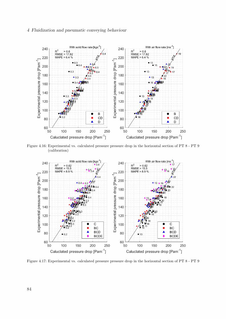
4 Fluidization and pneumatic conveying behaviour
Figure 4.16: Experimental vs. calculated pressure pressure drop in the horizontal section of PT 8 - PT 9(calibration)
Figure 4.17: Experimental vs. calculated pressure pressure drop in the horizontal section of PT 8 - PT 9
84

4.2 Pneumatic conveying
. . Impact of drilling fluid towards the pneumatic conveying behaviour
When sand samples mixed with drilling fluid (premix) were pneumatically conveyed, theydisplayed a different pressure drop compared to the dry condition at a particular air andsolid flow rate. The pneumatic conveying state diagrams of the sand mixture CD at dif-ferent premix concentrations are compared in the Figure 4.18. The pneumatic conveyingstate diagrams corresponding to other sand mixtures are given in the Appendix G.
According to the Figure 4.18, it can be clearly seen that when a drilling fluid is mixedwith the dry particles there is a considerable reduction in the pressure drop at a particularair flow rate and a solid flow rate compared to the dry conditions. However, there is nosignificant difference between the pressure drop at the drilling fluid concentrations of1.5% and 6.3%. When the drilling fluid concentration is increased upto 10%, the pressuredrop increases compared to the pressure drop at the drilling fluid concentration of 6.3%.A similar behaviour can be observed for the other sand mixtures for the drilling fluidconcentrations of 1.5% and 6.3%. It can be also seen that the shape of the state diagramsare not affected by the presence of drilling fluid at the drilling fluid concentrations of1.5% and 6.3% and the state diagrams suggest that the sand-drilling fluid mixtures areconveyed in the dilute phase under the considered air and solid flow rates.
The impact of the drilling fluid towards the horizontal pneumatic conveying pressuredrop displays a behaviour similar to the change of minimum fluidization velocity withdrilling fluid concentration. Therefore, it is interesting to compare the pressure dropratio, minimum fluidization velocity ratio and the bulk density ratio of a particular solid-drilling fluid mixture with the same drilling fluid concentration at a particular air andsolid flow rate. The pressure drop ratio, bulk density ratio and the minimum fluidizationvelocity (MFV) ratio are defined as follows,
Pressure drop ratio =Pressure drop o f a sand +drilling f luid mixture
Pressure drop o f the same sand mixture at dry conditions(4.3)
Bulk density ratio =Bulk density o f a sand +drilling f luid mixture
Bulk density o f the same sand mixture at dry conditions(4.4)
MFV ratio =MFV o f a sand +drilling f luid mixture
MFV o f the same sand mixture at dry conditions(4.5)
The Figure 4.19 compares the variation of actual pressure drop at air flow rate of 400Nm3hr−1 at different solid flow rates and drilling fluids concentrations for the sand mixtureof CD. The same figure compares the pressure drop ratio, minimum fluidization ratio andthe bulk density ratio for the same sand-drilling fluid mixture.
85

4 Fluidization and pneumatic conveying behaviour
Figure 4.18: Pneumatic conveying state diagrams for CD for the section of PT 8 - PT -9 at differentdrilling fluid concentrations
The actual pressure drop for the other sand-drilling fluid mixtures at different air flowrates and solid flow rates are presented in the Figures from H.1 to H.15 (for the horizontalsection of PT 8 - PT 9) in the Appendix H. The pressure drop ratio, minimum fluidizationvelocity ratio and the bulk density ratio of a particular solid-drilling fluid mixture at acertain air and solid flow rate are also compared in these figures.
The Figures from H.1 to H.15 show that both dry and wet samples have a higherpressure drop at higher air flow rates and at higher solid flow rates. All the consideredmixtures with 1.5% of drilling fluid (premix) display a reduced pressure drop compared tothe dry conditions. When thd drilling fluid concentration is increased up to 6.3%, BCDmixtures display a slight increasement in the pressure drop and the BCDE mixturesdisplay a higher increasement in the pressure drop while the CD mixtures display aslightly reduced pressure drop. However, for all the sand mixtures the pressure drop atthe drilling fluid concentration of 6.3% is less than the pressure drop corresponding to dryconditions. Pneumatic conveying tests for 10% of drilling fluid were conducted for the
86

4.2 Pneumatic conveying
Figure 4.19: Pressure drop vs. drilling fluid concentration for the mixture CD at air flow of 400 Nm3hr−1
CD mixture and it displayed a significant increasement of the pressure drop compared tothe pressure drop at 6.3% of drilling fluid and for most of samples with 10% drilling fluiddisplay a pressure drop higher than the dry conditions.
Based on the Figures from H.1 to H.15 it can be observed that the pressure drop ratioof a particular sand-drilling fluid mixture at a certain drilling fluid concentration remainsrelatively at a constant value with changing air and solid flow rates. When comparingthe pressure drop ratio with the bulk density ratio and the minimum fluidization velocityratio it can be observed that the pressure drop ratio in the BC and BCD mixtures areclosely related to the bulk density ratio except for the BCD mixtures at air flow rateof 250 Nm3hr−1. On the other hand the pressure drop ratio of the mixtures of CDand BCDE display a close relationship with the reciprocal of the minimum fluidizationvelocity ratio.
. . Correlation to predict the pneumatic conveying pressure drop of the
sand-drilling fluid mixtures
Based on the results it can be seen that the deviation of the pressure drop of a particularsand-drilling fluid mixture with respect to its dry condition is closely related to eitherbulk density ratio or the minimum fluidization velocity ratio. The model presented by
87

4 Fluidization and pneumatic conveying behaviour
the Equation 4.2 and the Table 4.2 can be used to estimate the pressure drop of thehorizontal pneumatic conveying dry material. Therefore, it is interesting to incorporatethe bulk density and the minimum fluidization velocity ratios in the model to predict thepressure drop of the pneumatic conveying of sand-drilling fluid mixtures. Initially theprediction capability of the proposed model is studied without any modification as thebulk density of the mixture is already a parameter in the Equation 4.2. The experimentalvs. the calculated pressure drop value based on the model for the sand-drilling fluidmixtures are presented in the Figure 4.20.
Figure 4.20: Pressure drop vs. drilling fluid concentration for the mixture BC at air flow of 250 Nm3hr−1
According to the Figure 4.20, it can be seen that except for the CD mixtures with 10%drilling fluid all the pressure drop for all the other mixtures are over predicted by themodel. Since the dry mixture of CD was used to calibrate the model and as the CD with10% drilling fluid mixtures have a pressure drop closer to dry conditions, the pressuredrop for those mixtures are estimated with a good accuracy. Therefore, the bulk densityterm in the Equation 4.2 is not adequate to estimate the pressure drop of the mixtureswith drilling fluids and the model has to be adjusted to suit the pneumatic conveyingof wet mixtures. Since the pressure drop reduction of the sand-drilling fluid mixturesare closely associated with the reciprocal of the minimum fluidization velocity ratio, themodel can be modified as follows,
88

4.2 Pneumatic conveying
λt = (1.55×10¹³)um f
um f ,dryη−0.34Fr−1.18
(dspan
D
)0.328(ρg
ρbulk
)4.025
(4.6)
The experimental vs. the calculated pressure drop based on the Equation 4.6 are presentedin the Figure 4.21. The model can be further improved by raising the minimum fluidizationvelocity ratio by a factor which has to be estimated by calibrating with experimentaldata. Since there are not enough data to calibrate and validate such a model, no furthermodification is done to the proposed model.
Figure 4.21: Pressure drop vs. drilling fluid concentration for the mixture BC at air flow of 250 Nm3hr−1
The comparison of the estimated values presented in the Figure 4.21 with the values in theFigure 4.20, it can be seen that the modified model has an improved prediction capability.The mean absolute error percentage has been reduced down to 35.3%
. . Summary
Under the considered regions of the superficial air velocities (10 - 22 ms−1) and the solidflow rates (0.2 - 0.4 kgs −1), dry sand mixtures were conveyed in dilute phase in the pneu-matic conveying experimental rig where the pipe diameter is 8.12 cm. When a drillingfluid is mixed with the sand mixtures, the pneumatic conveying pressure drop reduces
89

4 Fluidization and pneumatic conveying behaviour
relative to the pneumatic conveying pressure drop of the dry sand mixture. The devi-ation of pneumatic conveying pressure drop with the drilling fluid concentration display asimilar behaviour as the deviation of the minimum fluidization velocity with the drillingfluid concentration. Therefore the change in the minimum fluidization velocity can beincorporated into a model to predict the pressure drop of pneumatic conveying of wetparticles.
. Discussion
Based on the fluidization and pneumatic conveying tests it can be concluded that theparticles mixed with a drilling fluid exhibits a significantly deviated behaviour with respectto the dry particles. Basically the minimum fluidization velocity is increased and thepneumatic conveying pressure drop is decreased when drilling fluid is introduced to thedry particles. Since the drilling fluid has a lubricating effect, it lubricates the particlesurface and the wall of the pipe. Then the friction between the air and particles and thefriction between the wall and the particles reduce. As a result, in fluidization, air streamscan penetrate through the bed more easily and hence higher air velocity is required tocreate a pressure drop equal to the weight of the bed. In pneumatic conveying, thepressure losses due to friction is reduces and as a result the pressure drop is reduced formixtures with drilling fluid. However this phenomenon is valid only for low concentrationsof drilling fluids, where the amount of drilling fluids are adequate to form a thin film ofdrilling fluid on the particles’ surface. When the drilling fluid concentration is increasedbeyond a certain limit, drilling fluid tends to separate from the solids and accumulatein the voids. This was seen in the fluidization tests of 10% of drilling fluid. Underthese conditions the behaviour of the sand-drilling fluid mixtures deviate from the lowconcentration mixtures. Since the voids are filled with drilling fluid, air cannot penetratethrough the bed and as a result the minimum fluidization velocity will be reduced. Atthe same time as the mixture starts to behave more like a slurry, pneumatic conveyingcause higher pressure drop.
According to Mills [55] wet or damped material can be conveyed pneumatically but thechallenge is to feed them to the pipelines and to discharge from the hopper. If the materialcontains fine particles, wetness can be a challenge in pneumatically conveying systems asthey tend to coat the pipeline and finally causing blockages. If the material is not so wet,hot air flow can be used to overcome the issue of wetness. Otherwise single plug blowtank systems have to be adopted in handling wet material. However, Hollier and Reddoch[56] claim that they have implemented a vacuum conveying system to convey the wet drillcuttings successfully.
When considering the drill cuttings, particle size distribution is a important parameter asit tends to differ from one location to another in the drilling well. The study shows that
90

4.3 Discussion
conducting few pneumatic conveying tests of a dry sample with samples with same physicalproperties but with different particle size distributions, a reasonably good model can bedeveloped to predict the pressure drop of horizontal pneumatic conveying under dilutephase for the mixtures with different particle size distributions. It was also observed thatthe pressured drop reduction in the pneumatic conveying and the minimum fluidizationvelocity reduction in the fluidization tests can be also correlated. Therefore, this studyshows that a combination of pneumatic conveying of dry particles and the fluidization ofparticles mixed with drilling fluid can be used to develop a model to estimate the pressuredrop in pneumatic conveying of particles mixed with drilling fluids.
91

92

Flow properties of sand - drilling fluid
mixtures
In this chapter the flow properties of the sand - drilling fluid mixtures are analysed withvaring drilling drilling fluid concentrations. According to the Section 3.4 , the shear testswere conducted for the CD sand mixture. The sand - fluid samples were prepared withpremix, base oil, water and a soap mixture with concentrations of 10%, 20%, 30% and 40%(by volume). The analysis is conducted for both axial symmetric and plane symmetricsilos and the basic geometrical shape of those two silos are given in the Figure 5.1.
Figure 5.1: Plane and axial symmetric silos [49]
. Wall friction and the hopper angle
The friction between the bulk solid and the hopper wall is represented by the wall frictionangle. The wall friction angle between the experimental sand - fluid samples and thehopper wall are presented in the Figure 5.2 . The considered wall material is stainlesssteel.
Except for water, the other mixtures does not display a significant deviation from the dryconditions at low fluid concentrations (10% vol.). The wall friction angle of the premix
93

5 Flow properties of sand - drilling fluid mixtures
Figure 5.2: Wall friction angle vs. fluid concentration
samples reduces with increasing fluid concentration and reaches a minim at 30% of fluid.The wall friction angles of the base oil and soap mixtures start to reduce at 20% offluid levels and reach a minimum at the concentration of 30% of fluid. Beyond 30% offluid, the mixtures of premix, base oil and soap tend to have a increasing wall frictionangle until a fluid concentration of 40%. The Figure 5.2 clearly shows that the behaviourof the sand-water mixtures are significantly different from the rest of the mixtures atlow concentrations. The mixture with 10% of water has the highest wall friction angleand with increasing water concentration, the wall friction angle reduces dramatically andreaches a minimum at 20% of water. Beyond that the sand-water mixtures have a similarbehaviour as rest of the mixtures.
The wall friction angle directly affects the hopper angle. The hopper angle of the con-sidered mixtures are given for both axial and plane symmetric hoppers in the Figure 5.3.
The Figure 5.3 shows that the hopper angles of both silo types are inversely proportionalto the wall friction angle. A large wall friction angle indicates a higher friction betweenthe bulk solid and the hopper wall. Therefore, the flowability of the bulk solid decreaseswith increasing wall friction angle. A bulk solid with a high wall friction angle whichindicates a low flowability requires a small hopper angle to ensure to have a massflow silo.Hence the sand mixtures of premix, base oil and soap have the highest flowability at 30%of fluid with the minimum wall friction angle and highest hopper angle. According to thethe Figure 5.3 it can be seen that the hopper angle vs. fluid concentration profiles of thetwo silo types have the same shape but the hopper angle of a plane symmetric silo is largerthan the hopper angle of an axial symmetric silo at a particular fluid concentration.
Based on the Figures of 5.2 and 5.3, it can be seen that at 10% fluid concentration,the sand-premix mixture has a slightly better flowability compared to the sand-base oil
94

5.2 Effective angle of internal friction (δ)
Figure 5.3: Hopper angle vs. fluid concentration
mixture. However, beyond the fluid concentration of 20% the sand-base oil mixtures havea better flowability compared to the sand-premix mixtures. It is also interesting observethat the behaviour of the sand-soap mixture is similar to the sand-base oil mixturesbeyond the fluid concentration of 20%.
. Effective angle of internal friction (δ)
The effective angle of internal friction (δ) which is described under the Figure 2.5 in theSection 2.3.1 is plotted for the considered mixtures in the Figure 5.4.
As described in the Section 2.3.1, the effective angle of internal friction represents theresistance to the flow when the bulk solid is in flowing conditions. The angle increaseswith decreasing flowability of the material. There is no significant difference between theinternal friction angle of the base oil and soap mixtures at 10% of fluid when comparedto the dry conditions. Both base oil and soap mixtures display a gradual increase ofeffective angle of internal friction until the 20% of fluid and start to decrease with furtherincreasing fluid concentration and reach a minim angle at 30% of fluid. Similar to thewall friction and hopper angle plots, base oil and soap mixtures have a similar profileof effective angle of internal friction vs. fluid concentration. The sand-premix mixturedisplay a significant reduction of the internal friction angle at 10% of fluid, with respectto the dry conditions and beyond that the effective angle of internal friction is decreasingwith increasing drilling fluid concentration. The sand-water mixtures have the highestangle of internal friction at 10% of water and the minimum angle at 20% of water. With
95

5 Flow properties of sand - drilling fluid mixtures
Figure 5.4: Effective angle of internal friction vs. fluid concentration
further increment of water concentration, the effective angle of internal friction tends toincrease gradually.
. Flow function and the flowability
The flow function (FF) which gives the relationship between the unconfined yield strength( fc) and the major consolidation stress (σ1) for the considered sand-fluid mixtures aregiven in the Figure 5.5.
Schulze[49] describe a numerical method to represent the flowability of a bulk solid mixtureand it is given by,
f lowability ( f fc) =σ1
fc(5.1)
The lines of constant flowability are also plotted in the Figure 5.5. These constant flow-ability lines can be used to describe the boundaries of different flowing conditions [49].
• f fc < 1 : not flowing
• 1 < f fc < 2 : very cohesive
• 2 < f fc < 4 : cohesive
96

5.3 Flow function and the flowability
• 4 < f fc < 10: easy-flowing
• 10 < f fc : free-flowing
Figure 5.5: Instantaneous flow function vs. fluid concentration
According to this plot, the dry sand sample is a free flowing material as its flow functionlies parallel to the f fc = 10 line. All the sand-fluid mixtures except for the sand -baseoil mixture at 40%, have a higher unconfined yield strength than the dry sample at agiven major consolidation stress. The premix and the base oil mixtures with 10% ofliquid display a slight reduction in the flow function with respect to the dry conditions.
97

5 Flow properties of sand - drilling fluid mixtures
The flow functions of the both drilling fluid mixtures significantly increase when the liquidconcentration is increased up to 20%. However, the flow function of the mixtures decreaseas the unconfined yield strength corresponding to 30% of fluid is reduced compared to the20% of fluid. At 40% of concentrations both mixtures further decrease their flow functions.The plots also show that at a given fluid concentration, the sand-premix mixtures havea higher unconfined yield strength. The sand-soap mixture display a similar behaviouruntil the fluid concentration of 30%. Both the drilling fluid mixtures of 20% concentrationlies in the no-flow/very cohesive flow region. The 10% and the 40% mixtures of bothdrill fluids lies in the region of easy-flowing region. The sand-premix mixture at 30%concentrations mainly display cohesive behaviour while the 30% of the base oil mixturedisplay an easy-flowing/cohesive behaviour.
The flow function of the sand-soap mixture at 40% of fluid is significantly increased andwhen conducting the tests it was observed that some foam was formed at higher soapconcentrations. The sand-water mixtures behave rather differently when compared to theother mixtures. It shows a high flow function at 10% of water and at 20% of water theflow function reduces. The experimental results show that sand-water mixtures have thehighest flow function at 30% of water. The 30% of water mixture is basically in a no flowcondition while the 10% mixture displays a high cohesive features.
. Size of the hopper opening
Based on the results obtained from the Jenike shear test, the size of the hopper openingwas calculated by using the silo designing software at SINTEF-Tel-Tek. The calculatedhopper opening dimensions for both axial symmetric and plane symmetric hoppers aregiven in the Figure 5.6.
For both premix and base oil mixtures, the highest opening size is required at 20% ofliquid concentration. The reason for this is that the both drilling fluid mixtures displaythe lowest flowability at the concentration of 20%. Similarly sand-water mixture whichhas the lowest flowability at 30% of water, requires the largest opening at 30% of water.Some mixtures such as 10% of base oil display a minimum opening of 0 cm which impliesthat at any opening size, a massflow discharge pattern can be obtained. However, as arule of thumb the diameter of the opening should be 10 times the diameter of the largestparticle in the bulk solid. Since the mixture CD’s largest particle size is 2.5 mm, theminimum required diameter of the opening is 2.5 cm. Therefore, if the calculation resultsa diameter less than 2.5 cm, the required hopper opening dimension should be taken as2.5 cm.
98

5.5 Time consolidation
Figure 5.6: Hopper opening dimension [cm] vs. fluid concentration
. Time consolidation
The flow functions obtained from the 7 days time consolidation tests are given in theFigure 5.7.
When compared to the Figure 5.5, which illustrate the instantaneous flow functions, itcan be clearly seen that the flowability of all the mixtures have been reduced after 7 daysof consolidation. No mixture lies in the regions of free flowing or easy-flowing. Almost allthe mixtures display either no-flow or very cohesive flow features. For the sand-premixmixtures the lowest flowability is displayed at 20% of fluid while the sand-base oil andsand-water mixtures display the lowest flowability at 30% of liquid.
The hopper opening size of the considered samples after 7 days consolidation is given inthe Figure 5.8.
It can be clearly seen that the required minimum opening size of the hopper after 7 daysof consolidation has been increased compared to the required opening at instantaneousconditions. The sand-premix mixture requires the largest opening size at 20% of fluidconcentration while the sand-base oil and sand -water mixtures require the highest openingsize at 30% of fluid concentration. The sand-soap mixture displays significantly largeopening size at 40% of fluid level but it displays a similar behaviour as sand-base oilmixtures in the region of fluid levels of 10% - 30%
99

5 Flow properties of sand - drilling fluid mixtures
Figure 5.7: Instantaneous flow function vs. fluid concentration
. Discussion
This study basically concerns about the impact of the drilling fluid towards the storageand the flowability of a bulk solid material. Based on the results, it can be clearly seenthat the flowability of the considered sand mixture of CD is reduced with respect toits dry state when it is mixed with a liquid. The main reason for this phenomenon isthe increase of inter-particle forces within the bulk solid due to the formation of liquid
100

5.6 Discussion
Figure 5.8: Hopper opening dimension [cm] (time consolidation) vs. fluid concentration
bridges. It is also observed that the level of flowability depends on the type of the fluid, fluid concentration and the time period which the bulk solid has been subjected to aconsolidation stress.
Fluid concentration
The flowability of the sand-fluid mixtures are basically studied based on their flow func-tions. Under the instantaneous conditions the flowability is associated with the effectiveangle of internal friction. The lowest flowability is obtained at the fluid concentrationwhere the effective angle of internal friction is the highest.
Both premix and base oil mixtures have the lowest flowability at 20% of fluid concentrationat instantaneous conditions. After 7 days of consolidation, the sand-premix mixturehas the lowest flowability at 20% of fluid and the sand-base oil mixture has the lowestflowability at 30% of fluid. The sand-soap mixture also has the lowest flowability at40% fluid content under both instantaneous and 7 days time consolidation conditions.Since some foam was started to be formed beyond the soap concentration of 30%, theflowability at 40% of soap cannot be compared with the other mixtures. If the sand-soapmixture at 40% fluid content is considered as an outlier, the sand-soap mixtures have
101

5 Flow properties of sand - drilling fluid mixtures
the lowest flowability at 20% and 30% fluid concentrations under instantaneous and 7days time consolidation conditions respectively. Contrary to these mixtures, sand-watermixtures display the largest effective angle of internal friction at 10% of water. Whenconsidering the flowability, the lowest flowability occurs at 30% of water but contrast tothe other mixtures, sand-water mixture at 10% fluid content has a lower flowability thanthe sand-water mixture at 20% of water.
The fluctuation of the flowability with the fluid concentration can be described by theformation of liquid bridges. When a fluid is introduced in to a bulk solid, liquid bridgesstart to form and the inter-particle forces increase. With increasing fluid concentration,number of individual liquid bridges increase and the forces between the particles increase.As a result the flowability of the solid-liquid mixture is reduced. When the voidagesstarts to be filled with the fluid, the individual liquid bridges are diminished and a slurryis formed gradually. Beyond the liquid level where the individual liquid bridges start todiminish, the quantity of the inter-particle forces reduce. Therefore, the flowability willbe increased beyond that fluid concentration.
Type of fluid
When comparing the sand-premix and sand-base oil mixtures, the sand-premix mixtureshave a low flowability but the profile of the flow parameters with fluid concentration issimilar under instantaneous conditions. The purpose of conducting tests with soap andwater was to study the possibility of replacing the drilling fluid with a non-hazardous,easily available fluid to conduct laboratory test. It can be seen that sand-water mix-tures significantly deviate from the sand-drilling fluid mixtures. The sand-water mixturesdisplay a very low flowability when compared to the drilling fluid mixtures. This phe-nomenon justifies the reason for not adding sea water to drill cuttings when it get stuckin the screw conveyors. However in the fluid concentration level of 10% - 30%, the soapmixture display a similar behaviour as the sand - base oil mixture.
The flowability of the sand-water mixtures are significantly low compared to the othermixtures. The reason for that is water tends to form liquid bridges more easily. In a soapmixture, the surface tension is reduced and as a result there is a lubrication effect. Thislubrication effect reduces the inter-particle friction forces. Therefore, drilling fluid andsoap mixtures have a better flowability compared to the sand-water mixtures.
Time consolidation
The study shows that the time consolidation has reduced the flowability of the all themixtures significantly. The mixtures having a easy-flowing or cohesive flowing underinstantaneous conditions are transformed into cohesive or very cohesive flow after beingsubjected to time consolidation With time the inter-particle forces increase and as a resultof that the flowability reduces. Therefore, the designing should be based on the results oftime consolidation tests.
102

5.6 Discussion
Wall friction angle
Even though the addition of drilling fluid has reduced the flowability of the sand mixture,the friction between the bulk solid and the silo wall has been reduced due to the presenceof drilling fluid. The sand-drilling fluid mixtures display the lowest wall friction angle at30% of fluid and under that condition the required hopper angle will be maximum. Thereduction of the wall friction occurs due to lubrication effect of the fluids. A fluid layerformed on the wall of the silo reduces the friction forces between the bulk solid and thehopper wall. It can be also seen that the wall friction is significantly increased at 10% ofwater concentration. This increase of wall friction occurs due to the formation of liquidbridges but with increasing water content the individual liquid bridges diminish and thewall-particle forces reduce.
Size of the hopper opening
The required minimum opening size of the silos becomes larger as the flowability reduces.Therefore, both sand-drilling fluid mixtures have the largest opening size at the lowestflowability conditions. The study also shows that the time consolidation has reducedthe flowability of the sand-drilling fluid mixtures significantly. Therefore, the designingshould be based on the results of time consolidation tests.
Practical applications
When considering the practical applications it can be concluded that it will not be feasibleto store sand-drilling fluid mixtures with fluid concentrations of 10%-30% (vol.). It iseither better to have sand-drilling fluid mixtures with fluid concentration less than 10%or higher than 40%. The sand-drilling fluid mixtures with 40% of fluid display betterflowability due to its slurry like nature and it will be difficult to be conveyed even thoughit can be discharged from the silo easily. Eventhough the mass flow design can over comethe forming of arches and rat holing, the capacity of the silo is reduced due to the highangle conical bottom. Therefore, the potential of using silos with higher capacities (whichare not mass flow silos) has to be considered as the space available for storage of drillcuttings in a drilling platform is a critical factor. These alternative silo designs should beassisted by mechanical systems such as internal agitators or screw type augers. It shouldbe noted that such silos are more complex in design, expensive and have a potential formechanical failure. A novel design with multiple outlets knwon as the ’Honey comb basetank’ has been developed by Halliburton. In this design, compressed air is applied to thetop of the silo to push the drill cuttings and another air stream is injected to the baseof the tank to mechanically breakup and fluidize the cuttings. Therefore, no additionalmechanical agitation system is required [57].
103

104

Conclusion
As discussed in Chapter 1, the objective of this research was to study the influence ofdrilling fluids towards the pneumatic conveying and storage of wet particles to illustrateoffshore drill cutting handling. The basic findings of the study can be presented underfluidization and pneumatic conveying of wet particles and the storage of wet particles.
. Fluidization and pneumatic conveying of wet particles
Based on the experiments, it can be concluded that the presence of drilling fluid hasa significant impact towards the fluidization and pneumatic conveying behaviour of theconsidered sand mixtures. When a small amount of drilling fluid (about 1.5% by weight)is mixed with a sand mixture, both the minimum fluidization velocity and the pressuredrop in pneumatic conveying is reduced when compared to the fluidization and pneumaticconveying behaviour of the dry mixtures. The reduction of the minimum fluidizationvelocity and the pneumatic conveying pressure drop suggest that the presence of drillingfluid in a sand mixture acts as a lubricating agent. As a thin layer of drilling fluid isformed on the surface of the particles, the air-particle, particle-particle and particle-wallfrictions are reduced. However, it was also observed that the gradual increment of thedrilling fluid concentration does not affect the change of either the minimum fluidizationvelocity or the pneumatic conveying pressure drop until reaching a certain drilling fluidconcentration (approximately 6-10 % by weight). Beyond that concentration limit thedrilling fluid tends to get separated from the sand mixtures.
The study shows that an empirical model can be developed to predict the pressure dropin horizontal pneumatic conveying under dilute phase for dry particles. It is also observedthat the change of the minimum fluidization velocity, change of the bulk density and thechange of the pneumatic conveying pressure drop due to the presence of drilling fluid areclosely correlated. Hence by incorporating the change of minimum fluidization velocityfactor to the pneumatic conveying pressure drop model, the pressure drop of the sand -drilling fluid mixtures could be predicted approximately. Therefore, it can be concludedthat by conducting pneumatic conveying tests for dry mixtures and fluidization tests forparticle - drilling fluid mixtures, a model can be developed to predict the pneumaticconveying pressure drop of the particle - drilling fluid mixtures.
105

6 Conclusion
. Storage of wet particles
The study also shows that by conducting a proper bulk solid shear tests, both the impactof the drilling fluid towards the flow properties of the sand - mixtures and the designparameter for the storage silos can be estimated. It was observed that the presence ofdrilling fluid reduced the flowability of the bulk mixtures compared to the dry conditions.However, with increasing drilling fluid concentration flowability improves as the drillingfluid tends to lubricate the flow. The flowability depends on the fluid concentration, typeof the fluid and the amount of time consolidation.
The Jenike shear test clearly shows that the consolidation for 7 days significantly reducesthe flowability of the bulk solid compared to the instantaneous conditions. Therefore,when designing storage tanks the time period which the solids are to be stored in plays avital role. The study also shows that, presence of water reduces flowability compared tothe presence of drilling fluid. This shows the importance of not to add water to the drillcuttings during offshore handling. The use of soap mixture display a relatively similarbehaviour as the drilling fluids which suggests that it is possible to use a soap mixturewhich is a non-hazardous solution to replicate drilling fluids in lab scale shear tests.
. Recommendations
• This research study basically studies the impact of the drilling fluid concentrationtowards the pneumatic conveying and storage of particles relative to its dry condi-tions. The study can be further extended by conducting experiments with differentdrilling fluid types and different solid materials. It would be interesting to conductpneumatic conveying tests for different drill cuttings samples. These test can beused to develop a more comprehensive model based on the findings of this study.
• It is also recommended to utilize the experimental data obtained from fluidizationand pneumatic conveying tests in CFD simulations to predict the pressure drop andflow behaviour.
• It would be interesting to study the impact of the type and the amount of drillingfluids towards the interparticle forces.
• Process analytical technologies are recommended to be utilized for the online meas-urements of the particle size and the drilling fluid concentrations.
106

Bibliography
[1] U. S. E. I. Administration, Ed. (2016). Offshore production nearly 30% of globalcrude oil output in 2015, [Online]. Available: https://www.eia.gov/todayinenergy/detail.php?id=28492.
[2] J. Neff, “Fate and effects of water based drilling muds and cuttings in cold water en-vironments”, Houston (TX): Report to Shell Exploration and Production Company,2010.
[3] M. Holmager, Offshorebook: An Introduction to the Offshore Industry. Offshore Cen-ter Danmark, 2010.
[4] IOGP, “Drilling waste management technology review, iogp report 557”, Interna-tional Association of Gas & Oil Producers, 2016.
[5] Norskolje&gass, “Environmental report 2016 - environmental work by the oil and gasindustry facts and dvelopment trends”, The Norwegian Oil and Gaas Association,2017.
[6] J. Hartley, R. Trueman, S. Anderson, J. Neff, P. Dando and K. Fucik, “Drill cuttingsinitiative, food chain effects literature review”, United Kingdom Offshore OperatorsAssociation (UKOOA), 2003.
[7] R. Caenn, H. Darley and G. R. Gray, “Drilling and drilling fluids waste manage-ment”, in Composition and Properties of Drilling and Completion Fluids (SixthEdition). 2011.
[8] T. Svensen and K. Taugbol, “Drilling waste handling in challenging offshore op-erations”, in SPE Arctic and Extreme Environments Conference and Exhibition,Society of Petroleum Engineers, 2011.
[9] F. J. Santarelli, F. Sanfilippo, R. W. James, H. H. Nielsen, M. Fidan, G. T. Aamodtet al., “Injection in shale: Review of 15 years experience on the norwegian continentalshelf (ncs) and implications for the stimulation of unconventional reservoirs”, in SPEAnnual Technical Conference and Exhibition, Society of Petroleum Engineers, 2014.
[10] A. Saasen, K. Jodestol and E. Furuholt, “CO2 and NOx emissions from cuttingshandling operations”, in SPE Bergen One Day Seminar, Society of Petroleum En-gineers, 2014.
107

Bibliography
[11] S. Onwukwe and M. Nwakaudu, “Drilling wastes generation and management ap-proach”, International Journal of Environmental Science and Development, vol. 3,no. 3, p. 252, 2012.
[12] M. Mkpaoro, G. Okpokwasili, O. Joel et al., “A review of drill-cuttings treatmentand disposal methods in nigeria-the gaps and way forward”, in SPE Nigeria AnnualInternational Conference and Exhibition, Society of Petroleum Engineers, 2015.
[13] A. S. Ball, R. J. Stewart and K. Schliephake, “A review of the current options forthe treatment and safe disposal of drill cuttings”, Waste Management & Research,vol. 30, no. 5, pp. 457–473, 2012.
[14] D. Schonacher, J. Rojas, J. Gharst and B. Paiuk, “Meeting zero discharge re-quirements in the gulf of mexico using a unique cuttings transport system”, inSPE/EPA/DOE Exploration and Production Environmental Conference, Society ofPetroleum Engineers, 2003.
[15] A. Alba Rodriguez, F. E. Fragachan, A. Ovalle and T. A. Shokanov, “Environment-ally safe waste disposal: The integration of cutting collection, transportation andre-injection”, in International Oil Conference and Exhibition in Mexico, Society ofPetroleum Engineers, 2007.
[16] D. Kunii and O. Levenspiel, Fluidization engineering. Elsevier, 2013.[17] J. Richardson, J. Harker and J. Backhurst, “Fluidization”, in Coulson & Richard-
son’s Chemical Engineering Vol 2. Elsevier, 2008, ch. 6.[18] D. Gidaspow, Multiphase flow and fluidization: continuum and kinetic theory de-
scriptions. Academic press, 1994.[19] C. Wen and Y. Yu, “A generalized method for predicting the minimum fluidization
velocity”, AIChE Journal, vol. 12, no. 3, pp. 610–612, 1966.[20] J. Richardson, “Incipient fluidization and particulate systems”, Fluidization, vol. 2,
1971.[21] S. Saxena and G. Vogel, “The measurement of incipient fluidization velocities in
a bed of coarse dolomite at temperature and pressure”, Trans. Inst. Chem. Eng,vol. 55, no. 3, pp. 184–189, 1977.
[22] S. Babu, B. Shah and A. Talwalkar, “Fluidization correlations for coal gasifica-tion materials-minimum fluidization velocity and fluidized bed expansion ratio”, inAIChE Symp. Ser, vol. 74, 1978, pp. 176–186.
[23] J. Grace, “Fluidized bed hydrodynamics”, in Handbook of Multiphase Flow. Hemi-sphere, Washington, DC, 1982, ch. 8.1.
[24] D. C. Chitester, R. M. Kornosky, L.-S. Fan and J. P. Danko, “Characteristics offluidization at high pressure”, Chemical Engineering Science, vol. 39, no. 2, pp. 253–261, 1984.
108

Bibliography
[25] M. G. Jones and K. C. Williams, “Predicting the mode of flow in pneumatic con-veying systems—a review”, Particuology, vol. 6, no. 5, pp. 289–300, 2008.
[26] S. Shaul, E. Rabinovich and H. Kalman, “Typical fluidization characteristics forgeldart’s classification groups”, Particulate Science and Technology, vol. 32, no. 2,pp. 197–205, 2014.
[27] O. Molerus, “Interpretation of geldart’s type a, b, c and d powders by taking intoaccount interparticle cohesion forces”, Powder technology, vol. 33, no. 1, pp. 81–87,1982.
[28] J. Seville and R. Clift, “The effect of thin liquid layers on fluidisation characterist-ics”, Powder Technology, vol. 37, no. 1, pp. 117–129, 1984.
[29] L. J. McLaughlin and M. J. Rhodes, “Prediction of fluidized bed behaviour in thepresence of liquid bridges”, Powder Technology, vol. 114, no. 1, pp. 213–223, 2001.
[30] P. Wright and J. A. Raper, “Role of liquid bridge forces in cohesive fluidization”,Chemical Engineering Research and Design, vol. 76, no. 6, pp. 753–760, 1998.
[31] M. Hartman, O. Trnka and M. Pohořelý, “M. hartman, o. trnka, and m. pohořelý:Fluidization behavior of oil-contaminated sand”, vol. 61, pp. 236–236, Jun. 2007.
[32] O. Molerus, “Overview: Pneumatic transport of solids”, Powder technology, vol. 88,no. 3, pp. 309–321, 1996.
[33] G. E. Klinzing, “Challenges in pneumatic conveying”, KONA Powder and ParticleJournal, vol. 18, pp. 81–87, 2000.
[34] D. Mills, Pneumatic conveying design guide. Butterworth-Heinemann, 2003.[35] G. E. Klinzing, F. Rizk, R. Marcus and L. Leung, Pneumatic conveying of solids: a
theoretical and practical approach. Springer Science & Business Media, 2011, vol. 8.[36] R. Naveh, N. M. Tripathi and H. Kalman, “Experimental pressure drop analysis for
horizontal dilute phase particle-fluid flows”, Powder Technology, vol. 321, pp. 355–368, 2017.
[37] G. O. Brown, “The history of the darcy-weisbach equation for pipe flow resistance”,in Environmental and Water Resources History, 2003, pp. 34–43.
[38] H. Konno and S. Saito, “Pneumatic conveying of solids through straight pipes”,Journal of Chemical Engineering of Japan, vol. 2, no. 2, pp. 211–217, 1969.
[39] E. Rabinovich and H. Kalman, “Boundary saltation and minimum pressure velocit-ies in particle–gas systems”, Powder Technology, vol. 185, no. 1, pp. 67–79, 2008.
[40] G. Szikszay, “Friction factor for dilute phase pneumatic conveying”, Bulk SolidsHandling, vol. 8, no. 4, pp. 395–399, 1988.
[41] W. Wei, G. Qingliang, Z. Jiansheng and Y. Hairui, “A modified correlation to calcu-late solid friction factor for horizontal dilute phase pneumatic conveying”, Powdertechnology, vol. 218, pp. 64–68, 2012.
109

Bibliography
[42] H. Raheman and V. Jindal, “Pressure drop gradient and solid friction factor inhorizontal pneumatic conveying of agricultural grains”, Applied Engineering in Ag-riculture, vol. 17, no. 5, p. 649, 2001.
[43] L. C., Z. C.‐S., C. X.‐P., P. W.‐H., L. P. and F. C.‐L., “Flow characteristics andshannon entropy analysis of dense‐phase pneumatic conveying of pulverized coalwith variable moisture content at high pressure”, Chemical Engineering & Techno-logy, vol. 30, no. 7, pp. 926–931, 2007.
[44] “Effect of moisture content on conveying characteristics of pulverized coal for pres-surized entrained flow gasification”, Experimental Thermal and Fluid Science, vol. 35,no. 6, pp. 1143–1150, 2011.
[45] T. Sheer, “Dense-phase pneumatic conveying of slush ice through plastic pipes”,Particulate Science and Technology, vol. 26, no. 3, pp. 273–284, 2008.
[46] V. Ganesan, K. A. Rosentrater and K. Muthukumarappan, “Flowability and hand-ling characteristics of bulk solids and powders–a review with implications for ddgs”,biosystems engineering, vol. 101, no. 4, pp. 425–435, 2008.
[47] A. Jenike, “Storage and flow of solids. university of utah engineering experimentstation”, Bulletin, vol. 123, 1964.
[48] “Storage and flow of powders – hopper design”, in Introduction to Particle Techno-logy. John Wiley & Sons, 2008, ch. 10.
[49] D. Schulze, Powders and bulk solids, Behaviour, Characterization, Storage and Flow.Springer. Springer, 2008.
[50] I. Opaliński, M. Chutkowski and M. Stasiak, “Characterizing moist food-powderflowability using a jenike shear-tester”, Journal of food engineering, vol. 108, no. 1,pp. 51–58, 2012.
[51] A. S. Çağli, B. N. Deveci, C. Okutan, D. Sirkeci and E. Teoman, “Flow propertymeasurement using jenike shear cell for 7 different bulk solids”, in Proceedings ofEuropean Congress of Chemical Engineering (ECCE-6), Copenhagen, 2007, pp. 16–20.
[52] P. Pierrat, D. K. Agrawal and H. S. Caram, “Effect of moisture on the yield locus ofgranular materials: Theory of shift”, Powder Technology, vol. 99, no. 3, pp. 220–227,1998.
[53] IChemE, “Standard shear testing technique for particulate solids using the jenikeshear cell”, The Institution of Chemical Engineers, 1989.
[54] S. Shaul, E. Rabinovich and H. Kalman, “Generalized flow regime diagram of fluid-ized beds based on the height to bed diameter ratio”, Powder technology, vol. 228,pp. 264–271, 2012.
[55] D. Mills, M. G. Jones and V. K. Agarwal, Handbook of pneumatic conveying engin-eering. CRC Press, 2004.
110

Bibliography
[56] H. Hollier and J. Reddoch, “Successful optimization of advances in disposal andtreatment technologies, to cost effectively meet new oil-based cuttings environmentalregulations”, in AADE 2001 National drilling vonference, ¨Drilling Technology - Thenext 100 years¨, 2001, pp. 27–29.
[57] R. Morris and S. Seaton, “Design and testing of bulk storage tanks for drill cuttingsoffers operators safer solution in zero discharge operations”, in AADE 2006 FluidsConference, 2006.
111

112

Appendix A
Powder conveying principles for efficient
handling of offshore drill cuttings
This paper was published at the 8th International conference for conveying and handlingof particulate solids, Israel, May 2015.
113

The 8th International Conference for Conveying and Handling of Particulate Solids
Tel-Aviv, Israel, May 2015
POWDER CONVEYING PRINCIPLES FOR EFFICIENT HANDLING OF
OFFSHORE DRILL CUTTINGS
A. Malagalage1,2, C. Ratnayake1,2 and A. Saasen3,4
1. Department of POSTEC, Tel-Tek
Kjølnes ring 30, 3918 Porsgrunn, Norway
2. Telemark University College
Postboks 203, N-3901 Porsgrunn, Norway
3. Det norske oljeselskap ASA
Postboks 2070,Vika, 0125 Oslo, Norway
4. University of Stavanger
4036 Stavanger, Norway
Abstract - Drill cuttings generated by offshore drilling
operations are handled as a hazardous waste offshore. Its impact
towards the marine environment has been concerned by
different environmental regulatories. In sensitive marine
environments, the concept of zero discharge of waste is
implemented, which has emphasized the importance of having
an advanced drill cutting treating system. A typical offshore
well generates around 500-1000 tonnes of drill cuttings where
its properties such as size, shape, composition and the type of
the associated drilling fluid etc., change continuously and
sometimes unpredictably. Hence transporting drill cuttings
within the rig and from the rig to ships has become a challenge
as no proper scientific procedure has been developed to design
transportation and storage systems. Conventionally screw
conveyors, manual forces along with the skip and ship methods
have been utilized in transferring drill cuttings. As these
methods are both lacking in efficiency and are associated with
considerable health and safety issues, it has been focused on
replacing those operations by vacuum and blowing systems.
Powder technology principles have been successfully applied in
transporting and storing bulk powders such as weighting
materials and oil-well cement in offshore rigs. Therefore, it is a
potential to implement the same fundamentals in designing drill
cutting transportation and storage systems. Currently vacuum
systems are used in several offshore rigs to convey drill cuttings
from the shakers into the bulk storage tanks. From the bulk
storage tanks, cuttings are blown into the transporting vessels.
Due to the sticky nature of the cuttings, conveying and
discharging from the tanks is a challenge. Several mechanically
assisted tanks and pneumatic tanks with multiple discharge
points have been developed to overcome this issue. However the

lack of understanding of the flow properties of the drill cuttings
and their continuous changes of the properties, have caused
these systems to face frequent operational failures. This ongoing
research is focusing on characterizing the properties of the drill
cuttings and relating them with their transport characteristics. It
is necessary to control the flow behaviour of the drill cuttings
along with the amount of associated fluids with it. Based on
these relationships, it is proposed to develop a scientific method
to convey the drill cuttings pneumatically. The need for this
method is described in detail, and the basic principle of the
method is outlined in the current article.
1.INTRODUCTION
Disposal of waste, generated from drilling and completion operations in offshore rigs has
always been a challenge. These drilling wastes mainly consist of drill cuttings, drilling muds and
completion fluids. During the drilling and completion operations these residual materials have to
be transferred to the storage locations on the rig and then must be transferred to the treatment
facilities via transport vessels. Conveying of drill cuttings is a challenging task due its sticky
nature. Drill cuttings can be neither discharge into the marine environments directly nor can be
stored on the rigs due to the space limitation. Hence a new scientific study is required to
optimize the offshore drill cutting handling process.
1.1 Generation of the Drill Cuttings
Drill cuttings are the solid particles removed from the different rock layers which are
being drilled through. Isolated grains and clusters are generated when the drill bit makes contact
with the rock. These drill cuttings are carried to the surface with the drilling mud (drilling fluid)
that is being used. Drilling muds are used in drilling operations to control the pressure within the
wellbore, to cool down the drill bit and also to remove the drill cuttings from the wellbore.
According to Caenn [1], three types of drilling muds are used which can be classified as, Water
Based Muds (WBM), Oil Based Muds (OBM) and sometimes Synthetic Oil Based Muds (SBM).
The size and the shape of the drill cuttings have a strong relationship with the type of the drill
bit, rotation speed of the drill bit, lithology of the rock layer and the type of the drilling mud
being used.
Since the drill cuttings are removed from the wellbore along with the drilling muds, they
are contaminated with the solid and the liquid components associated with the adherent drilling
mud. According to Neff [2] the size of the drill cuttings vary in the range of clay sized particles
(~ 2μm) to coarse gravel particles (> 30mm). A sample of drill cuttings used by Saasen et al.
(2012) [3] to measure the particle size distribution of a top-hole shale section is shown in Fig.1.
This sample shows a significant variance of the size of the particles. The largest particle size was
roughly around 2cm while the rest of the cuttings were larger than 100 μm.

Fig.1: A sample of cuttings used to measure the particle size distribution. (Distance between each
line is 1 cm) (Saasen [3])
The volume of the drill cuttings generated from a particular well can be estimated by
using Eq.(1)
𝑉 =𝜋
4𝐷2𝐿(1 − 𝜑)(1 + 𝐸) − (1)
An example well can be assumed to be drilled with 17 ½¨ section followed by a 12 ¼¨
section and then finally followed by a 8 ½¨ section hole. For the example, the lengths of the
sections are assumed to be respectively 1700m, 1200m and 900m. It is calculated that the gauge
hole cuttings volume of the well is 388m3 while volume of the oil wet cuttings (including waste
oil) is 873 m3. As the densities of shale, sandstone and carbonates lie the range of 2200 kg/m3 –
2700 kg/m3, it can be roughly estimated that the considered example well has produced around
1000 tonnes of drill cuttings. The environmental impact assessment conducted by Irvine et al. [4]
shows that 17 different wells drilled using both WBM and non-aqueous drilling fluids (NADF),
have produced around 600 tonnes of drill cuttings on average. Hence depending on the length of
the well and the properties of the rocks, a typical offshore well produces around 500-1000 tonnes
of drill cuttings.
1.2 Chemical composition of the Drill Cuttings
The chemical and the mineral composition of the drill cuttings are closely associated with
the compositions of the sedimentary layers that are being drilled through. Hence the composition
and the properties of the cuttings differ from one location to another. Gerrard et al. [5] show that
the cuttings generated in North sea are primarily composed of sandstone and shale while NRC
(1983), cited in Neff [2] shows that the continental shelf cuttings contain 4 types of clay, quartz
and natural minerals. When the size of the cuttings reduce, it becomes difficult to separate them
from the drilling muds. Hence the amount of solid and liquid components of the drilling muds
which are associated with the drill cuttings vary with the size of the cuttings. More importantly
Wills [6] the drill cuttings are contaminated with heavy metals as well. Barium, zinc, chromium,
nickel, vanadium and copper are commonly found in drill cuttings while trace amounts of
arsenic, cadmium, mercury are silver are also found. According to Neff [2], the metal
concentrations in the drill cuttings are similar to the concentrations in the drilling muds used in
the drilling process. It can be seen that barium is a major component in barite used in drilling
muds and as a result it has a significant concentration in the drilling muds as well. But for zinc
the concentrations in the drilling muds are smaller than the concentrations in the cuttings. Neff
[2] mentioned that the presence of zinc in drilling cuttings must be due to the erosion of the dope
and not from the formation. Saasen et al. (2001) [7] illustrate the effect of low-toxic drilling
muds such as nonaromatic base oils (NAOBM) and linear alphaolephine (LAO) based drilling

muds which are used in Norway. Due to the less toxicity cuttings associated with synthetic based
muds are considered less harmful to the environment.
1.3 Discharge of drill cuttings into marine environments
According to Wills [6] until around year 2000, drill cuttings were freely discharged into
offshore environments. Around 1.3 million cubic meters of drill cuttings and associated drilling
wastes which have been discharged in the period of 1960-2000, are accumulated in the UK and
Norwegian sectors of the North Sea. It is estimated that the cutting piles on the sea bed have a
mass around 2 – 2.5 million tonnes. Other than that high concentration of heavy metals such as
chromium, copper, nickel etc. are causing harmful environmental impacts. Practically it is not
possible to completely remove the organic and inorganic traces from the drill cuttings by using
separation and cleaning techniques. Hence different authorities have imposed various rules and
regulations to control the discharge of drill cuttings. Some of the most influence offshore drilling
regulations are presented by Neff [2].
1.3.1 United States of America
Discharge of drill cuttings in the territorial seas from the outer boundary of the state
waters to the edge of the exclusive economic zone is regulated under the Outer Continental Shelf
Lands Act (OCSLA). Under this act, reinjection of drill waste is approved to be carried out in
suitable geological formations with necessary measurements to prevent any kind of leakages. It
is recommended that discharging of drilling waste into offshore environment can be considered
only if and only zero discharge techniques or reinjection are not feasible.
The Federal Water Pollution Control Act (CWA) regulates the discharge of drilling
wastes and cuttings in the State and Federal waters. OBMs and cuttings associated with it are not
allowed to be discharged in State waters or in Federal waters. Cuttings associated with WBM
and SBM are not allowed to be discharged if they contain refined, mineral or formation oil.
WBM and SBM associated cuttings can be discharged into marine environments if they do not
contain any free oil (if they do not produce an oil sheen with the bucket sheen test).
1.3.2 Canada
Under the Canadian regulations imposed by the National Energy Board of Canada
(NEBC), drill cuttings associated with SBM and OBM can be discharged into sea, only if
reinjection is not technically or economically feasible. Before discharging into sea, the cuttings
have to be treated with the best available technology and the concentration of the synthetic
chemical concentrations should be less than 6% on wet solids. Operators may discharge
untreated WBM associated cuttings under the approval of the National Energy Board.
1.3.3 Norway, UK and Netherlands
In the countries such as Norway, United Kingdom and Netherlands, offshore discharge of
drilling wastes is regulated under the Convention for the Protection of the marine Environment
of the North-East Atlantic (OSPAR) convention. These guidelines are applied to the regions of
North Sea, Norwegian Sea and Barents Sea. Discharge of OBMs and associated cuttings were
prohibited in 1996 in the OSPAR area. In order to discharge the cuttings into the sea, the
associated concentration of OBM and SBM should be less than 1% by weight on dry cuttings.

2. Application of powder conveying principles in drill cuttings transportation
Due to the strict regulations, practically it is not always possible to discharge drill
cuttings into the marine environments if drilling occurs with oil based drilling fluids. Therefore
the cuttings have to be either transferred to onshore treatment facilities or to be re-injected.
Transport methodology of the drill cuttings within the rig plays a vital role to ensure a
continuous and economical drilling process, regardless of the discharge method being adopted.
2.1 Current Drill Cutting Transportation systems
Alba et al. [8] mention four basic transport methods are used in drilling rigs. They can be
classified as,
1. Gravity collection methods
2. Augers belts and screw conveyors
3. Vacuum transportation
4. Pneumatic bulk transportation and storage systems
Both gravity assisted flow and the mechanical conveyors are simple and cheap methods
yet become impractical in most rigs due to space limitations. Practically it is difficult to transfer
drill cuttings vertically upwards and longer distances. Both these methods require significant
amount of drilling fluids to lubricate the drill cuttings flow. Amount of drilling fluid associated
with the drill cuttings is a significant economic factor in drill process. From one hand additional
drilling fluid is required to replace the drilling muds needed for the drilling process. On the other
hand high liquid content in the drill cuttings implies higher treatment costs. Hence the drilling
companies prefer to have drill cuttings as dry as possible. It is impossible to add sea water to
lubricate the drill cuttings flow, as water tends to form a sticky formation with the drill cuttings.
Hollier et al. [9] mention that the screw conveyors cause breakdown issues, failures and injuries
along with high maintenance costs. The design of the conveyors is not flexible and as a result of
that while installing they might need to penetrate the deck or walls. Conventionally ship and skip
method has been adopted in transporting drill cuttings from the offshore rigs to onshore/offshore
treatment facilities. These operations are both time consuming and inherit significant health and
safety risks which are a critical factor in offshore drilling operations.
2.2 Pneumatic and vacuum conveying systems
Several offshore drilling operators are currently considering the possibility of adopting
new transport techniques to convey the drill cuttings within the rig and also from the rig to
transportation vessels.
Vacuum transfer systems use vacuum blower units. According to Alba et al. [8], the main
limitations of this method are the short transfer distances, the effect of the properties of the drill
cuttings and the rate of drill cuttings being generated. Pneumatic conveying systems utilize
positive air pressure drive which enables longer transport distances. Both these transport
mechanisms are capable of conveying both wet and dry particles. Since the wetness of the
particles is the major challenge in conveying drill cuttings, ability to convey wet particles is an
important feature.
Schonacher et al. [10] claimed that they were able to implement a unique cuttings
transport system using a pneumatic conveying system. This new method has been able transport
oily clay like cuttings while replacing over 500 conventional crane lifts. The pneumatic bulk
transfer system delivers cuttings in a series of blows. The time gap between the blows can be
adjusted by using a level sensor.

By the work carried out by Hollier et al.[9], two gravity vacuum hoppers are used to
ensure a continuous flow as typical vacuum hoppers cannot discharge and vacuum
simultaneously. They also claim that this patented design is capable of handling oil based
cuttings effectively.
According to Alba et al. [8], cutting re-injection process can be optimized by coupling it
with a pneumatic conveying system. Their transportation system was designed in 1998 and
claimed that it has been proven efficient on various kinds of rigs. Saasen et al. (2014) [11]
clamed, cutting re-injection is not an environmental friendly process as a result, it is no longer a
desired method. However the approach to convey drill cuttings pneumatically still holds a valid
application.
All these applications of powder conveying principles ensure that they were able to
achieve zero discharge conditions while transferring the cuttings effectively. Even though the
basic concepts of their designs are presented, the relationship between the design parameters and
the drill cutting properties are not presented. Hence a proper scientific work has to be carried out
in understanding the design principles of conveying drill cuttings. Lack of understanding of the
wet granular behaviour in pneumatic conveying systems, causes excessive energy consumption,
frequent plugging leading to operational halts during the drilling operations. The economic
impact of these issues is so significant that it is vital to study the factors influencing the transport
of drill cuttings using pneumatic conveying methods.
2.3 Challenges of applying powder technology principles in drill cutting transportation
Currently powder technology principles have been applied in designing bulk conveying
systems in offshore drilling rigs to store materials such as barite, cement and liquids. Due to the
wetness and the continuous and random changing of the properties of the drill cuttings (size,
shape, associated drilling fluid type etc.), it is a challenging task to design a similar system to
convey drill cutting on the rig.
2.3.1 Wetness
Traditionally pneumatic conveying is considered to be capable of conveying any kind of
dry material. When it comes to wet material, pneumatic conveying becomes challenging due to
the possible blockages and excessive energy consumption. It is impossible to have dry drill
cuttings on the rig. Hence this challenge has to be overcome when applying powder conveying
principles in designing a drill cutting transfer system.
In a series of experiments conducted by Sheer [12] to develop models to predict the flow
regimes of wet ice with air flow have come out with significant finding with regarding
pneumatic conveying of wet material. Slush ice having ice content of 70-75% was unable to
move in dilute phase using acceptable air velocities. But they were able to convey dispersed
dense phase mixtures in small agglomerating using air velocities up to 25 m/s. When the ice
content was reduced down to 65% the nature of the ice was completely changed into a semifluid.
Then the flow regime was changed into slow moving longer slugs or full plugs due to low wall
resistance. This shows that the liquid content has a major impact towards the flow regime.
According to Mills [13] wet or damped material can be conveyed pneumatically but the
challenge is to feed them to the pipelines and to discharge from the hopper. If the material
contains fine particles, wetness can be a challenge in pneumatically conveying systems as they
tend to coat the pipeline and finally causing blockages. If the material is not so wet, hot air flow
can be used to overcome the issue of wetness. Otherwise single plug blow tank systems have to
be adopted in handling wet material. However, Hollier et al. [9] claimed that they have
implemented a vacuum conveying system to convey the cuttings successfully.

2.3.2 Scaling Up
In developing a pneumatic conveying system, a reliable characterization technique is still
unavailable for design calculation. The general approach is to conduct design calculations based
on the data obtained by the lab scale experiments. Since the design of a pneumatic conveying
system highly depends on the properties of the material being conveyed, these lab scale
experimental data possess valuable information. Basically two approaches are used in scaling up
the design, namely,
1. The global approach
2. The piecewise approach
In the global approach the whole conveying system is taken a single unit. The discrete
position of the components of the system is not considered. Equivalent length method is adopted
in designing such components. This approach is good for designing a particular conveying
system but it lacks the flexibility in altering the design. On the contrary the piecewise approach
considers the discrete position of the different components such as bends and vertical sections of
the conveying system. Ratnayake et al [14] shows how the piecewise scaling approaches can be
applied in designing bulk transfer systems to convey barite, bentonite and cement within drilling
rigs. As drill cuttings can be considered as a challenging material to be handled with, piecewise
approach can be considered as the most suitable one.
2.3.3 Storage
As the drill cuttings are wet and sticky, conventional single outlet silos may face the
problem of blockage and rat holing. Currently, it is investigating the possibility of having
mechanically assisted tanks by installing internal agitators, screw type augers or sliding tank
bases. On the other hand by installing such units make the storage tanks more complex and
increase the capital cost. Morris et al [15] claimed that Halliburton has come out with a new
concept of designing a storage tank for cuttings having multiple outlets, calling it as the Honey
comb base tank. This method has been used for storing fly ash and sewage sludge. As the
compressed air is injected from the bottom and top of the tank, no additional mechanical
agitation is required. They claim that this tank is capable of discharging cuttings to a horizontal
distance of 102m with a rate of 48 tonnes per hour (tank pressure is 4bar). It can also transfer
cuttings to a height of 55m at a rate of 30 tonnes per hour (tank pressure is 5 bar).
2.4 Development of a drill cutting transfer system
The objective of the proposed research work is to develop a scientific method to design
an efficient drill cutting transfer system. As the properties of the drill cuttings vary significantly
based on the location and the type of the drilling mud used, getting a representative sample is the
major challenge. It will be a challenge to develop relationships and models based on the limited
number of samples used in the experiments. In order to overcome this issue both theory of
sampling and multivariate data analysis techniques are expected to be applied.
As the properties and the flowrate of the drill cuttings are varying while drilling a
particular well, it is essential to have an online measurement system to detect the changes in the
process parameters. Hence the scientific design procedure is expected to integrate process
analytical tools (PAT) with the research work.

4.Conclusion
Transportation of drill cuttings within and from the offshore drill rigs is a very vital
process. Even though several pneumatic conveying systems have been applied in conveying drill
cuttings, no proper study has been conducted in designing an efficient drill cutting handling
system. The properties of the drill cuttings significantly vary from one location to another,
depending on the rock formation, drill bit type and on the type of the drilling mud used. As drill
cuttings are contaminated with oil and drilling muds they possess a wet and a sticky nature.
Hence designing a conveying and storage system based on the conventional powder principles is
challenging. Therefore it is proposed to conduct a proper scientific research work to understand
the behaviour of wet drill cuttings in pneumatically transferring systems and to develop a
scientific procedure for designing an efficient drill cutting transfer system.
5.Nomenclature
5.1 Symbols
D : Diameter of the well [m]
E : Expansion factor [-] (normally ~ 0.25)
L : Length of the well [m]
V : Volume [m3]
𝜑 : Porosity [-]
5.2Abbreviations
NADF : Non-Aqueous Drilling Fluids
OBM : Oil Based Muds
PAH : Polycyclic Aromatic Hydrocarbon
SBM : Synthetic Oil Based Muds
WBM : Water Based Muds
6.References
[1] R. Caenn, H. C. H. Darley, and G. R. Gray, Chapter 5 - The Rheology of Drilling Fluids, in Composition
and Properties of Drilling and Completion Fluids (Sixth Edition), R. Caenn, H. C. H. Darley, and G. R. Gray, Eds., Boston: Gulf Professional Publishing, 2011, pp. 179-269.
[2] J. M. Neff, Fate and effects of water based drilling muds and cuttings in cold water environments, May,25 2010. pp. 45-74. Available: http://s08.static-shell.com/content/dam/shell-new/local/country/usa/downloads/alaska/neff-final-draftgs072010.pdf, 'Accessed On:'[10/03/15]
[3] A. Saasen, B. Dahl, and K. Jødestøl, Particle Size Distribution of Top-Hole Drill Cuttings from Norwegian Sea Area Offshore Wells, Particulate Science and Technology: An International Journal, vol. 31,1 pp. 85-91, 2013. doi: 10.1080/02726351.2011.648824
[4] M. Irvine, A. d. Jong, and A. Armah, Environmental Impact Statement, Ghana Jubilee Phase 1 Development, Appendix B, Tullow Ghana Limited, 27 November 2009.
[5] S. Gerrard, A. Grant, R. Marsh, and C. London, Drill cuttings piles in the North Sea: management options during platform decommissioning,Research Report No 31, Center for Environmental risk, University of East Anglia, October 1999. pp. 14-48.
[6] J. Wills, Muddied Waters-A Survey of Offshore Oilfield Drilling Wastes and Disposal Techniques to Reduce the Ecological Impact of Sea Dumping, presented at the Ekologicheskaya Vahkta Sakhalina (Sakhalin Environment Watch), 25 May, 2000.

[7] A. Saasen, M. Berntsen, G. Løklingholm, H. Igeltjørn, and K. Åsnes, The effect of drilling fluid base-oil properties on occupational hygiene and the marine environment, SPE Drilling & Completion, vol. 16,03 pp. 150-153, 2001. doi: 10.2118/73193-PA
[8] A. Alba, F. Fragachan, A. Ovalle, and T. Shokanov, Environmentally Safe Waste Disposal: The Integration of Cuttings Collection, Transport, and Re-Injection, presented at the 2nd International Oil Conference and Exibition, Veracruz, Mexico, 27-30 June, 2007 pp. 528-538. doi: 10.2118/108912-MS
[9] C. Hollier and J. Reddoch, Successful optimization of advances in disposal and treatment technologies, to cost effectively meet new oil-based cuttings environmental regulations, AADE 01-NC-HO-13, presented at the AADE 2001 National drilling vonference, ¨Drilling Technology - The nest 100 years¨, Houston, Texas, 27-29, March, 2001.
[10] D. Schonacher, J. Rojas, J. Gharst, and B. Paiuk, Meeting Zero Discharge Requirements in the Gulf of Mexico Using a Unique Cuttings Transport System, SPE 80609, presented at the SPE/EPA/DOE Exploration and Production Environmental Conference, San Antonio, Texas, 10-12, March, 2003.
[11] A. Saasen, K. Jødestøl, and E. Furuholt, CO2 and NOx emissions from cuttings handling operations, presented at the SPE Bergen One Day Seminar, Grieghallen, Bergen, Norway, 2014. doi: 10.2118/169216-MS
[12] T. Sheer, Dense-phase pneumatic conveying of slush ice through plastic pipes, Particulate Science and Technology, vol. 26,3 pp. 273-284, May 2008.
[13] D. Mills, M. G. Jones, and V. K. Agarwal, Handbook of pneumatic conveying engineering: CRC Press, 2004, p. 23.
[14] C. Ratnayake and A. Saasen, Bulk Transfer on Oil Rigs: System Optimised Through Pilot Testing, SPE-171296-MS, presented at the SPE Russian Oil and Gas Exploration & Production Technical Conference and Exhibition, Moscow, Russia, 14-16,October, 2014.
[15] R. Morris and S. Seaton, Design and testing of bulk storage tanks for drill cuttings offers operators safer solution in zero discharge operations, AADE-06-DF-HO-17, presented at the AADE 2006 Fluids conference, Houstan, Texas, 11-12 April, 2006.

Appendix B
Experiments and simulations for horizontal
pneumatic transport of dry drill cuttings
This paper has been accepted in the Chemical Engineering & Technology journal. Thesubmitted paper is presented in this dissertation.
123

1. Title Experiments and simulations for horizontal pneumatic transport of dry drill cuttings
2. Authors Anjana Malagalage (MSc) – PhD candidate (Corresponding author)
W. K. Hiromi Ariyaratne (PhD)– Associate professor
Chandana Ratnayake (PhD) – Professor / Senior scientist
Morten C. Melaaen (PhD) – Professor / Dean
3. Author affiliations Anjana Malagalage 1 – [email protected]
W. K. Hiromi Ariyaratne 2,3
Chandana Ratnayake 1,2
Morten C. Melaaen 1,2
1 - Department of POSTEC, Tel-Tek, Kjølnes ring 30, N-3918 Porsgrunn, Norway
2 - Faculty of Technology, Natural Sciences and Maritime Sciences, University College of
Southeast Norway, Post box 235, N-3603, Norway
3 - Bilfinger Industrial Services Norway AS, Herøya Industripark, Hydrovegen 55, 3936
Porsgrunn, Norway
4. Abstract Investigation of the possibility of using pneumatic conveying technique for the transportation of
dry drill cuttings is the main objective of this study. Both pilot-scale experimental and simulation
approaches were carried out for sand which is used as a model material which mimics the
properties of dry drill cuttings. The simulations based on multiphase particle-in-cell method
(MP-PIC) which is an Eulerian-Lagrangian model is used to predict the pressure drop and the

predictions are in good agreement with experimental results. Both approaches confirm the
possibility of using pneumatic conveying technique for the transportation of dry drill cuttings
under tested conditions. The study provides a foundation for further analysis of pneumatic
conveying of wet drill cuttings.
5. Text
5.1 Introduction
Oil and gas drilling operation produces large amount of solid rock cuttings when drilling through
different rock layers. These solid rock cuttings are brought into the surface by means of drilling
fluid used for the drilling process. These solid cuttings which are contaminated with drilling fluid
are called drill cuttings. The drill cutting properties such as particle size, particle shape, particle
density, moisture content and oil content are dependent on the type of the drill bit used for
drilling, speed of the drill bit, lithology of the rock layer and type of the drilling fluid used. Once
these are brought to the surface, different solid control techniques (shale shakers, screens, etc.)
are used to separate the solids from the drilling fluid, and the clean drilling fluid is pumped into
the borehole again [1, 2].
Possible impacts of offshore drill cuttings (which are separated out through the solid separation
techniques but still contaminated with drilling fluid) on marine life have been identified by
environmental authorities, and it is categorized as a hazardous waste offshore [3, 4]. Therefore,
the drill cuttings are conveyed into intermediate storage silos instead of being dumped into the
sea. Eventually, these are transported to the onshore treatment facilities by the ships. However,
the conveying of drill cuttings is a vital process and the current practices are facing frequent
operational failures. Therefore, carrying out a proper scientific research on this topic is becoming
important nowadays [5].
Since wetness, oiliness, wide particle size distribution and large particle sizes of drill cuttings are
really challenging factors for pneumatic conveying; at first, a preliminary study is carried out for
dry model materials representing particle size ranges of real drill cuttings. Both pilot-scale
experiments and CFD simulation approaches are used for the investigation. Basically, the
pressure drop results of a particular horizontal section of the rig are analyzed for a certain range
of operating conditions i.e. the solid loading ratio between 2 to 4 and the superficial air velocity

at the inlet between 13 ms-1 to 22 ms-1. More details about the experiments and the simulations
are presented in the Sect. 5.2.
A detailed literature review on pneumatic conveying is presented by Malagalage [6]. It is
important to conduct set of experiments which covers the whole range of desired solid mass flow
rates and the potential air flow rates. The experimental pressure drop per unit length is plotted
against superficial air velocity for a particular solid flow rate. Combination of such plots at
different solid flow rates form a state diagram for the considered material in the considered
experimental rig [7]. A typical state diagram for horizontal pneumatic conveying is shown in
Fig.1
Figure 1 General state diagram for horizontal pneumatic conveying [8]
5.2 Experimental setup
A model material was selected for the experiments as the model drill cuttings, in order to
overcome the problem of obtaining adequate amounts of representative samples of dry drill
cuttings. A drill cutting sample was analyzed to specify the desired physical properties of the
model material. The density of the sample was 2598.25 kgm-3. The particle size was in the range
of 0.18 mm – 8 mm and is shown in Fig.2. Sand was selected as the model material as it has
equivalent density and particle size range of drill cuttings. The particle density of the sand
samples was 2718.5 kgm-3. Three size distributions were selected in the considered size range
and their particle size distributions are shown in Fig.2. The parameters of the particle size
distributions of the three sand samples and the drill cuttings are given in Tab.1. Particles larger

than sample D were not considered as it was not possible to use them in experiments as the
rotary feeder would get blocked.
Figure 2 Cumulative particle size distribution (weight % less than) of the sand particles used for the pneumatic conveying experiments and simulations.
Table 1: Particle size distribution of the drill cuttings and model material
Particle size
Material D90 (mm) D50 (mm) D10 (mm)
Drill cuttings 4.55 2.55 0.6
B (sand) 0.44 0.29 0.17
C (sand) 0.91 0.69 0.52
D (sand) 1.97 1.57 1.14
The experiments were carried out at the pneumatic conveying pilot rig at Tel-Tek, Norway and a
schematic diagram of the rig is shown in Fig. 3. The testing material was stored in the storage
tank and it was fed into the mixing chamber via a rotary feeder. In the mixing chamber, the
particles were mixed with compressed air and the resulting gas-solid mixture was transported
through the conveying line. The total length of the conveying line is around 40 m. During the

conveying, the local pressures at several points were measured by pressure transmitters as shown
in Fig. 3. After the conveying is completed, solid particles were collected in the receiving tank.
Material collected in the receiving tank can be loaded back into the storage tank to convey the
material repeatedly in batch wise. It is assumed that the experiments were conducted under
isothermal conditions at 290 K.
Figure 3 Schematic diagram of the pilot scale pneumatic rig used for the experiments
The experimental data from the horizontal section of PT-8 – PT-9 were selected since that
section provided reproducible results under same conditions. The inside diameter of the pipe is
81.2 mm and the considered section had a length of 11.5 m. The experiments were conducted
with air flow in the range of 13-22 ms-1 and with solid loading ratio in the range of 2-4. Solid
loading ratio less than 2 was not possible to achieve as the rotary feeder tends to get stuck at low
rotating speeds. Solid loading ration higher than 4 was not possible to achieve as the material
discharge rate from the storage tank was not adequate.
5.3 Modelling and simulations
The experimental cases were simulated using computational particle fluid dynamics (CPFD)
numerical scheme incorporated with the multiphase-particle-in-cell (MP-PIC) method. The
model equations can be found elsewhere [9].

The CPFD numerical methodology incorporated in the commercially available Barracuda®
17.0.3 code was used as the platform for the modelling and simulations. The horizontal pipe
section of PT-8 – PT-9 (Fig.1) was selected for the simulations as mentioned above. The particle
properties and pipe dimensions were as described in the Sect. 5.2 .The air viscosity was
1.84469×10⁻⁵ kgm-1s-1.
The mass flow rates of the air and the particles at the inlet of the selected pipe section for
different cases are specified in Tab. 2. Slip ratio between gas and particle velocities at the inlet
was assumed as 1. The solid loading ratios for the all simulation cases were in the range of
3.00±0.07. At the outlet, a pressure boundary condition was adopted with experimental pressure
measurements. A partial slip of the particles was assumed at wall boundary. A normal-to-wall
momentum retention = 0.95, a tangent-to-wall momentum retention = 0.87 and a particle-particle
restitution coefficient = 0.98 were used for the current simulations. Each simulation was run over
6 s (in flow time) to make sure the quasi-steady state.
Table 2: Details of the simulation cases
Description Case 1 Case 2 Case 3 Case 4 Case 5
)1-Superficial air velocity at the inlet (ms 12.88 15.20 17.51 19.62 21.64
Solid loading ratio (kg solids/kg air) 3.07 2.98 2.95 2.97 2.98
)1-Air mass flow rate (kgs 0.084 0.100 0.118 0.134 0.150
)1-Solids mass flow rate (kgs 0.258 0.299 0.347 0.398 0.448
Solid volume fraction at the inlet (%) 0.143 0.141 0.142 0.145 0.148
Reynolds number of the flow 73972 88358 103359 117732 132198
5.4 Results and discussion
Results are discussed under two sub-sections below; “Experiments” and “Modelling and
simulations”.
5.4.1 Experiments
The state diagram of the sample C that shows the pressure drop per meter in the section of PT-8
– PT-9 obtained from the experimental data is presented in Fig. 4. These data have been obtained

by averaging 3 replicate experimental data (each experiment has been time averaged). The
standard deviation of the measured values are also plotted in the Fig. 4. Second order polynomial
curve fitting has been used for each data series. It was not possible to obtain enough steady
replicates for the points at (solid loading = 4, air velocity ~ 13 ms-1) and (solid loading = 2, air
velocity ~ 17ms-1), hence the standard deviation values are not plotted for those two points. The
pneumatic conveying state diagram of the considered model drill cutting follows the standard
state diagram which is explained by Malagalage [6]. As the gas-solid mixture has a similar
behavior as the air only curve at velocities higher than ~17 ms-1 , it can be assumed that the
particles are conveyed in dilute phase. At air velocities less than ~17 ms-1 it can be seen that
there is a tendency to increase the pressure drop per meter with reducing air velocities. This has
to be verified by conducting more experimental tests. Since it was possible to get relatively better
reproducible data for the considered air velocity range, data with the solid loading ratio of 3 are
selected for the modelling and simulation purposes.
Figure 4 Experimental pressure drop per meter values in the section between pressure sensor 8 and 9 (PT8 – PT9) at different solid loading ratios
State diagrams can also be plotted for particular solid flow rates. Similar state diagrams were
achieved for both sample B and D and they are presented by Malagalage [6]. For the comparison
of the results, state diagram for sample C at different solid flow rates are plotted in Fig.5.

Figure 5 Experimental pressure drop per meter values in the section between pressure sensor 8 and 9 (PT8 – PT9) at different solid flow rates
According to Fig. 5 the superficial air velocities corresponding to the minimum pressure drop at
different solid flow rates can be calculated. This calculation is conducted based on second order
polynomial curve fitting for the experimental data. The results are tabulated in Tab.3 along with
the results presented by Malagalage [6].
Table 3: Minimum pressure drop and corresponding air velocities for the sand samples
Solid flow rate (kgs-1) 0.25 0.3 0.35
Sample B C B C D B C D
Minimum Pressure drop
(Pam-1)
96.87 99.72 114.80 127.13 131.58 137.80 133.01 149.90
Corresponding air
velocity (ms-1)
16.84 14.68 17.96 16.24 15.92 18.57 16.88 16.69

It is interesting to see that all three samples reach their minimum pressure drops in the same
range of superficial air velocities and the corresponding minimum pressure drops lie in the same
range as well. For further analysis of this behavior pressure drops the solid flow rates of 2.5 kgs-
1, 3 kgs-1 and 3.5 kgs-1 are plotted in Fig. 6a, Fig. 6b and Fig. 6c respectively.
Figure 6a Comparison of pressured drops of sample B,C and D at solid flow rate of 2.5 kgs-1
Figure 6b Comparison of pressured drops of sample B,C and D at solid flow rate of 3 kgs-1

Figure 6c Comparison of pressured drops of sample B,C and D at solid flow rate of 3.5 kgs-1
According to the Fig. 6 at low air velocities smaller particles (Sample B) have the highest
pressure drop and at higher air velocities larger particles (Sample D) have the highest pressure
drop. In between these two extreme cases all three samples reach their minimum pressure drop
within a similar range of superficial air velocity. In that region the pressure drop of the three
samples reach a relatively equal value regardless of the different particle sizes. Based on these
results it can be concluded that when operating at the minimum pressure drop region, the impact
of the particle size distribution would be minimum. This is an important phenomenon for drill
cuttings conveying as the particle size distribution of the drill cuttings can fluctuate in the
drilling operation.
5.4.2 Modelling and simulations
Fig. 7 shows the comparison of simulated pressure drop results with experimental data. The
simulated pressure drop results are taken by time-averaging pseudo steady state data at fully
developed region. For a particular solid loading ratio, the pressure drop increases with increase
of superficial air velocity. This is reasonable for a dilute phase gas-solid flow in a horizontal
pipe. It is because the gas phase shear is increased similar to a single-phase flow in very dilute
systems.
Moreover, the predicted pressure drops are in good agreement with experimental data for the
tested operating conditions. The deviation between the experiments and simulations ranges from

0% to 8%. However, it should be noted that the pressure drop results are predicted for a certain
particle-wall boundary condition, and one would expect different results when the particle-wall
collision parameters are changed.
Figure 7 Comparison of simulated pressure drop per meter values with experimental data where the solid loading ratio = 3
Fig. 8 shows the solid distribution pattern after stabilizing the flow (at 6s). The flow is dilute as
expected. The solid particles flow downwards after entering to the pipe due to the gravity effect.
Once these particles hit the rough wall these bounce back to the core region of the pipe.
Therefore, the maximum solid concentration can be found nearby central region towards bottom
side.
Figure 8 Predicted solids volume fraction of the pipe at time = 6s for the simulation case 5

5.5 Conclusion
As a preliminary step for investigating the possibility of using pneumatic conveying technique
for the transportation of drill cuttings, experiments and simulations were carried out for
conveying of a model material which mimics the dry drill cutting properties. The tested solid
loading ratios were in the range of 2-4 and the superficial air velocity range was 13-22 ms-1,
hence the flow was dilute. Basically, the pressure drop results for a particular horizontal section
of the rig are presented and analyzed.
Both experiments and simulations give physically reasonable pressure drop results. The
experimental pressure drop increases when the superficial air velocity is increased from 13 ms-1
to 22 ms-1. Moreover, the simulated pressure drop results are in good agreement with
experimental results and the deviations are in the range of 0-8% for the tested conditions and for
the selected particle-wall boundary conditions in the model. Simulation results also show axial
and radial solid distribution patterns which are reasonable for a dilute phase conveying.
According to the experiments and simulations, it can be concluded that the dilute phase
pneumatic conveying is viable and successfully used for the transportation of dry drill cuttings.
By comparing the results presented by Malagalage [6] it can be seen that sand with three
different particles size distributions would reach the minimum pressure drop when conveying
pneumatically in the region of superficial air velocity of 15-18 ms-1. The corresponding pressure
drop for the three samples are significantly similar in this range and it can be concluded that for
the same material, the impact of the particle size towards the minimum pressure drop and the
corresponding air velocity would be minimum when the solid flow rate is in the region of 2.5-3.5
kgs-1. These are some preliminary results of a scientific investigation, which is aimed enhance
the knowledge on drill cuttings handling in offshore applications. Advance experiments and
simulation methods are planned to investigate the influence of oil content, water content, particle
size distribution and other influential properties of dill cuttings in to their transport properties and
how computer simulation techniques could be used to predict the flow modes involved.
6. Acknowledgment
The authors would like to acknowledge the financial support provided by the Research Council
of Norway under PETROMAKS II program and Aker BP ASA for the scientific investigation.

7. References
1. Manjula, E., et al., A review of CFD modelling studies on pneumatic conveying and
challenges in modelling offshore drill cuttings transport. Powder Technol., 2017. 305: p.
782-793.
2. Neff, J.M., Fate and effects of water based drilling muds and cuttings in cold water
environments. Houston (TX): Report to Shell Exploration and Production Company,
2010.
3. Melton, H., et al. Environmental aspects of the use and disposal of non aqueous drilling
fluids associated with offshore oil & gas operations. in SPE International Conference on
Health, Safety, and Environment in Oil and Gas Exploration and Production. 2004.
Society of Petroleum Engineers.
4. Forrest, J., et al., Working document of the NPC North American resource development
study-unconventional oil. US National Petroleum Council (NPC), 2011.
5. Malagalage, A., C. Ratnayake, and A. Saasen. Powder Conveying Principles for Efficient
Handling of Offshore Drill Cuttings. in The 8th International Conference for Conveying
and Handling of Particulate Solids, Tel-Aviv, Israel. 2015.
6. Malagalage, A., et al. Pneumatic Conveying of Model Drill Cuttings-Pilot Scale
Experiments and Simulations. in SPE Bergen One Day Seminar. 2017. Society of
Petroleum Engineers.
7. Mills, D., Chapter 11 - Conveying characteristics, in Pneumatic Conveying Design
Guide (Second Edition). 2004, Butterworth-Heinemann: Oxford. p. 236-257.
8. Klinzing, G.E., et al., Pneumatic conveying of solids: a theoretical and practical
approach. Vol. 8. 2011: Springer Science & Business Media.
9. Ariyaratne, W.H., C. Ratnayake, and M.C. Melaaen, Application of the MP-PIC method
for predicting pneumatic conveying characteristics of dilute phase flows. Powder
Technology, 2017. 310: p. 318-328.

Appendix C
Particle size distributions of the sand
samples
Figure C.1: Particle size distribution of mixture B
Figure C.2: Particle size distribution of mixture C
137

Appendix C PSD of sand samples
Figure C.3: Particle size distribution of mixture D
Figure C.4: Particle size distribution of mixture E
Figure C.5: Particle size distribution of mixture BC
138

Figure C.6: Particle size distribution of mixture CD
Figure C.7: Particle size distribution of mixture BCD
Figure C.8: Particle size distribution of mixture BCDE
139

Appendix C PSD of sand samples
Figure C.9: Particle size distribution of mixture BCDEF
Figure C.10: Particle size distribution of mixture CDEF
Figure C.11: Particle size distribution of mixture DEF
140

Figure C.12: Particle size distribution of mixture EF
Figure C.13: Particle size distribution of the treated drill cuttings sample
141

142

Appendix D
Fluidization curves for dry sand samples
143

144

Appendix E
Fluidization curves for oily sand samples
Figure E.1: Fluidization curves for the C- base oil mixtures
145

Appendix E Fluidization curves for oily samples
Figure E.2: Fluidization curves for the C-premix mixtures
Figure E.3: Fluidization curves for the D- base oil mixtures
146

Figure E.4: Fluidization curves for the D-premix mixtures
Figure E.5: Fluidization curves for the CD- base oil mixtures
147

Appendix E Fluidization curves for oily samples
Figure E.6: Fluidization curves for the CD- premix mixtures
Figure E.7: Fluidization curves for the BC- base oil mixtures
148

Figure E.8: Fluidization curves for the BC- premix mixtures
Figure E.9: Fluidization curves for the BCD- base oil mixtures
149

Appendix E Fluidization curves for oily samples
Figure E.10: Fluidization curves for the BCD- base oil mixtures
Figure E.11: Fluidization curves for the BCDE- base oil mixtures
150

Figure E.12: Fluidization curves for theBCDE- premix mixtures
Figure E.13: Fluidization curves for the drill cuttings- base oil mixtures
151

Appendix E Fluidization curves for oily samples
Figure E.14: Fluidization curves for the drill cuttings - premix mixtures
152

Appendix F
Fluidization curves at different drilling fluid
concentrations
Figure F.1: Fluidization curves for mixtures with 1.5% of premix
153

Appendix F Fluidization curves at different oil concentrations
Figure F.2: Fluidization curves for mixtures with 1.5% of base oil
Figure F.3: Fluidization curves for mixtures with 6.3% of premix
154

Figure F.4: Fluidization curves for mixtures with 6.3% of base oil
Figure F.5: Fluidization curves for mixtures with 10% of premix
155

Appendix F Fluidization curves at different oil concentrations
Figure F.6: Fluidization curves for mixtures with 10% of base oil
156

Appendix G
Pneumatic conveying state diagrams
Figure G.1: Pneumatic conveying state diagram for mixture B (dry)
157

Appendix G Pneumatic conveying state diagrams
Figure G.2: Pneumatic conveying state diagram for mixture BC (dry)
Figure G.3: Pneumatic conveying state diagram for mixture C (dry)
158

Figure G.4: Pneumatic conveying state diagram for mixture CD (dry)
Figure G.5: Pneumatic conveying state diagram for mixture D (dry)
159

Appendix G Pneumatic conveying state diagrams
Figure G.6: Pneumatic conveying state diagram for mixture BCD (dry)
Figure G.7: Pneumatic conveying state diagram for mixture BCDE (dry)
160
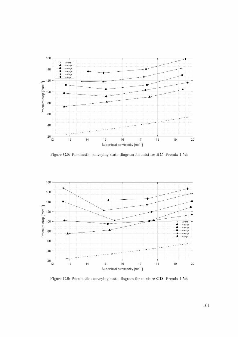
Figure G.8: Pneumatic conveying state diagram for mixture BC- Premix 1.5%
Figure G.9: Pneumatic conveying state diagram for mixture CD- Premix 1.5%
161

Appendix G Pneumatic conveying state diagrams
Figure G.10: Pneumatic conveying state diagram for mixture BCD- Premix 1.5%
Figure G.11: Pneumatic conveying state diagram for mixture BCDE- Premix 1.5%
162

Figure G.12: Pneumatic conveying state diagram for mixture CD- Premix 6.3%
Figure G.13: Pneumatic conveying state diagram for mixture BCD- Premix 6.3%
163

Appendix G Pneumatic conveying state diagrams
Figure G.14: Pneumatic conveying state diagram for mixture BCDE- Premix 6.3%
Figure G.15: Pneumatic conveying state diagram for mixture CD- Premix 10%
164

Appendix H
Comparison of pressure drop change and
MFV drop
Figure H.1: Pressure drop vs. drilling fluid concentration for the mixture BC at air flow of 250 Nm3hr−1
165

Appendix H Comparison of pressure drop change and MFV drop
Figure H.2: Pressure drop vs. drilling fluid concentration for the mixture BC at air flow of 300 Nm3hr−1
Figure H.3: Pressure drop vs. drilling fluid concentration for the mixture BC at air flow of 350 Nm3hr−1
166

Figure H.4: Pressure drop vs. drilling fluid concentration for the mixture BC at air flow of 400 Nm3hr−1
Figure H.5: Pressure drop vs. drilling fluid concentration for the mixture BCD at air flow of 250 Nm3hr−1
167

Appendix H Comparison of pressure drop change and MFV drop
Figure H.6: Pressure drop vs. drilling fluid concentration for the mixture BCD at air flow of 300 Nm3hr−1
Figure H.7: Pressure drop vs. drilling fluid concentration for the mixture BCD at air flow of 350 Nm3hr−1
168

Figure H.8: Pressure drop vs. drilling fluid concentration for the mixture BCD at air flow of 400 Nm3hr−1
Figure H.9: Pressure drop vs. drilling fluid concentration for the mixture BCDE at air flow of 250Nm3hr−1
169

Appendix H Comparison of pressure drop change and MFV drop
Figure H.10: Pressure drop vs. drilling fluid concentration for the mixture BCDE at air flow of 300Nm3hr−1
Figure H.11: Pressure drop vs. drilling fluid concentration for the mixture BCDE at air flow of 350Nm3hr−1
170

Figure H.12: Pressure drop vs. drilling fluid concentration for the mixture BCDE at air flow of 400Nm3hr−1
Figure H.13: Pressure drop vs. drilling fluid concentration for the mixture CD at air flow of 250 Nm3hr−1
171

Appendix H Comparison of pressure drop change and MFV drop
Figure H.14: Pressure drop vs. drilling fluid concentration for the mixture CD at air flow of 300 Nm3hr−1
Figure H.15: Pressure drop vs. drilling fluid concentration for the mixture CD at air flow of 350 Nm3hr−1
172

Doctoral dissertation no. 72018
—Pneumatic conveying and storage of wet
particles to illustrate offshore drill cutting handling
Dissertation for the degree of Ph.D—
Anjana Malagalage—
ISBN: 978-82-7206-481-4 (print) ISBN: 978-82-7206-482-1 (online)
usn.no

Pn
eum
atic conveyin
g an
d storag
e of wet p
articles to illustrate offsh
ore drill cu
tting
han
dlin
g - A
njan
a Malag
alage

Tittel i fet skrift - Navn
Navn
ese
n
University of South-Eastern Norway Faculty of Technology, Natural Sciences and Maritime Studies
—Doctoral dissertation no. 7
2018
Anjana Malagalage