Dynamically Controlled Resource Allocation in SMT Processors
Upload
helmholtz-muenchenCategory
view
3download
0
PLATHO - a simulation model of resource allocationin the plant-soil system
Sebastian Gayler & Eckart Priesack
December 1, 2005
!!! The documentation of thePLATHO-model is still underconstruction and will be up-dated continously!!!
For more information please contact:
Dr. Sebastian Gayler
Institute of Soil Ecology
GSF – National Research Center
for Environment and Health
Ingolstadter Landstraße 1
D – 85758 Oberschleißheim
E-mail: [email protected]
1

2
Introduction
Growth of an individual plant is determined by competition with other individuals for
the local resources light, water and nutrients. As plants in their natural environments
are almost always submitted to biotic (e.g. pathogens) and abiotic stresses (e.g. elevated
atmospheric ozone), plants in general are situated in an internal conflict: should they
invest their available assimilates into growth to increase the capacity for further uptake
of external resources or should they invest into defensive compounds to minimize possible
damages caused by biotic or abiotic stresses?
In order to get a tool for testing hypotheses concerning the trade off between growth and
defence on the level of single plants and to assess susceptibility against stress under field
conditions on the level of canopies, a new model was developed that links concepts from
existing plant growth simulation models and a mechanistic approach to simulate environ-
mental effects on secondary metabolite concentrations. This model was called PLATHO
(PLAnts as Tree and Herb Objects), as it considers the general processes common to
all plants and handles different herbaceous and woody species solely as special cases of
the class of plants. The long-term objective of model development is to get a tool that
makes it possible to minimize risks of biotic and abiotic stress and to reduce management
requirements in economic plant systems.

CONTENTS 3
Contents
1 Model overview 5
2 Technical realization 7
3 Process description 8
3.1 Morphology and canopy structure . . . . . . . . . . . . . . . . . . . . . . . 8
3.1.1 Plant area . . . . . . . . . . . . . . . . . . . . . . . . . . . . . . . 9
3.1.2 Calculation of competition coefficients . . . . . . . . . . . . . . . . 9
3.1.3 Plant height growth . . . . . . . . . . . . . . . . . . . . . . . . . . 10
3.1.4 Stem diameter . . . . . . . . . . . . . . . . . . . . . . . . . . . . . 11
3.1.5 Leaf area and leaf area distribution . . . . . . . . . . . . . . . . . . 12
3.1.6 Specific leaf weight . . . . . . . . . . . . . . . . . . . . . . . . . . . 13
3.1.7 Root system . . . . . . . . . . . . . . . . . . . . . . . . . . . . . . 14
3.2 Phenological development . . . . . . . . . . . . . . . . . . . . . . . . . . . 17
3.2.1 Influence of air temperature . . . . . . . . . . . . . . . . . . . . . . 18
3.2.2 Influence of light . . . . . . . . . . . . . . . . . . . . . . . . . . . . 18
3.2.3 Influence of atmospheric ozone concentration . . . . . . . . . . . . . 19
3.3 Growth and allocation to biochemical pools . . . . . . . . . . . . . . . . . 20
3.3.1 Maintenance . . . . . . . . . . . . . . . . . . . . . . . . . . . . . . . 20
3.3.2 Growth and allocation of assimilates to plant organs . . . . . . . . 22
3.3.3 Defensive compounds . . . . . . . . . . . . . . . . . . . . . . . . . . 27
3.3.4 Reserves pool . . . . . . . . . . . . . . . . . . . . . . . . . . . . . . 28
3.3.5 Growth capacities . . . . . . . . . . . . . . . . . . . . . . . . . . . . 29
3.4 Photosynthesis . . . . . . . . . . . . . . . . . . . . . . . . . . . . . . . . . 31
3.4.1 Light distribution . . . . . . . . . . . . . . . . . . . . . . . . . . . . 31
3.4.2 Radiation absorption and CO2 assimilation . . . . . . . . . . . . . . 34
3.4.3 Photosynthetic capacity of leaves and responses to external andinternal factors . . . . . . . . . . . . . . . . . . . . . . . . . . . . . 35
3.5 Transpiration and water uptake . . . . . . . . . . . . . . . . . . . . . . . . 40
3.5.1 Root resistance . . . . . . . . . . . . . . . . . . . . . . . . . . . . . 40
3.5.2 Soil resistance . . . . . . . . . . . . . . . . . . . . . . . . . . . . . . 40
3.5.3 Influence of climatic conditions . . . . . . . . . . . . . . . . . . . . 41

CONTENTS 4
3.6 Nitrogen uptake . . . . . . . . . . . . . . . . . . . . . . . . . . . . . . . . . 43
3.6.1 Nitrogen demand . . . . . . . . . . . . . . . . . . . . . . . . . . . . 43
3.6.2 Potential nitrogen uptake . . . . . . . . . . . . . . . . . . . . . . . 43
3.6.3 Actual nitrogen uptake . . . . . . . . . . . . . . . . . . . . . . . . . 44
3.6.4 Nitrogen distribution in the plant . . . . . . . . . . . . . . . . . . . 45
3.6.5 Nitrogen distribution in leaves . . . . . . . . . . . . . . . . . . . . . 46
3.7 Biomass loss and senescence . . . . . . . . . . . . . . . . . . . . . . . . . . 48
3.7.1 Relative death rate of leaves . . . . . . . . . . . . . . . . . . . . . . 48
3.7.2 Relative death rate of fine roots . . . . . . . . . . . . . . . . . . . . 49
3.7.3 Fruit fall . . . . . . . . . . . . . . . . . . . . . . . . . . . . . . . . . 49
3.7.4 Biomass loss of woody plant organs . . . . . . . . . . . . . . . . . . 49
3.7.5 Biomass loss caused by pathogens . . . . . . . . . . . . . . . . . . . 50
3.7.6 Biomass loss caused by ozone . . . . . . . . . . . . . . . . . . . . . 50
3.8 Ozone uptake . . . . . . . . . . . . . . . . . . . . . . . . . . . . . . . . . . 51
References 53
A List of variables 55
List of Variables 55

1 MODEL OVERVIEW 5
1 Model overview
PLATHO (PLAnts as Tree and Herb Objects) is a generic plant growth model, which
simulates C- and N-fluxes in shoot and mycorrhizosphere. It considers the general pro-
cesses common to all plants and handles different species solely as special cases of the
class of plants. Functionally equivalent plant species can be simulated by model re-
parameterisation using only different species-specific parameters. Differences in physio-
logical and ecological principles between plant classes (e.g. annuals and trees) are rep-
resented by modifications of single process formulations, without changing the overall
model structure. Thus, PLATHO was developed independent of a species to emphasize
similarities between trees and field crops.
PLATHO works on the level of physiological processes, which are integrated up to the
level of a single plant. It combines a new mechanistic approach to simulate environmen-
tal effects on synthesis of secondary metabolites on the whole plant level with concepts
from other, well established plant growth simulation models, mainly SPASS (Wang 1997;
Wang and Engel 2000; Gayler et al. 2002), CERES (Ritchie et al. 1987), SUCROS (Rab-
binge et al.) and TREEDYN (Bossel 1996). Starting from single plant individuals, each
characterized by an own parameter set, interactions of plants in a canopy are simulated.
Several plant species can be simulated simultaneously during one simulation run. In each
time step, a pool of assimilates available for growth, respiration and defense is calculated,
separately for each individual. The gain of resources resulting from photosynthesis and
retranslocation from storage organs and dying biomass as well as resource consumption
for growth, respiration and defense are calculated in units of glucose. In parallel, water-
and nitrogen uptake by roots are simulated.
All processes simulated by PLATHO are related to temperature and the availability of
the resources light, water and nitrogen. The model requires input data for climate (daily
values of radiation, minimum and maximum temperature, rainfall resp. irrigation and
relative air humidity), soil properties and data relating to fertilisation.
The model can be used to simulate growth of
1. single plant individuals without competition by neighbours
2. plant individuals competing for resources in canopies which are composed of

1 MODEL OVERVIEW 6
• identical individuals (intraspecific competition)
• different individuals of one or more species (inter- or intraspecific competition)
Plant individuals can differ in species, ecophysiological and genetic parameters and in the
start values of their state variables. Plant individuals are arranged in a rectangular grid
with periodical boundary conditions (boundary effects are not considered). The distance
between the individuals is determined by canopy density. Different plant individuals are
simulated simultaneously. Competition effects are simulated considering interactions with
the four next neighbours of each individual (see figure 1).
Figure 1: Arrangement of plant indi-viduals in a rectangular grid and sym-bols used for calculating interactionwith the next neighbours.
To simulate competition and genetic variation in canopies, more than one individual must
be defined in the input files. These individuals are grouped together in an elementary
grid which is periodically continued on the boundaries. For practical simulation purposes
it is useful to consider only a few different plant individuals (e.g. two species in a mixed
canopy, where all individuals of one species have identical parameters and start values,
or a monoculture with small and tall individuals). Figures 2 and 3 show examples for
elementary grids with three and four different individuals. The degree of competition
between individuals depends on canopy density. If only a single plant individual is defined
in the input files, a grid of identical individuals is simulated. Depending on canopy density
there will be either competition or no competition.

2 TECHNICAL REALIZATION 7
Figure 2: Example for periodicalboundary conditions in a 3 species(individuals) simulation
Figure 3: Example for periodicalboundary conditions in a 4 species(individuals) simulation
2 Technical realization
The model structure of PLATHO is highly modular. It is implemented in C within the
development tool Expert-N (Engel and Priesack 1993; Baldioli et al. 1995; Stenger et al.
1999). Expert-N consists of several modules for simulating different processes in the soil-
plant-atmosphere system, which can be coupled together in various combinations. Plant
processes simulated in PLATHO are governed by climate and soil processes, which can
be simulated using modules from Expert-N. The link between PLATHO modules (plant
process) and other modules of Expert-N (soil processes) is realized by defined interfaces.
This model structure makes PLATHO to be a useful research instrument, because it allows
to test several hypothesis for single processes of plant growth by changing single modules.

3 PROCESS DESCRIPTION 8
3 Process description
Processes simulated by PLATHO are morphological development, phenological develop-
ment, respiration, biomass growth and allocation to biochemical pools, photosynthesis,
water uptake, nitrogen uptake, uptake of ozone and senescence, .
3.1 Morphology and canopy structure
Competition for external resources on the level of single plants relates directly to space
sequestration of the competing individuals. Therefore a simplified plant morphology is
considered within the PLATHO model. It is assumed that all biomass of a plant is located
in a cylinder with flexible height to diameter proportion HD [–], where HD depends on
development stage and competitive situation of the plant (3.1.3). The base area of this
cylinder, AP lant [m2] (3.1.1), defines the influence zone of the plant individual and is
used to calculated competition coefficients Ci,j against neighbour individuals (above and
below ground, 3.1.2). Vertical distributions of leaf area (3.1.5) and root length (3.1.7)
are considered using species specific distribution functions. Plants are assumed to be
rotationally symmetric. The symbols used for the calculation of plant morphology are
shown in figure 4.
Aplant
z
h
xl = 1
n = N
n = 1
l l=zr
H
zR
l = L
Figure 4: Geometry and symbolsused for calculating plant morphol-ogy. H [m] is the actual height ofthe plant, zR [m] the actual depthof the root system. N simulationlayers are considered above groundand L layers below ground. lzR
isthe deepest rooted soil layer. h [m]isthe height over the ground and z [m]the depth in the soil. The distancex [m] from the center of the plant isused for the calculation of compe-tition coefficients, Aplant [m2] is thebasal area of the cylinder and de-scribes the zone that is influencedby the plant individual.

3 PROCESS DESCRIPTION 9
An example for the competitive situation in a mixed canopy (two species with individuals
differing in size) shows figure 5.
z
h
h = z = 0
Figure 5: Example for competition between two species
3.1.1 Plant area
The base area AP lant [m2] of the cylinder representing the shape of the plant, is calculated
from stem diameter dS [m] assuming a constant crown-to-stem diameter-ratio rC/S [–].
However, the radius of a plant cannot exceed the distance between two plants.
AP lant =
π4·(
rC/S · dS)2
if dS <2
rC/S ·√%Canopy
π%plant
if dS ≥ 2rC/S ·
√%Canopy
(1)
where %Canopy [plants ·m−2] is the density of the canopy.
3.1.2 Calculation of competition coefficients
Plant areas of two individuals i and j are overlapping if the distance d [m] between the
individuals is lower than the sum of both radii ri [m] and rj [m].
The competition coefficient between two (competing) individuals i and j is given by
equation 2, where Ai,j (equation 3) is the cross section of both plant areas and x = ξ (see
figure 6) is given by equation 4.
Ci,j =
0 if ri + rj ≤ d
Ai,j
r2i ·πif (ri + rj > d) ∧ (rj − ri < d)
1 if rj − ri ≥ d
(2)

3 PROCESS DESCRIPTION 10
Figure 6: Geometry and symbols used for the calculation of competition coefficient be-tween individuals i and j. ri is the radius of the zone influenced by individual i, d thedistance between individuals and Ai,j the intersection of both plant areas. x is the distancefrom individual i towards individual j.
with
Ai,j = 2 ·
ri∫
ξ
√
r2i − x2 dx+
ξ∫
d−rj
√
r2j − (rj − x′)2 dx′
(3)
and
ξ =r2i + d2 − r2
j
2 · d (4)
3.1.3 Plant height growth
The calculation of the increment in stem height follows Bossel (1996). Under light com-
petition (CL > 0), plants are assumed to grow in height until they reach the maximum
height-to-diameter ratio HDmax [–]. If HDmax has been reached, further growth will
continue at HD = HDmax. If there is no competition for light (CL = 0), plants are
assumed to pursue diameter growth until their minimum height-to-diameter HDmin [–]
has been reached. A single plant without light competition grows at height-to-diameter
ratio HD = HDmin. For annual plants, HDmax depends on actual height of the plant.
For trees, HDmax is constant during the simulation period. The light competition factor
CL [–] is calculated from the competition factors Ci,j [–] (see equation 2), the actual leaf
area index LAIj [m2(leaf) · m−2(soil)] (see equation 12) and the actual heights Hj [m] of

3 PROCESS DESCRIPTION 11
the next neighbours:
CL =
4∑
j=1Ci,j · LAIj · min {1, Hi/Hj}
4∑
j=1LAIj
(5)
Case 1 (only diameter growth):
dH
dt= 0 if HD > HDmax or CL = 0 ∧HD > HDmin (6)
Case 2 (only height growth):
dH
dt=
4 · dWS
dt
π · %S · d2S
if HD < HDmin or CL > 0 ∧HD < HDmax (7)
Case 3 (height/diameter is constant):
dH
dt=
4 · dWS
dt
3π · %S · d2S
if CL = 0 ∧HD = HDmin or CL > 0 ∧HD = HDmax (8)
HD is calculated from actual plant height H [m] and stem diameter dS [m]:
HD =H
dS(9)
3.1.4 Stem diameter
Stems are assumed to be cylinders having the same height as the plant. Thus stem
diameter dS [m] can be calculated from stem weight WS [kg] and stem density %S [kg ·m−3]:
dS =
√
4 ·WS
π ·H · %S(10)
where H [m] is the actual plant height.

3 PROCESS DESCRIPTION 12
3.1.5 Leaf area and leaf area distribution
Total (living) plant leaf area AL [m2] is calculated from actual leaf weight WL [kg], as-
suming a mean specific leaf weight, λ∗Lw [kg · m−2 (leaf)]:
AL = WL/λ∗Lw (11)
For calculating the leaf area index LAI [m2(leaf)·m−2(soil)], total plant leaf area is divided
by the area, which can be potentially covered by the plant:
LAI =
AL/AP lant if AP lant ≥ %−1Canopy
AL · %Canopy if AP lant < %−1Canopy
(12)
where AP lant [m2] is the base of the cylinder representing the shape of the plant and
%Canopy is [m−2] is the number of plant individuals per square meter.
The cumulative leaf area AL,cum [m2] over height h [m] is assumed to follow a species
specific leaf area distribution function:
AL,cum(h) = αL +βL
1 + e−4·(h/H−pL)
with
βL = AL · (e−4·(1−pL) +1) · (e4·pL +1)
e−4·(1−pL) − e4·pL
αL =−βL
e−4·(1−pL) +1(13)
where H [m] is the actual plant height and pL [–] is an input parameter that describes
the relative height of maximum leaf area density. The species specific form of leaf area
distribution is approximated using different values of pL.
The cumulated leaf area index LAIcum [m2(leaf) · m−2(soil)] above h (equation 14) and
leaf area density aL [m2(leaf) ·m−1] at height h (equation 15) are derived from AL,cum(h):
LAIcum(h) =AL,cum(h)
AP lant(14)
aL(h) =d
dhAL,cum(h) (15)

3 PROCESS DESCRIPTION 13
3.1.6 Specific leaf weight
Specific leaf weight depends strongly on light availability and nitrogen availability within
leaves. In the model it is assumed that in deeper leaf layers, where incoming radiation is
low, plants compensate this scarcity by thinner leaves (increased leaf area per unit leaf
biomass, i.e. decreased specific leaf weight). Further it is assumed that plants compen-
sate also low nitrogen concentrations in leaves by decreasing the specific leaf weight to
maximize photosynthic capacity per unit nitrogen in leaves. Therefore the mean spe-
cific leaf weight, λ∗Lw [kg · m−2 (leaf)], is estimated from actual leaf area index LAI,
[m2(leaf) · m−2(soil)] and the mean nitrogen concentration in leaves, νL,act [kg(N)·kg].
The dependency of specific leaf weight from height h is assumed to follow an exponential
distribution function.
λ∗Lw = max {λLw,max · (1 − αN · LAI) ; λ∗Lw,min}
with
αN =2 · νL,opt − νL,act − νL,min
4 · νL,opt · LAIcrit(16)
where αN is a function of νL,act which provides λ∗Lw = λ∗Lw,min in case of pessimal nitrogen
of leaves (νL,act = νL,min) and LAI ≥ LAIcrit. λ∗Lw is used to calculated total leaf area
from actual leaf weight (equation 11). The minimal value of mean specific leaf weight is
estimated from minimal and optimal leaf nitrogen concentrations:
λ∗Lw,min =λLw,max
2· νL,opt + νL,min
νL,opt(17)
The actual specific leaf weight of leaves at height h follows from the cumulative leaf area
index above h, LAIcum(h) [m2(leaf) · m−2(soil)].
λLw(h) = λLw,max · e−κ·LAIcum(h) (18)
κ [m2(soil) ·m−2(leaf)] describes the decrease in specific leaf weight if the cumulative leaf
area index LAIcum increases. κ is calculated from the relation
λ∗Lw =1
LAI·∫ LAI
0λLw(h) dLAIcum =
λLw,maxκ · LAI ·
(
1 − e−κ·LAI)
(19)

3 PROCESS DESCRIPTION 14
3.1.7 Root system
The calculation of rooting depth is adapted from the CERES model family (Jones and
Kiniry; Villalobos and Hall 1989; Wang 1997). It is assumed that root extension growth
only occurs if root weight increases. The increase of rooted depth zR [m] depends on
actual temperature, Tsoil [◦C], and actual soil water content, θact [m3 ·m−3], in the lowest
rooted soil layer lzR (see figure 4):
dzRdt
= rzR· fT (lzR
) · fθ(lzR) ·(
1 − zRzR,max
)
(20)
where rzR[m ·d−1] is the maximal root extension rate and fT [–] and fθ [–] are factors
relating to actual temperature and moisture in soil layer l (equations 27 and 28).
The calculation of root length distribution, lR(l) [m] is also based on the concept of
CERES-models: actually formed biomass of roots (see equation 66) is converted into root
length using a specific root length factor λlR [m · kg−1] and subsequently distributed to
soil layers (equation 22). The distribution of newly formed root length to rooted soil
layers depends on the species specific root length distribution function w(l) (equation 25)
and on actual distribution of moisture, fθ(l) (equation 28) and nitrogen, fN(l) (equation
29), in the soil. In addition, in the PLATHO model this concept is extended consider-
ing underground competition for space sequestration between neighbour individuals by
introducing a further stress factor, CRLD [–], which is estimated from actual root length
density of all individuals present in the respective soil disk (equation 24). The maximal
value of root length density KlR = 3 · 104 m/m3 is taken from Adiku et al. (1996).
The actual loss of root biomass (due to rhizodeposition and senescence, see equation 66
and section 3.7) is also converted to root length and subsequently distributed to rooted soil
layers (equation 23). The die off of roots occurs preferably in soil layers with unfavourable
moisture and nitrogen conditions.
d lR(l)
dt= l+R(l) − l−R(l) (21)
where
l+R(l) =GWR
ξWR
· λlR · w(l) · min{fθ(l), fN(l)} · CRLD(l)lZR∑
l=1[w(l) · min{fθ(l), fN(l)} · CRLD(l)]
(22)

3 PROCESS DESCRIPTION 15
l−R(l) = λR ·WR · λlR · lR(l) · max{1 − fθ(l), 1 − fN (l)}lZR∑
l=1[lR(l) · max{1 − fθ(l), 1 − fN(l)}]
(23)
CRLD(l) =
(
1 − lR,i(l) +∑4j=1 Cj,i · lR,j
KlR · Aplant · (zl − zl−1)
)
(24)
and
w(l) =αRβR
·∫ zl
zl−1
(
z
βR
)(αR−1)
· e−(z/βR)αRdz
with
αR = 1 + 2 · pR
βR =
zR
2if pR = 0
pR·zR(
αR−1
αR
) 1αR
else(25)
zL [m] denotes the depth of the bottom of soil layer l. Species specific forms of root
distribution are approximated by different values of the parameter pR, which describes
the relative position of maximal root density.
The root surface in soil layer l, aR(l) [m2], is calculated from root length in layer l, lR(l),
root density, %R [kg · m−3], and specific root length, λR [kg · m−1]:
aR(l) =
√
4π
%R · λlR· lR(l) (26)
Reduction functions
Reduction functions relating to soil temperature, soil moisture and mineral nitrogen con-
centration in soil are adapted from the modelling approach used in the SPASS model
(Wang 1997). Dependency of root depth growth on temperature in the lowest rooted
soil layer, Tsoil(lzR) [◦C] is calculated by help of an optimum function with three cardinal
temperatures Trt,min, Trt,opt and Trt,max.
fT =
0 if Tsoil(lzR) < Trt,min ∨ Tsoil(lzR
) > Trt,max
2·(Tmm·Tom)α−T 2αmm
T 2αom
if Trt,min ≤ Tsoil(lzR) ≤ Trt,max
(27)

3 PROCESS DESCRIPTION 16
Tmm = Tsoil(lzR) − Trt,min
with
Tmm = Tsoil(lzR) − Trt,min
Tom = Trt,opt − Trt,min
Txm = Trt,max − Trt,min
and
α =ln 2 · TomTxm
The increase in rooting depth as well as root length growth is reduced, if water content
in the respective soil layer, θact(l) [m3· m−3], decreases below the quarter of the available
field capacity:
fθ(l) =
0 if θact(l) < θpwp(l)
4·(θact(l)−θpwp(l))θfc(l)−θpwp(l)
if 0 ≤ θact(l) − θpwp(l) ≤ 14· (θfc(l) − θpwp(l))
1 if θact(l) − θpwp(l) >14· (θfc(l) − θpwp(l))
(28)
Root length growth is also reduced depending on mineral nitrogen concentration, cN(l)
[mg·kg−1] in soil:
fN(l) =
0.01 if cN(l) < 1.11 mg·kg−1
1 − 1.17 · e−0.15·cN (l) if cN(l) ≥ 1.11 mg·kg−1
(29)

3 PROCESS DESCRIPTION 17
3.2 Phenological development
The development of plants depends strongly on environmental factors. In this model, the
influences of temperature, length of the photoperiod and atmospheric ozone concentration
are considered. Six development stages are distinguished (see table 1). Development
stage i is reached, when the biological time tB [–] (equation 30) exceeds a threshold sum
of development days Di (Di+1 > Di). Biological time is the sum of development days
multiplied with the factors delaying phenological development. One day of biological
time corresponds to one real day with optimal temperature and optimal length of the
light period.
Table 1: Definition of development stages for herbs and treesHerbs Trees
0 ≤ tB < D1 before germination dormanceD1 ≤ tB < D2 germination - emergence breaking of the budsD2 ≤ tB < D3 vegetative growing complete unfolding of the leavesD3 ≤ tB < D4 begin of fructification maximal efficiency of leavesD4 ≤ tB < D5 only seeds/tubers are growing leaf fallD5 ≤ tB < D6 maturity leaf and fruit fall
tB =dact∑
d=1
min {fT,dev · fph} (30)
where fT,dev(Tm, Tdev,min, Tdev,opt, Tdev,max) and fph(ph) are the temperature and daylength
response functions of phenological development (equations 33 and 34). At the end of each
year, tB is set to zero. The actual development rate rdev [d−1] is given by
rdev =fT,dev · fph
∆D(31)
where
∆D = Di+1 −Di, i = 0, . . . , 5 (32)
is the number of development days in the actual development stage (D0 = 0).

3 PROCESS DESCRIPTION 18
3.2.1 Influence of air temperature
In order to consider the influence of daily mean air temperature Tm [◦C] on the actual
development rate, a response factor fT,dev [–] is introduced. fT,dev describes an optimum
function, where the shape of this function is determined by the minimal temperature for
phenological development, Tdev,min [◦C], the optimal temperature, Tdev,opt [◦C], and the
maximal temperature, Tdev,max [◦C].
fT,dev =
0 if Tm < Tdev,min ∨ Tm > Tdev,max
2·(Tmm ·Tom)α−T 2αmm
T 2αom
if Tdev,min ≤ Tm ≤ Tdev,max(33)
with
α =ln 2 · TomTxm
and
Tmm = Tm − Tdev,min
Tom = Tdev,opt − Tdev,min
Txm = Tdev,max − Tdev,min
3.2.2 Influence of light
Another factor that affects the rate of development is actual length of the photoperiod.
According to the type of the photoperiodic response, short-day plants, long-day plants
and day-neutral plants are distinguished in PLATHO.
fph =
1 for ”day-neutral” plants
1−e−ω·(ph−phopt+4ω )
1−e−4 for ”long day” plants
1−eω·(ph−phopt+−4ω )
1−e−4 for ”short day” plants
(34)
where ω is a photoperiod sensitivity coefficient.

3 PROCESS DESCRIPTION 19
3.2.3 Influence of atmospheric ozone concentration
High atmospheric ozone concentrations can accelerate senescence. In PLATHO therefore
the biological time of the begin of leaf fall, D4 is decreased under high ozone concen-
trations. The effect is assumed to be cumulative and only ozone concentrations above a
critical value cO3,crit [ppb] contribute to the acceleration of senescence.
D4 = max{
D4,0 · fO3,1
2· (D4,0 +D3)
}
(35)
where
fO3 = 1 − αO3 · IO3 (36)
D4,0 is the number of development days before leaf fall without the effect of ozone, αO3
is a ozone sensitivity coefficient and IO3 [–] is actual ozone stress intensity (see equation
153).

3 PROCESS DESCRIPTION 20
3.3 Growth and allocation to biochemical pools
Four aggregated biochemical pools are considered (see figure 7): assimilates (temporarily
existing products of photosynthesis and reserve remobilisation, handled as glucose), which
are immediately available for growth and maintenance processes, reserves, which can be
mobilized if required, defensive compounds (phenylpropanoids in case of apple trees) and
structural biomass. Structural biomass is divided in fine roots, gross roots, stem, branches,
leaves and fruits in case of trees and roots, stem leaves and fruits in case of herbs. Rates
of material fluxes between these pools depend on the actual plant internal availability of
carbon and nitrogen and on the actual demand for growth and defence, which are cal-
culated every time step. All conversion processes are calculated in units of glucose using
biochemical knowledge about energetics and stoichiometries of the dominating reaction
pathways. The amount of assimilates, Aav [kg(glucose)], which are available to fulfill the
demands of all energy consuming processes during a time step ∆t [d] is calculated from
actual photosynthesis rate Pact [kg(glucose)· d−1], potential remobilisation from reserves
R [kg] and the assimilate surplus remaining from the time step before Aold [kg(glucose)].
Maintenance processes take priority over all other processes. Thus, the amount of assim-
ilates, which are available for synthesising structural biomass and defensive compounds
results from
Aav = (Pact +R · τR) · ∆t−DM + Aold (37)
where DM [kg(glucose)] is the amount of assimilates required for maintenance processes
and τR [d−1] is the reserves remobilisation rate.
3.3.1 Maintenance
Estimation of the glucose demand for maintenance follows the concepts outlined by Pen-
ning de Vries et al. (1989) and Thornley and Johnson (1990). In the model it is assumed,
that maintenance respiration rate is independent of plant tissue growth. The glucose
requirement for maintenance comprises all energy demands to maintain the functional
and compositional status quo of the plant tissue. Three components of maintenance are
distinguished: turnover of proteins and lipids, maintenance of ion concentrations across
membranes and a component related to metabolic activity.

3 PROCESS DESCRIPTION 21
Figure 7: Fluxes between aggregated biochemical poolsthat are considered in the PLATHO model
The amount of glucose mtu,k [kg(glucose) · d−1] that is required to resynthesise proteins
and lipids in organ i follows from the fractions fp,k [–] and fl,k [–] of proteins and lipids
in organ k, the turnover rates kp [d−1] and kl [d−1] of both pools and the actual weight of
organ k, Wk [kg]:
mtu,k =180
36·(
fp,k · kp ·cATP,pMWp
+ fl,k · kl ·cATP,lMWl
)
·Wk (38)
where cATP,p = 4 ATP per peptide bond is the ATP cost of protein synthesis from amino
acids and cATP,l = 7 ATP per tryglyceride is the ATP cost of lipid resynthesis from glycerol
and free fatty acids. MWp = 120 [g · mol−1] and MWl = 900 [g · mol−1] are the average
molecular weights of one amino acid residue and one lipid respectively. The factor 180/36
considers the glucose equivalent of one mol ATP.
Costs to maintain concentrations of ions across membranes, mion [kg(glucose) · d−1], are
estimated in a similar way:
mion,k =180
36· fion,k · kion ·
cATP,ionMWion
·Wk (39)
where fion,k [–] is the fraction of minerals in organ k, kion [d−1] is the average ion leakage
rate through membranes, cATP,ion = 1 ATP per ion transported is the ATP cost for ion

3 PROCESS DESCRIPTION 22
transport and MWion = 40 [g · mol−1] is the average relative molecular mass of minerals.
Values of cATP and MW are taken from Thornley and Johnson (1990).
Gross photosynthesis, Pact [kg(CO2) · d−1], is assumed to be a measure for the estimation
of the component of maintenance respiration, mmet [kg(glucose) · d−1], that is due to
metabolic activity:
mmet = µmet · Pact (40)
where µmet [–] is the fraction of photosynthetic products that is used for metabolic pro-
cesses. The total demand for maintenance processes in a given time step ∆t than follows
from
DM =
(
∑
i
(mtu,i +mion,i) +mmet
)
· 2T−2010 · ∆t (41)
3.3.2 Growth and allocation of assimilates to plant organs
Two factors can limit the actual growth rate of the plant: the potential growth rate of the
plant or the plant internal availability of assimilates, ϕC (equation 49), and nitrogen, ϕN
(equation 50). The potential growth of total biomass, Gpot [kg(glucose)], is calculated by
means of equations 42 and 43. The actual usage of assimilates for synthesizing structural
biomass, GW [kg(glucose)], is calculated by equation 48, the actual usage for the synthesis
of defensive compounds, GS [kg(glucose)] by means of equation 67). Gpot depends on the
actual biological time, tB (equation 30) of the plant:
Herbs:
Gpot =
0 if 0 ≤ tB < D1
rdev ·Wseed · fT · ∆t if D1 ≤ tB < D2
rmax ·W · fT · ∆t if D2 ≤ tB < D3
%F ·WV 2 · fT · ∆t if D3 ≤ tB < D5
(42)
Trees:
Gpot =
0 if 0 ≤ tB < D1
rmax ·W · fT · ∆t if D1 ≤ tB < D4
rmax ·W · fAT· fT · ∆t if D4 ≤ tB < D6
(43)

3 PROCESS DESCRIPTION 23
rdev actual development rate [d−1] (equation 32)
rmax maximal growth rate of the plant [kg(glucose)· kg−1 · d−1]
Wseed seed weight in units of glucose [kg(glucose]
W actual structural biomass of the plant [kg]
fT temperature response function [–]
%F fruit flush rate [kg(glucose)· kg−1 · d−1]
WV 2 vegetative structural biomass at the end of stage 2 [kg]
fAT(= (D6 − tB)/2) factor relating to growth reduction in autumn [–]
Gpot is divided into demand for growth of structural biomassDW [kg(glucose)] and demand
for defence DS [kg(glucose)], similar to the model approach of Coley et al. (1985):
DW = Gpot · (1 − σ) (44)
DS = Gpot · σ (45)
with
σ = σ0 + σI (46)
σ [–] is the potential defence investment, which consists of a permanent part σ0 and an
induced part σI . σI is assumed to be greater than zero only in case of actual stress like a
pathogen attack or if the plant internal ozone concentration exceeds the threshold value
of ozone tolerance. σI is a function of stress intensity.
σI = aI · Iα (47)
In the PLATHO model, the demand for growth processes takes priority over that for
defence. Assimilates are only allocated to defence either if their available amount exceeds
growth demand, or if availability of nitrogen is lower than the demand required for growth
processes (see section 3.3.3). The actual amount of assimilates, which are used for growth

3 PROCESS DESCRIPTION 24
of structural biomass results from plant internal availability of assimilates, ϕC [–], and
nitrogen, ϕN [–]:
GW = DW · ϕC · ϕN (48)
where
ϕC = min{
1,AavDW
}
(49)
and
ϕN = min
{
1,Nav
Ndem,grw
}
(50)
where Nav [kg(N)] is the amount of plant internal nitrogen, which is potentially avail-
able for growth processes (equation 65) and Ndem,grw [kg(N)] is the demand for nitrogen
required to realise the potential plant organ growth (equation 123).
In a second step, GW is partitioned to the single plant organs k, where the index k denotes
roots (R), leaves (L), stem (S) and fruits (F) in case of herbaceous plants, and fine roots
(FR), gross roots (GR), leaves (L), branches (B), stem (S) and fruits (F) in case of trees
respectively (equation 51). The partitioning factors fk (∑
fk = 1) depend on actual
biological time tB of the plant (equations 54 – 63). Due to the endeavour of the plant to
compensate shortages in assimilates or in nitrogen, additional weighting factors wC,k and
wN,k are introduced to consider regulation in the allocation pattern.
GWk= GW · fk · wC,kwN,k
∑
k fk · wC,kwN,k(51)
where
wC,k =
γ1−ϕCC if k = L, S, B
γϕC−1C if k = R, FR, GR
1 if k = F
(52)

3 PROCESS DESCRIPTION 25
wN,k =
γ1−ϕNN if k = R, FR
γϕN−1N if k = S, B, GR
1 if k = L, F
(53)
γC and γN are parameters which characterise the ability of the plant to regulate the
allocation pattern. If no regulation is considered, these factors are set to 1.
Calculation of partitioning coefficients (herbs):
fR =
fRL·fLS
fRL·fLS+fLS+1if D1 ≤ tB < D2
%R·(KR−WR)rmax·W
if D2 ≤ tB < D3
%R·(KR−WR)·fAH
%F ·WV 2if D3 ≤ tB < D4
0 if D4 ≤ tB < D5
(54)
fL =
fLS
fRL·fLS+fLS+1if D1 ≤ tB < D2
%L·(KL−WL)rmax·W
if D2 ≤ tB < D3
%L·(KL−WL)·fAH
%F ·WV 2if D3 ≤ tB < D4
0 if D4 ≤ tB < D5
(55)
fS =
1fRL·fLS+fLS+1
if D1 ≤ tB < D2
1 − fR − fL if D2 ≤ tB < D3
rmax·W ·fAH
%F ·WV 2− fR − fL if D3 ≤ tB < D4
0 if D4 ≤ tB < D5
(56)
fF =
0 if D1 ≤ tB < D2
0 if D2 ≤ tB < D3
1 − fS − fR − fL if D3 ≤ tB < D4
1 if D4 ≤ tB < D5
(57)
Calculation of partitioning coefficients (trees):
fFR =
%FR·(KFR−WFR)rmax·W
if D1 ≤ tB < D6
0 else
(58)

3 PROCESS DESCRIPTION 26
fGR = fWood · fugwd (59)
fS = fWood · (1 − fugwd) · (1 − fbrf) (60)
fB = fWood · (1 − fugwd) · fbrf (61)
fL =
%L·(KL−WL)rmax·W
if D1 ≤ tB < D6
0 else
(62)
fF =
%F ·(KF−WF )rmax·W
if D1 ≤ tB < D6
0 else
(63)
where
fWood =
1 − fFR − fL − fF if D1 ≤ tB < D6
0 else
(64)
fRL allometric root to leaf ratio [d−1]
fLS allometric leaf to stem ratio [d−1]
%R root flush rate [kg(glucose)· kg−1· d−1]
%FR fine root flush rate [kg(glucose)· kg−1· d−1]
%L leaf flush rate [kg(glucose)· kg−1· d−1]
%F fruit flush rate [kg(glucose)· kg−1· d−1]
KR growth capacity of roots [kg] (equation 75)
KFR growth capacity of fine roots [kg] (equation 75)
KL growth capacity of leaves [kg] (equation 72)
KF growth capacity of fruits [kg] (equation 76)
W actual structural biomass of the plant [kg]
WR actual structural biomass of roots [kg]
WFR actual structural biomass of fine roots [kg]
WL actual structural biomass of leaves [kg]
WF actual structural biomass of fruits [kg]
rmax maximal growth rate of the plant [kg(glucose)· kg−1 · d−1]

3 PROCESS DESCRIPTION 27
WV 2 vegetative structural biomass at the end of stage 2 [kg]
fAH(= D4 − tB) factor relating to growth reduction in autumn [–]
The amount of nitrogen, which is potentially available for growth processes, Nav [kg], is the
sum of potential nitrogen uptake from soil Nupt,pot [kg] and potential nitrogen mobilisation
from nitrogen reserve pool Nmob [kg]:
Nav = Nupt,pot +Nmob (65)
where Nupt,pot (equation 127) is calculated from actual root surface, soil nitrogen availabil-
ity and soil moisture conditions. Nmob (equation 137) results from the difference between
actual and minimal nitrogen concentration in plant organs. The demand for nitrogen,
Ndem,grw [kg], is derived from the amount of nitrogen required to realize potential plant
organ growth (equation 123).
The total change of structural biomass Wk [kg] of organ k results from GWkand the actual
loss rate of living biomass of the respective organ λk [d−1]:
∆Wk =1
ξWk
·GWk− λk(I) ·Wk · ∆t (66)
where the ξWk[kg(glucose)·kg−1] are factors considering the conversion of glucose into
structural biomass of organ k. λk is a function of actual stress intensity I [–] (0 < I ≤ 1)
and the effectivity of plant defence. The effectivity of plant defence is a function of the
concentration sk of defensive compounds in organ k (see section 3.7).
3.3.3 Defensive compounds
After fulfilling the demand for growth, the conversion of assimilates to defensive com-
pounds can take place. We assume that the formation of defensive compounds, even if
they contain no nitrogen (e.g. phenylpropanoids), depends on the plant internal nitrogen
availability factor ϕN , due to the nitrogen requirements of precursory compounds and

3 PROCESS DESCRIPTION 28
enzymatic activity. The amount of assimilates converted to defensive compounds, GS
[kg(glucose)], is derived from
GS =
DS · ϕδN if Aav ≥ GW +DS
(Aav −GW ) · ϕδN if Aav < GW +DS
(67)
where
GW =∑
k
GWk(68)
and δ [–] is a form parameter, which allows the consideration of non-linear relations
between defensive compounds formation and plant internal nitrogen availability. The
total change of the pool of defensive compound, S [kg], results from GS, the turnover rate
of defensive compounds τS [d−1 and the actual loss of living biomass.
∆S =1
ξS·GS − τS · S · ∆t−
∑
λk · sk ·Wk · ∆t (69)
where ξS [g(glucose)·g] considers the conversion of glucose to the respective defensive
compound.
3.3.4 Reserves pool
In a final procedure it is checked whether the reserves pool, R [kg((starch)], must be
depleted to meet all demands, or if assimilates are still remaining and can be used to refill
the reserves pool. We assume that all the assimilate surplus from the prior time step, as
well as the actual gain resulting from photosynthesis will be first used. Mobilisation of
reserves will then occur only if the actual demand exceeds these amounts:
∆R =
1ξR
· (Pact · ∆t + Aold −DM −GW −GS) · rR · ∆t if χ ≤ 1
Pact · ∆t + Aold −DM −GW −GS if χ > 1
with
χ =DM +GW +GS
Aold + Pact · ∆t(70)
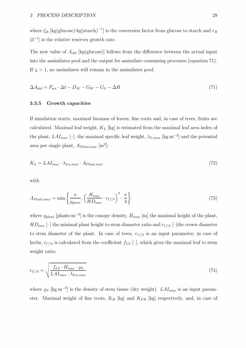
3 PROCESS DESCRIPTION 29
where ξR [kg(glucose)·kg(starch)−1] is the conversion factor from glucose to starch and rR
[d−1] is the relative reserves growth rate.
The new value of Aold [kg(glucose)] follows from the difference between the actual input
into the assimilates pool and the output for assimilate consuming processes (equation 71).
If χ > 1, no assimilates will remain in the assimilates pool.
∆Aold = Pact · ∆t−DM −GW −GS − ∆R (71)
3.3.5 Growth capacities
If simulation starts, maximal biomass of leaves, fine roots and, in case of trees, fruits are
calculated. Maximal leaf weight, KL [kg] is estimated from the maximal leaf area index of
the plant, LAImax [–], the maximal specific leaf weight, λL,max [kg·m−2] and the potential
area per single plant, AP lant,max [m2]:
KL = LAImax · λLw,max · AP lant,max (72)
with
AP lant,max = min
{
π
%plant,(
Hmax
HDmin· rC/S
)2
· π4
}
(73)
where %plant [plants·m−2] is the canopy density, Hmax [m] the maximal height of the plant,
HDmin [–] the minimal plant height to stem diameter ratio and rC/S [–]the crown diameter
to stem diameter of the plant. In case of trees, rC/S is an input parameter; in case of
herbs, rC/S is calculated from the coefficient fLS [–], which gives the maximal leaf to stem
weight ratio:
rC/S =
√
√
√
√
fLS ·Hmax · %SLAImax · λLw,max
(74)
where %S [kg·m−3] is the density of stem tissue (dry weight). LAImax is an input param-
eter. Maximal weight of fine roots, KR [kg] and KFR [kg] respectively, and, in case of

3 PROCESS DESCRIPTION 30
trees, maximal weight of fruits are estimated from allometeric coefficients fRL [–] and fFL
[–]:
K(F )R = KL · fRL (75)
KF = KL · fFL (76)
In case of herbs, growth of compartment stem is also limited:
KS = min
{
π ·H3max · %S
4 ·HD2min
;KL
fLS
}
(77)

3 PROCESS DESCRIPTION 31
3.4 Photosynthesis
Three steps are performed to calculate gross photosynthesis rate of the plant:
1. simulation of light distribution in the canopy (section 3.4.1)
2. calculation of radiation absorption per leaf layer and calculation of CO2 assimila-
tion(section 3.4.2)
3. integration of CO2 assimilation over plant height
Actual photosynthetic capacity per leaf layer in response to external environmental and
plant internal factors is in the last section of this chapter (section 3.4.3).
3.4.1 Light distribution
The calculation of light distribution in a canopy takes place according to the method
described by Kropff and Laar and Wang (1997). It is assumed that photosynthetic active
radiation, φPAR [W·m−2], reaching the top of the canopy, accounts for 50% of global
radiation, φg [W·m−2], at this site (input value).
φPAR = 0.5 · φg (78)
One part of the photosynthetic active radiation reaches the canopy as direct radiation,
φPAR,dir [W·m−2], the other part reaches the canopy in the form of diffuse radiation,
φPAR,dif [W·m−2].
φPAR,dir = φPAR · (1 − fdif ) (79)
φPAR,dif = φPAR · fdif (80)
The fraction of diffuse radiation, fdif [–] (equation 81), is estimated from the actual
transmissivity of the atmosphere, τA [–] (equation 82)
fdif =
0.23 if τA < 0.75
1.33 − 1.46 · τA if τA ≤ 0.75 ∧ τA > 0.35
1.0 − 2.3·(τA − 0.07)2 if τA ≤ 0.35 ∧ τA > 0.07
1 if τA ≤ 0.07
(81)

3 PROCESS DESCRIPTION 32
where τA is derived from the ratio of global radiation φg at the top of the canopy and the
actual value of extra-terrestrial radiation, φe [W·m−2].
τA(t) =
t+∆t2∫
t−∆t2
φg(t′)dt′
t+∆t2∫
t−∆t2
φe(t′)dt′
(82)
φe at solar time t [d] during a day d of the year, counted from January 1th, is derived
from the solar constant, φs = 1370 [W·m−2] (considering the eccentricity of the orbit of
earth) and the actual height of the sun, β [degree]:
φe(t) = 1370 · sin β ·[
1 + 0.033 · cos2π · (d+ 10)
365
]
(83)
where β(t, d) depends on the latitude λ [degree] of the geographic location of the plant
and the actual declination δs [degree] of the sun:
sin β(t, d) = sinλ · sin δs(d) + cosλ · cos δs(d) · cos 2π (t− 0.5) (84)
δs(d) = − arcsin
[
sin2π · 23.45
360cos
2π (d+ 10)
365
]
(85)
If daily input values of global radiation, φG [W·m−2] are used instead of actual values φg,
the distribution of actual global radiation over the day is calculated from the course of
solar height:
φg(t) = φG · sin β(t) · (1 + sin β(t))1∫
0sin β(t) · (1 + sin β(t)) dt
(86)
Within the canopy, radiation fluxes attenuate exponentially with the cumulative LAIcum
(equation 14), countered from the top of the plant downwards.
φPAR(h) = (1 − %) · φPAR(0) · e−k·∑
LAIcum(h) (87)
where % [–] is the reflexion coefficient of the canopy, k [–] the extinction coefficient of φPAR
and∑
LAIcum(h) the total cumulative leaf area index over height h. In the model, three

3 PROCESS DESCRIPTION 33
components of radiation fluxes are distinguished: the diffuse flux φdif [W·m−2], the total
direct flux φdir,tot [W·m−2] and the direct component of the direct flux (total direct flux
minus scattered light) φdir,dir [W·m−2]. Each form of radiation flux has its own extinction
coefficient (equations 91–92). The different light profiles are described in equations 88–90:
φdif(h) = φPAR,dif · (1 − %dif ) · e−
(
kdif ·LAIcum(h)+4∑
j=1
Ci,j ·kdif,j ·LAIcum,j(h)
)
(88)
φdir,tot(h) = φPAR,dir · (1 − %dir) · e−
(
kdir,tot·LAIcum(h)+4∑
j=1
Ci,j ·kdir,tot,j ·LAIcum,j(h)
)
(89)
φdir,dir(h) = φPAR,dir · (1 − σs) · e−
(
kdir,dir ·LAIcum(h)+4∑
j=1
Ci,j ·kdir,dir,j ·LAIcum,j(h)
)
(90)
where kdif [–] is the extinction coefficient for diffuse radiation (input),
kdir,tot =0.5 · kdif0.8 · sin β (91)
is the extinction coefficient for (total) direct radiation,
kdir,dir =0.5 · kdif
sin β · 0.8 ·√
1 − σs(92)
is the extinction coefficient for direct component of direct radiation,
%dif =1 −
√1 − σs
1 +√
1 − σs(93)
is the reflexion coefficient for diffuse radiation and
%dir =2 · %dif
1 + 2 · sin β (94)
is the reflexion coefficient for direct radiation. σs = 0.2 [–] is the scattering coefficient of
leaves for visible radiation and Ci,j are the competition coefficients between the regarded
plant i and its neighbours j.

3 PROCESS DESCRIPTION 34
3.4.2 Radiation absorption and CO2 assimilation
The amount of radiation captured by shaded leaves at height h [m] follows from the
derivation of diffuse radiation flux and the scattered component of the direct radiation
flux with respect to the cumulative leaf area index, LAIcum [m2(leaf) · m−2(soil)]:
φa,sh(h) = − dφdifdLAIcum
∣
∣
∣
∣
∣
h
−(
dφdir,totdLAIcum
∣
∣
∣
∣
∣
h
− dφdir,dirdLAIcum
∣
∣
∣
∣
∣
h
)
(95)
Sunlit leaves absorb the flux that shaded leaves absorb as well as the direct component
of the direct flux. The latter component differs for leaves with different orientation:
φa,su(h, β′) = φa,sh(h) + (1 − σ)
φPAR,dirsin β
· sin β ′ (96)
where sin β ′ is the sine of incidence of the direct beam.
The dependency of CO2 assimilation from light intensity is described by a negative ex-
ponential function, following Goudriaan and Laar (1994). This function is characterised
by the initial slope (light use efficiency, ε [kg (CO2)
m2·h/ J
m2·s ]) and the asymptote (gross
assimilation rate at light saturation, pmax [kg(CO2)·m−2·h−1], (equation 101)). The CO2
assimilation rate per leaf area of shaded leaves at height h follows from equation 97.
Assimilation rate of sunlit leaves is calculated by integration of the rate of radiation
absorption over β ′ (equation 98).
psh(h) = pmax ·[
1 − exp
(
−ε · φa,sh(h)pmax
)]
(97)
psu(h) = pmax ·π∫
0
ω(β ′)
(
1 − exp
(
−ε·φa,su(β′)
pmax
)
)
dβ ′ (98)
where ω(β ′) describes the leaf angle distribution (in case of a spherical leaf angle distri-
bution ω(β ′) = 1/π).
The fraction of sunlit leaf area at height h, fsu(h) [–], is estimated from the extinction
coefficient for the direct component of the direct beam, kdir,dir [–], and the cumulative leaf
area index above h:
fsu(h) = e−
(
kdir,dir ·LAIcum+4∑
j=1
Ci,j ·kdir,dir,j ·LAIcum,j
)
(99)

3 PROCESS DESCRIPTION 35
The actual gross photosynthesis rate of the plant, Pact(t) [kg(glucose) · d−1] follows from
integration of psh and psu over plant height h:
Pact(t) = 24 · 30
44·H∫
0
[fsu(h) · psu(h) + (1 − fsu(h)) · psh(h)] · aL(h) dh (100)
The factor 24 considers the conversion of h−1 to d−1, the factor 30/44 considers the
conversion from CO2 into glucose. If daily time steps are used, Pact(t) is calculated by
integration over one day using the Gaussian integration method (Kropff and Laar).
3.4.3 Photosynthetic capacity of leaves and responses to external and inter-
nal factors
In the model, the actual rate of photosynthesis at light saturation, pmax [kg(CO2) · m−2 ·h−1], can be affected by several factors: atmospheric CO2-concentration, leaf nitrogen
content, stomatal aperture, temperature, glucose level. Photosynthetic capacity of leaves
can also be reduced in case of damages caused by ozone or leaf pathogens. The model
considers these effects by help of response functions (equations 102–113).
pmax = popt · ϕCO2 · min {ϕν, ϕH2O, ϕT , ϕCH2O} · ϕO3 · ϕPath (101)
where popt [kg(CO2) · m−2 · h−1] is the photosynthetic capacity under light saturation,
ambient CO2 conditions and optimal physiological conditions.
In the following, the single response factors are explained.
CO2 effect:
The response of photosynthetic capacity with respect to concentration of atmospheric
CO2 is estimated by equation 102:
ϕCO2 = min
(
2.3,ci − Γ0
ci,amb − Γ0
)
(102)
with
ci = cCO2 ·Rci/ca (103)
and
ci,amb = cCO2,amb ·Rci/ca (104)

3 PROCESS DESCRIPTION 36
ϕCO2 CO2 response factor [–]
ci CO2 concentration in stomatal cavity [ppm]
ci,amb CO2 concentration in stomatal cavity under ambient conditions [ppm]
cCO2 atmospheric CO2 concentration [ppm]
cCO2,amb (=340) ambient atmospheric CO2 concentration [ppm]
Γ0 CO2 compensation point [ppm]
Rci/ca internal/external CO2 ratio [–]
Nitrogen:
ϕν(h) =
1 : νact,L(h) > νopt,L
ψN (h)γ ·(k+1)ψN (h)γ+k
: νmin,L ≤ νact,L(h) ≤ νopt,L
0 : νact,L(h) < νmin,L
(105)
where
ψN (h) =νact,L(h) − νmin,Lνopt,L − νmin,L
(106)
ϕν(h) leaf nitrogen response factor at height h [–]
νact,L(h) actual leaf nitrogen concentrationkg(N)kg
νmin,L minimal leaf nitrogen concentrationkg(N)kg
νopt,L optimal leaf nitrogen concentrationkg(N)kg
γ parameter [–]
k parameter [–]
Temperature:
ϕT =
0 if T < Tps,min ∨ T > Tps,max
2·(Tps,act−Tps,min)p·(Tps,opt−Tps,min)p−(T−Tps,min)2p
(Tps,opt−Tps,min)2p if Tps,min ≤ T ≤ Tps,max(107)

3 PROCESS DESCRIPTION 37
where
p =ln 2
ln(
Tps,max−Tps,min
Tps,opt−Tps,min
) (108)
ϕT temperature response factor [–]
T actual atmospheric temperature [◦C]
Tps,min temperature minimum for photosynthesis [◦C]
Tps,opt temperature optimum for photosynthesis [◦C]
Tps,max temperature maximum for photosynthesis [◦C]
Water relation:
ϕH2O =TactTpot
(109)
ϕH2O stomatal aperture response factor [–]
Tact actual transpiration rate [cm3]
Tpot potential transpiration rate [cm3]
Accumulation of assimilates:
Photosynthesis can be limited if the concentration of soluble carbohydrates (equivalent to
Aav in the model) exceeds a critical value lC . This critical value depends on the nitrogen
concentration in the leaves. It will be smaller if nitrogen is in shortage.
ϕCH2O = max
{
0 ; 1 −(
Aav/(WL +WS)
lc
)γ}
(110)
lC = 0.2 + α · ϕν (111)

3 PROCESS DESCRIPTION 38
ϕCH2O soluble carbohydrates response factor [–]
Aav pool of available assimilates (soluble carbohydrates) [kg]
WL actual weight of leaves [kg]
WS actual weight of stem [kg]
lC critical value for soluble carbohydrates in leaves [–]
ϕν nitrogen response factor [–]
γ form parameter [–]
α (= 0.1) parameter [–]
Ozone:
If leaf internal ozone concentration exceeds a critical value, photosynthesis rate is reduced.
ϕO3 = max {0 ; 1− βO3 · IO3} (112)
ϕO3 ozone response factor [–]
IO3 leaf internal ozone concentration [µg · m−3] (equation 153)
βO3 ozone sensitivity parameter [–]
Leaf pathogens:
If infestation of leaves by pathogens exceeds a critical value, photosynthesis rate will be
reduced.
ϕPath =
1 if IP,L ≤ IP,L,crit
max {0 ; 1 − βPath · (IP,L − IP,L,crit)αPath} else
(113)
ϕPath response factor [–]
IP,L fraction of infested leaf area [m2(infested leaf area) · m2(total leaf area)]
IP,L,crit critical fraction of infested leaf area [m2(infested leaf area) · m2(total leaf area)]

3 PROCESS DESCRIPTION 39
βPath parameter [–]
αPath parameter [–]

3 PROCESS DESCRIPTION 40
3.5 Transpiration and water uptake
Transpiration of a single plant is treated in the model as the actual water uptake by its
roots. It is either limited
• by root resistance
• by soil resistance for water transport
• or by climatic conditions.
3.5.1 Root resistance
Legitimation by root resistance of water uptake from soil disc l under plant i results
from the respective root surface aR [m2] of the plants that are present in this disc, and
the maximal water uptake rate per root surface, ζW [cm3 · m−2 · d−1]. The fractions of
root surface of the four next neighbours (j = 1 . . . 4), that meet disc l under plant i,
are calculated using competition factors Cj,i (see equation 2). Thus, the maximal water
uptake from soil disc l under plant i, qW,max(l) [cm3], is:
qW,max(l) =
Aroot,i(l) · ζW,i +4∑
j=1
Aroot,j(l) · ζW,j · Cj,i
· ∆t (114)
3.5.2 Soil resistance
Limitatation by soil resistance for water transport is introduced using the factor fθ(l) [–]
that considers the actual water content, θact(l) [cm3 · cm−3], in soil layer l. If θact(l) is
greater than permanent wilting point θpwp(l) [cm3 · cm−3] and lower than field capacity
θfc(l) [cm3 · cm−3], a linear relationship between water uptake rate and actual water
content is assumed. Water uptake is not limited, if actual water content is greater than
field capacity and lower than water saturation θsat(l) [cm3 · cm−3]. No water uptake is
possible, if actual water content is lower than permanent wilting point. Furthermore,
water uptake cannot exceed the amount of water, Wav [cm3], which is actual available for

3 PROCESS DESCRIPTION 41
root water uptake in the soil disc in consideration. Thus, potential water uptake from soil
disc l under plant i, qW,pot(l) [cm3], is:
qW,pot(l) =
qW,max(l) · fθ(l) if qW,max(l) · fθ(l) < Wav(l)
Wav(l) else(115)
where
fθ(l) =
0 if θact(l) ≤ θpwp(l)
θact(l)−θpwp(l)θfc(l)−θpwp(l)
if θpwp(l) < θact(l) < θfc(l)
1 if θfc(l) ≤ θact(l) ≤ θsat(l)
(116)
and
Wav(l) = (θact(l) − θpwp(l)) · Aplant,i · ∆z(l) · 106cm3·m−3 (117)
Aplant,i [m2] is the basal area of plant i and ∆z(l) [m] is the thickness of soil layer l.
If the hydraulic relation Ψ(θ) of the soil is known, the more realistic factor fΨ(l) [–] can
be used instead of fθ(l):
fΨ(l) =
0 if Ψact(l) ≥ Ψpwp(l)
Ψact(l)−Ψpwp(l)Ψfc(l)−Ψpwp(l)
if Ψfc(l) < Ψact(l) < Ψpwp(l)
1 if Ψsat(l) ≤ Ψact(l) ≤ Ψfc(l)
(118)
where Ψact(l) [mm] is the actual water potential in soil layer l and Ψpwp(l), Ψfc(l) and
Ψsat(l) [mm] are water potential in soil layer l at wilting point, at field capacity and at
saturation respectively.
3.5.3 Influence of climatic conditions
Limitation by climatic conditions occurs, if potential water uptake from all soil discs under
plant i is greater than potential transpiration, Tpot [cm3]. In this case, water uptake from
each disc is reduced by the same factor.
qW,act(l) =
qW,pot(l) if Tpot >∑
lqW,pot(l)
qW,pot(l) · Tpot∑
l
qW,pot(l)if Tpot ≤
∑
lqW,pot(l)
(119)

3 PROCESS DESCRIPTION 42
Potential transpiration results from the difference between potential evapotranspiration
and actual evaporation. For calculation of both, potential evapotranspiration and actual
evaporation, Expert-N provides several modules (e.g. Penman-Monteith equation), which
can be linked to the PLATHO model. For calculating the fraction of actual transpiration,
Ti,act [cm3], which is caused by plant i, the actual water uptake from each soil disc is
devided between plant i and the neighbours present in the soil disc according to the
respective water uptake capacity:
Ti,act =L∑
l=1
qW,act(l) · CW (l) (120)
where the root competition factor for water uptake in soil layer l is:
CW (l) =Aroot,i(l) · ζW,i
Aroot,i(l) · ζW,i +4∑
j=1Aroot,j(l) · ζW,j · Cj,i
(121)

3 PROCESS DESCRIPTION 43
3.6 Nitrogen uptake
• nitrogen demand of the plant
• nitrogen uptake capacity of roots
• nitrogen supply of the soil in root zone.
3.6.1 Nitrogen demand
The total nitrogen demand of a plant, Ndem [kg(N)], is divided into two parts: the first
part, Ndem,grw [kg(N)], is due to the nitrogen requirement for growth processes, the sec-
ond part, Ndem,opt [kg(N)], accounts for the effort of the plant to optimise the nitrogen
equipment of their organs:
Ndem = Ndem,grw +Ndem,opt (122)
where
Ndem,grw =∑ 1
ξWk
·GWk· νopt,k (123)
and
Ndem,opt =∑
k
Wk · (νk,opt − νk,act) (124)
where the ξWk[kg(glucose)·kg−1] are factors considering the conversion of glucose into
structural biomass of organ k, GWk[kg(glucose)] are the amount of assimilates allocated
to organ k (equation 51), and Wk [kg] is the actual weight of organ k. νact,k and νopt,k
[kg(N)·kg−1] are the actual and optimal nitrogen concentration in organ k.
3.6.2 Potential nitrogen uptake
In order to fulfill these demands, the single soil layers (l = 1 . . . L) can be depleted
according to the nitrogen uptake capacity of roots and the nitrogen supply of the respective
soil layers. Potential maximal uptake from a soil disc l under plant i, Nupt,max [kg(N)]
depends on: i) root surfaces, Aroot,i [m2], of all plants present in this disc; ii) the maximal

3 PROCESS DESCRIPTION 44
nitrogen uptake rates per unit root surface, ζN,i [kg(N)·m−2 · d−1] and iii) availability
factors, fN,i(l) [–], that consider the reduction of ζN,i depending on potential soil nitrogen
supply in layer l:
Nupt,max(l) =
Aroot,i(l) · ζN,i · fN,i +4∑
j=1
Aroot,j(l) · Cj,i · ζN,j · fN,j
· ∆t (125)
with
fN,i(l) = 1 − e−ηi·cN (l) (126)
where ηi are factors dependent on the plant species and cN(l) is the concentration of
mineral N [kg(N) · kg(soil)] in soil disc l.
The potential nitrogen uptake, Nupt,pot(l) [kg(N)], is calculated taking into account soil
moisture conditions using a factor fθ(l) [–], that decreases root function in dry soil or,
due to anaerobiosis, if soil is too wet.
Nupt,pot(l) =
Nupt,max(l) · fθ(l) if Nupt,max(l) · fθ(l) < Nsoil,av(l)
Nsoil,av else(127)
where
Nsoil,av(l) = (cN(l) − cN,min) · %soil(l) · Aplant,i · ∆z(l) (128)
is the amount of available mineral nitrogen in soil disc l and
fθ(l) =
θact(l)−θpwp(l)θfc(l)−θpwp(l)
if θmin(l) ≤ θact(l) ≤ θfc(l)
θsat(l)−θact(l)θsat(l)−θfc(l)
if θsat(l) ≥ θact(l) > θfc(l)(129)
3.6.3 Actual nitrogen uptake
If the total demand, Ndem, of plant i is greater than its total potential uptake, actual
and potential nitrogen uptake from soil disc l are identical. If less nitrogen is demanded

3 PROCESS DESCRIPTION 45
by the plant than could be absorbed by its roots, potential uptake from soil disc l will be
reduced in each layer by the same factor:
Nupt(l) =
Nupt,pot(l) · CN(l) if Ndem ≥L∑
l=1Nupt,pot(l) · CN(l)
Nupt,pot(l) · CN(l) · NdemL∑
l=1
Nupt,pot(l)·CN (l)
else(130)
where
CN(l) =Aroot,i(l) · ζN,i
Aroot,i(l) · ζN,i +4∑
j=1Aroot,j(l) · ζN,j · Cj,i
(131)
are nitrogen competion factors for each soil layer. The total nitrogen uptake of plant i is
Nupt,i =L∑
l=1
Nupt(l) (132)
3.6.4 Nitrogen distribution in the plant
The distribution of nitrogen between plant organs k is governed by the actual sink strength
of the single organs. Changes in nitrogen content Nk [kg] of organ k result from the
increment of new nitrogen, Ninc,k [kg], the translocation of mobile nitrogen, Nmob,k [kg],
and nitrogen losses due to senescence:
∆Nk = Ninc,k −Ntrans,k − λk ·Wk · νmin,k (133)
where Wk [kg] is actual structural biomass, λk [d−1] is the actual death rate and νmin,k
[kg kg−1] is the minimal nitrogen concentration of organ k.
Ninc,k =
Nupt+Nmob−Ndem,grw
Ndem,opt·Wk · (νopt,k − νact,k) + ∆Wk · νopt,k if Nupt +Nmob > Ndem,grw
∆Wk · νopt,k else
(134)
Ntrans,k =
Nmob,k if Ndem ≥ Nmob +Nupt
Nmob,k · Ndem−Nupt
Nmobif Nupt ≤ Ndem < Nmob +Nupt
0 if Ndem < Nupt
(135)

3 PROCESS DESCRIPTION 46
Nmob [kg(N)] denotes the amount of mobile nitrogen, which can be translocated in other
parts of the plant. Nmob,k [kg(N)] is the part of mobile nitrogen, which is located in organ
k.
Nmob,k = Wk · (νact,k − νmin,k) · τN · ∆t (136)
and
Nmob =∑
k
Nmob,k (137)
The actual nitrogen concentration in organ k, νact,k [kg(N) ·kg−1], is calculated in equation
138:
νact,k =Nk
Wk(138)
3.6.5 Nitrogen distribution in leaves
In the PLATHO model it is assumed, that leaf nitrogen, NL [kg(N)], is not distributed
homogeneously in the leaf compartment, but is distributed over plant height in a way
that optimises light use rate by leaves. As maximal photosynthesis rate per unit leaf area
is strongly related to leaf nitrogen content (see equation 101), nitrogen will accumulated
in the upper leaf layers.
νL(h) =
νL,min if νL,act <νL,opt+νL,min
2∧ wL(h) ≤ Wλ1
νL,min +νL,opt−νL,min
WL−Wλ1· (wL(h) −Wλ1) if νL,act <
νL,opt+νL,min
2∧ wL(h) > Wλ1
νL,min +νL,opt−νL,min
Wλ2· wL(h) if νL,act ≥ νL,opt+νL,min
2∧ wL(h) ≤ Wλ2
νL,opt if νL,act ≥ νL,opt+νL,min
2∧ wL(h) > Wλ2
(139)
with
Wλ1 = WL ·[
1 − 2 · (νL,act − νL,min)
νL,opt − νL,min
]
(140)

3 PROCESS DESCRIPTION 47
and
Wλ2 = 2 ·WL · νL,opt − νL,actνL,opt − νL,min
(141)
wL(h) [kg] is the cumulative leaf weight at height h. It is calculated from leaf area density,
aL(h) [m2 · m−1] (equation 15), and specific leaf weight, λL(h) [kg · m−2] (equation 18):
wL(h) =
h∫
0
aL(h′) · λL(h′) dh′ (142)

3 PROCESS DESCRIPTION 48
3.7 Biomass loss and senescence
The actual loss rate, λk [d−1], of organ k is the sum of loss rates due to senescence and
damages caused by stress.
λk = λk,snc + λk,I,pot − εk(sk) (143)
where λk,snc [d−1] is the actual loss rate of organ k due to senescence, λk,I,pot [d−1] is the
potential loss rate of organ k due to stress in case of no defence (equation 151) and ε(sk)
[d−1] describes the reduction of λk,I,pot due to the defence effectivity (equation 152).
3.7.1 Relative death rate of leaves
Senescence of leaves occurs due to aging or if leaves shade each other. In the model, the
relative death rate of leaf biomass, λL,snc [d−1], is set to be the larger one of both factors:
λL,snc = max {λage + λshade} (144)
In the model senescence due to aging starts if biological time, tB [–], reaches the critical
value D4 (see section 3.2). Death rate depends on air temperature (high temperatures
accelerate senescence) and nitrogen concentration in leaves, νL,act [kg(N) · kg−1].
λage =
λL,0 · fT · νL,opt
νL,actif tB < D4
WL,3 · ( tBD5−D4
) · fT · νL,opt
νL,actif D4 ≤ tB < D5
(145)
λL,0 [d−1] is the leaf loss rate, WL,3 [kg] the leaf dry weight at the end of stage 3, fT a tem-
perature response factor (input), νL,opt [kg(N) · kg−1] the optimal nitrogen concentration
in leaves.
Senescence caused by shading occurs, if the leaf area index, LAI [m2(leaf) · m−2(soil)],
reaches a critical value LAIcrit [m2(leaf) · m−2(soil)], which depends on actual nitrogen
concentration in leaves. In case of high leaf nitrogen concentrations, leaves can survive
under lower light conditions.
λshade =
λL,0 ·(
LAILAIcrit
)2 · fT if LAI > LAIcrit
λL,0 · fT else
(146)

3 PROCESS DESCRIPTION 49
where
LAIcrit = LAIcrit,0 ·νL,actνL,opt
(147)
LAIcrit,0 [m2(leaf) ·m−2(soil)] is the critical leaf area index in case of optimal leaf nitrogen
concentration.
3.7.2 Relative death rate of fine roots
The death rate of root biomass is related to the relative turnover rate, λR,0 [d−1] and on
nitrogen concentration of roots, νR,act [kg·kg−1].
λR,snc = λR,0 ·νR,optνR,act
(148)
3.7.3 Fruit fall
Fruit fall of trees occurs if biological time, tB [–], reaches D5 (see section 3.2). The loss
rate, λF [d−1], is assumed to be proportional to the actual development rate, rdev [d−1].
λF,snc =
0 if tB < D5
min {1, WF,4·rdev
WF} if tB ≥ D5
(149)
where WF [kg] is the actual fruit weight and WF,4 [kg] is the fruit weight at the end of
stage 4.
3.7.4 Biomass loss of woody plant organs
In case of trees, a permanent biomass loss rate of woody plant organs (k = S,B,GR) is
assumed due to the die off of the bark.
λk,snc = λk,0 · fT (150)

3 PROCESS DESCRIPTION 50
3.7.5 Biomass loss caused by pathogens
The potential biomass loss rate of an organ k, λk,I,pot [d−1], caused by pathogen diseases
is a function of stress intensity I [–] (0 < I ≤ 1). In the PLATHO model, only stress
induced biomass loss of leaves and fine roots are considered. In case of pathogen diseases,
I [–] is a forcing function (input) that describes the fraction of leaves or fine roots that
is infected with the pathogen 1. The intensity and form of potential biomass loss rate
λk,I,pot [d−1] on a pathogen disease is described by two input parameters nI , and νI .
λk,I,pot(I) = nI · IνI (151)
Due to the effectivity of defensive compounds in leaves or fine roots, the potential biomass
loss rate is reduced. This stress reduction is a function of concentration of defensive
compounds, sk [kg · kg−1], in the infected plant organ k. This function is also described
by help of two input parameters mε and µε.
εk(sk) = mε · sµε
k (152)
3.7.6 Biomass loss caused by ozone
In case of ozone stress (only leaf damage is considered), intensity of stress, I [–], is
calculated as a cumulative effect of leaf internal ozone cO3,L [µg·kg−1] concentrations
exceeding a critical value cO3,L,crit [µg·kg−1]:
IO3 =
∫ t0 F (t′) dt′
∫ t0 cO3,L(t
′) dt′(153)
where
F (t′) =
0 if cO3,L(t′) ≤ cO3,L,crit
cO3,L(t′) − cO3,L,crit if cO3,L(t
′) > cO3,L,crit
(154)
Leaf damage caused by ozone is also calculated by means of equation 151. A reduction
of the damage is only considered in a indirect way, as leaf internal ozone is degraded by
defensive compounds in leaves (see equation 155).
1a dynamic model of intensity of pathogen diseases including a feedback mechanism of plant reaction
to pathogens is not yet integrated in the PLATHO model

3 PROCESS DESCRIPTION 51
3.8 Ozone uptake
In order to take into account the relation between ozone exposition and plant reaction,
a simple ozone uptake model is integrated in PLATHO. The calculation of leaf internal
ozone concentration follows Trapp et al. (1994), who proposes a model for the uptake
of xenobiotics into plants. The uptake rate is assumed to be proportional to leaf area,
AL [m2], conductivity of leaves for ozone, gO3 [m s−1], and to the concentration gradient
between atmosphere, cO3 [µg m−3], and leaf material, cO3,L [µg kg−1]. In PLATHO, a
second order reaction kinetic is assumed for the degradation of leaf internal ozone by
defensive compounds in leaves, sL [kg·kg−1]. λO3 [d−1·(kg·kg−1)−1] considers that two
molecules of ascorbate are required per molecule ozone (Van der Vliet et al. 1995).
dcO3,L
dt=AL · gO3 ·
(
cO3 −cO3,L
KLA
)
WL− λO3 · cO3,L · sL (155)
KLA [(µg·kg−1)/(µg·m−3)] is the equilibrium distribution coefficient between the gaseous
phase and the cell wall. As ozone is taken up almost solely via stomata (Kerstiens and
Lendzian 1989), conductivity for ozone can be estimated from conductivity for water
vapour, gH2O [m·d−1]. gH2O depends on actaul arperture of the stomata and is estimated
from actual transpiration rate, qw [kg·d−1] and the difference of water concentration in
stomatal cavities and atmosphere.
gO3 = gH2O ·√
18
48(156)
with
gH2O =qw
AL · (PA− h · PA)(157)
and
PA = 611 · 107.5·T
T+237
461 · (T + 273)(158)
where PA [kg m−3] is the saturation concentration of water vapour, h [%/100] the actual
relative air humidity and T [◦C] the actual air temperature. The equilibrium distribution

3 PROCESS DESCRIPTION 52
coefficient between atmosphere and leaves, KLA [(µg · kg−1) · (µg · m−3)], depends also
from temperature:
KLA(T ) = KLA(T = 20) · e−∆H·(T−20)
R·293·(T+273) = 1.54 · 104 · e−6.7· T−20T+273 (159)
where T is actual air temperature [◦C] and KLA(T = 20) = 15.4 (Plochel et al. 2000). ∆H
is the enthalpy of dissolution (16319 J·mol−1) and R the universal gas constant (8.314
J·K−1·mol−1).

REFERENCES 53
References
Adiku S, Braddock R, Rose C (1996) Simulating root growth dynamics. Environmental
software 11(1-3):99–103
Baldioli M, Priesack E, Schaaf T, Sperr C, Wang E (1995) Expert-N, ein Baukasten zur
Simulation der Stickstoffdynamik in Boden und Pflanze. Version 1.0. Benutzerhand-
buch. Lehreinheit fr Ackerbau und Informatik im Pflanzenbau, TU Mnchen, Selbstver-
lag, Freising
Bossel H (1996) Treedyn3 forest simulation model. Ecological modelling 90:187–227
Coley P, Bryant J, Chapin F (1985) Resource availability and plant antiherbivore defense.
Science 230:895–899
Engel T, Priesack E (1993) Expert-n, a building-block system of nitrogen models as
resource for advice, research, water management and policy. In: Eijsackers H, Hamers
T, eds., Integrated Soil and Sediment Research: A Basis for Proper Protection. Kluwer
Academic Publishers, Dodrecht, Netherlands, pp. 503–507
Gayler S, Wang E, Priesack E, Schaaf T, Maidl FX (2002) Modeling biomass growth,
n-uptake and phenological development of potato crop. Geoderma 105:367–383
Goudriaan J, Laar HV (1994) Modelling potential crop growth processes. Textbook with
exercises. Kluwer Academic Publishers, Dordrecht
Jones CA, Kiniry JR, eds. () CERES-Maize. A Simulation Model of Maize Growth and
Development. Texas A&M University Press
Kerstiens G, Lendzian K (1989) Interactions between ozone and plant cuticles. 1. deposi-
tion and permeability. New Phytol 112:13–19
Kropff MJ, Laar HHv, eds. () Modelling Crop-Weed Interactions. CAB International,
Wallingford, UK
Penning de Vries FWT, Jansen DM, Berge HFMt, Bakema A (1989) Simulation of eco-
physiological processes of growth in several annual crops. Centre of Agricultural Pub-
lishing and Documentation (Pudoc), Wageningen, the Netherlands

REFERENCES 54
Plochl M, Lyons T, Ollerenshaw J,Barnes J (2000) Simulating ozone detoxification in the
leaf apoplast through the direct reaction with ascorbate. Planta 210:454–467
Rabbinge R, Ward S, van Laar H, eds. () Simulation and systems management incrop
protection. Simulation Monographs 32. PUDOC, Wageningen
Ritchie JT, Godwin DC, Otter-Nacke S (1987) CERES-WHEAT. A simulation model of
wheat growth and development. Texas A&M University Press, College Station, TX
Stenger R, Priesack E, Barkle G, Sperr C (1999) Expert-n, a tool for simulating nitrogen
and carbon dynamics in the soil-plant-atmosphere system. In: Tomer M, Robinson M,
Gielen G, eds., NZ Land Treatment Collective. Proceedings Technical Session: Mod-
elling of Land Treatment Systems. New Plymouth, 14-15 Oct., pp. 19–28
Thornley JHM, Johnson IR (1990) Plant and Crop Modelling. Oxford University Press,
New York
Trapp S, Farlane CM, Matthies M (1994) Model for uptake of xenobiotics into plants: vali-
dation with bromacil experiments. Environmental Toxicology and Chemistry 13(3):413–
422
Van der Vliet A, O’Neill C, Eiserich J, Cross C (1995) Oxidative damage to extracellular
fluids by ozone and possible protective effects of thiols. Arch Biochem Biophyss 321:43–
50
Villalobos F, Hall A (1989) Oilcrop-sun v5.1 technical documentation.
http://nowlin.css.msu.edu/sunflower doc
Wang E (1997) Development of a Generic Process-Oriented Model for Simulation of Crop
Growth. Herbert Utz Verlag Wissenschaft, Mnchen
Wang E, Engel T (2000) Spass: a generic process-oriented crop model with versatile
windows interfaces. Environmental Modelling & Software 15:179–188

A LIST OF VARIABLES 55
A List of variables
Symbol Meaning Unit Equation
Aav pool of assimilates kg(glucose) 37
AL total leaf area m2 11
AL,cum(h) cumulative leaf area over h m2 13
AP lant soil area covered by plant m2 1
Aold assimilate surplus from prior time step kg(glucose) 71
aL(h) leaf area density m2/m 15
aR(l) root surface in soil layer l m2 26
Ci,j competition coefficient between individuals iand j
– 2
CL light competition factor – 5
CN(l) nitrogen competition factor in soil layer l – 131
CRLD(l) root length density stress factor in soil layerl
– 24
CW (l) water competition factor in soil layer l – 121
cCO2 actual atmospheric CO2 concentration ppm input
ci leaf internal CO2 concentration ppm 103
ci,amb leaf internal CO2 concentration at ambientCO2 conditions
ppm 104
cN (l) concentration of mineral nitrogen in soil layerl
kg(N) · kg−1 extern
cN,min minimal concentration of mineral nitrogen insoil layer l
kg(N) · kg−1 input
cO3 atmospheric O3 concentration ppb input
cO3,L leaf internal O3 concentration ppb 155
cO3,crit critical leaf internal O3 concentration ppb input
Di phenological development days until stage i – input
D4 phenological development days until stage 4 – 35
D4,0 phenological development days until stage 4,without the effect of ozone
– input

A LIST OF VARIABLES 56
Symbol Meaning Unit Equation
DM assimilates required for maintenance – 41
DS demand for defensive compounds kg (glucose) 45
DW demand for growth of structural biomass kg (glucose) 44
d day number –
dact actual day number –
dS stem diameter m 10
fbrf allometric branch fraction – input
fcbh fraction of carbohydrates in structural drymatter
kg (carbohydrates)kg (dry matter)
input
fdif fraction of diffuse radiation at the top of thecanopyk
– 81
fFL allometric fruit to leaves ratio (trees) d−1 input
fk partitioning coefficients to organ k – 54 – 63
flig fraction of lignins in structural dry matterkg (lignins)
kg (dry matter)input
flip fraction of lipids in structural dry matterkg (lipids)
kg (dry matter)input
fLS allometric leaf to stem ratio d−1 input
fmin fraction of minerals in structural dry matterkg (minerals)
kg (dry matter)input
foac fraction of organic acids in structural drymatter
kg (organic acids)kg (dry matter)
input
fN nitrogen response factor – 29, 126
fO3 ozone response factor – 36
fph photoperiod response factor – 34
fprt fraction of proteins in structural dry matterkg (proteins)
kg (dry matter)input
fRL allometric (fine) root to leaf ratio d−1 input
fsu(h) fraction of sunlit leaves at height h [–] 99
fT temperature response factor – 27
fT,dev temperature response factor of phenologicaldevelopment
– 33

A LIST OF VARIABLES 57
Symbol Meaning Unit Equation
fugwd allometric underground wood fraction – input
fθ soil moisture response factor – 28, 129
fΨ water potential response factor – 118
Gpot potential growth of total biomass kg (glucose) 42,43
GS actual assimilate consumption for synthesisof defensive compounds
kg (glucose) 67
GW actual assimilate consumption for growth ofstructural biomass
kg (glucose) 48
GWkactual assimilate consumption for structuralgrowth of organ k
kg (glucose) 51
gO3 conductivity of leaves for ozone k m·d−1 156
H plant height m 6–8
HD height to diameter ratio – 9
HDmin minimal height to diameter ratio – input
HDmax maximal height to diameter ratio – input
h height m
I intensity of plant stress 0–1 input
IP,L intensity of plant stress caused by leafpathogens
0–1 input
IP,L,crit critical intensity of plant stress caused by leafpathogens
0–1 input
IP,R intensity of plant stress caused by rootpathogens
0–1 input
IP,R,crit critical intensity of plant stress caused byroot pathogens
0–1 input
Kk maximal weight of organ k kg 72, 75, 76
k index for plant organ. k = R (roots), S(stem), L (leaves), F (fruits/tubers) in caseof herbs, or k = FR (fine roots), GR (grossroots), S (stem), B (branches), L (leaves), F(fruits) in case of trees
– –

A LIST OF VARIABLES 58
Symbol Meaning Unit Equation
kdif light extinction coefficient for diffuse radia-tion
– input
kdir,dir light extinction coefficient for direct compo-nent of direct radiation
– 92
kdir,tot light extinction coefficient for total direct ra-diation
– 91
kion average ion leakage rate d−1 input
klip turnover rate of lipids d−1 input
kprt turnover rate of proteins d−1 input
LAI leaf area indexm2(leaf)m2(soil)
12
LAIcum(h) cumulative leaf area index over hm2(leaf)m2(soil)
14
LAIcrit(h) critical leaf aream2(leaf)m2(soil)
input
LAImax maximal leaf area indexm2(leaf)m2(soil)
input
lc critical value of soluble carbohydrates inleaves with respect to photosynthesis
– 111
lR(l) root length density in soil layer l m 21
mtu,k rate of assimilate consumption to resynthe-sise proteins and lipids in organ k
kg (glucose)·d−1 38
mion,k rate of assimilate consumption to maintainionic concentrations in organ k
kg (glucose)·d−1 39
mmet rate of assimilate consumption due tometabolic activities
kg (glucose)·d−1 40
mε parameter for efficiency of plant defense – input
Nav available plant internal nitrogen kg (N) 65
Ndem total nitrogen demand of the plant kg (N) 122
Ndem,grw nitrogen demand for growth kg (N) 123
Ndem,opt difference between optimal and actual nitro-gen level in the plant
kg (N) 123
Nk nitrogen content in organ k kg (N) 133
Nmob potential plant internal nitrogen mobilisation kg (N) 137
Nmob,k potential nitrogen mobilisation in organ k kg (N) 136
Ninc,k increment of nitrogen content in organ k kg (N) 134

A LIST OF VARIABLES 59
Symbol Meaning Unit Equation
Nsoil,av available mineral nitrogen in soil disc l kg (N) 128
Ntrans,k translocation of mobile nitrogen of organ k kg (N) 135
Nupt(l) actual nitrogen uptake from soil kg (N) 130
Nupt actual nitrogen uptake kg (N) 132
Nupt,max maximal nitrogen uptake from soil kg (N) 125
Nupt,pot potential nitrogen uptake from soil kg (N) 127
n index for leaf layer – –
nI parameter for potential damage in case ofstress
– input
ph(d) photoperiod of day d m extern
phopt optimal photoperiod for development h input
pL relative maximum of leaf area density (0-1) input
pR relative maximum of root length density (0-1) input
Pact actual gross assimilation rate kg(CO2)·d−1 100
pmax actual maximal assimilation rate kg(CO2)·m−2·h−1 101
popt maximal assimilation rate under optimalconditions
kg(CO2)·m−2·h−1 input
psh assimilation rate of shaded leaves kg(CO2)·m−2·h−1 97
psu assimilation rate of sunlit leaves kg(CO2)·m−2·h−1 98
qW,act(l) actual water uptake rate from soil disc l cm3 119
qW,max(l) maximal water uptake rate from soil disc l cm3 114
qW,pot(l) potential water uptake rate from soil disc l cm3 115
R pool of reserves kg(starch) 70
Rci/ca leaf internal/external CO2 ratio – input
rC/S crown to stem diameter ratio – input, 74
rdev actual development rate d−1 32
rmax maximal plant growth rate d−1 input

A LIST OF VARIABLES 60
Symbol Meaning Unit Equation
rFR/L potential fine root to leaf ratio – input
rR relative reserves growth rate d−1 input
rzRmaximal root extension rate m
d input
S pool of defensive compounds kg 69
sk concentration of defensive compounds in or-gan k
kg·kg−1
T actual air Temperature ◦C input
Tm daily mean air temperature ◦C input
Tact actual transpiration cm3 120
Tpot actual transpiration cm3 extern
Tdev,max maximal temperature for phenological devel-opment
◦C input
Tdev,min minimal temperature for phenological devel-opment
◦C input
Tdev,opt optimal temperature for phenological devel-opment
◦C input
Tps,max maximal temperature for photosynthesis ◦C input
Tps,min minimal temperature for photosynthesis ◦C input
Tps,opt optimal temperature for photosynthesis ◦C input
Trt,max maximal temperature for root extension ◦C input
Trt,min minimal temperature for root extension ◦C input
Trt,opt optimal temperature for root extension ◦C input
Tsoil(l) soil temperature in layer l ◦C extern
t time days
tB biological time – 30
W (=∑
Wk) total structural plant biomass kg –
Wav(l) available water in soil disc l cm3 117
WF,4 fruit biomass at the end of stage 4 kg –
Wk dry weight of organ k kg 66

A LIST OF VARIABLES 61
Symbol Meaning Unit Equation
Wseed seed weight in units of glucose kg (glucose) input
WV 2 vegetative structural biomass at the end ofstage 2
kg intern
wL(h) cumulative leaf weight under height h kg 142
z soil depth m intern
zl depth of soil layer l m input
zR rooting depth m 20
zR,max maximal rooting depth m input
αO3 ozone sensitivity parameter of development kg ·µg−1·d−1 input
βO3 ozone sensitivity parameter of photosynthe-sis
kg ·µg−1 input
β solar height degree 84
Γ0 CO2 compensation point ppm input
γC parameter for regulation of allocation in caseof plant internal C shortage
– input
γN parameter for regulation of allocation in caseof plant internal N shortage
– input
δz(l) thickness of soil layer l m input
δ parameter for defensive compounds forma-tion
– input
δs declination of the sun degree 85
ε light use efficiencykg
m2·h/ Jm2·s input
η parameter considering the effect of soil nitro-gen availability on nitrogen uptake rate perunit root surface
kg3kg(N)−1 input
ζN maximal nitrogen uptake ratekg(N)m2·d input
ζW maximal water uptake rate cm3
m2·d input
θact(l) actual water content in layer l cm3
cm3 extern
θfc(l) water content in layer l at field capacity cm3
cm3 extern
θpwp(l) water content in layer at permanent wiltingpoint l
cm3
cm3 extern

A LIST OF VARIABLES 62
Symbol Meaning Unit Equation
θsat(l) water content in layer l at water saturation cm3
cm3 extern
λ latitude of the location degree input
λage loss rate of leaves due to aging d−1 145
λk actual loss rate of organ k d−1 143
λk,snc actual loss rate of organ k due to senescence d−1 144,148–150
λk,I,pot potential loss rate of organ k due to stress d−1 151
λk,0 turnover rate of orgen k d−1 input
λlR specific root length m·kg−1 input
λLw(h) specific leaf weight of leaves at height h kg·m−2 18
λLw,max maximal specific leaf weight kg·m−2 input
λ∗Lw mean specific leaf weight kg·m−2 19
λ∗Lw,min minimal mean specific leaf weight kg·m−2 17
λ∗O3leaf internal ozone degradation rate d−1·(kg·kg−1)−1 input
λshade loss rate of leaves due to shading d−1 145
µε parameter for efficiency of plant defense – input
µmet fraction of gross photosynthesis used formetabolic processes
– input
νI parameter for potential damage in case ofstress
– input
νact,k actual nitrogen concentration in organ k kg(N)·kg−1 138
νact,L(h) actual nitrogen concentration in leaves atheight h
kg(N)·kg−1 138
νmin,k minimal nitrogen concentration in organ k kg(N)·kg−1 input
νopt,k optimal nitrogen concentration in organ k kg(N)·kg−1 input
ξWkgrowth efficiency of organ k
kg (glucose)kg
input
ξS efficiency of synthesis of defensive com-pounds
kg (glucose)kg input
ξR efficiency of conversion of glucose to starchkg (glucose)kg(starch)
input
%dif leaf reflexion coefficient for diffuse radiation – 93

A LIST OF VARIABLES 63
Symbol Meaning Unit Equation
%dir leaf reflexion coefficient for direct radiation – 94
%F fruit filling rate d−1 input
%L leaf flush rate d−1 input
%plant canopy density plantsm2 input
%R root density kg·m−3 input
%soil(l) soil density in soil layer kg·m−3 input
%(F )R (fine) root flush rate d−1 input
%S stem density kg·m−3 input
σ potential defence investment – 46
σs leaf scattering coefficient – input
σ0 potential permanent defence investment – input
σI potential induced defence investment – 47
τA atmospheric transmissivity – 82
τN nitrogen mobilisation rate d−1 input
τR reserves mobilisation rate d−1 input
τS turnover rate of defensive compounds d−1 input
φPAR photosynthetic active radiation W·m−2 78
φPAR,dif diffuse component of photosynthetic activeradiation
W·m−2 80
φPAR,dir direct component of photosynthetic activeradiation
W·m−2 79
φe extraterrestrial radiation W·m−2 83
φa,sh radiation absorption by shaded leaves W·m−2(leaf) 95
φa,su radiation absorption by sunlit leaves W·m−2(leaf) 96
φdif(h) flux of diffuse photosynthetic active radiationat height h
W·m−2 88
φdir,tot(h) flux of total direct photosynthetic active ra-diation at height h
W·m−2 89

A LIST OF VARIABLES 64
Symbol Meaning Unit Equation
φdir,dir(h) flux of direct component of direct photosyn-thetic active radiation at height h
W·m−2 90
φg global radiation W·m−2 input
ϕC plant internal C availability – 49
ϕN plant internal N availability – 50
ϕCO2 atmospheric CO2 response factor of photo-synthetic capacity
– 102
ϕν leaf nitrogen response factor of photosyn-thetic capacity
– 105
ϕT temperature response factor of photosyn-thetic capacity
– 107
ϕH2O stomatal aperture response factor of photo-synthetic capacity
– 109
ϕCH2O soluble sugars response factor of photosyn-thetic capacity
– 110
ϕO3 ozone response factor of photosynthetic ca-pacity
– 112
ϕPath leaf pathogens response factor of photosyn-thetic capacity
– 113
ω photoperiodism sensitivity parameter – input
Copyright © 2022 FDOKUMEN