
Advanced Testbed Resource Allocation - ETH Zürich
47
Institut für T echnische Informatik und Kommunikationsnetze
-
Upload
khangminh22 -
Category
Documents
-
view
4 -
download
0
Transcript of Advanced Testbed Resource Allocation - ETH Zürich

Institut fürTechnische Informatik undKommunikationsnetze
Roman May
Advanced Testbed Resource Allocation
Semester ProjectJanuar to April 2016
Supervisor: Prof. Dr. Lothar ThieleSupervisor: Roman Lim

Abstract
FlockLab [1] is a testbed for embedded wireless sensor network applications, built in2012. It is publicly accessible via a web front-end. Over the past few years the numberof users accessing FlockLab and hence the utizilation has increased drastically [2]. SinceFlockLab is only capable of running one test at a time, this has led to increased waitingtimes for all users.To counter this problem, the goal of this project is to increase the test throughput
of FlockLab by modifying it to run tests concurrently. To achieve this goal we modifyFlockLab on a test system and provide a scheduling for parallel tests.In the evaluation we compare di�erent variants of our scheduling algorithm and verify
the scheduling. Further, we execute tests with real observers of FlockLab to verifythat our setup works with real hardware. Finally, we compare sequential and parallelscheduling. The results show that parallel scheduling signi�cantly increases the testthroughput compared to sequential scheduling.
II

Contents
Contents
1. Introduction 11.1. Motivation and Contributions . . . . . . . . . . . . . . . . . . . . . . . . . . 1
2. Related Work 3
3. Background 43.1. Wireless Sensor Networks . . . . . . . . . . . . . . . . . . . . . . . . . . . . . 4
4. Design 54.1. FlockLab . . . . . . . . . . . . . . . . . . . . . . . . . . . . . . . . . . . . . . . 5
4.1.1. Overview . . . . . . . . . . . . . . . . . . . . . . . . . . . . . . . . . . 54.1.2. Webserver . . . . . . . . . . . . . . . . . . . . . . . . . . . . . . . . . . 54.1.3. Database . . . . . . . . . . . . . . . . . . . . . . . . . . . . . . . . . . 64.1.4. Test Management Server . . . . . . . . . . . . . . . . . . . . . . . . . 74.1.5. Observers . . . . . . . . . . . . . . . . . . . . . . . . . . . . . . . . . . 74.1.6. Test Cycle . . . . . . . . . . . . . . . . . . . . . . . . . . . . . . . . . 8
4.2. Test System Setup . . . . . . . . . . . . . . . . . . . . . . . . . . . . . . . . . 94.3. Concept . . . . . . . . . . . . . . . . . . . . . . . . . . . . . . . . . . . . . . . 10
4.3.1. Resource Constraints . . . . . . . . . . . . . . . . . . . . . . . . . . . 104.3.2. Performance Considerations . . . . . . . . . . . . . . . . . . . . . . . 12
4.4. Scheduling Algorithm . . . . . . . . . . . . . . . . . . . . . . . . . . . . . . . 134.4.1. Absolute Time Mode . . . . . . . . . . . . . . . . . . . . . . . . . . . 134.4.2. ASAP Mode . . . . . . . . . . . . . . . . . . . . . . . . . . . . . . . . 13
5. Implementation 155.1. Database . . . . . . . . . . . . . . . . . . . . . . . . . . . . . . . . . . . . . . . 155.2. Test Management Server and Observers . . . . . . . . . . . . . . . . . . . . 155.3. Webserver . . . . . . . . . . . . . . . . . . . . . . . . . . . . . . . . . . . . . . 165.4. Scheduling Algorithm . . . . . . . . . . . . . . . . . . . . . . . . . . . . . . . 16
5.4.1. General . . . . . . . . . . . . . . . . . . . . . . . . . . . . . . . . . . . 165.4.2. Get Resource Usage . . . . . . . . . . . . . . . . . . . . . . . . . . . . 175.4.3. Merge Resource Arrays . . . . . . . . . . . . . . . . . . . . . . . . . . 185.4.4. Scheduling . . . . . . . . . . . . . . . . . . . . . . . . . . . . . . . . . 195.4.5. Add Test to Database . . . . . . . . . . . . . . . . . . . . . . . . . . . 21
6. Evaluation 236.1. Scheduling Algorithm . . . . . . . . . . . . . . . . . . . . . . . . . . . . . . . 23
6.1.1. Di�erent Observers . . . . . . . . . . . . . . . . . . . . . . . . . . . . 236.1.2. Same Observers . . . . . . . . . . . . . . . . . . . . . . . . . . . . . . 24
6.2. FlockLab . . . . . . . . . . . . . . . . . . . . . . . . . . . . . . . . . . . . . . . 27
III

Contents
6.3. Past Tests . . . . . . . . . . . . . . . . . . . . . . . . . . . . . . . . . . . . . . 28
7. Outlook 30
8. Conclusion 31
A. Appendix 34A.1. Result Rescheduling of Past Tests . . . . . . . . . . . . . . . . . . . . . . . . 34A.2. Declaration of Originality . . . . . . . . . . . . . . . . . . . . . . . . . . . . . 41
IV

List of Figures
List of Figures
1. FlockLab - Number of Tests . . . . . . . . . . . . . . . . . . . . . . . . . . . 1
2. Test Cycle . . . . . . . . . . . . . . . . . . . . . . . . . . . . . . . . . . . . . . 93. Model of an Observer . . . . . . . . . . . . . . . . . . . . . . . . . . . . . . . 104. Scheduling Algorithm - Absolute Time . . . . . . . . . . . . . . . . . . . . . 145. Scheduling Algorithm - ASAP . . . . . . . . . . . . . . . . . . . . . . . . . . 14
6. Resource Usage . . . . . . . . . . . . . . . . . . . . . . . . . . . . . . . . . . . 187. Example Merge Resource Array . . . . . . . . . . . . . . . . . . . . . . . . . 19
8. Scheduling Performance - Di�erent Observers . . . . . . . . . . . . . . . . . 259. Scheduling Performance - Same Observer . . . . . . . . . . . . . . . . . . . 2710. Result Rescheduling of Past Tests. . . . . . . . . . . . . . . . . . . . . . . . 29
V

List of Tables
List of Tables
1. Example of a Resource Usage Table. . . . . . . . . . . . . . . . . . . . . . . 12
2. Result Rescheduling of Past Tests. . . . . . . . . . . . . . . . . . . . . . . . 28
VI

Listings
Listings
1. Scheduling version one . . . . . . . . . . . . . . . . . . . . . . . . . . . . . . . 202. Scheduling version two . . . . . . . . . . . . . . . . . . . . . . . . . . . . . . 21
3. Test Con�guration - Di�erent Observers . . . . . . . . . . . . . . . . . . . . 234. Test Con�guration - Same Observers Test 1 . . . . . . . . . . . . . . . . . . 265. Test Con�guration - Same Observers Test 2 . . . . . . . . . . . . . . . . . . 26
VII

1. Introduction
1. Introduction
1.1. Motivation and Contributions
In the development of wireless sensor network applications, testbeds are indispensible.They provide great opportunites for application debugging and performance and powermeasurements. FlockLab [1] is a publicly accessible wireless sensor network testbed lo-cated at ETH Zürich, that supports multiple wireless sensor nodes and provides accuratemeasurements and helpful functions for debugging. Since the start of operation in 2012,the number of users, as well as the number of executed tests, have grown (see �gure1). The increasing number of tests, and hence higher utilization of FlockLab, has led toincreased waiting times for the users.
Figure 1: Number of tests over the last years [2].
FlockLab is only capable of running one test after another even if only parts of thetestbed are used. In this project, we aim to modify FlockLab to run tests in parallel onunused components, thus increasing the test throughput.At the moment, FlockLab consists of 32 observers. Observers are platforms that host
up to four slots for sensor nodes and implement the necessary hard- and software for thedi�erent services of FlockLab. This gives us the opportunity to not only run tests inparallel on di�erent observers, but also on di�erent target nodes on the same observer,given that the tests don't interfere with each other.First, we create a concept on how to allow concurrent tests, that includes a model of
the resource constraints. The resource constraints are modeled with hardware resourcesand a mapping between the test con�gurations and these resources. Afterwards, we usethis model to develop an algorithm, which checks the schedulability of new tests andschedules them if it's possible. On a test system, we use this concept to modify FlockLabfor running test in parallel.In the evaluation, we verify the proper scheduling of the algorithm, measure it's perfor-
mance, execute parallel tests on real observers of FlockLab and �nally, compare sequentialand parallel test scheduling.
1

1. Introduction
This report is organized as follows. First, we cover related work in section 2, continuewith background information in section 3 and elaborate our concept in section 4. Theimplementation is covered in section 5, followed by the evaluation in section 6. Finally,we present an outlook and a conclusion in section 7 and 8, respectively.
2

2. Related Work
2. Related Work
As already mentioned in the previous section, our project is based on FlockLab. Weprovide an extension to run parallel tests. On FlockLab, this is the �rst project towardsparallelization of tests.There are several other testbeds for WSN, but there is often little information available
about parallel running tests. For example Kansei [3] and Twist [4] provide no clear infor-mation about parallel tests. However, there are still some testbeds that either indicateparallel tests like MoteLab [5], NetEye [6] and DSN [7] or clearly state it like SenseNeT [8]and MoteMaster [9]. Indriya [10] doesen't provide information about parallel tests in thepaper, but since it's based on MoteLab, it's likely that it supports the same features.MoteLab developed a feature that allows parallel tests in di�erent lab zones, while
DSN supports the use of multiple servers with di�erent DSN networks. The di�erenceto our solution is that they only allow parallel tests in di�erent zones or networks, whilewe support parallelization on observer and even node level.NetEye, SenseNet and MoteMaster let the user chose the target nodes separately and
therefore allow parallel tests on node level. However, our solution has the possibility ofusing di�erent target nodes on the same observer in parallel.Furthermore, it's often not clear from the descriptions of the di�erent testbeds if they
provide some kind of automatic scheduling like we do with the possibility to run tests assoon as possible. Also, the scheduling is more involved on FlockLab due to its complexhardware that supports more than just programming and logging of target nodes.
3

3. Background
3. Background
3.1. Wireless Sensor Networks
With the advance in technology, the need for accurate, real-time environment informa-tion arose. Wireless Sensor Networks (WSN) [11] are networks of small, low-power sensornodes capable of wireless communication. These small embedded systems typically con-sist of one or more sensors, a data processing unit and communication components. Thesensor nodes build a mobile ad-hoc network and send the processed sensor data to a sink.
Examples for WSN applications are:
� Permafrost data sensing [12]
� Structural monitoring [13]
Development of WSN applications is a non-trivial task. They usually have high re-quirements in terms of low power consumption and resource usage. Furthermore, thedebugging possibilities of WSN are limited. While simulations are helpful for debugging,they lack precise measurements. WSN testbeds are experimentation platforms that canbe used to evaluate WSNs on real hardware and often provide multiple measurementpossibilities along with useful services for debugging.
4

4. Design
4. Design
In this section, we �rst provide detailed information about the parts of FlockLab thatare a�ected by this project. Next, we describe the setup of our test system, followed bya conecpt on how to alter FlockLab for parallel tests.
4.1. FlockLab
Before explaining the modi�cations of FlockLab, some components and their functioningis outlined. In the following, we �rst provide a brief overview of FlockLab and thenexplain all parts that are important for our project in detail.
4.1.1. Overview
FlockLab is a testbed for WSN applications. It supports various sensor node platformsand provides multiple services to debug and evaluate WSN applications. These servicesare GPIO tracing, GPIO actuation, power pro�ling, adjusting the supply voltage andserial I/O.FlockLab currently consists of more than 30 observers. They contain a Gumstix XL6P
COM, slots for up to four target nodes and additional components for measurements andfor controlling the sensor nodes.The front-end is a publicly accessible web interface where users can submit tests, get
the results and, if necessary, abort them. Furthermore it provides information about theobserver deployment, link qualities between the di�erent observers, etc.Several servers build the back-end infrastructure: The NTP server is used for time
synchronization. The Web server provides the user interfaces and to schedule tests. Thetest management server is responsible to copy the target binaries to the right observers,starting and stopping of tests and collecting the test results. The database server hostsa MySQL database for data storage and the monitoring server is used to detect malfunc-tions of FlockLab.
4.1.2. Webserver
The webserver provides the user interface to administer tests and supplies the user withinformation about the state of FlockLab. To submit a new test, the user creates anXML �le for the test con�guration and submits it via the web interface. The possiblecon�guration blocks in the XML �le can be found below. Only the relevant parts of eachblock are described.
General Con�guration Each test needs exactly one general con�guration block. It de-�nes when the test should be started. The two options are as soon as possible
5

4. Design
(ASAP) or at a prede�ned, absolute time (absolute time). The test duration hasto be speci�ed for ASAP tests, while the end time is needed for absolute time tests.
Target Con�guration One or more target con�guration blocks de�ne which image forthe target architecture is used on each observer. The images can either be previ-ously uploaded via the web interface or embedded in the con�guration �le1.
Embedded Image Con�guration For each in a target con�guration referenced embed-ded image, there has to be an embedded image con�guration block, that holds animage for the target architecture.
Serial Con�guration In serial con�guration blocks, the user can con�gure the use of theserial I/O service for one ore more observers. Additionally, the port that is usedfor the service can be con�gured. The two options are serial or usb.
GPIO Tracing Service Con�guration The GPIO tracing service block holds the con�g-uration for the GPIO tracing service. It's possible to con�gure it once for multipleobservers if the use the same con�guration or to use multiple blocks.
GPIO Actuation Service Con�guration This con�guration part is similar to the GPIOtracing con�guration, but for the GPIO actuation service.
Power Pro�ling Service Con�guration This con�guration part is similar to the GPIOtracing con�guration, but for the power pro�ling service.
After the user uploads a new test con�guration �le the webserver �rst checks if thecon�guration �le is valid and schedules the test if possible. If the user con�gured the testto run ASAP, the scheduling calculates the next possible time for the test and stores itin the database. For absolute time, the webserver only submits the test to the databaseif no other test is planned at the desired time, else it's declined.
4.1.3. Database
The database contains tables with information about FlockLab's status, components,users and tests. In the following, all tables that are important for this project aredescribed.
tbl_serv_observer This table has entries for all observers in the Network. For eachobserver there are �elds for networking information, observer status and the ids ofthe target adapters connected to each of the four slots.
tbl_serv_tg_adapt_list Each target adapter used in FlockLab is listed in this tableand linked to the corresponding target adapter type.
tbl_serv_tg_adapt_types The di�erent target adapter types are listed in this table.Each of this entries is linked to the corresponding target architecture in the nexttable.
1 Mote Runner is another option, but it's not covered in our project and therefore left out.
6

4. Design
tbl_serv_architectures As mentioned before, each observer has four slots for targetadapters that can be connected to a target platform. All possible target architec-tures are listed in this table.
tbl_serv_tests If the webserver schedules a new test, it is saved in this table. The titleand description, start and end time, the con�guration �le and status of each testare stored along with other information.
tbl_serv_map_test_observer_targetimages An entry for each used observer in a testis created in this table in additional to the entry in the previous table. It holds theinformation about the target image id used in a test for each observer.
tbl_serv_targetimages The target images for the target platforms are stored in thistable. This can be done either manually via webinterface or the webserver will doit automatically if a test is submitted with an embedded image in the con�guration�le.
4.1.4. Test Management Server
The test management server is responsible for the test management. It periodicallyfetches tests from the database, prepares all target images and con�gurations for theobservers, starts and stops the tests and fetches the results. Finally, it provides theresults for the user. For this task, the server uses multiple python scripts. The mostimportant ones for our project are the following:
�ocklab_scheduler.py The scheduler script runs periodically on the test managementserver. It checks if tests have to be started, stopped or aborted. If so, it starts thedispatcher for this tests accordingly.
�ocklab_dispatcher.py The dispatcher is called by the scheduler for a single test withdi�erent modes for starting, stopping and aborting a test. To start a test, itfetches the test con�guration �les and target images, prepares them for all usedobservers and copies them to the observers. Eventually, it calls the script �ock-lab_starttest.py on the observers and invokes the fetcher. To stop or abort a test,the script python_stoptest.py is invoked on all used observers and then the dis-patcher waits for the fetcher to �nish.
�ocklab_fetcher.py The fetcher collects all test results from the di�erent observers andcopies them to the test management server. Additionally, it processes the fetchedtest results.
4.1.5. Observers
Each observer is equipped with an embedded computer to control the observer, four slotsfor the target nodes, an SD card to bu�er the test results and additional componentsfor control, measurement or communication. When the script python_starttest.py iscalled, the observer prepares the target architecture, starts the test on it and controlscon�gured services like power pro�ling or GPIO tracing. To stop a test, the script �ock-lab_stoptest.py is called.
7

4. Design
At the moment, FlockLab supports the following target platforms:
� TinyNode
� Tmote Sky
� Opal
� Iris
� Mica2
� Wismote
� CC430
� Asynchronous communication module (ACM2)
� OpenMote
� Dual Processor Platform (DPP)
4.1.6. Test Cycle
A single test is proceeded as follows:
1. The user submits a test con�guration �le.
2. The webserver schedules the test.
3. The test is then stored in the database.
4. The scheduler on the test management server fetches the test and calls the dis-patcher.
5. The dispatcher prepares the test �les, copies them to the used observers and startsthe test. Additionally, it starts the fetcher.
6. The test runs on the observers and test data is generated.
7. The fetcher periodically collects test data from the observers.
8. The scheduler gets the stop time of the test from the database and calls the dis-patcher to stop the test.
9. The dispatcher stops the test on the observers and tells the fetcher to clean up.
10. The fetcher collects the last test data and processes it.
11. The user gets the test results.
A schematic overview of this process is shown in �gure 2.
8

4. Design
Figure 2: Test Cycle: Proceeding of a single test.
4.2. Test System Setup
In this section, we describe the setup of our test system. We used a notebook with Ubuntu14.04 LTE and installed each component needed on this system. All of the necessary �lescan be found in the FlockLab SVN repository2. In the following we describe the setupof all components.
Database We installed a MySQL server on the system and created the database �ocklab.To add all tables and insert the content we used the script �ocklab_server_db.sql,which is a dump from database of FlockLab.
Webserver Apache2 was installed as webserver. We copied the data needed for thewebsite from the SVN repository and con�gured apache accordingly.
Test Management Server The test management server is basically a collection of scriptsand automated tasks. Therefore, we just copied the needed scripts to our systemand changed minor parts of them to suit our setup. These changes were for examplethe paths to the di�erent scripts in the con�guration �les. Additionally, we set upcronjobs to run scripts, like the scheduler, periodically.
Observer For our purpose, it was su�cient to create an additional user pro�le that wasaccessible via ssh to simulate an observer. We used the home directory of this useron the notebook to create folders for the test images and con�gurations as well as
2 https://svn.ee.ethz.ch/flocklab/
9
4. Design
for the test results and the scripts. Furthermore, we modi�ed the con�guration�les again to suit our simulated observer.
4.3. Concept
In order to modify FlockLab for running tests in parallel, we �rst introduce our concept:We model the resource constraints and use this model for the test scheduling. To do so,we de�ne a set of exclusive resources, as well as a mapping between these resources anda test con�guration. Exclusive resources are resources which can only be used by onetest at a time. To �nd them, we �rst examine the di�erent components of FlockLab.The next step is to �nd the relation between a test con�guration and the resources. Forexample an architecture or service that uses a speci�c hardware component in a test.When a new test is submitted, we calculate time intervals during which the same
exclusive resources are used. This resource usage time intervals are then compared topreviously scheduled tests in the database to �nd the next free time slot for ASAP testsor to decide if the test can be accepted or has to be declined for absolute time tests.
4.3.1. Resource Constraints
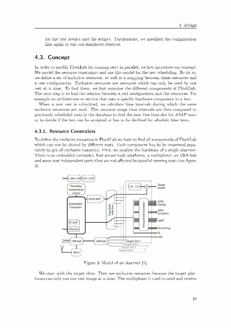
To de�ne the exclusive resources in FlockLab we have to �nd all components of FlockLabwhich can not be shared by di�erent tests. Each component has to be examined sepa-rately to get all exclusive resources. First, we analyze the hardware of a single observer:There is an embedded computer, four sensor node platforms, a multiplexer, an USB huband some test independent parts that are not a�ected by parallel running tests (see �gure3).
Figure 3: Model of an observer [1].
We start with the target slots. They are exclusive resources because the target plat-forms can only run one test image at a time. The multiplexer is used to send and receive
10

4. Design
information either directly from a sensor node or from one of the di�erent services likepower pro�ling. The multiplexer can only select one target slot at the same time, thus wemodel it as an exclusive resource.In contrast to the multiplexer, the USB hub can accessall slots simultaneously. Hence, we neglect it in the model of the resource constraints.The embedded computer is capable of multitasking and therefore not modeled as an ex-clusive resource. However, whether the embedded computer can manage the additionalload or not, is a di�erent aspect and is covered in the section 4.3.2.After the observer hardware is examined, there is still another factor which has to
be considered on a single observer: The frequency used by the targed node's wirelesscommunication system. As there are three di�erent frequencies used by the di�erenttarget platforms, 2.4 GHz, 868 kHz and 433 kHz, we model each frequency as a singleexclusive resource. The other components, the webserver, the database and the testmanagement, are capable to run parallel tasks and are therefore not exclusive resources.In conclusion, we de�ne the following exclusive resources for each observer of FlockLab:
� Platform slot 1
� Platform slot 2
� Platform slot 3
� Platform slot 4
� Frequency 2.4 GHz
� Frequency 868 kHz
� Frequency 433 kHz
� Multiplexer
After the above de�nition of the exclusive resources in FlockLab, the next step is to�nd a method to map a test con�guration to this resources. Additionally, we can useinformation from the database about the observers and the target architectures. In thefollowing, we examine all exclusive resources and specify the information needed for themapping.First, we examine the platform slots of the observers. As mentioned before, we can
only run one test on a single target at the same time. We can combine the informationfrom the con�guration �le about the used observer and platforms with data from thedatabase to get the used slots. With the target architecture determined, the frequencyis given as well.To get the multiplexer usage on each observer, we �rst have to �nd all services and
tasks that use the multiplexer. These services are: GPIO tracing, GPIO actuation,power pro�ling, adjusting the supply voltage and serial I/O tracing over the serial in-terface. Furthermore, the multiplexer is used for operating the Reset/Prog pin. Theobservers start and stop a test on the target platform with this pin. During the setupand the cleanup of a test, the multiplexer is used as well. The information if and whenthese services are used and the time intervals for the start, stop, setup and cleanup phase,are contained in the con�guration �le.
11

4. Design
Summarized, we need the following information for each test and observer:� observer Id + architecture ⇒ slots numbers� architecture ⇒ frequencies� used services + start/stop + setup/cleanup ⇒ multiplexer
With this mapping between test con�gurations and the exclusive resources we �nishedthe model the resource constraints. The next step is to �nd a representation of theresource usage that can be used for the scheduling of new tests.We chose to format the resource usage as a list of used resources in a time interval.
Since a test normally doesn't use all resources at all times of a test, we �rst calculate alltime intervals in which the resource usage is the same. Then, to store this informationin a table of the database, we generate arrays which have the start time of the intervalas the �rst and end time as the second element, followed by bits which represent theresource usage. An example of a resource table3 is shown in table 1. In the following wewill reference to one line of this table as a resource array and to the table itself as theresource table.
Table 1.: Example of a resource usage table.
Start End Res. 1 Res. 2 Res. 3 ... Res. n
12:00:00 12:03:00 1 0 0 ... 0
12:03:01 12:06:01 1 1 0 ... 1
12:06:02 12:09:02 1 0 0 ... 0
When a new test is submitted, we can now calculate the resource usage of the test andcompare it to the resource arrays from the database for the scheduling. The schedulingalgorithm is explained in detail in section 4.4.
4.3.2. Performance Considerations
In this section, we cover possible performance issues caused by parallel running tests.Two components of FlockLab are handled: The embedded computer on an observer andthe bandwidth needed by the test management server for the test data collection. Inthe following, we explain why we did not consider them in our model. However, if testsprove our assumption as wrong, it would be necessary to extent our model to cover thoseresources as well.Both, the bandwidth used for the data collection and the load on the embedded com-
puter of an observer are proportional to the amount of produced data by a test. Weassume, that all components of FlockLab can handle any arbitrary, single test withoutrunning on it's limits. A test that runs on all observers and uses all monitoring ser-vices clearly produces the highest amount of data, but at the same time only allowsparallel tests that do not use the multiplexer on any of the observers. Therefore, anadditional test can only use the serial I/O service over USB which generates signi�cantlyless data. We assume, that this relatively small amount of additional data will neither
3 The start and stop times in the example are changed to a readable form. For all calculations secondsfrom the epoch are used.
12

4. Design
push the embedded computer to it's limit, nor exceed the available bandwidth for thedata collection.
4.4. Scheduling Algorithm
In this section, we explain our scheduling algorithm which uses the previously built modelto schedule new tests. As mentioned before, the user can choose between two modes:ASAP and absolute time. We �rst go through the absolute time mode and then extendthe algorithm to support ASAP mode.
4.4.1. Absolute Time Mode
A �ow chart of the scheduling algorithm for absolute time mode is depicted in �gure 4.It gets a test con�guration �le as an input, has access to the data in the database andoutputs a boolean that indicates if it's possible to schedule the test at the desired timeor not.First, the algorithm calculates the usage of each exclusive resources from the con�g-
uration �le. Then it calculates time intervals in which the resource usage of the test isthe same and generates resource arrays. Next, the algorithm fetches the resource arrayswhich overlap in time from the resource table. Afterwards, the resource usage in the timeintervals is compared. The new test is accepted and added to the database if the resourceusage in overlapping time intervals is distinct, else it's declined.
4.4.2. ASAP Mode
We slightly change the previous algorithm to support ASAP Mode as well. Comparedto the absolute time mode, the algorithm doesn't have to accept or decline a test. It hasto return the next possible time slot to execute the submitted test. We extended theprevious algorithm to get a �rst time slot by using the actual time plus the setup time,which is needed to prepare a test, as start time. The end time is simply the start timeplus the duration of the test. Then we use a slightly modi�ed algorithm for absolute timetests and increase the starting time each time the algorithm returns decline test until weget a time slot that is accepted. A schematic of the extended algorithm is provided in�gure 5.
13

4. Design
Figure 4: Flow chart of the scheduling algorithm for absolute times.
Figure 5: Schematic of the extended scheduling algorithm that supports ASAP mode.
14

5. Implementation
5. Implementation
In this section, we �rst discuss the necessary modi�cations of the di�erent parts of Flock-Lab to support parallel tests. Then we show the implementation of the scheduling algo-rithm. The scripts are explained either directly or with the help of pseudo code.
5.1. Database
First, we have to store the information about which frequencies are used by the di�erenttarget platforms. As there is already a table tbl_serv_architectures in the database thatcontains information about the architectures, we simply add columns for all di�erentfrequencies, 2.4 GHz, 868 MHz and 433 Mhz. We �ll this colums with either True ifthe architecture uses this frequency or False if it doesn't. Compared to just use onecolumn with the used frequency as integer, this solution supports architectures whichuse multiple frequencies.In FlockLab, each previously scheduled test is stored in the database in the table
tbl_serv_tests. This table contains the start and stop times, the con�guration �le it-self and some other information. Additionally, there is the table tbl_serv_map_test_observer_targetimages which contains a mapping between observers and tests. We keepthis two tables as they are, but we also need information about the resource usage of theplanned tests. Therefore, we create a new table tbl_serv_test_resource in the form ofthe previously explained resource table to store the resource arrays.We chose the name of the resources and therefore the table columns to be in the
form: obs_<observer id>_<resource> (e.g. obs_007_mux or obs_202_slot_2 ). Thereason for this is that we can easily generate this names from the con�guration and usea mapping table between the resource names and their positions in the resource arrays.
5.2. Test Management Server and Observers
On the test management side, we have to modify some of the scripts to support paralleltests. In the following, we explain the changes in the di�erent scripts described in section4.1.4, including the �ocklab_starttest.py script on the observers from section 4.1.5.
�ocklab_scheduler.py Compared to the sequential test management, it's now possiblethat multiple tests have to be started, stopped or aborted at the same time. Wemodify the script that it �rst fetches all tests which have to be started from thedatabase. Then it starts separate threads for each of those tests. Afterwards, itdoes the same for the tests that have to be stopped or aborted. Additionally, wechange the start thread to �rst alter the status of the test in the database to plannedto prevent another scheduler from trying to start the same test again. Previously,this was done by the dispatcher. Finally, we add a delay to the start thread to
15

5. Implementation
prevent a test to be started before the planned time. This was no problem before,but with parallel tests, an early started test would falsify the resource table.
�ocklab_dispatcher.py We change two parts in the dispatcher script. First, the dis-patcher now saves the test con�gurations and images on the observer in a subfolder for this test and submits the test id as an argument when calling �ock-lab_starttest.py. Second, when scheduling a scheduler to stop the test, the dis-patcher �rst checks if there is already a scheduler scheduled at that time. If thereis already one it's not necessary to schedule another.
�ocklab_starttest.py We change this script to use the image and con�gurations formthe test id subfolder mentioned before. Furthermore, the observer now stores thetest results in a subfolder for the test.
�ocklab_fetcher.py The fetcher gets the test results from the corresponding test datafolder on the observers. There is no other modi�cation necessary as it alreadystores the test results in separate folders on the test management server.
With this modi�cations we make sure that neither the test con�gurations and imagesnor the test results of di�erent tests are mixed up.
5.3. Webserver
On the webserver, PHP scripts used to schedule new tests when they are submitted. Wechanged this part to call a python script instead. This script schedules tests by using theconcept explained in section 4.3.
5.4. Scheduling Algorithm
In this section, we show the new scheduling algorithm for parallel tests in detail. Asalready mentioned, the algorithm gets a new test con�guration �le as input and outputsif the test is schedulable. If so, the test is scheduled and stored in the database. Thealgorithm can be split in �ve parts: A general part, getting the resource usage from thecon�guration, merge the resource arrays, the actual scheduling of the test and �nallyadding the test to the database.
5.4.1. General
In the general section we execute tasks that are used by the other parts of the script. Be-sides standard tasks, like connecting to the database and creating a logger, the followingis done:
Create Resource Name to Position Mapping The order of the di�erent exclusiveresources from the resource table in the database and in the resource array has to be thesame, therefore, we �rst build a mapping between those. The algorithm fetches the titlesof the columns and stores them in a python dictionary with the name of the resource askey and position as value to keep this mapping dynamic for name changes or additionalresources. The dictionary is called resourcePosition.
16

5. Implementation
Parse XML File The test con�guration XML �le is the main source to get the resourceusage of a test. We parse it right at the beginning to make the di�erent con�gurationparts easy accessible for the following tasks.
Get Observer Ids and Architectures All of our exclusive resources are dependent onthe used observers. Hence, it is appropriate to get a list of them right at the beginning.Further, we store the information about which architecture is used on each observer. Weneed the architecture later to get the slot and frequency resources.
Get Test Times We need to fetch the start and end time of the test to get the timeintervals in which the resources are used. This information can be found in the con�g-uration for absolute time tests. For ASAP test on the other hand, we use the currenttime plus setup time as start time and use the test duration from the con�guration tocalculate the end time.In the evaluation of our system we noticed that in some cases it's bene�cial to round
up the start time to the next full minute. The advantages and disadvantages of therounding are explained in section 6.
5.4.2. Get Resource Usage
We use separate functions to get the usage of each of the di�erent resource types fre-quency, slot and multiplexer. Each of this functions returns resource arrays with theusage of this resources. The reason for this is to make it as simple as possible to adaptthis script for additional resources. To extend our algorithm for further resources, it issu�cient to add columns for the new resources in the resource table and write a functionthat generates resource arrays for them.The functions have in common that they �rst generate a list with the names of the used
resources together with the time intervals in which these resources are used. If the usage ofthe resources change throughout the test, multiple time intervals with the correspondingresource lists are calculated. To generate resource arrays out of the resource usage liststhe functions utilize a helper function getResourceArray. GetResourceArray gets timeintervals and a list of the used resources as input. It uses the resourcePosition dictionaryto translate this list of resources to an ordered array with the start time as �rst andend time as second element, with the following elements indicating if the resource at thisposition is used.An overview of the resource usage throughout a test is depicted in �gure 6. In the
�gure, the multiplexer resource is split, since the time intervals can di�er for varyingservice con�gurations. Multiplexer with and without service means with and withoutthe use of services that use the multiplexer.
Resource: Slot We already stored the observer ids and the used architectures in thegeneral section. Therefore, we can use this information together with data from thedatabase to get the slot number of the used architecture on each observer and generatethe resource usage list.To get the time interval, we need to consider the setup und cleanup times of a test.
The setup time is used to prepare the test on an observer, while the cleanup time is used
17

5. Implementation
Figure 6: Overview of the resource usage throughout a test.
to fetch the last results and clean up on the observer. In both of this phases, the targetarchitecture is already used. In conclusion, this resource generates a single time intervalbetween start time - setup time and end time + cleanup time.
Resource: Frequency We can fetch the used frequencies from the database with thepreviously stored information about the used architectures.Compared to the slot resource, the frequency is only used during the test, but not
during setup and cleanup. Therefore, we get a single time interval from the start timeto the end time of the test.
Resource: Multiplexer This functions scans through the XML �les and fetches allservice con�gurations. As mentioned in section 4, the multiplexer is used for the followingservices: GPIO tracing, GPIO actuation, power pro�ling and serial I/O service over theserial interface.Apart from those services, the multiplexer is used to setup and cleanup a test, as well
as to start and stop a test. Thus, each observer which uses one or more of the aboveservices is used from start time - setup time until end time + cleanup time. If an observeris not con�gured to use those services, it is still needed for the setup and start phase aswell as for the stop and cleanup phase of the test.In conclusion, this function can produce up to three time intervals with di�erent re-
source usage.
5.4.3. Merge Resource Arrays
Now we have multiple, overlapping resource arrays with distinct resources. The nextstep is to merge them in non-overlapping, timely ordered resource arrays before we canschedule the test. We do this by inserting them one by one to the right position of anew list and combining them if necessary. This process is best shown with the exampledepicted in �gure 7.The table on the left side shows four example resource arrays we want to merge. On
the right side, we see the resulting table after adding each of the resource arrays. Wesearch entries which overlap in time and merge the resource usage with an OR operationto add a new array. For the remaining time we insert new time intervals at the rightposition to keep the timely ordering. After this step, the resource arrays are ready forthe scheduling algorithm.
18

5. Implementation
Figure 7: Example of the merging of multiple, overlapping resource arrays.
5.4.4. Scheduling
In the course of this project, we developed two slightly di�erent scheduling algorithms.They generate the same output, but access the database in di�erent ways. In the fol-lowing, we show the di�erent variants of the scheduling and discuss the advantages anddisadvantages of them.The basic principle of both algorithms is same: They both consult the resource table
in the database and check if the used resources are available in the given time intervals.If they are, the test can be scheduled. If not, for ASAP tests, the start and stop timesof all resource arrays are increased and for absolute times, the test is declined. The timeincrement for the resource arrays is calculated as follows: We �rst locate the two resourcearrays that overlap in time and use partly the same resources. This is always one fromthe new test and one from the database. Then we choose the time increment to be theminimum that still ensures this two resource arrays to not overlap in time in the nextiteration. This method ensures that the start time of the test is minimally increased anddoes not lead to unnecessary long waiting times.The procedure of the two algorithms can be found in pseudo code in listing 1 and 2.
The di�erence between the two algorithms is, that the scheduling version one fetchesonly resource arrays from the database that overlap in time with the new test, whilethe scheduling version two fetches the whole database at the beginning. The advantageof scheduling version one is that it doesn't fetch more data from the database thannecessary for one iteration, the disadvantage that it has to fetch data in each iteration.The scheduling version two once loads the whole resource table, but doesn't have torepeat it each iteration, which results in much faster iterations. Therefore, schedulingversion one is better to minimize the memory usage, while version two is signi�cantly
19

5. Implementation
faster if there are a lot of previously scheduled tests. The evaluation of the di�erentversions can be found in section 6.
Listing 1: Scheduling version one
1 de f schedu le ( [ L i s t ] re sArrays ) :2 # repeat un t i l the t e s t i s scheduled and manually ex i t ed3 whi le not scheduled :4 i s S chedu l ab l e = True5 # Fetch r e sou r c e ar rays from db which over lap in time6 dbResArray = fetch_overlapping_resArrays_from_db ( )7 f o r new in resArrays :8 f o r o ld in dbResArray :9 i f t ime Inte rva l sOver l ap (new , o ld ) :
10 # check i f they use d i f f e r e n t r e s ou r c e s ( b i tw i s e or )11 i f any ( [ x&y f o r (x , y ) in z ip (new [ 2 : ] , o ld [ 2 : ] ) ] ) :12 i s S chedu l ab l e = Fal se13 t imeSh i f t = old [ 1 ] + 1 − new [ 0 ]14 break15
16 i f not i s S chedu l ab l e :17 break18
19 i f not i s S chedu l ab l e :20 i f ASAP:21 resArrays = increaseTimes ( resArray , t imeSh i f t )22 cont inue23 e l s e :24 re turn Fal se25 e l s e :26 re turn True
20

5. Implementation
Listing 2: Scheduling version two
1 de f schedu le ( [ L i s t ] re sArrays ) :2 # f i r s t get ALL re sou r c e ar rays from the db3 dbResArray = fetch_resArrays_from_db ( )4 whi le not scheduled :5 t imeSh i f t = 06 i s S chedu l ab l e = True7 # loop through a l l o ld r e s ou r c e ar rays8 f o r o ld in dbResArray :9 # compare them with the f i r s t one from the new t e s t (+ t imeSh i f t
)10 i f t ime Inte rva l sOver l ap ( resArrays [ 0 ] + t imeSh i f t , o ld ) :11 i f any ( [ x&y f o r (x , y ) in z ip (new [ 2 : ] , o ld [ 2 : ] ) ] ) :12 # i f the c o l l i d e and mode i s not ASAP −> return13 i f not ASAP:14 re turn Fal se15
16 # Else , add the nece s sa ry t ime s h i f t and cont inue17 e l s e :18 t imeSh i f t += old [ 1 ] + 1 − new [ 0 ]19 cont inue20
21 # i f the f i r s t r e s ou r c e array didn ' t c o l l i d e apply t imeSh i f t toa l l i n t e r v a l s and check the o the r s
22 resArrays = increaseTimes ( resArray , t imeSh i f t )23
24 i sSchedu lab l e , t imeSh i f t = checkOtherArrays ( resArrays , o ld )25 i f not i s S chedu l ab l e :26 # cont inue with the new t ime s h i f t i f the other did c o l l i d e27 cont inue28 e l s e :29 re turn True
5.4.5. Add Test to Database
Finally, if the scheduling returned a valid time slot, the only task left is adding thetest to the database. While the entries in the tables tbl_serv_tests and tbl_serv_map_test_observer_targetimages are done exactly the same as in the original FlockLab, theresource table entries are a bit trickier. The reason for this is that we have to merge theentries with existing ones if they overlap in time. We do this by fetching all resourcearrays from the resource table which overlap with the new ones and delete them in thedatabase. Then we feed all resource arrays, the ones we fetched from the database andthe ones from the new test, to the merging algorithm we used before. Finally, we canadd the now non-overlapping arrays to the resource table.This is exactly the point where the rounding of the start time to the next full minute
can make a di�erence. While the whole algorithm works in exactly the same manner forboth cases, the resulting resource table can be bigger if we don't round the start time.Assume two tests with the same con�guration, but with di�erent observers. We submitthem in the same minute, but a few seconds apart. When we don't round the start timeof the two tests, all time intervals will be shifted a few second. Thus, when we add thesecond test to the database, we have to split all of them. This results in the doubled
21

5. Implementation
number of resource arrays in the database. On the other hand, if we round the start timeto the next full minute, the intervals are exactly the same and we only have to updatethe existing ones when adding the second test. The impact of this behavior on the timeneeded to schedule a new test is discussed in section 6.
22

6. Evaluation
6. Evaluation
To test our modi�cations we executed multiple experiments. We �rst veri�ed the correctscheduling of our algorithm and measured it's performance on the test system witharti�cially generated tests. Then we tested our modi�cations with the real observers ofFlockLab. Finally, we fetched all past tests from the FlockLab database and rescheduledthem on our test system. The exact setup of our tests and their results are shown below.
6.1. Scheduling Algorithm
The �rst task of our evaluation was the veri�cation and performance measurement of ouralgorithm. We used scripts to generate arti�cial test con�guration �les in a certain wayand scheduled them. Afterwards, we fetched the scheduled test from the database andused di�erent checks to test if the scheduling was correct. We tested two speci�c cases:Parallel test on di�erent observers and parallel test on the same observer.
6.1.1. Di�erent Observers
To verify the scheduling for tests on di�erent observers, we used the XML in listing 3 asa base. The dbImageId points to an existing target image in the database with Tmotearchitecture and the obsIds are added later.
Listing 3: Test Con�guration - Di�erent Observers
1 <genera lConf>2 <name>FlockLab Test Schedul ing</name>3 <de s c r i p t i o n>Generated xml to t e s t s chedu l ing .</ d e s c r i p t i o n>4 <scheduleAsap>5 <durat ionSecs>600</ durat ionSecs>6 </scheduleAsap>7 <emai lResu l t s>yes</ ema i lResu l t s>8 </genera lConf>9
10 <targetConf>11 <obsIds></ obsIds>12 <vo l tage>3 .3</ vo l tage>13 <dbImageId>41</dbImageId>14 </ targetConf>15
16 <se r i a lCon f>17 <obsIds></ obsIds>18 <port>s e r i a l</ port>19 </ s e r i a lCon f>
We randomly separated all observers in three equally sized groups. For the �rst andsecond of these groups we modi�ed the base con�guration to use observer from therespective groups. We submitted each of these two test con�guration �les n-times in
23

6. Evaluation
random order to our scheduler. Each time we measured the time needed by the schedulingalgorithm to schedule a new test.After all tests are scheduled, we executed the following automatic checks to verify the
scheduling:
Observer Mapping Each of the observers in the �rst two groups are used in exactly ntests. None of the ones in the last group is used in any of the tests.
Resource Arrays Time Interval None of the resource arrays in the resource table overlapin time.
Parallel Tests The test are scheduled in parallel, if it's possible, not sequential.
To compare the two di�erent scheduling algorithms and the results with and withoutrounding of the start time, we repeated this procedure for each combination of them.All of this combinations successfully passed all tests without any errors. We repeatedthis whole process multiple times to get more reliable results. The performance of thedi�erent scheduling algorithms is depicted in �gure 8. We ran the test 50 times with atotal of 200 scheduled tests per run (100 tests per observer group). The top four graphsshow the time needed (y-axis) to schedule the n-th test (x-axis). The blue lines show theperformance for each individual run whereas the red line represents the mean of all runs.As expected, the scheduling algorithm version two is clearly faster and the time increaseto schedule an additional test is signi�cantly smaller than in the version one.The di�erence between rounded and not rounded start times can be seen in the top
right graph. The blue lines can clearly be separated into two groups. The bottom groupshows the same result as for the rounded start times while the top one is signi�cantlyslower. This happens when the �rst of the test on one of the observers groups is schedulednot at exactly at the same time as the �rst test of the other group. The reason for thisis that the �rst test of the second group is scheduled a minimum of one second laterthan the �rst one of the �rst group. This causes all tests of the di�erent groups to beshiftet one or more seconds and therefore the number of resource arrays in the resourcetable to double. Since the scheduling algorithms does an iteration for each resource arrayin the resource table that collides with the test, the number of iterations doubles aswell. The same explanation holds for the graph for the scheduling algorithm version twowithout rounding, but without the noticeable split, because the gradient of the curve ofthe scheduling algorithm version two is much smaller.The graphs at the bottom of the �gure show the comparison of the di�erent variants.
The combination with the best performance is the scheduling algorithm version two withrounding. However, since the rounding can cause a user to wait up to a minute morefor his test to start and the performance without rounding is only a�ected if multipletests are submitted in the same minute on di�erent observers, we recommend to using itwithout rounding. The use of version one is recommended if memory usage is an issue.
6.1.2. Same Observers
We used a similar approach to verify the scheduling algorithm for parallel tests on thesame observer. The two di�erent test con�gurations in listing 4 and 5 forced the schedul-ing algorithm to schedule the test in parallel on the same observer. Note the di�erent
24

6. Evaluation
0 50 100 150 200Test Number
0.0
0.2
0.4
0.6
0.8
1.0
1.2
1.4
1.6
1.8
Tim
e [s
]
Scheduling v1 Rounded
Mean
0 50 100 150 200Test Number
0.0
0.2
0.4
0.6
0.8
1.0
1.2
1.4
1.6
1.8
Tim
e [s
]
Scheduling v1 not rounded
Mean
0 50 100 150 200Test Number
0.0
0.2
0.4
0.6
0.8
1.0
1.2
1.4
1.6
1.8
Tim
e [s
]
Scheduling v2 Rounded
Mean
0 50 100 150 200Test Number
0.0
0.2
0.4
0.6
0.8
1.0
1.2
1.4
1.6
1.8
Tim
e [s
]Scheduling v2 not rounded
Mean
0 50 100 150 200Test Number
0.0
0.2
0.4
0.6
0.8
1.0
1.2
1.4
1.6
1.8
Tim
e [s
]
Comparision
Mean v1 roundedMean v1 not roundedMean v2 roundedMean v2 not rounded
V1 Rounded
V1 not Rounded
V2 Rounded
V2 not Rounded0.0
0.2
0.4
0.6
0.8
1.0
1.2
1.4
1.6
1.8
Tim
e [s
]
Rounded vs. not rounded
Figure 8: Performance of the scheduling algorithm for parallel test on di�erent observers.
25

6. Evaluation
observer images in the test con�guration. The �rst one is for Tmote and the second onefor TinyNode targets, which use di�erent communication frequencies. The obsIds areadded later.
Listing 4: Test Con�guration - Same Observers Test 1
1 <genera lConf>2 <name>FlockLab Test Schedul ing</name>3 <de s c r i p t i o n>Generated xml to t e s t s chedu l ing .</ d e s c r i p t i o n>4 <scheduleAsap>5 <durat ionSecs>600</ durat ionSecs>6 </scheduleAsap>7 <emai lResu l t s>yes</ ema i lResu l t s>8 </genera lConf>9
10 <targetConf>11 <obsIds></ obsIds>12 <vo l tage>3 .3</ vo l tage>13 <dbImageId>41</dbImageId>14 </ targetConf>15
16 <se r i a lCon f>17 <obsIds></ obsIds>18 <port>usb</port>19 </ s e r i a lCon f>
Listing 5: Test Con�guration - Same Observers Test 2
1 <genera lConf>2 <name>FlockLab Test Schedul ing</name>3 <de s c r i p t i o n>Generated xml to t e s t s chedu l ing .</ d e s c r i p t i o n>4 <scheduleAsap>5 <durat ionSecs>600</ durat ionSecs>6 </scheduleAsap>7 <emai lResu l t s>yes</ ema i lResu l t s>8 </genera lConf>9
10 <targetConf>11 <obsIds></ obsIds>12 <vo l tage>3 .3</ vo l tage>13 <dbImageId>42</dbImageId>14 </ targetConf>15
16 <se r i a lCon f>17 <obsIds></ obsIds>18 <port>usb</port>19 </ s e r i a lCon f>
For this test we fetched all observers that have both, a Tmote and a TinyNode, con-nected to one of their slots and added them in the con�guration. Then we alternatelysubmitted the two con�gurations n-times each. This results in a scheduling that startsthe �rst test on the observer and then, while the �rst test still runs, the second one. Thethird one can only be started after the second test �nishes because of the multiplexerresource, which is needed for the setup, start, cleanup and stop phase and because of thefrequency resources. So basically, the algorithm always scheduled the tests in packets of
26

6. Evaluation
two, shifted by the setup plus start time.The checks we executed afterwards were the same as in the last section, but with
modi�ed parameters for the calculations. The same holds for the performance di�erencesfor the di�erent algorithm variants. Therefore, we only show the results of the algorithmversion one with rounding in �gure 9. The zig-zag-pattern in the graph draws attention.The reason for this is because for every other test, the algorithm has to update theresource arrays from the previous test, which takes more time than simply add newresource arrays at the end of the table.
0 20 40 60 80 100Test Number
0.0
0.5
1.0
1.5
2.0
2.5
Tim
e [s
]
Scheduling
Mean
Figure 9: Performance of the scheduling algorithm for parallel test on the same observer.
6.2. FlockLab
After the veri�cation of our scheduling algorithm, the next step was to execute paralleltests on real observers. We tested this by connecting our test system to the FlockLabnetwork and scheduled tests, that were then executed on the real observers. Again, wetested two di�erent cases: Parallel tests on di�erent observers and parallel test on thesame observer.For the parallel tests on di�erent observers, we used the FlockLab Tutorial 4: GPIO
Actuation test con�guration from the FlockLab website [2] and changed them to usedi�erent observer. We ran up to �ve test on di�erent observers at the same time withouterrors and receiving the expected test results.To test parallel tests on the same observer, we used the Hello World test con�guration
from the FlockLab Tutorial 2: Getting Started and Serial Service as the test which onlyuses the serial I/O service over USB. We extended the test duration in the con�gurationto be ten minutes so that we could schedule another test between the starting and thestopping of this test. For the test we ran in between, we used the CC430 architecture withan image that lets the LEDs on the observer blink. Both test were scheduled correctlyand ran in parallel without errors and generating the expected test results.
27

6. Evaluation
6.3. Past Tests
We performed another experiment to examine the advantages of parallel test schedulingon FlockLab compared to sequential scheduling: We rescheduled the tests from theprevious years and compared the total duration needed to run all tests for the di�erentscheduling methods.First, we fetched all past tests1 from the FlockLab database, including the test con�g-
urations. Additionally, we made a dump of the tbl_serv_targetimages table and loadedit into our test system's database. This was necessary because it's the only way to getthe target architectures used in a test. Then we changed the con�gurations from absolutetime to ASAP, with the duration calculated form the start and end time of the test andsorted out the test whose target images were no longer available in the database. Afterthis preparation, we submitted all tests of each year and scheduled them2. For many ofthe tests, the scheduling was not successfull. This was because on most of the observers,the target architectures on the di�erent slots changed and were no longer available onthe observers. After all tests were scheduled, we calculated the time di�erence betweenthe start of the �rst to the end of the last test in the database and added the setup timefor the �rst test and cleanup time of the last test to get the total time used to run alltests. To get the total time for sequential scheduling, we simply added the duration ofeach successfully scheduled test including the setup and cleanup time. The comparisonof the total times for sequential and parallel scheduling are shown in table 2 and depictedin �gure 10. The whole statistics for each year can be found in the appendix.
Table 2.: Result Rescheduling of Past Tests.
Year Scheduled Tests Time Sequential Time Parallel Reduction
2012 134 241140 s 231691 s 3.918 %
2013 2539 4621449 s 4442505 s 3.872 %
2014 5332 11896608 s 10185745 s 14.381 %
2015 7223 13585914 s 10977309 s 19.201 %
2016 1183 2424814 s 2173069 s 10.382 %
The tiny improvement in the years 2012 and 2013 is, because for this years onlytests that use Tmote Sky targets were schedulable. That, and the fact that most of theobservers where used in more than 90 % of the total duration made a better improvementimpossible. In the years 2014 to 2016, the results were considerably better. For thoseyears, the variety of the target architectures made it possible to schedule more tests inparallel. But still, about 80 % of all tests used Tmotes and many observers, which arelimiting factors for the improvement.Event though the time reduction is not outstanding, the users can still highly pro�t
from the parallelization. For example when a test does not use all observers, it's possibleto run an arbitrary test on other observers. Or when a long test that only uses the serialI/O service over USB runs on all observers, another user can still run his own test if he
1 From 2012 up to the 15. March 2016.2 The XML con�guration syntax has changed in March 2013. This causes our scheduling algorithm
to not detect the multiplexer usage prior to the change. But since only Tmote architectures wereschedulable in the years 2012 and 2013 this did not a�ect the results.
28

6. Evaluation
2012 2013 2014 2015 2016Year
0
20
40
60
80
100
120
140
160
Tota
l Tim
e [d
]
Parallel vs. sequential scheduling
ParallelSequentialTime reduced
0
5
10
15
20
25
30
Tim
e re
duce
d [%
]
Figure 10: Total time reduction by parallel scheduling compared to sequential scheduling.
uses other target nodes. Therefore, we still expect the possibility to run tests in parallelto be highly bene�cial.
29

7. Outlook
7. Outlook
This project lays the foundation to modify FlockLab for running tests in parallel. How-ever, there is still work to do before our solution can be implemented on FlockLab. Inthis section, we propose some tasks that should be accomplished before bringing paralleltests to the live system.
Missing Functions All changes and algorithms necessary for scheduling and runningparallel tests on FlockLab are implemented and explained in this report, yet someimportant functions are missing. Probably the most important one is the option toremove a scheduled test or abort it. It is still possible to use the original functionto delete a scheduled test, but it will only remove it from the tables tbl_serv_testsand tbl_serv_map_test_observer_targetimages. This will cause the test to notstart. But as the resource usage in the tbl_serv_test_resource are not modi�ed,the resources will still be blocked. Therefore, the function to remove tests has tobe extended to clean up the resource table as well.
Extended Testing Although, we implemented scripts to automatically check our schedul-ing, we had only time to test a limited amount of di�erent cases. We recommendfurther testing with a higher variety of di�erent test con�gurations, before usingour modi�cations on the live system.
Additional Con�guration Options For some users it may falsify the results of their testsif other tests are running in parallel (e.g. a running test on neighboring observerswith the same frequency). Therefore, we suggest adding con�guration options inthe test con�guration XML to prevent parallel tests.
Modify Webinterface Without modifying the web interface as well, a user can not seewhich resources will be used in planned tests. Therefore, the user will assume thatthe whole testbed will be blocked during all planned test. For the user to takeadvantage of the parallelization of the testbed, it's necessary to modify the webinterface as well.
30

8. Conclusion
8. Conclusion
The goal of our project was to modify FlockLab for running tests in parallel. To ac-complish this, we �rst setup FlockLab in a test environment and then modify it to runparallel tests. We model the resource constraints by de�ning a set of exclusive resourcesand a mapping between test con�gurations and this resources. The scheduling algorithmprovided is based on this model to correctly schedule new tests. We outline the modi�ca-tions for FlockLab necessary to use the new scheduling algorithms and support paralleltests.The evaluation includes performance measurements of the di�erent scheduling algo-
rithm variants and their veri�cation. On the basis of this results, we show the advantagesand disadvantages of the di�erent variants. Furthermore, we show that our solution worksby scheduling and executing tests on real observers of FlockLab. To compare parallel andsequential test scheduling, we rescheduled past tests from previous years and comparedthe time needed to run all tests for parallel and sequential scheduling. The evaluationshows, that the test throughput of FlockLab can be signi�cantly higher with parallelrunning tests.In conclusion, we provide a working extension for FlockLab to run tests in parallel.
Yet, there is still room for improvement in terms of functionality.
31

Bibliography
Bibliography
[1] R. Lim, F. Ferrari, M. Zimmerling, C. Walser, P. Sommer, and J. Beutel. Flocklab:A testbed for distributed, synchronized tracing and pro�ling of wireless embeddedsystems. In Information Processing in Sensor Networks (IPSN), 2013 ACM/IEEEInternational Conference on, pages 153�165, April 2013.
[2] ETHZ. https://www.flocklab.ethz.ch, 2016. [Online; accessed 22-March-2016].
[3] E. Ertin, A. Arora, R. Ramnath, M. Nesterenko, V. Naik, S. Bapat, V. Kulathumani,M. Sridharan, H. Zhang, and H. Cao. Kansei: a testbed for sensing at scale. In In-formation Processing in Sensor Networks, 2006. IPSN 2006. The Fifth InternationalConference on, pages 399�406, 2006.
[4] V. Handziski, A. Köpke, A. Willig, and A. Wolisz. Twist: A scalable and recon�g-urable testbed for wireless indoor experiments with sensor networks. In Proceedingsof the 2Nd International Workshop on Multi-hop Ad Hoc Networks: From Theory toReality, REALMAN '06, pages 63�70, New York, NY, USA, 2006. ACM.
[5] G. Werner-Allen, P. Swieskowski, and M. Welsh. Motelab: a wireless sensor networktestbed. In Information Processing in Sensor Networks, 2005. IPSN 2005. FourthInternational Symposium on, pages 483�488, April 2005.
[6] X. Ju, H. Zhang, and D. Sakamuri. Neteye: a user-centered wireless sensor networktestbed for high-�delity, robust experimentation. International Journal of Commu-nication Systems, 25(9):1213�1229, 2012.
[7] M. Dyer, J. Beutel, T. Kalt, P. Oehen, L. Thiele, K. Martin, and P. Blum. Wire-less Sensor Networks: 4th European Conference, EWSN 2007, Delft, The Nether-lands, January 29-31, 2007. Proceedings, chapter Deployment Support Network,pages 195�211. Springer Berlin Heidelberg, Berlin, Heidelberg, 2007.
[8] T. Dimitriou, J. Kolokouris, and N. Zarokostas. Sensenet: A wireless sensor networktestbed. In Proceedings of the 10th ACM Symposium on Modeling, Analysis, andSimulation of Wireless and Mobile Systems, MSWiM '07, pages 143�150, New York,NY, USA, 2007. ACM.
[9] A. Achtzehn, E. Meshkova, J. Ansari, and P. Mahonen. Motemaster: A scalablesensor network testbed for rapid protocol performance evaluation. In Sensor, Meshand Ad Hoc Communications and Networks Workshops, 2009. SECON Workshops'09. 6th Annual IEEE Communications Society Conference on, pages 1�3, June 2009.
[10] M. Doddavenkatappa, M. Chan Choon, and A. L. Ananda. Testbeds and ResearchInfrastructure. Development of Networks and Communities: 7th International ICSTConference,TridentCom 2011, Shanghai, China, April 17-19, 2011, Revised Selected
32

Bibliography
Papers, chapter Indriya: A Low-Cost, 3D Wireless Sensor Network Testbed, pages302�316. Springer Berlin Heidelberg, Berlin, Heidelberg, 2012.
[11] I.F. Akyildiz, W. Su, Y. Sankarasubramaniam, and E. Cayirci. Wireless sensornetworks: a survey. Computer Networks, 38(4):393 � 422, 2002.
[12] J. Beutel, S. Gruber, A. Hasler, R. Lim, A. Meier, C. Plessl, I. Talzi, L. Thiele,C. Tschudin, M. Woehrle, and M. Yuecel. Permadaq: A scienti�c instrument forprecision sensing and data recovery in environmental extremes. In Proceedings ofthe 2009 International Conference on Information Processing in Sensor Networks,IPSN '09, pages 265�276, Washington, DC, USA, 2009. IEEE Computer Society.
[13] N. Xu, S. Rangwala, K. Chintalapudi, D. Ganesan, A. Broad, R. Govindan, andD. Estrin. A wireless sensor network for structural monitoring. In Proceedings ofthe 2Nd International Conference on Embedded Networked Sensor Systems, SenSys'04, pages 13�24, New York, NY, USA, 2004. ACM.
33

A. Appendix
A. Appendix
A.1. Result Rescheduling of Past Tests
start
####################################################################################################
# #
# 2012 #
# #
####################################################################################################
GENERAL:
---------------------------------------
| # Tests | scheduled | scheduled [%] |
|-------------------------------------|
| 157 | 134 | 85.350 |
---------------------------------------
----------------------------------------------------
| Architecture | Total | scheduled | scheduled [%] |
|--------------------------------------------------|
| Tmote | 134 | 134 | 100.000 |
| Mica2 | 1 | 0 | 0.000 |
| Opal | 1 | 0 | 0.000 |
| TinyNode | 21 | 0 | 0.000 |
|--------------------------------------------------|
-----------------------------------------------------------------------------
| Time Sequential [s]| Time Parallel [s]| Time Reduced [s]| Time Reduced [%]|
|---------------------------------------------------------------------------|
| 241140| 231691| 9449| 3.918|
-----------------------------------------------------------------------------
ARCHITECTURE STATISTICS:
---------------------------------------------------------------------------------------------------------------------
| Architecture| # Tests| # Tests [%]| Duration Tests| # no Mux| # no Mux [%]| Duration no Mux| Duration no Mux [%]|
|-------------------------------------------------------------------------------------------------------------------|
| Tmote| 134| 100.000| 241140| 134| 100.000| 241140| 100.000|
|-------------------------------------------------------------------------------------------------------------------|
| TOTAL| 134| 100.000| 241140| 134| 100.000| 241140| 100.000|
---------------------------------------------------------------------------------------------------------------------
OBSERVER/ARCHITECTURE USAGE (TIME):
----------------------------------
| Obs | Tmote || TOTAL |
|--------------------------------|
| 001 | 99.054 || 99.054 |
| 002 | 98.588 || 98.588 |
| 004 | 98.588 || 98.588 |
| 006 | 96.413 || 96.413 |
| 007 | 96.836 || 96.836 |
| 008 | 98.873 || 98.873 |
| 010 | 99.158 || 99.158 |
| 011 | 99.339 || 99.339 |
| 013 | 97.924 || 97.924 |
| 014 | 97.924 || 97.924 |
| 015 | 97.138 || 97.138 |
| 016 | 97.785 || 97.785 |
| 017 | 96.836 || 96.836 |
| 018 | 95.515 || 95.515 |
| 019 | 96.836 || 96.836 |
| 020 | 96.836 || 96.836 |
| 022 | 97.552 || 97.552 |
| 023 | 96.836 || 96.836 |
| 024 | 96.836 || 96.836 |
| 025 | 99.158 || 99.158 |
| 026 | 96.836 || 96.836 |
| 027 | 95.515 || 95.515 |
| 028 | 97.552 || 97.552 |
| 031 | 96.335 || 96.335 |
| 032 | 96.050 || 96.050 |
| 033 | 96.335 || 96.335 |
| 200 | 95.144 || 95.144 |
| 201 | 95.144 || 95.144 |
| 202 | 95.144 || 95.144 |
| 204 | 95.144 || 95.144 |
|--------------------------------|
34

A. Appendix
| TOTAL | 104.078 || |
----------------------------------
OBSERVER/ARCHITECTURE USAGE (# TESTS):
----------------------------------
| Obs | Tmote || TOTAL |
|--------------------------------|
| 001 | 85.075 || 85.075 |
| 002 | 84.328 || 84.328 |
| 004 | 84.328 || 84.328 |
| 006 | 75.373 || 75.373 |
| 007 | 73.134 || 73.134 |
| 008 | 84.328 || 84.328 |
| 010 | 85.075 || 85.075 |
| 011 | 82.090 || 82.090 |
| 013 | 76.119 || 76.119 |
| 014 | 76.119 || 76.119 |
| 015 | 78.358 || 78.358 |
| 016 | 79.851 || 79.851 |
| 017 | 73.134 || 73.134 |
| 018 | 70.896 || 70.896 |
| 019 | 73.134 || 73.134 |
| 020 | 73.134 || 73.134 |
| 022 | 76.866 || 76.866 |
| 023 | 73.134 || 73.134 |
| 024 | 73.134 || 73.134 |
| 025 | 81.343 || 81.343 |
| 026 | 73.134 || 73.134 |
| 027 | 70.896 || 70.896 |
| 028 | 76.866 || 76.866 |
| 031 | 74.627 || 74.627 |
| 032 | 73.881 || 73.881 |
| 033 | 74.627 || 74.627 |
| 200 | 70.149 || 70.149 |
| 201 | 70.149 || 70.149 |
| 202 | 70.149 || 70.149 |
| 204 | 70.149 || 70.149 |
|--------------------------------|
| TOTAL | 100.000 || |
----------------------------------
Maximal Number of Parallel tests: 3
####################################################################################################
# #
# 2013 #
# #
####################################################################################################
GENERAL:
---------------------------------------
| # Tests | scheduled | scheduled [%] |
|-------------------------------------|
| 4095 | 2539 | 62.002 |
---------------------------------------
----------------------------------------------------
| Architecture | Total | scheduled | scheduled [%] |
|--------------------------------------------------|
| Tmote | 2568 | 2539 | 98.871 |
| Iris | 158 | 0 | 0.000 |
| TinyNode | 520 | 0 | 0.000 |
| Opal | 379 | 0 | 0.000 |
| Wismote | 291 | 0 | 0.000 |
| Mica2 | 150 | 0 | 0.000 |
|--------------------------------------------------|
-----------------------------------------------------------------------------
| Time Sequential [s]| Time Parallel [s]| Time Reduced [s]| Time Reduced [%]|
|---------------------------------------------------------------------------|
| 4621449| 4442505| 178944| 3.872|
-----------------------------------------------------------------------------
ARCHITECTURE STATISTICS:
---------------------------------------------------------------------------------------------------------------------
| Architecture| # Tests| # Tests [%]| Duration Tests| # no Mux| # no Mux [%]| Duration no Mux| Duration no Mux [%]|
|-------------------------------------------------------------------------------------------------------------------|
| Tmote| 2539| 100.000| 4621449| 1501| 59.118| 3095172| 66.974|
|-------------------------------------------------------------------------------------------------------------------|
| TOTAL| 2539| 100.000| 4621449| 1501| 59.118| 3095172| 66.974|
---------------------------------------------------------------------------------------------------------------------
OBSERVER/ARCHITECTURE USAGE (TIME):
----------------------------------
| Obs | Tmote || TOTAL |
|--------------------------------|
| 001 | 93.886 || 93.886 |
| 002 | 95.353 || 95.353 |
| 004 | 95.268 || 95.268 |
| 006 | 93.334 || 93.334 |
35

A. Appendix
| 007 | 94.178 || 94.178 |
| 008 | 93.715 || 93.715 |
| 010 | 92.396 || 92.396 |
| 011 | 93.639 || 93.639 |
| 013 | 97.974 || 97.974 |
| 014 | 95.725 || 95.725 |
| 015 | 93.297 || 93.297 |
| 016 | 93.792 || 93.792 |
| 017 | 90.347 || 90.347 |
| 018 | 94.053 || 94.053 |
| 019 | 92.374 || 92.374 |
| 020 | 96.138 || 96.138 |
| 022 | 94.847 || 94.847 |
| 023 | 93.707 || 93.707 |
| 024 | 92.380 || 92.380 |
| 025 | 99.245 || 99.245 |
| 026 | 97.866 || 97.866 |
| 027 | 92.766 || 92.766 |
| 028 | 99.624 || 99.624 |
| 031 | 96.821 || 96.821 |
| 032 | 92.811 || 92.811 |
| 033 | 95.855 || 95.855 |
| 200 | 89.010 || 89.010 |
| 201 | 43.735 || 43.735 |
| 202 | 89.019 || 89.019 |
| 204 | 89.093 || 89.093 |
|--------------------------------|
| TOTAL | 104.028 || |
----------------------------------
OBSERVER/ARCHITECTURE USAGE (# TESTS):
----------------------------------
| Obs | Tmote || TOTAL |
|--------------------------------|
| 001 | 87.554 || 87.554 |
| 002 | 88.066 || 88.066 |
| 004 | 87.475 || 87.475 |
| 006 | 84.049 || 84.049 |
| 007 | 84.128 || 84.128 |
| 008 | 86.885 || 86.885 |
| 010 | 84.876 || 84.876 |
| 011 | 86.530 || 86.530 |
| 013 | 87.121 || 87.121 |
| 014 | 85.979 || 85.979 |
| 015 | 85.979 || 85.979 |
| 016 | 86.373 || 86.373 |
| 017 | 83.064 || 83.064 |
| 018 | 85.900 || 85.900 |
| 019 | 84.049 || 84.049 |
| 020 | 86.294 || 86.294 |
| 022 | 86.058 || 86.058 |
| 023 | 83.931 || 83.931 |
| 024 | 83.537 || 83.537 |
| 025 | 90.941 || 90.941 |
| 026 | 87.003 || 87.003 |
| 027 | 84.167 || 84.167 |
| 028 | 90.547 || 90.547 |
| 031 | 87.554 || 87.554 |
| 032 | 84.403 || 84.403 |
| 033 | 86.530 || 86.530 |
| 200 | 81.843 || 81.843 |
| 201 | 43.876 || 43.876 |
| 202 | 81.883 || 81.883 |
| 204 | 82.198 || 82.198 |
|--------------------------------|
| TOTAL | 100.000 || |
----------------------------------
Maximal Number of Parallel tests: 7
####################################################################################################
# #
# 2014 #
# #
####################################################################################################
GENERAL:
---------------------------------------
| # Tests | scheduled | scheduled [%] |
|-------------------------------------|
| 7107 | 5332 | 75.025 |
---------------------------------------
----------------------------------------------------
| Architecture | Total | scheduled | scheduled [%] |
|--------------------------------------------------|
| Tmote | 4383 | 4376 | 99.840 |
| Iris | 24 | 0 | 0.000 |
| TinyNode | 199 | 0 | 0.000 |
| Opal | 389 | 0 | 0.000 |
36

A. Appendix
| ACM2 | 825 | 823 | 99.758 |
| CC430 | 1149 | 133 | 11.575 |
| Mica2 | 42 | 0 | 0.000 |
|--------------------------------------------------|
-----------------------------------------------------------------------------
| Time Sequential [s]| Time Parallel [s]| Time Reduced [s]| Time Reduced [%]|
|---------------------------------------------------------------------------|
| 11896608| 10185745| 1710863| 14.381|
-----------------------------------------------------------------------------
ARCHITECTURE STATISTICS:
---------------------------------------------------------------------------------------------------------------------
| Architecture| # Tests| # Tests [%]| Duration Tests| # no Mux| # no Mux [%]| Duration no Mux| Duration no Mux [%]|
|-------------------------------------------------------------------------------------------------------------------|
| Tmote| 4376| 82.071| 10775028| 2031| 46.412| 3867085| 35.889|
| ACM2| 823| 15.435| 1018800| 0| 0.000| 0| 0.000|
| CC430| 133| 2.494| 102780| 0| 0.000| 0| 0.000|
|-------------------------------------------------------------------------------------------------------------------|
| TOTAL| 5332| 100.000| 11896608| 2031| 38.091| 3867085| 32.506|
---------------------------------------------------------------------------------------------------------------------
OBSERVER/ARCHITECTURE USAGE (TIME):
----------------------------------------------------------
| Obs | Tmote | ACM2 | CC430 || TOTAL |
|--------------------------------------------------------|
| 001 | 91.190 | 0.740 | 0.256 || 92.185 |
| 002 | 89.422 | 8.127 | 0.594 || 98.144 |
| 003 | 29.178 | 1.789 | 0.000 || 30.966 |
| 004 | 90.330 | 8.064 | 0.529 || 98.922 |
| 006 | 98.489 | 1.433 | 0.620 || 100.543 |
| 007 | 93.647 | 0.000 | 0.022 || 93.670 |
| 008 | 89.808 | 7.832 | 0.279 || 97.918 |
| 010 | 94.269 | 0.000 | 0.014 || 94.283 |
| 011 | 93.292 | 0.000 | 0.000 || 93.292 |
| 013 | 91.719 | 0.000 | 0.012 || 91.731 |
| 014 | 94.954 | 0.000 | 0.008 || 94.962 |
| 015 | 89.528 | 1.147 | 0.194 || 90.869 |
| 016 | 96.870 | 0.000 | 0.485 || 97.356 |
| 017 | 83.803 | 0.000 | 0.008 || 83.811 |
| 018 | 93.575 | 0.000 | 0.091 || 93.666 |
| 019 | 94.230 | 0.000 | 0.008 || 94.238 |
| 020 | 97.000 | 0.000 | 0.000 || 97.000 |
| 022 | 96.997 | 0.000 | 0.012 || 97.010 |
| 023 | 94.429 | 0.000 | 0.008 || 94.437 |
| 024 | 94.536 | 0.000 | 0.183 || 94.720 |
| 025 | 96.861 | 0.000 | 0.000 || 96.861 |
| 026 | 97.182 | 0.000 | 0.000 || 97.182 |
| 027 | 93.599 | 0.000 | 0.058 || 93.658 |
| 028 | 98.819 | 0.363 | 0.000 || 99.181 |
| 029 | 0.435 | 0.000 | 0.000 || 0.435 |
| 031 | 94.868 | 0.014 | 0.000 || 94.882 |
| 032 | 97.247 | 0.410 | 0.000 || 97.657 |
| 033 | 75.439 | 2.869 | 0.169 || 78.477 |
| 200 | 90.424 | 0.000 | 0.104 || 90.528 |
| 201 | 85.529 | 0.000 | 0.019 || 85.548 |
| 202 | 59.917 | 0.000 | 0.058 || 59.975 |
| 204 | 89.296 | 0.000 | 0.234 || 89.531 |
|--------------------------------------------------------|
| TOTAL | 105.785 | 10.002 | 1.009 || |
----------------------------------------------------------
OBSERVER/ARCHITECTURE USAGE (# TESTS):
----------------------------------------------------------
| Obs | Tmote | ACM2 | CC430 || TOTAL |
|--------------------------------------------------------|
| 001 | 62.228 | 2.926 | 0.638 || 65.791 |
| 002 | 59.677 | 9.565 | 1.369 || 70.611 |
| 003 | 25.525 | 5.814 | 0.000 || 31.339 |
| 004 | 60.709 | 9.377 | 1.238 || 71.324 |
| 006 | 65.548 | 4.670 | 1.519 || 71.737 |
| 007 | 53.957 | 0.000 | 0.094 || 54.051 |
| 008 | 60.296 | 9.696 | 0.788 || 70.780 |
| 010 | 55.608 | 0.000 | 0.056 || 55.664 |
| 011 | 53.788 | 0.000 | 0.000 || 53.788 |
| 013 | 56.077 | 0.000 | 0.056 || 56.133 |
| 014 | 55.833 | 0.000 | 0.038 || 55.870 |
| 015 | 62.697 | 3.507 | 0.431 || 66.635 |
| 016 | 64.141 | 0.000 | 1.088 || 65.229 |
| 017 | 55.701 | 0.000 | 0.038 || 55.739 |
| 018 | 54.201 | 0.000 | 0.188 || 54.389 |
| 019 | 56.133 | 0.000 | 0.038 || 56.170 |
| 020 | 60.578 | 0.000 | 0.000 || 60.578 |
| 022 | 64.291 | 0.000 | 0.019 || 64.310 |
| 023 | 57.052 | 0.000 | 0.038 || 57.089 |
| 024 | 56.377 | 0.000 | 0.338 || 56.714 |
| 025 | 59.771 | 0.000 | 0.000 || 59.771 |
| 026 | 59.959 | 0.000 | 0.000 || 59.959 |
| 027 | 54.295 | 0.000 | 0.131 || 54.426 |
37

A. Appendix
| 028 | 65.585 | 1.069 | 0.000 || 66.654 |
| 029 | 1.725 | 0.000 | 0.000 || 1.725 |
| 031 | 64.010 | 0.056 | 0.000 || 64.066 |
| 032 | 66.279 | 1.257 | 0.000 || 67.536 |
| 033 | 57.314 | 9.265 | 0.319 || 66.898 |
| 200 | 50.581 | 0.000 | 0.244 || 50.825 |
| 201 | 44.805 | 0.000 | 0.075 || 44.880 |
| 202 | 41.335 | 0.000 | 0.188 || 41.523 |
| 204 | 50.825 | 0.000 | 0.431 || 51.257 |
|--------------------------------------------------------|
| TOTAL | 82.071 | 15.435 | 2.494 || |
----------------------------------------------------------
Maximal Number of Parallel tests: 10
####################################################################################################
# #
# 2015 #
# #
####################################################################################################
GENERAL:
---------------------------------------
| # Tests | scheduled | scheduled [%] |
|-------------------------------------|
| 9006 | 7223 | 80.202 |
---------------------------------------
----------------------------------------------------
| Architecture | Total | scheduled | scheduled [%] |
|--------------------------------------------------|
| Tmote | 5500 | 5500 | 100.000 |
| None | 4 | 0 | 0.000 |
| TinyNode | 182 | 150 | 82.418 |
| OpenMote | 335 | 331 | 98.806 |
| Opal | 366 | 0 | 0.000 |
| ACM2 | 1651 | 1286 | 77.892 |
| CC430 | 1023 | 26 | 2.542 |
| Wismote | 8 | 8 | 100.000 |
|--------------------------------------------------|
-----------------------------------------------------------------------------
| Time Sequential [s]| Time Parallel [s]| Time Reduced [s]| Time Reduced [%]|
|---------------------------------------------------------------------------|
| 13585914| 10977309| 2608605| 19.201|
-----------------------------------------------------------------------------
ARCHITECTURE STATISTICS:
---------------------------------------------------------------------------------------------------------------------
| Architecture| # Tests| # Tests [%]| Duration Tests| # no Mux| # no Mux [%]| Duration no Mux| Duration no Mux [%]|
|-------------------------------------------------------------------------------------------------------------------|
| Tmote| 5500| 76.146| 11460394| 3071| 55.836| 9091419| 79.329|
| TinyNode| 150| 2.077| 129000| 0| 0.000| 0| 0.000|
| Wismote| 8| 0.111| 10080| 8| 100.000| 10080| 100.000|
| OpenMote| 331| 4.583| 389060| 7| 2.115| 3660| 0.941|
| ACM2| 1286| 17.804| 1633620| 0| 0.000| 0| 0.000|
| CC430| 26| 0.360| 17640| 0| 0.000| 0| 0.000|
|-------------------------------------------------------------------------------------------------------------------|
| TOTAL| 7223| 100.000| 13639794| 3086| 42.725| 9105159| 66.754|
---------------------------------------------------------------------------------------------------------------------
OBSERVER/ARCHITECTURE USAGE (TIME):
----------------------------------------------------------------------------------------------
| Obs | Tmote | TinyNode | Wismote | OpenMote | ACM2 | CC430 || TOTAL |
|--------------------------------------------------------------------------------------------|
| 001 | 91.082 | 0.000 | 0.000 | 0.000 | 11.159 | 0.130 || 102.371 |
| 002 | 90.117 | 0.000 | 0.000 | 0.000 | 11.220 | 0.152 || 101.490 |
| 003 | 92.278 | 0.000 | 0.000 | 0.885 | 12.598 | 0.000 || 105.760 |
| 004 | 93.072 | 0.000 | 0.000 | 0.000 | 11.238 | 0.146 || 104.456 |
| 006 | 80.936 | 0.000 | 0.000 | 0.759 | 12.147 | 0.000 || 93.842 |
| 007 | 83.648 | 1.175 | 0.000 | 0.000 | 0.000 | 0.009 || 84.832 |
| 008 | 95.563 | 0.000 | 0.000 | 0.911 | 11.725 | 0.146 || 108.346 |
| 010 | 93.673 | 1.175 | 0.000 | 0.000 | 0.000 | 0.000 || 94.848 |
| 011 | 83.041 | 1.167 | 0.000 | 0.000 | 0.000 | 0.000 || 84.208 |
| 013 | 89.627 | 1.175 | 0.000 | 0.000 | 0.000 | 0.000 || 90.802 |
| 014 | 87.723 | 1.175 | 0.000 | 0.000 | 0.000 | 0.009 || 88.907 |
| 015 | 94.791 | 0.000 | 0.000 | 0.713 | 11.024 | 0.048 || 106.577 |
| 016 | 94.962 | 0.000 | 0.000 | 2.573 | 11.319 | 0.000 || 108.854 |
| 017 | 87.110 | 1.112 | 0.000 | 0.000 | 0.000 | 0.009 || 88.231 |
| 018 | 91.177 | 0.000 | 0.000 | 2.974 | 10.773 | 0.000 || 104.925 |
| 019 | 88.777 | 1.167 | 0.000 | 0.000 | 0.000 | 0.000 || 89.945 |
| 020 | 91.957 | 0.000 | 0.092 | 0.000 | 0.000 | 0.000 || 92.049 |
| 022 | 96.126 | 0.000 | 0.000 | 2.821 | 0.000 | 0.000 || 98.947 |
| 023 | 89.872 | 0.000 | 0.000 | 3.341 | 0.000 | 0.000 || 93.214 |
| 024 | 86.611 | 0.000 | 0.000 | 3.229 | 0.000 | 0.000 || 89.841 |
| 025 | 87.452 | 1.175 | 0.000 | 0.000 | 0.000 | 0.009 || 88.636 |
| 026 | 90.450 | 1.175 | 0.000 | 0.000 | 0.000 | 0.000 || 91.626 |
| 027 | 90.415 | 0.000 | 0.057 | 0.000 | 10.743 | 0.000 || 101.215 |
| 028 | 96.834 | 0.000 | 0.000 | 0.000 | 11.076 | 0.000 || 107.910 |
| 029 | 0.361 | 0.000 | 0.000 | 0.000 | 0.000 | 0.000 || 0.361 |
38

A. Appendix
| 031 | 95.080 | 0.000 | 0.000 | 0.739 | 1.213 | 0.000 || 97.032 |
| 032 | 95.885 | 0.000 | 0.092 | 0.000 | 11.072 | 0.000 || 107.049 |
| 033 | 96.013 | 0.000 | 0.092 | 0.000 | 12.674 | 0.048 || 108.826 |
| 200 | 18.801 | 1.159 | 0.000 | 0.000 | 0.000 | 0.000 || 19.961 |
| 201 | 20.352 | 1.152 | 0.000 | 0.000 | 0.000 | 0.000 || 21.504 |
| 202 | 19.891 | 1.136 | 0.000 | 0.000 | 0.000 | 0.000 || 21.027 |
| 204 | 20.592 | 1.159 | 0.000 | 0.000 | 0.000 | 0.000 || 21.752 |
|--------------------------------------------------------------------------------------------|
| TOTAL | 104.401 | 1.175 | 0.092 | 3.544 | 14.882 | 0.161 || |
----------------------------------------------------------------------------------------------
OBSERVER/ARCHITECTURE USAGE (# TESTS):
----------------------------------------------------------------------------------------------
| Obs | Tmote | TinyNode | Wismote | OpenMote | ACM2 | CC430 || TOTAL |
|--------------------------------------------------------------------------------------------|
| 001 | 64.239 | 0.000 | 0.000 | 0.000 | 9.248 | 0.291 || 73.778 |
| 002 | 64.018 | 0.000 | 0.000 | 0.000 | 9.442 | 0.346 || 73.806 |
| 003 | 62.966 | 0.000 | 0.000 | 0.914 | 12.723 | 0.000 || 76.603 |
| 004 | 66.247 | 0.000 | 0.000 | 0.000 | 9.511 | 0.332 || 76.090 |
| 006 | 65.042 | 0.000 | 0.000 | 0.858 | 11.283 | 0.000 || 77.184 |
| 007 | 53.067 | 2.077 | 0.000 | 0.000 | 0.000 | 0.014 || 55.157 |
| 008 | 68.808 | 0.000 | 0.000 | 0.955 | 11.117 | 0.332 || 81.213 |
| 010 | 62.301 | 2.077 | 0.000 | 0.000 | 0.000 | 0.000 || 64.378 |
| 011 | 52.070 | 2.063 | 0.000 | 0.000 | 0.000 | 0.000 || 54.133 |
| 013 | 58.604 | 2.077 | 0.000 | 0.000 | 0.000 | 0.000 || 60.681 |
| 014 | 57.095 | 2.077 | 0.000 | 0.000 | 0.000 | 0.014 || 59.186 |
| 015 | 67.368 | 0.000 | 0.000 | 0.858 | 8.902 | 0.111 || 77.239 |
| 016 | 66.496 | 0.000 | 0.000 | 3.503 | 8.888 | 0.000 || 78.887 |
| 017 | 57.954 | 1.966 | 0.000 | 0.000 | 0.000 | 0.014 || 59.934 |
| 018 | 58.964 | 0.000 | 0.000 | 3.890 | 7.407 | 0.000 || 70.262 |
| 019 | 56.818 | 2.063 | 0.000 | 0.000 | 0.000 | 0.000 || 58.881 |
| 020 | 60.363 | 0.000 | 0.111 | 0.000 | 0.000 | 0.000 || 60.473 |
| 022 | 68.213 | 0.000 | 0.000 | 3.544 | 0.000 | 0.000 || 71.757 |
| 023 | 57.303 | 0.000 | 0.000 | 4.140 | 0.000 | 0.000 || 61.443 |
| 024 | 55.697 | 0.000 | 0.000 | 4.043 | 0.000 | 0.000 || 59.740 |
| 025 | 57.566 | 2.077 | 0.000 | 0.000 | 0.000 | 0.014 || 59.657 |
| 026 | 60.280 | 2.077 | 0.000 | 0.000 | 0.000 | 0.000 || 62.356 |
| 027 | 59.241 | 0.000 | 0.069 | 0.000 | 7.296 | 0.000 || 66.607 |
| 028 | 69.708 | 0.000 | 0.000 | 0.000 | 8.127 | 0.000 || 77.835 |
| 029 | 0.761 | 0.000 | 0.000 | 0.000 | 0.000 | 0.000 || 0.761 |
| 031 | 67.894 | 0.000 | 0.000 | 0.789 | 2.810 | 0.000 || 71.494 |
| 032 | 69.016 | 0.000 | 0.111 | 0.000 | 8.168 | 0.000 || 77.295 |
| 033 | 69.320 | 0.000 | 0.111 | 0.000 | 12.959 | 0.111 || 82.500 |
| 200 | 21.612 | 2.049 | 0.000 | 0.000 | 0.000 | 0.000 || 23.661 |
| 201 | 23.619 | 2.035 | 0.000 | 0.000 | 0.000 | 0.000 || 25.654 |
| 202 | 23.425 | 2.007 | 0.000 | 0.000 | 0.000 | 0.000 || 25.433 |
| 204 | 24.284 | 2.049 | 0.000 | 0.000 | 0.000 | 0.000 || 26.333 |
|--------------------------------------------------------------------------------------------|
| TOTAL | 76.146 | 2.077 | 0.111 | 4.583 | 17.804 | 0.360 || |
----------------------------------------------------------------------------------------------
Maximal Number of Parallel tests: 8
####################################################################################################
# #
# 2016 #
# #
####################################################################################################
GENERAL:
---------------------------------------
| # Tests | scheduled | scheduled [%] |
|-------------------------------------|
| 1333 | 1183 | 88.747 |
---------------------------------------
----------------------------------------------------
| Architecture | Total | scheduled | scheduled [%] |
|--------------------------------------------------|
| Tmote | 946 | 946 | 100.000 |
| CC430 | 185 | 120 | 64.865 |
| Opal | 74 | 70 | 94.595 |
| TinyNode | 49 | 47 | 95.918 |
| dpp | 79 | 0 | 0.000 |
|--------------------------------------------------|
-----------------------------------------------------------------------------
| Time Sequential [s]| Time Parallel [s]| Time Reduced [s]| Time Reduced [%]|
|---------------------------------------------------------------------------|
| 2424814| 2173069| 251745| 10.382|
-----------------------------------------------------------------------------
ARCHITECTURE STATISTICS:
---------------------------------------------------------------------------------------------------------------------
| Architecture| # Tests| # Tests [%]| Duration Tests| # no Mux| # no Mux [%]| Duration no Mux| Duration no Mux [%]|
|-------------------------------------------------------------------------------------------------------------------|
| Tmote| 946| 79.966| 2187300| 372| 39.323| 1465510| 67.001|
| CC430| 120| 10.144| 136494| 0| 0.000| 0| 0.000|
| Opal| 70| 5.917| 60200| 0| 0.000| 0| 0.000|
| TinyNode| 47| 3.973| 40820| 8| 17.021| 7080| 17.344|
39

A. Appendix
|-------------------------------------------------------------------------------------------------------------------|
| TOTAL| 1183| 100.000| 2424814| 380| 32.122| 1472590| 60.730|
---------------------------------------------------------------------------------------------------------------------
OBSERVER/ARCHITECTURE USAGE (TIME):
----------------------------------------------------------------------
| Obs | Tmote | CC430 | Opal | TinyNode || TOTAL |
|--------------------------------------------------------------------|
| 001 | 95.275 | 0.584 | 0.000 | 0.000 || 95.859 |
| 002 | 95.409 | 0.563 | 2.770 | 0.000 || 98.743 |
| 003 | 93.784 | 0.000 | 0.000 | 0.000 || 93.784 |
| 004 | 93.727 | 0.584 | 2.770 | 0.000 || 97.082 |
| 006 | 70.961 | 1.327 | 0.000 | 0.000 || 72.287 |
| 007 | 90.533 | 0.456 | 2.770 | 1.878 || 95.638 |
| 008 | 96.041 | 0.563 | 0.000 | 0.000 || 96.604 |
| 010 | 94.664 | 0.456 | 0.000 | 1.878 || 96.998 |
| 011 | 94.650 | 0.456 | 2.770 | 1.878 || 99.755 |
| 013 | 94.637 | 0.456 | 2.770 | 1.878 || 99.741 |
| 014 | 94.379 | 0.456 | 2.770 | 1.878 || 99.483 |
| 015 | 95.833 | 0.563 | 0.000 | 0.000 || 96.396 |
| 016 | 96.840 | 3.037 | 0.000 | 0.000 || 99.877 |
| 017 | 89.778 | 0.425 | 2.691 | 1.839 || 94.733 |
| 018 | 95.284 | 5.489 | 0.000 | 0.000 || 100.773 |
| 019 | 93.503 | 0.456 | 2.770 | 1.878 || 98.608 |
| 020 | 94.169 | 0.456 | 2.770 | 0.000 || 97.395 |
| 022 | 94.815 | 3.661 | 0.000 | 0.000 || 98.475 |
| 023 | 94.920 | 1.963 | 2.770 | 0.000 || 99.653 |
| 024 | 94.787 | 0.584 | 2.770 | 0.000 || 98.142 |
| 025 | 92.067 | 0.456 | 2.770 | 1.878 || 97.172 |
| 026 | 94.428 | 0.456 | 0.000 | 1.878 || 96.762 |
| 027 | 95.284 | 4.134 | 0.000 | 0.000 || 99.418 |
| 028 | 96.085 | 0.000 | 2.770 | 0.000 || 98.855 |
| 029 | 1.281 | 0.000 | 0.000 | 0.000 || 1.281 |
| 031 | 92.093 | 0.563 | 0.000 | 0.000 || 92.657 |
| 032 | 94.780 | 0.563 | 0.000 | 0.000 || 95.343 |
| 033 | 97.010 | 0.563 | 0.000 | 0.000 || 97.573 |
| 200 | 18.168 | 4.655 | 2.691 | 1.839 || 27.354 |
| 201 | 18.296 | 0.563 | 2.770 | 1.878 || 23.508 |
| 202 | 15.992 | 2.347 | 2.137 | 1.562 || 22.037 |
| 204 | 17.969 | 2.714 | 2.770 | 1.878 || 25.332 |
|--------------------------------------------------------------------|
| TOTAL | 100.655 | 6.281 | 2.770 | 1.878 || |
----------------------------------------------------------------------
OBSERVER/ARCHITECTURE USAGE (# TESTS):
----------------------------------------------------------------------
| Obs | Tmote | CC430 | Opal | TinyNode || TOTAL |
|--------------------------------------------------------------------|
| 001 | 70.752 | 1.606 | 0.000 | 0.000 || 72.358 |
| 002 | 71.260 | 1.522 | 5.917 | 0.000 || 78.698 |
| 003 | 65.004 | 0.000 | 0.000 | 0.000 || 65.004 |
| 004 | 65.173 | 1.606 | 5.917 | 0.000 || 72.697 |
| 006 | 56.551 | 2.959 | 0.000 | 0.000 || 59.510 |
| 007 | 60.101 | 1.268 | 5.917 | 3.973 || 71.260 |
| 008 | 72.189 | 1.522 | 0.000 | 0.000 || 73.711 |
| 010 | 70.161 | 1.268 | 0.000 | 3.973 || 75.402 |
| 011 | 70.161 | 1.268 | 5.917 | 3.973 || 81.319 |
| 013 | 70.161 | 1.268 | 5.917 | 3.973 || 81.319 |
| 014 | 69.484 | 1.268 | 5.917 | 3.973 || 80.642 |
| 015 | 72.020 | 1.522 | 0.000 | 0.000 || 73.542 |
| 016 | 71.344 | 4.818 | 0.000 | 0.000 || 76.162 |
| 017 | 58.242 | 1.183 | 5.748 | 3.888 || 69.062 |
| 018 | 70.414 | 8.369 | 0.000 | 0.000 || 78.783 |
| 019 | 67.456 | 1.268 | 5.917 | 3.973 || 78.614 |
| 020 | 68.808 | 1.268 | 5.917 | 0.000 || 75.993 |
| 022 | 69.992 | 5.917 | 0.000 | 0.000 || 75.909 |
| 023 | 70.245 | 3.635 | 5.917 | 0.000 || 79.797 |
| 024 | 70.076 | 1.606 | 5.917 | 0.000 || 77.599 |
| 025 | 68.132 | 1.268 | 5.917 | 3.973 || 79.290 |
| 026 | 69.231 | 1.268 | 0.000 | 3.973 || 74.472 |
| 027 | 70.414 | 7.270 | 0.000 | 0.000 || 77.684 |
| 028 | 70.837 | 0.000 | 5.917 | 0.000 || 76.754 |
| 029 | 4.142 | 0.000 | 0.000 | 0.000 || 4.142 |
| 031 | 61.200 | 1.522 | 0.000 | 0.000 || 62.722 |
| 032 | 69.484 | 1.522 | 0.000 | 0.000 || 71.006 |
| 033 | 72.105 | 1.522 | 0.000 | 0.000 || 73.626 |
| 200 | 20.626 | 8.030 | 5.748 | 3.888 || 38.292 |
| 201 | 20.879 | 1.522 | 5.917 | 3.973 || 32.291 |
| 202 | 18.090 | 3.973 | 4.565 | 3.297 || 29.924 |
| 204 | 21.640 | 4.903 | 5.917 | 3.973 || 36.433 |
|--------------------------------------------------------------------|
| TOTAL | 79.966 | 10.144 | 5.917 | 3.973 || |
----------------------------------------------------------------------
Maximal Number of Parallel tests: 5
End
40