FACULTY OF ENGINEERING AND SUSTAINABLE DEVELOPMENT Department of Electrical Engineering, Mathematics and Science

Amirhossein Hosseinzadeh Dadash

January 2020

Student thesis, Advanced level (Master degree, two years), 30 HE Electronics Master Program in Electronics/Automation

Supervisor: Niclas Björsell (PhD)1

Examiner: José Chilo (PhD)1

1Department of Electronics, Mathematics and Natural Sciences, University of Gävle

A Cyber-Physical Testbed for Wireless Networked Control Systems

Subtitle of your thesis, if any

Abstract

The cyber-physical system is the keyword of the fourth industrial revolution. The internet changed the waythat humans interact with each other, and cyber-physical systems will change the way that we interact withthe physical world around us. There are five levels for designing cyber-physical systems, the most importantlevel among these five levels in which the physical world gets connected to the cyber world is the cyber levelin which a cyber model of the system is built, following levels and any further decision will heavily dependon the cyber model that is derived in this level. In this project the network of wireless control cars will beused as a simulation of Wireless Networked Control system for testing and implementation of the cyber-physicalalgorithms, this network of cars is composed of three parts: cars, controllers and communication link. The cybermodel of the cars will be derived in the first part and will be validated through simulation. In the second part,three controllers will be designed for the cyber model and physical model, these controllers are: the controllerfor closed-loop control of one car, controller for distance and speed control of two cars and controller for distanceand speed control of platoon of cars, all of these controllers will be designed according to PID, Linear Quadraticand Model Predictive Control. Finally, the communication link between the cyber controller and physical devicewill be implemented and a cyber controller will be used for controlling the physical system.

i

Contents

1 Introduction 11.1 Goals . . . . . . . . . . . . . . . . . . . . . . . . . . . . . . . . . . . . . . . . . . . . . . . . . . . 21.2 Thesis Outline . . . . . . . . . . . . . . . . . . . . . . . . . . . . . . . . . . . . . . . . . . . . . . 3

2 Methods 42.1 Modeling the DC Motor . . . . . . . . . . . . . . . . . . . . . . . . . . . . . . . . . . . . . . . . . 4

2.1.1 Mathematical Model of the DC motor . . . . . . . . . . . . . . . . . . . . . . . . . . . . . 42.1.2 Resistance and Inductance . . . . . . . . . . . . . . . . . . . . . . . . . . . . . . . . . . . . 52.1.3 Motor Voltage and Current . . . . . . . . . . . . . . . . . . . . . . . . . . . . . . . . . . . 52.1.4 Angular Velocity . . . . . . . . . . . . . . . . . . . . . . . . . . . . . . . . . . . . . . . . . 52.1.5 Time Constant . . . . . . . . . . . . . . . . . . . . . . . . . . . . . . . . . . . . . . . . . . 62.1.6 Back-emf, Torque Constant, Friction Coefficient and Motor Inertia . . . . . . . . . . . . . 72.1.7 State Space of the DC Motor . . . . . . . . . . . . . . . . . . . . . . . . . . . . . . . . . . 7

2.2 Controller Design Methods . . . . . . . . . . . . . . . . . . . . . . . . . . . . . . . . . . . . . . . 92.2.1 PID Controller . . . . . . . . . . . . . . . . . . . . . . . . . . . . . . . . . . . . . . . . . . 92.2.2 Linear Quadratic Controller . . . . . . . . . . . . . . . . . . . . . . . . . . . . . . . . . . . 92.2.3 Model Predictive Controller for SISO Systems . . . . . . . . . . . . . . . . . . . . . . . . . 102.2.4 Model Predictive Controller for MIMO Systems . . . . . . . . . . . . . . . . . . . . . . . . 122.2.5 Model Predictive Control with Constraints . . . . . . . . . . . . . . . . . . . . . . . . . . 12

2.3 Controllers . . . . . . . . . . . . . . . . . . . . . . . . . . . . . . . . . . . . . . . . . . . . . . . . 142.3.1 Speed Control of One Car . . . . . . . . . . . . . . . . . . . . . . . . . . . . . . . . . . . . 142.3.2 Distance and Speed Control of Two Cars . . . . . . . . . . . . . . . . . . . . . . . . . . . 152.3.3 Distance and Speed Control of Platoon of Cars . . . . . . . . . . . . . . . . . . . . . . . . 17

2.4 Communication . . . . . . . . . . . . . . . . . . . . . . . . . . . . . . . . . . . . . . . . . . . . . . 20

3 Results 223.1 Motor Model . . . . . . . . . . . . . . . . . . . . . . . . . . . . . . . . . . . . . . . . . . . . . . . 22

3.1.1 Resistance and Inductance . . . . . . . . . . . . . . . . . . . . . . . . . . . . . . . . . . . . 223.1.2 Motor Voltage and Current . . . . . . . . . . . . . . . . . . . . . . . . . . . . . . . . . . . 223.1.3 Angular Velocity . . . . . . . . . . . . . . . . . . . . . . . . . . . . . . . . . . . . . . . . . 223.1.4 Time Constant . . . . . . . . . . . . . . . . . . . . . . . . . . . . . . . . . . . . . . . . . . 223.1.5 Back-emf, Torque Constant, Friction Coefficient and Motor Inertia . . . . . . . . . . . . . 233.1.6 Simulation of the Motor . . . . . . . . . . . . . . . . . . . . . . . . . . . . . . . . . . . . . 26

3.2 Closed-loop Control of One Car . . . . . . . . . . . . . . . . . . . . . . . . . . . . . . . . . . . . . 273.2.1 PID Controller . . . . . . . . . . . . . . . . . . . . . . . . . . . . . . . . . . . . . . . . . . 273.2.2 Linear Quadratic Controller . . . . . . . . . . . . . . . . . . . . . . . . . . . . . . . . . . . 273.2.3 Model Predictive Controller . . . . . . . . . . . . . . . . . . . . . . . . . . . . . . . . . . . 28

3.3 Distance and Speed Control of Two Cars . . . . . . . . . . . . . . . . . . . . . . . . . . . . . . . 293.3.1 PID Controller . . . . . . . . . . . . . . . . . . . . . . . . . . . . . . . . . . . . . . . . . . 293.3.2 Cyber Linear Quadratic Controller . . . . . . . . . . . . . . . . . . . . . . . . . . . . . . . 303.3.3 Cyber Model Predictive Controller . . . . . . . . . . . . . . . . . . . . . . . . . . . . . . . 313.3.4 Physical Linear Quadratic Controller . . . . . . . . . . . . . . . . . . . . . . . . . . . . . . 343.3.5 Physical Model Predictive Controller . . . . . . . . . . . . . . . . . . . . . . . . . . . . . . 353.3.6 Pysical Model Predictive Controller with Constraint . . . . . . . . . . . . . . . . . . . . . 37

3.4 Distance and Speed Control of Platoon of Cars . . . . . . . . . . . . . . . . . . . . . . . . . . . . 383.4.1 PID Control . . . . . . . . . . . . . . . . . . . . . . . . . . . . . . . . . . . . . . . . . . . 383.4.2 Cyber Linear Quadratic Control . . . . . . . . . . . . . . . . . . . . . . . . . . . . . . . . 433.4.3 Cyber Model Predictive Control . . . . . . . . . . . . . . . . . . . . . . . . . . . . . . . . 453.4.4 Physical Linear Quadratic Controller . . . . . . . . . . . . . . . . . . . . . . . . . . . . . . 46

ii

3.4.5 Physical Model Predictive Controller . . . . . . . . . . . . . . . . . . . . . . . . . . . . . . 483.5 Communication . . . . . . . . . . . . . . . . . . . . . . . . . . . . . . . . . . . . . . . . . . . . . . 50

4 Discussion 51

5 Conclusion 53

6 Appendix 566.1 MATLAB Code for Calculation of Motor Parameters from Recorded Data . . . . . . . . . . . . . 566.2 MATLAB Code for LQ Speed Control of One Car . . . . . . . . . . . . . . . . . . . . . . . . . . 586.3 MATLAB Code for MPC Speed Control of One Car . . . . . . . . . . . . . . . . . . . . . . . . . 596.4 MATLAB Code for Parameters of Cyber LQ Distance and Speed Control of Two Cars (SIMULINK

Parameters) . . . . . . . . . . . . . . . . . . . . . . . . . . . . . . . . . . . . . . . . . . . . . . . . 616.5 MATLAB Code for Cyber MPC Distance and Speed Control of Two Cars . . . . . . . . . . . . . 616.6 Parameters of Physical LQ Distance and Speed Control of Two Cars (SIMULINK Parameters) . 636.7 Physical MP Distance and Speed Control of Two Cars . . . . . . . . . . . . . . . . . . . . . . . . 646.8 Physical MP Distance and Speed Control of Two Cars with Constraints . . . . . . . . . . . . . . 676.9 Parameters of PID Distance and Speed Control of Platoon of Cars (SIMULINK Parameters) . . 696.10 Parameters of Cyber LQ Distance and Speed Control of Platoon of Cars (SIMULINK Parameters) 696.11 Cyber MP Distance and Speed Control of Platoon of Cars . . . . . . . . . . . . . . . . . . . . . . 706.12 Parameters of Physical LQ Distance and Speed Control of Platoon of Cars (SIMULINK Parameters) 726.13 Cyber MP Distance and Speed Control of Platoon of Cars . . . . . . . . . . . . . . . . . . . . . . 746.14 MATLAB Code for Car Remote Control . . . . . . . . . . . . . . . . . . . . . . . . . . . . . . . . 776.15 Python Code for Car Remote Control . . . . . . . . . . . . . . . . . . . . . . . . . . . . . . . . . 796.16 Python Functions for Car Remote Control . . . . . . . . . . . . . . . . . . . . . . . . . . . . . . . 81

iii

Figures

1.1 The Model Car[i] . . . . . . . . . . . . . . . . . . . . . . . . . . . . . . . . . . . . . . . . . . . . . 21.2 Cyber-Physical System . . . . . . . . . . . . . . . . . . . . . . . . . . . . . . . . . . . . . . . . . . 3

2.1 Motor Model[ii] . . . . . . . . . . . . . . . . . . . . . . . . . . . . . . . . . . . . . . . . . . . . . . 42.2 Motor Data[iii] . . . . . . . . . . . . . . . . . . . . . . . . . . . . . . . . . . . . . . . . . . . . . . 52.3 Motor Angular Velocity for Different Input Voltages . . . . . . . . . . . . . . . . . . . . . . . . . 62.4 Responses of the system to different step inputs . . . . . . . . . . . . . . . . . . . . . . . . . . . . 72.5 PID Controller Working Principle . . . . . . . . . . . . . . . . . . . . . . . . . . . . . . . . . . . . 92.6 LQG Controller Working Principle . . . . . . . . . . . . . . . . . . . . . . . . . . . . . . . . . . . 102.7 Open-loop Diagram of a Car . . . . . . . . . . . . . . . . . . . . . . . . . . . . . . . . . . . . . . 142.8 PID Controller Diagram . . . . . . . . . . . . . . . . . . . . . . . . . . . . . . . . . . . . . . . . . 142.9 LQ Controller Diagram . . . . . . . . . . . . . . . . . . . . . . . . . . . . . . . . . . . . . . . . . 142.10 Speed and Distance Control of Two Cars . . . . . . . . . . . . . . . . . . . . . . . . . . . . . . . 152.11 Block Diagram if PID Control for Speed and Distance Control of Two Cars . . . . . . . . . . . . 152.12 Step Response of the Two Car Platoon . . . . . . . . . . . . . . . . . . . . . . . . . . . . . . . . . 162.13 Physical World Control System . . . . . . . . . . . . . . . . . . . . . . . . . . . . . . . . . . . . . 172.14 General Structure of the System . . . . . . . . . . . . . . . . . . . . . . . . . . . . . . . . . . . . 20

3.1 Curve fitting of the angular velocity data . . . . . . . . . . . . . . . . . . . . . . . . . . . . . . . 233.2 Curve fitting Data . . . . . . . . . . . . . . . . . . . . . . . . . . . . . . . . . . . . . . . . . . . . 233.3 Step response of the system . . . . . . . . . . . . . . . . . . . . . . . . . . . . . . . . . . . . . . . 243.4 Validation of the Derived System Response with Recorded Data . . . . . . . . . . . . . . . . . . 243.5 Validation of the Derived System Response with Recorded Data . . . . . . . . . . . . . . . . . . 253.6 SIMULINK Model of the Motor . . . . . . . . . . . . . . . . . . . . . . . . . . . . . . . . . . . . . 263.7 Response of the Simulated Motor to Different Input Voltages . . . . . . . . . . . . . . . . . . . . 263.8 SIMULINK Model for PI Control of One Car . . . . . . . . . . . . . . . . . . . . . . . . . . . . . 273.9 Step Response of the Open-loop and Closed-loop system with PI Controller . . . . . . . . . . . . 273.10 Step Responses of The System with LQG Controller . . . . . . . . . . . . . . . . . . . . . . . . . 283.11 Step Response of the Systeam with MPC Controller . . . . . . . . . . . . . . . . . . . . . . . . . 283.12 Distance Control of Two Cars Using PID Controller . . . . . . . . . . . . . . . . . . . . . . . . . 293.13 Control Signals for Lead and Follower Cars . . . . . . . . . . . . . . . . . . . . . . . . . . . . . . 293.14 Abcolute Position of Lead and Follower Cars . . . . . . . . . . . . . . . . . . . . . . . . . . . . . 303.15 Step Response of the LQ Controller for Speed and Distance Control of Two Cars . . . . . . . . . 303.16 SIMULINK Model Validation of LQ Controller . . . . . . . . . . . . . . . . . . . . . . . . . . . . 313.17 States of the system controlled with LQ Controller . . . . . . . . . . . . . . . . . . . . . . . . . . 313.18 Input Signals to the Model Predictive Controller . . . . . . . . . . . . . . . . . . . . . . . . . . . 323.19 Response of the Model Predictive Controller . . . . . . . . . . . . . . . . . . . . . . . . . . . . . . 323.20 States of the System Controlled with Mpdel Predictive Controller . . . . . . . . . . . . . . . . . . 333.21 SIMULINK Model of the Physical LQ Controller . . . . . . . . . . . . . . . . . . . . . . . . . . . 343.22 Response of the Physical LQ Controller . . . . . . . . . . . . . . . . . . . . . . . . . . . . . . . . 343.23 Control Signals (Voltages to the Cars) Generated by Physical LQ Controller . . . . . . . . . . . . 353.24 Control Signals (Voltages to the Cars) Generated by Physical LQ Controller at t = 6 . . . . . . . 353.25 Control Signals and Corresponding Response of the Physical MP Controller . . . . . . . . . . . . 363.26 Control Signals (Voltages to the Cars) Generated by Physical MP Controller at t = 6 . . . . . . . 363.27 Control Signals and Corresponding Response of the Physical MP Controller According to Con-

straints . . . . . . . . . . . . . . . . . . . . . . . . . . . . . . . . . . . . . . . . . . . . . . . . . . 373.28 Control Signals (Voltages to the Cars) Generated by Physical MP Controller According to Con-

straints . . . . . . . . . . . . . . . . . . . . . . . . . . . . . . . . . . . . . . . . . . . . . . . . . . 373.29 Simulation of PID Controller for Controlling Platoon of Cars . . . . . . . . . . . . . . . . . . . . 383.30 Speed of the Cars Controlled by PID Controller for P = 20 and I = 3 . . . . . . . . . . . . . . . 39

iv

3.31 Position of the Cars Controlled by PID Controller for P = 20 and I = 3 . . . . . . . . . . . . . . 403.32 Control Signals Generated by PID Controller for P = 20 and I = 3 . . . . . . . . . . . . . . . . . 403.33 Speed of the Cars Controlled by PID Controller for P = 2 and I = 0.3 . . . . . . . . . . . . . . . 413.34 Position of the Cars Controlled by PID Controller for P = 2 and I = 0.3 . . . . . . . . . . . . . . 413.35 Control Signals Generated by PID Controller for P = 2 and I = 0.3 . . . . . . . . . . . . . . . . 423.36 Simulation of LQ Controller for Controlling Platoon of Cars . . . . . . . . . . . . . . . . . . . . . 433.37 Speed of the Cars Controlled by LQ Controller for Q1 = 10 and Q2 = 1 . . . . . . . . . . . . . . 433.38 Distance of the Cars Controlled by LQ Controller for Q1 = 10 and Q2 = 1 . . . . . . . . . . . . . 443.39 Control Signals Generated by LQ Controller for Q1 = 10 and Q2 = 1 . . . . . . . . . . . . . . . . 443.40 Speed of the Cars Controlled by Cyber MP Controller . . . . . . . . . . . . . . . . . . . . . . . . 453.41 Distance of the Cars Controlled by Cyber MP Controller . . . . . . . . . . . . . . . . . . . . . . . 453.42 Control Signals Generated by Cyber MP Controller . . . . . . . . . . . . . . . . . . . . . . . . . . 463.43 Speed of the Cars Controlled by Physical LQ Controller . . . . . . . . . . . . . . . . . . . . . . . 463.44 Distance of the Cars Controlled by Physical LQ Controller . . . . . . . . . . . . . . . . . . . . . . 473.45 Control Signals Generated by Physical LQ Controller . . . . . . . . . . . . . . . . . . . . . . . . . 473.46 Speed of the Cars Controlled by Physical MP Controller . . . . . . . . . . . . . . . . . . . . . . . 483.47 Distance of the Cars Controlled by Physical MP Controller . . . . . . . . . . . . . . . . . . . . . 483.48 Control Signals Generated by Physical MP Controller . . . . . . . . . . . . . . . . . . . . . . . . 493.49 IR Sensors Readings Duirng Test Travel . . . . . . . . . . . . . . . . . . . . . . . . . . . . . . . . 503.50 Distance to Front Obstacle Vs. Speed . . . . . . . . . . . . . . . . . . . . . . . . . . . . . . . . . 50

v

Tables

3.1 Mesured R and L . . . . . . . . . . . . . . . . . . . . . . . . . . . . . . . . . . . . . . . . . . . . . 223.2 Mesured Voltage and Current . . . . . . . . . . . . . . . . . . . . . . . . . . . . . . . . . . . . . . 223.3 Mesured Angular Velocity of the Wheel and Motor . . . . . . . . . . . . . . . . . . . . . . . . . . 22

vi

Chapter 1

Introduction

Industry has experienced three revolutions till now, the first revolution started with the mechanization andinvention of devices that could use the power of water and steam, second revolution happened after humancould generate and harness the electric power and use it for the mass production, the third revolution startedwhen electronics and automation became usable in the industry. At the moment the fourth revolution is goingon by the invention of cyber-physical systems. Three factors make the fourth revolution possible:

Computation: computation and digitization has become ubiquitous due to more powerful, more affordableand smaller processors

Sensing: sensing has become possible in almost every place and it is possible to measure practicallyanything in our environment

Connectivity: almost every device can connect to the internet or other networks

”Cyber-Physical System (CPS) is the keyword for the fourth industrial revolution. Cyber-physical systems areintegrations of computation and physical processes. Embedded computers and networks monitor and control thephysical processes, usually with feedback loops where physical processes affect computations and vice versa” [1].

In classical systems data from sensors is used by the embedded controller to control the actuators and as aresult, the system. In CPS, in parallel to embedded controller there exist a cyber controller that not only usesthe data from the device sensors and the embedded controller but also uses other data like historical data ofthe same device and data from similar devices and managerial data from the cloud to optimally control theprocess and optimize the process as time goes on. As internet changed the way people interact whit each otherthe cyber-physical system will change the interaction of human which its physical envrionment [2].

”Cyber-physical system together with the Internet of Things, Big Data, Cloud Computing, and Industrial Wire-less Networks are the core technologies allowing the introduction of the fourth industrial revolution, Industry4.0. Along with the advances in new-generation information technologies, smart manufacturing is becoming thefocus of global manufacturing transformation. Realistic virtual models mirroring the real world are becomingessential to bridge the gap between design and manufacturing”[3].

The design of the cyber-physical system is based on 5C architecture (connection, conversion, cyber, cognition,and configuration). These levels are designed so that they can convert big data that is gathered at the firstlevel to the small but valuable data in the fifth level. In the first level which is the “connection level” de-vices are designed so that they can have self-connect and self-sense ability to gather data from three sources:sensors, controllers and cloud data. In the “conversion level” data from the connected devices are monitoredand converted to the information for finding the critical issues and monitoring the health of the device, thiscan be known as self-awareness capability of the system, this data can be used for future prediction of thepotential problems in the next level. In the “cyber level”, for each machine in the system, a cyber twin ismade and each machine can further examine its health by comparing its functionality to its cyber-twin, com-plex deep learning, and machine learning algorithms are used in this level for examination of the health of thedevice and its working quality. In “cognition level” the results from the previous levels will be presented to theuser or the decision-making software for getting the decision about the further actions according to the ma-chine situation, finally in the “configuration level”, the machine can be reconfigured according to risks criteria[4].

As explained in the description of the cyber level in the previous part any physical entity can have its digitalreplica called ”Digital Twin”. By connecting the physical entity with its digital twin data can flow easily be-tween them and let the digital twin exist at the same time with its corresponding physical entity. Digital twin

1

uses several fields of engineering to create a live simulation model that get updated as its digital replica changes.For example, the recorded data from the sensor of the physical system can be used to update the state of itsdigital twin. The digital twin also updates itself by gathering information about the state of the real system andtry to improve its similarity to the real system using methods like machine learning and system identification.These twins can be used in industry for optimization of production or maintenance and also can be used fortesting new methods and algorithms before bringing them to reality.

On the other hand, investigation on the use of wired and wireless networked is going on in the industry formonitoring and control purposes [5]. There are many benefits for wireless networks compare to wired networks,the main benefits are installation cost from both labor cost for installation and the price of the cable pointof view and also more flexibility in placing the network sensors and nodes. In general, Wireless NetworkedControl System (WNCS) is a network of sensors and actuators working with wireless communication. The moreadvanced version of WNCS that has more flexibility uses multi-hop mobile ad-hoc networks (MANET) and canbe easily used without any infrastructure[6].

1.1 Goals

The goal of this project is to implement a cyber-physical testbed for wireless networked control systems. Thewireless networked system, in this case, is a platoon of Remotely Accessible Cars (RAC). These cars are modelcars equipped with the number of sensors (e.g. IR line following sensors and Ultrasonic obstacle avoidancesensor) and actuators (two DC motor and one servo motor). These cars are also equipped with Raspberry Pias an embedded controller and Wireless LAN as a communication link.

Figure 1.1: The Model Car[i]

For having cyber-physical testbed, it is needed to have a digital twin for anything that is available in the realworld so for this test bed there are going to be three parts available in real and cyber world at the same time

Cars

Controller

Communication Link

2

Figure 1.2: Cyber-Physical System

1.2 Thesis Outline

Modeling DC Motor: In the first part of this report, the method for implementation of the cybermodel of the car with the procedure used for this modeling will be discussed. The main part of thederivation of the cyber model of the car is the derivation of the cyber model of the DC motors used in thecars. DC motors are the key components that shape the movement of the cars as the main function of thetestbed. Usually, special sensors like tachometers or motor encoders are needed for derivation of the motormodel but as these sensors were not available on the cars a method which is composed of measurementand calculation according to physical laws were used for derivation of the DC motors cyber model.

Designing Cyber and Physical Controllers: In the second part, three kinds of control systemsfor controlling the cars will be discussed:

– Closeed-loop Control of One Car: In the first section, the controllers for closed-loop control ofone car will be designed and implemented. These controllers will change the system from working inan open-loop to work as a closed-loop.

– Distance and Speed Control of Two Cars: In the second section, three controllers will bedesigned for speed and distance control of two cars. At first, controllers will be designed based onthe physical law of motion in which input to the cars will be acceleration and desired distance andthe outputs will be velocities and distance. In the next part, these controllers will be adapted tothe physical system and instead of having an acceleration as input the voltage to the motor will beconsidered as an input. According to these derivations, it is possible to call the first two controllersthe cyber controllers as they can be used in the cyber world for test and simulation of any motionalgorithm. Also, it is possible to call the other controllers the physical controllers as are designed forthe physical world and they are adapted to inputs and outputs of the system in the real world.

– Distance and Speed Control of Platoon of Cars: In the third section, three controllers willbe designed for controlling the platoon of cars and their responses will be compared and discussed,like its previous section these controllers will also be designed as a cyber controller and physicalcontrollers. The platoon of six cars will be considered as a system to be controlled for the last section.

All of these controllers will be designed according to three methods

– PID Control

– Linear Quadratic Control

– Model Predictive Control

Implementation of Cyber Controller: In the final part the communication link will be imple-mented between the cars and host PC and a cyber controller will be implemented on the host PC, thenthis cyber controller will control the physical car and its functionalities will be studied.

It should be mentioned that all of the controllers are designed using MATLAB and all of the codes written canbe found in the appendix of this report. Also, Python codes have been used for some parts when dealing withcontrolling the cars in the real-world, these codes also can be found in the appendix.

3

Chapter 2

Methods

2.1 Modeling the DC Motor

In this section, the method for building the cyber model for the cars will be discussed. The method usedgeneration of the cyber model is a combination of a calculation of parameters according to mathematicalderived from physical laws and also measurements. In the first part, measurable parameters like voltage,current, inductance, and angular velocity will be discussed then the time constant of the motor will be derivedand finally with the use of time constant and measured parameters remaining parameters will be calculated.

2.1.1 Mathematical Model of the DC motor

The DC motor model can be seen in Fig. 2.1. According to this model, motor is a circuit composed of a resistorin series with an inductor, the applied voltage to the terminals of the motor will generate the current ”i”, thiscurrent then will generate the torque in the motor and rotates the rotor, the speed of rotation of the motor or asit is called the angular velocity is influenced by the motor parameters like torque constant, back-emf, frictionalforce and motor inertia. Torque constant is the motor torque divided by the armature current, the back-emfis the voltage across the motor winding divided by the angular velocity of the motor, the frictional force is theforce according to internal friction of the motor and (in this case where motor is connected to a gearbox and itis not possible to detach them) other frictions in the gearbox and motor inertia is motor resistance to changein speed.

Figure 2.1: Motor Model[ii]

Differential equations governing the dynamics of the DC motor can be written as 2.1 and 2.2 [7]:

uA(t) = Ldi(t)

dt+Ri(t) + kew(t) (2.1)

kti(t) = Jw(t) + fw(t) (2.2)

Motor parameters that are needed to be specified according to differential equations can be listed as follow:

Voltage(uA)

4

Current(iA)

Inductance(L)

Back-emf (ke)

Torque constant (kt)

Friction coefficient (f)

Motor inertia (J)

2.1.2 Resistance and Inductance

Resistance and inductance of DC motors can be measure with the use of RCL meter.

2.1.3 Motor Voltage and Current

Motor current can be measured for different applied voltages. The range of the working voltages was foundand the current was measured for different voltages in this range. The lowest voltage that rotated the motorwas measured as 1.1v and the highest voltage was measured by measuring the maximum output voltage of thedriver board which is 5V .

2.1.4 Angular Velocity

To calculate the precise angular velocity of the motor for having a trustworthy cyber model, a sensor (i.e.tachometer or encoder) is needed and the angle recorded by the sensor will be used in Euler’s backward methodto give the angular velocity but this is not the case as there are no sensors available on these devices. As aresult, there are two ways for calculation of the angular velocity of the motor:

1. using the information in the data sheet: which only contains the approximation (see Fig. 2.2).

Figure 2.2: Motor Data[iii]

2. use video recording to somehow calculate the angular speed.

5

Although video recording might not look like a good idea, it was followed as the only way of deriving somedata for the primitive motor model. This data then can be used in the more precise simulation to find suitableparameters.The video was recorded with 30 frames per second. The motor maximum speed according to datasheet afterthe reduction ratio is 180 rpm which gives:

180/60 = 3rps

3 ∗ 360 = 1080opersecond

1080/30 = 36operframe

which is is not a good estimation for high speeds but as the motor speed decreases the degree per frame willbecome smaller and for example, for motor voltage of 2v we reach to a number around 10o per frame.The recording was done and the result showed that the real motor speed with wheel connected to it is a lot lessthan values mentioned in the datasheet, this is because the data in the datasheet is for the no-load conditionbut with the load(the wheel and the gearbox connected to motor) the rotating speed is much less.

2.1.5 Time Constant

As explained before DC motors used in model cars are not equipped with motor encoder or tachometer for themeasurement of the time constant, so for calculation of the motor time constant, an experimental method wasdeveloped. In this method, the motor was fed with different voltage levels and its motion was recorded with anormal camera with 30 frames per second. Then the recorded movie was converted to images and the angle ofthe rotor recorded for each frame, then the angular velocity of the motor for each input voltage was calculatedaccording to the following formula:

w(t) =θt2 − θt1

t(2.3)

in which w is the angular velocity, θ is the rotor angle at each time slot, t is equal to 0.0333 seconds. Fig.2.3shows the angular velocity for different step input voltages. For each input voltage, three recordings were made.

Figure 2.3: Motor Angular Velocity for Different Input Voltages

In the next step the recorded data was used in curve fitting process and fitted with the exponential function

6

with two terms in the form of:

f(t) = aebt + cedt (2.4)

The first term in the exponential function represents the step input to the system and the second term representsthe response of the system, this is why exponential function with two terms is used for the curve fitting of themeasured data. The term representing the system response is constant in all the curve fittings and the otherterm changes according to the step input, so the constant term in all the curve fittings is the one we are lookingfor from which the mechanical time constant of the system can be derived. Figure 2.4 shows the second termof the curve fitting for 17 different unit steps.

Figure 2.4: Responses of the system to different step inputs

According to measurement, there are 17 system responses and the main response can be calculated by averagingall of them and the time constant of the system can be calculated according to this average.

2.1.6 Back-emf, Torque Constant, Friction Coefficient and Motor Inertia

Now that the time constant of the motor is known it is possible to calculate other motor parameters. Back-emfof the motor shows the amount of rotation that unit of the electrical energy can produce in a motor and it canbe calculated according to the following formula[8]:

ke =uA −Ri(t)

w(2.5)

The next parameter to be calculated is the torque constant which is equal to back-emf. For the next parameterwhich is the friction coefficient is possible to use steady-state of the 2.2 in which w is zero and gives

f =kti(t)

w(t)(2.6)

In 2.6, kt and i(t) and w(t) are already known and friction coefficient can be calculated easily. The finalparameter is motor inertia, we know that motor mechanical time constant is calculated according to[7]:

Tm =RJ

kekt +Rf(2.7)

where Tm is the mechanical time constant. In 2.7 mechanical time constant, back-emf, torque constant, resis-tance and friction coefficient are already known so J as motor inertia can easily be calculated.

2.1.7 State Space of the DC Motor

Differential equations governing the dynamics of the system as mentioned before are:

uA(t) = Ldi(t)

dt+Ri(t) + kew(t) (2.8)

kti(t) = Jw(t) + fw(t) (2.9)

7

The controller needs to have control on the output angular velocity with the voltage as an input so accordingto 2.8 and 2.9 we choose the state of the system to be:

x =

[x1x2

]=

[i(t)w(t)

](2.10)

According to chosen states (2.8) and (2.9) will be:

Li(t) +Ri(t) + kew(t) = uA (2.11)

kti(t)− Jw(t)− fw(t) = 0 (2.12)

They have to be rearranged to get a standard format, so they become:

i(t) = −RLi(t)− ke

Lw(t) +

uAL

(2.13)

w(t) =ktJi(t)− f

Jw(t) (2.14)

According to (2.13) and (2.14) the state space of the system becomes:[i(t)w(t)

]=

[−R

L −ke

Lkt

J − fJ

] [i(t)w(t)

]+

[1L0

]uA (2.15)

y =[0 1

] [ i(t)w(t)

](2.16)

Till now all the parameters and data needed for derivation of the state-space of the motor are calculated andthe state-space of the motor can be considered as the cyber model of the car from the motion point of view.

8

2.2 Controller Design Methods

In this section methods used for designing the controllers will be discussed. All the controllers that are goingto be disscussed will be designed using three different methods:

1. PID Controller

2. LQ Controller

3. MPC Controller

2.2.1 PID Controller

This controller is the simplest and most used controller in the industry, the control strategy is based on the errorsignal generated by comparing the reference signal and the system output, as the error signal gets bigger thecontrol signal to the plant will increase according to the coefficients that are defined for proportional, integraland derivative of the error. Figure 2.5 shows the working principle of the PID controller.

Figure 2.5: PID Controller Working Principle

2.2.2 Linear Quadratic Controller

Linear Quadratic controller or LQ controller is the optimal controller. The design of the controller is based onthe state space of the system [9]. This state-space of the system can be written:

x = Ax+Bu+Nv1

z = Mx

y = Cx+ v2

v =

[v1v2

]Φv(w) =

[R1 R12

RT12 r2

](2.17)

where A and B come from the mathematical model of the system, C is the measured parameters and M isthe parameters to be controlled,v1 is the input noise and v2 is the sensor noise and Φ is their correspondingcovariance matrix. The criterion that this controller minimizes is:

V =‖ z ‖2Q1+ ‖ u ‖2Q2

(2.18)

This controller can be used with optimal observer (Kalman Filter) in the case that the full state feedback is notpossible, if this is the case it is called LQG (Linear Quadratic Gaussian) Controller. The optimal control signalfor this controller with an optimal observer can be written as:

u = −Lx, (2.19)

˙x = Ax+Bu+K(y − Cx) (2.20)

The observer gain is calculated from the following formula:

K = (PCT +NR12)R−12 (2.21)

where P is calculated from solving the continuous Riccatti equation:

0 = AP + PAT +NR1NT − (PCT +NR12)R−1

2 (PCT +NR12)T (2.22)

9

Then the optimal feedback gain will be calculated from solving:

L = Q−12 BTS (2.23)

subjected to another continuous Riccatti equation:

0 = ATS + SA+MTQ1M − SBQ−12 BTS (2.24)

Figure 2.6 shows the working principal of LQG controller:

Figure 2.6: LQG Controller Working Principle

2.2.3 Model Predictive Controller for SISO Systems

The plant state-space realization can be written as [10]:x(k + 1) = Ax(k) +Bu

y = Cx(k)(2.25)

by taking the difference equation on both sides of 2.43, we obtain:

x(k + 1)− x(k) = A(x(k)− x(k − 1)) +B(u(k)− u(k − 1)) (2.26)

if we denote the difference of the state variable by:

∆x(k + 1) = x(k + 1)− x(k); ∆x(k) = x(k)− x(k − 1), (2.27)

∆u(k) = u(k)− u(k − 1) (2.28)

with this transformation, the difference of the state-space equation becomes:

∆x(k + 1) = A∆x(k) +B∆u(k) (2.29)

now the input to the system is ∆u(k). The next step is to connect ∆x(k) to the output y(k), to do so the newstate variable is chosen to be:

x(k) = [∆x(k) y(k)]T (2.30)

note that

y(k + 1)− y(k) = C(x(k + 1)− x(k)) = C∆x(k + 1) (2.31)

= CA∆x(k) + CB∆u(k) (2.32)

Putting together 2.29 with 2.32 leads to the following state-space model:[∆x(k + 1)y(k + 1)

]=

[A 0CA 1

] [∆x(k)y(k)

]+

[BCB

]∆u(k) (2.33)

y(k) =[0m 1

] [∆x(k)y(k)

](2.34)

where 0m = [00...0] of the size equal to the number of states. In the next step the future control trajectoryand future state variables will be calculated according to Nc as the control horizon and Np as the predictionhorizon:

∆u(ki),∆u(ki + 1), ...,∆u(ki +Nc − 1)

x(ki + 1 | ki), x(ki + 2 | ki), ..., (ki +m | ki), ..., x(k)i+Np | ki)

10

where x(ki +m | ki) is the predicted state variable at ki +m with given current plant information x(ki). Theprediction horizon is chosen to be less than (or equal to) the prediction horizon NP .Based on the state-space model, the future state variables are calculated sequentially using the set of futurecontrol parameters:

x(ki + 1 | ki) = Ax(ki) +B∆u(ki)

x(ki + 2 | ki) = Ax(ki + 1 | ki) +B∆u(ki + 1)

= A2x(ki) +AB∆u(ki) +B∆u(ki + 1)

...

x(ki +Np | ki) = ANP x(ki) +ANp−1B∆u(ki) +ANp−2B∆u(ki + 1)

+ ...+ANp−NcB∆u(ki +Nc − 1)

From the predicted state variable, the predicted output variables are, by substitution:

y(ki + 1 | ki) = CAx(ki) + CB∆u(ki) (2.35)

y(ki + 2 | ki) = CA2x(ki) + CAB∆u(ki) + CB∆u(ki + 1)

y(ki + 3 | ki) = CA3x(ki) + CA2B∆u(ki) + CAB∆u(ki) + CB∆u(ki + 2)

...

y(ki +Np | ki) = CANpx(ki) + CANp−1B∆u(ki) + CANp−2B∆u(ki + 1) (2.36)

+ ...+ CANp−NcB∆u(ki +Nc − 1)

Now the following vectors are defined:

Y =[y(ki + 1 | ki) y(ki + 2 | ki) y(ki + 3 | ki) ... y(ki +Np | ki)

]T∆U =

[∆u(ki) ∆u(ki + 1) ∆u(ki + 2) ... ∆u(ki +Nc − 1)

]Twhere in the SISO case the dimension of Y is Np and the dimension of ∆U is Nc. Now it is possible to write2.35 and 2.36 together in a compact matrix form as:

Y = Fx(ki) + Φ∆U, (2.37)

where

F =

CACA2

CA3

...CANp

; Φ =

CB 0 0 . . . 0CAB CB 0 . . . 0CA2B CAB CB . . . 0

...CANp−1B CANp−2B CANp−3 . . . CANp−NcB

(2.38)

Now assume that the data vector that contains the set-point information is:

RTs = [11...1]r(ki)

where r(ki) is the reference signal to the system to be followed. Then we define the cost function J that reflectsthe control objective as:

J = (Rs − Y )T (Rs − Y ) + ∆UT R∆U (2.39)

where R = rwINcxNc and rw is the tuning parameter. To find the optimal ∆U that will minimizeJ , by using2.37, J is expressed as:

J = (Rs − Fx(ki))T (Rs − Fx(ki))− 2∆UT ΦT (Rs − Fx(ki)) + ∆UT (ΦT Φ + R)∆U (2.40)

11

From the first derivative of the cost function J :

∂J

∂∆U= −2ΦT (Rs − Fx(ki)) + 2(ΦT Φ + R)∆U (2.41)

the necessary condition of the minimum J is obtained as:

∂J

∂∆U= 0

from which we find the optimal solution for the control signal as:

∆U = (ΦT Φ + R)−1ΦT (Rs − Fx(ki)) (2.42)

The ∆U calculated by this method is the optimal solution for the control signal according to the predictionhorizon and control horizon.

2.2.4 Model Predictive Controller for MIMO Systems

The method for calculation of the MPC controller for MIMO system is the same as SISO system, the differenceis in the state-space realization of the MIMO system. The state-space realization of the system together withaugmented state-space for the MIMO system with m inputs, q outputs, and n states is shown below[10]:

x(k + 1) = Ax(k) +Bmu+Bdw(k)

y = Cx(k)(2.43)

[∆x(k + 1)y(k + 1)

]=

[A 0TmCA Iqxq

] [∆x(k)y(k)

]+

[Bm

CBm

]∆u(k) +

[Bd

CBd

]ε

y(k) = [0mIqxq]

[∆x(k)y(k)

](2.44)

2.2.5 Model Predictive Control with Constraints

One important reason for using Model Predictive Controller is its ability to handle constraints on the controlsignal, increment of control signal and output. In LQ control it is possible to handle constraints by penalizingoutput or control signal, but even by applying big penalties there is no guarantee that signals stay in the definedlimit as this constraint won’t be inherent to the controller, in MP controller the constraint will be part of thecontroller and will always be applied. The method used in this project for handling the constraints in theMP controller is optimization using quadratic programming[12]. The idea behind quadratic programming is tominimize a quadratic objective function according to constraints. The quadratic function used to minimize canbe expressed as:

J =1

2xTEx+ xTF (2.45)

by comparing 2.45 to 2.40, x,E and F can be written as:

x = ∆U (2.46)

E = ΦT Φ + R (2.47)

F = −2ΦT (Rs − Fx(ki)) (2.48)

After defining the quadratic objective function it is time to formulate the constraints, as the method used fordesigning the MP controller is based on the calculation of ∆U all the constraints should be translated to thelimitation on ∆U . The main constraint that is going to be used in the design of the MP controller is theconstraint on the control signal, as mentioned before the voltage to the DC motors should not goes under zerovolt (change in the direction of the car) and also should not exceed five volts, this means the constraint ondesigning the controller is:

0 < U < 5

Note that [10]

u(ki) = u(ki − 1) + ∆u(ki) = u(ki − 1) +[1 0 ... 0

]∆U (2.49)

u(ki + 1) = u(ki) + ∆u(ki + 1) = u(ki − 1) + ∆u(ki) + ∆u(ki + 1) = u(ki − 1) +[1 1 ... 0

]∆U (2.50)

12

The general formula for relating u and ∆U can be written as:u(ki)

u(ki + 1)u(ki + 2)

...u(ki +Nc − 1)

=

III...I

︸︷︷︸C1

u(ki − 1) +

I 0 0 · · · 0I I 0 · · · 0I I I · · · 0...I I I · · · I

︸ ︷︷ ︸

C2

∆u(ki)

∆u(ki + 1)∆u(ki + 2)

...∆u(ki +Nc − 1)

(2.51)

Writing 2.51 in compact form and applying constraints will give:

−(C1u(ki − 1) + C2∆U) ≤ −Umin (2.52)

(C1u(ki − 1) + C2∆U) ≤ −Umax (2.53)

Now it is possible to minimize 2.45 according to constraints on control signal increment formulated as 2.52 and2.53.

13

2.3 Controllers

In the previous section, the methods for designing different controllers were discussed, these methods are goingto be used for designing three kinds of controllers for speed controlling of one car, distance and speed control oftwo cars and distance and speed control of a platoon of cars. In this section, the architecture of the controllersto be designed are going to be discussed.

2.3.1 Speed Control of One Car

Basic elements of the testbed are cars, these cars should be controllable according to desired control strategy,the main part affecting the control of the cars is the DC motor and the car’s motion is only dependent on theseDC motors. The open-loop diagram of the motors is shown in Fig.2.7. According to the figure, the input to thesystem is voltage and the output of the system is angular velocity. Closed-loop control of the system is neededfor more robust control of the cars.

Figure 2.7: Open-loop Diagram of a Car

As the first controller, the PID controller will be designed for closed-loop control of the car, as mentioned earlierthe PID controller works according to the error signal, the error signal is the difference between the referencesignal and the output signal, diagram of the PID controller for controlling the cars is shown in Fig. 2.8

Figure 2.8: PID Controller Diagram

In this controller the actual speed of the wheel recorded by the speed sensor will be subtracted from the referencesignal and generates the error signal, the error signal will be fed to the PID controller and the correspondingvoltage will be generated, this voltage will change the motor speed and accordingly the speed of the car. In thiscontroller, the reference signal and signal from the wheel must be the same kind, in this model they both areangular velocity.The second controller that will be designed for this part is the LQ controller. Figure 2.9 shows the block diagramof this controller:

Figure 2.9: LQ Controller Diagram

This controller which is known as the optimal controller tries to control the output and the control signal whichis the voltage according to 2.18. In this controller the data from the sensor which presents the ”w” state of the

14

system will be sent to the Kalman filter, Kalman filter then predicts the other state of the system which is ”i”with the help of control signal and the sensor data and sends the full-state feedback to Fy which is the optimalgain for both of the states. Then states of the system will be subtracted from the reference values for all ofthe states of the system that comes from Fr and generate the new control signal. In this way, this controllercontrols the angular velocity in an optimum way.The last controller that will be designed for closed-loop control of one car is the Model Predictive Controller.The block diagram of this system is very similar to the LQ controller but the principle for calculating FrFy isdifferent. Also for the design of the Model Predictive Controller, we consider full-state feedback and don’t usethe Kalman filter.

2.3.2 Distance and Speed Control of Two Cars

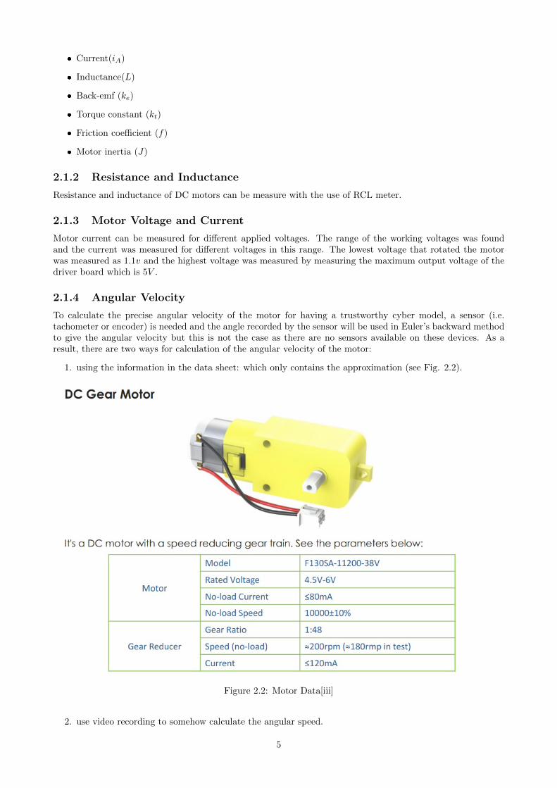
The second controller that will be designed is the controller that can control the distance of two cars at thesame time with keeping the desired speed. This controller can be considered as a ”system of systems” as twoseparate systems are going to be controlled for getting an outcome that is not an outcome of any of the systems.In this system, two cars will move according to the desired speed and at the same time, the distance betweencars will be controlled according to the desired distance. The desired speed of the motion of both cars will bethe input to the leader car and the second car tries to keep a desired distance with the lead car which means itshould keep the desired speed also, whenever the reference signal for the desired distance changes the speed ofthe second car also changes for compensation of the distance and when the desired speed signal changes bothof the cars speed will change according to the desired speed. Figure 2.10 shows the control system that is goingto be designed. This controller which is the MIMO controller will also be designed according to three methodsmentioned in the above.

Figure 2.10: Speed and Distance Control of Two Cars

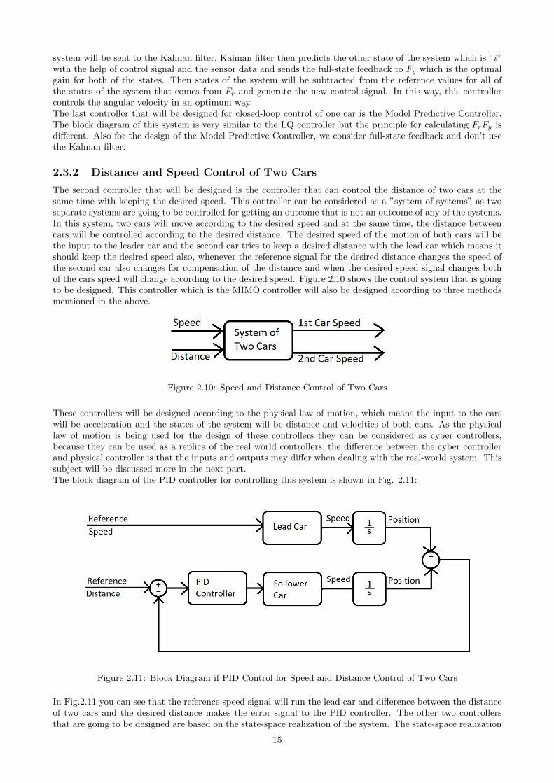
These controllers will be designed according to the physical law of motion, which means the input to the carswill be acceleration and the states of the system will be distance and velocities of both cars. As the physicallaw of motion is being used for the design of these controllers they can be considered as cyber controllers,because they can be used as a replica of the real world controllers, the difference between the cyber controllerand physical controller is that the inputs and outputs may differ when dealing with the real-world system. Thissubject will be discussed more in the next part.The block diagram of the PID controller for controlling this system is shown in Fig. 2.11:

Figure 2.11: Block Diagram if PID Control for Speed and Distance Control of Two Cars

In Fig.2.11 you can see that the reference speed signal will run the lead car and difference between the distanceof two cars and the desired distance makes the error signal to the PID controller. The other two controllersthat are going to be designed are based on the state-space realization of the system. The state-space realization

15

of the system that is going to be controlled is [11]:

Dvl(t)vf (t)

=

0 1 −10 0 00 0 0

. Dvl(t)vf (t)

+

0 01 00 1

. [al(t)af (t)

](2.54)

Where D, vl(t), vf (t), al(t) and af (t) are relative distance, velocity and acceleration of the lead and followercar respectively. The step response of the system is shown in Fig.2.12.

Figure 2.12: Step Response of the Two Car Platoon

For this system, we consider the full-state feedback and design the LQ controller which means:

z =

[1 0 00 1 0

] Dvl(t)vf (t)

(2.55)

y =

1 0 00 1 00 0 1

Dvl(t)vf (t)

(2.56)

According to the mentioned state-space system has three states, relative distance and leader and follower carsvelocities, inputs to the system are acceleration to the cars and output of the system are distance and velocities,states to be controlled are the distance and the lead car velocity.

The state-space that was discussed in this part is based on the physical laws of motion, the inputs to thesystem are acceleration and output of the system are the relative distance of the cars and cars’ velocities. Thiskind of controllers can be considered as cyber controllers, in the real world the inputs to the systems are voltagesand the outputs of the system are distance and velocity so it is necessary to adapt the cyber controller to thephysical systems. Figure 2.13 shows the system that should be designed to work in the real world:In this system inputs to the system are desired distance and speed the system tries to follow them, as the

16

Figure 2.13: Physical World Control System

input to the real-world cars are voltage the controller should convert the input signals to the voltage to sendto the cars, this voltage then will be translated to the angular velocity and accordingly the linear velocity, therelation between cars speed in each second will generate the desired speed of motion and desired distance. Thestate-space of the system that can work in the physical world is based on the state-space of the cars. Thenumber of states should be added to the system to make it able to control the distance (because the distanceis not presented in the state-space of the cars). The state-space of this system is as follows:

X =

0 0 1 −1 0 0

0 0 −ke

Lke

L −RL

RL

0 0 −c fJ 0 ckt

J 0

0 0 0 −c fJ 0 ckt

J

0 0 −ke

L 0 −RL 0

0 0 0 −ke

L 0 −RL

.Dirwl

wf

ilif

+

−1 0 00 0 00 0 00 0 00 1

L 00 0 1

L

.Dd

uluf

(2.57)

z =

[1 0 0 0 0 00 0 1 0 0 0

].

Dirwl

wf

ilif

(2.58)

y =

1 0 0 0 0 00 1 0 0 0 00 0 1 0 0 00 0 0 1 0 00 0 0 0 1 00 0 0 0 0 1

.Dirwl

wf

ilif

(2.59)

in which c is equal to wheel diameter divided by gearbox ratio, then c multiply with the angular velocity ofthe motor gives the linear velocity, the ”c” multiplied by the 3rd and 4th states changes the angular velocityto linear velocity. ”D” is the distance between two cars and ”ir” is the difference between two motors current.Other parameters are mechanical parameters that were derived earlier. The first state of the system is thedistance between two cars, the second state of the system is the relative motor currents, this state is designedso that any torque that was made in the lead car according to the voltage applied generates same torque inthe follower car in this way the follower car always follows the lead car, the controller tries to keep this statezero for all the time, the only times that this state changes from zero to a number is the time that the distancereference signal changes and the follower car try to compensate the distance. Other states of the system arethe same states from the car cyber model. The system is observable and controllable as the controllability andobservability matrices are full rank. The states of the system that are going to be controlled are the relativedistance and the leader car speed.

2.3.3 Distance and Speed Control of Platoon of Cars

All the controllers explained in the previous section can be extended and be used to control the platoon of cars.In the case of the PID controller, the philosophy of the control method is the same as explained in speed anddistance control of two cars. This method of control can easily be extended to distance and speed control ofthe platoon of cars.Although the philosophy of the control is also the same for LQ and MP controller the state space of the system

17

needs to be revised and extended. The state-space of the platoon of cars can be written as [11]:

X =

xl(t)− x1(t)x1(t)− x2(t)

...xN−2(t)− xN−1(t)

vl(t)v1(t)

...vN−1(t)

, U =

al(t)a1(t)

...aN−1(t)

(2.60)

A =

0(N−1)×(N−1)

1 −1 0 · · · 0

0 1 −1. . .

......

. . .. . .

. . . 0

0... 0 1 −1

0N×(N−1) 0N×N

, B =

[0(N−1)×N

IN×N

](2.61)

In this state-space realization of the system, the first group of states is the distances between cars and thesecond group are the velocities of the cars. Inputs to the system are acceleration to each car and outputs of thesystem are distances of the cars and speed of the cars, parameters to control are the distances of the cars andthe lead car velocity.In the final section the mentioned state-space for controlling the platoon of cars can be adapted to the realsystem inputs and outputs, in a way that the inputs to the system instead of accelerations become voltages.The adapted state-space for two cars can be seen in 2.57, 2.58 and 2.59. The extended adapted state-space is:

X =

D1

D2

D3

D4

D5

ir1ir2ir3ir4ir5w1

w2

w3

w4

w5

w6

i1i2i3i4i5i6

U =

Dd1

Dd2

Dd3

Dd4

Dd5

ulu1u2u3u4u5

(2.62)

18

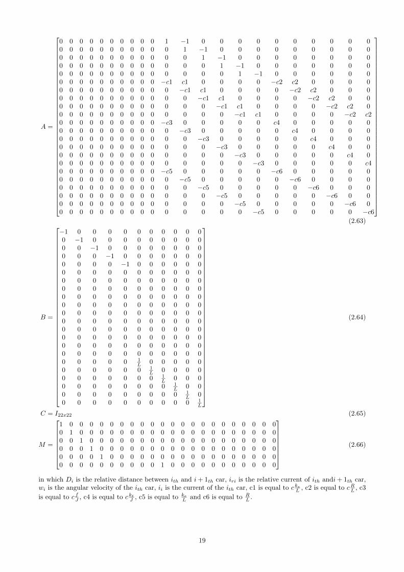
A =

0 0 0 0 0 0 0 0 0 0 1 −1 0 0 0 0 0 0 0 0 0 00 0 0 0 0 0 0 0 0 0 0 1 −1 0 0 0 0 0 0 0 0 00 0 0 0 0 0 0 0 0 0 0 0 1 −1 0 0 0 0 0 0 0 00 0 0 0 0 0 0 0 0 0 0 0 0 1 −1 0 0 0 0 0 0 00 0 0 0 0 0 0 0 0 0 0 0 0 0 1 −1 0 0 0 0 0 00 0 0 0 0 0 0 0 0 0 −c1 c1 0 0 0 0 −c2 c2 0 0 0 00 0 0 0 0 0 0 0 0 0 0 −c1 c1 0 0 0 0 −c2 c2 0 0 00 0 0 0 0 0 0 0 0 0 0 0 −c1 c1 0 0 0 0 −c2 c2 0 00 0 0 0 0 0 0 0 0 0 0 0 0 −c1 c1 0 0 0 0 −c2 c2 00 0 0 0 0 0 0 0 0 0 0 0 0 0 −c1 c1 0 0 0 0 −c2 c20 0 0 0 0 0 0 0 0 0 −c3 0 0 0 0 0 c4 0 0 0 0 00 0 0 0 0 0 0 0 0 0 0 −c3 0 0 0 0 0 c4 0 0 0 00 0 0 0 0 0 0 0 0 0 0 0 −c3 0 0 0 0 0 c4 0 0 00 0 0 0 0 0 0 0 0 0 0 0 0 −c3 0 0 0 0 0 c4 0 00 0 0 0 0 0 0 0 0 0 0 0 0 0 −c3 0 0 0 0 0 c4 00 0 0 0 0 0 0 0 0 0 0 0 0 0 0 −c3 0 0 0 0 0 c40 0 0 0 0 0 0 0 0 0 −c5 0 0 0 0 0 −c6 0 0 0 0 00 0 0 0 0 0 0 0 0 0 0 −c5 0 0 0 0 0 −c6 0 0 0 00 0 0 0 0 0 0 0 0 0 0 0 −c5 0 0 0 0 0 −c6 0 0 00 0 0 0 0 0 0 0 0 0 0 0 0 −c5 0 0 0 0 0 −c6 0 00 0 0 0 0 0 0 0 0 0 0 0 0 0 −c5 0 0 0 0 0 −c6 00 0 0 0 0 0 0 0 0 0 0 0 0 0 0 −c5 0 0 0 0 0 −c6

(2.63)

B =

−1 0 0 0 0 0 0 0 0 0 00 −1 0 0 0 0 0 0 0 0 00 0 −1 0 0 0 0 0 0 0 00 0 0 −1 0 0 0 0 0 0 00 0 0 0 −1 0 0 0 0 0 00 0 0 0 0 0 0 0 0 0 00 0 0 0 0 0 0 0 0 0 00 0 0 0 0 0 0 0 0 0 00 0 0 0 0 0 0 0 0 0 00 0 0 0 0 0 0 0 0 0 00 0 0 0 0 0 0 0 0 0 00 0 0 0 0 0 0 0 0 0 00 0 0 0 0 0 0 0 0 0 00 0 0 0 0 0 0 0 0 0 00 0 0 0 0 0 0 0 0 0 00 0 0 0 0 0 0 0 0 0 00 0 0 0 0 1

L 0 0 0 0 00 0 0 0 0 0 1

L 0 0 0 00 0 0 0 0 0 0 1

L 0 0 00 0 0 0 0 0 0 0 1

L 0 00 0 0 0 0 0 0 0 0 1

L 00 0 0 0 0 0 0 0 0 0 1

L

(2.64)

C = I22x22 (2.65)

M =

1 0 0 0 0 0 0 0 0 0 0 0 0 0 0 0 0 0 0 0 0 00 1 0 0 0 0 0 0 0 0 0 0 0 0 0 0 0 0 0 0 0 00 0 1 0 0 0 0 0 0 0 0 0 0 0 0 0 0 0 0 0 0 00 0 0 1 0 0 0 0 0 0 0 0 0 0 0 0 0 0 0 0 0 00 0 0 0 1 0 0 0 0 0 0 0 0 0 0 0 0 0 0 0 0 00 0 0 0 0 0 0 0 0 0 1 0 0 0 0 0 0 0 0 0 0 0

(2.66)

in which Di is the relative distance between ith and i+ 1th car, iri is the relative current of ith andi+ 1th car,wi is the angular velocity of the ith car, ii is the current of the ith car, c1 is equal to cke

L , c2 is equal to cRL , c3

is equal to c fJ , c4 is equal to ckt

J , c5 is equal to ke

L and c6 is equal to RL .

19

2.4 Communication

Implementation of communication between the physical model and cyber model is a crucial part of the cyber-physical systems, these systems should be designed in a way so that the physical device and its cyber modelcan communicate and data can flow between them easily. For this project, the communication link designedand implemented together with a simple cyber controller. As mentioned earlier cars are equipped with IRline follower sensors and ultrasonic distance measurement sensors, these sensors are used with the embeddedcontroller which is Raspberry PI and make the car able to follow the line and avoid hitting objects. As the firstlevel of implementation of cyber-physical system the cyber controller designed so that all the sensor readingsfrom the car were sent to the cyber controller which is a cyber twin for the physical controller of the device,then the process was done in the cyber controller and the states of the cyber model were updated according tothese sensors’ data, then commands for actuation were sent to the device, in this way cyber controller tried tocontrol the physical device.

The general idea behind this system is that data including line followers’ sensors data (five sensors), distancedata from the ultrasonic sensor, and speed data are gathered using car sensors, these data are packed by the carprocessor and send through WIFI, data is received by the cyber controller and get unpacked, then the processis done with the use of MATLAB functions, results which are actuation commands including car speed andturning angle to the servo and DC motors are packed and sent through WIFI to the car, car processor unpacksthe data and does the actuation.The following figure shows the whole the process:

Figure 2.14: General Structure of the System

Like previous system parts the communication link has two parts in this project, cyber communication, andphysical communication, cyber communication is the communication between the parts in the cyber model andcan use different protocols and coding architecture according to the software used for generation of the cybermodels. In this part of the project, the aim is to implement the link between the physical device and the cybercontrol so one of the defined communication protocols should be used for this reason. The protocol used forthis communication is UDP; UDP is not a safe communication as there is no guarantee that all packets reachthe destination but for the first step and in a laboratory environment it is a good choice for implementation.The structure of the program that makes the cyber controller able to control the physical device is shown inthe following lines:

1. Cyber controller sends a request for establishing a connection

2. Car accepts the connection

3. Cyber controller requests for the data from the five line-following sensors

4. Car sends five reading from the five IR line following sensors to the cyber controller

5. Cyber controller sends a request for distance to the front object and speed of the car

20

6. Car sends the information of ultrasonic sensor and velocities of the DC motors

7. Cyber controller calculates the speed and turning angle based on the received data

8. Cyber controller sends the speed and turning angle commands to the car

9. Car applies this data to the servo motor and DC motors

10. Whole system goes to step 1

According to the mentioned algorithm, the cyber controller would be able to control the physical device.

21

Chapter 3

Results

3.1 Motor Model

3.1.1 Resistance and Inductance

The following table shows the measure resistance and inductance of the motor.

Parameter SizeResistance 4.94 ΩInductance 1mH

Table 3.1: Mesured R and L

3.1.2 Motor Voltage and Current

The following table shows the motor current for different voltages applied to the motor.

Applied Voltage(V ) Motor Voltage(V ) Motor Current(A)1.1 0.97 0.092 1.88 0.113 2.84 0.124 3.85 0.135 4.89 0.14

Table 3.2: Mesured Voltage and Current

3.1.3 Angular Velocity

The following table shows the angular velocity of the wheel connected to the gearbox. The motor angularvelocity can be found in the third column of the Table

Applied Voltage(V ) Wheel Angular Velocity rad/sec Motor Angular Velocity rad/sec1.1 1.46 70.082 2.92 140.163 5.70 273.64 7.38 354.245 8.97 430.08

Table 3.3: Mesured Angular Velocity of the Wheel and Motor

3.1.4 Time Constant

Figure 3.1 shows the sample of curve fitting of the measured data with two terms exponential function.

The constant term in all of the curvefittings can be seen in the Fig.3.2:

f(t) = 8.1434e−1/0.0358t

22

Figure 3.1: Curve fitting of the angular velocity data

Figure 3.2: Curve fitting Data

The average step response of the system derived from averaging all the responses explained before gives thestep response that is shown in Fig.3.3To validate the data it is possible to plot the recorded data in the same plot with recorded data and see howmuch they fit together. In Fig.3.4 and 3.5 you can see the response of the derived system to different step inputversus the recorded data with the same input, as you can see the derived system response is very similar to therecorded data from real motor motion.

3.1.5 Back-emf, Torque Constant, Friction Coefficient and Motor Inertia

Followings are the calculated parameter of the motor

Back-emf (ke) = 0.0113 volt/rad/sec

Torque constant (kt) = 0.0113 Nm/A

Friction coefficient (f) = 7.1093*10−6

Motor inertia (J) = 9.2418*10−7 kg/m2

The MATLAB code for calculation of the mentioned parameters can be found in the Appendix of this report.

23

Figure 3.3: Step response of the system

Figure 3.4: Validation of the Derived System Response with Recorded Data

24

Figure 3.5: Validation of the Derived System Response with Recorded Data

25

3.1.6 Simulation of the Motor

Before finalizing the motor parameters is good to check them with a precise simulation. The motor model wasmade in SIMULINK and it can be seen in Fig. 3.6

Figure 3.6: SIMULINK Model of the Motor

The simulation result confirmed most of the derived parameter, the only parameter that needed a change wasfriction coefficient, the friction coefficient was derived by averaging all the statistical data that was recordedfrom the video recording. The suitable friction coefficient from the simulation is one-tenth of the calculatednumber which is 7.1093 ∗ 10−7. This result is not surprising because this parameter is very dependent on theinternal parts of the motor and it can change easily with a small difference in the production of the motor.Figure 3.7 shows the response of the simulation with the corrected friction coefficient to different voltage inputs.

Figure 3.7: Response of the Simulated Motor to Different Input Voltages

The resulting angular velocity from the simulation is shown in Fig. 3.7 and is closely matched with the angularvelocity derived from the video recordings.

26

3.2 Closed-loop Control of One Car

In this section, the response of the designed controllers for closed-loop control of one car will be presented anddiscussed.

3.2.1 PID Controller

The PI controller designed for speed control of the car. The SIMULINK model can be seen in Fig 3.8

Figure 3.8: SIMULINK Model for PI Control of One Car

The response of this system with P = 1 and I = 10 can be seen in Fig 3.9

Figure 3.9: Step Response of the Open-loop and Closed-loop system with PI Controller

3.2.2 Linear Quadratic Controller

LQG controller design is based on the state-space realization of the system, so in this part, the state-space ofthe system that was introduced in 2.13 and 2.14 is used. For simplicity these equations are written below:

[iw

]=

[−R

L −ke

Lkt

J − fJ

] [iw

]+

[1L0

]uA (3.1)

y =[0 1

] [ iw

](3.2)

27

According to (3.1) system has two states, it is not feasible to measure the first state of the system which is themotor current; so a Kalman filter should be designed for estimation of the state of the current. To implementthe Kalman filter the system must be ”observable” the observability matrix of the system is full rank whichmeans that the system is observable. The closed-loop versus the open-loop response of the system can be seenin Fig.3.10

Figure 3.10: Step Responses of The System with LQG Controller

MATLAB code for this part can be found in Appendix 1.

3.2.3 Model Predictive Controller

The MPC Controller was also designed for closed-loop control of each car. Figure 3.11 shows the response ofthe system with the MPC controller with the prediction horizon of 10 and the control horizon of three. Theaforementioned state-space was used in the design of the MPC controller. MATLAB code for designing theMPC controller can be found in the appendix of this report.

Figure 3.11: Step Response of the Systeam with MPC Controller

Before finishing this section, it should be mentioned that these three controllers showed very fast response inthe simulations that are not realistic, for example in the PID controller the response of the system from bothclosed and open-loop is normalized so the reader can see the difference, but even for such a small input signalthe control signal has been very high which means in real-world the system cannot handle the control signalneeded for this fast response, as a result, the control signal should be limited. In LQ and MP controller alsoaccording to delays imposed on the system by sensors and communication this response is also impossible evenif the control signal is kept inside the limits and also maybe in the real system penalizing the output error tothis level is not possible and make the system uncontrollable. It should be noted that these controllers shouldbe tuned and configured according to the real system when it comes to implementation.

28

3.3 Distance and Speed Control of Two Cars

In the previous section, the closed-loop control of one car was discussed and three controllers were introduced.In this section, three controllers will be introduced and discussed for distance and speed control of two cars.The distance control of two cars means that the front car which will be called the leader from now on will movewith the desired speed and the second car which will be called the follower car from now on will follow theleader and tries to keep a predefined distance with the front car.

3.3.1 PID Controller

For the first method, the PI controller was designed for controlling the distance between the lead car and thefollower car. The schematic of the simulation is shown in Fig.3.12.

Figure 3.12: Distance Control of Two Cars Using PID Controller

In Fig.3.13 the control signal generated as the input to the lead car vs. the control signal generated by the PIDcontroller of the second car can be seen.

Figure 3.13: Control Signals for Lead and Follower Cars

The relative distance between the two cars is shown in Fig.3.14. The PID controller is keeping the constantdistance by controlling the speed of the follower car.Although it is working, the main problem with the PI controller is that it is not an optimal controller, so in thenext part the LQ controller for this problem will be discussed.

29

Figure 3.14: Abcolute Position of Lead and Follower Cars

3.3.2 Cyber Linear Quadratic Controller

The Linear Quadratic Controller was designed according to 2.54,2.55 and 2.56 and the step response of thesystem can be seen in Fig.3.15

Figure 3.15: Step Response of the LQ Controller for Speed and Distance Control of Two Cars

To validate the result SIMULINK model for testing the controller was designed and can be seen in Fig.3.16,the result of the simulation can be seen in Fig.3.17, in this simulation at t = 1 the unit step is put on input twowhich is the speed of the leader car, as you can see the follower follows the leader as the desired input distanceis zero, this process goes on till t = 6, at this moment the desired distance changes from zero to one and LQcontroller successfully makes the distance while keeping the desired speed. The MATLAB code for this partcan be found in the appendix of this report.

30

Figure 3.16: SIMULINK Model Validation of LQ Controller

Figure 3.17: States of the system controlled with LQ Controller

3.3.3 Cyber Model Predictive Controller

The MPC controller was designed for the system in 2.54 and 2.55. Figure 3.18 shows the desired input signalto the system which is the same scenario like the one mentioned for the LQ controller. The MPC controller isdesigned with the prediction horizon of 10 and the control horizon of three.Figure 3.19 shows the response of the system at the same time with the control signals generated by thecontroller. The controller has the prediction horizon of 10 with the control horizon of three.Finally, for validation of the result, states of the system are plotted and can be seen in Fig.3.20. This is thesame figure as Fig.3.17 but this time generated with the model predictive controller for the same system.MATLAB code for this part can be found in appendix of this report.

31

Figure 3.18: Input Signals to the Model Predictive Controller

Figure 3.19: Response of the Model Predictive Controller

32

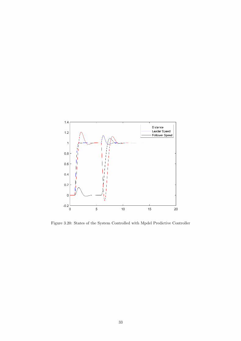
Figure 3.20: States of the System Controlled with Mpdel Predictive Controller

33

3.3.4 Physical Linear Quadratic Controller

In this section, the physical LQ controller for controlling the distance and speed of two cars will be shown.Figure 3.21 shows the SIMULINK model that is used for the validation of this controller.

Figure 3.21: SIMULINK Model of the Physical LQ Controller

Figure 3.22 shows the response of the system under the control of the LQ controller to the scenario that wasused for previous parts:

Figure 3.22: Response of the Physical LQ Controller

The control scenario is the same as before at t = 1 when the desired speed input changes from zero to one thefollower car closely follows the leader (the blue line is behind the red line). At t = 6 the desired distance ofthe cars changes from zero to one and as you can see system successfully follows the input signals. The timeit takes for the desired distance signal to settle is about two seconds, in this controller Q1 for penalizing thestate’s error is equal to 10 and Q2 for penalizing the control signal is one. Figure 3.23 shows the control signalgenerated by the controller according to mentioned Q1 and Q2:

34

Figure 3.23: Control Signals (Voltages to the Cars) Generated by Physical LQ Controller

To better see what is going on at t = 6 the zoomed version of the image is shown in Fig. 3.24:

Figure 3.24: Control Signals (Voltages to the Cars) Generated by Physical LQ Controller at t = 6

3.3.5 Physical Model Predictive Controller

Figure 3.25 shows the response of the MP conroller for the state-space given 2.57 and 2.58Figure 3.26 shows what is exactly happening to voltages to the cars at t = 6 when the dersired distance referencesignal changes from zero to one.

35

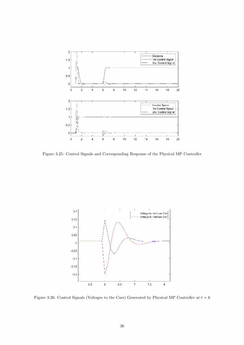
Figure 3.25: Control Signals and Corresponding Response of the Physical MP Controller

Figure 3.26: Control Signals (Voltages to the Cars) Generated by Physical MP Controller at t = 6

36

3.3.6 Pysical Model Predictive Controller with Constraint

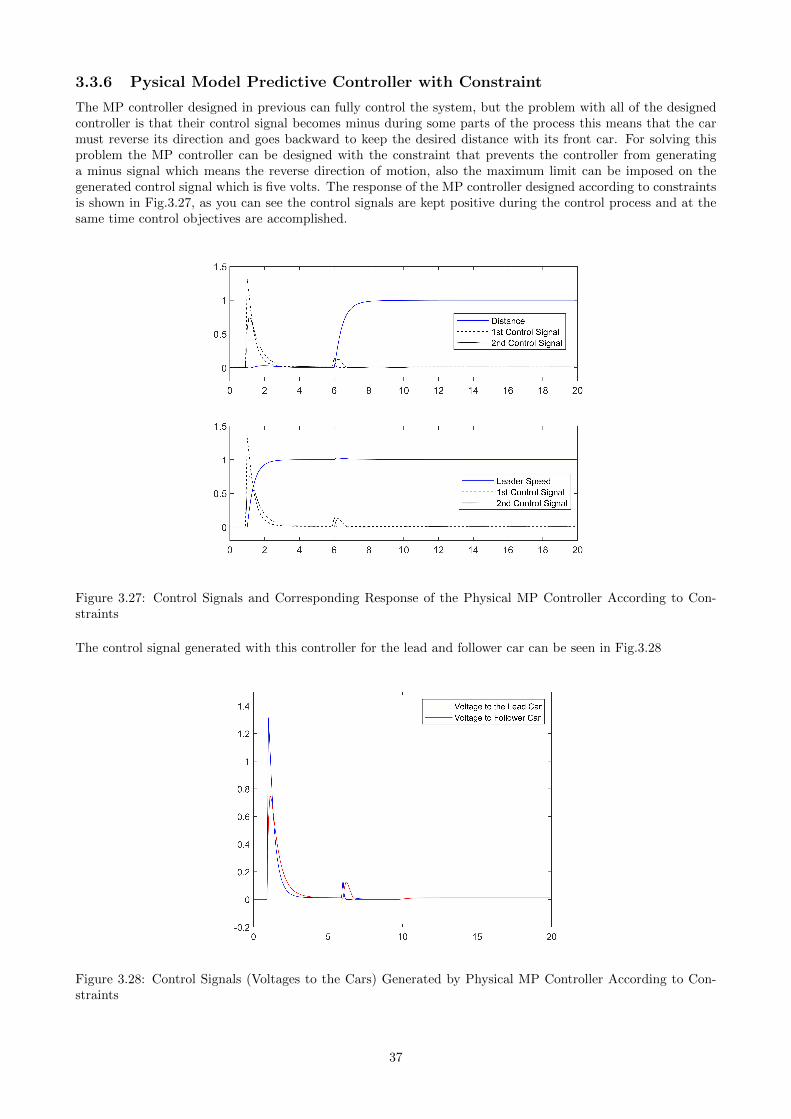
The MP controller designed in previous can fully control the system, but the problem with all of the designedcontroller is that their control signal becomes minus during some parts of the process this means that the carmust reverse its direction and goes backward to keep the desired distance with its front car. For solving thisproblem the MP controller can be designed with the constraint that prevents the controller from generatinga minus signal which means the reverse direction of motion, also the maximum limit can be imposed on thegenerated control signal which is five volts. The response of the MP controller designed according to constraintsis shown in Fig.3.27, as you can see the control signals are kept positive during the control process and at thesame time control objectives are accomplished.

Figure 3.27: Control Signals and Corresponding Response of the Physical MP Controller According to Con-straints

The control signal generated with this controller for the lead and follower car can be seen in Fig.3.28

Figure 3.28: Control Signals (Voltages to the Cars) Generated by Physical MP Controller According to Con-straints

37

3.4 Distance and Speed Control of Platoon of Cars

Like previous sections in this section response of the three controllers designed for controlling platoon of carswill be discussed.

3.4.1 PID Control

The PID controller was designed as the first controller for this section for speed and distance control of a platoonof cars, the SIMULINK model of this controller can be seen in Fig. 3.29. The Control scenario is the same asbefore, at t = 1 lead car starts to move with constant speed and other cars should follow it instantly, at t = 6the desired distance between cars changes from zero to one and the controller tries to fix the distance at thesame time with keeping the desired speed.

Figure 3.29: Simulation of PID Controller for Controlling Platoon of Cars

The resulting speed of the cars and distance between cars are shown in Fig.3.30 and Fig.3.31 for P = 20 andI = 3. Although the response seems satisfying by looking at control signal in Fig 3.32 generated for controllingthe platoon of cars it is obvious that this control is impossible with these choices of P and I parameters as thecontrol signal exceeds the maximum and minimum possible control signal accepted by the car which is ±5v.

To make a controller generate the control signal inside the limits of ±5v the P and I parameters reducet toP = 2 and I = 0.3, the corresponding outputs and control signals are shown in Fig.3.33, Fig.3.34 and Fig.3.35

As you can see even with this selection of P and I parameters the control signal is outside the limits and the

38

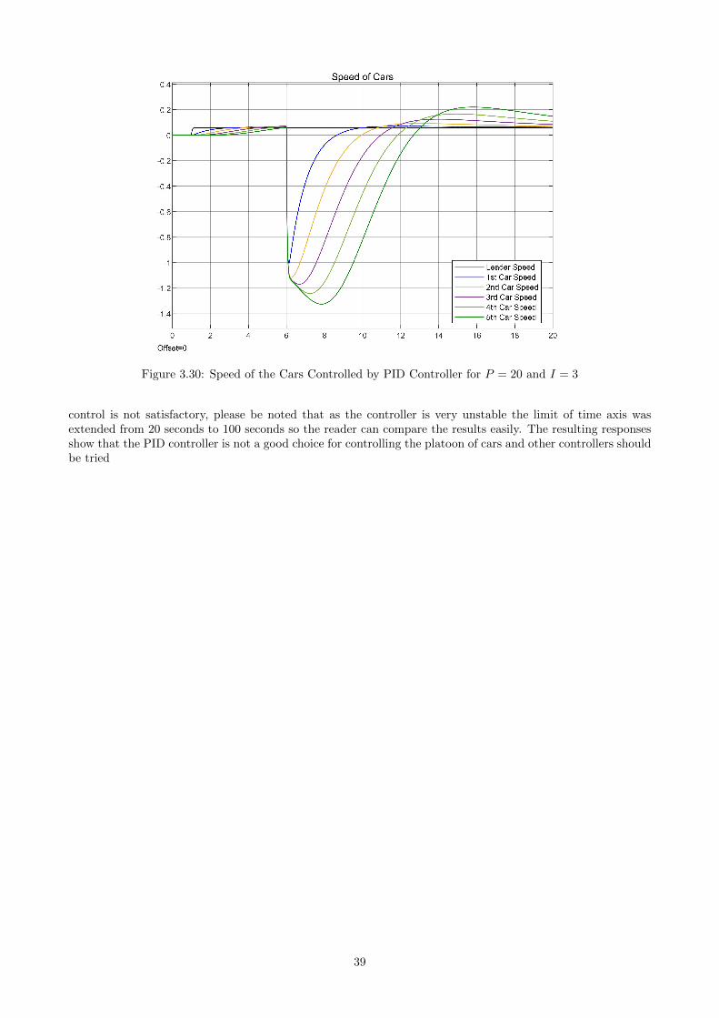
Figure 3.30: Speed of the Cars Controlled by PID Controller for P = 20 and I = 3

control is not satisfactory, please be noted that as the controller is very unstable the limit of time axis wasextended from 20 seconds to 100 seconds so the reader can compare the results easily. The resulting responsesshow that the PID controller is not a good choice for controlling the platoon of cars and other controllers shouldbe tried

39

Figure 3.31: Position of the Cars Controlled by PID Controller for P = 20 and I = 3

Figure 3.32: Control Signals Generated by PID Controller for P = 20 and I = 3

40

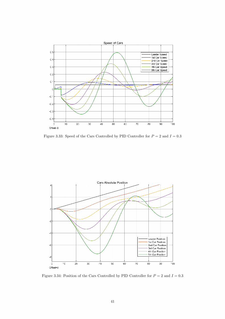
Figure 3.33: Speed of the Cars Controlled by PID Controller for P = 2 and I = 0.3

Figure 3.34: Position of the Cars Controlled by PID Controller for P = 2 and I = 0.3

41

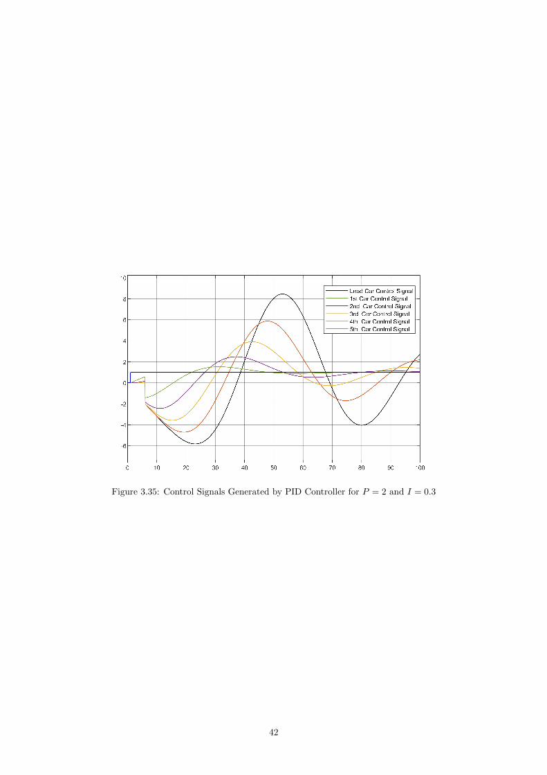
Figure 3.35: Control Signals Generated by PID Controller for P = 2 and I = 0.3

42

3.4.2 Cyber Linear Quadratic Control

Figure 3.36 shows the SIMULINK model for LQ control of the platoon of cars:

Figure 3.36: Simulation of LQ Controller for Controlling Platoon of Cars

In LQ controller it is possible to penalize the control signal so the problem with very big control signal as wesaw in PID controller does not exist, Fig.3.37, Fig.3.38 and Fig.3.39 show the cars’ speed, distance and controlsignal with the choice of Q1 = 1 and Q2 = 100.

Figure 3.37: Speed of the Cars Controlled by LQ Controller for Q1 = 10 and Q2 = 1

As the control signal is penalized the response of the system is slow but still much faster than PID controller.

43

Figure 3.38: Distance of the Cars Controlled by LQ Controller for Q1 = 10 and Q2 = 1

Figure 3.39: Control Signals Generated by LQ Controller for Q1 = 10 and Q2 = 1

44

3.4.3 Cyber Model Predictive Control

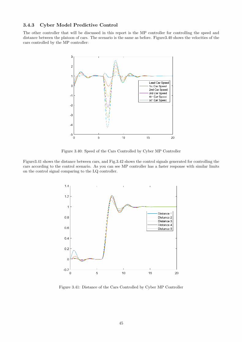
The other controller that will be discussed in this report is the MP controller for controlling the speed anddistance between the platoon of cars. The scenario is the same as before. Figure3.40 shows the velocities of thecars controlled by the MP controller:

Figure 3.40: Speed of the Cars Controlled by Cyber MP Controller

Figure3.41 shows the distance between cars, and Fig.3.42 shows the control signals generated for controlling thecars according to the control scenario. As you can see MP controller has a faster response with similar limitson the control signal comparing to the LQ controller.

Figure 3.41: Distance of the Cars Controlled by Cyber MP Controller

45

Figure 3.42: Control Signals Generated by Cyber MP Controller

3.4.4 Physical Linear Quadratic Controller

The LQ and MP controller designed for controlling the platoon of cars in previous sections were both cybercontrollers as they were based on physical laws of motion and the inputs to the system were acceleration to thecars. In this section, the LQ and MP controller will be discussed that are adapted to the physical system, whichmeans that their inputs are voltages to the DC motors of the cars instead of accelerations. The system to becontrolled is a platoon of six cars like before and the control scenario is exactly as before and the state-space ofthe system to be controlled was written in 2.63 to 2.66.

The first controller in this part is the LQ controller. Fig.3.43 shows the speed of cars and Fig. 3.44 shows thedistance between cars in the platoon controlled by the LQ controller:

Figure 3.43: Speed of the Cars Controlled by Physical LQ Controller

Finally, Fig.3.45 shows the voltage generated by the controller for controlling the cars:

46

Figure 3.44: Distance of the Cars Controlled by Physical LQ Controller

Figure 3.45: Control Signals Generated by Physical LQ Controller

47

3.4.5 Physical Model Predictive Controller

The final controller that will be designed in this section is the MP controller adapted with the physical system.Abilities of the MP controller in handling the constraint and optimization of the process throughout the definedprediction and control horizon is very important in designing the cyber-physical systems. As previous, theplatoon of six cars is going to be controlled with this controller and the control scenario is the same as before.Figure 3.46 shows the velocities of the cars during the control scenario:

Figure 3.46: Speed of the Cars Controlled by Physical MP Controller

Figure 3.47 and 3.48 show the distance between the cars and the control signal to the cars which are the voltageaccording to the constraints defined.

Figure 3.47: Distance of the Cars Controlled by Physical MP Controller

48

Figure 3.48: Control Signals Generated by Physical MP Controller

49

3.5 Communication

The scenario for testing the control of the car by cyber controller is to start with a straight line and one rightturn, then two left turns and in the middle of the third left turn the obstacle was put, the obstacle was keptconstant for some time and then removed, car kept the motion and this time the obstacle was put in the middleof the next straight line, following figures show the sensor readings from the car during the test of the scenariothat was explained, for better understandig the figure, five IR line following sensors are named as left, middleleft, center, middle right and righr sensors, the main purpose of designing the cyber controller was to keep theblack line under the center sensor which which its output is plotted using the yellow color in the graph, also itshould be mentioned that the lowest number read from each sensor reading shows where the line is, for examplewhen the blue line has the lowest number it means that the line to follow is under the left sensor, in this wayreader can follow and validate the result of the control process.

Figure 3.49: IR Sensors Readings Duirng Test Travel

In Fig.3.49 you can see that till sample 160 to 170 the system is working in a normal mode and tries to keepthe line in the middle of the car, in some points after sample 150 the car reaches the obstacle, and as theobstacle is in the middle of the left turn two left sensors absorb least IR signal, then the car stays in the sameposition till the obstacle is removed and it continues until it reaches the second obstacle which was placed inthe middle of the straight line, you can see that the center sensor has the least IR absorption. Figure 3.50shows the speed of the car and the distance sensed by the ultrasonic sensor during the test travel. As you cansee the speed is reduced as the car reaches the obstacle and it increased as the distance to the obstacle increases.

Figure 3.50: Distance to Front Obstacle Vs. Speed

50

Chapter 4

Discussion

In the first part of the report the car cyber model was derived, for doing this task number of parameters likevoltage, current, resistance, inductance, and angular velocity were measured, then the mechanical time constantof the motor was derived using the statistical data from the video recording and based on this time constantother motor parameters like torque constant, back-emf, motor inertia and friction coefficient were calculated.These data then used in the SIMULINK model of the motor which was designed according to the state-spaceof the DC motor, this simulation then showed that the friction coefficient calculated from the physical law’sformula is not correct, then experimentally the friction coefficient calculated. With the use of new frictioncoefficient the simulation gave the very close response to what was recorded.

Technically the only way to make sure about the derived parameters is to use the sensor like tachometer orencoder but considering the limitations, the simulation showed that the derived value for the parameters areacceptable and can be used for the derivation of the cyber model of the motor.

The other question that the reader may ask why other methods like system identification was not used, thereason for that is that for using the method like system identification the known input should be given to thesystem as an input and the output should be recorded and then by use of the methods like Least Squaresmethod identify the parameters, the problem here is that the output of the system here is angular velocity andrecording the output needs the use of the sensor that was not available on these cars.

On the next part of this report, three controllers were designed for closed-loop control of the DC motors, usually,the controller used for controlling the DC motor is the PID controller as it is simple comparing to other twocontrollers the reason for designing two other controller, considering their similar response to the PID controlleris that the objective of this testbed is to test the methods and algorithms of the cyber-physical systems, in thesesystems not only it is important to control the cars but it is important to monitor and control the states of thesystem, so using controllers that are based on the state-space of the system is necessary.

In the second part of designing controllers five controllers were designed to control the speed and distance oftwo cars, the first controller was the PID controller, as this controller works according to error signal thereis no difference between its cyber and physical model. Next two controllers that were designed in this partwere cyber LQ and MP controllers, these controllers were designed using only physical laws of motion andby looking at their design file it can be seen that no information from the physical system to be controlled isused in their design, this is why they were called cyber controllers, they can be used as the cyber model ofall physical controllers. These kinds of controllers can be used for high-level simulation of the cyber-physicalsystems when the general idea about the system is needed to be tested. Also, the state information of thesecyber models together with states of the physical system can be used in the machine learning algorithm forfurther process of the system. These part followed by the design of two physical controllers, these controllerswere completely based on the physical characteristics of the system, firstly, these controllers can be used as theembedded controller for controlling the physical process, secondly, they can be used for detailed simulation ofthe system for example for times when the system health should be checked.In the Third part of designing the controllers, cyber and physical controllers were designed for controlling theplatoon of cars. In the first section of this part, the PID controller was designed and it was shown that the PIDcontroller can not control this system according to the limitations. Then the other two controllers were designedand they have a very similar response but as the LQ controller can not handle the constraints the MP controllerseems to be a better choice. Although constraints might not seem to be very important in controlling theplatoon of cars, when they are imagined in the real cyber-physical system when the health of the system should

51

be kept until the desired overhaul time constraints become very important. As explained before in the specifi-cations of the cyber-physical systems in the fifth level which is ”configuration” the system parameters should beconfigured according to the risks that system is faced, this configuration which is defined according to systemlimitations and risks should be applied but at the same time the system should be worked in the most optimizedway, this is why handling the constraints and optimization with quadratic programming were discussed and used.

Generally, the main idea behind cyber-physical systems is the integration of the computation and physical sys-tem, controllers designed in the second and third section of this report are the controllers that are not only cancontrol system according to physical process they are implemented in a way that any data from outside worldcan influence the control of the system which is exactly the definition of the cyber-physical system. In this way,Model Predictive Controllers are playing a very important role as they can control linear and nonlinear systemsand also they are flexible in handling the constraints at the same time by optimizing the process over a de-fined horizon. This is why all sorts of MPC controllers were designed with their full functionality for this report.

In the final section of the report, the communication link was established between the cyber controller and thephysical device. In the cyber-physical system, the information should be able to flow between the cyber modeland the physical system easily. In the final part, the cyber model of the physical controller was implemented ona PC with the use of MATLAB and sensors data was used to update the states of the cyber model. Then theseupdated states were used for the generation of the actuation command. This process was done successfully andthe cyber controller could suitably control the physical system. The only problem that happened during thisimplementation was due to the processing time of the cyber model host processor. Using the cyber controllerfor controlling the physical system imposes some delays to the system due to time needed for communicationand processing time of the host device, these delays are measured and they are on the scale of 0.2 to 0.3 sec-onds. Although these delays seem very short they have a very crucial effect on the system control. To makethe cyber controller able to control the device the speed of the car motion was reduced to 60 percent of thefull speed. With this configuration, the cyber control was made possible. The other problem that happenedafter this change in the parameter was due to different processing time of the cyber controller host device, asthe host device used for this experiment was a PC the processing time of the same code took different time,in more than 90 percent of the time the processing time was about 0.2 to 0.3 seconds as mentioned but in 10percent of the time it was more and this affect the quality of the control. In the next step for advancement ofthese part, the control function should be divided into two parts and the embedded control should do the mainfunction control and cyber controller should only control the necessary managerial functions in this way theprocessing time of the host processor will be less and also won’t have any effect on the performance of the system.

In this report, the cyber model for all three main components (car, controller and communication) was im-plemented, and at the same time, it was tried to cover all the levels of the 5C architecture. The main reasonfor having this testbed is to test cyber-physical algorithms and methods, according to the definition of cyber-physical system the physical and cyber systems should work very close together and the cyber system statesshould be updated according to physical changes. The problem that arises here is that for the examinationof the health of the device and working condition information might be needed from the states that are notconsidered as the states of the system used for designing the controller, so this information should be generatedinside the cyber controller with the use of physical information. For generating these states system identificationmethods might be used. On the other hand, it is very hard to figure out what are the meaning of the states ofthe system that are derived with system identification as they might not have any real and physical meaningand also their number might be so big in the scale of 100 to 1000, for solving this problem methods like modelreduction can be used to find the important states of the system. In the next level when important states of thesystem were found other optimization algorithms like genetic algorithm can be used for system optimization.By using these methods the cyber controller with its ability to use information outside the physical boundariesof the device would be able to control the systems in a way that might be very different from the predefinedfunctionality of the device.

52

Chapter 5

Conclusion

In this thesis, the first step through the implementation of a cyber-physical testbed for wireless networked controlsystems was taken. The cyber models for all three parts of the system (cars, controllers, and communication)were developed. The cyber model of the car was implemented and tested and the results were validated bycomparison with the output of the physical device. Then three controllers were designed for closed-loop speedcontrol of the cars. In the next step, cyber and physical controllers were designed for speed and distance controlof two cars and platoon of cars, these controllers were designed as a cyber controller and physical controllersaccording to their inputs and connections and ability to control the physical system, the response of thesecontrollers were also discussed. Model Predictive Controllers where designed and implemented in this sectionaccording to constraints on the level of the input voltage, these controllers with their specifications will play animportant role in the real cyber-physical systems as they can handle optimization over a defined control andprediction horizons according to the constraints. Finally, the communication link was implemented between thecyber system and physical system and after resolving the limitations the cyber controller could control the car.Generally, a cyber-physical system was designed and implemented, the cyber model and physical system wereintegrated and the system was controlled not only by the embedded controller but also with the cyber controllerwhich can use all sorts of data from device sensors’ data to data from the cloud.

53

References

[1] Edward A. Lee, Cyber Physical Systems: Design Challenges. 11th IEEE Symposium on Object OrientedReal-Time Distributed Computing (ISORC)

[2] Ragunathan Rajkumar, Insup Lee, Lui Sha, John Stankovic Cyber-physical systems: The next computingrevolution. Design Automation Conference, Anaheim, CA, 2010, pp. 731-736

[3] Frontoni E., Loncarski J., Pierdicca R., Bernardini M., Sasso M. Cyber Physical Systems for Industry 4.0:Towards Real Time Virtual Reality in Smart Manufacturing. In: De Paolis L., Bourdot P. (eds) AugmentedReality, Virtual Reality, and Computer Graphics. AVR 2018. Lecture Notes in Computer Science, vol 10851.Springer, Cham

[4] Jay Lee, Behrad Bagheri, Hung-An Kao A Cyber-Physical Systems architecture for Industry 4.0-based man-ufacturing systems. Manufacturing Letters, Volume 3, January 2015

[5] P. Neumann Communication in industrial automation– What is going on? Control Engineering Practice,Special Issue on Manufacturing Plant Control: Challenges and IssuesINCOM 2004, vol. 15(11), pp. 1332-1347, 2007

[6] Magdi S. Mahmoud Wireless Networked Control System Design: An Overview 2014 IEEE 23rd InternationalSymposium on Industrial Electronics (ISIE)

[7] Sang-Hoon Kim Electric Motor Control. Amsterdam,Elsevier, 2017

[8] Wei Wu, DC Motor Identification Using Speed Step Responses. 2010 American Control Conference, June30-July 02, 2010

[9] Torkel Glad, Lennat Ljung Control Tehory, Multivariable and Nonlinear Methods. London,Taylor and Fran-cis, 2000

[10] Liuping Wang Model Predictive Control System Design and Implementation Using MATLAB. London,Springer, 2009

[11] Kim Sanggyum Design of the Adaptive Cruise Control Systems: An Optimal Control Approach. UC Berke-ley Electronic Theses and Dissertations, 2012

[12] Michael J. Best Quadratic Programming with Computer Programs. Boca Raton, Chapman and Hall/CRC,2017

54

Figure References

[i] https : //www.robotshop.com/en/sunfounder−picar−s−raspberry−pi−4−32b−smart−car−kit.html[ii] https : //www.control.isy.liu.se/student/tsrt21/file/pmdcmotor.pdf[iii] https : //www.sunfounder.com/learn/download/UGlDY XItU19V c2V yX01hbnV hbC5wZGY = /dispi

55

Chapter 6

Appendix

6.1 MATLAB Code for Calculation of Motor Parameters from RecordedData

1 %% Input data

2 T151 = readmatrix('151. xlsx');

3 T152 = readmatrix('152. xlsx');

4 T153 = readmatrix('153. xlsx');

56 T201 = readmatrix('201. xlsx');

7 T202 = readmatrix('202. xlsx');

8 T203 = readmatrix('203. xlsx');

910 T251 = readmatrix('251. xlsx');

11 T252 = readmatrix('252. xlsx');

12 T253 = readmatrix('253. xlsx');

1314 T301 = readmatrix('301. xlsx');

15 T302 = readmatrix('302. xlsx');

16 T303 = readmatrix('303. xlsx');

1718 T351 = readmatrix('351. xlsx');

19 T352 = readmatrix('352. xlsx');

20 T353 = readmatrix('353. xlsx');

2122 T401 = readmatrix('401. xlsx');

23 T402 = readmatrix('402. xlsx');

24 T403 = readmatrix('403. xlsx');

25 %% Speed calculation

26 v15 = vcalc(T151 ,T152 ,T153 ,1.5 ,5 ,0.09);

27 v151 = v15 (1:20 ,1);v152 = v15 (21:40 ,1);v153 = v15 (41:60 ,1);

28 v20 = vcalc(T201 ,T202 ,T203 ,2 ,5 ,0.11);

29 v201 = v20 (1:20 ,1);v202 = v20 (21:40 ,1);v203 = v20 (41:60 ,1);

30 v25 = vcalc(T251 ,T252 ,T253 ,2.5 ,5 ,0.115);

31 v251 = v25 (1:20 ,1);v252 = v25 (21:40 ,1);v253 = v25 (41:60 ,1);

32 v30 = vcalc(T301 ,T302 ,T303 ,3 ,5 ,0.12);

33 v301 = v30 (1:20 ,1);v302 = v30 (21:40 ,1);v303 = v30 (41:60 ,1);

34 v35 = vcalc(T351 ,T352 ,T353 ,3 ,5 ,0.125);

35 v351 = v35 (1:20 ,1);v352 = v35 (21:40 ,1);v353 = v35 (41:60 ,1);

36 v40 = vcalc(T401 ,T402 ,T403 ,4 ,5 ,0.13);

37 v401 = v40 (1:20 ,1);v402 = v40 (21:40 ,1);v403 = v40 (41:60 ,1);

38 %% Plot

39 t = 0:0.0333:(19*0.0333);figure (3)

40 subplot (3,2,1);plot (t,v15 (1:20) ,t,v15 (21:40) ,t,v15 (41:60))

41 title('V = 1.5v');xlabel('Time');ylabel('Angular Velocity ');

42 subplot (3,2,2);plot (t,v20 (1:20) ,t,v20 (21:40) ,t,v20 (41:60))

56

43 title('V = 2v');xlabel('Time');ylabel('Angular Velocity ');

44 subplot (3,2,3);plot (t,v25 (1:20) ,t,v25 (21:40) ,t,v25 (41:60))

45 title('V = 2.5v');xlabel('Time');ylabel('Angular Velocity ');

46 subplot (3,2,4);plot (t,v30 (1:20) ,t,v30 (21:40) ,t,v30 (41:60))

47 title('V = 3v');xlabel('Time');ylabel('Angular Velocity ');

48 subplot (3,2,5);plot (t,v35 (1:20) ,t,v35 (21:40) ,t,v35 (41:60))

49 title('V = 3.5v');xlabel('Time');ylabel('Angular Velocity ');

50 subplot (3,2,6);plot (t,v40 (1:20) ,t,v40 (21:40) ,t,v40 (41:60))

51 title('V = 4v');xlabel('Time');ylabel('Angular Velocity ');

52 %% Averaging the friction coefficent and back -emf from all recordings

53 [v15k v15f]= meancalc(v15);

54 [v20k v20f]= meancalc(v20);

55 [v25k v25f]= meancalc(v25);

56 [v30k v30f]= meancalc(v30);

57 [v35k v35f]= meancalc(v35);

58 [v40k v40f]= meancalc(v40);

59 f = (v15f + v20f + v25f + v30f + v35f + v40f)/6

60 kb = (v15k + v20k + v25k + v30k + v35k + v40k)/6

6162 %%

63 R = 4.95;

64 L = 10^-3;

65 expt = readmatrix('Curvetomatlab.xlsx');

66 expt = [expt zeros (17 ,1) zeros (17 ,1)];

67 expt (:,3) = expt (:,1)./expt (:,2); %K

68 expt (:,4) = -1./expt (:,2);% T

69 T = mean (expt (:,4))

70 K = mean (expt (:,3))

71 kt = kb

72 jco = (R/(kb*kt)+(R*f))

73 J = T / jco

74 c = size(expt);

75 figure (4)

76 title('Response of the system for different step inputs ');

77 t = 0:0.0333:(9*0.0333)

78 for i =1:c(1)

79 for j = 0:9

80 e1(i,j+1) = expt(i,1)*exp(expt(i,2)*j*0.0333)

81 end

82 plot(t,e1(i ,1:10));title('Response of the system for different step

inputs ');

83 hold on

84 end

85 %% State space

86 t = 0:0.0333:(19*0.0333);

87 A = [-R/L -kb/L;kt/J -f/J];

88 B = [1/L;0];

89 C = [0 1]

90 D = 0;

91 sys = ss(A,B,C,D)

92 figure (5)

93 subplot (3,1,1);plot (t,v15 (1:20) ,t,v15 (21:40) ,t,v15 (41:60));hold on

94 step (1.15*sys ,19*0.033 ,'k')

95 subplot (3,1,2);plot (t,v20 (1:20) ,t,v20 (21:40) ,t,v20 (41:60));hold on

96 step (1.88*sys ,19*0.033 ,'k')

97 subplot (3,1,3);plot (t,v25 (1:20) ,t,v25 (21:40) ,t,v25 (41:60));hold on

98 step (2.35*sys ,19*0.033 ,'k');figure (5)

99 subplot (3,1,1);plot (t,v30 (1:20) ,t,v30 (21:40) ,t,v30 (41:60));hold on

100 step (2.84*sys ,19*0.033 ,'k')

101 subplot (3,1,2);plot (t,v35 (1:20) ,t,v35 (21:40) ,t,v35 (41:60));hold on

102 step (3.35*sys ,19*0.033 ,'k')

57

103 subplot (3,1,3);plot (t,v40 (1:20) ,t,v40 (21:40) ,t,v40 (41:60));hold on

104 step (3.85*sys ,19*0.033 ,'k')

105 %% Function for calculation of the angular velocity ,back -emf and friction

106 %% coefficient from the recorded data

107 function v = vcalc(pos1 ,pos2 ,pos3 ,V,R,c)

108 s = size(pos1);

109 v1(1,1)=0;

110 v2(1,1)=0;

111 v3(1,1)=0;

112 for i = 2: s(1)

113 v1(i,1) =(48*(( pos1(i-1,1) - pos1(i,1)))/0.03333)*pi /180;%radian per

second

114 v1(i,2) = (V - R*c)/(v1(i-1,1)); % Kb

115 v1(i,3) = (v1(i,2)*c)/v1(i,1); %f

116117 v2(i,1) =(48*(( pos2(i-1,1) - pos2(i,1)))/0.03333)*pi /180;

118 v2(i,2) = (V - R*c)/(v2(i-1,1));

119 v2(i,3) = (v2(i,2)*c)/v2(i,1);

120121 v3(i,1) =(48*(( pos3(i-1,1) - pos3(i,1)))/0.03333)*pi /180;

122 v3(i,2) = (V - R*c)/(v3(i-1,1));

123 v3(i,3) = (v3(i,2)*c)/v3(i,1);

124125 end

126 v = [v1;v2;v3];

127 end

128 %% Function calculating the average

129 function [mk mf] = meancalc(mat)

130 c = size(mat);

131 j=0;

132 sumk = 0;

133 sumf = 0;

134 for i = 1:c(1)

135 if (mat(i,2) ==0|| mat(i,2) == inf)

136 pp=0;

137 else

138 sumk = mat(i,2) + sumk;

139 sumf = mat(i,3) + sumf;

140 j = j+1;

141 end

142 end

143144 mk = sumk / j;

145 mf = sumf / j;

146 end

6.2 MATLAB Code for LQ Speed Control of One Car

1 clear all

2 close all

3 %% Data

4 s = tf('s');

5 R = 4.95;

6 L1 = 10^ -3;

7 ke = 0.0113;

8 kt = 0.0113;

9 J = 9.2418e-07;

10 f = 7.1093e-07;

11 rw = 3.25/100; ng = 48;

58

12 c = rw/ng;

13 %% State space of individual car

14 Ai = [-R/L1 -ke/L1;

15 kt/J -f/J];

16 Bi = [1/L1;0];

17 Ci = [0 1];

18 Di = [0];

19 car = ss(Ai ,Bi ,Ci ,Di);

20 Gcar = tf(car);

21 Lr = 1/ dcgain(car);

22 figure (1)

23 step(Lr*car ,0.2)

24 hold on

25 %% Kalman Filter for individual car

26 [kesti ,Ki,Pi] = kalman(car ,1,1,0);

27 %% LQR for individual car

28 [Li ,Si,ei] = lqr(car ,eye(2) ,1,0);

29 Fyi = Li*inv(s*eye(size(Ai)) - Ai + Bi*Li + Ki*Ci)*Ki;

30 carc = feedback(car ,Fyi);

31 Lri = 1/ dcgain(carc);%*dcgain(car);

32 % Lr = 1;

33 carc = Lri*carc;

34 figure (1)

35 step(carc ,0.2)

36 legend('Open -loop Response ','Closed -loop Response ')

37 axis ([0 .2 0 1.1])

38 [Ac ,Bc,Cc,Dc] = ssdata(carc);

39 carcss = ss(Ac,Bc,Cc ,Dc);

6.3 MATLAB Code for MPC Speed Control of One Car

1 clear all

2 close all

3 %% Data

4 %% Data

5 s = tf('s');

6 R = 4.95;

7 L1 = 10^ -3;

8 ke = 0.0113;

9 kt = 0.0113;

10 J = 9.2418e-07;

11 f = 7.1093e-07;

12 rw = 3.25/100; ng = 48;

13 c = rw/ng;

14 %% State space

15 Ac = [-R/L1 -ke/L1;

16 kt/J -f/J];

17 Bc = [1/L1;0];

18 Cc = [0 1];

19 Dc = [0];

20 car = ss(Ac ,Bc ,Cc ,Dc);

2122 Gcar = tf(car);

23 Delta_t = 0.002;

24 [A,B,C,D] = c2dm(Ac,Bc,Cc,Dc,Delta_t);

25 sysd = ss(A,B,C,D,Delta_t);

26 Lr = 1/ dcgain(sysd);

27 Nc = 3;

28 Np = 10;

59

29 %% Augmented

30 [Aa ,Ba,Ca] = Augmented(A,B,C);

31 [F,Phi] = fandphi1(Aa,Ba,Ca,Np,Nc);

32 %% Dependancies

33 Phi_Phi = Phi '*Phi;

34 Phi_F = Phi '*F;

35 [rPF ,cPF] = size(Phi_F);

36 BarRs=ones(Np ,1);

37 Phi_R=Phi '* BarRs;

38 %% Initialization of the system states and augmented system states

39 xm =[0;0];

40 Xf = zeros (3,1);

41 N_sim = 100;

42 r = [zeros (1 ,10) ones (1 ,40) ones (1 ,50)];

43 u = [0];

44 y = [0];

45 %% Calculation of the result

46 for kk=1: N_sim;

47 DeltaU = inv(Phi_Phi+eye(Nc ,Nc))*( Phi_R*r(kk)-Phi_F*Xf);

48 deltau = DeltaU (1,1);

49 u = u+deltau;

50 u1(kk ,:) = u;

51 y1(kk) = y;

52 xm_old = xm;

53 xm = A*xm+B*u;

54 x(kk ,:)=xm;

55 y = C*xm;

56 Xf = [xm -xm_old;y];

57 end

58 t = 0:0.002:0.198;

59 figure

6061 lsim(sysd ,Lr*ones (100 ,1),t)

6263 hold on

64 lsim(sysd ,u1 ,t)

65 legend('Open -loop Response ','Closed -loop Response ')

6667 function [F,Phi] = fandphi1(Aa,Ba,Ca,Np,Nc)

68 f = Ca*Aa;

69 [rf ,cf] = size(f);

70 F = f;

71 for i = 2:Np

72 F1 = Ca*(Aa^i);

73 F = [F;F1];

74 end

7576 Phi1 = Ca*Ba;

77 [rp ,cp] = size(Phi1);

7879 for i = 1:Np -1

80 phi1 = Ca*(Aa^i)*Ba;

81 Phi1 = [Phi1;phi1];

82 end

83 [rP ,cP] = size(Phi1);

84 Phi = Phi1;

85 Phi2 = Phi1;

86 if Nc ~= 1

87 for i = 2:Nc

88 Phi2 = [zeros(rp ,cp);Phi2];

89 Phi3 = Phi2 (1:rP ,1:cP);

60

90 Phi = [Phi Phi3];

91 end

92 end

93 end

9495 function [Aa,Ba,Ca] = Augmented(A,B,C)

9697 [ra ,ca] = size(A);

98 [rb ,cb] = size(B);

99 [rc ,cc] = size(C);

100101 A1 = [A zeros(ra ,rc)];

102 A2 = C*A;

103 A3 = eye(rc);

104 A4 = [A2 A3];

105 Aa = [A1;A4];

106107 B1 = B;

108 B2 = C*B;

109 Ba = [B1;B2];

110111 C1 = zeros(ra ,rc);

112 C2 = eye(rc);

113 Ca = [C1 ' C2];

114 end

6.4 MATLAB Code for Parameters of Cyber LQ Distance and SpeedControl of Two Cars (SIMULINK Parameters)

1 clear all

2 close all

3 %% State Space of two cars

4 A = [0 1 -1;0 0 0;0 0 0];

5 B = [0 0;1 0;0 1];

6 C = eye(3);

7 D = [0 0;0 0;0 0];

8 sys = ss(A,B,C,D);

9 G = tf(sys);

10 %% Observability & Controlability

11 obs = obsv(A,C);co = size(obs);

12 observability = [co(2) rank(obs)]

13 ctr = ctrb(A,B);ct = size(ctr);

14 controlability = [ct(2) rank(ctr)]

15 %% Calculation of Feedback gain

16 M = [1 0 0;

17 0 1 0];

18 L = lqr(sys ,eye(3),eye(2))

19 Lr = pinv((M*inv(B*L -A)*B))

20 GC = feedback(sys ,L);

21 GC1 = GC*Lr;

22 step(GC1 ,4)

23 ssG = ss(GC1);

6.5 MATLAB Code for Cyber MPC Distance and Speed Control ofTwo Cars

61

1 close all; clear all

2 %% State Space

3 Ac = [0 1 -1;0 0 0;0 0 0];

4 Bc = [0 0;1 0;0 1];

5 Cc = [1 0 0;

6 0 1 0];

7 Dc = [0 0;0 0];

8 sysc = ss(Ac ,Bc ,Cc ,Dc);

9 %% Augmented state space

10 Delta_t =0.1;

11 [A,B,C,D] = c2dm(Ac,Bc,Cc,Dc,Delta_t);

12 sysd = ss(A,B,C,D,Delta_t);

13 Nc = 3;

14 Np = 10;

15 %% Calculation of F and PHI matrices

16 [Aa ,Ba,Ca] = Augmented(A,B,C);

17 [F,Phi] = fandphi(Aa,Ba,Ca,Np,Nc)

18 %% Calculation of dependancies

19 Phi_Phi = Phi '*Phi;

20 Phi_F = Phi '*F;

21 [rPF ,cPF] = size(Phi_F);

22 Phi_R = Phi_F(:,cPF -1:cPF);

23 BarRs = eye(9);

24 %% Initialization

25 xm =[0;0;0];

26 Xf = zeros (5,1);

27 N_sim = 200;

28 r1 = ones (1,10);

29 r0 = zeros (1,10);

30 r = [zeros (1 ,60) ones (1 ,140);

31 r0 r1 ones (1 ,180)];

32 u = [0;0];

33 y = [0;0];

34 %% Calculation of the control signal

35 for kk=1: N_sim;

36 DeltaU = inv(Phi_Phi +0.1* eye (2*Nc ,2*Nc))*( Phi_R*r(:,kk)-Phi_F*Xf);

37 deltau (1,1) = DeltaU (1,1);

38 deltau (2,1) = DeltaU (2,1);

39 % deltau = DeltaU (1:2 ,1);

40 u = u+deltau;

41 u1(kk ,:) = u;9

42 y1(kk ,:) = y;

43 xm_old = xm;

44 xm = A*xm+B*u;

45 x(kk ,:)=xm;

46 y = C*xm;

47 Xf = [xm -xm_old;y];

48 end

4950 %% Validation

51 t = 0:0.1:19.9;

52 figure

53 sim=lsim(sysd ,u1 ,t);

54 subplot (211);plot(t,sim(:,1),'b',t,u1(:,1),'k--',t,u1(:,2),'k:')

55 legend('Distance ','1st Control Signal ','2nd Control Signal ')

56 subplot (212);plot(t,sim(:,2),'b',t,u1(:,1),'k--',t,u1(:,2),'k:')

57 legend('Leader Speed','1st Control Signal ','2nd Control Signal ')

58 figure

59 plot(t,x(:,1),'k',t,x(:,2),'b',t,x(:,3),'r')

60 legend('Distance ','Leader Speed','Follower Speed ')

62

61 figure

62 plot(t,r(1,:),'b',t,r(2,:),'r')

63 axis ([0 20 -0.5 1.5])

64 legend('Distance Input ','Leader Speed Input')

6566 %% Calculation of F and PHI matrices

67 function [F,Phi] = fandphi(Aa,Ba,Ca,Np,Nc)

68 f = Ca*Aa;

69 [rf ,cf] = size(f);

70 F = f;

71 for i = 2:Np

72 F1 = Ca*(Aa^i);

73 F = [F;F1];

74 end

7576 Phi1 = Ca*Ba;

77 [rp ,cp] = size(Phi1);

7879 for i = 1:Np -1

80 phi1 = Ca*(Aa^i)*Ba;

81 Phi1 = [Phi1;phi1];

82 end

83 [rP ,cP] = size(Phi1);

84 Phi = Phi1;

85 Phi2 = Phi1;

86 if Nc ~= 1

87 for i = 2:Nc

88 Phi2 = [zeros(rp ,cp);Phi2];

89 Phi3 = Phi2 (1:rP ,1:cP);

90 Phi = [Phi Phi3];

91 end

92 end

93 end

94 %% Calculation of Augmented state space

95 function [Aa,Ba,Ca] = Augmented(A,B,C)

9697 [ra ,ca] = size(A);

98 [rb ,cb] = size(B);

99 [rc ,cc] = size(C);

100101 A1 = [A zeros(ra ,rc)];

102 A2 = C*A;

103 A3 = eye(rc);

104 A4 = [A2 A3];

105 Aa = [A1;A4];

106107 B1 = B;

108 B2 = C*B;

109 Ba = [B1;B2];

110111 C1 = zeros(ra ,rc);

112 C2 = eye(rc);

113 Ca = [C1 ' C2];

114 end

6.6 Parameters of Physical LQ Distance and Speed Control of TwoCars (SIMULINK Parameters)

63

1 clear all

2 close all

3 %% Data

4 s = tf('s');

5 R = 4.95;

6 L1 = 10^ -3;

7 ke = 0.0113;

8 kt = 0.0113;

9 J = 9.2418e-07;

10 f = 7.1093e-06;

11 rw = 3.25/100; ng = 48;

12 c = rw/ng;

13 %% State space of the adapted system

14 A = [0 0 1 -1 0 0;

15 0 0 -ke/L1 ke/L1 -R/L1 R/L1;

16 0 0 -c*f/J 0 c*kt/J 0;

17 0 0 0 -c*f/J 0 c*kt/J;

18 0 0 -ke/L1 0 -R/L1 0;

19 0 0 0 -ke/L1 0 -R/L1];

20 B = [-1 0 0;

21 0 0 0;

22 0 0 0;

23 0 0 0;

24 0 1/L1 0;

25 0 0 1/L1];

26 C = [1 0 0 0 0 0;

27 0 1 0 0 0 0

28 0 0 1 0 0 0;

29 0 0 0 1 0 0;

30 0 0 0 0 1 0;

31 0 0 0 0 0 1];

32 D = [0 0 0;0 0 0;0 0 0;0 0 0;0 0 0;0 0 0];

33 sys = ss(A ,B ,C ,D);

34 figure (1)

35 step(sys ,10)

36 sysd = c2d(sys ,0.02);

37 G = tf(sys)

38 eig(sysd.A)

39 %% Observability and Controlablity Matrix

40 ob = obsv(sys.A,sys.C)

41 rank(ob ,10^( -17))

42 Co = ctrb(sys.A,sys.B)

43 rank(Co ,10^( -17))

44 %% LQ Controller

45 M = [1 0 0 0 0 0;

46 0 0 1 0 0 0];

47 L2 = lqr(sys ,100* eye (6),eye (3))

48 Lr1 = pinv((M*inv(B*L2 -A)*B))

49 GC = feedback(sys ,L2);

50 GC1 = GC*Lr1;

51 step(GC1 ,4)

52 ssG = ss(GC1);

6.7 Physical MP Distance and Speed Control of Two Cars

1 close all; clear all

2 %% Data

3 s = tf('s');

4 R = 4.95;

64

5 L1 = 10^ -3;

6 ke = 0.0113;

7 kt = 0.0113;

8 J = 9.2418e-07;

9 f = 7.1093e-07;

10 rw = 3.25/100; ng = 48;

11 c = rw/ng;

12 %% system state space

13 Ac = [0 0 1 -1 0 0;

14 0 0 -c*ke/L1 c*ke/L1 -c*R/L1 c*R/L1;

15 0 0 -c*f/J 0 c*kt/J 0;

16 0 0 0 -c*f/J 0 c*kt/J;

17 0 0 -ke/L1 0 -R/L1 0;

18 0 0 0 -ke/L1 0 -R/L1];

19 Bc = [-1 0 0;

20 0 0 0;

21 0 0 0;

22 0 0 0;

23 0 1/L1 0;

24 0 0 1/L1];

25 Cc = [1 0 0 0 0 0;

26 0 1 0 0 0 0;

27 0 0 1 0 0 0];

28 Dc = [0 0 0;0 0 0;0 0 0];

29 Delta_t =0.1;

30 sysc = ss(Ac ,Bc ,Cc ,Dc);

31 [A,B,C,D] = c2dm(Ac,Bc,Cc,Dc,Delta_t);

32 sysd = ss(A,B,C,D,Delta_t);

33 Nc = 3;

34 Np = 10;

35 %% Generation of Augmented

36 [Aa ,Ba,Ca] = Augmented(A,B,C);

37 [F,Phi] = fandphi1(Aa,Ba,Ca,Np,Nc);

38 %% Generation of Dependancies

39 Phi_Phi = Phi '*Phi;

40 Phi_F = Phi '*F;

41 [rPF ,cPF] = size(Phi_F);

42 Phi_R = Phi_F(:,cPF -2:cPF);

43 BarRs = eye(9);

4445 %% Initialization of the Parameters

46 xm =[0;0;0;0;0;0];

47 Xf = zeros (9,1);

48 N_sim = 200;

49 r1 = [zeros (1,60) ones (1 ,140)];

50 r3 = zeros (1 ,200);

51 r2 = [zeros (1,10) ones (1 ,190)];

52 r =[r1;r3;r2];

53 u = [0;0;0];

54 y = [0;0;0];

55 %% Simulation of the Process

56 for kk=1: N_sim;

57 DeltaU = inv(Phi_Phi +.1* BarRs)*( Phi_R*r(:,kk)-Phi_F*Xf);

58 deltau =[eye (3) zeros (3) zeros (3)]* DeltaU;

59 u = u+deltau;

60 u1(kk ,:) = u;

61 y1(kk ,:) = y;

62 xm_old = xm;

63 xm = A*xm+B*u;

64 x(kk ,:)=xm;

65 y = C*xm;

65

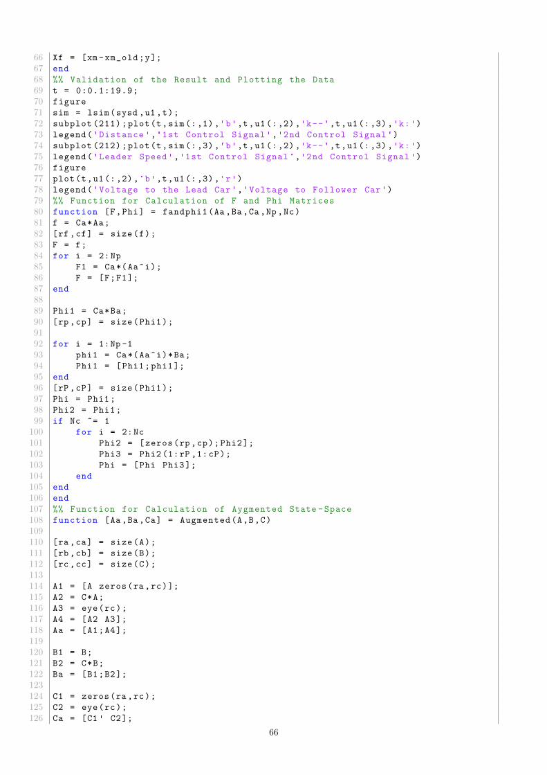
66 Xf = [xm -xm_old;y];

67 end

68 %% Validation of the Result and Plotting the Data

69 t = 0:0.1:19.9;

70 figure

71 sim = lsim(sysd ,u1 ,t);

72 subplot (211);plot(t,sim(:,1),'b',t,u1(:,2),'k--',t,u1(:,3),'k:')

73 legend('Distance ','1st Control Signal ','2nd Control Signal ')

74 subplot (212);plot(t,sim(:,3),'b',t,u1(:,2),'k--',t,u1(:,3),'k:')

75 legend('Leader Speed','1st Control Signal ','2nd Control Signal ')

76 figure

77 plot(t,u1(:,2),'b',t,u1(:,3),'r')

78 legend('Voltage to the Lead Car','Voltage to Follower Car')

79 %% Function for Calculation of F and Phi Matrices

80 function [F,Phi] = fandphi1(Aa,Ba,Ca,Np,Nc)

81 f = Ca*Aa;

82 [rf ,cf] = size(f);

83 F = f;

84 for i = 2:Np

85 F1 = Ca*(Aa^i);

86 F = [F;F1];

87 end

8889 Phi1 = Ca*Ba;

90 [rp ,cp] = size(Phi1);

9192 for i = 1:Np -1

93 phi1 = Ca*(Aa^i)*Ba;

94 Phi1 = [Phi1;phi1];

95 end

96 [rP ,cP] = size(Phi1);

97 Phi = Phi1;

98 Phi2 = Phi1;

99 if Nc ~= 1

100 for i = 2:Nc

101 Phi2 = [zeros(rp ,cp);Phi2];

102 Phi3 = Phi2 (1:rP ,1:cP);

103 Phi = [Phi Phi3];

104 end

105 end

106 end

107 %% Function for Calculation of Aygmented State -Space

108 function [Aa,Ba,Ca] = Augmented(A,B,C)

109110 [ra ,ca] = size(A);

111 [rb ,cb] = size(B);

112 [rc ,cc] = size(C);

113114 A1 = [A zeros(ra ,rc)];

115 A2 = C*A;

116 A3 = eye(rc);

117 A4 = [A2 A3];

118 Aa = [A1;A4];

119120 B1 = B;

121 B2 = C*B;

122 Ba = [B1;B2];

123124 C1 = zeros(ra ,rc);

125 C2 = eye(rc);

126 Ca = [C1 ' C2];

66

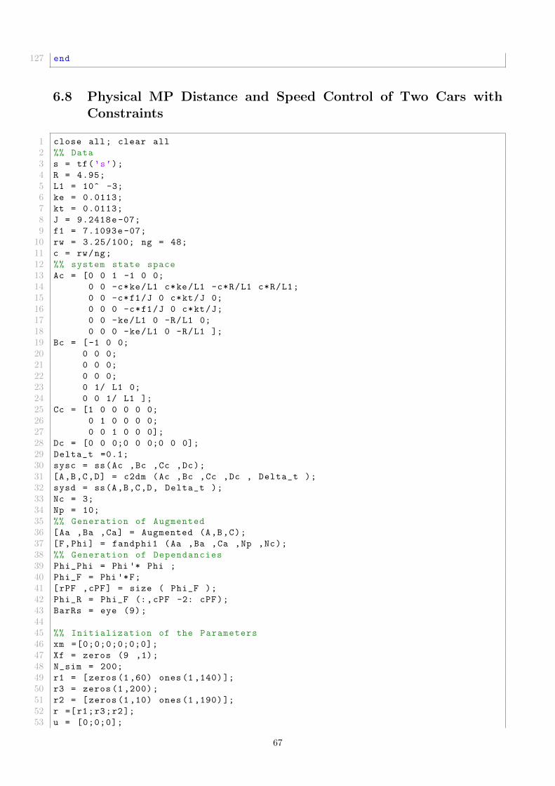
127 end

6.8 Physical MP Distance and Speed Control of Two Cars withConstraints

1 close all; clear all

2 %% Data

3 s = tf('s');

4 R = 4.95;

5 L1 = 10^ -3;

6 ke = 0.0113;

7 kt = 0.0113;

8 J = 9.2418e-07;

9 f1 = 7.1093e-07;

10 rw = 3.25/100; ng = 48;

11 c = rw/ng;

12 %% system state space

13 Ac = [0 0 1 -1 0 0;

14 0 0 -c*ke/L1 c*ke/L1 -c*R/L1 c*R/L1;

15 0 0 -c*f1/J 0 c*kt/J 0;

16 0 0 0 -c*f1/J 0 c*kt/J;

17 0 0 -ke/L1 0 -R/L1 0;

18 0 0 0 -ke/L1 0 -R/L1 ];

19 Bc = [-1 0 0;

20 0 0 0;

21 0 0 0;

22 0 0 0;

23 0 1/ L1 0;

24 0 0 1/ L1 ];

25 Cc = [1 0 0 0 0 0;

26 0 1 0 0 0 0;

27 0 0 1 0 0 0];

28 Dc = [0 0 0;0 0 0;0 0 0];

29 Delta_t =0.1;

30 sysc = ss(Ac ,Bc ,Cc ,Dc);

31 [A,B,C,D] = c2dm (Ac ,Bc ,Cc ,Dc , Delta_t );

32 sysd = ss(A,B,C,D, Delta_t );

33 Nc = 3;

34 Np = 10;

35 %% Generation of Augmented

36 [Aa ,Ba ,Ca] = Augmented (A,B,C);

37 [F,Phi] = fandphi1 (Aa ,Ba ,Ca ,Np ,Nc);

38 %% Generation of Dependancies

39 Phi_Phi = Phi '* Phi ;

40 Phi_F = Phi '*F;

41 [rPF ,cPF] = size ( Phi_F );

42 Phi_R = Phi_F (:,cPF -2: cPF);

43 BarRs = eye (9);

4445 %% Initialization of the Parameters

46 xm =[0;0;0;0;0;0];

47 Xf = zeros (9 ,1);

48 N_sim = 200;

49 r1 = [zeros (1,60) ones (1 ,140)];

50 r3 = zeros (1 ,200);

51 r2 = [zeros (1,10) ones (1 ,190)];

52 r =[r1;r3;r2];

53 u = [0;0;0];

67

54 y = [0;0;0];

55 deltau = zeros (3 ,1);

56 %% Simulation of the Process

57 for kk =1: N_sim ;

58 f = -2*( Phi_R *r(:, kk)-Phi_F *Xf);

59 H = ( Phi_Phi + 1* BarRs );

60 a = [0 -1 0 0 0 0 0 0 0;

61 0 -0 -1 0 0 0 0 0 0;

62 0 1 0 0 0 0 0 0 0;

63 0 0 1 0 0 0 0 0 0];

64 b = [u(2 ,1);u(3 ,1) ;(5 -u(2 ,1));(5 -u(3 ,1))];

65 DeltaU1 = quadprog (H,f,a,b);

66 deltau =[ eye (3) zeros (3) zeros (3) ]* DeltaU1 ;

676869 u = u+ deltau ;

70 u1(kk ,:) = u;

71 y1(kk ,:) = y;

72 xm_old = xm;

73 xm = A*xm+B*u;

74 x(kk ,:)=xm;

75 y = C*xm;

76 Xf = [xm - xm_old ;y];

77 end

78 %% Validation of the Result and Plotting the Data

79 t = 0:0.1:19.9;

80 figure

81 sim = lsim (sysd ,u1 ,t);

82 subplot (211) ; plot (t,sim (: ,1) ,'b',t,u1 (: ,2) ,'k--',t,u1 (: ,3) ,'k:'

)

83 legend ('Distance ','1st Control Signal ','2nd Control Signal ')

84 axis ([0 20 -0.2 1.5])

85 subplot (212) ; plot (t,sim (: ,3) ,'b',t,u1 (: ,2) ,'k--',t,u1 (: ,3) ,'k:'

)

86 legend ('Leader Speed ','1st Control Signal ','2nd Control Signal ')

87 axis ([0 20 -0.2 1.5])

88 figure

89 plot (t,u1 (: ,2) ,'b',t,u1 (: ,3) ,'r')

90 legend ('Voltage to the Lead Car ','Voltage to Follower Car ')

91 axis ([0 20 -0.2 1.5])

92 %% Function for Calculation of F and Phi Matrices

93 function [F,Phi] = fandphi1 (Aa ,Ba ,Ca ,Np ,Nc)

94 f = Ca*Aa;

95 [rf ,cf] = size (f);

96 F = f;

97 for i = 2: Np

98 F1 = Ca *( Aa^i);

99 F = [F;F1 ];

100 end

101102 Phi1 = Ca*Ba;

103 [rp ,cp] = size ( Phi1 );

104105 for i = 1:Np -1

106 phi1 = Ca *( Aa^i)*Ba;

107 Phi1 = [ Phi1 ; phi1 ];

108 end

109 [rP ,cP] = size ( Phi1 );

110 Phi = Phi1 ;

111 Phi2 = Phi1 ;

112 if Nc ~= 1

68

113 for i = 2: Nc

114 Phi2 = [ zeros(rp ,cp); Phi2 ];

115 Phi3 = Phi2 (1:rP ,1:cP);

116 Phi = [Phi Phi3];

117 end

118 end

119 end

120 %% Function for Calculation of Aygmented State - Space

121 function [Aa ,Ba ,Ca] = Augmented (A,B,C)

122123 [ra ,ca] = size (A);

124 [rb ,cb] = size (B);

125 [rc ,cc] = size (C);

126127 A1 = [A zeros(ra ,rc)];

128 A2 = C*A;

129 A3 = eye (rc);

130 A4 = [A2 A3 ];

131 Aa = [A1;A4 ];

132133 B1 = B;

134 B2 = C*B;

135 Ba = [B1;B2 ];

136 C1 = zeros (ra ,rc);

137 C2 = eye (rc);

138 Ca = [C1 ' C2 ];

139 end

6.9 Parameters of PID Distance and Speed Control of Platoon ofCars (SIMULINK Parameters)

1 clear all

2 close all

3 %% Data

4 s = tf('s');

5 R = 4.95;

6 L1 = 10^ -3;

7 ke = 0.0113;

8 kt = 0.0113;

9 J = 9.2418e-07;

10 f = 7.1093e-07;

11 rw = 3.25/100; ng = 48;

12 c = rw/ng;

13 %% State space of individual car

14 Ai = [-R/L1 -ke/L1;

15 kt/J -f/J];

16 Bi = [1/L1;0];

17 Ci = [0 1];

18 Di = [0];

19 car = ss(Ai ,Bi ,Ci ,Di);

20 Gcar = tf(car);

21 p = 20;

22 i = 3;

6.10 Parameters of Cyber LQ Distance and Speed Control of Pla-toon of Cars (SIMULINK Parameters)

69

1 clear all

2 close all

3 s = tf('s');

4 %% State Space of the Platoon

5 A1 = zeros (11 ,5)

6 A2 = [1 -1 0 0 0 0;

7 0 1 -1 0 0 0;

8 0 0 1 -1 0 0;

9 0 0 0 1 -1 0;

10 0 0 0 0 1 -1];

11 A3 = zeros (6,6);

12 A4 = [A2;A3];

13 Ap = [A1 A4];

14 B1 = zeros (5,6);B2 = eye (6);B3 = [1;1;1;1;1;0;0;0;0;0;0] , Bp = [B1;B2];

15 Cp = eye (11)

16 Dp = zeros (11 ,6);

17 sys = ss(Ap ,Bp ,Cp ,Dp);

18 G = tf(sys);

19 M = [eye(6) zeros (6,5)];

20 %% Observability & Controlability of the platoon

21 obsp = obsv(Ap ,Cp);co = size(obsp);

22 observability = [co(2) rank(obsp)]

23 ctrp = ctrb(Ap ,Bp);ct = size(ctrp);

24 controlability = [ct(2) rank(ctrp)]

2526 %% LQR for platoon

27 [Lp ,S,e] = lqr(sys ,10* eye (11) ,1*eye(6) ,0);

28 Lr = pinv((M*inv(Bp*Lp -Ap)*Bp))

29 % Lr1 = Lr1 *0.93;

30 GC = feedback(sys ,Lp);

31 GC1 = GC*Lr;

32 % step(GC1 ,4)

33 ssG = ss(GC1);

6.11 Cyber MP Distance and Speed Control of Platoon of Cars

1 close all; clear all

2 %% State Space of the Platoon

3 A1 = zeros (11 ,5);

4 A2 = [1 -1 0 0 0 0;

5 0 1 -1 0 0 0;

6 0 0 1 -1 0 0;

7 0 0 0 1 -1 0;

8 0 0 0 0 1 -1];

9 A3 = zeros (6,6);

10 A4 = [A2;A3];

11 Ac = [A1 A4];

12 B1 = zeros (5,6);B2 = eye (6);B3 = [1;1;1;1;1;0;0;0;0;0;0];

13 Bc = [B1;B2];

14 % Cc = eye (11);

15 Cc = [1 0 0 0 0 0 0 0 0 0 0;

16 0 1 0 0 0 0 0 0 0 0 0;

17 0 0 1 0 0 0 0 0 0 0 0;

18 0 0 0 1 0 0 0 0 0 0 0;

19 0 0 0 0 1 0 0 0 0 0 0;

20 0 0 0 0 0 1 0 0 0 0 0];

21 Dc = zeros (6,6);

22 sys = ss(Ac ,Bc ,Cc ,Dc);

70

23 G = tf(sys);

24 % figure (1)

25 % step(sys ,10)

26 Delta_t = 0.1;

27 [A,B,C,D] = c2dm(Ac,Bc,Cc,Dc,Delta_t);

28 sysd = ss(A,B,C,D,Delta_t);

29 Nc = 3;

30 Np = 10;

31 %% Augmented state -space

32 [Aa ,Ba,Ca] = Augmented(A,B,C);

33 [F,Phi] = fandphi1(Aa,Ba,Ca,Np,Nc);

34 %% Dependancies

35 Phi_Phi = Phi '*Phi;

36 Phi_F = Phi '*F;

37 [rPF ,cPF] = size(Phi_F);

38 Phi_R = Phi_F(:,cPF -5:cPF);

39 BarRs = eye (18);

40 %% Initialization of the parameters

41 xm =[0;0;0;0;0;0;0;0;0;0;0];

42 Xf = zeros (17 ,1);

43 N_sim = 200;

44 r0 = zeros (1,20);

45 r1 = ones (1,20);

46 R1 = [r0 r0 r0 r1 r1 r1 r1 r1 r1 r1];

47 R2 = [r0 r0 r0 r1 r1 r1 r1 r1 r1 r1];

48 R3 = [r0 r0 r0 r1 r1 r1 r1 r1 r1 r1];

49 R4 = [r0 r0 r0 r1 r1 r1 r1 r1 r1 r1];

50 R5 = [r0 r0 r0 r1 r1 r1 r1 r1 r1 r1];

51 R6 = [r1 r1 r1 r1 r1 r1 r1 r1 r1 r1];

52 r =[R1;R2;R3;R4;R5;R6];

53 u = [0;0;0;0;0;0];

54 y = [0;0;0;0;0;0];

55 %% Simulation

56 for kk=1: N_sim;

57 DeltaU = inv(Phi_Phi +0.1* BarRs)*( Phi_R*r(:,kk)-Phi_F*Xf);

58 deltau =[eye (6) zeros (6) zeros (6)]* DeltaU;

59 u = u+deltau;

60 u1(kk ,:) = u;

61 y1(kk ,:) = y;

62 xm_old = xm;

63 xm = A*xm+B*u;

64 x(kk ,:)=xm;

65 y = C*xm;

66 Xf = [xm -xm_old;y];

67 end

68 t = 0:0.1:19.9;

69 figure

70 plot(t,x(:,1),t,x(:,2),t,x(:,3),t,x(:,4),t,x(:,5))

71 legend('Distance 1','Distance 2','Distance 3','Distance 4','Distance 5')

72 figure

73 plot(t,x(:,6),t,x(:,7),t,x(:,8),t,x(:,9),t,x(:,10),t,x(:,11))

74 legend('Lead Car Speed','1st Car Speed ','2nd Car Speed ',...

75 '3rd Car Speed ','4th Car Speed ','5th Car Speed ')

76 figure

77 plot(t,u1)

78 legend('Lead Car Control Signal ','1st Car Control Signal ','2nd Car Control

Signal ',...

79 '3rd Car Control Signal ','4th Car Control Signal ','5th Car Control

Signal ')

8081 %% Function for generation of F and Phi matrices

71

82 function [F,Phi] = fandphi1(Aa,Ba,Ca,Np,Nc)

83 f = Ca*Aa;

84 [rf ,cf] = size(f);

85 F = f;

86 for i = 2:Np

87 F1 = Ca*(Aa^i);

88 F = [F;F1];

89 end

90 Phi1 = Ca*Ba;

91 [rp ,cp] = size(Phi1);

92 for i = 1:Np -1

93 phi1 = Ca*(Aa^i)*Ba;

94 Phi1 = [Phi1;phi1];

95 end

96 [rP ,cP] = size(Phi1);

97 Phi = Phi1;

98 Phi2 = Phi1;

99 if Nc ~= 1

100 for i = 2:Nc

101 Phi2 = [zeros(rp ,cp);Phi2];

102 Phi3 = Phi2 (1:rP ,1:cP);

103 Phi = [Phi Phi3];

104 end

105 end

106 end

107 %% FUnction for generation of the augmented state -space

108 function [Aa,Ba,Ca] = Augmented(A,B,C)

109110 [ra ,ca] = size(A);

111 [rb ,cb] = size(B);

112 [rc ,cc] = size(C);

113114 A1 = [A zeros(ra ,rc)];

115 A2 = C*A;

116 A3 = eye(rc);

117 A4 = [A2 A3];

118 Aa = [A1;A4];

119120 B1 = B;

121 B2 = C*B;

122 Ba = [B1;B2];

123124 C1 = zeros(ra ,rc);

125 C2 = eye(rc);

126 Ca = [C1 ' C2];

127 end

6.12 Parameters of Physical LQ Distance and Speed Control of Pla-toon of Cars (SIMULINK Parameters)

1 close all; clear all

2 %% Parameters

3 s = tf('s');

4 R = 4.95;

5 L1 = 10^ -3;

6 ke = 0.0113;

7 kt = 0.0113;

8 J = 9.2418e-07;

72

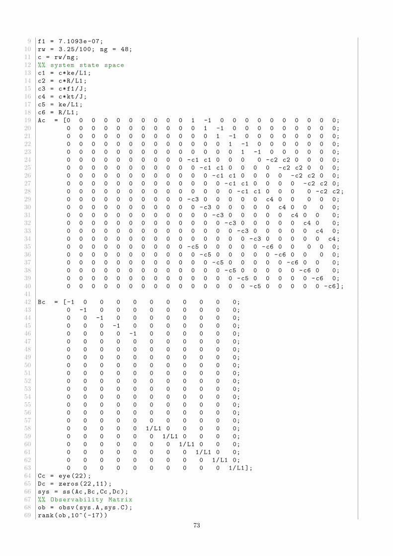
9 f1 = 7.1093e-07;

10 rw = 3.25/100; ng = 48;

11 c = rw/ng;

12 %% system state space

13 c1 = c*ke/L1;

14 c2 = c*R/L1;

15 c3 = c*f1/J;

16 c4 = c*kt/J;

17 c5 = ke/L1;

18 c6 = R/L1;

19 Ac = [0 0 0 0 0 0 0 0 0 0 1 -1 0 0 0 0 0 0 0 0 0 0;

20 0 0 0 0 0 0 0 0 0 0 0 1 -1 0 0 0 0 0 0 0 0 0;

21 0 0 0 0 0 0 0 0 0 0 0 0 1 -1 0 0 0 0 0 0 0 0;

22 0 0 0 0 0 0 0 0 0 0 0 0 0 1 -1 0 0 0 0 0 0 0;

23 0 0 0 0 0 0 0 0 0 0 0 0 0 0 1 -1 0 0 0 0 0 0;

24 0 0 0 0 0 0 0 0 0 0 -c1 c1 0 0 0 0 -c2 c2 0 0 0 0;

25 0 0 0 0 0 0 0 0 0 0 0 -c1 c1 0 0 0 0 -c2 c2 0 0 0;

26 0 0 0 0 0 0 0 0 0 0 0 0 -c1 c1 0 0 0 0 -c2 c2 0 0;

27 0 0 0 0 0 0 0 0 0 0 0 0 0 -c1 c1 0 0 0 0 -c2 c2 0;

28 0 0 0 0 0 0 0 0 0 0 0 0 0 0 -c1 c1 0 0 0 0 -c2 c2;

29 0 0 0 0 0 0 0 0 0 0 -c3 0 0 0 0 0 c4 0 0 0 0 0;

30 0 0 0 0 0 0 0 0 0 0 0 -c3 0 0 0 0 0 c4 0 0 0 0;

31 0 0 0 0 0 0 0 0 0 0 0 0 -c3 0 0 0 0 0 c4 0 0 0;

32 0 0 0 0 0 0 0 0 0 0 0 0 0 -c3 0 0 0 0 0 c4 0 0;

33 0 0 0 0 0 0 0 0 0 0 0 0 0 0 -c3 0 0 0 0 0 c4 0;

34 0 0 0 0 0 0 0 0 0 0 0 0 0 0 0 -c3 0 0 0 0 0 c4;

35 0 0 0 0 0 0 0 0 0 0 -c5 0 0 0 0 0 -c6 0 0 0 0 0;

36 0 0 0 0 0 0 0 0 0 0 0 -c5 0 0 0 0 0 -c6 0 0 0 0;

37 0 0 0 0 0 0 0 0 0 0 0 0 -c5 0 0 0 0 0 -c6 0 0 0;

38 0 0 0 0 0 0 0 0 0 0 0 0 0 -c5 0 0 0 0 0 -c6 0 0;

39 0 0 0 0 0 0 0 0 0 0 0 0 0 0 -c5 0 0 0 0 0 -c6 0;

40 0 0 0 0 0 0 0 0 0 0 0 0 0 0 0 -c5 0 0 0 0 0 -c6];

4142 Bc = [-1 0 0 0 0 0 0 0 0 0 0;

43 0 -1 0 0 0 0 0 0 0 0 0;

44 0 0 -1 0 0 0 0 0 0 0 0;

45 0 0 0 -1 0 0 0 0 0 0 0;

46 0 0 0 0 -1 0 0 0 0 0 0;

47 0 0 0 0 0 0 0 0 0 0 0;

48 0 0 0 0 0 0 0 0 0 0 0;

49 0 0 0 0 0 0 0 0 0 0 0;

50 0 0 0 0 0 0 0 0 0 0 0;

51 0 0 0 0 0 0 0 0 0 0 0;

52 0 0 0 0 0 0 0 0 0 0 0;

53 0 0 0 0 0 0 0 0 0 0 0;

54 0 0 0 0 0 0 0 0 0 0 0;

55 0 0 0 0 0 0 0 0 0 0 0;

56 0 0 0 0 0 0 0 0 0 0 0;

57 0 0 0 0 0 0 0 0 0 0 0;

58 0 0 0 0 0 1/L1 0 0 0 0 0;

59 0 0 0 0 0 0 1/L1 0 0 0 0;

60 0 0 0 0 0 0 0 1/L1 0 0 0;

61 0 0 0 0 0 0 0 0 1/L1 0 0;

62 0 0 0 0 0 0 0 0 0 1/L1 0;

63 0 0 0 0 0 0 0 0 0 0 1/L1];

64 Cc = eye (22);

65 Dc = zeros (22 ,11);

66 sys = ss(Ac ,Bc ,Cc ,Dc);

67 %% Observability Matrix

68 ob = obsv(sys.A,sys.C);

69 rank(ob ,10^( -17))

73

70 Co = ctrb(sys.A,sys.B);

71 rank(Co ,10^( -17))

72 %% LQ Controller

73 M = [1 0 0 0 0 0 0 0 0 0 0 0 0 0 0 0 0 0 0 0 0 0;

74 0 1 0 0 0 0 0 0 0 0 0 0 0 0 0 0 0 0 0 0 0 0;

75 0 0 1 0 0 0 0 0 0 0 0 0 0 0 0 0 0 0 0 0 0 0;

76 0 0 0 1 0 0 0 0 0 0 0 0 0 0 0 0 0 0 0 0 0 0;

77 0 0 0 0 1 0 0 0 0 0 0 0 0 0 0 0 0 0 0 0 0 0;

78 0 0 0 0 0 0 0 0 0 0 1 0 0 0 0 0 0 0 0 0 0 0];

79 Ly = lqr(sys ,10* eye (22),eye (11))

80 Lr = pinv((M*inv(Bc*Ly -Ac)*Bc))

81 GC = feedback(sys ,Ly);

82 GC1 = GC*Lr;

83 ssG = ss(GC1);

6.13 Cyber MP Distance and Speed Control of Platoon of Cars

1 close all; clear all

2 %% Data

3 s = tf('s');

4 R = 4.95;

5 L1 = 10^ -3;

6 ke = 0.0113;

7 kt = 0.0113;

8 J = 9.2418e-07;

9 f1 = 7.1093e-07;

10 rw = 3.25/100; ng = 48;

11 c = rw/ng;

12 %% system state space

13 c1 = c*ke/L1;

14 c2 = c*R/L1;

15 c3 = c*f1/J;

16 c4 = c*kt/J;

17 c5 = ke/L1;

18 c6 = R/L1;

19 Ac = [0 0 0 0 0 0 0 0 0 0 1 -1 0 0 0 0 0 0 0 0 0 0;

20 0 0 0 0 0 0 0 0 0 0 0 1 -1 0 0 0 0 0 0 0 0 0;

21 0 0 0 0 0 0 0 0 0 0 0 0 1 -1 0 0 0 0 0 0 0 0;

22 0 0 0 0 0 0 0 0 0 0 0 0 0 1 -1 0 0 0 0 0 0 0;

23 0 0 0 0 0 0 0 0 0 0 0 0 0 0 1 -1 0 0 0 0 0 0;

24 0 0 0 0 0 0 0 0 0 0 -c1 c1 0 0 0 0 -c2 c2 0 0 0 0;

25 0 0 0 0 0 0 0 0 0 0 0 -c1 c1 0 0 0 0 -c2 c2 0 0 0;

26 0 0 0 0 0 0 0 0 0 0 0 0 -c1 c1 0 0 0 0 -c2 c2 0 0;

27 0 0 0 0 0 0 0 0 0 0 0 0 0 -c1 c1 0 0 0 0 -c2 c2 0;

28 0 0 0 0 0 0 0 0 0 0 0 0 0 0 -c1 c1 0 0 0 0 -c2 c2;

29 0 0 0 0 0 0 0 0 0 0 -c3 0 0 0 0 0 c4 0 0 0 0 0;

30 0 0 0 0 0 0 0 0 0 0 0 -c3 0 0 0 0 0 c4 0 0 0 0;

31 0 0 0 0 0 0 0 0 0 0 0 0 -c3 0 0 0 0 0 c4 0 0 0;

32 0 0 0 0 0 0 0 0 0 0 0 0 0 -c3 0 0 0 0 0 c4 0 0;

33 0 0 0 0 0 0 0 0 0 0 0 0 0 0 -c3 0 0 0 0 0 c4 0;

34 0 0 0 0 0 0 0 0 0 0 0 0 0 0 0 -c3 0 0 0 0 0 c4;

35 0 0 0 0 0 0 0 0 0 0 -c5 0 0 0 0 0 -c6 0 0 0 0 0;

36 0 0 0 0 0 0 0 0 0 0 0 -c5 0 0 0 0 0 -c6 0 0 0 0;

37 0 0 0 0 0 0 0 0 0 0 0 0 -c5 0 0 0 0 0 -c6 0 0 0;

38 0 0 0 0 0 0 0 0 0 0 0 0 0 -c5 0 0 0 0 0 -c6 0 0;

39 0 0 0 0 0 0 0 0 0 0 0 0 0 0 -c5 0 0 0 0 0 -c6 0;

40 0 0 0 0 0 0 0 0 0 0 0 0 0 0 0 -c5 0 0 0 0 0 -c6];

4142 Bc = [-1 0 0 0 0 0 0 0 0 0 0;

74

43 0 -1 0 0 0 0 0 0 0 0 0;

44 0 0 -1 0 0 0 0 0 0 0 0;

45 0 0 0 -1 0 0 0 0 0 0 0;

46 0 0 0 0 -1 0 0 0 0 0 0;

47 0 0 0 0 0 0 0 0 0 0 0;

48 0 0 0 0 0 0 0 0 0 0 0;

49 0 0 0 0 0 0 0 0 0 0 0;

50 0 0 0 0 0 0 0 0 0 0 0;

51 0 0 0 0 0 0 0 0 0 0 0;

52 0 0 0 0 0 0 0 0 0 0 0;

53 0 0 0 0 0 0 0 0 0 0 0;

54 0 0 0 0 0 0 0 0 0 0 0;

55 0 0 0 0 0 0 0 0 0 0 0;

56 0 0 0 0 0 0 0 0 0 0 0;

57 0 0 0 0 0 0 0 0 0 0 0;

58 0 0 0 0 0 1/L1 0 0 0 0 0;

59 0 0 0 0 0 0 1/L1 0 0 0 0;

60 0 0 0 0 0 0 0 1/L1 0 0 0;

61 0 0 0 0 0 0 0 0 1/L1 0 0;

62 0 0 0 0 0 0 0 0 0 1/L1 0;

63 0 0 0 0 0 0 0 0 0 0 1/L1];

64 Cc = [eye (11) zeros (11 ,11)];

65 Dc = zeros (11 ,11);

66 Delta_t =0.1;

67 sysc = ss(Ac ,Bc ,Cc ,Dc);

68 [A,B,C,D] = c2dm(Ac,Bc,Cc,Dc,Delta_t);

69 sysd = ss(A,B,C,D,Delta_t);

70 Nc = 3;

71 Np = 10;

72 %% Generation of Augmented

73 [Aa ,Ba,Ca] = Augmented(A,B,C);

74 [F,Phi] = fandphi1(Aa,Ba,Ca,Np,Nc);

75 %% Generation of Dependancies

76 Phi_Phi = Phi '*Phi;

77 Phi_F = Phi '*F;

78 [rPF ,cPF] = size(Phi_F);

79 Phi_R = Phi_F(:,cPF -10: cPF);

80 BarRs = eye (33);

8182 %% Initialization of the Parameters

83 xm = zeros (22 ,1);

84 Xf = zeros (33 ,1);

85 N_sim = 200;

86 r1 = [zeros (1,60) ones (1 ,140)];

87 r2 = [zeros (1,60) ones (1 ,140)]

88 r3 = [zeros (1,60) ones (1 ,140)]

89 r4 = [zeros (1,60) ones (1 ,140)]

90 r5 = [zeros (1,60) ones (1 ,140)]

91 r6 = zeros (1 ,200);

92 r7 = zeros (1 ,200);

93 r8 = zeros (1 ,200);

94 r9 = zeros (1 ,200);

95 r10 = zeros (1 ,200);

96 r11 = [zeros (1,10) ones (1 ,190)];

97 r =[r1;r2;r3;r4;r5;r6;r7;r8;r9;r10;r11];

98 u = [0;0;0;0;0;0;0;0;0;0;0];

99 y = [0;0;0;0;0;0;0;0;0;0;0];

100 % deltau = zeros (3,1);

101 %% Simulation of the Process

102 for kk=1: N_sim;

103 f = -2*(Phi_R*r(:,kk)-Phi_F*Xf);

75

104 H = (Phi_Phi + .1* BarRs);

105 a = [0 0 0 0 0 -1 0 0 0 0 0 0 0 0 0 0 0 0 0 0 0 0 0 0 0 0 0 0 0 0 0 0 0;

106 0 0 0 0 0 0 -1 0 0 0 0 0 0 0 0 0 0 0 0 0 0 0 0 0 0 0 0 0 0 0 0 0 0;

107 0 0 0 0 0 0 0 -1 0 0 0 0 0 0 0 0 0 0 0 0 0 0 0 0 0 0 0 0 0 0 0 0 0;

108 0 0 0 0 0 0 0 0 -1 0 0 0 0 0 0 0 0 0 0 0 0 0 0 0 0 0 0 0 0 0 0 0 0;

109 0 0 0 0 0 0 0 0 0 -1 0 0 0 0 0 0 0 0 0 0 0 0 0 0 0 0 0 0 0 0 0 0 0;

110 0 0 0 0 0 0 0 0 0 0 -1 0 0 0 0 0 0 0 0 0 0 0 0 0 0 0 0 0 0 0 0 0 0;

111 0 0 0 0 0 1 0 0 0 0 0 0 0 0 0 0 0 0 0 0 0 0 0 0 0 0 0 0 0 0 0 0 0;

112 0 0 0 0 0 0 1 0 0 0 0 0 0 0 0 0 0 0 0 0 0 0 0 0 0 0 0 0 0 0 0 0 0;

113 0 0 0 0 0 0 0 1 0 0 0 0 0 0 0 0 0 0 0 0 0 0 0 0 0 0 0 0 0 0 0 0 0;

114 0 0 0 0 0 0 0 0 1 0 0 0 0 0 0 0 0 0 0 0 0 0 0 0 0 0 0 0 0 0 0 0 0;

115 0 0 0 0 0 0 0 0 0 1 0 0 0 0 0 0 0 0 0 0 0 0 0 0 0 0 0 0 0 0 0 0 0;

116 0 0 0 0 0 0 0 0 0 0 1 0 0 0 0 0 0 0 0 0 0 0 0 0 0 0 0 0 0 0 0 0 0];

117 b = [u(6,1);u(7,1);u(8,1);u(9,1);u(10,1);u(11,1);...

118 5-u(6,1);5-u(7,1);5-u(8,1);5-u(9,1);5-u(10,1);5-u(11,1)];

119 DeltaU1 = quadprog(H,f,a,b);

120 deltau =[eye (11) zeros (11) zeros (11)]* DeltaU1;

121122123 u = u+deltau;

124 u1(kk ,:) = u;

125 y1(kk ,:) = y;

126 xm_old = xm;

127 xm = A*xm+B*u;

128 x(kk ,:)=xm;

129 y = C*xm;

130 Xf = [xm -xm_old;y];

131 end

132 %% Validation of the Result and Plotting the Data

133 t = 0:0.1:19.9;

134 sim = lsim(sysd ,u1 ,t);

135 figure

136 plot(t,x(:,1),t,x(:,2),t,x(:,3),t,x(:,4),t,x(:,5))

137 legend('Distance 1','Distance 2','Distance 3','Distance 4','Distance 5')

138 figure

139 plot(t,x(: ,11),t,x(:,12),t,x(:,13),t,x(:,14),t,x(:,15),t,x(:,16))

140 legend('Lead Car Speed','1st Car Speed ','2nd Car Speed ','3rd Car Speed ',...

141 '4th Car Speed ','5th Car Speed ')

142 figure

143 plot(t,u1(:,6),t,u1(:,7),t,u1(:,8),t,u1(:,9),t,u1(:,10),t,u1(:,11))

144 legend('Voltage to the Lead Car','Voltage to the 1st Car','Voltage to the 2

nd Car',...

145 'Voltage to the 3rd Car','Voltage to the 4th Car','Voltage to the 5th

Car')

146 %% Function for calculation of F and Phi matrix

147 function [F,Phi] = fandphi1(Aa,Ba,Ca,Np,Nc)

148 f = Ca*Aa;

149 [rf ,cf] = size(f);

150 F = f;

151 for i = 2:Np

152 F1 = Ca*(Aa^i);

153 F = [F;F1];

154 end

155156 Phi1 = Ca*Ba;

157 [rp ,cp] = size(Phi1);

158159 for i = 1:Np -1

160 phi1 = Ca*(Aa^i)*Ba;

161 Phi1 = [Phi1;phi1];

162 end

76

163 [rP ,cP] = size(Phi1);

164 Phi = Phi1;

165 Phi2 = Phi1;

166 if Nc ~= 1

167 for i = 2:Nc

168 Phi2 = [zeros(rp ,cp);Phi2];

169 Phi3 = Phi2 (1:rP ,1:cP);

170 Phi = [Phi Phi3];

171 end

172 end

173 end

174 %% Function for Calculation of Aygmented State -Space

175 function [Aa,Ba,Ca] = Augmented(A,B,C)

176177 [ra ,ca] = size(A);

178 [rb ,cb] = size(B);

179 [rc ,cc] = size(C);

180181 A1 = [A zeros(ra ,rc)];

182 A2 = C*A;

183 A3 = eye(rc);

184 A4 = [A2 A3];

185 Aa = [A1;A4];

186187 B1 = B;

188 B2 = C*B;

189 Ba = [B1;B2];

190191 C1 = zeros(ra ,rc);

192 C2 = eye(rc);

193 Ca = [C1 ' C2];

194 end

6.14 MATLAB Code for Car Remote Control

1 %% Remote control

2 % reading sensor data e.g. IR, Ultrasonic and speed

3 % sending actuation data e.g. turning angle and speed

4 clear all; close all

5 port = 8088

6 ;

7 max_speed = 50;

8 angle_1 = 0;

9 t = tcpclient('192.168.1.34 ', port);

10 for i = 1:5

11 raw = read(t,5,'uint8 ')

12 data = num2str(char(raw))

13 status(i)=floor(str2num(data))

14 end

15 meand = status;

16 counter = 0;

1718 for i = 1:inf

19 tic

20 distance(i) = readd(1,3,port);

21 speedin(i) = readd(1,3,port);

22 input(i,:) = readd(5,3,port);

23 [angle_1 ,angle] = turn_angle(input(i,:),meand ,angle_1);

24 angle - 45;

77

25 speed = speed_calc(angle ,distance(i),max_speed);

26 send_data(angle ,port);

27 send_data(speed ,port);

28 toc

29 % plot(speedin)

30 % hold on

31 counter = counter + 1;

32 end

33 %% plot

34 figure (1)

35 plot(input); title('IR Sensors Readings ');legend('Left Sensor ',...

36 'Middle Left Sensor ','Center Sensor ','Middle Right Sensor ',...

37 'Right Sensor ');

38 figure (2)

39 plot(distance);hold on

40 plot(speedin);title('Speed Vs. Distance ');

41 legend('Distance to Front Obstacle ','Speed ');

42 %%

43 function [angle_1 ,angle] = turn_angle(input ,meand ,angle_1)

44 Mean = meand;

45 dis = input - Mean;

46 dis = abs(dis);

47 Max = find(dis == max(dis));

48 [m,n] = size(Max);

49 if n > 1

50 angle = angle_1

51 else

52 if Max == 1

53 angle = 0;

54 elseif Max == 5

55 angle = 90;

56 else

57 angle = get_angle(Max ,dis(Max),dis(Max -1),dis(Max+1));

58 end

59 end

60 angle_1 = angle;

61 end

62 % Calculation of the Parabola Parameters

63 function [a,b,c] = para(A,B,C)

64 w = [A(1)^2 A(1) 1;

65 B(1)^2 B(1) 1;

66 C(1)^2 C(1) 1];

67 y = [A(2);B(2);C(2)];

68 abc = linsolve(w,y);

69 a = abc(1);

70 b = abc(2);

71 c = abc(3);

72 end

73 % Calculation of Turning Angle

74 function angle = get_angle(Max ,in,in_1 ,in1)

75 Max = Max -3;

76 A = [Max -1 in_1];

77 B = [Max in];

78 C = [Max+1 in1];

79 [a,b,c] = para(A,B,C);

80 x = -2:0.1:2;

81 y = a.*x.^2 + b.*x + c;

82 maxy = find(y == max(y));

83 err = x(maxy);

84 % if err > 1

85 % err = 2

78

86 % elseif err <-1

87 % err = -2

88 % else

89 % err = err

90 % end

91 angle = 45+( err * 22.5);

9293 end

94 function send_data(data ,port)

95 t = tcpclient('192.168.0.105 ', port);

96 d = uint8(data);

97 write(t,d);

98 end

99100 function data = readd(j,l,port)

101 % Reading Distance From The Car

102 k = tcpclient('192.168.0.105 ', port);

103 for i = 1:j

104 raw = read(k,l,'uint8 ');

105 data1 = num2str(char(raw));

106 data(i)=floor(str2num(data1));

107 end

108 end

109110111 function speed = speed_calc(angle ,distance ,max_speed)

112 if distance > 50

113 if angle > 22.5

114 speed = 0.8 * max_speed;

115 elseif angle <-22.5

116 speed = 0.8 * max_speed;

117 else

118 speed = max_speed;

119 end

120 elseif distance <= 50 && distance > 10

121 speed = distance;

122 elseif distance <= 10

123 speed = 0;

124 end

125 end

6.15 Python Code for Car Remote Control

1 #!/usr/bin/env python

2 '''

3 **************************************************************

4 * Filename : line_follower

5 * Description : Line follower and lead car follower

6 * Author : Amirhossein Hosseinzadeh Dadash

7 * Brand : SunFounder

8 * E-mail : ahhzd86@gmail.com

9 * Website : www.sunfounder.com

10 * Update : Amirhossein Hosseinzadeh Dadash 2019 -00 -09

11 *************************************************************

12 '''

1314 from SunFounder_Ultrasonic_Avoidance import Ultrasonic_Avoidance1

15 import numpy as np

16 from SunFounder_Line_Follower import Line_Follower

79

17 from picar import front_wheels

18 from picar import back_wheels

19 import time

20 import picar

21 import socket

2223 picar.setup()

24 #Initialization of parameters

25 max_speed = 70

26 speed = 0

27 delay = 0.01

28 ua = Ultrasonic_Avoidance1.Ultrasonic_Avoidance (20)

29 s = socket.socket(socket.AF_INET ,socket.SOCK_STREAM)

30 fw = front_wheels.Front_Wheels(db='config ')

31 bw = back_wheels.Back_Wheels(db='config ')

32 lf = Line_Follower.Line_Follower ()

3334 fw.ready()

35 bw.ready()

36 fw.turning_max = 45

37 distance = ua.get_distance ()

38 print(ua.get_distance ())

39 print("put the car on the ground without line and press enter ")

40 input()

41 #Calibration to the color of the ground and calculation of noise variances

42 reference = np.zeros ((5 ,100))

43 for i in range (0 ,100):

44 cal = lf.read_analog ()

45 reference [0,i] = cal[0]

46 reference [1,i] = cal[1]

47 reference [2,i] = cal[2]

48 reference [3,i] = cal[3]

49 reference [4,i] = cal[4]

50 mean_row = reference.mean (1)

51 var_row = np.var(reference ,axis = 1);

52 print(mean_row)

53 st =ua.send_lf(mean_row)

54 print(st)

5556 R0 = var_row [0]*0.3

57 R1 = var_row [1]*0.3

58 R2 = var_row [2]*0.3

59 R3 = var_row [3]*0.3

60 R4 = var_row [4]*0.3

61 Q = 1.8

62 print("Now put the car on the line and press enter ")

63 input()

64 #step = lf.get_angle(mean_row)

65 ## print(step)

6667 # initializaing the noise parameters for kalman filtering

68 def main():

69 global speed

70 #main function

71 while True:

7273 status= lf.read_analog ()

74 distance = ua.get_distance ()

7576 ua.send_data(distance)

77 ua.send_data(speed)

80

78 lfsensor = ua.send_lf(status)

7980 angle = ua.rec_data ()

81 step = angle - 45

82 speed = ua.rec_data ()

83 # if angle > 22 or angle <-22:

84 # step = angle

85 # bw.speed = 70

86 # else:

87 # step = angle

88 # bw.speed = 70

8990 #safety mesure for the turning angle according to car manual

91 if step < -45:

92 step = -45

93 elif step > 45:

94 step = 45

95 else:

96 step = step

97 #Actuation

98 print ("step", step)

99 turning_angle = int(90 + step)

100 bw.speed = speed

101 fw.turn(turning_angle)

102 time.sleep(delay)

103104105 def destroy ():

106 bw.stop()

107 fw.turn (90)

108109 if __name__ == '__main__ ':

110 try:

111 try:

112 while True:

113 main()

114 #straight_run ()

115 except Exception as e:

116 print(e)

117 print('error try again in 5')

118 destroy ()

119 time.sleep (5)

120 except KeyboardInterrupt:

121 destroy ()

6.16 Python Functions for Car Remote Control

1 #!/usr/bin/env python

2 '''

3 **************************************************************

4 * Filename : Ultrasonic_Avoidance.py

5 * Description : A module for SunFounder Ultrasonic Avoidance

6 * Author : Cavon

7 * Brand : SunFounder

8 * E-mail : service@sunfounder.com

9 * Website : www.sunfounder.com

10 * Update : Amirhossein Hosseinzadeh Dadash 2019 -10 -09

11 **************************************************************

12 '''

81

13 import time

14 import RPi.GPIO as GPIO

15 import socket

16 s = socket.socket(socket.AF_INET ,socket.SOCK_STREAM)

17 s.bind(('192.168.0.105 ' ,1230))

18 s.listen (5)

1920 class Ultrasonic_Avoidance(object):

21 timeout = 0.05

2223 def __init__(self , channel):

24 self.channel = channel

25 GPIO.setmode(GPIO.BCM)

2627 def distance(self):

28 pulse_end = 0

29 pulse_start = 0

30 GPIO.setup(self.channel ,GPIO.OUT)

31 GPIO.output(self.channel , False)

32 time.sleep (0.01)

33 GPIO.output(self.channel , True)

34 time.sleep (0.00001)

35 GPIO.output(self.channel , False)

36 GPIO.setup(self.channel ,GPIO.IN)

3738 timeout_start = time.time()

39 while GPIO.input(self.channel)==0:

40 pulse_start = time.time()

41 if pulse_start - timeout_start > self.timeout:

42 return -1

43 while GPIO.input(self.channel)==1:

44 pulse_end = time.time()

45 if pulse_start - timeout_start > self.timeout:

46 return -1

4748 if pulse_start != 0 and pulse_end != 0:

49 pulse_duration = pulse_end - pulse_start

50 distance = pulse_duration * 100 * 343.0 /2

51 distance = int(distance)

52 #print('start = %s'%pulse_start ,)

53 #print('end = %s'%pulse_end)

54 if distance >= 0:

55 return distance

56 else:

57 return -1

58 else :

59 #print('start = %s'%pulse_start ,)

60 #print('end = %s'%pulse_end)

61 return -1

6263 def get_distance(self , mount = 5):

64 sum = 0

65 for i in range(mount):

66 a = self.distance ()

67 #print(' %s' % a)

68 sum += a

69 return int(sum/mount)

70 #Speed Calculation withoud using PI Controller

71 def get_speed(self ,distance ,max_speed):

72 distance = distance - 10

73 speed = max_speed

82

74 if distance > 50:

75 speed = round (0.9 * max_speed)

76 elif distance <= 50 and distance >10:

77 speed = max_speed

78 elif distance <= 10 and distance > 5:

79 speed = round (50 + distance)

80 elif distance < 5:

81 speed = 0

82 return speed

83 #Speed calculation according to distance with PI controller

84 def get_speed_pid(self ,speed_k_1 ,distance ,distance_k_1 ,max_speed):

85 distance = distance - 10

86 if distance > 100:

87 speed = round (.8 * max_speed)

88 elif distance <= 100 and distance > 0:

89 speed = speed_k_1 + (3* distance) - (1.44 * distance_k_1)

90 else: #distance <= 0:

91 speed = 0;

9293 if speed < 0:

94 speed = 0

95 elif speed > 100:

96 speed = 100

97 else:

98 speed = speed

99100 return (speed)

101 #Kalman Filter

102 def kalman(self ,data ,x0 ,P0 ,Q,R):

103 x_hat_n_1_n_1 = x0

104 P_n_1_n_1 = P0

105 x_hat_n_n_1 = x_hat_n_1_n_1

106 P_n_n_1 = P_n_1_n_1 + Q

107 K = P_n_n_1 *(1/( P_n_n_1 + Q))

108 x_hat_n_n = x_hat_n_n_1 + K * (data - x_hat_n_n_1)

109 P_n_n = (1-K)* P_n_n_1

110 return (x_hat_n_n ,P_n_n ,x_hat_n_n)

111112 def send_data(self ,data):

113 data = self.reform(round(data))

114 clientsocket , address = s.accept ()

115 clientsocket.send(bytes(data ,"utf -8"))

116117 def send_lf(self ,st):

118 st1 = self.reform(round(st[0]))

119 st2 = self.reform(round(st[1]))

120 st3 = self.reform(round(st[2]))

121 st4 = self.reform(round(st[3]))

122 st5 = self.reform(round(st[4]))

123 print(st1)

124 print(st2)

125 print(st3)

126 print(st4)

127 print(st5)

128 clientsocket , address = s.accept ()

129 clientsocket.send(bytes(st1 ,"utf -8"))

130 clientsocket.send(bytes(st2 ,"utf -8"))

131 clientsocket.send(bytes(st3 ,"utf -8"))

132 clientsocket.send(bytes(st4 ,"utf -8"))

133 clientsocket.send(bytes(st5 ,"utf -8"))

134

83

135 def reform(self ,var):

136 varm ="000"

137 if var >= 0 and var <10:

138 var1 = var

139 var2 = "00"

140 varm = "00" + str(var1)

141 elif var >= 10 and var < 100:

142 var1 = var

143 var2 = "0"

144 varm = var2 + str(var1)

145 elif var >= 100:

146 varm = str(var)

147 return ((varm))

148149 def rec_data(self):

150 s.listen (1)

151 conn , address = s.accept ()

152 data1 = conn.recv (1)

153 data = int.from_bytes(data1 , byteorder='big')

154 return(data)

155156157158159160 def test():

161 UA = Ultrasonic_Avoidance (17)

162 threshold = 10

163 while True:

164 distance = UA.get_distance ()

165 status = UA.less_than(threshold)

166 if distance != -1:

167 print('distance ', distance , 'cm')

168 time.sleep (0.2)

169 else:

170 print(False)

171 if status == 1:

172 print ("Less than %d" % threshold)

173 elif status == 0:

174 print ("Over %d" % threshold)

175 else:

176 print ("Read distance error .")

177178 if __name__ == '__main__ ':

179 test()

84