Power Control and Adaptive Resource Allocation in DS ...
195
RADIO COMMUNICATION S YSTEMS L ABORATORY Power Control and Adaptive Resource Allocation in DS-CDMA Systems FREDRIK BERGGREN
-
Upload
khangminh22 -
Category
Documents
-
view
1 -
download
0
Transcript of Power Control and Adaptive Resource Allocation in DS ...

RADIO COMMUNICATION SYSTEMS LABORATORY
Power Control and AdaptiveResource Allocation inDS-CDMA Systems
FREDRIK BERGGREN


RADIO COMMUNICATION SYSTEMS LABORATORYDEPARTMENT OF SIGNALS, SENSORS AND SYSTEMS
Power Control and AdaptiveResource Allocation inDS-CDMA Systems
FREDRIK BERGGREN
A dissertation submitted tothe Royal Institute of Technologyin partial fulfillment of the requirementsfor the degree of Doctor of Philosophy
June 2003
TRITA—S3—RST—0308ISSN 1400—9137ISRN KTH/RST/R--03/08--SE


Abstract
With an increased request for wireless data services, methods for managing thescarce radio resources become needful. Especially for applications characterizedby heterogeneous quality of service (QoS) requirements, radio resource allocationbecomes an extensive task. Due to the necessity of sharing the radio spectrum,mutual interference will limit system capacity. Transmitter power control is awell-known method for upholding required signal quality and reducing the energyconsumption.
In this thesis, transmission schemes based on distributed power control aredeveloped and analyzed for cellular DS-CDMA systems. The schemes are de-signed for providing various QoS, while assuring global stability and rapid con-vergence. First, we suggest an iterative power control algorithm which handlescongested situations by autonomously removing radio connections. This algo-rithm is then extended with a greedy rate allocation procedure, with the purposeto maximize throughput in a multirate system, where users have a limited num-ber of discrete transmission rates.
For supporting downlink nonreal time services with a required average datarate, joint power control and scheduling is investigated. It is found that timedivision has merits in terms of increased capacity and multiuser diversity effects.For this, we suggest and evaluate power control and channel adaptive schedulersof different adaptation rate.
Finally, a class of receivers, utilizing successive interference cancellation withsoft feedback is investigated. We determine the optimal power control solutionand characterize its user capacity region.
iii

iv Abstract

Acknowledgments
This work has been supported by many people to whom I wish to express mygratitude. I wish to thank my main adviser Prof. Jens Zander and Prof. BenSlimane at KTH; Prof. Seong-Lyun Kim at ICU, Korea, and Prof. Riku Janttiat HUT, Finland. Their positive attitude and encouragement provided inspi-ration to many ideas and undoubtedly gave dynamism to my research studies.Especially I want to thank Prof. Zander for the freedom I have been given inthis research project. I would like to thank Prof. Roy Yates and Prof. NarayanMandayam, both at the Wireless Information Network Laboratory (WINLAB),which I visited during the spring of 2002, for interesting discussions and feedbackon selected parts of this thesis.
Special thanks go to my colleagues at the Radio Communication Systems groupfor many valuable discussions. Thereto did Magnus Lindstrom never hesitate tocure my computer problems. Lise-Lotte Wahlberg’s assistance with all practicalmatters is greatly appreciated.
A major part of this work has been financially supported by VINNOVA withinthe Explorative Systems-Integrated Technologies (EXSITE) project. My tripsabroad have been supported by grants from Knut och Alice Wallenbergs Stiftelse,Pleijel fonden and the IEEE Communications Society.
Finally, the never-ending support from my parents made it all possible.
v

vi

List of Abbreviations
AGC Automatic Gain ControlALP Active Link ProtectionARQ Automatic Repeat reQuestATM Asynchronous Transfer ModeBER Bit Error RateCDMA Code Division Multiple AccessCDMA/HDR High Data Rate CDMACSMA Carrier Sense Multiple AccessDB Distributed BalancingDCPC Distributed Constrained Power ControlDPC Distributed Power ControlDS-CDMA Direct Sequence CDMAET Equal TimeFDMA Frequency Division Multiple AccessFEC Forward Error CorrectionFER Frame Error RateFF Fractional FairFM Foschini-MiljanicGDCPC Generalized DCPCGRP Greedy Rate PackingGRR Gradual Removals Restricted, Gradual Rate RemovalGSPC Generalized SPCIS-95 Interim Standard-95ISI InterSymbol InterferenceJOR Jacobi Over-RelaxationMC Multi CarrierMIMO Multiple Input Multiple OutputMPA Minimum Power AssignmentMUX MultiplexerOFDM Orthogonal Frequency Division MultiplexingPA Power Amplifier
vii
viii List of Abbreviations
PCMA Power Controlled Multiple AccessPCS Personal Communication SystemPF Proportional FairPRMA Packet Reservation Multiple AccessOFDM Orthogonal Frequency Division MultiplexingQoS Quality of ServiceRAKE RakeRB Relatively BestRF Radio FrequencyRR Round RobinRRM Radio Resource ManagementSAS Soft And SafeSCDMA Scheduled CDMASDMA Spatial Division Multiple AccessSIR Signal-to-Interference RatioSMIRA Stepwise Maximum Interference Removal AlgorithmSMS Short Message ServiceSNR Signal-to-Noise RatioSPC Selective Power ControlSRA Stepwise Removal AlgorithmTDMA Time Division Multiple AccessTPC Transmitter Power ControlUMTS Universal Mobile Telecommunications SystemWCDMA Wideband CDMAWLAN Wireless Local Area Network

Contents
1 Introduction 1
1.1 Wireless Data . . . . . . . . . . . . . . . . . . . . . . . . . . . . . 2
1.2 Radio Resource Management . . . . . . . . . . . . . . . . . . . . 5
1.2.1 Transmitter Power Control . . . . . . . . . . . . . . . . . 5
1.2.2 Transmission Rate Control . . . . . . . . . . . . . . . . . 6
1.2.3 Admission Control . . . . . . . . . . . . . . . . . . . . . . 7
1.2.4 Congestion Control . . . . . . . . . . . . . . . . . . . . . . 8
1.2.5 Transmission Scheduling . . . . . . . . . . . . . . . . . . . 8
1.3 Wireless Communications . . . . . . . . . . . . . . . . . . . . . . 9
1.3.1 Multiple Access . . . . . . . . . . . . . . . . . . . . . . . . 9
1.3.2 Cellular Radio Systems . . . . . . . . . . . . . . . . . . . 10
1.4 Previous Work . . . . . . . . . . . . . . . . . . . . . . . . . . . . 12
1.4.1 Fixed-Rate Power Control . . . . . . . . . . . . . . . . . . 12
1.4.2 Variable-Rate Power Control . . . . . . . . . . . . . . . . 16
1.4.3 Transmission Scheduling and Multiple Access . . . . . . . 18
1.5 Scope of the Thesis . . . . . . . . . . . . . . . . . . . . . . . . . . 20
1.5.1 Problem Background . . . . . . . . . . . . . . . . . . . . . 20
1.5.2 Scope . . . . . . . . . . . . . . . . . . . . . . . . . . . . . 21
1.5.3 Contributions . . . . . . . . . . . . . . . . . . . . . . . . . 22
1.6 Thesis Outline . . . . . . . . . . . . . . . . . . . . . . . . . . . . 25
2 Models and Performance Evaluation 27
2.1 Radio Wave Propagation . . . . . . . . . . . . . . . . . . . . . . . 27
2.2 System Architecture . . . . . . . . . . . . . . . . . . . . . . . . . 29
2.2.1 Receiver Model and Communication Quality . . . . . . . 29
2.2.2 System Layout and Access Scheme . . . . . . . . . . . . . 32
2.2.3 Control Signaling . . . . . . . . . . . . . . . . . . . . . . . 33
2.2.4 Power Control Functionality . . . . . . . . . . . . . . . . . 33
2.3 Performance Evaluation . . . . . . . . . . . . . . . . . . . . . . . 34
2.3.1 Performance Measures . . . . . . . . . . . . . . . . . . . . 35
ix

x Contents
3 Preliminaries 37
3.1 Noisy Power Control Problem . . . . . . . . . . . . . . . . . . . . 37
3.2 Iterative Solution Methods . . . . . . . . . . . . . . . . . . . . . 41
3.2.1 Matrix Norms . . . . . . . . . . . . . . . . . . . . . . . . . 41
3.2.2 Iterative Power Control . . . . . . . . . . . . . . . . . . . 41
3.2.3 Rate of Convergence . . . . . . . . . . . . . . . . . . . . . 43
3.2.4 Standard Interference Functions . . . . . . . . . . . . . . 46
3.3 Local Loop Stability . . . . . . . . . . . . . . . . . . . . . . . . . 46
4 Generalized DCPC 49
4.1 Introduction . . . . . . . . . . . . . . . . . . . . . . . . . . . . . . 49
4.2 Distributed Power Control Algorithm . . . . . . . . . . . . . . . 50
4.2.1 Energy Conservation . . . . . . . . . . . . . . . . . . . . . 50
4.2.2 Convergence in Feasible Systems . . . . . . . . . . . . . . 51
4.2.3 Convergence in Infeasible Systems . . . . . . . . . . . . . 54
4.3 Numerical Results . . . . . . . . . . . . . . . . . . . . . . . . . . 564.3.1 Feasible System . . . . . . . . . . . . . . . . . . . . . . . . 57
4.3.2 Infeasible System . . . . . . . . . . . . . . . . . . . . . . . 59
4.4 Concluding Remarks . . . . . . . . . . . . . . . . . . . . . . . . . 60
5 Multirate Power Control 63
5.1 Introduction . . . . . . . . . . . . . . . . . . . . . . . . . . . . . . 63
5.2 Transmission Rate Assignment . . . . . . . . . . . . . . . . . . . 64
5.2.1 Refined System Model . . . . . . . . . . . . . . . . . . . . 64
5.2.2 Greedy Rate Packing . . . . . . . . . . . . . . . . . . . . . 66
5.2.3 Throughput Maximization . . . . . . . . . . . . . . . . . . 68
5.2.4 Minimum Rate Requirements . . . . . . . . . . . . . . . . 69
5.2.5 Downlink GRP . . . . . . . . . . . . . . . . . . . . . . . . 70
5.3 Iterative Power Control . . . . . . . . . . . . . . . . . . . . . . . 71
5.4 Power Control with Gradual Rate Removal . . . . . . . . . . . . 74
5.5 Numerical Results . . . . . . . . . . . . . . . . . . . . . . . . . . 76
5.6 Concluding Remarks . . . . . . . . . . . . . . . . . . . . . . . . . 78
6 Joint Power Control and Intracell Scheduling 81
6.1 Introduction . . . . . . . . . . . . . . . . . . . . . . . . . . . . . . 81
6.2 Minimum Energy Problem . . . . . . . . . . . . . . . . . . . . . . 83
6.2.1 Refined System Model . . . . . . . . . . . . . . . . . . . . 836.2.2 Problem Definition . . . . . . . . . . . . . . . . . . . . . . 84
6.3 Intracell Scheduling . . . . . . . . . . . . . . . . . . . . . . . . . . 84
6.3.1 Energy Conservation . . . . . . . . . . . . . . . . . . . . . 87
6.3.2 Minimum Time Span . . . . . . . . . . . . . . . . . . . . 88
6.4 Distributed Power Control . . . . . . . . . . . . . . . . . . . . . . 89
6.4.1 Convergence . . . . . . . . . . . . . . . . . . . . . . . . . 90
6.4.2 Rate of Convergence . . . . . . . . . . . . . . . . . . . . . 92

Contents xi
6.5 Numerical Results . . . . . . . . . . . . . . . . . . . . . . . . . . 95
6.6 Concluding Remarks . . . . . . . . . . . . . . . . . . . . . . . . . 97
7 Transmission Scheduling over Fading Channels 101
7.1 Introduction . . . . . . . . . . . . . . . . . . . . . . . . . . . . . . 101
7.1.1 System Model . . . . . . . . . . . . . . . . . . . . . . . . . 102
7.2 Transmission Scheduling . . . . . . . . . . . . . . . . . . . . . . . 104
7.2.1 One-by-One Scheduling . . . . . . . . . . . . . . . . . . . 104
7.2.2 Slow Scheduling . . . . . . . . . . . . . . . . . . . . . . . 105
7.2.3 Fast Scheduling . . . . . . . . . . . . . . . . . . . . . . . . 107
7.3 Scheduling Gain . . . . . . . . . . . . . . . . . . . . . . . . . . . 109
7.3.1 Unconstrained Bandwidth Case . . . . . . . . . . . . . . . 110
7.3.2 Constrained Bandwidth Case . . . . . . . . . . . . . . . . 112
7.4 Multicellular Case . . . . . . . . . . . . . . . . . . . . . . . . . . 116
7.5 Measurement Delay . . . . . . . . . . . . . . . . . . . . . . . . . 118
7.6 Multiuser Scheduling . . . . . . . . . . . . . . . . . . . . . . . . . 120
7.6.1 Generalized Scheduler . . . . . . . . . . . . . . . . . . . . 121
7.6.2 Multiuser Scheduling Gain . . . . . . . . . . . . . . . . . 122
7.6.3 System Multiuser Scheduling Gain . . . . . . . . . . . . . 125
7.7 Concluding Remarks . . . . . . . . . . . . . . . . . . . . . . . . . 126
8 Linear Successive Interference Cancellation 129
8.1 Introduction . . . . . . . . . . . . . . . . . . . . . . . . . . . . . . 129
8.2 Receiver Analysis . . . . . . . . . . . . . . . . . . . . . . . . . . . 130
8.2.1 Single-rate System . . . . . . . . . . . . . . . . . . . . . . 131
8.2.2 Multirate System . . . . . . . . . . . . . . . . . . . . . . . 134
8.3 Power Control and User Capacity . . . . . . . . . . . . . . . . . . 134
8.3.1 Minimum Power Allocation . . . . . . . . . . . . . . . . . 135
8.3.2 Partial Successive Interference Cancellation . . . . . . . . 136
8.3.3 Limited Successive Interference Cancellation . . . . . . . 136
8.3.4 Effective Bandwidth . . . . . . . . . . . . . . . . . . . . . 137
8.4 Decoding Order . . . . . . . . . . . . . . . . . . . . . . . . . . . . 141
8.5 Iterative Power Control . . . . . . . . . . . . . . . . . . . . . . . 144
8.6 Numerical Results . . . . . . . . . . . . . . . . . . . . . . . . . . 145
8.7 Concluding Remarks . . . . . . . . . . . . . . . . . . . . . . . . . 148
9 Conclusions 149
9.1 Summary . . . . . . . . . . . . . . . . . . . . . . . . . . . . . . . 149
9.2 Discussion . . . . . . . . . . . . . . . . . . . . . . . . . . . . . . . 152
9.3 Further Studies . . . . . . . . . . . . . . . . . . . . . . . . . . . . 153
A Multicellular Outage Probability 155
B Average Throughput with Time Delays 157

xii Contents
C Scheduling Gain Expressions 159C.1 Equivalent Representations . . . . . . . . . . . . . . . . . . . . . 159
C.1.1 Equation 7.12 . . . . . . . . . . . . . . . . . . . . . . . . . 159C.1.2 Equation 7.26 . . . . . . . . . . . . . . . . . . . . . . . . . 160C.1.3 Equation 7.43 . . . . . . . . . . . . . . . . . . . . . . . . . 160C.1.4 Equation 7.45 . . . . . . . . . . . . . . . . . . . . . . . . . 161
C.2 Limit Values . . . . . . . . . . . . . . . . . . . . . . . . . . . . . 161
References 163

List of Figures
1.1 Example of a relation between transmission rate and SIR . . . . 71.2 Cellular system grid . . . . . . . . . . . . . . . . . . . . . . . . . 11
2.1 Block diagram of closed loop power control . . . . . . . . . . . . 34
4.1 Two-user example of fixed points . . . . . . . . . . . . . . . . . . 544.2 Outage probability of GDCPC . . . . . . . . . . . . . . . . . . . 564.3 Average power of GDCPC . . . . . . . . . . . . . . . . . . . . . . 574.4 Convergence rate of GDCPC . . . . . . . . . . . . . . . . . . . . 584.5 Outage probability for infeasible system of GDCPC . . . . . . . . 594.6 Sensitivity of the removal parameter . . . . . . . . . . . . . . . . 60
5.1 Two-user example with multiple rates . . . . . . . . . . . . . . . 745.2 Average power of GSPC . . . . . . . . . . . . . . . . . . . . . . . 765.3 Average throughput of GSPC . . . . . . . . . . . . . . . . . . . . 78
6.1 Two-user example of intracell scheduling . . . . . . . . . . . . . . 896.2 Relative energy efficiency . . . . . . . . . . . . . . . . . . . . . . 966.3 Convergence rate of power control . . . . . . . . . . . . . . . . . 976.4 Relative capacity increase . . . . . . . . . . . . . . . . . . . . . . 98
7.1 Feasible time fractions of the fast scheduler . . . . . . . . . . . . 1097.2 Scheduling gain for Ricean channels . . . . . . . . . . . . . . . . 1117.3 Scheduling gain with RAKE receiver . . . . . . . . . . . . . . . . 1127.4 Scheduling gain with rate constraint . . . . . . . . . . . . . . . . 1147.5 Relative throughput with discrete rates . . . . . . . . . . . . . . 1167.6 Scheduling gain for logarithmic rate . . . . . . . . . . . . . . . . 1177.7 Scheduling gain with measurement delay . . . . . . . . . . . . . . 1207.8 Multiuser scheduling gain . . . . . . . . . . . . . . . . . . . . . . 1227.9 Multiuser scheduling gain . . . . . . . . . . . . . . . . . . . . . . 1237.10 Multiuser scheduling gain . . . . . . . . . . . . . . . . . . . . . . 1247.11 Average scheduling gain . . . . . . . . . . . . . . . . . . . . . . . 126
8.1 Block diagram of SIC detector . . . . . . . . . . . . . . . . . . . 133
xiii

xiv List of Figures
8.2 Relative user capacity of SIC . . . . . . . . . . . . . . . . . . . . 1388.3 Relative user capacity of SIC . . . . . . . . . . . . . . . . . . . . 1398.4 Relative user capacity of SIC . . . . . . . . . . . . . . . . . . . . 1408.5 Relative power reduction of SIC . . . . . . . . . . . . . . . . . . . 1458.6 Relative received power reduction of SIC . . . . . . . . . . . . . . 1468.7 Average power of SIC . . . . . . . . . . . . . . . . . . . . . . . . 147

List of Tables
5.1 Steady state performance of GRR-GSPC . . . . . . . . . . . . . . 805.2 Steady state performance of GRR-GSPC2 . . . . . . . . . . . . . 805.3 Steady state performance of GRR-SPC . . . . . . . . . . . . . . . 80
xv

xvi List of Tables

Chapter 1
Introduction
RECENT YEARS tremendous success and sky-rocketing growth of wirelesspersonal communications have necessitated careful management of the com-
mon radio resources. As the demand for wireless speech- and wireless data ser-vices is likely to grow, developing transmission schemes that efficiently utilizethe available radio resources is of major importance. In comparison to a wirelinechannel, the radio channel is time variant and transmissions should preferablybe adapted to the channel quality as well as the service requirements. Withuser mobility, this imposes several challenges in providing tetherless communi-cations. Mainly due to the scarcity in available frequency spectrum, some formof resource sharing must be considered. In practice, all sharing methods in-troduce some form of interference, impairing the ability to communicate. Toward off a complete breakdown of the system, interference control is a necessity.Transmitter power control is a key technique to combat and reduce unnecessaryinterference. By adjusting the transmit powers, a better balance between thedesired signal and the interference can be achieved at the receiver. As a con-sequence, the capacity of the system may increase so that more users can beaccommodated and more data be transmitted. Ensuing gains also result in re-duced energy consumption of the transmitters. As wireless data services requiredifferent quality of service (QoS) as compared to pure speech services, a largerfreedom in allocating the system resources arises. Nevertheless, the problem ofsupporting the respective QoS while maintaining low energy consumption andhigh capacity becomes complex and resource allocation in this new context needsto be readdressed.
For wireline communications, extended capacity can be obtained by addingmore wires or fibers. Wireless bandwidth on the other hand, can usually notbe easily expanded. To increase the capacity of a wireless system for a givenbandwidth, more radio access ports could be added or methods for interferencesuppression could be deployed. In this thesis, we put focus on interference man-agement for cellular systems and develop adaptive schemes mainly suited for
1

2 Chapter 1. Introduction
providing wireless data delivery. Among the possible approaches, power controlis a versatile technique which can concurrently achieve many of the networkingobjectives. Therefore, distributed power control algorithms will be developed,serving as building blocks in the transmission schemes. To further exploit the re-source allocation possibilities, the power control functions will be combined withadaptive methods for transmission rate allocation and transmission scheduling,in order to provide heterogeneous QoS in a suitable way.
The following of this chapter briefly recaptures radio resource management(RRM) techniques, the concepts of cellular radio systems and highlights someof the most relevant previous work. The scope and contributions of this thesisare listed at the end of the chapter.
1.1 Wireless Data
The evolution of the Internet has undoubtedly created a vibrant source for in-formation retrieval and networking. Just a few clicks of the mouse away, is anenormous amount of data available, some of it useful. Motivated by the almostunprecedented success of the Internet, a great deal of research and recent productdevelopment have focused on making the data access wireless. Wireless local areanetworks (WLANs) provide access with a limited coverage to a relatively smalldeployment cost, whereas cellular systems tend to offer the opposite. As sec-ond generation cellular systems have limited capability of providing broadband1
wireless data, third generation cellular systems are currently being developed.The deployment of these systems has been spurred by the success of voice- andshort messaging services (SMSs) in second generation systems. However, theonce so rollicking mood of the communications industry faded as deploymentplans slowed down when markets took a downturn. The decline was certainlyfueled by the enormous costs of acquiring spectrum licenses or stipulating ex-cessive coverage promises. Thereto, the business models for these systems havebeen outpaced by the technology advancements and so far lack driving “killerapplications”. With more functionality, the price-alone competition of voice ser-vices has a compliment in value-added services as an alternate source of revenue,which could pedal these systems. To capture the attention of users satisfied withcurrent speech services and for wireless data to take off, more attractive optionsor improved services may have to be marketed and supported in forthcomingwireless systems. Multimedia, i.e., simultaneous transmission of several types ofinformation (e.g., voice, data and video) is such a direction that has given animpetus to communication networks in general. Typically a user could be inter-ested in setting up a video or speech call, which requires that the time relationbetween the information entities of the data stream must be preserved. For non-
1Several definitions of broadband exist, related either to the maximum data rate or thechannel bandwidth. WCDMA [32] targets rates of 384 kbps in urban and suburban areas andpeak rates of 2 Mbps for low-range and indoor environments.

1.1. Wireless Data 3
real time data services such as file retrieval and email delivery, the user receivesbandwidth when available, i.e., in a best effort fashion. Music and images, whichcan be characterized as some form of retrieval-type of service, have rather dif-ferent requirements compared to the conversational-type, like video-telephony,which has interaction between several end users. Many of the services availablethrough the Internet could indeed be interesting for wireless access but there arealso possibilities of wireless specific services, including interactive gaming withlocation and positioning features. Another service in current development, isthe use of video-telephony for telemedicine and remote diagnosing. The SMSin second generation cellular system, was initially believed to be attractive forbusiness customers only. Remarkably, this service is now widely used, and servesas a nonvanishing source of income for the network operators. Therefore, at thispoint it is difficult to predict what services will be requested or successful in thefuture. Anyhow, different type of services will generate traffic with varying datarate and the network control must consider and take advantage of the mixedtraffic properties for maximizing spectral efficiency. Spectral efficiency describesthe ability of the system to deliver useful data, given a certain amount of dedi-cated radio spectrum. In cellular systems, spectral efficiency is often measuredin the unit bits per second per Hertz per cell or Erlang per Hertz per cell. Aspectrally efficient system, offers reduced need for radio spectrum and a moresparse network infrastructure. Together, this will reduce capital- and operatingcosts for the operator. Several factors play a role in the efficiency measure, e.g.,the amount of overhead signaling and the features of the air interface, includingcoding and modulation formats. Moreover, which also is the main focus of thisthesis, to enable spectral efficiency on a network level, suitable multiple accessschemes and their resource allocation algorithms are essential.
An example is the universal mobile telecommunications system (UMTS) stan-dard, where a layered architecture for QoS support is outlined. The QoS supportstructure relies on layered bearer services, which are involved to compose theend-to-end bearer service. To each bearer service, QoS attributes are defined.These attributes serve to map the end-to-end QoS requirements to appropriaterequirements for each bearer service. The attributes typically describe require-ments on bit rates, delays and priorities. To classify the services, the trafficis in UMTS divided into the classes; conversational, streaming, interactive andbackground [1]. Problems in multirate schemes are both related to the bearermapping, i.e., how to choose rates and schedule the transmission for obtainingthe QoS and more physical layer type of issues, such as; how to map the bitrates into the given bandwidth and how to inform the receiver about the charac-teristics of the signal. For a service where the delay requirement is loose, longerdelays allows for longer interleaving, more retransmissions and therefore lowersignal-to-interference ratio (SIR) that in turn could increase capacity. On theprotocol level, it is necessary that the terminal capability can be matched to thecontent of the service as well as providing billing and security functionality.
Fueled by the growth of Internet use, applications for higher data rates and

4 Chapter 1. Introduction
advanced multimedia services can be expected. Thus the network should providedifferent transmission rates and/or QoS requirements, sharing the capacity in themost proper way. In contrast to speech services where the QoS metrics usuallyconsidered are call dropping- and blocking probability, other measures are morevalid for multimedia services. Throughput, delay and service outage probabilityare typical such measures commonly used in that respect. Clearly, they mayreflect the “speed” of the bits and therefore are naturally coupled to the perceivedquality. However, in this thesis we will additionally consider the transmissionpower as part of the QoS metric. For example, portable devices rely upona limited source of energy, the battery. Discouragingly, battery performancehas so far improved relatively slowly, forcing the network control to considerjudicious management of the energy resources, while taking into account the QoSrequirements and the ever changing wireless environment. Energy consumptionissues will become even more evident to the mobile terminal users if they willhave the option to transmit larger amount of data more rapidly, experiencingfaster battery drain. For such data service users, it could be so that the batterywill literally be perceived as a black box “containing” a limited amount of bitsrather than seeing it as an energy source, providing a certain operational time.Albeit the research in more efficient batteries and low-power electronics willresult in products that can cope with such a situation, a relevant criteria for thenetwork control still is to successfully deliver the data bits with as little energyas possible. Thus, ingenious resource allocation will help to “put” more bitsinto the battery and make the system energy-efficient. In the base station, thecost of energy is per se not that critical, as power is available from the mainsoutlet. Energy conservation in the base station, however, will lead to reducedinterference and therefore higher capacity and spectral efficiency of the system.
Energy-efficient wireless communications is a topic that appears frequentlyin the research literature of today. The research focus is wide and typicallyspans from; how to design protocols that minimize energy consumption but atthe same time are capable to drain the maximum energy out of the battery;to efficient signal processing implementation. Issues that are of concern in thelower layers include dynamic power management, modulation- and error controlschemes and reduction of mode2 transitions of the receiver. Not only shouldenergy conservation be considered at each single layer but also jointly for thewhole system. In the higher layers, an objective is to schedule the data flow inorder to minimize the time the radio needs to be powered. Also there is a tradeoffand close relation between throughput and energy consumption for the errorrecovery scheme in the transport protocols. That includes questions whether itwould be beneficial with many low power retransmissions or fewer with higherpower; automatic repeat request (ARQ) versus forward error correction (FEC)and to avoid retransmitting useless data. In this thesis, the aspect of energyefficiency will be limited to the transmitter power control and scheduling part.
2A mobile terminal can be regarded to be in a mode of, e.g., transmit, receive, idle, sleepor off.

1.2. Radio Resource Management 5
Interestingly it has been argued that a key issue and fundamental barrier for thesuccess of wireless data is low data rate, high energy consumption and high costper transmitted bit [124].
1.2 Radio Resource Management
One lesson to be drawn from the research efforts of cellular radio systems so far, isthe importance of radio resource management. As was mentioned, when havingdifferent QoS requirements, controlling the radio resources may not be straight-forward. However, suitable RRM tools can be identified that can constitute thebasic foundation also in this case. Typical such methods previously suggestedand successfully applied in single-rate systems are admission-, congestion- andpower control. These methods aim to provide a benign interference level in thesystem. Therefore, they will be naturally connected to the case of wireless datasystems. Furthermore, for wireless data, by exploiting the delay tolerance of cer-tain services, the area of transmission scheduling becomes a possible interferencemanagement method to incorporate. It should be pointed out here, that thereexist other interference suppression methods which would improve the energyefficiency and capacity, like adaptive antennas, multiple input multiple output(MIMO) systems as well as diversity schemes, but those are excluded in thiswork as we try to limit this thesis to the above RRM view.
1.2.1 Transmitter Power Control
One controllable radio resource, highly related to the network capacity, is thetransmitter power. For example, delay sensitive users with stringent bit errorrate (BER) requirements can be accommodated by adapting their transmit pow-ers to the channel so as to increase their SIR, resulting in a lower bit error rate.However, this causes an increase in the interference experienced by the otherusers, in turn increasing their BER. Consider for example a DS-CDMA system,which is known to be interference limited [116]. The system resource a user oc-cupies can be related to the generated interference spectral density level, whichis generally proportional to the received power level and therefore the data rate.Consequently, a larger received, and thus transmitted power, implies that themobile occupies a larger portion of the system resources. In this work will de-sign efficient resource allocation policies by the use of transmitter power controlas a common ingredient. Power control is an active area of research and muchwork has been performed already for the so called fixed-rate system. However,as variable transmission rates are introduced in the network, the dimension ofrate allocation is added to the power control.
In a real system, the effective transmission rate is closely coupled to the SIRand power control has shown to be an efficient instrument for controlling theSIRs. Hence, it becomes intriguing and natural to investigate joint power- andrate control schemes. The problem formulation for the classical fixed-rate power

6 Chapter 1. Introduction
control is usually considered to be; to find the minimum power assignment thatsupports the required SIR for as many users as possible. Due to the differentservices in next generation personal communication systems (PCSs) mentionedbefore, defining a general power control problem is not as straightforward andperhaps not that meaningful in a multirate system. Certain users may perhapsaccept a varying data rate as long as the average rate is satisfactory. Others mayprimarily be interested in delivering their data with minimum energy, while sac-rificing throughput and allowing large delays. Caused by the different purposesand performance measures, developing a generic power control algorithm seemsto be cumbersome. The areas of fixed- and variable-rate power control are notdisjoint. If the duration of the data message is sufficiently long and the powercontrol frequency is high, quality measurements can be obtained, which pavesthe way for executing SIR-based power control. For short messages, or verybursty interference, measuring the channel is more troublesome and other typesof power control [15, 76] should be considered, if any. If quality requirementsdependent on, e.g., the SIR can be specified, SIR-based power control can beperformed with those targets. When certain quantities like the SIR-targets, linkgains, noise etc., are known or can somehow be estimated, the fixed-rate powercontrol problem can be written as a linear programming problem. For a giveninstant, it can be shown that there exists a unique optimal solution, in terms offinding the componentwise smallest power vector, at which the SIR-targets aremet. A vast number of distributed and centralized algorithms have been devel-oped for solving this problem; consequently we may revisit them, or rather theprinciples upon which they rely, when the transmission rates have been assigned.Thus at this stage, we envisage that the problem of assigning transmitter powersfor multirate systems is as much a transmission rate assignment problem, fromwhich the power control problem is inherited.
1.2.2 Transmission Rate Control
In order to assign the data rates, one possibility is to relate them to SIR-targets.We may then for example assume access to infinitely many SIR-targets, result-ing in a continuous relation between transmission rate and SIR. If instead thenumber is limited, it becomes a discrete relation. In Fig. 1.1, an example of alinear and a discrete relation between the effective data rate and SIR is depicted.A linear relation is motivated in DS-CDMA systems where the processing gainis adapted by the symbol duration and also the fact that the rate in widebandGaussian channels is approximately linear (cf., footnote in Section 7.1.1). Withadaptive modulation and coding, a linear growth can be too optimistic and alogarithmic mapping is often used. An immediate interpretation of the assump-tion of a relation between rate and SIR-target, is a guaranteed maximum BER.If the connection is established at a certain SIR, say the predetermined target,it can be assumed that there exists a one-to-one relation to a corresponding biterror probability. Thus, by choosing the proper SIR-targets, the data rate can

1.2. Radio Resource Management 7
PSfrag replacements
Signal-to-Interference Ratio
Tra
nsm
issi
onR
ate
Figure 1.1: An example illustrating a continuous linear and discrete transmissionrate and SIR relation.
be offered with a specified bit error probability. In particular for a DS-CDMAsystem, a high SIR-target compensates for the low processing gain when us-ing a high data rate. To design algorithms that assign the proper SIR-targetsand rates to the users, is a key issue. Of practical interest in a wireless systemare algorithms of fully distributed or semi-distributed form; relying on limitedinformation, e.g., the link gains within the cell.
1.2.3 Admission Control
The purpose of admission control is to preserve the quality of ongoing connec-tions while admitting new ones. A good admission scheme would grant accessto as many users as possible without jeopardizing the maintenance of ongoingcalls. Data rate assignment can be viewed upon as a more general form of con-nection admission, where each link has several SIR-targets to choose from. Avery common type of problem definition for multirate systems is system through-put maximization. An approach for that problem is to admit as much data rateinto the system as possible while meeting constraints of quality, data rate, max-imum power etc. Several issues arise here though, since there must somehow bea decision of which user should be admitted to transmit and at what data rates.To use admission control for such a purpose, it is necessary to find constraintssuch that an admitted rate combination is feasible within the dynamic power

8 Chapter 1. Introduction
range. For analyzing CDMA systems, an often used simplification is to focuson a single cell only, while approximating interference coming from outside thecell to be constant. The single cell approach gives that closed form admissionconstraints can often be found rather straightforwardly, which will also be dealtwith in this thesis.
1.2.4 Congestion Control
When a system is highly congested, there might occur situations where a sub-group of users cannot be supported with their required data rate. Congestionmay occur when the aggregate resource requirements are close to the capacitylimit, traffic exhibits bursty behavior, radio channels are poor or an unevenlydistributed user population. Most power control algorithm would react to sucha situation by increasing the powers. The result will be very high interferenceand lower system performance. The notion of “power warfare” has been usedto characterize that phenomenon [44]. One cure for such an infeasible situationis reduce the load of the system. Typically this can be achieved by removingconnections from the channel, decreasing data rates and QoS requirements ofcertain links. How to deal with such issues will be very important in a mul-tirate system. As for admission control, congestion control could be used forthroughput maximization by filling the system up with data rate and decreaseuntil feasibility occurs. Yet from whom data rate is to be removed is an opencontrol problem. One important issue in congestion control is also to detect theinfeasible situations as fast as possible, so that actions can be quickly taken.Having only limited channel information of the users in the network makes theproblem difficult though. The congestion control should also exhibit certain de-gree of system robustness, such that recovery from overload situations becomessmooth.
1.2.5 Transmission Scheduling
Scheduling of transmission attempts in time can be used to differentiate be-tween service classes, sessions or to increase fairness among users. For CDMA,scheduling has an additional feature in interference management. In cellularsystem, interference can be decomposed into intracell interference, originatingfrom simultaneous transmissions within the cell and intercell interference causedby terminals transmitting in other cells. If properly done, a selective choice oftransmissions could therefore possibly reduce the interference amount withoutsacrificing throughput. Some services do not require an instantaneous data ratebut rather an average rate, i.e., that an amount of data is delivered over a certaintime interval, allowing for more flexible use of the channel. In addition to powercontrol, utilizing the possibility of scheduling the transmissions within the cell,intracell interference can be efficiently mitigated. Scheduling is highly relatedto the rate control previously described and is a special case of it, since setting

1.3. Wireless Communications 9
the data rate and power to zero can be regarded equivalent to scheduling. Pre-dictions suggest that future traffic will be highly asymmetric with the downlinkcarrying a major part of the load. For such a scenario, scheduling downlinktraffic in each cell locally, might be a simple and attractive candidate scheme forsupporting nonreal time data services.
1.3 Wireless Communications
By establishing a wireless connection, data from a transmitter can be deliveredto a receiver by means of an information-bearing signal. The flexibility of settingup a nonwired link between the communicators has become the driving force ofwireless information distribution and its widespread deployment. Early appli-cations of which wireless technology became synonymous of, were broadcastingservices such as radio and TV. As the radio channel is essentially a broadcastmedium with high connectivity, radio and TV fit well as applications. These ser-vices mainly relied upon continuous time and amplitude varying signaling, alsoknown as analogue communication systems. Much later, by the advent of moresophisticated transmission schemes processing the signals digitally, the PCSs aswe know them today, were getting a reality. Driven by competition between ser-vice providers and supervised by government regulations, a great deal of interesthas focused on enhancing the use of common radio resources.
1.3.1 Multiple Access
The wide coverage of the radio signal, which is a favorable property in broad-casting, is in a PCS instead problematic. When several users wish to accessa common channel, some form of separation of their waveforms must exist todistinguish between them at the receiver. The basis for any air interface designis to determine how to share the common medium among users, i.e., the mul-tiple access scheme. Depending on if the signaling bandwidth is chosen to besmall or large compared to the channel coherence bandwidth, different narrow-band or wideband techniques find their applications. The following are the mostwell-known.
• Frequency Division Multiple Access (FDMA)The separation is performed by dividing the radio spectrum into orthogonalchannels. Each user is assigned a unique frequency channel upon request,which is not used by others when idle.
• Time Division Multiple Access (TDMA)The separation is performed by dividing the radio spectrum into time slots.In each slot, only one user may transmit at a time.
By reusing the frequencies and time slots in geographical locations separatedsufficiently apart, more users can be accommodated. In spread spectrum mul-

10 Chapter 1. Introduction
tiple access, the information bearing signal is spread over a larger bandwidththan the signal itself. Not being spectrally efficient for one single user, spreadspectrum systems become bandwidth efficient in the multiuser case since it ispossible to share the same spreading bandwidth.
• Code Division Multiple Access (CDMA)The separation is performed by unique codes assigned to the users. Thecodes are used for either modulating the signal or alternating the carrierfrequency.
Usually FDMA is used together with TDMA or CDMA to separate the spectruminto smaller bands, which are then divided in a time- or code division fashion.Utilizing the geographical separation of the receiver, spatial multiple access canbe considered.
• Space Division Multiple Access (SDMA)The separation is performed by directing the emitted energy directly to-ward the receiver. Directional antennas support spatial separation.
Various hybrid schemes that consist of the aforementioned fundamental tech-niques also exist. Multicarrier (MC) techniques have also been outlined, e.g.,MC-CDMA. For WLANs, orthogonal frequency division multiplexing (OFDM)has drawn some interest considering its suitability for high-speed data transmis-sion. Several methods for providing multiple access with OFDM exist, designat-ing the subcarriers by TDMA, CDMA or adaptively within each cell. In prac-tice all these schemes require some form of “orthogonality” coordination, e.g.,frequency/time/code allocation, if the communication should be successful. An-other approach is to minimize the overhead information exchange by connection-free resource sharing. Schemes in this class, often referred to as packet data, offermore flexible use for shorter data deliveries but risk that the transmission failsdue to simultaneous transmissions, which necessitates retransmission policies.Various schemes exist and they are usually divided into random-, scheduled-and hybrid access. Common methods include ALOHA, carrier sense multipleaccess (CSMA) and packet reservation multiple access (PRMA). For moderateload, these type of access schemes are well suited for packet data since a ratherlow delay can be offered. Increasing the load though, can make them collapse.
1.3.2 Cellular Radio Systems
Inherent from the fact that the permitted spectrum to use is limited, the problemof supporting a larger population wireless communications arises. The conceptof cellular radio, which dates back to the 1960s [34], allows channels to be reusedover the geographical area having sufficient spatial separation. These systemsare mostly interference limited implying that the capacity is limited even in theabsence of maximum power constraints. Dividing the area into cells, provides

1.3. Wireless Communications 11
Figure 1.2: A cellular system with centrally located base stations using omni-directional antennas. The uniformly dispersed mobiles are displayed by dots.
system planning with higher spectral efficiency. To plan such a system, a com-mon way of breaking the area up, is to consider cells shaped as hexagons whichwill tessellate the service area. In each cell a portion of the available chan-nels is allocated and neighboring cells are assigned different channels. In thatway the spectrum can be reused as many times as necessary, if the interferencecan be kept below acceptable levels. For CDMA systems, frequency planningis unnecessary and a reuse of unity can be used. Channel assignment can beperformed dynamically, adapting to the geographical load variance, or in a fixedfashion. In fixed channel assignment, the channels are assigned, independentlyof traffic load, to cells rather than users. In contrast, a more spectral efficientpolicy is dynamic channel assignment which assigns users the most appropriatechannel. The price for this is more overhead signaling and channel measure-ments. Interference can also be suppressed by sectoring the antenna such thatinterference is not emitted in the direction at which the intended receiver is notlocated. Extending this principle, the concept of adaptive antennas combinedwith spatial- and temporal signal processing can further suppress interference.Let us henceforth denote by mobile or user, a member of the collective groupthat can communicate using some form of radio terminal. The radio access fora mobile is served by base stations, which usually are located in the middle orthe corner of a cell, see Fig. 1.2. While the user is roaming around over the

12 Chapter 1. Introduction
area, base station selection, or a handover, is performed so that a mobile usuallyis connected to one single serving base station at a time. F/TDMA schemesusually perform hard handover to a neighboring cell, if its signal strength plussome threshold exceeds the current cell’s signal strength. Hard handover canbe seamless or nonseamless. Seamless hard handover means that the handoveris not perceptible to the user. In practice, a handover that requires a changeof carrier frequency is usually performed as hard handover. In CDMA, due tothe unity reuse, two or more base stations can receive the same signal so that asoft handover can be performed. In the CDMA downlink, macro diversity canbe obtained by combining signals from different base stations, since they can beregarded as additional multipath components at the receiver. The gain of softhandover in the downlink is thus highly dependent on the ability of the receiverto resolve the multipath components. A special case of soft handover is the socalled softer handover, where the radio links that are added and removed belongto the same cell site of co-located base stations, from which several sector-cellsare served. During softer handover, a mobile is in the overlapping cell coveragearea of two adjacent sectors of a base station. Thus softer handover requiresthat the antennas cannot provide perfect sectorization. The communicationsbetween mobile and base station can take place concurrently via two air inter-face channels, one for each sector separately. In the downlink, there are veryfew differences between softer and soft handover. However, in the uplink direc-tion, soft handover differs significantly from softer handover since the receiveddata then typically undergoes selection combining rather than maximum ratiocombining as for softer handover.
1.4 Previous Work
The work in this thesis touches upon different areas of power control and trans-mission schemes, therefore this section is divided into parts. As the work inthese areas has been extensive, we limit this section to the most representativework in the respective direction.
1.4.1 Fixed-Rate Power Control
The major concern in this thesis is quality based power control. Early work onquality based power control for combating co-channel interference was performedby Bock and Ebstein [26] already in the year 1964. They found that the power as-signment problem can be formulated as a linear programming problem. Aein [2]investigated power assignment to mitigate co-channel interference in both noise-less and noisy satellite systems. It was found that the problem of SIR-balancingin noiseless systems, i.e., to obtain the same quality on all links, was reduced toan eigenvalue problem for nonnegative matrices. Existence and uniqueness of afeasible power solution associated with a link gain matrix were found as a conse-quence of Perron-Frobenius theorem. Nettleton and Alavi [3, 86], extended the

1.4. Previous Work 13
concept of SIR-balancing to spread spectrum systems without background noise.The above concepts were further enhanced when applied by Zander to narrow-band systems [128]. Therein, the optimum power assignment for minimizing theoutage probability in terms of finding the maximum achievable SIR that all linkscan simultaneously reach, is derived. If reciprocity in link gains can be assumed,it follows straightforwardly that downlink and uplink maximum achievable SIRare the same [3, 131]. Grandhi et al., show that for a noiseless system, thereexists only one common balanced SIR and only one positive power eigenvector,which also yields the maximum achievable SIR [37]. Recently, Wu [118] inves-tigated balancing for heterogeneous SIR-targets. Differing from the noisy case,these targets cannot be chosen individually, rather they are dependent on theratio with the minimum required SIRs. In [130], Zander extends the noiselesscase to include nonzero background noise and show that the same SIR can beachieved arbitrarily close, if there are no constraints on transmitter power. In[39], Grandhi et al., introduce maximum transmitter power constraints whichimply that in the noisy case, there will always be at least one user utilizing themaximum power.
Focus has also been on developing practical algorithms for solving the aboveproblems, without the excessive effort of collecting necessary information to acentralized controller. With respect to that, more appealing and simple dis-tributed schemes have drawn some attention. Based on Aein’s work, Meyerhoff[81] suggested an iterative procedure for finding the power vector. Moreover, itwas shown that equalizing the SIRs is equivalent to maximizing the minimumSIR. In Zander’s companion paper [129], the distributed balancing algorithm(DB), which only requires that local measurements are available, is introducedand shown to converge to the power solution that gives the maximum achievableSIR. Simulations indicated faster convergence by the distributed power control(DPC) algorithm, suggested by Grandhi et al., in [38]. Common for both thesealgorithms is the exclusion of background noise which makes scaling of the powervector necessary. Lee and Lin [74] proposed an algorithm not using any central-ized normalization. The convergence rate of the distributed schemes for noiselesssystems depends on the magnitude of the ratio between the second largest andthe largest eigenvalue. In [71, 72, 77], the technique of linear coordinate trans-formation was used to further improve the rate of convergence of SIR-balancingalgorithms for noiseless systems.
The power control problem was extended to include preset SIR-targets andnonzero background noise by Foschini and Miljanic [35]. Their distributed al-gorithm (FM) was shown to converge to the preset target, conditioned on thatit is less than the maximum achievable SIR. Furthermore, their algorithm caninclude user dependent targets, background noise and proportionality factors. Infact, the DPC algorithm can be considered as a special case of Foschini and Mil-janic’s algorithm in the noisy case. Although derived from another context, thealgorithm of Foschini and Miljanic fits nicely into the numerical linear algebraarea, since it is equivalent to the simultaneous Jacobi over-relaxation method

14 Chapter 1. Introduction
(JOR), cf., [125].
An asynchronous version of Foschini and Miljanic’s algorithm, where usersupdate their powers in an uncoordinated fashion with possibly outdated mea-surements, was proven by Mitra [83] to converge to the fixed point that supportsthe preset SIR-targets under stationary link gains.
An extension of the DPC algorithm to include background noise and maxi-mum power constraints called the distributed constrained power control (DCPC)algorithm was presented in [39]. It was shown to converge under both syn-chronous and asynchronous updates. The DCPC can also be interpreted as aconstrained variant of the FM algorithm with relaxation parameter unity. Thealgorithms so far were of first order, i.e., they only used power values from pre-vious iteration. In [55], Jantti and Kim proposed second-order iterative powercontrol having accelerated asymptotic rate of convergence as compared to thefirst-order DCPC. A second-order algorithm has also been suggested by puttinga difference equation obtained from a basic PI-controller on discrete form [112].
By applying iterative methods from numerical linear algebra, a general powercontrol algorithm was suggested by Jantti and Kim [53]. Their block-distributedalgorithm is general in the sense that it allows different degree of distributivenessand availability and reliability of used link gains. The idea is that by includingmore information about the link gains in the power control, convergence rate isimproved. From their framework, several algorithms can be deduced, e.g., theDCPC. Sung and Wong [104] suggested a semi-distributed algorithm for SIR-balancing which incorporated communication between neighboring base stationsfor providing the current minimum experienced SIR. Numerical results indicatethat it can outperform both DB and DPC algorithms.
Kim considered downlink power allocation for CDMA in [62]. The algorithmtakes into account a total sum power constraint and allocates the cell powerssuch that all users in the cell experience the same SIR during convergence to apreset target. However, this may cause a whole cell to have insufficient qual-ity for some instances. The power control problem was written on a form withdimensionality equal to the number of base stations rather than the numberof users. This technique was further generalized by Mendo and Hernando [80],which gave a more accurate interference description including orthogonality fac-tors and unequal quality targets. Also Kotsakis and Papavassiliou [68], give asystem description with the same dimensionality. Their convergence analysiscan be considered as a special case of [53].
The above work consider a continuous power domain, which is a relaxationof the quantized levels in a real system. Andersin et al., investigated the DCPCunder discrete power levels [8]. It was found that convergence must be statedin a weaker sense, within an envelope, and oscillations may occur. Herdtnerand Chong [47] analyze a single bit up/down power control algorithm and char-acterize its convergence region. They show that the convergence region growsexponentially with the measurement delay. In [103] Sung and Wong suggested,a two bit up/down power control algorithm which also exhibits active link pro-

1.4. Previous Work 15
tection so that supported links remain supported during convergence. Powercontrol with adaptive step sizes has been investigated by Lee and Steele [73]and incorporated with estimation of the tap weights in a RAKE receiver. Songet al., [102] showed that a step size ranging from 0.5-1.3 dB, is sufficient formaintaining acceptably low variance of the power control error. Their analysisencompasses nonlinear feedback effects and channel fading.
Another direction in power control, in particular for CDMA, are schemesthat offer constant received power at the base station [116]. For TDMA systemsit has been shown though, that these type of schemes do not significantly haveimpact on co-channel interference [106].
Almgren et al., [4] and Yates et al., [123] propose algorithms that decrease theSIR-targets linearly when the system becomes congested in order to reduce theprobability of an infeasible power control problem. The other direction for deal-ing with infeasible situations is to remove users from the current channel. Thework on centralized removal algorithms was initiated by Zander’s work on SIR-balancing [128], where a stepwise removal algorithm (SRA) was proposed. Later,the stepwise maximum interference removal algorithm (SMIRA) was shown tooutperform the SRA [72]. Andersin et al., suggested several removal algorithmsin [6]. Among the algorithms therein, the gradual removal restricted (GRR)algorithm allows for removing connections during power updates. The com-bined removal/power control algorithm, GRR-DCPC, in each instance removesa connection with a certain probability, if the demanded power level exceedsthe maximum power. Thus removals can be performed in a fully distributedway and it was shown that close to optimal performance can be obtained. Theremoval problem has also been studied from an optimization point of view byKim and Zander using the Lagrangian relaxation technique [63]. In the paperthey propose algorithms that give the same outage performance but with fasterconvergence than previous algorithms.
When new users are to access the network, admission control is requiredfor avoiding system congestion. To prevent that already existing connectionsexperience a drop in quality, the power of an admitted user has to be chosenso that the SIR does not fall below its target. Bambos et al., [11] suggestthe concept of active link protection (ALP), in which active links are given aSIR protection margin while admitted users are only allowed to power up incertain fixed steps performed by the FM algorithm. The resulting algorithm,called DPC-ALP, guarantees the quality of active calls. The concept was furtherexpanded to include maximum power constraints, which implies that some formof distress signaling has to be executed when users approach the maximum powerin order to preserve the active link protection. The DPC algorithm was also usedin [119] in a distributed admission scheme. The soft and safe (SAS) admissionalgorithm by Andersin et al., [7] avoids the loss of capacity due to operating witha fixed protection margin. Instead, they use DCPC where already admitted userscan adapt their margin while newly admitted power up gradually.
The minimum power assignment (MPA) problem, which includes base station

16 Chapter 1. Introduction
selection for finding the lowest possible uplink power vector, has independentlybeen solved by Yates and Huang [121] and Hanly [42]. Huang and Yates laterverified a geometric rate of convergence for their algorithm [51]. For the down-link, Rashid-Farrokhi et al., [93] showed that there may not necessarily exista Pareto optimal solution. However, they show that if the same base stationassignment obtained from solving the uplink problem is used in the downlink,the sum of powers is minimized if the background noise level is the same atall receivers. In [122], Yates gives a general framework with sufficient condi-tions for proving convergence of a big class of power control algorithms. Analgorithm exhibiting such conditions is referred to as a standard power controlalgorithm. Unfortunately, the rate of convergence is not easily determined fromthe framework.
Most of the above work consider time invariant models, which could be in-terpreted as the power control actions are performed much faster than the prop-agation situation changes. This has validated the use of snapshot evaluationhaving fixed link gains. However, Andersin and Rosberg found that snapshotevaluation under-estimates the outage probability and significant margins addedto the SIR-target have to be used [5]. Adaptive SIR margins are investigated byRosberg, utilizing the duration outage measure to the relate to the SIR-target[96]. A distributed power control algorithm was suggested that used the averageSIR-level crossing rate for determining the SIR target. Kandukuri and Boyd[58] considered a Rayleigh fading channel and minimized the outage probability.This problem reduced to nonlinear convex optimization and a heuristic approachreduced to an eigenvalue problem. The work of Mitra and Morrison [84] takesinto account the variance and mean of the interference due to randomness intransmissions but can also take into account variations in link gains. A powercontrol algorithm based on direct measurements of the bit error rate has beensuggested by Kumar et al., [69]. Perfect estimates of SIR, received power orbit error rates may be difficult to obtain though. Ulukus and Yates considerstochastic measurements in power control and study convergence in stochasticsense by means of mean square error [110].
The impact of time delays was studied by Gunnarsson et al., in [41]. Theysuggest time delay compensation by adjusting the powers taking into accountprevious power control commands that have been sent, but not yet been expe-rienced by the receiver.
1.4.2 Variable-Rate Power Control
Maximum achievable channel capacity has traditionally been a well-examinedtopic in the literature. Various capacity measures are used for nonreal timeservices. The ergodic capacity [36] describes the maximum achievable rate overall fading states. The ergodic capacity could be less relevant for real time ser-vices over slowly fading channels. Delay-limited capacity has been used for suchcases. A general information theoretic approach was considered by Hanly and

1.4. Previous Work 17
Tse [43, 108]. Therein, they find the capacity regions for the uplink single-cellmultiple access fading channel considering both delay tolerant and intolerantcases. Earlier, Knopp and Humblet [67] determined the optimal power controlregime from an information theoretic aspect for the single-cell multiple accessfading channel. The results show that to achieve capacity, only one user shouldtransmit at any given time over the entire bandwidth. Tse arrived at a similarconclusion for a downlink case in [107]. Common for these approaches is thatthey consider constraints on average transmit power.
As a means of supporting multiple data rates, adaptive modulation has drawnsome interest. In [91], Qiu and Chawla investigate joint optimization of modula-tion and powers to maximize the log-sum of the users’ SIR. The resulted powercontrol algorithms were not fully distributed but a large gain was also shownusing adaptive modulation solely. Leung and Wang [76] investigate combinedmodulation and power control to achieve a specified range of packet error ratefor real time applications, including Kalman filtering for accurate interferenceprediction.
Goldsmith and Varaiya [36] apply water filling in the time domain for powerand rate to achieve capacity over a fading channel. The results illustrate thecommon principal solution characteristic of throughput maximization; to allo-cate resources to good channels. A similar power control scheme, truncatedpower control, was considered over fading channels by Kim and Lee [65]. Therevariable processing gain was used in DS-CDMA to adapt transmission rate withthe objective of maximizing average transmission rate. The principle is that toavoid loss of capacity when compensating for deep fades, either transmission rateor power or both can be decreased. A truncated rate adaption scheme, whichsuspends transmission when the link gain is below some threshold, was suggestedfor traffic tolerating longer delays. Analysis of truncated channel inversion powercontrol was given by Ding and Lehnert [33], which included queuing effects. Itwas illustrated that to the price of queuing delay, energy conservation can beachieved. In [66], Kim and Honig determined the processing gain that minimizeaverage delay for a Poisson arrival packet process. It was found that multipleoperating points can be found, of which one results in infinite delay.
Early work on rate adaption in DS-CDMA by Yun and Messerschmitt [126]considered minimization of the total downlink transmitted power given con-straints on individual user data rates and the resulted problem was identifiedas a linear programming problem. In a sequel paper [127], they extended theanalysis to include statistics of code correlations and packet arrivals. Sampath etal., considered a similar problem in [98] and obtained the instantaneous capacityregion for a single cell. Further, they formulated the problem of maximizing thetotal transmission rate in the system, which reduced to a nonlinear programmingproblem with linear constraints. Subsequently, in [94], Reazaiifar and Holtzmanshow the convergence of a power control algorithm applied in a multicellularsystem updating the powers according to a linear approximation of the prob-lem stated in [98]. The same problem was also treated by Ramakrishna and

18 Chapter 1. Introduction
Holtzman [92] with two classes of users being tolerant and intolerant to delaysrespectively. Sung and Wong considered to maximize the sum of the effectivetransmission rates subject to a constraint on total received power [105]. In [101],Soleimanipour et al., give a more general problem definition of throughput max-imization in DS-CDMA, taking into account base station assignment, handover-and call-dropping cost. The problem was shown to belong to the set of NP-complete problems. Oh and Wasserman used a slightly different approach in[87], as compared to quality based power control, in the sense that no targetSIRs were set. The proposed algorithm, denoted greedy power control, assignshigh data rates starting with mobiles having high link gain. The power con-trol exhibits a similar “bang-bang” type of behavior, where either maximumor zero power is used. A similar problem formulation was also investigated byUlukus and Greenstein [111]. Kim [61] investigate regulation of transmitter ratesjointly with power control for maintaining signal quality over a certain require-ment. Most of the above work consider a continuous relation between throughputand transmission rate. However, in real systems the transmission modes, e.g.,modulation level, code rate, processing gain, are limited to a small number ofdiscrete values. Assuming a continuous relation greatly simplifies the problemand as a consequence, Kim et al., considered a discrete number of transmissionrates available [64]. For the purpose of maximizing throughput, two distributedpower/rate control algorithms were suggested, both of them heuristic due tothe NP-complete problem structure. The first one was based on the Lagrangianrelaxation technique while in the second, selective power control (SPC), everymobile chooses the maximum possible rate that can be achieved at every instant.
Utility based network control has also been used for wireless data. Xiao etal., [120] included the cost of energy in the objective function and relaxed theSIR-target from being a step-function to a sigmoid-function. A general utilityfunction approach was taken by Lee et al., in [75], where also the total powerconstraint of the downlink was included.
1.4.3 Transmission Scheduling and Multiple Access
A large amount of work has been carried out for scheduling user’s transmission toobtain higher throughput, guarantee maximum delays or minimize the energyconsumption. In particular when it comes to using scheduling as part of theinterference management, different hybrid access schemes have been suggested.A fundamental issue for these nonreal time services is the multiple access scheme,whether simultaneous transmissions are beneficial or not [87, 92, 132]. Althoughdifferent models are considered, the results of those works, to some extent exhibita time division solution for maximizing the system throughput. In [50], Honigand Madhow discuss the concept of utilizing a hybrid of TDMA and CDMA,as a way of taking advantage of the high intracell capacity of TDMA and theintercell interference suppression ability of CDMA. The notion Scheduled CDMA(SCDMA) was used by Arad and Leon-Garcia for supporting QoS in a wireless

1.4. Previous Work 19
ATM network [10], however their focus was more on admission criteria ratherthan time scheduling.
In [13], Bedekar et al., found that throughput in the DS-CDMA downlinkof a single cell with linear rate, is maximized when each base station transmitsto at most one user at a time and uses maximum power. Schemes which co-ordinate transmissions between cells were also suggested for a cellular highwaysystem. Intercell coordination for hexagonal systems was further considered byMaileander et al., in [79]. Recently, a similar concept to [13] based on currentCDMA physical layer structure [14], where simultaneous transmissions withinthe cell are avoided, has been proposed for supporting high data rates (HDRs)in the downlink. In the CDMA/HDR system, due to the vastly different require-ments, high data rate users are separated from low-rate voice users by differentRF carriers. The high data rate users are scheduled over time slots, where theslot lengths depend on channel conditions and transmission is executed with aconstant maximum power. Correspondingly, the results in [67, 87, 92] all exhibithybrid TDMA/CDMA behavior. UMTS has its counterpart in the high speeddownlink packet access (HSDPA) mode [88]. Several schedulers have been sug-gested for these systems [57]. The proportional fair scheduler is one well knowndirection [48, 49, 114]. This scheduler allocate channel access for a user when itschannel quality is good relative to its average quality. This creates multiuserdiversity effects and channel variations are desirable in that respect.
The issue of when to induce time division on a multiple access channel wasinvestigated by Rulnick and Bambos [97]. Their underlying idea is to induceTDMA without central control or synchronization when the channel conditionsare bad. The result is that the total energy consumed by the system can bereduced. The incentive for distributed time division was interference and back-log, i.e., the number of packets in the queue waiting for transmission. Later,Bambos [12] coined the notion of Power Controlled Multiple Access (PCMA) forthis type of autonomous power management/access control.
Aspects of power control and scheduling were investigated in [54] by Janttiand Kim, where the problem of minimizing the time-span for emptying all users’data buffers was addressed. This may be viewed upon as minimizing the max-imum delay for the buffered data. A discrete time model was assumed and theresults showed that the optimal solution may require that time division must beinduced. However, their work did not directly suggest any such practical algo-rithm. In [92], it has also been found that higher throughput in the DS-CDMAuplink can be obtained by scheduling delay tolerant users and this gain does notnecessarily require more average transmission power.

20 Chapter 1. Introduction
1.5 Scope of the Thesis
1.5.1 Problem Background
To provide heterogeneous services with high spectral efficiency, cellular systemswill benefit from adaptive and integrated network control. Practical resourceallocation for homogeneous services is fairly well understood in terms of, e.g.,power control and a vast number of solution methods exist. When it comes tosystems offering more functionality than voice, the actual meaning of the RRMmechanisms is not as clear and needs to be revisited. The scenario of wirelessdata described previously, indicates that new transmission schemes, includingpower control, offering high spectral efficiency should be considered. With thisthesis we shall to draw some insight on how to design such schemes. For this,we will mainly devote the study to DS-CDMA systems, which have multiratefunctionality and will be deployed in a near future. Of particular interest aredistributed control architectures. The purpose of the work is to characterize theprincipal solution behavior and help understanding suitable algorithm design.In particular we shall limit the study to the following main issues.
Global Stability
Users will request certain amount of QoS from the network and it is incumbenton the network control mechanisms to grant the requests. It is of utmost im-portance to admit services, not making the system load reach beyond feasiblesystem capacity. Since the resource allocations are interconnected through theinterference on the channel, a failure in this respect, can make the channel qual-ity oscillate and ultimately cause a system breakdown. Global stability will bea necessary requirement in the resource allocation.
Distributed Control
To be practical, a resource allocation scheme should be distributed and agile forfast tracking of channel variations. For wireless data, the more bursty interfer-ence will necessitate such a property even more than for speech services. Thebursty interference, in that sense, introduces more dynamics into the system.If the schemes react slowly to changes in the interference, stability and perfor-mance will be affected and the system will stall and in the worst case, collapse.Therefore, in the analysis when we are able to determine existence of an optimalsolution, for example in a power control problem, schemes should be designedthat find and converge to it. Convergence and global stability are tightly con-nected and rate of convergence will be a measure used in the algorithm designand for benchmarking.

1.5. Scope of the Thesis 21
Energy Efficiency
By QoS provisioning we typically mean that information should be delivered ata certain rate, within a certain period of time and/or with a maximum errorprobability. As a complement to this, it is beneficial if the transmit power werelow, limiting unnecessary interference. The benefit of low transmitter power isobvious for portable devices in terms of lower energy consumption. In addition,reducing the powers decreases the biological effect of the electromagnetic waves,which should not be ignored. Bringing the powers down in the downlink case forwireless data delivery leaves more of the total power budget for other services,e.g., voice and reduces the cost of electrical power. Hence, the transmitter powercan be regarded as a component in the QoS management which preferably shouldbe kept low. In this thesis, we will focus on proper assignment of the systemresources in order to provide high energy efficiency; that is a high amount ofdata should be delivered by a certain energy input to the system.
1.5.2 Scope
A common problem of network control is some form of throughput maximiza-tion. This problem is considered also in this thesis, subject to varying fairnessconstraints and system models. First we wish to address the problem with dis-crete rates, a highly practical scenario. That is, a user can only transmit witha finite set of rates. Unfortunately this problem is NP-complete which leads usto design heuristic schemes. They should possess properties of achieving highthroughput, low energy consumption and being distributed. Since this is a ratherdifficult problem, it is reasonable to attack the problem by considering first onlya single-rate system and then generalize. For the throughput maximization, twoconstraints will be considered; with and without a minimum transmission raterequirement, respectively. The latter one covers a best effort type of servicewhereas the former addresses delay sensitivity. Throughout the thesis, thereis also always a constraint of the received bit-energy-to-interference-spectral-density ratio, Eb/I0, being equal to some target. That is, data is guaranteeda maximum error rate. For these different cases, we seek to highlight tradeoffsbetween throughput and energy consumption. A common approach of powercontrol research, partly also utilized in this thesis, is to analyze the system as-suming that the environment changes slower than the updates of the resourcealgorithms. The benefit from this quasi-static model is that it is analyticallytractable which renders in that, e.g., convergence analysis can be performed andfeasibility conditions determined.
Next, we wish to approach the problem where users have a minimum averagedata rate requirement. That is a constraint somewhere in between the two formerones. Here, we focus exclusively on the DS-CDMA downlink and for analyticaltractability, allow the rates to be continuous. The immediate application can befound in HDR [14] and HSDPA [88]. In contrast to the previous problem, anaverage rate constraint makes the actual power control problem different from

22 Chapter 1. Introduction
before. Therefore, the problem that needs to be solved should first be identified.The issues associated with this problem also include whether time division isfavorable on the channel or if the usual pure CDMA offers better capacity.
Given that time division is used on the DS-CDMA downlink, transmissionscheduling becomes an inherited problem. That is, not only does the data rateneed to be determined but also should a proper user be granted to transmit. Allthe problems above considered static channels, i.e., a snapshot analysis. How-ever, in this case it is very important to include fading into the analysis. This isdue to that if users have asynchronously varying channels, we may try to allocatetransmissions when channels are near their peak quality. This option is similarto that of selection diversity and is in this context often referred to as multiuserdiversity. Our main idea is to set a fairness constraint which will asymptoti-cally provide all users with the same channel access time, i.e., a resource fairscheduler. The natural comparison can then be made with the common channelindependent round robin scheduler.
In the last problem, we leave the rate allocation procedures and solely con-sider the power control of successive interference cancellation (SIC). The softdecision SIC receiver is adopted, which is rather simple and a possible candidatefor real implementation. The basic problem is here how to control the powersfor achieving the requirement on Eb/I0 after cancellation. It is likely that if thiscan be done optimally, it will translate into significant system capacity gains.An issue here is to determine the decoding order of the users. Just ordering bythe strength of the received powers may not make sense, if we at the same timeuse some form of power control.
The general methodology pursued, is to formulate resource allocation prob-lems for which we suggest, analyze and evaluate algorithms. This thesis willprovide a sound theoretical approach to these problems and thereto shouldcontribute with schemes of reasonable complexity and distributiveness. Thepractical implication of the thesis is to address principles of resource allocationapplicable to a cellular system rather than detailing implementation aspects.
1.5.3 Contributions
Chapters 4-8 in this thesis are based on submitted and published papers [16–18, 20–25]. In addition to this, the author has published a journal paper onpower control for ALOHA [15], which will not be included in the thesis. Example3.2.4 is based on contributions of [19]. In what follows, a brief overview of thecontributions in the thesis is given.
Chapter 4
[17] F. Berggren, R. Jantti and S.-L. Kim, “A generalized algorithm for con-strained power control with capability of temporary removal,” IEEE Transac-tions on Vehicular Technology, vol. 50, no. 6, pp. 1604-1612, 2001.

1.5. Scope of the Thesis 23
For a fixed rate system with low traffic load, there exists a unique power solutionthat supports all users with the minimum individual power as well as sum power.However, while converging to the fixed point, it may occur that more than themaximum feasible power is requested. Using the maximum power may not leadto sufficient improvement on signal quality. Moreover, severe interference willhit other users. A new class of algorithms that under such conditions ratherdecrease the powers is proposed. Properties of convergence are provided. Forthe infeasible case, where not all connected mobiles can be supported, temporaryremovals by means of shutting the power off until channel conditions improve,are suggested and shown to decrease the probability of having a nonsupportedconnection.
Chapter 5
[22] F. Berggren and S.-L. Kim, “Energy-efficient control of rate and power inDS-CDMA systems,” to appear in IEEE Transactions on Wireless Communica-tions, 2003.
The above power control concept is extended to a multirate system with a set ofdiscrete rates. By using a semi-distributed scheme, sharing information withinthe cell but fully distributed between cells, we suggest an admission criteria calledgreedy rate packing, which can be used for the transmission rate allocation.We show that high rates should be assigned to mobiles with high link gains formaximizing capacity. The rate allocation is joined with a suggested power controlalgorithm, and convergence properties are provided. To ameliorate convergenceand improve energy efficiency, the gradual removal is extended to multiple ratesand is shown to bring the powers further down.
Chapter 6
[16] F. Berggren and S.-L. Kim, “Energy-efficient downlink power control andscheduling for CDMA non-real time data,” in Proc. IEEE MMT, pp. 171-182,2000.
[18] F. Berggren, S.-L. Kim, R. Jantti and J. Zander, “Joint power control andintracell scheduling of DS-CDMA nonreal time data,” IEEE Journal on SelectedAreas in Communications, vol. 19, no. 10, pp. 1860-1870, 2001.
To remedy intracell interference for nonreal time services, we suggest trans-mission in a one-by-one fashion in each cell. That is TDMA within the cellsbut CDMA between cells. It is proved for the downlink that if a data ratecan be achieved instantaneously, it can also be achieved in average by intracellscheduling. An important issue is the interpretation and meaning of a minimumpower solution; what is the minimum power solution for this form of discontin-uous transmission? We address this issue and show that it can be written in

24 Chapter 1. Introduction
matrix form similar to the standard power control problem. An iterative con-vergent algorithm is suggested for finding the solution. By comparing certainmatrix properties we find a gain in the capacity and rate of convergence of theT/CDMA scheme as compared to pure CDMA.
Chapter 7
[21] F. Berggren and R. Jantti, “Asymptotically fair scheduling on fading chan-nels,” in Proc. IEEE VTC Fall, vol. 4, pp. 1934-1938, 2002.
[23] F. Berggren and R. Jantti, “Asymptotically fair transmission scheduling overfading channels,” to appear in IEEE Transactions on Wireless Communications,2003.
[25] F. Berggren and R. Jantti, “Multiuser scheduling over Rayleigh fading chan-nels,” submitted to IEEE GLOBECOM, 2003.
Taking channel fading into account, multiuser diversity provides additional gainsfrom one-by-one scheduling. We extend the previous properties on time divisionto the case of fading. A fast channel adaptive scheduler is suggested and itsasymptotic performance evaluated. The scheduler is asymptotically resourcefair and allocates equal channel access times to the users while using the channelon good instants. The scheduler is generalized to allocate several simultaneoususers, which is shown to have merits when the average channel quality is good.
Chapter 8
[20] F. Berggren and S. B. Slimane, “Power allocation for a simple successiveinterference cancellation scheme in a multi-rate DS-CDMA system,” in Proc.IEEE ICC, vol. 1, pp. 351-355, 2002.
[24] F. Berggren and S. B. Slimane, “Linear successive interference cancellation inDS-CDMA systems,” submitted to Wiley Journal of Wireless Communicationsand Mobile Computing, 2003.
With a slightly more complex receiver, capacity gains can be achieved by can-celing detected signals. We analyze a class of successive interference cancellationreceivers which uses soft feedback. The results are general and include effects ofimperfect-, limited- and partial cancellation. The resulting user capacity regionis determined on closed-form and power control algorithms suggested.
In the above papers, the first author has been the major contributor of theproblem definitions, main concepts, analysis, numerical results and writing ofthe final paper. In Chapter 4, the convergence analysis was shared with R.Jantti. In Chapter 5, S.-L. Kim contributed to the optimality issues. In Chapter6, R. Jantti contributed to the eigenvalue analysis. In Chapter 7, R. Jantti

1.6. Thesis Outline 25
contributed to the proof of the time division property. In Chapter 8, S. B.Slimane contributed to the receiver analysis. Thereto, the clarity and accuracy ofthe chapters and manuscripts have been improved by feedback and contributionsfrom the coauthors.
1.6 Thesis Outline
This thesis is written as a monograph. Chapter 2 describes and reviews the sys-tem and simulation models used. In Chapter 3, some tools from numerical linearalgebra are applied to the model and introduced for subsequent use. Several ex-amples illustrate their applicability to the power control problem. Chapters 4-8are based on the material in [16–25]. The thesis is concluded and further workis outlined in Chapter 9.

26 Chapter 1. Introduction

Chapter 2
Models and Performance
Evaluation
THIS chapter describes the assumptions and models used in the subsequentanalysis and numerical evaluation of a wireless communication system. The
performance evaluation methodology and corresponding measures are describedand reviewed.
2.1 Radio Wave Propagation
In a mobile radio environment, radio wave propagation cannot be assumed to becharacterized as free-space and line-of-sight. As the radio channel is generallyregarded as being a hostile medium in comparison to a wireline channel, it isoften also difficult to predict. The radio channel causes the received signal tosuffer a path loss. Generally, the path loss is affected by antenna heights, car-rier frequency, local reflectors, absorbers and obstacles. In principle Maxwell’sequations suffice to describe electromagnetic propagation but in practice, othermore tractable methods, based on a statistical representation, are used. Thesemodels generally rely upon wave phenomena such as reflection, diffraction andscattering. Reflection from an object typically occurs when the wavelength of animpinging wave is much smaller than the object itself, creating multipath com-ponents. These components can have different phase, polarization and receivedpower. Therefore, they may add either constructively or destructively, resultingin a signal fade. Diffraction causes the wave to bend around obstacles and canbe explained by Huygen’s principle of seeing the wave front consisting of pointsources. When a wave travels in a medium with a large number of elementshaving small dimensions compared to the wavelength, the energy is scattered.The signal fading in a wireless environment is often considered to be decomposedinto three components with different time scales of variation; large-scale path
27

28 Chapter 2. Models and Performance Evaluation
loss, medium-scale slow fading and small-scale fast fading. Decreased receivedpower with distance, reflection and diffraction constitute the path loss. Theseare denoted large-scale since changes appear when moving over hundreds of me-ters. As the receiver can be shadowed by, e.g., buildings, trees and foliage, thelocal mean received power changes when moving just a few tens of meters, i.e.,on a medium-scale. Small-scale fast fading, or multipath fading, captures theeffect of multipath reflections by local scatterers and changes by the order ofwave lengths.
Empirical studies by, e.g., Hata [45] have shown that the large-scale path lossin a cellular system can be modeled as,
Lij = K0rαij (2.1)
where rij is the distance between transmitter j and receiver i, K0 is a constantdepending on antennas and wavelength and α > 0 the attenuation exponent.
Motivated by measurements, a common method to take the shadow fadinginto account, is modeling with a lognormal distribution
fS(x) =10√
2πσsx loge 10e−
(10 log10 x−µs)2
2σ2s , x ≥ 0 (2.2)
where µs (dB) and σs (dB) are the mean and standard deviation of 10 log10 Srespectively. The moments of (2.2) are given by, (see, e.g., [100])
E[Sk] = eloge 10
10 kµs+ 12 (
loge 1010 k)
2σ2
s (2.3)
where E[X] denotes the expectation operator of the random variable X. Forgenerating the shadowing effects between transmitter j and receiver i, we willuse
Sij = 10σs10 Xij (2.4)
in which Xij is Gaussian with zero mean and unit variance.Delayed replicas of the signal can cause intersymbol interference (ISI) and
frequency selective fading. A time varying frequency selective channel can bemodeled as a finite tapped-delay line. In general, the time varying lowpassequivalent channel impulse response can be defined as h(τ ; t) =
∑Ll=1 hl(t)δ(τ −
τl(t)), where L is the maximum number of resolvable multipath components,hl(t) is a complex random process and δ(·) is the Dirac delta function. Foreach resolvable path l, hl(t) is comprised by a summation of many physicalpaths, making a Gaussian process assumption plausible. Under a slow fadingassumption, L remains fixed over a longer period of time and {hl(t)}L
l=1 and{τl(t)}L
l=1 are constant over a symbol duration. If the multipath componentsare caused by different scatterers, the resolvable paths can be assumed mutuallyindependent. If the small-scale fading is frequency nonselective, no ISI occursand the channel is considered to be of flat fading type. Consider the variations ofthe signal power, or signal-to-noise ratio (SNR), ξi ∝ |hl|2 to be from small-scale

2.2. System Architecture 29
fading. The mean ξi can be regarded as being comprised by attenuation andshadowing effects, occurring on a much longer time scale. The channel fadingcan be assumed to follow the noncentral χ2 distribution with two degrees offreedom, defined by its density function
fξi(x) =
κ + 1
ξie−κ−
(κ+1)x
ξi · I0
(√4κ(κ + 1)x
ξi
), x ≥ 0 (2.5)
where κ is the Rice factor1 and I0 the zeroth-order modified Bessel function.The variance of ξi can be shown to be σ2
i = (2κ + 1)ξ2i /(κ + 1)2 [100]. The Rice
factor is the ratio of the power in the specular and scattered components. Whenκ = 0, the channel exhibits Rayleigh fading and when κ → ∞ the channel is notfading at all. Moreover, it has been observed that the amplitude distribution of adespread DS-CDMA signal, which is exposed to multipath propagation, becomesmore specular as the spreading bandwidth increases [82]. This is irrespective ofthe actual fading statistics of the received wave form. Thus its power statisticshave been found to be closely described by a Ricean fading distribution, viz.(2.5).
Channel fading implies that diversity methods can be applied for taking ad-vantage of instants with good quality. Combining signals from different suchbranches may therefore provide a better average quality had the channel beentime invariant. Traditionally, this is achieved over space (multiple transmit/receiveantennas), over time (channel interleaving) or over frequency (RAKE receivers,frequency hopping). Combinations of these techniques are also possible.
2.2 System Architecture
2.2.1 Receiver Model and Communication Quality
One of the most accepted and commonly used signal quality measures in theliterature is the SIR, which will also be used in this thesis. The SIR is stronglydependent on the received power and thus related to power control. Therefore,we adopt it due to its analytical suitability for global analysis and to keep ourwork comparable with a major part of previous research on power control andresource allocation. Although some of the concepts presented in this thesis applyto other multiple access methods, the schemes are evaluated for a DS-CDMAsystem. In this section we give the background to the chosen quality measure.
Consider a complex equivalent baseband model of a DS-CDMA system whereeach data symbol is assumed to have unity amplitude, i.e., |bi(t)|2 = 1 and thespreading waveform is denoted by ai(t). The spreading bandwidth is W ≈ 1/Tc
where Tc is the chip duration. In the absence of multipath propagation, the
1κ is here given in linear units.

30 Chapter 2. Models and Performance Evaluation
received lowpass equivalent signal can be expressed as
r(t) =N∑
i=1
√gipiai(t − τi)bi(t − τi) + n(t) (2.6)
where n(t) is a complex Gaussian process describing noise and other interferencesources, pi is the transmit power, gi is a constant path gain and N is the numberof users transmitting. We assume that coherent detection can be deployed. Atthe receiver, every user despreads the signal. Assuming that the delays {τi}N
i=1
are known, the output sample of user 1 becomes,
y1 =1√T
∫ T+τ1
τ1
r(t)a1(t − τ1) dt
=1√T
∫ T
0
√gipia1(t)
2b1(t) dt +1√T
∫ T
0
n(t + τ1)a1(t) dt +
N∑
i=2
∫ T
0
1√T
√gipiai(t − τi + τ1)a1(t)bi(t − τi + τ1) dt
def=
N∑
i=1
√gipiρi1 + n1
where T = 1/R is the data symbol time and
ρik =1√T
∫ T
0
ai(t − τi + τk)ak(t)bi(t − τi + τk) dt. (2.7)
If N is large, a Gaussian assumption2 is commonly made on the decision statisticas well as defining the individual interference terms being mutually independent.Then a communication quality measure that can be related to the BER is givenby its second order statistics,
(Eb
I0
)
1
=E[y1|b1(t)]E
∗[y1|b1(t)]
var[y1|b1(t)]=
g1p1/R∑Nj=2 θj1gjpj + N0
with θik = var[ρik] and
var[ni] =1
T
∫ T
0
∫ T
0
E[n(t + τi)n∗(u + τi)] dtdu
=1
T
∫ T
0
∫ T
0
N0δ(t − u) dtdu = N0.
2This can be shown in the limiting case using the central limit theorem. For finite N , a“fuzzy” central limit theorem says that data which are influenced by many small and unrelatedrandom effects are approximately normally distributed.

2.2. System Architecture 31
In the above we assumed that∫ T
0ai(t)
2 dt = T for all i. If the spreading wave-forms are long, over several symbols, the correlation properties of (2.7) are thesame as for
ρik =1√T
∫ T
0
ai(t − τi + τk)ak(t) dt. (2.8)
For a spreading waveform defined as
ai(t) =
+∞∑
n=−∞
ai,n uTc(t − nTc) (2.9)
where ai,n = ±1 with equal probability and uT (t) is a rectangular pulse oflength T and unity amplitude, the cross-correlations (2.8) can be determinedusing the results in [90]. Using our notation, it can be shown that when i 6= k,E[ρ2
ik] = 1/W for synchronous pulses and E[ρ2ik] = 1/3W for asynchronous
pulses. In WCDMA, the spreading is carried out by first modulating the signalwith orthogonal channelization codes and then cell-specific scrambling codes[32]. It is common to refer to the bandwidth expansion as the spreading factor,whereas the processing gain also includes the effect of FEC encoding.
Transmitted over a wideband radio channel, the signals will undergo timedispersion. If the spreading bandwidth is larger than the coherence bandwidth,the channel is considered frequency selective. A way of achieving diversity im-provement on a frequency selective channel is by the use of a RAKE receiver.The RAKE receiver tries to draw benefits from the diversity of multipath com-ponents while suppressing the extra interference they may give rise to. Such areceiver structure consists of a bank of correlators, each correlating to a respec-tive delay τl(t) of the received signal. These so called finger outputs are thenweighted and coherently combined to form a decision statistic. In this process,both hl(t) and τl(t) are needed and they are in practice typically estimated usingpilot symbols or a pilot channel. The greater the signal bandwidth, the higherthe order of diversity that could be obtainable by the RAKE. However, there isa tradeoff in the receiver design, since the energy-per-received resolvable pathdecreases as the spreading bandwidth increases [82]. This makes the channelestimation more difficult and suboptimal performance may occur. Recently, ageneralized RAKE receiver was proposed that could employ more fingers thansignal paths in order to further suppress the interference [28].
When dealing with stability analysis of the resource allocation schemes, wewill disregard fast channel variations. This could translate into an assumption ofusing a RAKE receiver, where the estimated tap weights are perfect so that theintersymbol interference becomes negligible. This means that the signal band-width provides sufficient frequency diversity such that fast fading can be effec-tively averaged out by combining different independent multipath components.Furthermore, if we assume interleaving and channel coding so that possible fastfading can be considered to be averaged out over the codewords, the local-mean

32 Chapter 2. Models and Performance Evaluation
received power at receiver i from transmitter j using power pj for a given instantfollows
prx,i =Sij
Lijpj . (2.10)
Denote by gij = Sij/Lij the power link gain at a certain instant from transmitterj to receiver i. Assume without loss of generality that transmitter i communi-cates with receiver i. We assume that each transmitter is connected to only onereceiver at a time. With this notation, receivers i and j may denote the samephysical one which may occur, e.g., in a CDMA system where several mobilesconnect to the same base station. The signal-to-interference ratio at the receiverfor transmitter i can generally be defined as,
SIRidef=
giipi∑Nj=1
j 6=iθijgijpj + νi
(2.11)
where νi > 0 is uncontrollable interference in terms of background noise. For aDS-CDMA system where multirate functionality is supported by different datasymbol duration Ti = 1/Ri, we shall assume that the quality measure of interestis given by (
Eb
I0
)
i
=W
Ri· SIRi. (2.12)
In the above definition, 0 ≤ θij ≤ 1 denotes the normalized cross-correlationbetween signal i and j at receiver i; that is the effective fraction of the receivedsignal power from transmitter j that contributes to the interference experiencedby user i. For orthogonal systems such as F/TDMA, θij is often assumed tobe unity. In DS-CDMA systems, the quantity is dependent on the spreadingcode characteristics. In the uplink, signals are generally asynchronous and donot exhibit orthogonality, unless the mobiles can be accurately synchronized andoperated in a channel with no multipath components present. In the downlink,interference originates from the same point and the codes can be synchronized.Ideally the codes will be orthogonal but due to multipath components, interfer-ence among same-cell users is introduced at the receiver, therefore some positivecorrelation may occur. For the DS-CDMA model, unless not specified, we assumethat orthogonality is lost in the uplink and θij = 1, whereas in the downlink, itcan take values 0 ≤ θij ≤ 1 if i and j are connected to the same base station,otherwise θij = 1. When the simplification θij = θ is assumed, we refer to θ asthe orthogonality factor of the system.
2.2.2 System Layout and Access Scheme
The algorithms suggested in this thesis are evaluated in a macro-cell system,commonly deployed in rural areas. It should be pointed out though, that theapplicability of the suggested transmission schemes is not strictly limited tothis particular system setup, only the numerical evaluation. For the numerical

2.2. System Architecture 33
evaluation in Chapters 4-6 and 8, the system architecture shown in Fig. 1.2is used; a hexagonal plan of two tiers where each cell has a radius of 1 km. Inaddition to the nineteen cells, the cell plan is wrapped around itself to avoid edgeeffects during simulations. The centrally located base stations are assumed touse omnidirectional antennas and each user is connected to the base station thatoffers the lowest signal attenuation. The underlying access method assumed isDS-CDMA, where variable processing gain is used for adapting the transmissionrates.
2.2.3 Control Signaling
A cellular PCS can be divided into access and core network parts. In the accessnetwork, all air-interface related functions are maintained, whereas switchingand call control is part of the core network. To distribute data and signalinginformation for setting up a connection, the base stations are connected via awired network. Base stations interconnected by the wired network are assumedto be able to exchange parameters and performed measurements. In this thesis,the algorithms work under different restrictions of available measurements. Inthe fully distributed schemes, each mobile acts independently and its measure-ments are used solely for its adaption. In the semi-distributed schemes, it isassumed that each base station has knowledge about parameters, such as datarates used within the cell and measurements of interference and channel gainsbut no knowledge about those of the neighboring ones. In the downlink, pilotand measurement channel can cause extra intercell interference. For simplicitysuch effects are ignored in this work and could be part of the additive backgroundnoise level ν.
2.2.4 Power Control Functionality
In real cellular PCSs, power control often rely on three mechanisms.
Open Loop
The open loop power control adjusts the initial access power of a mobile sta-tion and compensates for abrupt changes in propagation conditions. The powerupdates are based on estimates of the propagation loss, which are obtained bymeasuring the received signal strength at the receiver.
Closed Loop
Since the fast fading is not fully correlated on up- and downlink, closed looppower control is used. In the uplink power control, the base station measuresthe quality and sends power control commands to the mobile. The closed looppower control is deteriorated by feedback delays, imperfect power estimates anderrors in the feedback channel.

34 Chapter 2. Models and Performance Evaluation
MUX DEMUX DECODER
PA
TPCCommandGenerator
Quality SIR, Eb/Iomeasurement
DE−SPREADER
User data
User data
TPCcommand
SIRtarget
TPCcommand
AGC
DECODER
measurement
Outer Loop
Base Station Closed Loop Mobile Terminal Closed Loop
Figure 2.1: The figure shows a closed loop example where the TPC commandsare fed via a multiplexer (MUX) and extracted at the mobile after the AGC.
Outer Loop
The closed loop compares an estimated SIR with a target SIR. This targetis different for different propagation conditions, e.g., delay profile, number ofresolvable paths, Doppler frequency etc. The outer loop sets the target in orderto obtain a certain bit error rate, or a related quantity such as frame error rate(FER).
In Fig. 2.1, the closed loop power control of a CDMA system is schematicallyillustrated. The automatic gain circuitry (AGC), controls the amplifier gainsuch that the input to the receiver analog/digital converters is kept constant.From the outer loop, the binary transmitter power control (TPC) command isgenerated and added to the transmitted data which is then extracted at themobile and fed to the power amplifier (PA). This system can be viewed upon asa local loop interacting, through the interference on the channel, with the otherloops.
In this work, we will limit our study and not fully model all parts of thissystem. We will exclude tracking-, stability- and performance issues of the localloops and rather focus on the global aspects, where the interference managementis crucial. Therefore, any time delays will be neglected, continuous values for theTPC commands will be assumed and the preferred SIR-targets will be given.
2.3 Performance Evaluation
To evaluate the proposed schemes we are in certain situations obliged to systemsimulations. The simulation models in this thesis should closely correspond tothe system models utilized for analysis. In Chapters 4-6 and 8, we use a timeindependent analysis, often referred to as snapshot analysis. In the snapshot

2.3. Performance Evaluation 35
analysis, the link gains are frozen in time and neither measurement nor sam-pling errors occur. This could be interpreted as an observation of the system ata random instant of time and allowing the radio resource management functionsperform infinitely fast updates. Clearly, the results of this kind of analysis pro-vide upper-bounds on real performance in a time varying environment. However,according to Rosberg and Zander [95], the snapshot analysis could still be rele-vant when some favorable conditions occur. For instance, fast fading is averagedout, mobiles move slowly and power updates are relatively fast compared to thechanges in link gains. Under such conditions, the controlled powers are driftedtoward values which are in the vicinity of a temporary fixed point. Thus quasi-convergence and quasi-stability do occur. To assess the stability of a scheme,this model allows us to study convergence. In that sense, our algorithms will bedeterministic, as we get the exact knowledge or perfect estimates of determin-istic measures, e.g., SIR. An attempt of analyzing nondeterministic algorithmswas carried out in [110]. If a scheme performs poorly or converges slowly evenunder stable conditions, the performance on more severe channels is likely to bebad. It should be noted though, that snapshot simulations cannot fully replacefull-scale system simulations since time correlation properties of the traffic, suchas call arrivals and call duration, and performance of handover schemes are notconsidered.
A way of taking the dynamical aspects, like fading, into account is to considerSIR-margins [5, 96]. If a proper SIR margin is utilized, then at least convergencein terms of low probability of having a nonsupported connection does occur.This technique is utilized in practical systems to adapt the deterministic powercontrol algorithms to channel statistics. For instance, the outer loop powercontrol function suggested for WCDMA systems [59] increases or decreases theSIR-target according to channel statistics derived from the decoder. Keeping inmind that the results of snapshot analysis can be related to the real performanceof a system, we adopt it when analyzing SIR-based algorithms, because of itssimplicity and in order to keep our results comparable with a major part ofprevious work on power control.
In Chapter 7 where convergence is not studied, we relax the the stationarityassumption to capture small-scale fading effects. Therein, we will consider anergodic channel such that the time average can be evaluated by the ensembleaverage.
2.3.1 Performance Measures
Clearly there are many aspects of measuring performance of a cellular system,especially with diverse QoS objectives. Moreover, network operators and sub-scribers may have different perspectives on which is the primary performancemeasure. Users would typically be interested of the availability of the servicealong with its quality (data rates, delays, BERs etc.). Network operators seekto maximize revenue, consider network costs and performance of the system as

36 Chapter 2. Models and Performance Evaluation
a whole (fraction of satisfied users etc.). In this thesis we shall not considereconomical aspects but focus on end-user performance measures.
If for some SIR-target γt > 0, the obtained SIRi ≥ γt, connection i issaid to be supported, otherwise nonsupported. A user having a nonsupportedconnection is referred to as being in outage. The most commonly used measuresin this thesis are:
• Average transmitter power per user
Estimated as the sum of the total power used divided by the total numberof users in the system.
• Rate of convergence
Estimated as the normalized Euclidean distance to the fixed point.
• Outage probability
Estimated as the number of users having a nonsupported connection di-vided by the total number of users in the system..
• Average throughput per user
Estimated as the total system throughput divided by the total number ofusers in the system.
The average power connects to the energy efficiency as it is proportional to theenergy consumption a user would experience in average. Rate of convergenceis measured as a geometric distance and is further motivated in Chapter 3.The outage probability captures to what extent the users get served by thesystem at a given instant. For fixed-rate systems, the main RRM objective isto minimize this quantity. When there are multirate functionality, this may beinterpreted as a service outage, capturing the event where the allocated rate isnot delivered. For variable-rate systems, a measure of the system capacity is theaverage throughput that a user could expect. Additional measures are definedin the respective chapters.

Chapter 3
Preliminaries
IN this chapter we exploit the model from Chapter 2. Using the assumption ofstationary link gains, we state the power control problem and recapture some
useful results to be used in subsequent global convergence analysis of iterativepower control. Several examples show applications of the classical numericallinear algebra techniques. A note on the notation; throughout this thesis vectorsand matrices are typeset in bold font. Moreover we shall between vectors andmatrices use the following order relations. Let A = [aij ] and B = [bij ] bematrices. If aij ≤ bij for all i, j then A ≤ B while if aij < bij for all i, j thenA < B. A matrix A is referred to as nonnegative (positive) if A ≥ 0 (A > 0).The same notation applies to a vector a = (ai).
3.1 Noisy Power Control Problem
Let us consider the power control problem for N users when the transmissionrates are assigned. Denote by H = [hij ] an N × N matrix such that
hij =
{γt
iθijgij
gii, i 6= j
0, i = j.
Here, γti is a predetermined SIR-target of user i reflecting a required signal
quality at the receiver. Furthermore, define the N × 1 vector η = (ηi) whereηi = γt
iνi
gii. The power control problem is then to find a power vector such that
SIRi ≥ γti for all i, which by use of (2.11) can be equivalently expressed in
matrix form as
Ap ≥ η (3.1)
37

38 Chapter 3. Preliminaries
for A = I − H where I denotes the identity matrix and p = (pi) the powervector. Let us define the general problem of minimizing the sum of powers
(P≥) minp
1T p
Ap ≥ η
p ∈ P
where 1T = (1, 1, . . . , 1) and P denotes the set of feasible power vectors.
Definition 3.1 If there exists a vector p ∈ P that solves (P≥), we say that thesystem is feasible at the instant. Otherwise, the system is infeasible.
If P = {p : p ≥ 0} we shall refer to (P≥) as an unconstrained power controlproblem. We make use of the following property of H.
Lemma 3.1 H is an irreducible nonnegative matrix.
Proof: We base the proof on the connectivity of graphs. By Theorem 1.6 in[113]we have to show that the corresponding directed graph of H is stronglyconnected. The graph is generated by marking a connection between node i(row i) and node j (column j) if hij > 0. We only need to consider the worstcase in terms of connectivity, that is the downlink when θij = 0 if i and j areconnected to the same base station. Let user i be connected to base station bi.Let N = {i : 1 ≤ i ≤ N}, then for any node i there exists a connection toall nodes in the set Ci = {j : bj 6= bi}. For any j′ ∈ Ci we must have i ∈ Cj′ ,therefore (N\Ci) ⊂ Cj′ and there is a connection i → j′ → i′ where i, i′ ∈ (N\Ci)and the graph is strongly connected. Since H is nonnegative, the lemma follows.�
Alternative proof for the case when θij > 0 was given by Lemma 1 in [37].Irreducibility is related to the solvability of linear equation systems and providescertain properties of the eigenvalues of H, needful later on. Denote by thespectrum of the matrix H, the set SH = {λi}N
i=1 containing the, in generalcomplex, eigenvalues of H. Let ρ(H) = maxi∈SH
|λi| denote the maximummodulus eigenvalue which is referred to as the spectral radius of H. From thetheory of nonnegative matrices we have:
Proposition 3.1 (Perron-Frobenius Theorem)Let H ≥ 0 be a square irreducible matrix. Then:
a. ρ(H) is an eigenvalue of H.b. A positive eigenvector e > 0 corresponds to ρ(H).c. ρ(H) increases when any entry of H increases.d. ρ(H) is a simple eigenvalue of H.
Proof: See, e.g., Theorem 2.1 in [113].

3.1. Noisy Power Control Problem 39
The spectral radius plays a major role in the rate of convergence for variousiterative methods. As the system feasibility is germane to the magnitude of thespectral radius, it has also been proposed as a measure of congestion [40, 44].The following two results make the connection clear.
Proposition 3.2 If H ≥ 0 is a square matrix, then the following are equivalent:
a. α > ρ(H) and H is irreducible.
b. αI − H is nonsingular and (αI − H)−1 > 0.
Proof: See, e.g., Theorem 3.9 in [113].
Proposition 3.3 The matrix (I − H) is nonsingular and the series I + H + H2+· · · converges if and only if ρ(H) < 1. Moreover if ρ(H) < 1 then
(I − H)−1 = I + H + H2 + · · · =∞∑
i=0
Hi.
Proof: See, e.g., Theorem 2-4.4 in [125].
Let us define the following problem.
(P=) minp
1T p
Ap = η
p ∈ P
Then we can state the following property on (P=).
Corollary 3.1 If there exists a feasible solution to the problem (P≥), the opti-mum solution of (P≥) is equivalently obtained by solving (P=) and is given by
p∗ = A−1η.
Proof: We show that solving (P≥) is equivalent to solving (P=). We first showthat if a solution to (P=) exists, then it is the optimum solution to (P≥). Clearly,if there exists a feasible solution to (P≥), A must be nonsingular and there ex-
ists one to (P=). Let Γ∗ = diag[γ∗ti ] and F =
[θij
gij
gii
]so that A = I − Γ∗F and
η = Γ∗u for the N × 1 vector u = (ui) where ui = νi
gii. Let (I − Γ∗F)p∗ = Γ∗u.
For any other feasible solution (I − Γ∗F)p ≥ Γ∗u, there exists a matrix Γ withat least one element γt
i > γ∗ti , 1 ≤ i ≤ N such that (I − ΓF)p = Γu. We
have that I − ΓF ≤ I − Γ∗F and therefore (I − ΓF)−1 ≥ (I − Γ∗F)
−1, which by
Proposition 3.3 exists for a feasible system.Thus 1T p = 1T (I − ΓF)
−1Γu > 1T (I − Γ∗F)
−1Γ∗u = 1T p∗ and we have
shown that any other feasible solution than p∗ will yield a larger objective value.

40 Chapter 3. Preliminaries
From Proposition 3.1 c., it follows that if (P=) has no feasible solution, neitherdoes (P≥). �
A similar property was alternatively proven in [130]. Corollary 3.1 and the abovepropositions say that we may equivalently solve
(I − H)p = η (3.2)
for finding the optimal power vector. By Proposition 3.3 the resulting power so-lution is unique. From Proposition 3.3 having ρ(H) < 1 is a necessary conditionfor feasibility and also sufficient for the unconstrained problem. The resultingsolution is the Pareto optimal solution to the system of inequalities in (P≥) in
the following sense; any other feasible power vector will have every element not
less and at least one element greater than the corresponding in p∗ = (I − H)−1
η,which means that the optimum solution also minimizes every user’s power. Withpower constraints, the feasibility cannot be determined by the spectral radiussolely. In general, determining feasibility of a large system is difficult. Chapter4-5 will address these issues.
Example 3.1.1 Consider a single cell with N users in a CDMA system, each requir-ing a SIR-target γt. With the H matrix consisting of
hij =
{γt gj
gi, i 6= j
0, i = j
it is easy to see that there exists a positive eigenvector e = (1/gi) that gives aneigenvalue λ = γt(N − 1). Since H is nonnegative and irreducible, e is the Perroneigenvector and ρ(H) = λ. The optimal solution to this power control problem (3.2)
with background noise ν, can be shown to equal pi = νgi
γt
1−γt(N−1). Hence, the user
capacity is in the noisy unconstrained case given by N < 1− 1/γt. The limit 1− 1/γt
is sometimes known as the pole capacity of the cell.
Example 3.1.2 The previous example showed that the spectral radius in the single-cell case is independent of the link gains. Let us consider two cells, where user 1 and 2reside in one cell; and user 3 and 4 in the other. By symmetry reasons, g13 = g23, g14 =g24, g31 = g41, g21 = g11, g22 = g12, g33 = g43, g34 = g44 and g32 = g42. If we considerγt
i = γt and θij = 1, we can obtain the spectral radius
ρ(H) = γt
(1 +
√g31
g11+
g32
g22
√g13
g33+
g14
g44
)
which now depends on the link gains. Naturally large gii and small gij , will result inhigher achievable γt.

3.2. Iterative Solution Methods 41
3.2 Iterative Solution Methods
3.2.1 Matrix Norms
Let us consider the norms ||p||∞ = maxi |pi| and ||H||∞ = maxi
∑Nj=1 |hij |
for a vector and matrix, respectively. It can be easily proven that they areconsistent, ||Hp||∞ ≤ ||H||∞||p||∞. Further, define the weighted vector normof p as ||p||W∞ = ||Wp||∞ for a nonsingular matrix W. Then it follows from theconsistency that,
||Hp||W∞ = ||WHp||∞ = ||WHW−1Wp||∞≤ ||WHW−1||∞||Wp||∞ def
= ||H||W∞ ||p||W∞ .
Thus the consistent weighted matrix norm can be defined as||H||W∞ = ||WHW−1||∞. We shall also make use of the following result.
Lemma 3.2 For any matrix B and any ε > 0 there exists a nonsingular matrixW such that ||B||W∞ ≤ ρ(B) + ε.
Proof: By Theorem 2-1.15 in [125] there exists a nonsingular matrix P suchthat P−1BP = J where J is the Jordan canonical form of B. If we chooseD = diag[1, ε, ε2, . . . , εN−1] we can write D−1JD = J(ε) where J(ε) is the same asJ except that the off-diagonal elements are multiplied by ε. Therefore we obtainJ(ε) = Q−1BQ where Q = PD is nonsingular. Clearly, ||J(ε)||∞ ≤ ρ(B)+ ε and
||B||Q−1
∞ = ||Q−1BQ||∞ = ||J(ε)||∞, which means that there exists a nonsingularweight matrix W = Q−1. �
Thus when ρ(H) < 1, we can take ε = (1 − ρ(H))/2 and always find a weightmatrix such that ||H||W∞ < 1. In particular, if we let W = diag[e−1
i ] where e isthe Perron vector of H, we obtain
||H||W∞ = maxi
1
ei
N∑
j=1
hijej
= maxi
{1
eiρ(H)ei
}= ρ(H).
Theorem 2-3.4 in [125] states that, for any weighted matrix norm ρ(H) ≤ ||H||W∞ .Hence, it follows that the weight matrix W = diag[e−1
i ] will give the smallestpossible norm, which motivates its use in subsequent analysis.
3.2.2 Iterative Power Control
If N is large, inverting matrices like I − H in (3.2) may be cumbersome andcomputationally expensive. Therefore solving large size linear equation systems

42 Chapter 3. Preliminaries
iteratively, has become a key technique that appears in many practical prob-lems, see [113, 125]. In addition, for power control, even if the inverse couldbe computed by efficient methods, having knowledge about all elements in Hmay not always be possible. The iterative approach is further applicable froma practical point of view since ultimately, the environment will not be fully sta-tionary and updates are required. Let us specifically consider a first-order basicstationary iterative method for solving Ap = η. Let p(n) denote a power vectorat iteration n. Then, update the powers according to
p(n + 1) = M−1Np(n) + M−1η, n = 0, 1, 2, . . . (3.3)
where M and N are appropriately chosen matrices. How to choose them aredependent on two things, namely consistency and convergence. Let M be anonsingular matrix and A = M − N, which is known as a splitting of A. If weset p(0) = A−1η we get p(n) = M−1NA−1η + M−1η = M−1(M − A)A
−1η +
M−1η = A−1η, for all n > 0, thus (3.3) is said to be consistent with (3.2).Usually M−1N is called the iteration matrix. For proving convergence we needto find a proper norm. Generally we have,
Lemma 3.3 The sequence p(0),p(1), . . . converges to p∗ if and only iflimn→∞ ||p(n) − p∗|| = 0 for any vector norm || · ||.
Proof: See, e.g., Theorem 2-4.1 in [125].
Unless not specified, we shall say that a sequence is convergent if for all p(0) ≥ 0,the sequence converges to a limit independent of p(0). A sequence exhibitingthe property that ||p(n+1)−p∗|| ≤ α||p(n)−p∗|| with α < 1, is referred to as apseudo-contraction with rate α. By Lemma 3.3, it can be shown that a pseudo-contraction is convergent. Then we have that the above method converges underthe following condition.
Proposition 3.4 The sequence of vectors p(n) in (3.3) converges to the solutionof Ap = η for any p(0) if and only if ρ(M−1N) < 1.
Proof: Define the error vector ε(n) = p(n) − p∗. Since Mp∗ = Np∗ + η weget Mε(n + 1) = M(p(n + 1) − p∗) = Np(n) + η − Np∗ − η = N(p(n) − p∗)or equivalently Mε(n + 1) = Nε(n). By recursion, ε(m) = (M−1N)mε(0).If ρ(M−1N) < 1, we can choose ε > 0 such that ρ(M−1N) + ε < 1. FromLemma 3.2, there exists a matrix norm such that ||M−1N||W∞ ≤ ρ(M−1N) +ε < 1. Hence ||(M−1N)m||W∞ ≤ (||M−1N||W∞ )m → 0 as m → ∞. Therefore,limm→∞ ||ε(m)||W∞ ≤ limm→∞(||(M−1N)||W∞ )m||ε(0)||W∞ = 0 and by Lemma3.3, the iteration converges. Moreover, if it converges we must havelimm→∞(M−1N)m = 0. So for the Perron solution we must have ρ(M−1N)me =(M−1N)me = 0 as m → ∞, which means that ρ(M−1N) < 1. If ρ(M−1N) ≥1, we can choose an initial starting vector p(0) such that ε(0) becomes theeigenvector corresponding to ρ(M−1N).

3.2. Iterative Solution Methods 43
Then, limm→∞ ||ε(m)|| = ||ρ(M−1N)mε(0)|| 6= 0, and (3.3) cannot converge.which concludes the proposition. �
Example 3.2.1 Depending on how to split the matrix A, different power controlalgorithms of different distributiveness can be derived. If we let 0 < β ≤ 1 and chooseM = 1
βI and N =
(1β− 1)I + H, we obtain the componentwise update form
pi(n + 1) = (1 − β)pi(n) + βγt
i
SIRi(n)pi(n)
which is the Foschini-Miljanic algorithm [35]. Furthermore, ρ(M−1N) = ρ((1 − β)I +βH) = 1 − β + βρ(H). Thus, if ρ(H) < 1 it converges for all 0 < β ≤ 1 andminβ ρ(M−1N) = ρ(H) for β = 1. When β = 1 and power constraints are added, theresulting mapping is known as the DCPC algorithm [39].
3.2.3 Rate of Convergence
Once convergence is established, the rate of convergence is a useful measure tocompare iterative algorithms for different choices of M and N. As can be seenfrom the proof of Proposition 3.4, the norm of the iteration matrix M−1N, canbe taken for such a measure as it determines how fast the error vector decreases.Example 3.2.1 shows that the relaxation parameter β in the Foschini-Miljanicalgorithm should be taken to unity for minimizing the spectral radius of theiteration matrix. In a matrix norm, ||(M−1N)m|| is called the convergence factorfor m iterations and ||(M−1N)m|| 1
m the average convergence factor per iterationfor m iterations respectively. Unfortunately, these numbers may be difficultto obtain in a computationally cheap manner. Also, ||(M−1N)m|| may nothave to converge monotonically to zero which motivates the focus on asymptoticmeasures for rate of convergence. As a motivation for an estimate of the averageconvergence factor, limm→∞ ||(M−1N)m|| 1
m = ρ(M−1N), which can be proven(see, e.g., Corollary 3.7.3 [125]).
Definition 3.2 Denote by rm = − log10 ||(M−1N)m|| 1m the average rate of con-
vergence and r∞ = − log10 ρ(M−1N) the asymptotic average rate of conver-gence.
If for two different splittings A = M1 −N1 = M2 −N2 the convergence factors− log10 ||(M−1
1 N1)m|| 1
m < − log10 ||(M−12 N2)
m|| 1m , then the iteration matrix
M−12 N2 is said to be by definition iteratively faster [113] for m iterations than
M−11 N1. We will refer to the splitting M2 − N2 as having faster asymptotic
average rate of convergence if ρ(M−12 N2) < ρ(M−1
1 N1).
Example 3.2.2 We have ε(m) = (M−1N)mε(0) and by Lemma 3.2, for a feasiblesystem we can always find a norm such that the normalized error decays as ||ε(m)||
||ε(0)||≤
(ρ(M−1N) + ε)m. In particular when M−1N is nonnegative and irreducible, for someweighted maximum norm, the normalized error decays as ρ(M−1N)m. To reduce the

44 Chapter 3. Preliminaries
error norm by a factor 10−p, p > 0, the number of iterations required is the least valuem such that ρ(M−1N)m ≤ 10−p or m ≥ p
− log10 ρ(M−1N)= p
r∞holds. Therefore, it
also follows that r∞ finds its practical interpretation as it asymptotically is an estimateof the number of new correct decimals per iteration.
Definition 3.3 A sequence of vectors p(n) is said to converge geometricallyat a rate α to p∗ if there exist nonnegative constants A and α < 1 such that||p(n) − p∗|| ≤ Aαn.
Example 3.2.3 Consider the iterative method (3.3) with the choice of M = I and
N = H. Expanding (3.3), we get pi(n+1) =γt
i
SIRi(n)pi(n) which is the DPC algorithm
executed in a noisy system with ci = γti or the Foschini-Miljanic algorithm with β =
1. Proposition 3.4 says that it converges iff ρ(H) < 1 which was also a necessarycondition from Proposition 3.3 for finding a feasible solution. Thus it converges withthe asymptotic average rate of r∞ = − log10 ρ(H). Moreover, we have
||p(n) − p∗||W∞ = . . . = ||Hn(p(0) − p
∗)||W∞ ≤ ρ(H)n||p(0) − p∗||W∞
for W = diag[e−1i ] where e is the Perron vector. Thus, for the weighted maximum
norm it converges geometrically at rate ρ(H).
Example 3.2.4 Consider SIR-balancing in a noiseless system and an N ×N matrixH′ with elements h′
ij = gij/gii for i 6= j and 0 otherwise. For solving the resultingeigenvalue problem, i.e., to find the Perron vector, consider the following algorithm
p(n + 1) = (δ(n)H + ω(n)I)p(n) (3.4)
λ(n + 1) = ||p(n + 1)||∞ (3.5)
p(n + 1) = λ(n + 1)−1p(n + 1) (3.6)
where p(n) is the power vector at iteration n, I an identity matrix and λ(n + 1) is avalue distributed to each transmitter. If ω(n) = 1 or 0 and δ(n) = 1, we get the DBand DPC algorithms respectively. The procedure (3.4)-(3.6) can be expressed for eachuser i as
pi(n + 1) = λ(n + 1)−1
(δ(n)
SIRi(p(n))pi(n) + ω(n)pi(n)
). (3.7)
Define the diagonal matrix Λ = diag[λi] and let us assume that there exists a nonsin-gular matrix E such that HE = EΛ. Let the column vectors in E be denoted as ei.From the assumption, they must be the right-hand eigenvectors of H and we can orderthem so e1 is the Perron vector. Since E is nonsingular, they are linearly independent.It follows that the rows in E−1 are the left-hand eigenvectors of H. Since the eigenvec-tors span the N dimensional space, we can express any positive starting vector in theright-hand eigenvectors as p(0) = c1e1 + c2e2 + · · · + cNeN where it is assumed that||ei||∞ = 1 for all i. For any such vector we can obtain the coefficients as c = E−1p(0).By Perron-Frobenius theorem there must exist one positive row, namely the first, inE−1 consisting of the left-hand Perron vector. Therefore c1 > 0 for any positive p(0).Let us order the in general complex eigenvalues as ρ(H) = λ1 > |λ2| ≥ . . . ≥ |λN | and

3.2. Iterative Solution Methods 45
define ζn =∏n
k=1 λ(k). Iterating, we get
p(n) = ζ−1n
N∑
j=1
cj
n−1∏
k=0
(δ(k)λj + ω(k))ej
= ζ−1n c1
n−1∏
k=0
(δ(k)λ1 + ω(k))
(e1 +
N∑
j=2
cj
c1
∏n−1k=0 (δ(k)λj + ω(k))
∏n−1k=0 (δ(k)λ1 + ω(k))
ej
).
Define ω(k) = ω(k)/δ(k), then there exist constants A > 0, 0 < α < 1 so that the normof the error vector can be bounded as
||(ζ−1n c1
n−1∏
k=0
(δ(k)λ1 + ω(k)))−1p(n) − e1||∞
≤
N∑
j=2
|cj |
c1
∏n−1k=0 |(λj + ω(k))|
∏n−1k=0 |(λ1 + ω(k))|
≤ Aαn.
Clearly the right hand side goes to zero for any sequence 0 ≤ {ω(k)} < ∞ whichimplies a geometric rate of convergence. Define
βn = ζ−1n c1
n−1∏
k=0
(δ(k)λ1 + ω(k)),
so from the above, we have p(n) → βne1 and it follows that
limn→∞
βn = limn→∞
c1
∏n−1k=0 (λ1 + ω(k))
||∑N
j=1 cj
∏n−1k=0 (λj + ω(k))ej||∞
= 1
which concludes geometric convergence with respect to the maximum norm. The spec-tral radius can be estimated observing that
λ(n) → ||(δ(n)H + ω(n)I)e1||∞ = δ(n)ρ(H) + ω(n)
as n → ∞. For a given matrix H, the optimal ω and δ values in terms of offeringthe fastest rate of convergence, depend on the location of the eigenvalues, i.e., thesystem environment. Since time variant parameters ω and δ can be used, differentvalues can be utilized during iterations to enhance the rate of convergence. If all theeigenvalues of H are real and ordered as λ1 > λ2 ≥ . . . ≥ λN , it is easy to see that theasymptotically fastest convergence is obtained for ω/δ = −(λ2 + λN )/2. A limitationis that, for practical reasons, ω/δ must also be chosen so that a positive power valueis guaranteed.
It should be noted that the approach of designing algorithms that minimize thenorm of the error vector is not always strictly optimal for power control applica-tions. Even though the error may be arbitrarily small, in the pathological case,all users could still be in outage. However, rate of convergence clearly relates tohow “contractive” an algorithm is and could serve as comparison between algo-rithms, reflecting their ability to perform in a nonstationary environment andrapidly bring the powers to the neighborhood of a quasi-stationary fixed point.

46 Chapter 3. Preliminaries
3.2.4 Standard Interference Functions
A framework for distributed power control, not being based on matrix splittings,has been proposed by Yates [122]. Let T : R
N+ → R
N+ be a mapping of a power
vector and consider the following definition.
Definition 3.4 A power control mapping T is called a standard interferencefunction if for all p > 0 the following properties are satisfied.
a. Positivity. T (p) > 0
b. Monotonicity. If p ≥ p′, then T (p) ≥ T (p′).
c. Scalability. For all α > 1, αT (p) > T (αp).
If T is a standard interference function, the iteration p(n + 1) = T (p(n)) iscalled a standard power control algorithm. Then it follows that convergence isguaranteed if there exists a feasible solution.
Proposition 3.5 If there exists a feasible solution, then for any initial powervector p(0), the standard power control algorithm converges to a unique fixedpoint p∗.
Proof: See, e.g., Theorem 2 in [122].
It can easily be verified that the mapping T (p(n)) = M−1Np(n)+M−1η is alsoa standard power control algorithm. In a real system there are delays and not allpower control actions can be synchronized. Therefore it is important to establishstability when the powers are updated at different rates and under boundeddelays. Convergence in the asynchronous case is covered by the framework.
Proposition 3.6 If there exists a feasible solution, then for any initial powervector p(0), the asynchronous standard power control algorithm converges to aunique fixed point p∗.
Proof: See, e.g., Theorem 4 in [122].
It should be noted that the conditions stated in Definition 3.4 are only sufficientconditions. Convergent power control algorithms that are not standard may befound and will be exemplified in the next chapter.
3.3 Local Loop Stability
In addition to the issue of global feasibility discussed hitherto, the stability ofthe system is tightly intertwined with the dynamics of the power control loop.A system with closed loop power control may be regarded as a collection of localloops, interchanging information about the system-state via the interference. Itis well-known from control theory that, local loops may become unstable subject

3.3. Local Loop Stability 47
to time delays, forcing the control actions to be based on outdated information.As a consequence, this may give rise to oscillations, severely hampering thetracking capability and lowering signal quality. In this thesis, we shall focuson the resource allocation part, and therefore the global stability issues. Acomprehensive stability investigation of local loops can be found in [40].

48 Chapter 3. Preliminaries

Chapter 4
Generalized Distributed
Constrained Power Control
THE DISTRIBUTED constrained power control algorithm (DCPC) [39] hasbecome one of the most widely accepted practical power control algorithms
by the academic community. It frequently appears incorporated in radio resourcemanagement functions of related areas [6, 7, 11, 119, 121]. The DCPC algorithmhas a property that the power could reach its maximum level when a user isexperiencing degradation of channel quality. Unfortunately, using maximumtransmitter power may not necessarily lead to sufficient improvement of channelquality and will thereto generate severe interference, hitting other users. Thisundesirable phenomenon happens more often when the system is congested.
4.1 Introduction
In this chapter, we revisit and generalize the DCPC algorithm in order not tonecessarily use the maximum power when the channel quality is poor. Thesuggested generalized algorithm is general in the sense that DCPC is a specialcase of it. Moreover, for convergence analysis it does not fit directly into theframeworks of matrix splittings or standard interference functions. Based onthe generalization, we suggest two power control algorithms and compare themwith DCPC. We prove that, for the feasible system, the generalized algorithmconverges to the fixed point that supports every active transmitter, as DCPCdoes. Under poor conditions, rather than combating the interference by max-imizing the power, we suggest that the power may instead be temporarily setto zero, which we will call temporary removal. This is a softer form of the per-manent removal [6], which disconnects the user from the channel. In our casethe user stays on the same channel and transmission will be resumed if the in-terference situation becomes favorable again. This concept of high interference
49

50 Chapter 4. Generalized DCPC
inducing aborted transmission is particularly applicable for nonreal time dataservices where the delay tolerance is higher. Because of the decreased interfer-ence power, the capacity of the system is expected to increase and the energyconsumption decrease.
4.2 Distributed Power Control Algorithm
Let us consider a power constrained case with P = P1 × . . . × PN where Pi ={pi : 0 ≤ pi ≤ pi}. The DCPC algorithm suggested by Grandhi et al., [39] hasthe form;
(DCPC)
pi(n + 1) = T i(p(n))def= min{Ti(p(n)), pi}, n = 0, 1, . . . , (4.1)
for the mapping Ti(p(n))def=
γti
SIRi(n)pi(n) =∑N
j=1 hijpj(n) + ηi. Now considerthe following generalized algorithm for constrained power control;
(GDCPC)
pi(n + 1) = Ti(p(n))def=
{Ti(p(n)), if Ti(p(n)) ∈ Pi
pi(n), if Ti(p(n)) 6∈ Pin = 0, 1, . . . , (4.2)
where the power vector p(n) ∈ P. If we choose p(n) = p, GDCPC is reducedto the DCPC algorithm. When setting pi(n) = 0, it can be interpreted as atemporary connection removal, allowing the removed user to stay on the channeland automatically power up again if the interference has decreased. By settingthe transmitter power to zero, the user will not waste energy mitigating badchannel conditions and other users will benefit from lower interference. Whenp(n) 6= p, GDCPC violates the monotonicity property, and thus it is not astandard power control algorithm [122] that guarantees convergence. In somecases, it can also violate the scalability and positivity properties. However, wecan prove the convergence of GDCPC to the optimal solution in the feasiblecase, which will be given later in this section. To begin with, we describe theenergy conservation property of GDCPC. Note that from now on, we refer tothe case pi(n) 6= pi for some i as GDCPC and the case pi(n) = pi for all i asDCPC.
4.2.1 Energy Conservation
Let T n
i (p) and T ni (p) respectively, denote the power level of mobile i of DCPC
and GDCPC at iteration n, starting with a power vector p. Then we can provethe following property on the generated powers of GDCPC.
Proposition 4.1 For any p ≥ 0, T ni (p) ≤ T n
i (p) for all i and n.

4.2. Distributed Power Control Algorithm 51
Proof: From the definition of GDCPC, we have Ti(p) ≤ T i(p) for any non-negative power vector p. Also, from the definition of T i(p), we find that if0 ≤ p1 ≤ p2 then T i(p1) ≤ T i(p2). Therefore, if 0 ≤ p1 ≤ p2, then
Ti(p1) ≤ T i(p1) ≤ T i(p2). Using these relations, we have:
Ti(p) ≤ T i(p)
Ti(Ti(p)) ≤ T i(T i(p))...
T ni (p) ≤ T n
i (p) (4.3)
which concludes the proof. �
Furthermore, the total system power becomes strictly smaller if pi(n) is utilized,which is described by the next result.
Proposition 4.2 Let us assume that there exists an iteration n0 and user isuch that T n0
i (p) > pi and that pi(n) < pi for all i and n. Then,∑N
i=1 T ni (p) <∑N
i=1 Tn
i (p) for all n ≥ n0.
Proof: Since T ni (p) ≤ T n
i (p) from Proposition 4.1, it is sufficient to showthat there exists at least one user j ∈ Jn for any iteration n ≥ n0 whereJn = {j : T n
j (p) < T n
j (p)}. At iteration n = n0, user i ∈ Jn because T n0i (p) =
pi(n0) < pi = T n0
i (p). At iteration n0 + 1, from the definition of Ti(p), we can
find that T n0+1j (p) < T n0+1
j (p) for any j 6= i. In the same manner, we can seethat there exists a user j ∈ Jn for all n > n0 + 1. �
Note that Proposition 4.1 and 4.2 are general and hold for both feasible andinfeasible systems. Proposition 4.1 says that when starting from the same initialpower vector, the power value from GDCPC is not greater than that of DCPCin any iteration. Further, if there is an event that the required power is greaterthan the maximum allowed level, then from Proposition 4.2, we can expect acertain amount of energy conservation from GDCPC, compared to DCPC. Forpi(n) of GDCPC, we can use any nonnegative value less than or equal to pi.However, from the proof of Proposition 4.2, setting pi(n) = 0 will lead to themost energy-saving results. For simplicity, we will denote this version of GDCPCby GDCPC(I) throughout the chapter.
4.2.2 Convergence in Feasible Systems
As was mentioned before, GDCPC is not a standard interference function butconvergence is still guaranteed for a feasible system by the following property.
Proposition 4.3 Starting with any power vector p ∈ P, GDCPC converges top∗ of a feasible system.

52 Chapter 4. Generalized DCPC
Proof: From the definition of GDCPC, we have Ti(p) ≤ Ti(p) for any non-negative power vector p. Also, from the definition of Ti(p), we find that if0 ≤ p1 ≤ p2 then Ti(p1) ≤ Ti(p2). Therefore, if 0 ≤ p1 ≤ p2, then
Ti(p1) ≤ Ti(p1) ≤ Ti(p2). Using these relations, we have:
Ti(p) ≤ Ti(p)
Ti(Ti(p)) ≤ Ti(Ti(p))...
T ni (p) ≤ T n
i (p) (4.4)
From Proposition 3.1, it is known that 0 < ρ(H) < 1 for a feasible system. Let usconsider the weighted maximum norm of H with the nonsingular weight matrixW = diag[e−1
i ] where e is the Perron eigenvector of H. Then the convergentmapping T = (Ti) fulfills ‖T n(p) − p∗‖W∞ ≤ ρ(H)n‖p − p∗‖W∞ (Proposition3.1 [83] and Example 3.2.3). Therefore, for a feasible system1 , there exists aninteger n1 such that
Tn(p) < p for all n > n1. (4.5)
By denoting T = (Ti), it follows from Equation (4.4) that Tn(p) ≤ T
n(p), thusfor n > n1 we can write:
Tn+1
(p) = T (Tn(p)) ≤ T
n+1(p)...
Tn+m+1
(p) = Tm(T
n(p)) ≤ T
n+m+1(p) (4.6)
Therefore, limm→∞ Tn+m+1
(p) = p∗, due to the convergent mapping T . �
Remark 4.1 So far we have focused on generalizing DCPC but Propositions4.1-4.3 will still hold even if we choose other standard interference functions[51, 122] for T in (4.2).
Remark 4.2 The asynchronous DCPC, which is standard [122], can be gen-eralized to asynchronous GDCPC. By noting that the power vectors generatedby the asynchronous GDCPC are always less than or equal to the correspond-ing power vectors generated by the asynchronous DCPC and by changing theweighted maximum norm to the norm utilized by Mitra [83], its convergence canbe proved as in the proof of Proposition 4.3.
1To be strict, we do not allow any i such that p∗i = pi. In reality this event would occur
with zero probability. However, convergence for this pathological case can be shown using thepseudo-contractive property of Proposition 4.4.

4.2. Distributed Power Control Algorithm 53
From Proposition 4.2, we may have that∑N
i=1 T ni (p) <
∑Ni=1 T
n
i (p) for alln ≥ n0. However, Proposition 4.3 says that
limn→∞
N∑
i=1
T ni (p) = lim
n→∞
N∑
i=1
T n
i (p) =N∑
i=1
p∗i ,
in the feasible case.Besides the energy consumption, it is important how fast the power value
will converge. It has been reported that DCPC converges to p∗ at a geometricrate [39, 51]. So far the convergence rate of GDCPC is an open issue. However,let us choose in (4.2)
pi(n) = max{pi − (Ti(p(n)) − pi), 0
}(4.7)
and denote this choice by GDCPC(II). In GDCPC(II), if the required power islarger than the maximum power pi, a power lower than pi by the amount of thegap between the required power and pi is used. If the required power is twicelarger than the maximum power, the transmitter power is set to zero. Then wehave the following:
Proposition 4.4 Starting with any power vector p ∈ P, GDCPC(II) convergesto p∗ of a feasible system with the same geometric rate as DCPC.
Proof: If Ti(p(n)) ≤ pi for user i, then |pi(n + 1) − p∗i | = |Ti(p(n)) − p∗i |.However, if Ti(p(n)) > pi for user i, then we have
|pi(n + 1) − p∗i | = |max{2pi − Ti(p(n)), 0} − p∗i |.
When pi < Ti(p(n)) < 2pi, we have
|pi(n + 1) − p∗i | = |2(pi − Ti(p(n))) + Ti(p(n)) − p∗i | ≤ |Ti(p(n)) − p∗i |
and if Ti(P(n)) ≥ 2pi, it follows that
|pi(n + 1) − p∗i | = | − p∗i | ≤ |Ti(p(n)) − p∗i |.
Therefore, we can say that, for any user i,
|pi(n + 1) − p∗i | ≤ |Ti(p(n)) − p∗i |.
Consider the consistent matrix norm ‖H‖W∞ . If we choose the Perron eigenvector
e of H for the nonsingular weight matrix W = diag[e−1i
], we have
||p(n + 1) − p∗||W∞ ≤ ||T (p(n)) − p∗||W∞= ||H(p(n) − p∗)||W∞≤ ||H||W∞ ||p(n) − p∗||W∞= ρ(H)||p(n) − p∗||W∞ .

54 Chapter 4. Generalized DCPC
PSfrag replacements
pa pe p
pd
p pf
pcpb
p1 = h12p2 + η1
p2 = h21p1 + η2
p1 = 2p − h12p2 − η1
p2 = 2p − h21p1 − η2
p1
p2
Figure 4.1: Possible fixed points of DCPC, GDCPC(I) and GDCPC(II) in aninfeasible system.
Therefore,
||p(n) − p∗||W∞ ≤ ρ(H)n||p(0) − p∗||W∞ .
If the system is feasible, it can be shown (see, e.g., Proposition 3.3) that ρ(H) <1. Thus, we conclude that GDCPC(II) is a pseudo-contraction mapping with ageometric rate ρ(H), which is same as that of DCPC [39, 51]. �
With respect to Proposition 4.4, we conclude that within the class of GDCPC,there exists at least one p(n) 6= p which gives the same asymptotic convergencerate as DCPC and possibly increases the energy efficiency. Note that p(n) < pin GDCPC(II), and Proposition 4.2 is applicable to GDCPC(II).
4.2.3 Convergence in Infeasible Systems
Compared to DCPC, which also converges to a fixed point in an infeasible sys-tem, the convergence properties of GDCPC(I) and GDCPC(II) will differ. Letus consider an example in which two users are currently active. We can denotethis case by the two-dimensional power vector space in Fig. 4.1. In the figure,the p1 and p2 axes denote the power values of user 1 and 2, respectively. Themaximum power value that a user can transmit with, is limited to p. The SIRconstraints are given by (3.2) and are displayed by the solid lines in the figure.The dashed lines represent (4.7), which we will refer to as virtual targets. So, if

4.2. Distributed Power Control Algorithm 55
adjusting the power toward the real target with GDCPC(II) would require morepower than the maximum, the virtual target becomes active. In this example,the intersection between the solid lines, i.e., the fixed point that would sup-port both users, is outside the feasible power region so the system is infeasible.Hence no more than one user can be supported. For fixed points pe = (η1, 0)and pd = (0, η2), user 1 and 2 are supported with their minimum power respec-tively. The fixed point of DCPC will in this case be pf = (p, p) due to the powerconstraints. Clearly this point is the worst, considering no user is supportedwhile the power usage is maximized. From the figure we find that GDCPC(I)will, depending on the starting point, oscillate between the points pa = (0, 0)and pb = (η1, η2) or converge to pd or pe. In GDCPC(II), the fixed point maybe the intersection between the virtual targets, pc. However, GDCPC(II) doesnot always necessarily converge to a fixed point in an infeasible system, whichis exemplified next.
Example 4.2.1 Let e be the eigenvector corresponding to ρ(H). Assume that thereexists a p0 such that T (p0) = p0 and p < T (p0) < 2p. For example the point pc
in Fig. 4.1 would be the only such point. If we choose p0 + αe ≤ p where e is thePerron eigenvector satisfying He = ρ(H)e and α > 0 is a constant, then we have‖T (p0 +αe)− T (p0)‖
W∞ = ‖2p−H(p0 +αe)−η−2p+Hp0 +η‖W
∞ = ‖−Hαe‖W∞ =
‖ρ(H)αe‖W∞ . If ρ(H) > 1, by Proposition 3.1, e is still positive and we can write
‖T (p0 + αe) − T (p0)‖W∞ > ‖p0 + αe − p0‖
W∞ , i.e., a noncontractive mapping that
would yield a diverging sequence. The characteristics of p0 could be described as anunstable fixed point to which convergence is guaranteed only if the starting point isthe point itself, p0.
As illustrated in Fig. 4.1, GDCPC(I) and GDCPC(II) may converge to a fixedpoint but the dynamics are more unpredictable. Due to the possibility of oscil-lating powers, each user may generally expect a more varying SIR and its impacton the BER is not clear. Depending on power control interval, coding and in-terleaving strategies, the oscillation of SIR may or may not cause problems.
For an infeasible system, permanent connection removal has been utilized toincrease system capacity [6, 72, 128]. In GDCPC(I) and GDCPC(II), the pow-ers may oscillate, and thus certain removal algorithms relying on convergenceto some fixed points may not be utilized. For the purpose of permanent re-moval, we can extend the previously suggested, GRR-DCPC (Gradual RemovalRestricted) [6], which is an “on-the-fly” gradual removal combined with DCPC.Instead of DCPC, we combine the gradual removal procedure with GDCPC(I)and GDCPC(II). That is, our modified gradual removal algorithm, which in-corporates both temporary- and permanent removal, GRR-GDCPC, identifiesuser i as a candidate for permanent removal at iteration n0 if Ti(p(n0)) > pi
and sets pi(n) = 0 for all n > n0, with a given probability δ > 0. Otherwise,
pi(n0 + 1) = Ti(p(n0)) and the power control proceeds with the next power it-eration. In order to maximize system capacity and not over-aggressively removeconnections, the removal probability δ, should be taken so that in each iteration,a single removal at a time is more probable than multiple removals.

56 Chapter 4. Generalized DCPC
5 10 15 20 25 3010
−6
10−5
10−4
10−3
10−2
10−1
100
Iteration
Out
age
prob
abili
tyDCPC GDCPC(II)GDCPC(I)
Figure 4.2: Outage probability in a feasible system.
Remark 4.3 It has been shown that GRR-DCPC converges to a stationarypower vector [6]. Since GRR-GDCPC uses the same decision procedure as GRR-DCPC, it is clear that GRR-GDCPC will also converge.
4.3 Numerical Results
The main purpose of the numerical evaluation is to draw insight on how GD-CPC(I) and GDCPC(II) perform in terms of ability to increase the number ofsupported users, energy conservation and convergence. To compare the per-formance of our proposed algorithms, we use DCPC as a reference algorithmthroughout. Evaluation is performed in the DS-CDMA system described inChapter 2 and illustrated in Fig. 1.2. The cell radius is set to 1 km and a wrap-around technique is used along with omni-directional antennas. For a giveninstance, 10 mobiles/cell are generated, the locations of which are uniformlydistributed over the cells. At any given instance, the link gain is modeled bygij = Sij · r−4
ij , where Sij is the shadow fading factor and rij is the distancebetween base i and mobile j. The shadow fading factor is generated from alognormal distribution with µs = 0 dB, and σs = 8 dB, where the Sij ’s aremutually independent. The base station receiver noise is taken to be νi = 10−12
W and the maximum mobile power is set to unity. The initial power for eachmobile is randomly chosen from the interval [0,1]. Each user is assigned to the

4.3. Numerical Results 57
5 10 15 20 25 3010
−2
10−1
100
Iteration
Ave
rage
pow
er
DCPCGDCPC(II)GDCPC(I)
Figure 4.3: Average transmitter power per user in a feasible system.
base station that provides the lowest signal attenuation. The data rate is setto R = 9.6 kbps and the spreading bandwidth W = 1.2288 MHz. The receivedEb/I0 from user i at the corresponding base is calculated by adding the process-ing gain to the received SIR (in dB). The target Eb/I0 is set to 8 dB and 12 dBfor each user when analyzing a feasible and an infeasible system, respectively.In the infeasible case, the higher target value was chosen to represent highertraffic load. It could be interpreted as users demanding higher data rates orlower BERs, resulting in an infeasible system.
We have considered one thousand independent feasible and infeasible snap-shots of user locations and shadow fading factors respectively and the resultsare obtained as an average over these snapshots. To evaluate the impact on thesystem capacity, the outage probability is used as a performance measure. Aconnection is considered to be supported if the received Eb/I0 is above 7.5 dBand 11.5 dB, respectively. That is, a 0.5 dB fade margin is utilized.
4.3.1 Feasible System
In Fig. 4.2, we see that the outage probability in the feasible system is lowerover the whole range of iterations considered (except for the initial iterations)for both GDCPC(I) and GDCPC(II), compared to DCPC. Since we are start-ing from a random power vector, a large portion of the users are temporarily

58 Chapter 4. Generalized DCPC
5 10 15 20 25 3010
−3
10−2
10−1
100
101
Iteration
Nor
mal
ized
Euc
lidea
n di
stan
ceGDCPCGDCPC(II)GDCPC(I)
Figure 4.4: Convergence rate in feasible systems measured as normalized Eu-clidean distance to the fixed point.
removed the first iteration. This causes the crossover between DCPC and GD-CPC. However, when they start powering up, the outage decreases. To assessthe energy conservation, the average power, that is the total power used di-vided by the total number of mobiles in the system, is plotted. The energyconservation property is shown in Fig. 4.3, where GDCPC(I) obviously givesthe best performance. The curves of GDCPC(I) and GDCPC(II) indicate thatthere are many users for which the required power at iteration 1 is greaterthan the maximum and the rest of the iterations follow Proposition 4.2. It canalso be verified that the absolute gap among the three algorithms is decreas-ing with increasing iteration number as the power vectors converge to the fixedpoint for the feasible system. In Fig. 4.4, the convergence rate, measured as||ε(n)||2/||ε(0)||2 = ‖p(n) − p∗‖2/‖p(0) − p∗‖2, where ‖ · ‖2 denotes the Eu-clidean norm, empirically shows that GDCPC(I) is faster than GDCPC(II) andDCPC, both of which are proved to converge with a geometric rate. In conclu-sion, GDCPC(I) shows the best performance in terms of supporting more users,energy conservation and convergence rate while converging to the fixed point ina feasible system.

4.3. Numerical Results 59
50 100 150 200 250 30010
−1
100
Iteration
Out
age
prob
abili
ty
GRR−DCPC GRR−GDCPC(II)GRR−GDCPC(I)
Figure 4.5: Outage probability for infeasible systems with the permanent re-moval probability chosen to δ = 0.01.
4.3.2 Infeasible System
Now, let us consider the outage probability for infeasible systems. In Fig. 4.5, theoutage probability is plotted for each iteration when combining the algorithmswith gradual removals using the removal probability δ = 0.01. The suggestedalgorithms GRR-GDCPC(I) and GRR-GDCPC(II) reach a lower outage proba-bility and they also achieve it much faster than the GRR-DCPC. To verify thatthe above behavior is not specifically related to that particular δ, we performsimulations for various removal probabilities and collect data when the iterationhas reached 300. From Fig. 4.6, it can be seen that a lower outage is obtainedfor a range of removal probabilities with δ = 0.01 being the best one. We seethat if no permanent removal is used, δ = 0, the outage of GRR-GDCPC(I)and GRR-GDCPC(II) is much lower than that of GRR-DCPC, suggesting thatthe temporary removals alone, find the proper users to be removed. The figurealso shows the tradeoff between a low δ, offering lower outage but higher powerand a high δ offering higher outage but lower power. Therefore we concludethat both GRR-GDCPC(I) and GRR-GDCPC(II) seem to be superior to GRR-DCPC that was known to be the best distributed removal algorithm so far [6].
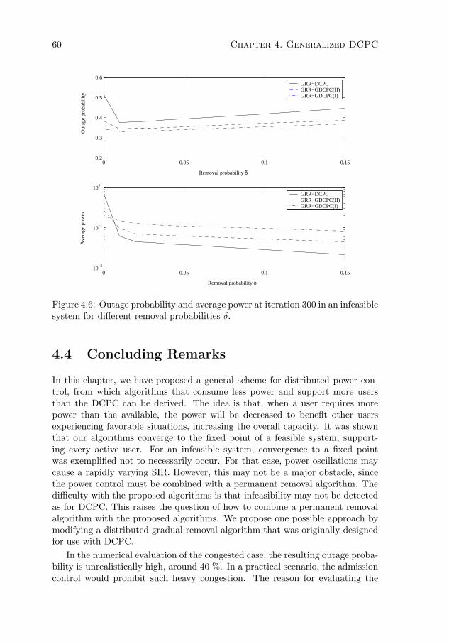
60 Chapter 4. Generalized DCPC
0 0.05 0.1 0.150.2
0.3
0.4
0.5
0.6
Removal probability δ
Out
age
prob
abili
tyGRR−DCPCGRR−GDCPC(II)GRR−GDCPC(I)
0 0.05 0.1 0.1510
−2
10−1
100
Removal probability δ
Ave
rage
pow
er
GRR−DCPCGRR−GDCPC(II)GRR−GDCPC(I)
Figure 4.6: Outage probability and average power at iteration 300 in an infeasiblesystem for different removal probabilities δ.
4.4 Concluding Remarks
In this chapter, we have proposed a general scheme for distributed power con-trol, from which algorithms that consume less power and support more usersthan the DCPC can be derived. The idea is that, when a user requires morepower than the available, the power will be decreased to benefit other usersexperiencing favorable situations, increasing the overall capacity. It was shownthat our algorithms converge to the fixed point of a feasible system, support-ing every active user. For an infeasible system, convergence to a fixed pointwas exemplified not to necessarily occur. For that case, power oscillations maycause a rapidly varying SIR. However, this may not be a major obstacle, sincethe power control must be combined with a permanent removal algorithm. Thedifficulty with the proposed algorithms is that infeasibility may not be detectedas for DCPC. This raises the question of how to combine a permanent removalalgorithm with the proposed algorithms. We propose one possible approach bymodifying a distributed gradual removal algorithm that was originally designedfor use with DCPC.
In the numerical evaluation of the congested case, the resulting outage proba-bility is unrealistically high, around 40 %. In a practical scenario, the admissioncontrol would prohibit such heavy congestion. The reason for evaluating the

4.4. Concluding Remarks 61
algorithm under this load is motivated for the approach of multirate systems,taken in next chapter. For a multirate system, the outage probability could beinterpreted as the fraction of users not being served with the maximum datarate. This level could be high and of the same order as here. The practicalapplicability of the concept of temporary removals, which GDCPC(I) and GD-CPC(II) benefit from, could for example be nonreal time data traffic where theflexibility of handling the transmission attempts is larger. This will be utilizedin the next chapter Finding necessary and sufficient conditions for convergencein infeasible systems is still an open issue. Also, there is a possibility of designingmore sophisticated removal algorithms suitable for our framework.

62 Chapter 4. Generalized DCPC

Chapter 5
Multirate Power Control
QUALITY-OF-SERVICE in DS-CDMA systems can be controlled by a suit-able selection of processing gain and transmitter powers. In this chapter,
distributed control of rate and power for best effort data services is considered.In particular, we elaborate on the problem of how to control the transmissionrates for maximizing system throughput while simultaneously minimizing thetransmitter powers. We assume a practical scenario, where every user has afinite set of discrete transmission rates and propose a simple heuristic rate allo-cation scheme, greedy rate packing (GRP), applicable in both up- and downlink.The scheme can be interpreted as a practical form of water-filling, in the sensethat high transmission rates are allocated to users having high link gains andlow interference. We show that GRP will under certain conditions, give max-imum throughput. The GRP is then extended to guarantee a minimum datarate while maximizing network excess capacity. A distributed power control al-gorithm, managing intercell interference, is suggested and analyzed for applyingGRP to a multicellular system.
5.1 Introduction
The service classes defined for multimedia services in UMTS include data rate,BER and delay constraints [1]. Our main focus will be on the throughput per-formance; resource allocation with delay considerations can be found in, e.g.,[33, 66]. Since the effective transmission rate and QoS objective are closely re-lated to the SIR, which can be efficiently controlled by SIR-based power control,it becomes natural to investigate a joint scheme for rate and power control. Oneapproach in previous work on resource allocation for multi QoS support, is tospecify no requirements on BERs and therefore no SIR-targets [87, 91, 105]. An-other direction of resource allocation is to specify a minimum SIR [92, 98, 126].The problem of throughput maximization was also studied in [94] for the mul-ticellular case and for different user classes in [92]. Some of the solutions in the
63

64 Chapter 5. Multirate Power Control
aforementioned work, set some transmitter powers to zero. This can be denotedas a hybrid of TDMA and CDMA, which also bears resemblance to our conceptof GRP. The main idea of the GRP is that the rates (and thus power values)of users with unfavorable link conditions are decreased, even to zero, while theusers with good channels transmit data with higher rates.
The practical applicability of the algorithms in [87, 91, 92, 94, 98, 105, 126] isnot clear because, either they require global information, consider only a sin-gle cell or use continuous transmission rates. In practical systems, the feasi-ble transmission modes are discrete and finite; the number of link adaptationschemes, code rates, processing gain, etc. Furthermore, the resource allocationshould preferably be distributed and function in multicellular systems. We shalladopt the discrete model for feasible transmission rates used in [64]. Therein asuggested distributed SPC algorithm was shown to converge to the power assign-ment that supports every active user with its maximum possible rate, using theminimum total transmitter power, if such a power assignment exists. Howeverfor a congested system, if no such assignment exists, little is known about itsproperties since convergence is not guaranteed. Due to the discreteness of rates,there may exist multiple rate combinations giving the same system throughputbut with different total transmitter power. Therefore, an important issue is howto assure the maximum total throughput to the system while using the minimumtotal transmitter power. For a single-rate system, the question is equivalentlyreduced to maximizing the number of supported users with the minimum to-tal transmitter power, which was shown to be NP-complete [5]. Therefore theproblem with multiple rates, which is the focus in this chapter, is in the generalmulticellular case also NP-complete.
5.2 Transmission Rate Assignment
5.2.1 Refined System Model
Consider a single cell1 in a DS-CDMA cellular radio system where N mobilesare using the same frequency channel. We will mainly consider the uplinkthroughout this chapter. Extension to the downlink will be discussed in Sec-tion 5.2.5. Each mobile i (1 ≤ i ≤ N) can transmit with a power from the setPi = {pi : 0 ≤ pi ≤ p}. We consider a short time interval such that the link gainbetween each mobile i and the base station is stationary and given by gi. Givena power vector p = (pi), the received SIR of mobile i, is for the uplink definedby
SIRi(p)def=
gipi∑Nj=1
j 6=igjpj + I + ν
, (5.1)
where I > 0 is the intercell interference power and ν > 0 is the backgroundnoise power at the base station. For the single cell analysis, I is considered to
1We will generalize the definition of a cell to a block in Section 5.3.

5.2. Transmission Rate Assignment 65
be fixed. Suppose that mobile i can utilize K > 1 discrete transmission ratesRi ∈ {r(1) < r(2) < . . . < r(K)} by varying its processing gain. Then, we candescribe the bit-energy-to-interference-power-spectral-density ratio of mobile iby (
Eb
I0
)
i
=W
Ri· SIRi(p), (5.2)
where W denotes the spreading bandwidth. The realized data rate of a mobiledepends on many factors such as receiver structure, user mobility, etc. Never-theless, SIR is a reasonable measure to match effective data rates. To properlyreceive information at transmission rate r(k), mobile i is required to attain anSIRi(p), not less than γ(k). Let γi be the SIR-target of mobile i such thatγi ∈ {γ(1) < γ(2) < . . . < γ(K)}, where each target element corresponds toeach rate, respectively. In the sequel, we will use rate assignment and target as-signment interchangeably. For setting the relationship among different γ(k), weassume a common target Γ being the same for all users and rates. This ensuresa constant BER regardless of the data rate. Then using (5.2), we can confineSIR-targets to the following relationship:
r(1)
γ(1)=
r(2)
γ(2)= · · · =
r(K)
γ(K)=
W
Γ(5.3)
This essentially describes K points from a linear relation between transmissionrate and SIR. Nonlinear relations can be considered by not keeping Γ uniformover all rates. With a certain assignment of SIR-targets, we can find the powervector that supports every mobile with the minimum power by solving the linearequation system (3.1), where H = [hij ] is an N × N matrix with elements
hij =
{γigj
gi, i 6= j
0, i = j
and η = (ηi) is an N × 1 vector with components ηi = γi(I+ν)gi
. For a feasible
system, the solution to (3.1) is found to be:
p∗i =I + ν
gi
γi
(1 + γi)
1
1 −∑Nj=1
γj
1+γj
. (5.4)
By Proposition 3.3, the spectral radius ρ(H) < 1 when∑N
j=1γj
1+γj< 1. Since
p∗i should also be less than or equal to p for all 1 ≤ i ≤ N , we can express theN constraints similar to [98]:
N∑
j=1
γj
1 + γj≤ 1 − max
1≤j≤N
[ γj
1+γj
gj pI+ν
](5.5)

66 Chapter 5. Multirate Power Control
Constraint (5.5) can be regarded as an instantaneous user capacity region forgiven link conditions. Considering γi/(1 + γi) as an effective bandwidth [109],the rightmost term in (5.5) can be interpreted as a relative utilization of themaximum achievable SIR2. We will assume that the maximum SIR, gip/(I + ν),is available at the base station and that the feedback channel is error free andwithout any delay.
As there can be a large number of feasible rate combinations that give thesame throughput for the cell, finding one which yields low total transmittedpower is desirable, especially for multicellular systems. In particular, we wishto design a scheme that finds solutions where the total throughput takes themaximum feasible value. Utilizing (5.3), (5.4) and (5.5), for a given throughputγ the power minimization problem can be formulated in terms of SIR-targetassignment,
minγj
I + ν
1 −∑Nj=1
γj
1+γj
N∑
j=1
γj
gj(1 + γj)(5.6)
s.t.
N∑
j=1
γj = γ (5.7)
N∑
j=1
γj
1 + γj≤ 1 − max
1≤j≤N
[ γj
1+γj
gj pI+ν
](5.8)
γj ∈ Υ (5.9)
where the set Υ = {0, γ(1), γ(2), . . . , γ(K)} contains the possible targets. Whenγj = 0, no transmission is performed for mobile j and it does not contributein (5.8). For a given γ, we will mean by feasible target assignment, an SIR-target assignment that satisfies constraints (5.7)-(5.9). Given a feasible targetassignment, the corresponding power value of each user can be computed by(5.4).
5.2.2 Greedy Rate Packing
From the structure of the objective function (5.6), it follows that when feasibleSIR-targets are assigned, their order does not change the value of the denom-inator. However, for the sum in the numerator, the total transmitted powerwill be affected by which target is assigned to which mobile, due to the linkgains. Obviously, the total transmitted power of a given cell can be minimizedby assigning high targets to mobiles with high link gains, which we state in theproposition below.
2The quantity γi/(1 + γi) is also the SIR-target if own-interference is included. Rewriting(5.1), we have
gipi∑j gjpj + I + ν
=γi
1 + γi.

5.2. Transmission Rate Assignment 67
Proposition 5.1 Let us assume that g1 ≥ g2 ≥ . . . ≥ gN and that there existsa feasible SIR-target assignment that satisfies (5.7)-(5.9). Among the feasiblereassignments of the SIR-targets, the total power is minimized by reassigningthem such that γ1 ≥ γ2 ≥ . . . ≥ γN .
Proof: Among the feasible target reassignments, let us assume there exists anassignment that minimizes the objective function (5.6) but does not satisfy
γ1 ≥ γ2 ≥ . . . ≥ γN . (5.10)
Then, we can find at least one pair of i and j (i < j) such that γi < γj . Now,since gi ≥ gj , we find from (5.5) that a new feasible target assignment can beconstructed by switching assignment γi and γj . Since
γj
1+γj> γi
1+γi, we can
defineγj
1+γj= γi
1+γi+ ∆, where the number ∆ is positive. For any reassignment,
the denominator of (5.6) remains the same, therefore it is sufficient to compare
γi
gi(1 + γi)+
γj
gj(1 + γj)−(
γj
gi(1 + γj)+
γi
gj(1 + γi)
)=
γi
gi(1 + γi)+
∆
gj+
γi
gj(1 + γi)−(
γi
gi(1 + γi)+
∆
gi+
γi
gj(1 + γi)
)=
∆
(1
gj− 1
gi
)≥ 0.
From the objective function (5.6), we have a contradiction that the new assign-ment has a lower objective function value than the optimal assignment. Thusfor any i, j with gi ≥ gj , an optimal assignment must fulfill γi ≥ γj �
To keep the analogy to water-filling principles, we can equivalently order themobiles by their link gains normalized with I+ν. Henceforth, we assume that theusers are ordered such as g1
I+ν ≥ g2
I+ν ≥ . . . ≥ gN
I+ν . In our case, they could also beordered by their maximum SIRs, pgi/(I + ν). The proposition says that we canreduce the total power of the mobiles while maintaining the same throughput,by reassigning SIR-targets in a decreasing manner. It should be pointed outthough, that such a solution does not necessarily minimize the powers in amulticellular system. Since the proposition holds for any feasible value of γ,an interesting task is to find a feasible target assignment that will achieve themaximal throughput while satisfying condition (5.10). For this purpose, we will,based on (5.5), suggest the following heuristic algorithm:
Greedy Rate Packing (GRP)γi = 0, ∀i
For i = 1 to N do
γ∗i = max
{γi ∈ Υ :
∑ij=1
γj
1+γj≤ 1 − max1≤j≤i
[ γj1+γjgj p
I+ν
]}
γi = γ∗i

68 Chapter 5. Multirate Power Control
The GRP procedure allocates the maximum feasible rate to each mobile, startingwith the mobile with the highest link gain, or equivalently the maximum SIR.Further, it never reallocates rates of mobiles previously assigned, taking no morethan N steps. It is easy to see that γ∗
1 ≥ γ∗2 ≥ . . . ≥ γ∗
N . However, the GRP isheuristic and does not necessarily find the solution to (5.6)-(5.9) but the resultin the next section shows that high throughput solutions may be found.
5.2.3 Throughput Maximization
With the feasible target assignment generated from GRP denoted by γ∗i , we
define γ∗ =∑N
i=1 γ∗i . A question at hand is how close the value γ∗ is to the
maximal throughput. This is generally difficult to answer, but for the specialcase where the upper bound on transmitter power is large enough compared tothe interference plus noise, the uplink pole capacity is solely governed by thesum of the effective bandwidths
N∑
j=1
γj
1 + γj< 1. (5.11)
The following observation, which indicates that splitting a rate over several usersconsumes more effective bandwidth, can be made.
Lemma 5.1 If γ ≤∑j γj, 0 ≤ γj < γ and θ > 0, then θγ1+θγ <
∑j
θγj
1+θγj.
Proof: Since γ1+γ is a monotonously increasing concave function,
θγ
1 + θγ≤
∑j θγj
1 +∑
j θγj<∑
j
θγj
1 + θγj.
�
Let us assume that the rates, and therefore the corresponding SIR-targets, aregeometrically related as r(i+1) = µr(i) with 1 ≤ i ≤ K − 1, µ > 1 and r(1) > 0.Hence, it follows that r(i) = µi−1r(1), 1 ≤ i ≤ K. Further, constrain µ to be aninteger, which is often the case in practical systems. The following result saysthat high rates achieve the most efficient resource allocation.
Lemma 5.2 For a rate allocation that maximizes throughput subject to (5.11),each of the rates r(1), r(2), . . . , r(K−1) can be used at most µ − 1 times.
Proof: Assume that r(i), 1 ≤ i < K is assigned to µ users. Obviously µr(i) =r(i+1), so by using Lemma 5.1 with θ = 1, the corresponding SIR-targets fulfill
γ(i+1)
1+γ(i+1) < µ γ(i)
1+γ(i) . Therefore, the same total throughput µr(i) can be assigned
with less utilization of the slack in the capacity constraint (5.11) by allocating

5.2. Transmission Rate Assignment 69
r(i+1) to one single user. Hence, splitting the rate r(i+1) over µ or more userscannot maximize throughput. �
Then, subject to (5.11) and the above assumptions, we can find that maximumthroughput is obtained from the GRP.
Proposition 5.2 If p → ∞, r(i+1) = µr(i) with 1 ≤ i ≤ K − 1, µ > 1 andr(1) > 0, GRP gives the maximum throughput.
Proof: Assume a stepwise rate allocation procedure starting with its highestrates. Further, assume that at some point of this procedure, user i is assigneda rate Ri = r(k), k < K which is lower than the one of the GRP allocation,say R∗
i = r(p), k < p ≤ K. By Lemma 5.2, the rates r(1), r(2), . . . , r(k) ina throughput maximizing solution can be only used at most µ − 1 times each.Therefore the remaining throughput of this rate allocation procedure is boundedby
N∑
j=i
Rj ≤ (µ − 1)k∑
j=1
r(j) = (µ − 1)k∑
j=1
µj−1r(1) = (µk − 1)r(1)
< µkr(1) = r(k+1)
≤ R∗i ≤
N∑
j=i
R∗j ,
which means that, if Ri = r(k) the total throughput of the remaining users willbe lower than if Ri = r(p). Therefore, to achieve a total throughput not lessthan the GRP solution, user i must be assigned a rate Ri > r(k). Recursivelyapplying this result, it follows that k must equal p, the GRP assignment. Thusin any step, GRP assigns the optimal rate. �
An interpretation of Proposition 5.2 is that, for an isolated or remote cell, wherethe intercell interference is small enough compared to the mobile’s maximumpower, we can guarantee a maximum throughput solution from GRP.
5.2.4 Minimum Rate Requirements
So far, the focus has been exclusively on best effort services, with maximumBER requirements but without delay constraints. It is possible to utilize theconcept of GRP for delay sensitive users with minimum rate requirements. Forthis purpose, a modified GRP procedure can be defined, aiming to support asmany users as possible with their minimum rate, while maximizing the networkexcess capacity in a best effort manner. Henceforth, we consider r(1) to be theminimum rate requirement for all users.

70 Chapter 5. Multirate Power Control
GRP2γi = 0, ∀i
Step 1.For i = 1 to N do
γ∗i = max
{γi ∈ {0, γ(1)} :
∑ij=1
γj
1+γj≤ 1 − max1≤j≤i
[ γj1+γjgj p
I+ν
]}
γi = γ∗i
Step 2.For i = 1 to N do
γ∗i = max
{γi ∈ Υ :
∑Nj=1
γj
1+γj≤ 1 − max1≤j≤N
[ γj1+γjgj p
I+ν
],
}
γi = γ∗i
The GRP2 has the property that it supports as many connections as possiblewith the minimum rate.
Proposition 5.3 The GRP2 procedure maximizes the number of users sup-ported with the minimum rate.
Proof: It suffices to show that the proposition holds after Step 1. Let M denotea partition of the users such that users in M obtain rate γ(1) while users not inM obtain rate zero. Let m = |M| denote the number of supported users. Inthis case, the inequalities (5.5) can be expressed in the form:
mγ(1)
1 + γ(1)+
γ(1)
1+γ(1)
gipI+ν
≤ 1 (5.12)
Since g1 ≥ g2 ≥ . . ., we must have that for i = 1, 2, . . . ,m, gi ≥ minj∈M gj .It follows that(5.12) must hold i = 1, 2, . . . ,m and that Step 1 for GRP2 willassign nonzero rate to at least the first m users. Hence Step 1 of GRP2 supportsat least as many users as any other assignment. �
5.2.5 Downlink GRP
For the downlink case, the equation system (3.2) takes this form
γi =gipi∑N
j=1
j 6=iθgipj + Ii + ν
(5.13)
where Ii is the intercell interference at mobile i and θ ∈ [0, 1] is the orthogonalityfactor. Straightforwardly, it can be shown that the minimum power solutionequals,
p∗i =γi
1 + θγi
(∑Nj=1
θγj
1+θγj
Ij+νgj
1 −∑Nj=1
θγj
1+θγj
+Ii + ν
gi
). (5.14)

5.3. Iterative Power Control 71
If in (5.13) θ depends on i, the power solution is given by (5.14) with θ = θi. Incontrast to the uplink, usually the sum of the users’ powers in the cell is limited,rather than the maximum power of each user. If the sum of all transmitterpowers in the cell is considered to be limited to P , based on (5.14) the followingfeasibility constraint can be derived
N∑
j=1
θγj
1 + θγj
(Ij + ν
gjP θ+ 1
)≤ 1 (5.15)
which could be used for a downlink greedy rate packing procedure. If (5.15)
holds, it follows from (5.14) that pi > 0 and∑N
i=1 pi ≤ P . Studying (5.15),it suggests that also in this case, to minimize the sum of powers, high ratesshould be assigned if gi/(Ii + ν) is large. Here it is required that gjP /(Ij +ν), the maximum achievable SIR for user j, can be perfectly estimated at thebase station. We will not elaborate further on the downlink in this chapter.However, we can generalize Lemma 5.2 to cover also the condition (5.15), ifwe consider users to be ordered such that g1/(I1 + ν) ≥ g2/(I2 + ν) ≥ . . . ≥gN/(IN + ν). Downlink throughput optimality can then be shown using thesame technique as for Proposition 5.2. In the downlink case, (5.15) is a truesingle-cell feasibility condition and optimality does not require an assumptionthat P → ∞. Hence, GRP will achieve maximum throughput in the downlink,given the same geometric rate relations as in Section 5.2.3.
5.3 Iterative Power Control
In this section, the GRP will be applied to a multicellular system. As the intercellinterference will vary after each round of GRP assignment, we approach theproblem by an iterative power/rate control algorithm. Consider the followingiterative algorithm for the combined rate and power assignment in a multicellularsystem.
Generalized Selective Power Control (GSPC) Each cell updates its SIR-target assignment for the users in the cell using GRP and correspondingly updatesthe power of each user using (5.4) in every iteration.
So far, we have assumed that N is the number of users in a given cell and thatthey all require the same maximum BER. Now, let us assume that the usersin a cell can be partitioned into a number of subsets, referred to as blocks, andconsider N to be the number of users in a given block. Within a block we requirethat Γ is constant. Consequently, users within a block are assumed to require anidentical service. In this setting, I denotes the interference coming from outsideof the given block. Then, our discussion so far is still valid even if we replacethe terminology “cell” by “block”. For example, in the GSPC description above,we may use GSPC for the block-wise rate and power update. Therefore, we will

72 Chapter 5. Multirate Power Control
hereafter use the term block, instead of cell. For the special case where there isjust a user in each block, GSPC is reduced to the following fully distributed SPCalgorithm for combined rate and power control, which was suggested in [64],
pi(n + 1) = maxγi∈Υ
{γi
SIRi(p(n))pi(n) · 1{ γi
SIRi(p(n))pi(n)∈Pi
}}
, (5.16)
where
1A =
{1, if A occurs
0, otherwise.
is the indicator function of the event A. The SPC selects independently for eachmobile, the maximum feasible SIR-target that it can achieve against the presentinterference. The GSPC on the other hand, can be interpreted as a locallycentralized algorithm which requires that the power and rate assignments areexecuted at the base station and delivered to the mobile. Then the base stationto which mobile i is connected, could estimate gi/(I + ν) needed for the GRP.
Let us define individual sets of transmission rates such that for user i, the setΥi ⊆ Υ contains its SIR-targets and let γi = supΥi be its maximum SIR-target.When the system is feasible for the targets γi, it was given in [64] that the SPCalgorithm converges to a state where every active mobile is supported with itsmaximum rate and the sum of the powers is minimized. For GSPC, we canprove similar properties which will be numerically verified in Section 5.5.
Proposition 5.4 For a feasible system, GSPC converges to the power vectorwhere every mobile is supported with its maximum rate and the sum of powersis minimized.
Proof: Let us first consider an unconstrained power control algorithm given by
pi(n + 1) = Ti(p(n)) =I(p(n)) + ν
gi
γi
1 + γi
1
1 −∑Nj=1
γj
1+γj
, (5.17)
where p(n) and I(p(n)) denote the power vector and intercell (interblock) in-terference at iteration n. It has been proven (see, e.g., Chapter 5 [56]) that theabove algorithm converges to the power vector that achieves γi for every userusing minimum total transmitter power, if such a power vector exists3. Nowlet us consider the generalized constrained power control algorithm suggested inChapter 4,
pi(n + 1) = Ti(p(n)) =
{Ti(p(n)), if Ti(p(n)) ∈ Pi
pi(n), if Ti(p(n)) 6∈ Pi(5.18)
3The proof of convergence in [56] was carried out with the technique of matrix splittings.Convergence could alternatively be performed by verifying consistency and show that (5.17)is a standard power control algorithm.

5.4. Power Control with Gradual Rate Removal 73
where 0 ≤ pi(n) ≤ p. By letting γi = γi, we can regard GSPC as a specialcase of the above algorithm (5.18), where pi(n) is utilized if lower targets areselected. Since Proposition 4.3 states that (5.18) converges, so will GSPC. �
Proposition 5.5 For a feasible system, SPC gives the slowest asymptotic rateof convergence among the class of GSPC algorithms.
Proof: Consider a power control algorithm given by
pi(n + 1) = T i(p(n)) =γi
SIRi(p(n))pi(n). (5.19)
It is well known (see, e.g., Chapter 3) that the above iteration converges tothe power vector, say p∗ that achieves γi for every user i with minimum totaltransmission power, if such a power vector exists. Define the error vector as
ε1(n) = T (p(n)) − p∗, n = 0, 1, . . . (5.20)
In the same way, we can define an error vector for the algorithm (5.17) by
ε2(n) = T (p(n)) − p∗, n = 0, 1, . . . (5.21)
For a given number δ > 0, let n1(δ) and n2(δ) denote the minimum number of it-erations that give ||ε1(n)|| ≤ δ · ||ε1(0)|| and ||ε2(n)|| ≤ δ · ||ε2(0)||, respectively.It has been proven (see, e.g., Proposition 5.2 [56]) that for a suitable norm,n1(δ) > n2(δ) as δ approaches zero, which means the mapping T is asymp-totically faster4 than T . It is easy to see that SPC is a special case of (5.18),equivalently expressed as
pi(n + 1) = Ti(p(n)) =
{Ti(p(n)), if Ti(p(n)) ∈ Pi
pi(n), if Ti(p(n)) 6∈ Pi(5.22)
where pi(n) ∈ Pi. Asymptotic rate of convergence is then reduced to if T
(GSPC) is asymptotically faster than T (SPC). Since both T and T will con-verge, each will follow the dynamics of T and T , respectively, as δ approacheszero. Therefore, we can say that T is asymptotically faster than T . ApplyingProposition 5.2 in [56], it follows that considering only one user per block (SPC)is the worst choice with respect to asymptotic average rate of convergence. �
The latter proposition is based on results from [56], saying that the more usersthe blocks contain, the faster the asymptotic rate of convergence becomes.Larger block size can be interpreted as a higher degree of centralization.
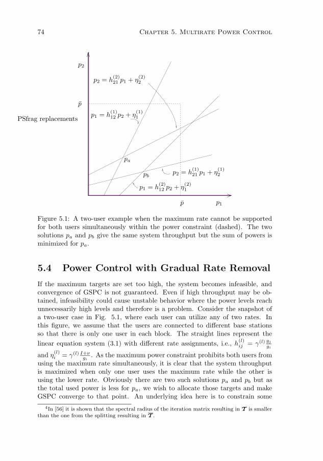
74 Chapter 5. Multirate Power Control
PSfrag replacements
p1
p2
pa
pb
p
p
p1 = h(1)12 p2 + η
(1)1
p1 = h(2)12 p2 + η
(2)1
p2 = h(1)21 p1 + η
(1)2
p2 = h(2)21 p1 + η
(2)2
Figure 5.1: A two-user example when the maximum rate cannot be supportedfor both users simultaneously within the power constraint (dashed). The twosolutions pa and pb give the same system throughput but the sum of powers isminimized for pa.
5.4 Power Control with Gradual Rate Removal
If the maximum targets are set too high, the system becomes infeasible, andconvergence of GSPC is not guaranteed. Even if high throughput may be ob-tained, infeasibility could cause unstable behavior where the power levels reachunnecessarily high levels and therefore is a problem. Consider the snapshot ofa two-user case in Fig. 5.1, where each user can utilize any of two rates. Inthis figure, we assume that the users are connected to different base stationsso that there is only one user in each block. The straight lines represent the
linear equation system (3.1) with different rate assignments, i.e., h(l)ij = γ(l) gj
gi
and η(l)i = γ(l) I+ν
gi. As the maximum power constraint prohibits both users from
using the maximum rate simultaneously, it is clear that the system throughputis maximized when only one user uses the maximum rate while the other isusing the lower rate. Obviously there are two such solutions pa and pb but asthe total used power is less for pa, we wish to allocate those targets and makeGSPC converge to that point. An underlying idea here is to constrain some
4In [56] it is shown that the spectral radius of the iteration matrix resulting in T is smallerthan the one from the splitting resulting in T .

5.4. Power Control with Gradual Rate Removal 75
users to lower its maximum rate so that the induced system becomes feasible.This can be done distributively by using the transmitter removal concept pre-viously applied in fixed rate systems in Chapter 4, which will be extended torate removal in this chapter. As we stated in the introduction, maximizing thesystem throughput in a multicellular system with maximum transmitter powersis NP-complete. Therefore, convergence to the optimal power and rate assign-ment cannot be guaranteed within a short computational time, which calls fora heuristic algorithm. Based on Proposition 5.1, which states that users withfavorable link gains should utilize high data rates, we can construct the followingrate removal algorithm.
Let Υi(n) be the set of possible SIR-targets at iteration n for user i andγi(n) = sup Υi(n) be its maximum target. Define in each block at each iteration,a set of mobiles V(n) = {i : γi < γi(n), γi(n) > 0}. This set contains themobiles not being assigned their maximum achievable rate during the GRP.Then consider5:
Gradual Rate Removal-GSPC (GRR-GSPC) After each iteration of GSPCand for each block; if V(n) 6= ∅, then with a given probability δ, remove one ratefrom user i0 such that Υi0(n+1) = Υi0(n)\γi0(n) where i0 = argmini∈V(n)gi/(I+ν).
In GRR-GSPC, if in each block, there exists any user that has been assigneda rate less than its maximum rate, then the maximum rate of the user withthe lowest link gain in the block will be decreased (one-step down) with a givenprobability δ. This will shape the rate distribution such that the system willeventually become feasible. Based on Theorem 6 in [5], it can be noted that forδ > 0, GRR-GSPC will converge to a stationary feasible power vector where allremaining users are supported with their resulting maximum rate. The corre-sponding concept of GRR-SPC yields:
pi(n + 1) = maxγi∈Υi(n)
{γi
SIRi(p(n))pi(n) · 1{ γi
SIRi(p(n))pi(n)∈Pi
}}
(5.23)
If γi(n)SIRi(p(n))pi(n) 6∈ Pi and γi(n) > 0, then Υi(n + 1) = Υi(n) \ γi(n) with a
given probability δ.
For GRR-SPC, where each user is its own block, there exists only one possiblei = i0 and hence it is a special case of GRR-GSPC and convergence applies toit as well. The reason for adopting a probabilistic removal procedure, δ < 1, isthat if too many users simultaneously remove their maximum rate, capacity mayget wasted, since removing only a subgroup of these rates might give a feasiblesystem. By defining GSPC2 as GSPC but with GRP2 instead of GRP, we havethe same type of block distributed algorithm and the rate removal procedure isapplicable also to GSPC2.
5In Chapter 4 and [5], GRR denoted Gradual Removals Restricted

76 Chapter 5. Multirate Power Control
5 10 15 20 25 30 35 4010
−5
10−4
10−3
10−2
10−1
100
Iteration
Ave
rage
pow
er [
W]
GSPCSPC
Figure 5.2: The average power in a feasible system where the target Eb/I0 = 7dB. The figure verifies that the rate of convergence is much faster for GSPCthan SPC.
5.5 Numerical Results
The algorithms are evaluated by simulations in a system consisting of 19 hexag-onal cells with centrally located base stations using omni-directional antennas.The cell radius is set to 1 km and a wrap-around technique is used. Evaluationis performed in the DS-CDMA system described in Chapter 2 and illustrated inFig. 1.2. The cell radius is set to 1 km and a wrap-around technique is usedalong with omni-directional antennas. For a given instance, 10 mobiles/cell aregenerated, the locations of which are uniformly distributed over the cells. Atany given instance, the link gain is modeled by gij = Sij · r−4
ij , where Sij is theshadow fading factor and rij is the distance between base i and mobile j. Theshadow fading factor is generated from a lognormal distribution with µs = 0 dB,and σs = 8 dB, where the Sij ’s are mutually independent. The base receivernoise is taken to be νi = 10−15 W and the maximum mobile power is set tounity. The initial power for each mobile is randomly chosen from the interval[0,1]. Each user is assigned to the base station that provides the lowest signalattenuation. We consider the uplink of a system that has a spreading bandwidthW = 1.2288 MHz and assume that the radio link can support four transmissionrates, r(k) = 9.6 · 1
2k−1 kbps (k = 1, 2, 3, 4) and the zero rate if necessary. As in

5.5. Numerical Results 77
(5.3), the required minimum SIR is assumed to be γ(k) = γ · 12k−1 for supporting
each 9.6 · 12k−1 kbps. Different values of γ can be considered for representing
different congestion scenarios. Two values γ = −14 dB and γ = −5 dB areset to represent low and high system loads respectively. Adding the processinggain, this is equivalent to 7 and 16 dB as the corresponding Γ values. In generalthe effective transmission rate for a given channel quality is dependent on thereceiver structure. In our simulation, we use a pessimistic effective rate. Thatis, either the attained SIR is above the required threshold and the throughput isthe selected rate or otherwise, no data is received. In each iteration, the averagethroughput per user, average transmitter power per user and outage probabilityare used as performance measures. The average throughput per user is computedby dividing the total throughput by the total number of users in the system, i.e.,in this case 190. The average power is obtained similarly. The outage probabilityis here defined as the fraction of users not receiving any data, which occurs whenthe obtained SIR is lower than the selected target or the zero rate is selected.In the rate and power assignment, a slight fade margin of 0.5 dB was added,implying that an outage event is declared if the received Eb/I0 is below 6.5 and15.5 dB, respectively. We assume that all users in a cell constitute a block inGSPC. To evaluate performance, we have taken 100 independent instances ofmobile locations and shadow fading. For each instance, we have performed thealgorithms until the iteration number reached 500, a number that yielded stablesolutions. In Fig. 5.2, where all users can be supported with the maximumdata rate, Proposition 5.5 is illustrated by that the average of the power vectorreaches its steady state faster for GSPC than SPC. When Γ = 16 dB, the systembecomes infeasible and the throughput curves in Fig. 5.3 indicate an oscillatingbehavior. It can be found by studying data from one single snapshot at a time,that SPC has a much more oscillative behavior for infeasible situations whichalso gives larger throughput variations than of GSPC. Clearly the throughputpenalty of GSPC2 for trying to guarantee the minimum rate is seen as well.As a benefit from the faster convergence, the GSPC algorithms also reach theirmaximum throughput levels much faster than the SPC.
In the first columns of Tables 5.1-5.3, the resulting values after 500 iterationsare contained for the case without removal, δ = 0. We see that GSPC givesabout 9 % higher throughput than SPC and at the same time about half theenergy consumption. The price of the greedy behavior of GSPC is the resultinghigher outage probability. In the other columns, the result of applying theGRR procedure can be seen for the respective δ values. When applying therate removal, the probability δ should be chosen moderately so that the setof rates removed in each iteration becomes relatively small. Too aggressive aremoval strategy might eventually result in an underutilization of the spectrum.For GRR-GSPC, rates may be removed from mobiles within the block that arenot transmitting, so the removal probability may be chosen much larger thanfor GRR-SPC. There is obviously a tradeoff between choosing a high removalprobability, making the system feasible rather quickly, which would give fast

78 Chapter 5. Multirate Power Control
5 10 15 20 25 30 35 401500
2000
2500
3000
3500
4000
Iteration
Ave
rage
dat
a ra
te [
bps]
GSPCSPCGSPC2
Figure 5.3: Average throughput per user of GSPC, SPC and GSPC2 underheavy load, Eb/I0 = 16 dB, without gradual rate removal.
convergence but low throughput and power, and a lower one which would givethe opposite. From Tables 5.1-5.3 we draw the following conclusions: The GRPprocedure seems to be superior in offering the highest throughput. The penaltyfrom guaranteeing a minimum rate, like GSPC2, is that it requires much morepower and lowers the total throughput but reduces outage. The gain from GRRis mainly that the powers will be decreased. Thus, even though high throughputcan be maintained for infeasible situations, infeasibility is undesirable from anenergy consumption point of view. The SPC is more sensitive to the choice of δin terms of throughput losses.
5.6 Concluding Remarks
We considered a DS-CDMA system where every user had a discrete set of pre-determined SIR-targets corresponding to different transmission rates. Sincethere are many combinations of transmission rates giving the same systemthroughput, we formulated the problem of minimizing the total transmissionpower while trying to maximize the throughput. For a single cell, we suggestedthat high data rates should be allocated to users with high link gains and lowinterference. That is, the area at which the service can be provided, will belocated close to the radio access point. We may think of this as a spatial dif-

5.6. Concluding Remarks 79
ferentiation. However, if users are mobile, all users could expect this servicelevel in average. The characteristics of the single cell solution were used as abuilding block for a simple greedy rate and power assignment algorithm, calledGSPC, for a multicellular system. The aim was to maximize the throughputbut minimum rate requirements could be included as well. Numerical resultsshowed that GSPC can attain higher throughput while the transmitter powersare considerably decreased, compared to a reference algorithm SPC [64]. Fur-thermore, GSPC has a merit of fast convergence and can significantly decreasethe energy consumption, when it is combined with rate removal. The cost ofthis concept is a slight increase of overhead information, as it is not fully dis-tributed but the gain seems to be large in terms of energy conservation as wellas increased system capacity. We exemplified that, when trying to assure eachuser a minimum rate, both system throughput and energy conservation will besacrificed for the fairness among the users. Further studies are needed on howto apply gradual removal for time varying channels. Somehow, some rates mustbe admitted again if the channel conditions have changed significantly.

80 Chapter 5. Multirate Power Control
δ 0 0.1 0.2 0.3 0.4 0.5 1
Throughput 3.56 3.57 3.56 3.57 3.56 3.56 3.56
Power 0.18 0.07 0.02 0.02 0.02 0.02 0.02
Outage 0.56 0.55 0.55 0.55 0.55 0.55 0.55
Table 5.1: Data for GRR-GSPC at iteration 500 for different removal probabil-ities δ. The first row is average throughput per user [kbps], the second row isthe average power per user [W] and the last row is the outage probability.
δ 0 0.1 0.2 0.3 0.4 0.5 1
Throughput 2.65 2.61 2.58 2.57 2.56 2.56 2.53
Power 0.27 0.14 0.03 0.03 0.02 0.03 0.02
Outage 0.02 0.02 0.02 0.02 0.02 0.02 0.02
Table 5.2: Data for GRR-GSPC2 at iteration 500 for different removal proba-bilities δ.
δ 0 0.02 0.04 0.06 0.08 0.1 1
Throughput 3.26 3.34 3.33 3.32 3.32 3.21 2.95
Power 0.36 0.21 0.11 0.08 0.05 0.04 0.0005
Outage 0.39 0.36 0.36 0.36 0.36 0.36 0.35
Table 5.3: Data for GRR-SPC at iteration 500 for different removal probabilitiesδ.

Chapter 6
Joint Power Control and
Intracell Scheduling
THE PERFORMANCE of DS-CDMA systems highly depends on the successin managing interference arising from both intercell and intracell transmis-
sions. Interference management in terms of power control for real-time dataservices has been widely studied and has shown to be a crucial component forthe functionality of such applications. In this chapter we consider the problem ofsupporting downlink nonreal time data services, where in addition to the powercontrol, there is also the possibility of controlling the interference by means oftransmission scheduling. One such decentralized schedule is to use time divisionso that users transmit in a one-by-one fashion within each cell. We show thatthis has merits in terms of energy conservation and increased system capacity.We combine this form of intracell scheduling with a suggested distributed powercontrol algorithm for the intercell interference management. We address its rateof convergence and show that the algorithm converges to a power allocation thatsupports the nonreal time data users using the minimum required power whilemeeting requirements on an average data rate.
6.1 Introduction
In the DS-CDMA cellular system, one adopted multiple access method for futurePCSs [32], the total received interference can be divided into intracell interfer-ence, originating from simultaneous transmissions within the cell and intercellinterference caused by terminals transmitting in other cells. To alleviate theimpact of intercell and intracell interference, transmitter power has turned outto be an important controllable resource for balancing the desired signal- andinterference power at the receiver, rendering in increased capacity and lowerenergy consumption. Much work has been performed in the area of designing
81

82 Chapter 6. Joint Power Control and Intracell Scheduling
quality based power control algorithms for finding the minimum power allocationwhen users require fixed data rates at a given target SIR, see Chapter 1 and 4.Typically this direction sees applications for voice services (see [95, 122] and ref-erences therein). The optimal power solution for this problem has been shown tobe Pareto optimal [83], i.e., minimizing each user’s transmitter power also mini-mizes the total sum power. Integrated over time, this solution also minimizes theenergy consumption. However, the requirement on a constant data rate and thusSIR, prohibits any interruption of the data stream and therefore the degree offreedom to co-ordinate the transmissions in time is limited. Herein, we considerthe problem to support a given set of nonreal time service users with a certainrequired average data rate with minimum energy consumption obtained via aminimum power solution. With average data rate, we mean that a least amountof data has to be delivered over a specified time interval, a more relaxed con-straint than a fixed data rate, which increases the options of adaptively planningthe transmissions. One scheme that does not require any co-ordination betweenbase stations, is to plan the transmissions independently in a cell-wise manner.Thus, in addition to power control, by utilizing the possibility of scheduling thetransmissions within the cell, the intracell interference can be efficiently avoided.Since DS-CDMA systems are considered to be interference limited, less interfer-ence allows for reduced transmission power, in turn increasing the capacity andlowering the energy consumption. Hence it suggests that, if the same amount ofdata can be delivered, the impact will be higher energy efficiency since no poweris wasted on combating the intracell interference.
In the chapter, we consider efficient use of the radio resources by exploitingthe delay tolerance of nonreal time service users. Particularly we elaborate on theone-by-one scheduling (TDMA) for the downlink transmission in a DS-CDMAsystem. A crucial component is quality based power control but rather thanfocusing on minimum power solutions as in Chapter 4, 5 and [83, 95, 122], wewill direct this work toward minimum energy solutions, a more natural measurefor an average data rate seen over a time interval. The main focus herein isto offer a given average data rate with minimum energy consumption whileallowing intracell scheduling, which is a form of time multiplexing. We showthat intracell scheduling in terms of time division within the cells merits ofhigher energy efficiency and system capacity than continuous transmission ata fixed data rate. For finding the optimal powers, a distributed power controlalgorithm is suggested and proven to drive the transmit power to the minimumpower level that guarantees the average data rate to the nonreal time users. Byminimizing their power usage, interference is minimized and also more of thecell’s available transmitter power is left for supporting real time services or morenonreal time users. With strong resemblance to the continuous transmissionproblem, the power allocation can be found from a linear equation system, as in(3.2) but expressed in the cell-site powers. It is found that this power solutionminimizes the energy consumption. Moreover, it is shown that the power controlcan converge at a faster rate in the average data rate case than for the fixed data

6.2. Minimum Energy Problem 83
rate case. Based on the spectral radius of the power control iteration matrix, wecan identify a capacity gain of the proposed power control/scheduling concept.
6.2 Minimum Energy Problem
6.2.1 Refined System Model
For treatment of the downlink, we refine the general system model of Chapter 2as follows. Consider the downlink of a DS-CDMA cellular system with M basestations where N nonreal time service users can access a common frequencychannel. Let user i be connected to base station bi and the set Bk = {i : bi =k, 1 ≤ i ≤ N} contain the users connected to base station k. Consider a timeinstant where the link gain between base station j and user i is stationary andgiven by gij . Denote by p = (pi) the N × 1 downlink powers dedicated to theusers. If i ∈ Bk, the SIR for user i can alternatively be written as
SIRi(p)def=
gikpi∑j 6=i
j∈Bk
θijgikpj + Ii(p) + νi(6.1)
where Ii(p) is the intercell interference for user i and νi is the thermal noise. Thequantity θij ∈ (0, 1] is the normalized cross-correlation between pi and pj at thereceiver of user i. In this chapter, we exclude θij = 0, since intracell schedulingwould in that ideal case be obsolete. Define P = (Pk) to be the M × 1 vector ofbase station powers where Pk =
∑i∈Bk
pi. We assume that transmission ratesare adapted by varying the processing gain and that the effective data rate ofuser i is given by the continuous and linear relation
Ri =W
Γi· SIRi(p). (6.2)
In (6.2), W is the common spreading bandwidth and Γi a required bit-energy-to-noise-spectral-density ratio. Therefore, Ri is achieved with a tolerable maximumbit error probability which is assumed to be a function of Γi, the desired Eb/I0.Due to hardware constraints, the output power of the power amplifier is limited.In the downlink, the power constraint is typically related to the sum of the cell’spower rather than individual powers of the users. Therefore, if the cells have themaximum power constraints given by a vector P, any feasible power assignmentmust then fulfill 0 ≤ P ≤ P. The minimum power assignment for achieving thedata rates Ri, is obtained by putting (6.1) and (6.2) on matrix form. Hence,solving the linear equation system, which has the same form as (3.2),
(I − H)p = η (6.3)

84 Chapter 6. Joint Power Control and Intracell Scheduling
where H = [hij ] denotes an N × N matrix with elements
hij =
RiΓi
W θij , i 6= j, bi = bj
RiΓi
W
gibj
gibi
, i 6= j, bi 6= bj
0, i = j
and η = (ηi) is an N × 1 vector with ηi = RiΓi
Wνi
gibi
, gives the componentwise
smallest power vector. In this notation, the indices j may correspond to thesame physical base station.
6.2.2 Problem Definition
Assume now that there exists a specified scheduling interval, 0 ≤ t ≤ Ts, overwhich a nonreal time service user i requires a minimum average data rate Ri.That is, at least TsRi bits have to be received over the scheduling interval at thequality specified by Γi. Consider the following problem of finding the transmis-sion powers during Ts that minimize the total energy consumed.
minp(t)
∑Ni=1
∫ Ts
0pi(t) dt (6.4)
s.t. 1Ts
∫ Ts
0ri(t) dt = Ri, ∀i (6.5)
∑i∈Bk
pi(t) = Pk, ∀k, 0 ≤ t ≤ Ts (6.6)
pi(t) ≥ 0, ∀i, 0 ≤ t ≤ Ts (6.7)
Pk ≤ Pk, ∀k (6.8)
The instantaneous data rate is assumed to follow
ri(t) =W
Γi· SIRi(p(t)), (6.9)
the same linear relation as in (6.2). Thus we seek the optimum stationary basestation power allocation which delivers the data within the interval Ts withminimum energy. Replacing constraint (6.6) with pi(t) = pi, the minimumenergy problem reduces to the minimum power assignment problem for contin-uous transmission considered in [55, 83, 122], that is (6.3). Constraint (6.6) alsorestricts the problem formulation from the use of intercell coordination by requir-ing all base stations to transmit with constant powers over the whole schedulinginterval.
6.3 Intracell Scheduling
As the service requirement is specified only in terms of an average rate over acertain interval, described by constraint (6.5), it opens possibilities of more flex-ible use of the spectrum, e.g., to schedule transmissions. One possible strategy

6.3. Intracell Scheduling 85
to provide the average data rate is continuous transmission with the rate Ri,i.e., reducing the problem to (6.3). Another way would be to transmit with ahigher rate but for a shorter time. This may not come for free though. When auser utilizes a higher data rate, a high transmission power might be needed tocompensate for the decreased processing gain, which causes increased interfer-ence for other users. Alternatively a user could transmit at a higher rate usingthe same power, if the experienced interference can be decreased by transmissionscheduling. Our approach is to decrease the interference by proper scheduling.To elaborate on this further, let us use the following definitions similar to thosein [132]:
Definition 6.1 A rate vector R = (R1, R2, . . . , RN ) is instantaneously achiev-able if there exists a feasible power vector p such that Ri ≤ W
ΓiSIRi(p) for all
1 ≤ i ≤ N .
Definition 6.2 A rate vector R = (R1, R2, . . . , RN ) is achievable in average ifit can be expressed as R =
∑t ΦtR
(t) where∑
t Φt ≤ 1 and Φt ∈ (0, 1).
To interpret Definition 6.2, suppose TsRi bits are transmitted during an intervalof length Ts using a sequence of rate vectors {R(t)}. Since TsR = Ts
∑t ΦtR
(t),Φt represents the fraction of the scheduling interval Ts the rate vector R(t) isused. Now, consider rate vectors R(t), such that not more than one user percell has nonzero rate simultaneously. With these vectors, we can define intracellone-by-one scheduling as follows:
Definition 6.3 If transmission is performed using a sequence of rate vectors
R(t), where for every t and k, there exists at most one R(t)i > 0 for all i ∈ Bk,
then it is referred to as (intracell) one-by-one scheduling.
Further letφi
def=
∑
t∈{t:R(t)i >0}
Φt
denote the fraction of the scheduling interval user i transmits in the one-by-oneschedule. Define for all i ∈ Bk
∆i(p)def=
pi
Pk, (6.10)
fi(p)def=
∑j 6=i
j∈Bk
θijgikpj
Ii(p) + νi, (6.11)
where fi denotes the other-cell interference ratio for user i. We can then provethe following proposition.
Proposition 6.1 If R = (R1, R2, . . . , RN ) is instantaneously achievable, it isachievable in average by one-by-one scheduling.

86 Chapter 6. Joint Power Control and Intracell Scheduling
Proof: We prove the proposition by showing the achievability of one-by-onescheduling when the total power that is used for all the users in the cell isinstead assigned to one single user at a time in the cell. Consider an arbitrarycell k. When assigning Pk to one single user in cell k, the generated intercellinterference remains the same as if the cell power were divided on several users.Thus other cells are not influenced by the intracell scheduling in cell k. Thereforeit is sufficient to prove the proposition for one single cell. For the proposition tobe true, there must exist φi:s such that for every user i ∈ Bk
Ri =W
Γi
gikpi∑j 6=i
j∈Bk
θijgikpj + Ii(p) + νi= φi
W
Γi
gikPk
Ii(p) + νi(6.12)
where φi > 0. Using (6.10) and (6.11), we obtain
φi =∆i(p)
fi(p) + 1.
Then the proposition is true for cell k if the average rate can be achieved for allusers in the cell within the interval Ts by one-by-one scheduling, i.e.,
∑i∈Bk
φi ≤1. Since θij > 0 it implies that 1/(fi(p) + 1) < 1 and we have
∑
i∈Bk
φi =∑
i∈Bk
∆i(p)
fi(P) + 1<∑
i∈Bk
∆i(p) = 1 (6.13)
Hence∑
i∈Bkφi < 1 and all users in cell k can be scheduled within Ts. �
Proposition 6.1 says that capacity is not lost for scheduling nonreal time services.In fact, since
∑i∈Bk
φi < 1, we can choose either to admit more nonreal timedata traffic or to lower the transmit power so that more of the cell’s power is leftfor real time traffic. Given a rate vector R, to determine if it is instantaneouslyachievable is rather difficult with limited information of the link gains. However,in the case where θij = θi applies, the following proposition gives a necessarycondition.
Proposition 6.2 If θij = θi, a necessary condition for a rate vector R to beinstantaneously achievable is
∑i∈Bk
RiΓiθi
W+RiΓiθi< 1 for all cells k.
Proof: Let θij = θi, then the power can be solved for from Equations (6.1) and(6.2),
pi =ΓiRi
W + ΓiRiθi·(θi
∑
j∈Bk
pj +Ii(p) + νi
gik
)
and therefore∑
i∈Bk
pi =
∑i∈Bk
RiΓi
W+RiΓiθi
( Ii(p)+νi
gik
)
1 −∑i∈Bk
RiΓiθi
W+RiΓiθi
.

6.3. Intracell Scheduling 87
Clearly the total power of any cell must be positive and limited, from which thecondition follows. �
A more conservative condition applicable to a single cell, can be found by includ-ing the maximum power constraint
∑i∈Bk
pi ≤ Pk. Following the proof above,this can equivalently be expressed as
∑
i∈Bk
RiΓiθi
W + RiΓiθi
(Ii(p) + νi
θigikPk+ 1
)≤ 1. (6.14)
Therefore, if θi and the maximum achievable SIR, gikPk/(Ii(p) + νi), can bemeasured for all users in the cell, the relation (6.14) can serve as an admissioncriteria in cell k for a given intercell interference level Ii(p).
6.3.1 Energy Conservation
A major benefit from using one-by-one scheduling is that it requires less energyfor delivering the same amount of data as for continuous transmission, which westate below.
Corollary 6.1 For any single cell, one-by-one scheduling requires the least en-ergy of all schedules for providing an average data rate.
Proof: Assume that the minimum energy solution requires that at least twousers transmit simultaneously between the times t1 and t2, 0 ≤ t1 < t2 ≤ Ts
and that the sum power of the users is Pk. Then the proof of Proposition 6.1gives that if Pk is assigned to one single user in the cell at a time, the same dataamount transmitted in [t1, t2] can be delivered in δ < t2− t1 units by one-by-onescheduling. Since the energy consumption in [t1, t2] of one-by-one scheduling isδPk < (t2 − t1)Pk, simultaneous transmissions cannot minimize the consumedenergy. �
Corollary 6.1 says that if no coordination between cells is considered, whichby constraint (6.6) is our assumption, one-by-one scheduling is necessary forminimizing the energy consumption. In other words, the solution of (6.4)-(6.8)will use time division within the cells. The energy consumed in a cell by one-by-one scheduling is
∑i∈Bk
φiPkTs when Pk is assigned to a single user. For asingle cell k, let us define the relative energy efficiency of one-by-one schedulingas compared to continuous transmission
Edef=
PkTs∑i∈Bk
φiPkTs=
1∑i∈Bk
φi> 1
where the last inequality follows from Proposition 6.1. For user i the relativeenergy efficiency is
Eidef=
piTs
φiPkTs= fi(p) + 1 > 1.

88 Chapter 6. Joint Power Control and Intracell Scheduling
This means that the whole system will use relatively less energy, as will everyuser in it. Assuming that θij = θi, from the definition of fi(p), the relativeenergy efficiency is approximately given by Ei ≈ 1+θigikPk/(Ii(p)+νi). This isintuitively understood as if there is much intracell interference (θigikPk high) andless intercell interference (Ii(p)+νi low), there is large possible gain from one-by-one scheduling in terms of improved energy efficiency. Closed form expressionsof E and Ei are given in [16].
Since∑
i∈Bkφi < 1, it is possible to lower the transmission power and com-
pensate the lower data rate by prolonging the duration of the transmissionso that users are scheduled over the whole interval Ts. For that purpose, wemay normalize the φi:s such that φ′
i = φi∑i∈Bk
φiwhich gives
∑i∈Bk
φ′i = 1.
From (6.12), when replacing φi with φ′i, we must consequently adjust the power
to P ′k =
∑i∈Bk
φiPk for maintaining the same average data rate. Therefore∑i∈Bk
φ′iP
′kTs =
∑i∈Bk
φiPkTs and the energy consumption remains the same,thus E and Ei are unchanged. This is illustrated in Fig. 6.1.
6.3.2 Minimum Time Span
For some services, the quality guarantee is in the form of a maximum messagedelay. The problem of minimizing the maximum message delay given a certainamount of data in each user’s buffer was studied in [54] and referred to asthe minimum time span problem. An analysis was carried out but practicalalgorithms for achieving the optimal schedule were not suggested. Consider anysingle cell in the system and the case where each user i has RiTs bits to transmit.Then one-by-one scheduling minimizes the total time it takes for all users in thecell to transmit their data.
Corollary 6.2 For any single cell, the minimum time span for transmitting thedata of all users, is achieved by one-by-one scheduling using Pk = Pk and isgiven by Ts ·
∑i∈Bk
φi.
Proof: Assume that the minimum time span solution requires that at least twousers transmit simultaneously between the times t1 and t2, 0 ≤ t1 < t2 ≤ Ts
and that the sum power of the users is Pk. Then the proof of Proposition 6.1gives that if Pk is assigned to one single user at a time in the cell, the same dataamount transmitted in [t1, t2] can be delivered in δ < t2− t1 units by one-by-onescheduling. This contradicts to the assumption, thus simultaneous transmissionscannot minimize the time span. From (6.2) it follows that the rate is maximizedand thus time span minimized when using maximum power, Pk. �
If no coordination between cells is considered, which is our assumption, one-by-one scheduling is necessary for minimizing the time span.

6.4. Distributed Power Control 89
PSfrag replacements
Pk
P ′k
t1 t2 Ts
Figure 6.1: An example of two users transmitting in a one-by-one fashion usingthe power Pk (solid). By utilizing the whole scheduling interval Ts, the powercan be decreased to P ′
k (dashed), where φ′1 = t1
t2, φ′
2 = 1 − φ′1 and P ′
kTs = Pkt2.
6.4 Distributed Power Control
Since∑
i∈Bkφi < 1 in all cells when using the same total transmission power as
for continuous transmission, it is possible to use one-by-one scheduling but withless transmission power. The lowest such power assignment will yield
∑i∈Bk
φi =1 for all cells k, which is found by utilizing the whole scheduling interval fortransmission. For that purpose we use (6.12) expressed in P to solve for a statesuch that,
∑
i∈Bk
φi =1
WPk
∑
i∈Bk
RiΓi
gik(Ii(P) + νi) = 1
for all M cells. With Ii(P) =∑M
l6=k
l=1gilPl, this is a linear equation system in P
and evaluating for k = 1 we get
P1 −(
1
W
∑
i∈B1
gi2
gi1RiΓi
)P2 − . . . −
(1
W
∑
i∈B1
giM
gi1RiΓi
)PM =
1
W
∑
i∈B1
RiΓiνi
gi1.
Proceeding in the same manner for the other rows, we can write the problem inmatrix form as
(I − H)P = η (6.15)

90 Chapter 6. Joint Power Control and Intracell Scheduling
where the matrix elements of the M × M iteration matrix H are
hij =
{ ∑k∈Bi
RkΓk
Wgkj
gki, i 6= j
0, i = j
and η is a M × 1 vector with ηi =∑
k∈Bi
RkΓk
Wνk
gki.
Now for the purpose of solving (6.15) in a distributed fashion, consider thefollowing iterative power control procedure,
P(n + 1) = HP(n) + η (6.16)
or equivalently for each cell k,
Pk(n + 1) =∑
i∈Bk
RiΓi
W
(Ii(P(n)) + νi)
gik.
With γi = RiΓi/W and SIRi(P(n)) = gikPk(n)/(Ii(P(n)) + νi) being the SIRa user would experience during its transmission, an equivalent representation is
Pk(n + 1) =∑
i∈Bk
γi
SIRi(P(n))Pk(n).
Taking into account the power constraint we can execute intracell schedulingpower control by defining the mapping
T (P)def= min{HP(n) + η, P}. (6.17)
6.4.1 Convergence
The following result guarantees that the optimal power allocation will be found.
Proposition 6.3 For any initial P(0) ≥ 0, the mapping T converges with ge-ometric rate to a power vector that supports
∑i φi = 1 for all cells, if such a
power allocation is feasible.
Proof: Consider the weighted maximum norm ||P||W∞ = ||WP||∞ and the con-
sistent weighted matrix norm ||H||W∞ = ||WHW−1||∞ where W = diag
[e−1i
].
It can be shown that H is irreducible and nonnegative and therefore has a pos-itive real eigenvalue equal to its spectral radius ρ(H). By Proposition 3.3, a
necessary condition for a feasible solution of (6.15) to exist is ρ(H) < 1. Let
e = (ei) be the Perron eigenvector, He = ρ(H)e, then
||T (P(n)) − P∗||W∞ ≤ ||HP(n) + η − P∗||W∞= ||HP(n) + η − (η + HP∗)||W∞≤ ||H||W∞ · ||P(n) − P∗||W∞ .

6.4. Distributed Power Control 91
Therefore,
||P(n) − P∗||W∞ ≤ ρ(H)n||P(0) − P∗||W∞ ,
so if ρ(H) < 1 and the fixed point is within the feasible power range, T is apseudo-contractive mapping with respect to the weighted maximum norm andconverges to a unique fixed point given by P∗ = T (P∗) which is the solution to
(I − H)P∗ = η �
Remark 6.1 It is also possible to prove convergence of T by verifying that itis a standard interference function [122], which also guarantees its asynchronousconvergence.
It should also be pointed out that (6.17) will converge to a fixed point even if Ris not achievable in average. In that case, at least one cell will use Pk = Pk. Thisphenomenon could be utilized as an incentive for removing users or decreasingsome users’ data rates. The power control algorithm (6.17) also exhibits theproperty that if all cells are supported, the powers decrease monotonously andall cells stay supported. This is stated below, where φi(n) denotes the value atiteration n.
Corollary 6.3 If there exists an iteration n where∑
i∈Bkφi(n) ≤ 1 for all cells
k, then
Pk(n + l) ≤ Pk(n + l − 1)
and ∑
i∈Bk
φi(n + l) ≤ 1
for all k and l ≥ 1.
Proof: Using (6.12), we can equivalently express the power control algorithmas
Pk(n + 1) =∑
i∈Bk
φi(n)Pk(n).
Let l = 1 and assume that∑
i∈Bkφi(n) ≤ 1 which gives gives Pk(n+1) ≤ Pk(n)
for all k. We have,
∑
i∈Bk
φi(n + 1) =1
WPk(n + 1)
∑
i∈Bk
RiΓi
gik(Ii(P(n + 1)) + νi)
=1
W 1W
∑i∈Bk
RiΓi
gik(Ii(P(n)) + νi)
∑
i∈Bk
RiΓi
gik(Ii(P(n + 1)) + νi)
≤ 1.
By mathematical induction, the relation holds for l ≥ 1. �

92 Chapter 6. Joint Power Control and Intracell Scheduling
6.4.2 Rate of Convergence
The proof of Proposition 6.3 illustrates how the rate of convergence is stronglyrelated to the spectral radius of the iteration matrix. Now, let us compare withthe continuous transmission problem in (6.3). A related way to distributivelyfind that optimal power allocation, neglecting the power constraints, is to usea mapping T (p(n)) = Hp(n) + η suggested in [35], also see Example 3.2.1.In a similar manner, it can be shown that this so called DPC algorithm, willasymptotically converge at the rate ρ(H). The issue of faster convergence is
then reduced to relating the different spectral radii of H and H. Define a newN × N matrix H with elements
hij =
0, i 6= j, bi = bj
RiΓi
W
gibj
gibi
, i 6= j, bi 6= bj
0, i = j.
Theorem 2.1-16 in [125] implies that ρ(H) ≤ ρ(H) with equality only if there
exists exactly one user per cell. The H matrix can be interpreted as the iterationmatrix of a problem where no intracell interference exists, for example by fullyorthogonal spreading sequences at the receiver but it is also useful for describingintracell time division. We can relate its spectral properties to H by a followingproposition. First we observe the following on its matrix spectrum.
Lemma 6.1 H has less than or equal to M distinct eigenvalues.
Proof: Consider the transposed matrix HT = [hji]. As all rows i ∈ Bk in HT
are equal for a given k it implies that it can have up to M distinct nonzeroeigenvalues. Using the well-known property that H shares the same matrixspectrum as HT , the lemma follows. �
Proposition 6.4 The spectral radius fulfills ρ(H) = ρ(H) ≤ ρ(H) where theinequality becomes equality only if there is exactly one user per cell. In particular,ρ(H) < 1 iff R is instantaneously achievable.
Proof: Let e = (ei) be an eigenvector such that He = λe. Then for any k ∈ Bi
N∑
j 6=k
j=1
hkjej =RkΓk
W
M∑
j 6=bkj=1
gkj
gkbk
∑
l∈Bj
el = λek
∑
k∈Bi
RkΓk
W
M∑
j 6=i
j=1
gkj
gki
∑
l∈Bj
el = λ∑
k∈Bi
ek. (6.18)

6.4. Distributed Power Control 93
Define
Fidef=∑
k∈Bi
ek (6.19)
so that (6.18) becomes
M∑
j 6=i
j=1
∑
k∈Bi
RkΓk
W
gkj
gki
︸ ︷︷ ︸hij
Fj = λFi.
Therefore we have shown that F = (Fi) is an eigenvector of H with eigenvalue λ.
By Lemma 6.1, H has ≤ M distinct eigenvalues which therefore also are eigen-values of H. It is clear that if zero is an eigenvalue of H, it is also an eigenvalueof H. We next show that H does not have any other nonzero eigenvalues. If Hhas exactly M distinct eigenvalues then it is trivial but if H has M ′ < M distincteigenvalues it must be shown that H does not have any additional eigenvalues.Assume that λ′ 6= 0 is an eigenvalue of H but not of H. Let F = (Fi) be the
eigenvector of H corresponding to λ′. If we choose
ek =1
λ′
RkΓk
W
M∑
m6=i
m=1
gkm
gkiFm, ∀k ∈ Bi
we obtain for row k
N∑
j 6=k
j=1
hkjej =RkΓk
W
M∑
j 6=i
j=1
gkj
gki
∑
l∈Bj
1
λ′
RlΓl
W
M∑
m6=i
m=1
glm
gljFm
=RkΓk
λ′W
M∑
j 6=i
j=1
gkj
gki
M∑
m6=j
m=1
∑
l∈Bj
RlΓl
W
glm
gljFm
︸ ︷︷ ︸λ′Fj
=RkΓk
W
M∑
j 6=i
j=1
gkj
gkiFj = λ′ek,
which contradicts to the assumption that λ′ is not an eigenvalue of H. ThereforeH and H have the same nonzero eigenvalues. Since ρ(H) is the maximum
modulus eigenvalue of H, it follows that it is also the spectral radius of H andthe corresponding Perron eigenvector can be found from (6.19). A necessarycondition for R to be instantaneously achievable is that (6.3) has a feasiblesolution. By Proposition 3.3, (6.3) has a unique and positive solution iff ρ(H) <

94 Chapter 6. Joint Power Control and Intracell Scheduling
1. Therefore, we can conclude that ρ(H) < 1 iff R is instantaneously achievable.�
Hence, if R is instantaneously achievable, the mapping (6.17) will always con-verge. If the mobiles connect to the base station with lowest attenuation, acondition for determining if R is achievable in average sense, is given by thefollowing result.
Corollary 6.4 When M ≥ 2, a sufficient condition for (6.15) to have a positivesolution P > 0 is that
∑
i∈Bk
RiΓi
W<
1
M − 1
for all cells k.
Proof: From Corollary 1, p. 17 in [113], ρ(H) is less than or equal to the
maximum modulus row sum of H. Since gij ≤ gik when i ∈ Bk and fromProposition 3.3, the spectral radius must be strictly less than unity.
ρ(H) ≤ max1≤k≤M
1
W
M∑
j 6=k
j=1
∑
i∈Bk
gij
gikRiΓi
≤ max1≤k≤M
1
W
M∑
j 6=k
j=1
∑
i∈Bk
RiΓi
= max1≤k≤M
{M − 1
W
∑
i∈Bk
RiΓi
}.
So, if M−1W
∑i∈Bk
RiΓi < 1 for all cells k, the corollary follows. �
It should be pointed out that Corollary 6.4 could be very conservative, especiallyif gij � gik. This is likely to occur when M increases, implying that Corollary6.4 has its practical applicability limited to low M .
Proposition 6.4 shows that the power control for the scheduled system (6.15)may be performed faster than for (6.3), which practically is important in an everchanging radio environment. Not only is the spectral radius important from arate of convergence point of view. It has also been identified as a measurestrongly related to congestion and capacity [44]. For example, an α ≥ 1 may
always be found so that ρ(αH) = ρ(H). For upholding the same congestion,spectral radius in this case, all users in the one-by-one scheduled system maytherefore increase their data rates α = ρ(H)/ρ(H) times. Thus the capacity isnot less by this transmission scheme, which was also shown by Proposition 6.1.

6.5. Numerical Results 95
A quantitative measure of α can be found by the following approximation.
α ≈ SIRi(p)|θ=0
SIRi(p)|θ 6=0=
gikpi
(0+θf−1i (p))
∑j 6=i
j∈Bk
gikpj
gikpi
(θ+θf−1i (p))
∑j 6=i
j∈Bk
gikpj
= 1 + fi(p) (6.20)
That is, the capacity gain is linear in the orthogonality factor.Since the power vector obtained from (6.15) is the smallest possible and the
necessary condition from Corollary 6.1 of one-by-one scheduling is fulfilled, wecan conclude that this cell-site power allocation is optimum and solves problem(6.4). There are however different orders in which the users in each cell couldbe scheduled but that does not violate any of the above results. Next chapterwill deal with this further. The practical version of the suggested scheduling andpower control procedure is to in each cell independently let one user i transmituntil RiTs bits have been delivered, then user i is shut off until all other usersin the cell have delivered their data in the same manner.
6.5 Numerical Results
The algorithms are evaluated by simulations in a system consisting of 19 hexag-onal cells with centrally located base stations using omni-directional antennas.The cell radius is set to 1 km and a wrap-around technique is used. Evaluationis performed in the DS-CDMA system described in Chapter 2 and illustrated inFig. 1.2. The cell radius is set to 1 km and a wrap-around technique is usedalong with omni-directional antennas. For a given instance, 10 mobiles/cell aregenerated, the locations of which are uniformly distributed over the cells. Atany given instance, the link gain is modeled by gij = Sij · r−4
ij , where Sij isthe shadow fading factor and rij is the distance between base i and mobilej. The shadow fading factor is generated from a lognormal distribution withµs = 0 dB, and σs = 8 dB, where the Sij ’s are mutually independent. Thebase receiver noise is taken to be νi = 10−15 W The required bit-energy-to-noise-spectral-density ratio is set to Γi = 8 dB for all users with a spreadingbandwidth W = 1.2288 MHz. In Fig. 6.2, the result of one thousand indepen-dently generated H matrices is depicted for different orthogonality factors θ andthe same data rate Ri = R is used by all users. The figure shows the overallsystem relative energy efficiency of the suggested power control and schedulingconcept for the cases where the rates are instantaneously achievable. That is,we plot 1T p∗Ts/1
T P∗Ts, where p∗ is the power vector for supporting R instan-
taneously which can be solved from (6.3) and P∗ = (I − H)−1
η. The plot showsthat for high data rates and orthogonality factors, the same data amount canbe delivered with approximately four times less energy if we are to use the pro-posed transmission scheme. For high data rates, the gain strongly varies withthe orthogonality factor. Fig. 6.3 shows the convergence rate of the power

96 Chapter 6. Joint Power Control and Intracell Scheduling
1000 2000 3000 4000 5000 6000 7000 8000 9000 100001
1.5
2
2.5
3
3.5
4
4.5
Data rate [bps]
Rel
ativ
e en
ergy
eff
icen
cy
θ=1
θ=0.8
θ=0.6
θ=0.4
θ=0.2
Figure 6.2: The relative system energy efficiency for different orthogonality fac-tors θ as function of the users’ data rate.
control algorithm, measured as the normalized Euclidean distance to the fixedpoint, ||ε(n)||2/||ε(0)||2 = ||P(n)−P∗||2/||P(0)−P∗||2, in each iteration for dif-ferent data rates. The initial power vector is chosen from a uniform distribution,P(0) ∈ [0, 1] and P is set to 5 W. It is for example seen that for R = 10 kbpsat 20 iterations, the normalized distance is about 10−9, which in turn suggeststhat the algorithm converges rapidly and is able to quickly react to changes intraffic. As the data rate is decreased by half to 5 kbps, the convergence is faster,which is expected since the spectral radius of the iteration matrix decreases bythe same portion.
The capacity increase is illustrated by Fig. 6.4 with a solid line whereρ(H)/ρ(H) is plotted as function of the orthogonality factor. The relation isverified to be linear with a maximum gain of approximately 2.7 times when theorthogonality factor is unity. In [116], values of f−1 have been obtained for theuplink using constant received power control. For small orthogonality factors,the optimal power solution contained in Proposition 6.2, quantitatively resem-bles a constant received power. Therefore, an approximation can be to considerthe f−1 values also for the downlink. It was shown in [116] that when thepropagation attenuation is of fourth power and lognormal fading has standarddeviation 8 dB, the factor is f−1 = 0.55. In Fig. 6.4, we plot the approximation(6.20) using f−1 = 0.55. For low θ, the curve shows a reasonable approximation
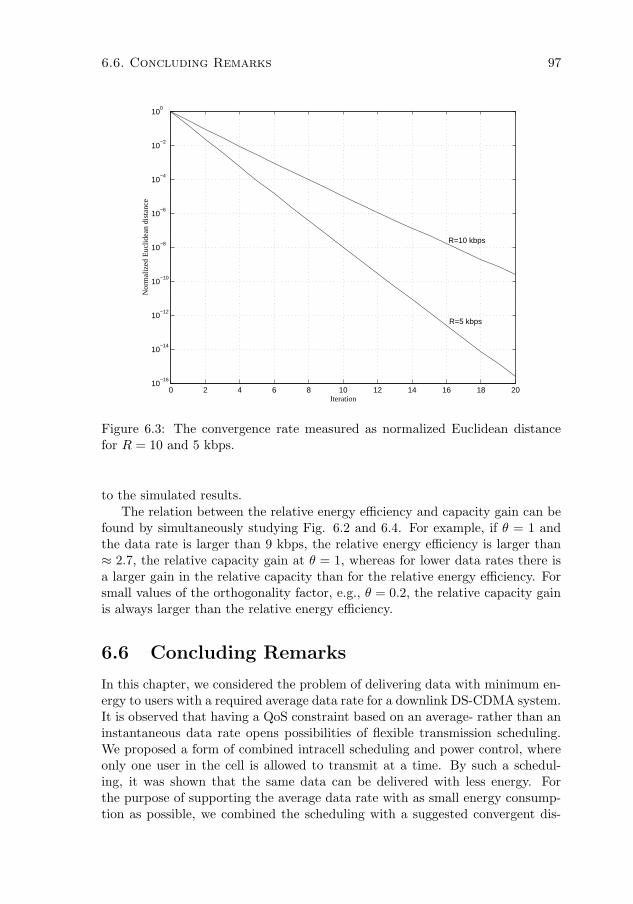
6.6. Concluding Remarks 97
0 2 4 6 8 10 12 14 16 18 2010
−16
10−14
10−12
10−10
10−8
10−6
10−4
10−2
100
Iteration
Nor
mal
ized
Euc
lidea
n di
stan
ce
R=10 kbps
R=5 kbps
Figure 6.3: The convergence rate measured as normalized Euclidean distancefor R = 10 and 5 kbps.
to the simulated results.The relation between the relative energy efficiency and capacity gain can be
found by simultaneously studying Fig. 6.2 and 6.4. For example, if θ = 1 andthe data rate is larger than 9 kbps, the relative energy efficiency is larger than≈ 2.7, the relative capacity gain at θ = 1, whereas for lower data rates there isa larger gain in the relative capacity than for the relative energy efficiency. Forsmall values of the orthogonality factor, e.g., θ = 0.2, the relative capacity gainis always larger than the relative energy efficiency.
6.6 Concluding Remarks
In this chapter, we considered the problem of delivering data with minimum en-ergy to users with a required average data rate for a downlink DS-CDMA system.It is observed that having a QoS constraint based on an average- rather than aninstantaneous data rate opens possibilities of flexible transmission scheduling.We proposed a form of combined intracell scheduling and power control, whereonly one user in the cell is allowed to transmit at a time. By such a schedul-ing, it was shown that the same data can be delivered with less energy. Forthe purpose of supporting the average data rate with as small energy consump-tion as possible, we combined the scheduling with a suggested convergent dis-
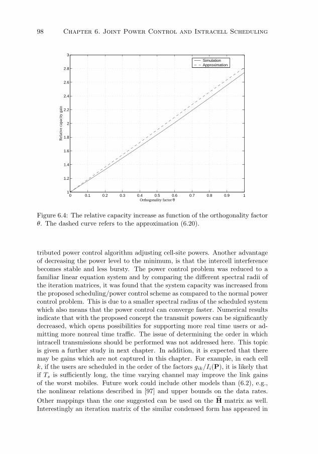
98 Chapter 6. Joint Power Control and Intracell Scheduling
0 0.1 0.2 0.3 0.4 0.5 0.6 0.7 0.8 0.9 11
1.2
1.4
1.6
1.8
2
2.2
2.4
2.6
2.8
3
Orthogonality factor θ
Rel
ativ
e ca
paci
ty g
ain
SimulationApproximation
Figure 6.4: The relative capacity increase as function of the orthogonality factorθ. The dashed curve refers to the approximation (6.20).
tributed power control algorithm adjusting cell-site powers. Another advantageof decreasing the power level to the minimum, is that the intercell interferencebecomes stable and less bursty. The power control problem was reduced to afamiliar linear equation system and by comparing the different spectral radii ofthe iteration matrices, it was found that the system capacity was increased fromthe proposed scheduling/power control scheme as compared to the normal powercontrol problem. This is due to a smaller spectral radius of the scheduled systemwhich also means that the power control can converge faster. Numerical resultsindicate that with the proposed concept the transmit powers can be significantlydecreased, which opens possibilities for supporting more real time users or ad-mitting more nonreal time traffic. The issue of determining the order in whichintracell transmissions should be performed was not addressed here. This topicis given a further study in next chapter. In addition, it is expected that theremay be gains which are not captured in this chapter. For example, in each cellk, if the users are scheduled in the order of the factors gik/Ii(P), it is likely thatif Ts is sufficiently long, the time varying channel may improve the link gainsof the worst mobiles. Future work could include other models than (6.2), e.g.,the nonlinear relations described in [97] and upper bounds on the data rates.
Other mappings than the one suggested can be used on the H matrix as well.Interestingly an iteration matrix of the similar condensed form has appeared in

6.6. Concluding Remarks 99
[62, 80] but in a different context.

100 Chapter 6. Joint Power Control and Intracell Scheduling

Chapter 7
Transmission Scheduling
over Fading Channels
SCHEDULING is a viable option in the provisioning of delay insensitive dataservices. Due to the delay tolerance, there exists a freedom in adapting
the transmission attempts to both the channel quality and the user QoS re-quirements. In this chapter, we consider scheduling over a DS-CDMA downlinkfading channel. We begin by building on the result from previous chapter, sayingthat by avoiding intracell interference, letting only one single user in each cellaccess the channel at a time, the average throughput will increase. This resultwas previously obtained for a nonfading channel. With fading, the channels canbe considered to vary asynchronously among the users and additional multiuserdiversity gains can be obtained by exploiting channel adaptive scheduling. Toharness varying channel conditions, schedulers of different adaptation rate aresuggested and compared. In particular we analyze a fast scheduler that schedulesa user to transmit when its channel is good relative to its mean. This principlecan asymptotically provide the same fairness, here defined as access to the chan-nel, as a round robin (RR) scheduler but with significantly improved throughput.The chapter contains evaluation of this scheduler for varying channel models.
7.1 Introduction
The varying channel conditions in a wireless system imply that, two users al-located the same amount of resources (bandwidth or power), could experiencedifferent performance. To schedule users for maximum channel utilization, re-sources should be allocated to the users with the highest channel quality. Thisform of water filling principle however, in terms of scheduling, could cause severefairness problem and potentially starve certain users. A well designed schedulerwould allow for long-term fairness and if the latency requirements are tight,
101
102 Chapter 7. Transmission Scheduling over Fading Channels
also short-term fairness. In conjunction with a fairness constraint, a schedulercould prioritize users with temporarily better channels. In the literature, severalschedulers and fairness criteria have been given. In [9], schedulers which arethroughput optimal were found. Such a scheduler, is able to keep all packetqueues stable, if it is at all feasible to do with any scheduler. Another direc-tion is Kelly’s proportional fairness [60]. There the objective is to maximize theproduct of the individual user throughputs, or their log sum. It was shown thatthe proportionally fair solution Ri is unique and characterized by, for any otherfeasible allocation R′
i,∑
i(R′i − Ri)/Ri ≤ 0. A proportional fair (PF) scheduler
to address this criterion was given in [48, 49, 114]. With ri(t) being the maximumsupportable data rate of user i, the algorithm schedules according to
i∗ = arg maxi
ri(t)
Ti(t)
where Ti(t) is the average throughput, updated through a filter
Ti(t + 1) =
(1 − 1
tc
)Ti(t) +
1
tcri(t)1{i∗=i}.
It was shown [114] that, if tc = ∞, this algorithm is proportionally fair and will
maximize∑N
j=1 log Tj , where Tj is the limit of the long-term average throughput.For long averaging windows users get scheduled the same amount of time [48].
Here, we will consider two classes of schedulers; slow (nonadaptive) and fast(adaptive). The slow scheduler base its decisions on slow channel variations, likeattenuation and shadowing, or does not adapt to the channel at all. Clearly,this form is robust and requires small overhead, to the price of performance.Similarly to [27, 48, 49], an asymptotic analysis is considered. That is long-runperformance is evaluated. A simple type of resource fair channel nonadaptivescheduling, known to allocate the access times fairly, is the RR scheduler. How-ever, although the time allocation of RR is fair, the performance is mostly notvery encouraging in fast fading environments. Therefore, a fast channel adap-tive scheduler is suggested, taking into account the average and instantaneouschannel conditions, where the user with the “relatively best” channel state isscheduled. As for the PF scheduler, the underlying principle is that a user whichhas a good quality relative to its expected quality, transmits. This concept verymuch resembles the principle of selection diversity. For a background on mul-tiuser diversity, [114] provides additional references. In the analysis, absolutedelay requirements and queue stability [9] are not considered. The throughputperformance with such additional constraints will likely be less than the resultsreported herein.
7.1.1 System Model
Consider a single cell in a DS-CDMA system with a spreading bandwidth W .The required bit-energy-to-interference-spectral-density ratio Eb/I0 is set to Γi

7.1. Introduction 103
for any user 1 ≤ i ≤ N . The data arrives to buffers of infinite length, whichare considered to be full all the time, i.e., aspects of queuing are not considered.No power control is exercised and the total downlink transmission power is fixedat P . With Ii + ν denoting the fixed intercell plus background interferencelevel and gi(t) the time varying link gain, we define the instantaneous channelstate as the SIR without intracell interferers, given by ξi(t) = gi(t)P/(Ii + ν).Different transmission rates are provided by adapting the processing gain. Here,we assume this is achieved by varying the symbol time and keeping a fixedchip rate and modulation format. Without restriction, we assume that theinstantaneous transmission rate of user i will follow a linear relation of its SIR1
ri(t) =W
Γi
ξi(t)∆i
θi(1 − ∆i)ξi(t) + 1. (7.1)
The factor ∆i ∈ [0, 1] denotes the fraction of the total transmission power al-located to user i and θi ∈ (0, 1] represents the orthogonality factor, which isassumed to be time-invariant. If one-by-one transmission is employed, all thetransmission power of the base station can be allocated to one particular userat a time. Consequently, ∆i = 1 and its instantaneous transmission rate duringtransmission becomes
ri(t) =W
Γiξi(t). (7.2)
Time is assumed to be a continuous variable without any restriction on schedul-ing instants or frame size granularity. Also, the rates are continuous and we donot impose any constraints on available bandwidth. Such restrictions are furtherinvestigated in Section 7.3.2. We assume that ξi(t) can be accurately estimatedand that it is a wide sense stationary and ergodic stochastic process for all users.These processes are assumed to be mutually independent of each other, for allusers. The channel state of each user has at any instant a mean E[ξi(t)|t] = ξi
for all t. From the these assumptions, we find the asymptotic data rate
Ridef= lim
T→∞
1
T
∫ T
0
ri(t)dt =W
Γiξi (7.3)
where the limit is stochastic and denotes convergence almost surely2. In thischapter, we will consider the variations of ξi(t) to be from small-scale fading.The mean ξi can be regarded as being comprised by attenuation and shadowingeffects, occurring on a much longer time scale. The channel fading is mainlyassumed to follow the noncentral χ2 distribution with two degrees of freedom,defined by its density function (2.5).
1The linear relation can be further motivated for large bandwidth channels, since the ca-pacity of a Gaussian channel with interference spectral density I0 Watt/Hz approaches
limW→∞
W log2
(1 +
prx
I0W
)=
prx
I0log2 e bps.
2In general, we shall require Pr[limT→∞
1T
∫ T0 ri(t)dt =
∫∞0 ri(ξi)fξi
(ξi) dξi
]= 1.

104 Chapter 7. Transmission Scheduling over Fading Channels
7.2 Transmission Scheduling
7.2.1 One-by-One Scheduling
It has been found, for both uplink [67] and downlink [107], that the information-theoretic capacity of a time-varying channel is maximized by letting the user withthe best channel transmit. In previous chapter, we found that for a nonfadingchannel with linear rate, simultaneous transmission is outperformed in terms ofthroughput by letting users transmit one-by-one. This can be interpreted as astatic gain from the multiple access technique itself, independent of any multiuserdiversity benefits. An interpretation thereof, is that we can always define aRR scheduler that will provide higher average throughput than simultaneoustransmissions. Hence a static gain would relax the requirements on designing ahigh throughput scheduler. However, that result was based on a continuous andlinear rate relation like (7.1), reasonable for systems with variable processinggain. For other nonlinear rate relations, implied by adaptive modulation andcoding, a single user may not necessarily be able to utilize the whole channelcapacity solely and it may be better to schedule users simultaneously, see, e.g.,[52]. The GRP procedure in Chapter 5 is another consequence of this. However,even if there would not be any static gain from time division, such a systemwould still exhibit the gain from multiuser diversity. Hence there could still bea net gain compared to the usual pure CDMA. Considering (7.1), we can easilyverify that there is a gain from time division also if we let the link gains betime varying and stochastic. This justifies our choice to focus on schedulingtransmissions one-by-one. Let φi be the fraction of time user i transmits, where0 ≤ φi ≤ 1 and
∑Ni=1 φi = 1. For a single cell, we can state the following
property.
Proposition 7.1 The total throughput∑N
i=1 Ri of a one-by-one transmissionscheme is greater than that of simultaneous transmission.
Proof. Consider the asymptotic fraction of time φi used in the one-by-onescheme, that is required to obtain the same average data rate as using simulta-neous transmission:
Ri = φiW
Γiξi =
W
ΓiE
[ξi∆i
θi(1 − ∆i)ξi + 1
]
Since the channel state ξi(t) is a stationary ergodic process, it follows that thechannel at certain time instant t is determined by a density function fξi
(ξi)which is independent of t. Furthermore, it is reasonable to assume that ξi(t) ≥ 0and the probability that ξi = 0 is strictly less than one. That is, fξi
(ξi) = 0for all ξi < 0 and fξi
(ξi) 6= δ(ξi) where δ(·) denotes the Dirac delta function. It

7.2. Transmission Scheduling 105
follows for any i with 0 < ∆i < 1 that
E
[ξi∆i
θi(1 − ∆i)ξi + 1
]=
∫ ∞
0
ξi∆i
θi(1 − ∆i)ξi + 1fξi
(ξi)dξi
<
∫ ∞
0
ξi∆ifξi(ξi)dξi = ∆iξi,
whence Ri = φiWΓi
ξi < WΓi
∆iξi. Solving for the sum of φi yields∑N
i=1 φi <∑N
i=1 ∆i = 1. The excess time fraction 1 −∑Ni=1 φi > 0 could be utilized to
transmit more data. Consequently, the throughput of one-by-one schedulingscheme is greater than that of simultaneous transmission. �
The proposition could easily be extended to a multicellular case by letting alsoIi be a random variable and observing that the average generated intercell in-terference from a cell, is the same as for simultaneous transmission. Hence itsuffices to prove the proposition for one single cell separately, see Proposition6.1. Proposition 7.1 implies that the increased throughput obtained by avoidingthe intracell interference, sufficiently compensates for the silent periods, result-ing in a higher average data rate than a simultaneous transmission. It shouldalso be noted that since the proof is based on time averaging, ordering of theusers is irrelevant, which means that multiuser diversity aspects are not takeninto account. Hence, we may expect additional gains from channel adaptiveschedulers. Now, consider two different classes of schedulers.
7.2.2 Slow Scheduling
A simple and robust type of scheduling policy is to ignore the instantaneouschannel variations and determine a transmission schedule in advance. Thus,the input parameters to the scheduler are measured on long term basis and donot adapt to the small-scale variations. As the time average of ξi(t) equals itsensemble mean ξi, the expected throughput of a user will asymptotically be
Ri = φiW
Γiξi. (7.4)
A slow scheduler is defined by the different allocations of φi, which could beassigned arbitrarily, subject to
∑Ni=1 φi = 1 and some underlying fairness phi-
losophy. Among them is the well known resource fair approach of round robin,
φi =1
N(7.5)
where the channel access is evenly allocated over all users. As comparison,a fully performance fair allocation would give equal throughput rather thantime fractions to all users. This can be achieved by an equal throughput (ET)

106 Chapter 7. Transmission Scheduling over Fading Channels
scheduler
φi =Γi/ξi∑Nj=1
Γj
ξj
(7.6)
which gives each user a throughput of R0 = W/∑N
i=1Γi
ξi. The ET scheduler
can be interpreted as a weighted RR scheduler, and in comparison allocatesmore channel time to users with unfavorable conditions in order to equalizethe throughputs, to the price of a total throughput decrease. A more greedystrategy for allocating the φi, opposite to ET, is to allocate more time to userswith favorable conditions and low quality requirements. Such a fractionally fair(FF) assignment could yield
φi =ξi/Γi∑N
j=1ξj
Γj
. (7.7)
The next proposition follows straightforwardly.
Proposition 7.2 The total throughput∑N
i=1 Ri of RR is greater than that ofET but smaller than that of FF.
Proof. First we show that ET ≤ RR. By observing that f(x) = x + x−1 ≥ 2for nonnegative x, we can write
N∑
i=1
xi
N∑
i=1
1
xi≥ N + 2
N∑
i=1
(N − i) = N2
which also is the well-known arithmetic-harmonic mean inequality. This meansthat
N ≤N∑
i=1
Γi
ξi
1
W
N∑
i=1
1
N
W
Γiξi
or equivalently
NR0 =NW
∑Ni=1
Γi
ξi
≤N∑
i=1
1
N
W
Γiξi.
To show that RR ≤ FF , the Chebyshev sum inequality3 gives
N∑
i=1
1
N
W
Γiξi
N∑
i=1
ξi
Γi≤
N∑
i=1
ξi/ΓiW
Γiξi
3The Chebyshev sum inequality states that, if a1 ≤ a2 ≤ . . . ≤ aN and b1 ≤ b2 ≤ . . . ≤ bN
are arbitrary real numbers, then
N∑
i=1
ai
N∑
i=1
bi ≤ N ·
N∑
i=1
aibi.
Equality holds iff, either a1 = a2 = . . . = aN or b1 = b2 = . . . = bN .

7.2. Transmission Scheduling 107
which can be rewritten as
N∑
i=1
1
N
W
Γiξi ≤
N∑
i=1
ξi/Γi∑Nj=1 ξj/Γj
W
Γiξi.
Equality is achieved iff, for all i, ξi/Γi = C, where C > 0 is an arbitrary constant.�
In the following sections we will focus on a fast scheduler that will be resourcefair, i.e., comparable to RR. Equivalently, since users get the same transmissionpower, the fairness criteria can be interpreted as every user is asymptoticallyallocated the same amount of energy. It can be noted that among the possibleslow schedulers, the aggregate of the proportional changes in throughput of RRis not positive. For any feasible allocation of φ
′
i 6= 1/N , the proportional fairness
condition of [60] holds,∑N
i=1R
′i−Ri
Ri=∑N
i=1φ′i−
1N
1N
= 0.
7.2.3 Fast Scheduling
Now, consider a situation where for any time instant the vector of samplesξ = (ξi) is perfectly available for the scheduling decision. The suggested rela-tively best (RB) scheduler decides from a normalized channel state such thatthe preferred user is
i∗(ξ) = arg max1≤i≤N
ξi − ξi
ci.
Ties are broken with equal probability. The ci are positive control parameters,resulting in different time fractions φi. Thus, the scheduling decision is madefrom a normalized channel state value, referred to as the “relatively best”. Theconsequence is that each user transmits only on good instants, but with a certainasymptotic channel access, controlled by the ci. Assume that the channels aremutually independent. For a Rayleigh fading channel, viz. a Rice factor κ = 0,the conditional probability that user i has a relatively better channel than userj is given by:
Pr
[ξj ≤ cj
ci(ξi − ξi) + ξj |ξi
]=
0,cj
ci(ξi − ξi) + ξj < 0
1 − e−
cjci
(ξi−ξi)+ξj
ξj ,cj
ci(ξi − ξi) + ξj ≥ 0.
If we let ξ0i = maxj 6=i{0, ξi − ci
cjξj}, the resulting asymptotic time fraction
assignment can be obtained as
φi =
∫ ∞
ξ0i
N∏
j 6=i
j=1
(1 − e−
cjci
(ξi−ξi)+ξj
ξj )1
ξ i
e−
ξiξi dξi. (7.8)

108 Chapter 7. Transmission Scheduling over Fading Channels
The feasible time fractions depend on the control parameters ci and the fadingcharacteristics and cannot take any values.
Example 7.2.1 Consider an example with N = 2, c1 = aξ1 and c2 = ξ2. Evaluatingthe integral (7.8) we obtain
φ1 =
{(1 − a
1+a)ea−1, 0 < a < 1
1 − a1+a
e−(1−1/a), a ≥ 1.(7.9)
Thus, the feasible time fraction in this case, becomes limited to e−1 ≤ φi ≤ 1 − e−1.The time span can be extended with a slight modification of the scheduling rule. If welet i∗(ξ) = arg max1≤i≤N ξi/ci and consider the same parameters,
φ1 =1
a + 1.
Hence, the feasible time fractions in this case can take any value 0 ≤ φi ≤ 1.
For fair comparison between schedulers, their asymptotic time fractions shouldbe the same. Importantly, it can easily be shown that when ci = ξi, the integral(7.8) reduces to φi = 1/N for any user i. From the variance of ξi it is evidentthat the means and also variances of (ξi − ξi)/ξi are the same for all users, alsowhen κ > 0. Therefore, the RB algorithm can provide the same asymptoticfairness as RR for channels described by (2.5).
Example 7.2.2 For further generalization, consider an example of two classes ofusers which could have different priorities. Let there be NA users with ci = aξi andN −NA users with cj = ξj . For 0 < a < 1, the resulting time fractions become for anyof the NA users
φi =
NA−1∑
k=0
N−NA∑
l=0
(NA − 1
k
)(N − NA
l
)(−1)k+l e
−(1−1/a)l−(k+1+l/a)(1−a)
k + 1 + l/a
and for a ≥ 1
φi =
NA−1∑
k=0
N−NA∑
l=0
(NA − 1
k
)(N − NA
l
)(−1)k+l e−(1−1/a)l
k + 1 + l/a
where a binomial expansion is performed in (7.8). In Fig. 7.1, this is plotted forN = 10 and NA = 1, 2, . . . , N . The arrows denote increasing values of NA. Asexpected, φi = 0.1 at a = 1. It should be pointed out that the characteristic of thetime fraction curves is very much dependent on the parameters N and NA, cf., the twodimensional case (7.9) above.
In [78], a suggested scheduler was shown to maximize the expected through-put subject to allocated time fractions. These time fractions could be as-signed arbitrarily. In the case of φi = 1/N the RB scheduler is equivalent

7.3. Scheduling Gain 109
0 1 2 3 4 5 6 7 8 9 100
0.05
0.1
0.15
0.2
0.25
0.3
0.35
0.4
0.45
a
Tim
e fr
actio
n φ i
NA
NA
Figure 7.1: Feasible time fractions for users in class A for different number ofusers NA = 1, 2, . . . , 10. The total number of users are N = 10 and the channelis Rayleigh fading.
to i∗(ξ) = argmaxi(log ξi − log ξi). According to Proposition 1 in [78], the RBwould then be optimal in the sense it maximizes
N∑
i=1
Ri =N∑
i=1
E[log ξi1{i∗(ξ)=i}]
where the event indicator was defined in Chapter 5. Thus RB maximizes theexpected throughput for ri(ξi) = log ξi and can be regarded as a proportionalfair scheduling rule. In comparison with the scheduler in [78], the RB sched-uler, as defined by (7.2.3), has a smaller feasible region of time fractions. Onthe other hand the scheduler in [78] is more complex since it uses an iterativeapproximation algorithm for achieving the desired time allocation.
7.3 Scheduling Gain
Let ri(ξi) be the instantaneous throughput of user i. The asymptotic throughputis defined as
Ri = E[ri(ξi)1{i∗(ξ)=i}]. (7.10)

110 Chapter 7. Transmission Scheduling over Fading Channels
With an assumption of independent fading among users, we can express
Pr[i∗(ξ) = i] = Pr
[ξi − ξi
ci> max
j 6=i
ξj − ξj
cj
]
=∏
j 6=i
Fξj
(cj
ci(ξi − ξi) + ξj
)
where Fj(·) is the cdf corresponding to fj(·). The scheduling gain can be com-puted from
Gidef=
∫∞
ξ0iri(ξi)
∏j 6=i Fξj
(cj
ci(ξi − ξi) + ξj
)fξi
(ξi) dξi
φi
∫∞
0ri(ξi)fξi
(ξi) dξi
. (7.11)
Throughout the chapter, we will evaluate (7.11) by numerical integration andderive supplementary closed-form expressions, if possible. Let us henceforthconsider φ = 1/N , that is ci = ξi and the throughput gain of RB compared toRR.
7.3.1 Unconstrained Bandwidth Case
Ricean Fading
The scheduling gain for the Rayleigh fading channel can, after a binomial ex-pansion and some algebra, be written as
G =
N∑
k=1
(N
k
)(−1)k+1 1
k=
N∑
k=1
1
k(7.12)
where the last equality is contained in Appendix C. From [31], G ≈ ln N + γ +1/2N where γ ≈ 0.577 is the Euler constant. That is, the more users to choosefrom, the higher benefit from multiuser diversity. This is in accordance withthe simulation studies of [48, 49, 114]. It can be noted that (7.12) describes thetotal throughput gain in the cell as well the individual user gain. In comparison,this scheduling gain is exactly as that of selection diversity on a Rayleigh fadingchannel [100] with ξi/N as the SNR in each diversity branch. Although G isincreasing in N , the average throughput per user decreases, and asymptoticallyRi = O(lnN/N). The closed form expression (7.12) accounts for the Rayleighfading case. If we consider general κ factors, it can be shown that [100]
Fξi(x) = 1 − Q1
(√
2κ,
√2(κ + 1)
ξix
)(7.13)
where Q1(·, ·) is the first-order Marcum Q-function4. The scheduling gain canbe found by numerical integration. In Fig. 7.2, we plot the scheduling gain as
4A common form equals Q1(α, β)def=∫∞
β xe−x2+α2
2 I0(αx) dx.

7.3. Scheduling Gain 111
5 10 15 20 25 30 35 40 45 501
1.5
2
2.5
3
3.5
4
4.5
5
Number of users N
Sche
dulin
g ga
in G
κ=0
κ=1
κ=2
κ=3
κ=10
Figure 7.2: The scheduling gain for different Ricean factors κ (linear) for a singlecell. The dashed line shows the gain in the multicellular case with Rayleighfading (κ = 0).
function of N for different values of κ. The result of (7.12) corresponds to thecurve of κ = 0. The results show that, the larger Rice factor, the less gain fromthe proposed scheduler but the gain is still significant for the depicted values.
RAKE Receiver
If a RAKE receiver is employed, combining signals from L independent identi-cally distributed Rayleigh fingers, the output channel state follows a χ2 distri-bution [100],
fξi(x) =
xL−1
(L − 1)!ξLi
e− x
ξi , x ≥ 0 (7.14)
having a mean Lξi and variance Lξ2i . Alternatively, (7.14) can be interpreted as
capturing the maximum ratio combined channel state resulting from transmitdiversity of L independent Rayleigh fading paths. The cdf is given by
Fξi(x) = 1 − e
− xξi
L∑
i=1
1
(i − 1)!
(x
ξi
)i−1
. (7.15)
The scheduling gain obtained by numerical integration is contained in Fig. 7.3.In this case, the scheduling gain decreases significantly as L increases. This is

112 Chapter 7. Transmission Scheduling over Fading Channels
5 10 15 20 25 30 35 40 45 501
1.5
2
2.5
3
3.5
4
4.5
Number of users N
Sche
dulin
g ga
in G
L=1
L=2
L=3
L=4
Figure 7.3: The scheduling gain on a Rayleigh fading channel for different num-ber of RAKE fingers L.
expected, since multipath combining can be regarded as time averaging of thechannel quality and will therefore reduce the scheduling gain [114].
7.3.2 Constrained Bandwidth Case
The assumed rate relation (7.1) can be rather optimistic as it assumes a linearbehavior between rate and SIR, i.e., effectively an infinite bandwidth. Such arelation may not be accurate if adaptive modulation- and coding techniques areemployed.
Maximum Rate Constraint
Let us consider (7.1) but imposed with a maximum achievable instantaneoustransmission rate. This may penalize one-by-one transmission, as the reductionin intracell interference may not directly translate to a higher transmission rate.If it is assumed that the transmission rate is constrained to ri ≤ R, the Rayleigh
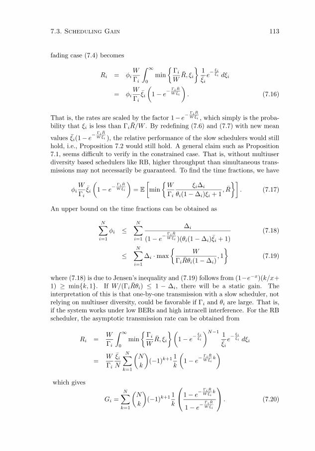
7.3. Scheduling Gain 113
fading case (7.4) becomes
Ri = φiW
Γi
∫ ∞
0
min
{Γi
WR, ξi
}1
ξie−
ξiξi dξi
= φiW
Γiξi
(1 − e
−ΓiR
W ξi
). (7.16)
That is, the rates are scaled by the factor 1− e−
ΓiR
W ξi , which simply is the proba-bility that ξi is less than ΓiR/W . By redefining (7.6) and (7.7) with new mean
values ξi(1− e−
ΓiR
W ξi ), the relative performance of the slow schedulers would stillhold, i.e., Proposition 7.2 would still hold. A general claim such as Proposition7.1, seems difficult to verify in the constrained case. That is, without multiuserdiversity based schedulers like RB, higher throughput than simultaneous trans-missions may not necessarily be guaranteed. To find the time fractions, we have
φiW
Γiξi
(1 − e
−ΓiR
W ξi
)= E
[min
{W
Γi
ξi∆i
θi(1 − ∆i)ξi + 1, R
}]. (7.17)
An upper bound on the time fractions can be obtained as
N∑
i=1
φi ≤N∑
i=1
∆i
(1 − e−
ΓiR
W ξi )(θi(1 − ∆i)ξi + 1)
(7.18)
≤N∑
i=1
∆i · max
{W
ΓiRθi(1 − ∆i), 1
}(7.19)
where (7.18) is due to Jensen’s inequality and (7.19) follows from (1−e−x)(k/x+1) ≥ min{k, 1}. If W/(ΓiRθi) ≤ 1 − ∆i, there will be a static gain. Theinterpretation of this is that one-by-one transmission with a slow scheduler, notrelying on multiuser diversity, could be favorable if Γi and θi are large. That is,if the system works under low BERs and high intracell interference. For the RBscheduler, the asymptotic transmission rate can be obtained from
Ri =W
Γi
∫ ∞
0
min
{Γi
WR, ξi
}(1 − e
−ξiξi
)N−11
ξie−
ξiξi dξi
=W
Γi
ξi
N
N∑
k=1
(N
k
)(−1)k+1 1
k
(1 − e
−ΓiR
W ξik)
which gives
Gi =
N∑
k=1
(N
k
)(−1)k+1 1
k
1 − e
−ΓiR
W ξik
1 − e−
ΓiR
W ξi
. (7.20)

114 Chapter 7. Transmission Scheduling over Fading Channels
5 10 15 20 25 30 35 40 45 501
1.5
2
2.5
3
3.5
4
4.5
Number of users N
Sche
dulin
g ga
in G
S=1
S=2
S=3
S=4
S=5
UnconstrainedConstrained
Figure 7.4: The scheduling gain on a Rayleigh fading channel with a constrainedmaximum rate for different values of S = ΓiR/W ξi.
Compared to the unconstrained case, the scheduling gain here depends on theabsolute value of ξi. It can be seen that as ΓiR/W ξi → ∞, the scheduling gainapproaches the unconstrained case (7.12). For ΓiR/W ξi → 0, it follows that
G → ∑Nk=1
(Nk
)(−1)k+1 = 1. Therefore, we conclude that an upper constraint
on the instantaneous transmission rate still renders in higher throughput for RBthan RR. In Fig. 7.4, (7.20) is plotted as function of N for different ratios ofΓiR/W ξi. To obtain a measure of the average system gain, ξi can be regardedas a random variable comprised of shadowing and attenuation and could thusbe averaged over.
Discrete Transmission Rates
In practice, the transmission rates are not only constrained by an upper level,but also confined to a set of discrete values. The consequence thereof is thatimproved channel states do not necessarily translate into higher rates, as theresults in the foregoing section showed. Assume a model where there are K

7.3. Scheduling Gain 115
discrete transmission rates, assigned to different intervals.
ri(ξi) =
0, ξi < x1
WΓi
xk, xk ≤ ξi < xk+1, 1 ≤ k ≤ K − 1WΓi
xK , ξi ≥ xK
(7.21)
This can be seen as a quantization of the linear model (7.1). We use the model ofChapter 5, where the rates are geometrically related, such that for µ > 1, xk =µxk−1. Thus it follows that xk = µk−1x1. If µ is small, a fine granularity canbe obtained, which will let performance approach the continuous case. However,this requires a large number of available rates K. In real systems, with variableprocessing gain, the rates are often related with µ = 2. Define xK+1 = ∞ sothat the asymptotic throughput can be found by evaluating
Ri =K∑
k=1
∫ xk+1
xk
ri(ξi)(1 − e−
ξiξi )N−1 1
ξie−
ξiξi dξi. (7.22)
Since∫ xp+1
xp(1 − e
−ξiξi )N−1 1
ξie−
ξiξi dξi =
∑Nk=1
(Nk
) (−1)k+1
N (e−
xpk
ξi − e−
xp+1k
ξi ), it
can be found that (7.22) equals
Ri =W
Γi
ξi
N
N∑
k=1
(N
k
)(−1)k+1 x1
ξi
(e−
x1k
ξi +K∑
m=2
µm−2(µ − 1)e−
µm−1x1k
ξi
).
(7.23)The scheduling gain can be obtained by normalizing (7.23) with its first term
(k = 1) divided by N . Clearly, Ri becomes a function of x1/ξi and for a fixed Nit can be found that the scheduling gain does not necessarily attain its maximumwhen the absolute level of (7.23) does. To compare throughput performance withthe RB scheduler in the continuous linear rate case, we plot (7.23) normalizedwith (Wξi)/(ΓiN) · G where G is defined by (7.12). In Fig. 7.5, the case ofN = 10 and µ = 2 is considered for different values of K and plotted as functionof x1/ξi. It can be seen that the maximum throughput in the discrete case ishere only about 72% of the continuous case. This value is reached by quite asmall number of rates though, and for the larger number of rates, the peak israther insensitive to the choice of x1/ξi.
Logarithmic Rate
If the intercell interference can be considered Gaussian and multiuser detectionis not employed, the information theoretic-rate is given by
ri(ξi) = W log2(1 + ξi). (7.24)
Consider a Rayleigh fading channel, then we can define
H(k, ξ)def=
∫ ∞
0
log2(1 + ξ)1
ξe− ξ
ξkdξ =
ekξ
k loge 2Γ
(k
ξ
)(7.25)

116 Chapter 7. Transmission Scheduling over Fading Channels
0 0.5 1 1.5 2 2.50
0.1
0.2
0.3
0.4
0.5
0.6
0.7
0.8
Relative threshold
Rel
ativ
e th
roug
hput
K=1
K=2
K=3
K=4
K=5
Figure 7.5: The relative throughput compared to a continuous linear rate on aRayleigh fading channel with N = 10 users. The number of discrete rates is setto K. The x-axis denotes the relative threshold x1/ξi.
where the last equality follows from∫ ∞
0
log2(b + aξ)e−cξ dξ =1
c loge 2
(e
bca Γ
(bc
a
)+ log2 b
)
and we define the incomplete gamma function Γ(x)def=∫∞
xt−1e−t dt. After some
manipulations, see Appendix C, the scheduling gain can be shown to be
Gi =1
H(1, ξi)·
N∑
k=1
(N
k
)(−1)k+1kH(k, ξi). (7.26)
As in the previous case with an upper bounded rate, the scheduling gain dependson the absolute value of ξi. In Fig. 7.6, it can be seen that the scheduling gainis significantly lower than in the unconstrained case. A small ξi, results in thatthe log function is close to linear, in the region of interest.
7.4 Multicellular Case
In (7.1), it was assumed that Ii + ν was fixed and a single cell analysis wasperformed. Assuming that Ii is also varying, the variance of ξi increases, which

7.4. Multicellular Case 117
5 10 15 20 25 30 35 40 45 501
1.2
1.4
1.6
1.8
2
2.2
2.4
2.6
2.8
3
Number of users N
Sche
dulin
g ga
in G
PSfrag replacements
ξi = 0 dB
ξi = 3 dB
ξi = 10 dB
ξi = 13 dB
Figure 7.6: The scheduling gain on a Rayleigh fading channel for a logarithmicrate relation with different mean SIR.
suggests higher scheduling gain. Consider the following extensions to cover avarying intercell interference. Assume that the intercell interference is due tothe first tier of base stations and that for any user i in the desired cell, theintercell interferers k have the same mean received power, Ck = C. If, forsimplicity, we let the background noise be ν = 0, the result from Appendix Agives the distribution and density functions for x ≥ 0
Fi(x) = Pr
[Ci∑
j 6=i Cj≤ x
]= 1 −
(Ci
Cx + Ci
)6
(7.27)
fi(x) =6CC6
i
(Cx + Ci)7(7.28)
where Ci is the mean received power of user i. We find that E
[Ci∑
j 6=i Cj
]= Ci
5C
def=
ξi and E
[(Ci∑
j 6=i Cj
)2]
=C2
i
10C2 . Thus the variance of ξi becomes 32 ξ2
i , which is

118 Chapter 7. Transmission Scheduling over Fading Channels
higher than for the single cell Rayleigh case. Then, for any user 1 ≤ i ≤ N ,
Fξi(x) = 1 −
(5ξi
x + 5ξi
)6
, x ≥ 0 (7.29)
fξi(x) =
6(5ξi)6
(x + 5ξi)7, x ≥ 0. (7.30)
Again consider the decision variable ξi−ξi
ξi, which can be shown to give φi = 1/N .
SinceN∏
j 6=i
j=1
Pr
[ξj ≤ ξj
ξiξi|ξi
]=
1 −
(1
ξi
5ξi+ 1
)6
N−1
the asymptotic data rate can be obtained as
Ri =W
Γi
∫ ∞
0
ξi
1 −
(1
ξi
5ξi+ 1
)6
N−1
· 6(5ξi)6
(ξi + 5ξi)7dξi
=W
Γi
5
6Nξi
N∑
k=1
(−1)k+1
(N
k
)1
k − 1/6. (7.31)
The scheduling gain can be expressed as
G =5
6
N∑
k=1
(−1)k+1
(N
k
)1
k − 1/6(7.32)
This is plotted in Fig. 7.2 as a dashed line, where it can be seen that the gainis larger than for the single cell case.
7.5 Measurement Delay
The gain of the fast scheduler relies, to a large extent, on that it can baseits actions on reliable channel measurements. The previous analysis assumedperfect channel estimates. In a more practical scenario, the estimates must beobtained in the presence of noise and time delays. Depending on the channelvariation, outdated measurements may cause erroneous scheduling actions andwill therefore degrade performance. Let us consider the RB scheduler subject toa time delay δ in the measurements as follows:
i∗(ξ(t)) = arg max1≤i≤N
ξi(t − δ) − ξi
ci.
The implication is that the scheduling decision lags δ time units to the channel.Clearly the performance will depend on the correlation of the channel fading. If

7.5. Measurement Delay 119
the correlation is high, the delay tolerance is higher since the correct user is likelyto be scheduled. If the correlation is zero and δ > 0, the scheduler effectivelymakes a random pick and performance will reduce to the RR scheduler. If δ = 0,we have the case previously analyzed.
Consider the following stochastic process for modeling the fast channel vari-
ation. For every user i, define two independent Gaussian processes {Z (k)i (t)},
k = 1, 2, with stationary means and variances, 0 and ξi/2, respectively. Eachprocess evolves independently according to the following correlated process,
Z(k)i (t + δ) = ρZ
(k)i (t) +
√1 − ρ2N
(k)i (t) (7.33)
where {N (k)i (t)} are independent normal random variables with zero mean and
variance ξi/2. The correlation can for a mobile radio channel be related to
the radio environment by Clarke’s model, ρ = J0
(2π·v·f ·δ
c
), where f is the
carrier frequency, v the velocity, c the speed of light and J0(·) is the zeroth-ordermodified Bessel function of the first kind. The channel fading process is obtainedby
ξi(t) = (Z(1)i (t))2 + (Z
(2)i (t))2 (7.34)
which is a correlated exponential process with mean ξi. Assume for simplicitythat all users have the same correlation ρ. The throughput for the model (7.1),is obtained by solving the following integral (see Appendix B),
Ri =W
Γi
∫ ∞
0
ξi(t + δ)
N∏
j 6=i
j=1
(1 − e−
ξi(t)
ξi )fξi(t)(ξi(t)) dξi(t)
=W
Γi
ξi
N
(ρ2
N∑
k=1
1
k+ 1 − ρ2
). (7.35)
Thus the scheduling gain, G = ρ2∑N
k=1 1/k + 1 − ρ2 is a linear function of thepower correlation ρ2. To numerically verify this, we can use the joint probabilitydensity function (see, e.g., [100]) of ξi(t) and ξi(t + δ),
fξi(t),ξi(t+δ)(x, y) =1
(1 − ρ2)ξ2i
e− x+y
(1−ρ2)ξi · I0
(2√
ρ2xy
(1 − ρ2)ξi
),
0≤ρ<1
x, y ≥ 0
where the mean is constant during [t, t + δ] due to the stationarity assumption.The pdf can also be used to represent estimation errors, where ρ is the correlationbetween actual and measured value. The asymptotic data rate can be evaluatedby computing the integral,
Ri =W
Γi
∫ ∞
0
∫ ∞
0
ξi(t + δ)
(1 − e
−ξi(t)
ξi
)N−1
×
fξi(t),ξi(t+δ)(ξi(t), ξi(t + δ)) dξi(t)dξi(t + δ). (7.36)

120 Chapter 7. Transmission Scheduling over Fading Channels
0 0.1 0.2 0.3 0.4 0.5 0.6 0.7 0.8 0.9 11
1.2
1.4
1.6
1.8
2
2.2
2.4
2.6
2.8
3
Correlation ρ
Sche
dulin
g ga
in G
AnalyticalIntegration
Figure 7.7: The scheduling gain on a Rayleigh fading channel with N = 10 users,as function of the correlation ρ.
In Fig. 7.7 we plot the scheduling gain based on (7.35) for N = 10. For com-parison, we evaluate the integral (7.36) numerically and plot the correspondingscheduling gain. It can be seen that the closed form expression (7.35) is matchedby the numerical integration.
7.6 Multiuser Scheduling
Results in this chapter, and other investigations [49], show that only one usershould be allocated to the channel at any instant, if the rate is growing linearlywith channel quality. With a nonlinear relation between effective transmissionrate and channel quality, it is not certain that scheduling one single user mayachieve highest throughput. The HSDPA mode will primarily use time multi-plexing of the channelization codes but code multiplexing is also supported [88].In Section 7.3.2 it was shown that under a logarithmic relation, the RB schedulerstill outperformed RR. However, this result is not tantamount to that RB alsois better than conventional CDMA transmission with all users on the channel.Therefore, we generalize the RB scheduler to allocate more than one user on thechannel. For pertinent comparison, we keep the fairness requirement that everyuser asymptotically shall be given the same amount of energy. For simplicity,we assume that P is shared equally among the users. Hence, we do not adapt

7.6. Multiuser Scheduling 121
the transmit power to the channel conditions, only to the number of users onthe channel. Consider the case where there are k users allocated to the channelgiving each user a power of P/k. In the absence of multiuser detection, theinstantaneous transmission rate of user i can be assumed to follow a logarithmicrelation
ri(ξi, k) = W log2
(1 +
ξi
θ(k − 1)ξi + k
). (7.37)
7.6.1 Generalized Scheduler
Now, let us generalize the RB scheduler by in any instant ordering the userssuch that their decision variables follow
ξ1 − ξ1
ξ1≥ . . . ≥ ξN − ξN
ξN
and schedule the L + 1 first users. Ties are broken with equal probability. Thevalues L = 0, . . . , N − 1 span one-by-one transmission to regular CDMA with Nusers on the channel.
For a Rayleigh fading channel, the conditional probability that user i isscheduled will then equal
Pr[i∗(ξ) = i] =
L∑
j=0
(N − 1
j
)(1 − e
−ξiξi )N−1−je
−ξiξi
j. (7.38)
Averaging (7.38) over (2.5), it can be found that any user will access the channela fraction (L + 1)/N of the time. Hence, with a fixed power P/(L + 1) per user,all users will asymptotically be allocated the same amount of energy. For a givennumber of users k the asymptotic throughput is again defined as
Ri(k)def= E[ri(ξi, k)1{i∗(ξ)=i}]. (7.39)
After some further manipulations, the asymptotic throughput of (7.38)-(7.39)can be obtained on closed-form
Ri(L + 1) =
∫ ∞
0
ri(ξi, L + 1)Pr[i∗(ξ) = i]fξi(ξi) dξi
=
L+1∑
j=1
N+1−j∑
k=1
(N
j
)(N + 1 − j
k
)(−1)N+1−j−k
N loge 2× (7.40)
j
(N + 1 − j)
k
(N + 1 − k)×
(V
((L + 1)(N + 1 − k)
ξi(θL + 1)
)− V
((L + 1)(N + 1 − k)
ξiθL
))
where V (x) = exΓ(x) and Γ(x) is the incomplete gamma function.
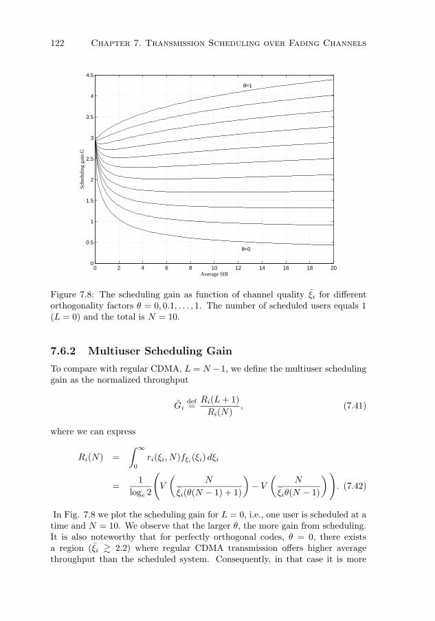
122 Chapter 7. Transmission Scheduling over Fading Channels
0 2 4 6 8 10 12 14 16 18 200
0.5
1
1.5
2
2.5
3
3.5
4
4.5
Average SIR
Sche
dulin
g ga
in G
θ=0
θ=1
Figure 7.8: The scheduling gain as function of channel quality ξi for differentorthogonality factors θ = 0, 0.1, . . . , 1. The number of scheduled users equals 1(L = 0) and the total is N = 10.
7.6.2 Multiuser Scheduling Gain
To compare with regular CDMA, L = N − 1, we define the multiuser schedulinggain as the normalized throughput
Gidef=
Ri(L + 1)
Ri(N), (7.41)
where we can express
Ri(N) =
∫ ∞
0
ri(ξi, N)fξi(ξi) dξi
=1
loge 2
(V
(N
ξi(θ(N − 1) + 1)
)− V
(N
ξiθ(N − 1)
)). (7.42)
In Fig. 7.8 we plot the scheduling gain for L = 0, i.e., one user is scheduled at atime and N = 10. We observe that the larger θ, the more gain from scheduling.It is also noteworthy that for perfectly orthogonal codes, θ = 0, there existsa region (ξi & 2.2) where regular CDMA transmission offers higher averagethroughput than the scheduled system. Consequently, in that case it is more

7.6. Multiuser Scheduling 123
0 2 4 6 8 10 12 14 16 18 200.5
1
1.5
2
2.5
3
Average SIR
Sche
dulin
g ga
in G
θ=0
θ=1
Figure 7.9: The scheduling gain as function of channel quality ξi for differentorthogonality factors θ = 0, 0.1, . . . , 1. The number of scheduled users equals 2(L = 1) and the total is N = 10.
favorable to let the user transmit the whole time with 1/N :th of the power than1/N :th of the time with full power. This is mainly due to that (7.37) flattens outfor large ξi. To fully assess performance, we study the limiting cases of high andlow average channel quality. Using relations from Appendix C, the schedulinggain (7.41) reduces to the form
limξi→∞
G =L + 1
N
loge
(1 + 1
θL
)
loge
(1 + 1
θ(N−1)
) . (7.43)
Further, it can be shown that for any L,
limξi→∞
G|θ=0 =L + 1
N≤ 1.
Thus, if the channels are perfectly orthogonal and ξi is large, regular CDMAtransmission is favored. That is, for high ξi, reducing the interference by schedul-ing results in an average throughput loss. This is due to that the effective trans-mission rate increases very little from the intracell interference reduction butthe channel utilization reduces to (L + 1)/N . For θ > 0 and L = 0, the gain
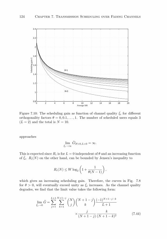
124 Chapter 7. Transmission Scheduling over Fading Channels
0 2 4 6 8 10 12 14 16 18 200.8
1
1.2
1.4
1.6
1.8
2
2.2
2.4
Average SIR
Sche
dulin
g ga
in G
θ=0
θ=1
Figure 7.10: The scheduling gain as function of channel quality ξi for differentorthogonality factors θ = 0, 0.1, . . . , 1. The number of scheduled users equals 3(L = 2) and the total is N = 10.
approaches
limξi→∞
G|θ>0,L=0 = ∞.
This is expected since Ri is for L = 0 independent of θ and an increasing functionof ξi. Ri(N) on the other hand, can be bounded by Jensen’s inequality to
Ri(N) ≤ W log2
(1 +
1
θ(N − 1)
),
which gives an increasing scheduling gain. Therefore, the curves in Fig. 7.8for θ > 0, will eventually exceed unity as ξi increases. As the channel qualitydegrades, we find that the limit value takes the following form:
limξi→0
G =
L+1∑
j=1
N+1−j∑
k=1
(N
j
)(N + 1 − j
k
)(−1)N+1−j−k
L + 1
× j
(N + 1 − j)
k
(N + 1 − k)2(7.44)

7.6. Multiuser Scheduling 125
In particular for L = 0, it can after some algebra be shown that
limξi→0
G|L=0 =N∑
k=1
(N
k
)(−1)N−k k
(N + 1 − k)2
=
N∑
k=1
1
k(7.45)
where the last equality is shown in Appendix C. As opposed to the case of large ξi,here, the scheduler gains over regular CDMA when N increases. It is noteworthythat G is in this case exactly equal to the scheduling gain that was found in (7.12)when the throughput was compared to that of a round robin scheduler, undera linear rate relation. This result is expected since log(1 + ξi) = ξi + O(ξ2
i ),i.e., a linear rate is well approximated in this region. In Fig. 7.9 and 7.10, weplot G when two and three users are scheduled, L = 1, 2. The region where thescheduling gain is larger than unity, is here broadened compared to the case ofL = 0 but the peak value at ξi = 0 is lower. Here the gain always decreases withincreasing ξi.
7.6.3 System Multiuser Scheduling Gain
As was found, the scheduling gain depends on the actual value of ξi. To de-termine the gain of a system, the variations in ξi must be accounted for. Byregarding the throughput Ri as a conditional result, the system gain can beobtained by averaging over ξi. If we let Si be lognormally distributed with zeromean and standard deviation σs dB, then we can define ξi as a random variable
ξi = Si ·K0
rαi
· P
Ii + ν, K0 > 0 (7.46)
where ri is the distance to the transmitter, also being as a random variable. Ifwe consider a circular cell with uniformly dispersed mobiles within the radius[rmin, rmax], the density function becomes for x ≥ 0
fξi(x) =
1√2π
10
σsx loge 10
∫ 1
rminrmax
e−12 (
10 log10 x+α10 log10 r−C
σs)2 2r
1 − r2min
r2max
dr (7.47)
where C = 10 log10(K0Pr−αmax/(Ii + ν)) is the expected SIR in dB at the cell
border. The system scheduling gain can be obtained by averaging (7.40) and(7.42) over (7.47) and taking their ratio. In Fig. 7.11, we plot results obtainedfrom numerical integration for different values of L and θ. Here rmax = 1000 ·rmin, α = 4 and σs = 6 dB. It can be verified that, except for the case L = 0and θ = 1, a higher average quality C provides less system gain from scheduling.If however, the orthogonality factor θ is known to take large values, single-usertransmissions are preferable. It is observed that the larger L becomes, the lessthe span in system gain becomes between θ = 0 and 1.
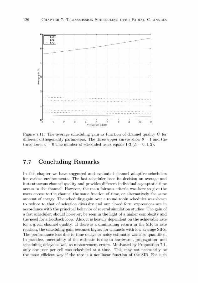
126 Chapter 7. Transmission Scheduling over Fading Channels
0 1 2 3 4 5 6 7 8 9 100
1
2
3
4
5
6
Average SIR C [dB]
Ave
rage
gai
n G
L=0L=1L=2
Figure 7.11: The average scheduling gain as function of channel quality C fordifferent orthogonality parameters. The three upper curves show θ = 1 and thethree lower θ = 0 The number of scheduled users equals 1-3 (L = 0, 1, 2).
7.7 Concluding Remarks
In this chapter we have suggested and evaluated channel adaptive schedulersfor various environments. The fast scheduler base its decision on average andinstantaneous channel quality and provides different individual asymptotic timeaccess to the channel. However, the main fairness criteria was here to give theusers access to the channel the same fraction of time, or alternatively the sameamount of energy. The scheduling gain over a round robin scheduler was shownto reduce to that of selection diversity and our closed form expressions are inaccordance with the principal behavior of several simulation studies. The gain ofa fast scheduler, should however, be seen in the light of a higher complexity andthe need for a feedback loop. Also, it is heavily dependent on the achievable ratefor a given channel quality. If there is a diminishing return in the SIR to raterelation, the scheduling gain becomes higher for channels with low average SIRs.The performance loss due to time delays or noisy estimates was also quantified.In practice, uncertainty of the estimate is due to hardware-, propagation- andscheduling delays as well as measurement errors. Motivated by Proposition 7.1,only one user per cell was scheduled at a time. This may not necessarily bethe most efficient way if the rate is a nonlinear function of the SIR. For such

7.7. Concluding Remarks 127
a scenario, the scheduler could be generalized to select several users. In thatcase, scheduling of several users simultaneously was found to have merits whenthe average channel quality was good. If the the orthogonality among the codesis small (θ large), one user should be allocated to the channel at a time. Incomparison, the PF scheduler suggested in [48, 49, 114], normalizes with a filteredthroughput value. Small values of the time constant tc result in more emphasis oncontrolling delays whereas large values utilize channel variations, which will givehigher throughput. Our scheduler normalizes with the channel mean, assumedto be estimated accurately. The consequence thereof is that short-term fairnesswill not be controlled. Hence, suitable applications are limited to best-effortdata with high elasticity. Since the throughput will be lower for small valuesof tc, one would expect that the larger the tc, the closer the throughput ofthe PF scheduler will approach the results presented in this chapter. Some ofthe analysis performed here, considered a Shannon type of rate mapping. Thisimplicitly assumes the interference to be Gaussian, which may be less valid whenfew users are scheduled. Additional work is required to validate this assumptionmore rigorously. Further extensions of this work include how scheduling in higherlayers could be intertwined with the given channel schedulers. Another issueis also to incorporate power control, which could be used to provide intercellscheduling. By time multiplexing transmissions from different base stations,the variance of the fading could be increased, which could lead to even highermultiuser diversity effects.

128 Chapter 7. Transmission Scheduling over Fading Channels

Chapter 8
Linear Successive
Interference Cancellation
POWER control is an effective and necessary instrument for controlling themultiple access interference between cells and, in particular for CDMA,
alleviating near-far effects within the cells. In addition to interference reductionby power control, the full potential of the DS-CDMA technique may be obtainedby exploiting useful information of the nonwhite interference, which is coloredby the structure of the spreading waveforms. Since the spreading waveforms areknown at the receiver, at least in the uplink direction, multiuser detection is aviable option. Successive interference cancellation is a sub-optimum but simplescheme, which successively subtracts off the decoded signal from the compositereceived signal. Subsequently decoded users will thereby experience reducedinterference. If done in conjunction with proper power control, this effect willtranslate into higher system capacity. In this chapter, we consider detection andpower control for a linear SIC receiver. A linear receiver is characterized by thatonly linear operations may be performed on the received signal vector. Henceit can be built around simple processing elements of the matched filter concept.Thereto, for this receiver, the required number of cancellation steps is linear inthe number of users.
8.1 Introduction
In order to implement ideal SIC detection, the receiver would typically need tohave knowledge of all spreading waveforms in the network. Usually, the mobilehas knowledge only about its own spreading waveform, whereas the base sta-tion has access to all spreading waveforms within the cell. For that reason, asignificant thrust of work has focused on the uplink, where the canceled usersare restricted reside in the same cell. For SIC, signal parameters such as am-
129

130 Chapter 8. Linear Successive Interference Cancellation
plitude, phase and timing are sometimes needed in the cancellation process toregenerate the detected signal. The accuracy in estimating these parameters hasinfluence on the detection of each user’s signal and resulting decoding errors canpotentially propagate, yielding imperfect cancellation and an unreliable decodingprocess. To maintain acceptable decoding performance, the power control musttake into account and mitigate the effects of incomplete cancellations. As theremaining interference becomes less with progressing cancellation, power controlfor multiuser detection will differ from the one of the single user spread spectrumreceiver. Integrated power control and SIC for a single cell has been consid-ered for both single-rate systems [29, 30, 46, 70, 89, 117] and multi-rate systems[99, 115]. However, a practical power control algorithm should be also able toperform in a multicellular network, preferably in a distributed fashion. Thereto,it should be fast and agile to varying channel and traffic conditions, to assurethat the powers are rapidly directed to levels at which the users meet their QoSrequirements.
In this chapter, we will consider SIC for a DS-CDMA system taking intoaccount effects of imperfect-, partial- and limited cancellation. We assume areceiver based on the same principle as in [29, 89], which uses soft feedback can-cellation by subtracting off signals based on spreading waveform correlations.This method eliminates the need for direct amplitude estimation and the risk oferror propagation due to hard decisions when regenerating the signal to be can-celed. A drawback though is that, due to cross-correlation between the spreadingwaveforms, each cancellation stage introduces extra noise. Further, imperfectcancellation may occur when the signals undergo channel fading. Extension ofthe principle includes partial- and limited cancellation. When performing par-tial cancellation, purposely only a fraction of the signal is canceled. A positiveconsequence thereof is reduced cancellation noise. Limited cancellation is a wayto reduce the complexity of the receiver by canceling only a subset of all signals.To minimize the transmitter powers, the problem of optimal power allocationfor this concept is considered. First, we determine a general closed form powersolution for a single cell. It is shown that the same type of closed form expressionapplies to many other receiver models as well, which serves as a succinct basisto compare capacity between them. Then, we investigate the decoding order ofthe SIC and find that under certain conditions, users should be decoded by theorder of their path gains in order to minimize the total transmitted power. Forthe multicellular cell case, two iterative distributed power control algorithms,which converge to the optimal solution, are suggested.
8.2 Receiver Analysis
The main principle of SIC is that, for a given decoding order, the received signalis passed through a first correlator. The soft output of the correlator is then usedto detect the first signal and also used to cancel the detected signal by subtraction

8.2. Receiver Analysis 131
from the total input signal. From the remaining signal, subsequently the nextsignal is detected, and so on.
8.2.1 Single-rate System
Let us for analytical simplicity consider a flat fading channel. The receivedlowpass equivalent signal can be expressed as
r(t) =
N∑
i=1
hi(t)√
gipiai(t − τi)bi(t − τi) + n(t) (8.1)
where hi(t) is a stationary complex Gaussian process. Moreover, let us redefinethe cross-correlation from (2.7),
ρik =1√T
∫ T
0
hi(t + τk)ai(t − τi + τk)ak(t)bi(t − τi + τk) dt, (8.2)
now including the channel fading. The output sample of the correlator, for thefirst symbol, of user 1 becomes
y1 =1√T
∫ T+τ1
τ1
r(t)a1(t − τ1) dt
=
N∑
i=1
√gipiρi1 + n1
def=
√g1p1ρ11 + η1
where n1 = 1/√
T∫ T+τ1
τ1n(t)a1(t − τ1) dt. Now, this soft output is modulated
and fed back such that the input signal to the correlator, for the first symbol ofuser 2 becomes
y2(t) = r(t) − y1
√Ra1(t − τ1) uT (t − τ1)
which gives its output sample1
y2 =1√T
∫ T
0
y2(t + τ2)a2(t) dt
= ε12
√g1p1
W+
N∑
i=2
√gipiρi2 − η1
√Rρ12 + n2
def=
√g2p2ρ22 + η2
1Here the effect of uncanceled future bits is ignored and it is assumed that∫ T+τ1−τ20 a1(t−
τ2)a2(t) dt = ρ12. This is reasonable if the system is (close to) synchronous or if data can bebuffered for simultaneous cancellations.

132 Chapter 8. Linear Successive Interference Cancellation
where
ε12 =√
W (ρ12 −√
Rρ11ρ12)
=
√W
T
∫ T
0
(h1(t + τ2)b1(t − τ1 + τ2) −
1
T
∫ T
0
h1(t + τ1)b1(t) dt
)a1(t − τ1 + τ2)a2(t) dt, (8.3)
and ρik is defined as in (2.8). If hi(t) is slowly varying, it can be noted from(8.3), that ε12 ≈ 0. Hence, the faster the channel varies the more imperfectcancellation. Generalizing, the input to correlator k takes the form
yk(t) = r(t) −k−1∑
i=1
yi
√Rai(t − τi) uT (t − τi) (8.4)
with the output sample
yk =1√T
∫ T
0
yk(t + τk)ak(t) dt
=k−1∑
i=1
εik
√gipi
W+
N∑
i=k
√gipiρik −
k−1∑
i=1
√Rηiρik + nk
def=
√gkpkρkk + ηk (8.5)
where εik =√
W (ρik −√
Rρiiρik). The receiver is depicted in Fig. 8.1. Itwill be assumed that for i 6= k, var[ρik] = %/W and var[ρik] = %/W where0 < {%, %} ≤ 1. With the assumption of the terms in (8.5) being Gaussian andmutually independent2, the variance of the interference becomes
σ2k
def= var[ηk] =
k−1∑
i=1
θikgipi
W+
N∑
i=k+1
%gipi
W+
k−1∑
i=1
%R
Wσ2
i + N0 (8.6)
where θik = var[εik]. Averaged over time, following the steps in Chapter 2, thepost-detection quality equals
(Eb
I0
)
k
=W
R· gkpk∑k−1
i=1 θikgipi +∑N
i=k+1 %gipi +∑k−1
i=1 %Rσ2i + ν
. (8.7)
with ν = N0W . As can be observed from the third term of (8.6), every stage ofthe SIC detector experiences extra noise accumulated from the previous stageseven when θik = 0. This agrees with the results in [29, 89]. It can be notedthat this receiver, due to the accumulated cancellation noise, can potentiallygive worse performance than conventional detection.
2For mathematical convenience,we assume that ηk is zero-mean and uncorrelated of thedata symbol of user k. It is further assumed that the fading process is ergodic and has zeromean and unit variance.

8.2. Receiver Analysis 133
PSfrag replacements
a1(t−τ1)√T
∫
T
(·)dt
∫
T
(·)dt
∫
T
(·)dt
∫
T
(·)dt
aM (t−τM )√T
aM+1(t−τM+1)√
T
aN (t−τN )√T
r(t)r1
r2
rM
rM+1
rN
t = T
b1
b2
bM
bM+1
bN
Decision
Decision
Decision
Decision
+
+
−
−
Figure 8.1: Simplified block diagram of a limited linear SIC detector for DS-CDMA signals. The first M + 1 users experience canceled interference whereasthe others deploy conventional single-user detection.

134 Chapter 8. Linear Successive Interference Cancellation
8.2.2 Multirate System
To generalize to a multirate system, the analysis can be carried out with differentsymbol times Ti. If the users are ordered such that T1 ≥ T2 ≥ . . . ≥ TN , thereceiver output of each user’s symbol can be found by small changes in notation.
yi =1√Ti
∫ Ti
0
yi(t + τi)ai(t) dt (8.8)
yk(t) = r(t) −k−1∑
i=1
yi
√Riai(t − τi) uTi
(t − τi) (8.9)
If there is no specified decoding order, the structure becomes more complex.
yi,l =1√Ti
∫ (l+1)Ti
lTi
yi(t + τi)ai(t) dt (8.10)
yk(t) = r(t) −k−1∑
i=1
Lk,i−1∑
l=0
yi,l
√Riai(t − τi) uTi
(t − lTi) (8.11)
Lk,i = max
{1,
⌊Tk
Ti
⌋}(8.12)
The value of Lk,i gives integration of interferers during the whole symbol intervalof the desired signal. With the same assumptions as in the previous case, thepost-detection quality of the first detected symbol of user k equals
(Eb
I0
)
k
=W
Rk· gkpk∑k−1
i=1 θikgipi +∑N
i=k+1 %gipi +∑k−1
i=1 %Riσ2i + ν
. (8.13)
8.3 Power Control and User Capacity
Let us assume again that each user k requires a maximum tolerable bit errorrate which can be mapped into an equivalent minimum Eb/I0 value, denoted Γk.Thus, as described in Chapter 3, a power control problem arises to determinethe individual powers pk so that (Eb/I0)k ≥ Γk. The problem of optimal powerallocation, for any user 1 ≤ k ≤ N , reduces to an equation of the form
Γk =W
Rk
gkpk∑k−1i=1 θgipi +
∑Ni=k+1 %gipi +
∑k−1i=1 %Riσ2
i + ν. (8.14)
where θik for simplicity is assumed the same for all i and independent of k. Thiscan be seen as a worst case scenario when choosing θ as the maximum of all θik.The SIC efficiency is captured by θ, where θ = 0 is referred to as perfect SIC.This type of problem formulation, results in a linear equation system like (3.2)and the resulting power solution will be Pareto optimal.

8.3. Power Control and User Capacity 135
8.3.1 Minimum Power Allocation
To probe further into issues on achievable capacity, i.e., if the selected Rk andΓk guarantee a feasible power solution, we start by obtaining the solution to theequation system (8.14). After some tedious algebra, we find that the solutioncan be written on this compact form
pk =ν
gk
wkRkΓk
W
1 + %RkΓk
W
1(1 −∑N
j=1wj %
RjΓjW
1+%RjΓj
W
) , (8.15)
where we have defined
wk =
{1, k = 1∏k−1
i=1 qi, k > 1(8.16)
with
qi =1 + %Ri
W
(1 + θΓi
%
)
1 + %RiΓi
W
. (8.17)
Remark 8.1 It can be shown that the more general problem obtained when θis replaced by θi in (8.14), is covered by replacing θ with θi in (8.17).
Further analysis shows that the structure of (8.15) applies to other receivers aswell. The receiver models in [99, 115] can be covered by excluding the accumu-lated cancellation noise. That is the recursive term of σ2
k is excluded. In thecase of % = % = 1, we obtain after some algebra that the power solution will begiven with
qi =1 + θ RiΓi
W
1 + RiΓi
W
. (8.18)
For example, with θ = 1 and no accumulated cancellation noise we obtain aconventional single-user receiver and it follows that qi = 1. Such a power solutionwas used as the building block of GRP in Chapter 5. In general, a small qi
value is desirable and would render in high user capacity. We observe in (8.17)that if θ < % − %/Γi then qi < 1, which means that the reduced interferencefrom the SIC is captured in (8.15) as the wk:s are decreasing with increasingdecoding number k. For θ > % − %/Γi, the power solution (8.15) can be greaterthan the one in the case without interference cancellation. This means that thecancellation efficiency is too low and the accumulated cancellation noise wouldnot be compensated for. Using the qi:s of (8.18), assuming perfect SIC andrearranging, (8.15) reduces to
pk =ν
gk
RkΓk
W·
N∏
j=k+1
(1 +
RjΓj
W
)(8.19)
which appeared in [99] and partly also in [29, 30, 115, 117].

136 Chapter 8. Linear Successive Interference Cancellation
8.3.2 Partial Successive Interference Cancellation
The penalty of soft feedback is the extra generated noise. A possible approachto reduce the accumulated cancellation noise, is to cancel only a fraction of thesignal. This can be represented as
yk(t) = r(t) −k−1∑
i=1
αiyi
√Riai(t − τi) uTi
(t − τi) (8.20)
where 0 < αi ≤ 1 is a control parameter. Repeating previous analysis, thevariance of the interference becomes
σ2k =
k−1∑
i=1
θikgipi
W+
N∑
i=k+1
%gipi
W+
k−1∑
i=1
%α2i
Ri
Wσ2
i + N0, (8.21)
where θik = var[√
W (ρik − αi
√Riρiiρik)]. It can be shown that for θik = θ, the
minimum power solution is also in this case given by (8.15), but with
qi =1 + %Ri
W
(α2
i + θΓi
%
)
1 + %RiΓi
W
. (8.22)
For comparison, consider the case of a slowly varying channel, where for i 6= k,var[ρik] = var[ρik] = %/W and var[ρii] = 1/Ri. Then, we find that
θi(αi) = %(1 − αi)2. (8.23)
It can be seen that, as we decrease αi, θi increases and there will be more interfer-ence due partial cancellation. On the other hand, the accumulated cancellationnoise decreases at the same time. If we focus on the numerator of (8.22), we findthat it is minimized by α∗
i = Γi/(1 + Γi). It follows that with θi = %(1 − α∗i )
2
qi|α∗i
=1 + %Ri
WΓi
1+Γi
1 + %RiΓi
W
<1 + %Ri
W
1 + %RiΓi
W
= qi|αi=1. (8.24)
Therefore, for a slowly varying channel, a lower qi value can be obtained by notcanceling the whole signal. Further, the lower the values of Γi, the less of thesignal should be canceled.
8.3.3 Limited Successive Interference Cancellation
A drawback with SIC is that additional delay is introduced by each cancellationstage. The receiver complexity can to some degree be reduced, to the price ofperformance, by canceling only a subgroup of all users. If we assume that M

8.3. Power Control and User Capacity 137
users are being canceled, there will be one set of users experiencing canceledinterference and another employing conventional single-user detection.
1, 2, . . . ,M︸ ︷︷ ︸Canceled signals
,M + 1,M + 2, . . . , N︸ ︷︷ ︸Uncanceled signals
The previous case of full cancellation is covered by letting M = N − 1. Thevariance of the interference becomes:
σ2k =
∑k−1i=1 θik
gipi
W +∑N
i=k+1 % gipi
W +∑k−1
i=1 %Ri
W σ2i + N0, 1 ≤ k ≤ M + 1
∑Mi=1 θik
gipi
W +∑N
i=M+1
i6=k% gipi
W +∑M
i=1 %Ri
W σ2i + N0, M + 2 ≤ k ≤ N
It can be shown that for θik = θ, the minimum power solution is also in thiscase given by (8.15), but with
qi =
1+%RiW
(1+
θΓi%
)
1+%RiΓi
W
, 1 ≤ i ≤ M
1, M + 1 ≤ i ≤ N.(8.25)
8.3.4 Effective Bandwidth
From a networking perspective, we can use (8.15) to characterize the achievableuser capacity of this receiver within a single cell. That is, given N , if the desiredlevels of Rk and Γk can be accommodated within the feasible dynamic powerrange of the transmitters or given Rk and Γk, the maximum N . Hence, we donot consider an information-theoretic capacity definition. Several comparisonsbetween different linear multiuser receivers based on the same approach werecarried out in [109]. The characterization of the user capacity was described interms of a decoupled quantity, effective bandwidth, defined for each user; theSIR requirements could be met iff the sum of all the effective bandwidths was lessthan a certain value. Let us here first observe the capacity characterization whenthe powers are only restricted to be positive. From (8.19), it is observed thatfor any assignment with Rk · Γk < ∞, there exists a positive and limited powersolution. Clearly that will not be the case for a receiver with qi given accordingto (8.17) and (8.18), which requires the denominator in (8.15) being positive.Therefore, we may regard (8.19) with θ = 0 as the solution to a noise-limitedsystem, whereas it otherwise becomes an interference-limited system.
Example 8.3.1 Consider the case with uniform parameters R and Γ and % = % = 1.
The feasibility is governed by∑N
j=1
wjRΓW
1+ RΓW
< 1. With γ = RΓ/W and
q = (1 + (Γ−1 + θ)γ)/(1 + γ) 6= 1, the maximum number of users N must fulfill thefeasibility condition
N < 1 + M + q−M
(1 +
1
γ−
qM+1 − 1
q − 1
), M < N.

138 Chapter 8. Linear Successive Interference Cancellation
0 0.1 0.2 0.3 0.4 0.5 0.6 0.7 0.8 0.9 10.6
0.8
1
1.2
1.4
1.6
1.8
2
2.2
M=1
M=N−1
SIC efficiency θ
Rel
ativ
e us
er c
apac
ityR=9.6 kbpsR=19.2 kbpsR=38.4 kbps
Figure 8.2: Relative user capacity compared to single-user detection for differentnumber of canceled signals M as function of the SIC efficiency. Parameters areset to W = 1.2288 MHz and Γ = 8 dB. For θ > 1 − 1/Γ ≈ 0.84, SIC is notbeneficial and a single-user detector would perform better.
For a conventional single-user receiver, M = 0, the above capacity reduces to
N < 1 +1
γ, (8.26)
which was also given in Example 3.1.1. For M = 1,
N < 1 +1
γq(8.27)
and for M = N − 1
N <log((
1 + 1γ
)(q − 1) + 1
)
log q. (8.28)
In Fig. 8.2 and 8.3, we plot the upper bounds (8.27) and (8.28) and normalize with thelimit in (8.26). In both Figs., it can be seen that for certain θ (when q > 1), SIC offersless user capacity than single-user detection. Fig. 8.2 contains curves for differentdata rates. We note that, when many cancellations are performed, the accumulatednoise, which in each step is proportional to the data rate, makes the relative usercapacity larger for low data rates. On the other hand, when few cancellation steps areperformed, the opposite behavior is shown. In Fig. 8.3, R is fixed but the threshold Γis varied. The relative user capacity is here found to decrease when Γ decreases. Also,

8.3. Power Control and User Capacity 139
0 0.1 0.2 0.3 0.4 0.5 0.6 0.7 0.8 0.9 10.6
0.8
1
1.2
1.4
1.6
1.8
2
2.2
M=N−1
M=1
SIC efficiency θ
Rel
ativ
e us
er c
apac
ity
Γ=8 dBΓ=5 dBΓ=2 dB
Figure 8.3: Relative user capacity compared to single-user detection for differentnumber of canceled signals M as function of the SIC efficiency. Parameters areset to R = 9.6 kbps and W = 1.2288 MHz. For θ > 1−1/Γ, SIC is not beneficialand a single-user detector would perform better.
the range in θ at which the SIC receiver may outperform single-user detection shrinks.It can be seen that for q < 1, M = N − 1, i.e., full cancellation maximizes the relativeuser capacity, whereas for q > 1 it becomes M = 0, i.e., single-user detection. Forq = 1, the maximum user capacity N is independent of the number of cancellations.For the chosen parameters, we conclude that the gain from canceling just one signalwas moderate.
Example 8.3.2 Using the same parameters as in previous example and assuming aslowly fading channel, the system capacity for the case of partial successive interferencecancellation can be upper bounded by the expression given in (8.28) with
q =1 + R
W(α2 + (1 − α)2Γ)
1 + RΓW
where 0 < α ≤ 1 represents the fraction of the signal canceled. Fig. 8.4 illustrates thecapacity upper bound relative to the single-user detection case (α = 0) as a functionof the parameter α and for different values of the threshold Γ. We notice that fullsignal cancellation does not achieve the maximum relative user capacity, which confirmswhat was stated in Section 8.3.2. In fact, as seen in Fig. 8.4, the maximum usercapacity is very much dependent on the kind of modulation scheme used. With a

140 Chapter 8. Linear Successive Interference Cancellation
0 0.1 0.2 0.3 0.4 0.5 0.6 0.7 0.8 0.9 11
1.5
2
2.5
Cancellation parameter α
Rel
ativ
e us
er c
apac
ity
Γ=8 dB
Γ=5 dB
Γ=2 dB
Figure 8.4: Relative user capacity compared to single-user detection for differentdegree of cancellation α. The number of canceled signals is M = N − 1 andparameters are set to W = 1.2288 MHz and R = 9.6 kbps.
robust modulation scheme (small Γ), SIC looses in efficiency and in this case less partof the signal should be canceled in order to maximize the capacity. As seen in Fig.8.4, with a proper selection of the parameter α, the user capacity can in some cases beincreased by as much as 25 % when compared to the full cancellation case.
Now, let γk = RkΓk/W be the SIR-target of user k and let the maximumachievable SIR for user k be denoted as γk = gkpk/ν. Then we can conclude thecapacity region for feasible power assignment in a single cell as
N∑
j=1
wjγj
1 + γj≤ 1 − max
1≤k≤N
1
γk
wkγk
1 + γk. (8.29)
The effective bandwidth of this receiver could correspondingly be defined aswjγj/(1 + γj). An important difference from [109], is that the effective band-widths are coupled due to the factors wj , which is inherent from the successivedecoding procedure. With respect to this, instead the decoupled qi could bethought of as an intermediate effective bandwidth that would characterize thereceiver efficiency. In the special case where qi is given by (8.18), % = % = 1 and

8.4. Decoding Order 141
θ = 0, (8.29) reduces to
N∏
j=1
(1 + γj) ≤ min1≤k≤N
γk
γk
k∏
j=1
(1 + γj) . (8.30)
Taking the logarithm and rearranging, we see that a proper definition of effectivebandwidth in this case is log(1 + γj), which is proportional to the information-theoretic rate.
N∑
j=1
log(1 + γj) ≤ 1 − max1≤k≤N
1 + log
γk
γk−
k∑
j=1
log(1 + γj)
(8.31)
The effective bandwidths are in this case decoupled. If γk and θ can be mea-sured, the feasibility of the single cell problem can easily be determined fromthe conditions above.
8.4 Decoding Order
To the SIC scheme, a decoding order has to be specified. For any given decodingorder, the power allocation in (8.15) makes the Eb/I0 for user k meet its targetΓk if it is feasible. In terms of multicellular network capacity, it is advantageousto minimize the interference and therefore the transmit powers. To determinethe decoding order that would minimize the transmit powers of a given cell, wefirst find the following result3.
Lemma 8.1 Under the optimal power control (8.15)-(8.17), the total receivedpower is minimized by decoding by the order of the targets, Γ1 ≥ Γ2 ≥ . . . ≥ ΓN .
Proof: Since the total received power is given by
N∑
k=1
gkpk =ν∑N
k=1wk
RkΓkW
1+RkΓk
W
1 −∑Nk=1
wkRkΓk
W
1+RkΓk
W
we only need to show that the sum in the numerator is minimized by the givendecoding order. Let us compare two such decoding orders, where under the firstdecoding order, user A is decoded as number 1 ≤ i < N and user B as numberi + 1 and in the second order vice versa. Then, with the assignments Ri,Γi in
3In the following we assume M = N − 1 and % = % = 1.

142 Chapter 8. Linear Successive Interference Cancellation
the first decoding order and R′i,Γ
′i in the second,
N∑
k=1
wkRkΓk
W
1 + RkΓk
W
−N∑
k=1
w′k
R′kΓ′
k
W
1 +R′
kΓ′
k
W
=1 + R1
W + θ R1Γ1
W
1 + R1Γ1
W
×· · ·×1 + Ri−1
W + θ Ri−1Γi−1
W
1 + Ri−1Γi−1
W
×
×(
RAΓA
W
1 + RAΓA
W
+1 + RA
W + θ RAΓA
W
1 + RAΓA
W
·RBΓB
W
1 + RBΓB
W
−RBΓB
W
1 + RBΓB
W
− 1 + RB
W + θ RBΓB
W
1 + RBΓB
W
·RAΓA
W
1 + RAΓA
W
)=
1 + R1
W + θ R1Γ1
W
1 + R1Γ1
W
× · · · × 1 + Ri−1
W + θ Ri−1Γi−1
W
1 + Ri−1Γi−1
W
×RARB
W 2 (ΓB − ΓA)(1 + RAΓA
W
) (1 + RBΓB
W
)
since Rk = R′k and Γk = Γ′
k for k 6= i, i + 1. Thus, the sum and therefore thereceived power of the first decoding order is smaller if ΓA ≥ ΓB . Therefore, wecan apply this argument recursively for any pair of users and it follows that thereceived power is minimized by decoding in the order of decreasing targets. IfΓk = Γ, the difference becomes zero and the total received power is constant forany decoding order. �
This result says that for a homogeneous case Γk = Γ, independent of the de-coding order within the cell, the total received power is constant for a givenSIC efficiency. Considering the case Γk = Γ and using Lemma 8.1, we find thefollowing condition for minimizing the transmit powers.
Proposition 8.1 Under the optimal power control (8.15)-(8.17) with Γk = Γand θ < 1 − Γ−1, the total transmitted power is minimized by decoding by theorder of the path gains, g1 ≥ g2 ≥ . . . ≥ gN .
Proof: Let under the first decoding order, user A be decoded as number 1 ≤i < N and user B as number i + 1 and in the second decoding order vice versa.Then, applying Lemma 8.1 with the power assignment pk in the first decoding

8.4. Decoding Order 143
order and p′k in the second,
(1 −
N∑
k=1
wkRkΓW
1 + RkΓW
)1
ν
N∑
k=1
pk −(
1 −N∑
k=1
w′k
R′kΓ
W
1 +R′
kΓ
W
)1
ν
N∑
k=1
p′k =
(1 −
N∑
k=1
wkRkΓW
1 + RkΓW
)1
ν
N∑
k=1
pk −N∑
j=k
p′k
=
1 + R1
W + θ R1ΓW
1 + R1ΓW
× · · · × 1 + Ri−1
W + θ Ri−1ΓW
1 + Ri−1ΓW
×
×(
1
gA
RAΓW
1 + RAΓW
+1
gB· 1 + RA
W + θ RAΓW
1 + RAΓW
·RBΓW
1 + RBΓW
− 1
gB·
RBΓW
1 + RBΓW
− 1
gA· 1 + RB
W + θ RBΓW
1 + RBΓW
·RAΓW
1 + RAΓW
)=
1 + R1
W + θ R1ΓW
1 + R1ΓW
×· · ·×1 + Ri−1
W + θ Ri−1ΓW
1 + Ri−1ΓW
×(
RARBΓW 2 (gB − gA)(Γ(1 − θ) − 1)
gAgB
(1 + RAΓ
W
)(1 + RBΓ
W
))
which is < 0 when gA > gB and ≥ 0 when gA ≤ gB , since Rk = R′k for
k 6= i, i + 1. Thus, the user with the highest path gain should be the firstdecoded user. Therefore, we can apply this argument recursively for any pair ofusers and it follows that the total transmit power is minimized by decoding bythe order of the path gains. �
The interpretation hereof, is that links with poor path gains should be allocatedlow interference. When θ = 1 − Γ−1, we have qi = 1 and the total powerbecomes independent of the decoding order. However, as was noted previously,if θ > 1−Γ−1, qi > 1 and each “cancellation” step introduces more interference.In this case, to provide the lowest interference to links with poor path gains,the decoding order need to be reversed. If instead of (8.17), the value (8.18)is used, Lemma 8.1 and Proposition 8.1 need to be reformulated. In that case,it can be found that the received power is always constant for any decodingorder and the transmitted power is always minimized by decoding by the orderof the path gains. It should be pointed out that Proposition 8.1 holds for asingle cell and is not necessarily an optimal decoding order for multicellularsystems. It is also noteworthy that, due to the variable rates and targets, thestrongest received signal may not have the highest path gain. In particular,the received signal power from user k + 1 is stronger than that from user k ifRk+1Γk+1 > WRkΓk/(W + Rk(1 − Γk(1 − θ))). This means that the strongestreceived signal is not necessarily the one of the first decoded user.

144 Chapter 8. Linear Successive Interference Cancellation
8.5 Iterative Power Control
Now consider an extension of the model to a multicellular system and the objec-tive to find the optimal power allocation given a certain decoding order. We willassume a given decoding order in every cell such that all users can be supportedwith their requirements Rk and Γk within the feasible dynamic power range. Fora power control scheme to be practical, it should allow for distributed implemen-tation. For this we suggest the following iterative power control algorithms,
(PC1)
pk(n + 1) = min
{ΓkRk
W
1
gk
(k−1∑
i=1
θgipi(n) +
N∑
i=k+1
%gipi(n)+
+
k−1∑
i=1
%Riσ2i (n) + Ik(n) + ν
), pk,
}
(PC2)
pk(n + 1) = min
Ik(n) + ν
gk
wkRkΓk
W
1 + %RkΓk
W
1(1 −∑N
j=1wj %
RjΓjW
1+%RjΓj
W
) , pk,
where pk(n) is the power value at iteration n and Ik(n) is the inter-cell inter-ference power at iteration n at user k:s receiver. For PC1, the power value foruser k can be computed based on measurements of the total interference aftereach cancellation stage and the path gain. Alternatively PC1 can be rewrittenas a DCPC mapping with the SIR measured after each cancellation step foreach user respectively. PC2 makes direct use of the SIC efficiency parameterθ through the wk:s. PC1 is fully distributed compared to PC2, which requiressome coordination at the base station to distinguish the intercell interferencefrom the intracell interference. It is assumed that the pk(n) values can be cor-rectly delivered to the mobile terminal for all users k and iterations n. Thegain of updating the powers according to PC2, can be understood from that theintracell interference is directly compensated for in each iteration, increasing therate of convergence to the optimal fixed point. The same principle was appliedfor the GSPC algorithm in Chapter 5. This we state below, omitting a ratherlengthy proof.
Proposition 8.2 The algorithms PC1 and PC2 converge to the fixed point of afeasible system and PC2 is asymptotically faster than PC1.
Sketch of Proof: A proof follows the same principle as was used in Chapter 5,

8.6. Numerical Results 145
1 2 3 4 5 6 7 8 9 101
1.1
1.2
1.3
1.4
1.5
1.6
1.7
1.8
1.9
Decoded user
Rel
ativ
e po
wer
red
uctio
nθ=0
θ=0.2
θ=0.4
θ=0.6
θ=0.8
Figure 8.5: Relative power reduction compared to θ = 1 as function of decodingnumber for different degrees of SIC efficiency. Parameters are set to R = 9.6kbps, W = 1.2288 MHz, Γ = 8 dB and N = 10 users.
comparing spectral radii of iteration matrices. Since (8.14) is a linear equationsystem in the powers, an H matrix can be determined and the problem canbe written in matrix form like (3.2). It can be verified that the steady statesolutions of PC1 and PC2 are consistent with (8.14). From Proposition 5.2 in[56], it follows that if N > 1, the matrix splitting of H reducing to PC2 isasymptotically faster than the one of PC1. �
Hence, if the SIC efficiency θ can be found, PC2 can be used and the convergencerate of the power control can be increased.
8.6 Numerical Results
Inherent from the SIC, for small θ interference is reduced as cancellation pro-ceeds, which implies less transmitter power is needed than for a conventionalsingle-user receiver. For the single cell homogeneous case γ = RΓ/W for allusers, % = % = 1 and M = N − 1, we plot reduction in transmitter powers asfunction of the SIC efficiency parameter θ. In Fig. 8.5, for every user, we plotits power when θ = 1, normalized with the power, for different cases of θ. Theparameters are set to Γ = 8 dB, R = 9.6 kbps, W = 1.2288 MHz and N = 10

146 Chapter 8. Linear Successive Interference Cancellation
0 0.1 0.2 0.3 0.4 0.5 0.6 0.7 0.8 0.9 11
1.05
1.1
1.15
1.2
1.25
1.3
1.35
1.4
1.45
1.5
SIC efficiency θ
Rel
ativ
e re
ceiv
ed p
ower
red
uctio
n
Figure 8.6: Relative received power reduction as function of SIC efficiency. Pa-rameters are set to R = 9.6 kbps and W = 1.2288 MHz, Γ = 8 dB and N = 10users.
users. The curves show that the results are quite sensitive to the value of θand that the relative gain is more pronounced for low θ. Naturally, the lateron decoded users experience a larger gain. Note that the curves of Fig. 8.5serve as an upper bound to a comparison with a single-user receiver, due to theaccumulated cancellation noise. The relative reduction in intracell interferenceis related to the total received power at the base station. The plot in Fig. 8.6shows the relative reduction of total received power as function of the SIC effi-ciency for the same parameters. A significant reduction can be seen over a bigrange of θ and this will correspond to increased multicellular capacity as well.The iterative algorithms are evaluated by simulations in a system consisting of19 hexagonal cells with centrally located base stations using omni-directionalantennas. The cell radius is set to 1 km and a wrap-around technique is used.Evaluation is performed in the DS-CDMA system described in Chapter 2 andillustrated in Fig. 1.2. The cell radius is set to 1 km and a wrap-around tech-nique is used along with omni-directional antennas. For a given instance, 10mobiles/cell are generated, the locations of which are uniformly distributed overthe cells. At any given instance, the link gain is modeled by gij = Sij · r−4
ij ,where Sij is the shadow fading factor and rij is the distance between base i andmobile j. The shadow fading factor is generated from a lognormal distribution

8.6. Numerical Results 147
5 10 15 20 25 3010
−2
10−1
100
Iteration
Ave
rage
pow
er
θ=1
θ=0.5
θ=0
PC1PC2
Figure 8.7: The average power for different degree of SIC efficiency. Parametersare set to R = 9.6 kbps, Γ = 8 dB and W = 1.2288 MHz and N = 10 users/cell.
with µs = 0 dB, and σs = 8 dB, where the Sij ’s are mutually independent. Thebase receiver noise is taken to be ν = 10−12 W and the maximum mobile poweris set to unity. The initial power for each mobile is randomly chosen from theinterval [0,1]. Each user is assigned to the base station that provides the lowestsignal attenuation. We consider the uplink of a system that has a spreadingbandwidth W = 1.2288 MHz, R = 9.6 kbps and a required bit-energy-to-noise-spectral-density ratio Γk = 8 dB for all users. Fig. 8.7 contains the result of onethousand independently generated snapshots. The decoding order is in each cellset according to Proposition 8.1. We let the algorithms iterate for thirty iter-ations for θ = 0, 0.5 and 1 respectively and plot the average power per user ineach iteration. We see that when θ = 0, the gain in rate of convergence for PC2is rather limited, mainly due to low intracell interference. For larger θ, the gainfrom PC2 becomes more distinct since it reaches the steady level much faster.It is noteworthy that the average power level decreases monotonously for PC2for all values of θ. This follows from that the intracell interference is inherentlycompensated for by PC2 in a more rapid sense. Further, the rate of convergencebecomes slower with increasing θ. This can be explained by writing PC1 andPC2 on matrix forms and observing that the magnitude of the eigenvalues ofthe resulting iteration matrices increases with increasing θ. It is also noticeablethat the magnitude of the steady state power levels is highly dependent on the

148 Chapter 8. Linear Successive Interference Cancellation
SIC parameter, which was also indicated in Fig. 8.5 and 8.6.
8.7 Concluding Remarks
Power controlled multiuser detection is an area that has not been that wellexamined. Since power control and resource allocation have significant impacton system performance, it is important to explore such features as well. Thischapter shows that achievable performance of a SIC scheme is dependent onsuitable power control. We have derived the optimal single cell power controllaw for imperfect cancellation with diverse QoS requirements. The analysis wasextended to include several other receiver models. From this, a condition forsingle-cell user capacity could be determined. The results indicate that thegain from SIC is significant when the channel fading is slow and the Eb/I0
requirements are high. Our results show that, among our schemes, partial SICis the most suited detection scheme as it achieves the maximum capacity whenits parameter α is adjusted accordingly. It is noteworthy that α∗ < 1, i.e., thewhole signal should never be canceled. The single cell result was extended to aniterative convergent algorithm for the multicellular case. We point out that ifthe SIC efficiency parameter can be estimated, it can be directly incorporatedinto the power control through an update form like PC2. Using this information,a gain in rate of convergence could be found, making the powers reach desirablelevels faster. In the expression (8.14), the fast fading is averaged out and hencethe power control does not explicitly track these fast variations. The powercontrol algorithms can however be straightforwardly modified to take this intoaccount.
We have used the terminology of effective bandwidth to characterize theuser capacity. In [109], several linear receivers were characterized by means ofthis quantity. However, their analysis included random spreading sequences andvery large systems. Large here means that both the number of users and theprocessing gain go to infinity but their ratio is fixed, e.g., β = N/(W/R). Torelate to their results, an asymptotic interpretation of the conventional receiverfeasibility condition is
N∑
i=1
ΓW/R
1 + ΓW/R
=
NΓW/R
1 + ΓW/R
→ βΓ < 1.
In [109], they give Γ as the effective bandwidth of a matched filter receiver.

Chapter 9
Conclusions
RADIO resource management plays an important role in the design of cellularradio systems. To allocate resources in real time for maximizing system
capacity, is an important but enormous task. Power control is one essential issuein this problem, in particular for DS-CDMA. The cellular systems deployed sofar, mainly have provided services characterized by being connection oriented,delay sensitive and offering a rather low transmission rate. Appropriate networkcontrol for delay insensitive and multirate applications is not as straightforwardto specify. In this thesis the main focus has been on heterogeneous resourceallocation. The main objective has been to suggest power control based RRMmethods, suitable for more complex QoS support.
9.1 Summary
The thesis started with the focus on the detrimental effect an overloaded systemcould have on system performance. In a highly congested system, powers maydrift toward their maximum and users cannot reach sufficient quality. The con-sequence is that an over-sized set of nonsupported connections appears. Thisundesirable event must be rapidly detected and congestion be avoided. Con-gestion control is an adopted terminology, which in our first sub-problem cor-responds to removing radio connections until a feasible power control solutioncan be found. Unfortunately, the connection removal problem is NP-complete,which motivates heuristic approaches. For keeping the practical relevance, lowcomplexity algorithms that lend themselves into distributed implementation aresought. The approach taken here, is to incorporate connection removals duringpower control execution, a natural way of handling congestion. The suggestedGDCPC algorithm, which is distributed, incorporates so called temporary re-movals. This happens if the requested power is too high. The algorithm thenprevents the user for making an attempt transmitting with maximum power.This was shown to quickly direct the powers, so that outage probability became
149

150 Chapter 9. Conclusions
low. The benefit from this is that the bandwidth can be utilized more efficientlyand terminals do not waste energy on bad channels. This may be interpreted asa distributed autonomous channel access mechanism integrated with the powercontrol. The interference levels can here be said to play the role of inducingthe removal/admission decision. Our numerical results demonstrated that thissimple algorithm could provide a suitable bridge to energy-efficient multirateRRM.
With multiple rates, there are several combinations of rate allocations thatwould yield the same total throughput. Due to the different propagation condi-tions among users, these combinations will result in different energy consump-tion. We formulated a throughput maximization problem, where the combina-tion requiring the least power is sought. Again we encounter a NP-completeproblem for which we suggest a heuristic greedy admission control algorithm,GRP, that allocates high data rates to channels with good quality. GRP haslinear complexity and is executed in a cell-wise manner. For a single cell anddownlink direction or unconstrained uplink direction, we found that the GRPscheme finds the optimal solution, which motivates its use under more generalconditions too. This algorithm constitutes a practical interpretation of the infor-mation theoretic water filling concept. Inevitably, this creates some unfairnessamong the users, so practically some mobility will be necessary if the resultingsolution should also be fair in the long run. Fairness versus maximum through-put though, was not specifically part of the problem definition for this best effortservice. However, a more conservative rate allocation algorithm, GRP2, coulddeal with issues of a minimum required data rate. The GRP uses knowledge oflink gains and assigned rates within the cell, i.e., slightly more information thana fully distributed scheme. This model is realistic when the resource allocationis done at each base station but distributed between them. The gain from semi-distributed allocation was shown to be large in terms of faster convergence andmore energy-efficient resource allocation. In principle, the transmission schemesapplied for throughput maximization, allocate more rate and sometimes morepower to good channels. That is, quite a different behavior from the usualSIR-balancing power control, which has its cause in the new application.
Another type of nonreal time data service is, where users require an averagedata rate. That is a certain amount of data should be received over a giventime period. It is easy to conclude that to use the minimum possible energyfor delivering the data, users should be scheduled to transmit in a one-by-onefashion within the cells. An important issue is whether such time division willcause a throughput loss. We found that if a throughput could be provided withsimultaneous transmission, it could also be achieved as an average rate with timedivision. It should be remarked though, that this claim is based on that the rateadaptation can be made in linear fashion to the channel quality. Our approachfor the QoS support encompasses a close relation between power control andmultiple access, as time division is introduced on the CDMA channel by pur-pose. The impact of this is lower intracell interference, which reduces the energy
9.1. Summary 151
consumption, and leads to higher system capacity. Also, the rate of convergenceof the power control can be improved. Differing from previous chapters, wherethe power control problem can rather easily be discerned, the power control hereattempts to allocate the minimum cell site power level that guarantees the av-erage rate. As was found, it has notationally quite a big resemblance with thenormal power control problem introduced in Chapter 3 and the suggested powercontrol algorithm can be analyzed similarly.
In the above approach, the transmission schedule is arbitrary. We refer toT/CDMA as a static gain that could be achieved by a simple round robin sched-uler. A large static gain means that simpler schedulers or less channel estimatescan be considered. For a fading channel, additional gains can also be obtained byselectively choosing the users with favorable channels. Therefore, there are twogains possible compared to pure CDMA; a static gain from the time divisionproperty and a dynamic gain from channel fading. To maximize throughputin a single cell, the maximum power level should be used, which could relaxthe requirements on sophisticated power control. Different fairness criteria canbe considered and we suggested a scheduler that will provide all users with thesame long-run channel access. This may alternatively be regarded as all users getasymptotically the same amount of energy. This is achieved by scheduling theuser with the best unbiased channel quality normalized with its average quality.The analysis shows that the throughput gain is equal to the one of a commonselection diversity scheme. The gain was further shown to decrease when therates were constrained or discrete. Our results agree with previous work in[48, 49, 114], where the gain increases with the variance of the channel fading. Ifthe relation between effective throughput and channel quality is nonlinear, e.g.,a logarithmic Shannon type of growth, several users could be scheduled simul-taneously to utilize the whole channel capacity. The results show that the gainfrom multiuser scheduling is to be found for channels with large average quality.
In the final chapter, the receiver model was modified slightly so that alreadydetected signals could be fed back for cancellation. Such a receiver could stillbe built around the matched filter concept. Here we considered soft feedbackin the cancellation step. This avoids error propagation, which can occur withhard decision feedback but instead accumulated cancellation noise is introduced.This extra noise could cause worse performance than conventional single-userdetection. Hence, suitable power control and achievable user capacity needs tobe found for this receiver. We determined the achievable user capacity on closed-form and found that it applies to a larger class of linear SIC receivers. Thegiven solution is general and provides results for imperfect-, partial- and limitedcancellation. It was exemplified that by canceling only part of the signal, higheruser capacity can be achieved. In fact, one should opt for partial cancellationfor maximizing user capacity. Although imperfect cancellation can cause worseperformance than a single-user detector, for the case of a slowly varying channel,the user capacity can be significantly increased with proper power control.
152 Chapter 9. Conclusions
9.2 Discussion
The work presented in this thesis has aimed to provide insight on how to im-prove system performance by means of suitable radio resource functions. Wehave focused on suggesting and evaluating transmission schemes based on powercontrol, transmission rate control and transmission scheduling. For this, we haveapplied referred system models which have allowed a close resemblance betweenthe analytical work and the numerical evaluation. The results are basic in na-ture and should be interpreted as such, providing insights of how to design realimplementable schemes and principal solution behavior.
A main focus has been on global stability and performance. Since the radioenvironment is highly changing, quick schemes are likely to allocate the resourcesbetter. Therefore, a common theme has been to focus on designing fast algo-rithms. From different matrix splittings, algorithms with different asymptoticaverage rate of convergence could be derived. In the studied schemes, fasterrate of convergence comes from semi-distributiveness, that is some more knowl-edge, like measurements, could be required than a fully distributed algorithm.For practical systems, time delays and information aging may be disastrous tothe stability of the local loops. Therefore, there should be some critical pointat which there is practically no gain of designing any theoretically faster algo-rithm, as the overhead signaling burden is too large or slow. In this thesis wehave limited the information exchange to be within the cell.
Temporary removals were suggested as a useful means toward better channelutilization. One drawback that temporary removals may face, is that they prac-tically may not be feasible on such a short term notice as was assumed. Theremay exist a positive minimum power level and some synchronization issues mayarise when shutting the power totally down. However, this is dependent on thetransceiver implementation. For example in WCDMA, during silent periods, nodata is transmitted on the in-phase branch, whereas pilot bits and power con-trol commands are still transmitted through the quadrature branch [32]. Fromtheoretical point of view, the results in Chapter 4-7, could be interpreted in awider perspective as PCMA, where transmission is executed depending on thecurrent interference level. Thus some TDMA behavior occurs and we can clas-sify this as a form of induced hybrid multiple access. In this thesis we suggestthat time division should be induced when interference is high, cf., the GDCPCalgorithm. The results on the multirate part touches upon the question if singletransmissions within the cells are always favorable. There exists a great deal ofinformation-theoretic results for this problem. Practically though, if throughputis not logarithmic, we may arrive at other conclusions. Therefore, general claimsshould be cautiously used. We find that the assumed model for the transmissionrates plays a major part of how many users will transmit simultaneously. Ifthere is a maximum rate, maximum power or discrete rates, the work presentedherein confirms that not only one single user can take the whole capacity. Thatis, under more practical conditions it may not be optimal to just let one user

9.3. Further Studies 153
transmit at a time.
In several of the chapters, a time independent model has been assumed.Hence, the algorithm analysis becomes deterministic. Reasonably, this can notcapture all effects of the channel and traffic characteristics. In practice, powercontrol algorithms are adapted to this by the outer loop. However, to assurereliable performance over a time varying channel, over-provisioning of radio re-sources is common. Therefore, a practically achievable capacity could be lowerthan the figures presented in this work.
The analysis in Chapter 8 concerned a linear SIC detector, i.e., the soft outputwas fed back. Another, perhaps more common approach of SIC, is to feed backthe hard decision output, resulting in a nonlinear detector. The main reason foradopting linear SIC is implementation aspects. For nonlinear SIC, first the datasymbol needs to be detected. An erroneous decision could propagate, causingunreliable decisions later on. Naturally, the first decision is very crucial. Thenthe wave form (amplitude, phase and timing) needs to be estimated separately.Poor estimation could therefore also be disastrous. Since most radio systemsof today use strong FEC, the symbol error probability could be made quitesmall. On the other hand, estimation is still important and if the FEC allowsfor operating at low SNRs, the estimation procedure could become more difficult,which would affect the signal regeneration. For linear SIC, a joint estimate ofbit and amplitude can be used. It has been claimed that, if the estimationprocess is accurate, nonlinear SIC generally outperforms linear SIC [85]. Withthe opposite, gains can be significantly reduced, or even reversed. Soft feedbackis often regarded as a way of improving the intermediate decisions. Anothermethod, which we also studied, is to rely less on the detected signals and useonly partial cancellation. Another important issue in SIC is the decoding order.For single-rate systems, it is intuitive that the strongest received user should bethe first to be decoded. This because its acquisition is better and it is morereliable. Canceling the strongest user also has a larger positive effect on theother users. A motivation for the linear SIC in [89] was that the ordering of userscould be performed directly on the correlation outputs, using no knowledge onthe received amplitudes. It has also been argued that it is simpler to implementnoncoherent detection with linear SIC [89].
We conclude this thesis by emphasizing proper RRM as a necessary mainstayfor QoS provisioning. This thesis has suggested transmission schemes that offerhigh capacity, energy conservation and fast convergence. We find that carefulresource allocation is essential and that significant improvements can be obtainedto reasonable complexity.
9.3 Further Studies
The schemes proposed in this thesis have been evaluated with rather simplechannel- and traffic models. To fully assess performance of these principles, full

154 Chapter 9. Conclusions
evaluation with more relevant traffic models would be needed. Further challengesinclude the introduction of mixed services, which adds another dimension to theresource allocation problem. Different service classes can be associated withservices of different elasticity. Radio resources should then also be allocatedsuch that relative service levels can be maintained between classes. For examplein Chapter 5, congestion was treated by that users back off their transmissionrates. In a more general setting, this should also be determined by the elasticityof the class to which the service belongs. Depending on which spreading codesthat are available, there may be other constraints on feasible rate combinations.Even if a preferred combination would not violate the channel capacity, codeblocking could occur.
With random data arrival, a scheduler needs to establish queue stability. Ifthe buffers are of finite length, risk of overflow or packet dropping must be takeninto account. For the current scheduler, queuing aspects are still an open issue.In its current form, there is a risk that the schedulers in this work could try toallocate resources to users with empty buffers. This could give rise to a situationwhere users with poor channels always have full buffers, whereas they are emptyfor favorable users. A related issue occurs when the analysis should encompass aslotted time scale. Then, there could be occasions where the amount of data inthe buffer is less than what can be transmitted during the slot. Scheduling sucha user could result in an underutilization of the channel. With finite amount ofdata for each user, a maximum SIR scheduler could be relevant. By schedulingthe best user, according to the minimum time-span solution [54], the total delaycould be minimized. Moreover, an open issue is to design scheduling algorithmsthat adapt also the number of allocated users to the channel conditions. Basedon our results of the multiuser scheduling, such a decision would be dependenton orthogonality factors and average channel qualities.
Some of our schemes encompass time division properties. The general validityof the gain of TDMA, e.g., stated in Chapter 6 is of course dependent on thesystem model. Other nonlinear rate versus SIR relations need to be investigated.The conclusions could also change if there is a finite amount of data in each user’sbuffer and the time scale is slotted.
Joint resource allocation and adaptive antennas is also an interesting topic.The results in [114] proposed scheduling combined with a rather different beam-forming technique, aiming to increase the channel variance.

Appendix A
Multicellular Outage
Probability
Consider a desired signal and B − 1 independent interfering intercell signals Ci,exponentially distributed, each with a mean Ci. The complementary outageprobability of user 1 can be obtained as:
Pr
[C1∑
j 6=1 Cj + ν> x
]=
∫ ∞
c2=0
· · ·∫ ∞
cB=0
Pr
C1 > x
∑
j 6=1
cj + xν
B∏
j=2
1
Cje−
cj
Cj dc2 . . . dcB =
∫ ∞
c2=0
· · ·∫ ∞
cB=0
e−
−x∑
j 6=1 cj
C1 e− xν
C1
B∏
j=2
1
Cje−
cj
Cj dc2 . . . dcB =
e− xν
C1
B∏
j=2
∫ ∞
cj=0
1
Cje−
(x
C1+ 1
Cj
)cj
dcj =
e− xν
C1
B∏
j=2
1
Cj
(x
C1+ 1
Cj
) =
e− xν
C1
B∏
j=2
1Cj
C1x + 1
155

156 Appendix A. Multicellular Outage Probability

Appendix B
Average Throughput with
Time Delays
From (7.33) and (7.34), it follows that
ξi(t + δ) = ρ2ξi(t) + (1 − ρ2)(N(1)i (t)2 + N
(2)i (t)2) +
2ρ√
1 − ρ2(Z(1)i (t)N
(1)i (t) + Z
(2)i (t)N
(2)i (t)).
Previously, this results was used.
∫ ∞
0
ξi(t)
N∏
j 6=i
j=1
(1 − e−
ξi(t)
ξi )fξi(t)(ξi(t)) dξi(t) =ξi
N
N∑
k=1
1
k
Now, consider the following integrals.
∫ ∞
0
∫ ∞
−∞
∫ ∞
−∞
(N(1)i (t)2 + N
(2)i (t)2)
N∏
j 6=i
j=1
(1 − e−
ξi(t)
ξi ) ×
fN
(1)i (t)
(N(1)i (t))f
N(2)i (t)
(N(2)i (t))fξi(t)(ξi(t))
dN(1)i (t)dN
(2)i (t)dξi(t)
= ξi
∫ ∞
0
N∏
j 6=i
j=1
(1 − e−
ξi(t)
ξi )fξi(t)(ξi(t)) dξi(t) =ξi
N
157

158 Appendix B. Average Throughput with Time Delays
The first equality is due to that N(1)i (t), N
(2)i (t) and ξi(t) are by definition mu-
tually independent.
∫ ∞
−∞
∫ ∞
−∞
∫ ∞
−∞
∫ ∞
−∞
(Z(1)i (t)N
(1)i (t) + Z
(2)i (t)N
(2)i (t))
N∏
j 6=i
j=1
(1 − e−
ξi(t)
ξi ) ×
fN
(1)i (t)
(N(1)i (t))f
N(2)i (t)
(N(2)i (t))f
Z(1)i (t)
(Z(1)i (t))f
Z(2)i (t)
(Z(2)i (t))fξi(t)(ξi(t))
dN(1)i (t)dN
(2)i (t))dZ
(1)i (t)dZ
(2)i (t))dξi(t) = 0
The integral equals zero since N(1)i (t) and N
(2)i (t) are zero mean Gaussian ran-
dom variables and by definition mutually independent from ξi(t). Thus theintegral (7.36) then equals (7.35).

Appendix C
Scheduling Gain
Expressions
C.1 Equivalent Representations
The following well-known relations will be used
N∑
k=1
(N
k
)(−1)k+1 = 1 (C.1)
(N + 1
k
)=
(N
k − 1
)+
(N
k
)(C.2)
k
N
(N
k
)=
(N − 1
k − 1
)(C.3)
(N
k
)=
(N
N − k
). (C.4)
C.1.1 Equation 7.12
Assume that∑N
k=1
(Nk
)(−1)k+1 1
k =∑N
k=11k . Since
N+1∑
k=1
(N + 1
k
)(−1)k+1 1
k=
N+1∑
k=1
(N
k − 1
)(−1)k+1 1
k+
N∑
k=1
(N
k
)(−1)k+1 1
k
=
N+1∑
k=1
(N + 1
k
)(−1)k+1 1
N + 1+
N∑
k=1
1
k
=N+1∑
k=1
1
k
159

160 Appendix C. Scheduling Gain Expressions
it follows by induction that it holds for any N ≥ 1.
C.1.2 Equation 7.26
The throughput is obtained from:
∫ ∞
0
log2(1 + ξi)(1 − e
−ξiξ
)N−1 1
ξie−
ξiξi dξi =
N−1∑
k=0
(N − 1
k
)(−1)k
∫ ∞
0
log2(1 + ξi)1
ξie−
ξi(k+1)
ξ dξi =
N∑
k=1
k
N
(N
k
)(−1)k+1H(k, ξi) (C.5)
The scheduling gain (7.26) is found by normalizing (C.5) with
1
N
∫ ∞
0
log2(1 + ξi)1
ξie−
ξiξi dξi =
1
NH(1, ξi). (C.6)
C.1.3 Equation 7.43
We find that
L+1∑
j=1
N+1−j∑
k=1
(N
j
)(N + 1 − j
k
)(−1)N+1−j−k
N
j
(N + 1 − j)
k
(N + 1 − k)=
L∑
j=0
N−1−j∑
k=0
(N
j + 1
)(N − j
k + 1
)(−1)N−1−j−k
N
j + 1
(N − j)
k + 1
(N − k)=
L∑
j=0
N−1−j∑
k=0
(N − 1
j
)(N − 1 − j
k
)(−1)N−1−j−k 1
(N − k).
From the mathematical software package Mathematica, an alternative represen-tation is given by
N−1−j∑
k=0
(N − 1 − j
k
)(−1)N−1−j−k 1
(N − k)= (−1)N−j Γ(−N)Γ(N − j)
Γ(−j)
where Γ(x) =∫∞
0tx−1e−t dt is the Gamma function. With the following known
representation,
Γ(z) ∝ (−1)n(1 + O(z + n))
n!(z + n), z → −n, n ∈ N+

C.2. Limit Values 161
we find that
N−1−j∑
k=0
(N − 1
j
)(N − 1 − j
k
)(−1)N−1−j−k 1
(N − k)=
1
N.
Hence, the following relation can be established
L+1∑
j=1
N+1−j∑
k=1
(N
j
)(N + 1 − j
k
)(−1)N+1−j−k
N
j
(N + 1 − j)
k
(N + 1 − k)=
L + 1
N.
C.1.4 Equation 7.45
We find by simple inspection that
N∑
k=1
(N
k
)(−1)N−k k
(N + 1 − k)2=
N∑
k=1
(N
N + 1 − k
)(−1)k−1 N + 1 − k
k2
=N∑
k=1
(N − 1
N − k
)(−1)k−1 N
k2
=
N∑
k=1
(N − 1
k − 1
)(−1)k−1 N
k2
=N∑
k=1
(N
k
)(−1)k−1 1
k
=
N∑
k=1
1
k.
C.2 Limit Values
The following relations can be found, which are useful in determining the schedul-ing gain.
limx→0
V (k/x) = 0
limx→∞
V (k/x) = ∞
For large x,
V (k/x) = −γ − loge k − loge 1/x +
(k + k(−γ − loge k − loge 1/x))
x+ O(x−2).
Γ(x) =
∫ ∞
x
t−1e−t dt ∝ x−1e−x(1 + O(1/x)), x → ∞

162 Appendix C. Scheduling Gain Expressions

References
[1] 3GPP, Tech. Spec. Group Services and System Aspects, “QoS Concept andarchitecture,” TS23.107 V5.7.0 (2002-12), 2002.
[2] J. M. Aein, “Power balancing in systems employing frequency reuse,” COM-SAT Technical Review, vol. 3, no. 2, pp. 277-300, 1973.
[3] H. Alavi and R. W. Nettleton, “Downstream power control for a spreadspectrum cellular mobile radio system,” in Proc. IEEE GLOBECOM, pp.84-88, 1982.
[4] M. Almgren, H. Andersson, and K. Wallstedt, “Power control in cellularsystem,” in Proc. IEEE VTC, vol. 2, pp. 833-837, 1994.
[5] M. Andersin, Z. Rosberg, and J. Zander, “Time variant power control incellular networks,” in Proc. IEEE PIMRC, vol. 1, pp. 193-197, 1996.
[6] M. Andersin, Z. Rosberg, and J. Zander, “Gradual removals in cellular PCSwith constrained power control and noise,” IEEE/ACM Wireless NetworksJournal, vol. 2, no. 1, pp. 27-43, 1996.
[7] M. Andersin, Z. Rosberg, and J. Zander, “Soft and safe admission controlin cellular networks,” IEEE/ACM Transactions on Networking, vol. 5, no.2, pp. 255-265, 1997.
[8] M. Andersin, Z. Rosberg, and J. Zander, “Distributed discrete power controlin cellular PCS,” Wireless Personal Communications, vol. 6, no. 3, pp. 211-231, 1998.
[9] M. Andrews, K. Kumaran, K. Ramanan, A. Stoylar, and P. Whiting, “Pro-viding quality of service over a wireless link,” IEEE Communications Mag-azine, vol. 39, no. 2, pp. 150-154, 2001.
[10] M. A. Arad and A. Leon-Garcia, “Scheduled CDMA: A hybrid multipleaccess scheme for wireless ATM networks,” in Proc. IEEE PIMRC, vol. 3,pp. 913-917, 1996.
163

164 References
[11] N. D. Bambos, S. C. Chen, and G. J. Pottie, “Channel access algorithmswith active link protection for wireless communication networks with powercontrol,” IEEE/ACM Transactions on Networking, vol. 8, no. 5, pp. 583-597, 2000.
[12] N. Bambos and S. Kandukuri, “Power controlled multiple access (PCMA)in wireless communication networks,” in Proc. IEEE INFOCOM, vol. 2, pp.386-395, 2000.
[13] A. Bedekar, S. Borst, K. Ramanan, P. Whiting, and E Yeh, “Downlinkscheduling in CDMA networks,” in Proc. IEEE GLOBECOM, vol. 5, pp.2653-2657, 1999.
[14] P. Bender, P. Black, M. Grob, R. Padovani, N. Sindhushyana, and A.Viterbi, “CDMA/HDR: A bandwidth-efficient high-speed wireless data ser-vice for nomadic users,” IEEE Communications Magazine, vol. 38, no. 7,pp. 70-77, 2000.
[15] F. Berggren and J. Zander, “Throughput and energy consumption tradeoffsin constrained pathgain based power control in ALOHA networks,” IEEECommunications Letters, vol. 4 , no. 9, pp. 283-285, 2000.
[16] F. Berggren and S.-L. Kim, “Energy-efficient downlink power control andscheduling for CDMA non-real time data,” in Proc. IEEE MMT, pp. 171-182, 2000.
[17] F. Berggren, R. Jantti, and S.-L. Kim, “A generalized algorithm for con-strained power control with capability of temporary removal,” IEEE Trans-actions on Vehicular Technology, vol. 50, no. 6, pp. 1604-1612, 2001.
[18] F. Berggren, S.-L. Kim, R. Jantti, and J. Zander, “Joint power control andintra-cell scheduling of DS-CDMA non-real time data,” IEEE Journal onSelected Areas in Communications, vol. 19, no. 10, pp. 1860-1870, 2001.
[19] F. Berggren, “Distributed power control for throughput balancing in CDMAsystems,” in Proc. IEEE PIMRC, vol. 1, pp. 24-28, 2001.
[20] F. Berggren and S. B. Slimane, “Power allocation for a simple successive in-terference cancellation scheme in a multi-rate DS-CDMA system,” in Proc.IEEE ICC, vol. 1, pp. 351-355, 2002.
[21] F. Berggren and R. Jantti, “Asymptotically fair scheduling on fading chan-nels,” in Proc. IEEE VTC Fall, vol. 4, pp. 1934-1938, 2002.
[22] F. Berggren and S.-L. Kim, “Energy-efficient rate and power control inDS-CDMA systems,” to appear in IEEE Transactions on Wireless Com-munications, 2003.

References 165
[23] F. Berggren and R. Jantti, “Asymptotically fair transmission schedulingover fading channels,” to appear in IEEE Transactions on Wireless Com-munications, 2003.
[24] F. Berggren and S. B. Slimane, “Linear successive interference cancellationin DS-CDMA systems,” submitted to Wiley Journal of Wireless Commu-nications and Mobile Computing, 2003.
[25] F. Berggren and R. Jantti, “Multiuser scheduling over Rayleigh fading chan-nels,” submitted to IEEE GLOBECOM, 2003.
[26] F. Bock and B. Ebstein, “Assignment of transmitter powers by linear pro-gramming,” IEEE Transactions on Electromagnetic Compatibility, vol. 6,no. 2, pp. 36-44, 1964.
[27] S. Borst and P. Whiting, “Dynamic rate control algorithms for HDRthroughput optimization,” in Proc. IEEE INFOCOM, vol. 2, pp. 976-985,2001.
[28] G. E. Bottomley, T. Ottosson, and Y.-P. E. Wang, “A generalized RAKEreceiver for interference suppression,” IEEE Journal on Selected Areas inCommunications, vol. 18, no. 8, pp. 1536-1545, 2000.
[29] R. M. Buehrer, “Equal BER performance in linear successive interferencecancellation for CDMA systems,” IEEE Transaction on Communications,vol. 49, no. 7, pp. 1250-1258.
[30] C. C. Chan and S. V. Hanly, “The capacity improvement of an integratedsuccessive decoding and power control scheme,” in Proc. IEEE UPCR, vol.2, pp. 800-804, 1997.
[31] J. H. Conway, and R. K. Guy, The Book of Numbers, Springer-Verlag, NewYork, 1996.
[32] E. Dahlman, P. Beming, J. Knutsson, F. Ovesjo, M. Persson, and C. Roobol,“WCDMA - The radio interface for future mobile multimedia communica-tions,” IEEE Transactions on Vehicular Technology, vol. 47, no. 4, pp.1105-1118, 1998.
[33] L. Ding and J. S. Lehnert, “An uplink power control based truncated chan-nel inversion for data traffic in a cellular CDMA system,” IEEE Transac-tions on Vehicular Technology, vol. 50, no. 3, pp. 854-866, 2001.
[34] V. H. Mac Donald, “The cellular concept,” The Bell System Technical Jour-nal, vol. 58, no. 1, pp. 15-41, 1979.
[35] G. J. Foschini and Z. Miljanic, “A simple distributed autonomous powercontrol algorithm and its convergence,” IEEE Transactions on VehicularTechnology, vol. 42, no. 4, pp. 641-646, 1993.

166 References
[36] A. J. Goldsmith and P. P. Varaiya, “Capacity of fading channels with chan-nel side information,” IEEE Transactions on Information Theory, vol. 43,no. 6, pp. 1986-1992, 1997.
[37] S. A. Grandhi, R. Vijayan, D. J. Goodman, and J. Zander, “Centralizedpower control in cellular systems,” IEEE Transactions on Vehicular Tech-nology, vol. 42, no. 4, pp. 466-468, 1993.
[38] S. A. Grandhi, R. Vijayan, and D. J. Goodman, “Distributed power controlin cellular radio systems,” IEEE Transactions on Vehicular Technology, vol.42, no. 2/3/4, pp. 226-228, 1994.
[39] S. A. Grandhi, J. Zander, and R. Yates, “Constrained power control,” Wire-less Personal Communications, vol. 1, no. 4, pp. 257-270, 1995.
[40] F. Gunnarsson, Power control in cellular radio systems: Analysis, De-sign and Estimation, Ph.D. Thesis, Department of Electrical Engineering,Linkoping University, 2000.
[41] F. Gunnarsson, F. Gustafsson, and J. Blom, “ Dynamical effects of timedelays and time delay compensation in power controlled DS-CDMA,” IEEEJournal on Selected Areas in Communications, vol. 19, no. 1, pp. 141-151,2001.
[42] S. V. Hanly, “An algorithm for combined cell-site selection and power con-trol to maximize cellular spread spectrum capacity,” IEEE Journal on Se-lected Areas in Communications, vol. 13, no. 7, pp. 1332-1340, 1995.
[43] S. V. Hanly and D. N. C. Tse, “Multiaccess fading channels- Part II: Delay-limited capacities,” IEEE Transactions on Information Theory, vol. 44, no.7, pp. 2816-2831, 1998.
[44] S. V. Hanly, “Congestion measures in DS-CDMA networks,” IEEE Trans-actions on Communications, vol. 47, no. 3, pp. 426-437, 1999.
[45] M. Hata, “Empirical formula for propagation loss in land mobile radio ser-vices,” IEEE Transactions on Vehicular Technology, vol. 29, no. 3, pp. 317-325, 1980.
[46] P. Hatrack and J. M. Holtzman, “Reduction of other-cell interference withintegrated interference cancellation/power control,” in Proc. IEEE VTC,vol. 3, pp. 1842-1846, 1997.
[47] J. D. Herdtner and E. K. P. Chong, “Analysis of a class of distributedasynchronous power control algorithms for cellular wireless systems,” IEEEJournal on Selected Areas in Communications, vol. 18, no. 3, pp. 436-446,2000.
References 167
[48] J. M. Holtzman, “CDMA forward link waterfilling power control,” in Proc.IEEE VTC Spring, vol. 3, pp. 1663-1667, 2000.
[49] J. M. Holtzman, “Asymptotic analysis of proportional fair algorithm,” inProc. IEEE PIMRC, vol. 2, pp. 33-37, 2001.
[50] M. L. Honig and U. Madhow, “Hybrid intra-cell TDMA/inter-cell CDMAwith inter-cell interference suppression for wireless networks,” in Proc. IEEEVTC, vol. 1, pp. 309-312, 1993.
[51] C.-Y. Huang and R. D. Yates, “Rate of convergence for minimum powerassignment algorithms in cellular radio systems,” ACM/Baltzer WirelessNetworks Journal, vol. 4, no. 3, pp. 223-231, 1998.
[52] S. A. Jafar and A. Goldsmith, “Optimal rate and power adaption for mul-tirate CDMA,” in Proc. IEEE VTC Fall, vol. 3, pp. 994-1000, 2000.
[53] R. Jantti and S.-L. Kim, “Power control with partially known link gainmatrix,” in Proc. IEEE ICC, vol. 2, pp. 882-886, 2002.
[54] R. Jantti and S.-L. Kim, “Transmission rate scheduling for the nonreal timedata in DS-CDMA systems,” IEEE Communications Letters, vol. 5, no. 5,pp. 200-202, 2001
[55] R. Jantti and S.-L. Kim, “Second-order power control with asymptoticallyfast convergence,” IEEE Journal on Selected Areas in Communications, vol.18, no. 3, pp. 447-457, 2000.
[56] R. Jantti, Power control and transmission rate management in cellular sys-tems, Ph.D. Thesis, Department of Automation and Systems Engineering,Helsinki University of Technology, 2001.
[57] N. Joshi, S. R. Kadaba, S. Patel, and G. S. Sundaram, “Downlink schedulingin CDMA data networks,” in Proc. ACM/IEEE MobiCom, pp. 179-190,2000.
[58] S. Kandukuri and S. Boyd, “Optimal power control in interference-limitedfading wireless channels with outage-probability specifications,” IEEETransactions on Wireless Communications, vol. 1, no. 1, pp. 46-55, 2002.
[59] H. Kawai, H. Suda, and F. Adachi, “Outer-loop control of target SIR forfast transmit power control in turbo-coded W-CDMA mobile radio,” IEEElectronics Letters, vol. 35, no. 9, pp. 699-701, 1999.
[60] F. Kelly, “Charging and rate control for elastic traffic,” European Transac-tions on Telecommunications, vol. 8, no. 3, pp. 33-37, 1997.
[61] D. Kim, “Rate-regulated power control for supporting flexible transmissionin future CDMA mobile networks,” IEEE Journal on Selected Areas inCommunications, vol. 17, no. 5, pp. 968-977, 1999.

168 References
[62] D. Kim, “A simple algorithm for adjusting cell-site transmitter power in aCDMA cellular system,” IEEE Transactions on Vehicular Technology, vol.48, no. 4, pp. 1092-1098, 1999.
[63] S.-L. Kim and J. Zander, “Optimization approach to gradual removal in acellular PCS with distributed power control,” to appear in IEEE Transac-tions on Vehicular Technology.
[64] S.-L. Kim, Z. Rosberg, and J. Zander, “Combined power control and trans-mission rate selection in cellular networks,” in Proc. IEEE VTC Fall, vol.3, pp. 1653-1657, 1999;
[65] S. W. Kim and Y. H. Lee, “Combined rate and power adaptation inDS/CDMA communications over Nakagami fading channels,” IEEE Trans-actions on Communications, vol. 48, no. 1, pp. 162-168, 2000.
[66] J. B. Kim and M. L. Honig, “Resource allocation for multiple classes ofDS-CDMA traffic,” IEEE Transactions on Vehicular Technology, vol. 49,no. 2, pp. 506-519, 2000.
[67] R. Knopp and P. A. Humblet, “Information capacity and power controlin single-cell multiuser communications,” in Proc. IEEE ICC, vol. 1, pp.331-335, 1995.
[68] G. V. Kotsakis and S. Papavassiliou, “An iterative approach to the powercontrol problem in multi-service CDMA systems: Distributed algorithmsand their convergence,” Wireless Personal Communications, vol. 22, no. 1,pp. 1-22, 2002.
[69] P. S. Kumar, R. D. Yates, and J. Holtzman, “Power control based on biterror rate (BER) measurements,” in Proc. IEEE MILCOM, vol. 2, pp. 617-620, 1995.
[70] P. S. Kumar and J. Holtzman, “Power control for a spread spectrum systemwith multi user receivers,” in Proc. IEEE PIMRC, vol. 3, pp. 955-959, 1995.
[71] C. Y. Lee and T. Park, “A parametric power control with fast convergencein cellular radio systems,” IEEE Transactions on Vehicular Technology, vol.47, no. 2, pp. 440-449, 1998.
[72] T.-H. Lee, J.-C. Lin, and Y. T. Su, “Downlink power control algorithms forcellular radio systems,” IEEE Transactions on Vehicular Technology, vol.44, no. 1, pp. 89-94, 1995.
[73] C.-C. Lee and R. Steele, “Closed-loop power control in CDMA systems,”IEE Proceedings Communications, vol. 143, no. 4, pp. 231-239, 1996.

References 169
[74] T.-H. Lee and J.-C. Lin, “A fully distributed power control algorithm forcellular mobile systems,” IEEE Transactions on Vehicular Technology, vol.14, no. 4, pp. 692-697, 1996.
[75] J. W. Lee, R. R. Mazundar, and N. B. Shroff, “Downlink power allocationfor multi-class CDMA wireless networks,” in Proc. IEEE INFOCOM, vol.3, pp. 1480-1489, 2002.
[76] K. K. Leung and L.-C. Wang, “Controlling QoS by integrated power controland link adaptation in broadband wireless networks,” European Transac-tions on Telecommunications, vol. 11, no. 4, pp. 383-393, 2000.
[77] Y.-W. Leung, “Power control in cellular networks subject to measurementerrors,” IEEE Transactions on Communications, vol. 44, no. 7, pp. 772-775,1996.
[78] X. Liu, E. K. P. Chong, and N. B. Shroff, “Opportunistic transmissionscheduling with resource-sharing constraints in wireless networks,” IEEEJournal on Selected Areas in Communications, vol. 19, no. 10, pp. 2053-2064, 2001.
[79] L. Mailaender, H. Huang, and H. Viswanathan, “Simple inter-cell coordi-nation schemes for a high speed CDMA packet downlink,” in Proc. IEEEVTC Spring, vol. 3, pp. 1845-1848, 2000.
[80] L. Mendo and J. M. Hernando, “On dimension reduction for the powercontrol problem,” IEEE Transactions on Communications, vol. 49, no. 2,pp. 243-248, 2001.
[81] H. J. Meyerhoff, “Method for computing the optimum power balance inmultibeam satellites,” COMSAT Technical Review, vol. 4, no. 1, pp. 139-147, 1974.
[82] L. B. Milstein, “Wideband code division multiple access,” IEEE Journal onSelected Areas in Communications, vol. 18, no. 8, pp. 1344-1354, 2000.
[83] D. Mitra, “An asynchronous distributed algorithm for power control in cel-lular radio systems,” in Proc. Fourth WINLAB Workshop on Third Gener-ation Wireless Information Networks, pp. 249-259, 1993.
[84] D. Mitra and J. A. Morrison, “A novel distributed power control algorithmfor classes of service in cellular CDMA networks,” in Proc. Sixth WINLABWorkshop on Third Generation Wireless Information Networks, pp. 1-18,1997.
[85] S. Moshavi, “Multi-user detection for DS-CDMA communications,” inIEEE Communications Magazine, vol. 34, no. 10, pp. 124-136, 1996.

170 References
[86] R. W. Nettleton and H. Alavi, “Power control for a spread spectrum cellularmobile radio system,” in Proc. IEEE VTC, pp. 242-246, 1983.
[87] S.-J. Oh and K. M. Wasserman, “Optimality of greedy power control andvariable spreading gain in multi-class CDMA mobile networks,” in Proc.ACM/IEEE MobiCom, pp. 102-112, 1999.
[88] S. Parkvall, E. Dahlman, P. Frenger, P. Beming, and M. Persson, “The highspeed packet data evolution of WCDMA,” in Proc. IEEE VTC Spring, vol.3, pp. 2287-2291, 2001.
[89] P. Patel and J. Holtzman, “Analysis of a simple successive interferencecancellation scheme in a DS/CDMA system,” IEEE Journal on SelectedAreas in Communications, vol. 12, no. 5, pp. 796-807, 1995.
[90] M. B. Pursley, “Performance evaluation for phase-coded spread spectrummultiple access communication – Part I,” IEEE Transactions on Commu-nications, vol. 25, no. 8 , pp. 795-799, 1977.
[91] X. Qiu and K. Chawla, “On the performance of adaptive modulation incellular systems,” IEEE Transactions on Vehicular Technology, vol. 47, no.6, pp. 884-895, 1999.
[92] S. Ramakrishna and J. M. Holtzman, “A scheme for throughput maximiza-tion in a dual-class CDMA system,” IEEE Journal on Selected Areas inCommunications, vol. 16, no. 6, pp. 830-844, 1998.
[93] F. Rashid-Farrokhi, K. J. R. Liu, and L. Tassiulas, “Downlink power controland base station assignment,” IEEE Communications Letters, vol. 1, no. 4,pp. 102-104, 1997.
[94] R. Rezaiifar and J. M. Holtzman, “Proof of convergence for the distributedoptimal rate assignment algorithm,” in Proc. IEEE VTC Spring, vol. 3, pp.21-25, 1999.
[95] Z. Rosberg and J. Zander, “Toward a framework for power control in cellularsystems,” ACM/Baltzer Wireless Networks Journal, vol. 4, no. 3, pp. 215-221, 1998.
[96] Z. Rosberg, “Transmitter power control with adaptive safety margins basedon duration outage,” Wireless Personal Communications, vol. 19, no. 1, pp.81-90, 2001.
[97] J. M. Rulnick and N. Bambos, “Power-induced time division on asyn-chronous channels,” ACM/Baltzer Wireless Networks Journal, vol. 5, no. 2,pp. 71-80, 1999.

References 171
[98] A. Sampath, P. S. Kumar, and J. M. Holtzman, “Power control and re-source management for a multimedia CDMA wireless system,” in Proc.IEEE PIMRC, vol. 1, pp. 21-25, 1995.
[99] S. M. Shum and R. S. Cheng, “Power control for multirate CDMA systemswith interference cancellation,” in Proc. IEEE GLOBECOM, vol. 2, pp.895-900, 2000.
[100] M. K. Simon and M.-S. Alouini, Digital Communication over Fading Chan-nels, Wiley, New York, 2000.
[101] M. Soleimanipour, W. Zhuang, and G. H. Freeman, ”Optimal resourcemanagement in wireless multimedia wideband CDMA systems,” IEEETransactions on Mobile Computing, vol. 1, no. 2, pp. 143-160, 2002.
[102] L. Song, N. B. Mandayam, and Z. Gajic, “Analysis of an up/down powercontrol algorithm for the CDMA reverse link under fading,” IEEE Journalon Selected Areas in Communications, vol. 19, no. 2, pp. 277-286, 2001.
[103] C. W. Sung and W. S. Wong, “A distributed fixed-step power controlalgorithm with quantization and active link protection,” IEEE Transactionson Vehicular Technology, vol. 48, no. 2, pp. 553-562, 1999.
[104] C. W. Sung and W. S. Wong, “The convergence of an asynchronous coop-erative algorithm for distributed power control in cellular systems,” IEEETransactions on Vehicular Technology, vol. 48, no. 2, pp. 563-570, 1999.
[105] C. W. Sung and W. S. Wong, “Power control and rate management forwireless multimedia CDMA systems,” IEEE Transactions on Communica-tions, vol. 49, no. 7, pp. 1215-1226, 2001.
[106] W. Tschirks, “Effect of transmission power control on the cochannel inter-ference in cellular radio networks,” Elektrotechnik und Informationstechnik,vol. 106, no. 5, pp. 194-196, 1989.
[107] D. N. C. Tse, “Optimal power allocation over parallel Gaussian broadcastchannels,” in Proc. Int. Symp. Information Theory, p. 27, 1997.
[108] D. N. C. Tse and S. V. Hanly, “Multiaccess fading channels- Part I: Poly-matroid structure, optimal resource allocation and throughput capacities,”IEEE Transactions on Information Theory, vol. 44, no. 7, pp. 2796-2815,1998.
[109] D. N. C. Tse and S. V. Hanly, “Linear multiuser receivers: Effective in-terference, effective bandwidth and user capacity,” IEEE Transactions onInformation Theory, vol. 45, no. 2, pp. 641-687, 1999.

172 References
[110] S. Ulukus and R. D. Yates, “Stochastic power control for cellular radiosystems,” IEEE Transactions on Communications, vol. 46, no. 6, pp. 784-798, 1998.
[111] S. Ulukus and L. J. Greenstein, “Throughput maximization in CDMAuplinks using adaptive spreading and power control,” in Proc. IEEE 6thInt. Symp. on Spread-Spectrum Tech. & Appli., vol. 2, pp. 565-569, 2000.
[112] Z. Uykan, R. Jantti, and H. N. Koivo, “A PI-power control algorithm forcellular radio systems,” in Proc. IEEE 6th Int. Symp. on Spread-SpectrumTech. & Appli., vol. 2, pp. 782-785, 2000.
[113] R. S. Varga, Matrix Iterative Analysis, Prentice-Hall, New Jersey, 1962.
[114] P. Viswanath, D. N. C. Tse, and R. Laroia, “Opportunistic beamformingusing dumb antennas,” IEEE. Transactions on Information Theory, vol. 48,no. 6, pp. 1277-1294, 2002.
[115] A. J. Viterbi, “Very low rate convolutional codes for maximum theoreticalperformance of spread-spectrum multiple-access channels,” IEEE Journalon Selected Areas in Communications, vol. 8, no. 4, pp. 641-649, 1990.
[116] A. J. Viterbi, Principles of Spread Spectrum Communication, Addison-Wesley, Reading, 1995.
[117] D. Warrier and U. Madhow, “On the capacity of cellular CDMA withsuccessive decoding and controlled power disparities,” in Proc. IEEE VTC,vol. 3, pp. 1873-1877, 1998.
[118] Q. Wu, “Optimum transmitter power control in cellular systems with het-erogeneous SIR thresholds,” IEEE Transactions on Vehicular Technology,vol. 49, no. 4, pp. 1424-1429, 2000.
[119] M. Xiao, N. B. Shroff, and E. K. P. Chong, “Distributed admission controlfor power-controlled cellular wireless systems.” IEEE/ACM Transactions onNetworking, vol. 9, no. 6, pp. 790-800, 2001.
[120] M. Xiao, N. B. Shroff, and E. K. P. Chong, “Utility-based power controlin cellular wireless systems,” IEEE INFOCOM, vol. 1, pp. 412 -421, 2001.
[121] R. D. Yates and C.-Y. Huang, “Integrated power control and base stationassignment,” IEEE Transactions on Vehicular Technology, vol. 44, no. 3,pp. 638-644, 1995.
[122] R. D. Yates, “A framework for uplink power control in cellular radio sys-tems,” IEEE Journal on Selected Areas in Communications, vol. 13, no. 7,pp. 1341-1347, 1995.

References 173
[123] R. D. Yates, S. Gupta, C. Rose, and S. Sohn, “Soft dropping power con-trol,” in Proc. IEEE VTC, vol. 3, pp. 1694-1698, 1997.
[124] R. D. Yates and N. B. Mandayam, “Challenges in low-cost wireless trans-mission,” IEEE Signal Processing Magazine, vol. 17, no. 3, pp. 93-102, 2000.
[125] D. M. Young, Iterative Solutions of Large Linear Systems, Academic Press,New York, 1971.
[126] L. C. Yun and D. G. Messerschmitt, “Power control for variable QoS on aCDMA channel,” in Proc. IEEE MILCOM, vol. 1, pp. 178-182, 1994.
[127] L. C. Yun and D. G. Messerschmitt, “Variable quality of service in CDMAsystems by statistical power control,” in Proc. IEEE ICC, vol. 2, pp. 713-719, 1995.
[128] J. Zander, “Performance of optimum transmitter power control in cellularradio systems,” IEEE Transactions on Vehicular Technology, vol. 41, no. 1,pp. 57-62, 1992.
[129] J. Zander, “Distributed cochannel interference control in cellular radiosystems,” IEEE Transactions on Vehicular Technology, vol. 41, no. 3, pp.305-311, 1992.
[130] J. Zander, “Transmitter power control for co-channel interference man-agement in cellular radio systems,” in Proc. Fourth WINLAB Workshop onThird Generation Wireless Information Networks, pp. 241-247, 1993.
[131] J. Zander and M. Frodigh, “Comment on “Performance of optimum trans-mitter power control in cellular radio systems”,” IEEE Transactions onVehicular Technology, vol. 43, no. 3, p. 636, 1994.
[132] J. Zander, “Performance bounds for joint power control and link adapta-tion for NRT bearers in centralized (bunched) networks,” in Proc. IEEEPIMRC, 1999.

174 References


TRITA—S3—RST—0308ISSN 1400—9137
ISRN KTH/RST/R--03/08--SE
Radio Communication Systems Lab.Dept. of Signals, Sensors and SystemsRoyal Institute of TechnologyS–100 44 STOCKHOLMSWEDEN

FREDRIK BERGGREN Power Control and Adaptive Resource Allocation in DS-CDMA Systems