plant wheat N. Se

520 Chapter 13 Dectsion Analysis and Games

2. For the upcoming planting season, Farmer McCoy can plant corn (a.1 .

plant soybeans (as), or use the land for grázing (a4). The pa

ferent actions are influenced by the amount of rain: heavy rainfall (s

(2), light rainfall (s), or drought season (s4).

The payoff matrix (in thousands of dollars) is estimated as

plant wheat ated with the payoffs associ

rate rainfal

$3 S4 S1

-20 60 30 -5

40 S0 35 0

-50 100 45 -10

12 15 15 10

Develop a course of action for Farmer McCoy.

3. One of N machines must be selected for manufacturing Q units of a specific product Th minimum and maximum demands for the product are 2* and "*, respectively. The total

production cost for Q items on machine i involves a fixed cost K; and a variable cost ner unit ci, and is given as

TC = K + cQ

(a) Devise a solution for the problem under each of the four criteria of decisions under

uncertainty. b) For 1000 Q s 4000, solve the problem for the following set of data:

Machine i K, ($) Ci($)

1 100 5 2 40 12

3, 150 3 4 90 3

13.4 GAME THEORY N. Se Game theory deals with decision situations in which two intelligent opponents flicting objectives are trying to outdo one another. Typical examples include launcning

mies vertising campaigns for competing products and planning strategies for warring tin

In a game conflict, two opponents, known as players, will each have a (tinite

finite) number of alternatives or strategies. Associated with each pair of strategies

rin-

payoff that one player receives from the other, Such games are knownas two-pers t suf

zero-sum games because a gain by one player signifies an equal loss to tnaring the

fices, then, to summarize the game in terms of the payoff to one player. Designating he

two players as A and B with m and n strategies, respectively, the game is usually repre-

sented by the payoff matrix to player A as

521 13.4 Game Theory

B B B

A a11 a12 dm

Az a22 dam

Am

The representation indicates that if A uses strategy i and B uses strategy j, the payoff to

A is ai, which means that the payoff to B is -d

Real-Life Application-Ordering Golfers on the Final Day of Ryder Cup Matches

In the final day of a golf tournament, two teams compete for the championship. Each team captain must submit an ordered list of golfers (a slate) that automatically deter mines the matches. It is plausible to assume that if two competing players occupy the same order in their respective slates then there is 50-50 chance that either golfer will win the match. This probability will increase when a higher-order golfer is matched with a lower-order one. The goal is to develop an analytical procedure that will support or re- fute the idea of using slates. Case 12, Chapter 24 on the CD provides details on the study.

/13.4.1 Optimal Solution of Two-Person Zero-Sum Games

Because games are rooted in conflict of interest, the optimal solution selects one or more strategies for each player such that any change in the chosen strategies does not improve the payoff to either player. These solutions can be in the form of a single pure strategy or several strategies mixed according to specific probabilities. The following two examples demonstrate the two cases.

Example 13.4-1

Iwo companies, A and B, sell two brands of flu medicine. Company A advertises in radio (A1). television (A2), and newspapers (A3). Company B, in addition to using radio (B,), television (B2), and newspapers (B3), also mails brochures (B). Depending on the effectiveness of each advertising campaign, one company can capture a portion of the market from the other. The following matrix summarizes the percentage of the market captured or lost by company A.

B2 B3 B Row min Bi

-2 -3 -3 A 8

8 5-Maximin Az

-9 4 -9 As

9 8 Column max 8

Minimax

e Ae aitre

522 Chapter 13 Decision Analysis and Games

The solution of the game is based on the principle of securing the best of the worst for each

player. If Company A selects strategy A1, then regardless of what B does, the worst that can han. pen is that A loses 3% of the market share to B. This is represented by the minimum value of th

entries in row 1. Similarly, the strategy A2 worst outcome is for A to capture 5% of the markes from B, and the strategy Az worst outcome is for A to lose 9% toB. These result are listed in the "row min" column. Tb achieve the best of the worst, Company A chooses strategy A2 because it

Corresponds to the maximin value, or the largest element in the "row min" column.

Next, consider Company B's strategy. Because the given payoff matrix is for A, B's best of

the worst criterion requires determining the minimax value. The result is that Company B should

select strategy B2. The optimal solution of the game calls for selecting strategies A2 and B2, which means that both companies should use television advertising. The payoff will be in favor of company A. be.

cause its market share will incrcase by 5%. In this case, we say that the value of the game is 5%

and that A and B are using a saddle-point solution. The saddle-point solution precludes the selection of a better strategy by either company. If

B moves to another strategy (B1, B3, or B�), Company A can stay with strategy A2, which en-

sures that B will lose a worse share of the market (6% or 8%). By the same token, A does not

want to use a different strategy because if A moves to strategy A3. B can move to B3 and realize

a 9% increase in market share. A similar conclusion is realized if A moves to A1, as B can move

to B and realize a 3% increase in market share. The optimal saddle-point solution of a game need not be a pure strategy. Instead, the solu-

tion may require mixing two or more strategies randomly, as the following example illustrates

7o,

Example 13.4-2

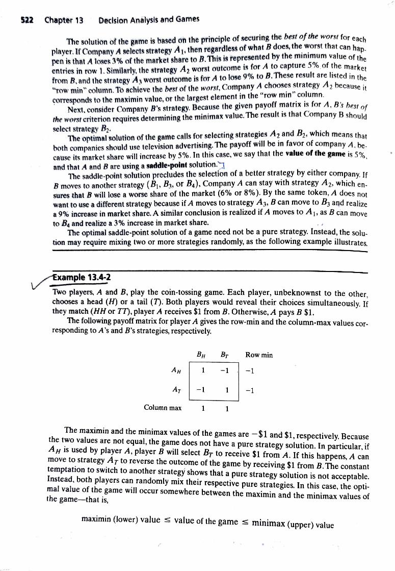
Two players, A and B, play the coin-tossing game. Each player, unbeknownst to the other, chooses a head (H) or a tail (7). Both players would reveal their choices simultaneously. If they match (HH or T). player A receives $1 from B. Otherwise, A pays B $1.

The following payoff matrix for player A gives the row-min and the column-max values cor responding to A's and B's strategies, respectively.

BH Br Row min

AH 1

|-1 Ar -1

Column max 1

The maximin and the minimax values of the games are -$1 and $1, respectively. Because the two values are not equal, the game does not have a pure strategy solution. In particular, if AH is used by player A, player B will select Br to receive $1 from A. If this happens, A can move to strategy A7 to reverse the outcome of the game by receiving $1 from B. The constant temptation to switch to another strategý shows that a pure strategy solution is not acceptable. Instead, both players can randomly mix their respective pure strategies. In this case, the opti-mal value of the game will occur somewhere between the maximin and the minimax values of the game-that is,

maximin (lower) value s value of the game minimax (upper) value PP


(See Problem 5, Set 13.4a.) Thus, in the coin-tossing example, the value of the game must lie be tween-$l and +$1,

PROBLEM SET 13.4A

1. Determine the saddle-point solution, the associated pure strategies, and the value of the game for each of the following games. The payoffs are for player A.

(a) B B B B (b) B B B B

A A 4 -4-5 6 8 2 8

A 4 Az3 -9-2 8 9 -4

-9 As 7 5 3 5 As 6

A 7 3-9 5

2 he following games give A's payoff. Determine the values of p and q that will make the entry (2,2) of each game a saddle point:

(a) B B B (b) B Ba B3

A1 1 6 A 2 4

Az P 5 10 Az 10 7

As 4 6 P As 6 2 3

3. Specify the range for the value of the game in each of the following cases, assuming that the payoff is for player A:

*(a) B B3 BA (b) B B B3 B

A -1 8 9 6 9 6 0

A2 -2 10 4 6 A 2 3 8 4

A 5 30 7 As -5 -2 10 -3

4 As 7 4-2-5 A 72 8

(d) Bi B B B B B2B3

A 3 7 1 3 A 3 6

4 8 0 -6 A Az 5 2 3

A 6 -9 2 As 4 2 -5

4 Two companies promote two competing products. Currently, each product controls 50% of the market. Because of recent improvements in the two products, each company is preparing to launch an advertising campaign. If neither company advertises, equal market


shares will continue. If either company launches a stronger campaign, the other is cert to lose a proportional percentage of its customers. A survey of the market shows that

50% of potential customers can be reached through television, 30% through newsnan and 20% through radio.

(a) Formulate the problem as a two-person zero-sum game, and select the appropiate advertising media for each company.

)Determine a range for the value of the game. Can each company operate with as gle pure strategy?

5. Let ay be the (, ,)th element of a payoff matrix with m strategies for player A andn strategies for player B. The payoff is for player A. Prove that

papers,

Sin

max min aij min max aij

13.4.2 Solution of Mixed Strategy Games

Games with mixed strategies can be solved either graphically or by linear programmijne The graphical solution is suitable for games in which at least one player has exactly two pure strategies. The method is interesting because it explains the idea of a saddle point graphically. Linear programming can be used to solve any two-person zero-sum game

Graphical Solution of Games. We start with the case of (2 X n) games in which player A has two strategies.

y2 yn B Bz.. B,

A| 1 a12 am A2 a2 an * azm 1 1

The game assumes that player A mixes strategies Aj and A2 with the respective prob- es x and 1- X1,0 S X1 S 1. Player B mixes strategies B, to B, with the proba-

bilities y, 2... , and y, wherey, 2 0 forj = 1,2,..., n, and y + 2 + +yn= 1. In this case, A's expected payoff corresponding to B's jth pure strategy is computed as

(4y4a)X1 +ar,j = 1,2,.,n

Player A thus seeks to determine the value of x that maximizes the minimum expect ed payoffs-that is,

max min{(a1 - a2j)x1 +a2j

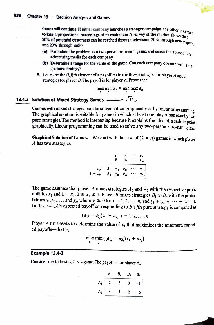
Example 13.4-3

Consider the following 2 x 4 game. The payoff is for player A.

B B Bs B

A 2 2 3-1

A4 32 6


ne game has no pure strategy solution. A's expected payoffs corresponding to B's pure strategies are given as

B's pure strateg A's expected payoff

2.x1 + 4

X +3 + 2

-7x +6

Figure 13.9 provides TORA plot of the four straight lines associated with B's pure strategies (file toraEx13.4-3.tNt).5 To determine the best of the worst, the lower envelope of the four lines (delineated by vertical stripes) represents the minimum (worst) expected payoff for A regardless of what B does. The maximum (best) of the lower envelope corresponds to the maximin solution point at xi = .5. This point is the intersection of lines associated with strategies B, and B. Play-

er A's optimal solution thus calls for mixing Aj and Az with probabilities .5, and.5, respectively.

FIGURE 13.9

TORA graphical solution of the two-person zero-sum game of Example 13.4-3 (file toraEx13.4-3.txt)

TORA C:zFinal8thlch13FilesitoraEx 13.4-3.txt DECISION ANALYSIS USING GAMES

GRAPHICALt TWO-PERSON ZERO-SUM GAME SOLUTION

LOam In Zoom Uu Prink Graph Examole 1343.

Ple As espected papoff

Suateg 2 200 1.00 Stuetegy 84 B004-7.oox

UptmalSohution

Value of the sme2.5

S A: 050 B

Suateg A2: 0.550

Player Bs mac ShateoyBI: 000 Sualegy B2 050 Suategy E3 U Suategy B: OLD B3

25 0,5

MAIN Meru Ext TORA View/Modiy Inpu Data

Lnks 840 AM

start 2Finalsth TORA C:\2Final8t.

SFrom Main menu select Zero-sum Games and input the problem data, then select Graphical from the

SOLVEMODIFY menu.


The corresponding value of the game, v, is determined by substituting X .5 in either of th

functions for lines 3 and 4, which gives the

+2 from line 3

-+6- from line 4

Player B's optimal mix is determined by the two strategies that define the lower envelope of the graph. This means that B can mix strategies B3 and Bg, in which case yi = y = 0 and

41-y. As a result, B's expected payoffs corresponding to A' S pure strategies are given as

A's pure strategy B's expected payoff

4y-1 -4y +6 2

The best of the worst solution for B is the minimum point on the upper envelope of the given two lines (you will find it instructive to graph the two lines and identify the upper envelope). This

process is equivalent to solving the equation

4y- 1 -4y3 +6

The solution gives y =which yields the value of the game as = 4 x (-1 =

The solution of the game calls for player A to mix A and A2 with equal probabilities and for player B to mix B, and B, with probabilities and. (Actually, the game has alternative solutions for B, becanse the maximin point in Figure 13.9 is determined by more than two lines. Any non- negative combination of these alternative solutions is also a legitimate solution.)

Remarks. Games in which player A has m strategies and player B has only two can be treated similarly. The main difference is that we will be plotting B's expected payoff corresponding to A's pure strategies. As a result, we will be seeking the minimax, rather than the maximin, point of the upper envelope of the plotted lines. However, to solve the problem with TORA, it is necessary to express the payoff in terms of the player that has two strategies by multiplying the payoff matrix by -1, if necessary.

PROBLEM SET 13.4B4

ASolve the coin-tossing game of Example 13.4-2 graphically *2. Robin, who travels frequenthly between two cities, has two route options: Route A is a fast four-lane highway, and route B is a long winding road. The highway patrol has a limited police force. If the full force is allocated to either route, Robin, with her passionate desire for driving "superfast," is certain to receive a $100 speeding ticket. If the force is split 50 50 between the two routes, there is a 50% chance she will get a $100 ticket on route A and only a 30% chance that she will get the same fine on route B.Develop a strategy for both Robin and the police.

The TORA Zero-sum Games module can be used to verify your answer.

13.4 Game Theory 527

3Bolve the following games graphically. The payoff is for Player A V (a) B, B B (b) B B

A 1 3 5 A 8

A2 4 -6 A2 6

A 1 4. Consider the following two-person, zero-sum game:

B B B

A 550 50

Aa 11 1

As 10 1 10

(a) Verity that the strategies0. for A and ) for B are optimal, and determine the value of the game.

(b) Show that the optimal value of the game equals

3 3

i=lj=1

Linear Programming Solution of Games. Game theory bears a strong relationship to linear programming, in the sense that a two-person zero-sum game can be expressed as a linear program, and vice versa. In fact, G. Dantzig (1963, p. 24) states that J. vonn Neumann, father of gam immediately recognized this relationship and further pinpointed and stressed the concept of duality in linear programming. This section illustrates the solution of games

by linear programming. Player A's optimal probabilities, X1, X2,..., and X, can be determined by solving

the following maximin problem:

theory when first introduced to the simplex method in 1947,

m

max min Zap a i=l

Xt X2 + * + Xm = 1|

x0,i 1,2,.., m

Now, let

=minek4aaa i=1 i=1

The equation implies that

24ijx2 v,j = 1,2, ..,n

/=]


Player As problem thus can be written as

Maximize z = v

subject to

24ij,0, j = 1,2,..,n

X tX2 +*** + Xm=1 x,0, i = 1,2,... m

v unrestricted

Note that the value of the game, v, is unrestricted in sign. Player B's optimal strategies, Y1, y2s., and y are determined by solving the

problem

min max a j=l

1+2 + + y = 1|

y0,j=1,2,... , n

Using a procedure similar to that of player A, B's problem reduces to

Minimize w = v

subject to

- 24 2 0,i = 1, 2,..., m

jF1| + + * + yn = 1

0,j 1,2,..., n vunrestricted

The two problems optimize the same (unrestricted) variable u, the value of the game. The reason is that B's problem is the dual of A's problem (verify this claim using the definition of duality in Chapter 4). This means that the optimal solution of one problem automatically yields the optimal solution of the other.

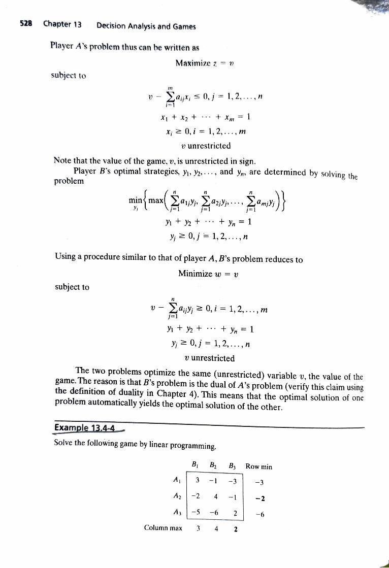
Example 13.4-4 Solve the following game by linear programming.

B B2 B Row min

A 3 -1 -3

Az-2 4 -1 -2

A-5-6 2 -6

Column max 3 4 2

13.4 Game Theory 529

The value of the game, , lies between -2 and 2.

Player As Linear Program

Maximize z = v

subject to

- 3x1 + 2x2 + 5x3 50

v+ -4x2 + 6x3s0

+3x1 + *2 2x2 0

1, X2, X3 20

v unrestricted

The optimum solution is x1 = 39, x2 = .31, x3 = 29, and v = -0.91.

Player B's Linear Program

Minimize z = v

subject to

-3y1 + h+3ys z0

v +2-4n+ 0

v+5y t 62 - 23 z0

v unrestricted

The solution yields yi .32, h = .08, = 60, and v = -0.91.

PROBLEM SET 13.4C 1. On a picnic outing, 2 two-person teams are playing hide-and-seek. There are four hiding

locations (A, B, C, and D), and the two members of the hiding team can hide separately in any two of the four locations. The other team will then have the chance to search any

two locations. The searching team gets a bonus point if they find þoth members of the

hiding team. If they miss both, they lose a point. Otherwise, the outcome is a draw.

*(a) Set up the problem as a two-person zero-sum game.

(b) Determine the optimal strategy and the value of the game.

2. UA and DU are setting up their strategies for the 1994 national championship college

basketball game. Assessing the strengths of their respective "benches," cach coach comes

up with four strategies for rotating his players during the game. The ability of each team

to score 2-pointers, 3-pointers, and free throws is a key factor in determining the final

TORA Zerosum GamesSolvëLP-based can be used to solve any two-person zero-sum game.

OR Unt

CHA PTER 10

Deterministic Dynamic Programming

Chapter Guide Dynamic programming (DP) determines the optimum solution of a multivariable problem by decomposing it into stages, each stage comprising a single variable subproblem. The advantage of the decomposition is that the optimization process at each stage involves one variable only, a simpler task computationally than dealing with all the variables simultaneously. A DP model is basically a recursive equa tion linking the different stages of the problem in a manner that guarantees that each stage's optimal feasible solution is also optimal and feasible for the entire problem.The notation and the conceptual framework of the recursive equation are unlike any you have studied so far. Experience has shown that the structure of the recursive equation may not appear "logical" to a beginner. Should you have a similar experience, the best course of action is to try to implement what may appear logical to you, and then carry out the computations accordingly. You will soon discover that the definitions in the book are the correct ones and, in the process, will learn how DP works. We have also included two partially automated Excel spreadsheets for some of the examples in which the user must provide key information to drive the DP computations. The exercise

should help you understand some of the subtleties of DP. Although the recursive equation is a common framework for formulating DP

models, the solution details differ. Only through exposure to different formulations will you be able to gain experience in DP modeling and DP solution. A number of

eterministic DP applications are given in this chapter. Chapter 22 on the CD presents probabilistic DP applications. Other applications in the important area of inventory modeling are presented in Chapters 11 and 14.

This chapter includes a summary of 1 real-life application, 7 solved examples 2 Excel spreadsheet models, 32 end-of-section problems, and 1 case. The case is in Ap- pendix E on the CD. The AMPL/Excel/Solver/TORA programs are in folder ch10Files

399

400 Chapter 10 Deterministic Dynamic Programming

Real-Life Application-Optimization of Crosscutting and Log Allocation at Weyerhaeuser. Mature trees are harvested and crosscut into logs to manufacture different end prod

Hcts (such as construction lumber. plywood, wafer boards, or paper). Log specification Clength and end diameters) differ depending on the mill where the logs are use With harvested trees measuring up to 100 feet in length, the number of croSSCut combj

nations meeting mill requirements can be large, and the manner in which a tree is di assembled into logs can affect revenues. The objective is to determine the crOSsCUt combinations that maximize the total revenue. The study uses dynamic programmine to optimize the process. The proposed system was first implemented in 1978 with an annual increase in profit of at least $7 million. Case 8 in Chapter 24 on the CD provides the details of the study.

10.1 RECURSIVE NATURE OF COMPUTATIONS IN DP

Computations in DP are done recursively, so that the optimum solution of one subproblem is used as an input to the next subproblem. By the time the last subproblem is solved, the optimum solution for the entire problem is at hand. The manner in which the recursive computations are carried out depends on how we decompose the original problem. In particular, the subproblems are normally linked by common constraints. As we move from one subproblem to the next, the feasibility of these common constraints must be maintained.

Example 10.1-1 (Shortest-Route Problem) Suppose that you want to select the shortest highway route between two cities. The network in Figure 10.1 provides the possible routes between the starting city at node 1 and the destination city at node 7. The routes pass through intermediate cities designated by nodes 2 to 6, Krol We can solve this problem by exhaustively enumerating all the routes between nodes 1 and 7 (there are five such routes). However, in a large network, exhakstivë enumeration may be intractable computationally.

To solve the problem by DP, we first decompose it into stages as delineated by the vertical dashed lines in Figure 10.2. Next, we carry out the computations for each stage separately.

FIGURE 10.1

12 Route network for Example 10.1-11

tart

10.1 Recursive Nature of Computations in DP 401

2 12

9 8

13

FIGURE 10.2

Decomposition of the shortest-route problem into stages

The general idea for determining the shortest route is to compute the shortest (cumulative) distances to all the terminal nodes of a stage and then use these distances as input data to the immediately succeeding stage. Starting from node 1, stage 1 includes three end nodes (2, 3, and 4) and its computations are simple.

Stage 1 Summary.

Shortest distance from node 1 to node 2 7 miles (from node 1) staj

Shortest distance from node 1 to node 3 8 miles (from node 1) Shortest distance from node 1 to node 4Sniles (from node 1))

Next, stage 2 has two end nodes, 5 and 6. Considering node 5 first, we see from Figure 10.2 that node 5 can be reached from three nodes, 2,3, and 4, by three different routes: (2, 5), (3,5), and (4,5). This information, together with the shortest distances to nodes 2,3, and 4, determines the shortest (cumulative) distance to node 5 as

(Shortest distance min Shortest distance( Distance from (node i to node 5/ to node 5 i=2,3,4 to node i

(7+ 12 19 &to min 8 + 8 = 16 - 12 (from node 4)

5+ 7 ( Node 6 can be reached from nodes 3 and 4 only. Thus

(Shortest distance Distancefrom Shortest distance min to node i node i to node 6/J

= mins5 + 13 = 18 * i7Urom node 3) 8te *

to node 6 i=3,4

8+9 17.= 17 (from node 3)


Stage 2 Summary

Shortest distance from node 1 to node 5 = 12 miles (from node 4)

Shortest distance from node I to node 6 = 17 miles (from node 3)

odes 5 The last step is to consider stage 3. The destination node 7 can be reached from either no

get or 6. Using the summary results frOm stage 2 and the distances from nodes 5 and6 to node 7

Distance from Shortest distance Shortest distance

to node 7 miR to node i node i to node 7/ =

12 +9 21 min 17 + 6 23)

21 (from node 5)

Stage 3 Summary.

Shortest distance from node 1 to node 7 = 21 miles (from node 5)

Stage 3 summary shows that the shortest distance between nodes 1 and 7 is 21 miles To deter. mine the optimal route, stage 3 summary links node 7 to node 5, stage 2 summary links node 4 to

node 5, and stage 1 summary links node 4 to node 1.Thus, the shortest route is 1>45>7. .

The example reveals the basic properties of computations in DP:

1. The computations at each stage are a function of the feasible routes of that stage, and that

stage alone.

2. A current stage is linked to the immediately preceding stage only without regard to earlier stages. The linkage is in the form of the shortest-distance summary thàt represents the out-

put of the immediately preceding stage.

Recursive Equation. We now show how the recursive computations in Example 10.1- can be expressed mathematically. Let f{r;) be the shortest distance to node x; at stage , and define d(xj-1, X1) as the distance from node xi-1 to node x; then f is computed from f-1 using the following recursive equation:

JA) = MiR {d(xi-1, X) +fi-ili-1)}, i = 1,2,3

(-1) routes

Starting ati=1, the recursion sets folxo) = 0. The equation shows that the

shortest distances fi(x;) at stage i must be expressed in terms of the next node, x, l" the DP terminology, x, is referred to as the state of the system at stage i. In effect, the state of the system at stage i is the information that links the stages together, so tnat optimal decisions for the remaining stages can be made without reexamining how

decisions for the previous stages are reached. The proper definition of the state allows us to consider each stage separately and guarantee that the solution is feasible for a the stages.

The definition of the state leads to the following unifying framework for DP

10.2 Forward and Backward Recursion 403

Principle of Optimality Future decisions for the remaining stages will constitute an optimal policy regardless of the policy adopted in previous stages

The implementation of the principle is evident in the computations in Example 10.1-1. For example, in stage 3, we only use the shortest distances to nodes 5 and 6, and do not concern ourselves with how these nodes are reached from node 1.Although the principle of optimality is "vague" about the details of how each stage is optimized, its

application greatly facilitates the solution of many complex problems.

PROBLEM SET 10.1A

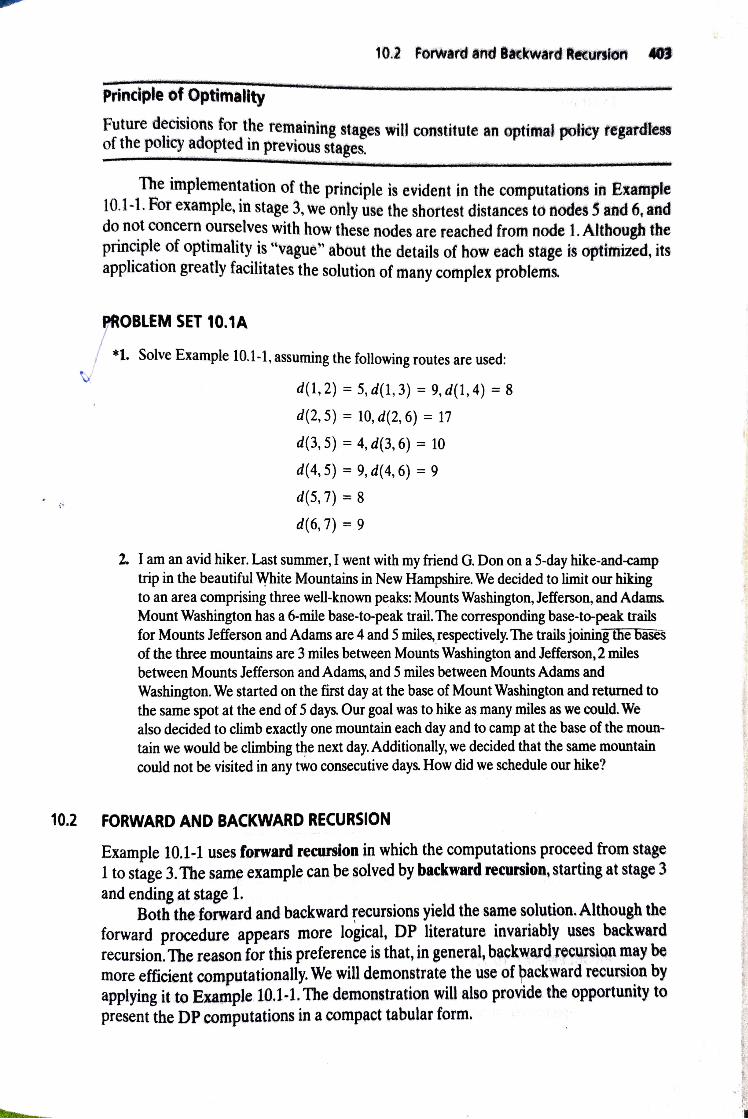
1. Solve Example 10.1-1, assuming the following routes are used:

d(1,2) = 5, d(1, 3) = 9, d(1, 4) = 8

d(2,5) = 10, d(2, 6) = 17

d(3,5) = 4, d(3,6) = 10

d(4.5) = 9, d(4,6) = 9

d(5,7) 8

d(6,7) = 9

2. I am an avid hiker. Last summer, I went with my friend G. Don on a 5-day hike-and-camp trip in the beautiful White Mountains in New Hampshire. We decided to limit our hiking to an area comprising three well-known peaks: Mounts Washington, Jefferson, and Adams Mount Washington has a 6-mile base-to-peak trail. The corresponding base-to-peak trails for Mounts Jefferson and Adams are 4 and 5 miles, respectively. The trails joining the bases of the three mountains are 3 miles between Mounts Washington and Jefferson, 2 miles between Mounts Jefferson and Adams, and 5 miles between Mounts Adams and Washington. We started on the first day at the base of Mount Washington and returned to the same spot at the end of 5 days. Our goal was to hike as many miles as we could. We also decided to climb exactly one mountain each day and to camp at the base of the moun-tain we would be climbing the next day.Additionally, we decided that the same mountain could not be visited in any two consecutive days. How did we schedule our hike?

10.2 FORWARD AND BACKWARD RECURSION

Example 10.1-1 uses forward recursion in which the computations proceed from stage 1 to stage 3. The same example can be solved by backward recursion, starting at stage 3

and ending at stage 1. Both the forward and backward recursions yield the same solution. Although the

forward procedure appears more logical, DP literature invariably uses backward

recursion. The reason for this preference is that, in general, backward recursion may be more efficient computationally. We will demonstrate the use of backward recursion by

applying it to Example 10.1-1. The demonstration will also provide the opportunity to

present the DP computations in a compact tabular form.

404 Deterministic Dynamic Programming

Chapter 10

Example 10.2-1

The backward recursive equation for Example 10.2-1 is

fx,)=min {d(x,xj+1) + f+i(j+1)},i = 1,2,3

routes (;t + 1

where f(xa) = 0 for ax = 7.The associated order of computations is fjf-f

Stage 3. Because node 7 (x4 = 7) is connected to nodes 5 and 6 (r3 = 5 and 6) with.

one route each, there are no alternatives to choose from, and stage 3 results can aCtly

rized as

umma-

Optimum solution

X47

9 5

6

Stage 2. Route (2, 6) is blocked because it does not exist. Given fa(x3) from stage 3, we can

compare the feasible alternatives as shown in the following tableau: can

dr, X3) + flxs) Optimum solution

X3 6 l) 2 3=5

21 12 +9 21 8 +9 17

7+9 16

2 15 9+6 15

13+6 = 19 3

16 4

The optimum solution of stage 2 reads as follows: If you are in cities 2 or 4, the shortest

route passes through city 5, and if you are in city 3, the shortest route passes through city 6.

Stage 1 From node 1, we have three alternative routes: (1,2), (1,3), and (1, 4). Using f2(12) from stage 2, we can compute the following tableau.

dr, x) + filr) Optimum solution

X22 23 24

7+21 = 28 8+15 23 5+16 21 21

The optimum solution at stage 1 shows that city 1 is linked to city 4. Next, the optimum son tion at stage 2 links city 4 to city 5. Finally, the optimum solution at stage 3 connects city 5 to city 1. Thus, the complete route is given as 1-45 7, and the associated distance is 21 miles

PROBLEM SET 10.2A

1. For Problem 1, Set 10.1a, develop the backward recursive equation, and use it to nu nd optimum solution.

he

405 10.3 Selected DP Applications

2

14 12

7)

FIGURE 10.3

Network for Problem 3, Set 10.2a

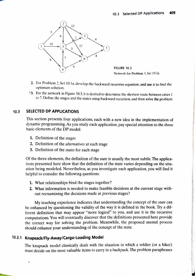
2. For Problem 2, Set 10.1a, develop the backward recursive equation, and use it to find the

optimum solution. 3. For the network in Figure 10.3, it is desired to determine the shortest route between cities I

to 7. Define the stages and the states using backward recursion, and then solve the problem.

10.3 SELECTED DP APPLICATIONS

This section presents four applications, each with a new idea in the implementation of dynamic programming. As you study each application, pay special attention to the three basic elements of the DP model:

1. Definition of the stages 2. Definition of the alternatives at each stage 3. Definition of the states for each stage

Of the three elements, the definition of the state is usually the most subtle. The applications presented here show that the definition of the state varies depending on the situ-ation being modeled. Nevertheless, as you investigate each application, you will find it helpful to consider the following questions:

1. What relationships bind the stages together?

2. What information is needed to make feasible decisions at the current stage without reexamining the decisions made at previous stages?

My teaching experience indicates that understanding the concept of the state can be enhanced by questioning the validity of the way it is defined in the book. Try a dif ferent definition that may appear "more logical" to you, and use it in the recursive computations. You will eventually discover that the definitions presented here provide the correct way for solving the problem. Meanwhile, the proposed mental process should enhance your understanding of the concept of the state.

10.3.1 Knapsack/Fly-Away/Cargo-Loading Model

The knapsack model classically deals with the situation in which a soldier (or a hiker) must decide on the most valuable items to carry in a backpack. The problem paraphrases


a general resource allocation model in which a single limited resource is assigned to a number of alternatives (e.g., limited funds assigned to projects) with the objective of ma

imizing the total return. Before presenting the DP model, we remark that the knapsack problem is al

known in the literature as the fly-away kit problem, in which a jet pilot must determina

the most valuable (emergency) items to take aboard a jet, and the cargo-loading proh. lem, in which a vessel with limited volume or weight capacity is loaded with the most

valuable cargo items. It appears that the three names were coined to ensure equal rep resentation of three branches of the armed forces: Air Force, Army, and Navy!

The (backward) recursive equation is developed for the general problem of an n-item W-b knapsack. Let m, be the number of units of item i in the knapsack and define r, and w, as the revenue and weight per unit of item i. The general problem is

represented by the following LP:

Maximizez = nm\ t 72/m2 +* tTn

subject to

Wm tWm2 + .: +w,mn W

m1, m2y., mn 2 0 and integer

The three elements of the model are

1. Stage i is represented by item i, i = 1,2,..., n. 2. The alternatives at stage i are represented by mj, the number of units of itemi

included in the knapsack. The associated return is rm, Definingas the largest inte ger less than or equal to it follows that m, = 0, 1,...

3. The state at stage i is represented by z, the total weight assigned to stages items) i, i +1,. and n. This definition reflects the fact that the weight constraint is the only restriction that links all n stages together.

Define

f{x) = maximum return for stages i, i + 1, and n, given state x;

The simplest way to determine a recursive equation is a two-step procedure:

Step 1. Express f{x;) as a function of f(x;+1) as follows:

fAz)=minrm, + fi+1(¥i+1)}, i = 1,2,...,n m=0,1,

Sn+n+1) =0

Step 2. Express Xj+1 as a function of x, to ensure that the left-hand side, f{¥i), 15 a function of x; only. By definition, xi -

Xi+1 = wm; represents the welg used at stage i. Thus, Xi+1 = X; - Wm, and the proper recursive equaion d

given as

fAx)= maxrm; + fi+1(x - wm;)}, i = 1,2,..,n m=0,1,.

SW

10.3 selected DP Applications Example 10.3-1

407A 4-ton vessel can be loaded with one or more of three items. The following table gives the unit

weight, j. in tons and the unit revenue in thousands of dollars,, for item i How should the ves-

sel be loaded to maximize the total return?

Item i

47 3 4 Because the unit weights w and the maximum weight W are integer, the state , assumes

integer values only. Stage 3. assume one of the values 0, 1,..., and 4 (because W = 4 tons). The states x 0 and x= 4, Te

spectively, represent the extreme cases of not shipping item 3 at all and of allocating the entire

vessel to it. The remaining values of x (= 1,2, and 3) imply a partial allocation of the vessel ca

pacity to item 3. In effect, the given range of values for x covers all possible allocations of the

vessel capacity to item 3.

The exact weight to be allocated to stage 3 (item 3) is not known in advance, but can

Given ws=1 ton per unit, the maximum number of units of item 3 that can be loaded is

4, which means that the possible values of my are 0, 1,2,3, and 4. An alternative m^ is feasi ble only if wzm3 xz. Thus, all the infeasible alternatives (those for which »m> x) are excluded.The following equation is the basis for comparing the alternatives of stage 3.

fslxs) = max

m30,l.4 14m The following tableau compares the feasible alternatives for each value of x3.

14m3 Optimum solution m3 0 m3 1 m3 = 2

m33 m34

14 14 14 28

28 28 12 42

0 14

28 12 56 0 14

Stage 2. maxfma} = =1, or m = 0,1

Sala)= max {47ma + (2 - 3m2)}

m0,1

Optimum solation 47m + - 3m)

m2 m 1 m2= 0 2

0+ 0 =0 0+ 14 14 0+ 28 28

0 +4242 0+56 = 56

14 28 47 47+ 0 47

47+14 61 61

408 Chapter 10o Deterministic Dynamic Programming

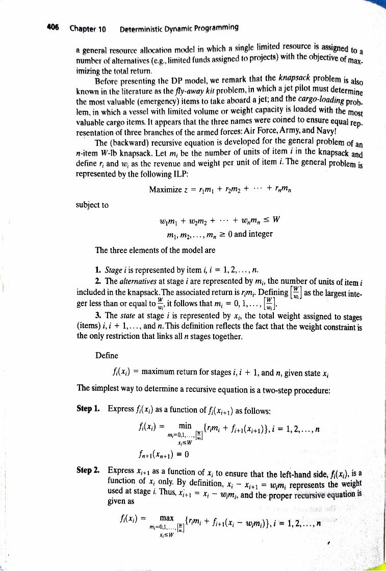
Stage 1. max{m,}-1 2 or mi = 0, 1,2

2m)). max({mi} = =2 f(r)= max {31m + /(1

my =0,1.2

Optimum solution 31m, +f2lx1- 2m) m

m= 2 m=0

0 0+0= 0 0+ 14= 14

0 14 31 31 +0= 31

31 + 14 = 45

0 + 28 = 28

47 0+ 47 47 0 0 +61 61 31 28= 59 62 +0 62 62

The optimum solution is determined in the following manner: Given W = 4 tons, from stage 1. x = 4 gives the optimum alternative mi = 2, which means that 2 units of item 1 will he

loaded on the vessel. This allocation leaves x2 1- 2m2 4 -2 X 2 = 0. From staoe 2. x2 = 0 yields m2 =0, which, in turn, gives xz = X2 - 3m2 =0-3 X0 = 0. Next, from stage

3, x3 = 0 gives m3 = 0. Thus, the complete optimal solution is m1 = 2, m =0, and m = 0.The

associated return is f(4) = $62,000.

In the table for stage 1, we actually need to obtain the optimum for x = 4 only because this is the last stage to be considered. However, the computations for X1 = 0, 1,2, and 3 are included

to allow carrying out sensitivity analysis. For example, what happens if the vessel capacity is 3 tons in place of 4 tons? The new optimum solution can be determined as

( 3) (mi = 0)> (x2 = 3)>(m2 = 1) (x3 = 0) (mj = 0)

Thus the optimum is (mi, m2, m3) = (0,1,0) and the optimum revenue is fi(3) = $47,000.

Remarks. The cargo-loading example represents a typical resource allocation model in which a

limited resource is apportioned among a finite number of (economic) activities. The objective

maximizes an associated return function. In such models, the definition of the state at each stage will be similar to the definition given for the cargo-loading model. Namely, the state at stage iis

the total resource amount allocated to stages i, i + 1,..., andn.

Excel moment

The nature of dynamic programming computations makes it impossible to develop a general computer code that can handle all DP problems. Perhaps this explains the per sistent absence of commercial DP software.

In this section, we present a Excel-based algorithm for handling a subclass o

DP problems: the single-constraint knapsack problem (file Knapsack.xls). The aigo rithm is not data specific and can handle problems in this category with 10 alterma tives or less.

Figure 10.4 shows the starting screen of the knapsack (backward) DP model. 1 screen is divided into two sections:The right section (columns Q:V) is used to sumnla

DATE pAGE

GameJheny 13134

ramic.reamnqnsLoa10d La3

- Opeima Paludm esamlsame 34

giatedstataa saa-

i Reusive Natpe Compstathons DP= 0e-

clii ) Selested Dp AecablosP e3-

plant wheat N. Se

Documents

Transcript of plant wheat N. Se