
Plant Availability of Water in Soils Being Reclaimed from the ...
167
Plant Availability of Water in Soils Being Reclaimed from the Saline-Sodic State Thesis submitted by Nguyen Duy Nang BSc (Agronomy), University of Agriculture and Forestry, Vietnam MSc (Soil Science), University of the Philippines, Philippines For the degree of Doctor of Philosophy in the School of Agriculture, Food and Wine Faculty of Sciences The University of Adelaide Adelaide, South Australia, Australia December 2012
-
Upload
khangminh22 -
Category
Documents
-
view
5 -
download
0
Transcript of Plant Availability of Water in Soils Being Reclaimed from the ...
Plant Availability of Water in Soils Being Reclaimed from the Saline-Sodic State
Thesis submitted by
Nguyen Duy Nang
BSc (Agronomy), University of Agriculture and Forestry, Vietnam MSc (Soil Science), University of the Philippines, Philippines
For the degree of Doctor of Philosophy
in the
School of Agriculture, Food and Wine Faculty of Sciences
The University of Adelaide Adelaide, South Australia, Australia
December 2012

ii
Table of contents Page
List of tables ....................................................................................................................................... v
List of figures .................................................................................................................................... vii
Abstract ............................................................................................................................................ xii
Declaration ........................................................................................................................................xv
Acknowledgment .............................................................................................................................. xvi
Chapter 1 Introduction and literature review ............................................................................... 1
1.1 Introduction .......................................................................................................................... 1
1.2 Literature review .................................................................................................................. 2
1.2.1 Factors affecting plant available water in soils.................................................................. 2
1.2.2 Factors affecting soil structure .......................................................................................... 9
1.2.2.1 Exchangeable cations ................................................................................................. 9
1.2.2.2 Organic matter ......................................................................................................... 12
1.2.2.3 Clay swelling and dispersion .................................................................................... 13
1.2.2.4 Nutritional effects ..................................................................................................... 15
1.2.3 Effects of soil structure on soil strength, aeration, and hydraulic conductivity ............... 16
1.2.4 Salt-affected soils and their reclamation ......................................................................... 18
1.2.5 Models of plant available water ....................................................................................... 21
1.2.5.1 Historical models ...................................................................................................... 21
1.2.5.2 Integral Water Capacity (IWC) model ..................................................................... 25
1.2.5.3 Example of IWC calculations ................................................................................... 26
1.2.6 Conclusions ..................................................................................................................... 35
1.3 Overall problem, research questions and hypotheses. ........................................................ 36
1.3.1 Research questions .......................................................................................................... 36
1.3.2 Hypotheses ...................................................................................................................... 37
Chapter 2 Variation in soil water availability down the profile of a saline soil
using the Integral Water Capacity (IWC) model ........................................................................ 38
2.1 Introduction ........................................................................................................................ 38
2.2 Materials and Methods ....................................................................................................... 39
2.2.1 Site selection and sample collection ................................................................................ 39
2.2.2 Saturated hydraulic conductivity, water retention, and soil penetration resistance. ........ 42
2.2.3 Salinity and osmotic stress .............................................................................................. 43
2.3 Result and discussion ......................................................................................................... 44
2.3.1 Saturated hydraulic conductivity ..................................................................................... 44
2.3.2 Water retention curves ..................................................................................................... 44

iii
2.3.3 Soil penetration resistance............................................................................................... 46
2.3.4 Salinity and osmotic stress .............................................................................................. 47
2.3.5 Weighting functions ........................................................................................................ 49
2.3.5.1 Weighting the differential water capacities for salinity ............................................ 49
2.3.5.2 Weighting the differential water capacity for high soil penetration resistance. ....... 50
2.3.5.3 Weighting the differential water capacity for poor soil aeration. ............................. 52
2.3.5.4 Weighting the differential water capacity for declining soil hydraulic
conductivity. .......................................................................................................................... 54
2.3.6 Summarizing the effects of weighting the water capacity .............................................. 56
2.4 Conclusions ........................................................................................................................ 60
Chapter 3 In situ response of plants to saline conditions in the field ......................................... 61
3.1 Introduction ........................................................................................................................ 61
3.2 Materials and methods ....................................................................................................... 62
3.2.1 Experimental design ........................................................................................................ 62
3.2.2 Water balance model ....................................................................................................... 64
3.2.3 Calibrating the CPN 503 Hydroprobe neutron moisture meter. ...................................... 68
3.3 Results and discussion ....................................................................................................... 71
3.3.1 Plant water use from full canopy establishment to plant death ....................................... 71
3.3.2 Plant water use and root distribution ............................................................................... 72
3.3.3 Evaluation of the IWC model against water use by real plants....................................... 76
3.4 Conclusions ........................................................................................................................ 80
Chapter 4. Changes in IWC during reclamation of a salt-affected soil ..................................... 81
4.1 Introduction ........................................................................................................................ 81
4.2 Materials and Methods ....................................................................................................... 82
4.2.1 Experimental approach and design ................................................................................. 82
4.2.2 Experimental units .......................................................................................................... 83
4.2.3 Experimental protocol ..................................................................................................... 84
4.3 Result and discussion ......................................................................................................... 86
4.3.1 Changes in saturated hydraulic conductivity during reclamation ................................... 86
4.3.2 Changes in water retention curves during reclamation ................................................... 88
4.3.3 Changes in soil penetration resistance during reclamation ............................................. 93
4.3.4 Changes in IWC during reclamation ............................................................................... 96
4.4 Conclusions ...................................................................................................................... 101
Chapter 5 Shape of the salinity weighting function, ��o(h), based upon early plant
response to osmotic and matric stresses ...................................................................................... 102
5.1 Introduction ...................................................................................................................... 102

iv
5.2 Materials and Methods ..................................................................................................... 103
5.3 Result and discussion ....................................................................................................... 106
5.3.1 Dry matter yield as a function of osmotic-, matric- and total water potential ............... 106
5.3.2 A plant-based weighting function to attenuate the water capacity ................................ 107
5.4 Conclusions ...................................................................................................................... 113
Chapter 6 General discussion and directions for future research ........................................... 115
6.1 Introduction ...................................................................................................................... 115
6.2 Major findings (and future research) ................................................................................ 116
Appendices .................................................................................................................................... 121
References ..................................................................................................................................... 141

v
List of tables Table 1.1 Available water capacity by soil texture ............................................................................ 3
Table 1.2 Criteria used to classify salt-affected soils in U.S. and Australia. .................................... 19
Table 1.3 Summary of physical restrictions on the differential water capacity and their
effect on IWC.......................................................................................................................... 35
Table 2.1 Fitting parameters, k0, k1 and n, for the water retention curves in each horizon
down the soil profile. Optimization of the fitting parameters was conducted with
fixed (measured) values of the volumetric water content at saturation, �s, and
permanent wilting point, �wp. .................................................................................................. 46
Table 2.2 Fitting parameters for Equation [2.1] describing the relation between soil
penetration resistance (MPa) and soil matric head (cm), plus the matric heads, hi
and hf, respectively, at which SR(hm) reached values of 0.5 and 2.5 MPa. ............................ 47
Table 2.3. Measured values of the electrical conductivity of 1:5 soil:water extracts and
gravimetric water contents at saturation, plus the corresponding electrical
conductivity of paste extracts (calculated from Slavich and Petterson (1993)) and
values of hos and hm at wilting point (calculated from Equation 12 in Groenevelt et
al. (2004)). .............................................................................................................................. 49
Table 2.4. Predictions of plant available water in a saline soil profile based upon various
degrees of weighting of the differential water capacity; integrals at the top of each
column indicate the type of weighting applied: PAW = classical approach with no
attenuation, IWC = integral water capacity with attenuations to account for,
respectively: salt alone, salt + poor aeration, salt + high soil resistance, salt +
declining hydraulic conductivity, and all factors combined. .................................................. 58
Table 3.1 Chemical properties (saturated paste extracts) of the soil profile in the plots
containing the neutron access tubes. ....................................................................................... 69
Table 3.2 Variation in the standard 15 second slow neutron count rate with salt
concentration. .......................................................................................................................... 70
Table 3.3. Correlations between relative slow neutron count rate, RCR, and volumetric
water content, �, at each depth in the soil profile. .................................................................. 72
Table 3.4. Predictions of plant available water in a saline soil profile (mm/m) based upon
various degrees of weighting of the differential water capacity (taken directly from
Table 2.3) compared with field-measured change in water contents with Rhodes
grass (Chloris gayana cv. Pioneer). ........................................................................................ 76
Table 3.5. Predictions of plant available water (mm/m) based upon the same weightings
of the differential water capacity but ignoring salt, compared with field-measured
change in water contents with Rhodes grass (Chloris gayana cv. Pioneer) ........................... 77

vi
Table 4.1. Bulk densities achieved for 150 mm columns of soil from each soil horizon
(cylindrical pot diameter = 152.5 mm; calculated volume of each soil column =
2740 cm3). .............................................................................................................................. 84
Table 4.2 Elemental analysis by ICP-MS for the major cations, plus SAR, EC and pH of
the saturation paste extracts in each of the 9 soil horizons. SAR was calculated by
dividing [Na] (mmol/L) by the square root of ([Ca] + [Mg]). The value for �
cations (mmolc L-1) was the sum of ([Na] + [K]) plus twice the sum of ([Ca] +
[Mg]). The values of ECmeas were measured and they compare well with the values
for ECcalc, which were calculated from � cations divided by 10. ........................................... 84
Table 4.3 Fitting parameters for the Groenevelt et al. (2001; 2004) soil water retention
curves shown in Figures 4.4, plus the penetration resistance curves for the 6
different leaching treatments in the 9 soil horizons shown in Figures 4.5. ............................ 92
Table 4.4. Integral water capacity, IWC, of each soil horizon after leaching with solutions
of differing salinity and sodicity. IWC calculated using different weighting
functions. Initial EC for each horizon indicated in parentheses (dS m-1). Shadings
in 3rd & 4th columns indicate treatments where data were combined to form single,
average water retention or soil resistance curves. .................................................................. 97
Table 5.1 Numbered list of osmotic and matric potentials/heads used in soil and solution
culture. Osmotic potentials were calculated from the ECe values. ....................................... 104
Table 5.2 Parameters and constants for Equation [5.1] to describe the relative growth,
G′(hom), of Faba beans and Rhodes grass. ............................................................................ 109
Table 5.3. Parameters from Equation [5.2] used in preparing a weighting function to
attenuate the water capacity for salinity, based upon soil and plant factors
combined. In this study, the initial onset of osmotic stress was deduced to occur
from hi = 0.0025 bar for all examples. The value of hf in this table is the matric
potential at which wilting occurs under the salinity conditions corresponding to the
ECe; values were calculated from Equation (12) of Groenevelt et al. (2004). Colour
shaded data are shown in Figure 5.4 above. ......................................................................... 111
Table 5.4 Estimates of plant available water in soil of varying salinity based on soil
properties, or a combination of soil properties and plant response for Faba beans
and Rhodes grass. ................................................................................................................. 113

vii
List of figures
Figure 1.1 Relative hydraulic conductivity as a function of matric head for coarse-
textured and fine-textured soils. ................................................................................................ 4
Figure 1.2a “Divisions for classifying crop tolerance to salinity” (after Maas and
Hoffman 1977). ......................................................................................................................... 7
Figure 1.2b Response of some grain crops (e.g. rice, corn, wheat, barley) to salinity (after
Maas and Hoffman 1977). ........................................................................................................ 7
Figure 1.3 Change in aggregate tensile strength with aggregate diameter as a function of
time (after Lal and Shukla 2004) ............................................................................................ 17
Figure 1.4 The non-limiting water range (NLWR) of water contents as influenced by
restricting soil factors for plant growth in soil with (a) good structure and (b) poor
structure (Letey 1985). ............................................................................................................ 24
Figure 1.5 Effect of increasing bulk density on the water content at which volumetric air
content = 0.10m3/m3 and soil resistance = 2 MPa, superimposed on the water
contents at FC and PWP (after da Silva et al.(1994)); shaded area represents
LLWR. .................................................................................................................................... 24
Figure 1.6 Differential water capacity, C(hm), for the wet end (—); effective differential
water capacity, EK(hm), when a hydraulic conductivity weighting function ,ωK(hm),
is applied (– –); effective differential water capacity, EKa(hm), when both ωK(hm)
and a aeration weighting function, ωa(hm), are applied(Groenevelt et al. 2001)..................... 25
Figure 1.7 Weighted differential water capacities for a loamy soil accounting for salt-free
conditions and for conditions where EC of the saturated soil = 1, 2, 4, and 7.2 dS/m
(Groenevelt et al. 2004). ......................................................................................................... 26
Figure 1.8 Representation of the water retention curve using data and model for a loamy
sand published in Groenevelt et al. (2004). ............................................................................ 28
Figure 1.9 Differential water capacities for the loamy sand of Figure 1.8 when the soil is
salt-free (solid blue line) and when the soil has an osmotic head of 2 m in its
saturated state (dashed red line). The dotted ellipse identifies the section of the
curves discussed in Figure 1.10. ............................................................................................. 31
Figure 1.10 Differential water capacities for salt-free soil (solid blue line, 1), Saline soil
with hos = 2 m (solid red line, 2), Saline soil with poor drainage (dashed red line
segment, 3), and Saline soil with poor drainage and high strength (dashed purple
line segment, 4). ..................................................................................................................... 32
Figure 1.11 Weighting function to attenuate the water capacity for the effect of poor soil
aeration between the matric heads of hm = 0.51 to 1.41 m. .................................................... 33

viii
Figure 1.12 Weighting function to attenuate the water capacity for the effect of
increasingly high soil penetration resistance between the matric heads of hm1 = 2 m,
hm2 = 5 m. ............................................................................................................................... 34
Figure 2.1 Roseworthy paddock C1 ................................................................................................ 40
Figure 2.2 Exposed soil profile. ....................................................................................................... 40
Figure 2.3 Collecting undisturbed soil cores down the profile in paddock C1 ................................ 40
Figure 2.4 Laboratory set-up to measure saturated hydraulic conductivity on undisturbed
soil cores prior to measuring their water retention curves using field-isotonic
solutions. ................................................................................................................................ 42
Figure 2.5 Saturated hydraulic conductivities of undisturbed soil cores down the soil
profile using isotonic solutions applicable to each depth (horizontal red bars are
standard errors. ....................................................................................................................... 44
Figure 2.6 Water retention curves for the 9 soil horizons examined in this study: a) 0 to
25 cm, b) 25 to 75 cm, c) 75 to 115 cm, and d) 115 to 150 cm. ............................................. 45
Figure 2.7 Soil penetration resistance (SR, MPa) as a function of matric head (hm, cm)
for the same soils presented in Figures 2.6. The data falling between the horizontal
green and red dashed lines represent conditions that increasingly restrict root
growth in the soil. ................................................................................................................... 48
Figure 2.8 Differential water capacities for the nine water retention curves shown in
Figure 2.1 weighted (dotted lines) or not weighted (solid lines) for salt content
according to Groenevelt et al. (2004). .................................................................................... 51
Figure 2.9 Three possible shapes for weighting functions to attenuate the water capacity
based upon the ability of different plants to exert higher or lower root growth
pressures on their surroundings. Upper dotted lines come from using � = 0.2 (for
strong plant roots), solid lines come from using � = 0.5 (for medium-strength plant
roots), and lower dash-dotted lines come from using � = 1 (for weak plant roots). .............. 52
Figure 2.10 Three possible shapes (of many) for weighting functions to attenuate the
water capacity for poor soil aeration by varying the A-parameter in Equation [2.5]
from 0.2 (upper dotted lines), 0.5 (middle solid lines), and 1.0 (lower dash-dot
lines) according to the ability of different plants to tolerate poor soil aeration...................... 54
Figure 2.11 Three possible shapes for weighting functions to attenuation the water
capacity based upon the ability of different plants to cope with declining hydraulic
conductivity in dry soils. The lowest dotted lines come from using � = 0.2 in
Equation [2.9] for sensitive plants; the highest dash-dot lines come from using � =
1.0 for tolerant plants, and the central solid lines come from using � = 0.5 for
medium plants. ....................................................................................................................... 57

ix
Figure 2.12 Amount of plant available water down the profile of a saline soil (mm/m)
predicted by taking into account different soil physical restrictions listed in Table
2.5. .......................................................................................................................................... 59
Figure 3.1 Diagram of experimental plots showing dimensions and locations of neutron
access tubes. ............................................................................................................................ 62
Figure 3.2 Preparation of the three isolated field plots for complete profile saturation and
planting of Rhodes grass (Chloris gayana cv. Pioneer). ......................................................... 63
Figure 3.3 Water supply system, rain-shelter frame, taking readings with neutron probe. .............. 65
Figure 3.4 Canvas suspended from rain shelter to shed any rain when expected (not
often). ...................................................................................................................................... 66
Figure 3.5 Photographs of the perennial Rhodes grass (Chloris gayana cv. Pioneer) plots
from the last irrigation (27 Jan 2011) until the plants stopped extracting water and
never recovered after rainfall (15 June 2011). ........................................................................ 67
Figure 3.6 Mean standard 15 second count rate, CRs, of CPN 503 Hydroprobe in a large
drum of water having different salt concentrations as measured by EC (dS m-1).
The red vertical bars through each point represent the ± standard error of the mean
of 20 readings.......................................................................................................................... 70
Figure 3.7a Volumetric water content as a function of depth for plots 1 and 2, from the
time of the initial profile saturation (03 Nov 2010) until the plants wilted
completely (15 June 2011). Horizontal bars represent ± standard error of the mean
water content. .......................................................................................................................... 73
Figure 3.7b Volumetric water content as a function of depth for plots 3 and 2, from the
time of the initial profile saturation (03 Nov 2010) until the plants wilted
completely (15 June 2011). Horizontal bars represent ± standard error of the mean
water content. .......................................................................................................................... 74
Figure 3.8 Distribution of Rhodes grass root mass per unit volume as a function of depth
below the soil surface. ............................................................................................................ 75
Figure 3.9. Real soil water extraction for Rhodes grass (Chloris gayana cv. Pioneer)
superimposed on estimates of water availability after various weightings of the soil
solution capacity (i.e. including consideration of salt). .......................................................... 77
Figure 3.11. Comparative estimates of water availability from Figure 3.10 adjusted with
‘gentler’ coefficients in the weighting functions. ................................................................... 79
Figure 3.12. Comparative estimates of water availability from Figure 3.11 adjusted with
significantly ‘gentler’ coefficients in the weighting functions. .............................................. 79
Figure 4.1 Dimensions of experimental pot of soil with 4 small soil cores embedded. ................... 83

x
Figure 4.2 Leaching and sampling protocol for each soil horizon. Treatment numbers are
indicated in the first pot on the left......................................................................................... 85
Figure 4.3 Changes in saturated hydraulic conductivity of repacked soil from a profile
using leaching solutions of different EC and SAR. ................................................................ 87
Figure 4.4 Summary of water retention curves grouped according to whether treatment
effects were obvious for soil horizons: a) 0-10 cm, b) 10-25 cm, c) 25-35 cm, and
d) 35-55 cm. Groupings of curves are indicated for each soil horizon. ................................. 89
Figure 4.4 Water retention curves grouped according to whether treatment effects were
obvious for soil horizons: e) 55-75 cm, f) 75-100 cm, g) 100-115 cm, and h) 115-
150 cm. Groupings of curves are indicated for each soil horizon. ......................................... 90
Figure 4.4 Water retention curves grouped according to whether treatment effects were
obvious for soil horizon: i) > 150 cm. Groupings of curves are indicated. ............................ 91
Figure 4.5 Soil resistance curves grouped according to whether treatment effects were
obvious for soil horizon: a) 0-10 cm, b) 10-25 cm, c) 25-35 cm, and d) 35-55 cm.
Groupings of curves are indicated for each soil horizon. ....................................................... 94
Figure 4.5 Soil resistance curves grouped according to whether treatment effects were
obvious for soil horizon: e) 55-75 cm, f) 75-100 cm, g) 100-115 cm, and h) 115-
135 cm. Groupings of curves are indicated for each soil horizon. ......................................... 95
Figure 4.5 Soil resistance curves grouped according to whether treatment effects were
obvious for soil horizon: i) > 150 cm. Groupings of curves are indicated. ............................ 96
Figure 4.6 Profiles of soil water availability calculated by weighting the water capacity
of the soil in its initial saline state for different limiting factors. ........................................... 98
Figure 4.7 Increases in plant available water (IWC) during reclamation of the soil profile
from its initially sodic-saline state to a calcic non-saline state calculated using a)
only the osmotic weighting function of Groenevelt et al. (2004), and b) all
weighting functions. NB. The scales on the available water axis for parts a) and b)
are different. ......................................................................................................................... 100
Figure 5.1 Soil water retention curve of Monarto soil packed at a bulk density of 1.4 g
cm-3. Parameter values for the Groenevelt et al. (2004) equation are: �s = 0.405, �wp
= 0.100; k0 = 0.409; k1 = 0.328, and n = 0.646. ................................................................... 105
Figure 5.2 Mean whole-plant dry matter yield per plant plotted as a function of the total
hydraulic potential (absolute value) for Faba beans and Rhodes grass grown in
solution culture and soil. The vertical bars represent standard deviations of each
mean point. ........................................................................................................................... 106

xi
Figure 5.3 Relative growth, G′(hom), as a function of the total hydraulic potential of the
water for a) Faba beans, and b) Rhodes grass. The red-dashed line represents
Equation [5.1], the parameters for which are given in Table 5.1. ......................................... 108
Figure 5.4 Four examples of weighting functions (Equation [5.2]) to account for salt in
the soil water for a) Faba Beans, and b) Rhodes Grass. The Blue, Green, Brown
and Red lines are for Pots 1, 11, 23 and 37 respectively (colour-coordinated data
highlighted in Table 5.3). ...................................................................................................... 110
Figure 5.5 Differential water capacity (solid black line) with 4 x examples of effective
water capacities superimposed for Pot 1 (solid blue line), Pot 11 (dashed green
line), Pot 23 (dash-dot brown line), and Pot 37 (solid red line) for a) Faba beans
and b) Rhodes grass. ............................................................................................................. 112
xii
ABSTRACT
The work reported in this thesis was motivated by a desire to improve our ability to estimate the
amount of plant available water in soils beyond the classical methods enveloped in the terms “Plant
Available Water” (PAW) and “Least Limiting Water Range” (LLWR). It took the view that soils
can be considered to be water ‘capacitors’ that are influenced primarily by the physical properties
of the soil. The soil properties of particular concern in this work were the soluble salt concentration
in the soil water, poor soil aeration in wet soils, rising penetration resistance and declining
hydraulic conductivity in drying soils. Their effects on soil water availability were embodied the
model proposed by Groenevelt et al. (2001; 2004) called the integral water capacity (IWC). The
theoretical framework for the IWC-model is quite strong, if not intuitive, but there is little
published evidence to date to evaluate its integrity using real plants growing in real soils. There is
also little information to enable one to calculate plant available water in soils being reclaimed from
the saline-sodic state. The work reported in this thesis therefore aimed to address four main
questions:
Question 1 (Chapter 2)
When soil salinity, aeration, strength and hydraulic conductivity are all taken into account, how
much soil water is available to nominally ‘salt-sensitive’ plants when calculated using the IWC
model of Groenevelt et al. (2004)?
Undisturbed soil samples were collected from the profile of a saline soil whose texture gradually
became heavier with depth. Water retention, soil resistance, soil aeration and soil salinity were all
measured and used to prepare appropriate weighting functions to attenuate the differential water
capacity and obtain different estimates of plant available water down the soil profile. All weighting
functions attenuated the water capacity and reduced the IWC to varying degrees, each of which
produced smaller estimates of plant available water than the classical PAW model. Weighting due
to salinity caused by far the greatest individual reduction in IWC, followed by soil resistance, soil
aeration, then hydraulic conductivity. The combination of all factors, of course, reduced IWC the
most. However, replication of the findings (and therefore a statistical evaluation of the effects) was
not possible, so these findings must be treated as tentative for now. Furthermore, many of the
weighting functions were applied with little or no knowledge of the real magnitude of their
parameters based upon real plant behaviour. To take this into account, weighting functions were
proposed for each limiting soil property having functional forms that included plant-specific
parameters, whose magnitude can be varied widely for different plants. The plant-specific

xiii
parameters attenuate the water capacity severely when a plant species is sensitive to a restricting
soil property and not as severely when a plant species is not sensitive to it.
Question 2 (Chapter 3)
To what extent do the (laboratory-based) estimates of soil water availability using IWC coincide
with the (field-based) measurements of soil water use by real plants?
A field experiment was conducted on a saline soil, in which a water budget was constructed to a
depth of 1.5 m and a crop of relatively salt-tolerant perennial Rhodes grass (Chloris gayana cv.
Pioneer) was grown to full canopy before stopping all water inputs. The volumetric water content
was monitored regularly (using a specially calibrated neutron moisture meter) as the crop
transpired water over several months until it eventually died from water stress. The total change in
water content down the profile was determined by the difference in water contents at the time of
saturation and those at the time of permanent plant wilting. The predicted and measured amounts of
available water were compared with the classical PAW model and it was concluded that the
magnitude of attenuation proposed by Groenevelt et al. (2004) was too severe. Some effort was
made to adjust the plant-specific slope parameters, �, A, and �, but with no real knowledge of the
magnitude of these parameters for different plants, it was considered futile to expend much time
adjusting the parameters without new information about real plants.
Question 3 (Chapter 4)
When saline-sodic soils are ‘reclaimed’ toward the non-saline, calcic state, to what extent does soil
water availability change (in terms of IWC) without significant soil disturbance in the process?
A column-leaching experiment was conducted in the laboratory using re-packed soil cores leached
first with a saline solution (isotonic with field conditions) then with various different salt solutions
to determine the extent to which changes in the pore size distribution would be accompanied by
measurable changes in salinity, soil strength, hydraulic conductivity and aeration – and thus, plant
available water (IWC). Fifty-four different average water retention curves were prepared in this
experiment, and the curves were differentiated to produce water capacities that were weighted
according to procedures outlined in Chapter 2. As in Chapter 3, it was found that the salinity
weighting function caused the greatest reduction in IWC and was probably too severe. It was also
found that the other factors reduced the water capacity somewhat, in declining order of importance:
salt > aeration > strength > hydraulic conductivity. It was a surprise to find that with no disturbance

xiv
of the re-packed soil samples, the structure of the soil was able to be changed to a small extent
without disturbing it mechanically, simply by changing the composition of the leaching solution.
Question 4 (Chapter 5)
To what extent does the response of plants to increasing salt concentration mimic the peculiar
shape of the weighting function proposed by Groenevelt et al. (2004)?
Plants of two different types (Faba beans, Vicia faba cv. Fiord; and Rhodes grass, Chloris gayana
cv. Pioneer) were grown in a glasshouse in either pots of salt-solutions or in soil having different
salt concentrations. The idea was to develop a weighting function for salinity based upon measured
plant growth responses to varying salinity, and compare this with the peculiarly shaped weighting
function for salt proposed by Groenevelt et al. (2004). The growth reduction pattern due to salt was
similar for both plants, so the relative growth of each plant was plotted as a function of the total
water potential. It was found that the relative growth of the solution-grown plants coincided with
those for the soil-grown plants, which implied the plants responded in the same way to both
osmotic and matric stresses. Relative growth responses were then fitted to a (rather inadequate)
model, which was then used in a weighting function that included both plant- and soil-specific
fitting parameters. The results produced a more gentle attenuation of the water capacity than the
model of Groenevelt et al. (2004), which suggests there is considerable room to adjust the
‘reflection coefficient’ in their model. Finally, the typical ‘bent-stick’ model used to describe plant
response to salinity was found to be out-dated and should be replaced by a more modest, smooth
decline in plant growth with increasing salt concentration.

xv
Declaration
This work contains no material which has been accepted for the award of any other degree
or diploma in any university or other tertiary institution and, to the best of my knowledge
and belief, contains no material previously published or written by another person, except
where due reference has been made in the text.
I give consent to this copy of my thesis, when deposited in the University Library, being
made available for loam and photocopying, subject to the provisions of the Copyright Act
1968.
I also give permission for the digital version of my thesis to be made available on the web,
via the University’s digital research repository, the Library catalogue, the Australian
Digital Thesis Program (ADTP) and also through web search engines, unless permission
has been granted by the University to restrict access for a period of time.
Dated:___________________ ______________________________
Duy Nang Nguyen

xvi
Acknowledgment
I would like to sincerely thank my supervisors Dr Cameron Grant and Dr Robert Murray for their
advice, sharing knowledge, valuable discussions and constructive criticism. I am very grateful to
both of them for providing me with the necessary facilities to carry on my research and during the
preparation of my thesis. I specially thank my principal supervisor Dr Cameron Grant who has
brought me throughout states of PhD life with full support, taking care and understanding my
difficult time and finance, without his support and encouragement I would never have reached this
state.
I would also like to sincerely thank my close friend Jennifer McKeon for her concern, support and
encouragement throughout four years of my study. With all my heart I have to say without her
support for taking care of my son I would have had much less time to study.
I would like to have a big thank go to Leonie McKeon and Shelley Rogers for all their concern,
support and encouragement throughout the years of my study.
I would like to thank Keith Cowley, Country Fire Service – Mudla Wirra, for valuable help with
supplying water to irrigate my field plots for eight months of experimental work.
Special thanks go to Hugh Cameron (Workshop co-ordinator at Roseworthy campus) who allowed
me to use many pieces of equipment during my field work at Roseworthy campus.
I would like to thank the Ministry of Education and Training of Vietnam for providing me a
scholarship which enabled me to undertake and complete this study. Also, special thanks to The
University of Adelaide for waving my tuition fee for the first semester 2012 which allowed me to
finish writing up my thesis.
I am deeply indebted to my parents for their love, long-term support and encouragement in all
aspects of my career and life.
Ultimately, I would like to thank my lovely son, Bao, firstly for his love, patience and
understanding during 4 years of my study, and secondly for taking care of himself during the time
his daddy frequently stayed back late to write the thesis.

1
Chapter 1 Introduction and literature review
1.1 Introduction
During the reclamation of saline land by leaching, excessive swelling and dispersion of soil
colloids can occur if soil electrolytes are not managed carefully. This invariably causes dramatic
structural decline leading to reduced drainage and aeration, increased resistance to root
penetration and thus reduced soil water availability to plants. The amount of water available to
plants will increase only after soil physical properties improve but a quantitative evaluation of
such increases has yet to be published. Calculating the amount of water that becomes available
to plants during reclamation is not simple because soil physical properties change and the
changes have complex effects on soil hydraulic properties.
The classical model to calculate plant available water (PAW) integrates the water content held
in the soil between field capacity (FC) and permanent wilting point (PWP) as shown in the
relation (Gardner 1960):
[1.1]
Of course, the PAW concept is too simplistic because it ignores all the effects of soil physical
and chemical properties affecting soil water extraction by plants. The model of Groenevelt et al.
(2001) calculates the amount of soil water potentially available to plants by applying weighting
functions to the differential water capacity and then integrating to produce an integral water
capacity, IWC. The IWC, however, remains rather theoretical and provides only a crude
estimate of water availability because it has never been checked against real plants in real soils
undergoing reclamation.
The presence of salt in soil is also a principal constraint that limits plant access to soil water,
because it decreases the osmotic potential and thus the total potential of water in the soil
solution. Different plant species have different ways to cope with osmotic effects of the soil
solution. Plants with high salt tolerance can overcome the osmotic stress by various mechanisms
so that their roots only face water stress as the matric potential drops. However, salt-sensitive
plants do not have special mechanisms to cope with osmotic stress so their growth rates in
saline environments reflect their ability to cope with osmotic stress.
Plants grow well in the presence of modest concentrations of soluble salts (e.g. nutrient salts
from fertilizers) but they begin to experience water stress as the salt concentration increases. An

2
analysis of data showing plant response to salinity (Maas and Hoffman 1977) suggests there is
an abrupt point at which plant growth declines linearly to zero with increasing salt concentration
(sometimes known as the ‘bent-stick’ model), although it is more likely that a gradual transition
occurs and that the end point is less rigid than originally thought (Steppuhn et al. 2005; Sheldon
2009). This study evaluates the integral water capacity (IWC) model using real plants grown
under saline conditions in the field and the laboratory. It also monitors changes in soil physical
properties and their effects on IWC during the process of reclamation. The observations of plant
response to different salinity will inform the choice of osmotic weighting functions to calculate
crop-specific estimates of soil water availability and thereby increase the general utility of the
IWC proposed by Groenevelt et al. (2001) in saline soil. The following Literature Review will
examine the historical development of the concept of soil water availability and the factors that
affect it, with special reference to what happens to water availability during reclamation of
saline sodic soils.
1.2 Literature review
1.2.1 Factors affecting plant available water in soils
The amount of soil water that is available to plants is largely controlled by the texture of the
soil, which dictates the general range of pore sizes. This is also controlled by the structural
arrangement of the particles, which is controlled, in turn, by many factors, including salinity and
exchangeable cations. It can also be argued that for plants to make use of the water held in soil
their roots need to be able to freely explore the soil, which depends on how hard the soil is and
how well aerated it is. In addition, the soil needs to be able to deliver water to the plant roots
upon demand, and this is controlled by the unsaturated hydraulic conductivity of the soil. The
role of each of these factors will be reviewed and then the potential to quantify their effects on
plant available water using the IWC will be explored.
Soil texture
Soil texture refers to the proportion by mass of sand-, silt-, and clay-sized particles and this
largely controls how much water can be stored in the soil. It is generally accepted that the water
holding capacity of coarse-textured (sandy) soils is much less than that of fine-textured (silty
and clayey) soils. This is because mixtures of large mineral particles produce soil matrices with
larger pores in them, which retain less water for plants to extract than soil matrices with smaller
particles. Large pores in sandy soils allow water to drain quickly under the influence of gravity
so this water is often lost from the root zone before plants can use it. The remaining water is
3
held in smaller pores by capillary forces, but sandy soils have a limited proportion of these
smaller pores so they do not store much water. By contrast, clayey soils contain many more tiny
particles which create large surface areas for water adsorption and a large volume of tiny pores.
These tiny pores hold water much more tightly, thus clay soils retain more water than do sandy
soils. However, because most plants can only exert up to approximately 1500 kPa of suction
(corresponding to pores > 0.2m diameter), a great deal of water is held in clay soils that plants
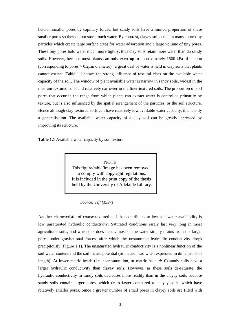
cannot extract. Table 1.1 shows the strong influence of textural class on the available water
capacity of the soil. The window of plant available water is narrow in sandy soils, widest in the
medium-textured soils and relatively narrower in the finer-textured soils. The proportion of soil
pores that occur in the range from which plants can extract water is controlled primarily by
texture, but is also influenced by the spatial arrangement of the particles, or the soil structure.
Hence although clay-textured soils can have relatively low available water capacity, this is only
a generalisation. The available water capacity of a clay soil can be greatly increased by
improving its structure.
Table 1.1 Available water capacity by soil texture
Source: Jeff (1997)
Another characteristic of coarse-textured soil that contributes to low soil water availability is
low unsaturated hydraulic conductivity. Saturated conditions rarely last very long in most
agricultural soils, and when this does occur, most of the water simply drains from the larger
pores under gravitational forces, after which the unsaturated hydraulic conductivity drops
precipitously (Figure 1.1). The unsaturated hydraulic conductivity is a nonlinear function of the
soil water content and the soil matric potential (or matric head when expressed in dimensions of
length). At lower matric heads (i.e. near saturation, or matric head 0) sandy soils have a
larger hydraulic conductivity than clayey soils. However, as these soils de-saturate, the
hydraulic conductivity in sandy soils decreases more readily than in the clayey soils because
sandy soils contain larger pores, which drain faster compared to clayey soils, which have
relatively smaller pores. Since a greater number of small pores in clayey soils are filled with
A NOTE:
This figure/table/image has been removed to comply with copyright regulations. It is included in the print copy of the thesis held by the University of Adelaide Library.

4
water the continuity of water-filled pores remains greater, the tortuosity of flow is smaller, and
so the hydraulic conductivity remains greater compared to that in sandy soils.
Figure 1.1 Relative hydraulic conductivity as a function of matric head for coarse-textured and fine-textured soils.
Soil structure
Soil structure can be defined in terms of form and stability (Kay 1990). Soil structural form
refers to the arrangement of soil particles into stable units called aggregates (Marshall et al.
1996), whereas the stability of soil structure is its ability to retain this arrangement when
exposed to different stresses (Angers and Carter 1996). The composition, size, and arrangement
of pore space located between aggregates are important factors contributing to water storage and
supply for plants. The ability of soil to transmit water depends on the presence of interlinked
pores and on their size and geometry. Pore diameters may range from < 0.2 μm to 10 mm or
more. Pores between 0.2 and 30 μm in diameter are important for storing soil water for later use
by plants. Pores < 30 μm allow rapid absorption of water into soil and pores between 30 and
300 μm are important for infiltration and drainage but generally do not retain water long enough
for plants to use it (Connolly 1998).
It has long been known (e.g.(Doneen and Henderson 1952; Quirk and Schofield 1955; Emerson
and Smith 1970; Bakker 1972) that soil structural stability depends mainly on four soil
properties: exchangeable cations (Ca, Mg, Na, K), electrolyte concentration (or salinity), pH,
and organic matter content. Conditions where there is a preponderance of monovalent
|Matric head|
Sandy soil
Clayey soil
Rel
ativ
e H
ydra
ulic
Con
duct
ivity
5
exchangeable cations (usually Na), low electrolyte concentration, high pH and low organic
matter content all lead to unstable soil structures in which aggregate slaking plus colloid
swelling and dispersion occur. By contrast, divalent exchangeable cations (especially Ca),
modest salt concentrations, neutral pH and high organic matter content all contribute to stable
soil structures. Stability of aggregates and the pores between them plays an important role in
movement and storage of water, aeration, biological activity and the growth of roots.
Aggregates that break down when wet have smaller pores, reduced pore continuity and
increased soil strength upon drying (Cresswell et al. 1992). For example, when aggregates
slake, swell and disperse, the average pore size decreases, which reduces infiltration and
hydraulic conductivity by as much as 2000 times (McIntyre 1958), increases surface crusting
and strength, which reduces root penetration and therefore effectively reduces the amount of
water available for plant extraction (Gupta et al. 1989; McGarry 1990; Lipiec et al. 1991).
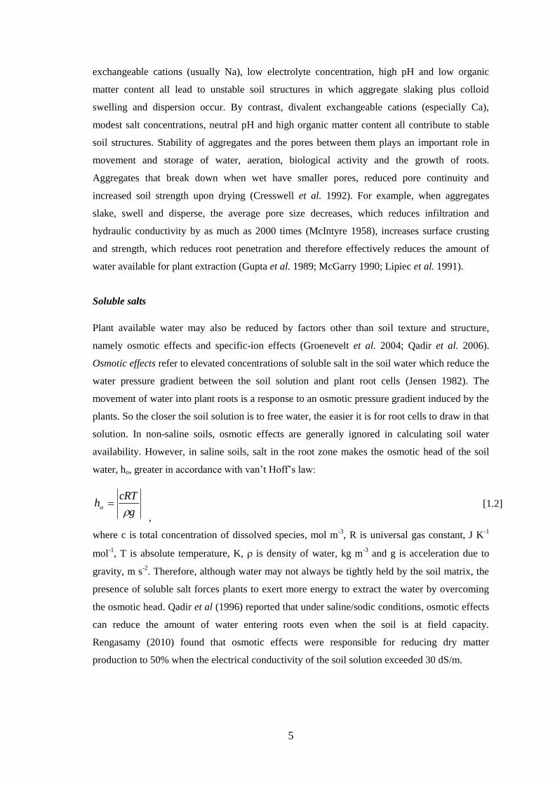
Soluble salts
Plant available water may also be reduced by factors other than soil texture and structure,
namely osmotic effects and specific-ion effects (Groenevelt et al. 2004; Qadir et al. 2006).
Osmotic effects refer to elevated concentrations of soluble salt in the soil water which reduce the
water pressure gradient between the soil solution and plant root cells (Jensen 1982). The
movement of water into plant roots is a response to an osmotic pressure gradient induced by the
plants. So the closer the soil solution is to free water, the easier it is for root cells to draw in that
solution. In non-saline soils, osmotic effects are generally ignored in calculating soil water
availability. However, in saline soils, salt in the root zone makes the osmotic head of the soil
water, ho, greater in accordance with van’t Hoff’s law:
gcRTho �
,
[1.2]
where c is total concentration of dissolved species, mol m-3, R is universal gas constant, J K-1
mol-1, T is absolute temperature, K, � is density of water, kg m-3 and g is acceleration due to
gravity, m s-2. Therefore, although water may not always be tightly held by the soil matrix, the
presence of soluble salt forces plants to exert more energy to extract the water by overcoming
the osmotic head. Qadir et al (1996) reported that under saline/sodic conditions, osmotic effects
can reduce the amount of water entering roots even when the soil is at field capacity.
Rengasamy (2010) found that osmotic effects were responsible for reducing dry matter
production to 50% when the electrical conductivity of the soil solution exceeded 30 dS/m.

6
In addition to osmotic effects, specific ion toxicities sometimes occur in sodic and saline soils
due to the presence of excess concentrations of the cation, Na+, or the anion, Cl-, both of which
interfere with normal physiological cell function in plant roots (Robinson 1971; Zaitseva and
Sudnitsyn 2001). Borate is another ion that commonly occurs at toxic concentrations in solution
with sodium and chloride (Bell 1999). Martin and Koebner (1995) demonstrated that chloride
ion toxicities were partly responsible for the dramatic reduction in vegetative and reproductive
growth in Mexican bread wheat (cv. Glennson) when the plant was exposed to medium-to-high
concentrations of NaCl (180 mM).
Plants differ in their ability to survive and yield satisfactorily when grown in saline soils. There
is much literature on the relative tolerance of different crops to soil salinity obtained under a
vast range of soil, climatic and salinity conditions. Previous studies (Pearson 1959; Kaddah and
Fakhry 1961; Pearson 1961) have shown that tolerance to salinity is not a fixed property of a
species but something that varies with the growth stage of the plant, climatic conditions and
even within the same species for different varieties. Furthermore, the methods used by different
workers to study salt tolerance vary from water culture experiments to field studies where there
is little control over the root zone salinity. Maas and Hoffman (1977) compiled and reviewed
the available data describing the relative (not absolute) salt tolerance of different agricultural
crops (Figure 1.2a). These figures show that, in general, crop yields are not reduced
significantly until a threshold salinity is exceeded, and then the yields decrease approximately
linearly as the salinity continues to increase. The salt tolerance line for each crop was obtained
by calculating a linear regression equation for the yield beyond a threshold point, although the
way in which this threshold was established was rather arbitrary. It is more likely that a
polynomial would describe most crop-response functions (Steppuhn et al. 2005).
The data plotted in Figure 1.2a are for saline conditions only and do not necessarily encompass
the separate effects of sodicity. Barley, for example, is known to be tolerant of saline conditions
(Figure 1.2b) but not very tolerant of sodic conditions, which is mainly due to poor soil aeration
in sodic soils. Similarly cotton, while tolerant of saline conditions, is only moderately tolerant of
sodic conditions, or even sensitive to sodic conditions at some growth stages. On the other hand,
rice is only moderately sensitive to saline conditions (Figure 1.2b) but is highly tolerant of sodic
conditions (Pearson 1959; Kaddah and Fakhry 1961; Pearson 1961).

7
Figure 1.2a “Divisions for classifying crop tolerance to salinity” (after Maas and Hoffman 1977).
Figure 1.2b Response of some grain crops (e.g. rice, corn, wheat, barley) to salinity (after Maas and Hoffman 1977).
A NOTE:
This figure/table/image has been removed to comply with copyright regulations. It is included in the print copy of the thesis held by the University of Adelaide Library.
A NOTE:
This figure/table/image has been removed to comply with copyright regulations. It is included in the print copy of the thesis held by the University of Adelaide Library.

8
One strategy to improve productivity of salt-affected soils is to use a range of plants having
different tolerance to sodicity. Bernstein (1975) observed that the growth of sensitive species
may be affected by soils with an exchangeable sodium percentage (ESP) as low as 10, while
many crops are moderately tolerant of sodicity and may not be affected until the ESP rises to
25. Highly tolerant crops may not be affected until the ESP exceeds 50. Tolerance of high ESP
depends on the ability of the plant to take up Ca and Mg despite low concentrations in the soil
solution and significant competition by Na for uptake (Bernstein 1975; Kinraide et al. 2004).
To link the soil properties with the salt tolerance of different plants, Kopittke and Menzies
(2005) introduced the concept of calcium activity ratio, CAR. CAR is the activity of calcium in
the soil solution is divided by the sum of all cation activities in the soil solution:
, [1.3]
where parentheses denote activity of each cation in solution.
Critical CAR values associated with a 10% reduction in root length were found to be 0.025 for
Mungbean and 0.034 for Rhodes grass across a range of Na concentration and pH in both soil
and solution culture (Kopittke and Menzies 2005). As the soil dries, the concentration of salt in
the soil solution increases, further increasing the osmotic head. To maintain water uptake from a
saline soil, plants must osmo-regulate (Morgan 1984). This is done either by taking up salts and
compartmentalizing them within plant tissue, or by synthesizing organic solutes to generate a
competitive osmotic potential within the plant. Plants which take up salts generally have a
higher salt tolerance and greater ability to store high salt concentrations in plant tissue without
affecting cell processes and are known as halophytes. Plants which synthesise organic solutes
are known as glycophytes and they try to prevent excess salt uptake because they can only
tolerate much lower concentrations of salt in plant tissues before cell processes are adversely
affected. Increasing uptake of salts by halophytic plants to adjust osmotic potential may result in
Na+ and Cl- toxicities. Accumulation of excess Na+ may also cause metabolic disturbances in
processes where low Na+ and high K+ or Ca2+ are required for optimum function (Marschner
1995). A decrease in nitrate reductase activity, inhibition of photosystem II (Orcutt and Nilsen
2000), and chlorophyll breakdown (Krishnamurthy et al. 1987) are all associated with increased
Na+ concentrations. Cell membrane function may be compromised as a result of Na+ replacing
Ca2+, resulting in increased cell leakiness (Orcutt and Nilsen 2000).
9
A study of non-halophytic plant response to salinity (Munns and Termaat 1986) pointed out that
leaf growth is more sensitive than root growth. Regulating leaf expansion in this study was
probably caused by a message from the roots because of the water status (Munns and Termaat
1986). Further research into plant response to salinity indicated that there were two phases
involved in this response, as follows (Munns et al. 1995):
The first phase involved a large decrease in growth rate caused by the salt outside of the roots
(osmotic response) and the second phase was an additional decline in growth caused by ion
toxicity within the plant. Results of a trial that investigated the response of halophytic plants to
salinity showed that all genotypes had a similar reduction in growth with salt. After an initial
period, the more sensitive genotypes showed greater reduction in growth. These data strongly
support the hypothesis of a two-phase response and therefore indicate that any genotypic
differences in the first phase relate to the osmotic effect and not to an ion specific effect. The
second phase began only after toxic levels had accumulated in the leaves in sufficient quantities
to cause leaf necrosis and therefore a resultant reduction in available assimilate (Munns et al.
1995).
The second phase of saline irrigation resulted in a degree of yield reduction that was greatly
affected by the stage of plant development at the time when saline irrigation began. Plots that
received the high salt treatment at an early stage suffered the greatest level of damage,
presumably due to a greater ionic accumulation over time, while a significant interaction
between genotype and salt treatment affected grain yield in this second phase. Munns et al.
(1995) concluded that the length of the first phase was dependent on the concentration of salt in
the soil, transpiration rate and the ability of the genotype to exclude Na. Other researchers
(Delane et al. 1982; Cranner and Bowman 1991; Yeo et al. 1991; Neuman 1993) also found that
the initial response to salinity was dependent on water potential, rather than the specific salt.
1.2.2 Factors affecting soil structure
1.2.2.1 Exchangeable cations
The suite of exchangeable cations on the soil exchange sites has an enormous influence on soil
hydraulic properties. The primary four cations of interest are sodium, calcium, magnesium and
potassium. Each of these will be examined in turn.
10
Sodium
It is generally accepted that exchangeable sodium causes soils to be weakly aggregated, and the
amount of exchangeable sodium is frequently used to represent the physical condition of a soil
(Kemper and Koch 1966). The effect of exchangeable sodium differs depending on the part of
the profile in which it is found. For example, high amounts of exchangeable sodium in the
surface layers will generate poor physical characteristics (e.g. high strength and low
permeability) if this layer is subject to mechanical stress (Rowell et al. 1969).
As the exchangeable sodium content of soil increases, repulsive forces develop between
particles and there is an increasing tendency towards excessive swelling and dispersion of the
colloidal fraction and this destroys soil structure and blocks soil pores (Doneen and Henderson
1952; Baver 1956; Bakker 1972; Bronick and Lal 2005). Even in non-sodic soils, the quality of
soil structure may be diminished by soluble and exchangeable Na (Bakker 1972), depending on
soil pH, clay mineralogy and the presence of electrolytes in the soil solution. Sodic soils may
not disperse if there is sufficient salt to depress swelling and maintain flocculation (Baver
1956).
Many soils around the world exhibit adverse physical properties when ESP > 15 (Richards
1953), although for Australian soils ESP > 5 or 6 is sufficient to generate soil physical problems
(Northcote and Skene 1972; Mikhail 1974).
Calcium
It is widely recognized that exchangeable calcium contributes to a strongly aggregated soil; the
poor structural qualities of sodic soils can be significantly improved if exchangeable sodium is
replaced by both soluble and exchangeable calcium (Bakker 1972; Greene et al. 1978a;
Grierson 1978). Calcium and magnesium are both believed to exert positive effects on soil
structure via cationic bridging with clay and soil organic carbon (Bronick and Lal 2005).
However, Ca2+ is more effective than Mg2+ in improving soil structure (Zhang and Norton
2002).
Magnesium
The effect of exchangeable magnesium on soil aggregate stability is somewhat controversial.
On the one hand, Mg is divalent so it is generally more effective at reducing swelling and
dispersion on its own than say Na. The effects of Mg, however, are not driven by valence alone

11
– they also depend on the prevailing soil conditions. For example, wet, sheared aggregates from
surface soils of low pH were found by Emerson and Smith (1970) to be more susceptible to
dispersion if leached with MgCl2 as opposed to CaCl2; this was thought to be related to the
different effects of Mg and Ca on the solubility of soil organic matter. For example, in a
hydromorphic grey clay-textured soil, which contained mainly montmorillonite, dispersion
occurred when the Mg saturation was > 30% in the presence of organic matter (Bakker 1972).
Regardless of the organic matter content, Joffe and Zimmerman (1945) and Mikhail (1974)
found that soils relatively high in Mg behaved like soils with high exchangeable Na, while soils
with relatively more Ca than Mg could tolerate higher amounts of exchangeable Na without
dispersing. Zhang and Norton (2002) have also noted that Mg2+ may have a deleterious effect on
soil aggregate stability by increasing clay dispersion and that Mg2+ may result in increased
swelling by expanding clays, resulting in disruption of aggregates.
Also, the soil moisture content at which dispersion becomes evident depends on the nature of
the dominant exchangeable cations (Bakker 1972). For example, in remoulded Shepparton fine
sandy loam, Mg-saturated soil begins to disperse at a matric head close to 150 m, whereas Ca-
saturated soil begins to disperse at a significantly greater water content, corresponding to a
matric head of only 1 m. Also the water content for dispersion at a given ESP for a Ca-Na soil is
much greater than that for a Mg-Na soil. This illustrates that the attractive forces between clay
crystals for the Mg-Na system are very low even when the soil is relatively dry.
However, not all soils behave the same in respect to exchangeable cations. For example, Ahmed
et al. (1969) found no difference between the effects of Ca and Mg on aggregate stability and
hydraulic conductivity, while El-Swaify et al. (1970) found no differences in degree of
dispersion, liquid limit and moisture retention for a montmorillonitic soil. Similarly, Koenigs
and Brinkman (1964) considered that low stability originated mainly from a combination of
high exchangeable Na and low organic matter content rather than from high Mg.
Potassium
Potassium, K, can have a similar effect to Na on soil aggregation (Ahmed et al. 1969), and in
some soils the application of potassium fertilizer can lead to soil structural degradation. In such
cases, the addition of K fertilizer needs to be conducted only where there is plenty of organic
matter (e.g. permanent pastures) to resist its dispersive effects. In other soils, however,
application of potassium fertilizer can increase soil aggregate stability and potassium nutrition
and yield of irrigated winter wheat, corn, sugar beet and potatoes. Furthermore, in soils of
relatively high organic matter content and higher pH (e.g. 8.2), Koenigs (1961) found that K-
12
rich aggregates were more water-stable than Mg-rich aggregates. Similarly, Weber and van
Rooyan (1971) concluded that K contributes to structural improvement by reducing the Na/K
ratio, and that exchangeable K seems to have a similar effect to Ca on soil stability if the soil is
acidic and exchangeable K exceeds 7%. Further study on the effect of potassium on soil
structure, Chan et al. (1983) found that at low concentration of K+ on exchange sites, there was
a positive effect on the hydraulic conductivity of sandy soils. However, the hydraulic
conductivity deteriorated at high K+ concentration. In dealing with the effect of potassium on
soil structure, Rengasamy and Marchuk (2011) have introduced the useful concept of ‘cation
ratio of soil structure stability’ (CROSS) which incorporates the differential dispersive powers
of Na and K and the difference in the flocculating effects of Ca and Mg. This work shows that
there is better correlation between CROSS and the hydraulic properties of soils than with SAR
which ignores K+ completely.
1.2.2.2 Organic matter
Organic matter is considered an important agent in maintaining the structural stability of a wide
range of soils such as Mollisols, Alfisols, Ultisols and Inceptisols (Baldock and Nelson 2000).
However, the importance of soil organic matter in soil aggregation tends to be less in some soils
such as Oxisols and Andisols due to the important stabilizing role of hydrous oxides or in
Vertisols which contain sufficient clay with substantial shrink/swell potential (Baldock and
Nelson 2000). In soils where organic matter is an important agent binding mineral particles
together, a hierarchical arrangement of soil aggregates exists in which aggregates break down in
a stepwise manner as the magnitude of an applied disruptive force increases (Tisdall and Oades
1982; Oades and Waters 1991; Oades 1993). In general, there are three levels of soil
aggregation proposed by Golchin et at. (1998): (1) the binding together of clay plates into
packets < 20 um, (2) the binding of clay packets into stable micro-aggregates (20 – 250um),
and (3) the binding of stable micro-aggregates into macro-aggregates (> 250 um). The degree of
aggregation and the stability of soil aggregates generally increases with soil organic carbon
(SOC), clay surface area and CEC. In soils low in SOC or clay concentration, aggregation may
be dominated by cations, whereas in soil with high SOC or clay concentration the role of cations
in aggregation may be minimal (Bronick and Lal 2005).
Soil solution composition and the exchange complex
The composition of soil solution and of the exchange complex are in equilibrium so that a
strong predominance of a particular cation in solution is reflected in its contribution to the
exchange complex. Of the four principal exchangeable cations listed above, potassium has
historically been regarded as the minor one so that sodium, calcium and magnesium are seen as

13
the major cations. The equilibrium between soil solution and the exchange complex is
summarized in the Gapon equation (Bresler et al. 1982):
ESR = kG SAR [1.4]
in which kG is the Gapon constant, ESR is the exchangeable sodium ratio given by:
, [1.5]
and describes the solid exchange complex in which Naexch is exchangeable sodium and CEC is
cation exchange capacity (both expressed as charge per unit mass of solid – e.g. cmol(+)/kg).
SAR is the sodium adsorption ratio given by:
, [1.6]
and describes the soil solution in which [Na+], [Ca2+] and [Mg2+] are the concentrations of the
major cations in mmol/L.
The more commonly used description of the exchange complex, ESP, the exchangeable sodium
percentage, is the percentage of the exchange complex accounted for by sodium:
, [1.7]
and is simply related to ESR as:
, [1.8]
The Gapon equation allows simple predictions of how the exchange complex might change
when soil solution composition changes, for example during irrigation and leaching.
1.2.2.3 Clay swelling and dispersion
Swelling is a process by which soil volume increases with water content and decreases (shrinks)
as water content decreases. The mechanism of swelling in sodic soils is well described by
diffuse double layer theory (van Olphen 1977), which accounts for the spatial distribution of a
diffuse layer of exchangeable cations in the space between negatively charged clay particles.
When clay crystals are in close proximity, their diffuse layers overlap, and the total
14
concentration of the ions mid-way between the particles is greater than that in the soil solution
in which the particles are immersed. The difference in concentrations results in a gradient in
osmotic pressure, which thus draws water in between the particles and causes them to move
further apart (i.e. swell). The double layers are extremely thin (ca. < 10-8 m) and can expand or
compress when the electrolyte concentration of the soil solution decreases or increases,
respectively (Quirk and Schofield 1955; Emerson and Chi 1977; Greene et al. 1978b; Arora and
Coleman 1979). The double layer is generally thinner when divalent cations (e.g. Ca2+, Mg2+)
balance the charge and it is thicker when monovalent cations such as Na+ are involved (Quirk
and Schofield 1955). Sodic soils have an elevated proportion of sodium ions on the exchange
complex (exchangeable sodium percentage, ESP > 6) and because sodium is monovalent it
cannot overcome the swelling forces in the double layer, so the clay particles swell and disperse
(Quirk 1986). In pure sodium montmorillonite (i.e. when the entire permanent charge of the
lattice surface is balanced by Na+ ions), large diffuse double layers occur on all clay surfaces
(Warkentin and Schofield 1962; Shainberg et al. 1971; Shainberg and Letey 1984). In dilute
electrolyte solutions, crystalline swelling can produce ten to twenty times the initial dry volume;
in more concentrated electrolytes, swelling is suppressed because the osmotic potential gradient
between the overlapping counter-ions of clay particles and the soil solution decreases
(Warkentin and Schofield 1962). Swelling of Ca-montmorillonite, by contrast, is limited
regardless of electrolyte concentration. This is because, firstly, Ca2+ largely resides in the Stern
layer (or adsorbed layer) and so the diffuse layer is far less populated. Secondly, the crystalline
swelling is not affected by the concentration of calcium with which the clay is in contact (Quirk
1994). Furthermore, when Ca-saturated montmorillonite platelets aggregate in groups of four to
nine platelets, called ‘tactoids’ (Blackmore and Miller 1961), the tactoids effectively reduce the
surface area of the montmorillonite and make them behave like larger particles – thus the
diffuse double layer can only fully manifest itself on the outside surfaces of the ‘tactoids’
(Sumner 1993) – this reduces overall swelling.
When swelling becomes excessive, this leads to dispersion in which clay particles become
separated and move independently of one another. Dispersion usually occurs in sodic soils
where excessive amounts of exchangeable Na are present. When unconfined clays swell in
water, the presence of Na on the exchange sites allows more water to enter between clay
particles and force them apart. The swelling and consequent dispersion both result in an overall
distribution of very small pores due to pore closure and blockage, which degrades the soil
structure, restricts water movement, and discourages root growth (Rengasamy 1983).
15
The minimum total electrolyte concentration required to prevent clay dispersion is called the
‘threshold concentration’ (Quirk and Schofield 1955). Whatever the ESP, the permeability of an
irrigated soil can be maintained by adjusting the electrolyte concentration of the irrigation water
to keep it above the ‘threshold concentration’. The greater the ESP the larger must be the
threshold concentration in the soil solution to maintain permeability. Furthermore, the threshold
concentration depends on the nature of the clay mineral. In Na/Ca systems of montmorillonite
and illite, Oster et al. (1980) found that increasing Na (at relatively low ESP), significantly
raised the threshold concentration required to maintain permeability. This effect was more
pronounced for montmorillonite than for illite; that is, at the same ESP, illite had a higher
threshold concentration than montmorillonite because attractive forces in illite are often smaller
due to differences in edge-to-face surfaces and their irregular step-like surfaces, which cause
mismatching and weaker net attraction between particles (Oster et al. 1980).
More recently Rengasamy and Marchuk (2011) and Marchuk and Rengasamy (2012) have
introduced the “cation ratio of soil structural stability” (CROSS) which provides a more
complete picture of the role of all four of the common exchangeable cations (Ca, Mg, Na, K) in
soil dispersion.
1.2.2.4 Nutritional effects
High levels of exchangeable sodium, and the frequent accompanying high pH of sodic soils,
also restrict the biological transformations and availability of several essential plant nutrients.
For example, the concentrations of calcium and magnesium in soil solution decline as pH
increases due to the formation of relatively insoluble calcium and magnesium carbonates by
reaction with the soluble carbonates that are the causes of the high pH.
Nitrogen deficiency is also a common problem in sodic soils. Excess sodium on the soil
exchange complex imparts structural instability to the soil and causes poor physical properties.
The infiltration rate of the soil is low so that it has restricted internal drainage. For this reason
the surface soil layers remain nearly saturated for prolonged periods following irrigation or rain
resulting in temporary anaerobic conditions. Under alternate aerobic and anaerobic conditions,
loss of nitrogen inevitably occurs through denitrification and volatilization (Patrick and Wyatt
1964). Van Hoorn (1958) also pointed out that under conditions of poor soil structure, twice as
much nitrogen was needed as under conditions of good soil structure.
Phosphorus deficiency in sodic soils is not generally a major problem. Chhabra (1985) reported
that sodic soils contained high concentrations of extractable phosphorus and that there was a
16
positive correlation between soluble P status and the electrical conductivity. Chhabra et al.
(1981) also observed that crops grown in freshly reclaimed sodic soils did not respond to
applied P fertilizer for 4 – 5 years because of their high available P status. However, the
presence of high concentrations of sodium carbonate and soluble P in sodic soils was associated
with calcium deficiencies due to precipitation of calcium phosphates and carbonates from soil
solution.
Potassium nutrition in sodic soils is not clearly understood yet. Some studies indicate that
increasing soil sodicity causes reduced uptake of potassium by crops (Singh et al. 1979), while
other studies (e.g. Martin et al. (1965) and Chhabra (1985) showed the opposite effect. High pH
and presence of calcium carbonate in sodic soil can lead to micronutrient deficiencies; for
example, iron is often limiting in sodic soils. By contrast, boron and molybdenum are rarely
limiting in sodic soils; in fact, they are often present at toxic concentrations. At high pH and
sodicity, boron and molybdenum are present as highly soluble forms that can be taken up by
plants and accumulate in excessive quantities (Pasricha and Randhawa 1971).
1.2.3 Effects of soil structure on soil strength, aeration, and hydraulic conductivity
Soil strength
As mentioned in Section 1.2.1 above, soil aggregates and their stability have an enormous
impact on soil structure and strength (Marshall et al. 1996; Kay 1990; Horn et al. 1995). When
structure becomes unstable or if smaller aggregates are generated, the packing density increases,
inter-particle contacts increase, pore sizes decrease and the overall strength of the soil at a given
water content increases (Lal and Shukla 2004) Horn et al. (1995) also found that soils with
smaller aggregates have greater tensile strength compared to soils with larger soil aggregates,
and that this increases over time with wetting and drying (Figure 1.3)..
This sort of structural degradation is common in saline/sodic soils, which often develop surface
crusts of high packing density and become hardsetting as they dry (Northcote 1979). Crusts
reduce infiltration, increase runoff and have high strength which can reduce crop emergence and
root exploration. Hardsetting soils are unstable when wet and they slump after cultivation to a
density similar to that before cultivation. Because of high density and low macro-porosity they
have low hydraulic conductivity.
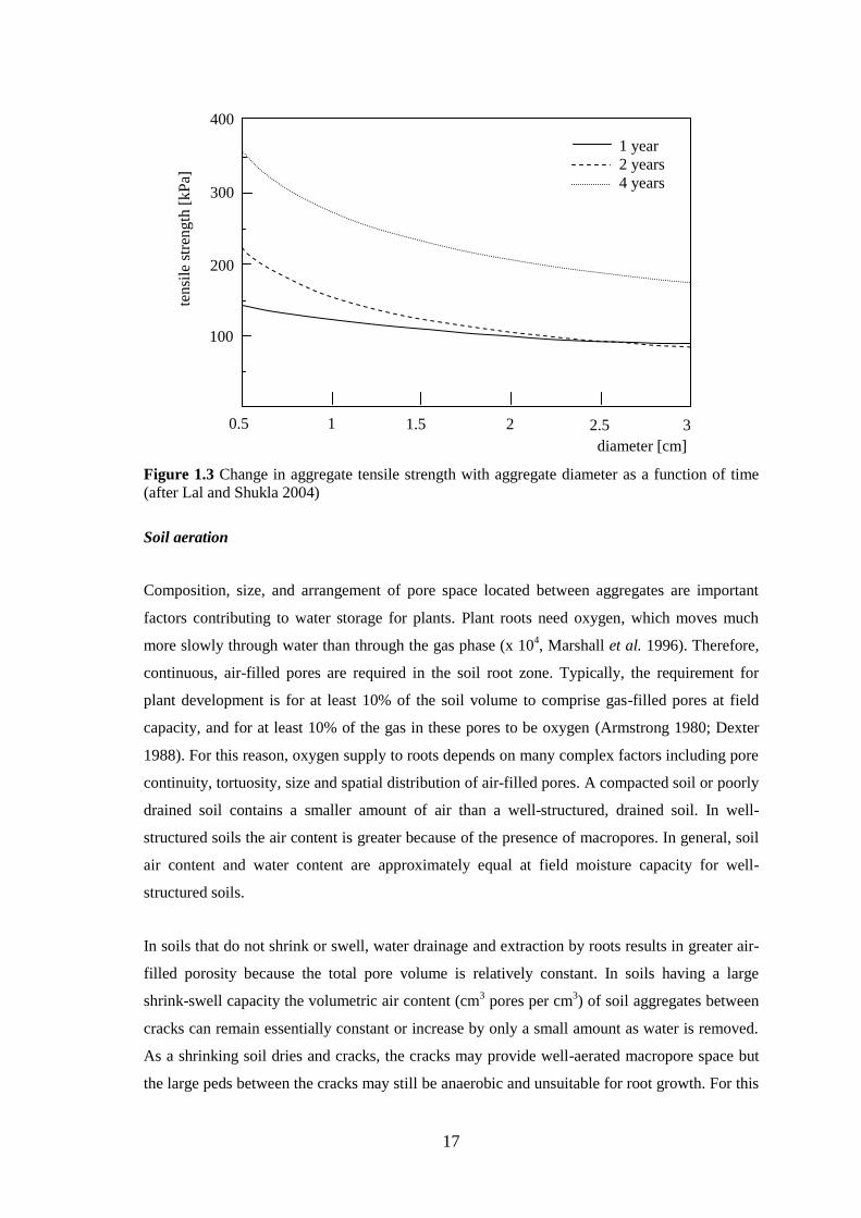
17
Figure 1.3 Change in aggregate tensile strength with aggregate diameter as a function of time (after Lal and Shukla 2004)
Soil aeration
Composition, size, and arrangement of pore space located between aggregates are important
factors contributing to water storage for plants. Plant roots need oxygen, which moves much
more slowly through water than through the gas phase (x 104, Marshall et al. 1996). Therefore,
continuous, air-filled pores are required in the soil root zone. Typically, the requirement for
plant development is for at least 10% of the soil volume to comprise gas-filled pores at field
capacity, and for at least 10% of the gas in these pores to be oxygen (Armstrong 1980; Dexter
1988). For this reason, oxygen supply to roots depends on many complex factors including pore
continuity, tortuosity, size and spatial distribution of air-filled pores. A compacted soil or poorly
drained soil contains a smaller amount of air than a well-structured, drained soil. In well-
structured soils the air content is greater because of the presence of macropores. In general, soil
air content and water content are approximately equal at field moisture capacity for well-
structured soils.
In soils that do not shrink or swell, water drainage and extraction by roots results in greater air-
filled porosity because the total pore volume is relatively constant. In soils having a large
shrink-swell capacity the volumetric air content (cm3 pores per cm3) of soil aggregates between
cracks can remain essentially constant or increase by only a small amount as water is removed.
As a shrinking soil dries and cracks, the cracks may provide well-aerated macropore space but
the large peds between the cracks may still be anaerobic and unsuitable for root growth. For this
0.5 1 1.5 2 2.5 3
100
200
300
400
diameter [cm]
tens
ile st
reng
th [k
Pa]
1 year 2 years 4 years

18
reason, only a small proportion of the total soil volume may be exploitable by roots in
swelling/shrinking soils.
Hydraulic conductivity
Stability of aggregates during wetting, and while wet, plays an important role in supplying
water for plants. Aggregates that break down when they are wet have smaller pores, reduced
pore continuity and increased strength upon drying (Cresswell et al. 1992). These all reduce
root penetration, decrease infiltration rate and hydraulic conductivity, and therefore effectively
reduce the amount of water available for plant extraction (Gupta et al. 1989; McGarry 1990;
Lipiec et al. 1991).
1.2.4 Salt-affected soils and their reclamation
Salt-affected soils refer to those exposed to soluble salts during some stage in their history. The
salts involved may include chlorides, sulphates, carbonates and bicarbonates of sodium,
potassium, magnesium and calcium, although the most common salt is sodium chloride. In
general soil salinity in Australia can be classified into two main types: transient salinity and
groundwater salinity. Transient salinity involves a seasonal accumulation of salts in the root-
zone (Rengasamy 2002) and ground-water salinity relates to upward movement of water and
salt by capillarity from a shallow saline water table. In both cases soils become saline when
enough salt remains in the root zone to adversely affect plant growth. Apart from the osmotic
effect of salts in the soil solution, excessive concentration and absorption of individual ions may
prove toxic to the plants and/or may retard the absorption of other essential plant nutrients.
In cases where much of the salt has left the soil profile yet appreciable amounts of exchangeable
sodium remain, the soil is considered to be sodic but not necessarily saline. The criteria used to
classify soils as being either saline or sodic vary across the world. In the United States, salt-
affected soils are classified on the basis of the characteristics of a saturated soil-paste extract
(Richards 1953). In Australia, soils are classified for salinity and sodicity according to the
nature and texture of the whole soil profile and whether the salts are concentrated in the root
zone or at depth (Northcote and Skene 1972). The different criteria for classification are show in
Table 1.3.
Excess soluble salt in soils keeps the clay in a flocculated state so the structure of these soils is
generally good and tillage characteristics and permeability to water can be even better than
those of some non-saline soils. However, when leached with water of low salinity, some saline
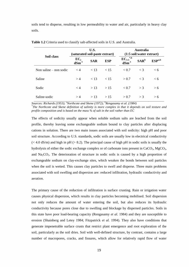
19
soils tend to disperse, resulting in low permeability to water and air, particularly in heavy clay
soils.
Table 1.2 Criteria used to classify salt-affected soils in U.S. and Australia.
Soil class
U.S. (saturated soil-paste extract) Australia
(1:5 soil:water extract) ECe
dSm-1 SAR ESP EC1:5*,b
dSm-1 SARb ESPa,b
Non saline – non sodic < 4 < 13 < 15 < 0.7 < 3 < 6
Saline > 4 < 13 < 15 > 0.7 < 3 < 6
Sodic < 4 > 13 > 15 < 0.7 > 3 > 6
Saline-sodic > 4 > 13 > 15 > 0.7 > 3 > 6
Sources: Richards (1953); aNorthcote and Skene (1972); bRengasamy et al. (1984) *The Northcote and Skene definition of salinity is more complex in that it depends on soil texture and profile composition and is based on the mass % of salt in the soil rather than EC
The effects of sodicity usually appear when soluble sodium salts are leached from the soil
profile, thereby leaving some exchangeable sodium bound to clay particles after displacing
cations in solution. There are two main issues associated with soil sodicity: high pH and poor
soil structure. According to U.S. standards, sodic soils are usually low in electrical conductivity
(< 4.0 dS/m) and high in pH (> 8.2). The principal cause of high pH in sodic soils is usually the
hydrolysis of either the sodic exchange complex or of carbonate ions present in CaCO3, MgCO3,
and Na2CO3. The deterioration of structure in sodic soils is caused by a high proportion of
exchangeable sodium on clay-exchange sites, which weaken the bonds between soil particles
when the soil is wetted. This causes clay particles to swell and disperse. Three main problems
associated with soil swelling and dispersion are: reduced infiltration, hydraulic conductivity and
aeration.
The primary cause of the reduction of infiltration is surface crusting. Rain or irrigation water
causes physical dispersion, which results in clay particles becoming mobilised. Soil dispersion
not only reduces the amount of water entering the soil, but also reduces its hydraulic
conductivity because pores close due to swelling and blockage by dispersed particles. Soils in
this state have poor load-bearing capacity (Rengasamy et al. 1984) and they are susceptible to
erosion (Shainberg and Letey 1984; Fitzpatrick et al. 1994). They also have conditions that
generate impenetrable surface crusts that restrict plant emergence and root exploration of the
soil, particularly as the soil dries. Soil with well-defined structure, by contrast, contains a large
number of macropores, cracks, and fissures, which allow for relatively rapid flow of water

20
through the soil. If water cannot pass through the soil, the upper layers can become
waterlogged. This results in anaerobic soils which can reduce or prevent plant growth and
decrease organic matter decomposition rate (Shainberg and Letey 1984; Quirk 1986;
Rengasamy and Sumner 1998).
Both swelling and dispersion are governed by the balance between attractive and repulsive
forces that arise from intermolecular and electrostatic interactions between aqueous and solid
phases in the soil (Rengasamy 1983); each will now be considered in the context of reclaiming
saline/sodic soils.
Two important aspects control the effective reclamation of saline/sodic soils: 1) reducing or
removing exchangeable Na by displacement and leaching, and 2) maintaining the electrolyte
concentration at levels that prevent clay dispersion during leaching (i.e. above the threshold
concentration). Removing Na+ involves its displacement by adding Ca2+. Maintaining the
electrolyte concentration involves the gradual reduction of salinity by leaching during this
displacement of Na+ with Ca2+.
These two requirements are usually achieved in the field by applying gypsum (calcium
sulphate), which is moderately soluble, readily available commercially, and relatively cheap
(Sumner 1993). Maintaining sufficient electrolyte concentrations is crucial because it maintains
water intake on which reclamation depends (Oster 1993). For example, McGeorge and Fuller
(1950) found that Cajon soil in Arizona (high ESP) experienced degradation of soil structure
when irrigated with low electrolyte water – they did not understand the threshold concentration
concept outlined later by Quirk and Schofield (1955). An extensive area of highly sodic pasture
soil (ESP 23) in the Riverina District of New South Wales faced the same problem which was
fixed by dissolving gypsum in irrigation water to decrease solution SAR and to increase the
electrolyte concentration above the threshold value (Davidson and Quirk 1961).
The salt used to keep the electrolyte concentration above the threshold need not be calcium-
based, at least in the first instance. For example, Amemiya et al. (1956) reclaimed a saline-
alkaline soil (ESP 37) in the Coachella Valley of California by mixing sea water with water
from the Colorado River to keep the electrolyte concentration above the threshold value – this
maintained soil permeability while the sea water was gradually diluted and calcium introduced,
and this reduced the period required for reclamation considerably.
Adding gypsum to some Australian red-brown earths (Glenloth and Raywood soils) reduced
ESP and clay dispersion; this also reduced soil strength and increased hydraulic conductivity

21
(Greene et al. 1988). Gypsum can also be added strategically, as done by Kamphorst (1990),
who introduced a solution of gypsum down into soil cracks during the dry season to stabilize the
material on the exterior surfaces of soil peds. This retarded crack-closure during the wet season,
which permitted downward transport of water and salts, improved topsoil aeration and vertical
extension of roots.
Aside from using calcium salts to reclaim sodic soils, one can also add organic polymers into
irrigation water to stabilise the structure and permeability (Kamphorst 1990; El-Morsy et al.
1991). For example, when polyacrylamide (PAM) is added to irrigation water, it can reduce
swelling and dispersion in mildly sodic soils at low EC (Aly and Letey 1990) and can also
increase hydraulic conductivity and leaching of sodic soils (El-Morsy et al. 1991; Zahow and
Amrhein 1992).
In the process of reclaiming saline, alkaline and sodic soils, plants can be used at certain stages
to enhance chemical and physical properties (Qadir et al. 1996). For example, in calcareous
soils, rice can be grown under flooded and ponded conditions in places where plenty of good-
quality water is available. Root and microbial growth in flooded conditions raises the
concentration of CO2 and thus increases the solubility of calcium carbonate (Shainberg and
Oster 1978). Other studies have found that growing Kallar grass over several years can improve
soil organic matter content, hydraulic conductivity, porosity, water retention, structural stability
and plant available water, at least in the surface soil (Akhter et al. 2004).
1.2.5 Models of plant available water
1.2.5.1 Historical models
The above-mentioned factors all influence the amount of water that a plant can extract from the
soil. Until relatively recently, however, most of these factors have not been taken into account
in models to calculate PAW. Early use of the term ‘PAW’ referred to the quantity of water in
the soil ranging from a nominal ‘field capacity’ to a nominal ‘permanent wilting point’
(Veihmeyer and Hendrickson 1927). Field capacity referred to the soil water content at which
excess water after a saturating rain or irrigation drained by gravitational force (in the absence of
evaporation) over a period of several days. The concept was agronomic and was only loosely
linked to a soil matric head (Simmonds et al. 1995). In fact, several different matric heads have
been proposed in different parts of the world (Groenevelt et al. 2001). The ‘permanent wilting
point’, PWP, referred to the soil water content remaining in the soil after plants wilted during

22
the day and did not recover even if placed in an atmosphere of 100% relative humidity
(Veihmeyer and Hendrickson 1949).
The range of soil water content between field capacity and permanent wilting point is rather
imprecise and so cannot accurately define the amount of water that plants can extract from the
soil. This concept of PAW relies on an assumption of equally available water between two
critical potentials, field capacity and permanent wilting point. In reality, it is clear that the
energy plants require to extract a unit of water from soil at field capacity is much lower than at
the permanent wilting point. Furthermore, PAW is also influenced by other factors such as soil
aeration, soil strength, hydraulic conductivity, and salinity. One might observe in some soils, for
example that during drying, plants can extract soil water well beyond PWP. In the same soil
when physical conditions are poor, however, water extraction may stop even when the soil is
quite wet, and certainly before it reaches PWP. Richards and Wadleigh (1952) remarked that the
concept plant water availability should involve two notions: the ability of plant roots to absorb
and use water with which it is in contact, and the readiness or velocity with which the soil water
moves into the root zone to replace that which has been taken up by the plant. Hillel (1971) felt
less confident that soil properties alone could be used to predict soil water availability – he felt
that soil water availability could only be assessed accurately using real plants in real soils under
real meteorological conditions.
To integrate soil physical properties associated with plant growth into the concept of PAW,
Letey (1985) introduced the qualitative concept called the Non-Limiting Water Range, NLWR,
which referred to the range of soil water contents across which limitations to plant growth were
negligible. Water uptake by roots was considered to be directly affected by soil physical
conditions, particularly aeration and mechanical resistance. Accordingly the NLWR became
narrower under conditions of poor aeration and high soil strength (Fig 1.4b) relative to that of
soil of good structural condition (Fig 1.4a).
Da Silva et al. (1994) refined this concept to make it quantitative and called it the Least
Limiting Water Range, LLWR. The LLWR merged the classical water contents at FC and PWP
with those at critical limits of soil aeration and mechanical resistance. In wet soils the upper
limit of LLWR corresponded to the water content at FC (matric head = 1 m), but if the
volumetric air content was less than a cut-off value of 0.10 m3/m3 (selected as being important
from historical literature), then the upper limit of LLWR was adjusted downward until the
volumetric air content reached 0.10. At the dry end, water availability was thought to diminish
due to increasing soil strength such that plant roots could not explore the soil to extract the
water; many plant roots cannot grow into soils that have a penetration resistance > 2 MPa

23
(Cockroft et al. 1969). If soil resistance to penetration was sufficiently low for root proliferation
(< 2 MPa) then the lower limit of LLWR corresponded to the water content at 150 m. However,
if penetration resistance was > 2 MPa before the soil dried to 150 m the lower limit of LLWR
was adjusted upward to a water content where the soil resistance = 2 MPa. The effect of
increasing bulk density on LLWR is shown in Figure 1.5.
Although LLWR incorporated some of the physical limitations affecting water availability (e.g.
aeration, strength) it did not deal with other equally important limitations such as declining
hydraulic conductivity and increasing osmotic stress in unsaturated soils. Furthermore, it used
abrupt cut-off points, whereas real plants experience (and respond to) physical and chemical
limitations in a gradual fashion rather than abruptly.
In earlier work, Feddes et al. (1978) introduced a model that used ‘reduction coefficients’
(varying between 0 and 1) to incorporate various physical and chemical limitations affecting
soil water availability. Their ‘reduction functions’ were fairly simple (linear) and did not
account for the complex nature of plant responses to soil limitations.
Eliminating the complexity of soil limiting factors (e.g. soil strength, aeration, hydraulic
conductivity) that affect plant ability to extract water from soil, Minasny and McBratney (2003)
introduced the concept of integral energy which focuses on the quantity of energy required by
the plant to remove a unit amount of water from the soil. The energy was calculated from the
integral of the soil water retention curve. This work indicated that the energy required to remove
the same amount water from a silty clay soil (within the range FC and PWP) was almost 1.5
times higher than that of clay soil (Minasny and McBratney 2003). The integral energy concept
is important in terms of plant physiology as it considers the plant energy requirements for water
uptake.

24
1.4(a)
1.4(b)
Figure 1.4 The non-limiting water range (NLWR) of water contents as influenced by restricting soil factors for plant growth in soil with (a) good structure and (b) poor structure (Letey 1985).
Figure 1.5 Effect of increasing bulk density on the water content at which volumetric air content = 0.10m3/m3 and soil resistance = 2 MPa, superimposed on the water contents at FC and PWP (after da Silva et al.(1994)); shaded area represents LLWR.
Water content
Fiel
d ca
paci
ty
Perm
anen
t w
iltin
g po
int NLWR
Unavailable water due to rapid drainage (textual limitation)
Water here is held in pores too small to be extracted by most plants (textural limitation)
Water content
Perm
anen
t w
iltin
g po
int NLWR
Water here is unavailable due to mechanical (textural and structural limitation)
Unavailable water due to poor aeration (textural and structural limitation)
Fiel
d ca
paci
ty
A NOTE:
This figure/table/image has been removed to comply with copyright regulations. It is included in the print copy of the thesis held by the University of Adelaide Library.
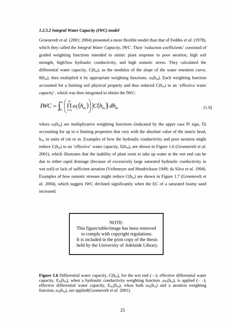
25
1.2.5.2 Integral Water Capacity (IWC) model
Groenevelt et al. (2001; 2004) presented a more flexible model than that of Feddes et al. (1978),
which they called the Integral Water Capacity, IWC. Their ‘reduction coefficients’ consisted of
graded weighting functions intended to mimic plant response to poor aeration, high soil
strength, high/low hydraulic conductivity, and high osmotic stress. They calculated the
differential water capacity, C(hm), as the modulus of the slope of the water retention curve,
�(hm), then multiplied it by appropriate weighting functions, ωi(hm). Each weighting function
accounted for a limiting soil physical property and thus reduced C(hm) to an ‘effective water
capacity’, which was then integrated to obtain the IWC:
� � mmmi
n
idhhChIWC �
���
����
0 1�
[1.9]
where ωi(hm) are multiplicative weighting functions (indicated by the upper case Pi sign, Π)
accounting for up to n limiting properties that vary with the absolute value of the matric head,
hm, in units of cm or m. Examples of how the hydraulic conductivity and poor aeration might
reduce C(hm) to an ‘effective’ water capacity, E(hm), are shown in Figure 1.6 (Groenevelt et al.
2001), which illustrates that the inability of plant roots to take up water at the wet end can be
due to either rapid drainage (because of excessively large saturated hydraulic conductivity in
wet soil) or lack of sufficient aeration (Veihmeyer and Hendrickson 1949; da Silva et al. 1994).
Examples of how osmotic stresses might reduce C(hm) are shown in Figure 1.7 (Groenevelt et
al. 2004), which suggest IWC declined significantly when the EC of a saturated loamy sand
increased.
Figure 1.6 Differential water capacity, C(hm), for the wet end (—); effective differential water capacity, EK(hm), when a hydraulic conductivity weighting function ,ωK(hm), is applied (– –); effective differential water capacity, EKa(hm), when both ωK(hm) and a aeration weighting function, ωa(hm), are applied(Groenevelt et al. 2001).
A NOTE:
This figure/table/image has been removed to comply with copyright regulations. It is included in the print copy of the thesis held by the University of Adelaide Library.
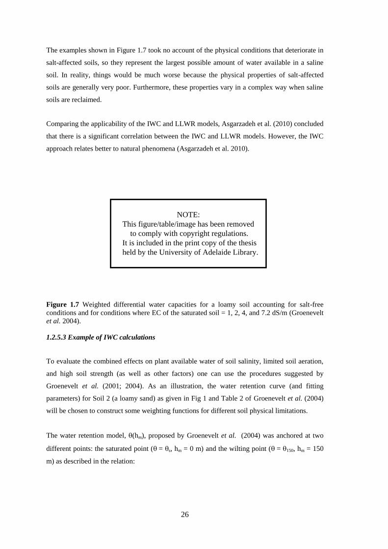
26
The examples shown in Figure 1.7 took no account of the physical conditions that deteriorate in
salt-affected soils, so they represent the largest possible amount of water available in a saline
soil. In reality, things would be much worse because the physical properties of salt-affected
soils are generally very poor. Furthermore, these properties vary in a complex way when saline
soils are reclaimed.
Comparing the applicability of the IWC and LLWR models, Asgarzadeh et al. (2010) concluded
that there is a significant correlation between the IWC and LLWR models. However, the IWC
approach relates better to natural phenomena (Asgarzadeh et al. 2010).
Figure 1.7 Weighted differential water capacities for a loamy soil accounting for salt-free conditions and for conditions where EC of the saturated soil = 1, 2, 4, and 7.2 dS/m (Groenevelt et al. 2004).
1.2.5.3 Example of IWC calculations
To evaluate the combined effects on plant available water of soil salinity, limited soil aeration,
and high soil strength (as well as other factors) one can use the procedures suggested by
Groenevelt et al. (2001; 2004). As an illustration, the water retention curve (and fitting
parameters) for Soil 2 (a loamy sand) as given in Fig 1 and Table 2 of Groenevelt et al. (2004)
will be chosen to construct some weighting functions for different soil physical limitations.
The water retention model, �(hm), proposed by Groenevelt et al. (2004) was anchored at two
different points: the saturated point (��= �s, hm = 0 m) and the wilting point (��= �150, hm = 150
m) as described in the relation:
A NOTE:
This figure/table/image has been removed to comply with copyright regulations. It is included in the print copy of the thesis held by the University of Adelaide Library.
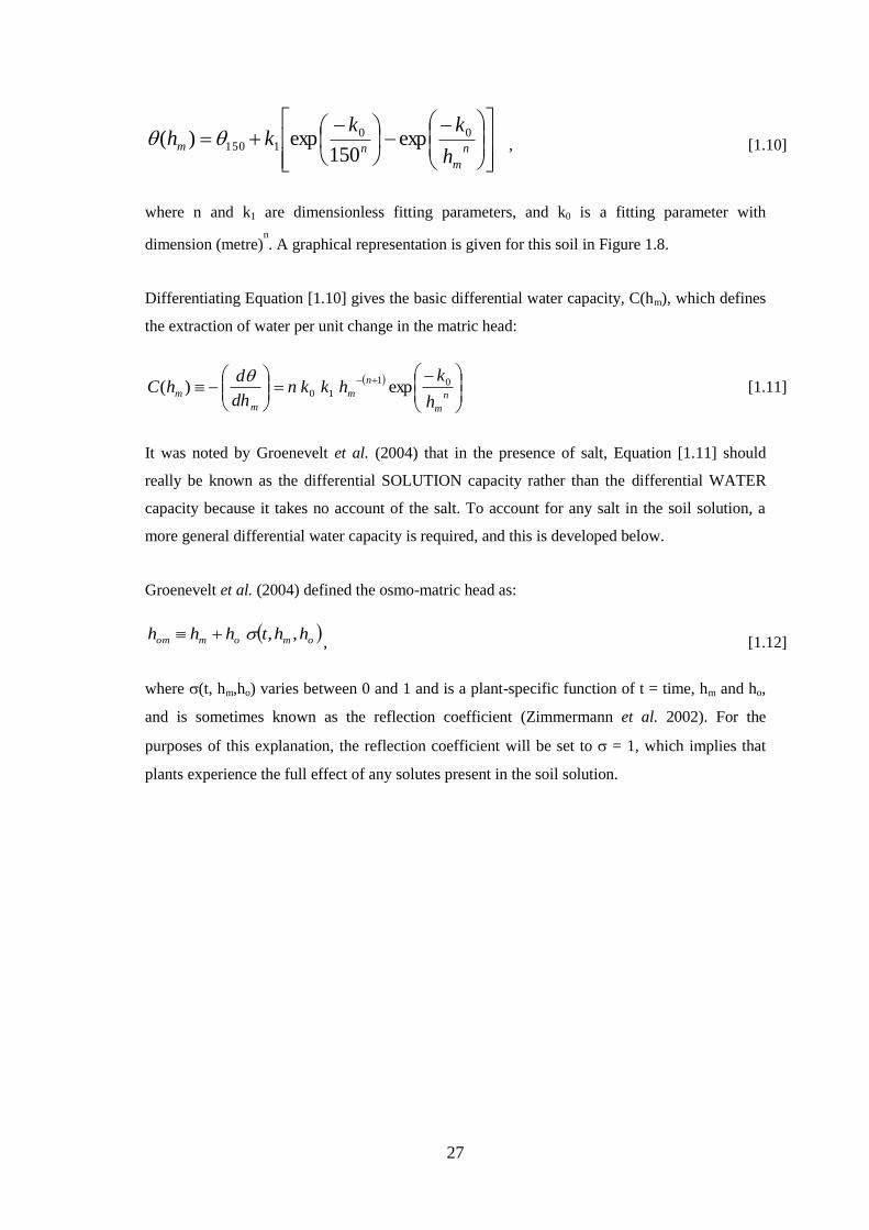
27
���
�
���
����
����
� �����
��� �� n
mnm h
kkkh 001150 exp
150exp)( �� , [1.10]
where n and k1 are dimensionless fitting parameters, and k0 is a fitting parameter with
dimension (metre)n. A graphical representation is given for this soil in Figure 1.8.
Differentiating Equation [1.10] gives the basic differential water capacity, C(hm), which defines
the extraction of water per unit change in the matric head:
����
����
� ����
����
��� ��
nm
nm
mm h
khkkndhdhC 01
10 exp)( � [1.11]
It was noted by Groenevelt et al. (2004) that in the presence of salt, Equation [1.11] should
really be known as the differential SOLUTION capacity rather than the differential WATER
capacity because it takes no account of the salt. To account for any salt in the soil solution, a
more general differential water capacity is required, and this is developed below.
Groenevelt et al. (2004) defined the osmo-matric head as:
�omomom hhthhh ,,��� , [1.12]
where �(t, hm,ho) varies between 0 and 1 and is a plant-specific function of t = time, hm and ho,
and is sometimes known as the reflection coefficient (Zimmermann et al. 2002). For the
purposes of this explanation, the reflection coefficient will be set to � = 1, which implies that
plants experience the full effect of any solutes present in the soil solution.
28
���
����
���
omomom dh
dhC �)(
���
����
���
���
����
����
����
����
���
om
mm
om
m
mmom dh
dhhCdhdh
dhdhC )()( �
Figure 1.8 Representation of the water retention curve using data and model for a loamy sand published in Groenevelt et al. (2004).
Equations [1.11] and [1.12] allow one to define the soil water capacity in terms of the total or
‘osmo-matric’ head, hom,:
. [1.13]
One can apply the chain rule to Equation [1.13] to re-define the soil solution capacity, Com(hom),
in terms of the more useful matric head, Com(hm):
. [1.14]
Equation [1.14] suggests (as a first approximation) that a relevant weighting function
accounting for the osmotic effects of solutes is simply the rate of change in the matric head per
unit change in the osmo-matric head, dhm/dhom, viz.
om
mmo dh
dhh �)(� . [1.15]
A NOTE:
This figure/table/image has been removed to comply with copyright regulations. It is included in the print copy of the thesis held by the University of Adelaide Library.
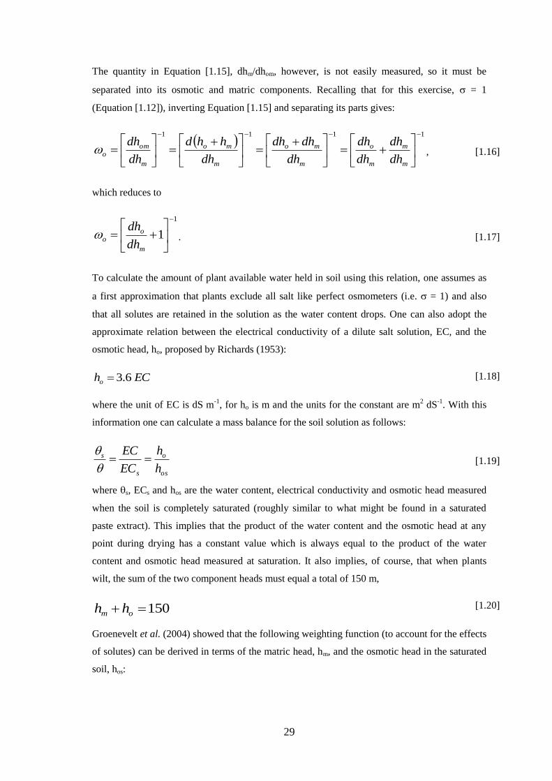
29
ECho 6.3
os
o
s
s
hh
ECEC
��
150� om hh
The quantity in Equation [1.15], dhm/dhom, however, is not easily measured, so it must be
separated into its osmotic and matric components. Recalling that for this exercise, � = 1
(Equation [1.12]), inverting Equation [1.15] and separating its parts gives:
� 1111 ����
��
���
���
�
���
� ��
�
���
� ��
�
���
�
m
m
m
o
m
mo
m
mo
m
omo dh
dhdhdh
dhdhdh
dhhhd
dhdh
� , [1.16]
which reduces to
1
1�
��
���
��
m
oo dh
dh� . [1.17]
To calculate the amount of plant available water held in soil using this relation, one assumes as
a first approximation that plants exclude all salt like perfect osmometers (i.e. � = 1) and also
that all solutes are retained in the solution as the water content drops. One can also adopt the
approximate relation between the electrical conductivity of a dilute salt solution, EC, and the
osmotic head, ho, proposed by Richards (1953):
[1.18]
where the unit of EC is dS m-1, for ho is m and the units for the constant are m2 dS-1. With this
information one can calculate a mass balance for the soil solution as follows:
[1.19]
where �s, ECs and hos are the water content, electrical conductivity and osmotic head measured
when the soil is completely saturated (roughly similar to what might be found in a saturated
paste extract). This implies that the product of the water content and the osmotic head at any
point during drying has a constant value which is always equal to the product of the water
content and osmotic head measured at saturation. It also implies, of course, that when plants
wilt, the sum of the two component heads must equal a total of 150 m,
[1.20]
Groenevelt et al. (2004) showed that the following weighting function (to account for the effects
of solutes) can be derived in terms of the matric head, hm, and the osmotic head in the saturated
soil, hos:
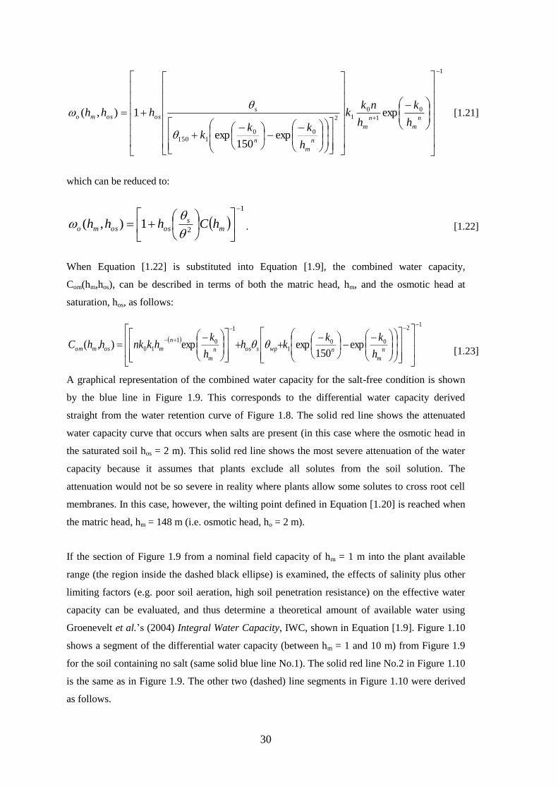
30
�
12
001
1
0110 exp
150expexp),(
���
��
��
�
�
��
�
�
���
�
���
����
����
����
����
� �����
��� ���
���
�
���
����
����
� � n
mnwpsosn
m
nmosmom h
kkkhh
khknkhhC ��
1
01
012
001150
exp
exp150
exp
1),(
�
�
������
�
�
������
�
�
���
����
� �
������
�
�
������
�
�
���
�
���
�
���
����
����
����
� �����
��� ��
� nm
nm
nm
n
sososmo h
kh
nkk
hkk
k
hhh
�
�� [1.21]
which can be reduced to:
�1
21),(�
��
���
����
���� m
sososmo hChhh��
� . [1.22]
When Equation [1.22] is substituted into Equation [1.9], the combined water capacity,
Com(hm,hos), can be described in terms of both the matric head, hm, and the osmotic head at
saturation, hos, as follows:
[1.23]
A graphical representation of the combined water capacity for the salt-free condition is shown
by the blue line in Figure 1.9. This corresponds to the differential water capacity derived
straight from the water retention curve of Figure 1.8. The solid red line shows the attenuated
water capacity curve that occurs when salts are present (in this case where the osmotic head in
the saturated soil hos = 2 m). This solid red line shows the most severe attenuation of the water
capacity because it assumes that plants exclude all solutes from the soil solution. The
attenuation would not be so severe in reality where plants allow some solutes to cross root cell
membranes. In this case, however, the wilting point defined in Equation [1.20] is reached when
the matric head, hm = 148 m (i.e. osmotic head, ho = 2 m).
If the section of Figure 1.9 from a nominal field capacity of hm = 1 m into the plant available
range (the region inside the dashed black ellipse) is examined, the effects of salinity plus other
limiting factors (e.g. poor soil aeration, high soil penetration resistance) on the effective water
capacity can be evaluated, and thus determine a theoretical amount of available water using
Groenevelt et al.’s (2004) Integral Water Capacity, IWC, shown in Equation [1.9]. Figure 1.10
shows a segment of the differential water capacity (between hm = 1 and 10 m) from Figure 1.9
for the soil containing no salt (same solid blue line No.1). The solid red line No.2 in Figure 1.10
is the same as in Figure 1.9. The other two (dashed) line segments in Figure 1.10 were derived
as follows.

31
Firstly, plants require oxygen to function normally and it has been postulated that this
corresponds with a minimum volumetric air content in the soil of �air = 0.1 m3 air per m3 soil
(Grable 1966) . If a soil has less air than this, water uptake slows down or stops altogether. One
can thus attenuate the differential water capacity using a weighting function that equals zero for
all matric heads where �air < 0.1 m3 m-3 and equals unity (i.e. no attenuation) for all matric heads
beyond which �air exceeds say 0.20 m3 m-3. The water retention curve shown in Figure 1.8 can
be used to identify the two points where attenuation should begin and end: (�a = 0.10 m3 m-3
when � = 0.357 m3m-3 at hm = 0.5108 m) and (�a = 0.20m3 m-3 when � = 0.257 m3m-3 at hm =
1.4148 m).
Thus the weighting function follows the restrictions:
Figure 1.9 Differential water capacities for the loamy sand of Figure 1.8 when the soil is salt-free (solid blue line) and when the soil has an osmotic head of 2 m in its saturated state (dashed red line). The dotted ellipse identifies the section of the curves discussed in Figure 1.10. ���(hm) = 0 , hm < 0.5108 m, 0 ≤ �(hm) ≤ 1, 0.5108 m ≤ hm ≤ 1.4148 m, [1.24] ��(hm) = 1, hm > 1.4148 m.

32
Figure 1.10 Differential water capacities for salt-free soil (solid blue line, 1), Saline soil with hos = 2 m (solid red line, 2), Saline soil with poor drainage (dashed red line segment, 3), and Saline soil with poor drainage and high strength (dashed purple line segment, 4). For the sake of illustration, a suitable form for this weighting function could be, �air(hm):
� ���
����
�
%10
loghhch m
mair� , 0.5108 m ≤ hm ≤ 1.4148 m, [1.25]
where h10% is the matric head at which the �air = 10% (or �a = 0.1 m3 m-3), and the dimensionless
fitting parameter, c, has a value of 2.262 for this soil. A graphical representation of this
weighting function is shown in Figure 1.11. Substituting Equation [1.25] into Equation [1.9]
along with the effects of salinity produces a small attenuation of the differential water capacity,
shown by the dashed red line segment (3) in Figure 1.10.
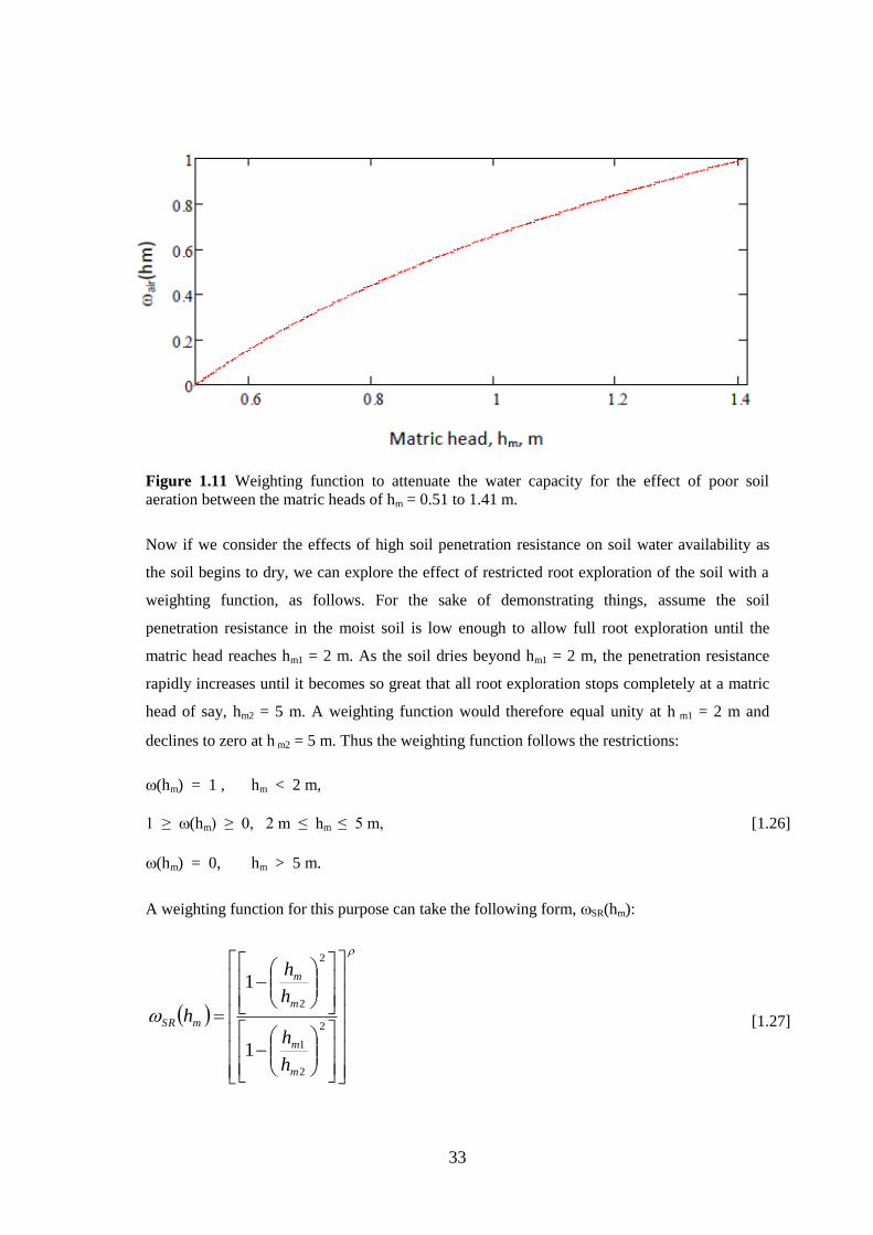
33
Figure 1.11 Weighting function to attenuate the water capacity for the effect of poor soil aeration between the matric heads of hm = 0.51 to 1.41 m.
Now if we consider the effects of high soil penetration resistance on soil water availability as
the soil begins to dry, we can explore the effect of restricted root exploration of the soil with a
weighting function, as follows. For the sake of demonstrating things, assume the soil
penetration resistance in the moist soil is low enough to allow full root exploration until the
matric head reaches hm1 = 2 m. As the soil dries beyond hm1 = 2 m, the penetration resistance
rapidly increases until it becomes so great that all root exploration stops completely at a matric
head of say, hm2 = 5 m. A weighting function would therefore equal unity at h m1 = 2 m and
declines to zero at h m2 = 5 m. Thus the weighting function follows the restrictions:��
�(hm) = 1 , hm < 2 m, 1 ≥ �(hm) ≥ 0, 2 m ≤ hm ≤ 5 m, [1.26] ��(hm) = 0, hm > 5 m.
A weighting function for this purpose can take the following form, �SR(hm):
�
�
�
������
�
�
������
�
�
���
�
���
����
����
��
���
�
���
����
����
��
2
2
1
2
2
1
1
m
m
m
m
mSR
hh
hh
h [1.27]

34
where hm1 = 2 m, hm2 = 5 m, and � is a dimensionless fitting parameter having a value of 3 for
this example. A graphical representation of this weighting function is shown in Figure 1.12. By
substituting Equation [1.27] into Equation [1.9] along with the other restrictions (salinity and
poor aeration), the water capacity becomes totally restricted and reduced to zero, as shown by
the dashed purple line segment (4) in Figure 1.10.
Figure 1.12 Weighting function to attenuate the water capacity for the effect of increasingly high soil penetration resistance between the matric heads of hm1 = 2 m, hm2 = 5 m.
Finally, we can integrate all of these restrictions on the water capacity using Groenevelt et al.’s
(2004) Integral Water Capacity (IWC) shown in Equation [1.9]. The results are summarized in
Table 1.2 and they represent hypothetical amounts of water available to plants. The extent to
which they are reasonable estimates has yet to verified. To do this requires extensive plant
response data, which are not yet widely available in the literature (a small data set was
assembled and published in the final stages of preparation of this thesis by Bazihizina et al.
2012).

35
Table 1.3 Summary of physical restrictions on the differential water capacity and their effect on IWC.
Soil restrictions Relevant integrals IWC
m3m-3 Line in Fig1.10
Unrestricted: Non-saline, well aerated, soft structure
� mmom dhhC�1
00,
� mmom dhhC�150
10,
� mmom dhhC�
1500,
0 0.237 0
solid blue
Saline but well aerated, soft structure
� mmom dhhC�1
02,
� mmom dhhC�95
12,
� mmom dhhC�
952,
0 0.154 0
solid red
Saline + poorly aerated but soft structure
� mmom dhhC�1
02,
� � mmommmommair dhhCdhhCh �� �95
4148.1
4148.1
12,2,)(
� mmom dhhC�
952,
0 0.151 0
dashed red
Saline + poorly aerated + hard structure
� mmom dhhC�1
02,
� � � � � mmommSRmmommmommair dhhChdhhCdhhCh ��� ��5
2
2
4148.1
4148.1
12,2,2,
� mmom dhhC�
52,
0 0.049 0
dashed purple
1.2.6 Conclusions
The literature suggests that plant available water, PAW, is influenced by a plethora of
interacting soil factors including the soil texture, the salinity of the soil solution, the soil
aeration and strength plus the unsaturated hydraulic conductivity. In this review, hypothetical
weighting functions and real soil data have been combined to predict the effects of each of these
factors on soil water availability using the integral water capacity, IWC, outlined by Groenevelt
et al. (2001; 2004). The model of the IWC considers a given soil to be a capacitor that can
release water in a graded fashion according to the severity of various limiting soil physical
properties.
With enough information, it is theoretically possible to calculate the amount of water a given
plant species can extract from the soil under a given set of environmental conditions. To be
universally useful, however, such theoretical calculations must be based on real plant behaviour
– otherwise they would be no better than the simple estimates of PAW proposed more than 50
years ago (Veihmeyer and Hendrickson 1927; Gardner 1960) nor would they offer an advance

36
beyond the linear approach to water extraction offered by Feddes et al. (1978). There are
numerous reports in the literature showing plant responses to various environmental stresses,
but almost none of them is linked quantitatively to soil hydraulic properties.
Furthermore, there is little information describing how plants respond to changes in water
availability, which occur in soils being reclaimed from the saline/sodic state. In the first
instance, there is little commercial interest and expertise to manage the full range of crops that
must be involved to reclaim low-value land, especially if relatively low-value halophytic plants
are needed initially. In saline soils, for example, the concept of plant available water for
Saltbush or Kallar grass might be considered meaningless in a commercial sense because water
use efficiency is not important for these crops. They are simply used to “kick-start” subsoil
drainage and to increase soil organic matter content so that leaching can occur and subsequent
(more valuable) crops can be introduced as part of a plant succession scheme. Furthermore as
salt is leached from the soil profile the physical properties of the soil change dramatically, such
that any new crops that replace the halophytes must deal with a very different set of soil
physical conditions.
Reclamation involves several steps and stages, and although it is broadly understood that the
electrolyte concentration and cation suites must be managed carefully to maintain permeability,
little is known about the changes that occur in soil structure and how these influence plant
available water at each stage of reclamation. A detailed study of soil water availability is
therefore required for a variety of crops at all stages of the reclamation process for a range of
different saline/sodic soils.
1.3 Overall problem, research questions and hypotheses.
1.3.1 Research questions
This study was designed to answer following questions:
1. When soil factors such as strength, hydraulic conductivity, aeration and salinity are taken into
account, how much water is available to nominally ‘salt-sensitive’ plants as predicted using the
Integral Water Capacity (IWC) model of Groenevelt et al. (2004)?
2. For in situ saline field conditions, to what extent does the amount of plant-available water
(predicted using the IWC) match the amount of water extracted from real soils by real plants?

37
3. How does the soil water availability change (as measured using IWC) during various stages
of reclamation of saline/sodic soil?
4. What is the shape of the weighting function describing plant response to increasing salt
concentration in soil? In particular: Is the bent-stick model too simple and is the shape of the
weighting function similar for all plants?
1.3.2 Hypotheses
1. The range in shape, magnitude, and integration limits of the relevant weighting functions (for
strength, aeration, hydraulic conductivity and salinity) will have minimal impact on the amount
of water available. This is because natural variation in the water capacity will be greater than the
variation caused by the relevant soil factors. The alternative hypothesis is that the relevant soil
factors will cause significant variation in the weighted water capacity because their effects apply
across a wide range of soil matric heads from 1 to 150 m and may even overlap. Thus a
significant reduction in the water capacity will be encountered somewhere across the relevant
plant-available range.
2. Extraction of water by plants in the field will match that predicted in the laboratory to be
‘available’ using the IWC. The alternative hypothesis is that the amount of water extracted in
the field will exceed or underestimate that predicted in the laboratory by the IWC, presumably
because certain factors have not been taken into account.
3. Soil water availability (as measured by the IWC) will increase monotonously from one
critical state to the next in soils being reclaimed from the saline/sodic state. The alternative
hypothesis is that the IWC will increase non-monotonously, depending upon the relative
importance of various soil physical properties at each stage of reclamation.
4. A weighting function to attenuate the water capacity for osmotic stress is best described by
the soil-based model of Groenevelt et al. (2004). The alternative hypothesis is that other models,
based upon plant response to salinity are better suited for such attenuation.
38
Chapter 2 Variation in soil water availability down the profile of a saline soil using the
Integral Water Capacity (IWC) model
2.1 Introduction
In Chapter 1, the factors that limit the amount of soil water that is available to plants were
explored and placed in the context of Groenevelt et al.’s (2001; 2004) model, the Integral Water
Capacity, IWC. Three particular soil factors that limit water availability to plants (i.e. salinity,
waterlogging, and high root penetration resistance) were chosen to illustrate the attenuating
effects on the differential soil water capacity of a soil of loamy sand texture. Hypothetical
weighting functions for each limitation were designed (using no real data) simply for illustrative
purposes. The amount of soil water available to plants in the field also depends upon the type of
plant and the variations in soil properties that occur with depth, because plants expand or limit
their root systems to take advantage of better conditions when encountered. Any estimate of soil
water availability for a given crop must therefore consider how the IWC varies down the soil
profile.
There are also other limiting factors to consider in calculating the amount of soil water available
to plants, such as the unsaturated soil hydraulic conductivity. Richards and Wadleigh (1952), for
example, stated that soil water availability involves two dynamic factors: “the ability of the
plant root to absorb and use the water with which it is in contact” as well as the “readiness with
which the soil water moves in to replace that which has been used by the plant”. Soil hydraulic
conductivity differs with texture, structure and tortuosity and of course soil water content or
matric head (Hillel 1982). Furthermore, the hydraulic conductivity of the soil can be too large,
such that excessively rapid drainage removes water from the root zone before it can be used by
plants. For example, Wesseling et al. (2009) found that the amount of plant available water in
coarse-textured soils increased greatly when organic matter was added because it retained water
in the root zone for longer and thus reduced the near-saturated hydraulic conductivity.
The work reported in this chapter describes the procedures used to calculate the variations in
IWC down the soil profile for a compacted, saline, texture-contrast soil. It presents data and
appropriate weighting functions for the limiting soil properties found at a field site (e.g. high
soil strength, low unsaturated hydraulic conductivity, poor soil aeration and high salinity). The
data and functions presented here will form the basis for a comparison with what happens after
land reclamation occurs (covered in subsequent chapters of this thesis).

39
2.2 Materials and Methods
2.2.1 Site selection and sample collection
A survey was conducted at the Roseworthy campus of the University of Adelaide on 15
December 2008 during which soil samples were collected in several paddocks (- 34.52892,
138.67954) to a depth of 20 cm, on which the electrical conductivity of 1:5 soil:water
suspensions was measured. A patch of non-productive, relatively saline, calcareous land was
located in Central-1 (C1) paddock (Figure 2.1) which had an EC1:5 of 0.86 - 0.93 dS m-1 in the
sandy surface horizon. A soil profile was exposed to a depth of 150 cm using a backhoe on 5
January 2009 (Figure 2.2) and the soil classified to the Family level using the Australian Soil
Classification (Isbell 2002) based inter alia upon descriptions of soil colour, texture and
structure (Table 2.1). Nine separate horizons were identified and the soil was classified as an
Epihypersodic Pedal Hypercalcic Calcarosol with Family codes: [C] for the thickness of soil
above Bk horizon, [H] for the gravel content of A1 horizon, [K] for the surface soil texture, [M]
for the maximum texture of B horizon, and [X] for the depth of the whole soil profile.
Disturbed and undisturbed soil samples were collected from the entire soil profile.
Approximately 30 kg of disturbed soil was collected from each horizon and placed in 20 L
buckets for transport to the laboratory for characterization and later use. Three undisturbed soil
cores1 were collected from each horizon by inserting stainless steel rings of dimensions: 50 mm
x 50 mm, vertically into each horizon (Figure 2.3); these were carefully dug out within larger
clods of soil and packed in sealed, insulated containers for transport to the laboratory. The
samples were subsequently used to measure the saturated hydraulic conductivities, water
retention curves, and penetration resistance curves.
Disturbed (bulk) soil samples
The disturbed soil from each horizon was air-dried in the laboratory, passed through a 2 mm
sieve (with gravel content measured), mixed well, and stored again. Subsamples (approximately
0.5 kg) were used to determine particle size distribution, particle density and organic carbon
content, as well as pH, EC and solution cations (Table 2.2). Soil physical properties such as
particle size distribution and particle density were determined by a pipette method (Day 1965)
and pycnometer method (Blake 1965), respectively; organic matter content was determined by
the Walkley and Black method (Allison 1965). pH and EC were measured using 1:5 soil
1 Actually, 5 soil cores were taken in the field but only the ‘best’ 3 were prepared for analysis. The ‘best’ 3 of the 5 were selected by inspection as those having no gaps, cracks or other disturbances.

40
suspensions (Rayment and Higginson 1992); soluble cations were determined on the basis of
saturated paste extract (Janzen 1993). The values presented in Table 2.2 are an average of two
replicates.
Figure 2.1 Roseworthy paddock C1 Figure 2.2 Exposed soil profile. (- 34.52892, 138.67954)
Figure 2.3 Collecting undisturbed soil cores down the profile in paddock C1
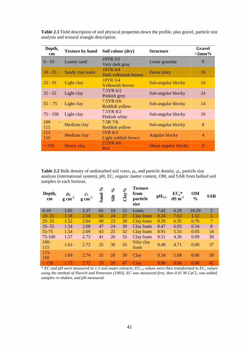
41
Table 2.1 Field description of soil physical properties down the profile, plus gravel, particle size analysis and textural triangle description.
Depth, cm Texture by hand Soil colour (dry) Structure Gravel
>2mm%
0 - 10 Loamy sand 10YR 3/1 Very dark gray Loose granular 9
10 - 25 Sandy clay loam 10YR 4/4 Dark yellowish brown Dense platy 16
25 - 35 Light clay 10YR 5/4 Yellowish brown Sub-angular blocky 24
35 - 55 Light clay 7.5YR 6/2 Pinkish grey Sub-angular blocky 24
55 – 75 Light clay 7.5YR 6/6 Reddish yellow Sub-angular blocky 14
75 - 100 Light clay 7.5YR 8/2 Pinkish white Sub-angular blocky 10
100 - 115 Medium clay 7.5R 7/6
Reddish yellow Sub-angular blocky 8
115 - 150 Medium clay 5YR 6/3
Light reddish brown Angular blocky 4
> 150 Heavy clay 2.5YR 4/6 Red Sharp angular blocky 0
Table 2.2 Bulk density of undisturbed soil cores, �b, and particle density, �s, particle size analysis (international system), pH, EC, organic matter content, OM, and SAR from bulked soil samples in each horizon.
Depth, cm
��b g cm-3
�s g cm-3 Sa
nd %
Silt
%
Cla
y% Texture
from particle size
pH1:5 ECe*
dS m-1 OM % SAR
0-10 1.05 2.37 65 19 15 Loam 7.42 6.29 10.29 2 10- 25 1.58 2.58 50 24 27 Clay loam 8.24 7.63 1.52 5 25- 35 1.52 2.64 49 23 28 Clay loam 8.30 6.35 0.76 7 35- 55 1.54 2.68 47 24 30 Clay loam 8.47 6.03 0.54 8 55-75 1.54 2.69 43 25 32 Clay loam 8.91 5.33 0.05 14 75-100 1.57 2.73 41 26 33 Clay loam 9.51 4.36 0.09 30 100-115 1.63 2.72 35 30 35 Silty clay
loam 9.48 4.71 0.00 37
115-150 1.69 2.74 35 26 39 Clay 9.34 5.68 0.00 39
> 150 1.73 2.72 33 20 47 Clay 8.86 6.66 0.00 42 * EC and pH were measured in 1:5 soil:water extracts; EC1:5 values were then transformed to ECe values using the method of Slavich and Petterson (1993). EC was measured first, then 0.01 M CaCl2 was added, samples re-shaken, and pH measured.
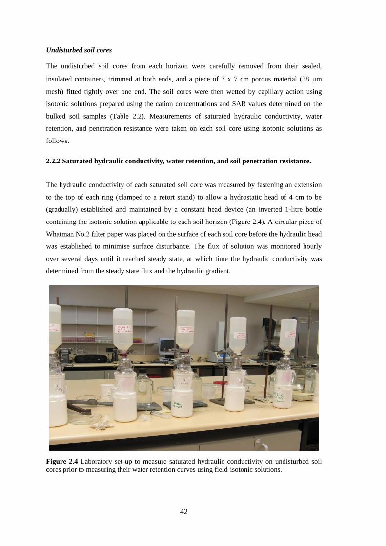
42
Undisturbed soil cores
The undisturbed soil cores from each horizon were carefully removed from their sealed,
insulated containers, trimmed at both ends, and a piece of 7 x 7 cm porous material (38 �m
mesh) fitted tightly over one end. The soil cores were then wetted by capillary action using
isotonic solutions prepared using the cation concentrations and SAR values determined on the
bulked soil samples (Table 2.2). Measurements of saturated hydraulic conductivity, water
retention, and penetration resistance were taken on each soil core using isotonic solutions as
follows.
2.2.2 Saturated hydraulic conductivity, water retention, and soil penetration resistance.
The hydraulic conductivity of each saturated soil core was measured by fastening an extension
to the top of each ring (clamped to a retort stand) to allow a hydrostatic head of 4 cm to be
(gradually) established and maintained by a constant head device (an inverted 1-litre bottle
containing the isotonic solution applicable to each soil horizon (Figure 2.4). A circular piece of
Whatman No.2 filter paper was placed on the surface of each soil core before the hydraulic head
was established to minimise surface disturbance. The flux of solution was monitored hourly
over several days until it reached steady state, at which time the hydraulic conductivity was
determined from the steady state flux and the hydraulic gradient.
Figure 2.4 Laboratory set-up to measure saturated hydraulic conductivity on undisturbed soil cores prior to measuring their water retention curves using field-isotonic solutions.
43
Each sample was then unclamped from its retort stand, its extension removed, and placed onto a
porous ceramic plate (saturated with an identical isotonic solution) held at a progressive series
of matric potentials to determine the water retention curve. Hanging columns of isotonic
solutions were used for the smaller pressure heads (e.g. 2.5 cm to 100 cm)2 soil cores were
exposed to these pressure heads successively over a period of 2 days (for h = -2.5 cm) or up to 7
days (for h = -100 cm). For greater pressure heads, sealed, high-pressure chambers (supplied
with pressurized N2 gas) were used for the following periods: 7 days for h = -500 cm, 15 days
for h = -1,000 cm, 25 days for h = -5,000 cm, 45 days for both h = -10,000 cm and -15,000 cm.
At each pressure head, samples were removed from their ceramic plates, weighed and placed
back onto their pressurized plates at the same pressure heads, with additional water added to the
soil samples to ensure good soil-plate connection, for a further 48 hours. This was repeated until
the weights did not change by more than 0.1% between readings, which ensured the samples
were as close to equilibrium as possible. The equilibrium weights at each pressure head were
recorded and the volumetric water contents calculated at the end of experiment after the oven
dried soil masses (105oC for 48 h) were measured and the bulk volumes checked.
After the final weight of each soil sample was recorded for each pressure head, the penetration
resistance was measured using a Lloyd Instrument LF-plus Penetrometer connected to a
computer with data-logging software NEXYGENPlus to record the penetration force
encountered by an 85 mm long stainless steel pin with 30o cone angle; 2.58 mm diameter cone-
tip (diameter of the recessed shaft behind the cone was 1.95 mm). The cone was inserted
vertically at a constant rate (2.8 mm/min) and the force recorded every 0.5 mm to a depth of 45
mm below the soil surface. The penetration resistance (force encountered divided by the cross-
sectional area of the cone) was calculated as the average value between the depths of 15 to 35
mm; this minimized surface effects at the top and bottom of cores.
2.2.3 Salinity and osmotic stress
As indicated in Chapter 1, the weighting-analysis for osmotic stress proposed by Groenevelt et
al.(2004) requires information on the salt concentration of the soil in its saturated state, ideally
from a saturated paste extract. In this work, I initially measured EC on 1:5 soil:water extracts,
not paste extracts, so the 1:5 EC values were transformed to paste extract EC using the method
proposed by Slavich and Petterson (1993).
2 Samples exposed to the hanging columns of solution were enclosed in a plastic membrane to reduce evaporation.

44
2.3 Result and discussion
2.3.1 Saturated hydraulic conductivity
As might be expected with increases in clay content with depth in the soil profile, the mean
saturated hydraulic conductivities, Ks (m s-1), declined by over 5 orders of magnitude from the
sandy-textured soil surface down to the heavy clay-textured subsoil at 1.5 m depth (Figure 2.5).
The variability in Ks values among the 3 samples, shown in Figure 2.5 using red horizontal
standard error bars, is surprisingly small for such readings, which are often log-normally
distributed (Hillel 1971). The values of Ks will be referred to later in reference to calculating the
unsaturated hydraulic conductivity function of Grant et al.(2010).
Figure 2.5 Saturated hydraulic conductivities of undisturbed soil cores down the soil profile using isotonic solutions applicable to each depth (horizontal red bars are standard errors.
2.3.2 Water retention curves
The water retention data for all 9 horizons (Figures 2.6) were fitted to Equation [1.10] using a
Levenberg-Marquarde least-squares optimization procedure, the parameter values for which are
given in Table 2.3. The water retention curves were grouped in Figures 2.6 based on their
texture and salt concentration: Figure 2.6a shows curves for the two light-textured horizons in
the top 25 cm, which had EC values ranging between 6 and 8 dS m-1. Figure 2.6b shows the
curves for the next 3 soil horizons (25 to 75 cm), which had medium textures and EC values
ranging between 5 and 6 dS m-1. Figure 2.6c shows the curves for the next two horizons (75 to
Depth, cm Mean Ks m s-1 (± std error)
0 - 10 6 x10⁻⁵ (3 x10⁻⁵)
10 - 25 3 x10⁻⁵ (8 x10⁻⁶)
25 - 35 4 x10⁻⁵ (6 x10⁻⁶)
35 - 55 3 x10⁻⁵ (4 x10⁻⁶)
55 – 75 2 x10⁻⁵ (7 x10⁻⁶)
75 - 100 2 x10⁻⁵ (3 x10⁻⁶)
100 - 115 7 x10⁻⁷ (2 x10⁻⁷)
115 - 150 2 x10⁻⁷ (6 x10⁻⁸)
> 150 8 x10⁻⁹ (1 x10⁻⁹)

45
115 cm), which had greater clay contents and less salt (ca. 4 dS m-1). The curves for the deepest
(heavy clay) horizons (115 to 150 cm) are grouped in Figure 2.6d...
Figure 2.6 Water retention curves for the 9 soil horizons examined in this study: a) 0 to 25 cm, b) 25 to 75 cm, c) 75 to 115 cm, and d) 115 to 150 cm.
a)
d)
c)
b)
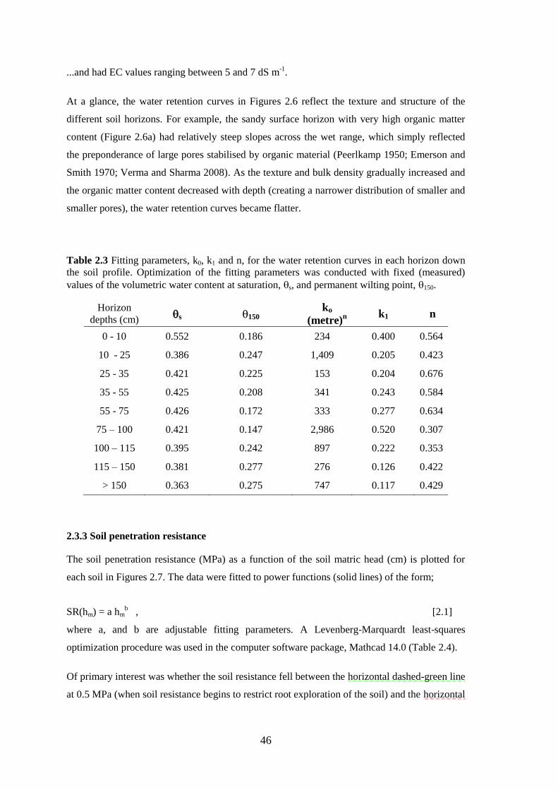
46
...and had EC values ranging between 5 and 7 dS m-1.
At a glance, the water retention curves in Figures 2.6 reflect the texture and structure of the
different soil horizons. For example, the sandy surface horizon with very high organic matter
content (Figure 2.6a) had relatively steep slopes across the wet range, which simply reflected
the preponderance of large pores stabilised by organic material (Peerlkamp 1950; Emerson and
Smith 1970; Verma and Sharma 2008). As the texture and bulk density gradually increased and
the organic matter content decreased with depth (creating a narrower distribution of smaller and
smaller pores), the water retention curves became flatter.
Table 2.3 Fitting parameters, k0, k1 and n, for the water retention curves in each horizon down the soil profile. Optimization of the fitting parameters was conducted with fixed (measured) values of the volumetric water content at saturation, �s, and permanent wilting point, �150.
Horizon depths (cm) ��s �150
ko (metre)n k1 n
0 - 10 0.552 0.186 234 0.400 0.564
10 - 25 0.386 0.247 1,409 0.205 0.423
25 - 35 0.421 0.225 153 0.204 0.676
35 - 55 0.425 0.208 341 0.243 0.584
55 - 75 0.426 0.172 333 0.277 0.634
75 – 100 0.421 0.147 2,986 0.520 0.307
100 – 115 0.395 0.242 897 0.222 0.353
115 – 150 0.381 0.277 276 0.126 0.422
> 150 0.363 0.275 747 0.117 0.429
2.3.3 Soil penetration resistance
The soil penetration resistance (MPa) as a function of the soil matric head (cm) is plotted for
each soil in Figures 2.7. The data were fitted to power functions (solid lines) of the form;
SR(hm) = a hmb , [2.1]
where a, and b are adjustable fitting parameters. A Levenberg-Marquardt least-squares
optimization procedure was used in the computer software package, Mathcad 14.0 (Table 2.4).
Of primary interest was whether the soil resistance fell between the horizontal dashed-green line
at 0.5 MPa (when soil resistance begins to restrict root exploration of the soil) and the horizontal

47
dashed-red line at 2.5 MPa (when soil resistance completely restricts all root growth of most
plants in the soil). The critical values of 0.5 and 2.5 MPa were chosen from historical data of
(Greacen et al. 1968) and (Cockroft et al. 1969). The soil matric heads at which penetration
resistances of 0.5 and 2.5 MPa were encountered for each soil were calculated by re-arranging
Equation [2.1], substituting the initial and final values of SR, and solving for hi and hf:
and [2.2] Values for hi and hf are shown in Table 2.4.
Table 2.4 Fitting parameters for Equation [2.1] describing the relation between soil penetration resistance (MPa) and soil matric head (cm), plus the matric heads, hi and hf, respectively, at which SR(hm) reached values of 0.5 and 2.5 MPa.
Horizon depth (cm)
a (MPa cm-b) b hi
(cm) hf
(cm) 0 – 10 0.12 0.26 215 103,900
10 - 25 0.29 0.24 10 8,824 25 – 35 0.05 0.42 221 10,127 35 – 55 0.24 0.25 22 14,094 55 – 75 0.12 0.40 36 2,035
75 – 100 0.06 0.42 146 6,784 100 – 115 0.06 0.46 117 3,828 115 – 150 0.09 0.45 53 1,905
> 150 0.024 0.56 239 4,283
It can be seen in Figure 2.7a that the soil resistance stayed well within the tolerable range across
all pressure heads for the top soil horizon (high organic matter). For the next soil horizon, the
soil resistance only just exceeded 2.5 MPa when the soil matric head dried to hm > 5,000 cm.
For all horizons from 55 cm downward (with greater densities, clay contents and lower organic
matter contents), the soil resistance significantly exceeded 2.5 MPa for hm < 5,000 cm (Figure
2.7 b, c and d). In fact, the soil resistance entered the restrictive range for some soil horizons
when the matric head was only hm = 100 cm.
2.3.4 Salinity and osmotic stress
The measured electrical conductivities were converted to ECe (Table 2.2), which will be used as
the first weighting function to attenuate the water capacity, following Groenevelt et al. (2004).
The measured and corrected EC values, plus the corresponding (calculated) values of the
osmotic head in the saturated soil, hos (cm), and the matric head at which (hos + hm) = 15000 cm
(i.e. the permanent wilting point) are shown in Table 2.5.
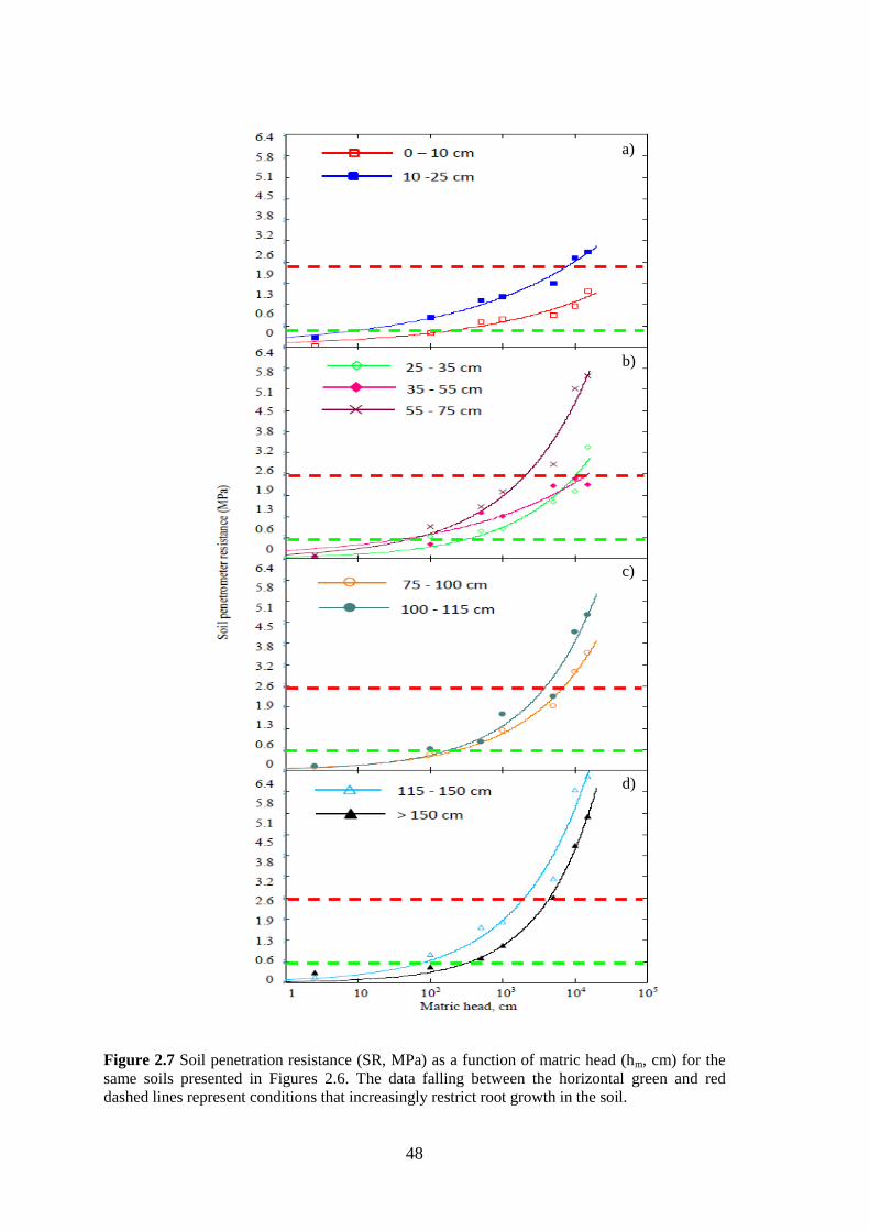
48
Figure 2.7 Soil penetration resistance (SR, MPa) as a function of matric head (hm, cm) for the same soils presented in Figures 2.6. The data falling between the horizontal green and red dashed lines represent conditions that increasingly restrict root growth in the soil.
a)
b)
c)
d)

49
Table 2.5. Measured values of the electrical conductivity of 1:5 soil:water extracts and gravimetric water contents at saturation, plus the corresponding electrical conductivity of paste extracts (calculated from Slavich and Petterson (1993)) and values of hos and hm at wilting point (calculated from Equation 12 in Groenevelt et al. (2004)).
Depth (cm)
Measured Calculated EC1:5
(dS m-1) �S
(g g-1) ECe
(dS m-1) hos (cm)
hm (cm)
0 - 10 0.96 0.74 6.29 2264 9420 10 - 25 0.80 0.43 7.63 2747 10708 25 - 35 0.71 0.46 6.35 2286 10883 35 - 55 0.65 0.45 6.03 2171 10879 55 -75 0.57 0.44 5.33 1919 10775 75 - 100 0.70 0.79 4.36 1570 10504 100 - 115 0.85 0.98 4.71 1696 12232 115 - 150 1.09 1.09 5.68 2045 12191 > 150 1.52 1.57 6.66 2398 11835
2.3.5 Weighting functions
2.3.5.1 Weighting the differential water capacities for salinity
The water retention curves, �(hm), shown in Figures 2.6 were differentiated with respect to hm to
produce differential water capacities, C(hm) according to Equation [1.11] after Groenevelt et al.
(2004). These were then transformed to differential soil solution capacities, Com(hm) by taking
into account the salt concentrations from saturated paste extracts3 according to Equations [1.12],
[1.13], and [1.14].
The soil solution capacities were then attenuated according to Equations [1.15] to [1.22], which
produced effective soil solution capacities for each saline condition using Equation [1.23]. The
attenuated curves (dotted lines) are shown together with the non-attenuated curves (solid lines)
in Figure 2.8.
The weighted differential water capacities in Figures 2.8 come from Equation [1.23] and
represent the starting points for all subsequent attenuations to account for other limiting soil
physical properties (e.g. high penetration resistance, poor soil aeration, low unsaturated
hydraulic conductivity). All soil horizons contained soluble salts so all of them experienced
some attenuation of the water capacity – some horizons more severely than others. The effects
3 Saturated paste extract-EC were estimated by correction of the EC1:5 according to the method proposed by Slavich and Petterson (1993).

50
of the different attenuations on the integral water capacity, IWC, will be summarised at the end
of this chapter.
2.3.5.2 Weighting the differential water capacity for high soil penetration resistance.
The weighting function developed here acknowledges that soil strength alone rarely stops plant-
extraction of water from the soil completely – it merely limits the volume of soil into which
roots can grow; soil water can still flow toward roots that enter cracks or biopores present in the
high-strength soil matrix so roots can still take up water. Acknowledging that a weighting
function for high soil resistance, SR(hm), needn’t necessarily end at zero simply because root
extension stops, the magnitude of SR(hm) is more flexible than for other physical restrictions.
The values of SR(hm) were therefore restricted as follows:
�SR(hm) = 1.0 for h < hi, and 0 < �SR(hm) < 1 for hi < hm < hf ,
where hi is the soil matric head at which SR(hm) = 0.5, and hf is the soil matric head at which
SR(hm) = 2.5. The values of hi and hf were calculated using Equations [2.2] and are shown in
Table 2.4.
The form of the weighting function chosen in this study for soil resistance took a more flexible
form than that described in Equation [1.22], and can be adjusted in future work for plants
having different ability to penetrate hard soils, as follows:
[2.3]
where SR(hi) = 0.5 MPa, SR(hf) = 2.5 MPa as described above.
The parameter � in Equation [2.3] is a dimensionless slope-parameter designed to create
different severities of attenuation depending on the ability of different plant species to exert root
growth pressures on their surroundings. For example smaller values of � would be used for
plant species that are able to exert higher root growth pressures, so the attenuation is less severe.
By contrast, a larger value of � would be used for plant species known to be sensitive to
compaction or that cannot exert high root growth pressures; so the attenuation would be much
more severe.

51
Figure 2.8 Differential water capacities for the nine water retention curves shown in Figure 2.1 weighted (dotted lines) or not weighted (solid lines) for salt content according to Groenevelt et al. (2004).
Figure 2.9 shows 3 possible weighting functions for each of the nine horizons by adjusting the
�-parameter from � = 0.2 to � = 0.5 to � = 1.0, respectively, for plants that can exert ‘high’
‘medium’ or ‘low’ root growth pressures on their surroundings. There is no published
information on the magnitude of such �-values, so in this study a value of � = 0.5 was chosen
for illustration purposes. Figure 2.9 shows that the attenuations occurred across a wide range of
different matric heads for the different soil horizons. Some attenuations are more moderate than
others, for example, the surface soil horizon (which contained 18% organic matter) was
attenuated the least, whereas the deeper soil horizons (which had very great strength) were
attenuated more severely. Notably, none of the weighting functions causes complete attenuation
to zero across the range of soil matric heads examined here, which (as explained above) is
probably realistic. As for the effects of salinity, the effects of high soil strength on IWC will be
summarized at the end of this Chapter, but will clearly be more severe in some horizons than in
others.
A NOTE:
This figure/table/image has been removed to comply with copyright regulations. It is included in the print copy of the thesis held by the University of Adelaide Library.
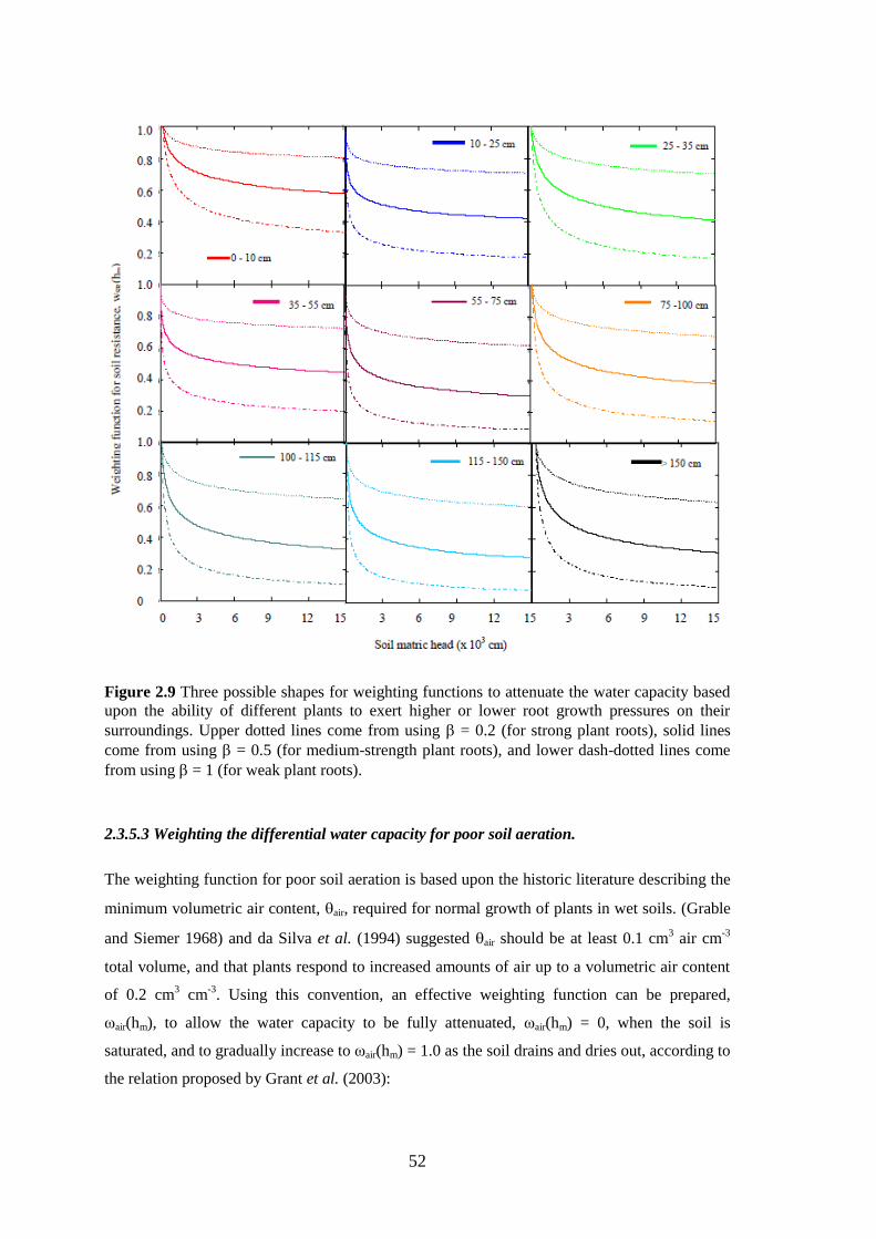
52
Figure 2.9 Three possible shapes for weighting functions to attenuate the water capacity based upon the ability of different plants to exert higher or lower root growth pressures on their surroundings. Upper dotted lines come from using � = 0.2 (for strong plant roots), solid lines come from using � = 0.5 (for medium-strength plant roots), and lower dash-dotted lines come from using � = 1 (for weak plant roots).
2.3.5.3 Weighting the differential water capacity for poor soil aeration.
The weighting function for poor soil aeration is based upon the historic literature describing the
minimum volumetric air content, �air, required for normal growth of plants in wet soils. (Grable
and Siemer 1968) and da Silva et al. (1994) suggested �air should be at least 0.1 cm3 air cm-3
total volume, and that plants respond to increased amounts of air up to a volumetric air content
of 0.2 cm3 cm-3. Using this convention, an effective weighting function can be prepared,
ωair(hm), to allow the water capacity to be fully attenuated, ωair(hm) = 0, when the soil is
saturated, and to gradually increase to ωair(hm) = 1.0 as the soil drains and dries out, according to
the relation proposed by Grant et al. (2003):
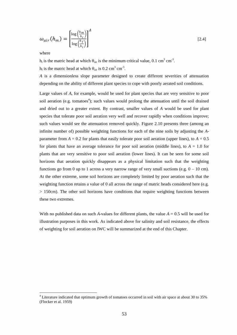
53
[2.4]
where
hi is the matric head at which �air is the minimum critical value, 0.1 cm3 cm-3.
hf is the matric head at which �air is 0.2 cm3 cm-3.
A is a dimensionless slope parameter designed to create different severities of attenuation
depending on the ability of different plant species to cope with poorly aerated soil conditions.
Large values of A, for example, would be used for plant species that are very sensitive to poor
soil aeration (e.g. tomatoes4); such values would prolong the attenuation until the soil drained
and dried out to a greater extent. By contrast, smaller values of A would be used for plant
species that tolerate poor soil aeration very well and recover rapidly when conditions improve;
such values would see the attenuation removed quickly. Figure 2.10 presents three (among an
infinite number of) possible weighting functions for each of the nine soils by adjusting the A-
parameter from A = 0.2 for plants that easily tolerate poor soil aeration (upper lines), to A = 0.5
for plants that have an average tolerance for poor soil aeration (middle lines), to A = 1.0 for
plants that are very sensitive to poor soil aeration (lower lines). It can be seen for some soil
horizons that aeration quickly disappears as a physical limitation such that the weighting
functions go from 0 up to 1 across a very narrow range of very small suctions (e.g. 0 – 10 cm).
At the other extreme, some soil horizons are completely limited by poor aeration such that the
weighting function retains a value of 0 all across the range of matric heads considered here (e.g.
> 150cm). The other soil horizons have conditions that require weighting functions between
these two extremes.
With no published data on such A-values for different plants, the value A = 0.5 will be used for
illustration purposes in this work. As indicated above for salinity and soil resistance, the effects
of weighting for soil aeration on IWC will be summarized at the end of this Chapter.
4 Literature indicated that optimum growth of tomatoes occurred in soil with air space at about 30 to 35% (Flocker et al. 1959)

54
Figure 2.10 Three possible shapes (of many) for weighting functions to attenuate the water capacity for poor soil aeration by varying the A-parameter in Equation [2.5] from 0.2 (upper dotted lines), 0.5 (middle solid lines), and 1.0 (lower dash-dot lines) according to the ability of different plants to tolerate poor soil aeration.
2.3.5.4 Weighting the differential water capacity for declining soil hydraulic conductivity.
Weighting the water capacity for declining hydraulic conductivity requires knowledge of the
unsaturated hydraulic conductivity function for a soil. A theoretical framework linking the water
retention curve to the hydraulic conductivity function was presented by Grant et al (2010), and it
is possible to use the parameters from this theory to develop an appropriate weighting function
as follows.

55
By scaling the water retention curve, �(hm), using the relative water content, �r = �/�sat, rather
than the absolute water content, �, the water retention model takes the form (Grant et al. 2010):
, [2.5]
where �s is the water content at saturation and k0, k1 and n are fitting parameters that depend on
the shape of the water retention data.
To obtain a relative hydraulic conductivity from Equation [2.5], it needs inter alia to be
integrated. The integrand of interest in this work has the form:
! � " , [2.6]
where ! = �s / k1, and " = 2/n following the Burdine restriction (Grant et al. 2010).
Inserting Equation [2.5] into Equation [2.6] and carrying out the integration yields an expression
that represents the unsaturated hydraulic conductivity as an incomplete gamma function, M(h):
�# $# $# $���
�
�
���
�
�
���
�
�
���
�
�
���
�
�
���
�
�
��
�
�
��
�
�
��
�
�
��
�
�
���
�
���
�
���
�
���
����
����
������%����%
n
msrLm h
kkhM 01 exp11ln,11ln,11)(�
!"�!"!
[2.7]
where �rL in Equation [2.7] is defined as the lower limit of integration (Grant et al. 2010), and
all other variables have been defined above.
To obtain an expression for the relative hydraulic conductivity, Kr(hm), Equation [2.7] is
substituted into the following expression:
, [2.8]
where M(1) is the expression for the hydraulic conductivity at saturation.
With this expression, it is now possible to produce a weighting function that addresses the
problem of declining unsaturated hydraulic conductivity and allows attenuation of the water
capacity from 1 down to 0 at specified matric heads:

56
, [2.9]
where k0 comes from the water retention curve (Equation [2.5]), hi and hf are the matric heads at
which plants initially experience water stress due to low hydraulic conductivity, and when they
finally wilt permanently and die. The matric heads at the onset and finality of water stress due to
declining hydraulic conductivity probably depend on plant species and environmental
conditions, and an investigation of this is beyond the scope of the present study. For lack of any
other information, one can select hi = 2500 cm, which was proposed by Gardner and Nieman
(1964) to be a reasonable average matric head at which water stress due to limited unsaturated
hydraulic conductivity begins to restrict the growth of many plants. One can also select hf =
15,000 cm, which is typically reported as permanent wilting point anyhow.
The parameter, �, in Equation [2.9] is proposed to be a plant-specific slope parameter, for which
small �-values apply to plants sensitive to low hydraulic conductivity and for which large �-
values apply to plants that cope well with declining hydraulic conductivity. In the complete
absence of any published literature on appropriate values for such a parameter, one can select �
= 0.2 as being ‘small’ for sensitive plants, � = 0.5 for plants of ‘medium’ sensitivity, and � = 1
as being a ‘large’ value for tolerant plants.
A set of three weighting functions for declining hydraulic conductivity are therefore plotted in
Figure 2.11 for plants differing in their ability to tolerate such conditions. Obviously they all
start and end at the same place and they all have similar shapes because there is no information
to vary the values of hi, hf and � in Equation [2.9] – this will require experimental work with real
plants under a range of controlled conditions – beyond the scope of this thesis!
2.3.6 Summarizing the effects of weighting the water capacity
For the purposes of demonstrating the effect of weighting the water capacity using the functions
displayed for salt (Equation [1.23]), soil resistance (Equation [2.3]), soil aeration (Equation
[2.4]) and hydraulic conductivity (Equation [2.9]), one can start with the attenuated ‘effective’
water capacity accounting for salt shown in Figure 2.8 and apply the weighting functions shown
in Figures 2.9, 2.10 and 2.11. Because there is no unbiased information to help select the slope-
parameters in the weighting functions mentioned above (i.e. � in Equation [2.3], A in Equation
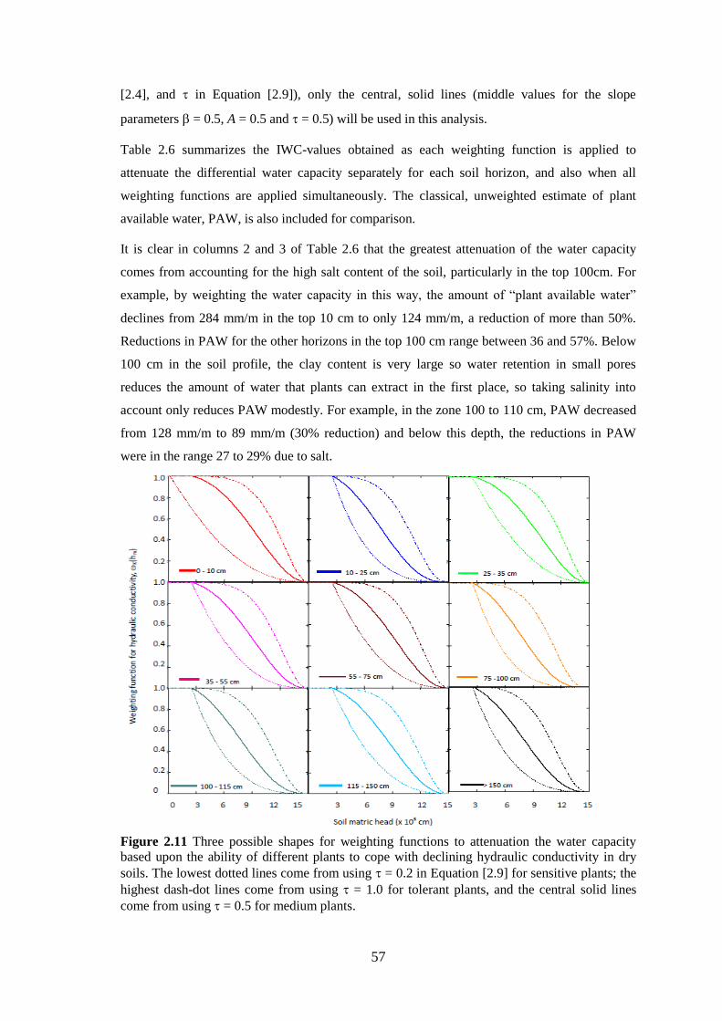
57
[2.4], and � in Equation [2.9]), only the central, solid lines (middle values for the slope
parameters � = 0.5, A = 0.5 and � = 0.5) will be used in this analysis.
Table 2.6 summarizes the IWC-values obtained as each weighting function is applied to
attenuate the differential water capacity separately for each soil horizon, and also when all
weighting functions are applied simultaneously. The classical, unweighted estimate of plant
available water, PAW, is also included for comparison.
It is clear in columns 2 and 3 of Table 2.6 that the greatest attenuation of the water capacity
comes from accounting for the high salt content of the soil, particularly in the top 100cm. For
example, by weighting the water capacity in this way, the amount of “plant available water”
declines from 284 mm/m in the top 10 cm to only 124 mm/m, a reduction of more than 50%.
Reductions in PAW for the other horizons in the top 100 cm range between 36 and 57%. Below
100 cm in the soil profile, the clay content is very large so water retention in small pores
reduces the amount of water that plants can extract in the first place, so taking salinity into
account only reduces PAW modestly. For example, in the zone 100 to 110 cm, PAW decreased
from 128 mm/m to 89 mm/m (30% reduction) and below this depth, the reductions in PAW
were in the range 27 to 29% due to salt.
Figure 2.11 Three possible shapes for weighting functions to attenuation the water capacity based upon the ability of different plants to cope with declining hydraulic conductivity in dry soils. The lowest dotted lines come from using � = 0.2 in Equation [2.9] for sensitive plants; the highest dash-dot lines come from using � = 1.0 for tolerant plants, and the central solid lines come from using � = 0.5 for medium plants.
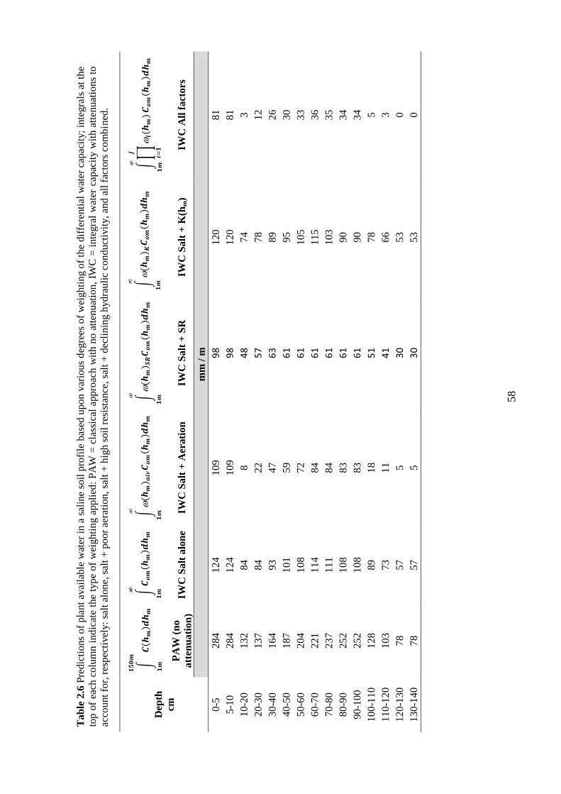
58
Tab
le 2
.6 P
redi
ctio
ns o
f pla
nt a
vaila
ble
wat
er in
a sa
line
soil
prof
ile b
ased
upo
n va
rious
deg
rees
of w
eigh
ting
of th
e di
ffer
entia
l wat
er c
apac
ity; i
nteg
rals
at t
he
top
of e
ach
colu
mn
indi
cate
the
type
of w
eigh
ting
appl
ied:
PA
W =
cla
ssic
al a
ppro
ach
with
no
atte
nuat
ion,
IWC
= in
tegr
al w
ater
cap
acity
with
atte
nuat
ions
to
acco
unt f
or, r
espe
ctiv
ely:
salt
alon
e, sa
lt +
poor
aer
atio
n, sa
lt +
high
soil
resi
stan
ce, s
alt +
dec
linin
g hy
drau
lic c
ondu
ctiv
ity, a
nd a
ll fa
ctor
s com
bine
d.
Dep
th
cm
�
�
�
�
PAW
(no
atte
nuat
ion)
IW
C S
alt a
lone
IW
C S
alt +
Aer
atio
n IW
C S
alt +
SR
IW
C S
alt +
K(h
m)
IWC
All
fact
ors
mm
/ m
0-
5 28
4 12
4 10
9 98
12
0 81
5-
10
284
124
109
98
120
81
10-2
0 13
2 84
8
48
74
3 20
-30
137
84
22
57
78
12
30-4
0 16
4 93
47
63
89
26
40
-50
187
101
59
61
95
30
50-6
0 20
4 10
8 72
61
10
5 33
60
-70
221
114
84
61
115
36
70-8
0 23
7 11
1 84
61
10
3 35
80
-90
252
108
83
61
90
34
90-1
00
252
108
83
61
90
34
100-
110
128
89
18
51
78
5 11
0-12
0 10
3 73
11
41
66
3
120-
130
78
57
5 30
53
0
130-
140
78
57
5 30
53
0
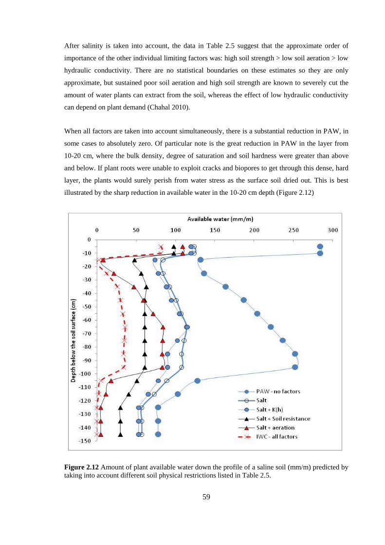
59
After salinity is taken into account, the data in Table 2.5 suggest that the approximate order of
importance of the other individual limiting factors was: high soil strength > low soil aeration > low
hydraulic conductivity. There are no statistical boundaries on these estimates so they are only
approximate, but sustained poor soil aeration and high soil strength are known to severely cut the
amount of water plants can extract from the soil, whereas the effect of low hydraulic conductivity
can depend on plant demand (Chahal 2010).
When all factors are taken into account simultaneously, there is a substantial reduction in PAW, in
some cases to absolutely zero. Of particular note is the great reduction in PAW in the layer from
10-20 cm, where the bulk density, degree of saturation and soil hardness were greater than above
and below. If plant roots were unable to exploit cracks and biopores to get through this dense, hard
layer, the plants would surely perish from water stress as the surface soil dried out. This is best
illustrated by the sharp reduction in available water in the 10-20 cm depth (Figure 2.12)
Figure 2.12 Amount of plant available water down the profile of a saline soil (mm/m) predicted by taking into account different soil physical restrictions listed in Table 2.5.

60
2.4 Conclusions
This study attempted to quantify how much water is available to nominally ‘salt sensitive’ plants in
a saline soil using the model proposed by Groenevelt et al. (2004). It was hypothesised that the
relevant weighting functions would have minimal impact on the amount of water available. The
alternative hypothesis proposed was that when the relevant soil factors were taken into account to
attenuate the differential water capacity, a significant reduction in available water would occur
because the effects of the physical limitations might be multiplicative across the normal range of
plant available water.
On the basis of the results present here, the null hypothesis can be safely rejected in this study and
the alternative tentatively accepted: ‘accepted’ because there were ‘clear’ effects of the weighting
functions, but ‘tentatively accepted’ because a statistical evaluation of the effects was not possible
and because many of the weighting functions were applied with little or no knowledge of the real
magnitude of their parameters based upon real plant behaviour. Given the limitations on the
findings in this Chapter, it is essential to obtain real plant responses on the same soil in the field,
which is the topic of Chapter 3.
61
Chapter 3 In situ response of plants to saline conditions in the field
3.1 Introduction
Plants growing under saline field conditions have to deal with both osmotic and specific-ion
stresses (Shainberg and Oster 1978). For example iso-osmotic solutions of various different salts
are known to reduce growth in similar fashions (Bernstein and Hayward 1958). Furthermore, soil
water matric and osmotic stresses have a similar and additive effect on plant growth (Wadleigh and
Ayers 1945) and these both reduce water uptake and transpiration of plants (Meiri and Poljakoff-
Mayber 1970; Hoffman et al. 1971). For the purposes of this work, I will exclude ion toxicities as a
variable in water uptake by using a plant that is relatively tolerant of chloride and sodium.
Salinity and sodicity vary with both the soil water content and with depth, so plant available water
varies down the soil profile and within the root zone of most soils. In the absence of significant
drainage and leaching of soluble salts, the salt concentrations generally increase during drying.
Even when leaching of salts is possible, the salt content at the bottom of the root zone can be
significantly greater than it is at the top, particularly if the leaching fraction drops below about 0.3
(Richards 1953).
As salt concentration declines during leaching, it is well known (Quirk and Schofield 1955) that
soil structure and structural stability begin to change and that these changes influence plant
available water through their effects on soil porosity, aeration, penetration resistance, and hydraulic
conductivity. Degraded soil structure in sodic soils has been reported by many researchers (e.g.
Richards (1953), Rengasamy and Olsson (1991), Jayawardane and Chan (1994)) as reduced
hydraulic conductivity and aeration and as increases in soil strength. Water movement in soils
slows down because the pore size distribution shifts toward smaller pores. Smaller pores remain
saturated (water-logged) and thereby reduce gas exchange between the soil and the atmosphere,
which restricts the normal uptake of soil water by roots. High soil strength, especially as soil dries,
prevents root penetration to deeper layers to access stored soil water.
Classical calculations of plant available water ignore many restrictions imposed by soil factors. In
Chapter 2 of this thesis, I evaluated the Integral Water Capacity (IWC) model of Groenevelt et
al.(2001); (2004) using a set of undisturbed soil cores taken from the field. The evaluation included
applying weighting factors to attenuate the differential water capacity for osmotic stress, high soil
penetration resistance, poor soil aeration and declining soil hydraulic conductivity. The estimates of
plant-available water from this model are theoretically based and they rely on various assumptions
that have never been tested and may or may not hold in reality. In this Chapter I examine the extent

62
to which the estimated amounts of plant-available water match the total amount of water extracted
from the same soil by a relatively salt-tolerant plant, Rhodes grass (Chloris gayana cv. Pioneer).
I started with the research question: “Does the amount of plant-available water predicted from a set
of soil cores in the laboratory using the IWC-model of Groenevelt et al.(2001; 2004) match the
amount of water extracted by plants growing in situ in the same soil under field conditions?” The
corresponding null hypothesis to address this question was: “Extraction of water by plants under
field conditions matches that predicted to be ‘available’ using the IWC model”. The alternative
hypothesis is, of course, that the amount of water extracted by plants in the field exceeds or
underestimates that predicted by the IWC.
3.2 Materials and methods
3.2.1 Experimental design
In the same saline area where the soil samples were taken for the laboratory analyses (outlined in
Chapter 2) an area of 10 m x 20 m was cleared of its native grasses to establish three experimental
plots of 3.5 x 3.5 m each and separated by paths 0.5 m wide (Figure 3.1). All three plots were used
for calculation of plant available water in the soil profile but only the central plot was used to
calibrate the neutron probe by destructive sampling throughout the growing season. The central
Plot 2 was also used for root sampling.
Figure 3.1 Diagram of experimental plots showing dimensions and locations of neutron access tubes.
Plot 1 Plot 2 Plot 3
Paths
3.5 m
3.5
m
0.5 m 0.5 m
0.5 m
Isolation trenches lined with polyethylene to 1.5 m
Neutron access tubes

63
To obtain a water balance for the three plots, they were isolated from the surrounding area (and
from each other) by excavating trenches to 1.8 m deep on all sides, then lining each plot with thick
plastic sheeting before back-filling (Figure 3.2).
Figure 3.2 Preparation of the three isolated field plots for complete profile saturation and planting of Rhodes grass (Chloris gayana cv. Pioneer).

64
3.2.2 Water balance model
The model used to create a water balance consisted of the usual components to describe the change
in storage of soil water, &S, as follows:
&S = (I + R + G + Li) – (T + E + D + Lo) , [3.1]
where the inputs (mm) are I = irrigation, R = rainfall, G = groundwater accession, Li = lateral input
of water, and where the outputs (mm) are T = crop transpiration, E = evaporation from the soil
surface, D = subsoil drainage, and Lo = lateral output of water.
Apart from the initial irrigation, all inputs and outputs of water in Equation [3.1], except &S and T,
were assumed to be negligible on the following basis. Groundwater accession, G, was unlikely
because the regional water table was far deeper than the base of the plots (20 m). Lateral inputs and
outputs, Li and Lo, were prevented by the plastic sheeting that isolated each plot. Subsoil drainage,
D, was assumed to be prevented by the sodic, heavy clay subsoil horizon, which formed an
effective natural hydraulic barrier at about 1.5 m depth. The only water allowed onto each plot was
controlled by irrigation, I (see below); the plots were covered by tarpaulins to shed rain, R, when
required (see below). From the beginning of the critical experimental period, all soil surfaces were
completely covered with a dense crop, so soil evaporation, E, was considered to be negligible.
When irrigation ceased, each plot was therefore assumed to be ‘closed’ with respect to all inputs
and outputs of water except by transpiration, T, and the water balance was reduced to:
T = -&S [3.2]
For the initial irrigation, I, a watering system was established on each plot to bring the water
content of the entire profile up to saturation. Thirty metre lengths of 13 mm diameter drip irrigation
tubing (with drippers spaced 0.5 m apart) were placed on the soil surface from the centre of each
plot in an outward spiral (Figure 3.2). The end of each tube was crimped at the plot centre and the
other end was connected to a water tank (1.0 m x 1.0 m x 0.8 m) set up to supply water at a small
positive head (ca. +50 cm) by syphoning (Figure 3.3).
It was calculated that 8 m3 of water was required to completely saturate each experimental plot (3.5
m x 3.5 m) to a depth of 1.8 m (based upon total porosities calculated from the measured bulk
density and particle density of each horizon shown in Table 2.2. This volume of water was applied
to each plot over a period of two weeks during October 2010 after which the soil surface was

65
allowed to dry for a few days. Loose, soft seedbeds were then prepared using a hand rake, and 10g
lots of perennial Rhodes grass (Chloris gayana) were mixed with 500 g coarse sand and broadcast
onto each plot5. During germination and establishment, irrigation continued, thinning and
transplanting were performed to achieve uniform and full soil coverage and weeds were removed to
establish uniform coverage of Rhodes grass (Chloris gayana cv. Pioneer). Water was supplied to
keep the profile very wet to 1.8 m for several months until full canopy coverage occurred with a
leaf area index of at least 4.0 m2 leaves per m2 soil. When the canopy was full, light interception at
the base of the canopy was measured using an LP-80 light interception meter, which confirmed that
96% (standard deviation ± 1%) of solar radiation was being intercepted by the Rhodes grass
(Chloris gayana cv. Pioneer). At this point, one final irrigation was applied on 25 January 2011 and
no further water was allowed to enter the plots. After 48 hours (e.g. 27 January 2011) the first
neutron probe reading within the experimental period were taken.
Figure 3.3 Water supply system, rain-shelter frame, taking readings with neutron probe.
5 Five g of additional seed was germinated in trays to transplant into areas where plant establishment in the plots was variable or low.

66
When irrigation stopped (I = 0), the entire soil profile was considered to be at a nominal field
capacity, such that all subsequent changes in water content, &S, were considered to have occurred
by transpiration, T. A metal frame was set up over the plots to allow short-term coverage and
prevent any further input of water after irrigation ceased (R = 0). When rain was expected during
the experimental period after irrigation stopped, the frame was used to secure a tarpaulin to shed all
rain and then remove it during fine weather, which was most of the time (Figure 3.4).
Figure 3.4 Canvas suspended from rain shelter to shed any rain when expected (not often).
Storage of soil water, &S, was monitored by measuring the volumetric water content of the soil
regularly throughout the experiment. Five neutron access tubes (1.5 m long and 0.05 m diameter)
were installed in each of Plots 1 and 3 to a depth of 1.4 m, while only two access tubes were
installed in centre Plot 2 (see Figure 3.1). Plot 2 was used to collect undisturbed soil cores down the

67
profile at the same time each water content reading was taken using the neutron probe. The soil
cores were used to calibrate the neutron moisture meter (a Campbell Pacific Nuclear Model
CPN503 Hydroprobe) at this site. A 50 mm diameter PVC cap was placed over the top of each of
the 12 neutron access tubes to prevent water entry for the duration of the experiment. The water
content down the entire soil profile was then monitored once each week from this point for several
months throughout the summer and autumn period until all the plants died from water stress and
dehydration (Figure 3.5).
Figure 3.5 Photographs of the perennial Rhodes grass (Chloris gayana cv. Pioneer) plots from the last irrigation (27 Jan 2011) until the plants stopped extracting water and never recovered after rainfall (15 June 2011).

68
Neutron moisture readings were taken in each of the 12 tubes at 0, 5, 15, 25, 33, 68 and 139 days
after irrigation stopped. Five6 x 15 second neutron moisture readings were taken at 10 cm depth
intervals to 140 cm, starting with the bottom layer (140 cm depth) and then increasingly shallow
layers.
After the soil moisture readings were taken each day, two complete soil cores were taken from the
centre plot down to 1.4 m using a drilling rig. Replicate samples were extracted from the cores in
every horizon and taken to the laboratory to measure water content and bulk density to calibrate the
CPN 503 Hydroprobe (see section 3.4.4 below).
On the final sampling date, four additional soil cores (diameter 43 mm) were taken from the centre
Plot No. 2 to a depth of 150 cm to measure the mass of root tissue per unit volume down the
profile. The soil cores were sectioned into 20 cm increments7, sealed quantitatively in plastic bags
and transferred to a laboratory freezer set at -20oC for temporary storage. Twenty four hours before
analyses was planned, the samples were withdrawn from the freezer to thaw at room temperature.
Once thawed, samples were placed into square containers (2 litre volume) to soak in 1 litre of water
for 1 hour to allow fragmentation of the soil core and for roots to float to the surface for separation.
The larger (floating) roots were collected using tweezers and the remaining suspension of soil and
roots transferred to a nest of 20 cm diameter brass sieves (1 mm mesh over 0.5 mm mesh) to
capture smaller roots. A further 1 litre of water was used to continue the soil root separation and
passed through the nest of sieves and this was repeated until no further roots were collected on the
sieves. The roots were then washed off the sieves into 250 mL containers and placed in an oven set
at 70oC to dry for 4 days. The dry mass of roots was recorded and the mass-density calculated
based upon the volume of the 20 cm long core of soil from which the roots came (mg cm-3).
3.2.3 Calibrating the CPN 503 Hydroprobe neutron moisture meter.
Aside from protons in water, the slow neutron count rate is affected by the presence of other large
atoms such as boron, iron and chlorine (Marshall et al. 1996). Under the saline soil conditions used
in this study, the abundance of chloride and sometimes boron causes fast neutrons to be absorbed;
this reduces the slow neutron count and thereby the accuracy of the volumetric water contents. The
concentration of the important elements was measured on saturation paste extracts (Table 3.1),
which indicated that although there was some boron present it was not concentrated enough to
6 The number of replicate neutron counts was based upon a statistical analysis outlined in Section 3.4.4. 7 The purpose of this exercise was to assess the depth of root penetration, not to measure root density in each soil horizon. Hence samples were not taken at the same intervals as neutron probe reading or within horizons. This saved a considerable amount of work.
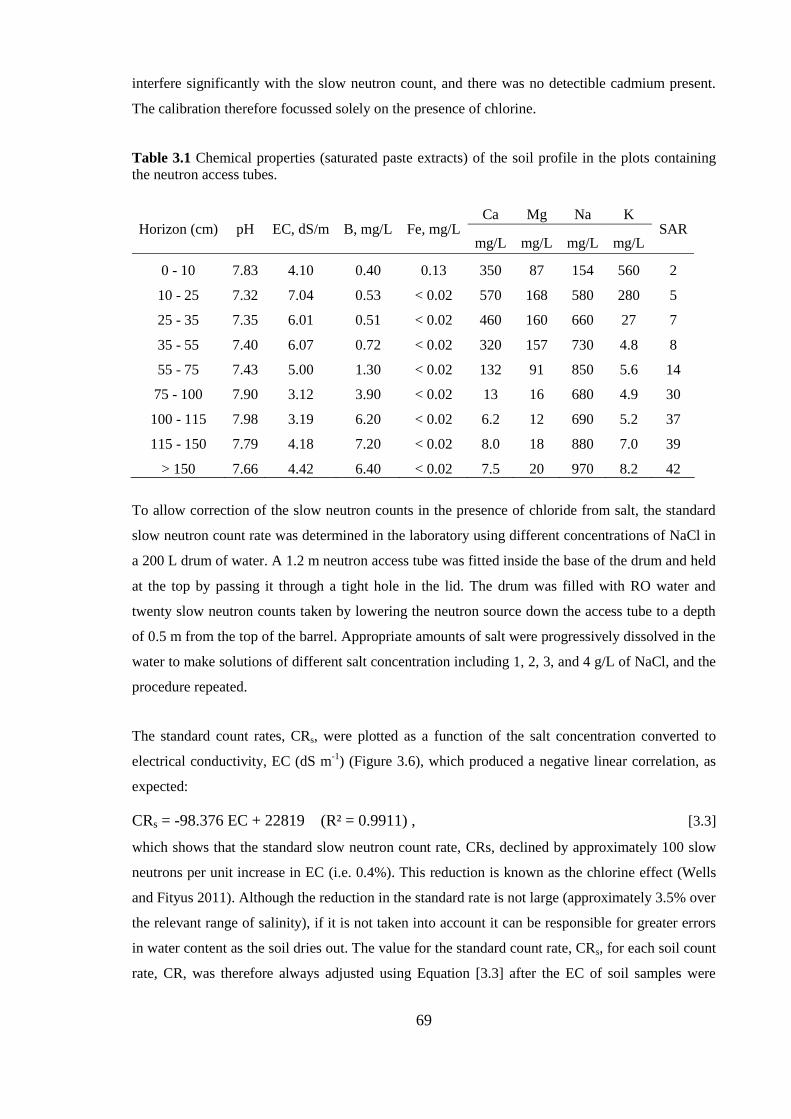
69
interfere significantly with the slow neutron count, and there was no detectible cadmium present.
The calibration therefore focussed solely on the presence of chlorine.
Table 3.1 Chemical properties (saturated paste extracts) of the soil profile in the plots containing the neutron access tubes.
Horizon (cm) pH EC, dS/m B, mg/L Fe, mg/L Ca Mg Na K
SAR mg/L mg/L mg/L mg/L
0 - 10 7.83 4.10 0.40 0.13 350 87 154 560 2
10 - 25 7.32 7.04 0.53 < 0.02 570 168 580 280 5
25 - 35 7.35 6.01 0.51 < 0.02 460 160 660 27 7
35 - 55 7.40 6.07 0.72 < 0.02 320 157 730 4.8 8
55 - 75 7.43 5.00 1.30 < 0.02 132 91 850 5.6 14
75 - 100 7.90 3.12 3.90 < 0.02 13 16 680 4.9 30
100 - 115 7.98 3.19 6.20 < 0.02 6.2 12 690 5.2 37
115 - 150 7.79 4.18 7.20 < 0.02 8.0 18 880 7.0 39
> 150 7.66 4.42 6.40 < 0.02 7.5 20 970 8.2 42
To allow correction of the slow neutron counts in the presence of chloride from salt, the standard
slow neutron count rate was determined in the laboratory using different concentrations of NaCl in
a 200 L drum of water. A 1.2 m neutron access tube was fitted inside the base of the drum and held
at the top by passing it through a tight hole in the lid. The drum was filled with RO water and
twenty slow neutron counts taken by lowering the neutron source down the access tube to a depth
of 0.5 m from the top of the barrel. Appropriate amounts of salt were progressively dissolved in the
water to make solutions of different salt concentration including 1, 2, 3, and 4 g/L of NaCl, and the
procedure repeated.
The standard count rates, CRs, were plotted as a function of the salt concentration converted to
electrical conductivity, EC (dS m-1) (Figure 3.6), which produced a negative linear correlation, as
expected:
CRs = -98.376 EC + 22819 (R² = 0.9911) , [3.3]
which shows that the standard slow neutron count rate, CRs, declined by approximately 100 slow
neutrons per unit increase in EC (i.e. 0.4%). This reduction is known as the chlorine effect (Wells
and Fityus 2011). Although the reduction in the standard rate is not large (approximately 3.5% over
the relevant range of salinity), if it is not taken into account it can be responsible for greater errors
in water content as the soil dries out. The value for the standard count rate, CRs, for each soil count
rate, CR, was therefore always adjusted using Equation [3.3] after the EC of soil samples were

70
collected each week during the drying period. The measured ECs were taken on 1:5 soil:water
extracts, so these were first corrected to the EC of paste extracts using Slavich and Petterson (1993)
method.
Figure 3.6 Mean standard 15 second count rate, CRs, of CPN 503 Hydroprobe in a large drum of water having different salt concentrations as measured by EC (dS m-1). The red vertical bars through each point represent the ± standard error of the mean of 20 readings.
The variability in slow neutron counts was not influenced by salt concentration. That is, there was
no trend in the measurement error with salt content. For example, the sample variance of the mean
neutron count rate, s2, ranged between 13806 and 22620, which produced very low standard errors
and coefficients of variation (Table 3.2).
Table 3.2 Variation in the standard 15-second slow-neutron count rate with salt concentration.
[NaCl] mg/L
Mean count rate, CRs
Standard deviation of mean CRs
Number of measurements
Coefficient variation of
mean CRs, %
Standard error of
mean CRs 0 22792 147.9 20 0.65 33.1
1000 22603 117.5 20 0.52 26.3 2000 22423 138.1 20 0.62 30.9 3000 22221 129.9 20 0.58 29.0 4000 22030 150.4 20 0.68 33.6
By choosing an ‘acceptable’ error in slow neutron count readings, it was possible to calculate the
number of readings, n, required to obtain acceptably accurate mean neutron counts for a given
instrument, using the relation (Snedecor and Cochran 1989):
, [3.4]
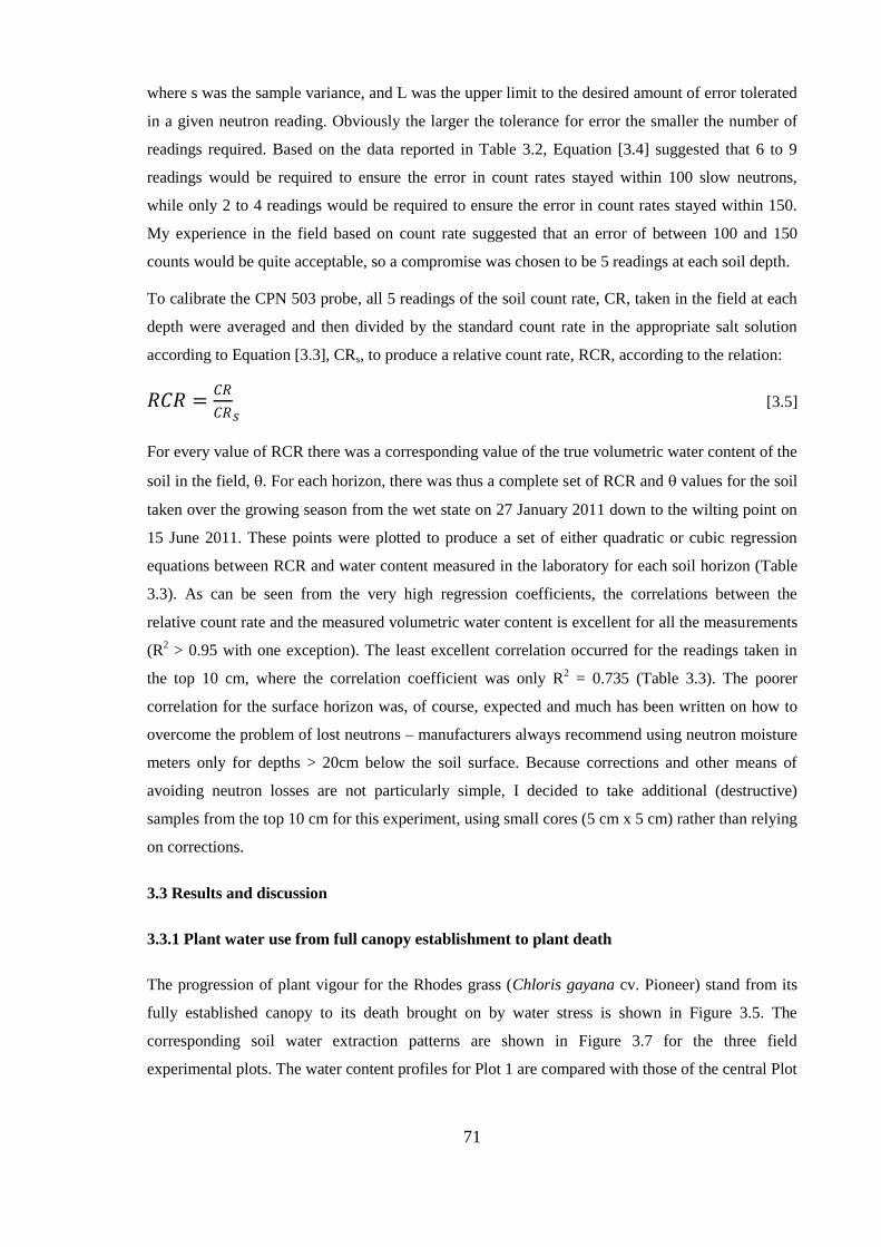
71
where s was the sample variance, and L was the upper limit to the desired amount of error tolerated
in a given neutron reading. Obviously the larger the tolerance for error the smaller the number of
readings required. Based on the data reported in Table 3.2, Equation [3.4] suggested that 6 to 9
readings would be required to ensure the error in count rates stayed within 100 slow neutrons,
while only 2 to 4 readings would be required to ensure the error in count rates stayed within 150.
My experience in the field based on count rate suggested that an error of between 100 and 150
counts would be quite acceptable, so a compromise was chosen to be 5 readings at each soil depth.
To calibrate the CPN 503 probe, all 5 readings of the soil count rate, CR, taken in the field at each
depth were averaged and then divided by the standard count rate in the appropriate salt solution
according to Equation [3.3], CRs, to produce a relative count rate, RCR, according to the relation:
[3.5]
For every value of RCR there was a corresponding value of the true volumetric water content of the
soil in the field, �. For each horizon, there was thus a complete set of RCR and � values for the soil
taken over the growing season from the wet state on 27 January 2011 down to the wilting point on
15 June 2011. These points were plotted to produce a set of either quadratic or cubic regression
equations between RCR and water content measured in the laboratory for each soil horizon (Table
3.3). As can be seen from the very high regression coefficients, the correlations between the
relative count rate and the measured volumetric water content is excellent for all the measurements
(R2 > 0.95 with one exception). The least excellent correlation occurred for the readings taken in
the top 10 cm, where the correlation coefficient was only R2 = 0.735 (Table 3.3). The poorer
correlation for the surface horizon was, of course, expected and much has been written on how to
overcome the problem of lost neutrons – manufacturers always recommend using neutron moisture
meters only for depths > 20cm below the soil surface. Because corrections and other means of
avoiding neutron losses are not particularly simple, I decided to take additional (destructive)
samples from the top 10 cm for this experiment, using small cores (5 cm x 5 cm) rather than relying
on corrections.
3.3 Results and discussion
3.3.1 Plant water use from full canopy establishment to plant death
The progression of plant vigour for the Rhodes grass (Chloris gayana cv. Pioneer) stand from its
fully established canopy to its death brought on by water stress is shown in Figure 3.5. The
corresponding soil water extraction patterns are shown in Figure 3.7 for the three field
experimental plots. The water content profiles for Plot 1 are compared with those of the central Plot

72
2 in Figure 3.7a; the profiles for Plot 3 are also compared with those of the central Plot 2 in Figure
3.7b. Finally, because all three plots showed essentially the same patterns over time, all three
profiles were averaged to produce a single set of temporal water content profiles in Figure 3.7c,
around which discussion will be focussed.
Table 3.3. Correlations between relative slow neutron count rate, RCR, and volumetric water content, �, at each depth in the soil profile.
Depth, (cm)
Correlation between volumetric water content and relative count rate from the neutron probe
Regression coefficient, R2
10 � = -9.68 RCR2 + 2.65RCR 0.735 20 � = 2.49 RCR3 - 5.44 RCR2 + 3.99 RCR - 0.61 0.935 30 � = 26.49 RCR3 - 34.69 RCR2 + 15.50 RCR – 2.13 0.993 40 � = 42.02 RCR3 - 60.29 RCR2 + 29.18 RCR – 4.50 0.993 50 � = 20.91 RCR3 - 28.89 RCR2 + 13.64 RCR – 1.94 0.983 60 � = 6.03 RCR3 - 8.14 RCR2 + 4.21 RCR – 0.55 0.992 70 � = 5.15 RCR3 - 6.84 RCR2 + 3.60 RCR – 0.44 0.997 80 � = 17.44 RCR3 - 22.46 RCR2 + 9.84 RCR – 1.22 0.991 90 � = 12.48 RCR3 - 16.43 RCR2 + 7.55 RCR – 0.94 0.996 100 � = 23.64 RCR3 - 31.11 RCR2 + 13.76 RCR – 1.79 0.964 110 � = 27.03 RCR3 - 36.22 RCR2 + 16.37 RCR – 2.22 0.952 120 � = 6.86 RCR3 - 8.91 RCR2 + 4.24 RCR – 0.44 0.996 130 � = 12.74 RCR3 - 17.62 RCR2 + 8.48 RCR – 1.11 0.962 140 � = 13.43 RCR3 - 21.01 RCR2 + 11.33 RCR – 1.78 0.980
3.3.2 Plant water use and root distribution
Assuming Equation [3.2] is valid and that all changes in the volumetric water content down the
profiles resulted from Rhodes grass transpiration alone, the greatest amount of active root water-
extraction occurred in the top 100 cm. The relatively slow reductions in water content below 100
cm in Figure 3.7c suggest either that roots were not very dense from that depth downward, or that
they were restricted in some way and were unable to extract as much water as the roots did in the
upper layers.
Root mass density measurements confirmed that roots were present all the way down the profile
(Figure 3.8) albeit at lower densities below 100 cm (Sheldon and Menzies 2005), and that these
roots did not extract as much water. Changes in the water content in the 100 to 140 cm zone may
simply reflect some upward capillary rise to replenish water use in the active part of the root zone,
but a complete evaluation of this idea is not within the scope of this thesis.

73
Figure 3.7a Volumetric water content as a function of depth for plots 1 and 2, from the time of the initial profile saturation (03 Nov 2010) until the plants wilted completely (15 June 2011). Horizontal bars represent ± standard error of the mean water content.
0
20
40
60
80
100
120
140
0.00 0.10 0.20 0.30 0.40 0.50
Dep
th, c
m
�v, cm3/cm3
0
20
40
60
80
100
120
140
0.00 0.10 0.20 0.30 0.40 0.50D
epth
, cm
�v, cm3/cm3
�v at saturation; these values are not included in the calculation of PAW
�v at saturation; these values are not included in the calculation of PAW
Plot 1
Plot 2 (centre)
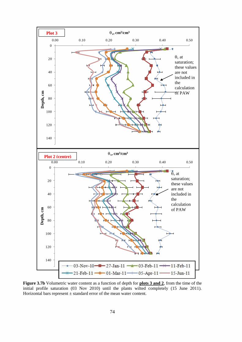
74
0
20
40
60
80
100
120
140
0.00 0.10 0.20 0.30 0.40 0.50D
epth
, cm
�v, cm3/cm3
Figure 3.7b Volumetric water content as a function of depth for plots 3 and 2, from the time of the initial profile saturation (03 Nov 2010) until the plants wilted completely (15 June 2011). Horizontal bars represent ± standard error of the mean water content.
0
20
40
60
80
100
120
140
0.00 0.10 0.20 0.30 0.40 0.50
Dep
th, c
m
�v, cm3/cm3
Plot 3
Plot 2 (centre)
�v at saturation; these values are not included in the calculation of PAW
�v at saturation; these values are not included in the calculation of PAW

75
Figure 3.7c Volumetric water content as a function of depth for plots all three plots averaged, from the time of the initial profile saturation (03 Nov 2010) until the plants wilted completely (15 June 2011). Horizontal bars represent ± standard error of the mean water content.
Figure 3.8 Distribution of Rhodes grass root mass per unit volume as a function of depth below the soil surface.
0
20
40
60
80
100
120
140
0.00 0.10 0.20 0.30 0.40 0.50D
epth
, cm
�v, cm3/cm3
All 3 plots averaged
�v at saturation; these values are not included in the calculation of PAW
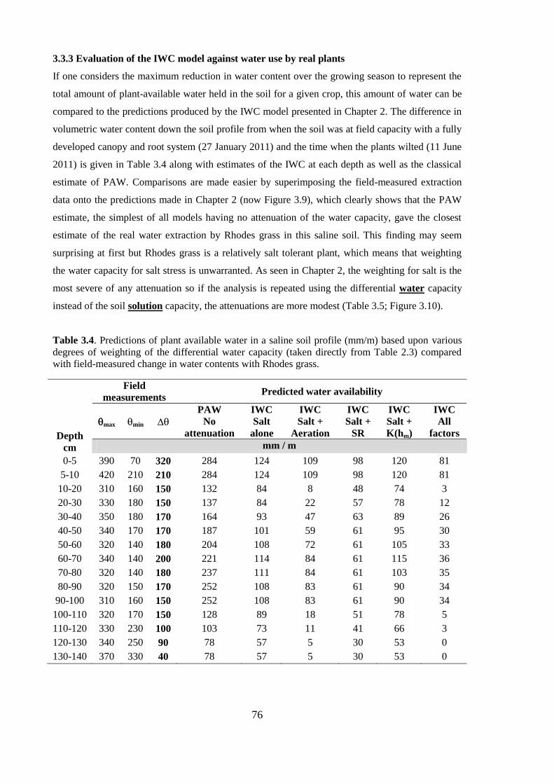
76
3.3.3 Evaluation of the IWC model against water use by real plants
If one considers the maximum reduction in water content over the growing season to represent the
total amount of plant-available water held in the soil for a given crop, this amount of water can be
compared to the predictions produced by the IWC model presented in Chapter 2. The difference in
volumetric water content down the soil profile from when the soil was at field capacity with a fully
developed canopy and root system (27 January 2011) and the time when the plants wilted (11 June
2011) is given in Table 3.4 along with estimates of the IWC at each depth as well as the classical
estimate of PAW. Comparisons are made easier by superimposing the field-measured extraction
data onto the predictions made in Chapter 2 (now Figure 3.9), which clearly shows that the PAW
estimate, the simplest of all models having no attenuation of the water capacity, gave the closest
estimate of the real water extraction by Rhodes grass in this saline soil. This finding may seem
surprising at first but Rhodes grass is a relatively salt tolerant plant, which means that weighting
the water capacity for salt stress is unwarranted. As seen in Chapter 2, the weighting for salt is the
most severe of any attenuation so if the analysis is repeated using the differential water capacity
instead of the soil solution capacity, the attenuations are more modest (Table 3.5; Figure 3.10).
Table 3.4. Predictions of plant available water in a saline soil profile (mm/m) based upon various degrees of weighting of the differential water capacity (taken directly from Table 2.3) compared with field-measured change in water contents with Rhodes grass.
Depth cm
Field measurements Predicted water availability
��max �min &� PAW
No attenuation
IWC Salt
alone
IWC Salt +
Aeration
IWC Salt +
SR
IWC Salt + K(hm)
IWC All
factors mm / m
0-5 390 70 320 284 124 109 98 120 81 5-10 420 210 210 284 124 109 98 120 81 10-20 310 160 150 132 84 8 48 74 3 20-30 330 180 150 137 84 22 57 78 12 30-40 350 180 170 164 93 47 63 89 26 40-50 340 170 170 187 101 59 61 95 30 50-60 320 140 180 204 108 72 61 105 33 60-70 340 140 200 221 114 84 61 115 36 70-80 320 140 180 237 111 84 61 103 35 80-90 320 150 170 252 108 83 61 90 34
90-100 310 160 150 252 108 83 61 90 34 100-110 320 170 150 128 89 18 51 78 5 110-120 330 230 100 103 73 11 41 66 3 120-130 340 250 90 78 57 5 30 53 0 130-140 370 330 40 78 57 5 30 53 0
77
Table 3.5. Predictions of plant available water (mm/m) based upon the same weightings of the differential water capacity but ignoring salt, compared with field-measured change in water contents with Rhodes grass.
Depth cm
Field measurements Predicted water availability
��max �min &� PAW
No attenuation
IWC Aeration
only
IWC SR only
IWC K(hm) only
IWC All factors
mm / m 0-5 390 70 320 284 189 243 270 151 5-10 420 210 210 284 189 243 270 151 10-20 310 160 150 132 12 75 114 3 20-30 330 180 150 137 44 116 137 28 30-40 350 180 170 164 80 121 176 39 40-50 340 170 170 187 80 121 176 39 50-60 320 140 180 204 80 121 176 39 60-70 340 140 200 221 117 124 210 51 70-80 320 140 180 237 117 124 210 51 80-90 320 150 170 252 150 160 212 61 90-100 310 160 150 252 150 160 212 61 100-110 320 170 150 128 22 79 112 6 110-120 330 230 100 103 22 79 112 6 120-130 340 250 90 78 1 43 72 0 130-140 370 330 40 78 0 52 69 0
Figure 3.9. Real soil water extraction for Rhodes grass (Chloris gayana cv. Pioneer) superimposed on estimates of water availability after various weightings of the soil solution capacity (i.e. including consideration of salt).
PAW – no factors Salt Salt + K(h) Salt + soil resistance Salt + aeration Salt + all factors Rhodes grass
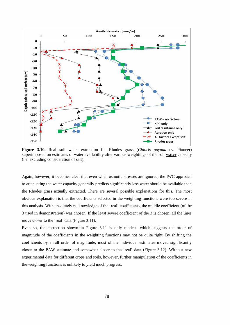
78
Figure 3.10. Real soil water extraction for Rhodes grass (Chloris gayana cv. Pioneer) superimposed on estimates of water availability after various weightings of the soil water capacity (i.e. excluding consideration of salt).
Again, however, it becomes clear that even when osmotic stresses are ignored, the IWC approach
to attenuating the water capacity generally predicts significantly less water should be available than
the Rhodes grass actually extracted. There are several possible explanations for this. The most
obvious explanation is that the coefficients selected in the weighting functions were too severe in
this analysis. With absolutely no knowledge of the ‘real’ coefficients, the middle coefficient (of the
3 used in demonstration) was chosen. If the least severe coefficient of the 3 is chosen, all the lines
move closer to the ‘real’ data (Figure 3.11).
Even so, the correction shown in Figure 3.11 is only modest, which suggests the order of
magnitude of the coefficients in the weighting functions may not be quite right. By shifting the
coefficients by a full order of magnitude, most of the individual estimates moved significantly
closer to the PAW estimate and somewhat closer to the ‘real’ data (Figure 3.12). Without new
experimental data for different crops and soils, however, further manipulation of the coefficients in
the weighting functions is unlikely to yield much progress.
PAW – no factors K(h) only Soil resistance only Aeration only All factors except salt Rhodes grass

79
Figure 3.11. Comparative estimates of water availability from Figure 3.10 adjusted with ‘gentler’ coefficients in the weighting functions.
Figure 3.12. Comparative estimates of water availability from Figure 3.11 adjusted with significantly ‘gentler’ coefficients in the weighting functions.
PAW – no factors K(h) only Soil resistance only Aeration only All factors except salt Rhodes grass
PAW – no factors K(h) only Soil resistance only Aeration only All factors except salt Rhodes grass

80
3.4 Conclusions
Even though the soil profile at this site was saline, estimates of plant-available water using IWC
with a weighting function for salinity proved too severe for the relatively salt tolerant Rhodes grass
(Chloris gayana cv. Pioneer). Adjusting the coefficients �, A and ' in the weighting functions to
minimize the attenuating effects of high soil resistance, low aeration and low hydraulic
conductivity, respectively, was only partly successful in bringing the IWC into line with measured
plant behaviour.
To make a thorough evaluation of the utility of weighting the water capacity for salinity with the
IWC, it will be necessary to use a range of different plants that vary in their tolerance of salt. Use
of very salt-sensitive plants in the first instance would go some way toward evaluating the merits of
the IWC model. However, this is easier said than done. The difficulty with such an approach would
be that to evaluate how much water a salt-sensitive root system can extract from a saline soil, a root
system must first be established in a medium in which it would not normally grow! A potential
solution might be to grow salt-sensitive plants in a non-saline medium and then expose it to salt
once the root system is fully established.
It is also possible that the assumptions used to establish some of the limits of integration in the
IWC model (e.g. hm = 10 kPa at the wet end, and hm = 1500 kPa at the dry end) are flawed. This
possibility needs to be evaluated using plants to establish the real limits. For example, given that
the water capacity has the greatest magnitude at the wet end, it is possible that plants can extract a
great deal more water before it drains away than is currently thought. Similarly, at the dry end,
some species are able to extract soil water well past the point that is nominally considered to be the
permanent wilting point. In this study, Rhodes grass (Chloris gayana cv. Pioneer) appeared to take
the soil matric head well past the point predicted from the water retention curve at 1500 kPa.
Greater understanding of the behaviour of a range of plants at the dry end would go some way
toward establishing plant-specific limits of integration.
81
Chapter 4 Changes in IWC during reclamation of a salt-affected soil
4.1 Introduction
Salt-affected soils are among the least productive soils in the world because they are often saline,
sodic and/or alkaline, which impedes plant water and nutrient uptake from them. Salinity, sodicity
and alkalinity generate osmotic stresses, element toxicities and poor soil physical conditions. In
particular, water may move slowly through them, be held in small (anaerobic) pores and the soil
may become hard and impenetrable to roots (Shainberg and Shalhevet 1984). To become
agriculturally productive, salt-affected soils must be reclaimed by draining and leaching them, and
by increasing the quantities of organic matter and calcium throughout the soil profile (e.g. (Jury et
al. 1979; Qadir et al. 1996; Ilyas et al. 1997; Akhter et al. 2004)
Reclamation of salt-affected soils, however, is no simple matter because any reduction in salt
concentration through leaching without a concomitant addition of divalent cations (e.g. calcium) to
replace sodium generally results in an immediate deterioration of soil hydraulic properties (c.f.
Chapter 1). Soils take on a massive structure with greatly reduced infiltration and hydraulic
conductivity and eventually become uninhabitable by plants. However, if dilute calcium salts are
gradually added such that the hydraulic conductivity is not reduced significantly during drainage
and leaching, the sodicity can be reduced at the same time that salt is removed and the physical
properties of the soil can gradually be improved (Quirk and Schofield 1955; Quirk 1986; Gupta and
Singh 1988; Rengasamy and Olsson 1991)
The improvement in soil properties during reclamation can dictate the productive capacity of the
soil for plants, especially on heavy clay-textured soils (Blokhuis 1980). The gradual success of
plants on reclaimed soils is due to a combination of improvements in nutrient availability, as well
as chemical and physical properties. In most cases, the re-introduction of plants occurs after
disturbance of the soil by some sort of tillage, the structure of which becomes stabilized to a large
extent by calcium and new plant roots. However, the extent to which improvements in soil
properties can be achieved without any tillage or other soil disturbance (i.e. simply by leaching
with appropriate salt solutions) is important to understand where deep tillage and disturbance are
neither feasible nor desirable.
If it is possible to make spontaneous changes in pore size distribution and structure simply by
leaching with calcium solutions, the magnitude of such changes should be reflected in the water
retention curve and possibly in other relevant soil physical properties. Jayawardane and Beattie
(1979) showed that leaching with solutions of differing SAR and EC made significant changes to
82
the water retention curve, but their study focussed solely on pore size distributions and ignored all
other soil physical properties and made no mention of plant available water. In the present study I
asked “how does soil water availability change (as measured using the IWC) during various stages
of reclamation of a saline-sodic soil?” I hypothesized that IWC would increase monotonously from
one critical state to the next during reclamation, but I acknowledged that an alternative hypothesis
would be that IWC would increase non-monotonously, depending upon the relative importance of
various soil physical properties at each stage of reclamation.
4.2 Materials and Methods
4.2.1 Experimental approach and design
This set of laboratory experiments was designed to take soil of the 9 horizons used in Chapters 2
and 3 from their initial saline-sodic states to various different, less saline and less sodic states, then
to measure the consequent changes in soil physical properties and determine whether they
influenced the IWC significantly.
Six different pathways (treatments) were chosen to take the soils from the saline-sodic state to a
lesser saline-sodic state. These consisted of a preliminary treatment applied to all samples of a
given horizon followed by a further treatment to reduce the salinity or sodicity:
1) Initial soil EC: Leaching with a solution having an EC & SAR to match that in the field; no
further leaching with any other solution – this was the ‘control’ treatment.
2) RO water: Treatment 1 followed by leaching with RO water – this was to maximize swelling
and dispersion and produce the most extreme effects on soil physical properties.
3) 0.1 M CaCl2: Treatment 1 followed by leaching first with 0.1 M CaCl2, then RO water – this
was to generate the extreme opposite effect to Treatment 2.
4) 1/2 initial EC: Treatment 1 followed by leaching first with a solution of identical composition
to Pre-treatment 1 but with only one half the initial EC (and ) this was to generate one
of three intermediate effects between Treatments 1 and 2.
5) 1/4 initial EC: Treatment 1 followed by Treatment 4 followed by leaching with a solution of
only one quarter the initial EC (and ) – this was to generate the second of three
intermediate effects between Treatments 1 and 2.
6) 1/16 initial EC: Treatment 1 followed Treatment 5 followed by leaching with a solution of
only one eighth the initial EC (and ) , followed by leaching with a solution of only
one sixteenth the initial EC (and ) – this was to generate the third of three intermediate
effects between Treatments 1 and 2.
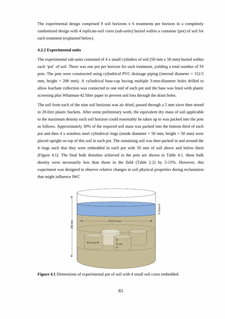
83
The experimental design comprised 9 soil horizons x 6 treatments per horizon in a completely
randomized design with 4 replicate-soil cores (sub-units) buried within a container (pot) of soil for
each treatment (explained below).
4.2.2 Experimental units
The experimental sub-units consisted of 4 x small cylinders of soil (50 mm x 50 mm) buried within
each ‘pot’ of soil. There was one pot per horizon for each treatment, yielding a total number of 54
pots. The pots were constructed using cylindrical PVC drainage piping (internal diameter = 152.5
mm, height = 200 mm). A cylindrical base-cap having multiple 3-mm-diameter holes drilled to
allow leachate collection was connected to one end of each pot and the base was lined with plastic
screening plus Whatman-42 filter paper to prevent soil loss through the drain holes.
The soil from each of the nine soil horizons was air dried, passed through a 5 mm sieve then stored
in 20-litre plastic buckets. After some preliminary work, the equivalent dry mass of soil applicable
to the maximum density each soil horizon could reasonably be taken up to was packed into the pots
as follows. Approximately 30% of the required soil mass was packed into the bottom third of each
pot and then 4 x stainless steel cylindrical rings (inside diameter = 50 mm; height = 50 mm) were
placed upright on top of this soil in each pot. The remaining soil was then packed in and around the
4 rings such that they were embedded in each pot with 50 mm of soil above and below them
(Figure 4.1). The final bulk densities achieved in the pots are shown in Table 4.1. these bulk
density were necessarily less than those in the field (Table 2.2) by 5-15%. However, this
experiment was designed to observe relative changes in soil physical properties during reclamation
that might influence IWC
Figure 4.1 Dimensions of experimental pot of soil with 4 small soil cores embedded.

84
Table 4.1. Bulk densities achieved for 150 mm columns of soil from each soil horizon (cylindrical pot diameter = 152.5 mm; calculated volume of each soil column = 2740 cm3).
Horizon, cm
Mass of soil, g
Bulk density, g/cm3
0 - 10 2603 0.95 10 - 25 3671 1.34 25 - 35 3973 1.45 35 - 55 4000 1.46 55- 75 4000 1.46
75 - 100 4055 1.48 100 - 115 4082 1.49 115 - 150 3973 1.45
> 150 4000 1.46
4.2.3 Experimental protocol
The appropriate composition of the leaching solutions was determined from an analysis of each soil
horizon. In this study (as distinct from the study reported in Chapter 2) all analyses were performed
on saturation paste extracts, the preparation of which is described in Appendix 18. Field-isotonic
solutions were prepared based upon the SAR and total cation concentrations shown in Table 4.2.
Table 4.2 Elemental analysis by ICP-MS for the major cations, plus SAR, EC and pH of the saturation paste extracts in each of the 9 soil horizons. SAR was calculated by dividing [Na] (mmol/L) by the square root of ([Ca] + [Mg]). The value for � cations (mmolc L-1) was the sum of ([Na] + [K]) plus twice the sum of ([Ca] + [Mg]). The values of ECmeas were measured and they compare well with the values for ECcalc, which were calculated from � cations divided by 10.
Soil depth Ca Mg Na K SAR �� cations ECcalc ECmeas pH cm mmol L-1 mmolc L-1 dS m-1
0 - 10 8.75 3.64 6.71 14.36 2 45.85 4.59 4.10 7.83 10 - 25 14.25 7.01 25.00 7.18 5 74.70 7.47 7.04 7.32 25 - 35 11.25 6.55 28.26 0.69 7 64.55 6.45 6.01 7.35 35 - 55 8.25 6.80 32.61 0.13 8 62.84 6.28 6.07 7.40 55 - 75 3.31 3.84 37.17 0.15 14 51.62 5.16 5.00 7.43 75 - 100 0.33 0.67 29.78 0.13 30 31.91 3.19 3.12 7.90 100 - 115 0.16 0.51 30.43 0.15 37 31.93 3.19 3.19 7.98 115 - 150 0.22 0.79 39.57 0.19 39 41.77 4.18 4.18 7.79 > 150 0.19 0.83 42.39 0.24 42 44.68 4.47 4.42 7.66
Each of the 54 pots was wetted with the appropriate isotonic solution (from Table 4.2) by capillary
action established in large rectangular baths containing a few centimetres of each solution. When
8 The study reported in Chapter 2 used 1:5 soil:water extracts to measure pH and EC and then converted to equivalent saturation paste-extract values using the method of Slavich and Petterson (1989); this was done so that results could be compared across Chapters.

85
the soil surface of each pot became wet by capillary rise, the level of the solution in each bath was
gradually raised to the top of each pot to completely saturate the soil. When saturation was
achieved, Whatman-42 filter paper was placed on the surface of each soil and a ponded head of 20
mm was established using a Mariotte bottle over each soil surface to begin the leaching process.
Each pot was suspended over a container in which the leachate was collected to measure the EC
until it reached the same value as the input-solution EC and until the flux of solution reached
steady state (this required approximately 2 days – see below). At this point the saturated hydraulic
conductivity was determined from the measured flux of leachate, the cross-sectional area of the pot,
and the hydraulic gradient, determined from the height of the soil column and of the static pond of
solution on the soil surface. After the saturated hydraulic conductivity was measured, one of the 6
pots for each soil horizon was removed and allowed to stand and drain under the influence of
gravity for 24 hours (total of 9 pots) prior to taking further measurements (Figure 4.2).
Figure 4.2 Leaching and sampling protocol for each soil horizon. Treatment numbers are indicated in the first pot on the left.
6
5
4
3
2
1
86
Each of the 9 selected pots was then carefully dismantled to release the four embedded soil cores
(sub-units) for analysis as follows. The soil surrounding each of the four embedded cores in each
pot was trimmed away and a nylon mesh fitted to one end of each core held in a ring. These four
sub-units were then re-saturated in their respective isotonic solutions and then taken through the
steps required to obtain water retention curves and soil resistance curves as described in Chapter 2.
After the first set of pots was removed for analysis, the remaining 5 pots for each soil horizon were
taken through the next leaching stage according to the treatments listed in Section 4.2.1 above.
After each leaching-treatment, a complete set of 9 pots was removed and analysed as described
above to produce another set of water retention curves and soil resistance curves. This procedure
was continued until all 6 treatments were applied to all 9 horizons (replicated on 4 sub-units/cores)
to generate 54 x 4 = 216 soil water retention curves and soil resistance curves.
An estimate of the period required for cation exchange and diffusion to occur during leaching was
estimated from the approximate relation:
[4.1]
where is the root mean square distance travelled in a time t by diffusing cations in the soil
matrix where the effective diffusion coefficient is D. In the saturated soil matrices used in these
leaching experiments, D was estimated to be at least 3.3x10⁻¹¹
m2 s-1 for the major cations (Rowell
et al. 1967; Gregory 2006). The diffusion path length was assumed to be equal to the radius of the
largest aggregates, which in this case was determined by the 5 mm sieve used in preparing the soil
(i.e. 0.0025 m). Equation [4.1] produces a time of 26 hours. It was decided to allow the soil
columns to leach for 48 hours before hydraulic conductivities were measured. At this time steady-
state flow rates were achieved.
The soil water retention and soil resistance data were fitted to the models of Groenevelt et al.
(2001; 2004) and Grant et al. (2010) using the mathematical software package, MathCAD 14
(Mathsoft 2008), and the integral water capacities (IWC) calculated.
4.3 Result and discussion
4.3.1 Changes in saturated hydraulic conductivity during reclamation
As might be expected in a soil where the texture gradually becomes heavier with depth, the
saturated hydraulic conductivity, Ks, of the “Initial EC” (Treatment 1) soils, decreased by several

87
orders of magnitude down the soil profile from approximately 2 x 10⁻⁶ m s-1 in the top horizon
down to 5 x 10⁻⁸ m s-1 in the heavy clay subsoil (Figure 4.3). In every horizon down the profile, the
“Initial EC” soil (red bars, Treatment 1) and the “0.1M CaCl2” soils (pink bars, Treatment 3) had
the highest salt concentrations so they maintained the largest hydraulic conductivities. By contrast,
the “RO water” soils (blue bars, Treatment 2) had the lowest salt (electrolyte) concentrations, so
their hydraulic conductivities were invariably the lowest in all soil horizons. The differences in soil
solution among the intermediate treatments (dark grey bars, Treatment 4; light grey bars, Treatment
5; and white bars, Treatment 6) were reflected in the saturated hydraulic conductivities, which fell
between the three extreme treatments, although there were no consistent changes among
Treatments 4, 5 and 6 (Figure 4.3). These observations are all consistent with predictions arising
from theory and practice (e.g. Quirk and Schofield 1955); furthermore the trends were enhanced in
the sub-soil layers with greater clay contents, where a greater degree of swelling and dispersion of
clay and pore blockage due to deposition at points of particle contact (Dikinya et al. 2008) was
possible – it should be noted that the scale for Ks in the three sub soil horizons is an order of
magnitude smaller than in the upper horizons.
Figure 4.3 Changes in saturated hydraulic conductivity of repacked soil from a profile using leaching solutions of different EC and SAR.

88
4.3.2 Changes in water retention curves during reclamation
The water retention data from the 4 cores per pot were averaged and plotted for the 6 treatments
and 9 soil horizons in 54 water retention curves, each shown in Appendix 2. The water retention
model of Groenevelt et al. (2004) and Grant et al. (2010) was fitted to all the data and the
parameters are listed in Table 4.3. Where treatment effects were not obviously different, the data
were grouped and averaged to plot them in Figures 4.4a) to i) for the 9 soil horizons. For 8 of the 9
soil horizons, there was a clear general trend in the water contents at a given matric potential viz.
(Initial soil EC, 0.1M CaCl2) < ( ½, ¼, 1/16 initial EC) < RO water). Within these 3 treatment
groups, there were no significant differences. Accordingly, the curves have been grouped in this
way to exhibit extremes of behaviour and avoid clutter. This trend was absent from the 0-10 cm
horizon, probably because of its substantially larger soil organic matter content and coarser texture.
As found by Jayawardane and Beattie (1979), all treatments that generated significant swelling and
dispersion of clay (and caused the pore size distribution to shift toward smaller pores) also
increased water retention and produced an upward shift in the water retention curves. For example,
the soils treated with electrolyte-rich sodium solution alone (initial soil EC Treatment 1) or else 0.1
M calcium chloride (Treatment 3), remained completely stable and generated water retention
curves that declined more sharply (bottom red lines in Figures 4.4). This is consistent with the
finding that these soils all had significantly greater saturated hydraulic conductivities, which
reflected a distribution of larger, more stable pores (Figure 4.3). By contrast, the soils treated with
electrolyte-rich sodium solutions then diluted with high SAR solutions of lower salt content
(Treatments 2, 4, 5 and 6), all became unstable to varying degrees and produced finer pore size
distributions and less abrupt water retention curves. Again, this is consistent with the significantly
lower saturated hydraulic conductivities shown in Figure 4.3 for these soils.

89
Figure 4.4 Summary of water retention curves grouped according to whether treatment effects were obvious for soil horizons: a) 0-10 cm, b) 10-25 cm, c) 25-35 cm, and d) 35-55 cm. Groupings of curves are indicated for each soil horizon.
a) b)
c) d)

90
Figure 4.4 Water retention curves grouped according to whether treatment effects were obvious for soil horizons: e) 55-75 cm, f) 75-100 cm, g) 100-115 cm, and h) 115-150 cm. Groupings of curves are indicated for each soil horizon.
e) f)
g) h)

91
Figure 4.4 Water retention curves grouped according to whether treatment effects were obvious for soil horizon: i) > 150 cm. Groupings of curves are indicated.
The effects shown in Figure 4.3 and 4.4 depended on soil texture, as might be expected. For
example, the surface soil horizon, which contained mainly sand and organic matter, displayed
absolutely no significant treatment effects whatsoever, which is why there is only one (average)
water retention curve shown in Figure 4.4a. As the clay content increased with depth in the soil
profile (and as the organic matter content decreased), the treatment effects were gradually
magnified and the water retention curves separated from one another more obviously. Furthermore,
the variability in the water retention data dropped significantly as the clay content increased such
that the standard deviation of the mean �v at each suction was hidden to a large extent by the points
themselves (2nd and 3rd decimal places).
i)
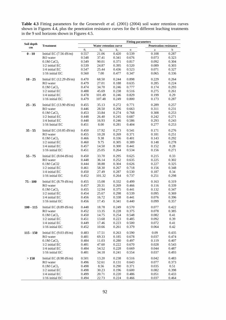
92
Table 4.3 Fitting parameters for the Groenevelt et al. (2001) (2004) soil water retention curves shown in Figures 4.4, plus the penetration resistance curves for the 6 different leaching treatments in the 9 soil horizons shown in Figures 4.5.
Soil depth cm Treatment
Fitting parameters Water retention curve Penetration resistance
�s k0 k1 n a b 0 - 10 Initial EC (7.56 dS/m) 0.557 21.06 0.420 0.539 0.108 0.287
RO water 0.548 37.41 0.341 0.676 0.073 0.323 0.1M CaCl2 0.549 90.01 0.371 0.817 0.092 0.304 1/2 initial EC 0.539 24.87 0.395 0.520 0.089 0.303 1/4 initial EC 0.547 25.44 0.436 0.523 0.071 0.327 1/16 initial EC 0.560 7.00 0.477 0.347 0.065 0.336
10 - 25 Initial EC (12.29 dS/m) 0.470 68.50 0.244 0.898 0.229 0.264 RO water 0.479 27.01 0.188 0.635 0.285 0.224 0.1M CaCl2 0.474 34.70 0.246 0.777 0.174 0.293 1/2 initial EC 0.488 45.69 0.238 0.516 0.275 0.261 1/4 initial EC 0.478 101.49 0.246 0.829 0.199 0.29 1/16 initial EC 0.479 107.48 0.249 0.800 0.173 0.287
25 - 35 Initial EC (13.90 dS/m) 0.455 35.13 0.272 0.771 0.289 0.257 RO water 0.446 28.50 0.206 0.663 0.311 0.231 0.1M CaCl2 0.453 33.84 0.274 0.768 0.308 0.253 1/2 Initial EC 0.448 26.40 0.245 0.687 0.242 0.271 1/4 Initial EC 0.448 16.93 0.246 0.586 0.293 0.243 1/16 Initial EC 0.451 8.00 0.281 0.404 0.277 0.253
35 - 55 Initial EC (10.85 dS/m) 0.450 17.92 0.273 0.541 0.171 0.276 RO water 0.455 10.28 0.269 0.371 0.181 0.251 0.1M CaCl2 0.466 9.38 0.336 0.401 0.143 0.292 1/2 initial EC 0.460 9.75 0.305 0.389 0.148 0.278 1/4 initial EC 0.457 14.50 0.300 0.441 0.152 0.28 1/16 initial EC 0.451 25.05 0.264 0.534 0.156 0.271
55 - 75 Initial EC (8.04 dS/m) 0.450 33.70 0.295 0.625 0.215 0.33 RO water 0.448 36.14 0.252 0.635 0.225 0.302 0.1M CaCl2 0.444 38.88 0.304 0.626 0.227 0.325 1/2 initial EC 0.461 58.30 0.267 0.718 0.156 0.348 1/4 initial EC 0.450 27.49 0.287 0.530 0.187 0.34 1/16 initial EC 0.452 101.32 0.264 0.737 0.251 0.298
75 - 100 Initial EC (8.79 dS/m) 0.455 15.08 0.332 0.499 0.163 0.319 RO water 0.457 20.31 0.269 0.466 0.116 0.339 0.1M CaCl2 0.455 12.94 0.375 0.441 0.132 0.347 1/2 initial EC 0.454 25.67 0.298 0.539 0.095 0.369 1/4 initial EC 0.456 16.72 0.338 0.441 0.076 0.396 1/16 initial EC 0.456 17.45 0.341 0.440 0.099 0.357
100 - 115 Initial EC (8.89 dS/m) 0.448 18.78 0.249 0.570 0.077 0.422 RO water 0.452 13.35 0.228 0.375 0.078 0.385 0.1M CaCl2 0.450 14.75 0.254 0.548 0.082 0.41 1/2 initial EC 0.451 13.68 0.223 0.485 0.092 0.39 1/4 initial EC 0.449 17.46 0.223 0.500 0.072 0.41 1/16 initial EC 0.452 10.66 0.261 0.379 0.064 0.42
115 - 150 Initial EC (9.03 dS/m) 0.483 17.51 0.263 0.590 0.09 0.435 RO water 0.481 69.33 0.185 0.678 0.037 0.474 0.1M CaCl2 0.484 11.03 0.280 0.497 0.119 0.407 1/2 initial EC 0.481 47.60 0.222 0.670 0.028 0.543 1/4 initial EC 0.484 54.52 0.228 0.669 0.044 0.487 1/16 initial EC 0.481 34.18 0.241 0.554 0.037 0.493
> 150 Initial EC (8.98 dS/m) 0.501 13.20 0.238 0.516 0.042 0.483 RO water 0.496 52.61 0.131 0.643 0.077 0.373 0.1M CaCl2 0.498 8.56 0.290 0.371 0.035 0.51 1/2 initial EC 0.498 30.23 0.196 0.600 0.082 0.398 1/4 initial EC 0.499 20.71 0.220 0.486 0.051 0.433 1/16 initial EC 0.494 22.73 0.224 0.466 0.037 0.464
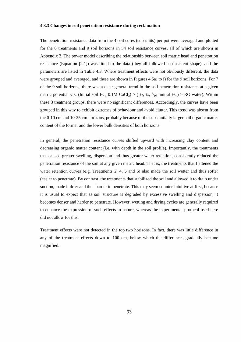
93
4.3.3 Changes in soil penetration resistance during reclamation
The penetration resistance data from the 4 soil cores (sub-units) per pot were averaged and plotted
for the 6 treatments and 9 soil horizons in 54 soil resistance curves, all of which are shown in
Appendix 3. The power model describing the relationship between soil matric head and penetration
resistance (Equation [2.1]) was fitted to the data (they all followed a consistent shape), and the
parameters are listed in Table 4.3. Where treatment effects were not obviously different, the data
were grouped and averaged, and these are shown in Figures 4.5a) to i) for the 9 soil horizons. For 7
of the 9 soil horizons, there was a clear general trend in the soil penetration resistance at a given
matric potential viz. (Initial soil EC, 0.1M CaCl2) > ( ½, ¼, 1/16 initial EC) > RO water). Within
these 3 treatment groups, there were no significant differences. Accordingly, the curves have been
grouped in this way to exhibit extremes of behaviour and avoid clutter. This trend was absent from
the 0-10 cm and 10-25 cm horizons, probably because of the substantially larger soil organic matter
content of the former and the lower bulk densities of both horizons.
In general, the penetration resistance curves shifted upward with increasing clay content and
decreasing organic matter content (i.e. with depth in the soil profile). Importantly, the treatments
that caused greater swelling, dispersion and thus greater water retention, consistently reduced the
penetration resistance of the soil at any given matric head. That is, the treatments that flattened the
water retention curves (e.g. Treatments 2, 4, 5 and 6) also made the soil wetter and thus softer
(easier to penetrate). By contrast, the treatments that stabilized the soil and allowed it to drain under
suction, made it drier and thus harder to penetrate. This may seem counter-intuitive at first, because
it is usual to expect that as soil structure is degraded by excessive swelling and dispersion, it
becomes denser and harder to penetrate. However, wetting and drying cycles are generally required
to enhance the expression of such effects in nature, whereas the experimental protocol used here
did not allow for this.
Treatment effects were not detected in the top two horizons. In fact, there was little difference in
any of the treatment effects down to 100 cm, below which the differences gradually became
magnified.

94
Figure 4.5 Soil resistance curves grouped according to whether treatment effects were obvious for soil horizon: a) 0-10 cm, b) 10-25 cm, c) 25-35 cm, and d) 35-55 cm. Groupings of curves are indicated for each soil horizon.
b) a)
c) d)

95
Figure 4.5 Soil resistance curves grouped according to whether treatment effects were obvious for soil horizon: e) 55-75 cm, f) 75-100 cm, g) 100-115 cm, and h) 115-135 cm. Groupings of curves are indicated for each soil horizon.
e) f)
g) h)
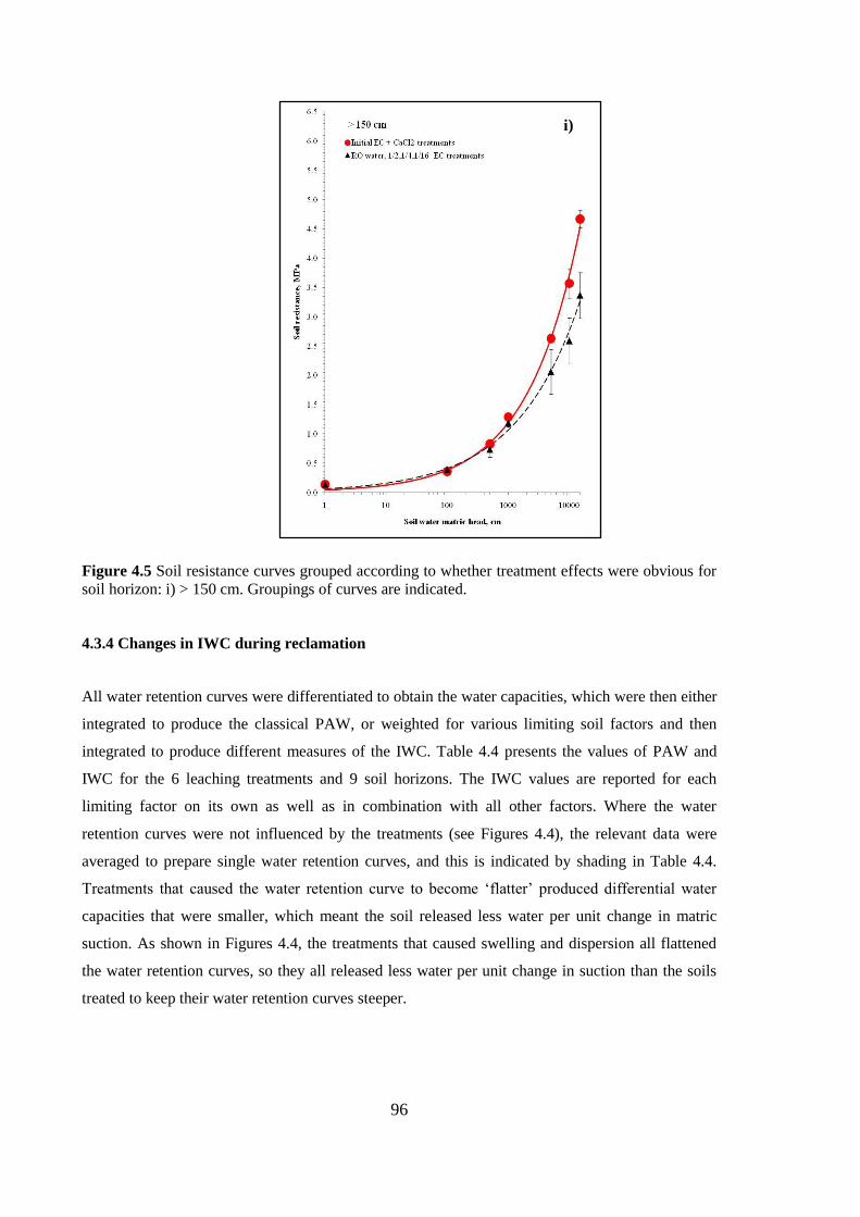
96
Figure 4.5 Soil resistance curves grouped according to whether treatment effects were obvious for soil horizon: i) > 150 cm. Groupings of curves are indicated.
4.3.4 Changes in IWC during reclamation
All water retention curves were differentiated to obtain the water capacities, which were then either
integrated to produce the classical PAW, or weighted for various limiting soil factors and then
integrated to produce different measures of the IWC. Table 4.4 presents the values of PAW and
IWC for the 6 leaching treatments and 9 soil horizons. The IWC values are reported for each
limiting factor on its own as well as in combination with all other factors. Where the water
retention curves were not influenced by the treatments (see Figures 4.4), the relevant data were
averaged to prepare single water retention curves, and this is indicated by shading in Table 4.4.
Treatments that caused the water retention curve to become ‘flatter’ produced differential water
capacities that were smaller, which meant the soil released less water per unit change in matric
suction. As shown in Figures 4.4, the treatments that caused swelling and dispersion all flattened
the water retention curves, so they all released less water per unit change in suction than the soils
treated to keep their water retention curves steeper.
i)
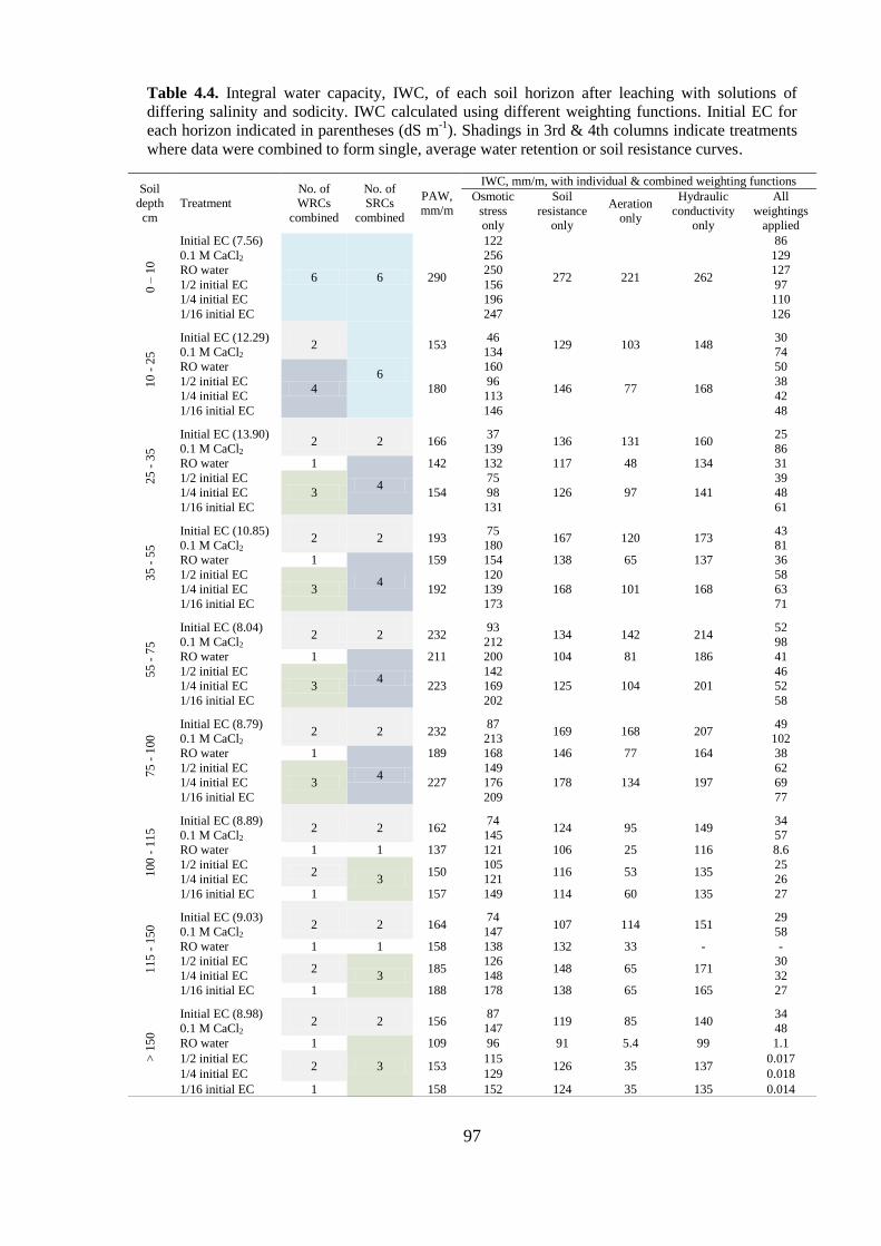
97
Table 4.4. Integral water capacity, IWC, of each soil horizon after leaching with solutions of differing salinity and sodicity. IWC calculated using different weighting functions. Initial EC for each horizon indicated in parentheses (dS m-1). Shadings in 3rd & 4th columns indicate treatments where data were combined to form single, average water retention or soil resistance curves.
Soil depth cm
Treatment No. of WRCs
combined
No. of SRCs
combined
PAW, mm/m
IWC, mm/m, with individual & combined weighting functions Osmotic
stress only
Soil resistance
only
Aeration only
Hydraulic conductivity
only
All weightings
applied
0 –
10
Initial EC (7.56)
6 6 290
122
272 221 262
86 0.1 M CaCl2 256 129 RO water 250 127 1/2 initial EC 156 97 1/4 initial EC 196 110 1/16 initial EC 247 126
10 -
25
Initial EC (12.29) 2
6
153 46 129 103 148 30 0.1 M CaCl2 134 74 RO water
4 180
160
146 77 168
50 1/2 initial EC 96 38 1/4 initial EC 113 42 1/16 initial EC 146 48
25 -
35
Initial EC (13.90) 2 2 166 37 136 131 160 25 0.1 M CaCl2 139 86 RO water 1
4
142 132 117 48 134 31 1/2 initial EC
3 154 75
126 97 141 39
1/4 initial EC 98 48 1/16 initial EC 131 61
35 -
55
Initial EC (10.85) 2 2 193 75 167 120 173 43 0.1 M CaCl2 180 81 RO water 1
4
159 154 138 65 137 36 1/2 initial EC
3 192 120
168 101 168 58
1/4 initial EC 139 63 1/16 initial EC 173 71
55 -
75
Initial EC (8.04) 2 2 232 93 134 142 214 52 0.1 M CaCl2 212 98 RO water 1
4
211 200 104 81 186 41 1/2 initial EC
3 223 142
125 104 201 46
1/4 initial EC 169 52 1/16 initial EC 202 58
75 -
100
Initial EC (8.79) 2 2 232 87 169 168 207 49 0.1 M CaCl2 213 102 RO water 1
4
189 168 146 77 164 38 1/2 initial EC
3 227 149
178 134 197 62
1/4 initial EC 176 69 1/16 initial EC 209 77
100
- 115
Initial EC (8.89) 2 2 162 74 124 95 149 34 0.1 M CaCl2 145 57 RO water 1 1 137 121 106 25 116 8.6 1/2 initial EC 2 3 150 105 116 53 135 25 1/4 initial EC 121 26 1/16 initial EC 1 157 149 114 60 135 27
115
- 150
Initial EC (9.03) 2 2 164 74 107 114 151 29 0.1 M CaCl2 147 58 RO water 1 1 158 138 132 33 - - 1/2 initial EC 2 3 185 126 148 65 171 30 1/4 initial EC 148 32 1/16 initial EC 1 188 178 138 65 165 27
> 15
0
Initial EC (8.98) 2 2 156 87 119 85 140 34 0.1 M CaCl2 147 48 RO water 1
3
109 96 91 5.4 99 1.1 1/2 initial EC 2 153 115 126 35 137 0.017 1/4 initial EC 129 0.018 1/16 initial EC 1 158 152 124 35 135 0.014

98
The application of various weighting functions to account for high salinity, poor soil aeration, high
soil penetration resistance, and low hydraulic conductivity altered the amount of available water
significantly. Examples are shown for the soil when it was leached with a salt solution having the
same chemistry as its initial field state in Figure 4.6. The profile of solid red triangles shown on the
far left-hand side of Figure 4.6 represents the most extreme weighting of the water capacity, while
the open circles with the dashed black line on the far right-hand side of Figure 4.6 represent the
classical PAW, which puts no weighting on the water capacity. The lines in between the two
extremes show profiles of available water where the water capacity was weighted for the individual
factors; the results are consistent with the findings of Chapter 2, namely, that the weighting for high
salinity is the most severe, followed by that for poor soil aeration, then high soil penetration
resistance, then least significant of all the weightings, the unsaturated hydraulic conductivity.
Figure 4.6 Profiles of soil water availability calculated by weighting the water capacity of the soil in its initial saline state for different limiting factors.

99
Table 4.4 shows that the magnitude of PAW was always greater than any IWC values; this, of
course, is because PAW is not attenuated in any way – it represents the maximum possible amount
of water that can be extracted from the soil. So any attenuation of the water capacity must
obviously reduce the amount of available water. As found in Chapter 2, weighting of the water
capacity for salt (osmotic stress) caused the greatest single reduction in available water of any of
the weighting factors. Groenevelt et al. (2004) acknowledged that this weighting function for
osmotic stress creates the most severe attenuation possible because it assumes plants completely
exclude all salt during water uptake, which of course is not true. They do not behave like perfect
osmometers (Bazihizina et al. 2012) – they actively adjust their root cell membranes to allow (or
prevent) cations and anions to be taken up or released as required, a process known as osmo-
regulation. The extent to which plant cell membranes ‘open’ or ‘close’ in response to osmotic
stresses is quantified using a reflection coefficient, �. Groenevelt et al. (2004) argued that, as a first
approximation, plants osmo-regulate by adjusting � such that the product of the osmotic head of
the soil solution and the reflection coefficient maintains a relatively constant cell turgor pressure, T,
viz.
T = ho x �(t, hm, ho) , [4.2]
where �(t, hm, ho) is a complex plant-specific function of time, soil matric and osmotic heads.
In the absence any real data on plant-reflection coefficients Groenevelt et al. (2004) chose a value
of � = 1, which implied that plants experience the full effect of any osmotic stress in the soil
solution. Given that different plants can vary their reflection coefficients in the range 0 < � < 1 over
time, it is likely that better estimates of IWC could be obtained by adjusting � downward in some
appropriate way. Exploring the nature of � for different plants under different soil and
environmental conditions is the subject of an entirely different research project, which is beyond
the scope of this thesis. The recent work of Bazihizina et al. (2012), however, provides useful data
that might be used in such an analysis.
Despite the severity of the osmotic attenuation applied above, the reclamation process of reducing
salinity and sodicity caused an increase in IWC even when salinity effects alone were considered
using Groenevelt et al.’s (2004) model – i.e. no other attenuation applied (Figure 4.7a). When all
weighting functions were applied (including salinity effects) the recovery of IWC during
reclamation was considerably less (Figure 4.7b). This again reflects the fact that the method to
account for salinity effects was too severe and needs to be adjusted using appropriate reflection
coefficients for different plants.

100
Figure 4.7 Increases in plant available water (IWC) during reclamation of the soil profile from its initially sodic-saline state to a calcic non-saline state calculated using a) only the osmotic weighting function of Groenevelt et al. (2004), and b) all weighting functions. NB. The scales on the available water axis for parts a) and b) are different.
a)
b)

101
4.4 Conclusions
Although it was already known from Jayawardane and Beattile’s (1979) work that the water
retention curve of a saline-sodic soil can be shifted by changing the composition of the soil solution
toward calcic and non-saline, the work of this chapter has demonstrated that the changes to water
retention are accompanied by changes in other soil physical properties that have consequences for
plant available water.
Under the conditions established in this experiment, it was possible to make modest changes in the
structure of a saline/sodic soil profile (with no mechanical disturbance) by leaching it with a
relatively concentrated solution of calcium. Although the soil penetration resistance tended to be
higher in the calcium-treated soils than other treatments (because they drained faster and were drier
at most matric heads), the water retention curves were steeper than the other treatments, which
promotes good aeration. Furthermore, once the calcium salt was leached out, the salinity dropped
and thus the plant available water (as measured by IWC) was higher than the other treatments.
By simply leaching out the high SAR soil solution from the soil using progressively more dilute
solutions, the soil experienced greater and greater swelling and dispersion, which shifted the pore
size distribution to finer and finer pores. This had the effect of making the water retention curves
flatter and thus more poorly aerated at most matric heads. Plant available water, as measured by the
IWC generally declined as swelling and dispersion progressed during leaching, even though the
penetration resistance declined and thus made the soil softer and easier to penetrate. This small
advantage was more than compensated for by the poor soil aeration that accompanied the excessive
swelling and dispersion in these soils.
While the slightly lower bulk density of the test soil cores may have influenced the magnitude of
some soil physical properties and their changes during reclamation, I believe the nature of the
changes is likely to be reflected in undisturbed field soil. The soil properties that had the greatest
limiting effect on soil water were (in order of declining importance: salinity >> aeration > soil
resistance > hydraulic conductivity. It is likely, however, that if more realistic reflection
coefficients can be devised to reduce the impact of salinity on IWC, the limiting role of poor soil
aeration will be shown to be considerably more important by comparison. It could be particularly
important in the lower horizons, where soil aeration is restricted by high bulk density.

102
Chapter 5 Shape of the salinity weighting function, ��o(h), based upon early plant response to
osmotic and matric stresses
5.1 Introduction
Many studies have shown that a wide variety of non halophytic plants struggle to survive in saline
soils (Bernstein and Hayward 1958; Hoffman and Rawlins 1971; Bernstein 1975; Maas and
Hoffman 1977; Grieve and Maas 1988). Most can tolerate a small amount of salt but there is a
threshold concentration above which growth declines in a linear fashion. The magnitude of this
threshold concentration (EC) and the slope of the decline in growth varies with plant species (Maas
and Hoffman (1977). Stepphun et al. (2005) suggested that the decline in plant growth occurs in a
more continuous, S-shaped fashion rather than abruptly like a bent-stick. Furthermore, Kopittke et
al. (2009) found that plant growth of non halophytes is retarded even at very low concentrations
and that a ‘threshold concentration’ of salt may not apply to some plants.
Groenevelt et al. (2004) suggested an attenuation method to calculate the effect of osmotic stress
on soil water availability. Their attenuating function presented the worst-case scenario for water
availability by assuming that plants behave just like perfect osmometers and exclude all salt from
the soil solution. They acknowledged that this assumption was not very realistic and that plant cell
membranes exhibit a ‘reflection coefficient’, � (varying between 1 and 0) to adjust the extent to
which salts are excluded during water uptake. In their work, Groenevelt et al. (2004) used a
reflection coefficient of � = 1 (total salt exclusion) to demonstrate the principles involved but also
because they lacked information on the real magnitude of � for different plants. They pointed out,
however, that the classical PAW model (and all other models for that matter) use a default value of
� = 0, which essentially implies that plants completely ignore all salt in the soil water. Neither of
these extreme �-values is particularly close to reality but there was no published literature on such
things at the time of publication, so they simply set � = 1 to show the lower limits of water
availability when salt is taken into account.
As the work reported in Chapter 3 indicated, application of the Groenevelt et al-weighting function
for salt produced estimates of plant available water that were only half the true quantity of water
used by Rhodes grass in the field. That is, the weighting function was too severe and represented
the absolute minimum in available water accessible to a very salt-sensitive plant. There remains no
concrete evidence in the literature to guide the preparation of appropriate weighting functions for
salt in soil water, so an attempt was made here to gather such evidence experimentally. The
purpose of this study was therefore to prepare a weighting function for the water capacity
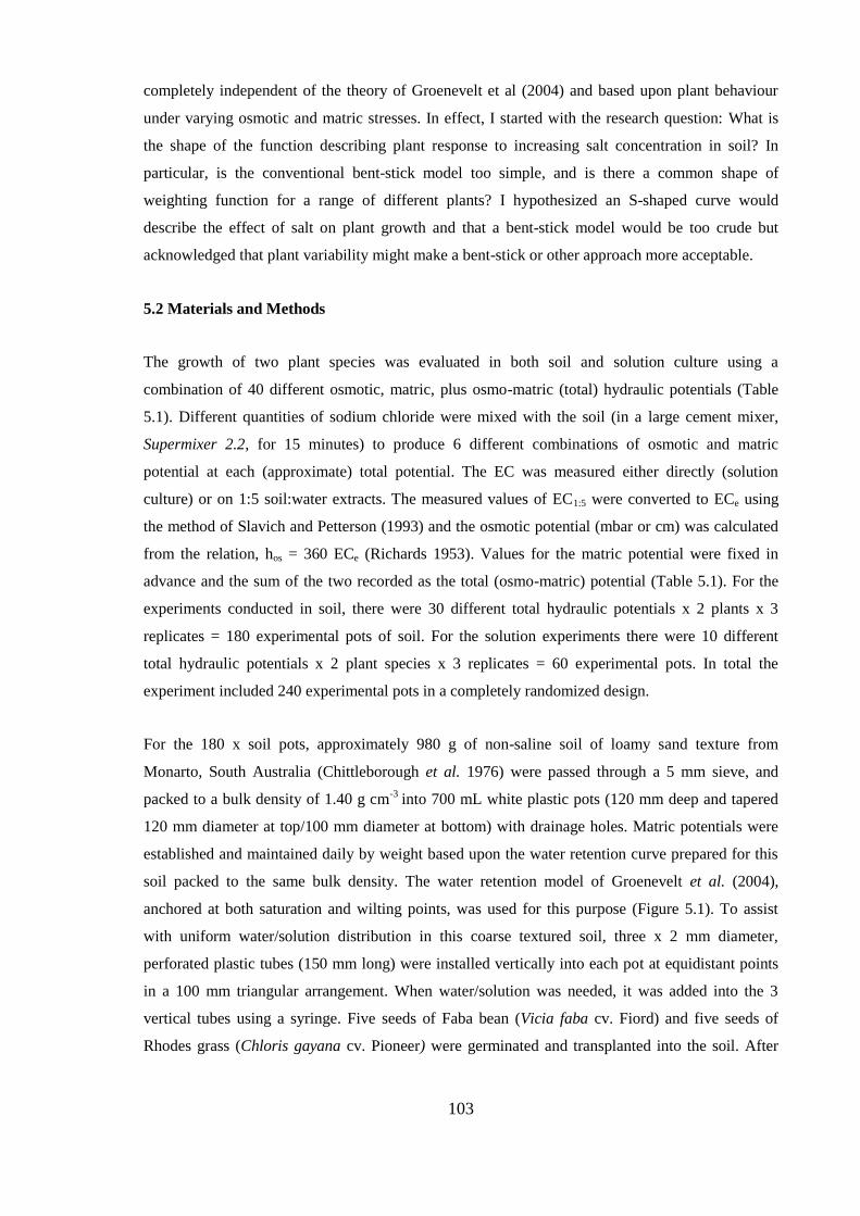
103
completely independent of the theory of Groenevelt et al (2004) and based upon plant behaviour
under varying osmotic and matric stresses. In effect, I started with the research question: What is
the shape of the function describing plant response to increasing salt concentration in soil? In
particular, is the conventional bent-stick model too simple, and is there a common shape of
weighting function for a range of different plants? I hypothesized an S-shaped curve would
describe the effect of salt on plant growth and that a bent-stick model would be too crude but
acknowledged that plant variability might make a bent-stick or other approach more acceptable.
5.2 Materials and Methods
The growth of two plant species was evaluated in both soil and solution culture using a
combination of 40 different osmotic, matric, plus osmo-matric (total) hydraulic potentials (Table
5.1). Different quantities of sodium chloride were mixed with the soil (in a large cement mixer,
Supermixer 2.2, for 15 minutes) to produce 6 different combinations of osmotic and matric
potential at each (approximate) total potential. The EC was measured either directly (solution
culture) or on 1:5 soil:water extracts. The measured values of EC1:5 were converted to ECe using
the method of Slavich and Petterson (1993) and the osmotic potential (mbar or cm) was calculated
from the relation, hos = 360 ECe (Richards 1953). Values for the matric potential were fixed in
advance and the sum of the two recorded as the total (osmo-matric) potential (Table 5.1). For the
experiments conducted in soil, there were 30 different total hydraulic potentials x 2 plants x 3
replicates = 180 experimental pots of soil. For the solution experiments there were 10 different
total hydraulic potentials x 2 plant species x 3 replicates = 60 experimental pots. In total the
experiment included 240 experimental pots in a completely randomized design.
For the 180 x soil pots, approximately 980 g of non-saline soil of loamy sand texture from
Monarto, South Australia (Chittleborough et al. 1976) were passed through a 5 mm sieve, and
packed to a bulk density of 1.40 g cm-3 into 700 mL white plastic pots (120 mm deep and tapered
120 mm diameter at top/100 mm diameter at bottom) with drainage holes. Matric potentials were
established and maintained daily by weight based upon the water retention curve prepared for this
soil packed to the same bulk density. The water retention model of Groenevelt et al. (2004),
anchored at both saturation and wilting points, was used for this purpose (Figure 5.1). To assist
with uniform water/solution distribution in this coarse textured soil, three x 2 mm diameter,
perforated plastic tubes (150 mm long) were installed vertically into each pot at equidistant points
in a 100 mm triangular arrangement. When water/solution was needed, it was added into the 3
vertical tubes using a syringe. Five seeds of Faba bean (Vicia faba cv. Fiord) and five seeds of
Rhodes grass (Chloris gayana cv. Pioneer) were germinated and transplanted into the soil. After
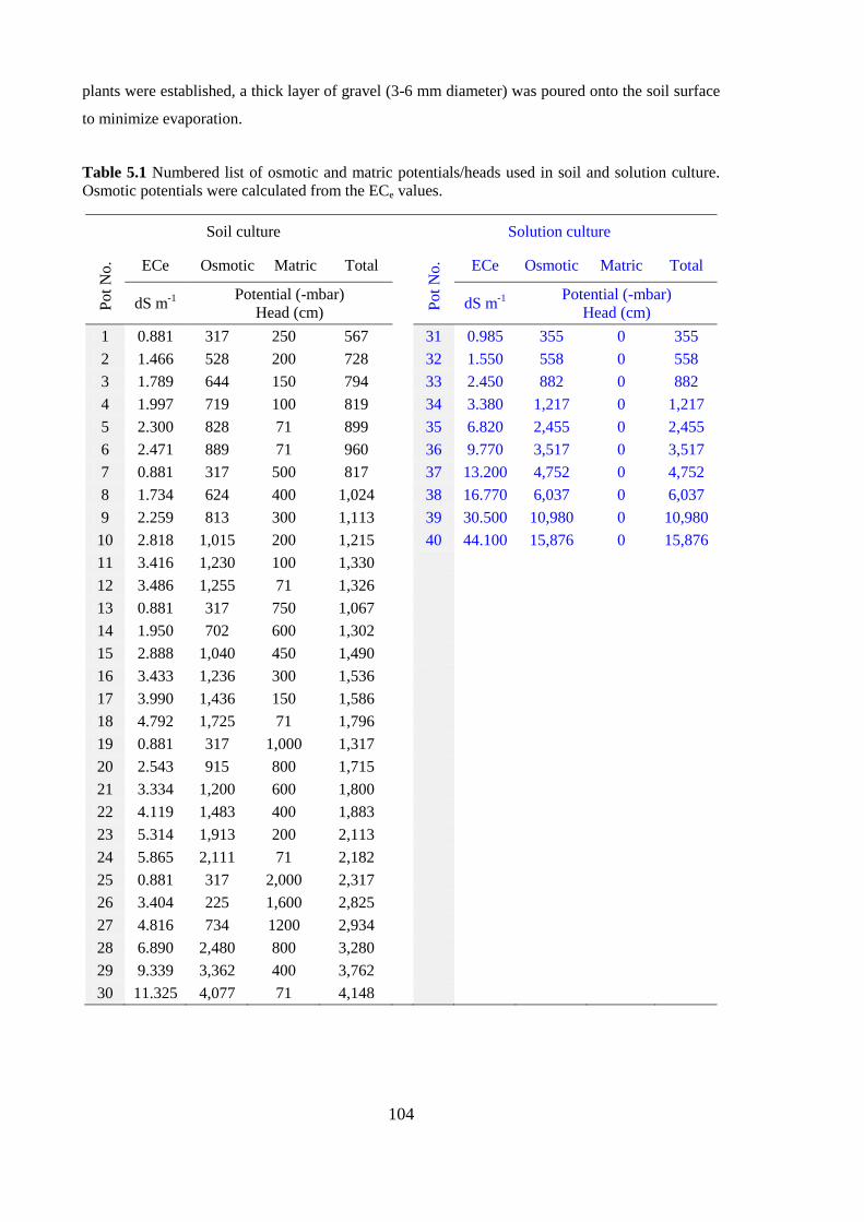
104
plants were established, a thick layer of gravel (3-6 mm diameter) was poured onto the soil surface
to minimize evaporation.
Table 5.1 Numbered list of osmotic and matric potentials/heads used in soil and solution culture. Osmotic potentials were calculated from the ECe values.
Soil culture Solution culture
Pot N
o. ECe Osmotic Matric Total
Pot N
o. ECe Osmotic Matric Total
dS m-1 Potential (-mbar) Head (cm) dS m-1 Potential (-mbar)
Head (cm) 1 0.881 317 250 567 31 0.985 355 0 355 2 1.466 528 200 728 32 1.550 558 0 558 3 1.789 644 150 794 33 2.450 882 0 882 4 1.997 719 100 819 34 3.380 1,217 0 1,217 5 2.300 828 71 899 35 6.820 2,455 0 2,455 6 2.471 889 71 960 36 9.770 3,517 0 3,517 7 0.881 317 500 817 37 13.200 4,752 0 4,752 8 1.734 624 400 1,024 38 16.770 6,037 0 6,037 9 2.259 813 300 1,113 39 30.500 10,980 0 10,980 10 2.818 1,015 200 1,215 40 44.100 15,876 0 15,876 11 3.416 1,230 100 1,330 12 3.486 1,255 71 1,326 13 0.881 317 750 1,067 14 1.950 702 600 1,302 15 2.888 1,040 450 1,490 16 3.433 1,236 300 1,536 17 3.990 1,436 150 1,586 18 4.792 1,725 71 1,796 19 0.881 317 1,000 1,317 20 2.543 915 800 1,715 21 3.334 1,200 600 1,800 22 4.119 1,483 400 1,883 23 5.314 1,913 200 2,113 24 5.865 2,111 71 2,182 25 0.881 317 2,000 2,317 26 3.404 225 1,600 2,825 27 4.816 734 1200 2,934 28 6.890 2,480 800 3,280 29 9.339 3,362 400 3,762 30 11.325 4,077 71 4,148

105
For the 60 x solution pots, each pot was filled with 3-6mm gravel to form a support-matrix into
which the plants could grow. Groups of 6 pots (2 plants x 3 reps) were placed into 10 litre
rectangular tubs (430 mm x 32 mm x 115 mm) containing 7 L of salt solution corresponding to
each osmotic potential. Dilute, water soluble fertilizer (Yates “Thrive”) was added to the solution at
a rate of 1.8 g/L and taken into account in calculating the osmotic potential; the EC of the solution
was monitored throughout the experiment. Five germinated seeds of the same plants were placed
carefully into the gravel in the different salt solutions. The solutions were refreshed every second
day to prevent algal growth and build up of salt.
All seedlings in both soil or solution culture were grown for 15 days after germination in
Glasshouse No.7 (Plant Research Centre, Waite Campus), which was set up to maintain appropriate
light, temperature and ventilation. At 15 days, all plants (roots and shoots) were harvested and
dried for 5 days at 65 C to measure dry matter production.
Figure 5.1 Soil water retention curve of Monarto soil packed at a bulk density of 1.4 g cm-3. Parameter values for the Groenevelt et al. (2004) equation are: �s = 0.405, �wp = 0.100; k0 = 0.409; k1 = 0.328, and n = 0.646.

106
5.3 Result and discussion
5.3.1 Dry matter yield as a function of osmotic-, matric- and total water potential
To prepare a weighting function for the differential water capacity in terms of the matric potential,
it was important first to establish the extent to which the water stress experienced by plants under
osmotic stress alone was equivalent to that experienced by plants under matric stress alone and
under both osmo-matric stresses at the same time. The experiments reported here were ideally set
up to make such a comparison because the range of osmotic solution potentials enveloped the range
of matric and osmo-matric potentials to which the plants were exposed.
Figure 5.2 shows the mean whole-plant dry matter yield of Faba bean (Vicia faba cv. Fiord) and of
Rhodes grass (Chloris gayana cv. Pioneer) grown in either soil media or solution media ranging in
total hydraulic potential from 0 to nearly -16 bar. As it turned out, neither Faba bean (Vicia faba cv.
Fiord) nor Rhodes grass (Chloris gayana cv. Pioneer) produced any dry matter whatsoever beyond
-11 bars, so there were no points between the total hydraulic potentials of -11 and -16 bar.
Identifying a definitive potential at which death occurred due to salt in these experiments was
therefore not possible, so the final potential was arbitrarily set at -15 bar to enable the theory
presented by Groenevelt et al. (2004) to be relied upon for the initial part of this analysis.
Figure 5.2 Mean whole-plant dry matter yield per plant plotted as a function of the total hydraulic potential (absolute value) for Faba beans and Rhodes grass grown in solution culture and soil. The vertical bars represent standard deviations of each mean point.

107
Figure 5.2 suggests that although the standard deviations for the soil-grown plants (red points) were
considerably greater than those for the solution-cultured plants (blue points), both sets of data
effectively occupied a single curve for each plant species within the range of common potentials.
This important result concurs with the work of Wadleigh and Ayers (1945) despite the fact that we
know the effects of matric stresses are often more complex than osmotic stresses (due to their
effects on hydraulic properties(Marshall et al. 1996). However, because hydraulic properties are
accounted for separately in weighting the water capacity for the IWC, it was possible to evaluate
the effects of osmotic stress independently here. Furthermore, the plant-effects were not related to
Na-induced calcium deficiencies (suggested by Kopittke and Menzies (2005)) or any other nutrient
deficiencies because tissue analysis was performed and indicated no such problems. There was
some necrosis of older leaf tips and leaf margin bronzing in the plants exposed to the highest salt
concentration but these were not nutritional symptoms (Weir and Creswell 1994). The reduction in
dry matter with total hydraulic potential in this short-term study can therefore be attributed largely
to water stress rather than any nutritional or toxicity problems (Munns and Termaat 1986).
Another important feature of the data shown in Figure 5.2 is that the patterns of growth reduction
are essentially the same for both Faba beans and Rhodes grass (logarithmic reductions) despite the
fact that Rhodes grass is nominally salt tolerant while Faba beans are nominally salt-sensitive. For
the purpose of developing a salt-weighting function for the water capacity, it will therefore be
accepted that matric and osmotic potentials influence uptake of water by plant roots in essentially
the same way. This has implications for the way in which the weighting function was developed
below.
5.3.2 A plant-based weighting function to attenuate the water capacity
To produce a salinity weighting function based upon a plant-growth response, the average plant dry
weights shown in Figure 5.2, G(hom), were divided by the maximum average dry weight of plants
grown in the soil or solution having the lowest salt concentration, G0(hom). This produced relative
growth values, G′(hom), which are plotted in Figure 5.3 as a function of the total hydraulic potential,
hom. A suitable function to describe the G′(hom) data is not immediately obvious from the shape of,
and variability in, the data so the following functional form was (tentatively) adopted as a first
approximation and fitted by eye rather than by a least squares analysis:
( � ( ���) [5.1]
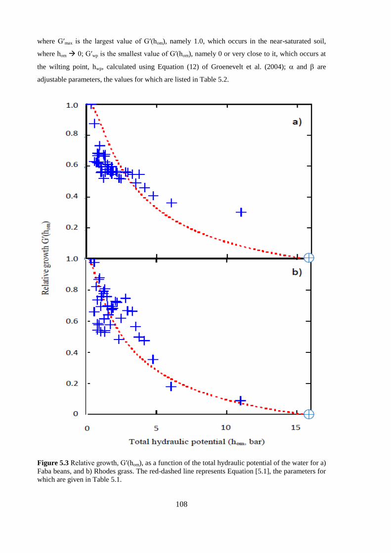
108
where G′max is the largest value of G′(hom), namely 1.0, which occurs in the near-saturated soil,
where hom � 0; G′wp is the smallest value of G′(hom), namely 0 or very close to it, which occurs at
the wilting point, hwp, calculated using Equation (12) of Groenevelt et al. (2004); ( and � are
adjustable parameters, the values for which are listed in Table 5.2.
Figure 5.3 Relative growth, G′(hom), as a function of the total hydraulic potential of the water for a) Faba beans, and b) Rhodes grass. The red-dashed line represents Equation [5.1], the parameters for which are given in Table 5.1.
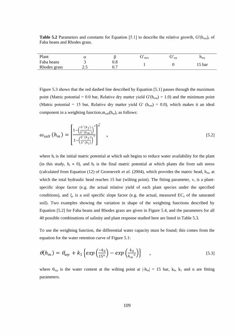
109
Table 5.2 Parameters and constants for Equation [5.1] to describe the relative growth, G′(hom), of Faba beans and Rhodes grass.
Plant ( � G′max G′wp hwp Faba beans 3 0.8 1 0 15 bar Rhodes grass 2.5 0.7
Figure 5.3 shows that the red dashed line described by Equation [5.1] passes through the maximum
point (Matric potential = 0.0 bar, Relative dry matter yield G′(hom) = 1.0) and the minimum point
(Matric potential = 15 bar, Relative dry matter yield G′ (hom) = 0.0), which makes it an ideal
component in a weighting function, salt(hm), as follows:
*
*
"
, [5.2]
where hi is the initial matric potential at which salt begins to reduce water availability for the plant
(in this study, hi + 0), and hf is the final matric potential at which plants die from salt stress
(calculated from Equation (12) of Groenevelt et al. (2004), which provides the matric head, hm, at
which the total hydraulic head reaches 15 bar (wilting point). The fitting parameter, *, is a plant-
specific slope factor (e.g. the actual relative yield of each plant species under the specified
conditions), and ", is a soil specific slope factor (e.g. the actual, measured ECe of the saturated
soil). Two examples showing the variation in shape of the weighting functions described by
Equation [5.2] for Faba beans and Rhodes grass are given in Figure 5.4, and the parameters for all
40 possible combinations of salinity and plant response studied here are listed in Table 5.3.
To use the weighting function, the differential water capacity must be found; this comes from the
equation for the water retention curve of Figure 5.1:
� � , [5.3]
where �wp is the water content at the wilting point at |-hm| = 15 bar, k0, k1 and n are fitting
parameters.
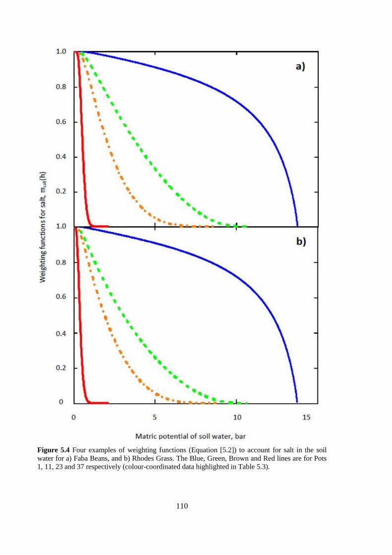
110
Figure 5.4 Four examples of weighting functions (Equation [5.2]) to account for salt in the soil water for a) Faba Beans, and b) Rhodes Grass. The Blue, Green, Brown and Red lines are for Pots 1, 11, 23 and 37 respectively (colour-coordinated data highlighted in Table 5.3).

111
Table 5.3. Parameters from Equation [5.2] used in preparing a weighting function to attenuate the water capacity for salinity, based upon soil and plant factors combined. In this study, the initial onset of osmotic stress was deduced to occur from hi = 0.0025 bar for all examples. The value of hf in this table is the matric potential at which wilting occurs under the salinity conditions corresponding to the ECe; values were calculated from Equation (12) of Groenevelt et al. (2004). Colour shaded data are shown in Figure 5.4 above.
Pot No.
Soil factors Plant factor "" = ECe (dS m-1) hf (-bar) **Faba **Rhodes
1 0.881 13.762 0.627 0.660 2 1.466 12.994 0.625 0.822 3 1.789 12.580 0.665 0.585 4 1.997 12.323 0.623 0.734 5 2.300 11.956 0.615 0.576 6 2.471 11.754 0.732 0.878 7 0.881 13.762 0.683 0.542 8 1.734 12.649 0.555 0.694 9 2.259 12.005 0.562 0.757 10 2.818 11.354 0.674 0.791 11 3.416 10.694 0.626 0.527 12 3.486 10.619 0.673 0.806 13 0.881 13.762 0.596 0.530 14 1.950 12.380 0.662 0.615 15 2.888 11.274 0.576 0.756 16 3.433 10.675 0.610 0.698 17 3.990 10.094 0.577 0.642 18 4.792 9.146 0.593 0.695 19 0.881 13.762 0.557 0.537 20 2.543 11.670 0.562 0.575 21 3.334 10.782 0.545 0.673 22 4.119 9.965 0.566 0.681 23 5.314 8.837 0.563 0.726 24 5.865 8.361 0.557 0.721 25 0.881 13.762 0.518 0.480 26 3.404 10.706 0.560 0.748 27 4.816 9.290 0.558 0.668 28 6.890 7.544 0.546 0.661 29 9.339 5.914 0.546 0.495 30 11.325 4.871 0.457 0.474 31 0.985 13.65 1.000 1.000 32 1.550 12.77 0.875 0.979 33 2.450 11.56 0.677 0.867 34 3.380 10.35 0.518 0.775 35 6.820 6.39 0.514 0.618 36 9.770 3.915 0.487 0.566 37 13.200 2.155 0.405 0.352 38 16.770 1.22 0.360 0.177 39 30.500 0.2 0.301 0.087 40 44.100 0 0.000 0.000
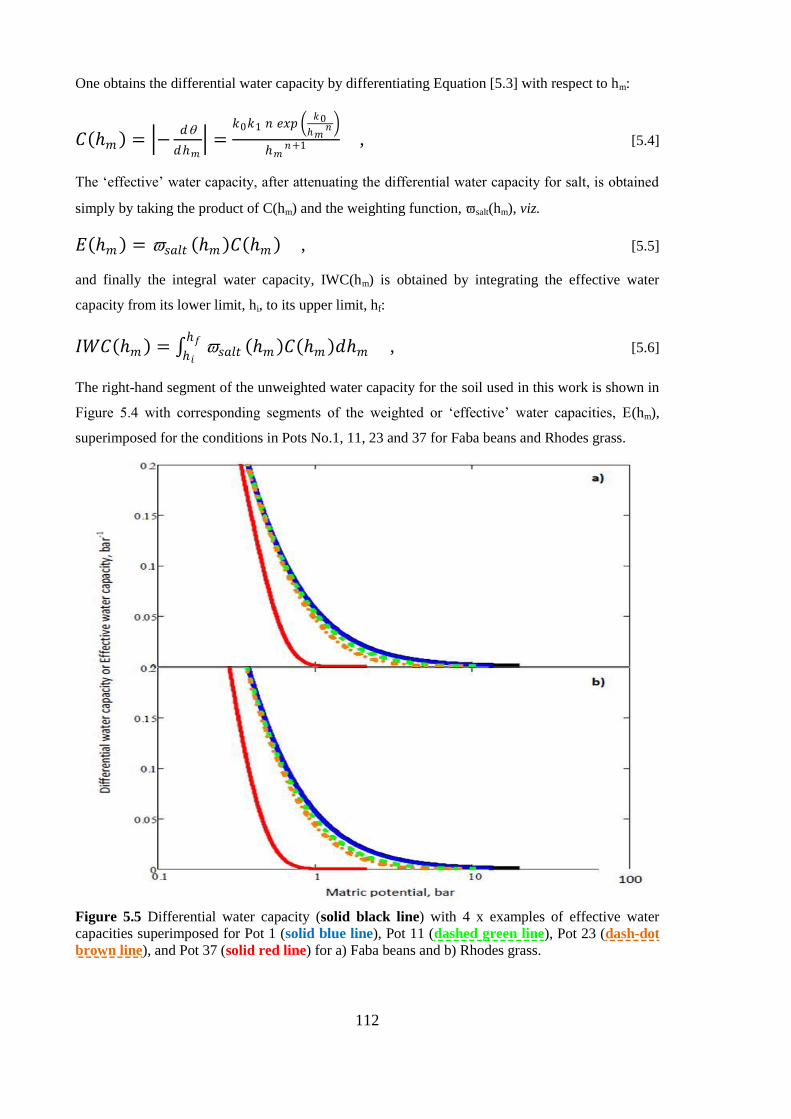
112
One obtains the differential water capacity by differentiating Equation [5.3] with respect to hm:
� , [5.4]
The ‘effective’ water capacity, after attenuating the differential water capacity for salt, is obtained
simply by taking the product of C(hm) and the weighting function, salt(hm), viz.
, [5.5]
and finally the integral water capacity, IWC(hm) is obtained by integrating the effective water
capacity from its lower limit, hi, to its upper limit, hf:
, [5.6]
The right-hand segment of the unweighted water capacity for the soil used in this work is shown in
Figure 5.4 with corresponding segments of the weighted or ‘effective’ water capacities, E(hm),
superimposed for the conditions in Pots No.1, 11, 23 and 37 for Faba beans and Rhodes grass.
Figure 5.5 Differential water capacity (solid black line) with 4 x examples of effective water capacities superimposed for Pot 1 (solid blue line), Pot 11 (dashed green line), Pot 23 (dash-dot brown line), and Pot 37 (solid red line) for a) Faba beans and b) Rhodes grass.

113
Clearly, the attenuation of the differential water capacity is relatively small until the salt
concentration becomes quite severe; this is in contrast to the very severe attenuation applied by the
equation of Groenevelt et al. (2004). The more modest attenuation embodied in the plant-based
weighting function of Equation [5.2] is consistent with the severely underestimated amount of plant
available water predicted using the Groenevelt et al. (2004) model in Chapter 2 for the field-based
study. A comparison of the integral water capacities calculated by the different approaches for the
examples shown in Figures 5.4 and 5.5 can be made from the data in Table 5.4.
Table 5.4 Estimates of plant available water in soil of varying salinity based on soil properties, or a combination of soil properties and plant response for Faba beans and Rhodes grass.
Unit
PAW by classical method
IWC by theory of Groenevelt et al. (2004)
IWC by plant-based weighting mm/m
mm / m mm / m Faba beans Rhodes grass Pot 1 252 211 244 243 Pot 11 252 134 213 204 Pot 23 252 108 192 187 Pot 37 252 63 122 97
5.4 Conclusions
The theoretical work of Groenevelt et al. (2004) laid the foundations for an attempt to take into
account osmotic stresses that plants experience in saline soils. Assuming conservation of mass,
they argued that the salt concentration increased as the water content decreased, which enabled
them to link the salt concentration to the water retention curve, which was an important advance.
Importantly they argued a case for setting the so-called plant-cell reflection coefficient, � = 1.0,
which meant that plant cell membranes completely excluded all salts (analogous to a perfect
osmometer). This meant, of course, that all their estimates of plant available water in the soil
represented the absolute lower boundary, which they freely acknowledged because they had no
knowledge of the appropriate reflection coefficients to use. The approach taken by Groenevelt et al.
(2004) was to express the classical differential WATER capacity, C(h), as a differential soil
SOLUTION capacity, Com(hm), which they expressed for each salt concentration in terms of an
osmotic potential, ho, and plotted it as a function of the matric potential, hm. The work presented in
this Chapter was intended to evaluate just how severe Groenevelt et al.’s (2004) attenuation
function really was by growing two different types of plants in saline soils and solutions and
evaluating their relative dry matter yields. The dry matter yields were then normalised and used to
develop a weighting function for the standard differential water capacity, C(hm).

114
The plant responses were highly variable but generally predictable but it was very difficult to fit a
response curve to the results using simple functions. A rather unsatisfactory model was fitted to the
data for the purposes of developing a function that could be readily used to attenuate the water
capacity. To the extent that the plant-response model was acceptable or satisfactory, its use in
defining a weighting function was highly successful. The model contained parameters that can be
linked to soil and plant properties that would be relatively easy to test. The estimates of plant
available water derived from the plant-based study sit on the high side of those produced by the
model of Groenevelt et al. (2004), and suggest that there is sufficient variation between two plant
species on different salt tolerance that a wider range of plants should be examined to determine
how broadly applicable the proposed weighting function is.

115
Chapter 6 General discussion and directions for future research
6.1 Introduction
The work reported in this thesis was motivated by a desire to improve our ability to estimate the
amount of plant available water in soils beyond the classical methods enveloped in the terms “Plant
Available Water” (PAW) and “Least Limiting Water Range” (LLWR). It took the view that soils
can be considered to be water ‘capacitors’ that are influenced primarily by the physical properties
of the soil. The soil properties of particular concern in this work were the soluble salt concentration
in the soil water, poor soil aeration in wet soils, rising penetration resistance and declining
hydraulic conductivity in drying soils. Their effects on soil water availability were embodied in the
model proposed by Groenevelt et al. (2001; 2004) called the integral water capacity (IWC). The
theoretical framework for the IWC model is quite strong but there is little published evidence to
date to evaluate its integrity using real plants growing in real soils. From a personal perspective, I
come from the agricultural regions of the Mekong Delta, Vietnam, which is under threat from
salinization. I was therefore especially interested to evaluate the veracity of the Groenevelt et al.
(2004) model (which is not very intuitive!) to calculate plant available water on soils being
reclaimed from the saline-sodic state. The work reported in this thesis therefore aimed to address
three main questions and hypotheses:
Question 1 (basis for Chapter 2 work)
When soil salinity, aeration, strength and hydraulic conductivity are all taken into account, how
much soil water is available to nominally ‘salt-sensitive’ plants when calculated using the IWC
model of Groenevelt et al. (2004)? It was (null-) hypothesized that the variation in IWC caused by
the above soil properties would have minimal impact beyond what would be expected with natural
variability. The expected (alternative) hypothesis was that the IWC would be significantly reduced
in some way based upon the (predictable) effects of the relevant soil properties.
Question 2 (basis for Chapter 3 work)
To what extent do the (laboratory-based) estimates of soil water availability using IWC coincide
with the (field-based) measurements of soil water use by real plants? It was (null-) hypothesized
that the laboratory estimates of IWC would match the water use by real plants in the field. The
alternative hypothesis was that there would be significant differences between the field and
laboratory estimates, presumably because certain factors were not taken into account.

116
Question 3 (basis for Chapter 4 work)
When saline-sodic soils are ‘reclaimed’ toward the non-saline, calcic state, to what extent does soil
water availability change (in terms of IWC) without significant soil disturbance in the process? I
(null-) hypothesized that there would be no change in soil physical properties and IWC during
leaching without physical disturbance of the soil throughout the reclamation process – as happens
in the field. The alternative hypothesis was that significant changes in IWC would occur during
leaching and that no disturbance would be required to achieve such changes.
Question 4 (basis for Chapter 5 work)
To what extent does the response of plants to increasing salt concentration mimic the peculiar
shape of the weighting function proposed by Groenevelt et al. (2004)? I (null-) hypothesized that
theory and reality would coincide, and that the Groenevelt et al. (2004) model would be confirmed.
The alternative hypothesis was that plants would behave quite differently from predictions based
on theory, and that the salinity impact on water uptake and plant growth would be much less severe
but would need to be characterized using some other weighting function based more closely upon
plant considerations.
6.2 Major findings (and future research)
The work to address Question 1 was achieved by taking undisturbed soil samples from the profile
of a saline soil whose texture gradually became heavier with depth. Water retention, soil resistance,
soil aeration and soil salinity were all measured and used to prepare appropriate weighting
functions to attenuate the differential water capacity and obtain different estimates of plant
available water down the soil profile. All weighting functions attenuated the water capacity and
reduced the IWC to varying degrees, each of which produced smaller estimates of plant available
water than the classical PAW model. Weighting due to salinity caused by far the greatest individual
reduction in IWC, followed by soil resistance, soil aeration, then hydraulic conductivity. The
combination of all factors, of course, reduced IWC the most. The null hypothesis can thus be
rejected and the alternative hypothesis tentatively accepted because there were clear effects of the
weighting functions; the alternative hypothesis is accepted ‘tentatively’, however, because a
statistical evaluation of the effects shown in Chapter 2 was not possible. Furthermore, many of the
weighting functions were applied with little or no knowledge of the real magnitude of their
parameters based upon real plant behaviour. It is known that some plants can survive in hard soil
better than other (Taylor and Ratliff 1969; Aggarwal and Prihar 1975; Clark et al. 1999), and some
plants grow well under water-logged conditions while others cannot. To take this into account,
117
weighting functions were proposed for each limiting soil property having functional forms that
included plant-specific parameters, whose magnitude can be varied widely for different plants. The
plant-specific parameters attenuate the water capacity severely when a plant species is sensitive to a
restricting soil property (e.g. soil strength, soil aeration, low hydraulic conductivity).
Future research directions: The magnitude of the plant-specific parameters, of course, was
unknown in this work, but the theoretical framework is now set for somebody to determine the
magnitude of these parameters using a wide range of different plants in either glasshouse or field
studies. The plant-specific parameter for high soil strength, � in Equation [2.3], varies in the range
0 < � < �m, where �m is the maximum value of � and must be established experimentally. The
plant-specific parameter for poor soil aeration, A in Equation [2.4], varies in the range 0 < A < Am,
where Am is the maximum value of A and must be established experimentally. Similarly, the plant-
specific parameter for declining hydraulic conductivity, � in Equation [2.9], varies in the range 0 <
� < �m, where �m is the maximum value of � and must be established experimentally.
The work to address Question 2 was conducted in the field on the same soil used to address
Question 1. A water budget was constructed by saturating 3 x isolated blocks of soil to a depth of
1.5 m and growing a crop of relatively salt-tolerant perennial Rhodes grass (Chloris gayana cv.
Pioneer) to full canopy coverage before stopping all water inputs. The volumetric water content
was monitored regularly (using a specially calibrated neutron moisture meter) as the crop
transpired water over several months until it eventually died from water stress. The total change in
water content down the profile was determined by the difference in water contents at the time of
saturation and those at the time of permanent plant wilting. The predicted and measured amounts of
available water were compared with the classical PAW model, and it was concluded that the
magnitude of attenuation proposed by Groenevelt et al. (2004) was too severe. Some effort was
made to adjust the plant-specific slope parameters, �, A, and �, but (as with the work in the
previous chapter) without any real knowledge of the magnitude of these parameters for different
plants, it was considered futile to expend much time adjusting the parameters without new
information about real plants.
Future research directions: The field work conducted in this chapter used a relatively salt-tolerant
plant rather than a salt-sensitive plant. It was considered more important to establish complete
canopy cover in this experiment (and thus ensure a successful field study) than to use a salt-
sensitive plant and achieve no germination and growth. The time required to repeat the work using
a salt-sensitive plant was prohibitive and therefore beyond the scope of this thesis. However, it will
be important to conduct the work using, at the very least, a salt-sensitive plant before concluding

118
that the Groenevelt et al. (2004) model produces an unrealistically severe attenuation of the water
capacity. Ideally such field work would be conducted on soils of varying salinity using plants
having a range of different salt tolerances. This would provide approximate magnitudes for the
plant-specific slope coefficients �, A and �. If it turns out to be too difficult to establish salt-
sensitive plants on saline soils, an alternative would be to establish the plants on a non-saline soil
and then apply saline irrigation water.
One other direction for future research in the field for this type of work is to evaluate the real limits
of water extraction from the soil – it is normal to assume upper and lower integration limits of
‘field capacity’ (10 kPa) and ‘permanent wilting point’ (1500 kPa). However, there is considerable
evidence to suggest that plants extract water from very wet soils (with matric heads smaller than 10
kPa) and from very dry soils (with matric heads greater than 1500 kPa). A combination of
measuring plant growth and monitoring the average soil water potential would produce more
realistic integration limits and thus go some way toward getting more accurate estimates of IWC.
The work to address Question 3 was conducted in the laboratory using re-packed soil cores
leached first with a saline solution (isotonic with field conditions) then with various different salt
solutions to determine the extent to which changes in the pore size distribution would be
accompanied by measurable changes in salinity, soil strength, hydraulic conductivity and aeration –
and thus, plant available water (IWC). Fifty-four different average water retention curves were
prepared in this experiment, and the curves were differentiated to produce water capacities that
were weighted according to procedures outlined in Chapter 2. As in Chapter 3, it was found that the
salinity weighting function caused the greatest reduction in IWC and was probably too severe. It
was also found that the other factors reduced the water capacity somewhat, in the declining order of
importance: salt > aeration > strength > hydraulic conductivity. It was a surprise to find that with
zero disturbance of the soil samples after packing them, the structure of the soil was able to be
changed to a small extent without disturbing it mechanically, simply by changing the composition
of the leaching solution.
Future research directions: Although it was possible to alter the structure and water retention
properties simply by leaching the soil columns with different solutions, the soil samples were really
only nominally ‘undisturbed’ because the soil was re-packed into the columns before leaching
began. To get a better feel for how this soil behaves with no disturbance during reclamation, it
would be important to obtain soil samples collected from the field in undisturbed soil cores.

119
One aspect of this work that remains unanswered is the extent to which the water retention curves
that were produced by leaching the saline soil with very dilute salt solutions (even distilled water)
could be recovered to their initial conditions by subsequently leaching them with calcium solutions.
It was possible to do this if the initially saline soil was leaching with calcium chloride, such that the
soil went from a flocculated, structurally stable state to another flocculated, structurally stable state
in one immediate step. It is less certain, however, whether structure once damaged by swelling and
dispersion, can be recovered back to its originally stable state simply through leaching. If it could
be shown that such a process is possible, there would be significant implications for the
reclamation of saline lands using minimum tillage schemes.
The work to address Question 4 was conducted to evaluate whether the very severe (theoretically
based) weighting function of Groenevelt et al. (2004) could be verified by plant observation. Plants
of two different types (Faba beans, Vicia faba cv. Fiord, and Rhodes grass, Chloris gayana cv.
Pioneer) were grown in a glasshouse in either pots of salt-solutions or in soil having different salt
concentrations. The idea was to develop a weighting function for salinity based upon measured
plant growth responses to varying levels of salinity, and compare this with the peculiarly shaped
weighting function for salt proposed by Groenevelt et al. (2004). The growth reduction pattern due
to salt was similar for both plants, so the relative growth of each plant was plotted as a function of
the total water potential. It was found that the relative growth of the solution-grown plants
coincided with those for the soil-grown plants, which implied the plants responded in the same way
to both osmotic and matric stresses. Relative growth responses were then fitted to a (rather
inadequate) model (Equation [5.1]), which was then used in a weighting function of the sort
proposed for other limiting factors. The weighting function included both plant- and soil-specific
fitting parameters that produced a much more gentle attenuation of the water capacity than the IWC
model of Groenevelt et al. (2004). This suggests there is considerable room to adjust the ‘reflection
coefficient’ in their model.
Plant responses to salinity have been investigated by many researchers on several plants and all of
them follow the classical ‘bent stick’ model, implying no plant response until the salt concentration
reaches a tipping point after which plant growth declines linearly to zero (Bernstein and Hayward
1958; Hoffman and Rawlins 1971; Bernstein 1975; Maas and Hoffman 1977; Grieve and Maas
1988). However, a more modest, smooth decline in plant growth with increasing salt concentration
is suggested by the present work.
Future research directions: The weighting function proposed in this chapter needs to be tested on
other plants and soils to determine whether the factors included in the fitting parameters of the

120
model are reasonably robust. The model suggested by Equation [5.1] for plant response does not
actually fit the data very well and so similar functions were used for both plants. In fact, the growth
response of the two plants was quite different, but there was insufficient time in this work to
explore other functions. A more accurate model based upon a more flexible function would
distinguish better between the species in terms of their response to salt.

121
Appendices
Appendix 1 Method used to prepare saturated paste extracts for analysis based upon Janzen
(1993).
Figure A1.1. Set-up used to obtain saturated paste extracts on which EC and pH were measured.
The gravimetric water content of air dried soil
was determined on samples ranging in weight
between 30 and 50 g. Separate samples of air-dry
soil were placed into containers with lids and their
weights recorded. (Depending on the volume of
solution extract required for analysis, the weight
of air-dry soil ranged between 200 and 400 g;
approximately one-third of the water added to
prepare the saturated paste could be recovered in
the saturation extraction process). Weighed
amounts of reverse osmosis de-ionized (RO)
water were mixed with the soil to bring it to saturation. Tests for complete saturation were
conducted as follows: at saturation, the soil paste glistened and flowed slightly when the container
was tilted on an angle; the paste slid cleanly from the spatula; when a trench was cut in the paste it
readily consolidated when the container was jarred. Samples were allowed to stand undisturbed and
covered for at least 4 h, then the above criteria for saturation were checked again. In cases where
free water ponded on the surface of the paste, additional air-dry soil was weighed-in and remixed.
In cases where the soil stiffened too much or did not glisten, some additional (weighed) RO water
was added and the mixing process repeated. With knowledge of the weighed amounts of soil and
water added, the water content of the saturation paste was determine, �SP. The saturation paste was
stood overnight to reach equilibrium, then re-mixed and pH was measured directly in the paste

122
(because this was more accurate than measuring the pH of the saturation paste extract). The paste
was then transferred to a Buchner funnel fitted with highly retentive filter paper; a suction was
applied using a vacuum pump to draw liquid out of the pastes; if colloids were present in the
filtrate, the filtering process was repeated until it was clear. The paste extracts were stored at 4oC
until analysed for EC and soluble cations and anions.

123
Appendix 2. Water retention curves for all 54 pots (6 treatments x 9 soil horizons) – each point is
an average of 4 points; vertical bars on each point represent ± 1 standard deviation of the mean..
Figure A2.1. Water retention curves for all 6 treatments of the soil horizon 0 to 10 cm.

124
Figure A2.2. Water retention curves for all 6 treatments of the soil horizon 10 to 25 cm.

125
Figure A2.3. Water retention curves for all 6 treatments of the soil horizon 25 to 35 cm.

126
Figure A2.4. Water retention curves for all 6 treatments of the soil horizon 35 to 55 cm.
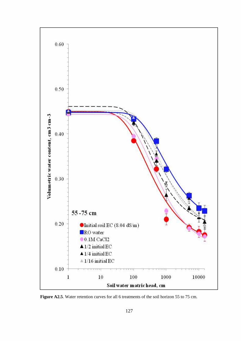
127
Figure A2.5. Water retention curves for all 6 treatments of the soil horizon 55 to 75 cm.

128
Figure A2.6. Water retention curves for all 6 treatments of the soil horizon 75 to 100 cm.
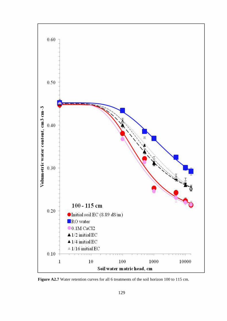
129
Figure A2.7 Water retention curves for all 6 treatments of the soil horizon 100 to 115 cm.
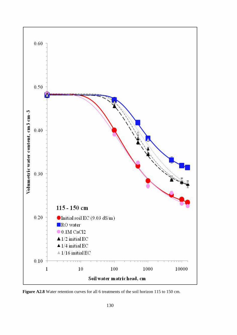
130
Figure A2.8 Water retention curves for all 6 treatments of the soil horizon 115 to 150 cm.

131
Figure A2.9 Water retention curves for all 6 treatments of the soil horizon > 150 cm.

132
Appendix 3. Soil resistance curves for all 54 pots (6 treatments x 9 soil horizons) – each point is an
average of 4 points; vertical bars on each point represent ± standard deviation of the mean.
Figure A3.1 Soil resistance curves for all 6 treatments of the soil horizon 0 - 10 cm.

133
Figure A3.2 Soil resistance curves for all 6 treatments of the soil horizon 10 - 25 cm.

134
Figure A3.3 Soil resistance curves for all 6 treatments of the soil horizon 25 - 35 cm.

135
Figure A3.4 Soil resistance curves for all 6 treatments of the soil horizon 35 - 55 cm.

136
Figure A3.5 Soil resistance curves for all 6 treatments of the soil horizon 55 - 75 cm.

137
Figure A3.6 Soil resistance curves for all 6 treatments of the soil horizon 75 - 100 cm.
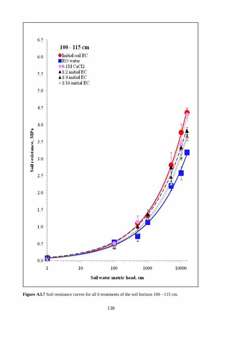
138
Figure A3.7 Soil resistance curves for all 6 treatments of the soil horizon 100 - 115 cm.

139
Figure A3.8 Soil resistance curves for all 6 treatments of the soil horizon 115 - 150 cm.
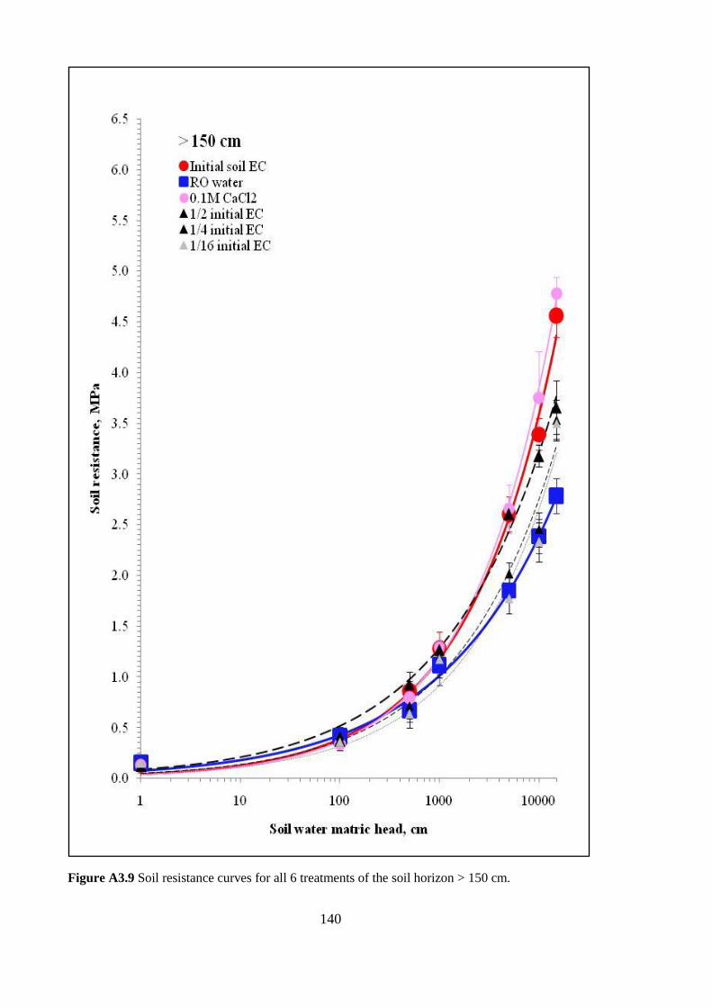
140
Figure A3.9 Soil resistance curves for all 6 treatments of the soil horizon > 150 cm.

141
References
Aggarwal GC, Prihar SS (1975) A simple technique to determine axial root growth force. Plant and Soil 42, 485-489. Ahmed S, Swindale LD, El-Swaify SA (1969) Effects of adsorbed cations on physical properties of tropical red earths and tropical black earths : I. Plastic limit, percentage stable aggregates, and hydraulic conductivity. Journal of Soil Science 20, 255-268. Akhter J, Murray RS, Mahmood K, Malik KA, Ahmed S (2004) Improvement of degraded physical properties of a saline-sodic soil by reclamation with kallar grass (Leptochloa fusca). Plant and Soil 258, 207-216. Allison IE (1965) Organic carbon. In 'Methods of Soil Analysis, Part 2, Chemical and microbiological properties' (Ed. CA Black et al.) pp. 1367-1378 (American Society of Agronomy: Madison,WI) Aly SM, Letey J (1990) Physical properties of sodium-treated soil as affected by two polymers. Soil Science Society of America Journal 54, 501-504. Amemiya M, Robinson CW, Cowley EW (1956) Reclamation of a saline-alkali soil in the upper Colorado River basin. Proceedings of Soil Science Society of America 3, 423-426. Angers DA, Carter MR (1996) Aggregation and organic matter storage in cool, humid agricultural soils. In 'Structure and Organic Matter Storage in Agricultural Soils.' (Eds MR Carter and BA Stewart) pp. 193-211. (Lewis-CRC Press: Boca Raton, FL). Armstrong W (1980) Aeration in higher plants. In 'Advances in Botanical Research.Vol. 7.' Ed. HW Woolhouse) pp. 225-332. (Academic Press). Arora HS, Coleman NT (1979) The influence of electrolyte concentration on flocculation of clay suspensions. Soil Science 127, 134-139. Asgarzadeh A, Mosaddeghi MR, Mahboubi AA, Nosrati A, Dexter AR (2010) Soil water availability for plants as quantified by conventional available water, least limiting water range and integral water capacity. Plant and Soil 335, 229-244. Bakker AC (1972) The comparative effect of exchangeable Ca, Mg, and Na on the stability in water of aggregates from the subsoil of red-brown earth. PhD Thesis. University of Adelaide, Adelaide. Baldock JA, Nelson PN (2000) Soil organic matter. In 'Handbook of Soil Science' (Ed. ME Sumner) pp. B33-B36. (CRC Press: London). Baver LD (1956) 'Soil Physics.' (John Wiley & Sons: New York). Bazihizina N, Barrett-Lennard EG, Colmer TD (2012) Plant growth and physiology under heterogeneous salinity. Plant Soil 354,1–19. Bell RW (1999) Boron. In 'Soil Analysis: An Interpretation Manual.' (Eds KI Preverill, LA Sparrow and DJ Reuter). pp. 309-316 (CSIRO publishing: Collingwood, Victoria).

142
Bernstein L (1975) Effects of salinity and socidity on plant growth. Annual Review of Phytopathology 13, 295-312. Bernstein L, Hayward HE (1958) Physiology of salt tolerance. Annual Review of Plant Physiology 9, 25-46. Blackmore AV, Miller RD (1961) Tactoid size and osmotic swelling in calcium montmorillonite. Soil Science Society of America Journal 25, 169-173. Blake GR (1965) Particle density. In 'Methods of Soil Analysis, Part 1, Physical and mineralogical properties, including statistics of measurement and sampling' (Ed. CA Black et al.) pp. 371-373 (American Society of Agronomy: Madison,WI). Blokhuis W (1980) Problem soils: their reclamation & management - Vertisols. In 'Land reclamation & water management: Development, problems & challenges.' IILRI Publication No.27, 43-72. (International Institute for Land Reclamation & Improvement: Wageningen, Netherlands). Bresler E, McNeal BL, Carter DL (1982) 'Saline and Sodic soils Principles-Dynamics-Modeling' (Springer-Verlag Berlin Heidelberg: New York). Bronick CJ, Lal R (2005) Soil structure and management: a review. Geoderma 124, 3-22.
Chahal SS (2010) Evaluation of soil hydraulic limitations in determining plant-available-water in light textured soils. PhD Thesis. University of Adelaide, South Australia.
Chan Y, Banin A, Borochovitch A (1983) Effect of potassium on soil structure in relation to hydraulic conductivity. Geoderma 30, 135-147.
Chhabra R (1985) Crop responses to phosphorus and potassium fertilization of a sodic soil. Agronomy Journal 77, 699-702. Chhabra R, Abrol IP, Singh MV (1981) Dynamics of phosphorus during reclamation of sodic soil. Soil Science 132, 319-324. Chittleborough DJ, Maschmedt DJ, Wright MJ (1976) Soils of the Monarto town site. Specific Land Use Survey Report No.SS-16. Department of Agriculture South Australia. Adelaide. 58p. Clark LJ, Bengough AG, Whalley WR, Dexter AR, Barraclough PB (1999) Maximum axial root growth pressure in pea seedlings: effects of measurement techniques and cultivars. Plant and Soil 209, 101-109. Cockroft B, Barley KP, Greacen EL (1969) The penetration of clays by fine probes and root tips. Australian Journal of Soil Research 7, 333-348. Connolly RD (1998) Modelling effects of soil structure on the water balance of soil–crop systems: a review. Soil and Tillage Research 48, 1-19. Cranner GR, Bowman DC (1991) Short-term leaf elongation kinetics of maize in response to salinity are independent of the root. Plant Physiology 95, 965-967.
143
Cresswell HP, Smiles DE, Williams J (1992) Soil structure, soil hydraulic properties and the soil water balance. Australian Journal of Soil Research 30, 265-283. da Silva AP, Kay BD, Perfect E (1994) Characterisation of the least limiting water range of soils. Soil Science Society of America Journal 58, 1775-1781. Davidson JL, Quirk JP (1961) The influence of dissolved gypsum on the pasture establishment on irrigated sodic clays. Australian Journal of Agricultural Research 12, 100-114. Day PR (1965) Particle fractionation and particle-size analysis. In 'Methods of Soil Analysis, Part 1, Physical and mineralogical properties, including statistics of measurement and sampling' (Ed. CA Black et al.) pp. 545-567 (American Society of Agronomy: Madison,WI) Delane R, Greenway H, Munns R, Gibbs J (1982) Ion concentration and carbohydrate status of elongating leaf tissue of Hordeum vulgare growing at high external NaCl. I Relationship between solute concentration and growth. Journal of Experimental Botany 33, 557-573. Dexter AR (1988) Advances in characterization of soil structure. Soil and Tillage Research 11, 199-238. Dikinya O, Hinz C, Aylmore G (2008) Decrease in hydraulic conductivity and particle release associated with self-filtration in saturated soil columns. Geoderma 146,192-200. Doneen LD, Henderson DW (1952) Soil conditions affecting infiltration of water and root development of crop plants. Proceedings of 7th General Meeting of American Society Sugar Beet Technologists, 7, 214-223. El-Morsy EA, Malik M, Letey J (1991) Polymer effects on the hydraulic conductivity of saline and sodic soil conditions. Soil Science 151, 430-435. El-Swaify SA, Ahmed S, Swindale LD (1970) Effects of adsorbed cations on physical properties of tropical red and tropical black earths : II. Liquid limit, degree of dispersion, and moisture retention. Journal of Soil Science 21, 188-198. Emerson WW, Chi CL (1977) Exchangeable calcium, magnesium and sodium and the dispersion of illites in water. II. Dispersion of illites in water. Australian Journal of Soil Research 15, 255-262. Emerson WW, Smith BH (1970) Magnesium, organic matter and soil structure. Nature 228, 453-454. Feddes RA, Kowalik PJ, Zaradny H (1978) 'Simulation of Field Water Use and Crop Yield.' Wiley & Sons. New York. 189p. Fitzpatrick RW, Boucher SC, Naidu R, Fritsch E (1994) Environmental consequences of soil sodicity. Australian Journal of Soil Research 32, 1069-1093. Flocker WJ, Vomocil JA, Howard FD (1959) Some growth responses of tomatoes to soil compaction. Soil Science Society of America Journal 23, 188-191. Gardner WR (1960) Dynamic aspects of water availability to plants. Soil Science 89, 63-73. Gardner WR, Nieman RH (1964) Lower limit of water availability to plants. Science 143, 1460-1462.

144
Golchin A, Baldock JA, Oades JM (1998) A model linking organic matter decomposition, chemistry and aggregate dynamics. In 'Soil Processes and The Carbon Cycle' (Ed. R. Lal, JM Kimble, RF Follett, BA Stewart) pp. 245-266. (CRC Press: Boca Raton). Grable AR (1966) Soil aeration and plant growth. Advances in Agronomy 18, 57–106 Grable AR, Siemer EG (1968) Effects of bulk density, aggregate size, and soil water suction on oxygen diffusion, redox potentials, and elongation of corn roots. Soil Science Society America Journal 32, 180-186. Grant CD, Groenevelt PH, Robinson NI (2010) Application of the Groenevelt–Grant soil water retention model to predict the hydraulic conductivity. Australian Journal of Soil Research 48, 447-458. Grant CD, Groenevelt PH, Semetsa S, Cass A (2003) Soil structure and available water in a fragile soil. 'Proceedings 16th Triennial Conference of International Soil and Tillage Research Organisation'. pp.498-504. Brisbane, Queensland. 13-18 July 2003. Greacen EL, Farrell DA, Cockroft B (1968) Soil resistance to metal probes and plant roots. Transactions 9th Congress of International Society of Soil Science. Vol. 1'. pp. 769-779. Greene RSB, Posner AM, Quirk JP (1978a) Interactions of suspensions of Ca-illite with PVA and Ca(OH)2. In 'Modfication of Soil Structure.' (Eds WW Emerson, RD Bond and AR Dexter) pp.157-163. (John Wiley & Sons: Bribane) Greene RSB, Posner AM, Quirk JP (1978b) A study of the coagulation of montmorillonite and illite suspensions using the electron microscope. In 'Modification of Soil Structure.' (Eds WW Emerson, RD Bond and AR Dexter). pp.35-40. (John Wiley and Sons: New York) Greene RSB, Rengasamy P, Ford GW, Chartres CJ, Millar JJ (1988) The effect of sodium and calcium on physical properties and micromorphology of two red-brown earth soils. Journal of Soil Science 39, 639-648. Gregory PJ (2006) 'Plant Roots: Their Growth, Activity, and Interaction with Soils'. Blackwell Publishing. Oxford. Grierson IT (1978) Gypsum and Red-brown Earth. In 'Modification of Soil Structure.' (Eds WW Emerson, RD Bond and AR Dexter). pp. 315-324. (John Wiley & Sons). Grieve CM, Maas EV (1988) Differential effects of sodium/calcium ratio on sorghum genotypes. Crop Science 28, 659-665. Groenevelt PH, Grant CD, Murray RS (2004) On water availability in saline soils. Australian Journal of Soil Research 42, 833-840. Groenevelt PH, Grant CD, Semetsa S (2001) A new procedure to determine soil water availability. Australian Journal of Soil Research 39, 577-598. Gupta RK, Singh RR (1988) A comparative evaluation of the reclamation efficiency of surface-concentrated versus internally incorporated calcium chloride and gypsum in an Alkali soil. Soil Science 146, 277-283. Gupta SC, Sharma PP, DeFranchi SA (1989) Compaction effects on soil structure. Advances in Agronomy 42, 311-338.

145
Hillel D (1971) 'Soil and Water: Physical Principles and Processes.' (Academic Press: New York). Hoffman GJ, Rawlins SL (1971) Growth and water potential of root crops as influenced by salinity and relative humidity. Agronomy Journal 63, 877-880. Hoffman GT, Rawlins SL, Garber MJ, Cullen EM (1971) Water relations and growth of cotton as influenced by salinity and relative humidity. Agronomy Journal 63, 822-826. Horn R, Baumgartl T, Kayser R, Baasch S (1995) Effect of aggregate strength on strength and stress distribution in structured soils. In 'Soil structure: its development and function.' (Eds KH Hartge and BA Stewart) pp. 31-52. (CRC Press, Inc.: Boca Raton, Florida) Ilyas M, Qureshi RH, Qadir MA (1997) Chemical changes in a saline-sodic soil after gypsum application and cropping. Soil Technology 10, 247-260. Isbell R (2002) 'The Australian Soil Classification.' (CSIRO: Melbourne) Janzen HH (1993) Soluble salts. In 'Soil Sampling and Methods of Analysis.' (Ed. MR Carter) pp. 161-166. (Lewis Publishers: Florida) Jayawardane NS, Beattie JA (1979) Effect of salt solution composition on moisture release curves of soil. Australian Journal of Soil Research 17, 89-99. Jayawardane NS, Chan KY (1994) The management of soil physical properties limiting crop production in Australian sodic soils--a review. Australian Journal of Soil Research 32, 13-44. Jeff B (1997) Soil and Water Relationships. http://www.noble.org/ag/soils/soilwaterrelationships/ (The Samuel Roberts Noble Foundation). Jensen CR (1982) Effect of soil water osmotic potential on growth and water relationships in barley during soil water depletion. Irrigation Science 3, 111-121. Joffe JS, Zimmerman M (1945) Sodium, calcium, and magnesium ratios in the exchange complex. Proceedings of Soil Science Society of America 9, 51-55. Jury WA, Jarrell WM, Devitt D (1979) Reclamation of saline-sodic soils by leaching. Soil Science Society of America Journal 43, 1100-1106. Kaddah MT, Fakhry SI (1961) Tolerance of Egyptian rice to salt. 1. Salinity effects when applied continuously and intermittently at different stages of growth after transplanting. Soil Science 91, 113-120. Kamphorst A (1990) Amelioration of sodic clay soils by crack stabilization: an experimental laboratory simulation. Soil Science 149, 218-227. Kay BD (1990) Rates of change of soil structure under different cropping systems. Advances in Soil Science 12, 1-52. Kemper WD, Koch EJ (1966) Aggregate stability of soils from western United States and Canada. USDA Technical Bulletin No.1355. US Government Printing Office. Washington DC.

146
Kinraide TB, Pedler JF, Parker DR (2004) Relative effectiveness of calcium and magnesium in the alleviation or rhizotoxicity in wheat induced by copper, zinc, aluminum, sodium, and low pH. Plant and Soil 259, 201-208. Koenigs FFR (1961) 'The mechanical stability of clay soils as influenced by moisture conditions and some other factors.' CLL Publication No.67-7. (Verslagen van landbouwkundige onderzoekingen: Wageningen). Koenigs FFR, Brinkman R (1964) Influence of partial sodium and magnesium saturation on the structural stability of clay soils. In 'The 8th International Congress of Soil Science,' 1964, Bucharest, pp. 219-225. Kopittke PM, Kopittke RA, Menzies NW (2009) Measurement and interpretation of salinity tolerance in four perennial grasses. Journal of Plant Nutrition 32, 30-43. Kopittke PM, Menzies NW (2005) Effect of high pH on Na induced Ca deficiency. Plant and Soil 269, 119-129. Krishnamurthy R, Anbazhagan M, Bhagwat KA (1987) Effect of NaCl toxicity of chlorophyll breakdown in rice. Indian Journal of Agricultural Science 57, 567-570. Lal R, Shukla MK (2004) 'Principles of Soil Physics.' (Marcel Dekker, Inc.: New York) 716p. Letey J (1985) Relationship between soil physical properties and crop production. Advances in Soil Science 1, 277-294. Lipiec J, Hakansson I, Tarkiewicz S, Kossowski J (1991) Soil physical properties and growth of spring barley as related to the degree of compactness of two soils. Soil and Tillage Research 19, 307-317. Maas EV, Hoffman GJ (1977) Crop salt tolerance - current assessment. Journal of the Irrigation and Drainage Division 103, 115-134. Marchuk A, Rengasamy P (2012) Threshold electrolyte concentration and dispersive potential in relation to CROSS in dispersive soils. Soil Research 50, 473-481. Marschner H (1995) 'Mineral Nutrition of Higher Plants.' (Academic Press: London, England) Marshall TJ, Holmes JW, Rose CW (1996) 'Soil physics' 3 edn. (Cambridge University Press: Cambridge). Martin JP, Ervin JO, Shepherd RA (1965) Decomposition and binding action of polysaccharides from Azotobacter Indicus (Beijerinckia) and other bacteria in soil. Proceedings of Soil Science of America 29, 397-400. Martin PK, Koebner RMD (1995) Sodium and chloride ions contribute synergistically to salt toxicity in wheat. Biologia Plantarum 37, 265-271. McGarry D (1990) Soil compaction and cotton growth on a Vertisol. Australian Journal of Soil Research 28, 869-877. McGeorge WT, Fuller WH (1950) Relation between the Na:Ca ratio in the saturation extract and the percentage sodium in the exchangeable complex. Transactions 4th International Congress of Soil Science 1, 400-403.
147
McIntyre DS (1958) Permeability measurements of soil crusts formed by raindrop impact. Soil Science 85, 185-189. Meiri A, Poljakoff-Mayber A (1970) Effect of various salinity regimes on growth, leaf expansion and transpiration rate of bean plants. Soil Science 109, 26-34. Mikhail EH (1974) Relationship between certain physical and chemical properties and subsoil friability in Lemnos loam. Australian Journal of Experimental Agriculture and Animal Husbandry 14, 694-697. Minasny B, McBratney (2003) Integral energy as a measure of soil-water availability. Plant and Soil 249, 253-262. Morgan JM (1984) Osmoregulation and water stress in higher plants. Annual Review of Plant Physiology 35, 299-319. Munns R, Schachtman DP, Condon AG (1995) The significance of a two phase growth response to salinity in wheat and barley. Australian Journal of Plant Physiology 22, 561-569. Munns R, Termaat A (1986) Whole-plant response to salinity. Australian Journal of Plant Physiology 13, 143-160. Neuman PM (1993) Rapid and reversible modification of extension capacity of cell walls in elongating maize leaf tissues responding to root addition and removal of NaCl. Plant, Cell and Environment 16, 1107-1114. Northcote KH (1979) 'A Factual Key for the Recognition of Australian Soils.' 4th edn. (Rellim Tech: Adelaide, South Australia) Northcote KH, Skene JKM (1972) 'Australian soils with saline and sodic properties.' (CSIRO Australia). Oades JM (1993) The role of biology in the formation stabilization and degradation of soil structure. Geoderma 56, 377-400. Oades JM, Waters AC (1991) Aggregate hierarchy in soils. Australian Journal of Soil Research 29, 815-828. Orcutt DM, Nilsen ET (2000) 'The Physiology of Plants Under Stress: Soil and Biotic Factors.' (John Wiley and Sons: New York). Oster JD (1993) Sodic soil reclamation. In 'Towards the Rational Use of High Salinity Tolerant Plants. Vol. 1.' (Eds H Leith and AA Masoom) pp. 485-490. (Kluwer Academic: The Netherlands). Oster JD, Shainberg I, Wood JD (1980) Flocculation value and gel structure of sodium/calcium montmorillonite and illite suspensions. Soil Science Society of America Journal 44, 955-959. Pasricha NS, Randhawa NS (1971) Available molybdenum status of some recently reclaimed saline sodic soils and its effect on concentration of molybdenum, copper,-sulphur and nitrogen in berseem (Trifolium alexandrinum) grown on these soils. Proceedings of International Symposium on Soil Fertility Evaluation. pp.1017-1026).

148
Patrick WH, Wyatt R (1964) Soil nitrogen loss as a result of alternate submergence and drying. Proceedings of Soil Science of America 28, 647-653. Pearson GA (1959) Factors influencing salinity of submerged soils and growth of Caloro rice. Soil Science 87, 198-206. Pearson GA (1961) The salt tolerance of rice. International Rice Communication Newsletter 10, 1-4. Peerlkamp PK (1950) The influence on soil structure of the “natural organic maturity” by roots and stubble of crops. Transactions 4th International Congress of Soil Science 2, 50-54. Qadir M, Noble AD, Shubert S, Thomas RJ, Arslan A (2006) Sodicity-induced land degradation and its sustainable management: Problems and Prospects. Land Degradation & Development 17, 661-676. Qadir M, Qureshi RH, Ahmad N (1996) Reclamation of a saline-sodic soil by gypsum and Leptochloa fusca. Geoderma 74, 207-217. Quirk JP (1986) Soil permeability in relation to sodicity and salinity. Philosophical Transactions of the Royal Society London 316, 297-317. Quirk JP (1994) Interparticle forces: A basis for the interpretation of soil physical behaviour. Advances in Agronomy 53, 121-183. Quirk JP, Schofield RK (1955) The effect of electrolyte concentration on soil permeability. Journal of Soil Science 6, 163-178. Rayment GE and Higginson FR (1992) 'Australian Laboratory Handbook of Soil and Water Chemical Methods' (Inkata Press: Melbourne) Rengasamy P (1983) Clay dispersion in relation to changes in the electrolyte composition of dialysed red-brown earths. Journal of Soil Science 34, 723-732. Rengasamy P (2002) Transient salinity and subsoil contraints to dryland farming in Australian sodic soils : an overview. Australian Journal of Experimental Agriculture 42, 351-361. Rengasamy P (2010) Osmotic and ionic effects of various electrolytes on the growth of wheat. Australian Journal of Soil Research 48, 120-124. Rengasamy P, Greene RSB, Ford GW, Mehanni AH (1984) Identification of dispersive behaviour and the management of Red-Brown earths. Australian Journal of Soil Research 22, 413-431. Rengasamy P, Marchuk A (2011) Cation ratio of soil structure (CROSS). Soil Research 49, 280-285. Rengasamy P, Olsson KA (1991) Sodicity and soil structure. Australian Journal of Soil Research 29, 935-952. Rengasamy P, Sumner ME (1998) Processes involved in sodic behavior. In 'Sodic soils: Distribution, Properties, Management, and Environmental Consequences.' (Eds ME Sumner and R Naidu). pp33-50. (Oxford University Press: New York)

149
Richards LA (1953) 'Diagnosis and improvement of saline and alkali soils.' USDA Handbook No.60. (United States Salinity Laboratory Staff: Riverside, CA). 160p. Richards LA, Wadleigh CH (1952) Soil water and plant growth. In 'Soil physical conditions and plant growth.' Ed. BT Shaw pp. 74-251. (Academic Press: New York). Robinson JB (1971) Salinity and the whole plant. In 'Salinity and water use.' (Eds T Talsma and JR Philip). pp.193-206. (The Macmillan Press: London). Rowell DL, Martin MW, Nye PH (1967) The measurement and mechanism of ion diffusion in soils III. The effect of moisture content and soil solution concentration on the self-diffusion of ions in soils. Journal of Soil Science 18, 204-222. Rowell DL, Payne D, Ahmad N (1969) The effect of the concentration and movement of solutions on the swelling dispersion and movement of clay in saline and alkali soils. Journal of Soil Science 20, 176-188. Shainberg I, Bresler E, Klausner Y (1971) Studies on Na/Ca, montmorillonite systems I. The swelling pressure. Soil Science 111, 214-219. Shainberg I, Letey J (1984) Response of soils to sodic and saline conditions. Hilgardia 52, 1-57. Shainberg I, Oster JD (1978) 'Quality of Irrigation Water.'IIIC Publication No.2.Volcani Centre. Bet Dagan. 65p Shainberg I, Shalhevet J (1984) 'Soil Salinity Under Irrigation: Processes and Management.' (Springer-Verlag: New York ) 349p. Sheldon AR (2009) Subsoil constraints to root growth and water use efficiency in northern grain soils: osmotic and toxic effects of salinity. PhD Thesis. University of Queensland, Brisbane. Sheldon AR, Menzies NW (2005) The effect of copper toxicity on the growth and root morphology of Rhodes grass (Chloris gayana Knuth.) in resin buffered solution culture. Plant and Soil 278, 341-349. Simmonds L, Mullins C, Schofield JL (1995) SPACTeach v1.0 MERTaLTM Courseware. In. ' Ed. SB Heath). (University of Aberdeen: Aberdeen, UK). Singh A, Chhabra R, Abrol IP (1979) Effect of fluorine and phosphorus applied to sodic soil on their availability and on yield and chemical composition of wheat. Soil Science 128, 90-97. Slavich PG, Petterson GH (1993) Estimating the electrical conductivity of saturated paste extracts from 1:5 soil, water suspensions and texture. Australian Journal of Soil Research 31, 73-81. Snedecor GW, Cochran WG (1989) 'Statistical Methods.' (Ames: Iowa State University Press). 503p. Steppuhn H, Van Genuchten MT, Grieve CM (2005) Root-zone salinity. II. Indices for tolerance in agricultural crops. Crop Science 45, 221-232. Sumner ME (1993) Sodic soils: new perspectives. Australian Journal of Soil Research 31, 683-750.

150
Taylor HM, Ratliff LF (1969) Root growth pressures of cotton, peas, and peanuts. Agronomy Journal 61, 398-402. Tisdall JM, Oades JM (1982) Organic matter and water-stable aggregates in soils. Journal of Soil Science 33, 141-163. van Hoorn JW (1958) Results of a groundwater level experimental field with arable crops on clay soils. Netherlands Journal Agricultural Science 6, 1-10. van Olphen H (1977) 'An introduction to clay colloid chemistry: for clay technologists, geologists, and soil scientists.' Second edn. (Wiley-Interscience: New York) 318p. Veihmeyer FJ, Hendrickson AH (1927) Soil-moisture conditions in relation to plant growth. Plant Physiology 1, 71-82. Veihmeyer FJ, Hendrickson AH (1949) Methods of measuring field capacity and wilting percentage of soils. Soil Science 68, 75-94. Verma S, Sharma PK (2008) Long-term effects of organics, fertilizers and cropping systems on soil physical productivity evaluated using a single value index (NLWR). Soil and Tillage Research 98, 1-10. Wadleigh CH, Ayers AD (1945) Growth and biochemical composition of bean plants as conditioned by soil moisture tension and salt concentration. Plant Physiology 20, 106-132. Warkentin BP, Schofield RK (1962) Swelling pressure of Na-montmorillonite in NaCl solutions. Journal of Soil Science 13, 98-105. Weber HW, van Rooyen PC (1971) Polysaccharides in molasses meal as an ameliorant for saline-sodic soils compared to other reclamation agents. Geoderma 6, 233-253. Weir RG, Creswell GC (1994) 'Plant Nutrient Disorders. 4. Pastures and Field Crops.' (Inkata Press: Melbourne). Wells T, Fityus S (2011) Neutron soil moisture probe operation in saline environments. Soil Science 176, 642-651. Wesseling JG, Stoof CR, Ritsema CJ, Oostindie K, Dekker LW (2009) The effect of soil texture and organic amendment on the hydrological behaviour of coarse-textured soils. Soil Use and Management 25, 274–283. Yeo AR, Lee KS, Izard P, Boursier PJ, Flowers TJ (1991) Short and long-term effects of salinity on leaf growth in rice (Oryza sative L.). Journal of Experimental Botany 42, 881-889. Zahow MF, Amrhein C (1992) Reclamation of a saline sodic soil using synthetic polymers and gypsum. Soil Science Society of America Journal 56, 1257-1260. Zaitseva RI, Sudnitsyn II (2001) The effect of mineral salts from soil solution on the water status and growth of barley seedlings. Eurasian Soil Science 34, 1240-1249. Zhang XC, Norton LD (2002) Effect of exchangeable Mg on saturated hydraulic conductivity, disaggregation and clay dispersion of disturbed soils. Journal of Hydrology 260, 194-205.

151
Zimmermann U, Schneider H, Wegner LH, Wagner HJ, Szimtenings M, Haase A, Bentrup FW (2002) What are the driving forces for water lifting in the xylem conduit? Physiologia Plantarum 114, 327-335.