PIXE and EDXRF studies on banded iron formations from eastern India

Nuclear Instruments and Methods in Physics Research B 215 (2004) 252–261

www.elsevier.com/locate/nimb

PIXE and EDXRF studies on banded iron formationsfrom eastern India

P.K. Nayak a,*, D. Das b, V. Vijayan c, P. Singh d, V. Chakravortty a,1

a Department of Chemistry, Utkal University, Vani Vihar, Bhubaneswar, Orissa 751 004, Indiab M€ossbauer Division, IUC-DAEF, Calcutta Centre, Kolkata 700 091, India

c Institute of Physics, Sachivalaya Marg, Bhubaneswar 751 005, Indiad Department of Geology, Utkal University, Bhubaneswar 751 004, India

Received 2 January 2003; received in revised form 8 May 2003

Abstract

A selected number of eastern Indian banded iron formations (BIFs) have been studied by using complementary non-

destructive X-ray techniques like proton-induced X-ray emission and energy dispersive X-ray fluorescence. Nineteen

trace elements including Co, Ni, Zr, Cr, Ti and Y were quantified in these BIFs, which have been used to interpret the

various physical–chemical conditions of the depositional basin. The study advocates the use of X-ray techniques

complementarily in quantifying trace elements in high-grade ores in order to reveal geochemistry successfully.

� 2003 Published by Elsevier B.V.

Keywords: PIXE; EDXRF; Complementary use of PIXE and EDXRF; Banded iron formation; Trace element studies; Geochemical

application

1. Introduction

The deposition of banded iron formations

(BIFs) occurred between early Archean to lateProterozoic period (3.5–1.8 billion years B.P.)

[1,2], and are considered to have formed as

chemical precipitates in relatively shallow primi-

tive seas [2,3]. These are mostly alternate bands of

iron and silica expected to contain lower trace

metal concentration. Although a considerable

current interest is under progress for understand-

* Corresponding author. Tel.: +91-674-2540466.

E-mail address: [email protected] (P.K. Nayak).1 Posthumously.

0168-583X/$ - see front matter � 2003 Published by Elsevier B.V.

doi:10.1016/j.nimb.2003.07.006

ing their trace element geochemistry [4,5] and un-

folding the primary–secondary processes those

have produced [5], the origin of these BIFs are

highly controversial [6–8].Until recently, there have been few systematic

geochemical studies carried out on BIFs, particu-

larly of their trace element geochemistry. Now

a days various multielemental techniques like

atomic absorption spectroscopy (AAS), electron

probe micro-analysis (EPMA), inductively cou-

pled plasma mass spectroscopy (ICP-MS) and

laser-ablation combined with inductively coupledplasma mass spectroscopy (LA-ICP-MS) are be-

ing used for quantification of trace elements in

geological materials. Among them, ICP-MS and

AAS are becoming more routine, but destructive

mail to: [email protected]

P.K. Nayak et al. / Nucl. Instr. and Meth. in Phys. Res. B 215 (2004) 252–261 253

chemical methods involving sample dissolution

procedure, inability for routine analysis of samples

in solid form imply their main drawbacks. The

EPMA technique is useful for the analysis of evena mono-mineral grain, but is limited to detection

of elements at concentration more than 200 ppm

[9], i.e. far more than the concentration present in

BIFs. The LA-ICP-MS technique is approaching

in more fascinating manner as it is rapid, highly

sensitive, having low background and mostly non-

destructive [10], but the unavoidable requirement

for extensive use of standards [11,12] constitute itsdrawback, particularly when heterogeneous ma-

terials like BIFs are to be analysed.

In this context, multi-elemental non-destructive

accelerator based proton-induced X-ray emission

(PIXE) technique looks more useful, as was used

earlier for this purpose several times [13–15]. It is

one way simultaneous, reliable, quantitative mul-

tielemental and non-destructive with a highersensitivity in the ppm level, can be thought of

analyzing BIFs which contains trace elements only

in parts per millions level especially for 3d ele-

ments (i.e. for 216Z < 31), and also for barium

which L X-rays lines falls in the 3d region. But this

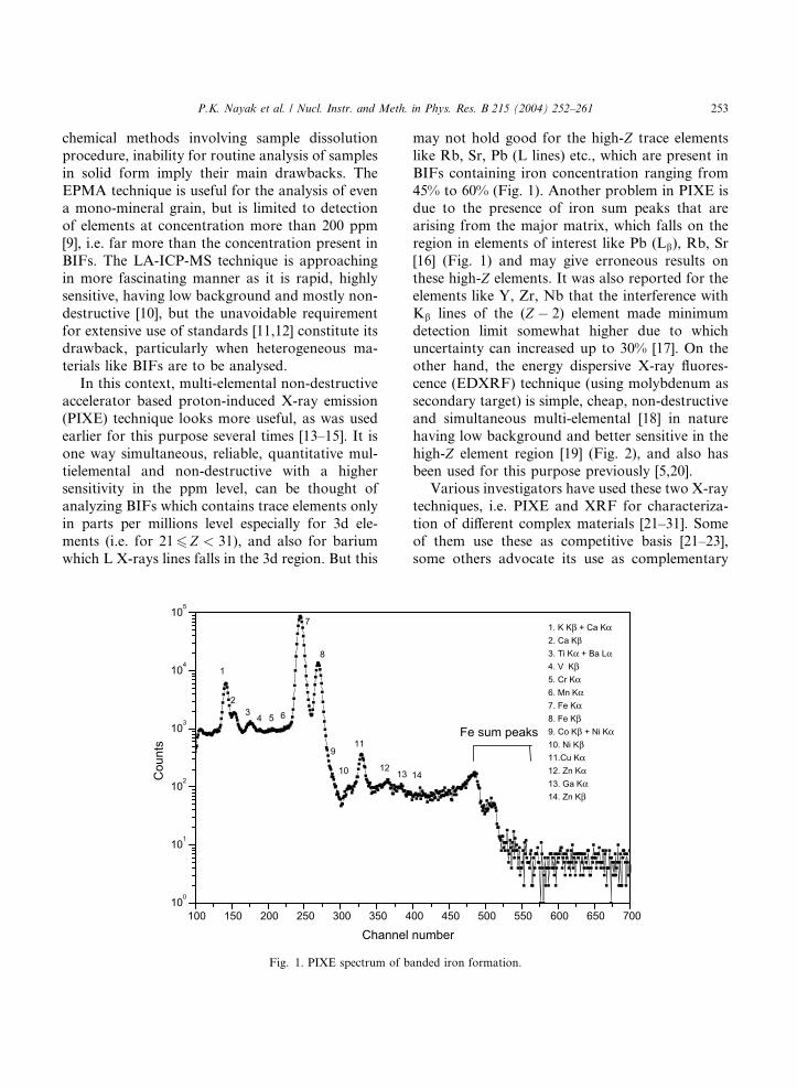
100 150 200 250 300 350 4100

101

102

103

104

105

1312

11

10

9

8

7

6543

2

1

Cou

nts

Channel

Fig. 1. PIXE spectrum of b

may not hold good for the high-Z trace elements

like Rb, Sr, Pb (L lines) etc., which are present in

BIFs containing iron concentration ranging from

45% to 60% (Fig. 1). Another problem in PIXE isdue to the presence of iron sum peaks that are

arising from the major matrix, which falls on the

region in elements of interest like Pb (Lb), Rb, Sr

[16] (Fig. 1) and may give erroneous results on

these high-Z elements. It was also reported for the

elements like Y, Zr, Nb that the interference with

Kb lines of the (Z � 2) element made minimum

detection limit somewhat higher due to whichuncertainty can increased up to 30% [17]. On the

other hand, the energy dispersive X-ray fluores-

cence (EDXRF) technique (using molybdenum as

secondary target) is simple, cheap, non-destructive

and simultaneous multi-elemental [18] in nature

having low background and better sensitive in the

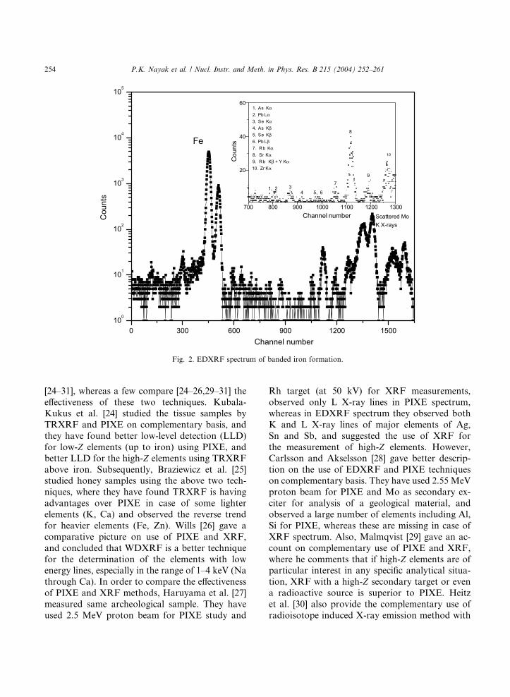
high-Z element region [19] (Fig. 2), and also has

been used for this purpose previously [5,20].Various investigators have used these two X-ray

techniques, i.e. PIXE and XRF for characteriza-

tion of different complex materials [21–31]. Some

of them use these as competitive basis [21–23],

some others advocate its use as complementary

00 450 500 550 600 650 700

Fe sum peaks

1. K Kβ + Ca Kα2. Ca Kβ3. Ti Kα + Ba Lα4. V Kβ 5. Cr Kα6. Mn Kα7. Fe Kα8. Fe Kβ9. Co Kβ + Ni Kα10. Ni Kβ11.Cu Kα12. Zn Kα13. Ga Kα14. Zn Kβ

14

number

anded iron formation.

0 300 600 900 1200 1500100

101

102

103

104

105

700 800 900 1000 1100 1200 1300

20

40

60

10

9

8

7

5, 6431, 2

1. As Kα 2. Pb Lα 3. Se Kα 4. As Kβ5. Se Kβ6. Pb Lβ 7. Rb Kα 8. Sr Kα9. Rb Kβ + Y Kα10. Zr Kα

Cou

nts

Channel number Scattered MoK X-rays

Fe

Cou

nts

Channel number

Fig. 2. EDXRF spectrum of banded iron formation.

254 P.K. Nayak et al. / Nucl. Instr. and Meth. in Phys. Res. B 215 (2004) 252–261

[24–31], whereas a few compare [24–26,29–31] the

effectiveness of these two techniques. Kubala-

Kukus et al. [24] studied the tissue samples by

TRXRF and PIXE on complementary basis, and

they have found better low-level detection (LLD)

for low-Z elements (up to iron) using PIXE, and

better LLD for the high-Z elements using TRXRF

above iron. Subsequently, Braziewicz et al. [25]studied honey samples using the above two tech-

niques, where they have found TRXRF is having

advantages over PIXE in case of some lighter

elements (K, Ca) and observed the reverse trend

for heavier elements (Fe, Zn). Wills [26] gave a

comparative picture on use of PIXE and XRF,

and concluded that WDXRF is a better technique

for the determination of the elements with lowenergy lines, especially in the range of 1–4 keV (Na

through Ca). In order to compare the effectiveness

of PIXE and XRF methods, Haruyama et al. [27]

measured same archeological sample. They have

used 2.5 MeV proton beam for PIXE study and

Rh target (at 50 kV) for XRF measurements,

observed only L X-ray lines in PIXE spectrum,

whereas in EDXRF spectrum they observed both

K and L X-ray lines of major elements of Ag,

Sn and Sb, and suggested the use of XRF for

the measurement of high-Z elements. However,

Carlsson and Akselsson [28] gave better descrip-

tion on the use of EDXRF and PIXE techniqueson complementary basis. They have used 2.55MeV

proton beam for PIXE and Mo as secondary ex-

citer for analysis of a geological material, and

observed a large number of elements including Al,

Si for PIXE, whereas these are missing in case of

XRF spectrum. Also, Malmqvist [29] gave an ac-

count on complementary use of PIXE and XRF,

where he comments that if high-Z elements are ofparticular interest in any specific analytical situa-

tion, XRF with a high-Z secondary target or even

a radioactive source is superior to PIXE. Heitz

et al. [30] also provide the complementary use of

radioisotope induced X-ray emission method with


PIXE on clays and ceramics. After irradiating

a thick clay pellet (3 MeV protons in PIXE and

59.6 keV radiation from 241Am for XRF), they

observed the high sensitivity of XRF for the hea-vier elements.

Benyaich et al. [31] gave fairly detailed com-

parative picture of the use of PIXE and EDXRF

as complementary basis. They have presented

PIXE and XRF spectra for the same sediment

sample, which was a typical silicate rock having

low trace elements content. On the PIXE spectrum

(2 MeV proton beam, 4 h acquisition time), themain peaks originate from Al, Si, K, Ca, Ti, Mn

and Fe while heavier elements such as Rb, Sr, Y

and Zr appear as trace elements with very low

peak to background ratios, and in the energy re-

gion of 10–14 keV, pile-up peaks are present

(similar to Fig. 1). In case of XRF spectrum (Ag

secondary target, 241Am source), it is the heavy

elements Rb, Y, Sr, Zr and Nb that have higherpeak to background ratios, compared to light

elements (Si, Ca, K) whose signals are almost

rubbed out (similar to Fig. 2). In the same report,

Benyaich et al. [31] further plotted the variations

of the intrinsic and effective sensitive ratios

ðSPIXE=SXRFÞ, versus the atomic number of the

emitting target element; computed for K lines for

Z6 42 and for L lines for Z > 42. They inferredthat PIXE is much more sensitive than XRF for

the low energy X-ray lines due to the higher ioni-

sation cross-section of protons, which balances the

strong self-absorption occurring at low energies;

while XRF is more sensitive at high X-ray energies

due to the combination of both high ionisation

cross-section and low self-attenuation. They con-

firm the complimentarily of the two techniques,that PIXE is more sensitive than XRF for low

energy X-ray lines, with MDL values falling down

to few atomic ppm; while at high X-ray energy,

XRF is the most sensitive with MDL values

ranging between 0.6 and 4 atomic ppm. Their

study advocated that in the adopted experimental

conditions (i.e. 2 MeV protons for PIXE, and

22–25 keV Ag K lines for XRF), the two tech-niques PIXE and XRF are complementary, the

former being very sensitive for light elements (low

energy X-ray emitters) and the later for heavier

elements.

Considering all these, we come to a reasonable

conclusion that at this particular situation PIXE

can give better low level detection at lower X-ray

energies for quantification of 3d elements (alongwith barium) whereas EDXRF (molybdenum as

secondary target) has privilege for higher X-ray

energies having better low level detection, and

both could be considered for quantification com-

plementarily. In this present investigation, an at-

tempt was made by the authors to quantify trace

elements in banded iron formations from eastern

Indian geological belt using PIXE and EDXRF,and the results were used in interpreting the envi-

ronmental condition of the depositional basin.

2. Experimental

2.1. Sample description and preparation

Banded iron formation (BIF) samples were

collected from Precambrian iron ore supergroup,

which is found in three major distinct geological

settings [32–34], known as BIF1, BIF2 and BIF3.

A total of 12 representative samples have been

selected for the present investigation. The geo-

graphical locations and local name of the deposits

(sampling stations) are provided in Table 1. Threesamples coded as IFA1, IFA2 and IFA3 are from

the mines of BIF1 region, four samples IFB1,

IFB2, IFB3 and IFB4 are from BIF2 region,

whereas five samples coded as IFC1, IFC2, IFC3,

IFC4 and IFC5 are selected from BIF 3 region.

As the original samples contain the alternative

bands of iron and silica, the required powdered

samples have been prepared only from the ironband. XRD and 57Fe M€ossbauer spectroscopic

studies of these samples reveal the presence of

hematite, magnetite and goethite as chief iron

bearing phases, also provided in Table 1 for in-

formation, and have been discussed elaborately

elsewhere [5,33,34]. For PIXE measurements, the

powdered samples were heated at 105 �C for 12 h

in an oven and allowed to cool slowly [15,22].After this, these samples are thoroughly mixed

with extra pure graphite powder (Merck) in the

ratio 1:1 by mass (200 mg each) [22]. Thick targets

are prepared by pressing the above mixture with a

Table 1

Sample location, their longitude and latitude and iron phases present therein

Region [32] Sample code Location Longitude Latitude Iron phases present

[5,33,34]

BIF 1 IFA1 Badampahar 22�040 86�050 Hematite, Goethite

IFA2 Gorumahisani 22�010 85�530 Hematite, Goethite

IFA3 Sulaipat 22�090 86�150 Hematite

BIF 2 IFB1 Daitary I 21�030 85�450 Hematite

IFB2 Daitary II 21�030 85�580 Hematite, Magnetite

IFB3 Tomaka I 21�120 85�490 Hematite, Goethite

IFB4 Tomaka II 21�120 85�530 Hematite

BIF 3 IFC1 Khondadhar 21�470 85�070 Hematite

IFC2 Malangtoli 21�480 85�190 Hematite

IFC3 Sakardihi 21�490 85�230 Hematite

IFC4 Mahaparbat 21�520 85�260 Hematite

IFC5 Palsa 21�550 85�250 Hematite


KBr press. Pellets of NIST coal fly ash standard

1632b and USGS nodule standard Nod-A-1 are

also prepared by the same procedure for calibra-

ting the PIXE set up. For EDXRF experiments,

powdered samples are mixed with cellulose (as

binder) in 1:1 ratios by mass and thick targets have

been prepared [5,38].

2.2. Instrumental measurements

The 3 MeV collimated proton beam, obtained

from the 3MV Tandem pelletron accelerator at

Institute of Physics (Bhubaneswar, India) was used

to irradiate the sample in vacuum (10�6 Torr) in-

side a PIXE chamber [33]. The targets were held at

45� to the beam direction on a sample holder [35].Measurements were carried out with a maximum

beam current of 3 nA. A Si (Li) detector (Can-

berra, active area 30 mm2, beryllium window

thickness of 8 m) with a resolution of 170 eV at

5.9 keV placed at 90� to the beam direction was

used to detect characteristic X-rays emitted from

the targets. X-rays exit the PIXE chamber through

a 50 lm Mylar window before entering the de-tector [36]. Spectra were recorded by using a

Canberra series S-100 MCA calibrated with 241Am

X-ray source [37].

The EDXRF system used for the analysis con-

sists of a low power (50 W) tungsten anode; air-

cooled X-ray tube with tri-axial geometry and a

multi-channel analyser [5,38]. Molybdenum is used

as a secondary target and the characteristic K

X-rays were used to irradiate the pellets. X-rays

from the samples are detected by a Si(Li) detector

(the same detector as used for PIXE). The signals

from the detector were amplified, fed to PC based

MCA and were recorded [22].

2.3. Data analysis

The PIXE spectral analyses were performed

using GUPIX-2000 software [39]. This provides a

non-linear least squares fitting of the spectrum,

together with subsequent conversion of the fitted

X-ray peak intensities into elemental concentra-

tions, utilizing the fundamental parameter method

(FPM) for quantitative analysis. It requires pa-rameters of experimental geometry and Si(Li) de-

tector (H -parameter), chamber window thickness,

energy of the incident particle, the net charge

collected, the target thickness along with the major

matrix, and the invisible element oxygen [33,

36,39,40]. The concentrations of the low-Z ele-

ments were estimated from the intensities of K

X-ray lines while that of barium was from theintensities of L X-ray lines, and the results of dif-

ferent trace elements thus obtained for various

banded iron formations are provided in Table 2.

We would like to mention here that the Co Kb line

has been fitted to the spectra in order to determine

its concentration as suggested in GUPIX especially

for iron-rich materials [39]. Furthermore, it must

Table 2

PIXE and EDXRF data of banded iron-formation samples (concentrations are in ppm)

Elements IFA1 IFA2 IFA3 IFB1 IFB2 IFB3 IFB4 IFC1 IFC2 IFC3 IFC4 IFC5 Average

Caa 1555.8 ± 38.7 1456.8 ± 30.4 1854.9 ± 46.5 1102.8 ± 25.6 842.7 ± 18.5 1457.2 ± 33.6 705.4 ± 17.5 2607.4 ± 57.2 1305.4 ± 30.0 1277.5± 28.4 1375.6 ± 31.0 1345.4 ± 31.0 1407.2

Sca bdl 22.4± 1.2 15.3 ± 0.9 bdl bdl bdl bdl bdl 17.5 ± 1.0 bdl bdl bdl 4.6

Tia 165.5 ± 10.2 135.4 ± 8.2 266.7 ± 15.2 19.9 ± 1.5 56.4 ± 3.6 26.5 ± 1.6 47.1± 2.8 25.2 ± 1.5 40.0 ± 2.4 27.0± 1.6 31.7 ± 1.8 75.0± 4.4 76.4

Va 18.0 ± 1.8 130.3 ± 11.9 28.8 ± 3.1 23.0 ± 2.4 18.6 ± 2.0 12.3 ± 1.1 16.1± 1.5 42.2 ± 3.9 24.3 ± 2.2 24.7± 2.2 19.3 ± 1.8 32.2± 2.9 32.4

Cra 11.6 ± 0.9 17.4± 1.4 13.6 ± 1.0 39.6 ± 3.1 bdl 46.5 ± 4.6 16.4± 1.3 16.0 ± 1.3 33.1 ± 2.8 29.5± 2.2 37.8 ± 3.2 45.8± 4.1 25.6

Mna 98.5 ± 7.8 178.5 ± 15.9 181.7 ± 16.0 140.5 ± 13.7 434.4 ± 28.7 157.8 ± 13.5 70.5± 5.4 510.9 ± 37.2 280.5 ± 20.1 335.4 ± 23.5 303.7 ± 21.5 202.5 ± 14.2 241.2

Coa 19.3 ± 3.4 32.8± 5.6 12.8 ± 2.1 26.7 ± 4.2 24.6 ± 4.3 12.3 ± 2.4 11.8± 2.0 31.5 ± 4.8 18.5 ± 3.0 21.3± 3.5 16.4 ± 2.8 12.6± 2.2 20.0

Nia 36.4 ± 4.6 66.4± 8.4 44.7 ± 7.5 42.4 ± 5.6 65.2 ± 8.0 27.4 ± 3.8 19.5± 2.6 69.4 ± 8.6 62.4 ± 8.1 62.7± 7.9 67.5 ± 7.9 45.8± 6.0 50.8

Cua 99.1 ± 5.9 128.8 ± 7.7 113.7 ± 7.1 80.7 ± 4.1 165.6 ± 9.1 106.6 ± 6.0 60.5± 3.9 215.6 ± 13.0 123.4 ± 6.9 81.4± 4.8 161.5 ± 9.1 82.9± 5.2 118.3

Zna 47.4 ± 2.9 62.6± 3.6 52.6 ± 3.1 19.5 ± 1.3 65.2 ± 3.9 29.5 ± 1.9 28.7± 1.7 68.3 ± 4.3 27.4 ± 1.8 25.8± 1.7 31.3 ± 2.1 57.5± 3.7 43.0

Gaa 5.4 ± 0.2 14.1± 0.6 7.8 ± 0.3 6.4 ± 0.3 4.4 ± 0.2 8.4 ± 0.4 4.5 ± 0.2 6.0 ± 0.3 7.6 ± 0.3 3.8 ± 0.2 5.3 ± 0.2 11.7± 0.5 7.1

Asb 12.7 ± 0.6 bdl 16.7 ± 0.7 15.5 ± 0.6 48.3 ± 1.9 17.4 ± 0.7 16.6± 0.7 92.4 ± 3.1 21.0 ± 0.9 13.2± 0.5 17.3 ± 0.7 22.4± 1.0 24.4

Seb 7.8 ± 0.6 2.2 ± 0.2 14.2 ± 1.2 7.8 ± 0.6 5.6 ± 0.5 15.6 ± 1.3 5.4 ± 0.4 5.3 ± 0.4 14.3 ± 1.0 5.5 ± 0.5 9.4 ± 0.8 16.3± 1.1 9.1

Rbb 6.8 ± 0.4 4.2 ± 0.3 5.7 ± 0.3 11.2 ± 0.7 15.3 ± 1.2 74.5 ± 4.0 26.2± 1.3 9.3 ± 0.3 28.2 ± 1.4 20.8± 1.1 24.5 ± 1.3 14.2± 0.5 126.8

Srb 86.9 ± 6.4 64.2± 4.3 75.1 ± 5.1 66.3 ± 4.4 60.7 ± 4.2 64.6 ± 4.3 39.4± 2.4 35.6 ± 1.9 79.3 ± 5.3 47.7± 2.7 55.3 ± 3.8 22.6± 1.2 58.1

Yb 9.6 ± 0.6 12.6± 0.7 9.8 ± 0.6 7.3 ± 0.5 15.3 ± 0.8 14.2 ± 0.7 18.3± 0.9 12.6 ± 0.6 10.7 ± 0.5 16.2± 0.8 13.0 ± 0.7 17.6± 0.8 13.1

Zrb 21.2 ± 0.6 45.8± 1.2 27.5 ± 0.8 25.0 ± 0.7 41.9 ± 1.7 41.0 ± 1.7 52.6± 2.4 36.3 ± 1.6 32.8 ± 1.5 49.4± 2.3 41.8 ± 2.0 47.4± 2.2 38.5

Baa 140.0 ± 7.2 115.7 ± 5.5 152.1 ± 7.4 107.8 ± 5.1 98.8 ± 4.9 124.4 ± 6.1 76.1± 3.8 268.7 ± 12.5 142.4 ± 6.9 94.0± 4.8 98.3 ± 4.7 102.9 ± 5.1 20.7

Pbb 23.3 ± 1.2 16.7± 0.9 13.3 ± 6.8 19.7 ± 1.0 28.7 ± 1.5 bdl 30.7± 1.6 19.3 ± 1.2 14.3 ± 0.9 19.0± 1.2 23.6 ± 1.4 10.6± 0.6 18.3

bdl¼ below detection limit.aQuantification by PIXE.bQuantification by EDXRF.

P.K.Nayaket

al./Nucl.

Instr.

andMeth

.in

Phys.Res.

B215(2004)252–261

257


be noted here that in case of some other elements,

the K X-ray component of one element ðZÞ over-laps with the Ka component of higher element (i.e.

Z þ 1), which were taken care by GUPIX itself,where there is a provision to correct for this

overlap, and thus giving the correct intensities of

the elements [39].

The EDXRF spectra were analysed using the

software AXIL [41]. The instrument was cali-

brated and checked using various certified refer-

ence materials before the analyses of these BIFs,

and was also verified with earlier published data[5].

3. Results and discussion

The measured elemental concentrations are

provided in Table 2. It is worth mentioning here

that the concentrations of seven elements such asAs, Se, Rb, Sr, Y, Zr and Pb were estimated from

EDXRF spectra (triplicate measurements), while

the rest of the elements have been quantified from

PIXE spectra (duplicate measurements).

The concentration of titanium has been con-

sidered by various investigators in order to differ-

entiate iron ores formed at high temperature

magmatic process from low temperature sedi-

Table 3

Comparative average trace elemental concentration of present study w

beltsa

Elements Present study

[32,33]

Olary Domain,

South Australia [8]

Kushtag

belt, Ind

Ti 76.4 719.2 N.R.

V 32.4 115 N.R.

Cr 25.6 24 109.9

Mn 241.2 309.8 N.R.

Co 20.0 35 1.6

Ni 50.8 14 25.3

Cu 118.3 42 N.R.

Zn 43.0 17 30.8

Rb 20.7 21 0.8

Sr 58.1 161 13.2

Y 13.1 10 7.1

Zr 38.5 24 10.1

Ba 126.8 6714 N.R.

Co/Ni ratio 0.394 2.5 0.06

N.R.¼ not reported.a Concentrations are in ppm.

mentary process. It may be noted here that the

Clarke value of lithospheric titanium for iron ores

is 1000 ppm [22]. In these iron-formation samples

the concentration of Ti is well below that of theClarke value suggesting the source of the materials

to be other than of igneous origin, and this favours

the theory of sedimentary deposition. Vanadium,

an element of industrial interest, is usually rich in

titanium-bearing minerals, and it is evidenced

from our earlier studies [22] that this is also an

important geochemical indicator. The abundance

of vanadium in these ores appears to be high, ingeneral, as compared to ores of Lake Superior type

of USA [42], but is rather low in comparison with

Algoma type of Canada [42] and South Australia

[8] (Table 3).

Frietsch [43] reported that Cr is present below

the lithospheric content in iron ores of N-Sweden,

which are non-magmatic in origin. Very low av-

erage chromium (25.6 ppm) content of the pres-ently studied BIFs, which are well below the

Clarke value of sediments (110 ppm) [44], suggests

the initial formation condition to be of sedimen-

tary environment. Hagemann and Albrecht [45]

reported fairly low concentrations of manganese,

generally up to 150 ppm in hematite from typical

sedimentary ores. In contrast, the Mn content in

magnetites from similar deposits is generally of the

ith that of different world deposits along with two major Indian

i schist

ia [50]

Sandur schist

belt, India [4]

Algoma facies,

Canada [42]

Lake-Superior

facies, USA [42]

300 860 160

11.3 97 30

55.7 78 122

N.R. 1400 4600

33.7 38 27

10.2 83 32

12.5 96 10

11.2 N.R. N.R.

2.7 N.R. N.R.

3.8 42 98

1.8 N.R. N.R.

4.0 56 84

14.5 170 180

3.3 0.457 0.843

50 100 150 20050

100

150

200

250

300

Con

entra

tion

of b

ariu

m (p

pm)

Concentration of copper (ppm)

Fig. 3. Scatter plot between Cu and Ba.


order of Clarke value for the upper lithosphere, i.e.

about 1000 ppm [43]. In this light, the observed

low levels of Mn in these iron formations appar-

ently offer strong support to the contention thatthe bulk of the iron was precipitated by sedimen-

tary process.

According to R€ossler and Lange [46], the av-

erage values of nickel in igneous rocks are 80–200

ppm. In these samples, nickel concentration is well

below (average 50.8 ppm, Table 2) the R€ossler andLange�s value for rocks of igneous origin. How-

ever, in some specific cases (samples IFC1, IFC4,IFA2, IFB2 and IFC4) the value is quite close to

the Clarke value (80 ppm), which is probably due

to the comparable radii of Ni2þ and Fe2þ, and this

may result in increase in nickel concentration.

Generally, the element strontium follows calcium

and barium in natural conditions [15] as it belongs

to the same group in the Moseley�s Periodic Table.The low content of strontium in these BIFs (bar-ium and calcium poor ores) seems to be geo-

chemically appropriate. Furthermore, the low

concentration of calcium (average 1407.2 ppm)

supports the non-volcanogenic origin of these

BIFs [47].

Another important geochemical parameter zir-

conium has been used as an effective indicator of

provenance, scarcely prone to weathering, and isbelieved not to be affected by transportation dur-

ing weathering or by any other specific later geo-

chemical events. It is immobile, highly stable and

rarely decomposes in nature [22]. So the concen-

tration of zirconium in ores represents the con-

stituent of source rock. In these samples the

content of zirconium is rather low (of an average

of 38.5 ppm) in comparison to other specific worlddeposits [8,42], leading to the situation that the

source solution had concentration of lower zirco-

nium-containing materials. Furthermore, barium

and zirconium are adsorbed in clay structure due to

their larger ionic radii and lower ionic potentials

[48]. The lower concentrations of these two ele-

ments (of an average of 126.8 and 38.5 ppm, re-

spectively) indicate the source material wasdeficient in clay minerals.

The Co/Ni ratio has been used by various

workers to differentiate between igneous and sed-

imentary origin of iron ores [43,48]. According to

Frietsch [43], Co/Ni ratio below unity for iron

oxides is indicative of low temperature and sedi-

mentary origin but higher values are obtained in

the iron oxides of igneous origin. In the presentwork this ratio is well below (average value 0.394,

Table 2) to that of Frietsch�s ratio confirming the

clear sedimentary environment of deposition.

However, from the concentrations of different

trace elements (Table 2), it is observed that there

are positive correlations and some similar asso-

ciative behaviour between two groups of elements,

i.e. Cu–Ba (Fig. 3) and Mn–Ni (Fig. 4) althoughwe do not know the exact cause and mechanism. It

may be possible that there is simultaneous pre-

cipitation between these two groups of elements

with that of the source solution. We would further

like to mention here that the presence and high

content of yttrium (average of 13.1 ppm) in these

samples indicates towards the possibility of the

existence of lanthanides in these BIFs [5], andfurther supported by a report by Majumdar et al.

[49].

The average trace elements� concentration in

Table 2 while compared with other world [8,42]

and Indian deposits [4,50] (Table 3), indicates that

these iron formations are neither comparable with

other world deposits nor with other Indian de-

posits, and were deposited at specific environmentcondition. The original source material is having

lower trace elements� content. Hence, on the basis

0 100 200 300 400 500

20

30

40

50

60

70

Con

cent

ratio

n of

Ni (

ppm

)

Concentartion of Mn (ppm)

Fig. 4. Scatter plot between Mn and Ni.


of PIXE and EDXRF study, one can conclude

that the Eastern Indian iron ore basin signifies

specific and independent deposition, and is notcomparable to any other iron formations either of

Canada, USA and Australia (Table 3). In supple-

mentary, we would like to mention here that the

variation of three large-ion lithophile elements (K,

U and Th) in these BIFs have been reported else-

where [51]. Further investigation is under progress

on the variation and distribution of rare earth el-

ements and isotopic ratios, which may explain thedepositional environment of the present geological

belt more comprehensively.

4. Conclusion

Selected numbers of banded iron formations

have been studied by using PIXE and EDXRF. Atotal of nineteen elements including Ca, Ti, V, Cr,

Mn, Ni, Cu, Zn, Sr, Y, Zr, Ba and Pb were esti-

mated in these ores. The Co/Ni ratio and the con-

tent of trace elements such as Ti, Cr, Ni, Zr have

been used in explaining the environment of the

depositional basin of these banded iron forma-

tions. The large variations in trace elements have

been observed though the positive correlationsbetween two groups of elements, i.e. Cu–Ba and

Mn–Ni have also been observed. The comparison

of the average trace element concentration with

that of other Indian and world banded iron for-

mation deposits indicates the eastern Indian iron

ore basin�s specific and independent deposition.

Acknowledgements

Authors wish to express their posthumous

gratitude to Prof. V. Chakravortty (Utkal Uni-

versity, Vani Vihar, Bhubaneswar). Heartfelt

thanks are due to Prof. S. Jena, Department of

Chemistry, Utkal University, Vani Vihar (Bhu-

baneswar), Prof. R.K. Choudhury and Prof. D.P.Mahapatra of Institute of Physics (Bhubaneswar)

and Prof. S. Acharya, Ex-Vice-Chancellor, Utkal

University, Vani Vihar (Bhubaneswar) for useful

discussions regarding the various aspects of the

present investigation. P.K.N. thanks to Prof. S.N.

Bhattacharyya, Dr. A.K. Sinha and Dr. A. Saha of

IUC-DAEF, Calcutta Center, Kolkata for their

constant inspiration. The scientific staffs andmembers of Ion Beam Lab, Institute of Physics are

thanked for providing accelerator facilities and

various necessary supports. P.K.N. is grateful to

IUC-DAEF, Calcutta Center (Kolkata) for a re-

search Fellowship. Authors acknowledge and are

grateful to an anonymous referee for the signifi-

cant improvement of the manuscript at the revi-

sion stage.

References

[1] S.J. Mojsis, G. Arrhenius, K.D. KcKeegan, T.M. Harri-

son, A.P. Nutman, C.R.L. Friend, Nature 384 (1996) 55.

[2] J.F. Kasting, Science 259 (1993) 920.

[3] I.W. Croudace, J.M. Gilligan, X-ray Spectrom. 19 (1990)

117.

[4] C. Manikyamba, V. Balaram, S.M. Naqvi, Precamb. Res.

61 (1993) 137.

[5] P.K. Nayak, D. Das, V. Vijayan, P. Singh, V. Chakra-

vortty, Nucl. Instr. and Meth. B 184 (2001) 649.

[6] M.M. Kimberley, Ore Geol. Rev. 5 (1989) 13.

[7] E. Dimroth, Geol. Soc. Ind. 28 (1986) 239.

[8] P.M. Ashley, B.G. Lottermoser, J.M. Westaway, Contr.

Miner. Petr. 64 (1998) 187.

[9] S. Murao, S.H. Sie, Resour. Geol. 47 (1) (1997) 21.

[10] J.S. Becker, Spectrochim. Acta B 57 (2002) 1805.

[11] J.D. Robertson, H. Neff, B. Higgins, Nucl. Instr. and

Meth. B 189 (2002) 378.

[12] L. Kempenaers, N.H. Bings, T.E. Jeffries, B. Vakemans, K.

Janssens, J. Anal. At. Spectrom. 16 (2001) 1006.


[13] I. Brissaud, A. de Chateau-Thierry, J.P. Frontier, G.

Lagarde, J. Radioanal. Nucl. Chem. 102 (1) (1986) 131.

[14] C.G. Ryan, D.R. Cousens, S.H. Sie, W.L. Griffin, G.F.

Suter, E. Clayton, Nucl. Instr. and Meth. B 87 (1990) 55.

[15] J.E. Martin, R. Garcia-Tenorio, M.A. Respaldiza, M.A.

Ontalba, J.E. Boliver, M.F. Da Silva, Appl. Radiat. Isot.

50 (1999) 445.

[16] J.L. Campbell, in: S.A.E. Johansson, K.G. Malmqvist

(Eds.), Particle Induced X-ray Emission Spectrometry:

Chemical Analysis Series, Chapter 6, Vol. 133, John Wiley

and Sons Inc., New York, 1995, p. 319.

[17] A.P. Santo, A. Paccerillo, P. Del Carmine, F. Lucarelli,

J.D. Macarthur, P.A. Mando, Nucl. Instr. and Meth. B 64

(1992) 517.

[18] A.C. Mandal, M. Sarkar, D. Bhattacharya, Eur. Phys. J.

AP 17 (2002) 81.

[19] J. Parus, W. Raab, D.L. Donohue, X-ray Spectrom. 30

(2001) 296.

[20] A.G. Revenko, X-ray Spectrom. 31 (2002) 264.

[21] F. Arauzo, T. Pinheiro, L.C. Alves, P. Valerio, F. Gaspar,

J. Alves, Nucl. Instr. and Meth. B 136–137 (1998) 1005.

[22] P.K. Nayak, D. Das, S.N. Chintalapudi, P. Singh, S.

Acharya, V. Vijayan, V. Chakravortty, J. Radioanal. Nucl.

Chem. 254 (2) (2002) 351.

[23] V. Vijayan, S.N. Behera, V.S. Ramamurthy, S. Puri, J.S.

Shahi, N. Singh, X-ray Spectrom. 26 (1997) 65.

[24] A. Kubala-Kukus, J. Braziewicz, D. Banas, U. Majewska,

S. Gozdz, A. Urbaniak, Nucl. Instr. and Meth. B 150

(1999) 193.

[25] J. Braziewicz, I. Fijal, C. Czyzewski, M. Jaskola, A.

Korman, D. Banas, A. Kubala-Kukus, U. Majewska, L.

Zemlo, Nucl. Instr. and Meth. B 187 (2002) 231.

[26] P. Wills, Nucl. Instr. and Meth. B 35 (1988) 378.

[27] Y. Haruyama, M. Saito, T. Muneda, M. Mitan, R.

Yamamoto, K. Yoshida, Int. J. PIXE 9 (3–4) (1999) 181.

[28] L.-E. Carlsson, K.R. Akselsson, Adv. X-ray Anal. 24

(1981) 313.

[29] K.G. Malmqvist, Nucl. Instr. and Meth. B 14 (1986) 86.

[30] C. Heitz, G. Lagarde, A. Pape, T. Tenorio, C. Zarate, M.

Menu, L. Scotee, A. Jaidar, R. Acosta, R. Alviso, D.

Gonzalez, V. Gonzalez, Nucl. Instr. and Meth. B 14 (1986)

93.

[31] F. Benyaich, A. Makhtari, L. Torrisi, G. Foti, Nucl. Instr.

and Meth. B 132 (1997) 481.

[32] S. Acharya, Ind. J. Earth Sci., SEISM seminar volume,

1984, p. 19.

[33] P.K. Nayak, Characterization of Iron Ores of Orissa by

PIXE, EDXRF and M€ossbauer spectroscopy, Ph.D. The-

sis, Utkal University, Bhubaneswar, India, 2003.

[34] P.K. Nayak, D. Das, P. Singh, V. Chakravortty, Commu-

nicated to J. Radioanal. Nucl. Chem., 2004, to be

published.

[35] R.K. Dutta, M. Sudarshan, S.N. Bhattacharyya, V.

Vijayan, S. Ghosh, V. Chakravortty, S.N. Chintalapudi,

J. Radioanal. Nucl. Chem. 221 (1997) 193.

[36] V. Vijayan, P.K. Nayak, V. Chakravortty, Ind. J. Phys. A

76 (2002) 477.

[37] P.K. Nayak, V. Chakravortty, V. Vijayan, P. Singh, Int. J.

PIXE, accepted.

[38] M. Ashok, T.R. Rautray, P.K. Nayak, V. Vijayan, V.

Jayanthi, S. Narayana Kalkura, J. Radioanal. Nucl. Chem.

257 (2) (2003) 333.

[39] J.L. Campbell, T.L. Hopman, J.A. Maxwell, Z. Nezedely,

Nucl. Instr. and Meth. B 170 (2000) 193.

[40] M. Sudarshan, R.K. Dutta, V. Vijayan, S.N. Chintalapudi,

Nucl. Instr. and Meth. B 168 (2000) 553.

[41] R.E. Van Griken, A.A. Markowictz, Handbook of X-ray

Spectrometry, Marcel Dekker, New York, 1993.

[42] G.A. Gross, C.R. Mcleod, Canadian Miner. 181 (1980)

223.

[43] R. Frietsch, Sveriges Geol. Unders Arsbok 64 (1970) 1.

[44] S. Landergren, Sveriges geol Unders Ser C 42 (5) (1948) 1.

[45] F. Hagemann, F. Albrecht, Chemie de Erde 17 (1954) 81.

[46] H.J. R€ossler, H. Lange, Geochemical Tables, Elsevier

publication, Amsterdam, 1972.

[47] T. Majumdar, Bull. Geol. Survey Finland 331 (1985) 201.

[48] T. Majumdar, K.L. Chakraborty, A. Bhattacharya, Miner.

Deposita 17 (1982) 107.

[49] T. Majumdar, J.E. Whitley, K.L. Chakraborty, Chem.

Geol. 45 (1984) 203.

[50] R.M.K. Khan, S. Das Sharma, D.J. Patil, S.M. Naqvi,

Geochim. Cosmochim. Acta 60 (1996) 3285.

[51] P.K. Nayak, V. Vijayan, V. Chakravortty, D. Bhatta, P.

Singh, Ind. J. Phys. A 77 (2003) 503.

PIXE and EDXRF studies on banded iron formations from eastern India

Documents

Transcript of PIXE and EDXRF studies on banded iron formations from eastern India