Phenomenological dynamic model of a

magnetostrictive actuator

D. Davino a, C. Natale b, S. Pirozzi b, and C. Visone a,∗

aDING, Universita degli Studi del Sannio, piazza Roma, 82100 Benevento, Italy 1

bDII, Seconda Universita degli Studi di Napoli, via Roma 29, 81031 Aversa, Italy

Abstract

The paper proposes a two-stage model able to describe the dynamic behavior of a

commercial magnetostrictive actuator in the frequency range of interest for fast ac-

tuation purposes. The first stage is a static model of hysteresis, while the second one

is a linear dynamic model. The model structure allows to define well-assessed identi-

fication procedures for both stages. In particular, the identification of the dynamic

stage is realized by the compensation of the transducer’s hysteresis, through the

employment of a pseudo-compensator. Experimental validation of the model is also

reported and further applications to other magnetostrictive actuators is addressed.

Key words: hysteresis, compensator, dynamic models, magnetostrictive actuators

∗ Corresponding author.Email address: visone@unisannio.it (C. Visone ).

1 Fax: +39-0824 30 58 40

Preprint submitted to Elsevier Science 18 July 2003

1 Introduction

In the last years the employment of hysteresis models for modelling of systems

with memory has resulted quite effective in the field of magnetics, and in sev-

eral applications as well. Among them, applications of giant magnetostrictive

materials have been widely investigated for mechanical actuation purposes [1].

The presence of hysteresis requires accurate modelling in order to correctly

describe the behavior of real materials (magnetostrictive or ferromagnetic),

employed in control systems or in electrical machines and thus simplifying the

design of such controllers or predicting with acceptable accuracy electromag-

netic fields in such devices. The issue of hysteresis has been tackled both on a

physical and on a phenomenological ground by mathematicians, physicists and

engineers (see Mayergoyz’s book [2] and references therein). The most used

model of hysteresis is the Preisach model, whose parameters can be identified

according to different approaches [2], [3].

Actuators employing magnetostrictive materials are often applied in broad

frequency ranges owing to their fast response to external fields. For sake of

example, in applications such as fast actuation or active vibration control,

dynamic effects taking place in the actuator are not negligible and require to be

suitably modelled to help in the design of feedback control systems employing

magnetostrictive actuators. In fact, it has been shown that hysteretic effects

can negatively influence the performance of the closed-loop system [4].

To this aim, a phenomenological model of a commercial actuator, taking into

account both hysteresis and dynamic effects in the design frequency range,

is defined and its parameters are identified. Experimental validation of the

2

model is also provided.

2 Definition of the dynamic model of the actuator

The available magnetostrictive actuator, provided by Energen inc. model 4-

Rxx, has been adopted for micro-positioning tasks in [4]. In that paper the

effects of hysteresis in feedback control systems were investigated. It was shown

that the performance of the control system can be improved by resorting to

a suitable hysteresis compensation algorithm [3]. The obtained results are

referred to a low frequency range up to about 10 Hz. The present paper is

focused on applications of the same actuator on a broader frequency range

(e.g. active vibration control) up to 500 Hz.

In order to select the proper dynamic model structure, a number of measure-

ments have been performed. The compensation algorithm has been applied

to compute the driving current corresponding to a desired sinusoidal displace-

ment, λd, for the actuator, ranging from 5 Hz to 500 Hz. The actuator has been

driven by this current and the actual displacement, λ, has been measured. The

results are reported in Fig. 2 where the shapes of λd vs. λ loops resembles to

the typical elliptic-shaped of the input-output loops of a linear time-invariant

system.

This suggests that the dynamic behavior of the actuator in the above frequency

range can be described by the two-stage dynamical model as in Fig. 1. The

first stage consists of a hysteresis operator devoted to describe the static mag-

netostrictive behavior; the second stage is a linear dynamic operator able to

model the frequency dependent behavior. Specifically, the hysteresis operator

3

is a Preisach model

λ =∫∫

α≥βµ (α, β) γαβ[i] dαdβ, (1)

where i is the input current, γαβ represents the relay operator (which takes

the values +1 and -1), α and β being the ‘up’ and ‘down’ relay’s switching

values, µ(α, β) is the Preisach distribution function, which can be determined

through suitable identification procedures as described in the next section.

The dynamic system is defined as

n∑

i=1

Didiλ

dt=

n∑

i=1

Nidiλ

dt(2)

being Di and Ni parameters to be determined from measured data. For iden-

tification purposes the continuous-time model (2) is converted to the discrete-

time model in the standard ARX (AutoRegressive eXogenous) form [5]

λ(k) = z−d B(z−1)

A(z−1)λ(k) (3)

being k the time variable, z−1 the unit delay operator, d the number of samples

representing the time delay between input and output of the system, A(·) and

B(·) polynomial functions, whose degrees n and m, respectively, and their

coefficients are determined in the identification procedure.

3 Model identification and experimental validation

The parametric identification of the whole model has been carried out in two

steps. First, it is well-known that the Preisach operator defined in (1) can

be written in terms of a two-variable function, the so-called Everett integrals

E(α, β). Then, this is parameterized by resorting to a fuzzy interpolator, whose

4

parameters can be estimated by means of a standard nonlinear optimization

algorithm, i.e.

E(α, β) =

∑nRi=1 ciµAαi

(α)µAβi(β)

∑nRi=1 µAαi

(α)µAβi(β)

(4)

where nR is the number of fuzzy rules, µAαi, µAβi

are double-sided Gaussians

membership functions of fuzzy sets, and ci is the consequent parameter of the

i−th fuzzy rule, while the antecedents are the parameters of the membership

functions. A more detailed description of the procedure can be found in [3].

To validate the identified model a quasi-static input current, generating high

order reversals, has been applied both to the actuator and the model. The

results, reported in Fig. 3 in terms of input-output loops and reconstruction

error, confirm that the model is able to accurately reproduce the displacement

λ of the actuator.

The second step is carried out according to a standard parametric identifica-

tion procedure for linear time-invariant systems, requiring the measurement

of the input and the output of the system to be identified. With reference to

Fig. 1, the input of the linear dynamic model λ is not directly accessible (it has

no physical meaning), but the input of the compensator λd can be considered

an estimate of λ, since the cascaded interconnection of the compensator and

the static hysteretic part of the actuator model is approximately an identity.

This is true independently of the frequency, owing to the rate independent na-

ture of the Preisach operator. This implies that it is possible to estimate any

input signal λ with a spectrum in the frequency range of interest. It is well-

known that to obtain a good estimate of the model parameters a persistently

exciting input signal has to be applied in the frequency range of interest, there-

fore a chirp signal from 0 Hz to 500 Hz has been used as desired displacement

λd ranging from the minimum allowed displacement 0 µm to the maximum

5

allowed displacement 26 µm (i.e. λd = 13 cos(2πkt2) + 13 µm). The driving

current i has been computed through the compensation algorithm and the ac-

tuator displacement λ has been measured with an eddy-current SMU 9000-2U

displacement sensor by Kaman. After a preprocessing of the acquired data,

the structure of the ARX model (3), is assumed with d = 1, n = 2 and m = 1.

The parametric identification, based on a least-square algorithm, determined

the following polynomials:

A(z−1) = 1− 0.4877z−1 − 0.2711z−2, B(z−1) = 1.015− 0.7727z−1

To validate the model, first, the auto-correlation of the residuals has been com-

puted; the resulting diagram is depicted in Fig. 4 and, with respect to 90%

confidence intervals, it is an impulsive function, namely the auto-correlation

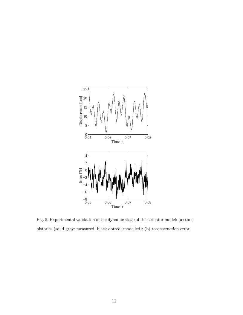
of white noise, as requested for a good identification result [5]. Then, in or-

der to check the reconstruction accuracy of minor loops inside the limit cy-

cle, the model has been validated by comparing the simulated output with

the measured one in the case of multi-sinusoidal λd signals. Fig. 5 shows the

simulated and measured output for a signal with components at frequencies

70, 180, 390 Hz. The reconstruction error is within 8 %.

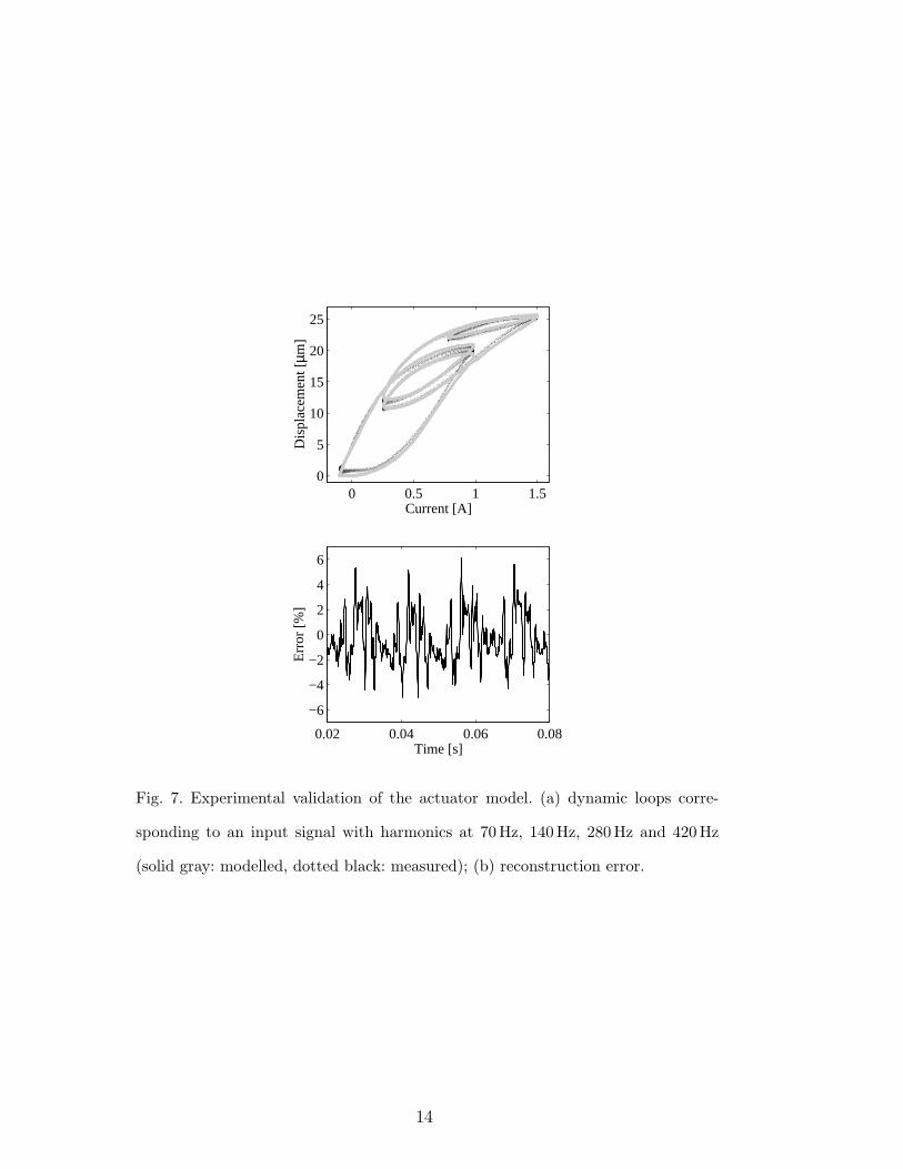
Moreover, the complete dynamic model has been tested with three-harmonic

and four-harmonic periodic current inputs. The first signal has frequencies at

70 Hz, 140 Hz and 280 Hz, where the second one has an additional harmonic at

420 Hz. The input-output loops, both measured and simulated, are shown in

Fig. 6 and Fig. 7, together with the corresponding reconstruction errors. The

results confirm the accuracy of the proposed dynamic model in the considered

frequency range.

6

4 Conclusions

A novel dynamic model for a commercial magnetostrictive actuator has been

proposed. The model is structured as a series-connection of a static hysteresis

Preisach operator and a linear time-invariant dynamic system. By exploiting

the idea of the compensator of hysteresis operator, an easy identification pro-

cedure can be adopted for the dynamic stage of the model. The identification

of static stage of the model is based on a fuzzy technique, while a standard

parametric identification is used for the linear time-invariant operator. Despite

of its very simple structure, the model is able to accurately reproduce the dy-

namic behaviour of the actuator in a broad frequency range, as confirmed

by a number of experimental tests. Future work will be devoted to test such

a modelling technique on a resonant magnetostrictive actuator with a very

rich dynamics, designed for vibration reduction. In fact, for those applications

it is mandatory to take into account the nonlinear dynamics of a hysteretic

resonant actuator employed in the feedback control system.

References

[1] G. Engdahl, Handbook of Giant Magnetostrictive Materials, Academic Press,

San Diego, 1999.

[2] I. Mayergoyz, Mathematical Models of Hysteresis, Springer-Verlag, New York,

1991.

[3] C. Natale, F. Velardi, C. Visone, Identification and compensation of preisach

hysteresis models for magnetostrictive actuators, Physica B: Condensed Matter

306 (2001) 161–165.

7

[4] A. Cavallo, C. Natale, C. Pirozzi, C. Visone, Effects of hysteresis compensation in

feedback control systems, IEEE Transactions on Magnetics 39 (2003) 1389–1392.

[5] L. Ljungz, System Identification: Theory for the User, Prentice Hall, Englewood

Cliffs, 1987.

8

List of Figures

1 Dynamic model of the actuator and compensator. 10

2 Compensated cycles at increasing frequencies for sinusoidal λd. 10

3 Experimental validation of the static stage of the actuator

model: (a) input-output loops (solid gray: modelled, black

dotted: measured); (b) reconstruction error. 11

4 Correlation function of model residuals. 11

5 Experimental validation of the dynamic stage of the actuator

model: (a) time histories (solid gray: measured, black dotted:

modelled); (b) reconstruction error. 12

6 Experimental validation of the actuator model. (a) dynamic

loops corresponding to an input signal with harmonics at

70 Hz, 140 Hz, 280 Hz (solid gray: modelled, dotted black:

measured); (b) reconstruction error. 13

7 Experimental validation of the actuator model. (a) dynamic

loops corresponding to an input signal with harmonics at

70 Hz, 140 Hz, 280 Hz and 420 Hz (solid gray: modelled, dotted

black: measured); (b) reconstruction error. 14

9

λλd i Magnetostrictiveactuator

λλz - d z -1

z -1

B( )A( )

Dynamic model of the actuator

i

Fig. 1. Dynamic model of the actuator and compensator.

0 10 20 300

5

10

15

20

25

30

Desired displacement [µm]

Dis

plac

emen

t [µm

]

Fig. 2. Compensated cycles at increasing frequencies for sinusoidal λd.

10

0 0.5 1 1.5

0

5

10

15

20

25

Current [A]

Dis

plac

emen

t [µm

]

0.4 0.42 0.44 0.46 0.48−5

0

5

Time [s]

Err

or [%

]

Fig. 3. Experimental validation of the static stage of the actuator model: (a) in-

put-output loops (solid gray: modelled, black dotted: measured); (b) reconstruction

error.

0 10 20 30 40 50

0

0.2

0.4

0.6

0.8

1

Lag

Fig. 4. Correlation function of model residuals.

11

0.05 0.06 0.07 0.080

5

10

15

20

25

Time [s]

Dis

plac

emen

t [µm

]

0.05 0.06 0.07 0.08−8

−6

−4

−2

0

2

4

Time [s]

Err

or [%

]

Fig. 5. Experimental validation of the dynamic stage of the actuator model: (a) time

histories (solid gray: measured, black dotted: modelled); (b) reconstruction error.

12

0 0.5 1 1.50

5

10

15

20

25

Current [A]

Dis

plac

emen

t [µm

]

0.02 0.04 0.06 0.08

−6

−4

−2

0

2

4

6

Time [s]

Err

or [%

]

Fig. 6. Experimental validation of the actuator model. (a) dynamic loops corre-

sponding to an input signal with harmonics at 70Hz, 140 Hz, 280 Hz (solid gray:

modelled, dotted black: measured); (b) reconstruction error.

13

0 0.5 1 1.50

5

10

15

20

25

Current [A]

Dis

plac

emen

t [µm

]

0.02 0.04 0.06 0.08

−6

−4

−2

0

2

4

6

Time [s]

Err

or [%

]

Fig. 7. Experimental validation of the actuator model. (a) dynamic loops corre-

sponding to an input signal with harmonics at 70Hz, 140 Hz, 280Hz and 420Hz

(solid gray: modelled, dotted black: measured); (b) reconstruction error.

14