
"PhD - Digital Predistortion and Equalization of the Non-Linear ...
132
Université libre de Bruxelles Ecole Polytechnique de Bruxelles Service OPERA Digital Predistortion and Equalization of the Non-Linear Satellite Communication Channel A thesis submitted for the degree of Docteur en Sciences de l’Ingénieur et Technologie by Thibault Deleu Jury : Prof. Philippe De Doncker Dr. Mathieu Dervin Prof. Jean-Michel Dricot Prof. Philippe Emplit Prof. François Horlin (Supervisor) Prof. Geert Leus Prof. Luc Vandendorpe
-
Upload
khangminh22 -
Category
Documents
-
view
1 -
download
0
Transcript of "PhD - Digital Predistortion and Equalization of the Non-Linear ...

Université libre de BruxellesEcole Polytechnique de Bruxelles
Service OPERA
Digital Predistortion and Equalization ofthe Non-Linear Satellite Communication
Channel
A thesis submitted for the degree of
Docteur en Sciences de l’Ingénieur et Technologie
byThibault Deleu
Jury :Prof. Philippe De DonckerDr. Mathieu DervinProf. Jean-Michel DricotProf. Philippe EmplitProf. François Horlin (Supervisor)Prof. Geert LeusProf. Luc Vandendorpe


Remerciements
Je tiens à remercier grandement mon directeur de thèse, François Horlin,pour toute l’aide qu’il m’a apportée durant ces quatre années. Son optimismesans borne m’a permis de toujours croire à ce que je faisais. Je lui suis parti-culièrement reconnaissant de la confiance qu’il m’a donnée, en ne m’imposantpas de directions à suivre dans ma recherche. Je suis convaincu que cela m’aappris beaucoup de choses, notamment en termes d’organisation, de rigueuret d’autonomie. J’aimerais aussi le remercier pour son ouverture d’esprit, enfavorisant notamment les collaborations avec d’autres centres de recherche.Cela m’a permis d’effectuer des séjours à Toulouse et à Tokyo extrêmementenrichissants d’un point de vue scientifique et personnel.
Je tiens également à remercier particulièrement Mathieu Dervin, qui a suivi detrès près ma thèse durant ces quatre années. Malgré un agenda bien rempli,il a toujours pris le temps de répondre à toutes mes questions. Nos longuesdiscussions m’ont permis de mieux comprendre les systèmes de communicationpar satellite, mais aussi de me poser les bonnes questions et de mieux formulerles problèmes. Sans jamais imposer sa vision, il m’a apporté de précieux conseils,qui m’ont fait progresser durant toute ma recherche. Par ailleurs, sa simplicité,sa modestie et son enthousiasme font de lui une personne extrêmement agréableà côtoyer.
Je tiens aussi à remercier Kenta Kasai, qui m’a encadré durant mes re-cherches au Japon. Le temps qu’il m’a consacré afin de m’expliquer les conceptsles plus farfelus en codes correcteurs d’erreurs m’a été particulièrement utilepour la suite de ma recherche. Sa bonne humeur et son extrême gentillesse m’ontpermis de me sentir rapidement à l’aise dans son laboratoire.
Je remercie également mon président de jury Philippe Emplit ainsi que lesmembres de mon jury Philippe De Doncker, Mathieu Dervin, Jean-MichelDricot, François Horlin, Geert Leus et Luc Vandendorpe pour le temps qu’ilsm’ont consacré. Leurs remarques constructives qu’ils mont données durant madéfense privée ont contribué à améliorer la qualité du manuscrit.

ii
Je ne peux évidemment manquer de remercier tous mes (ex-) collègues.Ceux du service OPERA pour tous ces moments partagés, que ce soit au serviceou en dehors du travail. Ceux de Toulouse, qui m’ont si bien accueilli malgrémes séjours assez courts. Ceux de Tokyo, qui m’ont rapidement inclus dans leurssoirées karaoké ou jeux vidéos. Je remercie aussi Natascha pour sa gentillesse ettoute l’aide qu’elle m’a apportée.
Je remercie aussi chaleureusement mes amis de Toulouse et de Tokyo quim’ont permis de pleinement vivre mes expériences à l’étranger. Je remercie aussiceux de Bruxelles, notamment pour ne pas m’avoir oublié malgré mes voyagesfréquents.
Enfin, je terminerai en remerciant mes proches, Sophie, pour le bonheurqu’elle m’apporte, ainsi que mes soeurs et mes parents pour leur soutien et leuraffection indéfectible.

Table of Content
Table of Content iii
Table of Figures vii
Table of Tables xi
List of Acronyms xiii
1 Introduction 11.1 General introduction . . . . . . . . . . . . . . . . . . . . . . . . . 11.2 The satellite communication channel . . . . . . . . . . . . . . . . 2
1.2.1 Channel model . . . . . . . . . . . . . . . . . . . . . . . . 31.2.2 Single versus multi-carrier per amplified channel scenarios 31.2.3 Transponder model . . . . . . . . . . . . . . . . . . . . . . 51.2.4 Transceiver model . . . . . . . . . . . . . . . . . . . . . . . 6
1.3 DVB-S2 communication system . . . . . . . . . . . . . . . . . . . 71.3.1 Introduction . . . . . . . . . . . . . . . . . . . . . . . . . . 71.3.2 FEC Encoding . . . . . . . . . . . . . . . . . . . . . . . . 71.3.3 Interleaver . . . . . . . . . . . . . . . . . . . . . . . . . . . 81.3.4 Bit mapping into constellations . . . . . . . . . . . . . . . 81.3.5 Shaping filter . . . . . . . . . . . . . . . . . . . . . . . . . 111.3.6 IMUX, OMUX and HPA characteristics . . . . . . . . . . 111.3.7 Other elements in the DVB-S2 standard . . . . . . . . . . 13
1.4 Effects of non-linearities on the system performance . . . . . . . . 141.4.1 Non-linear interference in a SC scenario . . . . . . . . . . . 141.4.2 Non-linear interference in a MC scenario . . . . . . . . . . 151.4.3 Total degradation . . . . . . . . . . . . . . . . . . . . . . . 15
1.5 The trade-off between power efficiency, spectral efficiency and com-plexity . . . . . . . . . . . . . . . . . . . . . . . . . . . . . . . . . 16
1.6 Other sources of interference . . . . . . . . . . . . . . . . . . . . . 181.7 Other analog impairments . . . . . . . . . . . . . . . . . . . . . . 18
1.7.1 Non-linear amplifier at the hub . . . . . . . . . . . . . . . 191.7.2 Uplink noise . . . . . . . . . . . . . . . . . . . . . . . . . . 191.7.3 Frequency offset and timing error . . . . . . . . . . . . . . 19

iv Table of Content
1.7.4 Phase noise . . . . . . . . . . . . . . . . . . . . . . . . . . 201.7.5 I/Q imbalances . . . . . . . . . . . . . . . . . . . . . . . . 20
1.8 Contribution and structure of the manuscripts . . . . . . . . . . . 21
2 Review of state-of-the-art interference mitigation algorithms 232.1 Introduction . . . . . . . . . . . . . . . . . . . . . . . . . . . . . . 242.2 System model . . . . . . . . . . . . . . . . . . . . . . . . . . . . . 242.3 Notations . . . . . . . . . . . . . . . . . . . . . . . . . . . . . . . 262.4 The Volterra model . . . . . . . . . . . . . . . . . . . . . . . . . . 27
2.4.1 SC scenario . . . . . . . . . . . . . . . . . . . . . . . . . . 272.4.2 MC scenario . . . . . . . . . . . . . . . . . . . . . . . . . . 29
2.5 Normalization and Gaussian detection in a non-linear channel . . 312.6 Review of existing predistortion algorithms in a non-linear channel 32
2.6.1 Power amplifier linearization . . . . . . . . . . . . . . . . . 322.6.2 Signal predistortion versus data predistortion . . . . . . . 332.6.3 Digital predistortion algorithms for non-linear channels
with memory . . . . . . . . . . . . . . . . . . . . . . . . . 342.6.4 Mathematical description of the main digital predistortion
algorithms . . . . . . . . . . . . . . . . . . . . . . . . . . . 352.7 Literature review of receiver compensation algorithms in a non-
linear channel . . . . . . . . . . . . . . . . . . . . . . . . . . . . . 382.8 Conclusion . . . . . . . . . . . . . . . . . . . . . . . . . . . . . . . 382.A Proof of the order p compensation algorithm . . . . . . . . . . . . 39
3 Per-block iterative predistortion algorithm 413.1 Introduction . . . . . . . . . . . . . . . . . . . . . . . . . . . . . . 413.2 Notations . . . . . . . . . . . . . . . . . . . . . . . . . . . . . . . 423.3 Small-variation algorithm in the SC scenario . . . . . . . . . . . . 43
3.3.1 Per block iterative predistortion . . . . . . . . . . . . . . . 433.3.2 Small-variation algorithm . . . . . . . . . . . . . . . . . . 453.3.3 Linearity assumption . . . . . . . . . . . . . . . . . . . . . 473.3.4 Calculation of the linear coefficients based on channel si-
mulations . . . . . . . . . . . . . . . . . . . . . . . . . . . 483.3.5 Linear filtering . . . . . . . . . . . . . . . . . . . . . . . . 48
3.4 Small-variation algorithm in the MC scenario . . . . . . . . . . . 493.5 Numerical results . . . . . . . . . . . . . . . . . . . . . . . . . . . 50
3.5.1 SVA in the SC scenario . . . . . . . . . . . . . . . . . . . . 50

Table of Content v
3.5.2 SVA in the MC scenario . . . . . . . . . . . . . . . . . . . 553.6 Summary . . . . . . . . . . . . . . . . . . . . . . . . . . . . . . . 593.A Calculation of the coefficients Ank,j(m1,m2) for some simple Vol-
terra models . . . . . . . . . . . . . . . . . . . . . . . . . . . . . . 593.B Proof of (3.18) . . . . . . . . . . . . . . . . . . . . . . . . . . . . . 603.C Channel simulation with constant Volterra coefficients . . . . . . . 61
4 Low-complexity predistortion algorithms based on the SVA andon the order p compensation 634.1 Introduction . . . . . . . . . . . . . . . . . . . . . . . . . . . . . . 634.2 Low-complexity algorithms based on the SVA . . . . . . . . . . . 64
4.2.1 Low-complexity approximations of the coefficientsAn,c1k,j,c(1, 0) and An,c1k,j,c(0, 1) . . . . . . . . . . . . . . . . . . . 64
4.2.2 Verification of the linearity assumption . . . . . . . . . . . 664.2.3 Comparison with SoA algorithms . . . . . . . . . . . . . . 66
4.3 Modified order p compensation . . . . . . . . . . . . . . . . . . . 674.4 Complexity analysis . . . . . . . . . . . . . . . . . . . . . . . . . 68
4.4.1 Complexity incurred by a convolution . . . . . . . . . . . . 684.4.2 Complexity incurred by one channel simulation . . . . . . 694.4.3 Complexity of the modified order p compensation . . . . . 704.4.4 Complexity of the SVA based on LUT . . . . . . . . . . . 714.4.5 Complexity of the SVA based on Volterra coefficients . . . 724.4.6 Complexity of the SVA . . . . . . . . . . . . . . . . . . . . 724.4.7 Conclusion . . . . . . . . . . . . . . . . . . . . . . . . . . . 72
4.5 Numerical results . . . . . . . . . . . . . . . . . . . . . . . . . . . 734.5.1 SC scenario . . . . . . . . . . . . . . . . . . . . . . . . . . 734.5.2 MC scenario . . . . . . . . . . . . . . . . . . . . . . . . . . 78
4.6 Conclusion and future work . . . . . . . . . . . . . . . . . . . . . 78
5 Turbo-equalization of the remaining interference after predistor-tion 815.1 Introduction . . . . . . . . . . . . . . . . . . . . . . . . . . . . . . 815.2 Literature review of equalization and detection algorithms for non-
linear channels . . . . . . . . . . . . . . . . . . . . . . . . . . . . 825.3 Notations . . . . . . . . . . . . . . . . . . . . . . . . . . . . . . . 835.4 Turbo-equalization in the un-predistorted channel . . . . . . . . . 84
5.4.1 Turbo-equalizer structure . . . . . . . . . . . . . . . . . . 84

vi Table of Content
5.4.2 Estimation of the conditional interference . . . . . . . . . . 865.5 Generalities on joint predistortion and turbo-equalization . . . . . 88
5.5.1 Simulation of the predistortion algorithm at the receiver . 885.5.2 No simulation of the predistortion algorithm at the receiver 88
5.6 Application of joint predistortion and turbo-equalization to specificpredistortion algorithms . . . . . . . . . . . . . . . . . . . . . . . 905.6.1 Joint predistortion and turbo-equalization based on the SVA 905.6.2 Joint predistortion and turbo-equalization based on LUT . 955.6.3 Modified order p predistortion algorithm . . . . . . . . . . 96
5.7 Comparison based on the total degradation . . . . . . . . . . . . . 1015.8 Conclusion . . . . . . . . . . . . . . . . . . . . . . . . . . . . . . . 102
6 Conclusion and future work 103
Bibliography 107
Publications 115

Table of Figures
1.1 Main components of the satellite communication channel . . . . . 21.2 Signal amplification scheme in a SC scenario . . . . . . . . . . . . 41.3 Signal amplification scheme in a MC scenario . . . . . . . . . . . 51.4 Transponder model . . . . . . . . . . . . . . . . . . . . . . . . . . 51.5 Transmitter model . . . . . . . . . . . . . . . . . . . . . . . . . . 61.6 Receiver model . . . . . . . . . . . . . . . . . . . . . . . . . . . . 61.7 Bit mapping into QPSK constellation . . . . . . . . . . . . . . . . 91.8 Bit mapping into 8APSK constellation . . . . . . . . . . . . . . . 91.9 Bit mapping into 16APSK constellation . . . . . . . . . . . . . . . 101.10 Bit mapping into 32APSK constellation . . . . . . . . . . . . . . . 101.11 IMUX frequency characteristics considered in the DVB-S2 standard 121.12 OMUX frequency characteristics considered in the DVB-S2 standard 121.13 HPA characteristics considered the DVB-S2 standard . . . . . . . 131.14 Impact of the channel non-linearities on the received samples,
32APSK, OBO = 2.3dB, α = 0.1, 36Mbaud . . . . . . . . . . . . 141.15 Normalized data throughput vers C/N (based on a packet error
rate equal to 10−7) . . . . . . . . . . . . . . . . . . . . . . . . . . 17
2.1 Mathematical model of the channel in the SC scenario . . . . . . 252.2 Mathematical model of the channel in the MC scenario . . . . . . 262.3 Frequency response of SRRC filter multiplications . . . . . . . . . 302.4 Ideal linearization (predistortion) . . . . . . . . . . . . . . . . . . 33
3.1 Received constellation after predistortion, 36Mbaud, α = 0.1,2.1dB OBO . . . . . . . . . . . . . . . . . . . . . . . . . . . . . . 50
3.2 Mean-square error (MSE) after each iteration of the SVA,36Mbaud, α = 0.1, 3dB IBO . . . . . . . . . . . . . . . . . . . . . 52
3.3 BER performance using the SVA and state-of-the-art pre-distortion methods, 36Mbaud, α = 0.1, 2.1dB OBO . . . . . . . . 52
3.4 Total degradation for the SVA and state-of-the-art pre-distortionmethods, 25Mbaud, α = 0.3 . . . . . . . . . . . . . . . . . . . . . 53
3.5 Total degradation for the SVA and state-of-the-art pre-distortionmethods, 36Mbaud, α = 0.1 . . . . . . . . . . . . . . . . . . . . . 53

viii Table of Figures
3.6 Total degradation for the small-variation algorithm (SVA) andstate-of-the-art pre-distortion methods, 38Mbaud, α = 0.05 . . . . 56
3.7 PAPR at the transmitter after each iteration of the SVA for dif-ferent combinations of symbol rates and rolloffs, 3dB IBO . . . . . 56
3.8 MSE after each iteration of the SVA, three carrier multiplex, outercarrier, 4dB IBO . . . . . . . . . . . . . . . . . . . . . . . . . . . 57
3.9 MSE after each iteration of the SVA, three carrier multiplex, innercarrier, 4dB IBO . . . . . . . . . . . . . . . . . . . . . . . . . . . 57
3.10 BER performance with and w/o SVA, three carrier multiplex, 2dBOBO . . . . . . . . . . . . . . . . . . . . . . . . . . . . . . . . . . 58
3.11 Total degradation with and w/o SVA, three carrier multiplex . . . 583.12 Received constellation simulated by the predistorter after predis-
tortion, 36Mbaud, α = 0.1, 2.1dB OBO . . . . . . . . . . . . . . . 61
4.1 Mean-square error (MSE) after each iteration of the small-variation algorithm, using the convergence method described inSection 4.2.2, 36Mbaud, α = 0.1, 3dB IBO . . . . . . . . . . . . . 73
4.2 MSE using the modified order p algorithm, 4dB IBO . . . . . . . 754.3 PAPR using the modified order p algorithm, 4dB IBO . . . . . . . 754.4 Total degradation for small-variation algorithm (SVA), reduced-
complexity algorithms and state-of-the-art pre-distortion methods,25Mbaud, α = 0.3 . . . . . . . . . . . . . . . . . . . . . . . . . . . 76
4.5 Total degradation for small-variation algorithm (SVA), reduced-complexity algorithms and state-of-the-art pre-distortion methods,36Mbaud, α = 0.1 . . . . . . . . . . . . . . . . . . . . . . . . . . . 76
4.6 Total degradation for small-variation algorithm (SVA), reduced-complexity algorithms and state-of-the-art pre-distortion methods,38Mbaud, α = 0.05 . . . . . . . . . . . . . . . . . . . . . . . . . . 77
4.7 MSE using the modified order p algorithm, three carrier multiplex 794.8 Total degradation with and w/o SVA and the reduced-complexity
algorithms, three carrier multiplex . . . . . . . . . . . . . . . . . . 79
5.1 Turbo-equalization interference cancellation equalizer . . . . . . . 855.2 Turbo-equalization strategies in a predistorted channel, Methods
I.A and I.B . . . . . . . . . . . . . . . . . . . . . . . . . . . . . . 895.3 Turbo-equalization strategies in a predistorted channel, Methods
II.A and II.B . . . . . . . . . . . . . . . . . . . . . . . . . . . . . 89

Table of Figures ix
5.4 Noiseless received samples after SVA, 38Mbaud, α = 0.05, 1.9dBOBO . . . . . . . . . . . . . . . . . . . . . . . . . . . . . . . . . . 92
5.5 Illustration of I(n), Ir(n) and Iφ(n) . . . . . . . . . . . . . . . . . 925.6 I0,r(n) versus Ir(n) and first and third order approximations using
the SVA algorithm, 38Mbaud, α = 0.05, 1.9dB OBO . . . . . . . 935.7 SVA predistortion + Turbo-equalization, 38Mbaud, α = 0.05,
1.9dB OBO . . . . . . . . . . . . . . . . . . . . . . . . . . . . . . 945.8 Noiseless received samples after LUT predistortion (Lp = 3),
36Mbaud, α = 0.1, 2.7dB OBO . . . . . . . . . . . . . . . . . . . 965.9 LUT predistortion + Turbo-equalization, 36Mbaud, α = 0.1,
2.7dB OBO . . . . . . . . . . . . . . . . . . . . . . . . . . . . . . 975.10 Noiseless received samples after modified order p compensation,
38Mbaud, α = 0.05, 1.9dB OBO . . . . . . . . . . . . . . . . . . . 985.11 I0,r(n) versus Ir(n) and first and third order approximations using
the modified order p compensation, 38Mbaud, α = 0.05, 1.9dB OBO 985.12 Order p predistortion + Turbo-equalization, 38Mbaud, α = 0.05,
1.9dB OBO . . . . . . . . . . . . . . . . . . . . . . . . . . . . . . 995.13 Total degradation, 36Mbaud, α = 0.1 . . . . . . . . . . . . . . . . 1005.14 Total degradation, 38Mbaud, α = 0.05 . . . . . . . . . . . . . . . 100


Table of Tables
1.1 Constellation radius ratio for 16-APSK constellation . . . . . . . . 81.2 Constellation radius ratio for 32-APSK constellation . . . . . . . . 111.3 Aggregate phase noise masks proposed in the DVB-S2 standard
(in dBc/Hz) . . . . . . . . . . . . . . . . . . . . . . . . . . . . . . 20
2.1 Main notations . . . . . . . . . . . . . . . . . . . . . . . . . . . . 27
3.1 Coefficients Ank,j(m1,m2) for the Fictive Model H3(0, 0, 0),H3(1, 0, 0) and H3(0, 1, 2) . . . . . . . . . . . . . . . . . . . . . . . 60
4.1 Performance of the reduced-complexity alternatives of the small-variation algorithm . . . . . . . . . . . . . . . . . . . . . . . . . . 74
5.1 Notations specific to Chapter 5 . . . . . . . . . . . . . . . . . . . 845.2 Minimum total degradation achieved by the different predistortion
algorithms +turbo-equalization . . . . . . . . . . . . . . . . . . . 101


List of Acronyms
16PSK 16-ary Phase Shift Keying
32PSK 32-ary Phase Shift Keying
8PSK 8-ary Phase Shift Keying
ACI Adjacent Channel Interference
ACM Adaptive Coding and Modulation
AWGN Additive White Gaussian Noise
BCH Bose-Chaudhuri-Hocquenghem multiple error correction binaryblock code
BER Bit Error Rate
ETSI European Technical Standards Institute
FEC Forward Error Correction
FER Frame Error Rate
HPA High-Power Amplifier
IBO Input Back off
IEEE Institute of Electrical and Electronics Engineers
IF Intermediate Frequency
IMI InterModulation Interference
IMUX Input Multiplexer
LDPC Low-Density Parity-Check
LLR Log-Likelihood Ratios
LUT Least Mean Square
LUT Look-Up Table
MC Multi-Carrier (per channel)
MMSE Minimum Mean Square Error

xiv List of Acronyms
NN Neural Networks
OBO Output Back off
ODEMUX Output DEMUltipleXer
OMUX Output Multiplexer
PAPR Peak-to-Average Power Ratio
PL Physical Layer
PSD Power Spectral Density
QPSK Quaternary Phase Shift Keying
RF Radio Frequency
RLS Recursive Least Square
SC Single-Carrier (per channel)
SNR Signal-to-Noise Ratio
SOA State-of-the-art
SRRC Square-Root-Raised-Cosine
SSPA Solid State Power Amplifier
SVA Small-Variation Algorithm
TD Total Degradation
TWTA Traveling WaveTube Amplifier

Chapitre 1
Introduction
Contents1.1 General introduction . . . . . . . . . . . . . . . . . . . . . 11.2 The satellite communication channel . . . . . . . . . . . . 2
1.2.1 Channel model . . . . . . . . . . . . . . . . . . . . . . . . . 31.2.2 Single versus multi-carrier per amplified channel scenarios . 31.2.3 Transponder model . . . . . . . . . . . . . . . . . . . . . . . 51.2.4 Transceiver model . . . . . . . . . . . . . . . . . . . . . . . 6
1.3 DVB-S2 communication system . . . . . . . . . . . . . . . 71.3.1 Introduction . . . . . . . . . . . . . . . . . . . . . . . . . . . 71.3.2 FEC Encoding . . . . . . . . . . . . . . . . . . . . . . . . . 71.3.3 Interleaver . . . . . . . . . . . . . . . . . . . . . . . . . . . . 81.3.4 Bit mapping into constellations . . . . . . . . . . . . . . . . 81.3.5 Shaping filter . . . . . . . . . . . . . . . . . . . . . . . . . . 111.3.6 IMUX, OMUX and HPA characteristics . . . . . . . . . . . 111.3.7 Other elements in the DVB-S2 standard . . . . . . . . . . . 13
1.4 Effects of non-linearities on the system performance . . 141.4.1 Non-linear interference in a SC scenario . . . . . . . . . . . 141.4.2 Non-linear interference in a MC scenario . . . . . . . . . . . 151.4.3 Total degradation . . . . . . . . . . . . . . . . . . . . . . . . 15
1.5 The trade-off between power efficiency, spectral effi-ciency and complexity . . . . . . . . . . . . . . . . . . . . . 16
1.6 Other sources of interference . . . . . . . . . . . . . . . . 181.7 Other analog impairments . . . . . . . . . . . . . . . . . . 18
1.7.1 Non-linear amplifier at the hub . . . . . . . . . . . . . . . . 191.7.2 Uplink noise . . . . . . . . . . . . . . . . . . . . . . . . . . . 191.7.3 Frequency offset and timing error . . . . . . . . . . . . . . . 191.7.4 Phase noise . . . . . . . . . . . . . . . . . . . . . . . . . . . 201.7.5 I/Q imbalances . . . . . . . . . . . . . . . . . . . . . . . . . 20

2 Chapitre 1. Introduction
1.8 Contribution and structure of the manuscripts . . . . . . 21
1.1 General introduction
Satellite communications are continuously evolving to adapt to the everincreasing demand for throughput required by the new user applications. Thisevolution is very challenging due to the constraints that need to be taken intoaccount in the system. The radio frequency spectrum being shared by severalapplications, the frequency bandwidth allocated to a satellite communicationsystem is limited. The power delivered by the satellite is also a sparse resource sothat power efficiency is also an issue. Weight of onboard power amplifiers and sizeof on ground equipment are further constraints on the system. Different areasof research have improved the overall system performance, as for instance theoptimization of power gathering and transfer aboard the satellite and the designof higher-gain antennas. The computational power at the transmitter and at thereceiver has also dramatically increased, allowing for the use of more efficienterror correcting codes for instance. Larger computational power also allows forbetter mitigating the impact of analog channel impairments, which becomesmore and more substantial for larger throughputs. The digital compensation ofanalog channel impairments is the general context of this thesis.
One of the main impairments in the satellite communication channel isthe non-linear distortion induced by the power amplifier aboard the satellite.This power amplifier is indeed driven close to its saturation point to maximizethe power efficiency. However, this non-linear power amplifier combined withlinear filters present in the channel creates non-linear interference, which canstrongly limit the system performance. Signal processing at the transmitter orreceiver side can mitigate this undesired effect.
The main focus of this manuscript is the broadcast and broadband satel-lite communication channel, where information is exchanged between one huband many user terminals in a so-called star topology. More particularly, theforward link will be considered, which is defined as the link from the hub to theuser terminals, in opposite to the return link. In this context, it is preferable toconcentrate the complexity as much as possible at the transmitter side. Other
1.2. The satellite communication channel 3
Satellite Transponder
Satellite terminal HUB
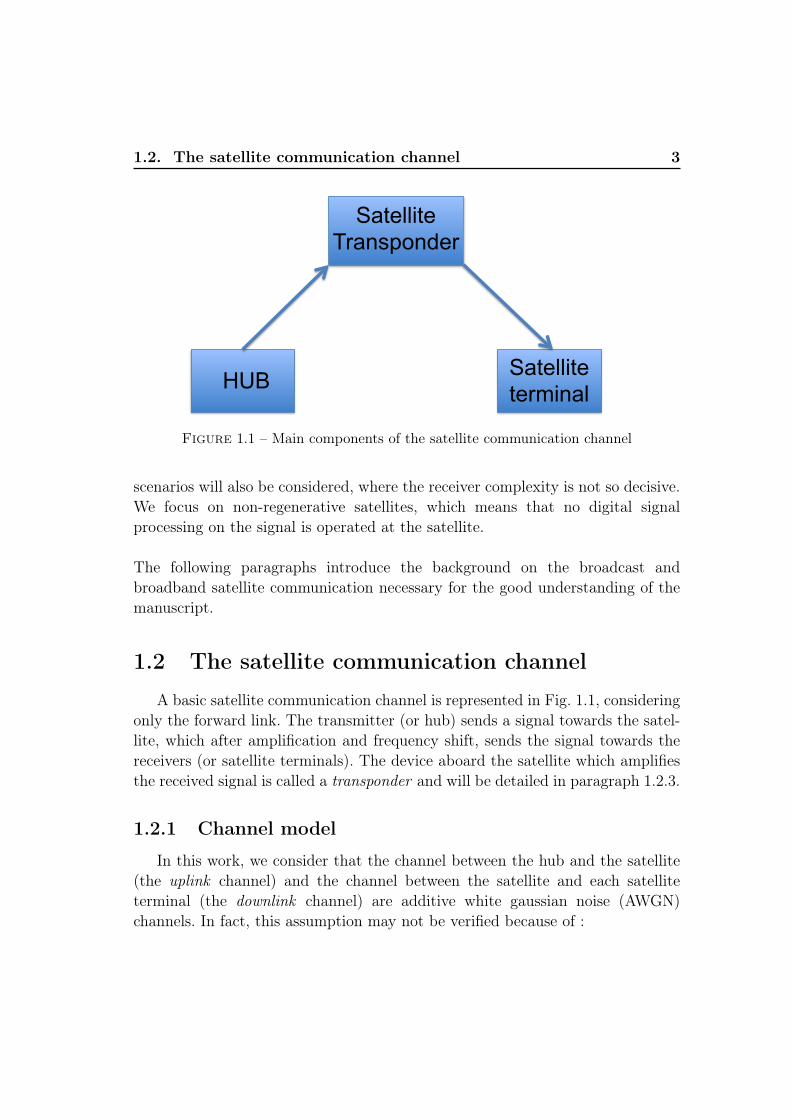
Figure 1.1 – Main components of the satellite communication channel
scenarios will also be considered, where the receiver complexity is not so decisive.We focus on non-regenerative satellites, which means that no digital signalprocessing on the signal is operated at the satellite.
The following paragraphs introduce the background on the broadcast andbroadband satellite communication necessary for the good understanding of themanuscript.
1.2 The satellite communication channel
A basic satellite communication channel is represented in Fig. 1.1, consideringonly the forward link. The transmitter (or hub) sends a signal towards the satel-lite, which after amplification and frequency shift, sends the signal towards thereceivers (or satellite terminals). The device aboard the satellite which amplifiesthe received signal is called a transponder and will be detailed in paragraph 1.2.3.
1.2.1 Channel model
In this work, we consider that the channel between the hub and the satellite(the uplink channel) and the channel between the satellite and each satelliteterminal (the downlink channel) are additive white gaussian noise (AWGN)channels. In fact, this assumption may not be verified because of :

4 Chapitre 1. Introduction
– Multipath components at the receiver.
– Atmospheric effects.
In this work, geostationary communication satellites are considered. Geosta-tionary satellites have an altitude of approximatively 36000km and an orbitsituated in the equatorial plane. For a stationary observer on earth, they seemto have a constant position in the sky. Due to the high path loss, highly directiveparabolic antennas are used at the transmitter and at the receiver. Moreover, thetransmitter and the receiver are placed in line-of-sight of the satellite, so thatmultipath components are negligible [1]. Geostationary satellites are used forfixed satellite services, such as direct-to-home television and broadcast networks.
Attenuation is the main impairment resulting from atmospheric effects,and is due to the rain, clouds and atmospheric gases. The level of attenuationvaries thus with time. The troposphere can also induce scintillation, which isa rapid variation in the signal amplitude. This effect can be significant for lowelevation satellite links, which is not the case for geostationary satellites [2].Finally, the polarization sense of the transmitted signal can also be affected,primarily due to the rain. If the satellite link is single-polarized, this effect can beseen as a further attenuation of the signal. If the satellite link is dual-polarized,the depolarization creates co-channel interference (or cross-polarization) [3].Cross-polarization effects will not be considered in this work.
1.2.2 Single versus multi-carrier per amplified channel sce-narios
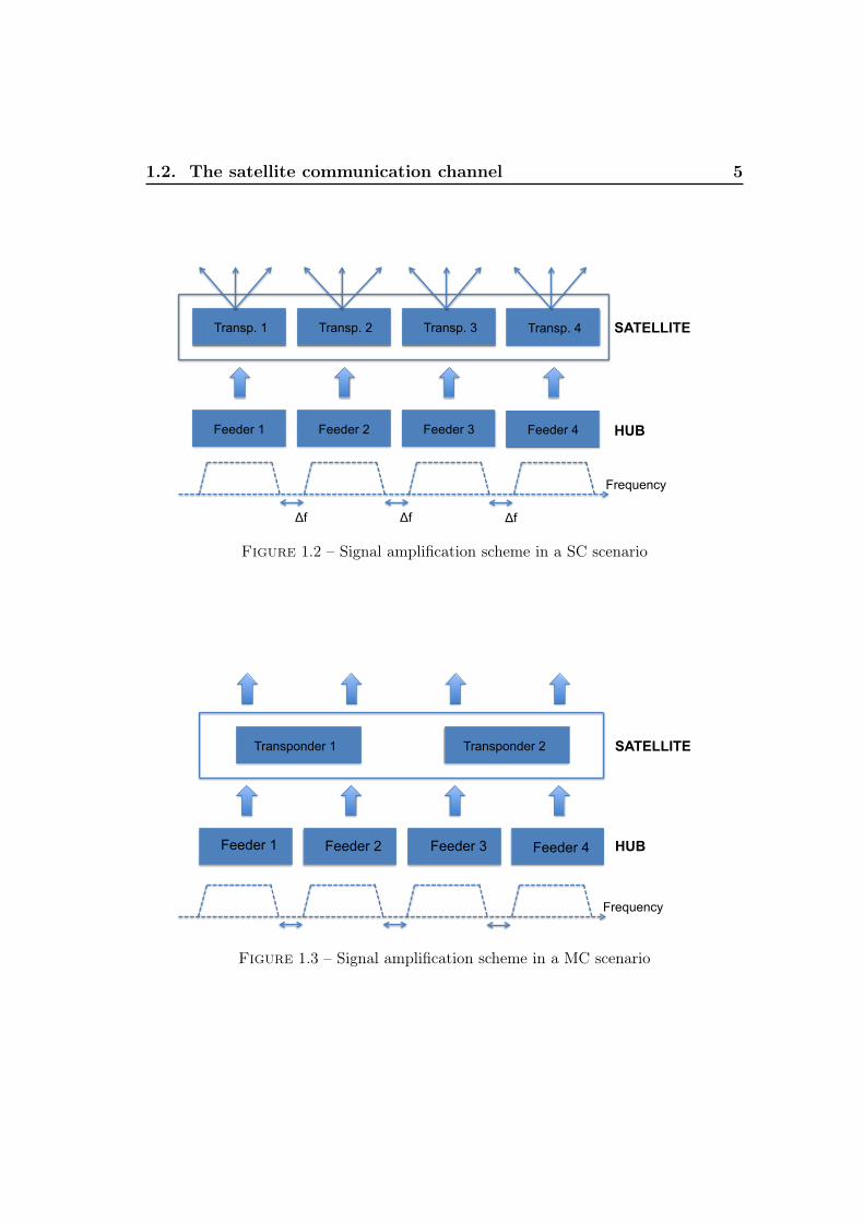
In practical systems, a satellite carries several transponders, which amplifymultiple signals coming from different hubs (at different frequencies). In a singlecarrier per channel (SC) scenario, each transponder only amplifies the signalcoming from one hub, while in a multi-carrier per channel (MC) scenario, atransponder amplifies signals coming from different hubs (at different frequen-cies), as illustrated in Fig. 1.2 and Fig. 1.3.
The capacity of a SC system is generally higher, but the number of ne-cessary transponders for a given number of carriers is obviously lower in the MCcase. A MC system allows therefore for decreasing the payload weight, which
1.2. The satellite communication channel 5
Feeder 1 HUB
Frequency
Δf Δf
Feeder 2 Feeder 3 Feeder 4
Δf
Transp. 1 Transp. 2 Transp. 3 Transp. 4 SATELLITE
Figure 1.2 – Signal amplification scheme in a SC scenario
Feeder 1 Feeder 2 Feeder 3 Feeder 4
Transponder 1 Transponder 2
Frequency
HUB
SATELLITE
Figure 1.3 – Signal amplification scheme in a MC scenario

6 Chapitre 1. Introduction
!"#$% &'(% )"#$%
Figure 1.4 – Transponder model
can be of crucial interest. The choice of the system depends on the consideredapplication. If information from one hub is broadcasted on a large area orspot (for instance Europe), SC systems are generally preferred to maximize thecapacity of the system. Nowadays, it becomes however more and more commonto broadcast information on smaller areas to take advantage of the frequencyreuse : since information coming from one hub is only broadcasted on a smallarea, it is possible to broadcast information from a second hub towards a differentarea using the same frequency band (but a different transponder). This improvesthe system flexibility, which is more and more required by new user applications.This kind of systems requires a larger number of carriers, so that MC systemsare usually considered to keep the payload weight acceptable. The number ofcarriers amplified by the same transponder is generally comprised between 2 and8 carriers.
1.2.3 Transponder model
The transponder can be modeled as the concatenation of a linear filter, apower amplifier and a second linear filter, as shown in Fig. 1.4. The first linearfilter, called an input multiplexer (IMUX) filter, is a bandpass filter that selectsthe signal(s) of interest to be amplified by the HPA. Except for very wide bandamplifiers, power amplifiers can be considered as non-linear memoryless devices.The second linear filter is called an output multiplexer (OMUX) filter, whichremoves the out-of-band components of the signal at the output of the HPA.These out-of-band emissions are due to spectral regrowth, which is a well-knownphenomenon of non-linear devices : the spectrum of the signal at the output ofthe amplifier is larger than the spectrum of the input signal. Besides removingthe out-of-band components, the OMUX filter can also have a second use in a

1.2. The satellite communication channel 7
!"#$%&'()*$ +,)&-*($ .,#*(/*01*($ 2&-'/0#&($ 345$ 6775$
Figure 1.5 – Transmitter model
!"#$ "%&%'()*$ ++,$'-.'/.-()*$ "%')0%1$2,,#$ "%34*&%1.%-54*6$
Figure 1.6 – Receiver model
MC system : if the different carriers amplified by the same power amplifier aretransmitted towards different geographical zones, the OMUX filter also separatesthe different carriers. The OMUX filter produces then several outputs, which aretransmitted by different circuits and antennas towards the earth. The OMUXfilter, which is then called an output demultiplexer (ODEMUX), can be seen asthe concatenation of parallel bandpass filters. In the following, only OMUX filterswill be considered for the sake of simplicity, but the work could equivalently beapplied using ODEMUX filters.
1.2.4 Transceiver model
The structure of a classical transmitter and receiver is given in Fig. 1.5 andFig. 1.6, respectively. At the transmitter, or hub, data bits are first encoded,interleaved and linearly modulated. The so-obtained symbols are analog conver-ted and filtered, most of the time using a square-Root-Raised-Cosine (SRRC)filter. At the receiver, or satellite terminal, the signal is filtered, generally with aSRRC filter and sampled. Symbol probabilities are computed performing Gaus-sian detection and transformed into bits probabilities, which are often expressedas Log-Likelihood-ratios (LLR). The LLR feed a decoder, which produces anestimate of the transmitted bits.

8 Chapitre 1. Introduction
1.3 DVB-S2 communication system
1.3.1 Introduction
The Digital Video Broadcasting-Satellite (DVB-S) standard, released in 1993,specifies the communication for the broadcasting of television to the homes [4]. Itis based on quaternary phase shift keying (QPSK) modulation and convolutionalforward error correction (FEC). To better answer the ever increasing demand forcapacity required by the new user applications, a second generation of satellitebroadband communication systems has been specified in 2003 (DVB-S2)[5]. DVB-S2 targets not only the broadcasting of standard definition and high definitionTV, but also the support of interactive services including internet access (notethat DVB-S2 specifies only the forward link). The system is built based on twocomplementary concepts : the best performance (high order modulation formatsup to 32 Amplitude Phase Shift Keying (APSK) combined with Low-DensityParity Check (LDPC) codes are foreseen) and the flexibility (the modulationorder and coding rate can be adjusted on a frame-by-frame basis according to thepropagation channel conditions - adaptive coding and modulation (ACM)). InMarch 2014, the DVB-S2 standard became a two-part document, with an optionalsecond part that includes DVB-S2 extensions. The extensions are identified by theS2X denomination. The main novelties are the introduction of lower roll-offs (0.05
and 0.1), the definition of higher order modulations (64, 128 and 256APSK), andthe ability to operate with very-low carrier-to-noise and carrier-to-interferenceratios [6]. Higher spectral efficiency is therefore achieved at the cost of lowerpower efficiency (see Section 1.5). In this work, the low roll-offs defined in theDVB-S2X extensions will be considered but the high modulation orders defined inthe DVB-S2X extensions are considered too low power efficient for broadband andbroadcast satellite communications. The novelties proposed in this manuscriptcould however be applied to these high order modulations.
1.3.2 FEC Encoding
The FEC encoding defined in the DVB-S2 standard relies on LDPC codes.Besides their ability to approach the system capacity, they allow for iterativebelief propagation decoding techniques, of complexity growing linearly with theblock length. The LDPC encoder processes blocks of kldpc input bits and producesnldpc output bits, producing a FECFRAME. Two different code block lengths areconsidered in the standard : 16200 bits for short FECFRAME, and 64800 for

1.3. DVB-S2 communication system 9
normal FECFRAME. Different code rates are also proposed, starting from 1/4up to 9/10. The encoding could be implemented by multiplying the uncodedbits with a generator matrix. However, LDPC codes rely on a sparse parity-check matrix (i.e. containing mostly 0-elements), and it can be proven that thegenerator matrix is therefore not sparse incurring therefore a high computationalcomplexity. Different encoding strategies exist, but will not be detailed here.
1.3.3 Interleaver
For 8PSK, 16APSK and 32APSK modulations, a block interleaver is used toavoid a burst of errors. The interleaver can be seen as a matrix, which is filled incolumn-wise with a block of input bits. The output of the interleaver is obtainedby reading the matrix row-wise. The number of columns is equal to 3, 4 and 5
respectively for the 8PSK, 16APSK and 32APSK. The number of rows can beeasily calculated knowing the size of the block and the number of rows.
1.3.4 Bit mapping into constellations
Four modulation modes are proposed : quaternary phase shift keying (QPSK),8- 16- and 32-ary Amplitude and Phase Shift Keying (APSK), given in Fig. 1.7,Fig. 1.8, Fig. 1.9 and Fig. 1.10, respectively. The unit average symbol energy isalways equal to 1. Gray encoding is used for the QPSK and 8-APSK modulations.The 16- (and 32- APSK) constellation is made of concentric circles, with uniformlyspaced 4- and 16- PSK symbols, and radius R1 and R2 (and R3). Tables 1.1 and1.2 define the values of γ1 = R2/R1 and γ2 = R3/R1.
Code rate γ
2/3 3.15
3/4 2.85
4/5 2.75
5/6 2.70
8/9 2.60
9/10 2.57
Table 1.1 – Constellation radius ratio for 16-APSK constellation

10 Chapitre 1. Introduction
Figure 1.7 – Bit mapping into QPSK constellation
Figure 1.8 – Bit mapping into 8APSK constellation

1.3. DVB-S2 communication system 11
Figure 1.9 – Bit mapping into 16APSK constellation
Figure 1.10 – Bit mapping into 32APSK constellation

12 Chapitre 1. Introduction
Code rate γ1 γ2
3/4 2.84 5.27
4/5 2.72 4.87
5/6 2.64 4.64
8/9 2.54 4.33
9/10 2.53 4.30
Table 1.2 – Constellation radius ratio for 32-APSK constellation
1.3.5 Shaping filter
The shaping filter proposed in the DVB-S2 standard is a SRRC filter with aroll-off factor equal to 0.2, 0.3 or 0.35. The spectral occupancy of the transmittedsignal, denoted as BW is given by :
BW = T−1s (1 + α) (1.1)
where T−1s is the symbol rate and α is the roll-off. Obviously, smaller roll-offs
increase the spectral efficiency. However, the side lobes of the impulse responsebecome higher, inducing more non-linearities. This will be detailed in next Sec-tion.
1.3.6 IMUX, OMUX and HPA characteristics
In satellite communications, traveling-wave tube amplifiers (TWTA) and solidstate amplifiers (SSPA) are both used. The (linearized) SSPA has usually morelinear characteristics [3] (see Section 2.6.1 for more details on linearization). InL and S bands, SSPA are generally used because of their smaller size [7], whileTWTA are generally preferred above C band for their high power and high powerefficiency [8]. In the DVB-S2 standard, the proposed HPA model has no memoryeffects. Based on a narrowband hypothesis, it can be shown that the HPA outputpower is only function of the HPA input power [9]. The relation is given by theso-called AM-AM characteristic. The phase at the output of the HPA is equal tothe phase of the input signal plus a phase shift which is also function of the inputpower. The relation is given by the so-called AM-PM characteristic.The referencecharacteristics of the DVB-S2 of the IMUX, OMUX and HPA (TWTA) are givenin Fig. 1.11, Fig. 1.12 and Fig. 1.13, respectively.

1.3. DVB-S2 communication system 13
−20 −10 0 10 20−40
−35
−30
−25
−20
−15
−10
−5
0
Frequency (MHz)
Gai
n (d
B)
−20 −10 0 10 200
10
20
30
40
50
60
70
Frequency (MHz)
Gro
up D
elay
(ns)
Figure 1.11 – IMUX frequency characteristics considered in the DVB-S2 standard
−20 −10 0 10 20
−30
−25
−20
−15
−10
−5
0
Frequency (MHz)
Gai
n (d
B)
−10 0 100
10
20
30
40
50
60
70
Frequency (MHz)
Gro
up D
elay
(ns)
Figure 1.12 – OMUX frequency characteristics considered in the DVB-S2 standard

14 Chapitre 1. Introduction
−20 −15 −10 −5 0 5 10−14
−12
−10
−8
−6
−4
−2
0O
BO (d
B)
IBO (dB)−20 −15 −10 −5 0 5 10
0
0.2
0.4
0.6
0.8
1
1.2
1.4
Phas
e sh
ift (r
ad)
Figure 1.13 – HPA characteristics considered the DVB-S2 standard
1.3.7 Other elements in the DVB-S2 standard
The other following elements of the DVB-S2 standard are not detailed, sincethey are not necessary for the good understanding of the contributions of thiswork :
– If very low bit error rates (BER) are targeted, an error floor inherentto the LDPC code can appear. A second encoding, which actuallycomes before the LDPC encoder, can be added to break this error floor.The code is a Bose-Chaudhuri-Hocquenghem multiple error correction bi-nary block code (BCH), of code rate fixed according to the LDPC code rate.
– After LDPC encoding, a physical layer frame, called PLFRAME, is createdby inserting a header and pilot symbols to groups of symbols correspondingto 16200 (short frame) or 64800 (normal frame) bits. The header is used atthe receiver to identify the FEC, the modulation and the length of the frame.Pilot symbols may be used for synchronization. Perfect synchronization willbe assumed in this work.

1.4. Effects of non-linearities on the system performance 15
1.4 Effects of non-linearities on the system per-formance
In this work, non-regenerative satellites are considered, which means that thereceived signal is not demodulated at the satellite. The signal received by the sa-tellite is RF converted to a lower frequency and amplified before being transmittedback towards the earth. In the ideal case, the satellite is completely transparentto the receiver so that the only unwanted effect brought by the channel is AWGN.In practice however, the amplifier aboard the satellite is non-linear, which createsnon-linear interference, illustrated in next Subsection. An analytical descriptionof non-linear interference is given in Chapter 2.
1.4.1 Non-linear interference in a SC scenario
Figure 1.14 – Impact of the channel non-linearities on the received samples,32APSK, OBO = 2.3dB, α = 0.1, 36Mbaud
Fig. 1.14 represents a typical noiseless received constellation, considering32APSK symbols, a roll-off factor equal to 0.2 and a symbol rate of 36Mbaud,

16 Chapitre 1. Introduction
and using the parameters given in Section 1.3.6 for the SC scenario. The recei-ved constellation suffers from two impairments [10]. Firstly, each received symboldepends on the corresponding transmitted symbol but also on the neighboringsymbols. This phenomenon is known as intersymbol interference (ISI), and re-sults in a received constellation being made of cloud of points. This is due tothe combination of the linear filters (IMUX, OMUX and SRCC filters) with thememoryless non-linear HPA. The second impairment is known as constellationwarping : the centroids of the received constellation do not correspond to thesymbols of the transmitted symbols. This effect, which only occurs in multi-levelconstellations, is due to the AM-AM characteristics of the HPA, since the high-power components of the signal are less amplified. In MC systems, this warpingis generally less pronounced.
1.4.2 Non-linear interference in a MC scenario
In a MC scenario, interference is more commonly divided into intersymboland intermodulation interference (ISI and IMI, respectively). ISI is defined as theinterference generated on a carrier by the symbols of the carrier itself, while IMIrefers to the interference coming from the other carriers.
1.4.3 Total degradation
In a noisy non-linear channel, the received samples suffer from both interfe-rence and AWGN. To counteract the effect of noise, the power of the receivedsignal has to be increased. Increasing the output power of the satellite howeverresults in higher non-linear interference induced by the channel. This leads to an
increase of the average symbol energy over noise power ratio, denoted as[EbN0
]NL
req,
required to achieve a given bit error rate (BER) or frame error rate (FER). Theoptimum trade-off maximizes the output power of the satellite minus the requi-
red[EbN0
]NL
reqat the receiver. This is equivalent to minimize the total degradation
defined as :
TD[dB] = OBO[dB] + Lomux[dB] +
[Eb
N0
]NL
req[dB]−
[Eb
N0
]AWGN
req[dB],
where OBO is the HPA power backoff, Lomux is the mean power loss in the
OMUX filter,[EbN0
]NL
reqand
[EbN0
]AWGN
reqare the average symbol energy over noise

1.5. The trade-off between power efficiency, spectral efficiency andcomplexity 17
power ratio required to achieve a given bit error rate (BER) or frame error rate(FER), in the non-linear and AWGN channels. The sum OBO[dB] + Lomux[dB]represents the mean power at the satellite output relative to the maximum poweravailable at the output of the HPA.
In MC scenarios, the total degradation can be defined as :
TD[dB] =OBOtot[dB] + Lomux[dB] +1
C
C∑c=1
{[Eb
N0
]NL
req,c[dB]−
[Eb
N0
]AWGN
req,c[dB]}.
where OBOtot is the mean power at the power amplifier output.The terms[EbN0
]NL
req,cand
[EbN0
]AWGN
req,care the average symbol energy over noise power ratio
required to achieve a given BER or FER on the carrier c, in the non-linear andAWGN channels.
1.5 The trade-off between power efficiency, spec-tral efficiency and complexity
The spectral efficiency of a given system is given by the data throughputdivided by the occupied bandwidth. There are three methods to improve thespectral efficiency of a system, based on the use of higher-order modulations,larger signal bandwidths and/or smaller roll-off values. All these methods resultin a lower power efficiency, which is defined as the data throughput over therequired SNR at the receiver (for a given bit or paquet error rate). The lossin power efficiency for high order modulations is illustrated in Fig.1.15 for anAWGN channel. Comparing the 8PSK 3/4 and the 16APSK 4/5 modulationsfor instance (with roll-off = 0.25), it can be seen that a C/N increase of 3dBis necessary to increase the normalized data throughput from 1.8 to 2.6, i.e.by a factor smaller than 1.5. More power per information bit is thus requiredusing the 16APSK modulation. It should also be noticed that high-order modu-lations are more sensitive to channel non-linearity. Therefore, the penalty term[EbN0
]NL
req−[EbN0
]AWGN
reqis more substantial when using high-order modulations in a
non-linear channel. The loss in power efficiency when increasing the symbol rateor decreasing the roll-off factor are both due to the creation of more non-linearinterference. Increasing the symbol rate results in more interference induced bythe IMUX/OMUX filters, while decreasing the roll-off factor results in higher

18 Chapitre 1. Introduction
Figure 1.15 – Normalized data throughput vers C/N (based on a packet error rateequal to 10−7)
side lobes of the impulse response of the shaping/receiver filters. Here again, this
results in an increase of the penalty term[EbN0
]NL
req−[EbN0
]AWGN
req.
For a given spectral efficiency, the power efficiency of a given system canbe increased using mitigation algorithms. They allow reducing the penalty term[EbN0
]NL
req−[EbN0
]AWGN
reqat the cost of a higher complexity at the transmitter and/or
receivers. Compensation at the transmitter is called predistortion while receivercompensation is usually divided into two categories : equalization or detectiondepending on the considered algorithm. In broadband and broadcast scenarios,predistortion has the advantage to concentrate the computational load at thesingle transmitter instead of at the several receivers.

1.6. Other sources of interference 19
1.6 Other sources of interference
Besides ISI and IMI, different sources of interference degrade the systemperformance. Theoretically, the carrier(s) amplified by a first HPA will notinterfere with the carrier(s) amplified by a second amplifier if they have at least
– different frequency allocations.– different spot allocations.– different polarizations.
In practice however, imperfections of the analog elements onboard the satellitehave to be taken into account :
– The OMUX filter is not perfectly zero outside its in-band.– The antenna is not perfectly isolated, resulting in out-of-spot emission.– When creating a desired polarization, some orthogonally polarized radia-
tion is created. This phenomenon is known as cross-polarization [11].
If the carriers amplified by a given HPA and the carriers amplified by a secondHPA are only separated in frequency, spot allocation or (XOR) polarization,these imperfections cannot be neglected. The interference due to the non-idealfrequency separation is denoted as adjacent channel interference (ACI), whilethe interference due to out-of-spot emission and cross-polarization are generallydenoted as frequency reuse interference.
1.7 Other analog impairments
The channel model, transmitter and receiver models described in Section 1.1are simplified models, where only the non-linear interference and the AWGNdegrade the communication. However, other analog impairments exist, which canalso be digitally compensated. In this section, the impairments affecting the mostthe system performance are discussed. The described impairments also occur interrestrial communications, and are mainly due to receiver imperfections.

20 Chapitre 1. Introduction
1.7.1 Non-linear amplifier at the hub
Up to now, we have always considered that the non-linearities are due tothe amplifier aboard the satellite. However, a power amplifier is also used at thehub to transmit the signal towards the satellite. Power constraints are generallymuch restrictive at the satellite level than at the ground level. Therefore, it maybe reasonably assumed that it is possible to operate the power amplifier at thehub far from its saturation point, so that the non-linearities are only due tothe HPA onboard the satellite. It should however be kept in mind that in caseof predistortion, the transmitted signal is modified. The peak-to-average-powerratio (PAPR) can increase, so that in some cases the non-linearities of the HPA atthe hub should also be taken into account. This is not investigated in this work.
1.7.2 Uplink noise
The receiving antenna and the low-noise amplifier at the satellite input ge-nerate noise denoted as uplink noise [12]. This noise has usually a non-negligibleimpact, but the downlink noise is most often the dominant source of noise. Inthe DVB-S2 standard, the uplink noise is not taken into account to reduce thenumber of cases to be simulated [10].
1.7.3 Frequency offset and timing error
The signal transmitted from the satellite is centered around a centralfrequency. This signal is referred to as the radio-frequency (RF) signal. At thereceiver, the signal is down-converted around the zero frequency by a mixer. Ina direct conversion architecture, the signal is directly converted to the zero fre-quency, while in an indirect architecture, an intermediate frequency (IF) signal isfirst produced. In all cases, the main operation of the mixer is the multiplicationof the received signal with harmonic signals produced by local oscillators atthe receiver. Due to the limited precision of the local oscillators, the centralfrequency of the down-converted signal is not exactly zero. This phenomenon,known as frequency offset, results in a phase error which grows linearly with time.
The received samples are produced by sampling the received signal at thesymbol rate, with as reference the sampling time at the transmitter plus thedelay introduced by the channel. In practice, the sampling frequency is notexactly the same, resulting in timing error. Frequency offset and timing error are

1.7. Other analog impairments 21
described in [13]. Synchronization algorithms are given in [13], [14], and in [10]for the DVB-S2 satellite channel.
1.7.4 Phase noise
Phase noise is an additive source of noise coming from the oscillators. Theoutput frequency of an oscillator is theoretically constant. However, due to noisesources inside the oscillator, the output frequency varies with time around amean frequency. The down-converted signal suffers then from a non-linear timedependent phase variation φ(t), due mainly to the mixing stage but also to thelow-noise amplification at the receiver input. Since φ(t) is stationary, it is usuallycharacterized by a phase noise mask, defined as its (long term) power spectraldensity Sφ(f). Phase noise has generally a high impact in satellite communica-tions. The reference phase noise mask proposed in the DVB-S2 standard is givenin Table 1.3. Compensation algorithms for phase noise are proposed in [15] and[16].
Frequency → 100Hz 1kHz 10kHz 100kHz 1MHz >10MHz
Aggregate 1 (typical) -25 -50 -73 -93 -103 -114
Aggregate 2 (critical) -25 -50 -85 -93 -103 -114
Table 1.3 – Aggregate phase noise masks proposed in the DVB-S2 standard (indBc/Hz)
1.7.5 I/Q imbalances
The real and imagery parts of the received samples are respectively obtainedby multiplying the received signal at RF or at intermediate frequency with a co-sine and a sine generated by the receiver. The sine and cosine signals are analogsignals, and they should have exactly the same amplitude and be perfectly inquadrature. If this is not the case, the imaginary part of the received samplesinterfere with its real part and vice versa. This phenomenon is known as I/Q im-balances, I/Q standing for in-phase and quadrature. I/Q imbalances and possiblecompensation algorithms are described in [17] for instance.

22 Chapitre 1. Introduction
1.8 Contribution and structure of the manuscripts
The main achievement of this work is to propose novel predistortion algo-rithms for the mitigation of the non-linear interference in a satellite channel.The algorithms outperform state-of-the-art algorithms in SC and MC scenarios,especially when high modulation orders, large channel memories, and/or a largenumber of carriers are considered. The complexity of the algorithms is themain issue, so that several methods to reduce the algorithm complexity areinvestigated. Finally, this paper proposes joint predistortion and equalizationalgorithms to increase the system performance.
This manuscript consists in 7 chapters :
Chapter 1 has presented the context of this work. It has been shownthat the analog devices inside the satellite greatly influences the system perfor-mance.
Chapter 2 presents an analytical model of the non-linear satellite chan-nel. It summarizes the state of the art (SoA) compensation methods formitigation of the non-linear interference in a satellite communication channel.
Chapter 3 presents a new predistortion algorithm, which we will refer toas the small-variation algorithm. The algorithm can be used both in SC and MCscenarios, but has a prohibitive complexity.
Chapter 4 discusses approximations of the small-variation algorithm, which area trade-off between performance and complexity.
Chapter 5 gives a numerical comparison of the SoA and the proposedpredistortion methods.
Chapter 6 proposes joint compensation algorithms at the transmitterand receiver. The proposed algorithms improve the performance achieved withpredistortion only, while keeping the receiver complexity at an acceptable level.
Chapter 7 concludes this work and summarizes our principal contributions.
Chapitre 2
Review of state-of-the-artinterference mitigation algorithms
Contents2.1 Introduction . . . . . . . . . . . . . . . . . . . . . . . . . . 242.2 System model . . . . . . . . . . . . . . . . . . . . . . . . . . 242.3 Notations . . . . . . . . . . . . . . . . . . . . . . . . . . . . 262.4 The Volterra model . . . . . . . . . . . . . . . . . . . . . . 27
2.4.1 SC scenario . . . . . . . . . . . . . . . . . . . . . . . . . . . 272.4.2 MC scenario . . . . . . . . . . . . . . . . . . . . . . . . . . . 29
2.5 Normalization and Gaussian detection in a non-linearchannel . . . . . . . . . . . . . . . . . . . . . . . . . . . . . . 31
2.6 Review of existing predistortion algorithms in a non-linear channel . . . . . . . . . . . . . . . . . . . . . . . . . . 32
2.6.1 Power amplifier linearization . . . . . . . . . . . . . . . . . 322.6.2 Signal predistortion versus data predistortion . . . . . . . . 332.6.3 Digital predistortion algorithms for non-linear channels
with memory . . . . . . . . . . . . . . . . . . . . . . . . . . 342.6.4 Mathematical description of the main digital predistortion
algorithms . . . . . . . . . . . . . . . . . . . . . . . . . . . . 352.7 Literature review of receiver compensation algorithms
in a non-linear channel . . . . . . . . . . . . . . . . . . . . 382.8 Conclusion . . . . . . . . . . . . . . . . . . . . . . . . . . . . 382.A Proof of the order p compensation algorithm . . . . . . . 39
2.1 Introduction
This chapter presents state-of-the-art algorithms for the interference compen-sation of a non-linear channel. We first define the notations and give a mathema-

24Chapitre 2. Review of state-of-the-art interference mitigation
algorithms
tical model of the non-linear satellite channel. We then discuss how normalizationand detection are performed at the receiver, before detailing the different miti-gation techniques at the transmitter and at the receiver sides, for single- andmulti-carrier per channel (SC and MC) scenarios.
2.2 System model
!"#$%& '()& *++)& ,-./&
0!(&
1-./&*++)&'()&
s(n) x(n) x{t}
xIN{t}
xOUT {t}y{t}y(n)
!"#$%%&#$'()"*+,&-$)'
.$/$&0$)'
Figure 2.1 – Mathematical model of the channel in the SC scenario
Fig. 2.1 represents the mathematical baseband model linking the symbolsobtained after modulation s(n) to the received samples y(n) in the SC scena-rio. The symbols s(n) feed the input of the predistorter, which produce thepre-distorted symbols x(n), which are the symbols actually transmitted on thechannel. If no predistortion occurs, x(n) is equal to s(n). More explanationon predistorted symbols will be given in Section 2.6.4. The symbols x(n) areanalog converted in a digital-to-analog converter (DAC) to produce the signalx{t}. The signal at the input of the HPA, denoted as xIN{t}, is obtained byconvolving the signal x{t} with the SRRC and IMUX filters. The signal at the

2.3. Notations 25
HPA output xOUT{t} is then convolved with the OMUX filter and the SRRCfilter at the receiver to produce the received signal y{t}. The signal is sampledby an analog-to-digital converter (DAC) to produce the received samples y(n).For the sake of simplicity, we denote by f1{t} the convolution of the SRRC filterat the transmitter and the IMUX filter, and by f2{t} the convolution of theOMUX filter and the SRRC filter at the receiver. It should be noticed that theSRRC filters can be digitally implemented. In this case, the SRRC filter is placedbefore the DAC at the transmitter and after the ADC at the receiver. From amathematical point of view, both structures are equivalent. Note that the uplinknoise is not considered here, as it is often negligible [3], and that the downlink isconsidered to behave like an AWGN channel, as discussed in Section 1.2.1.
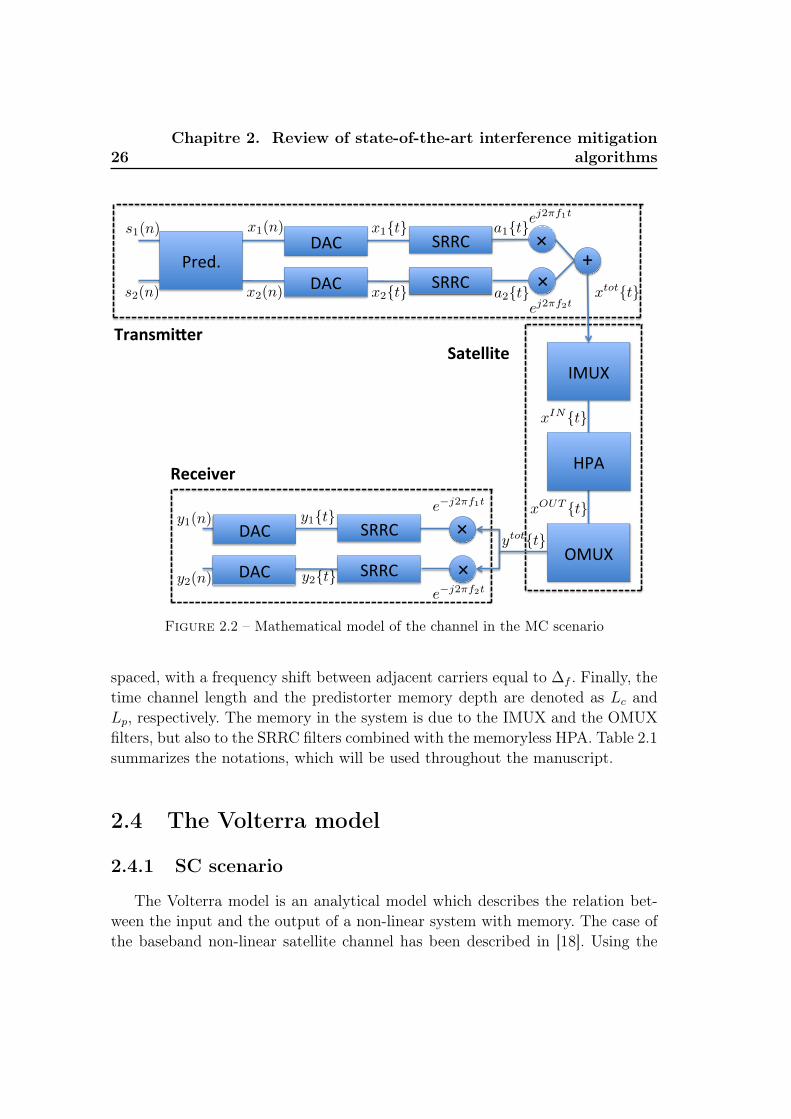
In the MC scenario, sc(n) represents the symbols of carrier c obtained af-ter modulation, and yc(n) the received samples of carrier c. Fig. 2.2 representsthe mathematical baseband model between sc(n), c = 1, 2, and yc(n) in theMC scenario, considering the case of two carriers for the sake of simplicity.We assume that the carriers are transmitted from the same physical hub, sothat joint predistortion of the symbols sc(n) can be performed, resulting inthe predistorted symbols xc(n). On each carrier, the predistorted symbols areanalog converted and SRRC filtered to produce the signals ac{t}. These signalsare frequency shifted, and the central frequency of each carrier is denoted asfc , with c = 1, 2 in this case. The signals are summed up and form the signalxtot{t}, which is sent towards the satellite. The signal obtained at the HPAinput after IMUX filtering is again denoted as xIN{t}. At the HPA output, thesignal xOUT{t} is filtered with the OMUX filter. The received signal on carrier cyc{t} is recovered after a frequency shift and SRRC filtering of the signal at thereceiver input ytot{t}. The received samples yc(n) are obtained by sampling thereceived signal yc{t}.
2.3 Notations
In addition to the notations introduced in the previous paragraph, we adoptthe following notations. The constellation size is equal to M , the symbol constel-lation points are denoted as ml for l = 1...M , and the corresponding centroidsof the received constellation are denoted as mrec
l , l = 1...M . The AWGN noisesamples are denoted as w(n), and the noise variance is equal to σn. In the MCscenario, C refers to the number of carriers. The carriers are assumed to be equally
26Chapitre 2. Review of state-of-the-art interference mitigation
algorithms
Pred. DAC SRRC
IMUX
HPA
OMUX
DAC SRRC
×
× +
x2{t}
x1{t}
xIN{t}
xOUT {t}
x1(n)
x2(n)s2(n)
s1(n)ej2πf1t
ej2πf2t
DAC SRRC
DAC SRRC
×
× e−j2πf2t
e−j2πf1t
y1{t}
y2{t}
y1(n)
y2(n)
Receiver
Transmi-er Satellite
xtot{t}
ytot{t}
a1{t}
a2{t}
Figure 2.2 – Mathematical model of the channel in the MC scenario
spaced, with a frequency shift between adjacent carriers equal to ∆f . Finally, thetime channel length and the predistorter memory depth are denoted as Lc andLp, respectively. The memory in the system is due to the IMUX and the OMUXfilters, but also to the SRRC filters combined with the memoryless HPA. Table 2.1summarizes the notations, which will be used throughout the manuscript.
2.4 The Volterra model
2.4.1 SC scenario
The Volterra model is an analytical model which describes the relation bet-ween the input and the output of a non-linear system with memory. The case ofthe baseband non-linear satellite channel has been described in [18]. Using the

2.4. The Volterra model 27
M Constellation size
ml Constellation symbol l
mrecl Centroid l of the received constellation (SC only)
C Number of carriers
fc Central frequency of carrier c
∆f Frequency shift between adjacent carriers
s(n) Symbol n after modulation (SC)
sc(n) Symbol n of carrier c after modulation (MC)
x(n) Symbol n actually transmitted on the channel (SC)
xc(n) Transmitted symbol n of carrier c (MC)
y(n) Received symbol n (SC)
yc(n) Received symbol n of carrier c (MC)
w(n) Noise sample n
σn Noise variance
Lc Time channel length
Lp Predistorter memory depth
Table 2.1 – Main notations
notations defined in Fig. 2.1 and 2.2, the following relations hold :
xIN{t} =∞∑
n=−∞
x(n)f1{t− nTs} (2.1)
xOUT{t} =∞∑m=0
γ2m+1(xIN{t})m+1(xIN{t}∗)m, (2.2)
y{t} =
∫ ∞τ=−∞
f2{τ}xOUT{t− τ}δτ. (2.3)
where γ2m+1 is a set of complex coefficients depending on the AM-AM and AM-PM characteristics of the HPA, and Ts is equal to the inverse of the symbol rateRs. The absence of even terms can easily be explained from the bandpass propertyof the non-linearity. The received signal y{t} is sampled every Ts to produce the

28Chapitre 2. Review of state-of-the-art interference mitigation
algorithms
received samples y(n). Combining (2.1), (2.2) and (2.3), the relation between thetransmitted symbols x(n) and the received samples y(n) takes the form :
y(n) =∞∑m=0
∑n1...n2m+1∈N
H2m+1(n1...n2m+1)[x(n− n1)x(n− n2)...x(n− nm+1)
x∗(n− nm+2)...x∗(n− n2m+1)] + w(n).
(2.4)
where H2m+1(n1...n2m+1) are called the Volterra coefficients of the system, andare mathematically expressed as :
H2m+1(n1...n2m+1) = γ2m+1
∫ ∞τ=−∞
f2{τ}m+1∏r=1
f1{nrTs − τ}m+1∏r=1
f1{nrTs − τ}∗
(2.5)
The first sum in (2.4) represents the different orders of the non-linearity inducedby the power amplifier. The second set of sums represents the memory of thesystem, which is theoretically infinite. In practice however, the channel can rea-sonably be assumed to be of finite length. We denote the causal memory of thechannel as L1 and the anti-causal memory of the channel as L2. The total channellength is denoted as Lc = L1 + L2 + 1. The number of Volterra coefficients oforder 2m+ 1 is then equal to L2m+1
c .
2.4.2 MC scenario
Since we consider equally spaced carriers, with frequency shift ∆f , the centerfrequency of each carrier fc can be mathematically expressed as a function of thenumber of carriers C and ∆f :
fc = (c− C + 1
2)∆f , (2.6)
The frequency occupancy of the carriers lie in the interval [−C+12
∆fC+1
2∆f ].
In the following, we will consider that the cutting frequency of the IMUX andOMUX filters are larger than C+1
2∆f and we consider here that xIN{t} = xtot{t}.
We can therefore express xIN{t} as :
xIN{t} =C∑c=1
ej(2πfct)ac{t} (2.7)

2.4. The Volterra model 29
The signal at the HPA output is again given by (2.2). We first focus on a third-order HPA, so that the HPA output is given by :
xOUT{t} = γ3
C∑c1=1
C∑c2=1
C∑c3=1
ej2π(fc1+fc2−fc3 )tac1{t}ac2{t}ac3{t}∗ (2.8)
Two important elements have to be derived from (2.8). Firstly, the non-linear HPAmixes the signals from the different carriers. It can be shown that the receivedsamples are now expressed as [19] :
yc(n) =∑
c1...c2m+1∈[1...C]
∞∑m=0
∑n1...n2m+1
Hc,c1...c2m+1
2m+1 (n1...n2m+1)
[xc1(n− n1)x(n− n2)...xc2m+1(n− nm+1)x∗(n− nm+2)...x∗(n− n2m+1)] + w(n).
(2.9)
Each received sample depends thus on the transmitted symbols of each car-rier. A second conclusion that can be drawn from (2.8) is that each combina-tion c1, c2, c3 produces interference terms which do not affect all carriers. It canbe easily verified that the term ac1{t}ac2{t}ac3{t}∗ has the same spectral oc-cupancy than g{t}3, g{t} being the impulse response of the SRRC filter. Sinceg{t} is band limited, g{t}3 is also band limited, as shown in Fig. 2.3. Therefore,the term ej2π(fc1+fc2−fc3 )tac1{t}ac2{t}ac3{t}∗ mostly impact the carrier with cen-tral frequency fc = fc1 + fc2 − fc3 and then the carriers with central frequencyfc = fc1 + fc2 − fc3 ± ∆f . It can be noticed that the non-linear interference de-pending only on one carrier (fc1 = fc2 = fc3) impacts the most the carrier itself(fc = f1). Some combinations fc1 , fc2 and fc3 create out-of-band interference, asfor instance for fc1 = fc2 = −fc3 . As already introduced in Chapter 1, this inter-ference is known as spectral regrowth and is removed by the OMUX filter.The same reasoning can be applied to higher order terms. In Fig. 2.3, the spectraloccupancy of g{t}m is illustrated for different m. The fifth order terms are in theform ej2π(fc1+fc2+fc3−fc4−fc5 )tac1{t}ac2{t}ac3{t}ac4{t}∗ac5{t}∗ and the carrier withcentral frequency fc = fc1 + fc2 + fc3 − fc4 − fc5 is the most impacted by thecombination c1, c2, c3, c4, c5.

30Chapitre 2. Review of state-of-the-art interference mitigation
algorithms
−4 −3 −2 −1 0 1 2 3 40
0.2
0.4
0.6
0.8
1
Normalized Frequency (1=1Ts)
|F(g
{t}m
)|
m=1m=3m=5m=7
Figure 2.3 – Frequency response of SRRC filter multiplications
2.5 Normalization and Gaussian detection in anon-linear channel
In a memoryless channel, the channel is normalized at the receiver so that thereceived samples can be written as :
y(n) = x(n) + w(n) (2.10)
Gaussian detection allows for calculating a posteriori symbol probabilities asfollows :
Pr[s(n) = ml|y(n)] =1√
2πσ2noise
exp[−|y(n)−ml|22σ2
noise
], l = 1...M, (2.11)
where ml, l = 1...M denotes the constellation points and σ2noise is the noise va-
riance.

2.6. Review of existing predistortion algorithms in a non-linearchannel 31
In a non-linear channel with memory, the non-linear interference is consideredas Gaussian. However, the centroids of the received constellation, denoted asmrecl , l = 1...M , are not equal to the constellation points. An accurate memory-
less detection can be done as follows. The received samples are first normalized tohave a unitary power, and the centroids mrec
l , l = 1...M are calculated as follows :
mrecl , E[y(n)|s(n) = ml], l = 1...M. (2.12)
The detector calculates the a posteriori symbol probabilities as follows :
Pr[s(n) = ml|y(n)] =1√
2πσ2l
exp[−|y(n)−mrecl |2
2σ2l
], l = 1...M, (2.13)
The sum of the noise and interference variances, denoted as σ2l , depends on the
considered symbols and is calculated as follows :
σ2l = E[|y(n)−mrec
l |2|s(n) = ml] (2.14)
In fact, the interference power is larger when |ml| is high, as it can be seenfrom (2.4). We will assume that the receiver knows the exact values of the cen-troids and the associated variances.
2.6 Review of existing predistortion algorithms ina non-linear channel
2.6.1 Power amplifier linearization
Linearization is the modification of the input or output signal of the HPA toinvert its non-linear characteristics. In satellite communications, the linearizeroccurs thus onboard the satellite. Different linearization techniques exist and aretrade-offs between complexity, stability, signal bandwidth and robustness to poorPA model. Linearization based on predistortion [20], [21] is the modification ofthe input of the HPA without using feedback from the output of the HPA. Thisis in opposition to cartesian feedback [22], which uses feedback of the cartesiancoordinates of the baseband symbols. The envelope elimination and restorationmethod uses feedback of the envelope of the HPA output signal. The differencein envelope between the input and output signals drives the bias of the HPAto restore the initial envelope at the HPA output [23]. In feedforward lineariza-tion [23], the input signal is compared to an attenuated version of the output

32Chapitre 2. Review of state-of-the-art interference mitigation
algorithms
signal. The difference is supposed to be sufficiently small to be linearly amplifiedby another HPA to reproduce the exact distortion, which is then subtracted fromthe original amplifier output. Predistortion is generally preferred in microwaveand satellite communications because of its relative wide band and because itcan be built as a stand alone unit [24]. TWTA predistortion techniques using16QAM modulation has been investigated in [25]. The predistorter can also takememory effects of the HPA into account, as considered in [26] and [27] for instance.
The concept of linearization using a predistortion block is illustrated in
0 0.5 1 1.5 2 2.5 30
0.1
0.2
0.3
0.4
0.5
0.6
0.7
0.8
0.9
1
Input amplitude
Out
put a
mpl
itude
HPALinearizer (pred.)HPA+Linearizer
Figure 2.4 – Ideal linearization (predistortion)
Fig. 2.4, considering a memoryless HPA. In the ideal case, we should obtain :
– A linear relation between the predistorter input amplitude and the HPAoutput amplitude if the input amplitude is below the saturation point.

2.6. Review of existing predistortion algorithms in a non-linearchannel 33
– A HPA output amplitude equal to the maximum HPA amplitude if thepredistorter input amplitude is above the saturation point.
– A constant phase shift between the predistorter input and the HPA output.
It should be noticed that the system composed of the ideal predistorter and theHPA is still a non-linear (memoryless) system. Non-linear interference is still crea-ted due to the combination with linear filters. The TWTA proposed in the DVB-S2 standard is not perfectly linearized, but even if this was the case, non-linearinterference still remains due to the saturation of the linearized HPA. Compen-sation algorithms at the transmitter or receiver can still be used to improve thesystem performance.
2.6.2 Signal predistortion versus data predistortion
Signal predistortion is the modification of the signal at the transmitter afterthe pulse shaping filter, while data predistortion is the modification of the trans-mitted symbols, occurring thus before the shaping filter [9]. In almost all cases,signal predistortion is not feasible in satellite communications, because it createsillegal out-of-band emissions. In terrestrial communications, signal predistortioncan be used to remove out-of-band emissions of the transmitter non-linear PA,as in [28] and [29]. In the literature, data/signal predistortion is generally des-cribed as one of the linearization techniques to compensate for the transmitternon-linear PA in terrestrial communications. In satellite communications, lineari-zation is the term used for the modification of the signal at the input of the satel-lite HPA and (data) predistortion refers to the signal processing at the hub. Forthe sake of completeness, it should be noticed that predistortion techniques canalso be divided into adaptive/non adaptive, analog/digital and baseband/IF/RFmethods [30]. Data predistortion is by definition a digital algorithm that is im-plemented in baseband, while signal predistortion can be both digitally or analogimplemented.
2.6.3 Digital predistortion algorithms for non-linear chan-nels with memory
Digital algorithms for signal and data predistortion of non-linear channelswith memory are very similar. Therefore, a general literature review on digital

34Chapitre 2. Review of state-of-the-art interference mitigation
algorithms
predistortion algorithms is proposed. The SC case is first considered, andextension of the algorithms to the MC case is discussed in next subsection.Exact inversion algorithms of non-linear systems have been studied in [31], [32]and [33]. These algorithms converge in very specific cases, since not all non-linearsystems do have an exact inverse. Schetzen introduced therefore the concept oforder p inverse [34], [35]. The idea is to remove the nonlinearities of the channelup to order p. Higher-order terms are however created, so that the algorithm isable to converge for p→∞ only for a finite range of input amplitude values [36].The order-p inverse has been applied to the satellite channel in [18].
The predistorter can also be built on a Volterra structure. The coefficientsof the predistorter are found using least-squares-type algorithms, so thatadaptive implementation can be easily made. To reduce the complexity ofsuch predistorters, reduced Volterra models are generally considered. Differenttechniques are detailed in [27] and references therein. The predistorters basedon a Volterra model are generally divided into two categories. Algorithms basedon direct learning architectures directly produce the predistorter coefficients,as in [37] and [38]. In the indirect learning architecture, the coefficients of aVolterra based equalizer are first calculated. The predistortion coefficients arethen obtained by simply copying the equalizer coefficients, as done in [39], [40].This architecture relies on the property that order p predistorters and equalizersare equal, as shown in [35] and [41]. There are two drawbacks that affect the per-formance of indirect learning methods [38]. Firstly, noise measurement producesbias in the estimation of the predistortion coefficients. Secondly, it is not correctto assume that the coefficients of the predistorter minimizing the MSE and thecoefficients of the equalizer minimizing the MSE are equal. In fact, it has only beproven that these coefficients are equal in the case where they perfectly inversethe non-linear system. There is therefore an inherent performance loss associatedto the architecture. The problem of the noise measurement has been addressedin [42], but the system performance becomes very sensitive to the quality of thesystem identification. Direct learning methods exhibit better performance, at thecost of slower convergence, higher complexity and more complicated structures.This issues have been addressed in [38].
Predistorters can also be constructed on neural networks (NN). The multi-layerperceptron is of the most popular neural network architecture in digital com-munications [9], and has been applied to the predistortion of power amplifiers

2.6. Review of existing predistortion algorithms in a non-linearchannel 35
in [43] and to the predistortion of SSPA in [44]. NN predistortion can also relyon local basis functions networks, as in [45]. The NN based on the generalizedcerebellar model articulation controller has been investigated in [46] for signaland data predistortion in GSM and UMTS systems. as in [47] and [48].
Another structure of interest relies on a look-up table (LUT). In [49], thevalue of each pre-distorted symbol is a function of the neighboring initial sym-bols, which can be calculated offline and stored in a LUT. The pre-computationof these values aims at minimizing the MSE between the initial and the receivedsamples. The performance of this algorithm has been assessed for high-ordermodulations in [10].
2.6.4 Mathematical description of the main digital predis-tortion algorithms
In this section, we detail some data predistortion algorithms proposed in theliterature, which will be used as benchmark in the following chapters. Predis-tortion algorithms based on NN are not considered. The NN techniques achievelower or equal performance compared to the LUT, at the cost of an increasedcomplexity [9].
2.6.4.1 Data predistortion based on the order p compensation
The order p compensation removes all interference terms up to order p. Tokeep the notations simple, we assume that there is no linear interference. Thegeneral case is described in [18]. In the SC scenario, the received samples aregiven by :
y(n) = x(n) + θ[x(n)] (2.15)
where x(n) , [x(n− L1), ..., x(n+ L2)] and θ[x(n)] is a non-linear function withLc complex inputs, and containing only third order or higher order terms. Theorder p compensation defines the pre-distorted symbols x(n) recursively :
x1(n) = s(n)
xi(n) = s(n)− θ[xi−2(n)] i = 3, 5...p
x(n) = xp(n), (2.16)

36Chapitre 2. Review of state-of-the-art interference mitigation
algorithms
i denoting the iteration number of the algorithm and xi−2(n) ,[xi−2(n − L1), ..., xi−2(n + L2)]. Even iteration numbers do not have to becalculated since the channel introduces only odd order non-linearities. It shouldalso be noticed that the pre-distorter block needs a perfect knowledge of thechannel.
In Appendix 2.A, it is shown that transmitting xp(n) instead of s(n) re-moves all interference terms up to order p between s(n) and y(n). However,the algorithm creates higher-order terms, and it has been observed that theorder p compensation algorithm results in poor performance in case of channelswith large memory and/or high non-linearities. In chapter 4, a modificationof the algorithm will be proposed in order to achieve better performance. Theextension of the algorithm to the multi-carrier case has not been considered inthe literature and will also be treated in Chapter 4.
2.6.4.2 Data predistortion using a Volterra model
Another approach is to build the pre-distorter as a Volterra structure. In theSC case, the pre-distorted symbols are given by :
x(n) =∞∑m=0
∑n1...n2m+1∈N
P2m+1(n1...n2m+1)[s(n− n1)x(n− n2)...s(n− nm+1)
s∗(n− nm+2)...s∗(n− n2m+1)]. (2.17)
The coefficients P2m+1(n1...n2m+1) are the Volterra coefficients of the pre-distorter. The number of predistortion coefficients is theoretically infinite, sincethe channel has a finite length (and possibly a infinite non-linearity order). Inpractice, the considered number of Volterra coefficients is limited by truncatingthe pre-distorter length and order. This truncation obviously impacts the bestachievable performance. The number of coefficients is then a trade-off betweencomplexity and performance.
The Volterra coefficients of the pre-distorter are chosen so as to minimizethe MSE between the initial and the received samples. This predistortionalgorithm can easily be extended to the MC case, where each pre-distortedsymbol is given by a Volterra model similar to (2.9). However, the number ofcoefficients exponentially increases with the number of carriers, so that muchsmaller pre-distorter lengths have to be considered compared to the SC case.

2.7. Literature review of receiver compensation algorithms in anon-linear channel 37
Predistortion based on a Volterra model in a MC scenario has been investigatedin [50] and [51].
2.6.4.3 Data predistortion using a look-up table
A third approach relies on the use of a look-up table (LUT). The pre-distortedvalue x(n) is a function of the neighboring un-pre-distorted symbols. In the SCscenario, the pre-distorted symbol can be written as
x(n) = FLUT [s(n− Lp1), ..., s(n+ Lp2)]. (2.18)
There are M1+Lp1+Lp2 possible values for x(n), which can all be stored in alook-up table at the transmitter. The main advantage of this approach is its lowcomplexity. The pre-distorted values are calculated offline so that no operationhas to be performed real-time. Moreover, the pre-distorted function is not limitedin order, unlike the pre-distorter based on a Volterra model. The drawback ofthis method is that the number of entries that need to be stored is equal toM1+Lp1+Lp2 , so that it exponentially increases with the pre-distorter length andthe modulation order. Considering large modulation order, a small pre-distorterlength has to be considered. This also results in performance loss considering alarge channel length and large modulation orders.
The M1+Lp1+Lp2 possible values of the function FLUT (·) are determinedusing an LMS algorithm which minimizes E[|y(n) − s(n)|2]. Here again, thealgorithm can easily be extended to the MC case. However, the number of entriesis then equal to MC(1+Lp1+Lp2 ), so that the number of entries quickly becomesimpractical.
2.7 Literature review of receiver compensation al-gorithms in a non-linear channel
In this work, the focus is set on predistortion algorithms. As explainedin Chapter 1, this allows relaxing the computational load at the receivers.Moreover, in MC scenarios, the different carriers are not always transmittedtowards the same geographical locations. Most of the above predistortionalgorithms can be applied at the receiver, but this will not be discussed here.However, we would like to draw the attention of the reader to two specific points :

38Chapitre 2. Review of state-of-the-art interference mitigation
algorithms
– Optimal algorithms such as the BCJR algorithm [52] and the Viterbialgorithm [53] are perfectly defined even for non-linear channels. They canbe expected to achieve better performance compared to the above SoApredistortion algorithms. However, such algorithms cannot be used whenconsidering large modulation orders and channel lengths because of theirlarge computational complexity. For each symbol, these methods requireto estimate the channel output for several input combinations. Since thereare MCLc possible input combinations, they usually can not be stored in aLUT. The calculation of these channel outputs is also not possible in realtime, since there is no easy relation between one input combination andthe resulting channel output.
– Joint compensation at the transmitter and receiver sides will be consideredin Chapter 6. The idea is to further improve the power efficiency of systemsusing predistortion algorithms, at the cost of additional complexity at thereceiver.
2.8 Conclusion
In this chapter, we first introduced the Volterra model, which is a mathema-tical tool to represent a non-linear system with memory. We have detailed themost common predistortion algorithms and we have discussed their limitations incase of large channel lengths and high modulation orders. In the next chapter, wewill discuss a new predistortion algorithm, which allows considering much largerpre-distorter lengths compared to SoA algorithms.
2.A Proof of the order p compensation algorithm
We now show that transmitting xp(n) instead of s(n) removes all interferenceterms up to order p between s(n) and y(n). The received samples can be expressedas :
y(n) = s(n)− θ[xp−2(n)] + θ[xp(n)] (2.19)
The bold operator θ[x(n)] can be seen as a vector of functions with elementsθ[x(n−L1)]...θ[x(n+L2)]. It takes as input the elements [x(n−2L1)...x(n+2L2)],

2.A. Proof of the order p compensation algorithm 39
which are also denoted as x(n) to simplify the notations. The terms θ[xp−2(n)]
and θ[xp(n)] can further be developed, using (2.16). For instance, we have :
θ[x1(n)] = θ[s(n)]
θ[x3(n)] = θ{s(n)− θ[s(n)]}θ[x5(n)] = θ
{s(n)− θ{s(n)− θ[s(n)]}
}... (2.20)
It can be seen from (2.20) that each θ[xp(n)] can be obtained from θ[xp−2(n)]
by replacing the colored s(n) by s(n)− θ[s(n)]. It can be verified that this thirdorder variation −θ[s(n)] is nested into (p−1
2) θ operator. Since each θ operator is
at least of order 3, this variation creates terms which are of order p+ 2 or higher.This proves that the difference −θ[xp−2(n)] + θ[xp(n)] in (2.19) contains terms oforder p+ 2 or higher.


Chapitre 3
Per-block iterative predistortionalgorithm
Contents3.1 Introduction . . . . . . . . . . . . . . . . . . . . . . . . . . 413.2 Notations . . . . . . . . . . . . . . . . . . . . . . . . . . . . 423.3 Small-variation algorithm in the SC scenario . . . . . . . 43
3.3.1 Per block iterative predistortion . . . . . . . . . . . . . . . . 433.3.2 Small-variation algorithm . . . . . . . . . . . . . . . . . . . 453.3.3 Linearity assumption . . . . . . . . . . . . . . . . . . . . . . 473.3.4 Calculation of the linear coefficients based on channel si-
mulations . . . . . . . . . . . . . . . . . . . . . . . . . . . . 483.3.5 Linear filtering . . . . . . . . . . . . . . . . . . . . . . . . . 48
3.4 Small-variation algorithm in the MC scenario . . . . . . 493.5 Numerical results . . . . . . . . . . . . . . . . . . . . . . . 50
3.5.1 SVA in the SC scenario . . . . . . . . . . . . . . . . . . . . 503.5.2 SVA in the MC scenario . . . . . . . . . . . . . . . . . . . . 55
3.6 Summary . . . . . . . . . . . . . . . . . . . . . . . . . . . . 593.A Calculation of the coefficients Ank,j(m1,m2) for some
simple Volterra models . . . . . . . . . . . . . . . . . . . . 593.B Proof of (3.18) . . . . . . . . . . . . . . . . . . . . . . . . . 603.C Channel simulation with constant Volterra coefficients . 61
3.1 Introduction
In this chapter, we propose a new predistortion algorithm, which can be bothused in single- or multi-carrier-per-channel (SC or MC) scenarios. We will refer tothis algorithm as the small-variation algorithm (SVA). The SVA can be seen as

42 Chapitre 3. Per-block iterative predistortion algorithm
a pre-distorter of infinite order and finite length. Very large pre-distorter lengthscan be considered because the algorithm complexity computed per symbol isindependent of this parameter. Improved performance is therefore expectedcompared to state-of-the-art predistortion methods presented in Chapter 2. Theproposed scheme independently pre-distorts successive symbol blocks, assumingthat the channel is perfectly known by the transmitter. To pre-distort each blockof symbols, an iterative algorithm is used, aiming at minimizing the Euclidiandistance between the initial symbol and the received sample sequence. Thechapter is divided as follows :
– Section 3.2 gives the notations specific to the SVA.– Section 3.3 describes the SVA for the SC case.– Section 3.4 describes the SVA for the MC case.– Section 3.5 compares the performance achieved with the SVA with the per-
formance of two SoA algorithms.– Section 3.6 concludes this chapter.
We refer to Chapter 1 for the description of the system model.
3.2 Notations
For a given block, we denote by sc the vector composed of the block of symbolstransmitted on carrier c : sc = [sc(1)...sc(N)]. For each symbol block of eachcarrier, the pre-distorter produces a modified symbol block of length N , denotedby the vector xc = [xc(1)...xc(N)]. At the receiver, N samples are also gatheredin a vector of size N , denoted by yc = [yc(1)...yc(N)]. In addition, we denoteby yc(x1,x2...xC) the vector yc of the received samples on carrier c when theblock x1...xC is sent at the channel input. We consider that no compensationalgorithms are further applied at the receiver side, and that only memorylessdetection is applied on consecutive received samples, as described in Section 2.5.This is why yc only consists in N samples. In the following paragraphs, it willbecome clear that N has to be taken as large as possible. However, N cannot betoo large to prevent high latency. In this work, we take N equal to the numberof symbols in the physical layer frame as defined in the DVB-S2 standard (a fewthousand symbols). Note that in the SC case, the carrier subscript c will not bespecified.

3.3. Small-variation algorithm in the SC scenario 43
3.3 Small-variation algorithm in the SC scenario
We first describe the SVA in the SC scenario. The small variation-algorithmtries to minimize the Euclidian distance between the initial symbols and recei-ved samples, i.e. ||y − s||2. The pre-distorter minimizes the Euclidian distanceassuming a noiseless channel. Since the AWGN is independent of the transmit-ted sequence, this also minimizes the MSE at the receiver in presence of AWGN.In Section 3.3.1, an intuitive but too complex approach is described in orderto minimize ||y − s||2. From there, the small-variation algorithm is derived inSection 3.3.2. It is based on a linear relation between the input and output va-riations, which may however not be met, so that Section 3.3.3 explains how tomodify the algorithm to overcome this limitation. The proposed algorithm mayalso not converge towards the global optimum. Linear filtering, detailed in para-graph 3.3.5, can improve the convergence of the algorithm.
3.3.1 Per block iterative predistortion
We describe here a first approach to determine the value of x so that||y(x) − s||2 is minimized. The term ||y(x) − s||2 can be developed using theVolterra model described in (2.4). However, there is no straightforward derivationof the block x. We therefore propose an iterative algorithm to determine thepre-distorted block x. Each iteration of the algorithm is divided into N steps,respectively focused on consecutive symbols of the block of interest. The pre-distorted block after Step j of Iteration k is denoted as xk,j = [xk,j(1)...xk,j(N)],where only the jth pre-distorted value is modified and is chosen to minimize||y − s||2 when xk,j is transmitted. All other pre-distorted values are thus keptequal to their values from the previous step. An iterative algorithm is herenecessary since the modification of symbol j at Step j can not take into accountthe future modification of symbols j + 1, j + 2, ..., N occurring in the followingsteps. Iterations are thus performed until no further performance improvementis noticed. They are other reasons why iterations are necessary, which will behighlighted later in the text.
For each iteration, xk,j(n) is mathematically expressed as follows. For the

44 Chapitre 3. Per-block iterative predistortion algorithm
first step (j = 1),
xk,1(n) =
xk−1,N(n), n 6= 1,
argminxk,1(1)
[||y − s||2∣∣∀i 6= 1 : x(i) = xk−1,N(i)], n = 1, (3.1)
and thereafter (j > 1),
xk,j(n) =
xk,j−1(n), n 6= j,
argminxk,j(j)
[||y − s||2∣∣∀i 6= j : x(i) = xk,j−1(i)], n = j. (3.2)
Note that xk,1(n) is calculated using the end values of the previous iteration,except for the first iteration where xk,1(n) is calculated using the un-pre-distortedvalues. The vector εk,j is defined as the difference between y and s when thesequence obtained after Step j of Iteration k is transmitted :
εk,j , y − s∣∣∀i : x(i) = xk,j(i). (3.3)
By definition of the algorithm, we have :
||εk,j||2 ≤ ||εk,j-1||2, (3.4)
so that the convergence of the proposed algorithm is ensured. The term ||y− s||2minimized in (3.2) can be seen as a non-linear function of the complex variablexk,j(n). The coefficients of this function can be found using the Volterra modeland depend on the fixed pre-distorted values in (3.2). Since the channel has finitelength, (3.2) can be simplified as :
xk,j(j) =argminxk,j(j)
[||y − s||2∣∣∀i 6= j : x(i) = xk,j−1(i)]
= argminxk,j(j)
[
min(N, j+L2)∑m=max(1, j−L1)
|y(m)− s(m)|2∣∣∀i 6= j : x(i) = xk,j−1(i)]. (3.5)
The complexity of the algorithm is very high since it is necessary to successivelyfind the minimum of N complex non-linear functions for each iteration. Moreover,the number of Volterra coefficients in each equation can be very high in thecase of high-order non-linearities. Therefore, the pre-distorted symbols definedin (3.1) are difficult to compute in practice. In the next subsection, we proposean algorithm of much lower complexity to compute the pre-distorted symbols.We refer to this algorithm as the small-variation algorithm.

3.3. Small-variation algorithm in the SC scenario 45
3.3.2 Small-variation algorithm
The small-variation algorithm has the same iterative structure as the algo-rithm presented in the previous subsection. However, at Step j of Iteration k, itcalculates a suboptimal value for xk,j(j) in a much less complex way. We firstdefine ∆k,j as :
xk,j(j) = xk,j−1(j) + ∆k,j (3.6)
Thus, the variation from xk,j−1(j) to xk,j(j) is considered as the unknown variableinstead of xk,j(j) itself. The case j = 1 is not explicitly given anymore in thefollowing derivations, as it is always similar to (3.1). The vector ∆k,j is definedas a zero vector of length N , except for the element j which is equal to ∆k,j, sothat :
xk,j = xk,j-1 + ∆k,j. (3.7)
We define the value ∆optk,j as the optimum value that minimizes (3.2) :
∆optk,j = argmin
∆k,j
[||y − s||2∣∣∀i 6= j : x(i) = xk,j−1(i), x(j) = xk,j−1(j) + ∆k,j] (3.8)
It is possible to simplify (3.8) as in (3.5), but we prefer to adopt the followingmore compact notation :
∆optk,j = argmin
∆k,j
[||y(xk,j-1 + ∆k,j)− s||2]. (3.9)
We define :
FNLk,j , y(xk,j-1 + ∆k,j)− y(xk,j-1) (3.10)
so that :
∆optk,j = argmin
∆k,j
[||y(xk,j-1)− s + FNLk,j ||2]
= argmin∆k,j
[||εk,j-1 + FNLk,j ||2]. (3.11)
Each element FNLk,j (n) represents the output n variation resulting from a variation
of the input symbol j at Step j during Iteration k. The vector FNLk,j can be seen as
a vector of functions depending on the scalar variable ∆k,j. Inspecting (2.4) and

46 Chapitre 3. Per-block iterative predistortion algorithm
(3.10), it can be mathematically computed that each element FNLk,j (n) takes the
form :
FNLk,j (n) =
{0, n < j − L2, n > j + L1,∑∞
m1=0
∑∞m2=0 A
nk,j(m1,m2)∆m1
k,j (∆∗k,j)
m2 , n ≥ j − L2, n ≤ j + L1,
(3.12)
where the coefficients Ank,j(m1,m2) depend on the Volterra coefficients and thesequence of pre-distorted symbols. For the sake of clarity, Appendix 3.A givessome examples for the coefficients Ank,j(m1,m2) in the case of simple Volterramodels consisting of only a single Volterra coefficient. In the general case ofa channel depending on several Volterra coefficients, the value of Ank,j(m1,m2)
can be obtained by first computing the value of Ank,j(m1,m2) corresponding toeach Volterra coefficient taken independently and then summing all the obtainedvalues.
The small-variation algorithm is based on the assumption that each func-tion FNL
k,j (n) can be approximated by keeping only its linear dependency on∆k,j :
FNLk,j (n) ≈ F Lin
k,j (n) , Ank,j(1, 0)∆k,j + Ank,j(0, 1)∆∗k,j. (3.13)
This will be more likely the case for small values of ∆k,j. Denoting FLink,j (∆k,j),
Ak,j(1, 0), and Ak,j(0, 1) the vectors obtained with elements F Link,j (n), Ank,j(1, 0)
and Ank,j(0, 1), with n varying from 1 to N , we have :
FNLk,j ≈ FLin
k,j , Ak,j(1, 0)∆k,j + Ak,j(0, 1)∆∗k,j (3.14)
Instead of calculating the value ∆optk,j from (3.9), the small-variation algorithm
calculates ∆Link,j defined as :
∆Link,j = argmin
∆k,j
[||εk,j−1 + FLink,j ||2] (3.15)
The objective function ||y(xk,j-1) − s + FNLk,j ||2 in (3.11) is approximated by a
second order equation, given by ||εk,j−1 + FLink,j ||2. Using partial derivatives, the
optimum value of ∆k,j that minimizes (3.15), can be found by solving a system oftwo linear equations with two unknowns (the real and imaginary parts of ∆k,j),which makes the calculation much easier than minimizing the exact non-linearequation. The main difficulty raised by the proposed algorithm is the complexityto assess the parameters Ak,j(m1,m2) as they depend on all Volterra coefficients.This issue will be address in Section 3.3.4.

3.3. Small-variation algorithm in the SC scenario 47
3.3.3 Linearity assumption
The variation ∆Link,j is computed based on the approximation (3.13), which
is only valid for small values of ∆Link,j . In practice, we consider that the applied
variation ∆appliedk,j has at least to decrease the Euclidian distance between the
initial and the received samples. Mathematically, this is expressed as :
(||εk,j−1 + FNLk,j ||2
∣∣∆k,j = ∆appliedk,j ) ≤ ||εk,j−1||2. (3.16)
Taking ∆appliedk,j = ∆Lin
k,j does not ensure that (3.16) is verified at each step sincethe linear assumption may not be met. Therefore, we consider instead that theapplied variation is given by :
∆appliedk,j = γ∆lin
k,j, (3.17)
where γ is a real number in the interval [0, 1]. It is proven in Appendix 3.Bthat γ∆lin
k,j is a sub-optimum solution of the second order approximation of theobjective function :
(||εk,j−1 + Flink,j||2
∣∣∆k,j = γ∆Link,j ) ≤ ||εk,j−1||2. (3.18)
It is always possible to define γ small enough to meet the linear approxima-tion (3.13), so that the sub-optimum solution of (3.15) becomes also a sub-optimum solution of (3.11), which means that ∆applied
k,j satisfies (3.16). The valueof γ could be optimized at each step of the algorithm. For instance, decreasingvalues of γ can be applied until (3.16) is true. However, the complexity of suchapproach is difficult to predict. In this work, we follow an approach similar to thetrust-region method described in [54], where the norm of the applied variation|∆applied
k,j | is limited to a pre-defined value ∆max. The value of γ is chosen so as tomake this statement true. Mathematically, γ is defined as follows :
γ =
{1, |∆lin
k,j| ≤ ∆max,
∆max|∆link,j|−1, |∆lin
k,j| > ∆max.(3.19)
If the so obtained γ and the resulting ∆appliedk,j does not meet (3.16), no variation
is applied at the given step. The value of ∆max is a trade-off between convergencespeed and maximum achievable performance, as shown in Chapter 5.

48 Chapitre 3. Per-block iterative predistortion algorithm
3.3.4 Calculation of the linear coefficients based on channelsimulations
The coefficients Ank,j(1, 0) and Ank,j(0, 1) can be estimated by the followingprocedure. At Step j of Iteration k, the channel outputs are calculated that resultfrom three different channel input variations :
1)∆k,j = 0 2)∆k,j = εr 3)∆k,j = εi (3.20)
where εr and εi are respectively small real and pure imaginary numbers. The res-pective channel outputs are denoted as y(n), yr(n) and yi(n). To ensure the conver-gence of the algorithm, the channel simulations are performed using constant Vol-terra coefficients, as detailed in Appendix 3.C. If εr and εi are chosen sufficientlysmall, there is a linear relation between the input and output variations :
yr(n) = y(n) + Ank,j(1, 0)εr + Ank,j(0, 1)εr
yi(n) = y(n) + Ank,j(1, 0)εi − Ank,j(0, 1)εi. (3.21)
For each n, (3.21) form a set of two equations with two unknowns, Ank,j(1, 0) andAnk,j(0, 1), so that they can easily be estimated. Only Lc sets of equations needto be solved due to the finite channel length assumption. The smaller εr and εi,the more accurate the calculation. This method still has a high complexity sincethree simulations of the channel are required at each step of each iteration.To simulate the channel, the predistortion block needs to oversample the signalby several times the symbol rate in order to avoid spectral aliasing from the non-linear interference. For channels with large memory, the channel simulations canrequire a high complexity. In the next chapter, we describe methods to obtainapproximations of the coefficients Ank,j(1, 0) and Ank,j(0, 1) with a lower complexity.
3.3.5 Linear filtering
Besides the iterative predistortion algorithm, a linear filter is applied to thetransmitted signal to invert the linear channel memory, which is due to the IMUXand OMUX filters. The linear filtering is applied after the predistortion algorithm,so that it can considered as part of the channel by the predistorter. Intuitivelythis improves the convergence of the predistortion algorithm because the optimumvalues of the pre-distorted symbols are closer to the values of the un-predistortedsymbols. Note that this filter could alternatively be applied at the receiver. Thiswould keep the peak-to-average power ratio (PAPR) lower at the transmitter

3.4. Small-variation algorithm in the MC scenario 49
and limit the induced higher-order terms (see [18]). However, this would alsoamplify the noise on the channel deeps. In this work, we stick to the transmitteralternative.
3.4 Small-variation algorithm in the MC scenario
In this Section, we extend the SVA to the MC scenario, where the objectivefunction of the predistorter is defined as
∑c ||yc − sc||2. As in the SC scenario,
the SVA consists in several iterations, which are divided into N steps. At eachstep, the value of all predistorted symbols with time index n are modified. Twostrategies will be investigated to calculate the C new predistorted values.
Firstly, each step of the algorithm can be divided into C substeps. At Ite-ration k, Step j and Substep c, only the symbol j of carrier c is modifiedwith a variation ∆k,j,c. This approach is very similar to the SC case. Thevariation FNL
k,j,c(n, c1) of symbol n on carrier c1 due to the variation ∆k,j,c can beapproximated as follows :
FNLk,j,c(n, c1) ≈ F Lin
k,j,c(n, c1) , An,c1k,j,c(1, 0)∆k,j,c + An,c1k,j,c(0, 1)∆∗k,j,c, (3.22)
where An,c1k,j,c(1, 0) and An,c1k,j,c(0, 1) are complex coefficients, similarly to Equa-tion (3.13). In (3.22), the subscripts k, j, c are kept together since they specifythe iteration, step and substep of the algorithm while subscripts n, c1 are kepttogether since they refer to the considered output symbol. At a given substep,LcC non-zero values of An,c1k,j,c(1, 0) and An,c1k,j,c(0, 1) have to be determined. Theoptimal value of ∆k,j,c is found similarly to (3.15) :
∆Link,j,c = argmin
∆k,j,c
[||εk,j,c−1
+ FLin
k,j,c||2]. (3.23)
The terms εk,j,c−1
and FLin
k,j,care now matrices, with N and C columns, corres-
ponding to the different symbols and the different carriers, respectively.
A second approach is to jointly optimize the symbol j on every carrier.At Iteration k of Step j, C complex unknowns are determined ∆k,j,c for c = 1...C.The variation of one output is now approximated as a linear combination of thedifferent input variations :
FNLk,j (n, c1) ≈ F Lin
k,j (n, c1) ,∑c
[An,c1k,j,c(1, 0)∆k,j,c + An,c1k,j,c(0, 1)∆∗k,j,c]. (3.24)

50 Chapitre 3. Per-block iterative predistortion algorithm
Injecting (3.24) in (3.23) results in a second-order equation with 2C real unk-nowns. Using partial derivatives, a system of 2C equations with 2C unknownsneed to be solved, requiring the inversion of a 2C × 2C matrix. To force thelinearity assumption, each variation can be multiplied by a factor γ so that∑
j |∆k,j,c|2 < γ. The proof that the so obtained variations are a sub-optimum so-lution of the second-order approximations is similar to the one given in Appendix3.B.
3.5 Numerical results
3.5.1 SVA in the SC scenario
−1.5 −1 −0.5 0 0.5 1 1.5−1.5
−1
−0.5
0
0.5
1
1.5
ℜ
ℑ
Received symbolsSymbol constellationCentroids of the received samples
Figure 3.1 – Received constellation after predistortion, 36Mbaud, α = 0.1, 2.1dBOBO
The system model has been described in Chapter 1. In the SC scenario, 32-APSK symbols are considered with a code rate equal to 4/5. As discussed in

3.5. Numerical results 51
Section 3.2, N is equal to the number of symbols in a PLFRAME of the DVB-S2standard, which is equal to 12960 for the case of 32-APSK modulation.Fig. 3.1 illustrates the noiseless received samples after predistortion and powernormalization, considering a symbol rate equal to 36Mbaud, a roll-off factor equalto 0.1 and an OBO equal to 2.1dB. The received samples have to be comparedwith Fig. 1.14, when no predistortion is made. The centroids of the receivedsamples are now almost equal to the symbol constellation and the ISI has stron-gly decreased.Fig. 3.2 illustrates the MSE between the initial and the received samples aftereach iteration of the small-variation algorithm for different values of ∆max, withor without a linear zero-forcing filter placed at the transmitter side. Other filtertypes, such as the (unbiased) Wiener filter, could be considered if the filter isplaced at the receiver side. The symbol rate is equal to 36Mbaud and the roll-offfactor is equal to 0.1. A better optimum is reached when a linear zero-forcingfilter is used so that it will always be considered in the following results. The li-near zero-forcing filter is placed at the transmitter. At each step of the algorithm,it is checked that the variation ∆applied
k,j decreases the square error so that thealgorithm always converges at least to a local optimum. It can be observed thatthe value ∆max has no impact on the value of the local optimum but controls theconvergence speed of the algorithm. Too small values of ∆max obviously decreasethe convergence speed of the algorithm, while too large values of ∆max increasethe number of steps where no variation is applied, so that the convergence speedalso decreases.Two SoA algorithms, detailed in Section 2.6.4, are considered in the followingfigures. The first algorithm is based on memory polynomials, where the pre-distorter is a reduced Volterra system described in [27]. Third order Volterracoefficients and a pre-distorter length Lp = 9 have been considered. The identifi-cation of the pre-distorter coefficients is based on the indirect learning architec-ture (see Section 2.6.2), and is locally performed at the transmitter, since it isassumed to have perfect knowledge of the channel.The second algorithm is theone proposed in [10], where the value of each pre-distorted symbol is a functionof the neighboring un-pre-distorted symbols. All possible combinations are pre-computed offline and stored in a look-up table. A pre-distorter memory depthLp = 3 is considered so that 323 entries are stored in the look-up table. Amongall pre-distortion methods, this approach has the lowest real-time complexity,since only one memory access per symbol needs to be performed.Performance comparison will also be made with an ideal linearizer onboard the

52 Chapitre 3. Per-block iterative predistortion algorithm
0 2 4 6 8 10 12 14 16 18 20−22
−20
−18
−16
−14
−12
−10
Number of iterations
MSE
(dB)
Δmax=0.05, No linear equalizer
Δmax=0.30, No linear equalizer
Δmax=1.00, No linear equalizer
Δmax=0.05, Linear equalizer
Δmax=0.30, Linear equalizer
Δmax=1.00, Linear equalizer
Figure 3.2 – Mean-square error (MSE) after each iteration of the SVA, 36Mbaud,α = 0.1, 3dB IBO
13 13.5 14 14.5 15 15.5 16 16.5 17 17.5 1810−7
10−6
10−5
10−4
10−3
10−2
10−1
SNR
BER
AWGN channelSmall−variation algorithmSOA based on LUT entriesSOA Memory polynomials
Figure 3.3 – BER performance using the SVA and state-of-the-art pre-distortionmethods, 36Mbaud, α = 0.1, 2.1dB OBO
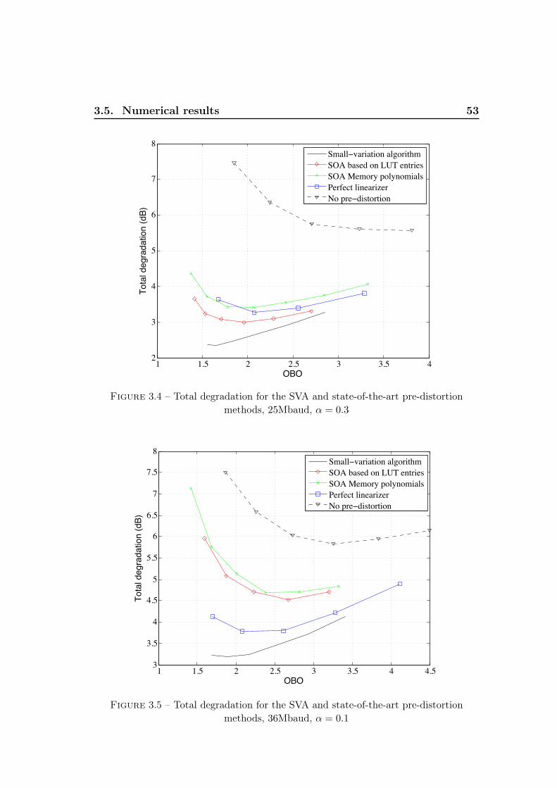
3.5. Numerical results 53
1 1.5 2 2.5 3 3.5 42
3
4
5
6
7
8
OBO
Tota
l deg
rada
tion
(dB)
Small−variation algorithmSOA based on LUT entriesSOA Memory polynomialsPerfect linearizerNo pre−distortion
Figure 3.4 – Total degradation for the SVA and state-of-the-art pre-distortionmethods, 25Mbaud, α = 0.3
1 1.5 2 2.5 3 3.5 4 4.53
3.5
4
4.5
5
5.5
6
6.5
7
7.5
8
OBO
Tota
l deg
rada
tion
(dB)
Small−variation algorithmSOA based on LUT entriesSOA Memory polynomialsPerfect linearizerNo pre−distortion
Figure 3.5 – Total degradation for the SVA and state-of-the-art pre-distortionmethods, 36Mbaud, α = 0.1
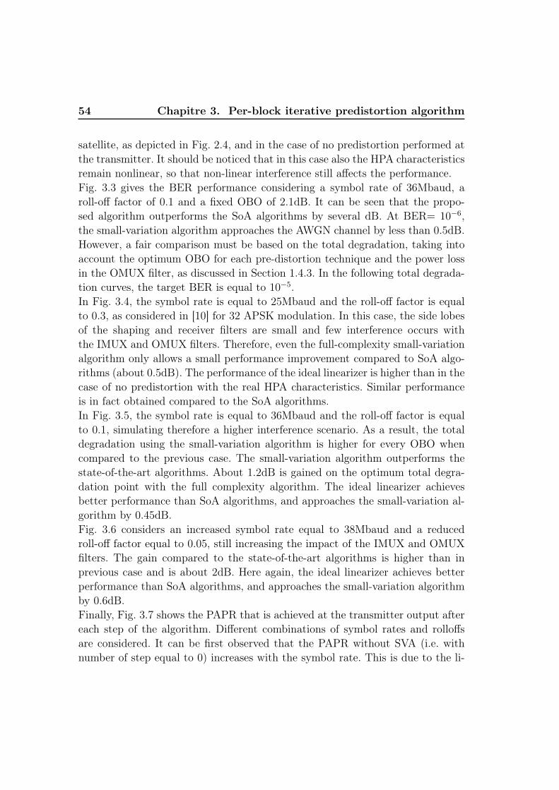
54 Chapitre 3. Per-block iterative predistortion algorithm
satellite, as depicted in Fig. 2.4, and in the case of no predistortion performed atthe transmitter. It should be noticed that in this case also the HPA characteristicsremain nonlinear, so that non-linear interference still affects the performance.Fig. 3.3 gives the BER performance considering a symbol rate of 36Mbaud, aroll-off factor of 0.1 and a fixed OBO of 2.1dB. It can be seen that the propo-sed algorithm outperforms the SoA algorithms by several dB. At BER= 10−6,the small-variation algorithm approaches the AWGN channel by less than 0.5dB.However, a fair comparison must be based on the total degradation, taking intoaccount the optimum OBO for each pre-distortion technique and the power lossin the OMUX filter, as discussed in Section 1.4.3. In the following total degrada-tion curves, the target BER is equal to 10−5.In Fig. 3.4, the symbol rate is equal to 25Mbaud and the roll-off factor is equalto 0.3, as considered in [10] for 32 APSK modulation. In this case, the side lobesof the shaping and receiver filters are small and few interference occurs withthe IMUX and OMUX filters. Therefore, even the full-complexity small-variationalgorithm only allows a small performance improvement compared to SoA algo-rithms (about 0.5dB). The performance of the ideal linearizer is higher than in thecase of no predistortion with the real HPA characteristics. Similar performanceis in fact obtained compared to the SoA algorithms.In Fig. 3.5, the symbol rate is equal to 36Mbaud and the roll-off factor is equalto 0.1, simulating therefore a higher interference scenario. As a result, the totaldegradation using the small-variation algorithm is higher for every OBO whencompared to the previous case. The small-variation algorithm outperforms thestate-of-the-art algorithms. About 1.2dB is gained on the optimum total degra-dation point with the full complexity algorithm. The ideal linearizer achievesbetter performance than SoA algorithms, and approaches the small-variation al-gorithm by 0.45dB.Fig. 3.6 considers an increased symbol rate equal to 38Mbaud and a reducedroll-off factor equal to 0.05, still increasing the impact of the IMUX and OMUXfilters. The gain compared to the state-of-the-art algorithms is higher than inprevious case and is about 2dB. Here again, the ideal linearizer achieves betterperformance than SoA algorithms, and approaches the small-variation algorithmby 0.6dB.Finally, Fig. 3.7 shows the PAPR that is achieved at the transmitter output aftereach step of the algorithm. Different combinations of symbol rates and rolloffsare considered. It can be first observed that the PAPR without SVA (i.e. withnumber of step equal to 0) increases with the symbol rate. This is due to the li-

3.5. Numerical results 55
near compensation placed at the transmitter side. It can also be noticed that thePAPR increases until convergence of the algorithm. In the worst case (38Mbaud,α = 0.05), the PAPR increase is about 3.5dB. Even if it is not considered asan issue in this work, it should be keep in mind that the power amplifier at thetransmitter has to be driven further from saturation to keep a linear behavior incase of predistortion.
3.5.2 SVA in the MC scenario
A three carrier multiplex is considered, with adjacent carriers. The symbolsare 16APSK symbols and the roll-off factor is equal to 0.2. A larger number ofcarriers will be considered in next chapter, using lower complexity predistortionalgorithms. The impact of the IMUX/OMUX filters is here neglected. Since theHPA produces out-of-band distortions, we implicitly assume that the OMUX fil-ter has a much larger bandwidth than the signal transmitted from the hub, so thatthe out-of-band emissions are filtered out by the receiver filter only. In practicalcases, this assumption is not realistic and the OMUX filter will always removesome out-of-band distortions, but both approaches are equivalent from a mathe-matical point of view. The numerical results become on this way independent ofthe considered IMUX/OMUX filters and of the symbol rate, limiting thereforethe number of cases to be simulated and allowing better reproductibility. Thisapproach is also followed in [55] and [19].Fig. 3.8 and Fig. 3.9 illustrate the MSE between the initial and the receivedsamples of the outer and inner carriers after each iteration of the SVA. Thecarrier-per-carrier and the joint predistortion method, described in Section 3.4,show similar results. However, the carrier-per-carrier method achieves a slightlylower MSE for the inner carrier. A possible explanation could come from thenormalization necessary to ensure the linearity assumption. If the variation on agiven carrier c1, denoted as ∆lin
k,j,c1, is much higher than ∆max, the variations on
all carriers ∆link,j,c will be multiplied by a small value of γ, degrading the conver-
gence of the algorithm. In both cases, the achieved MSE is lower for the outercarriers. The carrier-per-carrier (CPC) predistortion method achieves a slightlybetter performance for the inner carrier and will be considered in the following.The convergence speed is again depending on the parameters ∆max and similarconvergence speeds are obtained for both methods. The PAPR is not representedhere, since it is very similar to the SC scenario, with a PAPR increasing from8.2dB to 9.6dB.

56 Chapitre 3. Per-block iterative predistortion algorithm
1.5 2 2.5 3 3.5 4 4.5 53
4
5
6
7
8
9
OBO
Tota
l deg
rada
tion
(dB)
Small−variation algorithmSOA based on LUT entriesSOA Memory polynomialsPerfect linearizerNo pre−distortion
Figure 3.6 – Total degradation for the small-variation algorithm (SVA) andstate-of-the-art pre-distortion methods, 38Mbaud, α = 0.05
0 5 10 155.5
6
6.5
7
7.5
8
8.5
9
9.5
Number of steps
PAPR
[dB]
25Mbaud, α=0.336Mbaud, α=0.138Mbaud, α=0.05
Figure 3.7 – PAPR at the transmitter after each iteration of the SVA for differentcombinations of symbol rates and rolloffs, 3dB IBO

3.5. Numerical results 57
0 2 4 6 8 10 12 14 16 18 20−21
−20
−19
−18
−17
−16
−15
−14
−13
Number of steps
MSE
(dB)
Δmax=0.05, joint pred.
Δmax=0.10, joint pred.
Δmax=0.30, joint pred.
Δmax=0.05, cpc pred.
Δmax=0.10, cpc pred.
Δmax=0.30, cpc pred.
Figure 3.8 – MSE after each iteration of the SVA, three carrier multiplex, outercarrier, 4dB IBO
0 2 4 6 8 10 12 14 16 18 20−19
−18
−17
−16
−15
−14
−13
−12
−11
Number of steps
MSE
(dB)
Δmax=0.05, joint pred.
Δmax=0.10, joint pred.
Δmax=0.30, joint pred.
Δmax=0.05, cpc pred.
Δmax=0.10, cpc pred.
Δmax=0.30, cpc pred.
Figure 3.9 – MSE after each iteration of the SVA, three carrier multiplex, innercarrier, 4dB IBO

58 Chapitre 3. Per-block iterative predistortion algorithm
10 11 12 13 14 15 1610−7
10−6
10−5
10−4
10−3
10−2
10−1
SNR
BER
AWGN channelOuter carrier, with pred.Inner carrier, with pred.Outer carrier, w/o pred.Inner carrier, w/o pred.
Figure 3.10 – BER performance with and w/o SVA, three carrier multiplex, 2dBOBO
1.5 2 2.5 3 3.5 4 4.5 5 5.50
1
2
3
4
5
6
7
8
9
OBO
TD a
nd in
divi
dual
loss
on
each
car
rier [
dB]
No interference channelTD with pred.Loss on outer carrier, with pred.Loss on inner carrier, with pred.TD w/o pred.Loss on outer carrier, w/o pred.Loss on inner carrier, w/o pred.
Figure 3.11 – Total degradation with and w/o SVA, three carrier multiplex

3.6. Summary 59
Fig. 3.10 gives the BER performance considering a fixed OBO of 2dB. The SVAalgorithm produces a huge gain compared to the case of no predistortion. TheBER performance is better for the outer carriers, both with or without predis-tortion. As explained in Section 2.4, this is because more IM terms are involvedfor the inner carrier.Fig. 3.11 represents the total degradation with and without predistortion. TheSVA algorithm produces a gain of about 4dB compared to the case where nopredistortion occurs. It can also be seen that the loss on an individual carrier,
defined as[EbN0
]NL
req-[EbN0
]AWGN
req(see Section 1.4.3), is larger for the inner carrier,
with or w/o predistortion.
3.6 Summary
In this chapter, we have presented a new predistortion algorithm. It is an ite-rative algorithm which is based on a linear relation between the variation of onetransmitted symbol and the variations of the received samples. The algorithmcan be both used in SC and MC scenarios, outperforming SoA algorithms. Themain drawback of the proposed algorithm is its complexity. Channel simulationsare necessary to identify the linear coefficients between input and output varia-tions. Channel simulations are also used to check that the Euclidian distancebetween the initial and received samples effectively decreases after each (sub)stepof the algorithm. The next chapter will be mainly devoted to reduced-complexityalternatives of the SVA.
3.A Calculation of the coefficients Ank,j(m1,m2) for
some simple Volterra models
Let us first consider a channel consisting only of the third-order Volterra co-efficient H3(0, 0, 0). Each element of the difference between the output y(xk,j−1 +
∆k,j) and the output y(xk,j−1) is given by :
FNLk,j (j) = H3(0, 0, 0){|xk,j−1(j) + ∆k,j|2[xk,j−1(j) + ∆k,j]− |xk,j−1(j)|2xk,j−1(j)}
= H3(0, 0, 0)[xk,j−1(j)2∆∗k,j + 2|xk,j−1(j)|2∆k,j
+ 2xk,j−1(j)|∆k,j|2 + xk,j−1(j)∗∆2k,j + |∆k,j|2∆k,j]. (3.25)
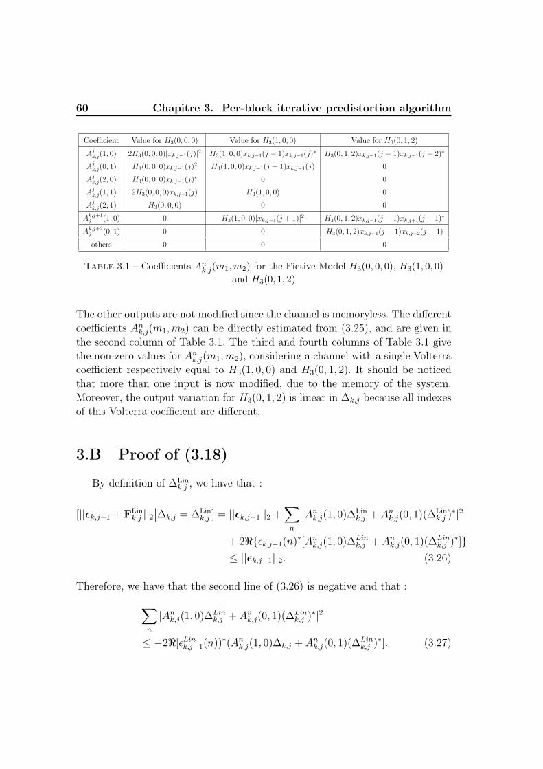
60 Chapitre 3. Per-block iterative predistortion algorithm
Coefficient Value for H3(0, 0, 0) Value for H3(1, 0, 0) Value for H3(0, 1, 2)
Ajk,j(1, 0) 2H3(0, 0, 0)|xk,j−1(j)|2 H3(1, 0, 0)xk,j−1(j − 1)xk,j−1(j)∗ H3(0, 1, 2)xk,j−1(j − 1)xk,j−1(j − 2)∗
Ajk,j(0, 1) H3(0, 0, 0)xk,j−1(j)2 H3(1, 0, 0)xk,j−1(j − 1)xk,j−1(j) 0
Ajk,j(2, 0) H3(0, 0, 0)xk,j−1(j)∗ 0 0
Ajk,j(1, 1) 2H3(0, 0, 0)xk,j−1(j) H3(1, 0, 0) 0
Ajk,j(2, 1) H3(0, 0, 0) 0 0
Ak,j+1j (1, 0) 0 H3(1, 0, 0)|xk,j−1(j + 1)|2 H3(0, 1, 2)xk,j−1(j − 1)xk,j+1(j − 1)∗
Ak,j+2j (0, 1) 0 0 H3(0, 1, 2)xk,j+1(j − 1)xk,j+2(j − 1)
others 0 0 0
Table 3.1 – Coefficients Ank,j(m1,m2) for the Fictive Model H3(0, 0, 0), H3(1, 0, 0)
and H3(0, 1, 2)
The other outputs are not modified since the channel is memoryless. The differentcoefficients Ank,j(m1,m2) can be directly estimated from (3.25), and are given inthe second column of Table 3.1. The third and fourth columns of Table 3.1 givethe non-zero values for Ank,j(m1,m2), considering a channel with a single Volterracoefficient respectively equal to H3(1, 0, 0) and H3(0, 1, 2). It should be noticedthat more than one input is now modified, due to the memory of the system.Moreover, the output variation for H3(0, 1, 2) is linear in ∆k,j because all indexesof this Volterra coefficient are different.
3.B Proof of (3.18)
By definition of ∆Link,j , we have that :
[||εk,j−1 + FLink,j ||2
∣∣∆k,j = ∆Link,j ] = ||εk,j−1||2 +
∑n
|Ank,j(1, 0)∆Link,j + Ank,j(0, 1)(∆Lin
k,j )∗|2
+ 2<{εk,j−1(n)∗[Ank,j(1, 0)∆Link,j + Ank,j(0, 1)(∆Lin
k,j )∗]}≤ ||εk,j−1||2. (3.26)
Therefore, we have that the second line of (3.26) is negative and that :∑n
|Ank,j(1, 0)∆Link,j + Ank,j(0, 1)(∆Lin
k,j )∗|2
≤ −2<[εLink,j−1(n))∗(Ank,j(1, 0)∆k,j + Ank,j(0, 1)(∆Link,j )∗]. (3.27)

3.C. Channel simulation with constant Volterra coefficients 61
Since γ2 < γ, it is easy to see that :
[||εk,j−1 + FLink,j ||2
∣∣∆k,j = ∆γk,j] = ||εk,j−1||2 + γ2
∑n
|Ank,j(1, 0)∆Link,j + Ank,j(0, 1)(∆Lin
k,j )∗|2
+ 2γ<{εk,j−1(n)∗[Ank,j(1, 0)∆Link,j + Ank,j(0, 1)(∆Lin
k,j )∗]}≤ ||εk,j−1||2. (3.28)
3.C Channel simulation with constant Volterracoefficients
−1.5 −1 −0.5 0 0.5 1 1.5−1.5
−1
−0.5
0
0.5
1
1.5
ℜ
ℑ
Received symbolsSymbol constellation
Figure 3.12 – Received constellation simulated by the predistorter afterpredistortion, 36Mbaud, α = 0.1, 2.1dB OBO
When simulating the satellite communication channel, two power normaliza-tions are generally considered : one at the HPA input, according to the fixed IBO,and one at the receiver input. The IBO quantifies the non-linearity induced bythe channel as well as the system power efficiency. The received signal is alsonormalized at the receiver to perform the detection, as described in Section 2.5.On this way, the received samples y(n) are the same if the transmitted symbols

62 Chapitre 3. Per-block iterative predistortion algorithm
are equal to x(n) or G1x(n), for any real value G1. From a mathematical pointof view, this is equivalent to say that if x(n) is modified into G1x(n), the filterf1{τ} is multiplied by G−1
1 to keep a constant IBO. This results in a modificationof the Volterra coefficients, as shown by (2.5). The SVA may on this way lead tounrealistic pre-distorted values, since the power of the predistorted symbols caninfinitely be increased without modification of the received samples. To avoid thisphenomenon, the predistortion algorithm simulates the channel always with thesame coefficients for f1{τ} and f2{τ}, so that the channel is always simulatedwith constant Volterra coefficients. Even if it is not considered as an issue, theIBO (and OBO) is modified after predistortion.Fig. 3.12 represents the same received constellation as Fig. 3.1, but as simula-ted by the predistorter. The error considered by the predistortion algorithm iscalculated using the constellation in Fig. 3.12 and the transmitted symbols as re-ference, while the receiver calculates the error using the constellation in Fig. 3.1and the centroids as reference.

Chapitre 4
Low-complexity predistortionalgorithms based on the SVA and
on the order p compensation
Contents4.1 Introduction . . . . . . . . . . . . . . . . . . . . . . . . . . 63
4.2 Low-complexity algorithms based on the SVA . . . . . . 64
4.2.1 Low-complexity approximations of the coefficientsAn,c1k,j,c(1, 0) and A
n,c1k,j,c(0, 1) . . . . . . . . . . . . . . . . . . . 64
4.2.2 Verification of the linearity assumption . . . . . . . . . . . . 66
4.2.3 Comparison with SoA algorithms . . . . . . . . . . . . . . . 66
4.3 Modified order p compensation . . . . . . . . . . . . . . . 67
4.4 Complexity analysis . . . . . . . . . . . . . . . . . . . . . 68
4.4.1 Complexity incurred by a convolution . . . . . . . . . . . . 68
4.4.2 Complexity incurred by one channel simulation . . . . . . . 69
4.4.3 Complexity of the modified order p compensation . . . . . . 70
4.4.4 Complexity of the SVA based on LUT . . . . . . . . . . . . 71
4.4.5 Complexity of the SVA based on Volterra coefficients . . . . 72
4.4.6 Complexity of the SVA . . . . . . . . . . . . . . . . . . . . . 72
4.4.7 Conclusion . . . . . . . . . . . . . . . . . . . . . . . . . . . 72
4.5 Numerical results . . . . . . . . . . . . . . . . . . . . . . . 73
4.5.1 SC scenario . . . . . . . . . . . . . . . . . . . . . . . . . . . 73
4.5.2 MC scenario . . . . . . . . . . . . . . . . . . . . . . . . . . . 78
4.6 Conclusion and future work . . . . . . . . . . . . . . . . . 78

64Chapitre 4. Low-complexity predistortion algorithms based on the
SVA and on the order p compensation
4.1 Introduction
The main drawback of the small-variation algorithm (SVA) presented inprevious chapter is its high complexity, since it necessitates to simulate thechannel several times at each step of the algorithm, as described in Section 3.3.4.In this chapter, we investigate different reduced-complexity algorithms basedon the SVA and on the order p compensation (described in Section 2.6.4.1).This allows for approaching the performance of the SVA with much smallercomplexity. The chapter is divided as follows :
– Section 4.2 describes low-complexity algorithms based on the SVA in theSC and MC scenarios.
– Section 4.3 proposes a modification of the order p compensation algorithmto improve its performance in the SC and MC scenarios.
– Section 4.4 proposes a complexity comparison.– Section 4.5 compares the performance achieved with the low-complexity
algorithms to the performance achieved with the SVA and SoA algorithms.– Section 4.6 concludes this chapter.
We refer to Chapter 1 for the description of the system model and to Sections 2.3and 3.2 for the notations.
4.2 Low-complexity algorithms based on the SVA
The complexity of the SVA is due to the several channel simulations that arerequired at each step of the algorithm. The SVA relies on the assumption of alinear relation between the variation of one transmitted symbol and the resultingvariation of the received samples, as described in Section 3.3.2. The linear coeffi-cients are obtained by channel simulations, as described in Section 3.3.4. At theend of each step, a channel simulation is further required to check that the Eu-clidian distance has effectively decreased. In this section, we propose alternativesto avoid these several channel simulations.

4.2. Low-complexity algorithms based on the SVA 65
4.2.1 Low-complexity approximations of the coefficientsAn,c1k,j,c(1, 0) and An,c1
k,j,c(0, 1)
We first propose two alternatives to compute the linear coefficients An,c1k,j,c(1, 0)
and An,c1k,j,c(0, 1) (the coefficients Ank,j(1, 0) and Ank,j(0, 1) in the SC scenario).
4.2.1.1 Calculations of the coefficients An,c1k,j,c(1, 0) and An,c1k,j,c(0, 1) basedon a reduced Volterra model
As described in Appendix 3.A, the coefficients An,c1k,j,c(1, 0) and An,c1k,j,c(0, 1)
can be computed by summing the contribution of each Volterra coefficient.By definition, An,c1k,j,c(1, 0) and An,c1k,j,c(0, 1) depend on the Volterra coefficientsH2m+1(n1...n2m+1) for which at least one index ni is equal to n − j. To de-crease the algorithm complexity, An,c1k,j,c(1, 0) and An,c1k,j,c(0, 1) can be approximatedby summing the contributions of only the most significant Volterra coefficients.A first way to limit the number of Volterra coefficients is obtained by trunca-ting the non-linearity order and by limiting the channel length. Truncating thechannel length to a given value L′
c implies that only the Volterra coefficientsH2m+1(n1...n2m+1) for which each index ni satisfies |ni| ≤ L
′c are considered, and
that Ank,j(m1,m2) = 0 for |n − j| > L′c. Different methods to approximate a
non-linear system are proposed in [27] to further decrease the number of Volterracoefficients. In this paper, we further reduce the number of Volterra coefficientsby only considering the ones depending on maximum 2 different indexes. Thenumber of Volterra coefficients however increase exponentially with the numberof carriers, so that this method becomes impractical in the MC case, so that thismethod will only be investigated in the SC case.
4.2.1.2 Calculations of the coefficients An,c1k,j,c(1, 0) and An,c1k,j,c(0, 1) using alookup table
The idea of this approximation is to pre-compute the values of An,c1k,j,c(1, 0)
and An,c1k,j,c(0, 1) and to store them in a lookup table. However, the linear coeffi-cients depend on the predistorted symbols, as shown in Appendix 3.A, which takeon continuous values, so that an infinite number of pre-computed table entrieswould need to be stored. Considering first the SC scenario, an approximation ofAnk,j(1, 0) is calculated by rounding each value in [xk,j−1(n−L2) ... xk,j−1(n+L1)]
to the closest value in C, where C = {c1, c2...cP} is a set of P complex numbers.To limit the size of the LUT, a truncated channel length L
′c is considered, so

66Chapitre 4. Low-complexity predistortion algorithms based on the
SVA and on the order p compensation
that approximately PL′c values need to be stored to approximate one coefficient
Ank,j(1, 0) or Ank,j(0, 1). This method requires thus to store 2LcPL′c values. The va-
lue of P is obviously a trade-off between the memory size and the accuracy of thelinear coefficients. To avoid the complexity of rounding each predistorted symbolto the closest value in C, a further approximation can be introduced, by calcu-lating the coefficients Ank,j(1, 0) and Ank,j(0, 1) using the un-predistorted symbolsinstead of the predistorted symbols. In this case, P is equal to the modulationorder M , and 2LcM
L′c values need to be stored. In the MC scenario, the number
of values increase to 2LcC2ML
′c .
4.2.2 Verification of the linearity assumption
At the end of each step (or substep in the MC scenario) of the SVA, it ischecked that the variation ∆applied
k,j (or ∆appliedk,j,c in the MC scenario) effectively de-
creases the Euclidian distance, i.e. to verify that the linearity assumption is met.Moreover, this channel iteration is also required to calculate the exact outputvariations, to avoid error propagation. To avoid this channel simulation, a prag-matic approach to keep the low-complexity advantage is to check the linearityassumption only at the end of each iteration by a single channel simulation. Ifafter a given iteration, the Euclidian distance stops decreasing, the algorithm isstopped and the predistorted values of the previous iteration are kept as the finalvalues. After each (sub)-step of the algorithm, the new channel outputs are onlyapproximated using the approximated values of An,c1k,j,c(1, 0) and An,c1k,j,c(0, 1). Theexact channel outputs are only known at the end of each iteration.
4.2.3 Comparison with SoA algorithms
The simplifications of the SVA proposed in Sections 4.2.1.1 and 4.2.1.2 respec-tively rely on a reduced Volterra model and on the use of LUT, similarly to theSoA algorithms presented in Sections 2.17 and 2.6.4.3. The proposed simplifica-tions could be expected to exhibit the same performance loss due to the limitationof the LUT size or of the number of Volterra coefficients. This is however not truesince the approximations are applied in a very different context. In the SoA algo-rithms, the (non-linear) optimum predistortion function is approximated, whilewe here approximate the linear relation between one input variation and the re-sulting output variations. Even if the coefficients An,c1k,j,c(1, 0) and An,c1k,j,c(0, 1) areonly approximated, the predistorted symbols can still approach their optimum

4.3. Modified order p compensation 67
values after several iterations. Moreover, An,c1k,j,c(1, 0) and An,c1k,j,c(0, 1) depend onlyon the Volterra coefficients of the channel which have at least one index equal ton− j. They depend on less Volterra coefficients than the optimum predistortionfunction, and can therefore be more easily well approximated.
4.3 Modified order p compensation
The order p compensation, presented in Section 2.6.4.1 for the SC scenario,is an iterative algorithm with low complexity, since it necessitates one channelsimulation per iteration. As discussed in Chapter 2, the order p compensationremoves all interference up to order p, but creates higher-order terms so thatthe algorithm diverges when considering a channel with too high non-linearitiesorders. In this section, we propose a simple way to modify the algorithm toimprove its performance, before discussing its extension to the MC case.
We propose to modify the algorithm defined in (2.16) as follows :
x1(n) = s(n)
xi(n) = x(n)− θ[xi−2(n)] i = 3, 5...p
x(n) = xp(n), (4.1)
In the initial algorithm, the red part in (4.1) is equal to s(n). This modifiedorder p compensation algorithm has exactly the same structure and complexityas the initial algorithm. However, it does not compensate for all interferenceterms up to order p. Instead, it mutst be seen as a simplified SVA, with all linearcoefficients equal to 0 except for Akk,j(1, 0) = 1. This means that the value of eachpredistorted symbol is optimized without taking into account the neighboringsymbols. Even if this approach is far from being optimal, we propose to investigateit for its low-complexity advantage. Similarly to the SVA, the (modified) order pcompensation algorithm predistorts symbol blocks of size N , N being a tradeoffbetween performance and latency.A main issue with the algorithm proposed in (4.1) is its convergence. To increasethe power of some received samples, the predistortion algorithm always increasesthe power of the corresponding transmitted symbols, without taking into accountthe saturation effect of the HPA. To avoid this effect, the power of the transmittedsymbols are limited to a maximum value. This means that after each iteration,

68Chapitre 4. Low-complexity predistortion algorithms based on the
SVA and on the order p compensation
the transmitted symbols are limited in amplitude :
xi(n)→ min[|xi(n)|, vmax]xi(n)
|xi(n)| (4.2)
where vmax is a real positive number.
The extension of 4.1 to the MC case is straighforward
x1c(n) = sc(n)
xic(n) = xc(n)− θ[xi−21 (n),xi−2
2 (n)...xi−2C (n)] i = 3, 5...p
xc(n) = xpc(n), (4.3)
where θ[·] is now a non-linear function with CLc complex inputs, and contai-ning only third order or higher order terms. At the end of each iteration, thepredistorted symbols are normalized as done in (4.2).
4.4 Complexity analysis
In this section, the complexity of the small-variation algorithm is comparedto that of its reduced-complexity alternatives. For the sake of simplicity, thecomplexity is calculated as the number of real or complex additions and multi-plications, or flops (floating-point operations). Other aspects, such as numericalaccuracy, size of the memory, or number of accesses to a lookup table are notconsidered. In the following, we will see that the complexity of the different pre-distortion algorithms is strongly related to the complexity required to simulatethe channel with N input symbols. We first discussed the complexity incurred bya convolution, which will be necessary to assess the complexity of one channelsimulation.
4.4.1 Complexity incurred by a convolution
It is well known that a frequency domain approach allows for performing aconvolution with complexity O(Nlog2(N)), while the time domain approach re-quires a complexity O(N2) [56]. A first and simple approach to perform a convo-lution in the frequency domain is to multiply the FFT of the input sequencewith the frequency response of the filter, and to take the IFFT of the resultingsequence. Usually, the convolution on long input sequences is rather performed

4.4. Complexity analysis 69
using the overlap-add or overlap-save algorithms to prevent too high latency [57].Since latency is not considered as an issue, the first approach will be considered,as it is slightly less complex [58].The choice of the optimum algorithm to compute the FFT/IFFT depends on thenumber of input samples, and in particular if the number of samples is a powerof two [59]. The complexity per input sample therefore depends on N. The algo-rithm with the lowest complexity per sample is achieved with the split radix FFTalgorithm, which requires 4log2N− 6 + 8
Nflops per sample (N being the number
of input samples) [60]. Even if the algorithm can only be used for N equal to apower of two, the complexity of a FFT/IFFT will be considered equal to 4Nlog2N
to simplify the discussion. We therefore consider that a convolution with N inputsamples require 8Nlog2N flops for the FFT/IFFT and N multiplications.
4.4.2 Complexity incurred by one channel simulation
In the SC case, a channel simulation with N input symbols consists in thefollowing operations (see Fig. 2.1) :
– The input symbols are first oversampled, with oversampling factor denotedas kOSF.
– The resulting signal is then convolved with the filter f1(n), consisting ofsamples of f1{t} at the rate kOSFT
−1s .
– The HPA can be simulated by interpolation using values stored in a LUT.Another approach is to use an analytical approximation of the HPA cha-racteristics.
– The resulting signal is convolved with the filter f2(n), consisting of samplesof f2{t} at the rate kOSFT
−1s .
– The resulting signal is finally down-sampled at the symbol rate.
Due to the spectral regrowth, kOSF is generally taken at least equal to 8 toavoid aliasing. The convolutions can be effectively performed in the frequencydomain, requiring one FFT, multiplication of the so obtained samples with theFourier transform of the filter, and one IFFT. The complexity of the channel isdetermined by :
– The complexity of the FFT and the IFFT. The first FFT can be efficientlyimplemented by exploiting the fact that only N of the NkOSF input samples
70Chapitre 4. Low-complexity predistortion algorithms based on the
SVA and on the order p compensation
are non-zero. The second IFFT can also be efficiently implemented by ex-ploiting the fact that only N output values have to be computed, since theoutput signal is downsampled afterwards. The FFT/IFFT related to onechannel simulation require thus 8NkOSF[log2(NkOSF) + log2(N)] flops. Fora large value of N , the multiplication of the signal after FFT with the filtercoefficients in the frequency domain has negligible complexity.
– The interpolations required to simulate the HPA characteristics. The lesscomplex approach is to store different values of the HPA characteristics ina LUT, and to round every input sample to its closest value in the LUT.The output samples are then equal to their corresponding output valueof the LUT. For the SVA however, channel simulations are performedusing very close values of input symbols (see (3.20)) to estimate thelinear coefficients. Therefore, the LUT needs to store a very tight meshof the HPA characteristics values to avoid rounding errors. Piecewiseinterpolation can also be used to obtain a better approximation. Linearapproximation requires two additions and one multiplication per sample,so that 3 operations are required per sample.
In the MC scenario, a channel simulation with C × N input symbols is slightlydifferent from the SC case. The bandwidth of the transmitted signal is equal toC(Ts)
−1(1 +α), so that the oversampling factor is higher than in the SC case. Toeasily compare the SC and MC scenarios, we will assume that the oversamplingfactor is C times higher than in the SC case, and is thus equal to CkOSF (withkOSF being at least equal to 8). The number of FFT and IFFT has also increased,as shown by Fig. 2.2, since C FFT are required before the SRRC filtering andC IFFT are required after the SRRC filtering at the receiver. It can be easilyverified that approximatively 8NCkOSF{log2[N(kOSF)] + Clog2(N)} flops perchannel iteration are required for the FFT and IFFT.
In conclusion, the complexity of one channel simulation is mainly definedby the complexity related to the FFT and IFFT for both the SC and MC cases.In the SC scenario, approximatively 8kOSF[log2(NkOSF) + log2(N)] flops arerequired per transmitted symbol, while 8kOSF[log2(NkOSF) +Clog2(N)] flops pertransmitted symbol are required in the MC scenario. In the following sections,we describe the complexity required for the different predistortion algorithms.

4.4. Complexity analysis 71
4.4.3 Complexity of the modified order p compensation
The modified order p compensation is the lowest complexity algorithm since itnecessitates one channel simulation of N input symbols per iteration. Consideringthe SC scenario, with N = 12960, which corresponds to the number of symbolsin a PLFRAME of the DVB-S2 standard for the case of 32-APSK modulation,and kOSF = 8, the algorithm necessitates approximatively 1900 flops per symbol,or 380 flops per bit, at each iteration. Considering a 8APSK modulation with 4
and 8 carriers, the algorithm necessitates approximatively 4800 and 8500 flopsper symbol, or 1600 and 2833 flops per bit.
4.4.4 Complexity of the SVA based on LUT
The SVA based on LUT also necessitates one channel simulation at the endof each iteration. This is necessary to check that the Euclidian distance has effec-tively decreased, compared to previous iteration, as described in Section 4.2.1.2.Considering first the SC scenario, each iteration also consists in N steps. At stepj, the predistorted symbol j is modified, requiring the following operations :
– The linear coefficients are first read in the LUT. No complexity is associatedto this operation.
– Evaluate ||εk,j−1 + FLink,j ||2 in (3.15), with FNL
k,j = FLink,j as defined in (3.14).
The computation of the norm of this vector is obtained by summing thenorm of each element of the vector εk,j−1 + FLin
k,j . It can be shown that thisnecessitates 10Lc multiplications and 5(Lc − 1) additions.
– Find the minimum of (3.15). Using partial derivatives, this requires theinversion of a 2× 2 (real) matrix, 4 multiplications, and 2 additions.
– Update the channel outputs for the next step (in fact calculate εk,j fromεk,j−1 using An,c1k,j,c(1, 0), An,c1k,j,c(0, 1) and the applied variation). This requires4Lc multiplications and 4Lc additions.
In the SC case, the SVA based on LUT requires thus approximatively 23Lcadditional flops per transmitted symbol. Assuming a reasonable channel length(Lc = 10 for instance), the main source of complexity remains the channelsimulation required at the end of each iteration.
In the MC scenario, each step is divided into C substeps. Comparing (3.15)and (3.23), it can be seen that the complexity related to each substep linearly
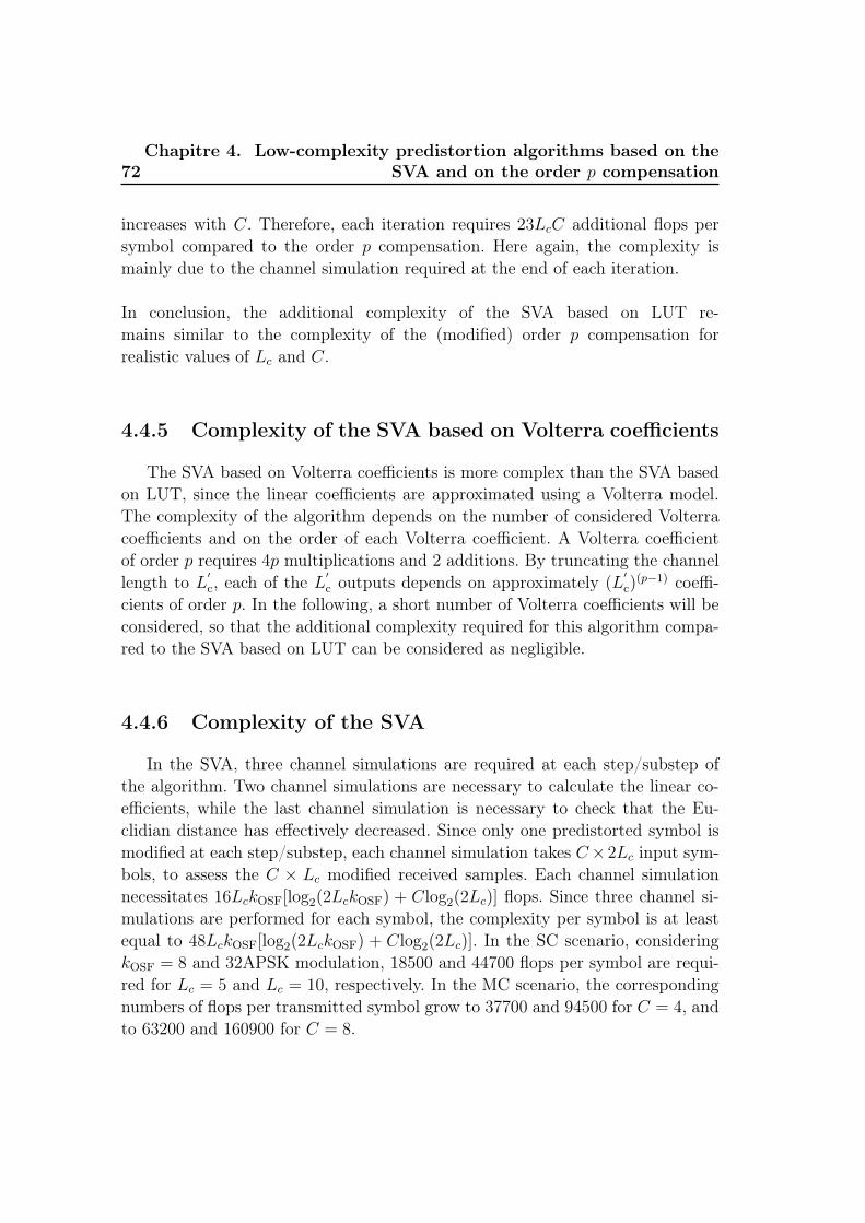
72Chapitre 4. Low-complexity predistortion algorithms based on the
SVA and on the order p compensation
increases with C. Therefore, each iteration requires 23LcC additional flops persymbol compared to the order p compensation. Here again, the complexity ismainly due to the channel simulation required at the end of each iteration.
In conclusion, the additional complexity of the SVA based on LUT re-mains similar to the complexity of the (modified) order p compensation forrealistic values of Lc and C.
4.4.5 Complexity of the SVA based on Volterra coefficients
The SVA based on Volterra coefficients is more complex than the SVA basedon LUT, since the linear coefficients are approximated using a Volterra model.The complexity of the algorithm depends on the number of considered Volterracoefficients and on the order of each Volterra coefficient. A Volterra coefficientof order p requires 4p multiplications and 2 additions. By truncating the channellength to L′
c, each of the L′c outputs depends on approximately (L
′c)
(p−1) coeffi-cients of order p. In the following, a short number of Volterra coefficients will beconsidered, so that the additional complexity required for this algorithm compa-red to the SVA based on LUT can be considered as negligible.
4.4.6 Complexity of the SVA
In the SVA, three channel simulations are required at each step/substep ofthe algorithm. Two channel simulations are necessary to calculate the linear co-efficients, while the last channel simulation is necessary to check that the Eu-clidian distance has effectively decreased. Since only one predistorted symbol ismodified at each step/substep, each channel simulation takes C×2Lc input sym-bols, to assess the C × Lc modified received samples. Each channel simulationnecessitates 16LckOSF[log2(2LckOSF) + Clog2(2Lc)] flops. Since three channel si-mulations are performed for each symbol, the complexity per symbol is at leastequal to 48LckOSF[log2(2LckOSF) + Clog2(2Lc)]. In the SC scenario, consideringkOSF = 8 and 32APSK modulation, 18500 and 44700 flops per symbol are requi-red for Lc = 5 and Lc = 10, respectively. In the MC scenario, the correspondingnumbers of flops per transmitted symbol grow to 37700 and 94500 for C = 4, andto 63200 and 160900 for C = 8.

4.5. Numerical results 73
4.4.7 Conclusion
We have shown that the low-complexity algorithms allow for decreasing thecomplexity of the algorithm by approximatively one order of magnitude. The com-plexity of the SVA behaves like O(CLckOSFlog2(LckOSF)), while the complexityof the low-complexity algorithms behaves like O(CkOSFlog2(NkOSF)).
4.5 Numerical results
4.5.1 SC scenario
The system model has been described in Chapter 1. In the SC scenario, 32-APSK symbols are considered with a code rate equal to 4/5 and N is equal to12960, similarly to Chapter 3.Fig. 4.1 illustrates the performance reached when the decrease of the square erroris checked only after each iteration, as described in Section 4.2.2. The asymptoticperformance depends on the considered ∆max. However, sufficiently small valuesof ∆max (0.05 and 0.1) allow to reach similar performance as that obtained inFig. 3.2, where the verification of the square error decrease is made at each step.In the following, ∆max will be considered equal to 0.1, as it has similar conver-gence speed as the SVA (see Fig. 3.2).Table 4.1 shows the performance loss associated to the reduced-complexity alter-
IBO=3dB IBO=4dB IBO=5dB
MSE small-variation algorithm (reference) Ref = −20.41dB Ref = −21.79dB Ref = −23.47dB
Look-up table, L′
c = 3 = Ref + 0.74dB = Ref + 0.55dB = Ref + 0.46dB
Look-up table, L′
c = 5 = Ref + 0.45dB = Ref + 0.32dB = Ref + 0.18dB
Reduced-Volterra model, L′
c = 3 = Ref + 1.41dB = Ref + 1.28dB = Ref + 1.18dB
Reduced-Volterra model, L′
c = 5 = Ref + 1.22dB = Ref + 1.04dB = Ref + 0.92dB
Mod. order p = Ref + 1.68dB = Ref + 1.33dB = Ref + 1.20dB
Table 4.1 – Performance of the reduced-complexity alternatives of the small-variationalgorithm
natives of the small-variation algorithm, proposed in Section 4.2.1.1 and 4.2.1.2.In all cases, a linear filter is considered at the transmitter, and is placed afterthe predistortion block. For both approximations, the performance loss decreases

74Chapitre 4. Low-complexity predistortion algorithms based on the
SVA and on the order p compensation
0 5 10 15−21
−20
−19
−18
−17
−16
−15
−14
−13
Number of iterations
MSE
(dB)
Δmax=0.05
Δmax=0.1
Δmax=0.3
Δmax=0.5
Figure 4.1 – Mean-square error (MSE) after each iteration of the small-variationalgorithm, using the convergence method described in Section 4.2.2, 36Mbaud,
α = 0.1, 3dB IBO
with the IBO. Considering a truncated channel length L′c = 5, a small perfor-
mance increase is allowed compared to L′c = 3. For the SVA based on Volterra
coefficients, each step of each iteration requires about 60 additional multiplica-tions and 30 additional additions to assess the linear coefficients (relying on thefact that some products of the predistorted symbols can be reused to calculatedifferent channel outputs). As discussed in Section 4.4.5, this complexity can beconsidered as negligible compared to the complexity of one channel simulation.The SVA based on LUT achieves slightly better performance, but it necessitatesmore complex pre-computing since 2Lc × 32L
′c entries need to be stored in the
LUT.Fig. 4.2 shows the MSE achieved with the modified order p compensation for dif-ferent values of ∆max. The parameter ∆max is here defined as the maximum allo-wed amplitude of the predistorted symbols compared to the maximum amplitudeof the un-predistorted symbols (in Section 4.3, it was defined as the maximumamplitude of the predistorted symbols). The optimum value of vmax is around

4.5. Numerical results 75
0 0.5 1 1.5 2 2.5 3 3.5 4 4.5 5−22.5
−22
−21.5
−21
−20.5
−20
−19.5
−19
−18.5
Maximum power increase [dB]
MSE
[dB]
25Mbaud, α = 0.336Mbaud, α =0.138Mbaud, α = 0.05
Figure 4.2 – MSE using the modified order p algorithm, 4dB IBO
0 0.5 1 1.5 2 2.5 3 3.5 46
6.5
7
7.5
8
8.5
9
9.5
10
10.5
Maximum power increase [dB]
PAPR
[dB]
25Mbaud, α = 0.336Mbaud, α = 0.138Mbaud, α = 0.05
Figure 4.3 – PAPR using the modified order p algorithm, 4dB IBO

76Chapitre 4. Low-complexity predistortion algorithms based on the
SVA and on the order p compensation
2dB for the considered IBO of 4dB. Low values of vmax obviously restrict thealgorithm performance while high values of vmax increase the MSE due to theHPA saturation, as explained in Section 4.3.Fig. 4.3 shows the PAPR obtained using the modified order p algorithm. Unsur-prisingly, it increases with vmax. The results are similar to the ones obtained withthe SVA, shown in Fig. 3.7.Fig. 4.4, 4.5 and 4.6 show the total degradation obtained using the SVA, thereduced complexity alternatives and the state-of-the-art algorithms, consideringdifferent combinations of symbol rate and rolloff. A truncated channel L′
C = 3
is considered for the SVA based on LUT, and vmax = 2dB is considered for themodified order p compensation. It can be observed that the SVA based on LUTis the low-complexity algorithm achieving the best performance. The modifiedorder p compensation algorithm is slightly less performant than the other low-complexity algorithms, but it has a lower complexity and does not necessitateany pre-compution. The low-complexity algorithms all outperform the state-of-the-art algorithms, especially when considering high symbol rates and small rolloffvalues.
4.5.2 MC scenario
Fig. 4.7 shows the MSE achieved with the order p compensation algorithm,considering a three carrier multiplex and different values of vmax. Increasing thevalue of vmax improves the performance on the outer carriers, but decreases theperformance on the inner carrier. It can be easily shown that increasing the valuesof the predistorted symbols on one carrier increases the MSE on the other carriers.This unwanted effect is here particularly penalizing for the inner carrier, whichsuffers the most from the intermodulation interference, as shown in Section 2.4.2.Fig. 4.8 shows the total degradation obtained with the SVA, the SVA based onLUT (with L′
c = 1), the modified order p compensation (with vmax = 1dB) andwhen no predistortion occurs. The performance of the SVA based on LUT isabout 0.25dB lower than the performance of the SVA, while the modified orderp compensation is about 1dB lower. However, high performance improvement isstill obtained compared to the case where no predistortion occurs.

4.5. Numerical results 77
1 1.5 2 2.5 3 3.5 42
3
4
5
6
7
8
OBO
Tota
l deg
rada
tion
(dB)
Small−variation algorithmSVA based on LUTSVA based on reduced Volterra modelModified order pSOA based on LUT entriesSOA Memory polynomialsNo pre−distortion
Figure 4.4 – Total degradation for small-variation algorithm (SVA),reduced-complexity algorithms and state-of-the-art pre-distortion methods, 25Mbaud,
α = 0.3
1 1.5 2 2.5 3 3.5 4 4.53
3.5
4
4.5
5
5.5
6
6.5
7
7.5
8
OBO
Tota
l deg
rada
tion
(dB)
Small−variation algorithmSVA based on LUTSVA based on reduced Volterra modelModified order pSOA based on LUT entriesSOA Memory polynomialsNo pre−distortion
Figure 4.5 – Total degradation for small-variation algorithm (SVA),reduced-complexity algorithms and state-of-the-art pre-distortion methods, 36Mbaud,
α = 0.1

78Chapitre 4. Low-complexity predistortion algorithms based on the
SVA and on the order p compensation
1.5 2 2.5 3 3.5 4 4.5 53
4
5
6
7
8
9
OBO
Tota
l deg
rada
tion
(dB)
Small−variation algorithmSVA based on LUTSVA based on reduced Volterra modelModified order pSOA based on LUT entriesSOA Memory polynomialsNo pre−distortion
Figure 4.6 – Total degradation for small-variation algorithm (SVA),reduced-complexity algorithms and state-of-the-art pre-distortion methods, 38Mbaud,
α = 0.05
4.6 Conclusion and future work
In this chapter, we have proposed new predistortion algorithms, whichoutperform the SoA algorithms at a much lower complexity than the SVA,both in SC and MC scenarios. In the considered scenarios, the low-complexityalgorithms closely approach the performance achieved with the SVA. However,the performance difference is expected to increase with the number of carriers.The SVA based on Volterra coefficients and on LUT achieve better performancecompared to the modified order p compensation, but they both require pre-computing and a higher complexity. Even for these low-complexity algorithms,the complexity remains an issue. This is because one channel simulation of (C)N
symbols is required at each iteration.
Parallelization is a possible track to decrease the complexity of the SVA
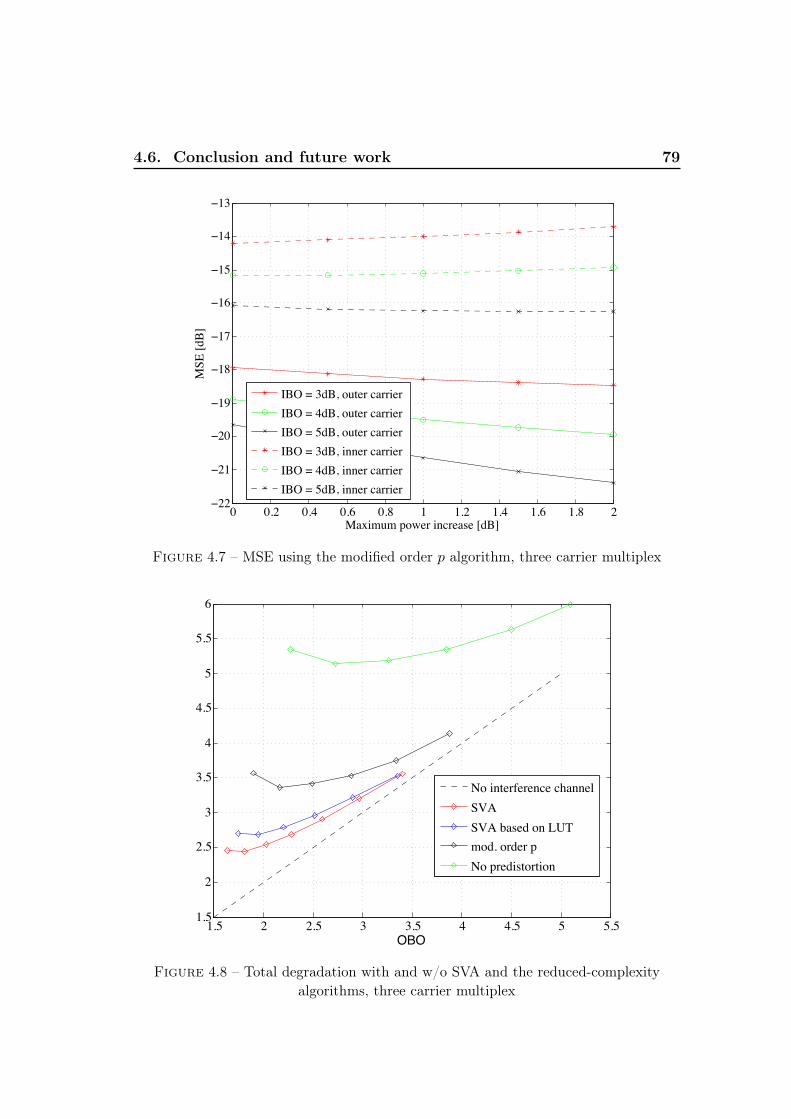
4.6. Conclusion and future work 79
0 0.2 0.4 0.6 0.8 1 1.2 1.4 1.6 1.8 2−22
−21
−20
−19
−18
−17
−16
−15
−14
−13
Maximum power increase [dB]
MSE
[dB]
IBO = 3dB, outer carrierIBO = 4dB, outer carrierIBO = 5dB, outer carrierIBO = 3dB, inner carrierIBO = 4dB, inner carrierIBO = 5dB, inner carrier
Figure 4.7 – MSE using the modified order p algorithm, three carrier multiplex
1.5 2 2.5 3 3.5 4 4.5 5 5.51.5
2
2.5
3
3.5
4
4.5
5
5.5
6
OBO
No interference channelSVASVA based on LUTmod. order pNo predistortion
Figure 4.8 – Total degradation with and w/o SVA and the reduced-complexityalgorithms, three carrier multiplex

80Chapitre 4. Low-complexity predistortion algorithms based on the
SVA and on the order p compensation
and of the reduced-complexity alternatives. For the SVA, each predistorted valuen, n + Lc, n + 2Lc... can be simultaneously optimized by different processingunits, reducing the complexity of each processing unit by a factor N/Lc. Thelow-complexity algorithms can also be parallelized, by predistorting separatelyN1 blocks of N2 symbols, with N1N2 = N . The complexity of each processingunit is then decreased by a factor N1.

Chapitre 5
Turbo-equalization of the remaininginterference after predistortion
Contents5.1 Introduction . . . . . . . . . . . . . . . . . . . . . . . . . . 815.2 Literature review of equalization and detection algo-
rithms for non-linear channels . . . . . . . . . . . . . . . . 825.3 Notations . . . . . . . . . . . . . . . . . . . . . . . . . . . . 835.4 Turbo-equalization in the un-predistorted channel . . . . 84
5.4.1 Turbo-equalizer structure . . . . . . . . . . . . . . . . . . . 845.4.2 Estimation of the conditional interference . . . . . . . . . . 86
5.5 Generalities on joint predistortion and turbo-equalization 885.5.1 Simulation of the predistortion algorithm at the receiver . . 885.5.2 No simulation of the predistortion algorithm at the receiver 88
5.6 Application of joint predistortion and turbo-equalization to specific predistortion algorithms . . . . . 90
5.6.1 Joint predistortion and turbo-equalization based on the SVA 905.6.2 Joint predistortion and turbo-equalization based on LUT . 955.6.3 Modified order p predistortion algorithm . . . . . . . . . . . 96
5.7 Comparison based on the total degradation . . . . . . . . 1015.8 Conclusion . . . . . . . . . . . . . . . . . . . . . . . . . . . . 102
5.1 Introduction
In previous chapters, we have seen that residual interference still remainswhen the transmitted symbols are predistorted. It was always considered thatthe receiver performs Gaussian detection on the received samples to concentrate

82Chapitre 5. Turbo-equalization of the remaining interference after
predistortion
the computational load into the single transmitter instead of in the numerous re-ceivers when considering broadcast and broadband applications. In this context,additional complexity at the receiver to compensate the remaining interferencecan only be considered if it is negligible compared to the initial receiver com-plexity, which is mainly defined by the decoder complexity. In some professionalapplications however, the cost of the receiver is not as critical as in consumer ap-plications, so that higher complexity at the receiver may also be an option. It canalso be preferable to concentrate the computational load into the receiver, as forinstance in telemetry payload for optical observation satellite. The predistortionalgorithm should in this case be as simple as possible. We start this chapter witha literature review of equalization and detection algorithms for non-linear chan-nels, which will motivate the choice of turbo-equalization to remove the remaininginterference after predistortion.
5.2 Literature review of equalization and detec-tion algorithms for non-linear channels
Equalization or detection in the case of a non-linear channel with memoryhas been widely studied in the literature. The non-linear satellite communicationchannel can be described as a trellis, so that the maximum-a-posteriori equalizerusing the BCJR algorithm [52] or the maximum likelihood equalizer using theViterbi algorithm [53] are perfectly defined. However, the number of channelstates exponentially grows with the modulation order and the channel memory.Therefore, considering high order modulations and large channel lengths, the useof such equalizer is not possible. Different sub-optimum algorithms have beenproposed, such as :
– The reduced state BCJR algorithm [61].– A reduced size Volterra structure optimized according to the MMSE cri-
terion. In [62], a second-order MMSE equalizer has been derived. In [62]and [63], adaptive MMSE equalizers have been investigated. The equalizerhas always been limited in length and non-linearity order for complexityreasons.
– The sum-product algorithm using a reduced size Volterra structure (MAPcriterion), as in [64].

5.3. Notations 83
The above sub-optimum algorithms are expected to poorly perform in case oflarge channel lengths and/or high modulation orders. To overcome this com-plexity issue, turbo-equalization based on soft interference cancelers (SIC) hasbeen proposed. In traditional turbo-equalization, soft information is exchangedbetween the equalizer and the decoder, as done in [65] and [66]. The severaliterations between the equalizer and the decoder allow for approaching optimumperformance. Such approach cannot be applied in case of a huge number ofchannel states for complexity issues. The use of interference cancellation equali-zers has been proposed in [67] and [68] as they require a lower computationalcomplexity, and applied to the satellite channel in [69] and [70]. The principleof interference cancellation equalizers is to use the decoder output probabilitiesto estimate the interference affecting the received samples. Using a feedbackstructure, the estimated interference is subtracted from the received samplesand a new detection is performed. The process is iterated several times until noperformance improvement is observed.
In this chapter, we investigate how SIC turbo-equalization can improvethe performance obtained with the predistortion algorithms proposed in previouschapters. In next section, we first present different interference cancellationturbo-equalization structures in the case of an un-predistorted channel. Twodifferent methods to extend this algorithm to the case of pre-distorted symbolsare then proposed. Performance results will then be given considering threepredistortion algorithms.
5.3 Notations
The notations defined in Sections 2.3 and 3.2 are still used. In this chapter,we define the interference term I(n) as :
I(n) , y(n)− s(n). (5.1)
The initial interference term I0(n) is defined as y(n) − s(n) as the transmittedsymbols are not predistorted, i.e. x(n) = s(n). The terms shard(n) and ssoft(n)
refer to the hard and soft symbol estimates. To keep the notations simple, no indexis used on the different estimates to refer to the considered iteration number ofthe turbo-equalizer. Finally, Ri denotes the constellation symbols belonging tothe ring i of the constellation. For 32APSK modulation, i = 1, 2 or 3. Table 5.1summarizes the notations used in this chapter.

84Chapitre 5. Turbo-equalization of the remaining interference after
predistortion
Ri Set of constellation symbols belonging to the ring i
M Constellation size
ml Constellation symbol l
s(n) Symbol n after modulation
x(n) Transmitted symbol n after precoding
y(n) Received sample n
w(n) Noise sample n
σn Noise variance
Lc Time channel length
Lp Predistorter memory depth
I(n) Interference term
I0(n) Interference term when x(n) = s(n)
shard(n) Hard estimate of s(n)
ssoft(n) Soft estimate of s(n)
Table 5.1 – Notations specific to Chapter 5
5.4 Turbo-equalization in the un-predistortedchannel
5.4.1 Turbo-equalizer structure
In this section, we assume that no predistortion occurs, i.e. x(n) = s(n).Fig. 5.1 represents the considered turbo-equalization structure, based on an inter-ference cancellation equalizer, similarly to [70]. The interference estimator takesas input the symbol probabilities PrD[s(n) = ml] coming from the decoder, andproduces a conditional interference estimate Iml(n), defined as :
Iml(n) = E[I(n)|s(n) = ml], (5.2)
where the expectation takes into account the probabilities PrD[s(n) = ml], asdetailed in next Section. The detector uses the conditional interference esti-mates Iml(n) to improve the memoryless Gaussian detection on the received
5.4. Turbo-equalization in the un-predistorted channel 85
!"#"$%&'( ))*($+,$-,+%&'( !"./'#"0,"+1/'2(
!"#"$%"&'
3&4(5"$&5/'2(
6'#"0,"+1/'2(6'#"07"0"'$"(".%8+%&'(
398:&,(;0&:+:/,/%".($+,$-,+%&'(
PrD[s(n) = ml]
PrE[s(n) = ml]
y(n)
Iml(n)
Figure 5.1 – Turbo-equalization interference cancellation equalizer
samples y(n) :
PrE[s(n) = ml|y(n)] =1√
2πσ2n
exp{−|y(n)− Iml(n)−ml|22σ2
n
}, l = 1...M. (5.3)
To simplify the notations, PrE[s(n) = ml|y(n)] will be denoted as PrE[s(n) = ml]
from now on. At the first iteration, Iml(n) = 0 so that the Gaussian detection isperformed as described in Section 2.5. The LLR calculator transforms the symbolprobabilities PrE[s(n) = ml] into bit probabilities, which feed the decoder afterdesinterleaving. The interleaver takes as input the output of the decoder to pro-duce bit probabilities from which new symbol probabilities PrD[s(n) = ml] arecalculated. Several iterations are performed until no performance improvementis observed. The proposed structure can be seen as a generalization of the struc-ture introduced in [70], where the interference estimator produces an interferenceestimation Iml(n) independent of ml.
5.4.2 Estimation of the conditional interference
The expectation in 5.3 is calculated as follows :
Iml(n) =∑
smln ∈S
mln
[I(n)|s = smln ]Pr(sml
n ), (5.4)

86Chapitre 5. Turbo-equalization of the remaining interference after
predistortion
where Smln denotes the set of all input sequences sml
n for which s(n) = ml. Theprobability Pr(sml
n ) is obtained from the symbol probabilities :
Pr(smln ) =
∏m 6=n
PrD[s(m) = smln (m)] (5.5)
The number of sequences in Smln is equal toMN−1 so that the required complexity
is very high. We now discuss how approximations of Iml(n), denoted as Iml(n),can be computed at a much lower complexity.
– The lowest complexity approach is to take hard/soft symbol estimates toproduce shard(n) or ssoft(n). Hard symbol estimates are simply obtained as :
shard(n) = argmaxml
{Pr[s(n) = ml]}. (5.6)
Soft symbol estimates are defined as :
ssoft(n) =∑l
Pr[s(n) = ml]ml. (5.7)
A single channel simulation is performed with input sequence shard/soft ofelements shard/soft(n) and received sequence y(shard/soft). The term Iml(n)
is equal to element n of [y(shard/soft)− shard/soft]. In this case, Iml(n) is thesame for each ml. This approach is followed in [70]. In the following, wewill denote this method as Method A.
– An intermediate approach is as follows. The term Iml(n) is assessed consi-dering all input symbols equal to their hard/soft estimates, similarly tothe previous approach, except for the input symbol n, which is equal toml. This allows for better estimating Iml(n) at the cost of higher com-plexity, since M × N channel simulations are required at each iteration.The number of channel simulations can be reduced assuming that the chan-nel has finite length Lc = 1 + L1 + L2, where L1 and L2 are the cau-sal and anti-causal memory of the channel. Denoting Lh =max(L1, L2),M× (Lh+1) channel simulations are required per iteration, since the termsIml(n), Iml(n ± Lh ± 1), Iml(n ± 2Lh ± 2), ..., can be jointly estimated.For instance, Iml(1), Iml(1 + Lh), Iml(1 + 2Lh) are jointly estimated bysimulating the channel with as input the hard/soft estimates, except :
s(1) = ml; s(1 + Lh) = ml; s(2 + 2Lh) = ml...

5.5. Generalities on joint predistortion and turbo-equalization 87
However, this method has a complexity which is M × (Lh + 1) times higherthan the previous method.
– Another approach is similar to the previous method, but with a lower com-plexity. The symbol constellation is first divided into group of symbols. Forinstance, let us consider the group of symbols Ri, which are the symbolsbelonging to the constellation ring i. A soft symbol ssofti (n) associated toeach group can be calculated as follows :
ssofti (n) =
1∑ml∈Ri
Pr[s(n) = ml]
∑ml∈Ri
Pr[s(n) = ml]ml (5.8)
The term Iml(n) is the same for all s(n) ∈ Ri, and is obtained by simulatingthe channel with the hard/soft estimates, except input symbol n, whichis equal to ssoft
i (n). Denoting by G the number of groups of symbols,G× (Lh + 1) channel simulations are required. We will refer to this methodas Method B. It should be noticed that this approach is equivalent to theprevious one when the number of groups is equal to the constellation size(G=M).
In conclusion, there are several methods to calculate Iml(n), which are a trade-offbetween complexity and accuracy. In this work, two methods will be inves-tigated, which require 1 and G×(Lh+1) channel simulations per turbo-iteration.
The choice of using hard or soft symbol estimates is a trade-off betweenperformance and complexity. Soft symbol estimates are more accurate butslightly more complex to produce, since they have to be computed using 5.7. Tolimit the number of cases for the simulations, soft symbol estimates will be usedwhenever it is possible.
5.5 Generalities on joint predistortion and turbo-equalization
In this section, we discuss two strategies to extend the interference cancel-lation turbo-equalizer from previous section to the case where the symbols arepredistorted at the transmitter side.

88Chapitre 5. Turbo-equalization of the remaining interference after
predistortion
5.5.1 Simulation of the predistortion algorithm at the re-ceiver
The easiest way to generalize the turbo-equalization structure to the casewhere the symbols are predistorted, is to consider the predistortion algorithmas part of the channel. Each channel simulation used in the block "Interferenceestimation" of Fig. 5.1 includes in this case a simulation of the predistortionalgorithm. The receiver complexity may however dramatically increase, dependingon the complexity of the predistortion algorithm.
5.5.2 No simulation of the predistortion algorithm at thereceiver
To avoid simulating the predistortion algorithm at the receiver, we approxi-mate the interference term by an analytical function, with as input the term I0(n).More specifically, assuming that I0(n) is equal to a given complex number a, weassume that the term I(n) with s(n) = ml, can be approximated as follows :
∀n|s(n) = ml : [I(n)|I0(n) = a] ≈ Fl(a) (5.9)
, Ek|s(k)=ml
[I(k)|I0(k) = a]. (5.10)
The key idea is that I0ml
(n) can be much easier calculated at the receiver, sinceit is not necessary to simulate the predistortion algorithm. The term Iml(n) isthen simply obtained as Fl[I0
ml(n)]. In next Section, it will be explained how
the functions Fl(·) are pre-computed. Fig. 5.2 and 5.3 summarize the proposedturbo-equalization strategies for a predistorted channel. Methods I.A and I.B arethe methods where the predistortion algorithm is simulated, unlike the methodsII.A and II.B. The letters A and B refer to the number of channel simulations(which include the predistortion algorithm for methods I.A and I.B) that areperformed at each iteration. Method I.A produces Iml(n), which is the same forevery ml and Method I.B procudes Iml∈Ri(n), being obviously the same for allml ∈ Ri. Methods II.A and II.B produce first I0
ml(n) and I0
ml∈Ri(n). Since, Fl(·)
is a different function for each l, Methods II.A and II.B produce Iml(n), whichdepends on l as well.

5.5. Generalities on joint predistortion and turbo-equalization 89
!"#$ !"%$
1 sim./
iteration
Predistortion
Iml∈Ri(n)I(n)
shard/soft(n)
xhard/soft(n)
G × (Lh + 1)
sim./iteration
Figure 5.2 – Turbo-equalization strategies in a predistorted channel, Methods I.Aand I.B
!!"#$ !!"%$
1 sim./
iteration
I0(n) I0ml∈Ri
(n)
shard/soft(n)
G × (Lh + 1)
sim./iteration
Fl(·)
Iml(n) Iml(n)
Fl(·)
Figure 5.3 – Turbo-equalization strategies in a predistorted channel, Methods II.Aand II.B

90Chapitre 5. Turbo-equalization of the remaining interference after
predistortion
5.6 Application of joint predistortion and turbo-equalization to specific predistortion algo-rithms
In the following, joint predistortion and SIC turbo-equalization will be in-vestigated for the small-variation algorithm introduced in Chapter 3. Two otherpredistortion algorithms will then be considered : the SoA algorithm based onLUT (introduced in Chapter 2) and the modified order p compensation algorithm(introduced in Chapter 4). The SoA algorithm based on Volterra coefficients isnot investigated, as it has a higher complexity than the SoA algorithm basedon LUT and generally achieved a lower performance in previous chapters. Otherlow-complexity algorithms could also be investigated. Only the modified orderp algorithm is here considered since it has the lowest complexity. The IMUX,OMUX and PA characteristics are given in Fig. 1.11, 1.12 and 1.13, respectively.The 32APSK modulation will be considered. The code rate of the LDPC code is45and the code length N = 64800. SRRC filters are considered for the shaping
and receiver filters.
5.6.1 Joint predistortion and turbo-equalization based onthe SVA
The small-variation algorithm has a very high complexity compared to theother predistortion algorithms. We consider that it is not possible to simulatethis algorithm at the receiver, so that only methods II.A and II.B are investiga-ted. After analyzing the received samples, we will derive an analytical expressionbetween I0(n) and I(n).
5.6.1.1 Analysis of the received samples
Fig. 5.4 represents the noiseless received samples using the SVA, consideringa symbol rate of 38Mbaud, a roll-off equal to 0.05, and an OBO equal to 1.9dB.It should be noticed that the received samples are not power normalized, andrepresent the received samples as simulated by the predistorter (see Section 3.C).This highlights that the predistorter is able to almost perfectly remove the interfe-rence, except for some symbols s(n) ∈ R3, for which in most cases |y(n)| < |s(n)|.The remaining interference is not due to the limitation of the pre-distorter inlength or non-linearity order, but rather to the limited maximum output power

5.6. Application of joint predistortion and turbo-equalization tospecific predistortion algorithms 91
Figure 5.4 – Noiseless received samples after SVA, 38Mbaud, α = 0.05, 1.9dB OBO
−0.2 0 0.2 0.4 0.6 0.8 1 1.2−0.2
−0.1
0
0.1
0.2
0.3
0.4
I(n)
Ir(n)
Iφ(n)
ℜ
ℑ
CenterConstellation symbolReceived symbol
Figure 5.5 – Illustration of I(n), Ir(n) and Iφ(n)

92Chapitre 5. Turbo-equalization of the remaining interference after
predistortion
of the HPA. The different MSE have been calculated :
E[|y(n)− s(n)|2∣∣s(n) ∈ R1] = −38dB
E[|y(n)− s(n)|2∣∣s(n) ∈ R2] = −34.7dB
E[|y(n)− s(n)|2∣∣s(n) ∈ R3] = −20.6dB,
which confirms that the remaining mainly affects the symbols from the upperring.
5.6.1.2 Relation between I0(n) and I(n)
In this Section, we investigate how to analytically determine the functionFl(·), which allows estimating I(n) from I0(n) for s(n) = ml, as described inSection 5.5.2. From the above discussion, the following assumption can alreadybe made :
I(n) = 0 for s(n) ∈ R1 or s(n) ∈ R2, (5.11)
which implies that Iml(n) = 0 if ml ∈ R1 or ml ∈ R2. Therefore, Fl(·) needs onlyto be determined if ml ∈ R3.The functions Fl(·) can easily be obtained by computer simulations. However, weprefer to introduce another method to simultaneously calculate Fl(·) for ml ∈ R3,since it better illustrates why the terms I(n) and I0(n) are correlated. We firstdivide I(n) into two orthogonal components, as illustrated in Fig. 5.5 :
I(n) = Ir(n) + Iφ(n) (5.12)
The term Ir(n) is the projection of I(n) on the axis drawn from the center to theconstellation point s(n) and Iφ(n) is the projection of I(n) on the perpendicularaxis. Based on Fig. 5.4, it can be reasonably assumed that Iφ(n) = 0 even fors(n) ∈ R3. In the proposed method, it is assumed that Ir(n) only depends onI0,r(n), and not on the specific value of s(n). The underlying assumption is thatthe predistortion algorithm is not able to strongly increase the power of thereceived samples y(n) for s(n) ∈ R3 due to the HPA saturation. Therefore, if|y(n)| << |s(n)| when the transmitted symbols are not predistorted, it is assumedthat |y(n)| << |s(n)| when the transmitted symbols are predistorted. We definethe function f(·) as :
f(a) , En|s(n)∈R3
[Ir(n)|I0,r(n) = a]. (5.13)

5.6. Application of joint predistortion and turbo-equalization tospecific predistortion algorithms 93
−0.7 −0.6 −0.5 −0.4 −0.3 −0.2 −0.1 0 0.1 0.2 0.3−0.5
−0.4
−0.3
−0.2
−0.1
0
0.1
0.2
0.3
I0,r(n)
I r(n)
Simulated Data
1st order approximation
3rd order approximation
Figure 5.6 – I0,r(n) versus Ir(n) and first and third order approximations using theSVA algorithm, 38Mbaud, α = 0.05, 1.9dB OBO
The relation between I0,r(n) and Ir(n) has been simulated in Fig. 5.6. It canbe noticed that for a given value of I0,r(n), several values of Ir(n) are possible.However, a strong correlation exists between I0,r(n) and Ir(n). The continuousfunction f(a), which should be defined for an infinite number of values, has beenapproximated with a first and a third order approximation. In the consideredexample, this allows for assessing I(n) with s(n) ∈ R3 with a remaining interfe-rence power equal to −19.7dB, −25.9dB and 26.7dB for approximations of orderrespectively equal to 0,1 and 3. In summary, I(n) is approximated as Ir(n), whichis then approximated from f [I0,r(n)]. The term Iml(n) is then approximated asf [Iml
0,r (n)].
5.6.1.3 BER performance
Fig. 5.7 gives the BER performance achieved with Methods II.A and II.B,which considers that all symbols s(n) ∈ R3 belong to the same group. For MethodII.B, only (Lh + 1) channel simulations are required, since it is assumed thatI(n) = 0 for s(n) ∈ R1 or R2. It can be seen that this method outperforms

94Chapitre 5. Turbo-equalization of the remaining interference after
predistortion
Method II.A, with a (Lh + 1) times higher complexity.
13 13.2 13.4 13.6 13.8 14 14.2 14.4 14.6 14.8 1510−7
10−6
10−5
10−4
10−3
10−2
10−1
SNR
BER
SVA onlySVA+Turbo II.ASVA+Turbo II.BAWGN channel
Figure 5.7 – SVA predistortion + Turbo-equalization, 38Mbaud, α = 0.05, 1.9dBOBO
5.6.2 Joint predistortion and turbo-equalization based onLUT
In this Section, we consider the predistortion algorithm based on LUT. Thecomplexity of the predistortion algorithm is negligible compared to the complexityof one channel simulation, so that Methods I.A and I.B have a similar complexityas Methods II.A and II.B, respectively. In this Section, Methods I.A and I.B arecompared, using hard symbol estimates since the predistortion algorithm takeshard inputs. Methods II.A and II.B could also be considered, but require a morecomplex pre-computing stage.
5.6.2.1 Analysis of the received samples
Fig. 5.8 represents the received samples after LUT predistortion for a noiselesssatellite transmission, considering a symbol rate of 36Mbaud, a roll-off equal to

5.6. Application of joint predistortion and turbo-equalization tospecific predistortion algorithms 95
0.1 and an OBO equal to 2.7dB. It can be seen that residual interference affectsevery received sample. Recalling that Ri denotes the set of symbols from the ringi of the symbol constellation, the following MSE have been obtained :
E[|y(n)− s(n)|2, s(n) ∈ R1] = −21.6dBE[|y(n)− s(n)|2, s(n) ∈ R2] = −20.6dBE[|y(n)− s(n)|2, s(n) ∈ R3] = −19.3dB
The interference power depends on the norm of the initial symbol |s(n)|, but it
Figure 5.8 – Noiseless received samples after LUT predistortion (Lp = 3), 36Mbaud,α = 0.1, 2.7dB OBO
remains of the same order of magnitude for all values of |s(n)|. This will be verydifferent considering the SVA and the modified order p compensation. The remai-ning interference can be explained due to the short memory of the predistorter

96Chapitre 5. Turbo-equalization of the remaining interference after
predistortion
5.6.2.2 BER performance
Fig. 5.9 gives the BER performance of joint LUT predistortion and turbo-equalization, considering again a symbol rate of 36Mbaud, a roll-off equal to0.1 and an OBO equal to 2.7dB. It is assumed that L1 = L2 and is equal to7, so that Lc = 15. For Method I.B, it is considered that G = M . It can beseen that methods I.A and I.B both offer a significant performance improvementcompared to LUT predistortion only. Method I.B gives slightly better results(about 0.2dB at BER=10−5, but at the cost of 192 instead of 1 channel simulationper iteration). In conclusion, the much more complex Method I.B only allows asmall performance improvement compared to Method I.A.
13.4 13.6 13.8 14 14.2 14.4 14.6 14.8 1510−7
10−6
10−5
10−4
10−3
10−2
10−1
SNR
BER
LUT pred. onlyLUT pred.+Turbo I.A (1 iter.)LUT pred.+Turbo I.A (10 iter.)LUT pred.+Turbo I.B (1 iter.)LUT pred.+Turbo I.B (10 iter.)AWGN channel
Figure 5.9 – LUT predistortion + Turbo-equalization, 36Mbaud, α = 0.1, 2.7dBOBO
5.6.3 Modified order p predistortion algorithm
The modified order p compensation algorithm necessitates to simulate thechannel a few times to produce the predistorted symbols. For this algorithm, all
5.6. Application of joint predistortion and turbo-equalization tospecific predistortion algorithms 97
Methods I.A, I.B, II.A and II.B can be investigated. Assuming that P channel si-mulations are required to simulate the predistortion algorithm, Methods I.A andI.B respectively need P and P ×G× (Lh + 1) channel simulations per iteration,while Methods II.A and II.B respectively need 1 and G× (Lh + 1) channel simu-lations per iteration. We have seen that Method II.A results in poor performanceimprovement for the SVA, so that similar conclusion can be here also expected.On the other hand, Method I.B has a very high complexity due to the severalchannel simulations and will not be considered here. Therefore, Methods I.A andII.B will be investigated for the modified order p predistortion algorithm.
5.6.3.1 Analysis of the received samples
Fig. 5.10 illustrates the received samples using the modified order p predistor-tion algorithm, considering a symbol rate of 38Mbaud, a roll-off equal to 0.05, andan OBO equal to 1.9dB. Comparing Fig. 5.10 with Fig. 5.4, it can be concludethat the estimation of Iml(n) can be similarly done as for the SVA algorithm.We first neglect the interference terms I(n) if s(n) ∈ R1 or s(n) ∈ R2, so thatonly Iml(n) needs to be calculated for ml ∈ R3. Here again, we neglect Iφ(n).The relation between I0,r(n) and Ir(n) has been simulated, as shown in Fig. 5.11.The term Ir(n) can again be approximated using a polynomial approximation. Tobetter fit the numerical simulations, piecewise approximations have been conside-red. In the considered example, this allows for assessing I(n) with s(n) ∈ R3 witha remaining interference power equal to 17dB, 22.7dB and 25.9dB for approxi-mations of order respectively equal to 0,1 and 3. The third order approximationallows for estimating Ir(n) from I0,r(n) with a residual error variance which isalmost 9dB more accurate than the approximation of order 0.
5.6.3.2 BER performance
Fig. 5.12 compares the BER performance achieved with Methods I.A andII.B. It is assumed that L1 = L2 = 7, and that the order p compensation ne-cessitates P = 6 steps to converge to its optimal values. Methods I.A and II.Brespectively require 6 and 8 channel simulations per turbo-iteration, having thusa similar complexity. Method II.B significantly outperforms Method I.A in termsof performance.

98Chapitre 5. Turbo-equalization of the remaining interference after
predistortion
Figure 5.10 – Noiseless received samples after modified order p compensation,38Mbaud, α = 0.05, 1.9dB OBO
−0.8 −0.6 −0.4 −0.2 0 0.2 0.4 0.6−0.7
−0.6
−0.5
−0.4
−0.3
−0.2
−0.1
0
0.1
0.2
I0r (n)
Ir (n)
Simulated data
1st order approximation
3rd order approximation
Figure 5.11 – I0,r(n) versus Ir(n) and first and third order approximations using themodified order p compensation, 38Mbaud, α = 0.05, 1.9dB OBO

5.7. Comparison based on the total degradation 99
13 13.2 13.4 13.6 13.8 14 14.2 14.4 14.6 14.8 1510−8
10−7
10−6
10−5
10−4
10−3
10−2
10−1
SNR
BER
Order p onlyOrder p+Turbo I.A (1 iter.)Order p+Turbo I.A (10 iter.)Order p+Turbo II.B (1 iter.)Order p+Turbo II.B (10 iter.)AWGN channel
Figure 5.12 – Order p predistortion + Turbo-equalization, 38Mbaud, α = 0.05,1.9dB OBO
5.7 Comparison based on the total degradation
In this section, we compare the performance achieved by the different predis-tortion algorithms with and without turbo-equalization. Only one turbo-equalizerstructure is considered for each predistortion algorithm, being the best tradeoffbetween performance improvement and complexity.In Fig. 5.13, the symbol rate and the roll-off factor are equal to 36Mbaud and 0.1.For the predistortion algorithm based on LUT, the turbo-equalization method I.Ais considered, which requires one channel simulation per iteration. The turbo-equalizer allows for a gain of more than 1dB. The value of the optimum OBO hasalso significantly decreased. For the order p predistortion and SVA, the turbo-equalization Method II.B is considered, requiring Lh + 1 channel simulations perturbo-iteration, as discussed in previous Section. In the simulations, Lh = 7 isconsidered. The turbo-equalizer allows for a gain of 0.4dB considering the orderp predistortion, and a gain of 0.2dB considering the SVA algorithm.

100Chapitre 5. Turbo-equalization of the remaining interference after
predistortion
1.5 2 2.5 3 3.53
3.5
4
4.5
5
5.5
6
OBO
Tota
l deg
rada
tion
(dB)
No compensationTurbo−eq. onlyLUT pred. onlyLUT pred. only+Turbo−eq.Mod. order p. onlyMod. order p+Turbo−eq.SVA onlySVA +Turbo−eq.
Figure 5.13 – Total degradation, 36Mbaud, α = 0.1
1.5 2 2.5 3 3.5 4
3.5
4
4.5
5
5.5
6
OBO
Tota
l deg
rada
tion
(dB)
Turbo−eq. onlyLUT pred. onlyLUT pred. only+Turbo−eq.Mod. order p. onlyMod. order p+Turbo−eq.SVA onlySVA +Turbo−eq.
Figure 5.14 – Total degradation, 38Mbaud, α = 0.05

5.8. Conclusion 101
Compensation algorithm Channel 36Mbaud Channel 38Mbaud
Turbo only 4.0dB 4.8dB
LUT+turbo 3.4dB 4.1dB
Order p+turbo 3.2dB 3.7dB
SVA+turbo 3dB 3.5dB
Table 5.2 – Minimum total degradation achieved by the different predistortionalgorithms +turbo-equalization
In Fig. 5.14, the symbol rate and the roll-off factor are equal to 38Mbaud and 0.05.The gain improvement brought by the turbo-equalizer is now equal to 1.7dB,0.5dB and 0.3dB considering the predistortion algorithm based on LUT, the SVAand the order p predistortion algorithm, respectively. Fig. 5.13 and Fig. 5.14 alsogive the performance of the turbo-equalizer only, where only one channel simula-tion is performed per turbo-equalization. Table 5.2 summarizes the performancebrought by the different predistortion algorithms in terms of minimum total de-gradation.
5.8 Conclusion
In this chapter, we have shown that joint predistortion and interference can-cellation turbo-equalization significantly improve the system performance compa-red to predistortion or turbo-equalization only. Different predistortion algorithmshave been considered. As in the case of predistortion only, best performance isachieved using the SVA algorithm. However, the performance gain brought bythe turbo-equalizer is higher for the low-complexity predistortion algorithms, sothat the performance difference between the different predistortion algorithms islower than in the case of predistortion only. A lower complexity turbo-equalizeris here considered for the predistorter based on LUT, since it requires only onechannel simulation per turbo-iteration, while between 5 to 10 channel simulationsper turbo-iteration are typically required for the order p predistortion algorithmand the SVA.

Chapitre 6
Conclusion and future work
In this manuscript, we have proposed a new iterative pre-distortion algo-rithm, referred to as the small-variation algorithm (SVA). The algorithm aimsat minimizing the Euclidian distance between the transmitted and receivedsymbols. The pre-distorted symbols are updated at each iteration based on alinear approximation of the channel output variation, which is only valid if thesymbol update is kept sufficiently local. In the single carrier per channel scenario,the SVA outperforms SoA algorithms, especially when high-order modulationsand large channel lengths are considered. The gain on the link budget representsup to 1.5dB with 32APSK modulation. Roll-off factors as low as 0.05 havebeen considered. The performance improvement is obtained at the cost of ahigher complexity and a higher latency, since the predistorted symbols arecalculated during the PLFRAME transmission, while it is usually implementedin the current DVB-S2 modems based on a offline creation of a LUT (static ordynamic). We have also shown that the SVA allows for a gain of several dBin the MC scenario compared to the case when no predistortion occurs. Threecarrier multiplexes and 16APSK have been considered, but the SVA is expectedto achieve high gains also in the case of a large number of carriers with smallermodulation orders. The major issue of the SVA is the complexity involved in theestimation of the linear relation between the channel input and output variations.Two approximations have been proposed to strongly decrease the complexityrelated to this calculation, at the cost of a small performance decrease. A thirdapproximation has been introduced to further decrease the complexity and toavoid any pre-computation, unlike the first two methods. This algorithm, referredto as the modified order p compensation algorithm, leads to slightly poorer results.
Clearly, the choice of the predistortion algorithm is a tradeoff betweenperformance and complexity. In most broadband and broadcast applications, theperformance gain brought by the SVA and the reduced complexity alternativesis probably high enough to motivate the extra complexity they require at the

104 Chapitre 6. Conclusion and future work
transmitter. The performance difference between the full complexity SVA and theSVA based on LUT is very small with a high difference in complexity. The low-complexity approach is therefore of more practical interest. In the multi-carrierper channel case with a large number of carriers, the SVA based on LUT cannotbe considered due to the large number of entries to be stored. The modifiedorder p compensation algorithm can instead be considered for its low complexity.However, the complexity can still remain an issue due to the complexity relatedto one channel simulation that is required at the end of each iteration. Futurework will include the parallelism of the algorithm to increase the algorithm speed.
We have also demonstrated that joint predistortion and turbo-equalizationcan further improve the system performance. We have considered a soft interfe-rence cancellation turbo-equalizer, for its relatively small complexity. Differentturbo-equalization strategies have been considered, and we have shown that atradeoff has also to be made between complexity and performance. Consideringthe SVA as predistortion algorithm, the gain is relatively small compared to thegain already brought by the predistorter. Much higher gains are obtained withless efficient predistortion algorithms, such as the modified order p algorithmor a SoA based on LUT. Since these predistortion algorithms have a lowercomplexity than the SVA, this joint predistortion and turbo-equalizer structurecan be particularly interesting for applications where the predistorter complexityis an issue. However, the receiver complexity is huge, so that future work willfocus on how to decrease the algorithm complexity while keeping significantperformance improvement. Moreover, synchronization issues have not beenconsidered. The turbo-equalizer could also be used to improve the frequency andtime synchronization.
In this work, we have considered fixed satellite services, so that the down-link channel behaves like an AWGN channel. A possible future work can alsofocus on the compensation of the remaining non-linear interference and themultipath components at the receiver side.
We have also always considered that the transmitter and the receiver havea perfect knowledge of the channel. However, the IMUX, OMUX and HPAcharacteristics vary with temperature, aging and radiation. Even if they arecharacterized in function of the temperature before being launched, their exactcharacteristics are not known. Future work can therefore include the study of

105
the algorithm sensitivity to the imperfect knowledge of the characteristics.
A last but not least future work is the experimental validation of the pro-posed algorithms on hardware platforms.


Bibliography
[1] L. Ippolito, Satellite Communications Systems Engineering : AtmosphericEffects, Satellite Link Design and System Performance. Wiley, 2008. 3
[2] D. Cheruku, Satellite Communication. I K International Publishing House,2009. 3
[3] T. Braun, Satellite Communications Payload and System. Wiley, 2012. 3,11, 24
[4] “Digital Video Broadcasting (DVB) ; Framing Structure, Channel Codingand Modulation for 11/12 GHz Satellite Services,” EN 300 421, V1.1.2, Aug.1997. 7
[5] “Digital Video Broadcasting (DVB) ; Second generation framing structure,channel coding and modulation systems for Broadcasting, Interactive Ser-vices, News Gathering and other broadband satellite applications (DVB-S2),” EN 302 307, V1.3.1, Mar. 2013. 7
[6] “Digital Video Broadcasting (DVB) ; Second generation framing structure,channel coding and modulation systems for Broadcasting, Interactive Ser-vices, News Gathering and other broadband satellite applications (DVB-S2),” EN 302 307-2, Mar. 2014. 7
[7] M. Kaliski, “Evaluation of the next steps in satellite high power amplifiertechnology : Flexible TWTAs and GaN SSPAs,” in Proc. IEEE InternationalVacuum Electronics Conference(IVEC ’09), Apr. 2009, pp. 211–212. 11
[8] E. Bosch, E. Seppelfeld, T. Monsees, and R. A. Nunn, “Twta dominance c-band traveling wave twts versus solid state amplifiers,” in 21st InternationalCommunications Satellite Systems Conference and Exhibit, Apr. 2003, pp.1–10. 11
[9] G. E. Corazza, Digital Satellite Communications. Springer, 2007. 11, 33,35
[10] E. Casini, R. De Gaudenzi, and A. Ginesi, “DVB-S2 modem algorithms de-sign and performance over typical satellite channels,” International SatelliteCommun. and Netw., vol. 22, no. 3, pp. 281–318, May 2004. 15, 19, 20, 35,51, 54
[11] D. Fang, Antenna Theory and Microstrip Antennas. CRC Press, 2009. 18

108 Bibliography
[12] D. Minoli, Satellite Systems Engineering in an IPv6 Environment. CRCPress, 2009. 19
[13] J. Proakis, Digital Communications. McGraw-Hill, 2007. 20[14] L. Franks, “Carrier and bit synchronization in data communication–a tutorial
review,” IEEE Trans. Commun., vol. 28, no. 8, pp. 1107–1121, Aug. 1980.20
[15] A. Hajimiri and T. Lee, “A general theory of phase noise in electrical oscil-lators,” IEEE J. Solid-State Circuits, vol. 33, no. 2, pp. 179–194, Feb. 1998.20
[16] G. Colavolpe, A. Barbieri, and G. Caire, “Algorithms for iterative decoding inthe presence of strong phase noise,” IEEE J. Select. Areas Commun., vol. 23,no. 9, pp. 1748–1757, Sep. 2005. 20
[17] F.-L. Luo, Digital Front-End in Wireless Communications and Broadcasting.Cambridge, 2011. 20
[18] S. Benedetto and E. Biglieri, “Digital transmission over nonlinear channels,”in Principles of Digital Transmission : With Wireless Applications, ser. In-formation Technology : Transmission, Processing, and Storage. SpringerUS, 2002, pp. 725–772. 27, 34, 36, 49
[19] B. Beidas, “Intermodulation distortion in multicarrier satellite systems : Ana-lysis and turbo volterra equalization,” IEEE Trans. Commun., vol. 59, no. 6,pp. 1580–1590, Jun. 2011. 29, 55
[20] A. D’Andrea, V. Lottici, and R. Reggiannini, “RF power amplifier lineari-zation through amplitude and phase predistortion,” IEEE Trans. Commun.,vol. 44, no. 11, pp. 1477–1484, Dec. 1996. 32
[21] W. Woo, M. Miller, and J. Kenney, “A hybrid digital/rf envelope predis-tortion linearization system for power amplifiers,” IEEE Transactions onMicrowave Theory and Techniques, vol. 53, no. 1, pp. 229–237, Jan. 2005. 32
[22] J. Dawson and T. H. Lee, “Automatic Phase Alignment for a Fully IntegratedCartesian Feedback Power Amplifier System,” IEEE Journal of Solid-StateCircuits, vol. 38, no. 12, pp. 2269–2279, Dec. 2003. 32
[23] R. Meyer, R. Eschenbach, and W. Edgerley, “A wide-band feedforward am-plifier,” IEEE Journal of Solid-State Circuits, vol. 9, no. 6, pp. 422–428, Dec.1974. 32
[24] A. Katz, “Twta linearization,” Microwave Journal, vol. 39, no. 4, pp. 78–90,Apr. 1996. 32

Bibliography 109
[25] A. Katz, “Multi-carrier 16QAM over a linearized TWTA,” in Proc. IEEEMTT-S International Microwave Symposium, vol. 2, May 2001, pp. 1145–1148. 32
[26] M. Berdondini, M. Neri, S. Cioni, and G. Corazza, “Adaptive fractionalpredistortion techniques for satellite systems based on neural networks andtables,” in Proc. 65th IEEE Vehicular Technology Conference (VTC 2007-Spring), Apr. 2007, pp. 1400–1404. 32
[27] D. Morgan, Z. Ma, J. Kim, M. Zierdt, and J. Pastalan, “A generalized me-mory polynomial model for digital predistortion of RF power amplifiers,”IEEE Trans. Signal Process., vol. 54, no. 10, pp. 3852–3860, Oct. 2006. 32,34, 51, 65
[28] A. Singh, J. Scharer, J. Booske, and J. Wohlbier, “Second- and third-order si-gnal predistortion for nonlinear distortion suppression in a twt,” IEEE Tran-sactions on Electron Devices, vol. 52, no. 5, pp. 709–717, May 2005. 34
[29] S. Bulja and D. Mirshekar-Syahkal, “Combined low frequency and third har-monic injection in power amplifier linearization,” Microwave and WirelessComponents Letters, IEEE, vol. 19, no. 9, pp. 584–586, Sept 2009. 34
[30] F.-L. Luo, Digital Front-End in Wireless Communications and Broadcasting,Circuits and Signal Processing. Cambridge, 2011. 34
[31] R. Nowak and B. Van Veen, “Volterra filter equalization : a fixed point ap-proach,” IEEE Trans. Signal Process., vol. 45, no. 2, pp. 377–388, Feb. 1997.34
[32] A. J. Redfern and G. Zhou, “A root method for volterra system equalization,”IEEE Signal Processing Letters, vol. 5, no. 11, pp. 285–288, Nov. 1998. 34
[33] A. Carini, G. Sicuranza, and V. J. Mathews, “On the inversion of certainnonlinear systems,” Signal Processing Letters, IEEE, vol. 4, no. 12, pp. 334–336, Dec 1997. 34
[34] M. Schetzen, “Theory of pth-order inverses of nonlinear systems,” IEEETransactions on Circuits and Systems, vol. 23, no. 5, pp. 285–291, May 1976.34
[35] M. Schetzen, The Volterra and Wiener Theories of Nonlinear Systems. NewYork : Wiley, 1980. 34, 35
[36] Y.-W. Fang, L.-C. Jiao, X.-D. Zhang, and J. Pan, “On the convergence ofvolterra filter equalizers using a pth-order inverse approach,” IEEE Trans.Signal Process., vol. 49, no. 8, pp. 1734–1744, Aug 2001. 34

110 Bibliography
[37] E. Abd-Elrady, L. Gan, and G. Kubin, “Adaptive predistortion of nonlinearVolterra systems using spectral magnitude matching,” in Proc. IEEE Inter-national Conference on Acoustics, Speech and Signal Processing (ICASSP2009), Apr. 2009, pp. 2985–2988. 34
[38] D. Zhou and V. DeBrunner, “Novel adaptive nonlinear predistorters basedon the direct learning algorithm,” IEEE Trans. Signal Process., vol. 55, no. 1,pp. 120–133, Jan. 2007. 34, 35
[39] A. Zhu and T. Brazil, “An adaptive Volterra predistorter for the lineariza-tion of RF high power amplifiers,” in IEEE MTT-S International MicrowaveSymposium Digest, vol. 1, 2002, pp. 461–464. 34
[40] C. Eun and E. Powers, “A new volterra predistorter based on the indirectlearning architecture,” IEEE Trans. Signal Process., vol. 45, no. 1, pp. 223–227, Jan. 1997. 34
[41] H. Jiang and P. Wilford, “Digital predistortion for power amplifiers usingseparable functions,” IEEE Trans. Signal Process., vol. 58, no. 8, pp. 4121–4130, Aug. 2010. 35
[42] D. Morgan, Z. Ma, and L. Ding, “Reducing measurement noise effects in di-gital predistortion of rf power amplifiers,” in IEEE International Conferenceon Communications (ICC ’03), vol. 4, May 2003, pp. 2436–2439. 35
[43] N. Naskas and Y. Papananos, “Neural-network-based adaptive baseband pre-distortion method for rf power amplifiers,” IEEE Transactions on Circuitsand Systems II : Express Briefs, vol. 51, no. 11, pp. 619–623, Nov. 2004. 35
[44] F. Langlet, H. Abdulkader, D. Roviras, A. Maller, and F. Castanie, “Adaptivepredistortion for solid state power amplifier using multilayer perceptron,”in Proc. IEEE Global Telecommunications Conference (GLOBECOM ’01),vol. 1, Nov. 2001, pp. 325–329 vol.1. 35
[45] M. Isaksson, D. Wisell, and D. Ronnow, “Nonlinear behavioral modeling ofpower amplifiers using radial-basis function neural networks,” in Proc. IEEEMTT-S International Microwave Symposium, Jun. 2005, pp. 1–4. 35
[46] J. Murillo-Fuentes and F. Gonzalez-Serrano, “Gcmac based predistortion ar-chitectures for personal mobile systems,” in Communications, 1999. ICC ’99.1999 IEEE International Conference on, vol. 2, Jun. 1999, pp. 963–967. 35
[47] M. Ibnkahla, “Neural network predistortion technique for digital satellitecommunications,” in Proc. IEEE International Conference on Acoustics,
Bibliography 111
Speech, and Signal Processing (ICASSP ’00), vol. 6, 2000, pp. 3506–3509.35
[48] R. Zayani and R. Bouallegue, “A neural network pre-distorter for the com-pensation of HPA nonlinearity : application to satellite communications,” in4th IEEE Consumer Communications and Networking Conference (CCNC2007), Jan. 2007, pp. 465–469. 35
[49] G. Karam and H. Sari, “A data predistortion technique with memory forQAM radio systems,” IEEE Trans. Commun., vol. 39, no. 2, pp. 336–344,1991. 35
[50] S. K. Myoung, D. Chaillot, P. Roblin, W. Dai, and S. J. Doo, “Volterracharacterization and predistortion linearization of multi-carrier power am-pliflers,” in ARFTG Microwave Measurements Conference, Fall 2004. 64th,Dec 2004, pp. 65–73. 37
[51] R. Piazza, B. Shankar, E. Zenteno, D. Ronnow, J. Grotz, F. Zimmer,M. Grasslin, and F. Heckmann, “Multicarrier digital pre-distortion/ equaliza-tion techniques for non-linear satellite channels,” in Proc. of the 30th AIAAInternational Communications Satellite Systems Conference (ICSSC), Ot-tawa, Canada, Sep. 2012, pp. 22–36. 37
[52] L. Bahl, J. Cocke, F. Jelinek, and J. Raviv, “Optimal decoding of linear codesfor minimizing symbol error rate,” IEEE Trans. Inform. Theory, vol. 20,no. 2, pp. 284–287, Mar. 1974. 38, 82
[53] G. Forney, “The viterbi algorithm,” Proceedings of the IEEE, vol. 61, no. 3,pp. 268–278, Mar. 1973. 38, 82
[54] J. Nocedal and S. Wright, “Trust-Regions Methods,” in Numerical Optimi-zation, ser. Operations Research and Financial Engineering. Springer, 2006,pp. 64–99. 47
[55] B. Beidas and R. Seshadri, “Analysis and compensation for nonlinear interfe-rence of two high-order modulation carriers over satellite link,” IEEE Trans.Commun., vol. 58, no. 6, pp. 1824–1833, Jun. 2010. 55
[56] S. Salivahanan and C. Gnanapriya, Digital Signal Processing. Tata McGraw-Hill Education, 2011. 68
[57] V. K. Madisetti and D. B. Williams, The Digital Signal Processing Handbook.CRC Press, 1997. 68
[58] D. L. Jones, Digital Signal Processing : A User’s Guide. Connexions, 2014.68

112 Bibliography
[59] M. Vetterli and P. Duhamel, “Split-radix algorithms for length-p/sup m/dft’s,” IEEE Transactions on Acoustics, Speech and Signal Processing,vol. 37, no. 1, pp. 57–64, Jan. 1989. 68
[60] W. Zheng, K. Li, and K. Li, “Scaled radix-2/8 algorithm for efficient compu-tation of length-n = 2m dfts,” IEEE Trans. Signal Process., vol. 62, no. 10,pp. 2492–2503, May 2014. 69
[61] G. Colavolpe, G. Ferrari, and R. Raheli, “Reduced-state BCJR-type algo-rithms,” IEEE J. Select. Areas Commun., vol. 19, pp. 848–859, May 2001.82
[62] C. Krall, K. Witrisal, G. Leus, and H. Koeppl, “Minimum mean-square errorequalization for second-order volterra systems,” IEEE Trans. Signal Process.,vol. 56, no. 10, pp. 4729–4737, Oct 2008. 82
[63] A. Gutierrez and W. Ryan, “Performance of adaptive volterra equalizerson nonlinear satellite channels,” in Proc. IEEE International Conference onCommunications (ICC 1995), vol. 1, Jun. 1995, pp. 488–492. 82
[64] G. Colavolpe and A. Piemontese, “Novel SISO Detection Algorithms for Non-linear Satellite Channels,” in Proc. IEEE Global Telecommunications Confe-rence (GLOBECOM 2011), Dec. 2011, pp. 22–25. 82
[65] C. Laot, A. Glavieux, and J. Labat, “Turbo equalization : adaptive equaliza-tion and channel decoding jointly optimized,” IEEE J. Select. Areas Com-mun., vol. 19, no. 9, pp. 1744–1752, Sep. 2001. 83
[66] C. Douillard, M. Jézéquel, and C. Berrou, “Iterative correction of intersymbolinterference : Turbo-equalization,” European Trans. on Telecommun., vol. 6,pp. 507–511, Sep./Oct. 1995. 83
[67] W. Zi-Ning and J. Cioffi, “Turbo decision aided equalization for magneticrecording channels,” in Proc. IEEE Global Telecommunications Conference(GLOBECOM 1999), vol. 1B, Dec. 1999, pp. 733–738. 83
[68] A. Ghrayeb, W. Ryan, and Y. Nan-Hsiung, “Performance of random-access-memory-based equalizers in magnetic recording,” IEEE Trans. on Magnetics,vol. 36, no. 6, pp. 4028–4035, Nov. 2000. 83
[69] D. Ampeliotis, A. Rontogiannis, K. Berberidis, M. Papaleo, and G. Corazza,“Turbo-equalization of non-linear satellite channels using soft interferencecancellation,” in Proc. IEEE 4th Advanced Satellite Mobile Systems Confe-rence (ASMS 2008), Aug. 2008, pp. 289–292. 83

Bibliography 113
[70] C. Burnet and W. Cowley, “Intersymbol interference cancellation for 16QAMtransmission through nonlinear channels,” in Proc. 10th IEEE Digital SignalProcessing Workshop and 2nd Signal Processing Education Workshop, Oct.2002, pp. 322–326. 83, 84, 85, 86

Publications
Journal
1. Th. Deleu, M. Dervin, K. Kasai and F. Horlin, “Iterative pre-distortion ofthe non-linear satellite channel,” IEEE Trans. on Communications, accep-ted, Jul. 2014
Conference
1. Th. Deleu, M. Dervin and F. Horlin, "Low complexity block pre-distortionof a multi-carrier non-linear satellite channel,” in International Conferenceon Communications (ICC 2014), June 2014.
2. Th. Deleu, M. Dervin and F. Horlin, "Turbo-Equalization of the Remai-ning Interference in a Pre-Distorted Non-Linear Satellite Channel,” in Proc.of the International Conference on Acoustics, Speech and Signal Processing(ICASSP 2014), May, 2014.
3. Th. Deleu, M. Dervin, J.-M. Dricot, P. De Doncker and F. Horlin, "Perblock Pre-distortion of a Two Carriers Non-linear Satellite CommunicationChannel,” in IEEE International Conference on Communication, Networksand Satellite, Nov. 2013.
4. Th. Deleu, M. Dervin, J.-M. Dricot, P. De Doncker and F. Horlin, "Perfor-mance and Improvement of the Finite Order Compensation in a Non-LinearDVB-S2 Communication Channel,” in Proc. of the IEEE First AESS Eu-ropean Conference on Satellite Telecommunications (ESTEL 2012), Apr.2012.
5. Th. Deleu, M. Dervin, J.-M. Dricot, P. De Doncker and F. Horlin, "FiniteOrder Compensation of Non-Linearities in DVB-S2 Communications,” inProc. of the 74th Vehicular Technology Conference (VTC 2011-fall), Sep.2011.
6. Th. Deleu, M. Dervin, J.-M. Dricot, P. De Doncker and F. Horlin, "Conver-gence of Order p Compensation in DVB-S2 satellite Communication,” inProc. of the First Joint WIC/IEEE SP Symposium on Information Theoryand Signal Processing in the Benelux (WICSP2011), May 2011.

116 Publications