Personalised Estimation of the Arterial InputFunction for Improved Pharmacokinetic

Modelling of Colorectal Cancer using dceMRI

Benjamin Irving1, Lydia Tanner1, Monica Enescu1, Manav Bhushan1, Esme J.Hill3, Jamie Franklin2, Ewan M. Anderson2, Ricky A. Sharma3, Julia A.

Schnabel1, and Sir Michael Brady3

1 Institute of Biomedical Engineering, Department of Engineering Science, Universityof Oxford, Old Road Campus Research Building, Oxford, UK, OX3 7DQ

benjamin.irving@eng.ox.ac.uk2 Department of Radiology, Churchill Hospital, Old Road, Oxford, UK, OX3 7LE

3 Department of Oncology, University of Oxford, Old Road Campus ResearchBuilding, Oxford, UK, OX3 7DQ

Abstract. dceMRI is becoming a key modality for tumour characterisa-tion and monitoring of response to therapy, because of the ability to iden-tify the underlying tumour physiology. Pharmacokinetic (PK) modelsrelate the contrast enhancement seen in dceMRI to physiological param-eters but require accurate measurement of the AIF, the time-dependantcontrast concentration in blood plasma. In this study, a novel method isintroduced that overcomes the challenges of direct AIF measurement, byautomatically estimating the AIF from the tumour tissue. This approachwas evaluated on synthetic data (10% noise) and achieved a relative errorin Ktrans and kep of 11.8±3.5% and 25.7±4.7%, respectively, comparedto 41 ± 15% and 60 ± 32% using a population model. The method im-proved the fit of the PK model to clinical colorectal cancer cases, wasstable for independent regions in the tumour, and showed improved lo-calisation of the PK parameters. This demonstrates that personalisedAIF estimation can lead to more accurate PK modelling.

Keywords: pharmacokinetic model, arterial input function, dceMRI

1 Introduction

Dynamic contrast-enhanced magnetic resonance imaging (dceMRI) is becomingincreasingly common for monitoring cancer response to therapy because of itsability to identify the underlying tissue physiology, such as microvasculatureand capillary leakage, from tissue contrast agent (CA) uptake. During dceMRIacquisition, a bolus injection of CA is injected into a peripheral vein, whichtravels through the vascular system and leaks from the capillary network intothe tissue extravascular-extracellular space (EES). Re-uptake and renal excretionthen lowers the CA. This observed signal enhancement (Se) can be modelled as

a convolution of an arterial input function (AIF) with a pharmacokinetic (PK)model to extract the physiological parameters of the tumour.

Accurate measurement of the AIF (the CA concentration in blood) is requiredfor calculation of the AIF and PK convolution, however direct measurement froman artery is invasive and adds complexity to the dceMRI acquisition. The AIFcan be measured directly from the dceMRI image by identification of an artery[1, 2], but the temporal resolution of dceMRI is generally too low to capturethe initial AIF shape. Including an additional perfusion CT scan has been pro-posed but is often not feasible and adds radiation dose [3]. Population models ofthe AIF may be used as a substitute for direct AIF measurements [4, 2]. How-ever, there is considerable inter- and intra-patient variability due to a numberof physiological factors including heart rate, renal function and injection timing.We propose a novel approach to estimate the AIF from the tissue concentrationcurves, which does not require use of any additional measurements, modalitiesor reference regions. The method improves upon the initial population AIF esti-mate by jointly determining the optimal patient specific AIF and PK parametersfrom the tumour tissue region of interest (ROI). Unlike attempting to directlymeasure the AIF from an artery in dceMRI, a high temporal resolution is notrequired when estimating AIF from tissue concentration.

Some previous studies have developed methods to estimate patient specificAIFs. Liberman et al. [5] perform a search for optimal AIF parameters butrequire strict selection of voxels (brain grey and white matter); concentrationcurves with a visible proportion of plasma, which may not be present especiallywith a low temporal resolution; and find AIF and PK parameters independently– not accounting for interdependence. A similar method to ours is presented byFluckiger et al. [6], by iteratively fitting the Tofts model [7] and an AIF modelto eight representative curves derived from the tissue ROI. However, the methodrequires an AIF measurement to normalise the model; computationally intensivecalculation of the convolution for each curve – therefore limited to eight curves;and an AIF model that requires 11 parameters to be fitted. The method wepropose overcomes these limitations by including: knowledge of the populationmean and variation to initialise and constrain the model, and an AIF modelthat requires fewer parameters. This allows an analytic solution to be found forthe tissue concentration curve, which in turn speeds up the optimisation andallows the AIF to be optimised directly on at least 500 voxel tissue CA curves.No additional AIF measurements are required. Section 2 outlines our patientspecific AIF estimation method to improve PK modelling, synthetic and clinicaldatasets are introduced in Section 3 and used for evaluation in Section 4.

2 Method

This section outlines our method to jointly determine the patient-specific AIFand PK parameters for a region of interest using dceMRI. As shown in Figure 1,the population AIF and tumour Se(t) curves are input into the model (Section2.2). In this study, the Orton AIF [4] with Tofts PK model [7] (Section 2.1) are

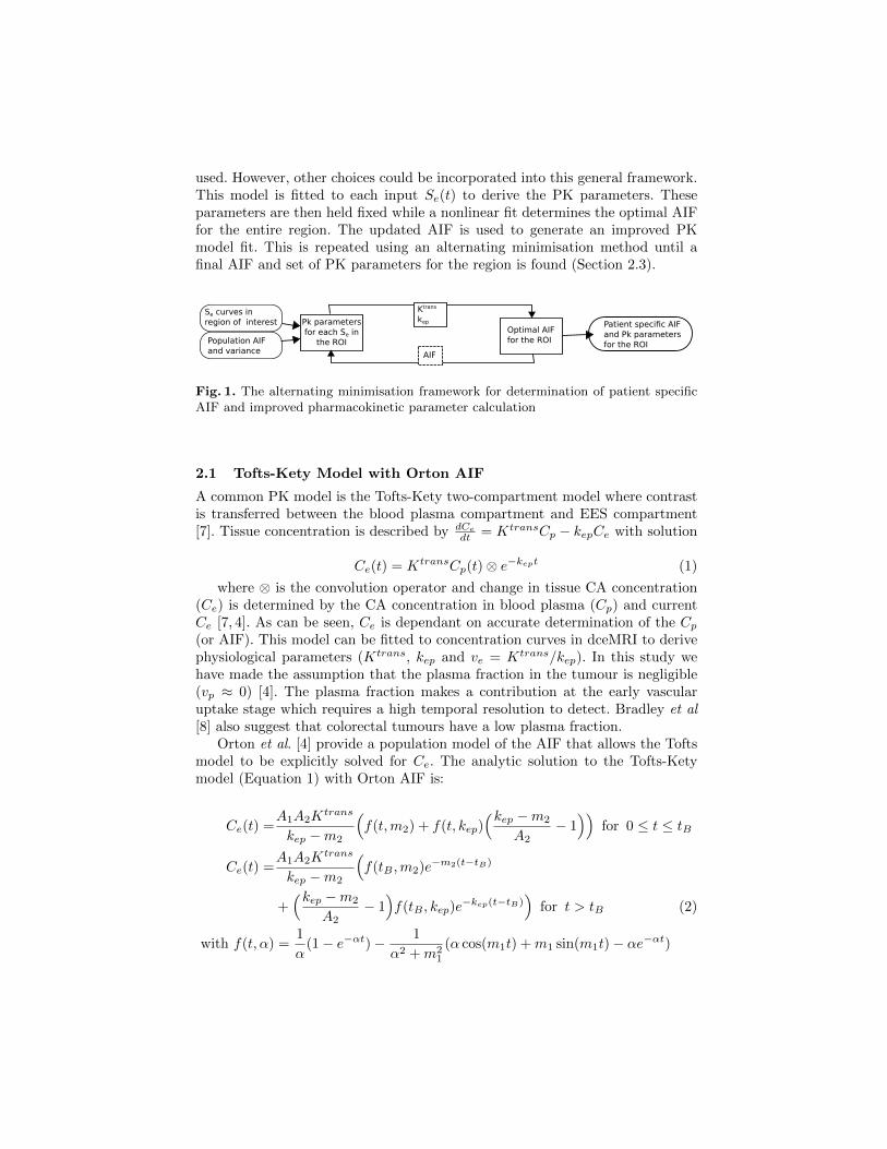
used. However, other choices could be incorporated into this general framework.This model is fitted to each input Se(t) to derive the PK parameters. Theseparameters are then held fixed while a nonlinear fit determines the optimal AIFfor the entire region. The updated AIF is used to generate an improved PKmodel fit. This is repeated using an alternating minimisation method until afinal AIF and set of PK parameters for the region is found (Section 2.3).

Population AIF and variance AIF

Ktrans

kep

Se curves inregion of interest

Optimal AIFfor the ROI

Pk parametersfor each Se in

the ROI

Patient specific AIFand Pk parametersfor the ROI

Fig. 1. The alternating minimisation framework for determination of patient specificAIF and improved pharmacokinetic parameter calculation

2.1 Tofts-Kety Model with Orton AIF

A common PK model is the Tofts-Kety two-compartment model where contrastis transferred between the blood plasma compartment and EES compartment[7]. Tissue concentration is described by dCe

dt = KtransCp − kepCe with solution

Ce(t) = KtransCp(t) ⊗ e−kept (1)

where ⊗ is the convolution operator and change in tissue CA concentration(Ce) is determined by the CA concentration in blood plasma (Cp) and currentCe [7, 4]. As can be seen, Ce is dependant on accurate determination of the Cp(or AIF). This model can be fitted to concentration curves in dceMRI to derivephysiological parameters (Ktrans, kep and ve = Ktrans/kep). In this study wehave made the assumption that the plasma fraction in the tumour is negligible(vp ≈ 0) [4]. The plasma fraction makes a contribution at the early vascularuptake stage which requires a high temporal resolution to detect. Bradley et al[8] also suggest that colorectal tumours have a low plasma fraction.

Orton et al. [4] provide a population model of the AIF that allows the Toftsmodel to be explicitly solved for Ce. The analytic solution to the Tofts-Ketymodel (Equation 1) with Orton AIF is:

Ce(t) =A1A2K

trans

kep −m2

(f(t,m2) + f(t, kep)

(kep −m2

A2− 1

))for 0 ≤ t ≤ tB

Ce(t) =A1A2K

trans

kep −m2

(f(tB ,m2)e−m2(t−tB)

+(kep −m2

A2− 1

)f(tB , kep)e

−kep(t−tB))

for t > tB (2)

with f(t, α) =1

α(1 − e−αt) − 1

α2 +m21

(α cos(m1t) +m1 sin(m1t) − αe−αt)

where A1, A1, m1 and m2 are the parameters of the AIF, Ktrans and kepare the PK parameters of interest, and tB = 2π/m1. AIF offset (τ) is includedin the AIF model to allow the bolus start time to be automatically determinedsuch that t = t̂− τ and Ce(t) = 0 for t < 0, where t̂ is the measured time.

The relationship between tissue concentration Ce(t) and observed signal en-hancement Se(t) in dceMRI is nonlinear. Ce(t) was converted to Se(t), using Se =

exp(−r2C(t)TE) 1−exp(−P−Q)−cosα(exp(−P )−exp(−2P−Q))1−exp(−P )−cosα(exp(−P−Q)−exp(−2P−Q)) , where P = TR/T10 and

Q = r1C(t)TR, TR is the repetition time, TE is the echo time and r1 and r2 areknown constants and α is the flip angle of the dceMRI image, from the SpoiledGradient Recalled (SPGR) sequence model [9].

A key limitation of fitting Equation 2 is that globally scaling the AIF pa-rameter A1 over the entire region has the same result as scaling Ktrans for eachvoxel. Therefore, A1 is fixed as the population average to form an additionalconstraint on the AIF model. In our method, we use this analytic solution toderive the patient specific AIF for the ROI and voxelwise PK parameters.

2.2 Population AIF

In our AIF estimation method, the population AIF with variance is used toinitialise and constrain the optimisation. Parker et al. [2] measured patient AIFsdirectly from high temporal-resolution dceMRIs of arteries of 67 scans of patientsbetween 18 - 80 years. They used these measurements to develop a parametricfunction of AIF variation in a population. This model cannot be used to solve Ceanalytically, and was used in our study to generate 1000 arterial input functionsby sampling from the population distribution. These curves provide an estimateof the population mean and variance, and Orton et al.’s [4] model was fittedto each curve to generate the population mean and standard deviation for themodel parameters: A1 = 2.65 ± 0.18mmol/l, A2 = 1.51 ± 0.68mmol/l, m1 =22.40 ± 0.73min−1 and m2 = 0.23 ± 0.46min−1. These mean values are used asthe initial AIF in order to derive a patient specific AIF.

2.3 Alternating Minimisation Method and Constraints

The previous sections outline the AIF and PK models that are used in ourpatient specific AIF estimation method. Optimal parameters for both the models(described in Section 2.1) are found from the dceMRI ROI in an alternatingminimisation method. The alternating minimisation method is initialised usingthe population AIF, and the model is fitted to each dceMRI Se curve to derivethe PK parameters using the ‘trust-region-reflective’ method for non-linear leastsquares curve fitting. In this initial step, PK parameters are derived for eachvoxel. These PK parameters are used to fit the same model over the entire regionto determine the optimal AIF parameters, while keeping the PK parametersfixed. This new AIF model is then used to improve the individual PK parameterestimation for each voxel. This is repeated until convergence (shown in Figure1).

Bounds are set on the AIF parameters to be within 4 standard deviations ofthe population average – representing 99.99% of the population – and a bound ofve ≤ 1. The lumen may be included in the ROI due to movement from peristalsis.To exclude these voxels, voxels that show no enhancement at temporal postionsafter initial enhancement are excluded.

Therefore, our model is able to obtain patient specific AIF and PK parame-ters without additional blood sampling, scans or the assumption of a populationAIF. This method was evaluated on synthetic and clinical datasets.

3 Materials

3.1 Synthetic Images

Synthetic data was used to evaluate the method by generating signal enhance-ment (Se) curves from known PK parameters and AIFs. These known PK pa-rameters and AIFs were compared to the parameters derived by our methodon the synthetic data. 30 synthetic cases were generated, each consisting 500signal enhancement curves. These were generated with 0%, 5% and 10% addednoise. Each of the 500 voxels consisted of 29 temporal positions with a temporalresolution of 9.5s – consistent with the clinical data in this Section.

Each case consisting of 500 voxels was generated from the same sampledAIF and each voxel from a set of PK parameters. AIFs were derived for eachcase by sampling from a Gaussian distribution over the means and standarddeviations of the Orton AIF parameters. This AIF was kept fixed for each ofthe 10 datasets while generating 500 Ktrans and kep pair to calculate individualsignal enhancement curves. Ktrans was derived from a uniform distribution onthe interval [0,2] and ve was derived from [0.4,1], kep = Ktrans/ve, and theoffset was sampled from [0, 0.5] minutes. These parameters and the AIF valueswere then used with the Tofts and Orton AIF model to generate the 500 signalenhancement curves. Noise was added to each temporal position of each voxel bysampling from a Gaussian distribution with standard deviation equal to 0%, 5%and 10% of the mean enhancement of the curve. Example synthetic Se curvesare shown in Figure 5c) and Figure 5f).

3.2 dceMRI Colorectal Cancer Cases

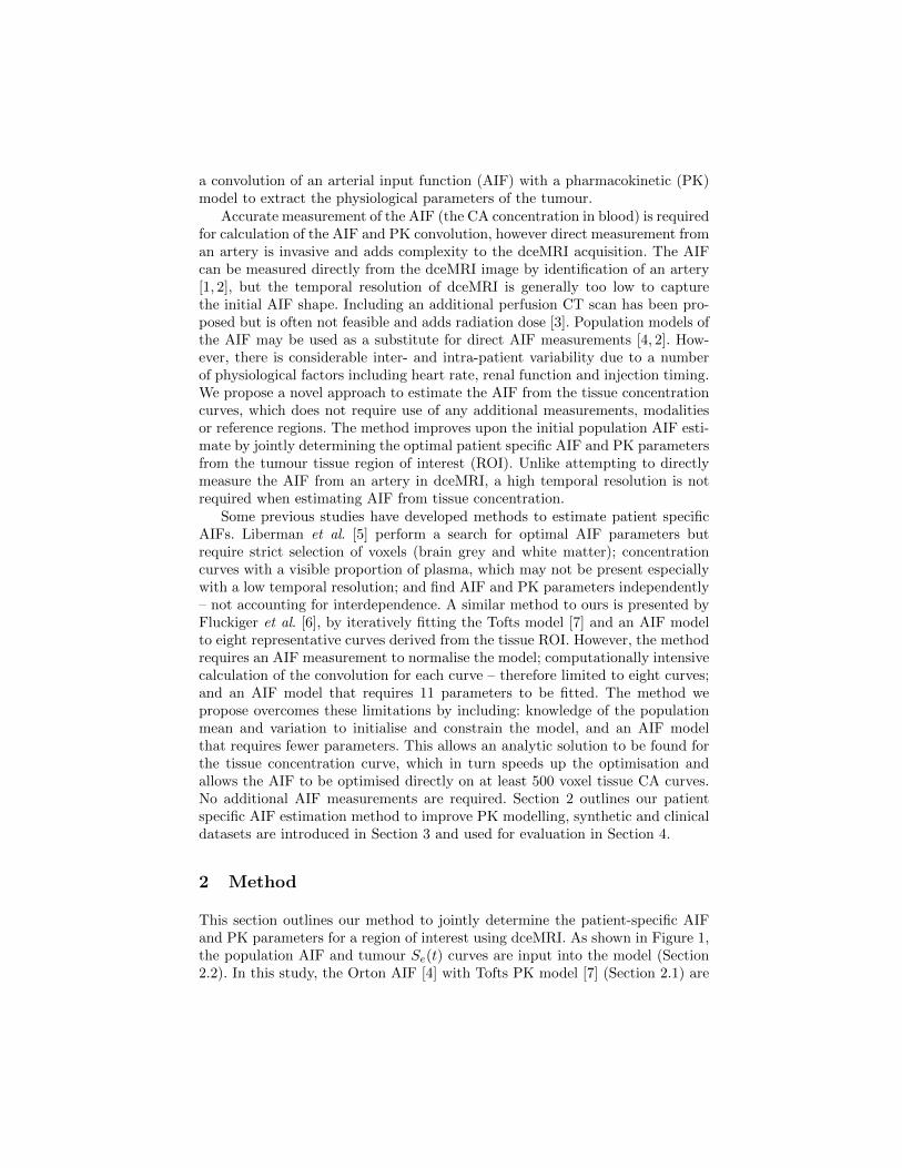
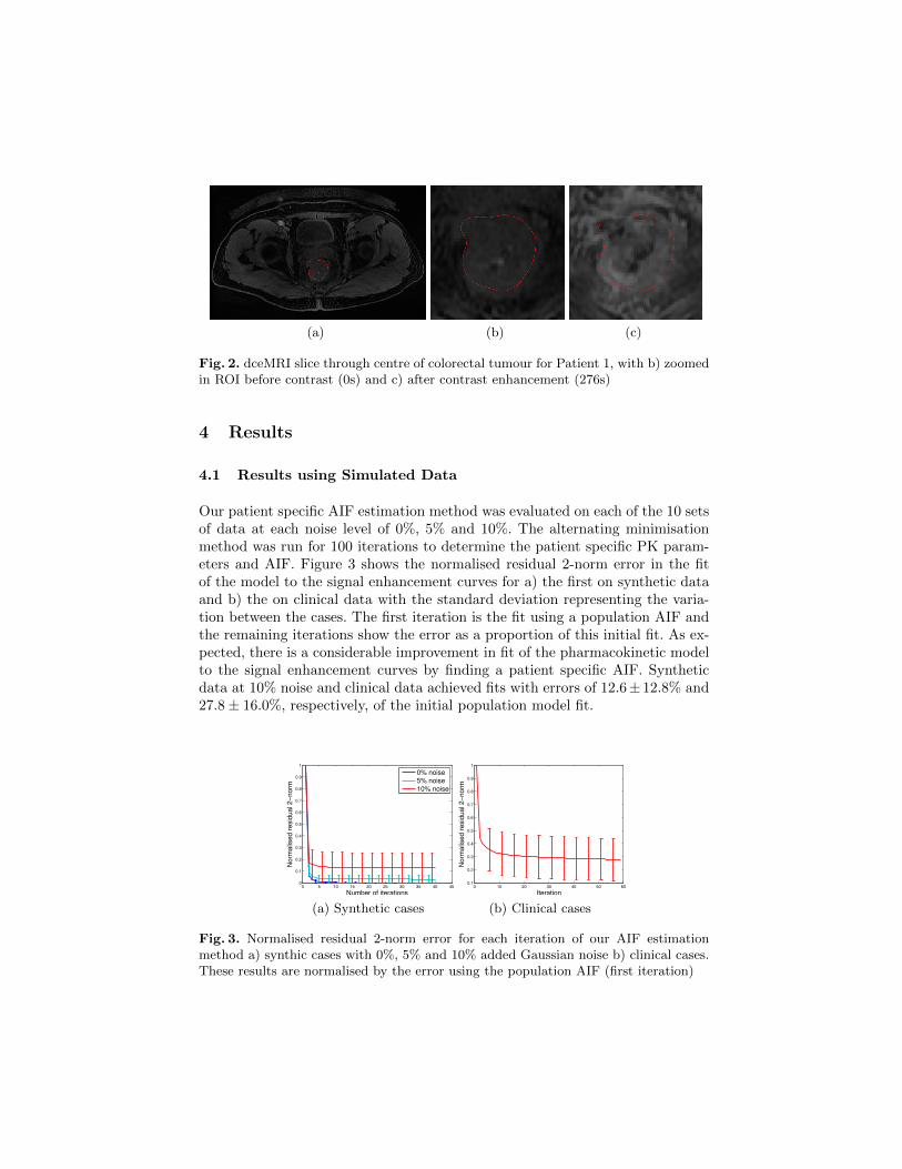
Six dceMRI images were acquired as part of a phase 0/1 drug trial with hy-pofractionated radiotherapy in patients with colorectal cancer. Pre- and post-treatment image sequences were acquired. A 3T GE scanner was used to ac-quire the dceMRI images with the LAVA protocol and spoiled gradient echosequence. Images with dimensions 512x512x52x29 were acquired with voxel sizeof 0.78x0.78x2.00mm, and a temporal resolution of 9.5s. ProHance (Gadoteriol)contrast was injected at a rate of 3 ml/sec, 0.1 mmol/kg body weight. Colorectaltumours were delineated by a clinician on T2 weighted images and registered tothe dceMRI image. Flip-angle images were not available and a uniform T10 mapof 1 was assumed. Figure 2 shows a cross section of a tumour ROI before andafter CA enhancement. Ktrans maps of this ROI are shown later in Figure 7.

(a) (b) (c)

Fig. 2. dceMRI slice through centre of colorectal tumour for Patient 1, with b) zoomedin ROI before contrast (0s) and c) after contrast enhancement (276s)

4 Results

4.1 Results using Simulated Data

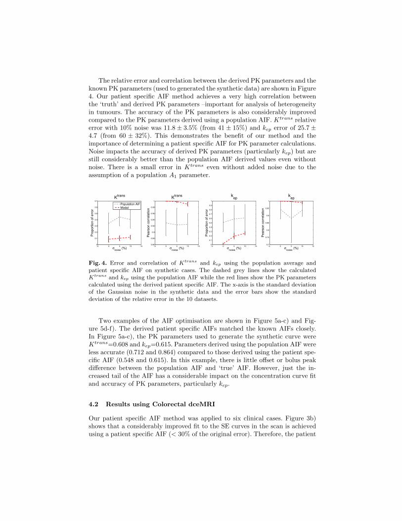
Our patient specific AIF estimation method was evaluated on each of the 10 setsof data at each noise level of 0%, 5% and 10%. The alternating minimisationmethod was run for 100 iterations to determine the patient specific PK param-eters and AIF. Figure 3 shows the normalised residual 2-norm error in the fitof the model to the signal enhancement curves for a) the first on synthetic dataand b) the on clinical data with the standard deviation representing the varia-tion between the cases. The first iteration is the fit using a population AIF andthe remaining iterations show the error as a proportion of this initial fit. As ex-pected, there is a considerable improvement in fit of the pharmacokinetic modelto the signal enhancement curves by finding a patient specific AIF. Syntheticdata at 10% noise and clinical data achieved fits with errors of 12.6± 12.8% and27.8 ± 16.0%, respectively, of the initial population model fit.

0 5 10 15 20 25 30 35 40 450

0.1

0.2

0.3

0.4

0.5

0.6

0.7

0.8

0.9

1

No

rma

lise

d r

esid

ua

l 2

−n

orm

Number of iterations

0% noise

5% noise

10% noise

(a) Synthetic cases

0 10 20 30 40 50 600.1

0.2

0.3

0.4

0.5

0.6

0.7

0.8

0.9

1

Iteration

No

rma

lise

d r

esid

ua

l 2

−n

orm

(b) Clinical cases

Fig. 3. Normalised residual 2-norm error for each iteration of our AIF estimationmethod a) synthic cases with 0%, 5% and 10% added Gaussian noise b) clinical cases.These results are normalised by the error using the population AIF (first iteration)

The relative error and correlation between the derived PK parameters and theknown PK parameters (used to generated the synthetic data) are shown in Figure4. Our patient specific AIF method achieves a very high correlation betweenthe ‘truth’ and derived PK parameters –important for analysis of heterogeneityin tumours. The accuracy of the PK parameters is also considerably improvedcompared to the PK parameters derived using a population AIF. Ktrans relativeerror with 10% noise was 11.8 ± 3.5% (from 41 ± 15%) and kep error of 25.7 ±4.7 (from 60 ± 32%). This demonstrates the benefit of our method and theimportance of determining a patient specific AIF for PK parameter calculations.Noise impacts the accuracy of derived PK parameters (particularly kep) but arestill considerably better than the population AIF derived values even withoutnoise. There is a small error in Ktrans even without added noise due to theassumption of a population A1 parameter.

−5 0 5 10 150

0.1

0.2

0.3

0.4

0.5

0.6

0.7

0.8

0.9

1

kep

σnoise

(%)

Pro

po

rtio

n o

f e

rro

r

−5 0 5 10 150.7

0.75

0.8

0.85

0.9

0.95

1

kep

σnoise

(%)

Pe

ars

on

co

rre

latio

n

−5 0 5 10 150

0.1

0.2

0.3

0.4

0.5

0.6

0.7

Ktrans

σnoise

(%)

Pro

po

rtio

n o

f e

rro

r

Population AIF

Model

−5 0 5 10 150.86

0.88

0.9

0.92

0.94

0.96

0.98

1

Ktrans

σnoise

(%)

Pe

ars

on

co

rre

latio

n

Fig. 4. Error and correlation of Ktrans and kep using the population average andpatient specific AIF on synthetic cases. The dashed grey lines show the calculatedKtrans and kep using the population AIF while the red lines show the PK parameterscalculated using the derived patient specific AIF. The x-axis is the standard deviationof the Gaussian noise in the synthetic data and the error bars show the standarddeviation of the relative error in the 10 datasets.

Two examples of the AIF optimisation are shown in Figure 5a-c) and Fig-ure 5d-f). The derived patient specific AIFs matched the known AIFs closely.In Figure 5a-c), the PK parameters used to generate the synthetic curve wereKtrans=0.608 and kep=0.615. Parameters derived using the population AIF wereless accurate (0.712 and 0.864) compared to those derived using the patient spe-cific AIF (0.548 and 0.615). In this example, there is little offset or bolus peakdifference between the population AIF and ‘true’ AIF. However, just the in-creased tail of the AIF has a considerable impact on the concentration curve fitand accuracy of PK parameters, particularly kep.

4.2 Results using Colorectal dceMRI

Our patient specific AIF method was applied to six clinical cases. Figure 3b)shows that a considerably improved fit to the SE curves in the scan is achievedusing a patient specific AIF (< 30% of the original error). Therefore, the patient

0 2 4 6 8 10 12 14 16 18 200

0.1

0.2

0.3

0.4

0.5

0.6

0.7

0.8

0.9

1

Iterations

Norm

alised r

esid

ual 2−

norm

(a)

0 0.5 1 1.5 2 2.5 3 3.5 40

1

2

3

4

5

6

7

Time (minutes)

Co

nce

ntr

atio

n (

mM

)

Truth

Population AIF

Patient specific AIF

(b)

0 1 2 3 4 50

0.2

0.4

0.6

0.8

1

1.2

1.4

1.6

1.8

Time (minutes)

Sig

nal enhancem

ent (S

(t)−

S(0

))/S

(0)

Simulated SE curve (5% noise)

SE (PS AIF)

SE (population AIF)

(c)

0 2 4 6 8 10 12 14 16 18 200

0.1

0.2

0.3

0.4

0.5

0.6

0.7

0.8

0.9

1

Iterations

Norm

alised r

esid

ual 2−

norm

(d)

0 0.5 1 1.5 2 2.5 3 3.5 40

1

2

3

4

5

6

7

Time (minutes)

Co

nce

ntr

atio

n (

mM

)

Truth

Population AIF

Patient specific AIF

(e)

0 1 2 3 4 50

0.2

0.4

0.6

0.8

1

1.2

1.4

1.6

1.8

Time (minutes)

Sig

nal enhancem

ent (S

(t)−

S(0

))/S

(0)

Simulated SE curve (10% noise)

SE (PS AIF)

SE (population AIF)

(f)

Fig. 5. Patient specific AIF compared to the known AIF for two synthetic cases a-cand d-f. a) and d) show the error between the known AIF and the estimated AIF overthe first 20 iterations of the algorithm. b) and e) compare the population AIF andthe derived patient specfic AIF to the known AIF used to generate the synthetic data(dashed curve). c) and e) show one example of the 500 signal enhancement curves ina case that are used to derive the parameters, where grey is the fitted curve using thepopulation AIF and black is the fitted curve using our patient specific AIF.

0 1 2 3 40

1

2

3

4

5

6

7

Time (minutes)

Concentr

ation (

mM

)

Pre−treatment 1

Pre−treatment 2

Post−treatment 1

Post−treatment 2

0 1 2 3 40

1

2

3

4

5

6

7

8

Time (minutes)

Concentr

ation (

mM

)

0 1 2 3 40

1

2

3

4

5

6

7

Time (minutes)

Concentr

ation (

mM

)

0 1 2 3 40

1

2

3

4

5

6

7

Time (minutes)

Concentr

ation (

mM

)

0 1 2 3 40

1

2

3

4

5

6

7

Time (minutes)

Concentr

ation (

mM

)

0 1 2 3 40

1

2

3

4

5

6

7

Time (minutes)

Concentr

ation (

mM

)

Fig. 6. Pre- and post-treatment AIFs found for 6 clinical colorectal cancer cases. TwoAIFs were generated using independent regions in the tumour in each image.

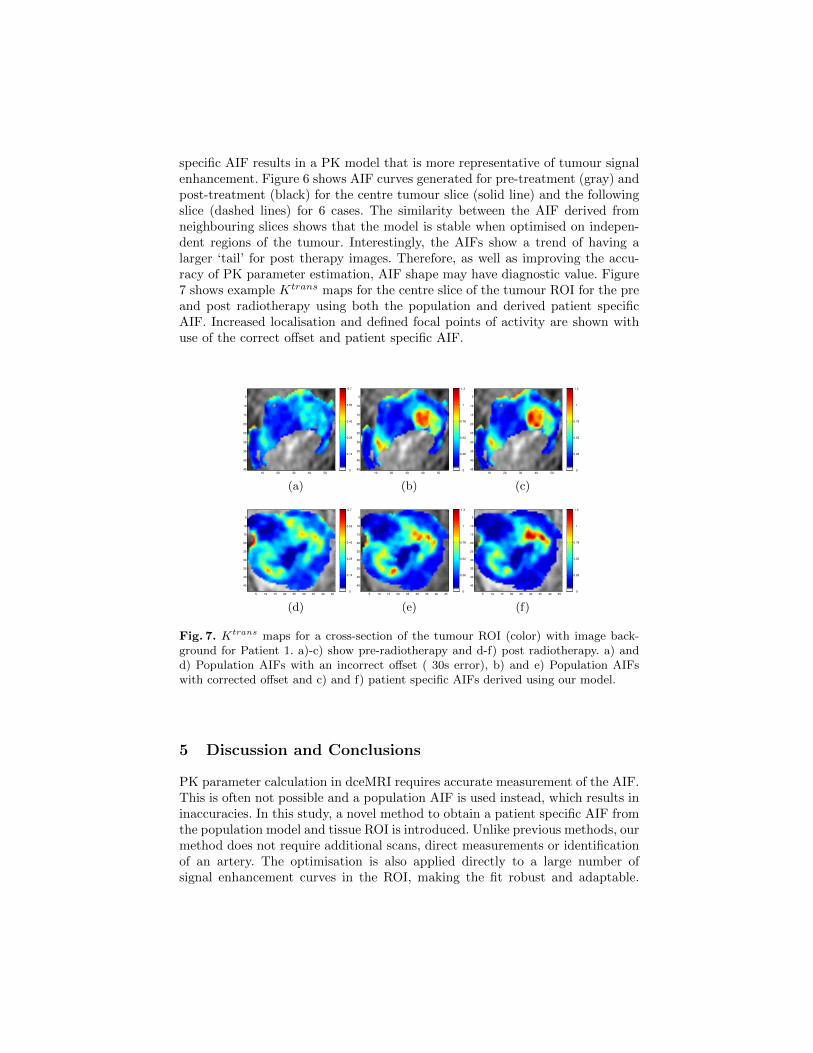
specific AIF results in a PK model that is more representative of tumour signalenhancement. Figure 6 shows AIF curves generated for pre-treatment (gray) andpost-treatment (black) for the centre tumour slice (solid line) and the followingslice (dashed lines) for 6 cases. The similarity between the AIF derived fromneighbouring slices shows that the model is stable when optimised on indepen-dent regions of the tumour. Interestingly, the AIFs show a trend of having alarger ‘tail’ for post therapy images. Therefore, as well as improving the accu-racy of PK parameter estimation, AIF shape may have diagnostic value. Figure7 shows example Ktrans maps for the centre slice of the tumour ROI for the preand post radiotherapy using both the population and derived patient specificAIF. Increased localisation and defined focal points of activity are shown withuse of the correct offset and patient specific AIF.

10 20 30 40 50

5

10

15

20

25

30

35

40

45 0

0.14

0.28

0.42

0.56

0.7

(a)

10 20 30 40 50

5

10

15

20

25

30

35

40

45 0

0.26

0.52

0.78

1

1.3

(b)

10 20 30 40 50

5

10

15

20

25

30

35

40

45 0

0.26

0.52

0.78

1

1.3

(c)

5 10 15 20 25 30 35 40 45

5

10

15

20

25

30

35

40

45

0

0.14

0.28

0.42

0.56

0.7

(d)

5 10 15 20 25 30 35 40 45

5

10

15

20

25

30

35

40

45

0

0.26

0.52

0.78

1

1.3

(e)

5 10 15 20 25 30 35 40 45

5

10

15

20

25

30

35

40

45

0

0.26

0.52

0.78

1

1.3

(f)

Fig. 7. Ktrans maps for a cross-section of the tumour ROI (color) with image back-ground for Patient 1. a)-c) show pre-radiotherapy and d-f) post radiotherapy. a) andd) Population AIFs with an incorrect offset ( 30s error), b) and e) Population AIFswith corrected offset and c) and f) patient specific AIFs derived using our model.

5 Discussion and Conclusions

PK parameter calculation in dceMRI requires accurate measurement of the AIF.This is often not possible and a population AIF is used instead, which results ininaccuracies. In this study, a novel method to obtain a patient specific AIF fromthe population model and tissue ROI is introduced. Unlike previous methods, ourmethod does not require additional scans, direct measurements or identificationof an artery. The optimisation is also applied directly to a large number ofsignal enhancement curves in the ROI, making the fit robust and adaptable.

This method considerably improves the PK model fit compared to the populationAIF for both synthetic and clinical dceMRI cases, leading to more accurate PKparameters. In synthetic data, the Ktrans relative error with 10% noise was11.8 ± 3.5% (from 41 ± 15%) and kep error of 25.7 ± 4.7 (from 60 ± 32%). Inclinical cases the AIF produces robust results for independent regions in thetumour. Future work will include: incorporation of motion correction into themethod and use of this patient specific AIF model to better estimate patientresponse to therapy. There is also potential to compare the personalised AIF todirect AIF measurements from high temporal resolution scans of an artery, andalso examine the effect of temporal resolution on AIF estimation.

Acknowledgements: This work was supported by the CRUK/EPSRC OxfordCancer Imaging Centre. We thank Prof. Fergus Gleeson for the dceMRI dataset.

References

1. Rijpkema, M., Kaanders, J.H., Joosten, F.B., van der Kogel, A.J., Heerschap, A.:Method for quantitative mapping of dynamic MRI contrast agent uptake in humantumors. Magn Reson Imaging 14, 457–63 (2001)

2. Parker, G., Roberts, C., Macdonald, A., Buonaccorsi, G., Cheung, S., Buckley, D.,Jackson, A., Watson, Y., Davies, K., Jayson, G.: Experimentally-derived functionalform for a population-averaged high-temporal-resolution arterial input function fordynamic contrast-enhanced MRI. Magn Reson Med 56, 993–1000 (2006)

3. Enescu, M., Bhushan, M., Hill, E.J., Franklin, J., Anderson, E.M., Sharma, R.A.,Schnabel, J.A.: pCT derived arterial input function for improved pharmacokineticanalysis of longitudinal dceMRI for colorectal cancer. SPIE p. 86690L (2013)

4. Orton, M.R., D’Arcy, J.a., Walker-Samuel, S., Hawkes, D.J., Atkinson, D., Collins,D.J., Leach, M.O.: Computationally efficient vascular input function models forquantitative kinetic modelling using DCE-MRI. Phys Med Biol 53, 1225–39 (2008)

5. Liberman, G., Louzoun, Y., Colliot, O., Ben Bashat, D.: T1 Mapping, AIF andPharmacokinetic Parameter Extraction from Dynamic Contrast Enhancement MRIData. In: Liu, T., Shen, D., Ibanez, L., Tao, X. (eds.) Multimodal Brain ImageAnalysis, LNCS, vol. 7012, pp. 76–83. Springer, Heidelberg (2011)

6. Fluckiger, J.U., Schabel, M.C., DiBella, E.V.R.: Model-based blind estimation ofkinetic parameters in dynamic contrast enhanced (DCE)-MRI. Magn Reson Med62, 1477–1486 (2009)

7. Tofts, P.S., Brix, G., Buckley, D.L., Evelhoch, J.L., Henderson, E., Knopp, M.V.,Larsson, H.B.W., Lee, T.Y., Mayr, N.A., Parker, Others: Estimating kinetic pa-rameters from dynamic contrast-enhanced T 1-weighted MRI of a diffusable tracer:standardized quantities and symbols. Magn Reson Imaging 10, 223–232 (1999)

8. Bradley, D.P., Tessier, J.L., Checkley, D., Kuribayashi, H., Waterton, J.C., Kendrew,J., Wedge, S.R.: Effects of AZD2171 and vandetanib (ZD6474, Zactima) on haemo-dynamic variables in an SW620 human colon tumour model : an investigation usingdynamic contrast-enhanced MRI and the rapid clearance blood pool contrast agent,20, 42–52 (2008)

9. Tofts, P.S., Kermode, A.G.: Measurement of the blood-brain barrier permeabilityand leakage space using dynamic MR imaging. 1. Fundamental concepts. MagnReson Med 17, 357–367 (1991)