www.elsevier.com/locate/yjtbi

Author’s Accepted Manuscript

Persistent random motion: uncovering cell migrationdynamics

Daniel Campos, Vicenç Méndez, Isaac Llopis

PII: S0022-5193(10)00496-0DOI: doi:10.1016/j.jtbi.2010.09.022Reference: YJTBI6162

To appear in: Journal of Theoretical Biology

Received date: 1 June 2010Revised date: 14 September 2010Accepted date: 15 September 2010

Cite this article as: Daniel Campos, Vicenç Méndez and Isaac Llopis, Persistent ran-dom motion: uncovering cell migration dynamics, Journal of Theoretical Biology,doi:10.1016/j.jtbi.2010.09.022

This is a PDF file of an unedited manuscript that has been accepted for publication. Asa service to our customers we are providing this early version of the manuscript. Themanuscript will undergo copyediting, typesetting, and review of the resulting galley proofbefore it is published in its final citable form. Please note that during the production processerrorsmay be discoveredwhich could affect the content, and all legal disclaimers that applyto the journal pertain.

Persistent random motion: Uncovering cell

migration dynamics

Daniel Campos ∗, Vicenc Mendez and Isaac Llopis

Grup de Fısica Estadıstica. Departament de Fısica. Universitat Autonoma de

Barcelona, 08193 Bellaterra (Cerdanyola) Spain

Preprint submitted to Journal of Theoretical Biology 14 September 2010

Abstract

In this paper we study analytically the stick-slip models recently introduced to

explain the stochastic migration of free cells. We show that persistent motion of

cells of many different types is compatible with stochastic reorientation models

which admit an analytical mesoscopic treatment. This is proved by examining and

discussing experimental data compiled from different sources in the literature, and

by fitting some of these results too. We are able to explain many of the ’apparently

complex’ migration patterns obtained recently from cell tracking data, like power-

law dependences in the mean square displacement or non-Gaussian behavior for the

kurtosis and the velocity distributions, which depart from the predictions of the

classical Ornstein-Uhlenbeck process.

∗ Corresponding author.

Email address: daniel.campos@uab.es (Daniel Campos).

2

1 Introduction

Studying the properties of cell movement is of fundamental interest to under-

stand many physiological processes in living organisms (embryogenesis, wound

healing, etc.) as well as their malfunctions (e.g. in tumors growth) . Exhaustive

research in this field is focused on the biophysical and biochemical intracellu-

lar processes driving cell signaling and motility. However, for many purposes

like the analysis of tracking experiments or the implementation of migration

algorithms into more general models, the use of phenomenological approaches

as those based on stochastic processes is extremely helpful. Within this con-

text, the Ornstein-Uhlenbeck (OU) process [1] has been considered for decades

the archetypal model to describe persistent random motion of cells or other

particles/organisms. This process is defined by the Langevin equation

dv

dt= −1

τv +

√2D

τξ(t), (1)

for the velocity vector v, where ξ(t) represents a vector with white-noise com-

ponents, D is the diffusion coefficient characteristic of Brownian motion, and

the timescale τ is often called the persistence time. Fibroblasts locomotion

[2], the motility of lung epithelial cells [3], microvessel endothelial cells [4] or

self-motile colloids [5] are just some examples from the vast amount of sys-

tems which have been successfully interpreted in the light of this model. Even

in recent studies where cells have been found experimentally to exhibit more

complex migration patterns, the OU process is still the reference model to

which more sophisticated approaches are compared [6–8].

The popularity of this approach is in part founded on the fact that the mean

square displacement (MSD) and the velocity auto-correlation function (VACF)

3

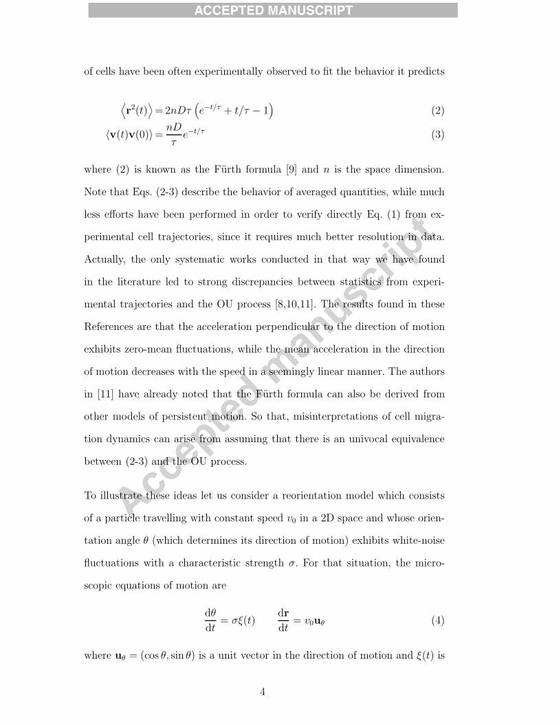
of cells have been often experimentally observed to fit the behavior it predicts

⟨r2(t)

⟩=2nDτ

(e−t/τ + t/τ − 1

)(2)

〈v(t)v(0)〉= nD

τe−t/τ (3)

where (2) is known as the Furth formula [9] and n is the space dimension.

Note that Eqs. (2-3) describe the behavior of averaged quantities, while much

less efforts have been performed in order to verify directly Eq. (1) from ex-

perimental cell trajectories, since it requires much better resolution in data.

Actually, the only systematic works conducted in that way we have found

in the literature led to strong discrepancies between statistics from experi-

mental trajectories and the OU process [8,10,11]. The results found in these

References are that the acceleration perpendicular to the direction of motion

exhibits zero-mean fluctuations, while the mean acceleration in the direction

of motion decreases with the speed in a seemingly linear manner. The authors

in [11] have already noted that the Furth formula can also be derived from

other models of persistent motion. So that, misinterpretations of cell migra-

tion dynamics can arise from assuming that there is an univocal equivalence

between (2-3) and the OU process.

To illustrate these ideas let us consider a reorientation model which consists

of a particle travelling with constant speed v0 in a 2D space and whose orien-

tation angle θ (which determines its direction of motion) exhibits white-noise

fluctuations with a characteristic strength σ. For that situation, the micro-

scopic equations of motion are

dθ

dt= σξ(t)

dr

dt= v0uθ (4)

where uθ = (cos θ, sin θ) is a unit vector in the direction of motion and ξ(t) is

4

white noise. One can now define the probability density P (r, θ, t) of finding the

particle at position r with orientation θ at time t, given the initial conditions

θ0, r0 = (0, 0). Applying standard techniques from stochastic calculus [12], we

can obtain the Fokker-Planck equation for the probability density P (see [13])

∂P

∂t=σ2

2

∂2P

∂θ2− v0uθ·�P. (5)

It is straightforward now to check from Eq. (5) that the MSD and the velocity

auto-correlation of a particle governed by this model also satisfy Eqs. (2-3),

with τ = 2/σ2, D = 2v20/σ2. So that it represents an alternative to the OU

process for describing persistent motion (see [13,14] for some seminal papers

on this field). The form of the first moments of P coincide for both models (1)

and (4), but their microscopic differences become apparent for higher-order

moments. For example, it is easy to check that the kurtosis 〈r4(t)〉 / 〈r2(t)〉2

is different in each model, though in both cases it tends to 3 for t → ∞, as

expected for a Gaussian variable.

Although it is not easy in general to elucidate the correct pattern of motion

from experimental data, we think that the reorientation model has some ad-

vantages over the classical approach in Eq. (1). Firstly, it seems more natural

to write the equations of motion in terms of the orientation coordinate θ (in-

stead of using a fixed coordinate system), according to the results for the

mean acceleration of cells reported in [8,11]. This will be specially appropriate

for the case of nonisotropic particles (for example, rod-shaped), which move

preferentially along one of their axis. Secondly, the simplicity of the reori-

entation model (4) makes generalizations of the model easier to implement,

while generalizations of the OU process often involve memory kernels or other

nontrivial effects. This has important implications on how experimental data

5

is interpreted, too. When the experimental results from cell trajectories are

observed to depart from the predictions of the OU process, it is often inter-

preted as a trace of complexity at some level. Here, we explore simple and

direct generalizations of the reorientation model which can explain many of

these ’apparently complex’ patterns of motion. Experimental data, obtained

from different works previously published, will be used to support these ideas

(Section 4).

2 Models overview

In this Section we summarize some of the different stochastic approaches that

have been recently proposed to explain the dynamics of self-propelled particles

(as is the case of cells in a diluted media). This will serve to put in context

the stick-slip model that will be presented and developed in Section 3.

2.1 Model in which speed and direction fluctuate independently

The assumption made in Eq. (4) that the particles travel with constant speed

can be relaxed by assuming instead that speed fluctuates around a mean value

〈v〉, giving rise to particles fluctuating both in their direction of motion and

their absolute speed. This model has been proposed recently to explain the

motion of propelled nanoparticles [15], but application to cell migration comes

straightforward. Actually, the same idea had also been explored in the context

of cell motion some years before [13], and similar models had already been used

to explain migration of Amoeba proteus [16,17] (though the results in those

works were mainly based in computer simulations).

6

Figure 1A describes schematically the microscopic behavior of a particle ac-

cording to this model. The dotted lines represent the cell trajectory, in which

changes of direction occur and the value of the speed changes at some instants

(these instants are marked by crosses). As can be seen from the situation of

the crosses, random changes in direction and speed are completely indepen-

dent processes. As a consequence, one can study separately the fluctuations in

speed and direction. If the cells are assumed to obey a certain velocity distri-

bution ρ(v) and the speed changes occur with a characteristic (constant) rate

β then

∂P (v, t)

∂t= −βP (v, t) + βρ(v) (6)

gives us the evolution of P (v, t), the probability density of particles traveling

with speed v at time t.

Similarly, for the orientation angle θ (defined as in the Introduction Section),

provided that orientation changes are smooth, one can use a diffusion approx-

imation

∂P (θ, t)

∂t= κ

∂2P (θ, t)

∂θ2. (7)

where κ is the diffusion parameter for the fluctuations in the direction of

motion.

The equations (6,7) can be exactly solved with the appropriate initial condi-

tions. Since changes in speed and direction are independent, one has P (v, θ, t) =

P (v, t) ·P (θ, t). Then, from standard statistics in 2D one can compute, for in-

stance, the mean distance travelled by the particle in this model < |r(θ, t)| >=∫ t0 dt

′∫∞

0 dvP (v, θ, t′)v, or any moment < rn >, < vn > of arbitrary order. So

it is found that the MSD reads [15]

7

⟨r2(t)

⟩=2〈v2〉 − 〈v〉2(κ+ β)2

(e−(κ+β)t + (κ + β)t− 1

)+

+2〈v〉2κ2

(e−κt + κt− 1

). (8)

The first term in Eq. (8) represents Brownian motion arising from a parti-

cle with a fluctuating speed, while the second term accounts for rotational

diffusion arising from the reorientation process.

For the VACF within this approach one obtains

〈v(t)v(0)〉 = 〈v〉2 e−κt +(⟨v2⟩− 〈v〉2

)e−(β+κ)t (9)

which exhibits a double-exponential decay, compared to the single exponential

one finds from the OU process.

2.2 Models with simultaneous fluctuations in speed and direction

In a recent work [18] two of the authors proposed a variation of the model

in Section 2.1. According to it, the time instants at which the speed of the

particle changes coincide with those where the direction changes (see Figure

1B). In the following, we will refer for simplicity to the models in Figures 1A

and 1B as ’model A’ and ’model B’, respectively. So, model B corresponds to a

motion pattern in which sojourns of constant speed are separated by (instanta-

neous) reorientation events. Though this is a relatively subtle modification of

the previous model, the fact that now both types of fluctuations are not inde-

pendent makes the present mathematical treatment quite different. In [18] we

use the framework of Continuous-Time RandomWalks (CTRW) to implement

this idea (see [19] for a comprehensive review on such models). Within this

framework one can derive an equation for the probability density P (r, θ, t). In

8

our specific case, this equation can only be explicitly written in the Fourier-

Laplace space; so the transformation P (r, θ, t) → P (qx, qy, θ, s) ≡ P is used,

with qx, qy, s being the transform variables of x, y, t respectively. The evolution

equation takes the form [18]

σ2

2

∂2P

∂θ2=

[s+ iv (qx cos θ + qy sin θ) +

v2D (qx cos θ + qy sin θ)2

s+ β + iv (qx cos θ + qy sin θ)

]P − 1

2π

(10)

where the parameter vD measures the amplitude of the speed fluctuations. So,

for vD = 0 it is clear that (5) will be recovered after inverting by Fourier-

Laplace.

From (10), the moments of P (r, θ, t) can also be found in a relatively easy way

(see [18] or the Appendix for further details). The expressions for the MSD and

the VACF one finds from (10) coincide with those from the model A (Eqs.

(8) and (9)) after redefining the parameter κ as σ2β. As it happened with

the two models discussed in the Introduction, these two approaches have the

same first and second-order moments, but the microscopic differences between

them (sketched in Figure 1) become evident for higher-order moments. The

main advantage of this second approach based in the CTRW is that different

extensions of the model can be implemented in a very natural way; this will

be shown in Section 3.

2.3 Models with memory kernels

In comparison with the two previous approaches, where the microscopic details

of the model (Figure 1) are absolutely clear, many other approaches used to fit

experimental data on cell migration are based on the introduction of memory

functions, or similar, into well established models, e.g. the OU process. One

9

example of this is the model presented in [10] and lately used in [8] to fit the

spontaneous movements of Dictyostelium cells. This approach is based on the

stochastic differential equations

dv

dt=−τ−1(v(t))v + μV(t) + σ(v(t))ξ(t) (11)

dV

dt=μv(t)− γV(t) (12)

where V(t) represents a memory function, whose time evolution is governed

by (12), while μ and γ represent constant parameters. Note also that velocity-

dependent friction (τ−1) and noise memory functions (σ) have been introduced

if compared with Eq. (1). All of these functions (V(t), σ(v(t)) and τ−1(v(t)))

are to be adjusted from data fitting.

Though this kind of models provide excellent agreement to data, their draw-

back is that they require the help of mechanistic models or similar in order

to justify the origin of such memory kernels so their hypothesis can be val-

idated. The aim of our work, however, is not to criticize models based on

kernels or memory effects, since the goodness of these models for fitting ex-

perimental data is clear. We just want to show that the experimental results

can often be explained too by means of approaches like those in Sections 2.1

and 2.2, or direct generalizations of them. In those cases, memory effects are

implicitly implemented through the time correlations introduced by the reori-

entation process. At this stage, we do not have any criteria to elucidate which

of these approaches work better. We just think that reorientation models rep-

resent a simpler and intuitive alternative to models based on kernels. Besides,

a complete analytical treatment is feasible for such models, which facilitates

understanding.

10

3 Mesoscopic description for stick-slip models

The concept of stick-slip processes has been introduced recently in [11]. Ac-

tually, it corresponds to the ”run and tumble” pattern long used to describe

bacterial motion [20]. However, in order to stress the connection of our work

with that in [11] we will rather use the term stick-slip.

In the original Reference [11], stick-slip processes have been introduced as a

sort of numerical models (algorithms) able to implement realistically protrusion-

retraction mechanisms responsible for cell migration. Here we will show that

the CTRW formalism we used in [18] can be extended to implement these

processes. By the analytical treatment of such models we expect to facilitate

their understanding and check their validity for fitting cell data.

According to the discussion in the Section 2.2, we will consider a cell trajectory

in 2D where the particle changes its direction of motion and absolute speed

jointly at some time instants with a characteristic rate β, while σ is a measure

of how much the orientation can change at each of these events. Now each

reorientation event is assumed to last a finite random time, controlled by a

constant characteristic rate β2. Regarding the distribution of speeds, we will

consider here the simplest version of the model, in which the particle travels

with constant speed v0 during the motion periods. We think that the general

model with an arbitrary distribution of velocities is also feasible analytically in

the light of the velocity models proposed in [21]; that case, however, involves

more complicated considerations, so we plan to deal with it in a separate

forthcoming work.

Following the lines of CTRW models (see [18,19] and the references therein),

11

we define Pi(r, θ, t) as the probability density for the particle to be located

at position r with orientation θ at time t. The label i = 1 stands for those

particles waiting (while reorienting) at that position, while i = 2 denotes the

particles in motion passing through that point. The total density of cells is

then computed as P = P1 + P2. Also, we need to introduce Ji(r, θ, t) as the

probability density of particles with orientation θ that at time t stop moving at

position r (i = 1), and those which start moving at position r after a waiting

period (i = 2). The evolution of the model is then given by the system of

mesoscopic equations

J1(r, θ, t) =∫

dr′∫ 2π

0dθ′

∫ t

0dt′J2(r− r′, θ′, t− t′)T (θ − θ′)ψ(r′, θ′, t′) +

δ(r)δ(t)

2π(13)

J2(r, θ, t) =∫ t

0dt′J1(r, θ, t− t′)ϕ(t′) (14)

P1(r, θ, t) =∫

dr′∫ t

0dt′J1(r, θ, t− t′)ϕ∗(t′) (15)

P2(r, θ, t) =∫

dr′∫ t

0dt′J2(r− r′, θ, t− t′)ψ∗(r′, θ, t′) (16)

where we have assumed for simplicity that initially all the particles start wait-

ing from position r = 0 at t = 0 (see the last term in Eq. (13)). The first

term on the right in (13) represents the contribution from those particles that

started moving at time t − t′ with orientation θ′ and then stop after cover-

ing a distance r′ in a travel time t′ (according to the probability distribution

ψ(r′, θ′, t′)) and take a new orientation value θ according to the distribution

T (θ−θ′). In Eq. (14) we apply the waiting times distribution ϕ(t′) for particles

which stopped moving at time t − t′ and start moving again at time t. The

distribution ϕ∗(t′) in (15) stands for the probability that the particle has not

started moving yet after a waiting time t′. Finally, in (16) ψ∗(r′,θ, t′) denotes

the probability that a particle has not stopped after a time t′ since it started

moving, during which it has covered a distance r′ in the direction θ.

12

Since we have assumed in Section 3 that moving and waiting periods are

governed by constant rates β and β2, respectively, we take the corresponding

probability distribution functions to be exponential (that is, a Markov assump-

tion). So that, for the constant speed case we have ψ(r, θ, t) = βe−βtδ(r−v0uθt)

and ϕ(t) = β2e−β

2t, where uθ represents, as mentioned above, a unit vector

in the direction of motion. Correspondingly, the other distributions will read

ψ∗(r, θ, t) = e−βtδ(r − v0uθt) and ϕ∗(t) = e−β2t. For further details on this

kind of models, the reader is addressed to the References [18,22,23].

For the case of a smooth reorientation process (smooth changes in θ), the

closed equations for P1 and P2 can be easily found and solved in the Fourier-

Laplace space (all the details are given in the Appendix). The moments of

these distributions can thus be found easily; for instance, we obtain for the

ensemble-averaged MSD

⟨r2(t)

⟩=∫ 2π

0dθ∫r2P (r, θ, t)dr = 2v20

(p0(t) + p1(t)e

−λ1t +5∑

k=2

pke−λkt

)(17)

where the functions p0(t), p1(t) are first-order polynomials in t and the pk’s

(for k = 2...5) are independent of t (the exact expressions for all of them are

provided in the Appendix). Likewise, the characteristic exponents λk read

λ1= β + β2

λ2=1

2

(β + β2 +

√(β + β2)

2 − 4ββ2σ2

)λ3=

1

2

(β + β2 −

√(β + β2)

2 − 4ββ2σ2

)λ4=

1

2

(β + β2 +

√(β + β2)

2 − 4β2σ2

)λ5=

1

2

(β + β2 −

√(β + β2)

2 − 4β2σ2

). (18)

From Eq. (17) and the explicit expression for p0(t) (see (32)) one finds out

13

how the asymptotic diffusion coefficient depends on the characteristics rates

in the model

D ≡ limt→∞

〈r2(t)〉4t

=v20βσ2

(β2

β + β2

)2

. (19)

On the other side, the VACF can be evaluated from (17) (since the motion

process is isotropic) by applying the Green-Kubo relation [24]

d⟨(x(t)− x(t0))

2⟩

dt0= 2

∫ t

t0〈vx(t′)vx(t0)〉 dt′ (20)

to each Cartesian coordinate, and evaluating this at t0 = 0, r(t0) = 0. That

calculation must be carried out only for the particles in state 2 (that is, for

P2(r, θ, t)), since particles in the state 1 have zero speed. The corresponding

result has the general form

〈v(t)v(0)〉 = v20

(m1(t)e

−λ1t +3∑

k=2

mke−λkt

), (21)

where again m1(t) is a first-order polynomial, and m2, m3 are constant param-

eters (combination of the pk’s). Although these are quite lengthy expressions,

the interesting feature from the results (17,21) is that they tell us that the

global dynamics of this stick-slip process is basically governed by up to 5 dif-

ferent timescales λ−1k (with k = 1...5) in the case of the MSD, or just 3 for the

case of the VACF. From that point of view, the stick-slip model considered

here involves an increasing level of complexity compared to the models A and

B, albeit the number of parameters in the model is the same (four) in both

cases (namely v0, β, β2, σ2). Obviously, introducing here an arbitrary distribu-

tion of speeds would increase this complexity even more. Note, however, that

Monte Carlo simulations of this process were conducted in [11] and the VACF

was fitted there just to a double-exponential (see Figure 5 in that Reference).

This is because for many choices of the parameters, two (or even the three) of

14

the timescales in (21) could take similar values and so in general they cannot

be distinguished graphically.

4 Experimental data for cell migration

In this Section we will try to show how reorientation models, as the stick-slip

case introduced in the previous Section, can explain many of the departures

from the OU process that have been found recently in different cell migration

experiments. To complete our discussion we will also compare with the results

obtained from the models A and B. We will discuss different parameters re-

ported in experimental works and will try to fit the experimental data to the

stick-slip process presented here. For such fitting procedure we will mainly

use the data collected in [8] for vegetative and starved (after 5.5 hours) Dic-

tyostelium discoideum cells (since this is one of the most exhaustive works we

have found in the literature), plus some data from References [6] and [11].

a) Mean-square displacement. This is probably the most recurrent pa-

rameter in studies on cell migration. The OU process predicts, according to

(2), a transition from ballistic to diffusive behavior which occurs at timescale

τ . However, departures from that formula have increasingly appeared during

the last years. Most of these departures consist of a power-law scaling of the

type 〈r2(t)〉 ∼ tα [6,8,25–27]. This easily connects with the theory of anoma-

lous diffusion, which is very popular among theoreticians at present [19], so

concepts like ’Levy flight’ or ’long-range memory’ are now relatively common

within this field. According to theoretical works, anomalous diffusion has dif-

ferent origins: i) long-range time correlations exist in the particles dynamics,

which can be a consequence of different internal or external mechanisms, or ii)

15

movement constraints are imposed by heterogeneous (fractal-like) media [28]

or by crowding effects [29]. In most works where power-law dependences of the

MSD have been found, the influence of external mechanisms or constraints has

been minimized. Thus, the only explanation seems to be that internal mech-

anisms in the cell should be responsible for the emergence of memory effects;

this has been the interpretation suggested by most of the authors. However,

this idea is quite speculative, since experimental evidence for these long-range

memory mechanisms is scarce, in the best case. According to that, we can

ask: ’Is there an alternative to explain why these power-law dependences are

observed so often without invoking such concepts from anomalous diffusion?’.

In our opinion a positive answer can be provided by the reorientation models

studied here (alternative answers have also been explored in the literature: for

example, it has been recently shown [30] that heterogeneous diffusivities in a

set of individual particles can lead statistically to the emergence of anomalous

diffusion at the ensemble level).

For the models depicted in Figure 1 the form of the MSD is given by (8).

According to that, the MSD will be mainly determined by the relative values

of the characteristic rates β and κ. For β � κ, the formula is completely

governed by κ and so a single ballistic-to-diffusive transition will be found,

as in the OU process. For β � κ two transitions at very different timescales

(one for each term in (8)) occur, so we observe a sequence ballistic-diffusive-

ballistic-diffusive [15]. Interestingly, for intermediate values of β the MSD often

fits quite well a power-law dependence 〈r2(t)〉 ∼ tα with an exponent α which

lies between 1 and 2. Exactly the same behavior holds for the expression (17)

we have derived for the stick-slip model.

These results for the MSD have been discussed in detail in [18], where they

16

have been used to interpret data from experiments with nanoparticles. Our

hypothesis is that the same could apply to cell migration data, so some of

the experimental works where anomalous diffusion has been reported could

actually correspond to a behavior like that in (8). There are some facts that

seem to support this idea:

i) The values of the anomalous exponents α found experimentally (in the

absence of crowding or geometrical constraints) are always between 1 and 2.

ii) The power-law tails in the MSD often extend over just one or two decades

of time values (in the best case) due to experimental limitations. So, it is not

clear that the asymptotic regime has been reached yet.

By ’asymptotic regime’ we mean here that the observational times have reached

the condition t� κ−1, where diffusive behavior should be recovered. This con-

dition is equivalent to the ’criterion for distinguishing true superdiffusion from

correlated random-walks’ given in [31]. The authors in that Reference already

detected the formal problem reported here and discuss its implications on the

analysis of cell motility data as well as for foraging in animals. So, this con-

troversy between anomalous or ’similar to anomalous’ is not a new problem.

Our hypothesis is tested by fitting the experimental data from [8] to the result

(17) and to the models A and B (Eq. (8)). Figure 2 (left) shows that both

models (solid and dotted lines, respectively) can fit reasonably well the ex-

perimental results, though apparently the data seems to exhibit a power-law

dependence (as claimed originally by the authors in [8]). For the sake of com-

pleteness, we also show the data fitting corresponding to the MSD results in

[6]. We stress, however, that from this fitting procedure it is very difficult to

determine which models fits the data best; anyway, this is not the aim of our

17

paper. To perform such a detailed study it would be necessary to have access

to the original raw data, and even in that case it is unlikely that concluding

results could be found.

b) Velocity autocorrelation function. We have already shown the results

for the VACF one obtains in the stick-slip model (Eq. (21)) and for reorienta-

tion models A and B (Eq. (9)). Such multi-exponential functions are able to

explain all the results of cell migration in 2D we have found in the literature.

For example, this double-exponential behavior has been explicitly observed in

experiments for HaCaT cells, dermal keratinocytes or different developmental

stages of Dictyostelium discoideum [8,10,11,32]. The single exponential decay

found in other works will be recovered when fluctuations in the speed are much

larger than fluctuations in the direction (β � κ). Also, in those cases when

the time resolution of observations is not good enough to reproduce accurately

the region t� (β + κ)−1, it will be impossible to observe experimentally the

second exponential term and a single exponential will be found. The only

exception is the case reported in [6], where the migration of epithelial Madin-

Carby canine kidney cells has been investigated. There, a power-law scaling

for the VACF has been observed. However, this behavior is found barely over

one decade of time values (see Figure 3 in [6]), so it is plausible that other

curves could be able to fit well the data, too.

The comparison between Eq. (21) (stick-slip model), Eq. (9) (obtained from

models A or B) and the data for Dictyostelium cells obtained from the exper-

imental setting in References [8] and [11] shows an excellent agreement too

(Figure 2, right and Figure 4, respectively). This reinforces the main idea of the

present paper, which is to show that stochastic reorientation models provide

an alternative description to cell migration patterns. Note that in Figure 2 we

18

have fitted simultaneously the MSD and the VACF just with the 4 parameters

of our model (see Figure Caption); the agreement found can be interpreted

as a verification of the Green-Kubo formula (20). More free parameters were

used in the original Reference [8] for the same fitting, though it must be noted

that the authors there also fitted the behavior of the cell acceleration as a

function of the velocity (this cannot be done in our case since we are not

using a Langevin description).

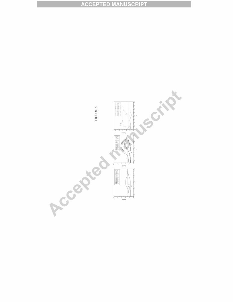
c) Kurtosis. Another parameter of special interest is the kurtosis 〈r4(t)〉 / 〈r2(t)〉2.It is known that this parameter must tend to 3 for a diffusive regime charac-

terized by a Gaussian distribution. This is not true, however, for anomalous

diffusion, since in that case the classical central limit theorem no longer ap-

plies. Unfortunately, the values of the kurtosis as a function of time are only

available for two of the references discussed throughout this paper [6,8]. In the

former [6] the asymptotic behavior of the kurtosis was found to tend asymptot-

ically to the value 2.3. This has been interpreted as a departure from Brownian

models, and so by the existence of a long-range memory effect. In the latter

[8], the tendency of the kurtosis towards 3 as t→∞ is found (note that in [8]

the kurtosis is defined as 〈r4(t)〉 / 〈r2(t)〉2 − 3 so there is a shift in the results

there). However, this asymptotic value is reached from above which is a de-

parture from the OU process, where the kurtosis is a monotonically increasing

function [1].

In fact, we show now that both results can be explained (qualitatively, at least)

from our reorientation models. Using the same calculation methods as reported

in [18] and [15], the fourth moment 〈r4(t)〉 can be calculated for the stick-slip

model and the two other models considered here. However, the corresponding

expressions one obtains are huge so we cannot reproduce them here; we just

19

show the corresponding plots for some arbitrary parameters (Figure 5). Note

that the two models in Figure 1 yield now different results, since (as stated

above) the microscopic differences between them become apparent for higher-

order moments.

Figure 5 confirms that the kurtosis exhibits a non-monotonic behavior which

is in a qualitative agreement with the results in [6,8]. Also, the stick-slip model

presented here is able to explain asymptotic deviations from the value 3 ex-

pected for Gaussian variables (Figure 5, right). In summary, this shows that

there is no need to account for memory effects or long tailed distributions

to explain such results. We must admit that a quantitative agreement with

experimental data, using the parameter values obtained from the fitting in

Figure 2, has been tried and the results are quite poor, specially for short

times (Figure 6). Note, however, that the models proposed in the References

[6,8] were not able to fit the short and intermediate-time regime for the kurto-

sis, neither. This is in fact a usual problem, which may be due to the fact that

discretization in data acquisition (both in time and space) strongly affect the

kurtosis values, specially for small times. This is another aspect of extreme

importance which requires further investigation [27].

d) Speed and velocity distributions. In the reorientation models consid-

ered here the speed probability distribution is a model input, so it cannot be

used to fit the experimental data; however, it is convenient to include some

comments about it. Usually, a standard assumption is to consider a Gaussian

distribution for v. However, several works have reported experimental evidence

of non-Gaussian (exponential or power-law-like) tails for these distributions.

To be more specific, one of the components of the velocity (for example, vx) is

observed to exhibit this unexpected behavior [8,10,25,26,33]. This is clearly a

20

departure from the OU process, where all the components of the velocity are

Gaussian variables. Instead, note this does not happen for the reorientation

models explored here. If one wants to find for the reorientation model the

probability distribution Q(vx) of the velocity component vx = v cos θ, this can

be done easily from probability theory. The formula [34]

Q(z) =∫∞

−∞

f(x,z

x

)1

| x |dx (22)

allows one to find the probability distribution of the product Z = XY of

two random variables X , Y , with f(x, y) being the joint distribution of these

two variables. For any reorientation model without a preferential direction of

motion, it can be assumed that the distribution of the θ values is uniform,

which leads to a probability distribution ∼ (1− cos2 θ)−1/2

for the variable

cos θ. Using this result and assuming a Gaussian distribution ∼ e−γv2

for the

speed, with a characteristic exponent γ, the Equation 22 can be applied. It

leads to the analytical solution

Q(vx) ∼ e−γv2x2π K0

(γv2x2π

)(23)

where K0() denotes the modified Bessel function of zeroth order. Clearly, the

expression (23) exhibits a non-Gaussian behavior for small and intermediate

times (in general it resembles very much an exponential decay). At long times,

however, it will tend to a Gaussian distribution, as the central limit theorem

requires. So, we see that, provided our window of experimental times cannot

reach the asymptotic regime t� κ−1 an exponential decay of the velocities will

be found, as observed in [10,33]. This cannot explain, however, why power-law

tails have been observed in other experimental works. In those works, it seems

that cell interactions were important (this happens for example in the case of

Hydra cells studied in [25]), while our approach here is restricted to free cells.

21

In other cases, velocities are computed from measuring the cell displacements

at scales smaller than the cell size [8]. For those observations cell deformation

is expected to play a major role in the short-time dynamics, so biomechanical

or mixed approaches [35] may be then more appropriate.

5 Conclusions

A reorientation model, equivalent to the stick-slip process introduced recently

in [11] has been presented and analytically explored from a mesoscopic CTRW

formalism in order to show its interest for cell migration. In addition, we have

provided an extensive review of those experimental works on cell migration

where departures from the OU process have been detected. By analyzing one

by one the main statistical parameters measured in those works we have been

able to show that our stochastic reorientation models are compatible with

most of the results observed. Again, we do not mean that motion of cells must

correspond necessarily to such microscopic patterns. Basically the contribution

of our work lies in showing that many departures from the OU process, which

had been previously attributed to memory kernels or other complex effects,

also admit a simpler interpretation. Since biological systems have multiple

and complex internal states, we think there is a great value in identifying

non-uniqueness in models that can describe experimental data. Models based

on memory kernels, as discussed in Section 2, rely on the hypothesis that

the interactions between the cells and the surrounding media leads to the

appearance of some specific memory effects, which requires justification from

biophysical (mechanistic) models. The approach presented here avoids that

drawback. Besides, the results obtained in [11,8], where the Langevin Equation

22

(1) has been tested directly, seem to support our general idea that reorientation

models represent a more appropriate way to describe cell motion.

While our approach can provide a quite general framework for the persistent

motion of free cells at low densities, it is clear that more complex situations

involving cell interactions or external stimuli are out of the scope of the present

work. More sophisticated approaches will be required for those situations, and

it is not clear yet if the CTRW formalism used here will be useful still in

that case. Note, for example, that even extremely simple interactions between

particles can lead to quite complicated collective and cooperative phenomena,

a topic which is at present under investigation (see [36] and the references

therein).

Anyway, even for the noninteracting particles considered here many questions

remain open. For example: if stochastic reorientation can really explain most

of cell migration patterns, do then these patterns correspond to any functional

advantage as an optimal search strategy (in the line of the results reported in

[37])? Is it really possible to describe the short-time dynamics of cell migration

(which is rather dominated by cell deformations) just by stochastic approaches

based in point particles? How does the time-discretization introduced in data

acquisition affect all these results? These questions are just to illustrate that

understanding cell migration patterns still represents a really challenging task.

6 Appendix

The system of Eqs. (13-16) can be explicitly solved for some particular cases

in order to reach an expression for the MSD. Introducing all the probability

23

distribution functions given in the text into (13-16), and transforming from

the real coordinates (r, t) to Fourier-Laplace coordinates (qx, qy, s) = (q, s),

this system of equations takes the much more manageable form

J1(q, θ, s) =∫ 2π

0dθ′

βT (θ − θ′)

s+ β + iv0 [qx cos (θ′) + qy sin (θ

′)]J2(q, θ

′, s) +1

2π(24)

J2(q, θ, s) =β2

s+ β2

J1(q, θ, s) (25)

P1(q, θ, s) =1

s+ β2

J1(q, θ, s) (26)

P2(q, θ, s) =1

s+ β + iv0(qx cos θ + qy sin θ)J2(q, θ, s) (27)

where we use the hat (·) to denote the Fourier-Laplace transform. In the

following, we will obviate for simplicity the explicit dependence of J and P

in their variables. Now, if we assume that orientation changes are smooth we

can expand (24) for θ→ θ′, which yields up to second order

J1 =

(1 + σ2 ∂

2

∂θ2

)β

s + β + iv0 (qx cos θ + qy sin θ)J2 +

1

2π(28)

where σ2 ≡ 12

∫ 2π0 θ2T (θ) is the variance of the distribution T (θ), a measure of

how much the orientation θ can be changed. Note also that we have assumed

in Eq. (28) the orientation process to be isotropic, so∫ 2π0 θT (θ) = 0. Now,

we can obtain from the system of Eqs. (25-28) the closed expressions for the

density distributions P1 and P2:

0= βσ2∂2P2

∂θ2+

(β − s+ β2

β2

[s+ β + iv0(qx cos θ + qy sin θ)]

)P2 +

1

2π(29)

P1=s+ β + iv0(qx cos θ + qy sin θ)

β2

P2 (30)

These equations can be formally inverted to the real coordinates (r, t) but

a solution for P1(r, θ, t), P2(r, θ, t) cannot be explicitly found. However, the

MSD is easier to compute in the Fourier-Laplace coordinates from 〈r2(s)〉 =

24

−[∂2P∂q2x

+ ∂2P∂q2x

]0, where P = P1 + P2 and the subindex 0 denotes that the

function is being evaluated at qx = 0, qy = 0. In [18] we have provided an

easy method for doing this. First we find[P1

]0and

[P2

]0by solving (29-

30), integrating then over θ and imposing the particle conservation condition

[P1 + P2]0 = 12πs

. Next, we differentiate (29-30) with respect to qx and use

the previous result to find[∂P1

∂qx

]0and

[∂P2

∂qx

]0, and we do the same for qy. By

repeating this procedure again, we finally find

⟨r2(s)

⟩=

2v20(s+ β2)2

s2(s+ β + β2)2

(β2

s2 + (β + β2) s+ ββ2σ2+

s+ β

s2 + (β + β2) s+ β2σ2

).

(31)

This expression, inverted from the Laplace coordinate s back to t, takes finally

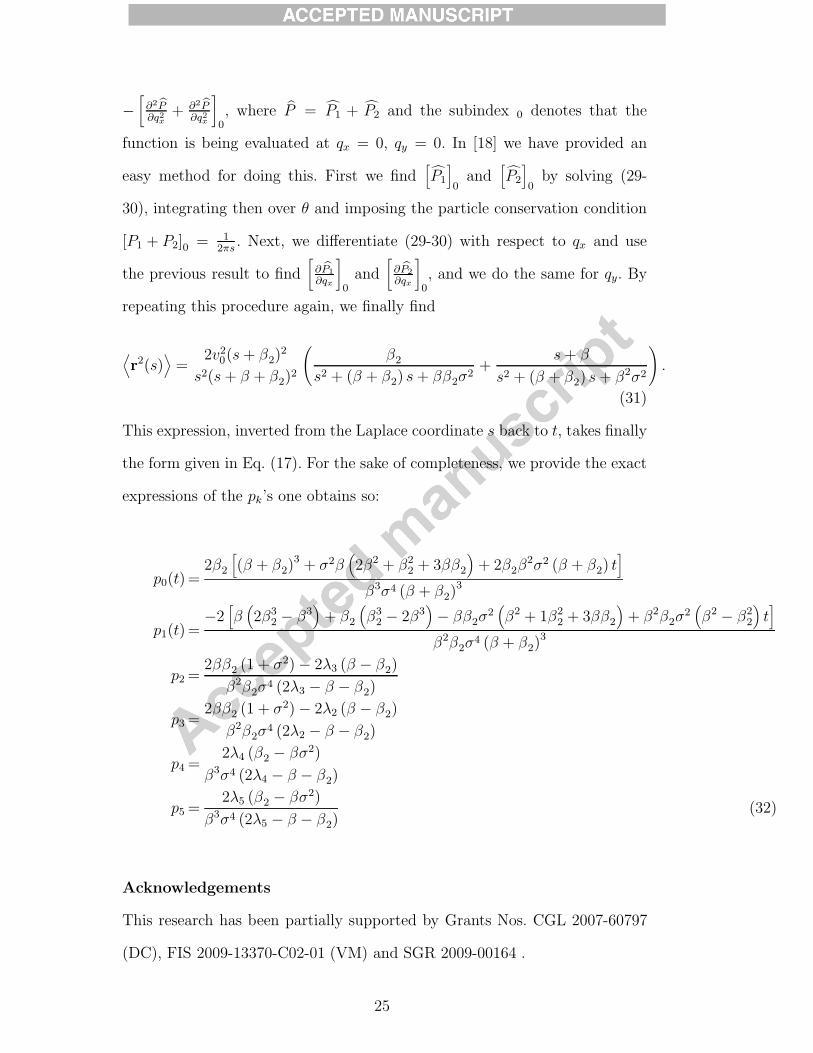
the form given in Eq. (17). For the sake of completeness, we provide the exact

expressions of the pk’s one obtains so:

p0(t)=2β2

[(β + β2)

3 + σ2β(2β2 + β2

2 + 3ββ2

)+ 2β2β

2σ2 (β + β2) t]

β3σ4 (β + β2)3

p1(t)=−2

[β(2β3

2 − β3)+ β2

(β32 − 2β3

)− ββ2σ

2(β2 + 1β2

2 + 3ββ2

)+ β2β2σ

2(β2 − β2

2

)t]

β2β2σ4 (β + β2)

3

p2=2ββ2 (1 + σ2)− 2λ3 (β − β2)

β2β2σ4 (2λ3 − β − β2)

p3=2ββ2 (1 + σ2)− 2λ2 (β − β2)

β2β2σ4 (2λ2 − β − β2)

p4=2λ4 (β2 − βσ2)

β3σ4 (2λ4 − β − β2)

p5=2λ5 (β2 − βσ2)

β3σ4 (2λ5 − β − β2)(32)

Acknowledgements

This research has been partially supported by Grants Nos. CGL 2007-60797

(DC), FIS 2009-13370-C02-01 (VM) and SGR 2009-00164 .

25

References

[1] Uhlenbeck, G.E. and L.S. Ornstein. 1931 On the Theory of Brownian Motion.

Phys. Rev. 36:823-841.

[2] Gail, M.H. and C.W. Boone. 1970 The Locomotion of Mouse Fibroblasts in

Tissue Culture. Biophys. J. 10:980-993.

[3] Wright, A., Y.-H. Li and C. Zhu. 2008 The Differential Effect of Endothelial

Cell Factors on in vitro Motility of Malignant and non-malignant Cells. Ann.

Biomed. Eng. 36:958-969.

[4] Stokes, C.L., D.A. Lauffenburger and S.K. Williams. Migration of individual

microvessel endothelial cells: stochastic model and parameter measurement. J.

Cell Sci. 99:419-430 (1991).

[5] Howse, J.R., R.A.L. Jones, A.J. Ryan, T. Gough, R. Vafabakhsh and R.

Golestanian. 2007 Self-Motile Colloidal Particles: From Directed Propulsion to

Random Walk. Phys. Rev. Lett. 99: 048102.

[6] Dieterich, P., R. Klages, R. Preuss and A. Schwab. 2008 Anomalous dynamics

of cell migration. Proc. Natl. Acad. Sci. USA 105:459-463.

[7] Li, L., S.F. Norrelykke and E.C. Cox. 2008 Persistent Cell Motion in the Absence

of External Signals: A Search Strategy for Eukaryotic Cells. PLoS One 3:e2093.

[8] Takagi, H., M.J. Sato, T. Yanagida and M. Ueda. 2008 Functional Analysis

of Spontaneous Cell Movement under Different Physiological Conditions. PLoS

One 3:e2648.

[9] Furth, R. 1920 Zeits f. Physik 2:244.

[10] Selmeczi, D., S. Mosler, P.H. Hagedorn, N.B. Larsen and H. Flyvbjerg. 2005 Cell

Motility as Persistent Random Motion: Theories from Experiments. Biophys.

J. 89:912-931.

26

[11] Selmeczi, D., L. Li, L.I.I. Pedersen, S.F. Nrrelykke, P.H. Hagedorn, S. Mosler,

N.B. Larsen, E.C. Cox and H. Flyvbjerg. 2008 Cell motility as random motion:

A review. Eur. Phys. J. Special Topics 157:1-15.

[12] Gardiner, C.W. 2004 Handbook of Stochastic Methods for Physics, Chemistry

and the Natural Sciences, 3rd Ed. Berlin: Springer.

[13] Schienbein, M. and H. Gruler. 1993. Langevin Equation, Fokker-Planck

Equation and Cell Migration. Bull. Math. Biol. 55:585-608.

[14] Othmer, H.G., S.R. Dunbar and W. Alt. 1988. Models of dispersal in biological

systems. J. Math. Biol. 26:263-298.

[15] Peruani, F. and L.G. Morelli. 2007 Self-Propelled Particles with Fluctuating

Speed and Direction of Motion in Two Dimensions. Phys. Rev. Lett. 99:010602.

[16] Miyoshi, H., N. Masaki and Y. Tsuchiya. 2003 Characteristics of trajectory in

the migration of Amoeba proteus. Protoplasma 222:175-181.

[17] Masaki, N., H. Miyoshi and Y. Tsuchiya. 2007 Characteristics of motive force

derived from trajectory analysis of Amoeba proteus. Protoplasma 230:69-74.

[18] Campos, D. and V. Mendez. 2009 Superdiffusive-like motion of colloidal

nanorods. J. Chem. Phys. 130:134711.

[19] Metzler, R. and J. Klafter. 2000 The Random Walk’s Guide to Anomalous

Diffusion: a Fractional Dynamics Approach. Phys. Rep. 339:1-77.

[20] Berg, H.C. 2004 E. Coli in Motion. New York: Springer.

[21] Zaburdaev, V., M. Schmiedeberg and H. Stark. 2008 Random walks with

random velocities. Phys. Rev. E 78:011119.

[22] Zumofen, G. and J. Klafter. 1993 Scale-invariant motion in intermittent chaotic

systems. Phys. Rev. E 47:851-863.

27

[23] Mendez, V., D. Campos and S. Fedotov. 2004 Front propagation in reaction-

dispersal models with finite jump speed. Phys. Rev. E 70:036121.

[24] Kubo, R., M. Toda and N. Hashitsume. 1991 Statistical physics II,

Nonequilibrium statistical mechanics, 2nd Ed. Berlin: Springer.

[25] Upadhyaya, A., J.-P. Rieu, J.A. Glazier and Y. Sawada. 2001 Anomalous

diffusion and non-Gaussian velocity distribution of Hydra cells in cellular

aggregates. Physica A 293:549-558.

[26] Thurner, S., N. Wick, R. Hanel, R. Sedivy and L. Huber. 2003 Anomalous

diffusion on dynamical networks: a model for interacting epithelial cell

migration. Physica A 320:475-484.

[27] Potdar, A.A., J. Lu, J. Jeon, A.M. Weaver and P.T. Cummings. 2009. Bimodal

Analysis of Mammary Epithelial Cell Migration in Two Dimensions. Ann.

Biomed. Eng. 37:230-245.

[28] Ben-Avraham, D. and S. Havlin. Diffusion and reactions in fractals and

disordered systems. Cambridge Univ. Press (Cambridge, 2005).

[29] Banks, D.S. and C. Fradin. 2005 Anomalous Diffusion of Proteins Due to

Molecular Crowding. Biophys. J. 89:2960-2971.

[30] S. Hapca, J.W. Crawfors and I. M. Young. 2009 Anomalous diffusion of

heterogeneous populations characterized by normal diffusion at the individual

level. J. R. Soc. Interface 6:111-122.

[31] Viswanathan, G.M., E.P. Raposo, F. Bartomeus, J. Catalan and M.G.E. da Luz.

2005 Necessary criterion for distinguishing true superdiffusion from correlated

random walk processes. Phys. Rev. E 72:011111.

[32] Maeda, Y.T., J. Inose, M.Y. Matsuo, S. Iwaya and M. Sano. 2008 Ordered

Patterns of Cell Shape and Orientational Correlation during Spontaneous Cell

Migration. PLoS One 3:e3734.

28

[33] Czirok, A., K. Schlett, E. Madarasz and T. Vicsek. 1998 Exponential

Distribution of Locomotion Activity in Cell Cultures. Phys. Rev. Lett. 81:3038-

3041.

[34] Rohatgi, V.K. 1976 An Introduction to Probability Theory and Mathematical

Statistics. New York: Wiley.

[35] Ohta, T. and T. Ohkuma. 2009 Deformable Self-Propelled Particles. Phys. Rev.

Lett. 102:154101.

[36] F. Ginelli, F. Peruani, M. Bar and H. Chate. 2010 Large-Scale Collective

Properties of Self-Propelled Rods. Phys. Rev. Lett. 104:184502.

[37] Friedrich, B.M. 2008 Search along persistent random walks. Phys. Biol.

5:026007.

Figure captions

Figure 1.

Random-walk representation of the model in [15] (Model A) and in [18] (Model

B). The dotted lines represent the trajectory of a particle, and the crosses are

the random instants at which it changes the value of speed.

Figure 2.

Comparison between the results from the stick-slip model presented here (solid

lines), the models A and B (dotted lines) and the experimental data extracted

from [8] for vegetative and starved Dictyostelium cells (symbols, see Legends).

A simultaneous fitting for the MSD and the VACF data has been performed.

The fitted parameters are, for the stick-slip model, β = 2.56 s−1, β2 = 3.64 s−1,

29

σ = 0.62, v0 = 6.80 μm/s (vegetative cells) and β = 2.11 s−1, β2 = 3.91 s−1,

σ = 0.48, v0 = 16.5 μm/s (starved cells). For the other case we obtain β = 4.87

s−1, κ = 0.64 s−1, < v >= 2.52 μm/s, < v2 >= 20.6 μm2/s2 (vegetative cells)

and β = 12.31 s−1, κ = 0.30 s−1, < v >= 9.79 μm/s, < v2 >= 376.7 μm2/s2

(starved cells).

Figure 3.

MSD comparison between the results from the stick-slip model presented here

(solid lines), the models A and B (dotted lines) and the experimental data

extracted from [6] for Madin-Darby canine kidney cell strains of the wild type

and NHE-deficient (symbols, see Legend). The fitted parameters are, for the

stick-slip model, β = 1.08 s−1, β2 = 0.19 s−1, σ = 0.36, v0 = 1.19 μm/s

(wild-type) and β = 1.02 s−1, β2 = 0.27 s−1, σ = 0.30, v0 = 1.42 μm/s

(NHE-deficient). For the other case we obtain β = 0.70 s−1, κ = 0.017 s−1,

< v >= 0.83 μm/s, < v2 >= 2.92 μm2/s2 (wild-type) and β = 0.14 s−1,

κ = 0.011 s−1, < v >= 0.49 μm/s, < v2 >= 1.01 μm2/s2 (NHE-deficient).

Figure 4.

VACF comparison between the results from the stick-slip model presented

here (solid lines), the models A and B (dotted lines) and the experimental

data for AX4 strains of Dictyostelium cells obtained in [11] (asterisks). The

fitted parameters are, for the stick-slip model, β = 1.20 s−1, β2 = 1.08 s−1,

σ = 0.41, v0 = 5.43 μm/s. For the models A and B we obtain β = 2.07 s−1,

κ = 0.10 s−1, < v >= 4.95 μm/s, < v2 >= 63.2 μm2/s2.

Figure 5.

Comparison for the kurtosis between models A (left) and B (middle), and the

30

stick-slip model presented here (right), for different (arbitrary) values of the

parameters. For the speed distributions we have taken for simplicity a double

Dirac delta 12[δ (〈v〉+ vD) + δ (〈v〉 − vD)] (the values of the parameters are

given in the legend). The dashed line denotes a value of the kurtosis equal to

3 (Gaussian variable). This relatively complex behavior is in contrast with the

monotonic growth one finds for the OU process.

Figure 6.

Comparison between the values of the kurtosis obtained from the stick-slip

model (solid lines), the model A (dotted lines) and the experimental data

extracted from [8] for vegetative and starved Dictyostelium cells (symbols).

The values of the parameters are the same as those adjusted in Figure 2.

31

xx

x

xx

x

x

x x

xx

x

���

���

FIG

UR

E 1

0.0

0.5

1.0

1.5

2.0

2.5

3.0

3.5

4.0

100

101

102

Veg

etat

ive c

ells

Sta

rved

cel

ls

VACF (µm2/min

2)

time (

min

)0.

010.

11

1010

-2

10-1

100

101

102

103

104

Veg

etat

ive

cells

Sta

rved

cel

ls

MSD (µm2)

time

(min

)

Figu

re 2

110

100

110100

1000

1000

0

FIG

UR

E 3

Wild

cel

ls N

HE-

defic

ient

cel

lsMSD (µm

2/min)

time

(min

)

05

1015

20110100

VACF (µm2/min

2)

time

(min

)

FIG

UR

E 4

100

101

102

103

104

105

106

107

108

0246810

(d)

(c)

(b)

(a)

(a) �

=0.

01 �

�=0.

03 �

=1.

0 v

0=1.

0

(b) �

=0.

1 � �

=0.

3 �

=0.

01 v

0=1.

0

(c) �

=0.

03 �

�=0.

01 �

=1.

0 v

0=1.

0

(d) �

=0.

3 � �

=0.

1 �

=0.

01 v

0=1.

0

kurtosis

t10

010

110

210

310

40246810

(d)

(c)

(b)

kurtosist

(a)

(a) �

=0.

3 �

=0.

01 <

v>=

2.0

v*=

1.0

(b) �

=0.

3 �

=0.

01 <

v>=

2.0

v*=

0.1

(c) �

=0.

01 �

=0.

3 <

v>=

2.0

v*=

1.0

(d) �

=0.

01 �

=0.

3 <

v>=

2.0

v*=

0.1

100

101

102

103

104

0246810

(d)

(c)

(b)

(a)(a

) �=

0.3 �

=0.

01 <

v>=

2.0

v*=

1.0

(b) �

=0.

3 �

=0.

01 <

v>=

2.0

v*=

0.1

(c) �

=0.

01 �

=0.

3 <

v>=

2.0

v*=

1.0

(d) �

=0.

01 �

=0.

3 <

v>=

2.0

v*=

0.1

kurtosis

t

FIG

UR

E 5

0.1

110

02040 V

eget

ativ

e ce

lls S

tarv

ed c

ells

kurtosis

time

(min

)

FIG

UR

E 6