Performance evaluation of carbon-dioxide sensors used in building HVAC applications
103
Graduate eses and Dissertations Graduate College 2009 Performance evaluation of carbon-dioxide sensors used in building HVAC applications Som Sagar Shrestha Iowa State University Follow this and additional works at: hp://lib.dr.iastate.edu/etd Part of the Mechanical Engineering Commons is Dissertation is brought to you for free and open access by the Graduate College at Digital Repository @ Iowa State University. It has been accepted for inclusion in Graduate eses and Dissertations by an authorized administrator of Digital Repository @ Iowa State University. For more information, please contact [email protected]. Recommended Citation Shrestha, Som Sagar, "Performance evaluation of carbon-dioxide sensors used in building HVAC applications" (2009). Graduate eses and Dissertations. Paper 10507.
-
Upload
independent -
Category
Documents
-
view
1 -
download
0
Transcript of Performance evaluation of carbon-dioxide sensors used in building HVAC applications

Graduate Theses and Dissertations Graduate College
2009
Performance evaluation of carbon-dioxide sensorsused in building HVAC applicationsSom Sagar ShresthaIowa State University
Follow this and additional works at: http://lib.dr.iastate.edu/etd
Part of the Mechanical Engineering Commons
This Dissertation is brought to you for free and open access by the Graduate College at Digital Repository @ Iowa State University. It has been acceptedfor inclusion in Graduate Theses and Dissertations by an authorized administrator of Digital Repository @ Iowa State University. For moreinformation, please contact [email protected].
Recommended CitationShrestha, Som Sagar, "Performance evaluation of carbon-dioxide sensors used in building HVAC applications" (2009). Graduate Thesesand Dissertations. Paper 10507.

Performance evaluation of carbon-dioxide sensors used in
building HVAC applications
by
Som Sagar Shrestha
A dissertation submitted to the graduate faculty
in partial fulfillment of the requirements for the degree of
DOCTOR OF PHILOSOPHY
Major: Mechanical Engineering
Program of Study Committee:
Gregory M. Maxwell, Major Professor
Ron M. Nelson
Steven J. Hoff
Michael B. Pate
Stephen B. Vardeman
Iowa State University
Ames, Iowa
2009
Copyright © Som Sagar Shrestha, 2009. All rights reserved.
ii
This work is dedicated to energy savvy professionals who are dedicated to energy efficiency enhancement in every engineering
application.

iii
Table of Contents
Acknowledgements ................................................................................................................................................... vi
Abstract ................................................................................................................................................................... vii
Chapter 1: General Introduction ............................................................................................................................... 1
Introduction ............................................................................................................................................................ 1
Dissertation Organization ....................................................................................................................................... 2
Literature Review ................................................................................................................................................... 2
Chapter 2: An Experimental Evaluation of HVAC-Grade Carbon-Dioxide Sensor: Part 1, Test and
Evaluation Procedure.............................................................................................................................................. 4
Abstract .................................................................................................................................................................. 4
Introduction ............................................................................................................................................................ 4
HVAC-Grade CO2 Sensors .................................................................................................................................... 6
Procurement and Handling of the Sensors ............................................................................................................. 8
Experimental Apparatus and Instrumentation ........................................................................................................ 9
Experimental Methodology .................................................................................................................................. 15
Data Analysis ....................................................................................................................................................... 23
Conclusions .......................................................................................................................................................... 26
Acknowledgements .............................................................................................................................................. 26
References ............................................................................................................................................................ 27
Appendix .............................................................................................................................................................. 28
Chapter 3: An Experimental Evaluation of HVAC-Grade Carbon-Dioxide Sensor: Part 2,
Performance Test Results .................................................................................................................................... 31
Abstract ................................................................................................................................................................ 31
Introduction .......................................................................................................................................................... 31
Previous Studies ................................................................................................................................................... 32
Configurations of NDIR CO2 Sensors .................................................................................................................. 33
iv
CO2 Sensor Specifications .................................................................................................................................... 34
Experimental Test Procedure ............................................................................................................................... 36
Accuracy Test Results .......................................................................................................................................... 37
Linearity Test Results ........................................................................................................................................... 48
Repeatability Test Results .................................................................................................................................... 49
Hysteresis Test Results ......................................................................................................................................... 50
Conclusions .......................................................................................................................................................... 50
Acknowledgements .............................................................................................................................................. 53
References ............................................................................................................................................................ 53
Chapter 4: An Experimental Evaluation of HVAC-Grade Carbon-Dioxide Sensor: Part 3, Humidity,
Temperature, and Pressure Sensitivity Test Results ........................................................................................ 54
Abstract ................................................................................................................................................................ 54
Introduction .......................................................................................................................................................... 55
Previous Studies ................................................................................................................................................... 55
CO2 Sensor Specifications .................................................................................................................................... 56
Experimental Test Procedure ............................................................................................................................... 57
Humidity Sensitivity Test Results ........................................................................................................................ 59
Temperature Sensitivity Test Results ................................................................................................................... 63
Pressure Sensitivity Test Results ......................................................................................................................... 67
Conclusions .......................................................................................................................................................... 72
Acknowledgements .............................................................................................................................................. 73
References ............................................................................................................................................................ 73
Chapter 5: An Experimental Evaluation of HVAC-Grade Carbon-Dioxide Sensor: Part 4, Effects of
Ageing on Sensor Performance ........................................................................................................................... 74
Abstract ................................................................................................................................................................ 74
Introduction .......................................................................................................................................................... 74
Previous Studies ................................................................................................................................................... 75

v
CO2 Sensor Specifications .................................................................................................................................... 76
Experimental Test Procedure ............................................................................................................................... 78
Ageing Test Results ............................................................................................................................................. 84
Conclusions .......................................................................................................................................................... 89
Acknowledgements .............................................................................................................................................. 89
References ............................................................................................................................................................ 89
Chapter 6: General Conclusions ............................................................................................................................. 90
General Discussion ............................................................................................................................................... 90
Recommendations for Future Research ................................................................................................................ 93
References ................................................................................................................................................................. 94

vi
Acknowledgements
I would like to express my sincere gratitude and appreciation to my major professor Dr. Gregory M.
Maxwell. I am glad to pronounce that I have had a wonderful time working under his supervision and cherished
each and every moment with him. He has always been there for me in time of need for every support and
guidance. I have been lucky to have been given a chance to work with Dr. Maxwell.
This research was performed for National Building Controls Information Program (NBCIP), which is
sponsored by the Iowa Energy Center, NSTAR Electric & Gas Corporation and the California Commission. I
am grateful for valuable advises and support from Dr. John House, Mr. Curtis J. Klaassen, and all individuals
who were involved directly or indirectly in this research. I am also thankful for the cooperation and assistance
from Larry Hanft and other technical staff in the Mechanical Engineering Department at Iowa State University.
Thanks to Dr. Ron M. Nelson, Dr. Steven J. Hoff, Dr. Michael B. Pate, and Dr. Stephen B. Vardeman for
their valuable feedback and participation in my program of study.
I would like to gratefully acknowledge my parents Ganga Sagar Shrestha and Bikumaya Sagar Shrestha,
wife Jarina Shrestha, daughter Swechha Shrestha, son Sakar Sagar Shrestha, brothers Krishna Sagar Shrestha
and Dev Sagar Shrestha and all family members for their constant support and encouragement to accomplish
this achievement.

vii
Abstract
Carbon-dioxide sensors are widely used as part of a demand controlled ventilation (DCV) system for
buildings requiring mechanical ventilation, and their performance can significantly impact energy use in these
systems. Therefore, a study was undertaken to test and evaluate the most commonly used CO2 sensors in HVAC
applications, namely the non-dispersive infrared (NDIR) type.
Fifteen models of NDIR HVAC-grade wall-mounted CO2 sensors were tested and evaluated to determine
the accuracy, linearity, repeatability, hysteresis, humidity sensitivity, temperature sensitivity, and pressure
sensitivity of each sensor as well as effect of long-term ageing on sensor performance. All tests were conducted
in a chamber specifically designed and fabricated for this research. In all, 45 sensors were evaluated: three from
each of the 15 models. Among the 15 models tested, eight models have a single-lamp, single-wavelength
configuration, four models have a dual-lamp, single-wavelength configuration, and three models have a single-
lamp, dual-wavelength configuration. All single-lamp single-wavelength sensors and one single-lamp dual-
wavelength sensor incorporate an “automatic baseline adjustment” algorithm in the sensor’s electronics
package.
The accuracy, linearity, repeatability, and hysteresis of the sensors were evaluated at a fixed relative
humidity, temperature, and pressure, by varying CO2 concentrations from 400 ppm to 1800 ppm. The test
results showed a wide variation in sensor performance among the various manufacturers and in some cases a
wide variation among sensors of the same model.
The humidity sensitivity was evaluated by varying the relative humidity from 20% to 60% while holding
the CO2 concentration, temperature, and pressure fixed. The temperature sensitivity was evaluated by varying
the temperature from 66°F (18.9°C) to 80°F (26.7°C) while holding the gas composition and pressure fixed.
The pressure sensitivity was evaluated by varying the pressure from 14.70 psia (101.35 kPa) to 11.80 psia
(81.36 kPa) while holding the gas composition and temperature fixed.
The test results showed that while humidity sensitivity of most of the sensors is negligibly small, some
sensors are strongly affected by humidity. The test results also showed that the effects of temperature and
pressure variation on NDIR CO2 sensors are unavoidable. For the range of temperature and pressure variation in
viii
an air-conditioned space, the effect of pressure variation is more significant compared to the effect of
temperature variation.
The long-term ageing effect was evaluated at four month intervals for one year. The result showed a wide
variation in ageing effect among manufacturers. Some sensor models showed a nominal ageing effect of less
than 30 ppm deviation in one year; whereas, all three sensors of one model showed significant ageing effects,
up to -376 ppm deviation, in one year at 1100 ppm CO2 concentration.
1
Chapter 1: General Introduction INTRODUCTION
Almost 40% of total energy consumption in the U.S. is used in buildings (DOE, 2007). Typical buildings
consume 20% more energy than necessary (CEC, 2002). Fortunately, the opportunities to reduce building
energy consumptions are significant (Sun et al, 2006). Six-quadrillion Btu of energy that accounts for about 6%
of national energy demand is consumed for space heating, cooling, and ventilation of commercial buildings.
Controlling ventilation air flow rates using CO2-based demand controlled ventilation (DCV) offers the
possibility of reducing the energy penalty associated with over-ventilation during periods of low occupancy,
while still ensuring adequate levels of outdoor air ventilation (Emmerich and Persily 2001). A report prepared
for the U.S. Department of Energy (Roth et al. 2005) suggests that demand controlled ventilation (DCV) can
reduce both heating and cooling energy of commercial buildings by about 10%.
Carbon-dioxide sensors are widely used as part of a demand controlled ventilation (DCV) system for
buildings requiring mechanical ventilation to monitor indoor air CO2 concentration and to control the outdoor
air intake rate to maintain indoor air quality (IAQ). Performance of CO2 sensors can significantly impact energy
use as well as IAQ in these buildings. Overestimation of the CO2 concentration by the sensors will lead to
increased outdoor air usage causing increased energy cost. Underestimation may lead to poor IAQ and Sick
Building Syndrome (SBS). The purpose of this research was to test and evaluate the most commonly used CO2
sensors in HVAC systems, namely the non-dispersive infrared (NDIR) type.
The procedures presented here provide a methodology to test and evaluate NDIR CO2 sensors for accuracy,
linearity, repeatability, hysteresis, humidity sensitivity, temperature sensitivity, and pressure sensitivity. The test
and evaluation procedures presented in this study are all inclusive in that they range from procuring the CO2
sensor to comparing the performance of the sensors. Specifically, a procedure is presented to both procure CO2
sensors from the manufacturers and to maintain quality control by controlling the storage and handling of the
sensors. Further, it describes the apparatus and instrumentation, along with test conditions, used to test the
sensors. Additionally, it outlines a detailed experimental procedure to evaluate the accuracy of the sensors.
Finally, a discussion is presented on analyzing and comparing the performance of CO2 sensors by using the test
data.

2
DISSERTATION ORGANIZATION
There are a total of four papers included in this dissertation (Chapters 2 to 5). The first paper has been
accepted for publication in ASHRAE Transactions and will be presented at the ASHRAE Summer meeting
(June 2009, Louisville, KY). The remaining papers are in the final stages of editing and will be submitted to
ASHRAE in the next few weeks.
The experimental procedure and the apparatus designed and fabricated for this research are discussed in
Chapter 2. This procedure provides a detailed description of the methodology used to evaluate the performance
of wall-mounted CO2 sensors for accuracy, linearity, repeatability, hysteresis, humidity sensitivity, temperature
sensitivity, and pressure sensitivity. Additionally, steady-state criteria for recording data from the CO2 sensors
as well as some preliminary test results are discussed.
Chapter 3 presents the performance test results, including accuracy, linearity, repeatability, and hysteresis
of CO2 sensors. The chapter describes the various configurations used by CO2 sensor manufacturers to
minimize ageing of the sensors and compares actual performance of the sensors with the manufacturer
specifications.
Humidity, temperature, and pressure sensitivity of CO2 sensors are discussed in Chapter 4. The sensitivity
of the sensor reading to each of these three parameters was computed and compared to the manufacturers’
specifications.
The effect of ageing on sensor drift is discussed in Chapter 5. The ageing tests are designed to assess the
long-term performance of the wall-mounted NDIR CO2 sensors that have been exposed to environmental
conditions of a building application. Sensor behavior during power-up and conditioning period is also discussed
in the chapter.
LITERATURE REVIEW
In the past, limited studies have been done to investigate the performance of HVAC-grade CO2 sensors
using a controlled environment. Fahlen et al. (1992) evaluated the performance of two CO2 sensors, one photo-
acoustic type and one infrared spectroscopy type, in lab tests and long term field tests. The lab tests included
performance and environmental tests. The authors conclude that the deviation between actual concentration and
the sensors’ reading are normally well within ± 50 ppm at a concentration level of 1000 ppm. However, at a

3
concentration of 2000 ppm the test results showed a deviation of up to -300 ppm. The output of one sensor
increased dramatically during environmental testing. This sensor failed to return to its normal value.
Fisk et al. (2006) conducted a pilot study that evaluated the in-situ accuracy of 44 NDIR CO2 sensors
located in nine commercial buildings. The evaluation was performed either by multi-point calibration using CO2
calibration gas or by a single-point calibration check using a co-located and calibrated reference CO2 sensor.
Their results indicated that the accuracy of CO2 sensors is frequently less than what is needed to measure peak
indoor-outdoor CO2 concentration differences with an error that is less than 20%. Thus, the authors conclude
that there is a need for more accurate CO2 sensors and/or better maintenance and calibration. The effects of
humidity, temperature, and pressure on the sensor readings were not considered in the study.
Pandey et al. (2007) evaluated the accuracy of two NDIR CO2 sensor models. They tested three sensors of
each model. The tests were performed in an enclosure designed for the experiment, where all six sensors were
simultaneously exposed to CO2 concentration of 0 ppm, 500 ppm, and 1000 ppm (other environmental
conditions, such as humidity, temperature, and pressure were not specified.) The maximum deviation was
observed as -73 ppm at a CO2 concentration of 500 ppm. The research focused on the sensor accuracy but did
not include effects of humidity, temperature, and pressure variation on the sensor output.
A study conducted at the Iowa Energy Center showed that, among the three new, co-located sensors, one
sensor read about 105 ppm higher, compared to the two other sensors, at about 400 ppm (House 2006). Nine
months later, the sensor that read 105 ppm higher at the beginning, read 265 ppm higher compared to the two
other sensors.
Further review of the literature reveled that there is no present standard method of test available by which
CO2 sensors are evaluated. Therefore, an experimental procedure for testing and evaluating the sensors was
developed for this research.

4
Chapter 2: An Experimental Evaluation of HVAC-Grade Carbon-Dioxide
Sensors: Part 1, Test and Evaluation Procedure
A paper accepted by the ASHRAE Transactions, 2009, 115 (2)
Som S. Shrestha Gregory M. Maxwell, PhD Student Member ASHRAE Member ASHRAE
ABSTRACT
Carbon-dioxide sensors are widely used as part of a demand controlled ventilation (DCV) system for
buildings requiring mechanical ventilation, and their performance can significantly impact energy use in these
systems. Therefore, a study was undertaken to test and evaluate the most commonly used CO2 sensors in HVAC
systems, namely the non-dispersive infrared (NDIR) type. The procedures presented here provide a
methodology to test and evaluate NDIR CO2 sensors for accuracy, linearity, repeatability, hysteresis, humidity
sensitivity, temperature sensitivity, and pressure sensitivity.
The test and evaluation procedures presented in this paper are all inclusive in that they range from
procuring the CO2 sensor to comparing the performance of the sensors. Specifically, a procedure is presented to
both procure CO2 sensors from the manufacturers and to maintain quality control by controlling the storage and
handling of the sensors. Further, it describes the apparatus and instrumentation, along with test conditions, used
to test the sensors. Additionally, it outlines a detailed experimental procedure to evaluate the accuracy of the
sensors. Finally, a discussion is presented on analyzing and comparing the performance of CO2 sensors by using
the test data. Partial results of the accuracy test and evaluation of the CO2 sensors and the results of the linearity,
repeatability, hysteresis, humidity sensitivity, temperature sensitivity, and pressure sensitivity evaluation are
included in this paper. The full test results will be presented in a later publication.
INTRODUCTION
Controlling ventilation air flow rates using CO2-based demand controlled ventilation (DCV) offers the
possibility of reducing the energy penalty associated with over-ventilation during periods of low occupancy,
while still ensuring adequate levels of outdoor air ventilation (Emmerich and Persily 2001). A report prepared

5
for DOE (Roth et al. 2005) suggests that DCV can reduce both heating and cooling energy by about 10% or
about 0.3 quadrillion Btu (316 quadrillion Joules) annually.
Carbon-dioxide (CO2) sensors are gaining popularity in building HVAC systems to monitor indoor air CO2
concentration and to control outdoor air intake rate. The sensing technology most commonly used for HVAC
applications is the optical method of non-dispersive infrared (NDIR). The performance of these sensors is
crucial not only to ensure energy savings but also to assure indoor air quality. In CO2-based DCV systems, the
CO2 level of indoor air is monitored and the outdoor air flow rate is adjusted based on the sensor output to
maintain acceptable CO2 concentration in the occupied space. Sensors which read high will call for more
outdoor air leading to an energy penalty. Sensors which read low will cause poor indoor air quality.
CO2 sensors are reported to have technology-specific sensitivities, and unresolved issues including drift,
overall accuracy, temperature effect, water vapor, dust buildup, and aging of the light sources, etc. (Dougan and
Damiano 2004). Fahlen et al. (1992) evaluated the performance of two CO2 sensors, one photo-acoustic type
and one IR spectroscopy type, in lab tests and long term field tests. The lab tests included performance and
environmental tests. The authors conclude that the error of measurement is normally well within ± 50 ppm at a
measured level of 1,000 ppm. However, the test results show the deviation up to -300 ppm at 2,000 ppm. The
output of one sensor increased dramatically during environmental testing and never recovered back to its
normal value.
A pilot study that evaluated in-situ accuracy of 44 NDIR CO2 sensors located in nine commercial buildings
indicated that the accuracy of CO2 sensors is frequently less than is needed to measure peak indoor-outdoor CO2
concentration differences with less than 20% error (Fisk et al. 2006). Thus, the authors conclude that there is a
need for more accurate CO2 sensors and/or better maintenance or calibration. The evaluation was performed
either by multi-point calibration using CO2 calibration gas or by a single-point calibration check using a co-
located and calibrated reference CO2 sensor. The test was not conducted in a controlled environment hence the
effect or humidity, temperature and pressure variation on the sensor output was not considered in the study.
Further review of the literature reveled that there is no present standard method of test available by which
CO2 sensors are evaluated. Therefore, an experimental procedure for testing and evaluating the sensors was
developed and is presented here. This procedure provides a detailed description of the methodology to evaluate

6
the performance of wall-mounted CO2 sensors for accuracy, linearity, repeatability, hysteresis, humidity
sensitivity, temperature sensitivity, and pressure sensitivity.
Further, this paper presents the details of the experimental test apparatus and instrumentation being used for
the test. Additionally, steady-state criteria for recording data from the CO2 sensors are also discussed, along
with some preliminary test results.
HVAC-GRADE CO2 SENSORS
For HVAC applications, two CO2 sensor technologies are available: photoacoustic and NDIR. Of these the
NDIR is the most commonly used technology for DCV application. As shown in Figure 1, the essential
components of a NDIR CO2 sensor include an IR (infrared) radiation source, detector, optical bandpass filter,
and an optical path between the source and the detector which is open to the air sample. The bandpass filter
limits the IR intensity that is measured in a specific wavelength region. The detector measures this intensity
which is proportional to the CO2 concentration. The main configurations used for HVAC grade CO2 sensors
are: (1) single-beam, single-wavelength, (2) dual-beam, single-wavelength, and (3) single-beam, dual-
wavelength.
Figure 1. Schematic of a NDIR CO2 sensor.
IR light interacts with most molecules by exciting molecular vibrations and rotations. When the IR
frequency matches a natural frequency of the molecule, some of the IR energy is absorbed.
While carbon dioxide has several absorption bands, the 4.26 µm band is the strongest. At this wavelength,
absorption by other common components of air is negligible. Hence, CO2 sensors use the 4.26 µm band.
Quantitative analysis of a gas sample is based on the Beer-Lambert law (Equation 1), which relates the amount
of light absorbed to the sample’s concentration and path length.
7
A = [log10 (I0 / I)] = εcl (1)
where,
A = decadic absorbance
I0 = light intensity reaching detector with no absorbing media in beam path
I = light intensity reaching detector with absorbing media in beam path
ε = molar absorption coefficient (absorption coefficient of pure components of interest at analytical
wavelength)
c = molar concentration of the sample component
l = beam path length
From Equation 1 it is evident that the attenuation of an IR beam at 4.26 µm is proportional to the number
density of CO2 molecules in the optical path. For gases, the molecular density is directly proportional to the
pressure and inversely proportional to the temperature. Thus temperature and pressure corrections must be
applied when using IR absorption to determine CO2 concentrations.
Operational and environmental conditions affect the performance of all CO2 sensors. An unavoidable
operational effect is a result of the degradation of the IR light source over time. Since the principle of operation
is based on measured attenuation of the IR beam, a decrease in lamp intensity affects the sensor output.
Environmental conditions such as dust, aerosols and chemical vapors may also affect the sensor performance by
altering the optical properties of the sensor components due to long-term exposure to these contaminants. To
minimize the effects of air-born particulates, sensor manufacturers use a filter media across the opening of the
sensor’s optical cavity where the air sample is analyzed.
Various techniques are used by CO2 sensor manufacturers to compensate for the long-term effects of
operational and environmental conditions. Some sensors automatically reset the baseline value (normally 400
ppm) according to a minimum CO2 concentration observed over a time period. However, the logic used to reset
the baseline and frequency of correction varies with manufacturer, and often it is not well documented. This
technique relies on the fact that many buildings experience an unoccupied period during which CO2 levels drop
to outdoor levels. Other compensation techniques include dual-beam, single-wavelength and single-beam, dual-
wavelength designs. The working principles, physical construction, advantages and disadvantages of NDIR CO2

8
sensors are well documented in the literature (Raatschen (1990), Emmerich and Persily (2001), Schell and Int-
House (2001), Fahlen et al. (1992)).
PROCUREMENT AND HANDLING OF THE SENSORS
HVAC CO2 sensors are available with various options such as digital display, selectable output signal
(voltage or current), output relay and selectable CO2 operating ranges (with 0 to 2000 ppm being the most
common). For this research, preference was given to the sensor models that meet Title 24 criteria of the
California Energy Commission (CEC 2006) for CO2 sensors that can be used for DCV. Among the acceptance
criteria are requirements that the CO2 sensor(s) have an accuracy of ±75 ppm, and a calibration interval of at
least five years. Similarly, preference was given to the sensor models with 0 to 10 V output, and with an
operating range of 0 to 2000 ppm.
Carbon dioxide sensors used for HVAC controls application are either duct mounted or wall mounted;
however, only wall-mounted sensors meet the Title 24 acceptance criteria. Wall mounted sensors package the
sensing element and electronics in a single unit that is mounted to a base plate secured to the wall. Most wall-
mounted sensors provide a port where calibration gas can flow across the sensing element for “field
calibration”.
Sensors are available from numerous suppliers. In some cases sensors are sold directly through the
manufacturer while in other cases manufacturers produce products which are sold under a variety of product
names. Due to the competitive nature of the sensor business and the various after markets, it is difficult to know
how many “unique” sensor products there are. In this study, fifteen models of sensors with three of each model
were purchased for the tests. The sensors are divided into three groups: A, B, and C, where each group contains
one sensor of each model.
The sensors were ordered in two separate batches over a period of several weeks to increase the probability
that they would come from different manufacturing lots. Manufacturer provided guidelines for installation and
operation of the sensors were adhered to.
After receiving all sensors, an “as received” test was conducted for each sensor to check its functionality.
This check is not a part of the formal testing of the sensors. The “as received” test consists of connecting the
9
sensor to the proper power supply, waiting for the appropriate warm-up time, and measuring the output signal
from the sensor. Handling of the sensors is always noted on log sheets.
All sensors used for testing are mounted on one of three fixtures specifically designed for this research
(referred to hereafter as “trays” and described more fully in Experimental Apparatus and Instrumentation
section). Each tray holds one of the three groups (A, B or C) of sensors. Prior to testing, all trays were placed
in the lab station and the sensors were powered up for a three week period before commencing the first formal
test. This time period provided assurance that all sensors acclimate to the conditions (temperature, humidity and
CO2 concentration) in the laboratory and that sensors which “self-calibrate” over a period of several weeks are
given adequate time to complete the calibration process. Ambient conditions in the laboratory (temperature,
relative humidity, and CO2 concentration) are continuously recorded to provide a record of the environmental
conditions.
EXPERIMENTAL APPARATUS AND INSTRUMENTATION
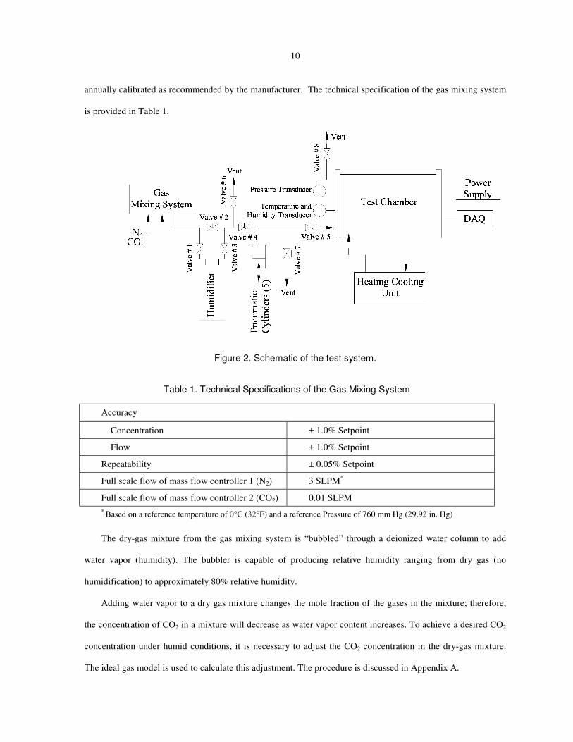
A test chamber (hereafter, chamber) was designed and fabricated for this study. Figure 2 is a schematic
diagram of the test system used. The sealed chamber is constructed of 8 in. (20.3 cm) square 0.25 in. (6.35 mm)
wall steel tubing. An external water jacket is used to maintain the desired temperature inside the chamber.
Flanges are welded to each end of the chamber to enable removable end plates with gaskets to be attached. The
front endplate is made of Lexan® while the rear endplate is 0.25 in. (6.35 mm) steel. The chamber was sized to
accommodate one tray of test sensors at a time.
Air cylinders are connected through one end plate and are used to control the pressure inside the chamber
during the pressure sensitivity tests. The chamber vent valve (valve #8) is partially closed to pressurize the test
chamber to sea-level pressure while allowing continuous flow of the gas mixture through the test chamber
during accuracy, linearity, repeatability, hysteresis, humidity sensitivity, and temperature sensitivity tests.
A gas mixture of CO2 and N2 is supplied to the test chamber from a commercially-available gas-mixing
system1. The gas-mixing system uses mass-flow controllers calibrated using a primary flow standard traceable
to the United States’ National Institute of Science and Technology (NIST). The system is capable of producing
gas mixtures from 334 to 3333 ppm CO2 (1% accuracy) at a flow rate of 3 liters/min. The gas mixing system is
1 Environics
® S-4000
10
annually calibrated as recommended by the manufacturer. The technical specification of the gas mixing system
is provided in Table 1.
Figure 2. Schematic of the test system.
Table 1. Technical Specifications of the Gas Mixing System
Accuracy
Concentration ± 1.0% Setpoint
Flow ± 1.0% Setpoint
Repeatability ± 0.05% Setpoint
Full scale flow of mass flow controller 1 (N2) 3 SLPM*
Full scale flow of mass flow controller 2 (CO2) 0.01 SLPM
* Based on a reference temperature of 0°C (32°F) and a reference Pressure of 760 mm Hg (29.92 in. Hg)
The dry-gas mixture from the gas mixing system is “bubbled” through a deionized water column to add
water vapor (humidity). The bubbler is capable of producing relative humidity ranging from dry gas (no
humidification) to approximately 80% relative humidity.
Adding water vapor to a dry gas mixture changes the mole fraction of the gases in the mixture; therefore,
the concentration of CO2 in a mixture will decrease as water vapor content increases. To achieve a desired CO2
concentration under humid conditions, it is necessary to adjust the CO2 concentration in the dry-gas mixture.
The ideal gas model is used to calculate this adjustment. The procedure is discussed in Appendix A.
11
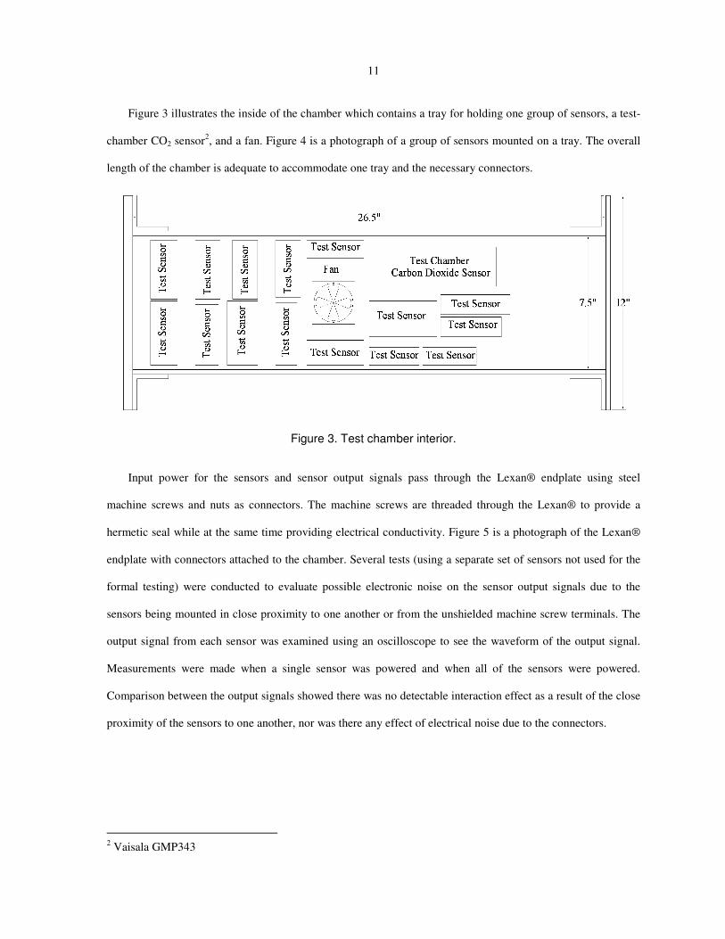
Figure 3 illustrates the inside of the chamber which contains a tray for holding one group of sensors, a test-
chamber CO2 sensor2, and a fan. Figure 4 is a photograph of a group of sensors mounted on a tray. The overall
length of the chamber is adequate to accommodate one tray and the necessary connectors.
Figure 3. Test chamber interior.
Input power for the sensors and sensor output signals pass through the Lexan® endplate using steel
machine screws and nuts as connectors. The machine screws are threaded through the Lexan® to provide a
hermetic seal while at the same time providing electrical conductivity. Figure 5 is a photograph of the Lexan®
endplate with connectors attached to the chamber. Several tests (using a separate set of sensors not used for the
formal testing) were conducted to evaluate possible electronic noise on the sensor output signals due to the
sensors being mounted in close proximity to one another or from the unshielded machine screw terminals. The
output signal from each sensor was examined using an oscilloscope to see the waveform of the output signal.
Measurements were made when a single sensor was powered and when all of the sensors were powered.
Comparison between the output signals showed there was no detectable interaction effect as a result of the close
proximity of the sensors to one another, nor was there any effect of electrical noise due to the connectors.
2 Vaisala GMP343

12
Figure 4. CO2 sensors mounted on tray.
Figure 5. Photograph of the Lexan® end plate with connectors mounted on the test chamber.
An absolute pressure sensor3 (hereafter, test chamber pressure sensor) is mounted on the steel end plate to
measure absolute pressure in the chamber. The technical specification of the test chamber pressure sensor is
3 Omega PX209

13
provided in Table 2. A humidity and temperature sensor4 (hereafter, test-chamber humidity sensor or test-
chamber temperature sensor) is also mounted on this end plate to measure relative humidity and temperature in
the chamber. The technical specification of the test chamber humidity and temperature sensor is provided in
Table 3.
Table 2. Technical Specifications of the Test Chamber Pressure Sensor
Description Value
Measurement range 0 to 15 psia (0 to 130.4 kPa)
Accuracy 0.25% FS
Response time 2 ms
The temperature inside the chamber is maintained at a prescribed value by controlling the temperature of
the water circulating through the water jacket. The water jacket temperature is controlled using a water bath5.
The DC axial fan installed inside the chamber provides a means of maintaining uniform temperature
conditions throughout the chamber’s interior. The circulating fan draws air from the top of the chamber and
blows air beneath the tray on which the sensors are mounted. The mounting tray has holes located below each
sensor to allow air to flow up and around each sensor. Tests were performed (using a separate set of sensors not
used for the formal testing) to check for uniformity of temperature in the chamber. RTD’s were used to measure
the temperature of the air being supplied to the sensors at various locations throughout the chamber. The
maximum variation in temperature between the RTD’s was 0.29°F (0.16°C).
A multimeter6 and a switch/control unit
7 are used to measure output from the CO2 sensors, the temperature
sensor, the humidity sensor, and the pressure sensor. National Instruments LabView software is used in
conjunction with the multimeter and switch/control unit as a data acquisition system to record the output from
each sensor.
4 Vaisala HMT334
5 Haake A81
6 Hewlett Packard 3457A
7 Hewlett Packard 3488A

14
Table 3. Technical Specifications of the Test Chamber Humidity and Temperature Sensor
Description Value
Relative humidity
Measurement range 0 to 100%
Accuracy at 59 to 77 °F (15 to 25 °C) ± 1% RH (0 to 90%),
± 1.7% RH (90 to100%)
Accuracy at -4 to 104 °F (-20 to 40 °C) ± (1.0 + 0.008 x reading) %RH
Temperature
Measurement range -94 to 356°F (-70 to 180°C)
Accuracy at 68°F (20°C) ± 0.36°F (± 0.2°C)
Accuracy over temperature range
Initially the gas mixture at the desired CO2 concentration flows continuously through the test chamber until
the concentration of the gas in the chamber has stabilized. As a way of monitoring the gas mixture in the
chamber, a test-chamber CO2 sensor is installed in the chamber to provide an independent measurement of CO2
concentration. Technical specifications of the test-chamber CO2 sensor are provided in Table 4.

15
Table 4. Technical Specifications of the Test Chamber CO2 Sensor
Description Value
Measurement range 0 to 2000 ppm
Accuracy ± 2.5% of reading
Accuracy at calibration points (at 370 ppm,
1000 ppm and 4000 ppm) ± 1.5% of reading
Accuracy below 300 ppm CO2 ± 5 ppm
Long-term stability (for easy operating
conditions) < ± 2% reading / year
Operating temperature -40 to + 140°F (- 40 to + 60°C)
Operating pressure 0 to 72.5 psia (0 to 500 kPa)
EXPERIMENTAL METHODOLOGY
The range of temperature, pressure, humidity, and CO2 concentration used for testing the CO2 sensor
performance is extended over the conditions encountered in a typical building HVAC application and for
building locations at various altitudes above sea level. The test includes evaluation of accuracy, linearity,
repeatability, hysteresis, humidity sensitivity, temperature sensitivity, and pressure sensitivity of the CO2
sensors.
Accuracy, Linearity, Repeatability, and Hysteresis Test
The accuracy, linearity, repeatability, and hysteresis of the sensors is evaluated by varying the CO2
concentration while maintaining the chamber relative humidity, temperature and pressure at 40%, 73ºF (22.8ºC)
and 14.70 psia (101.35 kPa), respectively. Vent valves #6 and #7 are closed and vent valve #8 is partially closed
to pressurize the test chamber to sea-level pressure while allowing continuous flow of the gas mixture through
the test chamber. Pressurization is necessary given that the testing location (Ames, Iowa) is 960 feet (293
meters) above sea level with an atmospheric pressure of 14.2 psia (97.9 kPa). The tests are performed in the
following sequence:
1. Initially the CO2 concentration in the test chamber is set at 400 ppm. The-gas mixing system runs
continuously providing continuous purge. Data collection at this condition and at all other conditions
follow a protocol described below.

16
2. Holding the chamber humidity, temperature, and pressure steady, the CO2 concentration is increased up to
1800 ppm in 350 ppm increments. These measurements, including the initial measurement at 400 ppm
(data points 1-5 in Figure 6), are referred to as the forward measurements.
3. After reaching 1800 ppm, the test is reversed, i.e., the CO2 concentration is decreased from 1800 ppm to
400 ppm in 350 ppm increments while maintaining the chamber humidity, temperature, and pressure
steady. These measurements (data points 6-9 in Figure 6) are referred to as the reverse measurements.
4. Once the 400 ppm level is attained, the CO2 concentration is increased to 1450 ppm in 350 ppm increments
while maintaining the chamber humidity, temperature, and pressure steady. These measurements (data
points 10-12 in Figure 6) are also referred to as the forward measurements.
Test data recording from all test sensors begins once steady-state conditions are established. Requirements
for steady-state conditions are detailed in the Test Procedure section. At each test condition, 10 samples of
sensor output collected at 1-minute intervals are averaged and used to report the “Measured CO2 Concentration”
for the sensor.
Accuracy and linearity are evaluated using the first forward and the reverse measurements (points 1-9 in
Figure 6). Repeatability is evaluated using the two forward measurements at 750, 1100 and 1450 ppm (data
points 2 and 10, 3 and 11, and 4 and 12 in Figure 6). Hysteresis is evaluated using the first forward
measurement and the reverse measurement at 750, 1100 and 1450 ppm (data points 2 and 8, 3 and 7, and 4 and
6 in Figure 6).
Figure 6. Example data set to illustrate numbering scheme used to identify data points.

17
Test Procedure. Output from the sensors is recorded while the test environment settles to the steady-state
conditions defined in Table 5. For clarity, this data is referred to as “settling data” and data collected at steady-
state conditions for quantifying the performance of the test sensors is referred to as “test data”. Interpreting
Table 5, to attain and maintain a steady-state condition in the test chamber, the following conditions must be
maintained for 10 minutes prior to the collection of the test data as well as throughout the collection of the test
data: the CO2 concentration reading from the test chamber CO2 sensor must not vary more than ± 20 ppm from
its mean output, the test chamber humidity sensor output must not vary more than ± 2.5% from the desired
relative humidity, the test chamber temperature sensor output must not vary more than ± 1.8ºF (1ºC) from the
desired temperature, and the test chamber pressure sensor output must not vary more than ± 0.14 psia (0.965
kPa) from the desired pressure.
Table 5. Steady-State Conditions for the Accuracy, Linearity, Repeatability and Hysteresis Tests
Parameter Steady-state condition
CO2 concentration Within ± 20 ppm of mean output from the test chamber CO2 sensor for 10
minutes prior to and during the collection of the test data
Temperature
Within ± 1.8ºF (1ºC) of the desired temperature condition measured by the
test chamber temperature sensor for 10 minutes prior to and during the
collection of the test data
Pressure
Within ± 0.14 psi (0.965 kPa) of the desired pressure condition measured by
the test chamber pressure sensor for 10 minutes prior to and during the
collection of the test data
Relative humidity
Within ± 2.5% of the desired relative humidity measured by the test chamber
humidity sensor for 10 minutes prior to and during the collection of the test
data
Effect of Humidity on CO2 Sensors
The effect of humidity on the CO2 sensors is evaluated by varying the relative humidity in the test chamber
while maintaining the chamber CO2 concentration, temperature, and pressure at 1100 ppm, 73ºF (22.8ºC) and
14.7 psia (101.35 kPa), respectively. The tests are performed in the following sequence:
1. Initially the relative humidity in the test chamber is set at 20%. The gas-mixing system runs continuously
allowing continuous purge (the vent valves #6 and #7 are closed and vent valve #8 is partially closed). Data
collection at this condition and at all other conditions follow a protocol described below.

18
2. Holding the CO2 concentration, temperature, and pressure steady, the test chamber relative humidity is
increased first to 40% and then to 60%.
Test data recording from all test sensors begins once steady-state conditions are established. Requirements
for steady-state conditions are defined in Table 5. At each test condition, 10 samples of sensor output collected
at 1-minute intervals are averaged and used to report the “Measured CO2 Concentration” for the sensor. The test
procedure is the same as the test procedure used for accuracy, linearity, repeatability, and hysteresis tests.
Effect of Temperature on CO2 Sensors
The effect of temperature on the CO2 sensors is evaluated by varying the temperature in the test chamber
while maintaining the chamber CO2 concentration and pressure at 1100 ppm, and 14.70 psia (101.35 kPa),
respectively. The relative humidity in the test chamber is maintained at 40% at 73°F (22.8°C) temperature. The
test chamber temperature is varied while maintaining the composition of the gas mixture steady. Hence, the
relative humidity varies at temperatures other than 73°F (22.8°C).
The tests are performed in the following sequence:
1. Initially the temperature in the test chamber is set at 73°F (22.8°C). The gas-mixing system runs
continuously allowing continuous purge (the vent valves #6 and #7 are closed and vent valve #8 is partially
closed). Data collection at this condition and at all other conditions follow a protocol described below.
2. Holding the CO2 concentration, gas mixture composition, and pressure steady, the test chamber
temperature is decreased first to 66°F (18.9°C) and then increased to 80°F (26.7°C).
Test data recording from all test sensors begins once steady-state conditions are established. Requirements
for steady-state conditions are detailed below in the Test Procedure section. At each test condition, 10 samples
of sensor output collected at 1-minute intervals are averaged and used to report the “Measured CO2
Concentration” for the sensor.
Test Procedure. Output from the sensors is recorded while the test environment settles to the steady-state
conditions defined in Table 6. For clarity, this data is referred to as “settling data” and data collected at steady-
state conditions for quantifying the performance of the test sensors is referred to as “test data”. Interpreting
Table 6, to attain and maintain a steady-state condition in the test chamber, the following conditions must be
maintained for 10 minutes prior to the collection of the test data as well as throughout the collection of the test

19
data: the CO2 concentration reading from the test chamber CO2 sensor must not vary more than ± 20 ppm from
its mean output, the test chamber temperature sensor output must not vary more than ± 1.8ºF (1ºC) from the
desired temperature, the test chamber pressure sensor output must not vary more than ± 0.14 psia (0.965 kPa)
from the desired pressure, and the test chamber relative humidity sensor output must not vary more than 2.5%
from the desired relative humidity at 73°F (22.8°C) temperature.
Table 6. Steady-State Conditions for the Temperature Sensitivity Test
Parameter Steady-state condition
CO2 concentration Within ± 20 ppm of mean output from the test chamber CO2 sensor for 10
minutes prior to and during the collection of the test data
Temperature
Within ± 1.8ºF (1ºC) of the desired temperature condition measured by the
test chamber temperature sensor for 10 minutes prior to and during the
collection of the test data
Pressure
Within ± 0.14 psia (0.965 kPa) of the desired pressure condition measured by
the test chamber pressure sensor for 10 minutes prior to and during the
collection of the test data
Relative humidity
Within ±2.5% of the desired relative humidity at 73ºF (22.8°C) temperature,
measured by the test chamber humidity sensor for 10 minutes prior to and
during the collection of the test data
Effect of Pressure on CO2 Sensors
The effect of pressure on the CO2 sensors is evaluated by varying the pressure in the test chamber while
maintaining the chamber CO2 concentration and temperature at 1100 ppm and 73°F (22.8°C), respectively.
Relative humidity in the test chamber is maintained at 40% at 14.70 psia (101.35 kPa) pressure. The test
chamber pressure is varied while maintaining the composition of the gas mixture steady. Hence, the relative
humidity varies at pressures other than 14.70 psia (101.35 kPa). The test is conducted at three pressures: 14.70
psia (101.35 kPa), 13.25 psia (91.36 kPa), and 11.80 psia (81.36 kPa). The pressure levels correspond to
standard atmospheric pressures for altitudes corresponding to sea level, 2838 feet (865 meters) and 5948 feet
(1813 meters) above sea level.
The gas mixture at the desired CO2 concentration and relative humidity (at 73°F (22.8°C) temperature and
14.70 psia (101.35 kPa) pressure), flows continuously through the test chamber until the CO2 concentration,
relative humidity, temperature, and pressure of the gas in the chamber has stabilized. The tests are performed in
the following sequence:

20
1. Initially the pressure in the test chamber is set at 14.70 psia (101.35 kPa). At steady-state conditions, the
test chamber is isolated by closing valves # 4, #5, #7, and #8. Data collection at this condition and at all
other conditions follow a protocol described below.
2. Holding the CO2 concentration, gas-mixture composition, and temperature steady, the test chamber
pressure is changed first to 13.25 psia (91.36 kPa) and then to 11.80 psia (81.36 kPa). To adjust the
chamber pressure, keeping valves #4, #7, and #8 closed, valve #5 is opened thus connecting the chamber to
the five pneumatic cylinders. The pneumatic cylinders (purged with the same gas concentration that is in
the chamber) are positioned to change the gas pressure in the chamber.
Test data recording from all test sensors begins once steady-state conditions are established. Requirements
for steady-state conditions are detailed below in the Test Procedure section. At each test condition, 10 samples
of sensor output collected at 1-minute intervals are averaged and used to report the “Measured CO2
Concentration” for the sensor.
Test Procedure. Output from the sensors is recorded while the test environment settles to the steady-state
conditions defined in Table 7. For clarity, this data is referred to as “settling data” and data collected at steady-
state conditions for quantifying the performance of the test sensors is referred to as “test data”. Interpreting
Table 7, to attain and maintain a steady-state condition in the test chamber, the following conditions must be
maintained for 10 minutes prior to the collection of the test data as well as throughout the collection of the test
data: the CO2 concentration reading from the test chamber CO2 sensor must not vary more than ± 20 ppm from
its mean output, the test chamber temperature sensor output must not vary more than ± 1.8ºF (1ºC) from the
desired temperature, the test chamber pressure sensor output must not vary more than ± 0.14 psia (0.965 kPa)
from the desired pressure, and the test chamber relative humidity sensor output must not vary more than 2.5%
from the desired relative humidity at 14.70 psia (101.35 kPa) pressure.

21
Table 7. Steady-State Conditions for the Pressure Sensitivity Test
Parameter Steady-state condition
CO2 concentration Within ± 20 ppm of mean output from the test chamber CO2 sensor for 10
minutes prior to and during the collection of the test data
Temperature
Within ± 1.8ºF (1ºC) of the desired temperature condition measured by the
test chamber temperature sensor for 10 minutes prior to and during the
collection of the test data
Pressure
Within ± 0.14 psia (0.965 kPa) of the desired pressure condition measured by
the test chamber pressure sensor for 10 minutes prior to and during the
collection of the test data
Relative humidity
Within ±2.5% of the desired relative humidity at 14.70 psia (101.35 kPa)
pressure, measured by the test chamber humidity sensor for 10 minutes prior
to and during the collection of the test data
Long-term test
This section describes the test procedure pertaining to the evaluation of long-term performance of CO2
sensors. The test will be conducted in four months interval for one year.
The sensors are located in the “lab station” apparatus (hereafter referred to as lab station) when they are not
undergoing performance testing in the chamber. The lab station allows for continuous monitoring of the sensors
while they are exposed to ambient conditions that exist in the laboratory space where the research project is
taking place. Since the laboratory space is large and well ventilated, CO2 levels are normally near outdoor CO2
concentrations. The lab station provides the capability to periodically expose the sensors to higher levels of
CO2 concentrations as they would experience in an office or classroom environment.
A photograph of the lab station is provided in Figure 7 while Figure 8 provides a schematic of the station.
The lab station consists of a wooden base with Plexiglas walls. The three trays on which the test sensors are
mounted are placed within the Plexiglas walls. During time periods when the sensors are only exposed to
ambient conditions in the lab, the top Plexiglas panel is removed allowing room air to freely interact with the
sensors. To produce conditions of higher CO2 concentrations (such as in an occupied space), the top panel is put
in place and a gas mixture is supplied into the plenum section below the trays. The gas mixture passes through
holes and flows past each CO2 sensor. The Plexiglas enclosure and fans (one mounted on each tray) provide a
near uniform CO2 concentration to all sensors.

22
During the four months in between performance testing, the sensors will be periodically exposed to higher
levels of CO2. For three days per week, the CO2 concentration will be increased to approximately 1100 ppm for
a period of 8 to 12 hours. The specific days of the week and number of hours per day are chosen at random. At
all other times, the sensors will experience ambient laboratory conditions. Sensor output and laboratory
conditions will be continuously recorded during the four months. At the end of the four-month time period, the
sensors will be tested following the same procedures as the performance tests (accuracy, linearity, repeatability,
hysteresis, humidity sensitivity, temperature sensitivity and pressure sensitivity).
Figure 7. Lab station.

23
Figure 8. Schematic of the lab station.
DATA ANALYSIS
The accuracy test results are presented in terms of the deviation of the measured CO2 concentration by a
sensor from the actual CO2 concentration in the test chamber (i.e., deviation = measured CO2 concentration –
actual CO2 concentration). Deviation is calculated for each sensor at each test condition. Mean deviation for a
given sensor at a given condition is the average deviation of the first forward measurement and the reverse
measurement.
The data plots are used to investigate and analyze the accuracy of the CO2 sensors. Specifically, a plot that
compares the mean deviation and actual CO2 concentration for a single sensor model at 40% relative humidity,
73ºF (22.8ºC) temperature, and 14.70 psia (101.35 kPa) pressure is created. Separate figures are created for each
sensor model. In addition, these plots are used to compare the manufacturer specified accuracy with the
measured sensor accuracy. A sample plot that shows the mean deviation of the measured CO2 concentration
from the actual CO2 concentration for three sensors of a single sensor model is shown in Figure 9. The dotted
lines in the figure illustrate the manufacturer’s specified accuracy.

24
Figure 9. Comparison of mean deviation from actual CO2 for three sensors of the same model.
The humidity sensitivity test results are presented in terms of the deviation from reading at 40% RH (i.e.,
deviation from reading at 40% RH = measured CO2 concentration at a particular RH – measured CO2
concentration at 40% RH). Humidity sensitivity is calculated for each sensor at each test condition.
The data plots are used to investigate and analyze the humidity sensitivity of the CO2 sensors. Specifically,
a plot that compares the deviation from reading at 40% RH for a single sensor model at 1100 ppm CO2
concentration, 73ºF (22.8ºC) temperature, and 14.70 psia (101.35 kPa) pressure is created. Separate figures are
created for each sensor model. Due to figure limitation in this paper, a sample plot that shows the humidity
sensitivity of three different sensor models is shown in Figure 10. Although no humidity dependence on sensor
performance is reported by the manufacturers, clearly some sensors are affected by humidity.
Figure 10. Humidity sensitivity of three different sensor models.
25
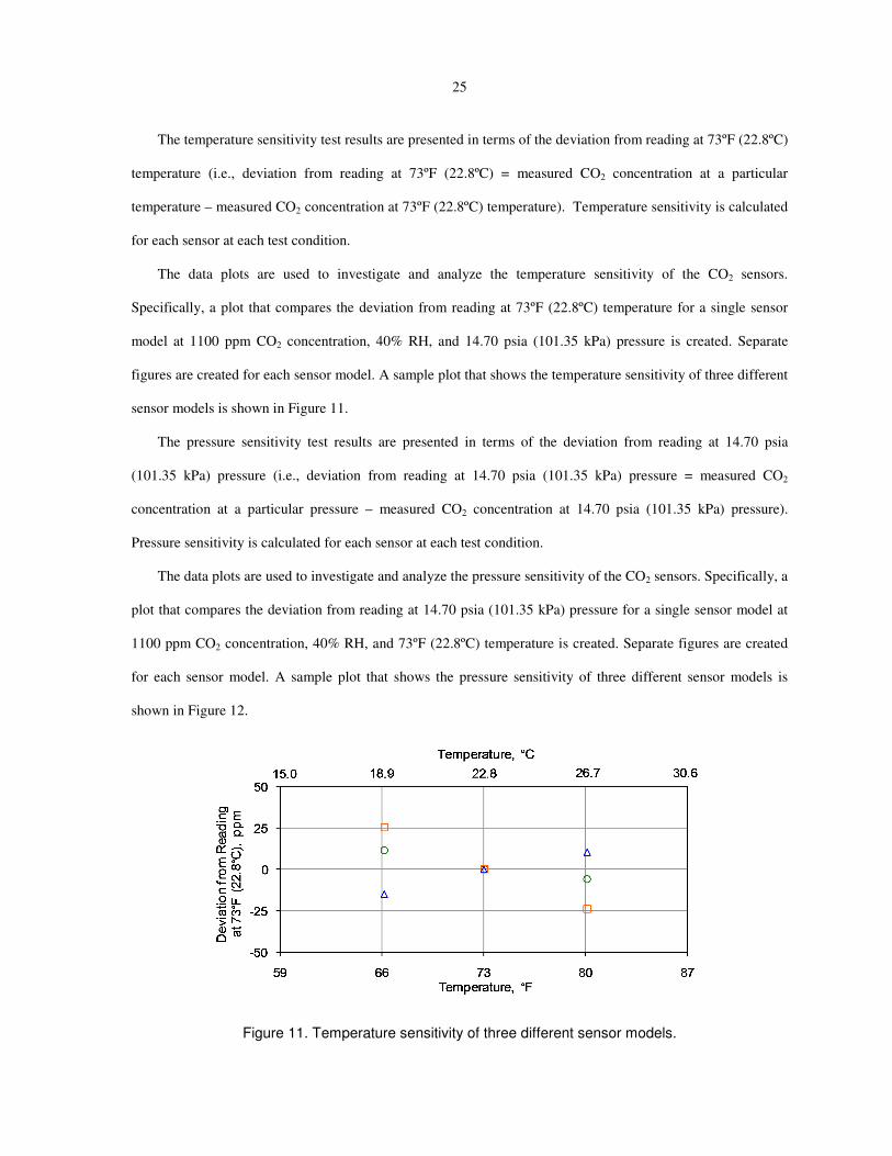
The temperature sensitivity test results are presented in terms of the deviation from reading at 73ºF (22.8ºC)
temperature (i.e., deviation from reading at 73ºF (22.8ºC) = measured CO2 concentration at a particular
temperature – measured CO2 concentration at 73ºF (22.8ºC) temperature). Temperature sensitivity is calculated
for each sensor at each test condition.
The data plots are used to investigate and analyze the temperature sensitivity of the CO2 sensors.
Specifically, a plot that compares the deviation from reading at 73ºF (22.8ºC) temperature for a single sensor
model at 1100 ppm CO2 concentration, 40% RH, and 14.70 psia (101.35 kPa) pressure is created. Separate
figures are created for each sensor model. A sample plot that shows the temperature sensitivity of three different
sensor models is shown in Figure 11.
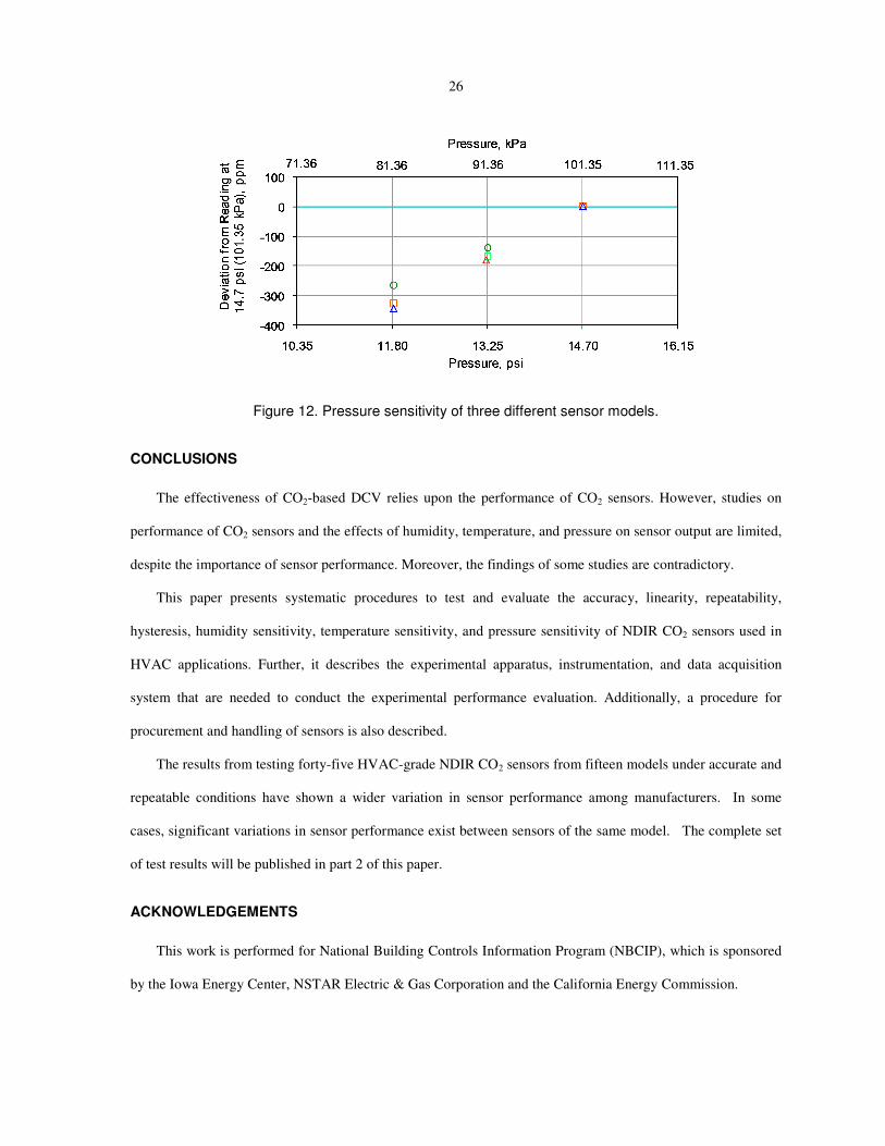
The pressure sensitivity test results are presented in terms of the deviation from reading at 14.70 psia
(101.35 kPa) pressure (i.e., deviation from reading at 14.70 psia (101.35 kPa) pressure = measured CO2
concentration at a particular pressure – measured CO2 concentration at 14.70 psia (101.35 kPa) pressure).
Pressure sensitivity is calculated for each sensor at each test condition.
The data plots are used to investigate and analyze the pressure sensitivity of the CO2 sensors. Specifically, a
plot that compares the deviation from reading at 14.70 psia (101.35 kPa) pressure for a single sensor model at
1100 ppm CO2 concentration, 40% RH, and 73ºF (22.8ºC) temperature is created. Separate figures are created
for each sensor model. A sample plot that shows the pressure sensitivity of three different sensor models is
shown in Figure 12.
Figure 11. Temperature sensitivity of three different sensor models.
26
Figure 12. Pressure sensitivity of three different sensor models.
CONCLUSIONS
The effectiveness of CO2-based DCV relies upon the performance of CO2 sensors. However, studies on
performance of CO2 sensors and the effects of humidity, temperature, and pressure on sensor output are limited,
despite the importance of sensor performance. Moreover, the findings of some studies are contradictory.
This paper presents systematic procedures to test and evaluate the accuracy, linearity, repeatability,
hysteresis, humidity sensitivity, temperature sensitivity, and pressure sensitivity of NDIR CO2 sensors used in
HVAC applications. Further, it describes the experimental apparatus, instrumentation, and data acquisition
system that are needed to conduct the experimental performance evaluation. Additionally, a procedure for
procurement and handling of sensors is also described.
The results from testing forty-five HVAC-grade NDIR CO2 sensors from fifteen models under accurate and
repeatable conditions have shown a wider variation in sensor performance among manufacturers. In some
cases, significant variations in sensor performance exist between sensors of the same model. The complete set
of test results will be published in part 2 of this paper.
ACKNOWLEDGEMENTS
This work is performed for National Building Controls Information Program (NBCIP), which is sponsored
by the Iowa Energy Center, NSTAR Electric & Gas Corporation and the California Energy Commission.

27
REFERENCES
CEC. 2006. 2005 Building Energy Efficiency Standards for Residential and Nonresidential Buildings.
CALIFORNIA ENERGY COMMISSION Title 24, Part 6, of the California Code of Regulations.
DOE. 2007. 2007 Building Energy Databook. http://buildingsdatabook.eere.energy.gov/ Washington, DC: U.S.
Department of Energy, Energy Efficiency and Renewable Energy.
Dougan, D.S., and L. Damiano. 2004. CO2-based demand control ventilation: do risk outweigh potential
rewards?. ASHRAE Journal Vol. 46, No. 10: 47-53.
Emmerich, S.J., and A.K. Persily. 1997. Literature review on CO2-based demand-controlled ventilation.
ASHRAE Transactions 103 (2): 229-43.
Emmerich, S.J., and A.K. Persily. 2001. State-of-the-art review of CO2 demand controlled ventilation
technology and application, Report NISTIR 6729, National Institute of Science and Technology (NIST),
USA.
Fahlen, P., H. Andersson, and S. Ruud. 1992. Demand Controlled Ventilating Systems - Sensor Tests. Swedish
National Testing and Research Institute, Boras, Sweden, SP Report 1992:13.
Fisk, W.J., D. Faulkner, and D.P. Sullivan. 2006. Accuracy of CO2 sensors in commercial buildings: a pilot
study. LBNL-61962, Lawrence Berkeley National Laboratory, Berkeley, CA.
Hyland, R.W., and A. Wexler. 1983. Formulations for the thermodynamic properties of the saturated phases of
H2O from 173.15 K to 473.15 K. ASHRAE Transactions 89(2A):500-519.
Raatschen, W., ed. 1990. Demand Controlled Ventilating System. State of the Art Review. Stockholm, Sweden:
Swedish Council for Building Research, Stockholm, Sweden, D9:1990.
Roth, K.W., D. Westphalen, M.Y. Pheng, P. Llana, and L. Quartararo. 2005. Energy impact of commercial
building controls and performance diagnostics: Market characterization, energy impact of building faults
and energy saving potential.
http://www.tiaxllc.com/aboutus/pdfs/energy_imp_comm_bldg_cntrls_perf_diag_110105.pdf
Schell, M., and D. Int-Hout. 2001. Demand control ventilation using CO2. ASHRAE Journal Vol. 43, No. 2: 18-
24.

28
APPENDIX
For a dry-gas mixture of nitrogen and carbon dioxide, the concentration of 2,dCO (The subscript, d, is
used to emphasize the dry-gas mixture) is achieved by accurately controlling the mass flow rate of each gas
during the mixing process. This process is controlled by the gas-mixing system. The concentration of the
2,dCO in units of parts per million (ppm) is the volume fraction of the 2,dCO expressed as the volume units of
2,dCO per 106 volume units of mixture. When water vapor is subsequently added to the mixture, (as a result of
bubbling the dry gas through a water column), the total number of moles in the mixture increases and the
concentration of 2,dCO is reduced. Thus, in order to achieve a particular value of CO2 concentration in the
moist gas mixture, a higher value of 2,dCO concentration must be produced by the gas-mixing system.
Determination of the CO2 concentration in the new mixture requires knowledge of the concentration of
water vapor in the moist-gas mixture. The concentration of water vapor present in a mixture of gases can be
calculated based on psychometric relations for ideal-gas mixtures and values of three independent
thermodynamic properties such as pressure, temperature and relative humidity. The concentration of water
vapor is directly related to the partial pressure of water vapor ( )wP in the mixture as given by Equation (A-1)
( )610w
w
Pppm
P= (A-1)
The partial pressure of the water vapor is related to the relative humidity and saturation pressure ( )wsP of water
through the definition of relative humidity ( )φ as given by Equation (A-2)
( )% *100w
ws
P
Pφ = (A-2)
The saturation pressure of the water vapor (ws
P ) is only a function of temperature and is computed using
the formula by Hyland and Wexler (Hyland and Wexler 1983) as given by Equation (A-3).
2 389 10 11 12 13ln ln
ws
CP C C T C T C T C T
T= + + + + + (A-3)
where
C8 = −1.044 039 7 E+04
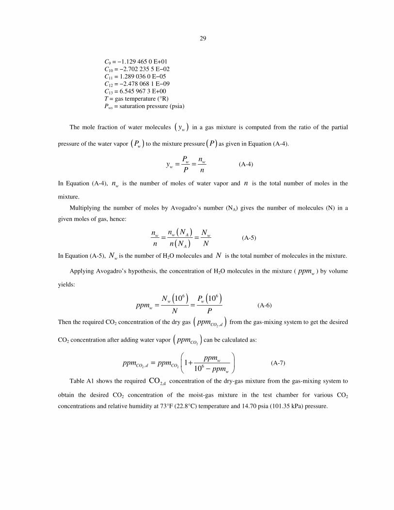
29
C9 = −1.129 465 0 E+01
C10 = −2.702 235 5 E−02
C11 = 1.289 036 0 E−05
C12 = −2.478 068 1 E−09
C13 = 6.545 967 3 E+00
T = gas temperature (°R)
Pws = saturation pressure (psia)
The mole fraction of water molecules ( )wy in a gas mixture is computed from the ratio of the partial
pressure of the water vapor ( )wP to the mixture pressure ( )P as given in Equation (A-4).
w ww
P ny
P n= = (A-4)
In Equation (A-4), w
n is the number of moles of water vapor and n is the total number of moles in the
mixture.
Multiplying the number of moles by Avogadro’s number (NA) gives the number of molecules (N) in a
given moles of gas, hence:
( )
( )w Aw w
A
n Nn N
n n N N= = (A-5)
In Equation (A-5), w
N is the number of H2O molecules and N is the total number of molecules in the mixture.
Applying Avogadro’s hypothesis, the concentration of H2O molecules in the mixture (w
ppm ) by volume
yields:
( ) ( )6 610 10w w
w
N Pppm
N P= = (A-6)
Then the required CO2 concentration of the dry gas ( )2 ,CO d
ppm from the gas-mixing system to get the desired
CO2 concentration after adding water vapor ( )2CO
ppm can be calculated as:
2 2, 61
10
wCO d CO
w
ppmppm ppm
ppm
= +
− (A-7)
Table A1 shows the required 2,dCO concentration of the dry-gas mixture from the gas-mixing system to
obtain the desired CO2 concentration of the moist-gas mixture in the test chamber for various CO2
concentrations and relative humidity at 73°F (22.8°C) temperature and 14.70 psia (101.35 kPa) pressure.
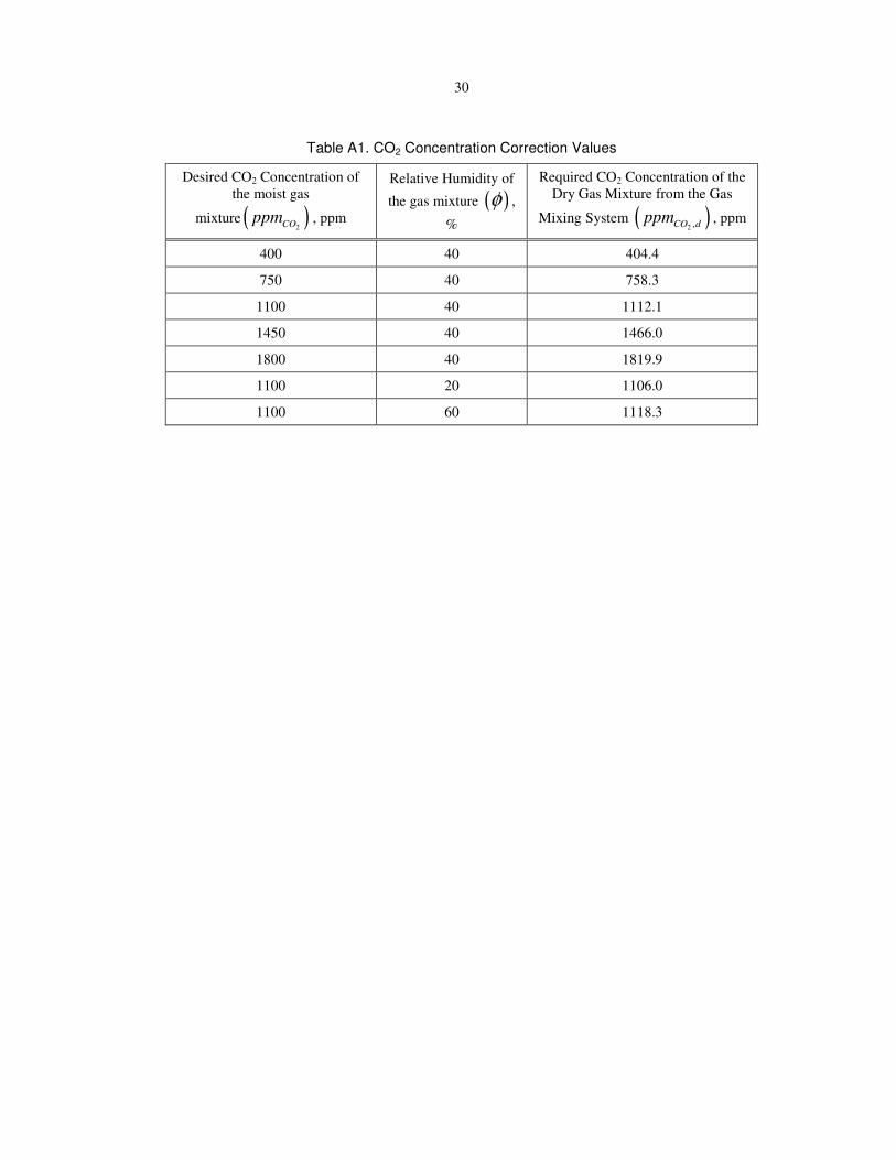
30
Table A1. CO2 Concentration Correction Values
Desired CO2 Concentration of
the moist gas
mixture ( )2CO
ppm , ppm
Relative Humidity of
the gas mixture ( )φ ,
%
Required CO2 Concentration of the
Dry Gas Mixture from the Gas
Mixing System ( )2 ,CO d
ppm , ppm
400 40 404.4
750 40 758.3
1100 40 1112.1
1450 40 1466.0
1800 40 1819.9
1100 20 1106.0
1100 60 1118.3

31
Chapter 3: An Experimental Evaluation of HVAC-Grade Carbon-Dioxide
Sensors: Part 2, Performance Test Results
A paper to be submitted to the ASHRAE Transactions
Som S. Shrestha Gregory M. Maxwell, PhD Student Member ASHRAE Member ASHRAE
ABSTRACT
This is the second paper in a four-part series reporting on the test and evaluation of typical carbon-dioxide
sensors used in building HVAC applications. Fifteen models of NDIR HVAC-grade CO2 sensors were tested
and evaluated to determine the accuracy, linearity, repeatability, and hysteresis of each sensor. This paper
describes the performance of the sensors and provides a comparison with the manufacturers’ specifications. The
sensors were tested at 40% relative humidity, 73oF (22.8
oC) temperature, 14.70 psia (101.35 kPa) pressure, and
at five different CO2 concentrations (400 ppm, 750 ppm, 1100 ppm, 1450 ppm, and 1800 ppm). The test results
showed a wide variation in sensor performance among the various manufacturers and in some cases a wide
variation among sensors of the same model.
In all, 45 sensors were evaluated: three from each of the 15 models. Among the 15 models tested, eight
models have a single-lamp, single-wavelength configuration, four models have a dual-lamp, single-wavelength
configuration, and three models have a single-lamp, dual-wavelength configuration.
INTRODUCTION
This is part two of a four-part series of papers reporting on the test and evaluation of typical CO2 sensors
used in building HVAC systems. In this study, fifteen models of NDIR (non-dispersive infrared) HVAC-grade
CO2 sensors were tested and evaluated. In all, 45 sensors (three from each model) were evaluated to determine
the sensor accuracy, linearity, repeatability, and hysteresis. The results are compared with the manufacturers’
specifications. The experimental procedure used to test and evaluate the sensors was described in Part 1
(Shrestha and Maxwell 2009) of this paper. Among the 15 models tested, eight models have a single-lamp,
single-wavelength configuration, four models have a dual-lamp, single-wavelength configuration, and three

32
models have a single-lamp, dual-wavelength configuration. All single-lamp, single-wavelength sensors and one
single-lamp, dual-wavelength sensor incorporate an “automatic baseline adjustment” algorithm in the sensor’s
electronics package.
This paper presents an overview of the past studies performed by researchers to evaluate the performance
of CO2 sensors used in HVAC application. Further, a brief discussion on CO2 sensor specifications and
experimental test procedures (detailed in Part 1 of this paper) is provided. In addition, the paper presents test
and evaluation results, including a comparison of the performance of various CO2 sensors.
PREVIOUS STUDIES
In the past, limited studies have been done to investigate the performance of HVAC-grade CO2 sensors
using a controlled environment. Fahlen et al. (1992) evaluated the performance of two CO2 sensors, one photo-
acoustic type and one infrared spectroscopy type, in lab tests and long term field tests. The lab tests included
performance and environmental tests. The authors conclude that the deviation between actual concentration and
the sensors’ reading are normally well within ± 50 ppm at a concentration level of 1000 ppm. However, at a
concentration of 2000 ppm the test results showed a deviation of up to -300 ppm. The output of one sensor
increased dramatically during environmental testing. This sensor failed to return to its normal value.
Fisk et al. (2006) conducted a pilot study that evaluated the in-situ accuracy of 44 NDIR CO2 sensors
located in nine commercial buildings. The evaluation was performed either by multi-point calibration using CO2
calibration gas or by a single-point calibration check using a co-located and calibrated reference CO2 sensor.
Their results indicated that the accuracy of CO2 sensors is frequently less than what is needed to measure peak
indoor-outdoor CO2 concentration differences with an error that is less than 20%. Thus, the authors conclude
that there is a need for more accurate CO2 sensors and/or better maintenance and calibration.
Pandey et al. (2007) evaluated the accuracy of two NDIR CO2 sensor models. They tested three sensors of
each model. The tests were performed in an enclosure where all six sensors were simultaneously exposed to
CO2 concentration of 0 ppm, 500 ppm, and 1000 ppm (other environmental conditions, such as humidity,
temperature, and pressure were not specified.) The maximum deviation was observed as -73 ppm at a CO2
concentration of 500 ppm.

33
CONFIGURATIONS OF NDIR CO2 SENSORS
Various techniques are used by CO2 sensor manufacturers to compensate for the long-term effects of
operational and environmental conditions. These techniques have lead to the three basic configurations
currently used in NDIR CO2 sensors: (1) single-lamp,8 single-wavelength, (2) dual-lamp, single-wavelength,
and (3) single-lamp, dual-wavelength. Figure 1 illustrates these configurations.
All single-lamp, single-wavelength sensors (illustrated in Figure 1a) incorporate an “automatic baseline
adjustment” algorithm in the sensor’s electronics package. The algorithm “adjusts” the sensor’s output
according to the minimum CO2 concentration observed over a time period. It is assumed that the minimum CO2
concentration observed corresponds to the outdoor CO2 concentration. A value of 400 ppm is commonly used
as the value for the outdoor CO2 concentration level to which the sensor output is set when the automatic
baseline adjustment is made. The programming logic used in the algorithm varies among sensor manufacturers.
Some algorithms adjust the baseline value as frequently as every hour. Other algorithms perform adjustments
based on several weeks of sampling and only make incremental step adjustments to the baseline value. It is
important to note that sensors which use any algorithm to adjust the sensor output based upon minimum CO2
concentration observed must only be used in applications where they will be periodically exposed to levels of
CO2 in the outdoor air.
The dual-lamp, single-wavelength configuration (illustrated in Figure 1b) uses two IR (infrared) sources
(lamps). One lamp pulses several times per minute while the second lamp pulses much less frequently (on the
order of one or two pulse every 24 hours). Due to the relatively infrequent pulsing of the second lamp, the
ageing of the second lamp is much less than the ageing of the first lamp, thus the second lamp is used as a
reference for sensor compensation.
Figures 1c and 1d illustrate two configurations which are both referred to as single-lamp, dual-wavelength
sensors. The principle behind either configuration is understood by examining the spectral properties of the
filters used. Filter 1 (Figure 1c) passes IR radiation in a portion of the IR spectrum that contains no absorption
bands for any of the gases commonly found in air. For this wavelength, the output from the IR detector is
8 The term “beam” is used by sensor manufacturers; however, this leads to confusion on the technology
employed in the sensor configuration. A single lamp can produce multiple “beams”, so when the term “dual
beam” is used, it is not clear if one or two lamps are employed.
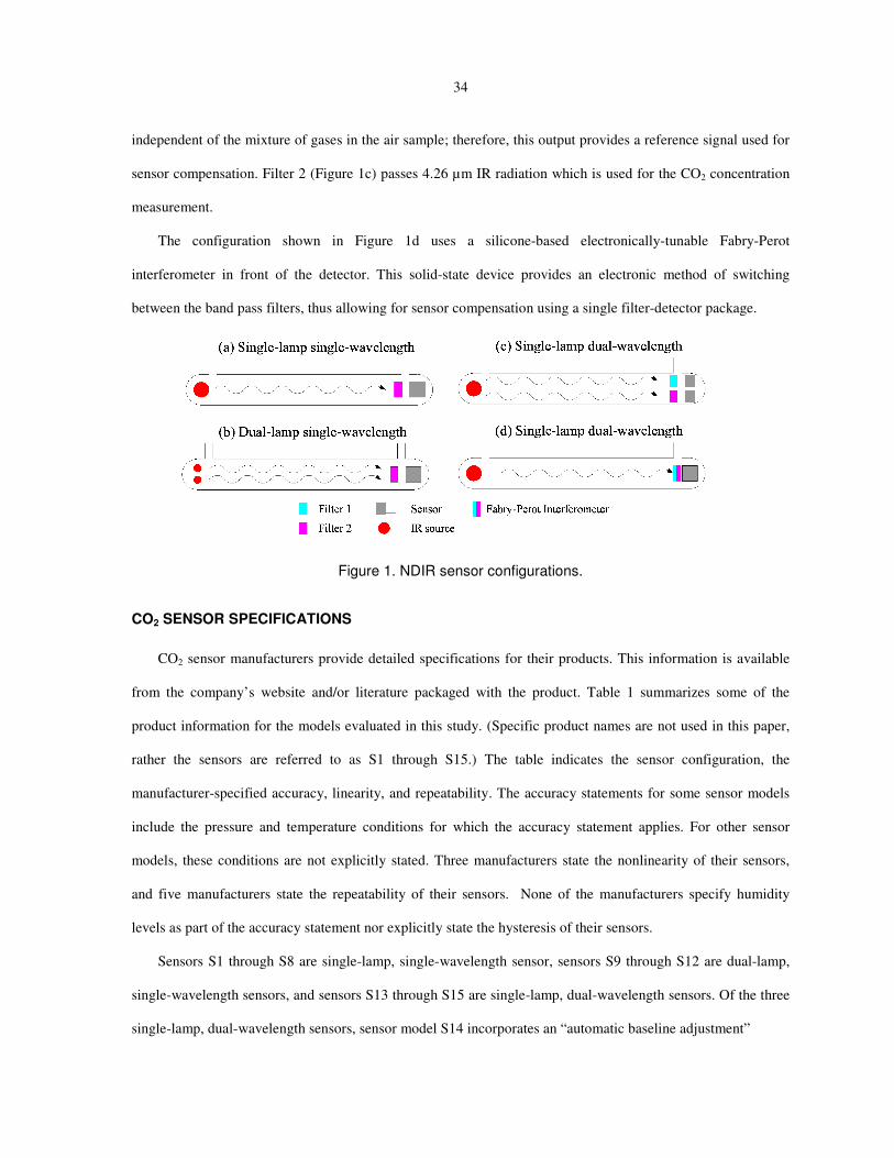
34
independent of the mixture of gases in the air sample; therefore, this output provides a reference signal used for
sensor compensation. Filter 2 (Figure 1c) passes 4.26 µm IR radiation which is used for the CO2 concentration
measurement.
The configuration shown in Figure 1d uses a silicone-based electronically-tunable Fabry-Perot
interferometer in front of the detector. This solid-state device provides an electronic method of switching
between the band pass filters, thus allowing for sensor compensation using a single filter-detector package.
Figure 1. NDIR sensor configurations.
CO2 SENSOR SPECIFICATIONS
CO2 sensor manufacturers provide detailed specifications for their products. This information is available
from the company’s website and/or literature packaged with the product. Table 1 summarizes some of the
product information for the models evaluated in this study. (Specific product names are not used in this paper,
rather the sensors are referred to as S1 through S15.) The table indicates the sensor configuration, the
manufacturer-specified accuracy, linearity, and repeatability. The accuracy statements for some sensor models
include the pressure and temperature conditions for which the accuracy statement applies. For other sensor
models, these conditions are not explicitly stated. Three manufacturers state the nonlinearity of their sensors,
and five manufacturers state the repeatability of their sensors. None of the manufacturers specify humidity
levels as part of the accuracy statement nor explicitly state the hysteresis of their sensors.
Sensors S1 through S8 are single-lamp, single-wavelength sensor, sensors S9 through S12 are dual-lamp,
single-wavelength sensors, and sensors S13 through S15 are single-lamp, dual-wavelength sensors. Of the three
single-lamp, dual-wavelength sensors, sensor model S14 incorporates an “automatic baseline adjustment”

35
Table 1. Manufacturer-Specified Accuracy, Nonlinearity, and Repeatability for CO2 Sensors
Sensor
Model Configuration Accuracy
Manufacturer-
Specified
Nonlinearity
Manufacturer-
Specified
Repeatability
S1 Single-lamp, single-
wavelength
± 1% of measurement range +
5% of measured value NA NA
S2 Single-lamp, single-
wavelength
± 100 ppm or 7% whichever is
greater NA NA
S3 Single-lamp, single-
wavelength
± 50 ppm or + 3% of reading
(at 25°C (77°F)at standard
pressure)
< 1% FS NA
S4 Single-lamp, single-
wavelength
± 5% of reading or 75 ppm,
whichever is greater NA ± 20 ppm
S5 Single-lamp, single-
wavelength
± 75 ppm or 3% of reading,
whichever is greater (15°C to
32°C (59°F to 90°F))
NA ± 20 ppm
S6 Single-lamp, single-
wavelength ± (30 ppm + 2% of reading) NA NA
S7 Single-lamp, single-
wavelength
± 5% of reading or ± 75 ppm,
whichever is greater NA ± 20 ppm
S8 Single-lamp, single-
wavelength
± 30 ppm ± 5% of measured
value NA
± 20 ppm ± 1%
measured value
S9 Dual-lamp, single-
wavelength
± 75 ppm if 0 to 1500 ppm: ±
5% if > 1500ppm (readings at
standard pressure 760 mm Hg &
25°C (77°F))
NA ± 8 ppm
S10 Dual-lamp, single-
wavelength
≤ ± 50 ppm + 2% of measured
value NA NA
S11 Dual-lamp, single-
wavelength ± 100 ppm + 3% of reading NA NA
S12 Dual-lamp, single-
wavelength
< ± (50 ppm + 2% of measure
value) at 20°C (68°F) NA NA
S13 Single-lamp, dual-
wavelength
< ± (30 ppm + 2.0% of reading)
at 68°F (20°C) < 1% FS NA
S14 Single-lamp, dual-
wavelength
± 50 ppm or 5% whichever is
greater (7% for levels over 1500
ppm) at 60°F to 90°F (15°C to
32°C)
NA NA
S15 Single-lamp, dual-
wavelength
< ± (30ppm + 2% of reading) at
25°C (77°F) < ± 1% FS NA
Notes: NA indicates that the information was not available in the manufacturer’s product literature. Full scale (FS) is 2000 ppm for
all sensors. The nominal operating temperature range is 32°F to 122° (0°C to 50°C) with 0% to 95% RH.
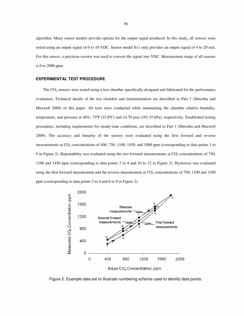
36
algorithm. Many sensor models provide options for the output signal produced. In this study, all sensors were
tested using an output signal of 0 to 10 VDC. Sensor model S11 only provides an output signal of 4 to 20 mA.
For this sensor, a precision resistor was used to convert the signal into VDC. Measurement range of all sensors
is 0 to 2000 ppm.
EXPERIMENTAL TEST PROCEDURE
The CO2 sensors were tested using a test chamber specifically designed and fabricated for the performance
evaluation. Technical details of the test chamber and instrumentation are described in Part 1 (Shrestha and
Maxwell 2009) of this paper. All tests were conducted while maintaining the chamber relative humidity,
temperature, and pressure at 40%, 73ºF (22.8ºC) and 14.70 psia (101.35 kPa), respectively. Established testing
procedures, including requirements for steady-state conditions, are described in Part 1 (Shrestha and Maxwell
2009). The accuracy and linearity of the sensors were evaluated using the first forward and reverse
measurements at CO2 concentrations of 400, 750, 1100, 1450, and 1800 ppm (corresponding to data points 1 to
9 in Figure 2). Repeatability was evaluated using the two forward measurements at CO2 concentrations of 750,
1100 and 1450 ppm (corresponding to data points 2 to 4 and 10 to 12 in Figure 2). Hysteresis was evaluated
using the first forward measurement and the reverse measurement at CO2 concentrations of 750, 1100 and 1450
ppm (corresponding to data points 2 to 4 and 6 to 8 in Figure 2).
Figure 2. Example data set to illustrate numbering scheme used to identify data points.

37
ACCURACY TEST RESULTS
The accuracy test results are presented in terms of the deviation of the measured CO2 concentration by a
sensor from the actual CO2 concentration in the test chamber (i.e., deviation = measured CO2 concentration –
actual CO2 concentration). Deviation is calculated for each sensor at each test condition. The mean deviation for
a given sensor at a given condition is the average deviation of the first forward measurement and the reverse
measurement. As mentioned above, three sensors from each of fifteen models were tested. The letters A, B and
C are used to distinguish between each sensor of a given model.
Data plots are used to illustrate the accuracy of the CO2 sensors while numerical results are provided in
tables. Specifically, a plot that compares the mean deviation and actual CO2 concentration for a single sensor
model was created. Each accuracy plot also illustrates the manufacturer-specified accuracy. The accuracy
statement appears as a set of dotted lines on the plot. For most sensor models, the accuracy band increases at
higher CO2 levels; therefore, the dotted lines are seen to diverge as the CO2 level increases.
Before discussing the results for each sensor, it should be pointed out that for some sensors the maximum
output voltage (nominally 10 VDC) was reached when the sensors were exposed to the higher level CO2
concentration test conditions. This is seen in Figure 3 which shows the output voltage from sensor S2B (model
S2, sensor group B) as the CO2 concentration in the test chamber increases. As seen in the figure, when the CO2
concentration reaches approximately 1700 ppm, the output voltage of the sensor is 10 VDC. Since this is the
maximum voltage produced by the sensor, further increases in CO2 concentration do not produce any change in
the output voltage. For sensor S2B, the output reading would indicate 2000 ppm for any CO2 concentration in
excess of 1700 ppm. The sensor is said to be saturated. For all sensor models tested, the operating range of each
sensor is 0 to 2000 ppm. Saturated data points were not considered for analysis.
Analysis of Deviations for each Sensor Model
Analysis of deviations for each sensor model is presented in this section. All sensors were tested under “as
received” conditions from the suppliers. No calibration was performed on the sensors prior to testing. Sensors
were powered up and allowed to stabilize in the laboratory environment before they were tested.
Single-lamp, single-wavelength sensors: Figure 4 shows the accuracy test results for the sensors that use
the single-lamp, single-wavelength configuration. These sensors use a manufacturer-specific proprietary

38
algorithm to periodically adjust the baseline CO2 concentration according to the minimum CO2 concentration
observed over a time period. It is assumed that the minimum CO2 concentration observed corresponds to the
outdoor CO2 concentration. A value of 400 ppm is commonly used as the value for the outdoor CO2
concentration level to which the sensor output is set when the automatic baseline adjustment is made.
Prior to placing the sensors in the test chamber for performance testing, all sensors were operating in the
laboratory environment where the average environmental conditions (relative humidity, temperature, and
barometric pressure) were, 14.7% , 76°F (24.2°C), and 14.3 psia (98.6 KPa), respectively. The minimum CO2
concentration in the laboratory varies on a daily basis according to the variation in the ambient CO2
concentration. Figure 5 shows the CO2 concentration in the laboratory for two weeks prior to the performance
test.
Operating in the laboratory environment for an extended period of time allowed the sensors with automatic
baseline adjustment algorithm to “adjust” their baseline; therefore, when these sensors are placed under test
conditions and compared to “actual” CO2 concentration levels, there is some bias in the measured value reported
by the sensor. Because this bias is unknown, no compensation was made when showing the test results. It is
therefore up to the reader to interpret the meaningfulness of the comparison of the sensor accuracy to the
accuracy statement for each sensor that uses an “automatic baseline adjustment” algorithm.
Table 2 shows the numerical values of the deviations for each sensor at each CO2 level. Data points
corresponding to saturated sensor output are highlighted in the table.
Figure 3. Saturated reading of S2B sensor at 1800 ppm.

39
Sensor S1
The deviations of the measured CO2 concentration from the actual CO2 concentration for Model S1 sensors
are presented graphically in Figure 4(a). The manufacturer-stated accuracy for this sensor model is ± 1% of
measurement range + 5% of measured value. The deviation of all three sensors shifts upward when the actual
CO2 concentration was increased. However, the slope of sensors A and C are a little higher than the slope of
sensor B. The reference relative humidity, temperature, and pressure for the stated accuracy were not specified
by the manufacturer.
The deviation of sensor B is within the manufacturer-stated accuracy at all CO2 levels. The deviations of
sensors A and C are also within the manufacturer-stated accuracy at 1800 ppm CO2. The maximum discrepancy
between the actual deviation and the manufacturer-stated accuracy is 22 ppm (sensor A at 750 ppm).
Sensor S2
The deviations of the measured CO2 concentration from the actual CO2 concentration for Model S2 sensors
are presented graphically in Figure 4(b). The manufacturer-stated accuracy for this sensor model is ± 100 ppm
or 7%, whichever is greater. The reference relative humidity, temperature, and pressure for the stated accuracy
were not specified by the manufacturer. The deviation of all three sensors shifts upward when the actual CO2
concentration was increased. The reading of sensor B is saturated at 1800 ppm reading.
The deviation of sensor C is within the manufacturer-stated accuracy at all CO2 levels. The deviation of
sensor A at 400 and 750 ppm CO2 and that of sensor B at 400 ppm CO2 are also within the manufacturer-stated
accuracy. The maximum discrepancy between the actual deviation and the manufacturer-stated accuracy is 109
ppm (sensor B at 1450 ppm).
Sensor S3
The deviations of the measured CO2 concentration from the actual CO2 concentration for Model S3 sensors
are presented graphically in Figure 4(c). The manufacturer-stated accuracy for this sensor model is ± 50 ppm or
3% of reading. The reference temperature and pressure for the stated accuracy are 77°F (25°C) and standard
pressure, respectively. When the actual CO2 concentration was increased, the deviation of sensors A and B
shifts upward, whereas the deviation of sensor C shifts downward. The reading of sensor A is saturated at 1800
ppm reading.
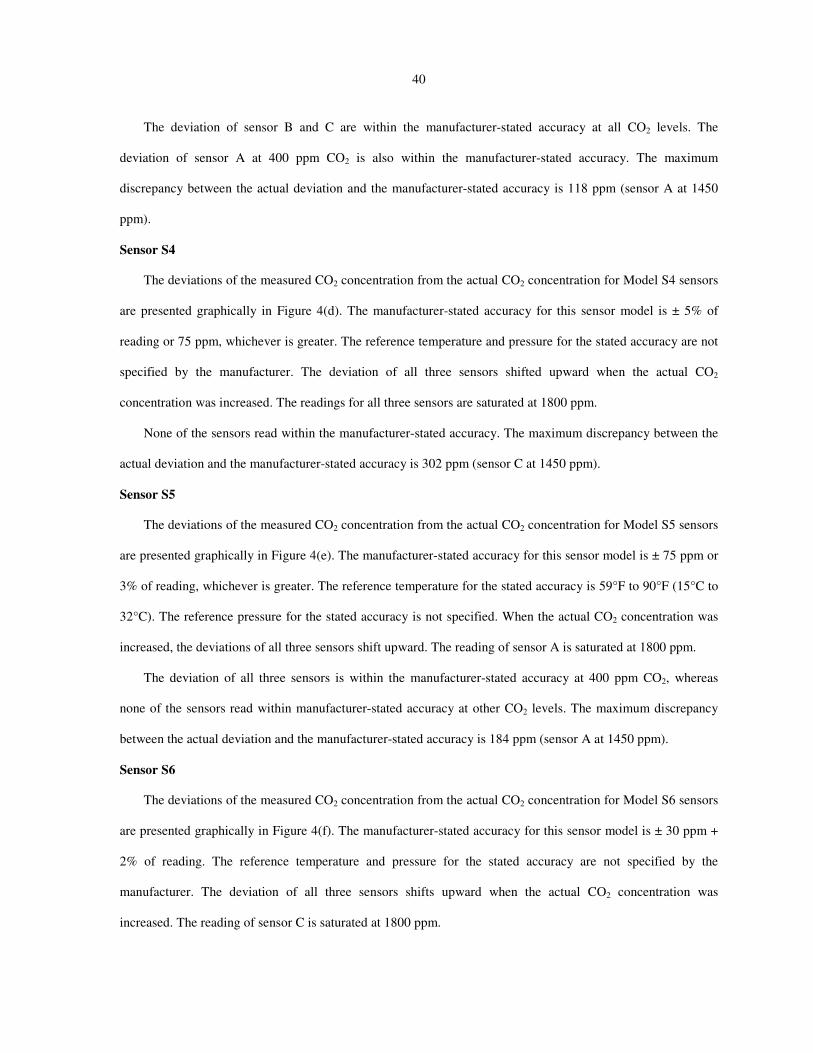
40
The deviation of sensor B and C are within the manufacturer-stated accuracy at all CO2 levels. The
deviation of sensor A at 400 ppm CO2 is also within the manufacturer-stated accuracy. The maximum
discrepancy between the actual deviation and the manufacturer-stated accuracy is 118 ppm (sensor A at 1450
ppm).
Sensor S4
The deviations of the measured CO2 concentration from the actual CO2 concentration for Model S4 sensors
are presented graphically in Figure 4(d). The manufacturer-stated accuracy for this sensor model is ± 5% of
reading or 75 ppm, whichever is greater. The reference temperature and pressure for the stated accuracy are not
specified by the manufacturer. The deviation of all three sensors shifted upward when the actual CO2
concentration was increased. The readings for all three sensors are saturated at 1800 ppm.
None of the sensors read within the manufacturer-stated accuracy. The maximum discrepancy between the
actual deviation and the manufacturer-stated accuracy is 302 ppm (sensor C at 1450 ppm).
Sensor S5
The deviations of the measured CO2 concentration from the actual CO2 concentration for Model S5 sensors
are presented graphically in Figure 4(e). The manufacturer-stated accuracy for this sensor model is ± 75 ppm or
3% of reading, whichever is greater. The reference temperature for the stated accuracy is 59°F to 90°F (15°C to
32°C). The reference pressure for the stated accuracy is not specified. When the actual CO2 concentration was
increased, the deviations of all three sensors shift upward. The reading of sensor A is saturated at 1800 ppm.
The deviation of all three sensors is within the manufacturer-stated accuracy at 400 ppm CO2, whereas
none of the sensors read within manufacturer-stated accuracy at other CO2 levels. The maximum discrepancy
between the actual deviation and the manufacturer-stated accuracy is 184 ppm (sensor A at 1450 ppm).
Sensor S6
The deviations of the measured CO2 concentration from the actual CO2 concentration for Model S6 sensors
are presented graphically in Figure 4(f). The manufacturer-stated accuracy for this sensor model is ± 30 ppm +
2% of reading. The reference temperature and pressure for the stated accuracy are not specified by the
manufacturer. The deviation of all three sensors shifts upward when the actual CO2 concentration was
increased. The reading of sensor C is saturated at 1800 ppm.

41
None of the sensors read within the manufacturer-stated accuracy at any CO2 levels. The maximum
discrepancy between the actual deviation and the manufacturer-stated accuracy is 129 ppm (sensor C at 1450
ppm).
Sensor S7
The deviations of the measured CO2 concentration from the actual CO2 concentration for Model S7 sensors
are presented graphically in Figure 4(g). The manufacturer-stated accuracy for this sensor model is ± 5% of
reading or 75 ppm, whichever is greater. The reference temperature and pressure for the stated accuracy are not
specified by the manufacturer. The deviation of all three sensors shifts upward when the actual CO2
concentration was increased. The reading of all three sensors is saturated at 1800 ppm.
None of the sensors read within the manufacturer-stated accuracy. The maximum discrepancy between the
actual deviation and the manufacturer-stated accuracy is 407 ppm (sensor A at 1450 ppm).
Sensor S8
The deviations of the measured CO2 concentration from the actual CO2 concentration for Model S8 sensors
are presented graphically in Figure 4(h). The manufacturer-stated accuracy for this sensor model is ± 30 ppm ±
5% of measured value. The reference temperature and pressure for the stated accuracy are not specified by the
manufacturer. The deviation of all sensors shifts upward when the actual CO2 concentration was increased. The
reading of sensor A is saturated at 1800 ppm reading.
The deviation of sensor B is within the manufacturer-stated accuracy at all CO2 levels. The deviations of
sensor C at 400 and 1800 ppm CO2 are also within the manufacturer-stated accuracy. The maximum
discrepancy between the actual deviation and the manufacturer-stated accuracy is 113 ppm (sensor A at 1450
ppm).
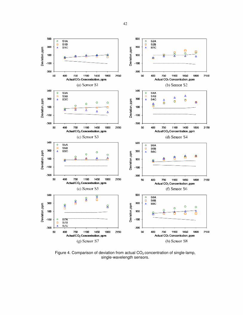
42
Figure 4. Comparison of deviation from actual CO2 concentration of single-lamp, single-wavelength sensors.

43
Table 2. Deviation from Actual CO2 Concentration (ppm), Single-Lamp, Single-Wavelength Sensors
Sensor
Model Sensor
Deviation at, ppm
400 750 1100 1450 1800
S1
A 47 79 86 96 99
B 26 59 62 58 49
C 42 78 91 102 109
S2
A 28 94 125 147 161
B 30 115 167 211 188
C 37 74 80 79 73
S3
A 49 129 174 212 206
B 26 57 73 80 90
C 29 34 21 -2 -22
S4
A 156 202 233 262 214
B 126 192 239 270 216
C 188 279 335 377 216
S5
A 64 151 208 259 197
B 71 96 95 91 85
C 56 97 113 123 126
S6
A 73 120 156 171 185
B 47 94 124 149 171
C 69 121 161 188 187
S7
A 257 361 428 482 240
B 171 288 359 385 201
C 233 337 390 452 202
S8
A 66 125 172 216 201
B 23 48 50 45 48
C 44 82 94 103 114
Note: The highlighted numbers indicate that the sensor
reading was saturated.
Figure 5. CO2 concentration in the laboratory for two weeks prior to commencing the performance test.

44
Dual-lamp, single-wavelength sensors: Figure 6 shows the accuracy test results of the sensors that use the
dual-lamp, single-wavelength configuration. Table 3 shows the numerical values of the deviation for each
sensor. In some cases, the sensors’ outputs corresponding to a concentration of 1,800 ppm are saturated. These
data points are highlighted in the table.
Sensor S9
The deviations of the measured CO2 concentration from the actual CO2 concentration for Model S9 sensors
are presented graphically in Figure 6(a). The manufacturer-stated accuracy for this sensor model is ± 75 ppm for
0 to 1500 ppm and 5% of reading for greater than 1500 ppm. The reference temperature and pressure for the
stated accuracy are 77°F (25°C) and 14.70 psia (101.35 kPa), respectively. The deviation of sensor A shifts
upward when the actual CO2 concentration was increased, whereas the deviation of the sensors B and C shifts
downward when the actual CO2 concentration was increased.
The deviation of sensor A at 400, 750, and 1100 ppm are within the manufacturer-stated accuracy at all
CO2 levels. The maximum discrepancy between the actual deviation and the manufacturer-stated accuracy is -
184 ppm (sensor B at 1800 ppm).
Sensor S10
The deviations of the measured CO2 concentration from the actual CO2 concentration for Model S10
sensors are presented graphically in Figure 6(b). The manufacturer-stated accuracy for this sensor model is ± 50
ppm + 2% of measured value. The reference temperature and pressure for the stated accuracy are not specified
by the manufacturer. The deviation of all three sensors shifts upward when the actual CO2 concentration was
increased. The reading of sensor C is saturated at 1800 ppm. None of the sensors read within the manufacturer-
stated accuracy. The maximum discrepancy between the actual deviation and the manufacturer-stated accuracy
is 141 ppm (sensor C at 1450 ppm).
Sensor S11
The deviations of the measured CO2 concentration from the actual CO2 concentration for Model S11
sensors are presented graphically in Figure 6(c). The manufacturer-stated accuracy for this sensor model is ±
100 ppm + 3% of reading. The reference temperature and pressure for the stated accuracy were not specified by
the manufacturer. The deviation of sensors B and C shifts upward when the actual CO2 concentration was

45
increased, whereas, the deviation of sensor A shifts downward when the actual CO2 concentration was
increased.
The deviations of sensors A and C are within the manufacturer-stated accuracy at all CO2 levels. The
deviation of sensor B is also within the manufactured stated accuracy at 400 ppm CO2. The maximum
discrepancy between the actual deviation and the manufacturer-stated accuracy is 46 ppm (sensor B at 1800
ppm).
Sensor S12
The deviations of the measured CO2 concentration from the actual CO2 concentration for Model S12
sensors are presented graphically in Figure 6(d). The manufacturer-stated accuracy for this sensor model is ± 50
ppm + 2% of measured value. The reference temperature for the stated accuracy is 68°F (20°C). The reference
pressure for the stated accuracy is not specified. Deviations of all three sensors shift upward when the actual
CO2 concentration was increased. The reading of sensors A and B are saturated at 1800 ppm. None of the
sensors read within the manufacturer-stated accuracy. The maximum discrepancy between the actual deviation
and the manufacturer-stated accuracy is 116 ppm (sensor B at 1450 ppm).
Figure 6. Comparison of deviation from actual CO2 concentration of dual-lamp, single-wavelength sensors.

46
Table 3. Deviation from Actual CO2 Concentration (ppm), Dual-Lamp, Single-Wavelength Sensors
Sensor
Model Sensor
Deviation at, ppm
400 750 1100 1450 1800
S9
A 23 39 64 77 94
B -172 -191 -226 -242 -274
C -140 -152 -158 -178 -207
S10
A 96 127 138 148 144
B 83 115 130 155 163
C 131 177 206 220 199
S11
A 57 64 55 38 17
B 97 143 164 171 200
C -93 -45 14 62 143
S12
A 79 127 158 183 199
B 85 129 159 195 200
C 92 126 153 169 185
Note: The highlighted numbers indicate that the sensor
reading was saturated.
Single-lamp, dual-wavelength sensors: Figure 7 shows the accuracy test results of the sensors that use the
single-lamp, dual-wavelength configuration. Table 4 shows the numerical values of the deviation for each
sensor. In some cases the sensor outputs at 1,800 ppm are saturated. These data points are highlighted in the
table.
Sensor S13
The deviations of the measured CO2 concentration from the actual CO2 concentration for Model S13
sensors are presented graphically in Figure 7(a). The manufacturer-stated accuracy for this sensor model is ± 30
ppm + 2% of reading. The reference temperature for the stated accuracy is 68°F (20°C). The reference pressure
for the stated accuracy is not specified. Deviations of all three sensors shift upward when the actual CO2
concentration was increased. The reading of sensors B and C are saturated at 1800 ppm. The deviation of sensor
A is within the manufacturer-stated accuracy at 400 ppm. The maximum discrepancy between the actual
deviation and the manufacturer-stated accuracy is 284 ppm (sensor B at 1450 ppm).
Sensor S14
The deviations of the measured CO2 concentration from the actual CO2 concentration for Model S14
sensors are presented graphically in Figure 7(b). The manufacturer-stated accuracy for this sensor model is ± 50

47
ppm or 5% of reading whichever is greater (7% for levels over 1500 ppm). The reference temperature for the
stated accuracy is 60°F to 90°F (15°C to 32°C). The reference pressure for the stated accuracy is not specified.
The deviations of sensor B at all CO2 levels, the deviation of sensor A at 400 ppm, and the deviation of sensor C
at 1800 ppm are within the manufacturer-stated accuracy. The maximum discrepancy between the actual
deviation and the manufacturer-stated accuracy is 92 ppm (sensor A at 1450 ppm). This sensor incorporates an
“automatic baseline adjustment” algorithm in the sensor’s electronics package.
Sensor S15
The deviations of the measured CO2 concentration from the actual CO2 concentration for Model S15
sensors are presented graphically in Figure 7(c). The manufacturer-stated accuracy for this sensor model is ± 30
ppm + 2% of reading. The reference temperature for the stated accuracy is 77°F (25°C). The reference pressure
for the stated accuracy is not specified. Deviations of all three sensors shift upward when the actual CO2
concentration was increased. The deviations of sensor A at all CO2 levels except at 400 ppm and the deviation
of sensor B at 1800 ppm are within the manufacturer-stated accuracy. The maximum discrepancy between the
actual deviation and the manufacturer-stated accuracy is 65 ppm (sensor C at 1100 and 1800 ppm).
Table 4. Deviation from Actual CO2 Concentration (ppm), Single-Lamp, Dual-Wavelength Sensors
Sensor
Model Sensor
Deviation at, ppm
400 750 1100 1450 1800
S13
A 16 55 83 105 137
B 159 233 288 343 206
C 111 175 217 256 208
S14
A -25 70 126 165 196
B 10 49 53 45 22
C 78 107 103 85 56
S15
A -44 -22 -18 -14 -13
B 54 74 75 70 65
C 67 101 117 122 131
Note: The highlighted numbers indicate that the sensor
reading was saturated.

48
Figure 7. Comparison of deviation from actual CO₂ concentration of single-lamp, dual-wavelength sensors.
LINEARITY TEST RESULTS
The term linearity denotes the extent to which a sensor input and output can be approximated by a linear
function. A sensor that is highly linear will be accurate over its operating range based on a two-point
calibration. A two-point calibration often includes two operating conditions that span the normal operating
range of the sensor. CO2 sensors are often calibrated using a zero (0 ppm CO2) gas and a span gas. Span gases
are available in any CO2 concentration with 500 ppm, 1000 ppm, 1500 ppm, and 2000 ppm being common.
Span gases most often use nitrogen as the base gas. Sensors that are non-linear will require a multi-point
calibration in order to establish the functional relationship of input/output.

49
Knowledge of a sensor’s linearity characteristics can be embedded in a controller to best represent and
compensate for the sensor’s true behavior. The nonlinearity is assessed as the difference between the measured
CO2 concentrations and a linear least-squares regression of the measured values. For the sensors that exhibited
saturation (as discussed previously), the data points at 1800 ppm were omitted from the regression calculation.
Nonlinearity for each sensor at 400, 750, 1100, 1450, and 1800 ppm is calculated using mean value of the
first forward measurement and the reverse measurement, at 40% relative humidity, 73ºF (22.8ºC) temperature,
and 14.7 psia (101.35 kPa) pressure as discussed in Part 1 (Shrestha and Maxwell 2009) of this paper. Only
three sensors models (S3, S13, and S15) specified their nonlinearity as less than 1% of full scale (20 ppm). All
three sensor models meet their linearity specification. Figure 8 shows the linearity plot of the sensor model with
largest nonlinearity (27 ppm). The maximum nonlinearity of each sensor is summarized in Table 5. Sensor
manufacturers may define and report linearity differently; therefore, the results in Table 5 should be used to
compare performance among sensor models, rather than comparing individual results with manufacturer
reported data.
Figure 8. Example of a linearity plot.
REPEATABILITY TEST RESULTS
Repeatability is the degree to which a CO2 sensor produces the same measurement when subjected
repeatedly to the same conditions as they are approached from the same direction. The repeatability error was
calculated as the difference between the two forward measurements at CO2 concentrations of 750 ppm, 1100
ppm, and 1450 ppm at 40% relative humidity, 73ºF (22.8ºC) temperature, and 14.7 psia (101.35 kPa) pressure
50
as discussed in Part 1 (Shrestha and Maxwell 2009) of this paper. Repeatability information was available from
five sensor models. Sensors S4, S5, and S7 specified their repeatability as ± 20 ppm, sensor S9 specified its
repeatability as ± 8 ppm, and sensor S8 specified its repeatability as ± 20 ppm ± 1% of measured value. All five
sensor models meet their repeatability specification. The maximum repeatability error of each sensor is
summarized in Table 5. Sensor S10 showed a maximum repeatability error of 25 ppm. All other sensors have
repeatability within 14 ppm.
HYSTERESIS TEST RESULTS
Hysteresis is the degree to which a CO2 sensor produces the same measurement when subjected repeatedly
to the same conditions as they are approached from a lower and then a higher concentration condition.
Hysteresis was calculated as the difference between the first forward measurement and the reverse measurement
at CO2 concentrations of 750 ppm, 1100 ppm, and 1450 ppm at 40% relative humidity, 73ºF (22.8ºC)
temperature, and 14.70 psia (101.35 kPa) pressure as discussed in Part 1 (Shrestha and Maxwell 2009) of this
paper. The maximum hysteresis of each sensor is summarized in Table 5. Sensor S10 showed a hysteresis value
of 31 ppm and sensor S11 showed a value of 18 ppm. All other sensors have values within 13 ppm.
CONCLUSIONS
The result from the tests conducted under accurate and repeatable conditions showed a wide variation in
sensor performance among the fifteen NDIR CO2 sensor models. In some cases, significant variations in sensor
performance exist between sensors of the same model while in other cases, all sensors of the same model
showed almost identical behavior. None of the sensor models meet their manufacturer specified accuracy
statement for all three sensors of a given model over the full range of test conditions. For some models, none of
the three sensors of the model meet the accuracy specifications over the range. Table 6 summarizes the sensor
models and the number of sensors of the given model that meet the accuracy statement for the model.
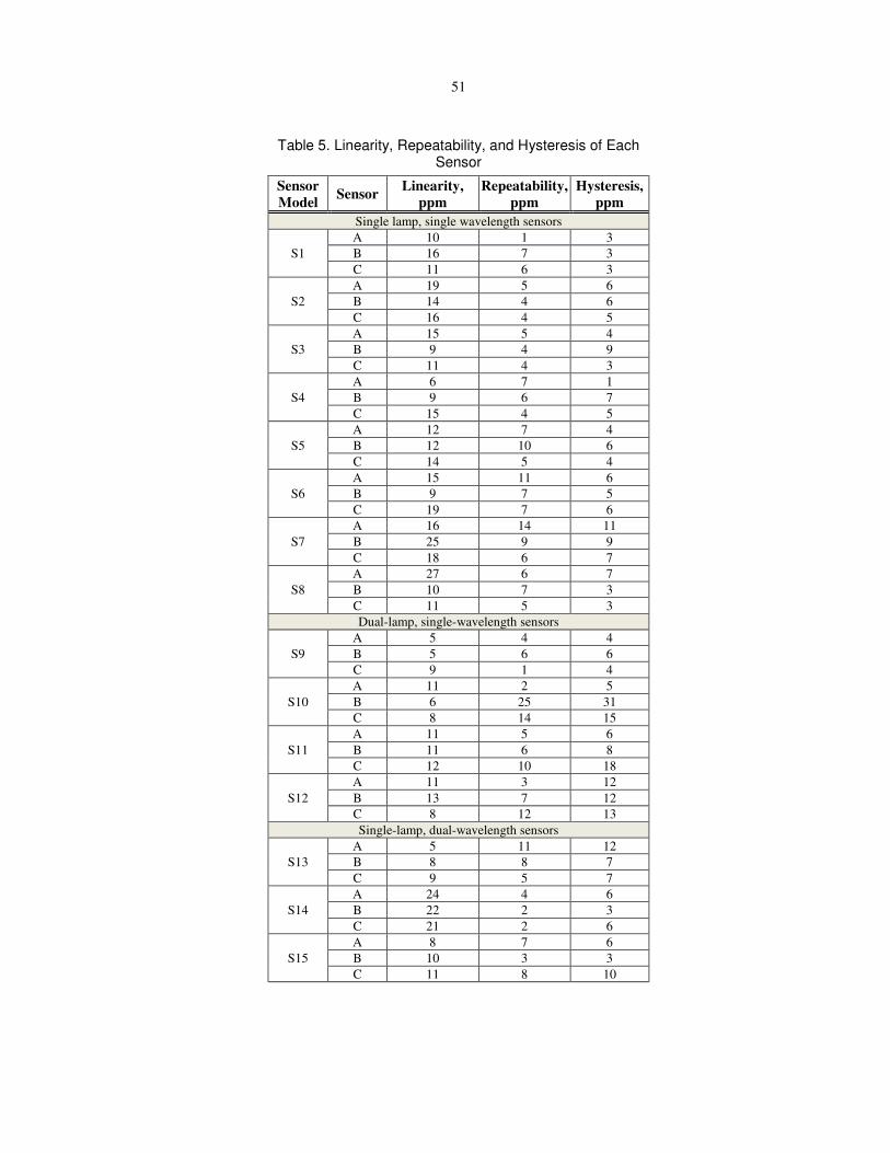
51
Table 5. Linearity, Repeatability, and Hysteresis of Each Sensor
Sensor
Model Sensor
Linearity,
ppm
Repeatability,
ppm
Hysteresis,
ppm
Single lamp, single wavelength sensors
S1
A 10 1 3
B 16 7 3
C 11 6 3
S2
A 19 5 6
B 14 4 6
C 16 4 5
S3
A 15 5 4
B 9 4 9
C 11 4 3
S4
A 6 7 1
B 9 6 7
C 15 4 5
S5
A 12 7 4
B 12 10 6
C 14 5 4
S6
A 15 11 6
B 9 7 5
C 19 7 6
S7
A 16 14 11
B 25 9 9
C 18 6 7
S8
A 27 6 7
B 10 7 3
C 11 5 3
Dual-lamp, single-wavelength sensors
S9
A 5 4 4
B 5 6 6
C 9 1 4
S10
A 11 2 5
B 6 25 31
C 8 14 15
S11
A 11 5 6
B 11 6 8
C 12 10 18
S12
A 11 3 12
B 13 7 12
C 8 12 13
Single-lamp, dual-wavelength sensors
S13
A 5 11 12
B 8 8 7
C 9 5 7
S14
A 24 4 6
B 22 2 3
C 21 2 6
S15
A 8 7 6
B 10 3 3
C 11 8 10
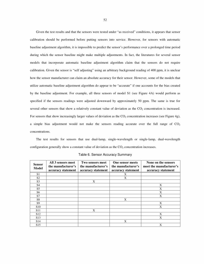
52
Given the test results and that the sensors were tested under “as received” conditions, it appears that sensor
calibration should be performed before putting sensors into service. However, for sensors with automatic
baseline adjustment algorithm, it is impossible to predict the sensor’s performance over a prolonged time period
during which the sensor baseline might make multiple adjustments. In fact, the literatures for several sensor
models that incorporate automatic baseline adjustment algorithm claim that the sensors do not require
calibration. Given the sensor is “self adjusting” using an arbitrary background reading of 400 ppm, it is unclear
how the sensor manufacturer can claim an absolute accuracy for their sensor. However, some of the models that
utilize automatic baseline adjustment algorithm do appear to be “accurate” if one accounts for the bias created
by the baseline adjustment. For example, all three sensors of model S1 (see Figure 4A) would perform as
specified if the sensors readings were adjusted downward by approximately 50 ppm. The same is true for
several other sensors that show a relatively constant value of deviation as the CO2 concentration is increased.
For sensors that show increasingly larger values of deviation as the CO2 concentration increases (see Figure 4g),
a simple bias adjustment would not make the sensors reading accurate over the full range of CO2
concentrations.
The test results for sensors that use dual-lamp, single-wavelength or single-lamp, dual-wavelength
configuration generally show a constant value of deviation as the CO2 concentration increases.
Table 6. Sensor Accuracy Summary
Sensor
Model
All 3 sensors meet
the manufacturer’s
accuracy statement
Two sensors meet
the manufacturer’s
accuracy statement
One sensor meets
the manufacturer’s
accuracy statement
None on the sensors
meet the manufacturer’s
accuracy statement
S1 X
S2 X
S3 X
S4 X
S5 X
S6 X
S7 X
S8 X
S9 X
S10 X
S11 X
S12 X
S13 X
S14 X
S15 X

53
Nonlinearity, repeatability and hysteresis do not appear to be significant for most of the sensors tested.
Only three sensors models specified their nonlinearity as less than 1% full scale (20 ppm), and all three sensor
models meet their linearity specification. The S8A sensor has the largest nonlinearity of 27 ppm, while many
sensors’ nonlinearity is less than 5 ppm.
Five sensor models specified their repeatability and all five sensor models meet their repeatability
specification. Sensor S10 showed maximum repeatability error of 25 ppm. All other sensors have repeatability
within 14 ppm.
None of the sensor manufacturers specified hysteresis for their sensors. Sensor S10 showed maximum
hysteresis of 31 ppm and sensor S11 showed maximum hysteresis of 18 ppm. All other sensors have hysteresis
within 13 ppm.
ACKNOWLEDGEMENTS
This work is performed for National Building Controls Information Program (NBCIP), which is sponsored
by the Iowa Energy Center, NSTAR Electric & Gas Corporation and the California Energy Commission.
REFERENCES
Fahlen, P., H. Andersson, and S. Ruud. 1992. Demand Controlled Ventilating Systems - Sensor Tests. Swedish
National Testing and Research Institute, Boras, Sweden, SP Report 1992:13.
Fisk, W.J., D. Faulkner, and D.P. Sullivan. 2006. Accuracy of CO2 sensors in commercial buildings: a pilot
study. LBNL-61962, Lawrence Berkeley National Laboratory, Berkeley, CA.
Pandey, S.K., K. Kim, and S. Lee. 2007. Use of a dynamic enclosure approach to test the accuracy of the NDIR
sensor: evaluation based on the CO2 equilibration pattern. Molecular Diversity Preservation International,
Matthaeusstrasse, Switzerland, ISSN: 1424-8220.
Shrestha, S.S., and G.M. Maxwell. 2009. An experimental evaluation of HVAC-grade carbon-dioxide sensors:
part 1, test and evaluation procedure. ASHRAE Transactions 115(2).
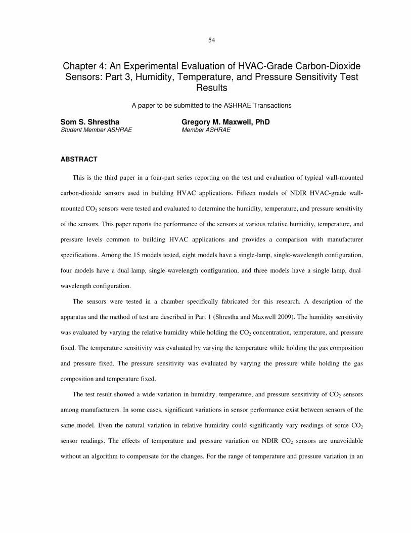
54
Chapter 4: An Experimental Evaluation of HVAC-Grade Carbon-Dioxide Sensors: Part 3, Humidity, Temperature, and Pressure Sensitivity Test
Results
A paper to be submitted to the ASHRAE Transactions
Som S. Shrestha Gregory M. Maxwell, PhD Student Member ASHRAE Member ASHRAE
ABSTRACT
This is the third paper in a four-part series reporting on the test and evaluation of typical wall-mounted
carbon-dioxide sensors used in building HVAC applications. Fifteen models of NDIR HVAC-grade wall-
mounted CO2 sensors were tested and evaluated to determine the humidity, temperature, and pressure sensitivity
of the sensors. This paper reports the performance of the sensors at various relative humidity, temperature, and
pressure levels common to building HVAC applications and provides a comparison with manufacturer
specifications. Among the 15 models tested, eight models have a single-lamp, single-wavelength configuration,
four models have a dual-lamp, single-wavelength configuration, and three models have a single-lamp, dual-
wavelength configuration.
The sensors were tested in a chamber specifically fabricated for this research. A description of the
apparatus and the method of test are described in Part 1 (Shrestha and Maxwell 2009). The humidity sensitivity
was evaluated by varying the relative humidity while holding the CO2 concentration, temperature, and pressure
fixed. The temperature sensitivity was evaluated by varying the temperature while holding the gas composition
and pressure fixed. The pressure sensitivity was evaluated by varying the pressure while holding the gas
composition and temperature fixed.
The test result showed a wide variation in humidity, temperature, and pressure sensitivity of CO2 sensors
among manufacturers. In some cases, significant variations in sensor performance exist between sensors of the
same model. Even the natural variation in relative humidity could significantly vary readings of some CO2
sensor readings. The effects of temperature and pressure variation on NDIR CO2 sensors are unavoidable
without an algorithm to compensate for the changes. For the range of temperature and pressure variation in an

55
air-conditioned space, the effect of pressure variation is more significant compared to the effect of temperature
variation.
INTRODUCTION
This is the third part of a four-part series of papers reporting on the test and evaluation of typical wall-
mounted CO2 sensors used in building HVAC systems. In this study, fifteen models of NDIR (non-dispersive
infrared) HVAC-grade wall-mounted CO2 sensors were tested and evaluated. In all, 45 sensors (three from
each model) were tested in order to determine the effects of humidity, temperature, and pressure on the CO2
sensors’ readings. The sensitivity of the sensor reading to each of these three parameters was computed and
compared to the manufacturers’ specifications. The experimental procedure used to test and evaluate the sensors
is described in Part 1 (Shrestha and Maxwell 2009) of this paper. Among the fifteen models tested, eight models
have a single-lamp, single-wavelength configuration, four models have a dual-lamp, single-wavelength
configuration, and three models have a single-lamp, dual-wavelength configuration. All single-lamp, single-
wavelength sensors and one single-lamp, dual-wavelength sensor incorporate an “automatic baseline
adjustment” algorithm in the sensor’s electronics package. The working principles of NDIR CO2 sensors are
described in Part 1 (Shrestha and Maxwell 2009) of this paper.
PREVIOUS STUDIES
In the past, limited studies have been done to investigate the effects of humidity, temperature, and pressure
variations on HVAC-grade CO2 sensors. Fahlen et al. (1992) evaluated the performance of two CO2 sensors,
one photo-acoustic type and one infrared spectroscopy type, in lab tests and long term field tests. The lab tests
included performance and environmental tests. The authors found that the CO2 sensors tested were sensitive to
humidity below a threshold value, however the threshold humidity level was not determined and the effect of
humidity on the sensors’ readings was not evaluated. During the low-temperature test at 5°C (which was within
the stated operating range of the sensors), the output of both sensors dropped to an unrealistic value. The
authors conclude that the deviation between actual concentration and the sensors’ reading are normally well
within ± 50 ppm at a concentration level of 1000 ppm. However, at a concentration of 2000 ppm the test results
showed a deviation of up to -300 ppm.

56
A pilot study that evaluated in-situ accuracy of 44 NDIR CO2 sensors located in nine commercial buildings
indicated that the accuracy of CO2 sensors is frequently less than is needed to measure peak indoor-outdoor CO2
concentration differences with less than 20% error (Fisk et al. 2006). The evaluation was performed either by
multi-point calibration using CO2 calibration gas or by a single-point calibration check using a co-located and
calibrated reference CO2 sensor. The effects of humidity, temperature, and pressure on the sensor readings were
not considered in the study.
Pandey et al. tested three NDIR CO2 sensors each from two sensor models. The tests were conducted in an
enclosure fabricated for the research. The sensors were tested with CO2 concentrations of 0 ppm, 500 ppm, and
1000 ppm. The research focused on the sensor accuracy but did not include effects of humidity, temperature,
and pressure variation on the sensor output.
CO2 SENSOR SPECIFICATIONS
CO2 sensor manufacturers provide detailed specifications for their products. This information is available
from the company’s website and/or literature packaged with the product. Table 1 summarizes some of the
product information for the models evaluated in this study. (Specific product names are not used in this paper,
rather the sensors are referred to as S1 through S15.) The table indicates the sensor configuration, the sensitivity
of the sensor reading due to variations in temperature, the sensitivity of the sensor reading due to variation in
pressure, and the operating range of temperature and relative humidity. None of the manufacturers specify the
sensitivity of the sensor reading due to variation in humidity.
Sensors S1 through S8 are single-lamp, single-wavelength sensor, sensors S9 through S12 are dual-lamp,
single-wavelength sensors, and sensors S13 through S15 are single-lamp, dual-wavelength sensors. All single-
lamp, single-wavelength sensors and one single-lamp, dual-wavelength sensor (S14) incorporate an “automatic
baseline adjustment” algorithm in the sensor’s electronics package. The details of the “automatic baseline
adjustment” algorithm are described in part 2 of this paper.
Of the fifteen sensor models considered in this study, seven do not explicitly state any sensitivity to
temperature. For the seven models that do provide temperature sensitivity statements, the affect of temperature
on the sensor reading is not clear. For example, model S1 states a temperature sensitivity of 5 ppm/°C. Does
this mean that the CO2 reading will increase by 5 ppm when the temperature increases by 1°C, or will the

57
reading decrease by 5 ppm? Furthermore, no reference temperature is provided on which to evaluate the
temperature change. Sensor S15 is the only model that provides a reference temperature.
Similarly, of the fifteen sensor models studied, seven do not explicitly state any sensitivity to pressure. For
the eight models that do indicate pressure sensitivity, seven specify a reference pressure (or altitude) on which
to base the pressure (or altitude) correction. For all sensors that show pressure dependence, a correction value
must be added to the sensor reading as the pressure decreases (or altitude increases).
EXPERIMENTAL TEST PROCEDURE
The CO2 sensors were tested using a test chamber specifically designed and fabricated for this study.
Technical details of the test chamber and instrumentation are described in Part 1 (Shrestha and Maxwell 2009)
of this paper. Humidity sensitivity tests were conducted at 20, 40 and 60% relative humidity while maintaining
the CO2 concentration, temperature, and pressure at 1100 ppm, 73ºF (22.8ºC) and 14.70 psia (101.35 kPa),
respectively.
Temperature sensitivity tests were conducted at 66°F (18.9°C), 73ºF (22.8ºC) and 80°F (26.7°C), while
maintaining the CO2 concentration and pressure at 1100 ppm, and 14.70 psia (101.35 kPa), respectively.
Pressure sensitivity tests were conducted at 14.70 psia (101.35 kPa), 13.25 psia (91.36 kPa) and 11.80 psia
(81.36 kPa) while maintaining the CO2 concentration and temperature at 1100 ppm and 73°F (22.8°C),
respectively. These pressures correspond to standard atmospheric pressures for altitudes at sea level, 2838 feet
(865 meters) above sea level, and 5948 feet (1813 meters) above sea level, respectively.
The temperature sensitivity and pressure sensitivity tests were conducted at a fixed gas mixture
composition. The humidity ratio was maintained at 0.0069 lb moisture/lb dry air (0.0069 kg moisture/kg dry
air), which corresponds to 40% RH at 73ºF (22.8ºC) temperature and 14.70 psia (101.35 kPa) pressure. Since
relative humidity depends on both pressure and temperature, the relative humidity varies during the pressure
and temperature sensitivity tests; however, the absolute humidity remained constant.
Established procedures, including guidelines for steady-state conditions, described in Part 1 (Shrestha and
Maxwell 2009) of this paper were used to perform the testing.

58
Table 1. Manufacturer-Specified Temperature Sensitivity, Pressure Sensitivity, and Operating Range for their Sensors
Sensor
Model Configuration
Temperature
Sensitivity Pressure Sensitivity
Temperature and
humidity
Operating Range
S1 Single-lamp, single-
wavelength 5 ppm/1.8°F (1°C) NA
32°F to 122°F
(0°C to 50°C)
0% to 95% RH
S2 Single-lamp, single-
wavelength NA
Add 6.7% of reading per psi (6.89 kPa)
decrease from 14.70 psia (101.35 kPa)*
60°F to 90°F
(15°C to 32°C)
0% to 95% RH
S3 Single-lamp, single-
wavelength 3 ppm/1.8°F (°C)*
6.7% of reading per psi (6.89 kPa) from
14.70 psia (101.35 kPa)*
59°F to 90°F
(15°C to 32°C)
0% to 95% RH
S4 Single-lamp, single-
wavelength NA NA
32°F to 122°F
(0°C to 50°C)
5% to 95% RH
S5 Single-lamp, single-
wavelength 4 ppm/1.8°F (°C)* 6.7% of reading per psi (6.89 kPa)*
32°F to 122°
(0°C to 50°C)
0% to 95% RH
S6 Single-lamp, single-
wavelength NA
9.6% of reading per psi (6.89 kPa)
deviation from 14.5 psia (100 kPa)*
32°F to 122°F
(0°C to 50°C)
0% to 95% RH
S7 Single-lamp, single-
wavelength NA
Add 7.2% of reading per psi (6.89 kPa)
decrease from 14.70 psia (101.35 kPa)*
32°F to 122°F
(0°C to 50°C)
0% to 90% RH
S8 Single-lamp, single-
wavelength NA NA
32°F to 122°F
(0°C to 50°C)
0% to 95% RH
S9 Dual-lamp, single-
wavelength 5 ppm/1.8°F (°C) 9.8% of reading per psi (6.89 kPa)*
32°F to 122°F
(0°C to 50°C)
5% to 95% RH
S10 Dual-lamp, single-
wavelength
± 2 ppm/1.8°F
(°C ) NA
23°F to 113°F
(-5°C to 45°C)
0% to 85% RH
S11 Dual-lamp, single-
wavelength NA NA
32°F to 100°F
(0°C to 40°C)
0% to 95% RH
S12 Dual-lamp, single-
wavelength 5 ppm/1.8°F (°C) NA
23°F to 131°F
(-5°C to 55°C)
0% to 90% RH
S13 Single-lamp, dual-
wavelength 2 ppm/1.8°F (°C )*
Add 10.2% of reading per psi (6.89 kPa)
decrease from 14.18 psia (97.77 kPa)*
23°F to 113°F
(-5°C to 45°C)
0% to 85% RH
S14 Single-lamp, dual-
wavelength NA
Add 6.7% of reading per psi (6.89 kPa)
decrease from 14.70 psia (101.35 kPa)*
32°F to 122°F
(0°C to 50°C)
0% to 95% RH
S15 Single-lamp, dual-
wavelength
3 ppm/1.8°F (°C)*
(reference 77°F
(25°C))
NA
23°F to 113°F
(-5°C to 45°C)
0% to 85% RH
Notes: NA indicates that the information was not available in the manufacturer’s product literature.
* indicates that the value was calculated from the manufacturer’s product literature
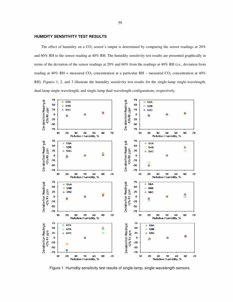
59
HUMIDITY SENSITIVITY TEST RESULTS
The effect of humidity on a CO2 sensor’s output is determined by comparing the sensor readings at 20%
and 60% RH to the sensor reading at 40% RH. The humidity sensitivity test results are presented graphically in
terms of the deviation of the sensor readings at 20% and 60% from the readings at 40% RH (i.e., deviation from
reading at 40% RH = measured CO2 concentration at a particular RH – measured CO2 concentration at 40%
RH). Figures 1, 2, and 3 illustrate the humidity sensitivity test results for the single-lamp single-wavelength,
dual-lamp single-wavelength, and single-lamp dual-wavelength configurations, respectively.
Figure 1. Humidity sensitivity test results of single-lamp, single-wavelength sensors.
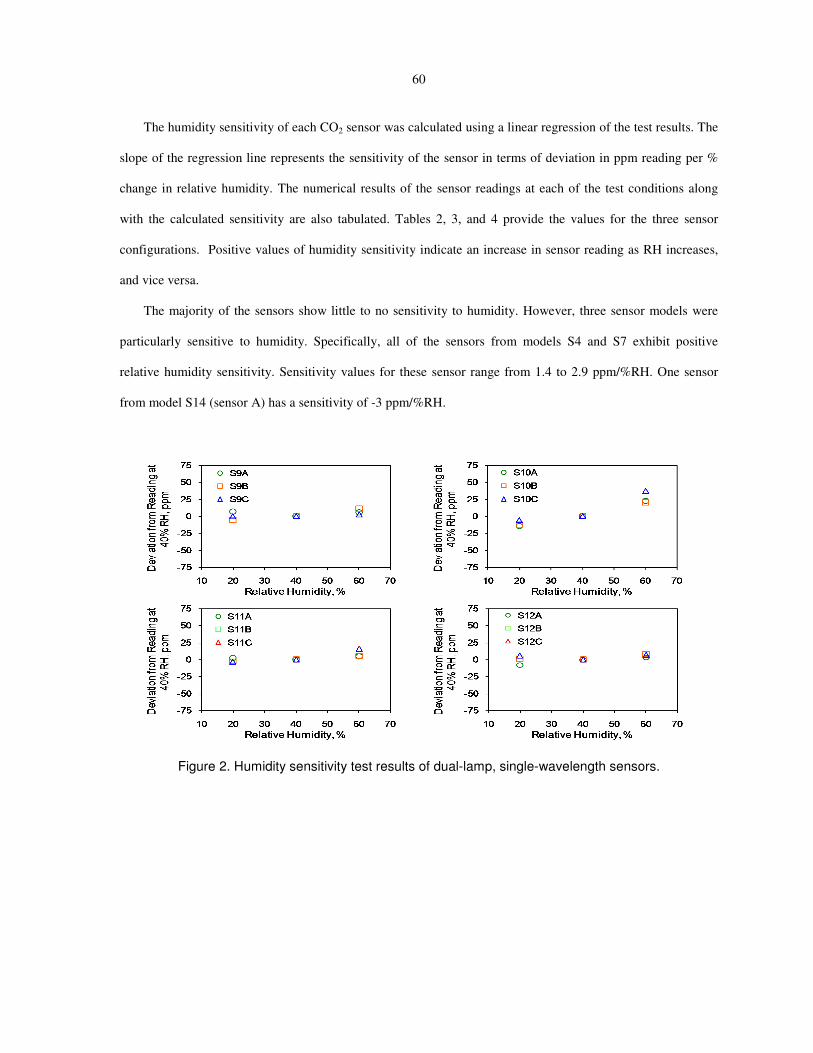
60
The humidity sensitivity of each CO2 sensor was calculated using a linear regression of the test results. The
slope of the regression line represents the sensitivity of the sensor in terms of deviation in ppm reading per %
change in relative humidity. The numerical results of the sensor readings at each of the test conditions along
with the calculated sensitivity are also tabulated. Tables 2, 3, and 4 provide the values for the three sensor
configurations. Positive values of humidity sensitivity indicate an increase in sensor reading as RH increases,
and vice versa.
The majority of the sensors show little to no sensitivity to humidity. However, three sensor models were
particularly sensitive to humidity. Specifically, all of the sensors from models S4 and S7 exhibit positive
relative humidity sensitivity. Sensitivity values for these sensor range from 1.4 to 2.9 ppm/%RH. One sensor
from model S14 (sensor A) has a sensitivity of -3 ppm/%RH.
Figure 2. Humidity sensitivity test results of dual-lamp, single-wavelength sensors.

61
Figure 3. Humidity sensitivity test results of single-lamp, dual-wavelength sensors.

62
Table 2. Humidity Sensitivity Test Results of Single-Lamp, Single-Wavelength Sensors
Sensor
Model Sensor
Reading at Sensitivity,
ppm / %RH 20% RH, ppm 40% RH, ppm 60% RH, ppm
S1
A 1192 1201 1212 0.5
B 1195 1203 1209 0.3
C 1212 1217 1225 0.3
S2
A 1222 1229 1236 0.3
B 1271 1277 1284 0.3
C 1177 1179 1185 0.2
S3
A 1273 1283 1295 0.6
B 1176 1181 1184 0.2
C 1125 1127 1130 0.1
S4
A 1282 1333 1373 2.3
B 1300 1335 1358 1.5
C 1363 1414 1458 2.4
S5
A 1296 1309 1319 0.6
B 1178 1187 1202 0.6
C 1211 1219 1226 0.4
S6
A 1255 1263 1271 0.4
B 1262 1282 1281 0.5
C 1303 1314 1328 0.6
S7
A 1448 1513 1557 2.7
B 1420 1451 1474 1.4
C 1422 1487 1539 2.9
S8
A 1275 1283 1293 0.4
B 1200 1205 1211 0.3
C 1222 1227 1236 0.3
Table 3. Humidity Sensitivity Test Results of Dual-Lamp, Single-Wavelength Sensors
Sensor
Model Sensor
Reading at Sensitivity,
ppm / %RH 20% RH, ppm 40% RH, ppm 60% RH, ppm
S9
A 1174 1167 1172 0.0
B 870 876 887 0.4
C 942 943 945 0.1
S10
A 1209 1223 1246 0.9
B 1218 1230 1250 0.8
C 1285 1291 1329 1.1
S11
A 1163 1161 1165 0.1
B 1261 1264 1269 0.2
C 1073 1077 1092 0.5
S12
A 1239 1247 1251 0.3
B 1258 1257 1264 0.2
C 1301 1295 1302 0.0

63
Table 4. Humidity Sensitivity Test Results of Single-Lamp, Dual-Wavelength Sensors
Sensor
Model Sensor
Reading at Sensitivity,
ppm / %RH 20% RH, ppm 40% RH, ppm 60% RH, ppm
S13
A 1185 1191 1187 0.1
B 1386 1391 1393 0.2
C 1316 1313 1320 0.1
S14
A 1368 1300 1246 -3.0
B 1172 1169 1160 -0.3
C 1177 1169 1195 0.4
S15
A 1096 1088 1080 -0.4
B 1174 1175 1180 0.2
C 1213 1215 1218 0.1
TEMPERATURE SENSITIVITY TEST RESULTS
The effect of temperature on a CO2 sensor’s output is determined by comparing the sensor readings at 66°F
(18.9°C) and 80°F (26.7°C) to the sensor reading at 73ºF (22.8ºC). The temperature sensitivity test results are
presented graphically in terms of the deviation of the sensor readings at 66°F (18.9°C) and 80°F (26.7°C) from
the reading at 73ºF (22.8ºC) (i.e., deviation from readings at 73ºF (22.8ºC) = measured CO2 concentration at a
particular temperature – measured CO2 concentration at 73ºF (22.8ºC)). Figures 4, 5, and 6 illustrate the
temperature sensitivity test results for the single-lamp single-wavelength, dual-lamp single-wavelength, and
single-lamp dual-wavelength configurations, respectively.
The temperature sensitivity of each CO2 sensor was calculated using a linear regression of the test results.
The slope of the regression line represents the sensitivity of the sensor in terms of deviation in ppm reading per
degree change in temperature. The numerical results of the sensor readings at each of the test conditions along
with the calculated sensitivity are also tabulated. Tables 5, 6, and 7 provide the values for the three sensor
configurations. Positive values of temperature sensitivity indicate an increase in sensor reading as temperature
increases, and vice versa.
Temperature sensitivity is not consistent between sensor models. For many sensors, the temperature
sensitivity is negligibly small. Nine sensor models showed temperature sensitivity within 5 ppm/1.8ºF (5
ppm/ºC). Sensor S12B showed the highest temperature sensitivity of 10 ppm increase in sensor reading per
1.8°F (1°C) decrease in temperature.
64
Figure 4. Temperature sensitivity test results of single-lamp, single-wavelength sensors.

65
Figure 5. Temperature sensitivity test results of dual-lamp, single-wavelength sensors.
Figure 6. Temperature sensitivity test results of single-lamp, dual-wavelength sensors.
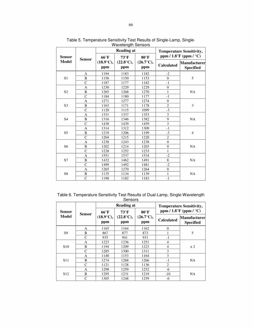
66
Table 5. Temperature Sensitivity Test Results of Single-Lamp, Single-Wavelength Sensors
Sensor
Model Sensor
Reading at Temperature Sensitivity,
ppm / 1.8°F (ppm / °C) 66°F
(18.9°C),
ppm
73°F
(22.8°C),
ppm
80°F
(26.7°C),
ppm Calculated Manufacturer
Specified
S1
A 1194 1183 1182 -2
5 B 1156 1150 1153 0
C 1187 1177 1182 -1
S2
A 1230 1229 1229 0
NA B 1265 1268 1270 1
C 1184 1180 1177 -1
S3
A 1271 1277 1274 0
3 B 1163 1171 1178 2
C 1120 1115 1099 -3
S4
A 1331 1337 1353 3
NA B 1316 1346 1382 9
C 1438 1439 1459 3
S5
A 1314 1312 1309 -1
4 B 1219 1206 1199 -3
C 1204 1215 1220 2
S6
A 1238 1243 1238 0
NA B 1202 1214 1203 0
C 1228 1252 1233 1
S7
A 1551 1537 1534 -2
NA B 1432 1462 1491 8
C 1499 1492 1481 -2
S8
A 1265 1270 1264 0
NA B 1135 1134 1139 1
C 1190 1182 1183 -1
Table 6. Temperature Sensitivity Test Results of Dual-Lamp, Single-Wavelength Sensors
Sensor
Model Sensor
Reading at Temperature Sensitivity,
ppm / 1.8°F (ppm / °C) 66°F
(18.9°C),
ppm
73°F
(22.8°C),
ppm
80°F
(26.7°C),
ppm Calculated Manufacturer
Specified
S9
A 1165 1164 1162 0
5 B 867 877 873 1
C 935 941 931 -1
S10
A 1223 1236 1251 4
± 2 B 1194 1209 1223 4
C 1285 1300 1311 3
S11
A 1140 1153 1164 3
NA B 1274 1268 1266 -1
C 1121 1128 1136 2
S12
A 1298 1259 1252 -6
NA B 1295 1231 1219 -10
C 1305 1248 1259 -6
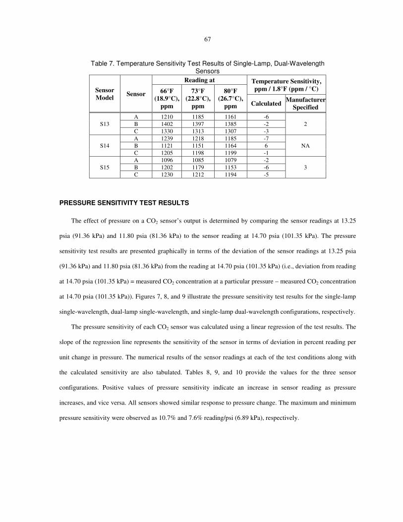
67
Table 7. Temperature Sensitivity Test Results of Single-Lamp, Dual-Wavelength Sensors
Sensor
Model Sensor
Reading at Temperature Sensitivity,
ppm / 1.8°F (ppm / °C) 66°F
(18.9°C),
ppm
73°F
(22.8°C),
ppm
80°F
(26.7°C),
ppm Calculated Manufacturer
Specified
S13
A 1210 1185 1161 -6
2 B 1402 1397 1385 -2
C 1330 1313 1307 -3
S14
A 1239 1218 1185 -7
NA B 1121 1151 1164 6
C 1205 1198 1199 -1
S15
A 1096 1085 1079 -2
3 B 1202 1179 1153 -6
C 1230 1212 1194 -5
PRESSURE SENSITIVITY TEST RESULTS
The effect of pressure on a CO2 sensor’s output is determined by comparing the sensor readings at 13.25
psia (91.36 kPa) and 11.80 psia (81.36 kPa) to the sensor reading at 14.70 psia (101.35 kPa). The pressure
sensitivity test results are presented graphically in terms of the deviation of the sensor readings at 13.25 psia
(91.36 kPa) and 11.80 psia (81.36 kPa) from the reading at 14.70 psia (101.35 kPa) (i.e., deviation from reading
at 14.70 psia (101.35 kPa) = measured CO2 concentration at a particular pressure – measured CO2 concentration
at 14.70 psia (101.35 kPa)). Figures 7, 8, and 9 illustrate the pressure sensitivity test results for the single-lamp
single-wavelength, dual-lamp single-wavelength, and single-lamp dual-wavelength configurations, respectively.
The pressure sensitivity of each CO2 sensor was calculated using a linear regression of the test results. The
slope of the regression line represents the sensitivity of the sensor in terms of deviation in percent reading per
unit change in pressure. The numerical results of the sensor readings at each of the test conditions along with
the calculated sensitivity are also tabulated. Tables 8, 9, and 10 provide the values for the three sensor
configurations. Positive values of pressure sensitivity indicate an increase in sensor reading as pressure
increases, and vice versa. All sensors showed similar response to pressure change. The maximum and minimum
pressure sensitivity were observed as 10.7% and 7.6% reading/psi (6.89 kPa), respectively.

68
Figure 7. Pressure sensitivity test results of single-lamp, single-wavelength sensors.

69
Figure 8. Pressure sensitivity test results of dual-lamp, single-wavelength sensors.
Figure 9. Pressure sensitivity test results of single-lamp, dual-wavelength sensors.

70
Table 8. Pressure Sensitivity Test Results of Single-Lamp, Single-Wavelength Sensors
Sensor
Model Sensor
Reading at Pressure Sensitivity,
% Reading / psi (6.89 kPa)
14.70 psia
(101.35 kPa),
ppm
13.25 psia
(91.36 kPa),
ppm
11.80 psia
(81.36 kPa),
ppm
Calculated Manufacturer
Specified
S1
A 1189 1018 853 9.8
NA B 1149 980 980 9.9
C 1184 1007 842 9.9
S2
A 1233 1070 921 8.8
6.7 B 1267 1093 1093 9.1
C 1180 1029 888 8.5
S3
A 1275 1102 944 9.0
6.7 B 1171 1017 1017 8.9
C 1114 971 835 8.6
S4
A 1330 1167 1024 8.0
NA B 1343 1182 1182 8.2
C 1438 1274 1116 7.7
S5
A 1315 1137 975 9.0
6.7 B 1210 1063 1063 8.4
C 1214 1056 909 8.6
S6
A 1240 1057 884 9.9
9.6 B 1204 1016 1016 10.2
C 1237 1050 885 9.8
S7
A 1539 1365 1203 7.6
7.2 B 1457 1296 1296 7.8
C 1485 1325 1154 7.7
S8
A 1260 1067 886 10.3
NA B 1132 962 962 10.0
C 1187 1007 845 9.9
Table 9. Pressure Sensitivity Test Results of Dual-Lamp, Single-Wavelength Sensors
Sensor
Model Sensor
Reading at Pressure Sensitivity,
% Reading / psi (6.89 kPa)
14.70 psia
(101.35 kPa),
ppm
13.25 psia
(91.36 kPa),
ppm
11.80 psia
(81.36 kPa),
ppm
Calculated Manufacturer
Specified
S9
A 1161 995 829 9.9
9.8 B 862 722 722 10.7
C 914 757 630 10.7
S10
A 1238 1090 952 8.0
NA B 1206 1056 1056 8.1
C 1293 1143 1002 7.7
S11
A 1150 1004 867 8.5
NA B 1263 1100 1100 8.6
C 1143 965 805 10.2
S12
A 1275 1121 976 8.1
NA B 1246 1097 1097 8.2
C 1277 1117 972 8.2
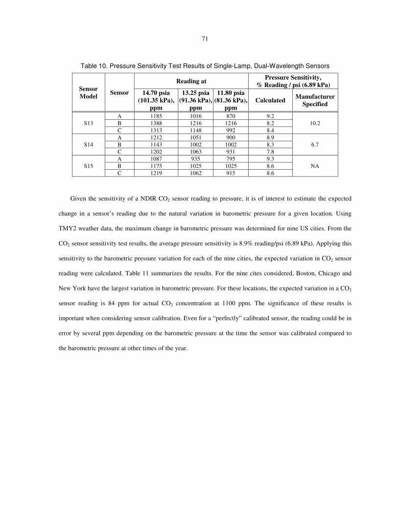
71
Table 10. Pressure Sensitivity Test Results of Single-Lamp, Dual-Wavelength Sensors
Sensor
Model Sensor
Reading at Pressure Sensitivity,
% Reading / psi (6.89 kPa)
14.70 psia
(101.35 kPa),
ppm
13.25 psia
(91.36 kPa),
ppm
11.80 psia
(81.36 kPa),
ppm
Calculated Manufacturer
Specified
S13
A 1185 1016 870 9.2
10.2 B 1388 1216 1216 8.2
C 1313 1148 992 8.4
S14
A 1212 1051 900 8.9
6.7 B 1143 1002 1002 8.3
C 1202 1063 931 7.8
S15
A 1087 935 795 9.3
NA B 1175 1025 1025 8.6
C 1219 1062 915 8.6
Given the sensitivity of a NDIR CO2 sensor reading to pressure, it is of interest to estimate the expected
change in a sensor’s reading due to the natural variation in barometric pressure for a given location. Using
TMY2 weather data, the maximum change in barometric pressure was determined for nine US cities. From the
CO2 sensor sensitivity test results, the average pressure sensitivity is 8.9% reading/psi (6.89 kPa). Applying this
sensitivity to the barometric pressure variation for each of the nine cities, the expected variation in CO2 sensor
reading were calculated. Table 11 summarizes the results. For the nine cites considered, Boston, Chicago and
New York have the largest variation in barometric pressure. For these locations, the expected variation in a CO2
sensor reading is 84 ppm for actual CO2 concentration at 1100 ppm. The significance of these results is
important when considering sensor calibration. Even for a “perfectly” calibrated sensor, the reading could be in
error by several ppm depending on the barometric pressure at the time the sensor was calibrated compared to
the barometric pressure at other times of the year.

72
Table 11. Expected Variation in CO2 Sensor Output due to Variation in Local Barometric Pressure (at 1100 ppm CO2
Concentration)
Location Variation in Barometric
Pressure, psi (kPa)
Variation in CO2
Reading, ppm
Atlanta 0.508 (3.502) 50
Boston 0.860 (5.930) 84
Chicago 0.855 (5.895) 84
Denver 0.590 (4.068) 58
Los Angeles 0.566 (3.902) 55
Miami 0.377 (2.599) 37
New York 0.855 (5.895) 84
Sacramento 0.435 (2.999) 43
San Francisco 0.493 (3.399) 48
CONCLUSIONS
The result from the tests conducted under accurate and repeatable condition showed a wide variation in
humidity and temperature sensitivity among the NDIR CO2 sensor models. In some cases, significant variations
in sensor performance exist between sensors of the same model while in other cases, all sensors of the same
model showed almost identical behavior.
None of the sensor manufacturors specified humidity dependence of their CO2 sensors. While majority of
the sensors show little to no sensitivity to humidity, the test results revealed that three sensor models are highly
sensitive to humidity. The maximum humidity sensitivity was observed as -3 ppm/% RH. It is suspected that the
sensors with high humidity sensitivity use hygroscopic material as an optical filter.
Theoretically, increase in temperature at a fixed gas composition and pressure should decrease the number
of molecules in optical path of a NDIR CO2 sensor and hence decrease the sensor reading. Some sensors
showed an opposite phenomenon. Nine sensor models showed temperature sensitivity within 5 ppm/1.8ºF (5
ppm/ºC). The maximum temperature sensitivity was observed as 10 ppm increase in sensor reading per 1.8°F
(1°C) decrease in temperature for actual CO2 concentration at 1100 ppm.
As was expected, the decrease in pressure decreased readings of all sensors. The maximum and minimum
pressure sensitivity were observed as 129 and 92 ppm/psi (ppm/6.89 kPa), respectively at actual CO2

73
concentration of 1100 ppm. Even for a best performing sensor, the natural barometric pressure variation results
in significant change in NDIR CO2 sensor reading.
The test results showed that the effects of temperature and pressure variation on NDIR CO2 sensors are
unavoidable. For the range of temperature and pressure variation in an air-conditioned space, the effect of
pressure variation is more significant compared to the effect of temperature variation. An important
consequence of the sensitivity of NDIR CO2 sensor readings to pressure and temperature is field calibration.
Some controls contactors field calibrate the sensors at the time the sensors are installed. In addition, many
sensor models require calibration every 3 to 5 years. Field calibration typically involves flowing a calibration
gas with a know concentration of CO2 through the sensor’s optical sensing element. Accurate calibration
requires knowing the temperature and the pressure of the gas in the optical sensing element. Of these two,
pressure is more important. If the calibration gas flow rate is low enough, then the pressure in the optical
element would not be significantly different from atmospheric conditions. However, if the gas flow rate were
too high, the gas pressure in the optical element would have an effect on the sensor reading.
ACKNOWLEDGEMENTS
This work is performed for National Building Controls Information Program (NBCIP), which is sponsored
by the Iowa Energy Center, NSTAR Electric & Gas Corporation and the California Energy Commission.
REFERENCES
Fahlen, P., H. Andersson, and S. Ruud. 1992. Demand Controlled Ventilating Systems - Sensor Tests. Swedish
National Testing and Research Institute, Boras, Sweden, SP Report 1992:13.
Fisk, W.J., D. Faulkner, and D.P. Sullivan. 2006. Accuracy of CO2 sensors in commercial buildings: a pilot
study. LBNL-61962, Lawrence Berkeley National Laboratory, Berkeley, CA.
Pandey, S.K., K. Kim, and S. Lee. 2007. Use of a dynamic enclosure approach to test the accuracy of the NDIR
sensor: evaluation based on the CO2 equilibration pattern. Molecular Diversity Preservation International,
Matthaeusstrasse, Switzerland, ISSN: 1424-8220.
Shrestha, S.S., and G.M. Maxwell. 2009. An experimental evaluation of HVAC-grade carbon-dioxide sensors:
part 1, test and evaluation procedure. ASHRAE Transactions 115(2).

74
Chapter 5: An Experimental Evaluation of HVAC-Grade Carbon-Dioxide
Sensors: Part 4, Effects of Ageing on Sensor Performance
A paper to be submitted to the ASHRAE Transactions
Som S. Shrestha Gregory M. Maxwell, PhD Student Member ASHRAE Member ASHRAE
ABSTRACT
This is the fourth paper in a four-part series reporting on the test and evaluation of typical wall-mounted
carbon-dioxide sensors used in building HVAC applications. Fifteen models of NDIR HVAC-grade wall-
mounted CO₂ sensors were tested and evaluated to determine the effect of ageing on the sensors’ performance.
In all, 45 sensors were evaluated: three from each of the 15 models. Among the 15 models tested, eight models
have a single-lamp, single-wavelength configuration, four models have a dual-lamp, single-wavelength
configuration, and three models have a single-lamp, dual-wavelength configuration. All single-lamp, single-
wavelength sensors and one single-lamp, dual-wavelength sensor incorporate an “automatic baseline
adjustment” algorithm in the sensor’s electronics package.
Each sensor was tested under “as received” conditions, and then, over the course of one year, performance
tests were conducted at four-month intervals. All tests were conducted at 40% relative humidity, 73oF (22.8
oC)
temperature, 14.70 psia (101.35 kPa) pressure, and 1100 ppm CO2 concentration. For each sensor, the readings
from the four tests were compared in order to evaluate the effect of continuous operation on the sensor’s
performance. The test results showed a wide variation in sensor performance among the various manufacturers.
The maximum deviation in a sensor’s reading was observed to be 420 ppm (38%) while the minimum deviation
in a sensor’s reading was observed to be 0 ppm.
INTRODUCTION
This is part four of a four-part series of papers reporting on the test and evaluation of typical CO2 sensors
used in building HVAC systems. In this study, fifteen models of NDIR (non-dispersive infrared) HVAC-grade
CO2 sensors were tested and evaluated to examine the affects of ageing on sensor performance. To compensate
75
for sensor ageing, some sensors automatically reset the baseline value (normally 400 ppm) according to
minimum CO2 concentration observed over a time period. This technique relies on the fact that many buildings
experience unoccupied periods during which CO2 levels drop to outdoor levels. Other techniques used to
compensate for the sensor ageing include dual-lamp, single-wavelength and single-lamp, dual-wavelength
configurations. The working principles, physical construction, advantages and disadvantages of NDIR CO2
sensors are well documented in the literature (Raatschen (1990), Emmerich and Persily (2001), Schell and Int-
House (2001), Fahlen et al. (1992)).
Among the 15 models tested, eight models have a single-lamp, single-wavelength configuration, four
models have a dual-lamp, single-wavelength configuration, and three models have a single-lamp, dual-
wavelength configuration. In all, 45 sensors (three from each model) were evaluated. The tests were designed to
assess the performance of the sensors while they operated under typical building conditions for a one-year
period.
PREVIOUS STUDIES
In the past, limited studies have been done to investigate the performance of HVAC-grade CO2 sensors
using a controlled environment. No published information is available that shows systematic study to quantify
effect of ageing on NDIR CO2 sensors.
Fahlen et al. (1992) evaluated the performance of two CO2 sensors, one photo-acoustic type and one
infrared spectroscopy type, in lab tests and long term field tests. The lab tests included performance and
environmental tests. The authors conclude that the deviation between actual concentration and the sensors’
reading are normally well within ± 50 ppm at a concentration level of 1000 ppm. However, at a concentration of
2000 ppm the test results showed a deviation of up to -300 ppm. The output of one sensor increased
dramatically during environmental testing. This sensor failed to return to its normal value.
Fisk et al. (2006) conducted a pilot study that evaluated the in-situ accuracy of 44 NDIR CO2 sensors
located in nine commercial buildings. The evaluation was performed either by multi-point calibration using CO2
calibration gas or by a single-point calibration check using a co-located and calibrated reference CO2 sensor.
Their results indicated that the accuracy of CO2 sensors is frequently less than what is needed to measure peak

76
indoor-outdoor CO2 concentration differences with an error that is less than 20%. Thus, the authors conclude
that there is a need for more accurate CO2 sensors and/or better maintenance and calibration.
Pandey et al. (2007) evaluated the accuracy of two NDIR CO2 sensor models. They tested three sensors of
each model. The tests were performed in an enclosure where all six sensors were exposed to CO2 concentration
of 0 ppm, 500 ppm, and 1000 ppm (other environmental conditions, such as humidity, temperature, and
pressure were not specified.) The maximum deviation was observed as -73 ppm at a CO2 concentration of 500
ppm.
A study conducted at the Iowa Energy Center showed that, among the three new, co-located sensors, one
sensor read about 105 ppm higher, compared to the two other sensors, at about 400 ppm (House 2006). Nine
months later, the sensor that read 105 ppm higher at the beginning, read 265 ppm higher compared to the two
other sensors.
This paper describes a series of tests conducted in four months interval for one year to evaluate effect of
ageing on performance of NDIR CO2 sensors. In addition, the paper presents test and evaluation results,
including the sensors behavior during initial power-up and conditioning period. The benefit of the present work
is that it provides repeated assessment of the performance of each sensor under repeatable conditions.
CO2 SENSOR SPECIFICATIONS
CO2 sensor manufacturers provide detailed specifications for their products. This information is available from
the company’s website and/or literature packaged with the product. Table 1 summarizes some of the product
information for the models evaluated in this study. (Specific product names are not used in this paper, rather the
sensors are referred to as S1 through S15 with the letters A, B and C used to differentiate between sensors of the
same model.) The table indicates the sensor configuration, manufacturer-specified long-term stability,
calibration time interval, and calibration procedure. As can be seen from the table, the models range from
sensors that require no calibration during their fifteen-year lifespan, to sensors that require calibration every
three to five years. Many sensors where calibration is suggested (or mandatory) require special calibration
software and the use of calibration gas. In some cases, a single-point calibration is all that is required.
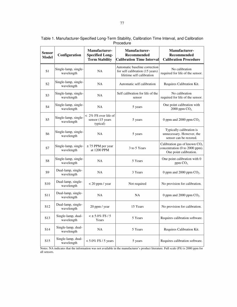
77
Table 1. Manufacturer-Specified Long-Term Stability, Calibration Time Interval, and Calibration
Procedure
Sensor
Model Configuration
Manufacturer-
Specified Long-
Term Stability
Manufacturer-
Recommended
Calibration Time Interval
Manufacturer-
Recommended
Calibration Procedure
S1 Single-lamp, single-
wavelength NA
Automatic baseline correction
for self calibration (15 years)
lifetime self calibration
No calibration
required for life of the sensor.
S2 Single-lamp, single-
wavelength NA Automatic self calibration Requires Calibration Kit.
S3 Single-lamp, single-
wavelength NA
Self calibration for life of the
sensor
No calibration
required for life of the sensor.
S4 Single-lamp, single-
wavelength NA 5 years
One point calibration with
2000 ppm CO2.
S5 Single-lamp, single-
wavelength
< 2% FS over life of
sensor (15 years
typical)
5 years 0 ppm and 2000 ppm CO2.
S6 Single-lamp, single-
wavelength NA 5 years
Typically calibration is
unnecessary. However, the
sensor can be rezored.
S7 Single-lamp, single-
wavelength
± 75 PPM per year
at 1200 PPM 3 to 5 Years
Calibration gas of known CO2
concentration (0 to 2000 ppm).
One point calibration.
S8 Single-lamp, single-
wavelength NA 5 Years
One point calibration with 0
ppm CO2.
S9 Dual-lamp, single-
wavelength NA 3 Years 0 ppm and 2000 ppm CO2.
S10 Dual-lamp, single-
wavelength < 20 ppm / year Not required No provision for calibration.
S11 Dual-lamp, single-
wavelength NA NA 0 ppm and 2000 ppm CO2.
S12 Dual-lamp, single-
wavelength 20 ppm / year 15 Years No provision for calibration.
S13 Single-lamp, dual-
wavelength
< ± 5.0% FS / 5
Years 5 Years Requires calibration software.
S14 Single-lamp, dual-
wavelength NA 5 Years Requires Calibration Kit.
S15 Single-lamp, dual-
wavelength < 5.0% FS / 5 years 5 years Requires calibration software.
Notes: NA indicates that the information was not available in the manufacturer’s product literature. Full scale (FS) is 2000 ppm for
all sensors.

78
Sensors S1 through S8 are single-lamp, single-wavelength sensor, sensors S9 through S12 are dual-lamp,
single-wavelength sensors, and sensors S13 through S15 are single-lamp, dual-wavelength sensors. All single-
lamp, single-wavelength sensors incorporate an “automatic baseline adjustment” algorithm in the sensor’s
electronics package. One single-lamp, dual-wavelength sensor (S14) also incorporates an “automatic baseline
adjustment” algorithm in it, with an option to turn on or off. The manufacturer’s default selection was “on”, and
no adjustment was made to change the setting. The details of the “automatic baseline adjustment” algorithm are
described in part 2 of this paper.
EXPERIMENTAL TEST PROCEDURE
The CO2 sensors were tested using two experimental apparatus specifically designed and fabricated for the
performance evaluation. Performance testing under controlled environmental conditions was conducted in the
test chamber shown in Figure 1 while continuous operation of the sensors in the laboratory environment was
conducted in the lab station shown in Figure 2. Technical details of these apparats and instrumentation are
described in Part 1 (Shrestha and Maxwell 2009) of this paper.
The performance of each sensor was evaluated under “as received” conditions, and then, over the course of
one year, performance tests were conducted every four months. All performance tests were conducted at 40%
relative humidity, 73oF (22.8
oC) temperature, 14.70 psia (101.35 kPa) pressure, and 1100 ppm CO2
concentration.
Before the first test was conducted, all sensors were placed in the lab station and powered up and allowed
to operate in the laboratory environment for at least a three weeks period. This time period was sufficient for all
sensor models to stabilize, and for sensors that make “automatic baseline adjustment” to complete their “self-
calibration process”. The environmental conditions in the laboratory are typical of air-conditioned, part-time
occupied space. Daily variations in space humidity, barometric pressure, temperature and levels of CO2
concentration were observed and recorded. Figure 3 shows the CO2 concentration in the laboratory for two
weeks prior to performance testing. Figure 4 shows the temperature and pressure in the laboratory for two
weeks prior to performance testing.

79
Figure 1. Test chamber.
Figure 2. Lab station.
Figure 3. CO2 concentration in the laboratory.
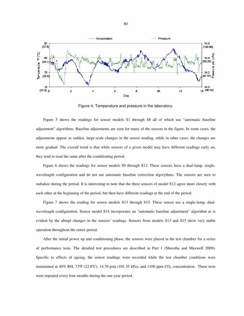
80
Figure 4. Temperature and pressure in the laboratory.
Figure 5 shows the readings for sensor models S1 through S8 all of which use “automatic baseline
adjustment” algorithms. Baseline adjustments are seen for many of the sensors in the figure. In some cases, the
adjustments appear as sudden, large-scale changes in the sensor reading, while in other cases, the changes are
more gradual. The overall trend is that while sensors of a given model may have different readings early on,
they tend to read the same after the conditioning period.
Figure 6 shows the readings for sensor models S9 through S12. These sensors have a dual-lamp, single-
wavelength configuration and do not use automatic baseline correction algorythms. The sensors are seen to
stabalize during the period. It is interesting to note that the three sensors of model S12 agree more closely with
each other at the beginning of the period, but then have different readings at the end of the period.
Figure 7 shows the reading for sensor models S13 through S15. These sensor use a single-lamp, dual-
wavelength configuration. Sensor model S14 incorporates an “automatic baseline adjustment” algorithm as is
evident by the abrupt changes in the sensors’ readings. Sensors from models S13 and S15 show very stable
operation throughout the entire period.
After the initial power up and conditioning phase, the sensors were placed in the test chamber for a series
of performance tests. The detailed test procedures are described in Part 1 (Shrestha and Maxwell 2009).
Specific to effects of ageing, the sensor readings were recorded while the test chamber conditions were
maintained at 40% RH, 73ºF (22.8ºC), 14.70 psia (101.35 kPa), and 1100 ppm CO2 concentration. These tests
were repeated every four months during the one-year period.

81
Figure 5. Power-up and conditioning of single-lamp, single-wavelength sensors.
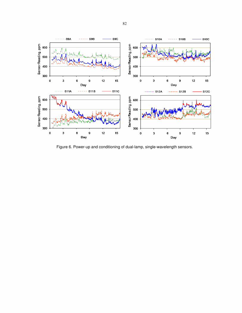
82
Figure 6. Power-up and conditioning of dual-lamp, single-wavelength sensors.

83
Figure 7. Power-up and conditioning of single-lamp dual-wavelength sensors.
On average, sensors would spend approximately two days in the test chamber during performance testing.
During the rest of the time, the sensors were located in the lab station where they would periodically be exposed
to higher levels of CO2. For three days per week, the CO2 concentration was increased to approximately 1100
ppm for a period of 8 to 12 hours. The specific days of the week and number of hours per day were chosen at
random. Figure 8 illustrates typicall CO2 concentrations during the “exercise period” At all other times, the
sensors experienced ambient laboratory conditions.

84
Figure 8. Lab Station CO2 concentration during exercise period.
AGEING TEST RESULTS
The effects of ageing on the sensors’ performance is presented in terms of the deviation of measured CO2
concentration by a sensor in a given test from the measured CO2 concentration by the sensor in the first test
(beginning of life) (i.e., deviation = measured CO2 concentration in a subsequent test – measured CO2
concentration in the first test). The deviation is calculated for each sensor reading at 1100 ppm CO2
concentration in the test chamber. As mentioned earlier, three sensors from each of fifteen models were tested.
The letters A, B and C are used to distinguish between each sensor of a given model. Data plots are used to
illustrate the effects of ageing on the CO2 sensors’ performance while numerical results are provided in tables.
Single-lamp, single-wavelength sensors: The test results for sensor models S1 through S8 are shown
graphically in Figure 9 and are presented numerically in Table 2. Recall that the tests were conducted with CO2
concentration of 1100 ppm; therefore, a deviation of 11 ppm corresponds to 1% change in the sensor
performance. The accuracy of the CO2 gas mixture in the test apparatus is 1% of the concentration which also
corresponds to 11 ppm. Thus, within the uncertainty of the experimental apparatus, sensor with deviations of
1% or less can be considered as stable with no affect of ageing.
From Table 1, sensor model S5 is expected to have a deviation less than 40 ppm over 15 years and sensor
model S7 is expected to have a deviation of ± 75 PPM per year at 1200 PPM. Upon examination of the
performance of these sensors as shown in Table 2, at the end of one year, these sensors are within the specified
limits.

85
Figure 9. Deviation from the reading from the first test for single-lamp, single-wavelength sensors.

86
Table 2. Ageing Test Result of Single-Lamp, Single-Wavelength Sensors
Sensor
Model Sensor
Deviation from Reading at First Test,
ppm
Second Test Third Test Fourth Test
S1
A 83 -17 -11
B 77 -17 3
C 53 -22 -20
S2
A 45 -26 0
B 65 4 6
C 25 -42 -33
S3
A 15 -39 -33
B 25 -38 -40
C -2 -78 -53
S4
A -63 -141 -53
B -13 -72 46
C -10 -74 -25
S5
A 19 -45 -19
B 25 -50 -40
C 17 -49 -38
S6
A 60 -44 -52
B 76 -30 -12
C 49 -38 17
S7
A 14 -47 -65
B -52 -113 -55
C -44 -47 -34
S8
A 101 -18 -33
B 92 4 11
C 52 -24 -19
Dual-lamp single-wavelength sensors: The test results for sensor models S9 through S12 are shown
graphically in Figure 10 and are presented numerically in Table 3. From Table 1, sensor models S10 and S12
are expected to have a deviation of 20 ppm per year. When compared to the results in Table 3, these sensor
models closely follow the specified deviation. Sensor model S9 shows the largest deviations for all three
sensors of this model.

87
Figure 10. Deviation from the reading from the first test for dual-lamp, single-wavelength sensors.
Table 3. Ageing Test Result of Dual-Lamp, Single-
Wavelength Sensors
Sensor
Model Sensor
Deviation from Reading at First Test,
ppm
Second Test Third Test Fourth Test
S9
A -226 -420 -376
B -181 -274 -256
C -155 -221 -152
S10
A 63 28 56
B -24 -30 -61
C -15 0 -28
S11
A -34 -32 -2
B -34 -37 -36
C 186 0 -66
S12
A 42 -8 26
B 13 -21 -3
C 15 -13 -34
Single-lamp dual-wavelength sensors: The test results for sensor models S13 through S15 are shown
graphically in Figure 11 and are presented numerically in Table 4. From Table 1, sensor models S13 and S15
have deviation less than 100 ppm in 5 years (< 5.0% FS / 5 years). When compared to the values in Table 4,
except for the “A” sensor of model S13, these sensors are within the specified deviation.

88
Sensor model S14 uses an “automatic baseline adjustment” algorithm. There is not specified value for the
deviation of this sensor (refer to Table 1); however, the deviations for this sensor model presented in Table 4 are
consistent with the other sensors that employ an “automatic background adjustment” scheme.
Figure 11. Deviation from the reading from the first test for single-lamp, dual-wavelength sensors.
Table 4. Ageing Test Result of Single-Lamp, Dual-Wavelength Sensors
Sensor
Model Sensor
Deviation from Reading at First Test,
ppm
Second Test Third Test Fourth Test
S13
A -49 -125 -142
B 36 8 9
C 9 -32 -18
S14
A 150 90 35
B 48 -15 -31
C -10 -64 -45
S15
A 4 -30 -24
B 11 -25 -27
C 15 -16 -10

89
CONCLUSIONS
The result from the tests conducted under accurate and repeatable condition showed a wide variation in
ageing effect among manufacturers. Some sensor models showed nominal ageing effect of less than 30 ppm
deviation, whereas all three sensors of one model that use dual-lamp, single-wavelength configuration showed
significant ageing effect, up to -376 ppm deviation, in one year at 1100 ppm CO2 concentration.
Sensor manufacturers use one of three configurations (single-lamp single-wavelength, dual-lamp single-
wavelength, or single-lamp dual-wavelength) to compensate for the long-term effects of operational and
environmental conditions. However there is no clear indication to conclude that any one configuration is better
than the rest, at least for one year of operation.
ACKNOWLEDGEMENTS
This work is performed for National Building Controls Information Program (NBCIP), which is sponsored
by the Iowa Energy Center, NSTAR Electric & Gas Corporation and the California Energy Commission.
REFERENCES
Emmerich, S.J., and A.K. Persily. 2001. State-of-the-art review of CO2 demand controlled ventilation
technology and application, Report NISTIR 6729, National Institute of Science and Technology (NIST),
USA.
Fahlen, P., H. Andersson, and S. Ruud. 1992. Demand Controlled Ventilating Systems - Sensor Tests. Swedish
National Testing and Research Institute, Boras, Sweden, SP Report 1992:13.
House, J. 2006. Personal communication.
Fisk, W.J., D. Faulkner, and D.P. Sullivan. 2006. Accuracy of CO2 sensors in commercial buildings: a pilot
study. LBNL-61962, Lawrence Berkeley National Laboratory, Berkeley, CA.
Pandey, S.K., K. Kim, and S. Lee. 2007. Use of a dynamic enclosure approach to test the accuracy of the NDIR
sensor: evaluation based on the CO2 equilibration pattern. Molecular Diversity Preservation International,
Matthaeusstrasse, Switzerland, ISSN: 1424-8220.
Raatschen, W., ed. 1990. Demand Controlled Ventilating System. State of the Art Review. Stockholm, Sweden:
Swedish Council for Building Research, Stockholm, Sweden, D9:1990.
Schell, M., and D. Int-Hout. 2001. Demand control ventilation using CO2. ASHRAE Journal Vol. 43, No. 2: 18-
24.
Shrestha, S.S., and G.M. Maxwell. 2009. An experimental evaluation of HVAC-grade carbon-dioxide sensors:
part 1, test and evaluation procedure. ASHRAE Transactions 115(2).

90
Chapter 6: General Conclusions
GENERAL DISCUSSION
The effectiveness of CO2-based demand controlled ventilation (DCV) relies upon the performance of CO2
sensors. However, studies on accuracy of CO2 sensors and the effects of humidity, temperature, and pressure
variations on sensor output are limited, despite the importance of sensor performance. Moreover, the findings of
some studies are contradictory.
Further review of the literature reveled that there is no present standard method of test (MOT) available by
which CO2 sensors are evaluated. Therefore, an experimental procedure for testing and evaluating the sensors
was developed for this research.
This study presents systematic procedures to test and evaluate the accuracy, linearity, repeatability,
hysteresis, humidity sensitivity, temperature sensitivity, and pressure sensitivity of NDIR CO2 sensors used in
DCV applications. Further, it describes the experimental apparatus, instrumentation, and data acquisition system
along with test conditions, used to test the sensors. Additionally, a procedure for procurement and handling of
sensors is also described.
The results from testing forty-five HVAC-grade NDIR CO2 sensors from fifteen models under accurate and
repeatable conditions have shown a wider variation in sensor performance among manufacturers. In some cases,
significant variations in sensor performance exist between sensors of the same model while in other cases, all
sensors of the same model showed almost identical behavior. None of the sensor models meet their
manufacturer specified accuracy statement for all three sensors of a given model over the full range of test
conditions. For some models, none of the three sensors of the model meet the accuracy specifications at any test
condition.
Given the test results and that the sensors were tested under “as received” conditions, it might appear that
sensor calibration should be performed before putting sensors into service. However, for sensors with automatic
baseline adjustment algorithm, it is impossible to predict the sensor’s performance over a prolonged time period
during which the sensor baseline might make multiple adjustments. In fact, the literatures for several sensor
models that incorporate automatic baseline adjustment algorithm claim that the sensors do not require

91
calibration. Given the sensor is “self adjusting” using an arbitrary background reading of 400 ppm, it is unclear
how the sensor manufacturer can claim an absolute accuracy for their sensor. However, some of the models that
utilize automatic baseline adjustment algorithm do appear to be “accurate” if one accounts for the bias created
by the baseline adjustment. Some sensors have provision for only one point calibration. For sensors that show
increasingly larger values of deviation as the CO2 concentration increases (see Figure 4g), a simple bias
adjustment would not make the sensors reading accurate over the full range of CO2 concentrations.
The test results for sensors that use dual-lamp, single-wavelength or single-lamp, dual-wavelength
configuration generally show a constant value of deviation as the CO2 concentration increases. Two of the dual-
lamp, single-wavelength sensors have no provision for on-site calibration.
Nonlinearity, repeatability and hysteresis do not appear to be significant for most of the sensors tested.
Only three sensors models specified their nonlinearity as less than 1% full scale (20 ppm), and all three sensor
models meet their linearity specification. While the largest nonlinearity was observed as 27 ppm, many sensors’
nonlinearity is less than 5 ppm.
Five sensor models specified their repeatability and all five sensor models meet their repeatability
specification. One sensor registered the maximum repeatability error as 25 ppm. All other sensors have
repeatability within 14 ppm.
None of the sensor manufacturers specified hysteresis for their sensors. The maximum hysteresis of a
sensor was 31 ppm. Most of the sensors have hysteresis within 13 ppm.
The result from the tests conducted under accurate and repeatable condition showed a wide variation in
humidity and temperature sensitivity among the NDIR CO2 sensor models. In some cases, significant variations
in sensor performance exist between sensors of the same model while in other cases, all sensors of the same
model showed almost identical behavior.
None of the sensor manufacturors specified humidity dependence of their CO2 sensors. While majority of
the sensors show little to no sensitivity to humidity, the test results revealed that three sensor models are highly
sensitive to humidity. The maximum humidity sensitivity was observed as -3 ppm/% RH. It is suspected that the
sensors with high humidity sensitivity use hygroscopic material as an optical filter.
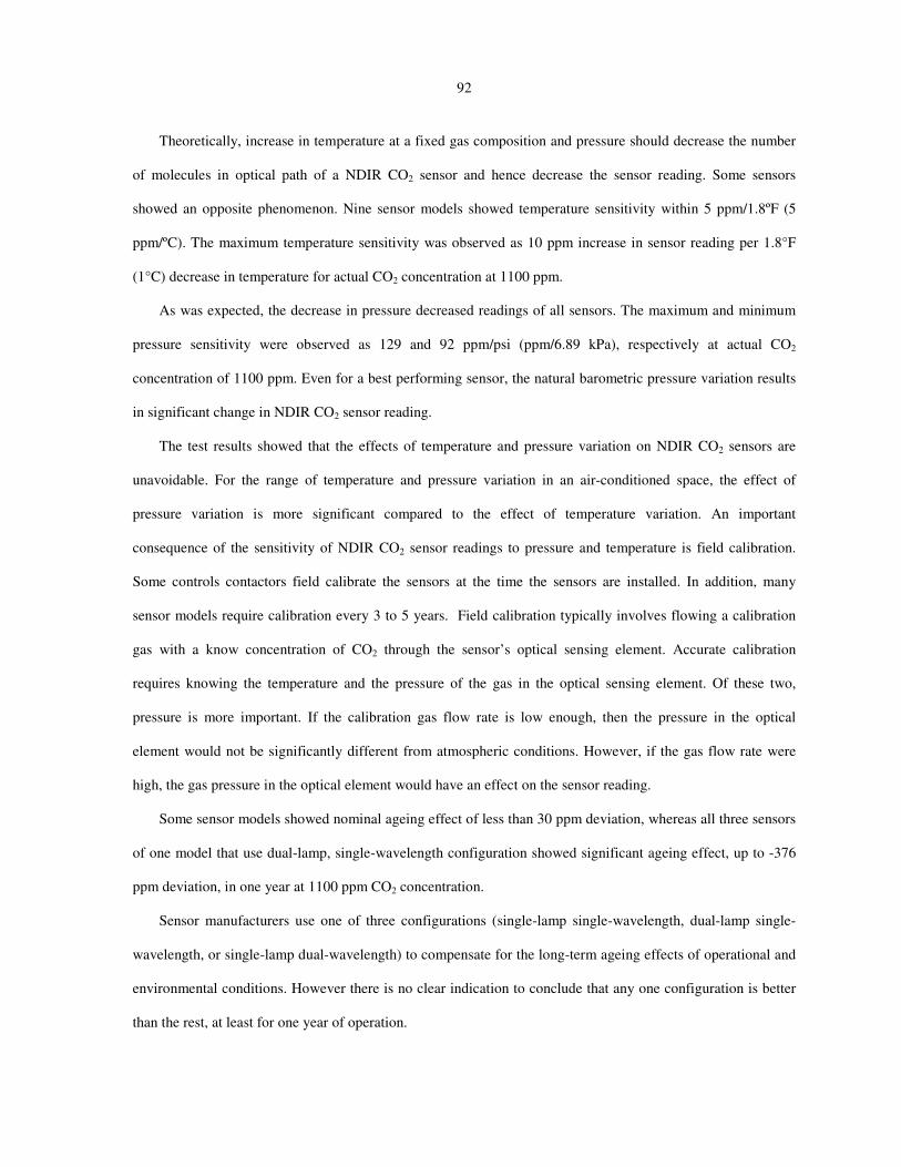
92
Theoretically, increase in temperature at a fixed gas composition and pressure should decrease the number
of molecules in optical path of a NDIR CO2 sensor and hence decrease the sensor reading. Some sensors
showed an opposite phenomenon. Nine sensor models showed temperature sensitivity within 5 ppm/1.8ºF (5
ppm/ºC). The maximum temperature sensitivity was observed as 10 ppm increase in sensor reading per 1.8°F
(1°C) decrease in temperature for actual CO2 concentration at 1100 ppm.
As was expected, the decrease in pressure decreased readings of all sensors. The maximum and minimum
pressure sensitivity were observed as 129 and 92 ppm/psi (ppm/6.89 kPa), respectively at actual CO2
concentration of 1100 ppm. Even for a best performing sensor, the natural barometric pressure variation results
in significant change in NDIR CO2 sensor reading.
The test results showed that the effects of temperature and pressure variation on NDIR CO2 sensors are
unavoidable. For the range of temperature and pressure variation in an air-conditioned space, the effect of
pressure variation is more significant compared to the effect of temperature variation. An important
consequence of the sensitivity of NDIR CO2 sensor readings to pressure and temperature is field calibration.
Some controls contactors field calibrate the sensors at the time the sensors are installed. In addition, many
sensor models require calibration every 3 to 5 years. Field calibration typically involves flowing a calibration
gas with a know concentration of CO2 through the sensor’s optical sensing element. Accurate calibration
requires knowing the temperature and the pressure of the gas in the optical sensing element. Of these two,
pressure is more important. If the calibration gas flow rate is low enough, then the pressure in the optical
element would not be significantly different from atmospheric conditions. However, if the gas flow rate were
high, the gas pressure in the optical element would have an effect on the sensor reading.
Some sensor models showed nominal ageing effect of less than 30 ppm deviation, whereas all three sensors
of one model that use dual-lamp, single-wavelength configuration showed significant ageing effect, up to -376
ppm deviation, in one year at 1100 ppm CO2 concentration.
Sensor manufacturers use one of three configurations (single-lamp single-wavelength, dual-lamp single-
wavelength, or single-lamp dual-wavelength) to compensate for the long-term ageing effects of operational and
environmental conditions. However there is no clear indication to conclude that any one configuration is better
than the rest, at least for one year of operation.

93
RECOMMENDATIONS FOR FUTURE RESEARCH
As discussed earlier, there is no present standard method of test (MOT) available by which NDIR CO2
sensors are evaluated. It would be desirable to develop the MOT presented in this research to make it a standard
method of test.
This research has a great potential to expanded to make CO2-based DCV system more energy efficient. For
a fixed composition of air, any change in temperature or pressure will change number of CO2 molecules in the
optical cavity of a NDIR CO2 sensor. Thus, the effects of temperature and pressure variation on NDIR CO2
sensors are unavoidable. Hence, an algorithm to account for the temperature, and more importantly the
preessure variation is important, not only to insure energy savings, but also to assure adequate IAQ.

94
References
CEC, 2002, High Performance Commercial Building Systems, California Energy Commission, Public Interest
Energy Research Program, HPCBS # E5P23T1b
CEC. 2006. 2005 Building Energy Efficiency Standards for Residential and Nonresidential Buildings.
CALIFORNIA ENERGY COMMISSION Title 24, Part 6, of the California Code of Regulations.
DOE. 2007. 2007 Building Energy Databook. http://buildingsdatabook.eere.energy.gov/ Washington, DC: U.S.
Department of Energy, Energy Efficiency and Renewable Energy.
Dougan, D.S., and L. Damiano. 2004. CO2-based demand control ventilation: do risk outweigh potential
rewards?. ASHRAE Journal Vol. 46, No. 10: 47-53.
Emmerich, S.J., and A.K. Persily. 1997. Literature review on CO2-based demand-controlled ventilation.
ASHRAE Transactions 103 (2): 229-43.
Emmerich, S.J., and A.K. Persily. 2001. State-of-the-art review of CO2 demand controlled ventilation
technology and application, Report NISTIR 6729, National Institute of Science and Technology (NIST),
USA.
Fahlen, P., H. Andersson, and S. Ruud. 1992. Demand Controlled Ventilating Systems - Sensor Tests. Swedish
National Testing and Research Institute, Boras, Sweden, SP Report 1992:13.
Fisk, W.J., D. Faulkner, and D.P. Sullivan. 2006. Accuracy of CO2 sensors in commercial buildings: a pilot
study. LBNL-61962, Lawrence Berkeley National Laboratory, Berkeley, CA.
Hyland, R.W., and A. Wexler. 1983. Formulations for the thermodynamic properties of the saturated phases of
H2O from 173.15 K to 473.15 K. ASHRAE Transactions 89(2A):500-519.
House, J. 2006. Personal communication.
Pandey, S.K., K. Kim, and S. Lee. 2007. Use of a dynamic enclosure approach to test the accuracy of the NDIR
sensor: evaluation based on the CO2 equilibration pattern. Molecular Diversity Preservation International,
Matthaeusstrasse, Switzerland, ISSN: 1424-8220.
Raatschen, W., ed. 1990. Demand Controlled Ventilating System. State of the Art Review. Stockholm, Sweden:
Swedish Council for Building Research, Stodcholm, Sweden, D9:1990.
Roth, K.W., D. Westphalen, M.Y. Pheng, P. Llana, and L. Quartararo. 2005. Energy impact of commercial
building controls and performance diagnostics: Market characterization, energy impact of building faults
and energy saving potential.
http://www.tiaxllc.com/aboutus/pdfs/energy_imp_comm_bldg_cntrls_perf_diag_110105.pdf
Schell, M., and D. Int-Hout. 2001. Demand control ventilation using CO2. ASHRAE Journal Vol. 43, No. 2: 18-
24.
Shrestha, S.S., and G.M. Maxwell. 2009. An experimental evaluation of HVAC-grade carbon-dioxide sensors:
part 1, test and evaluation procedure. ASHRAE Transactions 115(2):
Sun J., Reddy T.A, 2006, A new approach to developing building energy system simulation programs suitable
for both design and optimal operation, ASHRAE Transactions, Volume 112, Part 1 CH-06-13-4.