RSS-based Carrier Sensing and Interference Estimation in 802.11 Wireless Networks
Upload
independentCategory
view
2download
0
International Journal of Wireless & Mobile Networks (IJWMN) Vol. 5, No. 5, October 2013
DOI : 10.5121/ijwmn.2013.5511 165
PERFORMANCE AND INTERFERENCE ANALYSIS OF
802.11G WIRELESS NETWORK
Mingming Li1, Haiyang Liu
1, Haifeng Tan
2 and Miao Yang
1
1
State Radio Monitoring Center, Beijing and 100037, China
2 Beijing University of Posts and Telecommunications, Beijing and 100876, China
ABSTRACT This paper mainly presents Access Point s’ (APs’) performance and co-channel, adjacent channel
interference according to 802.11g standard. Firstly, our study illustrates the performance of one AP,
including its coverage performance, load-carrying properties and fairness. Next we propose the details
about co-channel, adjacent channel interference which should be paid attention to in deploying network
services. Then, performance analyses are evaluated by simulation and real test for a dense wireless
network. Our contribution is that the co-channel, adjacent channel interference analysis, the simulation
and test results can be the basis offered to network operators
KEYWORDS 802.11g network, Coverage performance, Fairness, Throughput, Co-channel Interference, adjacent
channel interference
1. INTRODUCTION
The WLAN network with IEEE 802.11g standard is one most-widely deployed as its high speed
and proven techniques. This technology operates in the 2.4GHz ISM (Industrial, Scientific, and
Medical) radio spectrum with signal bandwidth 20MHz. IEEE Std. 802.11g-2003[1], part 11
gives the specifications about 802.11g’s MAC layer and physical Layer (PHY). Extended Rate
PHY is the proprietary vocabulary for 802.11g standard. ERP-CCK, ERP-DSSS, ERP-OFDM,
ERP-PBCC and DSSS-OFDM are all key techniques used in the physical layer for the
compatibility for Std. 802.11g [1]. And also carrier sense multiple access with collision avoidance
(CSMA/CA) is used as key techniques in WLAN Medium Access Control (MAC) layer,
supporting data rates from 1 to 54Mbps.
IEEE 802.11g network occupies a bandwidth of about 20MHz and the available channels are
defined with 5 MHz separation between consecutive carriers. As a result, there are only three
non-overlapping channels (such as channels 1, 6, 11) in 2.4GHz. Bearing in mind a scenario with
high density of APs, three non-overlapping channels are not enough to guarantee an innocuous
coexistence between different WLAN networks. In this circumstance, how to reduce even avoid
interference is referred as an important question to network operators. Many studies have
presented the analytical study on this category about IEEE 802.11 networks. Co-channel and
adjacent channel interference, which are caused by transmissions in entirely or partially
overlapping channels, are learned much more recently. The authors in [2] learned the adjacent
channel interference in IEEE 802.11a/b/g WLANs and present new analytical and simulation
results for the conversational speech capacity of WLANs and compares the different WLAN
technologies in that regard. Reference [3] and [4] had done the similar studies focusing on DSSS
International Journal of Wireless & Mobile Networks (IJWMN) Vol. 5, No. 5, October 2013
166
technology about 802.11b network and found out some mechanisms may be available for radio
resource management in WLANs network, such as transmitted power assignments or rate
adaptation strategies. The impact of co-channel interference has been studied in [5] and [6] and
the approaches like power adjustment algorithm, channel adjustment algorithm have been
proposed for minimizing co-channel interference. In this paper, the author gives study illustrating
the performance of one AP characterized by IEEE 802.11g standard, discusses the influence of
interference caused by CSMA/CA media access method and channel overlap, especially shows all
results in the upper both by simulation and real test method. Then some details are referred to
give proposals to network operators how to design a WLAN network more standardized and
orderly.
The rest of this document is structured as follows: In Section 2, we give the performance learn of
one AP including its coverage performance, load-carrying properties and fairness. Section 3
quantifies the co-channel, adjacent channel interference which should be paid attention to in
deploying network services. And a particular introduction to 802.11g performance is provided
through simulation and test methods. At the end, some proposals are mentioned to network
operators and conclude our study.
2. ONE AP’S PERFORMANCE
2.1. Coverage Performance
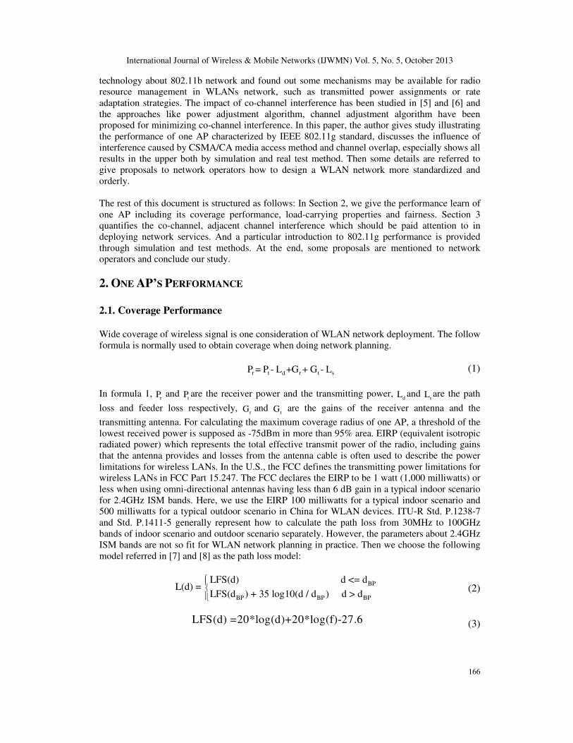
Wide coverage of wireless signal is one consideration of WLAN network deployment. The follow
formula is normally used to obtain coverage when doing network planning.
r t r t sdP = P - L +G + G - L (1)
In formula 1, rP and
tP are the receiver power and the transmitting power, dL and
sL are the path
loss and feeder loss respectively, rG and
tG are the gains of the receiver antenna and the
transmitting antenna. For calculating the maximum coverage radius of one AP, a threshold of the
lowest received power is supposed as -75dBm in more than 95% area. EIRP (equivalent isotropic
radiated power) which represents the total effective transmit power of the radio, including gains
that the antenna provides and losses from the antenna cable is often used to describe the power
limitations for wireless LANs. In the U.S., the FCC defines the transmitting power limitations for
wireless LANs in FCC Part 15.247. The FCC declares the EIRP to be 1 watt (1,000 milliwatts) or
less when using omni-directional antennas having less than 6 dB gain in a typical indoor scenario
for 2.4GHz ISM bands. Here, we use the EIRP 100 milliwatts for a typical indoor scenario and
500 milliwatts for a typical outdoor scenario in China for WLAN devices. ITU-R Std. P.1238-7
and Std. P.1411-5 generally represent how to calculate the path loss from 30MHz to 100GHz
bands of indoor scenario and outdoor scenario separately. However, the parameters about 2.4GHz
ISM bands are not so fit for WLAN network planning in practice. Then we choose the following
model referred in [7] and [8] as the path loss model:
BP
BP BP BP
LFS(d) d <= dL(d) =
LFS(d ) + 35 log10(d / d ) d > d
(2)
LFS(d) =20*log(d)+20*log(f)-27.6
(3)
International Journal of Wireless & Mobile Networks (IJWMN) Vol. 5, No. 5, October 2013
167
The path loss can be worked out with formula 2 and 3where d is the distance with the units
coming out in meter, BPd is the distance of breakpoint with the units being meter and f is the
frequency with the units of megahertz. Moreover shadow fading should be considered as: 2
2( )
21
( ) exp2
x
p x σ
πσ
−
= (4)
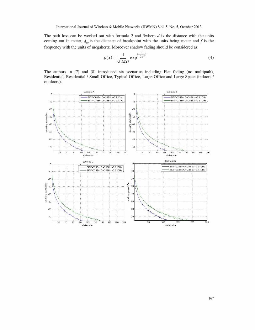
The authors in [7] and [8] introduced six scenarios including Flat fading (no multipath),
Residential, Residential / Small Office, Typical Office, Large Office and Large Space (indoors /
outdoors).
International Journal of Wireless & Mobile Networks (IJWMN) Vol. 5, No. 5, October 2013
168
Figure 1. AP’s maximum coverage radius under different scenarios
Figure 1 shows one AP’s maximum coverage radius under the upper scenarios. From figure 1, we
can get that one AP’s maximum coverage radius is about 140m for A\B\C scenarios and 300m for
D\E\F scenarios in 2.4 GHz bands. One AP’s maximum coverage radius can be manifested in the
following table 1 including with the scenarios.
Table 1. One AP’s maximum coverage radius
Type Scenarios description 2.4GHz,
G<10dBi
2.4GHz,
G>10dBi
A Flat fading (no multipath) 90m 140m
B Residential 90m 140m
C Residential/Small Office 90m 140m
D Typical Office 120m 180m
E Large Office 160m 250m
F Large Space (indoors/outdoors) 200m 300m
2.2. DCF Fairness
As we know, DCF is the forcing term in IEEE Std. 802.11. G. Bianchi, in the article [9], modelled
the DCF competing process as two-dimensional discrete time Markov chain. Making use of this
thesis, the authors intend to prove the fairness of DCF at first.
Lemma 1: Assuming that any ith UE and jth UE have the similar wireless channel condition to
access one AP, the ith UE and jth UE will have the same chance to transmit a packet in the
current time slot under DCF mechanism.
Proof: Gilles Berger-Sabbatel et.al had been modeled the fairness problem of DCF as Slotted
ALOHA [10]. Given a network with one AP and N UEs and iγ be the fraction of transmissions
performed by UE i during a time slot m, the fairness index is the following:
2
1
2
1
( )( )
N
iiJ N
ii
F mN
γ
γ
=
=
=∑∑
(5)
International Journal of Wireless & Mobile Networks (IJWMN) Vol. 5, No. 5, October 2013
169
Here, we assume that any ith UE and the jth UE have the similar wireless condition to access AP.
So we get 2 2
1 1( )
N N
i ii iNγ γ
= ==∑ ∑ , 1...i N= , which means ( ) 1
JF m = . That is to say that any UE
with the same wireless condition in the network has the same transmitting probability to access
the AP. Table 2. Parameters setup in fairness simulation
Parameters BSS Number AP Number UE Number service
Values 1 40 10 FTP
Parameters DATA
Length Time Power
Access
Mechanism
Values 1MB 0.32s 100mW CTS_self
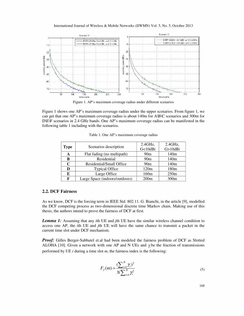
It is turn to prove fairness of DCF by simulation mentioned in the upper case. Announcing a
wireless network scene, forty users are located the same distance far away the centre AP at
downloading package of 1M bytes in every 0.32s. The users’ transmitting speed is 54Mbps and
CTS_self protocol are used in MAC layer. All parameters setup in this simulation are listed in
table 2. Without other limitation, we can get forty users’ total throughput is about 20.8Mbps and
every user is about 0.5Mbps from figure 2. From this simulation result, we can get forty users
have the same chance to access the channel and transmit packets. Thus, it is unfitted for network
operators to let all users compete with each other completely because CTS_self protocol can
bring out the possibility of collision severely which will lead to the decrease of total throughput
and single user’s throughput.
Figure 2. 40 UEs total throughput and 1UE’s under DCF mechanisms
International Journal of Wireless & Mobile Networks (IJWMN) Vol. 5, No. 5, October 2013
170
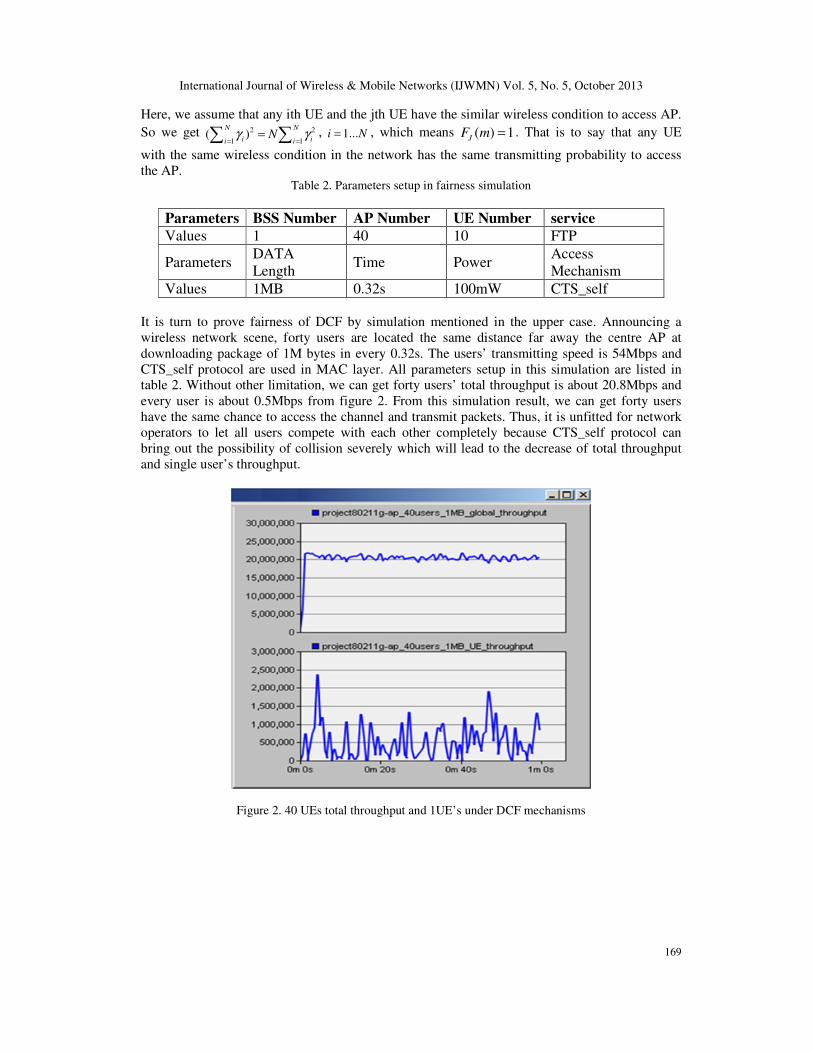
Figure 3. One UE’s throughput and time delay
2.3. Load-carrying properties with TCP Protocol
Many articles had learned the performance of 802.11 wireless network’s by theoretical analysis
like [9], [10] etc. We check the performance by simulation and test methods. First, we give out a
simulation to show the wireless network’s performance of application layer with TCP protocol.
Supposing that a BSS contains 1 UE only, this user is downloading package of 1M bytes in every
0.32s from the centre AP. The users’ transmitting speed is 54Mbps and CTS_self protocol are
used in MAC layer. That is to say that we use the parameters shown in table 2 but the UE Number
is 1 in this simulation. From figure 3, this user’s throughput is about 24.5Mbps and the time delay
is less than 2ms. Compared figure 2 with figure 3, we can get complete competition can lead to
the 40 users’ total throughput decreasing approximated 4.1Mbps.
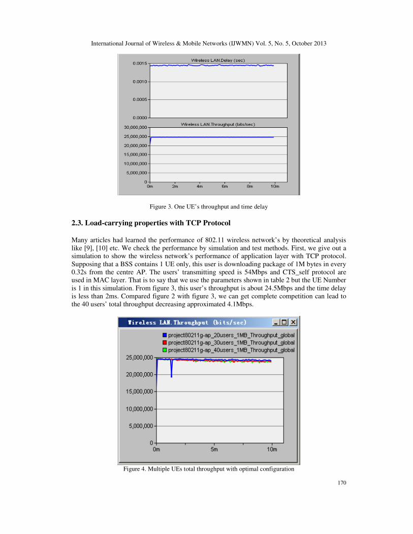
Figure 4. Multiple UEs total throughput with optimal configuration
International Journal of Wireless & Mobile Networks (IJWMN) Vol. 5, No. 5, October 2013
171
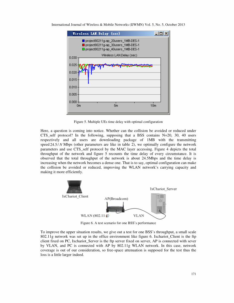
Figure 5. Multiple UEs time delay with optimal configuration
Here, a question is coming into notice. Whether can the collision be avoided or reduced under
CTS_self protocol? In the following, supposing that a BSS contains N=20, 30, 40 users
respectively and all users are downloading package of 1MB with the transmitting
speed 24.5 / N Mbps (other parameters are like in table 2), we optimally configure the network
parameters and use CTS_self protocol by the MAC layer accessing. Figure 4 depicts the total
throughput of the network and figure 5 recounts the time delay of every circumstance. It is
observed that the total throughput of the network is about 24.5Mbps and the time delay is
increasing when the network becomes a dense one. That is to say, optimal configuration can make
the collision be avoided or reduced, improving the WLAN network’s carrying capacity and
making it more efficiently.
Figure 6. A test scenario for one BSS’s performance
To improve the upper situation results, we give out a test for one BSS’s throughput, a small scale
802.11g network was set up in the office environment like figure 6. Ixchariot_Client is the ftp
client fixed on PC, Ixchariot_Server is the ftp server fixed on server, AP is connected with sever
by VLAN, and PC is connected with AP by 802.11g WLAN network. In this case, network
coverage is out of our consideration, so free-space attenuation is supposed for the test thus the
loss is a little larger indeed.
International Journal of Wireless & Mobile Networks (IJWMN) Vol. 5, No. 5, October 2013
172
Table 3. Parameters configuration in the test of the BSS’s Throughput
Parameters BSS
Number
AP
Number
UE
Number service
Values 1 1 1 FTP
Parameters DATA
Length Time Power
Access
Mechanism
Values 1MB 0.32s 100mW CTS_self
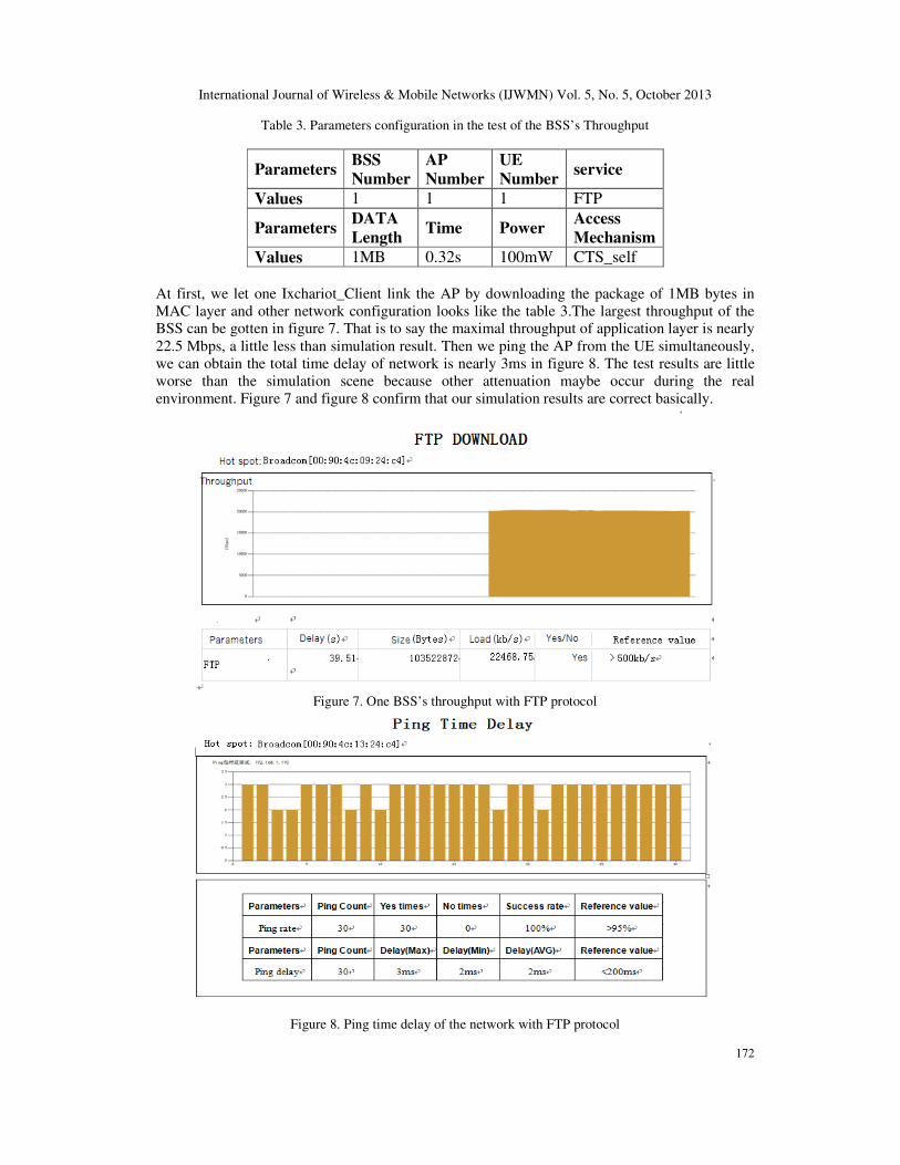
At first, we let one Ixchariot_Client link the AP by downloading the package of 1MB bytes in
MAC layer and other network configuration looks like the table 3.The largest throughput of the
BSS can be gotten in figure 7. That is to say the maximal throughput of application layer is nearly
22.5 Mbps, a little less than simulation result. Then we ping the AP from the UE simultaneously,
we can obtain the total time delay of network is nearly 3ms in figure 8. The test results are little
worse than the simulation scene because other attenuation maybe occur during the real
environment. Figure 7 and figure 8 confirm that our simulation results are correct basically.
Figure 7. One BSS’s throughput with FTP protocol
Figure 8. Ping time delay of the network with FTP protocol
International Journal of Wireless & Mobile Networks (IJWMN) Vol. 5, No. 5, October 2013
173
3. THE CONTRAST BETWEEN CO-CHANNEL INTERFERENCE AND ADJACENT
CHANNEL INTERFERENCE
As we know, 802.11g uses OFDM modulation to support the data rate 54Mbps. OFDM system is
easily affected by the frequency deviation, which makes the subcarrier orthogonality be
destroyed, resulting in mutual interference between signals of different channels. To evaluate the
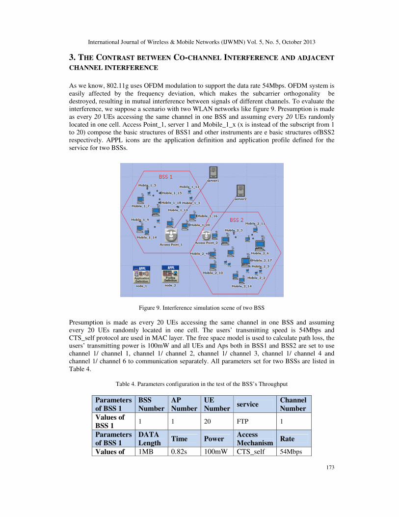
interference, we suppose a scenario with two WLAN networks like figure 9. Presumption is made
as every 20 UEs accessing the same channel in one BSS and assuming every 20 UEs randomly
located in one cell. Access Point_1, server 1 and Mobile_1_x (x is instead of the subscript from 1
to 20) compose the basic structures of BSS1 and other instruments are e basic structures ofBSS2
respectively. APPL icons are the application definition and application profile defined for the
service for two BSSs.
Figure 9. Interference simulation scene of two BSS
Presumption is made as every 20 UEs accessing the same channel in one BSS and assuming
every 20 UEs randomly located in one cell. The users’ transmitting speed is 54Mbps and
CTS_self protocol are used in MAC layer. The free space model is used to calculate path loss, the
users’ transmitting power is 100mW and all UEs and Aps both in BSS1 and BSS2 are set to use
channel 1/ channel 1, channel 1/ channel 2, channel 1/ channel 3, channel 1/ channel 4 and
channel 1/ channel 6 to communication separately. All parameters set for two BSSs are listed in
Table 4.
Table 4. Parameters configuration in the test of the BSS’s Throughput
Parameters
of BSS 1
BSS
Number
AP
Number
UE
Number service
Channel
Number
Values of
BSS 1 1 1 20 FTP 1
Parameters
of BSS 1
DATA
Length Time Power
Access
Mechanism Rate
Values of 1MB 0.82s 100mW CTS_self 54Mbps
International Journal of Wireless & Mobile Networks (IJWMN) Vol. 5, No. 5, October 2013
174
BSS 1
Parameters
of BSS 2
BSS
Number
AP
Number
UE
Number service
Channel
Number
Values of
BSS 2 2 1 20 FTP 1/2/3/4/6
Parameters
of BSS 2
DATA
Length Time Power
Access
Mechanism Rate
Values of
BSS 2 1MB 0.82s 100mW CTS_self 54Mbps
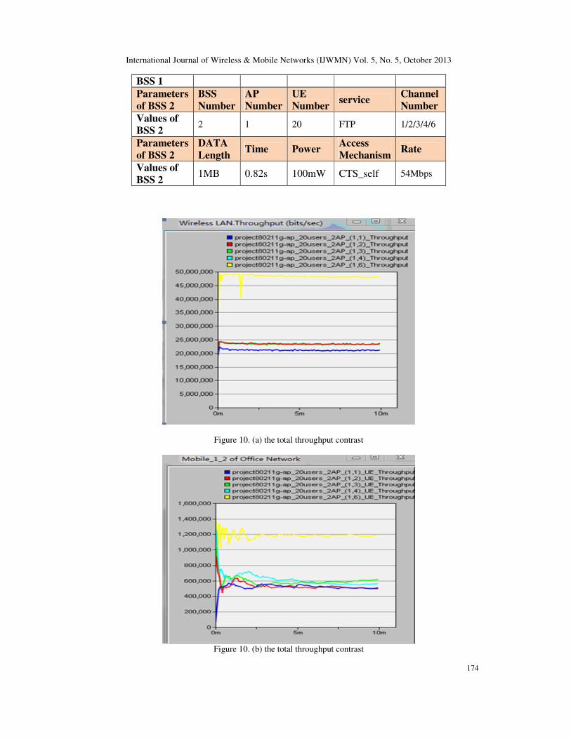
Figure 10. (a) the total throughput contrast
Figure 10. (b) the total throughput contrast
International Journal of Wireless & Mobile Networks (IJWMN) Vol. 5, No. 5, October 2013
175
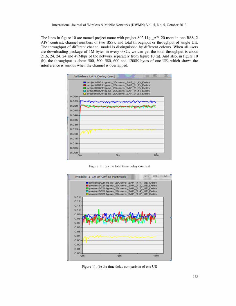
The lines in figure 10 are named project name with project 802.11g _AP, 20 users in one BSS, 2
APs’ contrast, channel numbers of two BSSs, and total throughput or throughput of single UE.
The throughput of different channel model is distinguished by different colours. When all users
are downloading package of 1M bytes in every 0.82s, we can get the total throughput is about
21.6, 24, 24, 24 and 49Mbps of the network separately from figure 10 (a). And also, in figure 10
(b), the throughput is about 500, 500, 580, 600 and 1200K bytes of one UE, which shows the
interference is serious when the channel is overlapped.
Figure 11. (a) the total time delay contrast
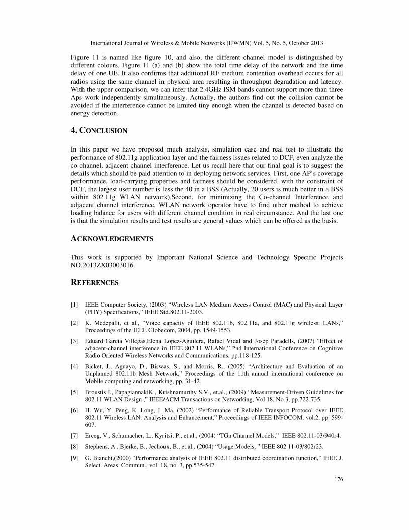
Figure 11. (b) the time delay comparison of one UE
International Journal of Wireless & Mobile Networks (IJWMN) Vol. 5, No. 5, October 2013
176
Figure 11 is named like figure 10, and also, the different channel model is distinguished by
different colours. Figure 11 (a) and (b) show the total time delay of the network and the time
delay of one UE. It also confirms that additional RF medium contention overhead occurs for all
radios using the same channel in physical area resulting in throughput degradation and latency.
With the upper comparison, we can infer that 2.4GHz ISM bands cannot support more than three
Aps work independently simultaneously. Actually, the authors find out the collision cannot be
avoided if the interference cannot be limited tiny enough when the channel is detected based on
energy detection.
4. CONCLUSION
In this paper we have proposed much analysis, simulation case and real test to illustrate the
performance of 802.11g application layer and the fairness issues related to DCF, even analyze the
co-channel, adjacent channel interference. Let us recall here that our final goal is to suggest the
details which should be paid attention to in deploying network services. First, one AP’s coverage
performance, load-carrying properties and fairness should be considered, with the constraint of
DCF, the largest user number is less the 40 in a BSS (Actually, 20 users is much better in a BSS
within 802.11g WLAN network).Second, for minimizing the Co-channel Interference and
adjacent channel interference, WLAN network operator have to find other method to achieve
loading balance for users with different channel condition in real circumstance. And the last one
is that the simulation results and test results are general values which can be offered as the basis.
ACKNOWLEDGEMENTS
This work is supported by Important National Science and Technology Specific Projects
NO.2013ZX03003016.
REFERENCES
[1] IEEE Computer Society, (2003) “Wireless LAN Medium Access Control (MAC) and Physical Layer
(PHY) Specifications,” IEEE Std.802.11-2003.
[2] K. Medepalli, et al., “Voice capacity of IEEE 802.11b, 802.11a, and 802.11g wireless. LANs,”
Proceedings of the IEEE Globecom, 2004, pp. 1549-1553.
[3] Eduard Garcia Villegas,Elena Lopez-Aguilera, Rafael Vidal and Josep Paradells, (2007) “Effect of
adjacent-channel interference in IEEE 802.11 WLANs,” 2nd International Conference on Cognitive
Radio Oriented Wireless Networks and Communications, pp.118-125.
[4] Bicket, J., Aguayo, D., Biswas, S., and Morris, R., (2005) “Architecture and Evaluation of an
Unplanned 802.11b Mesh Network,” Proceedings of the 11th annual international conference on
Mobile computing and networking, pp. 31-42.
[5] Broustis I., PapagiannakiK., Krishnamurthy S.V., et.al., (2009) “Measurement-Driven Guidelines for
802.11 WLAN Design ,” IEEE/ACM Transactions on Networking, Vol 18, No.3, pp.722-735.
[6] H. Wu, Y. Peng, K. Long, J. Ma, (2002) “Performance of Reliable Transport Protocol over IEEE
802.11 Wireless LAN: Analysis and Enhancement,” Proceedings of IEEE INFOCOM, vol.2, pp. 599-
607.
[7] Erceg, V., Schumacher, L., Kyritsi, P., et.al., (2004) “TGn Channel Models,” IEEE 802.11-03/940r4.
[8] Stephens, A., Bjerke, B., Jechoux, B., et.al., (2004) “Usage Models, ” IEEE 802.11-03/802r23.
[9] G. Bianchi,(2000) “Performance analysis of IEEE 802.11 distributed coordination function,” IEEE J.
Select. Areas. Commun., vol. 18, no. 3, pp.535-547.
International Journal of Wireless & Mobile Networks (IJWMN) Vol. 5, No. 5, October 2013
177
[10] E. Lopez, J. Casademont, J. Cotrina , (2004) “Outdoor IEEE 802.11g Cellular Network performance,”
Proceedings of IEEE Globecom04, Vol.5, pp.2992-2996.
Authors Mingming Li works in State Radio Monitoring Center of China as an engineer. Her research field is
frequency spectrum planning and spectrum demand forecasting.
Copyright © 2022 FDOKUMEN