Pattern Formation And Localized Structures In Acoustic Resonators Containing A Viscous Fluid

Eur. Phys. J. Special Topics 146, 407–425 (2007)c© EDP Sciences, Springer-Verlag 2007DOI: 10.1140/epjst/e2007-00196-5

THE EUROPEANPHYSICAL JOURNALSPECIAL TOPICS

Pattern formation and localized structures inmonoatomic layer deposition

M.G. Clerc1,a, E. Tirapegui1, and M. Trejo2

1Departamento de Fısica, Facultad de Ciencias Fısicas y Matematicas,Universidad de Chile, Casilla 487-3, Santiago, Chile2Laboratoire de Physique Statistique, Ecole Normale Superieure, 24 rue Lhomond, 75231 ParisCedex 05, France

Abstract. We study the nonlinear robust behaviors of a model for the depositionof a monolayer of molecules on a surface which takes into account the interactionsof the adsorbed molecules. The transport properties of the model lead to nonFickian diffusion. It is shown that we have generically Turing structures coexistingwith uniform concentrations and consequently localized structures through thepinning mechanism. The characteristic lengths are in the nanometer region inagreement with recent experiments.

1 Introduction

In the recent decades thin films used as electronic devices in industrial applications have becomemore and more complex. Due to this fact it is of great scientific and technological interest to un-derstand and control the thin film growth, since growth mechanisms determine film mechanical,electrical, magnetic, and texture properties. The development of experimental methods, suchas field ion microscopy or scanning tunneling microscopy, has opened up the possibility to mon-itor chemical reactions on the surface of metals in real time with an almost atomic resolution.The consequences of this microscopic reaction properties, which could previously could only bededuced through their influence on the global reaction rate or other macroscopic properties ofa reaction, become now directly observable. Experiments have shown that absorbed moleculesoften form clusters or islands [1]. In the presence of reactions, non-equilibrium spatio temporalpatterns with sizes lying in the nanometer range have been observed [2]. One has also observednano patterns on solid surfaces [3–7], and nano structure islands in absorbed mono atomiclayers [8]. These intriguing experimental observations have stimulated several theoretical andnumerical studies. A promising strategy to describe this type of problem is the use of molec-ular dynamics simulations, however, this requires deposition rates which are unattainable. Tosimulate thin-film growth under more realistic deposition rates, a Monte Carlo approach hasbeen developed. Unfortunately, the computational time required remains excessive. Indeed, asignificant limitation of these methods is that they can deal only with small systems (micron).Hence, the continuous approach remains interesting, since it is able to modelize the growth ofthin-films of larger sizes [9].The aim of this manuscript is to show how the interplay between local kinetic processes and

a simultaneously occurring phase transition, modelized by equations of the reaction diffusiontype, may provide a suitable mechanism for the formation of localized structures with sizeslying in the nanometer range. We call these solutions Nano localized structures. In the case of

a e-mail: [email protected]

408 The European Physical Journal Special Topics

a non linear kinetic processes, close to the spatial bifurcation we derive an adequate amplitudeequation, which can explain the observed patterns.The model that we consider takes into account both the kinetic exchange between the surface

and the gas bathing, and also the thermodynamics of phase coexistence over the surface. Belowa critical temperature Tc, lateral attractive interactions at long distance and repulsive at shortdistance between the absorbed molecules may induce a phase transition. To describe the kineticsof adsorption and activated desorption we introduce source terms in the mass balance equation.The local molecular coverage c(r, t) of the substrate (0 ≤ c ≤ 1) satisfies the equation

∂tc=R[c]−∇ · J, (1)

where R[c],J represents the reaction terms and the mass current flow, respectively. Hence, ifone has low coverage c(r, t) 1. The reaction rate has the expression R[c] = kadPs(1 − c) −kdesc

n, where P is the pressure of the gas above the adsorbed layer, s is the sticking coefficient,kad, and kdes are the adsorption and desorption constant rates, respectively, and n = 1, 2.This parameter gives account of the type of activated desorption processes considered: linear(n = 1) or nonlinear (n = 2). The adsorption and desorption rates are functions of the physicalparameters involved in the deposition mechanism and according to the processing method,they may also depend on the coverage field c(r, t) [10]. However, for processing methods suchas sputtering and laser assisted deposition (non equilibrium processes), in some temperaturerange the assumption of constant desorption rate independent of the coverage is fully justified[11]. The mass current flow satisfies

J = −M∇δFδc,

where M is the surface mobility which is supposed to be constant, and F is the free energyof the adsorbed monolayer. An explicit expression for this free energy can be obtained as acorrection of mean field theory [12] or from the microscopic lattice model with a metropolisalgorithm for the probability transition in the limit of the local approximation (the radius ofthe interaction between the adsorbed particles is much shorter than all characteristic lengthscale of emerging structures) [10], and it may be written as

F [c,∇c] =∫s

(kBTf(c)− εo

2c2 +

ζ2o2|∇c|2

)dr, (2)

where kBT is Boltzmann factor, and f(c) a function to be defined in the next section togetherwith the constants (εo, ζo).Our objective then is to study in detail the model we have the deposition of a monolayer

of molecules on a surface where they can move or react. We shall give in the appendix a shortderivation of the model in the spirit of the work of Mikhailov [10] which shows its limits andpossible generalizations. This description which involves partial differential equations of fieldsdescribing the deposition and the growth is able to explain the behavior at mesoscopic scales(from the order of nanometers to hundreds of nanometers), and plays then an intermediate rolebetween the macoscopic and the microscopic behavior. We shall concentrate here in trying togive an appropriate description of the dynamics of a monolayer which can give us an under-standing of the early behavior of the growth mechanism. Our analysis is done in the frameof reaction diffusion systems with non Fickian diffusion which we have recently studiedgenerically [13].In section 2, we present the reaction diffusion model which desorption and nonlinear diffusion

of molecules in a substrate. In section 3 and section 4, we study the dynamics exhibited by themodel for linear and nonlinear desorption rate, respectively. In section 5 we consider the case ofvery low or high coverage. In this situation the reaction terms can be treated as a perturbationof the transport term and the dynamics around the uniform coverage state can be approachedby a a modified Cahn–Hilliard model [6]. In section 6, we give our conclusions.

New Trends, Dynamics and Scales in Pattern Formation 409

2 Reaction diffusion model

The basic equation we shall use to describe the deposition of a mono layer of molecules in asurface where they can move or react, which is derived in the Appendix, is (see [10])

∂tc(r, t) = R[c(r, t)] +∇ ·(D∇c(r, t)− D

kBTc(1− c)∇U(r)

), (3)

which is of the type of equation (1) with the flux J[c(r, t)] = −(D∇c(r, t)− DkBTc(1− c)∇U(r)).

The field c(r, t), the local coverage, is defined as the quotient between the number of ad-sorbed molecules in a cell of the surface and the fixed number of available sites in each cell(c(r, t) ≤ 1). The term D∇2c in (3) is normal diffusion with coefficient D, kB is Boltzmannconstant, T the temperature and the last term represents the flow of the adsorbed moleculeswhich move under the force given by the gradient of the potential U(r) produced in that pointby the other molecules. The factor (1 − c) takes care of the fact that the flow can only passthrough the available vacant sites in each cell (a finite occupancy effect) and the potential canbe written as U(r) = − ∫ u(r − r′)c(r′)dr′ where the function u(r) is a spherically symmet-ric interaction potential between molecules separated by a distance |r| . When the interactionradius is small compared to the diffusion length and the covering c(r, t) does not vary signifi-cantly within the interaction radius, we can approximate the integral by εoc(r)+ζ

2o∇2c(r) with

εo =∫u(r)dr, ζ2o =

12

∫ |r|2u(r)dr, and we have used ∫ ru(r)dr = 0 due to symmetry.The flux J[c(r, t)] in equation (3) is proportional to the conjugate thermodynamic force

which arises from the spatial variation of the associated chemical potential ϕ[c(r, t)], i.e we canwrite J[c(r, t)] = −M(c)∇ϕ[c(r, t)], where M(c) = Dc(1 − c)/kBT is the mobility and ϕ willbe the functional derivate of a free energy Fϕ[c(r, t)] = δf [c(r)]/δc(r). Equation (3) can thenbe written in the form

∂tc(r, t) = R[c(r, t)] +∇ ·[M(c(r, t)∇δF [c(r)]

δc(r)

], (4)

with f(c) = (1− c) ln(1− c) + c ln(c).The reaction rate has the expression R[c] = αo(1− c)− βocn, We shall further simplify our

model taking a constant mobility M(c) = Mo independent of c(r, t), this will not change thequalitative dynamics of the model which is our interest here. The equations are then

∂tc = αo(1− c)− βocn +Mo∇2ϕ, (5)

ϕ = −εoc+ kBT ln[c

1− c]− ζ2o∇2c. (6)

We recall that stationary states and their linear stability have been studied in a similarmodel with constant or exponential dependence of desorption rate, for n = 1 [12,14,15], andfor n = 2 [11].It is important to remark that the model (5) has a Lypunov functional for the linear case

(n = 1):

F =

∫ [KBTf(r)− 12εoc(r)2 + 12ζ2o |∇c(r)|2

]dr+

αo

M

∫G(r, r′)c(r) dr′dr

+αo + βo2M

∫c(r)G(r, r′)c(r′) dr′dr. (7)

where G is the Green Function defined by the Poisson equation, ∇2G(r, r′) = −δ(r− r′), withboundaryconditions vanishing at infinity. In two and one dimensions this function takes theform

G(r, r′) = − 12πln |r− r′| ; G(r, r′) =

|r− r′|2,


respectively, and therefore the system can be written as:

∂tc(r, t) =M∇2 δFδc(r)

. (8)

The first terms of the free energy correspond to an attractive short range interaction given bythe parameters ζo, εo, and the two last terms of the free energy represent the nonlocal effectiverepulsive short range interaction governed by absorption and desorption processes. Hence, thedynamics of model (5) in the linear case is characterize by the minimization of the free energy(7), that is, the dynamics exhibited by the above model is of relaxation type.If one neglects the absorption and the desorption processes, the model (5) becomes a Cahn-

Hilliard type equation. This model is characterized by exhibiting a phase transition at a criticaltemperature Tc = ε0/4K, that is, for T > Tc, the uniform coverage states are stable and theyare unstable for T < Tc, giving rise to a region of high coverage surrounded by a region oflow coverage, and viceversa. This scenarios changes drastically when the absorption and thedesorption processes are taken into account.

3 Dynamics of the monolayer for linear desorption (n = 1)

3.1 Pattern formation in the weakly non linear regime

In the case of linear desorption, the above model only exhibits one uniform coverage state:co = k/s(1 + k), with k ≡ αo/βo, When the value of this homogeneous concentration cois moderate (0.3 ∼ co ∼ 0.7), we analyze the equation for small perturbations around co.Replacing c(r, t) = co + σ(r, t) in the equation (5), we find for σ(r, t) 1 :

∂tσ(r, t) = −Ωσ + Γ∇2[−σ(r, t) + µ ln

(co + σ(r, t)

1− co − σ(r, t))−∇2σ(r, t)

], (9)

where Γ = Doε2o/ζ

2oKBT = Moε

2o/ζ

2o , and Ω = αo + βo, µ = T/4Tc. Moreover, we can intro-

duce the spatial and temporal scaling X =√εo/ζ2ox and τ = Γt, these scalings normalize the

adsorption and desorption constant rates. The temporal scaling is equivalent to take units sothat Γ= 1. To analyze the linear stability we use the ansatz σ(r, t) = Aoe

λt+ikx. Replacing thisexpression in the equation (9), we obtain the relation

λ(k) = −Ω− εΓk2 − Γk4; (10)

where ε = −1 + µ/co(1− co). If we fix the values of deposition rates (αo, βo), then the onlyfree parameter is the temperature T . Therefore, for certain value T<TP ≡ 4Tcco(1 − co)[1 −k2p −Ω/k2pΓ](kp = 4

√Ω/Γ, and Tp < Tc) the homogeneous solution becomes unstable and gives

rise to an spatially periodic state, whose wavelength is of the same order of the wavelength ofthe unstable mode of the uniform coverage state. In figure 1, we show the spectrum λ(k)fordifferent temperature values and fixed deposition rates. Hence, the uniform coverage state cois stable for T > TP . Note that, for T > Tc the coefficient of the diffusion term of model (5) ispositives and becomes negatives in the interval Tp < T < Tc. In this parameter region, the longrange interactions dominate the system and the perturbations of the uniform coverage stateare characterized by hyper-diffusive dynamical behaviors.Close to the spatial instability, one can use the standard weakly nonlinear analysis

(amplitude equation), the system shows patterns with sizes lying in the nanometer range [14].In this reference the bifuraction diagram of pattern formation is determined close to the spatialinstability and it is shown that this bifurcation is of the supercritical type, that is, close to theinstability there appears a pattern with small amplitude (proportional to the square root ofthe bifurcation parameter). In 2D, close to threshold, the system exhibits stripes or hexagonsparameters values.


0.6

0.1

0.4

0.05

00.2

–0.05

–0.1

0.8

λ(k)

k

12 3

4

Fig. 1. Spectrum Λ(k) for different values of temperature.Diffusive regime (curve 1, ε = 0.37), hyperdiffusive (curve 2,ε = −0.12), marginal regime (curve 3, ε = 0.22), and onset ofinstability (curve 4. ε = −0.32).

Throughout the previous analysis the only free parameter has been the temperature. Inexperiments the deposition is an isothermal process, and in this case the reduced gaseous phaseabove the adsorbed layer is the only externally tunable parameter, producing simultaneouslythe variation in the adsorption rate αo = kadPs. This description has been considered in [11],and involves only a quantitative change of the scheme presented above.

3.2 Pattern formation and localized structures in the highly nonlinear regime

When the value of the homogeneous concentration is not moderated (co < 0.3 or co > 0.7), thenumerical simulations of equation (9) show that the spatial instability now is characterized bylarge amplitude. The region in the parameter space in which these patterns are obseryed isvery small. The typical pattern coverage state observed in this regime is depicted in figure 2for 1D. In this parameters region an interesting phenomenon can be observed. Nearby to thebifurcation point, pattern formation with large amplitude takes places (cf. figure 2), that is, tothe bifurcation point, pattern formation with large amplitude takes places (cf. figure 2) that is,a pattern coverage state and uniform coverage states are stable and coexist in a narrow region

100.000 200.000 300.000

-0.115

0 .365

0 .615

0.865

c(x)

x

100.000 200.000 300.000

0.135

0.385

0.635

0.885

1.000

c(x)

x

a)

b)

Fig. 2. Pattern coverage stage in one dimensional model (9). (a) Numerical simulation of highly non-linear pattern in one dimensional model (9) with high coverage for: co = 0.865, µ = 0.1, Ω = 0.005,Γ = 1, kad = 0.004325, kdes = 0.000675, σmin = −0.842, σmax = 0.126. (b) Numerical simulationof highly nonlinear pattern in one dimensional model (9) with low coverage for: co = 0.135, µ = 0.1,Ω = 0.005, Γ = 1, kad = 0.004325, kdes = 0.000675, σmin = −0.126, σmax = 0.857.


0.095 0.105 0.11 0.115 0.12 0.125 0.13

-1

-0.75

-0.5

-0.25

0.25

0.5

0.75

1 A

mm msnp m1

1

c

x

x

c

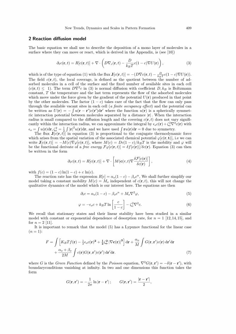
Fig. 3. Bifurcation diagram for n = 1. When µ1 = 0.1014 the pattern one propagates on the statehomogeneous. In µp = 0.10026 appear the periodical soultions by saddle node bifurcation. The insetfigures stand for the respective coverage states.

x

σ(x)a) σ(x)

x

b)

Fig. 4. Localized structures (adsorption and desorption island) in one and two dimensional system. Thisstructures are formed in the Pinning region in the highly nonlinear regime. a) Numerical simulation ofequation (9) in one and two dimensional system. We see the localized structures formation (Desorptionisland) for: µ = 0.105, co = 0.865, ω = 0.005,Γ = 1, β = 0.004325, α = 0.000675. In the inset figure wehave: σmin = −0.846, σmax = 0.119. b) Numerical simulation of equation (9) in one and two dimensionalsystem. We see the localized structures formation (Adsorption island) for: µ = 0.105, co = 0.1355,Ω =0.005,Γ = 1, α = 0.004325, β = 0.000675. In the inset figure we have: σmin = −0.119, σmax = −0.845.

of parameter space. In figure 3, we show the bifurcation diagram, that is, the amplitude A of thesteady state coverage pattern observed in the one dimensional model (5) as function of µ. Thisbifurcation is characterized by two critical points, the bifurcation point µp = T/4Tp (point in theparameter space where the uniform coverage states becomes unstable) and the bistablity pointµsn (point in the parameter space where the pattern state appears by saddle-node bifurcation).Between these two points the system exhibits coexistence between these coverage states. Notethat in general, it is a difficult task to find µsn. as function of the physical parameters. Inside ofthis parameter region, we observed localized pattern and nano localized structures in one andtwo spatial dimensions. In figure 4, we present the typical localized coverage patterns observedin this model. One can understand these localized structures as patterns extended only overa small portion of an extended system. From the point of view of dynamical systems theory,these solutions in 1D are homoclinic connections of the spatial dynamical system [16,17].Since in this regime the value of the homogeneous states co are far from the critical value

cc = 0.5, the highest orders in the logarithm expansion are important and one can not derive


an amplitude equation and a bifurcation diagram, because the numerical simulations show thatthe patterns have large amplitude and are far from being harmonic solutions, on the contrarythe interfaces are sharp. When two coverage states coexists (pattern and uniform coveragestates), we can expect the appearance of fronts, that is, dynamical solutions of equation (9),which connect spatially the two states. These fronts move with a characteristic speed andthe favorable state (energetically) invades the unfavorable one. Recently, it has been demon-strated geometrically [17] and also by means of an amplitude equation [16], that these fronts aremotionless in a range of parameters, the pinning range. It is important to remark that this re-gion contains the Maxwell point, where both states are energetically equivalent. Outside thisregion the front propagates. The localized patterns are observed close to the pinning range. Infigure 4, we show the typical localized coverage structure formed at the pinning region. We cansee the weak oscillation in the edge of the structure. From the values of the parameters used inthe simulations we can estimate the typical size of the localized coverage structure and we andthat it is d ≈ 8 nm.

4 Dynamics of the monolayer for nonlinear desorption (n = 2)

When we consider more complex processes for the desorption like chemical reactions betweenthe deposited atoms and the substrate or collisions processes between themselves (for instance adiatomic desorption process) [11], we must include nonlinear reaction terms in the equation (3),i.e. n = 2. As we shall see the inclusion of this term will modify the above bifurcation diagramscenarios. In particular, the system will exhibit localized coverage structure and patterns withsmall amplitude.

4.1 Linear stability analysis and extended pattern formation

The equation which describes the system reads

∂tc(r, t) = αo[1− c(r, t)]− βoc(r, t)2 +Mo∇2[−εoc(r, t) +KBT ln

[c(r, t)

1− c(r, t)]− ξ2o∇2c(r, t)

].

(11)

For nonlinear desorption, the system has two uniform coverage states, only one with physicalsense (co ≤ 1)

co =αo

2βo

(√1 +4βoαo− 1). (12)

The equation for the small perturbation σ(r, t) to this solution is then:

∂tσ(r, t) = −ασ − βoσ2 + Γ∇2[−σ(r, t) + µ ln

(co + σ(r, t)

1− co − σ(r, t))−∇2σ(r, t)

]. (13)

The last term, which represents the transport in equation (13), remains inalterable (µ and Γ are

exactly the same that the case n = 1). α ≡ αo√1 + 4βo/αo is the reduced adsorption cofficient.

In order to describe analytically the onset of the spatial instability, we linearize the abovemodel, we use the ansatz σ = σoe

λ(k)t+ikx, and we obtain the following dispersion relation

λ(k) = −α− εΓk2 − Γk4. (14)

Note that the only change with respect to the linear case n = 1 is the α coefficient instead of Ω inequation (10). Therefore, in this system the pattern formation takes place in a weak segregationregime [11]. The critical value of temperature for when the uniform coverage becomes spatiallyunstable is

Tp = 4Tcco(1− co)[1− k2 − α

k2Γ

], (15)


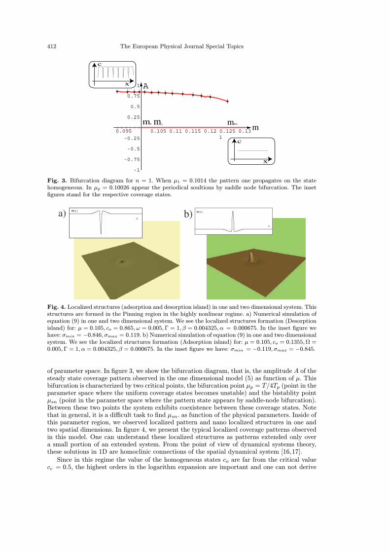
where kp =4√α/Γ. The above expression can be written as Tp = 4Tc(1− |εp|)co(1− co), with

|εp| = Tp/4Tc = 2√α/Γ. When the temperature decreases under a critical value (T < Tp), a

spatially modulated perturbation with wave number close to the critical wave number beginsto grow generating an extended pattern coverage state [11]. In this reference, one can foundthe typical competition between hexagons and stripes patterns. Note that the same dynamicalbehavior was found in the linear adsorption [12].

4.2 Localized patterns in the weakly nonlinear regime

For values of the uniform coverage co close to the critical concentration (cc = 0.5), we shall seethat it is possible to find localized patterns in the weakly nonlinear regime. The oscillations ofthese patterns will be smooth and with moderated amplitude, therefore, we can make an ana-lytical description by means of amplitude equations (weakly nonlinear analysis). The quadraticterm associated with the nonlinear desorption process plays an important role in the dynamicsof the monolayer, because it is able to change the type of bifurcation.In order to describe the dynamics of the monolayer we expand the equation (13) up to the

fifth order in σ

∂tσ(r, t) = −ασ(r, t)− βoσ(r, t)2 + Γ∇2[εσ(r, t) + ω σ(r, t)2 + θ σ(|bfr, t)3 + γ σ(r, t)4+ δ σ(r, t)5 + · · · − ∇2σ(r, t)], (16)

We can write this equation around the bifurcation, ε = −(|εp|+v), v > 0, v 1, and separatingthe linear and nonlinear terms, we have

∂tσ = L[σ] +NL[σ], (17)

were L is the operator of the linear part. In one dimension it has the formL = −α+ εΓ ∂xx − Γ ∂xxxx, (18)

The nonlinear part NL[σ] correspond to the logarithm expansion in power series. To describeanalytically the localized solutions observed in one dimensional extended systems close to thespatial instability, we use the ansatz (the nonlinear change of variables)

σ(x, t) = A(τ ≡ vt, y ≡ v1/2x)eikpx + c.c + · · ·+W, (19)

where A is the amplitude of the spatially oscillatory solution, kp is the critical wave-number(kp = 2π/λp), and W is a small correction function. Rewriting in a more suggestive form

σ(x, t) = σ[1] + σ[2] + σ[3] + · · · (20)

where σ[i] indicates order i in the power of A in the change of variables, that is, σ[1] =A(τ, y)eikpx + c.c, σ[2] = a1A

2e2ikpx + a1A2e−2ikpx + a2 |A|2 and so forth. Replacing (19) in

the equation (16) and linearizing in W one obtains the following solvability equation for thelinear part

v∂τA = k2pv ΓA+ 4vΓ ∂yyA, (21)

This equation is given by the terms proportional to the critical mode eikpx (the resonant term).Note that at the following order we have

∂tσ[2] = 0, (22)

and therefore, replacing the change of variable to order 2, we have for the same powers of A

−Lσ[2] = NLσ[1](2), (23)


where the bracket in the right hand side of the equation (23) stands for quadratic terms. Thislast equation allows us to find the coefficients a1,a1,a2, as function of the physical parameters.In this calculation the spatial derivatives on A are of order v and therefore they are negligible.We obtain

a1 = a1 =−βo − 4Γω k2p

α+ 4 ∈ Γκ2p + 16k4pΓ; a2 =

−2βoα, (24)

Iterative application of this method, allow us to obtain all the coefficients of the change ofvariables as function of the previous order according to

−Lσ[s] = NL[σ[s−1]](s). (25)

Then, introducing the ansatz in equation (5) and linearizing in W, we obtain the followingsolvability condition:

∂tA = c1A+ c3 |A|2A+ c5 |A|4A+D∂xxA+ h.o.t., (26)

where h.o.t stands for the resonant higher order terms and c1 = v |ε0|/2 is the bifurcationparameter. Hence, when c1 is positive the system exhibits pattern formation. The parameterc3 bifurcation (super or sub critical bifurcation depending on the sign of this coefficient, forc3 > 0 the bifurcation is super-critical), D is the effective diffusion for the amplitude A, andif c5 < 0 and c3 1, using the scaling A∼ 4

√c1, ∂t∼ c1, c3∼√c1, c5∼D∼O(1), and ∂x ∼ √c1,

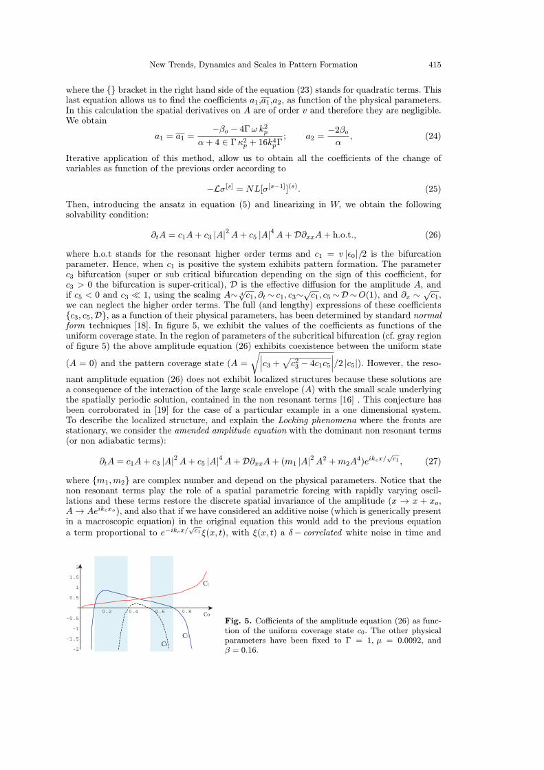
we can neglect the higher order terms. The full (and lengthy) expressions of these coefficientsc3, c5,D, as a function of their physical parameters, has been determined by standard normalform techniques [18]. In figure 5, we exhibit the values of the coefficients as functions of theuniform coverage state. In the region of parameters of the subcritical bifurcation (cf. gray regionof figure 5) the above amplitude equation (26) exhibits coexistence between the uniform state

(A = 0) and the pattern coverage state (A =

√∣∣∣c3 +√c23 − 4c1c5∣∣∣/2 |c5|). However, the reso-nant amplitude equation (26) does not exhibit localized structures because these solutions area consequence of the interaction of the large scale envelope (A) with the small scale underlyingthe spatially periodic solution, contained in the non resonant terms [16] . This conjecture hasbeen corroborated in [19] for the case of a particular example in a one dimensional system.To describe the localized structure, and explain the Locking phenomena where the fronts arestationary, we consider the amended amplitude equation with the dominant non resonant terms(or non adiabatic terms):

∂tA = c1A+ c3 |A|2A+ c5 |A|4A+D∂xxA+ (m1 |A|2A2 +m2A4)eikcx/√c1 , (27)

where m1,m2 are complex number and depend on the physical parameters. Notice that thenon resonant terms play the role of a spatial parametric forcing with rapidly varying oscil-lations and these terms restore the discrete spatial invariance of the amplitude (x → x + xo,A→ Aeikcxo), and also that if we have considered an additive noise (which is generically presentin a macroscopic equation) in the original equation this would add to the previous equationa term proportional to e−ikcx/

√c1ξ(x, t), with ξ(x, t) a δ− correlated white noise in time and

0.2 0.4 0.6 0.8

-2

-1.5

-1

-0.5

0.5

1

1.5

2

C5

C3

C1

CoFig. 5. Cofficients of the amplitude equation (26) as func-tion of the uniform coverage state c0. The other physicalparameters have been fixed to Γ = 1, µ = 0.0092, andβ = 0.16.


0.2 0.4 0.6

2 A

ν Fig. 6. Subcritical bifurcation diagram for the systemin the weakly nonlinear system for the same parametersthat in figure 7.

100.000 200.000 300.000

-0.500

-0.250

0.000

0.250

20 nm

2D

n = 2

1D

x

σ = c-c o

20 nm

a)

100.000 200.000 300.000

-0.500

-0.250

0.000

0.250

x

s(x)b)

Fig. 7. Localized pattern in one and two dimensional system. Numerical simulations of equation (11)for: µ = 0.0092; co = 0.5; αo = 0.008; βo = 0.16, Γ = 1. In addition we have for the inset figureσmin = −0− 49916, σmax = 0.370704, σ = c− co. a) Localized pattern and b) hole solution.

space (if the original noise had this property) which will give by itself the same effect as the pre-vious non resonant terms and moreover will in general be dominant near the bifurcation point[16,20,21].In figure 6, we show the subcritical bifurcation which exhibits the coexistence between two

coverage states, for the parameters in which we have observed the localized patterns forma-tion numerically. The resonant amplitude equation has analytical solutions for a front whichlinks the uniform to the spatially periodical coverage states, and this solution is the startingpoint to calculate the front interaction. Due to the oscillatory nature of the front interaction,which alternates between attractive and repulsive, we infer the existence, stability properties,dynamical evolution and bifurcation diagram of localized patterns. These localized structuresare a consequence of the pinning effect or Locking phenomena, as it can be seen in an alikeamended amplitude equation deduced from a prototype model of pattern formation [16]. Insidethe pinning range, we observe localized patterns in one and two spatial dimensions. In figure 7,we present the typical localized patterns observed in the model (4). One can understand theselocalized structures as patterns extended only over a small portion of an extended system.Moreover the existence of these localized structure can be proved rigourously in 1D using thetools of dynamical systems theory in the spatial dynamical system [17].In figure 7, we show the numerical simulation of equation (13) in the range of parameters

where the bifurcation is subcritical and that has been predicted by the calculations. Here, wecan see the smallest structure that can be formed figure 7(a). In figure 7(b), we can see alocalized pattern, in which the supported state is a pattern coverage state, that is, this state isa uniform state surround by a pattern one. This state is usually called Hole solution.

4.3 Pattern formation and localized structures in the highly nonlinear regime

At the onset of the spatial bifurcation of the uniform coverage state for large and small coverage(co < 0.3 or co > 0.7), the numerical simulation of the equation (13) shows pattern formation oflarge amplitude, such as in the linear desorption case (cf. figure 8). Again, we expect to find in


0.01 0.02 0.03

-1

-0.75

-0.5

-0.25

0.25

0.5

0.75

1

µ=µsn

A

x

c

c

x

T–Tp4Tc

a) b)

Fig. 8. Pattern formation in the highly nonlinear regime and numerical Bifurcation diagram. a) Numer-ical bifurcation diagram in the highly nonlinear regime for co = 0.86264, αo = 0.005, αo = 0.00379, βo =0.0007,Γ = 1. We can see that the structures formation happens in the hysteresis zone. b) Numericalsimulation of (13) in one (inset of figure) and two dimensional system. Pattern formation in the highlynonlinear regime for µ = 0.1, α = 0.005, αo = 0.00379, βo = 0.0007, co = 0.8626. The amplitude isσmin = −0.85116.

0.2 0.4 0.6 0.8 1

–1

–0.5

0.5

1

1.5ed

g

q w

co

b)σ(x)

x

a)

Fig. 9. Localized structures formation by the Pinning mechanism in the coexistence zone. a) Vacancyisland in two dimensional system for the equation (13) and b) Coefficients in the logarithmic expansion.

a certain region of the parameter space the coexistence between high amplitude patterns withstates of uniform coverage. In this zone of parameters, we expect to find localized structureswith different numbers of oscillations. The localized structure with a single oscillation will betermed vacancy island (adsorption island) in the case of high (low) value of the uniform coverageco. In figure 9 a vacancy island is displayed in this regionIn brief, in the coexistence zone of coverage states, we observe the localized structure for

mation by means of the pinning mechanism, that is, these solution are consequence of thefront interaction. In figure 8(a), we show the amplitude A of the steady state as functionof the bifurcation parameter µ. This bifurcation is characterized by two critical points, thebifurcation point µp = T/4Tp (cf. figure 8(a)), and the bistablity point µsn (point in theparameter space where the pattern coverage state appears by saddle-node bifurcation). Betweenthese two points, the system exhibits a coexistence between uniform and spatially periodiccoverage states (hysteresis region). Close to this parameter region, we observe localized patternin one and two spatial dimensions.

4.4 Two patterns states coexistence and Localized peaks

The equation (16) allowed us to have a region where the bifurcation was subcritical andthe coexistence between homogeneous and patterns states was possible. Nevertheless, it is


100.000 200.000 300.000

0.000

0.200

0.400

x

s (x)

100.000 200.000 300.000

0.000

0.200

0.400

x

σ(x)

Fig. 10. Numerical simulation of equation (16) show us localized peaks formation for: µ = 0.0126; co =0.0208;αo = 0.008, βo = 0.19;αo = 8.4×10−5. The values of amplitudes are: σA = 0.35 and σB = 0.04.

reasonable to take into account more terms in the expansion of equation (16) if we considerextremely low or high values for the uniform coverage co. One has an initial spatial supercritical bifurcation, followed by a secondary subcritical bifurcation, that is, a super-sub-criticalbifurcation. Hence, the system can exhibit coexistence of two spatially coverage periodic states.Recently in reference [22], by means of amended amplitude equation it has been shown that abi-pattern system generically exhibits localized peaks. This state appears as a large amplitudepeak nucleating over a pattern of lower amplitude. Localized states are pinned over a lat-tice spontaneously generated by the system itself. Numerical simulations of model (13) in thebi-pattern region exhibits localized peaks, in figure 10, we show these type of coverage states in1D. In figure 11(a), we show the bifurcation diagram obtained numerically for this bi-patternregion, where each branch represents a pattern coverage state. It is important to remark thatin this case it is not possible to make analytical calculations similar to those done in [22],since the interfaces of the coverage state are sharp and the highly nonlinear terms in the equa-tion (11) are very important, therefore weakly non linear analysis do not apply. However, thequalitative behavior and the underlying non linear analysis obtained in the non linear case leadsthe dynamics.

0.014 0.015 0.016

-0.4

-0.2

0.2

0.4

µ=T-Tp4Tc

A

µ1

a) b)

Fig. 11. Localized peaks and bifurcation diagram. a) Numerical bifurcation diagram in the coexistencezone for the same values that figure (10). In µ1 = 0.015 takes place the birth of greater amplitudepattern. b)Numerical simulation of equation (11)in two dimensional system for: µ1 = 0.0126, co =0.0208;βo = 0.19, αo = 8.4× 10−5.

5 The perturbed Cahn–Hilliard limit and nano-structures like bubble

In the previous sections, we have found Localized structures (adsorption and desorption islands)in the highly non linear regime for linear (n = 1) and nonlinear desorption (n = 2) due tothe coexistence between pattern and homogeneous states within the Pinning region. In thissame region ε < 0, the dynamical behavior of the system is of the hyper-diffusive type (Seefigure (1)) and the long range interaction dominate the dynamics. The competition betweenreaction and transport terms is at the origin of the patterns and localized structure formationin all previous regimes. The uniform coverage concentration co for this same parameter regionis in the following interval


1

2

[1−

√1− TTc

]< c <

1

2

[1− TTc

]. (28)

When co is outside of the interval (28), that is, the case of very low or high coverage, whichis observed for small desorption rate (Ω ≈ 10−4,αo, βo 1) the system is diffiusive (ε< 0, seefigure 1 or figure 9(b) and short range interaction are important. The reaction terms can betreated like a perturbation to the transport terms in the model (5) and the dynamics aroundthe uniform coverage state can be approached by a modified Cahn-Hilliard model [13]. It is wellknown that the Cahn–Hilliard model exhibits a family of localized solutions, bubbles solution[23], and we will study the persistence of these solutions in this modified Cahn–Hilliard equation.

5.1 Nano-structures like bubble

The starting point is the equation (16), close to the bifurcation point the equation reads forsmall σ

∂tσ(r, t) = αo[1− co − σ]−βo(co + σ)2 +Moεo∇2[εσ(r)+ω σ(r)2 + θ σ(r)3 · · ·+ ξ

2o

εo∇2σ(r)

],

(29)

where the coefficients of the logarithm expansion in the transport terms are given by:

µ ln

[co + σ

1− co − σ]= ln

[co

1− co

]+

∞∑m=1

gm(µ, co)σ(r)m,

with

gm(µ, co) =µ

m

[cmo − (co − 1)mcmo (1− co)m

],

here ε = −1 + g1, ω = g2, θ = g3, g4 = γ, g5 = δ. Figure 9(b) shows the five coefficient forfixed temperature (µ = 0.1) as function of the uniform coverage state co. We see that the oddcoefficients are always positive and the segmented lines are the even coefficients. The linearcoefficient ε is positive in a large region of uniform concentrations when µ < 0.25. For verysmall reaction terms, the concentrations are in the range co ∼ 0.1 or co ∼ 0.9 and thereforeε > 0.In order to describe and understand the dynamics exhibited by the system, we model it by

a perturbed Cahn–Hilliard equation. Therefore, we shall consider up to the cubic term in theexpansion. We make a translation σ = u− uo, in order to eliminate the quadratic term (ω) inequation (29). Finally, we scale the space and time variables and the system is modeled by

∂τu(y, τ) = A+Bu+ Cu2 +∇2[∈u+ u3 −∇2u], (30)

where X = ξ/√εoθx, τ = Γt, Γ = Γθ

2, ε = ε/θ − 3u2o, and uo = ω/3θ. The value of thiscoefficient is small, since the coefficients of the logarithm expansion are large. On the otherhand, the values of the coefficients A,B, and C depend on the type of desorption. For n = 1we have:

A =Ω

Γuo; B = −Ω

Γ; C = 0, (31)

and for quadratic desorption (n = 2) :

A =1

Γ(αuo − βou2o); B =

1

Γ(−α+ 2βouo); (32)

C = −βoΓ, (33)


The coefficients of expression (31, 32, 33) are small in this range of co. Numerical simulations ofthe equation (9) and (13) show the appearance of localized structures for linear and nonlineardesorption process (n = 1, 2).In the case of exclusively transport process (A = B = C = 0), the model (30) becomes the

Cahn–Hilliard equation [24]. This model has been initially proposed to describe the phase sep-aration dynamics in conservative system, such as binary alloys, binary liquids, glasses, polymersolutions, to mention a few. In the last decades the above model has been used to describe zig-zag instability undergone by straight rolls in two-dimensional extended systems like Rayleigh-Benard convection or electroconvection in fluid systems (see review [29] and references therein).A similar zig-zag instability affecting anisotropic interfaces has been described in terms of thismodel [25–28]. It is worthy to note that the dynamical behaviors of the one-dimensional Cahn–Hilliard is well understood [27,28]. In [27] it is shown that Cahn–Hilliard equation has a bubblesolution from two fronts interaction (Kink and Anti-Kink interaction), which has the form

U(x, x±(t)) = −√|ε| −

√|ε| tanh

[√|ε|2(x− x (t))

]+√|ε| tanh

[√|ε|2(x− x+(t))

]+ ω,

(34)

where x± = xo ± ∆/2 and ω is a small correction function of order O(√|ε|e−√2|ε|∆). Here

x−(t), x+(t) stand for the position of core of the kink and anti-kink, respectively. ∇(t) ≡x− − x+ is the width of the bubble, and xo(t) is the position of the bubble center. The abovebubble correspond to a localized structure of low coverage when adsorption and desorptionprocess have been neglected. To describe the nano-localized coverage pattern like bubble, whensmall reaction processes are take into account, we shall study the persistence of the bubblesolution (34) when co ≤ 0.1 (or co ≥ 0.9).Then, replacing ansatz (34) in equation (30) and linearizing in ω, we obtain

Lω = ∂z−u−x− + ∂z+u+x+A+Bρ+ Cρ2 + ∂xx[ερ+ ρ3 − ∂xxρ], (35)

where L is a linear operator which has the form L ≡ ε∂xx + 3∂xx(ρ2) − ∂xxxx, ρ is an

auxiliary function defined as ρ ≡ u−[z− ≡

√|ε| /2(x− x−)] + u+ [z+ ≡√|ε| /2(x− x+)] −√|ε| , u± ≡ ±

√|ε| tanh[√|ε|/2(x− x±)] are the kink and anti-kink solutions respectively, x±

stand for the position of the core of the kink and anti-kink, respectively. Note that the aboveequation can write as Lω = b. Hence, in order to have solution, we should imposes the Fred-holm alternative, that is, ω has solution if b is orthogonal to the elements of the kernel ofthe adjoint of L b⊥v, where vεKer(L†) then b is in the image of L(b ε Im(L)). Let us intro-duce the inner product 〈f | g〉 = 1/L ∫ L/2−L/2 fg dx, where L is the system size. So, L† has theform L† = ε∂xx + 3ρ2∂xx − ∂xxxx. A base of Ker(L†) is 1, x,

∫u+dx,

∫u−dx. Applying the

solvability condition (Fredholm alternative) for the constant function, we obtain

d∆ = AL+ 2B√ε∆−B√εL+ CLε− C∆ε, (36)

where d = ±〈1| ∂z±u±⟩. The above equation describes the kink and anti-kink interaction.

Then the equilibrium point must be ∆ = 0 and we obtain finally the expression for the widthof the localized solution of the perturbed Cahn–Hilliard model

∆eq = − (A−B√ε+ Cε)

2B√ε− Cε L. (37)

It is easy to verify that this equilibrium state is stable, i.e. the bubble solution is an attractorof equation model (36). It is worth to remark that in this extreme limit the localized coveragestates depends on the size of the system and when L → ∞ the system does not exhibit nano


100.000 200.000 300.000

-0.750

-0.500

-0.250

0.000

20 nm

20 nm

2D

n=2

s = c-co

x

1D

100.000 200.000 300.000

0.000

0.250

0.500

0.750

20 nm

20 nm

s = c-co

x

2D

1D

n=1a) b)

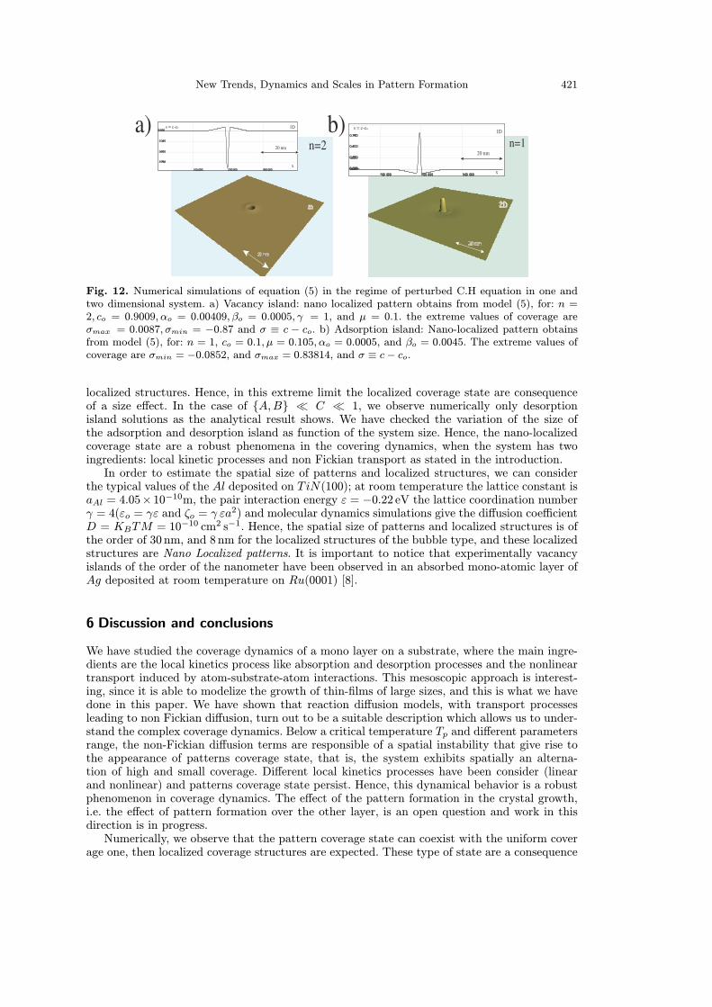
Fig. 12. Numerical simulations of equation (5) in the regime of perturbed C.H equation in one andtwo dimensional system. a) Vacancy island: nano localized pattern obtains from model (5), for: n =2, co = 0.9009, αo = 0.00409, βo = 0.0005, γ = 1, and µ = 0.1. the extreme values of coverage areσmax = 0.0087, σmin = −0.87 and σ ≡ c − co. b) Adsorption island: Nano-localized pattern obtainsfrom model (5), for: n = 1, co = 0.1, µ = 0.105, αo = 0.0005, and βo = 0.0045. The extreme values ofcoverage are σmin = −0.0852, and σmax = 0.83814, and σ ≡ c− co.

localized structures. Hence, in this extreme limit the localized coverage state are consequenceof a size effect. In the case of A,B C 1, we observe numerically only desorptionisland solutions as the analytical result shows. We have checked the variation of the size ofthe adsorption and desorption island as function of the system size. Hence, the nano-localizedcoverage state are a robust phenomena in the covering dynamics, when the system has twoingredients: local kinetic processes and non Fickian transport as stated in the introduction.In order to estimate the spatial size of patterns and localized structures, we can consider

the typical values of the Al deposited on TiN(100); at room temperature the lattice constant isaAl = 4.05× 10−10m, the pair interaction energy ε = −0.22 eV the lattice coordination numberγ = 4(εo = γε and ζo = γ εa

2) and molecular dynamics simulations give the diffusion coefficientD = KBTM = 10

−10 cm2 s−1. Hence, the spatial size of patterns and localized structures is ofthe order of 30 nm, and 8 nm for the localized structures of the bubble type, and these localizedstructures are Nano Localized patterns. It is important to notice that experimentally vacancyislands of the order of the nanometer have been observed in an absorbed mono-atomic layer ofAg deposited at room temperature on Ru(0001) [8].

6 Discussion and conclusions

We have studied the coverage dynamics of a mono layer on a substrate, where the main ingre-dients are the local kinetics process like absorption and desorption processes and the nonlineartransport induced by atom-substrate-atom interactions. This mesoscopic approach is interest-ing, since it is able to modelize the growth of thin-films of large sizes, and this is what we havedone in this paper. We have shown that reaction diffusion models, with transport processesleading to non Fickian diffusion, turn out to be a suitable description which allows us to under-stand the complex coverage dynamics. Below a critical temperature Tp and different parametersrange, the non-Fickian diffusion terms are responsible of a spatial instability that give rise tothe appearance of patterns coverage state, that is, the system exhibits spatially an alterna-tion of high and small coverage. Different local kinetics processes have been consider (linearand nonlinear) and patterns coverage state persist. Hence, this dynamical behavior is a robustphenomenon in coverage dynamics. The effect of the pattern formation in the crystal growth,i.e. the effect of pattern formation over the other layer, is an open question and work in thisdirection is in progress.Numerically, we observe that the pattern coverage state can coexist with the uniform cover

age one, then localized coverage structures are expected. These type of state are a consequence


of the appearance of nucleation barriers between the pattern and uniform coverage states, i.e.the pinning mechanism. For different parameters range of the coverage model, we have foundthe robust behavior of these structures. Analytically, we have find an amplitude equation fornano localized pattern formation in the nonlinear desorption case, and numerically patternand nano localized structure formation and bistablity of pattern solutions in both the n = 1and n = 2 cases. We have found besides the typical width of these localized structures in thecase when we can approximate the equation as a perturbed Cahn Hilliard model. Therefore, thenanolocalized solutions are a robust phenomena in the coverage dynamics, when the system hastwo ingredients: local kinetic processes and non Fickian transport as stated in the introduction.The localized coverage structures can exhibit complex dynamics, preliminary numerical simu-lations show that these states have repulsive interaction between them, work in this directionis in progress.The system also has coexistence between two pattern coverage states, in this parameter

region the system exhibits big localized patterns (localized peaks), that is, a localized patternstate surrounded by another pattern state.

The simulation software DimX developed at the INLN laboratory in France has been used for thenumerical simulations. M.G.C. and E.T acknowledges the support of FONDAP grant 1020374 andPrograma Bicentenario Anillo grant ACT15.

A Derivation of equation (3)

We shall give a short derivation of our starting equation (2). We divide the surface of depositionin cells of volume V = ad where d is the dimension (here d = 1 or d = 2), where the length a issmaller than the characteristic lengths of variation of the concentration c(r, t) of the adsorbedmolecules and of the range of interaction between them. Following the approach and notationsin [30], we assume complete diffusional mixing in each cell and call Nr the number of adsorbedmolecules in the cell of position r, and r±ai, ai = aei i = 1, 2 . . . d, are the position vectors ofthe 2d neighboring cells (|ai| = a), with e1, e2, . . . , ed) an orthonormal basis. We shall write amultivariate master equation for the probability p[Nr, t] of having Nr molecules in cell r attime t considering two type of contributions: i) Local processes in each cell such as adsorptionand desorption of the molecules which are in a gaseous state and in thermodynamic equilibriumover the substrate; ii) Transport processes between the different neighboring cells. In i) let Nbe the maximum number of available sites for deposition in each cell. The probabilities perunit time of an absorption or a desorption will be proportional to the number of empty sitesand the number of occupied sites in each cell, respectively, and can be written as ωa(Nr) =ωa(N − Nr), ωd(Nr) = ωdNr, where the probabilities of absorption an desorption for oneparticle in one site correspond to ωa = KaPs, ω

d = kd,o exp(βU(r)), β = kBT, with kd,o thedesorption rate and ka the absorption rate of one molecule in an isolated site, P the pressureof the thermal bath, s is the sticking coefficient, U(r) the interaction potential induced in cellr by the other adsorbed molecules, T the temperature and kB Boltzmann constant.We define the operators E±1

r− exp(± 1

N∂∂cr), cr = Nr/N, and we take the probabilities

per unit time of transition to neighboring cells with a Metropolis algorithm as ωrr±a i =

ωr −r ± a i(N−Nr± a i

N)Nr with

ωr→ r± a i =

veU(r)−U(r±a i) U(r) < U(r ± ai)v, U(r) < U(r ± ai)

where v is the rate of transition between cells in the absence of interaction. The master equationcan now be written as

∂tP [cr, t] = I +d∑i=1

II,


where IIi = II(+ai) + II(−ai),

I =∑r[(E−1r − 1)ωaN(1− cr) + (E+1r − 1)ωd(r)Ncr]p[cr, t],

II(±ai) =∑d

i=1

∑r(E+1r E

−1r+ai− 1)ωrr±a iNcr(1− r ± ai)p[cr, t].

In the equation for ∂tp the term I represents the local processes inside each cell and IIi thetransport contributions. We define the density of sites per unit volume µ = N/V, and thequantities (in the continuum limit a→ 0)

σi(r) =ωr→r+a i + ωr→r−a i

2

=v

2

[1 + exp

(−αβ

∣∣∣∣ ∂U∂x i∣∣∣∣)],

γi(r) =ωr→r+a i + ωr→r−a i

2

= −v2

[1− exp

(−aβ

∣∣∣∣ ∂U∂xi∣∣∣∣)]sign

(∂U∂xi

).

We can write E+1r E−1r±ai = exp[

1

µV∑′r (δr, r′′ − δr±a i, r′) ∂∂cr′ ]. In the continuum limit we have

1

Vδr,r′δ

(d)(r − r′); 1

V

∂

∂cr→ δ

δc(r),

and developing the exponentials we can write

II(±a i) = µV∑

r

[∑l≥1

1l!1µl

∫ ∏lk=1 drk

∏lk=1 (δ(r − rk) −δ(r ± ai − rk))

δ

δc(rk)

]×ω

r r±a ic(r)(1− c(r ± a i)p[cr, t].

From the previous formula we can expand IIi = II(+ai)+II(−ai) =∑l=∞l=l II

[l]i where l counts

the number of functional derivatives in each term of the expansion. Furthermore we expand in

powers of the small size a of the cells each II[l]i = II

[l](a2)i +II

[l](a2)i + . . . For the reaction part I

in each cell we expand also the exponentials and we write I = I [1]+I [2]+ . . .We shall take onlythe previous terms in the master equation which is a consistent Fokker-Planck approximation.Then our equation will be

∂tp[cr, t] = I [1] + I [2] +d∑i=1

[II[1](a)i + II

[1](a2)i + II

[2](a2)i

].

In the the continuous limit a→ 0 we shall have (we assume that in the limit a2v remains finiteand is equal to the diffusion constant)

lima→0 a

2σi(r) = lima→0a2v

2(1 + 1 +O(a)) = a2v = D

lim aγi(r) = lima→0−

av

2

(−aβ

∣∣∣∣ ∂U∂xi∣∣∣∣)sign

(∣∣∣∣ ∂U∂xi∣∣∣∣)=Dβ

2

∂U(r)

∂xi,


and we can finally write the equation for ∂tp when a→ 0 and in space dimension d = 2 (ordersµ0 and µ−1)

∂tp[c(r), t] =∫drδ

δc(r)

[−ωa(1− c(r)) + kd,oeβU(r)c(r)

−D∇2c(r)(1− c(r) + c(r)∇2c(r)−βD∂ic(r)(1− c(r))∂iU(r)p[c(r), t

]+1

2µ

∫dr

[[δ2

δc(r)2

[ωa(1− c(r)) + kd,oeβU(r)

]

+∂iδ

δc(r)∂iδ

δc(r)2Dc(r)(1− c(r))

]p[c(r), t

].

This is a functional Fokker-Planck equation which is equivalent to a Langevin equation whichwe can write unambiguously [31], since the stochastic part is completely characterized. One has

∂tc(r, t) = R(c(r, t)) + ∇ · (D∇c(r, t) + βDc(1− c)∇U(r))+1

µ12

[kaP (1− c(r, t))]12 fa(r, t)

+ (kd,o)12 e12βU(r)fd(r, t) + ∂i([2Dc(1− c)]

12 f i(r, t)

.

The term R(c(r, t)) represents the local processes which occur in each cell and the terms pro-portional to D are the transport between the cells. The other terms are stochastic and or-der 1/µ1/2 where (fa, fd, f

i, i = 1, 2) are gaussian white noises of zero mean and correlation〈fa(r, t)fa(r1, t1)〉 = δ(r − r1)δ(t − t1, 〈fd(r1, t1)〉 = δ(r − r1)δ(t − t1),

⟨f i(r, t)f j(r1, t1)

⟩=

δijδ(r − r1)δ(t− t1), i, j = 1, 2. Putting αo = ωa, βo = ωd, the term R(c(r, t)) takes the formR(c(r, t)) = αo(1− c) + βocn, n = 1, 2

In our derivation here we consider linear desorption which corresponds to n = 1, which wasintroduced in the first paragraph of this Appendix when we wrote ωd(Nr) = ω

dNr for the localdesorption term in the master equation (in cell r). There are however processing methods suchas sputtering and laser assisted deposition (non-equilibrium processes) where we have nonlineardesorption which corresponds to n = 2 in the previous equation. The equations that we haveconsider in our study is the deterministic part of the Langevin type equations written above.

References

1. T. Zambelli, J. Trost, J. Wintterlin, G. Ertl, Phys. Rev. Lett. 76, 795 (1996)2. V. Gorodestkii, J. Lauterbach, H.A. Rotermund, J.H. Block, G. Ertl, Nature 370, 276 (1994)3. K. Kern, H. Niehus, A. Schatz, P. Zeppenfeld, J. Goerge, G. Comsa, Phys. Rev. Lett. 67, 855(1991)

4. T.M. Parker, L.K. Wilson, N.G. Condon, F.M. Leibsle, Phys. Rev. B 56, 6458 (1997)5. H.Brune, M. Giovannini, K. Bromann, K. Kern, Nature 394, 451 (1998)6. H. Roder, R. Schuster, H. Brune, K. Kern, Phys. Rev. lett. 71, 2086 (1993)7. P.G. Clark, C.M. Friend, J. Chem. Phys. 111, 6991 (1999)8. K. Pohl, M.C. Bartelt, J. de la Figuera, N.C. Bartelt, J. Hrbek, R.Q. Hwang, Nature 397, 238(1999)

9. T.S Cale, V. Mahadev, Modeling of Film Deposition for Microelectronic-Applications, Vol. 22,(Academic Press, New York, 1996), p. 175

10. A.S. Mikhailov, M. Hildebrand, J. Phys. Chem. 100, 19089 (1996)11. J. Verdasca, G. Dewel, P. Borckmans, Phys. Rev. E. 55, 4828 (1997)


12. D. Waelgraf, Phil. Mag. 83, 3829 (2003)13. M.G. Clerc, M. Trejo, E. Tirapegui, Phys. Rev. Lett. 97, 176102 (2006)14. D. Waelgraf, Physica E 15, 33 (2002)15. M. Hildebrand, A.S. Mikhailov, G. Ertl, Phys. Rev. E 58, 5483 (1998)16. M.G. Clerc, C. Falcon, Physica A 356, 48 (2005)17. P. Coullet, C. Riera, C. Tresser, Rev. Lett. 84, 3069 (2002)18. C. Elphick, E. Tirapegui, M. Brachet, P. Coullet, G. Iooss , Physica D 29, 95 (1987)19. D. Bensimon, B. I. Sharaiman, V. Croquette, Phys. Rev. A 38, 5461 (1988)20. M.G. Clerc, C. Falcon, E. Tirapegui, Phys. Rev. Let. 94, 148302 (2005)21. M.G. Clerc, C. Falcon, E. Tirapegui, Phys. Rev. E 74, 011303 (2006)22. U. Bortolozo, M.G. Clerc, C. Falcon, S. Residori, R. Rojas, Phys. Rev. Lett. 96, 214501 (2006)23. H. Calisto, M. Clerc, R. Rojas, E. Tirapegui, Phys. Rev. Lett. 85, 3805 (2000); M. Argentina, M.G.Clerc, R. Rojas, E. Tirapegui, Phys. Rev. E 71, 046210 (2005)

24. J.W. Cahn, J.E. Hilliard, J. Chem. Phys. 31, 688 (1959)25. C. Chevallard, M. Clerc, P. Coullet, J.M. Gilli, Eur. Phys. J. E 1, 179 (2000)26. C. Chevallard, M. Clerc, P. Coullet, J.M. Gilli, Europhys. Lett. 58, 686 (2002)27. H. Calisto, M. Clerc, R. Rojas, E. Tirapegui, Phys. Rev. Lett. 85, 3805 (2000)28. M. Argentina, M.G. Clerc, R. Rojas, E. Tirapegui, Phys. Rev. E 71, 046210 (2005)29. M.C. Cross, P.C. Hohenberg, Rev. Mod. Phys. 65, 851 (1993)30. F. Langouche, D. Roekaerts, E. Tirapegui, Phys. Lett. A 82, 309 (1981)31. F. Langouche, D. Roekaerts, E. Tirapegui, Functional Integration and Semiclassical Expansions(Reidel, 1982)

Pattern Formation And Localized Structures In Acoustic Resonators Containing A Viscous Fluid

Documents

Transcript of Pattern Formation And Localized Structures In Acoustic Resonators Containing A Viscous Fluid