Ville Majuri

Parametric Modelling and Quality Verification of Castings

Thesis submitted for examination for the degree of Master of

Science in Technology.

Espoo, 6.9.2018

Supervisor: Prof. Juhani Orkas

Advisor: M.Sc. (Tech.) Mika Virnes

Aalto University, P.O. BOX 11000, 00076 AALTO

www.aalto.fi

Abstract of Master's Thesis

Author Ville Majuri

Title of thesis Parametric Modelling and Quality Verification of Castings

Master programme Master’s Programme in Mechanical Engineering Code ENG25

Thesis supervisor Prof. Juhani Orkas

Thesis advisor(s) M.Sc. (Tech.) Mika Virnes

Date 6.9.2018 Number of pages 81+6 Language English

Abstract

Even though 3D modelling and 3D scanning have been industry standards in casting de-sign and measurement for a long time, casting tolerance standards still usually rely on complete definition of castings in 2D drawings and linear dimensional tolerances. ISO 8062-4, published in 2017, is based on a general surface profile tolerance instead of sep-arate dimensional tolerances, thus forming a logical connection between 3D modelling, tolerancing and 3D scanning. As the contemporary 3D methods are prominently used, the outdated ISO 8062-3 should be replaced with the new standard in casting tolerance defi-nition. In this thesis, possibilities to include casting tolerances in casting CAD models are exam-ined. The aim is to create dependent but separate 3D models that depict the allowed min-imum and maximum state of the casting as allowed by the casting tolerance. The benefits of these tolerance models are evaluated considering quality verification, strength calcula-tions and collision detection. ISO 8062-4 casting tolerance and a traction sheave from an NMX hoisting machine are used for modelling case study. In addition, different measure-ment methods are reviewed to determine guidelines for casting measurement based on contemporary methods and standards. The case study revealed that tolerance model construction is difficult and time-consuming compared to the achieved benefits. Therefore, no implementation to every casting by de-fault is recommended. Attention was also paid to modelling techniques and conventions that should be followed regardless of the tolerance models. 3D scanning should be utilised in casting quality verification because of its coverage, speed and ability to compare scanned 3D model directly to the nominal model. Measurement instructions were deter-mined considering the requirements of ISO 8062-4 and the possibilities and restrictions of 3D scanning. An exemplary casting drawing of the traction sheave was created accord-ing to ISO 8062-4. Digital 3D product definition and 3D scanning were taken into account when determining the drawing indication.

Keywords casting tolerance, 3D scanning, ISO 8062-4, digital product definition

Aalto-yliopisto, PL 11000, 00076 AALTO

www.aalto.fi

Diplomityön tiivistelmä

Tekijä Ville Majuri

Työn nimi Valukappaleiden parametrinen mallinnus ja laadunvarmistus

Maisteriohjelma Master’s Programme in Mechanical Engineering Koodi ENG25

Työn valvoja Prof. Juhani Orkas

Työn ohjaaja(t) DI Mika Virnes

Päivämäärä 6.9.2018 Sivumäärä 81+6 Kieli Englanti

Tiivistelmä

Vaikka 3D-mallinnus sekä 3D-skannaus ovat jo pitkään olleet vallitsevat suunnittelu- ja mittausmenetelmät valuteollisuudessa, valutoleranssistandardit nojaavat pitkälti vielä valujen täydelliseen esittämiseen 2D-kuvissa sekä lineaaristen mittojen tolerointiin. Vuonna 2017 julkaistu ISO 8062-4 perustuu yleiseen pinnanmuototoleranssiin yksittäis-ten mittojen toleroinnin sijaan, jolloin uusi standardi muodostaa ehyen ja loogisen jatku-mon 3D-mallinnuksen ja 3D-skannauksen kanssa. Nykyaikaisia menetelmiä käytettäessä onkin syytä korvata vanhentuneisiin työkaluihin perustuva ISO 8062-3 uudella standar-dilla valutoleranssien määrityksessä. Tässä työssä selvitetään, miten valutoleranssin saa parametrisesti sisällytettyä valukap-paleen CAD-malliin, jolloin erilliset mallit kuvaisivat toleranssin sallimia valun minimi- ja maksimitiloja. Minimi- ja maksimitilojen mallien hyötyjä arvioidaan laadunvarmistuk-sen, lujuuslaskennan ja törmäystarkasteluiden kannalta. Toleranssimallien luonnissa käytetään standardin ISO 8062-4 mukaisia toleransseja sekä malliesimerkkinä NMX-his-simoottorin vetopyörää. Lisäksi tarkastellaan eri mittausmenetelmiä, ja pyritään määrit-tämään suuntaviivat nykyaikaisiin menetelmiin ja standardeihin perustuvaa mittausoh-jetta varten. Tarkasteluissa havaittiin toleranssimallien mallinnuksen olevan työlästä saatavaan hyö-tyyn nähden, jolloin niiden sisällyttäminen oletuksena jokaiseen valuun ei ole järkevää. Tarkastelun yhteydessä kiinnitettiin huomiota myös mallinnustekniikkaan ja tapoihin, joita tulisi valusuunnittelussa noudattaa riippumatta toleranssimallien käytöstä. Valujen mittaamisessa tulisi ensisijaisesti hyödyntää 3D-skannausta, jossa nimellistä CAD-mallia verrataan skannattuun 3D-malliin, ja joka kattavuutensa ja nopeutensa ansiosta onkin yleisesti käytössä valuteollisuudessa. Mittausprosessin kulku määritettiin samalla huomi-oiden standardin ISO 8062-4 vaatimukset sekä 3D-skannauksen mahdollisuudet ja ra-joitteet. Malliesimerkkinä käytetystä vetopyörästä laadittiin ISO 8062-4:n mukainen va-lupiirustus, jossa huomioidaan myös nimellisen muodon määritys CAD-mallilla sekä 3D-skannauksen käyttö laadunvarmistuksessa.

Avainsanat valutoleranssi, 3D-skannaus, ISO 8062-4, digitaalinen tuotemäärittely

4

Alkusanat Vuosien opiskelu huipentuu tähän ohuehkoon mustaan kirjaan, pääsylippuuni leveämmän

leivän ääreen. Opiskelijaelämä oli eittämättä eri hienoa aikaa, mutta olen myös varsin tyy-

tyväinen, että se lopulta päättyi.

Kiitokset KONEelle diplomityöni mahdollistamisesta, sekä Mikalle ja Jussille ohjauksesta.

Tahdon kiittää perhettäni niistä eväistä, joiden avulla olen tähän asti opinnoissani päässyt.

Suuret kiitokset Selinalle tuesta ja kärsivällisyydestä (ja ajoittaisesta patistamisesta).

Haluan erikseen kiittää niitä kaikkia tuttuja ja tuntemattomia, joiden kanssa olen Otanie-

messä ja satunnaisesti myös sen ulkopuolella aikaa viettänyt. Teidän ansiostanne opiskelijan

arki tuntui juhlalta. Lopuksi haluan vielä esittää äärettömän suuret kunnianosoitukset niille

nerokkaille muinaisille egyptiläisille ja mesopotamialaisille, jotka tuhansia vuosia sitten

keksivät, että ohraleivästä valmistettu seos voi ilmassa olevien mikrobien avulla spontaanisti

fermentoitua.

Helsingissä 6.9.2018

Ville Majuri

5

Table of Contents Alkusanat ............................................................................................................................... 4 1 Introduction .................................................................................................................... 8

2 Casting in General ....................................................................................................... 10 2.1 Casting Methods.................................................................................................... 10

2.1.1 Sand casting ................................................................................................... 10 2.1.2 Investment casting ......................................................................................... 11 2.1.3 Other expendable mould methods ................................................................. 11

2.1.4 Die casting ..................................................................................................... 12 2.1.5 Other permanent mould methods ................................................................... 12

2.2 Casting Materials .................................................................................................. 12 2.2.1 Introduction to cast irons ............................................................................... 12 2.2.2 Grey iron ........................................................................................................ 14

2.2.3 Spheroidal graphite iron ................................................................................. 14

2.2.4 Compacted graphite iron ................................................................................ 15 2.2.5 White iron and malleable iron ....................................................................... 15

2.2.6 Austempered irons ......................................................................................... 15 2.2.7 Steel ............................................................................................................... 15 2.2.8 Other materials ............................................................................................... 16

2.3 Designing Castings................................................................................................ 16

2.3.1 Basics ............................................................................................................. 16 2.3.2 3D-modelling ................................................................................................. 17

3 Casting Tolerance Systems .......................................................................................... 18 3.1 ISO 8062-2 and 8062-3 Casting Tolerances ......................................................... 18

3.1.1 Specification of casting .................................................................................. 18

3.1.2 Specification of casting tolerances ................................................................ 20 3.1.3 Weaknesses .................................................................................................... 21

3.2 ISO 8062-4 Casting Tolerances ............................................................................ 21 3.2.1 Background .................................................................................................... 21

3.2.2 General surface profile tolerance ................................................................... 22 3.2.3 Wall thicknesses and complete cylinders ...................................................... 22

3.2.4 Datum system RST ........................................................................................ 23 3.2.5 Drafts and RMAs ........................................................................................... 23

3.2.6 Machining ...................................................................................................... 23 3.2.7 Similar standards ............................................................................................ 24

4 Casting Measurement Techniques ............................................................................... 26

4.1 Coordinate Measuring Machines .......................................................................... 26 4.1.1 Bridge CMM .................................................................................................. 27

4.1.2 Articulated Arm CMM .................................................................................. 27

4.2 3D Scanning .......................................................................................................... 28

4.2.1 Time-of-flight sensors .................................................................................... 29 4.2.2 Laser triangulation ......................................................................................... 29 4.2.3 Interferometry ................................................................................................ 30 4.2.4 Stereo vision .................................................................................................. 30 4.2.5 Structured light .............................................................................................. 31

4.2.6 Photogrammetry ............................................................................................. 33 4.3 Combination Techniques ...................................................................................... 33

5 Parametric CAD Modelling ......................................................................................... 35 5.1 Definition .............................................................................................................. 35

6

5.2 Current Application ............................................................................................... 35

5.3 Design Intent ......................................................................................................... 36 5.4 Benefits ................................................................................................................. 37 5.5 Restrictions ............................................................................................................ 37

5.6 Direct Modelling ................................................................................................... 38 6 Casting Tolerance Parametrisation .............................................................................. 39

6.1 Background ........................................................................................................... 39 6.1.1 Purposes of tolerance parametrisation ........................................................... 39 6.1.2 NMX traction sheave properties .................................................................... 40

6.2 Implementation to NMX Traction Sheave CAD Model ....................................... 41 6.2.1 Uniform surface profile tolerance .................................................................. 41 6.2.2 Individually indicated surface profile tolerances ........................................... 43 6.2.3 Wall thicknesses ............................................................................................ 46 6.2.4 Machined models ........................................................................................... 50

6.3 Possibilities for General Implementation .............................................................. 53 6.3.1 Surface profile tolerance models ................................................................... 53

6.3.2 Wall thickness tolerance models .................................................................... 56 6.3.3 Custom imperative tolerance system ............................................................. 58 6.3.4 Summary ........................................................................................................ 59

7 Surface Profile Tolerance Based Casting Measurement .............................................. 61

7.1 Introduction ........................................................................................................... 61 7.2 Measuring Devices ................................................................................................ 61

7.3 ISO 8062-4 in Measuring ...................................................................................... 62 7.4 Dimensions to Be Measured ................................................................................. 63 7.5 Alignment .............................................................................................................. 64

7.5.1 Best fit alignment ........................................................................................... 64 7.5.2 RPS alignment ............................................................................................... 65

7.5.3 Local best fit .................................................................................................. 66 7.5.4 Datum system RST definition ........................................................................ 66

7.6 Tolerance Model Utilisation ................................................................................. 67 7.7 Rejection Limits .................................................................................................... 69

8 Design and Measurement Recommendations .............................................................. 70

8.1 CAD Model ........................................................................................................... 70 8.2 Drawing ................................................................................................................. 70

8.3 Measuring .............................................................................................................. 71 8.3.1 Options ........................................................................................................... 71

9 Conclusion and Recommended Further Actions ......................................................... 73

9.1 Modelling .............................................................................................................. 73 9.2 Casting Drawings .................................................................................................. 74

9.3 Measuring .............................................................................................................. 74

References ............................................................................................................................ 75

Appendices ........................................................................................................................... 81

7

Symbols and Abbreviations

𝐴𝑅𝑀𝐴 [mm] required machining allowance

𝑑𝐶 [mm] nominal dimension of casting

𝑑𝑀 𝑚𝑎𝑥 [mm] maximum dimension of machined part

𝑑𝑀 𝑚𝑖𝑛 [mm] minimum dimension of machined part

𝑡𝐷𝐶𝑇 [mm] dimensional tolerance of casting

𝑡𝐹𝐶𝑇 [mm] form tolerance of casting

𝑡𝐹𝑀𝑇 [mm] form tolerance of machined part

AACMM articulated arm coordinate measuring machine

ADI austempered ductile iron

AGI austempered grey iron

BSI British Standards Institution

CAD computer-aided design

CCD charge-coupled device

CEN European Committee for Standardization

CMM coordinate measuring machine

DCT dimensional casting tolerance

DCTG dimensional casting tolerance grade

EN European Standard

GCT geometrical casting tolerance

GCTG geometrical casting tolerance grade

GPS geometrical product specifications

NEN Netherlands Standardization Institute

PDM product data management

RMA required machining allowance

RMAG required machining allowance grade

RPS reference point system

SFS Finnish Standards Association

TED theoretically exact dimension

ToF time of flight

VBA Visual Basic for Applications

VDA German Association of the Automotive Industry

8

1 Introduction Casting is one of the most common metal manufacturing processes, referring to a family of

metal forming techniques in which molten metal takes the shape of a mould when cooled

and solidified. Several different casting methods exist, suitable for different metals, casting

sizes, and geometries. The accuracy of castings varies accordingly. The desired accuracy is

controlled by defining a casting tolerance, a system determining the allowed deviations from

the designed ideal form.

KONE is an international corporation manufacturing elevators, escalators and automatic

doors. With its over 50 000 employees and a revenue of over 8 billion euros, it is one of the

biggest companies in their field. At KONE, many hoisting machine components are ma-

chined castings, including the machine bodies and the traction sheave. The quality of the

components is particularly critical in elevator industry because of the safety aspect of the

products. The official regulations must be met to ensure the safety of the passengers in the

elevator car.

The quality and dimensional accuracy of the castings are often a topic of debate between the

foundry and the customer. Moreover, the currently used casting tolerance system based on

ISO 8062-2 and 8062-3 is not fully compatible with today’s 3D world, but rather stuck to

2D era. In contrast, casting design as well as pattern manufacturing utilise 3D modelling

extensively, and modern measurements methods rely on 3D scanning techniques.

This thesis answers the question ”How castings should be designed so that they are reliably

verifiable using contemporary measurement methods?” The expected result is a defined in-

structions framework for the casting from designing to measurement table considering cur-

rent technologies and tools. An update in the process is needed, because currently used cast-

ing tolerance standards are often outdated and no standard procedure exists for casting qual-

ity verification, especially considering modern 3D scanning solutions. All in all, the syn-

chronisation of CAD modelling, casting drawings, digital product definition and 3D meas-

urement needs standardising.

To achieve the said goal, casting design aspects are reviewed with emphasis on 3D model-

ling, casting tolerance systems are compared, and possible measuring technologies are ex-

amined and their suitability for castings is evaluated. In addition, parametric modelling tech-

nique is reviewed to determine whether any benefits can be acquired from incorporating the

casting tolerance limits to CAD models parametrically.

Parametric models are widely utilised with configurable products, but less attention has been

paid to their possible benefits for quality verification considering tolerances. True, many

tolerance analysis tools integrated in CAD environments are available, but they are intended

mainly for machined parts instead of casting quality verification. In this thesis, casting tol-

erances are incorporated into casting CAD models to generate the maximum and minimum

states of the casting as separate models. Furthermore, the usability of these tolerance models

in quality verification as limit references is evaluated. Beside the measurement, the tolerance

models might be useful in collision detection in assemblies or strength calculations. These

possibilities are examined as well. Based on the tolerance system review, the most suitable

system is selected as the basis for the tolerance parametrisation and for the definition of new

measurement guidelines.

9

As a case study, the parametrisation if performed to an NMX hoisting machine traction

sheave. Moreover, the traction sheave is considered when determining the casting tolerances

and the measurement procedure. The casting drawing of the traction sheave is updated to

correspond to the newly established guidelines.

10

2 Casting in General Casting is a metal manufacturing process where a workpiece is formed when molten metal

is cooled and solidified in the shape of a mould. Casting is one of the oldest known ways to

process metal, and hast been developed into a myriad of different techniques for different

materials and purposes. The size of castings varies from small precision-cast gears or turbine

blades to marine engine blocks weighing tens of tons. The wide use is based on the freedom

of shape combined with the reasonable costs. In this section, a few of the most common

casting methods and materials are reviewed. Sand casting and cast irons are emphasised

because of their frequency and their relevancy for the case study performed in the thesis.

2.1 Casting Methods

Casting methods are roughly categorised to expendable mould methods and permanent

mould methods based on the reusability of the mould. Expendable mould methods can be

further divided into permanent pattern methods and expendable pattern methods.

2.1.1 Sand casting

Sand casting is an expendable mould method where the primary mould material is quartz

sand blended with adhesives. The mould can be produced either by hand or by machine

moulding by filling sand in a flask with the pattern leaving a cavity in the mould. This is

demonstrated in Figure 1. Modern 3D printing technologies allow also additive manufactur-

ing of sand moulds. Gating systems are included to create a path for the melt to flow into the

cavity. Typically, the sand is squeeze moulded with bentonite providing the adhesion to so-

lidify the sand mould. With other adhesives, chemical hardening or heat treatments are also

possible methods to bind the sand together. The mould consists of at least two halves both

of which are moulded with their own patterns. Internal shapes can be achieved with cores,

pieces of mould material placed inside the actual mould. When the workpiece has been cast

and cooled, the sand mould is broken by e.g. vibration. The gating system as well as flashes

and fins are removed, and the final casting is cleaned.

Figure 1. Sand casting process. A) first half of the pattern in a flask, b) second half of the

pattern, c) first half of the mould, d) second half of the mould, e) assembled mould, f) solid

casting.

11

In a typical foundry, the sand is machine moulded in a flask the size of which determines the

maximum casting size. The mould consists of only two halves since the automated machine

moulding and pattern removal is done in only one direction. Cores can be used of course,

but the drafts are determined only by the seam of the two halves. Today, the patterns are

usually machined, and can be manufactured from e.g. plywood, but metals are extensively

used when the pattern must withstand more moulding cycles. The flasks and the pattern are

used repeatedly in an automatic production line, and even the sand obtained from broken

moulds is returned to the cycle, although adhesives must be added. Hand moulding is typi-

cally used only when the casting is too large to be machine moulded, the mould is too com-

plex with several separate parts, or the batch size is very small.

Sand casting is relatively cheap and simple. Furthermore, the size range is wide. It is suitable

for many materials, including iron, steel, and aluminium. For these reasons, sand casting is

one of the most used casting methods. The surfaces are quite rough because of the granular

nature of the mould, and the accuracy is worse than many other casting methods. Therefore,

sand castings are often machined to achieve sufficiently accurate and smooth functional sur-

faces. [1]

2.1.2 Investment casting

Investment casting is an expendable mould and expendable pattern method where the pattern

is manufactured from wax or certain plastics. A ceramic mould is produced by repeatedly

submerging the pattern into a liquid coating material that, once cured, forms a solid mould.

To remove the pattern, the mould is then heated to melt the wax. After pouring and cooling,

the mould is broken from around the casting.

In the past, manufacturing of the pattern has limited the complexity of shapes of investment

castings. Currently, 3D printing has been utilised also for waxes, allowing more geometri-

cally diverse patterns to be cast. Investment casting provides high accuracy and low surface

roughness, and it is suitable for nearly all metals. The method allows shapes that would be

impossible with a traditional two-piece mould. Cores, however, are more difficult to include

in the mould. Furthermore, the method is expensive, and the casting size is limited to only

small pieces. Typical applications include aerospace and power generation components,

most prominently turbine blades. [1]

2.1.3 Other expendable mould methods

Shell moulding is a sand casting method, where the mould is produced by coating the pattern

with sand, forming a thin-walled shell around the pattern instead of squeeze moulding in a

flask. The sand contains resin that is hardened by heating. The accuracy and surface quality

of shell moulded castings is better than traditional sand castings.

Plaster moulding resembles sand casting, but the mould material is gypsum plaster instead

of sand. Thermotolerant and fibrous additives are blended to the plaster to improve temper-

ature tolerance and strength of the mould. The accuracy and surface quality of plaster

moulded castings are superior to sand castings, but only materials with low melting point

can be used as the plaster mould disintegrates in high temperatures. Possible materials in-

clude alloys of aluminium, magnesium, zinc and copper. [1]

12

2.1.4 Die casting

Die casting refers to a family of permanent mould casting methods where the melt is led to

the mould cavity under pressure. The cavity is formed by two mould halves called dies,

usually manufactured of tool steel. When solidified, the die casting machine opens the mould

and removes the workpiece from the die using ejector pins. Two types of die casting ma-

chines exist: hot-chamber machine, where the pump and the melt are located in the same

machine, and cold-chamber machine, where the material is melted in a separate furnace out-

side the machine. Hot-chamber machines are suitable for materials with low melting point,

and cold-chamber machines must be used with higher temperatures to avoid heat damage to

the pumping system.

Die casting is mostly used for non-ferrous metals and relatively small workpieces from under

a kilogram to tens of kilograms. Since the moulds are machined, the accuracy and surface

finish are excellent. The pressurised cavity filling allows more complex shapes and thinner

walls than traditional pouring. However, the tooling is expensive, and therefore die casting

is profitable only with very large batches. [1]

2.1.5 Other permanent mould methods

Centrifugal casting can be used to produce hollow, axially symmetrical castings. The

mould rotates, forcing the melt against the walls of the mould. An open cavity is thus formed

in the middle of the casting without a core. Centrifugal casting is used for cylindrical pieces

such as pipes and valves. Possible materials include many metals, glass and even concrete.

Continuous casting is a method used for profiles and pipes. The mould is water-cooled so

that the profile can be pulled through the mould as the material solidifies. Melt flows to the

other side to fill the mould as the solid part is retracted. The use of steel is limited, but irons,

aluminium and copper alloys are more widely used. [1]

2.2 Casting Materials

2.2.1 Introduction to cast irons

Cast irons are alloys of iron that include at least 2 % carbon. With lower carbon content, the

material is called steel. Cast irons may include also other alloying elements, such as silicon,

manganese, chromium, molybdenum or nickel. 2.14 % is the maximum amount of carbon

soluble in iron in any circumstances, and the excessive carbon is precipitated to separate

phases, forming different microstructures with different casting parameters. [2]

Figure 2 shows the iron-iron carbide phase diagram. The diagram shows the allotropes of

iron as a function of temperature and carbon content, with α referring to ferrite, γ to austen-

ite, L to liquid, and Fe3C to cementite (iron carbide). Ferrite is very soft and ductile, whereas

cementite is hard and brittle. In pure iron-carbon alloy, no stable austenite can occur below

727°C. Nonetheless, with sufficient alloying with austenising elements, austenitic steels can

be produced.

Simplified, the figure shows that as the temperature decreases, austenite is turned into ferrite

in austenitic transformation. [3] Ferrite can dissolve considerably less carbon than austenite,

and cementite (and graphite) is formed. More iron is precipitated as cementite or graphite

when the carbon content increases. With a carbon content of 6.7 per cent, the material con-

sists entirely of cementite. [4] The point on the border of liquid and γ + Fe3C phases at 4.3

13

% carbon is called the eutectic point. With the said carbon content, the melting point is the

lowest.

By alloying iron with relatively large quantities of carbon and silicon, the composition is

brought near the eutectic point to lower the melting point, improve fluency and allow the

forming of graphite. Moreover, cooling rate and inoculation providing crystallisation nuclei

also affect the amount of graphite, with slow cooling resulting in more graphite and less

cementite. As opposed to graphite irons, white irons contain no free carbon as graphite, but

the carbon is bound as carbides. [5]

Figure 2. Iron-iron carbide phase diagram. [3]

A microstructure consisting of lamellar layers of ferrite and cementite is called pearlite. The

layers are oriented in the same direction within a grain, but the orientation varies from grain

to grain. [3] Pearlitic structure is achieved in austenitic transformation with a relatively low

cooling rate. [5] Even though cementite is hard and brittle, the greater proportion of ferrite

makes pearlite still quite ductile. [4] Also bainite can be produced in the austenitic transfor-

mation. Bainite is a strong steel microstructure consisting of ferrite and cementite, shaped as

very fine needles or plates. Bainite requires faster cooling in order to prevent the austenite

from diffusing into pearlite. [5][3] When the material is quenched into even lower tempera-

tures, strong and hard martensite is formed, another allotrope of iron. Ledeburite is a eu-

tectic mixture of austenite and cementite found in white irons. Ledeburitic microstructure is

hard and brittle, and is formed with fast cooling and low silicon content. [4]

14

2.2.2 Grey iron

Grey iron is the most used casting material. The graphite forms lamellar flakes in either

entirely or partly pearlitic matrix, the rest of the matrix being ferritic. [2] The microstructure

of grey iron visible on the left in Figure 3. When the graphite crystallises, the volume of the

material increases, compensating for the solidification shrinkage. Therefore, the castability

of grey iron is excellent. Because of the shape of the graphite, grey iron dampens vibrations

and conducts heat well, but on the other hand, it is mechanically weak and brittle as the load

is mainly carried by the thin matrix strips between the graphite flakes. The graphite helps

preserve oil film on lubricated sliding surfaces, making grey iron a lucrative material for

tribologically challenging applications. Grey iron is also very well machinable, especially

when the matrix includes soft ferrite. The graphite flakes cause the chips to be short, and

diminishes the wear of the tools due to its lubricating properties. Welding is not easily pos-

sible because of the brittleness.

Grey iron is typically used in low-cost applications with moderate mechanical load. How-

ever, its other properties allow using it more widely. For its heat conductivity and lubricating

properties, grey iron is a valid option for e.g. combustion engine components. Because of its

vibration-damping ability, it is well suitable for machine bodies and frames. [5]

Figure 3. Grey iron, compacted graphite iron and ductile iron graphite structures. [6]

2.2.3 Spheroidal graphite iron

Spheroidal graphite iron (also SG iron or ductile iron) contains the graphite as spherical

nodules as seen on the right in Figure 3. The nodular graphite structure is accomplished by

inoculating the molten iron with specific spheroidisation compounds, often including mag-

nesium. The matrix of ductile iron consists of ferrite and pearlite. Ferritic structure increases

ductility but decreases strength. The more pearlite the iron contains, the stronger the mate-

rial. Pure ferrite phases often occur around the graphite nodules as the carbon is retracted

into the nodule from its vicinity.

Ductile iron is stronger than grey iron as there are no graphite flakes dividing the matrix.

The material is stronger when the nodules are small-sized but their amount is large. The

mechanical properties can be even comparable to structural steels. [5] Generally, ductile iron

15

is well machinable. It is not as hard as grey iron, and the quality of machined surfaces is

good, but it requires greater cutting forces because of its greater strength. The weldability is

not optimal because brittle carbides are formed in the heat-affected zone. [5] However, the

quality of the weld can be improved with sufficient pre-heating. Due to its low cost, simplic-

ity of casting and its steel-like mechanical properties, the industrial application possibilities

of ductile iron are extremely broad. [7]

2.2.4 Compacted graphite iron

Both the mechanical properties and the microstructure of compacted (or vermicular) graphite

iron lie between those of grey iron and ductile iron. The microstructure is shown in the mid-

dle in Figure 3. The graphite shape is obtained by carefully controlled, incomplete spheroi-

disation of the graphite, and resembles the flakes in grey iron, although with rounded edges.

Compacted graphite iron is used when the properties of grey and ductile iron need to be

combined. It is stronger than grey iron, but conducts heat and dampens vibrations better than

ductile iron. Therefore, it is used as a compromise solution for thermally stressed applica-

tions where greater mechanical strength is required than grey iron can provide. Typical uses

are engine blocks, cylinder heads, gearboxes and turbochargers, especially with high-perfor-

mance applications where light weight is a critical requirement. [5][6][8]

2.2.5 White iron and malleable iron

White iron contains no carbon as free graphite, but the carbon is bound to cementite and

carbides of other alloying elements. The microstructure is ledeburitic. White iron is very

hard and brittle. Consequently, it is difficult to machine and has therefore little practical use.

However, white iron is used to manufacture malleable iron through annealing. The long heat

treatment leads again to the forming of graphite, resulting in mechanical properties compa-

rable to ductile iron. Malleable iron is ductile and weldable. However, the use of malleable

iron has decreased as the popularity of ductile iron has in turn increased. [5]

2.2.6 Austempered irons

Austempered irons are produced by heating the iron to 850-950 degrees Celsius to austenise

the matrix. Then, the iron is quenched into a salt bath the temperature of which is 250-450

°C, and subsequently cooled down. The temperatures and times of each step alongside with

many other process variables determine the amount and stability of austenite formed in the

material. Mechanical and tribological properties of austempered ductile iron (ADI) are su-

perior to even most steels. Grey iron can also be austempered (AGI), but lower strength

limits its use. [5]

2.2.7 Steel

Cast steels are alloys containing less than 2.1 % carbon, although often less than 1 %. Many

different cast steel types exist, categorised by their intended use. [2] Because of its high

shrinkage and higher melting temperature, the castability of steel is quite poor compared to

irons. Steel is a viable option for casting material only when very specific mechanical prop-

erties are required (although ductile iron is as strong or even stronger [5]), or weldability of

the material is critical.

16

2.2.8 Other materials

Aluminium is used for lightweight or corrosion-prone applications, and is often produced by

die casting. When the weight is even more critical, magnesium may be used. Typical appli-

cations are automotive and aerospace components as well as hand-held motorised tools.

Magnesium is problematic to cast because of its low boiling point and high reactivity. Again,

die casting is the most used method. For very corrosive environments, copper alloys are

possible. When more strength is required, aluminium bronze or brass may be used. Zinc is

very well castable for its low melting point, and is usually die cast. Possible uses include

automotive components and corrosion prevention. [9]

2.3 Designing Castings

2.3.1 Basics

Usually the mould consists of at least two halves, but complex shapes might require more

mould components. Parting surface separates the mould halves. Internal shapes are created

using cores that leave open cavities within the casting. The parting surface is not necessarily

a plane, but can be also a curved surface to adapt to the geometry of the casting. Neverthe-

less, simplicity should be pursued in casting design to avoid unnecessary costs.

Any surfaces parallel to the opening direction of the mould must be drafted. With expendable

mould methods such as sand casting, this allows the pattern to be removed from the sand

mould with ease. With e.g. die casting, drafting allows the casting itself to be removed from

the die. Counterdrafts – surfaces angled so that pattern removal is hindered – are not allowed.

When the mould consists of more than two parts, the drafts must be directed according to

the assembly order of the mould. Rounds must be added to corners to remove sharp edges.

Especially with sand castings, sharp outer corners in the mould break easily, and inner cor-

ners might not entirely fill with the melt. Furthermore, rounded corners ease the removal of

the pattern or the casting from the mould. Sufficient machining allowances must be included

in the nominal dimensions to ensure successful machining.

The flow of the material is crucial in order to achieve solid components with the melt filling

the entire mould. Sudden changes in the cross section must be avoided to prevent porosity

in thicker areas of the casting. Most methods, including sand casting, rely on mould filling

by gravity. Therefore, the mould must be designed so that the material flows freely down-

wards, and upwards flow must be avoided. The minimum wall thicknesses depend on the

material and the used method. For instance, thinner walls are allowed with die casting since

the material is forced to the cavity under pressure instead of only gravity. Not only the wall

thickness affects, but also the length of the thinnest part. The further the melt must flow in a

thin canal, the faster it cools down.

The pattern must be scaled before casting as the shrinkage affects the dimensional accuracy.

Moreover, the gating system with feeders must be added to the pattern and mould. These

operations are usually done by the foundry rather than being designed by the customer. How-

ever, the designer still needs to consider the gates and sprues to leave enough room to their

intended locations. When 3D CAD is utilised in casting design, the casting process can be

simulated using the CAD model, and corrections to the model can be made based on the

simulated flow and solidification of the melt.

17

The utilisation of the listed basic principles depends on the casting method. For instance, in

investment casting, the wax pattern is removed from inside the mould by melting and the

mould is broken from around the final workpiece, obviating the need for a multipart mould

or drafting. Furthermore, designing die castings requires considering the machinability of

the mould, ejector pins and the limitations of the used machine. [10][11]

2.3.2 3D-modelling

Even though a casting can be fully defined using only a machining drawing and leave the

calculation of casting nominal dimensions for the foundry, a common practice is to order

castings using only the 3D CAD model. Defining castings with a digital 3D model is cur-

rently the industry standard, and the model is used as the master representation. The casting

drawing is mainly intended to indicate casting specifications and tolerances, whereas the

actual product shape definition is done with the CAD model.

3D modelling benefits in many ways any design tasks, but the advantages are even more

prominent with castings. As a manufacturing method, casting supports curved or complex

features well and with reasonable costs, at least when compared to e.g. machining. Further-

more, castings must include draft surfaces and rounds, adding to the irregularity of the sur-

faces. As a result, defining every feature of the casting unambiguously in a 2D drawing

becomes difficult. The more complex the part, the more arduous the 2D definition. When

the 3D model is used as the master representation, the role of the drawing changes, and there

is no longer need to show every dimension or feature in the drawing. In conclusion, usage

of 3D models simplifies the product definition, thus saving recourses from both the designer

and the foundry.

A common modelling order with castings is as follows:

1. Base shapes,

2. cuts and holes,

3. definition of parting surface,

4. drafts,

5. rounds.

Casting modelling tools are included in many modern CAD software packages, and even

separate casting design extensions exist. This is to help with features only found in castings,

such as drafts. The benefits of using 3D models are not restricted to the ease of representation

and design, but the models can also be used as references in quality verification (3D scan-

ning), pattern or mould manufacturing and casting simulations.

Casting models are often designed emphasising the functionality and final use of the work-

piece, neglecting some aspects of the casting process. Therefore, the foundry checks the

delivered 3D models to ensure successful casting, and edits them before pattern manufactur-

ing and moulding. The most common issues include incorrect or missing drafts, minuscule

or missing rounds or other modelling errors. The gating and feeding system is also added by

the foundry. Moreover, the shrinkage must be compensated by scaling the model. In practice,

the model is scaled simply linearly even though the shrinkage may vary depending on the

direction and material thicknesses. For instance, the cores withstand pressure so well that the

shrinkage is directed almost entirely to the mould side. [12]

18

3 Casting Tolerance Systems Many factors affect the dimensional accuracy of castings. The chosen casting method lays

the basis for casting accuracy as the accuracy of mould manufacturing is directly inherited

to casting accuracy. For instance, machined moulds often deliver better accuracy than e.g.

squeeze moulded sand moulds. Furthermore, moulds and patterns may yield or deform. With

two-piece moulds, mould opening or mismatch negatively affects the correctness of the cast-

ing. The surface roughness varies depending on the casting method. The shrinkage and the

actions to compensate it have an effect, which again is related to the material choice. More-

over, the chosen material affects through its fluency, ergo, its ability to fill small cavities.

As the sources of defects vary, so do the types of defects. Not only the linear dimensions are

affected, but also the geometrical form. To address to the many sources of deviations from

the designed nominal, casting tolerances are needed to define which defects are acceptable

and which not considering both the dimensional accuracy and the correct shape of the cast-

ing.

3.1 ISO 8062-2 and 8062-3 Casting Tolerances

ISO 8062 standards are part of the ISO GPS system and the predominant standards used as

the basis for casting tolerancing. Until 2017, the tolerance had three parts: 8062-1 defines

the vocabulary [13], 8062-2 defines the rules for casting tolerancing, general tolerancing and

drawing indication [14] and 8062-3 defines the reference values for dimensional and geo-

metric tolerances as well as drafts and RMAs [15]. Casting tolerancing virtually relies on

two distinct tolerance definition types: individual and general. The designer defines individ-

ual tolerances for features with specific requirements, and the general tolerance applies to

all other features with no separately defined tolerances.

3.1.1 Specification of casting

ISO 8062-2 states two different methods to define castings in drawings: accumulation

method and multiple tolerancing method.

With accumulation method, the purchaser defines the casting indirectly using the final ma-

chined part. The caster calculates the nominal dimensions of the casting from the machined

dimensions considering the machining tolerances, the casting tolerances and the required

machining allowance (RMA) specified in the drawing by the customer. Where tolerances

are not specified, general tolerance values of ISO 8062-3 are used according to the general

tolerance grades indicated in the drawing. An exemplary drawing indication is shown in

Figure 4 a). Equation (1) shows an example calculation of nominal casting dimension of an

external feature both sides of which are machined without the envelope requirement .

𝑑𝐶 = 𝑑𝑀 𝑚𝑎𝑥 + 2 𝐴𝑅𝑀𝐴 + 𝑡𝐹𝐶𝑇 +𝑡𝐷𝐶𝑇

2+ 𝑡𝐹𝑀𝑇 (1)

where 𝑑𝐶 is the nominal dimension of the casting,

𝑑𝑀 𝑚𝑎𝑥 is the maximum dimension of the machined part,

𝐴𝑅𝑀𝐴 is the required machining allowance,

𝑡𝐹𝐶𝑇 is the form tolerance of the casting,

𝑡𝐷𝐶𝑇 is the dimensional tolerance of the casting, and

𝑡𝐹𝑀𝑇 is the form tolerance of the machined part.

19

The nominal dimension of an internal feature is calculated from

𝑑𝐶 = 𝑑𝑀 𝑚𝑖𝑛 − 2 𝐴𝑅𝑀𝐴 − 𝑡𝐹𝐶𝑇 −𝑡𝐷𝐶𝑇

2− 𝑡𝐹𝑀𝑇 (2)

where 𝑑𝑀 𝑚𝑖𝑛 is the minimum dimension of the machined part. [14]

Without the envelope requirement, the form tolerance of machined part 𝑡𝐹𝑀𝑇 is left out from

the equation. As seen from Equations (1) and (2), the nominal dimensions of the casting

depend on the form and dimensional tolerances of the casting. Contradictorily, the casting

tolerance depends on the nominal dimension of the casting. Therefore, initial values for the

tolerances 𝑡𝐹𝐶𝑇 and 𝑡𝐷𝐶𝑇 must be chosen for the calculation before the nominal dimension is

known based on a guess or the machined dimension. The result does not necessarily match

the expected range within which the first guess falls, and another calculation round must be

done, now with casting tolerances chosen based on the first result. As tolerance values are

directly used in the calculation of casting nominal dimensions, the outcome takes into ac-

count only the worst case of each tolerance. This might lead to an unnecessary increase in

the amount of material removed by machining. The effect can be diminished by assigning

smaller tolerances. [14]

Figure 4. Exemplary drawings according to ISO 8062-2. A) accumulation method with ISO

8062-3 general tolerances, b) multiple tolerancing method with general surface profile tol-

erances. Symbols and indicate the final moulded and machined conditions of the cast-

ing, respectively. [14]

With multiple tolerancing method, the customer supplies a drawing where both the final

machined part and the final casting are directly defined in total, either in a combined drawing

or separate drawings. An example drawing is presented in Figure 4 b). The drawing includes

separate tolerances for both states distinguished with condition symbols. General tolerance

applies to dimensions not separately toleranced in the drawing. As both states of the casting

20

are individually defined, it is possible to decrease the amount of removed material by ma-

chining compared to the accumulation method, but then again the workload of the designer

increases. [14]

The calculation of the nominal dimensions of a casting using multiple tolerancing method

does not utilise generally applicable equations. Still, the relation of the two conditions as

well as the tolerances must be defined so that the final machined part is achievable from the

casting with sufficient machining allowance between the two conditions. In other words, the

maximum material condition of the machined part must fit in the least material condition of

the final casting, also including RMA. [14]

3.1.2 Specification of casting tolerances

ISO 8062-2 defines how casting tolerances should be specified in a casting drawing. Since

functional features or otherwise critical surfaces must be anyway toleranced individually,

the emphasis is on the general tolerances. ISO 8062-2 specifies two alternative ways to de-

fine the general casting tolerance: general tolerances according to ISO 8062-3 and general

surface profile tolerance. [14]

General tolerances according to ISO 8062-3 are based on dimensional tolerancing of fea-

tures of size. The shape of the casting is further constrained with general geometrical toler-

ances. All dimensional and geometrical general tolerances apply independently from each

other. The tolerance values are defined using tolerance grades for both linear dimensional

tolerances and geometrical tolerances. The linear dimensional casting tolerances (DCT) de-

pend on the nominal dimension and the chosen dimensional casting tolerance grade (DCTG)

between DCTG 1 and DCTG 16. For wall thicknesses, DCTG is chosen one grade coarser

than the rest of the casting.

The general geometrical casting tolerances (GCT) according to ISO 8062-3 are defined using

geometrical casting tolerance grades (GCTG) from GCTG 2 to GCTG 8. As with DCTs,

GCTs depend on the nominal dimension and the chosen grade. GCTs are defined separately

for straightness, flatness and coaxiality, and with same values for roundness, parallelism,

perpendicularity and symmetry. A datum system for general orientation tolerances must be

defined in the drawing. However, it does not apply to general coaxiality and symmetry tol-

erances for which the standard defines separate methods to determine the datums.

As with the tolerances, ISO 8062-3 specifies required machining allowances (RMA) using

required machining allowance grades (RMAG) from RMAG A to RMAG K. RMA value

depends on the largest overall dimension of the casting as well as the chosen grade. The

standard includes suggestions for DCTG, GCTG and RMAG selection based on the casting

material and the casting method. All three grades must be specified in the casting drawing

by the customer if ISO 8062-3 general tolerances are to be used. [15]

The option for ISO 8062-3 general tolerances is general surface profile tolerance. Surface

profile tolerance is a geometrical tolerance defined in ISO 1101. The surface profile toler-

ance zone is defined by two surfaces enveloping spheres the diameter of which is the toler-

ance value and the centre of which is constrained to the nominal theoretically exact surface.

The principle is demonstrated in Figure 5, where the theoretically exact surface is determined

with its spherical radius and theoretically exact distance from datum A. [16] In practice, the

21

result is two limiting surfaces with an offset of half the tolerance value in the normal direc-

tion to the nominal surface. The general surface profile tolerance applies for all surfaces not

individually toleranced. The nominal geometry affected by the general surface profile toler-

ance is defined in the drawing using theoretically exact dimensions (TED). For sizes, such

as diameters, widths and wall thicknesses, dimensional tolerancing can be used. [14]

With both ISO 8062-3 and surface profile tolerance, a datum system must be specified for

the part in order to constrain the general tolerances. [14][15, p. 4]

3.1.3 Weaknesses

ISO 8062-2 and 8062-3 rely on defining the castings completely in the casting drawing. As

the casting is defined solely by dimensions and tolerances shown in the drawing, the dimen-

sion-based ISO 8062-3 suits well the presentation as the dimensions to be verified are di-

rectly presented. However, the tolerance system does not take into account the possibility to

define the casting using a 3D CAD model. The ISO 8062-3 tolerance system is complex,

and the shape of the castings difficult to verify when the dimensional tolerances are com-

bined with several geometrical tolerances.

Even though general surface profile tolerance is recommended in ISO 8062-2, the require-

ments and instructions for its use are quite vague. Defining the datum system for surface

profile tolerancing is only presented as an example instead of specifying the requirements

for utilisation in casting design, e.g. the datum system is not properly defined. In addition,

the calculation of nominal dimensions is specified only for ISO 8062-3 tolerances.

Figure 5. Surface profile tolerance definition. A) drawing indication, b) interpretation. [16]

3.2 ISO 8062-4 Casting Tolerances

3.2.1 Background

ISO 8062-4 is a new casting tolerance standard published in 2017 as an option for ISO 8062-

3. As 8062-3 relies solely on dimensional tolerances, it is in contradiction with ISO GPS

rules. Moreover, when the general tolerances are defined by a rather complicated system of

independent dimensional and geometrical tolerances, the allowed overall shape of the cast-

ing is very difficult if not completely impossible to determine. With CAD models, the nom-

inal dimensions are not even necessarily visible. ISO 8062-4 is based on general surface

profile tolerances with which the allowed shape is clearly defined, and the tolerance system

22

as well as the casting nominal dimension calculation are compatible with GPS rules and

digital 3D product definition. [17]

3.2.2 General surface profile tolerance

Instead of dimensional tolerances, ISO 8062-4 defines the general tolerances as an overall

surface profile tolerance. The theoretically exact surfaces (nominal shape) can be determined

using only a CAD model. The general surface profile tolerance must be related to a general

datum system for which letters R, S and T are reserved. Beside the surface profile tolerance,

individually indicated tolerances (e.g. surface profile, location, dimension) can be normally

defined. Any individually indicated tolerance overrules the general surface profile tolerance.

Also, the individually indicated tolerances are preferably related to the datum system RST.

The surface profile tolerance is defined with tolerance grades P ranging from P1 to P15. The

standard includes recommendations for tolerance grades P for each manufacturing method

and casting material. Every tolerance grade P has different surface profile tolerance values

for different casting sizes. The larger the casting, the wider the tolerance. The size of the

casting is determined by the moulded space diagonal, i.e. the diameter of the smallest envel-

oping sphere. [17] An exemplary drawing indication is presented in Figure 6 a).

Figure 6. Example drawing. A) drawing indication according to ISO 8062-4, b) datum sys-

tem RST definition. [17]

3.2.3 Wall thicknesses and complete cylinders

In addition to the general surface profile tolerance, ISO 8062-4 defines separate dimensional

tolerances for wall thicknesses and complete cylinders. These are considered separately de-

fined tolerances, thus overruling the surface profile tolerance. The dimensional tolerances

are defined with tolerance grades S ranging from S1 to S15. The tolerance depends on the

nominal dimension and the chosen tolerance grade S. The standard does not specify the def-

23

inition of “complete cylinders”, leaving the applicability of their tolerance vague. In addi-

tion, the standard defines tolerance values for wall thicknesses and complete cylinders only

up to 300 millimetres. Anyhow, the cylinder size tolerance should only be used when nec-

essary and together with positional tolerances. Moreover, even the wall thickness tolerance

can be left out of the drawing indication when using only surface profile tolerance is deemed

sufficient. For wall thicknesses, the tolerance grade is recommended to be one grade coarser

than for cylinder sizes. [17] In conclusion, the surface profile tolerance defines the allowed

shape of the casting, and the wall thickness and cylinder tolerance limits the actual dimen-

sions.

3.2.4 Datum system RST

To use the general surface profile tolerance, datum system RST must be defined according

to ISO 5459 to lock all degrees of freedom. The surface profile tolerance is related to the

datum system with TEDs defining the nominal surface. The datums for the datum system

RST can be defined either with datum targets or as integral datums. Datum targets are por-

tions of datum features used to establish the datum feature, whereas integral datums are con-

structed using the entire datum feature. [18] Datum targets are preferred since the general

surface profile tolerance applies also to the datum features only when datum targets are used.

If integral datum features are used, the surface profile tolerances must be defined separately

for datum features. The datums must be defined on surfaces remaining in the moulded con-

dition even after machining. [17, p. 4]

The casting drawing specifies the location and orientation of the nominal theoretically exact

surfaces in relation to the datum system with TEDs. On the other hand, the nominal surfaces

can be directly defined in a CAD model. Still, the datum system RST must be defined even

if the TEDs are not visible in the drawing. When measuring the physical casting, the surface

profile tolerance zones must be aligned to pre-defined surfaces of the casting, i.e. the ones

defined with the datum system RST. An example of defining datum system RST is presented

in Figure 6 b).

3.2.5 Drafts and RMAs

ISO 8062-4 defines draft angle reference values that depend on the casting method, the

height of the drafted feature and the selected draft grade (fine or coarse). As with the surface

profile tolerance grades P, the RMA grades are recommended based on the casting method,

material and size. RMA grades range from A to K. If the casting is defined using its ideal,

machined shape, the caster must add the drafts and RMAs for pattern manufacturing, and

the designer must specify whether the draft increases the feature or the tolerance of the ideal

model. Alternatively, drafts can be included in the nominal model in which case the surface

profile tolerance applies normally also to the draft surfaces. [17]

3.2.6 Machining

The casting and its tolerances must be defined in a way that the final machined condition is

achievable. The nominal dimensions of the casting are calculated from the machined condi-

tion nominal dimensions considering machining tolerance, casting surface profile tolerance

and RMA. The relation between the machined dimensions and the casting dimensions is

presented in Figure 7. Equation (3) shows the calculation in a similar situation and same

symbols as Equation (1) with a workpiece machined externally on both sides, whereas Figure

7 considers machining only one side.

24

𝑑𝐶 = 𝑑𝑀 𝑚𝑎𝑥 + 2 𝐴𝑅𝑀𝐴 + 𝑡𝐹𝐶𝑇 (3)

where now the form tolerance of the casting 𝑡𝐹𝐶𝑇 represents the surface profile tolerance. As

seen in Figure 7 and Equation (3), also this calculation method considers the worst-case

scenario with both machining and casting tolerances.

As the datum system RST is placed on surfaces remaining unmachined, the machining

should also be related to the datum system RST. When the casting nominal dimensions are

calculated as in Figure 7 and Equation (3), the casting and machining datums are the same

RST, and the measured casting surfaces are entirely within the tolerance zone, the final ma-

chined condition is always achieved. If the machining tolerances are related to a different

datum system, there is no guarantee that enough material exists for successful machining,

and additional material is needed. [17]

Figure 7. Calculation of casting nominal dimensions from machining nominal dimensions.

[17]

3.2.7 Similar standards

The surface profile tolerancing system of ISO 8062-4 has already been introduced in ISO

8062-2 and even recommended for use instead of ISO 8062-3 dimensional general tolerances

[14, p. 43]. Even the datum system definition for surface profile tolerancing is considered

[14, p. 48]. However, the older standards determine the use of general surface profile toler-

ance more as examples rather than a comprehensive tolerancing system. ISO 8062-4 takes

CAD models into account and further develops the tolerance system without mixing it with

the 8062-3 tolerances or the casting specification methods. Above all, the calculation of the

casting nominal dimensions is now clear and unambiguous.

Similar tolerancing systems have been developed also by companies, which suggests that a

real need exists for a tolerance system update. Volvo standard 101-0001 defines a framework

for digital product definition based on ISO 16792, but defines the general tolerance as a

surface profile tolerance related to datums, exactly as the datum system RST in ISO 8062-4

[19]. Voith VN 3212 has more comprehensively the same content as ISO 8062-4, including

the suggested surface profile tolerance values, individually indicated tolerances, wall thick-

nesses and datum targets. In addition, the Voith standard takes into account the possibility

to use UZ modifier in the surface profile tolerance definition to move the tolerance zone in

relation to the nominal surface. [20] Figure 8 shows the principle of UZ modifier according

to ISO 1101.

25

Figure 8. UZ modifier used to offset tolerance zone. UF modifier (united features) indicates

that the toleranced features are considered one feature. [16]

26

4 Casting Measurement Techniques

4.1 Coordinate Measuring Machines

Coordinate measuring machines or CMMs are measuring devices used extensively in man-

ufacturing industries for quality verification. CMMs measure the geometry of a physical

object by coordinates of discrete points on the surfaces of the object in relation to a reference

position. The interface between the machine and the measured surface is a probe that senses

contact or proximity of the measured surface. Varying types of probes exist, but the most

typical is a touch probe that triggers the measurement when it obtains physical contact with

the measured object. The machine measures and calculates the coordinates of the point

where the tip of the probe is in contact with the surface. The contacting part of the probe is

usually a hard, wear-resistant and very accurate sphere at the tip of a stylus. Ruby is a prom-

inently used material for stylus tips. Other types of probes include laser probes that require

no contact with the measured surface, but measure the distance between the probe and the

surface using e.g. laser triangulation [21]. Examples of a CMM and a touch probe are shown

in Figure 9.

Figure 9. Bridge CMM and an angled touch probe with a ruby stylus tip. [22]

CMMs are very accurate, capable of even sub-micrometre accuracies and resolutions [23].

The measuring software managing the measurement results is essential alongside the meas-

uring machine itself. The software is capable of creating shapes and elements based on the

measured point cloud and compare the results to the nominal piece. However, shape meas-

urement is prone to errors since only discrete points are measured. More accurate results

would require an excessive amount of points, resulting in slower and more expensive meas-

urement process.

For castings, CMM measurement is somewhat unpractical, at least for sand castings. The

relatively high surface roughness affects the point accuracy resulting in falsely constructed

features in the measuring software. In addition, curved, slanted or otherwise complex sur-

faces are typical for castings, but difficult to construct using only discrete points. When more

precise casting methods are used and the geometry of the casting is more even and regular,

CMM can still be a valid option. Otherwise, it is best suitable for measuring machined parts.

Even though the coordinate measuring principle is similar, quite different types of CMMs

27

exist for different purposes, the bridge CMM being the most recognizable. Articulated arm

CMMs or horizontal arm CMMs have their own applications.

4.1.1 Bridge CMM

Bridge CMM has three moving axes, X, Y and Z, orthogonal to each other to form a Carte-

sian coordinate system. Linear encoders measure the position of each axis, and when the

dimensions of the probe and stylus are known, the software can calculate the coordinates of

the point in relation to the reference position. With touch probes, the machine moves the

probe towards the surface until the probe touches the surface. The probe has a trigger mech-

anism so that when contact occurs, the movement stops and the coordinates are measured.

With non-contact probes, the coordinates of the point on the surface are calculated based on

the position of the machine as well as the distance between the probe and the measured

surface. The machines can be operated manually, but to improve the efficiency of the meas-

urements, CMM tasks can be automated with NC control so that a pre-defined movement

and measuring sequence is automatically performed for similar parts.

When measuring very long or tall workpieces, a horizontal arm CMM might be beneficial

[22]. The operating principle with three axes in a Cartesian coordinate system is similar to

that of bridge CMM, but the frame of the device is different. Horizontal arm CMM lacks the

bridge spanning over the measuring table, but instead utilises an arm extended to the side of

the frame. A horizontal arm CMM is shown in Figure 10.

4.1.2 Articulated Arm CMM

Another commonly used CMM type is an articulated arm coordinate measuring machine

(AACMM), shown in Figure 10. As the name suggests, the probe is mounted at the end of

an arm consisting of several beams assembled together with rotational joints. Whereas bridge

CMMs are more immobile measuring stations, AACMMs are often portable, and the probe

is moved and contacted with the measured surface by hand. The contacting probe utilises

similar techniques as any CMMs, but the coordinates are calculated based on the angles of

the joints measured with rotary encoders. The angular positions of the axes are converted

into Cartesian coordinates of the measured point with a series of coordinate transformations.

[24]

Figure 10. Horizontal arm CMM [22] and articulated arm CMM [25].

Bridge CMMs outperform articulated arm CMMs in terms of accuracy [25][26], but articu-

lated arm CMMs have other beneficial traits. Portability allows measuring larger objects on

site, and the mobility created by the articulations provides flexibility and allows reaching

28

also into difficult positions. The lower cost with the still satisfactory level of accuracy makes

AACMMs lucrative. Currently, many non-contact probes [24] or even laser scanners are

available for AACMMs, increasing the possibilities for different applications.

For castings, articulated arm CMMs are slightly more suitable than bridge CMMs. The com-

plex surfaces of castings are more easily probed with a flexible device moved by hand. The

measurer is able to perform visual inspection simultaneously, resulting in more carefully

selected measuring points. Still, the problems with the surface roughness, complex surfaces

and discrete point amount remain.

4.2 3D Scanning

3D scanning means any technique used to obtain a measurement over an entire surface at

once instead of discrete points. The result is usually a point cloud from which a 3D model is

constructed in e.g. STL format as a triangulated surface model. Hence, dimensions of the

scanned object can be measured using software and the 3D model depicting the physical

object instead of the actual physical object. Most 3D scanning techniques are based on op-

tics, but there are available also contact scanning techniques, where a tactile probe is travel-

ling on the surface to be measured. [27, p. 584][28][29][30]. However, optical techniques

are predominant in 3D scanning since they allow high point densities and data acquisition

rates. Because of the higher point density, also surface roughness can be estimated with suf-

ficiently accurate 3D scanning techniques.

Since scanners not only measure the object but create a 3D model of it, 3D scanning is widely

used in e.g. reverse engineering, quality verification, surface roughness verification, cultural

heritage documentation, medicine and dentistry. [27][31][32] In quality control, the ad-

vantages include speed, comprehensiveness and the possibility to compare the created 3D

model to the nominal CAD model to reveal deviations. With castings, 3D scanning addition-

ally benefits in mould inspection and pattern wear monitoring [12], and with some casting

methods, such as die casting, scanning even allows correcting the moulds to compensate for

deformation and errors [33].

Currently, several types of 3D scanners are available using different technologies. Optical

methods are quite usual because of their non-contact nature and the possibility to cover entire

surfaces at once. The optical techniques can be divided into active and passive methods

based on the need for an additional active light source instead of passive illumination of the

scene [27]. Reflective surfaces can pose a challenge when using optical methods for 3D

reconstruction since the illuminated spot is not so easily recognised and the sensor misinter-

prets the data acquired from the reflective surface. This can result in outliers, falsely meas-

ured points not on the actual scanned surface. The amount of outliers can be diminished by

computation or orientation of the part. [34] Castings often have rough surfaces not prone to

reflection errors, and small reflective areas (e.g. ground flashes or traces of sprues) can be

painted over to allow optical scanning. On the other hand, machined surfaces are usually

glossy and intended to be the final state of the part without further surface treatment. There-

fore, other techniques, such as CMMs, are more suitable for machined components.

Internal shapes are challenging to measure using any technique, and optical methods are not

an exception. The usual method is to cut the workpiece to scan or measure the difficult blind

areas. However, other possibilities exist. CMMs have customised probes with angled styli

to increase the reach to challenging locations, and AACMMs have a better reach e.g. around

29

corners because of their structure. Similar probing can increase the reach of optical methods

too, more precisely camera-based techniques. A probe contains a handle with a pattern rec-

ognised by the camera. As the camera captures the orientation of the pattern and the relation

of the pattern and the probe tip is known, the coordinates of the contact point can be calcu-

lated. [35] With current technology, scanning internal features without cutting the workpiece

is also possible. Non-destructive internal geometry can be inspected using X-ray CT (com-

puted tomography) scanning the accuracy of which is comparable to CMMs. [36] In manu-

facturing industry, the technique is especially beneficial with components like engine blocks

or gearboxes. [37]

In the following sections, a few common optical techniques are examined and their suitabil-

ity for castings is evaluated.

4.2.1 Time-of-flight sensors

As the name suggests, time-of-flight (ToF) sensors operate by measuring the time a pulse

needs to travel from the device to the measured object. A laser pulse is emitted towards the

object to be measured, and the sensor detects the reflected pulse. When the time between

emitting and detecting the reflected pulse is measured and the speed of light is known, the

distance to the object can be calculated. By scanning the object with the laser beam, the

measured distances at each point can be converted into Cartesian coordinates and a point

cloud.

As the measurement requires a laser light source, time-of-flight is an active scanning tech-

nique. Currently, ToF scanning is made renowned by LIDARs (light detection and ranging).

LIDARs are optical radars used in e.g. autonomous vehicles to acquire data of the environ-

ment to form a 3D model of the surrounding objects for the vehicle. [38] ToF scanners are

useful especially when scanning larger objects, e.g. landforms [39] or buildings [40]. The

maximum range can be up to several hundred meters with an accuracy from a few millime-

tres to centimetres. [40] Time-of-flight technique delivers excellent results with longer dis-

tances, but short, metre scale distances are problematic as the time of flight is diminished

and accurate distance calculation would require very fast processing. [27, p. 575]

4.2.2 Laser triangulation

Laser triangulation is a distance measurement method where laser illuminates the measured

surface, and a CCD image sensor captures the scene. The operating principle is shown in

Figure 11. The camera (lens and image sensor) sees the point illuminated by the laser in

different angles with different distances between the object and the device. Hence, the point

is captured on the CCD sensor at different positions depending on the distance. As the posi-

tions of the laser and the captured point on CCD and their orientation are known, the location

of the point can be calculated by simple triangulation. A single laser beam is used for dis-

tance measurements and laser stripes for scanning surfaces. [27] Laser triangulation is a typ-

ical scanning technique in e.g. quality control and reverse engineering applications, but also

outside manufacturing industries in e.g. restorative dentistry, where accurate models of the

mouth interior are needed for dental prosthesis fabrication. The dental scanners are small

enough to fit inside the patient’s mouth, but accurate enough to capture data for prosthesis

production. [31] At close ranges, the accuracy of laser triangulators is superior to ToF sen-

sors. [27] The range of laser triangulation sensors is up to a few meters with an accuracy of

mere micrometres [40, p. 424].

30

Figure 11. Laser triangulation operating principle. 1: laser, 2: object in two different posi-

tions, 3: lens, 4: CCD image sensor.

4.2.3 Interferometry

Interferometry in 3D scanning refers to techniques utilising interference in distance meas-

urement. A beam of light is projected onto the measured surface, and the reflected beam

forms an interference pattern with the reference beam. The phase difference between the

reflected beam and the reference beam can be deduced from the interference pattern. The

resolution with interferometric techniques is very high since distance differences smaller

than the wavelength of the light beam can be observed. [27] Several different measuring

methods utilise interference principle, e.g. white light interferometry [37] and coherence

scanning interferometry [41].

4.2.4 Stereo vision

Stereo vision scanning is based on the same principle as the depth perception of human eyes.

The principle is presented in Figure 12. Two cameras view the same object from different

angles, so point P is visible in different position on the image planes of each camera. As the

orientation and location of the cameras and the location of the imaged point on the sensors

of the cameras are known, the actual location of the point can be calculated with triangula-

tion.

Figure 12. Principle of stereo vision. [42]

31

The calculation of the point coordinates is similar to laser triangulation method, and the two

techniques resemble each other quite a lot. The major difference is that laser triangulation is

considered active as the object is illuminated, and stereo vision passive, as the location data

is acquired without auxiliary light sources. Stereo vision system is low-cost and fairly sim-

ple, but identifying the same point in both pictures is challenging [27, p. 574][43, p. 827].

4.2.5 Structured light

Structured light technique is an active imaging method where a projector illuminates the

object with a light pattern. The method is demonstrated in Figure 13. Regular light stripes

are projected onto the object, but the camera sees them as distorted because of the 3D shape

of the object. Since the orientation of the projector and the camera are known, the distance

calculation again relies on triangulation. Each point on each stripe is captured into different

position in the image sensor of the camera, whereupon the point coordinate calculation is

similar to that of laser triangulation. The difference between the two methods is that rather

than being scanned with a laser beam or laser stripe, the whole scene is illuminated at once

using the stripe pattern. This makes the technique fast and allows scanning even moving

targets, but the projected patterns and methods used may slow done the data acquisition rate

because of multiple shots of the scene or heavy calculation. Structured light scanner can save

as many data points as the camera has pixels, but the resolution of the projector limits the

number of stripes in the projected pattern.

Figure 13. Structured light imaging principle [44] and a fringe pattern projected on a

wheel rim [27].

The order of the projected stripes is not necessarily the same order observed by the camera

because of the distortion demonstrated in Figure 13. Therefore, the light stripes in the pro-

jected pattern must be somehow indexed so that they can be identified by the camera. [44]

There are various methods for identifying the stripes, but probably the simplest method is

binary coding demonstrated in Figure 14 a). The camera takes a series of shots, each with a

different pattern as shown. If illuminated state of the stripe is marked with 1 and non-illumi-

nated 0, the shot series creates a unique binary code for each stripe, and the camera can

recognize the stripe based on the order in which it is illuminated. [43] To reduce the number

of patterns and photos required for indexing, grey coding can be implemented. With grey

coding, the pattern includes more than two intensity levels, i.e. white, grey and black stripes

instead of only black and white as in binary coding. [44] Grey coding is presented in Figure

14 b). Another way to identify the stripes is a segment pattern, where each stripe includes a

unique segmented pattern allowing identification. The segment pattern is demonstrated in

32

Figure 14 d). However, segment pattern works only on smooth surfaces, as heavily distorted

pattern might hide parts of the stripe, disabling identification. Unlike binary and grey code,

segment pattern requires only one shot instead of a series of shots. [44]

To achieve better coverage over the scanned surface, discrete stripes can be replaced with

continuously changing patterns with intensity or colour varying over one or two axes. A

common method is phase shifting, where the pattern is constituted of sinusoidally varying

intensity levels. Several patterns are sequentially projected, each with the intensity periods

shifted as shown in Figure 14 c). At least three projections with shifted phases are required

to be able to construct a relative phase map from the intensity levels observed by the camera.

In the relative phase map, the phases within one cycle of the periodic sine pattern are solved.

Subsequently, the absolute phase must be solved to determine to which sinusoid intensity

period the phase belongs, i.e. phase unwrapping procedure must be performed. [44][45][46]

The absolute phase can be solved also by other means. For instance, combining the phase

shift method with grey coding, the period is identified with grey codes created with addi-

tional projected patterns [43][45]. Another way is to add another camera to the setup, and

determine the location of the point with stereo vision and triangulation principle. [47] Phase

shift method delivers accurate results with pixel level or even subpixel accuracy, but can be

relatively slow due to the needed calculation power. [46]

Other options for the projected pattern are shown in Figure 14 e) and f). In Figure 14 e), the

wavelength of the projected light is varied across the pattern, resulting in a rainbow-coloured

pattern. The stripe indexing is based on the different wavelengths, all visible at once. There-

fore, only one shot is needed, and each point location can be calculated quickly with trian-

gulation, making the system fast and suitable for also dynamic objects. [44] Figure 14 f)

shows a colour-coded grid, where also horizontal locations can be identified with projected

colours. Many other projecting methods exist based on e.g. coloured stripes, dot arrays or

phase shifting with multiple frequencies. [44][46]

Figure 14. Structured light projection patterns. A) binary, b) grey code, c) phase shift, d)

segment pattern, e) colour, f) colour coded grid. Adapted from [44].

33

4.2.6 Photogrammetry

Photogrammetry is a passive 3D reconstruction technique based on analysing photographs.

The technique shares the principles of stereo vision and triangulation, but where stereo vision

refers to a two-camera setup, photogrammetry means acquisition of geometric data from two

or more two-dimensional images in a broader sense. [27] The relation between the separate

photographs or the orientation of the camera or cameras are not necessarily known, as the

photographs can be taken with a single camera on different unrelated locations. One of the

main problems of the technique is determining the scale of the reconstructed point cloud.

The problem can be solved by using a known distance between two markers visible in the

photographs or by determining the position of the cameras, e.g. with GPS in aerial photog-

raphy. [48]

Photogrammetry is often combined with other measurement methods to increase measure-

ment performance and automation level. [27] Typical applications of photogrammetry in-

clude aerial photogrammetry, close range photogrammetry, city modelling, medical imaging

[27], landform documentation [39] and cultural heritage documentation [40]. As photogram-

metry relies on plain images, the distance range of the method spans from 10 millimetres to

100 kilometres. [41]

Since photogrammetry does not necessarily require any additional devices but is based solely

on photographs, even smartphones can utilise the technique. The object to be reconstructed

is photographed from different points of view, and a mobile app constructs a 3D model based

on the photo series. [49] Nonetheless, the smartphone apps are proven to provide excessively

varying results.

4.3 Combination Techniques

Instead of restricting to a single 3D reconstruction technique, commercial applications often

utilise multiple sensors whose acquired data is combined to achieve more holistic geomet-

rical measurements, to improve accuracy or to decrease uncertainty. [37] Combining struc-

tured light scanning with a CMM was proposed already in 2001. [50] The optical scanning

results in a rough 3D model the accuracy of which is then improved with points measured

with a CMM. [27, p. 584-585][50] Photogrammetry is often combined to improve its accu-

racy, but still to be able to include the visual appearance of the object in the model. For

instance, ToF sensors and photogrammetry in landform reconstruction provide accurate 3D

data, but also visual data for lithological examinations. [39] In cultural heritage documenta-

tion, ToF scanning is again used for 3D data acquisition, and photogrammetry to assign col-

ours to each point in the point cloud, resulting in a 3D model with real-life appearance. [40]

CMMs can be equipped with integrated scanners utilising e.g. laser triangulation principle.

This way, the system exploits the speed of the scanner, but also reduces the point cloud

shift caused by the scanning inaccuracy with tactile probing. [51] Optical probes or scanner

add-ons are commercially available for both bridge CMMs [52][53] and AACMMs

[26][54][55]. Instead of a scanner, the CMM can be equipped with only a camera, and by

means of photogrammetry, an optimal exploration path can be determined for the CMM

probe. [37]

Structured light with phase shift patterns can provide very accurate results, but the phase

unwrapping issue persists. By including two cameras in the setup and combining stereo vi-

sion with the phase shifted structured light, the absolute phase (the index of the stripe or

34

intensity period) can be determined with triangulation, and no conventional phase unwrap-

ping is needed. In addition, the phase shift method can ease the correspondence problem of

stereo vision: only points with the same phase value in both pictures are paired. [47, p.

18446-18447] The correspondence problem can be eased also with tracking stickers. The

tracking stickers are round spots applied evenly spaced on the surfaces of the measured

workpiece. When the workpiece is rotated to obtain surface data from all directions, the

cameras recognise the tracking stickers, and the device is able to align the separate scan

results based on the orientation of the tracking stickers. [12] Furthermore, a two-camera

setup leaves less blind spots and delivers better results with complex indentations. In com-

mercial applications, at least GOM ATOS shown in Figure 15 utilises the described combi-

nation method. [35]

Figure 15. GOM ATOS structured light 3D scanner and its stereo camera principle. [35]

35

5 Parametric CAD Modelling Parametric modelling refers to CAD modelling techniques where characteristics of the mod-

els are controlled by non-geometric features, i.e. parameters. [56] Parametric modelling was

pioneered by PTC’s Pro/ENGINEER already in late 1980s [57], and feature-based paramet-

ric CAD is today an industry standard [58]. Most modern CAD software utilise parametric

modelling principles.

5.1 Definition

Parametric CAD modelling can be characterised as history-based, feature-based and con-

straint-based. In practice, this means that the CAD model is constructed step by step of mul-

tiple form features that are sequentially saved to a data structure known as a design tree,

feature tree, history tree or model tree. For instance, the first feature can be a base shape of

a workpiece, and the second feature a hole or a cut defined and constrained using the existing

feature and its geometry, such as edges or dimensions. The order and the relationship of the

features – the model history – is saved to the model tree. The result is an associative model

structure with hierarchical parent-child dependencies between the features. An example is

shown in Figure 16.

The geometry is defined by parameters bound to the dimensions or other variables of each

feature. The geometry is constrained either within a feature or sketch, or in relation to other

features in the model tree. Therefore, if one parameter is changed, the associated features of

the model change according to the constraints when the model is regenerated. Possible con-

straints include dimensions that vary in relation to other dimensions, features that are altered

according to a defined function, geometrical constraints (tangential, middle point, perpen-

dicular etc.) defined in sketches, and directly referencing features to geometry of existing

features. In order to create effective parametric models, functional parameters must be iden-

tified in the model so that appropriate parametric structure can be constructed. [59][58][60]

5.2 Current Application

As parametric modelling is the industry standard and utilised by most CAD software, the

phrase “parametric modelling” is currently used to refer to a modelling style where external,

separately defined parameters drive the model instead of the original meaning of defining

features parametrically. These user-defined additional parameters correspond to the afore-

mentioned functional variables of the model. The additional parameters can be defined out-

side the features and are not necessarily bound to any dimension directly. Instead, separate

relations between the user-defined parameters and model properties can be defined. The ad-

ditional parameter values can be assigned to the model without the need to find the right

feature and modifying its parameters in the model tree. Hence, the additional parameters can

form an external user interface to drive the model.

The external parameters are chosen so that they represent the functional characteristics of

the physical product. The parameters may include e.g. dimensions, component amounts, fea-

ture amounts, locations or other configuration options of the product. The parameter data

type may be for instance integer, real number, string or Boolean. The parameters can be

bound to the characteristics of the model either directly or by separately defined constraints

using e.g. equations or conditionals considering both the additional and feature-bound pa-

rameters. Thus, the model can be configured to react appropriately to each parameter change.

Consequently, when any of the initial user-defined parameters is edited, the features related

36

to the parameter change according to the defined constraints, and subsequently, every feature

defined after the affected feature in the model tree is regenerated and changed according to

the pre-defined rules. As a result, the parametrised model delivers different configurations

of the product with little effort when different initial values are assigned to the initial param-

eters. The parameter values can be changed either inside the CAD software or in a PDM

system to better integrate the product configuration creation to production control and order

management.

Figure 16. An example of a model tree showing the structure of the model and the relation-

ships between the features. Adapted from [59].

5.3 Design Intent

With parametric models, design intent is a vital aspect that defines much of how useful the

model can be after all. Design intent means the way the model is constructed, and therefore

how it behaves when it is modified. [60] In other words, a parametric model contains addi-

tional information of the planned behaviour and purpose of the model, conveyed by the di-

mensions, geometry, constraints, feature names and relationships included in the model. [60]

The design intent must be kept in mind during the design process to fully benefit from par-

ametric modelling, because the next designer is not able to appropriately modify the model

if the design intent is not conveyed clearly enough. For instance, in programming, the design

rationale can be conveyed to the next editor through code comments, but because of the

complex nature of 3D CAD data, the design intent requires more than simple text comments.

[60] On the other hand, text annotations assigned to 3D models have been found to help

capture design intent. The purpose of each critical modelling decision can be shown as notes

37

pointing to the relevant features in the model, clarifying the proper alteration convention.

[61] An example of conveying design intent using annotation is shown in Figure 17.

Figure 17. Design intent reaffirmed with 3D annotations. [61]

5.4 Benefits

Parametric modelling and its current applications provide many benefits over plain geometry

modelling. History-based models constructed using the pre-defined rules benefit through

conveying the full design intent and subsequently easing the modification of the model. [62]

This directly creates savings as the editing process is easier and faster. When the essential

characteristics of the workpiece are chosen as the initial parameters, the model in its entirety

represents the real, physical part better as the starting points of the design correspond to the

purpose of the physical object. [58][59]. The reusability of the models is also better and more

efficient. [58] Consequently, parametric modelling allows easy creation of product configu-

rations by changing only the initial parameters as the subsequent features and parameters are

constrained to them. [59] For example, a customer’s order with specified properties can be

automatically realised into a CAD model and a drawing when the configurable characteris-

tics of the model are controlled by parameters.

5.5 Restrictions

Parametric modelling has also its limitations. As the geometric features are defined by pa-

rameters, failing geometries occur with inapt parameter values. The issue is demonstrated in

Figure 18. With the shown dimensions, the geometry fails when a greater value is assigned

to 𝑑2 than 𝑑1. The problem is to determine which parameter range results in valid geometry.

[57] With more complex geometries, the problem becomes increasingly difficult to solve.

Appropriate constraint usage affects the tendency for regeneration failure, thus increasing

the importance of proper design intent.

Even though a multitude of powerful parametric CAD software exists, construction of effi-

cient and reusable parametric models remains the designer’s responsibility. Parametric mod-

elling provides little advantage if the designer has insufficient perception of the principles.

[58] Similar geometry can be defined in a variety of ways [62], increasing the difficulty of

editing models created by other designers. The editor cannot know where in the model tree

the creator has hidden each parameter, and the order of the model tree does not necessarily

correspond to the relationships between the features. For these reasons, a pre-defined mod-

elling methodology is mandatory. [58][59] The formal modelling methodology must be fol-

lowed in order to create valid, editable models with a clear design intent. Parametric model-

ling methodologies have been studied a lot, and since capable modelling tools exist, the

38

problem reverts to the standardisation of modelling procedures considering the ease of edit-

ing, reusability, utilisation of parametrisation and the needs of the company. The modelling

methods determine how well the model can be parametrically modified. Therefore, compa-

nies often establish their own modelling standards to suit their specific needs. Numerous

different standardised methods and procedures have been established [59] some of which

have been even patented [58].

Figure 18. An example of failing geometry with out-of-range parameter values. [57]

To ensure the parametric model functions as intended, the quality of the model must be

checked. Low quality product data may cause delays and even decrease the quality of the

final physical product. The checking is vital because errors in the model are often unnotice-

able to the user. Many model quality testers have been developed to operate alongside the

CAD software. [62] The model testers can be used to check for instance the additional pa-

rameters, model and feature naming, geometric anomalies, model tree structure and feature

relationships. [62][63]

5.6 Direct Modelling

An alternative to parametric modelling, direct modelling means techniques where geometry

itself is modified instead of the parameters behind it. In practice, the model is modified

simply by dragging or otherwise manipulating the geometric entities directly in the model

view. Therefore, the features and the structure are hidden, and no access to model tree is

required for editing. [64] The benefits of direct modelling are flexibility and speed, as no

comprehension of the model tree is needed, but the editor relies more on the visible geome-

try. Furthermore, direct modelling allows easy modification of models imported from a par-

ametric environment or even from other CAD software. Hence, it is suitable for fast changes

or any other purpose where parametric approach would be too heavy. Moreover, the intui-

tiveness of direct modelling better supports creating free-form surfaces. On the other hand,

direct modelling lacks the reusability and configurability of parametric models. [64]

39

6 Casting Tolerance Parametrisation

6.1 Background

6.1.1 Purposes of tolerance parametrisation

In this chapter, tolerance models are derived from a nominal CAD casting model. The output

is a parametric model with which the minimum and maximum states of the casting can be

generated as 3D models that represent the allowed limits of the physical casting. Subse-

quently, the possibility to benefit from the minimum and maximum models is examined. The

minimum model might be usable in strength calculations so that the calculations could be

done with a model including least material, and the maximum model would be used in layout

design and assemblies to detect possible collisions with other parts. Both minimum and max-

imum models may be beneficial in quality control as the 3D model acquired by scanning the

physical casting can be compared directly to the tolerance models. Moreover, the mass range

of the final casting may be estimated using the tolerance limit models. If the measured mass

differs a lot from the estimated minimum and maximum values, casting defects are probable.

The tolerance modelling is somewhat related to conventional tolerance analysis that is a

common practice when inspecting interference of machined parts in assemblies. In addition,

studies have been done about constructing 3D models of the real workpiece, including devi-

ations created in every manufacturing step from casting to machining. The Model of Manu-

factured Part is created through error stack-up simulation. [65] Here, instead of the whole

manufacturing chain, the worst-case states of the casting are constructed based on the nom-

inal CAD model using conventional modelling tools. Machining is considered through sim-

ple dimensional tolerancing.

ISO 8062-4:2017 general casting tolerance standard was chosen for the basis of the tolerance

parametrisation. As 8062-3 relies solely on dimensional and general geometrical tolerances,

general tolerance modelling would not only require parametrising every dimension, but also

angles and feature locations due to geometrical tolerances. The new 8062-4 tolerance system

is simpler, more straightforward, more easily incorporated into the model and more in com-

pliance with the 3D model based manufacturing, thus simplifying the designer’s tasks.

The tolerance limits used in this section are based on ISO 8062-4 standard, but some devia-

tions might be acceptable also outside the standard tolerance zone with customer’s approval

[17, p. 15]. In other words, the tolerance model would not act as an absolute limit surface.

Therefore, a possibility to create customised imperative models not based on the existing

standards is examined. The aim of these absolute limits are tolerance models that include

every acceptable deviation already. If the measurement of the physical casting is not within

the boundaries of the absolute limit models, the piece would be automatically discarded.

This way, the measurement process would be straightforward with no additional flaw ap-

proval process or workpiece rejection uncertainty.

The tolerance models will be created using Creo Parametric 2.0 and its built-in tools as it is

the company’s primary software for casting design. Parametric modelling principles are ap-

plied where needed. The modelling and parametrisation procedure is intended to be imple-

mentable to all castings. Therefore, the amount of work, the complexity of the procedure and

the possible benefits of the tolerance models are considered.

40

6.1.2 NMX traction sheave properties

A traction sheave of an NMX hoisting machine was chosen for the tolerance model case

study. An NMX hoisting machine and its main components are presented in Figure 19, and

the traction sheave in more detail in Figure 20. A simplified casting drawing of the traction

sheave is presented in Appendix A. The traction sheave is the wheel that drives the ropes

connected to the car and the counterweight. The traction sheave also acts as a rotor for the

electric machine. Permanent magnets are installed onto the traction sheave, and the rear body

houses the coils. The casting material is ductile iron. Considering the material and the size

of the traction sheave, the most suitable manufacturing method is conventional sand casting

with machine moulding. The traction sheave was chosen for the case study because of its

criticality to the whole hoisting machine operation, but also for its relatively simple geome-

try. The axial symmetry of the casting makes it a suitable test piece for the parametrisation.

Compared to for example the front and rear bodies, the benefits of a simpler shape are obvi-

ous.

Figure 19. NMX hoisting machine and its main components. 1: rear body, 2: front body, 3:

rotor and traction sheave, 4: brakes.

Figure 20. Traction sheave with functional surfaces indicated. 1: rope grooves, 2: brake

surface, 3: bearing housings, 4: magnet surface, 5: possible fixing planes for machining.

41

The traction sheave has quite strict mechanical requirements. It is manufactured from ductile

iron, and has separately defined strength, hardness and casting defect requirements for sep-

arate areas. The required properties are defined in a separate casting specification for each

cast component. The traction sheave also acts as a rotor for the electric machine. Therefore,

the magnetic properties of the material are vital as the magnetic flux passes through the

sheave.

As for the dimensional requirements, the general tolerance is selected between CT8 and

CT12 according to ISO 8062-3 recommendations. Beside the general tolerance, there is only

one individually indicated tolerance in the casting drawing shown in Appendix A. The 18±1

millimetre dimension acts as an example of an individually toleranced dimension vital for

the functionality of the traction sheave. The thickness is affected if e.g. an angular mismatch

occurs in the mould. Different types of mould mismatch [13, p. 9-11] and pattern yielding

are also taken into account in the casting specification with different grades of allowed de-

fects the value of which is relative to casting tolerance grade. Despite the few specific re-

quirements that apply only for the traction sheave, the applicability for any castings is con-

sidered when creating the tolerance models.

6.2 Implementation to NMX Traction Sheave CAD Model

To examine the applicability and ease of use, three different CAD parts are created: one with

a uniform surface profile tolerance, one with different surface profile tolerances on different

surfaces, and one with wall thickness tolerances. The first two consider the shape require-

ment stated in ISO 8062-4 and the last the wall thickness requirement. The modelling tech-

niques and the amount of work are examined with these test parts. In addition, the compati-

bility of the tolerance models for machining is examined with an assembly CAD model. The

tolerance models are saved as different versions of the generic part, i.e. same document num-

ber with a different version number as indicated in Table 1. An established convention is to

name the casting v000, and the different machining versions from v001 up to v009. The

version numbering of the tolerance models is chosen as follows to avoid conflict with exist-

ing versions. The generic models used are complete representations of the casting with

drafts, RMAs and rounds included in the nominal model.

Table 1. Part and version numbers of tolerance test parts.

Type Generic Minimum Maximum

Uniform surface

profile tolerance 51475789v000 51475789v010 51475789v020

Individual surface

profile tolerances 51475790v000 51475790v010 51475790v020

Wall thicknesses

mock-up 51475791v000 51475791v010 51475791v020

Uniform surf. tol-

erance, machined 51475789v001 51475789v011 51475789v021

6.2.1 Uniform surface profile tolerance

The allowed shape limits of castings are defined in ISO 8062-4 using a surface profile toler-

ance. For a uniform surface profile tolerance, the tolerance models can be defined simply as

42

surfaces with an equal offset throughout the whole model in the normal direction to the

nominal surface. In Creo Parametric, all the surfaces in the model can be chosen using Ge-

ometry selection option and Seed and Boundary selection method. Another way is to select

any surface and use Solid Surfaces command in the drop-down menu. Once all the surfaces

are selected, the upper and lower limit surfaces are generated using Offset tool and Expand

Feature option. The offset value is set to zero to the base part.

The tolerance models are created using Creo’s Family Table functionality. Family Table is

a tool allowing easy generation of part variants by modifying only selected parameters of

the part in a table whilst all other properties are directly derived from a Generic base part.

Different values for different variants or Instances of the part are defined in the table, result-

ing in a family of similar parts with the selected properties varying. In conclusion, Family

Table acts as an interface for configuring product variants using only a table of parameters.

The tolerance models are created as two Family Table instances of the generic part as shown

in Figure 21. The dimension of the offset feature is selected as the only Family Table param-

eter to be changed between model instances. The offset value is set to half the surface profile

tolerance and to positive for one instance and negative for the other. The dimension must be

set contain an absolute value to avoid changing the direction of the feature each time the

model is regenerated as Creo does as default. Now the model has two solid models created

as Family Table instances, representing the surfaces between which the real measured sur-

face must fit. The comparison between the nominal and the tolerance models is shown in

Figure 22.

Figure 21. Family table with ID parameter and overall offset value. Dollar sign indicates

that absolute values are in use.

The method is so simple and easy to utilise that no additional parameters or relations need

to be defined as the feature is driven only by one dimension. However, the offset value has

its limitations. Surfaces with dimensions close to the tolerance value can fail model regen-

eration. The traction sheave has a few text markings (e.g. part number) that are too small

compared to the offset value, causing the geometry to overlap and regeneration to fail. There-

fore, the offset feature must be placed before any such markings in the model tree. Usually

this should pose no problem since castings cannot possibly have functional features that are

smaller than the tolerance value. Considering the minimum tolerance model, small round

radii should also be avoided. When the offset value is equal to a round radius, the round has

diminished into a right angle and the regeneration of the feature fails. However, such small

round radii should not be used at all due to the dimension being lost to the tolerance, but also

to avoid unfilled cavities in inner corners. In outer corners of the mould, small round radii

may cause fractures and overheating of the mould. Recommended surface profile tolerance

43

for a casting this size is from two to four millimetres [17, p. 8], so the offset value (half the

tolerance) remains quite small compared to the smallest functional features or smallest round

radius.

Figure 22. Uniform surface profile tolerance for the whole traction sheave.

6.2.2 Individually indicated surface profile tolerances

Without any special requirements, the same surface profile tolerance would be applied to

every surface making the implementation is easy. The 18±1 mm requirement in the traction

sheave drawing cannot be included in the tolerance model since the material may be located

anywhere between the minimum and maximum model surface. The dimension must be in

any case measured separately as would any other wall thicknesses when ISO 8062-4 is in

use. However, the 18±1 mm dimensional requirement could be replaced with an individually

indicated surface profile tolerance.

Individually indicated surface profile tolerances can be added to the CAD model quite sim-

ilarly to the uniform tolerance. With only one individual surface, the easiest way is to select

all surfaces, deselect the individual surface, offset all the other surfaces and separately offset

the deselected surface. Both offset values are added to the Family Table. However, the

rounds affect the offsetting. Since every corner is rounded, every surface is tangent to its

boundary surfaces. Tangential surfaces cannot be offset using a different value. Therefore,

the offset features must be done first and the rounds at the corners of the individually indi-

cated surface after. The rounds must be assigned so that the features reference the offset

surfaces rather than the original surfaces, even though the offset value in the generic part is

zero. The model tree with the rounds defined after the offsets is shown in Figure 23. Again,

the offset value is set to half the desired tolerance. The rounds are now referenced to the

offset feature, so they will regenerate even when the offset value is changed in Family Table.

In addition, the radii of the rounds must be changed by the amount of the offset value so that

the limit surfaces stay at the same distance from the nominal surface also at the rounded

corners (Figure 24). The said round dimensions must be added to the Family Table. The

orientation of the round must be considered when defining the values. For inner rounds, as

in this case, the minimum model must have the larger radius and maximum model the

smaller. For outer rounds, the minimum model has the smaller radius and the maximum

model the larger. Since the surfaces at the border of the individual surface have different

offset values, the round radius could be changed by either value. Here, the smaller value is

used to avoid problems with regeneration since the selected individual surface is quite nar-

row. In any case, the differences are so small that they have a minuscule effect on the cor-

rectness of the tolerance model.

44

Figure 23. Top left: the end of the model tree. The bordering round is added after the offset

features. The last two extrudes are the text markings. Top right: the relations for round radii

when using individually indicated surface profile tolerances. Bottom: tolerance parameters

in Family Table.

If there are multiple individually indicated surface profile tolerances, calculating the values

to the Family Table one by one can be arduous. Instead, the rounds can be set to follow the

offset values parametrically. The offset values (half the tolerance) are set to parameters in-

stead of directly to the offset feature dimension. This is to enable negative values, since Creo

handles all dimensions only as positive values with a direction. The parameters are then

altered similarly using the Family Table, leaving the value to zero for the generic part and to

negative and positive offsets for the minimum and maximum models, respectively. The

round radii are controlled with equations in Creo’s Relations window as shown in Figure 23.

The dollar sign allows the parameter value to be interpreted as an absolute value, so when

negative, the direction of the associated feature is opposite, thus enabling the minimum tol-

erance model to be generated using only the negative parameter value. The offset value is

reduced from the nominal radius with inner rounds and added to it with outer rounds. This

way, the negative value of the offset parameter turns to positive with minimum tolerance

45

model and inner round as it should. More individual surface profile tolerances could be de-

fined similarly as long as the bordering round features are taken into account as the ones in

Figure 23. A downside of defining round radii in relations is that the nominal radii cannot

be modified directly in the model or by editing the feature in the tree. Instead, the nominal

dimension is hidden in the relations. Creo notifies the user when trying to modify a dimen-

sion defined in the relations window, but it is easily missed by a designer other than the

creator of the model.

Figure 24. Tolerance of the 18 mm dimension replaced with an individual surface profile

tolerance tighter than the general surface profile tolerance. Left: all original radii. Right:

radii changed by offset value.

Modifying the rounds might again cause some issues that must be considered during the

designing process. In this case, the individually indicated surface is so narrow that when the

radii of the bordering rounds are increased for the limit models, the rounds may overlap

especially with larger offset values and the feature fails to regenerate. By decreasing the

other bordering round radii, the problem can be solved. However, with more complex parts,

the arising issues might not be as easily fixed.

If the surface tolerance model is wanted to be imperative, i.e. every allowed defect is already

taken into account in absolute limit tolerance models, every surface must be set individually.

In this case, the same offset method can be utilised, but this time all the round features in the

entire model must be defined after the offset features instead of only the one in the previous

example. Even if this sort of approach would be very simple and clear when it comes to

quality control, the benefits hardly outweigh the amount of work needed as the designer has

to consider every possible defect and inaccuracy on every surface to determine unconditional

limits.

As stated in ISO 8062-4 standard, the surface profile tolerance models act as limit surfaces

between which the measured surface must fit. This means that the minimum and maximum

models created are not the smallest or largest allowed models or include the least or most

material. The surface profile tolerance sets only the allowance for the overall shape of the

casting as the wall thickness tolerances are still defined separately. Therefore, these surface

profile models cannot be used in strength calculations or mass evaluations, but only in col-

lision detection in assemblies or in quality control as reference surfaces.

46

6.2.3 Wall thicknesses

As the wall material can be located at any position between the surface profile tolerance

limits, the wall thickness tolerance model is no use in quality verification. The overall shape

of the physical casting can be compared to the surface profile tolerance models, but wall

thicknesses must be measured separately. Therefore, the wall thickness model can only be

used to find the state of the casting with the least and most material at the walls. These might

be used in strength calculations or mass evaluation.

The generic (nominal) model has some requirements when it comes to wall thickness toler-

ances. Often castings, especially prototypes, are modelled using the final machined part as a

basis. Casting features are then modelled on top of that, for example RMAs are added to the

nominal machined condition as seen in Figure 25 a). The figure shows that none of the driv-

ing dimensions corresponds to actual wall thicknesses. Therefore, the dimensions shown

cannot be toleranced as they do not represent the final nominal wall thickness of the casting.

In this case, the final wall thicknesses and the base dimensions are within the same range in

the tolerance table [17, p. 8] and would result in the same tolerance, but this generalisation

cannot be made in every casting. In conclusion, to be able to include wall thickness and

complete cylinder tolerances to the model, the casting must be re-modelled with the dimen-

sions driving the final shape instead of a base shape.

Figure 25. a) Typical modelling technique. Red line represents the base shape (machined)

within the casting. b) Modelling style allowing wall thickness tolerancing.

To demonstrate the technique with which wall thickness tolerance modelling is possible, a

mock-up model shown in Figure 25 b) was constructed. The mock-up has the final wall

thicknesses and cylinder diameters of the casting as the driving dimensions of the model.

The nominal dimensions are calculated according to Equation (3). Since the wall can be

located anywhere within the surface profile tolerance limits, the actual position cannot be

known. Therefore, the wall thickness dimensions are constrained to the middle of their nom-

inal location as shown in Figure 25 b). This way, the variation in the dimension is equal in

each direction giving an approximation of the physical casting. As an exception to middle

point constraining, the 18 mm dimension is locked at its end point instead since it shares one

end with the 30 mm dimension. The difference is insignificant since the mid-point constrain-

ing itself is a vast approximation and in the worst case might represent the physical casting

quite poorly.

47

Nonetheless, middle point constraining may contradict with the complete cylinder tolerance

if the wall thickness is related to such cylinders. Moreover, ISO 8062-4 does not define

whether “complete cylinders” means strictly cylindrical features or also drafted cylindrical

features, thus leaving the interpretation of the rule for the designer. As with the wall thick-

nesses, also the cylinders must have the nominal casting diameter as the defining dimension

of the feature to successfully parametrise it instead of e.g. radius. Whether parametrised or

not, defining the outer diameter using the middle point dimension does not follow good

modelling practice as the outer dimension is anyway the most significant. In any case, the

complete cylinder tolerancing is optional [17, p. 12], and if needed, the required diameters

can be toleranced separately instead of general tolerancing. No cylinder sizes are para-

metrised in the mock-up part for simplicity.

The drafts cause some problems when implementing the wall thickness tolerances. Accord-

ing to ISO 8062-4, drafts add material to the nominal shape unless otherwise stated [17, p.

7]. Thus, the nominal dimension to be parametrised is usually the dimension driving the

geometry before the draft feature is added to the model. However, in Creo a split draft (part-

ing plane in the middle of the drafted surface) causes material to be removed from the base

shape. The comparison is shown in Figure 26. The nominal wall thickness is the narrowest

part of the demo piece in the figure. As the dimension drives the thickest part of the wall

instead of the nominal wall thickness, the dimension cannot be parametrised for wall thick-

ness tolerancing. To avoid this problem, the drafts must be done individually or using other

features so that the dimensions correspond directly to the nominal wall thickness. For exam-

ple, in the test part in Figure 25 b), the drafts are included in the base shape defined with a

Revolve feature. However, creating the drafts with other tools may increase the workload of

modelling when the case is not as simple.

Figure 26. Left: relation of draft angle to nominal dimensions [17]. Right: split draft feature

in Creo with parting plane in the middle. The driving dimension (30 mm) is not the nominal

wall thickness.

To achieve the minimum and maximum tolerance models, the corresponding dimensions

must be manually selected from the model. The tolerance table in ISO 8062-4 is not easily

included directly in the model, so Excel is used for generating the tolerance values. Creo can

be paired in a few ways with Excel. Creo’s Excel Analysis tool allows exporting dimensions

to an Excel file and importing values from the table to model parameters or dimensions.

However, using Excel analysis tool the parameter export and import must be done separately

resulting in more workload. In addition, the Family Table functionality is very useful with

48

the tolerance models, and the Excel analysis cannot be easily paired with the Family Table

as the imported parameters can only be set directly to dimensions instead of creating in-

stances with different dimensions.

The less arduous option is to modify the Family Table using Excel. After the wall thickness

and cylinder dimensions have been picked to the Family Table, the table is opened in Excel

using Edit the Current Table Using Excel command. Creo creates a temporary Excel file

based on what already is set to the Family Table, in this case the picked dimensions to which

the dimensional tolerances will be assigned. The temporary file contains only the values and

parameters set in the Family Table. Therefore, nothing else can be saved to the Excel file,

but Excel is only used to modify the table. This results in a procedure where the tolerance

table and calculations must be done in a different file. This could be overcome using the

Excel Analysis, where the values are imported from a stand-alone Excel file where any func-

tions or Visual Basic macros can be saved. However, Excel Analysis does not allow Family

Table instance creation. Therefore, every instance (minimum, nominal, and maximum

model) should be created as separate models, which is not desirable as the changes done to

the nominal model are wanted to update automatically also to the tolerance models. Further-

more, the table used with Excel Analysis tool must be saved separately from the model files,

which might cause compatibility problems with PDM systems. In conclusion, the most

straightforward method is to have only the one separate Excel file that is used to calculate

the tolerance values to the Family Table.

The Excel file used in the calculations is presented in Appendix B. The first sheet shows a

template to which the picked dimensions and parameters (IDs for different version numbers)

are copied from the Family Table temporary Excel file. Additionally, the desired tolerance

grade S is set on this sheet. The second sheet contains the tolerance table from ISO 8062-4.

Command Calculate Dimension Limits executes a VBA macro that goes through every di-

mension, checks the tolerancing range in which the dimension is, checks the tolerance ac-

cording to the selected grade and finally calculates the limit values for the dimension. The

VBA code is also presented in Appendix B. Now the tolerance values are calculated, and

they can be copied back to the Family Table temporary file. By saving the file, the changes

are saved to the Family Table, thus enabling the minimum and maximum dimensions to be

set to the Family Table instances. The resulting tolerance models are compared to the nom-

inal model in Figure 27.

Figure 27. Wall thickness tolerances imported from Excel. Used tolerance grade is exces-

sively large to better visualize the effect. The larger the dimension, the wider the tolerance

zone.

49

This method automates the calculation of the dimension limits, but the selection and mid-

point constraining of the dimensions must be done manually. In addition, each time the par-

ametrised dimensions are changed, the limit values must be calculated again using the

method described. However, only the critical ones could be parametrised as described to

save time and to decrease the workload. There is no need to parametrise wall thicknesses

with little significance. Only the critical ones to be shown in the drawing and to be measured

can be selected for parametrisation. Where the wall thickness or complete cylinder dimen-

sion is not that critical, the overall surface profile tolerance would be effective.

Although the wall thickness tolerance models can be generated with moderate amount of

work, the applicability of the tolerance models remains questionable. A model similar to the

wall thickness demo part might be applicable for strength analysis, but it does not represent

minimum or maximum material conditions of the casting which would be needed in order

to evaluate the mass range. For example, a casting includes most material when both the

surface profile tolerance and the wall thickness tolerance are at their maximum limit so that

the casting is largest and wall thickness smallest possible. On the other hand, the machined

part includes the least material when the surface profile tolerance is at its maximum, because

more material is removed by machining.

Figure 28. Minimum and maximum material usage conditions. A simplified presentation of

traction sheave outer surface. For clarity, only the one dimensioned wall thickness is exam-

ined here.

50

The tolerance conditions are shown in Figure 28 using a simplified representation of the

outer surface of the traction sheave. Figure 28 a) shows the nominal model, b) casting min-

imum, c) casting maximum, d) machined part minimum and e) machined part maximum.

Casting weight would be estimated using b) and c) and final machined part weight using d)

and e). Strength evaluation could be done using the final machined state d) with the least

material, whilst state e) contains the most material.

As seen in d) and e), the wall thickness of the casting can vary since the wall is at the surface

profile limit on the right side and the variation is located on the left side, removed by ma-

chining. Furthermore, the casting minimum in b) is adjacent to the left minimum surface

profile tolerance limit instead of the right maximum limit as with the machined maximum.

This is due to the surface profile tolerance. If the wall in b) was located similarly to e), the

surface limits prevent the wall thickness to be at its minimum tolerance limit.

To create a model that takes into account every state of the casting and thus would provide

the real weakest, strongest, lightest and heaviest parts allowed by the standard, every corre-

sponding dimension should be separately parametrised and toleranced. In other words, the

surface profile tolerance should be incorporated into the model using similar dimensional

tolerancing as in the wall thickness demo. The surface profile tolerance models created in

Chapters 6.2.1 and 6.2.2 would not help creating these models. Moreover, some dimensions

should use the surface profile tolerance grade P and some the wall thickness and complete

cylinder size tolerance grade S. Every condition shown in Figure 28 should be added as a

separate instance to the Family Table. The wall thickness is sometimes constrained to the

outer surface limit and sometimes to the inner limit, which yet again increases the amount

of work needed for a working model.

6.2.4 Machined models

The machined models must be considered since the real minimum and maximum states nat-

urally are the final machined states. The model that should be used in collision detection and

layout design would therefore be the maximum surface profile tolerance state of the casting

with the machining at its maximum limits, i.e. also the machined dimensions should be par-

ametrised to determine the real maximum. The machining dimensions could be toleranced

easily by simply setting the minimum and maximum limit to the Family Table. However,

also geometrical tolerances apply for the machined features. Those are too difficult to in-

clude manually in the model with reasonable workload. As with the wall thicknesses, the

machining features can be approximated to their nominal positions, and the geometrical tol-

erances can be considered when calculating clearances. With the machined part, the case

comes closer to a typical tolerance analysis for which already exists dedicated software.

Even for Creo, such plug-in is available. Creo Tolerance Analysis Extension (TAE) supports

dimension analysis, but also profile and positional geometrical tolerances. [66] However,

the tolerance analysis tools are mostly meant only for machined components and engineering

fits instead of castings or casting tolerances. Collisions of cast features must be examined

separately using e.g. surface profile tolerance models. For example, the machined traction

sheave is located inside the cast rear body. The worst-case scenario happens when both the

surface profile tolerance of the body and the machining tolerance of the traction sheave are

at their maximum. The casting tolerances are much greater than the machining tolerances,

thus contributing more to the needed minimum clearance between the parts. The minimum

clearance with the worst-case scenario must be chosen considering also the geometrical tol-

erances, but with the traction sheave and the brake surface, the geometrical tolerances are

51

quite tight and therefore the machined features can be approximated to their nominal posi-

tions. The small error can be compensated by increasing the minimum clearance.

The final machined workpieces are currently modelled using Creo’s External Inheritance

feature with which the casting 3D geometry is imported into the machining CAD model. To

create the machined model instances using the casting tolerance models, the reference model

of the External Inheritance feature must be changed. This can be done only if the reference

model has Family Table instances to preserve the existing parent-child relations. However,

even if the tolerance models are created using Family Table, some machined features must

be re-defined because of the offset feature. No machined geometry should be referenced to

the surfaces of the casting model since the surface is changed when the tolerance state is

changed. Most of the machined features are already defined using only datums, which sup-

ports the use of tolerance models. However, not all features can be defined only using da-

tums, e.g. chamfers always need a reference to actual geometry (edge). Such features must

be re-assigned to the geometry of the offset feature in a similar way to the rounds in Chapter

6.2.2. This causes only little additional work. The traction sheave required re-defining only

six such chamfers and rounds. When designing new models from scratch with the surface

profile tolerances, this problem disappears as the offset features are defined to the casting

model already before the machining model instead of forcing existing models to support

tolerance models.

In addition, some features might cause regeneration failures because of out-of-range dimen-

sions. For example, the chamfer shown in Figure 29 fails with the minimum tolerance model

because the size of the chamfer exceeds the dimensional difference between the machined

surface and the cast surface in the minimum state. This failure can be solved by simply re-

ducing the size of the chamfer. A better way would be to replace the chamfer with a revolve

feature with references to the cast and machined surfaces instead of the chamfered edge.

This way, the chamfer only has an angular dimension instead of a depth dimension, and the

size of the newly created chamfer changes in relation to the surfaces.

Figure 29. Failing chamfer replaced with a revolve feature constrained to the surfaces and

the lower edge instead of the upper edge as an actual chamfer feature.

Even though the reference model of the External Inheritance feature is easily changeable

between Family Table instances, creating the minimum and maximum models with machin-

ing requires changing the reference model manually for each tolerance model since External

Inheritance feature cannot be modified in the Family Table. If the machined tolerance mod-

els are wanted to be Family Table instances of the nominal instead of needing manual work

52

each time, the External Inheritance in a part file must be replaced by modelling the machin-

ing in assembly mode. An exemplary assembly CAD model is created to demonstrate the

technique. Uniform surface profile tolerance models are used as the machining base models,

but the same technique applies to the other tolerance models as well.

The only component in the machining assembly is the casting from which material is re-

moved as assembly cuts. In addition to the generic, two Family Table instances are created

for the assembly. In Family Table, the instance of the casting can be changed using Replace

Using Family Member command. The command lets the user choose which instance of the

component is used in each instance of the assembly. [67] This comes in handy if the ma-

chined part tolerance limit models are wanted to be automatically updateable Family Table

instances like the previously constructed surface profile tolerance models. Figure 30 presents

the Family Table of the machining assembly with machining tolerances and the casting in-

stances. Only the brake surface dimensions are shown here for demonstration. Here again

the references of the dimensions must be assigned to correspond to the toleranced dimen-

sions of the machining drawing. An excerpt from traction sheave machining drawing is pre-

sented in Figure 31 a) showing the dimensional tolerances. Figure 31 b) shows the defining

sketch, and Figure 31 c) the comparison between the tolerance models.

Figure 30. Family Table of machining assembly. Different instances of the casting compo-

nent are used for different instances of the machining assembly.

Figure 31. Brake surface machining tolerance modelling. A) drawing indication, b) sketch

definition, c) tolerance model comparison.

However, using assembly mode to model machined workpiece has its limitations. For ex-

ample, chamfer feature is not allowed in assembly mode to avoid using it on inner corners

where a chamfer would add material. With the traction sheave, this is not a problem since

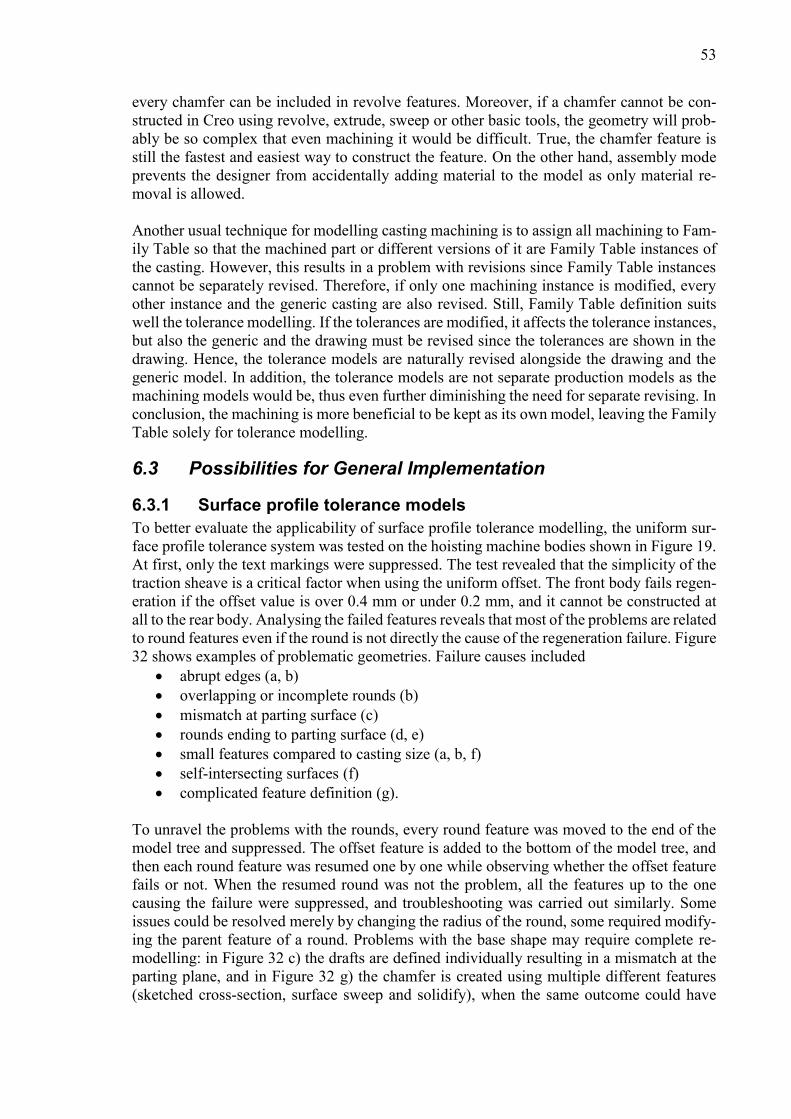
53

every chamfer can be included in revolve features. Moreover, if a chamfer cannot be con-

structed in Creo using revolve, extrude, sweep or other basic tools, the geometry will prob-

ably be so complex that even machining it would be difficult. True, the chamfer feature is

still the fastest and easiest way to construct the feature. On the other hand, assembly mode

prevents the designer from accidentally adding material to the model as only material re-

moval is allowed.

Another usual technique for modelling casting machining is to assign all machining to Fam-

ily Table so that the machined part or different versions of it are Family Table instances of

the casting. However, this results in a problem with revisions since Family Table instances

cannot be separately revised. Therefore, if only one machining instance is modified, every

other instance and the generic casting are also revised. Still, Family Table definition suits

well the tolerance modelling. If the tolerances are modified, it affects the tolerance instances,

but also the generic and the drawing must be revised since the tolerances are shown in the

drawing. Hence, the tolerance models are naturally revised alongside the drawing and the

generic model. In addition, the tolerance models are not separate production models as the

machining models would be, thus even further diminishing the need for separate revising. In

conclusion, the machining is more beneficial to be kept as its own model, leaving the Family

Table solely for tolerance modelling.

6.3 Possibilities for General Implementation

6.3.1 Surface profile tolerance models

To better evaluate the applicability of surface profile tolerance modelling, the uniform sur-

face profile tolerance system was tested on the hoisting machine bodies shown in Figure 19.

At first, only the text markings were suppressed. The test revealed that the simplicity of the

traction sheave is a critical factor when using the uniform offset. The front body fails regen-

eration if the offset value is over 0.4 mm or under 0.2 mm, and it cannot be constructed at

all to the rear body. Analysing the failed features reveals that most of the problems are related

to round features even if the round is not directly the cause of the regeneration failure. Figure

32 shows examples of problematic geometries. Failure causes included

• abrupt edges (a, b)

• overlapping or incomplete rounds (b)

• mismatch at parting surface (c)

• rounds ending to parting surface (d, e)

• small features compared to casting size (a, b, f)

• self-intersecting surfaces (f)

• complicated feature definition (g).

To unravel the problems with the rounds, every round feature was moved to the end of the

model tree and suppressed. The offset feature is added to the bottom of the model tree, and

then each round feature was resumed one by one while observing whether the offset feature

fails or not. When the resumed round was not the problem, all the features up to the one

causing the failure were suppressed, and troubleshooting was carried out similarly. Some

issues could be resolved merely by changing the radius of the round, some required modify-

ing the parent feature of a round. Problems with the base shape may require complete re-

modelling: in Figure 32 c) the drafts are defined individually resulting in a mismatch at the

parting plane, and in Figure 32 g) the chamfer is created using multiple different features

(sketched cross-section, surface sweep and solidify), when the same outcome could have

54

been achieved with a single chamfer feature. This kind of failures might be difficult to solve

in a complete existing model, so the best way to avoid these is again a good modelling tech-

nique from the beginning. Figure 32 d) is a good example of negligent modelling. The lower

half of the mould is left with a thin ledge with a counterdraft.

In Figure 32 e), the situation is more difficult to work around. There is no actual flaw in the

modelling technique as there is no other simple way to create the rounds shown. Still, the

offset feature fails at the vertices marked with red according to failure diagnostics. A simple,

yet not the most elegant solution, is to move the failing rounds to the end of the model tree

after the offset feature and defining the radii similarly to the ones in the individual surface

tolerance models. The radius of the round must be again added to the Family Table or set to

follow the offset value in the relations windows as described in Chapter 6.2.2.

Figure 32. Different geometries causing offset feature to fail regeneration in front and rear

bodies.

The failing offset features can also be seen as a modelling quality indicator. The testing on

the bodies suggested that the regeneration failures correspond somewhat to the casting de-

sign flaws. For example, a casting model should not have very small round radii, small edges

or small surfaces, since they are impossible to be duplicated to the pattern and subsequently

to the casting. If a feature in a model has dimensions close to the tolerance value, it is ques-

tionable whether the model should include that shape in the first place since the small shape

can be lost within the allowed variation. Sometimes round radii below the practical minimum

are used in CAD models if the feature fails with larger radii. Instead, the geometry should

be modified to allow the desired round radius since the reason for the failure is in the base

geometry, even if it is not very eminent. In any case, the supplier has to modify rounds too

small before the pattern manufacturing, resulting in a casting whose rounds do not match

those of the CAD model. Not all regeneration failures were caused by design flaws, but if

surface profile tolerance models are going to be used, the designer must consider it through-

out the whole modelling process and avoid the mentioned issues.

55

To monitor product model quality, automated tools can be used to verify that the company

guidelines are followed in CAD modelling. Creo has an integrated tool called ModelCHECK

whose purpose is to automatically detect whether the model is constructed according to pre-

defined principles. By default, ModelCHECK is run every time a model is saved, but the

report must be opened manually. The default ModelCHECK can be used to inspect e.g.

model names, parameters names, model units, missing parameters, missing ID parameters

in Family Table, children of drafts or rounds, and incomplete or failed features.

ModelCHECK also has geometry inspection capabilities and incorporates a pre-defined

VDA standard geometry check. [63] However, it is possible to create custom geometry

checks e.g. specifically for castings. The quality of the casting models could already be im-

proved by enforcing the default ModelCHECK that is now easily neglected, but customising

a complete casting check would ease even more. Available checks are listed in PTC’s doc-

umentation, and they can be customised by modifying ModelCHECK configuration files. In

addition to already mentioned references to drafts and rounds, useful checks could be

• standard draft angles

• early chamfers, drafts or rounds

• sharp and short edges

• small cylindrical surfaces

• surface gaps and overlaps [68].

Standard draft angles check reports if the model includes any draft features that do not have

standard angles. Early Chamfers, Early Drafts and Early Rounds checks cause a warning if

these features occur in the model before a certain percentage of all the features in the model

tree. This prevents referencing these features, but also ensures that the base geometry is de-

fined before it is modified to be suitable for casting. Sharp Edges check reports any angle

between two surfaces below a specified limit. Short Edges does the same, but with a dimen-

sional limit defined either as an absolute value or in relation to the size of the model. Small

Cylindrical Surfaces check finds any cylindrical surfaces, such as rounds, with a radius be-

low a specified limit. These three are useful not only for the tolerance modelling, but for the

casting as well since very small shapes do not duplicate to the pattern. Usually too small

shapes are anyway modified, removed or enlarged by the supplier. Surface Gaps and Over-

laps checks for any adjacent surfaces overlapping or with a gap between them. Even if the

nominal model would regenerate, the offset feature might not due to overlapping geometry.

[68]

Regardless of the possible benefits in measuring, the surface profile tolerance models are

beneficial when designing assemblies. The minimum and maximum models show the limits

beyond which no material is allowed. Therefore, the surface profile tolerance models must

be utilised when inspecting for collisions with other parts and designing required clearances

as the bounding box and thus the required space for the components are determined by the

tolerance limit models. The option for clearance investigation is to measure all clearances

manually from the nominal model. With simple assemblies, manual investigation is easy

enough, but with more complex structures, the benefit of the surface profile tolerance models

becomes more evident. On the other hand, also the tolerance implementation to complex

models is likely more difficult and time-consuming.

The workload of implementation was observed to depend greatly on the used modelling

techniques, the quality of modelling and the geometry of the workpiece. Unravelling the

issues with the hoisting machine bodies took several hours, yet the tolerance models are still

56

not complete. Contrarily, the same was done to the traction sheave in a couple of minutes.

This shows the vast effect of the geometry. The traction sheave is simple and contains no

small features close to the tolerance value.

6.3.2 Wall thickness tolerance models

As opposed to the surface profile tolerance models, the wall thickness tolerance model cre-

ated in Chapter 6.2.3 could be used only for strength calculations. As the examination re-

vealed, creating least and most material models would require a huge amount of additional

work. As the material amount limits cannot be easily included, the benefits of the wall thick-

ness tolerance model remain scarce. In addition, the casting tolerance might be already ad-

dressed to by the factors of safety used in the calculations. For example, in America, the

requirements are defined in ASME A17.1 elevator safety code that sets factors of safety for

hoisting machine components between 8 and 10 [69, p. 106]. However, the code defines

several other requirements for the components, and other regions have their own require-

ments. In conclusion, a tolerance model cannot take into account every requirement and

situation concerning strength. Therefore, it is advisable to construct strength calculation

models separately when needed for e.g. borderline cases, with or without the help of the

described wall thickness parametrisation procedure.

The parametrisation for the traction sheave was done without the cylinder tolerances. As for

general usage with other models, the cylinder dimension parametrisation is not that clear.

With internal cylindrical features e.g. holes, the amount of material is greater with the min-

imum tolerance and smaller with the maximum tolerance. This prevents the usage of the

tolerance calculator Excel table that always assigns minimum dimension to minimum toler-

ance model. Therefore, parametrising internal cylinders would require changing the mini-

mum and maximum of the diameter manually to Family Table. External cylinders work like

the wall thicknesses. However, it is debatable whether the cylinders need to be toleranced at

all. At least with the traction sheave, complete cylinder tolerance would more affect the

shape as the strength is still mostly determined by the wall thicknesses. This of course de-

pends on the geometry of the workpiece, but in any case, all the diameters to be toleranced

must be manually selected and minimum and maximum inverted with internal features.

Designing new casting CAD models is affected vastly depending on whether the models are

intended for wall thickness tolerance modelling or not. Requirements for a working wall

thickness tolerance model are

• dimensions of shapes also nominal wall thicknesses

• wall thicknesses constrained from middle point to nominal position and

• draft features increase the nominal model features.

When modelled from the beginning considering the future wall thickness parametrisation,

assigning the values to Family Table can be done in very little time. The biggest issue with

the implementation is therefore not running and assigning the tolerance limits using Excel

and the VBA code, but rather changing the company’s guidelines so that castings are mod-

elled to support wall thickness parametrisation. Even though the wall thickness model is not

reasonable to be implemented as a standard for every casting, some aspects of the modelling

style allowing it would be advisable. The casting would represent the real-world casting from

which material is machined away instead of representing a base to which material is added.

Furthermore, the dimensions in the model would correspond to those of the measurement of

57

the physical casting. If the base shape is wanted to be preserved anyhow, the different por-

tions of the nominal dimension of the casting (base, machining and casting tolerances, RMA)

can be shown in the base shape sketch as construction lines instead of defining separate

features for each. The same could be also achieved with a sketched skeleton model. Figure

33 shows a demonstration where the contributions to the casting nominal dimension are il-

lustrated with construction lines. The nominal dimensions are based on the machining di-

mensions according to ISO 8062-4 as presented in Figure 7 and Equation (3). Each of the

contributors are visible without affecting the actual nominal wall thickness to be para-

metrised as opposed to modelling style in Figure 25 a). This way, the model tree is cleaner,

clearer and easier for the next modeller to master, and the model is ready for wall thickness

tolerancing if needed while the components of the nominal dimensions are still visible. RMA

and surface profile tolerance are chosen according to ISO 8062-4 recommendations. RMA

grade E and surface profile tolerance grade P8 were used for calculating the nominal casting

dimensions.

Figure 33. RMA and tolerance contribution to casting nominal dimensions. Base shape is

shown with dashed construction lines and red dimensions, actual geometry with yellow lines

and black dimensions. Some constraints are hidden for clarity.

As for existing CAD models, the wall thickness tolerance models may require quite a lot of

re-modelling. If any wall thicknesses or complete cylinder sizes are modelled in multiple

steps with multiple features as in Figure 25 a), the base shape must be modelled again from

the beginning. Furthermore, not only the base shape would be re-modelled, but every child

feature referencing the re-modelled shapes and finally the assemblies referencing the re-

modelled surfaces. The amount of work required is proportional to the size and complexity

of the part. Whilst new models constructed from scratch can be modelled to support wall

thickness tolerancing by following the stated guidelines, the workload of converting existing

models outweighs the benefits. If needed, weakest states of the models can still be manually

constructed for the calculations of single parts as have been done this far.

58

In conclusion, wall thickness tolerances seem to provide quite little value to the designer.

Especially with existing models, it is certainly not worth the effort. Moreover, the older MX

hoisting machines series is designed using Vertex and include only combined drawings,

where machining and casting specification are defined in the same drawing. Therefore, im-

plementing wall thickness tolerances would not only mean complete re-modelling but trans-

ferring the models to Creo. If strength calculation requires tolerance models (e.g. borderline

cases), the approximated wall thickness models can be constructed singly instead of imple-

menting limit modelling for every casting. However, certain aspects of the modelling tech-

nique supporting wall thickness tolerancing should be encouraged not only because of pos-

sible tolerancing but to improve the practices as described above.

6.3.3 Custom imperative tolerance system

The aim of the custom tolerance model was to create an imperative system where there are

no additional conditions, but the individually indicated surface profile tolerance models

would act as absolute limits from which no deviation is allowed. This way, there is no un-

certainty since the limits are defined as absolute, and no discussion about allowed deviations

is needed between the customer and the foundry. If any deviation from the limit models is

allowed, the tolerances and the tolerance models should be modified so that they take into

account every acceptable deviation to obviate vague definitions.

Based on the test parts created, the best technique to carry out a custom tolerance system

would be similar to the individual surface profile tolerance system presented in Chapter

6.2.2. Only this time, every surface should be toleranced individually. As with the example

model, round features must be moved to the end of the model tree and re-assigned to the

edges of the offset features. Every surface must be thought out for every allowed defect,

resulting in drastically increased workload. The workload can be decreased by defining sev-

eral surfaces with the same surface profile tolerance, which also decreases the amount of

round features needing re-defining. This system, again, is closer to the original idea in ISO

8062-4.

Including all allowed deviations to the limit models requires using quite generous tolerances.

Excessive material is easily removed, but the minimal state of the casting has more impera-

tive limitations. This can be solved using UZ modifier in the surface profile tolerance defi-

nitions as in Figure 8. With the modifier, the tolerance zone can be offset from the nominal

middle so that larger deviations are allowed outwards and smaller deviations inwards from

the nominal surface. Implementing UZ offset to the CAD models can be done by simply

changing the positive and negative offset values in Family Table to correspond to the pro-

portions of the tolerance zone in each direction. The Family Table offset values in the ex-

ample case in Figure 8 would be 0.75 mm for the maximum model and -1.75 for the mini-

mum model, resulting in a tolerance of 2.5 mm.

The concept of imperative tolerance limits also remains questionable. Even if the limits are

by definition absolute and any deviation should cause rejection of the workpiece, there is no

reason to reject a piece with a single sub-millimetre excess over the limiting surface. Subse-

quently, the tolerance is loosened to allow the small deviations on that surface, what should

be done to a very small deviation from the new more generous tolerance? Loosening the

tolerances to allow small deviations works poorly since the whole surface can be at the loos-

ened tolerance limit, thus affecting the whole piece through weight, mass distribution and

59

material usage. The only solution is to keep the surface profile tolerances reasonable consid-

ering the shape and separately specifying the allowed deviations from the limit model, e.g.

the allowed amount and size of the areas crossing the tolerance limit.

The situation is anyway different with outer limit surface and inner limit surface. The inner

affects the machining, while the outer affects the assembly and interference with other parts.

Instead of trying to find absolute limits for any allowed shape defect, the surface profile

tolerances should be set as loose as possible to at least decrease the number of questionable

defects that must be approved by the customer. As the inner limit is more critical for suc-

cessful machining, it should be considered more imperative.

In conclusion, including every possible allowed deviation to the model is too arduous and

impractical to be carried out for every casting, especially when the surface profile tolerances

are not the only restriction for the shape, and wall thicknesses must be measured separately

in any case. Modelling of imperative system reverts to ISO 8062-4 principles and modelling

techniques described in Chapters 6.3.1 and 6.3.2. Individually indicated tolerances for criti-

cal surfaces and UZ modifier can be used to customise the general tolerancing system. In the

end, reducing the number of unclear situations or deviations needing customer’s approval is

more a question of company’s casting specification. For example, the minimum limit can be

specified as imperative with zero deviations allowed whereas exceeding the maximum limit

could be allowed solely for small deviations and limited areas and only with customer’s

approval, provided that the clearances in the assembly are adequate.

6.3.4 Summary

The tolerance model creation for general use was proven to be a lot more time-consuming

than the traction sheave made it seem. Existing models need so much re-modelling that the

use of tolerance models must be well justified. However, new castings modelled using the

principles described can support tolerance modelling with reasonable addition to workload.

Whether the tolerance models will be used or not in the future, it is advisable to utilise ISO

8062-4 for all new casting designs.

The examined tolerance models are applicable to following situations:

• surface profile tolerance models for casting measurement

• surface profile tolerance with machining for assembly and clearance examination

• wall thickness tolerance with machining for strength calculations.

The surface profile tolerance models proved to be simple enough to construct to get payback

for the effort. The benefit in assembly collision detection is evident, but the models might

also provide definitive limits for the supplier when measuring the castings. However, the

surface profile tolerance models are not necessary for either purpose. Clearances can be cal-

culated manually, and measuring can be done by estimating deviations by comparing meas-

urement results to the nominal model. Furthermore, to save workload, the surface profile

offset can be constructed to only those surfaces that might collide with other components in

an assembly. Of course, that type of model would not be applicable for quality verification

reference.

Test model construction revealed that the key requirements for surface profile tolerance

modelling are to

• avoid small (possibly self-intersecting) surfaces,

60

• avoid small round radii,

• avoid sharp edges,

• move required small features (such as markings) to the end of the model tree, and

• avoid referencing rounds and chamfers.

In addition, the bordering rounds and their relation to the tolerance values must be separately

defined when also individual surface profile tolerances are defined. Even though the test

models were done in Creo, the geometrical restrictions are valid with any other CAD soft-

ware.

Aiming for absolute imperative limit models was found to be impractical, but it is possible

using a combination of a general surface profile tolerance and individually defined surface

profile tolerances for surfaces with differing requirements. This is in any case the best way

to utilise the possibilities of surface profile tolerancing. By setting a generous general toler-

ance and individually defining more critical surfaces (both with UZ modifier if needed), the

procedure can be brought closer to the situation where the tolerance limits can be considered

absolute, even if it is not practical to stick to a strict go/no go policy. Imperative or not, the

modelling technique and the manufacturing drawing indications are similar.

As for the wall thickness and complete cylinder tolerancing, no simple way was found to

create weakest and strongest states of castings. Even the approximation modelling style de-

rived proved to be more arduous but less beneficial as the models are applicable only for

rough strength calculations. Wall thickness tolerancing cannot be recommended as a stand-

ard modelling style, but in some borderline cases it can be useful enough to be constructed

for single components.

With both surface profile and wall thickness tolerances, the tolerancing is closely integrated

into the design of the part and its geometry. This forces the designer to contemplate the

functionality and allowed defects throughout the designing process. Prototyping should be

done separately, and the final production model or tolerance model of a casting should con-

tain only features related to the casting itself instead of including e.g. the machined state as

a base shape.

These tolerance models are merely assistive instruments for layout and assembly inspection,

strength calculations or measuring. Therefore, the models can be generated separately when

needed instead of creating the tolerance models by assigning the values in PDM system as

with configurable parametric models. Still, to successfully generate the needed models even

manually, the principles described must be followed to at least achieve readiness for toler-

ance model generation.

To achieve the collision detection benefits from the surface profile tolerance models, the

machining models must be included. The prevalent practice was to use External Inheritance,

and assembly cut practice was tested. If automatically updating Family Table instances are

desired, assembly cut practice should be used in tolerance modelling. Contrarily, if singly

generating the model each time is deemed sufficient, External Inheritance is similarly ac-

ceptable. With both cases, some of the machining features must be re-defined to refer to the

offset surfaces of the generic part instead of the base geometry surfaces.

61

7 Surface Profile Tolerance Based Casting Measurement

7.1 Introduction

Even though different casting tolerance specifications exist, no comprehensive standard or

specification exists for casting shape and dimensions verification. Different suppliers use

different procedures and even different measurement techniques. In developing countries,

foundries may still use tape measure, compass and calliper for dimensional verification.

KONE utilises its own quality system alongside with the casting specification document, but

neither takes casting measurement into account to form comprehensive casting measuring

instructions.

When utilising ISO 8062-3, the measurement relies on the dimensional and geometrical tol-

erances. To determine whether any part of the workpiece exceeds the general tolerance,

every possible dimension should be measured, which of course is not virtually possible.

Therefore, only dimensions marked to the drawing are supposed to be measured by the sup-

plier. Nonetheless, the dimensional verification is known to cause dissonance between the

customer and the supplier.

In this chapter, different aspects affecting the measuring specification are examined. More-

over, a framework of measuring guidelines is proposed, aiming at a clarified measurement

specification defining which techniques should be used, which dimensions should be meas-

ured and what kind of deviations are allowed. Related to the NMX case study, AACMM and

3D scanner are compared through the traction sheave measurement to evaluate e.g. the time

required to carry out the measurements. Excerpts from exemplary measuring reports are pre-

sented in Appendices C and D. The measurements have been done at Componenta, Karkkila,

with a Faro Silver Arm AACMM together with Delcam Power Inspect software, and a GOM

ATOS II two-camera structured light scanner together with ATOS Professional V8 software.

7.2 Measuring Devices

A model of the physical casting obtained by 3D scanning is the best suitable measurement

system for castings. Scanning is usually fast, covers the entire workpiece, allows comparing

the scan to nominal or tolerance models, reveals holistically every deviation in a surface and

it preserves the created model allowing measurement of dimensions also afterwards. Of the

reviewed measurement techniques in Chapter 4, any scanning techniques with sufficient ac-

curacy and suitable distance range could be approved. This leaves out photogrammetry and

ToF sensors, whereas structured light and many combination techniques are very apt. Con-

ventional CMMs provide only discrete points, and the exactness of the measurement is pro-

portional to the amount of measured points. Even though CMM measurement results can be

compared to a nominal CAD model, all the necessary points must be measured at once as

only the selected points are saved. Still, arm CMMs are used to some extent to measure

castings mainly because of their cheaper price. Nonetheless, the ease of use, speed and ca-

pability of creating 3D models allow the 3D scanner to be used not only in casting verifica-

tion but also in monitoring e.g. pattern wear and moulds. If both available, arm CMM is

often used for castings only when the 3D scanner is in maintenance. In conclusion, a 3D

scanner can be considered a quite risk-free investment for foundries even if customers do

not require 3D scanning for their castings. [12]

62

Measuring the traction sheave using the GOM ATOS II took roughly an hour from applying

tracking stickers to acquisition of the final 3D model of the casting. The same outcome using

Faro Silver Arm required roughly twice that time. However, measuring single dimensions

required additional time with each device. The 3D model constructed required auxiliary da-

tum planes to allow the measurement of single dimensions with both ATOS and FaroArm

measurements. [12] The ATOS measuring report in Appendix D shows an excerpt of the

overall shape comparison on the first page and separate dimensional measurements of the

18 mm dimension on the second page.

As seen in the report, Faro software is also able to generate a point cloud out of measured

discrete points and show the deviations from the nominal model. However, the amount of

points is nowhere near the resolution of the 3D scanner since the arm must be manually

moved for every point. To achieve reliable results with an arm CMM, the amount of meas-

ured points per surface area unit should be defined in the customer’s casting and measuring

specification. The higher the measurement point density, the better the reliability of the

measurement, but at the expense of measurement speed. Furthermore, for critical surfaces

or surfaces with a tighter tolerance, the minimum point density should be specified sepa-

rately, leading again to increased workload for both the designer and the measurer, and to

less straightforward and clear measurement instructions. In conclusion, stated 3D scanning

techniques or techniques with similar properties can be recommended to be required from

the supplier as the measuring method for castings.

Nevertheless, the sufficient accuracy of the measurement must be defined. The required ac-

curacy is linked to the required part accuracy. The smaller the tolerance, the more accurate

measurement is required to observe the smaller deviations. The surface profile tolerance for

the traction sheave should be a few millimetres according to ISO 8062-4. As the tolerance

grades are defined to one decimal place, it is logical to require at least 0.1 millimetre meas-

urement accuracy. However, some of the measurement techniques struggle to achieve this

accuracy even though they might be otherwise very practical for casting measurement. For

instance, AACMMs with an integrated laser scanner provide an affordable 3D scanning so-

lution with accuracies varying between 0.05 and 0.2 millimetres [25][26], resulting in a sit-

uation where an approved measuring technique might not deliver sufficiently accurate re-

sults.

7.3 ISO 8062-4 in Measuring

The older ISO 8062-3 relies on toleranced dimensions the relations of which are constrained

using general geometrical tolerances. Verifying every feature to which general tolerances

apply is virtually impossible as every surface and its relation to others should be examined.

Therefore, the measurement in the ISO 8062-3 environment is restricted to dimensions and

geometrical tolerances marked to the manufacturing drawing. Even though some measuring

software support geometric tolerancing [70], the applicability for the uneven and curved

surfaces of sand castings remains weak. Measuring very complex parts becomes laborious,

still not resulting in a comprehensive perception over the entire workpiece.

By replacing ISO 8062-3 general tolerances with 8062-4, the measuring becomes simpler.

Now the nominal model with surface profile tolerance defines the shape instead of geomet-

rically constrained dimensions. Determining whether the shape of the casting is within its

limits no longer requires measuring discrete dimensions, but scanning all the surfaces of the

workpiece. Nevertheless, the surface profile tolerance only defines the shape, but even with

63

ISO 8062-4 in use, wall thicknesses must be separately measured. Still, it is a big improve-

ment since measuring the general shape of the casting is much clearer. However, utilising a

general surface profile tolerance requires measurement methods capable of comparing the

results directly to the 3D model. As for the AACMM and 3D scanning of the traction sheave,

both reports show the results as deviations from the nominal model in the normal direction

to the nominal surfaces. As CAD models are increasingly replacing drawings as the defining

representation of castings, it is beneficial to accordingly utilise the CAD models also in

measuring. 3D modelling, surface profile tolerancing and 3D scanning form the most logical

and coherent procedure for casting design and verification.

7.4 Dimensions to Be Measured

When a casting is scanned or otherwise measured to create a point cloud or 3D model, the

surface profile requirement for shape is already addressed. It is effortless to read from the

scanning results whether the deviation is within the surface profile tolerance zone at each

individually defined tolerance area, i.e. is the overall shape of the casting acceptable. The

nominal shape is defined with the CAD model to which the resulting 3D model can be com-

pared. Therefore, the shape measurement does not require dimensional drawing indication,

but merely the surface profile tolerance definitions. Still, the drawing is more informative

and easier to read with some major dimensions marked. Those affected by the surface profile

tolerance are shown as TEDs. However, measuring the wall thicknesses (and complete cyl-

inders if used) and other individually defined dimensions need specifying.

It is not worthwhile or even possible to measure every dimension that can be interpreted as

a wall thickness or cylinder. This leads to a similar solution as before: only dimensions pre-

sented in the casting drawing are measured, and only the dimensions to be measured are

presented. Wall thicknesses are shown as regular dimensions since they are affected by a

dimensional general tolerance as opposed to TEDs and geometrical tolerances. This is vir-

tually the clearest way to define what measurements are needed, and well in compliance with

ISO 8062-4. Using the CAD model as the basis, not all dimensions are needed in the draw-

ing, only the ones needing measuring. The amount of needed measurements stays moderate

since the overall shape of the casting is already considered with the surface profile tolerance

and the measured 3D model. Therefore, the problem concentrates on the wall thicknesses

and which of them are critical, at least with the traction sheave. Different castings have dif-

ferent dimensional requirements, but the designer’s task stays the same: to design the casting

according to its intended functionality and to determine which dimensions – be they wall

thicknesses or other – are more critical for functionality and which less.

In conclusion, each dimension type marked to the drawing is interpreted as follow:

• TED: nominal dimension of the casting. No need to show all, but some most crucial

for demonstrative purposes. Individual or general (grade P) surface profile tolerance

applies. Not measured separately, but considered in shape comparison.

• Normal dimension: wall thickness or complete cylinder size. All to be measured.

General dimensional tolerances for sizes (grade S) applies. Overrides surface profile

tolerances.

• Normal dimension with tolerance: all to be measured. The marked dimensional tol-

erance applies. Overrides both surface profile tolerances and general dimensional

tolerance.

64

When utilising the measuring, principles described above, all wall thicknesses not marked

to the drawing are left to the surface profile tolerance domain. The convention leaves open

whether the general wall thickness tolerance applies to every wall thickness regardless of the

designer’s selections and what is indicated in the drawing. In theory, the wall thickness tol-

erance should probably affect every wall thickness, but verifying the unmarked wall thick-

nesses is unnecessary. In conclusion, the designer decides to which wall thicknesses the gen-

eral wall thickness tolerance applies by indicating them to the drawing, whereas the surface

profile tolerance is applied for the rest.

For reliable results, the wall thickness must be measured at several locations. For example,

the measuring report in Appendix D shows eight different measuring points for the wall

thickness equally spaced around the traction sheave. The minimum amount of needed meas-

urements must be specified in either the casting drawing or a separate document. The casting

drawing should be preferred, since every casting and geometry have different requirements.

Therefore, no general specification for the amount of measurements can be defined, but the

definition must be done individually for each casting.

Using CAD model as the defining document and ISO 8062-4 surface profile tolerance as the

general tolerance system almost definitely requires 3D scanning for quality verification. This

is a problem with suppliers who have not yet invested in a 3D scanner or other adequate

measuring devices. The overall shape cannot be measured and fit between the surface profile

tolerance limits with only dimensional measurements. Such foundries could not utilise the

ISO 8062-4 at all, but would require a separate casting drawing leaning on the old ISO 8062-

3 and dimensional tolerancing with every possible dimension indicated in the drawing. This

is, however, undesirable from designer’s point of view and reverts the design procedure

backwards from the 3D CAD shape definition. Because of the extra design work, incompat-

ibility with surface profile tolerancing and less accurate measuring results, ordering castings

without 3D scanning requirement must be extremely well justified.

7.5 Alignment

7.5.1 Best fit alignment

When comparing the nominal CAD model to the scanned 3D model, the alignment of the

two models affects the outcome of the measurement. The default alignment often used is

best fit method that aligns the measured model with the CAD model minimising the overall

deviations between all the surfaces of the scanned model and the nominal model. However,

best fit alignment does not match the datum system RST definition and is not always appli-

cable at all. To take into account the datum system to which the TEDs and tolerances are

constrained, the alignment should be done using the datums of the scanned model defined

with the datum system RST and the corresponding surfaces from the nominal CAD model.

Possible alignment methods are e.g. local best fit alignment, RPS (reference point system)

alignment, local coordinate system alignment and hierarchical alignment by geometric ele-

ments, all of which are available in the GOM Professional software used together with the

ATOS scanner in the demo measurement [70].

The datum system RST must be determined based on the functionality of the casting. If the

casting is machined, the machining and the fixing for machining must be considered with

the RST datum system definition. As stated in ISO 8062-4, it is preferred to use the same

datum system to determine the machining and its tolerances to avoid unnecessary material

65

additions to machined areas of the casting. In addition, the datums must be surfaces that will

remain in the moulded condition, i.e. they are not machined. [17, p. 4-5] Therefore, the RST

datum system not only determines the references for the tolerances, but also defines the

measurement alignment and the zero point for machining.

The weakness of best fit alignment and the effect of the fixing for machining is demonstrated

in Figure 34 with a simplified workpiece. Figure 34 a) shows the casting in its nominal state

with the lathe jaw fixing surfaces. Figure 34 b) represents a measured casting that fulfils the

surface profile tolerance, but when fixed to the lathe, it sets askew (Figure 34 c), now leaving

some parts of the casting outside of the tolerance zone. With the traction sheave, the issue

could also be worked around by assigning smaller, individual tolerances on the fixing planes.

However, it is not practical to assign tighter tolerances to surfaces with no functionality in

the actual operation of the traction sheave. This becomes more evident when the fixing sur-

faces are large and flat planes or the workpiece can be fixed in several different positions.

Furthermore, the tighter individual tolerance for the fixing planes should be separately cal-

culated based on the other shape limits.

Figure 34. Alignment comparison. A) nominal model with fixing planes shown, b) best fit

alignment, c) local best fit alignment at machining fixing planes.

7.5.2 RPS alignment

The datum system RST can be defined for the casting using either integral features or datum

targets. The general surface profile tolerance does not apply for datums defined by integral

features but must be defined separately. Therefore, ISO 8062-4 recommends using datum

targets to define the datum system RST. [17, p. 4] It also suits the measurement better. Even

though the measurement software allows creating datum systems from integral features, the

datums are easily set incorrectly askew by the measuring software as cast surfaces are often

uneven, at least with sand castings [12]. Instead of entire surfaces, the use of datum target

points allows the measurer to constrain the models using RPS alignment. Even with datum

66

target lines, the construction of the datums in the measurement software is more straightfor-

ward than integral features. Whereas best fit alignment minimises the overall deviations on

all surfaces, the RPS alignment minimises only the deviations between the reference points

in the nominal model and the constructed datum points in the scanned 3D model.

In conclusion, RPS alignment corresponds to the use of datum target points. Of course, the

definition of the datum system also defines how the models should be aligned, so if the

casting utilises integral features for datums, the same should be used in the measurement

alignment. However, since the integral features are more difficult to construct with uneven

surfaces, the integral datum system would anyway be constructed using reference points.

7.5.3 Local best fit

Another alignment method that allows taking the fixing into account is local best fit. As

opposed to global best fit, the software calculates the best fit alignment considering only pre-

selected areas of the casting. The local best fit does not fully correspond to the RPS align-

ment based on RST datum targets, but can be useful. With the traction sheave, the fixing

planes can be aligned using datum targets and discrete points, but using local best fit, a larger

area near the fixing plane (or any other critical part in other castings) is considered, resulting

in a more average result. The traction sheave, however, requires three separate local best fit

zones, one for each fixing plane. Even if the machining fixing has the biggest effect on the

traction sheave alignment, in general the selection between RPS, local best fit or geometric

element alignment depends vastly on e.g. the casting geometry, machining and fixing. For

some simple parts, best fit might be enough, whereas more complex machined parts require

more carefully determined alignment.

7.5.4 Datum system RST definition

Regardless of the used alignment in measuring, the RST datum system must be defined to

be able to use ISO 8062-4 notation in the manufacturing drawing. The traction sheave is an

axially symmetrical part to be lathed to its final state. Therefore, it is logical to determine

the RST datum system by the axis of revolution, a datum to lock the axial movement and a

datum to lock the rotation around the axis of revolution. The axis could be determined using

any revolved surface of the workpiece, but because of the machining, the most appropriate

way is to use the surfaces from which the traction sheave is fixed to the lathe. The traction

sheave can be fixed for machining in many ways, but using the proposed fixing plane options

shown in Figure 20 and Appendix A, the sheave would be fixed with an outer three-jaw

chuck.

The definition of the datum system RST is presented in the update proposal drawing in Ap-

pendix E. The datum system is determined so that it locks all six degrees of freedom. Three

datum target lines are assigned to the middle of the fixing surfaces, ideally spaced every 120

degrees. The associated feature is a (virtual) cylinder, and the resulting datum R is the axis

of the cylinder determined by the three lines [18, p. 27]. The three datum target lines on

fixing surfaces are selected for the datum R to simulate the physical jaws of the lathe fixing.

The cylinder locks four degrees of freedom [18, p. 47-48]. To lock the axial movement, the

second datum S is selected to be the largest all around unmachined surface perpendicular to

the axis of revolution. The selected surface is also close to the parting line, thus balancing

possible deviations caused by mismatch to both sides. The plane is established using three

datum targets. The result is a datum system of an axis and a perpendicular plane [18, p. 15].

The remaining degree of freedom is rotation around the axis. One of the end points of the

67

datum target lines is used for the last datum target. The datum targets left hidden in the

drawing are indicated with a dashed datum target leader line [18, p. 20]. The defined datum

system RST is not fully compliant with the ISO 8062-4 and ISO 5459 standards, but not in

contradiction either. The fixing plane datum targets are on different surfaces instead of an

actual cylindrical surface [18, p. 25], and seven datum targets are used instead of the required

six [17, p. 14]. However, the datum system RST presented in Appendix E is unambiguous

and sufficient, and the differences with the standards are deliberate and made to establish a

more appropriate datum system for the traction sheave.

Using datum target points instead of datum target lines would be more in compliance with

the 3D measurement where uneven surfaces are more easily addressed with single points.

The three datum target lines could be replaced with three single datum target points since

three points are sufficient to define the axis of revolution. Three points define a plane and a

circle on that plane. The centre of the circle defines the location of the axis, and the plane

defines the direction of the axis by its normal. Even though the datum target lines are based

on the standard, the use of single points might be favourable from the measurer’s point of

view, depending on the used software. In addition, Creo Parametric 2.0 has only limited

support for datum targets in default drawing mode, as the default library includes symbols

only for datum target points without the hidden datum target style available. The symbols in

Appendix E are created manually as sketches to show them correctly. Therefore, the simpli-

fied representation with only points eliminates also unnecessary manual work required from

the designer, at least as long as the company uses the same software and the same version.

The definition of datum system RST cannot be generalised but must be contemplated sepa-

rately for each casting to best correspond to the physical workpiece and the functionality.

However, the measuring and the alignment must be also considered. As with the traction

sheave, some simplifications could be made to ease the RPS alignment. Even though con-

temporary devices and software allow constructing integral feature datums or even their de-

rivatives such as middle planes, it might not be worth the effort. Using integral datums can-

not be recommended except when the functionality absolutely requires measurement based

on integral features. All in all, datum targets are faster to define and reference points easier

to derive from the result 3D model for alignment.

As the definitive data container is the CAD model, the nominal dimensions and the locations

of the toleranced surfaces (TEDs) are defined only in the model. The datum system RST is

more vital if the nominal location of each surface is defined only in the drawing using TEDs.

Even without constraining the surfaces of the casting to a general datum system, the meas-

urement using the CAD model and a 3D scanner can be successful. Hence, it is possible to

leave the casting without a general datum system definition and use best fit alignment for

measurement [20, p. 4]. This leaves the designer the possibility to simplify the measurer’s

tasks when the alignment of the workpiece is not excessively crucial.

7.6 Tolerance Model Utilisation

The idea of comparing the scanned 3D model to the minimum and maximum models is

lucrative since any deviation outside the tolerance would be immediately revealed. With the

nominal model, the comparison results must be visually inspected throughout all the surfaces

considering whether the deviations exceed the tolerance value or not. The tolerance models

work similarly to the nominal model when measuring with best fit alignment: the software

calculates the position where the deviation is the smallest. However, the best fit alignment

68

might still not reveal whether the casting fits within the surface profile tolerance or not. Since

the best fit minimises the total deviation, it may lead to a situation where a small part of the

casting is outside the tolerance as long as most of the part is close enough to the nominal.

This is demonstrated in Figure 35. In Figure 35 a), best fit alignment leaves part of the casting

outside the tolerance zone even if the casting would fit between the limits as shown in Figure

35 b).

When using geometric, RPS or local best fit alignment, the utilisation of the tolerance models

becomes different. The measured 3D model must be aligned by its RST datums to its nomi-

nal location within the surface profile tolerance so that the tolerance is equally divided to

both sides of the reference datum. The tolerance models constructed earlier contain only the

minimum or maximum condition without the nominal data included in the same instance.

Therefore, the utilisation requires additional steps. The features used as datums or used to

define datum targets must be left to their nominal state to align the measured model to the

nominal location. Figure 35 c) shows why the surfaces of the tolerance model cannot be used

for alignment, and Figure 35 d) demonstrates how the surface profile tolerance models

should be constructed in order to use the tolerance models in measurement. The surfaces

related to the RST datums are deselected and excluded from the offset feature to leave them

to the nominal position. However, now the surface profile tolerance of the datum features is

not included in the model, but must be separately inspected during the measurement.

Figure 35. Alignment effect on the measurement results. A) and b) show the error with best

fit, c) and d) the error when comparing to the surface profile tolerance models.

Even if it is possible to use the tolerance models with the measurement, it is not necessary

nor worth the effort. Both measuring devices and software inspected showed the deviations

from the nominal surfaces in either direction, thus making it relatively easy and fast to only

check any areas where the deviation seems to exceed the general tolerance. What is more, at

least the GOM Professional software allows the user to change the scale of the colourised

legend so that the colour changes at a certain deviation, making the tolerance examination

even more intuitive and visual [12]. The question is, which causes more additional work:

modifying the tolerance models to exclude the datum surfaces from the surface profile tol-

erance and compare the measurement results to both the minimum and the maximum model,

or comparing the results to only the nominal model, but inspecting whether the deviations

69

are within the tolerance without the help of the limit surfaces? If the limits are intended to

be imperative, the first is the only option, but since the determination of imperative limits

was already found to be impractical, the latter is the easier way.

7.7 Rejection Limits

In practice, no imperative limit models can be defined since always some small deviation

can be acceptable to avoid unnecessary rejection. However, to eliminate uncertainty from

the measurement and rejection process, the limits for the acceptable deviations must be de-

fined. Many factors affect the criticality of the deviation: the location (e.g. machined sur-

face), the direction (removing or adding material), the size of the area intersecting with the

tolerance limit surface, and of course the deviation in normal direction to the nominal sur-

face. Furthermore, the size and number of allowed deviations would depend on the size of

the casting as well. The allowed wall thickness deviations would also have to be defined,

making the rejection limit specification even more complicated. The rejection limits would

then be specified almost individually for each casting, which again obsoletes the need for a

general rejection limit specification, and simultaneously increases the amount of work re-

quired from the designer.

If any general specification for allowed deviations must be made, it should allow only very

small deviations on non-critical surfaces affected only by the general surface profile toler-

ance. Any individually indicated tolerances (surface or dimensional) for e.g. functional fea-

tures or wall thicknesses should anyway be more strictly addressed to.

The most straightforward way would be to consider the general surface profile tolerance

imperative, and allow no deviations from it without customer’s approval, although this pol-

icy might lead to a situation where the customer continuously needs to address to dimen-

sional defects. Moreover, the same problem persists as with the imperative tolerance models:

even if the allowed defects are specified, is it necessary to reject a workpiece because of a

very minor exceeding over the defined limits? Then again, the purpose of the tolerance is to

determine the allowed limits, and if the foundry accepts the order as it is, the outcome should

be a casting matching the tolerances specified in the drawing.

In conclusion, for the simplicity of the entire process, it is best to dismiss the excess defect

specification, be it general or individual for each casting. Instead, the designer should deter-

mine the casting tolerances carefully, assigning tighter tolerances for critical areas and looser

for others using UZ modifier if needed. Thus, the casting tolerance is enforced and consid-

ered as the final shape requirement without exceptions. The other option is to establish a

sufficiently simple policy with the supplier concerning the approval process of the deviations

not within the casting tolerance. Additionally, an internal process for the company should be

established to modify the tolerances whenever a deviation (looser tolerance) is found to be

acceptable.

70

8 Design and Measurement Recommendations Based on the tolerance systems review, the tolerance model examination and the measure-

ment method examination, new guidelines for modelling, drawing creation and measurement

are suggested. The new guidelines also affect the casting specification. Therefore, the mod-

elling and drawing instructions as well as the casting specification must be revised. Moreo-

ver, the measurement instructions must be updated to correspond to the contemporary prin-

ciples.

8.1 CAD Model

As the workload is high compared to the gain, no tolerance models are recommended to be

included in any production model by default. It is recommended to construct them singly

only when needed. Then the principles described in Chapter 6.3.4 apply. However, con-

structing the models as per prevailing needs also leaves the designer the possibility to sim-

plify or adapt the tolerance modelling according to the case-specific requirements. Nonethe-

less, whether the tolerance models are used or not, casting modelling instructions should be

specified to achieve better model quality and consistency. The following principles apply

for all casting CAD models:

• Dimensions drive final, outmost shapes directly without cumulatively adding mate-

rial with several features.

• Dimensions drive functional, significant features (e.g. diameters instead of radii).

• No small surfaces, small round radii, or sharp edges are present in the model.

• No references to rounds or chamfers are present in the model.

• Parametric modelling must be utilised by referencing geometry instead of using blind

dimensions (see failing chamfer and parting plane mismatch in Figures Figure 29

and Figure 32 c).

• Nominal dimensions of castings are calculated according to ISO 8062-4.

• Drafts and rounds are included in the models by default.

Following the guidelines results in geometrically more intact CAD models with less features

in contradiction with the manufacturing method. Hence, the CAD models represent more

truthfully the physical castings, which again supports the use of CAD models as definitive

representations of castings. In addition, the model requires less modifications from the caster

when the designer already considers the limitations during the modelling.

8.2 Drawing

The proposed update for the traction sheave casting drawing according to ISO 8062-4 is

presented in Appendix E. The drawing includes a general surface profile tolerance indica-

tion, wall thickness general tolerance indication, RMA indication, manufacturing method

and draft grade indication and casting size indication. The grades were chosen based on the

manufacturing method (sand casting, machine moulding), material and the casting size of

the component (670 mm) according to ISO 8062-4, but for production models, the grades

must be revised based on the usual accuracy level of the supplier and of course the accuracy

requirements for the casting. The drawing states that the CAD model is to be used to define

the casting alongside with the requirements presented in the drawing. Dimensions belonging

to the domain of the general surface profile tolerance are marked with TEDs and wall thick-

nesses with normal dimensions. Not all dimensions are required to be visible in the drawing

because the CAD model is used to define the nominal shape, but all dimensions to be meas-

ured must be included. The TEDs in the example drawing are included only to show the

71

overall size of the casting. Surface profile tolerance applies to every dimension not visible

in the casting drawing. The datum system RST is visible and determined using datum targets

according to ISO 5459. The datum system RST must be individually defined for each casting

drawing based on the fixing or functionality of the casting. All shape requirements are pre-

sented in the drawing with no need for additional documents concerning the shape, dimen-

sions, their tolerances or rejection limits.

However, referring to ISO 8062-4 in the casting drawings might be problematic since the

standard is quite new, published only in 2017. The standard has not yet been approved by

either CEN or SFS, but it has been approved by e.g. NEN in the Netherlands and BSI in the

United Kingdom. Most foundries might still rely on the old 8062-3, but the recognition in

the mentioned countries is encouraging. The 8062-4 is clearer with the shape and tolerance

definition and considerably more compliant with CAD modelling and 3D scanning. The

content of the standard is so intuitive that any foundry relying on 3D scanning should be

happy to implement the newer standard.

8.3 Measuring

With the contemporary CAD-based design tools and measurement equipment, comprehen-

sive 3D scanning should be required from every supplier as the primary measurement

method. The 3D CAD model should be used as the determinative representation of the cast-

ing. The 3D model created by scanning is compared to the nominal CAD model using align-

ment specified in the casting drawing. If a datum system RST is defined, an RPS alignment

using the defined datums RST must be used. If no datum system is defined, best fit alignment

is used. Any existing specification on pattern yielding or mismatch is discarded as they are

already included in the general surface profile tolerance [17, p. 8]. The suggested instructions

for casting measurement are listed below:

1. Castings must be measured using a 3D scanner or other device that is capable of

creating a comprehensive 3D model of the casting with sufficient accuracy.

2. The 3D model created is compared to customer’s nominal CAD model.

3. The 3D model is aligned with the nominal model using the datum system RST indi-

cated in the manufacturing drawing of the casting and RPS alignment.

4. If no datum system RST is indicated, best fit alignment is used.

5. The deviations shown in the measuring report are compared to the surface profile

tolerances in the casting drawing.

6. Wall thicknesses and complete cylinder sizes marked to the drawing are measured

from the scanned 3D model and inspected according to general tolerance grade S.

7. Other individually indicated dimensions and tolerances are measured from the

scanned 3D model.

8. Foundry asks for approval from the customer for any found deviations considered

non-critical.

9. The customer/designer inspects the found deviations.

10. If any of the found deviations are approved, the designer evaluates whether the cast-

ing tolerance on that area can be loosened and revises the casting tolerances if

needed.

8.3.1 Options

Some options can be defined for the steps above as per the previously done examinations.

Firstly, the measured 3D model can be compared to the tolerance models instead of the nom-

72

inal model provided that the surfaces related to the datum system RST are left to their nom-

inal state. When best fit is used, the tolerance models can be constructed normally. This

option can be used if the limits are wanted to be imperative and absolute rejection limits are

wanted. The steps replaced in the instructions are

2. The 3D model created is compared to customer’s minimum and maximum tolerance

models.

5. Deviations from the tolerance models are inspected. Only negative deviation is al-

lowed from the maximum model and only positive deviation from the minimum

model.

Another option for the measurement is using local best fit alignment. The areas for local best

fit must be indicated in the casting drawing. The replaced steps are:

3. The 3D model is aligned with the nominal model using local best fit alignment on

the areas indicated in the casting drawing.

4. (Removed)

The tolerance model measurement and the local best fit alignment can also be used together

provided that all the surfaces within the local best fit zone are left to their nominal state in

the tolerance models to avoid the same misalignment as in Figure 35 c).

73

9 Conclusion and Recommended Further Actions The combination of digital 3D product definition, ISO 8062-4 and 3D scanning as the pri-

mary measurement method sets the framework for casting design and quality verification.

The overall procedure and workflow is demonstrated in Figure 36. Instead of coping with

outdated tools and standards, the proposed process is more up-to-date and compliant with

the methods that are already often used despite the lack of formally defined guidelines.

Figure 36. A flowchart depicting the casting design and measurement process.

The previous chapters have answered the questions about the preferred modelling methods,

tolerance model utilisation, casting drawing update, measuring techniques and measuring

procedures. Still, some further actions are required before the proposed procedures can be

considered for general implementation in the company. Even though the procedures and

their benefits and drawbacks have already been evaluated, the company needs to confirm the

applicability according to their actual needs and the compatibility with existing policies and

practices.

9.1 Modelling

As the tolerance models were discovered to be too impractical for systematic implementation

for production models, guidelines must be defined to clarify in which situations to construct

either of the tolerance models. To achieve comprehensive instructions, a further evaluation

of the possible benefits must be carried out simultaneously considering the policies of the

company and the needs encountered with production models.

A formal methodology for casting CAD modelling should be determined based on the rec-

ommendations stated in previous chapters but again reflecting the needs of the company. A

74

good, uniform modelling practice is vital for the reusability and editability of the models.

Possibilities to create a custom ModelCHECK specifically for castings should be examined.

Furthermore, similar modelling instructions must be defined for the different tolerance mod-

els, should they be found advantageous enough.

9.2 Casting Drawings

The casting specifications of the company should be updated to correspond to digital 3D

product definition and ISO 8062-4 tolerancing system as shown in the example in Appendix

E. Subsequently, the relationship between the casting drawing and the measurement process

(tolerances, dimensions and datum system indicated in the drawing) must be taken into ac-

count in the casting specification update. The possibility to define general guidelines for

selecting machining zero point and datum system RST should be evaluated.

9.3 Measuring

A formal measurement specification relying on the proposed measuring procedure should

be created. The specification should state not only the acceptable measuring techniques but

also the required accuracy. If the required accuracy is wanted to be variable in relation to

casting size, tolerance values or manufacturing method, these restrictions must also be stated.

The usage of the surface profile tolerance models or imperative tolerance models in meas-

urements should be decided, possibly in collaboration with foundries. A further evaluation

might be needed in order to determine whether the tolerance models provide any additional

value to the comparison-based 3D measurement. If decided to be used in the measurements,

a clear framework for the utilisation of the tolerance models must be determined.

Furthermore, the rejection practice must be determined. If the imperative tolerance system

is necessarily wanted, the procedure must be included in the measurement specification. If a

more flexible system is wanted, the approval process or threshold values for allowed devia-

tions must be defined. In short, a comprehensive practice to address to the deviations found

in the measurement must be established regardless of the used tolerancing system.

75

References

1. Meskanen, S. & Höök, T. ValuAtlas – Suunnittelijan perusopas: Valumenetelmät.

2015. [Cited 2018 Aug 22]. Available at: http://www.valuatlas.fi/tietomat/docs

/perusopas_03.pdf.

2. Meskanen, S. & Höök, T. ValuAtlas – Suunnittelijan perusopas: Valurauta ja valute-

räs. [Cited 2018 Aug 27]. Available at: http://www.valuatlas.fi/tietomat/docs

/perusopas_02.pdf.

3. Callister, W.D., Jr. & Rethwisch, D.G. Materials science and engineering: An intro-

duction. 8th ed. Hoboken, USA: John Wiley & Sons, Inc., 2009. 885 p. ISBN 978-0-

470-41997-7.

4. Meskanen, S. & Toivonen, P. Metallurgian perusteita. [Cited 2018 Aug 26]. Available

at: http://www.valuatlas.fi/tietomat/docs/vtp_sulatus_metallurgia.pdf.

5. Meskanen, S. & Niini, E. ValuAtlas – Valimotekniikan perusteet: Valuraudat. [Cited

2018 Aug 26]. Available at: http://www.valuatlas.fi/tietomat/docs

/vtp_mat_valuraudat.pdf.

6. SinterCast. Compacted Graphite Iron. [Cited 2018 Aug 2]. Available at:

https://sintercast.com/technology/compacted-graphite-iron.

7. Pascual, M. & Cembrero, J. & Salas, F. & Pascual Martínez, M. Analysis of the weld-

ability of ductile iron. Materials Letters. [Electronic journal]. Vol. 62(8–9). 2008. P.

1359–62. [Cited 2018 Aug 14]. ISSN 0167-577X. DOI:10.1016/j.matlet

.2007.08.070.

8. Gregorutti, R.W. & Grau, J.E. Mechanical properties of compacted graphite cast iron

with different microstructures. International Journal of Cast Metals Research. [Elec-

tronic journal]. Vol. 27(5). 2014. P. 275–81. [Cited 2018 Jun 29]. ISSN 1364-0461.

DOI:10.1179/1743133614Y.0000000118.

9. Meskanen, S. & Höök, T. ValuAtlas – Suunnittelijan perusopas: Metalliseokset.

[Cited 2018 Aug 27]. Available at: http://www.valuatlas.fi/tietomat/docs

/perusopas_21.pdf.

10. Niemi, P. ValuAtlas – Valunsuunnittelutekniikka. [Cited 2018 Aug 27]. Available at:

http://www.valuatlas.fi/?q=node/356.

11. Pere, A. Koneenpiirustus 1 & 2. 11th ed. Espoo, Finland: Kirpe Oy, 2012. ISBN 978-

952-67419-1-8.

12. Sirola, P. Engineering Manager. Componenta Finland Oy Högfors. Bremerintie 6,

03600 Karkkila, Finland. Interview 16.2.2018.

13. SFS-EN ISO 8062-1. Geometrical product specifications (GPS) – Dimensional and

geometrical tolerances for moulded parts – Part 1: Vocabulary. Geneva: International

Organization for Standardization. 2007. 21 p.

76

14. CEN ISO/TS 8062-2. Geometrical Product Specifications (GPS) – Dimensional and

geometrical tolerances for moulded parts – Part 2: Rules. Geneva: International Or-

ganization for Standardization. 2013. 56 p.

15. SFS-EN ISO 8062-3. Geometrical product specifications (GPS) – Dimensional and

geometrical tolerances for moulded parts – Part 3: General dimensional and geomet-

rical tolerances and machining allowances for castings. Geneva: International Organ-

ization for Standardization. 2007. 30 p.

16. SFS-EN ISO 1101. Geometrical product specifications (GPS) – Geometrical toler-

ancing – Tolerances of form, orientation, location and run-out. Geneva: International

Organization for Standardization. 2017. 151 p.

17. NEN-ISO 8062-4. Geometrical product specifications (GPS) – Dimensional and ge-

ometrical tolerances for moulded parts – Part 4: General tolerances for castings using

profile tolerancing in a general datum system. Geneva: International Organization for

Standardization. 2017. 25 p.

18. NEN-EN-ISO 5459. Geometrical product specifications (GPS) – Geometrical toler-

ancing – Datums and datum systems. Geneva: International Organization for Stand-

ardization. 2011. 81 p.

19. STD 101-0001. Digital Shape Model basis – DSM basis. Volvo Group. 2016. [Cited

2018 Jun 10]. Available at: https://webstd.volvo.com/webstd/docs/101-0001.

20. VN 3212. Verification of components by 3D-CAD data. Voith Turbo. 2015. [Cited

2018 Jun 12]. Available at: https://voith.com/corp-en/VN_3212_en.pdf.

21. Woźniak, A. & Dobosz, M. Metrological feasibilities of CMM touch trigger probes.

Part I: 3D theoretical model of probe pretravel. Measurement: Journal of the Interna-

tional Measurement Confederation. [Electronic journal]. Vol. 34(4). 2003. P. 273–86.

[Cited 2018 Jul 11]. ISSN 0263-2241. DOI:10.1016/j.measurement.2003.05.001.

22. Canadian Measurement-Metrology Inc. New CMM Equipment. [Cited 2018 Jul 11].

Available at: https://www.cmmxyz.com/new-cmm.html.

23. Mitutoyo. Mitutoyo CMM Accuracy Statements. [Cited 2018 Jul 23]. Available at:

https://www.mitutoyo.com/wp-content/uploads/2016/09/L-section-CMM.pdf.

24. Santolaria, J. & Aguilar, J.J. & Yagüe, J.A. & Pastor, J. Kinematic parameter estima-

tion technique for calibration and repeatability improvement of articulated arm coor-

dinate measuring machines. Precision Engineering. [Electronic journal]. Vol. 32(4).

2008. P. 251–68. [Cited 2018 Jul 12]. ISSN 0141-6359. DOI:10.1016/j.precisioneng

.2007.09.002.

25. FARO. FaroArm. [Cited 2018 Jul 11]. Available at: https://faro.com/en-gb

/products/factory-metrology/faroarm/.

26. Nikon Metrology. MCAx - Premium portable metrology. [Cited 2018 Jul 17]. Avail-

able at: https://www.nikonmetrology.com/en-gb/product/mcax.

77

27. Sansoni, G. & Trebeschi, M. & Docchio, F. State-of-the-art and applications of 3D

imaging sensors in industry, cultural heritage, medicine, and criminal investigation.

Sensors. [Electronic journal]. Vol. 9(1). 2009. P. 568–601. [Cited 2018 Jul 10]. ISSN

1424-8220. DOI:10.3390/s90100568.

28. Mitutoyo. CMM Probes-Scanning probe system. [Cited 2018 Jul 12]. Available at:

https://ecatalog.mitutoyo.com/CMM-Probes-Scanning-probe-system-C1018.aspx.

29. Renishaw. Scanning probes. [Cited 2018 Jul 12]. Available at:

http://www.renishaw.com/en/scanning-probes--6656.

30. Hexagon Manufacturing Intelligence. Scanning Probes. [Cited 2018 Jul 12]. Availa-

ble at: https://www.hexagonmi.com/products/coordinate-measuring-machines /cmm-

sensors/scanning-probes.

31. Logozzo, S. & Zanetti, E.M. & Franceschini, G. & Kilpelä, A. & Mäkynen, A. Recent

advances in dental optics - Part I: 3D intraoral scanners for restorative dentistry. Op-

tics and Lasers in Engineering. [Electronic journal]. Vol. 54. 2014. P. 203–21. [Cited

2018 Jul 11]. ISSN 0143-8166. DOI:10.1016/j.optlaseng.2013.07.017.

32. González de Villaumbrosia, P. & Martínez-Rus, F. & García-Orejas, A. & Salido,

M.P. & Pradíes, G. In vitro comparison of the accuracy (trueness and precision) of six

extraoral dental scanners with different scanning technologies. Journal of Prosthetic

Dentistry. [Electronic journal]. Vol. 116(4). 2016. P. 543–550.e1. [Cited 2018 Jun

14]. ISSN 0022-3913. DOI:10.1016/j.prosdent.2016.01.025.

33. Seno, T. & Ohtake, Y. & Kikuchi, Y. & Saito, N. & Suzuki, H. & Nagai, Y. 3D

scanning based mold correction for planar and cylindrical parts in aluminum die cast-

ing. Journal of Computational Design and Engineering. [Electronic journal]. Vol.

2(2). 2015. P. 96–104. [Cited 2018 Jun 20]. ISSN 2288-5048.

DOI:10.1016/j.jcde.2014.12.004.

34. Wang, Y. & Feng, H.Y. Effects of scanning orientation on outlier formation in 3D

laser scanning of reflective surfaces. Optics and Lasers in Engineering. [Electronic

journal]. Vol. 81. 2016. P. 35–45. [Cited 2018 May 29]. ISSN 0143-8166.

DOI:10.1016/j.optlaseng.2016.01.003.

35. GOM. ATOS - Industrial 3D Scanning Technology. [Cited 2018 Jul 15]. Available

at: https://www.gom.com/metrology-systems/atos.html.

36. Villarraga-Gómez, H. & Lee, C.B. & Smith, S.T. Dimensional metrology with X-ray

CT: A comparison with CMM measurements on internal features and compliant struc-

tures. Precision Engineering. [Electronic journal]. Vol. 51(August 2017). 2018. P.

291–307. [Cited 2018 Jul 14]. ISSN 0141-6359. DOI:10.1016/j.preci-

sioneng.2017.08.021.

37. Weckenmann, A. & Jiang, X. & Sommer, K.D. & Neuschaefer-Rube, U. & Seewig,

J. & Shaw, L. & et al. Multisensor data fusion in dimensional metrology. CIRP Annals

- Manufacturing Technology. [Electronic journal]. Vol. 58(2). 2009. P. 701–21.

[Cited 2018 Jul 17]. ISSN 0007-8506. DOI:10.1016/j.cirp.2009.09.008.

78

38. Adams, M.D. Coaxial range measurement - Current trends for mobile robotic appli-

cations. IEEE Sensors Journal. [Electronic journal]. Vol. 2(1). 2002. P. 2–13. [Cited

2018 Jul 11]. ISSN 1530-437X. DOI:10.1109/7361.987055.

39. Lim, M. & Petley, D.N. & Rosser, N.J. & Allison, R.J. & Long, A.J. & Pybus, D.

Combined digital photogrammetry and time-of-flight laser scanning for monitoring

cliff evolution. Photogrammetric Record. [Electronic journal]. Vol. 20(110). 2005. P.

109–29. [Cited 2018 Jul 17]. ISSN 0031-868X. DOI:10.1111/j.1477-9730

.2005.00315.x.

40. Yastikli, N. Documentation of cultural heritage using digital photogrammetry and la-

ser scanning. Journal of Cultural Heritage. [Electronic journal]. Vol. 8(4). 2007. P.

423–7. [Cited 2018 Jul 11]. ISSN 1296-2074. DOI:10.1016/j.culher.2007.06.003.

41. Leach, R. & Sims-Waterhouse, D. & Medeossi, F. & Savio, E. & Carmignato, S. &

Su, R. Fusion of photogrammetry and coherence scanning interferometry data for all-

optical coordinate measurement. CIRP Annals. [Electronic journal]. 2018. [Cited

2018 Jul 18]. ISSN 1726-0604. DOI:10.1016/j.cirp.2018.04.043.

42. Liu, W. & Li, X. & Jia, Z. & Yan, H. & Ma, X. A three-dimensional triangular vision-

based contouring error detection system and method for machine tools. Precision En-

gineering. [Electronic journal]. Vol. 50. 2017. P. 85–98. [Cited 2018 Jun 20]. ISSN

0141-6359. DOI:10.1016/j.precisioneng.2017.04.016.

43. Salvi, J. & Pagès, J. & Batlle, J. Pattern codification strategies in structured light sys-

tems. Pattern Recognition. [Electronic journal]. Vol. 37(4). 2004. P. 827–49. [Cited

2018 Jul 14]. ISSN 0031-3203. DOI:10.1016/j.patcog.2003.10.002.

44. Geng, J. Structured-light 3D surface imaging: a tutorial. Advances in Optics and Pho-

tonics. [Electronic journal]. Vol. 3(2). 2011. P. 128–60. [Cited 2018 Jun 13]. ISSN

1943-8206. DOI:10.1364/AOP.3.000128.

45. Pribanić, T. & Mrvoš, S. & Salvi, J. Efficient multiple phase shift patterns for dense

3D acquisition in structured light scanning. Image and Vision Computing. [Electronic

journal]. Vol. 28(8). 2010. P. 1255–66. [Cited 2018 Aug 30]. ISSN 0262-8856.

DOI:10.1016/j.imavis.2010.01.003.

46. Salvi, J. & Fernandez, S. & Pribanic, T. & Llado, X. A state of the art in structured

light patterns for surface profilometry. Pattern Recognition. [Electronic journal]. Vol.

43(8). 2010. P. 2666–80. [Cited 2018 Jun 13]. ISSN 0031-3203.

DOI:10.1016/j.patcog.2010.03.004.

47. Yatong, A. & Hyun, J.-S. & Zhang, S. Pixel-wise absolute phase unwrapping using

geometric constraints of structured light system. Vol. 24(16). 2016. P. 18445–59.

[Cited 2018 Jul 16]. ISSN 1094-4087. DOI:10.1364/OE.24.018445.

48. Percoco, G. & Modica, F. & Fanelli, S. Image analysis for 3D micro-features: A new

hybrid measurement method. Precision Engineering. [Electronic journal]. Vol. 48.

2017. P. 123–32. [Cited 2018 Jul 16]. ISSN 0141-6359. DOI:10.1016/j.precisioneng

.2016.11.012.

79

49. Papageorgiou, M. How to 3D scan with a smartphone. [Cited 2018 Jul 16]. Available

at: https://www.sculpteo.com/blog/2017/11/08/how-to-3d-scan-with-a-smartphone/.

50. Carbone, V. & Carocci, M. & Savio, E. & Sansoni, G. & De Chiffre, L. Combination

of a vision system and a coordinate measuring machine for the reverse engineering of

freeform surfaces. International Journal of Advanced Manufacturing Technology.

[Electronic journal]. Vol. 17(4). 2001. P. 263–71. [Cited 2018 Jul 10]. ISSN 0268-

3768. DOI:10.1007/s001700170179.

51. Bešić, I. & Van Gestel, N. & Kruth, J.P. & Bleys, P. & Hodolič, J. Accuracy improve-

ment of laser line scanning for feature measurements on CMM. Optics and Lasers in

Engineering. [Electronic journal]. Vol. 49(11). 2011. P. 1274–80. [Cited 2018 Aug

30]. ISSN 0143-8166. DOI:10.1016/j.optlaseng.2011.06.009.

52. Nikon Metrology. CMM scanning. [Cited 2018 Jul 17]. Available at:

https://www.nikonmetrology.com/en-gb/products/laser-scanning/cmm-scanning.

53. Hexagon Manufacturing Intelligence. Non-Contact Sensors. [Cited 2018 Jul 11].

Available at: https://www.hexagonmi.com/products/coordinate-measuring-machines

/cmm-sensors/non-contact-sensors/.

54. Hexagon Manufacturing Intelligence. ROMER Absolute Arm with integrated scan-

ner. [Cited 2018 Jul 17]. Available at: https://www.hexagonmi.com/en-GB

/products/portable-measuring-arms/romer-absolute-arm-with-integrated-scanner.

55. FARO. FARO ScanArm. [Cited 2018 Jul 17]. Available at: https://www.faro.com/en-

gb/products/factory-metrology/faro-scanarm/.

56. Bodein, Y. & Rose, B. & Caillaud, E. A roadmap for parametric CAD efficiency in

the automotive industry. Computer-Aided Design. [Electronic journal]. Vol. 45(10).

2013. P. 1198–214. [Cited 2018 Jun 21]. ISSN 0010-4485.

DOI:10.1016/j.cad.2013.05.006.

57. Hoffmann, C.M. & Kim, K.-J. Towards valid parametric CAD models. Computer-

Aided Design. [Electronic journal]. Vol. 33(1). 2001. P. 81–90. [Cited 2018 Jun 21].

ISSN 0010-4485. DOI:10.1016/S0010-4485(00)00073-7.

58. Camba, J.D. & Contero, M. & Company, P. Parametric CAD modeling: An analysis

of strategies for design reusability. Computer-Aided Design. [Electronic journal].

Vol. 74. 2016. P. 18–31. [Cited 2018 Jun 21]. ISSN 0010-4485.

DOI:10.1016/j.cad.2016.01.003.

59. Bodein, Y. & Rose, B. & Caillaud, E. Explicit reference modeling methodology in

parametric CAD system. Computers in Industry. [Electronic journal]. Vol. 65(1).

2014. P. 136–47. [Cited 2018 Aug 30]. ISSN 0166-3615. DOI:10.1016/j.com-

pind.2013.08.004.

60. Otey, J. & Company, P. & Contero, M. & Camba, J.D. Revisiting the design intent

concept in the context of mechanical CAD education. Computer-Aided Design and

Applications. [Electronic journal]. Vol. 15(1). 2018. P. 47–60. [Cited 2018 Jul 31].

ISSN 1686-4360. DOI:10.1080/16864360.2017.1353733.

80

61. Camba, J.D. & Contero, M. Assessing the impact of geometric design intent annota-

tions on parametric model alteration activities. Computers in Industry. [Electronic

journal]. Vol. 71. 2015. P. 35–45. [Cited 2018 Aug 7]. ISSN 0166-3615.

DOI:10.1016/j.compind.2015.03.006.

62. González-Lluch, C. & Company, P. & Contero, M. & Camba, J.D. & Plumed, R. A

survey on 3D CAD model quality assurance and testing tools. Computer-Aided De-

sign. [Electronic journal]. Vol. 83. 2017. P. 64–79. [Cited 2018 Jun 21]. ISSN 0010-

4485. DOI:10.1016/j.cad.2016.10.003.

63. Paukkunen, L. Development of metrics and automation for product model verifica-

tion. [online]. Master’s thesis. Aalto University, School of Engineering, Department

of Mechanical Engineering. Espoo, 2018. [Cited 2018 Jun 8]. Available at:

http://urn.fi/URN:NBN:fi:aalto-201802231631.

64. PTC. Creo Direct Modeling. [Cited 2018 Jul 24]. Available at:

https://www.ptc.com/en/products/cad/3d-design/direct-modeling.

65. Vignat, F. & Villeneuve, F. & Kamali Nejad, M. Analysis of the deviations of a cast-

ing and machining process using a Model of Manufactured Parts. CIRP Journal of

Manufacturing Science and Technology. [Electronic journal]. Vol. 2(3). 2010. P.

198–207. [Cited 2018 Jun 14]. ISSN 1755-5817. DOI:10.1016/j.cirpj.2010.04.008.

66. PTC. Creo® Tolerance Analysis Extension Powered by CETOLTM Technology. [Data

sheet]. [Cited 2018 Jun 7]. Available at: https://www.ptc.com/-/media/Files/PDFs

/CAD/Creo_4/Datasheet-Creo_Tolerance_Analysis_Extension_Powered-en.pdf.

67. PTC. Creo Parametric Help Center: About Assembly Family Tables. [Cited 2018 Jun

9]. Available at: https://support.ptc.com/help/creo/creo_pma/usascii/index.html#page

/assembly%2Fasm%2Fasm_one_sub%2FAbout_Assembly_Family_Tables.html.

68. PTC. Creo Parametric Help Center: Part Mode Checks. [Cited 2018 May 29]. Avail-

able at: https://support.ptc.com/help/creo/creo_pma/usascii/index.html#page

/model_analysis/modelcheck/Part_Mode_Checks.html.

69. ASME A17.1-2016/CSA B44-16. Safety Code for Elevators and Escalators. Includes

Requirements for Elevators, Escalators, Dumbwaiters, Moving Walks, Material Lifts,

and Dumbwaiters With Automatic Transfer Devices. New York: The American So-

ciety of Mechanical Engineers. 2016. 514 p.

70. GOM. ATOS Professional – 3D Scanning and Inspection Software. [Cited 2018 Jun

29]. Available at: https://www.gom.com/3d-software/gom-system-software

/atos-professional.html.

81

Appendices Appendix A. Simplified Casting Drawing of the Traction Sheave. 1 page.

Appendix B. Wall Thickness Tolerance Calculator. 1 page.

Appendix C. Excerpt from FaroArm Measuring Report. 1 page.

Appendix D. Excerpt from GOM ATOS Measuring Report. 2 pages.

Appendix E. Updated Casting Drawing of the Traction Sheave. 1 page.

Appendix A (1/1)

Appendix A. Simplified Casting Drawing of the Traction Sheave

Appendix B (1/1)

Appendix B. Wall Thickness Tolerance Calculator

First sheet of the calculator file with user interface.

Second sheet with wall thickness tolerance table.

VBA code associated with the Calculate Dimension Limits command button

Pro/E Family Table Tol. Grade S

9

INST NAME COMMON NAME DOCUMENT_ID OBJECT_ID FILENAME d20 d15 d14 d51

!GENERIC walls.prt 51475791V000 KM51475791V000 51475791V000 48,2 18 30 18,85

51465595V010 walls.prt 51475791V010 KM51475791V010 51475791V010 * * * *

51465595V020 walls.prt 51475791V020 KM51475791V020 51475791V020 * * * *

How to:

1 Open Family Table in Creo

2 Add instances e.g. V010 ja V020

3 Add needed parameters to columns (e.g. ID, see example above)

4 Add needed wall thickness and complete cylinder dimensions to table

5 Click "Edit current table using Excel"

6 Copy default values to right place to this table

7 Ensure tolerance grade S is chosen correctly above

8 Click "Calculate Dimension Limits"

9 Copy the calculated tolerance limit values bact to the Family Table Excel file

10 Save and ok

Calculate Dimension Limits

General dimensional tolerance grades S

Lower Upper, incl. 1 2 3 4 5 6 7 8 9 10 11 12 13 14 15

0 10 0,05 0,06 0,1 0,12 0,17 0,25 0,35 0,5 0,7 1 1,4 2

10 30 0,06 0,07 0,12 0,15 0,2 0,3 0,4 0,6 0,8 1,2 1,7 2,5 3 4 5

30 100 0,07 0,1 0,14 0,2 0,25 0,4 0,5 0,8 1 1,5 2 3 4 5 7

100 300 0,08 0,12 0,17 0,25 0,35 0,5 0,7 1 1,4 2 3 4 5 7 9

Appendix C (1/1)

Appendix C. Excerpt from FaroArm Measuring Report

Appendix D (1/2)

Appendix D. Excerpt from GOM ATOS Measuring Report

2

Appendix E (1/1)

Appendix E. Updated Casting Drawing of the Traction Sheave