Parametric identification of nonlinear systems using multiple trials

Nonlinear Dyn (2007) 48:341–360

DOI 10.1007/s11071-006-9085-1

O R I G I N A L A R T I C L E

Parametric identification of nonlinear systems usingmultiple trialsM. D. Narayanan · S. Narayanan ·Chandramouli Padmanabhan

Received: 21 November 2005 / Accepted: 16 May 2006 / Published online: 15 February 2007C© Springer Science + Business Media B.V. 2007

Abstract It is observed that the harmonic balance

(HB) method of parametric identification of nonlinear

system may not give right identification results for a sin-

gle test data. A multiple-trial HB scheme is suggested

to obtain improved results in the identification, com-

pared with a single sample test. Several independent

tests are conducted by subjecting the system to a range

of harmonic excitations. The individual data sets are

combined to obtain the matrix for inversion. This leads

to the mean square error minimization of the entire set

of periodic orbits. It is shown that the combination of

independent test data gives correct results even in the

case where the individual data sets give wrong results.

Keywords Harmonic balance . Method of least

squares . Multiple trials . Nonlinear system

identification

AbbreviationsHB Harmonic balance

MDOF Multidegree of freedom

DFT Discrete Fourier transform

FFT Fast Fourier transform

M. D. Narayanan · S. Narayanan · C. Padmanabhan (�)Machine Design Section, Department of MechanicalEngineering, Indian Institute of Technology, Chennai600 036, Indiae-mail: [email protected]

Nomenclature

m Mass

c Coefficient of damping

k Linear spring stiffness

α Coefficient of cubic

stiffness

F Amplitude of harmonic

excitation

� Frequency of excitation

t Time

x(t) Displacement response

�x(t) Periodic perturbation in

x(t)T Period of

excitation/response

M Number of harmonics in

the response

[a0 a1 b1 · · aM bM ] Fourier coefficients for

the response

p1(t), p2(t), p3(t), p4(t) Time series of

x(t), x(t), x(t) and x3(t)p5(t) Time series of excitation

N Number of discrete time

samples in a period

�t Sampling time interval

[G] Matrix containing the

discrete time values of

p1(t) , p2(t), etc. as

columns

Springer

342 Nonlinear Dyn (2007) 48:341–360

[G]+ Psuedo-inverse of [G] matrix

[G]j The G matrix for the jth trial, also

used for the jth subset selected in

the total data set

[D] [G]T [G]

[�G] Noise perturbed [G]

[�G]p Periodic perturbation in [G]

{r} Actual parameter set

{r}i Identified parameter set

{r}t The {r}i using the total data set

{r}p The {r}i when there is periodic

perturbation

{r}pt The {r}p with the total set

{f} Discrete time series of external

force

np Number of parameters

mi , ci , ki , αi Identified parameters

me, ce, ke, αe Normalized error in the parameters

n Number of independent trials

[H] Assembled version of [G]

[H]p Periodic perturbed [H]

[�H]p Periodic perturbation in [H]

{g} Assembled version of {f}[h] The random subset of [H]

{q} The random subset of {f}ωn Undamped natural frequency

η Frequency ratio, �/ωn

Ep Parametric error for the total set

Et Parametric error for the total set

{r}t Identified parameter with the total

data set

lc logarithm of condition number

lt logarithm of condition number for

total set

I Inertia force

Ii Inertia force based on mi

εn Noise to signal ratio

εp Periodic perturbation to signal ratio

v(k) Histogram count for the kth

parameter

σ Standard deviation

μ Mean

si Number of terms in the

polynomial type stiffness in the ithbranch of MDOF system

ki ith stiffness coefficient in the

polynomial-type stiffness

nonlinearity

[ki] Coefficients (set) of polynomial-type

stiffness in the ith branch of MDOF system

xi j Relative displacement between stations

i and jvi j Relative velocity between stations i and j[Q]ij The [G] like submatrices used in MDOF

systems

Subscripts

c Subsets

e Error

i Identified system

min Minimum

max Maximum

p Periodic perturbation

pt Periodic perturbation, total set

s Selected

t Total

Superscripts

+ Pseudo-inverse

n Noise

T Transpose

Overhead

∼ Average

ˆ Direct mean value

1 Introduction

Although the harmonic balance (HB) method is widely

used for the analysis of nonlinear systems [1], it is not

as popular for parametric identification of nonlinear

systems. In the conventional HB method of nonlinear

system identification, a periodic force is used to ex-

cite the system and a periodic response is induced. The

steady state response is resolved into its Fourier com-

ponents and is substituted in the original equation to

obtain an algebraic form of the differential equation.

This set of algebraic equations is solved by a psuedo

inversion to obtain the unknown parameters of the sys-

tem. This inversion can lead to erroneous results, if an

appropriate choice of the excitation parameters is not

made. In other words, the method based on a single set

of excitation parameters is not robust.

Springer

Nonlinear Dyn (2007) 48:341–360 343

In one of the early classical papers on nonlinear sys-

tem identification, Masri and Caughey [2] used the state

variables of nonlinear systems to express the system

characteristics in terms of orthogonal functions. Var-

ious works [3–7] have been done in the area of non-

linear vibratory system identification. Yasuda et al. [8]

applied the principle of HB for the identification of

nonlinear multidegree of freedom (MDOF) systems.

They approximated the nonlinearity in the system with

polynomials and the response of the system was ap-

proximated with a truncated Fourier series. However,

most of these studies were limited to a single set of

excitation parameters and the robustness of the tech-

nique for various excitation parameter sets were not

examined.

The basic idea of the scheme is mentioned in a work

of Yuan and Feeny [9]. However, any detailed study

of the present type has not been reported. To overcome

the limitations of single-trial experiments, a scheme for

obtaining the system parameters by conducting a lim-

ited number of independent trials is proposed in this

paper. These tests are conducted with different levels

of harmonic excitations. The obtained data sets are as-

sembled for the analysis, instead of being averaged to

get the result. It is seen that this scheme overcomes

the limitations of the conventional HB scheme. Also,

this method will enable the experimenter to employ

a relatively arbitrary set of excitation test signals for

identification.

2 Parametric identification using harmonicbalance method

A review of the parametric identification using HB

method [10] is given in this section. Let us consider

vibratory systems governed by nonlinear ordinary dif-

ferential equations and subjected to harmonic force ex-

citation. Further, one can assume that the response of

the system is periodic. In the HB method, the peri-

odic response of the system is expressed in terms of a

truncated Fourier series with terms having frequencies,

which are integer multiples/submultiples of the excita-

tion frequency. The coefficients of the harmonic terms

are obtained such that the resulting time series matches

with the original one to the required degree of accuracy.

The original response of the system, in general, cannot

be represented in an analytical form, as the system is

nonlinear. The HB solution thus obtained can be used

for system analysis as well as system identification.

In the identification scheme, the HB solution is sub-

stituted into the equation of motion, which gives an

algebraic equation in terms of system parameters. Im-

posing the condition that this equation should be satis-

fied at all sample points yields a system of linear alge-

braic equations. This is solved using a psuedo-inversion

technique to obtain the unknown system parameters.

2.1 Identification using harmonic balance method

To illustrate the procedure, the harmonically forced

Duffing oscillator is considered.

mx + cx + kx + αx3 = F cos �t (1)

where m, c, k, and α are the parameters of the system

to be determined from the known input-response data.

For identification purpose, the oscillator is assumed to

be excited with known harmonic excitation parameters,

F and � . Assume that the response x(t) of a vibrating

system is known and it is with a fundamental period

T=2π /� . Expressing the response in a truncated M-

term harmonic Fourier series one has

x(t) = a0 +M∑

j=1

(a j cos j�t + b j sin j�t) (2)

Substituting this periodic solution in Equation (1), one

obtains

−mM∑

j=1

(a j j2�2cos j�t + b j j2�2sin j�t)

+cM∑

j=1

(−a j j� sin j�t + b j j� cos j�t)

+k

(a0 +

M∑j=1

(a j cos j�t + b j sin j�t)

)

+α

(a0 +

M∑j=1


)3

= F cos �t (3)

Springer

344 Nonlinear Dyn (2007) 48:341–360

Equation (3) can be written compactly as

mp1(t) + cp2(t) + kp3(t) + αp4(t) = p5(t) (4)

where,

p1(t) = −�2M∑

j=1

j2(a j cos j�t + b j sin j�t);

p2(t) = �

M∑j=1

j(−a j sin j�t + b j cos j�t)

p3(t) = a0 +M∑

j=1

(a j cos j�t + b j sin j�t);

p4(t) =(

a0 +M∑

j=1


)3

(5)

p5(t) = F cos �t

For a set of N discrete time samples in one excitation

time period T, the matrix form of the above equation is

⎡⎢⎢⎢⎢⎢⎢⎢⎢⎢⎣

p1(0) p2(0) p3(0) p4(0)

p1(�t) p2(�T ) p3(�T ) p4(�T )

· · · ·· · · ·· · · ·

p1((N − 1)�t) p2((N − 1)�t) p3((N − 1)�t) p4((N − 1)�t)

⎤⎥⎥⎥⎥⎥⎥⎥⎥⎥⎦

×

⎧⎪⎪⎪⎪⎨⎪⎪⎪⎪⎩m

c

k

α

⎫⎪⎪⎪⎪⎬⎪⎪⎪⎪⎭ =

⎧⎪⎪⎪⎪⎪⎪⎪⎨⎪⎪⎪⎪⎪⎪⎪⎩

p5(0)

p5(�t)

··

p5((N − 1)�t)

⎫⎪⎪⎪⎪⎪⎪⎪⎬⎪⎪⎪⎪⎪⎪⎪⎭(6)

Equation (6) can be written compactly as

[G]{r} = { f } (7)

where {r} is the actual system parameter set, {r} ={m, c, k, α}T where the superscript T represents trans-

pose. The estimated value of {r}, denoted as {r}i is

obtained as

{r}i = [G]+{ f }= [D]−1[G]T{ f } (8)

where [G]+ is the pseudo-inverse of [G] and

[D] = [G]T [G] =

⎡⎢⎢⎢⎣p1(0) . . p1((N − 1)�t)

p2(0) . . p2((N − 1)�t)

p3(0) . . p3((N − 1)�t)

p4(0) . . p4((N − 1)�t)

⎤⎥⎥⎥⎦⎡⎢⎢⎢⎣

p1(0) p2(0) p3(0) p4(0)

· · · ·· · · ·

p1((N − 1)�t) p2((N − 1)�t) p3((N − 1)�t) p4((N − 1)�t)

⎤⎥⎥⎥⎦

=

⎡⎢⎢⎢⎣∑N−1

i=0 (p1(i�t))2∑

p1(i�t)p2(i�t)∑

p1(i�t)p3(i�t)∑

p1(i�t)p4(i�t)

· ∑(p2(i�t))2

∑p2(i�t)p3(i�t)


· · ∑(p3(i�t))2


· · · ∑(p4(i�t))2

⎤⎥⎥⎥⎦(9)

Pseudo-inverse [G]+ is the unique minimal two-norm

solution [11] to the problem, minG∈N×n p ||Gr − f ||2where np is the number of parameters.

The formulation similar to the above can be applied

to other types of systems having smooth nonlineari-

ties. Invertibility of the D matrix plays a crucial role

in successful identification. While it is clear that the

excitation parameters will influence the relative values

of the elements of [D], the appropriate choice of these

parameters a priori is difficult.

2.2 Implementation

If the periodic response of system is given, an approx-

imate solution for the system can be accomplished by

performing a discrete Fourier transform (DFT) on the

response data. The data points should be equally spaced

in time. In practice, a fast Fourier transform (FFT) is

used. The FFT coefficients, which are complex, may

be converted into equivalent real-valued Fourier coef-

ficients. Following this, the system identification by

pseudo-inverse as mentioned above can be done.

Parametric identification of the Duffing oscillator

illustrated in the previous section is carried out using the

HB method. To generate data for the study, the periodic

response of a known system to a harmonic excitation

is obtained by numerical integration in MATLAB. The

above data is transformed to the frequency domain,

to obtain the Fourier series solution to the problem.

Using the above input–output data again, the inverse

form of the HB method is made use of to identify the

parameters of the system. The result obtained for a case

with single harmonic excitation is shown in Table 1 and

Fig. 1. The number of sampling points N considered in

this case is 128. Thus, the equally spaced sampling

Springer

Nonlinear Dyn (2007) 48:341–360 345

Table 1 Comparison oforiginal and identifiedparameters

Excitation parameters: F = 2, � = 0.4

Original system parameters, {r}T = [m, c, k, α] = [1.0, 0.2, 1, 1]

Corresponding identified parameters, {r}Ti = [1.0000, 0.1994, 0.9988, 1.0010]

-1.5 -1 -0.5 0 0.5 1 1.5-0.8

-0.6

-0.4

-0.2

0

0.2

0.4

0.6

0.8

X

Y

Fig. 1 Phase plane plot of the original and the identified system.Solid line is the one-period steady state response of the originalsystem. The dot symbols stand for the corresponding identifiedsystem.

time interval is �t = T/N where T is the steady state

period of the response. Relatively insignificant Fourier

coefficient terms are not included in the analysis.

2.3 Direct determination of error in parameters

If the identification is carried out using the simulated

data as mentioned earlier, the parameters of the original

and the identified system are available for error estima-

tion. Error measure based on difference in parameter

values for a Duffing oscillator can be defined as

me = (m − m i)/m; ce = (c − ci)/c;

ke = (k − ki)/k; αe = (α − αi)/α

where suffix i represents the identified parameters with

m, c, k, and α being the mass, damping coefficient,

linear stiffness, and nonlinear stiffness, respectively,

and me, ce, ke, and αe are the normalized errors in the

identification of mass, damping, linear stiffness, and

nonlinear stiffness, respectively. The total parameter

error Ep is computed as

Ep =√(

m2e + c2

e + k2e + α2

e

)/np (10)

where np is equal to four in this case. The aim of para-

metric identification is to find the parameters {r}i such

that ||{r} − {r}i|| is a minimum. Equation (8) gives a

least square error in the algebraic system of equations,

which is the same as minimizing the mean square er-

ror in the net forces at all instants of time. Let xi (t)be the periodic orbit obtained by solving Equation (1)

using {r}i . The corresponding induced inertia force,

damping force, linear spring force, and nonlinear spring

force are m i xi , ci xi , kixi , and αix3i , respectively. Us-

ing these quantities, another possible estimate of error

can obtained based on the normalized forces such as1T

∫T ( mx(t)−mi xi (t)

mx(t) )2

dt . However, this error norm does

not guarantee the minimization of Ep. Thus, in order

to assess the quality of identification, the most direct

estimate as in Equation (10) is suggested.

An interpretation can be given for Equation (10) in

terms of errors in forces. Let the system with the iden-

tified parameters be forced through the original peri-

odic trajectory. The corresponding induced force { f }i

will be different from the actual excitation force. How-

ever, the pseudo-inversion gives a least square error in

||{ f } − { f }i||2. Let ‘I’ denote actual inertia force and Ii

the inertia force based on mi computed on the original

trajectory. It can be seen that the normalized error in

the inertia force assuming the response is the same, is

given by

1

N

N∑j=1

(I ( j) − Ii ( j)

I ( j)

)2

= 1

N

N∑j=1

(mx( j) − mi x( j)

mx( j)

)2

=(

m − mi

m

)2

= m2e

(11)

which leads to the same definition as parametric er-

ror. The parametric error is a valid measure only if the

assumed model is correct.

3 The multiple-trial scheme of identification

Consider a single degree of freedom (SDOF) sys-

tem excited by a harmonic force where the steady

Springer

346 Nonlinear Dyn (2007) 48:341–360

state response is periodic. The input–output data is

collected and the experiment is repeated with differ-

ent excitations to obtain force–displacement data sets

{( f ) j , (x) j }, j = 1, 2, . . . , n, generated from n in-

dependent trials of identification tests. Let N be the

number of sample points in a set. Perform HB on each

data set and the resulting algebraic equations can be

written in matrix form as [G] j {r} = { f } j for each of

the n trials as in Equation (7). Each one of the data

sets can be used to generate system parameters by the

method of least squares/pseudo-inversion. It is possible

that there are no consistent identification results from

the above. This is due to improper excitation used in

the identification. However, a priori knowledge of the

right excitation to be given is often not available for an

experimenter.

With an aim of getting the system parameters from

the multiple data sets, one can assemble the entire data

set by appending one by one and the total set is denoted

by the equation

[H ]{r} = {g} (12)

where

[H ] =

⎡⎢⎢⎢⎢⎣[G]1

[G]2

.

.

[G]n

⎤⎥⎥⎥⎥⎦ and {g} =

⎧⎪⎪⎪⎪⎨⎪⎪⎪⎪⎩{ f }1

{ f }2

.

.

{ f }n

⎫⎪⎪⎪⎪⎬⎪⎪⎪⎪⎭This set has Tp = n N data points. Now one can carry

out the identification with this total data set to obtain

{r}t = [H ]+{g} (13)

where {r}t is the identified parameter set using total

data set. It is seen that in many cases there is remark-

able improvement in the identification results, espe-

cially when the original data sets are not good enough.

The above idea is illustrated next.

3.1 Illustration–Duffing oscillator

First, a Duffing oscillator with the following parame-

ter values is considered as an example. The parameters

chosen are [m, c, k, α ] = [1, 0.02, 1, 0.02]. The exci-

tation is selected randomly from the range specified as

follows.

Force F: Fmin = 0.1, Fmax = 1; F = Fmin + rand

(1) (Fmax − Fmin) where rand(.) is a random number

with a uniform distribution over the interval [0, 1] and

frequency ratio η = (�/ωn): ηmin = 0.1, ηmax = 0.5; η

= ηmin + rand (1) (ηmax − ηmin) where ωn is the un-

damped natural frequency of the corresponding linear

system. A total of five simulation trials are conducted.

The result of the identification is given in Table 2. The

overall results are extremely inaccurate. This is due

to the very weak nonlinearity chosen for these cases as

well as the low excitation levels. The damping estimate

is correct in these cases as the corresponding column

vector for x is nearly orthogonal to other columns of the

[G] matrix. Since the parametric error is unknown to

the experimenter, the correctness of the results is to be

inferred from the consistency of the identified parame-

ter values. Nearly identical parameter values obtained

in say, three independent trials may be taken as the cor-

rect result. Such a case does not occur here. An orbital

error check can be made based on these parameters to

get a confidence in the results. This is explained at the

end of this section. A question is whether the above

data set is to be discarded to obtain a new set of data. A

simple solution would be to continue with extra trials

until the nearly repeated results are achieved. Another

question, which needs to be posed, is that, given such

a data set is there a solution hidden in the combination

Table 2 Duffing oscillator: Result of identification based on individual tests

Identified parameters

Trial F � η m c k α Ep lc

1 0.9850 0.3946 0.3946 0.8596 0.0200 0.9872 0.0110 0.2361 13.0192

2 0.5755 0.4583 0.4583 0.8747 0.0201 0.9756 0.0155 0.1284 14.3657

3 0.9533 0.2471 0.2471 1.4778 0.0200 1.0367 0.0099 0.3477 17.3513

4 0.5919 0.3558 0.3558 0.9640 0.0200 0.9973 0.0148 0.1315 11.2770

5 0.7105 0.4449 0.4449 1.2139 0.0199 1.0371 0.0294 0.2598 15.7134

Springer

Nonlinear Dyn (2007) 48:341–360 347

of these data? The answer to this question is attempted

using the examples as discussed later.

With reference to the Duffing oscillator, the identifi-

cation is carried out with the full set and the parametric

error Et based on {r}t is obtained. The identified pa-

rameters using the total data set is, {r}Tt = [m c k α]t =

[0.9987, 0.0200, 0.9999, 0.0201] and Et = 0.0019.

Accurate identification is obtained in this example even

though the excitation levels are low and the nonlinearity

weak; the original data sets separately gave extremely

wrong results.

Examining the possible reason for the improvement

of results, consider the condition number of the two

cases namely for the original data sets and the total

set. The condition number is the ratio of the largest

singular value to the smallest singular value of a ma-

trix. The last column of Table 2 gives the logarithm

of the condition number for the D matrix denoted as

lc. The corresponding condition number for the total

data set is 6.2341.There is a substantial reduction in

the condition number for the total set compared with

the original ones. The mixing of data from different sets

improves the linear independence of the total collection

of data. Since the trials are independent, the total data

set shows a better quality of inversion apart from con-

taining maximum information. Kundert et al. [12] have

developed a time-point selection algorithm using near

orthogonal selection of the data set for the analysis of

almost periodic circuits. However, such a procedure is

not considered in the case of the system identification.

In the previous case, the excitations were chosen

to be poor to demonstrate the method. If the original

data sets are better individually, then also this scheme

works, and gives better results. Thus, effort should be

made to conduct trials with an aim to collect best data

sets possible.

The algorithm for multiple-trial nonlinear system

identification can be summarized as

1. Conduct identification tests to collect input–output

data for a number of independent tests say, five, by

changing the excitation over a wide range of force

amplitude and frequency. Only periodic response is

to be considered. Care should be taken to collect the

best possible data.

2. Carry out HB on the above data sets and obtain the

necessary matrices for identification.

3. Use the total assembled data set in HB form to iden-

tify the parameters.

4. Conduct an orbital check as explained later.

One can do an orbital error check on each of the test

orbits to ensure that no test orbits deviate much from

the original ones. For this, a plot of all the original

test trajectories and the trajectories generated from the

identified parameters, {r}t are given for visual compar-

ison in Fig. 2. The trajectories of the identified system

are obtained by solving the equations of motion with an

initial condition of the original trajectory. An rms cri-

terion may also be used to quantify this. A force-based

check can also be done as shown in Fig. 3.

If the system is known to operate within the force ex-

citation ranges conducted in the trials, this closeness in

the orbits will suffice and in such cases, the orbit sketch

can be used to check the results. The success of the

method depends on the quality of the data sets and there

may be cases when the scheme does not yield a good

result. However, in such cases, the checks based on or-

bital error as mentioned above guards against picking

up a wrong answer. The number of tests in this study

is arbitrarily fixed as five and can be lower or higher.

Even a combination of two independent trials may give

excellent results.

The excitation parameters for trial tests may be gen-

erated from a uniform grid of points in the F–η plane.

A randomly generated data within the same range used

in this study is found to give better results. Due to ran-

dom generation of data, the excitation frequencies of

each trial are different and thus the fundamental period

of the response is different. Thus, the Fourier expan-

sion of the respective responses is in terms of different

frequency sets for each trial. This creates more linear

independency among the total test data.

3.2 Identification with noise

Now the identification is done when there is noise in the

signal. For this purpose, a uniformly distributed noise

with a specified noise-to-signal ratio, εn and a zero

mean value is added to the simulated response signal.

Since the addition of noise in the displacement ampli-

fies the velocity and acceleration signals, the noise is

added to the acceleration signal and the resulting ve-

locity and displacement signals are obtained by numer-

ical integration. The corresponding noise levels will

decrease progressively from acceleration to displace-

ment. The procedure used for generating the noise is

described in Appendix.

Springer

348 Nonlinear Dyn (2007) 48:341–360

-1.5 -1 -0.5 0 0.5 1 1.5-0.5

-0.4

-0.3

-0.2

-0.1

0

0.1

0.2

0.3

0.4

0.5

1

x

y2

3

4

5

OriginalIdentified

Fig. 2 State space orbits obtained from the original and the identified parameter from the total set. The trajectory number indicatedcorresponds to row entries in Table 2

0 20 40 60 80 100 120 140-1

-0.8

-0.6

-0.4

-0.2

0

0.2

0.4

0.6

0.8

1

Time index

f

1

2

3

4

5OriginalIdentified

Fig. 3 Original excitation force and the estimated induced force based on the identified parameters from total set, {f}i t = [G]{r}t

Springer

Nonlinear Dyn (2007) 48:341–360 349

Table 3 Duffing oscillator:comparison of results withand without noise

(a) Individual sets (b) Total seta

Ep Enp lc ln

c {r} {r}t v

1 0.2361 0.7905 13.0192 12.5991 1.0000 0.9987 1.0087

2 0.1284 1.0332 14.3657 12.4591 0.0200 0.0200 0.0208

3 0.3477 1.2146 17.3513 15.0934 1.0000 0.9999 1.0029

4 0.1315 0.6810 11.2770 11.2283 0.0200 0.0201 0.0190

5 0.2598 1.2216 15.7134 12.7870a Et = 0.0019, En

t = 0.0313;lt = 6.2341, ln

t = 6.2340

Consider the data set as given in Table 2. A uniform

random distributed noise with a noise-to-signal ratio,

εn = 0.01 (1%) is added to the acceleration signal. The

corresponding εn values for x , x, and x3 is found to be

0.0024, 0.0027, and 0.0059, respectively for the first

set of data. Now the identification is done based on

the noisy [G] matrix. Table 3a shows the results with-

out and with noise. The results with the noise are de-

noted with a superscript ‘n.’ This is repeated by adding

noise with the same εn to other trial sets and the order

of magnitude of noise-to-signal ratio obtained in other

terms are the same as for the first set. The parametric

error increases considerably with noise for individual

sets. This is because the individual [G] matrices are ill

conditioned. The identification based on the combined

noisy signal is found and the result is shown in Table

3b. The parametric error with the total set Ent is about

0.03, which is small, but acceptable.

3.2.1 Parameter averaging

In the previous section, only a single noise signal was

used. One can consider an ensemble of such signals and

keeping the εn the same, obtaining the Ent for each case.

A plot of Ent with respect to the set number is shown

in Fig. 4. Let J be the ensemble size. The mean value

of Ent is obtained as En

t = 1J

∑Jj=1 En

t j and is equal to

0.0279 and the standard deviation of the set of Ent is

0.0138. An estimate of the parameters is done based

on the average values of the parameters in these tests.

Defining the average values of parameters, where the

overhead ∼ represents the average values, we have

m = 1

J

J∑j=1

mnj , c = 1

J

J∑j=1

cnj ,

k = 1

J

J∑j=1

knj , α = 1

J

J∑j=1

αnj

me =(

m − m

m

), ce =

(c − c

c

),

ke =(

k − k

k

), αe =

(α − α

α

)and

En =√(

m2e + c2

e + k2e + α2

e

)/np (16)

For J = 25 tests, parameters values of m, c, k , and α

are, respectively, equal to 0.9972, 0.0203, 1.0001, and

0.0201. The corresponding parametric error, based on

the average values of these parameters is, En = 0.0074.

Thus, it can be observed that En < Ent . Moreover the

Enis close to Et. Thus, a better estimate of the parame-

ters can be made by this parameter averaging process.

In an experimental situation, data from a sequence of

several periodic orbit sets may be collected for each

trial to obtain the data for parameter averaging. Instead

of this, one could have averaged the noisy signal and

then carried out the parameter identification.

4 System with quadratic damping

Consider a system with quadratic damping

mx + c1 x + c2|x |x + kx = f (t) (17)

The actual system parameters are m = 1, c1 = 0.02,

c2 = 0.005, and k = 1. The excitation parameters are

chosen in the range Fmin = 5, Fmax = 10; ηmin = 0.1,

ηmax = 0.5. The system parameters identified using in-

dividual and total data sets are given in Tables 4 and

5, respectively. For the quadratic damping case also,

there is significant improvement by considering the to-

tal set for identification than by identification using the

individual set.

Springer

350 Nonlinear Dyn (2007) 48:341–360

Table 4 Quadratic damping: Identification results based on individual tests


Trial F � η m c1 c2 k Ep lc

1 8.9597 0.3462 0.3462 0.9865 0.0231 0.0039 0.9984 0.1320 10.9945

2 8.6910 0.4687 0.4687 0.4909 0.0403 0.0004 0.8882 0.7330 16.5512

3 7.0285 0.1705 0.1705 9.9123 0.0252 0.0000 1.2591 4.4879 27.2577

4 9.5845 0.4742 0.4742 0.4907 0.0424 0.0005 0.8855 0.7631 16.5660

5 9.4682 0.2641 0.2641 1.5366 0.0293 0.0009 1.0375 0.5393 17.5227

1 5 10 15 20 250.005

0.01

0.015

0.02

0.025

0.03

0.035

0.04

0.045

0.05

0.055

Set number

Etn

Fig. 4 Duffing oscillator. Variation of the parametric error for different trials of random noise.

Table 5 Quadratic damping: results with total data

{r}t m = 0.9999, c1 = 0.0205, c2 = 0.0049 , k = 1.0000

Et 0.0177 lt = 6.3506

4.1 Identification with noise

The identification with noise is done with the same

procedure as explained in Section 3.1. A uniform ran-

dom distributed noise with a noise-to-signal ratio, εn =0.0099 is added to the acceleration signal. The corre-

sponding εn values for x, x |x | , and x are found to be

0.0019, 0.0032, and 0.0017, respectively for the first set

of data for trial 1 in Table 4. Table 6a shows the results

with and without noise. The identification based on the

combined noisy signal is found and the result is shown

in Table 6b. The parametric error with the total set Ent

is about 0.044, which is small.

4.1.1 Parameter averaging

Now the parameter averaging is once again done with

noise added. A plot of Ent with respect to the set

number is shown in Fig. 5. Mean value Ent is 0.0467

and the standard deviation of Ent is 0.0362. Mean

values of the parameters based on these 25 tests for

m, c1, c2 , and k are, respectively, equal to 0.9984,

0.0201, 0.0049, and 1.0002. The corresponding para-

metric error, based on parameter average is, En =0.0103. Thus, it can be observed that En < En

t .

Moreover, in this case, En is even less than Et , which

appears to be paradoxical. Thus, in this case also a better

Springer

Nonlinear Dyn (2007) 48:341–360 351

Table 6 Qudratic damping:Comparison of results withand without noise

(a) Individual sets (b) Total seta

Trial Ep Enp lc ln

c {r} {r}t {r}nt

1 0.1320 0.4464 10.9945 10.9411 1.0000 0.9999 1.0012

2 0.7330 1.4354 16.5512 13.7537 0.0200 0.0205 0.0185

3 4.4879 1.2166 27.2577 16.2942 0.0050 0.0049 0.0052

4 0.7631 1.4170 16.5660 14.0147 1.0000 1.0000 1.0007

5 0.5393 0.6871 17.5227 14.4778Eat = 0.0177, En

t = 0.0440;lt = 6.3506, ln

t = 6.3499

estimate of the parameters is obtained by the parameter

averaging method.

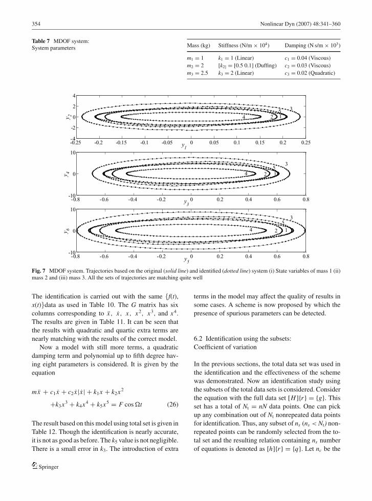
5 Multidegree of freedom (MDOF) system

A 3-DOF system shown in Fig. 6 is identified us-

ing the multiple-trial method. The basic formulation

as given in Section 2 is extended to this case and

the details are given below. Referring to the figure

[k1] = [k11 k12 . . k1s1], [k2] = [k21 k22 . . k2s2

], and

[k3] = [k31 k32 . . k3s3] are the coefficients of the poly-

nomial type stiffness, and s1, s2, and s3 are the re-

spective number of polynomial terms in the nonlinear

stiffness.

1 5 10 15 20 250

0.02

0.04

0.06

0.08

0.1

0.12

0.14

0.16

Set number

Etn

Fig. 5 Oscillator with quadratic damping . Variation of the parametric error for different trials of random noise

f3(t)m1 m2 m3

[k1][k1] [k3]

c1 c2 c3

x1(t) x2(t) x3(t)

[k2]

Fig. 6 MDOF system

Springer

352 Nonlinear Dyn (2007) 48:341–360

The equations of motion for the case where c3 is

quadratic damping are given by

m1 x1 +s1∑

j=1

k1 j xj1 + c1 x1 −

s2∑j=1

k2 j (x2 − x1) j

− c2(x2 − x1) = 0 (18a)

m2 x2 +s2∑

j=1

k2 j (x2 − x1) j + c2(x2 − x1)

−s3∑

j=1

k3 j (x3 − x2) j

− c3(x3 − x2)|(x3 − x2)| = 0 (18b)

m3 x3 +s3∑

j=1

k3 j (x3 − x2) j + c3(x3 − x2)|(x3 − x2)|

= f3(t) = F3 cos(�t) (18c)

where f3(t) is the external excitation acting on mass 3

which is assumed harmonic. The system of equations is

numerically solved. The steady state response, which

is periodic, is taken for analysis. The FFT of the time

series x1, x2, and x3 is carried out. Let � be the fun-

damental frequency of the total six-dimensional orbit.

The displacement and velocities in terms of real Fourier

series can be expressed as

x1(t) = a01 +M1∑

j1=1

(a j1 cos j1�t + b j1 sin j1�t

)x2(t) = a02 +

M2∑j2=1


)x3(t) = a03 +

M3∑j3=1


)(19a)

v1(t) = x1(t)

= �

M1∑j1=1

( − a j1 j1 sin j1�t + b j1 j1 cos j1�t)

v2(t) = x2(t)

= �

M2∑j2=1


v3(t) = x3(t)

= �

M3∑j3=1


(19b)

The accelerations are given by,

a1(t) = x1(t)

= −�2M1∑

j1=1

(a j1 j2

1 cos j1�t + b j1 j21 sin j1�t

)a2(t) = x2(t)

= −�2M2∑

j2=1

(a j2 j2


)a3(t) = x3(t)

= −�2M3∑

j3=1

(a j3 j2


)(19c)

Let

x21(t) = x2(t) − x1(t); x32(t) = x3(t) − x2(t)v21(t) = v2(t) − v1(t); v32(t) = v3(t) − v2(t)

(20)

The equations of motion take the form

m1a1(t) + c1v1(t) +s1∑

i=1

k1i (x1(t))i

−s2∑

i=1

k2i (x21(t))i − c2v21(t) = 0 (21a)

m2a2(t) +s2∑

i=1

k2i (x21(t))i + c2v21(t)

−s3∑

i=1

k3i (x32(t))i−c3v32(t)|v32(t)| = 0

(21b)

m3a3(t) +s3∑

i=1

k3i (x32(t))i

+ c3v32(t)|v32(t)| = f3(t) (21c)

The Equations (21) can be written in matrix form as

⎡⎣ [Q]11 [Q]12 [0]

[0] [Q]22 [Q]23

[0] [0] [Q]33

⎤⎦ ⎧⎨⎩{r}1

{r}2

{r}3

⎫⎬⎭ =⎧⎨⎩

{0}{0}

{Fe3}

⎫⎬⎭(22)

Springer

Nonlinear Dyn (2007) 48:341–360 353

where

[Q]11 =

⎡⎢⎢⎢⎢⎢⎢⎢⎢⎣

a1(1) v1(1) x1(1) (x1(1))2 (x1(1))3

. . . . .

. . . . .

. . . . .

a1(N ) v1(N ) x1(N ) (x1(N ))2 (x1(N ))3

⎤⎥⎥⎥⎥⎥⎥⎥⎥⎦; (23a)

[Q]12 =

⎡⎢⎢⎢⎢⎢⎢⎢⎢⎣

0 −v21(1) −x21(1) −(x21(1))2 −(x21(1))3

. . . . .

. . . . .

. . . . .

0 −v21(N ) −x21(N ) −(x21(N ))2 −(x21(N ))3

⎤⎥⎥⎥⎥⎥⎥⎥⎥⎦(23b)

[Q]22 =

⎡⎢⎢⎢⎢⎢⎢⎢⎢⎣

a2(1) v21(1) x21(1) (x21(1))2 (x21(1))3

. . . . .

. . . . .

. . . . .

a2(N ) v21(N ) x21(N ) (x21(N ))2 (x21(N ))3

⎤⎥⎥⎥⎥⎥⎥⎥⎥⎦(23c)

[Q]23 =

⎡⎢⎢⎢⎢⎢⎢⎢⎢⎣

0 −v32(1)|v32(1)| −x32(1) −(x32(1))2 −(x32(1))3

. . . . .

. . . . .

. . . . .

0 −v32(N )|v32(N )| −x32(N ) −(x32(N ))2 −(x32(N ))3

⎤⎥⎥⎥⎥⎥⎥⎥⎥⎦(23d)

[Q]33 =

⎡⎢⎢⎢⎢⎢⎢⎢⎢⎣

a3(1) v32(1)|v32(1))| x32(1) (x32(1))2 (x32(1))3

. . . . .

. . . . .

. . . . .

a3(N ) v32(N )|v32(N )| x32(N ) (x32(N ))2 (x32(N ))3

⎤⎥⎥⎥⎥⎥⎥⎥⎥⎦(23e)

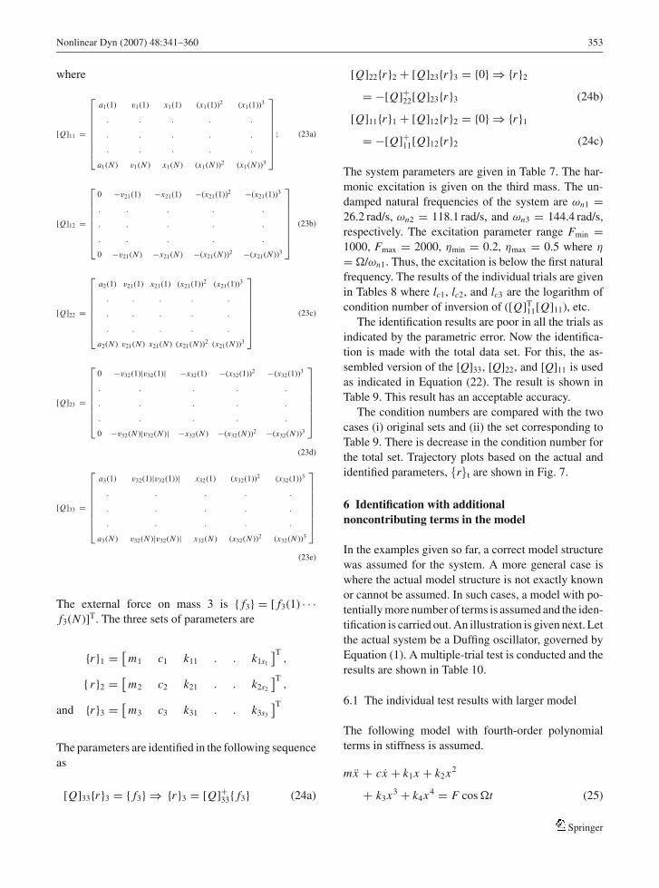
The external force on mass 3 is { f3} = [ f3(1) · · ·f3(N )]T. The three sets of parameters are

{r}1 = [m1 c1 k11 . . k1s1

]T,

{ r}2 = [m2 c2 k21 . . k2s2

]T,

and {r}3 = [m3 c3 k31 . . k3s3

]T

The parameters are identified in the following sequence

as

[Q]33{r}3 = { f3} ⇒ {r}3 = [Q]+33{ f3} (24a)

[Q]22{r}2 + [Q]23{r}3 = {0} ⇒ {r}2

= −[Q]+22[Q]23{r}3 (24b)

[Q]11{r}1 + [Q]12{r}2 = {0} ⇒ {r}1

= −[Q]+11[Q]12{r}2 (24c)

The system parameters are given in Table 7. The har-

monic excitation is given on the third mass. The un-

damped natural frequencies of the system are ωn1 =26.2 rad/s, ωn2 = 118.1 rad/s, and ωn3 = 144.4 rad/s,

respectively. The excitation parameter range Fmin =1000, Fmax = 2000, ηmin = 0.2, ηmax = 0.5 where η

= �/ωn1. Thus, the excitation is below the first natural

frequency. The results of the individual trials are given

in Tables 8 where lc1, lc2, and lc3 are the logarithm of

condition number of inversion of ([Q]T11[Q]11), etc.

The identification results are poor in all the trials as

indicated by the parametric error. Now the identifica-

tion is made with the total data set. For this, the as-

sembled version of the [Q]33, [Q]22, and [Q]11 is used

as indicated in Equation (22). The result is shown in

Table 9. This result has an acceptable accuracy.

The condition numbers are compared with the two

cases (i) original sets and (ii) the set corresponding to

Table 9. There is decrease in the condition number for

the total set. Trajectory plots based on the actual and

identified parameters, {r}t are shown in Fig. 7.

6 Identification with additionalnoncontributing terms in the model

In the examples given so far, a correct model structure

was assumed for the system. A more general case is

where the actual model structure is not exactly known

or cannot be assumed. In such cases, a model with po-

tentially more number of terms is assumed and the iden-

tification is carried out. An illustration is given next. Let

the actual system be a Duffing oscillator, governed by

Equation (1). A multiple-trial test is conducted and the

results are shown in Table 10.

6.1 The individual test results with larger model

The following model with fourth-order polynomial

terms in stiffness is assumed.

mx + cx + k1x + k2x2

+ k3x3 + k4x4 = F cos �t (25)

Springer

354 Nonlinear Dyn (2007) 48:341–360

Table 7 MDOF system:System parameters Mass (kg) Stiffness (N/m × 104) Damping (N s/m × 103)

m1 = 1 k1 = 1 (Linear) c1 = 0.04 (Viscous)

m2 = 2 [k2] = [0.5 0.1] (Duffing) c2 = 0.03 (Viscous)

m3 = 2.5 k3 = 2 (Linear) c3 = 0.02 (Quadratic)

-0.25 -0.2 -0.15 -0.1 -0.05 0 0.05 0.1 0.15 0.2 0.25-4

-2

0

2

4

y1

y 2 12

3

45

-0.8 -0.6 -0.4 -0.2 0 0.2 0.4 0.6 0.8-10

0

10

y3

y 4 12

3

45

-0.8 -0.6 -0.4 -0.2 0 0.2 0.4 0.6 0.8-10

0

10

y5

y 6 12

3

4

5

Fig. 7 MDOF system. Trajectories based on the original (solid line) and identified (dotted line) system (i) State variables of mass 1 (ii)mass 2 and (iii) mass 3. All the sets of trajectories are matching quite well

The identification is carried out with the same {f(t),x(t)}data as used in Table 10. The G matrix has six

columns corresponding to x, x, x, x2, x3, and x4.

The results are given in Table 11. It can be seen that

the results with quadratic and quartic extra terms are

nearly matching with the results of the correct model.

Now a model with still more terms, a quadratic

damping term and polynomial up to fifth degree hav-

ing eight parameters is considered. It is given by the

equation

mx + c1 x + c2 x |x | + k1x + k2x2

+k3x3 + k4x4 + k5x5 = F cos �t (26)

The result based on this model using total set is given in

Table 12. Though the identification is nearly accurate,

it is not as good as before. The k5 value is not negligible.

There is a small error in k3. The introduction of extra

terms in the model may affect the quality of results in

some cases. A scheme is now proposed by which the

presence of spurious parameters can be detected.

6.2 Identification using the subsets:

Coefficient of variation

In the previous sections, the total data set was used in

the identification and the effectiveness of the scheme

was demonstrated. Now an identification study using

the subsets of the total data sets is considered. Consider

the equation with the full data set [H ]{r} = {g}. This

set has a total of Nt = nN data points. One can pick

up any combination out of Nt nonrepeated data points

for identification. Thus, any subset of ns (ns < Nt) non-

repeated points can be randomly selected from the to-

tal set and the resulting relation containing ns number

of equations is denoted as [h]{r} = {q}. Let nc be the

Springer

Nonlinear Dyn (2007) 48:341–360 355

Tabl

e8

MD

OF

syst

em:

Ind

ivid

ual

tria

lre

sult

s Iden

tifi

edpar

amet

ers

Res

ult

sum

mar

y

Tri

alm

1c 1

k 1×

10

4m

2c 2

k 21×

10

3k 2

2×

10

3m

3c 3

k 3×

10

4F

orc

e(N

)F

requen

cyη

Ep

l c1

l c2

l c3

(�ra

d/s

)

1−2

.0574

40.1

700

0.9

935

2.2

356

29.9

195

5.0

613

0.8

849

2.8

208

18.9

771

2.0

114

1950.1

7.0

601

0.2

693

0.9

692

13.2

581

17.6

159

16.3

496

21

.1802

39.9

223

0.9

999

1.9

796

30.1

095

5.0

038

0.8

841

2.4

645

19.0

176

1.9

971

1606.8

9.0

641

0.3

458

0.0

697

11.8

524

16.7

772

16.1

011

3−0

.4547

39.7

019

1.0

170

2.6

907

30.0

271

5.1

438

1.2

792

2.7

378

18.9

302

2.0

231

1891.3

11.2

354

0.4

286

0.4

823

13.8

258

20.1

914

18.9

826

4−8

7.3

58

39.0

209

0.8

186

13.8

265

30.0

156

5.4

227

0.4

205

−0.1

457

27.5

196

1.9

442

1456.5

5.3

880

0.2

056

28.0

067

15.6

311

19.3

082

17.3

841

51

.0367

40.1

614

1.0

000

2.1

047

29.8

614

4.9

972

1.0

164

2.4

043

22.6

896

1.9

957

1821.4

8.7

395

0.3

334

0.0

489

11.3

358

16.0

809

15.4

130 number of such independent selections from the total

set. Thus, one gets matrix equations as [h] j {r} = {q} j

where suffix j = 1, 2,. . ., nc. Since the elements of these

sets are formed from different periodic orbits, these sets

cannot be pictorially represented as orbits. However,

these subcollections are valid sets for the purpose of

identification.

Now we carry out the identification with these

sets,{[h] j , {q} j }. It is seen that the identification results

are nearly the same, though not as good as that done

with the total set provided the number of elements in

each subsets are sufficiently large. The identification

results with these subsets will be used to obtain a level

of confidence in the correctness of the assumed model.

As mentioned earlier, a set of ns indices from the Nt

numbers is selected randomly. ns is taken as 128. The

pseudo inversion of this set {r} j = [h]+j {q} j gives the

identification parameters and the corresponding para-

metric error Ep for the jth set is found. The process is

repeated for nc = 10 000 sets. The computation mainly

involves a pseudo inversion and is executed very fast.

The multiple-trial scheme facilitates an almost unlim-

ited number of choices for the selection of data points

for identification, each one of them giving a result,

which is a candidate parameter set. The identified pa-

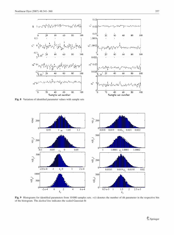
rameter values across 100 samples are shown in Figure

8 for each of the eight parameters. The histograms of the

corresponding full data are shown in Figure 9. Using the

mean value and the standard deviation of these respec-

tive data, a Gaussian density function is determined. It

is scaled (multiplied) by the area of the histogram and

is drawn in the same figure in order to see whether the

distribution is normal or not. It can be seen that the his-

togram closely matches with the Gaussian distribution.

A dimensionless term called the coefficient of varia-

tion Cv, which is defined as the ratio of the standard

deviation σ to the mean value μ(Cv = σ /μ) of the pa-

rameter is also determined. Table 13 gives the values

of μ, σ , and Cv for all the eight parameters. Cv is a

measure of fluctuation in the data among the samples.

A higher value of Cv indicates that the corresponding

data is inaccurate. The Cv for the parameters c2 , k2, k4,

and k5 is an order of magnitude higher when compared

to other parameters. It can be inferred that the error in

the parameters is linked to the high value of Cv. This

observation is useful because Cv for each parameter can

be obtained in a real test and it is a measure of confi-

dence in the result. The result in Table 13, however, has

to be properly interpreted. A relatively high value of Cv

Springer

356 Nonlinear Dyn (2007) 48:341–360

Table 9 MDOF system:Identified parameters usingtotal data set

Mass (kg) Stiffness (N/m ×104) Damping (N s/m)

m1 = 0.9737 k1 = 0.9998 (Linear) c1 = 40.0396 (Viscous)

m2 = 2.0370 [k2] = [0.5000 0.1009] (Duffing) c2 = 29.9033(Viscous)

m3 = 2.4746 k3 = 1.9986 (Linear) c3 = 20.1792 (Quadratic)

Et = 0.0115 lc1 = 10.7013 lc2 = 16.0757 lc3 = 14.6022

Table 10 Results forDuffing oscillator model,{r} = [1 0.02 1 0.02]T


Trial F � η m c k α Ep

1 0.3080 0.0480 0.0480 144.5197 0.0200 1.3322 0.0000 71.7618

2 0.5374 0.0343 0.0343 109.9303 0.0199 1.1324 −0.0006 54.4676

3 0.7859 0.0457 0.0457 63.9448 0.0199 1.1409 −0.0012 31.4769

4 0.1167 0.0283 0.0283 328.7730 0.0221 1.2620 −0.0000 163.8873

5 0.5002 0.0429 0.0429 115.4889 0.0201 1.2166 −0.0138 57.2508

Total set 0.9847 0.0200 1.0000 0.0200 0.0078

Table 11 Results for amodel having up tofourth-order polynomialterms in stiffness


Trial m c k1 k2 k3 k4 Ep

1 144.3894 0.0200 1.3319 −0.0000 0.0000 0.0000 71.7618

2 109.1251 0.0199 1.1314 −0.0000 −0.0004 −0.0000 54.4676

3 61.2064 0.0199 1.1347 −0.0000 −0.0003 0.0000 31.4769

4 359.7605 0.0221 1.2867 −0.0009 −0.0000 0.0483 163.8873

5 71.7278 0.0201 1.1338 −0.0000 −0.0010 −0.0000 57.2508

Total set 0.9847 0.0200 1.0000 −0.0000 0.0200 0.0001

Table 12 Results for amodel containing eightparameters


m c1 c2 k1 k2 k3 k4 k5

Total set 1.0117 0.0202 −0.0119 1.0001 −0.0000 0.0191 0.0001 0.0014

together with a nearly zero mean value for the param-

eters confirms that the parameter is negligible. If such

parameters are detected, they may be excluded from

the model and the parametric estimation can be redone

with the reduced model. The sensitivity of a parameter

to a given excitation is analogous to the reciprocal of

Cv. In the case of a correct model, also there is scope

for using Cv to detect poor identification, however, that

is not done here.

Larger-sized subsets give smaller Cv and vice versa.

However, the mean values of parameters and their rel-

ative Cv values remain nearly unchanged. In the next

Table 13 The coefficient ofvariation m c1 c2 k1 k2 k 3 k4 k5

{r}T 1 0.02 0 1 0 0.02 0 0

{r}Tt 1.0117 0.0202 −0.0119 1.0001 −0.0000 0.0191 0.0001 0.0014

μ 1.0119 0.0202 −0.0113 1.0001 −0.0000 0.0191 0.0001 0.0015

σ 0.0271 0.0007 0.0240 0.0000 0.0000 0.0002 0.0001 0.0003

cv 0.0268 0.0358 −2.1284 0.0000 −0.9554 0.0129 0.8005 0.2049

Springer

Nonlinear Dyn (2007) 48:341–360 357

Fig. 8 Variation of identified parameter values with sample sets

0.95 1 1.05 1.10

200

m

ν)

m(

0.018 0.019 0.02 0.021 0.0220

200

c1

νc(

1)

-0.1 -0.05 0 0.050

200

c2

νc(

2)

1 1.0001 1.0001 1.00020

500

k1

νk(

1)

-2.0 e-4 -1 0 1 2 e-40

500

k2

νk(

2)

0.0185 0.019 0.0195 0.020

200

k3

νk(

3)

-2 e-4 0 2 4 6 e-40

500

1000

k4

νk(

4)

0.5 e-3 1 1.5 2 2.5 e-30

500

k5

νk(

5)

Fig. 9 Histograms for identified parameters from 10 000 samples sets. ν(i) denotes the number of ith parameter in the respective binof the histogram. The dashed line indicates the scaled Gaussian fit

Springer

358 Nonlinear Dyn (2007) 48:341–360

section, the problem of finding the noncontributing pa-

rameters, which give rise to errors in the model, is han-

dled by considering a perturbation for the total data

set. This is a different approach from the one discussed

above.

6.3 Modeling error: Sensitivity study using

periodic perturbation

Consider a small periodic perturbation �x(t) given to

the response x(t). The induced periodic perturbations,

are determined for all columns of [G] to get a peri-

odic perturbation matrix [�G]p. The identified param-

eters {r}p in this case can be obtained as {r}p = ([G] +[�G]p)+{ f }. This process is repeated several times

with randomly chosen periodic perturbations, each hav-

ing a prescribed fixed rms ratio, εp = rms(�x)/rms(x).

The Cv of the parameters from the set can be determined

as explained in the previous section. The same data set

of the previous section is considered for illustration.

Since the individual test results in Table 10 is highly

erratic, it will not make sense to compute Cv based on

a single set. However, with the combination of multi-

ple trial data sets, the identification problem has been

changed to a well-posed problem and it is meaningful to

quantify Cv for the total data set. Each of the individual

trial matrices [G]i is given nonidentical perturbations

with the same value of εp to obtain the combined per-

turbed matrix, [H]p = [H] + [�H]p. The identified val-

ues for the total set are given by {r}pt = [H ]+p { f }. The

process is repeated 100 times and Cv of all the param-

eters are found. The calculations are done for different

values of εp and the results are shown in Figure 10.

The conclusion is that parameters with relatively high

values of Cv have negligible values and can be omit-

ted from the model. However, Cv cannot be used as

the sole criterion for rejecting the parameters as it was

mentioned in the last section. The point of cutoff can-

not be ascertained based on Cv alone, however it is a

good indicator.

7 Conclusion

A new study of nonlinear system identification incor-

porating a multiple-trial scheme in the conventional

HB method is given in this paper. The applicability of

-3-4-5-6-7-8-9-10-30

-25

-20

-1 5

-10

-5

0

1

2

3

4

5

6

78

logεp

C|golv|

1 m2 c

13 c

24 k

15 k

26 k

37 k

48 k

5

Fig. 10 Variation of Cv of the parameters with rms value ofperturbation. εp varies uniformly from 10−10 to 10−3 in the log-arithmic scale. The nonexistent parameters, which are c2, k2, k4,

and k5 have higher Cv values compared to other parameters. Theyare indicated by dotted lines with numbers 3, 5, 7, and 8

Springer

Nonlinear Dyn (2007) 48:341–360 359

the method is illustrated with several examples. This

method works well independent of the type of non-

linear system and thus one need not be familiar with

the nonlinear dynamics of a specific system to use this

method. Measures to identify noncontributing terms in

a model have also been suggested; this is shown to work

well through a Duffing oscillator example.

Further refinements in the scheme have to be tried

in which certain poor trial-set data is excluded from

the total set using some criterion. This is an attempt

to improve the quality of the result using the remain-

ing data. The ranges of the excitation parameters were

set somewhat arbitrarily, and it needs further stud-

ies to find out the guidelines for effective choices of

these.

Appendix

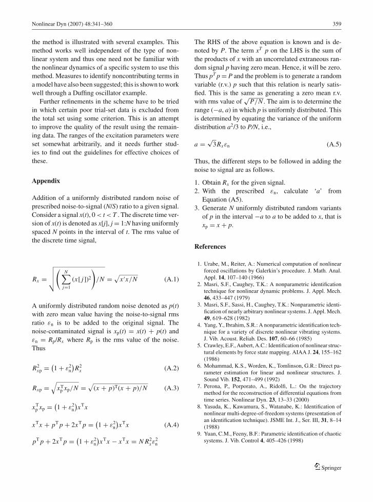
Addition of a uniformly distributed random noise of

prescribed noise-to-signal (N/S) ratio to a given signal.

Consider a signal x(t), 0 < t < T . The discrete time ver-

sion of x(t) is denoted as x[j], j = 1:N having uniformly

spaced N points in the interval of t. The rms value of

the discrete time signal,

Rx =√√√√(

N∑j=1

(x[ j])2

)/N =

√x ′x/N (A.1)

A uniformly distributed random noise denoted as p(t)with zero mean value having the noise-to-signal rms

ratio εn is to be added to the original signal. The

noise-contaminated signal is xp(t) = x(t) + p(t) and

εn = Rp/Rx where Rp is the rms value of the noise.

Thus

R2xp = (

1 + ε2n

)R2

x (A.2)

Rxp =√

xTp xp/N =

√(x + p)T(x + p)/N (A.3)

xTp xp = (

1 + ε2n

)xTx

xTx + pT p + 2xT p = (1 + ε2

n

)xTx (A.4)

pT p + 2xT p = (1 + ε2

n

)xTx − xTx = N R2

xε2n

The RHS of the above equation is known and is de-

noted by P. The term xT p on the LHS is the sum of

the products of x with an uncorrelated extraneous ran-

dom signal p having zero mean. Hence, it will be zero.

Thus pT p = P and the problem is to generate a random

variable (r.v.) p such that this relation is nearly satis-

fied. This is the same as generating a zero mean r.v.

with rms value of√

P/N . The aim is to determine the

range (−a, a) in which p is uniformly distributed. This

is determined by equating the variance of the uniform

distribution a2/3 to P/N, i.e.,

a =√

3Rxεn (A.5)

Thus, the different steps to be followed in adding the

noise to signal are as follows.

1. Obtain Rx for the given signal.

2. With the prescribed εn, calculate ‘a’ from

Equation (A5).

3. Generate N uniformly distributed random variants

of p in the interval −a to a to be added to x, that is

xp = x + p.

References

1. Urabe, M., Reiter, A.: Numerical computation of nonlinearforced oscillations by Galerkin’s procedure. J. Math. Anal.Appl. 14, 107–140 (1966)

2. Masri, S.F., Caughey, T.K.: A nonparametric identificationtechnique for nonlinear dynamic problems. J. Appl. Mech.46, 433–447 (1979)

3. Masri, S.F., Sassi, H., Caughey, T.K.: Nonparametric identi-fication of nearly arbitrary nonlinear systems. J. Appl. Mech.49, 619–628 (1982)

4. Yang, Y., Ibrahim, S.R.: A nonparametric identification tech-nique for a variety of discrete nonlinear vibrating systems.J. Vib. Acoust. Reliab. Des. 107, 60–66 (1985)

5. Crawley, E.F., Aubert, A.C.: Identification of nonlinear struc-tural elements by force state mapping. AIAA J. 24, 155–162(1986)

6. Mohammad, K.S., Worden, K., Tomlinson, G.R.: Direct pa-rameter estimation for linear and nonlinear structures. J.Sound Vib. 152, 471–499 (1992)

7. Perona, P., Porporato, A., Ridolfi, L.: On the trajectorymethod for the reconstruction of differential equations fromtime series. Nonlinear Dyn. 23, 13–33 (2000)

8. Yasuda, K., Kawamura, S., Watanabe, K.: Identification ofnonlinear multi-degree-of-freedom systems (presentation ofan identification technique). JSME Int. J., Ser. III, 31, 8–14(1988)

9. Yuan, C.M., Feeny, B.F.: Parametric identification of chaoticsystems. J. Vib. Control 4, 405–426 (1998)

Springer

360 Nonlinear Dyn (2007) 48:341–360

10. Narayanan, M.D., Narayanan, S., Padmanabhan, C.:Parametric identification of a nonlinear system usingmulti-harmonic excitation. In: Proceedings VETOMAC-3 &ACSIM-2004 Conference, vol. 2, pp 706–714, New Delhi,India (2004)

11. Golub, G.H., Van Loan, C.F.: Matrix Computations, 2nd edn.The Johns Hopkins University Press, Baltimore, MD (1989)

12. Kundert, K., Sorkin, G.B., Vincentelli, A.S.: Applying har-monic balance to almost-periodic circuits. IEEE Trans. Mi-crow. Theory Tech. 36, 366–378 (1988)

Springer

Parametric identification of nonlinear systems using multiple trials

Documents

Transcript of Parametric identification of nonlinear systems using multiple trials