Parameters of the O( 1S) excitation process deduced from photometer measurements of pulsating aurora

Pergamon Journal of Atmospheric and Terrestrial Physics, Vol. 57, No. 14, pp. 1799-1814, 1995

Copyright 0 1995 Ekvier Science Ltd Printed in Great Britain. All rights reserved

0021-9169(95)00099-2 WZl-9169/95 $9.50+0.00

Parameters of the 0(‘S) excitation process deduced from photometer measurements of pulsating aurora

A. R. Klekociuk and G. B. Burns Australian Antarctic Division, Kingston, Tasmania 7050, Australia

(Received injinalform 16 January 1995 ; accepted 17 February 1995)

Abstract-Intensity time-series of the 427.8 nm N: (1NG) (0,l) band and 557.7 nm 0(‘S_‘D) line emissions were obtained with 0.05 s time resolution during intervals of pulsating aurora. Using an impulse response function analy,,is technique in conjunction with synthetic intensity time-series constructed using measured data, we estimate the influence of measurement noise and a non-linear component of the covariance between the 557.7 nm and 427.8 nm intensity time-series on the inferred parameters of an 0(‘S) indirect excitation model.

Non-linear effects had no additional influence beyond that of measurement noise on estimates of an indirect process. After accounting for the influence of measurement noise, indirect excitation accounts for between 30% and 100% of 0(‘S) production, with an average for our measurements of 58%. The average effective lifetime of the species responsible for the indirect excitation process is 0.13 s. The average percentage contribution from the indirect process is 14% lower, and the effective lifetime slightly longer, than values obtained when noise is not accounted for.

Non-linearities between the aurora1 emissions limit the determination of the 0(‘S) effective lifetime by this technique. We obtain an 0(‘S) effective lifetime distribution with a mean of 0.71 s and a sharp cut-off at the radiative lifetime of -0.80 s. 0(‘S) state effective lifetimes decrease as average incident electron energies, determined from the relative 0(‘S_‘D) and N: (ING) intensities, increase. Collisional deactivation of the 0(‘S) state can account for only of the order of 55% of the energy dependence of the 0(‘S_‘D) and N: (1NG) intensity ratio.

1. [NTRODUCTION ted to result in a range of shorter ‘effective’ lifetimes.

The dominant emi&on feature in the visible aurora1 spectrum, the 557.7 mm ‘green line’, is the result of the transition 0(‘S’D). Despite the ease with which this natural emission maLy be studied, and its importance in diagnosing conditions in the lower thermosphere (at altitudes near 100 km), the mechanism by which the 0(‘S) state is excited in the aurora1 atmosphere has still to be conclusively defined.

The 0(‘S) state can be created in the upper atmosphere by direct electron impact on atomic and molecular oxygen (Rees et al., 1967, 1969 ; Donahue et al., 1968 ; Zipf and McL,aughlin, 1978). Evidence suggests that the direct process proceeds predominantly via electron impact on atomic oxygen. However it is generally accepted that one or more metastable inter- mediary species are important in indirectly exciting a portion of the O(%) population (Burns and Reid, 1984; Paulson et uI., 1990), with N,(A3XC:) being preferred (Paulson et al., 1990 ; Shepherd et al., 1991).

A convenient method of investigating the 0(‘S) excitation process utilises ground-based photometric time-series of the 0(‘S_‘D) line emission and one or more bands of the N:(lNG) emission system. It is widely accepted that the aurora1 N: (1NG) state is excited by the direct impact of electrons on N, (O’Neil et al., 1979). Due to the extremely short lifetime of the upper N$(lNG) state, the emission intensity of the N: (1 NG) band system is directly proportional to the rate of ionisation of molecular nitrogen. By assuming that the 0(‘S_‘D) intensity is ‘linearly’ related to the N: (ING) band emissions, we may write

lo(T) = r” Z,(T- t)h(t) dt = Z,(T)*h(t) (1) Jt=o

The theoretical free-space lifetime of the 0(‘S) state against radiation is -0.8 s (Nicolaides et al., 1971). Collisional quenching in the atmosphere is expec-

where lo(T) and IN(T) are the intensities of the 0(‘S_‘D) and N: (1NG) emissions, respectively, as a function of measurement time T, h(t) is a finite causal (i.e. t 2 0) linear filter or ‘impulse response function’ relating the two emissions, and ‘*’ denotes the convolution operator.

1799

1800 A. R. Klekociuk and G. B. Burns

Under the hypothesis that both direct and indirect processes excite the 0(‘S) state, where the rate of indirect excitation is proportional to the concentration of an intermediate species, and the rate of intermediate species production and direct excitation are independently proportional to the emission rate of the NT (1 NG) band system, then we may write

h(l) = Ae-‘iz__Be-‘! (2)

where A and B are constants, z is the effective lifetime of the O(S) state, and T’ is the effective lifetime of the intermediate species (Parkinson, 197 1; Henriksen 1973, 1974; Burns and Reid, 1984, 1985). The percentage contribution of the indirect process to 0(‘S) excitation is given by

p = B(z. lo()y/o,

Ar-Bz’

If the 0(‘S) state is excited solely by direct aurora1 particle impact, then the second term in equation (2) vanishes (i.e. B = 0).

In fitting the double-exponential function (equation (2)) to a measured impulse response there is no mathematical restriction to limit the derived values of A, B, z and z’ from yielding P (equation (3)) greater than 100%. Such a result would be unrealistic. Derivations of equations (2) and (3) are contained in Burns and Reid (1984) but readers should be aware of the following errors : for consistency with development presented in that paper, A in their equation (1) should be replaced with AT, Kin equation (3) by Kr and K’ in equation (4) by K’z’.

Two approaches have been adopted in the literature to evaluate the form of the impulse response function in equation (1). Brekke and Pettersen (1972), Brekke (1973), Paulson et al. (1990) and Shepherd et al. (1991) have used a cross spectral frequency-domain technique (developed by Paulson and Shepherd, 1965) to directly estimate the parameters in equation (2). Burns and Reid (1984) directly evaluate the impulse response function in the time domain and then least- squares fit a double-exponential (equation 2) to estimate the excitation parameters. Both methods are best suited to the analysis of aurora1 time-series where the variation of intensities on time-scales of the order of the effective lifetimes is significantly larger than the measurement uncertainty. Observations of pulsating aurora best meet this requirement.

Recent estimates give an average 0(‘S) effective lifetime of -0.7 s, near the theoretical free-space value, an effective lifetime of the intermediate species of -0.1 s, and suggest that the indirect process accounts for between 50% and 100% of 0(‘S) exci-

tation (Burns and Reid, 1984; Paulson et al., 1990). Furthermore, Paulson et al. (1990) argued in favour of N,(A3C:) as the intermediate species based on the plausibility of the emission heights inferred by assimi- lating laboratory rate constant measurements, the observed indirect effective lifetimes and the MSIS-86 atmospheric model. This conclusion is supported by Shepherd et al. (1991) who have found a correlation between simultaneous independent measurements of the effective lifetimes of the N,(A3C:) state and the 0(‘S) precursor. The significance of the indirect excitation mechanism involving impact of a directly excited state of O2 on 0, as proposed by Solheim and Llewellyn (1979), has yet to be fully experimentally investigated.

The central assumption in equation (1) is that of linearity between the time-series; that is, the invari- ance of the impulse response function over the measurement interval. Two processes specifically associated with pulsating aurora result in contributions to ‘non-linearity’ (i.e. a non-linear relationship) between the intensities of the 0(‘S’D) and N: (1NG) time-series. Firstly, the characteristic electron energy increases between the ‘off and ‘on’ states of aurora1 pulsations (McEwen et al., 1981). Secondly, the equatorial location of the electron modulation region causes the higher energy electrons of each pul- sation to arrive at the atmosphere first (Johnstone, 1983). It has been experimentally confirmed that there is a general decrease in the 0(‘S’D) to Nl (ING) column integrated intensity ratio as the energy of the precipitating electrons increases (Gerdjikova and Shepherd, 1987; Steele and McEwen, 1990), at least for mean electron energies near 1 keV. Other processes that may lead to variation of the aforementioned intensity ratio include variation of the wavelength dependent scattering of light in the atmosphere (most important at the blue end of the spectrum) and processes that influence the yield of 0(‘S’D) relative to N: (ING) such as variation in the concentration of the 0(‘S) quenching species, or the relative abundance of (principally) 0, 0, and N,. In order to effect the determination of the time-constants or the percentage contribution of an indirect excitation process (z, z’ and P), the variations must occur within a measurement interval, and will be more detrimental if they occur on time-scales comparable with the effective lifetimes.

Using synthetic time-series based on their observed data, Burns and Reid (1984) showed that non-linearity may influence estimates of the 0(‘S) effective lifetime obtained by their analysis technique. In addition, they showed that noise due to the measurement process may mimic the signature of an indirect excitation process. Burns and Reid (1984) developed

Pulsating aurora and 0(‘S) excitation 1801

a method of data selection that minimised the influence of non-linearity and noise on their estimates of the excitation model parameters.

In this paper, we have extended the simulation technique of Burns and Reid (1984) to estimate the influence of measurement noise and non-linearity on the parameters of a double-exponential fit to the impulse function relating the 0(‘S_‘D) and N$ (1NG) emissions in carefully selected pulsating aurora observations. We confirm the existence of an indirect excitation process, but with a lower percentage contribution than previously reported, and determine the relationship between. the 0(‘S) effective lifetime and the energy-dependent 551.1 nm to 427.8 nm intensity ratio.

2. DATA COLLECTION AND REDUCTION

2.1. Instrumentation

A dual-channel beam-splitting photometer was operated at Macquarie Island (geographic coor- dinates 54.5”S, 159.O”E; magnetic latitude 64.3%) between May, 1988, and February, 1989, to obtain digital intensity time-series of the 0(‘S_‘D) line (at 557.7 nm) and the hl: (1NG) (0,l) band (which has a ‘head’ at 427.8 nm) during intervals of rapidly fluctuating aurora. The photometer was directed towards the magnetic zenith. Each channel had an identical 1” field-of-view andi employed a 1.5 nm bandwidth interference filter to isolate the desired spectral region. A ‘pulse counting’ technique was used with a sample rate of 20 Hz (0.05 s counting interval). Data were stored in 5 minute sequences. The photomultipliers were cooled to -25°C to reduce the thermal contribution to pulse counting statistics.

Non-linearity in the photon-counting system was observed above 200 kHz. A correction accounting for this was applied to all raw photometer data as the first step in the calibration procedure. A monochromator was used to obtain in-situ profiles of the combined transmission of the beam-splitter/filter combination of each channel as a function of wavelength. These profiles were combined with measurements of a standard calibration lamp to calculate the scaling of the linearised dark-count corrected pulse frequency of each channel to the Il.ncident column emission intensity in Rayleighs (R). In evaluating the percentage of light in the N:(lNG) (0,l) band detected by the photometer, a synthletic spectrum with a characteristic temperature of 3001 K was generated using a model supplied by Dr Dick Gattinger (NRC, Ottawa), and then multiplied by the measured channel transmission profile. Unless otherwise noted, the inferred absolute

intensities have not been corrected for atmospheric extinction or the van Rhijn effect. The latter is neg- ligible as the zenith angle of the photometer was only 12 degrees.

2.2. Analysis method

The impulse function relating the O(‘S’D) line emission to the N$(lNG) (0,l) band emission was calculated using the method described by Burns and Reid (1984) for each of the 5 minute sequences. Each impulse function was calculated with 0.05 s resolution over the interval -2 s < t < 8 s and was scaled so that its total area excluding the first and last bins was unity. A double-exponential function was fitted to each scaled impulse response via an iterative realis- ation of Marquardt’s generalised non-linear least- squares technique (Bevington, 1969) over the interval 0.05 s < t < 2 s. Error estimates of the double- exponential parameters were also obtained. The t = 0 point was not included in the fits as its amplitude is modified from the double-exponential model by the discrete nature of the sampling.

The choice of the time window for model fitting is a compromise between the number of data bins required to provide adequate verification of the model, given the anticipated values of r and T’, in the face of measurement noise, and physical effects which are expected to influence the direct excitation term in equation (2). Because the 0(‘S) state is excited over a certain altitude interval, we anticipate the shape of the ‘tail’ of each impulse response to reflect the super- position of exponential decays with a range of r and A values due to the variation of excitation and quenching processes with altitude. A suitable upper time- limit for the fitting window was chosen by fitting out to the five limits separated by 0.5 s in the range 1.0 s to 3.0 s inclusive. The limit with the narrowest probability distribution of the resulting r values (namely 2.0 s) was selected.

2.3. Data selection

A set of parameters was obtained to characterise each recovered impulse function and its model fit. A series of correlation analyses was performed on the entire parameter set, irrespective of the influence of cloud or moonlight on the measurements, to determine the parameters that, when suitably restricted, would select impulse functions for which the effects of noise and non-linearity were minimised. The selection criteria were tightened until further restriction pro- duced no significant change to the mean, standard deviation or shape of the distribution of the 0(‘S) effective lifetimes, r. A stable distribution of T was


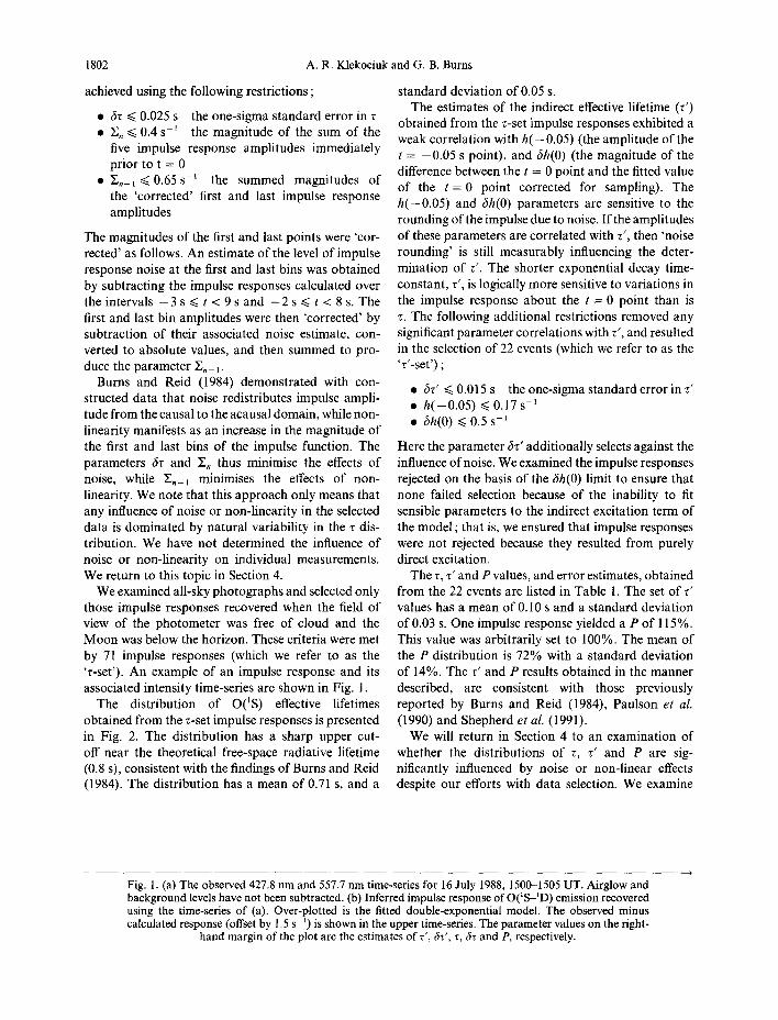
achieved using the following restrictions ; standard deviation of 0.05 s.

??Sz < 0.025 s the one-sigma standard error in 7 0 c, < 0.4 ss’ the magnitude of the sum of the

five impulse response amplitudes immediately prior to t = 0

??Z:._, < 0.65 s-1 the summed magnitudes of the ‘corrected’ first and last impulse response amplitudes

The magnitudes of the first and last points were ‘corrected’ as follows. An estimate of the level of impulse response noise at the first and last bins was obtained by subtracting the impulse responses calculated over theintervals -3s<t<9sand -2s,<t<8s.The first and last bin amplitudes were then ‘corrected’ by subtraction of their associated noise estimate, con- verted to absolute values, and then summed to pro- duce the parameter X,- ,

The estimates of the indirect effective lifetime (t’) obtained from the r-set impulse responses exhibited a weak correlation with h( - 0.05) (the amplitude of the t = -0.05 s point), and &r(O) (the magnitude of the difference between the t = 0 point and the fitted value of the t = 0 point corrected for sampling). The h(-0.05) and 6h(O) parameters are sensitive to the rounding of the impulse due to noise. If the amplitudes of these parameters are correlated with t', then ‘noise rounding’ is still measurably influencing the determination of 7’. The shorter exponential decay time- constant, T’, is logically more sensitive to variations in the impulse response about the t = 0 point than is 7. The following additional restrictions removed any significant parameter correlations with T', and resulted in the selection of 22 events (which we refer to as the ‘7’-set’) ;

Burns and Reid (1984) demonstrated with constructed data that noise redistributes impulse amplitude from the causal to the acausal domain, while non- linearity manifests as an increase in the magnitude of the first and last bins of the impulse function. The parameters 67 and I&, thus minimise the effects of noise, while &_, minimises the effects of non- linearity. We note that this approach only means that any influence of noise or non-linearity in the selected data is dominated by natural variability in the 7 distribution. We have not determined the influence of noise or non-linearity on individual measurements. We return to this topic in Section 4.

?? 67' < 0.015 s the one-sigma standard error in 7' 0 h(-0.05) < 0.17 s-1 0 6/z(O) < 0.5 s-1

Here the parameter 6~’ additionally selects against the influence of noise. We examined the impulse responses rejected on the basis of the ah(O) limit to ensure that none failed selection because of the inability to fit sensible parameters to the indirect excitation term of the model ; that is, we ensured that impulse responses were not rejected because they resulted from purely direct excitation.

We examined all-sky photographs and selected only those impulse responses recovered when the field of view of the photometer was free of cloud and the Moon was below the horizon. These criteria were met by 71 impulse responses (which we refer to as the ‘r-set’). An example of an impulse response and its associated intensity time-series are shown in Fig. 1.

The distribution of 0(‘S) effective lifetimes obtained from the z-set impulse responses is presented in Fig. 2. The distribution has a sharp upper cut- off near the theoretical free-space radiative lifetime (0.8 s), consistent with the findings of Burns and Reid (1984). The distribution has a mean of 0.71 s, and a

The z, 7' and P values, and error estimates, obtained from the 22 events are listed in Table 1. The set of r’ values has a mean of 0.10 s and a standard deviation of 0.03 s. One impulse response yielded a P of 115%. This value was arbitrarily set to 100%. The mean of the P distribution is 72% with a standard deviation of 14%. The 7' and P results obtained in the manner described, are consistent with those previously reported by Burns and Reid (1984), Paulson et al. (1990) and Shepherd et al. (1991).

We will return in Section 4 to an examination of whether the distributions of 7, T' and P are significantly influenced by noise or non-linear effects despite our efforts with data selection. We examine

, Fig. 1. (a) The observed 427.8 nm and 557.7 nm time-series for 16 July 1988, 15OtL-1505 UT. Airglow and background levels have not been subtracted. (b) Inferred impulse response of O(‘S’D) emission recovered using the time-series of (a). Over-plotted is the fitted double-exponential model. The observed minus calculated response (offset by 1.5 SK’) is shown in the upper time-series. The parameter values on the right-

hand margin of the plot are the estimates of T’, W, z, 6r and P, respectively.


800

400

0 50 100 150 200 250

9000

6000

7noo

6000

5OOO

41100

31100

0 50 100 150 200 250 Time (s) after 1500 UT

.4

.2

0

-.2’ ’ ’ ’ ’ ’ ’ ’ ’ ’ ’ I ’ I ’ ’ ’ ’ ’ -2 -1 0 1 2 3 4 5 6 I a Time 4s)


28,,,,,,,,,,,,,,,,,,1,,,1,,,,,1~,,,,,,1~,,,II,,,,~~~,,,~,,,1,,,,,,,, L

26 -

24 -

22 -

20 -

18 -

16 -

: + 14 - 1

12 -

10 -

a-

6-

4 -

2-

r

.40 .45 .50 .55 .60 .65 .70 .75 .EiO .85 .SO .95 1.00 1.05 01’51 Effectlvg Llfetlme Is1

Fig. 2. Distribution of the inferred 0(‘S) effective lifetime for 71 selected 5-minute intervals of pulsating aurora.

first the T distribution and its dependence on the energy of the incident aurora1 electrons, as determined from the 557.7 nm to 427.8 nm intensity ratio.

3. THE DISTRIBUTION OF O(%) EFFECTIVE LIFETIMES

AND THEIR DEPENDENCE ON THE 557.7 NM-

427.8 NM INTENSITY RATIO

The z distribution is shown in Fig. 2. We have noted that we chose our 2 s fitting window on the basis that this gave the narrowest r distribution. A concern is that if the emitting region is sufficiently wide, there will be an altitude distribution of 0(‘S) effective lifetimes which will be integrated along the line-of-sight by the photometer. We expect emissions from the peak altitude region will dominate near t = 0 in the impulse function, but as we move further away from this point, emissions having longer effective lifetimes will make a greater contribution. We looked for this effect in the T-set data. We averaged the residuals resulting from

the double-exponential model fit to each of the z-set impulse responses over contiguous groups of five bins in the interval 0.05 s < t < 4.0 s. In all cases, the mean residuals exhibited random fluctuation about zero in the interval 0.05 s d t < 2.0 s (the fitting window). In the interval 2.0 s < t < 4.0 s, there were eight cases where the residuals were consistently greater than zero, and one case with values consistently less than zero. The impulse response for the one case where the tail residuals were consistently less than zero was unusual in that it contained an underlying waveform of low amplitude and frequency which appeared to ‘pull down’ the residuals near t = 3.0 s.

Six of the eight events with positive tail residuals returned an average 7 of 0.64 s. This is at the lower end of the inferred 0(‘S) effective lifetime range, and fits the scenario we have presented above. For these events, the 7 values may be slightly longer than the value associated with the altitude of peak emission. The two other events have an average z of 0.78 s. This

Pulsating aurora and 0(‘S) excitation

Table 1. Observed and simulated parameter values for the 22 Y-set’ intervals

1805

Date Start Observed Simulated

(1988) time (UT) R: r (s) r’ (s) P (%) T’ 6) P (%)

11 Jul 11 Jul 11 Jul 12 Jul 15 Jul 15 Jul 16 Jul 16 Jul 16 Jul 16 Jul 16 Jul 16 Jul 16 Jul 16 Jul 16 Jul 16 Jul 16 Jul 16 Jul 5 Ott 6 Ott 6 Ott 6 Ott

Mean

1910 4.2 (0.20) 1930 3.9 (0.17) 1935 3.9 (0.20) 1500 3.3 (0.13) 1900 5.1 (0.21) 1905 4.9 (0.19) 1315 4.8 (0.25) 1500 5.1 (0.22) 1505 5.3 (0.25) 1535 5.8 (0.25) 1545 5.7 (0.27) 1610 5.2 (0.23) 1645 6.1 (0.25) 1705 5.9 (0.25) 1750 5.8 (0.24) 1805 5.5 (0.24) 1810 5.3 (0.22) 1840 5.3 (0.22) 1430 3.5 (0.16) 1330 4.1 (0.15) 1410 4.2 (0.19) 1420 4.1 (0.18)

Standard Deviation 0.05

0.68 (0.018) 0.09 (0.008) 0.64 (0.014) 0.13 (0.009) 0.66 (0.020) 0.10 (0.009) 0.63 (0.014) 0.09 (0.009) 0.70 (0.016) 0.06 (0.004) 0.67 (0.015) 0.08 (0.005) 0.69 (0.022) 0.11 (0.012) 0.69 (0.017) 0.07 (0.005) 0.68 (0.019) 0.11 (0.011) 0.75 (0.018) 0.09 io.oo;lj 0.77 (0.023) 0.07 (0.007) 0.73 (o.oi9j 0.10 (o.oiij 0.75 (0.016) 0.15 (0.009) 0.81 (0.020) 0.12 (0.011) 0.79 (0.019) 0.10 (0.008) 0.76 (0.019) 0.12 (0.010) 0.73 (0.016) 0.14 (0.010) 0.70 (0.015) 0.11 (0.007) 0.72 (0.021) 0.05 (0.006) 0.72 (0.014) 0.10 (0.010) 44 (9) 0.68 (0.018) 0.08 (0.009) 59 (15) 0.70 (o.oi9j 0.05 io.oosj 86 (24j

0.71 (0.018) 0.10 (0.008) 72 (16) 0.03 14 0.06

76 (17) 63 (10) 77 (18) 52 (11)

115 (26) 85 (15) 64 (16) 92 (20) 61 (14) 76 (16) 83 (22) 51 (13) 70 (11) 60 (12) 79 (isj 69 (13) 65 (11) 74 (13) 82 (25)

0.13 60 0.20 50 0.09 80 0.18 30 0.08 70 0.08 80 0.15 40 0.08 70 0.18 40 0.05 90 0.05 100 0.13 40 0.18 50 0.18 50 0.18 60 0.13 60 0.20 50 0.15 60 0.08 50 0.18 30 0.20 30 0.03 80

0.13 20

58

As described in Section 3, the parameter Rpis an estimator for the ratio between the intensities of the 557.7 nm and 427.8 nm time-series, corrected for scattering. The parameters r, 5’ and P are the 0(‘S) effective lifetime, the indirect effective lifetime, and the percentage of indirect excitation, respectively, as used in equations (2) and (3). The simulation technique to allow for the influence of noise is described in Section 5. The value in parentheses for the individual estimates of T, t’ and P is the 1~ confidence limit obtained from the fit of the double-exponential model to the associated impulse response function. The confidence limit for RF was calculated using the error estimates for the double-exponential fit parameters and assuming an error in the scattering correction factor of 0.02.

is at the upper end of our r distribution, and near the theoretical radiative lifetime. A longer 7 at larger displacements from t = 0 in the impulse response for these events is coniktent with a minor contribution from a longer lifetime indirect process. These events may be an indication of a high-altitude contribution from dissociative recombination of Oz. The two long 0(‘S) effective lifetime events returned an average for the ratio between the intensities of the 557.7 nm and 427.8 nm emissions of 7.5, while the six short lifetime events gave an average of 3.8. These ratios are consistent with low and high energy electron precipitation events, respectively.

Although these events were retained in the z-set, we were concerned the 7: distribution may be biased if low 7 values are preferentially rejected because of contributions from the long 7 tail resulting in a poor double-exponential fit. In these cases, we still expect a linear relationship between the two aurora1 emissions. Thus selection against the effects of ‘acausal rounding’

and non-linearity (by the parameters Z,, and &_, respectively) is appropriate, but events may be rejected by the 67 criterion because the impulse responses will differ from the double-exponential form. We examined the extra events recovered by maintaining the Z, and Em_, selection criteria, and relaxing the 67 criteria from 0.025 s to 0.050 s. An extra 31 events were selected, four of which exhibited dominantly positive residuals in the impulse response interval 2.0 s -=z t < 4.0 s. Three of these four events have low effective lifetimes and one has a long lifetime. These percentages are not significantly different from the 7-

set data. We conclude that the z-set is not biased by rejection of low effective lifetime values.

In order to obtain a ‘good’ impulse response, the interval of pulsating aurora must have a high signal- to-noise ratio (a high emission intensity is desirable), and contain rapid fluctuations. It is difficult to determine if this has resulted in bias to our 7 distribution. It would generally be accepted that high energy events


are favoured by these requirements. This implies that the distribution obtained may include lower T values than for average pulsating aurora conditions. As the r distribution is strongly peaked at values near the theoretical radiative lifetime, we claim that this is typical of pulsating aurora.

A suitable definition of the 557.7 nm427.8 nm intensity ratio time-series is

R(T) = 1(557.7)/1(427.8) = Zo(T+6T) -z,,

Z,(T) _ ZNB

(4)

where ZoA and Z,, are the inferred 557.7 nm ‘airglow plus background’ and 427.8 nm ‘background’ intensities, respectively, and 6T is a time lag which is a first- order correction for the delay introduced by the 0(‘S) effective lifetime. In our evaluation of R(T), 6T was taken as the mean lag of the maximum cross-correlation of each 557.7 nm time-series relative to the associated 427.8 nm time-series; this was typically 0.6 s. The values of IDA and Z,, were evaluated from clear intervals when aurora1 activity was absent. The value of ZNB adopted was 60 R-equivalent. This cor- responds to a continuum spectral radiant intensity of - 120 Rnm-‘. This value may be somewhat higher than obtained at ‘dark’ sites because of light scattered from local sources. The value of Zo, used ranged between 210 R and 84 R. The negative correlation between R(T) and the 427.8 nm intensity that is typical of aurora1 pulsations is shown in Fig. 3.

An estimate of 1(557.7)/1(427.8) across each 5- minute measurement interval can be obtained by inte- grating h(t) (equation (2)). This ‘impulse function ratio estimator’ (which we denote by R,) has the advantage of being independent of the estimated airglow and background intensities as only the correlated rapidly fluctuating intensity components contribute to the determination of the impulse function. In Fig. 4 we have compared RI with other measures of 1(557.7)/1(427.8) which rely on estimates of ZoA and Z,,. Twenty of the intervals in the z’-set consist of well defined pulsations on a relatively constant background. For each of these we calculated the mean and mode of R(T), and estimated ‘by eye’ (where possible) the mean ratio at the pulse ‘on’ and ‘off’ phases. At low emission intensities, uncertainties in ZoA and ZNB result in increased discrepancy between the estimators. Above N 400 R, the eye-estimated mean ratio at pulse- ‘on’ most closely matches R,.

Values of R, were obtained for the Y-set intervals, and these were multiplied by a factor of 0.83 to account for the expected combined effect of Rayleigh

and Mie scattering (Kneizys et al., 1988) in the atmosphere below the emission region. Scattering effec- tively removes more blue photons than green from the photometer field-of-view. In Fig. 5 we show that there is a significant correlation between r and the scattering-corrected values of R, (denoted R,*j. The probability that this correlation arises from a random process is 0.1%.

We do not attempt to convert the R:values in Fig. 5 to estimates of mean electron energy, but instead make inferences directly from the observed relationship between r and R,*. The interpretation of 1(557.7)/1(427.8) is not straightforward. Steele and McEwen (1990) experimentally found a general negative correlation between 1(557.7)/1(427.8) and the inferred mean electron energy during auroras of mainly low intensity. As summarised by Steele and McEwen (1990), this trend is expected for primarily three reasons. Firstly, the efficiency of direct excitation of 0(‘S) relative to N$ (1NG) is expected to decrease with increasing electron energy as the ratio in concentration of 0 to N, declines with decreasing altitude. Secondly, as the electrons become more energetic, the likely indirect excitation species N,(A) preferentially transfers more energy to 0, than 0. Thirdly, quenching of the 0(‘S) state is expected to increase as the excitation altitude drops. Gerdjikova and Shepherd (1987) have assumed that 0(‘S) is fully indirectly excited by N,(A) and modelled the dependence of column averaged 1(557.7)/1(427.8) on both the mean energy of a Maxwellian electron stream and the variation in 0 concentration from that predicted by the MSIS-83 atmospheric model. They obtained a weak negative dependence of 1(557.7)/1(427.8) on mean electron energy for energies above _ 1.5 keV (assuming a fixed 0 concentration profile). In addition, they obtained a positive non-linear relationship between 1(557.7)/Z(427.8) and 0 concentration relative to their assumed atmospheric model (using a particular electron energy spectrum).

The range of RF values is consistent with those obtained by Steele and McEwen (1990) and Gerd- jikova and Shepherd (1987) for average aurorae, and by McEwen et al. (1981) for pulsating aurora. The positive correlation of T with RF is what we would expect if 0(‘S) state is quenched lower in the atmosphere as the energy of the exciting electrons increases. By assuming a linear relationship between the z and Rf values presented in Fig. 5 (for the purposes of estimation only), we determine that approximately 30% of the variation in 1(557.7)/1(427.8) results from the quenching of the 0(‘S) state as the energy of the aurora1 electrons increases.

In Fig. 5, there is an indication that the relationship


0 50 100 150 200 250

100 150 200 250 Time (s) after 150010 UT

Fig. 3. The intlznsity time-series of 427.8 run emission (without the background contribution removed) and the corresponding Z(557.7)/1(427.8) intensity ratio R(T) (calculated using equation (4)) for 12 July 1988,

1500-1505 UT.

between r and Rf changes between the observation sessions of different days. A change in the level of atmospheric scattering during or between observation sessions, or variation of the concentration of relevant atmospheric constilltents (particularly oxygen) is expected to influence the value of Rft The majority of the estimates in Fig. 5 come from observations on 16 July 1988. Using only the data for this day, for which variation in atmospheric scattering and constituent concentration may reasonably be expected to’be less than for the entire data set, we calculate that 55% of the variation in 1(557.7)/1(427.8) results from quenching of the 0(‘S) state.

The data in Fig. 5 for observation sessions other than that of 16 Jul:y 1988 are sparse. However, for individual days there is some indication that the slope of the assumed relationship between r and Rrmay be similar to or steeper than that for 16 July 1988. Despite these uncertainties, it is apparent that a significant fraction of the variation of RFmust be accounted for

by an altitude variation in the relative production of the upper states of the emissions.

The r and RFestimates from the r-set data spanning a six hour interval on 16 July 1988 are shown in Fig. 6. Of interest is the gradual variation of the 0(‘S) effective lifetime over time intervals significantly longer that the 5-minute estimation interval, and the general correlation of these with Rc

4. CONSTRUCTED DATA ANALYSIS

Up to this point, we have assumed that the short time-scale term in equation (2) is due solely to the indirect excitation process. We now present results of simulations which test the hypothesis that the short time-scale term is contributed by the action of measurement noise, by itself or in combination with non-linear processes relating the O(‘S’D) and N: (1NG) emissions, on the signature of a purely direct excitation process.


1.8

I

a Mean R(T) at

A Mean R(T) at

0.6) t 1 I 7 1 I 1 0 300 600 900 1200

Mean 427.8nm Auroral Intensity (R)

Fig. 4. Comparison of estimators of the 1(557.7)/1(427.8) intensity ratio normalised by the ratio estimator R, obtained from the impulse analysis method as a function of mean aurora1 427.8 nm intensity for 20

selected 5-minute measurement intervals.

0.85

0.8

0.65

0.6 I ‘1, ” 7

---m-l 0 l l-Jul-88

A 12-J&88

A 15JU1-88

W 16-Jul-88

?? 5-Ott-88

o 6-Oct.88

3 3.5 4 4.5 5 5.5 6 6.5

Scattering-Corrected Mean 1(557.7)ZI(427.8) Intensity Ratio R;

Fig. 5. The variation of 0(‘S) effective lifetime z with the mean scattering-corrected 1(557.7)/1(427.8) intensity ratio estimator R: for 22 selected 5-minute intervals. The error limits are 5 la (as provided in

Table 1).


1300 1400 1500 1600 1700 1800 1900

1500 1600 1700 1800 1’ Time (UT hours) on 16-Jul-88

Fig. 6. Parameters inferred for the observation session of 16 July 1988; (a) 0(‘S) effective lifetime, (b) mean Z(557.7)/1(427.8) intensity ratio estimator RF The error limits are k ICT.

4.1. Simulation of the effects of measurement noise on a direct excitation process

A single-exponential model (B = 0 in equation (2)) was fitted to each of the 0(‘S) impulse functions in the z’-set over the window 0.5 s < t < 2.0 s. The range of recovered time-constants was 0.64 s-O.82 s, the mean was 0.72 s and the standard deviation was 0.05 s. The determined single-exponential time-constant and amplitude term were then used to create a synthetic impulse function h’(t) (with an amplitude at t = 0 that was corrected for the sampling effect) which was convolved with the observed 427.8 nm time-series Z,(T) to create a simulated 557.7 nm time-series Z;(T). The equation describing the discrete convolution is

Z&(T) = i ZN(T- t)h’(t) ,=O

where t, is the temporal limit of h’(t). Each time-series

value was then replaced by a random number selected from a Gaussian distribution with a mean equal to the initial value, and a standard deviation given by a factor N times the square root of the total number of counts in the sampling interval. The synthetic time- series were then fed into the impulse analysis procedure, and the resulting impulse function was fitted with a double-exponential model. The factor N used was identical for each of the two time-series, and was adjusted in an iterative manner until the standard deviation of the set of residuals resulting from the fit (excluding the end points and the three bins either side of and including the t = 0 bin) matched that for the impulse function recovered from the original data.

The value of N achieved for this scheme was typically 3 ; N should be unity for the simulation of noise contributed purely by the statistics of photon counting. Confirmation of the magnitude and similarity of N between the 557.7 nm and 427.8 nm time-series was obtained from calculations of the standard deviation


over short segments of data obtained during quiet aurora1 conditions.

The final set of synthetic impulse responses was then fitted with the double-exponential model. The r distribution obtained had a mean of 0.71 s and a standard deviation of 0.06 s. This is essentially the same as that for the single-exponential fits to the observed data. The r’ distribution peaked about a mean of 0.04 s. The P values were widely scattered over the (rlOO% range, with a maximum frequency near 50%, and five values greater than 100%. On setting these five values to lOO%, the mean of P was 65% with a standard deviation of -30%. Only six of the simulations passed the ?-set selection criteria. Importantly, most were rejected on the basis of their h( -0.05) value. An approximate doubling of the h(-0.05) limit would have passed all of the simulations. As expected, the values of the non-linearity parameter C,_, were very small compared with the experimentally determined values. It is apparent that the simulated level of measurement noise mimics a significant indirect excitation response with a very short 7’.

We performed model fits to the simulations for which r’ was held constant at the value obtained from the corresponding interval of original data, while the other parameters were free-ranging. The resulting r distribution had a mean of 0.69 s and a standard deviation of 0.05 s. The r distribution is thus essentially unchanged. The P values were symmetrically dis- tributed with a mean of -30% and a standard deviation of - 10%.

We conclude that measurement noise in our carefully selected C-set is responsible for adding a very short time-constant component to the impulse, but that the contribution is not such as to preclude the existence of a significant indirect process contribution. The effect of this noise contribution on the evaluation of the original data is likely to be a reduction in the estimated 7’ (from the contribution of the very short time-constant ‘noise’ component) and an increase in the estimated contribution of the indirect process. We quantify these effects in Section 5.

4.2. Simulation of the ejjkcts of ratio variation and measurement noise on a direct excitation process

We simulated the effect on a purely direct excitation process of non-linearity introduced between the measured time-series due to the observed variation of the 557.7 nm427.8 nm intensity ratio in the presence of measurement noise in the following manner. Under a purely direct excitation model, the amplitude of the corresponding impulse function, A, is given by

We created synthetic 557.7 nm time-series for which R, varies in the manner of R(T) using the convolution expression

IO(T) = i I&‘-t)hT_,(t) R ,=O

(6)

where

RV- 0 h,_,(t) = -e -t,r

7

and h,_,(O) is corrected for sampling. Here the 7 values used were those obtained from the single-exponential fits to the observed impulse functions. Noise was added to the time-series according the factor N used in the previously described simulations. The impulse response functions were then calculated.

Note that by assuming a fixed delay of the 557.7 nm emission with respect to the 427.8 nm emission, rather than accounting for the h(t) convolution, R(T) (see equation (4)) will overestimate the non-linearity due to variations in the energy of the incident electrons, inclusive of all phenomena which manifest as an 1(557.7)/1(427.8) variation.

We again fixed 7’ and allowed only three free-ranging parameters in the double-exponential fits to the impulse functions. Eight simulations passed the C-set selection criteria. All but two of those rejected, were rejected by the h( - 0.05) limit. However, the h( -0.05) values were generally lower than those for the measurement noise simulation, giving impulse responses that more closely resembled those of the observations (i.e. non-linearity appears to remove some of the acausal response contributed by noise). The distribution of ZZ_, was similar to that inferred from the observations, and this selection limit was not exceeded. The resultant measurements have a mean of 0.73 s and a higher standard deviation of 0.09 s. The simulated non-linearity symmetrically broadens the 7 distribution to a range of 0.5550.93 s. The standard deviation of the magnitude of the difference between the applied and derived 7 was -0.07 s. This is greater than the average - 0.02 s error determined mathematically from the double-exponential fit (see Table 1). The accuracy of the experimental 7 estimates will be greater than the 0.07 s value found in this simulation because of the excessive nature of the applied non-linearity and the forced fitting of the double-exponential function. However, the non-linearities between the two emissions have an effect on the accuracy to which 7 can be determined which is greater


than the mathematical limitations of the double- exponential fit.

The P values have a similar mean (-30%) and distribution (standar’d deviation of - 10%) as the values from the simuhttion of measurement noise. We conclude that the influence of the simulated level of non-linearity on an indirect process is masked by that of measurement noise. However, using the method of approximating non-linearity which we have adopted here, there is some broadening of the r distribution, although the mean is maintained.

5. QUANTIFICATlOh OF THE EFFECT OF NOISE ON

THE ?’ AND P VALUES

For each 5-minutl: data sequence represented in the Y-set, we created a series of synthetic double- exponential impulse functions, evaluated using the A and t values obtained from the observed data, but with r’ E (0.025 s, 0.05 s, . . . , 0.20 s) and B calculated using PE (O%, lo%, . . , 100%). Each such impulse function was convolved with its associated 427.8 nm time-series, to create a synthetic 557.7 nm time-series. Gaussian noise with the same amplitude term N as used in the simulations in Section 4, was added to each time-series. The impulse analysis procedure was then performed on the pairs of time-series, and the rms residual obtained from the subtraction of the expected impulse response from that recovered in the analysis over the interval 0.05 < t < 0.8 was retained. This entire procedure was repeated five times and mean residuals calculated. We adopt the approach of retaining the originally determined A and r values, because these are well defined in the region of the impulse away from I = 0.

The z’ and P values giving the lowest rms residual are given in Table 1. For each 5-minute data interval, contours of the mean rms residual from the five realis- ations were plotted in the P-z' plane. One such rep- resentative plot is shown in Fig. 7. The mean r’ value increases from 0.10 s to 0.13 s and the average P decreases from 72% to 58% when the effect of noise on the data is allowed for in this manner. The P value decreases by an average of 14% when the value r’ is allowed to vary, compared to an average -30% decrease when r’ is held fixed (see Section 4.1).

We cannot find significant evidence of an energy dependence of the indirect process parameters t’ and P. Fitting the short time-constant exponential to the determined impulse function is mathematically a poorly constrained problem. The average estimated error in P determined from the double-exponential fitting process is 16% (see Table 1). Further uncer-

tainty in the P values is added by the process of cor- recting for the influence of noise. A relationship between P and r’ can be seen in the P-r' plot (Fig. 7). The contours show that possible solutions lie along a line of decreasing P at higher r’. This is readily understood, as the best-fit short time-constant exponential must be close to a slightly shorter 7’ at a higher P and to a longer z’ at a lower P. A linear fit of r’ against P yields a negative correlation, but it is not significant as the probability of this arising from a random process is 36%. Given the possibility that this correlation is due to the fitting process, no physical credence should be given to this result.

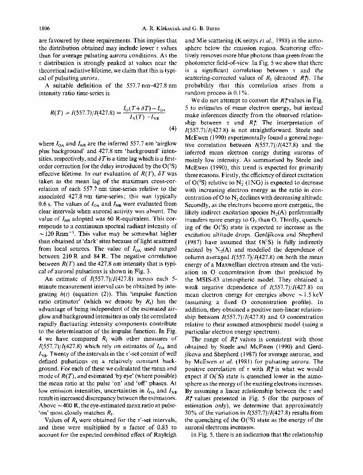
In Fig. 8, z’ and P are plotted against the corrected 1(557.7)/1(427X) value, Rf. No correlation of r’ with RF is apparent and there is only a weak correlation (probability of this arising from a random process is 18%) supporting a decrease in P as Rrdecreases. It is difficult to determine the dependence of the indirect process on the incident electron energy because of the uncertainty in the determination of the r’ and P parameters and because of the mathematical interdependence of these parameters, as discussed above. We investigated an energy dependence of P at a fixed r’ of 0.125 s (to reduce the influence of the ‘fit process’ induced interdependence of parameters), and looked for an energy relation of the indirect process parameters on a particular day (in an attempt to minimise the variability in background conditions, such as the 0 concentrations and atmospheric scattering). No approach yielded a significant correlation.

6. CONCLUSIONS

We have investigated if measurement noise, by itself or in combination with non-linear processes relating the 0(‘S’D) and Nl (ING) emissions, can influence determination of the existence and magnitude of an 0(‘S) indirect excitation process. We found that if the 0(‘S) state were solely directly excited and an amount of noise equivalent to our measured emissions were added to modelled time-series, then our analysis procedure interpreted this as a very short time-constant (average of 0.04 s) indirect process responsible for approximately 50% of the 0(‘S) excitation. This quantifies, for our most reliable data, the result of Burns and Reid (1984) that noise on the measured emissions results in a rounding of the determined impulse which may be mis-interpreted as the signature of an indirect process. For our carefully selected data, non-linear effects have no additional influence beyond that of measurement noise on estimates of the effective lifetime of the indirect species, r’, and the percentage


0.10 0.15 Indirect Effective Lifetime, T’ (s)

Fig. 7. Contours of the mean rms residual in the P-r’ plane for the simulation described in Section 5 applied to the data for 16 July 1988 1315-1320 UT. The contour values are in units of SK’. The global

minimum rms residual occurs for P = 40% and T’ = 0.15 s.

contribution of an indirect excitation process to the excitation of the O(]S) state, P. After allowing for the influence of measurement noise, we still found a significant contribution from an indirect excitation process. We measured an average z’ of 0.13 s and an average P of 58%. The z’ value is longer by 0.03 s and the P value lower by 14%, than average values obtained if no allowance is made for the influence of measurement noise.

We obtained a distribution of the 0(‘S) effective lifetime, z, that has a sharp cut-off near the theoretical free-space radiative lifetime. The z distribution has a mean value of 0.71 s and a standard deviation of 0.05 s. A non-linear contribution to the covariance of the 0(‘S’D) and N: (ING) (0,l) emissions is responsible for a greater uncertainty in the estimates of the 0(‘S) effective lifetime than the mathematical uncertainties of the fitting process. By using simulated data having a higher level of non-linearity than expected experimentally, we have shown that the z distribution may be broadened by the increased uncertainty in the individual z estimates, but that the mean is stable.

A positive correlation exists between the 0(‘S) effective lifetime and the ratio of the pulsating part of the O(‘S’D) and NC (ING) (0,l) emissions. This implies that the 0(‘S) effective lifetime decreases as the average energy of the incident electrons increases, implying a lower altitude in the atmosphere. A linear fit to the entire r’-set data implies that -30% of the variation in 1(557.7)/1(427.8) results from the quenching of the state as the energy of the aurora1 electrons increases. There is evidence that variations between observation sessions, perhaps in the concentration of atomic oxygen or variations in the level of atmospheric scattering, have contributed to lessening this value. Data from the 16 July 1988 indicate that - 55% of the variation of 1(557.7)/1(427X) results from quenching of the 0(‘S) state. This value appears to be more typical. Conversely, of the order of 45% of the variation in 1(557.7)/1(427.8) must result from a relative decrease in the production of 0(‘S) at lower altitudes. This may result from a decrease in the abundance of atomic oxygen relative to molecular nitrogen or a decreased contribution from an indirect


(a)

0.0 3 4 5 6

T +:: I

, :: :: 8 I :: T

T----+’ c-_l-

T rT,

(b)

i

oh ” 1 ” ” 1 ” ” I ““I 3 4’ 5 6 7

1(557.7)/I(427.8) Ratio Estimator R; Fig. 8. (a) Indirect effective lifetime, 7’, obtained using the method described in Section 5, as a function of the 1(557.7)/1(427.8) intensity ratio estimator RE (b) As for (a), except showing the inferred percentage of indirect excitation, P, as a function of Rf. The error limits on 7’ and P are the f lu values provided in

Table 1 for the associated observed data, and as such, are lower limits.

excitation process, or a combination of such effects. We have determined 1(557.7)/1(427X) as the inte-

gration of the impulse function, h(l), relating the two aurora1 emissions. An advantage of this technique is that the value obtained does not depend on an estimation of airglow or background contributions to the two emissions, as only the rapidly fluctuating components contri’bute to the evaluation of h(t).

We could not substantiate an energy dependence of the parameters of the indirect excitation process. Individual measurements of the indirect process contribution are found to be variable because of a mathematically poorly c’onstrained fit. We note the negative correlation of the t’ and P parameters which may result from the mathematical difficulty of fitting the short time-constant exponential term to an impulse response function.

Acknowledgements-The constructive comments of both ref- erees led us to develop the technique for allowing for the effect of noise on the data without constraint on the lifetime of the indirect process or its percentage contribution to excitation of the 0(‘S) state. The impulse analysis algorithm used in this research was developed by John Reid. Dick Gattinger of the National Research Council, Ottawa, Canada, assisted by providing a model of the spectral profiles of the N: (ING) emission bands. Denis O’Brien and Ross Mitchell of the CSIRO Division of Atmospheric Research, Melbourne, Australia helped with discussions concerning atmospheric scattering. The photometer was originally designed by Andre Phillips and the late Fred Jacka. Jon Reeve, Stephen McBurnie, and Ricky Besso provided invalu- able assistance with the installation of the photometer equip- ment at Macquarie Island. Jon Reeve provided additional support during the observing programme. ARK wishes to thank the 1988 and 1989 Macquarie Island ANARE expe- ditioners for their comradeship during the experimental phase of this project. We express our thanks to those others who have assisted with the research reported here.

1814 A. R. Klekociuk and G. B. Bums

Bevington, P.

Brekke, A.

REFERENCES

1969

1973

Brekke, A. and Pettersen, K. 1972

Burns, G. B. and Reid, J. S. 1984

Bums, G. B. and Reid, J. S. 1985

Donahue, T. M., Parkinson, T. D., Zipf, E. C., 1968 Doering, J. P., Fastie, W. G. and Miller, R. E.

Gerdjikova, M. G. and Shepherd, G. G. 1987

Henriksen, K. 1973

Henriksen, K. 1974

Johnstone, A. D.

Kneizys, F. X., Shettle, E. P., Abreu, L. W.,

1983

1988 Chetwynd, J. H., Anderson, G. P., Gallery. W. 0 Selby, J. E. A. and Clough, A. A.

McEwen, D. J., Duncan, C. N. and Montalbetti, R. 1981

Nicolaides, C., Sinanoglu, 0. and Westhaus, P. 1971

O’Neil, R. R., Lee, E. T. P., and Huppi, E. R. 1979

Paulson, K. V., Chang H. and Shepherd, G. G. 1990

Paulson, K. V. and Shepherd, G. G. 1965

Parkinson, T. D.

Rees, M. H., Stewart, A. I., and Walker, J. C. G.

Rees, M. H., Walker, J. C. G., and Dalgarno, A.

Shepherd, G. G., Paulson, K. V., Brown, S., Gault, W. A., Moise, A., and Solheim, B. H.

’

1971

1969

1967

1991

Solheim, B. H. and Llewellyn, E. J. 1979

Steele, D. P. and McEwen, D. J. 1990

Zipf, E. C. and McLaughlin, R. W. 1978

Data Reduction and Error Analysis for the Physical Sci- ences. McGraw-Hill, New York. 235.

A discussion of the energy transfer from Nz (A’Z: ) to 0(‘S) in pulsating aurora. Planet. Space Sci. 21,698- 702.

A possible method for estimating any indirect process in the production of the 0(‘S) atoms in aurora. Planet. Space Sci. 20, 1569-I 576.

Impulse response analysis of 5577 A emissions. Planet. Space Sci. 32, 5 15-523.

A comparison of methods for calculating 0(‘S) lifetimes. Aust. J. Phys. 38,647456.

Excitation of the amoral green line by dissociative recombination of the oxygen molecular line : analysis of two rocket experiments. Planet. Space Sci. 16, 737-747.

Evaluation of aurora1 5577-A excitation processes using Intercosmos Bulgaria 1300 satellite measurements. J. geophys. Res. 92,3367-3374.

Photometric investigation of the 4278 8, and 5577 8, emissions in aurora. J. atmos. terr. Phys. 35, 1341b 1350.

The reaction of nitric oxide with atomic nitrogen as a possible excitation source of the aurora1 green line. J. atmos. terr. Phys. 36, 1437-1439.

The mechanism of pulsating aurora. Ann. Geophys. 1, 397410.

Users guide to LOWTRAN7, Technical Report AFGL-TR-88-0177, Air Force Geophysics Labora- tory, Massachusetts.

Aurora1 electron energies: comparison of in situ measurements with spectroscopically inferred energies. Can. J. Phys. 59, 1116-l 123.

Theory of atomic structure in electron correlation. IV. Method for forbidden transition probabilities, with results for [01], [OH], PI], [NH] and [CI]. Phys. Rev. A. 4, 14Ot%l410.

Aurora1 0(‘S) production and loss processes : ground- based measurements of the artificial aurora exper- iment Precede. J. geophys. Res. 84,823-833.

The evaluation of time-varying parameters pertinent to the excitation of 0(‘S) in aurora. Planet. Space Sci. 38, 161-172.

A cross-spectral method for determining the mean lifetime of metastable oxygen atoms for photometric observations of quiet aurorae. J. atmos. terr. Phys. 27,831-841.

A phase and amplitude study of aurora1 pulsations. Planet. Space Sci. 19,251-255.

Secondary electrons in aurora. Planet. Space Sci. 17, 1997-2008.

Aurora1 excitation of the forbidden lines of atomic oxygen. Planet. Space Sci. 15, 1097-l 110.

Identification of the aurora1 0(‘S) precursor in photometric time sequences of pulsating aurora. Geophys. res. Lett. 18, 1939-1942.

An indirect mechanism for the production of 0(‘S) in the aurora. Planet. Space Sci. 27,473-479.

Electron amoral excitation efficiencies and intensity ratios. J. geophys. Res. 95, 10,321-10,336.

On the dissociation of nitrogen by electron impact and e.u.v. photo absorption. Planet. Space Sci. 26, 449% 462.

Parameters of the O( 1S) excitation process deduced from photometer measurements of pulsating aurora

Documents

Transcript of Parameters of the O( 1S) excitation process deduced from photometer measurements of pulsating aurora