Pain or gain? Short-term budgetary effects of surprise inflation

Kiss, Gábor P.

Working Paper

Pain or gain? Short-term budgetary effects ofsurprise inflation - The case of Hungary

MNB Occasional Papers, No. 61

Provided in Cooperation with:Magyar Nemzeti Bank, The Central Bank of Hungary, Budapest

Suggested Citation: Kiss, Gábor P. (2007) : Pain or gain? Short-term budgetary effects ofsurprise inflation - The case of Hungary, MNB Occasional Papers, No. 61, Magyar NemzetiBank, Budapest

This Version is available at:http://hdl.handle.net/10419/83545

Standard-Nutzungsbedingungen:

Die Dokumente auf EconStor dürfen zu eigenen wissenschaftlichenZwecken und zum Privatgebrauch gespeichert und kopiert werden.

Sie dürfen die Dokumente nicht für öffentliche oder kommerzielleZwecke vervielfältigen, öffentlich ausstellen, öffentlich zugänglichmachen, vertreiben oder anderweitig nutzen.

Sofern die Verfasser die Dokumente unter Open-Content-Lizenzen(insbesondere CC-Lizenzen) zur Verfügung gestellt haben sollten,gelten abweichend von diesen Nutzungsbedingungen die in der dortgenannten Lizenz gewährten Nutzungsrechte.

Terms of use:

Documents in EconStor may be saved and copied for yourpersonal and scholarly purposes.

You are not to copy documents for public or commercialpurposes, to exhibit the documents publicly, to make thempublicly available on the internet, or to distribute or otherwiseuse the documents in public.

If the documents have been made available under an OpenContent Licence (especially Creative Commons Licences), youmay exercise further usage rights as specified in the indicatedlicence.

MNB

Occasional Papers

61.

2007

GÁBOR P. KISS

Pain or Gain? Short-term Budgetary Effects

of Surprise Inflation – the Case of Hungary

Gábor P. Kiss

Pain or Gain? Short-term Budgetary Effects

of Surprise Inflation – the Case of Hungary

January 2007

The views expressed here are those of the authors and do not necessarily reflect

the official view of the central bank of Hungary (Magyar Nemzeti Bank).

Occasional Papers 61.

Pain or Gain? Short-term Budgetary Effects of Surprise Inflation – the Case of Hungary*

(Kín vagy kincs? Az inflációs meglepetés rövid távú hatása az államháztartásra – Magyarország esete)

Written by: Gábor P. Kiss

(Economics and Research D.)

Budapest, January 2007

Published by the Magyar Nemzeti Bank

Publisher in charge: Gábor Missura

Szabadság tér 8–9. Budapest 1850

www.mnb.hu

ISSN 1585-5678 (on-line)

* The author is indebted to Viktor Várpalotai for his valuable comments, and Balázs Párkányi, Zoltán M. Jakab and the

participants of the discussions at the Central Bank of Hungary. All remaining errors are the author’s responsibility.

Summary 5

1. Introduction 7

2. The scope of the study 9

2.1. The coverage of the study 9

2.2. The grouping of budget revenues and expenditures 10

2.3. Definition of the inflation surprise and the episodes 13

3. The assumed effect of surprise inflation on the deficit 15

3.1. Revenues and expenditures depending on private sector decisions 16

3.2. Items determined by decentralised government decisions 21

3.3. Items determined by the government 22

3.4. A summary of the breakdown of revenues and expenditures 24

4. The estimated effect of inflation in the years under review 25

4.1. Nominal-type items 25

4.2. Wage and consumption compensation in the private sector 25

4.3. Compensation of decentralised expenditures and revenues 29

5. Results 39

Bibliography 41

Annex 43

MNB OCCASIONAL PAPERS 61. • 2007 3

Contents


I study the short-term impact of surprise inflation on the primary balance by separating those budgetary items which

immediately respond to inflation from non-responding ones. I assume a passive fiscal policy in a one-year horizon;

therefore items fully controlled by the central government are treated as non-responding ones. In the case of the private

sector and decentralised government, their responses to inflation depend on decisions.

If a 1 percentage point inflation surprise is compensated in the private sector by an increase in wages and

consumption, then the nominal increase of the related tax revenue is equivalent to 0.26% of the GDP, i.e. their real value

and their proportion to the increase of the nominal GDP remains unchanged. Otherwise, the nominal value of the

revenue remains unchanged, resulting in a decrease in its real value and an increase in the deficit-to-GDP ratio by

0.26%. Compensation decided in a decentralised government has the opposite effect, because if it is implemented,

then the real value of decentralised expenditure and its proportion to the GDP remains the same through an increase

in the nominal expenditure, while if the nominal expenditure is fixed, it results in a decrease of the real expenditure and

approximately a 0.13% decrease in the deficit-to-GDP ratio. The fixing of the other nominal expenditure, which does not

respond to inflation, results in a 0.08% decrease in the GDP-proportionate expenditure and deficit compared to an

increase in the nominal GDP.

Reviewing certain episodes in Hungary, we have found that owing to planning errors, the official inflation forecast usually

resulted in a larger ‘surprise’ for the budget than for the private sector. Thus, at the time of the impact of the surprise on

the budget, the private sector experienced either no surprise or very little, which if materialising was in most cases

immediately compensated for. An exception in this case was the adjustment in 1995 – supported by an inflation surprise

– when the ratio of the moderately increasing nominal tax revenue to the GDP and its real value significantly decreased.

The increase of indirect taxes had an adversary effect on the increase in nominal consumption (inflationary

compensation) (1995 and 2004). In addition to moderating consumption, the indirect tax increase in mid-2006 can also

moderate wages in real terms since it was announced after the usual wage increases.

The decentralised government behaved similarly, as indicated by the experiences in the developed OECD countries.

The response of the decentralised government to the moderate nominal increase in central government transfers (i.e. to

the decrease in real value of their funds) was to moderate the nominal increase of decentralised expenditure, i.e. real

value loss was for the most part not compensated for. The rate of compensation was larger in those years when cheap

financing was available (funds from privatisation in 2000), or when the surprise was not sizeable and coincided with the

uprising phase of the election-related investment cycle (1998). In 2007 the optimistic inflation projection can result in

lower-than-planned central transfers in real terms, which can in turn moderate the nominal increase of decentralised

expenditure. Presumably, however, the size of the planning error and its deficit-decreasing effect will be not significant.

Keywords: surprise inflation, inflation sensitivity, decentralised government.

JEL: E31, E65, H61, H71, H72.

Summary

MNB OCCASIONAL PAPERS 61. • 20076

Az inflációs meglepetés elsõdleges deficitre gyakorolt rövid távú hatását vizsgálva különválasztom a magyar költségve-

tésben azokat a bevételi és kiadási tételeket, amelyek az inflációt követik, és amelyek azonnal nem reagálnak. Egyéves

horizonton a kormányzat által kontrollált tételeknél nem reagáló kormányzati politikát feltételezek, ezért ezeket nominális

típusú tételeknek minõsítem. A decentralizált államháztartás és a magánszektor esetében azonban döntéstõl függ, hogy

az infláció évközi kompenzációja megvalósul-e.

Amennyiben a magánszektor a bér és fogyasztás növelésével kompenzál egy 1 százalékpontos inflációs meglepetést,

akkor az ehhez kapcsolódó adóbevételek nominálisan a GDP ¼%-ával nõnek, vagyis megtartják reálértéküket és a no-

minálisan növekvõ GDP-hez mért arányukat. Ellenkezõ esetben a bevétel nominálisan változatlan marad, így a bevétel

reálértékének csökkenése és ezáltal a GDP-arányos deficit ¼%-os növekedése következik be. Ellentétes hatású a de-

centralizált államháztartási körben elhatározott kompenzáció, ha ugyanis erre sor kerül, akkor a kiadások nominális nö-

velése révén a decentralizált kiadás tartja meg reálértékét és GDP-arányát, a kiadás nominális rögzítése azonban a ki-

adás reálértékének csökkenését és a GDP-arányos deficit mintegy 0,13%-os csökkenését eredményezi. Az inflációra

nem reagáló kiadások nominális rögzítése a növekvõ nominális GDP-hez viszonyítva a GDP-arányos kiadás és hiány

0,08%-os csökkenését eredményezi.

Konkrét magyar epizódokat vizsgálva azt találtam, hogy a meglepetés gyakran aszimmetrikus volt, a hivatalos inflációs

prognózis a tervezési hiba miatt nagyobb „meglepetést” eredményezett az államháztartásban, mint amekkora a magán-

szektor várakozásaihoz képest bekövetkezett. Az államháztartási meglepetés idején a magánszektort vagy nem érte

meglepetés, vagy kisebb mértékû volt, és az így adódó értékvesztést azonnal kompenzálta. A kivétel az 1995. évi – inf-

lációs meglepetéssel támogatott – kiigazítás, amikor a mérsékelten növekvõ nominális adóbevételek GDP-aránya, reál-

értéke jelentõsen csökkent. A fogyasztás nagyobb nominális növekedése, kompenzációja ellenében hatott, hogy az inf-

láció hátterében indirekt adók emelése állt (1995 és 2004). A 2006-os indirektadó-emelés a fogyasztás mellett visszafog-

hatja a bérek reálnövekedését is, mert azt a béremeléseket követõen jelentették be.

A decentralizált államháztartás viselkedése hasonló volt ahhoz, amit a fejlett OECD-országok tapasztalatai mutatnak. A

központi támogatások mérsékelt nominális növekedésére (reálértéknek csökkenésére) a decentralizált kör úgy reagált,

hogy kiadásainak nominális növekedését mérsékelte, vagyis a reálértékvesztést nagyrészt nem kompenzálta. 1995–96-

ban a decentralizált kör kiadásait még a támogatáskiesésnél is nagyobb mértékben fogta vissza annak érdekében, hogy

az 1994-es deficitet megszüntesse. A mérsékelt összkiadáson belül azonban a mûködési – és esetenként a beruházási

– kiadásoknál mégis történhetett részleges kompenzáció; becslésem szerint a támogatáskiesésbõl az inflációs megle-

petésnek tulajdonítható rész egyötödét tudták azonnal ilyen típusú kiadásaik nominális növelésével kompenzálni. Ezt fe-

le részben fedezte a saját bevételek növekedése, ami azonban zömmel csak a következõ évben valósult meg. Maga-

sabb kompenzáció azokban az években történt, amikor olcsó finanszírozás állt rendelkezésre (privatizációs bevétel

2000-ben), vagy pedig a meglepetés kismértékû volt és egybeesett a választáshoz kötõdõ beruházási ciklus felszálló

ágával (1998). 2007-ben az optimista inflációs prognózis – a központi támogatáson keresztül – csökkentheti a decentra-

lizált államháztartás kiadásait. Feltehetõen azonban a tervezési hiba, és ennek egyenlegjavító hatása csekély mértékû

lehet.

Kulcsszavak: meglepetés infláció, inflációs érzékenység, decentralizált államháztartás.

JEL: E31, E65, H61, H71, H72.

Összefoglalás


Similar to the effect of the economic cycle through automatic stabilizers, inflation has significant impact on the budget in

most countries. The greater part of budgetary revenue is determined by nominal changes in wages and consumption in

the private sector, which is determined by inflation, too. Accordingly, in addition to a ‘growth dividend’, an ‘inflation

dividend’ may also appear on the revenue side. The larger part of the expenditures, however, is determined by

government decisions and not by the cycle or the inflation; the question is how a ‘neutral’ expenditure increase can be

separated from the impact of discretionary decisions (Buti and van den Noord

1

, 2003).

As regards the impact of inflation on budget deficit, the results of empirical investigations are rather varied in respect of

the OECD countries. According to some results, inflation has no significant effect on the deficit (e.g. Tujula-Wolswijk,

2004). Other studies, however, suggest that neither revenue nor expenditure respond either to past or to current inflation

(e.g. Mélitz, 2000). Alesina and Perotti (1995), on the other hand, show that a 1% acceleration of inflation has the impact

of a 0.05 percentage point decrease in the expenditure-to-GDP ratio, a 0.02 percentage point decrease in the revenue-

to-GDP ratio, and consequently a 0.03 percentage point decrease in the deficit. At the country level, however, the results

are different (Virén, 1998). In the majority of the countries, accelerating inflation caused the deficit to decrease, yet in a

few countries it just had the opposite effect. Virén argues that the deficit-decreasing effect was probably attributable to

the automatic effect of inflation on revenue and expenditure and not to the effect of discretionary decisions; however, he

fails to support his assumption with evidence.

Various factors may underlie the wide differences in these results. On the one hand, the direction of causality is

ambiguous, which means that the budget – in particular its composition, the changes in indirect taxes – also has an effect

on inflation. On the other hand, inflation works not only through automatisms, but it also exercises influence on the deficit

via discretionary decisions taken in the public and the private sectors. These decisions may be different in the short term

depending on whether it is an inflation surprise, or if inflation was as expected.

A significant part of the expenditure and the non-ad valorem tariffs

2

are fixed for a year in advance, taking into account

expected inflation. Thus an inflation surprise results in a decrease in real value with the nominal value remaining

unchanged. This, however, can be counterbalanced by discretionary decisions on increasing expenditure, which may

be described as ‘inflation compensation’.

The funds to be used as an ‘inflation compensation’ of fixed items are not necessarily available on the revenue side,

because an ‘inflation dividend’ is not always generated. If wages and consumption in the private sector do not follow the

surprise inflation in the short term, then the higher growth rate of the other components of the GDP (corporate income,

investment, net exports) may not have any effect because, owing to the very different effective tax burden on the different

tax bases, a composition-effect of this type puts a restraint on the nominal increase of the total revenue in the budget

(decrease in the revenue-to-GDP ratio) (P. Kiss-Vadas, 2004).

An ‘inflation dividend’ is generated if wages and consumption are compensated mid-year. The rate of nominal revenue

growth is, however, influenced by two inverse automatisms. On the one hand, a unit increase of wages, in the case of

progressive personal income tax, increases the nominal revenue at a rate exceeding the unit increase (owing to bracket-

creeping). The Olivera-Tanzi effect, however, has a restraining effect – the rate of growth of inflation does not immediately

increases the nominal revenue. Mélitz believed that the two opposing effects must have been similar in magnitude

because he found no revenue response to inflation (Mélitz, 2000).

1. Introduction

1

According to the OECD (Buti and van den Noord, 2003), in common with the output gap, the inflation gap (the difference between the expected inflation

and the inflation at normal capacity utilisation) may also serve for the calculation based on the tax elasticity of a revenue component, the so-called inflation

dividend, which may be set off against additional expenditure or a decrease deemed by us as neutral. An additional discretionary measure can ex ante

be distinguished from this neutral extra expenditure or hold back. Ex post, however, a revenue component and a discretionary measure can similarly be

assigned to surprise inflation.

2

These tariffs are expressed in units (e.g. litres of fuel or number of employees), independently from the values, e.g. sales or salary.

MAGYAR NEMZETI BANK


Calculations were made regarding automatic effects of expected or unexpected inflation. In Sweden, for example, in the

assumed case of an inflation level higher by 10 percentage points, real expenditure would have decreased owing to the

expenditure indexation technique, while the real value of revenue would have increased at a similar rate. This is mainly

owing to the positive resultant in Sweden of the two opposing effects on taxes (see Annex, Table 25). In relation to

unexpected inflation, the Member States of the European Union regularly publish calculations in their Stabilisation and

Convergence Programmes about the effect of a presumed difference of 1 percentage point compared to the forecast.

In the specific countries, the automatic response to inflation of the tax system and the expenditure side is greatly

determined by the actual solutions – i.e. indexation and nominal fixing.

In what follows, I study the specific effect of unexpected inflation –assuming a 1 percentage point difference – in Hungary

(for similar earlier results, see Kovács, 2005, and Table 24). From among the decisions made in the private sector, I

examine whether the inflation surprise is compensated for mid-year with a nominal increase in wages and consumption,

because this is decisive in terms of tax revenue. I provide figures in respect of the relatively independent local

governments and institutions in order to establish whether the effect of higher inflation is compensated for through the

nominal increase in their decentralised expenditure. However, I do not take into account the alternative options of similar

decisions by the government.

3

By assuming a passive fiscal policy (i.e. one not responding to an inflation surprise), only

those central expenditures are examined, the changes of which are determined by automatisms.

The calculation related to the alternative cases is supplemented with the investigation of those years when an inflation

surprise occurred, or when the inflation forecast underlying the Budget Law proved to be underestimated. All cases but

one occurred under tight (or neutral) fiscal policy. Tight fiscal policy resulted in a decrease of central transfers provided

to local governments. It is important to examine how local governments responded to this restraint and, more specifically,

to the effect of the inflation-related planning errors. The experiences obtained in developed OECD countries show that

the decentralised government sub-sector mainly responds to the decrease in central transfers by restraining expenditure

– among others on investment – while its revenue from fees is not raised and the tax receipts are only increased partly

and with lags (Darby et al., 2004).

This study is structured as follows. Chapter 2 specifies the scope of the study, looking at the grouping of budget

revenues and expenditures, and defining the inflation surprise and the episodes examined. Chapters 3 and 4 look at the

assumed and actual effects respectively of surprise inflation on the budget deficit in individual years. Finally, Chapter 5

summarises the results and compares them to the results of other similar studies.

3

If the effect of inflation improves (worsens) the deficit, the government may use it for extra expenditure (reduction of the expenditure), but it may also

choose not to respond, that is, to allow the deficit to improve (worsen).


2.1. THE COVERAGE OF THE STUDY

In this study, I investigate how budget revenues and expenditures react over a one-year time horizon – taking into

account the effects of automatic carryovers as well – to an unexpected increase in the consumer price index. I calculate

with 1-1 percentage point rates in the case of the inflation surprise affecting the private sector and in the case of the

underestimation of the government’s official forecast. I do not take into account the possible triggers of the surprise (e.g.

oil price rises, exchange rates, etc.). Owing to the annual character of the Budget Law, I focus on annual developments,

thus defining the inflation ‘shock’ at the level of average annual inflation. The same 1% average annual excess inflation

may develop in different ways; either as a result of 1% inflation at the beginning of the year, or of a 2% increase in the

price level in the middle of the year. In the first case, it may happen that wages and consumption in the private sector

and the expenditure of the decentralised government immediately compensate for the effect of the surprise, while in the

latter case, across-the-board wage compensation is unlikely.

In Chapter 3, I seek to find what effect alternative assumed cases of a 1 percentage point inflation surprise have on the

primary balance.

4

Assuming a passive fiscal policy, I disregard the secondary effect when the government may respond

to the primary effect with discretionary measures, for example, by using the ‘inflation dividend’ originating from the

nominal increase of taxes in the private sector for inflation-related compensation of the central expenditure.

5

Taking into account the volatility of past discretionary measures, the assumption of a passive fiscal policy is just such a

limitation in our case, which allows us to interpret the results only on a short-term basis. The calculations are, therefore,

made in respect of effects arising in the relevant year, but also include effects that have an impact in the next year too,

which automatically arise – even in the case of a passive fiscal policy.

6

This extended estimation shows the overall impact

of the inflation surprise on the initial level of the primary balance in the next year.

The extreme values in the alternative, assumed cases depend on whether the private sector compensates for the inflation

surprise in nominal wages and consumption (resulting in an inflation dividend), or whether any inflation compensation

occurs in relation to the nominal expenditure and revenue of the participants of the decentralised government.

In Chapter 4, when investigating actual episodes, the assumptions are resolved on the one hand, by taking into account

the date when the surprise arose during the year and, on the other hand, by taking into account the fact that the rate of

official underestimates in most cases actually exceeded the rate of the inflation surprise, and finally by distinguishing the

cases of surprises caused by indirect tax increases, because this in itself diminishes the probability of consumption

compensation.

I provide an estimate regarding the compensation rate in the private sector and the decentralised government, i.e. I attempt

to locate the most likely value in the range between the assumed extreme values. Owing to the small number of cases,

however, caution must be exercised when making conclusions as to the determinants of the rate of compensation.

2. The scope of the study

4

It is essentially the same as the 'impact effect' investigated by Persson et al. (1996). They investigated how sizeable measures can be subtituted by the

inflation effect, but unlike us, over a four-year time horizon.

5

The government may respond in a very different way if a fiscal rule prevails. If the rule applies to the balance and the government aims at comply with

the rule, then it immediately utilises any mid-year balance improvement, and compensates for any balance deterioration by taking measures. If the rule

applies to expenditure, limiting its nominal increase, then no compensation is made in respect of the expenditure side either during the year or in the next

year. In our case, there are no such rules, and therefore it depends on decisions whether any balance improvement is used by the government

immediately or in the next year (e.g. for extra expenditure), or whether the deficit is allowed to improve. Persson et al. (1996) assumed that the impact of

a higher inflation rate on the budget (i.e. savings) is permanent; therefore, they also expressed the components of this effect in net present value.

6

We calculated with a carryover, on the one hand, in the case of those items that are determined by the wages in the preceding period (unemployment,

sickness and child benefit, retrospective pension indexation), and, on the other hand, in the case of the phasing-out of the transitional effects (the Olivera-

Tanzi effect).

MAGYAR NEMZETI BANK


2.2. THE GROUPING OF BUDGET REVENUES AND EXPENDITURES

In principle, nominal revenues and nominal expenditures in the budget can be divided into two categories: the ‘real-type’

revenue (P · t), and ‘real-type’ expenditure (P · g) determined automatically by the price level (P), such as, for example,

pensions indexed to inflation.

7

‘Nominal-type’ revenue (T) and ‘nominal-type’ expenditure (G) are not determined by

inflation, e.g. nominally fixed transfers. The balance (B) can be stated as follows:

B = (T + P · t ) – (G + P · g). (1)

Owing to inflation (π), the nominal values of real-type items change as follows:

∆B = (π · t + P · ∆t) – (π · g + P · ∆g). (2)

Nominally fixed items do not change, whereas real-type items may respond in two different ways. On the one hand, items

fully indexed to inflation follow the rise in prices (π · t, π · g), hereinafter marked as: P · t*, P · g*. On the other hand, the

changes in the price level have an effect on the real developments themselves and may change them (P · ∆t and P · ∆g).

The balance following the surprise inflation (B1) may be stated as follows:

B1

= B0

+ ∆B, (3)

where B1

is the nominal deficit developed under the inflation surprise, ∆B is the estimated effect of the inflation surprise,

and B0

is the nominal deficit that would have occurred without the inflation surprise. To enable comparison between

years, it is expedient to express it in the normal form, which can be done by dividing by GDP.

iA

= ∆B/Y0

, (4)

where Y0

is the GDP level without the inflation surprise.

The indicator applied in this paper takes the difference between the proportion of the balance and the GDP with and

without the inflation surprise (Y1 is the GDP level after the inflation surprise):

iB

= B1

/Y1

– B0

/Y0

. (5)

Box Two kinds of indicators: when do

they have the same results?

The iA

indicator takes the balance of the nominal changes in revenues

and expenditures and divides it by the nominal GDP level excluding

the inflation surprise.

For the sake of simplicity, assume that there are only nominally fixed

(T, G) and fully indexed items (P · t* and P · g*). In this case, the iB

indicator can be expressed by rewriting formula (5) as

iB

= –πu · (T + P

1 · t* )/Y1

– (–πu · [G + P

1 · g*]/Y1), where the inflation

surprise πu

= (P1/P

0) – 1.

Assuming (Y1/Y

0) – 1 = π

u, then P

1 · t*/Y1

= P0 ·

t*/Y0, i.e. the

proportion of the indexed items to GDP does not change, while the

proportion of nominal-type items to GDP decreases, ∆T= T/Y1

– T/Y0

and ∆G = G/Y1

– G/Y0. Then i

B= –π

u · T/Y1

– (–πu · G/Y

1).

The results of the two indicators are the same (iA

= iB), if the balance

were in balance without the surprise, then the B0

= 0, and

(Y1/Y

0) – 1 = π

uassumptions are realised.

The problem is that the latter assumption cannot be checked; it is

unknown how the inflation surprise effects real GDP and the other

factors of the GDP deflator. The following example shows to what

extent the result is modified if a 1% surprise increases the actual

nominal GDP by 1% or by 0.5%.

7

In their study, Persson et al. (1996) divide revenue and expenditure into normal and real-type items. Since, in the case of Sweden, indexation is delayed

and partial, therefore, these items could not be deemed as being of the real type.

The changes in the price level have an effect on real developments themselves and change them. Within these

changes, as regards the effect on budget balance, I examine the effect of those compensation decisions that affect

wages and consumption as well as the items of the decentralised government. To this end, I break down revenues

and expenditures, depending on how inflation affects them (see the next chart). Inflation expectations affect part of

the tax revenue (P · tp

) and non-discretionary expenditure (P · gp

) through activities in the private sector. The official

inflation projection produces its effect through the four channels listed in the right column, namely: administered price

increase, valorisation of the nominal parameters of tax and transfer systems, and the increase of intra-governmental

and final expenditures.

8

These directly determine the centrally determined expenditure and the non-tax revenue

(G and T), and indirectly affect other expenditures and revenues by influencing the private sector and the

decentralised government (P · td

and P · gd

).

THE SCOPE OF THE STUDY


If Y0

=100 and Y1

=101, then the two methods yield the same results:

If Y0

= 100 and Y1

= 100,5, then the result hardly changes, but T/Y1

will decrease less compared to T/Y0, which is offset by the increase of the

proportion of real-type items to GDP, P1· t*/Y

1> P

0· t*/Y

0. Note that only the surplus-to-GDP ratio has been changed, without changing the

nominal values (∆B) and T and G in Table A. The result is therefore expressed in a different GDP-proportionate composition.

The two indicators differ from each other if the initial balance (B0) is not zero, because then the balance of the items taken into account in

respect of the first indicator (P ·t* - P ·g*) is not complementary to the balance of the items taken into account when calculating the second

indicator. If the expenditure is decreased by 1 in the above example, then in the case of a 1.5% initial primary surplus, the first indicator shows

a 0.220 balance improvement, and the second a 0.214 balance improvement. The majority of the years included in the investigation were

characterised by similarly low primary surpluses (“normal” years), except for 1996, when the balance was more favourable, and 2004, when

the balance was less favourable. In 1996 and 2004 the difference between the results of the two methods is twice or three times larger than in

the “normal” years.

T P · t* G P · g* B

Nominal value without surprise 13 30 34 9 0

Nominal value with surprise 13 30.3 34 9.09 0.21

Nominal difference 0 0.3 0 0.09 0.21

Table A

The development of the nominal values

T P · t* G P · g* B

Nominal difference/Y0

0 0.3 0 0.09 0.21

Ratio to GDP*– πu

-0.13 0 -0.34 0 0.21

Table B

Changes in GDP-proportions under 1% extra GDP

T P · t* G P · g* B

Nominal difference/Y0

0 0.3 0 0.09 0.210

Ratio to GDP*– πu

-0.065 0.149 -0.170 0.045 0.209

Table C

Changes in GDP proportions under a 0.5% extra GDP

8

For the sake of completeness, in the last line we indicate centralised (non-tax) revenues (Tc) as well, which are not fully controlled by the government;

for example, the receipt of EU transfers is determined by external factors as well.

Since we assume a passive fiscal policy, therefore, centrally determined expenditures (G) and revenues (T) are classified

as nominal-type items. In the case of the other items (P · tp

, P · td

, P · gp

and P · gd

), the breakdown according to nominal

and real types requires a more detailed investigation. On one hand, from among the items influenced by decisions by

the private sector, interest expenditure and seigniorage revenue are left out of the scope of the study. On the other hand,

certain expenditures are explicitly indexed to inflation, in other words, they are of the real type. Non-indexed social

transfers are of the nominal type, because in the case of a passive fiscal policy (i.e. one that does not respond to inflation

surprises), they are only determined by such factors – for example demographic factors – that in their case the possibility

of inflation-related compensation can be excluded. Finally, as regards the remaining expenditures and revenues, it is

impossible to know ex ante whether the surprise loss in real value will be compensated for. Although it can be stated ex

post whether there has been a compensation of the items (and if affirmative, they can subsequently be classified as

being of the real type; otherwise, they can be classified as nominal), the uncertainty ex ante will remain. This uncertainty

lies in the decisions of the private sector and the decentralised government. Based on the combinations of the alternative

decisions of these two actors, four basic cases can be calculated in relation to the ex ante effect of surprise inflation.

9

MAGYAR NEMZETI BANK


Inflationary expectation Governmental inflation forecast

Private sector (corporate and

households)

GovernmentPublic companies

Local governments, budgetary units

Administered price increase

Valorisation of the nominal parameters of the tax and transfers system

Intra-governmental transfers

G. Central final expenditure

(Investment, corporate transfer)

P · tp Revenue from taxes and contributions

(from the private sector, public companies)

P · gp Expenditure influenced by the

private sector

((interest, ¾ of the pension, pharmaceuticals,

transport and housing)

P · td Revenue depending on decentralised govt.

+ SSC

(paid by public employers)

T. Centralised revenue

(EU transfers, repayments)

P · gd Expenditure depending from

decentralised govt.

(wage, purchases, ¼ of pension, investment)

9

We do not examine to what extent the decisions of the private sector, the public companies and the budget influence each other, for example, as regards

wage raises. Accordingly, the decisions of the private sector and of the decentralised government are deemed independent in terms of compensation.

In the preceding chart, public companies were also indicated between the private sector and the decentralised

government. It is uncertain, though, in which category to include these companies based on their behaviour. As in the

case of the decentralised government, the operation of these companies is indirectly influenced by the government by

various means. As regards the reviewed period, it can be stated that – in contrast to nominal transfers to the

decentralised government, which increase at a rate below inflation – administered prices had no unfavourable effect on

the revenues of the public companies; prices related to public companies had been raised at a rate not only equivalent,

but exceeding the underestimated inflation forecast.

10

Since, regarding wage agreements, the behaviour of the

companies in question (e.g. Hungarian State Railways, Budapest Transport Company, the postal service) was similar to

that of the private sector, they can be therefore included in the private sector category for the purposes of this study.

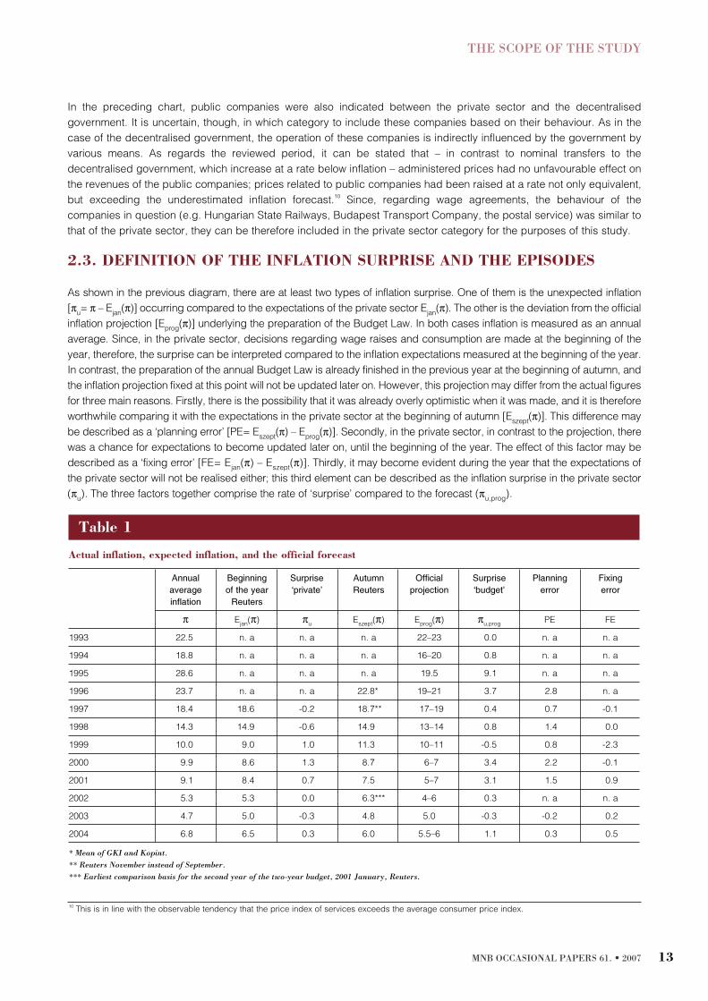
2.3. DEFINITION OF THE INFLATION SURPRISE AND THE EPISODES

As shown in the previous diagram, there are at least two types of inflation surprise. One of them is the unexpected inflation

[πu

= π – Ejan

(π)] occurring compared to the expectations of the private sector Ejan

(π). The other is the deviation from the official

inflation projection [Eprog

(π)] underlying the preparation of the Budget Law. In both cases inflation is measured as an annual

average. Since, in the private sector, decisions regarding wage raises and consumption are made at the beginning of the

year, therefore, the surprise can be interpreted compared to the inflation expectations measured at the beginning of the year.

In contrast, the preparation of the annual Budget Law is already finished in the previous year at the beginning of autumn, and

the inflation projection fixed at this point will not be updated later on. However, this projection may differ from the actual figures

for three main reasons. Firstly, there is the possibility that it was already overly optimistic when it was made, and it is therefore

worthwhile comparing it with the expectations in the private sector at the beginning of autumn [Eszept

(π)]. This difference may

be described as a ‘planning error’ [PE= Eszept

(π) – Eprog

(π)]. Secondly, in the private sector, in contrast to the projection, there

was a chance for expectations to become updated later on, until the beginning of the year. The effect of this factor may be

described as a ‘fixing error’ [FE= Ejan

(π) – Eszept

(π)]. Thirdly, it may become evident during the year that the expectations of

the private sector will not be realised either; this third element can be described as the inflation surprise in the private sector

(πu

). The three factors together comprise the rate of ‘surprise’ compared to the forecast (πu,prog

).

THE SCOPE OF THE STUDY


Table 1

Actual inflation, expected inflation, and the official forecast

Annual Beginning Surprise Autumn Official Surprise Planning Fixing

average of the year ‘private’ Reuters projection ‘budget’ error error

inflation Reuters

π Ejan

(π) πu

Eszept

(π) Eprog

(π) πu,prog

PE FE

1993 22.5 n. a n. a n. a 22–23 0.0 n. a n. a

1994 18.8 n. a n. a n. a 16–20 0.8 n. a n. a

1995 28.6 n. a n. a n. a 19.5 9.1 n. a n. a

1996 23.7 n. a n. a 22.8* 19–21 3.7 2.8 n. a

1997 18.4 18.6 -0.2 18.7** 17–19 0.4 0.7 -0.1

1998 14.3 14.9 -0.6 14.9 13–14 0.8 1.4 0.0

1999 10.0 9.0 1.0 11.3 10–11 -0.5 0.8 -2.3

2000 9.9 8.6 1.3 8.7 6–7 3.4 2.2 -0.1

2001 9.1 8.4 0.7 7.5 5–7 3.1 1.5 0.9

2002 5.3 5.3 0.0 6.3*** 4–6 0.3 n. a n. a

2003 4.7 5.0 -0.3 4.8 5.0 -0.3 -0.2 0.2

2004 6.8 6.5 0.3 6.0 5.5–6 1.1 0.3 0.5

* Mean of GKI and Kopint.

** Reuters November instead of September.

*** Earliest comparison basis for the second year of the two-year budget, 2001 January, Reuters.

10

This is in line with the observable tendency that the price index of services exceeds the average consumer price index.

The episodes of the inflation surprise affecting the private sector are as follows:

Between 1993 and 1996, I found no good comparison basis to measure expectations, but their rate was presumably not

far from the official projection. Owing to the size and causes of the surprise in 1995 (indirect tax and administered price

increases, exchange rate depreciation), I discuss this year separately.

The Reuters poll forecasts regarding annual average inflation are available monthly between 1997 and 2004, and thus

the surprise could be determined as the difference between the January forecast and the actual figures.

– The Reuters poll only roughly moves together with the inflation expectations of the employers, so the slight surprise can

be deemed to be within the error margin of +/-10% in all years apart from 2000.

– The likelihood of wage compensation is also influenced by timing, i.e. when the surprise inflation ‘shock’ occurs during

the year.

11

Inflation occurring at the beginning of the year may be immediately taken into account in the usual wage

raises, while the likelihood of mid-year compensation later on is small if the difference is insignificant. Of the four

inflation surprises, only in 2000 did the surprise occur late (the expectations became realistic only in the last quarter).

– The likelihood of consumption compensation is largely influenced if an indirect tax increase underlay the surprise. This

tax increase is the reason for the examination of the year 2004 with only a smaller surprise.

It was much simpler to identify the years in which the official forecast was underestimated. It is typical of forecasts to be

expressed in brackets. In this case, the deviation can be measured to the middle of the range, and the deviation is not

to be regarded as a surprise if the inflation is within the specified range (for example, in 1994, 1997 and 2002). Compared

to this benchmark, the surprise was more significant in 1995, 1996, 1998, 2000, 2001 and 2004, ranging between 1.5-3

percentage points in all years apart from 1995, when the surprise was a real surprise that occurred in the private sector

as well.

So the combined set of years that contains the two kinds of surprise comprises 1995, 1996, 1998, 2000, 2001 and 2004

(these will be discussed in more detail in Chapter 4). Within this set, the alternative, hypothetic calculation based on the

expenditure-revenue composition of the budget will only be performed for the last three years, because the composition

has significantly changed since the earlier period.

MAGYAR NEMZETI BANK


11

No information is available concerning the accurate appearance of the inflation shock during the year, since there is no relevant comparison basis

(Reuters poll). The monthly update of the annual expectations may, however, carry certain information, as expectations rise after the occurrence of a

surprise. The expectations in 1999 and 2004 came close to the final outcome after the first quarter, and in 2001, they even turned pessimistic.

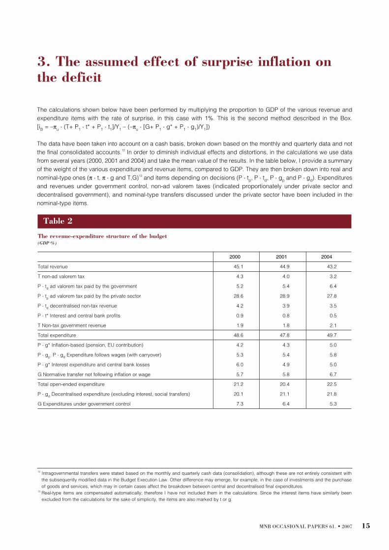
The calculations shown below have been performed by multiplying the proportion to GDP of the various revenue and

expenditure items with the rate of surprise, in this case with 1%. This is the second method described in the Box.

[iB

= –πu

· (T+ P1

· t* + P1

· t1

]/Y1

– (–πu

· [G+ P1

· g* + P1

· g1

)/Y1

])

The data have been taken into account on a cash basis, broken down based on the monthly and quarterly data and not

the final consolidated accounts.

12

In order to diminish individual effects and distortions, in the calculations we use data

from several years (2000, 2001 and 2004) and take the mean value of the results. In the table below, I provide a summary

of the weight of the various expenditure and revenue items, compared to GDP. They are then broken down into real and

nominal-type ones (π · t, π · g and T,G)

13

and items depending on decisions (P · tp

, P · td

, P · gp

and P · gd

). Expenditures

and revenues under government control, non-ad valorem taxes (indicated proportionately under private sector and

decentralised government), and nominal-type transfers discussed under the private sector have been included in the

nominal-type items.


3. The assumed effect of surprise inflation on

the deficit

Table 2

The revenue-expenditure structure of the budget

(GDP %)

2000 2001 2004

Total revenue 45.1 44.9 43.2

T non-ad valorem tax 4.3 4.0 3.2

P · td

ad valorem tax paid by the government 5.2 5.4 6.4

P · tp

ad valorem tax paid by the private sector 28.6 28.9 27.8

P · td

decentralised non-tax revenue 4.2 3.9 3.5

P · t* Interest and central bank profits 0.9 0.8 0.5

T Non-tax government revenue 1.9 1.8 2.1

Total expenditure 48.6 47.8 49.7

P · g* Inflation-based (pension, EU contribution) 4.2 4.3 5.0

P · gp

. P · gd

Expenditure follows wages (with carryover) 5.3 5.4 5.8

P · g* Interest expenditure and central bank losses 6.0 4.9 5.0

G Normative transfer not following inflation or wage 5.7 5.8 6.7

Total open-ended expenditure 21.2 20.4 22.5

P · gd

Decentralised expenditure (excluding interest, social transfers) 20.1 21.1 21.8

G Expenditures under government control 7.3 6.4 5.3

12

Intragovernmental transfers were stated based on the monthly and quarterly cash data (consolidation), although these are not entirely consistent with

the subsequently modified data in the Budget Execution Law. Other difference may emerge, for example, in the case of investments and the purchase

of goods and services, which may in certain cases affect the breakdown between central and decentralised final expenditures.

13

Real-type items are compensated automatically; therefore I have not included them in the calculations. Since the interest items have similarly been

excluded from the calculations for the sake of simplicity, the items are also marked by t or g.

3.1. REVENUES AND EXPENDITURES DEPENDING ON PRIVATE SECTOR

DECISIONS

From a fiscal point of view, regarding the activities within the private sector, the changes in household consumption and

in wages in the private sector have fundamental significance since these are the main tax bases, and household transfers

(e.g. indexed pension) are linked to them. Corporate profit is a tax base of smaller significance, and corporate

investments are exempt from tax.

Since certain household transfers are by definition of the nominal type, no full compensation is possible; the real value

of these expenditures will diminish in any case. According to one of the alternative scenarios, wages and consumption

in the private sector are not compensated, either; the rate of increase in real value therefore decreases compared to the

baseline case (e.g. the earlier trend). In this case, both the tax revenue and the household transfers concerned may be

described as being of the nominal type (at least in terms of the examined annual horizon). Depending on the type of the

inflation shock, the lack of compensation may result in an increase in the real value of the corporate income. However,

we have excluded this effect because the connection between corporate income and corporate tax in the short term is

less close owing to the various rules, the deferral of losses, and the tax allowances.

According to the other alternative scenario, wages and consumption are compensated, and thus their real value will

continue to increase in accordance with the earlier trend. In this case, the tax and contribution revenues and certain

household transfers concerned behave as real-type items. However, even in this case, inflation does have an impact on

both expenditures and tax revenues. Certain household transfers are by definition of the nominal type. Moreover,

because of the nominal features of the tax system, the nominal level of the tax base matters, too. As the study also covers

effects that automatically impact the next year as well, I therefore do not take into account the automatic phasing-out

effect on revenues, namely that if inflation accelerates, the real value of taxes diminishes, but only temporarily. In terms

of cash basis, compensation on the revenue side is delayed (the Olivera-Tanzi effect).

3.1.1. The effect of nominal-type elements in the tax system

A tax system has two kinds of nominally fixed parameters. One of them is the non-ad valorem tariffs, the other is the

nominal tax brackets, limits and caps applied within ad valorem taxes; the latter may be described as the progressivity

(or regressivity) of the tax system. While, similar to fixed expenditures, specific taxes do not follow inflation jumps during

the year, the effect of progressivity depends on whether wage compensation takes place based on inflation.

Non-ad valorem taxes – some parts of excise taxes and health care contributions – may be regarded as being of the

nominal type, and thus the specific effect can be calculated by taking 1% of the tax-to-GDP ratio of this revenue.

14

MAGYAR NEMZETI BANK


Table 3

The effect of a 1 percentage point inflation on the budget through nominal-type taxes

(GDP %)

2000 2001 2004

Fixed health care contribution -0.014 -0.013 -0.006

Non-ad valorem excise tax -0.029 -0.026 -0.026

Total -0.043 -0.040 -0.032

From private sector -0.036 -0.033 -0.028

From government -0.006 -0.006 -0.004

14

The actual effect depends on the surprise compared to the official inflation forecast, if the annual valorisation of the nominal elements depends on the

inflation forecast. This does not mean that they increase at the same rate as planned inflation, as valorisation below or exceeding inflation could be a

preference of the government.

The fixed health care contribution (HCC) depends on the number of employees if the value is fixed. Owing to its nominally

fixed rate, under inflation higher than 1 percentage point, the real value of the employers’ tax burden decreases;

however, I have assumed that this would not have an impact on the rate of employment. Owing to the gradual reduction

of the HCC, the role of this item diminishes. (Based on this, it seems that a significant reduction could slightly increase

the rate of employment, but this cannot be assumed.)

In the case of excise tax, the breakdown of tax revenue according to groups (spirits, tobacco, fuel, etc.) was available

in respect of most years; within these groups, however, the ad valorem and non-ad valorem groups could only be

separated approximately. Since a significant portion of the items of the excise tax (fuel) are inflexible, I therefore

supposed that the turnover of these items was non-responsive. (A significantly greater change would probably have a

non-linear effect.)

The effect of brackets and limits prevails only in the case if the wages in the private sector fully compensate the inflation

surprise. In this case, two opposing nominal effects occur; the bracket-creeping linked to the personal income tax (PIT)

brackets imposing a higher burden increases the nominal revenue at a rate higher than the unit value (progressivity),

while the increase remains below the unit value (regressivity) if the cap on the social security contribution (SSC) is

exceeded. To calculate these effects, the detailed data included in the tax returns are needed.

15

The distribution of taxable income in 2000, 2001 and 2004 underlie the calculation of the effect of bracket-creeping

(incomes moving into tax brackets of higher PIT rates).

16

Based on the distribution, it was possible to calculate the

realised tax revenue in the case of incomes exceeding the tax brackets and, compared to this, the nominal extra tax if

income was uniformly higher by 1%.

To calculate the effect of the cap on SSC, I took the distribution of the PIT tax base, as the two bases are nearly identical.

The method of calculation is similar, except that the fixing of the cap in this case means a more moderate increase in the

incomes. The specific effect of this item has significantly diminished over the examined years.

17

This result is considerably different from the 0.1% revenue-increasing effect calculated on the basis of the Swedish results

(Persson, 1996). The reason for this is that in the case of Sweden, only the revenue increasing effect of bracket-creeping in

the case of PIT was taken into account. Comparing only this single item, the specific effect in Sweden is six times higher

than our results. This may be explained by the higher GDP ratio and progressivity of income tax and the incomplete

valorisation of tax brackets, i.e. valorisation was always lower than the nominal dynamics of average wages in Sweden.

THE ASSUMED EFFECT OF SURPRISE INFLATION ON THE DEFICIT


15

For the sake of simplicity, I disregard the effect of the different caps on PIT tax allowances.

16

The assumed effects of bracket-creeping varied between 0.0155% and 0.0175% of GDP in these three years, which can be explained by the significant

changes in the tax schedule and the significant modifications in the distribution of taxable income – e.g. because of the minimum wage raise.

17

The revenue-decreasing effect the cap dropped from 0.008% of the GDP to 0.001% from 2000 by 2004. The explanation of this phenomenon is that the

cap has narrowed to the pension contributions in relation to individual SSC since 2001, and, on the other hand, the cap was raised to such an extent by

2004 that only an insignificant proportion of the incomes exceeded this level. This effect on revenue is conditional and it only prevails then and to the

extent that inflation is compensated in wages.

Table 4

The budgetary effect of 1 percentage point inflation through the progressivity of the tax system in the case of wage

compensation

(GDP %)

2000 2001 2004

PIT (brackets) 0.018 0.015 0.016

SSC (cap) -0.008 -0.003 -0.001

Total 0.009 0.012 0.015

From private sector 0.007 0.009 0.011

From government 0.002 0.003 0.004

Source: own calculation.

3.1.2. The effect of lagged cash flow (the Olivera-Tanzi effect)

The Olivera-Tanzi effect means that the real value of taxes – even in the case of full compensation – diminishes since the

effect of compensated inflation appears in the nominal increase of cash flow revenues only with a delay (Olivera, 1967,

Tanzi, 1977). A single jump in inflation decreases the real value of taxes in the first year. In the next year, however, the

cash flow revenue catches up with the earlier level, i.e. the effect only had a temporary nature. For this reason, we only

have to contend with this effect if we intend to analyse the actual deficit trend in the year concerned. As our focus is on

the full effect of inflation surprise, we may disregard this temporary effect. Nevertheless, for informative purposes,

I provide a brief summary of my estimate.

It should be noted that the Olivera-Tanzi effect is in itself linked with the acceleration or deceleration of the rate of inflation

and not with the inflation surprise. On the other hand, the calculation would only be accurate if, in addition to the effect

concerning taxes, the effect on expenditure, with an opposite sign, could be calculated as well. Much less information

is available regarding the latter (e.g. the lags regarding payment linked to the purchase of goods and services and

investments); therefore, I only present the result of the calculations regarding the traditional revenue side, correcting it

with the reverse effect of lagged tax refund.

I express the Olivera-Tanzi effect in figures by examining the amount involved in the cash flow carryover to the next year

in respect of tax revenues and tax refunds. For example, local taxes must be paid in two instalments, by 15th

March and

15th

September, respectively. This means that half the annual nominal amount is temporally paid based on the still

unchanged net sales revenue. A 1 percentage point increase in the tax base will thus only appear in the second half of

the year, and the total extent of the annual effect will only become apparent in the first quarter of the following year.

The result regarding gross revenue is close to the result of the calculations made in respect of Sweden, according to

which a 10 percentage point increase in inflation would result in a 0.4% increase in the deficit-to-GDP ratio (Persson et

al., 1996). The difference may partly be explained by a difference in approach; namely, that the Swedish calculations

take into account the fact that, because of the carryover, the public debt and the resulting interest burden are

permanently smaller. The difference, on the other hand, may also be explained by the fact that, because the final

advance payment of the corporate tax at the end of the year is a good approximation of the accrual revenue; therefore

the amount of the carryover is small. The effect of the carryover of gross revenue in our case is partly counterbalanced

by the reverse effect of the carryover of refunds. It is justified to disregard the effect of taxes originating within the

government (see Table 5), because, at the same time, it also appears as the expenditure of the decentralised

government, thus resulting in a zero overall effect.

18

MAGYAR NEMZETI BANK


Table 5

The Olivera-Tanzi effect under a 1 percentage point acceleration in inflation

(GDP %)

Gross revenue Refunds Balance

Corporate tax 0.000 -0.004 -0.004

PIT and SSC 0.011 -0.006 0.004

VAT and excise tax 0.015 -0.004 0.012

Local taxes 0.006 0.000 0.006

Total 0.033 -0.014 0.019

Of which private sector 0.028 -0.012 0.016

Source: own calculations based on 1999 data.

18

The extension of the Olivera-Tanzi effect to the total budget expenditure would further diminish the effect, but, because of the discretionary

acceleration/deceleration of the end-of-year expenditures, it is extremely difficult to calculate it.

3.1.3. Expenditures influenced by decisions in the private sector

There are numerous expenditures among the budget expenditures, the realisation of which is partly or entirely

independent of the budget. This type of expenditure includes interest expenditure and central bank losses, which have

not been included in this study. Household transfers and price subsidies belong to another type of expenditure. Their

actual realisation greatly depends on eligibility and consumption. This type of expenditure is regulated by the

government, which also determines the principles of the automatic indexation of expenditure and nominally fixed annual

rates (normative parameters).

19

These fixed conditions rarely change, and typically not at all during the year.

Real-type transfers following inflation automatically

The inflation surprise does not improve the deficit in relation to those types that are clearly expressed in real terms,

because they automatically follow inflation. Thus half the pension expenditure is directly linked to inflation, because

indexation takes into account inflation in 50%. The contribution payable to the EU since 2004 is an expenditure influenced

by the inflation trend. It is determined in proportion to the gross national income (GNI) and is reviewed during the year

based on actual developments. If inflation exceeds the forecast and the nominal GNI increases similarly, then the

expenditure automatically grows. Since the weight of the CPI has a major role within the GNI deflator, I therefore assume

that nominal GNI increased at the same rate. Should, in the case of a 1 percentage point inflation surprise, the growth

rate of nominal GNI accelerate at a rate of 0.75%, then this would further improve the primary balance by 0.001 to 0.002

percentage points.

Wage-related transfers

A significant part of household transfers depends on wage developments in the economy. Since, as regards wages in

the economy, the weight of the private sector is equivalent to three-quarters – based on the proportion of the number of

employed – we therefore only deal with the proportionate part – i.e. three-quarters – of this expenditure. Like the

revenues, the actual nominal value of these transfers was compared in the calculations to the actual GDP with inflation,

and the effect of the 1 percentage point inflation surprise calculated based on this.

In order to enable us to compare our result with the Swedish calculations concerning the entire economy, the effect of

private sector wages has to be combined with the effect of public wages, i.e. the result in the table has to be multiplied

by 1.33. In this case, we can see that, in the case of higher inflation, the partial indexation of transfers would have resulted

in three times higher savings in expenditure (Persson, 1996). The reason underlying this result was the prominently high

proportion at that time of transfers in Sweden, which were to be indexed incompletely and with a delay. The level of

transfers in Hungary is lower, in particular as regards unemployment benefits, whereas the Swiss-type indexation applied

in Hungary to pensions ensures a higher rate of growth.

This type of indexation links the increase in pension expenditure to the trends of the net wage index and the ‘pensioners’

inflation’ in the year concerned. Three-quarters of the net wage index is determined by private sector decisions, but, to



19

The expenditure appropriations specified upon the approval of the annual budget may be exceeded without modifying appropriations. These may only

be appropriations, in which case only a legal eligibility concerning transfer, provision may result in an expenditure exceeding the appropriation. The

modification in the legal provision of the conditions of the power entails the obligation to modify the appropriation as well. (§12(4) of Act XXXVIII of 1992

regarding the Budget).

Table 6

The effect of the lack of wage compensation on wage-related transfers

(GDP %)

2000 2001 2004

Effect in the current year 0.032 0.033 0.035

Effect carried over to the next year 0.008 0.007 0.009

Total impact 0.040 0.040 0.044

a smaller extent, the effect of the government may also be detected through the development of the public wage index

and the tax changes (through the difference between the gross and net wage indices). For example, the official inflation

projection may have an effect through public wages on roughly a quarter of the wage indices at present influencing the

Swiss-type index to 50%.

The other category in relation to which compensation occurs automatically is the category of transfers determined on the

basis of individual income in the previous period of the applicants, since disbursement in this category is by definition

determined independently from the budget. Individual wage changes in the previous period determine disbursements

related to sick leave, unemployment provision and maternity leave payment, so that this budgetary effect of the wage

dynamics in the private and public sector appears in the following year, although with a delay.

Subsidies linked to administered prices

In the case of producer and consumer price subsidies, higher inflation-related compensation may be implemented via

discretionary decisions by the government. Based on experiences, we can rule out the presumed case that the effect of

surprise inflation (or optimistic official projections) would have been compensated during the year, because, essentially,

the increase of administered prices at a rate exceeding inflation did not necessitate compensation in most cases. In other

words, I consider these expenditures as being of the nominal type.

20

Nominal-type transfers not determined by inflation during the year

The remaining part of household transfers is an expenditure category that is not determined nominally, and is possible

to exceed without necessitating modifying the appropriation, which is not determined by inflationary or wage

developments. Generally such real developments underlie their overruns, which are not determined by inflation

(demographic factors, etc.). Such transfers are provided by the Social Security Funds and the local governments, i.e.

maternity allowances, maternity grants, and other allowances (e.g. indemnification, travel and mother’s milk), other

budget-financed provisions, scholarship, and family allowances, except for maternity leave payments.

3.1.4. A summary of the breakdown of items determined by private sector decisions

In the above, I define which expenditures are determined by inflation automatically (i.e. of the real type) and for which

expenditures and revenue this can be ruled out (i.e. of the nominal type). The balance of the latter items improves the

primary balance by 0.02 to 0.04% of GDP. The rate of the nominal increase of the remaining significant revenues and

expenditures depends on whether wages and consumption in the private sector are compensated for by the rate of

unexpected inflation.

According to one of the alternative scenarios, full compensation takes place in relation to wages and consumption. In

this case, there is a nominal increase in the (ad valorem) tax revenue, but the rate of the increase is higher than the unit

value owing to the progressivity of the tax system. Based on this, in addition to the nominal increase, there is also a GDP-

proportionate 0.01% increase.

21

Wage-determined transfers will grow nominally, and thus there will be no change in their

ratio to GDP.

22

In sum, the progressivity and the nominal-type items improve the primary balance by 0.03 to 0.05% of

GDP.

MAGYAR NEMZETI BANK


20

As regards the budgetary deficit, administered prices – firstly transportation and pharmaceutical prices – produce their effect through changes in price

subsidies and certain corporate (producer) subsidies (Hungarian State Railways, local public transport). In the years concerned, the price trends in three

fields (long-distance transport, local public transport, and pharmaceuticals) show that the rate of price increases exceeded both the official projection

and the actual rate of inflation, while in a smaller part of the cases, the rate of the price increase was equivalent to the lower limit of the inflation projection,

or equivalent to, or exceeding the upper limit of the forecast. A price increase exceeding the rate of projected inflation increases consumer price

subsidies, and at the same time improves the profitability of the companies concerned, thus resulting in lower demand for producer subsidies and/or

smaller corporate losses. These factors had already been taken into account in the planning stage, thus the budget appropriations contained them

originally.

21

The sharp nominal rise in the revenues, however, results in cash flow delays, so that the revenue will temporarily be lower by 0.016% of GDP in the first

year, i.e. the effect will fully develop in the next year.

22

One-fifth of the growth will take place in the next year, and thus the GDP-proportionate compensation will only be complete by then.

In the alternative scenario, no wage or consumption compensation takes place in the private sector, in which case the

(ad valorem) tax revenue will not change nominally, and thus their ratio to GDP will diminish by 0.29 to 0.3%. The ratio

of wage-determined transfers to the GDP will decrease by 0.04%, since the nominal expenditure remaining the same.

Thus, the lack of compensation causes the primary balance to deteriorate by 0.25 to 0.26% of GDP.

3.2. ITEMS DETERMINED BY DECENTRALISED GOVERNMENT DECISIONS

A part of the discretionary expenditure is determined by the decisions of the lower tiers of the government: local

governments and budgetary units. The government may influence the expenditure developments to a lesser extent

through regulations, but, in the first place, through the extent of the transfers laid down in the Budget Law. The

investigation of the effect of the latter channel is particularly important in terms of our results. If, owing to inflation, the real

value of the transfers is lower than planned, the decentralised tiers may respond in three ways. On one hand, they may

compensate their expenditures through the deterioration of their balance, which can be regarded as real inflation

compensation. On the other hand, they may compensate their expenditures by increasing their revenues, which does

not represent compensation in terms of their balance. Finally, it may happen that no inflation compensation takes place

on the expenditure side; this, however, does not exclude the compensation of certain priority expenditures by decreasing

other expenditures.

Despite the legal commitments and the provisions putting restrictions on debts, local governments still have a

considerably higher degree of legal and fiscal independence than budget chapters and units.

23

The scope of action of

the budget chapters and units is more limited both in terms of the increase of their own revenues and of the regrouping

of appropriations between expenditures.

24

They can only influence their balance by accelerating or decelerating the

utilisation of the stock of appropriations carried over from year to year.



23

The restriction of borrowing means that the corrected own revenue is the upper limit of annual borrowing, bond issues, and guarantees issued. This

essentially means 70% of the own current revenues, from which the principal repayments and interest burden have been deducted, and which includes

local taxes and fines. The restriction does not apply to borrowings for the purpose of improving liquidity. In addition to this, the effect of the Bankruptcy Act

had been extended to cover most institutions of the local government, and then gradually to the remaining part, the health care institutions. Following the

launching of the Treasury system in 1996, net settlement was introduced with local governments, which meant that central transfers were made with the

payment obligations (taxes and contributions) deducted. This solution improved the liquidity of the central budget, but worsened that of the local

governments. Since 1990, the system of local taxes and duties, the tax bases and the maximum tariffs are all determined by laws passed by parliament.

24

From 1996 onwards, the institutes were allowed to regroup operating appropriations up to 10% and capital appropriations without any limitations.

Regrouping between operating and capital appropriations was a power of the government. Since 2000, chapters have been responsible for regrouping both

in the scope of activities (from the institutional level) and between operating and capital appropriations (from the government level). In relation to the

operating appropriations, the possibility to regroup between wage expenditures and the purchase of goods and services disappeared. Wage expenditures

can now be modified only under the same title, up to a maximum amount of 5% (otherwise the consent of the Ministry of Finance is needed).

Table 7

The effect of decisions in the private sector in the case of a 1 percentage point inflation surprise

(GDP %)

2000 2001 2004

Wage and consumption-related compensation yes no yes no yes no

took place

Taxes paid by the private sector -0.029 -0.329 -0.023 -0.328 -0.017 -0.310

Of which: non-ad valorem taxes -0.036 -0.033 -0.028

Ad valorem taxes and contribution 0.007 -0.293 0.009 -0.295 0.011 -0.282

Wage-determined transfers 0 0.040 0 0.040 0 0.044

Nominal-type transfers 0.058 0.060 0.067

Total 0.029 -0.231 0.037 -0.228 0.050 -0.200

Olivera-Tanzi effect (in the case of compensation) -0.016

The decisions of the decentralised government affect the following revenue and expenditure categories:

– The decentralised government determines its own revenue, the weight of which is relatively moderate, since a

significant part of its funds is provided to it by the central government. I have classified a part of the own revenues –

local taxes – under the items determined by the decisions of the private sector because I was unable to separate the

effect of the tax base increase from revenue growth resulting from tax rate increases by the local governments.

– Decisions regarding increases in its primary expenditures are made by the decentralised government. I treat social

transfers as an exception and have classified them under the items determined by private sector decisions, because

it is impossible to separate the effects of the local government decisions from the development of eligibility.

– The decisions of the decentralised government on whether to increase its operating expenditures (wages, purchases)

automatically determine the taxes and contributions of the central government. This effect is now taken into account,

since so far I have only dealt with revenue from the private sector. Similar to the private sector, the nominal elements

of the tax system (non-ad valorem taxes, progressivity) produce an effect even if compensation takes place, one-fourth

of the total effect is taken into account here. (see total effect in Tables 3 and 4).

– The proportionate part (one-fourth) of the household transfers determined by wages is also included here, because the

indirect effect of wages paid by the decentralised government has an impact on wage-determined transfers paid by

the central government as well.

3.3. ITEMS DETERMINED BY THE GOVERNMENT

In the case of (centralised) revenues and expenditures controlled by the government, the assumption of passive fiscal

policy means that I do not investigate whether decisions were taken regarding the compensation of these items, funded

by the nominal balance-improving effect of the inflation surprise (i.e. the inflation dividend). Actually, the fiscal policy was

not passive, because in certain years (e.g. 2001 and 2002), across-the-board decisions were made on extra expenditure

funding by the inflation and growth dividends, and sometimes simply by increasing the deficit. In the case of extra wages

paid in the decentralised government, I remove the distorting effect of decisions using the method examining the

difference between plan and implementation (see Tables 18 and 20). In the case of extra pensions, by employing actual

realisation data, half of the extra spending was included in the category of transfers determined by inflation, reducing

the distorting effect by 50%. In the other cases, the calculation starts from the actual realisation data, without removing

extra spending, i.e. the remaining distorting effect. The results of the investigation are, however, only affected by that

part of the extra expenditures which has been realised by funding using the inflation dividend. Since that portion of the

inflation dividend that had not been used by the decentralised government could only amount to a maximum of 0.2 to

0.5% of GDP (see Table 23) in the three years underlying the calculation, therefore, the potential distorting effect of the

method for calculating the 1% effect can amount, in extreme cases, to 0.002 to 0.005%, enhancing the balance-

improving effect to this extent.

MAGYAR NEMZETI BANK


Table 8

The presumed effect of decentralised government decisions in the case of inflation under-planned by 1 percentage point

(GDP %)

2000 2001 2004

Has compensation taken place in respect of the yes no yes no yes no

following items?

Own revenue excluding local taxes 0 -0.042 0 -0.040 0 -0.035

Expenditure excluding social transfers 0 0.202 0 0.213 0 0.219

The taxes and contributions content of expenditure -0.008 -0.059 -0.009 -0.061 -0.008 -0.068

Wage-determined transfers 0 0.013 0 0.013 0 0.015

Total -0.008 0.114 -0.009 0.125 -0.008 0.131

3.3.1. Expenditures controlled by the government

In this section I review those central final expenditures that do not respond to a higher inflation rate unless a central

measure is taken – in other words, one which can be regarded as being of the nominal type.

The central category includes central investments, capital transfers, and the current corporate (agriculture,

transportation) subsidies. In the case of household capital transfers, the interest subsidy was determined by the market

interest developments, therefore, like interest expenditures, this part has also been excluded from the calculation.

‘Extraordinary’ capital transfers that are used, usually subsequently, to finance quasi-fiscal activities (Hungarian

Development Bank (MFB Rt.), the Privatisation Agency (ÁPV Rt.), etc.) have also been excluded from the calculation. The

exclusion of subsequent financing would be consistent with adding that part of the quasi-fiscal expenditures in the year

concerned to the central expenditure, which has not yet been refunded by the budget, and therefore, is financed by

corporate loans (see the methodology of the analytical indicator of the Magyar Nemzeti Bank (MNB)). Since in 2000 this

was not significant in the balance of the non-refunded portion, therefore, it is the relatively high expenditure weight of this

year that most accurately reflects the true situation.

3.3.2. Other non-tax primary revenues

I classify other expenditures as being of a nominal type, i.e. I assume that the optimistic inflation projection or the inflation

surprise affecting the private sector has no impact on their development. These items do not change nominally, resulting

in a decrease in their real value and their ratio to GDP.

The other revenues partly originate from the repayment of government loans granted to earlier domestic and foreign

entities; the weight of this, however, gradually decreases over time.

25

The other part consists of EU pre-accession and

structural funds included in the budget revenue, the weight of which gradually increases.



Table 9

Distribution of central expenditure

(GDP %)

2000 2001 2004

Expenditure controlled by the government 7.4 6.4 5.3

Central investment 2.3 2.0 2.0

Other (e.g. corporate transfer) 5.0 4.5 3.3

Excluded quasi-fiscal items 0.1 1.4 2.0

25

Though inflation may have an indirect effect – realised through an exchange rate change – on the development of revenues arising in foreign currency.

This is, however, not discussed here.

Table 10

Distribution of the other revenue

(GDP %)

2000 2001 2004

Other primary revenue (non-tax) 1.9 1.8 2.1

Repayment received 0.4 0.2 0.2

EU transfers 0.2 0.2 0.5

Other 1.3 1.4 1.5

3.3.3. A summary of the effect of government expenditure and revenue

The table below clearly shows that the combined effects of the loss of government expenditures and revenues in real

terms cause the deficit to decrease. This effect decreases from 0.055 to 0.032% in time, because following 2000, a part

of the expenditures was gradually transformed into quasi-fiscal expenditure, and thus has been excluded from the study.

3.4. A SUMMARY OF THE BREAKDOWN OF REVENUES AND

EXPENDITURES

When calculating the effect of inflation, I employed the GDP ratio of the different items (see iB

indicator). Since the

balance of the nominal-type revenue-to-GDP and expenditure-to-GDP ratios (T-G) is negative, therefore, in this case, the

1% real value loss arising owing to the unchanged nominal level improves the deficit by 0.007% of GDP. This is modified

by the effect of the progressivity of the tax system (see Table 3), which, in the case of wage compensation, results in

revenues that exceedg GDP growth and contribute an additional 0.01% to the balance.

The balance of the expenditure-to-GDP and revenue-to-GDP ratios determined by the decentralised government

(P · tp

– P · gp

) is negative, too, which means that where no inflation compensation takes place, the unchanged nominal

level improves the GDP ratio of the balance by 0.13 percentage point.

The balance of the revenues and expenditures determined by the decisions of the private sector concerning wages and

consumption (P · td

– P · gd

) is, however, positive. Therefore, if no compensation takes place (inflation dividend), the

unchanged nominal level may cause the deficit-to-GDP ratio to increase by 0.258 percentage point on average.

MAGYAR NEMZETI BANK


Table 11

The assumed effect of the fixing of the government items in the case of a 1 percentage point under-planning of inflation

(GDP %)

2000 2001 2004

1. Other government revenue 0.019 0.018 0.021

2. Government-controlled expenditure 0.074 0.064 0.053

3. Balance 3= -1+ 2 0.055 0.046 0.032

Table 12

The effect of revenues and expenditures in the case of a 1% inflation surprise

(GDP %)

2000 2001 2004 Average

1. Revenue expenditure under government control -0.055 -0.046 -0.032 -0.044

2. Non-ad valorem tax – nominal transfer + progressivity -0.025 -0.033 -0.050 -0.036

3. Nominal-type (T-G) and progressivity total (1+2) -0.080 -0.079 -0.082 -0.080

4. Effect of the decentralised government (P · td

– P · gd

) -0.122 -0.132 -0.136 -0.130

5. Effect of the private sector (PS) (P · tp

– P · gp

) 0.260 0.265 0.250 0.258

6. No compensation by either DG or PS (3 + 4 + 5) 0.058 0.054 0.032 0.048

7. Compensation by both DG and PS ( 3) -0.080 -0.079 -0.082 -0.080

8. Compensation only by DG (3 + 5) 0.18 0.186 0.168 0.178

9. Compensation only by PS (3 + 4) -0.202 -0.211 -0.218 -0.21

In the previous chapter, I showed that some revenues and expenditures can clearly be divided into real and nominal-

type items. On this basis, the effect of the real value loss of nominally unchanged items on the revenue-to-GDP and

expenditure-to-GDP ratios can be calculated in a simple way. In the case of revenues and expenditures determined by

decisions in the private sector and the decentralised government, only alternative scenarios have been examined,

namely, these items either increased nominally by 1% (like the real-type ones), or nominally remained unchanged. Since

the actual situation probably lies between these two extremes, therefore, only by investigating concrete cases can we

determine the extent to which the inflation surprise was compensated for in the case of expenditures and revenues

determined by the decision, and to what extent their real value diminished.

Before performing the calculations, it must be clarified regarding each item whether it was influenced by the inflation

surprise or the optimistic official projection. In my calculations, I examine the effect of a 1 percentage point difference in

both cases; in reality, however, the extents of the two kinds of ‘surprise’ were different (see Table 1, columns πu

, and

πu

,ktg). Generally, official projections influence items determined by the government, transfers received by the

decentralised government from the government – and owing to the decisive weight of the latter, the final expenditures of

the decentralised government, indirectly – as well as the nominally determined elements of the tax system, and the extent

of transfers not determined by inflation during the year. The inflation surprise affecting the private sector influences the

development of the tax bases and the wage-determined transfers.

4.1. NOMINAL-TYPE ITEMS

The value loss of nominal-type items has been calculated by multiplying the GDP ratio of the items with the extent of the

inflation surprise (πu

,prog). This improved the GDP ratio of the primary balance by 0.1 to 0.8 percentage point. Similar to

the calculations above, no figures have been provided regarding the discretionary measures for the immediate use of

the savings. By assuming a passive fiscal policy (i.e. one not responding to the inflation surprise), I present the balance

improvement (the ‘inflation dividend’ minus compensation in the decentralised government) resulting solely from the

inflation surprise or the optimistic official projection.

4.2. WAGE AND CONSUMPTION COMPENSATION IN THE PRIVATE SECTOR

First I examine whether wage compensation has taken place during the year. I then examine how the decrease, if any,

in household real income has affected consumption. Finally, I address the issue of the corporate profit tax base. If the

inflation surprise results in a shift between corporate and household income, e.g. in the case of an administered price

increase or a food price shock, then the deficit in wage and consumption-related revenue is slightly moderated by the

extra corporate tax.

26

The calculation in the previous chapter, however, assumed that the revenue shortfall resulting from


4. The estimated effect of inflation in the years

under review

Table 13

Decrease in the ratio of nominal-type items to GDP

(GDP %)

1995 1996 1998 2000 2001 2004

Non-ad valorem taxes -0.258 -0.105 -0.033 -0.146 -0.123 -0.034

Nominal-type transfers -0.697 -0.237 -0.053 -0.198 -0.185 -0.071

Central expenditures -0.604 -0.163 -0.043 -0.250 -0.199 -0.056

‘Other’ central revenues -0.203 -0.100 -0.009 -0.064 -0.057 -0.022

Balance 0.840 0.195 0.054 0.239 0.204 0.070

26

I made this assumption in the calculations I had performed in relation to an earlier study (Kovács (2005); see Table II-2 in the annex.

a wage decrease would not be compensated at all by the extra corporate tax in the year concerned. Corporate

profitability will not necessarily improve in the case of an energy price shock, foreign exchange devaluation, or an

increase in indirect taxes. Conversely, the corporate tax base and the tax payment obligation will not necessarily

increase in the year concerned even if profitability improves, because, owing to the various regulations, deferral of

losses, and tax allowances, this relationship is less tight in the short run. The case of corporate tax was examined in the

course of the investigation.

4.2.1. Cases of inflation surprises caused by government measures: 1995 and 2004

The case of the nearly 10 percentage point inflation surprise in 1995 is the most complex episode. On the one hand, in

March, an indirect tax increase of a special nature occurred; the imposed 8% surtax only applied to imports for

consumption. In addition to this, there was a sizeable and unexpected foreign exchange devaluation followed by crawling

devaluation, the effect of which further increased the revenues from VAT and customs duties paid on imports. This also

contributed to the sharp rise in inflation, whereby the increase of the administered prices (energy, medicines) exceeded the

average inflation by a higher than usual rate.

27

On the other hand, in 2004 the rate of inflation surprise was insignificant, but

the surprise inflation may have had a connection with higher indirect taxes (which in this case was not unexpected).

Wage compensation

The effects of the devaluation in 1995 had already been simulated in an MNB study, using the Quarterly Projection Model

(NEM model). It was found that no wage compensation took place.

28

(Kovács, 2005) Using corporate-level data based

on the tax return (hereinafter corporate panel), the study showed the restraint applied to the wage bill since, compared

to the surrounding years, labour costs as a ratio of the revenue (sales) had diminished at an extraordinary rate.

29

Examining the quarterly wage time series reflecting the effects of indirect tax and official price increase, too, suggests

that in 1995, average wages in the competitive sector were not adjusted. This is not surprising considering that the

inflation shock occurred following the first quarter, after the wage increase. Only a minimum compensation occurred after

the third quarter, which resulted in a roughly 0.7% increase in the annual wage index. The underlying cause for this was

the government measure that enabled profit-making public companies to increase wages at a rate higher than the one

accepted by the Interest Reconciliation Council.

30

At the beginning of 2004, the sharp rise in inflation was followed by wage inflation that became more moderate in the

remaining part of the year. The one-off inflationary effect of the increase in VAT and excise taxes was not built into the

expectations regarding the next year. Even if inflation expectations had been realistic, wage inflation would have been

higher, albeit at a negligible rate; however, its trend showed a decrease, and what is more, there was not even an

insignificant inflation surprise after the first month owing to the higher expectations regarding 2004.

31

According to the

NEM simulation, the moderation of consumption in real terms affected the supply side as well owing to the decrease in

demand, which could result in a decrease in the wage bill, in the first place through the reduction in the number of

employed. Since the rate of surprise represented one-third of the entire shock, I therefore assume that only one-third of

the 0.03% effect is connected with the surprise.

MAGYAR NEMZETI BANK


27

According to Simon (1996), 40% of the inflation acceleration in 1995 was probably caused by the sharp rise in imported inflation pressure. This factor was

assigned a 30% weight in the Annual Report of the MNB (1995).

28

The model is built on interactions among macroeconomic variables generally accepted in theory. The NEM is primarily a forecast model, but under certain

conditions, estimations can be made regarding the past effect of surprise inflation, too. Earlier, this model was also used to simulate the extent of the effect

these unit-value fiscal corrections of various types (minimum 1% of GDP) had on growth and inflation. (Horváth et al. 2006) These simulations included the

increase of indirect taxes and the increase of the administered prices at a rate exceeding that of inflation, which can be compared with these recent results.

29

For detailed information regarding the cleaned and corrected database, see Kátay-Wolf (2004).

30

At the beginning of 1995, the weight of state-owned companies was significant. One-fourth of these companies were sold during the year; by the end of

1995, 70% of the earlier state property had been privatised. The wage bill could only increase by 6% in the case of loss-making public companies, and the

average wage could only increase by 15% in the case of profit-making companies, which was much less than wages increases at non-state-owned

companies. Therefore, this government decree, passed in March, was modified in November, enabling public companies with above-average profits to

achieve a 21% increase in average wages via an increase in the flexible part of wages, which was already close to the rate of the wage increase at private

companies.

31

The possible reason for the higher-than-expected effect of inflation was that the increase in VAT made an early price increase possible at the beginning of

the year. Gábriel and Reiff's results indicate this, which they arrived by examining prices registered at the shop-level and used in the Consumer Price Index

calculations by the Central Statistical Office (CSO).

Consumption compensation

No significant rise can be observed in the second quarter in 1995 in the quarterly time series of nominal household

consumption, so that there is accordingly a negative level shift in real value.

32

Owing to the under-development of the

financial system and the resulting high proportion of liquidity-constrained households, consumers with declining real

income were unable to smooth their consumption.

33

What is more, consumption – mainly the consumption of durable

goods, spirits and tobacco – decreased at a rate even higher than the rate of decrease of real income. The population

possibly partly considered the decline in its income as permanent, and the effect of the expected lower income therefore

also appeared in the decrease in consumption (Kovács, 2005). Based on precautionary savings, it cannot be ruled out

that uncertainties arose in households regarding future incomes.

In 2004 the increase in indirect taxes resulted in extra budget revenue amounting to 0.9% of GDP. In this case, higher

inflation resulted in a shift in the first place between the government and the private sector, and not between household

and corporate income.

34

Within the private sector, the tax increase was mainly paid for by the households. The effect of

the higher tax, however, only partly appeared in higher nominal consumption; owing to this partial compensation, the real

value of consumption decreased by 0.4% (see Table 14). I assume that the effect of surprise was possibly one-third of

that, resulting in partial consumption compensation and a 0.14% decrease in the real value of consumption.

The development of corporate profitability

In this section I examine the complex episode in 1995, as a result of indirect tax increases and an administered price rise.

Based on the results of Kovács (2005), it can be assumed that the balance of payments improved owing to the

devaluation, which was primarily a result of the improvement of company profitability. In the case of fixed nominal

contracts, the permanent exchange rate depreciation increased the sales revenue of export companies, but the nominal

wage bill did not change at first, while corporate profitability improved.

As we have seen earlier, Kovács (2005) included the examination of the corporate panel in the NEM simulation, because,

in explaining the profitability of the corporate sector, the NEM does not take into account the role of imported products

in production. Since the price of import products increased on account of the depreciation, it possibly had a negative

effect on profitability, which probably offset the improvement of profitability resulting from the decrease in real wages.

THE ESTIMATED EFFECT OF INFLATION IN THE YEARS UNDER REVIEW


32

As regards the compensation of consumption, the NEM results are less applicable when examining the indirect tax increase (additional customs duty) in

1995, because customs duties, the weight of which gradually decreased over the past decade, do not play an important role in the model. Comparing the

effect of additional customs duty to the effect of VAT would distort the results. As we have already seen, if no compensation takes place in the case of

wages and other household incomes, then the real value of consumption decreases. The decrease in demand has a negative effect on domestic

production. The result of imposing additional customs duty only differs to the extent that in this case, domestic producers become slightly more competitive

in relation to decreased demand, so that the result of the two effects should be estimated. The examination of the corporate panel showed no prominent

changes in the improvement of corporate profitability: therefore, based on this, we can assume that this effect was not significant in terms of its balance.

33

The rate of these limits decreases over time, but according to the calculations, during the period between 1970 and 1998, on average 83% of income was

at the disposal of such households that had limited liquidity (Menczel, 2000).

34

A European Central Bank study (Henry et al., 2004) simulated the effect of the increase in indirect taxes in eight central bank models. According to their

results, an indirect tax increase amounting to 1% of GDP results in an average 0.35% decrease in real GDP, which means a 0.65% increase in nominal

GDP. This is nearly identical with the result of the NEM simulation if the calculations are made based on a 1% shock.

Table 14

The effect of the surprise within the indirect tax increase in 2004

(%)

Consumer price index 0.25

Wage index in the private sector -0.01

Household consumption (nominal index) 0.11

Household consumption (real index) -0.14

Source: NEM simulation.

Based on the corporate panel, Kovács (2005) states that the effect of the stabilisation package cannot be detected in

the profitability of the corporate sector. Corporate profitability did increase in 1995 compared to the previous year, but

this does not represent a prominent difference from the trend observable between 1993 and 1997, namely that the profit

ratio continued to improve. The explanation provided in the study was that the wage-decreasing effect of exchange rate

depreciation was considerably offset by the reverse trend in import costs. In general, it can be stated that, on account

of the above relationship, the income in the corporate sector rather depends on other factors than foreign exchange

developments (Kovács, 2005). The only government measure that clearly increased corporate income in 1995 was the

drastic raising of medicine and energy prices; this, however, was not reflected in the above results.

4.2.2. External factors-related surprise: 2000

From among the examined years, 2000 is an exception in two respects. On one hand, the economic policy had a

disinflationary effect, the rate of administered price increase was less than the average inflation, and the crawling peg

rate decreased to a monthly 0.3% from April. Moreover, the rate of wage raise in the government sector was lower than

in the private sector.

35

On the other hand, the surprise occurred owing to exogenous factors: energy prices on the world

market increased from the beginning of 1999, and then, from the end of 1999, the prices of domestic food products

increased as well. This triggered inflation related to market services, which started accelerating from May 2000.

Notwithstanding the above, expectations regarding annual average inflation were realised by the last quarter – when the

annual average was already mostly determined – i.e. the surprise only became obvious late on.

Wage compensation

Owing to disinflation coming to a sudden halt and temporarily reversing in the second half of the year, after initially

decelerating, the wage dynamics in the private sector started accelerating as well (Annual Report of the MNB, 2000).

The relatively rapid mid-year nominal adjustment in the processing industry was rendered possible by the increase in

productivity, which meant that competitiveness did not deteriorate, though it did cease to improve. Consequently, wages

in the private sector, one of the main tax bases, preserved their real value, thus ensuring the public revenue of this origin

maintained its real value as well.

Consumption compensation

The inflation surprise probably had less of an effect on the other major tax base, household consumption. The dynamics

of consumption, however, decreased compared to the previous year. One of the reasons for this was probably the fact

that the cash income from the government (allowances, wages) increased only at a slower rate, partly in connection with

the fact that the budget was based on an inflation projection 3.4 percentage points lower than reality. The other reason

for the slower rate of increase in consumption was that the gap diminished between income and consumption dynamics.

The tendency, however, remained for households to increase their consumption at a rate exceeding that of the increase

in income, which was also a result of the relaxing liquidity constraints.

The development of corporate profitability

Not only did the real growth of the two major tax bases (wages, consumption) not differ significantly from the baseline

growth that would have occurred without the inflation surprise, but the same happened in the case of the increase of the

corporate tax base as well (Annual Report of the MNB, 2000). One of the reasons probably was that a significant part of

the inflation surprise occurred at the beginning of the year, and the wage raises in the private sector were adjusted within

a relatively short period of time.

MAGYAR NEMZETI BANK


35

See Government Resolution No 1113/1999. (XI. 19.) on expected price trends and price measures in 2000. In this Resolution, the rate of administered

price increase was maximised at 6% and local governments were requested to do so as well, while maximised tender prices were introduced in order

to limit the increase of medicine prices. The bodies representing employers and employees were requested to accept a 8 to 9% wage raise, also

requesting the state as owner to proceed similarly.

4.2.3. Effect of the private sector decisions on the primary balance

The effect of the inflation surprise affecting the private sector in the three years examined above may be summarised as

follows:

In 1995, the tax-to-GDP ratio decreased by 2.8 percentage points on account of the lack of wage and consumption

compensation, even if we disregard the effect of the slight compensation regarding state-owned companies’ wages.

Since the current year wage indexation of pension increases was replaced by retrospective indexation from 1996

onwards, the nearly total lack of wage compensation caused the real value of pensions to decrease twofold (over two

years). This explains the significant expenditure-decreasing effect amounting to 0.3% of the GDP (partly carried over to

1996 in terms of cash flow). In balance, the GDP ratio of the primary balance deteriorated by 1.5 percentage points.

In 2000, however, the 1.3 percentage point surprise was compensated, while the GDP-proportionate revenue increased

by 0.03% owing to progressivity (bracket-creeping). The effect of the progressivity was increased by the fact that

valorisation was affected by the official projection, 3.1 percentage points lower than the actual realisation.

In 2004 consumption was only partially compensated, the gap being 0.14%, which resulted in a 0.02 percentage point

decrease in the GDP ratio of the indirect taxes. The wage level was fully compensated, but the valorisation, based on

inflation under-planned by 1.1%, increased the effect of progressivity, and thus the revenue-to-GDP ratio increased by

0.01 percentage point. This counterbalanced the negative effect on public revenues of the -0.01% reduction in the

number of employed.

4.3. COMPENSATION OF DECENTRALISED EXPENDITURES AND

REVENUES

4.3.1. Compensation decisions of local governments

In terms of financing, the scope for action of local governments is curtailed by the relevant provision of the Act on Public

Finance which limits indebtedness, and by the net Treasury financing, which prevents tax arrears. 60 to 70% per cent of

the expenditure is covered by central transfers, which by international standards is rather high, while most of the

remaining part is financed by revenues (operating revenue (sales and fees), local taxes, sales of real assets) directly

collected by municipalities themselves. To a lesser extent, the deficit also covered expenditures, as the privatisation

revenue provided easy financing for local governments (see Chart 1).



Table 15

The actual effect of the private sector decisions

(GDP %)

1995 2000 2004

Lack of wage compensation -8.4 0 -0.01

Lack of consumption compensation -9.1 0 -0.14

Taxes paid by the private sector -2.837 0.031 -0.020

Transfers determined by wages -1.349 0 0.000

Balance -1.487 0.031 -0.020

The chart also shows that while the ratio of transfers has declined from 70 to 60%, the ratio of own revenues has

increased, and in some years the deficit financed expenditures. One way to cut transfers could be the inflation surprise

and/or the optimistic inflation projection. Local governments could immediately react to this in the given year by reducing

the real value of their expenditures (they did not compensate for the inflation), or they could opt for increasing their

revenues or deficits.

Experiences of developed OECD countries show that (in periods t and t+1) local governments react to reductions in

central transfers partly with tax increases, and do not raise their operating revenues. However, the tax increase is

temporary, i.e. developed OECD countries do not intend to cover their expenditures from taxes permanently. This

suggests that, as opposed to earlier assumptions, the ‘flypaper effect’ works in a symmetrical way, i.e. not only does the

received extra transfer result in extra expenditure, but the withdrawal of transfers also affects expenditures

36

(see Darby

et al., 2004).

If we examine the change in total own revenue as a proportion of GDP, the reaction is not unambiguous, and it seems

that in the next year there was an increase in each case, which already started to a lesser extent in the given year in

1998 and 2004. Therefore, the cover of the inflation compensation of the expenditure side in these two years was partly

provided by tax increases, and in case of subsequent episodes (1995-1996, 2000-2001), in the second year by the

subsequent correction in revenue of the previous year.

MAGYAR NEMZETI BANK


Chart 1

The structure of the cover of local government expenditure

0

0.1

0.2

0.3

0.4

0.5

0.6

0.7

0.8

0.9

1

1994 1995 1996 1997 1998 1999 2000 2001 2002 2003 2004 2005

Deficit/surplus Other Own revenue Transfer

36

In the US, according to Oates’ estimate, 10 to 15% of unconditional transfers appear as local government extra expenditure (the rest offsets the local

taxes). Other authors (Pechman or Gramlich) attribute a much higher extra expenditure of 52% and 40 to 50% respectively to the effect of these

unconditional transfers (Oates, 1994). This phenomenon is the so-called ‘flypaper effect’, which, according to these authors, is also characterised by

potential asymmetry. While local government expenditures perceptibly grow in case of extra transfers from the budget, their expenditures are relatively

insensitive to losing the transfers. This was the case in the US in the 1980s, when the Reagan administration implemented fiscal tightening (Gramlich,

1987). This adjustment greatly relied on the reduction of transfers from the budget to member states and local governments. In response, local

governments maintained their expenditure side almost unchanged by increasing local taxes.

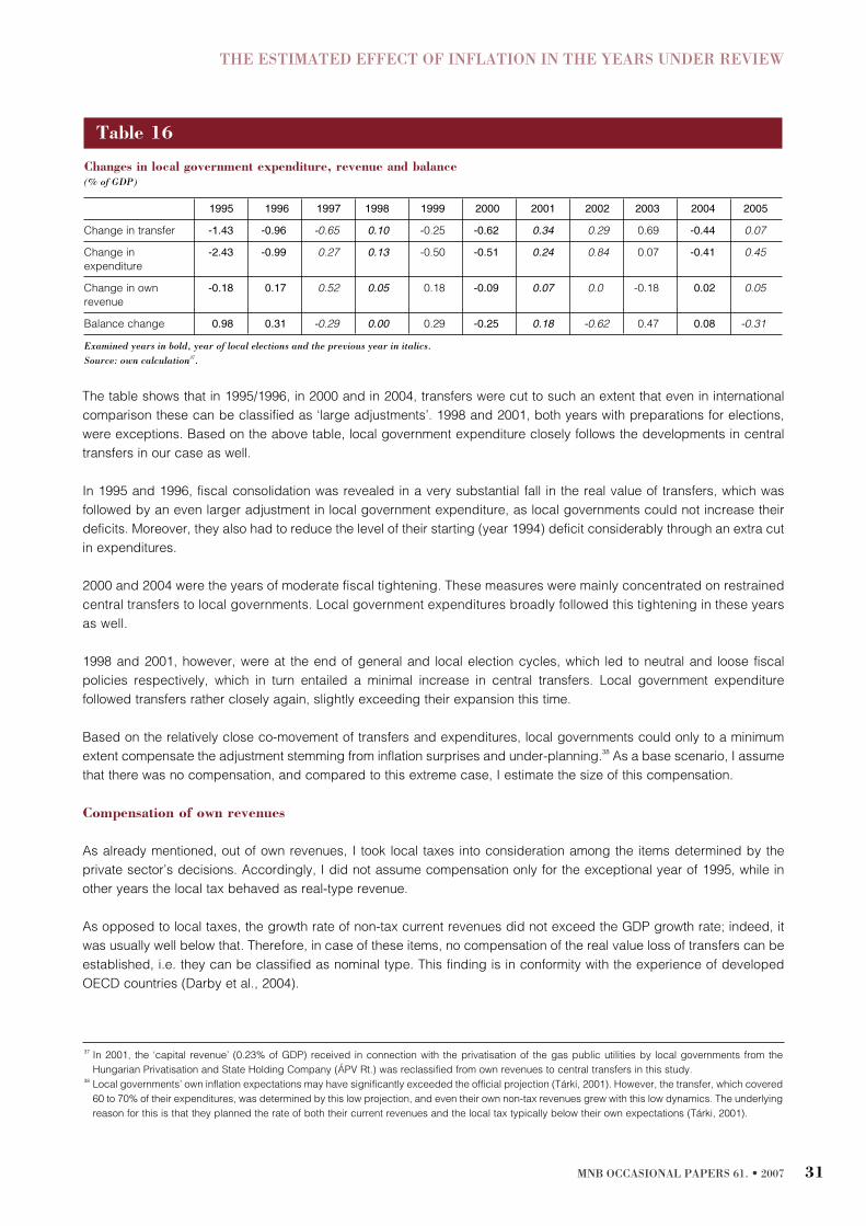
The table shows that in 1995/1996, in 2000 and in 2004, transfers were cut to such an extent that even in international

comparison these can be classified as ‘large adjustments’. 1998 and 2001, both years with preparations for elections,

were exceptions. Based on the above table, local government expenditure closely follows the developments in central

transfers in our case as well.

In 1995 and 1996, fiscal consolidation was revealed in a very substantial fall in the real value of transfers, which was

followed by an even larger adjustment in local government expenditure, as local governments could not increase their

deficits. Moreover, they also had to reduce the level of their starting (year 1994) deficit considerably through an extra cut

in expenditures.

2000 and 2004 were the years of moderate fiscal tightening. These measures were mainly concentrated on restrained

central transfers to local governments. Local government expenditures broadly followed this tightening in these years

as well.

1998 and 2001, however, were at the end of general and local election cycles, which led to neutral and loose fiscal

policies respectively, which in turn entailed a minimal increase in central transfers. Local government expenditure

followed transfers rather closely again, slightly exceeding their expansion this time.

Based on the relatively close co-movement of transfers and expenditures, local governments could only to a minimum

extent compensate the adjustment stemming from inflation surprises and under-planning.

38

As a base scenario, I assume

that there was no compensation, and compared to this extreme case, I estimate the size of this compensation.

Compensation of own revenues

As already mentioned, out of own revenues, I took local taxes into consideration among the items determined by the

private sector’s decisions. Accordingly, I did not assume compensation only for the exceptional year of 1995, while in

other years the local tax behaved as real-type revenue.

As opposed to local taxes, the growth rate of non-tax current revenues did not exceed the GDP growth rate; indeed, it

was usually well below that. Therefore, in case of these items, no compensation of the real value loss of transfers can be

established, i.e. they can be classified as nominal type. This finding is in conformity with the experience of developed

OECD countries (Darby et al., 2004).



37

In 2001, the ‘capital revenue’ (0.23% of GDP) received in connection with the privatisation of the gas public utilities by local governments from the

Hungarian Privatisation and State Holding Company (ÁPV Rt.) was reclassified from own revenues to central transfers in this study.

38

Local governments’ own inflation expectations may have significantly exceeded the official projection (Tárki, 2001). However, the transfer, which covered

60 to 70% of their expenditures, was determined by this low projection, and even their own non-tax revenues grew with this low dynamics. The underlying

reason for this is that they planned the rate of both their current revenues and the local tax typically below their own expectations (Tárki, 2001).

Table 16

Changes in local government expenditure, revenue and balance

(% of GDP)

1995 1996 1997 1998 1999 2000 2001 2002 2003 2004 2005

Change in transfer -1.43 -0.96 -0.65 0.10 -0.25 -0.62 0.34 0.29 0.69 -0.44 0.07

Change in -2.43 -0.99 0.27 0.13 -0.50 -0.51 0.24 0.84 0.07 -0.41 0.45

expenditure

Change in own -0.18 0.17 0.52 0.05 0.18 -0.09 0.07 0.0 -0.18 0.02 0.05

revenue

Balance change 0.98 0.31 -0.29 0.00 0.29 -0.25 0.18 -0.62 0.47 0.08 -0.31

Examined years in bold, year of local elections and the previous year in italics.

Source: own calculation37

.

This statement also holds true for non-tax capital revenues, i.e. for revenues from the sale of real assets. However, as I

have assumed that these nominal-type revenues may – though indirectly – be related to investment expenditure, these

revenues are also taken into account when examining local governments’ investment expenditure. Below we therefore

examine the compensation of ‘net investment’.

Compensation of net investment expenditure

Local government investment depends less on developments in central transfers than other expenditures. The next chart

demonstrates that investment follows a relatively cyclical pattern; the two years after elections usually result in declining

expenditure, whereas the election year and the preceding year result in increasing expenditure. The change brought into

this cycle pattern by the change in the central transfer was that the restraint in 1995 and 1996 temporarily deepened the

usual decline in investment, while no significant effect can be seen in the other years.

With the exception of 1995 and 2004, it is also observable with investment that the actual growth significantly exceeded

the dynamics of indicative numbers in the annual Budget Law, and there extra expenditure was even higher than the

compensation of the inflation which exceeded the official projection. In this calculation, investment expenditure of local

governments was taken into account as net expenditure, i.e. excluding the sale of real assets, as the magnitude of this

revenue target figure also proved under-planned year by year. This therefore partly covered the higher than expected

dynamics of investment expenditure. The size of extra expenditure exhibits a wider spread, ranging between 3.4 and

23.8%. The smallest extra increase in addition to inflation compensation took place in 1996, when owing to the fiscal

tightening, a 15.6% real value reduction was envisaged, even against the background of lower inflation. The highest extra

increase took place in 1998, when owing to the election year local governments invested more from their own resources

and received more capital transfers too. In 2000 extra expenditure stood at ‘only’ 16.1%, the underlying explanation of

which was also the higher than planned capital transfer. The 12.6% extra expenditure in 2001, in turn, may be attributable

to the approaching election year.

Compensation of operational expenditures

In principle, a distinction can be drawn between different types of expenditure from the aspect whether the intention to

offset inflation can be presumed immediately (during the year) or not – in other words, whether expenditure

MAGYAR NEMZETI BANK


Chart 2

Changes in central transfers and local government investment

(GDP %)

-2

-1.5

-1

-0.5

0

0.5

1

1994 1995 1996 1997 1998 1999 2000 2001 2002 2003 2004 2005

Investment Transfer

developments are important in real terms in the short term. Realistically, one may expect this in case of those operational

expenditures where the government receives something in return, such as in case of purchasing goods and services

and the compensation of public employees, i.e. in case of the wage bill.

39

In case of operational expenditures, it is difficult for both technical and factual reasons to examine what really has

happened.

On the one hand, it is a technical problem that budgetary appropriations and local governments’ centrally assumed

indicative numbers

40

refer to nominal values and not to percentage changes in expenditures. Consequently, while the

index of actual figures can easily be ascertained, it is often difficult to establish what the idea regarding the percentage

growth was, as at the time of planning only a forecasted value was available with regard to the base period. Accordingly,

the growth in individual expenditures both planned and actual can only be compared with reservations. Interpreting the

results therefore calls for considerable caution.

41

On the other hand, only the absence of compensation can be established on the basis of the actual data, when the

planned growth in individual expenditures was not attained. In other years, however, when the dynamics of actual figures

were higher than expected, it is not so simple to decide how much of it can be attributed to the effect of the compensation

of the under-planned inflation. Of course, where exceeding the planned growth does not reach the size of under-

planning, we can indicate only partial compensation. The problem is where plans contained moderation or restraint of

expenditure growth from the very beginning. (For the sake of simplicity, I chose actual nominal GDP growth as a basis

for comparison of the planned expenditure growth. I classified the planned expenditure growth which is lower than this

as moderated, and higher as dynamic.)

Two solutions can be chosen:

– Compensation can be divided proportionally between the size of the originally planned nominal moderation and the

size of under-planning. This approach assumes that the two kinds of ‘shock’ hit local governments simultaneously.

– Compensation can be identified with the residual value resulting in excess of the compensation of the originally

planned restraint. This approach assumes that the inflation shock appears later, and that local governments run out of

their compensation possibilities by then.

For the concrete calculation, I chose proportional division, except for the 1995 episode, when the inflation surprise

ensued only after the first quarter.



39

According to surveys, loans for operation were used by a greater part of those local governments which assessed their own economic situation

pessimistically. As opposed to this, investment credit demands were motivated by other factors. This result is in line with the existence of the observed

investment cycle related to elections (Tárki, 2001).

40

After the general description of the Budget Law, local governments' balance sheet is included in an annex. In this, budgetary transfers, sharing personal

income tax and social security transfers are classified as real appropriations, as they are identical to some budget appropriations of these Central

Government’s sub-sectors. Local governments’ own revenues and expenditures, in turn, are values assumed by the budget, and of course, local

governments may deviate from these values when preparing their budgets, although behind these values there are certain determinations (upper limit of

local taxes, required minimum supply levels, interest on debt, etc.). According to experiences, local governments’ own budgets often deviate to a greater

extent from actual implementation than the original projections in the Budget Act. Otherwise, until 1999 the data for the next year in local governments'

balance sheets were called ‘parliamentary appropriation’, whereas since 2000 the denomination has been an ‘indicative number’, which better suits the

real situation.

41

In principle, to examine the effect of optimistic inflation projections, one should start from local governments’ budgets and not from the indicative numbers

in the budget. In this case, however, even minimum consistency could not be provided, since assumptions for the base period cannot be established from

local governments' budgets, as the index serving as a basis for planning cannot be established with regard to individual expenditures.

In case of the wage bills, based on the difference between indicative numbers and actual realisations, it can be

established that extra wage payments took place in 1995 and 1996, when a small increase was planned. This was

however far below the size of surprise inflation, whereas in 2004, when growth was also moderate, there was no

compensation at all. In contrast, in 1998 a higher than planned increase in wage expenditures not only offset the effect

of higher than projected inflation, but even exceeded it by 2 to 2.5 percentage points. Within this, it cannot be established

whether the funds for the extra wage increase were provided by local governments or their institutions, as extra funds

were available at both levels. In 2000 and 2001 a more considerable real wage increase was already envisaged, but only

a quarter of the higher inflation could be compensated from local government funds. In the course of 2000, the one-off

budgetary wage supplement to health and social institutions of local governments added 2.8% to the wage bill, although

in the meantime, owing to the catastrophe situation (flood, drainage), 2.1% of the appropriation was blocked. It seems

that in 2001 the 3.1% extra inflation was offset only to the extent of 0.8 percentage point by local governments.

42

However,

the underlying reason is that 2 percentage point compensation was provided by the central transfers placed on a deposit

account classified as wage supplements at the end of 2000. These wage supplements were paid in 2001 as announced

at the end of 2000; therefore I took into account this pre-determined payment as a correction of the original indicative

wage increase in 2001. This additional one-off supplement was received by those areas where the magnitude of the pay

rise in the previous year was below the 13% which would have resulted on the basis of the government’s promise

(inflation plus half of economic growth). In other words, local governments (and to a lesser extent central budgetary units

as well) received the 2000 valorisation in 2001. I did not take into account these wage measures by the government

because I assume a passive fiscal policy.

In terms of purchases of goods and services, in 1995–1996, in 1998 and in 2000 there was an extra increase exceeding

the inflationary surplus by 2.5 to 3.7%. However, the underlying reason is that the planned increase in purchase of goods

and services was moderated even in nominal terms, whereas in real terms, based on the original or amended Budget

Law, in the years listed above it would have been -13%, -15%, -6.4% and -2.8%, respectively, i.e. any extra increase

could have only moderated these originally planned cuts in real terms. 2001 and 2004 constitute an exception. In 2001

the nominal increase in the purchase of goods and services was lower than indicated by 1.1% in a way that its

achievement, against the background of projected low inflation, would have meant a 4.7% increase in real terms. The

lower than planned nominal increase in expenditure and higher inflation together resulted in a modest 0.5% increase in

real terms. In 2004, in turn, even on the basis of the low inflation projection, there would have been a 1% increase in real

terms only, which finally declined to 0.6% as a result of higher inflation and partial compensation.

Compensation of other – neither operational nor investment – expenditures

The parameters of household transfers did not change during the year; their change is mainly influenced by develop-

ments in eligibility (e.g. demographic conditions). Therefore, this expenditure item was taken into account among items

determined by the private sector’s decisions, classified as nominal-type items which do not follow inflation.

MAGYAR NEMZETI BANK


Table 17

Compensation estimation on the basis of actual figures

Moderated plan Dynamic plan

Growth below the plan No compensation No compensation

Higher than planned growth, but not reaching the size of

under-planning Partial, proportional compensation Partial compensation

Lower than planned growth, exceeding the size of

under-planning Proportional compensation Full compensation

42

In 2001 both their wage and investment compensation could be funded by increasing central transfers; in addition to higher transfers, they also received

a one-off 0.23% capital transfer from the Hungarian Privatisation and State Holding Company (ÁPV Rt.).

Other expenditures reach 0.8 to 1% of GDP, of which subsidies to companies constitute a significant part. These

expenditures followed the changes in central transfers received from the government. The decline in total expenditure is

partly attributable to the decline in these expenditures, and half of the expenditure growth in 2001 also appeared here.

As the underlying reason for this, the only growth episode, is the significant increase in central transfers, we can assume,

based on the decline characterising the other years, that other expenditure behaves as a nominal-type item.

Summary of compensation by local governments

I assumed that there may be differences between various items in terms of the extent of the compensation of inflation.

Within operational expenditure, in principle, there may be higher compensation pressure in case of wages than in

case of purchase of goods and services. However, the findings show that priorities are changing year by year within

operational expenditure. On the whole, the compensation of the purchase of goods and services slightly exceeds that

of wages.

I also assumed that the character of investment expenditure is different from that of operational expenditure, as the

former takes longer to implement, and thus the determination of ongoing investment is significant. On the other hand,

there may be reallocation between investment and operational expenditures, because in the case of a need for

compensation of operational expenditure, postponing the launching of new investment may cover it. Based on

developed OECD countries’ experience as well, it seems that in case of any necessary adjustment, local governments

reduce their investment to a relatively greater extent than their operational expenditure (Darby et al., 2004). As opposed

to this, findings related to Hungary suggest that in the year of local elections, or preceding that, investment enjoys priority

over the compensation of current expenditure, as the usual investment cycle strongly prevails, and developments in

central transfers can only have a small impact on it.

43

An exception is the 1995 adjustment, when investment declined in

nominal terms as well, which is only partly attributable to the usual local government investment cycle. This year is

exceptional because in real terms the transfers were significantly restrained already before the inflation surprise, and the

exceptionally high base year (1994) level of the local government deficit was also unsustainable. The reduction of the

deficit and losing the central transfers exhausted local governments’ opportunities from the beginning, e.g. by restraining

investment and other expenditure. Therefore, they probably did not have any opportunity to compensate the inflation

surprise following the first quarter.



43

As a result of fluctuating local government investment, central capital transfers (earmarked to these investments) deviate from the original budget

appropriation in both directions. Owing to consolidation within the government sector, the changing effect of these central transfers does not have to be

taken into account, as they constitute expenditure for the central government and revenue for the local government at the same time.

Table 18

Magnitude and effect of compensation by local governments

Inflation Compensation % Extra expenditure (GDP %)

under-planning Wages Purchase of Net wages Purchase of Investment

goods and services goods and services

1995 9.1 0.0 0.0 0.0 0.0 0.00

1996 3.7 1.3 1.3 0.04 0.04 0.00

1998 0.8 0.8 0.2 0.02 0.01 0.02

2000 3.4 0.7 1.3 0.02 0.04 0.00

2001 3.1 0.8 0.0 0.02 0.00 0.07

2004 1.1 0.0 1.1 0.00 0.03 0.00

Source: own calculations.

4.3.2. Operational expenditures of central budgetary units

The room for manoeuvre of budget chapters and budgetary units is more limited than that of local governments. Their

expenditure appropriations are determined mostly by central transfer appropriations and to a lesser extent by their own

revenues, and by using the carryover of unused funds. During the years examined, own sales and fee revenues on the

whole – except 2004 – did not contribute to additional expenditures.

44

The balance of chapters and units is determined

by the acceleration or deceleration of the use of carryover funds. In addition, reallocations between individual

appropriations are also possible.

45

In principle, the stock of carryover funds may cushion the impact of changes in annual central transfer appropriations:

in the event of a tightening they are likely to decumulate faster, whereas in the event of extra transfers, their further

accumulation is likely. Based on the sum of carryover funds, decumulation can be seen only in 2002. However, this does

not reveal the developments in carryover funds of operational expenditures. The structure of such funds is also important,

as the carryover funds of capital expenditures cannot be used for the compensation of operational expenditures.

In the remainder of the section I estimate whether there was compensation in operational expenditures in the course of

the year, following the same approach in the case of local governments.

In case of appropriations which were moderated from the beginning, higher inflation results in an additional decline in

real terms. The room for manoeuvre of the budgetary units was smaller in this case, and owing to transfer cuts,

expenditures could only partly be increased. (In 1996 the wage bill and the purchase of goods and services were

planned to be cut in real terms. In 1995 and 1998 only the purchase of goods and services was planned to cut.)

If the transfers grew dynamically in real terms, the inflation surprise (or under-planning) only reduced its effect. In such

cases, it may also be likely that a higher central transfer appropriation consistent with a higher official inflation projection

would not have been spent completely in the given year, as the rapid accumulation of carryover funds may also indicate

that chapters and budgetary units spent less efforts on the immediate use of appropriations in a situation like this.

Compensation of wages

In terms of wages, across-the-board modification had three sources: government, chapter and institution-level sources.

Government-level compensation is disregarded owing to the assumption of a passive fiscal policy (i.e. one non-

responding to an inflation surprise). Without government corrections, wages grew faster than planned in only one year.

However, owing to the appropriations, which were originally tightened, the observable trend was that by reallocating their

MAGYAR NEMZETI BANK


44

Although the revenue exceeding GDP growth even in 2004 did not reach 0.1% of GDP, it is still conceivable that own revenue, which was growing more

slowly than GDP, was reallocated in a way that an increasing part of own revenues were directed to operational expenditures by withdrawing own revenues

from funding other expenditures.

45

Starting from 1996, budgetary units were entitled to reallocate their operational appropriations up to 10%, and without limitation in case of their capital

appropriations. However, reallocations between operational and capital appropriations were in the hands of the government. Starting from 2000, both

reallocations within a scope of activity (from the level of budgetary units) and between operational and capital appropriations (from government level) were

delegated to the power of chapters. However, within operational appropriations, the possibility of reallocation between wage bills and purchases of goods

and services ceased to exist. Modification of the wage bill became possible only within the same legal title, up to the extent of 5% (and only above this

value with the consent of the Ministry of Finance).

Table 19

Unused funds and their changes

(% of GDP)

1998 1999 2000 2001 2002 2003 2004

Carryover funds 1.02 1.80 1.81 2.69 2.52 2.52 2.53

Change 0.18 0.78 0.01 0.89 -0.17 0.00 0.01

Source: annual Budget Execution Laws.

own revenues, budgetary units carried out upward modification of wage appropriations in an increasing manner in the

course of the year.

46

In 1995 central transfer appropriations provided by the budget covered only the smaller part of the planned wage

increased. The increase should have been covered mainly through reducing the number of employed or savings on the

wage bill, which did not prove realistic. Although the wage increase turned out to be 1.9% higher than planned, this was

attributable to an across-the-board government measure corresponding to 5.2% (mainly dismissal wages). This

suggests that budgetary units were unable to compensate for inflation.

In 1996 wage increases as such were restrained, which was amplified by inflation under-planning. The sole underlying

reason for the 3.4% over-performance was the additional 6.5% government measure in this year as well.

In 1998 the trend of increasing funding out of own revenues temporarily ceased, and the higher-than-planned amount

used did not increase in the course of the year. The underlying reason is that only 11% of the 21% wage increase

planned by law was covered by central transfer appropriations, while the remaining 10% increase was to be provided

by the increase in the units’ own revenues. Inflation compensation could not be implemented in this year either, and even

the original plan could not have been fulfilled without an additional 1.8% government measure.

In 2000 and 2001 the higher-than-planned increase in the wage bill compensated for the effect of inflation, which was

higher than projected. Moreover, it provided an additional 0.5 to 0.9 percentage point additional increase in real terms.

However, even then 1.2 and 7.8 percentage points, respectively, were the effect of across-the-board measures by the

government. Based on this, in 2000 only partial compensation was attained from own funds, whereas in 2001 – also

because the government measure made it unnecessary – there was no own compensation.

Thus 2004 was the only year when the implemented wage dynamics were even lower than the planned – restrained –

increase, i.e. the higher inflation was not compensated for.

Compensation of purchase of goods and services

In terms of purchase of goods and services, a much higher fluctuation in appropriations and their partial compensation

can be observed.

47

This compensation took place in each year when a significant nominal decline was envisaged (1995,

1996 and 1998), whereas out of the years in which a considerable increase in real terms took place even exceeding GDP

growth, this can only be observed in 2000.

The question of compensation in 1995 is uncertain because it is difficult to establish the originally envisaged change in

central transfer appropriations. If there is a methodological change in the background of the 23% decline in central

transfer appropriations, then the actual much smaller (12%) decline cannot be classified as ‘partial compensation’ either.

The appropriation would have resulted in a considerable cut in real terms in 1996, a year of fiscal consolidation, and in the

1998 election year (when wages and investment enjoyed priority). The expenditure exceeding the plan by 5.5 to 6.5

percentage points may have tended partly to compensate the moderation in real terms and partly to reduce the effect of

unexpected inflation. Accordingly, the actual moderation in real terms in 1996 and 1998 – exceeding even the size of inflation

underestimation – can be attributed to the fact that budgetary units were only partly able to compensate higher inflation.

In 2000, 2001 and 2004 the opposite situation can be seen: the appropriation of purchase of goods and services – partly

in connection with additional tasks – was planned to be increased well above inflation. In 2000 consolidated purchase



46

If the expenditure appropriation was increased from own sources in the course of the year only to the extent corresponding to last year’s, this only financed

the wage level already paid in the previous period as well on top of the central transfer appropriations; the gap did not widen. In 1996, own revenues

allowed a 2.6% wage increase on the top of central transfer appropriations, and 2.8% in 1998, while in 2000 the original appropriation was increased by

5.1% from this source.

47

Of the transfers to non-profit organisations (for example, transfers to outsourced institutions performing government activities and to health care and

education), I treat current transfers together with the purchase of goods and services. In case of these expenditures, the official inflation projection may

also have had an impact.

of goods and services finally increased by 37% instead of 22.6%, which is probably also related to inflation

compensation, but a deviation of this size may partly stem from a technical accounting (e.g. consolidation within

government) problem as well. In 2001, in turn, there was a 14% increase instead of the planned 19.2% one. This may

partly be related to a modification of tasks, or also to the particularly high expenditure growth in the previous year. In any

case, it seems that in terms of purchase of goods and services, compensation for unexpected inflation was not

implemented in 2001. In 2004 the appropriation grew dynamically again by 27.3%, although the actual realisation 21.9%

was actually below the planned percentage. Although it represents a considerable increase in real terms, according to

our definition it cannot be considered as compensation for inflation.

4.3.3. Summary of the decentralised general government

Summary results reveal that two-thirds of cases are closer to the assumed scenario when the decentralised general

government does not compensate for the loss of its expenditures and revenues in real terms. If we compare to this

assumed extreme, it can be seen that there was no compensation at all in 1995, whereas in 1996, 2000 and 2004,

compensation amounted to 21 to 28% of the maximum loss in real terms. Conversely, compensation in 2000 and 1998

reached 57% and 80%, respectively.

MAGYAR NEMZETI BANK


Table 20

Magnitude and effect of institutions' compensation

Inflation Compensation % Extra expenditure (GDP %)

under-planning Wages Purchase of Net wage Purchase of

goods and services goods and services

1995 9.1 0.0 0.0 0.00 0.0

1996 3.7 0.0 1.2 0.00 0.04

1998 0.8 0.0 0.7 0.00 0.02

2000 3.4 2.1 3.4 0.05 0.10

2001 3.1 0.0 0.0 0.00 0.00

2004 1.1 0.0 0.0 0.00 0.00

Source: own calculations.

Table 21

Actual effect of the decisions of the decentralised general government

(GDP %)

1995 1996 1998 2000 2001 2004

Own revenue excluding local taxes -0.437 -0.164 -0.035 -0.143 -0.123 -0.037

Expenditure excluding social -2.014 -0.671 -0.077 -0.419 -0.553 -0.200

transfers

Tax and contribution content of -0.652 -0.232 -0.025 -0.136 -0.168 -0.071

expenditure

Wage-determined transfers -0.450 -0.080 -0.001 -0.028 -0.037 -0.017

Balance 1.375 0.355 0.017 0.168 0.298 0.109

Total compensation % 0.00 0.28 0.80 0.57 0.23 0.21

In Table 12 I presented the average weight of nominal-type items (0.08) and of items depending on the compensation

decisions of the private sector (-0.26) and of the decentralised government (0.13). The decline of nominal-type items in

real terms improves the primary balance in any case, although four cases result from combining the decisions of the

private sector and of the decentralised government. If both participants compensate for their losses in real terms, only

the nominal-type items improve the balance by 0.08% of GDP. If none of the participants compensates then, owing to

the private sector’s more sizeable negative revenue effect, the GDP ratio of the primary balance deteriorates by 0.05

percentage point. The negative effect is even greater if the decentralised general government compensates its

expenditures; in this case, the balance deteriorates by 0.18%. However, if the private sector compensates while the

decentralised general government does not, this increases the positive effect to 0.21% of GDP.

I compared these results with those of my earlier calculations (see Table 24). For the sake of comparability, first I made

a correction with the change in interest spending, as the present calculation concentrates on the primary balance.

However, I also excluded the effect of the corporate tax revenue, because the present calculation does not assume extra

revenue under this item. The corrected results are in brackets in the table. The underlying explanation for the difference

between the two kinds of values is in making the calculation more precise. One of the changes is that the effect of

compensation by the private sector is reduced by 0.03% by the expenditure effect (determined by wage developments),

which appears with lags in case of transfers. The weight of compensation by local governments is reduced by 0.04% by

the correction that, in addition to the expenditure, I also took into account the effect of the compensation of the non-tax

decentralised revenue. These two changes do not take place if none of the participants compensates, and their effects

almost offset one another when both compensate.

Another possible comparison is with the inflation sensitivity in the Convergence Programme, which is also corrected with

interest rate sensitivity for the sake of comparability. The resulting 0.18% sensitivity can probably be identified with the

assumed case when the private sector compensates, yet neither the government nor the decentralised government

respond. This value is not much different from the 0.21% effect that I calculated. In the updated Convergence

Programme, an oil price shock adds 2% to inflation, which increases the deficit-to-GDP ratio by 0.1% owing to the non-

realised compensation of private sector wages and consumption. In the event of a 1% surprise, this means a 0.05%

effect, which equals the value that I calculated.

An important experience that examining the actual inflationary effect reveals is that the frequency and size of the inflation

surprise for the private sector are much below the frequency and size of the under-planned inflation projection, which

influences the general government. Therefore, despite the fact that the weight of the private sector’s decision is twice as

much as the weight of the decisions of the decentralised government, the impact on the primary balance was still mostly

determined by the latter.


5. Results

Table 22

The effect of a 1% inflation surprise on the primary balance

(GDP %)

Local governments and institutions

compensate do not compensate

Private sector compensates 0.08 (0.07) 0.21 (0.25)

Private sector does not compensate -0.18 (-0.23) -0.05 (-0.05)

In case of the inflation surprise for the private sector, only in 1995 were neither wages nor consumption compensated,

whereas in 2000 compensation was almost complete. In 2004, the compensation of wages was complete, while

consumption was not compensated. The absence of compensation (inflation dividend) in 1995 may be attributed to the

size of the surprise (above 9%), its timing following a wage increase, and one factor of the surprise, i.e. the indirect tax

increase, which reduces consumption in any case.

Compensation decisions of the decentralised government were influenced by their financial opportunities (privatisation

revenue and transfers from the budget, which were increased prior to the elections, then cut again) on the one hand,

and by their expenditure (investment) motivation, which was affected by the election cycle, on the other hand. While

generally a quarter of the inflation under-planning was compensated in their expenditures, half of the under-planning was

compensated by privatisation revenues in 2000, and four-fifths owing to the election/investment cycle against the

background of increasing central transfers in 1998. Examining the whole period, it can be seen that half of this

expenditure compensation was financed by a local tax increase, which was mainly implemented in the following year.

Therefore, the immediate response of the decentralised government to the decline in central transfers in real terms was

that they did not compensate most of the loss of their expenditures in real terms.

The large adjustment episode in 1995-1996 improved the primary balance by 6.9% of GDP, partly because the

decentralised government did not compensate the envisaged 1.8% tightening of central transfers. Moreover, local

governments reduced their expenditure by another 1% (and their investment by 0.6%) in order to eliminate their high

1994 deficit. The further 2.5% improvement of the government balance is mainly attributable to the reduction in the

appropriations of nominal-type expenditures (and central investment within that). In the course of the year, the 2.8%

balance improvement owing to the inflation surprise not compensated in the general government and the 0.2% extra

revenue attributable to the temporary reversal of the declining trend of indirect taxes were added to the envisaged

adjustment, although all this was reduced by 1.5% by the absence of the compensation of wages and consumption

(inflation dividend) in the private sector.

I have not examined 2006 and 2007. In 2006, consumption is likely to be moderated in real terms by the mid-year

increase of indirect taxes, similar to the wages, since the tax increase was announced after the usual wage increases.

In 2007, the optimistic inflation projection can result in lower than planned central transfers in real terms which can

moderate the nominal increase in decentralised expenditure, improving the deficit by around 0.1% of GDP.

In summary, the inflation surprise can increase the deficit-to-GDP ratio if private sector wage and consumption are not

compensated in the short-term, while it can decrease the deficit if there is no across-the-board compensation in the

government expenditure.

MAGYAR NEMZETI BANK


Table 23

The effect of an inflation surprise/under-planning on the primary balance

(GDP %)

1995 1996 1998 2000 2001 2004

Nominal-type items 0.840 0.195 0.054 0.234 0.199 0.070

Private sector decisions -1.487 0.000 0.000 0.031 0.000 -0.020

Decentralised government 1.375 0.355 0.017 0.168 0.298 0.109

Balance 0.727 0.550 0.071 0.443 0.494 0.159

ALESINA, A. AND R. PEROTTI (1995): “Fiscal Expansions and Adjustments in OECD Countries”, Economic Policy 21, pp.

207-48.

BUTI, M. AND P. VAN DEN NOORD (2003): “Discretionary Fiscal Policy and Elections: The Experience of the Early Years of

EMU”, OECD Working Paper 351.

DARBY, J., A. MUSCATELLI AND G. ROY (2004): “Fiscal Federalism, Fiscal Consolidation and Cuts in Central Government

Grants: Evidence from an Event Study”, CESifo Working Paper Series No. 1305.

FORNI, L. AND S. MOMIGLIANO (2004): “Cyclical Sensitivity of Fiscal Policies Based on Real-time Data”, Temi di discussione,

Banca d’Italia.

GÁBRIEL, P. AND A. REIFF (2006): “How CPI Is Affected by Changes in VAT”, mimeo.

GRAMLICH, E. M. (1987): “Federalism and Federal Deficit Reduction”, National Tax Journal 40.

HENRY, J., P. H. DE COS AND S. MOMIGLIANO (2004): “The Short-term Impact of Government Budgets on Prices: Evidence

from Macroeconomic Models”, ECB Working Paper 369.

HORVÁTH, Á., Z. M. JAKAB, G. P. KISS AND B. PÁRKÁNYI (2006): “Myths and Maths: Macroeconomic Effects of Fiscal

Adjustment in Hungary”, MNB Occasional Papers 52.

KÁTAY, G. AND Z. WOLF (2004): “Investment Behavior, User Cost and Monetary Policy Transmission – The Case of

Hungary”, MNB Working Papers 2004/12.

KOVÁCS, M. A. (2005): “The Effects of the Exchange Rate: Our Knowledge and Lessons from the Stabilization in 1995” [in

Hungarian], MNB Background Studies 2005/6.

MAGYAR NEMZETI BANK (1995): “Annual Report” 1995.

MAGYAR NEMZETI BANK (2000): “Annual Report” 2000.

MÉLITZ, J. (2000): “Some Cross-country Evidence about Fiscal Policy Behaviour and Consequences for EMU”, European

Commission, European Economy, Reports and Studies, Public Debt and Fiscal Policy in EMU, No 2, Ch. 1.

MENCZEL, P. (2000): “What Do Savings Indicate” [in Hungarian], Bankszemle, August 2000.

OATES, W. (1994): “Federalism and Public Finance”, in: Quigley and Smolensky (eds), Modern Public Finance, Harvard

University Press.

OLIVERA, J. (1967): “Money, Prices and Fiscal Lags: A Note on the Dynamics of Inflation”, Banca Nationale del Lavoro

Quarterly Review Vol. 20.

PERSSON, M., T. PERSSON AND L. E. O. SVENSSON (1996): “Debt, Cash-flow and Inflation Incentives: A Swedish Example”,

NBER Working Paper 5772.

P. KISS AND G. VADAS (2004): “Mind the Gap – Watch the Ways of the Cyclical Adjustment of the Budget”, MNB Working

Papers 2004/7.


Bibliography

SIMON, A. (1996): “Determinants of Inflation in 1990-1995” [in Hungarian], MNB Working Papers 1996/1.

TÁRKI, (2001): “Report” (Local Government Data Collected by Tárki, Spring of 2001).

TANZI, V. (1977): “Inflation, Lags in Collection and the Real Value of Tax Revenue”, IMF Staff Papers vol. 24.

TUJULA, M. AND G. WOLSWIJK (2004): “What Determines Fiscal Balances? An Empirical Investigation in Determinants of

Changes in OECD Budget Balances”, ECB Working Paper 422.

VIRÉN, M. (1998): “Do the OECD Countries Follow the Same Fiscal Policy Rule?”, Helsinki, Government Institute for

Economic Research.

MAGYAR NEMZETI BANK



Annex

1988 budget

Real value of government debt 0.3

Seignorage 0.5

Transfers

Delayed indexation 0.5

Incomplete indexation 1.1

Taxes

Income tax schedules 1.0

Pension funds -0.3

Capital tax income 0.9

Tax collection -0.4

Total 3.6

Table 24

The effects of 1% surprise inflation on the nominal government deficit (GDP %)

(GDP %)

Table 25

Gains from increasing rate of inflation from 2 to 12 percent

(GDP %)

Private sector/Government Compensate Do not compensate

wages: +0.35 wages: +0.35

Tax and contribution content of government Automatic response in government expenditure: -0.2

Compensate

expenditure: +0.05

Automatic response in government expenditure: -0.2

Expenditures of decentralised government: -0.23

Total: -0.03 Total: +0.15

Corporate tax:+0.1 Corporate tax: +0.1

Tax and contribution content of government Automatic response in government

Do not compensate expenditure:: +0.05 expenditure:-0.15

Automatic response in government expenditure: -0.15

Expenditures of decentralised government: -0.23

Total: -0.23 Total: -0.05

Source: calculations of P. Kiss in Kovács (2005), table II-2.

Source: Persson, Persson and Svensson, 1996 (Table 1.)

MNB Occasional Papers 61.

January 2007

Print: D-Plus

H–1037 Budapest, Csillaghegyi út 19–21.

Pain or gain? Short-term budgetary effects of surprise inflation

Documents

Transcript of Pain or gain? Short-term budgetary effects of surprise inflation