Package 'CLME' - Microsoft R Application Network

Package ‘CLME’December 5, 2014

Title Constrained Inference for Linear Mixed Effects Models

Version 2.0-1

Depends R (>= 3.0.2)

Imports MASS, lme4, shiny, methods, isotone, stringr, prettyR, stats

Date 2014-12-01

DescriptionConstrained inference for linear mixed effects models using residual bootstrap methodology

Author Casey M. Jelsema

Maintainer Casey M. Jelsema <[email protected]>

BuildVignettes true

BugReports https://github.com/jelsema/CLME/issues

LazyLoad yes

License GPL-2 | GPL-3

NeedsCompilation no

Repository CRAN

Date/Publication 2014-12-05 05:01:25

R topics documented:CLME-package . . . . . . . . . . . . . . . . . . . . . . . . . . . . . . . . . . . . . . . 2AIC.clme . . . . . . . . . . . . . . . . . . . . . . . . . . . . . . . . . . . . . . . . . . 4clme . . . . . . . . . . . . . . . . . . . . . . . . . . . . . . . . . . . . . . . . . . . . . 5clme_em . . . . . . . . . . . . . . . . . . . . . . . . . . . . . . . . . . . . . . . . . . . 8clme_resids . . . . . . . . . . . . . . . . . . . . . . . . . . . . . . . . . . . . . . . . . 10confint.clme . . . . . . . . . . . . . . . . . . . . . . . . . . . . . . . . . . . . . . . . . 11create.constraints . . . . . . . . . . . . . . . . . . . . . . . . . . . . . . . . . . . . . . 12

1

https://github.com/jelsema/CLME/issues

2 CLME-package

fibroid . . . . . . . . . . . . . . . . . . . . . . . . . . . . . . . . . . . . . . . . . . . . 14fixef.clme . . . . . . . . . . . . . . . . . . . . . . . . . . . . . . . . . . . . . . . . . . 15formula.clme . . . . . . . . . . . . . . . . . . . . . . . . . . . . . . . . . . . . . . . . 16is.clme . . . . . . . . . . . . . . . . . . . . . . . . . . . . . . . . . . . . . . . . . . . . 17logLik.clme . . . . . . . . . . . . . . . . . . . . . . . . . . . . . . . . . . . . . . . . . 18lrt.stat . . . . . . . . . . . . . . . . . . . . . . . . . . . . . . . . . . . . . . . . . . . . 19minque . . . . . . . . . . . . . . . . . . . . . . . . . . . . . . . . . . . . . . . . . . . 20model.frame.clme . . . . . . . . . . . . . . . . . . . . . . . . . . . . . . . . . . . . . . 22model.matrix.clme . . . . . . . . . . . . . . . . . . . . . . . . . . . . . . . . . . . . . 23model_terms_clme . . . . . . . . . . . . . . . . . . . . . . . . . . . . . . . . . . . . . 24nobs.clme . . . . . . . . . . . . . . . . . . . . . . . . . . . . . . . . . . . . . . . . . . 25plot.clme . . . . . . . . . . . . . . . . . . . . . . . . . . . . . . . . . . . . . . . . . . 26print.clme . . . . . . . . . . . . . . . . . . . . . . . . . . . . . . . . . . . . . . . . . . 27print.varcorr_clme . . . . . . . . . . . . . . . . . . . . . . . . . . . . . . . . . . . . . . 28ranef.clme . . . . . . . . . . . . . . . . . . . . . . . . . . . . . . . . . . . . . . . . . . 29rat.blood . . . . . . . . . . . . . . . . . . . . . . . . . . . . . . . . . . . . . . . . . . . 30residuals.clme . . . . . . . . . . . . . . . . . . . . . . . . . . . . . . . . . . . . . . . . 31resid_boot . . . . . . . . . . . . . . . . . . . . . . . . . . . . . . . . . . . . . . . . . . 32shiny_clme . . . . . . . . . . . . . . . . . . . . . . . . . . . . . . . . . . . . . . . . . 34sigma.clme . . . . . . . . . . . . . . . . . . . . . . . . . . . . . . . . . . . . . . . . . 35summary.clme . . . . . . . . . . . . . . . . . . . . . . . . . . . . . . . . . . . . . . . . 36VarCorr.clme . . . . . . . . . . . . . . . . . . . . . . . . . . . . . . . . . . . . . . . . 37vcov.clme . . . . . . . . . . . . . . . . . . . . . . . . . . . . . . . . . . . . . . . . . . 38w.stat . . . . . . . . . . . . . . . . . . . . . . . . . . . . . . . . . . . . . . . . . . . . 39

Index 41

CLME-package Constrained inference for linear mixed models.

Description

Constrained inference on linear fixed and mixed models using residual bootstrap. Covariates andrandom effects are permitted but not required.

Appropriate credit should be given when publishing results obtained using CLME, or when devel-oping other programs/packages based off of this one. Use citation(package="CLME") for Bibtexinformation.

Details

Package: CLMEType: PackageVersion: 2.0Date: 2014-11-14License: GLP-2 | GLP-3

CLME-package 3

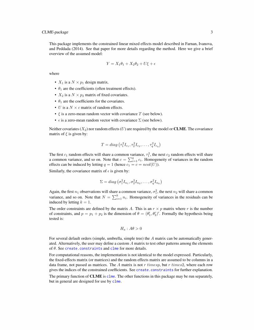
This package implements the constrained linear mixed effects model described in Farnan, Ivanova,and Peddada (2014). See that paper for more details regarding the method. Here we give a briefoverview of the assumed model:

Y = X1θ1 +X2θ2 + Uξ + ε

where

• X1 is a N × p1 design matrix.

• θ1 are the coefficients (often treatment effects).

• X2 is a N × p2 matrix of fixed covariates.

• θ1 are the coefficients for the covariates.

• U is a N × c matrix of random effects.

• ξ is a zero-mean random vector with covariance T (see below).

• ε is a zero-mean random vector with covariance Σ (see below).

Neither covariates (X2) nor random effects (U ) are required by the model or CLME. The covariancematrix of ξ is given by:

T = diag(τ21 Ic1 , τ

22 Ic2 , . . . , τ

2q Icq

)The first c1 random effects will share a common variance, τ21 , the next c2 random effects will sharea common variance, and so on. Note that c =

∑qi=1 ci. Homogeneity of variances in the random

effects can be induced by letting q = 1 (hence c1 = c = ncol(U)).

Similarly, the covariance matrix of ε is given by:

Σ = diag(σ21In1 , σ

22In2 , . . . , σ

2qInk

)Again, the first n1 observations will share a common variance, σ2

1 , the next n2 will share a commonvariance, and so on. Note that N =

∑ki=1 ni. Homogeneity of variances in the residuals can be

induced by letting k = 1.

The order constraints are defined by the matrix A. This is an r × p matrix where r is the numberof constraints, and p = p1 + p2 is the dimension of θ = (θ′1, θ

′2)′. Formally the hypothesis being

tested is:

Ha : Aθ > 0

For several default orders (simple, umbrella, simple tree) the A matrix can be automatically gener-ated. Alternatively, the user may define a customAmatrix to test other patterns among the elementsof θ. See create.constraints and clme for more details.

For computational reasons, the implementation is not identical to the model expressed. Particularly,the fixed-effects matrix (or matrices) and the random effects matrix are assumed to be columns in adata frame, not passed as matrices. The A matrix is not r timesp, but r times2, where each rowgives the indices of the constrained coefficients. See create.constraints for further explanation.

The primary function of CLME is clme. The other functions in this package may be run separately,but in general are designed for use by clme.

4 AIC.clme

Author(s)

Casey M. Jelsema <[email protected]>

References

Farnan, L., Ivanova, A., and Peddada, S. D. (2014). Linear Mixed Efects Models under InequalityConstraints with Applications. PLOS ONE, 9(1). e84778. doi: 10.1371/journal.pone.0084778http://www.plosone.org/article/info:doi/10.1371/journal.pone.0084778

See Also

create.constraints, clme

AIC.clme Akaike information criterion

Description

Calculates the Akaike and Bayesian information criterion for objects of class clme.

Usage

## S3 method for class 'clme'AIC(object, ..., k=2 )

Arguments

object object of class clme.

... space for additional arguments.

k value multiplied by number of coefficients

Details

The log-likelihood is assumed to be the Normal distribution. The model uses residual bootstrapmethodology, and Normality is neither required nor assumed. Therefore the log-likelihood andthese information criterion may not be useful measures for comparing models.

For k=2, the function computes the AIC. To obtain BIC, set k = log(n/(2 ∗ pi)); which the methodBIC.clme does.

Value

Returns the information criterion (numeric).

Author(s)


http://www.plosone.org/article/info:doi/10.1371/journal.pone.0084778

clme 5

See Also

CLME-package, clme

Examples

data( rat.blood )

cons <- list(order = "simple", decreasing = FALSE, node = 1 )clme.out <- clme(mcv ~ time + temp + sex + (1|id), data = rat.blood ,

constraints = cons, seed = 42, nsim = 0)

AIC( clme.out )AIC( clme.out, k=log( nobs(clme.out)/(2*pi) ) )

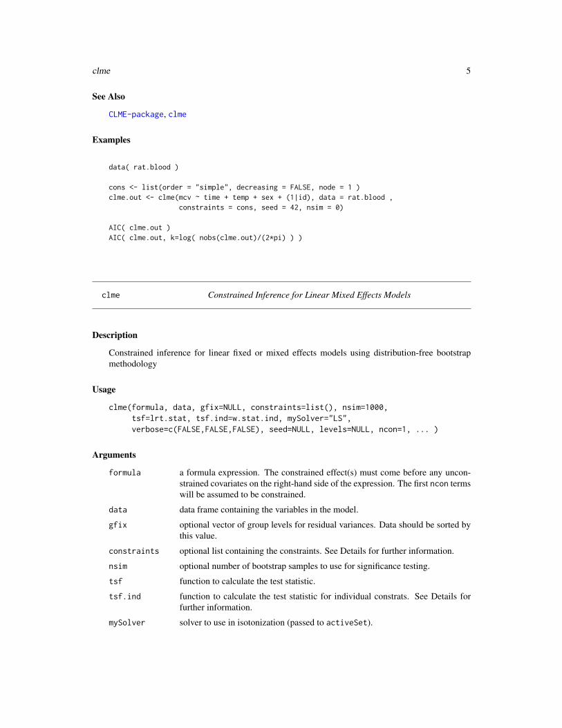
clme Constrained Inference for Linear Mixed Effects Models

Description

Constrained inference for linear fixed or mixed effects models using distribution-free bootstrapmethodology

Usage

clme(formula, data, gfix=NULL, constraints=list(), nsim=1000,tsf=lrt.stat, tsf.ind=w.stat.ind, mySolver="LS",verbose=c(FALSE,FALSE,FALSE), seed=NULL, levels=NULL, ncon=1, ... )

Arguments

formula a formula expression. The constrained effect(s) must come before any uncon-strained covariates on the right-hand side of the expression. The first ncon termswill be assumed to be constrained.

data data frame containing the variables in the model.

gfix optional vector of group levels for residual variances. Data should be sorted bythis value.

constraints optional list containing the constraints. See Details for further information.

nsim optional number of bootstrap samples to use for significance testing.

tsf function to calculate the test statistic.

tsf.ind function to calculate the test statistic for individual constrats. See Details forfurther information.

mySolver solver to use in isotonization (passed to activeSet).

6 clme

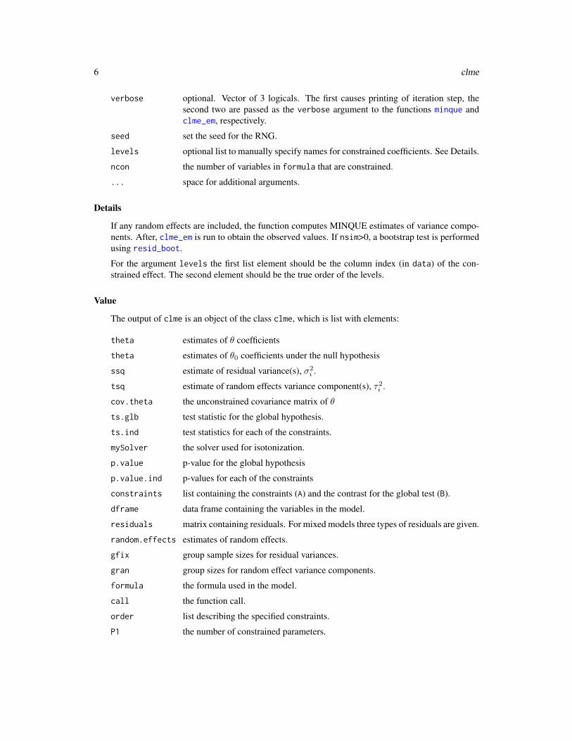
verbose optional. Vector of 3 logicals. The first causes printing of iteration step, thesecond two are passed as the verbose argument to the functions minque andclme_em, respectively.

seed set the seed for the RNG.

levels optional list to manually specify names for constrained coefficients. See Details.

ncon the number of variables in formula that are constrained.


Details

If any random effects are included, the function computes MINQUE estimates of variance compo-nents. After, clme_em is run to obtain the observed values. If nsim>0, a bootstrap test is performedusing resid_boot.

For the argument levels the first list element should be the column index (in data) of the con-strained effect. The second element should be the true order of the levels.

Value

The output of clme is an object of the class clme, which is list with elements:

theta estimates of θ coefficients

theta estimates of θ0 coefficients under the null hypothesis

ssq estimate of residual variance(s), σ2i .

tsq estimate of random effects variance component(s), τ2i .

cov.theta the unconstrained covariance matrix of θ

ts.glb test statistic for the global hypothesis.

ts.ind test statistics for each of the constraints.

mySolver the solver used for isotonization.

p.value p-value for the global hypothesis

p.value.ind p-values for each of the constraints

constraints list containing the constraints (A) and the contrast for the global test (B).

dframe data frame containing the variables in the model.

residuals matrix containing residuals. For mixed models three types of residuals are given.

random.effects estimates of random effects.

gfix group sample sizes for residual variances.

gran group sizes for random effect variance components.

formula the formula used in the model.

call the function call.

order list describing the specified constraints.

P1 the number of constrained parameters.

clme 7

Note

The argument constraints is a list containing the order restrictions. The elements are order,node, decreasing, A, and B, though not all are necessary. The function can calculate the last twofor default orders (simple, umbrella, or simple tree). For default orders, constraints should be alist containing any subset of order, node, and descending. See the figure below for a depiction ofthese values; the pictured node of the simple tree orders (middle column) is 1, and the node for theumbrella orders (right column) is 3. These may be vectors (e.g. order=(’simple’,’umbrella’) ). Ifany of these three are missing, the function will test for all possible values of the missing element(s),excluding simple tree.

For non-default orders, the elements A and B should be provided. A is an r × 2 matrix (where r isthe number of linear constraints, 0 < r. Each row should contain two indices, the first element isthe index of the lesser coefficient, the second element is the index of the greater coefficient. So arow of (1, 2) corresponds to the constraint θ1 ≤ θ2, and a row (4, 3) corresponds to the constraintθ4 ≤ θ3, etc. Element B should hold similar contrasts, specifically those needed for calculating theWilliams’ type test statistic (B is only needed if tsf=w.stat)

The argument tsf is a function to calculate the desired test statistic. The default function calculateslikelihood ratio type test statistic. A Williams type test statistic, which is the maximum of the teststatistic over the constraints in constraints$B, is also available, and custom functions may bedefined. See w.stat for details.

By default, homogeneity of variances is assumed for residuals (e.g., gfix does not define groups)and for each random effect.

Author(s)


References



8 clme_em

Examples

data( rat.blood )cons <- list(order="simple", decreasing=FALSE, node=1 )

clme.out <- clme(mcv ~ time + temp + sex + (1|id), data=rat.blood ,constraints=cons, seed=42, nsim=10, ncon=1)

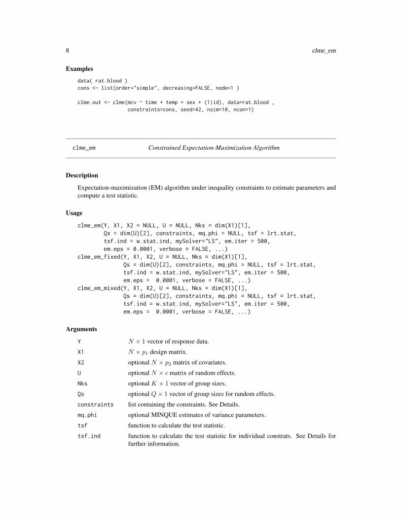
clme_em Constrained Expectation-Maximization Algorithm

Description

Expectation-maximization (EM) algorithm under inequality constraints to estimate parameters andcompute a test statistic.

Usage

clme_em(Y, X1, X2 = NULL, U = NULL, Nks = dim(X1)[1],Qs = dim(U)[2], constraints, mq.phi = NULL, tsf = lrt.stat,tsf.ind = w.stat.ind, mySolver="LS", em.iter = 500,em.eps = 0.0001, verbose = FALSE, ...)

clme_em_fixed(Y, X1, X2, U = NULL, Nks = dim(X1)[1],Qs = dim(U)[2], constraints, mq.phi = NULL, tsf = lrt.stat,tsf.ind = w.stat.ind, mySolver="LS", em.iter = 500,em.eps = 0.0001, verbose = FALSE, ...)

clme_em_mixed(Y, X1, X2, U = NULL, Nks = dim(X1)[1],Qs = dim(U)[2], constraints, mq.phi = NULL, tsf = lrt.stat,tsf.ind = w.stat.ind, mySolver="LS", em.iter = 500,em.eps = 0.0001, verbose = FALSE, ...)

Arguments

Y N × 1 vector of response data.

X1 N × p1 design matrix.

X2 optional N × p2 matrix of covariates.

U optional N × c matrix of random effects.

Nks optional K × 1 vector of group sizes.

Qs optional Q× 1 vector of group sizes for random effects.

constraints list containing the constraints. See Details.

mq.phi optional MINQUE estimates of variance parameters.

tsf function to calculate the test statistic.

tsf.ind function to calculate the test statistic for individual constrats. See Details forfurther information.

clme_em 9

mySolver solver to use in isotonization (passed to activeSet).

em.eps criterion for convergence for the EM algorithm.

em.iter maximum number of iterations permitted for the EM algorithm.

verbose if TRUE, function prints messages on progress of the EM algorithm.


Details

Argument constraints is a list including at least the elements A, B, and Anull. This argument canbe generated by function create.constraints.

Value

The function returns a list with the elements:

theta coefficient estimates.

theta.null vector of coefficient estimates under the null hypothesis.

ssq estimate of residual variance term(s).

tsq estimate of variance components for any random effects.

cov.theta covariance matrix of the unconstrained coefficients.

ts.glb test statistic for the global hypothesis.

ts.ind test statistics for each of the constraints.

mySolver the solver used for isotonization.

Note

There are few error catches in these functions. If only the EM estimates are desired, users arerecommended to run clme setting nsim=0.

By default, homogeneous variances are assumed for the residuals and (if included) random ef-fects. Heterogeneity can be induced using the arguments Nks and Qs, which refer to the vectors(n1, n2, . . . , nk) and (c1, c2, . . . , cq), respectively. See CLME-package for further explanation themodel and these values.

See w.stat and lrt.stat for more details on using custom test statistics.

Author(s)


References


See Also

CLME-package, clme, create.constraints, lrt.stat, w.stat


10 clme_resids

Examples

data( rat.blood )

model_mats <- model_terms_clme( mcv ~ time + temp + sex + (1|id) ,data = rat.blood )

Y <- model_mats$YX1 <- model_mats$X1X2 <- model_mats$X2U <- model_mats$U

cons <- list(order = "simple", decreasing = FALSE, node = 1 )

clme.out <- clme_em(Y = Y, X1 = X1, X2 = X2, U = U, constraints = cons)

clme_resids Computes various types of residuals

Description

Computes several types of residuals for objects of class clme.

Usage

clme_resids( formula, data, gfix=NULL, ncon=1 )

Arguments



gfix optional vector of group levels for residual variances. Data should be sorted bythis value.


Details

For fixed-effects models Y = Xβ + ε, residuals are given as e = Y −Xβ.

For mixed-effects models Y = Xβ++Uξ+ε, three types of residuals are available. PA = Y−Xβ\SS = Uξ\ FM = Y −Xβ − Uξ

confint.clme 11

Value

List containing the elements PA, SS, FM, cov.theta, xi, ssq, tsq.

PA, SS, FM are defined above (for fixed-effects models, the residuals are only PA). Then cov.thetais the unconstrained covariance matrix of the fixed-effects coefficients, xi is the vector of randomeffect estimates, and ssq and tsq are unconstrained estimates of the variance components.

Author(s)


See Also

CLME-package, clme

Examples

## Not run:

data( rat.blood )cons <- list(order = "simple", decreasing = FALSE, node = 1 )

clme.out <- clme_resids(mcv ~ time + temp + sex + (1|id), data = rat.blood, ncon=1 )

## End(Not run)

confint.clme Individual confidence intervals

Description

Calculates confidence intervals for fixed effects parameter estimates in objects of class clme.

Usage

## S3 method for class 'clme'confint(object, parm, level=0.95, ... )

Arguments


parm parameter for which confidence intervals are computed (not used).

level nominal confidence level.


12 create.constraints

Details

Confidence intervals are computed using Standard Normal critical values. Standard errors are takenfrom the covariance matrix of the unconstrained parameter estimates.

Value

Returns a matrix with two columns named lcl and ucl (lower and upper confidence limit).

Author(s)


See Also

CLME-package, clme

Examples

data( rat.blood )cons <- list(order = "simple", decreasing = FALSE, node = 1 )clme.out <- clme(mcv ~ time + temp + sex + (1|id), data = rat.blood ,


confint.clme( clme.out )

create.constraints Generate common order constraints

Description

Automatically generates the constraints in the format used by clme. Allowed orders are simple,simple tree, and umbrella orders.

Usage

create.constraints(P1, constraints)

Arguments

P1 the length of θ1, the vector constrained coefficients.

constraints List with the elements order, node, and decreasing. See Details for furtherinformation.

create.constraints 13

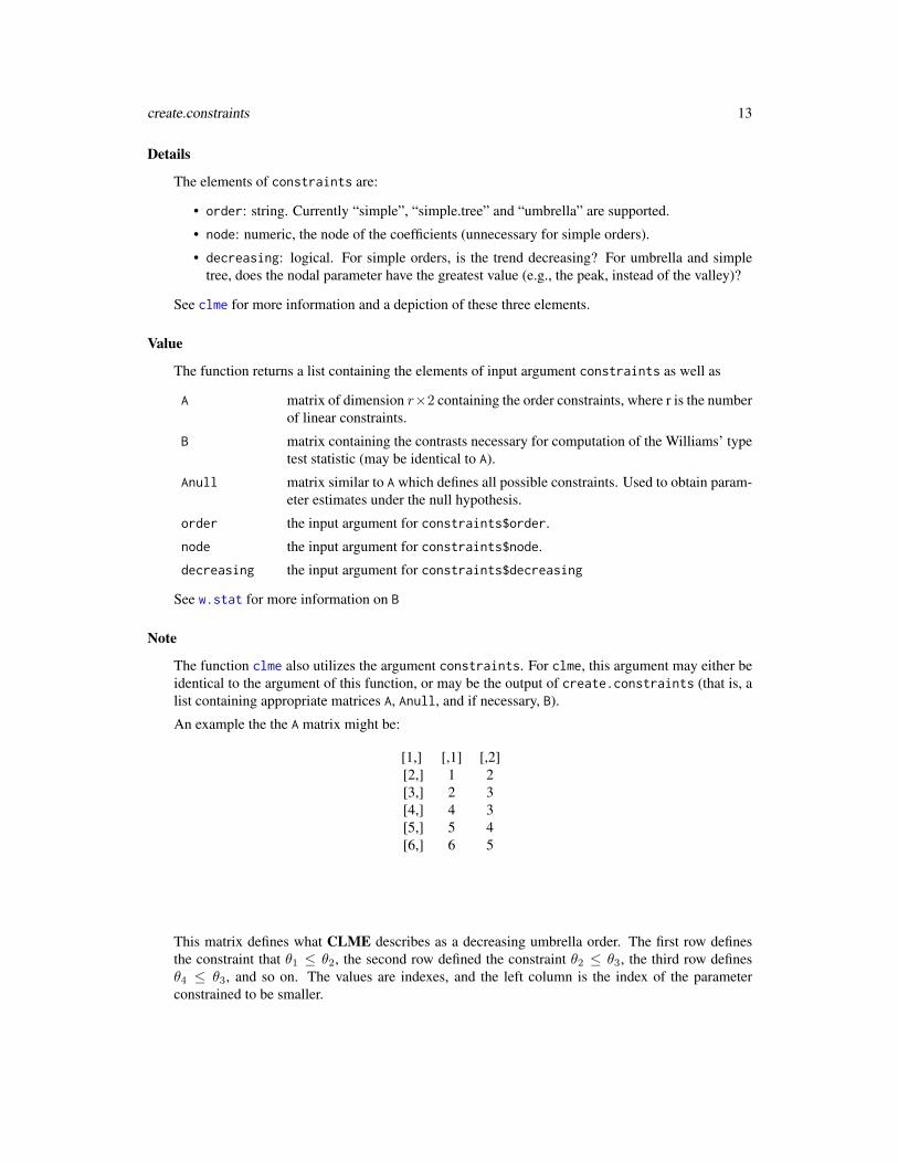
Details

The elements of constraints are:

• order: string. Currently “simple”, “simple.tree” and “umbrella” are supported.

• node: numeric, the node of the coefficients (unnecessary for simple orders).

• decreasing: logical. For simple orders, is the trend decreasing? For umbrella and simpletree, does the nodal parameter have the greatest value (e.g., the peak, instead of the valley)?

See clme for more information and a depiction of these three elements.

Value

The function returns a list containing the elements of input argument constraints as well as

A matrix of dimension r×2 containing the order constraints, where r is the numberof linear constraints.

B matrix containing the contrasts necessary for computation of the Williams’ typetest statistic (may be identical to A).

Anull matrix similar to A which defines all possible constraints. Used to obtain param-eter estimates under the null hypothesis.

order the input argument for constraints$order.

node the input argument for constraints$node.

decreasing the input argument for constraints$decreasing

See w.stat for more information on B

Note

The function clme also utilizes the argument constraints. For clme, this argument may either beidentical to the argument of this function, or may be the output of create.constraints (that is, alist containing appropriate matrices A, Anull, and if necessary, B).

An example the the A matrix might be:

[1,] [,1] [,2][2,] 1 2[3,] 2 3[4,] 4 3[5,] 5 4[6,] 6 5

This matrix defines what CLME describes as a decreasing umbrella order. The first row definesthe constraint that θ1 ≤ θ2, the second row defined the constraint θ2 ≤ θ3, the third row definesθ4 ≤ θ3, and so on. The values are indexes, and the left column is the index of the parameterconstrained to be smaller.

14 fibroid

Author(s)


See Also

clme, w.stat

Examples

## Not run:# For simple order, the node does not mattercreate.constraints( P1 = 5, constraints = list( order='simple' ,

decreasing=FALSE ))

# Compare constraints against decreasing=TRUEcreate.constraints( P1 = 5, constraints=list( order='simple' ,

decreasing=TRUE ))

# Umbrella ordercreate.constraints( P1 = 5, constraints=list( order='umbrella' , node=3

, decreasing=FALSE ))

## End(Not run)

fibroid Fibroid Growth Study

Description

This data set contains a subset of the data from the Fibroid Growth Study.

Usage

fibroid

Format

A frame containing 240 observations on 9 variables.

[,1] ID ID for subject.[,2] fid ID for fibroid (each women could have multiple fibroids).[,3] lfgr log fibroid growth rate. See details.[,4] age age category Younger, Middle, Older.[,5] loc location of fibroid, corpus, fundus, or lower segment.[,6] bmi body mass index of subject.[,7] preg parity, whether the subject had delivered a child.[,8] race race of subject (Black or White only).[,9] vol initial volume of fibroid.

fixef.clme 15

Details

The response variable lfgr was calculated as the change in log fibroid volume, divided by thelength of time between measurements. The growth rates were averaged to produce a single valuefor each fibroid, which was scaled to represent a 6-month percent change in volume.

References

Peddada, Laughlin, Miner, Guyon, Haneke, Vahdat, Semelka, Kowalik, Armao, Davis, and Baird(2008).Growth of Uterine Leiomyomata Among Premenopausal Black and White Women. Proceedings ofthe National Academy of Sciences of the United States of America, 105(50), 19887-19892. URLhttp://www.pnas.org/content/105/50/19887.full.pdf.

See Also

CLME-package, clme

fixef.clme Extract fixed effects

Description

Extracts the fixed effects estimates from objects of class clme.

Usage

## S3 method for class 'clme'fixef(object, ... )

Arguments



Value

Returns a numeric vector.

Author(s)


See Also

CLME-package, clme

http://www.pnas.org/content/105/50/19887.full.pdf

16 formula.clme

Examples



fixef.clme( clme.out )

formula.clme Extract formula

Description

Extracts the formula from objects of class clme.

Usage

## S3 method for class 'clme'formula(x, ... )

Arguments

x object of class clme.


Details

The package CLME parametrizes the model with no intercept term. If an intercept was included,it will be removed automatically.

Value

Returns a formula object.

Author(s)


See Also

CLME-package, clme

is.clme 17

Examples



formula.clme( clme.out )

is.clme Constructor method for objects S3 class clme

Description

Test if an object is of class clme or coerce an object to be such.

Usage

## S3 method for class 'clme'as(x, ... )## S3 method for class 'clme'is( x )

Arguments

x list with the elements corresponding to the output of clme.


Value

Returns an object of the class clme.

Author(s)


See Also

CLME-package, clme

18 logLik.clme

Examples

data( rat.blood )

cons <- list(order = "simple", decreasing = FALSE, node = 1 )clme.out <- clme(mcv ~ time + temp + sex + (1|id), data = rat.blood ,


is.clme( clme.out )as.clme( clme.out )

logLik.clme Log-likelihood

Description

Computes the log-likelihood of the fitted model for objects of class clme.

Usage

## S3 method for class 'clme'logLik(object, ... )

Arguments



Details

The log-likelihood is computed using the Normal distribution. The model uses residual bootstrapmethodology, and Normality is neither required nor assumed. Therefore the log-likelihood may notbe useful measures in the context of CLME.

Value

Numeric.

Author(s)


See Also

CLME-package, clme

lrt.stat 19

Examples



logLik.clme( clme.out )

lrt.stat Likelihood Ratio Type Test Statistic.

Description

Calculates the likeihood ratio type test statistic (under Normality assumption) for a constrainedlinear mixed effects model. This is the default test statistic for CLME.

Usage

lrt.stat( theta, theta.null, cov.theta, ... )

Arguments

theta estimated coefficients.

theta.null coefficients estimated under the null hypothesis.

cov.theta covariance matrix of the estimated coefficients. For CLME this is taken as thecovariance matrix of the unconstrained estimates.

... additional arguments, to enable custom test statistic functions.

Value

numeric value

Note

This is an internal function, unlikely to be useful outside of CLME-package. To define customfunctions, the arguments available are:

theta, theta.null, cov.theta, B, A, Y, X1, X2, U, tsq, ssq, Nks, and Qs.

Of the additional arguments, B and A are identical to those produced by create.constraints. Therest, Y, X1, X2, U, tsq, , ssq, Nks, and Qs, are equivalent to arguments to clme_em.

Custom functions must produce numeric output. Output may have length greater than 1, whichcorresponds to testing multiple global hypotheses.

20 minque

Author(s)


See Also

clme_em, w.stat

Examples

data( rat.blood )cons <- list(order = "simple", decreasing = FALSE, node = 1 )

clme.out <- clme(mcv ~ time + temp + sex + (1|id), data = rat.blood ,constraints = cons, seed = 42, nsim = 0)

# Individually compute lrt statisticlrt.stat(clme.out$theta, clme.out$theta.null, clme.out$cov.theta )

minque MINQUE Algorithm

Description

Algorithm to obtain MINQUE estimates of variance components of a linear mixed effects model.

Usage

minque( Y , X1 , X2 = NULL , U = NULL , Nks = dim(X1)[1] ,Qs = dim(U)[2], mq.eps = 0.0001 ,mq.iter = 500 , verbose = FALSE )

Arguments

Y N × 1 vector of response data.X1 N × p1 design matrix.X2 optional N × p2 matrix of covariates.U optional N × c matrix of random effects.Nks optional K × 1 vector of group sizes. See Details.Qs optional Q× 1 vector of group sizes for random effects.mq.eps criterion for convergence for the MINQUE algorithm.mq.iter maximum number of iterations permitted for the MINQUE algorithm.verbose if TRUE, function prints intermediate messages on progress of the MINQUE al-

gorithm.

minque 21

Details

By default, the model assumes homogeneity of variances for both the residuals and the randomeffects (if included). See the Details in clme_em for more information on how to use the argumentsNks and Qs to permit heterogeneous variances.

Value

The function returns a vector of the form (τ21 , τ22 , . . . , τ

2q , σ

21 , σ

22 , . . . , σ

2k)′. If there are no random

effects, then the output is just (σ21 , σ

22 , . . . , σ

2k)′.

Note

This function is called by several other function in CLME to obtain estimates of the random effectvariances. If there are no random effects, they will not call minque.

Author(s)


References


Examples

data( rat.blood )

model_mats <- model_terms_clme( mcv ~ time + temp + sex + (1|id) ,data = rat.blood )

Y <- model_mats$YX1 <- model_mats$X1X2 <- model_mats$X2U <- model_mats$U

# No covariates or random effectsminque(Y = Y, X1 = X1 )

# Include covariates and random effectsminque(Y = Y, X1 = X1, X2 = X2, U = U )


22 model.frame.clme

model.frame.clme Extracts the model frame

Description

Extracts the model frame from objects of class clme.

Usage

## S3 method for class 'clme'model.frame(formula, ... )

Arguments

formula a formula expression.

... space for additional arguments (should include argument data).

Value

Returns a data frame with the variables in the model.

Author(s)


See Also

CLME-package, clme

Examples

## Not run:data( rat.blood )model.frame.clme( mcv ~ time + temp + sex + (1|id), data = rat.blood )

## End(Not run)

model.matrix.clme 23

model.matrix.clme Extracts the fixed-effects design matrix

Description

Extracts the fixed-effects design matrix from objects of class clme.

Usage

## S3 method for class 'clme'model.matrix(object, ... )

Arguments



Value

Returns a matrix.

Author(s)


See Also

CLME-package, clme

Examples

## Not run:data( rat.blood )cons <- list(order = "simple", decreasing = FALSE, node = 1 )clme.out <- clme(mcv ~ time + temp + sex + (1|id), data = rat.blood ,


model.matrix.clme( clme.out )

## End(Not run)

24 model_terms_clme

model_terms_clme Create model matrices for clme

Description

Parses formulas to creates model matrices for clme.

Usage

model_terms_clme(formula, data, ncon=1)

Arguments

formula a formula defining a linear fixed or mixed effects model. The constrained ef-fect(s) must come before any unconstrained covariates on the right-hand side ofthe expression. The first ncon terms will be assumed to be constrained.



Value

A list with the elements:

Y response variableX1 design matrix for constrained effectX2 design matrix for covariatesP1 number of constrained coefficientsU matrix of random effects

formula the final formula call (automatically removes intercept)dframe the dataframe containing the variables in the modelREidx an element to define random effect variance components

REnames an element to define random effect variance components

Note

The first term on the right-hand side of the formula should be the fixed effect with constrainedcoefficients.

Random effects are represented with a vertical bar, so for example the random effect U would beincluded by Y ~ X1 + (1|U).

Author(s)


nobs.clme 25

See Also

CLME-package, clme

Examples

data( rat.blood )

model_terms_clme( mcv ~ time + temp + sex + (1|id) , data = rat.blood )

nobs.clme Number of observations

Description

Obtains the number of observations used to fit an model for objects of class clme.

Usage

## S3 method for class 'clme'nobs(object, ... )

Arguments

object object of class clme.... space for additional arguments.

Value

Numeric.

Author(s)


See Also

CLME-package, clme

Examples



nobs.clme( clme.out )

26 plot.clme

plot.clme S3 method to plot objects of class clme

Description

Generates a basic plot of estimated coefficients which are subject to constraints (θ1 ). Lines indicateindividual constraints (not global tests) and significance.

Usage

## S3 method for class 'clme'plot( x , alpha=0.05 , legendx="below" , inset=0.01,

ci=FALSE, ylim=NULL, cex=1.75, pch=21, bg="white" ,xlab = expression(paste("Component of ", theta[1])),ylab = expression(paste("Estimated Value of " , theta[1])),tree=NULL, ...)

Arguments

x object of class ’clme’ to be plotted.

alpha significance level of the test.

legendx character indicating placement of legend. See Details.

inset inset distance(s) from the margins as a fraction of the plot region when legendis placed by keyword.

ci plot individual confidence intervals.

ylim limits of the y axis.

cex size of plotting symbols.

pch plotting symbols.

bg background (fill) color of the plotting symbols.

xlab label of the x axis.

ylab label of the y axis.

tree logical to produce alternate graph for tree ordering.

... additional plotting arguments.

Details

All of the individual contrasts in the constraints$A matrix are tested and plotted. The global testis not represented (unless it happens to coincide with an individual contrast). Only the elements of θwhich appear in any constraints (e.g. the elements of θ1) are plotted. Coefficients for the covariatesare not plotted.

Solid lines denote no significant difference, while dashed lines denote statistical significance. Sig-nificance is determined by the individual p-value being less than or equal to the suppliedα threshold.By default a legend denoting the meaning of solid and dashed lines will be placed below the graph.

print.clme 27

Argument legendx may be set to a legend keyword (e.g. legend=''bottomright'') to place itinside the graph at the specified location. Setting legendx to FALSE or to a non-supported keywordsuppresses the legend.

Confidence intervals for the coefficients may be plotted. They are individual confidence intervals,and are computed using the covariance matrix of the unconstrained estimates of θ1. These confi-dence intervals have higher coverage probability than the nominal value, and as such may appear tobe in conflict with the significance tests. Alternate forms of confidence intervals may be providedin future updates.

Author(s)


See Also

CLME-package, clme

Examples

## Not run:set.seed( 42 )data( rat.blood )cons <- list(order = "simple", decreasing = FALSE, node = 1 )clme.out <- clme(mcv ~ time + temp + sex + (1|id), data = rat.blood ,


plot( clme.out )

## End(Not run)

print.clme Printout for fitted object

Description

Prints basic information on a fitted object of class clme.

Usage

## S3 method for class 'clme'print(x, ... )

Arguments

x object of class clme to be printed.


28 print.varcorr_clme

Value

Text printed to console.

Author(s)


See Also

CLME-package, clme

Examples

## Not run:set.seed( 42 )data( rat.blood )cons <- list(order = "simple", decreasing = FALSE, node = 1 )clme.out <- clme(mcv ~ time + temp + sex + (1|id), data = rat.blood ,


print.clme( clme.out )

## End(Not run)

print.varcorr_clme Printout for variance components

Description

Prints variance components of an objects of clme.

Usage

## S3 method for class 'varcorr_clme'print(x, ... )

Arguments

x object of class clme.


Value

Text printed to console.

ranef.clme 29

See Also

CLME-package, clme

Examples



print.varcorr_clme( clme.out )

## End(Not run)

ranef.clme Extract random effects

Description

Extracts the random effects estimates from objects of class clme.

Usage

## S3 method for class 'clme'ranef(object, ... )

Arguments



Value

Returns a numeric vector.

See Also

CLME-package, clme

30 rat.blood

Examples



ranef.clme( clme.out )

rat.blood Experiment on mice

Description

This data set contains the data from an experiment on 24 Sprague-Dawley rats from Cora et al(2012).

Usage

rat.blood

Format

A frame containing 241 observations on 13 variables.

[,1] id ID for rat (factor).[,2] time time period (in order, 0 , 6, 24, 48, 72, 96 hours).[,3] temp storage temperature reference (’’Ref’’) vs. room temperature (’’RT’’).[,4] sex sex, male (’’Male’’) vs. female (’’Female’’). Coded as ’’Female’’=1.[,5] wbc white blood cell count (103/µL).[,6] rbc red blood cell count )106/µL).[,7] hgb hemoglobin concentration (g/dl).[,8] hct hematocrit (%).[,9] spun (HCT %).

[,10] mcv MCV, a measurement of erythrocyte volume (fl).[,11] mch mean corpuscular hemoglobin (pg).[,12] mchc mean corpuscular hemoglobin concentration (g/dl).[,13] plts platelet count (103/µL).

References

Cora M, King D, Betz L, Wilson R, and Travlos G (2012). Artifactual changes in Sprauge-Dawleyrat hematologic parameters after storage of samples at 3 C and 21 C. Journal of the AmericanAssociation for Laboratory Animal Science, 51(5), 616-621. URL http://www.ncbi.nlm.nih.gov/pmc/articles/PMC3447451/.

http://www.ncbi.nlm.nih.gov/pmc/articles/PMC3447451/

http://www.ncbi.nlm.nih.gov/pmc/articles/PMC3447451/

residuals.clme 31

See Also

CLME-package, clme

residuals.clme Various types of residuals

Description

Computes several types of residuals for objects of class clme.

Usage

## S3 method for class 'clme'residuals(object, type='FM', ... )

Arguments


type type of residual (for mixed-effects models only).


Details

For fixed-effects models Y = Xβ + ε, residuals are given as

e = Y −Xβ

.

For mixed-effects models Y = Xβ++Uξ+ε, three types of residuals are available. PA = Y−Xβ\SS = Uξ\ FM = Y −Xβ − Uξ

Value

Numeric matrix.

Author(s)


See Also

CLME-package, clme

32 resid_boot

Examples


constraints = cons, seed = 42, nsim = 0)residuals.clme( clme.out, type='PA' )

## End(Not run)

resid_boot Obtain Residual Bootstrap

Description

Generates bootstrap samples of the data vector.

Usage

resid_boot(formula, data, gfix=NULL, eps=NULL, xi=NULL, null.resids=TRUE,theta=NULL, ssq=NULL, tsq=NULL, cov.theta=NULL, seed=NULL,nsim=1000, mySolver="LS", ncon=1, ... )

Arguments


data data frame containing the variables in the model.gfix optional vector of group levels for residual variances. Data should be sorted by

this value.eps estimates of residuals.xi estimates of random effects.null.resids logical indicating if residuals should be computed under the null hypothesis.theta estimates of fixed effects coefficients. Estimated if not submitted.ssq estimates of residual variance components. Estimated if not submitted.tsq estimates of random effects variance components. Estimated if not submitted.cov.theta covariance matrix of fixed effects coefficients. Estimated if not submitted.seed set the seed for the RNG.nsim number of bootstrap samples to generate.mySolver solver to use, passed to activeSet.ncon the number of variables in formula that are constrained.... space for additional arguments.

resid_boot 33

Details

If any of the parameters theta, ssq, tsq, eps, or xi are provided, the function will use those valuesin generating the bootstrap samples. They will be estimated if not submitted. Ifnull.resids=TRUE,then theta will be projected onto the space of the null hypothesis ( H0 : θ1 = θ2 = ... = θp1 )regardless of whether it is provided or estimated. To generate bootstraps with a specific theta, setnull.residuals=FALSE.

Value

Output is N timesnsim matrix, where each column is a bootstrap sample of the response data Y.

Note

This function is primarily designed to be called by clme.

By default, homogeneous variances are assumed for the residuals and (if included) random ef-fects. Heterogeneity can be induced using the arguments Nks and Qs, which refer to the vectors(n1, n2, . . . , nk) and (c1, c2, . . . , cq), respectively. See clme_em for further explanation of thesevalues.

Author(s)


References


See Also

clme

Examples

data( rat.blood )boot_sample <- resid_boot(mcv ~ time + temp + sex + (1|id), nsim = 10,

data = rat.blood, null.resids = TRUE, ncon = 1 )


34 shiny_clme

shiny_clme Shiny GUI for CLME

Description

A graphical user interface to run CLME, built from the shiny package.

Usage

shiny_clme()shinyServer_clme(input,output)shinyUI_clme()

Arguments

input input from GUI.

output output to GUI.

Details

Currently the GUI does not allow specification of custom orders for the alternative hypothesis.Future versions may enable this capability.

The data should be a CSV file with the first row being a header. Variables are identified using theircolumn letter or number (e.g., 1 or A). Separate multiple variables with a comma (e.g., 1,2,4 orA,B,D), or select a range of variables with a dash (e.g., 1-4 or A-D). Set to ’None’ to indicate nocovariates or random effects.

The group levels for the constrained effect may not have the correct order. An extra column maycontain the ordered group levels (it may therefore have different length than the rest of the dataset).

Author(s)


Examples

## Not run: shiny_clme()

sigma.clme 35

sigma.clme Residual variance components

Description

Extract residual variance components for objects of class clme.

Usage

## S3 method for class 'clme'sigma(object, ... )

Arguments



Value

Numeric.

Author(s)


See Also

CLME-package, clme

Examples



sigma.clme( clme.out )

36 summary.clme

summary.clme S3 method to summarize results for objects of class clme

Description

Summarizes the output of objects of class clme, such as those produced by clme. Prints a tabulateddisplay of global and individual tests, as well as parameter estimates.

Usage

## S3 method for class 'clme'summary(object, alpha=0.05, digits=4, ...)

Arguments

object an object of class clme.

alpha level of significance.

digits number of decimal digits to print.

... additional arguments passed to other functions.

Note

The individual tests are performed on the specified order. If no specific order was specified, thenthe individual tests are performed on the estimated order.

Author(s)


See Also

CLME-package, clme

Examples



summary( clme.out )

## End(Not run)

VarCorr.clme 37

VarCorr.clme Variance components

Description

Extracts variance components for objects of class clme.

Usage

## S3 method for class 'clme'VarCorr(object, ... )

Arguments



Value

Numeric.

Author(s)


See Also

CLME-package, clme

Examples



VarCorr.clme( clme.out )

38 vcov.clme

vcov.clme Variance-covariance matrix

Description

Extracts variance-covariance matrix for objects of class clme.

Usage

## S3 method for class 'clme'vcov(object, ... )

Arguments



Value

Numeric matrix.

Author(s)


See Also

CLME-package, clme

Examples



vcov.clme( clme.out )

w.stat 39

w.stat Williams’ Type Test Statistic.

Description

Calculates a Williams’ type test statistic for a constrained linear mixed effects model.

Usage

w.stat( theta , cov.theta , B , A , ...)w.stat.ind( theta , cov.theta , B , A , ...)

Arguments

theta estimated coefficients.

cov.theta covariance matrix of the (unconstrained) coefficients.

B matrix to obtain the global contrast.

A matrix of linear constraints.

... additional arguments, to enable custom test statistic functions.

Details

See create.constraints for an example of A. Argument B is similar, but defines the global con-trast for a Williams’ type test statistic. This is the largest hypothesized difference in the constrainedcoefficients. So for an increasing simple order, the test statistic is the difference between the twoextreme coefficients, θ1 and θp1

, divided by the standard error (unconstrained). For an umbrellaorder order, two contrasts are considered, θ1 to θs, and θp1

to θs, each divided by the appropriateunconstrained standard error. A general way to express this statistic is:

W = maxθB[i,2] − θB[i,1]/sqrt(V AR(θB[i,2] − θB[i,1]))

where the numerator is the difference in the constrained estimates, and the standard error in thedenominator is based on the covariance matrix of the unconstrained estimates.

The function w.stat.ind does the same, but uses the A matrix which defines all of the individualconstraints, and returns a test statistic for each constraints instead of taking the maximum.

Value

Output is a numeric value.

Note

See lrt.stat for information on creating custom test statistics.

40 w.stat

Author(s)


References


Examples

theta <- exp(1:4/4)th.cov <- diag(4)X1 <- matrix( 0 , nrow=1 , ncol=4 )const <- create.constraints( P1=4 , constraints=list(order='simple' ,

decreasing=FALSE) )

w.stat( theta , th.cov , const$B , const$A )

w.stat.ind( theta , th.cov , const$B , const$A )


Index

∗Topic datasetsfibroid, 14rat.blood, 30

AIC.clme, 4as.clme (is.clme), 17

CLME (CLME-package), 2clme, 3–5, 5, 9, 11–18, 22, 23, 25, 27–29, 31,

33, 35–38CLME-package, 2, 19clme_em, 6, 8, 19–21, 33clme_em_fixed (clme_em), 8clme_em_mixed (clme_em), 8clme_resids, 10confint.clme, 11create.constraints, 3, 4, 9, 12, 19, 39

fibroid, 14fixed.effects.clme (fixef.clme), 15fixef.clme, 15formula.clme, 16

is.clme, 17

logLik.clme, 18lrt.stat, 9, 19, 39

minque, 6, 20model.frame.clme, 22model.matrix.clme, 23model_terms_clme, 24

nobs.clme, 25

plot.clme, 26print.clme, 27print.varcorr_clme, 28

random.effects.clme (ranef.clme), 29ranef.clme, 29

rat.blood, 30resid_boot, 6, 32residuals.clme, 31

shiny_clme, 34shinyServer_clme (shiny_clme), 34shinyUI_clme (shiny_clme), 34sigma.clme, 35summary.clme, 36

VarCorr.clme, 37vcov.clme, 38

w.stat, 7, 9, 13, 14, 20, 39

41

Package 'CLME' - Microsoft R Application Network

Documents

Transcript of Package 'CLME' - Microsoft R Application Network