Addressing Linear Regression Models with Correlated

Regressors: Some Package Development in R

A thesis presented in candidature for the degree of Doctor of

Philosophy at the Bahauddin Zakariya University, Multan

SUBMITTED by

Muhammad Imdadullah

Roll No.: PHDS-11-08Session: 20112016

SUPERVISED by

Dr. Muhammad Aslam

Department of Statistics

Bahauddin Zakariya University Multan, Pakistan.

July, 2016

Chapter 1

Introduction

The past decades have been seen a great surge of activity in the general area of

regression model. Several factors have contributed to immense activity, not the least

of which is the penetration and extensive adoption of the computers and computing

software in statistical work.

The objective of multiple linear regression analysis is to estimate the relationship of

individual parameters of a dependency but not of interdependency by assuming that

the dependent variable y and independent variables X are linearly related to each

other (see Graybill, 1980; Johnston, 1963; Malinvaud, 1968). In regression, we try to

draw some inferences such as (i) identify the relative inuence of the regressors (ii)

prediction and/or estimation and (iii) selection of an appropriate set of variables for

the model. Similarly, one of the purpose of any regression model is to ascertain what

extent the dependent variable can be predicted by the independent variables (also

known as regressors predictors or explanatory variable in dierent application). For

this purpose R2 (the coecient of determination) is used to indicate the strength of

prediction i.e. goodness of t of regression model.

The tting of linear regression models by the ordinary least square (OLS) method

is the most widely used modeling procedure. For such model, a common but strong

1

assumption for classical linear regression models (CLRM) is that there should be no

linear relationship among regressors, i.e. there should be no collinearity. In other

words, regressors should be orthogonal, but in most of the application related to

regression analysis, regressors are not orthogonal which may lead to misleading or

erroneous inferences made from regression results, specially in case when regressors

are strongly and linearly correlated to each other in order to draw some suitable

inferences from regression analysis. This problem is also known as multicollinearity

and have adverse eects on the OLS estimates, making more dicult to draw some

suitable inferences from regression analysis and interpretation of regression equation

(see Ragnar, 1934; Mason et al., 1975; Gunst and Mason, 1977; Gunst, 1983; Hawking

and Pendleton, 1983).

Therefore, the interpretation of multiple regression model depends on the assumption

that regressors are not strongly or perfectly correlated and usually, the regression

coecient are interpreted as the change in dependent variable due to corresponding

regressor while keeping all other regressors as constant. However, this interpretation

does not remain valid when there is strong linear relationship among regressors or

when degree of multicollinearity is not ignorable, making impossible to estimate the

unique eects of individual variables in the regression model (Belsley, 1991; Belsley

et al., 1980; Hoerl and Kennard, 1970a,b). The estimated values of coecient from

regression model of (correlated regressors) are sensitive to a slight change in data,

even inclusion or exclusion of variable(s) or observation(s) in equation.

1.1 Background

In experimental designs, variable (regressors) that are orthogonal (non-collinear) to

each other and cause no problem can be created. However, collinear data that

usually arise and cause problems in dierent application of linear regression such as

econometrics, technology, geophysics, social science, nance, oceanography and

2

other elds that rely on non-experimental (observational) data. Multicollinearity is

considered as lack of sucient information in the sample data that foreclose to get

accurate estimation of individual regression parameters. Generally, multicollinearity

can be signalized if pairwise correlation among regressors is above 0.80, R2 is high

and signicant F -test of the model with non-signicant t-ratios of regression

coecients.

Problem of multicollinearity is extremely dicult to detect as it is not specication

error or modeling error that may be uncovered by, such as exploring the regression

residuals or by some other methods. Actually, multicollinearity is a condition of

decient data (Hadi and Chatterjee, 1988). Regressors in a model may be highly

collinear which is a fact of life and it makes dicult to infer the separate inuence

of collinear predictor variates on the response variate, because collinear regressors

do not render information which is very dierent from that already inherent in the

others, whereas data collection method used, constraints on the tted model, model

specication problem, overdened model and some common trend in time series data

may be some sources of multicollinearity (Belsley et al., 1980; Koutsoyiannis, 1977).

1.2 Motivation

Several methods of detection of multicollinearity are present in the existing

literature such as variance ination factor (VIF), high correlation among regressors,

high R2, condition number (CN) and condition index (CI) etc., among many others,

but there is no unique method of detection that measures or indicates the existence

of multicollinearity in data. In most of the statistical software such as SPSS, SAS,

STATA, R, NCSS and S-PLUS etc., multicollinearity detection techniques are

available, however, there is none of these software contains all possible or majority

of these existing collinearity diagnostic measures. Though some of the software

provides most widely used detection techniques such as VIF, R2, eigenvalues and

3

CN etc. Moreover, widely accepted methods for the detection of multicollinearity

such as VIF, CM and R2 etc., have no denite threshold value for the indication of

existence of multicollinearity. The values of indicators (detection methods) are not

comparable with each other, and their interpretation is also subjective sometimes.

For estimation of coecients when data is collinear, dierent biased regression

techniques are used that are available in the literature, such as the ridge regression

(RR) and Liu regression (LR), modied ridge regression (MRR) and principal

component regression (PCR) etc., but there are few software and packages that

provides the computation of these biased regression methods. Most of the available

software provide estimation of coecient using ridge regression such as SAS,

Statsgraphics, NCSS and some R packages such as "ridge", "bigRR" and "glmnet"

etc. There is no statistical software or R package that provides LR method except

an R package named "lrmest" as discussed by (Liu, 1993). Similarly, there is no

statistical software for the testing of coecients of RR and LR except "ridge" R

package for ridge regression and "lrmest" for LR. The existing software or R

packages though perform estimation and testing of ridge or Liu regression

coecients but either they perform estimation and/or testing of coecients with

out scaling of regressors or compute results for population size (see Appendix A for

further detail about these software and R packages). Furthermore, none of the

existing software or packages computes RR or LR related properties/ statistics.

The computation of dierent biasing parameters of the RR and LR is not available

in the existing software or R packages.

All these deciencies in detection and remedy of multicollinearity, estimation and

testing of multicollinear linear models, motivate us to develop better detection and

estimation technique(s) and also make a comprehensive statistical packages in R

language that have maximum possible detection methods coupled with estimation

and testing of collinear model's coecients. The package will also provide some

relevant graphical representations (such as ridge trace) of results from the RR and

4

LR. The computation of biasing parameters from dierent researchers, information

criteria (AIC and BIC), prediction sum of squares (PRESS) and cross validation

etc., are also available in our developed R packages (namely lmridge and liureg)

constructed in this work. The collinearity detection results from package mctest will

also interpret or indicate the regressor(s) causing collinearity problem.

1.3 Diagnosing Multicollinearity

Consider the linear regression model between two or more regressors is,

y = Xβ + u,

where E(u) = 0 and E[u′u] = σ2Ip. It is also considered that regressors are

collinear. The OLS estimate of the model and its Var-Cov matrix depends to a

great extent on the characteristics of the matrix X ′X. Therefore, various numerical

and graphical methods have been developed for the detection/ diagnosis of

existence of multicollinearity; some of them proposed by Belsley et al. (1980);

Farrar and Glauber (1967); Kendall (1957); Kumar (1975); Marquardt (1970)

among many. Dierent techniques for remedy of multicollinearity have been

developed that range from simple to more specied methods for regularization (see

Næs and Idahl, 1998). Complete elimination of multicollinearity is not possible but

the degree of multicollinearity can be reduced by adopting the RR, LR, and CPR

etc. Some widely used diagnostics for multicollinearity in the literature are VIF/

TOL, CN, CI, eigenvalues, R2 Farrar & Glauber's test and Theil's measure. For

detail and list of diagnostic measures, see Section 3.5 of Chapter 3.

5

1.4 Estimation

Under the usual assumptions of the CLRM, the OLS estimator (OLSE) is

considered to be the best choice, however, in case of existence of multicollinearity

among regressors, the OLSE becomes unstable as OLSE depends on the

characteristics of the design matrix X ′X. However, various methods to combat

multicollinearity are proposed; RR (Hoerl and Kennard, 1970a,b) and Liu

regression Liu (1993) are the most popular and widely used techniques.

1.4.1 Ridge Regression

The basic requirement for the OLS method is that (X ′X)−1 exists. There may be

two reasons that the inverse of X ′X does not exists (i) P < n and (ii) collinearity.

The RR technique is one of the most popular and best performing alternative to

the OLS methods (Frank and Friedman, 1993), as the RR procedure is based on the

matrix (X ′X+kI) instead of X ′X and is used in ill-condition situation causing X ′X

matrix to be close to singular.

The RR estimator (RRE) are given as βR = (X ′X + KI)−1X ′y, where k ≥ 0 is

biasing or ridge parameter, also known as shrinkage parameter. It is also assumed

that X and y are standardized so that X ′X is in the correlation form and X ′y is the

vector of correlation of the dependent variable with each of the regressors.

The RR procedure provides estimators having smaller mean square error (MSE)

than those of the common OLSE. However, MSE of ridge estimator is a function of

the unknown parameter k. A very important statistical challenge in the RR is to

determine the optimal value of k, because adding a small constant to the diagonal

elements of the matrix X ′X improves the conditioning of the matrix which can be

recognized by numerical analysis, as this would decrease its CN drastically (see Vinod

and Ullah, 1981; D'Ambra and Sarnacchiaro, 2010). For further details about RR,

its properties and working of lmrdige package, see Chapter 4.

6

1.4.2 The Liu Regression

Liu (1993) proposed a biased estimator by combining the advantages of ridge estimate

βR and the Stain estimator (see Stein, 1956; James and Stein, 1961) βs = cβ; where

0 < c < 1 is a parameter. The Liu estimator (LE) can be written as

βd = (X ′X + Ip)−1(X ′y + dβ),

where d is the Liu biasing parameter, Ip is the identity matrix of order p× p.

The βd is named as Liu estimator (LE) by Akdeniz and Kaciranlar (1995) and Gruber

(1998). The suitable selection of d at which MSE is minimum and eciency of

estimators improves as compared to other values of d is the main interest of the LE.

For selection d and to overcome the problem of collinearity in an eective manner, Liu

provided some important methods and also provided numerical example. For further

details about the LR, its properties and working of liureg package, See Chapter 5.

1.5 Testing

Investigation of the individual coecients in a linear but biased regression model,

ridge based exact and non-exact t-type and F -test would be used. Exact t-statistics

derived by Obenchain (1975) based on the RR for matrix G whose columns are the

normalized eigenvectors of X ′X, is

T ∗ =βRj − bj√ˆvar(βRj − bj)

,

where j = 1, 2, · · · , p, ˆvar(βRj − bj) is an unbiased estimator of the variance of the

numerator in above equation, and

bj = g′i∆G′[I − (X ′X)−1e′i(ei(X

′X)−1e′i)−1]β(0),

7

where g′i is the ith row of G, ∆ is the (p × p) diagonal matrix with ith diagonal

element given by δi = λiλi+k

and ei is the ith row of the identity matrix. Halawa

and El-Bassiouni (2000) presented to tackle the problem of testing H0 : βi = 0 by

considering a non-exact t-type test of the form

T =βRj√S2(βRj)

,

where βRj is the jth element of RE and S2(βRj) is an estimate of the variance of βRj

given by the ith diagonal element of the matrix (see Section 4.6.4).

Similarly, for testing the hypothesis H0 : β 6= β0, where β0 is vector of xed values.

The F -statistic for signicance testing of the ORR estimator βR with E(βR) = ZXβ

and estimate of Cov(βR) is

F =1

p(βR − ZXβ)′ (Cov(βR))

−1(βR − ZXβ)

Our developed packages for detection and remedy of collinearity among regressors

can be used for teaching purposes to get aware about concepts and existence of

collinearity. Variety of collinearity indicators bundled in mctest package will

provide an opportunity to researchers to constantly check their work and also

enable the researchers to acquire experience of the various collinearity indicators in

a self sucient way. Similarly, lmridge and liureg packages not only estimate and

perform testing of coecients for a vector of biasing parameters but also computes

dierent ridge and Liu related statistics with graphical outputs after scaling the

regressors. The developed packages have option of dierent scaling methods of

regressors such as scaling of regressors described by (Belsley et al., 1980; Draper

and Smith, 1998), the standardization, centering and without performing any

scaling on regressors.

Following diagram shows how user of these newly developed packages will interact:

8

Figure 1.1: Flow diagram how to deal with collinear data using these packages

1.6 Main Contribution

The contribution to this work is two fold. Our rst and main contribution to this

study is to develop 3 R packages (i) mctest (ii) lmridge and (iii) liureg for

various multicollinearity diagnostic tests, implementation of biased methods RR

and LR, respectively. mctest package not only computes 16 exiting and widely

used collinearity diagnostics and 2 proposed diagnostics but also interprets or

indicates the regressors causing the problem of collinearity, see Section 3.5 of

Chapter 3. The lmridge and liureg packages not only estimate respective

regression coecient but also computes dierent related properties. These packages

also have functions for graphical representation of dierent measures. lmridge and

liureg packages compute 22 biasing parameter for RR and 4 LR, proposed by

dierent authors along with related residuals, predicted & tted values, R2 &

adj-R2, F -test, testing of coecients, dierent model selection criteria, MSE, bias,

9

EFD, and ridge related plots. For further details, see Chapter 4, Section 4.10 and

Chapter 5, Section, 5.5.

Other contribution to present study is listing maximum available ridge and Liu

related properties. A concise discussion on their merits/ demerits, application and

use of properties along with discussion on their possible resulting outputs.

Similarly, listing of popular and widely used collinearity diagnostic measures, their

merits/ demerits, objection from dierent authors, application and use of

collinearity tests along with discussion on their possible resulting outputs and

diagnostic capabilities. Our proposed collinearity diagnostics IND1 and IND2 are

empirically veried in Imdadullah et al. (2016).

Our developed packages (mctest, lmridge and liureg) can be downloaded from

the comprehensive R archive network (CRAN) by following the URL https://cran.

r-project.org/web/packages/available_packages_by_name.html or it can also

be obtained by emailing to author at, mimdadasad@gmail.com.

The results/output of our all developed packages is consistent with existing software/

packages or outputs in textbook. The dierences that exist are only due to for

example, use of standard deviation from population and degrees of freedom (df) in

estimate of residual mean square.

In the next Chapter, we will discuss what is an R package, how it is developed and

example of ridge related package.

10

Chapter 2

R Package Development: Some

Preliminaries

2.1 Introduction

In many situations, data may be plagued with multicollinearity. Therefore, there is

need in statistical software to have routines for detection of multicollinearity. Most

of the available statistics related software or R packages detect collinearity through

VIF or CI/CN measures, though there are many other methods do exist in the

literature. Similarly, few of the statistical and econometric software contain remedy

of multicollinearity using the RR.

In the present work, we developed three packages in R language; one for collinearity

detection and other two for remedy of it. In this chapter, we present a comprehensive

review for such package development in R language using S3 class system.

R is a free object oriented programming (scripting) language and environment, used

for statistical data manipulation and analysis. The success of R Project (R Core

Team, 2015) is based on the R packaging system which allows easy, transparent and

variety of platforms (such as UNIX, FreeBSD, Linux and Windows, etc.) for the R

11

base system. The R package can be conceived as software equivalent of research

paper having some de facto standard and divided in dierent sections such as

introduction, literature review, research methodology, main results or ndings and

nally application or simulation of results; to communicate research paper to

researchers (Leisch, 2008). Similarly, R package system has some standards to

follow and it provides a communication channel for author's work, to organize and

administer in better way.

R packages can be considered as compendium of variety of dierent resources such

as R functions (source code), data sets and documentation that are all used to

distribute statistical methodology to colleagues and co-workers. The R packaging

system permits people to contribute to R, and also serves as a convenient way to

preserve private functions.

The functions and objects in a package can be installed on a machine and can easily

be loaded. R package contains methods that make use of new or existing statistical

techniques and provide tools to work with big data for graphics, data exploration,

complex numerical techniques, while simulated, existing and research data sets can

be shared, and R packages also support reproducibility.

During the R package development procedure, the les (source, data and help les

etc.) are organized in a standardized way, in a compressed single le and these

(compressed) les are used to build an installed version of the package being

developed in another directory. The R package development work-ow is to make

some changes, to build and install the package, unload and reload the package and

then test them as necessary. Using Build and Reload commands, all these steps

should be performed in sequence to fully rebuild a package. Technically, this means

that,in a package, R objects can be represented eciently, lazy loading of large

object(s) can be enabled, the functions they make are available publicly

(namespaces) and can have codes written in other languages (C/C++ or

FORTRAN). Similarly, help les about functions and data sets that can be in

12

dierent forms while other supporting les are also included (however, in R session

these les cannot be used directly) but permit to check that the developed R

package works as asserted (see Leisch, 2008; Team, 2015; Hadley, 2015, etc).

After successful installation of R packages and to use them in an R session, they

can be loaded and unloaded dynamically on runtime by using their name as

argument to library() or require() function and hence they occupy computer

memory only when they are actually used. The loading (attaching) of the package

refers to the name of a subdirectory (sub-folder) in a library directory. Inside these

package directory, les and their subdirectory are used by R evaluator and utilities,

whereas, installation and updates of R packages can be performed from inside or

outside R environment.

The R Packaging system has dierent tools that comes with R itself, used for software

installation and validation to check the existence of R documentation (manual or help

les), to check that does it is in sync with the code technically, to blot common errors

and also to assure that does provided example(s) in R documentation actually runs

or not. These tools also create compressed archive (.zip and/or .tar.zip) le and other

les needed to document the package so that they can be shared or reused easily.

Usually, these tools are accessed from a command prompt (command shell), such as

> R CMD operation

where operation is one of the R shell tools.

By executing these R tools (as R requires), one should ensure that the R tools have

access to information about the local installation of R. In developing (your) own R

package, the most important operations are installation, taking the source package

and making it available as an installed R package.

For building R packages in Windows operating systems, main prerequisites are:

1. GNU software development tools (Rtools utility) that include C/C++ compiler

2. Latex (MikTex distribution)

13

3. Microsoft Help Workshop for creating R manuals/ documentations and

vignettes

After successful installation of these required tools, the PATH variables are edited (or

checked) to make sure that operating system can nd the R commands rst, when

creating the R packages. Depending on the installation, the directory path may be;

PATH = C:\ Rtools\bin;

C:\ Rtools\MinGW\bin;

C:\ Program Files\HTML Help Workshop;

C:\ Program Files\R\Re -3.2.3\ bin;

C:\ Program Files\MiKTex2 .9\ miktex\bin\x64;

2.2 R Code for Linear Ridge Regression

For basic understanding of building an R package, we try to code (write) simple

function in R which computes the linear ridge estimate and has outcome similar to

lm.ridge() function of MASS package (Venables and Ripley, 2002a). We name this

exemplary package as lmridge, computes ridge coecients and their signicance

testing for single biasing parameter (k) by using some scaling scheme as describe in

equation (4.3) of Chapter 4. For R package development and R documentation (see

Leisch, 2008; Team, 2015; Hadley, 2015, etc).

Consider a standard linear regression model with issue of multicollinearity

y = X β + ε, ε ∼ N(0, σ2I ) (2.1)

For a given X (design matrix) and y (response vector), the linear ridge estimate

(Hoerl and Kennard, 1970b) is

βR = (X ′X + kIp)−1X ′y (2.2)

14

with V ar-Cov matrix

Cov(βR) = σ2(X ′X + kIp)−1X ′X(X ′X + kIp)

−1 (2.3)

To compute βR, we used singular value decomposition (SVD) ofX, which numerically

most stable (Seber and Lee, 2003). Few functions from package lmridge are provided

as an example here for illustration of R package development. A minimal R function

for estimation of linear RR coecient is;

lmridgeEst <-function(formula , data , K=0, ...)

if(is.null(K))

K<-NULL

else

K<-K

mf<-model.frame(formula=formula ,data=data)

x<-model.matrix(attr(mf ,"terms"), data=mf)

y<-model.response(mf)

mt <- attr(mf , "terms")

p<-ncol(x)

n<-nrow(x)

if(Inter <-attr(mt, "intercept"))

Xm<-colMeans(x[, -Inter ])

Ym<-mean(y)

Y<-y-Ym

p<-p-1

X<- x[,-Inter]-rep(Xm,rep(n,p))

else

Xm<-colMeans(x)

Ym<-mean(y)

Y<-y-Ym

X<-x-rep(Xm, rep(n,p))

Xscale <- (drop(rep(1/(n-1),n)%*%X^2) ^0.5)*sqrt(n-1)

X<-X/rep(Xscale ,rep(n,p))

Xs<-svd(X)

rhs <-t(Xs$u)%*%Y

d<-Xs$d

div <-d^2 + K

15

a <- drop(d*rhs)/div

coef <-Xs$v%*%a

rownames(coef)<-colnames(X)

Z<-solve(crossprod(X,X)+diag(K,p))%*%t(X)

rfit <-X%*%coef

resid <-Y-rfit

hatr <-X%*%Z

colnames(coef)<-paste("K=", K,sep="")

list(coef=coef , xscale=Xscale , xs=X, y=Y, d=d, xm=Xm, ym=Ym, K=K,

Inter=Inter , rfit=rfit , hatr=hatr , Z=Z, resid=resid)

The lmridgeEst() function computes estimate of the ridge coecient with further

required statistics such as the ridge residuals and tted values. The selection of

variable from a data frame for model tting is done using formula interface in R

standard way, such as

y ∼ x1 + x2 + x3 + x4 (2.4)

The key object generally created from formula, is model.frame() which is a generic

function that returns a data frame that contains only the variable that appear in

the formula, coupled with an interpretation of formula in the terms attributes. The

design matrix is created using function model.frame() for the regression model and

model.response() function is used to get the response variable. lmridgeEst() is

used to t linear RR model for the Hald data set (Hald, 1952) with biasing parameter

k = 0.1. The R command and its partial outputs are

> lmridgeEst(Y~X1+X2+X3+X4, data=Hald , K=0.1)

$coef

K=0.1

X1 22.407283

X2 15.624011

X3 -6.029576

X4 -19.928493

$d

[1] 1.49522708 1.25541470 0.43197934 0.04029573

16

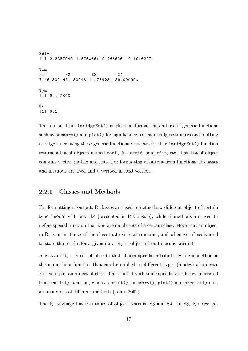
$div

[1] 2.3357040 1.6760661 0.2866061 0.1016237

$xm

X1 X2 X3 X4

7.461538 48.153846 11.769231 30.000000

$ym

[1] 95.42308

$K

[1] 0.1

This output from lmridgeEst() needs some formatting and use of generic functions

such as summary() and plot() for signicance testing of ridge estimates and plotting

of ridge trace using these generic functions respectively. The lmridgeEst() function

returns a list of objects named coef, k, resid, and rfit, etc. This list of object

contains vector, matrix and lists. For formatting of output from functions, R classes

and methods are used and described in next section.

2.2.1 Classes and Methods

For formatting of output, R classes are used to dene how dierent object of certain

type (mode) will look like (presented in R Console), while R methods are used to

dene special function that operate on objects of a certain class. Note that an object

in R, is an instance of the class that exists at run time, and whenever class is used

to store the results for a given dataset, an object of that class is created.

A class in R, is a set of objects that shares specic attributes while a method is

the name for a function that can be applied to dierent types (modes) of objects.

For example, an object of class "lm" is a list with some specic attributes generated

from the lm() function, whereas print(), summary(), plot() and predict() etc.,

are examples of dierent methods (John, 2002).

The R language has two types of object systems, S3 and S4. In S3, R object(s),

17

classe(s) and method(s) are informal and very interactive. This class system was

rst described by Chambers and Hastie (1992) and is called by S programmers as

"White Book". Object(s), class(es) and method(s) in class S4 are more formal and

rigorous. In other words, the S4 class system is less interactive as compared to S3.

The S4 system was rst described by Chamber (1998) in "Green Book". The packages

written in S4 class system are available in R since version 1.7.0 (see Leisch, 2008).

In S3 class system, there is no formal denition of a class. An R object can be created

from a new S3 class by simply setting the class attribute of the created object to the

name of the desired class (see John, 2002; Leisch, 2008). that is,

> results <- x

> class(results) <-"lmridge"

In R, classes are attached to an object as an attribute that determines the (specic)

behaviour of a generic function(s) such as print(), summary(), and plot() etc., by

invoking a method appropriate to the class of that object. Therefore, a generic

function can perform dierent operations on object(s) having dierent classes. In

the S3 class system, generic function(s) takes a look at the class of their rst

argument given and method dispatches, based on naming convention. In other

words, the generic methods pass an object to its specic method. That is, when

print() function is called with an argument of class "lmridge", it looks for a

function print.lmridge(). More technically, print() function does not display or

print the results actually, but it looks at the class of an object passed and then calls

the specic print method of that class. If no method for required object class

exists then default method such as print.default() will be used.

Once the classes are dened, we may need to perform some calculations on objects.

To perform computation on objects, it is required to use of generic functions and

method dispatch. A generic function has a special body that generally contains a

call to UseMethod(), that islmridge <- function(x , ...)

UseMethod("lmridge")

18

If author's package contains a function that intended to be used as a generic function,

for example, print.lmridge for class lmridge, then it should be indicated in the

NAMESPACE le (see Section 2.3.4) by using an S3method directives, to ensure

that these methods are available in the package. For example, following directive

will ensure that the method is registered and is available for UseMethod dispatch,

and print.lmridge needs not to be exported.

S3method(print , lmridge)

To write a formula interface, the main function lmridge() need to be generic and

need to write a method named "default" whose rst argument is a design matrix

(or some other data structure that can be converted to a matrix) that is

lmridge.default function is dened to have a default method.

lmridge <- function(x ,...)UseMethod("lmridge")

lmridge.default <- function(formula , data , K=0, ...)

est <- lmridgeEst(formula , data , K, ...)

est$call <- match.call()

class(est) <- "lmridge"

est

The default method, lmridge.default() is dened which calls lmridgeEst()

function for the estimation of ridge parameter. The class of the returned object by

the "default" method is set to "lmridge". The coef() function rescales ridge

coecients, that is,

coef.lmridge <-function(object , ...)

scaledcoef <-t(as.matrix(object$coef/object$xscale))

if(object$Inter)

inter <-object$ym-scaledcoef%*%object$xm

scaledcoef <-cbind(Intercept=inter , scaledcoef)

colnames(scaledcoef)[1] <-"Intercept"

else

scaledcoef <-t(as.matrix(object$coef/object$xscale))

drop(scaledcoef)

The coef() function need an argument of class "lmridge", such as

19

> coef(lmridge(Y~X1+X2+X3+X4, data=Hald , K=0.1))

Intercept X1 X2 X3 X4

86.7701594 1.0996246 0.2898463 -0.2717493 -0.3436969

The print() method for lmridge() is used to have formatted output of ridge model

coecients for given biasing parameter(s) k.

print.lmridge <-function(x, ...)

cat("Call:\n",paste(deparse(x$call),sep="\n",collapse="\n"),

"\n",sep="")

print(coef(x) ,...)

cat("\n")

invisible(x)

The enhanced output for linear ridge coecients for biasing parameter k = 0.1 is,

> lmridge(Y ~ X1 + X2 + X3 + X4 , data=Hald , K=0.1)

Call:

lmridge.default(formula = Y ~ X1+X2+X3+X4, data=Hald , K=0.1)

Intercept X1 X2 X3 X4

86.7701594 1.0996246 0.2898463 -0.2717493 -0.3436969

Note that, rescaled ridge coecients will be printed in R console because generic

function print calls an object of class "lmridge" in function coef() dened above.

After tting the model, dierent methods such as summary and plots are required

to investigate the results. The estimation of parameter of a regression model

provided are summarized using matrix that contain 5 columns namely estimate,

scaled estimate, standard error, t-test values and p-values for parameter estimates.

summary.lmridge <-function(object , ...)

res <-vector("list")

res$call <-object$call

y<-object$y

n<-nrow(object$xs)

rcoefs <-object$coef

hatr <-as.matrix(object$hatr)

edf <-n-sum(diag(2*hatr -hatr%*%t(hatr)))

ZZt <-object$Z%*%t(object$Z)

20

vcov <-sum(object$resid ^2)/edf * ZZt

SE<-sqrt(diag(vcov))

tstats <-(rcoefs/SE)

pvalue <-2*(1-pnorm(abs(tstats)))

coefs <-coef(object)

b0<-object$ym -colSums(rcoefs*object$xm)

seb0 <-sqrt(var(y)+sum(object$x)+sum(diag(vcov) ) )

summary <-vector("list")

if(object$Inter)

summary$coefficients <-cbind(coefs , c(b0 , rcoefs), c(seb0 , SE), c(

b0/seb0 , tstats), c(NA , pvalue))

colnames(summary$coefficients)<- c("Estimate", "Estimate (Sc)", "

StdErr (Sc)", "t-value (Sc)", "Pr(>|t|)")

else

summary$coefficients <-cbind(coefs[-1], rcoefs , SE , tstats ,

pvalue)

colnames(summary$coefficients)<- c("Estimate", "Estimate (Sc)", "

StdErr", "t-value", "Pr(>|t|)")

summary$K<-object$K

res$summary <-summary

class(res)<-"summarylmridge"

res

The print() method for summary function is dened to have computation and

display of results in R console separately.

print.summarylmridge <- function (x, digits = max(3, getOption("

digits") - 3), signif.stars = getOption("show.signif.stars"),

...)

CSummary <- x$summary

cat("\nCall :\n", paste(deparse(x$call), sep="\n", collapse="\n"),

"\n\n", sep="")

cat("Coefficients: for Ridge parameter K=", CSummary$K, "\n")

coefs <- CSummary$coefficients

printCoefmat(coefs , digits=digits , signif.stars=signif.stars , P.

values = TRUE , has.Pvalue = TRUE , na.print="NA", ...)

invisible(x)

The utility function printCoefmate() is used to display the matrix of output with

some rounding of digits and formating to print the outcome from

summary.lmridge().

21

Only few functions from our package lmridge are shown here and or not as in actual

package. Other function available in lmridge package and their description is in

table below. All function perform calculation on each biasing parameter provided as

argument in lmridge function our newly built lmridge package.

Table 2.1: Functions and methods in lmridge Package

Functions Description

lmridgeEst() The main model tting function for implementation of ridge regression

models in R.

lmridge() Generic function and default method that calls lmridgeEst function

and returns an object of S3 class "lmridge" with dierent set of methods

to standard generics. It has a print method for display of ridge de-scaled

coecients

press() Generic function that computes prediction residual error sum of squares

(PRESS) for ridge coecients.

summary() Standard ridge regression output (coecient estimates, scaled

coecients estimates, standard errors, t-values and p-values); returns

an object of class "summaryridge" containing the relative summary

statistics and have a print() method.

coef() Display de-scaled ridge coecients

vcov() Displays associated variance-covariance matrix with matching ridge

parameter k values

predict() Produces predicted value(s) by evaluating the function lmridgeEst in

the frame newdata

tted() Displays ridge tted values for observed data.

residuals() Display ridge residuals values.

kest() Displays various k (biasing parameter) values from dierent authors

available in literature and have a print() method.

22

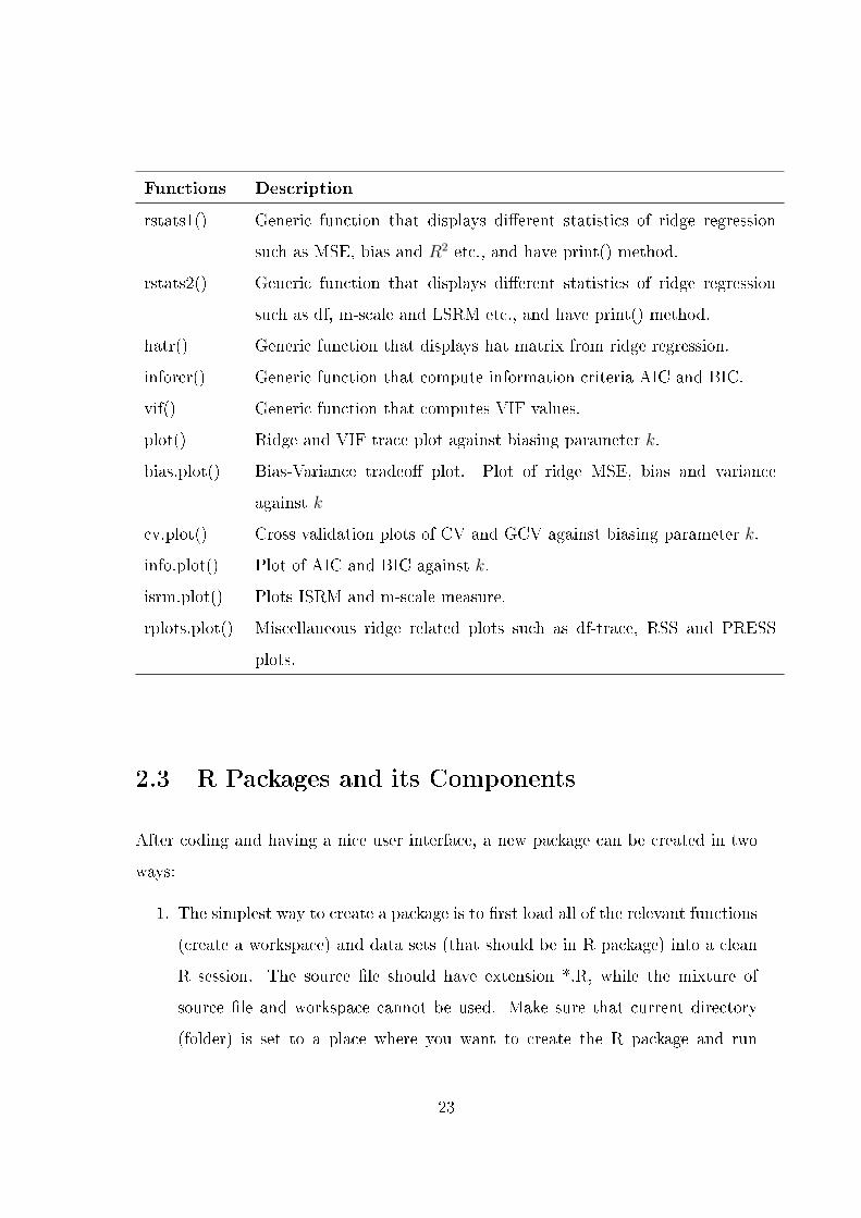
Functions Description

rstats1() Generic function that displays dierent statistics of ridge regression

such as MSE, bias and R2 etc., and have print() method.

rstats2() Generic function that displays dierent statistics of ridge regression

such as df, m-scale and LSRM etc., and have print() method.

hatr() Generic function that displays hat matrix from ridge regression.

inforcr() Generic function that compute information criteria AIC and BIC.

vif() Generic function that computes VIF values.

plot() Ridge and VIF trace plot against biasing parameter k.

bias.plot() Bias-Variance tradeo plot. Plot of ridge MSE, bias and variance

against k

cv.plot() Cross validation plots of CV and GCV against biasing parameter k.

info.plot() Plot of AIC and BIC against k.

isrm.plot() Plots ISRM and m-scale measure.

rplots.plot() Miscellaneous ridge related plots such as df-trace, RSS and PRESS

plots.

2.3 R Packages and its Components

After coding and having a nice user interface, a new package can be created in two

ways:

1. The simplest way to create a package is to rst load all of the relevant functions

(create a workspace) and data sets (that should be in R package) into a clean

R session. The source le should have extension *.R, while the mixture of

source le and workspace cannot be used. Make sure that current directory

(folder) is set to a place where you want to create the R package and run

23

package.skeleton() function to generate a package directory and several sub-

directory automatically in the required structure. This function prints out a

list of things that have to be done.

package.skeleton(name="lmridge", code_files =

c("fun1.R", "fun2.R", "fun3.R"), namespace=TRUE)

The newly created package has name lmridge dened in package.skeleton()

function that contains skeleton of the package for all functions, methods and

classes dened in the R code(s) passed on to the code_files argument. If

no source les are passed to package.skeleton() argument, then all available

objects in user's current workspace will be used.

2. Create package manually, but this is for experienced developers

A useful package have sub-directories of man, R and data. Following is a short detail

about content of package directory, created by package.skeleton() function.

Table 2.2: Package directory content and its description

Content Description

data A sub-directory that contains *.rda les for each data

object loaded in workspace

DESCRIPTION A general package information le that contains basic

description of the package created, author and license

conditions (such as GPL-2) in a structured text format

man A sub-directory that contains help les (R

documentations/ Manual). These le are in simple

markup language similar to LaTex and can be processed

to dierent formats such as LaTex, html and plain text

NAMESPACE Manages functions, methods and dependency information

R A sub-directory that contains *.R les for each function

src A sub-directory that contains C/ C++ or FORTRAN

functions only, if R functions calls these native code(s)

Read-and-delete-me This le contains some instructions for completing the

package and can be deleted

24

Note that the capitalization of les and directories in important because R language

is case-sensitive.

2.3.1 The Package DESCRIPTION File

The description le gives general information about the package in which it appears

(see Team, 2015, pp. 417) and (Leisch, 2008). The eld names are case sensitive

and should be written in ASCII format.

Table 2.3: Package description le

Fields Description

Package Used for giving an ocial name to package. The name should follow

certain rules such as the name of package must start with alphabet and

can contain combination of alphabets, numbers and dot character.

Version Used to dene the version of package. The Version is a sequence of

non-negative integers (at least two) separated by dots or dashes.

Title The Title eld is used in various package listing. The number of

character in Title should not be more than 65.

Author It describes who wrote the package. It should contain at least one

author.

Maintainer This eld should have one name and valid e-mail address (corresponding

author's email).

Description This led should contain comprehensive description of what package

does, and can be of any length but only one paragraph.

Suggest This eld informs that code in package uses some functionality from

another existing R package "lm".

Depend It can be comma-separated list of R package(s) that are needed to be

loaded in order to run the compiled package. It may also include details

of required package version, such as; Depends:R(>= 3.2.3), lm.License This eld can be free text, standardized abbreviation (such as GPL-2,

GPL-3, LGPL-3, and BSD_2_clause etc) can be used if package hat

to be submitted to CRAN, R Forge or Bioconductor repositories.

LazyData It is set to yes, if package contains data object and use lazy loading.

25

The minimal example of DESCRIPTION le for package lmridge is:

Package: lmridge

Title: Linear Ridge Regression

Version: 1.0

Date: 2015 -12 -01

Author: Muhammad Imdadullah and Muhammad Aslam

Maintainer: Muhammad Imdadullah <mimdadasad@gmail.com >

Description: A linear ridge regression for testing of ridge

coefficients and estimation of biasing parameter.

Suggests: lm

License: GPL (>= 2)

The mandatory elds are: Package, Title, Version, Author, Maintainer,

Description, and License, while remaining are optional such as Date, Suggests,

Depends and LazyData etc. The optional elds takes logical values that are

specied as "yes", "true", "no" or "false".

For further detail about all elds in package DESCRIPTION le see, "Writing R

Extensions" manual by R Development Core Team (2015).

2.3.2 R Documentation/ Help les

All exported function, objects and data sets in R package should have complete

documentation that describes how to use the functions and sample data. The sources

of R help les format is similar to LaTex and have le extension of .Rd or .rd, however

all LaTex commands are not available. The R documentation (Rd) les can be in

html, plain text, GNU info and old nro-based S help format too. A sub-directory

named "man" having no documentation may result an installation error (see Team,

2015, pp. 5774),and (Leisch, 2008). An exemplary help for "lmridge" function is.

\namelmridge

\aliaslmridge

\aliaslmridge.default

\aliaslmrdige.formula

\aliasprint.lmridge

\aliassummary.lmridge

\aliasprint.summary.lmridge

\titleLinear Ridge Regression

26

\descriptionFits linear RR for estimation of biasing parameter and

signifianct testing of ridge coefficient .

\usagelmridge(x, y, ...)

\methodlmridge defalut (x, y, ...)

\methodlmridge formula (formula , data=list(), ...)

\methodprint lmridge (x ,...)

\methodsummary lmridge (object , ...)

\arguments

\itemx regressors for model as design matrix (x)

\itemy vector of response variable (y)

\itemformula symbolic representation of the regression model to

be fit

\itemdataan optional dataframe that contain variable used in

the regression model

\itemobject an object of class \code"lmridge", a fitted model

\item\dotsnot used

\value

An object of class \codelmridge is a list that includes following

elements

\itemcoefficients a named vector of ridge coefficients

\itemK baising parameter

\itemscaling design matrix scaling

\authorMuhammad Imdadullah , Muhammad Aslam

\examples dt<-data(Hald)

mod1 <- lmridge(Y~., data=dt)

mod1

summary(mod1)

\keywordridge regression , regularization

27

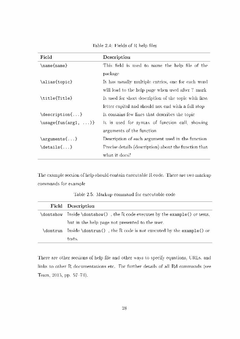
Table 2.4: Fields of R help les

Field Description

\namename This eld is used to name the help le of the

package

\aliastopic It has usually multiple entries, one for each word

will lead to the help page when used after ? mark

\titleTitle It used for short description of the topic with rst

letter capital and should not end with a full stop

\description... It contains few lines that describes the topic

\usagefun(arg1, ...) It is used for syntax of function call, showing

arguments of the function

\arguments... Description of each argument used in the function

\details... Precise details (description) about the function that

what it does?

The example section of help should contain executable R code. There are two markup

commands for example

Table 2.5: Markup command for executable code

Field Description

\dontshow Inside \dontshow() , the R code executes by the example() or tests,

but in the help page not presented to the user.

\dontrun Inside \dontrun() , the R code is not executed by the example() or

tests.

There are other sections of help le and other ways to specify equations, URLs, and

links to other R documentations etc. For further details of all Rd commands (see

Team, 2015, pp. 5774).

28

2.3.3 Data in R Package

Data can be used from recommended package because these packages are part of any

R installation. To add your own data set to the package you wrote, save the required

data using save() function and copy & pasting the resulting le (*.rda or *.Rdata)

to sub-directory named "data" in your package. Data can be in other recommended

data formats such as txt, csv, S code, etc.

Table 2.6: Documenting data sets elds

Field Description

\namename It is used to name the data object and help le

\docTypedata It is alway data for data sets

\aliastopic Topic as used for function

\titleTitle Short description of the data object

\usagename When lazy data is not in eect. The data(name) can be

used

\format... Description of object. If object is a list or a dataframe,

then each item need to be documented individually

\source... Detail of original source of the data object

\references... References to secondary sources

\examples... Examples about how to use the data object such as loading

data, making plot etc

\keyworddatasets Always datasets

2.3.4 Importing and Exporting Objects from Namespaces

R automatically creates a namespace for the package being build. When a package is

loaded (in R session), only items that are exported, are placed in the attached frame,

although all are loaded. Only those objects should be exported which author would

like to use. The skeleton will export everything which is not recommended because

29

you will be forced to create and write a help le for every object. For example, use

export(a,b) to export item say a and b, while use exportPattern("^\\,]") to

dene the items using pattern. For further detail, see (Team, 2015).

If someone has used an item (object) from a namespace from another package, he

should import it. For example, using import(package1, package2) will import all

items from packages mentioned in parenthesis, while using importFrom(package1,

package2, a, b) will import items a and b from package1 only.

2.3.5 Non-R Scripts

All non-R scripts (codes), compiled in C, C++ and FORTRAN etc., should be

included in src subdirectory.

2.4 To Build, Check and Install an R Package

R CMD is the program to build/ create an R package. On Windows machine this

program compile the package into zip le. The path of this program need to be set

using path variable in system environment variables. At DOS prompt type following

command after setting path to package, i.e.

R CMD INSTALL -- BUILD lmridge

Warnings and errors may occur in the check stage. CRAN does not accept any

package that has warnings and errors from check. Rtools and Latex compiler (such

as MiKTex distribution) is required if running check. Therefore, to check the quality

of our package lmridge, CHECK command is used;

R CMD CHECK lmridge

Note that without editing les created by package.skeleton() function, build and

check the package phase will fail. To build a package for other operating systems

such as Linux, use following command

30

R CMD BUILD lmridge

A compressed package of extension *.tar.gz le will be created, which ban be installed

on a non-windows based machines. For further details, read "Writing R Extensions"

from R CRAN.

To create the zip le (i.e., lmridge.zip) le of package, use

R CMD BUILD -- BINARY lmridge

The check tool, tests whether R source package works correctly. The series of checks

are run on a archive prepared by R CMD BUILD. The description of these checks are

given in Table 2.7.

Table 2.7: R CMD program's check List for the quality of R package

Check List Description

install Is it possible to install the package?

portability Are all le name used valid across le system and also

supported operating systems?

permission Do the les and directories have sucient permission?

binary Does binary (executable) les exists? Warning message

will appear.

description file Check for the completeness and partially for the

correctness of the DESCRIPTION le.

subdirectories Does subdirectories have suitable names and are not

empty?

R files Is the R syntax is correct?

load Can package be loaded?

Code problem Checks R code for problems and see if calls to

library.dynam and C etc. can be interpreted sensibly.

Rd Checks the format for correct syntax, metadata and

missing links.

31

Check List Description

undocumented items Does.Rd le exists corresponding to each exported

function?

documentation Checks for consistency exists between use of functions

and datasets.

usage Does function(s) arguments provided in usage eld of

le(s) having extension .Rd are documented in the

corresponding section of arguments?

examples Does examples provided in package's documentation run?

For further details about how to create a package in R language, see Leisch (2008),

Ligges (2003), Hornik (2015) and Team (2015).

32

Chapter 3

Multicollinearity Diagnostics and

mctest Package

3.1 Introduction

The linear regression model (LRM) and its oshoots such as two or three stage least

squares (2-SLS, 3-SLS) have been widely used as quantitative tools for the social

and physical sciences, over the last several decades. The use of OLS method is

popular due to its low computational cost, it visceral plausibility in a wide variety

of circumstances and its support by a spacious and sophisticated body of statistical

inferences. The OLS method First, applied descriptively as a mean of curve tting

merely. Second, it is used for testing of hypothesis and Thirdly, it provides an

environment in which statistical theory, subject eld related specic theory and data

may be brought together to enhance our realization of complex social and physical

phenomena. Relevant statistical theory has been originated from each of the above

three perspectives and practical guidelines have also been developed (Belsley et al.,

1980; Belsley, 1991).

The degree of understanding of practical experience and theoretical support cannot

33

be said to exist when examining and evaluating the quality and potential inuence

of the data (that are assumed "given") because the thrust of standard regression

theory is based on sampling variation or uctuation which is reected in the

regression coecients, V ar-Cov matrix and associated statistical tests such as

t-test, F -test, and prediction intervals etc. The regressors are treated as xed, but

actually, data and model may be in conict in ways not readily analyzed or

examined by existing standard statistical procedures. Thus, after examining the

signicance tests (such as t-test and F -test) and all the model variants have been

compared, the researcher often feels that his/ her results form regression analysis

are less meaningful (or signicant) and less trustworthy than might otherwise be

the case, because of potential problem(s) with the data the problem(s) that are

generally neglected in practice. Similarly, the dierent subsets of the data may

produce very dissimilar results, raising some questions about stability of the

statistical model. On the other hand, when the researcher knows that certain

observation (few data points) pertain to some unusual circumstances (such as

strikes, wars and ood etc.) but he/ she is unsure of the extent to which the results

depends for good or ominous. In data collecting procedure, more pernicious

situation may arise when an unknown error generates an anomalous data point(s)

that cannot be surmised (on some prior grounds). The researcher may feel that

collinearity is causing some trouble(s), possibly generating some non-signicant

estimates of regression coecients supposed to be important on the basis of

theoretical considerations (Belsley et al., 1980; Belsley, 1991).

For small regression model, researchers often detect some form of (multi)collinearity

or even some unusual data point(s) during the process of handling the data by using

statistical software and by some use of dierent descriptive statistics. The usage

of very high-speed computers in current era and use of large size data and models,

the researcher has become isolated from intimate knowledge about the data being

used, because of cursory examination for the suitability of data. Similarly, data

related problems are often ignored while all the data points are included due to the

34

law of large numbers. However, this is of course incongruous, if some of the data

are in error or they came from dierent regime. On the other hand, the researcher's

understanding of the degree to which regression results depend on specic data sample

being used, does not increase even if all the data are correct and is relevant to

regression model. The researcher may be ignorant of properties that additionally

collected data may have, either to reduce the sensitivity of the estimated regression

model to some part of the data, or to remedy ill-conditioned data that may be

precluding useful estimation of some parameters altogether (Belsley et al., 1980;

Belsley, 1991).

The objective of multiple regression analysis is to estimate the relationship of

individual parameters of a dependency but not of interdependency by assuming

that the response variable y and the regressors (X's) are linearly related to each

other (see Graybill, 1980; Johnston, 1963; Johnston and DiNardo, 1997; Malinvaud,

1968). Our focus is on to draw some inferences such as (i) identify the relative

inuence of the regressor(s), (ii) prediction and/or estimation and (iii) selection of

an appropriate set of regressor(s) for the regression model. So, our intention to use

regression model is to nd out at what extent the dependent variable can be

predicted by the relevant regressors. For this purpose, usually R2 (the coecient of

determination) is used to indicate the strength of prediction also called goodness of

t of the regression model. The model t is considered to be good if the overall

value of R2 is high enough, that is near to 1. The model t becomes poor or very

poorer when important signicant regressor(s) or variables(s) is/are omitted from

the model.

In order to draw inferences from regression analysis, the regressors should have no

linear relationship between themself, i.e they should be orthogonal, but in most of

the application of regression analysis, regressors are not orthogonal which leads to

misleading or erroneous inferences that made from regression analysis, specially, in

case when regressors are perfectly linearly or nearly perfectly related (dependent

35

with each other), which is known as problem of multicollinearity (see Gunst and

Mason, 1977; Gunst, 1983; Mason et al., 1975; Ragnar, 1934); a term rst used

by Ragnar (1934). Multicollinearity is the lack of independence or the presence

of interdependence signied by high inter-correlations (R = X ′X) within a set of

regressors (see Dorsett et al., 1983; Farrar and Glauber, 1967; Gunst, 1983; Gunst

and Mason, 1977; Mason et al., 1975). Perfect multicollinearity is not a problem as

it can easily be detected and resolved by dropping one of the regressor(s) causing

multicollinearity (Belsley et al., 1980). Multicollinearity is considered as the specic

characteristic of the design matrix X, not a statistical aspects of the LRM, described

in Eq. (2.1). Therefore, multicollinearity is a data related problem, not a statistical

problem (Belsley et al., 1980).

Collinear data usually arise and have potential harm when applying regression

analysis in geophysics, oceanography, econometrics, and all other eld that rely on

non-experimental data. Though many of the possible regressors are highly collinear

(correlated, confounded) which is a fact of life, however it becomes very dicult to

infer the separate inuence of these collinear regressors on the response variable,

because these collinear regressors do not provide information that is very dierent

from that already inherent in others regressor(s). On the other hand, perfect

collinearity destroys the uniqueness of the least square estimators (LSEs) (Belsley

et al., 1980).

Researcher is faced with a problem, when the degree of correlation between regressors

is high enough however not perfect, because, one of the assumption of CLRM is

that regressors are not collinear with each other, is violated. The other related

assumptions are that the number of observations in data must be greater than the

number of regressors being used in the regression model and there should be sucient

variability in the values of regressors.

Statistically, an exact linear relationship exists if c1X1+c2X2+· · ·+ckXk = 0 satised,

where c1, c2, · · · , ck are constants such that all of them are not zero simultaneously.

36

Now a day, multicollinearity is being used for perfect multicollinearity as well as for

not perfect multicollinearity (where the X variables are inter-related) i.e. c1X1 +

c2X2 + · · ·+ ckXk + vi = 0 where vi is stochastic error term.

Strictly speaking, the distinction between collinearity and multicollinearity is that,

the term multicollinearity is used when more than one exact linear relationship

exists among regressors, while term collinearity is used for existence of a single

linear relationship, however, multicollinearity refers to both of the cases now a days.

We will use both terms alternatively as required.

3.2 Sources of Multicollinearity

There are several sources of multicollinearity in data, therefore dierences among

them must be clearly understood, because the interpretation of resulting model

depends on some of the cause(s) of the problem. Following are the sources of

multicollinearity stated in dierent existing literature such as (Gujarati and Porter,

2008; Gunst and Mason, 1977; Koutsoyiannis, 1977; Mason et al., 1975;

Montgomery and Peck, 1982, among many others).

• The data collection method used, e.g. sampling over a limited range of the

values taken by the regressors in the population, i.e. samples are taken from

subspace of the region of regressors.

• Constraints on the tted model or on the population being sampled.

• Model specication problem, that is, when polynomial terms are added in

model, causing ill-conditioning of the X ′X matrix.

• In case when model is overdened, that is, model has more regressors than the

number of observation in the data set.

• When there is some common trend in time series data i.e. regressors may be

growing/ decaying over time approximately at the same (constant) rate.

37

• Improper use of dummy variables (dummy variable trap).

• Inclusion of the same variable twice in model. For example, variables height in

inches and height in feet.

• Inclusion or exclusion of a variable or even certain observation may greatly

change the estimated regression coecients showing the existence of

multicollinearity.

3.3 Consequences of Multicollinearity

Multicollinearity does not lessen the predictive power or reliability of the regression

model as whole, it only aects the individual regressor (Koutsoyiannis, 1977), i.e.

models having correlated regressors can indicate how well/ good the entire collection

of regressors is predicting the response variable, but it may not give valued results

about any individual regressor or about which regressors are redundant with respect

to others.

In case of near or high multicollinearity (existence of linear dependencies among

regressors), following are the potentially serious eects on the regression estimates

and are thoroughly discussed in literature (see Chen, 2012; Belsley, 1991; Gujarati

and Porter, 2008; Gunst, 1983; Rawlings et al., 1998; Swamy et al., 1985, among

many others).

• The statistical/ mathematical software fail to perform matrix inversion

because X ′X matrix becomes singular (ill-conditioned), therefore estimation

of coecients and standard errors is not possible.

• Although the regression coecients are BLUE, but in absolute value β's (|β|)

are too big but they tend to be far from true β's i.e. β is/are too big in absolute

value.

38

• The OLSEs have large variances, covariances and standard errors that make

precise/ accurate estimation of regression coecients dicult.

• Condence intervals tend to become wider due larger standard errors and lead

to accept the null hypothesis of β = 0.

• It also becomes dicult to isolate and measure the separate eect of regressor(s)

on the response variable, that is, estimation of regression coecients becomes

dicult because coecient(s) measures the eect of the corresponding regressor

while holding all other regressors as constant.

• Although the t-ratio of one or more regression coecients tends to be

statistically non-signicant, even though they have signicant eect on the

response variable, while R2 (explained variation) can be relatively very high.

• Increase in the type-II error, that is, failure to nullify the null hypothesis that

the regression coecients are not dierent from zero.

• Structural integrity of the econometric model is eected.

• The OLSEs and their standard errors can be sensitive to small change in the

data point(s), that is, results are not robust.

• The correlated X's, correspond to large values of (X ′X)−1, inates the

estimated variances for Y i.e.

V (y) = V (Xβ) = XV (βX ′)

= σ2X(X ′X)−1X ′

It means the existence of multicollinearity inates the estimated variances of

the predicted values for sets of x values, especially when these values are not

in the sample.

• The sign of parameter estimates dier from the sign of the true parameter.

39

All these theoretical considerations are thought to be important for detection of

multicollinearity among regressors (see Adnan et al., 2006; Belsley, 1991; Chatterjee

and Hadi, 2006; Chen, 2012; Greene, 1993; Younger, 1979, etc.).

3.4 Dealing with Multicollinearity

Following are the dierent ways already available in the literature (see Feldstein, 1973;

Gujarati and Porter, 2008; Johnston and DiNardo, 1997; Maddala, 1992; Wooldridge,

2009) to reduce or to minimize the existence of multicollinearity:

• Exclude one of the most correlated X variable(s) from the model, although

it may lead to model specication error. The objective is to avoid redundant

variable(s) in the regression model (Bowerman et al., 1993).

• Find another regressor (to include in model) related to the concept and study,

which is not collinear with the other regressors.

• Put some constraints on the eects of variables. For example, if two or more

variables have equal eects or eects of equal magnitude but opposite direction,

one might have to compute a new variable. For example, if years of education

and years of job experience are highly collinear, then compute a new variable

such as years of Education + Job Experience and use this instead.

• Increase the sample size, as larger sample reduces the problem of

multicollinearity by reducing standard errors, also additional data points will

tend to produce more variation across the columns of the X matrix, allowing

the better dierentiable eects of the variables.

40

3.5 Multicollinearity Detection Methods

Diagnosing collinearity is important to many practitioner/ researchers of the LS

method, that consists of two related but separate elements (1) detecting the existence

of collinear relationship between the data series (regressors) and (2) assessing the

extent to which these relationship have degraded the parameter estimates. These

diagnostics methods will assist the researcher in determining whether and where

some corrective action is necessary and worthwhile (Belsley et al., 1980).

Kmenta (1980), discussed some warning:

• "Multicollinearity is a question of degree and not of kind. The meaningful

distinction is not between the existence and the absence of (multi)collinearity,

but it is between its several degrees".

• "Multicollinearity refers to the condition of the regressors (that are assumed to

be non-stochastic), it is a characteristics of the sample not of the population".

Existence of multicollinearity should always be tested when examining a data set as

an initial step in multiple regression analysis, because the adverse eects of

multicollinearity and its pitfalls that may exist (see Section 3.3).

Several diagnostic measures for the quantication of collinearity are available in

literature, however, none of these diagnostic measures can be regarded as a

synthetic and normalized method at the same time (Belsley et al., 1980; Silvey,

1969; Kovács et al., 2005). These multicollinearity detection methods can be

classied in two ways:

1. Graphical methods for detection of multicollinearity

2. Numerical methods for detection of multicollinearity

41

3.5.1 Graphical Methods of Diagnostics

• Tableplot for Condition Indices and Variance Proportions

Friendly and Kwan (2003) used the tableplots by making improvement to the

standard tabular display that can be used for diagnostic purpose of

multicollinearity. The tableplot was developed by Kwan (2008) to render

numeric information in a table and are displayed appended by symbols that

have their sizes relative to the cell value and some visual attributed such as

shape, background ll and color ll etc., used to encode additional

information necessary for visual understanding and inspection of collinearity.

In rst column of the tableplot, the symbols are scaled relative to a maximum

CI of 30, while in remaining columns, variance proportions are scaled relative

to a maximum of 100.

• Collinearity Biplot

Friendly and Kwan (2003) also proposed a method through collinearity biplot

to visualize the contribution of regressors to multicollinearity. The standard

biplot (Gabriel, 1971; Gower and Hand, 1996) can be considered as

multivariate scatter-plot, obtained by projecting multivariate sample into a

low-dimensional space to account for the greatest variance in the data. In

biplot, (i) the mean value of each regressors is origin of the variable vector

and points in the direction of positive deviations from the average of each

variable, (ii) the angle between regressors depicts the degree of relationships

between regressors, (iii) the angles between each regressors and the biplot

axes approximate the relationship among regressors, (iv) because the

regressors were scaled to unit length, the relative length of each regressor

indicates the proportion of variance represented in the low-rank

approximation, (v) the orthogonal projections of the observation points on

the regressors show approximately the value of each observation on each

regressor, and (vi) the observations indicated as principal component scores

42

are uncorrelated by construction.

But still the standard biplot is less useful for visualizing the relations among

regressors contributing to near multicollinearity. Biplot of smallest dimensions

shows these relations directly and can be used to show other features of data

such as outliers, and leverage points.

• VIF and Eigenvalue Plots

Graphical representation of VIF values for each regressors can be used to

detect existence of collinearity graphically. Similarly, eigenvalues can be

plotted. Larger values of VIF or smaller eigenvalues can be depicted from

vertical axes for each regressors.

3.5.2 Numerical Method of Diagnostics

Following are dierent available numerical diagnostic measures used for detection

of multicollinearity in exiting literature provided or discussed by various authors

(Belsley et al., 1980; Curto and Pinto, 2011; Farrar and Glauber, 1967; Fox, 1986;

Greene, 1993; Gunst and Mason, 1977; Klein, 1962; Koutsoyiannis, 1977; Kovács

et al., 2005; Marquardt, 1970; Theil, 1971).

Widely used and most suggested diagnostics are value of pair-wise correlations, VIF,

TOL, eigenvalues and vector, CN & CI, Leamer's method, Klein's rule, tests proposed

by Farrar and Glauber (Farrar and Glauber, 1967), Red Indicator and Theil's measure

etc. Some details about these tests is described below.

1. High Correlation between Exogenous Variables

If zero-order or pairwise correlation coecient between two regressors is high

(say >0.8) then multicollinearity may be a serious problem (Gujarati and

Porter, 2008; Maddala, 1988), but it is not sucient and necessary condition

for the detection of multicollinearity because of linear dependencies existing

between regressors (Judge et al., 1985). Also multicollinearity may exist even

43

though the pairwise correlations are comparatively low (say <0.5). However,

multicollinearity may be harmful if rij ≥ R2 (Huang, 1970).

2. High R2 and low t-ratios

High R2 (say >0.8) may be considered as classic symptom of harmfulness of

multicollinearity (c.f. Gujarati and Porter, 2008). In most of the cases, overall

F -test rejects the null hypothesis of partial slope are simultaneously equal to

zero, but some or all individual t-ratio of partial slope will be non-signicant.

The weakness of this diagnostic is that "it is too strong in the sense that

collinearity is regarded as harmful destructive only when all of the inuences of

regressors on y (response variable) cannot be disentangled" (c.f. Gujarati and

Porter, 2008). A model having no multicollinearity problem, having high R2,

should also have high t-ratios of coecients.

3. The FarrarGlauber test

Farrar and Glauber (1967) suggested three set of statistical tests for testing

multicollinearity. The rst test is Chi-square test for detection strength of

multicollinearity over the complete set of regressors,

χ2 = −[n− 1− 1

6(2k + 5)].loge [value of standardized determinant] .

Second test is an F -test for locating the variables which are collinear by

computing the multiple correlation coecients among explanatory variables

F∗ =(R2

xj .x1x2···xk)/(k − 1)

(1−R2xj .x1x2···xk)/(n− k)

, j = 1, 2, · · · , p

and third test is for nding out the pattern of multicollinearity by nding the

partial correlation coecients among regressors,

t∗ =(rxixj .x1x2···xk)

√n− k√

1− r2xixj .x1x2···xk.

44

Studying partial correlation may be useful, however there is no guarantee that

partial correlations will provide an infallible guide to multicollinearity because

both the R2 and all the partial correlation may be suciently high.

Note that FarrarGlauber test of multicollinearity is based only on the

correlation or partial correlation coecient of regressors and make no use of

overall R2.

Wickers (1975) showed that the Farrar and Glauber (1967) partial correlation

test is inecient as given partial correlation may be compatible with dierent

multicollinearity pattern.

4. Determinant

X ′X matrix will be singular matrix (can't be inverted) if it contains linearly

dependent columns or rows. Therefore, it is better to calculate the

determinant of matrix X ′X (constant term is not included). Determinant of

normalized correlation matrix |X ′X| closer to zero indicate perfect

multicollinearity, while small value of determinant will indicate almost

singular matrix or near multicollinearity (Asteriou and Hall, 2007).

Determinant on the scale is 0 ≤ |X ′X| ≤ 1 (see Cooley and Lohnes, 1971).

This diagnostic is a very weak measure of harmfulness of (multi)collinearity.

It is better to use some other diagnostic measures that reect the sensitivity

of the parameters with respect to small changes in X ′X. Determinant does

not provides information about interdependence between regressors, it only

provide information about singularity (departure from orthogonality) of a

correlation matrix.

5. Variance Ination Factor (VIF) and Tolerance

The VIF terminology was introduced by Marquardt (1970), that measures how

much the variance of estimated regression coecients are increased over the

case of no correlation among p regressors.

45

The diagonal elements of C = (X ′X)−1p×p matrix are considered as very

important in detecting multicollinearity. The jth diagonal element of C can

be represented as Cjj =(1−R2

j

)−1, where R2

j is the coecient of

determination when regressor Xj is regressed on the remaining (p − 1)

regressors. R2j will be small and Cjj be close to one, when Xj is orthogonal or

nearly orthogonal to the other remaining (p − 1) regressors. In case, if the

regressor Xj is nearly dependent on some of the remaining (p − 1) regressors,

R2j will be near to one and Cjj will be large enough.

Collinearity of regressor Xj with remaining (p− 1) regressors increases as VIF

increases and it can be innite. If VIF of a variable exceeds 10 (happens when

R2j>0.9) that variable is said to be highly collinear (Kleinbaum et al., 1988).

It is better to examine the square root of VIF instead the VIF, because the

precision of estimation of βj is proportional to the standard error of βj not on

its variance (Stewart, 1987). Tolerance (TOL) can also be used as a measure

of existence of multicollinearity in view of its intimate connection with V IFj.

TOLj =1

V IFj= (1−R2

j )

It can be seen from formula that closer the TOLj to zero, the greater the degree

of collinearity of that variable with the other regressors, in other words it can

be said that if TOLj is closer to 1, the greater evidence that regressor Xj is

not collinear with the other remaining regressors.

Although VIF gives a good measure of multicollinearity, but still it is unable to

elucidate the structure of several existing near dependencies among regressors.

One advantage of using R2j = 1− 1

V IFis that it does not depend on scaling of

data. It is not aected by raw data, centered data and even standardized data.

However, the criticism on VIF is that V ar(βj) = σ2∑x2jV IFj depends on σ2,∑

x2j and V IFj, which shows that a high VIF can be counterbalanced by a

46

low σ2 or high∑x2j . So a high VIF is neither necessary nor sucient measure

of multicollinearity. Because of its simplicity and direct interpretation, VIF or

square root of VIF is considered as the principle diagnostic for the detection

of multicollinearity. That's why approximately all of the statistical software

report VIF and/or TOL in their regression output.

Multicollinearity can be detected by examining VIF and condition indices

(Neter et al., 1989), therefore, examination of the eigenvectors, corresponding

to small singular values should be done.

6. Sensitivity of Parameters

Simple regression yields the same parameter estimation than multiple

regression in case of zero multicollinearity. The problem of multicollinearity is

proportional to the sensitivity of the parameters with respect to the addition

of new regressors. Similarly, a slight change in data, in case of not perfect

multicollinearity, estimation of coecients is although possible but the

estimates and their standard errors becomes very sensitive. All this can be

used for detection of possible multicollinearity.

7. Auxiliary Regression

Using auxiliary regression, R2 designated by R2j is computed by regressing each

Xj on the other remaining X variables. Relationship between F and R2 for

each auxiliary regression is built by

Fj =

R2xj.x2,x3,··· ,xp

(p−2)1−R2

xj.x2,x3,··· ,xp(n−p−2)

∼ F ∗(p− 2, n− p+ 1)

where n is sample size, p is number of regressors including intercept

and R2xj .x2,x3,··· ,xp is coecient of determinant in the regression of variable Xj

on the remaining X variables.

If the computed F exceeds the critical Fj (Fj > F ∗)at the chosen level of

47

signicance, then it means that the regressor Xj is collinear with other

regressors. If Fj is statistically signicant, the particular Xj should be

dropped from model need some decision.

8. Klein's Rule of Thumb

Klein (1962) rule of thumb is that multicollinearity may be a dicult to detect,

if the R2j from an auxiliary regression is larger than the overall R2 (obtained

from the regression of y on all the regressors) Greene (1993).

9. Eigenvalues and Eigenvectors

Eigenvalue and eigenvectors of X ′X or its related correlation matrix R, were

used in dealing with multicollinearity for many years. Kloek and Mennes (1960)

depicted several ways of using principal components of X or related matrix to

reduce some ill eects of multicollinearity. For diagnostic purpose, Kendall

(1957) and Silvey (1969) suggested the use of eigenvalues of X ′X to check the

presence of multicollinearity by setting the criteria that small eigenvalue (near

to zero) is an indication of high collinearity, but did not mentioned how much

small should be the eigenvalue.

From eigenvalues, we can compute condition number κ, dened as κ =λmaxλmin

and condition index (CI) also called complaint number is dened as

CI =√κ =

√λmaxλmin

If the value of κ is between 100 and 1000 there is moderate to strong

multicollinearity and if it exceeds 1000 there is severe multicollinearity.

Alternatively, if CI =√κ is between 10 and 30, there is moderate to strong

multicollinearity and if it exceed 30 there is severe multicollinearity (Belsley,

1991).

Similarly, incremental percent of an eigenvalue to the total is also used for

detection of existence of collinearity among regressors. Incremental percent

48

value near to 0 indicates that data are collinear.

10. The sum of λ−1i

Investigation of eigenvalues and eigenvectors of the X ′X matrix helps in

assessing the degree of multicollinearity. In an orthogonal system

p∑j=1

λ∗j =

p∑j=1

λ∗−1j = p

where λ∗j correspond to the p eigenvalues of the correlation matrix R∗ = Ip×p.

Therefore, for a sample based correlation matrix R with eigenvalues λj, j =

1, 2, · · · , p, we can compare p as∑p

j=1 λ−1j .

Larger the values of∑p

i=1 λ−1j (say ve times the number of predictor variables)

indicate severe collinearity (Dillon and Goldstein, 1984; Chatterjee and Hadi,

2006).

11. Leamer's Method

Leamer (in Greene, 1993) suggested the following measure of the eect of

multicollinearity for the jth variable:

cj =

(∑

i

(Xij −Xj)2

)−1(X ′X)−1jj

12

where (X ′X)−1jj is the jth element of the matrix (X ′X)−1. This suggested

measure is the square root of the ratio of the variances of estimated coecients

(βj), when estimated without and with the other variables. IfXj is uncorrelated

with the other variables, cj would be 1, otherwise, cj will be equal to (1−R2j )

12 .

12. Theil's Measure

Theil (1971) proposed a measure of multicollinearity based on incremental

contribution (R2 − R2−j) to the squared multiple correlation, where R2

−j is the

49

R2 of the regression of the response variable on all the regressors excluding

Xj. Specically, the multicollinearity eect was measure by

m = R2 −p∑j=1

(R2 −R2−j)

If Theil's measure is zero, then all X's are mutually uncorrelated as the

incremental contributions all add up to R2. The m can be negative or highly

positive making dicult to use it for any guidance.

13. Red Indicator

Kovács et al. (2005) presented a synthetic and new normalized indicator for

diagnostic of multicollinearity by using eigenvalues or quantifying the average

correlation of the data. Since X ′X = R is a symmetrical matrix, the sum of

squares of the eigenvalues with spectral decomposition of this R matrix equals

the sum of squares of the matrix element (Peter Kovács,)

2∑j=1

λ2j =

p∑i=1

p∑j=1i 6=j

r2ij.

The greater the dispersion of eigenvalues, the greater will be the correlation of

the regressors. The extent of dispersion in eigenvalues is used to quantify the

extent of redundancy and is dened as

Red =

√p∑j=1

(λj − 1)2

p√p− 1

Red indicator of value zero (or zero percent) means the absence of redundancy

while the Red indicator value near to 1 means maximum redundancy. Red

indicator can be used to compare two or more redundant data, but cannot

make a direct conclusion about which one is more useful data. Red indicator

50

can be computed without knowing eigenvalues, because Red indicator value is

the quadratic mean of the elements outside the main diagonal of the correlation

matrix R, i.e.

Red =vλ√p− 1

=

√p∑i=1

(λj − 1)2

p√p− 1

=

√√√√√√p∑i=1

p∑j=1i 6=j

r2ij

p(p− 1)

Red indicator is a synthetic indicator as it quanties the average correlation

matrix of the entire data. Moreover, in comparison to known collinearity

diagnostic measures, the Red indicator reports correlation more precisely both

in quality and in size.

14. The Corrected VIF (CVIF)

Curto and Pinto (2011) proposed a new measure of multicollinearity diagnostic

to evaluate the impact of the correlation among regressors in the variance of the

OLSEs, named it as corrected variance ination factor (CVIF). The traditional

VIF overestimates when regression variables contain no redundant information

about the dependent variable.

CV IFj = V IFj ×1−R2

1−R20

,

where, R20 = R2

yx1+ R2

yx2+ · · · + R2

yxp , R2 is coecient of determination from

regression of y on all regressors, and V IFj is VIF values.

They set the rule of thumb (CV IFj ≥ 10) to decide when the variance

magnication eect is serious for the coecients βj.

We classied the collinearity diagnostics as overall and individual measures of

collinearity. The overall diagnostics measure helps to get idea about

existence/non-existence of collinearity among all regressors and results in a single

number, while individual diagnostics measure try to detect the existence/

51

non-existence of collinearity for each of the regressors. For simulated and existing

collinear data sets, and comparison of overall and individual measures of

collinearity see Table 3.1, Table 3.2 and Table 3.3. For listing of all collinearity

diagnostics with suggested detection criteria from dierent researchers with

corresponding references, see Appendix C.

3.6 New Proposed Diagnostics

The existence or detection of multicollinearity among regressors should always be

tested whenever examining a data set, so that its adverse eect and pitfall that may

exist in regression model may be avoided Kmenta (1980). Various graphical and

numerical diagnostic measures for quantication of multicollinearity are available

in literature as discussed above. However, none of the existing methods serves as

a synthetic and normalized indicator of multicollinearity (see Belsley et al., 1980;

Chen, 2012; Curto and Pinto, 2011; Green et al., 1978; Gujarati and Porter, 2008;

Kovács et al., 2005; Silvey, 1969; Ukoumunne et al., 2002).

We proposed two new diagnostics for measure of collinearity and depend on R2 and

R2adj values. The existing collinearity diagnostics heavily depends on either R

2 and/or

eigenvalues or some relation between R2 and eigenvalues, whereas R2, eigenvalues and

correlation among regressors are considered as an important collinearity detection

criteria.

The proposed collinearity detection measures depend on R2 and adjusted R2 (R2adj)'s

values. Using empirical results from regression analysis of correlated and uncorrelated

regressors by following the Monte Carlo scheme for dierent levels of correlation

among regressors with various samples sizes, it is tried to set some threshold for our

new proposed diagnostic measures.

The R2 indicates that how well data t a statistical model as it is the proportional

explained variation in dependent variable due to independent variables. The higher

52

the R2 value, the more chances of regressors to be plagued with multicollinearity (see

Asteriou and Hall, 2007; Gujarati and Porter, 2008; Maddala, 1988). The R2 is a

monotone non-decreasing function of number of regressors included in the model. It

means that R2 inates the estimate of how well the regression ts the data (Gujarati

and Porter, 2008; Stock and Watson, 2010). The R2adj is a modied version of R2

(due to Theil, 1961) that adjusts for number of regressors in a model relative to the

number of data points and hence it is an attempt to take account of the phenomenon

of spuriously increasing R2 automatically when extra regressors are added to model

Stock and Watson (2010). It deates the R2 by some factor i.e. n−1n−p−1 . For p > 1,

R2adj ≤ R2, implies that as the number of regressor(s) increases, the R2

adj increases

less than the (un-adjusted) R2, because R2 is aected by regressors sharing their

variances i.e., linear dependence exists among regressors (Gujarati and Porter, 2008;

Maddala, 1988). The above discussion about R2 and R2adj is the main reason to

consider R2adj in our new proposed diagnostic measures.

From empirical results of the Monte Carlo experiment, ination (spurious increase) in

R2 values due to addition of regressor(s) in model and deation in R2 by factor n−1n−p−1 ,

we suggest to take dierence of R2 and R2adj from auxiliary regression of regressors to

account the sharing of variances due to dierent regressors in each auxiliary regression

run, for the detection of multicollinearity (see Asteriou and Hall, 2007; Gujarati and

Porter, 2008; Maddala, 1988, for details of auxiliary regression). The dierence of

R2j and Rj .adj

2 is used as a new diagnostic measure and is referred to as Indicator 1

(IND1) for further discussion.

IND1 = R2j −Rj .adj

2 =(n− 1)(1−R2

j )

n− p+R2

j − 1,

= (R2j − 1)×

(1− pn− p

), (3.1)

where R2j and Rj .adj

2 are from the auxiliary regression of each explanatory variables.

For the simulated collinear and non-collinear data, using auxiliary regression, we

53

empirically, found that smaller the dierence or alternatively closer the value of

R2j and Rj .adj

2 i.e (R2j − Rj .adj

2 ≤ 0.020), greater the chances of multicollinearity.

Alternative, larger the value of (R2j−Rj .adj

2)−1 ≥ 50, more severe the multicollinearity

will be. This dierence of R2j and Rj .adj

2 from auxiliary regression of explanatory

variables lies in an interval [0.0104, 0.0418] for dierent sample size and correlation

level between generated regressors. Any of the extreme dierence value from the

interval can be used as criterion but we used central value (average value of dierences

for all sample size and correlation values) which is approximately 0.020.

From Eq. (3.1), as n → ∞, IND1 approaches to 0. Therefore, multicollinearity is

detected when IND1 < c for n < 100

IND1 <c

n× 100 for n > 100

The second diagnostic tool is the ratio of each R2 from the auxiliary regression (R2j ) to

the mean of all R2j (j = 1, 2, · · · , p) from the auxiliary regression i.e.,

R2j

m, where m =

p∑j=1

R2j

p. If this ratio for jth variable is greater than R2 (from regression of y on X's)

then the jth regressor will be highly collinear with others regressors. In denominator

of this diagnostic mean of all R2j (m) gives the average sharing of variances among

regressors accounted by using auxiliary regression for jth regressor as dependent

variable on the remaining regressors, whereas the distribution of R2j for dierent

sample size and correlation level between variable was found to be approximately

normally distributed. Note that if correlation among regressors is small then this

proposed indicator (say IND2 for further reference) will give false positive detection

of collinearity, as magnitude of R2J

mwill be larger than the average of R2

j 's (j =

1, 2, · · · , p) in this case. Since the classic symptom of multicollinearity is R2 ≥ 0.7,

therefore, to avoid the false positive detection of multicollinearity, the IND2 species

54

multicollinearity when

|R2j−1|m

> R2, if 0.70 ≥ R2 < 0.80

R2j

m> R2, if R2 > 0.80

no collinearity if R2 < 0.70

We compared the existing and proposed multicollinearity diagnostic tools for their

detection performance under dierent level of correlation and sample size.

3.7 Numerical Evaluation

For the numerical evaluation of dierent diagnostic measures of multicollinearity, we

have followed the similar Monte Carlo schemes used by many other researchers (see,

e.g., Aslam, 2014b; Clark and Troskie, 2006; Månsson et al., 2010; McDonald and

Galarneau, 1975; Newhouse and Oman, 1971, etc). The simulation deals with six

parameter case. The regressors are computed as

xij = (1− ρ)1/2zij +√ρZi7; i = 1, 2, · · · , n, j = 1, 2, · · · , 6,

where zi1, zi2, · · · , zi7 are independent standard normal pseudorandom numbers, and

correlation between any regressors is given by ρ. Without loss of generality, these

variables are standardized so thatX ′X form a usual correlation matrix. Five dierent

sets of correlations are considered corresponding to ρ = 0.7, 0.8, 0.9, 0.95, 0.99. The

values of such generated predictors are kept xed for simulation.

The sample size (n) is set to 50, 100, 150, 200. The number of Monte Carlo

replications is set to be 5000. In addition to this simulation study, for illustration

purpose, dierent diagnostic measures were evaluated on some popular collinear

data sets available in few previous studies (see Hald, 1952; Longley, 1967;

Malinvaud, 1968). All the calculations are performed making routines in the

55

R-Language.

Table 3.1 contains the simulated results for the overall measure of collinearity

diagnostics in percentage of detection that indicates existence of collinearity among

all the regressors. It can be seen that the determinant X ′X, the Farrar-Glauber

chi-square (FGC) test, red indicator and Theil's measure detect collinearity

correctly than the CI and sum of reciprocal of eigenvalues for all ρ > 0.8 and for

dierent sample size (n = 50, 100 and 200) while only determinant detects the

collinearity poorly for ρ = 0.7. Percentage of detection by the CI is lowest than all

the other overall diagnostics for dierent sample sizes, but it detects well as ρ

increases than ρ = 0.90 while for ρ ≥ 0.95 detection becomes 100% for all sample

sizes. For ρ = 0.7 and ρ = 0.8, the sum of reciprocal of eigenvalues detects existence

of collinearity among regressors at low percentage, but relatively much higher than

that by the CI. The FGC and Theil indicator successfully diagnose the collinearity

between regressors.

Table 3.2 contains simulated results of collinearity diagnostics for each regressor

Xj, referred to as individual measure of diagnostics. For ρ ≥ 0.90 and sample

size n = 50, 100 and 200, all diagnostics successfully detect the collinearity among

regressors Xj, except VIF/TOL, Leamer's measure and CVIF. For correlation level

ρ = 0.70 and 0.8, the diagnostic measures VIF/TOL, CVIF and Leamer's method

could not successfully detect the existence of collinearity among regressors. For

sample size of 50, the percentage of detection by VIF/TOL and Leamer's method

(when ρ = 0.7) are less than approximately 4% and 17%, respectively. For sample

of size 100, the percentages of detection by VIF/TOL and Leamer's method (when

ρ = 0.70) are less than 1% and 4.2%, respectively. Similarly, for ρ = 0.80, percentage

detection is less than 25% and 71%, respectively. Percentage of collinearity detection

by CVIF indicator is smaller as compared to the other indicators, while percentage

of detection by this indicator for sample of size 50 and ρ = 0.70 is less than 1%,

whereas, the percentage of detection increases as correlation among regressors and

56

Table 3.1: Percentage detection of collinearity by overall diagnostics measures

n Indicatorsρ

0.7 0.8 0.9 0.95 0.99

50

Determinant 61.34 99.10 100 100 100

FGC 100 100 100 100 100

Red Indicator 99.90 100 100 100 100

CI 0.00 0.16 44.62 99.32 100

Theil 99.98 100 100 100 100

Sum of reciprocal of eigenvalues 0.46 39.54 99.76 100 100

100

Determinant 54.34 99.86 100 100 100

FGC 100 100 100 100 100

Red Indicator 100 100 100 100 100

CI 0.00 0.00 10.16 100 100

Theil 100 100 100 99.82 100

Sum of reciprocal of eigenvalues 0.00 19.48 100 100 100

200

Determinant 48.60 100 100 100 100

FGC 100 100 100 100 100

Red Indicator 100 100 100 100 100

CI 0.00 0.00 0.28 99.90 100

Theil 100 100 100 100 100

Sum of reciprocal of eigenvalues 0.00 5.42 100 100 100

the sample size both increases. It is worthy to note that the percentage of detection

decreases with the increase of sample size which follow the theory that collinearity

among regressors reduces with the increase of sample size.

Our proposed collinearity diagnostics (IND1 and IND2) detect 100% existence of

collinearity among regressorsXj for dierent sample sizes and correlation level. When

the regressors are collinear at ρ = 0.70 and sample size of 50, 100 and 200, the

percentage of collinearity detection is less than 65%, 75% and 84% respectively by

by IND1, while IND2 detects 100% existence of collinearity for dierent correlation

57

level and sample sizes. For ρ ≥ 0.80, the percentage of detection is about 100%.

Thus, when collinearity is needed to be detected rightly, the new proposed measure

do it correctly.

We also performed simulation on very large sample size (n = 500, 1000, and 2000)

with very high or low correlation level (ρ = 0.1, 0.3, and 0.5) among regressors. For

example when n = 100 and ρ = 0.30, the overall diagnostic tool Theil's measure and

FGC still results in 100% false positive collinearity detection. Among the individual

diagnostic measures, the Farrar wi, F -test and Klein's rule detected collinearity in

most of the cases, reecting very high false positive rate. On the other hand, the new

proposed indicators IND1 and IND2 also detect collinearity about 10% of the times.

These results are not presented due to huge volume of diagnostic's output.

In Table 3.3, we tested all collinearity diagnostics on already existing and tested

data available in the literature. The results indicate that whether dierent

collinearity diagnostic tools detected the collinearity or they failed to detect the

collinearity among regressors for three dierent existing datasets already available

in the literature. The datasets by Longley (1967), Malinvaud (1968) and Hald

(1952), extremely plagued with multicollinearity, were used. All of the overall

diagnostic measures successfully detected the existence of collinearity among

regressors for these datasets except Theil's measure for Malinvaud data set.

Individual diagnostic measures, Klein's rule and CVIF failed to detect the

collinearity among regressors for the Longley and Hald datasets. However, Farrar

and Glauber's wi and F -test also detected the existence of collinearity due to

regressors x5 for the Longley dataset that was not reported by other indicators.

Our proposed indicators (IND1 and IND2) correctly detected the existence of

collinearity among regressors for all three datasets. Correct detection by these new

indicators also followed the results from the existing literature.

Note that, Farrar and Glauber's wi, F -test, FGC, Klein's rule and CVIF may not be

preferred because Farrar and Glauber's tests are criticized by many researchers (see

58

Table3.2:

Percentagedetectionof

collinearityby

individualdiagnostics(for

each

regressorXj)

Indicators

ρ=

0.7

ρ=

0.8

ρ=

0.9

ρ=

0.9

5ρ=

0.9

9

X1

X2

X3

X4

X5

X6

X1

X2

X3

X4

X5

X6

X1

X2

X3

X4

X5

X6

X1

X2

X3

X4

X5

X6

X1

X2

X3

X4

X5

X6

n=

50

VIF

3.20

2.98

3.50

3.40

3.34

3.54

38.58

38.86

38.26

39.96

38.94

39.00

98.94

99.08

98.94

98.86

99.06

98.96

100

100

100

100

100

100

100

100

100

100

100

100

TOL

3.20

2.98

3.50

3.40

3.34

3.54

38.58

38.86

38.26

39.96

38.94

39.00

98.94

99.08

98.94

98.86

99.06

98.96

100

100

100

100

100

100

100

100

100

100

100

100

Farrarw

i100

100

100

100

100

100

100

100

100

100

100

100

100

100

100

100

100

100

100

100

100

100

100

100

100

100

100

100

100

100

Leamer

15.72

15.56

16.76

16.32

16.12

16.10

71.32

73.40

71.24

72.54

71.94

71.30

99.96

99.92

99.94

99.92

99.98

99.94

100

100

100

100

100

100

100

100

100

100

100

100

F-test

100

99.98

99.98

99.98

100

99.98

100

100

100

100

100

100

100

100

100

100

100

100

100

100

100

100

100

100

100

100

100

100

100

100

Klein

100

100

100

100

100

100

100

100

100

100

100

100

100

100

100

100

100

100

100

100

100

100

100

100

100

100

100

100

100

100

CVIF

0.44

0.44

0.50

0.42

0.44

0.46

2.30

2.14

2.06

2.26

2.34

2.32

40.66

40.10

39.60

40.50

40.52

40.32

99.70

99.7099.70

99.70

99.70

99.70

99.62

99.62

99.62

99.62

99.62

99.62

IND1

64.5664.8265.6265.2864.8064.8497.6897.4697.5897.5497.7097.84

100

100

100

100

100

100

100

100

100

100

100

100

100

100

100

100

100

100

IND2

99.8499.8299.7899.8899.8099.9299.8699.9699.9099.8299.9299.8499.9499.9899.9899.9099.9099.9699.98

100

100

99.98

100

99.9899.9699.9899.9099.9099.9499.90

n=

100

VIF

0.16

0.08

0.10

0.28

0.18

0.10

23.86

24.92

24.04

24.52

24.04

24.58

99.90

99.78

99.88

99.88

99.94

99.90

100

100

100

100

100

100

100

100

100

100

100

100

TOL

0.16

0.08

0.10

0.28

0.18

0.10

23.86

24.92

24.04

24.52

24.04

24.58

99.90

99.78

99.88

99.88

99.94

99.90

100

100

100

100

100

100

100

100

100

100

100

100

Farrarw

i100

100

100

100

100

100

100

100

100

100

100

100

100

100

100

100

100

100

100

100

100

100

100

100

100

100

100

100

100

100

Leamer

3.90

3.42

4.10

3.96

4.18

3.92

70.84

71.40

70.56

70.38

70.54

70.46

100

100

100

100

100

100

100

100

100

100

100

100

100

100

100

100

100

100

F-test

100

100

100

100

100

100

100

100

100

100

100

100

100

100

100

100

100

100

100

100

100

100

100

100

100

100

100

100

100

100

Klein

100

100

100

100

100

100

100

100

100

100

100

100

100

100

100

100

100

100

100

100

100

100

100

100

100

100

100

100

100

100

CVIF

00

00

00

0.06

0.06

0.04

0.06

0.06

0.06

26.96

27.18

26.50

26.68

26.74

26.68

99.82

99.7099.62

99.56

99.76

99.7499.9899.9899.9899.9899.9899.98

IND1

73.7273.9274.2472.7473.8074.2699.8499.8299.8299.8499.7899.90

100

100

100

100

100

100

100

100

100

100

100

100

100

100

100

100

100

100

IND2

100

100

100

100

99.98

100

100

100

100

100

100

100

100

100

100

100

100

100

100

100

100

100

100

100

100

100

100

100

100

100

n=

200

VIF

00

00

00

11.92

11.62

12.12

11.52

12.32

12.16

100

100

99.98

100

100

100

100

100

100

100

100

100

100

100

100

100

100

100

TOL

00

00

00

11.92

11.62

12.12

11.52

12.32

12.16

100

100

100

100

100

100

100

100

100

100

100

100

100

100

100

100

100

100

Farrarw

i100

100

100

100

100

100

100

100

100

100

100

100

100

100

100

100

100

100

100

100

100

100

100

100

100

100

100

100

100

100

Leamer

0.54

0.22

0.26

0.20

0.44

0.38

73.32

72.44

72.58

72.70

71.84

72.60

100

100

100

100

100

100

100

100

100

100

100

100

100

100

100

100

100

100

F-test

100

100

100

100

100

100

100

100

100

100

100

100

100

100

100

100

100

100

100

100

100

100

100

100

100

100

100

100

100

100

Klein

100

100

100

100

100

100

100

100

100

100

100

100

100

100

100

100

100

100

100

100

100

100

100

100

100

100

100

100

100

100

CVIF

00

00

00

0.08

0.12

0.16

0.12

0.12

0.12

13.16

14.02

13.34

13.45

13.24

14.36

99.98

99.9699.98

100

99.98

100

100

100

100

100

100

100

IND1

83.0083.2484.0683.1283.5683.38

100

100

100

100

100

100

100

100

100

100

100

100

100

100

100

100

100

100

100

100

100

100

100

100

IND2

100

100

100

100

99.98

100

100

100

100

100

100

100

100

100

100

100

100

100

100

100

100

100

100

100

100

100

100

100

100

100

59

Table 3.3: Collinearity detection by overall and individual indicators for existingcollinear datasets

Diagnostic Data Set Indicators Results *

Overall

Longley

Determinant 1Farrar χ2 1

Red Indicator 1CI 1

Theil 1Sum of reciprocal of eigenvalues 1

X1 X2 X3 X4 X5 X6

Individual

VIF 1 1 1 1 0 1TOL 1 1 1 1 0 1

Farrar wi 1 1 1 1 1 1Leamer 1 1 1 1 0 1F-test 1 1 1 1 1 1Klein 1 0 1 0 0 1CVIF 0 0 0 0 0 0IND1 1 1 1 1 0 1

IND2 1 1 1 1 0 1

Overall

Malinvaud

Determinant 1Farrar χ2 1

Red Indicator 1CI 1

Theil 0Sum of reciprocal of eigenvalues 1

Individual

X1 X2 X3VIF 1 0 1TOL 1 0 1

Farrar wi 1 0 1Leamer 1 0 1F-test 1 0 1Klein 1 0 1CVIF 1 0 1IND1 1 0 1

IND2 1 0 1

Overall

Hald

Determinant 1Farrar χ2 1

Red Indicator 1CI 1

Theil 1Sum of reciprocal of eigenvalues 1

X1 X2 X3 X4

Individual

VIF 1 1 1 1TOL 1 1 1 1

Farrar wi 1 1 1 1Leamer 1 1 1 1F-test 1 1 1 1Klein 0 1 0 1CVIF 0 0 0 0IND1 1 1 1 1

IND2 1 1 1 1

* 1 indicates that collinearity is detected by indicator while 0 indicates no collinearity

60

Haistovsky, 1969; Kumar, 1975; O'Hagan and McCabe, 1975) because of statistical

properties and high false positive detection by these diagnostic measures.

3.8 mctest: An R Package for Collinearity Detection

In this section, we illustrate the use of our developed R package mctest

(Imdadullah and Aslam, 2016) for the detection of existence of collinearity among

regressors. Popular and widely used diagnostic measures that are already available

in existing the literature and our proposed diagnostic measures are implemented in

our developed package named mctest. This package contains functions namely

imcdiag, omcdiag, mc.plot and mctest. For detection of collinearity using

numerical methods, see Section 3.7. imcdiag function can be used to compute and

list individual diagnostic measures, while omcdiag function displays overall

collinearity diagnostics, and mc.plot function draws VIF and eigenvalues plots.

Functions imcdiag and omcdiag not only compute individual and overall diagnostic

measures respectively but also return results with indication of either collinearity

exist or not among regressors for overall diagnostic measures, while results from

individual diagnostic measures also indicate that which regressors may be the

reason of multicollinearity. The package can be downloaded from

https://cran.r-project.org/web/packages/mctest/.

The mctest package must be installed and loaded in the system memory, that is,

> install.packages("mctest")

Therefore, after the mctest package is installed successfully, it needs to be loaded,

so that package functions become accessible in the current R session, that is,

> library(mctest)

For package help and working examples of available functions, use the following

command,

> help("mctest")

61

The main function mctest is used to display overall, individual or both diagnostic

measures of collinearity. The syntax of mctest is,

mctest(x, y, type=c("o","i","b"), na.rm = TRUE , Inter=T, method=NULL

, corr=FALSE , detr =0.01, red=0.5, theil =0.5, cn=30, vif=10, tol

=0.10 , conf =0.95 , cvif=10, ind1 =0.02, ind2 =0.7, leamer =0.1, ...)

The description of mctest's arguments is;

Table 3.4: Description of mctest Package's arguments

Argument Description

x A numeric matrix of regressors and should contain two or more regressory A numeric vector of response variabletype For choice of overall, individual or both types of diagnostic measures.

Option "i" prints individual, "o" overall while "b prints both(individual and overall) diagnostic measures.

na.rm whether to remove missing observation. By default, missingobservations will be removed from data

Inter Inclusion or exclusion of intercept term in X matrix for eigenvalues andCN.

method For choice of certain individual diagnostic measures. Following optionsare for the choice of dierent individual measures such as "VIF", "Wi","Fi", "Leamer", "CVIF", "IND1", "IND2", "Klein". If no optionis selected all of the individual diagnostic measures will be printed.

corr Whether to display correlation matrix. By default, correlation matrixwill not be printed.

detr default threshold of Determinant detr = 0.01

red default threshold of Red indicator red = 0.50

theil default threshold of Theil's indicator theil = 0.50

cn default threshold of Condition Number cn = 30

vif default threshold of VIF measure vif = 10

tol default threshold of TOL measure tol = 0.10

conf default condence level for Farrar's tests conf = 0.95

cvif default threshold for CVIF measure cvif = 10

ind1 default threshold for IND1 indicator ind1 = 0.02

ind2 default threshold for IND2 indicator ind2 R2 = 0.70

leamer default threshold for Leamer's method leamer = 0.10

... extra arguments if used will be ignored.

62

3.8.1 Collinearity Detection using mctest Package

For the detection of collinearity among regressors, we used the Hald data as an

example, which is already bundled in mctest package and can be loaded by using

data command. After loading the data in computer memory, the regressors and

response variables are stored in x and y variables respectively as given below,

> data(Hald)

> x <- Hald[,-1] # regressors

> y <- Hald[, 1] # response variable

3.8.1.1 Overall Collinearity Diagnostics

For computation of overall diagnostics, following commands with dierent

argument(s) can be used to get results with indication of existence of collinearity

among regressors.

> mctest (x, y)

> mctest (x, y, Inter=FALSE)

> mctest (x, y, cn=20, detr =0.001)

> mctest (x, y, type="o")

The results from command mctest(x,y, cn=20, detr=0.001) are;

Call:

omcdiag(x = x, y = y, Inter = TRUE , detr = detr , red = red , conf =

conf , theil = theil , cn = cn)

Overall Multicollinearity Diagnostics

MC Results detection

Determinant |X'X|: 0.0011 0

Farrar Chi -Sqaure: 59.8700 1

Red Indicator: 0.5414 1

Sum of Lambda Inverse: 622.3006 1

Theil 's Method: 0.9981 1

Condition Number: 249.5783 1

1 --> COLLINEARITY is detected

0 --> COLLINEARITY in not detected by the test

====================================

Eigven values with INTERCEPT

63

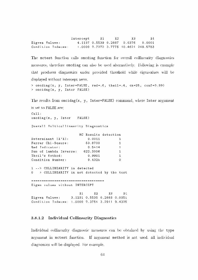
Intercept X1 X2 X3 X4

Eigven Values: 4.1197 0.5539 0.2887 0.0376 0.0001

Condition Indeces: 1.0000 2.7272 3.7775 10.4621 249.5783

The mctest function calls omcdiag function for overall collinearity diagnostics

measures, therefore omcdiag can also be used alternatively. Following is example

that produces diagnostics under provided threshold while eigenvalues will be

displayed without intercept term.

> omcdiag(x, y, Inter=FALSE , red=.6, theil=.4, cn=25, conf =0.99)

> omcidag(x, y, Inter=FALSE)

The results from omcidag(x, y, Inter=FALSE) command, where Inter argument

is set to FALSE are;

Call:

omcdiag(x, y, Inter = FALSE)

Overall Multicollinearity Diagnostics

MC Results detection

Determinant |X'X|: 0.0011 1

Farrar Chi -Sqaure: 59.8700 1

Red Indicator: 0.5414 1

Sum of Lambda Inverse: 622.3006 1

Theil 's Method: 0.9981 1

Condition Number: 9.4325 0

1 --> COLLINEARITY is detected

0 --> COLLINEARITY in not detected by the test

===================================

Eigen values without INTERCEPT

X1 X2 X3 X4

Eigven Values: 3.1231 0.5535 0.2883 0.0351

Condition Indeces: 1.0000 2.3754 3.2911 9.4325

3.8.1.2 Individual Collinearity Diagnostics

Individual collinearity diagnostic measures can be obtained by using the type

argument in mctest function. If argument method is not used, all individual

diagnostics will be displayed. For example,

64

> mctest (x , y , type=" i " )

Ca l l :

imcdiag (x = x , y = y , method = method , co r r = FALSE, v i f = v i f , t o l=to l , conf = conf

, c v i f = cv i f , ind1 = ind1 , ind2 = ind2 , leamer = leamer )

Ind i v i dua l Mu l t i c o l l i n e a r i t y D iagnos t i c s

VIF TOL Wi Fi Leamer CVIF IND1 IND2 Klein

X1 38.4962 0 .0260 112.4886 187.4811 0 .1612 −0.5846 0 .0087 0 .9875 0

X2 254.4232 0 .0039 760.2695 1267.1158 0 .0627 −3.8635 0 .0013 1 .0099 1

X3 46.8684 0 .0213 137.6052 229.3419 0 .1461 −0.7117 0 .0071 0 .9923 0

X4 282.5129 0 .0035 844.5386 1407.5643 0 .0595 −4.2900 0 .0012 1 .0103 1

1 −−> COLLINEARITY i s detec ted

0 −−> COLLINEARITY in not detec ted by the t e s t

X1 , X2 , X3 , X4 , c o e f f i c i e n t ( s ) are non−s i g n i f i c a n t may be due to

mu l t i c o l l i n e a r i t y

∗ use method argument to check which r e g r e s s o r s may be the reason o f c o l l i n e a r i t y

===================================

To get specic individual diagnostics such as VIF, Leamer's method or IND1 etc.,

use method argument. for example,

> mctest(x, y, type="i", method="VIF")

> mctest(x, y, type="i", method="IND1")

> mctest(x, y, type="i", method="CVIF", cvif =5)

> imcdiag(x, y)

> imcdiag(x, y, method="VIF", vif =10)

The last command imcdiag(x, y, method="VIF", vif=10) will display VIF values

and indicate either regressor is collinear or not by comparing with threshold dened

in argument as vif=10. VIF values larger than 10 will be indicated by 1.

Call:

imcdiag(x = x, y = y, method = "VIF", vif = 10)

Individual Multicollinearity Diagnostics

VIF detection

X1 38.4962 1

X2 254.4232 1

X3 46.8684 1

X4 282.5129 1

Multicollinearity may be due to X1 X2 X3 X4 regressors

1 --> COLLINEARITY is detected

0 --> COLLINEARITY in not detected by the test

===================================

65

Both individual and overall collinearity diagnostics can also be obtained by setting

type argument to "b", that is,

> mctest(x, y, type="b")

> mctest(x,y, type="b", method="VIF", vif=5, detr =0.01)

The command mctest(x,y, type="b", method="VIF", vif=5, detr=0.01)

produces both overall and individual collinearity diagnostics. The determinate

threshold is set of 0.01 (detr=0.01) for overall and VIF set to 5 (vif=5). From

command above individual collinearity diagnostic for VIF with detection indication

will be displayed and all overall collinearity diagnostics with intercept term

included for eigenvalues.

3.8.1.3 Graphical Detection

The function mc.plot can be used to get plot of VIF and eigenvalues for graphical

detection of collinearity among regressors. A horizontal red dotted line will be

produced against default threshold of VIF and eigenvalues respectively. The default

threshold for VIF and eigenvalues are set to 10 and 0.01 respectively. The values of

VIF and eigenvalues will be shown for each regressors according to their computed

values. If argument Inter is set to TRUE, the eigenvalues plot will be produced

with intercept term, otherwise without it. For example,

> mc.plot(x, y, vif=10, ev =0.01)

> mc.plot(x, y, vif=10, ev=0.01 , Inter=TRUE)

> mc.plot(x, y, Inter=TRUE)

In the next chapter, we will discuss widely used biased method to overcome the

problem of multicollinearity, that is, RR.

66

Figure 3.1: VIF and Eigenvalues plot without intercept term

Figure 3.2: VIF and Eigenvalues plot with intercept term

67

Chapter 4

Ridge Regression: Construction of R

Package

4.1 Introduction

As already discussed, for data collected either from a designed experiment or from

observational study, the multiple regression analysis is used to nd the eect of certain

explanatory variable(s) while keeping all other variables as constant. The ordinary

regression technique does not provide precise estimates of the eect of any particular

explanatory variable, especially when they are interdependent (collinear).

The OLSE or the maximum likelihood estimators (MLE) of β of Eq. (2.1) is,

β = (X ′X)−1X ′y, (4.1)

which depends on the characteristics of the matrix X ′X. If X ′X is ill-conditioned

(near dependencies among regressors or various columns ofX ′X exists or det(X ′X) ≈

0, whereas 0 < |X ′X| < 1), then LSEs are sensitive to a number of errors, such as

non-signicant or imprecise regression coecients (Kmenta, 1971) with wrong sign

68

and non-uniform eigenvalues spectrum.

Usually regressors under considerations in multiple linear regression analysis are not

all orthogonal i.e. X ′X 6= I, meaning that the correlation matrix of the regressors

departs from identity matrix, equivalently there is linearity among regressors or

correlation matrix approaches to singular having inated variances of parameters

being estimated. If this departure is large enough in absolute value with higher

standard errors then the regression coecients tends to be unstable, therefore there

is no unique solution for regression coecients and it is dicult to interpret (see

Chapter 3, Section 3.3). Similarly, collinearity remedies may be time consuming,

computationally expensive, controversial, costly or even impossible to achieve

Maddala (1992). Therefore, collinearity diagnostic techniques that signal the

existence of collinearity are crucial.

In case of multicollinearity, the researcher may be tempted to eliminate regressor(s)

causing the problem by consciously removing them from the model or by using some

screening method such as stepwise and best subset regression, etc. However, these

methods can destroy the usefulness of the model by removing relevant regressors from

the model. To control variance and instability of LS estimates, one might regularize

the coecients, as regularization methods are used to nd the model coecients β.

Two commonly used regularization methods are RR and Lasso regression and are

alternative to the OLS for collinear data (Dempster et al., 1977), especially when all

of the regressors are needed in the model, provided that ridge estimators are closer to

the parameter being estimated as compared to the LS estimator on average (Rawlings

et al., 1998). Computationally, RR suppresses the eects of collinearity and reduces

the apparent magnitude of the correlation among regressors (Rawlings et al., 1998), to

obtain more stable estimates of the coecients than the OLS estimates (Montgomery

and Peck, 1982; Myers, 1986; Tripp, 1983). In the resent Chapter, we focus on the

RR only.

Hoerl (1959, 1962, 1964), and Hoerl and Kennard (1970a,b) have developed ridge

69

analysis technique that purports the departure of the data from orthogonality i.e.

when X ′X matrix is singular or near to singular. (Hoerl, 1962) introduced RR

based on the James-Stein estimator by stating that existence of correlation

(multicollinearity) among regressors can cause errors (see Chapter 2, Section 3.3) in

estimating coecients while applying the LS method. The RR is like the LS

technique that shrinks the estimated coecients towards zero by minimizing the

mean squared error (MSE; a measure of average closeness of an estimator to the

parameter being estimated, John (see 1998)) of the estimates, making the RR

technique better than the usual LSE with respect to MSE when regressors are

collinear. As a penalty (degree of bias) is imposed on the sizes of coecients in RR,

a substantial reduction in their variances occurs, while the expected values of these

estimates are not equal to the true values and tend to under estimate the true

parameter. Though the ridge estimates are still biased but have lower MSE (more

precision) than the LS estimates (Mardikyan and Cetin, 2008), less sensitive to

sampling uctuations or model misspecication if number of explanatory variable is

more than the number of observations in data set (i.e. p > n), and omitted

variables specication bias (Theil, 1957). In summary, RR procedure is intended to

overcome the ill-conditioned situation, and is used to improves the estimation of

regression coecients when regressors are correlated and it also improve the

accuracy of prediction (Seber and Lee, 2003).

Obtaining the ridge model coecients βR is relatively straight forward, as ridge

coecients can be obtained by solving a modied form of the LS normal equations.

Suppose that the standardized regression model is

y = βR1X1 + βR2X2 + · · ·+ βRpXp + ε (4.2)

70

For RR coecients, the estimating equations will be

(1 + k)βR1 + r12βR2 + · · ·+ r1pβRp =r1y

r21βR1 + (1 + k)βR2+ · · ·+ r2pβRp =r2y... +

... + · · ·+ ... =...

rp1βR1 + rp2βR2 + · · ·+ (1 + k)βRp=rpy,

where rij is the correlation between the ith and jth regressor and riy is the correlation

between the ith regressor and the centered response variable y (y = y − y). The

βRj ; j = 1, 2, · · · , p is the vector of estimated ridge coecients and k is the non-

negative shrinkage parameter that distinguishes the RR from the OLS. The statistical

model for RR and its assumptions are the same as that of the OLS regression, such

as linearity, constant variance and independence.

All of the regressors can be standardized, scaled or centered. The standardization as

described by Belsley et al. (1980) and Draper and Smith (1998), is xj =xij−xj√∑(xij−xj)2

;

where j = 1, 2, · · · , p such that Xj = 0 and X ′jXj = 1 where Xj is the j th column of

the matrix X. Therefore, the new design matrix X matrix contains the standardized

p columns (regressors) instead of (p+ 1) with data points as follows;

X =

x11−x1√∑(xi1−x1)2

x12−x2√∑(xi2−x2)2

· · · x1p−xp√∑(xip−xp)2

x21−x1√∑(xi1−x1)2

x22−x2√∑(xi2−x2)2

· · · x2p−xp√∑(xip−xp)2

......

. . ....

xn1−x1√∑(xi1−x1)2

xn2−x2√∑(xi2−x2)2

· · · xnp−xp√∑(xip−xp)2

, (4.3)

such that, the X ′X is the correlation matrix of regressors. To avoid complexity of

dierent notations and terms, through-out this and following section, the center and

scaled design matrix X will be represented by X and centered response as y.

71

Imposing the ridge constraint:

minimizen∑i=1

(yi − β′Xi)2 s.t.

p∑j=1

β2j ≤ t,

Therefore, penalized residual sum of squares (PRSS) can be computed from

PRSS(β)l2 =n∑i=1

(yi −X ′iβ)2 + k

p∑j=1

β2j ,

= (y − Zβ)′(y − Zβ) + k‖β‖22 . (4.4)

The solution of this PRSS may have smaller average prediction error (PE) than the

OLS (βols). From Eq. (4.4) PRSS(β)l2 has unique solution and is convex. For data

points (x1, y1), (x2, y2), · · · , (xn, yn), the ridge model coecients βR are dened as

∂PRSS(β)l2∂β

= −2X ′(y −Xβ) + 2kβ ,

βRK = (X ′X + kIp)−1X ′y , (4.5)

where βRk is the vector of the standardized RR coecients of order (p − 1) × 1, as

intercept term is not included in the model and kIp is a positive semidenite matrix

added to the X ′X matrix. Note that for k = 0, βRk = β.

The bias (say k where k > 0) is introduced (called biasing or ridge parameter also

known as penalty or shrinkage parameter) after the standardization of the design

matrix X. The addition of this constant value to the diagonal elements of X ′X

matrix, guarantee the invertibility of matrix X ′X, such that there is always a unique

solution βR exists (Draper and Smith, 1998; Hoerl and Kennard, 1970a; McCallum,

1970), and the CN of X ′X + kI, i.e., CNK =√

λ1+kIλp+kI

will reduce compared to X ′X,

where λ1 = 1, is the largest and λp, is the smallest eigenvalues of the correlation

matrix X ′X. Note that, the CN of X ′X+kI decreases as k increases. Therefore, the

ridge estimator is an improvement over the LSE for collinear data and it is dierent

72

from LS due to addition of the perturbation matrix kIp to X ′X. The addition of this

perturbation matrix could take dierent forms.

The biasing parameter k ≥ 0 is non-stochastic ridge constant, increases from zero

and continues upto innity, and it is used to control the size of regression coecients

and amount of regularization. As k → 0, βR → β and as k → ∞, βR → 0, while the

tted values becomes more smoother. In case of orthonormal design matrix X, the

βRj =βolsj1+k

.

The βR is computed on standardized variables, so they need back to the original

scale, that is;

βR =

(βRjSxj

). (4.6)

The intercept term for RR βR0 can be estimated for standardized RR by using the

following relation

βR0K = y − (β1R · · · βpR)x′ .

= y −p∑j=1

xjβjR . (4.7)

The RR method also knows as the Tikhonov regularization (Tikhonov, 1943) and it

is intended to overcome ill-conditioned situation where near dependencies between

various columns of matrix X, causing the X ′X to be singular or near to be

singular, giving rise to unstable regression coecients (parameters) estimates,

typically with large standard errors. Therefore, it is desirable to select the smallest

value of k (amount of bias) for which stability of regression coecients occurs, and

there always exists a particular value of k for which the total MSE of the ridge

estimates is less than the MSE of the OLS estimators, however, the optimum value

of k (which produces minimum MSE as compared to other values of ks) varies from

one application to another and is unknown. Any estimator that has a small amount

73

of bias (k), less variance and considerably more precise than an unbiased estimator,

may be preferred due to larger probability of being close to the true parameter

being estimated. Therefore, the criterion of goodness of estimation considered in

the RR is the minimum total MSE, while in the OLS regression is the minimum

RSS.

The ridge solution are not equivariant under scaling of the regressors (Berk, 2008;

Brown, 1977; Smith and Campbell, 1980) because the ridge coecients can change

to great extent when a predictor is multiplied by a constant. XjβjjRk depends not

only on the value of k but also on the scaling of the j th predictor. XjβjjRk may also

depend on the scaling of other predictors too (James et al., 2013). Therefore, before

solving βR, regressors need to be standardized. Most penalties are on the magnitude

(size) of the coecients, as it is important to normalize the predictors, so they are

unit-less i.e. in comparable numerical units. Therefore, ridge solutions are dicult

to interpret as some of the ˆβRj's are set exactly to zero. This does not mean that all

biased model are not better, we need a way to nd "good" biased model.

4.2 Hoerl and Kennard's Reasoning

Pindyck and Rubinfeld (1979) proved that the MSE can be decomposed into two

quantities (i) total variance and (ii) total squared bias of each regression coecient,

i.e.,

MSE =

p∑j=1

V ar(βRj) +Bias2(βR) (4.8)

The ridge estimator (βRj) inates the RSS and which can be written as

74

φ = RSS = ε′ε = (y −XβR)′(y −XβR) ,

= (y −Xβ)′(y −Xβ) + (βR − β)′X ′X(βR − β) ,

= φmin + φ0(βR) , (4.9)

where φ0(βR) = (βR− β)′X ′X(βR− β) is the ination in the RSS. The RR minimizes

the squared length of the coecients subject to constant ination in RSS φ0(βR),

which is determined by the minimum MSE.

The βR is a solution to minimize β′RβR subject to

φ0 = (βR − β)′X ′X(βR − β)

The solution of this problem is obtained by minimizing the Lagrangian function

f(βR) = β′RβR +1

k[(βR − β)′X ′X(βR − β)− φ0]

where 1kis the Lagrangian multiplier. At minimum f(βR), we have

∂

∂βR= 2βR +

1

k2X ′X(βR − β) = 0

= (X ′X + kI)βR = X ′Xβ = X ′y

⇒ βR = (X ′X + kI)−1X ′y

The ridge estimator βR is a vector of shortest coecients among those that have

constant inated RSS (φ0) and φmin is the RSS for OLS model.

75

4.3 Reparameterization of the model

Let the linear model as given in Eq. (2.1) and assumes that the data are in

standardized form as described by Belsley (1991), and Draper and Smith (1998).

4.3.1 Singular Value Decomposition (SVD)

Usually, matrix inversion is avoided when computing βR as inverting X ′X can be

computationally expensive and due to collinear data inversion may be impossible.

Rather we use some popular parameterization in the RR based on the SVD of X.

Though SVD is the most computationally expensive but numerically most stable

(Seber and Lee, 2003) and it gives insight into the nature of RR.

The n× p design matrix X can be reparameterized using SVD as:

X = UDV ′,

where Un×p = (u1, u2, · · · , up) is an orthogonal matrix basis for the space spanned by

the columns of X, Dp×p = diag(d1, d2, · · · , dp) is a diagonal matrix of the singular

values d1 ≥ d2 ≥ · · · ≥ dp ≥ 0. Note that, if one or more values of dj = 0 then

X is singular, and Vp×p = (v1, v2, · · · , vp) is a orthogonal matrix basis for the space

spanned by the rows of X.

Therefore, we can write,

βR = (X ′X +KIp)−1X ′y ,

= (X ′X +KIp)−1X ′Xβ ,

= [Ip +K(X ′X)−1]−1β ,

= V diag

(dj

d2j +K

)U ′y .

76

The eigen (or spectral) decomposition of X ′X,

X ′X = (UDV ′)′(UDV ′) ,

= UD′U ′UDV ′ ,

= UD′DV ′ ,

= V D2V ′ .

The coordinates of y, w.r.t. the orthogonal basis U are computed in the RR and

these coordinates are shrunk by factord2j

d2j+k. Therefore, a greater amount of shrinkage

occurs when k is large and djs are smaller.

y = Xβ ,

= X(X ′X)−1X ′y = UU ′y ,

yR = X βR, X(X ′X + kIp)−1X ′y , (4.10)

= HRk y ,

= UD(D2 + kIp)−1DU ′y ,

where HRk is hat matrix (smoother matrix). Notice that for k ≥ 0, thed2j

d2j+k≤ 1.

4.3.2 Eigenvalues and the RR

Let Λp×p be a diagonal matrix of eigenvalues of X ′X. Following Hilt et al. (1977)

and Hemmerle and Carey (1983), there always exists an orthogonal transformation

matrix P of normalized eigenvectors associated with Λ, such that Λ = P ′X ′XP then

Eq. (4.10) can be written in canonical linear model or uncorrelated component model

(orthogonal form) as,

y = XPP ′β + ε ,

= X∗α + ε ,

77

where X∗ = XP and α = P ′β, P ′P = I = PP ′, Λ = X ′∗X∗.

The OLSE for α in canonical form is,

α = (P ′X ′XP )−1X ′∗y ,

= Λ−1X ′∗y = P ′β , (4.11)

⇒ β = Pα .

The αj are called uncorrelated components, Pagel and Lunneborg (1985) and

V ar(α) = σ2Λ−1 = σ2(X ′∗X∗)−1 , (4.12)

= P ′ V ar(β)P .

For improved estimate of α (say αR), Hoerl and Kennard (1970b) showed that taking

kj = σ2

α2j, the MSE of αRk is minimized,

αRk = (Λ + kIp)−1X ′∗y , (4.13)

= (I + kΛ−1)−1αRk , (4.14)

βRk = PαR , (4.15)

V ar(αRk) = σ2(Λ + k)−1Λ(Λ + k)−1 . (4.16)

Since V ar(αRk) = σ2 λj(λj+kj)2

, the ridge estimator has a smaller variance compared to

OLSE, for kj > 0, However E(αRjk) = αjλj

(λj+kj), αRjk is biased for kj not equal to

zero.

From Eq. (4.13) to (4.16), the relationship between k and βR is that the bias of βR

increases as k increases while the variance decreases. Therefore, for known value of k,

βRk has a smaller MSE than βls. The true value of k depends on unknown parameter

α and σ2.

78

4.4 The RR Methods

There are three dierent RR methods that can be used to reduce the existence of

collinearity problem in data set. These methods are (i) Ordinary Ridge Regression

(ORR), (ii) Generalized Ridge Regression (GRR) and (iii) Directed Ridge Regression

(DRR). All these methods of RR are better than that of the OLS method (El-Dereny

and Rashwan, 2011). A short description about each method is as given below.

4.4.1 Ordinary Ridge Regression (ORR)

If the values of all k's are the same, (k1 = k2 = · · · = kp), in other words k is xed

(k is scalar), the resulting estimators are called the ORREs (John, 1998),

βRk = (X ′X + kIp)−1X ′y; k ≥ 0 ,

Note that:

• There are several biasing parameter values (ks) for which the ridge estimator

has smaller MSE than the OLSE.

• The ridge MSE has two components (i) Total Variance (ii) The Total Bias

MSER = σ2

p∑j=1

λj(λj + k)2

+

p∑j=1

k2α2j

(λj + k)2, (4.17)

where λj are the eigenvalues of X ′X. The RHS of Eq. (4.17) shows the eect

of k on the total variance of the ridge estimates on the regression coecients

for k = 0, Total Variance = MSE(αols) = σ2∑p

j=1 = 1λj, i.e. MSE of OLS

estimator.

• The total variance is decreasing function of k.

• The total bias is increasing function of k and is bounded above by β′β

79

4.4.2 Generalized Ridge Regression (GRR)

The GRR estimators can be given as follows

αRk = (X ′∗X∗ + k)−1X ′∗y ,

= (Λ + k)−1X ′∗y ,

= (I + kΛ−1)−1α ,

where k = diag(k1, k2, · · · , kp), kj > 0, the OLSE for α and V arα is as in Eq. (4.11)

and (4.12), respectively.

α = (X ′∗X∗)−1X ′∗Y ,

= Λ−1X ′∗y ,

and V (α) = σ2(X ′∗X∗)−1

= σ2Λ−1 .

It follows from (Hoerl and Kennard, 1970b) that the value of kj which minimizes the

MSE(βRk), where

MSE(βRk) = σ2

p∑j=1

λj(λj + kj)2

+

p∑j=1

k2jα2j

(λj + kj)2,

where kj = σ2

α2j, σ2 represents the error variance of the model shown in equation (4.1),

and αj is the jth element of α.

Hocking et al. (1976) showed that for known optimal kj, theoretically the GRR

estimator is superior to all other class of biased estimators they considered, however,

empirically it may be opposite. Note that, the optimal value of kj depends on the

unknown parameters σ2 and αj and must be estimated from the data.

Hoerl and Kennard (1970b), suggested to replace σ2 and α2j by their corresponding

80

unbiased estimator, i.e. kj = σ2

α2j, where σ2 =

∑ε2i

n−p is the residual mean square

estimate (RMS), which is unbiased estimator of σ2 and αj is the jth element of α,

(an unbiased estimator of α).

4.4.3 Direct Ridge Regression (DRR)

Guilkey and Murphy (1975) proposed the method of estimation (which is an

improvement of Hoerl's iterative procedure) based on the relationship between

eigenvalues of X ′X and the variance of αj. Since V (α) = σ2Λ−1, relatively precise

estimation is achieved for corresponding to large eigenvalues, on the other hand,

relatively imprecise estimation is achieved for αj corresponding to small eigenvalues.

The DRR estimator (DRRE) results in an estimate of αj which is less biased than

the that of GRR estimator, when adjusting only those elements of Λ corresponding

to the small eigenvalues of X ′X.

The steps of computing the DRREs are summarized as follow:

1. Find MSE from OLS model, σ2 and α = Λ−1X ′∗y.

2. Find the eigenvalues λj eigenvectors P of X ′X and X∗ = PX.

3. Find kj(0) = σ2

α2j, note that k is only added to diagonal element of

λj ≥ 10−cλmax, where c is arbitrary constant.

4. Compute the DRRE

α(0)kDRR

= (Λ + kI)−1X ′∗y .

5. Re-estimate

kj(1) =σ2

αj(0)kDRR

6. Optimal values of kj are obtained by repeating Steps 4 and 5 such that the

dierence of squared length of αj2DDR and α2j+1DDR is very small. Form number

81

of iterations,

αmkDRR = (Λ + kI)−1X ′∗y .

where k is the diagonal matrix with elements

k1(m− 1), k2(m− 1), · · · , kp(m− 1). Note that the original regression of the

ORR is

αkORR = Pα

(m)kDRR

.

4.5 Alternative Way of Understanding RR

For linear regression, we don't expect that an estimator have too large coecients

(βs). Therefore, the value of β can be penalized. Given a response variable yεRn

and design matrix XεRn×p, in the LS estimation

n∑i=1

(yi −Xiβ)2 or minβ

n∑i=1

(yi −Xiβ)2,

is minimized. To penalize the value of βs, we can estimate βRs by minimizing

βRk = argminβ εRp

n∑i=1

(yi − x′iβ)2 + k

p∑j=1

β2j ,

= ‖y −Xβ‖22β εRp

+ k‖β‖22 .

The solution of β is βRk = (X ′X + kIp)−1X ′y.

The shrinkage parameter k controls the strength of the penalty introduced. Larger

the k, stronger the penalty on β and the solution of βRk will be smaller in size as

compared to LS coecients.

The βR is a biased estimator but reduces the variance of the estimate, and is a linear

transformation of the OLS, while the sum of squared residuals (SSR) is an increasing

function of k. There always exists a k > 0, such that βR has smaller MSE than βols.

82

i.e. MSE(βR) < MSE(βOLS), (Gruber, 1998; Judge, 1998).

4.6 Properties of Ridge Estimators

Let Xj denote the jth column of X (1, 2, · · · , p), where Xj = (x1j, x2j, · · · , xnj)′.

As already discussed, assume that the regressors are centered and normalized, such

thatn∑i=1

xij = 0 andn∑i=1

x2ij = 1. Centering and normalizing the regressors allows one

to interpret all eects in a comparable manner. Assume that the response is also

centered. In this case, the intercept is zero, and can thereby be removed from the

model.

The RR is the most popular among biased methods, because its relationship to the

OLS method and its statistical properties are well dened. Most of the RR

properties have been discussed, proved and extend by many researchers such as

(Allen, 1974; Hemmerle, 1975; Hoerl and Kennard, 1970a,b; Marquardt, 1970;

McDonald and Galarneau, 1975; Newhouse and Oman, 1971).

4.6.1 Mean of mathbfβR

The expected value of the βR is:

E(βR) = E(X ′X + kIp)−1X ′(Xβ + ε) ,

= (X ′X + kIp)−1X ′Xβ ,

= [I + k(X ′X)−1]−1β .

4.6.2 Shorter Regression Coecients

The RR makes the assumption that the RR coecients after normalization are not

likely to be very large, i.e. ridge regression gives a shorter regression coecients (for

83

k > 0) than the OLS regression, that is, (β′RβR ≤ β′β).

β′β = y′X(X ′X)−2X ′y = y′X∗Λ−2X ′∗y ,

=

p∑j=1

[(X ′∗y)2jλ2j

], (4.18)

β′RβR = y′X(X ′X + kI)−2X ′y = y′X∗(Λ + kI)−2X ′∗y ,

=

p∑j=1

((X ′∗y)2j

(λj + k)2

); k ≥ 0 . (4.19)

From Eq. (4.18) and Eq. (4.19), it is obvious that βRβR ≤ ββ.

4.6.3 Linear Transformation

The βR is a linear transformation of the OLSE, that is,

βR = Zβ,

where,

Z = (X ′X + kI)−1X ′X ,

= Pdiag

(λj

(λj + k)

)P ′ ,

= P

λ1

λ1+k

λ2λ2+k

. . .λp

λp+k

P ′ .

84

4.6.4 Variance Covariance Matrix of βR

Since estimator βR is a linear transformation of βols (see, 4.6.3), and if V ar(ε) = σ2In

then the variance-covariance matrix of βR is

Cov(βR) = Cov(Zβ) ,

= Z Cov (β)Z ′ ,

= σ2(X ′X + kIp)−1X ′X(X ′X + kIp)

−1 , (4.20)

= σ2[V IF ] ,

where σ2 = 1v(y −XβR)′(y −XβR), v = n− p (see Halawa and El-Bassiouni, 2000),

however, Cule and De Iorio (2012) suggested to the residual eective degrees of

freedom, given by Hastie and Tibshirani (1990), that is v = n − tr(2H − HH ′)

reduces to n− p when k = 0 and V IF = (X ′X + kI)−1X ′X(X ′X + kI)−1 in matrix

form and VIF in terms of eigenvalues of the correlation matrix X ′X,

V IF = diag(Pdiag

(λj

(λj + k)2

)P ′) ,

= P (Λ + kIp)−1Λ(Λ + kIp)

−1P ′ .

A suitably chosen value for k may substantially reduce the estimated variance and

hence increases overall estimation accuracy.

4.6.5 Smaller Variance

RR produces smaller variances of coecients relative to the OLS regression,

however it is not necessary that it reduces the covariance or correlation between

ridge coecients as Cov(βRk) = σ2V IF .

85

For k > 0, the variance of RR coecients reduces, that is;

V (βR) = σ2

p∑j=1

λj(λj + k)2

. (4.21)

The reduction in variance can also be observed from VIF values, that is;

V IFjj =

p∑j=1

λj(λj + k)2

P 2ji; ∀ j = 1, 2, · · · , p . (4.22)

However, the Cov can be inated or deated due to the negative or positive sign of

P 2ji = PjiPli and can be seen from the expression;

V IFjl =

p∑j=1

λj(λ+ k)2

PjiPli; for j 6= l, and∀ j, l = (1, 2, · · · , p) .

4.6.6 Bias of βR

The least square method has no bias (they are BLUE) but have larger variance than

the RRE. The sampling variance of βR decreases monotonically as value of k increases

(see Eq. (4.21) and (4.22)), while bias of the ridge estimator increases with increase

of k (Judge et al., 1985; Vinod and Ullah, 1981). The ridge estimator is negatively

biased with the amount of bias given below:

Bias(βR) = E(βR)− β ,

= −k(X ′X + kI)−1β ,

Bias(βR) = −kPdiag(

1

λj + k

)P ′β .

It can be seen that the bias produced by the RR is negative and it is a function of

an unknown population regression coecient β.

86

4.6.7 The MSE of βR

The total MSE of ridge estimator is as follows:

MSE = E||βR − β||2 ,

=∑

V ar(βjR)

+Bias2(βjR) ,

MSE = σ2

p∑j=1

λj(λj + k)2

+

p∑j=1

k2α2j

(λj + k)2.

All eorts are made to nd a value of k such that MSE(βR) < MSE(βols), whereas,

theMSE(βR) depends on unknown parameters, k, β and σ2 (Vinod and Ullah, 1981),

which cannot be calculated in practice, but k has to be estimated from the real data.

The rst part of MSE is the total variance of ridge estimates, which is a monotone

decreasing function of k. Since k and λj's are positive quantities, following relation

can be used to nd total variance of the estimates using V ar-Cov matrix or

eigenvalues;

∑V ar(βR) = tr[Cov(βR)]

= σ2

p∑j=1

(λj

(λj + k)2

)

The total variance (describes the random portion of error) ranges from

(σ2

2∑j=1

1λj

)to 0; when k varies from 0 to ∞, meaning that total variance reduces to zero when

k →∞.

The second term of MSE is the total square bias (describes the systematic portion

of error) of ridge estimates is a monotone increasing function of k with a range of

(0,p∑j=1

β2j ) for values of k = 0 to ∞. The total square bias also depends upon the

unknown population regression coecient vector β and it is the squared distance of

87

Xβ to β, i.e., the squared of a bias introduced when βR is used instead of β.

Bias2(βR) = k2β′(X ′X + kIp)−2β ,

= k2β′diag

[1

(λi + k)2

]β ,

= k2p∑j=1

α2j

(λj + k)2.

4.6.8 Minimum Distance between βR and β

The distance between βR and the true vector β is minimum, making the sense that

ridge estimator βR are better than the OLSE. This distance is small because the RR

have smaller MSE than the LS regression.

4.6.9 Inated RSS

From Eq. (4.4), larger the value of penalty (biasing parameter k), the larger the

kp∑j=1

β2j , and hence larger the increment to RSS because k is the weight to the

penaltyp∑j=1

β2j (Berk, 2008). All the estimators based on criterion of minimum MSE

will inate the RSS (cf, Lee, 1979). From Eq. (4.9),

φ0 = k2β′R(X ′X)−1βR ,

φ0 = k2α′RΛ−1αR ,

= k2p∑j=1

α2Rj

λj,

where αRj = P ′βR is the vector of ridge coecients in a factor space dened by

orthogonal transformation of X, as described in Section 4.3. Note that, at a certain

value of k, the RSS will not have been inated to an unreasonable values (Hoerl and

Kennard, 1970b).

88

4.6.10 Smaller R2

The multiple R2 for RR (R2R) is smaller than that of the OLS (R2

R ≤ R2ols) and can

be expressed as

R2R =

Regression SS

Total SS=y′y

y′y,

=β′RX

′XβRy′y

,

=β′RX

′y − kβ′RβRy′y

.

In term of eigenvalues of X ′X, the denominator can be

= α′R Λ αR ,

=

p∑j=1

λjα2Rj,

=

p∑j=1

λj(λj + k)2

(X ′∗y)2j .

The R2R is an monotone decreasing function of k, such that if R2

R = 0 then V IF = 1

and if R2R = 1 then V IF = ∞. Therefore, ridge estimate may not impart the best

t to the data.

4.6.11 Sensitivity to sampling Fluctuations

The βR estimates are less sensitive to the sampling uctuation/ variation than the

OLS estimates because the RR gives smaller sampling variance than the OLS, see

Section (4.6.5).

89

4.6.12 More Accurate Prediction

If bias is not too large, then the RR procedure produce more accurate prediction

than the OLS. The unbiased forecasting error variance is

σ2f = σ2[1 + x′V x] = σ2

[1 +

p∑j=1

x∗2jλj

], (4.23)

where σ2V is the V ar-Cov matrix of the estimator estimated.

For ridge estimate, in forecasting error variance a squared bias is added i.e.

σ2fR

= σ2f +Bias2(βR) , (4.24)

= σ2

[1 + x′PDiag

(λj

(λj + k)2

)P ′x

]+Bias2(βR) , (4.25)

= σ2

[1 +

p∑j=1

λjx∗2j(λj + k)2

]+Bias2(βR) . (4.26)

From Eq. (4.23) and (4.24 to 4.26), the forecasting error variance for OLS estimate

is much larger than the ridge estimate, if the bias produced by the RR is not large

enough relative to the reduction in variance. The forecasting error variance consists

of (i) random error and (ii) systematic error. Note that when bias is relatively large,

more accurate prediction can be obtained by dividing the sample (sample should

be large) into two sets, one of the sample is used to estimate the biased parameter

and the other sample is used to estimate the bias in the prediction of the dependent

variable.

4.6.13 Wide range of Biasing Parameter

There exists a wide range of biasing parameter k; 0 < k < kmax, having smaller set

of MSE than the OLS estimates.

The eectiveness index (EF) of RR is the ratio of reduction in total variance to the

90

total squared bias by the RR, i.e.

EF =Reduction in total variance

Bias2(βR),

=σ2tr(X ′X)−1 − σ2tr(V IF )

Bias2(βR),

=σ2[∑p

j=11λj−∑ λj

(λj+k)2

]k2∑p

j=1

α2j

(λj+k)2

.

The EF is a decreasing function of k because the total variance of RR is a monotone

decreasing function and Bias2(βR) is an increasing function of k. As k varies from

zero to innity, the EF of RR ranges from innity to zero. Further,

MSE(β)−MSE(βR) =∑

V ar(β)−∑

V ar(βR)−Bias2(βR) ,

= EF ×Bias2(βR)−Bias2(βR) ,

= (EF − 1)Bias2(βR) .

For any k, if EF > 1, then MSE(β) −MSE(βR) > 0, i.e., the RR have smaller

MSE. Setting k = kmax such that EFk = 1, then all k's that are less than kmax would

have smaller MSE.

EFk can be used to indicate the performance of a RR. If EFk>1, the ridge regression

is valid, but if is a sucient but not a necessary condition as EFk is a conservative

estimate of the true eectiveness index (Billor, 1992).

4.6.14 Optimal Value of k

There always exists a positive optimal ridge parameter k (say kopt) which gives

minimum MSE (Kasarda and Shih, 1977; Theobald, 1974), Hoerl and Kennard

(1970b), called this as "existence theorem". The demand for uniqueness and

objectivity has energize the search for an optimal choice of biasing parameter k.

91

4.6.15 Optimal k as non-stochastic parameter

The optimal kopt depends on the true regression coecient (β) and the variance of

the residuals of the linear model σ2 and should be estimated from the observed data.

The methods that uses the y data for choosing the optimal value of biasing parameter

k are called stochastic methods. The choice of k as a function of only regressors is

non-stochastic, that is, k is not a random variable, for example V IF does not depend

on y observation, so its non-stochastic in nature.

The multicollinearity problem is due to correlation among regressors themselves,

it is not the correlation between regressors and regresand, therefore to reduce the

harmful eect of multicollinearity using RR, the optimal kopt should not depend on

any parameter that depends on the y variable such as β and σ2. In other words the

optimal k should be a non-stochastic parameter.

4.6.16 Eective Degrees of Freedom (EDF)

The ridge parameter is not really interpretable between the models. It is not on a

natural scale and is not the most useful for understanding the amount of shrinkage

taking place. Instead, the EDF allows to interpret the impact of penalty. To measure

exibility in t, the hat matrix (HRk = X(X ′X + kI)−1X ′) is used to compute the

EDF, dened as

dfRk = trace[HRk ] ,

=

p∑j=1

λj(λj + k)

,

=

p∑j=1

d2jd2j + k

,

where λjλj+k

is called shrinkage factor. EDF is a decreasing function of k and have the

property that dfR0 = p and as k →∞, dfRk → 0.

92

Setting dfRk = trace[HRk ] is a common approximation of EDF for the RR model.

The error df can be given by n− tr(2H −HH ′) and used in denominator of the σ2

estimate. Therefore, the tr(2H −HH ′) is the eective number of parameter in the

df of error.

4.7 Methods of selecting values of k

As already discussed, the optimal value of k is one which gives minimum MSE. There

is one optimal k for any problem, while a wide range of k, (0 < k < kopt) give smaller

MSE as compared to OLS. The addition of a small number to the diagonal elements

of matrix X ′X decreases the CN and improves the conditioning of matrix (Vinod

and Ullah, 1981).

For collinear data a small change in k values, varies the RR coecients rapidly. At

some value of k, ridge coecients stabilize and the rate of change slows down

gradually to almost zero. Therefore, a disciplined way of selecting shrinkage

parameter (k) is require that minimizes the MSE. The biasing parameter k depends

on the true regression coecients β and the variance of the residuals σ2,

unfortunately which are unknown, but can be estimated from the sample data.

Theoretically and practically the RR is used to propose some new methods for the

choice of k to investigate the properties of ridge estimates, since biasing parameter

plays a key role, while the optimal/proper choice of k is the main issue in this contexts.

In the literature, there are many methods for estimating the biasing parameter k, for

example, (see Allen, 1974; Aslam, 2014a; Guilkey and Murphy, 1975; Hemmerle, 1975;

Hoerl et al., 1975; McDonald and Galarneau, 1975; Obenchain, 1975; Hocking et al.,

1976; Lawless and Wang, 1976; Vinod, 1976; Kasarda and Shih, 1977; Hemmerle and

Brantle, 1978; Wichern and Churchill, 1978; Nordberg, 1982; Saleh and Kibria, 1993;

Singh and Tracy, 1999; Wencheko, 2000; Kibria, 2003; Khalaf and Shukur, 2005;

Alkhamisi et al., 2006; Alkhamisi, 2007; Khalaf, 2011, 2013) among many more, but

93

there is no consensus about which method is preferable (Chatterjee and Hadi, 2006).

Each of the estimation method of biasing parameter cannot guarantee to give a better

k or even cannot give a smaller MSE compared to the OLS, and also have their own

advantages and disadvantages. These estimation methods can be classied as (i)

Subjective and (ii) Objective methods. In this section various methods of estimating

k by dierent researchers will be discussed.

4.7.1 Subjective Methods

A good estimator should have small prediction error (PE) on average, because the

ridge estimates for β leads to a substantial decrease in the PE and variance due to

small bias introduced in the model. Despite of this, there are considerable controversy

exists in the selection of biasing parameter k. Therefore, there are ways to see if there

is reasonable choice of k (Gruber, 1998). The ridge trace, df-trace, and VIF-trace

etc., provides graphical evidence of the eect of multicollinearity on the regression

coecient estimate and also account variation by the ridge estimator as compared

to the OLSE. Selection of k from these methods is judgmental or subject.

• Ridge Trace

The ridge trace plot is used to nd the best value of the ridge biasing parameter

k. Ridge trace is a plot of the regression coecients βR as a function of k in

interval of [0, 1], and used to depicts the eect of collinearity on each of the

coecients. The eect of collinearity is repress when in ridge trace, value of k

increases and all the coecients of estimates are stabilized (see Chatterjee and

Hadi, 2006; Ahmad and Gilani, 2010).

The optimal value of k is selected visually (subjective approach) from horizontal

axis which start to give stabilized coecients. At certain selected value of k,

the RSS remains closed to its minimum value and the V IFj gets closer to or

less than 10, where V IFj = 1 is a characteristic of an orthogonal system and

94

V IFj < 10 would indicate a non-collinear or stable system (Chatterjee and

Hadi, 2006), while the incorrect signs of coecients at k = 0 would change to

the proper signs at optimal value of k. The ridge trace is not purported to

give a unique solution, rather it render a vaguely dened class of acceptable

solutions.

For higher value k, the trace appear to be more stable, meaning that larger

values of k cannot guarantee to obtain optimal value of k which gives estimates

that are better than the OLS. In spite of limitations, the ridge trace is still

a useful graphical representation to check the optimal k, new methods are

available in the literature.

• df-Trace criterion

A ridge trace like method called df-trace criterion, non-stochastic in nature

(Tripp, 1983) is based on the EDF. For computation, see Section, 4.6.16. The

procedure of df-trace is plotting of the EDF against k and choosing k for which

trace becomes more stable (Tripp, 1983).

The EDF is monotone decreasing function of ridge parameter k of the RR t.

Note that dfRk = 0 when k = 0 i.e., no regularization is done and dfRk →

0 as k →∞.

• VIF Trace

VIF trace is also like ridge trace and df trace. The procedure of VIF trace is

to plot VIF values against k and choosing k for which VIF is less than 10 or

near to 1.

4.7.2 Objective Method (Based on Mathematical Formula)

Suppose we have set of observations (x1, y1), (x2, y2), · · · , (xn, yn) and RR model as

given in Eq. (4.5). Following are also subjective or judgmental methods for selection

of biasing parameter k, but they required some calculations to obtain these biasing

95

parameters.

• Ck Statistic

Ck is similar to Mallows Cp statistic (Kennard, 1971; Mallows, 1973), it is

based on the use of prediction criteria for the better choice of k and consists of

selecting the values of ridge parameter k for which Ck is minimized.

Ck =SSRk

s2− n+ 2 + 2trace(HRk) ,

=SSRk

s2+ 2(1 + trace(HRk))− n ,

where SSRk is the SSR and HR is the hat matrix from RR. The use of Ck

statistic may be plotting of Ck against dierent ks, and selecting a k at which

Ck is minimized.

• PRESSk

Predicted residual sum of squares (PRESS) measure, introduced by (Allen,

1971, 1974) and is computed by dropping only one observation at a time from

the model tting and predicting the left-out observation for each choice of

biasing parameter k. The procedure of dropping one observation is repeated n

times.

PRESSk =n∑i=1

(yi − y(i,−i)k)2 =

n∑i=1

e2(i,−i)k ,

where i = 1, 2, · · · , n, y(i,−i)k is the predicted value at the ith x data point from

the tted model to the data that leaves out yi. y(i,−i)k cannot be too close to

y values as yi is not used in calculating the y(i,−i)k . The PRESS residuals are

true prediction errors with y(i,−1)k independent of yi. All of the n leave-one-out

PRESS residuals can be calculated by tting full regression model by using,

PRESS =n∑i=1

(eik

1− 1n−HiiRk

),

96

where eik is the ith residual at specic value of k and hiiRk is the diagonal

element from hat matrix. Plotting PRESS against k may help in selecting

optimal value of biasing parameter.

The PRESS measure can be used to compute cross validated R-square, that is,

R2cv = 1− PRESSK

TSSn−1

.

• Selection of k via Cross Validation (CV)

The cross validation (CV) method can be used to access the predictive quality

of the penalized prediction models, such as ridge regression. It is also used to

compare the predictive ability of dierent values of the shrinkage parameters

k. Therefore, a large range for possible values of k : [0, c] is selected. For each

xed values of k in [0, c], consider the CV as follows, for each regressor j. The

PE for (Xi, yj) is

errjk = (yi −XjβjRk)2 .

The CV values is then

CVk = n−1n∑i=1

errjk .

The best k is the minimum point of CVk.

• Selection of k via Generalized Cross Validation (GCV)

Golub et al. (1979) recommended a method based on minimization of the

PRESS Criterion and called it GCV that has some advantages over Allen's

PRESS. With k, the RR will give a t to the observation as

y = XβR = X(X ′X + kI)−1X ′y = HRky .

97

The GCV is then,

GCVk =

n∑i=1

e2ik

[n− (1 + trace(HRk))]2,

=SSRK

[n− (1 + trace(HRK ))]2,

=1

n

n∑i=1

e2ik

[ 1n−

n∑i=1

(1− hiik)]2,

where 1 + trace(HRk) is eective sample size. The best k is the minimum point

of GCVk. For further details, Golub et al. (see 1979).

• Index of Stability of Relative Magnitude (ISRM)

For quantication of concept of stable region, Vinod (1976) purported a

numerical measure called ISRM,

ISRMk =

p∑j=1

p(

λjλj+k

)2∑p

j=1λj

(λj+k)2λj− 1

2

.

For orthogonal system, ISRM will be zero, while for k = 0, ISRM will be largest.

Plotting the ISRMk as a function of k can have multiple local minima. The

global minimum of ISRMk tends to emphasize stability without regard to the

bias. Considering the importance of bias (Vinod and Ullah, 1981), suggested a

situation where the bulk of the potential reduction in ISRM is achieved, say

at the rst local minimum or at the pre-specied percentage (say 50%) of the

potential reduction.

• Multicollinearity Allowance (m-scale)

Hoerl and Kennard (1970b) suggested the range for plotting ridge trace (0 ≤

k ≤ 1) which can be misleading, because in general it can range innite 0 <

k < ∞. Therefore, Vinod (1976) proposed another non-stochastic choice of

98

k, based on a new horizontal scaling for the ridge trace having nite range

(0 ≤ m ≤ p), and called this scale as multicollinearity allowance m or modied

Hoerl's and Kennard Ridge Trace. Vinod (1976) suggested that instead of

plotting ridge coecients as a function of biasing parameter k, it should be

plotted as a function of m, dened below;

m = p−p∑j=1

λjλj + k

,

= p−p∑j=1

d2jd2j + k

.

When k = 0, m = 0 and k = ∞, m = p, where p is number of regressors.

There is a unique value of m for each k and vice versa. Essentially m indicates

deciency in the rank of X ′X.

• Using Information Criteria

Information criteria are common way of choosing among model while balancing

the competing goals of t and parsimony. In order to apply AIC or BIC to the

problem of choosing k, an estimate of the df is required, see Section 4.6.16.

The model selection criteria AIC and BIC are computed by quantifying the df

in ridge regression model and can be used for the choice of optimal k:

AIC = nlog(RSS) + 2df ,

BIC = nlog(RSS) + dflog(n) ,

where RSS is the ridge RSS.

There are other methods to estimate biasing parameter k. Following is the list

of various k from dierent author.

99

Table 4.1: Existing Ridge Parameter k already available literature

Sr. # Formula Reference

1) KHKB = pσ2

β′βHoerl and Kennard (1970b)

2) KTH = (p−2)σ2β′β

Thisted (1976)

3) KLW = pσ2∑pj=1 λj α

2j

Lawless and Wang (1976)

4) KDS = σ2

β′βDwividi and Shrivastava (1978)

5) KLW = (p−2)σ2×nβ′X′Xβ

Venables and Ripley (2002b)

6) KAM = 1p

p∑j=1

σ2

α iKibria (2003)

7) KGM = σ2(p∏j=1

α2j

) 1p

Kibria (2003)

8) KMED = Median σ2

α2j Kibria (2003)

9) KKM2 = max

1√ˆσ2

α2j

Muniz and Kibria (2009)

10) KKM3 = Max

(√σ2j

α2j

)Muniz and Kibria (2009)

11) KKM4 =

p∏j=1

1√σ2j

α2j

1p

Muniz and Kibria (2009)

12) KKM5 =

(p∏j=1

√σ2j

α2j

) 1p

Muniz and Kibria (2009)

13) KKM6 = Median

1√σ2j

α2j

Muniz and Kibria (2009)

14) KKM8 = max

1√λmaxσ2

(n−p)σ2+λmaxα2j

Muniz et al. (2012)

15) KKM9 = max(√

λmaxσ2

(n−p)σ2+λmaxα2j

)Muniz et al. (2012)

16) KKM10 =

p∏j=1

1√λmaxσ2

(n−p) ˆσ2+λmaxα

2j

1p

Muniz et al. (2012)

100

Sr. # Formula Reference

17) KKM11 =

(p∏j=1

√λmaxσ2

(n−p)σ2+λmaxα2j

) 1p

Muniz et al. (2012)

18) KKM12 = Median

1√λmaxσ2

(n−p)σ2+λmaxα2j

Muniz et al. (2012)

19) KKD = max(

0, pσ2

α′α− 1

n(V IFj)max

)Dorugade and Kashid (2010)

20) K4(AD) = HarmonicMean[Ki(AD)]

=2p

λmax

p∑j=1

σ2

α2j

Dorugade (2014)

4.8 Performance Criteria

The quality of a regression method is often determined by performance of estimator(s)

by their predictive capability. Therefore, the goal is usually to select a regression

model that has best prediction. For this purpose, dierent model selection criteria

are used to measure the goodness of prediction. The SSR, R2 do not reect the

future prediction capability of the regression model, but are measure of goodness of

t. To check the performance of estimator(s), the cross-validation methods can be

used to obtain superior parameter estimate and model predictive power (Månsson

et al., 2010). Gauss, 1809, suggested MSE criterion for choice of among estimators

(Vinod and Ullah, 1981).

4.9 Estimation and Testing of Ridge Coecients

Coutsourides and Troskie (1979) and Obenchain, 1975 have shown that for non-

stochastic biasing ridge parameter k yields the same exact t or F -tests for the test of

101

any linear hypothesis as the OLS does. Halawa and El-Bassiouni, 2000, investigated

non-exact t-type test for the individual RR coecients based on t-test. It has been

established that βR ∼ N(ZXβ, φ = ZΩZ ′), where Z = (X ′X+kIp)−1X ′. Therefore,

for jth ridge coecient βR ∼ N(ZjXβ, φjj = ZjΩZ′j) (see Aslam, 2014b; Halawa and

El-Bassiouni, 2000). For testing H0 : βRj = 0 against H1 : βRj 6= 0, Halawa and El

Bassiouni dene a non-exact t-statistic as

Tkj =βRkj

SE(βRkj ),

where βRkj is the j th RR coecient and SE(βRkj ) is an estimate of standard error,

which is the square root of the jth diagonal element of the covariance matrix from

Eq. (4.20).

The statistic tkj is assumed to follow a Student's t distribution with (n − p) d.f.

(Halawa and El-Bassiouni, 2000). Hastie and Tibshirani (1990); Cule and De Iorio

(2012) suggested to use [n − tr(H)] d.f. For large sample size, the asymptotic

distribution of this statistic is normal (Halawa and El-Bassiouni, 2000). Thus reject

H0, when |T | > Z1−α2.

For testing the signicance of the ORRE βR with E(βR) = ZXβ and estimate of

Cov(βR), the F -statistic is

F =1

p(βR − ZXβ)′ (Cov(βR))

−1(βR − ZXβ)

4.10 R Package Development for RR

In this Section, we will illustrate the implementation of linear RR, estimation of ridge

biasing parameters on the Hald data, testing of ridge coecients and dierent ridge

related measures available in literature for the selection of biasing parameter k. The

biasing parameters are computed using methods already available in literature and

102

proposed by dierent authors see Table 4.1. Intercept is not be penalized, however,

it is estimated by the relation in Eq. (4.7).

We developed lmridge package in R language and it contains functions related to

tting of linear RR model.

The lmridge package must be installed and loaded in system memory. Therefore,

after the lmridge package is installed successfully, it needs to be loaded, so that

package functions becomes accessible in the current R session, that is,

> library(lmridge)

For help on dierent functions available in this packages use the following command

(help="lmridge")

The lmridge objects contains a set of standard methods such as print(),

summary(), plot(), predict() etc. Inferences can be made easily using

summary() method for assessing the regression coecients, their standard errors,

t-values and their respective p-values. The basic function of the lmridge() calls

lmridgeEst() which perform estimation for given values of non-stochastic biasing

parameter k. The syntax is,

lmridge(formula , data , scaling , K, ...)

The argument for lmridge are:

Table 4.2: Description of lmridge package arguments

Argument Description

formula: formula is a symbolic representation for linear ridge regression modelof the form response variable ∼ predictors

data data frame contains the variables that have to be used in ridgeregression model

K Biasing parameter, may be a scalar or vector. IfK value is not provided,K = 0 will be used as default value, i.e. OLS results will be produced.

scaling The methods for scaling the predictors. The "sc" option isdefault scaling of the predictors in correlation form, "scaled" optionstandardizes the predictors having zero mean and unit variance while"centered" option centers the predictors.

103

The lmridge() return an object of class "lmridge". The functions summary(),

kest(), and vif() etc., are used to compute and print a summary of RR results,

list of biasing parameters and VIF values etc., respectively after bias introduced.

An object of class "lmridge" is a list that contains the following components:

Table 4.3: Objects from "lmridge" class

Object Description

coef A named vector of tted ridge coecients.

xscale The scales used to standardize the predictors.

xs The scaled matrix of predictors.

y The centered response variable.

Inter whether intercept is include in the model or not.

K The RR (biasing) parameter(s).

xm A vector of means of design matrix X.

ym the mean of response variable.

rt vector(s) of ridge tted values for each biasing parameter k.

d Singular values of the SVD of the scaled predictors.

div Eigenvalues of scaled regressors for each biasing parameter k.

scaling the method of scaling used to standardized the predictors.

call The matched call.

terms The terms object used.

Z A matrix (X ′X + kIp)−1X ′ for each biasing parameter.

For further detail about dierent available functions in the package, see Section 2.1

and the documentation bundled in lmridge package.

4.10.1 Use of lmridge Package

4.10.1.1 Numerical Example

The use of lmridge will be explained through examples by using the Hald data.

104

> data(Hald)

> mod <- lmridge(y~ X1+X2+X3+X4 , data= as.data.frame(Hald), scaling=

"sc", K=c(0.01, 0.05, 0.5, 0.9, 1))

The output of linear RR from lmridge package is assigned to object mod. The

rst argument of package is "formula", which is used to specify the required linear

RR model for the data provided in second argument. By simply typing the object

"mod" at R prompt will yields, object of class "lmridge" with the following descaled

coecients> mod

Call:

lmridge.default(formula = y ~ X1 + X2 + X3 + X4, data = as.data.

frame(Hald), K = c(0.01 , 0.05, 0.5, 0.9, 1), scaling = "sc")

Intercept X1 X2 X3 X4

K=0.01 82.67556 1.3152096 0.3061154 -0.1290181 -0.3429388

K=0.05 85.83062 1.1917230 0.2885040 -0.2179601 -0.3542328

K=0.5 89.19604 0.7882243 0.2709639 -0.3639132 -0.2806435

K=0.9 90.22732 0.6535144 0.2420838 -0.3476935 -0.2415216

K=1 90.42083 0.6285484 0.2353990 -0.3411940 -0.2335823

To get the ridge scaled coecients use mod$coef, the results will be> mod$coef

K=0.01 K=0.05 K=0.5 K=0.9 K=1

X1 26.800306 24.28399 16.061814 13.316802 12.808065

X2 16.500987 15.55166 14.606166 13.049400 12.689060

X3 -2.862655 -4.83610 -8.074509 -7.714626 -7.570415

X4 -19.884534 -20.53939 -16.272482 -14.004088 -13.543744

The object of class "lmridge" returns components such as rfit, K, and coef etc.

For tted model, generic method summary() is used to investigate the ridge

coecients. The parameter estimates of ridge model are summarized using a matrix

of 5 columns for namely estimates, estimates (Sc), StdErr (Sc), t-values (Sc) and

P(>|t|) for ridge coecients. Following results shown only for biasing parameter

k = 0.0132, which produces minimum MSE as compared to others given in

argument.> summary(mod)

Ca l l :

lmr idge . d e f au l t ( formula = y ~ X1 + X2 + X3 + X4 , data = as . data . frame (

Hald ) , K = 0.0132 , s c a l i n g = " sc " )

105

Co e f f i c i e n t s : f o r Ridge parameter K= 0.0132

Estimate Estimate ( Sc ) StdErr ( Sc ) t−value ( Sc ) Pr(>| t | )

Int . 83 .4374 −236.2124 123.6106 −1.911 NA

X1 1.2989 26.4687 3 .7460 7 .066 1 .60 e−12 ∗∗∗X2 0.2997 16.1574 4 .3183 3 .742 0.000183 ∗∗∗X3 −0.1425 −3.1607 3 .6834 −0.858 0.390833

X4 −0.3488 −20.2234 4 .3581 −4.640 3 .48 e−06 ∗∗∗−−−S i g n i f . codes : 0 ' ∗∗∗ ' 0 .001 ' ∗∗ ' 0 .01 ' ∗ ' 0 .05 ' . ' 0 . 1 ' ' 1

Ridge Summary

R2 adj−R2 DF r idge F AIC BIC

0.96870 0.95820 3.02928 134.22765 23.22356 58.27929

Ridge minimum MSE= 390.6084 at K= 0.0132

The summary() function also displays R2, adjusted-R2, df, F -statistics, AIC, BIC

and minimum MSE at certain k given in lmridge(). The kest() function which

works with tted model, computes dierent biasing parameters developed by various

authors, see Table (4.1) . The list of dierent k values (22 in number) may help in

deciding the amount of bias in regression.

>kest(mod)

Ridge k from different Authors

k values

Thisted (1976): 0.00581

Dwividi & Srivastava (1978): 0.00291

LW (lm.ridge) 0.05183

LW (1976) 0.00797

HKB (1975) 0.01162

Kibria (2003) (AM) 0.28218

Minimum GCV at 0.01320

Minimum CV at 0.01320

Kibria 2003 (GM): 0.07733

Kibria 2003 (MED): 0.01718

Muniz et al. 2009 (KM2): 14.84574

Muniz et al. 2009 (KM3): 5.32606

Muniz et al. 2009 (KM4): 3.59606

Muniz et al. 2009 (KM5): 0.27808

Muniz et al. 2009 (KM6): 7.80532

Mansson et al. 2012 (KMN8): 14.98071

Mansson et al. 2012 (KMN9): 0.49624

Mansson et al. 2012 (KMN10): 6.63342

Mansson et al. 2012 (KMN11): 0.15075

Mansson et al. 2012 (KMN12): 8.06268

Dorugade et al. 2010: 0.00000

Dorugade et al. 2014: 0.00000

106

The rstats1() and rstats2() can be used to compute dierent statistics of ridge

biasing parameter such as MSE, Squared Bias, F -test, ridge variance, degrees of

freedom, condition numbers, PRESS and ISRM etc. Following are results using

rstats1() and rstats1() functions, for some (k = 0, 0.1, 0.0132 and 0.2).

> rstats1(mod)

Ridge Regres s ion S t a t i s t i c s 1 :

Variance Bias^2 MSE F r f a c t R2 adj−R2 CN

K=0 3309.5049 0 .0000 3309.5049 125.4142 622.3006 0 .9824 0 .9765 1376.8806

K=0.1 19.8579 428.4112 448.2692 114.1900 3 .3998 0 .8914 0 .8552 22.9838

K=0.0132 65.2404 325.3680 390.6084 134.2277 13.1295 0 .9687 0 .9582 151.7096

K=0.2 16.5720 476.8887 493.4606 87.1322 2 .1649 0 .8170 0 .7560 12.0804

> rstats2(mod)

Ridge Regres s ion S t a t i s t i c s 2 :

CK RSigma^2 DF r idge REDF EF ISRM m s c a l e PRESS

K= 0 6.0000 5 .3182 4 .0000 9 .0000 0 .0000 3 .9872 0 .0000 110.3470

K= 0.1 4 .2246 5 .8409 2 .5646 10.0954 7 .6829 2 .8471 1 .4354 121.2892

K= 0.0132 4 .8560 4 .9690 3 .0293 9 .7974 9 .9570 3 .5806 0 .9707 92.9892

K= 0.2 3 .8630 7 .6547 2 .2960 10.2710 6 .9156 2 .5742 1 .7040 162.2832

The residuals, tted values from RR and predicted values of response variable y can

be computed using functions residual(), fitted() and predict(). To obtain

variance-covariance matrix, VIF and Hat matrix, the function vcov(), vif() and

hatr() can be used. Note that df are computed by following Hastie and Tibshirani

(1990). The results for VIF, V ar-Cov and diagonal elements of the hat matrix from

these functions are given below for k = 0.0132. For detail description see lmridge

package documentation.

> hatr(mod) #hat matrix for all K's

> hatr(mod)[[1]] #hat matrix for first K

> diag(hatr(mod)[[1]]) #diagonal element for first K

> predict(mod) #predicted values

> mod$rfit #ridge fitted values

> resid(mod) #residuals for given K

> infocr(mod) #AIC and BIC values

> vif(mod) #vif values

X1 X2 X3 X4

K=0 38.4962115 254.4231659 46.8683863 282.5128648

K=0.1 1.2839005 0.5157626 1.2040981 0.3960310

K=0.0132 2.8239987 3.7528395 2.7303625 3.8223356

K=0.2 0.7868168 0.3453035 0.7519627 0.2808451

107

> vcov(mod)

$`K=0.0132 `

X1 X2 X3 X4

X1 14.0324002 0.6832754 11.014289 3.062890

X2 0.6832754 18.6477943 1.957465 16.115540

X3 11.0142893 1.9574655 13.567124 3.404259

X4 3.0628896 16.1155403 3.404259 18.993119

For given value of X such as for rst ve rows of X matrix, the predicted values will

be,

> predict(mod , newdata=as.data.frame(Hald [1:5 ,-1]))

K=0 K=0.1 K=0.0132 K=0.2

1 78.49524 79.75123 78.54153 80.73845

2 72.78880 74.32685 73.15534 75.38193

3 105.97094 106.04949 106.39587 105.62443

4 89.32710 89.52352 89.48523 89.65431

5 95.64924 96.56705 95.75191 96.99775

4.10.1.2 Graphical Results

The eect of multicollinearity on the coecient estimates can be identied using

dierent graphical displays such as ridge, VIF and df traces, plotting of RSS against

df, and PRESS vs k etc. Therefore, for selection of optimal k using subjective

(judgmental) methods, dierent plot functions are also build. For example, the ridge

or vif trace plot can be plotted using plot() function. The argument to plot functions

are abline=TRUE and type=c("ridge", "vif"). By default, ridge trace will be

plotted having horizontal line on y-axis at y = 0 and vertical line at minimum GCV

for given k on x-axis.

> mod <-lmridge(Y~.,data=dt, K=seq(0, 0.5, 0.001))

> plot(mod)

> plot(mod , type="vif", abline=FALSE)

> plot(mod , type="ridge", abline=TRUE)

108

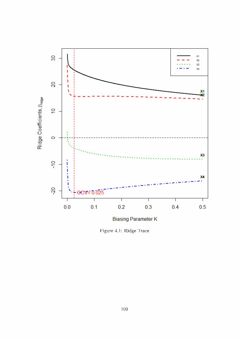
Figure 4.1: Ridge Trace

109

Figure 4.2: VIF Trace

110

The bias-variance tradeo plot can be used to select optimal k using bias.plot()

function.

> bias.plot(mod , abline=TRUE))

Figure 4.3: Bias Variance Tradeo

111

The plot of model selection criteria AIC and BIC for choosing optimal k,

info.plot() function can be used

> info.plot(mod , abline=TRUE)

Figure 4.4: ACI and BIC model selection Criteria

112

Function cv.plot() plots the CV and GCV cross validation against biasing

parameter k for the optimal selection of k, that is,

> cv.plot(mod , abline=TRUE)

Figure 4.5: CV and GCV, Cross Validation Plots

113

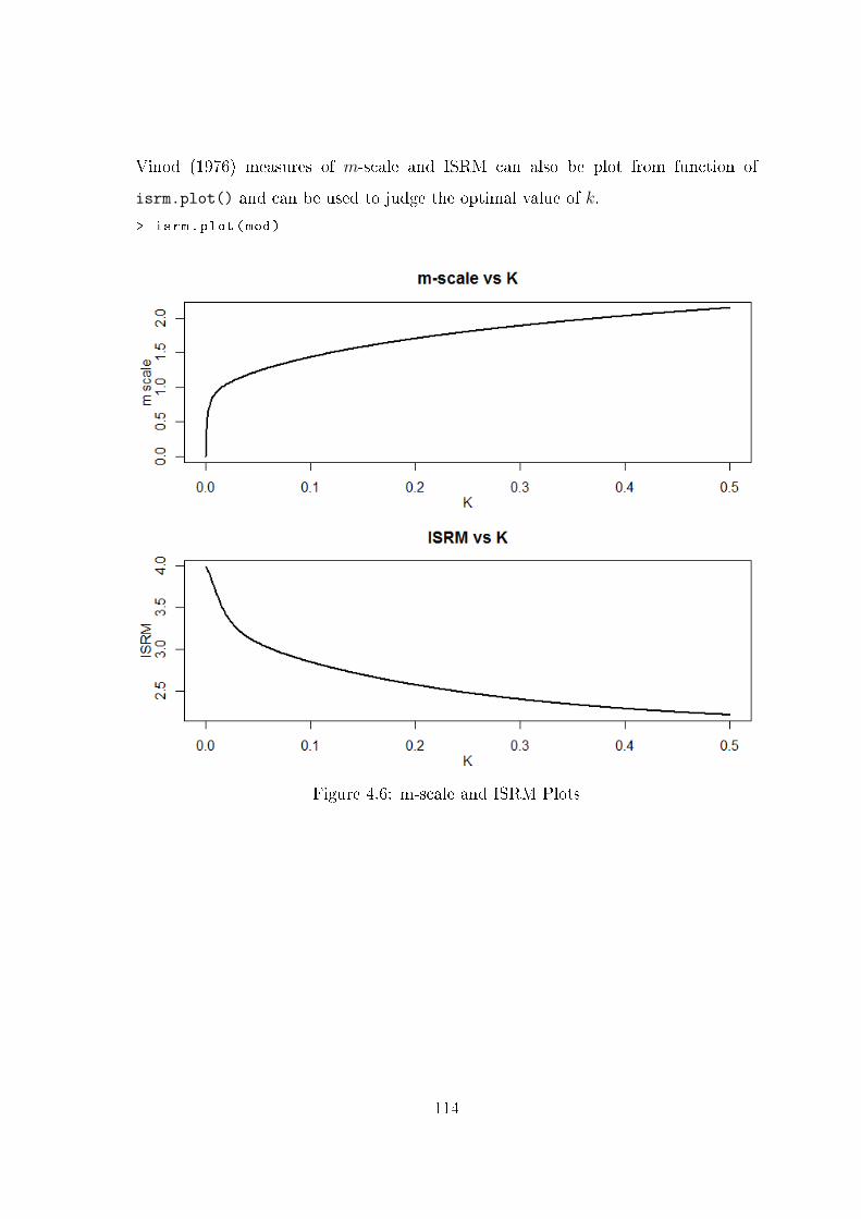
Vinod (1976) measures of m-scale and ISRM can also be plot from function of

isrm.plot() and can be used to judge the optimal value of k.

> isrm.plot(mod)

Figure 4.6: m-scale and ISRM Plots

114

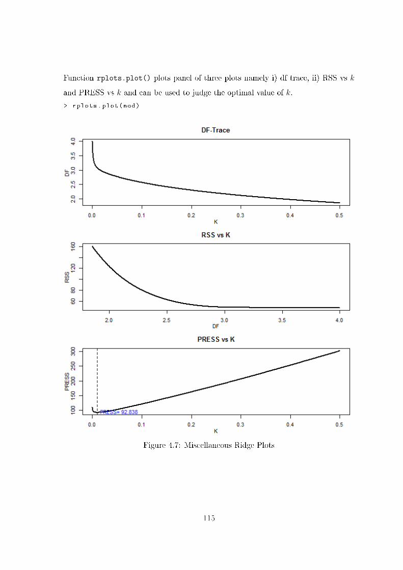
Function rplots.plot() plots panel of three plots namely i) df trace, ii) RSS vs k

and PRESS vs k and can be used to judge the optimal value of k.

> rplots.plot(mod)

Figure 4.7: Miscellaneous Ridge Plots

115

Chapter 5

The Liu Estimator: A Concise

Review and R Package Development

In case of existence of severe collinearity (non-orthogonal problems) among regressors,

the ridge biasing parameter k selected by dierent existing methods may not fully

address the problem of ill-conditioning. For larger value of k, the distance between

estimated and true value of regression parameter increases.

The ridge coecient βk is a complicated function of k when some popular methods

such as Golub et al. (1979), Mallows (1973) and McDonald and Galarneau (1975) etc.

are used for (optimal) selection of k. Usually k is quite small in dierent applications,

that's why, selection of small k may not be enough to correct the problem of ill-

condition X's. In such cases, the RR may still be unstable. Similarly, the choice of

k belongs to the researcher and also there is no consensus regarding how to select

optimal k, therefore other innovative methods were needed to deal with collinear

data.

In the literature, mixed regression estimation (MRE) and ridge type regression are

suggested to overcome the collinearity eect on regressors. To deal with multicollinear

data, Liu (1993) formulated a new class of biased estimate that has combined benets

116

of ORR by Hoerl and Kennard (1970b), see Eq., 4.5 and Stein type estimator (1956),

βs = cβ where c is parameter 0 < c < 1 and avoid their disadvantages. The LE can

be written as

βd = (X ′X + Ip)−1(X ′y + dβ) ,

= (X ′X + Ip)−1(X ′X + dIp)β ,

= Fd β , (5.1)

where d is the Liu parameter also known as biasing (tuning or shrinkage) parameter

and lies between 0 and 1 (i.e. 0 ≤ d ≤ 1), Ip is identity matrix of order p ×

p, β is OLSE and Fd = (X ′X + Ip)−1(X ′X + dIp). The βd is named as the Liu

estimator (LE) by Akdeniz and Kaciranlar (1995) and Gruber (1998). Recently, in

econometrics, engineering and other statistical areas, the LE has produced a number

of new techniques and ideas, see for example redAkdeniz and Kaciranlar (2001);

Hubert and Wijekoon (2006); Jahufer and Chen (2009, 2011, 2012); Kaciranlar and

Sakalho§lu (2001); Kaciranlar et al. (1999); Torigoe and Ujiie (2006).

Augmenting 0 =√k β + ε and d βd = β + ε to Eq. (2.1), βR and βd, can be obtained

by using the OLS method, respectively. Like ridge, Liu regression also penalizes the

coecient's size and d controls the strength of penalty term used in model.

However, Liu (2011) and Druilhet and Mom (2008) have made statement that the

biasing parameter d may lie outside the range given by Liu (1993), that is, it may

be less than 0 or greater than 1. The LE is linear transformation of the OLSE, that

is, LE is shrunken estimator of the OLS for d = 1 and βd = βols. The linear LE has

been widely used and is also powerful tool for detection of inuentials observations.

The suitable selection of d at which MSE is minimum and eciency of estimators

improves as compared to other values of d is the main interest of LE. Liu (1993)

provided some important methods for the selection of d and also provided numerical

example by iterative minimum MSE method to get the smallest possible value to

117

overcome the problem of collinearity in an eective manner.

5.1 Reparameterization

It is encouraged that Xn×p and yn×1 should be standardized rst such that

information matrix X ′X is in the correlation form and vector X ′y is in form of

correlation among regressors and the response. Therefore, for estimation of the Liu

parameter, the regressors and response variable are centered.

Consider regression model, y = β01 + Xβ1 + ε, where X is centered and

1 = c(1, 1, · · · , 1)′, while β0 can be estimated by using y. Let

λ1 ≥ λ2 ≥ · · · ≥ λp ≥ 0, be the ordered eigenvalues of matrix X ′X and q1, q2, · · · , qpbe the eigenvectors corresponds to their eigenvalues, such that Q = (q1, q2, · · · , qp)

is orthogonal matrix of X ′X and Λ =

λ1 . . .λ

, therefore model can be

rewritten in canonical form as y = β01 + Zα + ε, where Z = XQ and α = Q′β1.

Note that, Λ = Z ′Z = Q′X ′XQ. The estimate of α is α = Λ−1Z ′y. Similarly, Eq.

(5.1) can be rewritten in canonical form as

αd = (Λ + Ip)−1(Z ′y + dα)

Corresponding estimate of β1 and βd can be obtained by following relation of β1 =

Qα and βd = Qαd, respectively. For simplication of notations, X and α will be

represented as X and β, respectively.

The tted values of the LE can be found using Eq. (5.1),

yd = Xβd

= X(X ′X + Ip)−1(X ′y + d)β

= Hd y,

118

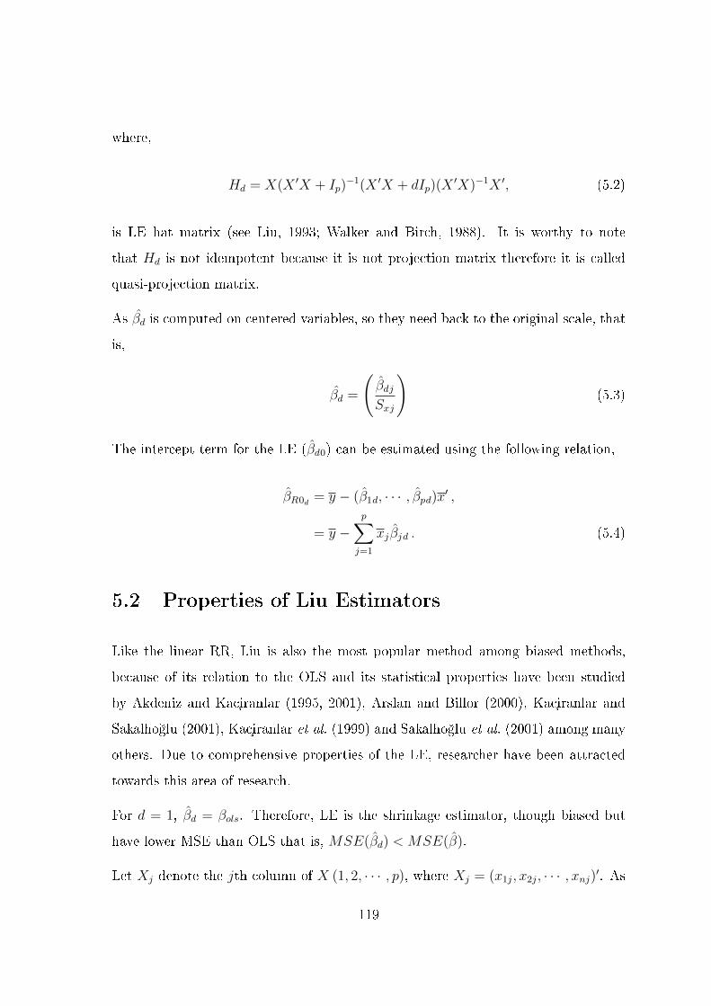
where,

Hd = X(X ′X + Ip)−1(X ′X + dIp)(X

′X)−1X ′, (5.2)

is LE hat matrix (see Liu, 1993; Walker and Birch, 1988). It is worthy to note

that Hd is not idempotent because it is not projection matrix therefore it is called

quasi-projection matrix.

As βd is computed on centered variables, so they need back to the original scale, that

is,

βd =

(βdjSxj

)(5.3)

The intercept term for the LE (βd0) can be estimated using the following relation,

βR0d = y − (β1d, · · · , βpd)x′ ,

= y −p∑j=1

xjβjd . (5.4)

5.2 Properties of Liu Estimators

Like the linear RR, Liu is also the most popular method among biased methods,

because of its relation to the OLS and its statistical properties have been studied

by Akdeniz and Kaciranlar (1995, 2001), Arslan and Billor (2000), Kaciranlar and

Sakalho§lu (2001), Kaciranlar et al. (1999) and Sakalho§lu et al. (2001) among many

others. Due to comprehensive properties of the LE, researcher have been attracted

towards this area of research.

For d = 1, βd = βols. Therefore, LE is the shrinkage estimator, though biased but

have lower MSE than OLS that is, MSE(βd) < MSE(β).

Let Xj denote the jth column of X (1, 2, · · · , p), where Xj = (x1j, x2j, · · · , xnj)′. As

119

already discussed, the regressors are centered, thus, the intercept will be zero and

can thereby be removed from the model. However, it can be estimated from relation

given in Eq. (5.4).

5.2.1 Mean of βd

Since βd is biased, the expected value of Eq. (5.1) is

E(βd) = Fdβ ,

= (X ′X + Ip)−1(X ′X + dIp)β ,

E(αd) = (Λ + Ip)−1(Λ + d Ip)α .

when d = 1, βd = βls. Therefore, βd is a biased shrinkage estimate.

5.2.2 Var-Cov matrix of βd

The Var-Cov (dispersion) matrix of βd from Kaciranlar et al. (1999) is

Cov(βd) = σ2Fd(X′X)−1F ′d ,

Cov(αd) = σ2(Λ + Ip)−1(Λ + dIp)Λ

−1(Λ + dIp)(Λ + Ip)−1 ,

where σ2 is computed with df from Hastie and Tibshirani (1990).

120

5.2.3 MSE of βd

The MSE of βd obtain from

MSE(βd) = traceCov(βd) + ‖E(αd)− α‖2 ,

MSE(βd) = σ2Fd(X′X)−1F ′d + (Fd − Ip)ββ′(Fd − Ip)′ ,

MSE(αd) = σ2

p∑j=1

(λj + d)2

λj(λj + 1)2+ (d− 1)2

p∑j=1

α2j

(λj + 1)2.

Liu (1993) showed that the MSE of the LE is less than that of the OLSE at d

(0 < d < 1) for all values of β and σ2.

5.2.4 Linear Transformation

The LE (βd) is a linear transformation of the OLSE (β), that is,

βd = Fd β,

where, Fd = (X ′X + Ip)−1(X ′X + d Ip)β.

5.2.5 Wide Range of Biasing Parameter

There always exists a wide range of biasing parameter d having smaller MSE than

the OLS.

5.2.6 Optimal value of d

There always exists an optimal Liu parameter d (say dopt) which gives minimum

MSE, (see Akdeniz and Kaciranlar, 1995; Liu, 1993; Sakalho§lu et al., 2001) among

many others.

121

5.2.7 Eective Degrees of Freedom (EDF)

The EDF allows to interpret the impact of penalty. The hat matrix from Eq. (5.2)

can be used to compute the EDF, dened as

dfLd = trace[Hld] .

The error df can be given by n− trace(2H −HH ′) and used in denominator of the

σ2 estimate. Therefore, the trace(2H − HH ′) is the eective number of parameter

in the df of error.

5.3 Methods of Selecting values of d

The existing methods to select biasing parameter in the RR may not fully address

the problem of ill-conditioning when there exists severe multicollinearity, while the

appropriate selection of biasing parameter d also remains a problem of interest. The

biasing parameter d should be selected when there are improvements in the estimates

(have stable estimates) or prediction is improved.

5.3.1 MSE Minimizer

Liu (1993) proposed to nd the optimal d that minimizes MSE and MSE(β1d) <

MSE(β1).

dopt =

∑pj=1

[α2j−σ2

(λj+1)2

]∑p

j=1

[σ2+λjα2

j

λj(λj+1)2

] .TheMSE(αd) is minimized at dopt. Replacing α2

j and σ2 by their unbiased estimates

α2i − σ2

λjand σ2 respectively. The estimate of dopt is called as minimum MSE estimate

122

by Liu (1993).

d = 1− σ2

p∑j=1

1λj(λj+1)

p∑j=1

α2j

(λj+1)2

.

The biasing parameter d named as improved Liu estimator (ILU) proposed by Liu

(2011) using PRESS criteria is,

dimp =

n∑i=1

e′

1−gii

(e

1−h1−ii −e

1−hii

)n∑i=1

(e′

1−gii −e

1−hii

)2 ,

where, e = yi−x′i(X ′X−xix′i)−1(X ′y−xiyi) and e′ = yi−x′i(X ′X+Ip−xix′i)−1(X ′y−

xiyi) with gii and hii are the ith diagonal elements of hat matrix dened as G =

X(X ′X + Ip)−1X ′ and H ∼= X(X ′X)−1X ′ respectively. Though ILE is biased but

yield lower MSE than the LE.

In literature, many methods for selection of appropriate biasing parameter d have

been studied by Akdeniz and Oøzkale (2005), Arslan and Billor (2000), Akdeniz et al.

(2006), Oøzkale and Kaciranlar (2007) and Liu (1993).

5.3.2 Performance Criteria

The value of biasing parameter d must be selected such that βd improves β in the

sense of MSE. In other words, there always exists a certain value of d such that

MSE(βd) < MSE(β). Liski (1982) proposed MSE as a powerful criteria to select

123

between shrinkage estimator and LSE. The MSE of LE is,

MSE(βd) = traceCov(βd) + ‖E(βd)− β‖2 ,

= σ2

p∑j=1

(λj + d)2

λj(λj + 1)2+ (d− 1)2

2∑j=1

β2

(λ+ 1)2.

Liu (1993) showed that their proposed estimator (dopt) is superior to the OLSE both

in the sense of scalar and matrix MSE.

For prediction purposes, it is appropriate to use prediction-oriented criteria for the

selection of d. Liu (2011) derived the improved Liu estimator (ILE) and recommended

PRESS criteria for the selection of optimal d.

• PRESS

To improve the quality of model prediction performance, minimizing the PRESS

is another alternative suggested by Allen (1974) and further developed by Golub

et al. (1979). Small value of PRESS statistics represents a model having smaller

MSE and hence the regression model will provide good predictions of new

observations.

For PRESS statistics, Liu (1993) did not give the minimizer for LE, however

Oøzkale and Kaciranlar (2007) proposed the PRESS statistics for the LE and

also provide an example based on data for Portland cement.

The PRESS statistics for LE

PRESSd =n∑i=1

(ed(i))2 ,

=n∑i=1

[(1− d)

eRi(1)

1− h1−ii+ d

ei1− hii

]2.

• CL Criteria

Liu (1993) also provided other estimates of d by analogy with the estimate of k

in the RR and suggested CL statistics like Cp of Mallows (1973) for the selection

124

of d that minimizes CL value.

CL =SSRd

σ2+ 2trace(Hd)− (n− 2)

where SSRd is SSR from Liu regression at specic d, σ2 is the estimate of σ2

from LS regression and Hd is hat matrix of LE given in Eq. (5.2). Since, CL is

a quadratic function of d, the minimum of CL can be obtained by using,

dCL = 1− σ2

p∑i=1

1λi+1

p∑j=1

λiα2

(λi+1)2

.

Plotting CL against d for which CL is minimized with the use of d values.

• GCV

For LE, the prediction oriented-method GCV, is another good method to select

appropriate d,

GCVd =SSRd

[n− [1 + trace(Hd)]]2

The minimizer of CL and GCVd is the same Liu (1993) and d can be selected

by minimizing GCV and CL, respectively. The minimizer dLC of GCV and CL

is,

dCL = 1− σ2

p∑i=1

1λi+1

p∑j=1

λiα2

(λi+1)2

5.3.3 Using Information Criteria

Information criteria such as AIC and BIC can be used to get some idea about

appropriate selection of d. An estimate of AIC and BIC can be computed, as given

125

below,

AIC = n log(RSS) + 2 df ,

BIC = n log(RSS) + df log(n) ,

where df is degrees from freedom, computed by following Hastie and Tibshirani

(1990), see Section (5.2.7) and (4.6.16).

5.3.4 Subjective Methods

For selection of biasing parameter d, many methods are available in literature. The

graphical evidence of the eect of multicollinearity on the regression coecient and

account of variation by LE compared to the LSE can be judged by graphing the Liu

coecients, MSE, variance and bise due to biasing parameter d.

• Liu Trace

The plotting of Liu coecient as a function of biasing parameter d can be used

to depict the eect of collinearity on each of the coecients. For certain value

of d the trace appear to be more stable as compared to smaller or higher of d

than optimal d.

• Bias Variance trade-o

Plotting bias, variance and MSE from the LE can be helpful in selecting

appropriate value of d. At the cost of bias optimal d can be selected at which

MSE is minimum.

5.4 Estimation and Testing of Liu Coecients

Testing of Liu coecients is performed by following Aslam (2014b) and Halawa and

El-Bassiouni (2000). For testing H0 : βdj = 0 against βdj 6= 0, the non-exact t-

126

statistics dened by Halawa and El-Bassiouni (2000) is

Tdd =βdj

SE(βdj),

where βdj is the jth Liu coecient and SE(βdj) is an estimate of standard error,

which is the square root of the jth diagonal element of the covariance matrix from

Section (5.2.2).

The statistic tdj is assumed to follow Student's t distribution with (n − p) df

(Halawa and El-Bassiouni, 2000). Hastie and Tibshirani (1990) and Cule and

De Iorio (2012) suggested to use df from (n − tr(Hd)). For large sample size, the

asymptotic distribution of this statistic is normal Halawa and El-Bassiouni (2000).

Thus reject H0 when |T | > Z1−α2.

For testing the signicance of LE βd with E(βd) = Fdβ and Cov(βd), the F -statistic

is

F =1

p(βd − Fdβ)′ (Cov(βd))

−1(βd − Fdβ)

5.5 R Package Development and Implementation

In this section, we will illustrate the development and implementation of the linear

Liu regression, estimation of Liu biasing parameter d, testing of the Liu coecients

and dierent Liu related measures by applying them to a data set. The biasing

parameters are computed by following Liu (1993). Note that if intercept is present in

the model, then it will not be penalized, however, will be estimated by the relation

dened in equation (5.4).

We developed liureg package in R language and it contains functions related to

tting linear Liu regression model. The liureg package estimates coecients from

Liu regression and also performs testing of these coecients. This package also

computes dierent properties of LE, biasing parameters residual, tted & predicted

127

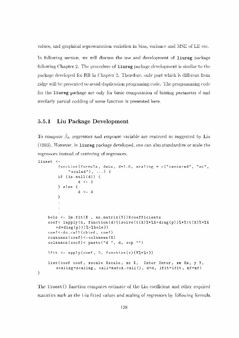
values, and graphical representation variation in bias, variance and MSE of LE etc.

In following section, we will discuss the use and development of liureg package

following Chapter 2. The procedure of liureg package development is similar to the

package developed for RR in Chapter 2. Therefore, only part which is dierent from

ridge will be presented to avoid duplication programing code. The programming code

for the liureg package are only for basic computation of biasing parameter d and

similarly partial codding of some function is presented here.

5.5.1 Liu Package Development

To compute βd, regressors and response variable are centered as suggested by Liu

(1993). However, in liureg package developed, one can also standardize or scale the

regressors instead of centering of regressors.

liuest <-

function(formula , data , d=1.0, scaling = c("centered", "sc",

"scaled"), ...)

if (is.null(d))

d <- 1

else

d <- d

.

.

.

bols <- lm.fit(X , as.matrix(Y))$coefficients

coef <-lapply(d, function(d)(solve(t(X)%*%X+diag(p))%*%(t(X)%*%X

+d*diag(p)))%*%bols)

coef <-do.call(cbind , coef)

rownames(coef)<-colnames(X)

colnames(coef)<-paste("d=", d, sep="")

lfit <- apply(coef , 2, function(x)X%*%x)

list(coef=coef , xscale=Xscale , xs=X, Inter=Inter , xm=Xm, y=Y,

scaling=scaling , call=match.call(), d=d, lfit=lfit , mf=mf)

The liuest() function computes estimate of the Liu coecient and other required

statistics such as the Liu tted values and scaling of regressors by following formula

128

interface. To perform further computation on objects, the main function liu()

is made generic and have default method (liu.default) whose rst argument is a

design marix (or something other data structure which can be converted to a matrix).

This default method calls liuest() and returns the object having class names as

"liu".

Like lmridge package, the Liu coecients are rescaled using the relation described

in Eq. (5.3). Similarly, print() method prints the Liu coecients for each biasing

parameter d in standard format. For estimation and testing of Liu coecients

summary() method is used to summarize the model for each given value of d. The

output of summary method contains 5 columns namely "Estimate", "Estimate

(Sc)", "StdErr (Sc)", "t-val (Sc)" and "Pr(>|t|)" for given biasing parameter(s).

For computation of dierent d values proposed by Liu (1993), the dest() function

can be used. The R code for computation is,

dest <- function(object ,...)

UseMethod("dest")

dest.liu <- function(object ,...)

x <- object$xs

y <- object$y

p <- ncol(x)

n <- nrow(x)

d <- object$d

EVal <- eigen(t(x) %*% x)$values

EVec <- eigen(t(x) %*% x)$vectors

ols <- lm.fit(x, y)

coefols <- ols$coef

fittedols <- ols$fitted.values

residols <- ols$residuals

sigma2 <- sum(residols ^ 2) / (n - p)

alphaols <- t(EVec) %*% coefols

rownames(alphaols) <- colnames(x)

diaghat <- lapply(hatl(object), function(x) diag(x) )

diaghat <- do.call(cbind , diaghat)

SSER <-lstats(object)$SSER

129

GCV <-matrix(0,1,nrow=length(d) )

for(i in seq(length(d)))

GCV[i,]<-SSER[i]/(n-1-sum(diaghat[,i]))^2

rownames(GCV) <- paste("d=", d, sep = "")

colnames(GCV) <- c("GCV")

if (length(GCV) > 0)

l <- seq_along(GCV)[GCV == min(GCV)]

dGCV <- object$d[l]

dopt <-(sum(( alphaols^2-sigma2)/(EVal +1) ^2))/(sum(( sigma2+EVal*

alphaols ^2)/(EVal*(EVal +1)^2)))

numdmm <- 1 / (EVal * (EVal + 1))

dnumdmm <- (alphaols ^ 2) / ((EVal + 1) ^ 2)

dmm <- (1 - sigma2) * sum(numdmm) / sum(dnumdmm)

numdcl <- 1 / (EVal + 1)

dnumdcl <- (EVal * alphaols ^ 2) / ((EVal + 1) ^ 2)

dcl <- (1 - sigma2) * sum(numdcl) / sum(dnumdcl)

desti <- list(dmm = dmm , dcl = dcl , GCV=GCV , dGCV=dGCV , dopt=dopt ,

sigma2=sigma2)

class(desti) <- "dliu"

desti

print.dliu <- function(x,...)

cat("Liu biasing parameter d\n")

dest <- cbind(dopt=x$dmm , dd=x$dcl , dopt=x$dopt , dGCV=x$dGCV)

rownames(dest) <- "d values"

colnames(dest) <- c("dmm", "dcl", "dopt", "min GCV at")

print(t(round(dest ,5)) ,...)

Following is complete list of functions available in liureg package for computation

of the LE related statistics and optimal value of d from Liu (1993).

130

Table 5.1: Functions and methods available in liureg package.

Functions Description

liuest() The main model tting function for implementation of the Liu

regression models in R.

liu() Generic function and default method that calls liuest function and

returns an object of S3 class "liu" with dierent set of methods

to standard generics. It has print method to display de-scaled Liu

coecients

summary() Standard Liu regression output (coecient estimates, scaled coecients

estimates, standard errors, t-values and p-values); returns an object of

class "summaryliu" containing the relative summary statistics and have

a print() method.

coef() Computes re-scaled Liu coecients see Eq. (5.3)

vcov() Displays associated variance-covariance matrix with matching the Liu

parameter d values

predict() Produces predicted value(s) obtained by evaluating the liuest function

in the frame newdata

tted() Displays the Liu tted values for observed data

residuals() Displays the Liu residuals values

dest() Displays various d (biasing parameter) values from Liu (1993)

lstats() Displays dierent statistics of the Liu regression such as mse, bias, etc

plot() Liu trace of biasing parameter d.

plot.biasliu() Bias, variance trade-o plot as function of d

plot.infoliu() Plot of AIC and BIC against d

hatl() Displays hat matrix from the Liu regression

infoliu() Compute information criteria AIC, BIC

For selection of appropriate d, the variance-bias trade-o plot can be carried out by

the following function

plot.rbias <- function(x, abline=TRUE ,...)

bias2 <-lstats(x)$bias2

131

var <-lstats(x)$var

mse <-lstats(x)$mse

minmse <-min(mse)

mind <-x$d[which.min(mse)]

col=cbind("black", "red", "green")

liutrace <-cbind(var , bias2 , mse)

if(length(x$d)==1)

plot(x=rep(x$d, length(liutrace)), y=liutrace , main="Bias ,

Variance Trade -off",

xlab="Liu Biasing Parameter", ylab="", col=col , lwd=2, lty=

c(1,4,5))

legend("topright", legend=c("var", "bias^2","mse"),col=col , lwd

=2, fill =1:3,

lty=c(1,4,5), cex=.6, pt.cex=.7, bty="o", y.intersp = .7)

else

matplot(x$d, liutrace , main="Bias , Variance Trade -off", xlab="

Liu Biasing Parameter",

col=col , lwd=2, lty=c(1,4,5), type='l')

legend("topright", legend=c("var", "bias^2", "mse"), col=col ,

lwd=2, fill =1:3,

lty=c(1,4,5), cex=.6, pt.cex=.5, bty="o", y.intersp = .7)

if(abline)

abline(v=mind , lty=2)

abline(h=minmse , lty=2)

text(mind , max(lstats(x)$mse), paste("mase=",round(minmse ,3)),

col="blue", pos=1)

text(mind , minmse , paste("d=", mind), pos=4, col="blue")

5.5.2 The Liu Package Implementation

The liureg package must be installed and loaded in system memory, so that package

functions becomes accessible in the current R session, that is,

> library(liureg)

For a complete list of functions available in liureg package use the command,

> help("liu")

132

The liureg package contains a set of standard methods such as print(), summary(),

plot() and predict() etc. and return objects of class "liu". Inferences can be

made easily by using summary() method for assessing the regression coecients,

their standard errors, t-values and their respective p-values. The function liu() is

set as default function to call liuEst which performs computation for given values

of biasing parameter d. The syntax is,

liu(formula , data , scaling , d, ...)

The arguments for liu are;

Table 5.2: Description of liureg Package's argument

Argument Description

formula A symbolic representation for linear Liu regression model of the

form response variable ∼ predictors

data data frame that contains the variables and have to be used in

the model

d Biasing parameter, may be a scalar or vector. If d value is not

provided, d = 1 will be used as default value, that is, linear

regression (d = 1) results will be produced

scaling The methods for scaling the predictors. The "centered"

option, centers the predictors and is default scaling options for

predictors, the "sc" option, scales the predictors in correlation

form as described in Belsley (1991); Draper and Smith (1998)

and "scaled" option standardizes the predictors having zero

mean and unit variance. Note that the response variable is

"centered" for all scaling option.

The liu() return an object of class "liu". The function summary(), dest() and

lstats() etc., can be used to compute and print (display) a summary of Liu

regression results, list of biasing parameters and optimal d by following Liu (1993)

respectively, after bias is introduced in regression model. An object of class liu()

133

is a list that contains the following components:

Table 5.3: Objects from "liu" class

Object Description

coef A vector of scaled tted Liu coecients

xs The scaled matrix of predictors according to scaling option in liu()

function

Inter Whether intercept is included in the model or not

d The Liu regression (biasing ) parameter(s), it can be scaler or vector

xm A vector of means of design matrix X

ym The mean of response variable

scaling The methods of scaling used to standardize the predictors

5.5.2.1 Numerical Results

A numerical example is presented for the Hald's data set to explain the use of liureg

to produce linear Liu regression results. The Hald data is already included in package

and can be used by following codes give below,

> data(Hald)

> mod <- liu(y~X1+X2+X3+X4 , data=as.data.frame(Hald), scaling="

centered", d=seq(0, 1, 0.001) )

> mod

Call:

liu.default(formula = y~X1+X2+X3+X4, data=as.data.frame(Hald),

scaling = "centered", d = seq(0, 1, 0.01))

Intercept X1 X2 X3 X4

d=0 75.01755 1.41348 0.38190 -0.03582 -0.27032

d=0.01 74.89142 1.41486 0.38318 -0.03445 -0.26905

d=0.49 68.83758 1.48092 0.44475 0.03167 -0.20845

d=0.5 68.71146 1.48229 0.44603 0.03304 -0.20719

d=0.9 63.66659 1.53734 0.49734 0.08814 -0.15669

d=1 62.40537 1.55110 0.51017 0.10191 -0.14406

The output of the linear LR from liureg package is assigned to object mod. The rst

argument of function liu is "formula" which is used to specify the required linear LR

134

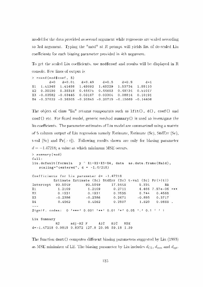
model for the data provided as second argument while regressors are scaled according

to 3rd argument. Typing the "mod" at R prompt will yields list of de-scaled Liu

coecients for each biasing parameter provided in 4th argument.

To get the scaled Liu coecients, use mod$coef and results will be displayed in R

console. Few lines of output is

> round(mod$coef , 5)

d=0 d=0.01 d=0.49 d=0.5 d=0.9 d=1

X1 1.41348 1.41486 1.48092 1.48229 1.53734 1.55110

X2 0.38190 0.38318 0.44475 0.44603 0.49734 0.51017

X3 -0.03582 -0.03445 0.03167 0.03304 0.08814 0.10191

X4 -0.27032 -0.26905 -0.20845 -0.20719 -0.15669 -0.14406

The object of class "liu" returns components such as lfit(), d(), coef() and

coef() etc. For tted model, generic method summary() is used to investigate the

liu coecients. The parameter estimates of Liu model are summarized using a matrix

of 5 column output of Liu regression namely Estimate, Estimate (Sc), StdErr (Sc),

t-val (Sc) and Pr(>|t|). Following results shown are only for biasing parameter

d = −1.47218; a value at which minimum MSE occurs.

> summary(mod)

Call:

liu.default(formula = y ~ X1+X2+X3+X4, data= as.data.frame(Hald),

scaling="centered", d = -1.47218)

Coefficients for Liu parameter d= -1.47218

Estimate Estimate (Sc) StdErr (Sc) t-val (Sc) Pr(>|t|)

Intercept 93.5849 93.5849 17.5448 5.334 NA

X1 1.2109 1.2109 0.2711 4.466 7.97e-06 ***

X2 0.1931 0.1931 0.2595 0.744 0.4568

X3 -0.2386 -0.2386 0.2671 -0.893 0.3717

X4 -0.4562 -0.4562 0.2507 -1.820 0.0688 .

---

Signif. codes: 0 `***' 0.001 `**' 0.01 `*' 0.05 `.' 0.1 ` ' 1

Liu Summary

R2 adj -R2 F AIC BIC MSE

d= -1.47218 0.9819 0.8372 127.8 23.95 59.18 1.39

The function dest() computes dierent biasing parameters suggested by Liu (1993)

as MSE minimizer of LE. The biasing parameter by Liu includes dCL, dmm and dopt.

135

For appropriate selection of d, GCV is also computed. The argument of dest() is

object of class "liu", i.e., the object that is used to store results from liu() function,

in this example is "mod". The output of function for the Hald data set is,

> dest(mod)

Liu biasing parameter d

d values

dmm -5.61494

dcl -5.66240

dopt -1.47218

min GCV at 0.00000

The lstats() computes dierent statistics for biasing parameter of LE such as mse,

squared bias, F-test, liu variance, degrees of freedom for Hastie and Tibshirani (1990),

R2 etc. Following are results for some d = −0.06, 0, 0.1, 0.05 and 1.> l s t a t s (mod)

Liu Regres s ion S t a t i s t i c s :

EDF Sigma2 CL VAR Bias^2 MSE F R2 adj−R2d=−0.06 9 .0760 5 .2989 5 .5077 1 .0195 0 .2050 1 .2246 125.8693 0 .9823 0 .8406

d=0 9.0677 5 .3010 5 .5315 1 .0625 0 .1825 1 .2450 125.8194 0 .9823 0 .8407

d=0.1 9 .0548 5 .3043 5 .5722 1 .1362 0 .1478 1 .2840 125.7427 0 .9823 0 .8408

d=0.5 9 .0169 5 .3139 5 .7488 1 .4561 0 .0456 1 .5018 125.5157 0 .9824 0 .8412

d=1 9.0000 5 .3182 6 .0000 1 .9119 0 .0000 1 .9119 125.4141 0 .9824 0 .8414

minimum MSE occurred at d= −0.06

The residuals, tted values from the Liu regression and predicted values of response

variable y can be computed using functions such as residual(), fitted() and

predict() respectively. For computation of variance-covariance and hat matrix for

Liu regression vcov() and hatl() can be used respectively for computation of other

statistics not available in this package. These functions computes corresponding

statistics for each value of d and can be used as,

> hatl(mod) # hat matrix for each d

> hatl(mod)[[1]] # hat matrix for first value of d

> residual(mod) # residuals for each d

> fitted(mod) # fitted value for each d

> vcov(mod) # Var -Cov matrix for each d

> diag(hatl(mod)[[1]]) # diagonal elements for first d

> predict(mod) # predicted values for each d

136

For given value of X such as for rst ve rows of X matrix, the predicted values will

be,

> predict(mod , newdata=as.data.frame(Hald [1:5 ,-1]))

d= -0.06 d=0 d=0.1 d=0.5 d=1

1 78.40208 78.40736 78.41615 78.45130 78.49524

2 72.91968 72.91227 72.89992 72.85053 72.78880

3 106.27656 106.25926 106.23043 106.11510 105.97094

4 89.41842 89.41325 89.40463 89.37017 89.32710

5 95.63443 95.63527 95.63667 95.64226 95.64924

The model selection criteria's of AIC and BIC can be computed using infoliu()

function for each value of d used in argument of liu() function, that is,

> infoliu(liu(y~ X1+X2+X3+X4, data=as.data.frame(Hald), d=c(-0.06,

0, 0.1, 0.5, 1)))

AIC BIC

d= -0.06 24.43818 59.88178

d=0 24.46352 59.91621

d=0.1 24.50663 59.97446

d=0.5 24.69007 60.21849

d=1 24.94429 60.54843

The model selection criteria's are carried out by the following function

infoliu <-function(x,...) UseMethod("infoliu")

infoliu.liu <-function(object , ...)

SSER <-apply(resid(object) ,2, function(x)sum(x^2))

df <- as.vector(lapply(hatl(object), function(x)

sum(diag(x))

))

n<-nrow(object$xs)

AIC <-mapply(function(x,y)n*log(x/n)+2*y, SSER , df , SIMPLIFY

= FALSE)

AIC <-do.call(cbind ,AIC)

BIC <-mapply(function(x,y)n*log(x)+y*log(n), SSER , df,

SIMPLIFY = FALSE)

BIC <-do.call(cbind ,BIC)

resinfo <-rbind(AIC , BIC)

rownames(resinfo)<-c("AIC", "BIC")

t(resinfo)

137

Other examples and use of dierent functions can be seen from the R documentation

of liureg package. The coding of some function (such as summary(), predict(),

fitted() and resid() etc.) are not presented here to avoid duplication or repetition

of content with minor dierences and also to avoid huge volume of pages.

5.5.2.2 Graphical Results

The eect of biasing parameter d on (i) Liu coecients, (ii) variation in bias,

variance, and MSE, can be explored by using plot() and plot.biasliu()

functions respectively. Similarly, plot.infoliu can be used to choose d value by

plotting information criteria's such as AIC and BIC against given values of d as

liu() function's argument. The plot of Liu coecients against biasing parameter

d, can be achieved,

> plot(mod)

Figure 5.1: Liu Trace: Liu Coecient against Biasing Parameter d

138

To get bias variance trade-o plot, use command,

> plot.biasliu(mod)

Figure 5.2: Bias Variance trade-o

139

The plot of AIC and BIC criteria's against d can be obtained,

> plot.infoliu(mod)

Figure 5.3: Information Criteria vs d

140