Outdoor-to-Indoor Office MIMO Measurements and Analysis at 5.2 GHz

MITSUBISHI ELECTRIC RESEARCH LABORATORIEShttp://www.merl.com

Outdoor-to-Indoor Office MIMOMeasurements and Analysis at 5.2 GHz-

Shurjeel Wyne, Andreas Molisch, Peter Almers, Gunnar Eriksson, Johan Karedal, FredrikTufvesson

TR2008-048 August 2008

AbstractThe outdoor-to-indoor wireless propagation channel is of interest for cellular and wireless localarea network applications. This paper presents the measurement results and analysis based onour multiple-input-multiple-output (MIMO) measurement campaign, which is one of the first tocharacterize the outdoor-to-indoor channel. The measurements were performed at 5.2 GHz; thereceiver was placed indoors at 53 different locations in an office building, and the transmitter wasplaced at three ”base stations” positions on a nearby rooftop. We report on the root-mean-square(RMS) angular spread, building penetration, and other statistical parameters that characterize thechannel. Our analysis is focused on three MIMO channel assumptions often used in stochasticmodels. 1) It is commonly assumed that the channel matrix can be represented as a sum of aline-of-sight (LOS) contribution and a zero-mean complex Gaussian distribution. Our investiga-tion shows that this model does not adequately represent our measurement data. 2) It is oftenassumed that the Rician K-factor is equal to the power ratio of the LOS component and the othermultipath components (MPCs). We show that this is not the case, and we highlight the differencebetween the Rician K-factor often associated with LOS channels and a similar power ratio for theestimated LOS MPC. 3) A widespread assumption is that the full correlation matrix of the chan-nel can be decomposed into a Kronecker product of the correlation matrices at the transmit andreceive array. Our investigations show that the direction-of-arrival (DOA) spectrum noticeablydepends on the direction-of-departure (DOD); therefore, the Kronecker model is not applicable,and models with less-restrictive assumptions on the channel, e.g., the Weichselberger model orthe full correlation model, should be used.

IEEE Transactions on Vehicular Technology

This work may not be copied or reproduced in whole or in part for any commercial purpose. Permission to copy in whole or in partwithout payment of fee is granted for nonprofit educational and research purposes provided that all such whole or partial copies includethe following: a notice that such copying is by permission of Mitsubishi Electric Research Laboratories, Inc.; an acknowledgment ofthe authors and individual contributions to the work; and all applicable portions of the copyright notice. Copying, reproduction, orrepublishing for any other purpose shall require a license with payment of fee to Mitsubishi Electric Research Laboratories, Inc. Allrights reserved.

Copyright c©Mitsubishi Electric Research Laboratories, Inc., 2008201 Broadway, Cambridge, Massachusetts 02139

MERLCoverPageSide2

1374 IEEE TRANSACTIONS ON VEHICULAR TECHNOLOGY, VOL. 57, NO. 3, MAY 2008

Outdoor-to-Indoor Office MIMO Measurementsand Analysis at 5.2 GHz

Shurjeel Wyne, Student Member, IEEE, Andreas F. Molisch, Fellow, IEEE, Peter Almers, Gunnar Eriksson,Johan Karedal, Student Member, IEEE, and Fredrik Tufvesson, Senior Member, IEEE

Abstract—The outdoor-to-indoor wireless propagation channelis of interest for cellular and wireless local area network applica-tions. This paper presents the measurement results and analysisbased on our multiple-input–multiple-output (MIMO) measure-ment campaign, which is one of the first to characterize theoutdoor-to-indoor channel. The measurements were performed at5.2 GHz; the receiver was placed indoors at 53 different locationsin an office building, and the transmitter was placed at three“base station” positions on a nearby rooftop. We report on theroot-mean-square (RMS) angular spread, building penetration,and other statistical parameters that characterize the channel.Our analysis is focused on three MIMO channel assumptions oftenused in stochastic models. 1) It is commonly assumed that thechannel matrix can be represented as a sum of a line-of-sight(LOS) contribution and a zero-mean complex Gaussian distri-bution. Our investigation shows that this model does not ade-quately represent our measurement data. 2) It is often assumedthat the Rician K-factor is equal to the power ratio of the LOScomponent and the other multipath components (MPCs). We showthat this is not the case, and we highlight the difference betweenthe Rician K-factor often associated with LOS channels and asimilar power ratio for the estimated LOS MPC. 3) A widespreadassumption is that the full correlation matrix of the channel can bedecomposed into a Kronecker product of the correlation matricesat the transmit and receive array. Our investigations show thatthe direction-of-arrival (DOA) spectrum noticeably depends onthe direction-of-departure (DOD); therefore, the Kronecker modelis not applicable, and models with less-restrictive assumptions onthe channel, e.g., the Weichselberger model or the full correlationmodel, should be used.

Index Terms—Angular dispersion, channel sounding, direction-of-arrival (DOA), direction-of-departure (DOD), Kroneckermodel, line-of-sight (LOS) power factor, multiple-input multiple-

Manuscript received August 27, 2006; revised May 28, 2007 and July 22,2007. This work was supported in part by the Swedish Foundation for StrategicResearch under an INGVAR Grant, in part by the Swedish Science Council,and in part by the SSF Inter-University Center of Excellence for High-SpeedWireless Communications. This paper was presented in part at the IEEEVehicular Technology Conference (VTC), Los Angeles, CA, September 2004(Fall), and IEEE VTC 2005 Spring. The review of this paper was coordinatedby Dr. K. Dandekar.

S. Wyne, P. Almers, J. Karedal, and F. Tufvesson are with the Department ofElectrical and Information Technology, Lund University, 221 00 Lund, Sweden(e-mail: [email protected]; [email protected]; [email protected]; [email protected]).

A. F. Molisch is with Mitsubishi Electric Research Labs, Cambridge,MA 02139, USA, and also with the Department of Electrical andInformation Technology, Lund University, 221 00 Lund, Sweden(e-mail:[email protected]).

G. Eriksson is with the Department of Electrical and Information Technol-ogy, Lund University, 221 00 Lund, Sweden, and also with the Swedish DefenceResearch Agency, 581 11 Linköping, Sweden (e-mail: [email protected]).

Color versions of one or more of the figures in this paper are available onlineat http://ieeexplore.ieee.org.

Digital Object Identifier 10.1109/TVT.2007.909272

output (MIMO), Rician K-factor, virtual channel representation(VCR), Weichselberger model.

I. INTRODUCTION

MULTIPLE-INPUT–multiple-output (MIMO) systemscan result in tremendous capacity improvements over

single-antenna systems [1], [2]. However, the capacity gainsdepend on the propagation channel in which the system oper-ates. The most important requirement for any channel model isagreement with reality; hence, the measurement of propagationchannels and the subsequent parameterization of models basedon these measurements are critically important. There havebeen a number of double-directional outdoor-to-outdoor andindoor-to-indoor measurement results reported in the literature,e.g., [3]–[7]. However, there has been a remarkable lack ofoutdoor-to-indoor measurement results, although the outdoor-to-indoor scenario has important applications for voice–datatransmission in third-generation cellular systems as well aswireless local area networks. The measurement campaign re-ported in this paper (first published in [8]), together with[9] and [10], is the first published result of outdoor-to-indoormeasurements characterizing the MIMO channel.

There are two main categories of channel models for MIMOsystems, both of which will be used in this paper. The double-directional channel models [3] describe the MIMO channel byparameters of the multipath components (MPCs): direction-of-departure (DOD), direction-of-arrival (DOA), delay, andcomplex amplitudes. A double-directional channel character-ization is highly useful because it is independent of antennaconfigurations, describes the physical propagation alone, andserves to point out the dominant propagation mechanisms. Onthe other hand, analytical channel models describe the statisticsof the transfer function matrix. Each entry in that matrix givesthe transfer function from the ith transmit to the jth receiveantenna element. Almost all of the analytical channel models,with the exception of the keyhole model [11], are based onthe assumption that the entries of the transfer function matrixare zero-mean complex Gaussian, with the possible addition ofa line-of-sight (LOS) component. Furthermore, many modelsdescribe the correlation matrix of those entries as a Kroneckerproduct of the correlation matrices at the transmit and receivesides. The first assumption has, to our knowledge, generallyremained unquestioned.1 The Kronecker assumption has been

1With the exception of the rare “keyhole scenario” (see [11] and [12]).

0018-9545/$25.00 © 2008 IEEE

WYNE et al.: OUTDOOR-TO-INDOOR OFFICE MIMO MEASUREMENTS AND ANALYSIS AT 5.2 GHz 1375

recently more extensively discussed [7], [13]. Considering thatthe measurement data from outdoor scenarios seem to indicategood agreement with this assumption [13], the indoor data seemto deviate more [14], and, as a consequence, a more generalmodel has, e.g., been developed by Weichselberger et al. [7].

In this paper, we present the results of a double-directionalMIMO channel measurement campaign for an outdoor-to-indoor office scenario (carried out at 5.2 GHz) and evaluatethe validity of the standard assumptions of analytical channelmodels (the first results were published in [15]). Our maincontributions are the following.

• We analyze the DOD and DOA and discuss the dominantpropagation mechanisms.

• We give the distributions of root-mean-square (RMS) di-rectional spreads and delay spreads.

• We present a statistical analysis of the measured fadingand compare it with popular models.

• We investigate the validity of the “LOS-plus-Gaussian-remainder” assumption and show that it does not hold forall measurement locations in our campaign.

• We explain this result by investigating in detail the differ-ence between “LOS power factor” and “Rician K-factor.”

• We analyze the validity of the Kronecker model andpresent detailed results on the coupling between DOAsand DODs.

This paper is organized as follows. Section II describes themeasurement setup and scenario and the procedure for dataevaluation. In Section III, the physical propagation processesare described. Furthermore, Section IV contains an analy-sis of the dispersion in angular and delay domains, andSection V compares three analytical channel models. Finally, inSection VI, we summarize the results.

II. MEASUREMENT SETUP AND EVALUATION

A. Equipment and Scenario

For the measurements, we used the RUSK ATM [16] channelsounder to measure the transfer function between transmit(Tx) and receive (Rx) antenna elements. This sounder usesthe multiplexing principle (subsequently connecting the Tx,and Rx, antenna elements to the radio frequency chains) forobtaining MIMO transfer function matrices. The measurementswere performed at a center frequency of 5.2 GHz and a signalbandwidth of 120 MHz using a transmit power of 33 dBm.The Tx antenna was an eight-element dual-polarized uniformlinear array (ULA) of patch elements with element spacing≈ λ/2 (half wavelength). We only considered the eight ver-tically polarized elements in our analysis. The Rx antennawas a 16-element uniform circular array (UCA) of verticallypolarized monopole elements (radius ≈ λ). Both array con-figurations were calibrated prior to measurement so that thearray response data were available for the application of high-resolution algorithms. The Tx signal had a period of 1.6 µs, andthe sampling time for one MIMO snapshot was 819 µs, which iswithin the coherence time of the channel. At each Rx location,13 snapshots were measured with a time spacing of 4.1 ms be-tween successive snapshots. Our measurement results directly

Fig. 1. Site map showing the locations of Tx (second floor) and Rx positions(first floor). The free space distance between the blocks is also indicated. The4–7 positions were measured in rooms 2334, 2336, 2337, and 2339 (referred toas north) and 2345, 2343, 2342A, and 2340B (referred to as south).

give the channel transfer function matrix sampled at 193 fre-quency subchannels. For the double-directional channel char-acterization, we needed the parameters like delay, DOA, DOD,and complex amplitude of the MPCs. Those were obtainedwith the high-resolution SAGE algorithm [17] (see Section II-Bfor details).

The test site is the E building at Lund University, Lund,Sweden. A map of the site is shown in Fig. 1. The transmitterwas placed at three different positions on the roof of a nearbybuilding. For each Tx position, the receiver was placed at 53measurement positions located in eight different rooms andthe corridor between the rooms. The measurement positions ineach room were placed on a 3 × 3 grid spanning an area ofapproximately 6 × 3 m2. The three positions in the north–southdirection were denoted north, middle, and south, and the threepositions in the east–west direction were denoted east, middle,and west. The Rx position in a room was described by a pair ofletters suffixed to the room number to indicate the north–southand east–west positions, respectively. As a sample result,Fig. 1 shows the strongest four of the estimated MPCs for Txposition 1 and receiver placed at 2334 NM.

B. SAGE Analysis

1) Signal Model: The data evaluation is based on the as-sumption that the received and transmitted signals can be


described as a finite number of plane waves [18], i.e.,

hm,n

(k, i, αl, τl, φ

Rxl , φTx

l , νl

)=

L∑l=1

αle−j2π∆fτlkGTx

(n, φTx

l

)GRx

(m,φRx

l

)ej2π∆tνli (1)

where L is the total number of extracted MPCs, and αl, τl, φRxl ,

φTxl , and νl are the complex amplitude, delay, DOA in azimuth,

DOD in azimuth, and Doppler frequency, respectively, of thelth MPC. The impact of elevation is neglected. Furthermore,k, i, m, n, GRx, and GTx are the frequency subchannel in-dex, snapshot index, Rx element number, Tx element number,Rx antenna pattern, and Tx antenna pattern, respectively. Basedon this data model, the SAGE algorithm can, using an iterativemethod, provide a maximum-likelihood estimate of the MPCparameters from the measured transfer functions. In our evalu-ations, we used 30 iterations of the algorithm.

All 13 snapshots that were taken at a given Rx position wereused in data processing, with 40 MPCs being extracted fromeach measurement position. The path parameters, DOA, DOD,and delay were cross checked at a number of positions withthe geometry of the measurement site and provided a goodmatch. It must be stressed that the high-resolution algorithmsbased on the sum-of-plane-waves model cannot explain all thepossible propagation processes. For example, diffuse reflectionsand spherical waves are not covered by the model of (1).For this reason, the total power of the MPCs extracted bySAGE does not necessarily equal the total power of the signalsobserved at the antenna elements. This can be compounded bythe fact that for some locations, more than 40 MPCs might carrysignificant energy. A quantitative discussion of this is given inSection II-B2.

The estimated Doppler frequency for most MPCs was lessthan 1 Hz, although at a few locations, Doppler frequencies ofaround 2–3 Hz were measured. Since the inverse of the Dopplerfrequency was significantly larger than the total measurementduration of 13 snapshots, this indicates a relatively static mea-surement scenario.2) Relative Extracted Power: The received power estimated

by SAGE is dependent on, e.g., the environment and the numberof extracted MPCs L. The relative extracted power is com-puted as2

Q(L) =

∥∥∥H(L)∥∥∥2

F

‖Hmeas‖2F − σ2

n

(2)

where Hmeas is the measured transfer matrix, and H(L) isthe channel matrix reconstructed from the SAGE estimates of

2We use the following notation throughout the paper: A denotes the estimateof A, ‖A‖F denotes the Frobenius norm of the matrix A, AT denotes thetranspose (A), A∗ denotes the conjugate (A), AH denotes (A∗)T , and A1/2

is the matrix square root defined in this paper as A1/2(A1/2)H = A. Theoperator vecA stacks the columns of A on top of each other, and un-vecAis the inverse operation. Furthermore, trA is trace(A), Aij is the entry inthe ith row and jth column of A, and A B is the element-wise productof A with matrix B. Finally, G is a random matrix with elements that areindependent identically distributed zero-mean circularly symmetric complexGaussian random variables with unit variance.

Fig. 2. CDF of the power captured by 40 estimated MPCs, expressed as thepercentage of the power calculated from the measured transfer matrix. All159 measurement positions have been used in calculating the CDF.

L = 40 MPCs inserted into the channel model of (1). The esti-mate of the noise power σ2

n was calculated at each measurementposition as

σ2n =

I−1∑i=1

‖Hi+1 − Hi‖2F

2(I − 1)(3)

where Hi is the measured channel transfer matrix for the ithsnapshot, and I is the total number of snapshots. This noiseestimation was possible because we have an (approximately)time-invariant channel, which we confirmed from our measure-ments (see above). The cumulative distribution function (CDF)of the relative extracted power is shown for all 159 locations inFig. 2. As shown in the figure, the extracted power with a sourceorder of 40 significantly varies over the measurement locations.In the majority of measurement locations, more than 85% of thepower is captured, although at some positions, only about 60%of the power is captured.3) Source Order Effects: For different initial estimates of

the source order, we have investigated the mean square re-construction error between the measured data and the matrixreconstructed from MPC parameters estimated by SAGE. Foreach initial estimate of the source order in the range from 1to 100 MPCs, the mean square relative reconstruction error(MSRRE) was defined as

MSRRE = E

[‖Hmeas − Hreconstruct‖2

F

‖Hmeas‖2F

](4)

where Hmeas is the NR × NT measured channel, andHreconstruct is the matrix reconstructed by (1) from MPCsestimated by SAGE. The expectation is over different frequencysubchannels in one measured time snapshot that we use asrealizations of the channel. The error from (4) is plotted inFig. 3 for a typical LOS and non-LOS (NLOS) scenario. Itcan be observed from Fig. 3 that as we increase the sourceorder (collect more MPCs), the slope of the reconstruction


Fig. 3. MSRRE between measured data and the SAGE signal model fordifferent source orders. A typical LOS and NLOS scenario is shown.

error flattens out, which can be interpreted as an indication thatwe begin to estimate noise spikes (or that we begin to esti-mate wave parameters that have small correlation peaks in theM-step of the SAGE). By extracting 40 MPCs at each location,we are not in the flat part of the reconstruction error curve,which suggests that we do not estimate noise spikes as specularcomponents. As a further check, we have also verified for eachmeasurement that the difference in power between the strongestand weakest MPCs estimated by SAGE is within the dynamicrange of our channel sounder and within the sum (in decibels)of the correlation gain provided by SAGE and the measurementSNR at the respective location to lower the probability thatwe estimate noise spikes. Although Fig. 3 may suggest thatextracting 40 MPCs could lead to an underestimated sourceorder, particularly for the NLOS scenarios, we believe (basedon sample evaluations not presented here) that the potentialdifference in source order will not significantly alter the resultspresented in this paper. In general, a correct source orderestimation is an open research topic, and, in the extreme case, asource order of a few thousand has been used [19].

III. PHYSICAL PROPAGATION PROCESSES

In Fig. 4, the 40 extracted MPCs are plotted for each of the53 Rx positions corresponding to Tx position 1. The linelengths represent the MPC amplitudes at each measurementlocation, relative to the strongest MPC at the same location.

This figure allows us to make some important conclusionsabout the dominant propagation processes.

1) In the north rooms, propagation through walls and win-dows shows an almost equal efficiency, as one can seefrom the (relative) strength of the LOS components in thedifferent rooms. The reason lies in the strong attenuationby the windows and walls. The (exterior) walls consist ofbricks and reinforced concrete, whereas the windows arecoated with a metallic film for energy conservation.3 Ad-

3In most countries with a cold climate, such metal-coated windows aretypically used in residential and office buildings.

ditional measurements of the propagation characteristicsof walls and windows showed that the attenuation of thewindows is actually slightly larger than the attenuation ofthe walls.

2) The reflection and diffraction by the window frames areefficient propagation mechanisms. This is evident, e.g.,from the DOAs in rooms 2334 and 2336. It is particularlynoteworthy that the propagation via the frames of the win-dows results in an attenuation similar to the attenuationof the brick wall, e.g., see the delay–azimuth plots forposition Tx1Rx2336NM in Fig. 5.

3) Each window is split into two glass panes by a hori-zontal middle section with a metal handle and lockingmechanism. There are strong MPCs coming from thewindow direction; see, e.g., position Tx1Rx2336NM. Thedelay–azimuth plot in Fig. 5 shows a number of MPCsof similar strength and very similar delays (note that theDOAs are around 180, which corresponds to the windowdirection).

4) For some south rooms, propagation through north roomsvia doors constitutes a strong propagation mechanism.This is clearly shown, e.g., in the delay–azimuth plot forposition Tx1Rx2343SM in Fig. 5.

5) There are strong reflections observed in the south roomscoming from the south. These reflections are from struc-tures along the south walls of the rooms, e.g., metal pipesof heaters mounted on the south wall (refer to Fig. 5 forposition Tx1Rx2343SM).

6) While the strengths of the MPCs are widely differing, thedirections of the MPCs are more uniformly distributed.Typically, only two or three MPCs show similar DOAs,e.g., refer to Fig. 4. On the other hand, all the DODs areclosely grouped together.

Similar results were observed for all three Tx positions.

IV. STATISTICAL ANALYSIS OF ANGULAR

AND DELAY DISPERSION

A. Angular Dispersion

The angular dispersion is an important parameter for thecharacterization of a spatial channel. In this paper, we use di-rection spread [20] as a measure for the angular dispersion. Thedirection spread parameter does not suffer from the ambiguityrelated to the choice of the origin of the coordinate system. TheRMS direction spread is calculated as4

σang =

√√√√ L∑l=1

|ejφl − µang|2Pang(φl) (5)

where

µang =L∑

l=1

ejφlPang(φl). (6)

4In [20], “direction” is given by the unity vector in the spherical coordinatesystem. The direction spread is a dimensionless quantity.


Fig. 4. DOAs at all the receiver positions for transmit position 1. North corresponds to 180 DOA.

Fig. 5. Joint delay–azimuth plot for two Rx positions. The marker diameter is scaled according to the relative power (in decibels) of each MPC, and theMPC powers are normalized with the power of the strongest MPC extracted at the respective Rx position. The measurement position is indicated in each subplot.Note the different scaling for the delay axis.

Pang(φl) is the angular power spectrum normalized as∑L Pang(φl) = 1. Figs. 6 and 7 present the CDF of the DOA

and DOD spreads for different Tx and Rx locations. Thedifferences between the north and south rooms are evident,particularly at the Rx side. In the corridor, the spread is closeto that of the south offices.

The mean direction spreads are presented in Table I. Wecan immediately see that the angular dispersion at the Rx ismarkedly higher than for the Tx. This result is intuitive, as theTx is located outdoors and radiates only toward the Rx, whereasthe Rx sees MPCs that can come through the windows and wallsor are reflected from walls all around the Rx. Furthermore, itis evident that the transmit position does not affect the meanvalue of the DOA spread, and there is no large difference inmean spread for the north rooms, corridor, and the south rooms.However, there are large differences in the DOD spread for thedifferent transmit positions. The coupling between the DOAsand DODs will be discussed in Section V-C.

B. Delay Dispersion

The RMS delay spread roughly characterizes the multipathpropagation in the delay domain and is conventionally definedas [21]

στ =

√−τ2 −(

−τ)2 (7)

where the mean excess delay−τ and the noncentral second

moment of the average power delay profile−τ2 are defined

as [21]

−τ=

∑L Pdel(τl)τl∑L Pdel(τl)

and−τ2=

∑L Pdel(τl)τ2

l∑L Pdel(τl)

(8)


Fig. 6. CDFs of the RMS DOA spread. The subplots from top to bottom are for the north rooms, south rooms, and the corridor, respectively.

Fig. 7. CDFs of the RMS DOD spread. The subplots from top to bottom are for the north rooms, south rooms, and the corridor, respectively.

where Pdel(τl) is the delay power spectrum, and τl is the delayof the lth MPC. Fig. 8 presents the CDF for the RMS delayspread in the north and south rooms. The delay spread hasbeen evaluated using the MPCs as extracted from the SAGEalgorithm. This has the drawback that diffuse contributions arenot reflected in the obtained delay spreads (which, therefore,tend to be somewhat low). On the other hand, delay spreadvalues that are directly extracted from the measured power de-lay profiles show too many high values, as noise contributionsat large delays have a disproportionate influence. The usualtechnique of thresholding the average power delay profile (for

noise reduction) cannot be applied in our case, since, in somecases, the measurement SNRs are too low for this purpose.5

5Note that the low SNR problem is mitigated when evaluating the delayspread based on the MPCs. The SAGE algorithm estimates the MPC pa-rameters, including delays by maximizing a correlation function. Due to alarge correlation gain accumulated over a typical number of space, time, andfrequency samples employed in measurements, the wave parameters can bereliably estimated from a noisy environment. The correlation gain from ourmeasurement parameters (16 × 8 MIMO, 193 frequency subchannels, and13 time snapshots) is in excess of 50 dB.


TABLE IMEAN DIRECTION SPREAD

Therefore, the delay spread values obtained from the MPCparameters were deemed more reliable.

For the measured outdoor-to-indoor scenario, a cluster analy-sis of the MPCs has also been performed in the delay–DOA–DOD parameter space. The results are reported in [22].

V. STATISTICAL ANALYSIS

A. LOS Scenario—Fading Statistics

It is widely assumed that in LOS scenarios, the channelcoefficients have a nonzero-mean complex Gaussian distri-bution; this results in a Rician distribution of the amplitudes.The measured channel matrix can be modeled as the weightedsum of an estimated LOS contribution (deterministic) and aresidue component drawn from a zero-mean complex Gaussiandistribution [23], i.e.,

Hmodel(m) =√

κH(n)LOS +

√1 − κH(n)

res (m) (9)

=√

κH(n)LOS +

√1 − κ · un-vecR1/2G (10)

where HLOS is the LOS contribution, Hres(m) is the residuein the mth realization of the channel model, and the super-script (n) represents the fact that the matrices are normalizedas E[‖H‖2

F ] = NRNT . The scalar κ = (KLOS/(KLOS + 1)),where KLOS is the LOS power factor defined as KLOS =(power in LOS component/power in all other components) (seeSection V-B). The full channel correlation matrix R is esti-mated as

R =1M

M∑m=1

vecH(n)

res (m)

vecH(n)

res (m)H

. (11)

In this paper, a measured scenario is treated as an LOS scenarioif the strongest estimated MPC has a DOA and DOD thatcorrespond to the hypothetical line connecting the Tx antennato the Rx antenna. Note that due to this definition of the LOS,a specific antenna element need not have an LOS, although thearray is defined to be in an LOS scenario. We have analyzed thevalidity of the modeling approach in (9) for our LOS scenariosand found that it is not well fulfilled for all our measured data.For example, the data in Fig. 9 have been taken from an LOSscenario; the top figure shows that the magnitudes of the mea-sured channel coefficients do not exhibit a Rician distribution,although after subtracting the estimated LOS contribution, theresidue component has a Rayleigh distribution. The CDF isbased on the data from a single measurement location, such

that both spatial realizations and the 193 frequency subchannelsconstitute the statistical ensemble. In an attempt to fit varioustheoretical distributions to the amplitude of the LOS data, wefound that the generalized Gamma distribution [24], [25] bestrepresented our measurements. The CDF of the distribution canbe expressed as the incomplete Gamma function [26]

ProbGG(r < r0) = P

(α,

(r0

β

)c)(12)

where P (·) is the incomplete Gamma function, andα, β, and c are the distribution parameters with β =√

E[r2]((Γ(α))/(Γ(cα + 2/c))), and Γ(·) is the Gammafunction [27]. For all the LOS scenarios that were analyzed,the theoretical CDF of (12) provided a good fit to the measureddata with α in the range 1.2–3.5 and c in the range 0.7–1.6. Forthe residue channel as well as NLOS scenarios, the parametervalues c = 2 and α = 1, which correspond to a Rayleighfading statistic [25], provide a good match to the measureddata distribution.

The generalized Gamma distribution has been used in [28]to represent a composite fading distribution. We investigatedpossible reasons why the fading distribution in our LOS sce-narios deviated from the “standard” model and found that someRx elements experienced shadow fading, i.e., the mean receivedpower at the Rx elements considerably varied over the array.The shadow fading was a consequence of the absorber6 thatwas part of the array construction; see Fig. 10(a).

Fig. 10(b), together with Fig. 11, illustrates how the absorberattenuates the LOS contribution received at the back elementsof the array. Therefore, the fading distribution of the channelcoefficients becomes a function of which Rx elements areconsidered for the ensemble. We conjecture that a similar effectwould be found with a circular array of patch antennas. Thus,as an important consequence of our investigation, we find thatthe “standard” model of (9) is applicable for some specificreceiver configurations, and the definition of, e.g., a Rice factorbased on the model is meaningful. However, the model isnot universally applicable, i.e., in LOS scenarios, the small-scale fading statistics may not necessarily be Rician. In ourcase, it is shadowing due to the array configuration that causesa composite fading distribution over a small-scale area, theRx array, and the generalized Gamma distribution rather thanthe Rician is in good agreement with the measured LOS data.

B. LOS Power Factor and Rician K-Factor

We make a distinction between the conventional RicianK-factor KRice and what we term the LOS power factor KLOS.We define the latter as

KLOS =E

[‖HLOS‖2

F

]E

[‖Hres‖2

F

] . (13)

6The absorber suppresses the back-lobe of the elements. This indicatesa lower probability of locking into false and local minima in the iterativeestimation procedure, and, hence, a better performance of the high-resolutionalgorithm.


Fig. 8. CDF of the RMS delay spread for the north and south rooms and the corridor.

Fig. 9. Generalized Gamma CDF fit to the data distribution for position Tx1Rx2334SM. The top figure shows the measured channel, whereas the bottom figureshows the estimated residue channel. Note that in the bottom figure, the generalized Gamma curve is exactly traced over the Rayleigh curve.

It is essentially the ratio between the power in the estimatedLOS component and the power in all the other components. TheLOS estimate HLOS can be extracted from a high-resolutionalgorithm such as SAGE by inserting channel parameters of theLOS path into the signal model assumed by the algorithm. Notethat matrices with unnormalized power are used in calculatingKLOS.

It should be stressed that KLOS is different from KRice. TheLOS power factor physically relates to the LOS component,which is strong but is not necessarily the only strong componentpresent in the measured scenario. Still, it can be uniquely

identified in a MIMO scenario by its DOA and DOD (theyhave to agree with the angles that correspond to the “directline” between the Tx and Rx antennas). On the other hand,KRice is a characteristic parameter of the Rician amplitudedistribution. It is conventionally related to the narrowbandamplitude distribution; even when it is used to describe theamplitude characteristics of the first delay bin, it does not havea strict correspondence to the LOS component. The RicianK-factors can be extracted, e.g., with the method-of-moments,as suggested by Greenstein et al. [29]. Table II compares theestimated values of KRice and KLOS in some of our measured


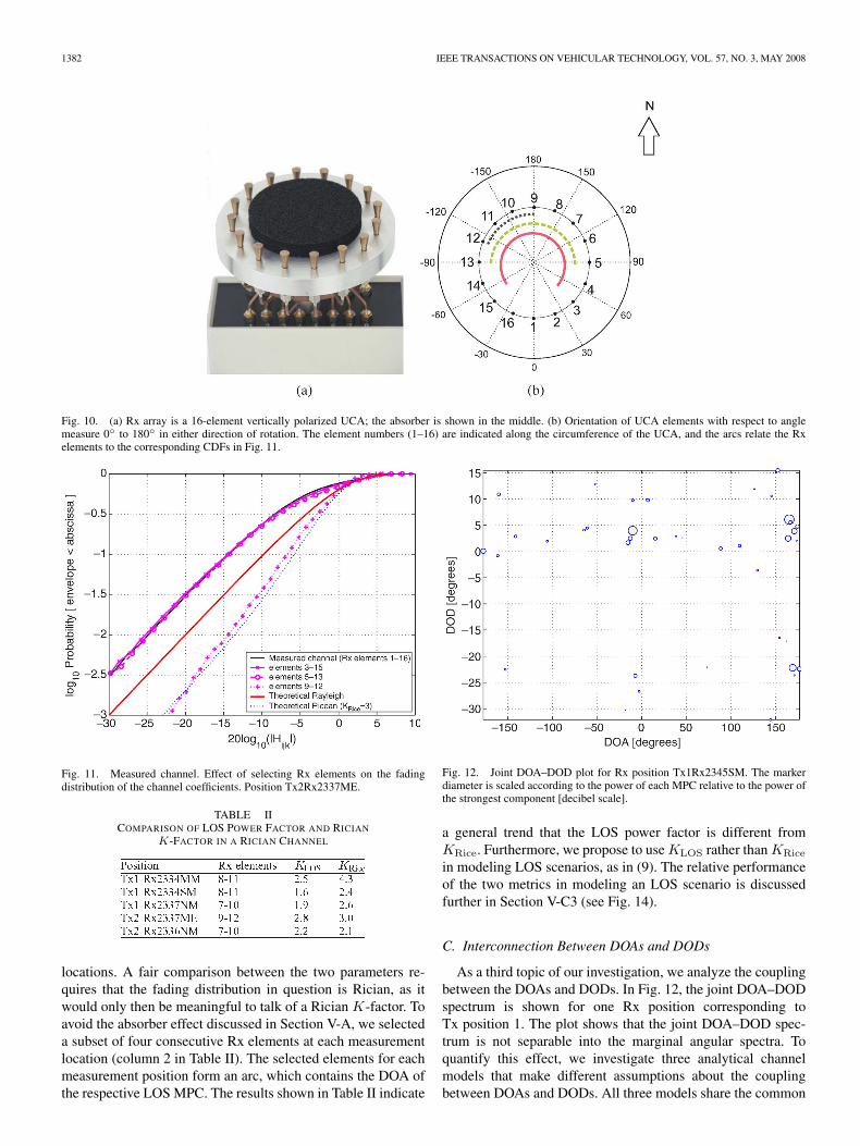
Fig. 10. (a) Rx array is a 16-element vertically polarized UCA; the absorber is shown in the middle. (b) Orientation of UCA elements with respect to anglemeasure 0 to 180 in either direction of rotation. The element numbers (1–16) are indicated along the circumference of the UCA, and the arcs relate the Rxelements to the corresponding CDFs in Fig. 11.

Fig. 11. Measured channel. Effect of selecting Rx elements on the fadingdistribution of the channel coefficients. Position Tx2Rx2337ME.

TABLE IICOMPARISON OF LOS POWER FACTOR AND RICIAN

K-FACTOR IN A RICIAN CHANNEL

locations. A fair comparison between the two parameters re-quires that the fading distribution in question is Rician, as itwould only then be meaningful to talk of a Rician K-factor. Toavoid the absorber effect discussed in Section V-A, we selecteda subset of four consecutive Rx elements at each measurementlocation (column 2 in Table II). The selected elements for eachmeasurement position form an arc, which contains the DOA ofthe respective LOS MPC. The results shown in Table II indicate

Fig. 12. Joint DOA–DOD plot for Rx position Tx1Rx2345SM. The markerdiameter is scaled according to the power of each MPC relative to the power ofthe strongest component [decibel scale].

a general trend that the LOS power factor is different fromKRice. Furthermore, we propose to use KLOS rather than KRice

in modeling LOS scenarios, as in (9). The relative performanceof the two metrics in modeling an LOS scenario is discussedfurther in Section V-C3 (see Fig. 14).

C. Interconnection Between DOAs and DODs

As a third topic of our investigation, we analyze the couplingbetween the DOAs and DODs. In Fig. 12, the joint DOA–DODspectrum is shown for one Rx position corresponding toTx position 1. The plot shows that the joint DOA–DOD spec-trum is not separable into the marginal angular spectra. Toquantify this effect, we investigate three analytical channelmodels that make different assumptions about the couplingbetween DOAs and DODs. All three models share the common


Fig. 13. Scatter plot of average modeled capacity against the average measured capacity of the channel. The top figure is for LOS 2 × 8 MIMO, whereas thebottom figure is for NLOS 16 × 8 MIMO. The identity line indicates points of no modeling error.

assumption that the channel matrix has zero-mean complexGaussian entries. For analyzing the LOS scenarios, we consideronly a subset of the full LOS channel matrix, i.e., those rowsin the matrix that correspond to Rx elements that receive theLOS component free from the absorber effect. The analysisin Sections V-A and B guarantees that the subset channel hasRician fading. We then model this subset channel according to(9), where only Hres is modeled by the zero-mean Gaussianmodels. For NLOS scenarios, no such limitation exists, and wecan test the model validity for larger channel matrices.1) Kronecker Model: The Kronecker model [6], [13] ap-

proximates the full channel correlation matrix R by theKronecker product of the transmit and receive antenna corre-lation matrices RTx and RRx, respectively. Equivalently, theMIMO channel matrix is modeled as

HKron =1√

trRRxR

12RxGR

T2Tx. (14)

The Kronecker model assumes that the DOA spectrum, andhence, the structure of the Rx correlation matrix does notchange for different DODs.7 In the context of Fig. 12, theKronecker assumption, when fulfilled, would imply a rectan-gular structure, i.e., if one groups the estimated DODs intonarrow angular bins, where each bin results in a set of DOAsand path powers according to (1), the Kronecker assumption isconsidered fulfilled if the DOA power spectrum for each of theDOD bins is similar. We have analyzed the validity of theKronecker model for both LOS and NLOS scenarios. Fig. 13shows the modeled ergodic capacity plotted against the mea-sured one for a number of measurement locations. In the top

7However, the total power in the spectrum, which is a scale factor for thecorrelation matrix, is allowed to change.

figure (a 2 × 8 LOS setup), the Kronecker model deviatesonly very little from the measured results. This nice fit isdue to the small rank of the channel matrix [30]. The bottomhalf of Fig. 13 is a 16 × 8 NLOS setup. This setup showslarge deviations between the modeled and measured capacitydue to the Kronecker assumption about the joint DOA–DODspectrum. In [7], it is suggested that the Kronecker model, ingeneral, underestimates the channel capacity. This is validatedfor the outdoor-to-indoor scenario by our results.

Note that the LOS locations considered in Fig. 13 have ameasured SNR in the range of 14–20 dB. When computingthe ergodic capacity at those locations, the evaluation SNRin the capacity formula was always set to 10 dB below thecorresponding measured value. In a previous work [12] thatanalyzes the impact of measurement noise on capacity, it wasestablished that even for a “keyhole” MIMO channel (in whichthe capacity is very sensitive to measurement noise), the capac-ity calculations are correct as long as the measurement SNRis 10 dB better than the evaluation SNR. Thus, our reportedresults are not influenced by measurement noise. For the NLOSscenarios considered in Fig. 13, the measurement SNR was ina considerably lower range of 1–13 dB. However, we mitigatedthe measurement noise at each location by coherently averagingthe channel matrices over the available 13 time snapshots; thisimproves the measurement SNR by a factor exceeding 10 dB.For capacity evaluation, we always use the noise-suppressedchannel matrices and set the evaluation SNR in the capacityformula to the unprocessed value of the measured SNR so thatwe have a 10-dB difference between measured and evaluationSNR. Therefore, our NLOS capacity results also represent thetrue channel capacity.2) VCR: The virtual channel representation (VCR) was in-

troduced in [31] for a ULA at each link end and allows an arbi-trary coupling between predetermined directions at the Tx and


Rx sides. The model uses discrete Fourier transform matricesARx and ATx at respective link ends such that the measuredchannel and the virtual channel are unitarily equivalent. Therealizations of the channel model can be generated as

HVCR = ARx(Ω G)ATTx (15)

where the columns of ARx and ATx are based on the arrayresponse (steering) vectors computed at fixed virtual directions,and the matrix Ω is the element-wise square root of the powercoupling matrix Ω. The entry Ωij gives the average powercoupled between the ith receive and jth transmit direction.This beamforming approach thus incorporates the antenna arrayeffects. However, since the directions are predetermined, andscatterers within the spatial resolution of the array will not beresolved, it is possible that the true spatial characteristics of thechannel will not be accurately rendered for some scenarios.

In our measurement setup, the Rx array was not a ULAbut rather a UCA with an absorber in the center. We thususe a generalization of (15) that combines the standard virtualchannel model at the Tx side with a “canonical” representation,based on the channel statistics, at the Rx side, i.e.,

HVCR = URx(Ω G)ATTx

where URx is an estimate of the receive eigenvector matrix ob-tained by the eigenvalue decomposition of RRx. In Fig. 13, theergodic capacities computed from this model are also shown.For the 16 × 8 NLOS setup, the capacity from this model tendsto slightly overestimate the measured values.3) Weichselberger Model: Like the Kronecker model, the

Weichselberger model [7] represents the measured channelin the eigenvector domain, although, unlike the Kroneckermodel, it strives to jointly model channel correlations at bothlink ends. This is achieved by defining a power couplingmatrix between the eigenvectors of the two link ends. TheWeichselberger model assumes that the eigenvector matrix atthe Rx is independent of the spatial Tx weight vector, i.e., DOD,that is considered. However, the corresponding eigenvalues ofthe spatial correlation matrix at Rx can differ for differentDODs. The same argument applies to the reverse link. Thephysical interpretation of the modeling assumptions can befound in [7], wherein the channel is modeled as

Hweichsel = URx(Ω G)UTTx (16)

where URx and UTx are estimates of the receive and transmiteigenvector matrices obtained by the eigenvalue decompositionof RRx and RTx, respectively. The elements of the powercoupling matrix Ωij now give the average power coupledbetween the ith receive and jth transmit eigenvector; the matrixis estimated as

Ω =1M

M∑m=1

[K K∗] (17)

where K = (UHRxH(m)U∗

Tx), and H(m) is the mth channelrealization. It should be noted that the Kronecker model isa special case of the Weichselberger model. In Fig. 13, the

Fig. 14. Performance comparison of KLOS and KRice in modeling anLOS scenario. The Weichselberger model is used in both cases.

ergodic capacity computed from the Weichselberger model isshown for the same measurement locations as for the previouscases. Compared to the Kronecker model, the Weichselbergermodel provides a better fit to the measured data. This result isexpected from Fig. 12, where the joint spectrum is not separableinto the marginal spectra. The Weichselberger model fits themeasured data better than the VCR case as well. This can beexplained because in the former case, the channel statisticsdetermine the unitary matrices at both link ends. Our results,which were obtained for the outdoor-to-indoor scenario, areconsistent with the observations in [7], which separately con-sidered the pure indoor and outdoor cases. As a follow-up toSection V-B, we use the Weichselberger model and the ergodiccapacity as a metric to compare the performance of KRice andKLOS in modeling an LOS scenario according to (9). The plotsare shown in Fig. 14 for a 2 × 8 LOS setup. Although therestriction to use a small rank LOS channel will result in aconvergence of performance of the two metrics, from the figure,the KLOS metric appears to perform better.

VI. CONCLUSION

In this paper, we have presented the results of a double-directional measurement campaign for an outdoor-to-indooroffice scenario. Our characterization of the outdoor-to-indoorscenario indicates that the angular dispersion at the outdoor linkend is rather small; the mean direction spread is in the range of0.09–0.24. At the indoor link end, MPCs of significant energyarrive from all directions; therefore, the angular dispersion ismuch larger, we observed mean direction spreads in the rangeof 0.69–0.82. The delay spread was measured to be in the rangeof 5–25 ns. By considering 40 MPCs at each measured position,more than 85% of the received power could be accounted for in60% of the 159 measurement locations.

Our statistical analysis shows that the widely used assump-tion in MIMO channel modeling, i.e., that the channel can berepresented as a sum of a weighted LOS component plus azero-mean complex Gaussian distribution, may not adequately


represent the measured data. In general, the small-scale fadingin an LOS scenario may not be Rician. We observed a compos-ite fading distribution caused by our antenna configuration andfound the generalized Gamma distribution to be a useful tool forverifying this. Furthermore, we have highlighted the differencebetween the LOS power factor and the Rician K-factor andsupport this assertion with the measured data from a Ricianfading channel. We show that the DOA spectrum noticeablydepends on the DOD. Using the ergodic channel capacity as ametric, we have compared the performance of the Kronecker,VCR, and Weichselberger models for the outdoor-to-indoorscenario. The Kronecker model is not applicable in our case dueto the breakdown of the DOA–DOD decoupling assumptions;this holds true even for the NLOS scenarios. Compared to theVCR model, the Weichselberger model provides a better fit tothe measured capacity for both the LOS and NLOS scenarios.

Our results can serve as a basis for understanding theoutdoor-to-indoor MIMO channels and have served as an inputto the COST 273 MIMO channel model [32].

ACKNOWLEDGMENT

The authors would like to thank Prof. L. Greenstein,Prof. E. Bonek, and members of the COST 273 subwork-ing group 2.1 for fruitful discussions regarding the RicianK-factor; the informative input from Dr. A. Sayeed regardingthe generalization of the VCR to UCAs; and TU Ilmenau,Ilmenau, Germany, for the loan of their antenna arrays.

REFERENCES

[1] J. H. Winters, “On the capacity of radio communications systems withdiversity in Rayleigh fading environments,” IEEE J. Sel. Areas Commun.,vol. SAC-5, no. 5, pp. 871–878, Jun. 1987.

[2] G. J. Foschini and M. J. Gans, “On limits of wireless communicationsin a fading environment when using multiple antennas,” Wirel. Pers.Commun., vol. 6, no. 3, pp. 311–335, Mar. 1998.

[3] M. Steinbauer, A. F. Molisch, and E. Bonek, “The double-directionalradio channel,” IEEE Antennas Propag. Mag., vol. 43, no. 4, pp. 51–63,Aug. 2001.

[4] D. Chizhik, J. Ling, P. W. Wolniansky, R. A. Valenzuela, N. Costa, andK. Huber, “Multiple-input-multiple-output measurements and modelingin Manhattan,” IEEE J. Sel. Areas Commun., vol. 21, no. 3, pp. 321–331,Apr. 2003.

[5] R. Thomä, D. Hampicke, M. Landmann, G. Sommerkorn, and A. Richter,“MIMO measurement for double-directional channel modelling,” in Proc.IEE Semin. MIMO: Commun. Syst. From Concept to Implementations(Ref. No. 2001/175), Dec. 2001, pp. 1/1–1/7.

[6] K. Yu, M. Bengtsson, B. Ottersten, D. McNamara, P. Karlsson, andM. Beach, “Second order statistics of NLOS indoor MIMO channelsbased on 5.2 GHz measurements,” in Proc. IEEE Globecom, 2001, vol. 1,pp. 156–160.

[7] W. Weichselberger, M. Herdin, H. Özcelik, and E. Bonek, “A stochasticMIMO channel model with joint correlation of both link ends,” IEEETrans. Wireless Commun., vol. 5, no. 1, pp. 90–100, Jan. 2006.

[8] S. Wyne, P. Almers, G. Eriksson, J. Karedal, F. Tufvesson, andA. F. Molisch, “Outdoor to indoor office MIMO measurementsat 5.2 GHz,” in Proc. IEEE VTC—Fall, Los Angeles, CA, 2004,pp. 101–105.

[9] J. Medbo, F. Harrysson, H. Asplund, and J. E. Berg, “Measurements andanalysis of a MIMO macrocell outdoor–indoor scenario at 1947 MHz,” inProc. IEEE VTC—Spring, 2004, vol. 1, pp. 261–265.

[10] H. T. Nguyen, J. B. Andersen, and G. F. Pedersen, “Characterization ofthe indoor/outdoor to indoor MIMO radio channel at 2.140 GHz,” Wirel.Pers. Commun., vol. 35, no. 3, pp. 289–309, Nov. 2005.

[11] D. Gesbert, H. Bolcskei, D. A. Gore, and A. J. Paulraj, “Outdoor MIMOwireless channels: Models and performance prediction,” IEEE Trans.Commun., vol. 50, no. 12, pp. 1926–1934, Dec. 2002.

[12] P. Almers, F. Tufvesson, and A. F. Molisch, “Keyhole effect in MIMOwireless channels: Measurements and theory,” IEEE Trans. WirelessCommun., vol. 5, no. 12, pp. 3596–3604, Dec. 2006.

[13] J. P. Kermoal, L. Schumacher, K. I. Pedersen, P. E. Mogensen, andF. Frederiksen, “A stochastic MIMO radio channel model with experi-mental validation,” IEEE J. Sel. Areas Commun., vol. 20, no. 6, pp. 1211–1226, Aug. 2002.

[14] H. Özcelik, N. Czink, and E. Bonek, “What makes a good MIMOchannel model,” in Proc. IEEE VTC—Spring, Stockholm, Sweden,May/Jun. 2005, pp. 156–160.

[15] S. Wyne, A. F. Molisch, P. Almers, G. Eriksson, J. Karedal, andF. Tufvesson, “Statistical evaluation of outdoor-to-indoor office MIMOmeasurements at 5.2 GHz,” in Proc. IEEE VTC—Spring, Stockholm,Sweden, 2005, pp. 146–150.

[16] [Online]. Available: http://www.channelsounder.de[17] B. H. Fleury, M. Tschudin, R. Heddergott, D. Dahlhaus, and K. Pedersen,

“Channel parameter estimation in mobile radio environments using theSAGE algorithm,” IEEE J. Sel. Areas Commun., vol. 17, no. 3, pp. 434–450, Mar. 1999.

[18] A. F. Molisch, Wireless Communications. Piscataway, NJ: IEEEPress–Wiley, 2005.

[19] J. Medbo, M. Riback, H. Asplund, and J. Berg, “MIMO channel char-acteristics in a small macrocell measured at 5.25 GHz and 200 MHzbandwidth,” in Proc. IEEE VTC—Fall, 2005, vol. 1, pp. 372–376.

[20] B. H. Fleury, “First- and second-order characterization of direction disper-sion and space selectivity in the radio channel,” IEEE Trans. Inf. Theory,vol. 46, no. 6, pp. 2027–2044, Sep. 2000.

[21] P. A. Bello, “Characterization of randomly time-variant linear channels,”IEEE Trans. Commun., vol. COM-11, no. 4, pp. 360–393, Dec. 1963.

[22] S. Wyne, N. Czink, J. Karedal, P. Almers, F. Tufvesson, and A. F. Molisch,“A cluster-based analysis of outdoor-to-indoor office MIMO measure-ments at 5.2 GHz,” in Proc. IEEE VTC—Fall, Montreal, QC, Canada,2006, pp. 1–5.

[23] P. Soma, D. S. Baum, V. Erceg, R. Krishnamoorthy, and A. J. Paulraj,“Analysis and modeling of multiple-input multiple-output (MIMO) radiochannel based on outdoor measurements conducted at 2.5 GHz for fixedBWA applications,” in Proc. IEEE ICC, 2002, vol. 1, pp. 272–276.

[24] E. W. Stacy, “A generalisation of the Gamma function,” Ann. Math. Stat.,vol. 33, pp. 1187–1192, 1962.

[25] J. Griffiths and J. McGeehan, “Interrelationship between some statisticaldistributions used in radio wave propagation,” Proc. Inst. Electr. Eng.—F,vol. 129, no. 6, pp. 411–417, Dec. 1982.

[26] R. Vaughan and J. B. Andersen, Channels, Propagation and Antennas forMobile Communications, 1st ed. London, U.K.: IEE, 2003.

[27] M. Abramowitz and I. Stegun, Handbook of Mathematical Functions.New York: Dover, 1966.

[28] A. J. Coulson, A. G. Williamson, and R. G. Vaughan, “Improved fad-ing distribution for mobile radio,” Proc. Inst. Electr. Eng.—Commun.,vol. 145, no. 3, pp. 197–202, Jun. 1998.

[29] L. J. Greenstein, D. G. Michelson, and V. Erceg, “Moment-method es-timation of the Ricean K-factor,” IEEE Commun. Lett., vol. 3, no. 6,pp. 175–176, Jun. 1999.

[30] M. A. Jensen and J. Wallace, “A review of antennas and propagationfor MIMO wireless communications,” IEEE Trans. Antennas Propag.,vol. 52, no. 11, pp. 2810–2824, Nov. 2004.

[31] A. M. Sayeed, “Deconstructing multiantenna fading channels,” IEEETrans. Signal Process., vol. 50, no. 10, pp. 2563–2579, Oct. 2002.

[32] COST 273 Final Report: Towards Mobile Broadband MultimediaNetworks, L. Correia, Ed. Amsterdam, The Netherlands: Elsevier, 2006.

Shurjeel Wyne (S’03) received the B.Sc. degree inelectrical engineering from the University of En-gineering and Technology (UET) Lahore, Lahore,Pakistan, and the M.S. degree in digital commu-nications from Chalmers University of Technology,Göteborg, Sweden. In 2003, he joined Lund Univer-sity, Lund, Sweden, where he is working towards thePh.D. degree with the Department of Electrical andInformation Technology.

His research interests are in the field of measure-ment and modeling of wireless propagation channels,

particularly for MIMO systems. He has participated in the European researchinitiatives “COST 273” and the European network of excellence “NEWCOM.”


Andreas F. Molisch (S’89–M’95–SM’00–F’05) re-ceived the Dipl.Ing., Dr. Techn., and Habilita-tion degrees from the Technical University Vienna(TU Vienna), Vienna, Austria, in 1990, 1994, and1999, respectively.

From 1991 to 2000, he was with TU Vienna,where he became an Associate Professor in 1999.From 2000 to 2002, he was with the Wireless Sys-tems Research Department, AT&T (Bell) Laborato-ries Research, Middletown, NJ. Since 2002, he hasbeen with Mitsubishi Electric Research Laboratories,

Cambridge, MA, where he is currently a Distinguished Member of TechnicalStaff. He is also a Professor and a chair holder for radio systems withLund University, Lund, Sweden. He has participated in the European researchinitiatives “COST 231,” “COST 259,” and “COST 273,” where he was theChairman of the MIMO Channel Working Group, the IEEE 802.15.4a ChannelModel Standardization Group, and Commission C (signals and systems) of theInternational Union of Radio Scientists (URSI). He has authored, coauthored,or edited four books, among them, the recent textbook Wireless Communica-tions (Wiley-IEEE Press), 11 book chapters, some 100 journal papers, andnumerous conference contributions. He has done research in the areas ofSAW filters, radiative transfer in atomic vapors, atomic line filters, smart anten-nas, and wideband systems. His current research interests are the measurementand modeling of mobile radio channels, UWB, cooperative communications,and MIMO systems.

Dr. Molisch is an IEEE Distinguished Lecturer and the recipient of severalawards. He is an Editor of the IEEE TRANSACTIONS ON WIRELESS

COMMUNICATIONS and a Co-Editor of recent and upcoming special issues onUWB (in the IEEE JOURNAL ON SELECTED AREAS IN COMMUNICATIONS

and the PROCEEDINGS OF THE IEEE). He has been a member of numerousTechnical Program Committees (TPCs), e.g., Vice Chair of the TPC of theVehicular Technology Conference (VTC) 2005 Spring, General Chair of theInternational Conference on Ultra-Wideband (ICUWB) 2006, and TPC Cochairof the wireless symposium of Globecom 2007.

Peter Almers received the M.S. degree in electricalengineering and the Ph.D. degree in radio systemsfrom Lund University, Lund, Sweden, in 1998 and2007, respectively.

In 1998, he was with the Radio Research Depart-ment, TeliaSonera AB (formerly Telia AB), Malmö,Sweden, where he mainly worked with WCDMAphysical layer issues and 3GPP WG1 standardiza-tion. In 2001, he was with the Radio Systems Group,Lunds Tekniska Högskola (LTH), Lund University,as a Ph.D. student (50% funded by TeliaSonera AB).

He has participated in the European research initiative COST 273 andthe European network of excellence NEWCOM and is currently involved inthe NORDITE project WILATI. He is currently a Research Fellow with theDepartment of Electrical and Information Technology, Lund University.

Dr. Almers received the IEEE Best Student Paper Award at the 2002 Interna-tional Symposium on Personal, Indoor, and Mobile Radio Communications.

Gunnar Eriksson received the M.S. degree inapplied physics and electrical engineering fromLinkoping University, Linköping, Sweden, in 1987.He is currently working toward the Ph.D. degreewith the Department of Electrical and InformationTechnology, Lund University, Lund, Sweden.

Since 1987, he has been with the Departmentof Communication Systems, Swedish Defence Re-search Agency (FOI), Linköping, where he is mainlyworking with channel characterization, modeling,and prediction of radio-wave propagation for the

assessment of communication and radar systems performance within a widerange of the radio frequency spectrum. His current research interests aremainly in the field of channel measurements and modeling for MIMO systems,particularly for peer-to-peer systems and with a focus on frequencies in the lowUHF region.

Johan Karedal (S’04) received the M.S. degree inengineering physics in 2002 from Lund University,Lund, Sweden, where he is currently working towardthe Ph.D. degree with the Department of Electricaland Information Technology.

His research interests include channel measure-ment and modeling for MIMO and UWB systems.He has participated in the European research initia-tive “MAGNET.”

Fredrik Tufvesson (S’97–A’00–M’04–SM’07) wasborn in Lund, Sweden, in 1970. He received theM.S. degree in electrical engineering, the Licentiatedegree, and the Ph.D. degree from Lund University,in 1994, 1998, and 2000, respectively.

After almost two years at a startup company(Fiberless Society), he is currently an AssociateProfessor with the Department of Electrical and In-formation Technology, Lund University. His mainresearch interests are channel measurements andmodeling for wireless communication, including

channels for both MIMO and UWB systems. In addition, he also works withchannel estimation and synchronization problems, OFDM system design, andUWB transceiver design.

Outdoor-to-Indoor Office MIMO Measurements and Analysis at 5.2 GHz

Documents

Transcript of Outdoor-to-Indoor Office MIMO Measurements and Analysis at 5.2 GHz