Organic and inorganic nanofilms on Nitinol and Phynox - DIAL ...

�

Organic and inorganic nanofilms on Nitinol

and Phynox: from fundamental towards

applications in biomaterials

Committee Members

Prof. Patrik Schmuki

Prof. Catherine Combellas

Prof. Catherine Michaux

Prof. Joseph Delhalle

Prof. Zineb Mekhalif (Advisor)

2012

FUNDP

Faculté des Sciences

Département de Chimie

Laboratoire de Chimie et d’Electrochimie des Surfaces

Rue de Bruxelles, 61

B-5000 Namur

Belgium

Ph. Doctor in Sciences

Dissertation presented by

Sébastien Devillers

Facultés Universitaires Notre-Dame de la Paix

Faculté des Sciences

Rue de Bruxelles, 61, B-5000 Namur, Belgique

Organic and inorganic nanofilms on Nitinol and Phynox: from fundamental toward

applications in biomaterials

By Sébastien Devillers

Abstract:

This thesis is devoted to the improvement of biomaterials and more specifically of two

increasingly used ones: Nitinol and Phynox. Nitinol is a very complex yet promising material

especially in the field of biomedical applications because of its remarkable mechanical

properties (shape memory alloy). Phynox is another alloy very commonly used for the design

of biomedical devices such as stents and coils specifically because of its important corrosion

resistance.

In the first part of this thesis, the characterization of the Nitinol and Phynox surface states are

reported as well as several surface modification methods applied to these materials. The goal

of these surface modifications is not to obtain a perfect “ready to use” biomaterial but rather

to provide interesting functionalization methods with two targets: to protect the underlying

substrate against corrosion (and avoid ions leaching) and to form functional platforms for the

post-grafting of a broad range of molecules in order to improve the material-biological

environment interactions.

Regarding Nitinol, the impact of typical shape-setting heat treatment and chemical etching on

the surface composition and the resulting resistance to corrosion of Nitinol wires identical to

the ones used for the fabrication of braided Nitinol stents is studied. The modification of

Nitinol by the electrografting of 1,4-carboxybenzene diazonium and the formation of a 11-

phosphoundecanoïc acid monolayer is carried out with the prospect of using these coatings as

platform for post-grafting chemical reactions. The electrografting method is proved to have

negative impact on the corrosion resistance of Nitinol and the resulting electrografted

carboxybenzene coating leads to a poor efficiency for these post-grafting chemical reactions.

On the other hand, 11-phosphoundecanoic acid monolayers exhibit a much better efficiency to

act as a platform for post-grafting chemical reactions and no negative impact on the corrosion

resistance of the underlying substrate. A brief study of the impact of the solvent and

temperature on the grafting of phosphonic acids on the surface of mechanically polished

Nitinol is also carried out. On the one hand, it turns out that water is a very suitable solvent

for this surface modification method. On the other hand, increasing the temperature does not

lead to an increase of the quantity of grafted phosphonic acids but to an improvement of the

organization of the resulting monolayer and therefore of its efficiency as corrosion inhibitor.

Finally, induction heating of Nitinol in pure water appears to be an original and promising

alternative to conventional hydrothermal treatment usually applied in order to decrease the

surface nickel concentration and reinforce the resistance of the oxide layer to corrosion. Both

induction and conventional heating treatments lead to similar results. However, on the whole,

induction heating leads to slightly better results than conventional heating does (i.e. a higher

hydroxylation of the surface, a more important decrease of the nickel surface concentration

and a similar corrosion resistance improvement).

Regarding Phynox, a systematic corrosion resistance evaluation of Phynox stents provided by

Cardiatis is carried out after several different surface treatments. It appears that Phynox have a

remarkable resistance to corrosion and especially to localized corrosion phenomena.

However, despite this very good corrosion resistance, there is a strong interest in modifying

its surface with the prospect of improving the material-biological environment interactions.

Therefore, similarly to Nitinol, the Phynox surface functionalization with bifunctional

phosphonic acid molecules toward a versatile platform for post-grafting chemical reactions is

carried out. The effect of induction heating on the grafting of such bifunctional phosphonic

acids is also studied. It turns out that induction heating can lead to a much more selective

adsorption of bifunctional phosphonic-carboxylic molecules via the phosphonic acid function,

leaving a higher amount of free carboxylic acid functions to react during the second

modification step. Finally, it is shown that such phosphonic acid monolayers perfectly resist

the typical ethylene oxide sterilization process applied to biomaterials before their

conditioning and utilization.

In the second part of this thesis, we present a research carried out at the University Hospital of

Geneva (HUG) in the frame of the FIRST-DEI VISMAT convention (RW – n°516114) in

collaboration with Cardiatis and the HUG. This work is dedicated to a study of the impact of

different surface treatments and of the imaging parameters and conditions on the MRI

visibility of Nitinol and Phynox wires and stents. Two main types of artifacts are investigated:

susceptibility and RF artifacts.

By means of an algorithm developed for this purpose, it is shown that the surface state of the

observed material can have a significant influence on the produced susceptibility artifact. Heat

treatment of Nitinol appears to have a negative impact on its apparent magnetic susceptibility

while the removal of the oxide layer by chemical etching is favorable to a low apparent

magnetic susceptibility. Phynox is a much less suitable material for MRI examinations given

its apparent magnetic susceptibility about 10-fold higher than the one of Nitinol. In the case of

Phynox, however, the heat treatment of Phynox induces a slight decrease of this apparent

magnetic susceptibility while its chemical etching does not appear to have any significant

impact.

The impact of several parameters on the MRI visibility of braided stents i.e. on the importance

of the produced susceptibility and RF artifacts is also studied. SE sequences are less sensitive

to susceptibility artifacts and lead to the acquisition of better images than the GRE sequences

do. The stent orientation with respect to the main magnetic field is also crucial. Interestingly,

it is shown that the RF artifacts could be beneficial as they could lead to a signal enhancement

in the stent lumen at low flip angles.

Finally, antiferromagnetic NiO and CoO layers are formed on Nitinol and Phynox wires,

respectively, by electrodeposition and thermal oxidation. The impact of such oxide layers on

the MRI behavior of Nitinol and Phynox appears to be dramatically negative.

God made solids, but surfaces were the work of the devil - Wolfgang Pauli

Acknowledgements

Foremost, I would like to express my sincere gratitude to my advisor Prof. Zineb Mekhalif as

well as to Prof. Joseph Delhalle. Their guidance and their precious advices helped me for my

research and the writing of this thesis. Obviously, I would also like to thank the Region

Wallonne for the financial support of the FIRST-DEI VISMAT project (convention n°516114)

and the Cardiatis team for all the technical knowledge they provided to me concerning stents

fabrication. This thesis would not have been possible without them.

I am also grateful to Professors Catherine Combellas (ESPCI, Paris), Catherine Michaux and

Patrik Schmuki (Friedrich-Alexander University, Erlangen) for their insightful comments on

this thesis.

During my stay in Geneva, I had the opportunity to work and/or have scientific discussions

with many people. Among them, I would like to thank especially M.D. Daniel Rüfenacht and

Ph.D. Lucas Augsburger for their warm welcome in Switzerland, Ph.D. François Lazeyras

(CIBM director) and all the CIBM members for their numerous advices and technical

assistance regarding MRI utilization as well as Tiziano Binzoni for his precious help in the

development of MATLAB algorithms.

I would also like to thank my past and present labmates in the CES laboratory: Isa,

Christelle, Jess, François, Jorge, Praveen, Anthony (Toto), Greg (Pinpin), Amory, Simon,

Bastien, Jeff, Nathalie, Larissa, Isabelle, Malau, Steph, Nico, Quentin, Alex, the younger ones

Jean-François, Simon, Benjamin and Julien and a special thank to Tania for all her little but

precious technical helps that make our life easier.

I also had the great opportunity to spend a month in the LKO laboratory where I met

unforgettable people. Even if the work carried out there is not included in this thesis, I would

like to thank especially Felix Schmidt-Stein and his wife Conzie for their warm welcome in

Germany. My discussions with Felix were much inspiring not only about science but also

about Germany and a lot more about rockabilly. Keep on rockin’ dude !

Thank also to my bands members for their patience. Being a Ph.D. student often requires

canceling extra activities and I can’t remember how many training sessions I missed! They

always supported me and pretended to understand what I was saying when I explained my

work.

Last but not least, my deepest thanks are to my family, my closest friends Oli, John, Hélène

and Becky and Alix, the girl who shares my life. They have always been present to believe in

me, cheer me up or simply change my mind.

And to all those I could have forgotten or just didn’t mention here: Thank you!

Table of Contents

�

�

Chapter 1. General introduction 1

1.1. Stents and biomaterials: general considerations 2

1.1.1. Biocompatibility 2

1.1.2. Stents 3

1.2. Molecular surface modification of oxidizable metals 3

1.2.1. Organothiol monolayers 4

1.2.2. Organosilanes monolayers 8

1.2.3. Organocarboxylic acid monolayers 9

1.2.4. Organophosphonic acid monolayers 10

1.3. Nitinol 11

1.3.1. History, mechanical properties and applications 11

1.3.1.1. History 11

1.3.1.2. Mechanical properties 12

1.3.1.2.1. Simple shape memory effect 13

1.3.1.2.2. Superelasticity 14

1.3.1.3. Applications of SMA’s 16

1.3.1.3.1. Non-medical applications 16

1.3.1.3.2. Medical applications 16

1.3.2. Nitinol biocompatibility and resistance to corrosion 18

1.3.3. Inorganic coatings 20

1.3.4. Organic coatings 21

1.4. Phynox 23

1.4.1. History, properties and applications 23

�

�

1.4.2. Surface modification 23

Chapter 2. Study and modification of the Nitinol surface state 24

2.1. Nitinol wires 24

2.1.1. Heat treatment 24

2.1.1.1. Introduction 24

2.1.1.2. Samples preparation 24

2.1.1.3. XPS analysis 25

2.1.1.4. ToF-SIMS analysis 30

2.1.1.5. Polarization curves measurements 32

2.1.1.6. Conclusions 35

2.1.2. Chemical etching 36




2.1.2.4. SEM analysis 41

2.1.2.5. ToF-SIMS analysis 42

2.1.2.6. Polarization curves measurements 44


2.2. Nitinol plates 46

2.2.1. Analysis and heat treatment of “as received” Nitinol plates 47





2.2.2. Analysis and modification of mechanically polished Nitinol plates 50


2.2.2.2. Surface state of the Nitinol plates after mechanical polishing 50

2.2.2.3. Functionalization of Nitinol surface toward a versatile platform for post-grafting

chemical reactions 52

�

�

2.2.2.3.1. Introduction 52

2.2.2.3.2. Samples preparation 52

2.2.2.3.3. Electrografting of the 1,4-carboxybenzene diazonium 54

2.2.2.3.4. Grafting of the 11-phosphonoundecanoïc acid 58

2.2.2.3.5. Grafting of the CF alcohol on the modified Nitinol substrates 61

2.2.2.3.6. Conclusions 66

2.2.2.4. Assessment of the solvent and temperature impact on the grafting of phosphonic acid

molecules on Nitinol surface 67



2.2.2.4.3. Solvent effect 68

2.2.2.4.4. Temperature effect 70


2.2.2.5. Induction heating of Nitinol in water: study of the impact on the oxide layer 72



2.2.2.5.3. Temperature measurements 73

2.2.2.5.4. XPS characterizations 74

2.2.2.5.5. Electrochemical characterizations 78


Chapter 3. Study and modification of the Phynox surface state 80

3.1. Corrosion study of Phynox braided stents 80

3.1.1. Introduction 80

3.1.2. Results 81

3.1.3. Conclusions 82

3.2. Surface modification of Phynox substrates 82

3.2.1. XPS analysis of bare Phynox substrates 83

3.2.2. Grafting PEG Fragments on Phynox substrates modified with 11-

phosphonoundecanoic acid 84



3.2.2.3. Grafting of the n-dodecylphosphonic acid 85

�

�

3.2.2.4. Grafting of the n-dodecanoic acid 88

3.2.2.5. Grafting of the 11-phosphonoundecanoic acid 91

3.2.2.6. Grafting of PEG oligomers on 11-phosphonoundecanoic acid modified surface 95


3.2.3. Grafting of bifunctional phosphonic and carboxylic acids on Phynox :

impact of induction heating 103



3.2.3.3. Temperature measurements 103

3.2.3.4. Grafting of the n-dodecylphosphonic acid 105

3.2.3.5. Grafting of the n-dodecanoic acid 110

3.2.3.6. Grafting of bifunctional molecules 114

3.2.3.7. Grafting of alcohol on 6-phosphonohexanoic acid modified Phynox susbtrates 119


3.2.4. Grafting of the 11-phosphonoundecanoic acid on Phynox: study of the

impact of ethylene oxide sterilization process 122



3.2.4.3. Results 123


Chapter 4. VISMAT - Influence of the surface treatment of Phynox

and Nitinol on the MRI artifacts 126

4.1. Basic principles of MRI 126

4.1.1. Resonance phenomenon 126

4.1.2. Relaxation phenomena 128

4.1.3. MRI image acquisition principles 131

4.1.4. Main types of imaging sequences 133

4.1.5. Contrast mechanisms 135

�

�

4.1.6. Artifacts related to metallic implants imaging 138

4.1.6.1. Susceptibility artifacts 138

4.1.6.1.1. Slice selection 141

4.1.6.1.2. Geometrical distortion of the image plane 141

4.1.6.1.3. Distortion of the pixels intensity 142

4.1.6.2. RF artifacts 143

4.1.6.3. Study of the artifacts caused by stents 144

4.1.6.4. Other artifacts caused by stents 144

4.2. Results and discussion 145

4.2.1. Quantitative assessment of the apparent magnetic susceptibility of wires 145

4.2.1.1. Materials and method optimization 145

4.2.1.2. Phase measurement method 150

4.2.1.3. Iterative susceptibility artifact measurement method 152

4.2.1.3.1 Algorithm conception method 152

4.2.1.3.2 Results 153

4.2.2. Assessment of the stents behavior in MRI 159

4.2.2.1. Study of the imagery parameters influence 159

4.2.2.2. Study of the stent composition and surface treatment influence 162

4.2.2.3. Study of the stent composition and orientation on the RF artifacts 169

4.2.3. Electrodeposition, characterization and assessment of the impact on MRI

imaging of thin nickel and cobalt oxide layers 174

4.2.3.1. Electrodeposition of nickel and cobalt layers on Nitinol and Phynox 174

4.2.3.1.1. Electrodeposition of nickel on Nitinol 174

4.2.3.1.2. Electrodeposition of cobalt on Phynox 177

4.2.3.2. Study of the impact of the nickel oxide and cobalt oxide layers on the MRI behavior of

Nitinol and Phynox wires 180

4.3. Conclusions 184

Chapter 5. General conclusions and outlooks 186

5.1. Conclusions 186

�

�

5.2. Outlooks 188

Bibliography 190

General Introduction

��

�

Chapter 1. General introduction

The research presented in this manuscript deals with two increasingly used biomaterials i.e.

Nitinol and Phynox. This manuscript is divided into two main parts: a first one (including

chapters 2 and 3) gathering several studies about the characterization and the application of

various surface treatments on Nitinol and Phynox and a second one consisting in a study of

the MRI visibility of these materials (chapter 4).

Among the surface treatments presented in the first part, some have already been largely

studied in the literature. This manuscript aims to bring supplementary data on these topics in

order to clarify some controversial results presented in the literature. Other treatments

presented in this work are innovative and could constitute an effective basis for the further

improvement of the surface properties of these biomaterials. The goal of these surface

modifications is thus not to obtain a perfect “ready to use” biomaterial but rather to provide

interesting functionalization methods with two targets: to protect the underlying substrate

against corrosion (and avoid ions leaching) and to form functional platforms for the post-

grafting of a broad range of molecules in order to improve the material-biological

environment interactions.

This manuscript is divided into four chapters. The first one is an introductive chapter

dedicated to a review of the literature concerning the considered topics. General

considerations about stents and biomaterials and about the molecular surface modification of

oxidizable metals with self-assembled monolayers are first presented. Then the reader is

introduced to the Nitinol discovery, its remarkable mechanical properties and its various

application fields. Nitinol biocompatibility and resistance to corrosion is discussed as well as

various reported methods aiming to improve these properties. This first chapter ends with a

few words about Phynox and more generally about Co-Cr alloys, their properties and surface

modification.

The second chapter is dedicated to Nitinol. In a first part, we report on the impact of typical

shape-setting heat treatment and chemical etching on the surface composition and the

resulting resistance to corrosion of Nitinol wires identical to the ones used for the fabrication

of braided Nitinol stents. In a second part, we report on studies carried out on plane Nitinol

substrates. These Nitinol substrates were analyzed in their “as received”, heat treated and

mechanically polished states. The rest of the second part of this chapter is dedicated to the

surface modification of mechanically polished plane Nitinol substrates toward a versatile

platform for post-grafting chemical reactions, the study of parameters influencing the grafting

of phosphonic acids SAMs on these surfaces and on an original and promising alternative to

conventional hydrothermal treatment usually applied in order to reinforce the resistance of the

oxide layer to corrosion.

The third chapter focuses on the case of Phynox. In the first part, we present the results of a

systematic corrosion resistance evaluation of Phynox stents provided by Cardiatis after

��

�

several different surface treatments. The second part of this chapter is dedicated to the study

of Phynox surface functionalization with bifunctional phosphonic-carboxylic acid molecules

toward a versatile platform for post-grafting chemical reactions. In this context, the impact of

induction heating on the grafting of these bifunctional molecules has been assessed as well as

the resistance of the obtained coating to the ethylene oxide sterilization treatment.

In the fourth chapter of this manuscript, we present a research carried out at the University

Hospital of Geneva (HUG) in the frame of the FIRST-DEI VISMAT convention (RW –

n°516114) in collaboration with Cardiatis and the HUG. This work is dedicated to a

systematic study of the impact of different surface treatments and of the imaging parameters

and conditions on the MRI visibility of Nitinol and Phynox wires and stents. Two main types

of artifacts are presented and investigated: susceptibility and RF artifacts. In the first part of

this chapter, we report on the influence of the Nitinol and Phynox surface state on their

apparent magnetic susceptibility assessed by means of an algorithm developed in the frame of

this work. The second part is dedicated to the study of the impact of several parameters on the

MRI visibility of braided stents. In the last part of this chapter, we report on the creation, the

characterization and the impact of NiO and CoO layers on the MRI behavior of Nitinol and

Phynox.

1.1. Stents and biomaterials: general considerations

1.1.1. Biocompatibility

The consensus conference of the European Society for Biomaterials defined the biomaterial as

“a nonviable material used in a medical device, intended to interact with biological systems”

(Chester, UK, 1986). During the second Biomaterials Consensus Conference, this definition

has been updated as “a material intended to interface with biological systems to evaluate,

treat, augment, or replace any tissue, organ, or function of the body” (Chester, UK, 1992).

This definition extends the use of the “biocompatibility” term to any kind of device intended

to interface with biological systems and not only prostheses.

When a synthetic material interacts with a biological system, one should consider two types of

effects: the effects of the biological system on the biomaterial (i.e. wear, fatigue, degradation

or corrosion, etc.) and the effects of the biomaterial on the biological system (i.e. its aimed

effect but also all the possible side effects such as possible inflammatory responses, ions

releases that could lead to allergenic/carcinogenic effects, …). Thus a biomaterial has to be

inert toward the biological system i.e. to not lead to negative responses of the body but also to

resist degradation in the biological system.

In this context, the choice of the material is obviously crucial in order to obtain a biomedical

device with the desired bulk properties and able to play its role. However, the surface of the

biomaterial is the only part of the device which is in direct contact with the biological

environment. Therefore, the surface properties of a biomedical device are one of the key

factors to control in order to improve the biomaterial-biological system interactions.

��

�

1.1.2. Stents

In medicine, a stent is a tubular device inserted into the lumen of an anatomical vessel to

prevent or counteract a localized flow constriction. Most of the time, stents are made of metal

alloys such as SS316L, Co-Cr alloys or Ti-alloys. Although stents can basically be used to

maintain any tubular structure opened (e.g. laryngeal and tracheal stents, urethral stents, etc.),

one of the most common use of such implants is the treatment of cardiovascular diseases by

angioplasty with vascular stenting. Angioplasty is a minimally invasive procedure performed

to improve blood flow in the body’s arteries and veins. This procedure is commonly used to

treat conditions that involve a narrowing or blockage of arteries or veins including narrowing

of large arteries due to atherosclerosis, peripheral artery disease, renal vascular hypertension,

carotid or coronary artery diseases just to name a few of them. In an anglioplasty procedure,

imaging techniques are used to guide a balloon-tipped catheter into an artery or vein and

advance it to where the vessel is narrow or blocked. The balloon is then inflated to open the

vessel, deflated and removed. During this procedure, a stent may be permanently placed in the

newly opened artery or vein to help it remain open 1. Even if the use of stents contributes to

decrease the restenosis phenomenon (reobstruction of the vessel after the angioplasty), in-

stent restenosis remains a great concern 2. Restenosis can be due to an exaggerated

deployment of the stent 3, an inappropriate design 4,5 or the leaching of potentially toxic

metallic elements 6,7. The combination of these factors results in the formation of a thrombus,

inflammation reactions, an exaggerated cellular proliferation and the formation of a new

extracellular matrix inside the vessel 4. The restenosis and stent corrosion (thus metallic ion

leaching) issues strongly depend on the surface properties of the implant. It is thus clear that

the control of these surface properties is essential in order to decrease at most the risk of

restenosis.

1.2. Molecular surface modification of oxidizable metals

Since R. G. Nuzzo and D. L. Allara first reported on the self-assembling of disulfide on gold

in 1983 8, self-assembled monolayers (SAMs) have attracted immense attention for both

fundamental and applied research. By definition, SAMs are ordered molecular assemblies that

are formed spontaneously by the adsorption of a surfactant with a specific affinity of its head

group to a substrate 9. A SAM is composed of a large number of molecules with a head group

that chemisorbs onto a substrate, an end group that interacts with the outer surface of the film,

and a spacer (backbone) chain group that connects the head and end groups resulting in a

coating. Interactions between spacer groups of different molecules, such as Van der Waals

forces and/or electrostatic interactions (e.g. hydrogen bonding), hasten SAM film formation,

contribute to its stability and lead to the organization and close packing of the SAM. At their

best, self-assembled monolayers provide a dense, nearly crystalline organic skin on an

underlying solid surface (Figure 1.1).

��

�

Figure 1.1. Schematic representation of a surfactant molecule in interaction with a surface and

the rest of the monolayer.

Nowadays, numerous publications report on the use of surface modification with SAMs for

various purposes such as adherence, lubrication, the study of electrochemical processes and of

biological interfaces, catalysis, corrosion inhibition, etc. Actually, one can impart the desired

surface properties or activity to a substrate by choosing properly the end group of the grafted

molecules.

The choice of the head group is obviously also crucial in order to form a strongly attached

SAM to the desired surface. Several chemical functions can be used as head group for the

formation of SAMs. Among them, the most studied ones are the organothiols, organosilanes,

carboxylic acids and organophosphonic acids. In the following sections, we will provide an

overview of the scientific literature content regarding the formation of SAMs with these head

groups.

�

1.2.1. Organothiol monolayers

Due to their ease of preparation and well-defined order and also the relative inertness of the

substrate, which makes it comparatively easy to clean, thiols on gold have become a model

system for SAMs 9-11. However, there are also practical interests in modifying oxidizable

metal surfaces (e.g. silver, copper, nickel, iron, zinc, etc.) with such SAMs.

It is usually assumed that stable SAMs involve the oxidative addition of the S-H bond to the

metal surface, followed by a reductive elimination of the hydrogen as described in the

reaction (1.1).

� � ��

�

�� (1.1)

where Me is the metal surface 10.

��

�

The formation of an alkanethiol monolayer can be schematized as the succession of two

distinct steps 12:

• The first and quick one consists in the chemisorption of most of the molecules

constitutive of the monolayer. For example, the adsorption of n-alkanethiols from a

dilute solution at room temperature leads to the formation of a relatively dense

monolayer in a few minutes. At the end of this step, the hydrocarbonated chains

(spacers) are close enough to each other to allow Van der Waals interactions to appear

but the monolayer is still poorly organized.

• The second step is much longer (from several hours to a few days) and consists in an

optimization of the interchain interactions and a densification of the monolayer.

Supplementary thiols adsorb on the surface and the grafted molecules organize

themselves in order to obtain a stable and organized configuration.

The structure of the SAM strongly depends on the underlying surface. Probably the most

popular system is that of n-alkanethiols on Au(111). In the full coverage phase (that

corresponds to the highest possible packing of molecules by definition), n-alkanethiols on

Au(111) adopt a (��x��)R30° structure relative to the underlying Au(111) substrate

corresponding to a molecule-molecule spacing of ~5 Å. This structure implies that

hydrocarbon chains of the grafted alkanethiols are tilted away from the normal by about 32°

with the structure consisting of an all-trans zig-zag chain 9. The tilt of the hydrocarbonated

chains maximizes the attractive interactions (Van der Waals type interactions of about 5.8-7.5

kJ.mol-1) between them 12.

Ethanol is the solvent that is most widely used for preparing SAMs even if the limiting mass

coverage and wettability of SAMs formed with other solvents (e.g. tetrahydrofuran,

dimethylformamide, acetonitrile, cyclooctane or toluene) do not vary significantly from those

formed from ethanolic solutions. The widespread use of ethanol is due to the fact that it

solvates a variety of alkanethiols with varying degrees of polar character and chain length, it

is inexpensive, available in high purity and has a low toxicity. The effect of the solvent on the

kinetics of formation and the mechanism of assembly are complex and poorly understood.

However, some studies on this topic have led to a qualitative understanding of how solvent

can affect the assembly process: solvent-substrate and solvent-adsorbate interactions

complicate the thermodynamics and kinetics of the assembly. For example, solvent-substrate

interactions can decrease the rate of adsorption of thiols from solution because the solvent

molecules must be displaced from the surface prior to the adsorption of thiols, which are less

prevalent in solution than the solvating molecules 11. The use of long hydrocarbons, such as

dodecane and hexadecane, as solvents may improve the kinetics of formation in some cases,

but the strong solvent-adsorbate interactions impede the organization of the resulting

alkanethiol SAMs.

As already said, gold is a model substrate for the study of organothiol SAMs because of its

inertness (it does not oxidize at temperatures below its melting point, it does not react with

atmospheric O2, it does not react with most chemicals), the commercial availability of gold

single crystals and its ability to bind thiols with high affinity 11. However, there is a

��

�

significant interest in modifying more complex metals such as Ag, Cu, Ni, Zn, Fe or even

alloys such as steel 13-15. These metals and alloys are oxidizable i.e. unlike gold, an oxide

layer spontaneously forms at their surface.

When grafted on silver surface, organothiol monolayers adopt a different structure than on

gold i.e. the hydrocarbon chains are canted 12° relative to the surface normal (vs. 32° for

SAMs on gold) 16,17. The packing density of alkyl thiolates is thus greater on silver than on

gold 16,18. Note that it is actually thought that the alkyl chains tilt to acquire a closer packing

of the molecules without changing the 2D periodicity of the anchoring groups 17. The nature

of the Ag-S bond is described as covalent 19 with a small ionic contribution 20. Such

monolayers have been shown to be able to effectively block the oxidation of the underlying

substrate as well as the electrochemical reactions at the surface 21-23.

Even more interestingly, authors pointed out the ability of organothiols to remove the oxides

as well as the physisorbed atmospheric carbon contaminants present at the silver surface 16,24.

Himmelhaus et al. investigated this phenomenon and stated that the self-assembling of

organothiols on silver occurs following an island growth model i.e. that well-packed island of

molecules appears on the surface before reaching a high coverage 25. Initial adsorption occurs

into a physisorbed state on the oxidized silver surface, which is contaminated by adsorbed

hydrocarbons or solvent and molecular contaminants from the alkanethiol solution.

In the physisorbed phase, reduction of the surface oxide by the alkanethiols creates active

surface sites for silver-thiolate formation. According to their results, they proposed the

following equations for the grafting of organothiols on oxidized silver surface

� � �� (1.2)

� � �� (1.3)

However, the initial oxide layer is often removed before the self-assembling process in order

to decrease the amount of oxides to be reduced by the thiols 23.

Organothiol self-assembled monolayers have also been shown to form protective monolayers

on both electroreduced 26 and oxidized copper surface 27,28. The alkanethiol monolayers

formed on copper are structurally similar to those formed on silver (i.e. the hydrocarbon chain

is oriented more perpendicularly with respect to the surface than on gold) 29. However, the

alkanethiol monolayers formed on copper and silver exhibit similar wetting properties than

the ones formed on gold, although they differ significantly in structure 30. Folkers et al.

showed that the oxidation of an organothiol SAM on copper proceeds with a transformation

of the adsorbed thiolates into sulfonates which are then quickly displaced when the surface is

exposed to fresh organothiols 31. Note than it has also been shown that such oxidized sulfur

species can appear during the self-assembling process and not be replaced by fresh thiols if

the steric hindrance of the grafted molecules is too important 32. As is the case of silver, the

cleaning and reducing properties of organothiols have been largely reported and discussed 33-

36. It has been showed 37 that the alkanethiols are not adsorbed directly on the CuO surface but

reduce the oxide layer with disulfide formation:

��

�

�� (1.4)

or

�� (1.5)

This reaction continues to reduce all the CuO layer and the monolayer is formed on the

reduced surface by the following equations:

��

�

� (1.6)

or

�� (1.7)

Note also that a better efficiency in reducing the copper oxide layer is obtained when the

organothiol concentration is increased 38.

Zinc is a material of interest for many applications including the replacement of chromate

conversion coatings. In this context, it has been shown that freshly electrodeposited Zn layers

can be successfully modified with organothiols used as a junction between zinc and polymer

coatings 39,40. More fundamentally, Nogues and Lang studied the modification of metallic zinc

with pure organothiols of different chain length and showed that zinc behaves similarly to Ag

and Cu. They deduced from their analysis that the alkyl chains tilt angle is 14° for n-

decanethiol and 18° for n-dodecanethiol (and thus depends on the chain length) 41. Note that

good quality organothiol SAMs can also be obtained on oxidized zinc surfaces 42,43. However,

the modification of oxidized zinc surfaces leads to the oxidation of anchored thiolate species

to sulfinates and sulfonates. Therefore, the modification is of much better quality when

carried out on oxide-free zinc surface (e.g. electroreduced) 44. As the organothiols act as

reductive agents on oxidized zinc like in the case of Cu and Ag 45, the immersion solution

concentration has also a critical influence on the quality of the resulting SAM 44.

The case nickel surface is somewhat different from the cases of silver, zinc and copper in the

sense that organothiols have been shown to be inefficient in reducing nickel oxides present at

the surface of the substrate during the immersion step 46. As a result, the oxides present at the

surface cause the thiolate species to transform into sulfinates and sulfonates which are known

to be responsible for poor organization and stability of the monolayer. It is thus necessary to

get rid of this oxide layer prior to the exposure of the surface to thiols. This can be made by an

electrochemical reduction before 46 or during 47 the exposure of the surface to organothiols.

The choice of the solvent is also critical for obtaining a good monolayer on nickel. Ethanol

molecules can adsorb on nickel surface and therefore compete the adsorption of organothiols.

Exposing the oxide free nickel surface to pure organothiol liquids has been shown to lead to

the formation of organized and chemically stable SAMs with only thiolates as anchoring

groups (with a small amount of disulfide species) 46,48. Note that good quality monolayers can

nevertheless be obtained from organothiol solutions in polar solvents (for example ethanol or

acetonitrile) provided using sufficiently high concentrations and long immersion times while

apolar solvents do not lead to the formation of SAMs on Ni 49,50. Iron is somewhat similar to

�

�

nickel in the sense that one has to get rid of the oxides present at the surface prior to the SAM

formation because of the inability of organothiols to reduce iron oxides present at the surface

of the substrate during the immersion step 51. Nevertheless, provided having an oxide-free

surface, fairly packed self-assembled monolayers comparable to the ones obtained on copper

can be formed on iron and efficiently protect its surface from corrosion 52,53.

1.2.2. Organosilanes monolayers

Like organothiols, the formation of SAMs from organosilicon compounds is one of the oldest

and most studied methods for forming organic monolayers particularly often applied on glass

and on the native surface oxide layer of silicon 54. Aswal et al. wrote a review gathering the

typical conditions used for the formation of organosilicon SAMs and the formation

mechanism of these SAMs during the silanization process 55.

Typically, the chemisorption of silane molecules is achieved by immersion of freshly

prepared hydroxylated surfaces into a reaction bath which is usually a 10-3 M solution of

silane (RSiX3 where X=H, Cl, OCH3 or OC2H5) in alkane solvent such as dicyclohexyl or n-

hexane (the addition of a fraction of CCl4 favoring the solubility of polar end group –SiX3 of

the silane molecule). As they are extremely water sensitive, trichlorosilanes or

trialkoxysilanes are incorporated at the last moment under inert atmosphere to avoid their

polymerization in the medium. Monolayers prepared with trichlorosilane molecules typically

form in about 1 h, while for trimethoxysilane or triethoxysilane molecules the monolayer

formation takes about 2 days. Note that, like for alkanethiols, the choice of the solvent is

critical for the formation of organosilicon monolayers. For instance, while hexane or heptanes

solvent results in the formation of compact high-quality octadecyltrichlorosilane monolayers,

dodecane causes the formation of multilayered films.

The mechanism of SAM formation during silanization process takes place in four steps

schematized in Figure 1.2. The first step consists in the physisorption of the silane molecules

at the hydrated oxide surface. In the second step the silane head groups arriving close to the

substrate undergo a hydrolysis (in the presence of the adsorbed water layer on the surface)

into highly polar trihydroxysilane –Si(OH)3. These polar –Si(OH)3 groups form covalent

bounds with the hydroxyl groups on the oxide surface and finally, the condensation reaction

goes on between silanol functions of neighbor molecules leading to the formation of a

siloxane network at the surface.

�

�

Figure 1.2. Schematic representation of different steps involved in the mechanism of

organosilanes SAM formation on a hydrated oxide surface 55.

It has been shown 56 that the lateral condensation reaction (formation of the siloxane network)

dominates the anchorage at the surface. As a consequence, organosilicon monolayers most

likely grow via island nucleation (islands of well-ordered and reticulated molecules) followed

by the coalescence of these islands 55,57.

Note also that the reactivity of the organosilanes depends on the anchoring group nature.

Fadeev established the following reactivity ranking among three commonly used anchoring

groups: R-SiCl3 > R-Si(OCH3)3 > R-SiH356. However, alkyltrichlorosilanes have a major

drawback i.e. hydrochloric acid is produced at the surface during their hydrolysis. This acid

can induce the corrosion of the substrate and therefore alters the modified material but also

decreases the uniformity of the formed monolayer 57.

Similarly to gold for organothiols, silicon is the typical model substrate for the study of

organosilicon compounds SAMs. However, unlike organothiols, organosilicon compounds

form SAMs on hydrated oxide layers. Therefore, this method appears to be a priori more

suitable for the formation of SAMs on oxidizable substrates. As a result, numerous

publications report on the surface modification of oxidizable metals such as Ag 58,59, Al and

its alloys 60-64, Cu 65-67, Fe 68-70, Ta 71,72, Ti 73-90, Zn 91, Zr and Hf 56 and alloys such as steel 92,93 but also glasses such as ITO 94-101.

1.2.3. Organocarboxylic acid monolayers

Among the different possible head groups, carboxylic acid function has received considerable

attention for the formation of SAMs 102. Alkanecarboxilic acids have been shown to form

compact SAMs on oxidizable metals such as Ag 103-106, Al 107-109, Cu 110, Fe 111-113, Ti 114-116,

Zn 117-119, on alloys such as steel 120-123 and Mg alloys 124 or on glasses such as ITO 125.

It is known that carboxylate ion CO2- can coordinate to a metal M ion three mode as described

in Figure 1.3. 126.

�

Figure 1.3. Schematic representation of the three modes of meta

function: monodentate complex

The binding mode of alkanecarboxylates depends on t

examples, carboxylates exhibits bidentate bonding on

monodentate bonding on copper

1.2.4. Organophosphonic acid monolayers

Organophosphonic acids constitute another class of

organosilicons and carboxylic acids,

at the surface of oxidizable metals

Al 144-151, Si 152-156, Cu 157,158 or

In the literature, the grafting of phosphonic acids

base reaction between the phosphonic acid functions

surface of the oxide layer, resulting in covalent

bonds depends on the substrate

bi- 131,135,143,162 or tridentate way

phosphonic acids can change over time

of modification, all phosphonic acid are bound to t

the modification time increases, bidentate and even

surface along with a decrease of the tilt a

surface.

Schematic representation of the three modes of metal coordination by CO

dentate complex (a), bidentate chelate (b) and bridging complex (c)

The binding mode of alkanecarboxylates depends on the nature of the modified surface.

carboxylates exhibits bidentate bonding on silver 127 or iron 128

copper 110, aluminum 129, titanium 130 and magnesium alloys

Organophosphonic acid monolayers

Organophosphonic acids constitute another class of compounds that can form SAMs.

organosilicons and carboxylic acids, phosphonic acids are able to graft the oxide layer

at the surface of oxidizable metals alloys such as steel 131-134, Ta135-139, Ti

or Zn 159-161.

In the literature, the grafting of phosphonic acids on oxide surfaces is described as an acid

base reaction between the phosphonic acid functions and the hydroxide groups present at the

, resulting in covalent P-O-M bounds. The number of formed

bonds depends on the substrate. Organophosphonic acids can bind a surface is a mo

or tridentate way 143,153,155,158,163 (Figure 1.4). Note that the binding mode of

phosphonic acids can change over time. Indeed, Pellerite et al.164 showed that at low degree

of modification, all phosphonic acid are bound to the Al surface in a tridentate way while, as

the modification time increases, bidentate and even monodentate binding mode appear on the

surface along with a decrease of the tilt angle of the spacer groups with respect to the norma

��

l coordination by CO2-

(a), bidentate chelate (b) and bridging complex (c) 126.

he nature of the modified surface. For

oxide surfaces and

and magnesium alloys 124.

compounds that can form SAMs. Like

phosphonic acids are able to graft the oxide layer present

, Ti 57,140-142, Zr 142,143,

on oxide surfaces is described as an acid-

hydroxide groups present at the

he number of formed P-O-M

. Organophosphonic acids can bind a surface is a mono- 135,143,

Note that the binding mode of

showed that at low degree

he Al surface in a tridentate way while, as

monodentate binding mode appear on the

ngle of the spacer groups with respect to the normal

�

Figure 1.4. Schematic representation of the three binding modes of an org

molecule on the oxide layer present at the surface

or tridentate (c).

Phosphonic acids have two main

they are resistant to homocondensation

siloxane networks 165. As a consequence, the formation of organ

is more similar to the formation of organothiol mon

organosilicons ones: while organosilicons SAMs

formation of Si-O-Si bounds between the molecules), organophosphonic

and randomly on the surface, leading to the formation of

SAMs at low coverage 57. The second advantage of organophosphonic acids is t

resistance to hydrolysis 142,163,165

interesting candidates for the formation of SAMs de

1.3. Nitinol

1.3.1. History, mechanical

1.3.1.1. History 166

This Ni-Ti alloy was discovered by W. J. Buehler in 1959 at

and named it Nitinol as an acronym for

demonstrated the material’s unique fatigue

E. Wang joined Buehler’s group at the NOL. His expe

discover how the shape-memory of N

However, progress in getting Nitinol into consumer

problems with its manufacture and because of its

was the Raychem Corporation’s Cryofit

which solved the problem of coupling hydraulic

representation of the three binding modes of an organophosphonic acid

molecule on the oxide layer present at the surface of the metallic substrate

two main advantages compared to organosilicons compounds. First

are resistant to homocondensation (creation of P-O-P bounds) while organosilicons form

. As a consequence, the formation of organophosphonic acid monolayers

is more similar to the formation of organothiol monolayers than to the formation of

while organosilicons SAMs have an islandlike growth (due to the rapid

Si bounds between the molecules), organophosphonic acids bind uniformly

, leading to the formation of loose-packed and

The second advantage of organophosphonic acids is t142,163,165. This makes phosphonic acid compounds

interesting candidates for the formation of SAMs designed to be applied in aqueous medium.

mechanical properties and applications

Ti alloy was discovered by W. J. Buehler in 1959 at the Naval Ordnance Laboratory

and named it Nitinol as an acronym for Nickel Titanium Naval Ordnance

demonstrated the material’s unique fatigue-resistant and shape memory properties.

E. Wang joined Buehler’s group at the NOL. His expertise in crystal physics

memory of Nitinol works.

However, progress in getting Nitinol into consumer applications came slowly because of early

problems with its manufacture and because of its cost. The first successful Nitinol product

was the Raychem Corporation’s CryofitTM “shrink-to-fit” pipe coupler, introduced in 1969

which solved the problem of coupling hydraulic-fluid lines in the F-14 jet fighter built by the

��

representation of the three binding modes of an organophosphonic acid

of the metallic substrate: mono- (a), bi- (b)

to organosilicons compounds. First,

P bounds) while organosilicons form

phosphonic acid monolayers

olayers than to the formation of

th (due to the rapid

Si bounds between the molecules), organophosphonic acids bind uniformly

packed and weakly organized

The second advantage of organophosphonic acids is their important

This makes phosphonic acid compounds particularly

signed to be applied in aqueous medium.

the Naval Ordnance Laboratory

rdnance Laboratory. He

properties. In 1962, F.

rtise in crystal physics allowed him to

applications came slowly because of early

The first successful Nitinol product

ipe coupler, introduced in 1969

14 jet fighter built by the

��

�

Grumman Aerospace Corporation. Another early use of Nitinol was in orthodontic bridge

wires by the Dr. G. Andreasen. With improved manufacturing techniques the commercial use

of Nitinol increased during the 1970s and 1980s.

1.3.1.2. Mechanical properties 167

Nitinol is known to be a shape memory alloy (SMA). These materials are characterized by a

solid-solid (austenite-martensite) transformation through a critical temperature range or in

special situations with applied stress and strain. Thus Nitinol is said to undergo a martensite

transformation. In the austenite (high temperature) form, the Nitinol crystal structure is that of

an “ordered” cubic structure. As the alloy cools through the transformation temperature range,

its atoms “shear”, forming the new martensite phase. In the Nitinol-type alloys, this

transformation temperature range can be varied over a realistic temperature range from 100°C

to well below the liquid nitrogen temperature (-195.8°C) by varying the nickel-titanium ratio

or ternary alloying with small amounts of other metallic elements, e.g. Co, Fe, V, etc.166 The

two external variables inducing the martensite transformation are the temperature and the

stress. It is thus possible to draw the stability domains of these two crystalline phases with

respect to these two variables (Figure 1.5).

Figure 1.5. Martensite and austenite stability domains as a function of the stress and the

temperature 167.

On this phase diagram, four points can be defined:

• Ms (martensite start): the temperature or the stress value at which the martensite phase

starts to form in an austenite SMA

• Mf (martensite finish): the temperature or the stress value at which the austeniste phase

has completely disappeared (the SMA being in the martensite phase at 100%)

��

�

• As (austenite start): the temperature or the stress value at which the austenite phase

starts to form in a martensite SMA

• Af (austenite finish): the temperature or the stress value at which the martensite phase

has completely disappeared (the SMA being in the austenite phase at 100%)

The origin of the special mechanical properties of Nitinol lies in the reversibility of the

martensite transformation. This transformation is characterized by a hysteresis as shown in

Figure 1.6.

Figure 1.6. Representation of the phase transformation hysteresis: volume fraction of austenite

vs. stress (left part) and volume fraction of austenite vs. temperature (right part) 167.

Two very interesting properties ensue from this reversible phase transformation: the simple

shape memory effect and the superelasticity.

1.3.1.2.1. Simple shape memory effect

If one applies a sufficient stress (�) to an “ordinary” alloy, it undergoes a permanent strain

(�p) which remains after the removal of the stress (see Figure 1.7). This plastic strain does not

evolve if the alloy is then submitted to temperature variations. The pure elastic strain

(corresponding to the elastic limit �E) does not exceed a few per thousands (‰) while the

plastic strain varies from a few per cents (%) to a few dozen of per cents (%).

On the other hand, a SMA in a complete martensite state (T0 < Mf) can undergo an apparent

plastic deformation of a few per cents (up to 6%) and completely recovers its initial shape by

a simple heating up to T1 (T1 > Af). This effect is called the simple shape memory effect.

��

�

Figure 1.7. Illustration of the simple shape memory effect of SMA’s 167.

The low temperature phase of a SMA is constituted of martensite small plates randomly

oriented. The application of an external strain at T0 induces mainly a motion of the interfaces

between theses small martensite plates (which orient themselves) associated to the shape

change. During heating, the material undergoes a martensite-austenite phase transformation

between the As and Af temperatures. The oriented martensite variants (associated with the

shape change) disappear and the alloy returns to its original shape.

1.3.1.2.2. Superelasticity

There are two main types of superelasticity effects: the superelasticity by transformation and

the superelasticity by reorientation.

• Superelasticity by transformation

In the range of temperatures in which the SMA is in the austenitic phase (T > Af), the

martensite transformation is induced by the application of a stress inducing a deformation.

The stress-strain curve (Figure 1.8) presents a normal elastic strain up to a critical stress value

(point B in Figure 1.8). From this critical stress value, martensite plates start to form and the

strain continues as for a plastic strain (BC segment in Figure 1.8). When the stress in

��

�

removed, the formed martensite phase disappears (as T > Af) and the alloy returns to the

austenite phase recovering its original shape.

Figure 1.8. Illustration of the superlasticity by transformation of SMA’s 167.

• Superelasticity by reorientation

For this superelasticity phenomenon, the alloy is initially in the martensite phase and its

stress-strain curve is analogous to the one presented in Figure 1.8. In this situation, the

deformation is essentially associated with a motion of the interfaces between the martensite

plates and to the growth of the most favorably orientated martensite variants. This

microstructural motion can lead to the formation of a martensite monocrystal.

The two deformation processes (by transformation and by reorientation) can be combined to

obtain the stress-strain curve presented in Figure 1.9.

��

�

Figure 1.9. Illustration of the superlasticity effect of SMA’s (superelasticity by transformation

and reorientation) 167.

On the strain-stress diagram presented in Figure 1.9, the formation of the martensite phase

starts at point A and continues to point B. The BC section represents the elastic deformation

of the martensite phase while the BC section represents the martensite phase reorientation

process responsible of the superelasticity by reorientation.

1.3.1.3. Applications of SMA’s

1.3.1.3.1. Non-medical applications 168

Nowadays, the diversity of potential applications using SMA’s has become quite large.

Besides the interest of such materials in medical technology, they can also be used in several

other fields.

A first application area could be described as “fashion, decoration and gadgets” including eye

glass frames, antennas for portable cellular telephones, headbands of headphones, supporting

frames for clothes (e.g. wedding dresses), etc. It is interesting to notice that also artists see

SMA as an original tool in dynamic sculptures. A reference example is “The Skier”, designed

for the Winter Olympic Games of Albertville in 1990. SMA’s are also used for couplings and

fasteners design by making use of the force created by a deformed SMA element during

constrained recovery. Actuators and microactuators, adaptive materials and hybrid composites

constitute other examples of application area of SMA’s.

1.3.1.3.2. Medical applications

Nitinol is now a common and well-known engineering material in the medical industry 169-172

even if its application took a long time to start. There appear to be three primary reasons for

the sudden success of Nitinol for biomedical applications. Perhaps most importantly, the

medical industry itself has been driven towards less and less invasive medical procedures.

��

�

This, in turn has created a demand for new medical devices that could not be made with

conventional materials. Other factors were the availability of microtubing and the ability to

laser cut tubing with very high precision. Finally, the “release” of the technology from

material science technologists and companies to product designers and doctors is not to be

neglected 170. Nowadays, there are numerous examples of medical application of Nitinol and

SMA’s in general. We will here present a few of them.

One of the first medical applications of Nitinol are orthodontic archwires as a superelastic

wire can deliver a constant stress when deformed between 1.5% and 7%. Here the archwire is

constrained while being installed into brackets mounted on mal-aligned teeth. During the

treatment, the arch struggles to restore the teeth to their proper location, but always applies

forces according to the unloading plateau of the arch’s stress-strain curve. This maintains a

therapeutically ideal force while eliminating adjustments, causing the patient less discomfort

and accelerating treatment 169.

SMA’s have a large number of orthopedic applications 171. For example, several types of

shape memory orthopedic staples are used to accelerate the healing process of bone fractures.

With respect to the healing of fractured bones, one can also point out shape memory plates for

the recovery of bones. These plates are primarily used in situations where a cast cannot be

applied to the injured area i.e. nose, jaw or eye socket. They are placed on the fracture and

fixed with screws, maintaining the original alignment of the bone and allowing cellular re-

generation. Another example of orthopedic applications of SMA’s is the spinal vertebra

spacer. The insertion of this spacer between two vertebrae assures the local reinforcement of

the spinal vertebrae, preventing any traumatic motion during the healing process. The use of a

shape memory spacer permits the application of a constant load regardless of the position of

the patient, who preserves some degree of motion. This device is used in the treatment of

scoliosis.

As the medical industry has been driven towards less and less invasive medical procedures,

shape memory surgical instruments have been developed. Among the advantages of these

tools, one can emphasize their flexibility as well as their possibility to recover their former

shape when heated. Laparoscopy (which involves performing operations though very small

ports into the body called trocars and cannulae) is one of the procedures where SMA’s have

been employed 169,171. This field requires highly specialized and complex instruments in order

to pass through a narrow cannula yet be able to perform tasks such as gripping, cutting,

retracting, viewing, etc.169

Another medical application field of Nitinol (and maybe the most well-known) is the

treatment of cardiovascular diseases. In 1975, Simon proposed to use Nitinol for a vena cava

filter to break-up blood clots (thrombus) in the vena cava which can lead to life threatening

pulmonary embolism 169. Persons who cannot take anticoagulant medicines are the major

users of the Simon filter. The purpose of this device is to filter clots that travel inside the

bloodstream. The Simon filter traps these clots that in time are dissolved by the bloodstream.

The insertion of the filter inside the human body is done by exploiting the shape memory

��

�

effect. From its original shape in the martensitic state the filter is deformed and placed on a

catheter tip. Saline solution flowing through the catheter is used to keep a low temperature,

while the filter is placed inside the body. When the catheter releases the filter, the flow of the

saline solution is stopped. As a result, the bloodstream promotes the heating of the filter that

returns to its former shape 171.

Another example of the use of Nitinol for the treatment of cardiovascular diseases (and the

one that interests us particularly in the frame of this research) is the self-expanding stent. As

we already explained earlier, stents are small tubular devices used to scaffold or brace the

inside circumference of tubular passages or lumens, such as the esophagus, biliary duct, or

blood vessels including coronary, carotid, iliac, aorta and femoral arteries. Stenting in the

cardiovascular system is most often used as a follow-up to balloon angioplasty, a procedure in

which a balloon is placed in the diseased vessel and expanded in order reopen a closed lumen.

These balloons are introduced percutaneously (non-surgically), most often through the

femoral artery. Ballooning provides immediate improvement in blood flow, but 30% of the

patients have restenosed within a year and need further treatment. The placement of a stent

immediately after angioplasty has been shown to significantly decrease the propensity for

restenosis 170. Stents are also used to support grafts or to canalize the blood flow in the

treatment of aneurysms. An aneurysm is caused by the weakening of an arterial wall that

balloons out and presents a risk of rupture. Most stents today are 316L stainless steel, and are

expanded against the vessel wall by plastic deformation caused by the inflation of a balloon

placed inside the stent. Nitinol stents, on the other hand, are self-expanding i.e. they are

shape-set to the open configuration, compressed into a catheter, then pushed out of the

catheter and allowed to expand against the vessel wall by recovering their original shape due

to the body temperature 170,171. Stents made of conventional alloys such as 316L stainless steel

have to be balloon expanded to a diameter much bigger than the target artery one in order to

ensure the stent anchors firmly in place. However, this stent over-expansion may cause

injuries to the artery wall and therefore induce a faster restenosis. One of the main advantages

of self-expanding stents if that they can be manufactured so that their open diameter is greater

than the vessel lumen (typically, about 10% greater 170) to ensure a firm anchoring of the

device without causing injuries to the vessel wall. Another very interesting feature of self-

expanding Nitinol stents is their superelasticity properties. The stent flexibility induced by

these superelasticity properties plays a role in some superficial stent applications such as the

carotid and femoral arteries, where the vessels may be subject to outside pressures that would

cause conventional stents to crush. Such deformations have been observed in stainless steel

stents, and can lead to serious consequences 170.

1.3.2. Nitinol biocompatibility and resistance to corrosion

As we have seen, Nitinol is a very innovative and interesting alloy in the field of metallic

biomaterials. However, this alloy contains a high amount of nickel which is proven to have

cytotoxic effects and therefore to be a non biocompatible material 173. Therefore, the question

of the Nitinol biocompatibility remains controversial. On the one hand, numerous studies

show negative results 174 such as possible cytotoxic effects 175 or a risk of promoting

inflammatory response in soft tissues by activating monocytes 176. Shih et al. also showed that

��

�

the precipitated corrosive products of Nitinol stent wires were potentially toxic to vascular

smooth muscle cells, especially when the released nickel concentration was higher than 9 ppm 177. On the other hand, many other authors claim that Nitinol has a good biocompatibility 178

i.e. no or very low cytotoxic 179-185, allergic or genotoxic activity 186,187 related to a low release

of nickel ions 188-192, with concentrations below the normal human daily intake 193,194 (i.e.

between 300 and 500 µg/day/person, depending on the environmental pollution of water with

nickel and on the dietary preference 195), a low adsorption of fibrinogen 196 and a low platelet

adhesion 197 or a high fibroblast proliferation rate compared to other biologically applied

materials such as pure titanium or Ti6Al4V 198.

Obviously, the biocompatibility of a material strongly depends on its resistance to corrosion.

Therefore, an overview of the literature reveals the same kind of controversy regarding the

corrosion resistance of Nitinol than the one that can be found regarding its biocompatibility.

Some studies report on a very good resistance to corrosion 199,200 while some other are more

nuanced stating that Nitinol presents a good corrosion resistance but is very sensitive to

localized corrosion 201,202 or that even if Nitinol exhibits small passive currents and large

passive potential ranges, strong anodic dissolution of the passive film occurs during

potentiodynamic and potentiostatic polarizations in Ringer’s solution resulting in a thinning of

the passive film 203. However, a large number of corrosion studies carried out on bare Nitinol

substrates concludes on a poor resistance of this alloy 204 i.e. a passivity current density higher

than other materials commonly used as implants 205 and a high susceptibility to localized

corrosion 206-213 that could be related to surface defects due to fabrication processes 214 or

inhomogeneities in the passive oxide layer 215. This is confirmed by in vivo studies. For

example, Eliades at al. reported on the identification of delamination, pitting and crevice

corrosion defects in Nitinol orthodontic archwires retrieved after 1-6 mouths use 216.

Therefore, it clearly appears that the use of Nitinol with original oxides for long-term

implantation is not necessarily safe. This is especially true for Ni-enriched surfaces such as

heat treated Nitinol 217 but also if the external surface layers are adjusted to relatively low Ni

concentrations because of the possible presence of Ni-rich buried surface sublayers serving as

permanent Ni reservoir 218.

Note that heat treatment is nearly systematically applied during the processing of Nitinol in

order to set the desired final shape and to optimize the mechanical properties of the SMA.

Usually, this treatment involves temperatures in the range of approximately 350 to 550°C.

Heat treatment of Nitinol in atmospheric conditions at these temperatures is reported to induce

a strong increase of the oxide layer thickness 219,220 and a diffusion of nickel to the surface

nickel resulting in an increased nickel surface concentration 220,221. After typical heat

treatment, the oxide layer consists in a mechanical mixture of TiO2 (dominant oxide) and

nickel oxides (mainly NiO) 222,223. Note that the oxidation of Ti is a much more favorable

process than the oxidation of Ni as the free energy of formation �G (298 K) of NiO, TiO and

TiO2 is -50.6, -118.3 and -212.6 kcal mol-1, respectively 222. This leads to the appearance of a

Ni-enriched sublayer between the oxide layer and the bulk material 220,223. Heat treatment

induces a decrease of the Nitinol corrosion resistance 219,224. Therefore, a surface treatment of

the material is reported as necessary in order to reduce the surface nickel levels 217,221.

Furthermore, it has been showed that thick oxide layers can crack when strained in the

superelastic regime and do not repair after unloading, exposing Ni-enriched regions 225,226.

��

�

Chemical etching is one of the most commonly applied methods to get rid of this original

oxide layer. This treatment is carried out by immersion of the alloy in a HF/HNO3 aqueous

solution and commonly followed by a hydrothermal treatment 218,221,223,227.

The hydrothermal treatment also called boiling procedure (immersion of Nitinol in boiling

water) was introduced for Nitinol many years ago 228, induces an increase of the oxide layer

thickness 229 and proved to be very effective in blocking Ni release 229,230. Shabalovskaya et

al. also showed that boiling in water of chemically etched samples results in a slight extension

of the passivity region and a reduction of the current density by one order of magnitude at the

potentials above the corrosion potential, indicating a significant drop in the anodic dissolution

of material 225.

1.3.3. Inorganic coatings

Since Nitinol is considered as a promising biomaterial, an important number of researches

have been undertaken in order to improve its biocompatibility and its corrosion resistance.

Among those, numerous publications report on the creation of an inorganic layer using

various physical or (electro)chemical methods.

One of the most common physical surface modification methods applied to Nitinol implies

ions implantation and/or deposition 231,232. In this context, nitrogen is very widely used. It has

been shown during the 90’s that nitrogen ions implantation can significantly improve the

corrosion 233 and wear 234 resistance as well as an increase of the surface harness and a

decrease of the surface friction coefficient 235. Plasma immersion ion implantation (PIII) of

nitrogen has been shown as an efficient method to obtain a titanium nitride (TiN) surface

layer (i.e. a Ni depleted layer and a Ni enriched sublayer 236) which is effective in impeding

the out-diffusion of Ni ions 237 and allows a better proliferation of cells such as osteoblasts 238,

leads to a significant improvement of the corrosion and localized corrosion resistance 239 but

also improves the mechanical properties of the surface 240 such as the wear resistance 241,242 or

the surface hardness 243. Several other methods such as plasma immersion ion implantation

and deposition (PIII&D) 244-248, pulse-biased arc ion plating 249, PIRAC (Powder Immersion

Reaction-Assisted Coating) nitriding 250-252, laser gas nitriding 253-255 or DC magneton

sputtering 256 has been used to form a TiN layer at the Nitinol surface and lead to similar

results.

Carbon is another widely used atom for the formation of a protective inorganic layer. Plasma

ion implantation can be used to form titanium carbide (TiC) at the surface of Nitinol leading

to an increase of its corrosion resistance 257-259 and a decrease of the Ni release 258, an

improvement of its mechanical properties (such as harness 258,260 and wear resistance 259) as

well as its cytocompatibility 257,259. More commonly, PIII&D is used to form a diamond like

carbon (DLC) film which can also considerably enhance the corrosion resistance 261-264,

improve the mechanical properties 262,263, decrease the Ni release 264 and increase the

biocompatibility 261 of Nitinol. Similar DLC films can also be obtained by arc discharge ion

plating 265 or by arc enhanced magnetic sputtering (AEMS) 266.

��

�

Obviously, PIII is also widely used to implant oxygen into the Nitinol surface. This method

has been shown to lead to the formation of a TiO2 (rutile) layer and a Ni enriched (Ni3Ti)

sublayer 267-270. The PIII of oxygen can improve the resistance to corrosion 271, to localized

and to wear corrosion 272, increase the wear resistance 273 and the biocompatibility 274 of

Nitinol and reduce the Ni release 275,276. Note that comparative studies have shown that PIII of

nitrogen, carbon and oxygen leads to similar results 258,277 but that better biological effects are

obtained with nitrogen 258. Note also that nitrogen, carbon and oxygen are not the only

elements that have been considered for implantation on the surface of Nitinol. For examples,

high dose ion implantation of Cu and Ti has been shown to have a protective effect against

crack formation and to reduce the Ni amount at the surface 278, high energy argon

implantation may be beneficial for the wear and fatigue resistance of Nitinol due to the

formation of an amorphous surface layer 279 or plasma based ion implantation of phosphorus

leads to an increase of the open-circuit potential and a decrease of the corrosion current

density 280. Tantalum has also been used for PIII 281,282 and zirconium for PIII&D 283284 in

order to increase the corrosion resistance of Nitinol. Such ZrO2 and Ta2O5 layers can also be

created by electrodeposition 285,286. Note that tantalum has the important advantage to

considerably increase the X-ray visibility of the material which is an essential requirement to

help surgeons or cardiologists to determine the location and orientation of the implanted

device more accurately 287.

An alumina (Al2O3) layer can also be formed on the surface on Nitinol by micro-arc oxidation

deposition in order to increase its resistance to corrosion 288-291 and surface mechanical

properties 292,293. Obviously, as the TiO2 present at the surface of Nitinol is considered as

responsible of its inherent relative biocompatibility, many studies have been led in order to

form a pure TiO2 layer by various ways such as sol-gel 294-296, soaking into a Ti4+ solution 297,298, cathodic deposition 299 or plasma deposition 300.

1.3.4. Organic coatings

With the prospect of improving the corrosion resistance and the biocompatibility of Nitinol,

many works have been published on the modification of its surface with organic coatings.

Most of these studies report on the Nitinol coating with a polymeric layer such as

polyurethane 301-303, poly(p-xylene) derivatives 304,305, hyaluronan 306 or

polytetrafluoroethylene 307-309 derivatives, N-isopropylacrylamide and N-tert-butylacrylamide

copolymers 310 or thermoplastic polyamides 311, polypyrrole 312, phosphorylcholine 313, or

polyethylene glycol derivatives 314-316. These polymer layers are often used as reservoir for

drugs elution 313 or as platform for the immobilization of an antithrombogene agent such as

heparin 317,318. Polyethylene glycol (PEG) is one of the most commonly used polymers in this

context as it has been widely reported that it has very interesting anti-biofouling properties 319-

321 and it can decrease platelet adhesion 322 as well as cell-attachment 320,321 but

phosphorylcholine (PC) derivatives are also widely used.

In a recent paper, Chen et al. review the role of protein-surface interactions for such

biocompatible polymer materials as well as the interest of using an anticoagulant such as

heparin in the coating 323.

��

�

Regarding PEG, it is believed that its protein resistance is associated with two main

mechanisms including steric repulsion and a hydratation layer formation. However, those

models present an incomplete description of a more complex reality since the adsorption

mechanism can be influenced by many parameters such as the size of the adsorbing protein,

the distance between the grafted chains (density), chain length, chain-protein interactions,

protein-surface interactions and so on.

Regarding the zwitterionic PC anti-fouling properties, the mechanism describing how PC-

containing polymers and proteins interplay with each other to prevent protein adsorption has

also not yet been completely elucidated. However, several comparatively reasonable

explanations have been brough forward. One explanation considers that on a material surface

there are abundant free water molecules around the PC group, and it is this large hydratation

layer that permits the protein to remain in a stable conformation when the protein contacts the

material surface while other more conventional hydrophobic material surfaces result in

significant change in protein confirmation. Therefore, the PC-containing hydratation layer is

believed to be responsible for the repelling property of PC-containing polymers.

Heparin is a sulfated polysaccharide which is not only used as an anticoagulant drug based on

its ability to interfere in the coagulation cascade, but also mediates various physiological and

pathophysiological processes based on its interaction with heparin-binding proteins. It is well-

established that the reduced thrombogenicity of a heparin-coated surface can be attributed to

the catalytic effects of heparin on antithrombin III. Additionally, some studies have also

suggested that heparin-modified surfaces lead to reduced or selective adsorption of other

plasma proteins as well as the maintenance of the proteins in their native state.

Since the last few years, several publications report also on the formation of layer-by-layer

assembly of polyanions and polycations into multilayers on Nitinol. Biomedical purposed

polyelectrolyte coatings are often composed of polysaccharides combinations such as

hyaluronan and chitosan 324, alginate and heparin (using a photosensitive cross-linker) 325,

chitosan and heparin 326,327, heparin and dextran sulfate 328 but also synthetic polymers such as

polyacrylic acid (PAA) and polyallylamine hydrochloride (PAH) 329 or polyethyleneimine

(PEI) used with heparin 330. Note however that PEI which is commonly used as precursor base

layer in polyelectrolyte multilayer films can be potentially cytotoxic and may not be

biocompatible enough for clinical applications 331.

Another common way used to create a protective organic coating on oxides surfaces such as

Nitinol is the formation of a self-assembled monolayer. Several publications report on the

modification of the Nitinol oxide layer with organosilanes 332, organophosphonic acids 333-336

and the use of such covalently grafted organic monolayers as adhesion promoters or

polymerization initiators for the formation of a polymeric layer 337,338. Note that the important

resistance of organophosphonic acids to homocondensation and hydrolysis make them

particularly interesting candidates for Nitinol surface functionalizations when aiming

applications in aqueous medium.

��

�

1.4. Phynox

1.4.1. History, properties and applications

Phynox, Conichrome and Elgiloy are all trademark names for the cobalt-chromium-nickel-

molybdenum-iron alloy specified by ASTM F1058 and ISO 5832-7 339. Elgiloy was

developed at the Elgin Watch Company (Elgin, IL, USA). At the end of World War II,

returning servicemen complained that their Elgin watches could not withstand the punishment

of corrosive environmental situations encountered during active service. The Elgin team took

those complaints to heart and after four years of research, “Elgiloy” (a non-corroding watch

spring material) was born 340.

Phynox is an austenitic alloy capable of additional hardening by aging at a moderate

temperature (around 500°C). Its elastic modulus in the fully hardened condition is of the order

of 210 000 MPa. In addition to its very high yield strength, Phynox has a wide range of

physical and chemical properties such as an important resistance to corrosion, a good fatigue

strength, the ability to be used over a wide range of temperatures (from liquid helium to about

500°C), etc.341.

Besides springs for watch motors, Phynox is used in numerous applications fields such as

electrical and electronic apparatus, equipment for the chemicals and oil and gas industries,

weaponry (e.g. special collars for missiles), aeronautical and aerospace equipment,

automotive industry (ABS and injection systems), etc 341. Phynox finds also numerous

applications in the biomedical field e.g. for the conception of stents 342,343, aneurysm clips 344,

vena cava filters 345 or septal occluders (for atrial septal defects treatment) 346.

1.4.2. Surface modification

Despite the fact that cobalt-based alloys are known for their generally superior mechanical

properties and corrosion resistance compared to stainless steels, failures have been reported.

For example, Es-Souni et al.347 point out that Elgiloy is characterized by lower corrosion

resistance and biocompatibility (high Ni and Co ions release, poor repassivation ability, etc.)

than other commonly used alloys for biomedical applications. They attribute this to the lower

surface finish quality, the in-process strain hardening and the presence of numerous inclusions

and precipitates. It thus appears that surface modification treatments are required in order to

obtain reproducible and biocompatible Phynox surface. However, only a few studies have

been published recently on the surface modification of CoCr alloys with SAMs of

organosilanes 348 or organophosphonic acids 349,350.

Part I

Characterization and application of surface

treatments on Nitinol and Phynox

��

�

Chapter 2. Study and modification of the Nitinol surface state

As described in the general introduction, Nitinol is a very complex yet promising material

especially in the field of biomedical applications.

In the first part of this chapter, we report on the impact of typical shape-setting heat treatment

and chemical etching on the surface composition and the resulting resistance to corrosion of

Nitinol wires identical to the ones used for the fabrication of braided Nitinol stents.

In the second part, we report on studies carried out on plane Nitinol substrates. The choice of

plane Nitinol substrates instead of wires is justified by the convenience of plane substrates for

many surface characterization techniques. These Nitinol substrates were analyzed in their “as

received”, heat treated and mechanically polished states. The rest of the second part of this

chapter is dedicated to the surface modification of mechanically polished plane Nitinol

substrates toward a versatile platform for post-grafting chemical reactions, the study of

parameters influencing the grafting of phosphonic acids SAMs on these surfaces and on an

original and promising alternative to conventional hydrothermal treatment usually applied in

order to reinforce the resistance of the oxide layer to corrosion.

2.1. Nitinol wires

2.1.1. Heat treatment

2.1.1.1. Introduction

During the processing of Nitinol, a heat treatment is applied after the last cold work step to

impart a “memory” of the desired final shape (shape setting treatment) and to optimize the

shape memory, superelastic and mechanical properties of the material. Usually, shape setting

involves annealing the material while constrained in a final shape at a temperature in the

range of approximately 350 to 550°C 217,351. Therefore, despite the consequent literature

already published on this topic 217-226, we carried out an examination of the typical shape

setting heat treatment impacts on the surface composition and on the corrosion resistance of

commercially available Nitinol wires i.e. 240 µm diameter wires supplied by SAES Memry

and 50 µm diameter wires supplied by Fort Wayne Metals. The choice of using wires as

substrates is justified by the fact that Nitinol stents are often composed of several Nitinol

wires braided together. Thus working with wires allows us to characterize Nitinol in a

situation really close to the one corresponding to its application.

2.1.1.2. Samples preparation

The Nitinol wires were cut in small segments, cleaned by sonication 15 minutes in ethanol

and dried overnight at room temperature in a closed box in order to avoid recontaminations.

These segments were then submitted to heat treatment at air in a resistance furnace according

��

�

to the usual shape setting procedure which depends on the wire diameter. The different tested

heat treatments parameters for each type of Nitinol wire are summarized in Table 2.1.

Table 2.1. Heat treatments applied to Nitinol wires according to their diameter

Ø 240 µm Ø 50 µm

Temperature (°C) 480 480 550 430 430 500

Time (min) 15 60 15 15 60 15

After the heat treatment, the wires were allowed to cool down for several hours at room

temperature, cleaned again by sonication 15 minutes in ethanol and dried overnight at room

temperature in a closed box.

2.1.1.3. XPS analysis

In order to collect a sufficient XPS signal from these wires, the analysis area had to be

significantly increased. This was done by sticking several wire segments side by side (at least

10 wire segments for the 240 µm wire and at least 50 wire segments for the 50 µm wire).

The XPS survey spectra obtained for 240 µm wires and 50 µm wires are presented in Figures

2.1 and 2.2, respectively.

First of all, the peaks characteristic of the main elements present in Nitinol i.e. the titanium

(Ti3p, Ti2p and Ti2s around 38 eV, 455 eV and 565 eV, respectively) and the nickel (Ni3p,

Ni3s and Ni2p around 68 eV, 110 eV and 855 eV, respectively) are clearly visible. Beside

those elements, an intense O1s core level photoelectron peak (centered around 530 eV)

attributed to the oxygen present in the oxide layer as well as a C1s core level photoelectron

peak (centered around 285 eV) can be pointed out for each analyzed sample. The presence of

the C1s peak is attributed to the presence of adsorbed atmospheric contaminations remaining

on the surface of the analyzed wires. Note also the presence of relatively intense silicon peaks

on the survey spectra of the 50 µm wires. This silicon signal is attributed to the electrically

conductive tape used to immobilize the wires to the sample holder (the XPS survey spectrum

of this tape being presented in Figure 2.3).

��

�

Figure 2.1. XPS survey spectra of 240 µm Nitinol wires untreated (a) and after a heat

treatment of 15 min at 480°C (b), 60 min at 480°C (c) and 15 min at 550°C (d).

Figure 2.2. XPS survey spectra of 50 µm Nitinol wires untreated (a) and after a heat treatment

of 15 min at 430°C (b), 60 min at 430°C (c) and 15 min at 500°C (d).

1000 900 800 700 600 500 400 300 200 100 0

a

Binding energy (eV)

b

cIn

tensity (

arb

. u

nits)

d Ni2p

C1s

O1s

Ti2p Ni3p

Ni3s

Ti3pTi2s

1000 900 800 700 600 500 400 300 200 100 0

c

b

a

Binding energy (eV)

d

Inte

nsity (

arb

. un

its)

Ti2p

C1sO1s

Si2pSi2sNi2p

��

�

Figure 2.3. XPS survey spectrum of the electrically conductive tape used to immobilize the

Nitinol wires to the XPS sample holder.

For both 240 µm and 50 µm Nitinol wires, it can be pointed out that the heat treatment

induces an important increase of the nickel signal intensity. The Ni/Ti ratio calculation (i.e.

the ratio of the corresponding XPS peak areas normalized with the corresponding Scofield

factors) allows us to assess the proportion of nickel at the surface of the oxide layer (Table

2.2).

Table 2.2. Ni/Ti ratios calculated on the basis of XPS analysis of 240 µm and 50 µm Nitinol

wires untreated and heat treated with different times and temperatures.

Ø 240 µm Ø 50 µm

Untreated 0.16 0.00 Untreated

480°C / 15 min 0.66 0.38 430°C / 15 min

480°C / 60 min 0.82 0.54 430°C / 60 min

550°C / 60 min 0.72 0.58 500°C / 60 min

It clearly appears that heat treatment of Nitinol induces an important increase of the nickel

proportion in the oxide layer i.e. a diffusion of the nickel toward the surface. An increase of

the time and temperature of the heat treatment reinforces this diffusion phenomenon and

induces a further increase of the nickel proportion in the oxide layer. For 240 µm wires, it

seems that the nickel proportion increases more with the time than with the temperature while

the opposite is observed for 50 µm wires. In any case, an increase of the temperature and time

of the heat treatment induces a further diffusion of nickel toward the surface of the Nitinol

oxide layer.

1000 900 800 700 600 500 400 300 200 100 0

O1s C1s Si2sSi2p

Inte

nsity (

arb

. u

nits)

Binding energy (eV)

��

�

The high resolution XPS analysis of the Ti2p and Ni2p core level photoelectron peaks has

also been carried out systematically for all these wires. Representative spectra are presented in

Figures 2.4 and 2.5 for 240 µm and 50 µm wires, respectively.

Figure 2.4. High resolution XPS spectra of the Ti2p (a, c, e and g) and Ni2p (b, d, f and h)

core level photoelectron peaks of 240 µm Nitinol wires untreated (a and b), and after a heat

treatment of 15 min at 480°C (c and d), 60 min at 480°C (e and f) and 15 min at 550°C (g and

h).

TiO2

g Ni(OH)2 NiO

h

e

a

Inte

nsity (

arb

. units)

f

c d

465 460 455 450

Binding energy (eV)

875 870 865 860 855 850

b

Binding energy (eV)

��

�


core level photoelectron peaks of 50 µm Nitinol wires untreated (a and b), and after a heat

treatment of 15 min at 430°C (c and d), 60 min at 430°C (e and f) and 15 min at 500°C (g and

h).

For each analyzed Nitinol sample, the Ti2p3/2 peak is centered at 458.9 eV. This binding

energy is characteristic of titanium in TiO2. Therefore, titanium in the outermost part of the

oxide layer is fully oxidized, even before thermal oxidation treatment. Quite obviously, it

remains in the TiO2 state after thermal oxidation treatment.

Regarding nickel, the Ni2p peak is almost completely absent in the spectra obtained from the

50 µm untreated wires while the 240 µm untreated wires Ni2p spectra show only one Ni2p3/2

component centered around 856.2 eV. This binding energy is characteristic of nickel in nickel

hydroxide (Ni(OH)2). First, this is a clear evidence that the surface composition of Nitinol

wires (and therefore their properties) strongly depends on the manufacturer as it has already

been described in the literature 194,208,221,352-354 and justifies the application of a surface

treatment of this material before any biomedical application in order to achieve a control of its

surface state. The hydroxylated nature of the nickel in the untreated 240 µm wires oxide layer

suggests that Ni is mainly located in the outermost part of the oxide layer and therefore

exposed to the atmospheric humidity.

After heat treatment, each sample shows an important increase of the nickel signal (as

described before). For both 240 µm and 50 µm wires and all the applied heat treatments, the

Ni2p3/2 core level photoelectron peak has the same shape i.e. much broader than the Ni2p3/2

TiO2

g

NiO

Ni(OH)2h

e

Inte

nsity (

arb

. u

nits)

f

c d

465 460 455 450

a

Binding energy (eV)

875 870 865 860 855 850

b

Binding energy (eV)

�

peak of the untreated 240 µm Nitinol wire: a second

characteristic of nickel in nickel oxide (NiO). The

the oxide layer can be attributed to the nickel dif

its thermal oxidation as well as to some nickel hy

could be made between the surfaces resulting from t

2.1.1.4. ToF-SIMS analysis

In order to have more information on the effects of

layer, ToF-SIMS analysis of the 50 µm Nitinol wires set

The main goal of these depth profile experiments wa

on the evolution of the oxide layer thickness under

carried out with a Xe+ beam for sputtering and a G

main elements present in Nitinol (Ni and Ti) are ra

were acquired.

Note that the acquired profiles had to be reconstructed by selecting a very small

sample i.e. by taking only the data from the center

very sensitive to the surface roughness and morphol

sputtered and analyzed, the obtained signal obviously always c

the signal from the extreme surface (this proportion being different at

sputtering) as schematized in

geometrical effect.

Figure 2.6. Schematic representation of the slice of a 50µm Nitinol wire

SIMS: horizontal lines (Step 1, 2 and 3) represent

collected at different analysis times; dark gre

area represents the bulk material.

peak of the untreated 240 µm Nitinol wire: a second component clearly a

characteristic of nickel in nickel oxide (NiO). The appearance of NiO in the outermost part of

the oxide layer can be attributed to the nickel diffusion phenomenon toward the surface and

its thermal oxidation as well as to some nickel hydroxide dehydratation. No further distinction

could be made between the surfaces resulting from the different studied heat treatments.

In order to have more information on the effects of the heat treatment on the Nitinol oxide

SIMS analysis of the 50 µm Nitinol wires set have been carried out

The main goal of these depth profile experiments was to obtain complementary information

on the evolution of the oxide layer thickness under thermal oxidation. Theses analyses were

beam for sputtering and a Ga+ beam for secondary ions ejection.

main elements present in Nitinol (Ni and Ti) are rather electropositive, positive ions spectra

s had to be reconstructed by selecting a very small

sample i.e. by taking only the data from the center of the wire into account. ToF

very sensitive to the surface roughness and morphology, when a cylindrical sample is

nd analyzed, the obtained signal obviously always contains a certain proportion of

extreme surface (this proportion being different at each step of the

sputtering) as schematized in Figure 2.6. The reconstruction aims to minimize at mos

representation of the slice of a 50µm Nitinol wire analyzed with ToF

SIMS: horizontal lines (Step 1, 2 and 3) represent the surfaces from which the signal is

collected at different analysis times; dark grey area represents the oxide layer and light grey

area represents the bulk material.

�

component clearly appears at 854.2 eV

appearance of NiO in the outermost part of

fusion phenomenon toward the surface and

droxide dehydratation. No further distinction

he different studied heat treatments.

the heat treatment on the Nitinol oxide

have been carried out (Table 2.1).

s to obtain complementary information

Theses analyses were

beam for secondary ions ejection. As the

, positive ions spectra

s had to be reconstructed by selecting a very small surface of the

of the wire into account. ToF-SIMS being

ogy, when a cylindrical sample is

ontains a certain proportion of

extreme surface (this proportion being different at each step of the

reconstruction aims to minimize at most this

representation of the slice of a 50µm Nitinol wire analyzed with ToF-

the surfaces from which the signal is

y area represents the oxide layer and light grey

��

�

The thickness of the different oxide layers have been compared taking benefit of the well-

known “matrix” effect i.e. that the presence of oxygen in the analyzed material induces a

strong increase of the positive ions emission yield. The attenuation of this matrix effect can be

assessed by measuring the profiling time needed to reach a certain percentage of a positive ion

maximum value. Therefore, this profiling time is proportional to the oxygen abundance and

thus to the oxide layer thickness. The obtained profiles for 50 µm Nitinol wires untreated,

heat treated for 15 min at 430°C, for 60 min at 430°C and for 15 min at 500°C are presented

in Figure 2.7.

Figure 2.7. ToF-SIMS positive ions profiles obtained for an untreated 50 µm Nitinol wire (a)

and for a 50 µm Nitinol wire heat treated for 15 min at 430°C (b), heat treated for 60 min at

430°C (c) and heat treated for 15 min at 500°C (d).

TiO+ ions signal has been selected to trace this attenuation of the matrix effect: the profiling

times needed to induce a decrease of this signal down to 10% and 1% of its maximum value

(called TiO10% and TiO1%, respectively) have been measured. In order to ensure the

reliability of the obtained results, the profiling time at which the TiO+ signal (characteristic of

the oxide layer) crosses the NiTi+ signal (characteristic of the bulk material) has also been

measured. This profiling time is noted TiOxNiTi. The results of these measurements are

presented in Figure 2.8.

0 200 400 600 800 1000

1

10

100

1000

10000

a O47

Ti58

Ni

TiO

NiTi

Cn

ts

Time (s)

0 200 400 600 800 1000

1

10

100

1000

10000

b O47

Ti58

Ni

TiO

NiTi

Cn

ts

Time (s)

0 200 400 600 800 1000

1

10

100

1000

10000

c O47

Ti58

Ni

TiO

NiTi

Cn

ts

Time (s)

0 200 400 600 800 1000

1

10

100

1000

10000

d O47

Ti58

Ni

TiO

NiTi

Cn

ts

Time (s)

��

�

Figure 2.8. Profiling time needed to induce a decrease of the TiO+ signal down to 1%

(TiO1%) and 10% (TiO10%) of its maximum value of the profiling time at which the TiO+

signal cross the NiTi+ signal (TiOxNiTi) for 50 µm Nitinol wires untreated (A), heat treated

for 15 min at 430°C (B), for 60 min at 430°C (C) and for 15 min at 500°C (D).

First, it can be pointed out that a heat treatment of 15 min at 430°C induces an important

increase of the oxide layer thickness (the oxide layer being about 1.5-fold thicker after the

heat treatment). An increase of the heat treatment time induces a further increase of the oxide

layer thickness (the oxide layer being about 2.5-fold thicker after the heat treatment).

However, the most important thickness increase is recorded with a higher heat treatment

temperature. Indeed, while a heat treatment of 15 min at 430°C leads to an oxide layer about

1.5-fold thicker than the native one, a heat treatment of the same time at 500°C leads to an

oxide layer about 4.2-fold thicker than the native one. Note also that after each studied heat

treatment, the nickel signal is much higher than for the untreated wires and much more

subject to matrix effect. These observations support the results obtained by XPS i.e. that heat

treatment of Nitinol induces an important nickel diffusion toward the surface of the material

and, therefore, an increase of the nickel proportion in the oxide layer.

2.1.1.5. Polarization curves measurements

The impact of heat treatments on the corrosion resistance of Nitinol has been assessed by

polarization curves measurements. These polarization curves measurement have been carried

��

��

��

��

��

��

��

��

��

��

��

��

�

�

�

�

�

��

��

��

��

� � �

��

��

��

��

��

��

�

�

out in a Hank’s solution (composition provided in Table 2.3) thermostatized at 37±1°C with

the pH adjusted to 7.40±0.05 (by addition of HCl or NaOH 1M aqueous solution). The

electrochemical setup used is a conventional three electrodes electrochemical cell with a Pt

foil as counter electrode, a saturated calomel electrode (SCE) connected with a salt bridge

junction as reference electrode and a ~4 cm segment of Nitinol wire as working electrode.

Note that knowing the precise length and diameter of the tested wire segments, it was always

possible to calculate the area exposed to the electrolyte and therefore to normalize the

measured current densities. It also important to note that, in order to characterize exclusively

the oxide layer behavior, we covered the immersed extremity of the tested wire segments with

a drop of varnish. According to ASTM F2129-04 (Electrochemical Corrosion Testing of

Surgical Implants), the Hank’s solution was deaerated for 30 min with a nitrogen flow prior

the wire immersion. The wire segment is then immersed and its open circuit potential (OCP)

curve measured for one hour. The polarization experiment itself is then started at a potential

100 mV more cathodic than the measured final OCP. The wire segment is polarized up to 1 V

vs. SCE at a sweeping rate of 10 mV/s.

Table 2.3. Composition of the Hank’s solution used for the polarization curves experiments

NaCl CaCl2.2H2O KCl MgCl2.6H2O MgSO4.7H2O

8.0 g 0.163 g 0.4 g 0.10 g 0.10 g

NaHCO3 Na2HPO3 KH2PO4 Phenol Red Glucose

0.337 g 0.12 g 0.06 g 0.02 g 1.00 g

Using this method, the corrosion resistance of 240 µm Nitinol wires has been assessed before

and after the three heat treatments described in Table 2.1 have been assessed. As the results

were quite different from one test to another, the experiment has been reproduced nine times

for each studied surface state. The mean open circuit potentials (OCP), corrosion potentials

(Ecor), corrosion current densities (icor), breakdown potentials (Ebr) and passivity potential

ranges (Epass) as well as the corresponding standard deviations are summarized in Table 2.4.

Representative OCP and polarization curves are presented in Figures 2.9 and 2.10,

respectively.

��

�

Figure 2.9. Open circuit potential curves of 240 µm Nitinol wires untreated (plain line) and

submitted to a heat treatment for 15 min at 480°C (dashed line), 60 min at 480°C (dotted line)

and 15 min at 550°C (dash-dotted line).

Figure 2.10. Polarization curves of 240 µm Nitinol wires untreated (plain line) and submitted

to a heat treatment for 15 min at 480°C (dashed line), 60 min at 480°C (dotted line) and 15

min at 550°C (dash-dotted line).

0 500 1000 1500 2000 2500 3000 3500

-550

-500

-450

-400

-350

-300

-250

-200

-150

-100

-50

15 min at 550°C

60 min at 480°C

15 min at 480°C

untreated

Pote

ntial (m

V v

s S

CE

)

Time (s)

-800 -600 -400 -200 0 200 400 600 800 1000 1200

1E-8

1E-7

1E-6

1E-5

1E-4

1E-3

0,01

0,1

1

10

100

1000

15 min at 550°C

60 min at 480°C

15 min at 480°C

untreated

Cu

rre

nt

de

nsity (

A/c

m²)

Potential (mV vs SCE)

��

�

Table 2.4. Numerical results of the polarization curves experiments carried out on 240 µm

Nitinol wires untreated, submitted to heat treatment for 15 min at 480°C, for 60 min at 480°C

and for 15 min at 550°C.

OCP

(mV vs SCE)

Ecor

(mV vs. SCE)

icor

(A/cm²)

Ebr

(mV vs. SCE)

Epass

(mV)

Untreated -153 ± 27 -201 ± 39 4.0x10-6 ± 2.3x10-6 238 ± 190 439 ± 195

480°C / 15 min -228 ± 54 -302 ± 52 1.4x10-6 ± 4.3x10-7 147 ± 90 449 ± 94

480°C / 60 min -454 ± 52 -505 ± 57 1.8x10-6 ± 7.5x10-7 294 ± 355 799 ± 380

550°C / 60 min -489 ± 44 -523 ± 48 6.6x10-6 ± 2.0x10-6 -5 ± 22 518 ± 27

First of all, it can be pointed out that the heat treatment of the Nitinol for 15 min at 480°C

leads to a significant shift of the corrosion potential toward more cathodic values as well as to

a slight decrease of the corrosion current density. This is characteristic of a mainly cathodic

corrosion inhibition which is in good accordance with the results presented previously i.e. as

the heat treatment induces an increase of the oxide layer thickness, the transfer of electrons

from the metal to the solution is inhibited and therefore, the cathodic reaction rate (reduction

of the protons into molecular hydrogen) is decreased. Both untreated and heat treated Nitinol

wires show susceptibility to pitting corrosion. The passivity potential range of untreated and

heat treated wires is similar. However, the results obtained with heat treated wires are slightly

more reproducible as shown by the decreased standard deviation.

An increase of the heat treatment time induces a further shift of the corrosion potential toward

more cathodic values. However, the corrosion current density does not change significantly

with an increase of the heat treatment time from 15 to 60 minutes. Regarding pitting corrosion

resistance, the Nitinol wires treated for 60 min at 480°C show a much higher mean

breakdown potential. However, it is important to point out the evident lack of reproducibility

of these results as shown by the huge corresponding standard deviation.

Interestingly, with an increase of the heat treatment temperature, the corrosion current density

slightly increases while the corrosion potential is further shifted toward more cathodic values.

Thus, even if an increase of the heat treatment temperature leads to the thickest oxide layer

(explaining the more cathodic corrosion potential), this oxide layer does not seem to provide

an efficient corrosion resistance to the material 217.

2.1.1.6. Conclusions

As shown in this section, the typical shape-setting heat treatment of Nitinol has a significant

effect on its surface composition and resistance to corrosion.

First, we have seen that the heat treatment induces an important diffusion of nickel toward the

surface of the material leading to a more important amount of nickel in the oxide layer.

Furthermore, while the oxide layer of untreated Nitinol wires is mainly composed of TiO2 and

nickel hydroxide, the heat treatment leads to a significant increase of the NiO proportion

among the nickel oxide species present at the surface of Nitinol.

ToF-SIMS analysis allowed us to characterize the relative thicknesses of the obtained oxide

layers. It appeared that the heat treatment induces a significant increase of the oxide layer

thickness. It was also shown that an increase of the heat treatment temperature leads to a

��

�

much more important increase of the resulting oxide layer than an increase of the heat

treatment time does.

Finally, polarization curves experiments were carried out to study the impact of the heat

treatment on the resistance to corrosion of Nitinol. It is found that the typical shape-setting

heat treatment induces a very slight decrease of the corrosion current density and a significant

cathodic shift of the corrosion potential. An increase of the time or the temperature of the heat

treatment induces a further cathodic shift of the corrosion potential but no reduction of the

corrosion current density. Note that all the tested Nitinol wires were sensitive to pitting

corrosion. The largest passive ranges were measured for longer heat treatment times but the

corresponding results were highly irreproducible.

Therefore, the oxide layer obtained after the heat treatment should be considered as bad

regarding the Nitinol biocompatibility as it induces the presence of a higher amount of nickel

at the surface of the material (which could a priori lead to a higher toxic nickel ions leaching)

without improving significantly its resistance to corrosion. This confirms the necessity of

further surface treatments of the alloy in order to improve its biocompatibility.

2.1.2. Chemical etching


As we have just seen, the presence of a thick oxide layer on the surface of Nitinol is not

necessary beneficial regarding the nickel abundance at the surface (and therefore the material

biocompatibility) as well as the material resistance to corrosion. Chemical etching is a

common way to remove the formed oxide layer 218,221,223,227. In line with the heat treatment

study presented here above, we studied the impact of a chemical etching treatment on Nitinol

surface composition, morphology and resistance to corrosion.


The Nitinol 50 µm and 240 µm diameter wires were cut in small segments, cleaned by

sonication 15 minutes in ethanol and dried overnight at room temperature in a closed box in

order to avoid recontaminations.

Half of these segments were then submitted to heat treatment at air in a resistance furnace for

15 min at 480°C for the 240 µm diameter wires and 430°C for the 50 µm diameter wires.

After the heat treatment, the wires were allowed to cool down for several hours at room

temperature, cleaned again by sonication 15 minutes in ethanol and dried overnight at room

temperature in a closed box.

Untreated and heat treated wires were then submitted to a chemical etching treatment by

immersion 5 min in a 5% vol. HF/12% vol. HNO3 aqueous solution. The sample were then

copiously rinsed several times with milli-Q water, cleaned by sonication 15 minutes in

ethanol and dried overnight at room temperature in a closed box.

��

�


As described previously, the analysis area has been increased by sticking several wire

segments side by side (at least 10 wire segments for the 240 µm wire and at least 50 wire

segments for the 50 µm wire) in order to collect a sufficient XPS signal from these wires. The

XPS survey spectra for 240 µm wires and 50 µm wires are presented in Figures 2.11 and 2.12,

respectively.

First of all, as previously, the peaks characteristic of the main elements present in Nitinol i.e.

the titanium (Ti3p, Ti2p and Ti2s around 38 eV, 455 eV and 565 eV, respectively) and the

nickel (Ni3p, Ni3s and Ni2p around 68 eV, 110 eV and 855 eV, respectively) are visible on

each spectrum. Beside those elements, the presence of an intense O1s core level photoelectron

peak (centered around 530 eV) attributed to the oxygen present in the oxide layer as well as a

C1s core level photoelectron peak (centered around 285 eV) is noticed on each analyzed

sample (attributed to the presence of adsorbed atmospheric contaminations). Note that for the

chemically etched samples, no nitrogen or fluorine peak can been observed indicating that no

chemical from the etching bath remain on the treated surfaces.

Figure 2.11. XPS survey spectra of 240 µm Nitinol wires untreated (a), after a chemical

etching of 5 min (b), after a heat treatment of 15 min at 480°C (c) and after a heat treatment of

15 min at 480°C followed by a chemical etching of 5 min (d).

1000 900 800 700 600 500 400 300 200 100 0

a

Binding energy (eV)

b

c

Inte

nsity (

arb

. un

its)

d Ni2p

C1s

O1s

Ti2p Ni3p

Ni3s

Ti3pTi2s

��

�

Figure 2.12. XPS survey spectra of 50 µm Nitinol wires untreated (a), after a chemical etching

of 5 min (b), after a heat treatment of 15 min at 430°C (c) and after a heat treatment of 15 min

at 430°C followed by a chemical etching of 5 min (d).

On the basis of these XPS analysis, the Ni/Ti ratios have been calculated in order to assess the

proportion of nickel at the surface of the wires. These ratios are presented in Table 2.5.

Table 2.5. Ni/Ti ratios calculated on the basis of XPS analysis of 240 µm and 50 µm Nitinol

wires untreated, etched, heat treated and etched after a heat treatment.

Ø 240 µm Ø 50 µm

Untreated 0.16 0.00

Etched 0.13 0.30

Heat treated 0.66 0.38

Heat treated and etched 0.14 0.31

When applied to 240 µm untreated wires, a chemical etching does not change significantly the

Ni/Ti ratio. On the opposite, when applied after a heat treatment, the chemical etching

treatment induces an important decrease of this ratio. Regarding the 50 µm diameter wires, a

chemical etching of the surface leads to the appearance of nickel at the surface of the material

while the oxide layer of the untreated wires was only composed of titanium oxide (TiO2).

When applied on heat treated 50 µm wires, the chemical etching induces an important

decrease of the Ni/Ti ratio as observed for 240 µm wires.

In order to explain these results, the high resolution XPS analysis of the Ti2p and Ni2p core

level photoelectron peaks has been carried out systematically for all these wires.

Representative spectra are presented in Figures 2.13 and 2.14 for 240 µm and 50 µm wires,

respectively.

1000 900 800 700 600 500 400 300 200 100 0

c

b

a

Binding energy (eV)

d

Inte

nsity (

arb

. u

nits)

Ti2p

C1sO1s

Si2pSi2sNi2p

��

�


core level photoelectron peaks of 240 µm Nitinol wires untreated (a and b), after a chemical

etching of 5 min (c and d), after a heat treatment of 15 min at 480°C (e and f) and after a heat

treatment of 15 min at 480°C followed by a chemical etching of 5 min (g and h).

Timet

TiO2

g Ni(OH)2

NiO

h

e

a

Inte

nsity (

arb

. units)

Nimet

f

c d

465 460 455 450

Binding energy (eV)

875 870 865 860 855 850

b

Binding energy (eV)

��

�


core level photoelectron peaks of 50 µm Nitinol wires untreated (a and b), after a chemical

etching of 5 min (c and d), after a heat treatment of 15 min at 430°C (e and f) and after a heat

treatment of 15 min at 430°C followed by a chemical etching of 5 min (g and h).

For all the analyzed Nitinol samples, the main Ti2p3/2 peak is centered at 458.9 eV

(characteristic of titanium in TiO2). However, for each chemically etched set of wires, a

titanium Ti2p3/2 peak centered at 454.2 eV (characteristic of titanium in the metallic state)

appears. As the origin of this metallic titanium signal is the bulk material, it can reasonably

assumed that the oxide layer resulting from a chemical etching treatment is thinner than the

analysis depth of the spectrometer i.e. about 10 nm.

Regarding the Ni2p regions from 240 µm wires, it clearly appears that the chemical etching

induces a significant decrease of the nickel oxides signal and the appearance of an important

component centered at 852.2 eV, characteristic of nickel in the metallic state. This behavior

can be observed on both untreated and heat treated samples. Regarding the 50 µm diameter

wires, a nickel signal appears on chemically etched samples while no signal could be detected

on the untreated ones. Again, the main component of this nickel signal, centered at 852.2 eV,

is characteristic of metallic nickel while a second component centered around 856.2 eV

(characteristic of nickel in nickel hydroxide (Ni(OH)2) can be pointed out. When applied to

the heat treated 50 µm wires, the chemical etching treatment induces a significant decrease of

the nickel oxides signal and the appearance of an important metallic nickel component.

TiO2

g

NiO

Ni(OH)2h

e

Inte

nsity (

arb

. units)

f

Timet

c Nimet

d

465 460 455 450

a

Binding energy (eV)

875 870 865 860 855 850

b

Binding energy (eV)

��

�

These XPS results suggest that the chemical etching treatment completely remove the existing

oxide layer from the surface of the Nitinol wires. The resulting “naked” surface being exposed

to an aqueous solution containing oxidative nitrate ions, a new native oxide layer is directly

formed.

2.1.2.4. SEM analysis

In order to confirm the hypothesis built on the basis of XPS results, a SEM analysis of 240

µm Nitinol wires have been carried out just after the chemical etching treatment. Note that in

order to characterize to the best the chemical etching process, we observed heat treated wires

(whose oxide layer is much more important as described before) gently removed from the

etching bath and not rinsed and compared these results with heat treated wires before the

chemical etching treatment. Representative pictures are presented in Figure 2.15 and 2.16.

Figure 2.15. Representative SEM images of 240 µm Nitinol wires heat treated for 15 min at

480°C.

Pictures from the heat treated Nitinol wires surface show a relatively rough oxide layer with

longitudinal strips resulting from the drawing process. A closer look at the surface

morphology reveals several cracks and pits in the oxide layer. These structures are weak

points and most probably, at least to some extent, responsible of the pitting corrosion

susceptibility of the Nitinol wires that we described earlier 214,215.

��

�

Figure 2.16. Representative SEM images of heat treated (480°C / 15 min) 240 µm Nitinol

wires after a 5 min chemical etching without rinsing.

From the pictures of the chemically etched samples, it clearly appears that the etching process

results in a complete removal of the original oxide layer. This confirms our hypothesis built

on the basis of XPS results. The resulting surface morphology appears much rougher than the

original oxide layer but also much more homogeneous and without clearly apparent defects

that could enhance pitting corrosion phenomenon.

2.1.2.5. ToF-SIMS analysis

In order to further characterize the oxide layer formed on Nitinol after the chemical etching

treatment, ToF-SIMS analysis of 50 µm Nitinol wires have been carried out following the

experimental method described in section 2.1.1.4. The Nitinol wires were analyzed in four

different surface states: untreated, chemically etched, heat treated (15min at 430°C) and

chemically etched after a heat treatment. The obtained profiles and the corresponding etching

time measurements (TiO10%, TiO1% and TiOxNiTi) are presented in Figures 2.17 and 2.18,

respectively.

��

�

Figure 2.17. ToF-SIMS positive ions profile obtained for a 50 µm Nitinol wire untreated (a),

heat treated for 15 min at 430°C (b), chemically etched for 5 min in a

HF5%vol./HNO312%vol. aqueous solution (c) and chemically etched after a heat treatment

(d).

0 200 400 600 800 1000

1

10

100

1000

10000

a O47

Ti58

Ni

TiO

NiTi

Cn

ts

Time (s)

0 200 400 600 800 1000

1

10

100

1000

10000

b O47

Ti58

Ni

TiO

NiTi

Cn

ts

Time (s)

0 200 400 600 800 1000

1

10

100

1000

10000

c O47

Ti58

Ni

TiO

NiTi

Cnts

Time (s)

0 200 400 600 800 1000

1

10

100

1000

10000 d O47

Ti58

Ni

TiO

NiTi

Cnts

Time (s)

�

Figure 2.18. Profiling time needed to induce a decrease of

(TiO1%) and 10% (TiO10%) of its maximum value of th

signal cross the NiTi+ signal (TiOxNiTi) for 50

etched for 5 min in a HF5%vol./HNO

at 430°C (C) and chemically etched after a heat tre

These measurements confirm our

leads to the formation of a much thinner oxide laye

6-fold thinner than the native one (present on untrea

the oxide layer present on the surface of heat treated Nitino

significant thickness difference between the oxide

of a heat treated wire and of an untreated wire. Th

complete removal of the oxide layer resulting from

from the shape setting heat treatment.

2.1.2.6. Polarization curves measurements

The corrosion resistance of chemically etched 240 µ

polarization curves measurements. The experimental

2.1.1.5. Again, the experiment has been reproduced n

Representative OCP and polarization curves are pres

respectively.

��

��

��

�

�

�

�

�

�

�

.18. Profiling time needed to induce a decrease of the TiO+ signal down to 1%

(TiO1%) and 10% (TiO10%) of its maximum value of the profiling time at which the TiO

signal (TiOxNiTi) for 50 µm Nitinol wires untreated (A), chemically

etched for 5 min in a HF5%vol./HNO312%vol. aqueous solution (B), heat treated for 15 m

at 430°C (C) and chemically etched after a heat treatment (D).

These measurements confirm our previous results i.e. that the chemical etching tre

leads to the formation of a much thinner oxide layer. This newly formed oxide layer is about

fold thinner than the native one (present on untreated wires) and about 18

layer present on the surface of heat treated Nitinol wires. Note that there is no

significant thickness difference between the oxide layers resulting from the chemical etching

of a heat treated wire and of an untreated wire. This method seems therefore sui

complete removal of the oxide layer resulting from the manufacturing process (untreated) or

from the shape setting heat treatment.

Polarization curves measurements

The corrosion resistance of chemically etched 240 µm Nitinol wires has

polarization curves measurements. The experimental method has been described in

.1.1.5. Again, the experiment has been reproduced nine times for each studied surface state.

Representative OCP and polarization curves are presented in Figures

��

��

��

��

��

�

��

�

� �

��

signal down to 1%

e profiling time at which the TiO+

µm Nitinol wires untreated (A), chemically

12%vol. aqueous solution (B), heat treated for 15 min

previous results i.e. that the chemical etching treatment

r. This newly formed oxide layer is about

ted wires) and about 18-fold thinner than

l wires. Note that there is no

layers resulting from the chemical etching

is method seems therefore suitable for a

the manufacturing process (untreated) or

m Nitinol wires has been assessed by

method has been described in section

ine times for each studied surface state.

in Figures 2.19 and 2.20,

��

��

��

��

��

��

�

Figure 2.19. Open circuit potential curves of 240 µm Nitinol wires untreated (plain line) and

submitted to a chemical etching treatment (dashed line).

Figure 2.20. Polarization curves of 240 µm Nitinol wires untreated (plain line) and submitted

to a chemical etching treatment (dashed line).

From these analyses, it appears that the chemical etching of Nitinol wires induces a significant

shift of the corrosion potential toward more cathodic values. Furthermore on Figure 2.20, it

can clearly be pointed out that both cathodic and anodic branches are lower after the chemical

etching treatment. This is indicative of a mixed corrosion inhibition with a more pronounced

inhibition of the cathodic reaction i.e. the formation of molecular hydrogen by reduction of

0 500 1000 1500 2000 2500 3000 3500

-500

-450

-400

-350

-300

-250

-200

-150

-100

-50

Po

ten

tia

l (m

V v

s S

CE

)

Time (s)

-800 -600 -400 -200 0 200 400 600 800 1000 1200

1E-13

1E-12

1E-11

1E-10

1E-9

1E-8

1E-7

1E-6

1E-5

1E-4

1E-3

0,01

0,1

1

Curr

en

t de

nsity (

A/c

m²)


��

�

the protons in solution. This observation is surprising as we showed that the oxide layer

resulting from a chemical etching treatment is much thinner than the native oxide layer of

untreated Nitinol wires. Therefore, we could have expected the opposite behavior i.e. that a

thinner oxide layer would have allowed an easier electron transfer from the metal to the

electroactive species in solution. However, previous results showed that the chemical etching

treatment also results in a much more elementally and morphologically homogeneous oxide

layer. Indeed, the proportion of oxidized nickel is much less important after chemical etching

and the newly formed oxide layer appeared to be exempt of structural weaknesses such as

cracks and pits. These important factors could explain the much better resistance to corrosion

of chemically etched Nitinol wires.

Note that the obtained polarization curves are very noisy. Therefore, it was impossible to

measure precisely the corrosion potential and corrosion current density values for chemically

etched wires. However, it clearly appears that the corrosion current density value of these

wires is around 1x10-8 A/cm² i.e. about 100-fold lower than the one obtained for untreated

wires (4x10-6 ± 2.3x10-6). Furthermore, all the chemically etched wires analyzed showed a

very good resistance to pitting corrosion.


In this section, the impact of a chemical etching treatment on the surface of Nitinol wires has

been studied. We showed that the chemical etching of Nitinol wires in a HF/HNO3 solution

results in a complete removal of the pre-existing oxide layer and the formation of a new

native oxide layer.

This new oxide layer is very thin (<10 nm) and mainly composed of TiO2 with a small

amount of nickel oxides. Morphologically, the Nitinol surface appears to have a more

important roughness after chemical etching but also to be much more homogeneous than the

pre-existing oxide layer. Regarding the polarization curves experiments, the chemical etching

treatment induces an important cathodic shift of the corrosion potential and a decrease of

about two decades of the corrosion current density. Even more interestingly, the chemically

etched Nitinol wires show a very good resistance to pitting corrosion.

Thus the chemical etching treatment appears to be a valuable solution to remove the oxide

layer obtained after the shape-setting heat treatment and therefore obtain a Nitinol surface

which contains much less nickel and provides a better resistance to corrosion (and therefore

resulting a priori in a better biocompatibility of the alloy).

2.2. Nitinol plates

As a proper characterization of Nitinol wires is tricky for geometrical reasons (as we have

seen in the frame of XPS and ToF-SIMS analyses), the choice has been made to work on

planar Nitinol substrates for the rest of this study.

��

�

2.2.1. Analysis and heat treatment of “as received” Nitinol plates


The Nitinol (2x1x0.2 cm³) plates (SE-508, lot # 82199, Af 15°C max.) were provided by AMF

France. Their bulk composition is presented in Table 2.6.

Table 2.6. Bulk composition of the LM81 Nitinol plates provided by AMF France

Ti % Ni % O % H % Co % Fe % Cu % C %

Bal. 56.2 0.0257 0.0009 0.005 0.005 0.005 0.002


First of all, the native oxide layer present on theses substrates as well as the impact of a

typical heat treatment on the composition of this oxide layer have been characterized. The

Nitinol plates were cleaned by sonication 15 minutes in ethanol and flushed dry with a

nitrogen steam. These substrates were then submitted to heat treatment at air in a resistance

furnace for different times and temperatures: 20 minutes at 490°C, 60 minutes at 490°C and

20 minutes at 550°C. After the heat treatment, the substrates were allowed to cool down for

several hours at room temperature, cleaned again by sonication 15 minutes in ethanol and

flushed dry with a nitrogen steam.


These substrates were systematically analyzed with XPS. The characteristic survey spectra are

presented in Figure 2.21. First of all, as it was observed for Nitinol wires, the peaks

characteristic of the main elements present in Nitinol i.e. the titanium (Ti3p, Ti2p and Ti2s

around 38 eV, 455 eV and 565 eV, respectively) and the nickel (Ni3p, Ni3s and Ni2p around

68 eV, 110 eV and 855 eV, respectively) are well visible on these spectra. Furthermore, the

presence of an important O1s core level photoelectron peak (centered around 530 eV)

attributed to the oxygen present in the oxide layer as well as a C1s core level photoelectron

peak (centered around 285 eV) can be observed on each analyzed sample. This C1s peak is

attributed to the presence of adsorbed atmospheric contaminations remaining on the surface of

the analyzed substrates.

��

�

Figure 2.21. XPS survey spectra of Nitinol plates untreated (a) and after a heat treatment of 20

min at 490°C (b), 60 min at 490°C (c) and 20 min at 550°C (d).

Compared to the results obtained for Nitinol wires, it clearly appears that the nickel content of

the untreated is much more important in the case of Nitinol plates. This is another clear

evidence of the fact that the surface composition of Nitinol strongly depends on the provider

and the manufacturing process as it was already suggested in the literature 194,208,221,352-354.

This implies again the necessity of applying a surface modification to Nitinol prior any

biomedical application. As noticed for Nitinol wires, the heat treatment of Nitinol induces an

increase of the nickel proportion in the oxide layer i.e. a diffusion of the nickel to the surface.

In order to further characterize this nickel proportion increase as well as the homogeneity of

the Nitinol substrates, three different points of the surface were analyzed and the Ni/Ti ratios

have been calculated on the basis of these analyses. These ratios are presented in Table 2.7.

Table 2.7. Ni/Ti ratios calculated on the basis of XPS analysis of 3 different points on Nitinol

plates untreated and heat treated with different times and temperatures.

Untreated 490°C / 20 min 490°C / 60 min 550°C / 20 min

Point #1 1.9 2.6 1.8 5.4

Point #2 1.8 3.7 2.3 4.7

Point #3 1.6 2.1 3.4 2.7

Mean 1.8 2.8 2.5 4.2

From these analyses, it clearly appears that the oxide layer on the surface of these samples is

not homogeneous. This inhomogeneity is much more evident on heat treated surfaces

suggesting that the outward nickel diffusion depends on the pre-existing oxide layer and can

vary significantly at different places of the same substrate. Note that in the case of plane

1000 900 800 700 600 500 400 300 200 100 0

a

Binding energy (eV)

b

cIn

ten

sity (

arb

. u

nits)

C1sTi2p

O1sNi2pd

��

�

Nitinol substrates, the increase of the heat treatment temperature seems to enhance the

outward diffusion of nickel while the increase of the heat treatment time does not seem to

change significantly the proportion of nickel in the resulting oxide layer.

The high resolution XPS analysis of the Ti2p and Ni2p core level photoelectron peaks has

also been carried out systematically for all these substrates. Representative spectra are

presented in Figure 2.22.


core level photoelectron peaks of Nitinol plates untreated (a and b), and after a heat treatment

of 20 min at 490°C (c and d), 60 min at 490°C (e and f) and 20 min at 550°C (g and h).

Like in the case of Nitinol wires, the Ti2p3/2 peak is systematically centered at 458.9 eV

(characteristic of titanium in TiO2). Therefore, titanium in the oxide layer is fully oxidized,

even before thermal oxidation treatment.

Unlike Nitinol wires, beside a strong proportion of Ni(OH)2 (Ni2p3/2 peak centered at 856.2

eV), the nickel present in the oxide layer of untreated Nitinol plates already shows a

significant component relative to NiO (centered at 854.2 eV). After the heat treatment, the

Ni2p spectrum of each sample shows a significant broadening of the nickel peak toward lower

binding energies indicating an increase of the NiO proportion among the nickel oxides present

at the surface of Nitinol. This latter observation is consistent with the observations carried out

on Nitinol wires i.e. that the typical shape setting heat treatment of Nitinol induces a

gTiO

2

NiONi(OH)2h

e f

c

Inte

nsity (

arb

. u

nits)

d

465 460 455 450

a

Binding energy (eV)

875 870 865 860 855 850

b

Binding energy (eV)

��

�

significant increase of the proportion of NiO in the oxide layer beside the already mentioned

increase of the Ni/Ti ratio.


As shown in this section, the oxide layer present on “as received” Nitinol plates is spatially

inhomogeneous and significantly different from the one present on the surface of Nitinol

wires. Obviously, the study and development of any further surface treatment and/or coating

requires the control of the initial surface. Therefore, for the sequel of the studies carried out

on Nitinol plates, an initial mechanical polishing step will be applied in order to remove

completely the initial oxide layer. Note that mechanical polishing is not always considered as

the most appropriate pretreatment in the literature 207,209,220,355 but has the advantages of being

quick, convenient and to lead to a homogeneous and reproducible surface state.

2.2.2. Analysis and modification of mechanically polished Nitinol plates


In this chapter, we will expose three different studies carried out on polished Nitinol plates.

The first one consists in a comparison study of the Nitinol surface modification by

electrografting of a diazonium salt and by the formation of an organophosphonic acid

monolayer. The ability of these two coatings to act as a convenient platform for post-grafting

chemical reactions has been assessed with the prospect of grafting biocompatible molecules

such as PEG.

The second part is a more fundamental examination of the solvent and temperature impact on

the grafting of the n-dodecylphosphonic acid on Nitinol surface and of the resulting corrosion

inhibition.

The last part of this chapter consists in a comparison of a conventional boiling water treatment

of heat treated Nitinol plates with a similar oxidation treatment implying an original heat

treatment i.e. induction heating.

2.2.2.2. Surface state of the Nitinol plates after mechanical polishing

The Nitinol substrates were mechanically polished down to 1 µm on a Buehler Phoenix 4000

instrument using various grit silicon carbide papers and diamond pastes. At the end of the

polishing steps, the metal coupons were cleaned by sonication 15 min in ethanol, blown dry

under a nitrogen flow and stored until their characterization.

The mean roughness of these substrates has been measured with a DEKTAK profilometer. It

turns out that the mechanical polishing method applied to the Nitinol substrates induces a

strong decrease of their mean roughness from 460 nm to 85 nm.

The high resolution XPS spectra of the Ti2p and Ni2p core level photoelectron regions have

also been acquired. These spectra are presented in Figure 2.23.

��

�

Figure 2.23. High resolution XPS spectra of the Ti2p (left) and Ni2p (right) core level

photoelectron peaks of Nitinol plates after a mechanical polishing treatment.

On the Ti2p core level photoelectron spectrum, two main Ti2p3/2 components can be pointed

out. The first one, centered at 458.9 eV, is characteristic of oxidized titanium in TiO2 while

the second one, centered at 424.2 eV, is characteristic of titanium in the metallic state. As the

origin of this metallic titanium signal is the bulk material, we can reasonably conclude that the

oxide layer formed on Nitinol substrates after mechanical polishing is thinner than the

analysis depth of the spectrometer i.e. about 10 nm.

The Ni2p3/2 component centered at 852.7 eV clearly dominates the Ni2p region spectrum.

This peak being characteristic of metallic nickel from the bulk material, this observation

allows us to confirm the previous conclusion i.e. that the obtained oxide layer is thinner than

10 nm. Another low intensity component can be pointed out at 856.2 eV, characteristic of the

nickel oxidized (Ni(OH)2).

From the comparison of these two spectra and the calculation of the Ni/Ti ratio (about 0.27),

it can be reasonably stated that the native oxide layer formed on the mechanically polished

Nitinol substrates is mainly composed of TiO2 and a very small amount of oxidized nickel.

This confirms the widely reported preferential oxidation of titanium over nickel 222,225,356.

Note that unlike unpolished Nitinol plates, the surface composition of mechanically polished

Nitinol plates is spatially homogeneous. This provides us a convenient reference surface for

further functionalizations.

470 465 460 455

Timet

TiO2

Inte

nsity (

arb

. u

nits)

Binding energy (eV)

875 870 865 860 855 850

Ni(OH)2 Ni

met

Binding energy (eV)

��

�

2.2.2.3. Functionalization of Nitinol surface toward a versatile platform for post-grafting

chemical reactions

2.2.2.3.1. Introduction

Since the covalent modification of carbon surfaces by electrochemical reduction of diazonium

salts has been first described by M. Delamar et al.357, this surface modification method has

been largely reported in the literature 358-363 and applied to several other materials such as gold 364-372, platinum 373, nickel 374, ZnNi 375 or carbon nanotubes 376.

With the prospect of improving the Nitinol-biological environment interactions,

biocompatibility and hemocompatibility in particular, the aim of the present study is to

compare the Nitinol surface modification by electrochemical reduction of the 1,4-

carboxybenzene diazonium and its modification by formation of a 11-phosphonoundecanoic

acid monolayer. The resulting surface is meant to constitute a reference platform for a large

variety of post-grafting chemical reactions, e.g. with alcohols, amines, etc., to modify and

control the surface properties of Nitinol. To assess this potential, we carried out the post-

grafting with a fluorinated alcohol (the 1H,1H-perfluoro-1-decanol) by the Steglich

esterification reaction between the carboxylic acid function of the grafted carboxybenzene or

11-phosphonoundecanoic acid molecules and the alcohol function. Note that this molecule is

not grafted for biocompatibility purposes but used as a model. Indeed, the interest of working

with such a fluorinated alcohol is the possibility to assess the “yield” of post-grafting with

XPS analysis because of the absence of any fluorine atom in the initial system. Therefore, this

study should be considered as a proof of concept work as the choice of a fluorinated molecule

is clearly not the most suitable one for the improvement of the biocompatibility of the

modified material.

2.2.2.3.2. Samples preparation

The Nitinol substrates were mechanically polished as described previously (see section

2.2.2.2) and stored until their modification.

Just before the electrografting of the 1,4-carboxybenzene diazonium, the Nitinol substrates

were cleaned again by sonication 15 min in ethanol and blown dry under a nitrogen flow. The

electrografting of the 1,4-carboxybenzene diazonium was carried out in a 0.1 M

tetrabutylammonium tetrafluoroborate and 2 mM 1,4-carboxybenzene diazonium

tetrafluoroborate solution in acetonitrile with a three electrodes electrochemical setup using a

Pt foil as counter electrode, a saturated calomel electrode (SCE) connected with a salt bridge

junction as reference and a controlled area of the Nitinol substrate (1 cm²) as working

electrode. A schematic representation of this reaction is presented in Figure 2.24.

�

Figure 2.24. Schematic representation of the electr

diazonium on a surface.

The 1,4-carboxybenzene diazonium was electroreduced on Niti

range of potentials from 0.4 V to

corresponding electroreduction curve

substrates were copiously rinsed with water and ace

characterized directly or submitted to the post

-1400 -1200 -1000

-120

-100

-80

-60

-40

-20

0

20

40

Curr

en

t d

en

sity (

A/c

m²)

Figure 2.25. Characteristic cyclic voltammogram of the 1,4

electrografting on polished Nitinol substrate (in a

tetrafluoroborate and 2 mM

acetonitrile / scan rate : 10 mV/s)

Figure 2.24. Schematic representation of the electrografting of the 1,4

carboxybenzene diazonium was electroreduced on Nitinol surface by sweeping a

potentials from 0.4 V to -1.4 V vs. SCE with a scan rate of 10 mV/s. The

corresponding electroreduction curve is presented in Figure 2.25. After this step, the

substrates were copiously rinsed with water and acetone, blown dry under

racterized directly or submitted to the post-grafting Steglish esterification reaction.

-1000 -800 -600 -400 -200 0 200


. Characteristic cyclic voltammogram of the 1,4-carboxybenzene diazonium

electrografting on polished Nitinol substrate (in a 0.1 M tetrabutylammonium

2 mM 1,4-carboxybenzene diazonium tetrafluoroborate

acetonitrile / scan rate : 10 mV/s).

��

ografting of the 1,4-carboxybenzene

nol surface by sweeping a

1.4 V vs. SCE with a scan rate of 10 mV/s. The

After this step, the

a nitrogen flow and

grafting Steglish esterification reaction.

200 400

carboxybenzene diazonium

tetrabutylammonium

carboxybenzene diazonium tetrafluoroborate solution in

��

�

Before the grafting of the 11-phosphonoundecanoic acid, the Nitinol substrates were cleaned

again by sonication 15 min in ethanol, blown dry under a nitrogen flow and submitted to a

UV/O3 treatment for 30 min. The substrates were then directly immersed in a 1 mM ethanolic

solution of 11-phosphonoundecanoic acid for 24 h at 50°C. The substrates were then

copiously rinsed with ethanol, cleaned by sonication 15 min in ethanol, blown dry under a

nitrogen flow and characterized directly or submitted to the post-grafting Steglish

esterification reaction.

The last step of this study is the assessment of the efficiency of the modified Nitinol

substrates as a platform for post-grafting chemical reactions. This has been done by studying

the grafting of the 1H,1H-perfluoro-1-decanol (called CF) on the carboxylic functions

available on modified Nitinol substrates via a Steglich esterification reaction. The general

reaction is described in equation (2.1).

R-C(O)OH + R’-OH R-C(O)-O-R’ (2.1)

This reaction is carried out in anhydrous environment under nitrogen atmosphere. The

modified Nitinol substrates were immersed in a solution of 20 ml anhydrous CH2Cl2, 1 mmol

1,3-dicyclohexylcarbodiimide (DCC), 1mmol 4-N,N-dimethylaminopyridin (DMAP) and 1

mmol CF. This system was cooled at 0°C and maintained under continuous stirring. After 24

hours of reaction, the substrates were removed from the solution, copiously rinsed with

anhydrous CH2Cl2, cleaned by two successive sonication steps of 15 min in CH2Cl2 and

ultrapure water and finally blown dry with a nitrogen flow.

2.2.2.3.3. Electrografting of the 1,4-carboxybenzene diazonium

After the electrografting step, as described in the experimental section, Nitinol substrates were

first characterized by XPS. The corresponding survey spectra are presented in Figure 2.26. On

the bare NiTi spectra, the characteristic peaks of the different elements present at Nitinol

surface, namely titanium, nickel and oxygen, can be pointed out. Note also the presence of a

relatively important C1s peak attributed to the presence of some physisorbed atmospheric

contaminations. Beside these elements, we can also point out the presence of a significant N1s

core level photoelectron peak on the spectrum of the electrografted sample.

DCC

DMAP (cat.)

��

�

b

Ni2

p O1

s

Ti2

p

N1

s

C1

s

1100 1000 900 800 700 600 500 400 300 200 100 0

a

Nia

Inte

nsity (

arb

. u

nits)

Binding energy (eV)

Figure 2.26. XPS survey spectra of a bare polished Nitinol substrate (a) and a Nitinol

substrate modified by electrografting the 1,4-carboxybenzene diazonium (b).

In order to determine the origin of this significant amount of nitrogen on the electrografted

Nitinol substrates, the high resolution spectra of the N1s and C1s regions have been acquired

(Figure 2.27). The C1s photoelectron peak has been analyzed with four peaks centered at

284.4, 285.0, 286.3 and 288.4 eV attributed to aromatic (“sp2”), aliphatic (“sp3”), slightly

oxidized (“SO”) and highly oxidized (“HO”) carbon atoms, respectively. The peak

characteristic of aromatic carbon allows us to confirm the presence of carboxybenzene on the

electrografted Nitinol surfaces as well as the HO peak centered at 288.4 eV corresponding to

the carboxylic function of the grafted molecule. However, the ratio of areas sp2/HO is around

2.6 which is far lower than the theoretical value (sp2/HO = 6 according to the molecule

stoechiometry). A significant part of the HO peak is thus attributed to physisorbed

atmospheric contaminations as well as the SO and sp3 peaks corresponding to slightly

oxidized carbon and aliphatic carbon atoms both absent in the grafted molecule. The N1s

photoelectron peak has been analyzed with two components. The first one, centered at 400.0

eV, can be assigned to the nitrogen atom of the acetonitrile used as solvent for the

electrografting. Considering the composition of acetonitrile, this is consistent with the

analysis of the C1s spectrum; the CH3 group corresponds to the sp3 peak and the

photoelectrons from the carbon atom of the nitrile function have a binding energy

corresponding to the SO peak. Note that this peak could also be attributed to some N2

adsorbed contaminations (from the atmosphere or from the drying step). The second

component, centered at 401.7 eV, can either be assigned to the nitrogen atom of the

��

�

tetrabutylammonium cation or to some unreduced diazonium functions. However, the

complete absence of any reduction peak on the electroreduction voltammogram after the first

cathodic sweep suggests the fact that the electrografted layer has reached a sufficient

thickness to become insulating enough to prevent any further diazonium ion addition (see

Figure 2.25). As a consequence, the N1s photoelectron peak component centered at 401.7 eV

can only be assigned to tetrabutylammonium. Again this is consistent with our analysis of the

C1s spectrum as the carbon atoms of the tetrabutylammonium are aliphatic and therefore

included in the sp3 peak. It thus appears that some solvent molecules as well as some

tetrabutylammonium cations are entrapped in the formed layer. As it is a well-known fact that

the electroreduction of diazonium salts can lead to the formation of a reticulated multilayer

instead of a monolayer 362,366,373,375, we can reasonably make the hypothesis that the

electroreduction of the 1,4-carboxybenzene diazonium in the conditions used in the frame of

this work leads to the formation of such a reticulated multilayer comforting the hypothesis on

the entrapment of solvent molecules and tetrabutylammonium cations. It is also interesting to

notice that several publications reporting on the electrografting of diazonium salts mention the

possibility of the formation of azo bridges in the electrografted layer 377-382. In these studies,

the binding energy of the N1s photoelectrons in these azo bridges is reported to be 400.0 eV

with all spectra corrected according to the C1s peak at 284.5 eV 381 i.e at 400.5 eV with all

spectra corrected according to the C1s peak at 285.0 eV for the present study. As a

consequence, the azo bridges N1s photoelectron peak should be located between the two

peaks of the Figure 2.27. Therefore it is difficult to confirm or infirm the presence of such azo

bridges in the grafted multilayer.

��

�

408 406 404 402 400 398 396 394 392 390 388

401.7 eVIn

ten

sity (

arb

. u

nits) N1s

400.0 eV

292 290 288 286 284 282 280 278 276

288.4 eV

286.3 eV

285.0 eV

284.4 eV C1s

Inte

nsity (

arb

. u

nits)

Binding energy (eV)

Figure 2.27. XPS high resolution spectra of the N1s and C1s core level photoelectron peaks of

Nitinol substrates modified by electrografting the 1,4-carboxybenzene diazonium.

The electrografting of 1,4-carboxybenzene diazonium is associated with an important increase

of the surface hydrophilicity as the contact angle decreases from 64° for a bare Nitinol

substrate to 48° for a modified Nitinol substrate. This behavior is in good correlation with the

nature of the electrografted molecule itself i.e. each 1,4-carboxybenzene diazonium brings

one hydrophilic carboxyl group on the NiTi surface and with the XPS data i.e. that the formed

layer is a non-compact reticulated multilayer (which obviously leads to the presence of more

hydrophilic carboxyl groups per unit area than a monolayer).

In order to characterize the impact of the electrografted layer on the corrosion resistance of

Nitinol, polarization curves analysis of bare and modified Nitinol substrates have been carried

out. These polarization curves experiments have been carried out in a 0.5 M NaCl aqueous

solution by sweeping a range of potentials from -1 to 1 V vs. SCE at 1 mV/s (see Figure

2.28). First of all, it can be seen that the corrosion current density of the modified sample is

higher than for the bare Nitinol sample. It also clearly appears that the increase of the cathodic

part of the curve is more important than the anodic one, leading to a shift of the corrosion

potential from -377 to -224 mV vs. SCE. Furthermore, the passivity domain (potential range

between the corrosion potential and the pitting corrosion potential) of Nitinol is drastically

reduced when its surface is modified with an electrografted carboxybenzene layer (from 460

mV for a bare Nitinol substrate to 235 mV for a modified one). All these observations can be

explained by the nature of the grafted layer and the process used to graft this layer. First, the

electrografting is a reductive process which obviously leads to an alteration of the passivating

��

�

native oxide layer present at the surface of bare polished Nitinol substrate. Furthermore, the

resulting electrografted layer is a non-compact hydrophilic multilayer which does not prevent

accessibility of electroactive species to the NiTi surface.

-1000 -800 -600 -400 -200 0 200 400 600 800 1000

1E-14

1E-13

1E-12

1E-11

1E-10

1E-9

1E-8

1E-7

1E-6

1E-5

1E-4

1E-3

0,01

Curr

en

t d

en

sity (

A/c

m²)


Reference : icor

= 4,0x10-8 A/cm²

Ecor

= -377 mV

Modified : icor

= 8,9x10-8 A/cm²

Ecor

= -224 mV

Figure 2.28. Polarization curves of a bare polished Nitinol substrate (thick plain line) and a

Nitinol substrate modified by electrografting the 1,4-carboxybenzene diazonium (dashed line)

acquired by sweeping a range of potentials from -1 to 1 V vs. SCE at 1 mV/s in a 0.5 M

sodium chloride solution.

2.2.2.3.4. Grafting of the 11-phosphonoundecanoic acid

The grafting of the 11-phosphonoundecanoic acid has been carried out on Nitinol as described

previously. The modified Nitinol substrates were first characterized by XPS. By comparison

of the survey spectra of a bare Nitinol substrate with a modified one, an increase of the C1s

signal as well as the appearance of a P2p core level photoelectrons peak accompanying the

grafting of the 11-phosphonoundecanoic acid monolayer can be pointed out (see Figure 2.29).

The presence of a small N1s peak on the survey spectrum of the modified Nitinol substrate

can also be noticed. As no nitrogen is present in the grafted molecule, this peak is attributed to

adsorbed N2 contaminations.

��

�

b

Ni2

p

O1

s

Ti2

p

N1

s

C1

s

1100 1000 900 800 700 600 500 400 300 200 100 0

138 136 134 132 130 128 126 124 122

P2p

Inte

nsi

ty (arb

. units

)

Binding energy (eV)

Inte

nsity (

arb

. u

nits)

Binding energy (eV)

Nia

a

�

Figure 2.29. XPS survey spectra of a bare polished Nitinol substrate (a) and a Nitinol

substrate modified by immersion 24h in a 1 mM 11-phosphonoundecanoic acid solution in

ethanol at 50°C (b).

Beside the presence of photoelectron peaks characteristic of phosphorus atoms, the high

resolution C1s core level XPS spectrum can be analyzed with three peaks that can be related

to the grafted molecule: the first one centered at 285.0 eV is attributed to the alkyl chain

between the phosphonic and the carboxylic acid functions, the second one centered at 286.5 is

attributed to the carbon atom directly linked to the phosphorus atom and the last one centered

at 288.7 eV is characteristic of strongly oxidized carbon atoms and attributed to the carboxylic

acid function of the grafted molecule (see Figure 2.30). This confirms the presence of a 11-

phosphonoundecanoic acid monolayer on the Nitinol surface. However, each of these peaks

can also be related to carbonated atmospheric contaminations as explained previously.

Therefore, the C/P intensities ratio has been calculated and appears to be around 29. This

value is far higher than the one expected from the molecule stoechiometry (C/P = 12)

confirming that a significant proportion of the C1s signal of the modified substrates have to be

attributed to strongly physisorbed contaminations.

��

�

136 134 132 130 128 126 124 122 120

P2pIn

ten

sity (

arb

. u

nits)

292 290 288 286 284 282 280 278 276

288.7 eV286.5 eV

285.0 eV

C1s

Inte

nsity (

arb

. u

nits)

Binding energy (eV)

�

Figure 2.30. XPS high resolution spectra of the P2p and C1s core level photoelectron peaks of

Nitinol substrates modified by immersion in a 11-phosphonoundecanoic acid 1 mM solution

in ethanol for 24 h at 50°C.

The grafting of this layer induces a significant increase of the surface hydrophobicity as the

contact angle increases from 49° (measured on a UV/O3 treated bare Nitinol substrate) to 67°

for a modified Nitinol substrate while we could have expected an increase of the hydrophilicy

as the grafted molecules have a hydrophilic (carboxylic acid) terminal group. This can be

explained by the ability of the carboxylic acid function to bind the oxide surface as described

in the introduction (section 1.2.3). Therefore, the formed monolayer is a complex system in

which a certain proportion of the molecules are grafted via the phosphonic acid moiety,

another via the carboxylic acid moiety and other molecules can be bound to the surface via

both functions (as a bridge or laying on the surface). Thus the formed monolayer exposes

carboxylic and phosphonic acid moieties but also methylene groups (in the case of bridge-

grafted molecules) at its extreme surface. This explains the relative hydrophobic property of

the obtained surface compared to the UV/O3 treated bare Nitinol one.

Polarization curves characterization of these surfaces has also been systematically carried out.

Representative curves are presented in Figure 2.31. It appears that the grafting of a 11-

phosphonoundecanoic acid monolayer on Nitinol induces a slight increase of the cathodic

current while the anodic part of the polarization curve is a little lower than the reference one.

This results in a slight increase of the corrosion current density and shift of the corrosion

current potential toward more anodic values. These observations are consistent with the

hydrophilic nature of the end function of 11-phosphonoundecanoic acid and the method used

to form a monolayer of this molecule. Regarding the small increase of the cathodic current

��

�

density, one should consider that the obtained monolayer is a complex system of

simply/doubly bound molecules and therefore not close-packed. As the grafted molecules

have a hydrophilic nature, the aqueous electrolyte and thus the electroactive species in it are

free to reach the surface for being reduced. The small decrease of the anodic part of the

polarization curves can be explained by the fact that the grafted 11-phosphonoundecanoic

acid molecules induce a decrease of the number of active sites at Nitinol surface (preventing

its oxidation) and by the absence of alteration of the oxide layer during the grafting process

(contrary to the electrografting process). Regarding the passivity domain, it seems mostly

unchanged since the pitting corrosion potential is also shifted toward more anodic values

(from 82 mV vs. SCE for the reference to 219 mV vs. SCE for the modified samples).

-1000 -800 -600 -400 -200 0 200 400 600 800 1000

1E-14

1E-13

1E-12

1E-11

1E-10

1E-9

1E-8

1E-7

1E-6

1E-5

1E-4

1E-3

0,01

Reference : icor

= 4,0x10-8 A/cm²

Ecor

= -377 mV

Modified : icor

= 5,4x10-8 A/cm²

Ecor

= -198 mV

Cu

rre

nt d

en

sity (

A/c

m²)


�

Figure 2.31. Polarization curves of a bare polished Nitinol substrate (thick plain line) and a

Nitinol substrate modified by immersion in a 11-phosphonoundecanoic acid 1 mM solution in

ethanol for 24 h at 50°C (dashed line) acquired by sweeping a range of potentials from -1 to 1

V vs. SCE at 1 mV/s in a 0.5 M sodium chloride solution.

2.2.2.3.5. Grafting of the CF alcohol on the modified Nitinol substrates

As mentioned previously, this last step aims to assess the efficiency of modified Nitinol

substrates to act as a platform for post-grafting chemical reactions with the prospect of

grafting biocompatible molecules such as PEG. The particular case of the 1H,1H-perfluoro-

1-decanol (called CF) grafting via a Steglich esterification reaction has been studied. It is

important to remind that this molecule is not grafted for biocompatibility purposes but used as

a model to assess the “yield” of grafting with XPS analysis.

��

�

ATR characterization has been carried out systematically before and after the CF grafting on

Nitinol substrates pre-modified either by electrografting of the 1,4-carboxybenzene or by

grafting of a 11-phosphonoundecanoic acid monolayer. The corresponding spectra are

presented in Figure 2.32 and 2.33. In both cases, the appearance of three strong absorption

bands around 1110, 1260 and 1730 cm-1 can be pointed out after the Steglich esterification.

The bands at 1110 and 1260 cm-1 are attributed to the symmetric and asymmetric stretching

modes of the formed ester function and the band around 1730 cm-1 is attributed to the C=O

stretching mode. The presence of these absorption bands on the ATR spectra of Nitinol

substrates confirms that the CF alcohol molecules are covalently bound to the first grafted

layer and thus that the Steglich esterification reaction involving the carboxyl groups present

on the surface works for both pre-layers.

1731 cm-1

b 1110 cm-1

1258 cm-1

3400 3200 3000 2800 2600 2400 2200 2000 1800 1600 1400 1200 1000 800

a

Abso

rba

nce

(a

rb. u

nits)

Wavenumber (cm-1)

�

Figure 2.32. ATR spectra of a Nitinol substrate modified by electrografting the 1,4-

carboxybenzene diazonium before (a) and after the grafting of the CF alcohol via a Steglich

esterification reaction (b).

��

�

1731 cm-1

1110 cm-1

1264 cm-1

3400 3200 3000 2800 2600 2400 2200 2000 1800 1600 1400 1200 1000 800

b

a

Abso

rba

nce

(a

rb. u

nits)

Wavenumber (cm-1)

Figure 2.33. ATR spectra of a Nitinol substrate modified by electrografting the 1,4-



Systematic XPS characterization of these substrates has also been carried out. Representative

survey spectra are presented at Figure 2.34 and 2.35. In each case, the F1s core level

photoelectron peak appears confirming the presence of the CF alcohol on Nitinol surface. In

order to compare the amount of grafted CF and thus the efficiency of the two tested coatings

to act as a platform for post-grafting chemical reactions, we calculated and compared the

F/substrate ratios where “F” is the normalized area of the F1s peak and “substrate” is the sum

of the normalized areas of the Ti2p and Ni2p peaks. It turns out that the F/substrate ratio is

almost twice higher when the CF grafting is carried out on the 11-phosphonoundecanoic acid

monolayer than on the 1,4-carboxybenzene electrografted layer (F/substrate ratios of 0.53 and

0.21, respectively).

��

�

695 690 685 680

Inte

nsi

ty (arb

. units)

Binding energy (eV)

F1sb

1100 1000 900 800 700 600 500 400 300 200 100 0

a

Inte

nsity (

arb

. u

nits)

Binding energy (eV)

Figure 2.34. XPS survey spectra of a Nitinol substrate modified by electrografting the 1,4-



694 692 690 688 686 684 682 680

Inte

nsi

ty (

arb

. units

)

Binding energy (eV)

F1sb

1100 1000 900 800 700 600 500 400 300 200 100 0

138 136 134 132 130 128 126 124 122

P2p

Inte

nsi

ty (arb

. units

)

Binding energy (eV)

Inte

nsity (

arb

. u

nits)

Binding energy (eV)

a

�

Figure 2.35. XPS survey spectra of a Nitinol substrate modified by immersion 24h in a 1 mM

11-phosphonoundecanoic acid solution in ethanol at 50°C before (a) and after the grafting of

the CF alcohol via a Steglich esterification reaction (b).

��

�

As expected, the grafting of the CF alcohol on the initial layers induces an important increase

of the surface hydrophobicity in both cases (see Figure 2.36). However, the water contact

angle appears to be slightly higher when CF is grafted on the 11-phosphonoundecanoic acid

monolayer than on the 1,4-carboxybenzene electrografted layer (77° and 73°, respectively).

This confirms the trend revealed by the XPS analysis results i.e. that the 11-

phosphonoundecanoic acid monolayer seems to be a better platform than the 1,4-

carboxybenzene layer for carrying out the grafting of an alcohol via a Steglich esterification

reaction.

Ref UV/O3 C12P C12P - CF N2+ N2+ - CF

0

10

20

30

40

50

60

70

80

Wate

r C

on

tact A

ng

le (

°)

Figure 2.36. Water contact angle measured on a bare polished Nitinol substrate (Ref), a bare

Nitinol substrate submitted to a UV/O3 treatment for 30 min (UV/O3), a Nitinol substrate

modified with a 11-phosphonoundecanoic acid monolayer (C12P), a CF grafted 11-

phosphonoundecanoic acid monolayer (C12p - CF), a Nitinol substrate modified with an

electrografted 1,4-carboxybenzene layer (N2+) and a CF grafted 1,4-carboxybenzene layer

(N2+ - CF).

The polarization curves analysis of the obtained Nitinol surfaces reveals that the CF grafting

induces a significant decrease of the corrosion current density with respect to the results

obtained for both initial layers (see Figure 2.37). No matter the initial layer, it appears that the

grafting of the CF alcohol leads to a decreased anodic current density and thus a shift of the

corrosion potential toward higher potentials. It is also interesting to point out the complete

absence of any pitting corrosion for both CF grafted Nitinol surfaces. The hydrophobicity

conferred to the Nitinol surface by the presence of the CF alcohol has thus a very beneficial

effect on the corrosion resistance of modified Nitinol. Note also that this effect is slightly

��

�

more pronounced when the CF grafting is carried out on the 11-phosphonoundecanoic acid

monolayer than when it is carried out on the carboxybenzene electrografted layer which is in

good correlation with the results presented here above.

-1000 -800 -600 -400 -200 0 200 400 600 800 1000

1E-14

1E-13

1E-12

1E-11

1E-10

1E-9

1E-8

1E-7

1E-6

1E-5

1E-4

1E-3

0,01

Reference : icor

= 4,0x10-8 A/cm²

Ecor

= -377 mV

N2+ : icor

= 2,3x10-8 A/cm²

Ecor

= -372 mV

C12P : icor

= 2x10-8 A/cm²

Ecor

= -354 mV

Curr

en

t d

en

sity (

A/c

m²)


Figure 2.37. Polarization curves of a bare polished Nitinol substrate (thick plain

line/Reference), a Nitinol substrate modified with a CF grafted carboxybenzene layer (dotted

line/N2+) and a Nitinol substrate modified by a CF grafted 11-phosphonoundecanoic acid

monolayer (dashed line/C12P) acquired by sweeping a range of potentials from -1 to 1 V vs.

SCE at 1 mV/s in a 0.5 M sodium chloride solution.

2.2.2.3.6. Conclusions

This work aimed to study the modification of Nitinol by the electrografting of the 1,4-

carboxybenzene diazonium and the formation of a 11-phosphonoundecanoic acid monolayer

as well as to assess the efficiency of these coatings to act as a platform for post-grafting

chemical reactions. This has been done by studying the grafting of the 1H,1H-perfluoro-1-

decanol (called CF) on the carboxylic functions available on modified Nitinol substrates via a

Steglich esterification reaction.

The electrografting of the 1,4-carboxybenzene diazonium has been carried out successfully.

The obtained layer appeared to be a non-compact hydrophilic multilayer with some

acetonitrile (solvent) and tetrabutylammonium cations entrapped in it. This layer has a

negative impact on the Nitinol corrosion resistance properties (increased corrosion current

density and decreased passivity domain) that can be explained by the reductive nature of the

electrografting process (altering the Nitinol passivating native oxide layer) and by the non-

��

�

compact and hydrophilic nature of the resulting layer which do not leads to a decreased

accessibility of electroactive species to the Nitinol surface.

The grafting of 11-phosphonoundecanoic acid on Nitinol has also been studied. The resulting

monolayer showed less pronounced hydrophilic properties than the electrografted

carboxybenzene layer did. This has been explained by the ability of the 11-

phosphonoundecanoic acid to bind the surface via both extremities leading to a complex

monolayer structure with simply and doubly bond molecules. However, the corrosion

resistance behavior of the Nitinol substrates is slightly better when their surface is modified

with an 11-phosphonoundecanoic acid monolayer than with an electrografted carboxybenzene

layer but still not better than in the case of a bare Nitinol substrate. Note that from the study of

this first modification step, it appears that even if hydrophilicity is desirable for the

antithrombogen surface properties, it has a negative impact on the corrosion resistance of

Nitinol.

The grafting of the CF alcohol via a Steglich esterification reaction with available carboxylic

groups on the modified Nitinol surfaces has been carried out for both coatings. In each studied

situation, it has been shown that this esterification reaction has been successfully achieved.

The consequences of this CF grafting are an important increase of the surface hydrophobicity

and a significant improvement of the corrosion resistance of modified Nitinol. However, it

clearly appeared that the CF grafting is more efficient when carried out on an 11-

phosphonoundecanoic acid monolayer than on the carboxybenzene electrografted layer.

2.2.2.4. Assessment of the solvent and temperature impact on the grafting of phosphonic acid

molecules on Nitinol surface


This study aims to overview the solvent and temperature impact on the grafting of the n-

dodecylphosphonic acid on Nitinol surface and of the resulting corrosion inhibition. In a first

time, XPS characterizations were used to determine the more suitable solvents among the

three tested ones (THF, absolute ethanol or water). In a second time, XPS, contact angle

measurements and polarization curves analysis were applied in order to determine the impact

of a heating of the immersion solution on the obtained monolayer and its ability to improve

the corrosion resistance of Nitinol.



2.2.2.2) and stored until their modification. Before the grafting of the n-dodecylphosphonic

acid, the Nitinol substrates were cleaned again by sonication 15 min in ethanol, blown dry

under a nitrogen flow and submitted to a UV/O3 treatment for 30 min.

For the solvent effect study, the substrates were immersed in a 1 mM solution of n-

dodecylphosphonic acid in THF, absolute ethanol or water for 24 h at room temperature. The

substrates were then copiously rinsed with the solvent used for the modification, cleaned by

sonication 15 min in the same solvent, blown dry under a nitrogen flow and characterized

��

�

directly. For the temperature effect study, the Nitinol samples were immersed in a 1 mM

solution of n-dodecylphosphonic acid in the most suitable solvent for 24 h at room

temperature or 50°C. The substrates were then copiously rinsed with the solvent used for the

modification, cleaned by sonication 15 min in the same solvent, blown dry under a nitrogen

flow and characterized directly.

2.2.2.4.3. Solvent effect

Directly after their modification in the three tested solvents, the Nitinol substrates were

characterized by XPS. The corresponding representative spectra are presented in Figure 2.38.

By comparison of the survey spectra of a bare polished Nitinol substrate and of the Nitinol

substrates modified in the three different tested solvents, the appearance of a P2p

photoelectron peak accompanying the grafting of the n-dodecylphosphonic acid can be

pointed out in each situation.

Figure 2.38. XPS survey spectra of a bare polished Nitinol substrate (a) and of a Nitinol

substrate modified by immersion 24h at room temperature in a 1 mM n-dodecylphosphonic

acid solution in THF (b), absolute ethanol (c) and ultra pure water (d).

C1s and P2p core level photoelectrons high resolution spectra of these modified Nitinol

substrates have also been systematically acquired (Figure 2.39). Beside the presence of a P2p

photoelectron peak centered around 133.3 eV on each modified substrate, the high resolution

C1s core level XPS spectrum can be analyzed with four peaks in each case. The first one

centered at 285.0 eV, characteristic of aliphatic carbon atoms, can be attributed to the alkyl

chain of the grafted molecule and to some physisorbed carbonated contaminations. The

second and last ones, centered at 285.7 and 288.7 eV are characteristic of weakly and strongly

1000 900 800 700 600 500 400 300 200 100 0

d

c

b

a

Binding energy (eV)

Inte

nsity (

arb

. u

nits)

P2pP2s

C1sTi2p

O1sNi2p

��

�

oxidized carbon atoms, respectively, and attributed to physisorbed carbonated contaminations.

The second component, centered at 286.5 eV can be attributed to the carbon atom directly

linked to the phosphorus atom of the grafted molecule.

Figure 2.39. XPS high resolution spectra of the P2p and C1s core level photoelectron peaks of

Nitinol substrates modified by immersion in 1 mM n-dodecylphosphonic acid solution in ultra

pure water for 24 h at room temperature.

These results confirm the presence of a n-dodecylphosphonic acid layer on each modified

Nitinol substrate. However, atmospheric contaminations are systematically present no matter

the modification conditions. In order to assess the amount of contaminations, the C/P ratio has

been calculated for each formed monolayer (a complete absence of any carbonated

contaminations being characterized by a C/P ratio close to 12 according to the grafted

molecule stoechiometry). The ratio of the normalized area of the P2p peak on the sum of the

normalized areas of the Ni2p and Ti2p peaks i.e. P/(Ni+Ti) has also been systematically

calculated in order to assess the quantity of grafted n-dodecanethiol molecules in function of

the solvent used for the modification. These ratios are presented in Table 2.8.

Table 2.8. C/P and P/(Ni+Ti) ratios calculated on the basis of XPS analysis of Nitinol

substrates modified by immersion 24h at room temperature in a 1 mM n-dodecylphosphonic

acid solution in absolute ethanol (EtOH), in THF (THF) and ultra pure water (H2O).

EtOH THF H2O

C/P 25.4 17.1 15.7

P/(Ni+Ti) 0.06 0.11 0.33

292 290 288 286 284 282 280 278 276

C1s

286.5 eV

285.7 eV

285.0 eV288.7 eV

Inte

nsity (

arb

. u

nits)

Binding energy (eV)

140 138 136 134 132 130 128 126 124 122

P2p

Inte

nsity (

arb

. un

its)

��

�

From the calculation of these ratios, it clearly appears that the solvent used for the

modification has a significant impact on the formed monolayer. Regarding the C/P ratio, the

modification in absolute ethanol seems to lead to the highest amount of carbonated

contaminations while the use of ultra pure water as solvent for this modification lead to a ratio

of 15.7 close to the theoretical one (12). The amount of n-dodecylphosphonic acid molecules

grafted on Nitinol surface is also much higher when water is used as solvent for the

modification while absolute ethanol again appears as the worse choice. Regarding both ratios,

THF leads to intermediate results.

Despite the common use of THF or ethanol in the literature 333,336,338, ultra pure water thus

appears to be the best choice of solvent among the three tested ones for the grafting of n-

dodecylphosphonic acid on mechanically polished Nitinol substrates and therefore has been

selected to study the impact of the temperature on the formed monolayer.

2.2.2.4.4. Temperature effect

As described in the sample preparation section, the temperature effect study was carried out

by comparison of the monolayers obtained by immersion of Nitinol substrates in a 1 mM

solution of n-dodecylphosphonic acid in the most suitable solvent (i.e. ultra pure water) for 24

hours at room temperature and at 50°C.

The Nitinol substrates modified this way were systematically analyzed by XPS. The obtained

spectra are similar to the ones presented in Figures 2.38 and 2.39 (not shown here). The C/P

and P/(Ni+Ti) ratios have been calculated on the basis of these analysis and presented in

Table 2.9.

Table 2.9. C/P and P/(Ni+Ti) ratios calculated on the basis of XPS analysis of Nitinol

substrates modified by immersion 24h in a 1 mM n-dodecylphosphonic acid solution in ultra

pure water at room temperature and at 50°C.

Room temperature 50°C

C/P 15.7 16.1

P/(Ni+Ti) 0.33 0.29

From these ratios, it appears that an increase of the immersion temperature does not induce

any significant change of the amount of physisorbed contaminations and of the quantity of

grafted molecules.

However, the measurement of water contact angles on these modified surfaces shows a

significant increase of the surface hydrophobicity along with an increase of the immersion

temperature. Indeed, the contact angle increases from 64° for a bare polished Nitinol substrate

to 94° and 102° for Nitinol substrates modified at room temperature and at 50°C, respectively.

This suggests that increasing the immersion temperature does not lead to an increase of the

quantity of adsorbed molecules but rather to an improvement of the resulting monolayer

organization.

The protective nature of the formed monolayers against corrosion of Nitinol has been assessed

by polarization curves measurements. These measurements have been carried out in a NaCl

��

�

0.5 M aqueous solution by sweeping a range of potentials from -0.5 to 1 V vs. SCE at 1 mV/s.

The representative curves are presented in Figure 2.40.

Figure 2.40. Polarization curves of a bare polished Nitinol substrate (plain line) and of a

Nitinol substrate modified modified by immersion 24h in a 1 mM n-dodecylphosphonic acid

solution in ultra pure water at room temperature (dashed line) and at 50°C (dotted line)

acquired by sweeping a range of potentials from -0.5 to 1 V vs. SCE at 1 mV/s in a 0.5 M

sodium chloride solution.

As noticed previously, bare polished Nitinol substrate are susceptible to pitting corrosion as

proved by the important current density increase around 710 mV vs. SCE. On the contrary,

Nitinol substrates modified with a n-dodecylphosphonic acid monolayer show a very good

resistance to pitting corrosion up to 1 V vs. SCE. Regarding corrosion current densities and

potentials (presented in Table 2.10), it clearly appears that the modification of Nitinol with a

n-dodecylphosphonic acid monolayer has a beneficial effect on the resistance of this alloy to

corrosion. After a modification at room temperature, the corrosion current density is about

twice lower than the one measured for a bare Nitinol substrate while the corrosion potential is

slightly shifted toward more cathodic values indicating a mixed corrosion inhibition with a

slightly preferential inhibition of the cathodic reaction. An increase of the modification

solution temperature from ~21°C to 50°C allows an enhancement of this behavior i.e. a more

important decrease of the corrosion current density and a further shift of the corrosion

potential toward more cathodic values.

-600 -400 -200 0 200 400 600 800 1000

1E-10

1E-9

1E-8

1E-7

1E-6

1E-5

1E-4

1E-3C

urr

en

t d

en

sity (

A/c

m²)


��

�

Table 2.10. Numerical results of the polarization curves experiments carried out on bare

polished Nitinol substrates and Nitinol substrates modified by immersion 24h in a 1 mM n-

dodecylphosphonic acid solution in ultra pure water at room temperature and at 50°C.

Corrosion potential

(mV vs. SCE)

Corrosion current density

(A/cm²)

Reference -297 1.8x10-8

Room temperature -326 1.1x10-8

50°C -400 6.0x10-9


From this set of analysis, it clearly appears that the formation of a n-dodecylphosphonic acid

monolayer can be highly beneficial for the Nitinol corrosion resistance. It has been shown that

the quality of the formed monolayer strongly depends on the solvent used for the preparation

of the modification solution (ultra pure water leading to the best results for the three solvents

tested in the frame of this study) and on the temperature of this modification solution. The

choice of the solvent appeared to be critical regarding the amount of grafted n-

dodecylphosphonic acid molecules. While an increase of the temperature does not seem to

increase significantly the amount of grafted phosphonic acid molecules, the hydrophobic and

corrosion resistance properties obtained with a higher modification temperature clearly

indicate a better organization of the resulting monolayer and is therefore beneficial.

2.2.2.5. Induction heating of Nitinol in water: study of the impact on the oxide layer


The boiling procedure (immersion of Nitinol in boiling water) was introduced for Nitinol

many years ago 228 and it proved to be very effective in blocking the Ni release 229,230.

Shabalovskaya et al. also showed that boiling in water of chemically etched samples results in

a slight extension of the passivity region and a reduction of the current density by one order of

magnitude at the potentials above the corrosion potential, indicating a significant drop in the

anodic dissolution of material 225.

The aim of the present work is to study the induction heating behavior of Nitinol and compare

the impact of the heating method (induction heating vs. conventional heating) on the boiling

procedure result. In order to compare the impact of these treatments on the nickel amount

present at the surface of Nitinol, this study has been carried out on nickel enriched surfaces

i.e. heat treated Nitinol substrates.

Induction heating is a heating method based on Faraday’s law of induction and Joule’s law

which allows heating of a piece of metal directly and contactless (see Annex 2). In practice,

the piece of metal is placed in a solenoid in which a high frequency alternating current flows.

The piece of metal is thus exposed to rapid magnetic field changes that induce eddy currents

in it and therefore a temperature increase according the Joule’s law. In addition to being

��

�

contactless and localized, this heating method has the main advantages to be more rapid and

energetically economic than other conventional heating methods.



2.2.2.2) before being submitted to a thermal treatment for 15 minutes at 500°C (similar to the

shape setting treatment). The substrates are then either immersed in boiling milli-Q water for

1 hour (named “CH” for “conventional heating”) or immersed in 10 ml room temperature

milli-Q water and submitted to the selected induction heating profile (named “IH” for

“induction heating”). After this treatment, the substrates are rinsed copiously with ethanol,

cleaned by sonication 15 minutes in the same solvent and blown dry under a nitrogen flow

and characterized directly.

2.2.2.5.3. Temperature measurements

The first step of this study is obviously to characterize the efficiency of the induction heating

(IH) of Nitinol substrates. Induction heating was performed with an Ambrell EasyHeat

induction heating system with a power output of 725 W and a frequency of 198 kHz. The

used solenoid is composed of 7 loops with an internal diameter of 9 cm. Temperature

measurements were made with K-type thermocouples soldered on the substrate surface. Note

that with this method, it is impossible to measure the temperature of the substrate during the

induction phase because of the creation of eddy currents in the thermocouple wires

themselves. The heating experiments were thus realized by applying sequences of induction

heating followed by cooling periods allowing temperature measurements. The substrates were

immersed into a controlled volume of milli-Q water (10 ml) and centered into the solenoid

with their plane perpendicular to the solenoid axis. Several heating sequences were tested (not

shown here) and we selected one of them for the rest of this study. This sequence consists in

an alternation of a 120 s IH pulse and a 180 s cooling period. This 5 minutes sequence is

repeated during 1 hour (thus 12 times). The temperature curve of this profile is presented in

Figure 2.41. Note that after the third 120 s IH pulse, the water starts to boil at the surface of

the Nitinol substrate. After this point, boiling is observed at the surface during each induction

heating pulse and stops during each cooling period.

��

�

0 600 1200 1800 2400 3000 3600

20

30

40

50

60

70

80

90

100

Tem

pera

ture

(°C

)

Time (s) �

Figure 2.41. Evolution of the temperature at the surface of a heat treated (15 min at 500°C)

NiTi substrate immersed into 10 ml milli-Q water during the induction heating sequence.

2.2.2.5.4. XPS characterizations

First of all, the surface state and nickel content of untreated and heat treated polished Nitinol

plates were compared (see Figure 2.42). As described earlier, before heat treatment the

titanium Ti2p signal is dominated by the Ti2p3/2 component centered at 458.9 eV

characteristic of titanium in TiO2 but a second Ti2p3/2 component centered at 424.2 eV and

characteristic of metallic titanium is clearly visible. After heat treatment, this metallic

titanium component completely disappears from the Ti2p spectrum indicating that the

titanium is completely oxidized in TiO2. Regarding the Ni2p spectra, it clearly appears that

the heat treatment induces an important decrease of the metallic nickel component centered at

852.7 eV (attributed to metallic nickel) which is the main component of the Ni2p spectra of

the untreated Nitinol surface. At the same time, an important peak appears around 854.2 eV

with a small shoulder around 856.2 eV characteristic of nickel oxide and hydroxide (NiO and

Ni(OH)2), respectively. Furthermore, the heat treatment induces a significant increase of the

Ni/Ti ratio from 0.27 for an untreated mechanically polished Nitinol substrate to 0.51 for the

same substrate after a heat treatment at 500°C for 15 min.

These observations are consistent with the results obtained from the study of the impact of the

heat treatment on Nitinol wires i.e. that the typical shape setting heat treatment of Nitinol

induces an obvious further oxidation of the surface, an outward diffusion of the nickel and

therefore a significant increase of the proportion of NiO in the oxide layer.

��

�

Figure 2.42. High resolution XPS spectra of the Ti2p (a and c) and Ni2p (b and d) core level

photoelectron peaks of mechanically polished Nitinol plates untreated (a and b), and after a

heat treatment of 15 min at 500°C (c and d).

Systematic XPS characterizations of Nitinol substrates treated in boiling milli-Q water for one

hour with a conventional heating (CH treated) and submitted to induction heating in 10 ml

milli-Q water (IH treated) have also been carried out.

The experimental O1s core level photoelectrons XPS spectra of these samples can be

analyzed with three to four different peaks. The first one, centered at 530.0 eV, is attributed to

the photoelectrons coming from the metal oxides (mainly TiO2 and NiO) and is noted “O2-”.

The second peak, centered at 531.5 eV, corresponds to the different metal hydroxides present

at the surface (mainly Ti(OH)4 and Ni(OH)2) and is noted “OH-”. The third peak, centered at

532.8 eV is related to oxygen atoms from atmospheric carbonated contaminations. In the case

of IH treated samples, a fourth peak centered at 533.7 eV can be pointed out and attributed to

adsorbed water molecules on the surface. All these spectra are presented in Figure 2.43. From

this analysis, the OH-/O2- ratio (representative of the hydroxylation level of the outer part of

the oxide layer) can be calculated (see Figure 2.44). The OH-/O2- ratio obtained for the

reference sample is around 0.25 while it is drastically increased after the CH treatment (one

hour immersion in boiling water) to 0.38 and even more after the IH treatment (induction

heating for one hour in 10 ml milli-Q water) that leads to a OH-/O2- ratio of 0.56. In the case

of the IH treated sample, the presence of strongly adsorbed water on the Nitinol surface has

been pointed out. This is indicative of a reaction between the metal oxides at the outer surface

of Nitinol and the water leading to hydroxylation of these oxides. This increase of the OH-/O2-

ratio maybe beneficial for at least two reasons: it is expected on the one hand to increase the

hydrophilicity of the surface (the measured water contact angle being 68°, 59° and 55° for

reference, CH treated and IH treated samples, respectively; see Figure 2.45) and thus the

hemocompatibility of Nitinol devices 343,383,384 and, on the other hand to improve the grafting

Timet

TiO2

c

b

Ni(OH)2

NiO

Nimetd

470 465 460 455

a

Inte

nsity (

arb

. units)

Binding energy (eV)

885 880 875 870 865 860 855 850

Binding energy (eV)

��

�

of phosphonic acids on the oxide layer as these molecules bind the substrates via a reaction

between the phosphonic acid function and the hydroxyl groups on the surface 163,333,338.

C

O2-

OH-cont.

adsH

2O

B

Inte

nsity (

arb

. units)

540 538 536 534 532 530 528Binding energy (eV)

A

Figure 2.43. O1s core level photoelectrons high resolution XPS spectra of heat treated Nitinol

samples without any further treatment (A), immersed in boiling water for one hour (B) and

submitted to induction heating in milli-Q water (C).

As said before, another essential consideration when aiming to use Nitinol for biological

applications is the nickel quantity in the oxide layer. Roughly speaking, as nickel ions may

have toxic and carcinogenic effects, the lowest quantity of nickel at the surface leads to the

more biologically compatible Nitinol device. To assess this parameter, the Ni/Ti ratio has

been calculated from XPS spectra for each of the studied samples (see Figure 2.44). This ratio

is much more important for reference samples (0.51) than for the CH and IH treated samples

(0.37 and 0.31, respectively).

��

�

A B C0,0

0,1

0,2

0,3

0,4

0,5

0,6 Ni/Ti

Sample

OH-/O2-

A B C0,0

0,1

0,2

0,3

0,4

0,5

0,6

Sample �

Figure 2.44. Left part: OH-/O2- ratio; Right part: Ni/Ti ratio of heat treated Nitinol samples

without any further treatment (A), immersed in boiling water for one hour (B) and submitted

to induction heating in milli-Q water (C) calculated on the basis of the relative XPS analysis.

A B C

0

10

20

30

40

50

60

70

Wa

ter

Co

nta

ct

Ang

le (

°)

Sample �

Figure 2.45. Contact angle of a 2.0 µl milli-Q water droplet on heat treated Nitinol sample

without any further treatment (A), immersed in boiling water for one hour (B) and submitted

to induction heating in milli-Q water (C).

These first results indicate that the IH treatment leads to similar results than a classical boiling

treatment with conventional heating i.e. a hydroxylated Nitinol surface with a lower amount

of nickel in the outer part of the oxide layer (and thus a bigger proportion of TiO2).

Nevertheless, it appears that the surface hydroxylation and the Ni/Ti ratio decrease are more

important when IH is used instead of CH.

��

�

2.2.2.5.5. Electrochemical characterizations

Polarization curves experiments were used to assess the impact of the two studied treatments

on the corrosion resistance of Nitinol. These experiments have thus been systematically

carried out on our Nitinol samples using a three-electrode electrochemical setup with SCE as

reference electrode and a platinum foil as counter electrode in a 0.5 M sodium chloride

solution by sweeping a range of potential from -1 to 1 V vs. SCE at 1 mV/s. The resulting

curves and corresponding numerical values are presented in Figure 2.46 and Table 2.10,

respectively. For each of the treated samples, an important decrease of the corrosion current

density and a shift of the corrosion potential towards more cathodic values are observed. Note

that the corrosion current density measured for CH treated samples is slightly lower than the

one measured for IH treated samples (7.5x10-9 and 2.2x10-8 A.cm-2, respectively). However,

corrosion current densities measured for treated samples are always at least 10-fold lower than

for the reference samples indicating an improvement of the general corrosion resistance of

Nitinol. The observed cathodic shift of the corrosion potentials is indicative of a mixed but

slightly more cathodic corrosion inhibition. This can be related to the XPS analysis i.e. that

CH treatment as well as IH treatment leads on the one hand to a bigger proportion of TiO2 in

the outer part of the oxide layer (which is more stable than nickel oxides) and on the other

hand, to a hydroxylation of the surface and thus a reaction of the oxides with water leading

most probably to a slight restructuration/growing of the oxide layer. This can explain either

the decrease of the cathodic current density and the observed flat anodic part of the curves for

treated samples indicative of a good passivity of the oxide layer.

-1000 -500 0 500 1000

1E-10

1E-9

1E-8

1E-7

1E-6

1E-5

1E-4

1E-3

0,01

Curr

en

t de

nsity (

A/c

m²)


�

Figure 2.46. Polarization curves of a mechanically polished and heat treated (500°C 15 min)

Nitinol sample without any further treatment (thick plain line); after the CH treatment

(immersion of 1 hour in boiling water) (dotted line) and after the IH treatment (induction

heating in 10 ml milli-Q water) (dashed line).

��

�

Table 2.10. Corrosion potentials and corrosion current densities measured for a mechanically

polished and heat treated (500°C 15 min) Nitinol without any further treatment (Reference),

after a 1 h immersion in boiling water (CH treated) and after being submitted to induction

heating in 10 ml milli-Q water (IH treated).

Ecor

(mV vs. SCE)

icor

(A.cm-2)

Reference -220 7.8x10-7

CH treated -275 7.5x10-9

IH treated -355 2.2x10-8


The impact of an induction heating treatment in pure water (IH treatment) on heat treated (15

min at 500°C) Nitinol surface composition and corrosion resistance has been investigated for

the first time and compared with a conventional boiling water treatment (CH treatment). Both

IH and CH treatments leads to similar results. It has been shown that the amount of hydroxyl

groups on Nitinol surface is much more important after the CH treatment than for the

untreated samples and even more important after the IH treatment. At the same time, the Ni/Ti

ratio is drastically decreased with both CH and IH treatments. The measured corrosion current

densities for IH and CH treated Nitinol substrates are about 10-fold lower than the one

measured for untreated Nitinol substrates indicating an important increase of the corrosion

resistance.

It thus appears that induction heating can be considered as a very promising alternative to

other conventional heating methods for surface treatments that require thermal activation.

Beyond these results one should also consider the potential advantages of the induction

heating method such as its high versatility resulting from its nature (heating of the surface

itself) and the possibility post- and/or pre-treatment of the surface combined with the one

studied in the frame of this work.

��

�

Chapter 3. Study and modification of the Phynox surface state

Phynox being another alloy very commonly used for the design of biomedical devices such as

stents and coils, several studies of corrosion resistance and modification of its surface have

been carried out with the prospect of improving the alloy-biological environment interactions.

In the first part of this chapter, we will present the results of a systematic corrosion resistance

evaluation of Phynox stents provided by Cardiatis after several different surface treatments. In

the second part of this chapter, the study of the Phynox surface functionalization with

bifunctional phosphonic acid molecules toward a versatile platform for post-grafting chemical

reactions will be presented.

3.1. Corrosion study of Phynox braided stents

3.1.1. Introduction

Nine groups of Phynox braided stents provided by Cardiatis were tested in accordance to the

ASTM F2129 standard: "Standard Test Method for Conducting Cyclic Potentiodynamic

Polarization Measurements to Determine the Corrosion Susceptibility of Small Implant

Devices". The surface treatments applied to each group, as well as the acronyms used

throughout this chapter to designate these treatments are given in Table 3.1 hereunder.

Table 3.1. Treatments applied to each group of tested stents and corresponding acronyms

Group Stent diameter 5mm 6-7mm 8-9mm

Wire diameter Phynox 75 µm Phynox 80 µm Phynox 90 µm

1 Rough braid B

2 Treated stent TT

3 Treated, pickled, passivated stent TDP

4 Treated, sterilized stent TT St

5 Treated, pickled, sterilized stent TD St

6 Treated, passivated, sterilized

stent TP St

7 Treated, pickled, passivated,

sterilized stent TDP St Ø5mm TDP St Ø7mm TDP St Ø9mm

The stents were fabricated according to Cardiatis manufacturing process. Rough braid stents

did not undergo any post-treatment after their fabrication except for a cleaning by sonication

15 minutes in ethanol. This surface state is the starting point for any subsequent treatment.

Treated stents were submitted to a heat treatment at 550°C in air for 3 hours. The pickling

treatment (chemical etching) has been carried out by immersion of the stents for 5 minutes in

an HF 5% vol./HNO3 12% vol. aqueous solution. The passivation treatment consists in an

immersion of the stent for 30 minutes in a HNO3 20% vol. aqueous solution. Sterilization was

achieved in compliance with the validated cycle for Cardiatis i.e. by a controlled exposition to

��

�

ethylene oxide in a humid atmosphere. Group no.7 samples were included beforehand in their

release system (catheter) before being sterilized in compliance with the sterilization cycle

validated for Cardiatis.

The corrosion tests by polarization curves measurements were carried out with a three

electrode electrochemical setup using saturated calomel electrode (SCE) as the reference

electrode and a platinum sheet was used as the counter-electrode. A salt bridge was inserted

between the reference electrode and the working electrode. Tests were carried out in Hank’s

solution with 7.40±0.05 pH in a thermostatized electrochemical cell at 37±1°C.

As a first step, the electrolytical solution was de-oxygenated for 30 minutes, using a stream of

nitrogen. The stent was then immersed, and its equilibrium potential (Er) was measured for

1h. Next, cyclic polarization was started 100 mV below final equilibrium potential, scanning

to anodic potentials up to 1V at 1mV/s. This step was immediately followed by a reverse

scan. The resistance of the tested stents to corrosion was characterized in terms of corrosion

potential (Ecorr), corrosion current density (icorr) and breakdown corrosion potential (Ebr).

3.1.2. Results

The values of these various corrosion parameters are presented in Table 3.2.

Interestingly, none of the tested stents showed a sudden increase in current density during the

anodic scan up to 1V, which would have indicated pitting corrosion. This shows that Phynox

is inherently an excellent material to resist this type of corrosion.

Table 3.2. Representative averaged results of corrosion tests performed on the various groups

of Phynox stents

Ecorr

(mV vs. SCE)

icorr

(A/cm²)

Standard Deviation

(A/cm²)

Ebr

(mV vs. SCE)

Rough -180 3.40x10-9 1.32x10-9 -

TT -415 6.10x10-8 2.25x10-8 -

TT St -435 4.00x10-8 9.49x10-9 -

TD St -240 7.30x10-9 2.06x10-9 -

TP St -225 1.50x10-8 6.12x10-9 -

TDP -240 1.00x10-8 4.83x10-9 -

TDP St Ø7mm -280 1.70x10-8 1.14x10-8 -

TDP St Ø5mm -260 1.70x10-8 5.18x10-9 -

TDP St Ø9mm -280 9.00x10-9 2.50x10-9 -

As far as surface corrosion is concerned, the thermal treatment causes a significant increase of

the corrosion current density (from 3.4x10-9 A/cm² on average for rough braids to 6.1x10-8

A/cm² on average for TT stents), while the corrosion potential is significantly shifted towards

��

�

more cathodic values (from -180 mV on average for rough braids to - 415 mV on average for

TT stents). The sterilization of TT stents seems to slightly decrease the corrosion current

density (4x10-8 A/cm² on average after sterilization), while the average corrosion potential

remains practically unchanged.

The pickling treatment of TT stents, followed by sterilization, results in stents having an

average corrosion current density significantly lower than TT and TT St stents (7.3x10-9

A/cm²), and a mean corrosion potential shifted towards anodic values (-240 mV for TD St

stents vs. -435 mV for TT St stents), which means a significant decrease of material-oxidation

speed in a TD St state vs. TT and TT St states.

Thermally-treated, passivated and sterilized stents (TP St) show an average corrosion

potential quite similar to that of pickled stents (TD St), but a slightly higher mean corrosion

current density (1.5x10-8 A/cm² for the TP St vs. 7.3x10-9 A/cm² for the TD St stents). Thus,

passivation of thermally-treated Phynox stents improves their resistance to corrosion, but

slightly less than with a pickling treatment.

Thermally-treated, pickled, and passivated stents (TDP) give intermediary results vs. TD St

and TP St stents. Their mean corrosion potential is the same as that of TD St stents, while

their mean corrosion current density is 1x10-8 A/cm².

After a sterilization treatment with ethylene oxide, these stents exhibit a slightly more

cathodic average corrosion potential (-280 mV for TDP St vs. -240mV for TDP stents) while

their mean corrosion current density seems to be slightly higher (1.7x10-8 A/cm² for TDP St

vs. 1x10-8 A/cm² for TDP stents). Nevertheless, the small differences noticed between mean

corrosion current densities and mean corrosion potentials cannot be considered as really

significant, given the variations observed between various samples in a same group.

Regarding the 5mm- and 9mm-diameter stents, we did not notice significant differences when

compared to 7mm-diameter stents. In particular, 5mm- and 7mm-diameter stents have almost

identical mean corrosion current density values and mean corrosion potential values.

However, the stents with a larger diameter showed a lower mean corrosion current density

(9x10-9 A/cm² vs. 1.7x10-8 A/cm² for stents with a shorter diameter) and much more

reproducible results.

3.1.3. Conclusions

This systematic analysis shows that all braided Phynox stents are resistant to corrosion, and in

particular to the pitting-corrosion phenomenon which is especially harmful. The thermal

treatment needed to achieve the desired mechanical properties of the material, induces a

steady increased corrosion rate. Nevertheless, the treatments applied by Cardiatis after

thermal treatment results in a very good resistance to corrosion (comparable to the resistance

of the rough material).

3.2. Surface modification of Phynox substrates

As mentioned earlier, this part of the chapter focuses on the modification of Phynox surface

toward a versatile platform for post-grafting chemical reactions. Indeed, even if Phynox has a

��

�

very good corrosion resistance as shown in the previous section, there is a strong interest in

modifying its surface with the prospect of improving the material-biological environment

interactions. In order to be able to carry out surface characterization easily, plane Phynox

substrates were used instead of Phynox wires.

3.2.1. XPS analysis of bare Phynox substrates

The surface state of the Phynox substrates was characterized before any modification. Those

substrates (foils of about 0.1 mm thickness) were purchased from Arcelor Mittal Imphy

Service (Clichy, France). Phynox is mainly composed of Co (39-41%), Cr (19-21%), Ni (15-

16%), Mo (6.5-7.5%), Mn (1.5-2.0%) and Fe (balance) with small percentages of other

elements such as Si (�1.2%), C (�0.15%), P (�0.015%), S (�0.015%) and Be (�0.001%). The

substrates were mechanically polished down to 1 µm on a Buehler Phoenix 4000 instrument

using various grit silicon carbide papers and diamond pastes. At the end of the polishing steps,

the metal coupons are cleaned by sonication 15 min in ethanol and blown dry under a nitrogen

flow. Phynox substrates were thus characterized in two different states: as received (after a

cleaning step by sonication 15 minutes in ethanol) and after being mechanically polished.

Representative XPS survey spectra are presented in Figure 3.1.

Figure 3.1. XPS survey spectra of Phynox substrates as received (a) and after a mechanical

polishing step (b).

1000 800 600 400 200 0

a

Energie de liaison (eV)

Si2p

bNi2p

Co2p

Fe2p

Mn2p

Cr2p

O1sC1s Mo3d

Inte

nsité

(un

ités a

rb.)

��

�

On both spectra, the presence of the peaks of the main elements present in Phynox is noticed

i.e. Si, Mo, Cr, Mn, Fe, Co and Ni but also a very intense O1s peak attributed to the oxygen of

the oxide layer as well as a C1s peak attributed to physisorbed atmospheric carbonated

contaminations.

Table 3.3. Percentages of the main metallic elements present at the surface of Phynox

substrates as received and after a mechanical polishing step

Si Mn Ni Cr Mo Fe Co

As received 17 5 5 22 6 18 27

Mechanically polished 14 5 7 35 6 13 20

The surface composition of Phynox substrates is somewhat different from the bulk

composition: the main metallic elements constitutive of the protective oxide layer present on

as received Phynox substrates are Co (27%), Cr (22%), Si (17%), Fe (18%), Mn (5%), Mo

(6%) and Ni (5%). The mechanical polishing of these surfaces induces a change in the surface

composition. The same main metallic elements are present but their abundance varies

significantly: the percentages of Si, Co and Fe decrease from 17 to 14%, 27 to 20 % and 18 to

13%, respectively while the percentage of Cr increases from 22 to 35%.

3.2.2. Grafting PEG Fragments on Phynox substrates modified with 11-

phosphonoundecanoic acid


The aim of the present work was to functionalize the Phynox surfaces with 11-

phosphonoundecanoic acid monolayers. The resulting surface is meant to constitute a

reference platform for a large variety of post-grafting chemical reactions, e.g. with alcohols,

amines, etc., to modify and control the surface properties of Phynox. To illustrate this

potential, we report on the post-grafting of small PEG fragments by the Steglich esterification

reaction between the carboxylic end function of the grafted 11-phosphonoundecanoic acid

molecules and the alcohol function of PEG fragments. Three different PEG fragments were

used in this work: HO-(CH2)2-O-CH3, HO-(CH2)2-O-(CH2)2-O-CH3 and HO-(CH2)2-O-

(CH2)2-O-(CH2)2-O-CH3 called PEG1, PEG2 and PEG3, respectively.

First, the interaction between the phosphonic acid anchoring group of n-dodecanephosphonic

acid and the Phynox oxide layer was studied. Then the grafting of n-dodecanoic acid was

studied using in the same conditions in order to assess the competition of the carboxylic

function with the phosphonic group to bind the surface. Grafting of the 11-

phosphonoundecanoic acid was then achieved, followed by the binding of different alcohols

by a Steglich esterification reaction. The different steps of the work are schematically

summarized in Figure 3.2.

��

�

Figure 3.2. Schematic of the Phynox surface modification methodology used in this work.


The Phynox substrates were mechanically polished as described previously (see section 3.2.1)

and stored until their modification. Just before modification, the substrates were cleaned again

by sonication 15 minutes in ethanol and undergo a UV/O3 treatment of 30 minutes. The

monolayers were then formed by immersing the samples in 1 mM aqueous solutions of the

molecule to graft during 5 hours. They were then rinsed copiously with ethanol, cleaned by

sonication 15 min in the same solvent, blown dry under a nitrogen flow and characterized

directly.

3.2.2.3. Grafting of the n-dodecylphosphonic acid

After the n-dodecylphosphonic acid grafting, as described in the experimental section, Phynox

substrates were first characterized by XPS. Survey spectra of the bare and modified Phynox

are shown in Figure 3.3. The appearance of the P2p photoelectrons peaks in the modified

substrate spectrum indicates the presence of the molecule at the surface. These substrates

were also characterized by PM-IRRAS (see Figure 3.4). The spectra of the unmodified

Phynox substrates contained no peaks attributable to organic deposition (figure not shown). In

the spectra of the modified substrates, the presence of an important bands overlapping in the

1000-1500 cm-1 region corresponding to the different vibration modes of the phosphonic

moiety is clearly visible, confirming the grafting of the n-dodecylphosphonic acid on the

Phynox surface. However, this spectrum does not provide information about the grafting

mode of the molecule (mono-, bi- or tridentate). In the 2850-3000 cm-1 region of the spectra,

very weak C-H asymmetric and symmetric stretching vibrations bands are observed at 2920

and 2854 cm-1 (�CH2asym and �CH2sym, respectively) and at 2966 and 2877 cm-1 (�CH3asym and

�CH3sym, respectively). These values are indicatives of a weakly organized monolayer.

��

�

1100 1000 900 800 700 600 500 400 300 200 100 0

Ni2pCo2p

Fe2p

Mn2p

Cr2p

O1s

C1s

Mo3d

a

Binding energy (eV)

P2p

b

Inte

nsity (

arb

. u

nits)

Figure 3.3. XPS survey spectra of bare mechanically polished Phynox (a) and mechanically

polished Phynox modified by immersion 5 h in a 1 mM aqueous solution of n-

dodecylphosphonic acid at 100°C (b).

3000 2800 2600 2400 2200 2000 1800 1600 1400 1200 1000

a

Wavenumber (cm-1)

b

Abso

rba

nce (

arb

. u

nits)

Figure 3.4. PM-IRRAS spectra of a mechanically polished Phynox modified by immersion 5

h in a 1 mM aqueous solution of n-dodecylphosphonic acid at 100°C (a) and IR spectra of the

n-dodecylphosphonic acid dispersed in a KBr pellet (b).

The characterization of the layer by cyclic voltammetry reveals a blocking factor of 98%. The

obtained voltammogram is presented in Figure 3.5. It indicates that grafting of

��

�

organophosphonic acids on Phynox oxide layer leads to a high coverage ratio and thus a high

degree of functionalization of the surface.

-700 -600 -500 -400 -300 -200 -100 0 100 200 300 400 500 600 700

-10

0

10

20

30

40

50

60

bare Phynox

modified PhynoxC

urr

en

t d

en

sity (

µA

/cm

²)


�

Figure 3.5. Voltammograms of a bare mechanically polished Phynox (dotted line) and a

modified Phynox substrate by immersion 5 h in a 1 mM aqueous solution of n-

dodecylphosphonic acid at 100°C (plain line).

Polarization curves technique reveals that the modification of Phynox with n-

dodecylphosphonic acid does not change significantly its corrosion potential (Figure 3.6).

However, the corrosion current density of the modified Phynox is about 10-fold lower than

the bare one (6.5x10-8 A/cm² and 1.5x10-6 A/cm², respectively), indicating a mixed corrosion

inhibition. The planned surface modification is thus expected to be beneficial in terms of

corrosion resistance of Phynox.

��

�

-1000 -500 0 500 1000

1E-14

1E-13

1E-12

1E-11

1E-10

1E-9

1E-8

1E-7

1E-6

1E-5

1E-4

1E-3

0,01

0,1

bare Phynox

modified Phynox

Cu

rre

nt d

en

sity (

A/c

m²)


Figure 3.6. Polarization curves of a bare mechanically polished Phynox (dotted line) and a

modified Phynox substrate by immersion 5 h in a 1 mM aqueous solution of n-

dodecylphosphonic acid at 100°C (plain line).

3.2.2.4. Grafting of the n-dodecanoic acid

In order to assess the ability of the carboxylic function to bind the Phynox surface and thus

compete with the phosphonic function, the grafting of n-dodecanoic acid has been studied in

the same conditions. In this case, XPS analysis does not provide information on its presence

on the surface since no specific atom is present in this molecule (like phosophorus in n-

dodecylphosphonic acid). However, PM-IRRAS analysis of the treated samples reveals the

presence of absorption bands attributable to organic deposition (Figure 3.7): the different

angular deformation absorption bands of the CH2 and CH3 moieties in the region between

1000 and 1800 cm-1 of the spectra as well as the �CH2asym and �CH2sym bands (at 2925 and 2854

cm-1, respectively) and the �CH3asym and �CH3sym bands (at 2965 and 2877 cm-1, respectively)

are well visible. These latter bands are again characteristics of a weakly organized layer. Note

that the �C=O band at 1700 cm-1 which is expected to be very strong is not present in the PM-

IRRAS of the treated Phynox substrates. This could be explained either by the involvement of

this moiety in the binding of the molecule to the surface (implying a shift of the band towards

lower frequencies) or, as the molecule is bound to the surface, by the orientation of the C=O

bond parallel to the surface. In this case, the dipolar moment variations would be cancelled by

the creation of an image dipolar moment in the metallic substrate.

��

�

3000 2800 2600 2400 2200 2000 1800 1600 1400 1200 1000

a

Wavenumber (cm-1)

b

Abso

rba

nce (

arb

. u

nits)

�


h in a 1 mM aqueous solution of n-dodecanoic acid at 100°C (a) and IR spectra of the n-

dodecanoic acid dispersed in a KBr pellet (b).

Cyclic voltammetry analysis of the treated samples reveals that the presence of n-dodecanoic

acid molecules at the surface induces a blocking factor of 86%, significantly lower than in the

case of n-dodecylphosphonic acid grafting (Figure 3.8). As the grafting conditions used are

the same in both cases, it can be concluded that carboxylic functions are able to bind the

Phynox substrate but have a lower affinity to it than the phosphonic acid functions. Moreover,

in the case of substrates treated with n-dodecanoic acid, we can observe a high increase of the

current density at potentials higher than 300 mV vs. SCE which was not observed in the case

of substrates treated with n-dodecylphosphonic acid. This could be explained by an oxidation

and a degradation of the grafted molecules at the surface of the electrode. The degradation of

the layer at high potential is confirmed by the appearance of the reduction peak on the reverse

scan of the modified substrates. This confirms the lower stability and affinity for the substrate

of the n-dodecanoic acid in comparison with the n-dodecylphosphonic acid.

��

�

-600 -400 -200 0 200 400 600

-20

0

20

40

60

80

100

120 bare Phynox

modified Phynox

Cu

rre

nt de

nsity (

µA

/cm

²)


�


modified Phynox substrate by immersion 5 h in a 1 mM aqueous solution of n-dodecanoic

acid at 100°C (plain line).

Porarization curves analysis reveals that the modification of Phynox with n-dodecanoic acid

does not change significantly its corrosion potential (Figure 3.9). However, the corrosion

current density of the modified Phynox is lower than the bare one (2.6x10-7 A/cm² and

1.5x10-6 A/cm², respectively), indicating a mixed corrosion inhibition like in the case of

Phynox substrates modified with n-dodecylphosphonic acid. However, the lower decrease of

the current density confirms that the n-dodecanoic acid, and thus the carboxylic acid function,

has a lower affinity for the Phynox surface and leads to a monolayer of lower quality than the

phosphonic acid function does. Bifunctional molecules such as the 11-phosphonoundecanoic

acid are thus expected to bind the substrate mainly via the phosphonic acid moiety.

��

�

-1000 -500 0 500 1000

1E-14

1E-13

1E-12

1E-11

1E-10

1E-9

1E-8

1E-7

1E-6

1E-5

1E-4

1E-3

0,01 bare Phynox

modified Phynox

Cu

rre

nt d

en

sity (

A/c

m²)



modified Phynox substrate by immersion 5 h in a 1 mM aqueous solution of n-dodecanoic

acid at 100°C (plain line).

3.2.2.5. Grafting of the 11-phosphonoundecanoic acid

After the individual characterization of the carboxylic acid and phosphonic acid grafting on

Phynox, the grafting of the 11-phosphonoundecanoic acid (in which both functions are

present) has been studied.

XPS characterizations of the 11-phosphonoundecanoic acid modified Phynox substrates

reveal the presence of the P2p photoelectrons peaks, indicative of the presence of the

molecule on the surface (Figure 3.10).

��

�

1100 1000 900 800 700 600 500 400 300 200 100 0

Ni2pCo2p

Fe2p

Mn2p

Cr2p

O1s

C1s

Mo3d

a

Binding energy (eV)

P2p

b

Inte

nsity (

arb

. un

its)

Figure 3.10. XPS survey spectra of bare mechanically polished Phynox (a) and mechanically

polished Phynox modified by immersion 5 h in a 1 mM aqueous solution of 11-

phosphonoundecanoic acid at 100°C (b).

The PM-IRRAS spectrum of the modified substrate is presented in the Figure 3.11. The

�CH2asym and �CH2sym bands can be observed at 2925 and 2850 cm-1, respectively. This indicates

no improvement of the organization of the monolayer. Note that contrary to the case of the n-

dodecanoic acid grafting, the absorption band of the C=O stretching (around 1700 cm-1) is

now visible on the PM-IRRAS spectrum. As it was not when the carboxylic function was

bound to the substrate, this indicates that at least a certain proportion of the bifunctionnal

molecules are bound to the substrate via the phosphonic acid function, confirming our

previous hypothesis.

��

�

3000 2800 2600 2400 2200 2000 1800 1600 1400 1200 1000

a

Wavenumber (cm-1)

b

Abso

rba

nce (

arb

. u

nits)

Figure 3.11. PM-IRRAS spectra of a mechanically polished Phynox modified by immersion

5 h in a 1 mM aqueous solution of 11-phosphonoundecanoic acid at 100°C (a) and IR spectra

of the 11-phosphonoundecanoic acid dispersed in a KBr pellet (b).

Cyclic voltammetry analysis of the treated samples reveals a blocking factor of 74%,

significantly lower than in both previous cases (Figure 3.12). This could be explained on the

one hand by the hydrophilicity of the monolayer (-COOH and/or –PO(OH)2 termination)

allowing the aqueous electrolytic solution to reach the substrate more easily than in the case

of methyl terminated molecules and, on the other hand, by the most probably more important

interchain distance in the bifunctional molecules monolayer induced by the steric hindrance of

the terminal groups. Moreover, we notice a high increase of the current density at potentials

over 400 mV vs. SCE like in the case of a n-dodecanoic acid monolayer. This indicates

clearly that a certain amount of the bifunctional molecules are grafted via the carboxylic

function.

��

�

-600 -400 -200 0 200 400 600

-30

0

30

60

90

120

150

180 bare Phynox

modified Phynox

Curr

ent d

ensity (

µA

/cm

²)



modified Phynox substrate by immersion 5 h in a 1 mM aqueous solution of 11-

phosphonoundecanoic acid at 100°C (plain line).

Polarization curves of the treated samples are presented in Figure 3.13. The electrochemical

behavior of the modified Phynox is radically different than in both previous cases: an

important shift of the corrosion potential towards cathodic values (from -438 to -814 mV vs.

SCE for unmodified and modified substrates, respectively) can be observed. On the other

hand, the corrosion current density does not seem to vary significantly.

��

�

-1000 -500 0 500 1000

1E-14

1E-13

1E-12

1E-11

1E-10

1E-9

1E-8

1E-7

1E-6

1E-5

1E-4

1E-3

0,01 bare Phynox

modified Phynox

Curr

en

t d

en

sity (

A/c

m²)



modified Phynox substrate by immersion 5 h in a 1 mM aqueous solution of 11-

phosphonoundecanoic acid at 100°C (plain line).

3.2.2.6. Grafting of PEG oligomers on 11-phosphonoundecanoic acid modified surface

The last step of this surface modification is the grafting of alcohol terminated PEG oligomers

on the carboxylic functions of the formed monolayer via a Steglich esterification reaction.

This grafting step is carried out in anhydrous environment under nitrogen atmosphere. The

11-phosphonoundecanoic acid grafted substrates are immerged in a solution of 20 ml

anhydrous CH2Cl2, 1 mmol DCC (dicyclohexylcarbodiimide), 1mmol DMAP (4-N,N-

dimethylaminopyridin) and 1 mmol of the alcohol to be grafted on the external carboxylic

functions of the monolayer. This system is cooled at 0°C and maintained under continuous

stirring. After 24 hours of reaction, the substrates are removed from the solution, copiously

rinsed with anhydrous CH2Cl2, cleaned by sonication 15 min in ultrapure water and blown dry

with a nitrogen flow.

Four different alcohols have been grafted this way: three PEG oligomers (HO-(CH2)2-O-CH3,

HO-(CH2)2-O-(CH2)2-O-CH3 and HO-(CH2)2-O-(CH2)2-O-(CH2)2-O-CH3 called PEG1, PEG2

and PEG3, respectively) and one fluorinated alcohol (HO-CH2-(CF2)8-CF3 called CF) for

comparison. As described in section 2.2.2.3, the interest of working with such fluorinated

alcohol is the possibility to assess the “yield” of grafting with XPS analysis i.e. the quantity of

grafted alcohol vs. the quantity of grafted phosphonic acid because of the presence of specific

functions for each of the two steps of the grafting process (phosphorus for the phosphonic

acid and fluorinated carbon atoms for the alcohol).

��

�

XPS analyses have thus been systematically carried out. The high resolution C1s core level

photoelectrons spectra of these four types of samples and their developed formulae are

presented in Figures 3.14-3.17. As the only difference between PEG1, PEG2 and PEG3

molecules is the number of (CH2-CH2-O) monomeric units, a parallel analysis of their XPS

spectra can be carried out. The experimental C1s core level spectra of these layers can be

analyzed with five different peaks. The first one, centered at 286.4 eV is related to the carbon

atom directly bound to the phosphorus atom of the phosphonic acid moiety (C1 in Figures

3.14-3.16). The peak of the photoelectrons from the aliphatic carbon atoms, noted C2 in

Figures 3.14-3.16, is centered at 285.0 eV. Note that, in each studied case, the experimental

ratio of the peaks area C2/C1 is higher than the theoretical ratio of 8. This means that a certain

quantity of atmospheric contaminations is still present at the surface after the cleaning step of

the substrates. The third peak, centered at 285.7 eV, is related to the carbon atom bound to the

carbonyl function of the phosphonic acid as well as to the carbon atom bound to the oxygen in

the ethylene glycol units (C3 in Figures 3.14-3.16). This peak can also be related to the

slightly oxidized carbon atoms of some atmospheric contaminations. The peak centered at 287

eV is attributed to the carbon atoms bound to the oxygen atom of the formed ester function as

well as to the terminal methyl function of the grafted alcohols (C4 in Figures 3.14-3.16). As

this peak is only attributed to carbon atoms presents in the grafted alcohols, its presence on

the C1s core level spectra confirms the achievement of the esterification reaction. Finally, the

peak of the most oxidized carbon atoms (C5 in Figures 3.14-3.16) is centered at 289 eV. This

peak is attributed to the carbon atom of the carbonyl function but a certain proportion of its

area can also be attributable to highly oxidized carbon atoms of the atmospheric

contaminations presents at the surface.

��

�

Figure 3.14. XPS C1s core level spectrum of the PEG1 grafted 11-phosphonoundecanoic acid

monolayer and the corresponding developed formula.

P

O---O

---O

O

O

O

CH38

C1

C2

C3

C4

C5

295 290 285 280 275

289.0 eV

287.0 eV

286.3 eV

285.6 eV

285.0 eV

Binding energy (eV)

��

�



295 290 285 280 275

289.1 eV

287.1 eV

286.4 eV

285.7 eV

285.0 eV

Binding energy (eV)

P

O---O

---O

O

O

O

O

CH3

8

C1

C2

C3

C4

C5

��

�



The C1s core level spectra of the CF grafted monolayer is obviously radically different from

the PEG grafted monolayers (Figure 3.17) and has been analyzed with height peaks. C1, C2,

C3 and C5 carbon atoms peaks (centered at 286.5, 285.0, 285.8 and 289.2 eV, respectively)

are the same as in the PEG grafted monolayers, being attributed to carbon atoms presents in

the 11-phosphonoundecanoic acid monolayer and/or in atmospheric contaminations (C2, C3

and C5). The peak centered at 287.7 eV is attributed to the only hydrogenated carbon atom of

the CF alcohol (C4 in Figure 3.17). The peak of the first carbon atom of the fluorinated

moiety (C6 in Figure 3.17) is centered at 291.8 eV while the highest binding energy peak

(294.6 eV) is attributed to the terminal CF3 (C8 in Figure 3.17). Finally, the C1s core level

photoelectrons peak of the carbon atoms in the middle of the fluorinated moiety of the

molecule (C7 in Figure 3.17) is centered at 292.5 eV. As the C6 and C8 atoms are only related

to the grafted alcohol and C1 to the 11-phosphonoundecanoic acid, the ratio of the area of

their C1s peaks can be used to assess the “yield” of the esterification reaction. The value of

these calculated ratios C8/C1 and C6/C1 is 0.4, indicating that more or less half of the 11-

phosphonoundecanoic acid molecules has been involved into the esterification reaction.

295 290 285 280 275

289.0 eV

287.0 eV

286.4 eV

285.7 eV

285.0 eV

Binding energy (eV)

P

O---O

---O

O

O

O

O

O

CH38

C1

C2

C3

C5

C4

��

�

Several hypotheses are proposed to explain this result. First, we have shown that the

carboxylic acid function is able to bind the Phynox surface. It is thus reasonable to think that a

certain proportion of the grafted 11-phosphonoundecanoic acid molecules are bound to the

substrate via the carboxylic acid function, making it inaccessible to the esterification reaction.

Secondly, we have to consider the possibility of dimerisation reactions between neighbouring

carboxylic functions, making them much less prone to be involved in the esterification

reaction. Moreover, after the very first steps of the esterification reaction, the steric hindrance

induced by the presence of the grafted alcohols makes difficult the access of other free

carboxylic functions present on the surface. It thus appears that the alcohols are probably not

grafted in a dense configuration but rather spaced. This observation, based on the results of

the fluorinated alcohol grafting, can be logically generalized to the grafting of PEG1, PEG2

and PEG3 molecules.

Figure 3.17. XPS C1s core level spectrum of the CF grafted 11-phosphonoundecanoic acid


PM-IRRAS analysis of the formed layers has also been systematically carried out. On the

spectra of all esterified monolayers (Figure 3.18), we can clearly see the appearance of a

strong absorption band at 1264 cm-1 and a weaker one at 1110 cm-1 attributed to the

295 290 285 280

294.6 eV

292.5 eV

291.8 eV

289.2 eV

287.7 eV

286.5 eV

285.8 eV

285.0 eV

Energie de liaison (eV)

P

O---O

---O

O

O

F F

F F

F

F

F8

C1

C2

C3

C4

C5 C

6

C7

7

C8

��

�

asymmetric and symmetric stretching of the formed ester function, respectively. This

confirms that the alcohols are not simply physisorbed on the 11-phosphonoundecanoic acid

monolayer but covalently bound to the terminal carboxylic functions of this monolayer.

3000 2800 2600 2400 2200 2000 1800 1600 1400 1200 1000

a

Wavenumber (cm-1)

b

c

d

eA

bso

rba

nce

(a

rb.

un

its)

Figure 3.18. PM-IRRAS spectra of a 11-phosphonoundecanoic acid monolayer (a), PEG1

grafted 11-phosphonoundecanoic acid monolayer (b), PEG2 grafted 11-phosphonoundecanoic

acid monolayer (c), PEG3 grafted 11-phosphonoundecanoic acid monolayer (d) and CF

grafted 11-phosphonoundecanoic acid monolayer (e).

Blocking factors calculated on the basis of cyclic voltammetry experiments are presented in

Table 3.4. It appears that the grafting of the different alcohols used in this work do not seem

to change significantly the initial blocking factor of the 11-phosphonoundecanoic acid

monolayer (despite a very small increase of this factor when a longer PEG fragment is

grafted). This could be explained by the important spacing of the grafted alcohols suggested

by the XPS analyses results.

Table 3.4. Blocking factors of a 11-phosphonoundecanoic acid monolayer, PEG1 grafted 11-

phosphonoundecanoic acid monolayer, PEG2 grafted 11-phosphonoundecanoic acid

monolayer, PEG3 grafted 11-phosphonoundecanoic acid monolayer and CF grafted 11-

phosphonoundecanoic acid monolayer.

Surface Coating Blocking Factor (%)

11-phosphonoundecanoic monolayer 74

PEG1 78

PEG2 79

PEG3 82

CF 75

��

�

Polarization curves experiments have been systematically carried out. Related numerical

values are presented in Table 3.5. The grafting of PEG fragments and CF alcohols induces a

small shift of the corrosion potential towards more anodic values relatively to the 11-

phosphonoundecanoid acid monolayer. Even if this monolayer alone does not lead to any

significant decrease of the corrosion current density of the Phynox, the esterified samples

exhibit corrosion current densities 10-fold lower than the bare Phynox substrate. The final

state of the created layer is thus expected to improve the biological response of the body to the

implant but also to improve the resistance of the alloy to corrosion.

Table 3.5. Corrosion potentials and corrosion current densities of polished Phynox substrate

untreated, treated with a 11-phosphonoundecanoic acid monolayer, PEG1 grafted, PEG2

grafted, PEG3 grafted and CF grafted.

Surface Coating Corrosion Potential

(mV vs. SCE)

Corrosion Current Density

(A.cm-2

)

Untreated Phynox -438 1.5x10-6

11-phosphonoundecanoic acid monolayer -814 1.2x10-6

PEG1 -783 1.9x10-7

PEG2 -689 1.2x10-7

PEG3 -752 1.7x10-7

CF -691 8.1x10-8


11-Phosphonoundecanoic acid monolayers on Phynox surfaces have been used as platforms to

graft PEG segments of increasing length. This was achieved through a Steglich esterification

reaction. The modifications on the surfaces have been characterized by XPS and PM-IRRAS

and the properties of the films have been assessed by electrochemical characterizations.

Functionalizations of Phynox with n-dodecanephosphonic acid and n-dodecanoic acid

indicate that the carboxylic function competes to a certain extent with the grafting of the

phosphonic group on the Phynox surfaces.

In order to understand the possible competition between the two different end functions of the

11-phosphonoundecanoic acid (phosphonic acid and carboxylic acid functions) with the

Phynox surfaces, the grafting of the n-dodecylphosphonic acid and n-dodecanoic acid on this

substrate has been studied separately. The conclusion of this preliminary study is that, even if

carboxylic acid function is able to bind the substrate, phosphonic acid function has a greater

affinity for the Phynox substrate as n-dodecylphosphonic acid grafting leads to a more stable

monolayer and a higher coverage than the n-dodecanoic acid grafting.

The 11-phosphonoundecanoic acid mainly binds the substrate via the phosphonic acid

function, leaving a sufficient number of carboxylic functions available for the second step of

the functionalization. Even if it was possible to graft different alcohol molecules to these

carboxylic functions via an esterification reaction, about half of the grafted 11-

phosphonoundecanoic acid molecules were involved in this reaction. Small PEG oligomers

are thus dispersed over the 11-phosphonoundecanoic acid monolayer. The final functionalized

��

�

surfaces exhibit corrosion current densities about ten times lower than the bare Phynox

substrates.

3.2.3. Grafting of bifunctional phosphonic and carboxylic acids on Phynox :

impact of induction heating


The aim of the present work was to study the influence of induction heating vs. conventional

heating method on the functionalization of Phynox surfaces with bifunctional

organophosphonic acid monolayers. Again, the resulting surface is meant to constitute a

reference platform for a large variety of post-grafting chemical reactions, e.g. with alcohols,

amines, etc., to modify and control the surface properties of Phynox. To assess this potential,

we report on the post-grafting of a fluorinated alcohol (the 1H,1H-perfluoro-1-decanol) by the

Steglich esterification reaction between the carboxylic end of the grafted 6-

phosphonohexanoic acid molecules and the alcohol function.

First, the interaction between the phosphonic acid anchoring group of n-dodecanephosphonic

acid and the Phynox oxide layer and the influence of the heating method on the resulting

monolayer has been investigated. Then the grafting of n-dodecanoic acid has been studied

using the same conditions in order to assess the competition of the carboxylic function with

the phosphonic group to bind the surface. The influence of induction heating on the grafting

of 6-phosphonohexanoic acid and 11-phosphonoundecanoic acid has then been investigated

and followed by the reaction with the 1H,1H-perfluoro-1-decanol by Steglich esterification

process.


The Phynox substrates were mechanically polished as described previously (see section 3.2.1)

and stored until their modification. Just before modification, the substrates were cleaned again

by sonication 15 minutes in ethanol and undergo a UV/O3 treatment of 30 minutes. The

monolayers were then formed by immersing the samples in 1 mM aqueous solutions of the

molecule to graft during 1 hour for the different heating parameters under study. They were

then rinsed copiously with ethanol, cleaned by sonication 15 min in the same solvent, blown

dry under a nitrogen flow and characterized directly.

3.2.3.3. Temperature measurements

Efficiency of the induction heating of polished Phynox coupons has been assessed. Induction

heating was performed with an Ambrell EasyHeat induction heating system with a power

output of 725 W and a frequency of 198 kHz. Like previously, the heating experiments were

realized by applying sequences of induction heating followed by cooling periods allowing

temperature measurements. The substrates were immersed into milli-Q water and centered

��

�

into the solenoid with their plane perpendicular to the solenoid axis. Two different heating

profiles were assessed. Profile A begins with a very long heating pulse (480 s) followed by a

180 s cooling period. The rest of the profile is an alternation of 120 s heating pulses and 180 s

cooling periods. Profile B begins with shorter pulses (120 s) followed by cooling periods of

60 s. This sequence is repeated three times. Then, like in profile A, the rest of the profile is an

alternation of 120 s heating pulses and 180 s cooling periods. The temperature curves of these

two profiles are shown in Figures 3.19 and 3.20.

Figure 3.19. Evolution of the temperature at the surface of a Phynox coupon immersed into 10

ml milli-Q water during the induction heating sequences (profile A).

��

�

Figure 3.20. Evolution of the temperature at the surface of a Phynox coupon immersed into 10

ml milli-Q water during the induction heating sequences (profile B).

In the case of profile A, it appears that after 480 s of induction heating, the temperature at the

surface of the Phynox coupon has reached its highest value (100°C) as all measurements are

made in water. During the 180 s after the end of the first induction pulse, the surface

temperature decreases from 100°C to 77°C. The aim of the rest of the profile is to maintain

the temperature in the same range (between 100 and 70°C) for longer times (e.g. 1 hour). In

the case of profile B, it appears that a 120 s induction pulse increases the temperature from

21°C to 65°C. After 60 s of cooling and again 120 s of induction, the final surface

temperature is higher (83°C). A third 120 s induction pulse allows the Phynox surface to

reach the highest temperature possible in water (100°C). Like in the case of profile A, the aim

of the rest of the profile is to maintain the temperature in the same range for longer times as it

is not possible to maintain a stable and constant surface temperature with this heating method.

As the presented induction heating profiles keeps the temperature between 100 and 70°C, an

intermediate temperature of 85°C has been selected for the conventional heating experiments.

3.2.3.4. Grafting of the n-dodecylphosphonic acid

After the n-dodecylphosphonic acid grafting, as described in the experimental section, Phynox

substrates were first characterized by cyclic voltammetry. For the induction heated samples,

the A and B profiles were prolonged to maintain the temperature between 100 and 70°C, as

described in the previous section. The resulting representative voltammograms are presented

in Figure 3.21. It appears that the sample modification at room temperature leads to

unreproducible coverage values (from 50 to 82 %). The coverage obtained for a modification

under induction heating with profile A is a little bit better (90 %) but the best results are

obtained for Phynox samples modified in a conventionally heated solution and under

induction heating with profile B (99 and 98 %, respectively). Hence, induction heating allows

obtaining similar results than the ones obtained with a conventional heating method, as soon

as proper induction heating parameters are used. Indeed, it seems that starting the

modification with short pulses (profile B) leads to better results than starting with a long pulse

(profile A), even if the highest temperature is reached earlier with profile A.

��

�

-600 -400 -200 0 200 400 600

0,00

0,05

0,10

0,15

Cur

rent

den

sity

(m

A/c

m²)


bare Phynox

Room temperature

Induction heating (profile A)

Induction heating (profile B)

Conventional heating (85°C)

Figure 3.21. Voltammograms of a bare mechanically polished Phynox (thick plain line) and

modified Phynox substrates by immersion 1 h in a 1 mM aqueous solution of n-

dodecylphosphonic acid at room temperature (dashed line), 85°C (short dashed line), with

induction heating profile A (dotted line) and induction heating profile B (short dotted line).

Contact angle measurements (Table 3.6) confirm that induction heating leads to results similar

to the ones obtained with a conventional heating method. Nevertheless, the two different

induction heating profiles seem to lead to the same hydrophobicity (101°) while a

conventional heating method leads to a little bit more hydrophobic surface (105°).

Table 3.6. Contact angles of milli-Q water droplets deposited on bare Phynox substrates

(pretreated with UV/O3 for 30 min) and Phynox substrates modified with n-

dodecylphosphonic acid for the different studied conditions.

Water contact angle (°)

Bare Phynox 43

Room temperature 96

Conventional heating (85°C) 105

Induction heating (profile A) 101

Induction heating (profile B) 101

These substrates were also characterized by PM-IRRAS (see Figure 3.22). The spectra of the

unmodified Phynox substrates contain no peaks attributable to an organic deposition (figure

not shown). In the spectra of the modified substrates, an important bands overlapping in the

1000-1500 cm-1 region corresponding to the different vibration modes of the phosphonic

moiety can be pointed out, confirming the grafting of the n-dodecylphosphonic acid on the

Phynox surface. However, the spectra do not provide information about the grafting mode of

the molecule (mono-, bi- or tridentate). In the 2850-3000 cm-1 region of the spectra, very

weak C-H asymmetric and symmetric stretching vibrations bands are observed around 2920

��

�

and 2854 cm-1 (�CH2asym and �CH2sym, respectively) and around 2966 and 2877 cm-1 (�CH3asym

and �CH3sym, respectively). These values are indicatives of weakly organized monolayers.

e

d

c

Absorb

ance (

arb

. units)

b

3000 2800 2600 2400 2200 2000 1800 1600 1400 1200 1000

Wavenumber (cm-1)

a


h in a 1 mM aqueous solution of n-dodecylphosphonic acid at room temperature (a), at 85°C

(b), with induction heating profile A (c), with induction heating profile B (d) and IR spectra of

the n-dodecylphosphonic acid dispersed in a KBr pellet (e).

Polarization curves measurements reveal that the modification of Phynox with n-

dodecylphosphonic acid does not change significantly its corrosion potential (Figure 3.23 and

Table 3.7). Nevertheless, the corrosion current densities of the modified Phynox substrates are

lower than for the bare Phynox and characteristic of a mixed corrosion inhibition, except in

the case of the room temperature modification where not significant change in corrosion

current density and corrosion potential can be pointed out. The same observation can be made

in the case of a substrate modified with induction heating profile A. The lowest corrosion

current density is measured for a Phynox sample modified with the n-dodecylphosphonic acid

under induction heating (profile B). This heating method yields better results in terms of

corrosion resistance than the conventional heating method.

��

�

-1000 -500 0 500 1000

1E-13

1E-12

1E-11

1E-10

1E-9

1E-8

1E-7

1E-6

1E-5

1E-4

1E-3

IHpA

IHpBCH

Cu

rre

nt

den

sity (

A/c

m²)


RT

Figure 3.23. Polarization curves of a bare mechanically polished Phynox (thick plain line) and

modified Phynox substrates by immersion 1 h in a 1 mM aqueous solution of n-

dodecylphosphonic acid at room temperature (RT in dashed line), 85°C (CH in short dashed

line), with induction heating profile A (IHpA dotted line) and induction heating profile B

(IHpB in short dotted line).

Table 3.7. Corrosion potentials and corrosion current densities measured for bare Phynox

substrates (pretreated with UV/O3 for 30 min) and Phynox substrates modified with n-

dodecylphosphonic acid for the different studied conditions.

Corrosion potential

(mV vs SCE)


(A.cm-²)

Bare Phynox -454 4.9x10-6

Room temperature -418 8.4x10-6

Conventional heating (85°C) -386 2.4x10-7

Induction heating (profile A) -436 3.8x10-6

Induction heating (profile B) -424 8.7x10-8

XPS characterization of the obtained Phynox substrates has also been carried out

systematically. The corresponding XPS survey spectra are presented in Figure 3.24. First, the

presence of the P2p core level photoelectrons peak for each modified substrate confirms the

presence of the grafted molecule on the Phynox surface. Calculation of the P2p/Metals ratio,

in which “P2p” represents the normalized area of the P2p photoelectrons peak and “Metals”

represents the sum of the normalized area of the different metallic elements of the substrate

(Ni2p, Co2p, Fe2p, Mn2p, Cr2p and Mo3d), allows us to compare the different grafting

conditions in terms of “quantity” of grafted molecules. Theses calculated ratios are presented

in Table 3.8.

��

�

eP2p

dP2p

cP2p

In

ten

sity (

arb

. u

nits)

bP2p

Ni2pCo2p

Fe2p

1100 1000 900 800 700 600 500 400 300 200 100 0

Mn2pCr2p

O1s C1s

Binding energy (eV)

Mo3da

Figure 3.24. XPS survey spectra of a bare mechanically polished Phynox (a) and modified

Phynox substrates by immersion 1 h in a 1 mM aqueous solution of n-dodecylphosphonic acid

at room temperature (b), 85°C (c), with induction heating profile A (d) and induction heating

profile B (e).

Table 3.8. P2p/Metals ratios calculated on basis of the XPS analysis of Phynox substrates

modified with n-dodecylphosphonic acid for the different studied conditions.

P2p/Metals ratio

Room temperature 0.15

Conventional heating (85°C) 0.22

Induction heating (profile A) 0.21

Induction heating (profile B) 0.36

It clearly appears that a Phynox modification at room temperature leads to the lowest amount

of phosphorus on the surface while using induction heating profile B leads to the highest one.

Both conventional heating method and induction heating profile A lead to similar values of

P2p/Metals ratio. The trends pointed out from previous experiments are thus confirmed here:

a room temperature modification is quite inefficient in forming a good organophosphonic acid

monolayer compared to a higher temperature modification, induction heating can lead to

similar or even better results than a conventional heating method and, in our specific case,

induction heating parameters of the profile B seems to be the best one for obtaining a dense

and protective n-dodecylphosphonic acid monolayer on Phynox surface.

��

�

3.2.3.5. Grafting of the n-dodecanoic acid

In order to assess the ability of the carboxylic function to bind the Phynox surface and thus

compete with the phosphonic function, the grafting of n-dodecanoic acid has been studied in

the three best grafting conditions for the n-dodecylphosphonic acid: with a conventional

heating of the solution at 85°C, with the induction heating profile A and with the induction

heating profile B. These modified Phynox substrates were first characterized by cyclic

voltammetry (the resulting voltammograms are presented in Figure 3.25).

-600 -400 -200 0 200 400 600

0,0

0,1

0,2

0,3

0,4

0,5

0,6

0,7

bare Phynox

Conventional heating (85°C)

Induction heating (profile A)

Induction heating (profile B)

Cu

rren

t de

nsity (

mA

/cm

²)


Figure 3.25. Voltammograms of a bare mechanically polished Phynox (thick plain line) and

modified Phynox substrates by immersion 1 h in a 1 mM aqueous solution of n-dodecanoic

acid at 85°C (dashed line), with induction heating profile A (dotted line) and induction

heating profile B (dash-dotted line).

It appears that the presence of n-dodecanoic acid molecules at the surface of the Phynox

substrates modified at 85°C (conventional heating) induces a coverage of 90 %, significantly

lower than in the case of n-dodecylphosphonic acid grafting. Carboxylic functions are thus

able to bind the Phynox substrate but have a lower affinity to it than the phosphonic acid

functions does. Moreover, in the case of substrates treated with n-dodecanoic acid with a

conventional heating of the solution up to 85°C, a high increase of the current density can be

observed at potentials higher than 300 mV vs. SCE (which was not observed in the case of

substrates treated with n-dodecylphosphonic acid) that could be explained by an oxidation of

the grafted molecules at the surface of the electrode and thus a degradation of the monolayer.

This confirms the lower stability and affinity for the substrate of the n-dodecanoic acid in

comparison with the n-dodecylphosphonic acid. On the other hand, when the n-dodecanoic

acid grafting is carried out with induction heating, the resulting coverages are 74 % and 54 %

for the induction heating profiles A and B, respectively. Thus it seems that the induction

heating profile B leads to a much less efficient grafting of the carboxylic acid functions to the

��

�

Phynox surface. Furthermore, the high current density pointed out at potentials higher than

300 mV vs. SCE in the case of a n-dodecanoic acid monolayer formed under conventional

heating takes place at lower potentials when the grafting is carried out under induction heating

conditions (around 200 mV vs. SCE). This is indicative of a weaker and less stable

monolayer. Induction heating is somewhat aggressive, since it increases rapidly the surface

temperature and provokes cavitations phenomena when applied to a substrate immersed in an

aqueous solution. Our hypothesis to explain this behavior is that this heating prevents the Van

der Waals interactions between the grafting molecules to develop thereby leading to a more

disorganized monolayer thus less stable than the more densely packed monolayer obtained

with the conventional heating method.

This trend is confirmed by the contact angle measurements (Table 3.9) as the conventional

heating of the modification solution at 85°C leads to the most hydrophobic surface after

grafting (99°). Note that even if the coverage obtained with the induction heating profile A is

lower than the one obtained with the conventional heating method, both methods lead to the

same surface hydrophobicity. The grafting of n-dodecanoic acid on Phynox surface with the

induction heating profile B leads to the lowest contact angle (94°) confirming that this

grafting method is not favorable to the attachment and organization of alkanecarboxylic acids

on this substrate.


(pretreated with UV/O3 for 30 min) and Phynox substrates modified with n-dodecanoic acid

for the different studied conditions.


Bare Phynox 43


Induction heating (profile A) 99


PM-IRRAS analysis of the treated samples reveals the presence of absorption bands

attributable to organic deposition (Figure 3.26). The angular deformation absorption bands of

the CH2 and CH3 moieties in the region between 1000 and 1800 cm-1 of the spectra as well as

the �CH2asym and �CH2sym bands (at 2925 and 2854 cm-1, respectively) and the �CH3asym and

�CH3sym bands (at 2965 and 2877 cm-1, respectively) can be pointed out. These latter bands are

again characteristic of a weakly organized layer. Note that the �C=O band at 1700 cm-1 which

is expected to be very strong is not visible in the PM-IRRAS of the treated Phynox substrates.

This could be explained either by the involvement of this moiety in the binding of the

molecule to the surface (implying a shift of the band towards lower frequencies) or, as the

molecule is bound to the surface, by the orientation of the C=O bond parallel to the surface. In

this case, the dipolar moment variations would be cancelled by the creation of an image

dipolar moment in the metallic substrate.

��

�

Absorb

ance

(arb

. un

its)

d

c

b

3000 2800 2600 2400 2200 2000 1800 1600 1400 1200 1000

Wavenumber (cm-1)

a

Figure 3.26. PM-IRRAS spectra of a mechanically polished Phynox modified by immersion

1h in a 1mM aqueous solution of n-dodecanoic acid at 85°C (a), with induction heating

profile A (b), with induction heating profile B (c) and IR spectra of the n-dodecanoic acid

dispersed in a KBr pellet (d).

The analysis of these monolayers by polarization curves has also been systematically carried

out. The resulting curves and corresponding numerical values are presented in Figure 3.27 and

Table 3.10, respectively. The corrosion current density does not seem to be significantly

changed by the presence of the n-dodecanoic acid monolayer. However, the systematic

repetition of the characterizations allowed us to deduce a trend from these results: corrosion

current densities measured from a monolayer formed under induction heating are always

higher than when the monolayer is formed under conventional heating conditions. The

corrosion potential is not significantly changed by the presence of the n-dodecanoic acid

monolayer.

��

�

-1000 -500 0 500 1000

1E-8

1E-7

1E-6

1E-5

1E-4

1E-3

IHpB

IHpA

Cu

rre

nt den

sity (

A/c

m²)


CH

Figure 3.27. Polarization curves of a bare mechanically polished Phynox (thick plain line) and

modified Phynox substrates by immersion 1 h in a 1 mM aqueous solution of n-dodecanoic

acid at 85°C (CH in dashed line), with induction heating profile A (IHpA in dotted line) and

induction heating profile B (IHpB in short dotted line).


substrates (pretreated with UV/O3 for 30 min) and Phynox substrates modified with n-

dodecanoic acid for the different studied conditions.

Corrosion potential

(mV vs SCE)


(A.cm-²)

Bare Phynox -454 4.9x10-6

Conventional heating (85°C) -386 3.7x10-6

Induction heating (profile A) -436 7.5x10-6

Induction heating (profile B) -424 7.8x10-6

Regarding the results presented at this stage, it appears that the phosphonic acid function has a

definitely greater affinity for the Phynox surface than the carboxylic acid function does,

leading to a better and more stable monolayer, in line with the results presented by A. Raman

et al.335. Moreover, it also appears that applying the induction heating profile B during de

surface modification is favorable to the grafting of a phosphonic acid function while

disadvantaging the grafting of a carboxylic function. Thus this induction heating profile seems

adequate for the selective grafting of a more complex bifunctional molecule bearing both

chemical functions via the phosphonic acid one, thereby leaving the carboxylic acid function

free for future chemical reaction.

��

�

3.2.3.6. Grafting of bifunctional molecules

After studying individually the grafting of the phosphonic acid and carboxylic acid functions

on Phynox surface, the grafting of two bifunctional molecules has been carried out: 11-

phosphonoundecanoic acid and 6-phosphonohexanoic acid. Note that these two molecules

have both a phosphonic and a carboxylic acid functions. The only difference is in the length

of the alkyl chain between these two chemical functions.

The Phynox substrates were modified with these molecules considering two different

temperature conditions: a conventional heating of the modification solution at 85°C and the

application of the induction heating profile B during the modification.

These substrates were first characterized by cyclic voltammetry (the resulting voltammograms

are presented in Figure 3.28). The modification of Phynox surface with the 6-

phosphonohexanoic acid in a conventionally heated solution (85°C) leads to a coverage of 50

% while the coverage obtained in the same conditions with the 11-phosphonoundecanoic acid

is around 72 %. When the surface modification is carried out with the induction heating

profile B, the obtained coverages are 39 % and 72 % for the 6-phosphonohexanoic acid and

the 11-phosphonoundecanoic acid, respectively.

-600 -400 -200 0 200 400

-100

0

100

200

300

400

500

600

700

800

11-phosphoundecanoic acid - CH

11-phosphoundecanoic acid - IHpB

6-phosphohexanoic acid - IHpB

Cur

rent

den

sity

(µ

A/c

m2 )


6-phosphohexanoic acid - CH

Figure 3.28. Voltammograms of a bare mechanically polished Phynox (thick plain line),

modified Phynox substrates by immersion 1 h in a 1 mM aqueous solution of 11-

phosphonoundecanoic acid at 85°C (11-phosphonoundecanoic acid – CH in dashed line), with

induction heating profile B (11-phosphonoundecanoic acid – IHpB in dash dotted line) and


��

�

phosphonohexanoic acid at 85°C (6-phosphonohexanoic acid – CH in dotted line) and with

induction heating profile B (6-phosphonohexanoic acid – IHpB in dash dot dotted line).

In each case, a quick current density increase at high potentials characteristic of a degradation

of the monolayer is observed like in the case of a n-dodecanoic acid monolayer. As this

behavior was only observed in the case of a carboxylic acid function, it can reasonably be

assumed that at least a certain proportion of the bifunctional molecules are bound to the

Phynox surface via the -COOH function, even if the phosphonic acid function has a greater

affinity for the substrate.

This degradation of the monolayer begins earlier for 6-phosphonohexanoic acid monolayers

formed under induction heating profile B (around 225 mV vs. SCE) than for 6-

phosphonohexanoic acid monolayers formed under conventional heating conditions (around

330 mV vs. SCE). Regarding the 11-phosphonoundecanoic acid monolayers, it appears that

the heating method influences much less the degradation potential which is around 330 mV

and 350 mV vs. SCE for a 11-phosphonoundecanoic acid monolayer grafter under induction

heating and conventional heating conditions, respectively.

When the Phynox modification is carried out under induction heating conditions, the length of

the alkyl chain of the grafted bifunctional molecules seems to have a significant impact on the

stability of the resulting monolayer: the shorter the chain is the less stable is the monolayer.

On the other hand, when the Phynox modification is carried out under conventional heating

conditions, the length of this alkyl part seems to affect much less the stability of the resulting

monolayer at high potentials.

These observations can be explained by the vigorous nature of the induction heating. Indeed,

when the induction heating is applied to Phynox in aqueous solution, the water directly in

contact with the surface quickly starts to boil. Moreover, even when induction heating is not

applied (during the relaxation periods), temperature gradients exist in the modification bath

leading to convection movements above the surface. Compared to conventional heating,

induction heating leads thus to a much more energetic modification conditions disturbing the

stabilization of the assembling monolayer by interchain Van der Waals interactions. On the

other hand, from the results obtained with the 11-phosphonoundecanoic acid, it can be seen

that when the grafted bifunctional molecule has a longer alkyl chain, the resulting monolayer

is more stable at high potentials, even when induction heating is used. This confirms our

hypothesis that induction heating disturbs the appearance of interchain Van der Waals

interactions but also shows that this disadvantage can be thwarted by increasing the length of

the hydrocarbonated part of the grafted molecule.

Contact angle measurements (Table 3.11) show that the modification of Phynox surface with

these two bifunctional molecules in the different studied heating conditions lead to

comparable hydrophobicities. Moreover, the modified surfaces are slightly more hydrophobic

than the unmodified surface. This latter observation can be explained by the presence of a

certain quantity of hydrophobic CH2 groups at the extreme surface of the monolayer due to its

weak organization while contact angle on unmodified substrates where measured just after a

UV/O3 treatment which is known to increase the amount of hydroxide groups on the surface

(and thus its hydrophilicity).

��

�


(pretreated with UV/O3 for 30 min) and Phynox substrates modified with 6-

phosphonohexanoic acid and 11-phosphonoundecanoic acid for the different studied heating

conditions.


Bare Phynox 43

6-phosphonohexanoic acid Conventional heating (85°C) 47


11-phosphonoundecanoic

acid



PM-IRRAS spectra of these different monolayers are presented in Figure 3.29. In each of

these spectra, the presence of an important bands overlapping in the 900-1800 cm-1 region

corresponding to the different vibration modes of the phosphonic and carboxylic moieties is

clearly visible, confirming the grafting of the bifunctional molecules on the Phynox surface.

Unfortunately, the absorption bands in this region are too poorly defined to clearly identify

them and eventually determine the way the bifunctional molecules bind the surface.

The �CH2asym and �CH2sym bands can also be pointed out in the 2800-2900 cm-1 region. Again,

the signal/noise ratio is too low to allow any measurement of the position of these bands and

thus any assessment of the monolayers organization.

Regarding the results presented at this stage about grafting of bifunctional molecules and

knowing the ability of both carboxylic and phosphonic acid function to bind the Phynox

surface, it can be reasonably deduced that a certain proportion of the grafted bifunctional

molecules bind the Phynox surface via the carboxylic acid moiety, via the phosphonic acid

moiety but also via both moieties at the same time. The 6-phosphonohexanoic acid and 11-

phosphonoundecanoic acid monolayers are thus most probably complex systems in which a

certain part of the grafted molecules bind the surface via the carboxylic function, another part

bind the surface via the phosphonic function and even some molecules could be doubly

bound. This complex configuration could explain the absence of the �C=O band at 1700 cm-1 in

the monolayer PM-IRRAS spectra (Figure 3.29). Indeed, because a certain proportion of the

carboxylic acid functions are involved in the binding of the bifunctional molecules to the

surface and also because of the very weak intensity of the spectra, the carbonyl function

absorption band at 1700 cm-1 is most likely present but too weak to be detectable.

��

�

d

c

Ab

so

rba

nce

(a

rb. u

nits)

b

3000 2800 2600 2400 2200 2000 1800 1600 1400 1200 1000

Wavenumber (cm-1)

a


h in a 1 mM aqueous solution of 6-phosphonohexanoic acid at 85°C (a), with induction

heating profile B (b) and Phynox modified by immersion 1 h in 1 mM aqueous solution of 11-

phosphonoundecanoic acid at 85°C (c) and with induction heating profile B (d).

XPS characterization of these modified substrates has been carried out systematically. Again,

the presence of the P2p core level photoelectrons peak can be pointed out on each modified

substrate, confirming the presence of the grafted molecules on the Phynox surface (figure not

shown). As previously, calculation of the P2p/Metals ratio allows us to compare the different

grafting conditions in terms of “quantity” of grafted molecules. Theses calculated ratios are

presented in Table 3.12. It clearly appears that the amount of phosphorus (and thus the

amount of grafted molecules) is more important when the Phynox substrates are modified

with the 11-phosphonoundecanoic acid. Furthermore, when the 6-phosphonohexanoic acid is

grafted, the induction heating profile B seems to lead to a higher amount of grafted molecules

than when the modification solution is conventionally heated at 85°C. This result is quite

surprising, knowing that the grafting of the 6-phosphonohexanoic acid with induction heating

profile B leads to the lowest coverage and the less stable monolayer (from CV results). On the

contrary, the heating method does not seem to have a significant impact on the amount of

grafted molecules when the 11-phosphonoundecanoic acid is used.

��

�

Table 3.12. P2p/Metals ratios calculated on basis of the XPS analysis of Phynox substrates

modified with 6-phosphonohexanoic acid and 11-phosphononoundecanoic acid for the

different studied conditions.

P2p/Metals ratio

6-phosphonohexanoic acidConventional heating (85°C) 0.12



acid



Polarization curves experiments allow us to assess the impact of the formed monolayers on

the corrosion resistance of Phynox. The resulting curves and corresponding numerical values

are presented in Figure 3.30 and Table 3.13, respectively. For each of the studied monolayers,

a decrease of the cathodic current density and a shift of the corrosion potential towards more

cathodic values are observed. The corrosion current densities measured for modified Phynox

substrates are slightly lower than for the bare Phynox substrates. Nevertheless, the difference

is too low to be really significant. Grafting these bifunctional molecules on Phynox leads thus

to a slight and mainly cathodic inhibition of the corrosion while the alkane phosphonic acid

and alkane carboxylic acid monolayers led to a mixed inhibition of the corrosion.

Furthermore, it appears clearly that the presence of these monolayers on Phynox lead to a

considerable enlargement of the passivity domain (from about 650 mV before modification to

about 1000 mV, after modification as shown in Figure 3.30). Even if the corrosion current

density is not significantly decreased, the grafting of these bifunctional molecules increases to

a certain degree the protection of Phynox against corrosion.

��

�

-1000 -800 -600 -400 -200 0 200 400 600 800 1000

1E-8

1E-7

1E-6

1E-5

1E-4

1E-3

1000 mV

6-phosphohexanoic acid - IHpB

6-phosphohexanoic acid - CH

11-phosphoundecanoic acid - IHpB

Cu

rre

nt

de

nsity (

A/c

m²)


11-phosphoundecanoic acid - CH

650 mV

Figure 3.30. Polarization curves of a bare mechanically polished Phynox (thick plain line),


phosphonoundecanoic acid at 85°C (11-phosphonoundecanoic acid – CH in dashed line), with

induction heating profile B (11-phosphonoundecanoic acid – IHpB in dash dotted line) and


phosphonohexanoic acid at 85°C (6-phosphonohexanoic acid – CH in dotted line) and with

induction heating profile B (6-phosphonohexanoic acid – IHpB in dash dot dotted line).


substrates (pretreated with UV/O3 for 30 min) and Phynox substrates modified with 6-

phosphonohexanoic acid and 11-phosphonoundecanoic acid for the different studied

conditions.

Corrosion potential

(mV vs. SCE)

Corrosion

current density

(A.cm-²)

Bare Phynox - 467 5.2x10-6

6-phosphonohexanoic acidConventional heating (85°C) - 823 3.4x10-6

Induction heating (profile B) - 824 3.1x10-6


acid

Conventional heating (85°C) - 744 3.2x10-6

Induction heating (profile B) - 764 2.5x10-6

3.2.3.7. Grafting of alcohol on 6-phosphonohexanoic acid modified Phynox susbtrates

The effect of induction heating being more pronounced when the 6-phosphonohexanoic acid

is used, the last step of this study has been carried out with this molecule. This last step aims

��

�

at exploiting the free carboxylic acid functions at the surface of 6-phosphonohexanoic acid

modified Phynox substrates to graft alcohols via a Steglich esterification reaction. The

Steglich esterification reaction has been carried out using the same experimental protocol as

the one described in section 3.2.1.

This experimental protocol was used to graft a fluorinated alcohol (HO-CH2-(CF2)8-CF3

called CF) on two different 6-phosphonohexanoic acid monolayers: a first one formed with a

conventional heating of the modification solution at 85°C and a second one formed under

induction heating profile B. The obtained system is called and P-C-CF (after CF grafting).

XPS analysis of this system has been systematically carried out as well as PM-IRRAS

analysis aiming to confirm the ester function formation. Representative PM-IRRAS spectra

are presented in Figure 3.31. After the CF grafting on both 6-phosphonohexanoic monolayers

(formed under conventional or induction heating), strong absorption bands appear at 1265 and

1104 cm-1 characteristic of the asymmetric and symmetric stretching mode of the ester

function, respectively. The presence of these absorption bands indicates that the CF alcohol

molecules are successfully chemisorbed on the 6-phosphonohexanoic acid monolayer via the

formation of an ester function and not only physisorbed on the surface.

c1104 cm

-1

Absorb

ance (

arb

. units)

1265 cm-1 d

1104 cm-1

1265 cm-1

3000 2750 2500 2250 2000 1750 1500 1250 1000

Wavenumber (cm-1)

a

3000 2750 2500 2250 2000 1750 1500 1250 1000

b

Wavenumber (cm-1)


h in a 1 mM aqueous solution of 6-phosphonohexanoic acid at 85°C (a and c), with induction

heating profile B (b and d) before (a and b) and after (c and d) the CF grafting via a Steglich

esterification reaction.

��

�

Regarding the XPS analysis, as there are 19 fluorine atoms in each grafted alcohol and one

phosphorus atom for each initially grafted bifunctional molecule, the normalized area under

the F1s photoelectrons peak has been divided by 19 (the resulting value being noted “F”) and

the F/P ratio has been calculated (where “P” is the normalized area under the P2p

photoelectrons peaks). These ratios, indicative of the “yield” of the Steglich esterification

reaction, are presented in Table 3.14. Note that if each molecule of the initial monolayer was

implied in the esterification reaction with CF, the value of this ratio would be close to 1. It

clearly appears that the F/P value is twice larger when the initial monolayer was formed under

induction heating profile B. This result indicates a preferential grafting of the phosphonic acid

moiety when the modification is carried out under induction heating profile B than with a

conventional heating of the solution at 85°C. Moreover, the “yield” of esterification is quite

low (at most around 36%). This can be explained not only by the ability of carboxylic acid

functions to bind the substrate (rendering them useless regarding the esterification reaction)

but also by the steric hindrance induced by the presence of the first grafted CF alcohols,

probably preventing the alcohols to reach the surface after a few minutes of reaction.

Nevertheless, it has been shown that using a suitable induction heating profile during the

initial monolayer formation can lead to a much more selective adsorption of the phosphonic

acid function (at least when the grafted bifunctional molecule is short enough), leaving a

higher amount of free carboxylic acid functions for post-chemistry on the resulting

monolayer.

Table 3.14. Normalized fluorine/phosphorus ratios after CF grafting on 6-phosphonohexanoic

acid monolayers formed in the different studied conditions (theoretical F/P ratio = 1).

F/P ratio




The effect of induction heating on the grafting of the 6-phosphonohexanoic acid and the 11-

phosphonoundecanoic acid on Phynox surface has been studied. Such bifunctional molecules

can be successfully used to functionalize the surface with the perspective of post-grafting

biocompatible chemical functions via a Steglich esterification reaction involving the

carboxylic acid function. Therefore, it is of great interest to keep this function free at the top

of the formed monolayer while functionalizations of Phynox with n-dodecanephosphonic acid

and n-dodecanoic acid indicate that the carboxylic function competes to a certain extent with

the grafting of the phosphonic group on the Phynox surfaces.

In order to understand the possible competition between the two different end groups of the 6-

phosphonohexanoic acid and the 11-phosphonoundecanoic acid (phosphonic acid and

carboxylic acid functions) with the Phynox surfaces, the grafting of the n-dodecylphosphonic

acid and n-dodecanoic acid on this substrate and the influence of the heating method on the

resulting monolayer has been studied separately. The conclusions of this preliminary study is

that, even if carboxylic acid function is able to bind the substrate, phosphonic acid function

��

�

has a greater affinity for the Phynox substrate as n-dodecylphosphonic acid grafting leads to a

more stable monolayer and a higher coverage than the n-dodecanoic acid grafting.

Furthermore, it has been shown that induction heating can lead to similar results than a

conventional heating method regarding the grafting of phosphonic acid functions while the

same induction heating profile lead to a lower grafting of carboxylic acid functions.

The 6-phosphonohexanoic acid and the 11-phosphonoundecanoic acid mainly bind the

substrate via the phosphonic acid function, leaving a sufficient number of carboxylic

functions available for a second step of functionalization. It has also been shown by studying

the impact of the heating method on the grafting of the two bifunctional molecules on Phynox

that the differences in the resulting monolayer are much more important when the alkyl chain

separating the two end functions is shorter.

Even if it was possible to graft an alcohol molecule to the free carboxylic functions via an

esterification reaction, only a limited proportion of the 6-phosphonohexanoic acid on the

surface of Phynox was involved in this reaction. Nevertheless, the amount of grafted alcohols

is much more important when the 6-phosphonohexanoic acid monolayer was initially grafted

under induction heating conditions. This confirmed the hypothesis that induction heating can

lead to a much more selective adsorption of bifunctional molecules on the surface of Phynox,

leaving a higher amount of free carboxylic acid functions to react during the second

modification step.

3.2.4. Grafting of the 11-phosphonoundecanoic acid on Phynox: study of the

impact of ethylene oxide sterilization process


We have seen in the previous sections that the 11-phosphonoundecanoic acid can be

successfully used to form a monolayer on Phynox surface. The free carboxylic acid functions

exhibited at the surface of the formed monolayer were then exploited as anchoring group for

the grafting of small PEG oligomers via a Steglich esterification reaction. However,

regardless the surface treatment applied to the material, the very last treatment applied to any

biomaterial is sterilization. Ethylene oxide sterilization process being one of the most used

ones in the field of stenting, we asked ourselves two questions. The first one is quite evident:

can the formed monolayer resist this sterilization treatment? The second one is based on the

fact that ethylene oxide is actually the monomer of PEG. Therefore, it would be of great

interest if the sterilization process could lead to the formation of a PEG layer on the sterilized

surfaces. Thus the second question to answer is “does the presence of free carboxylic

functions at the surface of Phynox lead to the PEG polymerization during the ethylene oxide

sterilization process?”

��

�

Figure 3.32. Schematic of the Phynox surface modification methodology used in this work.


The Phynox substrates were mechanically polished as described previously (see section

3.2.1). These samples were then submitted to a heat treatment for 3 hours at 550°C and

allowed to cool down at air. Just before modification, the substrates were cleaned again by

sonication 15 minutes in ethanol and underwent a UV/O3 treatment of 30 minutes. The

monolayers were then formed by immersing the samples in 1 mM 11-phosphonoundecanoic

acid aqueous solutions for 1 hour at 100°C. They were then rinsed copiously with ethanol,

cleaned by sonication 15 min in the same solvent, blown dry under a nitrogen flow and

conditioned for the ethylene oxide sterilization process.

3.2.4.3. Results

The ATR analysis of the modified Phynox substrates has been systematically carried out

before and after their sterilization (see Figure 3.33). The presence of the absorption bands of

the CH2 groups (around 2854 and 2922 cm-1) in both situations is indicative of the

preservation of the initial monolayer during the sterilization process. However, there is no

sign of the appearance of absorption bands at 1264 and 1110 cm-1 characteristic of the ester

function that would have appeared if the ethylene oxide had polymerized on the top of the

monolayer. Note that the water contact angles do not change significantly with the

sterilization treatment (i.e. 60° and 59° before and after the sterilization, respectively),

confirming these observations.

��

�

1110 cm-1

After sterilization

Tra

nsm

itan

ce

(arb

. un

its)

1264 cm-1

3000 2800 2600 2400 2200 2000 1800 1600 1400 1200 1000

Before sterilization

Wavenumber (cm-1)

�

Figure 3.33. ATR spectra of a mechanically polished Phynox modified by immersion 1h in a

1mM 11-phosphonoundecanoic acid aqueous solution at 100°C before (lower part) and after

(upper part) the ethylene oxide sterilization process.

XPS analysis of the samples has also been carried out systematically before and after

sterilization. The detailed examination of the C1s core level photoelectron region does not

reveal any difference between the two situations. This confirms that no PEG was formed

during the sterilization process. The calculation of the ratio of the normalized P2p peak area

on the sum of the normalized areas of the metal peaks (called P/TotMet and presented in

Table 3.15) indicates that the amount of phosphorus on the surface remains the same after the

sterilization treatment and therefore allows us to confirm the 11-phosphonoundecanoic acid

monolayer resistance to this treatment.

��

�

Figure 3.34. XPS C1s core level photoelectron spectra of a mechanically polished Phynox

modified by immersion 1 h in a 1 mM 11-phosphonoundecanoic acid aqueous solution at

100°C before (lower part) and after (upper part) the ethylene oxide sterilization process.

Table x.15. P2p/Metals ratios calculated on basis of the XPS analysis of Phynox substrates

modified by immersion 1 h in a 1 mM 11-phosphonoundecanoic acid aqueous solution at

100°C before (lower part) and after (upper part) the ethylene oxide sterilization process.

P/Metals ratio

Reference 0

Before sterilization 0,2

After sterilization 0,2


In order to determine the impact of the ethylene oxide sterilization process on 11-

phosphonoundecanoic acid monolayer (and more generally on phosphonic acid monolayers)

grafted on Phynox surface, modified Phynox substrates were submitted to the sterilization

protocol validated for Cardiatis (and actually applied to stents before implantation). From this

quick study, it appeared that the phosphonic acid monolayers perfectly resist the sterilization

treatment. However, no polyethylene glycol formation from the free carboxylic acid functions

present on the top of the 11-phosphonoundecanoic acid monolayer could be pointed out.

294 292 290 288 286 284 282 280 278 276

Before sterilization

Inte

nsity (

arb

. units)

Binding energy (eV)

287.7 eV

288.7 eV

286.4 eV

After sterilization

285.5 eV

285.0 eV

Part II

Study of the MRI artifacts induced by Nitinol

and Phynox

��

�

Chapter 4. VISMAT - Influence of the surface treatment of

Phynox and Nitinol on the MRI artifacts

During this thesis, several ways have been explored to improve Nitinol and Phynox stents

properties in terms of corrosion resistance and biocompatibility. However, after stent

deployment, surgeons need to assess the efficiency of the intervention. Biomedical imaging is

used in this context to follow the evolution of the treated artery segment in order to detect in-

stent restenosis or stent displacements. Nowadays, X-ray angiography is the most commonly

used imaging technique for post-stenting patient monitoring. However, this technique has the

main inconvenient to repetitively submit the patient to relatively high X-ray doses. There is

thus an increasing interest in MRI monitoring because it allows noninvasive determination of

coronary blood flow velocities after stent deployment (similar to Doppler flow measurements)

and can be used to detect in-stent restenosis to some extent while being completely harmless

for the patient 385. However, it is well known that the presence of stents induces the

appearance of artifacts and signal loss on the acquired MRI images 386-390. There is thus a

great interest in having a better understanding of these artifacts and in decreasing them as

much as possible to improve the efficiency and the medical relevance of MRI stent imaging.

In this chapter, we report on the assessment of the artifacts caused by several types of Nitinol

and Phynox wires and stents after a brief introduction part describing the basic principles of

MRI and the origin of the main artifacts.

4.1. Basic principles of MRI 391

Magnetic Resonance Imaging technique is based on the nuclear magnetic resonance

phenomenon (NMR) and particularly on the water protons NMR. Note that the following

explanation of the technique is obviously simplified as it aims to present only the principles

required to understand this study.

4.1.1. Resonance phenomenon

The hydrogen atom nucleus is constituted of only one proton having a spin property that can

be considered schematically as the fact that it can turn on himself. This confers to the proton

an angular moment on one hand and, given its nonzero electrical charge, a magnetic dipole

moment (µ) on the other hand. These two factors are related to each other via a constant �

called the gyromagnetic ratio (different for each atomic nucleus).

When placed into a magnetic field B0, this nuclear magnetic dipole moment will align itself

along the field direction and precess around B0 with an angular frequency �0 described by the

Larmor’s equation (4.1) according to the equation of motion (4.2).

�0 = �B0 (4.1)

��

�

0. Bµdt

µd ��

×= γ (4.2)

Given a B0 magnetic field applied along the z axis, if we place ourselves in a (x’,y’,z)

reference frame rotating at �0 around B0 (in which the spin is immobile) and apply a B1

magnetic field along the x’ direction, the magnetic dipole moment will precess around this B1

magnetic field according to Larmor’s equation. This is the resonance phenomenon: when a B1

magnetic field rotating at the precession frequency of the spins is applied, these spins will

enter into resonance. Practically, this is done with a coil (RF transmitter) in which a controlled

and time-variable current flows. The spins leave then their equilibrium alignment along B0

direction. If B1 is applied during a very short and controlled time �, the flip angle of the spins

can be controlled as described by the equation (4.3).

� = �B1� (4.3)

As soon as B1 is not applied anymore, the spins return to their equilibrium position along B0

according to different relaxation phenomena that will be described here under.

If we consider a small volume of a material (V) placed into a B0 magnetic field, the sum of all

spins in precession around the B0 direction with the same angular frequency will result in the

appearance of nonzero magnetization M along B0 according to equation (4.4).

ivolume

µV

M��

�=1

(4.4)

The equation of motion (4.2) can thus be expressed as follows:

0. BMdt

Md ��

×= γ (4.5)

Given an external magnetic field B0 along the z axis of a motionless reference frame, when all

the spins are at their equilibrium position, the resulting magnetization M0 has only one

component parallel to the z axis. When these spins enter into resonance, the resulting

magnetization M will be tipped away from the z axis. Therefore, M components in the two

other directions of space become nonzero. The magnetization vector can thus be decomposed

into a parallel (Mz) and a perpendicular ( yMxMM yxˆˆ +=⊥ where �� and �� are unitary

vectors) component.

Note that as the signal acquisition is carried out with the same RF coil used to produce the B1

rotating magnetic field (thus in the xy plane), only the perpendicular component of the

magnetization vector can be detected.

�

Figure 4.1. Schematic representation of the spins in preces

field B0, of the resulting magnetization vector M and of

application of a rotating B1

application time.

4.1.2. Relaxation phenomena

When the rotating magnetic field B

equilibrium position along the B

phenomenon is called relaxation. They are actually

(longitudinal and transverse relaxation), each of t

The value of these constants is mainly related to the type of tissue which is

The longitudinal relaxation, characterized by the t

time’), is due to the thermal interactions between

describe the regrowth of the longitudinal component of t

equation (4.6).

and thus

where M0 is the equilibrium magnetization.

.1. Schematic representation of the spins in precession around the external magnetic

, of the resulting magnetization vector M and of the flip of this vector due to the

magnetic field, the flip angle being proportional t

.1.2. Relaxation phenomena

When the rotating magnetic field B1 is not applied anymore, the spins flipped from thei

equilibrium position along the B0 direction will tend to return to this position. Thi

phenomenon is called relaxation. They are actually two main relaxation phenomena

(longitudinal and transverse relaxation), each of them being characterized by a time constant.

ts is mainly related to the type of tissue which is observed.

The longitudinal relaxation, characterized by the time constant T1 (‘spin

time’), is due to the thermal interactions between the spins and their atomic neighborhood and

ibe the regrowth of the longitudinal component of the magnetization M according to

( )1

10

TMM

dt

dMz

z −=

( )1/0

1/ 1)0()( TtTt

zz eMeMtM −− −+=

is the equilibrium magnetization.

��

sion around the external magnetic

the flip of this vector due to the

magnetic field, the flip angle being proportional to the B1

is not applied anymore, the spins flipped from their

direction will tend to return to this position. This

two main relaxation phenomena

hem being characterized by a time constant.

ts is mainly related to the type of tissue which is observed.

ime constant T1 (‘spin-lattice relaxation

the spins and their atomic neighborhood and

he magnetization M according to

(4.6)

(4.7)

��

�

Figure 4.2. Regrowth of the longitudinal component of the magnetization vector M after a flip

of 90° (Mz(0)=0). After a long relaxation time, the longitudinal component reaches a plateau

at the equilibrium value M0.

The transverse relaxation, characterized by the time constant T2 (‘spin-spin relaxation time’),

is due to the dephasing of the spins contained in a voxel (small volume element) due to the

local precession frequencies variations and describe the disappearance of the transversal

component of the magnetization M. Note that T2 is often replaced by T2* (smaller than T2) in

order to consider a supplementary decrease of the transverse component of M due to the spins

dephasing caused by local B0 inhomogeneities.

The variation of the transverse component of M with time can be described according to

equation (4.8) in a motionless reference frame and according to equation (4.9) in a reference

frame rotating at the precession frequency of the spins.

⊥⊥⊥ −×= M

TBM

dt

dM ��

2

1. 0γ (4.8)

⊥⊥ −=��

��

�M

Tdt

Md ��

2

1'

(4.9)

and thus

2/)0()( TteMtM −

⊥⊥ =��

(4.10)

Note that T2 takes into account the effect of ‘spin-spin’ and the ‘spin-lattice’ interactions. As

a consequence, the transverse relaxation rate is higher than the longitudinal one (T2 < T1).

��

�

Figure 4.3. Decay of the transverse component of the magnetization vector M after a flip of

90° (the initial transverse component being equal to M0). After a long relaxation time, the

transverse component tends to zero.

The spins phase difference due to the B0 inhomogeneities is characterized by a time constant

T2’. The actually observed T2* time constant is therefore a combination of T2 and T2’

(equation (4.11)).

1/T2* = 1/T2 + 1/T2’ (4.11)

Note that the term 1/T2 takes into account the spins dephasing due to local and random

variation of the magnetic field (and thus non reversible) while the term 1/T2’ describes the

spins phase difference due to the static external magnetic field B0 inhomogeneities. These

inhomogeneities being constant, this dephasing is reversible.

Figure 4.4. Evolution of the transverse component of the magnetization vector M in an ideal

situation (upper curve) and in a realistic situation taking into account the external magnetic

field B0 inhomogeneities (lower curve).

The combination of the precession, the longitudinal and the transverse relaxation (equations

(4.5), (4.6) and (4.8)) leads to the expression of the Bloch’s equation:

( ) ⊥−−+×= MT

zMMT

BMdt

Mdz

��

2

1ˆ

1

1. 00γ (4.12)

��

�

Considering B0 in the z axis direction, this equation can be decomposed as follows:

10

T

MM

dt

dM zz −= (4.13)

20

T

MM

dt

dM xy

x −= ω (4.14)

20

T

MM

dt

dM y

x

y−= ω (4.15)

If we replace Mx = mxe-t/T2, My = mye

-t/T2 and integrate these equations, we obtain the

equations describing the evolution of the three components of the magnetization vector M

with time:

( )1/0

1/ 1)0()( TtTt

zz eMeMtM −− −+= (4.16)

( ))sin()0()cos()0()( 002/ tMtMetM yx

Tt

x ωω += − (4.17)

( ))sin()0()cos()0()( 002/ tMtMetM xy

Tt

y ωω −= − (4.18)

It clearly appears that when t increases, the transversal components Mx and My tend to zero

while the longitudinal component Mz tends to M0 which is the equilibrium value.

The precessing spins phase can be described according to equation (4.19).

�� (4.19)

where the vector �� is the position vector.

Note that �� can be fixed to zero by choosing properly the direction of the RF field (and

thus the direction of the magnetic field B1 in the rotating referential).

4.1.3. MRI image acquisition principles

The aim of MRI is to decompose the NMR signal of water protons into signals from small

volume elements (called voxels) and to relocate these signals into space. Thus the intensity of

each voxel corresponds to the intensity of a pixel in the resulting image.

In a homogeneous magnetic field B0, all the water protons have the same resonance frequency

as this frequency only depends on the intensity of the applied magnetic field (according to

Larmor’s equation). If we overlay a magnetic field gradient to this initial B0 field in only one

direction (the z direction for example), the protons will enter into resonance at different

frequencies as a function of their position along the z axis according to equation (4.20).

�(z) = �B(z) = �B0 + �Gzz (4.20)

��

�

where Gz is the intensity of the applied gradient.

In these conditions, it is possible to induce the resonance phenomenon in a “slice” of an

imaged body by applying a rotating B1 magnetic field at the proper frequency. The gradient

Gz is thus called “slice selection gradient”. A slice with a thickness �z can thus be selected by

applying a rotating magnetic field B1 such as:

�� = �Gz�z (4.21)

Note that slices can be selected in every desired direction by combination of different

gradients in the three directions of space.

Figure 4.5. Schematic representation of the selection of a slice in a sample (upper part) and

the corresponding applied slice selection gradient (lower part).

In order to obtain an MRI image, it is necessary to encode the signal from the selected slice

into the two other directions (x and y in our example). This encoding is carried out by the

successive application of gradients in these two directions before the spins of the selected

slice return to their equilibrium position.

The first of these two gradient, called “phase encoding gradient” (which we will consider

along the y axis) aims to induce a phase shift of the precessing spins along the gradient

direction. This allows determining the origin of the signal along this direction according to the

phase of the signal. Note that it is necessary to make as many acquisitions (with different

phase encoding gradients) as the number of points along the encoded direction. The

acquisition sequence has thus to be repeated several times in order to obtain an image. The

repetition time of a sequence (thus the time between two excitations of the selected slice) is

called TR.

The second gradient, called “readout gradient” or “frequency encoding gradient” (which is

along the x axis in our example) is applied during the signal acquisition itself. As a

consequence, the measured precession frequency depends on the position of the spins along

the x axis. This allows determining the origin of the signal along this direction according to

the frequency of the signal.

��

�

This intensity of the applied magnetic field gradients is about 10 mT/m. This intensity of

these gradients is actually ruled by three imaging parameters: the field of view (FOV

expressed in mm), the size of the image matrix (MS expressed in number of pixels) and the

bandwidth (BW expressed in Hz/pixel) such as:

�� !"#$% & (4.22)

The total signal is processed by two dimensional Fourier transform.

-1,0

-0,5

0,0

0,5

1,0

Time

Sig

nal A

mp

litude

Time

-1,0

-0,5

0,0

0,5

1,0

Sig

nal A

mp

litude

Sig

na

l A

mplit

ude

Frequency

Sig

na

l A

mplit

ude

Frequency

Figure 4.6. Upper part: free precession spins signal without (left) and with (right) frequency

encoding allowing to relocate the origin of the signal along the encoding direction. Lower

part: corresponding signal after its Fourier transform.

4.1.4. Main types of imaging sequences

The signal of water protons contained in the imaged the object or body can be acquired in

many different ways. However, most of the imaging sequences are based on two basis

sequences that are the spin echo sequences (SE) and the gradient echo sequences (GRE).

Spin echo sequences involve two RF pulses (thus two successive applications of a rotating

magnetic field B1). The first of these two pulses aim to bring into resonance the spins of a

slice of the sample. As explained before, the flip angle of the spins is proportional to the

intensity of the rotating magnetic field but also to the application time of this rotating

magnetic field. Usually, the first pulse flips the spins by 90° i.e. in the plane perpendicular to

��

�

the static magnetic field B0. As soon as the first pulse stops, the spins are in free precession

and are thus submitted to relaxation phenomena. The signal that would be measured at that

moment decays proportionally to e-t/T2*. However, we have seen that the signal decay due to

the B0 inhomogeneities is reversible. If a second RF pulse of 180° and perpendicular to the

first one is applied after a time �, the spins which had previously accumulated extra positive

phase now have the negative of that phase and vice versa. After a time 2� called echo time

(TE), all the spins will be realigned. This induces an increase of the signal intensity called

spin echo. This echo is the actually measured signal in SE sequences. These sequences have

the main advantage to get rid of the B0 inhomogeneities.

Figure 4.7. Schematic representation of the dephasing spins in free precession and of their

rephasing with a 180° RF pulse.

Figure 4.8. Diagram of a basic SE sequence. Upper part: schematic representation of the

obtained signal. Note that the envelope of the actually measured signal is proportional to T2*

but that the curve proportional to T2 can be recovered by measuring several echoes at

different times. Lower part: Schematic representation of the different parts of the sequence i.e.

an excitation RF pulse (90°), a rephasing RF pulse (180°) and the consecutive echo. The time

between two repetitions of the sequence is called “repetition time” (TR).

��

�

Gradient echo sequences (GRE) involve only one RF pulse to bring into resonance the spins

of a slice of the sample. Once again, the signal actually measured is an echo but in this case,

the echo is produced differently than in SE sequences. After the excitation of a slice of the

sample and the phase encoding of this slice in one of the two directions of the imaged plane, a

magnetic field gradient is applied in the second direction of this plane during a time t inducing

a dephasing of the spins in this direction. The polarity of this gradient is then inverted. This

leads to the rephasing of the spins. An echo will thus appear a time t after the inversion of the

gradient polarity. Contrary to SE sequences, GRE sequences do not cancel the spins

dephasing due to B0 inhomogeneities but allow obtaining images much faster than SE

sequences.

Figure 4.9. Diagram of a basic GRE sequence. The RF pulse is applied along with the slice

selection gradient (GSL). Note that the inversion of the GSL after the slice selection aims to

cancel the spins dephasing induced by this first gradient. GPE is the phase encoding gradient.

GRO represent the readout gradient (frequency encoding gradient) which also aims to induce

the echo in the frame of a GRE sequence. ACQ represent the time interval in which the signal

is acquired.

4.1.5. Contrast mechanisms

According to Bloch’s equation, the acquired signal intensity can be expressed as:

S ~ � (1 – e-t/T1) e-t/T2* (4.23)

where � is the proton density.

We have seen previously that a sequence has to be repeated several times in order to obtain an

image. The time between two repetitions (and thus the time between two excitations of the

imaged slice) is called repetition time (TR). We have also pointed out that the values of the

time constants T1 and T2 are mainly dependent of the nature of the imaged tissue.

On Figure 4.10 we can see that for the same TR, the regrowth of the longitudinal component

of the magnetization vector (Mz) is different for tissues with different T1. After the excitation

��

�

pulse at TR (flipping Mz into the xy plane), the component of the magnetization vector in the

xy plane (plane of signal acquisition) will thus be more important for short T1 tissues than for

long T1 tissues. Therefore, it is possible to differentiate tissues by choosing TR properly. On

Figure 4.10 for example, using TR1 will lead to a good T1 contrast on the resulting image i.e.

the short T1 tissue will appear much brighter than the long T1 tissue while using TR2 will lead

to a poor T1 contrast, the Mz regrowth being too similar between the different imaged tissues.

Figure 4.10. Schematic representation of the Mz regrowth for tissues having a different T1

constant.

Choosing TE properly also allows introducing contrast in the obtained image. As we can see

on Figure 4.11, the signal difference between the three represented tissues will be more

important for TE1 than for TE2.

TR2

TR1

M0

Short T1

Intermediate T1

Long T1

Mz r

eg

row

th

Time

��

�

Figure 4.11. Schematic representation of the Mxy decay for tissues having a different T2

constant.

Therefore, for one specific sequence, the signal intensity can be expressed as follows.

S ~ � (1 – e-TR/T1) e-TE/T2* (4.24)

Let us imagine a SE sequence with an initial RF pulse of 90°. The obtained contrast between a

tissue A and a tissue B is:

CAB = SA – SB = �A (1 – e-TR/T1,A) e-TE/T2,A* – �B (1 – e-TR/T1,B) e-TE/T2,B* (4.25)

Three types of contrast can be obtained: spin density weighting (related to the proton density),

T1-weighting and T2*-weighting contrast.

� Spin density weighting

In order to get a spin density weighted image, the influence of T1 and T2* of the imaged

tissues on the contrast have to be minimized. Therefore TE and TR are chosen such that

TE << T2A,B* e-TE/T2A,B* ~= 1

TR >> T1A,B e-TR/T1A,B ~= 0

0

TE2

TE1

Mxy d

ecay

Time

Short T2

Intermediate T2

Long T2

��

�

In these conditions,

CA,B ~= �A – �B

� T1-weighting

As the spin density cannot be neglected, the T2* effect has to be minimized. Therefore, TE

has to be chosen such that TE >> T2A,B*.


CA,B ~= (�A – �B) – (�Ae-TR/T1,A – �Be-TR/T1,B)

� T2-weighting

In order to get a T2-weighting of the image, the T1 effect has to be minimized by choosing a

TR >> T1A,B.


CA,B ~= �Ae-TE/T2,A* – �Be-TE/T2,B*

Table 4.1. General set of rules for generating tissue contrast

Type of contrast TR TE

Spin density As long as possible As short as possible

T1-wheighted Of the order of the T1 values As short as possible

T2-weighted As long as possible Of the order of the T2 values

4.1.6. Artifacts related to metallic implants imaging

4.1.6.1. Susceptibility artifacts

Susceptibility artifacts are quite easy to understand intuitively: when a metallic implant is

placed into a magnetic field, this field is modified in the neighborhood of the implant. As

MRI is based on the accurate control of the magnetic field in the space, the presence of a

metallic implant leads to a distortion of the image in its neighborhood.

These artifacts obviously depend on the magnetic susceptibility of the metal but also on the

geometry of the metallic piece, on its orientation with respect to the external magnetic field

(B0), on the intensity of B0, on the type of sequence applied (SE or GRE), on the intensity of

the gradients, on the echo time (for GRE sequences), etc. 388,392-398

To understand these artifacts, a simple geometrical model has been previously studied i.e. the

model of an infinite cylinder immersed in a magnetic field 391-393,399. This model is particularly

consistent with our study as the geometry of the metallic wires used to design braided stents is

analogous. Consider this cylinder aligned with the external magnetic field B0, the magnetic

field stays unchanged outside the cylinder. Inside the cylinder, the magnetic field B can be

expressed as follow.

��

�

B = [1 + (�i - �e)] B0 (4.26)

where �i and �e are the magnetic susceptibility of the materials inside and outside the cylinder,

respectively.

On the contrary, when the cylinder main axis is not aligned with B0, the magnetic field is also

modified outside the cylinder. As we are interested in studying metallic (Nitinol and Phynox)

wires that do not contain any water and thus do not provide any MRI signal, we will focus on

the magnetic field perturbation outside the cylinder. This perturbation obviously depends on

the magnetic susceptibility difference between the cylinder and its surrounding but also on the

angle between the cylinder main axis and B0 direction such that

�'� � �� ()* + ,- � �� *./ + 0�� 12 345612 34 78

9:3 �� ()* �� *./ ��; (4.27)

The different variables of this equation are summarized on Figure 4.12.

Figure 4.12. Schematic representation of a cylinder parallel to the z axis and of the different

variables involved in the equation (4.27) of the magnetic field variation outside the cylinder.

Using this formula and Matlab© software, we could simulate the variation of the magnetic

field B0 (3T) around a cylinder of 240 µm diameter perpendicular to B0 with a magnetic

susceptibility difference of 10-4 between the cylinder and the medium materials which is a

situation similar to a Nitinol wire immersed into water. The algorithm is presented in Annex

3.1 and the simulated images are presented in Figure 4.13.

��

�

Figure 4.13. Variation of the magnetic field around a cylinder of 240 µm diameter

perpendicular to B0 (3T) with a magnetic susceptibility difference of 10-4 between the cylinder

and the medium materials.

Consider a simple MRI experiment in which the main magnetic field B0 and the readout

gradient direction are aligned along the z axis and the selected slice is in the xy plane 392.

Consider also a cylinder of a material whose magnetic susceptibility is �i oriented along the y

axis (thus perpendicular to B0) in a medium whose magnetic susceptibility is �e such that �i >

�e. As stated by equation (4.27), the magnetic field will be perturbed in the cylinder

neighborhood. The component of the resulting magnetic field in the direction of B0 can be

expressed as follow.

��<� � �� => � ?@A?B?@6?B C� ��AD�

EF G (4.28)

with r² = x²+z²

and where e and i are the relative magnetic permeabilities of the materials outside and

inside the cylinder, respectively

R is the cylinder radius.

For magnetic susceptibility values << 1, we can approximate that H@AHBH@6HB I J2

3392.

��

Mag

neti

c fi

eld

vari

atio

n in

the

B0

dire

ctio

n (m

T)

Mag

neti

c fi

eld

vari

atio

n in

the

B0

dire

ctio

n (m

T)

Distance (mm) Distance (mm) Distance (mm)

Distance (mm) Distance (mm)

Mag

neti

c fi

eld

vari

atio

n in

the

B0

dire

ctio

n (m

T)

Dis

tanc

e (m

m)

��

�

This magnetic field perturbation will interfere with the gradients applied during the imagery

experiment. This will result in the selection of a non-plane slice, a geometrical distortion of

the image plane and a non-uniform pixel intensity.

4.1.6.1.1. Slice selection

In the presence of such a cylinder, a frequency 2f = �(B0+yGy) applied to select a slice at y

(along the y axis) results in an exited slice at y’(x,y,z) defined by

Bz(x,y’,z) + y’Gy = B0 + yGy (4.29)

Using equation (4.28) together with the approximation H@AHBH@6HB I J2

3 ,

K� � � � � � � J23

�LMN CO �OADO

EF (4.30)

The selected slice has thus the typical shape presented in Figure 4.14.

Figure x.14. Representation of the shape of a slice selected perpendicularly to a cylinder of

240 µm diameter perpendicular to B0 (3T) with a magnetic susceptibility difference of 10-4

between the cylinder and the medium materials (algorithm presented in Annex 3.1).

4.1.6.1.2. Geometrical distortion of the image plane

As a consequence of the magnetic field variations in the direction of B0 (along the z axis),

pixels of the resulting image and the original voxels (small imaged volume elements) will not

match anymore. A pixel at the position (x,z) will be moved after the Fourier transform

operation to the position (x,z’) such that

,P � , � J�Q�D�RS��MQ � , � K, (4.31)

Using equations (4.28) and (4.31) together with the approximation H@AHBH@6HB I J2

3 , the

displacement �ze in the image plane outside the cylinder can be expressed as follow.

��

��

�

K,< � � J23

�LMQ CO �OADO

�DO6�OO (4.32)

The image outside the cylinder will thus be deformed (typically in an arrow shape) in the

readout gradient direction (Figure 4.15).

Figure 4.15. Representation of the voxels deformation in the surrounding of a cylinder of 240 µm

diameter perpendicular to a 3T B0 (in the z direction) with a magnetic susceptibility difference of 10-6

between the cylinder and the medium materials in a slice imaged with a readout gradient of 10 mT/m

parallel to the z axis. The voxels size has been set to 0.05x0.05 mm (left) and 0.01x0.01 mm (right)

(algorithm presented in Annex 3.1).

4.1.6.1.3. Distortion of the pixels intensity

In a homogeneous area of the medium in the neighborhood of the cylinder, the relative pixels

intensity is related to their relative size (thus the size of the corresponding voxel) but also to

the possibility for the signal of a voxel to be dispatched into several pixels (leading to a

hyposignal) or conversely, the possibility for the signal of several voxels to be assigned to the

same pixel (leading to a hypersignal).

The influence of the type of sequence on the susceptibility artifacts is quite obvious and

largely reported in the literature 388,393-397: as we have seen previously, SE sequences are

characterized by a RF pulse of 180° aiming to thwart the spins dephasing due to the main

magnetic field inhomogeneities. On the opposite, GRE sequences do not include such

refocusing RF impulsion. Therefore, magnetic field variations around a metallic implant

induce a dephasing of the spins inside the voxels (the magnetic field being inhomogeneous

inside the voxels) that leads to an important signal loss. This signal loss can be reduced by

using an echo time as short as possible (thus by measuring the signal as soon as possible after

the spins excitation to limit the intravoxel dephasing of the spins) but also by reducing the

voxels size.

��

�

4.1.6.2. RF artifacts

RF artifacts are another kind of artifacts frequently observed in the context of stents MRI

imaging 388,400. They have been theoretically studied by Camacho et al.401.

This kind of artifacts occurs when a conductive loop is imaged. As MRI implies the

application of RF pulses and therefore the application of oscillating magnetic field B1, an

electromotive force is induced in the conductive loop according to Faraday’s law:

TUV � � W X�'�XY" �Z� (4.33)

where Emf is the induced electromotive force in the conductive loop, �'� is the magnetic field

vector, t is the time and �Z� is a vector perpendicular to the surface S formed by the loop.

Note that the negative sign of the equation (4.33) translates the Lenz law which states that

when an emf is generated by a change in magnetic flux, the polarity of the induced emf is

such that it produces a current whose magnetic field opposes the change which produces it

(and thus opposes the oscillating magnetic field B1). Moreover, we have seen that the flip

angle of the spins is controlled and determined by the time of B1 application and by B1

intensity (equation (4.3)). RF artifacts are thus caused by variations of the spins flip angle.

These artifacts obviously depend on the RF pulse frequency (B1 angular rate) and therefore on

B0 intensity as it governs the precession speed of the spins according to Larmor’s equation

(equation (4.1)).

Camacho et al. imaged a copper loop immersed into water 401. As copper has a magnetic

susceptibility very similar to the water one, susceptibility artifacts are as limited as possible.

Observed RF artifacts consist in a signal loss inside the loop and an annular hypersignal area

outside the loop. Unlike susceptibility artifacts (whose shape depends on the orientation of the

readout gradient and therefore on the orientation of the imaged slice), RF artifacts do not

depend on the orientation of the imaged slice, the oscillating magnetic field B1 being itself

independent of this orientation. This characteristic confers to RF artifacts a fixed

tridimensional nature.

RF artifacts also depend on the type of sequence and are usually more pronounced with SE

sequences than with GRE sequences 394,401. This may be due to the fact that SE sequences

require a correct adjustment of the spins flip angle, this condition being not fulfilled anymore

inside stents 394.

Actually, stents can be considered as Faraday cages as they are constituted of an important

number of conductive loops. If a current is induced into the stent wires, B1 intensity (and

therefore the spins flip angle) will be decreased inside the stent lumen. This leads to a signal

decrease of the tissue located inside the implant. Moreover, the signal of the spins precessing

inside the implant is also diminished by the same phenomenon. Thus RF artifacts strongly

depend on the implant geometry, on its orientation with respect to the RF antenna and on the

electrical conductivity of the metal used for its manufacturing 402.

��

�

4.1.6.3. Study of the artifacts caused by stents

Numerous studies have been carried out in order to determine the more MRI adapted stents 386,388-390,400,403 or the impact of the conditions and imagery parameters on the intensity of

these artifacts 386-390,400,402,404.

It appears that stents made of stainless steel and cobalt alloys induce enormous susceptibility

artifacts preventing the visibility of the stent lumen (the area inside the stent). On the contrary,

Nitinol and tantalum stents usually induce less pronounced susceptibility artifacts.

Nevertheless, stents made of the same material can have different behavior when imaged with

MRI (regarding susceptibility as well as RF artifacts). RF artifacts differences between stents

made from the same material are clearly indicative of the crucial impact of the stent geometry.

The MRI parameters influencing artifacts during stents imaging correspond to the parameters

influencing susceptibility and RF artifacts (described here above).

Several authors pointed out a method allowing a reduction of RF artifacts 400,402,404. We have

seen that these artifacts are caused by a decrease of B1 intensity inside the stent. Therefore, it

is possible to “recover” the signal from this area by using a flip angle much more important

than the ideal one used for the imagery of the external areas. This is done by applying B1 for a

longer time.

4.1.6.4. Other artifacts caused by stents

Another kind of artifacts related to the induction phenomenon has been reported in the

literature. This kind of artifacts is produced by the switching on and off of the different

magnetic field gradients used for signal encoding (Gradient Field Switching Artifacts or

GFSA) 405,406.

In this case, induced current appears in the implant during the switching on and off of the

gradients. This intensity of these induced currents (and thus of the resulting artifacts) depends

on the intensity of the applied magnetic field gradients but also on their evolution over time

and therefore on different imagery parameters such as the gradient switching rate, the field of

view, the resolution and the position of the implant into the magnet. Stent imaging has thus to

be carried out with the stent positioned as close as possible to the center of the magnet (where

the gradients intensities are the weakest) 405.

Note that GFSA artifacts are maximal when the axis of the conductive loop is parallel to the

main magnetic field B0 (and thus parallel to the direction of the gradients) unlike RF artifacts

that are maximal when the axis of the conductive loop is perpendicular to B0 direction (and

thus parallel to the plane in which the oscillating magnetic field B1 is applied) 405.

As the currents induced by the switching on and the switching off of a same gradient have

more or less the same intensity but opposite signs, a refocusing of the spins is possible. This

refocusing occurs for all the gradients switched on and off between the excitation RF pulse

and the signal acquisition (such as phase encoding gradients) 406.

��

�

Obviously, GFSA artifacts depend on the electrical resistivity of the material used for the

manufacture of the implant (like RF artifacts). Note that GFSA artifacts are not important for

small implants like Nitinol or titanium stents and clips 406.

In the frame of blood vessels imaging, artifacts related to the blood flow can appear. These

flow artifacts a related to an intravoxal dephasing of the spins (and thus a signal loss) due to a

flow perturbation. In the case of stents for example, turbulences can appear when the stent is

not well attached to the vessel wall 388.

4.2. Results and discussion

The present work aims to systematically study the impact of different surface treatments and

of the imaging parameters and conditions on the MRI visibility of Nitinol and Phynox wires

and stents.

4.2.1. Quantitative assessment of the apparent magnetic susceptibility of wires

In order to characterize the influence of the surface treatment (and thus of the surface

composition) on the apparent magnetic susceptibility of Nitinol and Phynox wires, the simple

geometric model of the infinite cylinder immersed into a magnetic field has been used.

Indeed, this model fits the real situation of a wire held perpendicularly to the main magnetic

field B0. The basic idea of the apparent magnetic susceptibility estimation consists in the

characterization and the quantification of the susceptibility artifact due to the magnetic

susceptibility difference between the medium and the metallic wire. Knowing the magnetic

susceptibility of the medium, this artifacts measurement allows us to determine the apparent

magnetic susceptibility of the immersed wire.

4.2.1.1. Materials and method optimization

All measurements have been carried out with a Siemens Trio MRI with a 3T main magnetic

field B0.

The tested wires were held horizontally in a phantom i.e. a non-living object containing a

material proving MRI signal. In a first time, we used a phantom made from a plastic container

filled with distillated water (about 1 liter) in which the wires were drawn tight between two

plastic bars as schematized in Figure 4.16.

��

�

Figure 4.16. Schematic representation of the phantom used for the quantitative assessment of

the apparent magnetic susceptibility of metal wires in MRI.

However, pure water has a very long transverse relaxation time constant (T2). As a result, the

signal obtained from this medium (and therefore the background of our measurements) is

extremely inhomogeneous due to the motion of water molecules (see Figure 4.17). Thus we

had to reduce the T2 constant of our medium in order to reach a T2 value low enough

(compared to the echo time of the used sequence) to decrease the effects of the water

molecules motion. Note that the parameters of all the sequences used in the frame of this

study are detailed in Annex 3.2.

The most common method to reduce T2 is to introduce a paramagnetic contrast agent in the

medium (typically a gadolinium complex). However, this solution did not fit the goal of our

study. Indeed, the introduction of a paramagnetic contrast agent in the medium would have

led to an increase of its magnetic susceptibility and therefore a decrease of the susceptibility

difference (and thus of the resulting artifact). The measurable effect would thus have been

reduced.

��

�

Figure 4.17. MRI image of a sagittal slice of the phantom filled with distillated water

(acquired with a SE sequence identical to the one used for the apparent magnetic

susceptibility measurements). Beside the evident inhomogeneity of the signal in the middle of

the phantom, some image deformations and pixels intensity variations at the borders of the

phantom due to the magnetic susceptibility difference between water and the surrounding air

can be noticed.

Therefore, we adopted an alternative solution described in the literature by H.J. Laubach et al.

i.e. that it is possible to decrease the transverse relaxation time of water by adding sucrose to

it 407. This method does not change significantly the magnetic susceptibility of the aqueous

medium i.e. -9.05x10-6 399.

Several sucrose concentrations have been tested: 10, 20 and 30 w/w (in sucrose mass

percentage per water mass). The T2 constant of these solutions has been measured by imaging

several times the phantom with SE sequences keeping all the sequence parameters strictly the

same except the echo time. Images were acquired with five different echo times: 15, 30, 50,

100 and 150 ms. By measuring the intensity of the signal obtained in a region of interest

(ROI) in the middle of the phantom for these different echo times, intensity values of the

transversal magnetization decay curve are obtained (see Figure 4.18). Therefore, it is possible

to fit this curve with a function f = y.e-t/x (similar to the transversal magnetization decay curve

function) and deduce the T2 value (the x variable in the general function).

��

�

Figure 4.18. Schematic representation of the T2* and T2 signal decay curves. The signal

measurement at different echo times allows finding the envelope of the T2 decay.

The measured signal intensities and the corresponding fitted curves are presented in Figure

4.19. It can be clearly seen that an increase of the sucrose concentration leads to a decrease of

T2. It can also be pointed out that this T2 decrease is very fast at the beginning (a 55 ms

decrease when the concentration increases from 10 to 20 w/w) and much slower at higher

concentrations (a 9 ms decrease when the concentration increases from 20 to 30 w/w). This is

in good accordance with results presented by H.J. Laubach et al. i.e. that at sucrose

concentrations higher than 20 w/w, the T2 constant of the solution tends to a limit value 407.

��

�

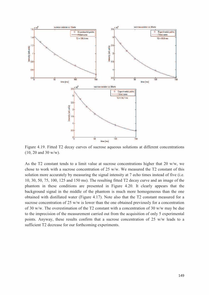
Figure 4.19. Fitted T2 decay curves of sucrose aqueous solutions at different concentrations

(10, 20 and 30 w/w).

As the T2 constant tends to a limit value at sucrose concentrations higher that 20 w/w, we

chose to work with a sucrose concentration of 25 w/w. We measured the T2 constant of this

solution more accurately by measuring the signal intensity at 7 echo times instead of five (i.e.

10, 30, 50, 75, 100, 125 and 150 ms). The resulting fitted T2 decay curve and an image of the

phantom in these conditions are presented in Figure 4.20. It clearly appears that the

background signal in the middle of the phantom is much more homogeneous than the one

obtained with distillated water (Figure 4.17). Note also that the T2 constant measured for a

sucrose concentration of 25 w/w is lower than the one obtained previously for a concentration

of 30 w/w. The overestimation of the T2 constant with a concentration of 30 w/w may be due

to the imprecision of the measurement carried out from the acquisition of only 5 experimental

points. Anyway, these results confirm that a sucrose concentration of 25 w/w leads to a

sufficient T2 decrease for our forthcoming experiments.

��

�

Figure 4.20. Fitted T2 decay curve of 25 w/w sucrose aqueous solutions (left) and the

corresponding phantom image acquired with a SE sequence and an echo time of 15 ms (right).

4.2.1.2. Phase measurement method

The phase measurement method is described in Magnetic Resonance Imaging – Physical

Principles and Sequence Design391 as a way to measure the magnetic susceptibility according

to the cylinder geometrical model. This method is based on the measurement of the spins

phase with a GRE sequence. As shown previously, when magnetic field gradients are applied,

the phase of the precessing spins can be expressed as follow.

�� (4.34)

In the case of a GRE sequence applied with a magnetic field deformed by the presence of a

material with a magnetic susceptibility different from the imaged medium, the phase can be

expressed according to equation (4.35)

�� [T � �� [T (4.35)

where TE is the sequence echo time i.e. the time interval between the spins excitation RF

pulse and the signal measurement (in the case, the measurement of the spins phase).

If two GRE sequences are applied with two different echo times (all other parameters being

kept strictly identical), two phase images corresponding to the following equations are

obtained.

�� [T5 � �� [T5 (4.36)

�� [T3 � �� [T3 (4.37)

Subtraction of equations (4.36) and (4.37) leads to equation (4.38).

K�� \�E��]^_A\�E��]^`&�]^`A]^_ (4.38)

��

�

Therefore, this kind of measurement gives a direct access to the magnetic field variations

induced by the presence of a metallic wire. Furthermore, as we know from equation (4.28)

that

K� � J23 CO ROADO

�D_6ROO (4.39)

the measurement of the magnetic field variations can lead to the determination of the apparent

magnetic susceptibility difference between the metallic wire and the medium.

This measurement has been carried out on an untreated Nitinol wire of 170 µm diameter. The

wire was held horizontally in a phantom filled with a 25 w/w sucrose aqueous solution and

placed in the middle of the MRI, perpendicular to B0 direction. Sagittal slices images

(perpendicular to the wire) have been acquired with GRE sequences fully described in Annex

3.2. These two GRE sequences are strictly identical except for their echo time (3.2 and 6.2

ms). In order to minimize the signal loss due to intravoxel spins dephasing, the highest

possible readout gradient was used. The obtained phase images are presented in Figure 4.21.

Figure 4.21. Sagittal phase images of the precessing spins in the neighborhood of an untreated

Nitinol wire of 170 µm diameter acquired with an echo time of 3.2 ms (left), 6.2 ms (center)

and the image resulting from the substraction of these two phase images (right). The black

arrow indicates the direction of the B0 magnetic field and of the readout gradient.

As expected, the image resulting from the subtraction of the two phase images has the typical

shape of the magnetic field deformation around a cylinder with a magnetic susceptibility

different from the one of the medium (Figure 4.13). Note that the important intensity

variations at very short distance of the wire are due to the aliasing phenomenon (i.e. a “phase

folding”). Indeed, the measured phase values are obviously always comprised between – and

radiants. This implies that when the “real” phase of the spins quickly increases (and is

therefore more important than like in the very close neighborhood of a metallic wire) it is

encoded as a succession of switching from – and radiants (periodic evolution) instead of as

a continuous evolution.

The magnetic field variation profile obtained in the direction of B0 is in good accordance with

the theoretically expected one as shown in Figure 4.22. However, it is not possible to obtain

any accurate information from this experimental profile as the region of interest is extremely

��

�

narrow. Indeed, the main part of the magnetic field variation profile is unexploitable because

of the aliasing phenomenon. This makes impossible an accurate positioning of the wire on the

experimental profile and therefore the fitting of the magnetic field variation profile.

Figure 4.22. Simulated profile of the magnetic field variation in the B0 direction (left) and the

corresponding experimental profile obtained with an untreated Nitinol wire of 170 µm diameter

(right).

4.2.1.3. Iterative susceptibility artifact measurement method

As the phase measurement method did not allow the determination of the apparent magnetic

susceptibility of Nitinol and Phynox wires, we considered an alternative method based on the

measurement of the geometric distortion of the image plane and the distortion of pixels

intensity. As specified previously, the image plane is deformed in the direction of the readout

gradient (now set along the y axis) and is proportional to the magnetic susceptibility

difference between the metallic wire and the medium as expressed in equation (4.40).

K� � J23

�LMN CO ROADO

�DO6ROO (4.40)

Each parameter of this equation (except ��) being determined by the experimental setup and

the used MRI sequences, it possible to calculate �y (and thus to simulate the image

deformation) for a given ��. Thus, we created an algorithm that allows a simulation of the

image plane deformation via a numerical method.

4.2.1.3.1 Algorithm conception method

The medium being homogeneous (25 w/w aqueous sucrose solution), the intensity of each

pixel has been arbitrarily set to a value of 1. Without any image deformation, the area and the

position of a pixel are the same than the area and the position of the corresponding voxel. Let

us consider the middle pixel on the Figure 4.23. The corresponding voxel is submitted to a

deformation in the direction of the readout gradient. The deformation of its upper (red) and

lower (blue) boundaries is thus calculated according to equation (4.40). The new deformed

Mag

neti

c fi

eld

vari

atio

n in

the

B0

dire

ctio

n (m

T)

Distance (mm)

��

�

voxel boundaries can thus be determined (i.e. the dark red and dark blue curves on Figure

4.23). The new voxel area is calculated by integration of the area between its deformed

boundaries. Finally, the voxel intensity (renormalized with respect to its new area) is

dispatched among the different surrounding pixels. The complete algorithm is presented in

Annex 3.1.

Figure 4.23. Schematic representation of three pixels of the deformed image. The

corresponding voxel original boundaries are represented in red (upper one) and blue (lower

one). The deformed voxel boundaries are represented in dark red (upper one) and dark blue

(lower one).

This image simulation algorithm has then been used as a basis to build up another algorithm

aiming at fitting experimental images in order to determine the magnetic susceptibility

difference between the metallic wire and the medium (�� being the only unknown variable in

equation (4.40)). Basically, this algorithm simulates a first image, compares it with the

experimental one (by the method of least squares), adjusts �� and simulates a new image, etc.

The process stops when the simulated image is similar enough to the experimental one. Note

also that the simulation algorithm set all the pixels intensity to unity which is obviously not

the case anymore for experimental images. The fitting algorithm is therefore designed to

determine not only �� but also the normalization factor value. The complete algorithm is

presented in Annex 3.1.

4.2.1.3.2 Results

All the Nitinol and Phynox wires tested with this method and the surface treatments applied to

them are presented in Tables 4.2, 4.3 and 4.4.

The experimental setup is strictly the same as the one used for the phase measurement

method. SE sequences were used in order to minimize the signal loss due to intravoxel spin

dephasing (encountered with GRE sequences) thanks to the characteristic 180° RF pulse as

well as to keep only the geometric distortion of the image plane. As said previously, the

readout gradient has a strong impact of the size of the susceptibility artifacts. Therefore, for

Rea

dout

gra

dien

t di

rect

ion

��

�

each of the tested wires, the same SE sequence was repeated with two different bandwidths

i.e. 100 and 150 Hz/pxl. These bandwidths values correspond to readout gradient intensities

of 8.6 and 12.9 mT/m, respectively. Note that these SE sequences are fully described in

Annex 3.2. Each wire has been imaged with 8 parallel slices for each sequence. 16 images per

wire have thus been acquired. The apparent magnetic susceptibilities values obtained and

presented in Tables 4.5, 4.6 and 4.7 are the arithmetic mean of the values obtained from these

16 images. Experimental representative images obtained with a bandwidth of 150 Hz/pxl and

the corresponding simulated images are also presented in Tables 4.5, 4.6 and 4.7.

Table 4.2. List of the 240 µm diameter Nitinol wires tested with the artifact fitting algorithm

Material Diameter Treatments Acronyms

Nitinol 240 µm none NiTi240 NT

Nitinol 240 µm Ethylene oxide sterilization NiTi240 NT St

Nitinol 240 µm Thermal treatment of 20 min at 490°C NiTi240 TT490_20

Nitinol 240 µm Thermal treatment of 20 min at 490°C

+ Ethylene oxide sterilization NiTi240 TT490_20 St







Nitinol 240 µm Chemical etching by 5 min immersion in

5%vol HF/12%vol HNO3 solution NiTi240 D5

Table 4.3. List of the 170 µm diameter Nitinol wires tested with the artifact fitting algorithm


Nitinol 170 µm none NiTi170 NT

Nitinol 170 µm Ethylene oxide sterilization NiTi170 NT St










Nitinol 170 µm Chemical etching by 5 min immersion in

5%vol HF/12%vol HNO3 solution NiTi170 D5

��

�

Table 4.4. List of the 80 µm diameter Phynox wires tested with the artifact fitting algorithm


Phynox 80 µm none Ph80 NT

Phynox 80 µm Ethylene oxide sterilization Ph80 NT St

Phynox 80 µm Thermal treatment of 3 hours at 550°C Ph80 TT550_3h

Phynox 80 µm Thermal treatment of 3 hours at 550°C

+ Ethylene oxide sterilization Ph80 TT550_3h St







Phynox 80 µm Chemical etching by 30 min immersion

in 5%vol HF/12%vol HNO3 solution Ph80 D30

��

�

Table 4.5. Apparent magnetic susceptibilities assessed for the 240 µm diameter Nitinol wires

Wire Apparent magnetic

susceptibility

Experimental

image

Simulated

image

NiTi240 NT 3.16x10-4

� �

NiTi240 NT St 2.53x10-4

� �

NiTi240 TT490_20 4.46x10-4

� �

NiTi240 TT490_20 St 4.44x10-4

� �

NiTi240 TT490_60 4.51x10-4

� �

NiTi240 TT490_60 St 4.95x10-4

� �

NiTi240 TT550_20 5.04x10-4

� �

NiTi240 TT550_20 St 4.40x10-4

� �

NiTi240 D5 2.39x10-4

� �

��

�

Table 4.6. Apparent magnetic susceptibilities assessed for the 170 µm diameter Nitinol wires


susceptibility

Experimental

image

Simulated

image

NiTi170 NT 2.42x10-4

� �

NiTi170 NT St 2.08x10-4

� �

NiTi170 TT490_20 3.38x10-4

� �

NiTi170 TT490_20 St 3.59x10-4

� �

NiTi170 TT490_60 3.50x10-4

� �

NiTi170 TT490_60 St 3.37x10-4

� �

NiTi170 TT550_20 5.50x10-4

� �

NiTi170 TT550_20 St 4.50x10-4

� �

NiTi170 D5 1.60x10-4

� �

��

�

Table 4.7. Apparent magnetic susceptibilities assessed for the 80 µm diameter Phynox wires


susceptibility

Experimental

image

Simulated

image

Ph80 NT 5.25x10-3

� �

Ph80 NT St 5.31x10-3

� �

Ph80 TT550_3h 3.97x10-3

� �

Ph80 TT550_3h St 3.59x10-3

� �

Ph80 TT550_5h 3.82x10-3

� �

Ph80 TT550_5h St 3.76x10-3

� �

Ph80 TT600_3h 4.18x10-3

� �

Ph80 TT600_3h St 4.20x10-3

� �

Ph80 D30 5.08x10-3

� �

First of all, it can be pointed out that the surface state of Nitinol and Phynox wires has an

actual impact on the apparent magnetic susceptibility of the material. For two untreated

Nitinol wires of different diameters (240 µm and 170 µm), the apparent magnetic

susceptibility varies slightly but significantly. This confirms that the surface state of Nitinol

strongly depends on the provider and the manufacturing process.

Heat treatment induces a clear increase of the apparent magnetic permeability and therefore of

the size of the resulting susceptibility artifact. This behavior is much more enhanced when the

heat treatment is carried out at a higher temperature than when the heat treatment is carried

out for longer times. Several hypotheses can be formulated to explain this behavior. It has

been shown in Chapter 2 that the heat treatment of Nitinol induces an important increase of

the oxide layer thickness and that an increase of the temperature induces a more important

further increase of the oxide layer thickness than an increase of the heat treatment time does.

There may thus be a relationship between the oxide layer thickness and the apparent magnetic

susceptibility of Nitinol. Indeed, even if the heat treatment induces the appearance of

��

�

antiferromagnetic NiO at the surface of Nitinol (which could a priori have a beneficial effect

on the resulting susceptibility artifacts), it also induces an increase of the TiO2 quantity

present at the surface (TiO2 being a paramagnetic material). Furthermore, heat treatment is an

oxidative treatment and it has been shown that the paramagnetic behavior of a Ti-O system

increases with the concentration of oxygen 408. It has also been shown that in a thin TiO2

layer, interfacial defects can induce an enhanced magnetism 409. After the heat treatment, the

resulting oxide layer is not only thicker but also more heterogeneous given the fact that the

heat treatment induces a strong diffusion of nickel toward the surface and thus the formation

of a mixed Ni and Ti oxides layer. Another possible explanation of this susceptibility artifact

enhancement could be a change of the TiO2 crystalline state in the Nitinol oxide layer with the

heat treatment. Indeed, it has been shown that TiO2 can start changing from anatase to rutile

in the heat treatment conditions applied in this work (490°C or 550°C) 410,411 but also that

rutile has a more important magnetic susceptibility than anatase 412.

The ethylene oxide sterilization of untreated Nitinol wires seems to decrease their apparent

magnetic susceptibility. On the other hand, this sterilization process does not seem to have a

significant impact on the apparent magnetic susceptibility of heat treated Nitinol wires except

for the ones treated at higher temperature (550°C for 20 min).

Nitinol wires submitted to a chemical etching treatment induce less important susceptibility

artifacts than heat treated wires: their apparent magnetic susceptibility is similar to the one of

untreated sterilized Nitinol wires. This could be explained by the fact that the oxide layer

resulting from a chemical etching is much thinner and homogeneous than the original oxide

layer (only composed of TiO2) and by the absence of any heat treatment of this TiO2 layer

(and therefore the absence of rutile phase in this layer).

For comparison, the measurements carried out on Phynox wires show that the apparent

magnetic susceptibility of this alloy is 10-fold more important than the one of Nitinol. Nitinol

is thus intrinsically a particularly well suited material for MRI examinations compared to

other alloys commonly used for biomedical applications even without specific surface

treatment. Contrary to what was observed for Nitinol wires, the heat treatment of Phynox

seems to decrease its apparent magnetic susceptibility. Regarding the other tested treatments,

neither the ethylene oxide sterilization nor the chemical etching treatment seem to have a

significant impact on the Phynox apparent magnetic susceptibility.

4.2.2. Assessment of the stents behavior in MRI

4.2.2.1. Study of the imagery parameters influence

This study has been carried out with the same phantom than the one used for the quantitative

assessment of the apparent magnetic susceptibility of wires (described in section 4.2.1.1) on a

7 mm diameter braided Nitinol stent. This stent is constituted of 24 braided 170 µm diameter

Nitinol wires and was submitted to a heat treatment for 20 min at 490°C.

The stent has been imaged in two extreme positions with respect to the main magnetic field

B0: parallel and perpendicular. Three main imagery parameters have been studied: the

��

�

orientation of the stent with respect to the main magnetic field B0, the intensity of the readout

gradient and the type of imaging sequence. Five sequences (fully described in Annex 3.2)

were used in the frame of this study:

- a GRE sequence (noted TOF3D) typically used for MRI angiography examinations

- a second typical TOF-GRE sequence (noted TOF2D)

- a SE sequence with a bandwidth of 160 Hz/pixel (noted TSE160). This sequence is

actually a Turbo Spin Echo one which means that several signal acquisitions are

carried out after only one excitation pulse (using several successive 180° refocusing

pulses)

- a second SE sequence identical to the previous one except for a bandwidth of 425

Hz/pixel instead of 160 Hz/pixel (noted TSE425)

- a simple SE sequence identical to the one used for the quantitative assessment of the

apparent magnetic susceptibility of wires.

The obtained images are presented in Table 4.8.

From these images, the strong impact of the stent orientation with respect to the main

magnetic field B0 can be clearly pointed out. When the stent is oriented perpendicularly to B0

direction, susceptibility artifacts are the more important ones: the typical arrow shape image

distortion in the readout gradient direction can be observed on transverse images. This

behavior is easily understandable as the stents have a cylindrical geometry. Indeed it has been

shown that the main magnetic field deformation (and therefore the resulting artifact size) is

maximal when the cylinder is oriented perpendicularly to this magnetic field.

When the stent is parallel to the main magnetic field, the quality of transverse images is much

better (no arrow shape deformation). In this case, the arrow shape image deformation is

visible on sagittal images and located at the stent extremities (more visible on SE sequence

images).

The influence of the readout gradient intensity can be clearly observed on the images of the

Nitinol stent oriented perpendicularly to the main magnetic field obtained with TSE160 and

TSE425 sequences. On the transverse images obtained in these conditions, the arrow shape

distortion is much more pronounced with a 160 Hz/pixel readout gradient than with a higher

readout gradient.

��

�

Table 4.8. MRI images obtained a 7 mm diameter Nitinol stent constituted of 24 braided 170

µm diameter wires.

Parallel to B0 TOF3D TOF2D TSE160 TSE425 SE

Perpendicular to B0 TOF3D TOF2D TSE160 TSE425 SE

��

��

��

��

��

�

The type of used sequence has also a critical impact on the artifacts caused by the stent. The

signal loss in pixels located near the stent wall is much more important with GRE sequences

than with SE sequences. This is explained by the fact that with GRE sequences, the main

magnetic field deformation close to the Nitinol wires induces an intravoxel dephasing of the

spins which is not corrected by refocusing pulses like the ones used for SE sequences.

Finally, hypo- and hypersignal areas can be observed in the stent lumen. The non-uniformity

of the lumen signal is not explained. Nevertheless, these signal intensity variations are

attributed to RF artifacts and not to susceptibility artifacts for two reasons. First, susceptibility

artifacts are easily recognizable (typical arrow shape) and have a small influence area (located

really close to the stent walls). Second, the signal intensity variations inside the stent lumen

are much more pronounced with SE sequences than with GRE sequences. This observation is

in good agreement with the well known fact that SE sequences are much more sensitive to the

B1 rotating magnetic field variations than GRE sequences do.

4.2.2.2. Study of the stent composition and surface treatment influence

In the frame of this study, 15 stents have been studied. These stents are composed of braided

Nitinol, NiTiDFT10% or Phynox wires. Note that DFT is an acronym that stands for Drawn

Filled Tube. The DFT10% wires are composite materials composed of Nitinol around a Pt

core (fill ratio 10%). The interest of using such wires for stents design is the important

radioopacity of Pt compared to Nitinol alone and therefore allowing much more efficient X-

ray angiography examinations. Table 4.9 summarizes the different stents used in this study,

their diameter, composition and diameter of the constituting wires and the surface treatments

applied to the stent i.e. heat treatment, chemical etching and ethylene oxide sterilization

process.

These stents were expanded in artery silicon models (with an adapted diameter), immersed in

a Plexiglas container filled with water heated at 37°C and oriented parallel to the main

magnetic field B0. The sequences used (a GRE and a SE sequence) are fully described in

Annex 3.2.

Note that only representative images are presented here. The entire set of images is presented

in Annex 3.3.

��

�

Table 4.9. Characteristics of the stents used for the study of the influence of the stent

composition and surface treatment on the obtained MRI images.

Stent # Alloy Wire

diameter

Stent

diameter# wires

Heat

treatment

Chemical

etching

Ethylene oxide

Sterilization

1 NiTi 170 µm 7 mm 24 490°C-20min no no

2 NiTi 170 µm 7 mm 24 490°C-20min no yes

3 NiTi

DFT10%80 µm 8 mm 80 500°C-15min no no

4 NiTi

DFT10%80 µm 8 mm 80 500°C-15min no yes

5 NiTi 100 µm 4mm 16 490°C-15min no no

6 NiTi 100 µm 4mm 16 490°C-15min no yes

7 NiTi 100 µm 4mm 16 490°C-15min yes no

8 NiTi 100 µm 4mm 16 490°C-15min yes yes

9 Phynox 80 µm 8mm 80 550°C-3h no no

10 Phynox 80 µm 8mm 80 550°C-3h no yes

11 Phynox 80 µm 8mm 80 550°C-3h yes no

12 Phynox 80 µm 8mm 80 550°C-3h yes yes

13 NiTi 50 µm 5 mm 64 490°C-15min no no

14 NiTi

DFT10%80 µm +/- 4 mm 56 490°C-15min no no

15 NiTi

DFT10%80 µm +/- 4 mm 56 500°C-30 min no no

As susceptibility artifacts have been previously studied with a simple geometric model which

allows avoiding any other kind of artifact, we focused here on the RF artifacts induced by the

presence of these different stents. The key parameter in the frame of this study is thus the

spins flip angle. It is essential to remind that the spins flip angle is related to the intensity and

the application time of the oscillating magnetic field B1 (equation (4.3)) and that, when RF

artifacts occur, the real spins flip angle inside the stents lumen is different than the one

expected from equation (4.3). This induces a difference in the signal intensity between the

area inside the lumen of the stent and the surrounding medium.

Let us first focus on Nitinol and NiTiDFT10% stents (stents # 1 to 6, see Figure 4.24). First of

all, we can point out again the clearly more important sensitivity of SE sequences to RF

artifacts compared to GRE sequences. On the other hand, susceptibility artifacts are much

more important on GRE images than on the SE ones. The signal intensity inside the stents

lumen is clearly different for GRE sequences than for SE sequences.

��

�

Gradient Echo (GRE)

5° 10° 15° 20° 25° 30°

Spin Echo (SE)

50° 70° 90° 110° 130°

Figure 4.24. MRI images of the stent #1 obtained with various flip angles (°) with GRE and

SE sequences

Regarding the GRE sequences, a slight hypersignal can be pointed out inside the stent lumen

when small flip angles are used. This hypersignal is less and less pronounced as the flip angle

is increased. This behavior is opposite to the one usually observed with RF artifacts and could

be explained by the nature of the electrically conductive loops inducing these artifacts.

Indeed, these stents being composed of braided wires covered with a relatively thick oxide

layer, the nature of the electrical contacts between these wires is more capacitive than

inductive. Furthermore, in capacitive electric circuits, the induced current has a 180° phase

difference with the induced electromotive force (and therefore with the oscillating magnetic

��

�

field B1). This leads to a slight increase of spins flip angle inside the lumen of the stents and

thus a slight hypersignal (instead of a hyposignal) which has already been reported by

Camacho et al.401. It also clearly appears that this hypersignal is less and less pronounced as

the flip angle is increased. A reasonable hypothesis to explain this behavior is that, with a low

flip angle, the TR (repetition time of the sequence) is long enough to allow a complete

regrowth of the longitudinal component of the spins magnetization vector both inside and

outside the stent. On the contrary, when the applied flip angle is bigger, it seems that the real

spins flip angle inside the stents lumen is too important to allow a complete regrowth of the

longitudinal component of the spins magnetization vector between two repetitions of the

sequence. This induces a decrease of the signal intensity inside the stent lumen while, outside

the stent, the applied (non-altered) flip angle is still small enough to allow a complete

regrowth of the longitudinal component of the spins magnetization vector between two

repetitions of the sequence. By increasing the flip angle, one thus reaches a situation where

the signal outside the stent keeps increasing while the signal inside the stent lumen is limited

by the regrowth of the longitudinal component of the spins magnetization vector.

Regarding the images obtained with SE sequences, the origin of the signal heterogeneity

inside the stents lumen is not clear. However, signal variations inside the lumen definitely

depend on the flip angle. This is a clear evidence of the fact that these signal variations are

related to RF artifacts.

The same observations can be made for the stents # 5 and 6 as well as for the stents # 13 to

15. This indicates that, even if the stent geometry (number of wires in the braid, wires

diameter and stent diameter) and the electrical conductivity of the wires (Nitinol or Nitinol

with a platinum core for DFT wires) have an evident impact on the intensity of the resulting

RF artifacts, similar surface states induce RF artifacts of the same nature.

Note also that no significant difference between stents submitted or not to the ethylene oxide

sterilization treatment could have been observed. Therefore, as observed for the susceptibility

artifacts, the sterilization treatment does not seem to have a significant impact on the resulting

RF artifacts.

Stents # 7 and 8 (chemically etched) seem to induce much less pronounced RF artifacts than

the non-etched ones (see Figure 4.25). Regarding the GRE sequences results, no significant

difference of the signal intensity inside and outside the stent lumen could have been pointed

out even with the lowest flip angle. Regarding the images obtained with SE sequences, the

signal intensity is quite homogeneous except for very high flip angle values. Again, the

ethylene oxide sterilization treatment does not seem to induce any significant variation of the

stent behavior in MRI. Note the poor image quality obtained for these stents with GRE

sequences is not due to the presence of the stent but to an aliasing phenomenon (due to a too

small sampling area).

��

�

Gradient Echo (GRE)

5° 10° 15° 20° 25° 30°

� � � � � �

Spin Echo (SE)

50° 70° 90° 110° 130°

� � � � �


SE sequences

Four Phynox stents were assessed the same way (stents # 9 to 12). For all these stents, very

important susceptibility artifacts can be pointed out (as observed in the frame of the

susceptibility artifacts study). Regarding the RF artifacts, the non-etched stents (stents # 9 and

10, see Figure 4.26) have a behavior similar to the non-etched Nitinol and NiTiDFT10%

stents but much less pronounced. The chemically etched Phynox stents (stents # 11 and 12,

see Figure 4.27) show the classical behavior related to RF artifacts with GRE sequences i.e.

��

�

the signal (weak and homogeneous inside the stent lumen) increases when the applied flip

angle is increased. The images of these stents obtained with SE sequences show a nearly

complete signal loss into the stent lumen for all the tested flip angles. Thus in this case the

chemical etching treatment induces the appearance of electrical contacts between the wires

and these electrical contacts are important enough to result in inductive conductive loops

rather than capacitive ones as it was the case when the original oxide layer is conserved. Note

that, again, the ethylene oxide sterilization treatment does not seem to have a significant

influence on the Phynox stent behavior in MRI.

Gradient Echo (GRE)

5° 10° 15° 20° 25° 30°

� � � � � �

Spin Echo (SE)

50° 70° 90° 110° 130°

� � � � �


SE sequences

��

�

Gradient Echo (GRE)

5° 10° 15° 20° 25° 30°

� � � � � �

Spin Echo (SE)

50° 70° 90° 110° 130°

� � � � �


SE sequences

Finally, the imaging of a commercial Nitinol stent has been carried out: the Enterprise stent

provided by Cordis Corporation (Johnson&Johnson). The Enterprise in a laser cut Nitinol

stent thus there is a very good electrical connection between the different struts. Therefore,

the Enterprise stent should exhibit the classical RF artifacts behavior. This behavior can be

actually observed (see Figure 4.28) even if it is much less pronounced than for the Phynox

etched stents (stents # 11 and 12). This could be explained by the fact that the braided stents

exhibit much more current loops per unit area than the Enterprise stent does.

��

�

Gradient Echo (GRE)

5° 10° 15° 20° 25° 30°

� � � � � �

Spin Echo (SE)

50° 70° 90° 110° 130°

� � � � �

Figure 4.28. MRI images of the Cordis Enterprise Nitinol stent obtained with various flip

angles (°) with GRE and SE sequences

4.2.2.3. Study of the stent composition and orientation on the RF artifacts

In the frame of this study, 3 stents have been examined: a first one composed of 40 braided

NiTiDFT30% 40 µm diameter wires, a second one composed of 40 braided Nitinol 50 µm

diameter wires and a last (hybrid) one composed of 8 Nitinol 50 µm diameter wires and 32

NiTiDFT30% 40 µm diameter wires braided together. All these stents were submitted to a

shape setting heat treatment, a chemical etching and an ethylene oxide sterilization treatment.

They were placed in the phantom described in section 4.2.1.1 and imaged with two typical

sequences (a SE sequence and a GRE sequence) and different flip angles. These sequences are

fully described in Annex 3.2. Each imagery experiment has been repeated with the stent in

two extreme positions: parallel and perpendicular to the main magnetic field B0. The obtained

images are presented in Figures 4.29, 4.30 and 4.31.

��

�

Perpendicular to B0

GRE

Sagittal

Flip angle

10°

Transverse

Flip angle

10°

Sagittal

Flip angle

20°

Transverse

Flip angle

20°

Sagittal

Flip angle

30°

Transverse

Flip angle

30°

�

�

�

�

�

�

SE

Sagittal

Flip angle

50°

Transverse

Flip angle

50°

Sagittal

Flip angle

90°

Transverse

Flip angle

90°

Sagittal

Flip angle

130°

Transverse

Flip angle

130°

�

�

�

�

�

�

Parallel to B0

GRE

Sagittal

Flip angle

10°

Transverse

Flip angle

10°

Sagittal

Flip angle

20°

Transverse

Flip angle

20°

Sagittal

Flip angle

30°

Transverse

Flip angle

30°

�

�

�

�

�

�

SE

Sagittal

Flip angle

50°

Transverse

Flip angle

50°

Sagittal

Flip angle

90°

Transverse

Flip angle

90°

Sagittal

Flip angle

130°

Transverse

Flip angle

130°

�

�

�

�

�

�

Figure 4.29. MRI images of the stent NiTiDFT30% oriented parallel or perpendicular to the

main magnetic field B0 obtained with various flip angles (°) with GRE and SE sequences

��

�

Perpendicular to B0

GRE

Sagittal

Flip angle

10°

Transverse

Flip angle

10°

Sagittal

Flip angle

20°

Transverse

Flip angle

20°

Sagittal

Flip angle

30°

Transverse

Flip angle

30°

�

�

�

�

�

�

SE

Sagittal

Flip angle

50°

Transverse

Flip angle

50°

Sagittal

Flip angle

90°

Transverse

Flip angle

90°

Sagittal

Flip angle

130°

Transverse

Flip angle

130°

�

�

�

�

�

�

Parallel to B0

GRE

Sagittal

Flip angle

10°

Transverse

Flip angle

10°

Sagittal

Flip angle

20°

Transverse

Flip angle

20°

Sagittal

Flip angle

30°

Transverse

Flip angle

30°

�

�

�

�

�

�

SE

Sagittal

Flip angle

50°

Transverse

Flip angle

50°

Sagittal

Flip angle

90°

Transverse

Flip angle

90°

Sagittal

Flip angle

130°

Transverse

Flip angle

130°

�

�

�

�

�

�

Figure 4.30. MRI images of the stent Nitinol oriented parallel or perpendicular to the main

magnetic field B0 obtained with various flip angles (°) with GRE and SE sequences

�

GRE

Sagittal

Flip angle

10°

Transverse

Flip angle

10°

SE

Sagittal

Flip angle

50°

Transverse

Flip angle

50°

GRE

Sagittal

Flip angle

10°

Transverse

Flip angle

10°

�

SE

Sagittal

Flip angle

50°

Transverse

Flip angle

50°

�

Figure 4.31. MRI images of the hybrid stent Nitinol/NiTIDFT30% (

perpendicular to the main magnetic field B

and SE sequences

Perpendicular to B0

Transverse

angle

10°

Sagittal

Flip angle

20°

Transverse

Flip angle

20°

Sagittal

Flip angle

30°

Transverse

Flip angle

50°

Sagittal

Flip angle

90°

Transverse

Flip angle

90°

Sagittal

Flip angle

130°

Parallel to B0

Transverse

Flip angle

10°

Sagittal

Flip angle

20°

Transverse

Flip angle

20°

Sagittal

Flip angle

30°

�

�

�

Transverse

Flip angle

50°

Sagittal

Flip angle

90°

Transverse

Flip angle

90°

Sagittal

Flip angle

130°

�

�

�

MRI images of the hybrid stent Nitinol/NiTIDFT30% (8/32) oriented parallel or

perpendicular to the main magnetic field B0 obtained with various flip angles (°) with GRE

��

Sagittal

Flip angle

Transverse

Flip angle

30°

Sagittal

Flip angle

130°

Transverse

Flip angle

130°

Sagittal

Flip angle

Transverse

Flip angle

30°

�

�

Sagittal

Flip angle

130°

Transverse

Flip angle

130°

�

�

8/32) oriented parallel or

obtained with various flip angles (°) with GRE

��

�

All these stents induce susceptibility artifacts of a reasonable size in the readout gradient

direction. When the stents are placed parallel to B0, these susceptibility artifacts are limited to

an area really close to the stent wall.

When the implants are parallel to the main magnetic field, the induced RF artifacts are quite

weak even with SE sequences (particularly sensitive to RF artifacts). On the contrary, when

the stents are perpendicular to B0, a complete signal loss can be observed for SE sequences at

high flip angles. It thus clearly appears that the stent orientation has a significant influence on

the resulting RF artifacts.

To explain the orientation influence on RF artifacts, let us consider a braided stent parallel to

the main magnetic field B0 (see Figure 4.32). The rotating magnetic field B1 is thus

perpendicular to the stent (the B1 rotation plane being perpendicular to the Figure 4.32(a)

plane). In this situation, the conductive loops responsible of the appearance of RF artifacts are

the meshes of the braid. These ones are very small (important variations of the magnetic flux)

but each conducting loop is constituted of four small conducting segments and four contact

points susceptible to block the induced currents. Let us now consider the same stent

perpendicular to the main magnetic field (see Figure 4.32(b)). In this situation, the conductive

loops responsible of the appearance of RF artifacts follow the entire circumference of the

stent wall. These ones are much bigger than in the previous situation (smaller variations of the

magnetic flux) but each conductive loop is constituted of only two long conductive segments

and two contact points susceptible to block the induced currents. It clearly appears from the

MRI examination that these bigger conductive loops are responsible of more important RF

artifacts.

Figure 4.32. Schematic representation of a braided stent oriented parallelly (a) and

perpendicularly (b) to the main magnetic field, of the different applied magnetic fields and of

the corresponding conductive loops responsible of the appearance of RF artifacts.

From the comparison of the different stents composition, it can be observed that the

introduction of pure Nitinol wires (less electrically conductive than the Pt core in the

NiTiDFT wires) in a NiTiDFT30% braided stent clearly induces a decrease of the RF artifacts

��

��

�

intensity. Therefore, it can be reasonably concluded that the use of a weakly conductive

material and the presence of an insulating material at the surface of the braided wires are two

parameters allowing a significant limitation of the RF artifacts.

4.2.3. Electrodeposition, characterization and assessment of the impact on MRI

imaging of thin nickel and cobalt oxide layers

Nickel oxide (NiO) and cobalt oxide (CoO) are known to have antiferromagnetic properties.

Thus a priori the creation of an antiferromagnetic NiO or CoO layer on the surface of Nitinol

or Phynox wires (respectively) could be beneficial for the MRI behavior of these materials.

Therefore, in the frame of this chapter topic, it was interesting to assess the possible decrease

of susceptibility artifacts induced by such oxide layers.

4.2.3.1. Electrodeposition of nickel and cobalt layers on Nitinol and Phynox

In order to make the surface characterization easier, the deposition parameters were optimized

on plane mechanically polished Nitinol and Phynox substrates (for the substrates preparation

method, see Chapters 2 and 3).

4.2.3.1.1. Electrodeposition of nickel on Nitinol

The nickel electrodeposition has been carried out in a nickel chloride (300g/l) and boric acid

(30g/l) aqueous solution under slight and constant stirring. We used a two electrodes

electrochemical setup with a pure nickel wire as the counter-electrode and the Nitinol

substrate as the working electrode. Note that the Nitinol surface has been activated by

immersion 1 h in a 30% vol. H2SO4 aqueous solution prior electrodeposition. The

electrodeposition was carried out in galvanostatic conditions by applying a constant current

density of -10 mA/cm² to the working electrode for 10 minutes. The Nitinol substrate was

then copiously rinsed with ultra pure water and cleaned by sonication 15 minutes in ultra pure

water before being submitted to an oxidizing heat treatment of 15 minutes at 480°C. The

Nitinol substrate was then cleaned again by sonication 15 minutes in ultra pure water before

being analyzed or sent for an ethylene oxide sterilization treatment before analysis.

First, the thickness and roughness of the obtained deposit has been characterized (before and

after the heat treatment) with a DEKTAK profilometer and its morphology by SEM analysis.

Representative SEM pictures are presented in Figures 4.33 and 4.34. Before the heat

treatment, the nickel coating has a mean thickness of 1.7 µm and a mean roughness of 90 nm.

SEM pictures of this deposit shows that the nickel layer obtained under these conditions is

complete, dense and homogeneous. The highly crystalline morphology of this nickel layer is

well visible on high magnification images (Figure 4.33).

�

Figure 4.33. Representative SEM pictures of the nickel layer

electrodeposited on mechanically polished Nitinol s

(30g/l) aqueous solution.

After the oxidative heat treatment of 15 minutes at 480°C

1.3 µm has been measured as well as a slightly lower mean roughness of 50 nm

observation of the nickel deposit after the heat tr

defect free and homogeneous. However, the microscop

highly crystalline morphology

deposit, the heat treated deposit appears to be muc

��

��

. Representative SEM pictures of the nickel layer galvanostatically (

electrodeposited on mechanically polished Nitinol substrates in a NiCl

heat treatment of 15 minutes at 480°C, a slightly lower mean thickness of

as well as a slightly lower mean roughness of 50 nm

observation of the nickel deposit after the heat treatment shows that the nickel

defect free and homogeneous. However, the microscopic structure has been altered: while a

highly crystalline morphology was observed on high magnification pictures of the untreated

deposit, the heat treated deposit appears to be much less crystalline (Figure 4.3

��

��

��

�

galvanostatically (-10 mA/cm²)

in a NiCl2 (300g/l)/H3BO3

, a slightly lower mean thickness of

as well as a slightly lower mean roughness of 50 nm. SEM

eatment shows that the nickel layer remains

ic structure has been altered: while a

on high magnification pictures of the untreated

Figure 4.34).

�

Figure 4.34. Representative SEM pictures of the nickel layer g

electrodeposited on mechanically polished Nitinol s

(30g/l) aqueous solution and heat treated at 480°C

The XPS analysis of this deposit has been carried out after the heat treatme

the ethylene oxide sterilization treatment. The cor

photoelectron peaks spectra are presented in Figure

sterilization treatment, the Ni2p high resolution spectrum exhibits

centered at 854.2 eV attributed to NiO and a smalle

presence of nickel hydroxide (Ni(OH)

is the characteristic binding energy of Ni2p

The oxidative heat treatment allow

without metallic nickel at least in the first ~10 n

of the spectrometer). The presence of nickel hydroxide is probably due to

the NiO at the extreme surface.

After the sterilization process, the component rela

854.2 eV) is clearly less important

attributed to nickel hydroxide.

coating to a hot and extremely humid atmosphere dur

component could be observed at 852.2 eV which is th

Ni2p3/2 photoelectrons from nickel

��

��

. Representative SEM pictures of the nickel layer galvanostatically (

electrodeposited on mechanically polished Nitinol substrates in a NiCl

(30g/l) aqueous solution and heat treated at 480°C for 15 minutes.

deposit has been carried out after the heat treatment before and after

the ethylene oxide sterilization treatment. The corresponding high resolution Ni2p core level

photoelectron peaks spectra are presented in Figure 4.35. Before the ethylene oxide

the Ni2p high resolution spectrum exhibits a main Ni2p

centered at 854.2 eV attributed to NiO and a smaller one at 856.2 eV characteristic of the

presence of nickel hydroxide (Ni(OH)2). No component could be observed at

is the characteristic binding energy of Ni2p3/2 photoelectrons from nickel in

The oxidative heat treatment allows thus to obtain a completely oxidized nickel deposit

without metallic nickel at least in the first ~10 nm below the extreme surface (analysis depth

The presence of nickel hydroxide is probably due to the

the NiO at the extreme surface.

After the sterilization process, the component relative to the presence of NiO (centered

854.2 eV) is clearly less important while the main component is now centered at 856.2 eV and

attributed to nickel hydroxide. This could be explained by the long time exposure o

coating to a hot and extremely humid atmosphere during the sterilization process.

component could be observed at 852.2 eV which is the characteristic binding energy of

ns from nickel in the metallic state.

��

��

��

alvanostatically (-10 mA/cm²)

ubstrates in a NiCl2 (300g/l)/H3BO3

deposit has been carried out after the heat treatment before and after

responding high resolution Ni2p core level

Before the ethylene oxide

a main Ni2p3/2 component

r one at 856.2 eV characteristic of the

). No component could be observed at 852.2 eV which

in the metallic state.

oxidized nickel deposit

low the extreme surface (analysis depth

The presence of nickel hydroxide is probably due to the hydroxylation of

tive to the presence of NiO (centered at

centered at 856.2 eV and

This could be explained by the long time exposure of the

ing the sterilization process. Again, no

e characteristic binding energy of

��

�

Figure 4.35. High resolution XPS spectra of the Ni2p core level photoelectron peaks of nickel

layer galvanostatically (-10 mA/cm²) electrodeposited on mechanically polished Nitinol

substrates in a NiCl2 (300g/l)/H3BO3 (30g/l) aqueous solution and heat treated at 480°C for 15

minutes before (a) and after (b) being submitted to an ethylene oxide sterilization treatment.

4.2.3.1.2. Electrodeposition of cobalt on Phynox

The cobalt electrodeposition has been carried out in a cobalt chloride (550g/l) and boric acid

(30g/l) aqueous solution under slight and constant stirring. Again, a two electrodes

electrochemical setup has been used with a pure cobalt plate as the counter-electrode and the

Phynox substrate as the working electrode. Note that the Phynox surface has been activated

by immersion 10 minutes in a 30% vol. H2SO4 aqueous solution. The electrodeposition was

carried out in galvanostatic conditions by applying a constant current density of -1 mA/cm² to

the working electrode for 10 minutes. The Phynox substrate was then copiously rinsed with

ultra pure water and cleaned by sonication 15 minutes in ultra pure water before being

submitted to an oxidizing heat treatment of 3 hours at 550°C. A cleaning by sonication 15

minutes in ultra pure water has been carried out before the coated Phynox substrates have

been analyzed or sent for an ethylene oxide sterilization treatment before analysis.

The morphology of the obtained cobalt deposits has been characterized (before and after the

heat treatment) by SEM analysis. Representative SEM pictures are presented in Figures 4.36

and 4.37. The cobalt layer observed before the heat treatment appears to be complete, dense

890 880 870 860 850 840

a

Binding energy (eV)

856.2 eV

854.2 eV

852.2 eV

bIn

ten

sity (

arb

. un

its)

�

and homogeneous. A quite crystalline morphology of this cobalt layer

magnification images.

Figure 4.36. Representative SEM pictures of the

electrodeposited on mechanically polished

(30g/l) aqueous solution.

After the oxidative heat treatment of 3 hours at 55

homogeneous but the initial crystalline structure visible at hi

treatment has changed to a granular structure. This

of 320 nm and a mean roughness of 90 nm (vs. 15 nm

Phynox substrate).

��

��

quite crystalline morphology of this cobalt layer is also

. Representative SEM pictures of the cobalt layer galvanostatically (

electrodeposited on mechanically polished Phynox substrates in a CoCl

After the oxidative heat treatment of 3 hours at 550°C, the cobalt layer remains complete and

but the initial crystalline structure visible at high magnification before the heat

treatment has changed to a granular structure. This heat treated deposit has a mean thickness

of 320 nm and a mean roughness of 90 nm (vs. 15 nm for a mechanically polished

��

��

��

is also visible on high

layer galvanostatically (-1 mA/cm²)

Cl2 (550g/l)/H3BO3

0°C, the cobalt layer remains complete and

gh magnification before the heat

heat treated deposit has a mean thickness

for a mechanically polished bare

�

Figure 4.37. Representative SEM pictures of the cobalt layer g

electrodeposited on mechanically polished Phynox su

(30g/l) aqueous solution and heat treated at 550°C

Again, the XPS analysis of the deposit has been carried out

after the ethylene oxide sterilization treatment. T

level photoelectron peaks spectra are presented in

sterilization treatment, only one

CoO is visible on the XPS Co2p high resolution spectrum

no component characteristic of the cobalt

observed. The oxidative heat treatment allow

deposit without metallic cobalt

After the sterilization process,

could have been observed: only one main component

the CoO. However, Co2p photoelectrons from COOH and Co(OH)

similar binding energy (less than 1 eV difference). It

the extreme surface is hydroxylated during the ster

did) even if the XPS spectrum remains very similar.

at 778.2 eV which is the characteristic binding ene

in the metallic state.

��

��

. Representative SEM pictures of the cobalt layer galvanostatically (

electrodeposited on mechanically polished Phynox substrates in a CoCl

(30g/l) aqueous solution and heat treated at 550°C for 3 hours.

he XPS analysis of the deposit has been carried out after the heat treatment before and

after the ethylene oxide sterilization treatment. The corresponding high resolution

level photoelectron peaks spectra are presented in Figure 4.38. Before the ethylene oxide

only one main Co2p3/2 component centered at 780.2

is visible on the XPS Co2p high resolution spectrum. Like in the case

characteristic of the cobalt in the metallic state (centered at 778.2 eV)

observed. The oxidative heat treatment allows thus to obtain a completely oxidized

cobalt at least in the first ~10 nm below the extreme surf

After the sterilization process, no significant difference of the Co2p high resolution spectrum

observed: only one main component is visible at 780.2 eV, characteristic of

wever, Co2p photoelectrons from COOH and Co(OH)2 species have a very

ilar binding energy (less than 1 eV difference). It is thus possible that the cobalt oxide at

the extreme surface is hydroxylated during the sterilization process (like the nickel oxid

did) even if the XPS spectrum remains very similar. Again, no component

at 778.2 eV which is the characteristic binding energy of Co2p3/2 photoelectrons from cobalt

��

��

��

alvanostatically (-1 mA/cm²)

bstrates in a CoCl2 (550g/l)/H3BO3

after the heat treatment before and

he corresponding high resolution Co2p core

. Before the ethylene oxide

780.2 eV attributed to

Like in the case of nickel deposits,

the metallic state (centered at 778.2 eV) could be

thus to obtain a completely oxidized cobalt

at least in the first ~10 nm below the extreme surface.

of the Co2p high resolution spectrum

at 780.2 eV, characteristic of

species have a very

is thus possible that the cobalt oxide at

ilization process (like the nickel oxide layer

Again, no component could be observed

photoelectrons from cobalt

��

�

Figure 4.38. High resolution XPS spectra of the Co2p core level photoelectron peaks of cobalt

layer galvanostatically (-1 mA/cm²) electrodeposited on mechanically polished Phynox

substrates in a CoCl2 (550g/l)/H3BO3 (30g/l) aqueous solution and heat treated at 550°C for 3

hours before (a) and after (b) being submitted to an ethylene oxide sterilization treatment.

4.2.3.2. Study of the impact of the nickel oxide and cobalt oxide layers on the MRI behavior

of Nitinol and Phynox wires

These coating methods have been applied to Nitinol wires (50 µm, 170 µm and 240 µm

diameter) and Phynox wires (80 µm diameter) in order to assess their impact on the

susceptibility artifacts of these wires in MRI. The MRI analyses have been carried out with

the same phantom and experimental conditions as the ones described in section 4.2.1.1 and

the same sequence used for the iterative susceptibility artifact measurement method (section

4.2.1.3.2) i.e. a SE sequence with a bandwidth of 100 Hz/pixel. This sequence is fully

described in Annex 3.2.

Regarding Phynox, the MRI examinations of 80 µm diameter wires in four different surface

states have been carried out: untreated and sterilized (called “Ste”), heat treated for 3 hours at

550°C and sterilized (called “HT Ste”), coated with an electrodeposited cobalt layer and

sterilized (called “Co Ste”) and finally, coated with an electrodeposited cobalt layer, heat

820 810 800 790 780 770

a

780.2 eV

Inte

nsity (

arb

. un

its)

Binding energy (eV)

b

��

�

treated for 3 hours at 550°C and sterilized (called “Co HT Ste”). The corresponding

transverse MRI images are presented in Figure 4.39.

Phynox 80 µm

Ste

Phynox 80 µm

HT Ste

Phynox 80 µm

Co Ste

Phynox 80 µm

Co HT Ste

Figure 4.39. Transverse MRI images of a 80 µm diameter Phynox wire untreated and

sterilized (Ste), heat treated and sterilized (HT Ste), coated with an electrodeposited cobalt

layer and sterilized (Co Ste) and coated with an electrodeposited cobalt layer, heat treated and

sterilized (Co HT Ste).

First of all, it clearly appears that the heat treatment of bare Phynox wires induces a slight

decrease of the susceptibility artifact size. This confirms the results presented in section

4.2.1.3.2. On the contrary, the “Co Ste” Phynox wire shows a susceptibility artifact 3- to 4-

fold bigger than the untreated one (“Ste”). Even if this artifact seems a little smaller when the

coated wire is submitted to an oxidative heat treatment (“Co HT Ste”), it clearly appears that

this coating is unfavorable to a decrease of the susceptibility artifacts induced by the presence

of Phynox wires in MRI.

Similarly, the MRI examinations of 50 µm, 170 µm and 240 µm diameter Nitinol wires in

height different surface states have been carried out: untreated (called “bare”), untreated and

sterilized (called “Ste”), heat treated for 20 min at 480°C (called “HT”), heat treated for 20

min at 480°C and sterilized (called “HT Ste”), coated with an electrodeposited nickel layer

(called “Ni”), coated with an electrodeposited nickel layer and sterilized (called “Ni Ste”),

coated with an electrodeposited nickel layer and heat treated for 20 min at 480°C (called “Ni

HT”) and finally, coated with an electrodeposited nickel layer, heat treated for 20 min at

480°C and sterilized (called “Ni HT Ste”). The corresponding transverse MRI images are

presented in Figures 4.40, 4.41 and 4.42.

��

�

Nitinol 240 µm

bare

Nitinol 240 µm

HT

Nitinol 240 µm

Ni

Nitinol 240 µm

Ni HT

Nitinol 240 µm

Ste

Nitinol 240 µm

HT Ste

Nitinol 240 µm

Ni Ste

Nitinol 240 µm

Ni HT Ste

Figure 4.40. Transverse MRI images of a 240 µm diameter Nitinol wire untreated (bare),

untreated and sterilized (Ste), heat treated (HT), heat treated and sterilized (HT Ste), coated

with an electrodeposited nickel layer (Ni), coated with an electrodeposited nickel layer and

sterilized (Ni Ste), coated with an electrodeposited nickel layer and heat treated (Ni HT) and

coated with an electrodeposited nickel layer, heat treated and sterilized (Ni HT Ste).

Nitinol 170 µm

bare

Nitinol 170 µm

HT

Nitinol 170 µm

Ni

Nitinol 170 µm

Ni HT

Nitinol 170 µm

Ste

Nitinol 170 µm

HT Ste

Nitinol 170 µm

Ni Ste

Nitinol 170 µm

Ni HT Ste






��

�

Nitinol 50 µm

bare

Nitinol 50 µm

HT

Nitinol 50 µm

Ni

Nitinol 50 µm

Ni HT

Nitinol 50 µm

Ste

Nitinol 50 µm

HT Ste

Nitinol 50 µm

Ni Ste

Nitinol 50 µm

Ni HT Ste






Again, these analyses allow us to confirm the results presented in section 4.2.1.3.2 i.e. unlike

Phynox, the heat treatment of Nitinol wires induces a small increase of their susceptibility

artifact size. This can be pointed out easily by simply measuring the artifact size (in pixels).

Note also that again, the sterilization treatment seems to slightly decrease the susceptibility

artifact size of HT Nitinol wires (see Figure 4.41).

Nitinol wires coated with a nickel layer induce much bigger susceptibility artifacts than the

uncoated ones. This behavior was expected for the wires coated with a nickel layer and not

submitted to a heat treatment given the ferromagnetic nature of metallic nickel. However, no

significant improvement of the susceptibility artifact is noticed with sterilization or with a

heat treatment of this nickel coating (both oxidative treatments) while the XPS analysis of the

heat treated nickel coating showed the presence of NiO in the coating. Therefore, it clearly

appears that this coating is unfavorable to a decrease of the susceptibility artifacts induced by

the presence of Nitinol wires in MRI. Note that the sterilization of the heat treated nickel

coating induces a small decrease of the susceptibility artifact size.

In conclusion, even if nickel oxide (NiO) and cobalt oxide (CoO) are known to have

antiferromagnetic properties, the creation of NiO or CoO layer on the surface of Nitinol or

Phynox wires (respectively) has a highly negative impact on the MRI behavior of these

materials.

��

�

4.3. Conclusions

This last chapter aimed to study the impact of different surface treatments and of the imaging

parameters and conditions on the MRI visibility of Nitinol and Phynox wires and stents. Two

main types of artifacts were investigated: susceptibility and RF artifacts.

In the first part of this study, the influence of the Nitinol and Phynox surface state on their

apparent magnetic susceptibility (and therefore the importance of the resulting susceptibility

artifact) has been assessed. It appeared that the surface state of the observed material can have

a significant influence on the produced susceptibility artifact.

Regarding Nitinol, it has been shown that the shape-setting heat treatment induces an increase

of the Nitinol apparent magnetic susceptibility. An increase of the time or the temperature of

this treatment reinforces this behavior. The ethylene oxide sterilization treatment slightly

increases the Nitinol apparent magnetic susceptibility when applied to untreated wires. On the

contrary, it does not have any significant impact when applied on heat treated Nitinol wires

except for the ones treated at higher temperatures. Finally, the chemical etching of Nitinol

was favorable to a low apparent magnetic susceptibility.

Phynox appeared to be a less suitable material for MRI examinations. Indeed, its apparent

magnetic susceptibility is always about 10-fold higher than the one of Nitinol. However, the

heat treatment of Phynox induces a slight decrease of its apparent magnetic susceptibility

while the chemical etching and the sterilization treatments do not seem to have any significant

impact.

In the second part of this chapter, the impact of several parameters on the MRI visibility of

braided stents i.e. on the importance of the produced susceptibility and RF artifacts has been

studied.

Regarding the susceptibility artifacts, it has been shown that SE sequences are less sensitive

and lead to the acquisition of better images than the GRE sequences do. The stent orientation

with respect to the main magnetic field is also crucial: when the stent is placed

perpendicularly to B0, the artifacts are much more important than when the stent is placed

parallelly to B0. When the stent is oriented parallelly to B0, the produced artifacts are localized

at the stent extremities. Again, we confirmed that Phynox stents produce much more

important susceptibility artifacts than the Nitinol ones.

Contrary to the susceptibility artifacts, RF artifacts are much more important when SE

sequences are used than with GRE sequences. Again, the stent orientation with respect to the

main magnetic field B0 and thus to the rotating magnetic field B1 plane has a strong influence

on the intensity of the produced RF artifact: in the case of braided stents such as the ones we

studied in the frame of this work, the RF artifacts are more important when the stent is

oriented perpendicularly to B0. Both for susceptibility and RF artifacts, there is thus an

interest in placing the stent as parallel as possible to B0. Interestingly, it has been shown that

the RF artifacts could be beneficial as they could lead to a signal enhancement in the stent

lumen at low flip angles. This behavior has been explained by the nature of the conductive

loops (capacitive rather than inductive) and therefore by the geometry of the stents (braided

rather than laser cut). It has also been shown that even if the stent geometry (number of wires

��

�

in the braid, wires diameter and stent diameter) and the electrical conductivity of the wires

(Nitinol or Nitinol with a platinum core for DFT wires) have an evident impact on the

intensity of the resulting RF artifacts, similar surface states induce RF artifacts of the same

nature. There could thus be an interest in the creation of electrically insulating contact

between the wires of the stent in order to get RF artifacts leading to a hypersignal in the stent

lumen. In line with this result, it appeared that the introduction of a less electrically

conductive material in the braid of the stent (pure Nitinol wires in a NiTiDFT braid) leads to a

decrease of the RF artifact intensity.

The last part of this chapter reports on the creation, the characterization and the impact of NiO

and CoO layers on the MRI behavior of Nitinol and Phynox. Nickel oxide (NiO) and cobalt

oxide (CoO) are known to have antiferromagnetic properties. Thus a priori the creation of an

antiferromagnetic NiO or CoO layer on the surface of Nitinol or Phynox wires (respectively)

could have been beneficial for the MRI behavior of these materials.

These layers were produced by electroreduction followed by an oxidative heat treatment and

characterized by SEM and XPS. Both obtained nickel and cobalt deposits were complete and

homogeneous. XPS analysis showed that the applied oxidative heat treatments lead to a

complete oxidation of at least 10 nm of the deposits.

Unfortunately, the creation of such NiO or CoO layer on the surface of Nitinol or Phynox

wires (respectively) appeared to have a highly negative impact on the MRI behavior of these

materials.

General conclusions and outlooks

��

�

Chapter 5. General conclusions and outlooks

5.1. Conclusions

This work focused on the surface characterization and modification of two widely used

biomaterials i.e. Nitinol and Phynox and aimed to bring supplementary data for some topics

appearing as controversial in the literature as well as to introduce original surface treatments

that could constitute interesting basis for the further improvement of the surface properties of

these biomaterials.

Nitinol has been studied in two different shapes: wires (used for the fabrication of braided

stents) and sheets (more convenient than wires for many surface characterization methods).

The typical shape-setting heat treatment of Nitinol wires has been shown to have a significant

negative impact on their surface composition and resistance to corrosion. Therefore, the oxide

layer obtained after the heat treatment must be considered as bad regarding the Nitinol

biocompatibility as it induces the presence of a higher amount of nickel at the surface of the

material (which could a priori lead to a higher toxic nickel ions leaching) without improving

significantly its resistance to corrosion. The chemical etching of Nitinol wires in a HF/HNO3

solution results in a complete removal of the pre-existing oxide layer and the formation of a

new native oxide layer. Chemical etching appeared to be a valuable solution to remove the

oxide layer obtained after the shape-setting heat treatment and therefore obtain a Nitinol

surface which contains much less nickel and provides a better resistance to corrosion.

The oxide layer present on “as received” Nitinol sheets has been showed to be spatially

inhomogeneous and significantly different from the one present on the surface of Nitinol

wires confirming the widely reported fact that the Nitinol surface state strongly depends on

the manufacturing process.

The functionalization of mechanically polished Nitinol sheets surface toward a versatile

platform for post-grafting chemical reactions has been studied. In this context, the

electrografting of 1,4-carboxybenzene diazonium and the grafting of a 11-

phosphonoundecanoic acid monolayer have been carried out in order to exploit the covalently

attached carboxylic acid functions as anchoring points for the post-grafting of alcohols via a

Steglish esterification reaction. This post-grafting reaction has been shown to be more

efficient when carried out on an 11-phosphonoundecanoïc acid monolayer than on the

carboxybenzene electrografted layer.

A systematic assessment of the solvent and temperature impact on the grafting of phosphonic

acid molecules on Nitinol surface has also been carried out. Ultra pure water has been shown

to lead to the best results among the three solvents tested in the frame of this study and an

increase of the temperature leads to an increase of the obtained hydrophobic and corrosion

resistance properties indicating a better organization of the resulting monolayer.

Finally, the impact of an induction heating treatment in pure water on heat treated Nitinol

surface composition and corrosion resistance has been investigated for the first time and

compared with the impact of a conventional boiling water treatment. It appeared that

��

�

induction heating led to similar (or slightly better) results than conventional heating and thus

can be considered as a very promising alternative to other conventional heating methods for

surface treatments that require thermal activation.

Regarding Phynox, the systematic corrosion study shows that all the tested braided Phynox

stents are resistant to corrosion, and in particular to the pitting-corrosion phenomenon which

especially harmful. The thermal treatment needed to achieve the desired mechanical

properties of the material induces a steady increased corrosion rate. Nevertheless, the

treatments applied by Cardiatis after thermal treatment results in a very good resistance to

corrosion (comparable to the resistance of the rough material).

11-phosphonoundecanoic acid monolayers have been formed on mechanically polished

Phynox surfaces and used as platforms to graft PEG segments of increasing length exploiting

the free carboxylic acid functions at the surface of the formed monolayers. The 11-

phosphonoundecanoic acid have been shown to binds the substrate mainly via the phosphonic

acid function, leaving a sufficient number of carboxylic functions available for the second

step of the functionalization. However, only about half of the grafted 11-

phosphonoundecanoic acid molecules were involved in this post-grafting reaction.

In order to improve the amount of free carboxylic acid functions available after the grafting of

bifunctional phosphonic-carboxylic acid molecules, the effect of induction heating on the

grafting of the 6-phosphonohexanoic acid and the 11-phosphonoundecanoic acid on Phynox

surface has been studied. Induction heating has been shown to lead to a much more selective

adsorption of short bifunctional molecules on the surface of Phynox, leaving a higher amount

of free carboxylic acid functions to react during the second modification step.

Finally, the impact of ethylene oxide sterilization process on 11-phosphonoundecanoic acid

monolayers grafted on mechanically polished Phynox surfaces has been assessed. These

monolayers perfectly resist the sterilization treatment.

The last chapter of this work was dedicated to a study of the impact of different surface

treatments and of the imaging parameters and conditions on the MRI visibility of Nitinol and

Phynox wires and stents.

In this context, the influence of the Nitinol and Phynox surface state on their apparent

magnetic susceptibility (and therefore the importance of the resulting susceptibility artifact)

has been assessed by means of an algorithm developed for this purpose. It appeared that the

surface state of the observed material can have a significant influence on the produced

susceptibility artifact. Regarding Nitinol, heat treatment appeared to have a negative impact

on the apparent magnetic susceptibility while the removal of the oxide layer by chemical

etching is favorable to a low apparent magnetic susceptibility. Phynox appeared to be a less

suitable material for MRI examinations: its apparent magnetic susceptibility is always about

10-fold higher than the one of Nitinol. In the case of Phynox, however, the heat treatment of

Phynox induces a slight decrease of its apparent magnetic susceptibility while the chemical

etching and the sterilization treatments do not appear to have any significant impact.

The impact of several parameters on the MRI visibility of braided stents i.e. on the importance

of the produced susceptibility and RF artifacts was also studied. SE sequences are less

sensitive to susceptibility artifacts and lead to the acquisition of better images than the GRE

��

�

sequences do. The stent orientation with respect to the main magnetic field is also crucial:

when the stent is placed perpendicularly to B0, the susceptibility artifacts are much more

important than when the stent is parallel to B0. When the stent is parallel to B0, the produced

artifacts are localized at the stent extremities. Again, it has been confirmed that Phynox stents

produce much more important susceptibility artifacts than the Nitinol ones. On the contrary of

the susceptibility artifacts, RF artifacts are much more important when SE sequences are used

than with GRE sequences. Furthermore, the stent orientation has a strong influence on the

intensity of the produced artifacts: in the case of braided stents such as the ones we studied in

the frame of this work, the RF artifacts are more important when the stent is oriented

perpendicularly to B0. Both for susceptibility and RF artifacts, there is thus an interest in

placing the stent as parallel as possible to B0. Interestingly, it has been shown that the RF

artifacts could be beneficial as they could lead to a signal enhancement in the stent lumen at

low flip angles. Even if the stent geometry and the electrical conductivity of the wires have an

evident impact on the intensity of the resulting RF artifacts, similar surface states induce RF

artifacts of the same nature. There could thus be an interest in the creation of electrically

insulating contact between the wires of the stent in order to get RF artifacts leading to a

hypersignal in the stent lumen. In line with this result, we showed that the introduction of a

less electrically conductive material in the braid of the stent (pure Nitinol wires in a NiTiDFT

braid) leads to a decrease of the RF artifact intensity.

Finally, antiferromagnetic NiO and CoO layers were successfully formed on Nitinol and

Phynox wires, respectively, by electrodeposition and thermal oxidation. The impact of such

oxide layers on the MRI behavior of Nitinol and Phynox appeared to be dramatically

negative.

5.2. Outlooks

Even if this work clearly does not bring any radical solution to the biocompatibility and

corrosion resistance issues linked to the use of Nitinol and Phynox as biomaterials, several

interesting outlooks can be drawn.

The study of the bifunctional phosphonic-carboxylic acids molecules grafting on Nitinol and

Phynox showed the existence of a competition between the two terminals functions (both able

to act as anchoring group). Nevertheless, we showed that induction heating could be used to

reach a more selective adsorption of short bifunctional molecules, leaving a higher amount of

free carboxylic acid functions for post-grafting chemical reactions. This behavior has an

important fundamental interest. Therefore, it would be interesting to study the impact of

induction heating on the grafting of different other bifunctional molecules. Furthermore, the

surface modification of Nitinol and Phynox with phosphonic acids monolayers could be

applied for the grafting of polymerization initiator (whose terminal function cannot bind the

surface) and the growth of bioactive polymer layers.

Induction heating treatment of Nitinol in pure water revealed to be slightly more efficient than

a conventional hydrothermal treatment to decrease the Ni surface concentration and to

��

�

increase the amount of OH groups on the surface. This higher OH groups availability can in

turn be beneficial for the grafting of phosphonic acids monolayers. More generally, induction

can be considered as a very promising alternative to other conventional heating methods for

surface treatments that require thermal activation and could thus be applied to a very wide

range of surface treatments. Indeed, this heating method has several important advantages

compared to other heating methods i.e. it is contactless, the heat is generated directly into the

target material and very effectively, leading to a significantly lower energy consumption than

conventional heating ways.

The systematic study of the MRI imaging parameters revealed that RF artifacts can lead to a

signal enhancement in the stent lumen at low flip angles and thus be beneficial for the post

implantation examinations. This behavior is observed when the conductive loops of the

imaged stent are capacitive rather than inductive. Therefore, it could be highly interesting to

study the impact of the presence of a highly capacitive (and biologically suitable) material

such as Ta2O5 on the intra-lumen signal enhancement induced by RF artifacts.

Bibliography

��

�

Bibliography

(1) RadiologyInfo Website accessed on November 22th 2011

(http://www.radiologyinfo.org/en/info.cfm?pg=angioplasty).

(2) Kastrati, A.; Mehilli, J.; Dirschinger, J.; Pache, J.; Ulm, K.; Schühlen, H.; Seyfarth, M.;

Schmitt, C.; Blasini, R.; Neumann, F. J.; Schömig, A. The American Journal of

Cardiology 2001, 87, 34-39.

(3) Strauss, B. H.; Serruys, P. W.; de Scheerder, I. K.; Tijssen, J. G.; Bertrand, M. E.; Puel,

J.; Meier, B.; Kaufmann, U.; Stauffer, J. C.; Rickards, A. F. Circulation 1991, 84,

1636-1643.

(4) Palmaz, J. C.; Bailey, S.; Marton, D.; Sprague, E. A. Journal of Vascular Surgery

2002, 36, 1031-1039.

(5) Kastrati, A.; Mehilli, J.; Dirschinger, J.; Dotzer, F.; Schühlen, H.; Neumann, F.-J.;

Fleckenstein, M.; Pfafferott, C.; Seyfarth, M.; Schömig, A. Circulation 2001, 103,

2816-2821.

(6) Bertrand, O. F.; Sipehia, R.; Mongrain, R.; Rodés, J.; Tardif, J. C.; Bilodeau, L.; Côté,

G.; Bourassa, M. G. Journal of the American College of Cardiology 1998, 32, 562-571.

(7) Assad, M.; Lemieux, N.; Rivard, C. H.; Yahia, L. Bio-medical Materials and

Engineering 1999, 9, 1-12.

(8) Nuzzo, R. G.; Allara, D. L. Journal of the American Chemical Society 1983, 105,

4481-4483.

(9) Schreiber, F. Progress in Surface Science 2000, 65, 151-257.

(10) Vericat, C.; Vela, M. E.; Benitez, G. A.; Gago, J. A. M.; Torrelles, X.; Salvarezza, R.

C. Journal of Physics: Condensed Matter 2006, 18, R867-R900.

(11) Love, J. C.; Estroff, L. A.; Kriebel, J. K.; Nuzzo, R. G.; Whitesides, G. M. Chemical

reviews 2005, 105, 1103-69.

(12) Dubois, L. H.; Nuzzo, R. G. Annual Review of Physical Chemistry 1992, 43, 437-463.

(13) Zhang, H.; Romero, C.; Baldelli, S. The Journal of Physical Chemistry B 2005, 109,

15520-15530.

(14) Mahapatro, A.; Johnson, D. M.; Patel, D. N.; Feldman, M. D.; Ayon, A. A.; Agrawal,

C. M. Nanomedicine: nanotechnology, Biology, and Medicine 2006, 2, 182-190.

(15) Cimatu, K.; Baldelli, S. Journal of Physical Chemistry C 2007, 111, 7137-7143.

(16) Laibinis, P. E.; Fox, M. A.; Folkers, J. P.; Whitesides, G. M. Langmuir 1991, 7, 3167-

3173.

(17) Fenter, P.; Eisenberger, P.; Li, J.; Camillone, N.; Bernasek, S.; Scoles, G.;

Ramanarayanan, T. A.; Liang, K. S. Langmuir 1991, 7, 2013-2016.

(18) Brewer, N. J.; Foster, T. T.; Leggett, G. J.; Alexander, M. R.; McAlpine, E. The

Journal of Physical Chemistry B 2004, 108, 4723-4728.

(19) Sandhyarani, N.; Skanth, G.; Berchmans, S.; Yegnaraman, V.; Pradeep, T. Journal of

Colloid and Interface Science 1999, 209, 154-161.

(20) Ł�ska, B.; Pankiewicz, R.; Gierczyk, B.; Schroeder, G.; Brzezinski, B. Journal of

Materials Science 2008, 43, 3459-3465.

(21) Doubova, L. M. Russian Journal of Electrochemistry 2009, 45, 1115-1126.

��

�

(22) Doubova, L. M. Russian Journal of Electrochemistry 2010, 46, 450-460.

(23) Laffineur, F.; Auguste, D.; Plumier, F.; Pirlot, C.; Hevesi, L.; Delhalle, J.; Mekhalif, Z.

Langmuir 2004, 20, 3240-3245.

(24) Kawasaki, M.; Nagayama, H. Surface Science 2004, 549, 237-245.

(25) Himmelhaus, M.; Gauss, I.; Buck, M.; Eisert, F.; Wöll, C.; Grunze, M. Journal of

Electron Spectroscopy and Related Phenomena 1998, 92, 139-149.

(26) Mekhalif, Z.; Sinapi, F.; Laffineur, F.; Delhalle, J. Journal of Electron Spectroscopy

and Related Phenomena 2001, 121, 149-161.

(27) Sinapi, F.; Delhalle, J.; Mekhalif, Z. Materials Science and Engineering C 2002, 22,

345-353.

(28) Sinapi, F.; Lejeune, I.; Delhalle, J.; Mekhalif, Z. Electrochimica Acta 2007, 52, 5182-

5190.

(29) Laibinis, P. E.; Whitesides, G. M.; Allara, D. L.; Tao, Y. T.; Parikh, A. N.; Nuzzo, R.

G. Journal of the American Chemical Society 1991, 113, 7152-7167.

(30) Laibinis, P. E.; Whitesides, G. M. Journal of the American Chemical Society 1992,

114, 1990-1995.

(31) Folkers, J. P.; Laibinis, P. E.; Whitesides, G. M. Langmuir 1992, 8, 1330-1341.

(32) Amato, C.; Devillers, S.; Calas, P.; Delhalle, J.; Mekhalif, Z. Langmuir 2008, 24,

10879-10886.

(33) Whelan, C. M.; Kinsella, M.; Ho, H. M.; Maex, K. Journal of Electronic Materials

2004, 33, 1005-1011.

(34) Laffineur, F.; Delhalle, J.; Guittard, S.; Géribaldi, S.; Mekhalif, Z. Colloids and

Surfaces A 2002, 198-200, 817-827.

(35) Mekhalif, Z.; Fonder, G.; Auguste, D.; Laffineur, F.; Delhalle, J. Journal of

Electroanalytical Chemistry 2008, 618, 24-32.

(36) Mekhalif, Z.; Fonder, G.; Laffineur, F.; Delhalle, J. Journal of Electroanalytical

Chemistry 2008, 621, 245-253.

(37) Sung, M. M.; Sung, K.; Kim, C. G.; Lee, S. S.; Kim, Y. The Journal of Physical

Chemistry B 2000, 104, 2273-2277.

(38) Fonder, G.; Laffineur, F.; Delhalle, J.; Mekhalif, Z. Journal of Colloid and Interface

Science 2008, 326, 333-338.

(39) Berger, F.; Delhalle, J.; Mekhalif, Z. Electrochimica Acta 2009, 54, 6464-6471.

(40) Berger, F.; Delhalle, J.; Mekhalif, Z. Applied Surface Science 2010, 256, 7131-7137.

(41) Nogues, C.; Lang, P. Langmuir 2007, 23, 8385-8391.

(42) Zhang, H.; Baldelli, S. The Journal of Physical Chemistry B 2006, 110, 24062-24069.

(43) Hou, X.; Zhou, F.; Yu, B.; Liu, W. Materials Science and Engineering A 2007, 452-

453, 732-736.

(44) Mekhalif, Z.; Massi, L.; Guittard, F.; Geribaldi, S.; Delhalle, J. Thin Solid Films 2002,

405, 186-193.

(45) Sinapi, F.; Issakova, T.; Delhalle, J.; Mekhalif, Z. Thin Solid Films 2007, 515, 6833-

6843.

(46) Mekhalif, Z.; Riga, J. Pireaux, J.-J.; Delhalle, J. Langmuir 1997, 13, 2285-2290.

��

�

(47) Bengió, S.; Fonticelli, M.; Benítez, G.; Creus, A. H.; Carro, P.; Ascolani, H.; Zampieri,

G.; Blum, B.; Salvarezza, R. C. The Journal of Physical Chemistry B 2005, 109,

23450-23460.

(48) Mekhalif, Z.; Delhalle, J.; Pireaux, J.-J.; Noël, S.; Houzé, F.; Boyer, L. Surface and

Coatings Technology 1998, 100-101, 463-468.

(49) Mekhalif, Z.; Laffineur, F.; Couturier, N.; Delhalle, J. Langmuir 2003, 19, 637-645.

(50) Tortech, L.; Mekhalif, Z.; Delhalle, J.; Guittard, F.; Géribaldi, S. Thin Solid Films

2005, 491, 253-259.

(51) Pirlot, C.; Delhalle, J.; Pireaux, J. J.; Mekhalif, Z. Surface and Coatings Technology

2001, 138, 166-172.

(52) Nozawa, K.; Nishihara, H.; Aramaki, K. Corrosion Science 1997, 39, 1625-1639.

(53) Nozawa, K.; Aramaki, K. Corrosion Science 1999, 41, 57-73.

(54) Wasserman, S. R.; Tao, Y. T.; Whitesides, G. M. Langmuir 1989, 5, 1074-1087.

(55) Aswal, D. K.; Lenfant, S.; Guerin, D.; Yakhmi, J. V.; Vuillaume, D. Analytica Chimica

Acta 2006, 568, 84-108.

(56) Fadeev, A. Y.; Helmy, R.; Marcinko, S. Langmuir 2002, 18, 7521-7529.

(57) Helmy, R.; Fadeev, A. Y. Langmuir 2002, 18, 8924-8928.

(58) Thompson, W. R.; Pemberton, J. E. Chemistry of Materials 1993, 5, 241-244.

(59) Łuczak, T.; Pankiewicz, R.; Ł�ska, B.; Schroeder, G.; Bełtowska-Brzezinska, M.; Brzezinski, B. Journal of Molecular Structure 2006, 800, 140-145.

(60) Yasseri, A. A.; Kobayashi, N. P.; Kamins, T. I. Applied Physics A 2006, 84, 1-5. (61) Hintze, P. E.; Calle, L. M. Electrochimica Acta 2006, 51, 1761-1766. (62) Mitchon, L. N.; White, J. M. Langmuir 2006, 22, 6549-6554. (63) Chen, H.; Wang, J.; Huo, Q. Thin Solid Films 2007, 515, 7181-7189. (64) Vast, L.; Delhalle, J.; Mekhalif, Z. International Journal of Adhesion and Adhesives

2009, 29, 286-293. (65) Tremont, R. J.; Blasini, D. R.; Cabrera, C. R. Journal of Electroanalytical Chemistry

2003, 556, 147-158. (66) Hoque, E.; DeRose, J. A.; Hoffmann, P.; Mathieu, H. J. Surface and Interface Analysis

2006, 338, 62-68. (67) Yuan, S.; Pehkonen, S. O.; Liang, B.; Ting, Y. P.; Neoh, K. G.; Kang, E. T. Corrosion

Science 2010, 52, 1958-1968. (68) Rozenfeld, O.; Koltypin, Y.; Bamnolker, H.; Margel, S.; Gedanken, A. Langmuir 1994,

10, 3919-3921. (69) Aramaki, K.; Shimura, T. Corrosion Science 2006, 48, 2332-2347. (70) Song, H.-J.; Shen, X.-Q.; Ji, H.-Y.; Jing, X.-J. Applied Physics A 2010, 99, 685-689. (71) De Palma, R.; Laureyn, W.; Frederix, F.; Bonroy, K.; Pireaux, J.-J.; Borghs, G.; Maes,

G. Langmuir 2007, 23, 443-451. (72) Aubry, D.; Volcke, C.; Arnould, C.; Humbert, C.; Thiry, P. A.; Delhalle, J.; Mekhalif,

Z. Applied Surface Science 2009, 255, 4765-4772. (73) Haick, H.; Paz, Y. The Journal of Physical Chemistry B 2001, 105, 3045-3051. (74) Liu, Q.; Ding, J.; Mante, F. K.; Wunder, S. L.; Baran, G. R. Biomaterials 2002, 23,

3103-3111. (75) Haick, H.; Segatelian, Y.; Paz, Y. Langmuir 2003, 19, 2540-2544.

��

�

(76) Iwasaki, Y.; Saito, N. Colloids and Surfaces B 2003, 32, 77-84. (77) Senadeera, G. K. R.; Kitamura, T.; Wada, Y.; Yanagida, S. Journal of Photochemistry

and Photobiology A 2004, 164, 61-66. (78) Liu, D. P.; Majewski, P.; O’Neill, B. K.; Ngothai, Y.; Colby, C. B. Journal of

Biomedical Materials Research Part A 2006, 77, 763-772. (79) Raynor, J. E.; Petrie, T. A.; García, A. J.; Collard, D. M. Advanced Materials 2007, 19,

1724-1728. (80) Lai, Y.; Lin, C.; Wang, H.; Huang, J.; Zhuang, H.; Sun, L. Electrochemistry

Communications 2008, 10, 387-391. (81) Jian, L. Journal of Experimental Nanoscience 2008, 3, 307-317. (82) Kim, W.-J.; Kim, S.; Lee, B. S.; Kim, A.; Ah, C. S.; Huh, C.; Sung, G. Y.; Yun, W. S.

Langmuir 2009, 25, 11692-11697. (83) Schmidt-Stein, F.; Gnichwitz, J.-F.; Salonen, J.; Hahn, R.; Hirsch, A.; Schmuki, P.

Electrochemistry Communications 2009, 11, 2000-2003. (84) Hsieh, S.-N.; Chen, S.-P.; Li, C.-Y.; Wen, T.-C.; Guo, T.-F.; Hsu, Y.-J. Organic

Electronics 2009, 10, 1626-1631. (85) Yang, Y.; Lai, Y.; Zhang, Q.; Wu, K.; Zhang, L.; Lin, C.; Tang, P. Colloids and

Surfaces B 2010, 79, 309-313. (86) Song, Y.-Y.; Hildebrand, H.; Schmuki, P. Surface Science 2010, 604, 346-353. (87) Yamaguchi, Y.; Adachi, M.; Iijima, M.; Wakamatsu, N.; Kamemizu, H.; Omoto, S.;

Doi, Y. Journal of the Ceramic Society of Japan 2010, 118, 458-461. (88) Cossement, D.; Delrue, Y.; Mekhalif, Z.; Delhalle, J.; Hevesi, L. Surface and Interface

Analysis 2000, 30, 56-60. (89) Cossement, D.; Pierard, C.; Delhalle, J.; Pireaux, J.-J.; Hevesi, L.; Mekhalif, Z. Surface

And Interface Analysis 2001, 31, 18-22. (90) Mekhalif, Z.; Cossement, D.; Hevesi, L.; Delhalle, J. Applied Surface Science 2008,

254, 4056-4062. (91) Badre, C.; Pauporté, T. Advanced Materials 2009, 21, 697-701. (92) Meth, S.; Savchenko, N.; Koltypin, M.; Starosvetsky, D.; Viva, F. A.; Groysman, A.;

Sukenik, C. N. Corrosion Science 2010, 52, 125-129. (93) Sinapi, F.; Naji, A.; Delhalle, J.; Mekhalif, Z. Surface and Interface Analysis 2004, 36,

1484-1490. (94) Chong, L.-W.; Lee, Y.-L.; Wen, T.-C. Thin Solid Films 2007, 515, 2833-2841. (95) Arya, S. K.; Datta, M.; Singh, S. P.; Malhotra, B. D. Analytical and Bioanalytical

Chemistry 2007, 389, 2235-2242. (96) Hwang, E.; de Silva, K. M. N.; Seevers, C. B.; Li, J.-R.; Garno, J. C.; Nesterov, E. E.

Langmuir 2008, 24, 9700-9706. (97) Ozmen, M.; Can, K.; Ersoz, M. Journal of Electroanalytical Chemistry 2009, 633, 228-

234. (98) Ling, I.-M.; Chen, L.-H. Current Applied Physics 2010, 10, 346-350. (99) Wu, Y.-F.; Huang, B.-R. Materials Letters 2010, 64, 133-135. (100) Nakanishi, T.; Ueno, T.; Matsunaga, M.; Khan, M. Z. H.; Osaka, T. Electroanalysis

2010, 22, 393-398.

��

�

(101) Cossement, D.; Plumier, F.; Delhalle, J.; Hevesi, L.; Mekhalif, Z. Synthetic Metals

2003, 138, 529-536. (102) Jadhav, S. A. Central European Journal of Chemistry 2011, 9, 369-378. (103) Samant, M. G.; Brown, C. A.; Gordon II, J. G. Langmuir 1993, 9, 1082-1085. (104) Tao, Y. T.; Huang, C. Y.; Chiou, D. R.; Chen, L. J. Langmuir 2002, 18, 8400-8406. (105) Hsu, M.-H.; Hu, W.-S.; Lin, J.-J.; Hsu, Y.-J.; Wei, D.-H.; Yang, C.-W.; Chang, C.-S.;

Tao, Y.-T. Langmuir 2004, 20, 3641-3647. (106) Cho, C.-P.; Tao, Y.-T. Langmuir 2007, 23, 7090-7095. (107) Bommarito, G. M.; Pocius, A. V. Thin Solid Films 1998, 327-329, 481-485. (108) Pertays, K. M.; Thompson, G. E.; Alexander, M. R. Surface and Interface Analysis

2004, 36, 1361-1366. (109) DeRose, J. A.; Hoque, E.; Bhushan, B.; Mathieu, H. J. Surface Science 2008, 602,

1360-1367. (110) Lin, S.-Y.; Tsai, T.-K.; Lin, C.-M.; Chen, C.-H.; Chan, Y.-C.; Chen, H.-W. Langmuir

2002, 18, 5473-5478. (111) Aramaki, K.; Shimura, T. Corrosion Science 2009, 51, 1887-1893. (112) Aramaki, K.; Shimura, T. Corrosion Science 2010, 52, 1-6. (113) Aramaki, K.; Shimura, T. Corrosion Science 2010, 52, 1464-1471. (114) Tekiel, A.; Prauzner-Bechcicki, J. S.; Godlewski, S.; Budzioch, J.; Szymonski, M.

Journal of Physical Chemistry C 2008, 112, 12606-12609. (115) Mann, J. R.; Nevins, J. S.; Soja, G. R.; Wells, D. D.; Levy, S. C.; Marsh, D. A.;

Watson, D. F. Langmuir 2009, 25, 12217-12228. (116) Rahe, P.; Nimmrich, M.; Nefedov, A.; Naboka, M.; Woll, C.; Kuhnle, A. The Journal

of Physical Chemistry C 2009, 113, 17471-17478. (117) Badre, C.; Pauporté, T.; Turmine, M.; Lincot, D. Nanotechnology 2007, 18, 365705. (118) Forster, R. J.; Pellegrin, Y.; Keyes, T. K. Electrochemistry Communications 2007, 9,

1899-1906. (119) Yip, H.-L.; Hau, S. K.; Baek, N. S.; Ma, H.; Jen, A. K.-Y. Advanced Materials 2008,

20, 2376-2382. (120) Shustak, G.; Domb, A. J.; Mandler, D. Langmuir 2004, 20, 7499-506. (121) Shustak, G.; Domb, A. J.; Mandler, D. Langmuir 2006, 22, 5237-5240. (122) Shustak, G.; Shaulov, Y.; Domb, A. J.; Mandler, D. Chem. Eur. J. 2007, 13, 6402-

6407. (123) Ghareba, S.; Omanovic, S. Corrosion Science 2010, 52, 2104-2113. (124) Liu, Y.; Yu, Z.; Zhou, S.; Wu, L. Applied Surface Science 2006, 252, 3818-3827. (125) Kim, D. H.; Chung, C. M.; Park, J. W.; Oh, S. Y. Ultramicroscopy 2008, 108, 1233-

1236. (126) Aramaki, K.; Shimura, T. Corrosion Science 2004, 46, 2533-2548. (127) Han, S. W.; Ha, T. H.; Kim, C. H.; Kim, K. Langmuir 1998, 14, 6113-6120. (128) Aramaki, K.; Shimura, T. Corrosion Science 2004, 46, 2563-2581. (129) Öberg, K.; Persson, P.; Shchukarev, A.; Eliasson, B. Thin Solid Films 2001, 397, 102-

108. (130) Dibbell, R. S.; Soja, G. R.; Hoth, R. M.; Watson, D. F. Langmuir 2007, 23, 3432-3439. (131) Raman, A.; Dubey, M.; Gouzman, I.; Gawalt, E. S. Langmuir 2006, 22, 6469-6472.

��

�

(132) Raman, A.; Gawalt, E. S. Materials Science and Engineering C 2010, 30, 1157-1161. (133) Minet, I.; Delhalle, J.; Hevesi, L.; Mekhalif, Z. Journal of Colloid and Interface

Science 2009, 332, 317-326. (134) Minet, I.; Hevesi, L.; Azenha, M.; Delhalle, J.; Mekhalif, Z. Journal of

Chromatography A 2010, 1217, 2758-2767. (135) Textor, M.; Ruiz, L.; Hofer, R.; Rossi, A.; Feldman, K.; Hähner, G.; Spencer, N. D.

Langmuir 2000, 16, 3257-3271. (136) Oberoi, S.; Jaehne, E.; Adler, H.-J. P. Macromolecular Symposia 2007, 254, 284-291. (137) Arnould, C.; Delhalle, J.; Mekhalif, Z. Electrochimica Acta 2008, 53, 5632-5638. (138) Arnould, C.; Volcke, C.; Lamarque, C.; Thiry, P. A.; Delhalle, J.; Mekhalif, Z. Journal

of Colloid and Interface Science 2009, 336, 497-503. (139) Arnould, C.; Denayer, J.; Planckaert, M.; Delhalle, J.; Mekhalif, Z. Journal of Colloid

and Interface Science 2010, 341, 75-82. (140) Gawalt, E. S.; Lu, G.; Bernasek, S. L.; Schwartz, J. Langmuir 1999, 15, 8929-8933. (141) Mani, G.; Johnson, D. M.; Marton, D.; Dougherty, V. L.; Feldman, M. D.; Patel, D.;

Ayon, A. A.; Agrawal, C. M. Langmuir 2008, 24, 6774-6784. (142) Marcinko, S.; Fadeev, A. Y. Langmuir 2004, 20, 2270-2273. (143) Gao, W.; Dickinson, L.; Grozinger, C.; Morin, F. G.; Reven, L. Langmuir 1996, 12,

6429-6435. (144) Maege, I.; Jaehne, E.; Adler, H.-J. P.; Bram, C.; Jung, C.; Stratmann, M. Progress in

Organic Coatings 1997, 34, 1-12. (145) Hoque, E.; DeRose, J. A.; Hoffmann, P.; Mathieu, H. J.; Bhushan, B.; Cichomski, M.

The Journal of Chemical Physics 2006, 124, 174710. (146) Hoque, E.; DeRose, J. A.; Kulik, G.; Hoffmann, P.; Mathieu, H. J.; Bhushan, B. The

Journal of Physical Chemistry B 2006, 110, 10855-10861. (147) Giza, M.; Thissen, P.; Grundmeier, G. Langmuir 2008, 24, 8688-8694. (148) Hauffman, T.; Blajiev, O.; Snauwaert, J.; van Haesendonck, C.; Hubin, A.; Terryn, H.

Langmuir 2008, 24, 13450-13456. (149) Liakos, I. L.; McAlpine, E.; Chen, X.; Newman, R.; Alexander, M. R. Applied Surface

Science 2008, 255, 3276-3282. (150) Forget, L.; Wilwers, F.; Delhalle, J.; Mekhalif, Z. Applied Surface Science 2003, 205,

44-55. (151) Fonder, G.; Delhalle, J.; Essahli, M.; Ameduri, B.; Mekhalif, Z. Surface and Interface

Analysis 2008, 40, 85-96. (152) Woodward, J. T.; Ulman, A.; Schwartz, D. K. Langmuir 1996, 12, 3626-3629. (153) Hanson, E. L.; Schwartz, J.; Nickel, B.; Koch, N.; Danisman, M. F. Journal of the

American Chemical Society 2003, 125, 16074-16080. (154) Midwood, K. S.; Carolus, M. D.; Danahy, M. P.; Schwarzbauer, J. E.; Schwartz, J.

Langmuir 2004, 20, 5501-5505. (155) Gouzman, I.; Dubey, M.; Carolus, M. D.; Schwartz, J.; Bernasek, S. L. Surface Science

2006, 600, 773-781. (156) Hsu, C.-W.; Liou, H.-R.; Su, W.-F.; Wang, L. Journal of Colloid and Interface Science

2008, 324, 236-239.

��

�

(157) Hoque, E.; DeRose, J. A.; Bhushan, B.; Hipps, K. W. Ultramicroscopy 2009, 109, 1015-1022.

(158) Fonder, G.; Minet, I.; Volcke, C.; Devillers, S.; Delhalle, J.; Mekhalif, Z. Applied

Surface Science 2011, 257, 6300-6307. (159) Sinapi, F.; Forget, L.; Delhalle, J.; Mekhalif, Z. Surface and Interface Analysis 2002,

34, 148-154. (160) Pilbath, A.; Bertoti, I.; Sajo, I.; Nyikos, L.; Kalman, E. Applied Surface Science 2008,

255, 1841-1849. (161) Pilbáth, A.; Bertóti, I.; Pfeifer, É.; Mink, J.; Nyikos, L.; Kálmán, E. Surface and

Coatings Technology 2009, 203, 1182-1192. (162) Schwartz, J.; Avaltroni, M. J.; Danahy, M. P.; Silverman, B. M.; Hanson, E. L.;

Schwarzbauer, J. E.; Midwood, K. S.; Gawalt, E. S. Materials Science and Engineering

C 2003, 23, 395-400. (163) Guerrero, G.; Mutin, P. H.; Vioux, A. Chemistry of Materials 2001, 13, 4367-4373. (164) Pellerite, M. J.; Dunbar, T. D.; Boardman, L. D.; Wood, E. J. The Journal of Physical

Chemistry B 2003, 107, 11726-11736. (165) Mutin, P. H.; Guerrero, G.; Vioux, A. Comptes Rendus Chimie 2003, 6, 1153-1164. (166) Kauffman, G. B.; Mayo, I. The Chemical Educator 1996, 2, 1-21. (167) CARMA Alliages à mémoire de forme; Centre d’animation régional en matériaux

avancés, 2001. (168) van Humbeeck, J. Materials Science and Engineering A 1999, 273-275, 134-148. (169) Duerig, T. Materials Research Society Symposium Proceedings; 1995; pp. 497-506. (170) Duerig, T.; Pelton, A.; Stöckel, D. Materials Science and Engineering A 1999, 273-

275, 149-160. (171) Machado, L. G.; Savi, M. A. Brazilian Journal of Medical and Bological Research

2003, 36, 683-691. (172) Stoeckel, D. Minimally Invasive Therapy & Allied Technologies 2000, 9, 81-88. (173) Lü, X.; Bao, X.; Huang, Y.; Qu, Y.; Lu, H.; Lu, Z. Biomaterials 2009, 30, 141-148. (174) McLucas, E.; Rochev, Y.; Carroll, W. M.; Smith, T. J. Journal of Materials Science:

Materials in Medicine 2008, 19, 975-980. (175) Berger-Gorbet, M.; Broxup, B.; Rivard, C.; Yahia, L. H. Journal of Biomedical

Materials Research 1996, 32, 243-248. (176) Wataha, J. C.; Lockwood, P. E.; Marek, M.; Ghazi, M. Journal of Biomedical

Materials Research 1999, 45, 251-257. (177) Shih, C.-C.; Lin, S.-J.; Chen, Y.-L.; Su, Y.-Y.; Lai, S.-T.; Wu, G. J.; Kwok, C.-F.;

Chung, K.-H. Journal of Biomedical Materials Research 2000, 52, 395-403. (178) Kapanen, A.; Ryhänen, J.; Danilov, A.; Tuukkanen, J. Biomaterials 2001, 22, 2475-

2480. (179) Bogdanski, D.; Köller, M.; Müller, D.; Muhr, G.; Bram, M.; Buchkremer, H. P.;

Stöver, D.; Choi, J.; Epple, M. Biomaterials 2002, 23, 4549-4555. (180) Dinca, V. C.; Soare, S.; Barbalat, A.; Dinu, C. Z.; Moldovan, A.; Stoica, I.; Vassu, T.;

Purice, A.; Scarisoareanu, N.; Birjega, R.; Craciun, V.; Ferrari DeStefano, V.; Dinescu, M. Applied Surface Science 2006, 252, 4619-4624.

��

�

(181) El Medawar, L.; Rocher, P.; Hornez, J.-C.; Traisnel, M.; Breme, J.; Hildebrand, H. F. Biomolecular engineering 2002, 19, 153-160.

(182) Jia, W.; Beatty, M. W.; Reinhardt, R. A.; Petro, T. M.; Cohen, D. M.; Maze, C. R.; Strom, E. A.; Hoffman, M. Journal of Biomedical Materials Research B 1999, 48, 488-495.

(183) Kapanen, A.; Ilvesaro, J.; Danilov, A.; Ryhänen, J.; Lehenkari, P.; Tuukkanen, J. Biomaterials 2002, 23, 645-650.

(184) Rocher, P.; El Medawar, L.; Hornez, J.-C.; Traisnel, M.; Breme, J.; Hildebrand, H. F. Scripta Materialia 2004, 50, 255-260.

(185) Wirth, C.; Comte, V.; Lagneau, C.; Exbrayat, P.; Lissac, M.; Jaffrezic-Renault, N.; Ponsonnet, L. Materials Science and Engineering C 2005, 25, 51-60.

(186) Wever, D. J.; Veldhuizen, A. G.; Sanders, M. M.; Schakenraad, J. M.; van Horn, J. R. Biomaterials 1997, 18, 1115-1120.

(187) Assad, M.; Yahia, L. H.; Rivard, C. H.; Lemieux, N. Journal of Biomedical Materials

Research 1998, 41, 154-161. (188) Ryhänen, J.; Kallioinen, M.; Serlo, W.; Perämäki, P.; Junila, J.; Sandvik, P.; Niemelä,

E.; Tuukkanen, J. Journal of Biomedical Materials Research 1999, 47, 472-480. (189) Manceur, A.; Chellat, F.; Merhi, Y.; Chumlyakov, Y.; Yahia, L. Journal of Biomedical

Materials Research A 2003, 67, 641-646. (190) Es-Souni, M.; Fischer-Brandies, H.; Es-Souni, M. Journal of Biomedical Materials

Research Part A 2006, 80, 159-166. (191) Ryhänen, J.; Niemi, E.; Serlo, W.; Niemelä, E.; Sandvik, P.; Pernu, H.; Salo, T.

Journal of Biomedical Materials Research 1997, 35, 451-457. (192) Okazaki, Y.; Gotoh, E. Corrosion Science 2008, 50, 3429-3438. (193) Es-Souni, M.; Es-Souni, M.; Fischer-Brandies, H. Analytical and Bioanalytical

Chemistry 2005, 381, 557-567. (194) Huang, H.-H.; Chiu, Y.-H.; Lee, T.-H.; Wu, S.-C.; Yang, H.-W.; Su, K.-H.; Hsu, C.-C.

Biomaterials 2003, 24, 3585-3592. (195) Arndt, M.; Brück, A.; Scully, T.; Jäger, A.; Bourauel, C. Journal of Materials Science

2005, 40, 3659-3667. (196) Bai, Z.; Filiaggi, M. J.; Dahn, J. R. Surface Science 2009, 603, 839-846. (197) Thierry, B.; Merhi, Y.; Bilodeau, L.; Trépanier, C.; Tabrizian, M. Biomaterials 2002,

23, 2997-3005. (198) Ponsonnet, L.; Comte, V.; Othmane, A.; Lagneau, C.; Charbonnier, M.; Lissac, M.;

Jaffrezic, N. Materials Science and Engineering C 2002, 21, 157-165. (199) Rondelli, G.; Torricelli, P.; Fini, M.; Rimondini, L.; Giardino, R. Journal of

Biomedical Materials Research B 2006, 79, 320-324. (200) Petoumeno, E.; Kislyuk, M.; Hoederath, H.; Keilig, L.; Bourauel, C.; Jäger, A. Journal

of Orofacial Orthopedics 2008, 69, 411-423. (201) Figueira, N.; Silva, T. M.; Carmezim, M. J.; Fernandes, J. C. S. Electrochimica Acta

2009, 54, 921-926. (202) Rondelli, G.; Vicentini, B. Biomaterials 1999, 20, 785-792. (203) Sun, E. X.; Fine, S.; Nowak, W. B. Journal of Materials Science: Materials in

Medicine 2002, 13, 959-964.

��

�

(204) Schiff, N.; Grosgogeat, B.; Lissac, M.; Dalard, F. Biomaterials 2002, 23, 1995-2002. (205) Rondelli, G. Biomaterials 1996, 17, 2003-2008. (206) Cheng, F. T.; Lo, K. H.; Man, H. C. Journal of Alloys and Compounds 2007, 437, 322-

328. (207) Cheng, Y.; Cai, W.; Zhao, L. C. Journal of Materials Science Letters 2003, 22, 239 -

240. (208) Huang, H.-H. Journal of Biomedical Materials Research A 2005, 74, 629-639. (209) Kaczmarek, M. Archives of Materials Science and Engineering 2008, 29, 69-72. (210) Kanemura, T.; Yokoyama, K.; Sakai, J. Corrosion Science 2008, 50, 2785-2795. (211) Kuphasuk, C.; Oshida, Y.; Andres, C. J.; Hovijitra, S. T.; Barco, M. T.; Brown, D. T.

The Journal of Prosthetic Dentistry 2001, 85, 195-202. (212) Shahrabi, T.; Sanjabi, S.; Saebnoori, E.; Barber, Z. H. Materials Letters 2008, 62,

2791-2794. (213) Wang, J.; Li, N.; Han, E.-H.; Ke, W. Journal of Materials Science: Materials in

Medicine 2006, 17, 885-890. (214) Huang, H.-H. Journal of Biomedical Materials Research A 2003, 66, 829-839. (215) Schulte, A.; Belger, S.; Etienne, M.; Schuhmann, W. Materials Science and

Engineering A 2004, 378, 523-526. (216) Eliades, T.; Eliades, G.; Athanasiou, A. E.; Bradley, T. G. European Journal of

Orthodontics 2000, 22, 317-326. (217) Clarke, B.; Carroll, W.; Rochev, Y.; Hynes, M.; Bradley, D.; Plumley, D. Journal of

Biomedical Materials Research Part A 2006, 79, 61-70. (218) Shabalovskaya, S. A.; Tian, H.; Anderegg, J. W.; Schryvers, D. U.; Carroll, W. U.; van

Humbeeck, J. Van Biomaterials 2009, 30, 468-477. (219) Zhu, L.; Trépanier, C.; Pelton, A. R.; Fino, J. ASM Materials & Processes for Medical

Device Conference; 2003. (220) Shabalovskaya, S. A.; Anderegg, J.; van Humbeeck, J. Acta Biomaterialia 2008, 4,

447-467. (221) Shabalovskaya, S. A.; Anderegg, J.; Laab, F.; Thiel, P. A.; Rondelli, G. Journal of

Biomedical Materials Research B 2003, 65, 193-203. (222) Chan, C.-M.; Trigwell, S.; Duerig, T. Surface and Interface Analysis 1990, 15, 349-

354. (223) Shabalovskaya, S. A. Bio-Medical Materials and Engineering 2002, 12, 69-109. (224) Carroll, W. M.; Kelly, M. J. Journal of Biomedical Materials Research A 2003, 67,

1123-1130. (225) Shabalovskaya, S. A.; Rondelli, G. C.; Undisz, A. L.; Anderegg, J. W.; Burleigh, T. D.;

Rettenmayr, M. E. Biomaterials 2009, 30, 3662-3671. (226) Undisz, A.; Schrempel, F.; Wesch, W.; Rettenmayr, M. Journal of Biomedical

Materials Research A 2009, 88, 1000-1009. (227) Shabalovskaya, S. A.; Rondelli, G. C.; Anderegg, J. W.; Simpson, B.; Budko, S.

Journal of Biomedical Materials Research B 2003, 66, 331-340. (228) Shabalovskaya, S. A.; Anderegg, J. W. Journal of Vacuum Science & Technology A

1995, 13, 2624-2632.

��

�

(229) Pérez, L. M.; Gracia-Villa, L.; Puértolas, J. A.; Arruebo, M.; Irusta, S.; Santamaría, J. Journal of Biomedical Materials Research B 2009, 91, 337-347.

(230) Shabalovskaya, S. A. Bio-Medical Materials and Engineering 1996, 6, 267-289. (231) Chu, P. K. Nuclear Instruments and Methods in Physics Research B 2006, 242, 1-7. (232) Chu, P. K. Surface and Coatings Technology 2007, 201, 5601-5606. (233) Green, S. M.; Grant, D. M.; Wood, J. V.; Johanson, A.; Johnson, E.; Sarholt-

Kristensen, L. Journal of Materials Science Letters 1993, 12, 618-619. (234) Rapisarda, E.; Bonaccorso, A.; Tripi, R.; Fragalk, I.; Condorelli, G. G. Oral Surgery,

Oral Medicine, Oral Pathology, Oral Radiology & Endodontics 2000, 89, 363-368. (235) Grant, D. M.; Green, S. M.; Wood, J. V. Acta Metallurgica et Materialia 1995, 43,

1045-1051. (236) Shevchenko, N.; Pham, M.-T.; Maitz, M. F. Applied Surface Science 2004, 235, 126-

131. (237) Poon, R. W. Y.; Ho, J. P. Y.; Liu, X.; Chung, C. Y.; Chu, P. K.; Yeung, K. W. K.; Lu,

W. W.; Cheung, K. M. C. Thin Solid Films 2005, 488, 20-25. (238) Liu, X. M.; Wu, S. L.; Chan, Y. L.; Chu, P. K.; Chung, C. Y.; Chu, C. L.; Yeung, K.

W. K.; Lu, W. W.; Cheung, K. M. C.; Luk, K. D. K. Journal of Biomedical Materials

Research A 2007, 82, 469-478. (239) Liu, X. M.; Wu, S. L.; Chu, P. K.; Chung, C. Y.; Chu, C. L.; Chan, Y. L.; Yeung, K.

W. K.; Lu, W. W.; Cheung, K. M. C.; Luk, K. D. K. Surface and Coatings Technology

2008, 202, 2463-2466. (240) Liu, X.; Wu, S.; Chan, Y. L.; Chu, P. K.; Chung, C. Y.; Chu, C. L.; Yeung, K. W. K.;

Lu, W. W.; Cheung, K. M. C.; Luk, K. D. K. Materials Science and Engineering A

2007, 444, 192-197. (241) Yeung, K. W. K.; Poon, R. W. Y.; Liu, X. M.; Chu, P. K.; Chung, C. Y.; Liu, W. Y.;

Chan, S.; Lu, W. W.; Chan, D.; Luk, K. D. K.; Cheung, K. M. C. Surface and Coatings

Technology 2007, 201, 5607-5612. (242) Alves-Claro, A. P. R.; Claro, F. A. E.; Uzumaki, E. T. Journal of Materials Science:

Materials in medicine 2008, 19, 3273-3277. (243) Levintant-Zayonts, N.; Kucharski, S. Vacuum 2009, 83, S220-S223. (244) Cheng, Y.; Zheng, Y. F. Materials Letters 2006, 60, 2243-2247. (245) Cheng, Y.; Zheng, Y. F. Materials Science and Engineering A 2006, 434, 99-104. (246) Cheng, Y.; Zheng, Y. F. Materials Science and Engineering A 2006, 438-440, 1146-

1149. (247) Cheng, Y.; Zheng, Y. F. Thin Solid Films 2006, 515, 1358-1363. (248) Cheng, Y.; Zheng, Y. F. Surface and Coatings Technology 2007, 201, 6869-6873. (249) Liu, C.; Chu, P. K.; Lin, G.; Yang, D. Corrosion Science 2007, 49, 3783-3796. (250) Mashal, I.; Klinger, L.; Gotman, I.; Gutmanas, E. Y. Surface and Coatings Technology

2006, 200, 3561-3566. (251) Starosvetsky, D.; Gotman, I. Surface and Coatings Technology 2001, 148, 268-276. (252) Starosvetsky, D.; Gotman, I. Biomaterials 2001, 22, 1853-1859. (253) Cui, Z. D.; Man, H. C.; Yang, X. J. Applied Surface Science 2003, 208-209, 388-393. (254) Cui, Z. D.; Man, H. C.; Cheng, F. T.; Yue, T. M. Surface and Coatings Technology

2003, 162, 147-153.

��

�

(255) Zhao, N. Q.; Man, H. C.; Cui, Z. D.; Yang, X. J. Surface and Coatings Technology

2006, 200, 4879-4884. (256) Kumar, A.; Kaur, D. Surface and Coatings Technology 2009, 204, 1132-1136. (257) Poon, R. W. Y.; Yeung, K. W. K.; Liu, X. Y.; Chu, P. K.; Chung, C. Y.; Lu, W. W.;

Cheung, K. M. C.; Chan, D. Biomaterials 2005, 26, 2265-72. (258) Yeung, K. W. K.; Poon, R. W. Y.; Liu, X. Y.; Ho, J. P. Y.; Chung, C. Y.; Chu, P. K.;

Lu, W. W.; Chan, D.; Cheung, K. M. C. Journal of Biomedical Materials Research A

2005, 75, 256-267. (259) Yeung, K. W. K.; Chan, Y. L.; Lam, K. O.; Liu, X. M.; Wu, S. L.; Chung, C. Y.; Lu,

W. W.; Chan, D.; Luk, K. D. K.; Cheung, K. M. C. Materials Science and Engineering

C 2008, 28, 454-459. (260) Tan, L.; Crone, W. C. Thin Solid Films 2005, 472, 282-290. (261) Sui, J. H.; Cai, W. Diamond and Related Materials 2006, 15, 1720-1726. (262) Sui, J. H.; Cai, W.; Liu, L. H.; Zhao, L. C. Materials Science and Engineering A 2006,

438-440, 639-642. (263) Sui, J.; Cai, W.; Zhao, L. Nuclear Instruments and Methods in Physics Research B

2006, 248, 67-70. (264) Sui, J. H.; Cai, W. Applied Surface Science 2006, 253, 2050-2055. (265) Ohgoe, Y.; Kobayashi, S.; Ozeki, K.; Aoki, H.; Nakamori, H.; Hirakuri, K. K.;

Miyashita, O. Thin Solid Films 2006, 497, 218-222. (266) Hang, R.; Qi, Y. Diamond and Related Materials 2010, 19, 62-66. (267) Mändl, S.; Gerlach, J. W.; Rauschenbach, B. Surface and Coatings Technology 2005,

196, 293-297. (268) Mändl, S.; Lindner, J. K. N. Nuclear Instruments and Methods in Physics Research B

2006, 249, 355-357. (269) Schirmer, S.; Linder, J. K. N.; Mändl, S. Nuclear Instruments and Methods in Physics

Research B 2007, 257, 714-717. (270) Yankov, R. A.; Shevchenko, N.; Rogozin, A.; Maitz, M. F.; Richter, E.; Möller, W.;

Donchev, A.; Schütze, M. Surface and Coatings Technology 2007, 201, 6752-6758. (271) Poon, R. W. Y.; Ho, J. P. Y.; Liu, X.; Chung, C. Y.; Chu, P. K.; Yeung, K. W. K.; Lu,

W. W.; Cheung, K. M. C. Materials Science and Engineering A 2005, 390, 444-451. (272) Tan, L.; Dodd, R. A.; Crone, W. C. Biomaterials 2003, 24, 3931-3939. (273) Tan, L.; Shaw, G.; Sridharan, K.; Crone, W. C. Mechanics of Materials 2005, 37,

1059-1068. (274) Mändl, S.; Sader, R.; Thorwarth, G.; Krause, D.; Zeilhofer, H.-F.; Horch, H. H.;

Rauschenbach, B. Biomolecular Engineering 2002, 19, 129-32. (275) Wu, S. L.; Chu, P. K.; Liu, X. M.; Chung, C. Y.; Ho, J. P. Y.; Chu, C. L.; Tjong, S. C.;

Yeung, K. W. K.; Lu, W. W.; Cheung, K. M. C.; Luk, K. D. K. Journal of Biomedical

Materials Research A 2006, 79, 139-146. (276) Ho, J. P. Y.; Wu, S. L.; Poon, R. W. Y.; Chung, C. Y.; Tjong, S. C.; Chu, P. K.; Yeung,

K. W. K.; Lu, W. W.; Cheung, K. M. C.; Luk, K. D. K. Surface and Coatings

Technology 2007, 201, 4893-4896.

��

�

(277) Poon, R. W. Y.; Ho, J. P. Y.; Liu, X.; Chung, C. Y.; Chu, P. K.; Yeung, K. W. K.; Lu, W. W.; Cheung, K. M. C. Nuclear Instruments and Methods in Physics Research B

2005, 237, 411-416. (278) Meisner, L. L.; Sivokha, V. P.; Lotkov, A. I.; Derevyagina, L. A. Physica B 2001, 307,

251-257. (279) Pelletier, H.; Muller, D.; Mille, P.; Grob, J. J. Surface and Coatings Technology 2002,

158-159, 301-308. (280) Zhao, X.; Cai, W.; Zhao, L. Surface and Coatings Technology 2002, 155, 236-238. (281) Cheng, Y.; Wei, C.; Gan, K. Y.; Zhao, L. C. Surface and Coatings Technology 2004,

176, 261-265. (282) Li, Y.; Wei, S.; Cheng, X.; Zhang, T.; Cheng, G. Surface and Coatings Technology

2008, 202, 3017-3022. (283) Sui, J. H.; Cai, W. Nuclear Instruments and Methods in Physics Research B 2006, 251,

402-406. (284) Zheng, Y. F.; Liu, D.; Liu, X. L.; Li, L. Applied Surface Science 2008, 255, 512-514. (285) Giacomelli, F. C.; Giacomelli, C.; De Oliveira, A. G.; Spinelli, A. Materials Letters

2005, 59, 754-758. (286) Zein El Abedin, S.; Welz-Biermann, U.; Endres, F. Electrochemistry Communications

2005, 7, 941-946. (287) Cheng, Y.; Cai, W.; Li, H. T.; Zheng, Y. F. Journal of Materials Science 2006, 41,

4961-4964. (288) Xu, J. L.; Liu, F.; Wang, F. P.; Yu, D. Z.; Zhao, L. C. Current Applied Physics 2009, 9,

663-666. (289) Xu, J. L.; Liu, F.; Wang, F. P.; Yu, D. Z.; Zhao, L. C. Journal of Alloys and

Compounds 2009, 472, 276-280. (290) Xu, J. L.; Liu, F.; Wang, F. P.; Zhao, L. C. Materials Letters 2008, 62, 4112-4114. (291) Xu, J. L.; Liu, F.; Wang, F. P.; Yu, D. Z.; Zhao, L. C. Applied Surface Science 2008,

254, 6642-6647. (292) Liu, F.; Xu, J. L.; Yu, D. Z.; Wang, F. P.; Zhao, L. C. Materials Chemistry and Physics

2010, 121, 172-177. (293) Liu, F.; Xu, J. L.; Yu, D. Z.; Wang, F. P.; Zhao, L. C. Journal of Alloys and

Compounds 2009, 487, 391-394. (294) Liu, J.-X.; Yang, D.-Z.; Shi, F.; Cai, Y.-J. Thin Solid Films 2003, 429, 225-230. (295) Cheng, F. T.; Shi, P.; Man, H. C. Scripta Materialia 2004, 51, 1041-1045. (296) Chiu, K. Y.; Wong, M. H.; Cheng, F. T.; Man, H. C. Applied Surface Science 2007,

253, 6762-6768. (297) Wu, J.-M.; Xiao, F.; Hayakawa, S.; Tsuru, K.; Takemoto, S.; Osaka, A. Journal of

Materials Science: Materials in Medicine 2003, 14, 1027-1032. (298) Cheng, F. T.; Shi, P.; Man, H. C. Surface and Coatings Technology 2004, 187, 26-32. (299) Wong, M.-H.; Cheng, F.-T.; Man, H.-C. Journal of the American Ceramic Society

2008, 91, 414-420. (300) Wang, G.-X.; Shen, Y.; Zhang, H.; Quan, X.-J.; Yu, Q.-S. Journal of Biomedical

Materials Research A 2008, 85, 1096-1102.

��

�

(301) Rechavia, E.; Litvack, F.; Fishbien, M. C.; Nakamura, M.; Eigler, N. Journal of the

American College of Cardiology 1998, 207, 202-207. (302) Han, Y.-M.; Hwang, S.-B.; Lee, S.-T.; Lee, J.-M.; Chung, G.-H. Cardiovascular and

Interventional Radiology 2002, 25, 381-387. (303) Tepe, G.; Schmehl, J.; Wendel, H. P.; Schaffner, S.; Heller, S.; Gianotti, M.; Claussen,

C. D.; Duda, S. H. Biomaterials 2006, 27, 643-650. (304) Lahann, J.; Klee, D.; Pluester, W.; Hoecker, H. Biomaterials 2001, 22, 817-826. (305) Kong, X.; Grabitz, R. G.; van Oeveren, W.; Klee, D.; van Kooten, T. G.; Freudenthal,

F.; Qing, M.; von Bernuth, G.; Seghaye, M. C. Biomaterials 2002, 23, 1775-1783. (306) Thierry, B.; Winnik, F. M.; Merhi, Y.; Griesser, H. J.; Tabrizian, M. Langmuir 2008,

24, 11834-11841. (307) Duda, S. H.; Bosiers, M.; Pusich, B.; Hüttl, K.; Oliva, V.; Müller-Hülsbeck, S.; Bray,

A.; Luz, O.; Remy, C.; Hak, J. B.; Beregi, J.-P. Cardiovascular and Interventional

Radiology 2002, 25, 413-418. (308) Li, L.; Zi, F. T.; Zheng, Y. F. Applied Surface Science 2008, 255, 432-434. (309) Chung, H.-H.; Lee, S. H.; Cho, S. B.; Park, H. S.; Kim, Y. S.; Kang, B. C.; Frisoli, J.

K.; Razavi, M. K. Cardiovascular and Interventional Radiology 2008, 31, 619-628. (310) Burke, M.; Clarke, B.; Rochev, Y.; Gorelov, A.; Carroll, W. Journal of Materials

Science: Materials in Medicine 2008, 19, 1971-1979. (311) Neuking, K.; Abu-Zarifa, A.; Eggeler, G. Materials Science and Engineering A 2008,

481-482, 606-611. (312) Flamini, D. O.; Saidman, S. B. Corrosion Science 2010, 52, 229-234. (313) Babapulle, M. N.; Eisenberg, M. Circulation 2002, 106, 2734-2740. (314) McPherson, T. B.; Shim, H. S.; Park, K. Journal of Biomedical Materials Research

1997, 38, 289-302. (315) Yang, J.; Wang, J. Journal of Materials Science and Technology 2004, 20, 769-771. (316) Shin, H.-S.; Park, K.; Kim, J.-J.; Moon, M.-W.; Lee, K.-R. Journal of Bioactive and

Compatible Polymers 2009, 24, 316-328. (317) Sheth, S.; Dev, V.; Jacobs, H.; Forrester, J. S.; Litvack, F.; Eigler, N. L. Journal of the

American College of Cardiology 1995, 25, 348A-349A. (318) Xu, F. J.; Li, Y. L.; Kang, E. T.; Neoh, K. G. Biomacromolecules 2005, 6, 1759-1768. (319) Popat, K. C.; Mor, G.; Grimes, C. A.; Desai, T. A. Langmuir 2004, 20, 8035-8041. (320) Fan, X.; Lin, L.; Messersmith, P. B. Biomacromolecules 2006, 7, 2443-2448. (321) Ito, Y.; Hasuda, H.; Sakuragi, M.; Tsuzuki, S. Acta Biomaterialia 2007, 3, 1024-1032. (322) Fushimi, F.; Nakayama, M.; Nishimura, K.; Hiyoshi, T. Artificial Organs 1998, 22,

821-826. (323) Chen, H.; Yuan, L.; Song, W.; Wu, Z.; Li, D. Progress in Polymer Science 2008, 33,

1059-1087. (324) Thierry, B.; Winnik, F. M.; Merhi, Y.; Silver, J.; Tabrizian, M. Biomacromolecules

2003, 4, 1564-1571. (325) Liu, M.; Yue, X.; Dai, Z.; Xing, L.; Ma, F.; Ren, N. Langmuir 2007, 23, 9378-9385. (326) Schweizer, S.; Taubert, A.; Siekmeyer, G. European Cells and Materials 2008, 16, 11. (327) Schweizer, S.; Schuster, T.; Junginger, M.; Siekmeyer, G.; Taubert, A.

Macromolecular Materials and Engineering 2010, 295, 535-543.

��

�

(328) Ma, Y.; Liu, M.; Yue, X.; Zha, Z.; Dai, Z. International Journal of Biological

Macromolecules 2010, 46, 109-114. (329) Lackmann, J.; Regenspurger, R.; Maxisch, M.; Grundmeier, G.; Maier, H. J. Journal of

the Mechanical Behavior of Biomedical Materials 2010, 3, 436-445. (330) Dong, P.; Hao, W.; Wang, X.; Wang, T. Thin Solid Films 2008, 516, 5168-5171. (331) Brunot, C.; Ponsonnet, L.; Lagneau, C.; Farge, P.; Picart, C.; Grosgogeat, B.

Biomaterials 2007, 28, 632-640. (332) Sargeant, T. D.; Rao, M. S.; Koh, C.-Y.; Stupp, S. I. Biomaterials 2008, 29, 1085-

1098. (333) Quiñones, R.; Gawalt, E. S. Langmuir 2007, 23, 10123-10130. (334) Zorn, G.; Adadi, R.; Brener, R.; Yakovlev, V. A.; Gotman, I. Gutmanas, E. Y.;

Sukenik, C. N. Chemistry of Materials 2008, 20, 5368-5374. (335) Raman, A.; Quiñones, R.; Barriger, L.; Eastman, R.; Parsi, A.; Gawalt, E. S. Langmuir

2010, 26, 1747-1754. (336) Maxisch, M.; Ebbert, C.; Torun, B.; Fink, N.; de los Arcos, T.; Lackmann, J.; Maier, H.

J.; Grundmeier, G. Applied Surface Science 2011, 257, 2011-2018. (337) Smith, N. A.; Antoun, G. G.; Ellis, A. B.; Crone, W. C. Composites A 2004, 35, 1307-

1312. (338) Quiñones, R.; Gawalt, E. S. Langmuir 2008, 24, 10858-10864. (339) Fort Wayne Metals Website accessed on November 22th 2011

(http://www.fwmetals.com/high-performance-alloys.php). (340) The Manufacturer Website accessed on November 22th 2011

(http://www.themanufacturer.com/us/profile/2148/Elgiloy_Specialty_Metals). (341) Arcelor Mittal Website accessed on November 22th 2011

(http://www.arcelormittal.com/stainlessandnickelalloys/en/markets/clock-watch-industry/other-components.html).

(342) Lim, I. A. L. Mehran University Research Journal 2004, 11, 33-37. (343) Mani, G.; Feldman, M. D.; Patel, D.; Agrawal, C. M. Biomaterials 2007, 28, 1689-

1710. (344) Otawara, Y.; Ogasawara, K.; Kubo, Y.; Kashimura, H.; Ogawa, A.; Watanabe, K.

Neurosurgical Review 2009, 32, 193-197. (345) Martin, M. J.; Blair, K. S.; Curry, T. K.; Singh, N. Current problems in surgery 2010,

47, 524-618. (346) Kretschmar, O.; Sglimbea, A.; Daehnert, I.; Riede, F. T.; Weiss, M.; Knirsch, W.

International Journal of Cardiology 2010, 143, 373-377. (347) Es-Souni, M.; Fischer-Brandies, H.; Es-Souni, M. Journal of Orofacial Orthopedics

2003, 64, 16-26. (348) Mani, G.; Feldman, M. D.; Oh, S.; Agrawal, C. M. Applied Surface Science 2009, 255,

5961-5970. (349) Bhure, R.; Abdel-Fattah, T. M.; Bonner, C.; Hall, F.; Mahapatro, A. Applied surface

science 2011, 257, 5605-5612. (350) Kaufmann, C.; Mani, G.; Marton, D.; Johnson, D.; Agrawal, C. M. Journal of

Biomedical Materials Research B 2011, 98B, 280-289.

��

�

(351) Biscarini, A.; Mazzolai, G.; Tuissi, A. Recent Patents on Biomedical Engineering

2010, 1, 180-196. (352) Widu, F.; Drescher, D.; Junker, R.; Bourauel, C. Journal of Materials Science:

Materials in Medicine 1999, 10, 275-281. (353) Es-Souni, M.; Es-Souni, M.; Fischer-Brandies, H. Biomaterials 2002, 23, 2887-2894. (354) Ahn, H.-S.; Kim, M.-J.; Seol, H.-J.; Lee, J.-H.; Kim, H.-I.; Kwon, Y. H. Journal of

Biomedical Materials Research B 2006, 79, 7-15. (355) Trigwell, S.; Hayden, R. D.; Nelson, K. F.; Selvaduray, G. Surface and Interface

Analysis 1998, 26, 483-489. (356) Liu, K. T.; Duh, J. G. Journal of Electroanalytical Chemistry 2008, 618, 45-52. (357) Delamar, M.; Hitmi, R.; Pinson, J.; Savéant, J.-M. Journal of the American Chemical

Society 1992, 114, 5883-5884. (358) Harnisch, J. A.; Gazda, D. B.; Anderegg, J. W.; Porter, M. D. Analytical Chemistry

2001, 73, 3954-3959. (359) Yu, S. S. C.; Tan, E. S. Q.; Jane, R. T.; Downard, A. J. Langmuir 2007, 23, 11074-

11082. (360) Santos, L. M.; Ghilane, J.; Fave, C.; Lacaze, P.-C.; Randriamahazaka, H.; Abrantes, L.

M.; Lacroix, J.-C. Journal of Physical Chemistry C 2008, 112, 16103-16109. (361) Baranton, S.; Belanger, D. Electrochimica Acta 2008, 53, 6961-6967. (362) Malmos, K.; Dong, M.; Pillai, S.; Kingshott, P.; Besenbacher, F.; Pedersen, S. U.;

Daasbjerg, K. Journal of the American Chemical Society 2009, 131, 4928-4936. (363) Santos, L.; Ghilane, J.; Martin, P.; Lacaze, P.-C.; Randriamahazaka, H.; Lacroix, J.-C.

Journal of the American Chemical Society 2010, 132, 1690-1698. (364) Stockhausen, V.; Ghilane, J.; Martin, P.; Trippé-Allard, G.; Randriamahazaka, H.;

Lacroix, J.-C. Journal of the American Chemical Society 2009, 131, 14920-14927. (365) Corgier, B. P.; Bellon, S.; Anger-Leroy, M.; Blum, L. J.; Marquette, C. A. Langmuir

2009, 25, 9619-9623. (366) Kullapere, M.; Marandi, M.; Sammelselg, V.; Menezes, H. A.; Maia, G.; Tammeveski,

K. Electrochemistry Communications 2009, 11, 405-408. (367) Mahouche, S.; Mekni, N.; Abbassi, L.; Lang, P.; Perruchot, C.; Jouini, M.; Mammeri,

F.; Turmine, M.; Ben Romdhane, H.; Chehimi, M. M. Surface Science 2009, 603, 3205-3211.

(368) Harper, J. C.; Polsky, R.; Wheeler, D. R.; Lopez, D. M.; Arango, D. C.; Brozik, S. M. Langmuir 2009, 25, 3282-3288.

(369) March, G.; Reisberg, S.; Piro, B.; Pham, M.-C.; Fave, C.; Noel, V. Analytical

Chemistry 2010, 82, 3523-3530. (370) Kullapere, M.; Kozlova, J.; Matisen, L.; Sammelselg, V.; Menezes, H. A.; Maia, G.;

Schiffrin, D. J.; Tammeveski, K. Journal of Electroanalytical Chemistry 2010, 641, 90-98.

(371) Gehan, H.; Fillaud, L.; Felidj, N.; Aubard, J.; Lang, P.; Chehimi, M. M.; Mangeney, C. Langmuir 2010, 26, 3975-3980.

(372) Gam-Derouich, S.; Carbonnier, B.; Turmine, M.; Lang, P.; Jouini, M.; Ben Hassen-Chehimi, D.; Chehimi, M. M. Langmuir 2010, 26, 11830-11840.

��

�

(373) Ghilane, J.; Delamar, M.; Guilloux-Viry, M.; Lagrost, C.; Mangeney, C.; Hapiot, P. Langmuir 2005, 21, 6422-6429.

(374) Kullapere, M.; Matisen, L.; Saar, A.; Sammelselg, V.; Tammeveski, K. Electrochemistry Communications 2007, 9, 2412-2417.

(375) Berger, F.; Delhalle, J.; Mekhalif, Z. Electrochimica Acta 2008, 53, 2852-2861. (376) LeGoff, A.; Moggia, F.; Debou, N.; Jegou, P.; Artero, V.; Fontecave, M.; Jousselme,

B.; Palacin, S. Journal of Electroanalytical Chemistry 2010, 641, 57-63. (377) Lyskawa, J.; Bélanger, D. Chemistry of Materials 2006, 18, 4755-4763. (378) Baranton, S.; Bélanger, D. The Journal of Physical Chemistry B 2005, 109, 24401-

24410. (379) Doppelt, P.; Hallais, G.; Pinson, J.; Podvorica, F.; Verneyre, S. Chemistry of Materials

2007, 19, 4570-4575. (380) Saby, C.; Ortiz, B.; Champagne, G. Y.; Bélanger, D. Langmuir 1997, 13, 6805-6813. (381) Toupin, M.; Belanger, D. Journal of Physical Chemistry C 2007, 111, 5394-5401. (382) Toupin, M.; Bélanger, D. Langmuir 2008, 24, 1910-1917. (383) Tulloch, A. W.; Chun, Y.; Levi, D. S.; Mohanchandra, K. P.; Carman, G. P.; Lawrence,

P. F.; Rigberg, D. A. The Journal of Surgical Research 2010, 6, 1-6. (384) Michiardi, A.; Aparicio, C.; Ratner, B. D.; Planell, J. A.; Gil, J. Biomaterials 2007, 28,

586-594. (385) Nagel, E.; Thouet, T.; Klein, C.; Schalla, S.; Bornstedt, A.; Schnackenburg, B.; Hug, J.;

Wellnhofer, E.; Fleck, E. Circulation 2003, 107, 1738-43. (386) Hug, J.; Nagel, E.; Bornstedt, A.; Schnackenburg, B.; Oswald, H.; Fleck, E. Radiology

2000, 216, 781-787. (387) Lenhart, M.; Manke, C.; Nitz, W. R.; Strotzer, M.; Feuerbach, S.; Link, J. Radiology

2000, 217, 173-178. (388) Bartels, L. W.; Smits, H. F.; Bakker, C. J.; Viergever, M. A. Journal of vascular and

interventional radiology 2001, 12, 365-71. (389) Meyer, J. M.; Buecker, A.; Schuermann, K.; Ruebben, A.; Guenther, R. W.;

Investigative radiology 2000, 35, 739-46. (390) Maintz, D.; Kugel, H.; Schellhammer, F.; Landwehr, P. Investigative radiology 2001,

36, 218-24. (391) Haacke, E. M.; Brown, R. H.; Thompson, M. R.; Venkatesan, R. Magnetic Resonance

Imaging - Physical Principles and Sequence Design; Wiley-Liss, 1999. (392) Lüdeke, K. M.; Röschmann, P.; Tischler, R. Magnetic Resonance Imaging 1985, 3,

329-343. (393) Abduljalil, A. M.; Robitaille, P. M. Journal of computer assisted tomography 1999, 23,

832-841. (394) Klemm, T.; Duda, S.; Machann, J.; Seekamp-Rahn, K.; Schnieder, L.; Claussen, C. D.;

Schick, F. Journal of Magnetic Resonance Imaging 2000, 12, 606-615. (395) Port, J. D.; Pomper, M. G. Journal of computer assisted tomography 2000, 24, 958-64. (396) Guermazi, A.; Miaux, Y.; Zaim, S.; Peterfy, C. G.; White, D.; Genant, H. K. Clinical

Radiology 2003, 58, 322-328. (397) Olsrud, J.; Lätt, J.; Brockstedt, S.; Romner, B.; Björkman-Burtscher, I. M. Journal of

Magnetic Resonance Imaging 2005, 22, 433-437.

��

�

(398) Matsuura, H.; Inoue, T.; Ogasawara, K.; Sasaki, M.; Konno, H.; Kuzu, Y.; Nishimoto, H.; Ogawa, A. Neurologia Medico-Chirurgica 2005, 45, 395-399.

(399) Bakker, C. J. G.; Bhagwandien, R.; Moerland, M. A.; Fuderer, M. Magnetic Resonance

Imaging 1993, 11, 539-548. (400) Wang, Y.; Truong, T. N.; Yen, C.; Bilecen, D.; Watts, R.; Trost, D. W.; Prince, M. R.

Magnetic Resonance in Medicine 2003, 49, 972-976. (401) Camacho, C. R.; Plewes, D. B.; Henkelman, R. M. Journal of Magnetic Resonance

Imaging 1995, 5, 75-88. (402) Bartels, L. W.; Bakker, C. J. G.; Viergever, M. A. Magnetic Resonance in Medicine

2002, 47, 171-180. (403) Hähnel, S.; Nguyen-Trong, T. H.; Rohde, S.; Hartmann, M.; Braun, C.; Sartor, K.;

Heiland, S. Journal Of Neuroradiology 2006, 33, 75-80. (404) Meyer, J. M.; Buecker, A.; Spuentrup, E.; Schuermann, K.; Huetten, M.; Hilgers, R.-

D.; Van Vaals, J. J.; Guenther, R. W. Investigative Radiology 2001, 36, 677- 681. (405) Shenhav, A.; Azhari, H. Magnetic Resonance in Medicine 2004, 52, 1465-1468. (406) Graf, H.; Steidle, G.; Martirosian, P.; Lauer, U. A.; Schick, F. Magnetic Resonance in

Medicine 2005, 54, 231-234. (407) Laubach, H. J.; Jakob, P. M.; Loveblad, K. O.; Baird, A. E.; Bovo, M. P.; Edelman, R.

R.; Warach, S. Journal of Magnetic Resonance Imaging 1998, 8, 1349-1354. (408) Keys, L. K.; Mulay, L. N. Phys. Rev. 1967, 154, 453-456. (409) Yoon, S. D.; Chen, Y.; Yang, A.; Goodrich, T. L.; Zuo, X.; Arena, D. A.; Ziemer, K.;

Vittoria, C.; Harris, V. G. Journal of Physics: Condensed Matter. 2006, 18, 355-371. (410) Park, H.; Jie, H.-S.; Chae, H.-H.; Park, J.-K.; Anpo, M.; Lee, D.-L. Current Applied

Physics 2008, 8, 778-783. (411) Moritz, N.; Areva, S.; Wolke, J.; Peltola, T. Biomaterials 2005, 26, 4467-4467. (412) Sentfle, F. A.; Pankey, T.; Grant, F. A. Phys. Rev. 1960, 120, 820-825.

Annexes

1. Characterization techniques

1.1. X-ray Photoelectron Spectroscopy (XPS)

1.2. Infrared Techniques

1.3. Time-of-Flight Secondary Ion Mass Spectrometry (ToF-SIMS)

1.4. Scanning Electron Microscopy (SEM)

1.5. Contact Angle Measurements

1.6. Contact Profilometry

1.7. Electrochemical Techniques

2. Induction Heating

2.1. Basic Principles

2.2. Experimental setup

3. Informations related to the study of the influence of the surface

treatment of Phynox and Nitinol on the MRI artifacts

3.1. Algorithms

3.2. Acquisition parameters of the MRI Sequences used

3.3. MRI images of the studied stents obtained with various flip angles with

Gradient Echo and Spin Echo sequences

4. Technical datas

4.1. Substrates

4.2. Chemicals

1. Characterization techniques

1.1. X-ray Photoelectron Spectroscopy (XPS)

1.1.1. Basic Principles

This spectroscopic technique, also known as ESCA (Electronic Spectroscopy for Chemical

Analysis) is based on the photoionization phenomenon: a photon X can induce the ejection of

an electron (called photoelectron) from an atom if its energy is superior to the ionization

energy. The analysis of the emitted photoelectrons energy allows the study of the elemental

composition as well as of the electronic state of a surface.

XPS analyses are thus carried out by irradiation of a surface with a monochromatic X-ray

beam. These X-rays deeply penetrate into the material (several hundreds of nanometers) but

the detection of the ejected photoelectrons is limited by their small mean free path inside this

material as they quickly undergo inelastic collisions with other atoms. Therefore, the

information provided by the detection of these photoelectrons concerns only the few first

nanometers under the surface (typically between 4 and 10 nm). This makes XPS a particularly

suitable technique for surface analyses.

The principle of photoelectrons excitation and emission is based on the energy conservation

principle i.e. the energy of the photon X leads to the ejection of an electron and the energy

excess is provided to the electron as kinetic energy according to the following formula:

where h is the Planck constant (6.62x10-34 J.s)

ν is the frequency of the incident radiation

Eb is the binding energy of the emitted photoelectron

Ek is the kinetic energy of the emitted photoelectron

Φ is the work function of the spectrometer (i.e. the energy needed to remove an

electron from a solid to a point immediately outside the solid surface)

The binding energy of a core level photoelectron is a very informative value: not only it is

characteristic of the atom and the considered core level but it is characteristic of the chemical

environment of this atom as well. An atom located in an electronegative environment tends to

cede its valence electrons. As a result, its core electrons will tend to get closer to the nucleus

resulting in a higher binding energy.

After the emission of a photoelectron, the emitting atom is in an excited state. Two relaxation

phenomena can then occur: the emission of X-rays (fluorescence) or the emission of an Auger

electron (Figure A1). When the emitting atom is in its ionized state, an electron located on a

higher energetic level relaxes to the electronic level left unoccupied by the photoelectron. The

energy lost by this electron can be emitted as photons (X-rays) or provided to another electron

which is, in turn, ejected (Auger electron). Note that the X-ray emission probability is very

weak for light elements and quickly increases with the atomic number proportionally to Z4.

After these relaxation phenomena, the atom recovers its neutral state by ground connection.

Figure A1. Schematic representation of the photoionization process and the two main

relaxation phenomena that can occur: the emission of X-rays (fluorescence) or the emission of

an Auger electron.

1.1.2. Quantitative Aspect

As the intensity of the photoelectron peaks is proportional to the amount of atoms, XPS also

provides quantitative information about of the atoms present at the surface of a sample. The

intensity of a photoelectron peak can be expressed as follows:

where K is a constant

N is the number of atoms/cm³

t is the signal acquisition time

σ is the ionization cross-section of the considered element

λ is the mean free path of the photoelectron

A is the analyzed area of the surface

T is the transmission function of the analyzer

Each spectrometer is provided with a table of sensitivity factors for the different orbitals of

each element. This factor F (also called Scofield factor) allows the normalization of the

different measured intensities:

Therefore, for an element X, the number of atoms per cubic centimeter can be expressed as

follows:

Thus the calculation of atomic ratios provides information on the relative abundance of two

elements A and B:

1.1.3. Experimental setup

The schematic representation of the XPS used in the frame of this work (SSX-100 from

Surface Science Instrument) is presented in Figure A2. The X-rays are produced from a

rotating aluminum anode. A quartz monochromator allows keeping only the Al Kα line

(1486.6 eV). The photoelectrons emitted from the sample are collected by an analyzer (at 35°

take off angle with respect to the normal surface) measuring their kinetic energy.

Figure A2. Schematic representation of the experimental XPS setup.

The analysis of the photoelectron peaks were carried out using the WINSPEC software

developed at the LISE laboratory. The binding energy of core levels spectra was calibrated

against the C1s binding energy set at 285.0 eV, an energy characteristic of alkyl moieties. The

peaks were analyzed using mixed Gaussian-Lorentzian curves (80% of Gaussian character).

1.2. Infrared Techniques

Besides the conventional transmission IR characterization method, two specific techniques

were used in the frame of this work: Polarization Modulation Infrared Reflection Absorption

Spectroscopy (PM-IRRAS) and Attenuated Total Reflectance (ATR).

Infrared spectroscopy is a widely used method exploiting the fact that molecules absorb

electromagnetic waves at specific frequencies that are characteristic of their structure. These

absorptions are resonant frequencies i.e. the frequency of the absorbed radiation matches the

frequency of the chemical function that vibrates. Thus this technique allows the

characterization of the chemical functions present in an organic compound. Using a grazing

incidence IR beam (IRRAS) makes the characterization of organic molecules on a surface

possible if the surface is able to reflect this incident IR beam. However, a major problem

arises from the very low quantity of organic material present at the surface for systems such

as thin organic films or SAMs. Indeed, IRRAS requires a reference sample whose spectrum is

used as a background. This background is subtracted from the sample spectrum in order to get

rid of the signal from the contaminants present on the surface and in the device itself.

Concretely, these contaminants are the water and carbon dioxide present in the atmosphere

producing an intense signal preventing the correct acquisition of the surface signal.

1.2.1. Polarization Modulation – Infrared Reflection Absorption Spectroscopy

In order to resolve this issue, PM-IRRAS involves the use of a polarization modulation. This

modulation consists in an alternative polarization of the IR light polarization parallel (s) and

perpendicular (p) to the surface (Figure A3).

Figure A3. Schematic representation of p (left) and s (right) polarized IR light.

In PM-IRRAS, like in conventional IR spectroscopy, the electromagnetic field of the incident

radiation interacts with the oscillating dipoles associated with the vibrational modes of the

molecules adsorbed on the surface. However, on a metallic surface, only the perpendicular

component of the vectors associated to the dipole moment variations is observed. Indeed, the

electrical fields associated to the dipole moments induce the appearance of image dipoles into

the metallic surface (Figure A4). If the dipole moment of an adsorbed molecule is parallel to

the surface, the image dipole compensates it and the resulting electric field is zero. On the

contrary, if the dipole moment of the adsorbed molecule is perpendicular to the surface, the

image dipole reinforces it. Note that for dipole moments having both a parallel and

perpendicular component, the only reinforced component is the perpendicular one. Therefore,

when the IR light is polarized perpendicular to the surface (p), the obtained signal corresponds

to the one of the organic molecules at the surface and the environment (CO2 and H2O) while

when it is polarized parallel to the surface (s), the obtained response does not contain the

signal of the molecules at the surface but only the signal of the environment.

Figure A4. Schematic representation of the reinforcement of perpendicular dipoles and the

cancellation of parallel dipoles by image dipoles in PM-IRRAS

Furthermore, the perpendicular component of the vector associated to the dipole moment of a

vibrational mode is dependent of position of the atoms implied in this vibrational mode. Thus

PM-IRRAS can also provide information on the orientation of the chemical groups with

respect to the surface.

In the frame of this work, the obtained spectra where acquired on a Bruker Equinox 55-

PMA37 equipped with a liquid nitrogen cooled mercury-cadmium-telluride (MCT) detector

and a zinc-selenide photoelastic modulator. The infrared light was modulated between s- and

p-polarization at a frequency of 50 kHz and an incident angle upon the sample surface of

around 85°. Signals generated from each polarization (Rs and Rp) were detected

simultaneously by a lock-in amplifier and used to calculate the differential surface reflectivity

(ΔR/R)=(Rp-Rs)/(Rp+Rs). All spectra are the average of 512 scans at a spectral resolution of

2 cm-1.

1.2.2. Attenuated Total Reflectance

Attenuated total reflectance (ATR) is a particular sampling method using a property of total

internal reflection resulting in an evanescent wave. The IR beam is passed through ATR

crystal with an appropriate angle such that it reflects at the internal surface in contact with the

sample (Figure A5). This reflection leads to the formation of an evanescent wave into the

sample. The number of reflections may be varied by varying the angle of incidence. The IR

beam is then collected by a detector as it exits the crystal.

Figure A5. Schematic representation of the ATR setup

This evanescent effect only works if the ATR crystal material has a higher refractive index

than the sample being studied. In the case of a solid sample (like in the frame of this work), it

is pressed into direct contact with the crystal. Typical materials for ATR crystals include

germanium and zinc selenide.

In the frame of this work, we used a MIRacleTM ATR device (PIKE technologies) with a

Bruker Equinox 55 setup. This ATR device is equipped with a single reflection Ge crystal

plate (refractive index 4 at 1000 cm-1; spectral range 5500-780 cm-1).

1.3. Time-of-Flight Secondary Ion Mass Spectrometry (ToF-SIMS)

1.3.1. Basic Principles

Secondary ion mass spectrometry is the mass spectrometry of ionized particles which are

emitted when a surface is bombarded with energetic primary particles, usually ions (for

example, Ar+, Ga+, Cs+). The emitted (sputtered) “secondary” particles will be electrons;

neutral species atoms or molecules; atomic and cluster ions. The vast majority of species

emitted are neutral but it is the secondary ions that are detected and analyzed by a mass

spectrometer. It is this process which provides a mass spectrum of a surface and enables a

detailed chemical analysis of a surface or solid to be performed.

Time-of-flight SIMS (ToF-SIMS) is the dominant experimental variant of static SIMS that

emerged as a technique of potential importance in surface science in the late 1960’s.

Conceptually the process is very simple (Figure A6).

Figure A6. Schematic representation of the SIMS process.

When a high energy (between 1 and 25 keV) beam of ions or neutrals bombards a surface, the

particle energy is transferred to the atoms of the solid by a billiard-ball-type collisional

process. A “cascade” of collisions occurs between the atoms in the solid; some collisions

return to the surface and result in the emission of atoms and atom clusters, some of which are

ionized in the course of leaving the surface. While the technique is apparently destructive, the

essence of the static mode is to use an extremely low dose of primary ions (never more than

1013 ions/cm2), such that within the time scale of the experiment very much less than 1% of

the top surface layer of atoms or molecules receives an ion impact. Under these conditions on

a random impact basis no spot on the surface should receive more than one primary ion strike.

Over 95% of the secondary particles originate from the top two layers of the solid. Thus the

possibility of a soft ionization mass spectrometry of the surface layers emerges.

1.3.2. Experimental Parameters

1.3.2.1. Basic Equation

Static SIMS (SSIMS) is thus concerned with the analysis of secondary ions. Ionization occurs

at, or close to, emission of the particles from the surface with the consequence that the matrix

participates in the electronic processes involved. This means that the yield of secondary ions

is strongly influenced by the electronic state of the material being analyzed with consequent

complications for quantitative analysis. The basic SIMS equation is

where Im is the secondary ion current of species m, Ip is the primary particle flux, Ym is the

sputter yield, α+ is the ionization probability to positive ions, θm is the fractional concentration

of the species m in the surface layer and η is the transmission of the analysis system.

1.3.2.2. Sputtering and Ionization

The two fundamental parameters are Ym and α+. Ym is the total yield of sputtered particles of

species m, neutral and ionic, per primary particle impact. It increases linearly with primary

flux. It also increases with primary particle mass, charge and energy, although not linearly.

The crystallinity and topography of the bombarded material will also affect the yield. The

threshold for sputtering occurs at about 20 to 40 eV primary particles energy and Y tends to

maximize with energy at around between 5 and 50 keV. Beyond this energy yield drops away

as the primary beam penetrates deeper into the solid and less energy returns to the surface

region.

Secondary ion formation is strongly influenced by electron exchange processes between the

departing species and the surface. Thus the electronic state of the surface is critical. The yields

of elemental secondary ions can vary by several orders of magnitude across the periodic table

and are very dependent on the chemical state of the surface (the matrix effect). Thus the ion

yield for a particular element will vary dramatically, from example, from a metal as compared

to its oxide. It can be seen that oxidation changes the elemental ion yields to differing extents

resulting in significant complications when absolute quantitative data is required.

1.3.2.3. The ToF-SIMS Experiments

There are four main components for the static SIMS experiments: the primary particles

source, the mass spectrometer and, since the secondary ions are emitted with a range of

kinetic energies, an ion optical system which selects ions within a defined energy band

compatible with the capability of the mass analyzer and finally a detector. An electron source

will also be required for charge compensation.

Time-of-Flight mass spectrometry is conceptually the simplest means of mass separation. In

ToF analysis pulses of secondary ions are accelerated to a given potential (3 to 8 keV) such

that all ions possess the same kinetic energy; they are allowed to drift through a field free

space before striking the detector. According to the equation of kinetic energy, heavier masses

travel more slowly through the “flight tube” and so the measured flight time, t, of ions of mass

to charge ratio, m/z, accelerated by a potential V down a flight path of length L provides a

simple means of mass analysis.

The basic experimental requirements are a precisely-pulsed primary ion source, a highly

accurate computer clock, a drift tube and considerable computing power for data acquisition.

The flight times of all the ions to the detector are electronically measured and related to ion

mass. Thus a mass spectrum of all the ions is generated from the flight time spectrum. Mass

resolution is critically dependent on the pulse length of the generated secondary ion pulse

which should be precisely defined and very short. This in turn is dependent on the pulse

length of primary beam which is typically in the order of nanoseconds.

In the frame of this work, the depth profile experiments were carried out with a ToF-SIMS IV

from ION-TOF GmbH using a Ga+ gun for analysis and a Xe+ gun for sputtering.

1.4. Scanning Electron Microscopy (SEM)

This imaging technique, based on the electrons-material interactions, is widely used for the

morphological study of surfaces. In a typical SEM, an electron beam is emitted from an

electron gun. The electron beam (which typically has an energy ranging from 0.5 keV to 40

keV) is focused to a spot. This beam is then deflected in the x and y axes so that it scans in a

raster fashion over a rectangular area of the sample surface.

When the primary electron beam interacts with the sample, the electrons lose energy within a

teardrop-shaped volume of the specimen known as the interaction volume (Figure A7). The

energy exchange between the electron beam and the sample results in the reflection of high-

energy electrons by elastic scattering, the emission of secondary electrons by inelastic

scattering and the emission of electromagnetic radiations (X-rays). Electronic amplifiers are

used to amplify the signals which are displayed as variations in brightness. The resulting

image is thus a distribution map of the intensity of the signal being emitted from the scanned

area of the specimen.

Figure A7. Schematic representation of the interaction volume of a primary electron beam

with a surface.

The most common imaging mode collects low-energy secondary electrons emitted by

inelastic scattering interactions with the primary electrons beam. The secondary electrons are

collected and further accelerated towards a scintillator which then emits flashes of light

conducted to a photomultiplier. The amplified electrical signal output by the photomultiplier

is displayed as a two-dimensional intensity distribution that can be displayed and saved as a

digital image. The brightness of the signal depends on the number of secondary electrons

reaching the detector. If the beam enters the sample perpendicular to the surface, the activated

region is uniform and a certain number of electrons "escape" from within the sample. As the

angle of incidence increases, the "escape" distance will decrease and more secondary

electrons will be emitted. Thus edges tend to be brighter than flat surfaces, which results in

images with a well-defined, three-dimensional appearance.

In the frame of this work, SEM characterizations have been carried out using a JEOL 7550

FEG-SEM microscope.

1.5. Contact Angle Measurements

The contact angle measurements are convenient for the determination of the affinity of a

surface for a solvent. Therefore, when water is used as solvent, the contact angle

measurements provide an indication of the hydrophilic or hydrophobic nature.

A drop of a liquid is deposited on a solid surface spreads until it reaches an equilibrium shape

as schematized in Figure A8.

Figure A8. Schematic representation of a liquid drop deposited on a solid surface and of the

solid/liquid (γSL), liquid/vapor (γLV) and solid/vapor (γSV) interfacial tensions.

The contact angle θ formed by the drop on the surface results from the equilibrium formed

between three interfacial tensions: solid/liquid (γSL), liquid/vapor (γLV) and solid/vapor (γSV).

These three interfacial tensions and the contact angle value are related by the Young’s

equation:

The θ angle value for a water droplet provides information on the wettability of the surface.

These values can be classified as follow:

· θ = 0° is the theoretical situation for a perfectly hydrophilic surface.

· 0° < θ < 90° is the typical range of θ values for surfaces considered as hydrophilic.

· 90° < θ < 180° is the typical range of θ values for surfaces considered as hydrophobic.

· θ = 180° is the theoretical situation for a perfectly hydrophobic surface.

Four conditions are essential for a stable equilibrium of the drop at the surface and thus for a

correct contact angle measurement:

· a rigid and motionless surface

· a smooth surface (an important roughness can lead to wrong interpretations)

· an homogeneous surface composition

· no reactivity between the liquid and the surface

In the frame of this work, we carried out contact angle measurements with a DIGIDROP

Contact Angle Meter from GBX from milli-Q water droplets of 2 µl. Several measurements

(at least five) have been carried out on each sample. The values presented are the mean values

of these measurements results.

1.6. Contact Profilometry

This technique uses a probe (a stylus) to physically measure the topography of a surface. This

probe is placed in contact (with a specified contact force) and moved across the surface (for a

specified distance). The height position of the stylus generates an analog signal which is

converted into a digital signal recorded and displayed. In this manner, surface roughness and

step heights can be measured.

In the frame of this work, we used a Dektak 8 Stylus Profilometer (Veeco Metrology Group)

with a 5 µm Ø diamond stylus.

1.7. Electrochemical Techniques

Two electrochemical techniques were used: the cyclic voltammetry and the polarization

curves measurement, also called linear sweep voltammetry (LSV). For both techniques, a

classical three electrodes cell is used (Figure A9) with a Pt foil as counter electrode, a

saturated calomel electrode (SCE) as reference electrode (E=242 mV vs. SHE) and the

substrate to characterize as working electrode.

Figure A9. Schematic representation of the electrochemical setup used in the frame of this

work (WE: working electrode; RE: reference electrode; CE: counter electrode).

For the analysis of a controlled area of a plane electrode, a spot cell was used (Figure A10).

The analyzed electrode is placed on the spot of this cell with a fixed size o-ring (0.28 cm²).

Figure A10. Picture of an electrochemical spot cell.

1.7.1. Cyclic Voltammetry

Voltammetry describes the electrochemical techniques based on the measurement of the

current response obtained when an electrode is submitted to a potential variation.

In cyclic voltammetry, a range of potential is linearly scanned forward and backward (from an

initial potential Ei to a final potential Ef and vice versa) while the current response is

measured.

Figure A11. Representation of the linear potential scans used for cyclic voltammetry.

From the obtained current vs. potential curves, it is possible to assess the coverage of an

electrode surface with a self-assembled monolayer i.e. the surface percentage

electrochemically blocked by the presence of the monolayer. This coverage is calculated by

measuring the area of the oxidation peak for an unmodified electrode (Au) and for a modified

one (Am) and by applying the following formula:

1.7.1. Linear Sweep Voltammetry

Linear sweep voltammetry (LSV, also called polarization curves measurements) aims to

characterize the corrosion resistance of an electrode. As indicated by its name, this technique

is based on the linear scanning of a range of potentials and the measurement of the current

response.

The electrochemical reactions taking place at the electrode surface can be limited by charge

transfer or mass transfer. Thus these two parameters play an important role in the kinetics of

electrochemical reactions at the surface of an electrode. However, the mass transfer limitation

can be considered as negligible in some conditions such as with a stirring of the electrolyte or

with a very low potential scan rate (condition applied in the frame of LSV).

The Butler-Volmer describes the relation between the overpotential (i.e. the difference

between the applied potential and the reversible potential) and the current density i for a

system submitted to charge transfer limitation. The reversible potential corresponds to the

potential spontaneously reached by the electrode without any external current (i.e. the open

circuit potential).

where ia is the anodic current density

ic is the cathodic current density

i0 is the exchange current density characterizing the charge transfer rate at the

equilibrium

α is the charge transfer coefficient

η is the overpotential

n is the number of electron implied in the considered reaction

T is the temperature

R is the ideal gas constant (8.314 J.K-1.mol-1)

F is the Faraday constant (96485 C.mol-1)

Anodic and cathodic Tafel coefficients are thus defined as:

and the Butler-Volmer equation can be written as follows:

When the overpotential is high enough, the kinetics of one of the two reactions becomes

negligible. Therefore, a linear relationship exists between the current density logarithm and

the overpotential. By neglecting successively the cathodic and anodic reactions, the

expression of the anodic and cathodic Tafel lines is:

where a and b are the Tafel constants.

Figure A12. Representation of the current density variation as a function of the overpotential

and the corresponding Tafel lines.

In the case of a mixed electrode i.e. a system in which two different reactions can occur (in

the presence of the redox couple of the electrode and another one), the corrosion potential is

defined as the potential spontaneously reached by the electrode without any external current.

A variation of the potential with respect to the corrosion potential is called polarization (ζ). A

positive polarization leads to an anodic current while a negative polarization leads to a

cathodic current. Therefore, for a corrosion reaction involving an anodic reaction (M ® Mn+

+ ne-) and a cathodic reaction (Xn+ + ne- ® X), a current density corresponding to the sum of

the partial current densities is observed when the electrode is polarized:

At potentials close to the corrosion potential, ic,M and ia,X are negligible and thus:

This situation is similar to the case of a simple electrode near the reversible potential (Figure

A12). At the corrosion potential, the electrons produced by the anodic reaction are fully

consumed by the cathodic reaction. Thus the total current density is zero. The Evans diagram

represents the partial anodic and cathodic current densities of each reaction (Figure A13). On

the Evans diagram schematized in Figure A13, the bold lines correspond to the ones measured

in practice during an LSV experiment. The corrosion potential is located between the

reversible potentials of the two considered electrochemical couples. Its exact position depends

on ic,X and ia,M. Similarly, the corrosion current density value depends on the partial current

values.

Figure A13. Evans diagram for a corrosion reaction involving an anodic reaction (M ® Mn+ +

ne-) and a cathodic reaction (Xn+ + ne- ® X)

Polarization curves measurements allow thus to study the corrosion phenomenon on an

electrode and to characterize the efficiency of a coating to protect the electrode against

corrosion. As shown in Figure A14, an cathodic shift of the corrosion potential indicates an

inhibition of the cathodic reaction while an anodic shift indicates an inhibition of the anodic

reaction. Obviously, a mixed inhibition is also possible. In this situation, the shift of the

corrosion potential is small while the corrosion current density decreases significantly.

Therefore, LSV allows determining the kind of inhibition induced by a coating.

Figure A14. Schematic representation of the cathodic and anodic shift of the corrosion

potential induced by a cathodic or anodic corrosion inhibition, respectively.

2. Induction Heating

Induction heating is a non-contact heating process that uses high frequency electricity to heat

materials that are electrically conductive. Compared to other conventional heating methods,

induction heating has the advantage to avoid material contamination as it is non-contact but

also to be very efficient since the heat is actually generated inside the workpiece.

2.1. Basic Principles

2.1.1. Electromagnetic Induction

Induction heating is based on electromagnetic induction which was first discovered by

Faraday in 1831. On one hand, Faraday’s law of induction states that any change in the

magnetic environment of a coil of wire will cause a voltage (emf) to be "induced" in the coil.

On the other hand, Lenz’s law states that when an emf is generated by a change in magnetic

flux, the polarity of the induced emf is such that it produces a current whose magnetic field

opposes the change which produces it.

��

When a solid piece of metal is exposed to a magnetic flux change (or placed in an alternating

magnetic field), induced currents that appear are called eddy currents. These eddy currents

induce heating of the material via internal electrical resistance according to Joule’s law that

states that when a current (i) flows through a conductor with an electrical resistance R during

a time t, the energy dissipated in the conductor is expressed as:

� � ��Induction heating is based on this phenomenon. A source of high frequency electricity is used

to drive a large alternating current through a work coil. The passage of current through this

coil generates a rapidly changing magnetic field in the space within the work coil. The

workpiece to be heated is placed within this intense alternating magnetic field. In addition to

this, the high frequency used in induction heating applications gives rise to a phenomenon

called skin effect.

2.1.2. Skin effect

One of the general characteristics of alternative currents is to not use the entire useful section

of a conductor to flow but to concentrate in the peripheral parts of the conductor. This

phenomenon is called “Skin effect” or “Kelvin effect”. The current density in an infinitely

thick plane conductor decreases exponentially with depth d from the surface according to the

following equation:

� � ��

where i is the current density

is is the current density at the extreme surface

d is the distance from the surface

� is the skin depth constant

Thus this skin effect forces the alternating current to flow in a thin layer towards the surface

of the workpiece. In the frame of induction heating, the eddy currents induced in the

workpiece are thus more important in the outside parts than in the bulk. Heat is thus mainly

generated in these parts. The skin effect increases the effective resistance of the metal to the

passage of the large current. Therefore it greatly increases the heating effect caused by the

current induced in the workpiece.

The skin depth constant is related to the electrical and magnetic properties of the considered

material and the frequency of the alternating current according to the following equation:

� � � ��where � is the resistivity of the material

µ is the absolute magnetic permeability of the material

f is the frequency of the alternating current

2.1.3. Hysteresis loss

When a ferromagnetic material (like iron, nickel, some types of steel, etc.) are submitted to

induction heating, an additional heating mechanism takes place at the same time than the eddy

currents mentioned above. These materials are characterized by the existence of magnetic

domains (Weiss domains). When they are exposed to the strong alternating magnetic field

inside the working coil, the material is rapidly magnetized and de-magnetized. This rapid

flipping of the magnetic domains causes considerable friction and heating inside the material.

This heating mechanism, known as “Hysteresis loss”, is more important for materials that

have a large area inside their B-H curve. This is the reason why magnetic materials are

heating more easily than non-magnetic materials. The fact that copper and aluminum are both

non-magnetic and very good electrical conductors can make these materials a challenge to

heat efficiently.

Note that ferromagnetic materials lose their magnetic properties when heated above the Curie

temperature. This Curie temperature (or Curie point) is the temperature at which a

ferromagnetic material becomes paramagnetic on heating. Above the Curie point, any further

heating of the material must be due to induced eddy current alone.

2.2. Experimental setup

In the frame of this work, induction heating was performed with an Ambrell EasyHeat

induction heating system with a power output of 725 W and a frequency of 198 kHz. The

used solenoid is composed of 7 spires with an internal diameter of 9 cm.

Temperature measurements were carried out with a K-type thermocouple soldered at the

center of the sample with a Fluke 54II thermometer.

3. Informations related to the study of the influence of the surface

treatment of Phynox and Nitinol on the MRI artifacts

3.1. Algorithms

3.1.1. Algorithm developed for the calculation of the main magnetic field

deformation around a cylinder with a magnetic susceptibility different from the

one of the surrounding medium

function mapfield()

Bo=input('Bo (in Tesla) ');

th=input('theta (in radians) ');

a=input('a (in mm) ');

chi=input('magnetic susceptibility difference ');

step=input('steps length ');

m=1;

for x=-2:step:2,

n=1;

for y=-2:step:2,

[phi,rho] = cart2pol(x,y);

dB=dfield (Bo, th, phi, chi, a, rho);

[Bov]=af(Bo, th);

dBpsBov=dB*(Bov'/norm(Bov));

zf(m,n)=dBpsBov;

if x^2+y^2 < a^2

zf(m,n)=NaN;

end

n=n+1;

end

m=m+1;

end

x=-2:step:2;

y=-2:step:2;

[X,Y]=meshgrid(x,y);

Zf=zf';

Zf=Zf*1000;

mesh(X,Y,Zf);

xlabel('distance (mm)');ylabel('distance (mm)');zlabel('');

axis([-2 2 -2 2 -0.2 0.2]);

end

function [dB]=dfield (Bo, th, phi, chi, a, rho)

% dfield calculates the vector dB which is the variation of the magnetic

field

% near an infinite cyclindrical metallic object (the main axis of the

cylinder

% beeing the z-axis)

chi=chi/2;

dBx=Bo*(chi/(1+chi))*(a/rho)^2*cos(2*phi)*sin(th);

dBy=Bo*(chi/(1+chi))*(a/rho)^2*sin(2*phi)*sin(th);

dBz=0;

dB=[dBx dBy dBz];

chi=chi*2;

end

function [Bov]=af(Bo, th)

% af calculates the component in x, y and z of the Bo vector in function of

% its magnitude (variable "Bo") and the angle between this vector and the z

axis

% (variable "th").

% Note that the Bo vector stays in the 'x-z' plane

Box=Bo*sin(th);

Boy=0;

Boz=Bo*cos(th);

Bov=[Box Boy Boz];

End

3.1.2. Algorithm developed for the calculation of the voxels deformation in the

imaged plane perpendicular to a cylinder with a magnetic susceptibility different

from the one of the surrounding medium

function voxeldistorsion()

Bo=input('Bo in T ');

dchi=input('magnetic susceptibility difference ');

Gz=input('readout gradient in mT/m ');

Gz=Gz*0.000001;

R=input('radius of the wire in mm ');

step=input('voxel size in mm ');

limit=0.5;

% plot of the distorted horizontal lines

x=-limit:0.001:limit;

rangez=-limit:step:limit;

figure(1); clf;

graphlim=0;

for z=rangez,

dz=deformfunct(x,z,Bo,dchi,Gz,R);

%test to define the axes ranges

graphlimtotest=z+max(dz);

if graphlimtotest>graphlim

graphlim=graphlimtotest;

end

%-------------------------------------

figure(1);

plot(x,z+dz,'black');

hold on;

end

%Drawing of the distorded wires shape

[xwire zwire]=drawwire(R);

endwire=length(xwire);

for j=1:endwire,

xfor=xwire(j);

zfor=zwire(j);

dzwire=-(dchi/2)*(Bo/Gz)*R^2*((zfor^2-xfor^2)/(zfor^2+xfor^2)^2);

zdefwire(j)=zwire(j)+dzwire;

end

figure(1);

plot(xwire,zdefwire,'g');

%-------------------------------

%Definition of two vectors determining the limits of the NaN area in the

%plot of the vertical lines

for x=0:step:R,

if x<=R

limix=x;

end

end

rangewirex=-limix:step:limix;

lengthx=length(rangewirex);

zdownstop=zeros(1,lengthx);

zdownstop=zdownstop-limit;

zupstop=zeros(1,lengthx);

zupstop=zupstop+limit;

testNaNforzdownstop=0;

testNaNforzupstop=0;

for k=1:lengthx,

x=rangewirex(k);

bornestopdown=0;

bornestopup=0;

phi=acos(x/R);

zdownonwire=-R*sin(phi);

zuponwire=R*sin(phi);

dzdownonwire=-(dchi/2)*(Bo/Gz)*R^2*((zdownonwire^2-

x^2)/(zdownonwire^2+x^2)^2);

dzuponwire=-(dchi/2)*(Bo/Gz)*R^2*((zuponwire^2-x^2)/(zuponwire^2+x^2)^2);

zdownonwire=zdownonwire+dzdownonwire;

zuponwire=zuponwire+dzuponwire;

for z=-limit:step:limit,


z=z+dz;

testNaNforzdownstop=isnan(z);

if bornestopdown == 1

zdownstop(k)=zdownstop(k);

elseif testNaNforzdownstop == 1

zdownstop(k)=zdownstop(k);

bornestopdown=1;

elseif z > zdownstop(k)

if z < zdownonwire

zdownstop(k)=zdownonwire;

elseif z > zdownonwire

zdownstop(k)=z;

end

end

end

for z=limit:-step:-limit,


z=z+dz;

testNaNforzupstop=isnan(z);

if bornestopup == 1

zupstop(k)=zupstop(k);

elseif testNaNforzupstop == 1

zupstop(k)=zupstop(k);

bornestopup=1;

elseif z < zupstop(k)

if z > zuponwire

zupstop(k)=zuponwire;

elseif z < zuponwire

zupstop(k)=z;

end

end

end

end

%-------------------------------------------------------------------------

% Plot of the vertical lines

rangex=-limit:step:limit;

lengthx=length(rangex);

ind=find(rangex>=-R & rangex<=R);

minind=min(ind);

maxind=max(ind);

for k=1:minind,

x=rangex(k);

z=-limit:0.001:limit;

upz=recal(x,limit,Bo,dchi,Gz,R);

z=z+upz;

figure(1);

plot(x,z,'black');

hold on;

end

n=1;

for k=minind:maxind,

x=rangex(k);

zdownstopn=zdownstop(n);

zupstopn=zupstop(n);



z=z+upz;

indi=find(z>zdownstopn & z<zupstopn);

z(indi)=NaN;

figure(1);

plot(x,z,'black');

hold on;

n=n+1;

end

for k=maxind:lengthx,

x=rangex(k);



z=z+upz;

figure(1);

plot(x,z,'black');

hold on;

end

%----------------------------------

graphlim=graphlim+step;

figure(1);

xlabel('x axis'); ylabel('z axis');

axis([-graphlim graphlim -graphlim graphlim]);

end

function [dz]=deformfunct(x,z,Bo,dchi,Gz,R)

dR=x.^2+z^2;

ind=find(dR<=R^2);

x(ind)=NaN;

dz=-(dchi/2)*(Bo/Gz)*R^2*((z^2-x.^2)./(z^2+x.^2).^2);

end

function [xwire zwire]=drawwire(R)

i=1;

for th=0:0.1:2*pi

xwire(i)=R*cos(th);

zwire(i)=R*sin(th);

i=i+1;

end

end

function [upz]=recal(x,limit,Bo,dchi,Gz,R)

limit=-limit;

upz=-(dchi/2)*(Bo/Gz)*R^2*((limit^2-x^2)/(limit^2+x^2)^2);

limit=-limit;

end

3.1.3. Algorithm developed for the fitting of experimental susceptibility artifacts

images

3.1.3.1. Main algorithm

function

[fitdchi,fact,resnorm]=loopfitsimulimage(dcmimg,Bo,Gz,R,limit,step)

vectresnorm=zeros(1,6);

vectfitdchi=zeros(1,6);

vectfact=zeros(1,6);

vectdchio=zeros(1,6);

n=1;

for i=3:8,

%dchio=input('dchi0 ');

dchio=-1/10^i;

%facto=input('fact0 ');

facto=250;

%chimin=input('chimin ');

dchimin=-1e-2;

%chimax=input('chimax ');

dchimax=0;

%factmin=input('factmin ');

factmin=0;

%factmax=input('factmax ');

factmax=1000;

ydata=double(dcmimg);

sizex=size(ydata);

xdata=zeros(sizex);

display(dchio);

options=optimset('lsqcurvefit');

options=optimset(options,'Display','iter');

Xo=[dchio facto];

lb=[dchimin factmin];

ub=[dchimax factmax];

save LoopFit

[X,resnorm]=lsqcurvefit(@(X,xdata)Simuli(X,xdata,Bo,Gz,R,limit,step),Xo,xda

ta,ydata,lb,ub,options);

dchi=X(1);

fact=X(2);

display(dchi);

display(fact);

display(resnorm);

vectresnorm(1,n)=resnorm;

vectfitdchi(1,n)=dchi;

vectfact(1,n)=fact;

vectdchio(1,n)=dchio;

n=n+1;

save LoopFit

end

ind=find(vectresnorm <= min(vectresnorm));

dchio=vectdchio(ind);

display('selected dchio= ');display(num2str(dchio));

save LoopFit

Xo=[dchio facto];

options=optimset('lsqcurvefit');

options=optimset(options,'Display','iter','DiffMinChange',1e-11,'TolX',1e-

10);

[X,resnorm]=lsqcurvefit(@(X,xdata)Simuli(X,xdata,Bo,Gz,R,limit,step),Xo,xda

ta,ydata,lb,ub,options);

fitdchi=X(1);

fact=X(2);

end

3.1.3.2. Subroutine 1 (image simulation)

function img = Simuli(X,xdata,Bo,Gz,R,limit,step)

xdata=xdata*1;

fact=X(2); %Multiplication factor applied on calculated normalized values

dchi=X(1);

Gz=Gz*0.000001;

matriceimage=-limit:step:limit;

matriceimage=length(matriceimage);

img=zeros(matriceimage,matriceimage);

for cntx=1:matriceimage,

for cntz=1:matriceimage,

Voxeldefsansnan=0; %preparation of the variable in case of NaN segment

%aim : complete the intensity of the deformed voxel for the normalization

including

%the absence of signal from the wire

xvoxelstart=-limit-step+cntx*step;

xvoxelend=xvoxelstart+step;

x=xvoxelstart:0.001:xvoxelend;

%redefinition of z

z=-limit+cntz*step;

zdefup=zdisto(x,z,dchi,Bo,Gz,R);

maxzup=max(zdefup);

minzup=min(zdefup);

%redefinition of z

z=z-step;

zdefdown=zdisto(x,z,dchi,Bo,Gz,R);

maxzdown=max(zdefdown);

minzdown=min(zdefdown);

% -> Each subroutine is started with z=inferior limit of the voxel

% VERTICAL SEGMENTATION OF THE VOXEL

groups=zdefup-zdefdown;

signgroups=sign(groups);

lengthz=length(x);

for i=1:lengthz,

testifisnaninsigngroups = isnan(signgroups(i));

if testifisnaninsigngroups == 1

signgroups(i) = 2; % a value of NaN différent of -1, 0 or 1

end

end

vertcut=0;

xvertcut=0;

for i=2:lengthz,

if signgroups(i) ~= signgroups(i-1)

vertcut=vertcut+1;

xvertcut(vertcut)=i;

%xvertcut signalize the position of the first step of different sign

end

end

xvertcut=xvertcut-1; % !!! -1 !!!

if vertcut == 0 % MAIN IF : if the voxel is not segmented

if signgroups(1) == 2 && signgroups(lengthz) == 2

%display('voxel NaN')

IPartielsup=0;

IPartielinf=0;

Voxeldef=0;

elseif signgroups(1) > 0 && signgroups(lengthz) > 0

%display('zdown below')

%

BASE ROUTINE

% Part over the considered pixel

%redefinition of z !! UP

z=z+step;

%Determination of the number of cycles

cycl=abs(maxzup/step);

cycl=uint16(cycl);

cycl=double(cycl);

cycl=cycl+matriceimage;

n=1;

for i=1:cycl,

testif=maxzup-i*step;

zup=z;

zdown=z-step;

if testif <= zup && testif >= zdown

n=i;

end

end

Isup=quadl(@(x)zdisto(x,z,dchi,Bo,Gz,R),xvoxelstart,xvoxelend);

IPartielsup=zeros(1,n);

Itocutfromup=0;

for i=n:-1:1,

placetocut=z-step+i*step;

Itocut=quadl(@(x)zdistoapplatieup(x,z,dchi,Bo,Gz,R,placetocut),xvoxelstart,

xvoxelend);

IPartielsup(i)=Isup-Itocut-Itocutfromup;

Itocutfromup=Itocutfromup+IPartielsup(i);

end

%redefinition of z !! DOWN

z=z-step;


cycl=abs(maxzdown/step);

cycl=uint16(cycl);

cycl=double(cycl);


n=1;

for i=1:cycl,

testif=maxzdown-i*step;

zup=z+step;

zdown=z;


n=i;

end

end

Iinf=quadl(@(x)zdisto(x,z,dchi,Bo,Gz,R),xvoxelstart,xvoxelend);

%Calculation of the voxel area for normalization

Voxeldef=Isup-Iinf;

%

ItocutfromPartielsup=zeros(1,n);

Itocutfromup=0;

for i=n:-1:1,

placetocut=z+i*step;


xvoxelend);

ItocutfromPartielsup(i)=Iinf-Itocut-Itocutfromup;

Itocutfromup=Itocutfromup+ItocutfromPartielsup(i);

end

for i=1:n,

IPartielsup(i)=IPartielsup(i)-ItocutfromPartielsup(i);

end

%-------------------------------------------------------------------

% Part under the considered pixel


cycl=abs(minzdown/step);

cycl=uint16(cycl);

cycl=double(cycl);


n=1;

for i=1:cycl,

testif=minzdown+i*step;

zup=z+step;

zdown=z;


n=i;

end

end

IPartielinf=zeros(1,n);

Itocutfromdown=0;

for i=n:-1:1,

placetocut=z+step-i*step;

Itocut=quadl(@(x)zdistoapplatiedown(x,z,dchi,Bo,Gz,R,placetocut),xvoxelstar

t,xvoxelend);

IPartielinf(i)=abs(Iinf-Itocut)-Itocutfromdown;

Itocutfromdown=Itocutfromdown+IPartielinf(i);

end


z=z+step;


cycl=abs(minzup/step);

cycl=uint16(cycl);

cycl=double(cycl);


n=1;

for i=1:cycl,

testif=minzup+i*step;

zup=z;

zdown=z-step;


n=i;

end

end

ItocutfromPartielinf=zeros(1,n);

Itocutfromdown=0;

for i=n:-1:1,

placetocut=z-i*step;


t,xvoxelend);

ItocutfromPartielinf(i)=abs(Isup-Itocut)-Itocutfromdown;

Itocutfromdown=Itocutfromdown+ItocutfromPartielinf(i);

end

for i=1:n,

IPartielinf(i)=IPartielinf(i)-ItocutfromPartielinf(i);

end

% END OF THE BASE ROUTINE

elseif signgroups(1) < 0 && signgroups(lengthz) < 0

%display('zdown au dessus')

% INVERSE ROUTINE


%redefinition of z !! UP so zdown is kept as inferior limit



cycl=uint16(cycl);

cycl=double(cycl);


n=1;

for i=1:cycl,


zup=z+step;

zdown=z;


n=i;

end

end



Itocutfromup=0;

for i=n:-1:1,



xvoxelend);



end

%redefinition de z !! DOWN

z=z+step;



cycl=uint16(cycl);

cycl=double(cycl);


n=1;

for i=1:cycl,


zup=z;

zdown=z-step;


n=i;

end

end



Voxeldef=Isup-Iinf;

%


Itocutfromup=0;

for i=n:-1:1,



xvoxelend);



end

for i=1:n,


end

%-------------------------------------------------------------------




cycl=uint16(cycl);

cycl=double(cycl);


n=1;

for i=1:cycl,


zup=z;

zdown=z-step;


n=i;

end

end


Itocutfromdown=0;

for i=n:-1:1,



t,xvoxelend);



end

%redefinition of z !!

z=z-step;



cycl=uint16(cycl);

cycl=double(cycl);


n=1;

for i=1:cycl,


zup=z+step;

zdown=z;


n=i;

end

end


Itocutfromdown=0;

for i=n:-1:1,



t,xvoxelend);



end

for i=1:n,


end

% FIN DU PROGRAMME INVERSE

end

elseif vertcut ~= 0 % MAIN IF : if the voxel is segmented

bornestosegmentx=zeros(1,vertcut);

for i=1:vertcut,

bornestosegmentx(i)=xvoxelstart+xvertcut(i)*0.001;

end

segmentsign=zeros(1,vertcut+1);

segmentsign(1)=signgroups(1);

for i=1:vertcut

n=xvertcut(i)+1;

segmentsign(i+1)=signgroups(n);

end

numberofsegements=length(segmentsign);

cellx=cell(1,numberofsegements);

cellx{1}=xvoxelstart:0.001:(bornestosegmentx(1)-0.001);

for i=1:vertcut-1,

segstop=bornestosegmentx(i+1)-0.001;

cellx{i+1}=bornestosegmentx(i):0.001:segstop;

end

cellx{numberofsegements}=bornestosegmentx(vertcut):0.001:xvoxelend;

cellVoxeldef=cell(1,numberofsegements);

cellIPartielsup=cell(1,numberofsegements);

cellIPartielinf=cell(1,numberofsegements);

for cntofseg=1:numberofsegements,

if segmentsign(cntofseg) == 2

%display('segment NaN')

cellIPartielsup{cntofseg}=0;

cellIPartielinf{cntofseg}=0;

cellVoxeldef{cntofseg}=0;

%redefinition of x!!

segvoxelstart=min(cellx{cntofseg});

segvoxelend=max(cellx{cntofseg});

Voxeldefsansnan=abs(segvoxelend-segvoxelstart)*step;

elseif segmentsign(cntofseg) > 0

%display('segment where zdown is below')

% BASE ROUTINE FOR SEGMENT


x=cellx{cntofseg};





z=z+step;

segzdefup=zdisto(x,z,dchi,Bo,Gz,R);

segmaxzup=max(segzdefup);

segminzup=min(segzdefup);


cycl=abs(segmaxzup/step);

cycl=uint16(cycl);

cycl=double(cycl);


n=1;

for i=1:cycl,

testif=segmaxzup-i*step;

zup=z;

zdown=z-step;


n=i;

end

end

Isup=quadl(@(x)zdisto(x,z,dchi,Bo,Gz,R),segvoxelstart,segvoxelend);


Itocutfromup=0;

for i=n:-1:1,


Itocut=quadl(@(x)zdistoapplatieup(x,z,dchi,Bo,Gz,R,placetocut),segvoxelstar

t,segvoxelend);



end


z=z-step;

segzdefdown=zdisto(x,z,dchi,Bo,Gz,R);

segmaxzdown=max(segzdefdown);

segminzdown=min(segzdefdown);


cycl=abs(segmaxzdown/step);

cycl=uint16(cycl);

cycl=double(cycl);


n=1;

for i=1:cycl,

testif=segmaxzdown-i*step;

zup=z+step;

zdown=z;


n=i;

end

end

Iinf=quadl(@(x)zdisto(x,z,dchi,Bo,Gz,R),segvoxelstart,segvoxelend);


Voxeldef=Isup-Iinf;

%


Itocutfromup=0;

for i=n:-1:1,



t,segvoxelend);



end

for i=1:n,


end

%-------------------------------------------------------------------



cycl=abs(segminzdown/step);

cycl=uint16(cycl);

cycl=double(cycl);


n=1;

for i=1:cycl,

testif=segminzdown+i*step;

zup=z+step;

zdown=z;


n=i;

end

end


Itocutfromdown=0;

for i=n:-1:1,


Itocut=quadl(@(x)zdistoapplatiedown(x,z,dchi,Bo,Gz,R,placetocut),segvoxelst

art,segvoxelend);



end


z=z+step;


cycl=abs(segminzup/step);

cycl=uint16(cycl);

cycl=double(cycl);


n=1;

for i=1:cycl,

testif=segminzup+i*step;

zup=z;

zdown=z-step;


n=i;

end

end


Itocutfromdown=0;

for i=n:-1:1,



art,segvoxelend);



end

for i=1:n,


end

%redefinition of z !! in order to reach the next segment with z=zdown

z=z-step;

%-----------------------------------------------------------------

cellIPartielsup{cntofseg}=IPartielsup;

cellIPartielinf{cntofseg}=IPartielinf;

cellVoxeldef{cntofseg}=Voxeldef;

% END OF THE BASE ROUTINE FOR SEGMENT

elseif segmentsign(cntofseg) < 0

%display('segment where zdown is above')

% INVERSE ROUTINE FOR SEGMENT


x=cellx{cntofseg};




%redefinition of z !! UP so zdown is kept as upper limit






cycl=uint16(cycl);

cycl=double(cycl);


n=1;

for i=1:cycl,


zup=z+step;

zdown=z;


n=i;

end

end



Itocutfromup=0;

for i=n:-1:1,



t,segvoxelend);



end


z=z+step;






cycl=uint16(cycl);

cycl=double(cycl);


n=1;

for i=1:cycl,


zup=z;

zdown=z-step;


n=i;

end

end



Voxeldef=Isup-Iinf;

%


Itocutfromup=0;

for i=n:-1:1,



t,segvoxelend);



end

for i=1:n,


end

%-------------------------------------------------------------------




cycl=uint16(cycl);

cycl=double(cycl);


n=1;

for i=1:cycl,


zup=z;

zdown=z-step;


n=i;

end

end


Itocutfromdown=0;

for i=n:-1:1,



art,segvoxelend);



end


z=z-step;



cycl=uint16(cycl);

cycl=double(cycl);


n=1;

for i=1:cycl,


zup=z+step;

zdown=z;


n=i;

end

end


Itocutfromdown=0;

for i=n:-1:1,



art,segvoxelend);



end

for i=1:n,


end

%-----------------------------------------------------------




% END OF THE INVERSE ROUTINE FOR SEGMENT

end %if segmentsign(cntofseg) > < ou =

end %for cntofseg=1:numberofsegements

% Compilation of the different segments

Voxeldef=0;

for i=1:numberofsegements,

Voxeldef=Voxeldef+cellVoxeldef{i};

end

lenghtIPartielsup=zeros(1,numberofsegements);


lenghtIPartielsup(i)=length(cellIPartielsup{i});

end

lenghtmaxIPartielsup=max(lenghtIPartielsup);


lengthvect=length(cellIPartielsup{i});

toadd=lenghtmaxIPartielsup-lengthvect;

matrixtoadd=zeros(1,toadd);

cellIPartielsup{i}=[cellIPartielsup{i} matrixtoadd];

end

for i=1:lenghtmaxIPartielsup,

element=0;

for j=1:numberofsegements,

element=element+cellIPartielsup{j}(i);

end

IPartielsup(i)=element;

end

lenghtIPartielinf=zeros(1,numberofsegements);


lenghtIPartielinf(i)=length(cellIPartielinf{i});

end

lenghtmaxIPartielinf=max(lenghtIPartielinf);


lengthvect=length(cellIPartielinf{i});

toadd=lenghtmaxIPartielinf-lengthvect;


cellIPartielinf{i}=[cellIPartielinf{i} matrixtoadd];

end

for i=1:lenghtmaxIPartielinf,

element=0;


element=element+cellIPartielinf{j}(i);

end

IPartielinf(i)=element;

end

%

end % OF THE MAIN IF

%Normalization

if Voxeldef == 0

stayin=0;

IPartielsupnl=IPartielsup;

Ipartielinfnl=IPartielinf;

elseif Voxeldef ~= 0

IPartielsupnl=IPartielsup./(Voxeldef+Voxeldefsansnan);

Ipartielinfnl=IPartielinf./(Voxeldef+Voxeldefsansnan);

stayin=Voxeldef/(Voxeldef+Voxeldefsansnan);

end

n=length(IPartielsupnl);

for i=1:n,

stayin=stayin-IPartielsupnl(i);

end

n=length(Ipartielinfnl);

for i=1:n,

stayin=stayin-Ipartielinfnl(i);

end

%Fill of the considered voxel by stayin

counter=matriceimage-cntz+1;

img(counter,cntx)=img(counter,cntx)+stayin;

% Repartition of the narmalized partial integrals


for i=1:n,

mobilecounter=counter-i;

if mobilecounter < 1

mobilecounter=1;

IPartielsupnl(i)=0;

end

%IPartielsupnl(i)

img(mobilecounter,cntx)=img(mobilecounter,cntx)+IPartielsupnl(i);

end


for i=1:n,

mobilecounter=counter+i;

if mobilecounter > matriceimage

mobilecounter=matriceimage;

Ipartielinfnl(i)=0;

end

%Ipartielinfnl(i)

img(mobilecounter,cntx)=img(mobilecounter,cntx)+Ipartielinfnl(i);

end

end %for cntz=1:matriceimage,

end %for cntx=1:matriceimage,

%But : ligne inférieure de l'image doit recevoir du signal d'en-dessous

%Aim : the lowest line of the image must receive signal from below

img(:,cntx)=[]; %remove the last column

img(:,1)=[]; %remove the first column

img(cntz,:)=[]; %remove the last line

img(1,:)=[]; %remove the first line

img=fact*img;

end %of the function simulimage

3.1.3.3. Subroutine 2 (image simulation and result display)

function Simulimage(dchi,fact,Bo,Gz,R,limit,step)

Gz=Gz*0.000001;

matriceimage=-limit:step:limit;

matriceimage=length(matriceimage);

img=zeros(matriceimage,matriceimage);

for cntx=1:matriceimage,

for cntz=1:matriceimage,

Voxeldefsansnan=0; %preparation of the variable in case of NaN segment

%aim : complete the distorted voxel intensity for normalization and thus

include

%the absence of signal from the wire

xvoxelstart=-limit-step+cntx*step;

xvoxelend=xvoxelstart+step;

x=xvoxelstart:0.001:xvoxelend;


z=-limit+cntz*step;

zdefup=zdisto(x,z,dchi,Bo,Gz,R);

maxzup=max(zdefup);

minzup=min(zdefup);

%redéfinition de z !!

z=z-step;

zdefdown=zdisto(x,z,dchi,Bo,Gz,R);

maxzdown=max(zdefdown);

minzdown=min(zdefdown);

% -> each subroutine is started wih z=inferior limit of the voxel

% VERTICAL SEGMENTATION OF THE VOXEL

groups=zdefup-zdefdown;

signgroups=sign(groups);

lengthz=length(x);

for i=1:lengthz,

testifisnaninsigngroups = isnan(signgroups(i));

if testifisnaninsigngroups == 1

signgroups(i) = 2; % a value for NaN différent from -1, 0 or 1

end

end

vertcut=0;

xvertcut=0;

for i=2:lengthz,

if signgroups(i) ~= signgroups(i-1)

vertcut=vertcut+1;

xvertcut(vertcut)=i; %xvertcut signalize the first step of different

sign

end

end

xvertcut=xvertcut-1; % !!! -1 !!!

if vertcut == 0 % MAIN IF : if the voxel is not segmented

if signgroups(1) == 2 && signgroups(lengthz) == 2

%display('voxel NaN')

IPartielsup=0;

IPartielinf=0;

Voxeldef=0;

elseif signgroups(1) > 0 && signgroups(lengthz) > 0

%display('zdown en dessous')

%

% BASE ROUTINE


%redefinition de z !! UP

z=z+step;



cycl=uint16(cycl);

cycl=double(cycl);


n=1;

for i=1:cycl,


zup=z;

zdown=z-step;


n=i;

end

end



Itocutfromup=0;

for i=n:-1:1,



xvoxelend);



end


z=z-step;



cycl=uint16(cycl);

cycl=double(cycl);


n=1;

for i=1:cycl,


zup=z+step;

zdown=z;


n=i;

end

end



Voxeldef=Isup-Iinf;

%


Itocutfromup=0;

for i=n:-1:1,



xvoxelend);



end

for i=1:n,


end

%-------------------------------------------------------------------




cycl=uint16(cycl);

cycl=double(cycl);


n=1;

for i=1:cycl,


zup=z+step;

zdown=z;


n=i;

end

end


Itocutfromdown=0;

for i=n:-1:1,



t,xvoxelend);



end


z=z+step;



cycl=uint16(cycl);

cycl=double(cycl);


n=1;

for i=1:cycl,


zup=z;

zdown=z-step;


n=i;

end

end


Itocutfromdown=0;

for i=n:-1:1,



t,xvoxelend);



end

for i=1:n,


end

% END OF THE BASE ROUTINE

elseif signgroups(1) < 0 && signgroups(lengthz) < 0

%display('zdown au dessus')

% INVERSE ROUTINE


%redefinition of z !! UP so zdown is kept as upper limit



cycl=uint16(cycl);

cycl=double(cycl);


n=1;

for i=1:cycl,


zup=z+step;

zdown=z;


n=i;

end

end



Itocutfromup=0;

for i=n:-1:1,



xvoxelend);



end


z=z+step;



cycl=uint16(cycl);

cycl=double(cycl);


n=1;

for i=1:cycl,


zup=z;

zdown=z-step;


n=i;

end

end



Voxeldef=Isup-Iinf;

%


Itocutfromup=0;

for i=n:-1:1,



xvoxelend);



end

for i=1:n,


end

%-------------------------------------------------------------------




cycl=uint16(cycl);

cycl=double(cycl);


n=1;

for i=1:cycl,


zup=z;

zdown=z-step;


n=i;

end

end


Itocutfromdown=0;

for i=n:-1:1,



t,xvoxelend);



end


z=z-step;



cycl=uint16(cycl);

cycl=double(cycl);


n=1;

for i=1:cycl,


zup=z+step;

zdown=z;


n=i;

end

end


Itocutfromdown=0;

for i=n:-1:1,



t,xvoxelend);



end

for i=1:n,


end

% END OF THE INVERSE ROUTINE

end

elseif vertcut ~= 0 % MAIN IF : if the voxel is segmented

bornestosegmentx=zeros(1,vertcut);

for i=1:vertcut,

bornestosegmentx(i)=xvoxelstart+xvertcut(i)*0.001;

end

segmentsign=zeros(1,vertcut+1);

segmentsign(1)=signgroups(1);

for i=1:vertcut

n=xvertcut(i)+1;

segmentsign(i+1)=signgroups(n);

end

numberofsegements=length(segmentsign);

cellx=cell(1,numberofsegements);

cellx{1}=xvoxelstart:0.001:(bornestosegmentx(1)-0.001);

for i=1:vertcut-1,

segstop=bornestosegmentx(i+1)-0.001;

cellx{i+1}=bornestosegmentx(i):0.001:segstop;

end

cellx{numberofsegements}=bornestosegmentx(vertcut):0.001:xvoxelend;

cellVoxeldef=cell(1,numberofsegements);

cellIPartielsup=cell(1,numberofsegements);

cellIPartielinf=cell(1,numberofsegements);

for cntofseg=1:numberofsegements,

if segmentsign(cntofseg) == 2

%display('segment NaN')

cellIPartielsup{cntofseg}=0;

cellIPartielinf{cntofseg}=0;

cellVoxeldef{cntofseg}=0;




Voxeldefsansnan=abs(segvoxelend-segvoxelstart)*step;

elseif segmentsign(cntofseg) > 0

%display('segment where zdown is below')

% BASE ROUTINE FOR SEGMENT


x=cellx{cntofseg};





z=z+step;






cycl=uint16(cycl);

cycl=double(cycl);


n=1;

for i=1:cycl,


zup=z;

zdown=z-step;


n=i;

end

end



Itocutfromup=0;

for i=n:-1:1,



t,segvoxelend);



end


z=z-step;






cycl=uint16(cycl);

cycl=double(cycl);


n=1;

for i=1:cycl,


zup=z+step;

zdown=z;


n=i;

end

end



Voxeldef=Isup-Iinf;

%


Itocutfromup=0;

for i=n:-1:1,



t,segvoxelend);



end

for i=1:n,


end

%-------------------------------------------------------------------




cycl=uint16(cycl);

cycl=double(cycl);


n=1;

for i=1:cycl,


zup=z+step;

zdown=z;


n=i;

end

end


Itocutfromdown=0;

for i=n:-1:1,



art,segvoxelend);



end


z=z+step;



cycl=uint16(cycl);

cycl=double(cycl);


n=1;

for i=1:cycl,


zup=z;

zdown=z-step;


n=i;

end

end


Itocutfromdown=0;

for i=n:-1:1,



art,segvoxelend);



end

for i=1:n,


end

%redefinition of z !! in order to reach the next segment with z=zdown

z=z-step;

%-----------------------------------------------------------------




% END OF THE BASE ROUTINE FOR SEGMENT

elseif segmentsign(cntofseg) < 0

%display('segment where zdown is above')

% INVERSE ROUTINE FOR SEGMENT

%redefinition de x!!

x=cellx{cntofseg};




%redefinition of z !! UP thus zdown is kept as upper limit






cycl=uint16(cycl);

cycl=double(cycl);


n=1;

for i=1:cycl,


zup=z+step;

zdown=z;


n=i;

end

end



Itocutfromup=0;

for i=n:-1:1,



t,segvoxelend);



end

%redefinition de z !! DOWN

z=z+step;






cycl=uint16(cycl);

cycl=double(cycl);


n=1;

for i=1:cycl,


zup=z;

zdown=z-step;


n=i;

end

end



Voxeldef=Isup-Iinf;

%


Itocutfromup=0;

for i=n:-1:1,



t,segvoxelend);



end

for i=1:n,


end

%-------------------------------------------------------------------




cycl=uint16(cycl);

cycl=double(cycl);


n=1;

for i=1:cycl,


zup=z;

zdown=z-step;


n=i;

end

end


Itocutfromdown=0;

for i=n:-1:1,



art,segvoxelend);



end


z=z-step;



cycl=uint16(cycl);

cycl=double(cycl);


n=1;

for i=1:cycl,


zup=z+step;

zdown=z;


n=i;

end

end


Itocutfromdown=0;

for i=n:-1:1,



art,segvoxelend);



end

for i=1:n,


end

%-----------------------------------------------------------




% END OF THE INVERSE ROUTINE FOR SEGMENT

end %if segmentsign(cntofseg) > < or =

end %for cntofseg=1:numberofsegements

% Compilation of the different segments

Voxeldef=0;


Voxeldef=Voxeldef+cellVoxeldef{i};

end

lenghtIPartielsup=zeros(1,numberofsegements);


lenghtIPartielsup(i)=length(cellIPartielsup{i});

end

lenghtmaxIPartielsup=max(lenghtIPartielsup);


lengthvect=length(cellIPartielsup{i});

toadd=lenghtmaxIPartielsup-lengthvect;


cellIPartielsup{i}=[cellIPartielsup{i} matrixtoadd];

end

for i=1:lenghtmaxIPartielsup,

element=0;


element=element+cellIPartielsup{j}(i);

end

IPartielsup(i)=element;

end

lenghtIPartielinf=zeros(1,numberofsegements);


lenghtIPartielinf(i)=length(cellIPartielinf{i});

end

lenghtmaxIPartielinf=max(lenghtIPartielinf);


lengthvect=length(cellIPartielinf{i});

toadd=lenghtmaxIPartielinf-lengthvect;


cellIPartielinf{i}=[cellIPartielinf{i} matrixtoadd];

end

for i=1:lenghtmaxIPartielinf,

element=0;


element=element+cellIPartielinf{j}(i);

end

IPartielinf(i)=element;

end

%

end % OF THE MAIN IF

%Normalization

if Voxeldef == 0

stayin=0;

IPartielsupnl=IPartielsup;

Ipartielinfnl=IPartielinf;

elseif Voxeldef ~= 0

IPartielsupnl=IPartielsup./(Voxeldef+Voxeldefsansnan);

Ipartielinfnl=IPartielinf./(Voxeldef+Voxeldefsansnan);

stayin=Voxeldef/(Voxeldef+Voxeldefsansnan);

end


for i=1:n,

stayin=stayin-IPartielsupnl(i);

end


for i=1:n,

stayin=stayin-Ipartielinfnl(i);

end

% Fill of the considered voxel with stayin

counter=matriceimage-cntz+1;

img(counter,cntx)=img(counter,cntx)+stayin;

% Repartition of the normalized partial integrals


for i=1:n,

mobilecounter=counter-i;

if mobilecounter < 1

mobilecounter=1;

IPartielsupnl(i)=0;

end

img(mobilecounter,cntx)=img(mobilecounter,cntx)+IPartielsupnl(i);

end


for i=1:n,

mobilecounter=counter+i;

if mobilecounter > matriceimage

mobilecounter=matriceimage;

Ipartielinfnl(i)=0;

end

img(mobilecounter,cntx)=img(mobilecounter,cntx)+Ipartielinfnl(i);

end

end %for cntz=1:matriceimage,

end %for cntx=1:matriceimage,

%Aim : the lowest line of the image have to receive signal from below

img(:,cntx)=[]; %removes the last column

img(:,1)=[]; %removes the first column

img(cntz,:)=[]; %removes the last line

img(1,:)=[]; % removes the first line

img=fact*img;

img=uint16(img);

imtool(img);

end %of the function simulimage

3.1.3.4. Subroutine 3 (distortion calculation)

function zdef=zdisto(x,z,dchi,Bo,Gz,R)

dR=x.^2+z^2;

ind=find(dR<=R^2);

x(ind)=NaN;


zdef=z+dz;

end

3.1.3.5. Subroutine 4 (calculation of the distortion for the repartition of the signal in the

lowest pixels)

function zapl = zdistoapplatiedown(x,z,dchi,Bo,Gz,R,placetocut)

dR=x.^2+z^2;

ind=find(dR<=R^2);

x(ind)=NaN;


zapl=z+dz;

lengthx=length(x);

for i=1:lengthx,

zapli=zapl(i);

if zapli < placetocut

zapl(i) = placetocut;

end

end

end

�

3.1.3.6. Subroutine 5 (calculation of the distortion for the repartition of the signal in the upper

pixels)�

function zapl = zdistoapplatieup(x,z,dchi,Bo,Gz,R,placetocut)

dR=x.^2+z^2;

ind=find(dR<=R^2);

x(ind)=NaN;


zapl=z+dz;

lengthx=length(x);

for i=1:lengthx,

zapli=zapl(i);

if zapli > placetocut

zapl(i) = placetocut;

end

end

end

�

3.1.3.7. Subroutine 6 (calculation of the distortion without the mathematic aberrations)

function zdef=zdistosansnan(x,z,dchi,Bo,Gz,R)


zdef=z+dz;

end

�

3.1.3.8. Graphical interface algorithm

function varargout = DefFitting(varargin)

% DEFFITTING M-file for DefFitting.fig

% DEFFITTING, by itself, creates a new DEFFITTING or raises the

existing

% singleton*.

%

% H = DEFFITTING returns the handle to a new DEFFITTING or the handle

to

% the existing singleton*.

%

% DEFFITTING('CALLBACK',hObject,eventData,handles,...) calls the local

% function named CALLBACK in DEFFITTING.M with the given input

arguments.

%

% DEFFITTING('Property','Value',...) creates a new DEFFITTING or

raises the

% existing singleton*. Starting from the left, property value pairs

are

% applied to the GUI before DefFitting_OpeningFunction gets called.

An

% unrecognized property name or invalid value makes property

application

% stop. All inputs are passed to DefFitting_OpeningFcn via varargin.

%

% *See GUI Options on GUIDE's Tools menu. Choose "GUI allows only one

% instance to run (singleton)".

%

% See also: GUIDE, GUIDATA, GUIHANDLES

% WEditFOV the above text to modify the response to help DefFitting

% Last Modified by GUIDE v2.5 18-Dec-2006 19:19:05

% Begin initialization code - DO NOT WEDITFOV

gui_Singleton = 1;

gui_State = struct('gui_Name', mfilename, ...

'gui_Singleton', gui_Singleton, ...

'gui_OpeningFcn', @DefFitting_OpeningFcn, ...

'gui_OutputFcn', @DefFitting_OutputFcn, ...

'gui_LayoutFcn', [] , ...

'gui_Callback', []);

if nargin && ischar(varargin{1})

gui_State.gui_Callback = str2func(varargin{1});

end

if nargout

[varargout{1:nargout}] = gui_mainfcn(gui_State, varargin{:});

else

gui_mainfcn(gui_State, varargin{:});

end

% End initialization code - DO NOT WEDITFOV

% --- Executes just before DefFitting is made visible.

function DefFitting_OpeningFcn(hObject, eventdata, handles, varargin)

% This function has no output args, see OutputFcn.

% hObject handle to figure

% eventdata reserved - to be defined in a future version of MATLAB

% handles structure with handles and user data (see GUIDATA)

% varargin command line arguments to DefFitting (see VARARGIN)

handles.DefBo='3';

handles.DefGro='8.6';

handles.DefR='0.12';

handles.DefFOV='140';

handles.DefMatrix='512';

handles.Bo='';

handles.Gro='';

handles.R='';

handles.FOV='';

handles.Matrix='';

% Choose default command line output for DefFitting

handles.output = hObject;

% Update handles structure

guidata(hObject, handles);

% UIWAIT makes DefFitting wait for user response (see UIRESUME)

% uiwait(handles.figure1);

% --- Outputs from this function are returned to the command line.

function varargout = DefFitting_OutputFcn(hObject, eventdata, handles)

% varargout cell array for returning output args (see VARARGOUT);

% hObject handle to figure



% Get default command line output from handles structure

varargout{1} = handles.output;

function WEditFilename_Callback(hObject, eventdata, handles)

% hObject handle to WEditFilename (see GCBO)



handles.filename=get(hObject,'String');

guidata(hObject,handles)

% Hints: get(hObject,'String') returns contents of WEditFilename as text

% str2double(get(hObject,'String')) returns contents of

WEditFilename as a double

% --- Executes during object creation, after setting all properties.

function WEditFilename_CreateFcn(hObject, eventdata, handles)

% hObject handle to WEditFilename (see GCBO)


% handles empty - handles not created until after all CreateFcns called

% Hint: weditfov controls usually have a white background on Windows.

% See ISPC and COMPUTER.

if ispc && isequal(get(hObject,'BackgroundColor'),

get(0,'defaultUicontrolBackgroundColor'))

set(hObject,'BackgroundColor','white');

end

% --- Executes on button press in WPushImport.

function WPushImport_Callback(hObject, eventdata, handles)

% hObject handle to WPushImport (see GCBO)



handles.sliceimg=dicomread(handles.filename);


% --- Executes on button press in WPushVisualize.

function WPushVisualize_Callback(hObject, eventdata, handles)

% hObject handle to WPushVisualize (see GCBO)



handles.sliceimg=dicomread(handles.filename);


imtool(handles.sliceimg);

% --- Executes on selection change in WPopInapxl.

function WPopInapxl_Callback(hObject, eventdata, handles)

% hObject handle to WPopInapxl (see GCBO)



val = get(hObject,'Value');

switch val

case 1

handles.size=0;

handles.limit=0;


case 2

handles.size=22;


case 3

handles.size=10;


case 4

handles.size=20;


case 5

handles.size=30;


case 6

handles.size=40;


case 7

handles.size=50;


case 8

handles.size=60;


end

% Hints: contents = get(hObject,'String') returns WPopInapxl contents as

cell array

% contents{get(hObject,'Value')} returns selected item from

WPopInapxl


function WPopInapxl_CreateFcn(hObject, eventdata, handles)

% hObject handle to WPopInapxl (see GCBO)



% Hint: popupmenu controls usually have a white background on Windows.





end

% --- Executes on selection change in WPopBtwn2pxls.

function WPopBtwn2pxls_Callback(hObject, eventdata, handles)

% hObject handle to WPopBtwn2pxls (see GCBO)



val = get(hObject,'Value');

switch val

case 1

handles.size=0;

handles.limit=0;


case 2

handles.size=21;


case 3

handles.size=11;


case 4

handles.size=31;


case 5

handles.size=41;


case 6

handles.size=51;


case 7

handles.size=61;


end

% Hints: contents = get(hObject,'String') returns WPopBtwn2pxls contents as

cell array

% contents{get(hObject,'Value')} returns selected item from

WPopBtwn2pxls


function WPopBtwn2pxls_CreateFcn(hObject, eventdata, handles)

% hObject handle to WPopBtwn2pxls (see GCBO)



% Hint: popupmenu controls usually have a white background on Windows.





end

% --- Executes on button press in WPushVisualizeROI.

function WPushVisualizeROI_Callback(hObject, eventdata, handles)

% hObject handle to WPushVisualizeROI (see GCBO)



imtool(handles.ROI);

function WEditCutleft_Callback(hObject, eventdata, handles)

% hObject handle to WEditCutleft (see GCBO)



handles.cutleft=str2double(get(hObject,'String'));

if isnan(handles.cutleft)

errordlg('You must enter a numeric value','Bad Input')

end


% Hints: get(hObject,'String') returns contents of WEditCutleft as text

% str2double(get(hObject,'String')) returns contents of WEditCutleft

as a double


function WEditCutleft_CreateFcn(hObject, eventdata, handles)

% hObject handle to WEditCutleft (see GCBO)








end

function WEditCuttop_Callback(hObject, eventdata, handles)

% hObject handle to WEditCuttop (see GCBO)



handles.cuttop=str2double(get(hObject,'String'));

if isnan(handles.cuttop)


end


% Hints: get(hObject,'String') returns contents of WEditCuttop as text

% str2double(get(hObject,'String')) returns contents of WEditCuttop

as a double


function WEditCuttop_CreateFcn(hObject, eventdata, handles)

% hObject handle to WEditCuttop (see GCBO)








end

% --- Executes on button press in WPushSelectROI.

function WPushSelectROI_Callback(hObject, eventdata, handles)

% hObject handle to WPushSelectROI (see GCBO)



size=handles.size-1;

i=handles.cuttop;

j=i+size;

k=handles.cutleft;

l=k+size;

handles.ROI=handles.sliceimg(i:j,k:l);


function WEditBo_Callback(hObject, eventdata, handles)

% hObject handle to WEditBo (see GCBO)



handles.Bo=str2double(get(hObject,'String'));

if isnan(handles.Bo)


end


% Hints: get(hObject,'String') returns contents of WEditBo as text

% str2double(get(hObject,'String')) returns contents of WEditBo as a

double


function WEditBo_CreateFcn(hObject, eventdata, handles)

% hObject handle to WEditBo (see GCBO)








end

function WEditGro_Callback(hObject, eventdata, handles)

% hObject handle to WEditGro (see GCBO)



handles.Gro=str2double(get(hObject,'String'));

if isnan(handles.Gro)


end


% Hints: get(hObject,'String') returns contents of WEditGro as text

% str2double(get(hObject,'String')) returns contents of WEditGro as

a double


function WEditGro_CreateFcn(hObject, eventdata, handles)

% hObject handle to WEditGro (see GCBO)








end

function WEditR_Callback(hObject, eventdata, handles)

% hObject handle to WEditR (see GCBO)



handles.R=str2double(get(hObject,'String'));

if isnan(handles.R)


end


% Hints: get(hObject,'String') returns contents of WEditR as text

% str2double(get(hObject,'String')) returns contents of WEditR as a

double


function WEditR_CreateFcn(hObject, eventdata, handles)

% hObject handle to WEditR (see GCBO)








end

% --- Executes on button press in WPushDef.

function WPushDef_Callback(hObject, eventdata, handles)

% hObject handle to WPushDef (see GCBO)



set(handles.WEditBo,'string',handles.DefBo);

set(handles.WEditGro,'string',handles.DefGro);

set(handles.WEditR,'string',handles.DefR);

set(handles.WEditFOV,'string',handles.DefFOV);

set(handles.WEditMatrix,'string',handles.DefMatrix);

handles.Bo=str2double(handles.DefBo);

handles.Gro=str2double(handles.DefGro);

handles.R=str2double(handles.DefR);

handles.FOV=str2double(handles.DefFOV);

handles.Matrix=str2double(handles.DefMatrix);


% --- Executes on button press in WPushSaveasdef.

function WPushSaveasdef_Callback(hObject, eventdata, handles)

% hObject handle to WPushSaveasdef (see GCBO)



handles.DefBo=handles.Bo;

handles.DefGro=handles.Gro;

handles.DefR=handles.R;

handles.DefFOV=handles.FOV;

handles.DefMatrix=handles.Matrix;


% --- Executes on button press in WPushFit.

function WPushFit_Callback(hObject, eventdata, handles)

% hObject handle to WPushFit (see GCBO)



handles.step=handles.FOV/handles.Matrix;

handles.step=handles.step*10;

handles.step=round(handles.step);

handles.step=handles.step/10;

handles.limit=((handles.size+1)/2)*handles.step;

[handles.dchi,handles.fact,handles.resnorm]=loopfitsimulimage(handles.ROI,h

andles.Bo,handles.Gro,handles.R,handles.limit,handles.step);

set(handles.WEditdX,'string',handles.dchi);

set(handles.WEditFact,'string',handles.fact);

set(handles.WEditResnorm,'string',handles.resnorm);


function WEditdX_Callback(hObject, eventdata, handles)

% hObject handle to WEditdX (see GCBO)



handles.dchi=str2double(get(hObject,'String'));

if isnan(handles.dchi)


end


% Hints: get(hObject,'String') returns contents of WEditdX as text

% str2double(get(hObject,'String')) returns contents of WEditdX as a

double


function WEditdX_CreateFcn(hObject, eventdata, handles)

% hObject handle to WEditdX (see GCBO)








end

function WEditFact_Callback(hObject, eventdata, handles)

% hObject handle to WEditFact (see GCBO)



handles.fact=str2double(get(hObject,'String'));

if isnan(handles.fact)


end


% Hints: get(hObject,'String') returns contents of WEditFact as text

% str2double(get(hObject,'String')) returns contents of WEditFact as

a double


function WEditFact_CreateFcn(hObject, eventdata, handles)

% hObject handle to WEditFact (see GCBO)








end

function WEditResnorm_Callback(hObject, eventdata, handles)

% hObject handle to WEditResnorm (see GCBO)



% Hints: get(hObject,'String') returns contents of WEditResnorm as text

% str2double(get(hObject,'String')) returns contents of WEditResnorm

as a double


function WEditResnorm_CreateFcn(hObject, eventdata, handles)

% hObject handle to WEditResnorm (see GCBO)








end

% --- Executes on button press in WPushSimuli.

function WPushSimuli_Callback(hObject, eventdata, handles)

% hObject handle to WPushSimuli (see GCBO)



Simulimage(handles.dchi,handles.fact,handles.Bo,handles.Gro,handles.R,handl

es.limit,handles.step);

function WEditFOV_Callback(hObject, eventdata, handles)

% hObject handle to WEditFOV (see GCBO)



handles.FOV=str2double(get(hObject,'String'));

if isnan(handles.FOV)


end


% Hints: get(hObject,'String') returns contents of WEditFOV as text

% str2double(get(hObject,'String')) returns contents of WEditFOV as

a double


function WEditFOV_CreateFcn(hObject, eventdata, handles)

% hObject handle to WEditFOV (see GCBO)








end

function WEditMatrix_Callback(hObject, eventdata, handles)

% hObject handle to WEditMatrix (see GCBO)



handles.Matrix=str2double(get(hObject,'String'));

if isnan(handles.Matrix)


end


% Hints: get(hObject,'String') returns contents of WEditMatrix as text

% str2double(get(hObject,'String')) returns contents of WEditMatrix

as a double


function WEditMatrix_CreateFcn(hObject, eventdata, handles)

% hObject handle to WEditMatrix (see GCBO)








end

3.2. Acquisition parameters of the MRI Sequences used

3.2.1. Optimization of the phantom medium composition

se_5mm_140_bw150

Type : Spin Echo

Orientation: sagittal

TR: 500 ms

TE: 10,15, 30, 50, 75, 100, 125 or 150 ms

Base resolution: 512

Phase resolution: 100%

FOV read: 140 mm

FOV phase: 100% (of the FOV read)

Slice thickness: 5 mm

Distance factor between slices: 100% (of the slice thickness)

Voxel size: 0.3 x 0.3 x 5.0 mm

Flip angle: 90° - 180°

Phase encoding direction: A>>P

Bandwidth: 150 Hz/px

3.2.2. Phase images acquisition

gre_5mm_140_bw520_te3.2

Type : Gradient Echo


TR: 400 ms

TE: 3.2 ms



FOV read: 140 mm





Flip angle: 60°



gre_5mm_140_bw520_te6.2



TR: 400 ms

TE: 6.2 ms



FOV read: 140 mm





Flip angle: 60°



3.2.3. Iterative susceptibility artifact measurement method

se_5mm_140_bw100

Type : Spin Echo


TR: 500 ms

TE: 15 ms



FOV read: 140 mm








se_5mm_140_bw150

Type : Spin Echo


TR: 500 ms

TE: 15 ms



FOV read: 140 mm








3.2.4. Study of the imagery parameters influence

TOF3D


Orientation: sagittal/transversal

TR: 10 ms

TE: 3.69 ms



FOV read: 220 mm




Flip angle: 10°



TOF2D



TR: 20 ms

TE: 4.77 ms



FOV read: 220 mm

FOV phase: 81.3% (of the FOV read)



Flip angle: 10°



TSE160

Type : Spin Echo


TR: 11295 ms

TE: 102 ms



FOV read: 200 mm


Slice thickness: 1.5 mm



Flip angle: 150 - 180°



TSE425

Type : Spin Echo


TR: 8590 ms

TE: 80 ms



FOV read: 200 mm








SE

Type : Spin Echo


TR: 836 ms

TE: 9.8 ms



FOV read: 220 mm







3.2.5. Study of the stent composition and surface treatment influence

TOF3D-flp***


TR: 10 ms

TE: 3.69 ms



FOV read: 220 mm




Flip angle: *** ° (5 – 10 – 15 – 20 – 25 – 30)



SE-flp***


TR: 836 ms

TE: 9.8 ms



FOV read: 220 mm




Flip angle: *** ° - 180° (50 – 70 – 90 – 110 – 130)



3.2.6. Study of the stent composition and orientation influence on the resulting

RF artifacts

TOF3D-flp***

Type: Gradient Echo


TR: 10 ms

TE: 3.69 ms



FOV read: 220 mm





Flip angle: *** ° (10 – 20 - 30)



SE-flp***

Type: Spin Echo


TR: 836 ms

TE: 9.8 ms



FOV read: 220 mm





Flip angle: *** ° (50 – 90 - 130)



3.2.7. Study of the impact of the nickel oxide and cobalt oxide layers on the

MRI behavior of Nitinol and Phynox wires

se_5mm_140_bw100

Type : Spin Echo


TR: 500 ms

TE: 15 ms



FOV read: 140 mm








3.3. MRI images of the studied stents obtained with various flip angles (°)

with Gradient Echo and Spin Echo sequences

Stent #1. Nitinol stent (diameter 7 mm) composed of 24 braided wires (Ø 170 µm) heat

treated for 20 min at 490°C.

Gradient Echo

5° 10° 15° 20° 25° 30°

Spin Echo

50° 70° 90° 110° 130°

�

� �


treated for 20 min at 490°C and submitted to ethylene oxide sterilization treatment.

Gradient Echo

5° 10° 15° 20° 25° 30°

Spin Echo

50° 70° 90° 110° 130°

� � � � �

�

� �

Stent #3. Nitinol DFT10% stent (diameter 8 mm) composed of 80 braided wires (Ø 80 µm)

heat treated for 15 min at 500°C.

Gradient Echo

5° 10° 15° 20° 25° 30°

� � � � � �

Spin Echo

50° 70° 90° 110° 130°

� � � � �


heat treated for 15 min at 500°C and submitted to ethylene oxide sterilization treatment.

Gradient Echo

5° 10° 15° 20° 25° 30°

� � � � � �

Spin Echo

50° 70° 90° 110° 130°

� � � � �



Gradient Echo

5° 10° 15° 20° 25° 30°

� � � � � �

Spin Echo

50° 70° 90° 110° 130°

� � � � �


treated for 15 min at 490°C and submitted to ethylene oxide sterilization treatment.

Gradient Echo

5° 10° 15° 20° 25° 30°

� � � � � �

Spin Echo

50° 70° 90° 110° 130°

� � � � �


treated for 15 min at 490°C and chemically etched.

Gradient Echo

5° 10° 15° 20° 25° 30°

� � � � � �

Spin Echo

50° 70° 90° 110° 130°

� � � � �


treated for 15 min at 490°C, chemically etched and submitted to ethylene oxide sterilization

treatment.

Gradient Echo

5° 10° 15° 20° 25° 30°

� � � � � �

Spin Echo

50° 70° 90° 110° 130°

� � � � �

Stent #9. Phynox stent (diameter 8 mm) composed of 80 braided wires (Ø 80 µm) heat treated

for 3 h at 550°C.

Gradient Echo

5° 10° 15° 20° 25° 30°

� � � � � �

Spin Echo

50° 70° 90° 110° 130°

� � � � �

Stent #10. Phynox stent (diameter 8 mm) composed of 80 braided wires (Ø 80 µm) heat

treated for 3 h at 550°C and submitted to ethylene oxide sterilization treatment.

Gradient Echo

5° 10° 15° 20° 25° 30°

� � � � � �

Spin Echo

50° 70° 90° 110° 130°

� � � � �


treated for 3 h at 550°C and chemically etched.

Gradient Echo

5° 10° 15° 20° 25° 30°

� � � � � �

Spin Echo

50° 70° 90° 110° 130°

� � � � �


treated for 3 h at 550°C, chemically etched and submitted to ethylene oxide sterilization

treatment.

Gradient Echo

5° 10° 15° 20° 25° 30°

� � � � � �

Spin Echo

50° 70° 90° 110° 130°

� � � � �



Gradient Echo

5° 10° 15° 20° 25° 30°

� � � � � �

Spin Echo

50° 70° 90° 110° 130°

� � � � �

Stent #16. Cordis Enterprise Nitinol stent.

Gradient Echo

5° 10° 15° 20° 25° 30°

� � � � � �

Spin Echo

50° 70° 90° 110° 130°

� � � � �

�

4. Technical datas

4.1. Substrates

4.1.1. Nitinol

Different Nitinol substrates were used in this work i.e. wires and plates.

• 240 µm diameter wires supplied by SAES Memry



• 80 µm diameter wires (Ni 56.0 %) supplied by Fort Wayne Metals

• 50 µm diameter wires (Ni 56.0 %) supplied by Fort Wayne Metals

• 80 µm diameter DFT10% wires (Ni 56.0 %) supplied by Fort Wayne Metals

• 2x1x0.2 cm³ Nitinol plates (Ni 56.2 %) supplied by AMF France

4.1.2. Phynox

Like Nitinol, Phynox was studied in two different forms.

• 80 µm diameter wires supplied by Fort Wayne Metals

• 2x1x0.1 cm³ Phynox plates supplied by Arcelor Mittal Imphy Service, Clichy, France

4.2. Chemicals

n-Dodecylphosphonic acid (95% purity) was purchased from Polycarbon Industries Inc. n-

Dodecanoic acid (98% purity), 11-phosphoundecanoic acid (96% purity), anhydrous 2-

methoxyethanol (99.8% purity), diethylene glycol methyl ether (99.0% purity), triethylene

glycol monoethyl ether (95% purity), 2,2,3,3,4,4,5,5,6,6,7,7,8,8,9,9,10,10,10-nonadecafluoro-

1-decanol(98% purity), 1,3-dicyclohexylcarbodiimide (DCC, 99% purity),

tetrabutylammonium tetrafluoroborate, nickel chloride and boric acid were purchased from

Aldrich. 4-N,N-dimethylaminopyridin(DMAP, 99% purity) was purchased from Janssen

Chimica. 1,4-carboxybenzene diazonium tetrafluoroborate was purchased from Best West

Laboratories (USA). Sodium hydroxide, sodium chloride, potassium chloride, magnesium

chloride hexahydrate, potassium sulfate heptahydrate, sodium bicarbonate, sodium hydrogen

phosphate, potassium dihydrogen phosphate, hydrofluoric acid (48-51%), nitric acid (63%),

phenol red, cobalt chloride octahydrate, alpha-D(+)-glucose and D(+)-sucrose were purchased

from Acros Organics. Calcium chloride dehydrate, absolute ethanol and anhydrous

dichloromethane were purchased from Merck. Acetonitrile was purchased from Chem-Lab.

All these chemicals were used without any further purification. Milli-Q water was used for the

preparation of all aqueous solutions.

Publications

1. Publications related to this thesis

(1) Sébastien Devillers, Nathalie Cuvelier, Joseph Delhalle and Zineb Mekhalif, Grafting

PEG Fragments on Phynox Substrates Modified with 11-Phosphoundecanoic Acid,

Journal of the Electrochemical Society 2009, 156 (12), P177-P184.

(2) Sébastien Devillers, Larissa Lanners, Joseph Delhalle and Zineb Mekhalif, Grafting of

bifunctional phosphonic and carboxylic acids on Phynox: Impact of induction heating,

Applied Surface Science 2011, 257, 6152-6162.

(3) Sébastien Devillers, Bastien Barthélémy, Isabelle Fery, Joseph Delhalle and Zineb

Mekhalif, Functionalization of Nitinol surface toward a versatile platform for post-

grafting chemical reactions, Electrochimica Acta 2011, 56, 8129-8137.

(4) Sébastien Devillers, Bastien Barthélémy, Joseph Delhalle and Zineb Mekhalif,

Induction Heating vs Conventional Heating for the Hydrothermal Treatment of Nitinol

and Its Subsequent 2-(Methacryloyloxy)ethyl 2-(trimethylammonio)ethyl Phosphate

Coating by Surface-Initiated Atom Transfer Radical Polymerization, Applied Materials

and Interfaces 2011, 3, 4059-4066.

2. Other publications

(5) Claire Amato, Sébastien Devillers, Patrick Calas, Joseph Delhalle and Zineb Mekhalif,

New Semifluorinated Dithiols Self-Assembled Monolayers on a Copper Platform,

Langmuir 2008, 24, 10879-10886.

(6) Bastien Barthélémy, Sébastien Devillers, Isabelle Minet, Joseph Delhalle and Zineb

Mekhalif, Induction heating for surface triggering styrene polymerization on titanium

modified with ATRP initiator, Journal of Colloid and Interface Science 2011, 354, 873-

879.

(7) Sébastien Devillers, Quentin Lemineur, Joseph Delhalle and Zineb Mekhalif,

Exploratory study of copper particles electrodeposition on nickel by induction heating,

Electrochimica Acta 2011, 56, 4953-4959.

(8) Sébastien Devillers, Quentin Lemineur, Joseph Delhalle and Zineb Mekhalif, Induction

vs. Conventional Heating: Impact on the Morphology and Crystallinity of Copper

Electrodeposits on Nickel, Journal of the Electrochemical Society 2011, 158 (11),

E111-E118.

(9) Sébastien Devillers, Alexandre Hennart, Joseph Delhalle and Zineb Mekhalif, 1-

Dodecanethiol Self-Assembled Monolayers on Cobalt, Langmuir 2011, 27 (24), 14849-

14860.

(10) Bastien Barthélémy, Sébastien Devillers, Isabelle Minet, Joseph Delhalle and Zineb

Mekhalif, Surface-initiated ATRP of 2-(methacryloyloxy)ethyl 2-

(trimethylammonio)ethyl phosphate on Phynox, Applied Surface Science 2011, 258,

466-473.

(11) Gregory Fonder, Isabelle Minet, Cédric Volcke, Sébastien Devillers, Joseph Delhalle

and Zineb Mekhalif, Anchoring of alkylphosphonic derivatives molecules on copper

oxide surfaces, Applied Surface Science 2011, 257, 6300-6307.

(12) Simon Detriche, Sébastien Devillers, Jean-François Seffer, Janos B. Nagy, Zineb

Mekhalif and Joseph Delhalle, The use of water-soluble pyrene derivatives to probe the

surface of carbon nanotubes, Carbon 2011, 49, 2935-2943.

3. Submitted publications

(13) Sundar Rajalingam, Sébastien Devillers, Joseph Delhalle and Zineb Mekhalif, An easy

two step process to form organothiol self-assembled monolayers on nickel surfaces, in

Thin Solid Films.

4. Publications to be submitted

(14) Bastien Barthélémy, Marie-Laure Piedboeuf, Sébastien Devillers, Amory Jacques,

Joseph Delhalle and Zineb Mekhalif, Pyrrole-dodecylphosphonic acid monolayer:

nanolink between polypyrrole and Nitinol platform.

(15) Sébastien Devillers, Jean-François Lemineur, Bastien Barthélémy, Joseph Delhalle and

Zineb Mekhalif, Organophosphonic acids nanofilms and LBL films on nickel:

electrochemical and spectroscopic evaluation for biomaterials applications on Nitinol

5. Contributions to other publications

(16) A.G. Radaelli, L. Augsburger, J.R. Cebral, M. Ohta, D.A. Rüfenacht, R. Balossino, G.

Benndorf, D.R. Hose, A. Marzo, R. Metcalfe, P. Mortier, F. Mut, P. Reymond, L. Socci,

B. Verhegghe and A.F. Frangi, Reproducibility of haemodynamical simulations in a

subkect-specific stented aneurysm model - A report on the Virtual Intracranial Stenting

Challenge 2007, Journal of Biomechanics 2008, 41, 2069-2081.

Organic and inorganic nanofilms on Nitinol and Phynox - DIAL ...

Documents

Transcript of Organic and inorganic nanofilms on Nitinol and Phynox - DIAL ...