INORGANIC MESOPOROUS MEMBRANES FOR WATER PURIFICATION APPLICATIONS: SYNTHESIS, TESTING AND MODELING

DISSERTATION

Presented in Partial Fulfillment for the Requirements for

the Degree Doctor of Philosophy in the

Graduate School of The Ohio State University

By

Di Yu, M.S.

* * * * *

The Ohio State University

2006

Approved by

Adviser

Graduate Program in Materials Science and Engineering

Dissertation Committee:

Professor Henk Verweij, Adviser

Professor Patricia A. Morris

Professor Rudy Buchheit

1

ii

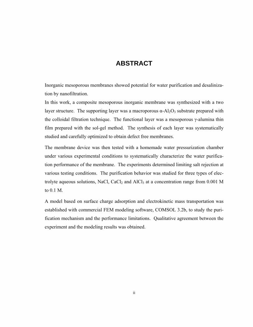
ABSTRACT

Inorganic mesoporous membranes showed potential for water purification and desaliniza-

tion by nanofiltration.

In this work, a composite mesoporous inorganic membrane was synthesized with a two

layer structure. The supporting layer was a macroporous α-Al2O3 substrate prepared with

the colloidal filtration technique. The functional layer was a mesoporous γ-alumina thin

film prepared with the sol-gel method. The synthesis of each layer was systematically

studied and carefully optimized to obtain defect free membranes.

The membrane device was then tested with a homemade water pressurization chamber

under various experimental conditions to systematically characterize the water purifica-

tion performance of the membrane. The experiments determined limiting salt rejection at

various testing conditions. The purification behavior was studied for three types of elec-

trolyte aqueous solutions, NaCl, CaCl2 and AlCl3 at a concentration range from 0.001 M

to 0.1 M.

A model based on surface charge adsorption and electrokinetic mass transportation was

established with commercial FEM modeling software, COMSOL 3.2b, to study the puri-

fication mechanism and the performance limitations. Qualitative agreement between the

experiment and the modeling results was obtained.

iii

DEDICATION

Dedicated to

My parents

iv

ACKNOWLEDGMENTS

I would like to express my deepest gratitude to my advisor, Dr. Henk Verweij, who has

given me encouragement, guidance, support and inspiration over the past five years. I

also want to thank Dr. Rudy Buchheit and Dr. Patricia Morris for serving on my disserta-

tion committee and providing valuable suggestions.

I am especially grateful to Matthew L. Mottern, Krenar Shqau and Jingyu Shi for the

supply of alumina porous supports, many scientific discussions and assistance for the

TEM work. I also wish to thank all the members of IMS group, especially Melissa

Schillo, and Lanlin Zhang for their sincere help in this dynamic working environment. I

can not forget the help and friendship of previous CISM members, especially Chonghoon

Lee, Jin Wang, Sehoon Yoo, Santi Chrisanti, Greg Quickel, Nick Szabo, and Vishnu Ra-

vula. Characterization work could not have been accomplished without the help of

Hendrik O. Colijn, Cameron Begg and Steven Bright.

Lastly, I wish to thank my parents and my sister for their love, support and encourag-

ment.

v

VITA

November 15 1978.........................................Born - Xiangtan, P.R.China

2001................................................................B.S, Materials Science and Engineering,

Jilin University.

2004................................................................M.S, Materials Science and Engineering,

The Ohio State University.

PUBLICATIONS

1. G.T. Quickel, M. L. Mottern, D. Yu, and Henk Verweij, “Thin Supported Inorganic Membranes for H2 and O2 Separation,” Proc. Annual Meeting AIChE, 17-21 October 2003.

2. M.L. Mottern, G.T. Quickel, J.Y. Shi, D. Yu, and H. Verweij, “Processing and prop-erties of homogeneous supported γ-alumina membranes”; pp. 26-29 in: Proc. 8th Int. Conf. Inorganic Membranes, July 18-22, 2004. Edited by Y.S. (Jerry) Lin, Cincin-nati, OH, USA. Adams Press, Chicago, IL.

3. D. Yu, M.L. Mottern, G.T. Quickel, H. Verweij, J. Bukowski, and J.A. Lewis, “Highly permeable supported γ-alumina membranes for water purification”; pp. 491-94 in: Proc. 8th Int. Conf. Inorganic Membranes, July 18-22, 2004. Edited by Y.S. (Jerry) Lin, Cincinnati, OH, USA. Adams Press, Chicago, IL.

4. D. Yu, M.L. Mottern, H. Verweij, J. Bukowski, and J.A. Lewis, “Highly permeable supported γ-alumina membranes for water purification,” Proc. Annual Meeting AIChE, 7-12 November 2004.

vi

5. K. Shqau, M.L. Mottern, D. Yu, and H. Verweij, “Effect of Aluminon Aqueous Solu-tion Chemistry on the Homogeneity of Compacts by Colloidal Filtration of α-Al2O3 Dispersions,” Proceedings of the American Ceramic Society Annual meeting, Balti-more, 2005.

6. K. Shqau, M.L. Mottern, D. Yu, and H. Verweij, “Preparation of defect-free porous alumina membrane supports by colloidal filtration,” Proceedings PCM 2005, Brugge, Belgium, October 20-21, 2005.

7. M.L. Mottern, M. Oyola, K. Shqau, D. Yu, and H. Verweij, “Permeation porometry of membrane supports and thin supported γ-alumina membranes,” Proceedings PCM 2005, Brugge, Belgium, October 20-21, 2005.

8. D. Yu, M.L. Mottern, H. Verweij, J.M. Bukowski, and J.A. Lewis, “Synthesis and optimization of tailored mesoporous membranes for water purification applications,” Proceedings PCM 2005, Brugge, Belgium, October 20-21, 2005.

9. K. Shqau, M.L. Mottern, D. Yu, and Henk Verweij, “Preparation and properties of porous α-Al2O3 membrane supports,“ J. Am. Ceram. Soc., 89 [6] 1790–94 (2006).

10. D. Yu, M.L. Mottern, K. Shqau, and H. Verweij, “Synthesis and Optimization of sup-ported γ-alumina membranes for water purification,” pp. 491-94 in: Proc. 9th Int. Conf. Inorganic Membranes, June 18-22, 2006. Edited by, Lillehammer, Norway.

11. M.L. Mottern, K. Shqau, D. Yu and H. Verweij, “A closer examination of permeation porometry,” pp. Proc. 9th Int. Conf. Inorganic Membranes, June 18-22, 2006. Edited by, Lillehammer, Norway.

FIELDS OF STUDY

Major Field: Materials Science and Engineering

vii

TABLE OF CONTENTS

Page

Abstract ............................................................................................................................ ii

Dedication .......................................................................................................................... iii

Acknowledgments.............................................................................................................. iv

Vita .............................................................................................................................v

List of Tables .......................................................................................................................x

List of figures..................................................................................................................... xi

Chapter 1 Inorganic/Organic Reverse Osmosis/Nanofiltration Membranes for Water

Desalinization Applications ................................................................................1

1.1 Introduction..................................................................................................1

1.2 Organic RO/NF membranes ........................................................................4

1.2.1 Asymmetric membranes ..................................................................4

1.2.2 Composite membranes.....................................................................7

1.2.3 Models for separation process .......................................................16

1.3 Inorganic NF membranes...........................................................................18

1.3.1 Synthesis and properties of inorganic NF membranes ..................18

1.3.2 Separation mechanism and modeling ............................................26

1.4 Conclusion and future work in the membrane area ...................................31

Chapter 2 Synthesis and Optimization of High Surface Quality Alumina Compact

Membrane Support............................................................................................33

2.1 Introduction................................................................................................33

2.2 Experimental procedures ...........................................................................35

viii

2.3 Results and discussion ...............................................................................37

2.4 Conclusions................................................................................................46

Chapter 3 OPTimization of Mesoporous Gamma Alumina Membrane Sol

Preparation ........................................................................................................47

3.1 Introduction................................................................................................47

3.2 Experimental Section .................................................................................49

3.3 Results and Discussion ..............................................................................52

3.3.1 Solid load and filtration rate comparison.......................................52

3.3.2 Size distributions by Dynamic Light Scattering. ...........................54

3.3.3 Particle size and shape from AFM measurement. .........................56

3.3.4 DLS and AFM measurement comparison......................................60

3.3.5 Process contamination ...................................................................65

3.4 Conclusions................................................................................................66

Chapter 4 Water Purification with Inorganic Mesoporous Membrane..............................68

4.1 Introduction................................................................................................69

4.2 Experimental Setup....................................................................................69

4.3 Operational Condition Determination........................................................72

4.4 Membrane Performance Summary ............................................................75

4.4.1 Permeability comparison ...............................................................76

4.4.2 Viscosity correction for flowrate data............................................78

4.4.3 Purification results .........................................................................82

4.4.4 Osmotic effect................................................................................87

4.5 Conclusion .................................................................................................93

Chapter 5 Mesoporous Membrane Nanofiltration Modeling with COMSOL

Multiphysics......................................................................................................95

5.1 Introduction................................................................................................96

5.2 Theory ........................................................................................................97

5.2.1 Surface charge density ...................................................................97

5.2.2 Electrostatics: electrical double layer (EDL).................................99

ix

5.2.3 Diffusion and convection: Nernst-Planck....................................101

5.2.4 Flow: Navier-Stokes ....................................................................104

5.2.5 Geometry and mesh .....................................................................104

5.3 Results and discussion .............................................................................105

5.3.1 Channel length, tortuosity and branching ....................................105

5.3.2 Concentration profile ...................................................................107

5.3.3 Model validation ..........................................................................112

5.4 Conclusions and future work ...................................................................115

Conclusions......................................................................................................................117

Bibliography ....................................................................................................................120

Distribution list ................................................................................................................135

x

LIST OF TABLES

Table Page

Table 1.1: γ-Alumina membrane structural properties and performance. ................. 21

Table 1.2: Titania membrane structure and performance. ......................................... 22

Table 1.3: Zirconia membrane structure and performance. ....................................... 23

Table 2.1: Direct observation of colloidal filtration compacts, initially stabilized in

aqueous HNO3 at various pH values......................................................................... 38

Table 3.1: Volumetric average particle diameter 3S

3Ø 2 [nm]4V

=π

, using 2

i ii

i ii

N VV

N V=∑∑

.

Here Vi is the median volume (in nm3) of particles for one size interval of 0.5 nm,

and Ni is the total number of particles in that size interval. ...................................... 65

Table 3.2: Contamination levels (ppm weight) in the sols......................................... 66

Table 4.1: Water permeability, thickness and resistance of components of a

membrane device. ..................................................................................................... 78

Table 4.2: Pitzer parameters for osmotic coefficient calculation............................... 89

Table 5.1: Terminology summary............................................................................ 103

xi

LIST OF FIGURES

Figure Page

Figure 1.1: Definition of industrial membrane applications in terms of size range and

porosity. ..................................................................................................................... 2

Figure 1.2: Osmotic and RO process............................................................................. 3

Figure 1.3: SEM picture of the cross section of an polysulfone asymmetric membrane

(10,000x) [17]. ............................................................................................................ 5

Figure 1.4: Cellulose triacetate and the solvent............................................................. 6

Figure 1.5: layer structure of composite membrane...................................................... 7

Figure 1.6: polysulfone and solvent. ............................................................................. 8

Figure 1.7: Interfacial polymerization......................................................................... 10

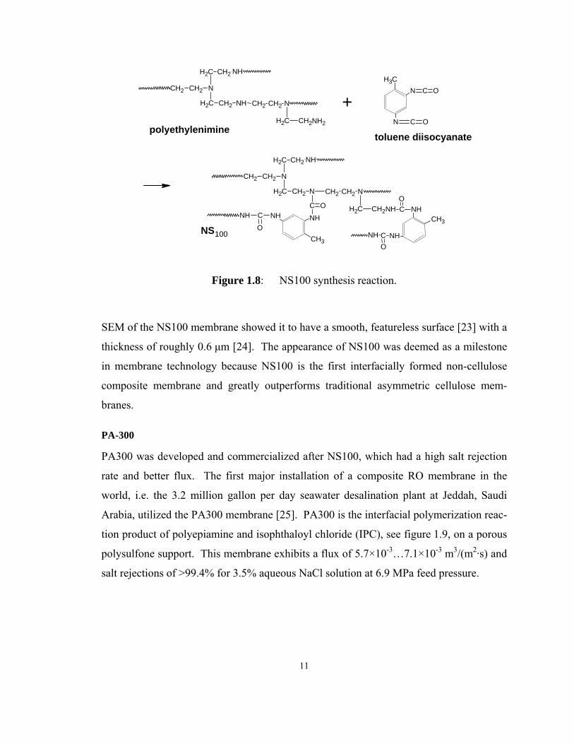
Figure 1.8: NS100 synthesis reaction.......................................................................... 11

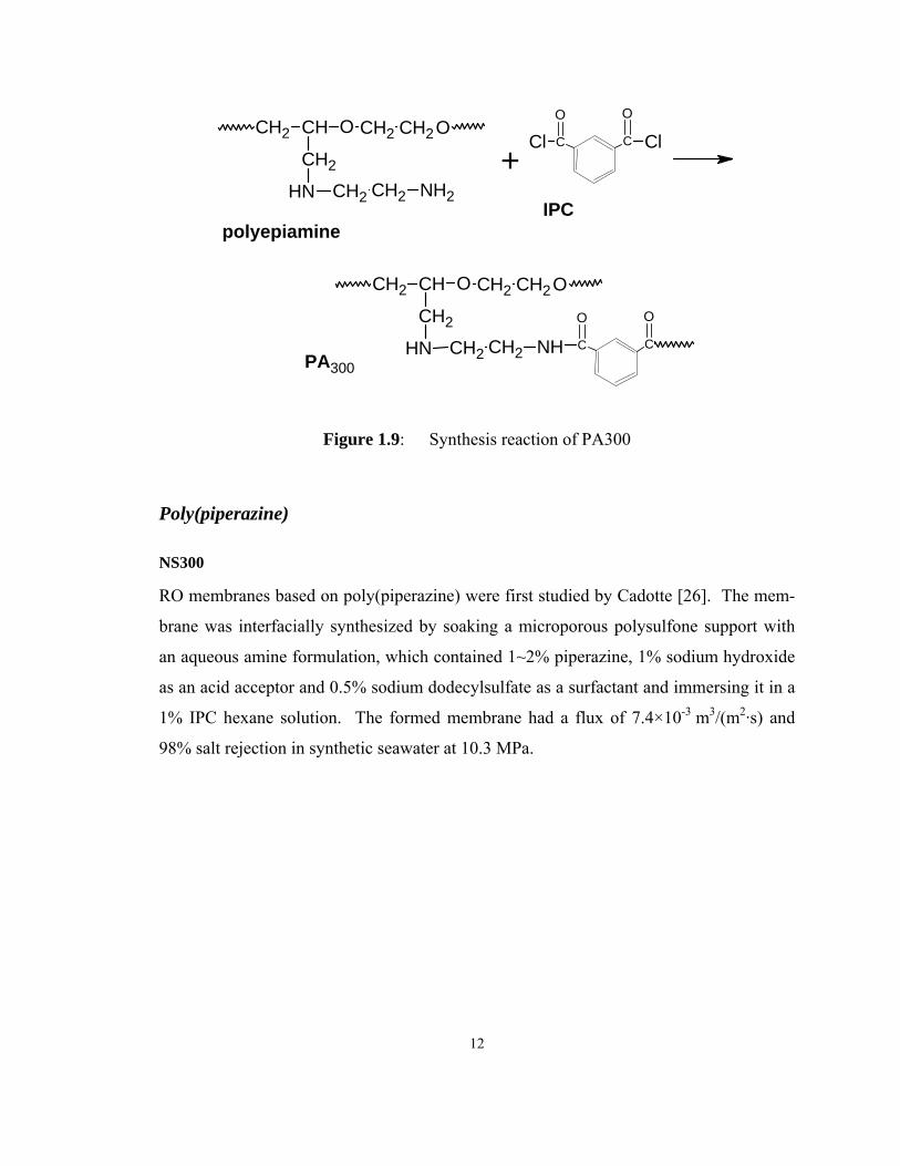
Figure 1.9: Synthesis reaction of PA300..................................................................... 12

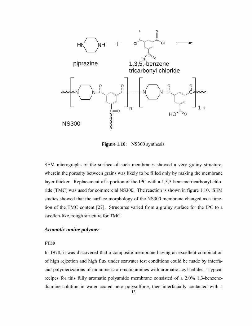
Figure 1.10: NS300 synthesis............................................................................ 13

Figure 1.11: FT30 synthesis. ............................................................................. 14

Figure 1.12: SEM picture of FT30 surface........................................................ 15

Figure 1.13: Schematic representation of PSCF model..................................... 17

Figure 1.14: Sol-gel method. ............................................................................. 19

Figure 1.15: Schematic of a diffuse electric double layer. ................................ 27

Figure 1.16: Concentration and potential profile for positively charged flat

surface. ....................................................................................................... 28

Figure 1.17: Donnan exclusion effect for separation. ....................................... 30

Figure 2.1: Apparent density data of AKP15 and AKP30 compacts made by filtration

of 20 vol% alpha alumina suspension vs. Aluminon concentration and initial pH,

respectively. .............................................................................................................. 39

xii

Figure 2.2: Apparent density data of sintered compacts; AKP30 supports made by

filtration of aqueous HNO3 dispersions at initial pH = 2, and AKP15 supports made

by filtration of aqueous Aluminon dispersions at 0.5wt%........................................ 40

Figure 2.3: Effect of sintering temperature on the surface of S2.00pH compacts

observed by SEM...................................................................................................... 41

Figure 2.4: SEM image of cross section of α-Al2O3 compacts (S2.00ph) sintered at (a)

1150 C and (b) 1350 C.............................................................................................. 42

Figure 2.5: Water permeability of AKP15 and AKP30 supports as a function of

sintering temperature. ............................................................................................... 43

Figure 2.6: Temperate development of gas (He) permeability for AKP15 and AKP30

supports. ................................................................................................................... 44

Figure 2.7: TEM images of FIB cross-sections of sintered S2.00pH compacts coated

with zirconia based ceramic taken from [126].......................................................... 45

Figure 3.1: Funnel setup. ............................................................................................. 50

Figure 3.2: 20 nm Anodisc membrane. (a) FIB cross section of the branched top layer

(b) top layer surface and (c) surface area with defect. .............................................. 51

Figure 3.3: Yield of the filtration process with and without the presence of ultrasonic

vibration. ................................................................................................................... 53

Figure 3.4: Standing wave on the surface of an Anodisc filter membrane,

demonstrated by decoration with small black particles added for this purpose. ...... 54

Figure 3.5: DLS particle size distribution of the sols.................................................. 56

Figure 3.6: C-γ spin coated on mica. ........................................................................... 57

Figure 3.7: C-γ dip-coated on a silicon wafer. ............................................................ 58

Figure 3.8: Volumetric particle size distributions from AFM image analysis. ........... 60

Figure 3.9: Data processing for DLS and AFM measurements. ................................. 61

Figure 3.10: Diameter vs. thickness from AFM analysis. ............................................ 62

xiii

Figure 3.11: Differential accumulated volume vs. particle Ø for each sol, using the

spherical and the oblate model.................................................................................. 64

Figure 4.1: Water purification chamber design........................................................... 70

Figure 4.2: Water purification membrane testing setup. ............................................. 72

Figure 4.3: Rejection under various stirring conditions for aqueous NaCl solutions. 73

Figure 4.4: Rejection vs flow velocity for aqueous NaCl solutions............................ 75

Figure 4.5: Temperature vs. viscosity for pure H2O. .................................................. 80

Figure 4.6: Viscosity vs concentration for aqueous NaCl. .......................................... 81

Figure 4.7: Viscosity vs concentration for aqueous CaCl2.......................................... 82

Figure 4.8: Rejection vs. flowrate for various concentrations of NaCl....................... 83

Figure 4.9: Rejection vs. flowrate for various concentrations of CaCl2...................... 84

Figure 4.10: Rejection vs. flowrate for various concentrations of

NaCl+1%AlCl3. ....................................................................................................... 85

Figure 4.11: Rejection vs. flowrate for various concentrations of

CaCl2+1wt%AlCl3. ................................................................................................... 86

Figure 4.12: Rejection vs. flowrate for various concentrations of AlCl3. ......... 87

Figure 4.13: The pressure vs. flowrate w/o osmotic effect for NaCl. ............... 90

Figure 4.14: The pressure vs. flowrate w/o osmotic effect for CaCl2. .............. 91

Figure 4.15: The pressure vs. flowrate w/o osmotic effect for NaCl+1%AlCl3. ..

....................................................................................................... 91

Figure 4.16: The pressure vs. flowrate w/o osmotic effect for CaCl2+1%AlCl3. .

....................................................................................................... 92

Figure 4.17: The pressure vs. flowrate w/o osmotic effect for AlCl3................ 92

Figure 5.1: Geometries and renders of modeling results. a…f are various 2D

geometries with a color map of the Na+ concentration. g is the only 3D geometry

that has been modeled. c1 is the closeup of the 2D modeling result with a color map

of the Na+ concentration, with blue stream lines of the velocity field; c2 is the

xiv

corresponding mesh. g1 is a closeup of the 3D modeling result with colored slices

of space charge density, and blue stream lines; g2 shows the 3D mesh.. ............... 106

Figure 5.2: Concentration profile along the channel. ................................................ 108

Figure 5.3: Concentration profile at various applied pressures. ................................ 109

Figure 5.4: Normalized mass transport terms. The feed side bulk solution is from

z = -2.0E-8 to z = 0, the membrane pore channel region is from z = 0 to z = 3.0E-8,

and the permeate side bulk solution is from z = 3.0E-8 to z = 1.2E-7.................... 111

Figure 5.5: Comparison of rejection performance for 2D models versus channel

length. ................................................................................................................. 113

Figure 5.6: Comparison of rejection performance for experimental result 1 (solid

symbols), experimental result 2 (open symbols) and 3D model results (drawn line)...

................................................................................................................. 114

1

CHAPTER 1

INORGANIC/ORGANIC REVERSE

OSMOSIS/NANOFILTRATION MEMBRANES FOR WATER

DESALINIZATION APPLICATIONS

1.1 Introduction

Membrane separation processes are rapidly expanding in many existing and emerging

applications, such as chemical engineering [1], petroleum industries [2], environment sci-

ence [3,6], biotechnology science [4], pharmaceuticals [5], water treatment [1,5-7],

dairy/beverage/food industries [5], pulp/paper manufactures, textile industries, metallur-

gical and electronic industries [7]. In all these industries, various water purification proc-

esses are among the most widely used. According to the sizes of the species that the

membrane retains, water purification membranes can be classified into 4 categories [7,8]:

reverse osmosis (RO) (0.1-1 nm), nanofiltration (NF) (1-2 nm), ultrafiltration (UF) (2-

100 nm) and microfiltration membranes (100 nm-10 μm). A comparison between the

definition of membrane types and definition of material porosity is provided in figure 1.1

2

Figure 1.1: Definition of industrial membrane applications in terms of size range and porosity.

As one important subcategory of water purification applications, water desalinization is a

process by which the loading of dissolved solids is reduced, especially electrolytes, in

various aqueous solutions. Examples include seawater and brackish water desalinization,

water softening, waste water recycling/regeneration and industrial ultrapure water supply.

Since most dissolved species/electrolytes in aqueous media have relatively small size

(<1nm), membrane technologies for water desalinization are normally confined to RO

and NF type membranes.

A brief description of the osmotic process is provided below to help visualizing the re-

verse osmosis process (figure 1.2). Osmosis is a universal phenomenon in which solvent

spontaneously passes through a semipermeable (no or very low solute flow) membrane

from the side with lower solute concentration (higher solvent chemical potential) to the

side with higher solute concentration (lower solvent chemical potential) until the chemi-

cal potentials of solvent at both sides are equal. At equilibrium the pressure difference

between the two sides of the membrane is equal to the osmotic pressure Δπ. An RO

membrane acts as such a semipermeable barrier which allows passage of a particular spe-

cies (solvent) while other species (solutes) are retained partially or completely. To re-

verse the spontaneous flow of the solvent, a pressure difference larger than the osmotic

pressure must be applied and, as a result, separation of the solvent from solution is

achieved as shown in figure 1.2.

3

Figure 1.2: Osmotic and RO process.

NF membranes may be described as very coarse RO membranes when solutes are mac-

romolecules. However, the mechanisms of ion separation in NF and RO are substantially

different. The permselectivity and flux of the RO/NF membranes depend on the mem-

brane material, the preparation procedure and the microstructure of the functional mem-

brane barrier layer [9,10]. When the filtration media is an aqueous system, as in water

desalinization, a hydrophilic barrier layer with low solubility towards the solutes is favor-

able for high flux and high permselectivity.

The materials for RO/NF membranes can be either organic polymers or inorganic ceram-

ics. Organic polymer RO/NF membranes dominate the water desalinization market, be-

4

cause of their relatively simple synthesis methods and satisfactory performance. How-

ever, new NF ceramic membranes have been attracting more and more attention due to

many of their merits [18]. Their chemical/thermal stability and mechanical strength en-

able ceramic membranes to work in harsh/dirty environments and under a wider pres-

sure/temperature/pH range. Thorough cleaning and regeneration is possible and hence a

longer membrane life time can be obtained. Resistance to organic solute and microbial

attack reduces the fouling problems associated with traditional organic membranes [18].

The ceramic membranes are also believed to have a higher porosity and permeability

when compared with their polymeric counterparts.

This introductory literature review focuses on the RO/NF membrane technologies for wa-

ter desalinization applications. It summarizes the chemistry, morphology, preparation,

performance and separation mechanisms for both organic and inorganic materials. This

review is organized as follows. Section 2 focuses on commercially important organic

RO/NF membranes; section 3 is dedicated to research progress in inorganic NF mem-

branes and section 4 provides a predictive survey of the future research.

1.2 Organic RO/NF membranes

Organic RO/NF membranes have been developed and commercialized for more than 50

years and most of the synthesis research has been carried out by private companies, and

not been made available to the public. Therefore, very few academic research papers are

found in the RO membrane field, other than application studies and mathematical model-

ing of membrane performance. Recent examples of review papers include those of

Robert J. Petersen 1993, Petersen and Cadotte 1990, Allegrezza 1988 and Cadotte 1985

[11-14].

1.2.1 Asymmetric membranes

Structure & Benefit

Commercial polymer RO membranes mainly come in two categories, single component

asymmetric membranes (or briefly asymmetric membranes) and multiple layer composite

membranes (or briefly composite membranes).

5

Asymmetric RO membranes have an anisotropic structure, consisting of a dense surface

skin on a porous sublayer structure (figure 1.3). Both skin and sublayer have the same

composition [15, 16]. Normally the asymmetric RO membrane is formed by a single-

step phase inversion method, which is relatively simple and cheap. The most important

example is cellulose acetate.

Figure 1.3: SEM picture of the cross section of an polysulfone asymmetric membrane (10,000x) [17].

Cellulose acetate

Polymeric cellulose triacetate, see figure 1.4, with segment number, n, between 3000 and

9000 is first dissolved in an organic solvent or solvent mixture to form a casting solution.

The casting solution is then applied to the surface of a carrier, which can be a flat support

or hollow fiber tube. After that, the carrier is immersed into a non-solvent (normally wa-

ter) bath, where the coagulation of the polymer occurs to form the membrane morphol-

ogy. The formed membrane can be post-treated (washed and heated) and collected for

6

usage. The morphology and performance of the membrane are controlled by various fac-

tors, such as polymer concentration, evaporation time, humidity, temperature and the com-

position of the casting solution [17]. Asymmetric cellulose acetate membranes normally

have a flux of 2.8×10-3…8.5×10-3 m3/(m2·s), and a rejection rate of 91…97% under the test-

ing conditions of 0.5wt% NaCl, 4.1 MPa and 25ºC [11]. Cellulose acetate based membranes

are normally very sensitive to thermal, chemical and biological degradation, which limits the

application of this type of membrane.

C O

* O

O

O

O *

O

O

C On

N CH OCH3

CH3NCH3

CH3

Ac

Ac Ac

Ac

AcAccellulose triacetate

solvents

dimethylformamide dimethylacetamide

Ac

Figure 1.4: Cellulose triacetate and the solvent.

7

1.2.2 Composite membranes

Structure & Benefit

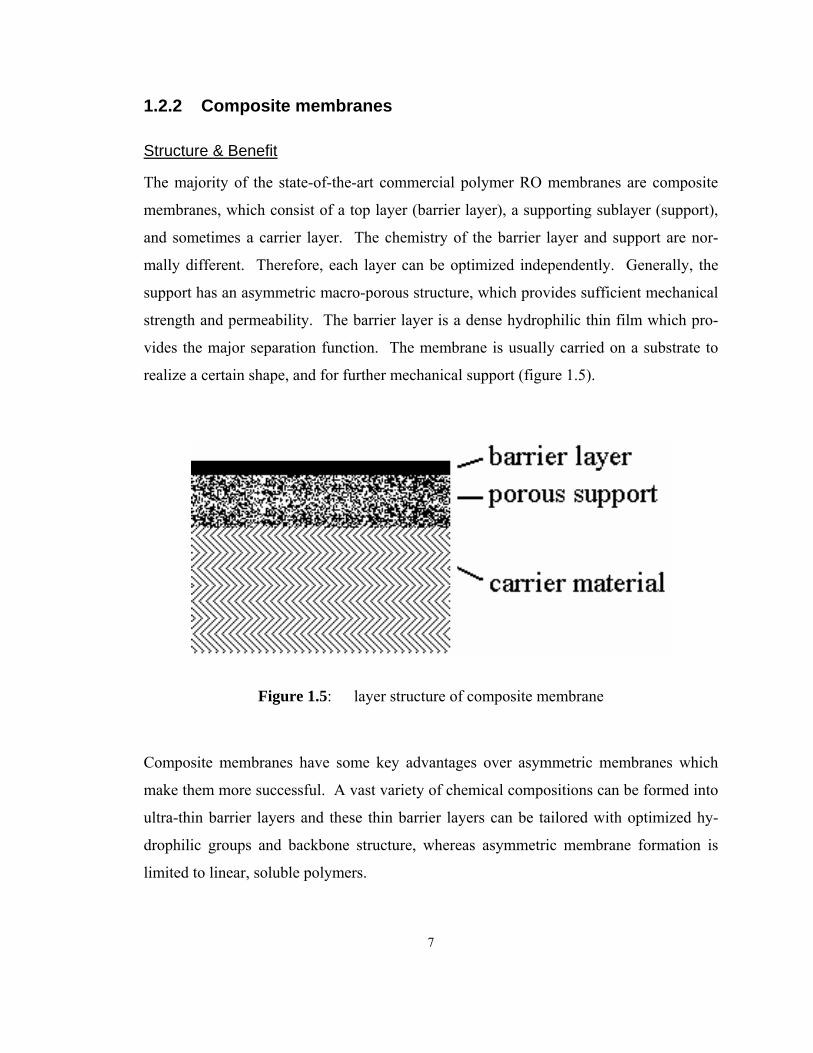
The majority of the state-of-the-art commercial polymer RO membranes are composite

membranes, which consist of a top layer (barrier layer), a supporting sublayer (support),

and sometimes a carrier layer. The chemistry of the barrier layer and support are nor-

mally different. Therefore, each layer can be optimized independently. Generally, the

support has an asymmetric macro-porous structure, which provides sufficient mechanical

strength and permeability. The barrier layer is a dense hydrophilic thin film which pro-

vides the major separation function. The membrane is usually carried on a substrate to

realize a certain shape, and for further mechanical support (figure 1.5).

Figure 1.5: layer structure of composite membrane

Composite membranes have some key advantages over asymmetric membranes which

make them more successful. A vast variety of chemical compositions can be formed into

ultra-thin barrier layers and these thin barrier layers can be tailored with optimized hy-

drophilic groups and backbone structure, whereas asymmetric membrane formation is

limited to linear, soluble polymers.

8

The composite membranes have the disadvantage of requiring a more expensive method

for membrane manufacturing. This requires at least two major steps:

• First, a macro-porous support is synthesized (normally with the immersion precipita-

tion technique).

• Second, the thin barrier layer is synthesized (or synthesized and applied) on the mi-

croporous support. Two major routes of barrier layer preparation: interfacial polym-

erization and dip-coat methods are used most for industrial composite RO membrane

manufacturing.

Macro-porous support

Many materials that have been investigated include Polyethersulfone, cellulose mixed

esters, polyimides, and polyphenylene oxides [11]. The most successful microporous

support is polysulfone (figure 1.6), which has remained a mainstay in composite mem-

branes to this day.

Microporous polysulfone is normally prepared by the immersion precipitation technique.

The typical procedure is as follows. The Udel P-3500 (polysulfone with MW 30,000) is

dissolved in N,N-dimethylformamide to obtain a 15 wt% solution. After degassing

treatments, the solution is spread coated on a clean glass plate with a doctor blade and

then immersed into a water bath. The liquid solution film is then converted into the mi-

croporous membrane by precipitation of the polysulfone.

Figure 1.6: polysulfone and solvent.

Polysulfone (commercial name Udel P-3500)

Me

Me

S

O

O

OO

C

n

Solvent: N,N-dimethylformamide

N CHH3 C

CH 3

O

9

Numerous morphology studies have been carried out with SEM techniques. It has been

reported that the shiny surface (corresponding to the original air interface) has a denser

layer with pores diameters ranging from 1.9 to 15 nm. The surface area attributed to

pores was measured to be 16%. The mean pore size was 7.5 nm. The dull surface (cor-

responding to the interface contacting the glass plate) contained pores ranging from 0.3 to

2.0 μm [20]. Merin and Cheryan [21] reached a similar conclusion by examining the sur-

face porosity of a commercial polysulfone ultrafiltration membrane with SEM. They

found a surface pore concentration of about 4×1011 pores/cm2, and ranging in size from 1

to 15 nm in diameter. The pores occupied 7…12% of the surface area.

Polysulfone has a much higher pH tolerance than cellulose acetate, which enables one to

use barrier layer formation solutions that are highly acidic or alkaline.

Barrier layer

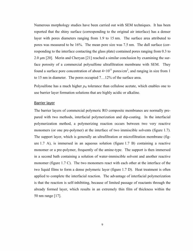
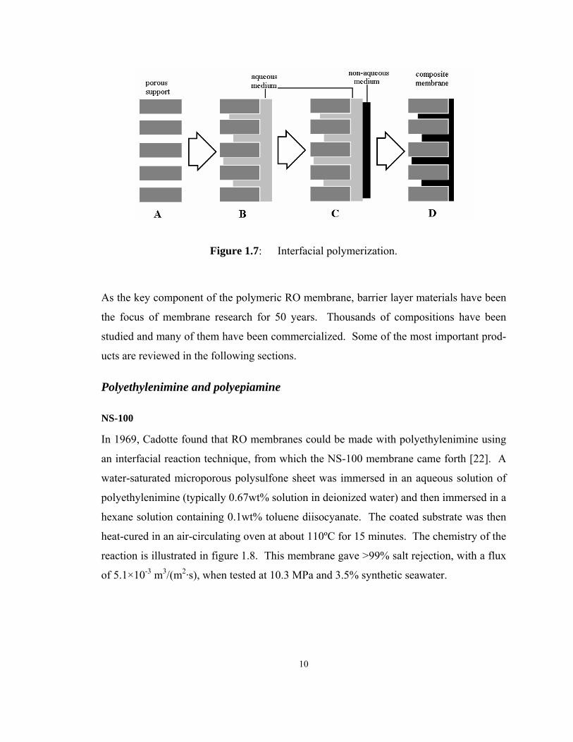
The barrier layers of commercial polymeric RO composite membranes are normally pre-

pared with two methods, interfacial polymerization and dip-coating. In the interfacial

polymerization method, a polymerizing reaction occurs between two very reactive

monomers (or one pre-polymer) at the interface of two immiscible solvents (figure 1.7).

The support layer, which is generally an ultrafiltration or microfiltration membrane (fig-

ure 1.7 A), is immersed in an aqueous solution (figure 1.7 B) containing a reactive

monomer or a pre-polymer, frequently of the amine-type. The support is then immersed

in a second bath containing a solution of water-immiscible solvent and another reactive

monomer (figure 1.7 C). The two monomers react with each other at the interface of the

two liquid films to form a dense polymeric layer (figure 1.7 D). Heat treatment is often

applied to complete the interfacial reaction. The advantage of interfacial polymerization

is that the reaction is self-inhibiting, because of limited passage of reactants through the

already formed layer, which results in an extremely thin film of thickness within the

50 nm range [17].

10

Figure 1.7: Interfacial polymerization.

As the key component of the polymeric RO membrane, barrier layer materials have been

the focus of membrane research for 50 years. Thousands of compositions have been

studied and many of them have been commercialized. Some of the most important prod-

ucts are reviewed in the following sections.

Polyethylenimine and polyepiamine

NS-100

In 1969, Cadotte found that RO membranes could be made with polyethylenimine using

an interfacial reaction technique, from which the NS-100 membrane came forth [22]. A

water-saturated microporous polysulfone sheet was immersed in an aqueous solution of

polyethylenimine (typically 0.67wt% solution in deionized water) and then immersed in a

hexane solution containing 0.1wt% toluene diisocyanate. The coated substrate was then

heat-cured in an air-circulating oven at about 110ºC for 15 minutes. The chemistry of the

reaction is illustrated in figure 1.8. This membrane gave >99% salt rejection, with a flux

of 5.1×10-3 m3/(m2·s), when tested at 10.3 MPa and 3.5% synthetic seawater.

11

CH2 CH2 N

CH2 CH2 NH

CH2 CH2 NH CH2 CH2 N

CH2 CH2NH2

+CH3

N

N

C O

C O

CH3

NH

NH

CO

CO

NHCH3

NH NHC

O

C O

CH2 CH2 N

CH2 CH2 NH

CH2 CH2 N CH2 CH2 N

CH2 CH2NHNH

polyethyleniminetoluene diisocyanate

NS100

Figure 1.8: NS100 synthesis reaction.

SEM of the NS100 membrane showed it to have a smooth, featureless surface [23] with a

thickness of roughly 0.6 μm [24]. The appearance of NS100 was deemed as a milestone

in membrane technology because NS100 is the first interfacially formed non-cellulose

composite membrane and greatly outperforms traditional asymmetric cellulose mem-

branes.

PA-300

PA300 was developed and commercialized after NS100, which had a high salt rejection

rate and better flux. The first major installation of a composite RO membrane in the

world, i.e. the 3.2 million gallon per day seawater desalination plant at Jeddah, Saudi

Arabia, utilized the PA300 membrane [25]. PA300 is the interfacial polymerization reac-

tion product of polyepiamine and isophthaloyl chloride (IPC), see figure 1.9, on a porous

polysulfone support. This membrane exhibits a flux of 5.7×10-3…7.1×10-3 m3/(m2·s) and

salt rejections of >99.4% for 3.5% aqueous NaCl solution at 6.9 MPa feed pressure.

12

CH2 CH O

CH2

CH2 CH2O

NH CH2 CH2 NH2

+ClCl CC

OO

CC

OO

CH2 CH O

CH2

CH2 CH2O

NH CH2 CH2 NH

polyepiamineIPC

PA300

Figure 1.9: Synthesis reaction of PA300

Poly(piperazine)

NS300

RO membranes based on poly(piperazine) were first studied by Cadotte [26]. The mem-

brane was interfacially synthesized by soaking a microporous polysulfone support with

an aqueous amine formulation, which contained 1~2% piperazine, 1% sodium hydroxide

as an acid acceptor and 0.5% sodium dodecylsulfate as a surfactant and immersing it in a

1% IPC hexane solution. The formed membrane had a flux of 7.4×10-3 m3/(m2·s) and

98% salt rejection in synthetic seawater at 10.3 MPa.

13

+ ClClCC

OO

ClC

O

NH NH

N N CC

OO

C O

N N CC

OO

OHC

On 1-n

piprazine

NS300

1,3,5,-benzene tricarbonyl chloride

Figure 1.10: NS300 synthesis.

SEM micrographs of the surface of such membranes showed a very grainy structure;

wherein the porosity between grains was likely to be filled only by making the membrane

layer thicker. Replacement of a portion of the IPC with a 1,3,5-benzenetricarbonyl chlo-

ride (TMC) was used for commercial NS300. The reaction is shown in figure 1.10. SEM

studies showed that the surface morphology of the NS300 membrane changed as a func-

tion of the TMC content [27]. Structures varied from a grainy surface for the IPC to a

swollen-like, rough structure for TMC.

Aromatic amine polymer

FT30

In 1978, it was discovered that a composite membrane having an excellent combination

of high rejection and high flux under seawater test conditions could be made by interfa-

cial polymerizations of monomeric aromatic amines with aromatic acyl halides. Typical

recipes for this fully aromatic polyamide membrane consisted of a 2.0% 1,3-benzene-

diamine solution in water coated onto polysulfone, then interfacially contacted with a

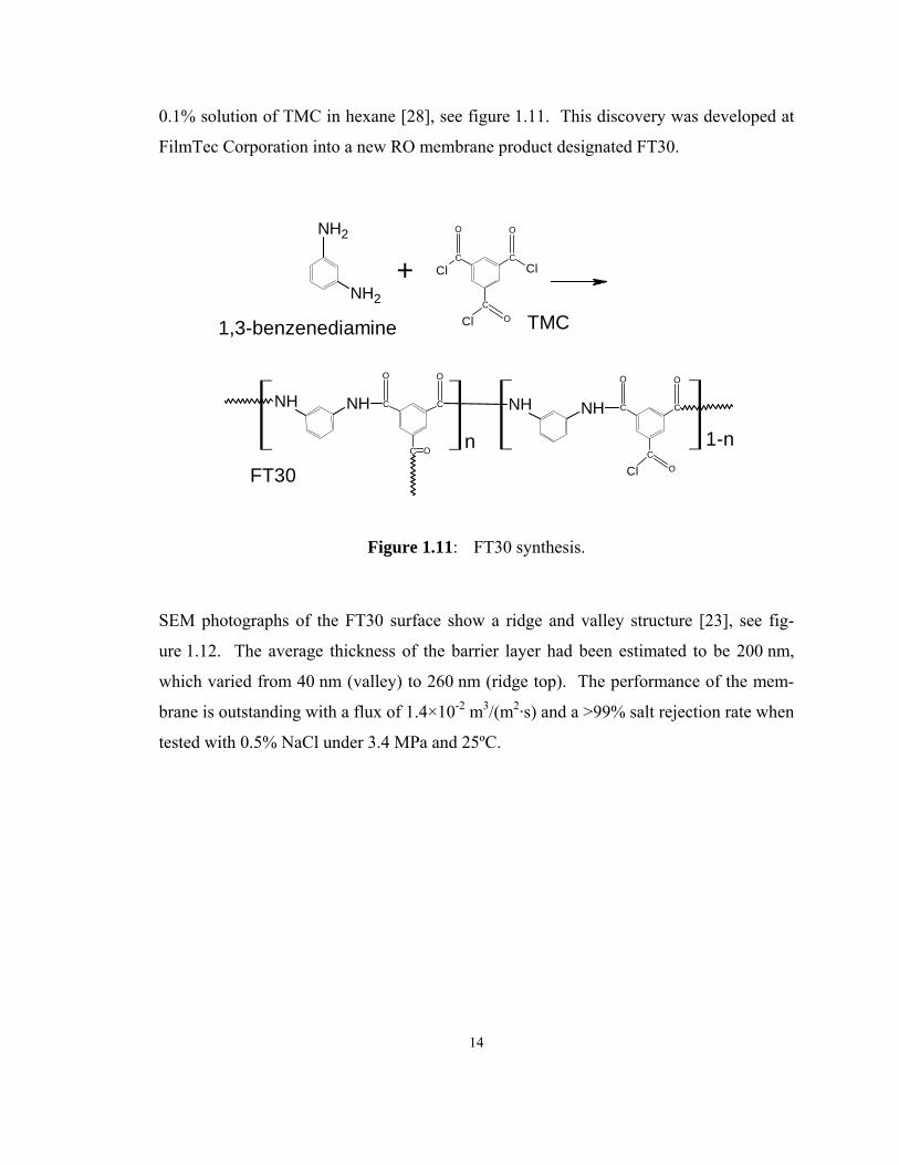
14

0.1% solution of TMC in hexane [28], see figure 1.11. This discovery was developed at

FilmTec Corporation into a new RO membrane product designated FT30.

ClClCC

OO

ClC

O

NH2

NH2

+

CC

OO

ClC

O

NH NHCC

OO

C O

NH NH

n 1-n

1,3-benzenediamine TMC

FT30

Figure 1.11: FT30 synthesis.

SEM photographs of the FT30 surface show a ridge and valley structure [23], see fig-

ure 1.12. The average thickness of the barrier layer had been estimated to be 200 nm,

which varied from 40 nm (valley) to 260 nm (ridge top). The performance of the mem-

brane is outstanding with a flux of 1.4×10-2 m3/(m2·s) and a >99% salt rejection rate when

tested with 0.5% NaCl under 3.4 MPa and 25ºC.

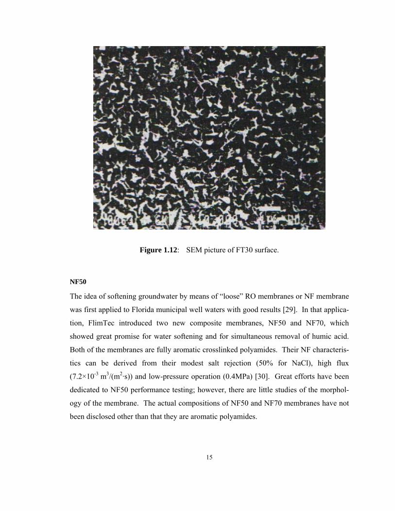
15

Figure 1.12: SEM picture of FT30 surface.

NF50

The idea of softening groundwater by means of “loose” RO membranes or NF membrane

was first applied to Florida municipal well waters with good results [29]. In that applica-

tion, FlimTec introduced two new composite membranes, NF50 and NF70, which

showed great promise for water softening and for simultaneous removal of humic acid.

Both of the membranes are fully aromatic crosslinked polyamides. Their NF characteris-

tics can be derived from their modest salt rejection (50% for NaCl), high flux

(7.2×10-3 m3/(m2·s)) and low-pressure operation (0.4MPa) [30]. Great efforts have been

dedicated to NF50 performance testing; however, there are little studies of the morphol-

ogy of the membrane. The actual compositions of NF50 and NF70 membranes have not

been disclosed other than that they are aromatic polyamides.

16

1.2.3 Models for separation process

Separation of RO membranes has long been described by using various theories and

models. The central goal of most modeling research is the prediction of the solvent and

the solute flux through the membrane. Currently, several models for RO membranes are

available. Among them, two categories: non-porous dense membrane structures, and po-

rous membrane structure, are most well developed. Recently, the NF separation mecha-

nism based on the interaction between electrolytes and the charged pore surface has be-

come an active area of research. However, this topic will be discussed in more detail for

inorganic membranes in section 1.3.2. The nonporous/porous membrane models will be

introduced briefly in the following sections with emphasis on the fundamental physical

principles that underlies the models.

Models based on dense membranes

The solution diffusion model was originally developed by Lonsdale, Merten, and Riley in

1965 [31]. This model assumes that both the solute and solvent dissolve in the nonporous

and homogenous surface layers of the membrane and then each diffuse across the mem-

brane in an uncoupled manner in response to gradients in their chemical potential. This

gradient is the result of concentration and/or pressure differences across the membrane.

Many modifications have been made in solution diffusion models to account for non

ideal situations. One example is the work of Sherwood, Brian and Fisher [32], which in-

cludes pore flow as well as diffusion of the solute and solvent. This model recognizes

that imperfections (pores) exist on the membranes surface through which solute and sol-

vent can flow.

Solution diffusion models provide straightforward routines for estimating the perform-

ance of RO membranes. However, the models are based on phenomenological experi-

mental data, which will not give us the knowledge of the relationship between the mem-

brane structure and its properties.

17

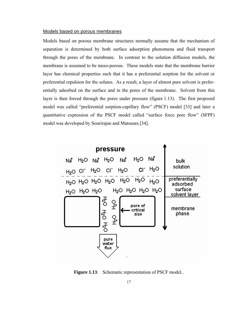
Models based on porous membranes

Models based on porous membrane structures normally assume that the mechanism of

separation is determined by both surface adsorption phenomena and fluid transport

through the pores of the membrane. In contrast to the solution diffusion models, the

membrane is assumed to be meso-porous. These models state that the membrane barrier

layer has chemical properties such that it has a preferential sorption for the solvent or

preferential repulsion for the solutes. As a result, a layer of almost pure solvent is prefer-

entially adsorbed on the surface and in the pores of the membrane. Solvent from this

layer is then forced through the pores under pressure (figure 1.13). The first proposed

model was called “preferential sorption-capillary flow” (PSCF) model [33] and later a

quantitative expression of the PSCF model called “surface force pore flow” (SFPF)

model was developed by Sourirajan and Matsuura [34].

Figure 1.13: Schematic representation of PSCF model..

18

Refinement was made by considering the pore radius distribution rather than the average

pore size. Sophisticated numerical techniques were used to solve the model and a good

agreement with experimental results of FT30 membrane was obtained by Bhattacharyya

et al. [35]

1.3 Inorganic NF membranes

In the area of RO and NF, research on inorganic membrane materials is still in a rela-

tively early stage of development. Most of the available inorganic membrane materials

have pore size distributions in the range of NF rather than RO. This is mainly due to the

technical difficulties of synthesizing fine pore sizes for RO membranes (<1 nm). Prepa-

rations of metal oxide particles in the size range of less than 10 nm have been realized in

many laboratories. Therefore, new inorganic membrane materials with pore sizes rang-

ing from 1 nm to 5 nm have been reported in literatures in the last 15 years. Inorganic

NF membranes may have comparable separation performance as organic NF membranes.

In addition, numerous potential benefits arising from the inherent properties of inorganic

materials have been recognized, such as chemical, mechanical and thermal stabilities,

wider pressure/temperature/pH operation range, compatibility with organic solvent sys-

tems and the ability of regeneration.

1.3.1 Synthesis and properties of inorganic NF membranes

Sol-gel method

The mostly adopted route for the synthesis of inorganic NF membrane is the sol-gel tech-

nique (figure 1.14). In this method, a sol is synthesized and applied to a coarse porous

support, which results in gel formation on the surface. This is followed by a heat treat-

ment to solidify the gel layer and to convert it into a microporous or mesoporous mem-

brane. Therefore, the sol-gel method includes two major steps: sol preparation and gel

formation.

A sol is a suspension of colloidal particles, generally made from a solution of polymeriz-

able metallorganic precursors. A gel refers to the semi-rigid layer formed by the agglom-

eration of colloidal particles or the polymerization of metallorganic precursors [36].

19

Figure 1.14: Sol-gel method.

The sol synthesis normally employs metal alkoxides, M(OR)n, as the metallorganic pre-

cursors. Alkoxides are easily hydrolyzed with water and form macromolecular structures

through condensation reactions. A dispersion, consisting of alkoxides, a solvent (such as

an alcohol), water and possible other additives, is formulated so that gelation does not

occur before deposition. The solution is then coated on the support via dip-coating or

slip-casting methods and a subsequent gelation reaction is triggered to form the NF

membrane. The formed membranes are usually solidified by heat treatments. The pore

size of porous membranes by the sol-gel process can be controlled by colloidal particle

diameters and the heat treatment temperature. The majority of the inorganic NF mem-

branes are formed with this method. Summaries of the membranes prepared by the sol-

gel method are provided in the following sections.

20

Many other methods have been investigated for inorganic microporous membrane prepa-

ration. Some of them were initially developed for gas separation purposes, but showed

potential for producing NF membranes for liquid filtration applications. However, com-

pared with the sol-gel process, none of these preparation methods have been applied

widely for NF water purification membranes. This is because of their high cost, narrow

applicable materials range, and lack of microstructure control.

Alumina

Alumina is the first material that has been used for inorganic membrane preparation, due

to its well known colloidal chemistry [37]. Most alumina NF membranes were produced

with the sol-gel method, in which a boehmite sol was synthesized by the hydrolysis of

aluminum butoxide or aluminum propoxide in hot water (higher than 80ºC), followed by

peptization with acids such as nitric acid. The resulting boehmite sol was coated on a

macroporous support and formed a layer of boehmite gel. γ-Alumina membranes were

obtained after firing the boehmite layer at a suitable temperature. To characterize the mi-

crostructure of the membrane, two physical properties were most frequently cited, i.e. the

mean pore size and the molecular weight cut-offs (MWCO). MWCO are defined as a

molecular weight showing a rejection of 90% when a permselectivity test is done with a

solution composed of species of various molecular weights, normally polyethylene glycol

(PEG). It was shown that the MWCO increased when membrane was fired at higher

temperature because of the growth in particle size and pore size (coarsening effect) [40,

42]. A summarization of properties of alumina membranes is listed in the table 1.1:

21

Ref. Firing

temp.(ºC) MWCO/dp(nm)

Thickness

(μm) Separation system

Lp×1011

(m3m-2s-1Pa-1)

38 450 500/1 <1 Acid orange 0.97

42,45 200-900 2000-20000/2.5-5.4 20 PEG 0.38-3.1

43 450-650 400-600/1.35-1.7 -- Saccharose, Direct red 0.3-0.6

41 600 7000/3 3-8 PEG 0.75

46 -- 1000/0.5-0.7 2 PEG 0.68

39,66 450 460/0.65 0.5-1 Saccharose, organic electrolytes 0.3-0.6

40 400-900 900-40000/3.4-8.7 ~6 PEG 1.3

44 -- 600/0.6-1 1-2 PEG 0.68

PEG = polyethylene glycol.

Table 1.1: γ-Alumina membrane structural properties and performance.

Consistent characterizations of the pore size and MWCO are always difficult and the val-

ues critically depend on the synthesis conditions, measurement methods and testing envi-

ronments. Therefore, the relationships between mean pore size and MWCO may have

certain deviation for the data obtained in the different laboratories. However, it is agreed

that increasing firing temperature results in increasing pore size and MWCO.

Titania

Titania membranes show excellent chemical resistance, and can be used in wider pH

range than γ-alumina membranes. At present, extensive efforts have focused on the

preparation of porous TiO2 membranes having small pore sizes in the NF range. Mem-

brane with nano-sized TiO2 particles (3-5 nm) can be prepared with sol-gel methods by

carrying out hydrolysis and condensation reactions of titanium alkoxides (such as tita-

nium tert-amyloxide / titanium tetraisopropoxide / tetraethyl orthotitanate) with a certain

amount of water in the alcohol media (such as tert-amyl alcohol/ isopropanol/)[48,54].

The reaction conditions (temperature, time etc.) are controlled according to individual

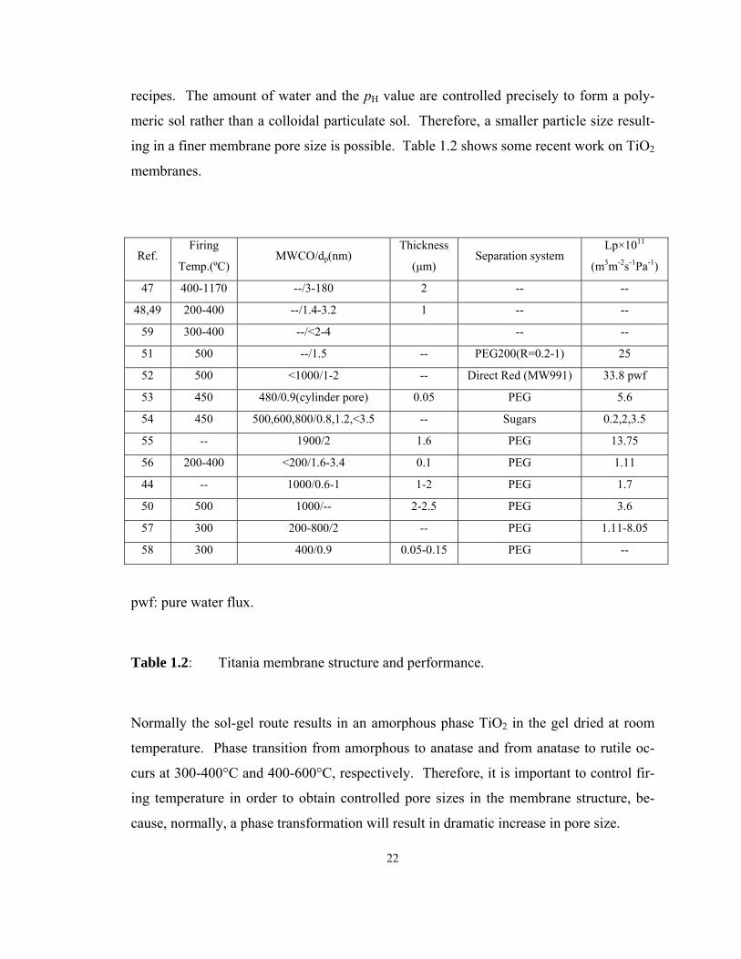
22

recipes. The amount of water and the pH value are controlled precisely to form a poly-

meric sol rather than a colloidal particulate sol. Therefore, a smaller particle size result-

ing in a finer membrane pore size is possible. Table 1.2 shows some recent work on TiO2

membranes.

Ref. Firing

Temp.(ºC) MWCO/dp(nm)

Thickness

(μm) Separation system

Lp×1011

(m3m-2s-1Pa-1)

47 400-1170 --/3-180 2 -- --

48,49 200-400 --/1.4-3.2 1 -- --

59 300-400 --/<2-4 -- --

51 500 --/1.5 -- PEG200(R=0.2-1) 25

52 500 <1000/1-2 -- Direct Red (MW991) 33.8 pwf

53 450 480/0.9(cylinder pore) 0.05 PEG 5.6

54 450 500,600,800/0.8,1.2,<3.5 -- Sugars 0.2,2,3.5

55 -- 1900/2 1.6 PEG 13.75

56 200-400 <200/1.6-3.4 0.1 PEG 1.11

44 -- 1000/0.6-1 1-2 PEG 1.7

50 500 1000/-- 2-2.5 PEG 3.6

57 300 200-800/2 -- PEG 1.11-8.05

58 300 400/0.9 0.05-0.15 PEG --

pwf: pure water flux.

Table 1.2: Titania membrane structure and performance.

Normally the sol-gel route results in an amorphous phase TiO2 in the gel dried at room

temperature. Phase transition from amorphous to anatase and from anatase to rutile oc-

curs at 300-400°C and 400-600°C, respectively. Therefore, it is important to control fir-

ing temperature in order to obtain controlled pore sizes in the membrane structure, be-

cause, normally, a phase transformation will result in dramatic increase in pore size.

23

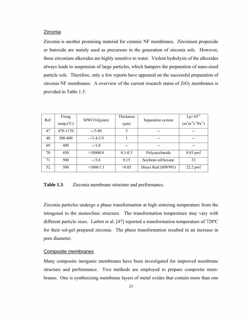
Zirconia

Zirconia is another promising material for ceramic NF membranes. Zirconium propoxide

or butoxide are mainly used as precursors in the generation of zirconia sols. However,

these zirconium alkoxides are highly sensitive to water. Violent hydrolysis of the alkoxides

always leads to suspension of large particles, which hampers the preparation of nano-sized

particle sols. Therefore, only a few reports have appeared on the successful preparation of

zirconia NF membranes. A overview of the current research status of ZrO2 membranes is

provided in Table 1.3:

Ref. Firing

temp.(ºC) MWCO/dp(nm)

Thickness

(μm) Separation system

Lp×1011

(m3m-2s-1Pa-1)

47 470-1170 --/3-80 3 -- --

48 300-400 --/1.4-3.9 1 -- --

69 400 --/1.0 -- -- --

70 450 >10000/4 0.1-0.3 Polysaccharide 0.83 pwf

71 500 --/3.6 0.15 Soybean oil/hexane 33

52 500 <1000/1.3 <0.05 Direct Red (MW991) 22.2 pwf

Table 1.3: Zirconia membrane structure and performance.

Zirconia particles undergo a phase transformation at high sintering temperature from the

tetragonal to the monoclinic structure. The transformation temperature may vary with

different particle sizes. Larbot et al. [47] reported a transformation temperature of 720ºC

for their sol-gel prepared zirconia. The phase transformation resulted in an increase in

pore diameter.

Composite membranes

Many composite inorganic membranes have been investigated for improved membrane

structure and performance. Two methods are employed to prepare composite mem-

branes. One is synthesizing membrane layers of metal oxides that contain more than one

24

metal element. The other one is producing multiple layers of different compositions.

The first method is predominantly applied for composite membrane preparation.

Guizard et al. [61, 62] reported the synthesis of electrically conductive RuO2+TiO2 mem-

branes on alumina supports through either colloidal suspension or polymeric gel routes.

Precursors were Ti(OPr)4 and RuCl3·3H2O (1/1 molar ratio) dissolved in propanol

(2-10%). Organic binder was added to help the formation of the gel layer on the support.

It is followed by sintering the membrane at 400-700ºC. Membranes were reported with

mean pore diameters of 10-20 nm by using colloidal gels and 5 nm from polymeric gels.

Uhlhorn et al. [63] reported the synthesis of three types of binary membranes

γ-Al2O3+TiO2, γ-Al2O3+CeO2 and γ-Al2O3+ZrO2. These membranes were formed by

slip-casting the mixed dispersion of two oxides on an α-alumina support or on supported

γ-alumina membranes. The sintering temperature ranged from 450-600ºC and the pore

diameters were well controlled around 2.4-2.6 nm.

Qunyin Xu et al. [59] reported thermal stability improvements for 20%ZrO2+80%TiO2 or

90%ZrO2+10%TiO2 mixed-oxide membranes. A 1.4 nm mean pore size structure was

thermally stable up to 500ºC and 400ºC for 20%ZrO2 and 90%ZrO2 mixed-oxide mem-

branes, respectively. Therefore, an improved mechanical strength was obtained without

sacrificing the microporous properties.

A magnesium oxide (13 mol%) stabilized zirconia membrane (ZrO2+MgO) was synthe-

sized and characterized by R. Vacassy et al. [69]. It was believed that the addition of

magnesium helped to stabilize zirconia into a cubic crystal structure up to 900ºC. The

pore radius and the thickness of the membrane when sintered at 400ºC were 0.43 nm and

50-200 nm, respectively. High water permeability (3.4×10-11 m3/m2sPa) and a good salt

rejection rate (66.3% for sulfates) were reported for this membrane.

SiO2+ZrO2 composite membranes were fabricated by T. Tsuru et al. [65-68] and

T. Yazawa et al. [64] with colloidal sol mixtures (molar ratio Si/Zr 7/3…9/1). According

to T. Tsuru, the MWCO of a sugar solution was controlled between 200 and 1000 by

regulating the colloidal diameters of sol solutions in the final coating stage. The pore size

was from 1.0 to 2.9 nm and the water permeabilities ranged from 0.15 to

25

1.5×10-11 m3/m2sPa, respectively, when membranes were fired at 570ºC. The purpose of

doping silica with zirconia was to improve the stability of silica in aqueous solutions and

it was reported that the membranes were stable in aqueous solution at pH = 5 and 25ºC for

periods as long as 100 days.

One case of composite membranes with multiple layers of different compositions was the

work done by Y. Elmarraki et al. [60]. They investigated the properties of TiO2-ZnAl2O4

membranes. They prepared a bilayer membrane with a (ZnAl2O4 layer)/(TiO2 layer)

structure and also a single layer membrane of a ZnAl2O4+TiO2 mixture. It was specu-

lated that the membrane consisting of two different materials with opposite surface

charge increased the electrostatic interactions with the filtered ionic species. The pore

sizes of the bilayer membrane and the mixed oxide membrane were 3.5 nm and 6 nm,

respectively. It was concluded that the performance of the bilayer membrane was

muchimproved, especially with M2+A2- type electrolytes.

Many cases of successful modification/improvement have been demonstrated by various

groups, which indicate the great potential of inorganic NF membranes.

New materials

Besides the predominant research effort based on Al2O3, TiO2 and ZrO2 as the matrix ma-

terials for NF membranes, many other ceramic materials have been investigated by sev-

eral groups.

Uhlhorn et al. [63] reported the properties of microporous ceria membranes in 1988, and

compared them with their work on titania membranes. Sintering of single phase CeO2

membranes at higher temperatures always resulted in denser coatings. The 2 nm mean

pore size of 300ºC sintered CeO2 membranes became undetectable when the membrane

was sintered at 600ºC. The overall porosity of CeO2 is much lower than TiO2 mem-

branes.

R. Vacassy et al. [72] synthesized a microporous MgAl2O4 spinel membrane from a

stoichiometric mixture of isopropanol solutions of aluminium isopropoxide and magne-

sium ethoxide. Because of the absence of any phase transition up to 2000ºC, MgAl2O4

26

spinel was considered as a good candidate for inorganic membrane materials. Micropor-

ous MgAl2O4 spinel membrane sintered at 380-480ºC showed a pore size ranging from

0.95-1.03 nm. A membrane of 300 nm thickness was prepared on a mesoporous zirconia

substrate.

Hafnia ceramic NF membranes were prepared by J. Palmeri et al. [73, 74]. The reason

for considering HfO2 was its high thermal stability (up to 1850ºC without allotropic trans-

formation of the monoclinic form) and high chemical stability. The hafnium alkoxide

precursor was synthesized in their laboratory and the sol-gel routine was carried out for

nano-pore size membrane preparation. The membranes were sintered in a temperature

range of 450…650ºC and showed a pore radius of 0.7…2.0 nm. The thickness of the

membrane range was 0.1…0.2 μm. The PEG solution testing showed a 420 MWCO at

0.67×10-11 m3/m2sPa. The salt rejection behavior of the membrane could be explained by

the Donnan exclusion mechanism [74].

L.R.B. Santos et al. [75] reported sol-gel synthesized SnO2 ultrafiltration membranes.

SnO2 offers higher chemical and thermal resistance compared with the well known mate-

rials such as silica, alumina and zirconia etc. The SnO2 membrane of 0.3 μm layer thick-

ness had a 3.0 nm mean pore size when sintered at 400ºC. A high CaCl2 rejection rate

(95%) was reported for this membrane.

Recent research interests of materials for NF membranes focus on new metal oxides that

are more stable, controllable and predictable. Development of membrane materials with

different ionic adsorption/surface charging properties is also an attractive topic for further

exploration. More and more new membrane materials have enriched this research area

and broadened the application of inorganic NF membranes.

1.3.2 Separation mechanism and modeling

In industrial water desalination applications, NF membranes are normally employed for

those processes that require high flux and modest purification capability, such as brackish

water softening. When the media to be filtered is an aqueous electrolyte, surface charge

phenomena plays an important role in determining the separation behavior based on elec-

trokinetic effects. Ion separation is possible due to the electrostatic interaction between

27

ions and surface charge, even if the pore size of the membrane is much larger than the ion

size [87-91]. Transport mechanisms through charged porous membranes, where electric

migration, chemical diffusion and convection occur simultaneously, has been investi-

gated by assuming different geometries for the pore structures of the membranes

[90,92,93]. The complicated nature of this problem requires modern computational tools

to obtain quantitative preductions for the separation process. The details of each individ-

ual model will not be described in this literature review. The focus will be put on the un-

derlying physical concepts.

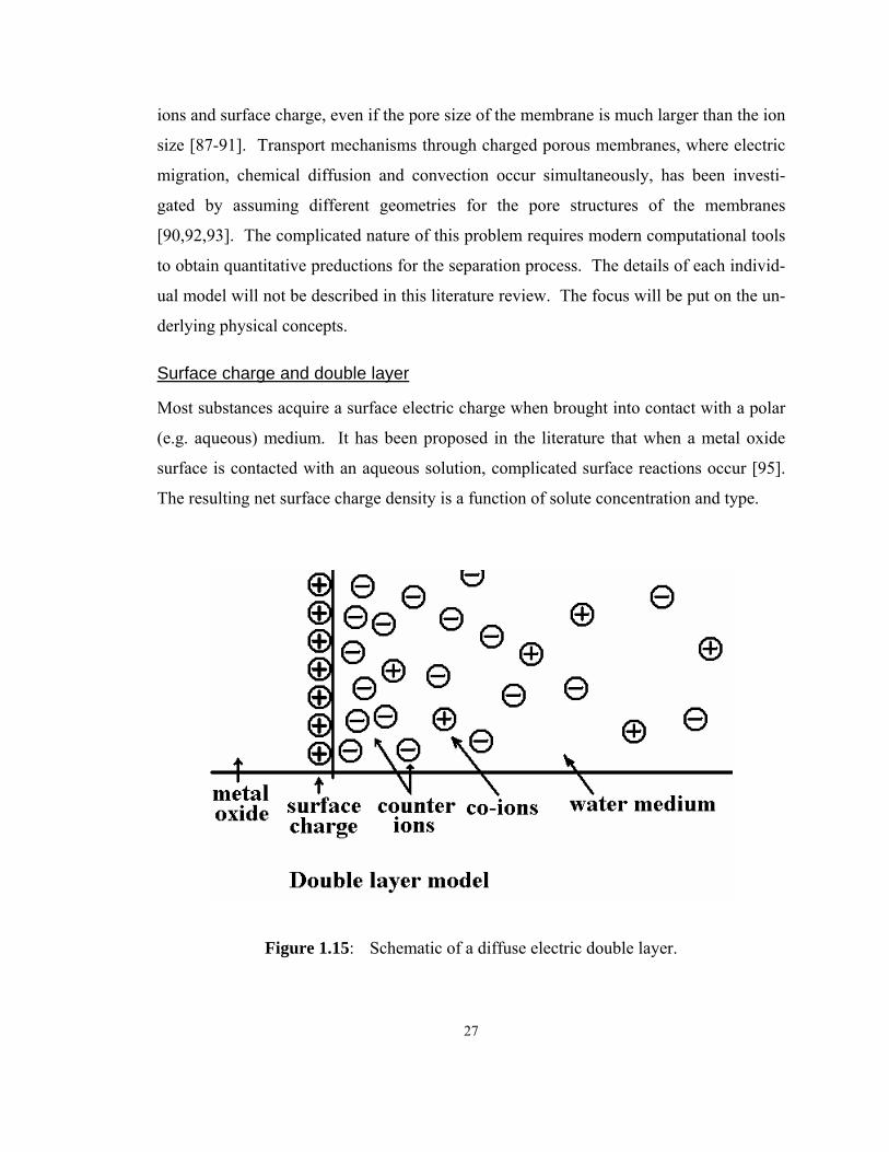
Surface charge and double layer

Most substances acquire a surface electric charge when brought into contact with a polar

(e.g. aqueous) medium. It has been proposed in the literature that when a metal oxide

surface is contacted with an aqueous solution, complicated surface reactions occur [95].

The resulting net surface charge density is a function of solute concentration and type.

Figure 1.15: Schematic of a diffuse electric double layer.

28

Once the surface obtains a net charge, it will influence the distribution of nearby ions.

Ions of opposite charge (counter-ions) are attracted towards the surface and ions of like

charge (co-ions) are repelled away from the surface. This, together with the randomizing

effect of thermal motion, leads to the formation of an electric double layer made up of the

charged surface and a neutralizing excess of counter-ions, distributed in a diffuse manner

[ 1.15].

Potential and concentration distribution

Quantitative treatment of the electric double layer is a difficult problem. However, with

various simplifications and approximations, this problem can be simplified and solved to

provide a reasonable level of sophistication and usefulness.

Figure 1.16: Concentration and potential profile for positively charged flat surface.

The simplest quantitative treatment of the diffuse part of the double layer is based on an

infinite extended, uniformly charged flat surface. It is shown that the potential decays

exponentially as a function of distance from the surface (x = 0) to the bulk solution

(x = +∞). The local concentrations of counter-ions and co-ions, which are functions of

the local potential, decrease or increase accordingly until the bulk concentration is

reached. A qualitative schematic representation of the potential and charge distribution is

shown in figure 1.16 for a positively charged surface. Here 1/κ is called the Debye

29

length, which is usually considered as the thickness of the double layer as shown in fig-

ure 1.16.

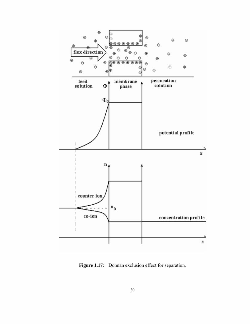
Donnan exclusion and extended Nernst-Planck model

To simplify the explanation, a capillary model will be taken to represent the pore struc-

ture of the membrane. After the membrane is immersed in an aqueous electrolyte solu-

tion, a spontaneous preferential adsorption occurs and net surface charge is formed on the

pore surface, which results in the presence of a potential and concentration profile. When

the pore diameter is small enough (1/κ has the magnitude of several tens to several hun-

dreds of nm), the potential profiles overlap significantly and so does the concentration

profile. Under such conditions, it is appropriate to consider the pore surface and the solu-

tion inside the pores as a spatial region with the same potential, Φ0. This potential (Φ0) is

higher (or lower) than the bulk solution (Φ=0 at x>>1/κ) for the case of a positively (or

negatively) charged surface (figure 1.17). The potential difference between the feed bulk

and the pore liquid is referred to as the Donnan potential [7].

30

Figure 1.17: Donnan exclusion effect for separation.

31

It is intuitively clear that the counter ion concentration is higher while the co-ion concen-

tration is lower in the mobile pore phase compared to the bulk phase. It can be seen that

the Donnan potential attracts counter ions from bulk phase to the membrane phase and

repulses the co-ions from the membrane phase to the bulk phase. Combined with the dif-

fusion movement of the ions, concentration profiles of counter-ions and co-ions, which

are similar to those of charged flat surface, will form from the membrane phase to the

bulk solution. When a pressure difference is applied across the membrane, the permeat-

ing liquid will flow through the pore. Due to the requirement of overall electrical neutral-

ity, the concentration of counter ion and the co-ion in the permeation flux must be equal.

However, the co-ion concentration in permeation flux can not be higher than that in its

source, which is the membrane phase. Therefore, the counter/co ions concentration in the

permeation flux has to be equal to the co-ion concentration in the membrane phase and

lower than that in the bulk phase. This is called the Donnan exclusion effect and it under-

lies the separation mechanism of meso-porous NF membranes.

The models based on the Donnan effect were able to qualitatively predict that the rejec-

tion is a function of the feed solution concentration, ionic valences, pH value, and surface

adsorption properties [94]. However, this model did not take into account the diffusive

and convective fluxes, which are also important for the separation mechanism. For in-

stance, when the potential and concentration profiles at the interface of the permeation

side and membrane phase are under consideration, a decaying curve rather than an abrupt

drop is more likely to occur. The extended Nernst-Planck model has recently been ap-

plied for a quantitative description of the transport phenomena in NF membranes. By

taking the diffusion and convection fluxes into account, the extended Nernst-Planck rela-

tion is able to predict the separation behavior much more accurately. Calculations of the

model always requires advanced computational techniques and normally leads to predic-

tive numerical solution with no adjustable parameters.

1.4 Conclusion and future work in the membrane area

Organic membrane and inorganic membrane have been reviewed and compared in this

chapter. Organic membrane is much easier to manufacture and becomes dominantly

32

commercialized. Inorganic membrane is more stable in extreme operation conditions,

such as high or low pH solution and better chloride tolerance. They are also believed to

have better resistance against particular and chemical impurities that present in water, and

therefore require less restrict pre-treatment for the feed water. Due to the inert nature of

inorganic materials, they have longer life time and can be regenerated and reused. How-

ever, the properties of inorganic membrane is more sensitive to defects and therefore, the

synthesis process of inorganic membrane is much more difficult than organic membranes.

This future work section is presented to summarize the review in the chapter and to pro-

vide a perspective for future research.

1. The field of commercial organic RO membranes is dominated by two types of

polymer compositions, polyamide and cellulose acetates. More than two decades

have passed since the development of the NS300 and FT30 polyamide composite

membranes, without a major new development in the composition. This field

may possibly have reached a maturity in terms of major membrane chemistries.

The research opportunities are now more in the areas of solvent-resistant supports,

improvements in salt rejections, improved fouling resistance and modeling [11]

2. Inorganic NF membranes hold considerable promise in applications such as water

purification, high temperature separation, catalytic membrane structures, and

membrane reactors. The related colloidal chemistry and sol-gel processing meth-

ods need further investigation. New membrane synthesis methods may be ex-

plored.

3. Membranes with new composition and structure should be explored. Application-

oriented membrane devices and modules should be designed, developed and op-

timized.

4. Modeling of membrane separation behavior is becoming an attractive research

area. With the development of insights in interfacial chemistry, more capable

models will be proposed. Determination of consistent and accurate membrane

transport parameters will help improving the reliability of the models.

33

CHAPTER 2

SYNTHESIS AND OPTIMIZATION OF HIGH SURFACE

QUALITY ALUMINA COMPACT MEMBRANE SUPPORT

Filtration casting is used to produce homogeneous porous α-Al2O3 disks with a high

quality surface, suitable for thin membrane deposition with thickness less than 100 nm.

This forming method combines the ability of conditioning a powder into a dilute disper-

sion of dense particles with a very efficient particle packing process, resulting in very

homogeneous compacts with at least one high quality surface. Aqueous slurries of

α-Al2O3 with solids content of 20 vol% and low viscosity were prepared by using a small

amount of dispersion stabilizer and introducing ultrasonic agitation treatment. Relatively

high green densities were obtained by vacuum filtration of dispersions with an optimized

concentration of stabilizer. The influence of dispersant concentration on surface mor-

phology of compacts is investigated by SEM. In addition mechanical strength, density,

water/gas permeability, as well as grain size have been studied to establish the proper sin-

tering temperature for specific membrane support applications.

2.1 Introduction

Inorganic ceramic membranes, based on alumina, mullite, cordierite, zirconia, silica and

titania are considered for several applications due to their excellent mechanical strength

and resistance to extremely harsh conditions (such as high or low pH, oxidizing condi-

tions and high temperatures). on the availability of such membranes enabled several new

developments such as include H2 [96] and O2 [97] separation, as well as water purifica-

34

tion [98]. Usually, inorganic ceramic membranes have an asymmetric multi-layer struc-

ture. Their foundation is a macro-porous support sufficiently permeable, strong and also

suitable for deposition of successive intermediate and membrane layers [99]. Application

of current ceramic membranes is hindered by insufficient flux at acceptable pressure dif-

ferences. This can be improved by developing thinner quasi-homogeneous membranes

with a film thickness down into the 10 nm range.

Because conventional forming methods such as the dry pressing and extrusion may lead

to micro-structural inhomogeneity and high surface roughness, the ceramic supports pre-

pared using the above-mentioned technique are inappropriate for application of very thin

and perfect membranes.

By insuring the break-down of soft agglomerates as well as removal of hard agglomer-

ated and other impurities in diluted particle dispersions, colloidal processing methods are

most suitable for preparing macro-porous defect free supports. Few studies have shown

that these methods result in minizing the occurrence of macro-defects in quasi-

homogeneous ceramic particle compact structures [100].

Colloidal processing of α-Al2O3 using charge stabilizers was extensively studied as a

convenient route to quasi-homogeneous structures [101-104]. The advantage of using

charge stabilizers is that they do not affect the viscosity of the dispersion therefore the

formation of random dense particle packing structures is promoted.

Recent studies on colloidal processing have focused at different aspects of colloidal com-

pact formation. Many efforts related to α-Al2O3 colloidal processing are dedicated to “di-

lute” state properties such as stability, rheology, and electro-kinetics [105-112]. Other

studies describe the sintering process of colloidal filtration compacts and the preparation

of fully dense, translucent alumina compacts [113-115]. In addition a few papers pay at-

tention to the “condensed” green or partially sintered compact [112, 116].

In the present study, the method of colloidal filtration is optimized for fine-porous

α-Al2O3 supports with a very smooth surface and a homogenous pore structure that en-

ables the deposition of uniform ceramic layers with a thickness of less than 100 nm.

35

2.2 Experimental procedures

Studies were carried out with two commercially available high purity α-Al2O3 powders,

AKP15 and AKP30, (Sumitomo Chemical Co. Ltd, Tokyo Japan) with an average parti-

cle size of 600 and 300 nm, respectively. Defect-free compacts could be obtained by col-

loidal filtration of α-Al2O3 dispersion with the optimum dispersant concentration. For the

preparation of AKP30 supports, 50 g of α-Al2O3 AKP30 powder was mixed with 50 mL

of HNO3 solution with concentration of 10-2 mol L-1 (pH=2.0) to have a 1.6 μmol-

HNO3/m2-α-Al2O3 powder. Dispersion of as-delivered alpha alumina powder was

achieved by ultra-sonic treatment (Model 102C, Branson, USA) for 10 minutes [117] at a

power level of 60 W. During this treatment, the temperature of the mixture was kept be-

low 20ºC by flowing tap water between the double walls of the glass treatment vessel.

For removing large agglomerates and other impurities the dispersions used for compact

formation were screened with a 20 μm aperture Nylon mesh after ultrasonic treatment. In

addition to avoid air born contamination the filtration procedure is carried out at

Class 100 cleaning room. Disk-shaped α-Al2O3 compacts were made by vacuum filtra-

tion on an Ø 220 nm pore polysulfone membrane (Millipore, Billerica, MA). The com-

pacts always had a dull (rough) surface at the filtration membrane side, while the oppo-

site (upper) surface of the most homogeneous compacts had a very smooth shiny appear-

ance. This compact surface is further referred to as “top surface”. The AKP15 supports

were prepared in the same manner except that the α-Al2O3 powder was AKP15 and the

dispersion agent was 50 ml aqueous solution of Aluminon at 0.2 wt%, with pH adjusted

by ammonia to 9.5.

The compacts encapsulated in alumina trays and cover plates were sintered in air, with a

heating/cooling rate of 2ºC/minute and the sintering temperature varying between 650

and 1350ºC with 10 hrs dwell time.

The compacts’ apparent density was investigated with a commercially available mercury

pycnometer (DBA100-1, PMI, Ithaca, NY) that was modified for improved accuracy. In

addition the influence of charge stabilizer concentration on compact formation was stud-

ied.

36

The AKP30 compacts are further indicated as S2.00pH750C to indicate the initial pH of

the dispersion and the sintering temperature, 2.00 and 750ºC, respectively, in this exam-

ple.

Water permeation was determined with the dead-end technique. While the compacts

were maintained at a constant applied pressure difference, Δp of 400 kPa, the accumu-

lated weight of pure water permeate was recorded as a function of time with an electronic

balance, and converted into mechanical permeability according to

VP

j Xkpη

=Δ

(2.1)

where jV is the volumetric flux, X the compact thickness in the permeation direction, and

η the dynamic viscosity, in this case of pure water.

In addition gas permeability was determined in a home-made setup, configured for the

non-stationary dead-end mode [118]. The sample mounted in a gas permeation cell was

kept at constant temperature inside a drying stove. A constant pressure of testing gas was

supplied at feed side. At the start of the measurement, gas passes through the compact

into a pre-evacuated reservoir with constant volume, Vcell. Assuming the ideal gas law to

be valid the gas permeability, k, is determined for isothermal conditions by non-linear

regression from:

0f

0f p cell

Rln p A Tk tp p X V

⎛ ⎞ ⎛ ⎞⎛ ⎞=⎜ ⎟ ⎜ ⎟⎜ ⎟⎜ ⎟− ⎝ ⎠⎝ ⎠⎝ ⎠ (2.2)

where k is the gas permeability, A the exposed homogenous support surface, R the gas

constant, T the absolute temperature, and t the relative time.

The microstructure of the top surface of the compacts as well as of the cross section per-

pendicular to the disk surface, made by fracture, grinding and polishing was investigated

with scanning electron microscopy (Field-Emission Environmental SEM Philips XL30).

To qualitatively analyze the homogeneity of alpha alumina compacts, a very thin slice of

compacts was cut by Focused Ion Beam (FIB) (Philips DB235 SEM) milling and imaged

with TEM (CM200).

37

2.3 Results and discussion

It is well known that for the application of membrane supports, high permeability and

strong mechanical strength are two desirable properties that are normally contradictory to

each other. Therefore, the strategy employed in our synthesis was that one of these two

properties was emphasized. For example, AKP30 supports have a low permeability since

the particle and pore sizes of such supports were small, therefore, HNO3 was used as dis-

persant agent to increase the mechanical strength. On the other hand, Aluminon prepared

supports were weaker and therefore, AKP15 was chosen as the particle to have larger

pore size and permeability.

The packing density and microstructure of colloidally prepared compacts can be influ-

ence by type as well as by the strength of the interaction between the ceramic particles in

suspension, described as electrostatic; steric or a combination of those. For AKP30 sup-

ports, nitric acid (HNO3) used in present study provides charge-type colloidal stabiliza-

tion by preferential proton-sorption. Direct observation of the influence of concentration

of charge stabilizer, expressed as pH = -log [HNO3], on colloidally compact formation

process has been summarized in table 2.1.

Initial pH Upper surface appearance Drying effects

1.0 Rough Little shrinkage; warping; release difficult

1.5 Smooth Release difficult

2.0 Smooth Some shrinkage; start to release easily

2.5 Smooth Significant shrinkage causing cracking

3.0 Smooth Significant cracking

38

Table 2.1: Direct observation of colloidal filtration compacts, initially stabilized in aqueous HNO3 at various pH values.

In the investigated pH interval (from 1.0 to 3.0) the radial shrinkage was found to in-

crease with the initial pH. According to the data shown in Table 1, optimized alpha alu-

mina compacts could be obtained only with initial nitric acid concentrations equal to

10-5mol g-1, based on the dry solid. At nitric acid concentrations, higher than the opti-

mum value, corresponding to pH values lower than 2, excessive warping was observed

during drying. Moreover high dispersant concentrations resulted in difficulties to release

the compact from the filtration mold after drying. In addition crack formation at very

high nitric acid concentrations has been also observed. The supernatant of the α-Al2O3

suspension stabilized at optimum dispersant concentration was found to contain

1300 ppm Al3+ and had a pH ~ 4. HNO3 tends to be most effective at a pH < 4, where

part of the α-Al2O3 and residual transition alumina structures start to dissolve [119].

While this dissolution may be an advantage in the breakdown of weak agglomerates, it

may affect sintering and eventual properties of the compacts [119].

Mercury Pycnometry results for AKP15 and AKP30 compacts obtained by colloidal fil-

tration of aqueous alumina suspension dispersed with Aluminon and HNO3, respectively,

and sintered at 650 C for 10 hrs are shown in figure 2.1. At each concentration, the den-

sity was taken from an average of at least five individual samples. Due to the reaction

between nitric acid and AKP30 the initial pH was found to change, but details about the

time dependence and location could not be obtained. Therefore the density plotted in

figure 2.1 is discussed only in terms of initial pH.

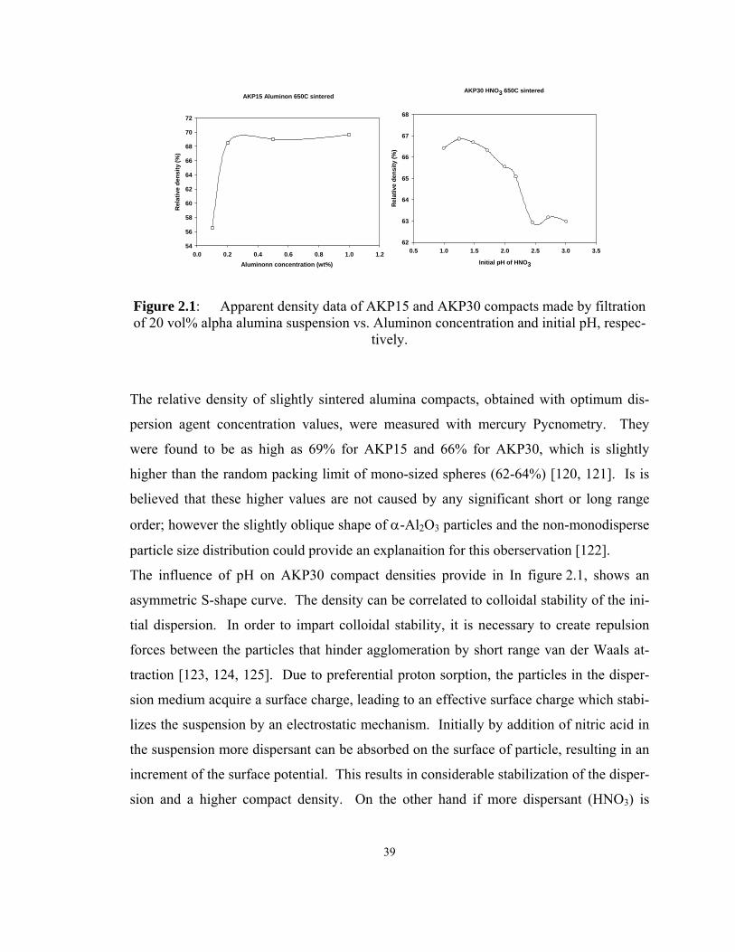
39

AKP15 Aluminon 650C sintered

Aluminonn concentration (wt%)0.0 0.2 0.4 0.6 0.8 1.0 1.2

Rel

ativ

e de

nsity

(%)

54

56

58

60

62

64

66

68

70

72

AKP30 HNO3 650C sintered

Initial pH of HNO3

0.5 1.0 1.5 2.0 2.5 3.0 3.5

Rel

ativ

e de

nsity

(%)

62

63

64

65

66

67

68

Figure 2.1: Apparent density data of AKP15 and AKP30 compacts made by filtration of 20 vol% alpha alumina suspension vs. Aluminon concentration and initial pH, respec-

tively.

The relative density of slightly sintered alumina compacts, obtained with optimum dis-

persion agent concentration values, were measured with mercury Pycnometry. They

were found to be as high as 69% for AKP15 and 66% for AKP30, which is slightly

higher than the random packing limit of mono-sized spheres (62-64%) [120, 121]. Is is

believed that these higher values are not caused by any significant short or long range

order; however the slightly oblique shape of α-Al2O3 particles and the non-monodisperse

particle size distribution could provide an explanaition for this oberservation [122].

The influence of pH on AKP30 compact densities provide in In figure 2.1, shows an

asymmetric S-shape curve. The density can be correlated to colloidal stability of the ini-

tial dispersion. In order to impart colloidal stability, it is necessary to create repulsion

forces between the particles that hinder agglomeration by short range van der Waals at-

traction [123, 124, 125]. Due to preferential proton sorption, the particles in the disper-

sion medium acquire a surface charge, leading to an effective surface charge which stabi-

lizes the suspension by an electrostatic mechanism. Initially by addition of nitric acid in

the suspension more dispersant can be absorbed on the surface of particle, resulting in an

increment of the surface potential. This results in considerable stabilization of the disper-

sion and a higher compact density. On the other hand if more dispersant (HNO3) is

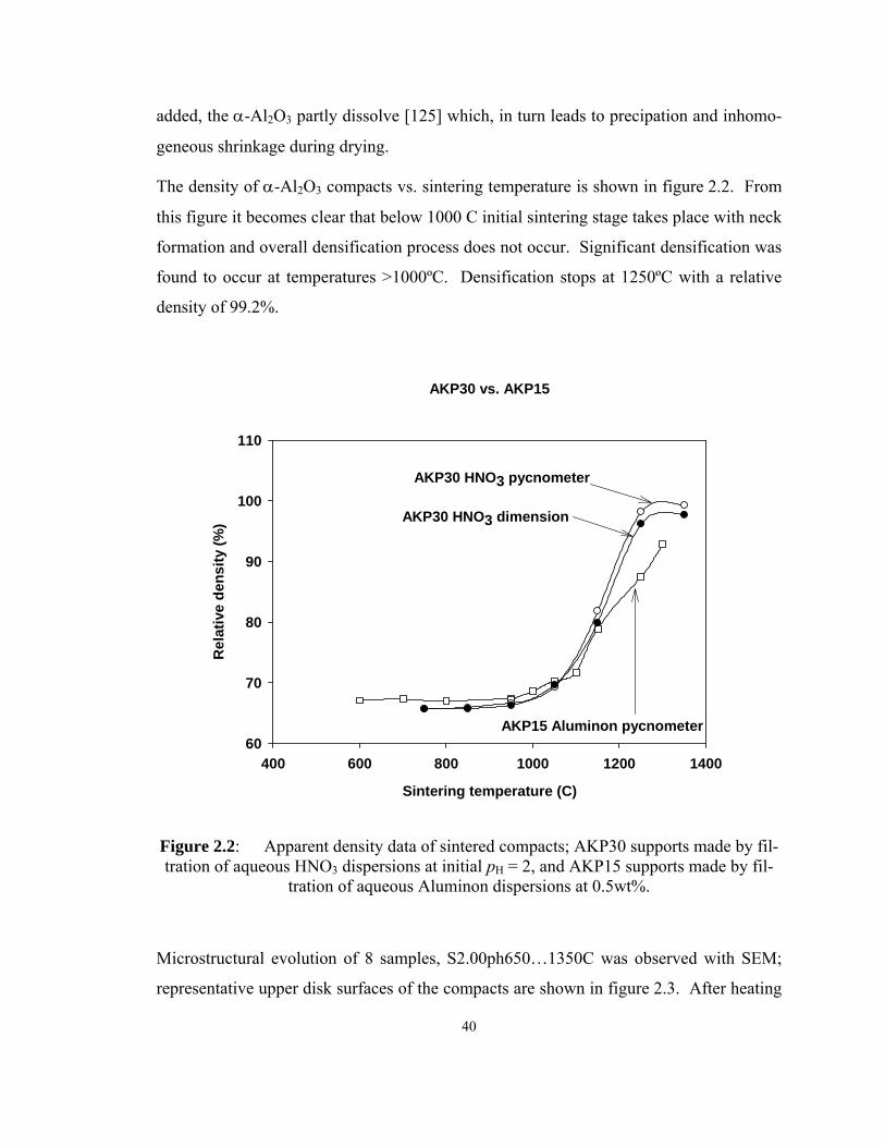
40

added, the α-Al2O3 partly dissolve [125] which, in turn leads to precipation and inhomo-

geneous shrinkage during drying.

The density of α-Al2O3 compacts vs. sintering temperature is shown in figure 2.2. From

this figure it becomes clear that below 1000 C initial sintering stage takes place with neck

formation and overall densification process does not occur. Significant densification was

found to occur at temperatures >1000ºC. Densification stops at 1250ºC with a relative

density of 99.2%.

AKP30 vs. AKP15

Sintering temperature (C)

400 600 800 1000 1200 1400

Rel

ativ

e de

nsity

(%)

60

70

80

90

100

110

AKP30 HNO3 pycnometer

AKP30 HNO3 dimension

AKP15 Aluminon pycnometer

Figure 2.2: Apparent density data of sintered compacts; AKP30 supports made by fil-tration of aqueous HNO3 dispersions at initial pH = 2, and AKP15 supports made by fil-

tration of aqueous Aluminon dispersions at 0.5wt%.

Microstructural evolution of 8 samples, S2.00ph650…1350C was observed with SEM;

representative upper disk surfaces of the compacts are shown in figure 2.3. After heating

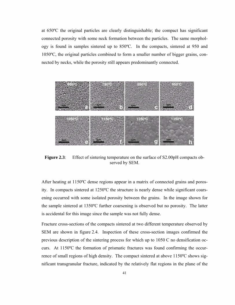
41

at 650ºC the original particles are clearly distinguishable; the compact has significant

connected porosity with some neck formation between the particles. The same morphol-

ogy is found in samples sintered up to 850ºC. In the compacts, sintered at 950 and

1050ºC, the original particles combined to form a smaller number of bigger grains, con-

nected by necks, while the porosity still appears predominantly connected.

Figure 2.3: Effect of sintering temperature on the surface of S2.00pH compacts ob-served by SEM.

After heating at 1150ºC dense regions appear in a matrix of connected grains and poros-

ity. In compacts sintered at 1250ºC the structure is nearly dense while significant coars-

ening occurred with some isolated porosity between the grains. In the image shown for

the sample sintered at 1350ºC further coarsening is observed but no porosity. The latter

is accidental for this image since the sample was not fully dense.

Fracture cross-sections of the compacts sintered at two different temperature observed by

SEM are shown in figure 2.4. Inspection of these cross-section images confirmed the

previous description of the sintering process for which up to 1050 C no densification oc-

curs. At 1150ºC the formation of prismatic fractures was found confirming the occur-

rence of small regions of high density. The compact sintered at above 1150ºC shows sig-

nificant transgranular fracture, indicated by the relatively flat regions in the plane of the

42

picture. Moreover it was clearly visible that at 1350 C the porosity is completely con-

verted in to closed and isolated.

(a)

(b)

Figure 2.4: SEM image of cross section of α-Al2O3 compacts (S2.00ph) sintered at (a) 1150 C and (b) 1350 C.

The water permeability of S2.00ph750…1150C is shown in figure 2.5. From this figure

can be observed that water permeability shows a maximum at a sintering temperature of

950 C. Such behavior could be explained by the occurrence of coarsening in combination

with little overall shrinkage. According to the Carman-Kozeny equation, valid for a

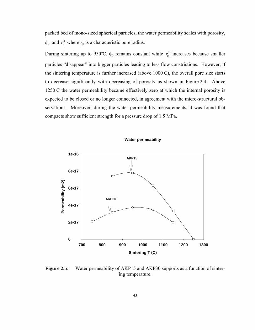
43

packed bed of mono-sized spherical particles, the water permeability scales with porosity,

φp, and 2pr where rp is a characteristic pore radius.

During sintering up to 950ºC, φp remains constant while 2pr increases because smaller

particles “disappear” into bigger particles leading to less flow constrictions. However, if

the sintering temperature is further increased (above 1000 C), the overall pore size starts

to decrease significantly with decreasing of porosity as shown in Figure 2.4. Above

1250 C the water permeability became effectively zero at which the internal porosity is

expected to be closed or no longer connected, in agreement with the micro-structural ob-

servations. Moreover, during the water permeability measurements, it was found that

compacts show sufficient strength for a pressure drop of 1.5 MPa.

Water permeability

Sintering T (C)

700 800 900 1000 1100 1200 1300

Perm

eabi

lity

(m2)

0

2e-17

4e-17

6e-17

8e-17

1e-16AKP15

AKP30

Figure 2.5: Water permeability of AKP15 and AKP30 supports as a function of sinter-ing temperature.

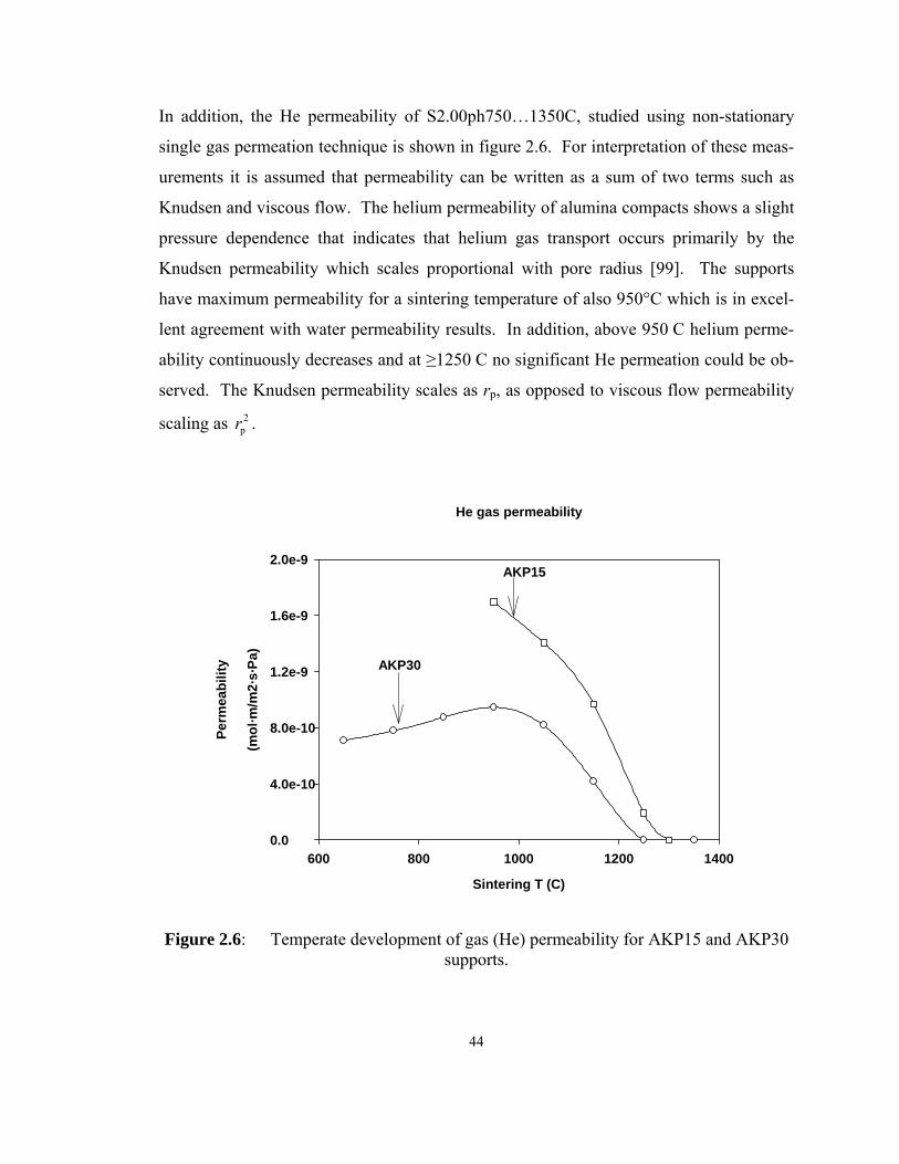
44

In addition, the He permeability of S2.00ph750…1350C, studied using non-stationary

single gas permeation technique is shown in figure 2.6. For interpretation of these meas-

urements it is assumed that permeability can be written as a sum of two terms such as

Knudsen and viscous flow. The helium permeability of alumina compacts shows a slight

pressure dependence that indicates that helium gas transport occurs primarily by the

Knudsen permeability which scales proportional with pore radius [99]. The supports

have maximum permeability for a sintering temperature of also 950°C which is in excel-

lent agreement with water permeability results. In addition, above 950 C helium perme-

ability continuously decreases and at ≥1250 C no significant He permeation could be ob-

served. The Knudsen permeability scales as rp, as opposed to viscous flow permeability

scaling as 2pr .

He gas permeability

Sintering T (C)

600 800 1000 1200 1400

Perm

eabi

lity

(mol

·m/m

2·s·

Pa)

0.0

4.0e-10

8.0e-10

1.2e-9

1.6e-9

2.0e-9AKP15

AKP30

Figure 2.6: Temperate development of gas (He) permeability for AKP15 and AKP30 supports.

45

α-Al2O3 compacts prepared using the above-mentioned optimized colloidal technique

posses a very smooth, homogeneous surface roughness that make them excellent candi-

dates for deposition of very thin inorganic film membrane on the order of <100 nm . As

an example, a well-defined membrane film with thickness around 50 nm [126] is shown

in figure 2.7. From Focused Ion Beam (FIB) cross sections of supported membranes,

observed by TEM it can be concluded that the surface roughness of compacts prepared

using colloidal filtration technique is estimated to be less than 20 nm. From figure 2.7 it

can be also seen that packing of α-Al2O3 particles, obtained using nitric acid as a charge

stabilizer, is quas-homogeneous over >100 nm length scales.

Figure 2.7: TEM images of FIB cross-sections of sintered S2.00pH compacts coated with zirconia based ceramic taken from [126].

The supported membrane structures as shown in figure 2.7 is considered to be a good

starting point for high-efficiency nano-filtration membranes and fuel cell structures. In

46

addition, it offers perspectives on the development of very thin membrane layers for

high-flux, high-selectivity gas separation.

2.4 Conclusions

Colloidal filtration of well-dispersed α-Al2O3 particles with effective particle size 300 nm

(AKP30) and 600 nm (AKP15) was successfully applied to produce defect-free, porous,

disk-shaped compacts with a superior quality of the upper disk surface. This surface is

suitable for deposition of continues film membranes with thickness of less than 100 nm.

Alumina compacts with a well-defined surface quality were obtained with sonification

and colloidal filtration of 50 wt% α-Al2O3 particles in aqueous solution of HNO3 at

pH 2.0 for AKP30 and, aqueous solution of 0.2 wt% Aluminon at pH 9.5 for AKP15.

Water and gas permeability, density as well as grain size can be used to establish the

proper sintering temperature for specific membrane support application. Both water and

gas permeability of optimized compacts show a maximum for a sintering temperature of

950ºC for AKP30 and AKP15, explained by the occurrence of pore-coarsening, com-

bined with little overall shrinkage. During the water permeability measurements, com-

pacts have shown sufficient strength for a pressure drop of 1.5 MPa for AKP30 and

1.0 MPa for AKP15. The optimized sintering temperatures were found to be 950 C for

AKP30 supports and 1050 C for AKP15 supports by taking the permeability and me-

chanical strength into consideration.

47

CHAPTER 3

OPTIMIZATION OF MESOPOROUS GAMMA ALUMINA

MEMBRANE SOL PREPARATION

Mesoporous γ-alumina membranes are been prepared with the well established and

documented sol-gel route [140]. To obtain a defect free membrane, it is critical to have a

nanoparticle solution available with a narrow particle size distribution and without any

other large particle contamination. An innovative ultrasound assisted screening process

was developed to purify Boehmite nanoparticle solutions that were used for the sol-gel

route of membrane preparation. Systematic studies have been carried out to compare the

treated sol quality. The chapter focuses on the ultrasound assisted screen process, which

was found to be a potential universal method for nanoparticle solution purification.

3.1 Introduction

The realization of unique physical properties of nano scale materials depends critically on

the possibility to produce homogeneous micro-structures with characteristic features in

the <100 nm size range. A viable approach to synthesize such materials consists of col-

loidal deposition of well-dispersed particles, followed by thermal processing. However,

practical syntheses of nanoparticle dispersions often lead to partial agglomeration and a

broad size distribution which has an unfavorable effect on the final result. It is therefore

interesting to develop size-based methods for efficient removal of agglomerates and large

particles. Many existing methods were primarily developed for bio-molecular or organic

supra-molecular applications and target dimensions in the 0.5…5 nm range. Recent pro-

48

gress in the application of these separation techniques to inorganic nanoparticles has ex-

tended their capabilities, however, with several limitations. For instance, chromatogra-

phy [127…129], field flow fractionation [130,131], and capillary electrophoresis

[134,135] can only process low particle concentrations or small volumes of liquid. As a

result these methods are used, primarily, as characterization techniques rather than as

manufacturing/processing methods. The solvent/anti-solvent precipitation method

[132,133] is very system-dependent and normally consumes large amounts of solvent.

High speed centrifugation has long been used as an initial purification step after nanopar-

ticle synthesis. However, this method also removes part of the smaller particles and

therefore inevitably reduces the yield. Another drawback of centrifuge method is that the

sediment formed by the particles re-disperses quickly into the supernatant after the centri-

fuge’s rotation stops, which has a negative effect of the quality of the treated sol.

Traditional screening by filtration has also been widely applied for purification of disper-

sions. However, the application of this method for polydisperse and agglomerated

nanoparticle dispersions gives rise to several technical difficulties, such as clogging of

the filter and poor size selectivity [136]. These problems, on the other hand, can be over-

come by employing an ultrasound-assisted filtration setup similar to the one described in

[137] and a carefully chosen meso-porous straight pore membrane as the filter. For in-

stance, anodic aluminum membranes offer a 20 nm pore size; much larger pore density

and hence larger yield than the track etched membrane used in [137].

The purpose of the present paper is to demonstrate the merits of ultrasound-assisted-

screening in the purification of nanoparticle suspensions, using anodic alumina mem-

branes with pores sizes, tailored to the primary particle size. A Boehmite sol, prepared

by the well-established Yoldas route [138] is used for the purpose of demonstration.

Such sols have a relatively wide particle size distribution in the range of

10 nm…1000 nm, and are used, for instance, in the preparation of thin supported

γ-alumina membranes with a pore Ø of approximately 4 nm [139]. To prepare homoge-

neous membranes with a narrow pore size distribution, all particles with a diameter

>20 nm need to be removed [139]. In [140] it is shown how removal of larger particles

and agglomerates by centrifugation at 59,000g for 3 hours results in major improvement

49

of membrane quality. This result led us to use this centrifugation treatment as a reference

for comparison with the ultra-sound-assisted screening method.

3.2 Experimental Section

A concentrated Boehmite nanoparticle sol was prepared by hydrolysis of ATSB, followed

by peptization [138]. The screening filter is suspended with its edge clamped to the fun-

nel to allow for maximum transverse vibration in the filter plane. This avoids the forma-

tion of a layer of clogged particles to maintain a stable filtrate flux. It is critical that no

solid mechanical support is present directly below the filter material so that the ultra-

sound can propagate unconstrained in the filter/sol interface. Therefore, only a small

pressure difference could be applied to promote the filtration flow without disrupting the

filter. This pressure difference was maintained at approximately 15 mBar and <30 mBar

in any case by using the pressure controller of a Buchi rotovaper system [R-205V,

Brinkmann].

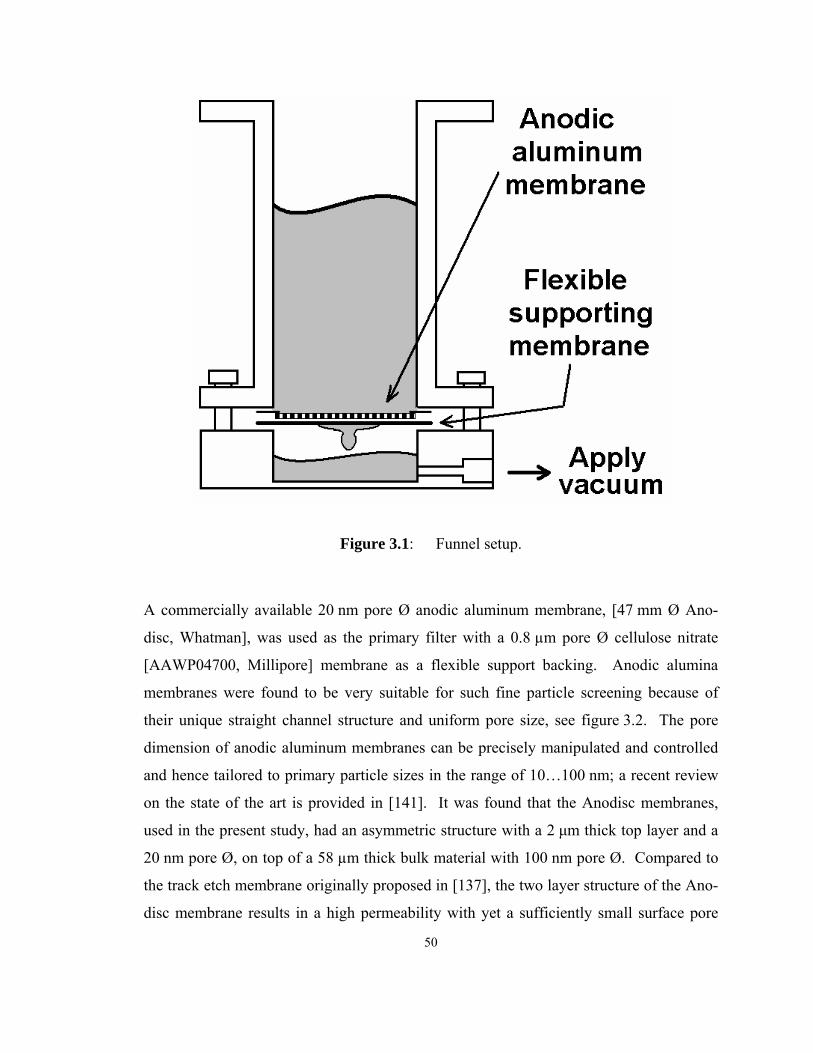
50

Figure 3.1: Funnel setup.

A commercially available 20 nm pore Ø anodic aluminum membrane, [47 mm Ø Ano-

disc, Whatman], was used as the primary filter with a 0.8 µm pore Ø cellulose nitrate

[AAWP04700, Millipore] membrane as a flexible support backing. Anodic alumina

membranes were found to be very suitable for such fine particle screening because of

their unique straight channel structure and uniform pore size, see figure 3.2. The pore

dimension of anodic aluminum membranes can be precisely manipulated and controlled

and hence tailored to primary particle sizes in the range of 10…100 nm; a recent review

on the state of the art is provided in [141]. It was found that the Anodisc membranes,

used in the present study, had an asymmetric structure with a 2 μm thick top layer and a

20 nm pore Ø, on top of a 58 µm thick bulk material with 100 nm pore Ø. Compared to

the track etch membrane originally proposed in [137], the two layer structure of the Ano-

disc membrane results in a high permeability with yet a sufficiently small surface pore

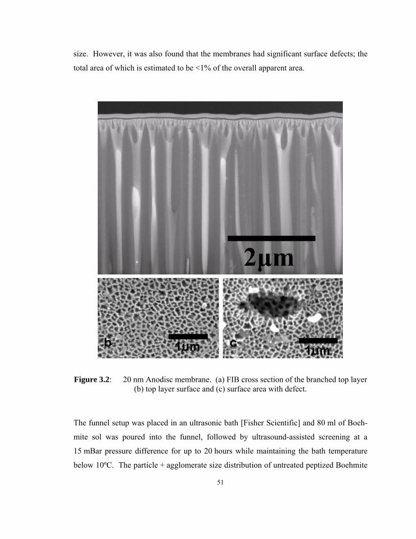
51

size. However, it was also found that the membranes had significant surface defects; the

total area of which is estimated to be <1% of the overall apparent area.

Figure 3.2: 20 nm Anodisc membrane. (a) FIB cross section of the branched top layer (b) top layer surface and (c) surface area with defect.

The funnel setup was placed in an ultrasonic bath [Fisher Scientific] and 80 ml of Boeh-

mite sol was poured into the funnel, followed by ultrasound-assisted screening at a

15 mBar pressure difference for up to 20 hours while maintaining the bath temperature

below 10ºC. The particle + agglomerate size distribution of untreated peptized Boehmite

52

sol (O-γ), centrifuged sol (C-γ), screened sols with (U-γ) and without (F-γ) ultrasound-

assistance, were characterized with Atomic Force Microscopy (AFM) [multimode Nano-

scope IIIa, Veeco] with a silicon tip of 5…10 nm radius [NSC18, MikroMasch] and Dy-

namic Light Scattering (DLS) [BI-200SM, Brookhaven]. The as-prepared sols were di-

luted with aqueous HNO3 at pH = 3.5 to a concentration of 2×10-3 g/ml for DLS meas-

urements and further diluted with 18.2 MΩ·cm high purity water [Mili-Q A10 Gradient

System, Millipore] to a concentration of 5×10-5 g/ml for AFM sample preparation. The

AFM sample was prepared by spin coating on a 1 cm×1 cm mica surface by application

of one droplet of 5×10-5 g/ml sol at 200 rpm. All sample preparation was carried out at

class 100 clean room conditions to avoid airborne particle contamination. The Boehmite

content of all sols was obtained by determination of the weight of the gel formed after

drying at 70ºC for 2 days.

An ion chromatograph [ICS2500 Ion Chromatograph, Dionex] was utilized to test the

contamination that is introduced into the sols during the screening process. Before intro-

ducing the sol into the ion chromatograph, it was filtered with a 0.1ºµm nitrate-cellulose

membrane [VCWP02500, Millipore] to remove most of the particles to minimize the risk

of clogging ion the chromatograph column [IonPac AS19 Analytical Column, Dionex].

3.3 Results and Discussion

3.3.1 Solid load and filtration rate comparison

Figure 3.3 shows a comparison of the yield of the filtration process with and without ul-

trasonic agitation. This comparison shows clearly that without ultrasonic vibration, the

filter clogs very soon and the filtration process stops. The reproducibility of the filtration

yield measurement was not very good due to large variations in the properties of the as-

delivered Anodisc membranes. Nevertheless, ultrasound-assisted filtration always exhib-

ited a significantly higher filtration rate which is be explained by a reduction of the clog-

ging effect. During the screening process, a standing wave formed on the surface of the

membrane that could be made visible by adding insoluble black particles into the funnel,

53

as shown in figure 3.4. The formation of this standing wave likely avoids particle clog-

ging and thus results in a sustained, stable and high flow rate for a prolonged period.

Time (min)0 500 1000 1500 2000 2500

Col

lect

ed V

olum

e (m

L)

0

10

20

30

40

50U - γF - γ

Figure 3.3: Yield of the filtration process with and without the presence of ultrasonic vibration.

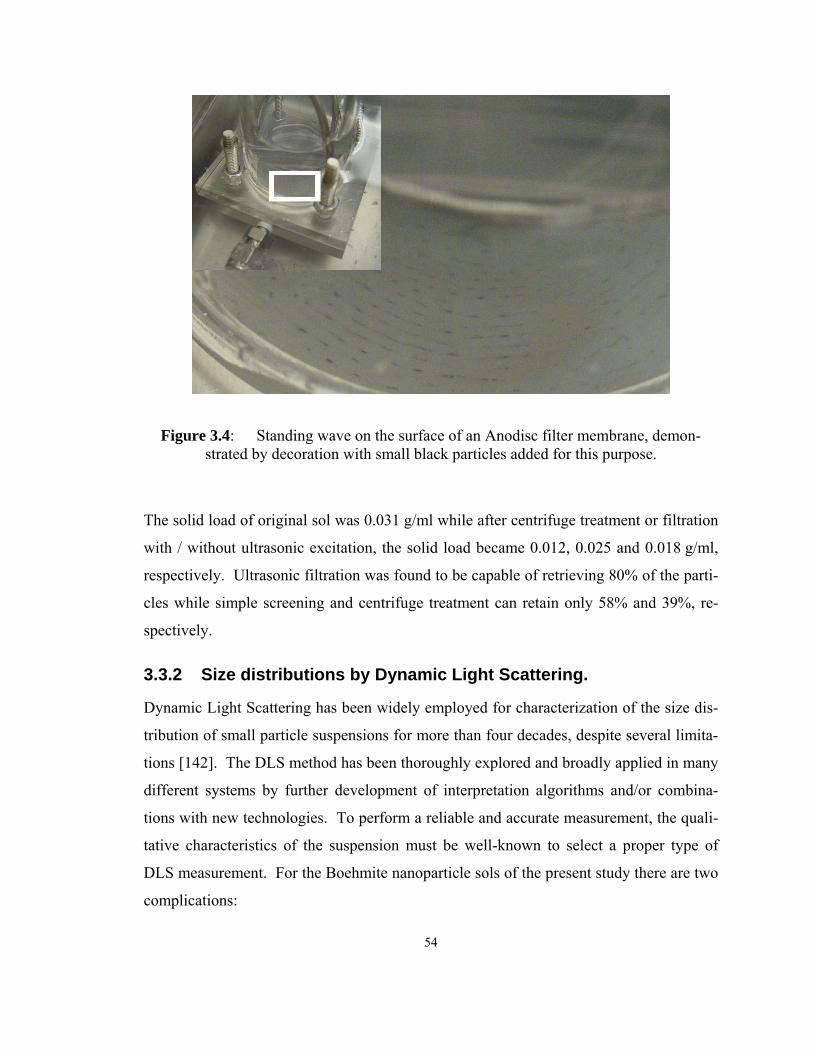
54

Figure 3.4: Standing wave on the surface of an Anodisc filter membrane, demon-strated by decoration with small black particles added for this purpose.

The solid load of original sol was 0.031 g/ml while after centrifuge treatment or filtration

with / without ultrasonic excitation, the solid load became 0.012, 0.025 and 0.018 g/ml,

respectively. Ultrasonic filtration was found to be capable of retrieving 80% of the parti-

cles while simple screening and centrifuge treatment can retain only 58% and 39%, re-

spectively.

3.3.2 Size distributions by Dynamic Light Scattering.

Dynamic Light Scattering has been widely employed for characterization of the size dis-

tribution of small particle suspensions for more than four decades, despite several limita-

tions [142]. The DLS method has been thoroughly explored and broadly applied in many

different systems by further development of interpretation algorithms and/or combina-

tions with new technologies. To perform a reliable and accurate measurement, the quali-

tative characteristics of the suspension must be well-known to select a proper type of

DLS measurement. For the Boehmite nanoparticle sols of the present study there are two

complications:

55

• The particle shape is non-spherical. From the AFM measurements, discussed in

section 3.3, it is concluded that platelets are present with ~20 nm Ø and a thick-

ness ~3 nm. This aspect is further discussed at the AFM measurements.

• The particle size distribution is bimodal with the major fraction of particles hav-

ing a largest dimension of ~20 nm and the minor fraction a largest dimension of

~500 nm.

Detection of a bimodal particle size distributions by multi-angle DLS is described in

[143,144]. However, a widely accepted algorithm for solving the multi-angle autocorre-

lation functions is still under development. On the other hand, combinations of state of

art interpretation algorithms, and single angle DLS measurements can result in fairly ac-

curate bimodal distributions, provided two criteria are met:

• The size difference between the two modes must be large: Øbig/Øsmall > 2.

• The intensity of the light, scattered by the two particle modes must be similar: Is-

trong/Iweak < 20) [145].

Fortunately, our Boehmite nanoparticle suspensions were found to meet these require-

ments and therefore, a single angle measurement at 90º with a conventional CONTIN in-

terpretation algorithm [146] could be used to characterize the particle size distribution of

each sol. 5 sets of data were selected for each sol and averaged to produce the results,

shown in figure 3.5. This figure indicates that O-γ has a wide, multi-modal particle size

distribution in the range of 10…1000 nm. The centrifuge treatment appears to be capable

of removing part of the big agglomerates in O-γ; however, there is still a substantial

amount of coarse particles in the range of 250…400 nm left. This is ascribed to the

re-dispersion of sediments shortly after the centrifuge treatment stopped. On the other

hand, U-γ showed a much smaller DLS intensity for the same large particle population,

while in F-γ that intensity is virtually absent. The larger particles, present in U-γ, are

likely due to migration of agglomerates through defects in the Anodisc membrane as

shown in figure 3.2(c). The absence of larger agglomerates in F-γ is explained by plug-

ging of surface defects in the Anodisc screen in the absence of ultrasonic agitation. It is

expected that this plugging occurs due to the initially very high particle flux at the de-

fects. To verify that the occurrence of larger particles was not due to agglomeration over

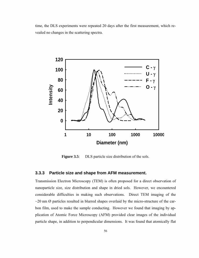
56

time, the DLS experiments were repeated 20 days after the first measurement, which re-

vealed no changes in the scattering spectra.

Diameter (nm)1 10 100 1000 10000

Inte

nsity

0

20

40

60

80

100

120C - γU - γF - γO - γ

Figure 3.5: DLS particle size distribution of the sols.

3.3.3 Particle size and shape from AFM measurement.

Transmission Electron Microscopy (TEM) is often proposed for a direct observation of

nanoparticle size, size distribution and shape in dried sols. However, we encountered

considerable difficulties in making such observations. Direct TEM imaging of the

~20 nm Ø particles resulted in blurred shapes overlaid by the micro-structure of the car-

bon film, used to make the sample conducting. However we found that imaging by ap-

plication of Atomic Force Microscopy (AFM) provided clear images of the individual

particle shape, in addition to perpendicular dimensions. It was found that atomically flat

57

mica provided a very suitable substrate because the mica surface is hydrophilic and nega-

tively charged at pH = 3.5. This is thought to be beneficial in the formation of an imme-

diate strong adhesion of the positively charged Boehmite particles. It is speculated that

the application of the dispersions by spin coating resulted in an instantaneous removal of

liquid, such that the particles did not have time to agglomerate during drying. Examples

of tapping mode AFM images of C-γ on mica and silica are provided in figure 3.6 and

figure 3.7, clearly demonstrating the effect of the substrate on agglomeration during

deposition.

Figure 3.6: C-γ spin coated on mica.

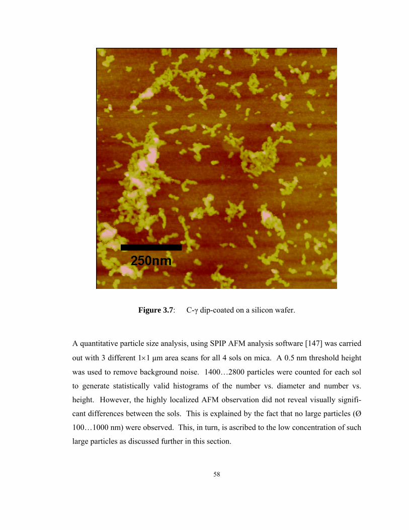
58

Figure 3.7: C-γ dip-coated on a silicon wafer.

A quantitative particle size analysis, using SPIP AFM analysis software [147] was carried

out with 3 different 1×1 μm area scans for all 4 sols on mica. A 0.5 nm threshold height

was used to remove background noise. 1400…2800 particles were counted for each sol

to generate statistically valid histograms of the number vs. diameter and number vs.

height. However, the highly localized AFM observation did not reveal visually signifi-

cant differences between the sols. This is explained by the fact that no large particles (Ø

100…1000 nm) were observed. This, in turn, is ascribed to the low concentration of such

large particles as discussed further in this section.

59

Under the SPIP software platform, a tip characterization command was carried out for

each image followed by a tip deconvolution command to compensate for the convolution

effect of the finite tip size of 5~10 nm. On average, the tip characterization command,

using default settings, reported a tip size of 4…7 nm. A threshold value of 1±0.1 nm was

applied for particle size analysis. This threshold value was fine-tuned to isolate closely

located particles without introducing too much apparent size reduction for the particle

measurement. The collected 3D information of each recognized particle was then sorted

and classified according to its diameter. The differential particle volume vs diameter was

generated for each sol and the 4 curves obtained in this way are shown in figure 3.8.

From this figure it is clear that each sol has similar characteristics in the small size region

(<20 nm), while O-γ has significantly more particle volume in the larger size region

(30…60 nm). The particles sizes detected by AFM ranged from 2.2 nm to 60 nm and

belonged to the group of smaller particles (<100 nm) detected in the DLS measurements.

This is explained by the fact that the particle concentration decreases dramatically as the

size increases so that many more microscopic images are needed to detect just one such

particle, and even more to obtain a statistically correct analysis for larger particles. In

practice, it was virtually impossible to obtain relevant population data from AFM for the

larger particle group (100…1000 nm) as found in the DLS measurements. A simple es-

timation shows that, for a well prepared AFM sample, one needs to examine 100 µm2

area to find one 100 nm particle and 1 mm2 area for one 1000 nm particle. Despite their

rarity, the larger particles play a key role in the formation of defects (pinholes) in thin

porous films and supported membranes.

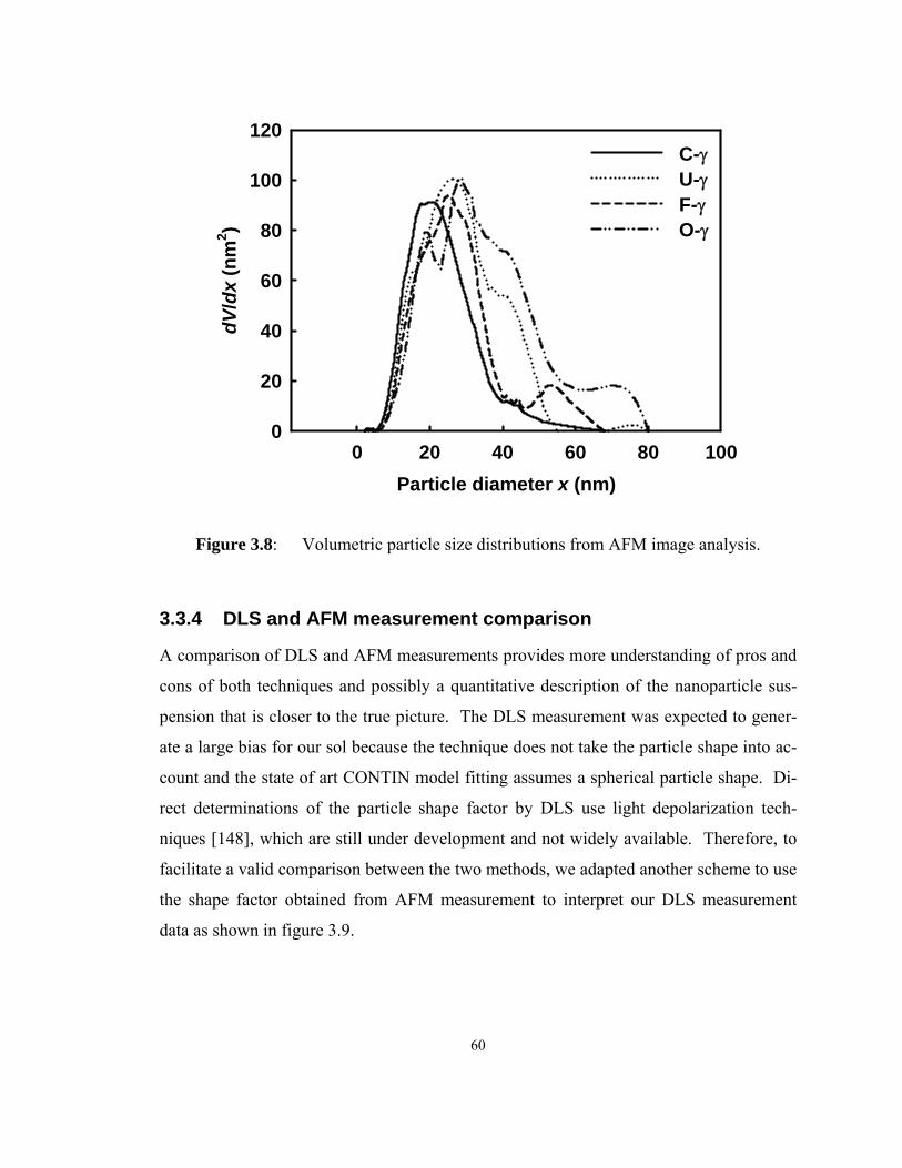
60

Particle diameter x (nm)0 20 40 60 80 100

dV/ d

x (n

m2 )

0

20

40

60

80

100

120C-γU-γF-γO-γ

Figure 3.8: Volumetric particle size distributions from AFM image analysis.

3.3.4 DLS and AFM measurement comparison

A comparison of DLS and AFM measurements provides more understanding of pros and

cons of both techniques and possibly a quantitative description of the nanoparticle sus-

pension that is closer to the true picture. The DLS measurement was expected to gener-

ate a large bias for our sol because the technique does not take the particle shape into ac-

count and the state of art CONTIN model fitting assumes a spherical particle shape. Di-

rect determinations of the particle shape factor by DLS use light depolarization tech-

niques [148], which are still under development and not widely available. Therefore, to

facilitate a valid comparison between the two methods, we adapted another scheme to use

the shape factor obtained from AFM measurement to interpret our DLS measurement

data as shown in figure 3.9.

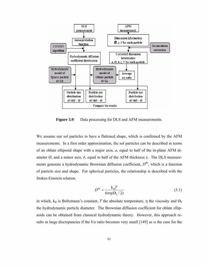
61

Figure 3.9: Data processing for DLS and AFM measurements.

We assume our sol particles to have a flattened shape, which is confirmed by the AFM

measurements. In a first order approximation, the sol particles can be described in terms

of an oblate ellipsoid shape with a major axis, a, equal to half of the in-plane AFM di-

ameter Ø, and a minor axis, b, equal to half of the AFM thickness z. The DLS measure-

ments generate a hydrodynamic Brownian diffusion coefficient, DBr, which is a function

of particle size and shape. For spherical particles, the relationship is described with the

Stokes-Einstein relation.

Br B

h

k6 (Ø / 2)

TD =πη

(3.1)

in which, kB is Boltzmann’s constant, T the absolute temperature, η the viscosity and Øh

the hydrodynamic particle diameter. The Brownian diffusion coefficient for oblate ellip-

soids can be obtained from classical hydrodynamic theory. However, this approach re-

sults in large discrepancies if the b/a ratio becomes very small [149] as is the case for the

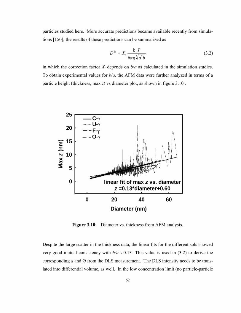
62

particles studied here. More accurate predictions became available recently from simula-

tions [150]; the results of these predictions can be summarized as

Br Bt 3 2

k6

TD Xa b

=πη

(3.2)

in which the correction factor Xt depends on b/a as calculated in the simulation studies.

To obtain experimental values for b/a, the AFM data were further analyzed in terms of a

particle height (thickness, max z) vs diameter plot, as shown in figure 3.10 .

Diameter (nm)0 20 40 60

Max

z (n

m)

0

5

10

15

20

25 C-γU-γF-γO-γ

linear fit of max z vs. diameterz =0.13*diameter+0.60

Figure 3.10: Diameter vs. thickness from AFM analysis.

Despite the large scatter in the thickness data, the linear fits for the different sols showed

very good mutual consistency with b/a ≈ 0.13 This value is used in (3.2) to derive the

corresponding a and Ø from the DLS measurement. The DLS intensity needs to be trans-

lated into differential volume, as well. In the low concentration limit (no particle-particle

63

interaction) and using assumptions of a spherical particle shape and a particle size that is

small compared to wave length, the intensity of light scattered from one particle, Is, can

be expressed as [151]

2s n iI K C V= × × (3.3)

in which K is a factor that depends on the incident beam intensity, wave length, scattering

angle and other instrument parameters. Cn is the particle concentration and Vi is the vol-

ume of one single particle of a particular size i. To derive a similar equation for oblate

ellipsoids is beyond the scope of this work; therefore, we will just use equation (3.3) to

calculate our relative differential volume values. The correction for the oblate particle

shape is carried out for particles with Øp < 100 nm only. Any particles larger than that

are very likely agglomerations for which a spherical shape can be assumed. Figure 3.11

shows the curves after rescaling, using a particle refractive index of 1.624 for the real part

and 0 the imaginary part [152]. It is clearly shown that with the oblate model, the esti-

mated particle diameter (2×a) is slightly larger than the hydrodynamic diameter. The

volumetric average particle volume is used to calculate an average spherical diameter for

each sol, as is summarized in table 3.1:

64

dV/d

Ø

0

50

100

dV/d

Ø

0.00.10.2

DLS Sphere ModelDLS Oblate ModelAFM measurement

dV/d

Ø

0

50

100

dV/d

Ø

0.00.10.2

dV/d

Ø

0

50

100

dV/d

Ø

0.00.10.2

Ø (particle diameter in nm)1 10 100 1000 10000

dV/d

Ø

0

50

100

dV/d

Ø

0.00.10.2

C-γ

O-γ

F-γ

U-γ

Figure 3.11: Differential accumulated volume vs. particle Ø for each sol, using the spherical and the oblate model.

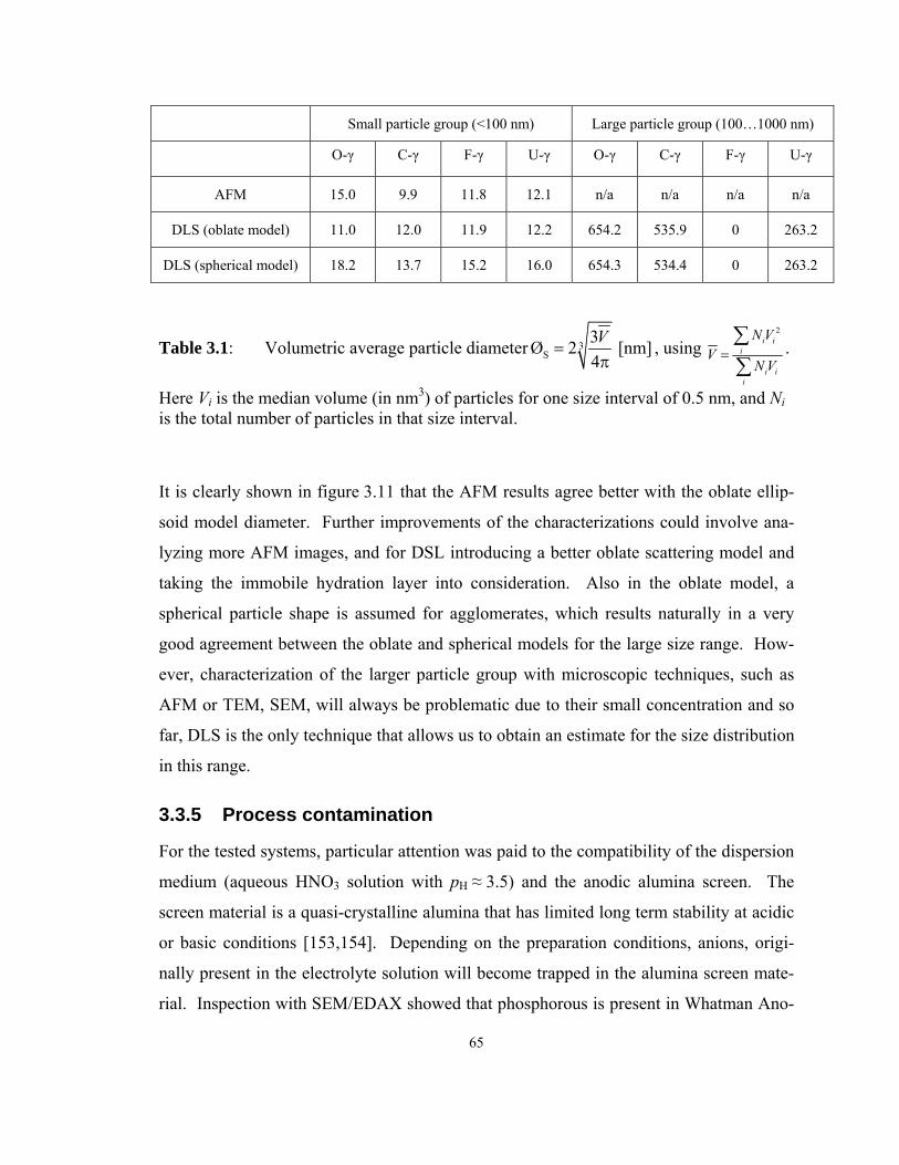
65

Small particle group (<100 nm) Large particle group (100…1000 nm)

O-γ C-γ F-γ U-γ O-γ C-γ F-γ U-γ

AFM 15.0 9.9 11.8 12.1 n/a n/a n/a n/a

DLS (oblate model) 11.0 12.0 11.9 12.2 654.2 535.9 0 263.2

DLS (spherical model) 18.2 13.7 15.2 16.0 654.3 534.4 0 263.2

Table 3.1: Volumetric average particle diameter 3S

3Ø 2 [nm]4V

=π

, using 2

i ii

i ii

N VV

N V=∑∑

.

Here Vi is the median volume (in nm3) of particles for one size interval of 0.5 nm, and Ni is the total number of particles in that size interval.

It is clearly shown in figure 3.11 that the AFM results agree better with the oblate ellip-

soid model diameter. Further improvements of the characterizations could involve ana-

lyzing more AFM images, and for DSL introducing a better oblate scattering model and

taking the immobile hydration layer into consideration. Also in the oblate model, a

spherical particle shape is assumed for agglomerates, which results naturally in a very

good agreement between the oblate and spherical models for the large size range. How-

ever, characterization of the larger particle group with microscopic techniques, such as

AFM or TEM, SEM, will always be problematic due to their small concentration and so

far, DLS is the only technique that allows us to obtain an estimate for the size distribution

in this range.

3.3.5 Process contamination

For the tested systems, particular attention was paid to the compatibility of the dispersion

medium (aqueous HNO3 solution with pH ≈ 3.5) and the anodic alumina screen. The

screen material is a quasi-crystalline alumina that has limited long term stability at acidic

or basic conditions [153,154]. Depending on the preparation conditions, anions, origi-

nally present in the electrolyte solution will become trapped in the alumina screen mate-

rial. Inspection with SEM/EDAX showed that phosphorous is present in Whatman Ano-

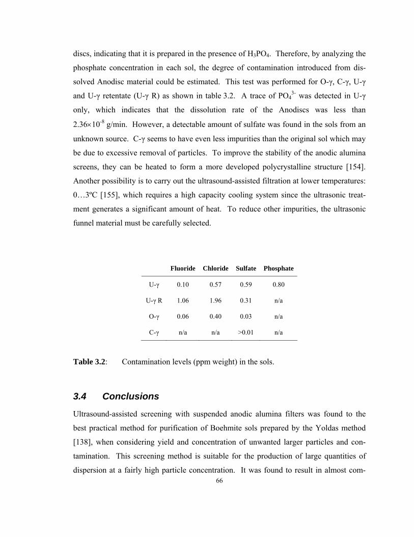
66

discs, indicating that it is prepared in the presence of H3PO4. Therefore, by analyzing the

phosphate concentration in each sol, the degree of contamination introduced from dis-

solved Anodisc material could be estimated. This test was performed for O-γ, C-γ, U-γ

and U-γ retentate (U-γ R) as shown in table 3.2. A trace of PO43- was detected in U-γ

only, which indicates that the dissolution rate of the Anodiscs was less than

2.36×10-8 g/min. However, a detectable amount of sulfate was found in the sols from an

unknown source. C-γ seems to have even less impurities than the original sol which may

be due to excessive removal of particles. To improve the stability of the anodic alumina

screens, they can be heated to form a more developed polycrystalline structure [154].

Another possibility is to carry out the ultrasound-assisted filtration at lower temperatures:

0…3ºC [155], which requires a high capacity cooling system since the ultrasonic treat-

ment generates a significant amount of heat. To reduce other impurities, the ultrasonic

funnel material must be carefully selected.

Fluoride Chloride Sulfate Phosphate

U-γ 0.10 0.57 0.59 0.80

U-γ R 1.06 1.96 0.31 n/a

O-γ 0.06 0.40 0.03 n/a

C-γ n/a n/a >0.01 n/a

Table 3.2: Contamination levels (ppm weight) in the sols.

3.4 Conclusions

Ultrasound-assisted screening with suspended anodic alumina filters was found to the

best practical method for purification of Boehmite sols prepared by the Yoldas method

[138], when considering yield and concentration of unwanted larger particles and con-

tamination. This screening method is suitable for the production of large quantities of

dispersion at a fairly high particle concentration. It was found to result in almost com-

67

plete removal of particles, larger than 100 nm. Screening without ultrasound resulted in a

more complete removal of large agglomerates but had a very low yield. To further im-

prove the performance of the screening process, the ultra-sound intensity and frequency

might be optimized, or different agitation methods can be considered such as stirring very

close to the filter surface. This should lead to a minimization of particle accumulation at

the membrane surface while, at the same time, the particles keep plugging the membrane

defects. Another approach might involve anodic membranes with straight pores only,

instead of the branching structure used in the present studies. Ultra-sonic assisted screen-

ing resulted in a small particle (<100 nm) distribution similar to that of purification by

ultra-centrifugation, but resulted in less larger particles. This suggests that colloidal

deposition of sols, purified by ultra-sonic assisted screening will lead to the formation of

higher quality thin films. AFM and DLS measurement can be combined to obtain a de-

tailed analysis of the distribution of particle size and shape. AFM has the advantage of

providing detailed information on the particle shape and size distribution, however, lacks

the capability of detecting particle size groups that are present at relatively low concen-

trations. DLS is particularly sensitive in the large size range; however, interpretation of

the DLS results can be ambiguous due to fact that unique solution for the autocorrelation

functions are not yet available. On the other hand, DLS samples a relatively large disper-

sion volume, which provides better statistically averaged data than the AFM method.

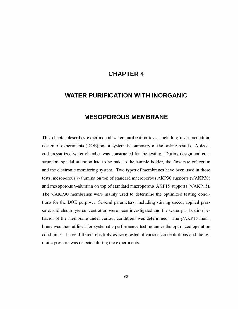
68

CHAPTER 4

WATER PURIFICATION WITH INORGANIC

MESOPOROUS MEMBRANE

This chapter describes experimental water purification tests, including instrumentation,

design of experiments (DOE) and a systematic summary of the testing results. A dead-

end pressurized water chamber was constructed for the testing. During design and con-

struction, special attention had to be paid to the sample holder, the flow rate collection

and the electronic monitoring system. Two types of membranes have been used in these

tests, mesoporous γ-alumina on top of standard macroporous AKP30 supports (γ/AKP30)

and mesoporous γ-alumina on top of standard macroporous AKP15 supports (γ/AKP15).

The γ/AKP30 membranes were mainly used to determine the optimized testing condi-

tions for the DOE purpose. Several parameters, including stirring speed, applied pres-

sure, and electrolyte concentration were been investigated and the water purification be-

havior of the membrane under various conditions was determined. The γ/AKP15 mem-

brane was then utilized for systematic performance testing under the optimized operation

conditions. Three different electrolytes were tested at various concentrations and the os-

motic pressure was detected during the experiments.

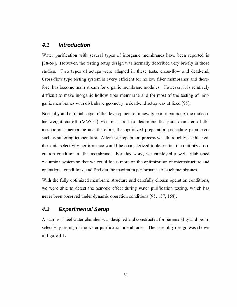
69

4.1 Introduction

Water purification with several types of inorganic membranes have been reported in

[38-59]. However, the testing setup design was normally described very briefly in those

studies. Two types of setups were adapted in these tests, cross-flow and dead-end.

Cross-flow type testing system is every efficient for hollow fiber membranes and there-

fore, has become main stream for organic membrane modules. However, it is relatively

difficult to make inorganic hollow fiber membrane and for most of the testing of inor-

ganic membranes with disk shape geometry, a dead-end setup was utilized [95].

Normally at the initial stage of the development of a new type of membrane, the molecu-

lar weight cut-off (MWCO) was measured to determine the pore diameter of the

mesoporous membrane and therefore, the optimized preparation procedure parameters

such as sintering temperature. After the preparation process was thoroughly established,

the ionic selectivity performance would be characterized to determine the optimized op-

eration condition of the membrane. For this work, we employed a well established

γ-alumina system so that we could focus more on the optimization of microstructure and

operational conditions, and find out the maximum performance of such membranes.

With the fully optimized membrane structure and carefully chosen operation conditions,

we were able to detect the osmotic effect during water purification testing, which has

never been observed under dynamic operation conditions [95, 157, 158].

4.2 Experimental Setup

A stainless steel water chamber was designed and constructed for permeability and perm-

selectivity testing of the water purification membranes. The assembly design was shown

in figure 4.1.

70

Figure 4.1: Water purification chamber design.

The chamber was pressurized with a nitrogen gas tank up to 1.5 MPa. An autoclave stir-

rer was installed to introduce sufficient agitation under pressurized conditions. This me-

chanical stirring was inevitable for a dead-end setup because, during operation, the accu-

mulated ions at the feed side of the membrane must be mixed back in the bulk of the feed

to reduce external mass transfer limitations effect. The membrane holder was designed to

have two outlets, for center flow and edge leak flow. The center flow collected purified

water that passed through the membrane layer and support perpendicularly. The edge

flow collected possible water leakage through the membrane sealing and the rough sur-

71

face region and avoided internal pressure build up. This configuration prevented mixing

of the edge leakage stream to the center flow and thus, avoided contamination of the cen-

ter flow. The collected water in the center flow was then directed to a container that was

continuously weighted with a digital analytic balance. The reading of the balance was

simultaneously transferred to a computer. Additional data that were automically col-

lected consisted of:

• the pressure of the chamber,measured with a digital pressure gauge,

• the temperature of the feed solution, measured with a thermocouple probe,

• the rotation speed of the stirrer measured with a tachometer installed in the stirrer ax-

ial.

All the data was monitored and recorded with National Instruments Labview™ software.

After one round of experiments was done, the collected sample was tested with ion

chromatography for to obtain ion concentrations in the feed. The entire water purifica-

tion membrane testing setup is shown in figure 4.2.

72

Figure 4.2: Water purification membrane testing setup.

4.3 Operational Condition Determination

The membrane utilized for the optimized operation testing condition was mesoporous

γ-alumina on top of standard macroporous AKP30 supports (γ/AKP30), due to the avail-

ability of such membrane at the early stage of the experiments. NaCl aqueous solutions

of various concentrations at pH 4.6 were used as the testing electrolyte. The applied

pressure was 0.7…17 MPa (10…250 PSI). Membrane performance was characterized

with two parameters; permeability and permselectivity. The permeability is definedas:

PX dVk

A p dtη

=Δ

(4.1)

where, η is the viscosity of the solution, X is the thickness of the membrane, A is the ap-

parent surface of the membrane, Δp is the pressure difference between the feed side and

73

the permeate side, and dVdt

is the flow rate. Permeability is a characteristic property of a

specific membrane, which is independent of the testing conditions. To characterize the

permselectivity, the rejection was used, defined as follows:

f

p

1 cRc

= − (4.2)

where, cf is the feed side electrolyte concentration and cp the permeate side concentration.

By studying the R value under various operation conditions, one can determine the water

purification behavior of the membrane. The first investigated operation condition is the

stirring rate as shown in the figure 4.3.

Aqueous NaCl@pH 4.6, Δp=1.38 MPa

Stirrer speed (rpm)0 500 1000 1500 2000 2500 3000 3500

Rej

ectio

n

0.0

0.2

0.4

0.6

0.8

1.00.001 M

0.01 M

0.1 M

Figure 4.3: Rejection under various stirring conditions for aqueous NaCl solutions.

74

It is easily understood that a larger stirring speed causes a better mixing and less external

mass transfer limitations at the feed side of the membrane and therefore, generated better

rejection until the stirring effect reaches a saturation plateau region. For dilute electrolyte

solutions, the plateau region was reached at a lower stirring speed. In order to be consis-

tent, a 2000 rpm stirring speed was chosen for the later systematic studies to guarantee

sufficient mixing for all experiments.

A similar plateau type rejection vs. flow velocity behavior was found for the membrane

data shown in figure 4.4. This type of purification behavior was found for many mem-

branes and electrolyte systems. As the pressure increased, the flow velocity and rejection

increased until it reached a plateau value. This phenomenon was used as a guideline to

determine the maximum rejection. More comprehensive results will be presented in the

next section when multiple electrolytes are compared.

75

Aqueous NaCl @ pH 4.6

Flow velocity (m/s)0 5e-6 1e-5 2e-5 2e-5 3e-5 3e-5

Rej

ectio

n

0.0

0.2

0.4

0.6

0.8

1.00.001 M

0.01 M

0.1 M

Figure 4.4: Rejection vs flow velocity for aqueous NaCl solutions.

To achieve the best performance, the applied pressure should be as high as possible to

obtain a high rejection and flowrate. This implies that mechanical strength of the mem-

brane becomes the limiting factor if the cost of generating high pressure is not taken into

account.

4.4 Membrane Performance Summary

Once the optimized operational conditions were determined for mesoporous γ-alumina

membranes, systematic water purification tests were carried out for the routinely prepared

one layer γ-alumina/AKP15 support membrane structure. It was noticed that the chemi-

cal stability of such a membrane is not sufficient for prolonged operation under standard

water purification conditions, i.e. an electrolyte solution at pH = 4.6. Tested electrolytes

76

included CaCl2 and AlCl3. Only with AlCl3 solutions, the membrane showed a com-

pletely stable performance because in that case the process of γ-alumina dissolution is

fully suppressed. Therefore, a new series of electrolyte tests was carried out with the ad-

dition of a small amount of AlCl3.

4.4.1 Permeability comparison

The permeability value for each layer of the membrane was calculated and compared.

The permeability of the supports could be determined directly with stand-alone supports,

while the permeability of the γ-alumina layer could be determined with a series resistor

model described as follows. In case one or more support (u) layers are present, in addi-

tion to a functional membrane (m) at the feed side, the permeability of each layer and the

total permeability are related by:

max-1 max1 1 1 2

1 max

1 max

u /u pf m/u m/u u /uf ptot,m ,u ,utot

m u u

p pp p p pp pj k k k k

X X X X−− −−

= = = = = (4.3)

where, j is the flux; c, ,mk ,1,uk , and

max,uk are the permeability of the entire membrane

device including every layer, the top membrane layer, the layer u1, and the layer umax, re-

spectively; fp , pp , 1m/up , and

1 2u /up etc. are the pressure at the feed side, permeate side,

interface between membrane layer and the u1 layer, and interface between u1 layer and u2

layer etc., respectively; totX , mX , 1uX , and

maxuX are the thickness of the entire mem-

brane device including every layer, the membrane top layer, the u1 layer and the umax

layer, respectively. Determination of k for one layer from totk , requires knowledge of

the thickness of all layers, and the k of all other layers. The latter should be obtained

from other experiments with identical quasi-homogeneous layers in simpler structures.

As an example we show the calculation of ,γk of 1 γ-alumina membrane (γ) layer on 1

α-Al2O3 support (α) layer with known permeability ,αk .

77

f p / pf /tot, ,tot

p p p pp pj k k k

X X Xα γα γ

γ αγ α

− −−= = = (4.4)

tottot

,,tot tot tot

, , ,

X X k kXX kk k k X k X k

γ γ ααγ

γ α α α

= + → =−

(4.5)

In an initial experiment, Xtot = 2.0225×10-3 m, totk = 2.7125×10-17 m2,

Xα ≈ Xtot = 2.0225×10-3 m, ,k α = 3.1499×10-17 m2, Xγ≈0.8×10-6 m. Substitution of these

values in (4.5) leads to kγ = 7.7267×10-20 m2. The same permeation experiments have

been carried out at different pressures for the supports. The permeability is found to be

independent from the applied pressure as expected.

From the perspective of membrane technology, it would be valuable to find the resistance

from each layer of the membrane device. The resistance of a layer was defined as:

Pη

p XRj k AΔ

= = (4.6)

Even though the γ-alumina layer had very low permeability, because it was significantly

thinner than the support, it only contributed to ½ to ⅓ of the total resistance of the mem-

brane. This can be further reduced to approximately half of the current value if a thinner

layer was made. The results are summarized in table 4.1. Any given membrane device

would be a combination of γ-alumina and AKP30 or γ-alumina and AKP15.

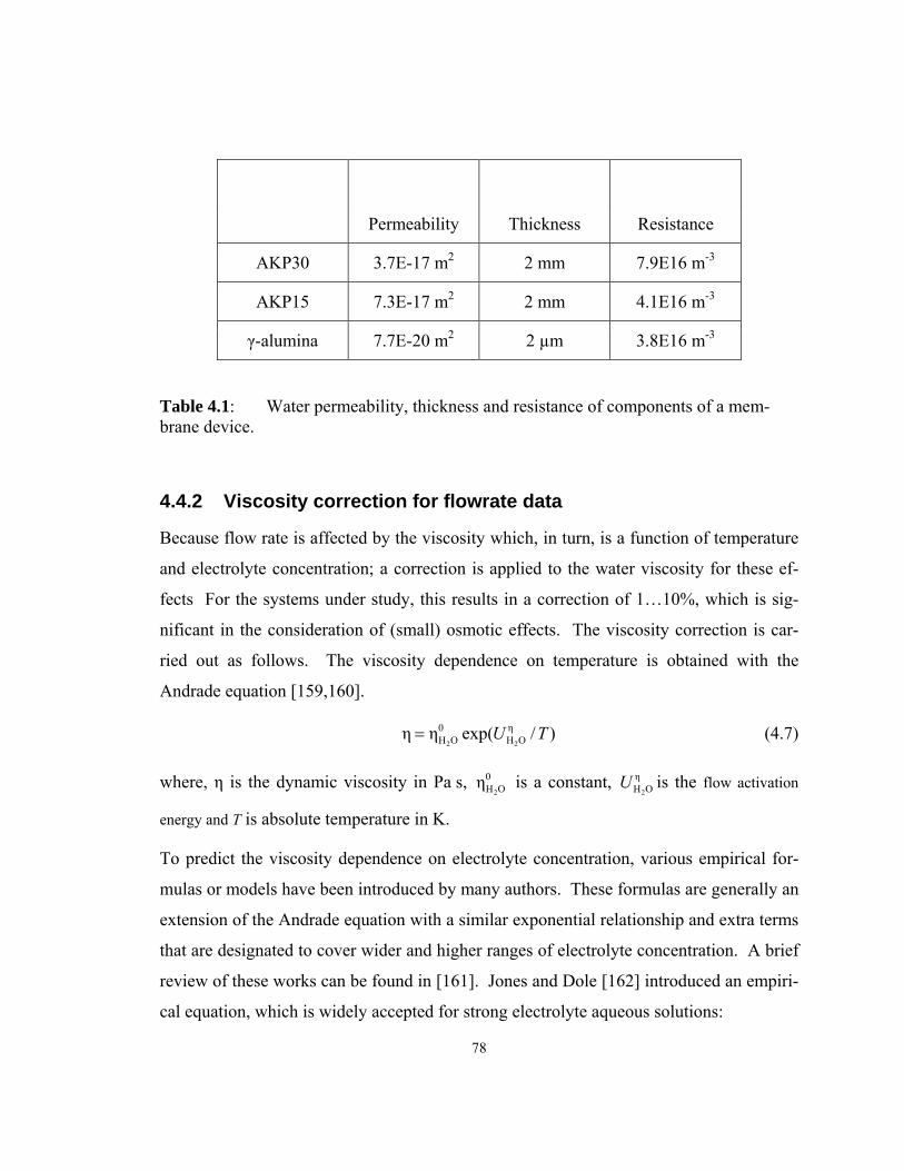
78

Permeability Thickness Resistance

AKP30 3.7E-17 m2 2 mm 7.9E16 m-3

AKP15 7.3E-17 m2 2 mm 4.1E16 m-3

γ-alumina 7.7E-20 m2 2 µm 3.8E16 m-3

Table 4.1: Water permeability, thickness and resistance of components of a mem-brane device.

4.4.2 Viscosity correction for flowrate data

Because flow rate is affected by the viscosity which, in turn, is a function of temperature

and electrolyte concentration; a correction is applied to the water viscosity for these ef-

fects For the systems under study, this results in a correction of 1…10%, which is sig-

nificant in the consideration of (small) osmotic effects. The viscosity correction is car-

ried out as follows. The viscosity dependence on temperature is obtained with the

Andrade equation [159,160].

2 2

0 ηH O H Oη η exp( / )U T= (4.7)

where, η is the dynamic viscosity in Pa s, 2

0H Oη is a constant,

2

ηH OU is the flow activation

energy and T is absolute temperature in K.

To predict the viscosity dependence on electrolyte concentration, various empirical for-

mulas or models have been introduced by many authors. These formulas are generally an

extension of the Andrade equation with a similar exponential relationship and extra terms

that are designated to cover wider and higher ranges of electrolyte concentration. A brief

review of these works can be found in [161]. Jones and Dole [162] introduced an empiri-

cal equation, which is widely accepted for strong electrolyte aqueous solutions:

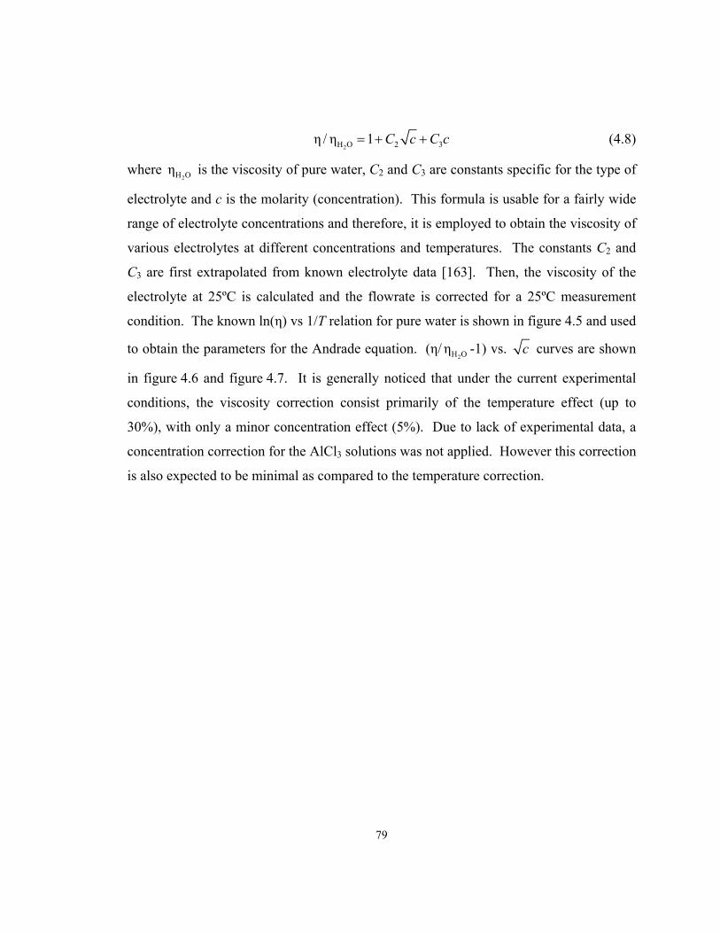
79

2H O 2 3η / η 1 C c C c= + + (4.8)

where 2H Oη is the viscosity of pure water, C2 and C3 are constants specific for the type of

electrolyte and c is the molarity (concentration). This formula is usable for a fairly wide

range of electrolyte concentrations and therefore, it is employed to obtain the viscosity of

various electrolytes at different concentrations and temperatures. The constants C2 and

C3 are first extrapolated from known electrolyte data [163]. Then, the viscosity of the

electrolyte at 25ºC is calculated and the flowrate is corrected for a 25ºC measurement

condition. The known ln(η) vs 1/T relation for pure water is shown in figure 4.5 and used

to obtain the parameters for the Andrade equation. (η/2H Oη -1) vs. c curves are shown

in figure 4.6 and figure 4.7. It is generally noticed that under the current experimental

conditions, the viscosity correction consist primarily of the temperature effect (up to

30%), with only a minor concentration effect (5%). Due to lack of experimental data, a

concentration correction for the AlCl3 solutions was not applied. However this correction

is also expected to be minimal as compared to the temperature correction.

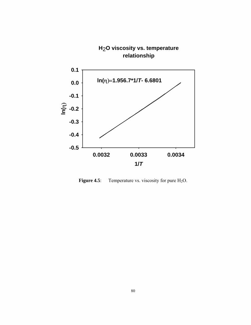
80

H2O viscosity vs. temperaturerelationship

1/T0.0032 0.0033 0.0034

ln( η)

-0.5

-0.4

-0.3

-0.2

-0.1

0.0

0.1

ln(η)=1.956.7*1/T- 6.6801

Figure 4.5: Temperature vs. viscosity for pure H2O.

81

viscosity vs. NaCl concentration

c^0.50.0 0.2 0.4 0.6

η/η H

2O-1

-0.01

0.00

0.01

0.02

0.03

0.04

2H Oη / η 1 0.0056 0.0889c c− = +

Figure 4.6: Viscosity vs concentration for aqueous NaCl.

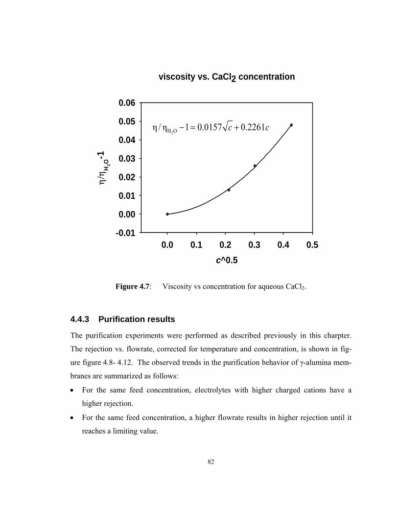
82

viscosity vs. CaCl2 concentration

c^0.50.0 0.1 0.2 0.3 0.4 0.5

η/η H

2O-1

-0.01

0.00

0.01

0.02

0.03

0.04

0.05

0.06

2H Oη / η 1 0.0157 0.2261c c− = +

Figure 4.7: Viscosity vs concentration for aqueous CaCl2.

4.4.3 Purification results

The purification experiments were performed as described previously in this charpter.

The rejection vs. flowrate, corrected for temperature and concentration, is shown in fig-

ure figure 4.8- 4.12. The observed trends in the purification behavior of γ-alumina mem-

branes are summarized as follows:

• For the same feed concentration, electrolytes with higher charged cations have a

higher rejection.

• For the same feed concentration, a higher flowrate results in higher rejection until it

reaches a limiting value.

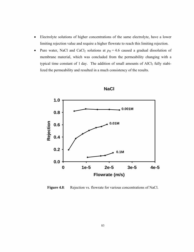
83

• Electrolyte solutions of higher concentrations of the same electrolyte, have a lower

limiting rejection value and require a higher flowrate to reach this limiting rejection.

• Pure water, NaCl and CaCl2 solutions at pH = 4.6 caused a gradual dissolution of

membrane material, which was concluded from the permeability changing with a

typical time constant of 1 day. The addition of small amounts of AlCl3 fully stabi-

lized the permeability and resulted in a much consistency of the results.

NaCl

Flowrate (m/s)0 1e-5 2e-5 3e-5 4e-5

Rej

ectio

n

0.0

0.2

0.4

0.6

0.8

1.0

0.001M

0.01M

0.1M

Figure 4.8: Rejection vs. flowrate for various concentrations of NaCl.

84

CaCl2

Flowrate (m/s)0 1e-5 2e-5 3e-5 4e-5

Rej

ectio

n

0.0

0.2

0.4

0.6

0.8

1.00.0007M

0.007M

0.021M

0.07M

Figure 4.9: Rejection vs. flowrate for various concentrations of CaCl2.

85

NaCl+1wt%AlCl3

Flowrate (m/s)0 1e-5 2e-5 3e-5 4e-5

Rej

ectio

n

0.0

0.2

0.4

0.6

0.8

1.00.001M

0.01M

0.1M

Figure 4.10: Rejection vs. flowrate for various concentrations of NaCl+1%AlCl3.

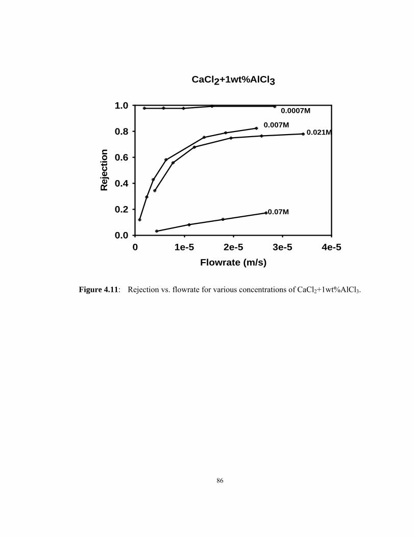
86

CaCl2+1wt%AlCl3

Flowrate (m/s)0 1e-5 2e-5 3e-5 4e-5

Rej

ectio

n

0.0

0.2

0.4

0.6

0.8

1.0 0.0007M

0.007M0.021M

0.07M

Figure 4.11: Rejection vs. flowrate for various concentrations of CaCl2+1wt%AlCl3.

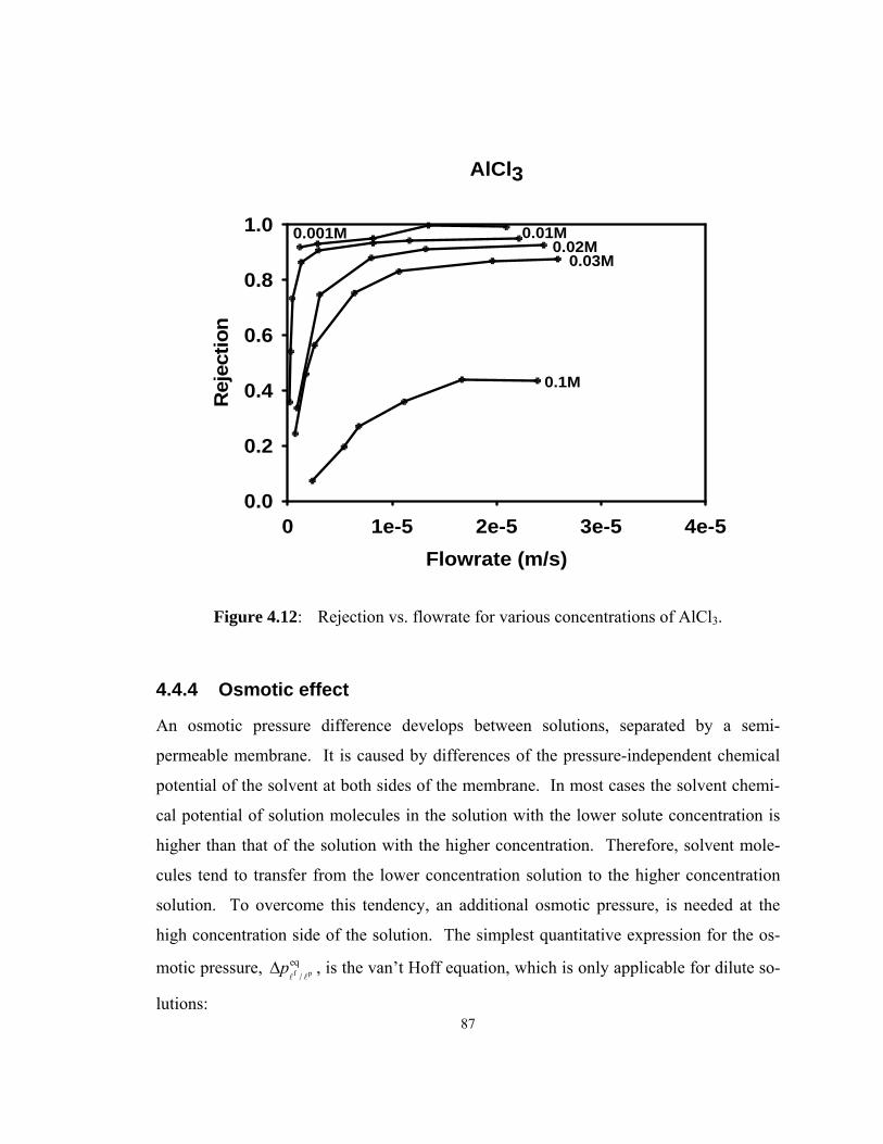
87

AlCl3

Flowrate (m/s)0 1e-5 2e-5 3e-5 4e-5

Rej

ectio

n

0.0

0.2

0.4

0.6

0.8

1.0 0.001M 0.01M0.02M

0.03M

0.1M

Figure 4.12: Rejection vs. flowrate for various concentrations of AlCl3.

4.4.4 Osmotic effect

An osmotic pressure difference develops between solutions, separated by a semi-

permeable membrane. It is caused by differences of the pressure-independent chemical

potential of the solvent at both sides of the membrane. In most cases the solvent chemi-

cal potential of solution molecules in the solution with the lower solute concentration is

higher than that of the solution with the higher concentration. Therefore, solvent mole-

cules tend to transfer from the lower concentration solution to the higher concentration

solution. To overcome this tendency, an additional osmotic pressure, is needed at the

high concentration side of the solution. The simplest quantitative expression for the os-

motic pressure, f peq

/pΔ , is the van’t Hoff equation, which is only applicable for dilute so-

lutions:

88

f peq

/Rp c TΔ = (4.9)

Here M, R, and T are the molarity concentration of the solutions, gas constant

(8.314472 J K-1 mol-1), and absolute temperature (K), respectively. However, the van’t

Hoff equation is not applicable at higher concentrations because in that case the free en-

ergy of solvent starts to deviate from linear dependence on concentration. Therefore, to

accurately predict the osmotic effect, the thermodynamic properties of the solution sys-

tem must be thoroughly understood. Such studies for aqueous systems have been exten-

sively investigated both experimentally and theoretically. Regardless of the recent pro-

gress in this area, Pitzer and Mayorga's work [164-166] in the 1970s remains the most

concise and accurate method for describing low to intermediate concentration (<6M)

electrolyte solutions which are used in this study. The formulation is introduced below

for a pure electrolyte M X

M Xv v with tabulated parameters for NaCl, CaCl2, and AlCl3.

f peq

/φ Rp c TΔ = (4.10)

( )3/ 2φ φ 2 φ22φ 1 M XM X

M X MX MX

v vv vz z f m B m Cv v

⎡ ⎤⎛ ⎞− = + + ⎢ ⎥⎜ ⎟⎝ ⎠ ⎢ ⎥⎣ ⎦

(4.11)

1/ 2

φφ1/ 21

A If

bI−

=+

(4.12)

( ) ( ) ( )0 1φ 1/ 2β β exp αMX MX MXB I= + − (4.13)

3/ 21/ 2 2

AV W el

B

2 N q13 1000 k

ATϕ

⎛ ⎞π ρ⎛ ⎞= ⎜ ⎟⎜ ⎟ ε⎝ ⎠ ⎝ ⎠ (4.14)

89

( )0βMX ( )1βMX φMXC

NaCl [168] 0.0738 0.2712 0.00167

CaCl2 [168] 0.3076 1.6432 0.00169

AlCl3 [169] 0.6993 5.84467 0.00273

Table 4.2: Pitzer parameters for osmotic coefficient calculation.

where, Aφ is the Debye-Huckel coefficient, NAV Avogadro’s number, ρw the density of

the solvent (normally water), qel the elementary charge, ε the dielectric constant of the

solvent, kB Boltzmann’s constant, ( )0βMX and ( )1βMX second viral coefficients indicated in the

table 4.2, α a fitting constant found to be satisfactory for all solutes considered in [165]

when it is 2.0, I the ionic strength 1/2Σmizi2, b another fitting constant obtained as 1.2 in

[164], zM and zX the respective numbers of elementary charges of M and X, m the mo-

lality of the solution, v = vM + vX is the number of ions in the electrolyte formula, and φMXC is another coefficient provided for each electrolyte in table 4.2. The quantity φ is

known as the “osmotic coefficient”. Because the dielectric constant of water is very sen-

sitive to temperature; Aφ also becomes strongly temperature dependent. Pitzer [167] in-

troduced a data array for fitting the relative dielectric constant of water at various tem-

peratures. A single parameter equation [170] is used to simplify that expression with:

ε 305.7 exp( exp( 12.741 0.01875 ( 273.15)) ( 273.15) / 219.)T T= × − − + × − − − (4.15)

This equation is adapted in this work to determine Aφ at various temperatures. Once the

osmotic pressure difference was found for each tested solution, corrected flow rate data

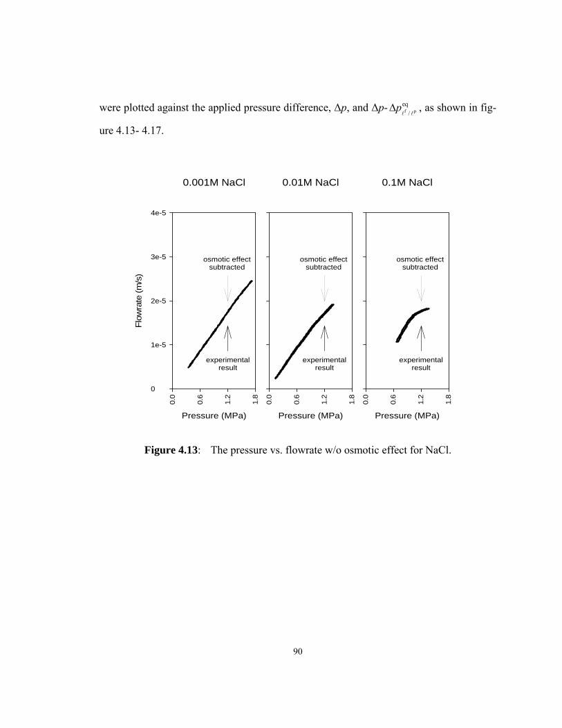
90

were plotted against the applied pressure difference, Δp, and Δp- f peq

/pΔ , as shown in fig-

ure 4.13- 4.17.

0.001M NaCl

Pressure (MPa)

0.0

0.6

1.2

1.8

Flow

rate

(m/s

)

0

1e-5

2e-5

3e-5

4e-5

0.01M NaCl

Pressure (MPa)

0.0

0.6

1.2

1.8

0.1M NaCl

Pressure (MPa)

0.0

0.6

1.2

1.8

osmotic effectsubtracted

experimentalresult

osmotic effectsubtracted

experimentalresult

osmotic effectsubtracted

experimentalresult

Figure 4.13: The pressure vs. flowrate w/o osmotic effect for NaCl.

91

0.0007M CaCl2

Pressure (MPa)

0.0

0.6

1.2

1.8

Flow

rate

(m/s

)

0

1e-5

2e-5

3e-5

4e-5

0.007M CaCl2

Pressure (MPa)

0.0

0.6

1.2

1.8

0.021M CaCl2

Pressure (MPa)

0.0 0.6 1.2 1.8

0.07M CaCl2

Pressure (MPa)

0.0 0.6 1.2 1.8

osmotic effectsubtracted

experimentalresult

osmotic effectsubtracted

experimentalresult

osmotic effectsubtracted

experimentalresult

osmotic effectsubtracted

experimentalresult

Figure 4.14: The pressure vs. flowrate w/o osmotic effect for CaCl2.

0.001M NaCl+1E-5M AlCl3

Pressure (MPa)

0.0

0.6

1.2

1.8

Flow

rate

(m/s

)

0

1e-5

2e-5

3e-5

4e-5

0.01M NaCl+1E-4M AlCl3

Pressure (MPa)

0.0

0.6

1.2

1.8

0.1M NaCl+1E-4M AlCl3

Pressure (MPa)

0.0

0.6

1.2

1.8

osmotic effectsubtracted

experimentalresult

osmotic effectsubtracted

experimentalresult

osmotic effectsubtracted

experimentalresult

Figure 4.15: The pressure vs. flowrate w/o osmotic effect for NaCl+1%AlCl3.

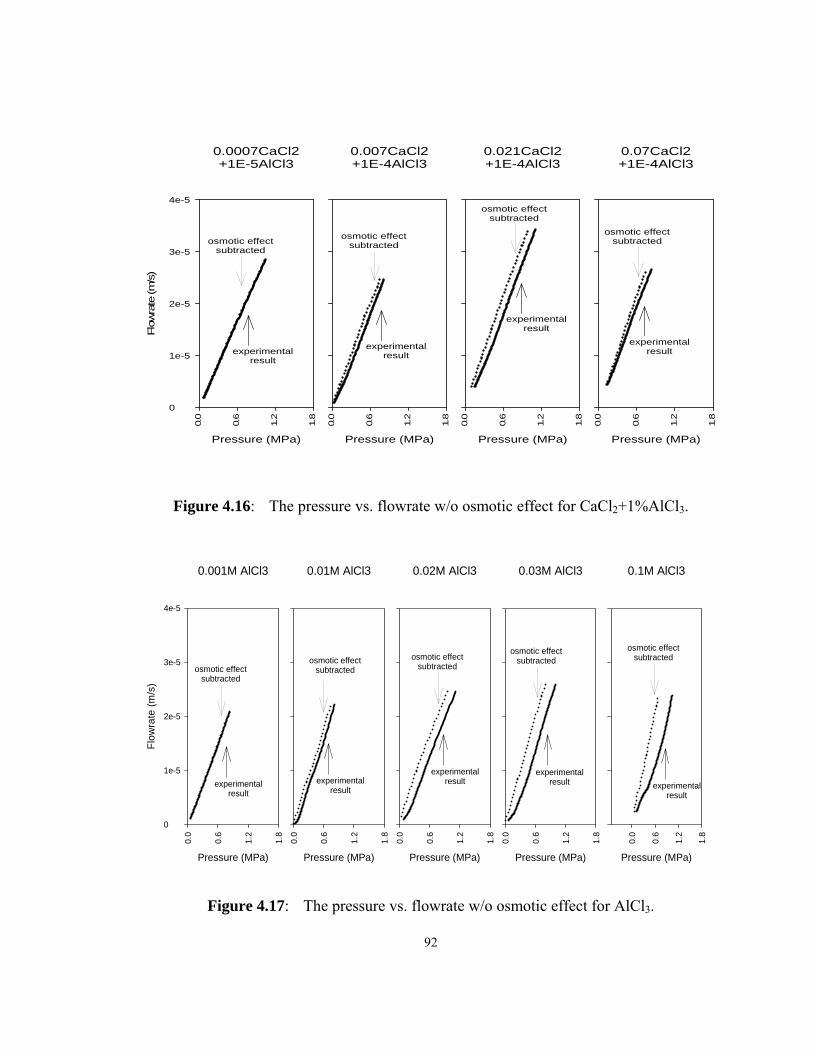
92

0.0007CaCl2+1E-5AlCl3

Pressure (MPa)

0.0

0.6

1.2

1.8

Flow

rate

(m/s

)

0

1e-5

2e-5

3e-5

4e-5

0.007CaCl2+1E-4AlCl3

Pressure (MPa)

0.0

0.6

1.2

1.8

0.021CaCl2+1E-4AlCl3

Pressure (MPa)

0.0

0.6

1.2

1.8

0.07CaCl2+1E-4AlCl3

Pressure (MPa)

0.0

0.6

1.2

1.8

osmotic effectsubtracted

experimentalresult

osmotic effectsubtracted

experimentalresult

osmotic effectsubtracted

experimentalresult

osmotic effectsubtracted

experimentalresult

Figure 4.16: The pressure vs. flowrate w/o osmotic effect for CaCl2+1%AlCl3.

0.001M AlCl3

Pressure (MPa)

0.0

0.6

1.2

1.8

Flow

rate

(m/s

)

0

1e-5

2e-5

3e-5

4e-5

0.01M AlCl3

Pressure (MPa)

0.0

0.6

1.2

1.8

0.02M AlCl3

Pressure (MPa)

0.0

0.6

1.2

1.8

0.03M AlCl3

Pressure (MPa)

0.0

0.6

1.2

1.8

0.1M AlCl3

Pressure (MPa)

0.0

0.6

1.2

1.8

osmotic effectsubtracted

experimentalresult

osmotic effectsubtracted

experimentalresult

osmotic effectsubtracted

experimentalresult

osmotic effectsubtracted

experimentalresult

osmotic effectsubtracted

experimentalresult

Figure 4.17: The pressure vs. flowrate w/o osmotic effect for AlCl3.

93

The subtraction of the osmotic effect at higher concentrations results in a linear relation

between the flow rate and (corrected) applied pressure. This indicates that the osmotic

effect provides an internal pressure difference that counteracts the applied pressure. For

this effect to be readily noticed, however, several criteria must be satisfied.

• The concentration of the tested solution must be high enough and the rejection must

be sufficient to generate enough concentration difference so that the resulting osmotic

pressure is more than 5…10% of the applied pressure.

• The membrane must be chemically stable to obtain a reproducible flow rate.

The osmotic effect is most convincingly demonstrated with moderately concentrated

electrolyte solutions with zM > 1, which show a saturated region in their rejection vs. flow

rate curve. At a relatively high differential pressure, the rejection reaches a maximum

value and a constant concentration difference is maintained between the feed and perme-

ate side so that a constant osmotic pressure difference can be derived from the flow rate

vs applied pressure curve. When a lower Δp is applied, the rejection decreases to zero

and as does the osmotic pressure. Therefore, for relatively low Δp, the flow rate vs Δp

curve starts to approach the flow rate vs (p- f peq

/pΔ ) curve. The resulting nonlinear be-

havior can be only explained by the osmotic effect since pure viscous flow results in lin-

ear behavior, and all possible corrections, including the effects of temperature and elec-

trolyte concentration, on and viscosity have been applied.

4.5 Conclusion

With a carefully designed and constructed water purification setup and a thoroughly

planned experimental procedure, consistent water purification results were ontained with

a γ-alumina membrane.

For the first time, the osmotic effect was clearly detected during the testing; provided the

electrolyte system was properly chosen, and any membrane degrading situations, such as

clogging and dissolving had been kept at their minimum level.

94

Our observation and calculation indicate that, under current experimental conditions,

temperature and electrolyte concentration have a small effect on the value of the solu-

tion’s dynamic viscosity, in the order of 1…3%.

The Pitzer and Mayorga's model for the thermodynamic properties of electrolyte solu-

tions is sufficiently accurate for using in the analysis of current water purification ex-

periments.

95

CHAPTER 5

MESOPOROUS MEMBRANE NANOFILTRATION MODELING

WITH COMSOL MULTIPHYSICS

Nanofiltration with meso-porous membranes can be used in water desalinization, water

softening and purification applications. The purification mechanism rests upon an elec-

trostatic field effect, induced by charged groups adsorbed or imbedded on the membrane

surface. When immersed in aqueous electrolyte solution, the charged surface will spon-

taneously develop a diffuse layer of excess countercharge in the solution. This will cause

a deviation of ion concentration distribution within the pore phase from the original solu-

tion values. This effect will have the result that, under pressure-driven operation, the so-

lution at the membrane permeate side has an ionic concentration that is less than that at

the feed side. Since the concentrations of positive and negative charges due not exactly

cancel out in the pore phase, a strong electrical field will form at the exit of the pore and

promote a strong migration of ionic species, which will counteract the normal diffusive

and convective transport. This process can be described by modeling three phenomena

that occur simultaneously in the system: incompressible fluid flow; chemical diffusion,

field-driven migration and convection of ionic species; and electrostatic interaction. To

obtain a quantitatively valid model, several corrections; such as non-ideal solution ther-

modynamics, dependence of the diffusion coefficient on ion concentration, variations in

local water permittivity, have been taken into account in this model. The simulation re-

sults demonstrated correctly the experimental trends, and predicted limiting performance

at extreme conditions.

96

5.1 Introduction

Modeling of the nanofiltration process of mesoporous (pore diameter Øp = 2…50 nm)

membranes involves a thorough investigation at the intersection of four major fields: sur-

face chemistry, electrostatic interactions, mass transportation and fluid dynamics. The

purpose of the modeling is to understand the species’ transportation process and to pre-

dict purification performance under defined operation conditions.

Many authors have taken up this challenge task with various approaches [171-188]. The

majority of these studies are based on a one-dimensional FEA approach, which considers

transportation phenomena along the membrane thickness direction, and using the simpli-

fication of averaging physical phenomena and membrane properties in the other two per-

pendicular directions. Such simplifications reduce computational expenses, but some-

times generate relatively crude results such as a discontinuity in the ion concentration

profile. In addition they result in intuitively inaccurate assumptions such as uniform po-

tential and electrical neutrality for each slice, perpendicular in the pore direction. As

more advanced and powerful modeling tools become available, these simplified models

can be revised and rebuilt by using a more consistent physical framework and a larger

degree of detail. This work focuses on establishing a 3D transportation model that incor-

porates detailed electrokinetic interactions and ionic charge distributions. For instance,

one of the major differences between this work and previous studies is that in this work,

the electrical double layer inside the membrane pore phase was modeled with the FEM

method to obtain a detailed axial distribution profile; while in previous work, the poten-

tial was assumed axially uniform and the charge concentration was directly calculated

from the Boltzmann relation.

Similar FEM approaches have been taken recently by the microfluidics community. A

typical microfluidics model investigates the fluid flow confined in micrometer scale

channels, and the effect of various physical-chemical phenomena such as thermal effects

[189], electrokinetics [190], diffusion, and surface reactions [191]. In state-of-the-art

nanofiltration membranes, the membrane pores have a much smaller channel cross sec-

tion and a more torturous geometry than what is normally considered in micro-fluidics.

97

The practical membrane pore geometry, as it turns out, can be simplified with to a

straight channel with a minimal effect on the purification results. However, the compli-

cations raised by nanoscale pore dimension need to be thoroughly analyzed and modeled,

which is the subject of this work.

5.2 Theory

5.2.1 Surface charge density

The water purification mechanism of the inorganic nanofiltration membrane rests upon

the spontaneous chemi-sorption of charged species of one sign, resulting in the develop-

ment of an electrical double layer (EDL). This occurs when the membrane material is

brought into contact with an aqueous solution. This work considers, the case of a

mesoporous γ-alumina membrane immersed in NaCl solutions at pH = 4.6. Several sur-

face reactions take place and four of them are considered here, following a widely

adapted 2-pK charge-regulation model [188, 192-197]

C

A

+2

+

+ +2 2

OH OH H (s)

OH O H (s)

O C O C (s)

OH A OH A (s)

K

K

Kn n

Km m

+

−

+

− +

− − +

− −

− − +

− − +

− − +

− − +

(5.1)

Here, OH− is a hydroxyl group on the surface of γ-alumina membrane, +2OH− and O−−

result from ionization of this group by either adsorption or desorbtion of a proton. Such

charged groups can further adsorb cations Cn+ or anions Am- to form, respectively,

O Cn− +− or, +2OH Am−− surface groups. The equilibrium constants K+, K-, KA, and KC are

obtained from the literature [188]. A net surface charge, σ, results from the summation of

all the chemisorbed, charged groups on the surface. It can be further expressed as a func-

tion of the concentration of the mobile ions close to the surface, H (s)

c + , C (s)nc + , and

A (s)mc −

as:

98

2

H (s)+tot 2 C 2 A

H (s) H (s) C (s) H (s) A (s)

( )F

( ) / ( ) /n m

c K Kc

K c c K K K K c K c c K+

+ + + + −

+ −

+ + − + −

−σ = ⋅

+ + + + (5.2)

where F is the Faraday constant. The total surface site concentration, +totc , can be ob-

tained from the literature [188]. The surface ion concentrations, H (s)

c + , C (s)nc + , and

A (s)mc − , are related to the bulk concentrations, H (b)

c + , C (b)nc + , and

A (b)mc − , through the

Boltzman relationship,

(s) (b)F ( )exp( )R

ii i i

zc cT

− ⋅ ⋅ ΔΦ= γ (5.3)

Where x can be H+, Cn+, or Am- ; γi is the activity of the corresponding species i, which

can be obtained as a function of c by using a widely accepted empirical expression by

Davies [198] as 2log( ) 0.51 0.21i i

Iz II

⎛ ⎞− γ = −⎜ ⎟⎜ ⎟+⎝ ⎠

; zi is the charge carried by i; R, T are

the ideal gas constant and temperature respectively; ΔΦ is the potential difference be-

tween the bulk and the surface and the only dependent variable. This potential difference

is connected to the surface charge density σ through the experimental data of double layer

capacitance, , as

σ = ⋅ΔΦC (5.4)

Therefore, the surface charge model contains a set of self-confined equations that can be

solved numerically to determine the value of the surface charge density σ at any given

bulk solution composition.

Once the surface charge density is determined for one type of feed solution, it is applied

to the entire membrane pore channel and the electrical double layer modeling uses this

value. This assumption can be justified by considering the “gate effect” at the interface

between bulk solution and the membrane phase. Once the electrolyte solution passes the

“gate region” (EDL at the interface) and enters the pore, the ion concentration will not

vary significantly within the pore channel and therefore, the surface charge density will

be approximately a constant.

99

5.2.2 Electrostatics: electrical double layer (EDL)

The occurrence of an electrical double layer (EDL) plays an essential role in the purifica-

tion mechanism of nanofiltration with mesoporous membranes. The key problem, ad-

dressed in double layer studies is to reveal the relationship between the potential differ-

ence across the interface and the spatial distribution of the species within the interfacial

region. Even to this day the EDL is not completely understood, while it has been studied

extensively for 150 years when the first capacitor model was introduced by Helmholtz

[200]. A more realistic EDL model with a diffusive distribution of ions, rather than a

single plane, in the electrolyte was first proposed by Gouy [201] and Chapman [202] and

became the basis of modern EDL descriptions. In the 1980s, a group of new models

identified as restricted primitive models (RPM) were proposed for describing EDLs at

high concentrations and high surface charge densities [203]. A common feature of these

models is that the electrolyte is represented by a fluid of charged hard spheres of finite

diameter and the solvent by a continuum with an isotropic dielectric constant. Another

promising approach was based on density-functional theories [204]. This approach de-

scribes the Helmholtz free energy as a function of the particle density, and minimizes that

free energy to obtain a solution for the equilibrium distribution. These refined models

were able to predict the behavior of the EDL at high surface charge densities and concen-

trations, such as oscillations in the concentration profile, and charge inversion phenom-

ena. As modem computation tools became available, investigators started modeling the

EDL by calculating the interaction between large amounts of individual molecules. In

these efforts, one of two techniques was generally used to perform the simulations [205]:

molecular dynamics (MD), in which the equations of motion are solved simultaneously

for each molecule, and the Monte Carlo method (MC), in which an equilibrium ensemble

is generated from a random walk algorithm. In case the intermolecular potential is

known with sufficient detail, the properties and structure of the EDL can be computed for

systems consisting of a few hundred to a few thousand particles. Without further ex-

perimental evidence being currently available, computational simulation provides a

shortcut to the reality of the EDL structure and may be the only way to address problems

as in the current paper. However, the scale of current MD or MC simulation is still far

100

from sufficient to model a macro scale phenomena such as the nanofiltration process.

Therefore, continuum finite element methods are still employed and will be still on the

stage for a while for this type of modeling work.

In this work, we determined the concentration profile of the EDL numerically instead of

analytically to bypass two complications:

• The confined membrane pore size is of the same order of magnitude as the EDL

thickness.

• Interactions with other phenomena such as convection.

We applied the classic Gouy-Chapman approach instead of the newly (in 80s) developed

EDL models by assuming point charges and a continuum dielectric medium. The new

EDL theories are not considered here for two reasons:

• The systems studied are relatively dilute with a modest surface charge density, which

can be modeled with sufficient accuracy by the Gouy-Chapman theory.

• Advanced models, generally not based on simple partial differential equations, are

difficult to implement in the COMSOL platform.

While it is well-known that FEM is not suitable for very small length scales where sizes

of individual molecules start to play a significant roles, our system turns out to be still

marginally solvable with the FEM method.

A combination of Poisson’s equation combined with diffusion theory is employed to de-

termine the development of the EDL in the pore entrance and along the channel. We

write Poisson’s equation as:

0 r e−∇⋅ε ε ∇Φ = ρ (5.5)

It has been noticed by many researchers that the dielectric constant of aqueous electrolyte

solutions is no longer a constant, close to a solid liquid interface. This deviation was be-

lieved to result from two phenomena:

• Preferred orientation of water dipoles around charged species.

• Restrictions in the free movement of water molecules in a confined space of nm di-

mensions. In our system, both effects may present simultaneously.

101

For the first, a widely accepted empirical formula proposed by Podgornik [206] is used

( ) maxr

max min1 ( / 1)exp( 2 / )y

yε

ε =+ ε ε − − λ

(5.6)

where the dielectric constant εr(y) is a function of the distance, y, away from the interface.

λ is the Debye length of the electrolyte under consideration [206]. εmax is the bulk dielec-

tric constant of the media, which is 78.5 for water. εmin is the surface dielectric constant

of the media, which is 4 for water at a charged mica surface according to Teschke [207].

We use a similar equation for the external γ-alumina membrane water interface, since for

most of operation conditions, the γ-alumina surface is strongly charged. Therefore a

maximum water molecule rearrangement at the interface, and hence a minimum dielectric

constant was anticipated. On the other hand, no correction was applied to εr inside the

pore channel because due to symmetry, the electrical fields from the walls of the pore

channel partly canceled each other out so that little water molecule re-orientation occurs.

Another effect that will reduce εr of water is a confinement effect in pores of <10 nm di-

mensions. Molecular dynamics simulations indicated a 10% reduction of εr in a spherical

cavity of about 4.8 nm in diameter [208, 209]. However, due to lack of modeling data for

the present case, and the fact that the predicted reduction is limited, this effect is not in-

cluded in current modeling work. However, this refinement can be easily added to the

model if these data are available.

5.2.3 Diffusion and convection: Nernst-Planck

A modified Nernst-Planck equation was applied to describe the ionic species transporta-

tion phenomena, as described by the equation below:

Fln( )R R

ii i i i i i i i i i

VD c c D c z c c pT T

= − ∇ γ − ∇Φ − − ∇j v (5.7)

In the simplest purification test, for example, with an NaCl solution at pH = 4.6, 3 spe-

cies, concentrations of H+, Na+, and Cl- are obtained from the model and the concentra-

tion of OH- is calculated on the assumption that the water autoprotolysis reaction equili-

brates everywhere. For each given charged species in the electrolyte solution, the total

flux of this species, ji, equals to the summation of the four terms. The right side the first

102

term is the chemical-diffusion that takes place under the influence of a chemical potential

gradient, exclusive of the electrostatic contribution. Di is the component diffusion coeffi-

cient of species i, ci is the concentration of i, and γi is the activity coefficient of i. The

second term represents the migration term, which is driven by the electrical potential gra-

dient (field). The third term is the (fluid-flow-caused transportation term) convection

term, where v is convection flow velocity of the solvent, water. The fourth term is an-

other migration term, which takes the effect of solute on the liquid volume into account

[188], however, it is noticed in the model that this term is generally significantly smaller

than the other terms. The terminology is summarized in table 5.1. At current stage, the

model does not calculate the osmotic effects because relatec diffusion coefficient is not

avialbe and therefore the diffusion term of water due to 2H Oμ∇ , is ignored.

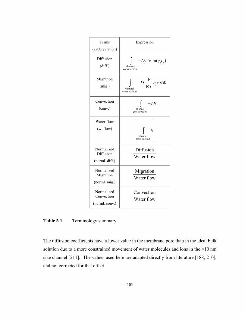
103

Terms

(aabbreviation)

Expression

Diffusion

(diff.) channelcorss seciton

ln( )i i i iD c c− ∇ γ∫

Migration

(mig.) channel

corss seciton

FRi i iD c z

T− ∇Φ∫

Convection

(conv.) channelcorss seciton

ic−∫ v

Water flow

(w. flow)

channelcross section

∫ v

Normalized Diffusion

(norml. diff.)

DiffusionWater flow

Normalized Migration

(norml. mig.)

MigrationWater flow

Normalized Convection

(norml. conv.)

ConvectionWater flow

Table 5.1: Terminology summary.

The diffusion coefficients have a lower value in the membrane pore than in the ideal bulk

solution due to a more constrained movement of water molecules and ions in the <10 nm

size channel [211]. The values used here are adapted directly from literature [188, 210],

and not corrected for that effect.

104

5.2.4 Flow: Navier-Stokes

The incompressible Navier-Stokes equation can be expressed as

2( ) pt

∂ρ +ρ ⋅∇ = −∇ + +η∇

∂v v v F v (5.8)

Here, ρℓ is the density of the liquid, v the velocity, t time, p pressure, F the external body

force and η the viscosity of the liquid. For the steady state analysis that we conduct here,

the first term vanishes. In this simulation, the force term represents the electrokinetic ef-

fect [212] and can be expressed by the equation below [190]:

e= −ρ ∇ΦF (5.9)

The electrokinetic term generally does not affect the linearity of the flowrate vs. pressure

relationship. It was noticed in this model that at the interface between the bulk solution

and the membrane surface the fluid sensed an attraction force, which promoted the en-

trance and resisted the exit of the fluid. These two trends cancelled each other out so that

the total flow was then not significantly affected by the electrokinetic force.

Another effect associated with the nanoscale dimensions is that at the solid liquid inter-

face, the liquid molecules interact with the channel wall and classic Navier-Stokes on-slip

boundary condition does not apply. For this reason, a “slip contact” boundary condition

or modified hydrodynamic model was developed for nanoscale fluids [213]. However,

these studies are still under development and, therefore, are not considered for the present

case.

5.2.5 Geometry and mesh

The model was applied to both 2D and 3D channels. The model geometry contains 3

sections: a bulk solution at the feed side, a membrane pore channel, and a bulk solution at

the permeate side. At the feed side, convection worked against the diffusion of ion spe-

cies and compressed the EDL; while at the permeate side, convection and diffusion

worked together to elongate the EDL. Therefore, the feed side geometry was taken

shorter than the permeate side geometry. The lengths of the bulk solution were deter-

mined by trial and error. The criterion is that the concentration profile gradient at the en-

trance and exit boundaries of the modeled geometry must be less than 1E-6 M/m. The

105

membrane pore channel diameter was set to 4 nm, which was based on numerous ex-

perimental observations [214]. The length of the channel varied from 30~120 nm for the

2D model and was 30 nm for the 3D model, because computational resource limitations

(8Gb of memory) did not allow for larger lengths. The effects of the channel tortuosity

and channel splitting and joining were investigated with the 2D model only. For the 3D

model, solutions for such complicated geometries were not feasible for the same reason.

The mesh was rough in the bulk solution sides and very fine in the interface and channel

region. As a rule of thumb, the cross section of the channel region should have at least 10

grid points to generate a reasonable concentration profile gradient. To do so, the “maxi-

mum element size” and “element growth rate” of the interface boundaries at the mesh

parameter dialog window were set to “4E-9/20” and “1.05” for the 2D model and

“4E-9/12” and “1.05” for the 3D model. The degree of freedom (DOF) of the model was

96…390K for the 2D model and 255K for the 3D model.

5.3 Results and discussion

5.3.1 Channel length, tortuosity and branching

Several channel types with different lengths and shapes were used, as summarized in fig-

ure 5.1. Geometries a, b, and c were used to examine the effect of channel length (30, 60,

120 nm respectively) on rejection performance, d for the tortuosity effect, and e, f for the

splitting and mixing effect. Rejection is defined as 1-cf/cp, where cf is the feed side elec-

trolyte concentration and cp the permeate side electrolyte concentration. The optimized

flow velocity is defined as the flow velocity at which the rejection had a maximum value.

Since it was shown, with the 2D models, that the channel length, tortuosity and branching

did not affect the maximum (limiting) rejection significantly, the 3D model was used

only with the straight channel geometry only to keep it simple, and to evade computa-

tional resource limitations.

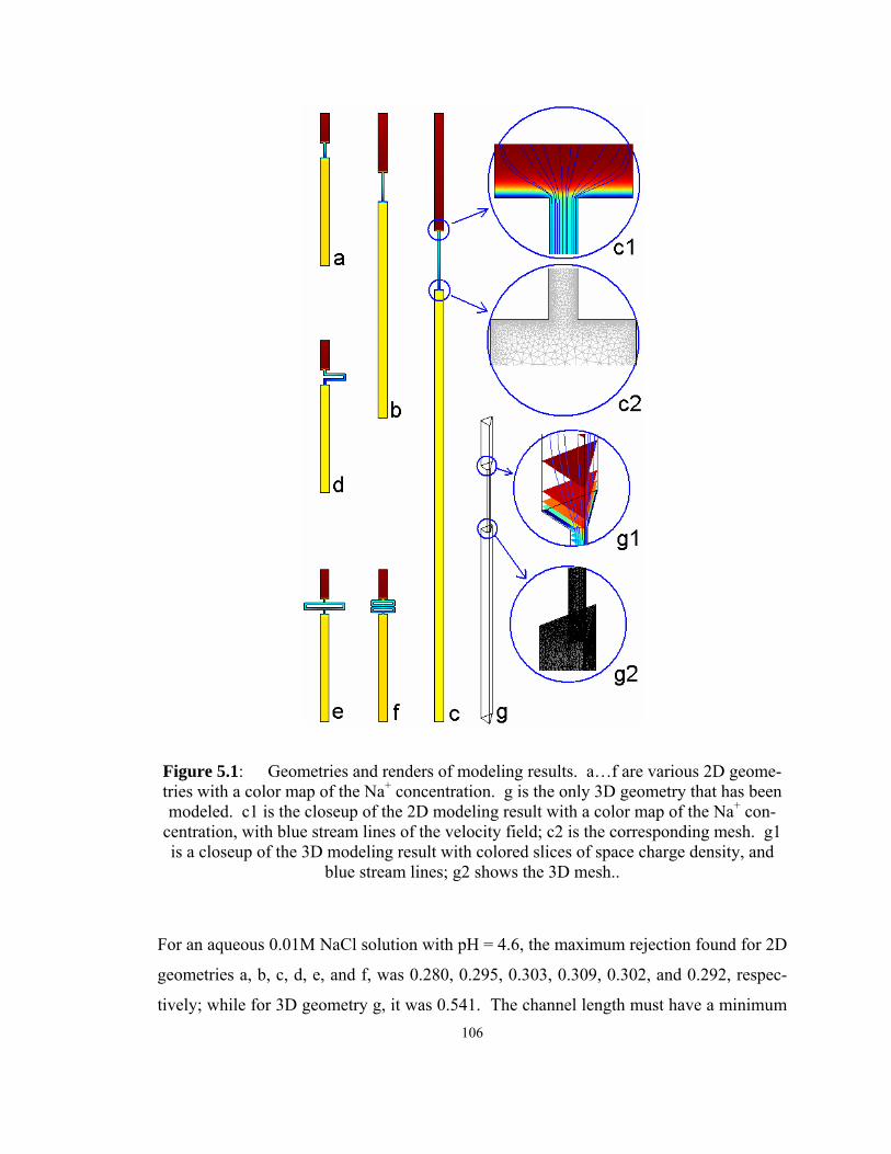
106

Figure 5.1: Geometries and renders of modeling results. a…f are various 2D geome-tries with a color map of the Na+ concentration. g is the only 3D geometry that has been modeled. c1 is the closeup of the 2D modeling result with a color map of the Na+ con-

centration, with blue stream lines of the velocity field; c2 is the corresponding mesh. g1 is a closeup of the 3D modeling result with colored slices of space charge density, and

blue stream lines; g2 shows the 3D mesh..

For an aqueous 0.01M NaCl solution with pH = 4.6, the maximum rejection found for 2D

geometries a, b, c, d, e, and f, was 0.280, 0.295, 0.303, 0.309, 0.302, and 0.292, respec-

tively; while for 3D geometry g, it was 0.541. The channel length must have a minimum

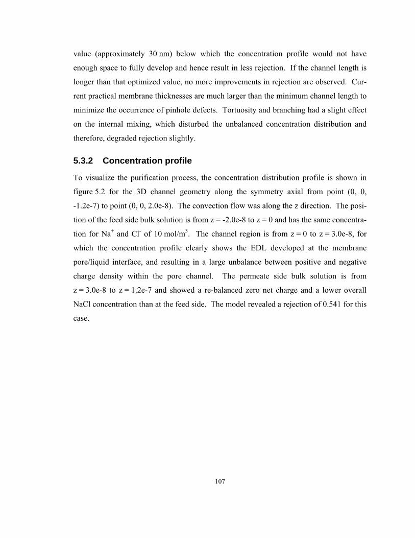
107

value (approximately 30 nm) below which the concentration profile would not have

enough space to fully develop and hence result in less rejection. If the channel length is

longer than that optimized value, no more improvements in rejection are observed. Cur-

rent practical membrane thicknesses are much larger than the minimum channel length to

minimize the occurrence of pinhole defects. Tortuosity and branching had a slight effect

on the internal mixing, which disturbed the unbalanced concentration distribution and

therefore, degraded rejection slightly.

5.3.2 Concentration profile

To visualize the purification process, the concentration distribution profile is shown in

figure 5.2 for the 3D channel geometry along the symmetry axial from point (0, 0,

-1.2e-7) to point (0, 0, 2.0e-8). The convection flow was along the z direction. The posi-

tion of the feed side bulk solution is from z = -2.0e-8 to z = 0 and has the same concentra-

tion for Na+ and Cl- of 10 mol/m3. The channel region is from z = 0 to z = 3.0e-8, for

which the concentration profile clearly shows the EDL developed at the membrane

pore/liquid interface, and resulting in a large unbalance between positive and negative

charge density within the pore channel. The permeate side bulk solution is from

z = 3.0e-8 to z = 1.2e-7 and showed a re-balanced zero net charge and a lower overall

NaCl concentration than at the feed side. The model revealed a rejection of 0.541 for this

case.

108

10 mol/m3 NaCl @pH4.6Applied pressure=1.1 MPa

z Coordinate (m) -4.0e-8 0.0 4.0e-8 8.0e-8 1.2e-7 1.6e-7

Con

cent

ratio

n (m

ol/m

3 )

0

10

20

30

40

50

Na+

Cl-

Figure 5.2: Concentration profile along the channel.

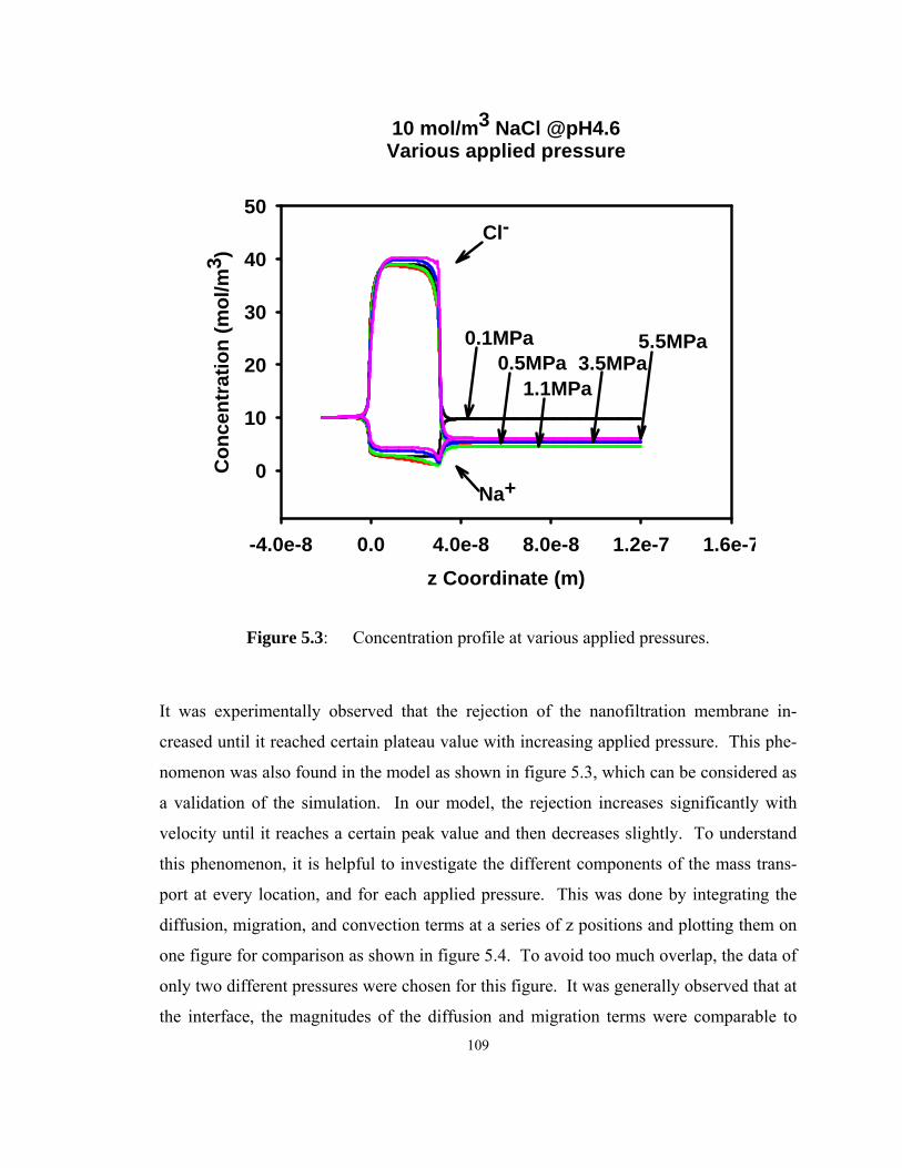
109

10 mol/m3 NaCl @pH4.6Various applied pressure

z Coordinate (m)-4.0e-8 0.0 4.0e-8 8.0e-8 1.2e-7 1.6e-7

Con

cent

ratio

n (m

ol/m

3 )

0

10

20

30

40

50

0.1MPa0.5MPa

1.1MPa3.5MPa

5.5MPa

Cl-

Na+

Figure 5.3: Concentration profile at various applied pressures.

It was experimentally observed that the rejection of the nanofiltration membrane in-

creased until it reached certain plateau value with increasing applied pressure. This phe-

nomenon was also found in the model as shown in figure 5.3, which can be considered as

a validation of the simulation. In our model, the rejection increases significantly with

velocity until it reaches a certain peak value and then decreases slightly. To understand

this phenomenon, it is helpful to investigate the different components of the mass trans-

port at every location, and for each applied pressure. This was done by integrating the

diffusion, migration, and convection terms at a series of z positions and plotting them on

one figure for comparison as shown in figure 5.4. To avoid too much overlap, the data of

only two different pressures were chosen for this figure. It was generally observed that at

the interface, the magnitudes of the diffusion and migration terms were comparable to

110

each other and much larger than the convection term; while in the bulk solution, they

were almost zero. This is understandable because the concentration profile remained

constant in the bulk region and changed only significantly at the EDL region, close to the

interface of the pore and bulk solution. A close look at the diffusion, migration and con-

vection terms provides a good insight into the purification mechanism. As the applied

pressure increases, every transport component increases. However, the pressure-driven

viscous flow increases even more. Therefore, it makes more sense to compare normal-

ized transport terms, obtained by dividing each term by the pressure-driven water flux,

and excluding the pressure-driven flow. It was then noticed that, as the applied pressure

increases, the normalized transport terms decrease, which means that each term contrib-

utes less to the ion concentration profile. After normalization, the migration and diffu-

sion term were still large compared to the convection term. However, these two large

terms always had opposite signs and mainly canceled each other. As a net result, the

summation of normalized diffusion and migration became comparable to the convection

term and generally worked against that term, reducing the overall total transport of ionic

species. A closer look at the entrance of the pore makes this clear. For the co-ion Na+,

the normalized migration term was larger than the diffusion term. When the applied

pressure increases, both normalized terms decrease but the normalized migration term

changes not as fast as the diffusion term. Therefore, the net result is that the diffu-

sion+migration term becomes larger and holds back more Na+ ions at higher applied

pressure. On the other hand, for the case of the counter ion Cl-, the magnitude of the dif-

fusion term is larger than the migration term and the summation of diffusion+migration

was still against the convection term. At a higher applied pressure this effect also be-

comes stronger and holds back more Cl- ions as well. The large oscillation of the diffu-

sion+migration term of Cl- at the interface might be caused by an insufficiently fine mesh

and numerical noise. With the availability of more computer memory, a finer mesh

might improve this issue.

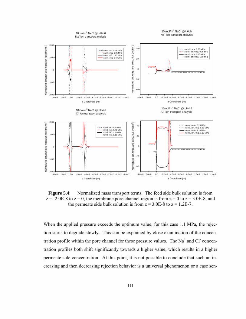
111

10mol/m3 NaCl @ pH4.6Na+ ion transport analysis

z Coordinate (m)

-1.4e-7-1.2e-7-1.0e-7-8.0e-8-6.0e-8-4.0e-8-2.0e-80.02.0e-84.0e-8

Nor

mal

ized

diff

usio

n an

d m

igra

tion

flux

(mol

/m3 )

-2000

-1000

0

1000

2000

norml. diff. 0.26 MPanorml. mig. 0.26 MPanorml. diff. 1.10 MPanorml. mig. 1.10MPa

10 mol/m3 NaCl @4.6phNa+ ion transport analysis

z Coordinate (m)

-1.4e-7-1.2e-7-1.0e-7-8.0e-8-6.0e-8-4.0e-8-2.0e-80.02.0e-84.0e-8

Nor

mal

ized

diff

.+m

ig. a

nd c

onv.

flux

(mol

/m3 )

-40

-20

0

20

40 norml. conv. 0.26 MPanorml. diff.+mig. 0.26 MPanorml. conv. 1.10 MPanorml. diff.+mig. 1.10 MPa

10mol/m3 NaCl @ pH4.6Cl- ion transport analysis

z Coordinate (m)

-1.4e-7-1.2e-7-1.0e-7-8.0e-8-6.0e-8-4.0e-8-2.0e-80.02.0e-84.0e-8

Nor

mal

ized

diff

usio

n an

d m

igra

tion

flux

(mol

/m3 )

-2000

-1000

0

1000

2000

norml. diff. 0.26 MPanorml. mig. 0.26 MPanorml. diff. 1.10 MPanorml. mig. 1.10 MPa

10mol/m3 NaCl @ pH4.6Cl- ion transport analysis

z Coordinate (m)

-1.4e-7-1.2e-7-1.0e-7-8.0e-8-6.0e-8-4.0e-8-2.0e-80.02.0e-84.0e-8

Nor

mal

ized

diff

.+m

ig. a

nd c

onv.

flux

(mol

/m3 )

-40

-20

0

20

40 norml. conv. 0.26 MPanorml. diff.+mig. 0.26 MPanorml. conv. 1.10 MPanorml. diff.+mig. 1.10 MPa

Figure 5.4: Normalized mass transport terms. The feed side bulk solution is from z = -2.0E-8 to z = 0, the membrane pore channel region is from z = 0 to z = 3.0E-8, and

the permeate side bulk solution is from z = 3.0E-8 to z = 1.2E-7.

When the applied pressure exceeds the optimum value, for this case 1.1 MPa, the rejec-

tion starts to degrade slowly. This can be explained by close examination of the concen-

tration profile within the pore channel for these pressure values. The Na+ and Cl- concen-

tration profiles both shift significantly towards a higher value, which results in a higher

permeate side concentration. At this point, it is not possible to conclude that such an in-

creasing and then decreasing rejection behavior is a universal phenomenon or a case sen-

112

sitive special situation. No experimental results are yet available to validate the decreas-

ing rejection after the maximum value.

5.3.3 Model validation

The 3D modeled results were compared with experimental membrane results. In the

model, it was noticed that the longer the membrane pore channel, the lower the optimum

flow velocity. Such behavior was indeed observed with the 2D model for various chan-

nel lengths as shown in figure 5.5. It was further estimated that the optimized flow veloc-

ity was proportional to 1/channel length. Such a relationship was also assumed for the

3D model and will be tested if appropriate computational resources become available. In

direct comparisons with experimental results, we noticed a discrepancy that could be re-

moved by scaling down the model velocity with a flow velocity scale factor of 50, see

figure 5.6. To understand this scale factor, one needs to consider the actual experimental

membrane pore length, which is equal to the membrane thickness, 500 nm for a single

coated membrane, times the tortuosity, τ=3…4 for a γ-alumina membrane [214]. The

total length of a realistic membrane pore was then found to be 1500…2000 nm, which

was 50…67 times longer than the modeled 30 nm channel length. This is in very good

agreement with our scaling factor.

Another possible factor that might affect the flow velocity scale factor estimation rose

from the effective membrane area. However, this effect had already been taken into ac-

count when the geometry of the membrane channel was constructed. The effective mem-

brane area can be characterized with a quantity, φp, which is the ratio between total open

area of the pore and membrane cross section area. For close packed sphere, φp is

2 32 3

− π , which is approximately 0.1. Unfortunately, no data of this quantity was avail-

able yet for our mesoporous γ-alumina membrane. Therefore, when the geometry of the

model was constructed, the ratio between the cross section area of the bulk feed solution

and the membrane pore channel was chosen to be 0.35, to compensate this effect without

making the channel geometry become unfavorable for mesh generation. The results were

not further modified thereafter.

113

The qualitative agreement between the computational and experimental results was very

good if the flow velocity scale factor was taken into account as shown in figure 5.6.

10mol/m3 NaCl@ph4.6 various pressure2D pore length effect comparison

flow velocity (m/s)0.000 0.004 0.008 0.012 0.016

Rej

ectio

n

0.00

0.05

0.10

0.15

0.20

0.25

0.30

0.3530nm60nm120nm

Figure 5.5: Comparison of rejection performance for 2D models versus channel length.

114

NaCl@pH4.6Rejection vs. flow velocity ofmodel and experiment results

Flow velocity (m)0 5e-6 1e-5 2e-5 2e-5 3e-5 3e-5

Rej

ectio

n

0.0

0.2

0.4

0.6

0.8

1.0

1mol/m3

10mol/m3

100mol/m3

Figure 5.6: Comparison of rejection performance for experimental result 1 (solid symbols), experimental result 2 (open symbols) and 3D model results (drawn line).

However, the rejection of the 3D model was more dramatically affected by the feed solu-

tion concentration than in the experiments. The reason of this discrepancy might be that

the FEM continuum approach starts to break down at higher concentrations where the

EDL becomes very thin, of atomic dimensions. Also the Davies thermodynamics correc-

tion may be an oversimplification for the higher concentrations. However, more ad-

vanced thermodynamic equations, such as Pitzer-Mayorga’s method [165], could not be

applied because our current implementation could not handle that level of complexity. It

was observed that tortuosity and branching effects did not change the maximum rejection

value significantly, but tended to stabilize the rejection value after the flow velocity be-

came larger than the optimized value. Explanations for these experimental and computa-

tional observations still need to be explored. The model predicts a decrease of rejection

115

with flow velocity at very high values. This could not be found in the experiments since

the state-of-the-art membranes can not sustain the required high levels of applied pres-

sure. Instead, only a very blurred trend of rejection diminishing could be observed for

NaCl solution at very dilute concentration (1mol/m3). However, as the technology

evolves, and more permeable, stronger supported membranes become available, the ef-

fect of diminishing rejections at high pressures may become observable.

5.4 Conclusions and future work

The process of nanofiltration of mesoporous membranes can be qualitatively modeled

with FEM methods, provided sufficient computational resources are available to handle

this calculation-intensive task. The present implementation coupled three major physics

processes, mass transport, fluid dynamics and electrostatic interaction, and successfully

revealed the purification mechanism. The effect of the pore morphology, including the

channel length, the tortuosity, and the branching effect, was studied with 2D models. It

was found that channel length, tortuosity and branching did not affect the maximum re-

jection value significantly, while the channel length scaled reciprocally with the opti-

mized flow velocity. This observation was used to correct the 3D model results and a

good agreement was found between the model and experimental value.

To obtain a model that is more accurate and reliable for the nanofiltration process, several

refinements should be considered in the future. The most important factor is to develop

an algorithm to connect the discrete phenomenon at the nanoscale to a continuum ap-

proach that is compatible with finite element methods so that more accurate EDL model-

ing can be realized. The second significant improvement may be the construction of a

more realistic channel that includes the channel morphology, such as tortuosity and chan-

nel branching. Conventional 1D models tend to simplify this aspect by averaging mem-

brane properties and introducing experimental fitting parameters into the models. This

work did not consider fitting parameters to obtain a model that is more independent of the

experimental results, and relies more on the physical membrane structure itself. A third

improvement would be to obtain more accurate surface charge calculation algorithms,

preferably implanted into the frame work of the FEM model, and real-time calculation of

116

the surface charge from local concentrations within the channel. However, this effort re-

quires a substantial rebuild of the surface charge modeling algorithm. The surface reac-

tion data necessary for such a model may not be readily available since the large charge

unbalance in the membrane pore channel is difficult to establish in conventional surface

charging experiments. A fourth aspect that can be further fine tuned are the effects

caused by the nanoscale dimensions, such as the dielectric constant changing at the sur-

face and nanofluidic dynamics. Many of these related topics are still active research ar-

eas, and a widely accepted methodology and algorithm is yet to be developed.

A FEM membrane nanofiltration model as presented will enable further membrane de-

vice design and optimization, by considering the supported layer and materials morphol-

ogy. In addition the model may provide a starting point for the investigation of the effect

of an externally applied electric field [216].

117

CONCLUSIONS

Inorganic mesoporous membrane can be used for nanofiltration processes. They show

great potential in water purification applications such as seawater desalinization, brackish

water softening, waste water recycling/regeneration and industrial ultrapure water supply.

This concept was verified with a membrane consisting of a mesoporous γ-alumina layer

on top of a macroporous α-Al2O3 support.

The colloidal filtration casting technique was adapted and fully optimized to produce

homogeneous porous α-Al2O3 disks with a high quality surface, suitable for thin mem-

brane deposition. The colloidal filtration of well-dispersed α-Al2O3 particles with effec-

tive particle size 300 nm (AKP30) and 600 nm (AKP15) was successfully applied to pro-

duce defect free porous disk shape compacts with a superior quality of the upper disk sur-

face. Alumina compacts with well define surface smoothness were obtained with sonifi-

cation and colloidal filtration of 50 wt% α-Al2O3 particles in aqueous solution of HNO3

at pH 2.0 for AKP30 and, aqueous solution of 0.2 wt% Aluminon at pH 9.5 for AKP15.

Observation of water and gas permeability, density as well as grain size can be used to

establish the proper sintering temperature for specific membrane support application.

Both water and gas permeability of optimized compacts show a maximum for a sintering

temperature of 950ºC for AKP30 and AKP15, explained by the occurrence of pore coars-

ening combined with little overall shrinkage. The optimized sintering temperatures were

found to be 950 C for AKP30 supports and 1050 C for AKP15 supports.

Mesoporous γ-alumina membranes were prepared with the well established and docu-

mented sol-gel routine. An innovative ultrasound assisted screen process was developed

to purify the Boehmite nanoparticle dispersion that was used for the sol-gel route of

membrane preparation. Systematic studies with AFM and DLS methods have been car-

ried out to compare the treated sol quality. It is found that this screening method is suit-

118

able for the production of large quantities of dispersion at a fairly high particle concentra-

tion. It results in almost complete removal of particles, larger than 100 nm. Screening

without ultrasound resulted in a more complete removal of large agglomerates but had a

very low yield. The colloidal deposition of sols, purified by ultra-sonic assisted screen-

ing will lead to the formation of higher quality thin films.

A dead-end pressurized water chamber was constructed to perform an accurate, compre-

hensive and reproducible testing of the water purification membrane. The testing first

determined the optimized testing conditions, with several parameters, including stirring

speed, applied pressure, and electrolyte concentration. The membrane was then tested

systematically under the optimized operation conditions. Three different electrolytes

were tested at various concentrations and the osmotic pressure was detected during the

experiments. It is noticed that environmental effects such as temperature and electrolyte

concentration only slightly affected the flowrate measurement to the extent of 1~3% for

most of the cases. For the first time, the osmotic effect was clearly detected during the

testing and quantitatively characterized with the thermodynamic model of Pitzer and

Mayorga. Sufficient accuracy for the osmotic effect correction was obtained.

The water purification mechanism of the inorganic mesoporous membrane rests upon an

electrostatic field effect, induced by charged groups adsorbed on the surface of the mem-

brane. The nanofiltration process was described with a FEM scheme by modeling three

phenomena that occur simultaneously in the system: incompressible fluid flow; chemical

diffusion and field-driven migration, and convection of ionic species; and electrostatic

interaction. Several corrections; such as non-ideal solution thermodynamics, dependence

of the diffusion coefficient on location, variations in local water permittivity; were taken

into account in this model to obtain quantitatively valid results. The effect of the pore

morphology, including the channel length, the tortuosity, and the branching effect, was

studied with 2D models. It was found that channel length, tortuosity and branching did

not affect the maximum rejection value significantly, while the channel length scaled re-

ciprocally with the optimized flow velocity. The simulation results demonstrated cor-

rectly the experimental trends, and predicted limiting performance at extreme conditions.

119

The current study covered a full spectrum of research activities from support preparation,

membrane synthesis, water purification testing to mechanistic modeling. Within each of

these areas, our principle goals were reached and in-depth knowledge was obtained.

Based on the thorough understanding of these subjects, topics worth of further investiga-

tion are summarized as follows:

• The membrane support must be more permeable. New materials and new preparation

methods can be studied. One promising candidate is anodic alumina prepared with

electrochemical oxidation of aluminum. The preparation process must be customized

and fine-tuned to obtain an anodic alumina membrane with balanced properties of

permeability, mechanical strength, thermal/chemical stability and surface smoothness.

• New membrane materials should be studied further. Meso-porous γ-alumina mem-

branes are very suitable for fundamental studies because of their strong tendency to-

wards surface adsorption that amplifies the purification effect. However they are not

very stable in extreme (high or low pH) and even mild operation conditions. New

materials should be studied, such as meso/micro porous titania or tin oxide mem-

branes, which are known to be more stable in extreme conditions.

• New membrane operation configurations and conditions can be studied. It should be

possible to utilize a semi-conductive membrane, such as SnO2, and apply an external

potential to alter the surface charge density of the membrane. This is expected to

make the performance of the membrane more controllable and less dependent on the

electrolyte properties, such as solution pH, electrolyte type and concentration. How-

ever, the manner of attaching the electrode can be critical for such application, and

therefore, should be carefully considered and studied, possibly combined with the

modeling approach shown.

• In the area of modeling, some aspects of the current model can be refined, such as the

implementation of an osmotic effect, real time surface charge density calculation and

better algorithms for electrical double layer modeling. To expand the model to other

electrolytes, mixed electrolytes and other membrane materials, one must obtain more

experimental data for surface reactions, diffusion coefficients and material properties.

120

BIBLIOGRAPHY

1. V.V. Guliants,; M.A. Carreon,; Y.S. Lin, “Ordered mesoporous and macroporous in-organic films and membranes,” Journal of Membrane Science 235 [1-2] 53-27 (2004).

2. J. N. Armor, “Applications of catalytic inorganic membrane reactors to refinery prod-ucts,” Journal of Membrane Science 147 [2] 217-233 (1998).

3. Sikdar, Subhas K.; Grosse, Douglas; Rogut, Ian, “Membrane technologies for reme-diating contaminated soils: a critical review,” Journal of Membrane Science 151 [1] 75-85 (1998).

4. Cui, Z.F.; Chang, S.; Fane, A.G. “The use of gas bubbling to enhance membrane processes”, Journal of Membrane Science 221 [1-2] 1-35 (2003).

5. Gabelman, Alan; Hwang, Sun-Tak, “Hollow fiber membrane contactors” Journal of Membrane Science 159 [1-2] 61-106 (1999).

6. V. B. Bart, V. Carlo, V. G. Tim and D. W. L. Roger, “A review of pressure-driven membrane processes in wastewater treatment and drinking water production,” Envi-ronmental Progress, 22 [1] 46-56 (2003).

7. W.S.W. Ho and K. K. S. Eds, Membrane handbook, Chapman&Hall, 1992.

8. W. J. Koros, Y. H. Ma, and T. Shimidzu, “Terminology for Membranes and Mem-brane Processes IUPAC Recommendations 1996,” J. Membrane Sci., 120 149 (1996).

9. D. Lloyd, Material science of synthetic membranes. ACS Symp. Series No. 269. Washington, DC: American Chemical Society, 1985.

10. S. Sourirajan, and T. Matsuura, Reverse Osmosis/Ultrafiltration Principles. Ottawa, Canada: National Research Council of Canada, 1985.

11. R.J. Petersen, “Composite reverse osmosis and nanofiltration membranes,” Journal of membrane science, 83 81-150 (1993).

121

12. R.J. Petersen and J.E. Cadotte, “Thin film composite reverse osmosis membranes,” pp.307 in: Handbook of Industria1 Membrane technology. M.E. Porter (Ed.), Noyes Publications, Park Ridge, NJ, 1990.

13. A.E. AllegreZra Jr., “Commercial reverse osmosis membranes and modules,” pp.53 in: Reverse Osmosis Technology. Applications for High-Purity-Water production. B.S. Parekh (Ed.), Marcel Dekker, New York, NY, 1988.

14. J.E. Cadotte, “Evolution of composite reverse osmosis membranes,” Material Science of Synthetic Membranes, ACS Symp. Ser. No. 269, American Chemical Society, Washington, DC, D.R. Lloyd (Ed.), 1985.

15. R.E. Kesting, “The four tiers of structure in integrally skinned phase inversion mem-branes and their relevance to the various separation regimes,” J. Appi. Polym. Sci., 41 2739 (1990).

16. K. Kimme and H. Strathmann, “Analysis of the process of phase inversion mem-branes,” Desalination, 79 283 (1990).

17. Marcel Mulder, Basic Principles of membrane technology, 2nd Ed, Kulwer Academic Publishers, 1996.

18. T. Tsuru, “Inorganic porous membranes for liquid phase separation,” Separation and purification methods, 30 [2] 191-220 (2001).

19. J. E. Cadotte and R. J. Petersen, “Thin-film composite reverse-osmosis membranes: origin, development and recent advances,” pp.305 in: Synthetic membranes, Vol. I, Desalination, A.F. Turbak (Ed.) ACS Symp.Ser.No.153 American Chemistry Soci-ety, Washington, DC, 1981.

20. L. T. Rozelle, J. E. Cadotte, W. L. King, A. J. Senechal and B. R. Nelson, “Develop-ment of ultrathin reverse osmosis membranes for desalination,” NTIS report No.PB-202748,loc.cit. (May 1971).

21. U. Merin and M. Cheryan, “Ultrastructure of the surface of a polysulfone ultrafiltra-tion membrane,” J. Appl. Polym. Sci., 25 2139 (1980).

22. J. E. Cadotte, U.S. Pat.4,039,440 (Aug 2,1977).

23. R. J. Petersen and J. E. Cadotte, “Thin film composite reverse osmosis membranes,” pp307 in: Hankbook of Industrial Membrane Technology, M.E.Porter (Ed.), Noyes Publications, Park Ridge, NJ, 1990.

24. C. R. Bartels, “A surface science investigation of composite membranes,” J. Mem-brane Sci., 45 225 (1989).

122

25. C. E. Hickman, I. Jamjoon, A. B. Riedinger and T. E. Seaton, “Jeddah seawater re-verse osmosis installation,” Desalination, 30 259 (1979).

26. J. E. Cadotte, U.S. Pat 4,259,183 (Mar 31,1981).

27. J. E. Cadotte, R. S. King, R. J. Majerle and R. J. Petersen, “Interfacial synthesis in the preparation of reverse osmosis membranes,” J. Macromol. Sci.-Chem., A-15 727 (1981).

28. J. E. Cadotte, U.S. Pat.4,277,344 (Jul 7,1981).

29. W. J. Conlon and S. A. McClellan, “Membrane softening: a treatment process comes of age,” J. Am. Water Works Assoc., 81 [11] (1989).

30. P. Eriksson, “Nanofiltration extends the range of membrane filtration,” Enciron. Prog., 7 58 (1988).

31. H. Lonsdale, , U. Merten, and R. Riley.. “Transport properties of cellulose acetate osmotic membranes,” J. Appl. Polym. Sci., 9 1341 (1965)

32. T. Sherwood, P. Brian and R. Fisher, “Desalination by reverse osmosis,” Ind. Eng. Chem. Fundam., 6 2 (1967).

33. S. Sourirajan, Reverse Osmosis. New York: Academic Press. 1970.

34. S. Sourirajan and T. Matsuura. Reverse Osmosis/Ultrafiltration Principles. Ottwa, Canada: National Research Council of Canada. 1985.

35. D. Bhattacharyya, M. Jevtitch, J. Schrodt, and G. Fairweather. “Prediction of mem-brane separation characteristics by pore distribution measurements and surface force-pore flow model,” Chem. Eng. Comm., 42 111 (1986).

36. L. F. Francis, “Sol-gel methods for oxide coatings,” pp.31-38 in: Intermetallic and ceramic coatings. Edited by N.B. Dahotre and T.S. Sudarshan. Marcel Dekker, New York, 1999.

37. H. P. Hsieh, R. H. Bhave, H. L. Fleming, “Microporous alumina membranes,” J. Membr. Sci. 39 221 (1988).

38. A. Larbot, D. Young, C. Guizard, B. Paterson and L. Cot, “Alumina nanofiltration membrane from sol-gel process,” Key Eng. Mater., 61-62 395 (1991).

39. A. Larbot, S. Alami-Younssi, M. Tersin, J. Sarrazin, L. Cot, “Preparation of a gamma alumina nanofiltration membrane,” J. Membr. Sci., 97 167-173 (1994).

123

40. J. Schaep, C. Vandecasteele, B. Peeters, J. Luyten, C. Dotremont, D. Roels, “Charac-teristics and retention of a mesoporous gamma-Al2O3 membrne for nanofiltration,” J. Membr. Sci. 163 229-237 (1999).

41. R. J. R. Uhlhorn, M. H. Huisin’tveld, K. Keizer, and A. J. Burggraaf, J. Mater. Sci., 27 527 (1992).

42. A. F. M. Leenaars, K. Keizer, and A. J. Burggraaf, J. Mater. Sci., 19 1077 (1984).

43. M. Persin, A. Larbot, S. Alami-Younssi, F. Elbaz-Poulichet, J. Sarrazin, and L. Cot, in “Proceedings of Third International Conference on Inorganic Membranes,” 525 1993.

44. S. J. Sarrade, G. M. Rios, and M. Carlès, in “Proceedings of Fourth International Conference on Inorganic Membranes,” 157 1996.

45. A. F. M. Leenaars and A. J. Burggraaf “The preparation and characterization of alu-muna membranes with ultra-fine pores” J. Membr. Sci. 24 261(1985).

46. S. J. Sarrade, G. M. Rios, and M. Carlès, “Dynamic characterization and transport mechanisms of two inorganic membranes for nanofiltration,” J. membrane Sci. 97 155-166 (1994)

47. A. Larbot, J. P. Fabre, C. Guizard, J. Gillot and L. Cot, “New inorganic ultrafiltration membranes: Titania and zirconia membranes,” J. Am. Ceram. Soc. 72 257 (1989).

48. Q. Xu and M. A. Anderson, “Sol-Gel route to synthesis of microporous ceramic membranes: Preparation and characterization of microporous TiO2 and ZrO2 Xe-rogels”, J. Am. Ceram. Soc., 77 1939 (1994).

49. R. A. Peterson, M. A. Anderson and C. G. Hill, Jr., “Application of ceramic mem-brane to reverse osmosis,” Sep. Sci. Tech., 28 327(1992).

50. R. Soria and S. Cominottim, in “Proceedings of Fourth International Conference on Inorganic Membranes,” 194 1996.

51. D. L. Wildman, R. A. Peterson, M. A. Anderson, and C. G. Hill, in “Proceedings of Third International Conference on Inorganic Membranes,” 111 1993.

52. S. Benfer, U. Popp, H. Richter, C. Siewert and G.Tomandl, Sep. Purif. Tech. 22–23 231 (2001).

53. P. Puhlfürβ, A. Voigt, R. Weber and M. Morbé, J.Membr. Sci., 174 123 (2000).

54. T. Tsuru, D. Hironaka, T. Yoshioka and M. Asaeda, Sep. Purif. Technol., 25 307-314 (2001).

124

55. C. Labbez, P. Fievet, A. Szymczyk, A. Vidonne, A. Foissy, and J. Pagetti. “Analysis of the salt retention of a Titania membrane using the “DSPM” model: effect of pH, salt concentration and nature,” J. Membr. Sci. 208 315-329 (2002).

56. T. V. Gestel, C. Vandecasteele, A. Buekenhoudt, C. Dotremont, J. Luyten, R. Leysen, B. V. Bruggen and G. Maes., “Alumina and titania multilayer membranes for nanofil-tration:preparation, characterization and chemical stability,” J. Membrane. Sci. 207 73-89 (2002).

57. J. Luyten, T. Van Gestel, J. Cooymans, C. Smolders, “Processing of multilayer ce-ramic nanofiltration membranes, Innovative Processing/Synthesis: Ceramics, Glasses, Composites IV,” Ceramic Transactions, 115 (2000).

58. J. Sekulić, J.E. ten Elshof, and D.H.A. Blank, “A microporous titania membrane for nanofiltration and pervaporation,” Advanced Materials 16 [17] 1546-1550 (2004).

59. Q. Xu and M. A. Anderson, J. Am. Ceram. Soc., 76 2093 (1993).

60. Y. Elmarraki, M. Cretin, M. Persin, J. Sarrazin, and A. Larbot, Materials Res. Bull. 36 227 (2001).

61. C. Guizard, N. Idrissi, A. Larbot and L. Cot. “An electronic conduxtive membrane from a sol-gel process.” Proc.Brit.Ceramic Soc. 38 264-75 (1986).

62. C. Guizard, F. Legault, N. Idrissi, L. Cot and C. Gavach. “Electroncally conductive mineral membranes designed for electro-ultrafiltration,” J. Membrane Science, 41 127-42 (1989).

63. R. J. R. Ulhorn, M. H. B. J. Huis in’t Veld, K. Kerzer and A. J. Burggraaf. “New ce-ramic membrane materials for use in gas separation applications,” Science of Ceram-ics 14 551-556 (1988).

64. T. Yazawa, H. Tanaka, H. Nakamichi, and T. Yokoyama, J. Membr. Sci., 60 307 (1991).

65. T. Tsuru, S. Wada, S. Izumi, and M. Asaeda, “Silica-Zirconia membranes for nanofil-tration”, J.Membr. Sci., 149 127 (1998).

66. T. Tsuru, H. Takezoe, and M. Asaeda, “Ion separation by porous solica-zirconia nan-ofiltration membranes”, AIChE J., 44 765 (1998).

67. T. Tsuru, S. Izumi, T. Yoshioka, and M. Asaeda, AIChE J., 46 565 (2000).

68. T. Tsuru, M. Miyawaki, H. Kondo, T. Yoshiioka and M. Asaeda, “Inorganic porous membranes for nanofiltration of nonaqueous solutions,” Sep. Purif. Tech. 32 105-109 (2003).

125

69. R. Vacassy, C. Guizard, V. Thoraval and L. Cot, “Synthesis and characterization of microporous zirconia powders: application in nanofilters and nanofiltration character-istics,” J. Membr. Sci. 132 109 (1997).

70. J. Etienne, A. Larbot, A. Julbe, C. Guizard and L. Cot, “Microporous zirconia mem-brane prepared by the sol-gel process from zirconyl oxalate,” J. Memb. Sci., 86 95 (1994).

71. J. C. Wu, and L. Cheng, J. Membr. Sci., 167 253 (2000).

72. R. Vacassy, C. Guizard, A. Larbot and L. Cot, “Synthesis of a microporous MgAl2O4 spinel from alkoxide sols containing acetylacetone,” J. Mater. Sci. Lett., 15 2019 (1996).

73. P. Blanc, A. Labot, J. Palmeri, M. Lopez, L. Cot., J. Membrane. Sci., 149 151-161 (1998).

74. J. Palmeri, P. Blanc, A. Labot and P. David, J. Membrane. Sci., 179 243-266 (2000).

75. L. R. B. Santos, C. V. Santilli, A. Larbot, M. Persin, and S. H. Pulcinelli, “Influence of membrane-solution interface on the selectivity of SnO2 ultrafiltration membranes”, Sep. Purif. Technol. 22–23 17 (2001).

76. G. R. Gavalas, C. E. Megiris, and S. W. Nam, Chem. Eng. Sci., 44 1829 (1989).

77. M. Tsapatsis, G. R. Gavalas, and G. Xomeritakis, “Recent Advances in Gas Separa-tion by Microporous Ceramic Membranes,” N. K. Kanellopoulos, ed., Elsevier, Am-sterdam, 397 (2000).

78. S. Nakao, T. Suzuki, T. Sugawara, T. Tsuru, and S. Kimura, Microporous and Mesoporous Materials, 37 145 (2000).

79. T. Sano, H. Yanagishita, Y. Kiyozumi, F. Mizukami, K. Haraya, J. Membr. Sci., 95 221 (1994).

80. H. Kita, K. Hori, Y. Ohtoshi, K. Tanaka and K. Okamoto, J. Mat. Sci. Let., 14 206 (1995).

81. J. Coronas and J. Santamaria, Separation Purification Methods, 28 127 (1999).

82. K. Kusakabe, T. Kuraoka, K. Uchino, Y. Hasegawa and S. Morooka, AIChE J., 45 1220 (1999).

83. S. Ichimura, T. Tsuru, S. Nakao, and S. Kimura, J. Chem. Eng. Japan, 33 141 (2000).

84. T. H. Elmer, in “Engineered Materials Handbooks Volume 4: Ceramics and Glasses,” ASM International, 427 1992.

126

85. A. B. Shelekhin, A. G. Dixon, and Y. H. Ma, AIChE J., 41 58 (1995).

86. K. Kuraoka, R. Amakawa, K. Matsumoto, and T. Yazawa, J. Membr. Sci., 175 215 (2000).

87. T. Tsuru, H. Takezoe, and M. Asaeda, AIChE J., 44 765 (1998).

88. G. M. Rios, R. Joulie, S. J. Sarrade, and M. Carlès, AIChE J., 42 2521 (1996).

89. J. M. M. Peeters, J. B. Boom, M. H. V. Mulder, and H. Strathmann, J. Membr. Sci., 145 199 (1998).

90. T. Tsuru, M. Urairi, S. Nakao and S. Kimura, J. Chem. Eng. Japan, 24 518 (1991).

91. X. Wang, T. Tsuru, M. Togoh, S. Nakao and S. Kimura, J. Chem. Eng. Japan, 28 186 (1995).

92. X. Wang, T. Tsuru, S. Nakao and S. Kimura, J. Membr. Sci., 103 117 (1995).

93. J. Palmeri, P. Blac, A. Larbot, P. David, J. Membr. Sci., 160 141 (1999).

94. D. Bhattacharyya and C. Cheng, “Separation of metal chelates by charge composite membranes.” pp707 in: Recent Development in Separation Science, ed. N.N Li, Vol, 9, Boca Raton, FL:CRC Press. 1986.

95. W.B.S. de Lint, Transport of electrolytes through ceramic nanofiltration membranes Thesis, University of Twente, Enschede, Netherlands, 2003.

96. R.M. de Vos and H. Verweij, “High-Selectivity, High-Flux Silica Membranes for Gas Separation,” Science, 279 [5357] 1710-11 (1998).

97. P.S.S. Badwal and T.F. Ciacchi, “Ceramic membrane technologies for oxygen separa-tion,” Adv. Mater., 13 [12-13] 993-996 (2001).

98. T. Tsuru, “Inorganic porous membranes for liquid phase separation,” Sep. Purif. Meth., 30 [2] 191-220 (2001).

99. H. Verweij, “Ceramic membranes: Morphology and transport,” J. Mater. Sci., 38 [23] 4677-95 (2003).

100. A. Nijmeijer, C. Huiskes, N.G.M Sibelt, H. Kruidhof and H. Verweij, “Centrifugal casting of Tubular membrane supports,” Am. Ceram. Soc. Bull, 77 [4], 95-8 (1998).

101. P. Hidber, F. Baader, T. Graule and L.J. Gauckler, “Sintering of Wet-Milled Cen-trifugal Cast Alumina,“ J. Eur. Ceram. Soc., 13 [4], 211-19 (1994).

102. W. Huisman, T. Graule and L.J. Gauckler, “Alumina of High Reliability by Cen-trifugal Casting,” J. Eur. Ceram. Soc., 15, 811-21 (1995).

127

103. K. Darcovich, D. Roussel and F.N. Toll, “Sintering Effects Related to Filtration Properties of Porous Continuously Gradient Ceramic Structures,” J. Membrane Sci., 183, 293-303 (2001).

104. K-H. Kim, S-J. Cho, K-J. Yoon, J-J. Kim, J. Ha and D-II. Chun, “Centrifugal Casting of Alumina Tube for Membrane Application,” J. Membrane Sci., 199, 69-74 (2002).

105. Z. Sadowski and R.W. Smith, “Stability of mineral suspensions in the absence and presence of collectors, dispersants and flocculants.” Minerals & Metallurgical Proc-essing, 2 [4] 217-22 (1985).

106. A.S. Rao, “Effect of the surface active agents on the rheology of aqueous alumina slips,” Ceram. Int., 14 [1] 17-25 (1988).

107. P.C. Hidber, T.J. Graule and L.J. Gauckler, “Influence of the dispersant structure on properties of electrostatically stabilized aqueous alumina suspensions,” J. Eur. Ceram. Soc., 17 [2-3] 239-249 (1997).

108. B.J. Briscoe, A.U. Khan, P.F. Luckham and N. Ozkan, “Optimization of ceramic suspensions,” Key Eng. Mater., 132-136 [Pt. 1, Euro Ceramics V] 281-4 (1997).

109. E.V. Golikova, Yu.M. Chernoberezhskii and O.M. Ioganson, “On a correlation between the aggregation stability and integral electrosurface characteristics of oxide dispersions,” Coll. J. USSR (Translated), 62 [5] 532-40 (2000).

110. C.A. Gutierrez and R. Moreno, “Interparticle potentials of aqueous Al2O3 sus-pensions,” Brit. Ceram. Trans., 102 [5] 219-224 (2003).

111. B.P. Singh, S. Bhattacharjee, L. Besra and D.K. Sengupta, “Evaluation of dis-persibility of aqueous alumina suspension in presence of Darvan C,” Ceram. Int., 30 [6] 939-46 (2004).

112. E.S. Tormey, L.M. Robinson, W.R. Cannon, A. Bleier, H.K. Bowen, “Adsorption of dispersants from nonaqueous solutions,” Mater. Sci. Res., 14 [Surf. Interfaces Ce-ram. Ceram.-Met. Syst.] 121-36 (1981).

113. M.P.B. Van Bruggen, R.T.A. Apetz, T.A. Kop, A. Krell and T. Hutzler, “Fabrica-tion of translucent and transparent polycrystalline alumina with fine grain size for discharge lamps by doping with ZrO2,” PCT Int. Appl., WO 2004007398 A1, (Janu-ary 22, 2004).

114. M.P.B. Van Bruggen, T.A. Kop and T.A.P.M. Keursten, “Fabrication of transpar-ent polycrystalline alumina with fine grain size for discharge lamps by doping with Y2O3, Er2O3, La2O3 or MgO,” PCT Int. Appl., WO 2004007397 A1, (January 22, 2004).

128

115. A. Krell, P. Blank, H. Ma, T. Hutzler, M.P.B. Van Bruggen and R. Apetz, “Transparent sintered corundum with high hardness and strength,” J. Am. Ceram. Soc., 86 [1] 12-18 (2003).

116. Y. Benjamin C, M.P. Biesheuvel and F.F. Lange, “Compact formation during col-loidal isopressing,” J. Am. Ceram. Soc., 85 [6] 1456-60 (2002).

117. A. Mutsuo, T.A. Ring and J.S. Haggerty, “Analysis and modeling of ultrasonic dispersion technique,” Adv. Ceram. Mater. 2 [3A] 209-12 (1987).

118. Y.S. Lin and A.J. Burggraaf, “Experimental studies on pore size change of porous ceramic membranes after modification,” J. Membrane Sci., 79 [1] 65-82 (1993).

119. P. Hidber, F. Baader, T. Graule and L.J. Gauckler, “Sintering of Wet-Milled Cen-trifugal Cast Alumina,“ J. Eur. Ceram. Soc., 13 [4], 211-19 (1994).

120. W.O. Smith, P.D. Foote, and P.F. Busang, “Packing of homogeneous spheres,” Phys. Rev., 34 [9] 1271-1274 (1929).

121. J.G. Berryman, “Random close packing of hard spheres and disks,” Phys. Rev. A 27 [2] 1053-1061 (1983).

122. A. Donev, I. Cisse, D. Sachs, E. A. Variano, F. H. Stillinger, R. Connelly, S. Tor-quato, and P. M. Chaikin, “Improving the Density of Jammed Disordered Packings Using Ellipsoids,” Sci. 303 [5660] 990-993 (2004).

123. J. A. Lewis, “Colloidal Processing of Ceramics,” J. Am. Ceram. Soc., 83 [10] 2341-59 (2000).

124. W.M. Sigmund, N.S. Bell, and L. Bergstrom, “Novel Powder-Processing Meth-ods for Advanced Ceramics,” J. Am. Ceram. Soc., 83 [7] 1557-74 (2000).

125. R.G. Horn, “Surface Forces and Their Action in Ceramics Materials,” J. Am. Ce-ram. Soc., 73 [5] 1117-35 (1990)

126. J.Y. Shi, M.L. Mottern, K. Shqau, and H. Verweij, “Nanostructured ceramic thin films and membranes by wet chemical processing methods,” in proceedings CIMTEC 2006.

127. Fischer, Ch.-H.; Weller, H.; Katsikas, L.; and Henglein, A. Langmuir. 1989, 5, 429-432.

128. Fischer, Ch.-H.; Weller, H.; Fojtik, A.; Lume-Pereira, C.; Janata, E.; Henglein, A. Ber. Bunsen-Ges. Phys. Chem. 1986, 90, 46-49.

129. Fischer, Ch.-H.; Lilie, J.; Weller, H.; Kataikas, L.; Henglein, A. Ber. Bunsen-Ges. Phys. Chem. 1989, 93, 61-64.

129

130. Dondi, F.; Blo, G.; Martin, M. Annali Di Chimica. 1997, 87, 113-127.

131. Lao, Alex I. K.; Trau, Dieter; Hsing, I-Ming. Analytical Chemistry. 2002, 74, 5364-5369.

132. Murray, C. B.; Norris, D. J.; Bawendi, M. G. J. Am. Chem. Soc. 1993, 115, 8706-8715.

133. McLeod, M. C.; Anand, M.; Kitchens, C. L.; and Christopher B. R.; Nano Letters. 2005, 5, 3 461-465.

134. Liu F. K.; Ko F. H.; Huang P. W.; Wu C. H.; and Chu T. C.; Journal of chroma-tography. A. 2005, 1062(1), 139-45.

135. Quang, C.; Petersen, S.L.; Ducatte, G.R.; and Ballou, N.E.; J. Chromatogr. A. 1996, 732, 377.

136. Droppo, I. G.; Krishnappan, B. G.; Rao, S. S.; and Ongley, E. D.; Envrron. Scz. Technol. 1995, 29, 546-50.

137. Johnson, M.; Brit. UK Pat. Appl. 2004, Application: GB 2003-15195.

138. Yoldas,B.E.; J. Appl. Biotech. 1973 23 803-9.

139. Mottern, M. L.; Quickel, G.T.; Shi, J.Y.; Yu, D.; and H. Verweij, Proc. 8th Int. Conf. Inorganic Membranes, July 18-22, 2004. 26-29.

140. M.L. Mottern, G.T. Quickel, D. Yu and H. Verweij, Journal of Membrane Sci-ence, to be submitted.

141. Hoenicke, D.; Dietzsch, E.; Handbook of Porous Solids, 2002, 3, 1395-1431.

142. Weiner, B. B.; Special Publication - Royal Society of Chemistry. 1992, 102(Part. Size Anal.), 173-85.

143. Bryant, G.; Abeynayake, C.; Thomas, J. C. Langmuir. 1996, 12(26), 6224-6228.

144. Vega, J. R.; Gugliotta, L. M.; Gonzalez, V. D. G.; Meira, G. R. Journal of Colloid and Interface Science 2003, 261(1), 74-81.

145. Flambergt, A.; and Pecora, R.; J. Phys. Chem. 1984, 88, 3026-3033.

146. Provencher, S. W. Comput. Phys. Commun. 1982, 27, 213-227.

147. Hübner, U.; Morgenroth, W.; Meyer, H.G.; Sulzbach, T.; Brendel, B.; Mirandé, W. Applied Physics A: Materials Science & Processing. April 2003, 76, 6, 913-917.

130

148. Chang, P. C. Y.; Hopcraft, K. I.; Jakeman, E.; and Walker, J. G.; Meas. Sci. Technol. 2002, 13, 341–348.

149. Schmitz, K. S. An introduction to dynamic light scattering by macromolecules. Boston : Academic Press, 1990.

150. Allison, S. A. Macromolecules 1999, 32, 5304-5312

151. Pecora, R.; Dynamic light scattering application of phonton correlation spectros-copy. New York, Plenum Press. 1985, 11-27.

152. Staiger, M.; Bowen, P.; Ketterer, J.; and Bohonek, J. Journal of Dispersion Sci-ence and Technology 2002, 23, (5), 619–630.

153. Mardilovich, P. P.; Govyadinov, A. N.; Mukhurov, N. I.; Rzhevskii, A. M. and Paterson, R. Journal of membrane science. 1995. 98. 131-142.

154. Mardilovich, P. P.; Govyadinov, A. N.; Mukhurov, N. I.; Rzhevskii, A. M. and Paterson, R. Journal of membrane science. 1995. 98 143-155.

155. Tian, M. L.; Xu, S.; Wang, J.; Kumar, N.; Wertz, E.; Li, Q. Campbell, P. M.; Chan M. H. W. and Mallouk. T. E.; Nano Letters. 2005. 5. (4) 697-703.

156. Iwunze, M. O.; Sucheta, A.; Rusling, J.; F. Anal. Chem. 1990, 62, 644-649.

157. Baticle P., Kiefer C., Lakhchaf N., Larbot A., Leclerc O., Persin M., and Sarrazin J., “Salt Filtration on Gamma Alumina Nanofiltration Membranes Fired at Two Dif-ferent Temperatures,” J. Membrane Sci., 135, 1 (1997).

158. Afonso M.D., and De Pinho M.N., “Transport of MgSO4, MgCl2 and Na2SO4 across an Amphoteric Nanofiltration Membrane,” J. Membrane Sci., 179, 137 (2000).

159. E. N. da C. Andrade, Phil. Mag. 17, 698 (1934).

160. Da. Andrade, E.N., 1947. Viscosity and Plasticity. W. Heffner and Sons Ltd., Cambridge.

161. Ilmutdin M. Abdulagatov,* Adelya B. Zeinalova, and Nazim D. Azizov. “Viscos-ity of Aqueous Electrolyte Solutions at High Temperatures and High Pressures. Vis-cosity B-coefficient. Sodium Iodide” J. Chem. Eng. Data, ASAP Article 10.1021/je060124c S0021-9568(06)00124-5

162. Jones, G.; Dole, M. The viscosity of aqueous solutions of strong electrolytes with special reference to barium chloride. J. Am. Chem. Soc. 1929, 51, 2950-2964.

163. Handbook of Chemistry and Physics, CRC Press; 81st edition (June 6, 2000)

131

164. K.S. Pitzer. “Thermodynamics of Electrolytes I: theoretical basis and general equation,” Journal of Physical Chemistry 77 (2) p268-277 (1973)

165. K.S. Pitzer and G. Mayorga. “Thermodynamics of Electrolytes II: Activity and Osmotic Coefficients for Strong Electrolytes with One or Both Ions Univalent,” Jour-nal of Physical Chemistry 77 p2300-2308 (1973)

166. K.S. Pitzer and G. Mayorga. “Thermodynamics of Electrolytes III: Activity and Osmotic Coefficients for 2-2 Electrolytes,” Journal of Physical Chemistry No.3 p539 (1974)

167. Pitzer, K.S. and L. F. Silvester, “Thermodynamics of electrolytes. 8. High-Temperature properties, including enthalph and heat capacity, with application to so-dium chloride”, J. Phys. Chem., 81, 1822 (1977)

168. Mohamed El Guendouzi,a Abderrahim Dinane, Abdelfetah Mounir. Water activi-ties, osmotic and activity coefficients in aqueous chloride solutions at T = 298.15 K by the hygrometric method. J. Chem. Thermodynamics, 2001, 33, 1–14

169. Activity coefficients in electrolyte solutions. Ed. Pitzer K.S. 2nd ed. CRC Press, Inc., Boca Raton, Florida, 1991, P. 75-153.

170. Zemaitis, J.F., D.M. Clark, M. Rafal, and N.C. Scrivner. 1986. Handbook of aqueous electrolyte thermodynamics. Am. Inst. of Chem. Engineers, Inc., New York.

171. Tsuru, T., Urairi, M., Nakao, S.-I., and Kimura, S., Desalination 81, 219 (1991).

172. Jacazio, G., Probstein, R. F., Sonin, A. A., and Yung, D., J. Phys. Chem. 26, 4015 (1972).

173. Basu, S., and Sharma, M. M., J. Membr. Sci. 124, 77 (1997).

174. Sasidhar, V., and Ruckenstein, E., J. Colloid Interface Sci. 82, 439 (1981).

175. Morrison, F. A., Jr., and Osterle, J. F., J. Chem. Phys. 43, 2111 (1965).

176. Gross, R. J., and Osterle, J. F., J. Chem. Phys. 49, 228 (1968).

177. Fair, J. C., and Osterle, J. F., J. Chem. Phys. 54, 3307 (1971).

178. Westermann-Clark, G. B., and Anderson, J. L., J. Electrochem. Soc. 130, 839 (1983).

179. Sonin, A. A., in “Charged Gels and Membranes I,” p. 255. Reidel, Dordrecht, 1976.

132

180. Hawkins, Cwirko, E., and Carbonell, R. G., J. Colloid Interface Sci. 129, 513 (1989).

181. Yang, Y., and Pintauro, P. N., AIChE J. 46, 1177 (2000).

182. Deen, W. M., AIChE J. 33, 1409 (1987).

183. Bowen, W. R., and Mukhtar, H., J. Membr. Sci. 112, 263 (1996).

184. Bowen, W. R., Mohammad, A. W., and Hildal, N., J. Membr. Sci. 126, 91 (1997).

185. De Groot, S. R., and Mazur, P., “Non-Equilibrium Thermodynamics,” p. 423. In-terscience, New York, 1962.

186. Spiegler, K. S., and Kedem, O., Desalination 1, 311–326 (1966).

187. Taylor, R., and Krishna, R., “Multicomponent Mass Transfer,” p. 37.Wiley, New York, 1993.

188. W. B. Samuel de Lint, P. Maarten Biesheuvel, and Henk Verweij, J. Colloid Inter-face Sci. 251, 131–142 (2002)

189. Gongyue Tang, Deguang Yan, Chun Yang, Haiqing Gong, John Chee Chai, Yee Cheong Lam, Electrophoresis 2006, 27, 628–639

190. Chun Yanga, Dongqing Lia, Jacob H. Masliyahb, International Journal of Heat and Mass Transfer 41, 1998, 4229-4249.

191. an Male, P.; de Croon, M. H. J. M.; Tiggelaar, R. M.; van den Berg, A.; Schouten, J. C. Heat and mass transfer in a square microchannel with asymmetric heating. In-ternational Journal of Heat and Mass Transfer (2003), 47(1), 87-99.

192. Biesheuvel, P. M., and De Lint,W. B. S., J. Colloid Interface Sci. 241, 422 (2001).

193. Biesheuvel, P. M., Langmuir 17, 3553 (2001).

194. Biesheuvel, P. M., and Lange, F. F., Langmuir 17, 3557 (2001).

195. Ninham, B. W., and Parsegian, V. A., J. Theor. Biol. 31, 405 (1971).

196. Healy, T.W., Chan, D., and White, L. R., Pure Appl. Chem. 52, 1207 (1980).

197. Biesheuvel, P. M., J. Colloid Interface Sci. 238, 362 (2001).

198. C.W.Davies, Ion Association, London, Butterworths, 1962.

199. Chan, D. Y. C., Perram, J.W.,White, L. R., and Healy, T.W., J. Chem. Soc. Fara-day Trans. I 71, 1046 (1975). (the one with K equilibrium constants)

133

200. Von Helmholtz, H. L. F.; Ann. Physik 1853, 89, 211. and Von Helmholtz, H. L. F.; Ann. Physik 1879, 7, 337.

201. Gouy, G.; J. Phys.,Paris, 1910, 9,457.

202. Chapman, D. L.; Phil. Mag. 1913, 25, 475.

203. Schmickler, W. and Henderson, D. Prog. Surf. Sci., 1986, 22, 323.

204. Percus, J.K., J.Chem.Phys., 1981, 75,1316

205. Hansen., Theory of simple liquids., Academic Press 1976

206. R. Podgornik, G. Cevc, and B. Zeks, J. Chem. Phys. 87, 5957 (1987).

207. Teschke, O. and Ceotto, G. and de Souza, E. F. Interfacial water dielectric-permittivity-profile measurements using atomic force microscopy Phys. Rev. E 64 011605 (2001)

208. Sanjib Senapati and Amalendu Chandra. J. Phys. Chem. B 2001, 105, 5106-5109

209. M. S. P. Sansom, 1. D. Kerr, J. Breed, and R. Sankararamakrishnan Water in Channel-Like Cavities: Structure and Dynamics Biophysical Journal 70 693-702 (1996).

210. Cussler, E. L., “Diffusion. Mass Transfer in Fluid Systems,” p. 147. Cambridge Univ. Press, Cambridge, 1984.

211. R. M. Lynden-Bell Jayendran C. Rasaiah Mobility and solvation of ions in channels J. Chem. Phys. 105 (20), 9266-9280 (1996).

212. Sunderland, J. G. “Electrokinetic dewatering and thickening. I. Introduction and historical review of electrokinetic applications.” Journal of Applied Electrochem-istry, v. 17 issue 5, 1987, p. 889.

213. Zhaoli Guo, T. S. Zhao and Yong Shi Generalized hydrodynamic model for fluid flows: From nanoscale to macroscale PHYSICS OF FLUIDS 18, 067107 (2006)

214. M.L. Mottern, M. Oyola, K. Shqau, D. Yu, and H. Verweij, “Permeation porome-try of membrane supports and thin supported γ-alumina membranes,” Proceedings PCM 2005, Brugge, Belgium, October 20-21, 2005.

215. K.S. Pitzer and G. Mayorga. “Thermodynamics of Electrolytes II: Activity and Osmotic Coefficients for Strong Electrolytes with One or Both Ions Univalent,” Jour-nal of Physical Chemistry 77 p2300-2308 (1973)

134

216. R. SchmuhP, J.E. ten Elshof, K. Keizer, A. van den Bergb “Tunable ion-selective inorganic membranes” Desalination 146 (2002) 29-33

135

DISTRIBUTION LIST

Dr. Henk Verweij

Dr. Rudy Buchheit

Dr. Patricia Morris

Graduate School

The Ohio State University