Optimizing Performance of Automatic Training

Phase for Application Performance Prediction inthe Grid

Farrukh Nadeem, Radu Prodan, and Thomas Fahringer

Institute of Computer Science, University of InnsbruckTechnikerstraße 21a, A-6020 Innsbruck, Austria

{farrukh,radu,tf}@dps.uibk.ac.at

Abstract. Automatic execution time prediction of the Grid applica-tions plays a critical role in making the pervasive Grid more reliable andpredictable. However, automatic execution time prediction has not beenaddressed due to the diversity of the Grid applications, usability of anapplication in multiple contexts, dynamic nature of the Grid, and con-cerns about result accuracy and time expensive experimental training.We introduce an optimized, low-cost, and efficient yet automatic trainingphase for automatic execution time prediction of Grid applications. Ourapproach is supported by intra- and inter-platform performance sharingand translation mechanisms. We are able to reduce the total number ofexperiments from an polynomial complexity to a linear complexity.

1 Introduction

Automatic execution time prediction of the Grid applications plays a criticalrole in making the pervasive Grid more reliable and predictable. Applicationexecution time prediction based on historical data is a generic technique usedfor application performance prediction of scientific and business applications inthe Grid infrastructures [14]. Historical data obtained through carefully de-signed experiments can minimize the need and cost of performance modeling.Controlling number of experiments to get the historical/training data, in or-der to control the complexity of training phase is challenging. Methods fromthe field of experimental design have been applied to similar control problems inmany scientific and engineering fields for several decades. However, experimentaldesign to support automatic training phase and performance prediction in theGrid has been largely ignored due to diversity of the Grid applications, usabilityof applications in different contexts and heterogeneous environments, and con-cerns about the result accuracy and time expensive experimental training. Theremay be some applications whose scientific phenomenon of performance behav-ior could be well understood, and useful results including performance modelscan be developed, but, this is not possible for all applications because of expen-sive performance modeling, which makes it almost impractical to serve severalpredictions using these models at run time. Moreover, the size, diversity, and

R. Perrott et al. (Eds.): HPCC 2007, LNCS 4782, pp. 309–321, 2007.c© Springer-Verlag Berlin Heidelberg 2007

310 F. Nadeem, R. Prodan, and T. Fahringer

extensibility of heterogeneous resources make it even harder for the Grid. Thesechallenging issues lead to the requirement of a generic and robust experimentaldesign for automatic training phase that maximizes the amount of informationgained in minimum number of experiments by optimizing the combinations ofindependent variables.

To overcome this situation, we present a generic experimental design EXD(Extended Experimental Design) for compute intensive applications. EXD isformulated by modifying the traditional experimental design steps to eliminatetime taking modeling and optimization steps that make it inefficient and appli-cation specific. We also introduce inter- and intra-platform performance sharingand translation mechanisms to later support EXD. Through EXD, we are able toreduce the polynomial complexity of training phase to a linear complexity, andto show up to a 99% reduction in total number experiments for three scientificapplications, while maintaining an accuracy of more than 90%. We have imple-mented a prototype of the system based on the proposed approach in ASKALONproject [12], as a set of Grid services using Globus Toolkit 4.

The rest of the paper is organized as follows: Section 2 describes an intro-duction to Automatic Training Phase and System Architecture of automatictraining phase is presented in Section 3. Section 4 describes the performancesharing and translation mechanisms, which support our design of experiments.Section 5 narrates design and composition of EXD. Section 6 explains the Auto-matic Training phase based on EXD. Application performance prediction basedon the training set is described in Section 7, and experimental results with anal-ysis are summarized in Section 8. Finally we describe related work in Section 9.

2 Training Phase on the Grid

The training phase for an application consists of the application executions fordifferent setups of problem-size and machine-size on different Grid-sites, to ob-tain execution times (training set or historical data) for those setups. Automaticperformance prediction based on historical data needs enough amounts of datapresent in database. The historical data needs to be generated for every new ap-plication ported to a Grid environment, and/or for every new machine (differentfrom existing machines) added to the Grid. To support the automatic applica-tion execution time prediction process experiments should be made against someexperimental design and the generated training data be archived automatically.However, to automatize this whole process is a complex problem and we addressit in Section 2.1. Here, we describe some of the terms that we use in this paper.

- Machine-size: The total number of processors on a Grid site.- Grid-size: The total number of Grid-sites in the Grid.- Problem-size: Set of input parameter(s) effecting performance of application.

2.1 Problem Description

Conducting an automatic training for application execution time predictions onthe Grid is a complex problem due to complexity of the factors involved in it.

Optimizing Performance of Automatic Training Phase 311

Generally speaking, automatic training phase is the execution of E experiments,for a set of applications α, on a selected set of Grid sites β each with a scarcecapacity (e.g. number of processors pi), for a set of problem-sizes λ. Execution ofeach experimental e ∈ E for a Grid application α ∈ αi , for a problem-size r ∈ λ,on a Grid site g ∈ β, at a certain site capacity p ∈ γ yields the execution timeinterval (duration) T (e) = endt(e) − startt(e). More formally, the automatictraining phase comprises of:

– A set of Grid applications: α = {α1, ..., αn}|n ∈ N.– A set of selected non-identical Grid sites:

β = ∪mi=1gi | β ⊆ GT , |β| = m

where GT represents set of all the Grid sites. Thus the total Grid capacityin terms of processors is γ =

∑mi=1 pi, where pi is number of processor on

the Grid-site i.– A set of different machine-sizes ω, encompassing different machine sizes forz different (heterogeneous) types of CPUs on each of the Grid-sites gi, whereωi =

⋃zk=1{1, ..., Sk}. Here Sk represents maximum number of CPUs of type

k. We categorize CPUs to be different if their architecture and/or speedis/are different.

– A set of problem-sizes λ = {r1, r2, ..., rx} | ri = ∪yj=1paramj , |λ| = x, here

paramj represents value of an input parameter j of the Grid application αhaving y parameters in total, which depends upon the Grid application.

In this way, for n applications, m Grid-sites, zi different types of CPUson a Grid-site i where maximum number of CPUs of category k is Sk, thetotal number of experiments N is given by:

N =n∑

h=1

m∑

i=1

zi∑

k=1

Sk∑

s=1

pik,s × xh

Where pik,s denotes s processors of type k on Grid-site i, and xh denotes the

number of different problem sizes of application h.The size of each of α, β, γ, λ and ω has a significant effect on the overall

complexity of the automatic training phase.The goal is to come up with aset of execution times from E experiments ψ : ψ = {t1, ..., tE}||ψ| < N , suchthat utility U of execution times

∑Ee=1 U(ti) is maximized, N is minimized,

and the accuracy ξ is maximized.

3 System Architecture

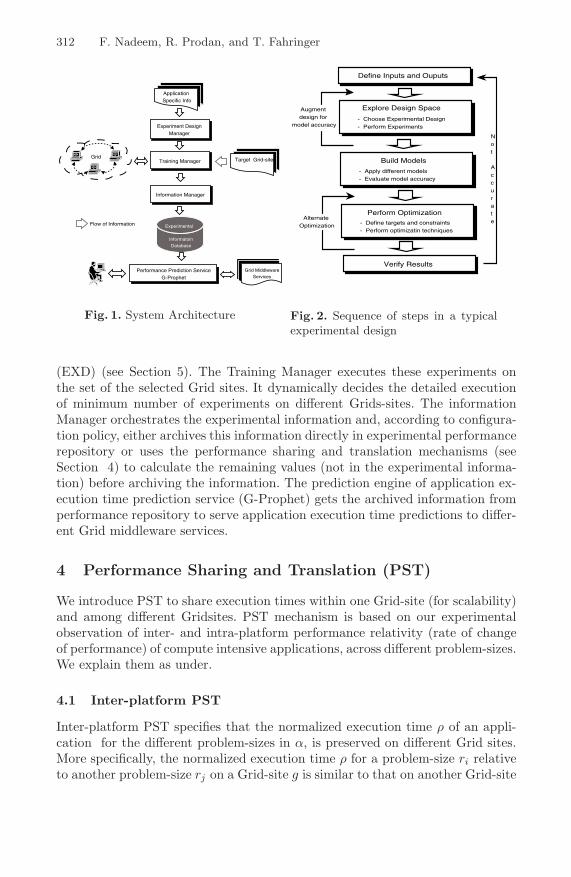
The Architecture of the system is simple and shown in Figure 1. Applicationspecific information (the different parameters affecting execution time of theapplication, their ranges and effective step sizes) is provided to Experiment De-sign Manager, which plans experiments through Extended Experimental Design

312 F. Nadeem, R. Prodan, and T. Fahringer

Application Specific Info

Training Manager Target Grid-sites

Experimental

InformatoinDatabase

Information Manager

Grid

Experiment DesignManager

Grid MiddlewareServices

Performance Prediction ServiceG-Prophet

Flow of Information

Fig. 1. System Architecture

- Choose Experimental Design- Perform Experiments

Explore Design Space

- Apply different models- Evaluate model accuracy

Build Models

- Define targets and constraints- Perform optimizatin techniques

Perform Optimization

Define Inputs and Ouputs

Verify Results

Augment design for

model accuracy

Alternate Optimization

Not

Accurate

Fig. 2. Sequence of steps in a typicalexperimental design

(EXD) (see Section 5). The Training Manager executes these experiments onthe set of the selected Grid sites. It dynamically decides the detailed executionof minimum number of experiments on different Grids-sites. The informationManager orchestrates the experimental information and, according to configura-tion policy, either archives this information directly in experimental performancerepository or uses the performance sharing and translation mechanisms (seeSection 4) to calculate the remaining values (not in the experimental informa-tion) before archiving the information. The prediction engine of application ex-ecution time prediction service (G-Prophet) gets the archived information fromperformance repository to serve application execution time predictions to differ-ent Grid middleware services.

4 Performance Sharing and Translation (PST)

We introduce PST to share execution times within one Grid-site (for scalability)and among different Gridsites. PST mechanism is based on our experimentalobservation of inter- and intra-platform performance relativity (rate of changeof performance) of compute intensive applications, across different problem-sizes.We explain them as under.

4.1 Inter-platform PST

Inter-platform PST specifies that the normalized execution time ρ of an appli-cation for the different problem-sizes in α, is preserved on different Grid sites.More specifically, the normalized execution time ρ for a problem-size ri relativeto another problem-size rj on a Grid-site g is similar to that on another Grid-site

Optimizing Performance of Automatic Training Phase 313

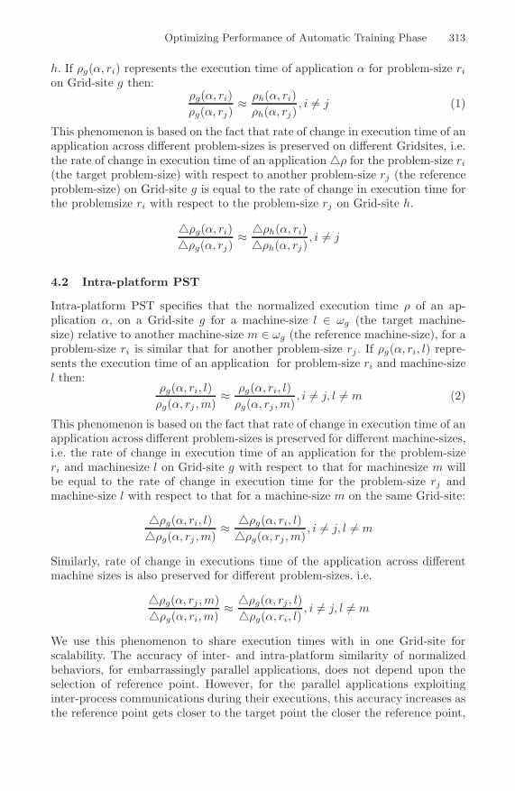
h. If ρg(α, ri) represents the execution time of application α for problem-size rion Grid-site g then:

ρg(α, ri)ρg(α, rj)

≈ ρh(α, ri)ρh(α, rj)

, i �= j (1)

This phenomenon is based on the fact that rate of change in execution time of anapplication across different problem-sizes is preserved on different Gridsites, i.e.the rate of change in execution time of an application �ρ for the problem-size ri(the target problem-size) with respect to another problem-size rj (the referenceproblem-size) on Grid-site g is equal to the rate of change in execution time forthe problemsize ri with respect to the problem-size rj on Grid-site h.

�ρg(α, ri)�ρg(α, rj)

≈ �ρh(α, ri)�ρh(α, rj)

, i �= j

4.2 Intra-platform PST

Intra-platform PST specifies that the normalized execution time ρ of an ap-plication α, on a Grid-site g for a machine-size l ∈ ωg (the target machine-size) relative to another machine-size m ∈ ωg (the reference machine-size), for aproblem-size ri is similar that for another problem-size rj . If ρg(α, ri, l) repre-sents the execution time of an application for problem-size ri and machine-sizel then:

ρg(α, ri, l)ρg(α, rj ,m)

≈ ρg(α, ri, l)ρg(α, rj ,m)

, i �= j, l �= m (2)

This phenomenon is based on the fact that rate of change in execution time of anapplication across different problem-sizes is preserved for different machine-sizes,i.e. the rate of change in execution time of an application for the problem-sizeri and machinesize l on Grid-site g with respect to that for machinesize m willbe equal to the rate of change in execution time for the problem-size rj andmachine-size l with respect to that for a machine-size m on the same Grid-site:

�ρg(α, ri, l)�ρg(α, rj ,m)

≈ �ρg(α, ri, l)�ρg(α, rj ,m)

, i �= j, l �= m

Similarly, rate of change in executions time of the application across differentmachine sizes is also preserved for different problem-sizes. i.e.

�ρg(α, rj ,m)�ρg(α, ri,m)

≈ �ρg(α, rj , l)�ρg(α, ri, l)

, i �= j, l �= m

We use this phenomenon to share execution times with in one Grid-site forscalability. The accuracy of inter- and intra-platform similarity of normalizedbehaviors, for embarrassingly parallel applications, does not depend upon theselection of reference point. However, for the parallel applications exploitinginter-process communications during their executions, this accuracy increases asthe reference point gets closer to the target point the closer the reference point,

314 F. Nadeem, R. Prodan, and T. Fahringer

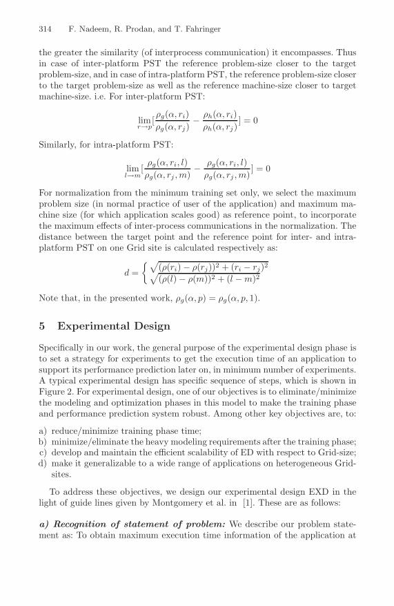
the greater the similarity (of interprocess communication) it encompasses. Thusin case of inter-platform PST the reference problem-size closer to the targetproblem-size, and in case of intra-platform PST, the reference problem-size closerto the target problem-size as well as the reference machine-size closer to targetmachine-size. i.e. For inter-platform PST:

limr→p

[ρg(α, ri)ρg(α, rj)

− ρh(α, ri)ρh(α, rj)

] = 0

Similarly, for intra-platform PST:

liml→m

[ρg(α, ri, l)ρg(α, rj ,m)

− ρg(α, ri, l)ρg(α, rj ,m)

] = 0

For normalization from the minimum training set only, we select the maximumproblem size (in normal practice of user of the application) and maximum ma-chine size (for which application scales good) as reference point, to incorporatethe maximum effects of inter-process communications in the normalization. Thedistance between the target point and the reference point for inter- and intra-platform PST on one Grid site is calculated respectively as:

d ={√

(ρ(ri) − ρ(rj))2 + (ri − rj)2√(ρ(l) − ρ(m))2 + (l −m)2

Note that, in the presented work, ρg(α, p) = ρg(α, p, 1).

5 Experimental Design

Specifically in our work, the general purpose of the experimental design phase isto set a strategy for experiments to get the execution time of an application tosupport its performance prediction later on, in minimum number of experiments.A typical experimental design has specific sequence of steps, which is shown inFigure 2. For experimental design, one of our objectives is to eliminate/minimizethe modeling and optimization phases in this model to make the training phaseand performance prediction system robust. Among other key objectives are, to:

a) reduce/minimize training phase time;b) minimize/eliminate the heavy modeling requirements after the training phase;c) develop and maintain the efficient scalability of ED with respect to Grid-size;d) make it generalizable to a wide range of applications on heterogeneous Grid-

sites.

To address these objectives, we design our experimental design EXD in thelight of guide lines given by Montgomery et al. in [1]. These are as follows:

a) Recognition of statement of problem: We describe our problem state-ment as: To obtain maximum execution time information of the application at

Optimizing Performance of Automatic Training Phase 315

different problem-sizes on all heterogeneous Grid-sites with different possiblemachine-sizes in minimum number of the experiments.

b) Selection of response variables: In our work the response variable is theexecution time of the application.

c) Choice of factors, levels and ranges: The factors affecting the responsevariable are the problem-size of the application, the Grid-size and the machine-size. The range of problem-size incorporates ranges of each of input variablesand the levels consist of their values at effective step sizes specified by the userof the application. The range of the Grid-size is {1, 2, ,m}, and the levels includenumeration of non-identical Grid-sites gi. The range of machine-size spans overall different subsets of number of (heterogeneous) processors on a Grid-site andits levels include of all these individual subsets. Consider a simple case, for oneGrid application with x different problem sizes and m Grid sites with pi machinesizes. If we include all the respective levels of the above described factors, thenthe total number of possible experiments N is given by:

N =∑m

i (pi × x)

For single processor Grid-sites the above formula reduces to N = x × m. Theobjective function f of the experimental design is:

f : R × N+ × N

+ → N+

f(β, γ, λ) = MinN : ξ ≥ 90%

where ξ represents accuracy.

d) Choice/Formulation of Experimental Design: In our Extended Exper-imental Design (EXD), we minimize the combinations of Grid-size with problem-size and then, combinations of Gridsize with machine-size. By minimizing thecombinations of Grid-size with problem-size, we actually minimize number ofexperiments against different problem-sizes across the heterogeneous Grid-sites.Similarly, by minimizing the Grid-size combinations with machine-size factor, weactually minimize number of experiments against different problem-sizes acrossdifferent number of processors. To meet these objective, we employ PST [2]mechanisms (see Section 4.2).

In our design, we choose one Grid-site (the fastest one, based on the ini-tial runs) as a base Grid-site and make a full factorial of experiments on it.Later, we use its execution times as reference values to calculate predictions forother platforms (the target Grid-sites) using inter-platform PST and thus min-imize problem-size combinations with Grid-size. We also make one experimenton each of other different Grid-sites to make PST work. Similarly, to minimizemachine-size combinations with Grid-size, we need a full factorial of experimentswith one machine-size, the base machine-size (which we already have while min-imizing problem-size combinations with Grid-size), and later use these valuesas reference values. We make one experiment each for all other machine-sizes,to translate the reference execution times to that for other machine-sizes using

316 F. Nadeem, R. Prodan, and T. Fahringer

intraplatform PST. The approach of making full factorial design of experimentsis also necessary because we neither make any assumptions about the perfor-mance models of different applications, nor we make their analytical models atrun time, because making analytical performance models for individual appli-cations is more complex and less efficient than making full factorial design ofexperiments for once. In initial phase, we restrict the full factorial design ofexperiments to the commonly used range of problem-size.

By means of inter-platform PST, the total number of experiments N reducesfrom a polynomial complexity of p×x×m to p×x+(m−1) for parallel machines,and from a polynomial complexity of x×m to a linear complexity of x− 1 +mfor single processor machines. Introducing intra-platform PST, we are able toreduce total number of experiments for parallel machines (Grid-sites) further toa linear complexity of p+ (x− 1) + (m− 1) or p+m+ x− 2.

e) Performing of experiments: We address performing of experiments underautomatic training phase as described in Section 6.

We design above step d to eliminate the need of next two steps presentedby Montgomery et. al. the statistical analysis & modeling and conclusions, tominimize the serving costs on the fly.

6 Automatic Training Phase Based on EXD

If we consider the whole training phase as a process then, in executing the de-signed experiments, the process variables are application problem-size, machine-size and Grid-size. Our automatic training phase is a three layered approach;layer 1 for the initial test runs, layer 2 for the execution of experiments designedin experimental design phase, and layer 3 for the PST mechanism. In the initialtest runs of the training phase, we need to make some characterizing or screeningto establish some conjectures for the next set of experiments. This information isused to decide the base Grid-site. In layer 2, execution of experiments on differ-ent Grid-sites is planned according to the experimental design, and the trainingmanager executes these experiments on the selected Grid-sites. The collectedinformation is passed through layer 3, the PST mechanism, to store in a per-formance repository. First, the training manager makes one initial experimenton all non-identical Grid-sites G from Grid-site sample space GT for maximumvalues of problem-sizes. Second, it selects the Gridsite with minimum executiontime as base Grid-site and makes a full factorial design of experiments on it.We categorize two Grid-sites to be identical if they have same number of pro-cessors, processor architecture, processor speed, and memory. We also excludethose identical Grid-sites with i processors gi for which gi ⊂ gj for i ≤ j, i.e.if a cluster or a sub-cluster is identical to another cluster or sub-cluster thenonly one of them will be included in training phase. Similarly, if a cluster or asub-cluster is a subset of another cluster or sub-cluster then only the super setcluster is included in the training phase

The information from these experiments is archived to serve prediction pro-cess. For applications having a wide range of problem-size, we have support of

Optimizing Performance of Automatic Training Phase 317

distributed training phase. In distributed training phase we split the full fac-torial design of experiments from one machine to different Grid-sites which areincluded in the training phase. Distributed training phase exploits opportunisticload balancing [15] for executing experiments to harness maximum paralleliza-tion of training phase.

7 Application Performance Prediction System:G-Prophet

The ultimate goal of automatic training phase is to support performance predic-tion service, to serve automatic execution time predictions. To serve applicationperformance prediction prediction system G-Prophet (Grid- Prophet), imple-mented under ASKALON, utilizes the inter- and intra-platform PST mecha-nisms to furnish the predictions using Equation 1 as:

ρg(α, ri) =ρh(α, ri)ρh(α, rj)

× ρg(α, ri)

and/or Equation 2 as:ρg(α, ri, l) =

ρg(α, ri, l)ρg(α, rj ,m)

× ρg(α, ri,m)

G-Prophet uses the the nearest possible reference values for serving the predic-tions, available from the training phase or actual run times. From the minimumtraining set, we observe a prediction accuracy of more than 90% and a standarddeviation of 2% in the worst case.

8 Experiments and Analysis

In this section, we describe the experimental platform and real world applica-tions used for our experiments, the scalability and performance results from ourproposed experimental design against the different changes in the factors in-volved (as defined in Section 5). For our results presented here, each result istaken as an average of five repetitions of the experiment to guard against theanomalous results.

8.1 Experimental Platform

We have conducted all of our experiments on the Austrian Grid environment.The Austrian Grid consortium combines Austria’s leading researchers in ad-vanced computing technologies with well-recognized partners in Grid-dependantapplication areas. The description of Austrian test bed sites for our experi-ments is given in Table 2. Our experiments are conducted on three real worldapplications Wien2k [3], Invmod [2] and meteoAG [4]. Wien2k applicationallows performing electronic structure calculations of solids using density func-tional theory based on the full-potential augmented planewave ((L)APW) and

318 F. Nadeem, R. Prodan, and T. Fahringer

local orbital (lo) method. Invmod application helps in studying the effects of cli-matic changes on the water balance through water flow and balance simulations,in order to obtain improved discharge estimates for extreme floods. MeteoAGproduces meteorological simulations of precipitation fields of heavy precipitationcases over the western part of Austria with RAMS, at a spatially and temporallyfine granularity, in order to resolve most alpine watersheds and thunderstorms.

8.2 Performance and Scalability Analysis

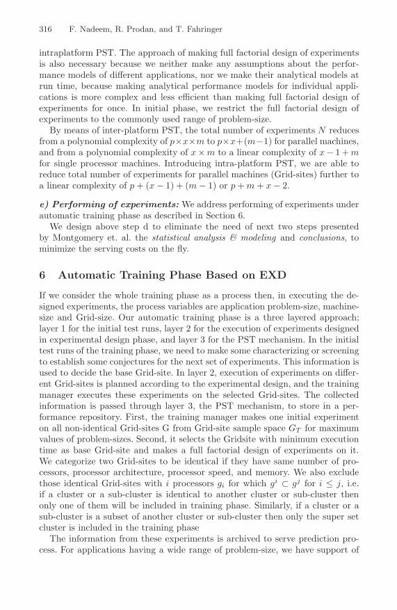
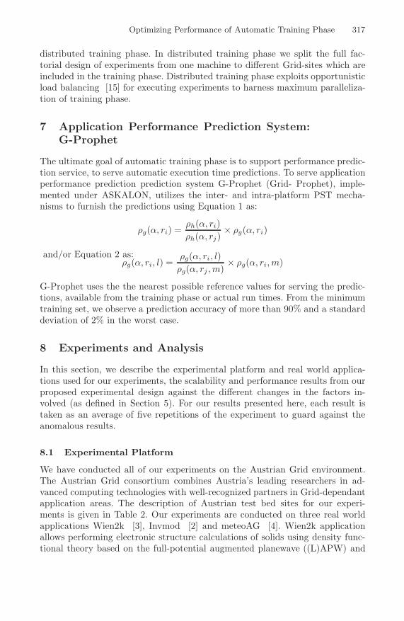
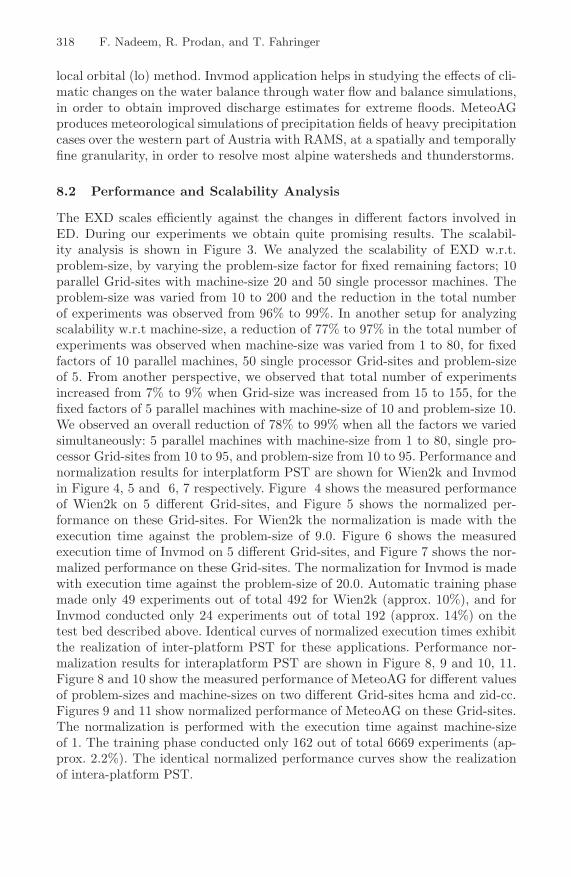
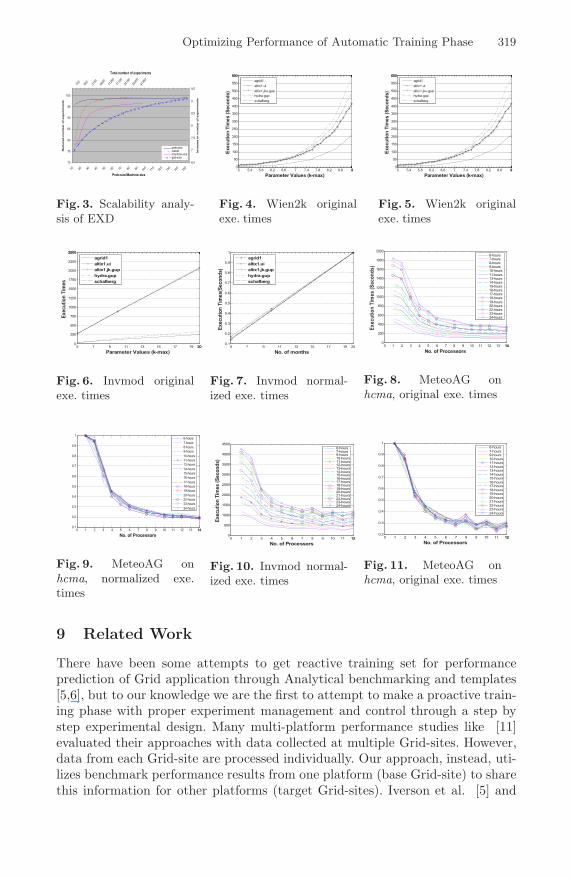
The EXD scales efficiently against the changes in different factors involved inED. During our experiments we obtain quite promising results. The scalabil-ity analysis is shown in Figure 3. We analyzed the scalability of EXD w.r.t.problem-size, by varying the problem-size factor for fixed remaining factors; 10parallel Grid-sites with machine-size 20 and 50 single processor machines. Theproblem-size was varied from 10 to 200 and the reduction in the total numberof experiments was observed from 96% to 99%. In another setup for analyzingscalability w.r.t machine-size, a reduction of 77% to 97% in the total number ofexperiments was observed when machine-size was varied from 1 to 80, for fixedfactors of 10 parallel machines, 50 single processor Grid-sites and problem-sizeof 5. From another perspective, we observed that total number of experimentsincreased from 7% to 9% when Grid-size was increased from 15 to 155, for thefixed factors of 5 parallel machines with machine-size of 10 and problem-size 10.We observed an overall reduction of 78% to 99% when all the factors we variedsimultaneously: 5 parallel machines with machine-size from 1 to 80, single pro-cessor Grid-sites from 10 to 95, and problem-size from 10 to 95. Performance andnormalization results for interplatform PST are shown for Wien2k and Invmodin Figure 4, 5 and 6, 7 respectively. Figure 4 shows the measured performanceof Wien2k on 5 different Grid-sites, and Figure 5 shows the normalized per-formance on these Grid-sites. For Wien2k the normalization is made with theexecution time against the problem-size of 9.0. Figure 6 shows the measuredexecution time of Invmod on 5 different Grid-sites, and Figure 7 shows the nor-malized performance on these Grid-sites. The normalization for Invmod is madewith execution time against the problem-size of 20.0. Automatic training phasemade only 49 experiments out of total 492 for Wien2k (approx. 10%), and forInvmod conducted only 24 experiments out of total 192 (approx. 14%) on thetest bed described above. Identical curves of normalized execution times exhibitthe realization of inter-platform PST for these applications. Performance nor-malization results for interaplatform PST are shown in Figure 8, 9 and 10, 11.Figure 8 and 10 show the measured performance of MeteoAG for different valuesof problem-sizes and machine-sizes on two different Grid-sites hcma and zid-cc.Figures 9 and 11 show normalized performance of MeteoAG on these Grid-sites.The normalization is performed with the execution time against machine-sizeof 1. The training phase conducted only 162 out of total 6669 experiments (ap-prox. 2.2%). The identical normalized performance curves show the realizationof intera-platform PST.

Optimizing Performance of Automatic Training Phase 319

70

75

80

85

90

95

100

10 20 30 40 50 60 70 80 90 100

110

120

130

140

150

Prob-size/Machine-size

Red

uced

nu

mb

er

of

exp

eri

men

ts

6,5

7

7,5

8

8,5

9

9,5

150

900

3150

6600

1125

0

1710

0

2415

0

3240

0

4185

0

Total number of experiments

Incre

ase i

n n

um

ber

of

exp

eri

men

ts

prob-sizeoverallmachine-sizegrid-size

Fig. 3. Scalability analy-sis of EXD

5 5.4 5.8 6.2 6.6 7 7.4 7.8 8.2 8.6 990

50

100

150

200

250

300

350

400

450

500

550

600600

Parameter Values (k-max)

Exe

cutio

n Ti

mes

(Sec

onds

)

agrid1

altix1.ui

altix1.jku.gup

hydra.gup

schafberg

Fig. 4. Wien2k originalexe. times

5 5.4 5.8 6.2 6.6 7 7.4 7.8 8.2 8.6 990

50

100

150

200

250

300

350

400

450

500

550

600600

Parameter Values (k-max)

Exe

cutio

n Ti

mes

(Sec

onds

)

agrid1

altix1.ui

altix1.jku.gup

hydra.gup

schafberg

Fig. 5. Wien2k originalexe. times

5 7 9 11 13 15 17 19 20200

250

500

750

1000

1250

1500

1750

2000

2250

25002500

Parameter Values (k-max)

Exec

utio

n Ti

mes

agrid1altix1.uialtix1.jk.guphydra.gupschafberg

Fig. 6. Invmod originalexe. times

5 7 9 11 13 15 17 19 200.1

0.2

0.3

0.4

0.5

0.6

0.7

0.8

0.9

1

No. of months

Exec

utio

n Ti

mes

(Sec

onds

)

agrid1altix1.uialtix1.jk.guphydra.gupschafberg

Fig. 7. Invmod normal-ized exe. times

0 1 2 3 4 5 6 7 8 9 10 11 12 13 14140

200

400

600

800

1000

1200

1400

1600

1800

2000

No. of Processors

Exec

utio

n Ti

mes

(Sec

onds

)

6-hours7-hours8-hours9-hours10-hours

11-hours13-hours14-hours15-hours16-hours17-hours18-hours

19-hours20-hours22-hours23-hours24-hours

Fig. 8. MeteoAG onhcma, original exe. times

0 1 2 3 4 5 6 7 8 9 10 11 12 13 14140.1

0.2

0.3

0.4

0.5

0.6

0.7

0.8

0.9

1

No. of Processors

6-hours

7-hours

8-hours

9-hours

10-hours

11-hours

13-hours

14-hours

15-hours

16-hours

17-hours

18-hours

19-hours

20-hours

22-hours

23-hours

24-hours

Fig. 9. MeteoAG onhcma, normalized exe.times

0 1 2 3 4 5 6 7 8 9 10 11 12120

500

1000

1500

2000

2500

3000

3500

4000

4500

No. of Processors

Exec

utio

n Ti

mes

(Sec

onds

)

6-hours7-hours9-hours10-hours11-hours12-hours13-hours14-hours15-hours16-hours17-hours18-hours19-hours20-hours21-hours22-hours23-hours24-hours

Fig. 10. Invmod normal-ized exe. times

0 1 2 3 4 5 6 7 8 9 10 11 12120.2

0.3

0.4

0.5

0.6

0.7

0.8

0.9

1

No. of Processors

6-hours

7-hours9-hours

10-hours11-hours

12-hours13-hours

14-hours15-hours

16-hours17-hours

18-hours19-hours

20-hours21-hours

22-hours23-hours

24-hours

Fig. 11. MeteoAG onhcma, original exe. times

9 Related Work

There have been some attempts to get reactive training set for performanceprediction of Grid application through Analytical benchmarking and templates[5,6], but to our knowledge we are the first to attempt to make a proactive train-ing phase with proper experiment management and control through a step bystep experimental design. Many multi-platform performance studies like [11]evaluated their approaches with data collected at multiple Grid-sites. However,data from each Grid-site are processed individually. Our approach, instead, uti-lizes benchmark performance results from one platform (base Grid-site) to sharethis information for other platforms (target Grid-sites). Iverson et al. [5] and

320 F. Nadeem, R. Prodan, and T. Fahringer

Marin et al. [13] use parameterized models to translate execution times acrossthe heterogeneous platforms but their models need human interaction to param-eterize all machines performance attributes. In contrast, we make our models onthe basis of normalized/relative performance, which does not need any sourcecode and manual intervention. Moreover it is difficult to use their approach fordifferent languages. Leo et al. [7] use partial executions for cross platform per-formance translation. Their models need source code instrumentation and thusrequire human intervention. To contrast, our approach does not require sourcecode and code instrumentation. Systems like Prophesy [9], PMaC [8], andconvolution methods to map hand-coded kernels to Grid-site profiles [10] baseon modeling computational kernels instead of complex applications with diversetasks. In contrast, we develop observation-based performance translation, whichdoes not require in-depth knowledge of parallel systems or codes. This makesour approach application- , language- and platform-independent. Reducing thenumber of experiments in adaptive environments dedicated to applications, bytuning parameters at run time have been applied by couple of works like AT-LAS [15] (tuning performance of libraries by tuning parameters at run time).Though this technique improves the performance, yet is very specific to the ap-plications. Unlike this work, we do not do run time modeling/tuning at runtime, as modeling individual applications is more complex and less efficient thanmaking the proposed experiments.

References

1. Douglas, C., Montgomery: Design and Analysis of Experiments. ch. 1, vol. 6. JohnWiley & Sons, New York (2004)

2. Theiner, D., et al.: Reduction of Calibration Time of Distributed HydrologicalModels by Use of Grid Comp. and Nonlinear Optimisation Algos. In: InternationalConference on Hydroinformatics, France (2006)

3. [3] Blaha, P., Schwarz, K., Madsen, G., Kvasnicka, D., Luitz, J.: WIEN2k: AnAugmented Plane Wave plus LocalOrbitals Program for Calculating Crystal Prop-erties, Instituteof Physical and Theoretical Chemistry, TU Vienna (2001)

4. Schller, F., Qin, J., Farrukh N.: Performance, Scalability and Quality of the Mete-orological Grid Workflow MeteoAG. In: 2nd Austrian Grid Symposium, Innsbruck,Austria. OCG Verlag (2006)

5. Iverson, M.A., et al.: Statistical Prediction of Task Execution Times Through An-alytic Benchmarking for Scheduling in a Heterogeneous Environment. In: Hetero-geneous Computing Workshop (1999)

6. Smith, W., Foster, I., Taylor, V.: Predicting Application Run Times Using His-torical Information. In: Proceedings of the IPPS/SPDP (1998) Workshop on JobScheduling Strategies for Parallel Processing (1998)

7. Yang, L.T., Ma, X., Mueller, F.: Cross- Platform Performance Prediction of ParallelApplications Using Partial Execution. In: Supercomputing, USA (2005)

8. Carrington, L., Snavely, A., Wolter, N.: A performance prediction framework forscientific applications,Future Gener. Computing Systems, vol. 22, Amsterdam, TheNetherlands (2006)

Optimizing Performance of Automatic Training Phase 321

9. Taylor, V., et al.: Prophesy: An Infrastructure for Performance Analysis and Mod-eling of Parallel and Grid Applications. ACM Sigmetrics Performance EvaluationReview 30(4) (2003)

10. Bailey, D.H., Snavely, A.: Performance Modeling: Understanding the Present andPredicting the Future. In: Euro-Par Conference (August 2005)

11. Kerbyson, D.J., Alme, H.J., et al.: Predictive Performance and Scalability Modelingof a Large-Scale Application. In: Proceedings of Supercomputing (2001)

12. Fahringer, T., et al.: ASKALON: A Grid Application Development and ComputingEnvironment. In: 6th International Workshop on Grid, Seattle, USA (November2005)

13. Marin, G., Mellor-Crummey, J.: Cross-Architecture Performance Predictions forScientific Applications Using Parameterized Models. In: Joint International Con-ference on Measurement and Modeling of Computer Systems (2004)

14. Nadeem, F., Yousaf, M.M., Prodan, R., Fahringer, T.: Soft Benchmarks-based Ap-plication Performance Prediction using a Minimum Training Set. In: Second Inter-national Conference on e-Science and Grid computing, Amsterdam, Netherlands(December 2006)

15. Whaley, R.C., Petitet, A.: Petitet: Minimizing development and maintenancecosts in supporting persistently optimized BLAS. Software: Practice and Expe-rienc 35(2):1012̆013121 (2005)