Optimizing Mobile Application Performance throughNetwork Infrastructure Aware Adaptation

by

Qiang Xu

A dissertation submitted in partial fulfillmentof the requirements for the degree of

Doctor of Philosophy(Computer Science and Engineering)

in the University of Michigan2013

Doctoral Committee:

Associate Professor Z. Morley Mao, ChairAssociate Professor Robert DickAssociate Professor Jason N. FlinnTechnical Staff Feng Qian, AT&T Labs Research

c© Qiang Xu 2013

All Rights Reserved

To my family.

ii

ACKNOWLEDGEMENTS

I would like to appreciate many people who helped me during this time. Without

them, it would be impossible for me to complete the dissertation.

First, I would like to thank my advisor Prof. Z. Morley Mao, who has broad

interests in networking systems, routing protocols, mobile and distributed systems,

and network security. Working with her, I not only have learned how to develop

professional research skills in mobile networking but also have deepened my

research interests in other system areas. It is my great pleasure to work with

Morley in past 4.5 years. I appreciate Prof. Jason Flinn, Prof. Robert Dick, and Dr.

Feng Qian for serving on my thesis committee. They have provided valuable

comments and suggestions for refining my dissertation.

I would also like to thank my mentors: Alexandre Gerber, Jeffrey Pang, Sanjeev

Mehrotra, Jin Li, Yong Liao, and Stanislav Miskovic, along with other researchers in

these collaborations: Ming Zhang, Paramvir Bahl, Yi-Min Wang, Jeffrey Erman,

Shobha Venkataraman, Mario Baldi, and Antonio Nucci. They have shared their

great knowledge and experience to help me shape research problems and address

challenges.

My life in Michigan has been wonderful because of many colleagues and

friends. I would like to thank Ying Zhang, Xu Chen, Feng Qian, Zhiyun Qian,

Yudong Gao, Junxian Huang, Birjodh Tiwana, Ni Pan, Zhaoguang Wang, Mark

Gordon, Sanae Rosen, Thomas Andrews, Yihua Guo, Mehrdad Moradi, Haokun

Luo, Qi Chen, Yuanyuan Zhou, Ashkan Nikravesh, Yunjing Xu, Timur Alperovich,

iii

Lujun Fang, Li Qian, and Jie Yu. There is a special thank you to my roommate Wen

Chen for the encouragement during tough days.

Finally, the help from my wife, Jinhua Quan, is tremendous. She is always a

source of love and encouragement. I have been very fortunate to have so many

wonderful people around since I was born. I dedicated this dissertation to all of

them.

iv

TABLE OF CONTENTS

DEDICATION . . . . . . . . . . . . . . . . . . . . . . . . . . . . . . . ii

ACKNOWLEDGEMENTS . . . . . . . . . . . . . . . . . . . . . . . . . iii

LIST OF FIGURES . . . . . . . . . . . . . . . . . . . . . . . . . . . . vii

LIST OF TABLES . . . . . . . . . . . . . . . . . . . . . . . . . . . . . ix

ABSTRACT . . . . . . . . . . . . . . . . . . . . . . . . . . . . . . . x

CHAPTER

I. INTRODUCTION . . . . . . . . . . . . . . . . . . . . . . . . . . 1

1.1 Revealing Fundamental Cellular Characteristics . . . . . . 31.2 Decomposing the Impact of Cellular Characteristics . . . . 41.3 Identifying the Usage Patterns of Mobile Applications . . . . 51.4 Optimizing Applications via Network-Aware Adaptation . . . 61.5 Thesis Organization . . . . . . . . . . . . . . . . . . . . . 7

II. BACKGROUND . . . . . . . . . . . . . . . . . . . . . . . . . . 8

2.1 Cellular Network Hierarchy . . . . . . . . . . . . . . . . . 82.2 Cellular Network Mobility Management . . . . . . . . . . . 102.3 Cellular Network Resource Allocation . . . . . . . . . . . . 12

III. CELLULAR INFRASTRUCTURE DISCOVERY . . . . . . . . . . 14

3.1 Determining IPs’ Geographic Coverage . . . . . . . . . . . 173.1.1 Datasets . . . . . . . . . . . . . . . . . . . . . 193.1.2 Operating Datasets to Identify IPs’ Geographic Cov-

erage . . . . . . . . . . . . . . . . . . . . . . . 223.2 Inferring GGSNs from IPs’ Geographic Coverage . . . . . . 23

3.2.1 Clustering IPs . . . . . . . . . . . . . . . . . . . 24

v

3.2.2 Validating GGSN Clusters . . . . . . . . . . . . . 333.3 Impact of the Routing Restriction due to GGSNs . . . . . . 38

3.3.1 Content Placement . . . . . . . . . . . . . . . . 383.3.2 Server Selection . . . . . . . . . . . . . . . . . 40

3.4 Summary of Cellular Infrastructure Charateristics . . . . . . 42

IV. APPLICATION USAGE IDENTIFICATION . . . . . . . . . . . . . 44

4.1 Traffic Classification at Network Gateways . . . . . . . . . 454.1.1 Techniques . . . . . . . . . . . . . . . . . . . . 494.1.2 System Design . . . . . . . . . . . . . . . . . . 544.1.3 Datasets . . . . . . . . . . . . . . . . . . . . . 574.1.4 Classification Performance . . . . . . . . . . . . 594.1.5 Limitation . . . . . . . . . . . . . . . . . . . . . 74

4.2 Application Usage Characterization . . . . . . . . . . . . . 774.2.1 Datasets . . . . . . . . . . . . . . . . . . . . . 804.2.2 Smartphone Application Usage Patterns . . . . . 814.2.3 Implications of Application Usage Patterns . . . . 102

4.3 Summary of Identifying Application Usage . . . . . . . . . 105

V. APPLICATION PERFORMANCE OPTIMIZATION . . . . . . . . . 108

5.1 PROTEUS Overview . . . . . . . . . . . . . . . . . . . . 1115.2 Prediction Using PROTEUS . . . . . . . . . . . . . . . . 115

5.2.1 Characterizing Cellular Networks . . . . . . . . . 1155.2.2 Constructing Regression Trees . . . . . . . . . . 1205.2.3 Evaluating Forecast Accuracy . . . . . . . . . . . 124

5.3 Application of PROTEUS . . . . . . . . . . . . . . . . . . 1335.3.1 Video Conferencing System . . . . . . . . . . . . 1335.3.2 Interactive Software Application . . . . . . . . . . 140

5.4 Summary of Optimizing Real-Time, Interactive Applications 142

VI. RELATED WORK . . . . . . . . . . . . . . . . . . . . . . . . . 144

6.1 Cellular Infrastructure . . . . . . . . . . . . . . . . . . . . 1446.2 Application Usage . . . . . . . . . . . . . . . . . . . . . 1466.3 Application Optimization . . . . . . . . . . . . . . . . . . 148

VII. CONCLUDING REMARKS . . . . . . . . . . . . . . . . . . . . . 150

BIBLIOGRAPHY . . . . . . . . . . . . . . . . . . . . . . . . . . . . . 152

vi

LIST OF FIGURES

Figure

1.1 Task breakdown. . . . . . . . . . . . . . . . . . . . . . . . . . 32.1 Cellular network infrastructure. . . . . . . . . . . . . . . . . . . 93.1 Workflow for determining IPs’ geographic coverage. . . . . . . . . 183.2 Similarity of IPs’ geographic coverage. . . . . . . . . . . . . . . 253.3 Number of records of individual prefixes in YellowPage dataset. . . 263.4 Tuning the input SSE in bi-sect K-means clustering. . . . . . . . . 273.5 Geographic coverage of individual GGSN clusters. . . . . . . . . 293.6 Overlap degree across GGSN clusters. . . . . . . . . . . . . . . 313.7 Four major carriers’ GGSN clusters. . . . . . . . . . . . . . . . . 323.8 Geographic clusters based on local DNS resolvers. . . . . . . . . 353.9 Latency to GGSNs against landmark servers. . . . . . . . . . . . 394.1 FLOWR’s workflow. . . . . . . . . . . . . . . . . . . . . . . . . 494.2 Types of URIs used in FLOWR. . . . . . . . . . . . . . . . . . . 514.3 Uniqueness of user-agents and contacted hostnames. . . . . . . 614.4 Persistence of KVs. . . . . . . . . . . . . . . . . . . . . . . . . 614.5 Uniqueness of KVs. . . . . . . . . . . . . . . . . . . . . . . . . 634.6 Web analytics and ad services in paid and free apps. . . . . . . . 644.7 Time difference between two flows from the same app. . . . . . . 654.8 System memory consumption under workload growth. . . . . . . 664.9 Identifiability of KVs. . . . . . . . . . . . . . . . . . . . . . . . . 674.10 Identifiability of unique/non-unique KVs. . . . . . . . . . . . . . . 694.11 Mapping from identifiability to false positive. . . . . . . . . . . . . 704.12 Flow coverage starting with doubleclick apps. . . . . . . . . . . . 714.13 Number of identified doubleclick apps. . . . . . . . . . . . . . . 734.14 The uniqueness of HTTP certificates. . . . . . . . . . . . . . . . 754.15 Tokenization over compressed or hashed traffic flows. . . . . . . 764.16 Traffic volume/access time/number of users for individual apps. . . 824.17 Single-user traffic volume/access time for individual apps. . . . . 834.18 Contributions of the top X apps. . . . . . . . . . . . . . . . . . . 854.19 Traffic volume contribution from the top X states. . . . . . . . . . 874.20 Breakdown of the top X states of the local apps. . . . . . . . . . . 884.21 Geographic usage distribution of app genres. . . . . . . . . . . . 89

vii

4.22 Geographic usage difference across app genres. . . . . . . . . . 904.23 Geographic usage distribution in the same app genre. . . . . . . 914.24 Travel area of apps. . . . . . . . . . . . . . . . . . . . . . . . . 924.25 Coefficient between the apps sharing users. . . . . . . . . . . . 944.26 Dependency between popular apps. . . . . . . . . . . . . . . . 954.27 Diurnal patterns of app usage. . . . . . . . . . . . . . . . . . . 984.28 Significance of late night apps. . . . . . . . . . . . . . . . . . . 984.29 Diurnal patterns across app genres. . . . . . . . . . . . . . . . . 1004.30 Impact of the device type on app usage. . . . . . . . . . . . . . 1015.1 Design of PROTEUS. . . . . . . . . . . . . . . . . . . . . . . . 1135.2 Autocorrelation coefficient of throughput. . . . . . . . . . . . . . 1175.3 Cross correlation coefficient between performance metrics. . . . . 1195.4 One-way delay for the time windows with and without loss. . . . . 1205.5 Example of a regression tree predicting loss rate. . . . . . . . . . 1215.6 Attributes of the loss regression tree. . . . . . . . . . . . . . . . 1225.7 Accuracy in loss prediction. . . . . . . . . . . . . . . . . . . . . 1265.8 Quantitative accuracy. . . . . . . . . . . . . . . . . . . . . . . . 1285.9 Impact of the cellular network. . . . . . . . . . . . . . . . . . . . 1315.10 Impact of the time window size. . . . . . . . . . . . . . . . . . . 1315.11 Impact of the information window size. . . . . . . . . . . . . . . 1325.12 Platform setup to emulate mobile video conferencing. . . . . . . . 1345.13 PSNR for PROTEUS, AD1, AD2, TCP, and OPT. . . . . . . . . . 1375.14 FEC overhead. . . . . . . . . . . . . . . . . . . . . . . . . . . 1375.15 Perceptual video quality. . . . . . . . . . . . . . . . . . . . . . . 1405.16 Perceptual delay in Draw Something. . . . . . . . . . . . . . . . 141

viii

LIST OF TABLES

Table

2.1 Terminology of network elements in various cellular technologies. 103.1 Statistics of YellowPage. . . . . . . . . . . . . . . . . . . . . . . 203.2 Statistics of MobiPerf. . . . . . . . . . . . . . . . . . . . . . . . 203.3 Cross overlap between YellowPage and MobiPerf. . . . . . . . . 213.4 Clustering parameters and results . . . . . . . . . . . . . . . . . 283.5 Statistics of local DNS discovery. . . . . . . . . . . . . . . . . . 353.6 GGSN locations inferred from traceroute paths. . . . . . . . . . . 374.1 Applicability and coverage of FLOWR. . . . . . . . . . . . . . . . 484.2 Datasets used in evaluating FLOWR. . . . . . . . . . . . . . . . 574.3 Categories of flow signatures. . . . . . . . . . . . . . . . . . . . 724.4 Genres of apps. . . . . . . . . . . . . . . . . . . . . . . . . . . 864.5 Local apps from Louisiana. . . . . . . . . . . . . . . . . . . . . 884.6 Genres of the apps with large travel areas. . . . . . . . . . . . . 934.7 Dependency between genres. . . . . . . . . . . . . . . . . . . . 964.8 Overview description of late night apps. . . . . . . . . . . . . . . 995.1 Types of applications based on the sensitivity to network loss, OWD,

and throughput. . . . . . . . . . . . . . . . . . . . . . . . . . . 1115.2 Devices and cellular networks covered by the experiments. . . . . 1165.3 Video sequences to reproduce video conferencing streams. . . . 136

ix

ABSTRACT

Optimizing Mobile Application Performance through Network Infrastructure AwareAdaptation

by

Qiang Xu

Chair: Z. Morley Mao

Encouraged by the fast adoption of mobile devices and the widespread

deployment of mobile networks, mobile applications are becoming the preferred

“gateways” connecting users to networking services. Although the CPU capability of

mobile devices is approaching that of off-the-shelf PCs, the performance of mobile

networking applications is still far behind. One of the fundamental reasons is that

most mobile applications are unaware of the mobile network specific

characteristics, leading to inefficient network and device resource utilization. Thus,

in order to improve the user experience for most mobile applications, it is essential

to dive into the critical network components along network connections including

mobile networks, smartphone platforms, mobile applications, and content partners.

We aim to optimize the performance of mobile network applications through

network-aware resource adaptation approaches. Our techniques consist of the

following four aspects: (i) revealing the fundamental infrastructure characteristics of

cellular networks that are distinctive from wireline networks; (ii) isolating the impact

of important factors on user perceived performance in mobile network applications;

x

(iii) determining the particular usage patterns of mobile applications; and (iv)

improving the performance of mobile applications through network aware

adaptations.

xi

CHAPTER I

INTRODUCTION

Due to the emergence of smartphones and the ubiquitous wireless network

deployment, smartphone user experience has been significantly enriched in recent

years. However, the performance of mobile network applications is still far behind

our expectation despite the rapid increase in the computational capabilities with

more powerful processors and multi-core designs for mobile platforms. One of the

fundamental reasons is that many mobile applications are unaware of or do not fully

understand the mobile network specific characteristics, leading to inefficient

resource utilization, which often results in performance bottlenecks eventually. In

order to effectively adapt mobile networking applications to cellular network

conditions, in this thesis, we investigate the unique cellular network

characteristics that are fundamentally different from the wireline Internet’s,

determine the impact of such characteristics on application performance,

and eventually leverage such knowledge to optimize mobile application

designs.

To achieve the goal, it is essential to dive into all the critical network

components along end-to-end network connections including the content partner,

the mobile network, the smartphone platform, the application implementation, and

the usage pattern. First, the current routing of cellular network traffic is quite

1

restricted, as it must traverse a rather limited number (e.g., 4–6) of infrastructure

gateways, which is in sharp contrast to wireline Internet traffic. Such centralized

infrastructure directly affects the network performance and application design.

Second, the on-device networking performance is highly variable, affected by a

multitude of factors including channel quality, radio resource allocation, cellular

network infrastructure, etc. Therefore, decomposing the impact of individual

network components is an essential step towards improving the performance of

smartphone applications from the perspectives of users, developers, network

operators, and smartphone vendors. Third, unlike desktop applications assuming

network resource always desirable, mobile applications have to apply performance

adaptation techniques to accommodate performance variation. As cellular networks

have very unique characteristics in performance and infrastructure, these

techniques have to be aware of such factors. Fourth, as applications are known to

be diverse, before we can invent sophisticated performance optimization

techniques, a prerequisite is the knowledge of application behaviors and usage

patterns.

Accordingly, our techniques consist of the following four thrusts as shown in

Figure 1.1: (i) revealing the fundamental infrastructure characteristics of cellular

networks that are distinctive from wireline networks; (ii) identifying the important

factors that affect the user perceived performance of mobile network applications;

(iii) determining the particular usage patterns of mobile applications; and (iv)

developing performance adaptation techniques to optimize the performance of

mobile applications accordingly. We will introduce each of the four thrusts

respectively in the following.

2

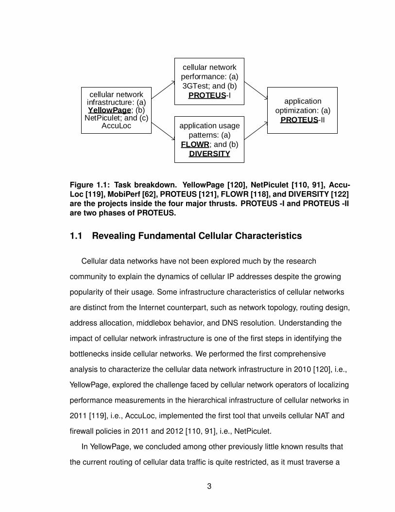
cellular networkinfrastructure: (a)YellowPage; (b)

NetPiculet; and (c)AccuLoc

cellular network

performance: (a)

3GTest; and (b)

PROTEUS-I

application usage

patterns: (a)

FLOWR; and (b)

DIVERSITY

application

optimization: (a)

PROTEUS-II

Figure 1.1: Task breakdown. YellowPage [120], NetPiculet [110, 91], Accu-Loc [119], MobiPerf [62], PROTEUS [121], FLOWR [118], and DIVERSITY [122]are the projects inside the four major thrusts. PROTEUS -I and PROTEUS -IIare two phases of PROTEUS.

1.1 Revealing Fundamental Cellular Characteristics

Cellular data networks have not been explored much by the research

community to explain the dynamics of cellular IP addresses despite the growing

popularity of their usage. Some infrastructure characteristics of cellular networks

are distinct from the Internet counterpart, such as network topology, routing design,

address allocation, middlebox behavior, and DNS resolution. Understanding the

impact of cellular network infrastructure is one of the first steps in identifying the

bottlenecks inside cellular networks. We performed the first comprehensive

analysis to characterize the cellular data network infrastructure in 2010 [120], i.e.,

YellowPage, explored the challenge faced by cellular network operators of localizing

performance measurements in the hierarchical infrastructure of cellular networks in

2011 [119], i.e., AccuLoc, implemented the first tool that unveils cellular NAT and

firewall policies in 2011 and 2012 [110, 91], i.e., NetPiculet.

In YellowPage, we concluded among other previously little known results that

the current routing of cellular data traffic is quite restricted, as it must traverse a

3

rather limited number (e.g., 4–6) of infrastructure gateways, which is in sharp

contrast to wireline Internet traffic. Such a significant difference could demand new

provisioning support for mobile applications.

In NetPiculet, we designed and implemented a measurement tool for accurately

and efficiently identifying middlebox policies in cellular networks. We released

NetPiculet in January 2011 and collected enough measurements for 107 cellular

network operators over the world. In the long run, NetPiculet is highly valuable to

provide visibility into opaque cellular network policies and expose their impact as

networks and applications continue to evolve.

In AccuLoc, we developed a system for network operators to localize

performance measurements to lower aggregation levels such as cell sectors, cell

sites, and RNCs. Applying AccuLoc in performance anomaly detection, we

achieved both the lowest false positive and negative compared with the solutions

based on other forms of clustering. We believe that our work can be an important

utility for cellular operators for the purpose of performance monitoring, network

maintenance, and anomaly detection.

1.2 Decomposing the Impact of Cellular Characteristics

Unlike the traditional network applications running on PCs, whose performance

is mostly constrained by the wired network, network application performance on

smartphones with limited physical resources also heavily depends on factors

including the hardware and the software on the phone as well as the quality and

load of wireless link. Isolating the impact on smartphone application performance

due to each of such factors is important for cellular network operators, smartphone

vendors, and application developers to optimize applications for better user

perceived experiences.

4

In 2009 and 2010, we developed a systematic methodology for comparing this

performance along several key dimensions such as carrier networks, device

capabilities, and server configurations. To ensure a fair and representative

comparison, we implemented MobiPerf (a.k.a. 3GTest), a cross-platform

measurement tool installed by more than 300K users from all over the world.

Running MobiPerf, a user can have the knowledge of his smartphone’s networking

properties, such as field test results, UDP and TCP benchmark performance, HTTP

benchmark performance, and much more. Our analysis based on MobiPerf’s

measurements provides insights into how network operators and smartphone

vendors can improve 3G or cellular networks and mobile devices, and how content

providers can optimize for mobile devices.

1.3 Identifying the Usage Patterns of Mobile Applications

The rapid adoption of mobile devices is dramatically changing the access to

various networking services, i.e., rather than browsers, mobile applications are

becoming the preferred “gateways” connecting users to the Internet. Despite the

increasing importance of applications as gateways to network services, we have a

much limited understanding of how, where, and when they are used compared to

traditional web services, particularly at scale.

Identifying application usage patterns at scale is not straightforward because

applications are indistinguishable as they are communicating predominantly over

HTTP. In 2012, we developed FLOWR (i.e., Flow Recognition System) that

identifies the applications originating the real-time network flows in mobile networks

without supervised learning effort [118].

The goal of FLOWR is to identify mobile network applications. In 2011, we

undertook a first step in identifying the usage patterns of smartphone network

5

applications [122], i.e., DIVERSITY. We studied smartphone network applications

from the angle of their spatial and temporal prevalence, locality, and correlation. We

believe that our findings on the diverse usage patterns of smartphone applications

in spatial, temporal, user, device dimensions will motivate future work in the mobile

community.

1.4 Optimizing Applications via Network-Aware Adaptation

The rapid adoption of mobile devices is resulting in the migration of real-time

communication (RTC) applications from desktop machines to mobile devices. To

adapt and deliver good performance, RTC applications require accurate

estimations of short-term network performance metrics, e.g., loss rate, one-way

delay, and throughput. However, the wide variation in mobile cellular network

performance makes them running on these networks problematic. To address this

issue, various performance adaptation techniques have been proposed, but one

common problem of such techniques is that they only adjust application behavior

reactively after performance degradation is visible. Thus, proactive adaptation

based on accurate short-term, fine-grained network performance prediction can be

a preferred alternative that benefits RTC applications. Since 2011, we have started

to investigate the predictability of cellular network performance [121]. We observed

that forecasting the short-term performance in cellular networks is possible in part

due to the channel estimation scheme on the device and the radio resource

scheduling algorithm at the base station. Thus, we developed a system interface

called PROTEUS, which passively collects current network performance, such as

throughput, loss, and one-way delay, and then uses regression trees to forecast

future network performance. We demonstrated how PROTEUS can be integrated

with RTC applications to significantly improve the perceptual quality.

6

1.5 Thesis Organization

To summarize, this is my thesis that: we (i) reveal the unique

characteristics of cellular networks in terms of network infrastructure,

network management, and resource allocation; (ii) evaluate the impact of

such unique characteristics on mobile application performance, and (iii)

develop performance adaptation techniques accordingly to improve mobile

application performance.

This dissertation is structured as follows. In §II, we provide sufficient

background of cellular network infrastructure. §III introduces our work YellowPage

identifying the routing restriction issue in cellular networks. §IV proposes FLOWR

for network operators to classifying mobile traffic into applications and

characterizes the usage patterns of mobile networking applications. §V describes

the proposal of PROTEUS to adapt mobile applications to cellular networks. The

previous related studies are summarized in §VI. §VII concludes the dissertation.

7

CHAPTER II

BACKGROUND

In this chapter, we introduce the necessary background knowledge of cellular

networks emphasizing on the fundamental cellular network infrastructure, network

management, and resource allocation.

2.1 Cellular Network Hierarchy

Despite the differences among cellular technologies, a cellular data network is

usually divided into two parts, the radio access network (RAN) and the core

network. The RAN contains the infrastructure differences supporting 2G

technologies (e.g., GPRS, EDGE, 1xRTT, etc.), 3G technologies (e.g., UMTS,

EV-DO, HSPA, etc.), and 4G ones (e.g., WiMAX, LTE, etc.), but the structure of the

core network does not differ across 2G, 3G, and 4G technologies.

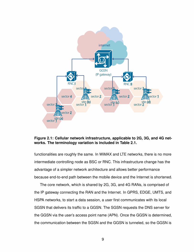
Figure 2.1 illustrates the internal of a typical cellular network taking a UMTS

network as an example. The RAN architecture, which allows the connectivity

between user handsets and the core network, consists of the base station and the

radio network controller (RNC). Across various cellular technologies, the exact

names of base stations and RNCs differ, e.g., the base station is named as the

base transceiver station (BTS) in GPRS, EDGE, 1xRTT, and EV-DO networks, and

Node B in UMTS and HSPA networks, as shown in Table 2.1, but their

8

sector 3

sector 3

sector 2

sector 1site (b)

sector 2

sector 4

sector 1

sector 3

sector 2

sector 1site (c)

RNC I

sector 3

sector 1

sector 2site (d)

RNC II

site (a)

GGSN

(IP gateway)

internet

Figure 2.1: Cellular network infrastructure, applicable to 2G, 3G, and 4G net-works. The terminology variation is included in Table 2.1.

functionalities are roughly the same. In WiMAX and LTE networks, there is no more

intermediate controlling node as BSC or RNC. This infrastructure change has the

advantage of a simpler network architecture and allows better performance

because end-to-end path between the mobile device and the Internet is shortened.

The core network, which is shared by 2G, 3G, and 4G RANs, is comprised of

the IP gateway connecting the RAN and the Internet. In GPRS, EDGE, UMTS, and

HSPA networks, to start a data session, a user first communicates with its local

SGSN that delivers its traffic to a GGSN. The SGSN requests the DNS server for

the GGSN via the user’s access point name (APN). Once the GGSN is determined,

the communication between the SGSN and the GGSN is tunneled, so the GGSN is

9

2G 3G 4GGPRS,EDGE 1xRTT UMTS,HSPA EV-DO WiMAX LTE

cell site (basestation)

BTS BTS Node B BTSBS eNodeB

RNC BSC BSC RNC BSCGSN SGSN,GGSN PDSN SGSN,GGSN PDSN ASN-GW SGW,PGW

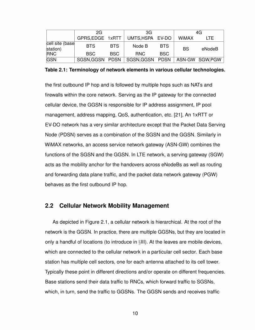
Table 2.1: Terminology of network elements in various cellular technologies.

the first outbound IP hop and is followed by multiple hops such as NATs and

firewalls within the core network. Serving as the IP gateway for the connected

cellular device, the GGSN is responsible for IP address assignment, IP pool

management, address mapping, QoS, authentication, etc. [21], An 1xRTT or

EV-DO network has a very similar architecture except that the Packet Data Serving

Node (PDSN) serves as a combination of the SGSN and the GGSN. Similarly in

WiMAX networks, an access service network gateway (ASN-GW) combines the

functions of the SGSN and the GGSN. In LTE network, a serving gateway (SGW)

acts as the mobility anchor for the handovers across eNodeBs as well as routing

and forwarding data plane traffic, and the packet data network gateway (PGW)

behaves as the first outbound IP hop.

2.2 Cellular Network Mobility Management

As depicted in Figure 2.1, a cellular network is hierarchical. At the root of the

network is the GGSN. In practice, there are multiple GGSNs, but they are located in

only a handful of locations (to introduce in §III). At the leaves are mobile devices,

which are connected to the cellular network in a particular cell sector. Each base

station has multiple cell sectors, one for each antenna attached to its cell tower.

Typically these point in different directions and/or operate on different frequencies.

Base stations send their data traffic to RNCs, which forward traffic to SGSNs,

which, in turn, send the traffic to GGSNs. The GGSN sends and receives traffic

10

from the Internet.

An important characteristic of cellular networks is that IP traffic sent by mobile

devices is tunneled to the GGSN using lower layer 3GPP tunneling protocols. As a

consequence, none of the intermediate nodes in the cellular network can directly

inspect the sent IP packets and a mobile device’s IP address is “anchored” to the

GGSN, regardless of where it moves in the network. This characteristic ensures

that the mobile device can maintain its IP address (and thus, its IP connections)

even as it is mobile.

The tunnel between the SGSN and the GGSN is called the PDP Context, and it

uses the GPRS Tunneling Protocol (GTP) (GTP-U to carry data traffic and GTP-C

for signaling control messages. When a mobile device first connects to the UMTS

network, the PDP Context that carries its IP traffic is set up. At this point, the

originating cell sector and RNC is reported to the GGSN via GTP-C protocol. When

a mobile device moves to a different sector, the path that its data takes through the

cellular network changes.1 RNCs manage the operation of handovers when a

mobile device moves from one sector to another (e.g., by coordinating base

stations and other RNCs). However, to avoid unnecessary signaling overhead, the

change of cell sectors is not reported to the higher in the hierarchy. Thus, the

GGSN is not informed that a mobile device has moved unless the SGSN in its

network path changes. This can occur for two reasons: (i) it moves far enough

away that the SGSN changes (typically into a different metro area); or (ii) the device

changes between technologies, e.g., 3G, 2G, WiFi, or vice versa. This scenario

typically occurs if a device moves from 3G/4G areas that cover primary urban and

suburban areas to 2G/3G areas that cover less populated areas.1In practice, a device can be connected to multiple nearby sectors at the same time. This set of

sectors, typically 1 to 4 in size, is called the active set. While all sectors in the active set coordinateto receive uplink data sent by the device, only one, the serving cell, transmits downlink data to thedevice at a given time. This is typically the sector with the highest signal-to-noise ratio.

11

2.3 Cellular Network Resource Allocation

In cellular networks, a mobile device estimates the channel quality through the

perceived signal-to-noise ratio of the pilot signal from the base station in every time

slot, e.g., 1.67ms for EV-DO. The device determines the modulation and coding

scheme (i.e., DRC) from the channel quality and reports back to the base station.

Depending on the channel quality, the base station allocates time slots via

proportional fair scheduling to fairly allocate radio resource while maximizing the

overall radio resource utilization [22].

To precisely understand how the proportional fair scheduler works, let W[n]

denote the exponentially averaged throughput at time slot n which is computed

from W[n]=(1−α)·W[n−1]+α·I[n−1]·C[n−1], where I[·] is the indicator function

on whether the user is served in a given time slot, C[·] is the function of channel

quality report, and α is the discount factor controlling the aggressiveness for the

base station switching time slots across users [72]. The proportional fair scheduler

allocates time slot n to a user with the maximum value of C[n]

W[n]to balance serving

between the device with the best channel quality and the device consuming the

most resources.

The average duration of staying in a DRC is hundreds to thousands of time slots

for stationary devices and tens of time slots for moving devices [75]. Moreover, a

device spends a large fraction of time in one dominant DRC, indicating the

presence of a dominant channel condition [75]. Thus, the number of continuous

time slots that a device can occupy is decided by 1

W[n], which is affected by the

discount factor α. To encourage a device to access a time slot in time [43] and to

occupy enough continuous time slots to efficiently deliver a non-trivial amount of

data, α is usually set to a small value (e.g., 0.001) [63]. This allows a device to

occupy the order of ≈ 1

α=1000 time slots, which means that a device can occupy

the channel with the same DRC on the order of ≈1.67s. Since the network

12

performance on a wireless link between the device and base station is largely a

function of the channel condition and the DRC value, we expect that it should be

possible to predict network performance on a similar time scale, i.e., 1.67s. Note

that we expect the presence of network predictability in other variants of 3G or 4G

networks as well due to the consistent utilization of proportional fair scheduling and

channel quality report scheme [69].

13

CHAPTER III

CELLULAR INFRASTRUCTURE DISCOVERY

To achieve the thesis goal of effectively adapting mobile networking applications

to cellular networks, we first explore the characteristics of cellular network

infrastructure. The characteristics of cellular networks can be significantly different

from those of the wireline Internet. One example is the locality of IP addresses. On

the Internet, IP addresses indicate to some degree the identity and location of

end-hosts. IP-based geolocation is widely used in different types of network

applications such as content customization and server selection. Using IP

addresses to geolocate wireline end-hosts is known to work reasonably well

despite the prevalence of NAT, since most NAT boxes consist of only a few

hosts [37]. However, one recent study [28] exposed very different characteristics of

IP addresses in cellular networks, i.e., cellular IP addresses can be shared across

geographically very disjoint regions within a short time duration. This observation

suggests that cellular IP addresses do not contain enough geographic information

at a sufficiently high fidelity. Moreover, it implies only a few IP gateways may exist

for cellular data networks, and that IP address management is much more

centralized than that for wireline networks, for which tens to hundreds of Points of

Presence (PoPs) are spread out at geographically distinct locations.

Cellular data networks have not been explored much by the research

14

community to explain the dynamics of cellular IP addresses despite the growing

popularity of their use. The impact of the cellular architecture on the performance of

a diverse set of smartphone network applications and cellular users has been

largely overlooked. We perform the first comprehensive characterization study of

the cellular data network infrastructure to explain the diverse geographic

distribution of cellular IP addresses, and to highlight the key importance of the

design decisions of the network infrastructure that affect the performance,

manageability, and evolvability of the network architecture. Understanding the

current architecture of cellular data networks is critical for future improvement.

Since the observation of the diversity in the geographic distribution of cellular IP

address in the previous study [28] indicates that there may exist very few cellular IP

data network gateways, identifying the location of these gateways becomes the key

for cellular infrastructure characterization in our study. The major challenge is

exacerbated by the lack of openness of such networks. We are unable to infer

topological information using existing probing tools. For example, merely sending

traceroute probes from cellular devices to the Internet IP addresses exposes mostly

private IP addresses along the path within the UMTS architecture. In the reverse

direction, only some of the IP hops outside the cellular networks respond to

traceroute probes.

To tackle these challenges, instead of relying on those cellular IP hops, we use

the geographic coverage of cellular IP addresses to infer the placement of IP

gateways following the intuition that those cellular IP addresses with the same

geographic coverage are likely to have the same IP allocation policy, i.e., they are

managed by the same set of gateways. To obtain the geographic coverage, we use

two distinct data sources (i.e., YellowPage and MobiPerf) and devise a systematic

approach for processing the data reconciling potential conflicts, combined with

other data obtained via simple probing and passive data analysis.

15

One key contribution of our work is the measurement methodology for

characterizing the cellular network infrastructure, which requires finding the relevant

address blocks, locating them, and clustering them based on their geographic

coverage. This enables the identification of IP gateways within cellular data

networks, corresponding to the first several outbound IP hops used to reach the

rest of the Internet. We draw parallels with many past studies in the Internet

topology characterization, such as Rocketfuel [102] characterizing ISP topologies,

while our problem highlights additional challenges due to the lack of publicly

available information and the difficulties in collecting relevant measurement data.

We enumerate our key findings and major contributions below.

• We comprehensively characterize the cellular network infrastructure for four major

U.S. carriers including both UMTS and EV-DO networks by clustering their IP

addresses based on their geographic coverage. Our technique relies on the

device-side IP behavior easily collected through our lightweight measurement tool

instead of requiring any proprietary information from network providers. Our

characterization methodology is applicable to all cellular access technologies (2G,

3G, or 4G).

• We observe that the traffic for all four carriers traverses through only 4–6 IP

gateways, each encompassing a large geographic coverage, implying the sharing

of address blocks within the same geographic area. This is fundamentally different

from wireline networks with more distributed infrastructure. The restricted routing

topology for cellular networks creates new challenges for applications such as CDN

service.

• We perform the first study to examine the geographic coverage of local DNS

servers and discussed in depth its implication on content server selection. We

observe that although local DNS servers provide coarse-grained approximation for

users’ network location, for some carriers, choosing content servers based on local

16

DNS servers is reasonably accurate for the current cellular infrastructure due to

restricted routing in cellular networks.

• We investigate the performance in terms of end-to-end delay for current content

delivery networks and evaluated the benefit of placing content servers at different

network locations, i.e., on the Internet or inside cellular networks. We observe that

pushing content close to GGSNs can potentially reduce the end-to-end latency by

50% excluding the variability from air interface. Our observation strongly

encourages CDN service providers to place content servers inside cellular

networks for better performance.

The rest of this chapter is organized as follows. §3.1 explains the high-level

solution to discover IP gateways in cellular infrastructure and the main methodology

in the data analysis and the data sets studied. The results in characterizing cellular

data network infrastructure along the dimensions of IP address, topology, local

DNS server, and routing behavior are covered in §3.2. We discuss the implications

of these results in §3.3 and summarize in §3.4 with key observations and insights.

3.1 Determining IPs’ Geographic Coverage

Identifying GGSNs in the cellular infrastructure is the key to explain the

geographically diverse distribution of cellular addresses discovered by the recent

study [28]. GGSNs serve as the gateway between the cellular and the Internet

infrastructure and thus play an essential role in determining the basic network

functions, e.g., routing and address allocation. We leverage the geographic

coverage of cellular addresses to infer the placement of GGSNs, assuming that

prefixes sharing similar IP behaviors are likely to have the same IP allocation policy,

i.e., they are managed by the same GGSN. Considering geographic coverage as

one type of IP behaviors, we cluster prefixes based on the feature of geographic

17

associate IP addresses

with geographic locations

prefix-to-geographic

mapping

aggregate IP addresses

into Prefixes

differentiate cellular

prefixes

coarse prefix-to-carrier

mapping

resolve mapping conflicts

accurate prefix-to-carrier

mapping

identify cellular/WiFi

prefixes

cellular

prefixes

WiFi

prefixes

prefix-to-geographic-to-carrier mapping

××

YellowPage

MobiPerf

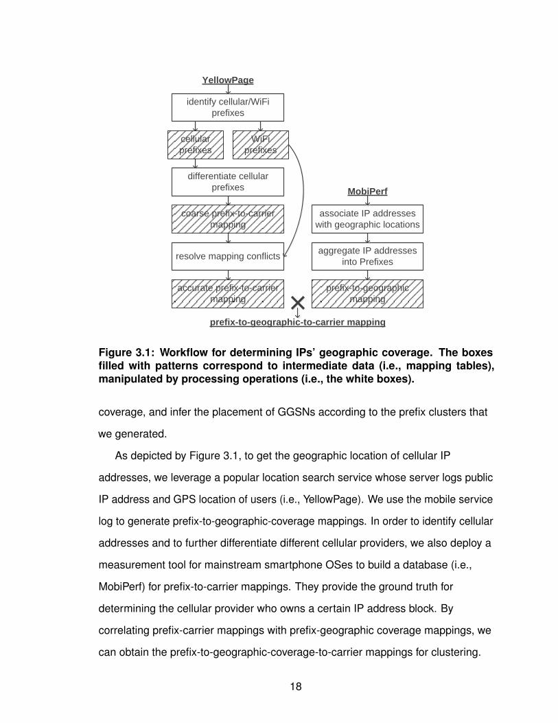
Figure 3.1: Workflow for determining IPs’ geographic coverage. The boxesfilled with patterns correspond to intermediate data (i.e., mapping tables),manipulated by processing operations (i.e., the white boxes).

coverage, and infer the placement of GGSNs according to the prefix clusters that

we generated.

As depicted by Figure 3.1, to get the geographic location of cellular IP

addresses, we leverage a popular location search service whose server logs public

IP address and GPS location of users (i.e., YellowPage). We use the mobile service

log to generate prefix-to-geographic-coverage mappings. In order to identify cellular

addresses and to further differentiate different cellular providers, we also deploy a

measurement tool for mainstream smartphone OSes to build a database (i.e.,

MobiPerf) for prefix-to-carrier mappings. They provide the ground truth for

determining the cellular provider who owns a certain IP address block. By

correlating prefix-carrier mappings with prefix-geographic coverage mappings, we

can obtain the prefix-to-geographic-coverage-to-carrier mappings for clustering.

18

Once the clustering is finished, we validate the clustering results via three

independent ways: clustering using the mobile application log, identifying the

placement of local DNS servers in cellular networks, and classifying traceroute

paths. Based on our findings during clustering and validation, we investigate

implications of the cellular infrastructure on content delivery service for mobile

users.

In §3.1.1, we introduce the datasets of YellowPage and MobiPerf, and in §3.1.2,

we detail our methodology for identifying cellular addresses and cellular providers.

Note that we design our methodology to be generally applicable for any data cellular

network technologies (2G, 3G, and 4G), and particularly from the perspective of

data requirement. Any mobile data source that contains IP addresses, location

information, and network carrier information can be used for our purpose of

characterizing the cellular data network infrastructure. Based on our experience of

deploying smartphone applications, it is not difficult to collect such data.

3.1.1 Datasets

The first data set used is from server logs associated with a popular location

search service for mobile users [18]. We refer to this data source as YellowPage. It

contains the IP address, the timestamp, and the GPS location of mobile devices.

The GPS location is requested by the application and is measured from the device.

The data set ranges from August 2009 until September 2010, containing several

million records. This comprehensive data set covers 16,439 BGP prefixes, 121,567

/24 address blocks from 1,862 AS numbers. However, YellowPage does not

differentiate the carrier for each record. Later we discuss how to map YellowPage’s

records to corresponding cellular carriers or WiFi networks with the help of

MobiPerf’s prefix-to-carrier table in §3.1.2. Users of the search service may also

use WiFi besides cellular networks to access the service.

19

operator 3Gtechnology

% ofrecords

# ASnumbers

# of BGPprefixes

# of /24address blocks

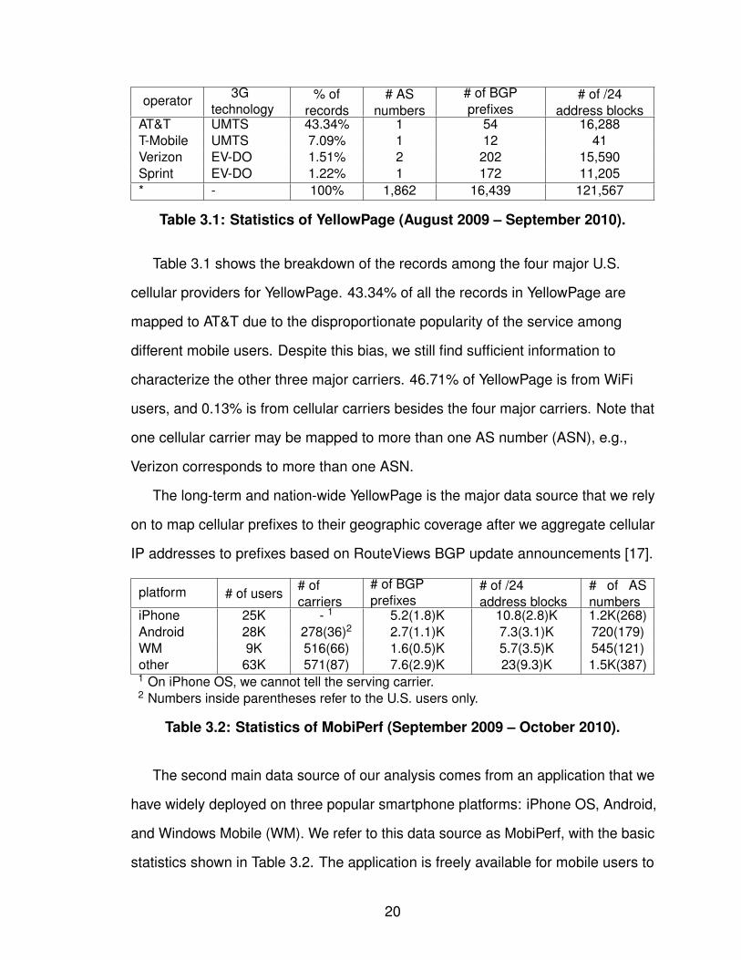
AT&T UMTS 43.34% 1 54 16,288T-Mobile UMTS 7.09% 1 12 41Verizon EV-DO 1.51% 2 202 15,590Sprint EV-DO 1.22% 1 172 11,205* - 100% 1,862 16,439 121,567

Table 3.1: Statistics of YellowPage (August 2009 – September 2010).

Table 3.1 shows the breakdown of the records among the four major U.S.

cellular providers for YellowPage. 43.34% of all the records in YellowPage are

mapped to AT&T due to the disproportionate popularity of the service among

different mobile users. Despite this bias, we still find sufficient information to

characterize the other three major carriers. 46.71% of YellowPage is from WiFi

users, and 0.13% is from cellular carriers besides the four major carriers. Note that

one cellular carrier may be mapped to more than one AS number (ASN), e.g.,

Verizon corresponds to more than one ASN.

The long-term and nation-wide YellowPage is the major data source that we rely

on to map cellular prefixes to their geographic coverage after we aggregate cellular

IP addresses to prefixes based on RouteViews BGP update announcements [17].

platform # of users# ofcarriers

# of BGPprefixes

# of /24address blocks

# of ASnumbers

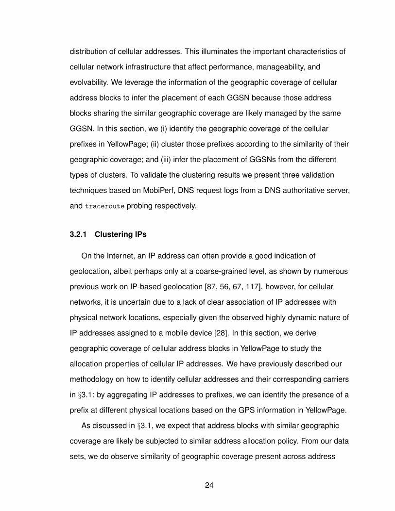
iPhone 25K - 1 5.2(1.8)K 10.8(2.8)K 1.2K(268)Android 28K 278(36)2 2.7(1.1)K 7.3(3.1)K 720(179)WM 9K 516(66) 1.6(0.5)K 5.7(3.5)K 545(121)other 63K 571(87) 7.6(2.9)K 23(9.3)K 1.5K(387)1 On iPhone OS, we cannot tell the serving carrier.2 Numbers inside parentheses refer to the U.S. users only.

Table 3.2: Statistics of MobiPerf (September 2009 – October 2010).

The second main data source of our analysis comes from an application that we

have widely deployed on three popular smartphone platforms: iPhone OS, Android,

and Windows Mobile (WM). We refer to this data source as MobiPerf, with the basic

statistics shown in Table 3.2. The application is freely available for mobile users to

20

download for the purpose of evaluating and diagnosing their networks from which

we can collect common network characteristics such as the IP address, the carrier

name, the local DNS server, and the outbound traceroute path. The hashed unique

device ID provided by the smartphone application development API allows us to

distinguish devices while preserving user privacy. Our application also asks users

for access permission for their GPS location. So far, this application has already

been executed more than 143,700 times on 62,600 distinct devices. MobiPerf

covers about the same time period as YellowPage: from September 2009 till

October 2010. Given that the application is used globally, we observe a much

larger number of carriers, many of which are outside the U.S. Note that this method

of collecting data provides some ground truths for certain data which is unavailable

in YellowPage, e.g., IP addresses associated with cellular networks instead of

Internet end-points via WiFi network can be accurately identified because of the

API offered by those mobile OSes.

set # of BGP prefixes % in YellowPage % in MobiPerfYellowPage ∪ MobiPerf 453 - -YellowPage ∩ MobiPerf 259 99.97% 98.96%∈ YellowPage,/∈ MobiPerf 181 0.03% -∈ MobiPerf,/∈ YellowPage 13 - 1.04%

Table 3.3: Cross overlap between YellowPage and MobiPerf.

Characterizing the overlap between our two data sources helps us estimate the

effectiveness of using MobiPerf to identify the carrier name of YellowPage’s cellular

prefixes. Moreover, a significant overlap can confirm the representativeness of both

YellowPage and MobiPerf on cellular IP addresses as those two data sources are

collected independently. We first compare the overlap between YellowPage and

MobiPerf’s records in the U.S. in terms of number of prefixes within the four carriers

as shown in Table 3.3. Although YellowPage and MobiPerf do not overlap much in

terms of number of prefixes, e.g., 181 prefixes in YellowPage are excluded by

21

MobiPerf, in terms of number of records the overlap is still significant due to the

disappropriate usage of prefixes, i.e., overlapped prefixes contribute to the majority.

99.97% of YellowPage’s records are covered by the prefixes shared by both

YellowPage and MobiPerf. Therefore, we have high confidence in identifying the

majority of cellular addresses based on MobiPerf. In addition, the big overlap

indicates that both data sources are likely to represent the cellular IP behavior of

active users well.

3.1.2 Operating Datasets to Identify IPs’ Geographic Coverage

One important general technique we adopt in this work, commonly used by

many measurement studies, is to intelligently combine multiple data sources to

resolve conflicts and improve accuracy of the analysis. This is necessary as each

data source alone has certain limitations and is often insufficient to provide

conclusive information.

Correlating YellowPage and MobiPerf allows us to tell based on the IP address

whether each record in YellowPage is from cellular or WiFi networks and recognize

the correct carrier names for those cellular records. Under the assumption that a

longest matching prefix is entirely assigned to either a cellular network or an

Internet wireline network, the overall idea for correlating YellowPage and MobiPerf

depicted by Figure 3.1 is as follows. Both data sources directly provide the IP

address information: Each record in YellowPage contains the GPS location

information reported by the device allocated with the cellular IP address; while

MobiPerf contains the carrier names of those cellular IP addresses. We first map IP

addresses in both data sets into their longest matching prefixes obtained from

routing table data of RouteViews. After mapping cellular IP addresses into prefixes,

we have a prefix-to-location table from YellowPage and a prefix-to-carrier table from

MobiPerf. Note that the prefix-to-location mapping is not one-to-one mapping

22

because one IP address can be present at multiple locations over time. Combining

these two tables results in a prefix-to-carrier-to-location table, which is used to infer

the placement of GGSNs after further clustering discussed later.

We believe that cellular network address blocks are distinct from Internet

wireline host IP address blocks for ease of management. To share address blocks

across distinct network locations requires announcing BGP routing updates to

modify the routes for incoming traffic, affecting routing behavior globally. Due to the

added overhead, management complexity, and associated routing disruption, we do

not expect this to be done in practice and thus assume that a longest matching

prefix is either assigned to cellular networks or Internet wireline networks. That is

why we map the IP addresses in both data sets to their longest matching prefixes.

One issue in Figure 3.1 still requires additional consideration, i.e., building the

prefix-to-carrier mapping via MobiPerf. We expect MobiPerf to provide the ground

truth for differentiating IP addresses from cellular networks and identifying the

corresponding carriers of cellular IP addresses. Each record in MobiPerf contains

the network type, i.e., cellular vs. WiFi, reported by APIs provided by the OS. The

carrier name is only available on Android and Windows Mobile due to the API

limitation on iPhone OS. After mapping IP addresses to their longest matching BGP

prefixes, we can build a table mapping from the BGP prefix to the carrier name for

Android and Windows Mobile separately. Although we cannot have a

prefix-to-carrier table from iPhone OS, we do not expect that IP allocation

differentiates towards device types.

3.2 Inferring GGSNs from IPs’ Geographic Coverage

As mentioned in §3.1, discovering the placement of GGSNs is the key to

understanding the cellular infrastructure, explaining the diverse geographic

23

distribution of cellular addresses. This illuminates the important characteristics of

cellular network infrastructure that affect performance, manageability, and

evolvability. We leverage the information of the geographic coverage of cellular

address blocks to infer the placement of each GGSN because those address

blocks sharing the similar geographic coverage are likely managed by the same

GGSN. In this section, we (i) identify the geographic coverage of the cellular

prefixes in YellowPage; (ii) cluster those prefixes according to the similarity of their

geographic coverage; and (iii) infer the placement of GGSNs from the different

types of clusters. To validate the clustering results we present three validation

techniques based on MobiPerf, DNS request logs from a DNS authoritative server,

and traceroute probing respectively.

3.2.1 Clustering IPs

On the Internet, an IP address can often provide a good indication of

geolocation, albeit perhaps only at a coarse-grained level, as shown by numerous

previous work on IP-based geolocation [87, 56, 67, 117]. however, for cellular

networks, it is uncertain due to a lack of clear association of IP addresses with

physical network locations, especially given the observed highly dynamic nature of

IP addresses assigned to a mobile device [28]. In this section, we derive

geographic coverage of cellular address blocks in YellowPage to study the

allocation properties of cellular IP addresses. We have previously described our

methodology on how to identify cellular addresses and their corresponding carriers

in §3.1: by aggregating IP addresses to prefixes, we can identify the presence of a

prefix at different physical locations based on the GPS information in YellowPage.

As discussed in §3.1, we expect that address blocks with similar geographic

coverage are likely be subjected to similar address allocation policy. From our data

sets, we do observe similarity of geographic coverage present across address

24

25

30

35

40

45

50

-120 -110 -100 -90 -80 -70

lati

tude

longitude

25

30

35

40

45

50

-120 -110 -100 -90 -80 -70

lati

tude

longitude

(a) AT&T’s /24 address block #22. (b) AT&T’s /24 address block #5.

Figure 3.2: Similarity of IPs’ geographic coverage (AT&T).

blocks. In Figure 3.2, both /24 address blocks 22 and 5 from AT&T have more

records in the southeast region of the U.S.. The geographic coverage of these two

prefixes is clearly different from the distribution of all AT&T’s addresses in

YellowPage shown in Figure 3.5, which is influenced by the population density as

well as AT&T’s user base. Moreover, we confirm and further investigate the

observation in study [28] that a single prefix can be observed at many distinct

locations, clearly illustrating that the location property of cellular addresses differs

significantly from that of Internet wireline addresses. The large geographic

coverage of these /24 address blocks also indicates that users from both Florida

and Georgia are served by the same GGSN within this region.

We intend to capture the similarity in geographic coverage through clustering to

better understand the underlying network structure. Also, to verify our initial

assumption that carriers do not aggregate their internal routes, we repeat the

clustering for /24 address blocks instead of for BGP prefixes by aggregating

addresses into /24 address blocks. If cellular carriers do aggregate their internal

routes, the number of clusters based on /24 address blocks should be larger than

that based on BGP prefixes.

The logical flow to systematically study the similarity of geographic coverage is

as follows. Firstly, we quantify the geographic coverage. By dividing the entire U.S.

25

continent into N tiles, we assign each prefix a N-dimension feature vector, each

element corresponding to one tile and the number of records located in this tile

from this prefix. As a result, the normalized feature vector of each prefix is the

probability distribution function (PDF) of the girds where this prefix appears.

Secondly, we cluster prefixes based on their normalized feature vectors using the

bisect K-means algorithm for each of the four carriers. The choice of N, varying

from 15 to 150 does not affect the clustering results, this is because the geographic

coverage of each cluster is so large that the clustering results are insensitive to the

granularity of the tile size.

The process of clustering prefixes consists of two steps: (i) pre-filtering prefixes

with very few records; and (ii) tuning the maximum tolerable average sum of

squared error (SSE) of bisect K-means. We present the details next.

3.2.1.1 Pre-filtering the prefixes with few Records

Before clustering, we perform pre-filtering to exclude prefixes with very few

records so that the number of clusters would not be inflated due to data limitations.

Note that aggressive pre-filtering may lead to losing too many records in

YellowPage.

10-3

10-2

10-1

100

101

102

100 101 102 103 104 105

CC

DF

# of records

AT&TT-MobileVerizon

Sprint

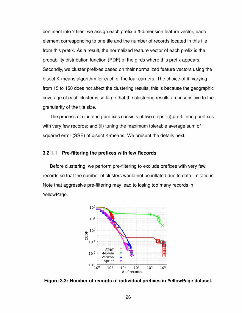
Figure 3.3: Number of records of individual prefixes in YellowPage dataset.

26

One intuitive way to filter out those prefixes is to set a threshold on the minimum

number of records that a prefix must have. However, the effectiveness of this

pre-filtering depends on the distribution of the number of records of prefixes. We

plot the complementary cumulative distribution function (CCDF) of the number of

records of prefixes in Figure 3.3. All the four carriers have bi-modal distributions on

the number of records of prefixes, implying that we can easily choose the threshold

without losing too many records. In our experiments, we choose a threshold for

each prefix to be 1% of its carrier’s records.

3.2.1.2 Tuning the SSE in bisect K-means algorithm

To compare the similarity across prefixes and further cluster them we use the

bisect K-means algorithm [106] which automatically determines the number of

clusters with only one input parameter, i.e., the maximum tolerable SSE. In each

cluster, consisting of multiple elements, the SSE is the average distance from the

element to the centroid of the cluster. A smaller value of SSE generates more

clusters. The clustering quality is determined by the geographic coverage similarity

of the prefixes within a cluster, which is measured by the SSE.

0

2

4

6

8

10

0.2 0.4 0.6 0.8 1

# o

f cl

ust

ers

SSE

AT&TT-Mobile

SprintVerizon

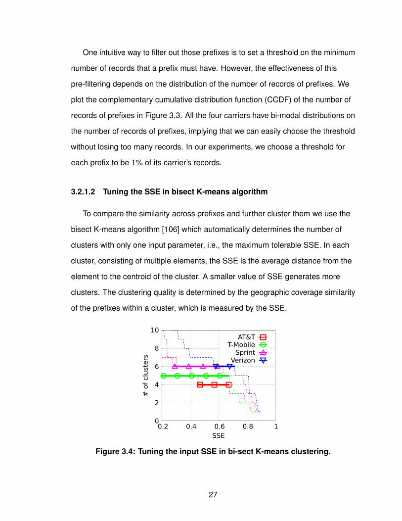
Figure 3.4: Tuning the input SSE in bi-sect K-means clustering.

27

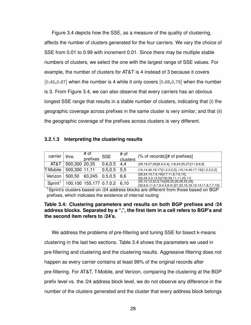
Figure 3.4 depicts how the SSE, as a measure of the quality of clustering,

affects the number of clusters generated for the four carriers. We vary the choice of

SSE from 0.01 to 0.99 with increment 0.01. Since there may be multiple stable

numbers of clusters, we select the one with the largest range of SSE values. For

example, the number of clusters for AT&T is 4 instead of 3 because it covers

[0.45,0.67] when the number is 4 while it only covers [0.68,0.78] when the number

is 3. From Figure 3.4, we can also observe that every carriers has an obvious

longest SSE range that results in a stable number of clusters, indicating that (i) the

geographic coverage across prefixes in the same cluster is very similar; and that (ii)

the geographic coverage of the prefixes across clusters is very different.

3.2.1.3 Interpreting the clustering results

carrier thre.# ofprefixes SSE

# ofclusters

(% of records)[# of prefixes]

AT&T 500,300 20,35 0.6,0.5 4,4 (28,19,27,26)[6,5,5,4], (18,24,25,27)[11,8,8,8]

T-Mobile 500,300 11,11 0.5,0.5 5,5 (10,14,40,19,17)[1,2,3,2,2], (10,14,40,17,19)[1,2,3,2,2]

Verizon 500,50 63,245 0.5,0.5 6,6 (28,24,10,7,9,19)[17,11,8,7,6,14],(50,24,3,3,12,5)[130,59,11,11,23,11]

Sprint1 100,100 155,177 0.7,0.2 6,10 (30,10,13,22,9,14)[28,25,28,28,22,24],(32,6,6,11,6,7,9,4,4,8,4) [27,23,16,16,12,14,11,8,7,7,10]

1Sprint’s clusters based on /24 address blocks are different from those based on BGPprefixes, which indicates the existence of internal routing

Table 3.4: Clustering parameters and results on both BGP prefixes and /24address blocks. Separated by a “,”, the first item in a cell refers to BGP’s andthe second item refers to /24’s.

We address the problems of pre-filtering and tuning SSE for bisect k-means

clustering in the last two sections. Table 3.4 shows the parameters we used in

pre-filtering and clustering and the clustering results. Aggressive filtering does not

happen as every carrier contains at least 99% of the original records after

pre-filtering. For AT&T, T-Mobile, and Verizon, comparing the clustering at the BGP

prefix level vs. the /24 address block level, we do not observe any difference in the

number of the clusters generated and the cluster that every address block belongs

28

to. Unlike AT&T, T-Mobile, and Verizon, Sprint does have finer-grained clusters

based on its /24 address blocks. We observe that some Sprint’s prefix-level clusters

are further divided into smaller clusters at the level of /24 address blocks. These

results answer our previous question on the existence of internal route aggregation.

Since no internal route aggregation observed for AT&T, T-Mobile, and Verizon, BGP

prefixes are sufficiently fine-grained to characterize the properties of address

blocks. For Sprint, although the clustering based on /24 address blocks is

finer-grained, it does not affect our later analysis. We have applied the clustering on

YellowPage’s records month by month as well, but we do not see any different

numbers of clusters for these 4 carriers.

25

30

35

40

45

50

-120 -110 -100 -90 -80 -70

lati

tude

longitude

25

30

35

40

45

50

-120 -110 -100 -90 -80 -70

lati

tude

longitude

(a) (b)

25

30

35

40

45

50

-120 -110 -100 -90 -80 -70

lati

tude

longitude

25

30

35

40

45

50

-120 -110 -100 -90 -80 -70

lati

tude

longitude

(c) (d)

Figure 3.5: Geographic coverage of individual GGSN clusters (AT&T).

Figure 3.5 shows the geographic coverage of each AT&T’s cluster, from the

perspective of the U.S. mainland ignoring Alaska and Hawaii, illustrating the

29

diversity across clusters as well as the unexpected large geographic coverage of

every single cluster. Note that each cluster consists of prefixes with similar

geographic coverage. Each AT&T’s cluster has different geographic spread and

center, i.e., Cluster 1 mainly covers the western, Cluster 2 mainly covers the

southeastern, Cluster 3 mainly covers the southern and the mid-eastern, which are

two very disjoint geographic areas, and Cluster 4 mainly covers the eastern.

However, note that the clusters are not disjoint in its geographic coverage, i.e.,

overlap exists among clusters although those clusters have different geographic

centers. For example, comparing Figure 3.5(b) and 3.5(d), we can observe that

Cluster 2 and Cluster 4 overlap in the northeast region.

We further quantify the overlap among clusters at tile level. Given a tile, based

on all the records located in this tile, we count how many records are from each

prefix. Since we know which cluster each prefix belongs to, we can calculate the

fraction of records for each tile contributed by different clusters. As a result, for

each tile overlapped by multiple clusters, we have a probability distribution function

(PDF) on the cluster covering this tile. Based on the PDF, we can calculate the

Shannon entropy for each tile. For example, four clusters have 300, 700, 600, and

400 records at tile X respectively, then the PDF for tile X is [0.3,0.7,0.6,0.4] whose

Shannon entropy is −0.3lg0.3−0.7lg0.7−0.6lg0.6−0.4lg0.4. Smaller values of

the entropy reflect smaller overlapping degree, e.g., if all the records for a tile are

from the same cluster, the tile has an entropy of −∞. Given the number of clusters

is N, the theoretical maximum entropy for a tile is lgN.

Figure 3.6 draws the CDF of the entropy of the tile. We can observe that overlap

at tile level is quite common for all four carriers, e.g., AT&T’s median entropy value

close to 1 means that the records in the corresponding tiles are evenly divided by

two clusters. We conjecture two reasons for the overlap. The first reason is due to

load balancing. Because of user mobility, the regional load variation can be high.

30

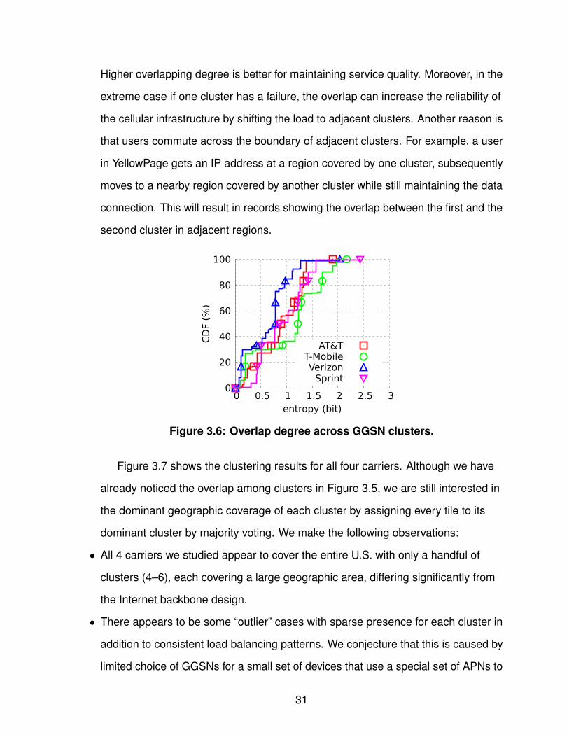
Higher overlapping degree is better for maintaining service quality. Moreover, in the

extreme case if one cluster has a failure, the overlap can increase the reliability of

the cellular infrastructure by shifting the load to adjacent clusters. Another reason is

that users commute across the boundary of adjacent clusters. For example, a user

in YellowPage gets an IP address at a region covered by one cluster, subsequently

moves to a nearby region covered by another cluster while still maintaining the data

connection. This will result in records showing the overlap between the first and the

second cluster in adjacent regions.

0

20

40

60

80

100

0 0.5 1 1.5 2 2.5 3

CD

F (%

)

entropy (bit)

AT&TT-MobileVerizon

Sprint

Figure 3.6: Overlap degree across GGSN clusters.

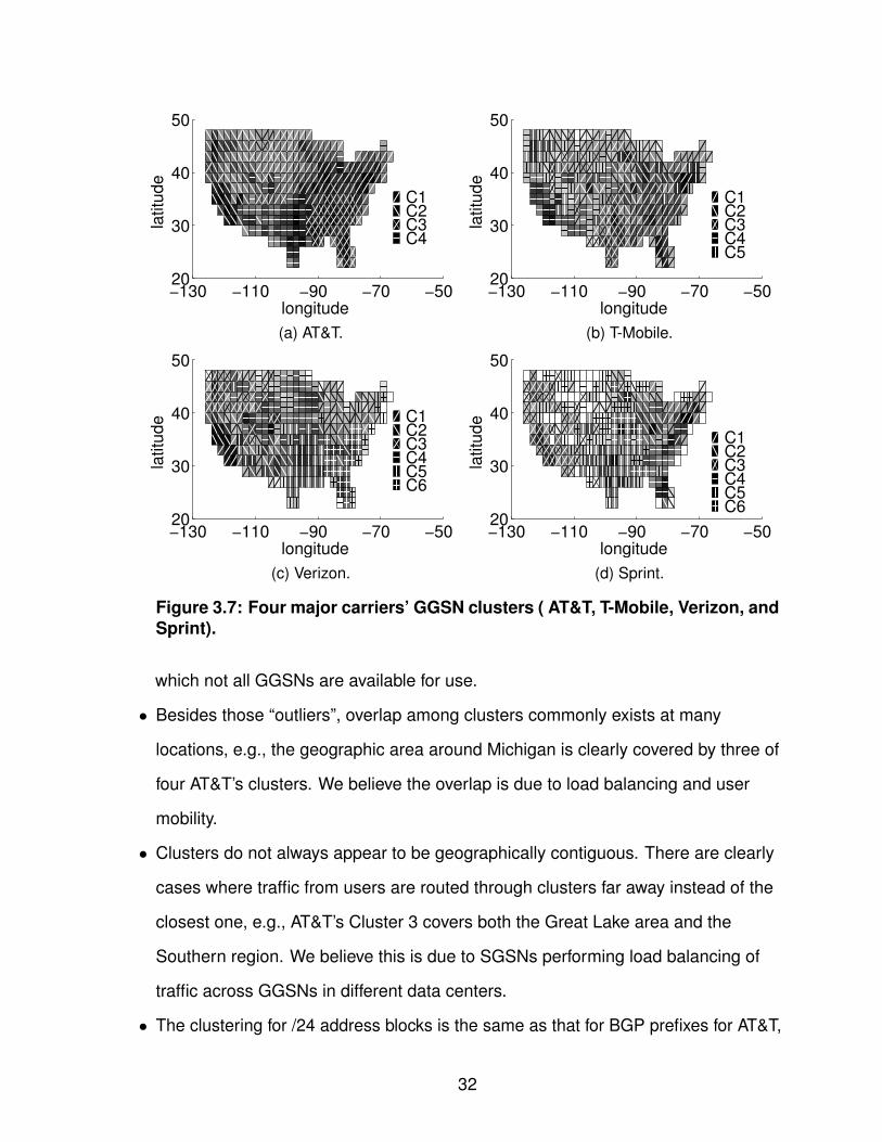
Figure 3.7 shows the clustering results for all four carriers. Although we have

already noticed the overlap among clusters in Figure 3.5, we are still interested in

the dominant geographic coverage of each cluster by assigning every tile to its

dominant cluster by majority voting. We make the following observations:

• All 4 carriers we studied appear to cover the entire U.S. with only a handful of

clusters (4–6), each covering a large geographic area, differing significantly from

the Internet backbone design.

• There appears to be some “outlier” cases with sparse presence for each cluster in

addition to consistent load balancing patterns. We conjecture that this is caused by

limited choice of GGSNs for a small set of devices that use a special set of APNs to

31

−130 −110 −90 −70 −5020

30

40

50

longitude

latitu

de

C1C2C3C4

−130 −110 −90 −70 −5020

30

40

50

longitude

latitu

de

C1C2C3C4C5

(a) AT&T. (b) T-Mobile.

−130 −110 −90 −70 −5020

30

40

50

longitude

latitu

de C1

C2C3C4C5C6

−130 −110 −90 −70 −5020

30

40

50

longitude

latitu

de

C1C2C3C4C5C6

(c) Verizon. (d) Sprint.

Figure 3.7: Four major carriers’ GGSN clusters ( AT&T, T-Mobile, Verizon, andSprint).

which not all GGSNs are available for use.

• Besides those “outliers”, overlap among clusters commonly exists at many

locations, e.g., the geographic area around Michigan is clearly covered by three of

four AT&T’s clusters. We believe the overlap is due to load balancing and user

mobility.

• Clusters do not always appear to be geographically contiguous. There are clearly

cases where traffic from users are routed through clusters far away instead of the

closest one, e.g., AT&T’s Cluster 3 covers both the Great Lake area and the

Southern region. We believe this is due to SGSNs performing load balancing of

traffic across GGSNs in different data centers.

• The clustering for /24 address blocks is the same as that for BGP prefixes for AT&T,

32

T-Mobile, Verizon confirming that there is no internal route aggregation performed

by their cellular IP networks. However, Sprint has finer-grained clustering for /24

address blocks than that for visible BGP prefixes. Despite this observation, its

number of clusters for /24 address blocks is only 10 which is still very limited.

In our analysis, we discover that the infrastructure of cellular networks differs

significantly from the infrastructure of wireline networks. The cellular networks of all

four carriers exhibit only very few types of geographic coverage. As we expected,

the type of geographic coverage reflects the placement of IP gateways. Since the

GGSN is the first IP hop, we can conclude the surprisingly restricted IP paths of

cellular data network. This network structure implies that routing diversity is limited

in cellular networks, and that content delivery service (CDN) cannot deliver content

very close to cellular users as each cluster clearly covers large geographic areas.

3.2.2 Validating GGSN Clusters

We validate the clustering result in three independent ways: clustering using

MobiPerf’s records, identifying the placement of local DNS servers in cellular

networks, and classifying traceroute paths.

3.2.2.1 Via YellowPage

Although the size of MobiPerf is much smaller than that of YellowPage, we can

still use MobiPerf to validate the clustering results obtained from YellowPage. We

repeat the clustering on the prefixes with more than 100 records from the MobiPerf.

Besides, we repeat the clustering on different types of device, i.e., Android, iPhone,

and WM based on MobiPerf’s records. The clustering results are consistent with

those of YellowPage in terms of the number of clusters and the cluster that each

prefix belongs to. Moreover, all the observations from YellowPage listed in §3.2.1

consistently apply to MobiPerf.

33

3.2.2.2 Via local DNS server

The configuration of the local DNS infrastructure is essential to ensure good

network performance. Besides performance concerns, local DNS information is

often used for directing clients to the nearest cache server expected to have the

best performance. This is based on the key assumption that clients tend to be close

to their configured local DNS servers, which may not always hold [100]. In this

work, we perform the first study to examine the placement and configuration of the

local DNS servers relative to the cellular users and the implication of the local DNS

configuration of cellular users on mobile content delivery. It is particularly

interesting to study the correlation between the local DNS server IP and the

device’s physical location. Since DNS servers are expected to be placed at the

same level as IP gateways, i.e., GGSNs, we expect to see similar clusters of

cellular local DNS servers based on the geographic coverage.

To collect a diverse set of local DNS server configurations, we resort to our

MobiPerf application by having the client send a specialized DNS request for a

unique but nonexistent DNS name which embeds the device identifier and the

timestamp (id_timestamp_example.com) to a domain (example.com) where we

have access to the DNS request logs on the authoritative DNS server. The device

identifier, id timestamp, is used for correlating the corresponding entry in the

MobiPerf’s log which stores the information such as the GPS information, the IP

address, etc. The timestamp ensures that the request is globally unique so that it is

not cached. This is a known technique used in previous studies for recording the

association between clients and their local DNS servers [79]. Since most DNS

servers operate in the iterative mode, from the authoritative DNS server, we can

observe the formatted incoming DNS requests from local DNS servers.

We summarize our results in Table 3.5. The four carriers appear to have

different policies for configuring local DNS servers. All the local DNS servers of

34

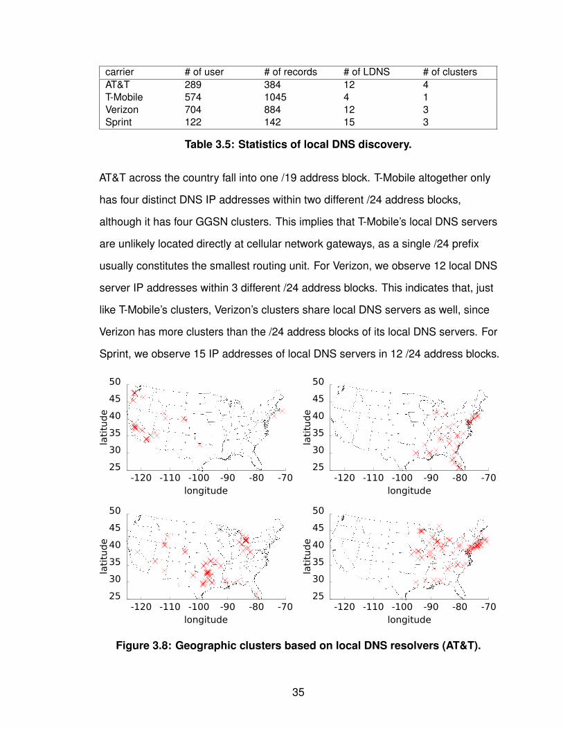
carrier # of user # of records # of LDNS # of clustersAT&T 289 384 12 4T-Mobile 574 1045 4 1Verizon 704 884 12 3Sprint 122 142 15 3

Table 3.5: Statistics of local DNS discovery.

AT&T across the country fall into one /19 address block. T-Mobile altogether only

has four distinct DNS IP addresses within two different /24 address blocks,

although it has four GGSN clusters. This implies that T-Mobile’s local DNS servers

are unlikely located directly at cellular network gateways, as a single /24 prefix

usually constitutes the smallest routing unit. For Verizon, we observe 12 local DNS

server IP addresses within 3 different /24 address blocks. This indicates that, just

like T-Mobile’s clusters, Verizon’s clusters share local DNS servers as well, since

Verizon has more clusters than the /24 address blocks of its local DNS servers. For

Sprint, we observe 15 IP addresses of local DNS servers in 12 /24 address blocks.

25

30

35

40

45

50

-120 -110 -100 -90 -80 -70

lati

tude

longitude

25

30

35

40

45

50

-120 -110 -100 -90 -80 -70

lati

tude

longitude

25

30

35

40

45

50

-120 -110 -100 -90 -80 -70

lati

tude

longitude

25

30

35

40

45

50

-120 -110 -100 -90 -80 -70

lati

tude

longitude

Figure 3.8: Geographic clusters based on local DNS resolvers (AT&T).

35

For each carrier, we cluster its local DNS servers based on their geographic

coverage without any other prior knowledge and show the results in Figure 3.8.

Comparing the clusters based on the local DNS servers with previous clustering

based on prefixes in §3.2.1, we observe that AT&T’s clusters for local DNS servers

match very well with the clusters for address blocks (shown in Figure 3.8). AT&T’s

users sharing the same local DNS server IP belong to the same cluster based on

cellular prefixes. This serves as another independent validation for previous

clustering. T-Mobile’s users across the U.S. all share the same four local DNS

servers, while Verizon’s and Sprint’s clusters based on local DNS servers are

“one-to-many” mapped to their clusters based on address blocks, indicating that

their local DNS servers are shared across multiple clusters as well.

On the current Internet, local DNS-based server selection is widely adopted by

commercial CDNs. For AT&T, Verizon, Sprint since their local DNS servers are

”one-to-one” or ”one-to-many” mapped to GGSNs, server selection based on local

DNS servers cannot be finer-grained than the GGSN level. For T-Mobile, server

selection can be even worse because all T-Mobile’s local DNS servers are used

across the entire U.S.

3.2.2.3 Via traceroute probing

Since the clusters created based on cellular prefixes should correspond to the

prefixes serving clients within the same network location, we use bi-directional

traceroute to further validate this. For the inbound direction, for each prefix of these

four carriers in YellowPage, we run traceroute on 5 PlanetLab nodes at

geographically distinct locations within the U.S. to one IP address in this prefix for

four days. We make the following observations.

• Stability of traceroute paths at IP level: All traceroute paths obtained from our

experiments are found to be very stable without any change at DNS or IP level.

36

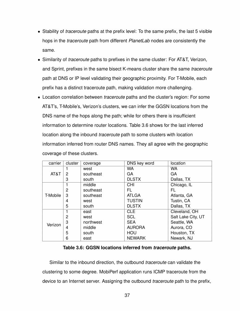
• Stability of traceroute paths at the prefix level: To the same prefix, the last 5 visible

hops in the traceroute path from different PlanetLab nodes are consistently the

same.

• Similarity of traceroute paths to prefixes in the same cluster: For AT&T, Verizon,

and Sprint, prefixes in the same bisect K-means cluster share the same traceroute

path at DNS or IP level validating their geographic proximity. For T-Mobile, each

prefix has a distinct traceroute path, making validation more challenging.

• Location correlation between traceroute paths and the cluster’s region: For some

AT&T’s, T-Mobile’s, Verizon’s clusters, we can infer the GGSN locations from the

DNS name of the hops along the path; while for others there is insufficient

information to determine router locations. Table 3.6 shows for the last inferred

location along the inbound traceroute path to some clusters with location

information inferred from router DNS names. They all agree with the geographic

coverage of these clusters.

carrier cluster coverage DNS key word location

AT&T1 west WA WA2 southeast GA GA3 south DLSTX Dallas, TX

T-Mobile

1 middle CHI Chicago, IL2 southeast FL FL3 southeast ATLGA Atlanta, GA4 west TUSTIN Tustin, CA5 south DLSTX Dallas, TX

Verizon

1 east CLE Cleveland, OH2 west SCL Salt Lake City, UT3 northwest SEA Seattle, WA4 middle AURORA Aurora, CO5 south HOU Houston, TX6 east NEWARK Newark, NJ

Table 3.6: GGSN locations inferred from traceroute paths.

Similar to the inbound direction, the outbound traceroute can validate the

clustering to some degree. MobiPerf application runs ICMP traceroute from the

device to an Internet server. Assigning the outbound traceroute path to the prefix,

37

we have the following observations:

• For all four carriers, their traceroute paths in the same cluster have the same path

pattern, i.e., the sequence of IP addresses or the sequence of address blocks are

the same. All clusters are “one-to-one” or “one-to-many” mapped to traceroute path

patterns, so each cluster has very different traceroute patterns from the others.

• The prefixes in the same AT&T’s cluster always go through the same set of IP

addresses, while for T-Mobile, Verizon, and Sprint, their prefixes in the same cluster

always go through the same set of /24 address blocks. Therefore we can always

tell a prefix’s corresponding cluster based on the IP addresses or the /24.

3.3 Impact of the Routing Restriction due to GGSNs

Based on the previous characterization of cellular data network infrastructure,

we highlight the key impact of cellular infrastructure by examining its implication on

content delivery networks from the perspectives of content placement and server

selection.

3.3.1 Content Placement

On today’s Internet, CDN plays an important role of reducing the latency for

accessing web content. The essential idea behind CDN is to serve users from

nearby CDN servers that replicate the content from the origin server located

potentially far away. By characterizing the cellular infrastructure, we have observed

that the current restrictive cellular topology route all traffic through only a handful

GGSNs. Therefore, no matter how close to a CDN server the user is, the content

still has to go through the GGSN before reaching the destination. The possible

reasons for such a restrictive topology design by routing all traffic through GGSNs

include simplicity and ease of management, e.g., billing and accounting.

38

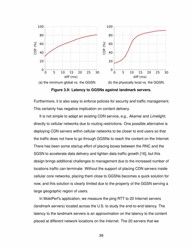
0

20

40

60

80

100

0 5 10 15 20 25 30

CD

F (%

)

diff (ms)

0

20

40

60

80

100

0 5 10 15 20 25 30

CD

F (%

)

diff (ms)

(a) the minimum global vs. the GGSN. (b) the physically local vs. the GGSN.

Figure 3.9: Latency to GGSNs against landmark servers.

Furthermore, it is also easy to enforce policies for security and traffic management.

This certainly has negative implication on content delivery.

It is not simple to adapt an existing CDN service, e.g., Akamai and Limelight,

directly to cellular networks due to routing restrictions. One possible alternative is

deploying CDN servers within cellular networks to be closer to end users so that

the traffic does not have to go through GGSNs to reach the content on the Internet.

There has been some startup effort of placing boxes between the RNC and the

SGSN to accelerate data delivery and lighten data traffic growth [16], but this

design brings additional challenges to management due to the increased number of

locations traffic can terminate. Without the support of placing CDN servers inside

cellular core networks, placing them close to GGSNs becomes a quick solution for

now, and this solution is clearly limited due to the property of the GGSN serving a

large geographic region of users.

In MobiPerf’s application, we measure the ping RTT to 20 Internet servers

(landmark servers) located across the U.S. to study the end-to-end latency. The

latency to the landmark servers is an approximation on the latency to the content

placed at different network locations on the Internet. The 20 servers that we

39

choose are very popular servers geographically distributed across 20 states. To

estimate the benefit of placing content close to GGSN, we compare the latency to

landmark servers with the latency to the first cellular IP hop, i.e., the first IP hop

along the outbound path where GGSN is located.

Each time MobiPerf’s application runs, it only probes these landmark servers

twice to save the resource consumption on devices. In order to eliminate the

variability from air interface so that we can isolate the impact from the wireline hops,

we follow the splitting method in §3.2.1 dividing the U.S. continent into N tiles. Within

each tile, we compare the minimum RTT to the first cellular IP hop against these 20

landmark servers. In Figure 3.9(a), we show the absolute difference between the

latency to the first cellular IP hop and the minimum latency the landmark servers.

Because these 20 landmark servers are widely distributed across the U.S., the

minimum latency to landmark servers should be a good estimation of the latency to

the current content providers. We can observe that placing content close to the

GGSN can reduce the end-to-end latency by 6ms. Note that the 6ms saving may

be minor to 3G networks, but can be very critical to 4G such as LTE networks,

where the median end-to-end latency is around 60ms [61].

3.3.2 Server Selection

Besides the challenge of mobile content placement, server selection is another

important issue for CDN service providers. Some existing CDN services, e.g.,

Akamai and Limelight, choose the content server based on the incoming DNS

requests from the local DNS server assuming the address of the local DNS can

accurately represent the location of those end hosts behind the local DNS server.

However, this assumption rarely holds for cellular networks. In §3.2.2.2, we know

that AT&T, Verizon, and Sprint have different local DNS servers for different GGSN

clusters, while T-Mobile’s clusters share the same set of local DNS servers.

40

Although AT&T, Verizon, and Sprint have different local DNS server for different

GGSN clusters, the IP addresses are very similar. Without the information of the

correlation between the local DNS server and the GGSN cluster, it is difficult to

choose content servers for different GGSN clusters according to their local DNS

server IP address. As T-Mobile’s GGSN clusters share the same set of local DNS

servers, it is impossible to choose content servers for different GGSN clusters

based on the DNS request alone.

Interestingly even if content providers can obtain the accurate physical location

based on some application-level knowledge, e.g., Google Gears [7], directing the

traffic to the content server physically closest to the mobile device can be grossly

suboptimal due to the placement of the GGSN and the cellular network routing

restrictions. Traffic still needs traverse through the GGSN, despite the close

proximity between the mobile device and the content server. To estimate the

difference in performance between choosing a server physically closest to the

mobile device and one closest to the GGSN node, we do the following analysis.

Using the GPS location information reported by MobiPerf’s application, in all the

experiments from AT&T’s Cluster 2, we compare the latency to the landmark server

closest to the mobile device with the latency to the landmark server closet to the

corresponding GGSN. Figure 3.9(b) shows that the latency to the closet landmark

server has high probability to be larger than the latency to the Georgia landmark

server and on average by about 10ms, indicating that choosing the server

according to the physical location of the mobile device is suboptimal due to the

routing restriction imposed by GGSNs.

Overall, if mobile content providers want to adopt the short-term solution to

reduce the end-to-end latency, they have to solve two issues: (i) placing content

servers as close as to GGSNs; and (ii) effectively directing traffic to the content

server closest to the GGSN that originates the traffic based on information such as

41

the correlation between local DNS servers and GGSNs.

3.4 Summary of Cellular Infrastructure Charateristics

In this chapter, we comprehensively characterized the infrastructure of cellular

data network of four major wireless carriers within the U.S. including both UMTS

and EV-DO technology. We unveiled several fundamental differences between

cellular data networks and the wireline networks in terms of placement of GGSNs,

local DNS server behavior, and routing properties. One of the most surprising

findings is that cellular data networks have severe restriction on routing by

traversing only a few limited GGSNs to interface with external Internet networks.

We observed that all 4 carriers we studied divide the U.S. among only 4–6 GGSNs,

each serving a large geographic area. Since the GGSN is the first IP hop, it implies

that CDN servers cannot consistently serve content close to end users.

Our study also showed that in the best case local DNS servers for some carriers

can be close to GGSNs. Since traffic from and to local DNS servers and cellular

users must traverse one of those few GGSNs, using local DNS servers and the

knowledge of the mapping to the GGSN to identify the best server to deliver mobile

content currently can be sufficient despite the routing restrictions.

Regarding content placement, we investigated and compared two choices: (i)

placing content at the boundary between the cellular backbone and the Internet;

and (ii) placing content at the GGSN in the cellular backbone. We observed that

pushing content close to GGSNs could potentially reduce the end-to-end latency by

more than 6ms. If pushing content into the proprietary cellular backbone is not

permitted, placing content at the boundary still gives considerable benefit.

We believe our findings in characterizing the infrastructure for cellular data

networks directly motivate future work in this area. Our observations on the cellular

42

infrastructure guide CDNs to provide better service to mobile users, and our

methodology for discovering cellular data network properties will continue to reveal

new behavior as cellular networks evolve.

43

CHAPTER IV

APPLICATION USAGE IDENTIFICATION

In §III, we identified the routing restriction issue due to the limited number of

cellular network gateways, and we further investigated the impact of such issue on

latency sensitive applications starting with CDN services. Besides YellowPage, we

have other projects showing certain previously little known impact due to cellular

network infrastructure. For example, in NetPiculet [110], we observed that cellular

middleboxes, such as NAT boxes and firewalls apply policies that can seriously

interrupt application communications and lead to additional energy waste. A

common impression from these observations is that application designs should

adapt to those fundamentally unique cellular network characteristics in order to in

maximum improve application performance. However, before we introduce our

hand-on experience in application optimizing in §V, we in general characterize

mobile application behaviors.

The rapid adoption of mobile devices is dramatically changing the access to

various networking services: instead of using web browsers, mobile users

increasingly choose mobile apps1 as the preferred “gateways” connecting them to

the Internet [11]. Android has 150K apps and 350K daily activations [55].

Pre-installed with marketplace portals such as the AppStore on iOS, Google Play

on Android, and MarketPlace on Windows Phone, popular smartphone platforms1We use “apps” to emphasize more on individual application packages throughout this section.

44

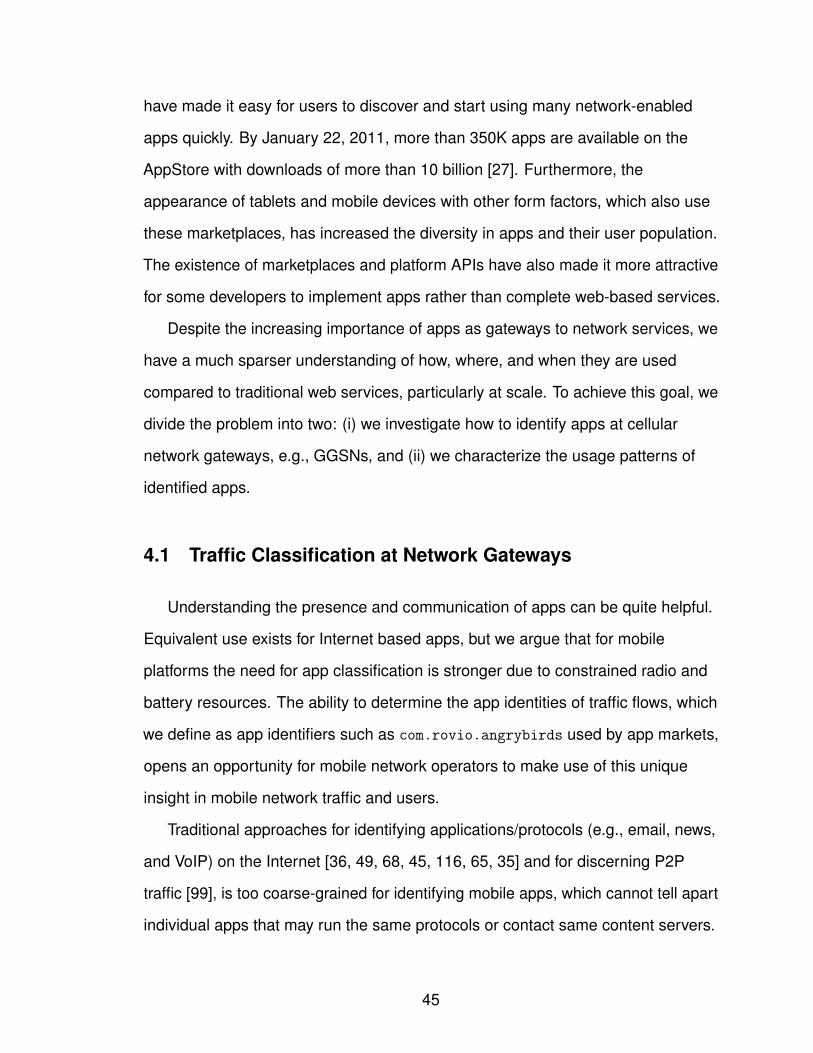
have made it easy for users to discover and start using many network-enabled

apps quickly. By January 22, 2011, more than 350K apps are available on the

AppStore with downloads of more than 10 billion [27]. Furthermore, the

appearance of tablets and mobile devices with other form factors, which also use

these marketplaces, has increased the diversity in apps and their user population.

The existence of marketplaces and platform APIs have also made it more attractive

for some developers to implement apps rather than complete web-based services.

Despite the increasing importance of apps as gateways to network services, we

have a much sparser understanding of how, where, and when they are used

compared to traditional web services, particularly at scale. To achieve this goal, we

divide the problem into two: (i) we investigate how to identify apps at cellular

network gateways, e.g., GGSNs, and (ii) we characterize the usage patterns of

identified apps.

4.1 Traffic Classification at Network Gateways

Understanding the presence and communication of apps can be quite helpful.

Equivalent use exists for Internet based apps, but we argue that for mobile

platforms the need for app classification is stronger due to constrained radio and

battery resources. The ability to determine the app identities of traffic flows, which

we define as app identifiers such as com.rovio.angrybirds used by app markets,

opens an opportunity for mobile network operators to make use of this unique

insight in mobile network traffic and users.

Traditional approaches for identifying applications/protocols (e.g., email, news,

and VoIP) on the Internet [36, 49, 68, 45, 116, 65, 35] and for discerning P2P

traffic [99], is too coarse-grained for identifying mobile apps, which cannot tell apart

individual apps that may run the same protocols or contact same content servers.

45

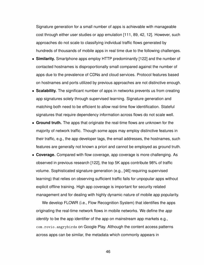
Signature generation for a small number of apps is achievable with manageable

cost through either user studies or app emulation [111, 89, 42, 12]. However, such

approaches do not scale to classifying individual traffic flows generated by

hundreds of thousands of mobile apps in real time due to the following challenges.

• Similarity. Smartphone apps employ HTTP predominantly [122] and the number of

contacted hostnames is disproportionally small compared against the number of

apps due to the prevalence of CDNs and cloud services. Protocol features based

on hostnames and ports utilized by previous approaches are not distinctive enough.

• Scalability. The significant number of apps in networks prevents us from creating

app signatures solely through supervised learning. Signature generation and

matching both need to be efficient to allow real-time flow identification. Stateful

signatures that require dependency information across flows do not scale well.

• Ground truth. The apps that originate the real-time flows are unknown for the

majority of network traffic. Though some apps may employ distinctive features in

their traffic, e.g., the app developer tags, the email addresses, the hostnames, such

features are generally not known a priori and cannot be employed as ground truth.

• Coverage. Compared with flow coverage, app coverage is more challenging. As

observed in previous research [122], the top 5K apps contribute 98% of traffic

volume. Sophisticated signature generation (e.g., [46] requiring supervised

learning) that relies on observing sufficient traffic fails for unpopular apps without

explicit offline training. High app coverage is important for security related

management and for dealing with highly dynamic nature of mobile app popularity.

We develop FLOWR (i.e., Flow Recognition System) that identifies the apps

originating the real-time network flows in mobile networks. We define the app

identity to be the app identifier of the app on mainstream app markets e.g.,

com.rovio.angrybirds on Google Play. Although the content access patterns

across apps can be similar, the metadata which commonly appears in

46

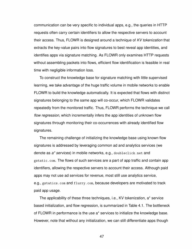
communication can be very specific to individual apps, e.g., the queries in HTTP

requests often carry certain identifiers to allow the respective servers to account

their access. Thus, FLOWR is designed around a technique of KV tokenization that

extracts the key-value pairs into flow signatures to best reveal app identities, and

identifies apps via signature matching. As FLOWR only examines HTTP requests

without assembling packets into flows, efficient flow identification is feasible in real

time with negligible information loss.

To construct the knowledge base for signature matching with little supervised

learning, we take advantage of the huge traffic volume in mobile networks to enable

FLOWR to build the knowledge automatically. It is expected that flows with distinct

signatures belonging to the same app will co-occur, which FLOWR validates

repeatedly from the monitored traffic. Thus, FLOWR performs the technique we call

flow regression, which incrementally infers the app identities of unknown flow

signatures through monitoring their co-occurrences with already identified flow

signatures.

The remaining challenge of initializing the knowledge base using known flow

signatures is addressed by leveraging common ad and analytics services (we

denote as a* services) in mobile networks, e.g., doubleclick.net and

gstatic.com. The flows of such services are a part of app traffic and contain app

identifiers, allowing the respective servers to account their access. Although paid

apps may not use ad services for revenue, most still use analytics service,

e.g., gstatics.com and flurry.com, because developers are motivated to track

paid app usage.

The applicability of these three techniques, i.e., KV tokenization, a* service

based initialization, and flow regression, is summarized in Table 4.1. The bottleneck

of FLOWR in performance is the use a* services to initialize the knowledge base.

However, note that without any initialization, we can still differentiate apps though

47

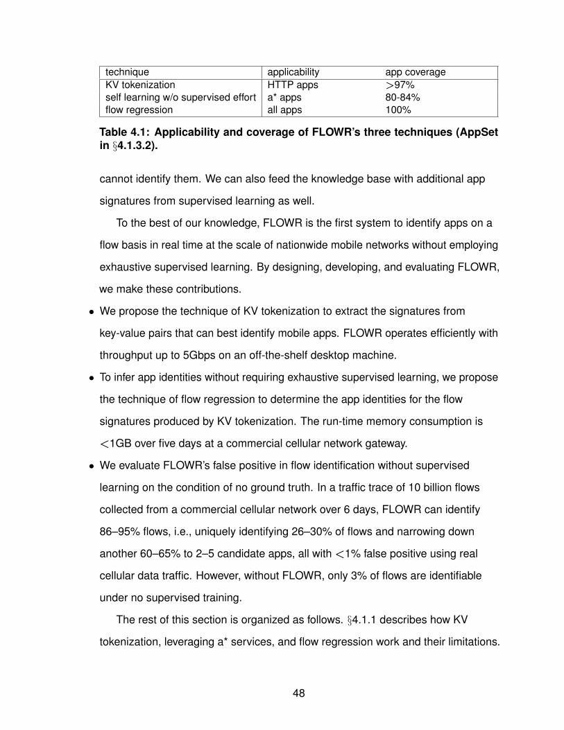
technique applicability app coverageKV tokenization HTTP apps >97%self learning w/o supervised effort a* apps 80-84%flow regression all apps 100%

Table 4.1: Applicability and coverage of FLOWR’s three techniques (AppSetin §4.1.3.2).

cannot identify them. We can also feed the knowledge base with additional app

signatures from supervised learning as well.

To the best of our knowledge, FLOWR is the first system to identify apps on a

flow basis in real time at the scale of nationwide mobile networks without employing

exhaustive supervised learning. By designing, developing, and evaluating FLOWR,

we make these contributions.

• We propose the technique of KV tokenization to extract the signatures from

key-value pairs that can best identify mobile apps. FLOWR operates efficiently with

throughput up to 5Gbps on an off-the-shelf desktop machine.

• To infer app identities without requiring exhaustive supervised learning, we propose

the technique of flow regression to determine the app identities for the flow

signatures produced by KV tokenization. The run-time memory consumption is

<1GB over five days at a commercial cellular network gateway.

• We evaluate FLOWR’s false positive in flow identification without supervised

learning on the condition of no ground truth. In a traffic trace of 10 billion flows

collected from a commercial cellular network over 6 days, FLOWR can identify

86–95% flows, i.e., uniquely identifying 26–30% of flows and narrowing down

another 60–65% to 2–5 candidate apps, all with <1% false positive using real

cellular data traffic. However, without FLOWR, only 3% of flows are identifiable

under no supervised training.

The rest of this section is organized as follows. §4.1.1 describes how KV

tokenization, leveraging a* services, and flow regression work and their limitations.

48

§4.1.2 presents the system details of FLOWR. We describe the dataset for

evaluation in §4.1.3 and evaluate FLOWR in §4.1.4.

4.1.1 Techniques

The goal of FLOWR is to identify flows, defined to be a bi-directional TCP/UDP

connection, generated by mobile apps with minimal supervised training. The

approach is to infer the app identities of flow signatures from their co-occurrences

with already identified flow signatures, and construct a knowledge base accordingly.

Using this knowledge base, FLOWR can perform signature matching to identify

flows efficiently in real time.

request capturing

signature tokenization

signature matching

pending signatures

co-occur.checking

co-occur.counters

identified signatures

real-timepackets

HTTPrequests

flow signatures

identified flows

unique app (e.g., FP<1%)

candidate apps (e.g., FP<1%)

matchany identified

signature

Y

pool

knowledge base

identified signatures

co-occur.signatures

add/del

co-occur.signatures

flow signatures

identified signatures

<<<

>>>

N

Figure 4.1: FLOWR’s workflow, i.e., KV tokenization and flow regression.

To implement the strategy, FLOWR adopts two major techniques as illustrated

by Figure 4.1: KV tokenization and flow regression. KV tokenization extracts

signatures from real-time network packets and identifies apps via signature

matching against FLOWR’s current knowledge base of known flow signatures.

Depending on the quality of the matched signatures, FLOWR either identifies the

49

flow as a unique app or narrows it down to a few (e.g., 2–5) candidate apps. To

minimize supervised learning, FLOWR takes advantage of the huge traffic volume

available in mobile networks and applies flow regression accordingly. In flow

regression, FLOWR infers the app identities for most signatures by monitoring their

co-occurrences with identified flow signatures, which only requires some initial

ground truth as the “seeds” to initialize its knowledge base2.

In summary, FLOWR addresses three issues: (i) in KV tokenization, how to

extract signatures from flows, i.e., discovering the potential features best

representing app identities (e.g., the app ID, the package name, or the hostname);

(ii) in flow regression, how to feed the initial knowledge base of identified flow

signatures; and (iii) in flow regression, how to examine co-occurrence events in

inferring app identifies.

4.1.1.1 Extracting flow signatures

FLOWR is designed as a general approach to be applicable to a broad class of

flow signatures based on information such as user-agents, contacted hostnames,

web objects, etc. However, flow signatures can have very different accuracy in

identifying apps, e.g., user-agents are shared across apps, hostnames in URIs and

DNS queries are not unique across apps due to cloud and CDN services

(evaluated in §4.1.4.2). Among the potential flow signatures, the query fields in

HTTP URIs can be a better candidate, which facilitate the exchange of additional

information between apps and content servers (evaluated in §4.1.4.2). A commonly

observable set of URIs is between apps and a* services [70, 59]. These URIs often

embed app identifiers to enable the respective servers to account their visits,

e.g., ad engines may want to perform ad delivery customization on app basis, and

analytics servers may want to know the visit patterns of apps. Accordingly, we2Imitating “flower/seed” is another reason for FLOWR’s name.

50

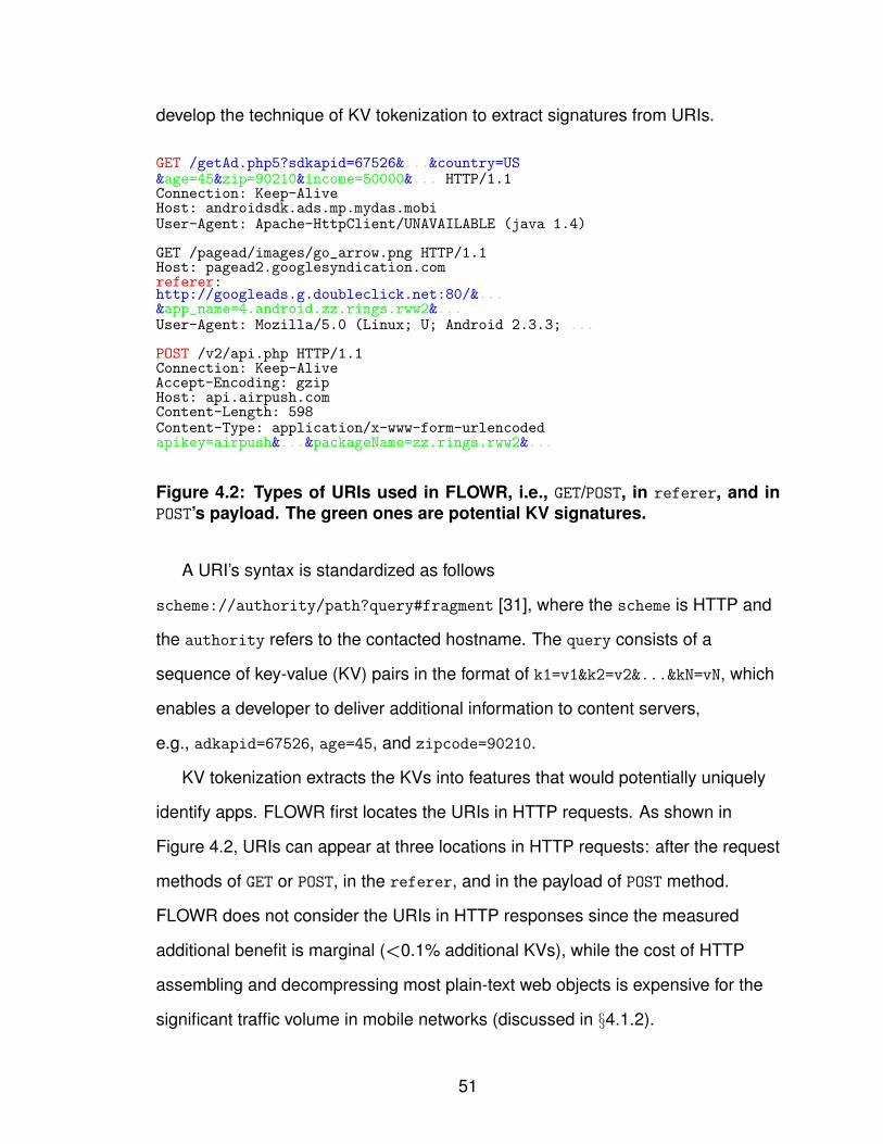
develop the technique of KV tokenization to extract signatures from URIs.

GET /getAd.php5?sdkapid=67526&...&country=US&age=45&zip=90210&income=50000&... HTTP/1.1Connection: Keep-AliveHost: androidsdk.ads.mp.mydas.mobiUser-Agent: Apache-HttpClient/UNAVAILABLE (java 1.4)

GET /pagead/images/go_arrow.png HTTP/1.1Host: pagead2.googlesyndication.comreferer:http://googleads.g.doubleclick.net:80/&...&app_name=4.android.zz.rings.rww2&...User-Agent: Mozilla/5.0 (Linux; U; Android 2.3.3; ...

POST /v2/api.php HTTP/1.1Connection: Keep-AliveAccept-Encoding: gzipHost: api.airpush.comContent-Length: 598Content-Type: application/x-www-form-urlencodedapikey=airpush&...&packageName=zz.rings.rww2&...

Figure 4.2: Types of URIs used in FLOWR, i.e., GET/POST, in referer, and inPOST’s payload. The green ones are potential KV signatures.

A URI’s syntax is standardized as follows

scheme://authority/path?query#fragment [31], where the scheme is HTTP and

the authority refers to the contacted hostname. The query consists of a

sequence of key-value (KV) pairs in the format of k1=v1&k2=v2&...&kN=vN, which

enables a developer to deliver additional information to content servers,

e.g., adkapid=67526, age=45, and zipcode=90210.

KV tokenization extracts the KVs into features that would potentially uniquely

identify apps. FLOWR first locates the URIs in HTTP requests. As shown in

Figure 4.2, URIs can appear at three locations in HTTP requests: after the request

methods of GET or POST, in the referer, and in the payload of POST method.

FLOWR does not consider the URIs in HTTP responses since the measured

additional benefit is marginal (<0.1% additional KVs), while the cost of HTTP

assembling and decompressing most plain-text web objects is expensive for the

significant traffic volume in mobile networks (discussed in §4.1.2).

51

Once FLOWR has located the URIs in a flow, it extracts the KVs and produces a

signature for each KV as authority:key=value3. To ensure the compatibility with

a flow that does not contain any KV, FLOWR creates an empty signature

authority:no key=no value for it. Eventually, FLOWR compares the extracted

flow signatures against the app signatures in the knowledge base to identify the

incoming flow.

4.1.1.2 Seeding knowledge base

There are three general types of KVs based on the amount of app identity

information they contain: the irrelevant KVs (e.g., age=45), the KVs that explicitly

refers to obvious app identifiers (e.g., packageName=zz.rings.rww2), and the

remaining KVs, whose app identities are initially ambiguous (e.g., sdkapid=67526),

but we need to verify how specific they are to their apps through flow regression.

The simplest task for FLOWR is to determine the KVs that explicitly refer to app

identifiers, which should have the following characteristics.

• Uniqueness. An explicit identifier should be unique to the app. Otherwise, we can

only use the identifier to constrain app identification to a set of candidate apps.

• Persistence. An explicit identifier should appear often in the app’s traffic. Such

persistence property depends on the app’s implementation and usage patterns.

• Expressiveness. An explicit identifier should contain features that are indicative of

the app’s ID on mainstream app markets, e.g., Android’s Google Play. Otherwise,

the identifier only allows the differentiation between apps, without establishing an

app’s identity.

Apparently, the published names of apps as well as app package names

(e.g., com.instagram.android) that appear in mainstream app markets are good

candidates for explicit app identifiers. These two features are commonly present in3“KV”, “KV signature”, and “flow signature” are used inter-changeably. An “app signature” refers

to an identified “flow signature”.

52

HTTP requests of ad and analytics services. Moreover, the app identifiers

appearing in such services have a hidden advantage of augmented identification

coverage, given that most apps employ a* services. According to our evaluation in

§4.1.4.2, >80% of either free apps or paid apps utilize one or more a* services.

Though paid apps may not use ad services, most of them still use analytics

services to track their app usage.

Some major a* services use the app IDs (e.g., com.instagram.android) that

are embedded in the app descriptions on Google Play or AppStore,

i.e., doubleclick.net, admob.com, airpush.com, and smaato.com. FLOWR can

identify these flows and the other flows originated by the same apps (using flow

regression) pointed to by such a* services without any supervised learning effort.

Other a* services do not employ any app market content, but instead may contain

proprietary registration identifiers of apps or developers, such as their own app IDs,

developer IDs, billing IDs. Such identifiers, although not expressive, are very

distinct and can be related to some of the previous expressive identifiers with

additional but offline supervised training. FLOWR leverages offline supervised

training via techniques such as emulation described in §4.1.3.2. For apps that do

not employ any a* services, it is difficult to identify them without comprehensive

training due to the lack of initial ground truth.

4.1.1.3 Inferring KV identities

Although we can leverage the app identifiers on mainstream app markets to

detect the majority of apps, in terms of flow identification, the coverage is negligible

(<1% of network flows according to Figure 4.13(a)). FLOWR’s flow regression is

the approach to eliminate irrelevant KVs (defined in §4.1.1.2) and infer the app

identities of the undetermined KVs.

Intuitively, if two flows repeatedly co-occur, i.e., they regularly share the source

53

IP addresses and often appear in close time proximity, then the flows are likely to

be originated from the same app. Otherwise, it is impossible for them to co-occur

repeatedly over various users, days, locations, devices, etc., even if the mobile

devices are behind NAT boxes. As a result, to infer the app identity of an

undetermined flow, FLOWR detects the co-occurrence likelihoods (described in

§4.1.2) of the flow’s KVs with the KVs of known apps.

FLOWR digests co-occurrence likelihoods as follows. In the background, if

almost every time a KV appears closely to some flow related to an app X,

i.e., P[A=X|KV]≈1, FLOWR adds KV to its signature set (i.e., UR) that uniquely

identifies the app in the knowledge base of app identities. Instead of P[A=X|KV]≈1,

a more common case is that KV co-occurs with X with a certain likelihood less than

1, i.e., 0�P[KV|A=X]<1, which indicates that KV may be generated by apps other

than X as well. Then, as a best effort, FLOWR puts KV into a signature set (i.e., CR)

that narrows down the set of the flow’s candidate apps.

In the foreground, FLOWR may produce more than one KV for a network flow in

KV tokenization. FLOWR determines the app identity according to the best

identifiable KV. The identifiability of a KV is defined as the co-occurrence likelihood

with the most frequently co-occurred app. The identifiabilities of KVs in UR are

close to 1, while for KVs in CR, the identifiabilities are far less than 1. A flow’s

different KVs could have very different quality in identifying the app, but as long as

there is at least one KV with a high identifiability (evaluated in §4.1.4.4), the flow

identification is granted.

4.1.2 System Design

As depicted in Figure 4.1, we describe the proposed techniques introduced in

§4.1.1 and develop several optimizations to keep FLOWR efficient and scalable.

Request Capturing & Signature Tokenization. Expecting that most app

54

identity information is contained within the metadata rather than the content,

FLOWR only examines the packets corresponding to HTTP requests to eliminate

the overhead in HTTP flow assembly. According to our investigation, the benefit of

adding HTTP responses is marginal (<0.1%), but the HTTP assembly overhead is

nontrivial as most plain-text objects are compressed. To capture an HTTP request,

FLOWR only needs to examine a few packets immediately after the TCP

handshake of a flow.

As discussed in §4.1.1.1, FLOWR examines URIs from three locations in HTTP

requests, i.e., after GET, in referer, and in POST’s payload. Further, FLOWR

extracts key-value (KV) pairs from the queries of URIs into signatures. Excluding

the time spent on I/O, FLOWR’s compute-bound throughput with in-memory reads

in HTTP request capturing, signature tokenization, and signature matching is up to

5Gbps on a machine with a 2.67GHz 6-core Xeon processor and 100GB RAM,

which is efficient to handle the traffic load in mobile networks (discussed in

§4.1.3.2). Though FLOWR uses linear matching, it can be further optimized using

complex indexing.

Once a flow is tokenized, to determine its app identity, FLOWR only needs to

perform signature matching to either uniquely identify its origin app or narrow down

it to a few candidates. On average, FLOWR collects 300K app signatures in the

knowledge base of app signatures over 24 hours in a commercial cellular network,

i.e., FlowSet (discussed in §4.1.3.1). The knowledge base for signature matching is

initialized using the KVs explicitly referring to app identifiers in a* service flows

(e.g., doubleclick:app name=com.instagram.android and

airpush:packageName=zz.rings.rww2 in §4.1.1.2). Also, it can be enhanced using

external supervised learning effort, such as done in prior approach [46].

Knowledge Base & flow regression. To keep growing the knowledge base of

app signatures, FLOWR runs flow regression in the background. To implement flow

55

regression, we need to make three design decisions in interpreting co-occurrence

events: (i) how to filter the majority of KVs that are irrelevant for app identification,

(ii) how to decide if two KVs co-occur; and (iii) how to compute co-occurrence

likelihoods, i.e., P[A=X|KV] where KV is the undetermined KV and A=X is the app

corresponding to the identified KV.

In examining co-occurrence events, FLOWR has to maintain a pool for pending

signatures (as shown in Figure 4.1) that contains the recently appeared KVs. In

order to be efficient, FLOWR has to eliminate most of the irrelevant KVs to keep the

pool compact. To achieve that, FLOWR detects and eliminates conflicted KVs: two

KVs are considered to be conflicted if they share the same key but have different

values. If two KVs indicate the same app, they must not conflict with each other.

We observe that many KVs refer to the information other than app identity such as

the information of HTTP sessions, ads, devices, and user details. Such KVs will be

conflicted because apps are used in variable scenarios. The conflict property

exhibits transitivity. A pair of co-occurring KVs, i.e., an undetermined KV and an

identified KV, will be conflicted if there is another undetermined KV that co-occurs

with the identified KV but conflicts with the undetermined KV. FLOWR eliminates

such flow triplets, i.e., the identified KV and two undetermined KVs.

To illustrate the co-occurrence verification algorithm, we consider two KVs, KV1

and KV2, and check whether KV1 and KV2 overlap within T sec, i.e., whether

S(KV1)−T<E(KV2) and E(KV1)+T>S(KV2). S(·) and E(·) are the flow start time

function and flow end time function respectively, and T is a time gap parameter. The

impact of T is evaluated in §4.1.4.3.

To compute co-occurrence likelihoods, a naıve approach would be to count the

number of co-occurrence events. However, we observe that some KVs in flows are

generated tens of times within few seconds, which biases the computation of

P[A=X|KV]. This often happens on a* service flows, which are produced

56

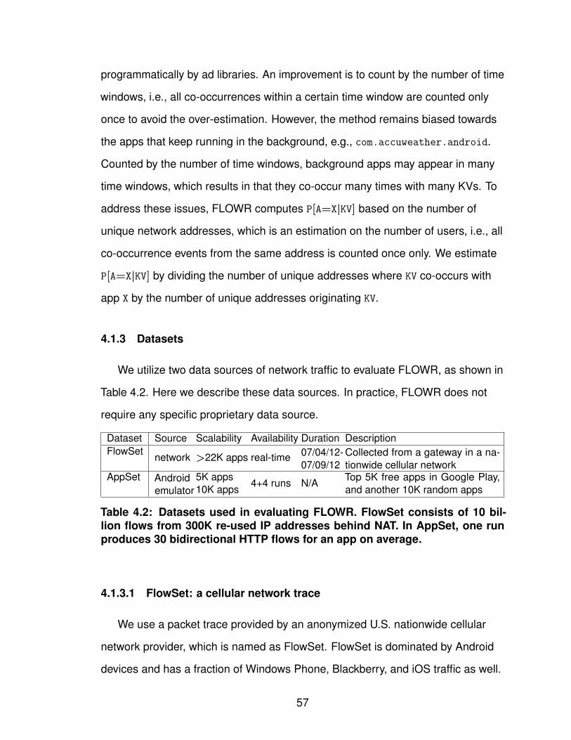
programmatically by ad libraries. An improvement is to count by the number of time

windows, i.e., all co-occurrences within a certain time window are counted only

once to avoid the over-estimation. However, the method remains biased towards

the apps that keep running in the background, e.g., com.accuweather.android.

Counted by the number of time windows, background apps may appear in many

time windows, which results in that they co-occur many times with many KVs. To

address these issues, FLOWR computes P[A=X|KV] based on the number of

unique network addresses, which is an estimation on the number of users, i.e., all

co-occurrence events from the same address is counted once only. We estimate

P[A=X|KV] by dividing the number of unique addresses where KV co-occurs with

app X by the number of unique addresses originating KV.

4.1.3 Datasets

We utilize two data sources of network traffic to evaluate FLOWR, as shown in

Table 4.2. Here we describe these data sources. In practice, FLOWR does not

require any specific proprietary data source.

Dataset Source Scalability Availability Duration DescriptionFlowSet

network >22K apps real-time 07/04/12-07/09/12

Collected from a gateway in a na-tionwide cellular network

AppSet Androidemulator

5K apps4+4 runs N/A Top 5K free apps in Google Play,

and another 10K random apps10K apps

Table 4.2: Datasets used in evaluating FLOWR. FlowSet consists of 10 bil-lion flows from 300K re-used IP addresses behind NAT. In AppSet, one runproduces 30 bidirectional HTTP flows for an app on average.

4.1.3.1 FlowSet: a cellular network trace

We use a packet trace provided by an anonymized U.S. nationwide cellular

network provider, which is named as FlowSet. FlowSet is dominated by Android

devices and has a fraction of Windows Phone, Blackberry, and iOS traffic as well.

57

FlowSet captures the traffic traversing through a gateway of the network provider of

six days (from July 4th to July 9th, 2012) with more than 10 billion traffic flows. We

observe 22K apps in FlowSet just by counting the KVs of app name in the HTTP

requests to doubleclick.net. However, it does not have the ground truth of the

app identity for every network flow. One use of FlowSet is the input to FLOWR’s

flow regression, the source information of which flow signatures co-occur. The

other use of FlowSet is for evaluating FLOWR’s performance in §4.1.4.

4.1.3.2 AppSet: an emulation trace

As FlowSet does not provide us the ground truth of the origins of network flows,

we produce AppSet by emulating apps in Android emulators. We do not and cannot

simulate comprehensive app behavior in AppSet. As long as the emulated traffic

covers some traffic that can be potentially observed in FlowSet, it is qualified

enough. We do not emulate on other systems such as iOS and Windows Phone

because the emulation on Android already meets our purpose. In §4.1.1.3, §4.1.4.2,

and §4.1.4.4, we discuss how we utilize AppSet.

In order to emulate apps, we have to (i) determine the target apps as it is

impossible to emulate all the apps on Google Play, (ii) crawl the installation

packages of the target apps, and (iii) emulate the target apps in Android emulators

configured with different Android OS versions.

• Determining target apps. Given it is prohibitive to dump the entire set of apps on

Google Play, we decide to download the most popular apps first. On Google Play,

only the top 5K apps are directly open to the public. As indicated by previous

studies [122], no matter how apps are ordered, i.e., by the traffic volume, by the

access time, or by the number of users, the total contribution of the top 5K apps

should consistently cover 98% of traffic volume. Thus, the top 5K apps on Google

Play should represent the dominant apps in FlowSet. In addition to the top 5K apps,

58

we automate random searching on Google Play and discover another 10K apps.

• Crawling installation packages. In order to download installation packages through

app identifiers, we modify a Chrome Browser extension named APK

Downloader [2] to download the target installation packages in parallel, i.e., 6

packages per “Chrome New Page” action. On average, we can download 12

installation packages from Google Play every minute.

• Emulating apps. We run the crawled app packages on two different Android OS

emulators, i.e., Gingerbread and Ice Cream Sandwich. In emulation, the emulator

interacts with apps through automated random clicks and random inputs. One run

of an app generates 600 random events including clicks and inputs. On average,

we can emulate 10K apps once every 24 hours via 10 Ubuntu 12.04 virtual

machines on an off-the-shelf machine.

4.1.4 Classification Performance

As described, to address the challenge of flow identification, FLOWR performs

two-phase operations: KV tokenization and flow regression. We first evaluate KV

tokenization by characterizing the flow signatures produced by KV tokenization, and

then we evaluate flow regression from the aspects of false positive, flow coverage,

and app coverage, along with how we develop the approach to quantify the false

positive without the ground truth of app identities.

4.1.4.1 Terminology

We use the following terminology to discuss evaluation results.

• Uniqueness. As a KV can be related with multiple apps, such as a KV

corresponds to a developer ID that holds several apps. Thus, the uniqueness of KV

is to evaluate how specific it is to an app. uniq(KV) returns whether KV is unique to

an app.

59

• Identifiability. As defined in §4.1.1.3, the identifiability of a KV is the co-occurrence

likelihood with the most frequently co-occurred app, i.e., id(KV).

• Probabilistic false positive. Given a random KV whose identifiability is above a

threshold P0, the probability that it is not unique to an app,

i.e., P[!uniq(KV)|id(KV)>P0].

4.1.4.2 Signature quality

We first investigate the uniqueness of user-agents and contacted hostnames,

which is a baseline for the quality of the flow signatures produced from KV

tokenization. Figure 4.3 shows the uniqueness of user-agents and hostnames

among the traffic flows generated by apps in AppSet. As shown in Figure 4.3,

among the traffic produced in emulating the 5K apps, we observe only 200 unique

user-agents. Even worse in the 10K apps, we observe around 400 unique

user-agents in 10K. Aggregating the 5K and 10K apps together, we observe <500

unique user-agents in total. In AppSet, a single app can have 3 unique user-agents

on average. Apparently, the information revealed from the distinctness among

user-agents is insufficient, particularly for a larger number of apps. Similarly, the

uniqueness of the domains access by the apps in AppSet is not sufficient either

although it is slightly better.

To justify if the flow signatures produced in KV tokenization are of good quality,

we rely on two criteria: persistence and uniqueness. There are nontrivial KVs that

are for one-time usage, e.g., the KVs of session IDs and request IDs. There are

also considerable KVs that are specific to the device, the user, the time, etc. These

KVs can be very unique, but not persistent over multiple runs. In flow regression,

such non-persistent KVs will be eliminated by screening conflicted KV as described

in §4.1.1.3. In evaluation, we eliminate these non-persistent KVs before we

evaluate the uniqueness.

60

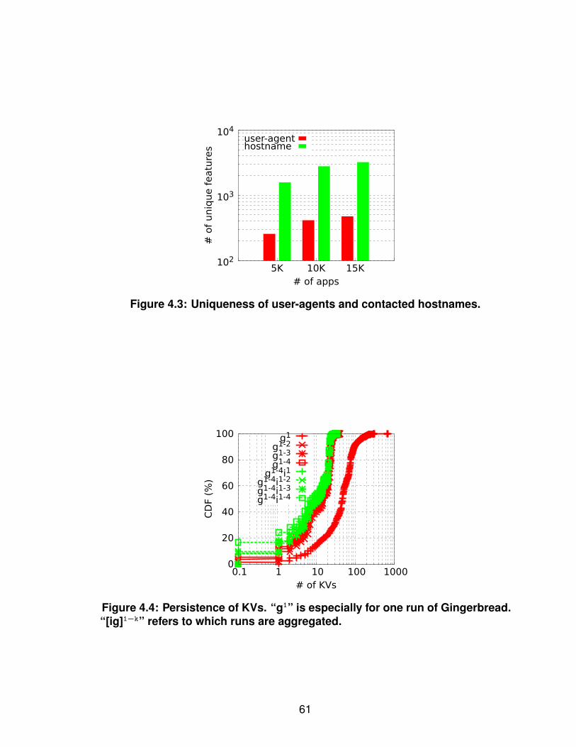
102

103

104

5K 10K 15K

# o

f uniq

ue f

eatu

res

# of apps

user-agenthostname

Figure 4.3: Uniqueness of user-agents and contacted hostnames.

0

20

40

60

80

100

0.1 1 10 100 1000

CD

F (%

)

# of KVs

g1

g1-2

g1-3

g1-4

g1-4i1g1-4i1-2

g1-4i1-3

g1-4i1-4

Figure 4.4: Persistence of KVs. “g1” is especially for one run of Gingerbread.“[ig]1−k” refers to which runs are aggregated.

61

Persistence. We rely on the flows in AppSet to quantify the quality of KVs

because it provides us the ground truth on the origin of each flow. As shown in

Table 4.2, we have 8 independent runs for each app in AppSet, among them 4 runs

are on Gingerbread and the other 4 are on Ice Cream Sandwich. We consider a KV

as a persistent one if it appears on both Gingerbread and Ice Cream Sandwich and

it does not conflict with any KV else. We aggregate multiple runs together, eliminate

conflicted KVs, and leave the remaining ones as persistent KVs. We show the

distribution of the number of persistent KVs for the apps in AppSet in Figure 4.4.

On average, an app has around 50 KVs in one emulation run. Aggregating two

Gingerbread runs, the number of consistent KVs per app immediately drops to

around 10. Apps vary a lot depending on how many content servers and a* service

providers they contact. With further aggregations, the number of consistent KVs

becomes stable even after we aggregate the total 4 Gingerbread and 4 Ice Cream

Sandwich runs. We have two observations from Figure 4.4: (i) there are nontrivial

consistent KVs although the majority of KVs are non-persistent; and (ii) the

consistent KVs repeat over runs as reflected by the stabilized number of persistent

KVs after aggregating two or more runs.

Uniqueness. To prevent the quantification on the uniqueness of consistent KVs

being limited by the apps in AppSet or the emulation setup, we attempt to discover

certain trend that is applicable to universal apps. We measure the entropy of the

dissimilarity across flows signatures from the apps that visit the same domain in

AppSet.

Given a domain D that appears in AppSet, we know all the apps in AppSet visit

the domain and the consistent KVs for each of these apps. Across apps visiting D,

they may or may not have the same set of consistent KVs. Assuming these

consistent KV sets are {KV}1,{KV}2,...,{KV}K, where K is the number of unique

consistent KV sets. The entropy of D is −∑K

i=0P[{KV}i]log2P[{KV}i].

62

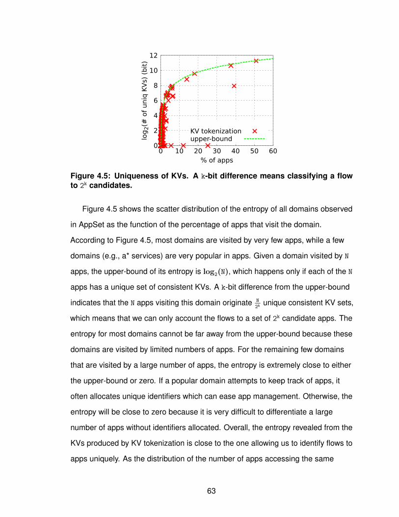
0

2

4

6

8

10

12

0 10 20 30 40 50 60lo

g2(#

of

uniq

KV

s) (

bit

)

% of apps

KV tokenizationupper-bound

Figure 4.5: Uniqueness of KVs. A k-bit difference means classifying a flowto 2k candidates.

Figure 4.5 shows the scatter distribution of the entropy of all domains observed

in AppSet as the function of the percentage of apps that visit the domain.

According to Figure 4.5, most domains are visited by very few apps, while a few

domains (e.g., a* services) are very popular in apps. Given a domain visited by N

apps, the upper-bound of its entropy is log2(N), which happens only if each of the N

apps has a unique set of consistent KVs. A k-bit difference from the upper-bound

indicates that the N apps visiting this domain originate N

2kunique consistent KV sets,

which means that we can only account the flows to a set of 2k candidate apps. The

entropy for most domains cannot be far away from the upper-bound because these

domains are visited by limited numbers of apps. For the remaining few domains

that are visited by a large number of apps, the entropy is extremely close to either

the upper-bound or zero. If a popular domain attempts to keep track of apps, it

often allocates unique identifiers which can ease app management. Otherwise, the

entropy will be close to zero because it is very difficult to differentiate a large

number of apps without identifiers allocated. Overall, the entropy revealed from the

KVs produced by KV tokenization is close to the one allowing us to identify flows to

apps uniquely. As the distribution of the number of apps accessing the same

63

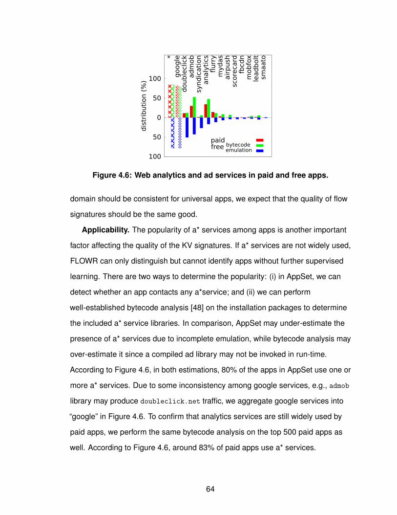
100

50

0

50

100

dis

trib

uti

on (

%)

paid free bytecode

double

clic

kadm

ob

syndic

ati

on

analy

tics

flurr

ym

ydas

air

push

score

card

fbcd

nm

obfo

xle

adbolt

smaato

google*

emulation

Figure 4.6: Web analytics and ad services in paid and free apps.

domain should be consistent for universal apps, we expect that the quality of flow

signatures should be the same good.

Applicability. The popularity of a* services among apps is another important

factor affecting the quality of the KV signatures. If a* services are not widely used,

FLOWR can only distinguish but cannot identify apps without further supervised

learning. There are two ways to determine the popularity: (i) in AppSet, we can

detect whether an app contacts any a*service; and (ii) we can perform

well-established bytecode analysis [48] on the installation packages to determine

the included a* service libraries. In comparison, AppSet may under-estimate the

presence of a* services due to incomplete emulation, while bytecode analysis may

over-estimate it since a compiled ad library may not be invoked in run-time.

According to Figure 4.6, in both estimations, 80% of the apps in AppSet use one or

more a* services. Due to some inconsistency among google services, e.g., admob

library may produce doubleclick.net traffic, we aggregate google services into

“google” in Figure 4.6. To confirm that analytics services are still widely used by

paid apps, we perform the same bytecode analysis on the top 500 paid apps as

well. According to Figure 4.6, around 83% of paid apps use a* services.

64

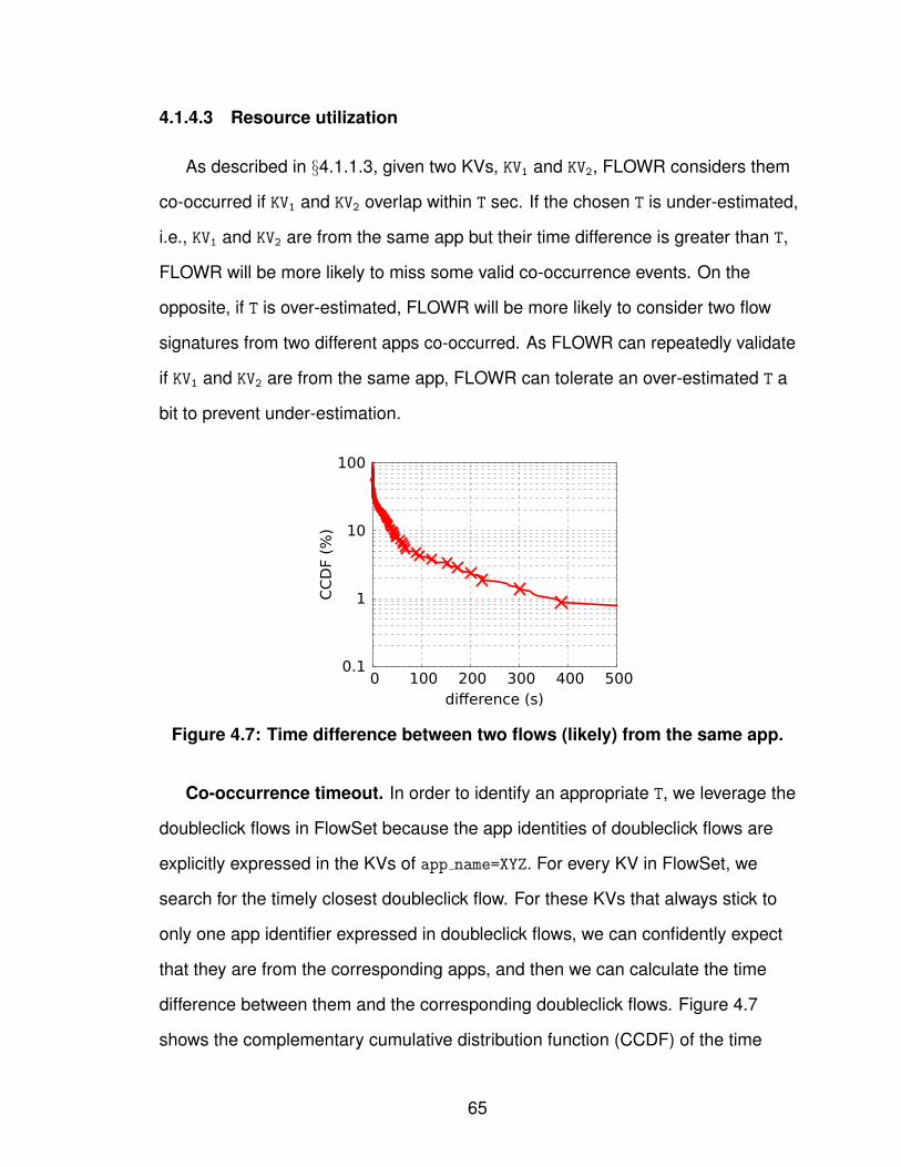
4.1.4.3 Resource utilization

As described in §4.1.1.3, given two KVs, KV1 and KV2, FLOWR considers them

co-occurred if KV1 and KV2 overlap within T sec. If the chosen T is under-estimated,

i.e., KV1 and KV2 are from the same app but their time difference is greater than T,

FLOWR will be more likely to miss some valid co-occurrence events. On the

opposite, if T is over-estimated, FLOWR will be more likely to consider two flow

signatures from two different apps co-occurred. As FLOWR can repeatedly validate

if KV1 and KV2 are from the same app, FLOWR can tolerate an over-estimated T a

bit to prevent under-estimation.

0.1

1

10

100

0 100 200 300 400 500

CC

DF

(%)

difference (s)

Figure 4.7: Time difference between two flows (likely) from the same app.

Co-occurrence timeout. In order to identify an appropriate T, we leverage the

doubleclick flows in FlowSet because the app identities of doubleclick flows are

explicitly expressed in the KVs of app name=XYZ. For every KV in FlowSet, we

search for the timely closest doubleclick flow. For these KVs that always stick to

only one app identifier expressed in doubleclick flows, we can confidently expect

that they are from the corresponding apps, and then we can calculate the time

difference between them and the corresponding doubleclick flows. Figure 4.7

shows the complementary cumulative distribution function (CCDF) of the time

65

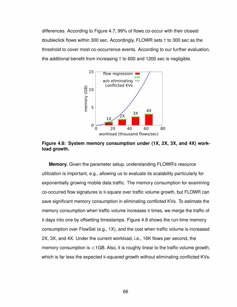
differences. According to Figure 4.7, 99% of flows co-occur with their closest

doubleclick flows within 300 sec. Accordingly, FLOWR sets T to 300 sec as the

threshold to cover most co-occurrence events. According to our further evaluation,

the additional benefit from increasing T to 600 and 1200 sec is negligible.

0

5

10

15

0 20 40 60 80

mem

ory

(G

B)

workload (thousand flows/sec)

flow regression

1X2X

3X4X

w/o eliminatingconflicted KVs

Figure 4.8: System memory consumption under (1X, 2X, 3X, and 4X) work-load growth.

Memory. Given the parameter setup, understanding FLOWR’s resource

utilization is important, e.g., allowing us to evaluate its scalability particularly for

exponentially growing mobile data traffic. The memory consumption for examining

co-occurred flow signatures is N-square over traffic volume growth, but FLOWR can

save significant memory consumption in eliminating conflicted KVs. To estimate the

memory consumption when traffic volume increases N times, we merge the traffic of

N days into one by offsetting timestamps. Figure 4.8 shows the run-time memory

consumption over FlowSet (e.g., 1X), and the cost when traffic volume is increased

2X, 3X, and 4X. Under the current workload, i.e., 16K flows per second, the

memory consumption is <1GB. Also, it is roughly linear to the traffic volume growth,

which is far less the expected N-squared growth without eliminating conflicted KVs.

66

4.1.4.4 Identification accuracy

According to Figure 4.6, the apps utilizing a* services such as

doubleclick.net and airpush.com generate traffic with app identifiers embedded

somewhere so that FLOWR can identify them through flow regression without any

supervised learning effort. For the apps utilizing other a* services without app

identifiers but with some unique identifiers such as google-analytics.com and

fbcdn.com, FLOWR can identify them with negligible training effort in mapping the

unique identifiers to the app identifiers on app market. It can be done via various

approaches such as the emulation in §4.1.3.2. In evaluating flow regression, we

consider only doubleclick apps4. The evaluation results should be extendable to

apps using other a* services. In previous §4.1.1.3 and §4.1.4.3, we show the

detection of co-occurrences. In the following, we evaluate the performance of the

identified flow signatures from the aspects of the false positive (§4.1.4.4), the flow

coverage (§4.1.4.5), and the number of identified apps (§4.1.4.5).

0

20

40

60

80

100

0 0.2 0.4 0.6 0.8 1

CD

F (%

)

identifiability

# IPs > 1000# IPs > 2000

Figure 4.9: Identifiability of the KVs whose id(KV)>0.5.

Identifiability. Once we have identified the appropriate timeout T sec for

co-occurrence examination, a remaining decision is how we decide if the4We name the apps with doubleclick flows as doubleclick apps.

67

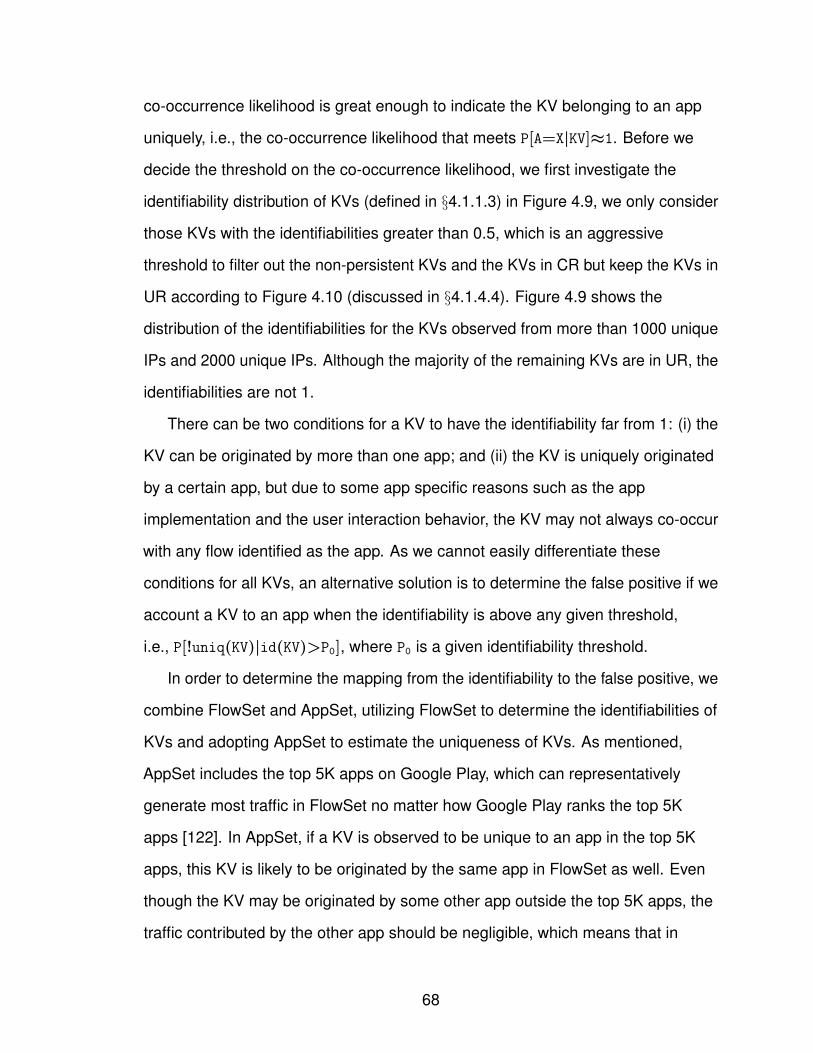
co-occurrence likelihood is great enough to indicate the KV belonging to an app

uniquely, i.e., the co-occurrence likelihood that meets P[A=X|KV]≈1. Before we

decide the threshold on the co-occurrence likelihood, we first investigate the

identifiability distribution of KVs (defined in §4.1.1.3) in Figure 4.9, we only consider

those KVs with the identifiabilities greater than 0.5, which is an aggressive

threshold to filter out the non-persistent KVs and the KVs in CR but keep the KVs in

UR according to Figure 4.10 (discussed in §4.1.4.4). Figure 4.9 shows the

distribution of the identifiabilities for the KVs observed from more than 1000 unique

IPs and 2000 unique IPs. Although the majority of the remaining KVs are in UR, the

identifiabilities are not 1.

There can be two conditions for a KV to have the identifiability far from 1: (i) the

KV can be originated by more than one app; and (ii) the KV is uniquely originated

by a certain app, but due to some app specific reasons such as the app

implementation and the user interaction behavior, the KV may not always co-occur

with any flow identified as the app. As we cannot easily differentiate these

conditions for all KVs, an alternative solution is to determine the false positive if we

account a KV to an app when the identifiability is above any given threshold,

i.e., P[!uniq(KV)|id(KV)>P0], where P0 is a given identifiability threshold.

In order to determine the mapping from the identifiability to the false positive, we

combine FlowSet and AppSet, utilizing FlowSet to determine the identifiabilities of

KVs and adopting AppSet to estimate the uniqueness of KVs. As mentioned,

AppSet includes the top 5K apps on Google Play, which can representatively

generate most traffic in FlowSet no matter how Google Play ranks the top 5K

apps [122]. In AppSet, if a KV is observed to be unique to an app in the top 5K

apps, this KV is likely to be originated by the same app in FlowSet as well. Even

though the KV may be originated by some other app outside the top 5K apps, the

traffic contributed by the other app should be negligible, which means that in

68

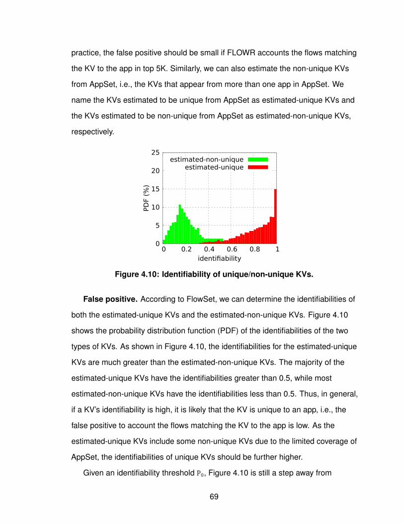
practice, the false positive should be small if FLOWR accounts the flows matching

the KV to the app in top 5K. Similarly, we can also estimate the non-unique KVs

from AppSet, i.e., the KVs that appear from more than one app in AppSet. We

name the KVs estimated to be unique from AppSet as estimated-unique KVs and

the KVs estimated to be non-unique from AppSet as estimated-non-unique KVs,

respectively.

0

5

10

15

20

25

0 0.2 0.4 0.6 0.8 1

PD

F (%

)

identifiability

estimated-non-uniqueestimated-unique

Figure 4.10: Identifiability of unique/non-unique KVs.

False positive. According to FlowSet, we can determine the identifiabilities of

both the estimated-unique KVs and the estimated-non-unique KVs. Figure 4.10

shows the probability distribution function (PDF) of the identifiabilities of the two

types of KVs. As shown in Figure 4.10, the identifiabilities for the estimated-unique

KVs are much greater than the estimated-non-unique KVs. The majority of the

estimated-unique KVs have the identifiabilities greater than 0.5, while most

estimated-non-unique KVs have the identifiabilities less than 0.5. Thus, in general,

if a KV’s identifiability is high, it is likely that the KV is unique to an app, i.e., the

false positive to account the flows matching the KV to the app is low. As the

estimated-unique KVs include some non-unique KVs due to the limited coverage of

AppSet, the identifiabilities of unique KVs should be further higher.

Given an identifiability threshold P0, Figure 4.10 is still a step away from

69

0.01

0.1

1

10

100

0.01 0.1 1FP

(%

)

1 - identifiability

0.68, 10%0.80, 5%

0.97, 100%

0.93, 1%

Figure 4.11: Mapping from identifiability to false positive.

determining the probabilistic false positive, i.e., P[!uniq(KV)|id(KV)>P0].

Figure 4.10 tells us two functions: P[id(KV)>P0|uniq(KV)] and

P[id(KV)>P0|!uniq(KV)], denoted as PU and PN respectively. Applying Bayes’

theorem, we have P[uniq(KV)|id(KV)>P0]=PU·P[uniq(KV)]

PU·P[uniq(KV)]+PN·P[!uniq(KV)] . P[uniq(KV)]

and P[!uniq(KV)] can be estimated from AppSet. Based on the above

transformation, Figure 4.11 shows the mapping from the identifiability to the false

positive, which is weighted based on the number of flows that each KV matches in

FlowSet. According to Figure 4.11, it is common that a flow signature is unique to

an app but its identifiability is far less than 1. To guarantee the false positive less

than 5%, FLOWR can label all flows whose flow signatures have the identifiabilities

greater than 0.8. If FLOWR wants to further relax the false positive lower-bound to

10%, all flows whose flow signatures have the identifiabilities greater than 0.68 can

be uniquely identified, but the benefit in terms of flow coverage is marginal (to

discuss in Figure 4.13(a)). After the threshold on the identifiability is increased to

0.93, the false positive drops to less than 1%. In our dataset, we never see that any

flow signature with the identifiability higher than 0.97 is originated by more than one

app.

70

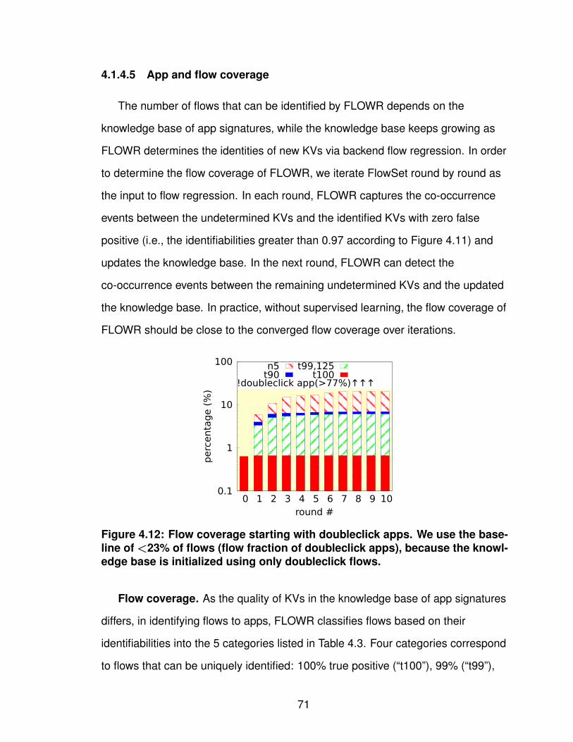
4.1.4.5 App and flow coverage

The number of flows that can be identified by FLOWR depends on the

knowledge base of app signatures, while the knowledge base keeps growing as

FLOWR determines the identities of new KVs via backend flow regression. In order

to determine the flow coverage of FLOWR, we iterate FlowSet round by round as

the input to flow regression. In each round, FLOWR captures the co-occurrence

events between the undetermined KVs and the identified KVs with zero false

positive (i.e., the identifiabilities greater than 0.97 according to Figure 4.11) and

updates the knowledge base. In the next round, FLOWR can detect the

co-occurrence events between the remaining undetermined KVs and the updated

the knowledge base. In practice, without supervised learning, the flow coverage of

FLOWR should be close to the converged flow coverage over iterations.

0.1

1

10

100

0 1 2 3 4 5 6 7 8 9 10

perc

enta

ge (

%)

round #

!doubleclick app(>77%)↑↑↑

n5t90

t99,125t100

Figure 4.12: Flow coverage starting with doubleclick apps. We use the base-line of <23% of flows (flow fraction of doubleclick apps), because the knowl-edge base is initialized using only doubleclick flows.

Flow coverage. As the quality of KVs in the knowledge base of app signatures

differs, in identifying flows to apps, FLOWR classifies flows based on their

identifiabilities into the 5 categories listed in Table 4.3. Four categories correspond

to flows that can be uniquely identified: 100% true positive (“t100”), 99% (“t99”),

71

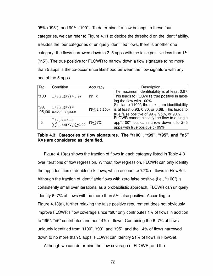
95% (“t95”), and 90% (“t90”). To determine if a flow belongs to these four

categories, we can refer to Figure 4.11 to decide the threshold on the identifiability.

Besides the four categories of uniquely identified flows, there is another one

category: the flows narrowed down to 2–5 apps with the false positive less than 1%

(“n5”). The true positive for FLOWR to narrow down a flow signature to no more

than 5 apps is the co-occurrence likelihood between the flow signature with any

one of the 5 apps.

Tag Condition Accuracy Description

t100 ∃KV,id(KV)≥0.97 FP=0

The maximum identifiability is at least 0.97.This leads to FLOWR’s true positive in label-ing the flow with 100%.

t99,t95,t90

∃KV,id(KV)≥0.93,0.80,0.68

FP≤1,5,10%Similar to “t100”, the maximum identifiabilityis at least 0.93, 0.80, or 0.68. This leads totrue false positive of 99%, 95%, or 90%.

n5∃KVi,i=1...5,∑5

i=1id(KVi)≥0.99FP≤1%

FLOWR cannot classify the flow to a singleapp“t100”, but can narrow down it to 2–5apps with true positive > 99%.

Table 4.3: Categories of flow signatures. The “t100”, “t99”, “t95”, and “n5”KVs are considered as identified.

Figure 4.13(a) shows the fraction of flows in each category listed in Table 4.3

over iterations of flow regression. Without flow regression, FLOWR can only identify

the app identities of doubleclick flows, which account ≈0.7% of flows in FlowSet.

Although the fraction of identifiable flows with zero false positive (i.e., “t100”) is

consistently small over iterations, as a probabilistic approach, FLOWR can uniquely

identify 6–7% of flows with no more than 5% false positive. According to

Figure 4.13(a), further relaxing the false positive requirement does not obviously

improve FLOWR’s flow coverage since “t90” only contributes 1% of flows in addition

to “t95”. “n5” contributes another 14% of flows. Combining the 6–7% of flows

uniquely identified from “t100”, “t99”, and “t95”, and the 14% of flows narrowed

down to no more than 5 apps, FLOWR can identify 21% of flows in FlowSet.

Although we can determine the flow coverage of FLOWR, and the

72

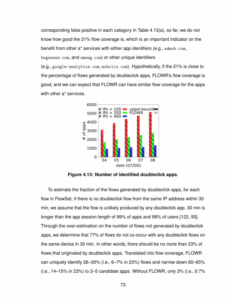
corresponding false positive in each category in Table 4.13(a), so far, we do not

know how good the 21% flow coverage is, which is an important indicator on the

benefit from other a* services with either app identifiers (e.g., admob.com,

bugsense.com, and umeng.com) or other unique identifiers

(e.g., google-analytics.com, mobclix.com). Hypothetically, if the 21% is close to

the percentage of flows generated by doubleclick apps, FLOWR’s flow coverage is

good, and we can expect that FLOWR can have similar flow coverage for the apps

with other a* services.

0

1000

2000

3000

4000

5000

6000

04 05 06 07 08

# o

f apps

date (07/DD)

# IPs > 100# IPs > 200# IPs > 400

upper-boundFLOWR

Figure 4.13: Number of identified doubleclick apps.

To estimate the fraction of the flows generated by doubleclick apps, for each

flow in FlowSet, if there is no doubleclick flow from the same IP address within 30

min, we assume that the flow is unlikely produced by any doubleclick app. 30 min is

longer than the app session length of 99% of apps and 99% of users [122, 50].

Through the over-estimation on the number of flows not generated by doubleclick

apps, we determine that 77% of flows do not co-occur with any doubleclick flows on

the same device in 30 min. In other words, there should be no more than 23% of

flows that originated by doubleclick apps. Translated into flow coverage, FLOWR

can uniquely identify 26–30% (i.e., 6–7% in 23%) flows and narrow down 60–65%

(i.e., 14–15% in 23%) to 2–5 candidate apps. Without FLOWR, only 3% (i.e., 0.7%

73

in 23%) can be identified.

App coverage. Above we evaluate the performance of FLOWR based on the

flow coverage. As flow contribution is uneven across apps due to their diverse

usage, we are interested in the number of identified apps by FLOWR in addition.

FLOWR has a threshold on the number of occurrences of flow signatures to

prevent that the flow signatures with the high identifiabilities but insufficient samples

from polluting FLOWR’s the knowledge base. Given the threshold on the number of

occurrences of flow signatures, we compare (i) the baseline, i.e., the number of

apps producing doubleclick flows against (ii) the number of apps whose flows are

identified by FLOWR in Figure 4.13(b). On July 4th 2012, the total number of

appeared doubleclick apps from more than 100 IPs is around 3000. Among the

flows generated by these 3000 apps excluding doubleclick flows, FLOWR identifies

around 2700 apps, which means that FLOWR’s flow regression technique works for

90% of apps. If we further increase the threshold on the number of flow

occurrences to 200 and 400, FLOWR can identify 1500 from 1700 apps, and 700

from 900 apps respectively. Another aspect is that the number of identified apps by

FLOWR should grow over time rather than converge after sometime. To evaluate

the number of additional identified apps over time, we aggregate the flows from July

4th to different end dates, i.e., 5th–8th. According to Figure 4.13(b), the number of

identified apps grows linearly over time, consistently identifying more than 90% of

doubleclick apps.

4.1.5 Limitation

FLOWR has the weakness in identifying encrypted or hashed network traffic or

the traffic originated by the apps not using any a* services.

74

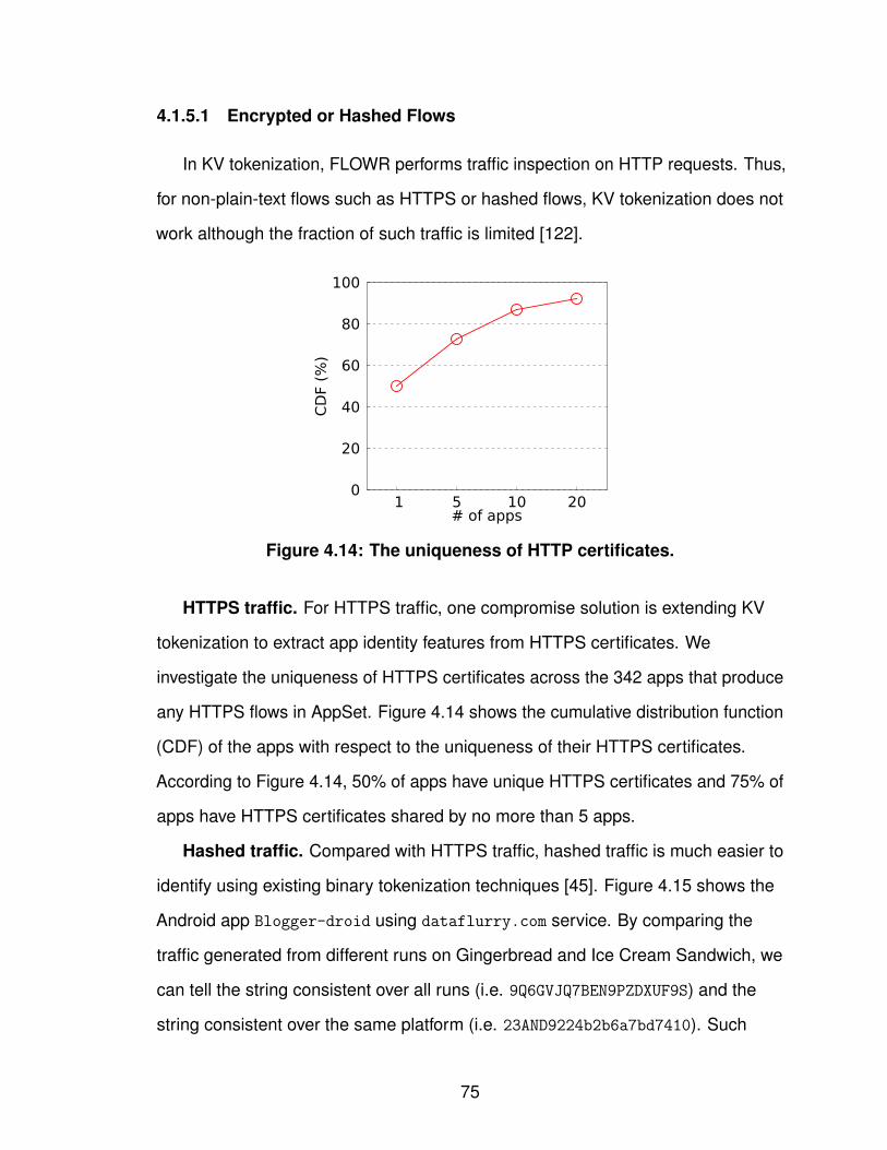
4.1.5.1 Encrypted or Hashed Flows

In KV tokenization, FLOWR performs traffic inspection on HTTP requests. Thus,

for non-plain-text flows such as HTTPS or hashed flows, KV tokenization does not

work although the fraction of such traffic is limited [122].

0

20

40

60

80

100

1 5 10 20

CD

F (%

)

# of apps

Figure 4.14: The uniqueness of HTTP certificates.

HTTPS traffic. For HTTPS traffic, one compromise solution is extending KV

tokenization to extract app identity features from HTTPS certificates. We

investigate the uniqueness of HTTPS certificates across the 342 apps that produce

any HTTPS flows in AppSet. Figure 4.14 shows the cumulative distribution function

(CDF) of the apps with respect to the uniqueness of their HTTPS certificates.

According to Figure 4.14, 50% of apps have unique HTTPS certificates and 75% of

apps have HTTPS certificates shared by no more than 5 apps.

Hashed traffic. Compared with HTTPS traffic, hashed traffic is much easier to

identify using existing binary tokenization techniques [45]. Figure 4.15 shows the

Android app Blogger-droid using dataflurry.com service. By comparing the

traffic generated from different runs on Gingerbread and Ice Cream Sandwich, we

can tell the string consistent over all runs (i.e. 9Q6GVJQ7BEN9PZDXUF9S) and the

string consistent over the same platform (i.e. 23AND9224b2b6a7bd7410). Such

75

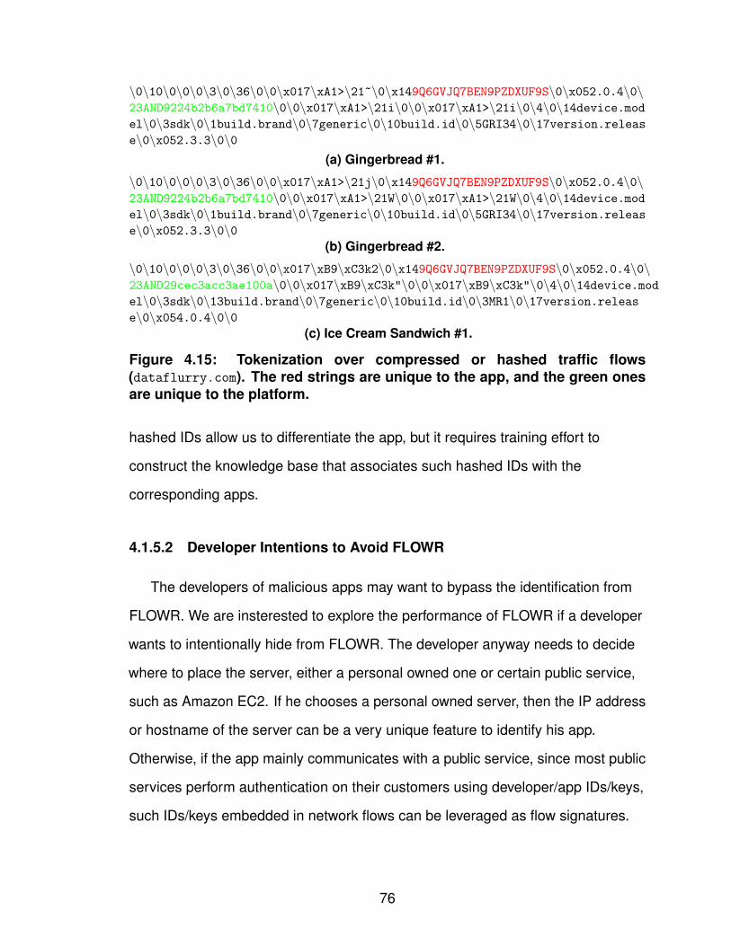
\0\10\0\0\0\3\0\36\0\0\x017\xA1>\21~\0\x149Q6GVJQ7BEN9PZDXUF9S\0\x052.0.4\0\23AND9224b2b6a7bd7410\0\0\x017\xA1>\21i\0\0\x017\xA1>\21i\0\4\0\14device.model\0\3sdk\0\1build.brand\0\7generic\0\10build.id\0\5GRI34\0\17version.release\0\x052.3.3\0\0

(a) Gingerbread #1.

\0\10\0\0\0\3\0\36\0\0\x017\xA1>\21j\0\x149Q6GVJQ7BEN9PZDXUF9S\0\x052.0.4\0\23AND9224b2b6a7bd7410\0\0\x017\xA1>\21W\0\0\x017\xA1>\21W\0\4\0\14device.model\0\3sdk\0\1build.brand\0\7generic\0\10build.id\0\5GRI34\0\17version.release\0\x052.3.3\0\0

(b) Gingerbread #2.

\0\10\0\0\0\3\0\36\0\0\x017\xB9\xC3k2\0\x149Q6GVJQ7BEN9PZDXUF9S\0\x052.0.4\0\23AND29cec3acc3ae100a\0\0\x017\xB9\xC3k"\0\0\x017\xB9\xC3k"\0\4\0\14device.model\0\3sdk\0\13build.brand\0\7generic\0\10build.id\0\3MR1\0\17version.release\0\x054.0.4\0\0

(c) Ice Cream Sandwich #1.

Figure 4.15: Tokenization over compressed or hashed traffic flows(dataflurry.com). The red strings are unique to the app, and the green onesare unique to the platform.

hashed IDs allow us to differentiate the app, but it requires training effort to

construct the knowledge base that associates such hashed IDs with the

corresponding apps.

4.1.5.2 Developer Intentions to Avoid FLOWR

The developers of malicious apps may want to bypass the identification from

FLOWR. We are insterested to explore the performance of FLOWR if a developer

wants to intentionally hide from FLOWR. The developer anyway needs to decide

where to place the server, either a personal owned one or certain public service,

such as Amazon EC2. If he chooses a personal owned server, then the IP address

or hostname of the server can be a very unique feature to identify his app.

Otherwise, if the app mainly communicates with a public service, since most public

services perform authentication on their customers using developer/app IDs/keys,

such IDs/keys embedded in network flows can be leveraged as flow signatures.

76

4.1.5.3 Remaining Apps Not Using A*

Without training effort, the optimal flow coverage that FLOWR can pursue is the

flows originated by the a* services embedded with either app identifiers on app

market or other unique identifiers as shown in Table 4.1. However, some apps do

not use a* services. To save supervised learning effort for the remaining 20% of

apps, we need to explore further intelligence such as CAPTCHA [5].

4.2 Application Usage Characterization

Given the prerequisite for understanding mobile app usage is fulfilled by

FLOWR, we start to investigate the usage patterns of smartphone apps in this

section. A previous study found evidence that there is substantial diversity in the

way that different people use smartphone apps [50]. However, because the study

relied on volunteers using instrumented phones, it was limited to two platforms and

less than three hundred users in a few geographic areas. Other studies of mobile

application/app usage [53, 77, 108] have been similarly limited in scope. Thus, it is

difficult to extrapolate these results to make representative conclusions about

spatial locality, temporal variation, and correlation of apps at scale. For example,

“where are apps more popular?”, “How is their usage distributed across a country?”,

“How does their usage vary throughout the day?”. While there have been studies of

smartphone performance at larger scales [62, 29, 52], which use volunteer

measurements or network data to obtain measurements at scale, measuring the

usage of different apps from these data sources is more challenging. Volunteer

measurements are typically obtained by deploying a measurement tool via an app

marketplace, but many popular platform APIs do not permit the measurement of

other apps in the background, so it is difficult to write an app that captures this

information. Network data may contain information that can identify app behaviors,

77

but this information is not typically part of standard traces. To make representative

conclusions about apps, we require a network data set that identifies apps in

network traffic and contains a significant number of measurements covering a

representative number of devices, users, locations, and times.

We address the limitations by collecting anonymized IP-level networking traces

in a large tier-1 cellular network in the U.S. for one week in August 2010. In contrast

to previous work, we use signatures based on HTTP headers (included in the

IP-level trace) to distinguish the traffic from different apps. Due to the format of

User-Agent in HTTP headers when mobile apps use standard platform APIs, this

technique gives us the ability to gather statistics about each individual app in a

marketplace, not just categories of network traffic characterized by port number.

Moreover, our work examines the spatial and temporal prevalence, locality, and

correlation of apps at a national scale, not just in one area or over a small

population of users.

To our best knowledge, this is the first to investigate the diverse usage behaviors

of individual mobile apps at scale, and we make the following five contributions:

• The data set that we use to study mobile apps is significantly more diverse

geographically and in user base than previous studies. It covers hundreds of

thousands of smartphones throughout the U.S. in a tier-1 cellular network. This

allows us to make more generalizable conclusions about smartphone usage

patterns.

• We find that a considerable number of popular apps (20%) are local, in particular,

radio and news apps. In terms of traffic volume, these apps are accountable for 2%

of the traffic in the smartphone apps category (i.e., all the marketplace apps that

can be identified by User-Agent) – that is, their user base is limited to a few U.S.

states. This suggests significant potential for content optimization in such access

networks as LTE and WiFi where content can be placed on servers closer to clients.

78

Furthermore, it suggests that network operators need to understand the impact of

different app mixes in different geographical areas to best optimize their network for

user experience.

• Despite this diversity in locality, we also find that there are similarities across apps

in terms of geographic coverage, diurnal usage patterns, etc. For example, we find

that some apps have a high likelihood of co-occurrence on smartphones – that is,

when a user uses one app, he or she is also likely to use another one. Users also

use several alternatives for the same type of app (e.g., multiple news apps). These

findings suggest that some apps can be treated as a “bundle” when trying to

optimize for their user experience and that there may be opportunities for

integration.

• We also find that the diurnal patterns of different genres of apps can be remarkably

different. For example, news apps are much more frequently used in the early

morning, sports apps are more frequently used in the evening, while other apps

have diurnal patterns less visible and their usage is more flat during a day. These

findings suggest that cloud platforms that host mobile application servers can

leverage distinct usage patterns in classes of apps to maximize the utilization of

their resources. Furthermore, network operators may be able to leverage these

results by optimizing their network for different apps during different times of the

day.

• Mobility patterns can be inferred from network access patterns. Some apps are

more frequently used when users are moving around; some of them are used more

often when users are stationary. Mobility affects connectivity and performance, so

bandwidth sensitive apps that are mobile may need to consider techniques to

compensate for bandwidth variability. We find that there is a significant degree of

diversity in the mobility of apps.

The rest of this section is organized as follows: §4.2.1 describes our data set,

79

§4.2.2 presents our measurement results, §4.2.3 outlines some implications.

4.2.1 Datasets

We use an anonymized data set from a tier-1 cellular network provider in the

U.S. It is collected during the week of August 24th, 2010 – August 30th, 2010. The

data set contains flow-level information about IP flows carried in PDP Context

tunnels (i.e., all data traffic sent to and from cellular devices). This data set is

collected from all links between SGSNs and GGSNs in tier-1 network’s UMTS core

network. Hence, we have a nationwide view of cellular data traffic. Due to volume

constraints, only traffic from a uniform random sample of devices is collected. For a

random sample of devices, the data contains the following information for each IP

flow per minute: the start and the end timestamps, per-flow traffic volume in terms

of both the bytes and the number of packets, the device identifier, and the app

identifier. All device and subscriber identifiers (e.g., IMSI, IMEI) are anonymized to

protect privacy without affecting the usefulness of our analysis. Furthermore, the

data sets do not permit reversing the anonymization or re-identification of

subscribers.

We are concerned about four main features per app: traffic volume, access

time, unique subscribers, and locations. We estimate traffic volume as the sum

of the flow byte counts, access time as the sum of the flow durations (with a

precision of seconds), and the number of unique subscribers as the number of

distinct anonymous device identifiers. There is only one anonymized identifier per

distinct device. To determine the location of each device at the time a flow is in

progress, we use the cell sector identified in the PDP context used to tunnel the

flow. This cell sector is typically recorded when the PDP context begins, when a

device moves far enough that the SGSN its traffic routes through changes, switches

from 2G to 3G (or vice versa), or switches from 3G to WiFi. While this sector may

80

be slightly stale, previous work [119] showed that they are still almost always

accurate to within 40 kilometers. Thus, they suffice for most of our results that only

look at U.S. states as distinct regions. For other results we present on sector

changes, we may underestimate the number of changes due to this limitation.

In total, the sample data set includes approximately 600K distinct subscribers

and approximately 22K distinct smartphone apps.

4.2.2 Smartphone Application Usage Patterns

In this section, we investigate how, where, and when smartphone apps are used

from spatial, temporal, and user perspectives. We first choose appropriate metrics

to evaluate smartphone apps, and then attempt to understand the impact of

location, time, user, and app interest accordingly.

4.2.2.1 Overall app usage

We begin our analysis by presenting some broad characteristics of smartphone

app usage. For our analysis, we choose a number of different natural metrics that

profile network activity. We use the following three metrics for each app through

most of our analysis: (i)traffic volume, defined as the number of bytes consumed

by all subscribers using the app; (ii)number of subscribers, defined as the

number of unique subscribers using this app throughout our week-long data set;

(iii)network access time, defined as the total duration summed across all the IP

flows generated by the app over our week-long data set.

Figure 4.16 shows CDFs of these metrics for the apps. For each metric, we

aggregate together all the users of a particular app. The long tail of these CDFs

directly shows the huge diversity in smartphone apps and their network

characteristics. The top app in Figure 4.16(a) is a “personalized Internet radio app”,

and is responsible for more than 3TB data in one week, while the majority of

81

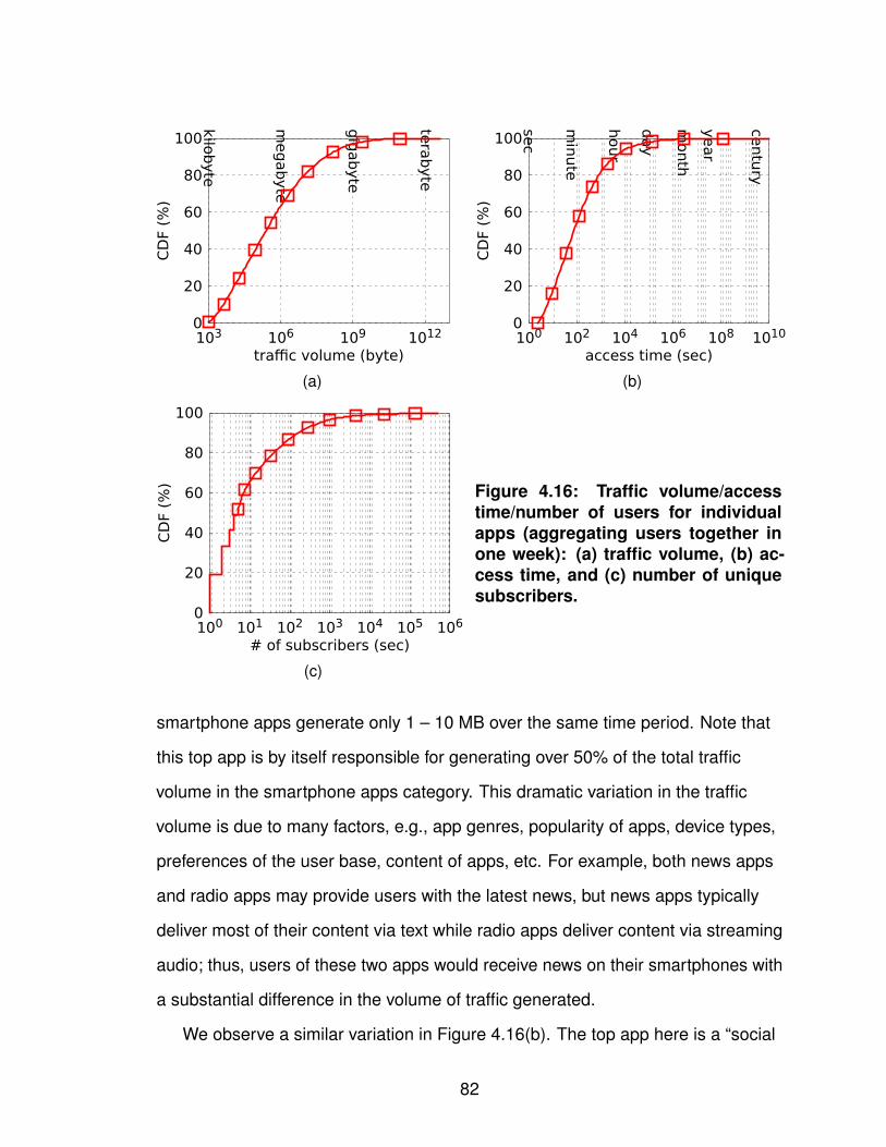
0

20

40

60

80

100

103 106 109 1012

kilobyte

megabyte

gig

abyte

tera

byte

CD

F (%

)

traffic volume (byte)

0

20

40

60

80

100

100 102 104 106 108 1010

sec

min

ute

hour

day

month

year

centu

ry

CD

F (%

)

access time (sec)

(a) (b)

0

20

40

60

80

100

100 101 102 103 104 105 106

CD

F (%

)

# of subscribers (sec)

(c)

Figure 4.16: Traffic volume/accesstime/number of users for individualapps (aggregating users together inone week): (a) traffic volume, (b) ac-cess time, and (c) number of uniquesubscribers.

smartphone apps generate only 1 – 10 MB over the same time period. Note that

this top app is by itself responsible for generating over 50% of the total traffic

volume in the smartphone apps category. This dramatic variation in the traffic

volume is due to many factors, e.g., app genres, popularity of apps, device types,

preferences of the user base, content of apps, etc. For example, both news apps

and radio apps may provide users with the latest news, but news apps typically

deliver most of their content via text while radio apps deliver content via streaming

audio; thus, users of these two apps would receive news on their smartphones with

a substantial difference in the volume of traffic generated.

We observe a similar variation in Figure 4.16(b). The top app here is a “social

82

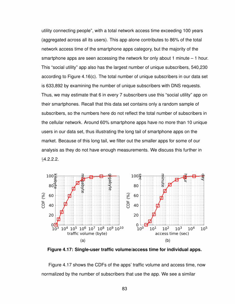
utility connecting people”, with a total network access time exceeding 100 years

(aggregated across all its users). This app alone contributes to 86% of the total

network access time of the smartphone apps category, but the majority of the

smartphone apps are seen accessing the network for only about 1 minute – 1 hour.

This “social utility” app also has the largest number of unique subscribers, 540,230

according to Figure 4.16(c). The total number of unique subscribers in our data set

is 633,892 by examining the number of unique subscribers with DNS requests.

Thus, we may estimate that 6 in every 7 subscribers use this “social utility” app on

their smartphones. Recall that this data set contains only a random sample of

subscribers, so the numbers here do not reflect the total number of subscribers in

the cellular network. Around 60% smartphone apps have no more than 10 unique

users in our data set, thus illustrating the long tail of smartphone apps on the

market. Because of this long tail, we filter out the smaller apps for some of our

analysis as they do not have enough measurements. We discuss this further in

§4.2.2.2.

0

20

40

60

80

100

103 104 105 106 107 108 109 1010

kilobyte

megabyte

gig

abyte

CD

F (%

)

traffic volume (byte)

0

20

40

60

80

100

100 101 102 103 104 105

sec

min

ute

hour

day

CD

F (%

)

access time (sec)

(a) (b)

Figure 4.17: Single-user traffic volume/access time for individual apps.

Figure 4.17 shows the CDFs of the apps’ traffic volume and access time, now

normalized by the number of subscribers that use the app. We see a similar

83

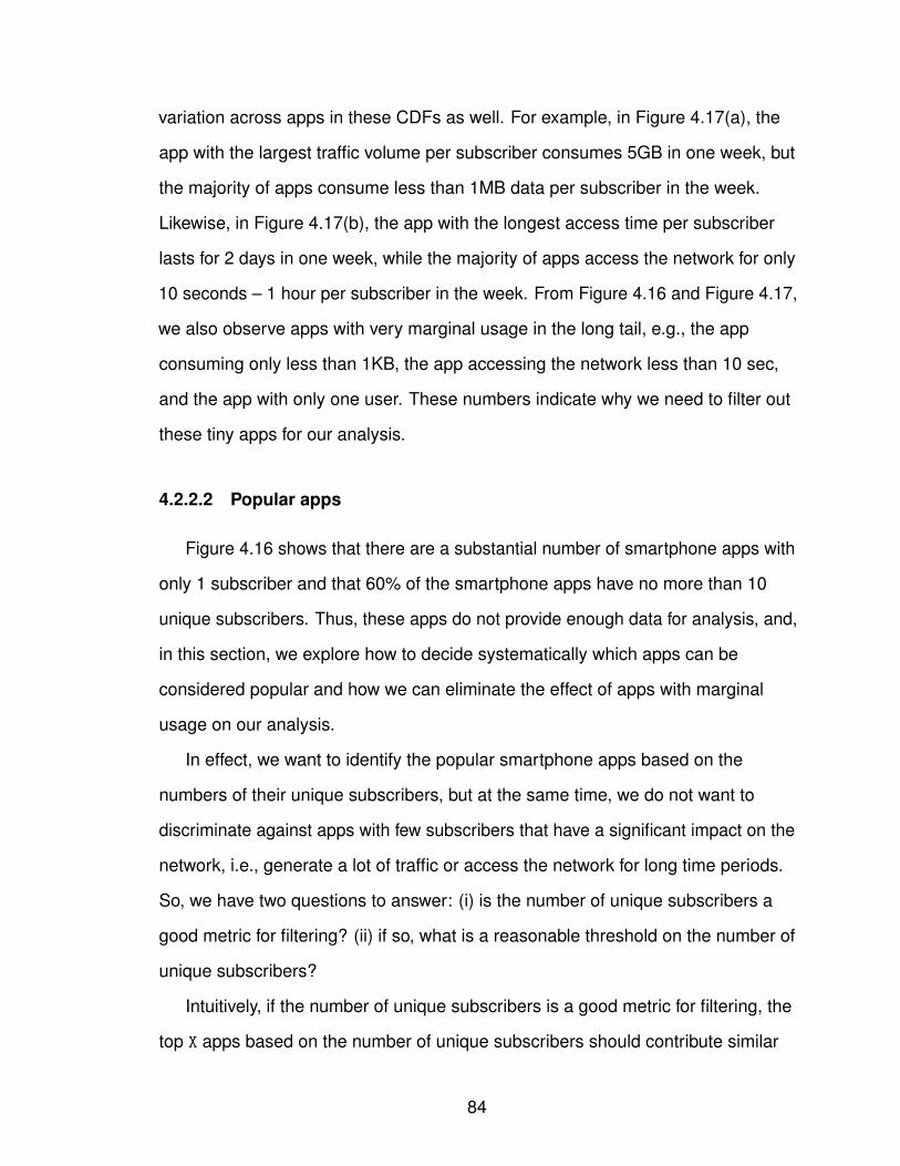
variation across apps in these CDFs as well. For example, in Figure 4.17(a), the

app with the largest traffic volume per subscriber consumes 5GB in one week, but

the majority of apps consume less than 1MB data per subscriber in the week.

Likewise, in Figure 4.17(b), the app with the longest access time per subscriber

lasts for 2 days in one week, while the majority of apps access the network for only

10 seconds – 1 hour per subscriber in the week. From Figure 4.16 and Figure 4.17,

we also observe apps with very marginal usage in the long tail, e.g., the app

consuming only less than 1KB, the app accessing the network less than 10 sec,

and the app with only one user. These numbers indicate why we need to filter out

these tiny apps for our analysis.

4.2.2.2 Popular apps

Figure 4.16 shows that there are a substantial number of smartphone apps with

only 1 subscriber and that 60% of the smartphone apps have no more than 10

unique subscribers. Thus, these apps do not provide enough data for analysis, and,

in this section, we explore how to decide systematically which apps can be

considered popular and how we can eliminate the effect of apps with marginal

usage on our analysis.

In effect, we want to identify the popular smartphone apps based on the

numbers of their unique subscribers, but at the same time, we do not want to

discriminate against apps with few subscribers that have a significant impact on the

network, i.e., generate a lot of traffic or access the network for long time periods.

So, we have two questions to answer: (i) is the number of unique subscribers a

good metric for filtering? (ii) if so, what is a reasonable threshold on the number of

unique subscribers?

Intuitively, if the number of unique subscribers is a good metric for filtering, the

top X apps based on the number of unique subscribers should contribute similar

84

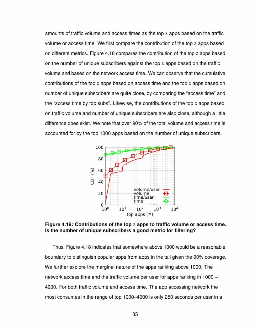
amounts of traffic volume and access times as the top X apps based on the traffic

volume or access time. We first compare the contribution of the top X apps based

on different metrics. Figure 4.18 compares the contribution of the top X apps based

on the number of unique subscribers against the top X apps based on the traffic

volume and based on the network access time. We can observe that the cumulative

contributions of the top X apps based on access time and the top X apps based on

number of unique subscribers are quite close, by comparing the “access time” and

the “access time by top subs”. Likewise, the contributions of the top X apps based

on traffic volume and number of unique subscribers are also close, although a little

difference does exist. We note that over 90% of the total volume and access time is

accounted for by the top 1000 apps based on the number of unique subscribers.

0

20

40

60

80

100

100 101 102 103 104

CD

F (%

)

top apps (#)

volume/uservolumetime/usertime

Figure 4.18: Contributions of the top X apps to traffic volume or access time.Is the number of unique subscribers a good metric for filtering?

Thus, Figure 4.18 indicates that somewhere above 1000 would be a reasonable

boundary to distinguish popular apps from apps in the tail given the 90% coverage.

We further explore the marginal nature of the apps ranking above 1000. The

network access time and the traffic volume per user for apps ranking in 1000 –

4000. For both traffic volume and access time. The app accessing network the

most consumes in the range of top 1000–4000 is only 250 seconds per user in a

85

week, and the app transferring the most data generates only 500 KB per user in a

week. Because of these small traffic volumes and short access times, we do not

consider these apps to be sufficiently active for our analysis.

genrebooks

business

education

entertainment

financegames

healthcare

lifestyle

medical

musicnavigation

newsphotography

productivity

reference

social net.

sportstravel

utilitiesweather

unknown

total351 418 643 1827

283 3108368 1298

205 1296450 1126

475 527 515 721 787 590 1079236 5865

popular7 8 13 95 13 199 23 71 4 34 23 89 17 23 26 58 33 29 49 16 170

Table 4.4: Genres of apps.

Our discussion suggests that a natural threshold would be the top 1000 apps

ranked by the number of unique subscribers. Table 4.4 shows the number of apps

in each genre, both for the top 1000 apps as well as all the 22K apps. In the

remainder, we will refer to these top 1000 apps as popular apps.

4.2.2.3 Spatial patterns: geographic usage distribution

Next, we investigate the diversity of smartphone apps being used by

subscribers in different geographic locations. Understanding the spatial usage

patterns of smartphone apps suggests ways to improve user experience and

performance from many aspects, such as content placement, context-aware

applications, and mobile advertisement system. Taking content placement as an

example, if content providers know that some of their apps are most used at certain

locations, they may choose to place content close to those locations so that users

experience better performance.

We first examine whether any apps are local apps, i.e., whether the majority of

an app’s traffic comes from a region. We perform the following analysis: for each

app, we divide its traffic by (U.S.) state of the user, and compute the top 1, 3 and 5

state(s) that contribute the most traffic volume or the longest network access times.

86

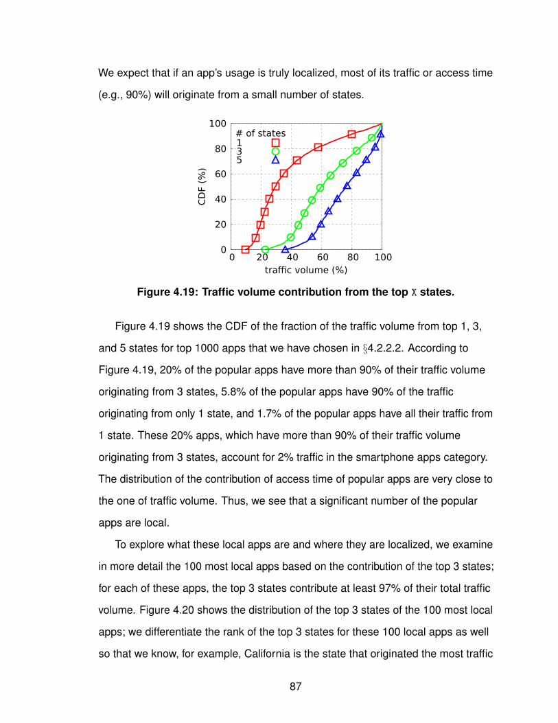
We expect that if an app’s usage is truly localized, most of its traffic or access time

(e.g., 90%) will originate from a small number of states.

0

20

40

60

80

100

0 20 40 60 80 100

CD

F (%

)

traffic volume (%)

# of states135

Figure 4.19: Traffic volume contribution from the top X states.

Figure 4.19 shows the CDF of the fraction of the traffic volume from top 1, 3,

and 5 states for top 1000 apps that we have chosen in §4.2.2.2. According to

Figure 4.19, 20% of the popular apps have more than 90% of their traffic volume

originating from 3 states, 5.8% of the popular apps have 90% of the traffic

originating from only 1 state, and 1.7% of the popular apps have all their traffic from

1 state. These 20% apps, which have more than 90% of their traffic volume

originating from 3 states, account for 2% traffic in the smartphone apps category.

The distribution of the contribution of access time of popular apps are very close to

the one of traffic volume. Thus, we see that a significant number of the popular

apps are local.

To explore what these local apps are and where they are localized, we examine

in more detail the 100 most local apps based on the contribution of the top 3 states;

for each of these apps, the top 3 states contribute at least 97% of their total traffic

volume. Figure 4.20 shows the distribution of the top 3 states of the 100 most local

apps; we differentiate the rank of the top 3 states for these 100 local apps as well

so that we know, for example, California is the state that originated the most traffic

87

012

4

8

16

# o

f apps

top 1top 2top 3

AL

AR

AZ

CA

CO

FLID

ILIN

KYLA

ME

MI

MN

MO MS N

CN

JN

VN

YO

HO

K OR

PATN

TXUT

VA VI

WA

WI W

V

Figure 4.20: Breakdown of the top X states of the local apps.

app description on GoogleWWLTV New Orleans News, Breaking News, Weather ...

KATC News Coverage at Acadiana-Lafayette, Louisiana ...KSLANews12 News, Weather and Sports at Shreveport, Louisiana ...KPLC 7 News Lake Charles, Louisiana – kplctv.com ...

WBRZ TV Channel 2 Baton Rouge, LA ...GoWAFB Local news, weather ... at Baton Rouge, LA ...

Table 4.5: Local apps from Louisiana.

for 19 apps, the state originated the second most traffic for 15 apps, and the state

originated the third most traffic for 12 apps. As expected, California, Texas, and

New York are the states with most local apps – these are the states with large

populations of smartphone users. However, there are many states with much

smaller populations such as Louisiana, Wyoming, and Kentucky that also have

some local apps; upon further analysis, this turn out to be because content from

some apps is tailored specifically for users from some regions, e.g., local TV

programs, news, radio, weather apps, etc. As an example for validation, we show

the local apps for Louisiana in Table 4.5; we see that the six apps that have most of

their traffic originating from Louisiana provide TV, news, radio and weather

specifically for Louisiana residents.

Next, we examine the spatial patterns of smartphone app usage nation-wide.

88

For this analysis, we remove the 100 apps identified as local in the previous

analysis (Section 4.2.2.3), and examine the nation-wide usage of the remaining

apps’ traffic. We term these remaining apps as national apps. Our analysis

explores whether certain genres are more popular (or have heavier usage) in some

areas than in other areas; in general, we do not expect users to prefer using apps

of a specific genre as a function of their geographic location, but our results show

that this does happen under certain conditions.

0 x % 25

10

20

50

100

0 x % 25

10

20

50

100

0 x % 25

10

20

50

100

0 x % 25

10

20

50

100

(a) aggregate. (b) social networking. (c) photography.

0 x % 25

10

20

50

100

0 x % 25

10

20

50

100

(d) education. (e) weather. (f) tornado activity.

Figure 4.21: Geographic usage distribution of app genres.

For ease of reference, we term geographic usage distribution of a quantity X

to be the the empirical probability distribution function (PDF) of X by U.S. state.

First, we compute the geographic usage distribution of the unique subscribers and

of the aggregate traffic volume generated by all national smartphone apps. We

then use them to compute the geographic usage of traffic volume normalized by the

number of unique subscribers in the state. Figure 4.21(a) is the PDF of the

geographic usage of the aggregate traffic of all national apps together, while

Figure 4.21(b) is the PDF of the geographic usage of the normalized traffic of all

national apps. As expected, California, Texas, New York, Florida, and Illinois are

the states that have the highest aggregate traffic from the national apps in

Figure 4.21(a). However, after normalizing the volume to account for the number of

89

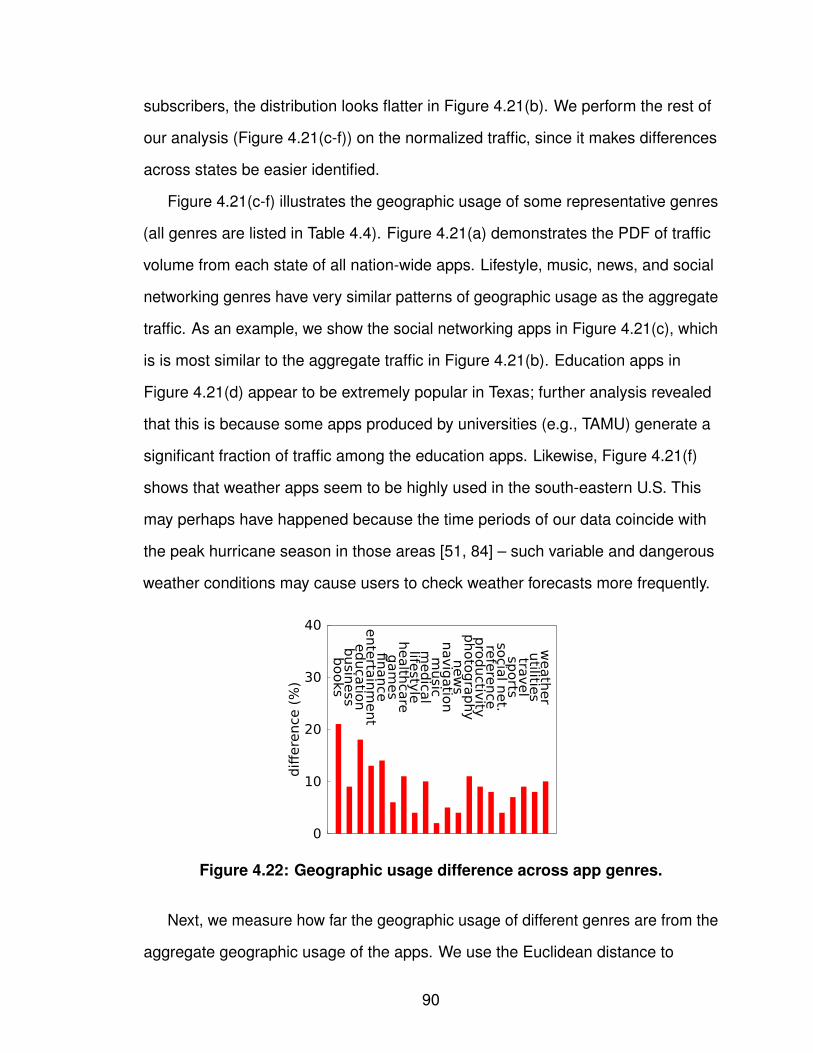
subscribers, the distribution looks flatter in Figure 4.21(b). We perform the rest of

our analysis (Figure 4.21(c-f)) on the normalized traffic, since it makes differences

across states be easier identified.

Figure 4.21(c-f) illustrates the geographic usage of some representative genres

(all genres are listed in Table 4.4). Figure 4.21(a) demonstrates the PDF of traffic

volume from each state of all nation-wide apps. Lifestyle, music, news, and social

networking genres have very similar patterns of geographic usage as the aggregate

traffic. As an example, we show the social networking apps in Figure 4.21(c), which

is is most similar to the aggregate traffic in Figure 4.21(b). Education apps in

Figure 4.21(d) appear to be extremely popular in Texas; further analysis revealed

that this is because some apps produced by universities (e.g., TAMU) generate a

significant fraction of traffic among the education apps. Likewise, Figure 4.21(f)

shows that weather apps seem to be highly used in the south-eastern U.S. This

may perhaps have happened because the time periods of our data coincide with

the peak hurricane season in those areas [51, 84] – such variable and dangerous

weather conditions may cause users to check weather forecasts more frequently.

0

10

20

30

40

diff

ere

nce

(%

)

books

busin

ess

educa

tion

ente

rtain

ment

finance

gam

es

health

care

lifesty

lem

edica

lm

usic

navig

atio

nnew

sphoto

gra

phy

pro

ductiv

ityre

fere

nce

socia

l net.

sports

travel

utilitie

sw

eath

er

Figure 4.22: Geographic usage difference across app genres.

Next, we measure how far the geographic usage of different genres are from the

aggregate geographic usage of the apps. We use the Euclidean distance to

90

measure the distance between a pair of geographic usage distributions. The

Euclidean distance between a pair of distributions [x1,x2,···,xn] and [y1,y2,···,yn] is

defined as√∑n

i=1(xi−yi)2. Figure 4.22 shows the distance between each genre’s

geographic usage distribution and the distribution of aggregate national apps. We

note that some genres, such as books and education, are disproportionately used

in some states, while others, such as social networking apps generate traffic more

proportionate to the total traffic generated by that state.

0 x % 25

10

20

50

100

0 x % 25

10

20

50

100

0 x % 25

10

20

50

100

0 x % 25

10

20

50

100

(a) aggregate news apps (b) @ATLANTA1 (c) @NEW YORK2

0 x % 25

10

20

50

100

0 x % 25

10

20

50

100

0 x % 25

10

20

50

100

(d) @WASH., D.C.2 (e) @CHICAGO2 (f) @VIRGINIA1

1: The names of these apps do not have any location indicated.2: The names of these apps include locations.

Figure 4.23: Geographic usage distribution in the same genre (news).

The distribution of geographic usage of different apps within the same genre

may also differ. Figure 4.23 shows the geographic usage distribution of a number of

smartphone apps in the news genre. For this analysis, we select the apps of a few

newspapers that are well-known across the entire U.S., and cover news relating to

any part of the world. The location of each news app in Figure 4.23 only reflects

where the newspaper headquarter is located. However, some of them have a

location indicated in their names (marked with 2 in Figure 4.23). Although all these

apps are used nation-wide, we note that apps whose names have a location

indicated seem to be disproportionally preferred at those respective locations. In

addition, the Washington D.C. news app seems to be highly preferred in

91

Washington state as well, thus suggesting users look for apps that appear to be

local to their region.

Our final analysis of the spatial patterns of app usage examines whether

individual users use some apps across larger geographic areas than others, e.g.,

whether Internet radio apps, which users may listen to during their commute, are

used across a larger area than books. Such an analysis can help understand what

kinds of apps need to be more robust to variations in network quality.

For this analysis, we define the travel area as a smartphone’s geographic

coverage per individual subscriber over short time, e.g., 6 hours. We use the

number of sectors to estimate the geographic coverage, since we do not have

access to the device’s exact locations. As noted in Section 4.2.1, the number of

sectors observed in our data set is an underestimate of the actual number of

sectors that the device passes through, but our results still give an idea of the

relative travel area of different apps. Specifically, for each app, we compute the

average number of unique sectors used by active subscribers in each 6 hour time

interval.

0

20

40

60

80

100

1 2 3 4 5 6

CD

F (%

)

# of sector

Figure 4.24: Travel area of apps.

Figure 4.24 shows the distribution of the average travel area of the top 1000

popular apps. It shows that 10% apps access the network from more than two

92

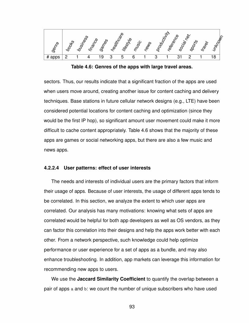
genr

e

book

sbu

sine

ssfin

ance

gam

eshe

alth

care

lifest

yle

mus

icne

ws

prod

uctiv

ityre

fere

nce

soci

alne

t.sp

orts

trave

lun

know

n

# apps 2 1 4 19 3 5 6 1 3 1 31 2 1 18

Table 4.6: Genres of the apps with large travel areas.

sectors. Thus, our results indicate that a significant fraction of the apps are used

when users move around, creating another issue for content caching and delivery

techniques. Base stations in future cellular network designs (e.g., LTE) have been

considered potential locations for content caching and optimization (since they

would be the first IP hop), so significant amount user movement could make it more

difficult to cache content appropriately. Table 4.6 shows that the majority of these

apps are games or social networking apps, but there are also a few music and

news apps.

4.2.2.4 User patterns: effect of user interests

The needs and interests of individual users are the primary factors that inform

their usage of apps. Because of user interests, the usage of different apps tends to

be correlated. In this section, we analyze the extent to which user apps are

correlated. Our analysis has many motivations: knowing what sets of apps are

correlated would be helpful for both app developers as well as OS vendors, as they

can factor this correlation into their designs and help the apps work better with each

other. From a network perspective, such knowledge could help optimize

performance or user experience for a set of apps as a bundle, and may also

enhance troubleshooting. In addition, app markets can leverage this information for

recommending new apps to users.

We use the Jaccard Similarity Coefficient to quantify the overlap between a

pair of apps a and b: we count the number of unique subscribers who have used

93

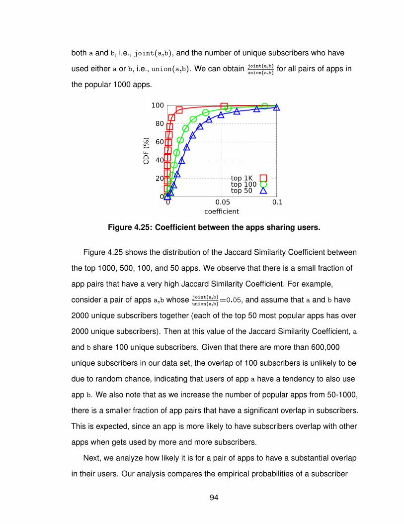
both a and b, i.e., joint(a,b), and the number of unique subscribers who have

used either a or b, i.e., union(a,b). We can obtain joint(a,b)

union(a,b)for all pairs of apps in

the popular 1000 apps.

0

20

40

60

80

100

0 0.05 0.1

CD

F (%

)

coefficient

top 1Ktop 100top 50

Figure 4.25: Coefficient between the apps sharing users.

Figure 4.25 shows the distribution of the Jaccard Similarity Coefficient between

the top 1000, 500, 100, and 50 apps. We observe that there is a small fraction of

app pairs that have a very high Jaccard Similarity Coefficient. For example,

consider a pair of apps a,b whose joint(a,b)

union(a,b)=0.05, and assume that a and b have

2000 unique subscribers together (each of the top 50 most popular apps has over

2000 unique subscribers). Then at this value of the Jaccard Similarity Coefficient, a

and b share 100 unique subscribers. Given that there are more than 600,000

unique subscribers in our data set, the overlap of 100 subscribers is unlikely to be

due to random chance, indicating that users of app a have a tendency to also use

app b. We also note that as we increase the number of popular apps from 50-1000,

there is a smaller fraction of app pairs that have a significant overlap in subscribers.

This is expected, since an app is more likely to have subscribers overlap with other

apps when gets used by more and more subscribers.

Next, we analyze how likely it is for a pair of apps to have a substantial overlap

in their users. Our analysis compares the empirical probabilities of a subscriber

94

0

20

40

60

80

100

1 10 100 1000C

DF

(%)

dependency

Figure 4.26: Dependency between popular apps..

using each app individually to the empirical probability of a subscriber using both

apps together. More precisely, let a,b denote apps, and Pr[a],Pr[b] denote the

empirical probabilities of a subscriber using app a,b respectively. Let Pr[ab] denote

the empirical probability of a subscriber using both apps a and b. If the subscribers

for each app are selected at random from the total population, then we would

expect that Pr[ab] to be somewhat close to the product Pr[a]Pr[b]. Figure 4.26

shows the distribution of the ratio Pr[ab]

Pr[a][b](we term this quantity the dependency

ratio for ease of reference). It shows that nearly 10% of the app pairs have a

dependency ratio that exceeds 10, and 254 pairs have a ratio exceeding 100.

Table 4.7 shows the frequency distribution of the genres of these 254 pairs (i.e.,

pairs with dependency-ratio exceeding 100). We can make two immediate

observations from this table. First, apps in the same genre are much more likely

have correlated usage. For example, 110 pairs of two games apps that have high

dependency-ratio, but games apps are part of a only 230 pairs in total. Second,

apps in similar genres are more likely to have high dependence-ratio, e.g.,

entertainment and games, news and entertainment, entertainment and social

networking, travel and navigation, weather and news, social networking and news,

95

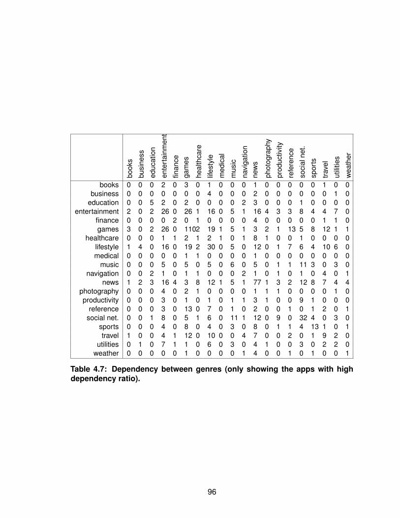
book

s

busi

ness

educ

atio

n

ente

rtai

nmen

t

finan

cega

mes

heal

thca

re

lifes

tyle

med

ical

mus

ic

navi

gatio

nne

ws

phot

ogra

phy

prod

uctiv

ity

refe

renc

e

soci

alne

t.

spor

ts

trave

l

utili

ties

wea

ther

books 0 0 0 2 0 3 0 1 0 0 0 1 0 0 0 0 0 1 0 0business 0 0 0 0 0 0 0 4 0 0 0 2 0 0 0 0 0 0 1 0

education 0 0 5 2 0 2 0 0 0 0 2 3 0 0 0 1 0 0 0 0entertainment 2 0 2 26 0 26 1 16 0 5 1 16 4 3 3 8 4 4 7 0

finance 0 0 0 0 2 0 1 0 0 0 0 4 0 0 0 0 0 1 1 0games 3 0 2 26 0 1102 19 1 5 1 3 2 1 13 5 8 12 1 1

healthcare 0 0 0 1 1 2 1 2 1 0 1 8 1 0 0 1 0 0 0 0lifestyle 1 4 0 16 0 19 2 30 0 5 0 12 0 1 7 6 4 10 6 0medical 0 0 0 0 0 1 1 0 0 0 0 1 0 0 0 0 0 0 0 0

music 0 0 0 5 0 5 0 5 0 6 0 5 0 1 1 11 3 0 3 0navigation 0 0 2 1 0 1 1 0 0 0 2 1 0 1 0 1 0 4 0 1

news 1 2 3 16 4 3 8 12 1 5 1 77 1 3 2 12 8 7 4 4photography 0 0 0 4 0 2 1 0 0 0 0 1 1 1 0 0 0 0 1 0productivity 0 0 0 3 0 1 0 1 0 1 1 3 1 0 0 9 1 0 0 0

reference 0 0 0 3 0 13 0 7 0 1 0 2 0 0 1 0 1 2 0 1social net. 0 0 1 8 0 5 1 6 0 11 1 12 0 9 0 32 4 0 3 0

sports 0 0 0 4 0 8 0 4 0 3 0 8 0 1 1 4 13 1 0 1travel 1 0 0 4 1 12 0 10 0 0 4 7 0 0 2 0 1 9 2 0

utilities 0 1 0 7 1 1 0 6 0 3 0 4 1 0 0 3 0 2 2 0weather 0 0 0 0 0 1 0 0 0 0 1 4 0 0 1 0 1 0 0 1

Table 4.7: Dependency between genres (only showing the apps with highdependency ratio).

96

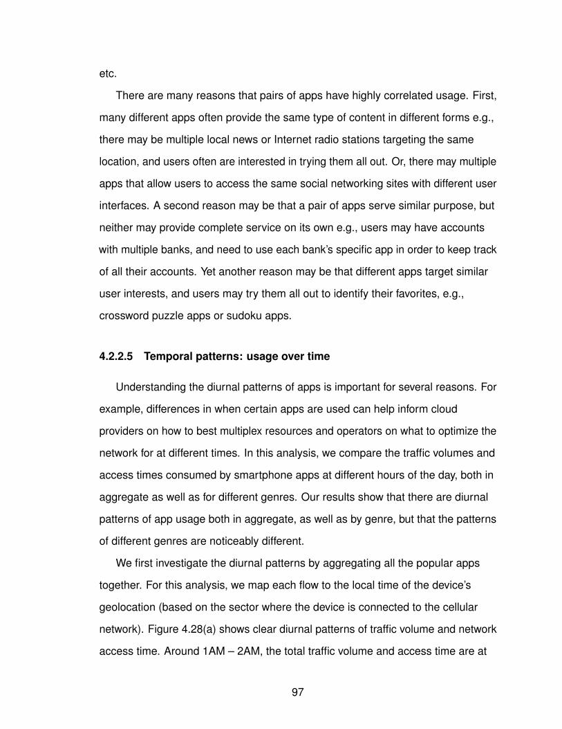
etc.

There are many reasons that pairs of apps have highly correlated usage. First,

many different apps often provide the same type of content in different forms e.g.,

there may be multiple local news or Internet radio stations targeting the same

location, and users often are interested in trying them all out. Or, there may multiple

apps that allow users to access the same social networking sites with different user

interfaces. A second reason may be that a pair of apps serve similar purpose, but

neither may provide complete service on its own e.g., users may have accounts

with multiple banks, and need to use each bank’s specific app in order to keep track

of all their accounts. Yet another reason may be that different apps target similar

user interests, and users may try them all out to identify their favorites, e.g.,

crossword puzzle apps or sudoku apps.

4.2.2.5 Temporal patterns: usage over time

Understanding the diurnal patterns of apps is important for several reasons. For

example, differences in when certain apps are used can help inform cloud

providers on how to best multiplex resources and operators on what to optimize the

network for at different times. In this analysis, we compare the traffic volumes and

access times consumed by smartphone apps at different hours of the day, both in

aggregate as well as for different genres. Our results show that there are diurnal

patterns of app usage both in aggregate, as well as by genre, but that the patterns

of different genres are noticeably different.

We first investigate the diurnal patterns by aggregating all the popular apps

together. For this analysis, we map each flow to the local time of the device’s

geolocation (based on the sector where the device is connected to the cellular

network). Figure 4.28(a) shows clear diurnal patterns of traffic volume and network

access time. Around 1AM – 2AM, the total traffic volume and access time are at

97

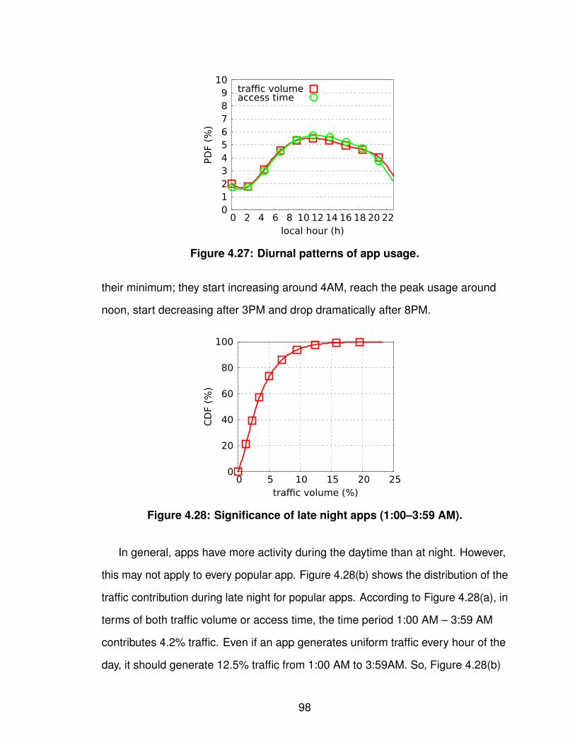
0 1 2 3 4 5 6 7 8 9

10

0 2 4 6 8 10 12 14 16 18 20 22PD

F (%

)

local hour (h)

traffic volumeaccess time

Figure 4.27: Diurnal patterns of app usage.

their minimum; they start increasing around 4AM, reach the peak usage around

noon, start decreasing after 3PM and drop dramatically after 8PM.

0

20

40

60

80

100

0 5 10 15 20 25

CD

F (%

)

traffic volume (%)

Figure 4.28: Significance of late night apps (1:00–3:59 AM).

In general, apps have more activity during the daytime than at night. However,

this may not apply to every popular app. Figure 4.28(b) shows the distribution of the

traffic contribution during late night for popular apps. According to Figure 4.28(a), in

terms of both traffic volume or access time, the time period 1:00 AM – 3:59 AM

contributes 4.2% traffic. Even if an app generates uniform traffic every hour of the

day, it should generate 12.5% traffic from 1:00 AM to 3:59AM. So, Figure 4.28(b)

98

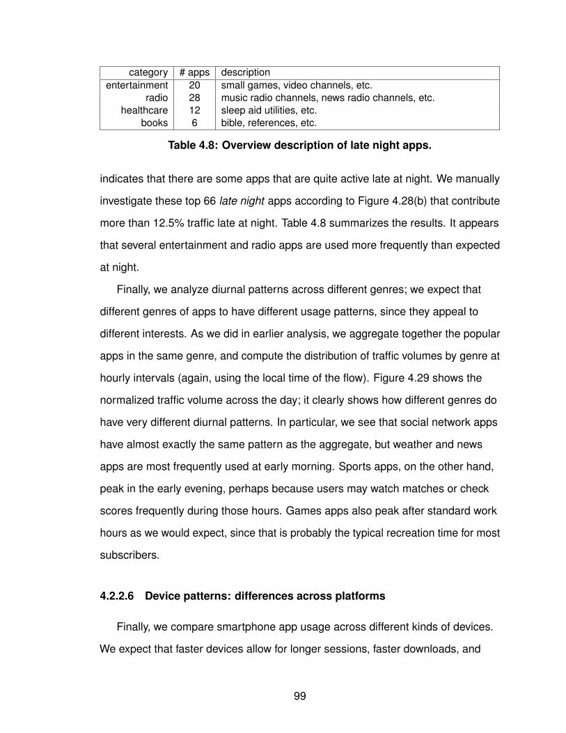
category # apps descriptionentertainment 20 small games, video channels, etc.

radio 28 music radio channels, news radio channels, etc.healthcare 12 sleep aid utilities, etc.

books 6 bible, references, etc.

Table 4.8: Overview description of late night apps.

indicates that there are some apps that are quite active late at night. We manually

investigate these top 66 late night apps according to Figure 4.28(b) that contribute

more than 12.5% traffic late at night. Table 4.8 summarizes the results. It appears

that several entertainment and radio apps are used more frequently than expected

at night.

Finally, we analyze diurnal patterns across different genres; we expect that

different genres of apps to have different usage patterns, since they appeal to

different interests. As we did in earlier analysis, we aggregate together the popular

apps in the same genre, and compute the distribution of traffic volumes by genre at

hourly intervals (again, using the local time of the flow). Figure 4.29 shows the

normalized traffic volume across the day; it clearly shows how different genres do

have very different diurnal patterns. In particular, we see that social network apps

have almost exactly the same pattern as the aggregate, but weather and news

apps are most frequently used at early morning. Sports apps, on the other hand,

peak in the early evening, perhaps because users may watch matches or check

scores frequently during those hours. Games apps also peak after standard work

hours as we would expect, since that is probably the typical recreation time for most

subscribers.

4.2.2.6 Device patterns: differences across platforms

Finally, we compare smartphone app usage across different kinds of devices.

We expect that faster devices allow for longer sessions, faster downloads, and

99

0

2

4

6

8

10

0 5 10 15 20PD

F (%

)

local hour (h)

genreaggr.socialweather

sportsgamesnews

Figure 4.29: Diurnal patterns across app genres.

more interactivity, thus enhancing the end-user experience. Power users, who use

their devices more, may also gravitate to newer and faster devices. We focus on

three different devices from the same device family, as we expect device operating

system to also affect overall usage patterns. We compare three devices in the same

device family but of different generations – we term these iPhone 3, iPhone 3GS,

and iPhone 4G in Figure 4.30. iPhone 3 is a HSDPA category 6 device (capable of

3.6Mbps downlink rate), and iPhone 3GS and iPhone 4G are in HSDPA category 8

(capable of 7.2Mbps downlink) [112]. iPhone 3 and iPhone 3GS are not HSUPA

enabled while iPhone 4G is HSUPA category 6 (capable of 5.76Mbps uplink) [113].

For this analysis, we use slightly different metrics than we have used in the

following, since our goal is to measure how long a user interacts with the device,

and compare these measurements across different devices. For this, we define

individual access time and the individual traffic volume to be the network

access time and the traffic volume per flow respectively. We use these metrics for

our analysis as we expect the individual access time to provide a measure of how

long a user spends with an app, and the individual traffic volume to reflect how

much data is transferred each time a user interacts with an app. Obviously not

every flow will be larger or longer, but we expect that a device that allows for better

100

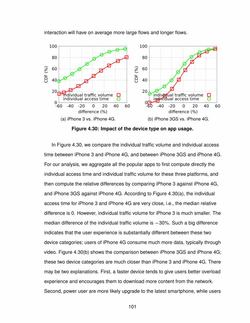
interaction will have on average more large flows and longer flows.

0

20

40

60

80

100

-60 -40 -20 0 20 40 60

CD

F (%

)

difference (%)

individual traffic volumeindividual access time

0

20

40

60

80

100

-60 -40 -20 0 20 40 60

CD

F (%

)

difference (%)

individual traffic volumeindividual access time

(a) iPhone 3 vs. iPhone 4G. (b) iPhone 3GS vs. iPhone 4G.

Figure 4.30: Impact of the device type on app usage.

In Figure 4.30, we compare the individual traffic volume and individual access

time between iPhone 3 and iPhone 4G, and between iPhone 3GS and iPhone 4G.

For our analysis, we aggregate all the popular apps to first compute directly the

individual access time and individual traffic volume for these three platforms, and

then compute the relative differences by comparing iPhone 3 against iPhone 4G,

and iPhone 3GS against iPhone 4G. According to Figure 4.30(a), the individual

access time for iPhone 3 and iPhone 4G are very close, i.e., the median relative

difference is 0. However, individual traffic volume for iPhone 3 is much smaller. The

median difference of the individual traffic volume is −30%. Such a big difference

indicates that the user experience is substantially different between these two

device categories; users of iPhone 4G consume much more data, typically through

video. Figure 4.30(b) shows the comparison between iPhone 3GS and iPhone 4G;

these two device categories are much closer than iPhone 3 and iPhone 4G. There

may be two explanations. First, a faster device tends to give users better overload

experience and encourages them to download more content from the network.

Second, power user are more likely upgrade to the latest smartphone, while users

101

not as active may be more likely to keep using their older devices.

4.2.3 Implications of Application Usage Patterns

In previous sections, we investigate the usage patterns of smartphone apps

from spatial, temporal, user, and device perspectives. We believe that our previous

observations have important implications for the smartphone community. In this

section, we discuss these implications following our previous observations.

4.2.3.1 Content providers

In the analysis of spatial patterns of smartphone usages, we observe a

considerable number of local apps (20%) which contribute 2% of the traffic volume

in the smartphone apps category. The content provided by these local apps are

very deterministic, e.g., news apps, regional radio online services, weather forecast

apps, etc. Given both the customers and locations for these apps are very closely

clustered, content placement and delivery can be further optimized accordingly. It is

therefore beneficial to place the content close to GGSNs in the cellular

networks [120] for cellular users and place the content close to the geographic

location of WiFi users. Besides local apps, for national apps, the distribution of

geographic coverage is still very dependent on the genre (e.g., weather apps are

highly used in the south-eastern U.S.), even the app’s name (e.g., the news app

headquartered in CHICAGO), etc. Therefore, content placement according to the

geographic coverage is advisable for both national and local apps.

4.2.3.2 Context-aware applications

Despite very diverse usage usage patterns across different smartphone apps,

they still have some common traits. According to our observations, first, apps in the

102

same genre share similar geographic coverage. Second, some apps share a large

set of common users due to the similarity of content and interests, e.g., social

networking apps strongly correlate with entertainment apps, music apps, news

apps, etc. Third, some apps share similar diurnal patterns due to content

characteristics, e.g., the peak hours of news apps and weather apps come at early

morning.

Context-aware applications can take advantage of the existing

similarity/correlation across smartphone apps. Take smartphone apps

recommendation systems as an example. Unlike normal PC users, smartphone

users depend on apps far more than browsers. Since a smartphone apps

recommendation system is the first approach for users to explore various

smartphone apps that meet their interests, these systems can be quite important.

As the bridge between app marketplace and app customers, if apps

recommendation systems can learn user interests and dependency across apps,

they can identify more appropriate apps for users, e.g., suggesting gaming fans

more entertainment apps and social networking apps.

Another example of context-aware application is advertisement systems, which

upon learning user’s interests in apps, can deliver more relevant ads to users.

Camera or camcorder advertisements may target more smartphone users that use

more entertainment and game apps because photography apps are more

correlated with entertainment and game apps.

4.2.3.3 Network providers

Besides content providers, cellular network providers also play an important role

in content delivery and customization. By understanding the access patterns of

smartphone apps, network providers can benefit in allocating radio resource,

setting caching policy, compression policy, etc.

103

If a large number of smartphone apps are targeted, their traffic volume and

access time roughly have linear correlation with their number of unique subscribers.

Accordingly, cellular providers can estimate and allocate radio resources.

We observe that the several few top apps contribute the majority traffic. For

example, the app with the largest traffic volume is accountable for 50% of the total

traffic volume of the smartphone apps category, and the app with the longest

network access time takes 86% of the total network access time of the smartphone

apps category. Understanding the usage patterns of these apps, network providers

may do certain optimizations case by case.

The temporal patterns of smartphone apps help network providers allocate

radio resource. For example, the access time per IP flow helps network providers

decide the timers in state promotion [90].

We observe that some smartphone apps have large usage radius, i.e., users of

certain social networking apps and games apps are more likely to move around

across several base stations. In future, LTE networks will push the first IP hop

forward to base stations, which increases the flexibility of content placement and

optimization. However, if users frequently move around, the corresponding mobility

may increase the complexity to decide where to cache content and what content to

cache.

4.2.3.4 OS vendors and apps designers

Since smartphones have limited resources, the OS is accountable for resource

management, e.g., the push notification on iOS, Android, Windows Phone.

Understanding the access patterns of apps on device, OS can add some flexibility

to apps and optimize the resource usage. For example, if a user frequently resorts

to a certain sleep aid app, then OS may allocate less resource to those apps that

may interrupt the user’s sleep.

104

Certain genres of smartphone apps have different characteristics, which may be

taken advantage by apps designers. We observe that news and weather apps have

distinctive diurnal patterns. Since the content of these apps usually are very time

dependent and content fetching time is very predictable, apps designer can

implement some prefetching mechanism to reduce the latency perceived by users.

Similarly, the content of social networking apps can be prefetched before dinner

time.

4.3 Summary of Identifying Application Usage

In §4.1, we developed FLOWR, a system determining the app identities of

network flows in mobile networks in real time with minimal supervised learning

through three creative techniques: KV tokenization, a* service based training, and

flow regression. The entropy inside signatures produced by KV tokenization

corresponds to the amount of information sufficient to uniquely differentiate the

apps or to narrow down to a few (e.g., 2–5) candidate apps. leveraging a* services

allows FLOWR to minimize supervised learning for identifying both free and paid

apps. Without consuming exhaustive training effort, flow regression can determine

the app identities for the flow signatures produced by KV tokenization through

monitoring the co-occurrence events between flow signatures. FLOWR’s

throughput is up to 5Gbps an off-the-shelf machine.

Although we do not have the ground truth of the app identities of network flows,

we successfully estimated the upper-bound false positive of FLOWR in evaluation.

Evaluated using the apps with doubleclick, FLOWR can uniquely identify 26–30%

of flows and narrow down another 60–65% to 2–5 candidate apps, with <1% false

positive. In contrast, only 3% of flows can be identified without FLOWR. We believe

that FLOWR enables mobile network operators to extract valuable insight from

105

mobile network traffic.

Under the support of FLOWR, in §4.2, we comprehensively investigated the

diverse usage patterns of smartphone apps via network measurements from a

national level tier-1 cellular network provider in the U.S. This is the first attempt in

addressing the lack of how, where and when smartphone apps are used at the

scale of the entire U.S.

We observed that a considerable fraction of popular apps (20%) are local

because their content are expected to serve local users such as news and radio

apps. This suggests that there is significant possibility for content optimization in

LTE and WiFi access networks where the flexibility of placing content is high.

We also found out that there are similarities across apps in terms of geographic

coverage, diurnal usage patterns, etc. Certain apps have a high likelihood of

co-occurrence – that is, (i) when a user uses one app, he is also likely to use

another one; or (ii) users use alternatives for the same type of interests, e.g.,

multiple news apps, bank apps. These observations suggest that some apps

should be treated as a “bundle” when trying to optimize for their user experience.

There may be opportunities for integrating these apps together.

Diurnal patterns of smartphone apps can be remarkably different. For instance,

news apps are much more frequently used in the early morning while sports apps

are more frequently used in the evening. These findings suggest that content

providers (e.g., hosted on cloud) can leverage distinct usage patterns in classes of

apps to maximize the utilization of their resources.

Many social networking and games apps are more frequently used when users

are moving around. Mobility affects connectivity and performance, so bandwidth

sensitive content that are mobile may need to consider techniques to compensate

for bandwidth variability.

We believe that our findings on the diverse usage patterns of smartphone apps

106

in spatial, temporal, user, device dimensions will motivate future work in the mobile

community.

107

CHAPTER V

APPLICATION PERFORMANCE OPTIMIZATION

One lesson we learned from YellowPage in §III is that latency sensitive

application can be very challenging in cellular networks. In §IV, we also had many

observations and findings showing the distinctive behaviors of mobile applications.

In this section, we adapt application behaviors to cellular networks starting with

real-time, interactive mobile applications in particular.

One of the biggest trends today is the accelerated adoption of mobile devices,

whose power is approaching that of PCs. The rapid adoption of mobile devices is

resulting in the migration of real-time communication (RTC) applications from PCs

to mobile devices. RTC applications include (i) online streaming including

VoIP/video conferencing applications such as Skype, FaceTime, and Google+

Hangout; (ii) interactive multi-player gaming applications such as Draw Something,

Modern Combat 3, and Call of Duty; and (iii) application sharing, desktop sharing,

and virtual desktop interface (VDI). RTCWeb (Real-Time Collaboration over Web)

is an ongoing effort to enable RTC applications to run inside browsers without

plug-ins [15].

Running RTC applications in mobile networks presents a major challenge since

they require accurate short-term estimates of network metrics, e.g., loss rate,

one-way delay (OWD), and throughput, whereas cellular network performance

108

varies rapidly and widely [62, 107, 40]. Although performance adaptation solutions

have been proposed [126, 96, 81, 9, 4, 1, 13], they are ineffective for RTC

applications, where the end-to-end delay between content generation and content

consumption is on the order of network latencies. Thus, techniques such as packet

retransmissions or use of large client-side de-jitter buffers to absorb jitter variations,

effective for web browsing and video playback, will lead to intolerable delays in RTC

applications.

Instead, RTC applications need to rely on an appropriate amount of forward

error correction (FEC) to correct for packet loss and a small yet appropriately sized

de-jitter buffer to absorb varying packet delay. Over-protection using FEC wastes

precious bandwidth, while under-protection negates the effectiveness of FEC, as

any unrecoverable packet loss will lead to severe quality degradation in voice calling

and video conferencing. Similarly, if the de-jitter buffer size is too large, it adds to

the application latency. If it is too small, late arriving packets will be considered lost,

which also leads to significant quality degradation. Accurate throughput prediction

is also necessary to allow bandwidth intensive applications to maximize throughput

without incurring additional queuing delay. Thus, short-term, fine-grained network

performance prediction on mobile networks is of great importance.

Existing work on mobile network performance measurement and prediction is of

limited importance to RTC applications for several reasons: (i) the measurement or

prediction approaches are carried out on coarse-grained time granularity or offline,

which are not suitable for RTC applications; (ii) the performance adaptation

techniques react to performance only after observing any degradation, when the

user experience has already been negatively impacted; and (iii) the existing

techniques used by RTC applications for network prediction are usually naıve such

as using the previous performance or the average of previous performance, which

work well only for relatively stable wired networks.

109

We propose a system interface named PROTEUS designed to accurately

predict fine-grained detailed network performance in real time over short time

scales allowing applications to adjust their behavior to best optimize their

performance. The fine-grained and accurate performance prediction in real time is

necessary yet challenging from three aspects: (i) cellular network performance may

be affected by a multitude of unobservable factors, such as radio resource

scheduling, other users sharing the spectrum, and signal-to-noise ratio; (ii) network

performance predictions on fine-grained time granularity is inherently noisier than

coarse-grained predictions; and (iii) active probing is prohibitive for RTC

applications due to significant resource consumption, while passive monitoring has

limited visibility only based on traffic generated by applications.

To address the above challenges, PROTEUS utilizes a machine learning

framework based on regression trees to learn the trend of network performance

over short, fine-grained time windows using previous available observations. Even

though past work has provided the evidence that cellular networks have a potential

to have predictability for network performance, to our best knowledge, PROTEUS is

the first system to forecast short-term network performance in real time, and the

first to demonstrate the benefit of proactively adjusting the operating parameters in

real time for use by mobile RTC applications. The key contributions are as follows.

• We characterize short-term network behavior and investigate the performance

predictability in three major cellular networks of AT&T, T-Mobile, and Sprint based

on more than 400 hours of traces across 3 locations. We identify the existence of

strong predictability over short time scales for these cellular networks.

• We discover that loss rate, one-way delay, and throughput in cellular networks can

be accurately predicted in real time from past measurements by feeding past

network performance metrics into regression trees. For a following 0.5s time

window, we can predict loss occurrence with 98% accuracy, late packet arrival with

110

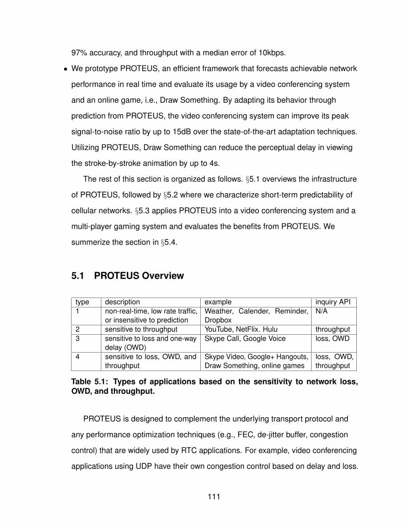
97% accuracy, and throughput with a median error of 10kbps.

• We prototype PROTEUS, an efficient framework that forecasts achievable network

performance in real time and evaluate its usage by a video conferencing system

and an online game, i.e., Draw Something. By adapting its behavior through

prediction from PROTEUS, the video conferencing system can improve its peak

signal-to-noise ratio by up to 15dB over the state-of-the-art adaptation techniques.

Utilizing PROTEUS, Draw Something can reduce the perceptual delay in viewing

the stroke-by-stroke animation by up to 4s.

The rest of this section is organized as follows. §5.1 overviews the infrastructure

of PROTEUS, followed by §5.2 where we characterize short-term predictability of

cellular networks. §5.3 applies PROTEUS into a video conferencing system and a

multi-player gaming system and evaluates the benefits from PROTEUS. We

summerize the section in §5.4.

5.1 PROTEUS Overview

type description example inquiry API1 non-real-time, low rate traffic,

or insensitive to predictionWeather, Calender, Reminder,Dropbox

N/A

2 sensitive to throughput YouTube, NetFlix. Hulu throughput3 sensitive to loss and one-way

delay (OWD)Skype Call, Google Voice loss, OWD

4 sensitive to loss, OWD, andthroughput

Skype Video, Google+ Hangouts,Draw Something, online games

loss, OWD,throughput

Table 5.1: Types of applications based on the sensitivity to network loss,OWD, and throughput.

PROTEUS is designed to complement the underlying transport protocol and

any performance optimization techniques (e.g., FEC, de-jitter buffer, congestion

control) that are widely used by RTC applications. For example, video conferencing

applications using UDP have their own congestion control based on delay and loss.

111

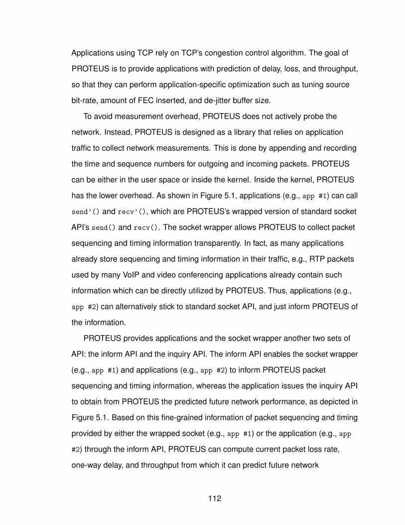
Applications using TCP rely on TCP’s congestion control algorithm. The goal of

PROTEUS is to provide applications with prediction of delay, loss, and throughput,

so that they can perform application-specific optimization such as tuning source

bit-rate, amount of FEC inserted, and de-jitter buffer size.

To avoid measurement overhead, PROTEUS does not actively probe the

network. Instead, PROTEUS is designed as a library that relies on application

traffic to collect network measurements. This is done by appending and recording

the time and sequence numbers for outgoing and incoming packets. PROTEUS

can be either in the user space or inside the kernel. Inside the kernel, PROTEUS

has the lower overhead. As shown in Figure 5.1, applications (e.g., app #1) can call

send’() and recv’(), which are PROTEUS’s wrapped version of standard socket

API’s send() and recv(). The socket wrapper allows PROTEUS to collect packet

sequencing and timing information transparently. In fact, as many applications

already store sequencing and timing information in their traffic, e.g., RTP packets

used by many VoIP and video conferencing applications already contain such

information which can be directly utilized by PROTEUS. Thus, applications (e.g.,

app #2) can alternatively stick to standard socket API, and just inform PROTEUS of

the information.

PROTEUS provides applications and the socket wrapper another two sets of

API: the inform API and the inquiry API. The inform API enables the socket wrapper

(e.g., app #1) and applications (e.g., app #2) to inform PROTEUS packet

sequencing and timing information, whereas the application issues the inquiry API

to obtain from PROTEUS the predicted future network performance, as depicted in

Figure 5.1. Based on this fine-grained information of packet sequencing and timing

provided by either the wrapped socket (e.g., app #1) or the application (e.g., app

#2) through the inform API, PROTEUS can compute current packet loss rate,

one-way delay, and throughput from which it can predict future network

112

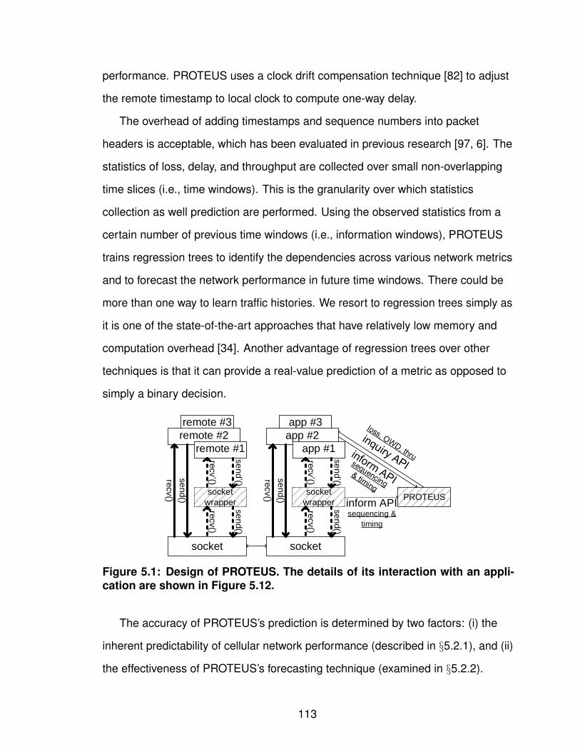
performance. PROTEUS uses a clock drift compensation technique [82] to adjust

the remote timestamp to local clock to compute one-way delay.

The overhead of adding timestamps and sequence numbers into packet

headers is acceptable, which has been evaluated in previous research [97, 6]. The

statistics of loss, delay, and throughput are collected over small non-overlapping

time slices (i.e., time windows). This is the granularity over which statistics

collection as well prediction are performed. Using the observed statistics from a

certain number of previous time windows (i.e., information windows), PROTEUS

trains regression trees to identify the dependencies across various network metrics

and to forecast the network performance in future time windows. There could be

more than one way to learn traffic histories. We resort to regression trees simply as

it is one of the state-of-the-art approaches that have relatively low memory and

computation overhead [34]. Another advantage of regression trees over other

techniques is that it can provide a real-value prediction of a metric as opposed to

simply a binary decision.

socket

socket

wrapper

remote #3

socket

PROTEUS

app #3

app #2

app #1

remote #2

remote #1

socket

wrapper

sequencing &

timing

se

nd()

recv()

se

nd

()

recv

()

inform APIse

nd()

recv()

se

nd

()

recv

() recv()

se

nd()

recv()

se

nd()

Figure 5.1: Design of PROTEUS. The details of its interaction with an appli-cation are shown in Figure 5.12.

The accuracy of PROTEUS’s prediction is determined by two factors: (i) the

inherent predictability of cellular network performance (described in §5.2.1), and (ii)

the effectiveness of PROTEUS’s forecasting technique (examined in §5.2.2).

113

The information exchanged through the inform API between applications and

PROTEUS is common across applications. However, the information from the

inquiry API and the resulting action taken by each application may be very different.

In Table 5.1, we classify applications into four broad categories depending on how

sensitive their performance is to the three network parameters of packet loss,

one-way delay, and throughput and show how PROTEUS can be useful.

• Type 1 consists of the applications whose performance is not sensitive to loss,

one-way delay, or throughput. These are either non-real-time, low bandwidth

applications insensitive to network performance, or applications that do not benefit

much from prediction. For example, the performance of Dropbox and other file

transfer applications depend on throughput, but there is little adaptation in response

to throughput prediction.

• Type 2 consists of the applications whose performance is not sensitive to packet

loss or one-way delay but is sensitive to throughput. These are non-real-time, high

bandwidth applications such as video on demand (VOD). Such applications can

take steps to improve performance such as adapting the rate of the stream served

to the client [9] in response to throughput prediction.

• Type 3 consists of the applications whose performance is sensitive to packet loss

and/or one-way delay but is not sensitive to throughput. These are real-time,

interactive, low bandwidth applications such as VoIP. For these applications,

throughput prediction is of little benefit. However, loss prediction can be used to

control the amount of FEC used [32]. The one-way delay prediction can be used to

adjust the de-jitter buffer size for adaptive playout to reduce both late arrival

induced loss [32] and de-jitter buffer induced delay.

• Type 4 consists of the applications whose performance is sensitive to packet loss,

one-way delay, and throughput prediction. These are real-time, interactive, high

bandwidth applications such as video conferencing, and real-time software

114

applications such as desktop sharing. PROTEUS can be used for throughput

prediction to control the source rate produced by the source. The amount of FEC

packets to insert can be inferred from loss prediction, and the de-jitter buffer size

can be determined from one-way delay prediction.

Type 3 and Type 4 are real-time, interactive applications which can benefit from

PROTEUS. Type 2 consists of non-real-time applications which can still benefit

from throughput prediction.Although a coarse-grained predictor may work for

Type 2 applications, it may not work for RTC applications. A coarse-grained

predictor can be built upon a fine-grained predictor such as PROTEUS by simply

averaging the prediction over multiple time windows.

Types 2, 3, and 4 applications are becoming increasingly popular and contribute

to a majority of the traffic on the Internet [122]. This trend is readily visible by the

increasing popularity of Skype, FaceTime, and Google+ Hangouts. The increasing

push towards the cloud also makes other RTC applications such as online gaming

and VDI scenarios even more important. The broad industry interest in the

performance of such applications is apparent from recent efforts around

RTCWeb [15] and DASH (Dynamic Adaptive Streaming over HTTP) [10].

5.2 Prediction Using PROTEUS

In this section, we investigate the predictability of cellular network performance

and evaluate the accuracy of PROTEUS’s forecasting.

5.2.1 Characterizing Cellular Networks

Although the understanding of the channel estimation scheme on mobile

devices and the radio resource scheduling algorithm at base stations, along with

the performance predictability observations from previous studies [75] give us

115

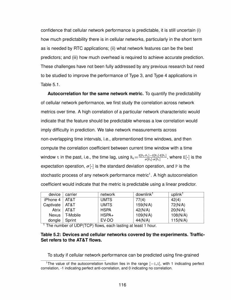
confidence that cellular network performance is predictable, it is still uncertain (i)

how much predictability there is in cellular networks, particularly in the short term

as is needed by RTC applications; (ii) what network features can be the best

predictors; and (iii) how much overhead is required to achieve accurate prediction.

These challenges have not been fully addressed by any previous research but need

to be studied to improve the performance of Type 3, and Type 4 applications in

Table 5.1.

Autocorrelation for the same network metric. To quantify the predictability

of cellular network performance, we first study the correlation across network

metrics over time. A high correlation of a particular network characteristic would

indicate that the feature should be predictable whereas a low correlation would

imply difficulty in prediction. We take network measurements across

non-overlapping time intervals, i.e., aforementioned time windows, and then

compute the correlation coefficient between current time window with a time

window t in the past, i.e., the time lag, using Rt=E[P0·Pt]−E[P0]·E[Pt]

σ[P0]·σ[Pt], where E[·] is the

expectation operation, σ[·] is the standard deviation operation, and P is the

stochastic process of any network performance metric1. A high autocorrelation

coefficient would indicate that the metric is predictable using a linear predictor.

device carrier network downlink1 uplink1

iPhone 4 AT&T UMTS 77(4) 42(4)Captivate AT&T UMTS 159(N/A) 72(N/A)

Atrix AT&T HSPA 42(N/A) 20(N/A)Nexus T-Mobile HSPA+ 109(N/A) 108(N/A)dongle Sprint EV-DO 44(N/A) 115(N/A)

1 The number of UDP(TCP) flows, each lasting at least 1 hour.

Table 5.2: Devices and cellular networks covered by the experiments. Traffic-Set refers to the AT&T flows.

To study if cellular network performance can be predicted using fine-grained1The value of the autocorrelation function lies in the range [−1,1], with 1 indicating perfect

correlation, -1 indicating perfect anti-correlation, and 0 indicating no correlation.

116

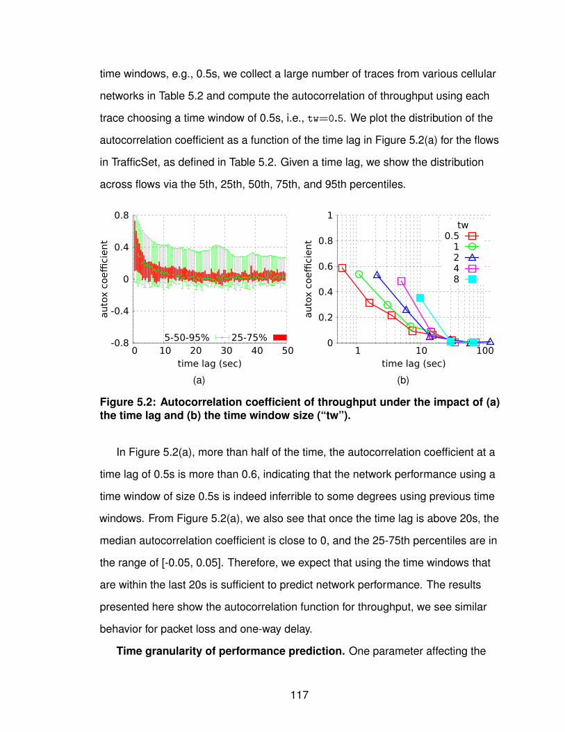
time windows, e.g., 0.5s, we collect a large number of traces from various cellular

networks in Table 5.2 and compute the autocorrelation of throughput using each

trace choosing a time window of 0.5s, i.e., tw=0.5. We plot the distribution of the

autocorrelation coefficient as a function of the time lag in Figure 5.2(a) for the flows

in TrafficSet, as defined in Table 5.2. Given a time lag, we show the distribution

across flows via the 5th, 25th, 50th, 75th, and 95th percentiles.

-0.8

-0.4

0

0.4

0.8

0 10 20 30 40 50

auto

x c

oeffi

cient

time lag (sec)

5-50-95% 25-75% 0

0.2

0.4

0.6

0.8

1

1 10 100

auto

x c

oeffi

cient

time lag (sec)

tw0.5

1248

(a) (b)

Figure 5.2: Autocorrelation coefficient of throughput under the impact of (a)the time lag and (b) the time window size (“tw”).

In Figure 5.2(a), more than half of the time, the autocorrelation coefficient at a

time lag of 0.5s is more than 0.6, indicating that the network performance using a

time window of size 0.5s is indeed inferrible to some degrees using previous time

windows. From Figure 5.2(a), we also see that once the time lag is above 20s, the

median autocorrelation coefficient is close to 0, and the 25-75th percentiles are in

the range of [-0.05, 0.05]. Therefore, we expect that using the time windows that

are within the last 20s is sufficient to predict network performance. The results

presented here show the autocorrelation function for throughput, we see similar

behavior for packet loss and one-way delay.

Time granularity of performance prediction. One parameter affecting the

117

autocorrelation coefficient is the size of the time window. If the time window chosen

is small, the measurements may show high variability which may be more difficult to

predict. However, if the time window chosen is large, the measurements may be

affected by long term drift and cannot accurately reflect the fine-grained

performance needed by RTC applications. To appropriately select a time window

size, we study the effect of time window size on the autocorrelation function.

Figure 5.2(b) shows the median autocorrelation coefficient for UDP throughput as a

function of the time lag for various time window sizes, i.e., 0.5s, 1s, 2s, 4s, and 8s.

We expect that as the time window size increases, the autocorrelation coefficient for

a given time lag should also increase until it eventually converges. In Figure 5.2(b),

“tw=4” being close to “tw=8” indicates that using time windows greater than 4s

provides no additional benefit. However, we see that even with a window size of “tw

= 0.5”, the average autocorrelation coefficient at a time lag of 0.5s is above 0.6 and

is similar to that using a larger time window. Thus, we conclude that we can indeed

predict network performance from previous time windows using fine-grained

windows, e.g., 0.5s, as needed by RTC applications.

In total, we have three observations from studying the autocorrelation function:

(i) the current network performance is correlated with the network performance in

the previous time windows; (ii) to predict the network performance, the time window

size can be as short as 0.5s as required by RTC applications; and (iii) using

information within the previous 20s should be sufficient for accurate prediction.

Cross correlation between network metrics. These three observations

answer the question of whether network performance is predictable on cellular

networks using previous values of a particular metric to predict future values of the

same metric. However, the question of whether previous values of other metrics

can also be used to improve prediction remains. To study this, we study the

cross-correlation coefficient across various different network metrics.

118

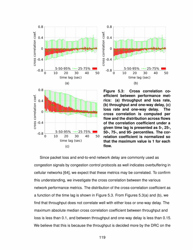
-0.8

-0.4

0

0.4

0.8

0 10 20 30 40 50

cross

corr

ela

tion c

oef.

time lag (sec)

5-50-95% 25-75% -0.8

-0.4

0

0.4

0.8

0 10 20 30 40 50

cross

corr

ela

tion c

oef.

time lag (sec)

5-50-95% 25-75%

(a) (b)

-0.8

-0.4

0

0.4

0.8

0 10 20 30 40 50

cross

corr

ela

tion c

oef.

time lag (sec)

5-50-95% 25-75%

(c)

Figure 5.3: Cross correlation co-efficient between performance met-rics: (a) throughput and loss rate,(b) throughput and one-way delay, (c)loss rate and one-way delay. Thecross correlation is computed perflow and the distribution across flowsof the correlation coefficient under agiven time lag is presented as 5-, 25-,50-, 75-, and 95- percentiles. The cor-relation coefficient is normalized sothat the maximum value is 1 for eachflow.

Since packet loss and end-to-end network delay are commonly used as

congestion signals by congestion control protocols as well indicates overbuffering in

cellular networks [64], we expect that these metrics may be correlated. To confirm

this understanding, we investigate the cross correlation between the various

network performance metrics. The distribution of the cross-correlation coefficient as

a function of the time lag is shown in Figure 5.3. From Figures 5.3(a) and (b), we

find that throughput does not correlate well with either loss or one-way delay. The

maximum absolute median cross correlation coefficient between throughput and

loss is less than 0.1, and between throughput and one-way delay is less than 0.15.

We believe that this is because the throughput is decided more by the DRC on the

119

link between the device and the base station, while the loss and one-way delay are

affected more by the congestion along the path. However, from Figure 5.3(c), we

see that loss rate and one-way delay do have a strong correlation with each other.

When the time lag is close to 0, the median cross correlation coefficient is around

0.5.

0

0.05

0.1

0.15

0.2

0 100 200 300 400 500

one-w

ay d

ela

y (

sec)

time (sec)

loss = 0loss > 0

Figure 5.4: One-way delay for the time windows with and without loss.

Figure 5.4 further shows this correlation by showing the average one-way delay

for each time window as a function of time for time windows with loss and those

without loss. We clearly see that for those windows where loss occurs, the average

one-way delay is also significantly higher than for those where there is no loss. As

a result, the forecasts of loss and one-way delay use both previous loss rate and

one-way delay, while throughput prediction uses just the throughput from previous

time windows.

5.2.2 Constructing Regression Trees

We utilize a framework based on regression trees to automatically learn the

correlation between previous network performance and current network

performance [34].

120

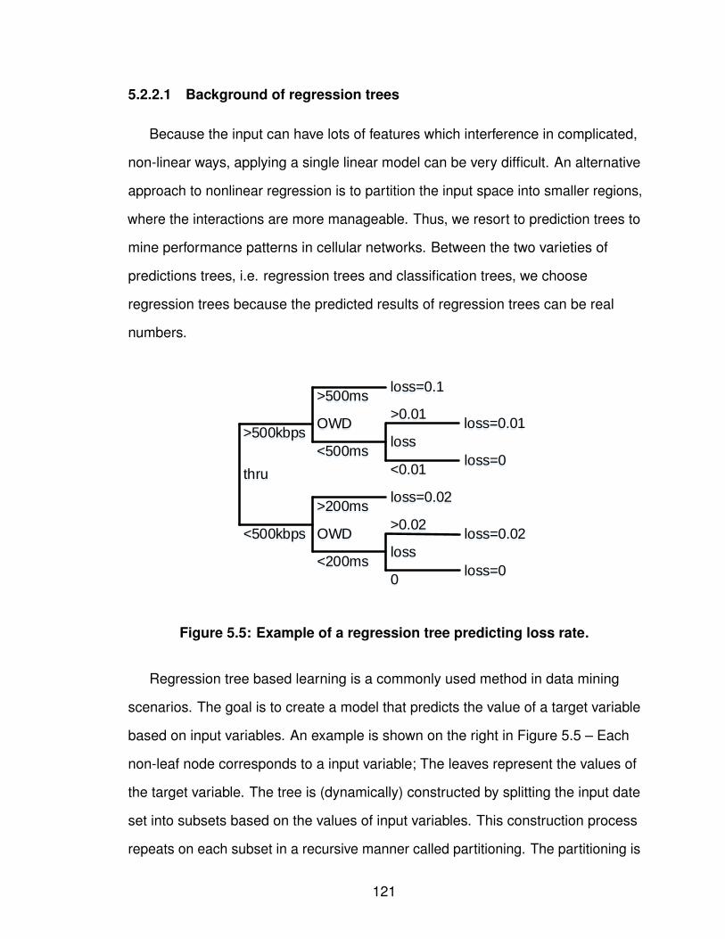
5.2.2.1 Background of regression trees

Because the input can have lots of features which interference in complicated,

non-linear ways, applying a single linear model can be very difficult. An alternative

approach to nonlinear regression is to partition the input space into smaller regions,

where the interactions are more manageable. Thus, we resort to prediction trees to

mine performance patterns in cellular networks. Between the two varieties of

predictions trees, i.e. regression trees and classification trees, we choose

regression trees because the predicted results of regression trees can be real

numbers.

loss=0.02

loss=0.1

loss=0.01>0.01

loss=0<0.01

loss<500ms

>500ms

OWD

>200ms

loss=0.02>0.02

loss=00

loss<200ms

OWD

>500kbps

<500kbps

thru

Figure 5.5: Example of a regression tree predicting loss rate.

Regression tree based learning is a commonly used method in data mining

scenarios. The goal is to create a model that predicts the value of a target variable

based on input variables. An example is shown on the right in Figure 5.5 – Each

non-leaf node corresponds to a input variable; The leaves represent the values of

the target variable. The tree is (dynamically) constructed by splitting the input date

set into subsets based on the values of input variables. This construction process

repeats on each subset in a recursive manner called partitioning. The partitioning is

121

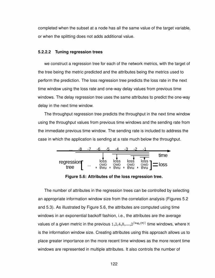
completed when the subset at a node has all the same value of the target variable,

or when the splitting does not adds additional value.

5.2.2.2 Tuning regression trees

we construct a regression tree for each of the network metrics, with the target of

the tree being the metric predicted and the attributes being the metrics used to

perform the prediction. The loss regression tree predicts the loss rate in the next

time window using the loss rate and one-way delay values from previous time

windows. The delay regression tree uses the same attributes to predict the one-way

delay in the next time window.

The throughput regression tree predicts the throughput in the next time window

using the throughput values from previous time windows and the sending rate from

the immediate previous time window. The sending rate is included to address the

case in which the application is sending at a rate much below the throughput.

time

... -7 -6 -5 -4 -3 -2 -1

lossOWDthru[ loss]=, , ,

regression tree

-8

,...lossOWDthru

lossOWDthru

lossOWDthru

Figure 5.6: Attributes of the loss regression tree.

The number of attributes in the regression trees can be controlled by selecting

an appropriate information window size from the correlation analysis (Figures 5.2

and 5.3). As illustrated by Figure 5.6, the attributes are computed using time

windows in an exponential backoff fashion, i.e., the attributes are the average

values of a given metric in the previous 1,2,4,8,...,2dlog2(M)e time windows, where M

is the information window size. Creating attributes using this approach allows us to

place greater importance on the more recent time windows as the more recent time

windows are represented in multiple attributes. It also controls the number of

122

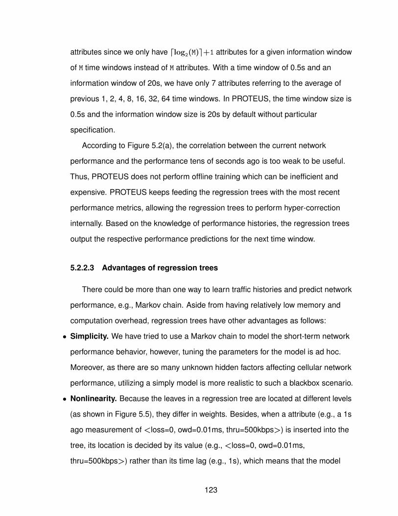
attributes since we only have dlog2(M)e+1 attributes for a given information window

of M time windows instead of M attributes. With a time window of 0.5s and an

information window of 20s, we have only 7 attributes referring to the average of

previous 1, 2, 4, 8, 16, 32, 64 time windows. In PROTEUS, the time window size is

0.5s and the information window size is 20s by default without particular

specification.

According to Figure 5.2(a), the correlation between the current network

performance and the performance tens of seconds ago is too weak to be useful.

Thus, PROTEUS does not perform offline training which can be inefficient and

expensive. PROTEUS keeps feeding the regression trees with the most recent

performance metrics, allowing the regression trees to perform hyper-correction

internally. Based on the knowledge of performance histories, the regression trees

output the respective performance predictions for the next time window.

5.2.2.3 Advantages of regression trees

There could be more than one way to learn traffic histories and predict network

performance, e.g., Markov chain. Aside from having relatively low memory and

computation overhead, regression trees have other advantages as follows:

• Simplicity. We have tried to use a Markov chain to model the short-term network

performance behavior, however, tuning the parameters for the model is ad hoc.

Moreover, as there are so many unknown hidden factors affecting cellular network

performance, utilizing a simply model is more realistic to such a blackbox scenario.

• Nonlinearity. Because the leaves in a regression tree are located at different levels

(as shown in Figure 5.5), they differ in weights. Besides, when a attribute (e.g., a 1s

ago measurement of <loss=0, owd=0.01ms, thru=500kbps>) is inserted into the

tree, its location is decided by its value (e.g., <loss=0, owd=0.01ms,

thru=500kbps>) rather than its time lag (e.g., 1s), which means that the model

123

based on regression trees is not linear.

• Dynamic. We need a model that can dynamically adapt to performance changes.

In cellular networks, the performance can change rapidly, so does the performance

model. However, utilizing regression trees, the model can dynamically grow

towards the most recently observed performance measurements.

5.2.3 Evaluating Forecast Accuracy

To evaluate the performance of PROTEUS, we carry out controlled experiments

to measure its forecasting accuracy. The forecasting accuracy may be variable due

to several aspects. When a mobile device is in communication over cellular

networks, the network, the device, and even the different cellular technology

generations under the same network can influence network predictability. Thus, we

conduct the experiments using diverse setups as shown in Table 5.2. Table 5.2 lists

the device, the network, and the cellular technology used. As TCP has built-in

congestion control and retransmission, the objective of evaluating TCP is its direct

impact to RTC applications, described in §5.3. To minimize bias, we repeat our

experiments at different time of day and at different locations. To directly control the

sending rate and to easily observe loss, one-way delay, and throughput, we

conduct most of our experiments over UDP. Even though most RTC applications

operate directly over UDP, the applicability of PROTEUS is not limited by the

transport protocol used by the application.

In the experiments, the mobile device communicates with a remote server in our

campus in either the downlink or uplink direction and keeps the packet rate constant

over the entire flow. To choose the sending rates, we saturate the end-to-end

connection using UDP and estimate the bandwidth from the receiving rate. Based

on the estimated bandwidth, the sending rate steps from 50% of the estimated

bandwidth to 150% by 10% every time and each flow of a sending rate lasts at least

124

one hour. On both the mobile and the remote server, we monitor packet traces

using tcpdump. From the collected packet traces, we identify throughput, loss rate,

and one-way delay. Here, we investigate one-way delay instead of round trip time

because one-way delay is a more accurate measurement of network characteristics

in a single direction and directly affects application performance. As mentioned in

§5.1, PROTEUS performs clock drift compensation to compute one-way delay.

In the evaluation, we compare PROTEUS with two performance adaptation

approaches, AD1 and AD2, which represent the state-of-the-art [9, 4, 1, 13, 23].

AD1 and AD2 are described as follows.

• AD1 assumes the performance in the next time window is the same as the

performance observed in the current time window.

• AD2 is less aggressive than AD1 to circumvent random variation in cellular

networks. AD2 assumes that the performance in the next time window is the

average of the performance in the information window, i.e., the same as

PROTEUS’s information window.

Although AD1 and AD2 may seem simple and naıve, most existing RTC applications

estimate loss rate and one-way delay using such methods since they work relatively

well on wired networks.

PROTEUS’s performance in loss prediction. We first investigate

PROTEUS’s accuracy in predicting the presence of any packet loss in the next time

window by measuring the false positive and false negative rates in TrafficSet. A

false positive occurs when PROTEUS predicts a packet loss in the time window but

there is none. False positives can cause inefficient usage of network resources. For

example, an application may introduce unnecessary FEC which would reduce the

rate available for the actual coding of media. In contrast, a false negative occurs

when PROTEUS predicts no packet loss but packet is lost in a time window. For

many applications, the false negatives may result in degraded application

125

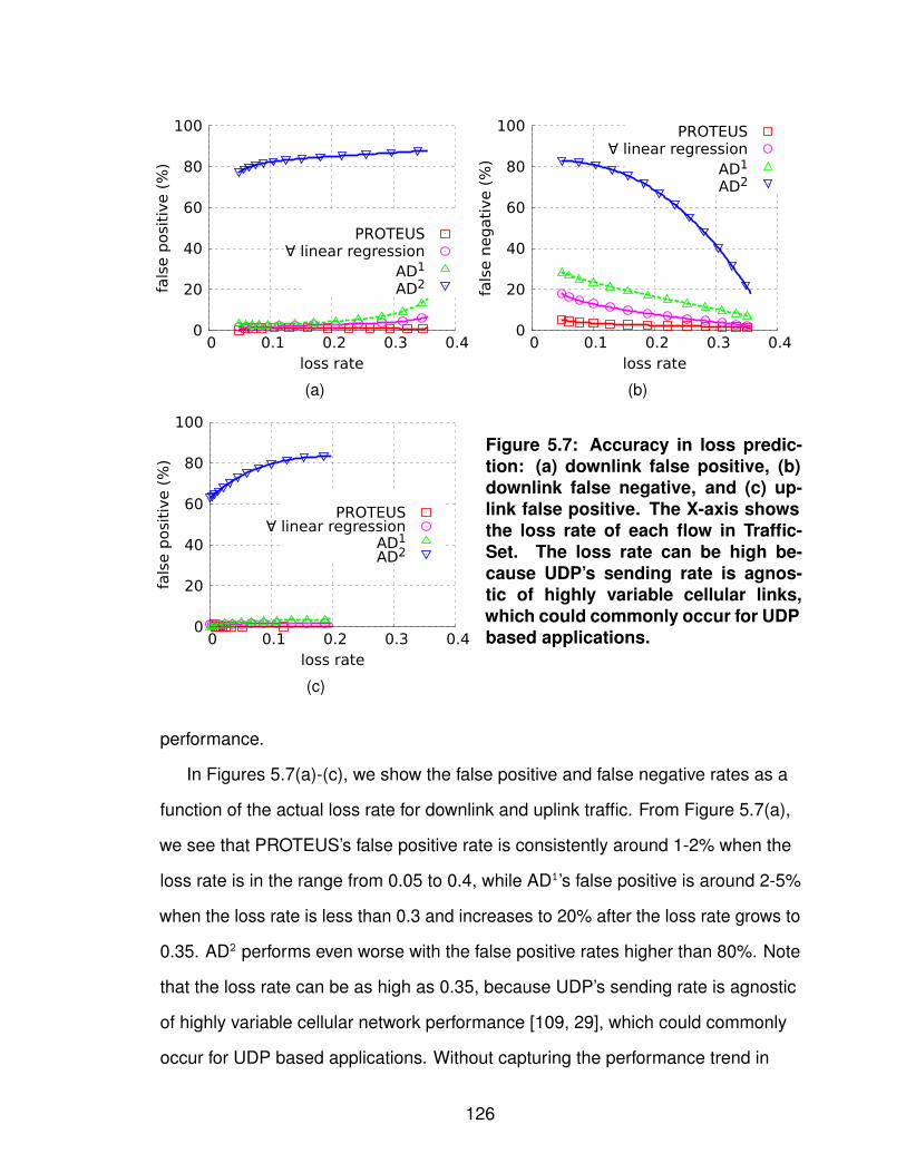
0

20

40

60

80

100

0 0.1 0.2 0.3 0.4

fals

e p

osi

tive (

%)

loss rate

PROTEUS∀ linear regression

AD1

AD2

0

20

40

60

80

100

0 0.1 0.2 0.3 0.4

fals

e n

egati

ve (

%)

loss rate

PROTEUS∀ linear regression

AD1

AD2

(a) (b)

0

20

40

60

80

100

0 0.1 0.2 0.3 0.4

fals

e p

osi

tive (

%)

loss rate

PROTEUS∀ linear regression

AD1

AD2

(c)

Figure 5.7: Accuracy in loss predic-tion: (a) downlink false positive, (b)downlink false negative, and (c) up-link false positive. The X-axis showsthe loss rate of each flow in Traffic-Set. The loss rate can be high be-cause UDP’s sending rate is agnos-tic of highly variable cellular links,which could commonly occur for UDPbased applications.

performance.

In Figures 5.7(a)-(c), we show the false positive and false negative rates as a

function of the actual loss rate for downlink and uplink traffic. From Figure 5.7(a),

we see that PROTEUS’s false positive rate is consistently around 1-2% when the

loss rate is in the range from 0.05 to 0.4, while AD1’s false positive is around 2-5%

when the loss rate is less than 0.3 and increases to 20% after the loss rate grows to

0.35. AD2 performs even worse with the false positive rates higher than 80%. Note

that the loss rate can be as high as 0.35, because UDP’s sending rate is agnostic

of highly variable cellular network performance [109, 29], which could commonly

occur for UDP based applications. Without capturing the performance trend in

126

previous time windows, AD1 and AD2 can only achieve the accuracy as poor as

random guessing by merely estimating based on the last time window or

aggregated history information.

In Figure 5.7(b), we show the false negative rate of the flows in TrafficSet. As

mentioned, a false negative is more critical than a false positive, for RTC

applications. From Figure 5.7(b), PROTEUS’s false negative is consistently less

than 1%, AD1’s false negative is 5-20% and AD2’s false negative is around 2-4%,

slightly worse than PROTEUS. When the loss rate is low, the running flow may not

provide sufficient information of true positives, i.e., lost packets. Thus, as the loss

rate decreases, PROTEUS, AD1, and AD2 all have increasing false negative rates.

Although AD2’s false negative is only slightly worse than PROTEUS, PROTEUS’s

false positive is significantly better. Compared to AD1, AD2 has low false positive

rate, but does not retain a low false negative rate at the same time.

Besides downlink traffic, we also investigate uplink traffic as uplink traffic is

significant in applications such as Skype, FaceTime, and Google+ Hangouts.

Similar to Figure 5.7(a), PROTEUS is slightly better than AD1 and much better than

AD2 in false positive according to Figure 5.7(c). PROTEUS’s false positive is less

than 1% over the flows in TrafficSet, AD1’s false positive ranges from 3% to 5%, and

AD2’s false positive is no less than 40%. We observe similar performance for

PROTEUS, AD1, and AD2 in their false negative for uplink flows.

The false positive and false negative results for the packet loss presented above

show the prediction accuracy. Moreover, the regression tree used in PROTEUS

also predicts the packet loss rate quantitatively rather than giving a simple binary

decision of whether there will be packet loss. In Figure 5.8(a), we show the

accuracy of this quantitative prediction of packet loss rate. We show the error in

packet loss rate prediction for each of the three categories according to the error

type, i.e., false negative, false positive, and true positive. Only true negative does

127

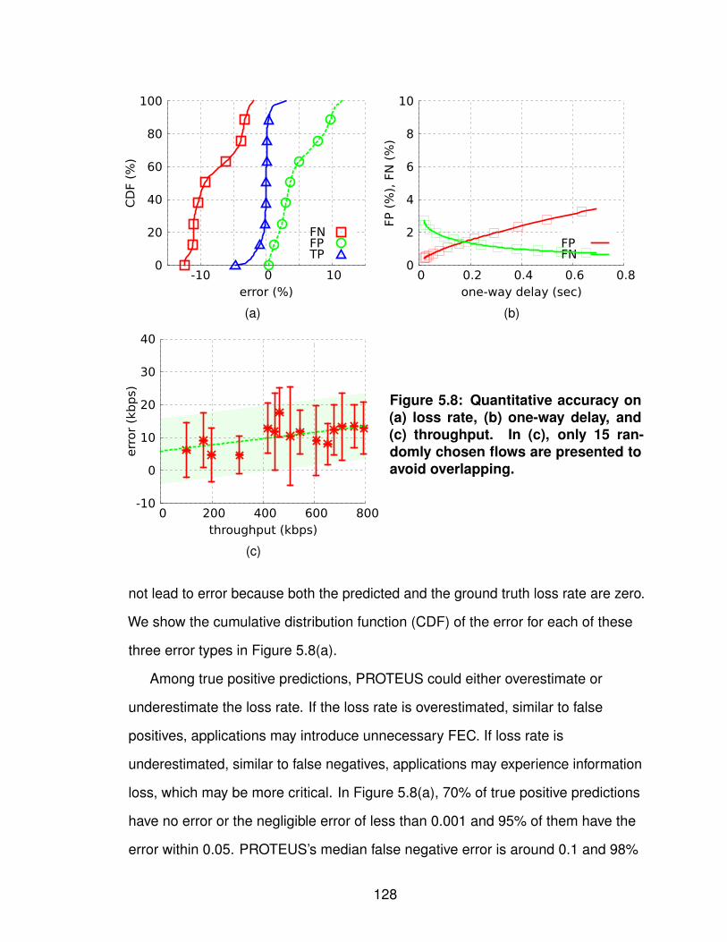
0

20

40

60

80

100

-10 0 10

CD

F (%

)

error (%)

FNFPTP

0

2

4

6

8

10

0 0.2 0.4 0.6 0.8

FP (

%),

FN

(%

)

one-way delay (sec)

FPFN

(a) (b)

-10

0

10

20

30

40

0 200 400 600 800

err

or

(kbps)

throughput (kbps)

(c)

Figure 5.8: Quantitative accuracy on(a) loss rate, (b) one-way delay, and(c) throughput. In (c), only 15 ran-domly chosen flows are presented toavoid overlapping.

not lead to error because both the predicted and the ground truth loss rate are zero.

We show the cumulative distribution function (CDF) of the error for each of these

three error types in Figure 5.8(a).

Among true positive predictions, PROTEUS could either overestimate or

underestimate the loss rate. If the loss rate is overestimated, similar to false

positives, applications may introduce unnecessary FEC. If loss rate is

underestimated, similar to false negatives, applications may experience information

loss, which may be more critical. In Figure 5.8(a), 70% of true positive predictions

have no error or the negligible error of less than 0.001 and 95% of them have the

error within 0.05. PROTEUS’s median false negative error is around 0.1 and 98%

128

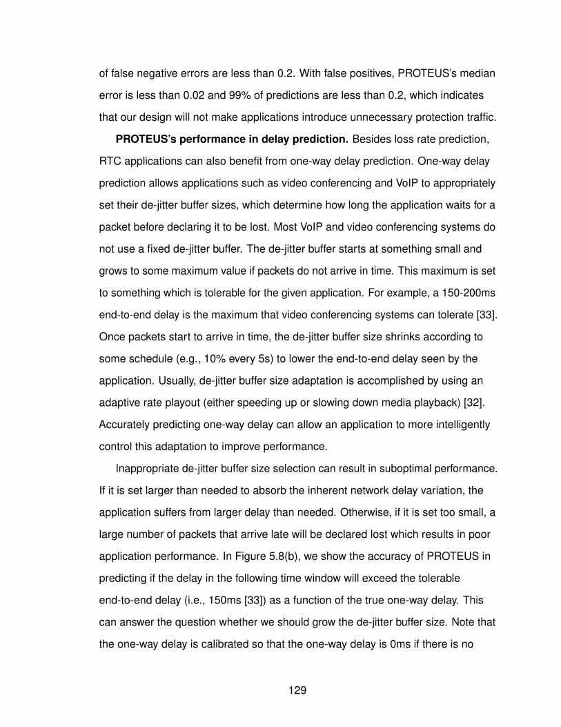
of false negative errors are less than 0.2. With false positives, PROTEUS’s median

error is less than 0.02 and 99% of predictions are less than 0.2, which indicates

that our design will not make applications introduce unnecessary protection traffic.

PROTEUS’s performance in delay prediction. Besides loss rate prediction,

RTC applications can also benefit from one-way delay prediction. One-way delay

prediction allows applications such as video conferencing and VoIP to appropriately

set their de-jitter buffer sizes, which determine how long the application waits for a

packet before declaring it to be lost. Most VoIP and video conferencing systems do

not use a fixed de-jitter buffer. The de-jitter buffer starts at something small and

grows to some maximum value if packets do not arrive in time. This maximum is set

to something which is tolerable for the given application. For example, a 150-200ms

end-to-end delay is the maximum that video conferencing systems can tolerate [33].

Once packets start to arrive in time, the de-jitter buffer size shrinks according to

some schedule (e.g., 10% every 5s) to lower the end-to-end delay seen by the

application. Usually, de-jitter buffer size adaptation is accomplished by using an

adaptive rate playout (either speeding up or slowing down media playback) [32].

Accurately predicting one-way delay can allow an application to more intelligently

control this adaptation to improve performance.

Inappropriate de-jitter buffer size selection can result in suboptimal performance.

If it is set larger than needed to absorb the inherent network delay variation, the

application suffers from larger delay than needed. Otherwise, if it is set too small, a

large number of packets that arrive late will be declared lost which results in poor

application performance. In Figure 5.8(b), we show the accuracy of PROTEUS in

predicting if the delay in the following time window will exceed the tolerable

end-to-end delay (i.e., 150ms [33]) as a function of the true one-way delay. This

can answer the question whether we should grow the de-jitter buffer size. Note that

the one-way delay is calibrated so that the one-way delay is 0ms if there is no

129

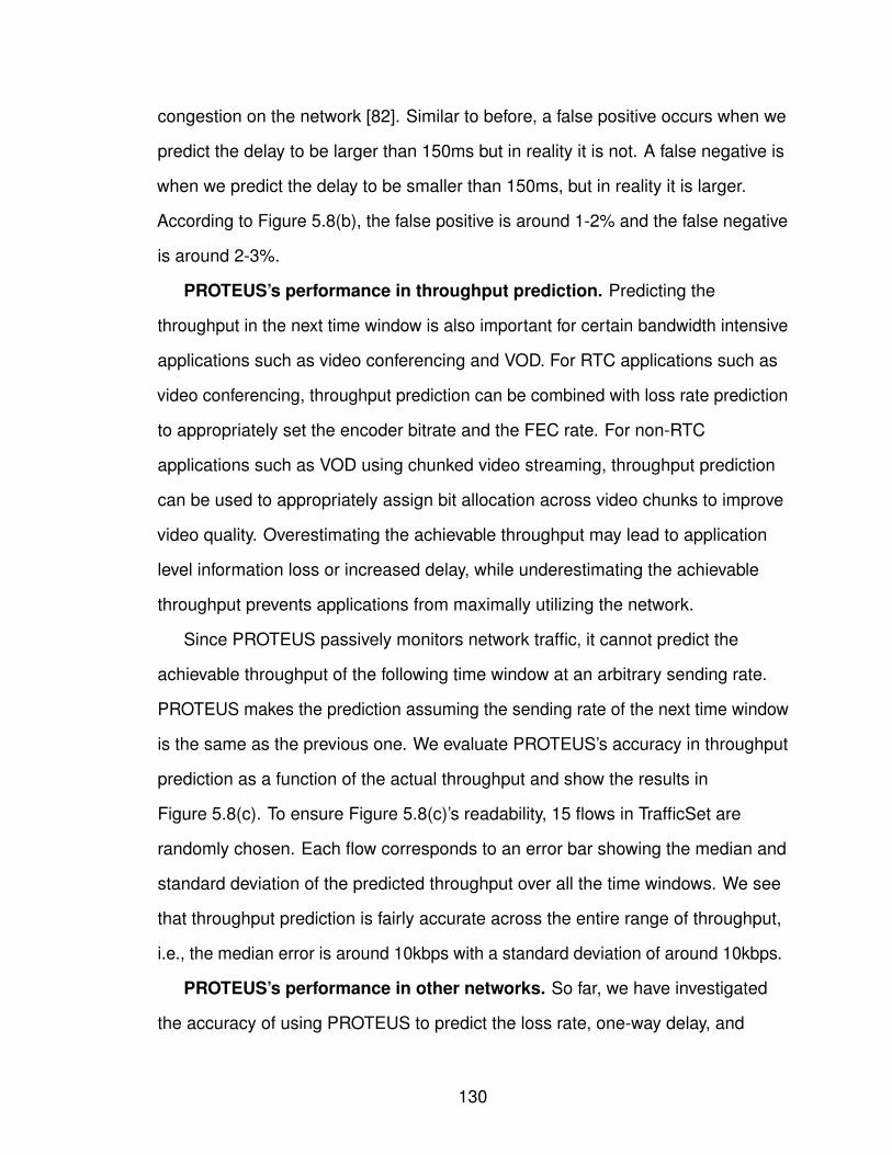
congestion on the network [82]. Similar to before, a false positive occurs when we

predict the delay to be larger than 150ms but in reality it is not. A false negative is

when we predict the delay to be smaller than 150ms, but in reality it is larger.

According to Figure 5.8(b), the false positive is around 1-2% and the false negative

is around 2-3%.

PROTEUS’s performance in throughput prediction. Predicting the

throughput in the next time window is also important for certain bandwidth intensive

applications such as video conferencing and VOD. For RTC applications such as

video conferencing, throughput prediction can be combined with loss rate prediction

to appropriately set the encoder bitrate and the FEC rate. For non-RTC

applications such as VOD using chunked video streaming, throughput prediction

can be used to appropriately assign bit allocation across video chunks to improve

video quality. Overestimating the achievable throughput may lead to application

level information loss or increased delay, while underestimating the achievable

throughput prevents applications from maximally utilizing the network.

Since PROTEUS passively monitors network traffic, it cannot predict the

achievable throughput of the following time window at an arbitrary sending rate.

PROTEUS makes the prediction assuming the sending rate of the next time window

is the same as the previous one. We evaluate PROTEUS’s accuracy in throughput

prediction as a function of the actual throughput and show the results in

Figure 5.8(c). To ensure Figure 5.8(c)’s readability, 15 flows in TrafficSet are

randomly chosen. Each flow corresponds to an error bar showing the median and

standard deviation of the predicted throughput over all the time windows. We see

that throughput prediction is fairly accurate across the entire range of throughput,

i.e., the median error is around 10kbps with a standard deviation of around 10kbps.

PROTEUS’s performance in other networks. So far, we have investigated

the accuracy of using PROTEUS to predict the loss rate, one-way delay, and

130

0

1

2

0 0.1FP

(%

)

loss rate

T-MobileSprint

Figure 5.9: Impact of the cellular network.

0.1

1

10

100

0.5 1 2 5 10 20

FN (

%),

FP (

%)

size (sec)

FPFN

Figure 5.10: Impact of the time window size.

throughput for one particular cellular carrier. To be broadly applicable, we need to

verify if PROTEUS’s accuracy applies to other cellular carriers as well. Figure 5.9

shows the false positive rate of loss predictions for T-Mobile and Sprint, whose

setup is described in Table 5.2. According to Figure 5.9, both T-Mobile and Sprint

have even a lower false positive than AT&T. We only include the evaluation on false

positive rate of T-Mobile and Sprint, but have verified that PROTEUS also has high

prediction accuracy in terms of the false negative and false positive rates in

one-way delay and throughput prediction.

PROTEUS’s performance affected by the time and information window

131

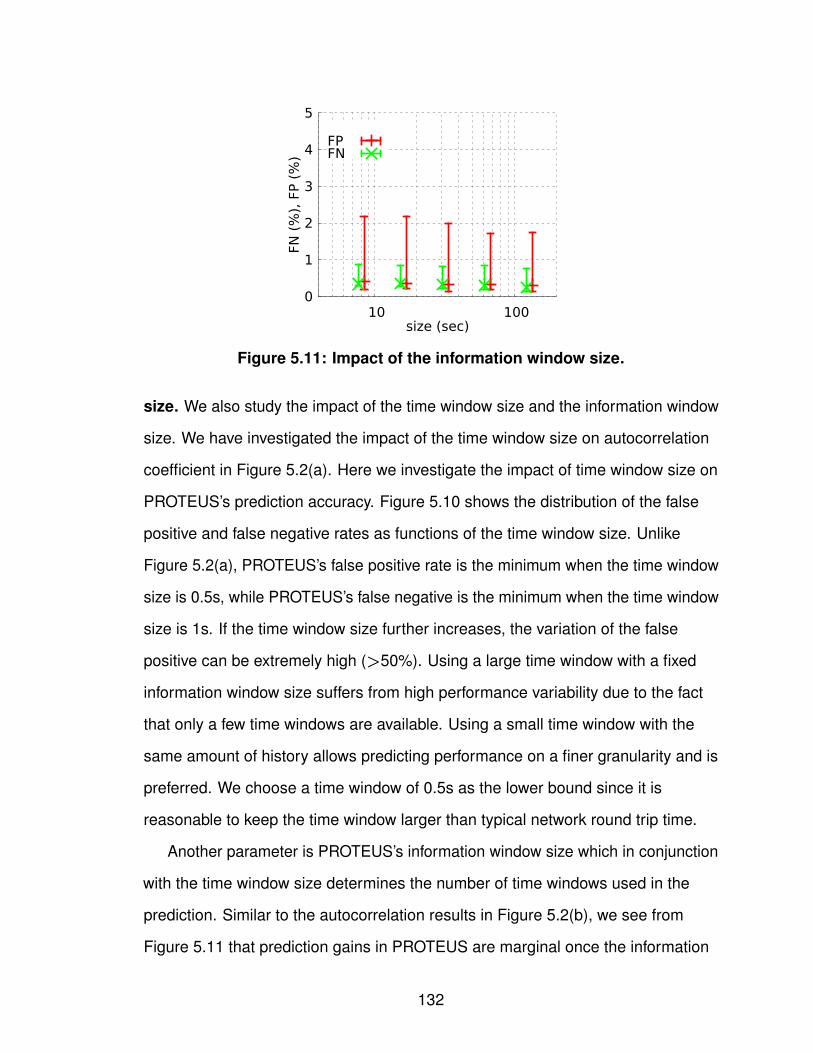
0

1

2

3

4

5

10 100FN

(%

), F

P (

%)

size (sec)

FPFN

Figure 5.11: Impact of the information window size.

size. We also study the impact of the time window size and the information window

size. We have investigated the impact of the time window size on autocorrelation

coefficient in Figure 5.2(a). Here we investigate the impact of time window size on

PROTEUS’s prediction accuracy. Figure 5.10 shows the distribution of the false

positive and false negative rates as functions of the time window size. Unlike

Figure 5.2(a), PROTEUS’s false positive rate is the minimum when the time window

size is 0.5s, while PROTEUS’s false negative is the minimum when the time window

size is 1s. If the time window size further increases, the variation of the false

positive can be extremely high (>50%). Using a large time window with a fixed

information window size suffers from high performance variability due to the fact

that only a few time windows are available. Using a small time window with the

same amount of history allows predicting performance on a finer granularity and is

preferred. We choose a time window of 0.5s as the lower bound since it is

reasonable to keep the time window larger than typical network round trip time.

Another parameter is PROTEUS’s information window size which in conjunction

with the time window size determines the number of time windows used in the

prediction. Similar to the autocorrelation results in Figure 5.2(b), we see from

Figure 5.11 that prediction gains in PROTEUS are marginal once the information

132

window size used for prediction is larger than 8s. Thus we can achieve accurate

prediction using time windows within the last 8s.

5.3 Application of PROTEUS

Applications can take advantage of network metric prediction to improve their

performance. The exact benefit will depend on how each application uses the

information obtained from PROTEUS. Here we show the improvement PROTEUS

can provide to two RTC applications: a video conferencing application and an

interactive software application, i.e., Draw Something.

5.3.1 Video Conferencing System

Equivalent video conferencing emulation. We describe how we realistically

evaluate the video conferencing application to make use of PROTEUS in a working

system, considering all the overhead of the associated changes with the small

difference of running the client software on a legacy laptop instead of a mobile

device due to software constraints.

There are standard methods to evaluate video conferencing using the

H.264/AVC reference software [8] on PCs. However, there is no such equivalent

open-source encoding/decoding suite on mobile platforms. Thus, to best effectively

evaluate video conferencing on mobile platforms, we take the following steps: (i),

we modify the H.264/AVC reference software so that the H.264 encoder can adjust

the video codec bitrate and FEC rate for each video frame rather than sticking to

fixed codec bitrate and FEC rate for an entire video stream; (ii), we use a 2GHz

dual core Thinkpad T60 with 2G RAM to run the H.264 decoder, with the

computation performance as close to off-the-shelf mobile devices as possible; and

(iii), we replay the packet traces collected in cellular networks (i.e., TrafficSet) to

133

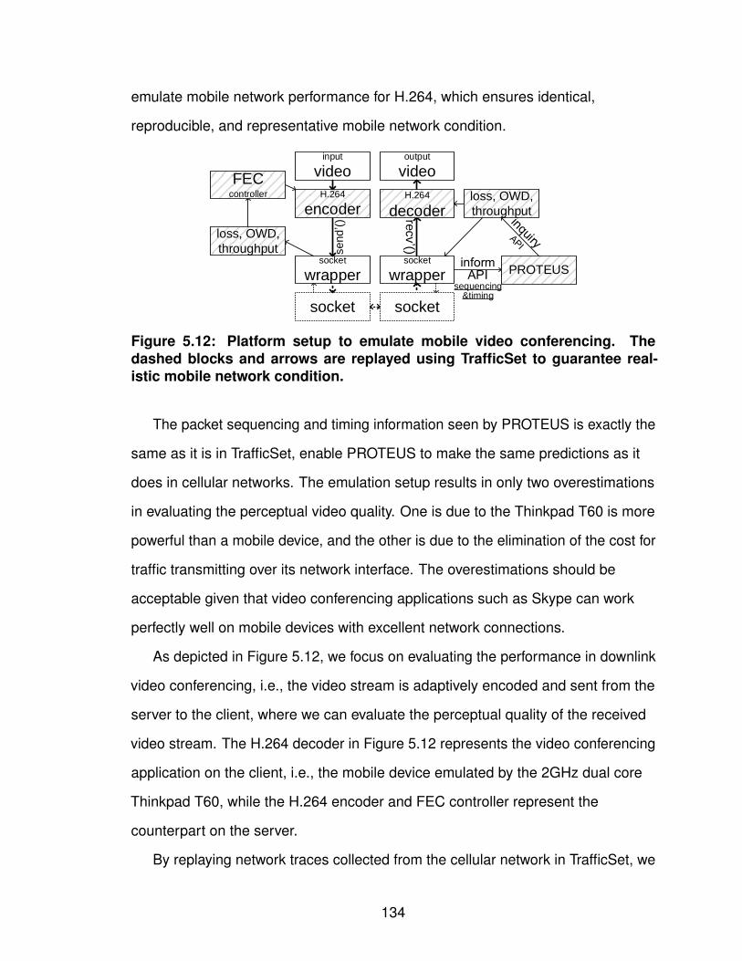
emulate mobile network performance for H.264, which ensures identical,

reproducible, and representative mobile network condition.

send

() re

cv

()

sequencing&timing

socket

PROTEUS

loss, OWD,

throughput

loss, OWD,

throughput

FECcontroller

input

video

socket

wrapper

socket

output

video

H.264

decoder

socket

wrapper

H.264

encoder

Figure 5.12: Platform setup to emulate mobile video conferencing. Thedashed blocks and arrows are replayed using TrafficSet to guarantee real-istic mobile network condition.

The packet sequencing and timing information seen by PROTEUS is exactly the

same as it is in TrafficSet, enable PROTEUS to make the same predictions as it

does in cellular networks. The emulation setup results in only two overestimations

in evaluating the perceptual video quality. One is due to the Thinkpad T60 is more

powerful than a mobile device, and the other is due to the elimination of the cost for

traffic transmitting over its network interface. The overestimations should be

acceptable given that video conferencing applications such as Skype can work

perfectly well on mobile devices with excellent network connections.

As depicted in Figure 5.12, we focus on evaluating the performance in downlink

video conferencing, i.e., the video stream is adaptively encoded and sent from the

server to the client, where we can evaluate the perceptual quality of the received

video stream. The H.264 decoder in Figure 5.12 represents the video conferencing

application on the client, i.e., the mobile device emulated by the 2GHz dual core

Thinkpad T60, while the H.264 encoder and FEC controller represent the

counterpart on the server.

By replaying network traces collected from the cellular network in TrafficSet, we

134

can reproduce representative mobile network condition. We measure the video

quality performance using standard video sequences shown in Table 5.3 (referred

as VideoSet) [19]. As illustrated in Figure 5.12, given a video sequence in VideoSet,

the H.264 encoder on the server translates the video sequence to a RTP network

stream. To test the video quality under various and reproducible network condition,

for each flow in TrafficSet, we replace its content with the encoded network stream

respectively. On the client, the H.264 decoder decodes the received network

stream and constructs the video for users. According to TrafficSet, if a packet is lost

or does not arrive in time at the de-jitter buffer, the corresponding frame may be

corrupted so that the perceptual quality of the decoded video will be affected.

PROTEUS utilization in video conferencing. Based on past work, there are

well established adaptations that applications take in response to changing network

condition. The quality of video conferencing is very sensitive to three network

metrics, i.e., the packet loss, the one-way delay, and the throughput. To ensure

good quality, the video conferencing application can tune several parameters.

• The video codec can adjust the compression ratio, trading source video quality with

codec bitrate, by adjusting the quantization parameter (QP) of macroblocks [73, 74].

A smaller QP value results in better visual quality at the expense of a higher bitrate

and higher bandwidth requirement.

• The application can insert an appropriate number of forward error correction (FEC)

packets. This process allocates the total transmission rate amongst source bitrate

and channel (error correction) bitrate.

• The application can adjust the de-jitter buffer size which specifies how long the

receiving end waits for data to arrive before it is played back. The de-jitter buffer

size trades application latency with late loss. A larger de-jitter buffer size increases

the chance that a packet will arrive in time for playback, but increases the

end-to-end application latency. For video conferencing applications, the user

135

cannot perceive an end-to-end delay (including propagation delay, network queuing

delay, and time spent in the de-jitter buffer) lower than 200ms [20]. However, when

the end-to-end delay is above this threshold, there is perceived degradation.

video # of frames sequence resolution size (MB)akiyo 300 10/IPPP QCIF,CIF 44

bowing 300 10/IPPP QCIF,CIF 44bridge(close) 2001 10/IPPP QCIF,CIF 291

bridge(far) 2101 10/IPPP CIF 305foreman 300 10/IPPP QCIF,CIF 44highway 2000 10/IPPP CIF 291

Table 5.3: Video sequences to reproduce video conferencing streams(VideoSet). The frame rate for all these video sequences is 30fps.

We denote the predicted packet loss rate, one-way delay, and throughput by the

triplet with (ε,δ,T). This is the predicted network performance obtained from the

regression tree on the mobile device and delivered to the server. Given this network

prediction, we set the application parameters as follows: (i) the video codec bitrate

for a given frame is set to R=(1−αε)T (α≥1); (ii) the FEC rate to αεT; and (iii) the

receiver de-jitter buffer size to βδ seconds. α is a constant that determines the

actual amount of FEC protection used. In the evaluation, α=1. The total estimated

throughput T is divided amongst source rate and FEC rate. As an example,

suppose T is estimated as 500kbps, the estimated loss rate is ε=0.06, and α=2 is

used. With this, 440kbps should be used for source coding and 60kbps for FEC

protection. With a video frame rate of 15fps and a packet size of 500 bytes, this

approximately translates to 7 packets per frame of source coding and 1 packet per

frame of FEC.

Once the video frames are coded into packets, the evaluation platform assumes

that these packets go through a network which has characteristics obtained from

the collected network trace. If the actual loss on the network is less than or equal to

αεT, the receiver has sufficient information to decode the frame, otherwise the

frame is assumed to be lost. In addition to packet loss on the network, we also

136

consider delay in the evaluation, assuming a de-jitter buffer size of βδ (β≥1), which

is slightly larger than the estimated δ. In the above example, if two or more packets

are lost or delayed later than βδ, the respective frame is lost. In the evaluation,

β=1.

10

20

30

40

50

0 0.1 0.2 0.3 0.4

PSN

R (

dB

)

loss rate

PROTEUSAD1

AD2TCP

OPT 10

20

30

40

50

0 0.1 0.2 0.3 0.4PSN

R (

dB

)

loss rate

PROTEUSAD1

AD2TCP

OPT

(a) 5th percentile PSNR. (b) 25th percentile PSNR.

Figure 5.13: PSNR for PROTEUS, AD1, AD2, TCP, and OPT, , which assumesthat we a priori know the exact loss rate.

0

10

20

30

40

FEC

(kb

ps)

PROTEUSAD1

AD2OPT

0

10

0 0.1 0.2 0.3 0.4loss rate

Figure 5.14: FEC overhead. “OPT” shows the total FEC overhead in theoptimal scenarios.

Perceptual video quality assessment. The H.264 decoder provides the

ability to conceal lost frames. Upon decoding the sequence, which may potentially

137

have some frames lost, we compare the decoded video sequence to the original

and measure the peak signal-to-noise ratio (PSNR) which is a commonly used

metric to measure video quality. This setup is used to repeatedly measure the

video quality using the prediction obtained from PROTEUS, AD1, and AD2 over the

various video sequences in VideoSet and over the various network traces in

TrafficSet.

If we underestimate ε (i.e., loss rate), then the application may add insufficient

redundancy which results in unrecoverable packet loss for the application.

Otherwise, if we overestimate ε, then the application may add too much

redundancy which causes the video codec bitrate to be lower than needed,

resulting in poorer video quality. Thus, both underestimation and overestimation of

the future network performance can lower the perceptual video quality. We analyze

the effect of network parameter mis-prediction on video quality for the three

prediction techniques, PROTEUS, AD1, and AD2. We also analyze the performance

hypothesizing that we exactly know the loss rate and insert just the right amount of

FEC to counteract any packet loss. It is possible as we have the network traces.

This optimal scheme is denoted as OPT.

For each video sequence in VideoSet, we run all the network traces from

TrafficSet using each of the four methods (PROTEUS, AD1, AD2, and OPT). For

each of the four methods, we compute a distribution of PSNR. In Figure 5.13, we

show the 5th and 25th percentiles of the PSNR as a function of loss rate for each of

the four methods. We purposefully show the low PSNR values in the distribution

since this is what most affects overall user satisfaction and is a measure of how

each of the three schemes performs in tough network condition. In addition to the

four adaptive methods using UDP, we evaluate the adaptive bitrate streaming over

TCP as well assuming that the encoded bitrate is always adapted to the throughput

in the current time window. To guarantee the network condition for TCP and UDP

138

experiments are comparable, for each TCP flow, we create UDP packets

back-to-back lasting for the same duration. In Figure 5.13, the distribution of PSNR

for TCP flows is represented as the function of the loss rate of the back-to-back

UDP flow’s loss rate.

In general, if a frame is lost, the PSNR of the other frames that reference the

lost frame becomes very low, e.g., PSNR<25dB. Since PROTEUS can accurately

predict loss rate with almost 99% accuracy, there are very few cases (i.e., <1%)

where we see unrecoverable packet loss. Thus, as we see from Figure 5.13(a),

even the 5th percentile PSNR shows no packet loss using PROTEUS. The only

reason the 5th percentile PSNR is below OPT is due to over-protection which

reduces the video codec bitrate. This reduction in PSNR in PROTEUS when

compared to OPT (due to over-protection) is on the order of 1dB, whereas the

reduction in PSNR in AD1 and AD2 (due to unrecoverable lost packets) is on the

order of 15dB. As loss rate increases, the PSNR using PROTEUS decreases but

stays close to OPT. It is obvious that increasing loss rate results in decreased

capacity. Since a larger portion of the total throughput has to be allocated to FEC,

we see a reduction in PSNR. To show the visual effect of unrecoverable packet loss,

we show representative frames in the 5th percentile of PSNR values in Figure 5.15

using the schemes AD1,2, TCP, and PROTEUS. It is clear that unrecoverable packet

loss results in substantial video quality degradation.

As PROTEUS may overestimate the actual loss rate, there will inevitably be

some cases where we over-protect. In Figure 5.14, we show the bitrate taken by

FEC packets which are not used to correct any loss. The bottom plot shows the

amount of needed FEC to correct for packet loss. As we see, as the loss rate

increases, the amount of needed protection also increases. The top plot in

Figure 5.14 shows the amount of additional FEC beyond the needed amount which

is applied when using each of the three schemes to predict the loss rate. We see

139

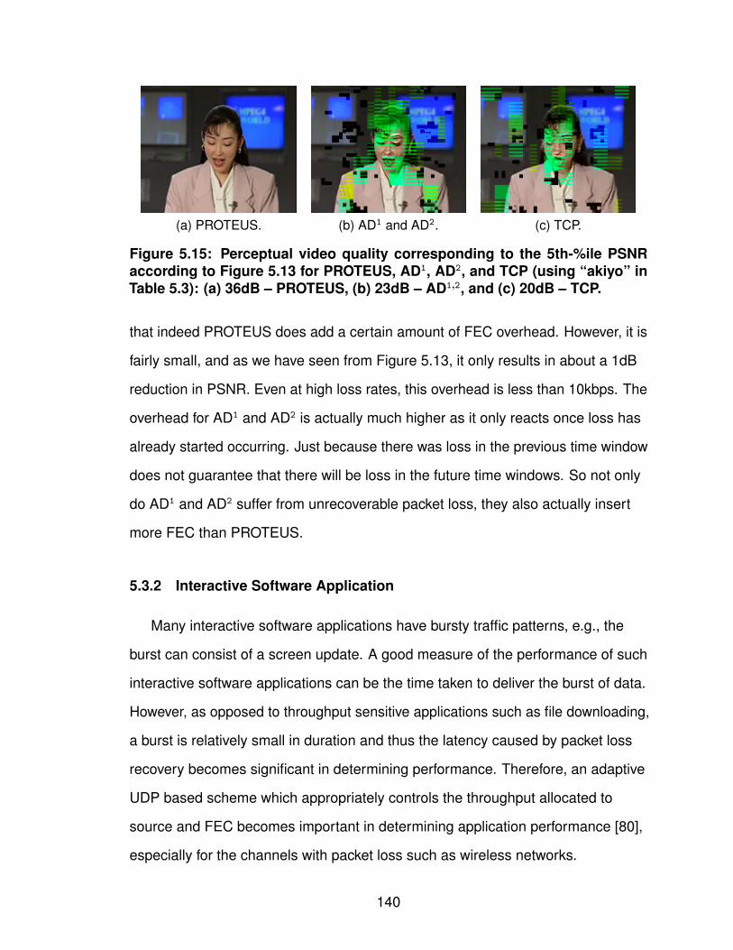
(a) PROTEUS. (b) AD1 and AD2. (c) TCP.

Figure 5.15: Perceptual video quality corresponding to the 5th-%ile PSNRaccording to Figure 5.13 for PROTEUS, AD1, AD2, and TCP (using “akiyo” inTable 5.3): (a) 36dB – PROTEUS, (b) 23dB – AD1,2, and (c) 20dB – TCP.

that indeed PROTEUS does add a certain amount of FEC overhead. However, it is

fairly small, and as we have seen from Figure 5.13, it only results in about a 1dB

reduction in PSNR. Even at high loss rates, this overhead is less than 10kbps. The

overhead for AD1 and AD2 is actually much higher as it only reacts once loss has

already started occurring. Just because there was loss in the previous time window

does not guarantee that there will be loss in the future time windows. So not only

do AD1 and AD2 suffer from unrecoverable packet loss, they also actually insert

more FEC than PROTEUS.

5.3.2 Interactive Software Application

Many interactive software applications have bursty traffic patterns, e.g., the

burst can consist of a screen update. A good measure of the performance of such

interactive software applications can be the time taken to deliver the burst of data.

However, as opposed to throughput sensitive applications such as file downloading,

a burst is relatively small in duration and thus the latency caused by packet loss

recovery becomes significant in determining performance. Therefore, an adaptive

UDP based scheme which appropriately controls the throughput allocated to

source and FEC becomes important in determining application performance [80],

especially for the channels with packet loss such as wireless networks.

140

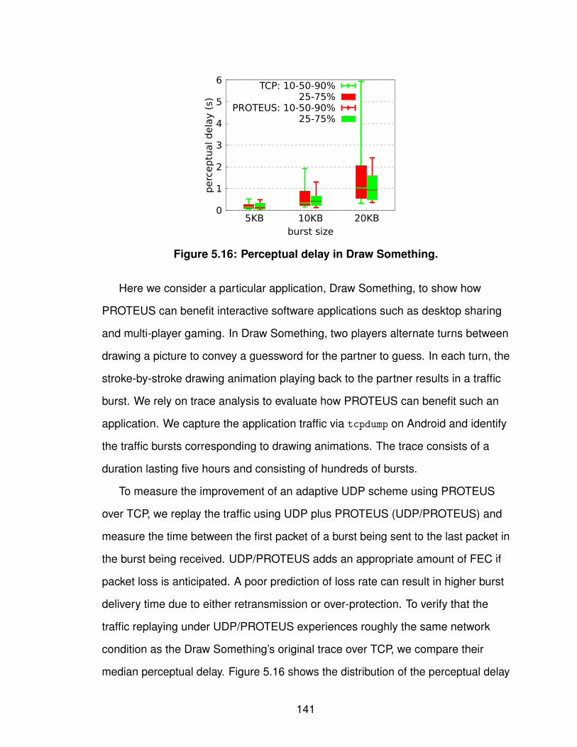
0

1

2

3

4

5

6

5KB 10KB 20KBperc

eptu

al dela

y (

s)

burst size

TCP: 10-50-90%25-75%

PROTEUS: 10-50-90%25-75%

Figure 5.16: Perceptual delay in Draw Something.

Here we consider a particular application, Draw Something, to show how

PROTEUS can benefit interactive software applications such as desktop sharing

and multi-player gaming. In Draw Something, two players alternate turns between

drawing a picture to convey a guessword for the partner to guess. In each turn, the

stroke-by-stroke drawing animation playing back to the partner results in a traffic

burst. We rely on trace analysis to evaluate how PROTEUS can benefit such an

application. We capture the application traffic via tcpdump on Android and identify

the traffic bursts corresponding to drawing animations. The trace consists of a

duration lasting five hours and consisting of hundreds of bursts.

To measure the improvement of an adaptive UDP scheme using PROTEUS

over TCP, we replay the traffic using UDP plus PROTEUS (UDP/PROTEUS) and

measure the time between the first packet of a burst being sent to the last packet in

the burst being received. UDP/PROTEUS adds an appropriate amount of FEC if

packet loss is anticipated. A poor prediction of loss rate can result in higher burst

delivery time due to either retransmission or over-protection. To verify that the

traffic replaying under UDP/PROTEUS experiences roughly the same network

condition as the Draw Something’s original trace over TCP, we compare their

median perceptual delay. Figure 5.16 shows the distribution of the perceptual delay

141

over different burst size. As the median perceptual delay for UDP/PROTEUS is very

close to TCP’s, we expect that UDP/PROTEUS experiences similar network

condition. According to Figure 5.16, when the burst size is very small, TCP and

UDP/PROTEUS perform equally at any percentile in the distribution. However,

when the burst size grows to 10KB and larger (e.g., 20KB), UDP/PROTEUS

performs much better, particularly in the 75-90th percentile perceptual delay, which

may easily produce user dissatisfaction. UDP/PROTEUS reduces the 90th

percentile perceptual delay by roughly 1s When the burst size is around 10KB.

When the burst size is around 20KB, UDP/PROTEUS’s 90th percentile perceptual

delay is 2s while TCP’s is up to 6s.

5.4 Summary of Optimizing Real-Time, Interactive

Applications

In this section, we systematically quantified the predictability of network

performance metrics in three major cellular networks: AT&T, T-Mobile, and Sprint.

In all three carriers, we identified the existence of strong predictability of network

performance, even over a short term window e.g., 0.5s. To take advantage of this

predictability, we proposed a system PROTEUS, which collects network

performance information being observed by applications, employs regression trees

to learn network performance patterns, and forecasts future network performance

to benefit application performance. PROTEUS can predict the occurrence of packet

loss within a time window for 98% of the time windows, occurrence of long one-way

delay for 97% of the time windows, and the throughput within a median error of

10kbps. By using PROTEUS in a video conferencing scenario, we can improve the

PSNR of the perceived video by 15dB when compared against traditional

performance adaptation techniques. Compared with the hypothesized optimal

142

scenario in which the application knows exactly which packets will be lost,

PROTEUS is only 1-2dB worse.

We believe that PROTEUS is a comprehensive and effective network

performance forecasting framework for use by mobile applications especially for

use over cellular networks. PROTEUS can also inspire the development of

challenging applications on mobile devices.

143

CHAPTER VI

RELATED WORK

We broadly classify previous studies into (i) cellular infrastructure, (ii) application

usage, and (iii) application optimization, and position our studies accordingly as

follows.

6.1 Cellular Infrastructure

YellowPage is motivated by numerous previous measurement

studies [105, 125, 76], e.g., Rocketfuel [102] to characterize various properties of

the Internet through passive monitoring using data such as server logs and packet

traces, as well as active measurement such as probing path changes. Efforts on

reverse engineering properties of the Internet [103] have been shown to be quite

successful; however, very little work has been done in the space of cellular IP

networks. Complementary to YellowPage, the most recent work by Keralapura et al.

profiled the browsing behavior by investigating whether there exists distinct

behavior pattern among mobile users [68]. Their study implemented effective

co-clustering on large scale user-level web browsing traces collected from one

cellular provider. As far as we know, our study is the first to comprehensively

characterize cellular IP networks covering all the major cellular carriers in the U.S.,

focusing on key characteristics such as network topological properties and dynamic

144

routing behavior. From the characterization of the cellular data network structure,

we also draw conclusions on content placement, which is essential given the rapidly

growing demand for mobile data access.

We build our work upon a recent study by Balakrishnan et al. [28] in which they

highlighted unexpected dynamic behavior of cellular IP addresses. YellowPage

performs a more complete and general study covering a wider set of properties,

illustrating carrier-specific network differences, explaining the observed diverse

geographic distribution of cellular IP addresses, also investigating associated

implications of observed network designs.

Although there have been studies characterized the CDNs relative to the end

users accessing from the wireline networks [79, 100, 41, 92, 60], very little

attention has been paid to the cellular users. These previous studies are mainly

from two perspectives, i.e., content placement and server selection. YellowPage is

complementary to these studies by investigating the implication of cellular network

infrastructure on mobile data placement and server selection. To our best

knowledge, YellowPage is the first to investigate the content placement and content

server selections for cellular users.

Previous studies on cellular networks can be classified approximately into

several categories, namely from ISP’s view point of managing network

resources [54, 104], from end-user’s perspectives of optimizing energy efficiency

and network performance at the device [25, 126, 30], and finally developing

infrastructure support for improving mobile application performance [38, 94].

YellowPage is complementary to them by exposing the internal design of the

cellular data network structure that can be useful to guide such optimization efforts.

There have also been several measurement studies in understanding the

performance and usage of cellular networks. One recent study focuses on mobile

user behavior from the perspective of applications such as [108] which

145

characterized the relationship between users’ application interests and mobility.

Other examples include a study of the interaction between the wireless channels

and applications [75], and performance of TCP/IP over 3G wireless with rate and

delay variation [40]. Note that our work fills an important void in the space of

cellular data network by focusing on the network architectural design: IP address

allocation, local DNS service setup, and routing dynamics.

6.2 Application Usage

There have been numerous previous effort in investigating mobile apps from

different aspects. Among the previous work, mobile or smartphone app profiling

has yielded insights into many ones in the mobile community including users,

developers, OS vendors, network operators, and content partners. To our best

knowledge, none of the prior studies have proposed any online approach to trace

network traffic back to individual apps, which is essential in many practical

scenarios.

There have been studies focusing on profiling apps at the granularity of app

types (e.g., email, social networking, music, and

gaming) [68, 108, 122, 116, 66, 45], or groups of apps (e.g., P2P vs. non-P2P) [99].

compared with identifying individual apps, identifying app types or groups is easier

by the port number, the hostname, and the application-level protocol. Identifying

individual apps has different usage scenarios such as app-wise policy enforcement,

anomaly detection. Thus, FLOWR is a further step along the path of profiling apps.

In app-wise profiling, NetworkProfiler [46], ProfileDroid [111], PowerTutor [14],

TaintDroid [47], and App Profiles [3] perform individual app profiling via

instrumented devices or emulators, which limit themselves to small scales. Unlike

these studies, FLOWR is an attempt to identify individual apps at a large scale

146

targeting the majority of apps on mainstream app markets. Without on-device

information, FLOWR is aimed at identifying the network traffic originated by apps.

Thus, FLOWR is complementary to previous on-device app profiling approaches.

Diverse information inside network traffic has been explored by previous studies

from many aspects, e.g., user browsing pattern [68, 108], content

diversity [122, 77], privacy leakage [70, 83, 71, 93]. Standing on the shoulder of

previous studies, FLOWR leverages the rich information inside traffic that can

reveal app identities to construct flow signatures. Rather than investigating the

user-centric information, it emphasizes on app-centric information. FLOWR

attempts to determine which part of the network traffic originated by apps can best

identify apps.

Also related are studies that proposed measurement tools for smartphone

devices characterizing either the device performance or the performance of certain

apps [62, 124, 89], e.g., 3GTest [62] measures the network performance of popular

smartphone platforms, PowerTutor [124] profiles energy consumption of running

apps on Android, ARO [89] characterizes the radio resource usage of mobile apps,

etc. Compared to these studies, we focus on usage patterns of mobile apps rather

than their performance, but our work also has implications on resource

consumption.

Besides app usage, app selection has been explored as well in context-aware

mobile apps recommendation systems [114, 123]. A key requirement for an app

recommendation system is to identify the users who share certain similar app

interests so that it can predict apps of interest. Understanding patterns in user

interests is fulfilled in DIVERSITY.

We believe that our study makes an important step in addressing the lack of

knowledge of usage behaviors of mobile apps.

147

6.3 Application Optimization

A group of studies attempted to improve the performance of mobile apps via OS

infrastructure support [44, 58, 52, 47], e.g., offloading resource intensive

computation to cloud [44], providing clean intermediate interface for apps by the

OS [58], and signaling mobile devices by network providers via notification channel

to save resource [52]. PROTEUS is complementary to these, as it focuses on

real-time, interactive applications in cellular networks.

There has been a significant amount of previous work proposing solutions for

adapting to varying network performance [81, 126, 39, 1, 4, 9, 13, 98, 57].

However, all of these proposed solutions only adjust application behavior once

degradation is observed. PROTEUS is fundamentally different from these previous

adaptation approaches in that PROTEUS proactively forecasts the achievable

network performance rather than passively reacting to performance degradation.

This allows applications to modify their behavior in anticipation of degrading

network condition which can significantly improve performance.

The key to the effectiveness of PROTEUS is network performance predictability.

There have been previous measurement studies to investigate the network

behavior of cellular networks [75, 62, 40, 39, 107, 78, 26]. Among these

measurement studies, the existence of network predictability has been indicated

from certain aspects. For example, Liu et al. observed that the time for a mobile

device to stay in any particular data rate state is on the order of hundreds of time

slots (with each time slot being 1.67ms) in a EV-DO network [75]. Manweiler et al.

found that in AT&T and T-Mobile networks, the network latency measured in a 15

min time window has certain dependency on the latency of a previous time

window [78]. Standing upon the shoulder of previous studies, PROTEUS answers

the following three questions. First, how predictable are cellular networks? Second,

what network features can be used for performance prediction? Third, how

148

accurate is the prediction?

There has also been a significant amount of previous work which studies

predictability in mobile (cellular) networks with the goal of improving application

performance [86, 78, 115, 96, 95]. Access pattern predictability is investigated with

the attempt to reduce connectivity overhead due to frequent user mobility

in [86, 85] and with the attempt to switch to better access networks in [101, 24, 88].

PROTEUS distinguishes itself from these studies in two aspects. First, PROTEUS

forecasts network performance in run time, rather than offline. As cellular networks

are well-known to be highly variable, a one-time, offline prediction will not work well

because it will be quickly out-dated. Second, PROTEUS’s performance prediction

is much more fine-grained. Unlike previous studies that usually attempt to improve

performance for non-real-time bandwidth intensive applications which are not

sensitive to packet loss and one-way delay, PROTEUS targets a broad spectrum of

applications including RTC applications which are sensitive to packet loss and

one-way delay.

To our best knowledge, PROTEUS is the first one proposing a fine-grained,

real-time solution for predicting future network performance over cellular networks

which allows applications to react before network degradation occurs.

149

CHAPTER VII

CONCLUDING REMARKS

The dissertation is dedicated to address four challenges: (i) revealing the

internal of cellular network infrastructure, (ii) isolating the impact of a multitude of

factors on cellular network performance, (iii) identifying diverse usage patterns of

smartphone applications, and (iv) optimizing networking performance of real-time,

interactive applications.

In YellowPage, we identified the routing restriction issue due to the limited

number of cellular network gateways, which narrows down the performance

bottleneck to the part from the mobile device to the GGSN, i.e., the IP gateway. The

routing restriction could affect latency sensitive applications significantly. In

particular, even placing content servers close to GGSNs, the saving in latency is

limited, i.e., <6ms.

The routing restriction in cellular networks negatively affect latency sensitive

applications. To improve one type of latency sensitive applications, i.e.,

real-time/interactive applications to cellular networks, we quantified the network

performance predictability in short-term time granularity, and proposed PROTEUS

to allow applications to leverage such predictability. Using PROTEUS, a video

conferencing application can improve its PSNR of the perceived video by 15dB

against traditional performance adaptation techniques.

150

Moving beyond optimizing a single type of applications to more, we proposed

FLOWR to identify individual mobile applications at cellular network gateways, and

then comprehensively characterized the usage patterns of mobile applications in

DIVERSITY and collected many mobile application specific observations and

findings that can benefit application design in practice.

Although cellular technologies have been upgraded to LTE, our research

contributions remain. The routing restriction issue identified in YellowPage still

applies for cellular network operators due to management overhead and flexibility

concern. As high performance variation is a nature of cellular networks, we expect

that PROTEUS always benefit performance sensitive applications, which are

expected to enrich mobile users significantly in future. The techniques in FLOWR,

the motivations for understanding application usages, and the observations and

findings in DIVERSITY are independent from the technology.

151

BIBLIOGRAPHY

152

BIBLIOGRAPHY

[1] Adobe HTTP Dynamic Streaming.http://www.adobe.com/products/hds-dynamic-streaming.html.

[2] APK Downloader. http://codekiem.com/2012/02/24/apk-downloader.

[3] APP Profiles. http://appprofiles.eecs.umich.edu.

[4] Apple HTTP Live Streaming.https://developer.apple.com/resources/http-streaming.

[5] CAPTCHA: Telling Humans and Computers Apart Automatically.http://www.captcha.net/.

[6] Cisco TelePresence Secure Communications and Signaling.http://www.cisco.com/en/US/docs/solutions/Enterprise/Video/

telepresence.html.

[7] Google Gears API – Google Developers.https://developers.google.com/gears.

[8] H.264/AVC JM Reference Software. http://iphome.hhi.de/suehring/tml.

[9] IIS Smooth Streaming. http://www.iis.net/download/SmoothStreaming.

[10] ISO/IEC DIS 23009-1.2 Dynamic Adaptive Streaming over HTTP (DASH).http://www.iso.org/iso/iso_catalogue/catalogue_tc/catalogue_

detail.htm?csnumber=57623.

[11] Mobile Apps Put the Web in Their Rear-View Mirror.http://blog.flurry.com/bid/63907/.

[12] Netsense. http://netsense.nd.edu.

[13] Octoshape Broadcasting Flash Media Multi-Bit Rate.https://support.octoshape.com/entries/

20655458-broadcasting-flash-media-multi-bit-rate.

[14] PowerTutor. http://powertutor.org.

[15] RTCWeb Status Pages. http://tools.ietf.org/wg/rtcweb/.

153

[16] Stoke / Home / Mobile Broadband Access Solutions.http://www.stoke.com/.

[17] University of Oregon Route Views Archive Project. www.routeviews.org.

[18] YPMobile - Yellow Pages on your iPhone, BlackBerry or Android!http://www.yellowpages.com/products.

[19] YUV Video Sequences. http://trace.eas.asu.edu/yuv.

[20] ITU-T recommendation G. 114, 2000.

[21] 3GPP. General Packet Radio Service (GPRS); GPRS Tunnelling ProtocolGPT) across the Gn and Gp Interface.http://www.3gpp.org/ftp/Specs/html-info/0960.htm, 2003.

[22] 3GPP. Analysis of Higher Chip Rates for UTRA TDD Evolution. http://www.3gpp.org/ftp/tsg_ran/tsg_ran/TSGR_25/Docs/PDF/RP-040361.pdf, 2004.

[23] AKHSHABI, S., BEGEN, A., AND DOVROLIS, C. An Experimental Evaluationof Rate-Adaptation Algorithms in Adaptive Streaming over HTTP. In Proc.ACM MMSys (2011).

[24] ALJADHAI, A., AND ZNATI, T. Predictive Mobility Support for QoSProvisioning in Mobile Wireless Environments. IEEE J. Selected Areas inCommunications (2001).

[25] ANAND, M., NIGHTINGALE, E. B., AND FLINN, J. Self-Tuning WirelessNetwork Power Management. SPRINGER Wireless Networks 11, 4 (2005).

[26] ANTUNES, N., FRICKER, C., ROBERT, P., AND TIBI, D. Metastability ofCDMA Cellular Systems. In Proc. ACM MOBICOM (2006).

[27] APPLE. Apple’s App Store Downloads Top 10 Billion.http://www.apple.com/pr/library/2011/01/22appstore.html.

[28] BALAKRISHNAN, M., MOHOMED, I., AND RAMASUBRAMANIAN, V. Where’sThat Phone?: Geolocating IP Addresses on 3G Networks. In Proc. ACMSIGCOMM IMC (2009).

[29] BALASUBRAMANIAN, A., MAHAJAN, R., AND VENKATARAMANI, A.Augmenting Mobile 3G Using WiFi: Measurement, System Design, andImplementation. In Proc. ACM MobiSys (2010).

[30] BALASUBRAMANIAN, N., BALASUBRAMANIAN, A., AND VENKATARAMANI, A.Energy Consumption in Mobile Phones: A Measurement Study andImplications for Network Applications. In Proc. ACM SIGCOMM IMC (2009).

[31] BERNERS-LEE, T., FIELDING, R., AND MASINTER, L. Uniform ResourceIdentifier (URI): Generic Syntax. RFC 3986, 2005.

154

[32] BOLOT, J.-C., AND VEGA-GARCIA, A. Control Mechanisms for Packet Audioin the Internet. In Proc. IEEE INFOCOM (1996).

[33] BOUCH, A., SASSE, M., AND DEMEER, H. Of Packets and People: AUser-Centered Approach to Quality of Service. In Proc. IEEE/ACM IWQoS(2000).

[34] BREIMAN, L. Classification and Regression Trees. Chapman & Hall/CRC,1984.

[35] BRUMLEY, D., CABALLERO, J., LIANG, Z., NEWSOME, J., AND SONG, D.Towards Automatic Discovery of Deviations in Binary Implementations withApplications to Error Detection and Fingerprint Generation. In Proc. USENIXSecurity (2007).

[36] CABALLERO, J., YIN, H., LIANG, Z., AND SONG, D. Polyglot: AutomaticExtraction of Protocol Message Format Using Dynamic Binary Analysis. InProc. ACM CCS (2007).

[37] CASADO, M., AND FREEDMAN, M. J. Peering through the Shroud: The Effectof Edge Opacity on IP-Based Client Identification. In Proc. USENIX NSDI(2007).

[38] CHAKRAVORTY, R., BANERJEE, S., AGARWAL, S., AND PRATT, I. MoB: AMobile Bazaar for Wide-Area Wireless Services. In Proc. ACM MOBICOM(2005).

[39] CHAKRAVORTY, R., BANERJEE, S., RODRIGUEZ, P., CHESTERFIELD, J., ANDPRATT, I. Performance Optimizations for Wireless Wide-Area Networks:Comparative Study and Experimental Evaluation. In Proc. ACM MOBICOM(2004).

[40] CHAN, M., AND RAMJEE, R. TCP/IP Performance over 3G Wireless Linkswith Rate and Delay Variation. In Proc. ACM MOBICOM (2002).

[41] CHENG, S. J., JIN, C., KURC, A. R., RAZ, D., AND SHAVITT, Y. ConstrainedMirror Placement on the Internet. In Proc. IEEE INFOCOM (2001).

[42] CHIN, E., FELT, A., GREENWOOD, K., AND WAGNER, D. AnalyzingInter-Application Communication in Android. In Proc. ACM MobiSys (2011).

[43] CHUAH, M., LUO, W., AND ZHANG, X. Impacts of Inactivity Timer Values onUMTS System Capacity. In Proc. IEEE Wireless Communications andNetworking Conference (WCNC) (2002).

[44] CUERVO, E., BALASUBRAMANIAN, A., KI CHO, D., WOLMAN, A., SAROIU, S.,CH, R., AND BAHL, P. MAUI: Making Smartphones Last Longer with CodeOffload. In Proc. ACM MobiSys (2010).

155

[45] CUI, W., KANNAN, J., AND WANG, H. Discoverer: Automatic ProtocolReverse Engineering from Network Traces. In Proc. USENIX Security(2007).

[46] DAI, S., TONGAONKAR, A., WANG, X., NUCCI, A., AND SONG, D.Networkprofiler: Towards Automatic Fingerprinting of Android Apps. In Proc.IEEE INFOCOM (2013).

[47] ENCK, W., GILBERT, P., CHUN, B., COX, L., JUNG, J., MCDANIEL, P., ANDSHETH, A. TaintDroid: An Information-Flow Tracking System for RealtimePrivacy Monitoring on Smartphones. In Proc. USENIX OSDI (2010).

[48] ENCK, W., OCTEAU, D., MCDANIEL, P., AND CHAUDHURI, S. A Study ofAndroid Application Security. In Proc. USENIX Security (2011).

[49] FALAKI, H., LYMBEROPOULOS, D., MAHAJAN, R., KANDULA, S., ANDESTRIN, D. A First Look at Traffic on Smartphones. In Proc. ACMSIGCOMM IMC (2010).

[50] FALAKI, H., MAHAJAN, R., KANDULA, S., LYMBEROPOULOS, D., GOVINDAN,R., AND ESTRIN, D. Diversity in Smartphone Usage. In Proc. ACM MobiSys(2010).

[51] FEDERAL EMERGENCY MANAGEMENT AGENCY. Tornado Activity in theUnited States. http://www.fema.gov/plan/prevent/saferoom/tsfs02_torn_activity.shtm.

[52] FICEK, M., POP, T., VLACIL, P., DUFKOVA, K., KENCL, L., AND TOMEK, M.Performance Study of Active Tracking in a Cellular Network Using a ModularSignaling Platform. In Proc. ACM MobiSys (2010).

[53] GEMBER, A., ANAND, A., AND AKELLA, A. A Comparative Study of Handheldand Non-Handheld Traffic in Campus WiFi Networks. In Proc. InternationalConference on Passive and Active Network Measurement (PAM) (2011).

[54] GHADERI, M., SRIDHARAN, A., ZANG, H., TOWSLEY, D., AND CRUZ, R.TCP-Aware Resource Allocation in CDMA Networks. In Proc. ACMMOBICOM (2006).

[55] GOOGLE. Eric Schmidt at Mobile World Congress 2011.http://www.youtube.com/watch?v=ClkQA2Lb_iE&feature=related.

[56] GUEYE, B., ZIVIANI, A., CROVELLA, M., AND FDIDA, S. Constraint-BasedGeolocation of Internet Hosts. IEEE/ACM Trans. Networking.

[57] HIGGINS, B., FLINN, J., GIULI, T., NOBLE, B., PEPLIN, C., AND WATSON, D.Informed Mobile Prefetching. In Proc. ACM MobiSys (2012).

156

[58] HIGGINS, B. D., REDA, A., ALPEROVICH, T., FLINN, J., GIULI, T. J., NOBLE,B., AND WATSON, D. Intentional Networking: Opportunistic Exploitation ofMobile Network Diversity. In Proc. ACM MOBICOM (2010).

[59] HORNYACK, P., HAN, S., JUNG, J., SCHECHTER, S., AND WETHERALL, D.These Aren’t the Droids You’re Looking for: Retrofitting Android to ProtectData from Imperious Applications. In Proc. ACM CCS (2011).

[60] HUANG, C., WANG, A., LI, J., AND ROSS, K. W. Measuring and EvaluatingLarge-Scale CDNs. In Microsoft Research Technical ReportMSR-TR-2008-106 (2008).

[61] HUANG, J., QIAN, F., GERBER, A., MAO, Z. M., SEN, S., AND SPATSCHECK,O. A Close Examination of Performance and Power Characteristics of 4GLTE Networks. In Proc. ACM MobiSys (2012).

[62] HUANG, J., XU, Q., TIWANA, B., MAO, Z. M., ZHANG, M., AND BAHL, P.Anatomizing Application Performance Differences on Smartphones. In Proc.ACM MobiSys (2010).

[63] JALALI, A., PADOVANI, R., AND PANKAJ, R. Data Throughput of CDMA-HDRa High Efficiency-High Data Rate Personal Communication Wireless System.In Proc. IEEE Vehicular Technology Conference (VTC) (2000).

[64] JIANG, H., LIU, Z., WANG, Y., LEE, K., AND RHEE, I. UnderstandingBufferbloat in Cellular Networks. In Proc. ACM SIGCOMM IMC (2012).

[65] KANNAN, J., JUNG, J., PAXSON, V., AND KOKSAL, C. Semi-AutomatedDiscovery of Application Session Structure. In Proc. ACM SIGCOMM IMC(2006).

[66] KARAGIANNIS, T., PAPAGIANNAKI, K., AND FALOUTSOS, M. BLINC:Multilevel Traffic Classification in the Dark. In Proc. ACM SIGCOMM (2005).

[67] KATZ-BASSETT, E., JOHN, J. P., KRISHNAMURTHY, A., WETHERALL, D.,ANDERSON, T., AND CHAWATHE, Y. Towards IP Geolocation Using Delayand Topology Measurements. In Proc. ACM SIGCOMM IMC (2006).

[68] KERALAPURA, R., NUCCI, A., ZHANG, Z., AND GAO, L. Profiling Users in A3G Network Using Hourglass Co-Clustering. In Proc. ACM MOBICOM(2010).

[69] KOLEHMAINEN, N., PUTTONEN, J., KELA, P., RISTANIEMI, T., HENTTONEN,T., AND MOISIO, M. Channel Quality Indication Reporting Schemes forUTRAN Long Term Evolution Downlink. In Proc. IEEE Vehicular TechnologyConference (VTC) (2008).

157

[70] KRISHNAMURTHY, B., NARYSHKIN, K., AND WILLS, C. Privacy Leakage vs.Protection Measures: the Growing Disconnect. In Proc. IEEE Workshop onWeb 2.0 Security and Privacy (W2SP) (2011).

[71] KRISHNAMURTHY, B., AND WILLS, C. E. On the Leakage of PersonallyIdentifiable Information via Online Social Networks. In Proc. ACM Workshopon Online Social Networks (WOSN) (2009).

[72] KUSHNER, H., AND WHITING, P. Convergence of Proportional-Fair SharingAlgorithms under General Conditions. IEEE Trans. Wirelss Communications(2004).

[73] LEE, H., CHIANG, T., AND ZHANG, Y. Scalable Rate Control for MPEG-4Video. IEEE Trans. Circuits and Systems for Video Technology (2000).

[74] LI, Z., PAN, F., LIM, K., LIN, X., AND RAHARDJA, S. Adaptive Rate Controlfor H. 264. In Proc. IEEE ICIP (2004).

[75] LIU, X., SRIDHARAN, A., MACHIRAJU, S., SESHADRI, M., AND ZANG, H.Experiences in a 3G Network: Interplay between the Wireless Channel andApplications. In Proc. ACM MOBICOM (2008).

[76] MADHYASTHA, H., ISDAL, T., PIATEK, M., DIXON, C., ANDERSON, T.,KRISHNAMURTHY, A., AND VENKATARAMANI, A. iPlane: An InformationPlane for Distributed Services. In Proc. USENIX OSDI (2006).

[77] MAIER, G., SCHNEIDER, F., AND FELDMANN, A. A First Look at MobileHand-Held Device Traffic. In Proc. International Conference on Passive andActive Network Measurement (PAM) (2010).

[78] MANWEILER, J., AGARWAL, S., ZHANG, M., ROY CHOUDHURY, R., ANDBAHL, P. Switchboard: A Matchmaking System for Multiplayer MobileGames. In Proc. ACM MobiSys (2011).

[79] MAO, Z. M., CRANOR, C., DOUGLIS, F., RABINOVICH, M., SPATSCHECK, O.,AND WANG, J. A Precise and Efficient Evaluation of the Proximity betweenWeb Clients and their Local DNS Servers. In Proc. USENIX ATC (2002).

[80] MEHROTRA, S., LI, J., AND HUANG, Y.-Z. Optimizing FEC TransmissionStrategy for Minimizing Delay in Lossless Sequential Streaming. IEEE Trans.Multimedia (2011).

[81] MOHOMED, I., CAI, J., CHAVOSHI, S., AND DE LARA, E. Context-AwareInteractive Content Adaptation. In Proc. ACM MobiSys (2006).

[82] MOON, S., SKELLY, P., AND TOWSLEY, D. Estimation and Removal of ClockSkew from Network Delay Measurements. In Proc. IEEE INFOCOM (1999).

158

[83] MULLINER, C. Privacy Leaks in Mobile Phone Internet Access. In Proc.International Conference on Intelligence in Next Generation Networks (ICIN)(2010).

[84] NATIONAL HURRICANE CENTER. National Hurricane Center.http://www.nhc.noaa.gov/pdf/TAFB_Trifold.pdf.

[85] NICHOLSON, A., CHAWATHE, Y., CHEN, M., NOBLE, B., AND WETHERALL, D.Improved Access Point Selection. In Proc. ACM MobiSys (2006).

[86] NICHOLSON, A., AND NOBLE, B. Breadcrumbs: Forecasting MobileConnectivity. In Proc. ACM MOBICOM (2008).

[87] PADMANABHAN, V. N., AND SUBRAMANIAN, L. An Investigation ofGeographic Mapping Techniques for Internet Hosts. In Proc. ACMSIGCOMM (2001).

[88] PANG, J., GREENSTEIN, B., KAMINSKY, M., MCCOY, D., AND SESHAN, S.WiFi-Reports: Improving Wireless Network Selection with Collaboration. InProc. ACM MobiSys (2009).

[89] QIAN, F., WANG, Z., GERBER, A., MAO, Z., SEN, S., AND SPATSCHECK, O.Profiling Resource Usage for Mobile Applications: A Cross-Layer Approach.In Proc. ACM MobiSys (2011).

[90] QIAN, F., WANG, Z., GERBER, A., MAO, Z. M., SEN, S., AND SPATSCHECK,O. Characterizing Radio Resource Allocation for 3G Networks. In Proc. ACMSIGCOMM IMC (2010).

[91] QIAN, Z., WANG, Z., XU, Q., MAO, Z. M., ZHANG, M., AND WANG, Y.-M.You Can Run, but You Can’t Hide: Exposing Network Location for TargetedDoS Attacks in 3G Networks. In Proc. ISOC NDSS (2012).

[92] QIU, L., PADMANABHAN, V. N., AND VOELKER, G. M. On the Placement ofWeb Server Replicas. In Proc. IEEE INFOCOM (2001).

[93] RIEDERER, C., ERRAMILLI, V., CHAINTREAU, A., KRISHNAMURTHY, B., ANDRODRIGUEZ, P. For Sale: Your Data: By: You. In Proc. Workshop on HotTopics in Networks (HotNets) (2011).

[94] RODRIGUEZ, P., CHAKRAVORTY, R., CHESTERFIELD, J., PRATT, I., ANDBANERJEE, S. MAR: A Commuter Router Infrastructure for the MobileInternet. In Proc. ACM MobiSys (2004).

[95] SCHUBERT, S., UYEDA, F., VASIC, N., CHERUKURI, N., AND KOSTIC, D.Bandwidth Adaptation in Streaming Overlays. In Proc. InternationalConference on Communication Systems and NetworkS (COMSNETS)(2010).

159

[96] SCHULMAN, A., NAVDA, V., RAMJEE, R., SPRING, N., DESHPANDE, P.,GRUNEWALD, C., JAIN, K., AND PADMANABHAN, V. Bartendr: A PracticalApproach to Energy-Aware Cellular Data Scheduling. In Proc. ACMMOBICOM (2010).

[97] SCHULZRINNE, H. RTP: A Transport Protocol for Real-Time Applications.IETF, Request For Comments 3550 (2003).

[98] SEN, S., MADABHUSHI, N., AND BANERJEE, S. Scalable WiFi MediaDelivery through Adaptive Broadcasts. In Proc. USENIX NSDI (2010).

[99] SEN, S., SPATSCHECK, O., AND WANG, D. Accurate, Scalable In-NetworkIdentification of P2P Traffic Using Application Signatures. In Proc.International Conference on World Wide Web (WWW) (2004).

[100] SHAIKH, A., TEWARI, R., AND AGRAWAL, M. On the Effectiveness ofDNS-based Server Selection. In Proc. IEEE INFOCOM (2001).

[101] SONG, L., DESHPANDE, U., KOZAT, U., KOTZ, D., AND JAIN, R.Predictability of WLAN Mobility and Its Effects on Bandwidth Provisioning. InProc. IEEE INFOCOM (2006).

[102] SPRING, N., MAHAJAN, R., AND WETHERALL, D. Measuring ISP Topologieswith Rocketfuel. In Proc. ACM SIGCOMM (2002).

[103] SPRING, N., WETHERALL, D., AND ANDERSON, T. Reverse-Engineering theInternet. In Proc. Workshop on Hot Topics in Networks (HotNets) (2002).

[104] SRIDHARAN, A., SUBBARAMAN, R., AND GUERIN, R. Distributed UplinkScheduling in CDMA Networks. In Proc. IFIP NETWORKING (2007).

[105] SUBRAMANIAN, L., AGARWAL, S., REXFORD, J., AND KATZ, R. H.Characterizing the Internet Hierarchy from Multiple Vantage Points. In Proc.IEEE INFOCOM (2002).

[106] TAN, P.-N., STEINBACH, M., AND KUMAR, V. Introduction to Data Mining.Addison-Wesley, 2006.

[107] TAN, W., LAM, F., AND LAU, W. An Empirical Study on 3G Network Capacityand Performance. In Proc. IEEE INFOCOM (2007).

[108] TRESTIAN, I., RANJAN, S., KUZMANOVIC, A., AND NUCCI, A. MeasuringSerendipity: Connecting People, Locations And Interests In A Mobile 3GNetwork. In Proc. ACM SIGCOMM IMC (2009).

[109] TSO, F., TENG, J., JIA, W., AND XUAN, D. Mobility: A Double-Edged Swordfor HSPA Networks: A Large-Scale Test on Hong Kong Mobile HSPANetworks. In Proc. ACM MobiHoc (2010).

160

[110] WANG, Z., QIAN, Z., XU, Q., MAO, Z., AND ZHANG, M. An Untold Story ofMiddleboxes in Cellular Networks. In Proc. ACM SIGCOMM (2011).

[111] WEI, X., GOMEZ, L., NEAMTIU, I., AND FALOUTSOS, M. ProfileDroid:Multi-Layer Profiling of Android Applications. In Proc. ACM MOBICOM(2012).

[112] WIKIPEDIA. High-Speed Downlink Packet Access.http://en.wikipedia.org/wiki/High-Speed_Downlink_Packet_Access.

[113] WIKIPEDIA. High-Speed Uplink Packet Access.http://en.wikipedia.org/wiki/High-Speed_Uplink_Packet_Access.

[114] WOERNDL, W., SCHUELLER, C., AND WOJTECH, R. A Hybrid RecommenderSystem for Context-aware Recommendations of Mobile Applications. In Proc.IEEE ICDE (2007).

[115] WOLSKI, R., SPRING, N., AND PETERSON, C. Implementing A PerformanceForecasting System for Metacomputing The Network Weather Service. InProc. International Conference for High Performance Computing, Networking,Storage and Analysis (SC) (1997).

[116] WONDRACEK, G., COMPARETTI, P., KRUEGEL, C., KIRDA, E., AND ANNA, S.Automatic Network Protocol Analysis. In Proc. ISOC NDSS (2008).

[117] WONG, B., STOYANOV, I., AND SIRER., E. G. Octant: A ComprehensiveFramework for the Geolocalization of Internet Hosts. In Proc. USENIX NSDI(2007).

[118] XU, Q., ANDREWS, T., LIAO, Y., MISKOVIC, S., MAO, Z. M., BALDI, M., ANDNUCCI, A. FLOWR: A Self-Learning System for Classification of Mobile AppTraffic. In Submission.

[119] XU, Q., GERBER, A., MAO, Z. M., AND PANG, J. AccuLoc: PracticalLocalization of Peformance Measurement in 3G Networks. In Proc. ACMMobiSys (2011).

[120] XU, Q., HUANG, J., WANG, Z., QIAN, F., GERBER, A., AND MAO, Z. M.Cellular Data Network Infrastructure Characterization and Implication onMobile Content Placement. In Proc. ACM SIGMETRICS (2011).

[121] XU, Q., MEHROTRA, S., MAO, Z. M., AND LI, J. PROTEUS: NetworkPerformance Forecast for Real-Time, Interactive Mobile Applications. In Proc.ACM MobiSys (2013).

[122] XU, Q., PANG, E., GERBER, A., MAO, Z. M., PANG, J., ANDVENKATARAMAN, S. Identify Diverse Usage Behaviors of Smartphone Apps.In Proc. ACM SIGCOMM IMC (2011).

161

[123] YAN, B., AND CHEN, G. AppJoy: Personalized Mobile Application Discovery.In Proc. ACM MobiSys (2011).

[124] ZHANG, L., TIWANA, B., QIAN, Z., WANG, Z., DICK, R. P., MAO, Z. M., ANDYANG, L. Accurate Online Power Estimation and Automatic Battery BehaviorBased Power Model Generation for Smartphones. In Proc. InternationalConference on Hardware/Software Codesign and System Synthesis(CODES+ISSS) (2010).

[125] ZHANG, M., ZHANG, C., PAI, V., PETERSON, L., AND WANG, R. PlanetSeer:Internet Path Failure Monitoring and Characterization in Wide-Area Services.In Proc. USENIX OSDI (2004).

[126] ZHUANG, Z., CHANG, T., SIVAKUMAR, R., AND VELAYUTHAM, A. A3:Application-Aware Acceleration for Wireless Data Networks. In Proc. ACMMOBICOM (2006).

162