Optimizing capacity, pricing and location decisions on a congested network with balking
23
Math Meth Oper Res (2011) 74:233–255 DOI 10.1007/s00186-011-0361-6 ORIGINAL ARTICLE Optimizing capacity, pricing and location decisions on a congested network with balking Hossein Abouee-Mehrizi · Sahar Babri · Oded Berman · Hassan Shavandi Received: 20 January 2011 / Accepted: 3 June 2011 / Published online: 1 July 2011 © Springer-Verlag 2011 Abstract In this paper, we consider the problem of making simultaneous decisions on the location, service rate (capacity) and the price of providing service for facilities on a network. We assume that the demand for service from each node of the net- work follows a Poisson process. The demand is assumed to depend on both price and distance. All facilities are assumed to charge the same price and customers wishing to obtain service choose a facility according to a Multinomial Logit function. Upon arrival to a facility, customers may join the system after observing the number of people in the queue. Service time at each facility is assumed to be exponentially dis- tributed. We first present several structural results. Then, we propose an algorithm to obtain the optimal service rate and an approximate optimal price at each facility. We also develop a heuristic algorithm to find the locations of the facilities based on the tabu search method. We demonstrate the efficiency of the algorithms numerically. Keywords Facility location · Congested network · Balking · Capacity planning H. Abouee-Mehrizi (B ) Department of Management Sciences, University of Waterloo, Waterloo N2L 3G1, Canada e-mail: [email protected] O. Berman Joseph L. Rotman School of Management, University of Toronto, Toronto M5S 3E6, Canada e-mail: [email protected] S. Babri · H. Shavandi Department of Industrial Engineering, Sharif University of Technology, Tehran, Iran e-mail: [email protected] H. Shavandi e-mail: [email protected] 123
-
Upload
independent -
Category
Documents
-
view
2 -
download
0
Transcript of Optimizing capacity, pricing and location decisions on a congested network with balking

Math Meth Oper Res (2011) 74:233–255DOI 10.1007/s00186-011-0361-6
ORIGINAL ARTICLE
Optimizing capacity, pricing and location decisionson a congested network with balking
Hossein Abouee-Mehrizi · Sahar Babri ·Oded Berman · Hassan Shavandi
Received: 20 January 2011 / Accepted: 3 June 2011 / Published online: 1 July 2011© Springer-Verlag 2011
Abstract In this paper, we consider the problem of making simultaneous decisionson the location, service rate (capacity) and the price of providing service for facilitieson a network. We assume that the demand for service from each node of the net-work follows a Poisson process. The demand is assumed to depend on both price anddistance. All facilities are assumed to charge the same price and customers wishingto obtain service choose a facility according to a Multinomial Logit function. Uponarrival to a facility, customers may join the system after observing the number ofpeople in the queue. Service time at each facility is assumed to be exponentially dis-tributed. We first present several structural results. Then, we propose an algorithm toobtain the optimal service rate and an approximate optimal price at each facility. Wealso develop a heuristic algorithm to find the locations of the facilities based on thetabu search method. We demonstrate the efficiency of the algorithms numerically.
Keywords Facility location · Congested network · Balking · Capacity planning
H. Abouee-Mehrizi (B)Department of Management Sciences, University of Waterloo,Waterloo N2L 3G1, Canadae-mail: [email protected]
O. BermanJoseph L. Rotman School of Management, University of Toronto,Toronto M5S 3E6, Canadae-mail: [email protected]
S. Babri · H. ShavandiDepartment of Industrial Engineering, Sharif University of Technology,Tehran, Irane-mail: [email protected]
H. Shavandie-mail: [email protected]
123

234 H. Abouee-Mehrizi et al.
NotationN A discrete set of demand nodes, N = {1, 2, . . . , n}m Predefined number of facilities to be located on the networkwi Potential demand rate of node ic Unit cost of service at facilitiesdi j Distance between nodes i, j ∈ Nαi The price sensitivity at node i, αi > 0l Queue length thresholdβ Fraction of demand that abandon the facility when the queue length exceeds
the threshold lλ j Demand rate of facility jps
j Probability that a customer joins the queue at facility jpri j Fraction of demand of node i that arrives at facility j
c jμ Variable cost per unit of service rate at node j
c j0 Fixed cost of locating a facility at node j
Decision VariablesY j If a facility is located at node j, 0 otherwiseP Price of the serviceμ j Service rate at facility j
1 Introduction
In this paper, we consider the problem of making simultaneous decisions on the loca-tion, price and service rate for a set of facilities trying to capture demand that issensitive to price, distance and waiting time in the system. More specifically, we con-sider a “firm” that is planning to locate a certain number of facilities to maximizeprofit by capturing the potential demands from the nodes of a network. The main goalis to develop an analytical model to answer the following questions: (1) Where shouldfacilities be located? (2) What price should be charged to the customers? (3) Withwhat service rate each facility should operate?
Location models with congestion where demand is sensitive to distance have beenconsidered in the literature. Marianov and Serra (1998) and Marianov and Rios (2000)incorporate stochastic demand and queueing behavior into the location problem for thefirst time. They assume that demand is not sensitive to the distance as long as there is afacility within a “coverage radius” and that the demand falls to zero outside this radius.Marianov et al. (2008) consider a facility location problem in which a firm would liketo locate new facilities in a network that already contains a competitor. They assumethat demand is sensitive to both distance and waiting time. They develop a heuristic tosolve the problem. Wang et al. (2002), Berman and Drezner (2006), and Aboolian et al.(2008) seek to minimize a weighted combination of the travel time and the expectedwaiting time. These papers do not capture the elasticity of demand explicitly. The firstpaper to explicitly model demand losses resulting from the elasticity with respect totravel distance and congestion is Berman and Kaplan (1987), who study a one-facility
123

Capacity, pricing and location 235
system and are able to decouple the location and capacity decisions. Berman et al.(2006) assume a gradual loss of demand due to travel distance and that the demand islost when the waiting time exceeds a certain threshold. Recently, Zhang et al. (2009)analyze a multi-location model with elastic demand and congested-related delays inwhich the customers select facilities that minimize the sum of travel and waitingtimes.
To the best of our knowledge, the first Location-Pricing-Queuing paper in the lit-erature is Berman et al. (2010a) which considers the simultaneous decision makingon location, pricing and capacity for a single facility on a network to maximize profit.Demands are generated from the nodes of the network and are sensitive to the price,distance and waiting time at the facility. They prove that it is optimal to locate thefacility in one of the nodes of the network and present an algorithm to obtain the opti-mal price and capacity. The model is extended to a multiple-facility model in Bermanet al. (2010b). Two models are considered: (1) system optimization model, in whichcustomers cooperate with the firm to maximize the profit, (2) user equilibrium model,in which customers are self interested and the firm maximizes its profit subject to theequilibrium behavior of the customers.
In this paper we consider location, pricing and service capacity decisions simulta-neously for a firm that plans to open m facilities on a network with n demand nodeswhere customers may balk the system upon their arrival. We assume that all the facil-ities charge the same price for service. This assumption is referred to as the “uniformpricing assumption” (for a discussion of the uniform pricing assumption the reader canrefer to Aboolian et al. 2008). The potential demand at each node follows a Poissonprocess and the service time at each facility is exponentially distributed. The demandfor service is assumed to depend on the price and proximity to the facility. More spe-cifically, the demand for service for a given facility is assumed to be a product oftwo functions: one representing the dependency on price and the other representingthe proximity to the facility. The latter is modeled according to a Multinomial Logitfunction that is based on the distances. Furthermore, a new customer decides whetherto join the system upon the arrival to a facility based on the number of people in thequeue.
There are three important differences between our problem and Berman et al.(2010b) (and Berman et al. (2010a) which is a special case of Berman et al. (2010b)where the number of locations is 1). The first difference is that we assume that a cus-tomer arriving to a facility decides whether or not to join the queue whereas Bermanet al. (2010b) assume that if a customer arrives at a facility, she will join the queueeven if the number of customers in the queue is very large. The second difference isthat we assume that customers do not have information about the waiting time in thesystem. However in Berman et al. (2010b) it is assumed that customers are aware ofthe expected waiting time in the system and therefore proximity to the facility is alsobased on the expected waiting time at the facility in addition to the distance to thefacility. The third difference is that we use a Multinomial Logit function to representthe proximity to the facility. This is in contrast to assuming that proximity is expressedin term of distance to the facility plus waiting time at the facility.
Methodologically our paper is very different from Berman et al. (2010b). Themain challenge in Berman et al. (2010b) is due to the assumption that customers have
123
236 H. Abouee-Mehrizi et al.
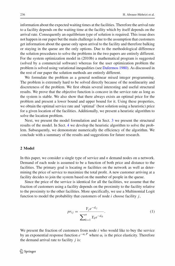
information about the expected waiting times at the facilities. Therefore the arrival rateto a facility depends on the waiting time at the facility which by itself depends on thearrival rate. Consequently an equilibrium type of solution is required. This issue doesnot happen in our paper but the main challenge is due to the assumption that customersget information about the queue only upon arrival to the facility and therefore balkingor staying in the queue are the only options. Due to the methodological differencethe solution procedures to solve the problems in the two papers are entirely different.For the system optimization model in (2010b) a mathematical program is suggested(solved by a commercial software) whereas for the user optimization problem theproblem is solved using variational inequalities (see Dafermos 1980). As discussed inthe rest of our paper the solution methods are entirely different.
We formulate the problem as a general nonlinear mixed integer programming.The problem is extremely hard to be solved directly because of the nonlinearity anddiscreteness of the problem. We first obtain several interesting and useful structuralresults. We prove that the objective function is concave in the service rate as long asthe system is stable. We also show that there always exists an optimal price for theproblem and present a lower bound and upper bound for it. Using these properties,we obtain the optimal service rate and ’optimal’ (best solution using a heuristic) pricefor a given location of the facilities. Additionally, we present a heuristic algorithm tosolve the location problem.
Next, we present the model formulation and in Sect. 3 we present the structuralresults of the model. In Sect. 4 we develop the heuristic algorithm to solve the prob-lem. Subsequently, we demonstrate numerically the efficiency of the algorithm. Weconclude with a summary of the results and suggestions for future research.
2 Model
In this paper, we consider a single type of service and n demand nodes on a network.Demand of each node is assumed to be a function of both price and distance to thefacilities. The primary goal is locating m facilities on the network as well as deter-mining the price of service to maximize the total profit. A new customer arriving at afacility decides to join the system based on the number of people in the queue.
Since the price of the service is identical for all the facilities, we assume that thefraction of customers using a facility depends on the proximity to the facility relativeto the proximity to the other facilities. More specifically, we use a Multinomial Logitfunction to model the probability that customers of node i choose facility j ,
pri j = Y j e−di j
∑n
k=1Yke−dik
. (1)
We present the fraction of customers from node i who would like to buy the serviceby an exponential response function e−αi P where αi is the price elasticity. Thereforethe demand arrival rate to facility j is:
123
Capacity, pricing and location 237
λ j =n∑
i=1
wi pri j e−αi P . (2)
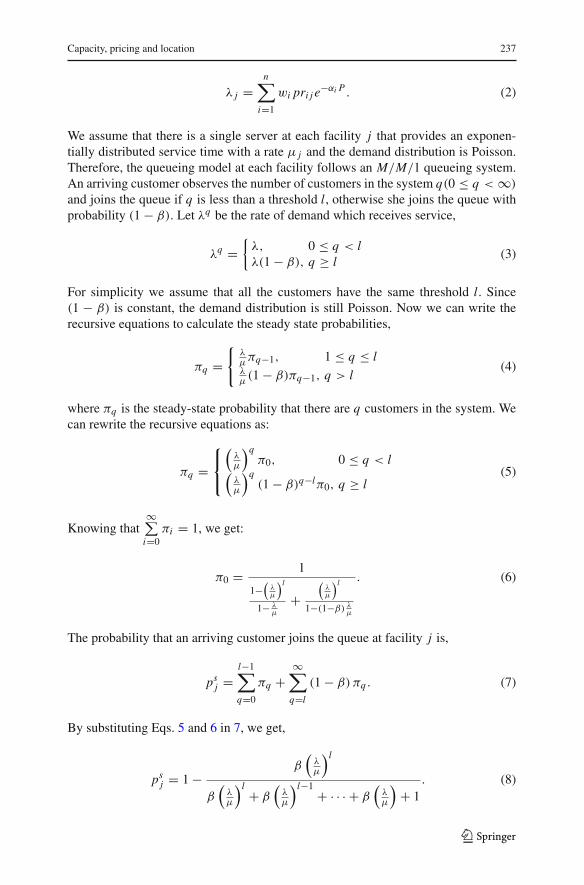
We assume that there is a single server at each facility j that provides an exponen-tially distributed service time with a rate μ j and the demand distribution is Poisson.Therefore, the queueing model at each facility follows an M/M/1 queueing system.An arriving customer observes the number of customers in the system q(0 ≤ q < ∞)
and joins the queue if q is less than a threshold l, otherwise she joins the queue withprobability (1 − β). Let λq be the rate of demand which receives service,
λq ={
λ, 0 ≤ q < lλ(1 − β), q ≥ l
(3)
For simplicity we assume that all the customers have the same threshold l. Since(1 − β) is constant, the demand distribution is still Poisson. Now we can write therecursive equations to calculate the steady state probabilities,
πq ={
λμπq−1, 1 ≤ q ≤ l
λμ(1 − β)πq−1, q > l
(4)
where πq is the steady-state probability that there are q customers in the system. Wecan rewrite the recursive equations as:
πq =⎧⎨
⎩
(λμ
)qπ0, 0 ≤ q < l
(λμ
)q(1 − β)q−lπ0, q ≥ l
(5)
Knowing that∞∑
i=0πi = 1, we get:
π0 = 1
1−(
λμ
)l
1− λμ
+(
λμ
)l
1−(1−β) λμ
. (6)
The probability that an arriving customer joins the queue at facility j is,
psj =
l−1∑
q=0
πq +∞∑
q=l
(1 − β) πq . (7)
By substituting Eqs. 5 and 6 in 7, we get,
psj = 1 −
β(
λμ
)l
β(
λμ
)l + β(
λμ
)l−1 + · · · + β(
λμ
)+ 1
. (8)
123

238 H. Abouee-Mehrizi et al.
Therefore we can formulate the problem as follows,
Max Z = ∑nj=1 Y j
((P − c) λ j ps
j −(
c jμμ j + c j
0
))(9)
pri j = Y j e−di j
∑nk=1 Yk e−dik
i, j = 1, . . . , n (10)
λ j = ∑ni=1 wi pri j e−αi P j = 1, . . . , n (11)
psj = 1 −
β
(λ jμ j
)l
β
(λ jμ j
)l
+β
(λ jμ j
)l−1
+···+β
(λ jμ j
)+1
j = 1, . . . , n (12)
μ j − λ j > 0 j = 1, . . . , n (13)∑n
j=1 Y j = m (14)
Y j ∈ {0, 1} , μ j , λ j ≥ 0 j = 1, . . . , n (15)
The objective function Eq. 9 is to maximize the profit. Constraints Eq. 13 ensure thestability of the queue whereas constraints Eq. 14 limits the number of open facilitiesto m.
3 Analytical results
In this section we demonstrate several properties of the model. We first consider theproblem of determining the optimal capacity of facilities given the price and locations.We show that the objective function is concave in the service rate. Then, we investigatethe optimal price given the service rates and locations.
3.1 Optimal service rate at each facility
In this section, we assume that the location of facilities and the price of the service areknown and study the structural properties of the optimal capacity. From Eq. 9,
Z =∑
j∈J
((P − c) λ j ps
j −(
c jμμ j − c j
0
)). (16)
where J is the set of the open facilities. Applying the first order condition we get foreach j ∈ J ,
∂ Z
∂μ j=
((P − c) λ j
∂psj
∂μ j− c j
μ
)= 0. (17)
123

Capacity, pricing and location 239
Therefore, the optimal service rate at each facility is determined by solving the fol-lowing equation,
∂psj
∂μ j= c j
μ
(P − c) λ j. (18)
In the next two lemmas, we obtain several mathematical properties that will be usedto investigate the structure of ps
j with respect to μ j . Proofs of results that are neededto obtain the main analytical results are provided in the Appendix A.
Lemma 1 For 0 ≤ x ≤ 1, we have,
(n + 1)
n∑
i=1
xi − 2n∑
i=1
i xi ≥ 0. (19)
Lemma 2 Suppose a ≥ 1 and n is a positive integer. Therefore, f (x) which is definedby Eq. 20 is always positive and increasing in x for 0 ≤ x ≤ 1.
f (x) = xn+1(xn−1 + 2xn−2 + 3xn−3 + · · · + (n − 1)x + na
)(xn + xn−1 + · · · + x + a
)2 . (20)
Theorem 1 psj is concave and increasing in μ j for λ j < μ j < ∞.
Proof Recall that β is a positive number between zero and one, and λ j is a positivenumber.
psj = 1 −
(λ jμ j
)l
(λ jμ j
)l +(
λ jμ j
)l−1 + · · · +(
λ jμ j
)+ 1
β
The derivative of psj with respect to μ j is,
dpsj
dμ j= λ j
(μ j
)2
(λ jμ j
)l−1((
λ jμ j
)l−1 + 2(
λ jμ j
)l−2 + · · · + (l − 1)(
λ jμ j
)+ l
β
)
((λ jμ j
)l +(
λ jμ j
)l−1 + · · · +(
λ jμ j
)+ 1
β
)2
= 1
λ j
(λ jμ j
)l+1((
λ jμ j
)l−1 + 2(
λ jμ j
)l−2 + · · · + (l − 1)(
λ jμ j
)+ l
β
)
((λ jμ j
)l +(
λ jμ j
)l−1 + · · · +(
λ jμ j
)+ 1
β
)2 (21)
Let us define x j = λ jμ j
and β = 1a . Then, Eq. 21 is positive in x j for 0 ≤ x j <
1 (λ j < μ j < ∞). Therefore, psj is increasing in μ j .
123
240 H. Abouee-Mehrizi et al.
To show the concavity of psj , we show that the second derivative of ps
j with respect
to μ j is negative. Let us define h(x j ) = dpsj
dμ j. Recall that x j = λ j
μ j, therefore
dh(x j )
dμ j= dx j
dμ j
dh(x j )
dx j.
Based on Lemma 2,dh(x j )
dx jis positive for 0 ≤ x j < 1 (λ j < μ j < ∞). Knowing
thatdx jdμ j
= − λ j
(μ j)2 is negative for λ j < μ j < ∞, we conclude that the second
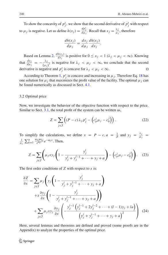
derivative is negative and psj is concave for λ j < μ j < ∞. ��
According to Theorem 1, psj is concave and increasing in μ j . Therefore Eq. 18 has
one solution for μ j that maximizes the profit value of the facility. The optimal μ j canbe found numerically as discussed in Sect. 4.1.
3.2 Optimal price
Now, we investigate the behavior of the objective function with respect to the price.Similar to Sect. 3.1, the total profit of the system can be written as,
Z =∑
j∈J
((P − c) λ j ps
j −(
c jμμ j − c j
0
)). (22)
To simplify the calculations, we define x = P − c, a = 1β
and y j = λ jμ j
=1
μ j
∑nk=1
wk prk jeαk c e−αk x . Then,
Z =∑
j∈J
(μ j xy j
(1 − yl
j
ylj + yl−1
j + · · · + y j + a
)−
(c jμμ j − c j
0
)). (23)
The first order conditions of Z with respect to x is:
∂ Z
∂x=
∑
j∈J
μ j
(y j
(1 − yl
j
ylj + yl−1
j + · · · + y j + a
)
+x∂y j
∂x
(1 − yl
j
ylj + yl−1
j + · · · + y j + a
))
+∑
j∈J
μ j xy j∂y j
∂x
⎛
⎜⎝−yl−1
j
(yl−1
j + 2yl−2j + · · · + (l − 1)y j + la
)
(yl
j + yl−1j + · · · + y j + a
)2
⎞
⎟⎠ (24)
Here, several lemmas and theorems are defined and proved (some proofs are in theAppendix) to analyze the properties of the optimal price.
123
Capacity, pricing and location 241
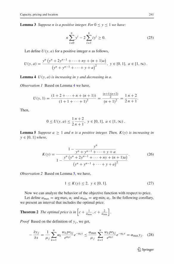
Lemma 3 Suppose n is a positive integer. For 0 ≤ y ≤ 1 we have:
nn∑
i=0
yi − 2n∑
i=1
iyi ≥ 0. (25)
Let define U (y, a) for a positive integer n as follows,
U (y, a) = yn(yn + 2yn−1 + · · · + ny + (n + 1)a
)(yn + yn−1 + · · · + y + a
)2 , y ∈ [0, 1], a ∈ [1,∞) .
Lemma 4 U (y, a) is increasing in y and decreasing in a.
Observation 1 Based on Lemma 4 we have,
U (y, 1) = (1 + 2 + · · · + n + (n + 1))
(1 + 1 + · · · + 1)2 =(n+1)(n+2)
2
(n + 1)2 = 1
2
n + 2
n + 1.
Then,
0 ≤ U (y, a) ≤ 1
2
n + 2
n + 1, y ∈ [0, 1], a ∈ [1,∞) .
Lemma 5 Suppose a ≥ 1 and n is a positive integer. Then, K (y) is increasing iny ∈ [0, 1] where,
K (y) =1 − yn
yn + yn−1 + · · · + y + a
1 − yn(yn + 2yn−1 + · · · + ny + (n + 1)a
)(yn + yn−1 + · · · + y + a
)2
. (26)
Observation 2 Based on Lemma 5, we have,
1 ≤ K (y) ≤ 2, y ∈ [0, 1]. (27)
Now we can analyze the behavior of the objective function with respect to price.Let define αmax = arg maxi αi and αmin = arg mini αi . In the following corollary,
we present an interval that includes the optimal price.
Theorem 2 The optimal price is in[c + 1
αmax, c + 2
αmin
].
Proof Based on the definition of y j , we get,
− ∂y j
∂x= 1
μ j
n∑
k=1
αkwk prk j
eαk ce−αk x ≤ αmax
μ j
n∑
k=1
wk prk j
eαk ce−αk x = αmax y j . (28)
123

242 H. Abouee-Mehrizi et al.
Similarly,
− ∂y j
∂x= 1
μ j
n∑
k=1
αkwk prk j
eαk ce−αk x ≥ αmin
μ j
n∑
k=1
wk prk j
eαk ce−αk x = αmin y j . (29)
Consider Eq. 24. Then:
∂ Z
∂x= 0 ⇒ x =
∑j∈J μ j y j
(1 − yl
j
ylj +yl−1
j +···+y j +a
)
−∑j∈J μ j
∂y j∂x
(1 − yl
j
(yl
j +2yl−1j +···+ly j +(l+1)a
)
(yl
j +yl−1j +···+y j +a
)2
) . (30)
Using Eq. 28 and 29 we get,
∑j∈J μ j y j
(1 − yl
j
ylj +yl−1
j +···+y j +a
)
αmax∑
j∈J μ j y j
(1 − yl
j
(yl
j +2yl−1j +···+ly j +(l+1)a
)
(yl
j +yl−1j +···+y j +a
)2
)
≤∑
j∈J μ j y j
(1 − yl
j
ylj +yl−1
j +···+y j +a
)
−∑j∈J μ j
∂y j∂x
(1 − yl
j
(yl
j +2yl−1j +···+ly j +(l+1)a
)
(yl
j +yl−1j +···+y j +a
)2
)
≤∑
j∈J μ j y j
(1 − yl
j
ylj +yl−1
j +···+y j +a
)
αmin∑
j∈J μ j y j
(1 − yl
j
(yl
j +2yl−1j +···+ly j +(l+1)a
)
(yl
j +yl−1j +···+y j +a
)2
) (31)
Recalling the definition of K (y) in Eq. 26, based on Observation 2 we have,
1 ≤μ j y j
(1 − yl
j
ylj +yl−1
j +···+y j +a
)
μ j y j
(1 − yl
j
(yl
j +2yl−1j +···+ly j +(l+1)a
)
(yl
j +yl−1j +···+y j +a
)2
) ≤ 2.
Since minnanbn
≤∑
n an∑n bn
≤ maxnanbn
if minnanbn
≥ 0, then,
1
αmax≤
∑j∈J μ j y j
(1 − yl
j
ylj +yl−1
j +···+y j +a
)
−∑j∈J μ j
∂y j∂x
(1 − yl
j
(yl
j +2yl−1j +···+ly j +(l+1)a
)
(yl
j +yl−1j +···+y j +a
)2
) ≤ 2
αmin. (32)
123
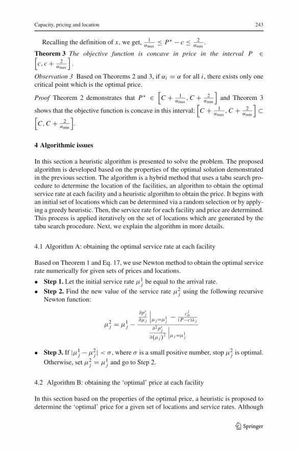
Capacity, pricing and location 243
Recalling the definition of x , we get, 1αmax
≤ P∗ − c ≤ 2αmin
.
Theorem 3 The objective function is concave in price in the interval P ∈[c, c + 2
αmax
].
Observation 3 Based on Theorems 2 and 3, if αi = α for all i , there exists only onecritical point which is the optimal price.
Proof Theorem 2 demonstrates that P∗ ∈[C + 1
αmax, C + 2
αmin
]and Theorem 3
shows that the objective function is concave in this interval:[C + 1
αmax, C + 2
αmin
]⊂
[C, C + 2
αmin
].
4 Algorithmic issues
In this section a heuristic algorithm is presented to solve the problem. The proposedalgorithm is developed based on the properties of the optimal solution demonstratedin the previous section. The algorithm is a hybrid method that uses a tabu search pro-cedure to determine the location of the facilities, an algorithm to obtain the optimalservice rate at each facility and a heuristic algorithm to obtain the price. It begins withan initial set of locations which can be determined via a random selection or by apply-ing a greedy heuristic. Then, the service rate for each facility and price are determined.This process is applied iteratively on the set of locations which are generated by thetabu search procedure. Next, we explain the algorithm in more details.
4.1 Algorithm A: obtaining the optimal service rate at each facility
Based on Theorem 1 and Eq. 17, we use Newton method to obtain the optimal servicerate numerically for given sets of prices and locations.
• Step 1. Let the initial service rate μ1j be equal to the arrival rate.
• Step 2. Find the new value of the service rate μ2j using the following recursive
Newton function:
μ2j = μ1
j −∂ps
j∂μ j
∣∣∣μ j =μ1j
− c jμ
(P−c)λ j
∂2 psj
∂(μ j)2
∣∣∣μ j =μ1j
• Step 3. If |μ1j − μ2
j | < σ , where σ is a small positive number, stop μ2j is optimal.
Otherwise, set μ2j = μ1
j and go to Step 2.
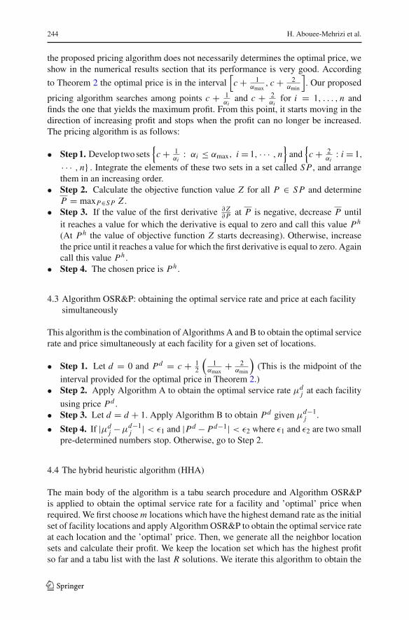
4.2 Algorithm B: obtaining the ‘optimal’ price at each facility
In this section based on the properties of the optimal price, a heuristic is proposed todetermine the ‘optimal’ price for a given set of locations and service rates. Although
123
244 H. Abouee-Mehrizi et al.
the proposed pricing algorithm does not necessarily determines the optimal price, weshow in the numerical results section that its performance is very good. According
to Theorem 2 the optimal price is in the interval[c + 1
αmax, c + 2
αmin
]. Our proposed
pricing algorithm searches among points c + 1αi
and c + 2αi
for i = 1, . . . , n andfinds the one that yields the maximum profit. From this point, it starts moving in thedirection of increasing profit and stops when the profit can no longer be increased.The pricing algorithm is as follows:
• Step 1. Develop two sets{
c + 1αi
: αi ≤ αmax, i = 1, · · · , n}
and{
c + 2αi
: i = 1,
· · · , n} . Integrate the elements of these two sets in a set called S P , and arrangethem in an increasing order.
• Step 2. Calculate the objective function value Z for all P ∈ S P and determineP = maxP∈S P Z .
• Step 3. If the value of the first derivative ∂ Z∂ P at P is negative, decrease P until
it reaches a value for which the derivative is equal to zero and call this value Ph
(At Ph the value of objective function Z starts decreasing). Otherwise, increasethe price until it reaches a value for which the first derivative is equal to zero. Againcall this value Ph .
• Step 4. The chosen price is Ph .
4.3 Algorithm OSR&P: obtaining the optimal service rate and price at each facilitysimultaneously
This algorithm is the combination of Algorithms A and B to obtain the optimal servicerate and price simultaneously at each facility for a given set of locations.
• Step 1. Let d = 0 and Pd = c + 12
(1
αmax+ 2
αmin
)(This is the midpoint of the
interval provided for the optimal price in Theorem 2.)• Step 2. Apply Algorithm A to obtain the optimal service rate μd
j at each facility
using price Pd .• Step 3. Let d = d + 1. Apply Algorithm B to obtain Pd given μd−1
j .
• Step 4. If |μdj −μd−1
j | < ε1 and |Pd − Pd−1| < ε2 where ε1 and ε2 are two smallpre-determined numbers stop. Otherwise, go to Step 2.
4.4 The hybrid heuristic algorithm (HHA)
The main body of the algorithm is a tabu search procedure and Algorithm OSR&Pis applied to obtain the optimal service rate for a facility and ’optimal’ price whenrequired. We first choose m locations which have the highest demand rate as the initialset of facility locations and apply Algorithm OSR&P to obtain the optimal service rateat each location and the ’optimal’ price. Then, we generate all the neighbor locationsets and calculate their profit. We keep the location set which has the highest profitso far and a tabu list with the last R solutions. We iterate this algorithm to obtain the
123
Capacity, pricing and location 245
optimal locations with the constraint that the new solution should not be in the tabulist. (see Berman and Drezner 2006, for the details of the tabu search procedure.)
5 Numerical results
We first investigate the performance of HHA. We demonstrate numerically that theaccuracy and efficiency of our algorithm are quite good. Then, we investigate thesensitivity of the optimal profit to the queue length threshold l and the balkingprobability β.
5.1 Accuracy of the algorithm
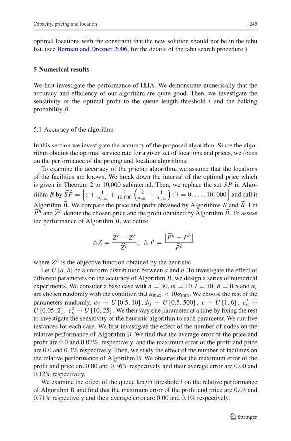
In this section we investigate the accuracy of the proposed algorithm. Since the algo-rithm obtains the optimal service rate for a given set of locations and prices, we focuson the performance of the pricing and location algorithms.
To examine the accuracy of the pricing algorithm, we assume that the locationsof the facilities are known. We break down the interval of the optimal price whichis given in Theorem 2 to 10,000 subinterval. Then, we replace the set S P in Algo-
rithm B by S̃ P ={
c + 1αmax
+ i10,000
(2
αmin− 1
αmax
): i = 0, . . . , 10, 000
}and call it
Algorithm B̃. We compare the price and profit obtained by Algorithms B and B̃. LetP̃h and Z̃ h denote the chosen price and the profit obtained by Algorithm B̃. To assessthe performance of Algorithm B, we define
�Z = Z̃ h − Zh
Z̃h, � P =
∣∣P̃h − Ph∣∣
P̃h
where Zh is the objective function obtained by the heuristic.Let U [a, b] be a uniform distribution between a and b. To investigate the effect of
different parameters on the accuracy of Algorithm B, we design a series of numericalexperiments. We consider a base case with n = 30, m = 10, l = 10, β = 0.5 and αi
are chosen randomly with the condition that αmax < 10αmin. We choose the rest of theparameters randomly, wi ∼ U [0.5, 10] , di j ∼ U [0.5, 500] , c ∼ U [1, 6] , c j
μ ∼U [0.05, 2] , c0
μ ∼ U [10, 25] . We then vary one parameter at a time by fixing the restto investigate the sensitivity of the heuristic algorithm to each parameter. We run fiveinstances for each case. We first investigate the effect of the number of nodes on therelative performance of Algorithm B. We find that the average error of the price andprofit are 0.0 and 0.07%, respectively, and the maximum error of the profit and priceare 0.0 and 0.3% respectively. Then, we study the effect of the number of facilities onthe relative performance of Algorithm B. We observe that the maximum error of theprofit and price are 0.00 and 0.36% respectively and their average error are 0.00 and0.12% respectively.
We examine the effect of the queue length threshold l on the relative performanceof Algorithm B and find that the maximum error of the profit and price are 0.03 and0.71% respectively and their average error are 0.00 and 0.1% respectively.
123
246 H. Abouee-Mehrizi et al.
Table 1 The performance of Algorithm HHA
m �Z H M m �Z H M l �Z H M l �Z H M β �Z H M β �Z H M
1 0.000 10 0.000 1 0.002 15 0.000 0 0.001 0.5 0.000
0.000 0.002 0.010 0.002 0.002 0.000
0.000 0.000 0.002 0.000 0.000 0.000
0.000 0.000 0.005 0.001 0.001 0.000
0.000 0.002 0.001 0.000 0.001 0.000
2 0.000 12 0.001 2 0.001 20 0.000 0.1 0.001 0.6 0.000
0.003 0.000 0.006 0.002 0.002 0.000
0.000 0.000 0.001 0.000 0.000 0.000
0.000 0.001 0.003 0.001 0.002 0.000
0.000 0.001 0.001 0.000 0.002 0.000
3 0.000 15 0.002 5 0.001 25 0.000 0.2 0.001 0.8 0.000
0.002 0.001 0.003 0.002 0.002 0.000
0.000 0.000 0.001 0.000 0.000 0.000
0.000 0.000 0.002 0.001 0.002 0.000
0.000 0.000 0.000 0.000 0.002 0.000
5 0.003 18 0.000 7 0.000 30 0.000 0.3 0.001 0.9 0.000
0.002 0.000 0.003 0.002 0.002 0.000
0.000 0.000 0.000 0.000 0.000 0.000
0.000 0.000 0.001 0.001 0.002 0.000
0.000 0.000 0.000 0.000 0.002 0.000
7 0.000 20 0.000 10 0.000 40 0.000 0.4 0.001 1 0.000
0.002 0.000 0.002 0.002 0.002 0.000
0.000 0.000 0.000 0.000 0.000 0.000
0.002 0.000 0.001 0.001 0.002 0.000
0.001 0.000 0.000 0.000 0.002 0.000
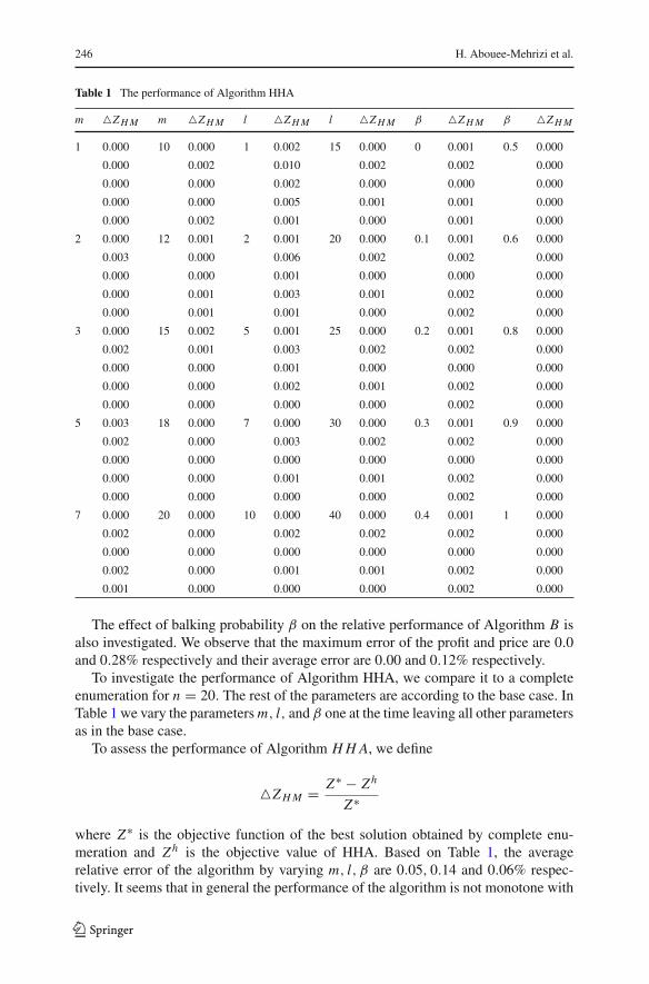
The effect of balking probability β on the relative performance of Algorithm B isalso investigated. We observe that the maximum error of the profit and price are 0.0and 0.28% respectively and their average error are 0.00 and 0.12% respectively.
To investigate the performance of Algorithm HHA, we compare it to a completeenumeration for n = 20. The rest of the parameters are according to the base case. InTable 1 we vary the parameters m, l, and β one at the time leaving all other parametersas in the base case.
To assess the performance of Algorithm H H A, we define
�Z H M = Z∗ − Zh
Z∗
where Z∗ is the objective function of the best solution obtained by complete enu-meration and Zh is the objective value of HHA. Based on Table 1, the averagerelative error of the algorithm by varying m, l, β are 0.05, 0.14 and 0.06% respec-tively. It seems that in general the performance of the algorithm is not monotone with
123
Capacity, pricing and location 247
Table 2 Effects of β and l on the profit
β Prof i t Prof i t Prof i t Prof i t Prof i t(l = 1) (l = 5) (l = 10) (l = 15) (l = 20)
0 13,25,085 13,25,085 13,25,085 13,25,085 13,25,085
0.1 13,06,087 13,23,106 13,24,390 13,24,759 13,24,932
0.2 12,97,730 13,22,714 13,24,270 13,24,694 13,24,890
0.3 12,91,366 13,22,472 13,24,199 13,24,661 13,24,871
0.4 12,86,029 13,22,295 13,24,152 13,24,638 13,24,857
0.5 12,81,354 13,22,156 13,24,118 13,24,620 13,24,847
0.6 12,77,144 13,22,042 13,24,089 13,24,608 13,24,839
0.7 12,73,288 13,21,945 13,24,066 13,24,599 13,24,833
0.8 12,69,714 13,21,864 13,24,049 13,24,590 13,24,829
0.9 12,66,366 13,21,790 13,24,032 13,24,584 13,24,826
1 12,63,213 13,21,725 13,24,020 13,24,578 13,24,821
respect to m. The relative error of the algorithm first increases when m increases tillit reaches some threshold, and then it starts decreasing. However, it seems that therelative error of Algorithm HHA remains the same when increasing l, and decreaseswhen β increases.
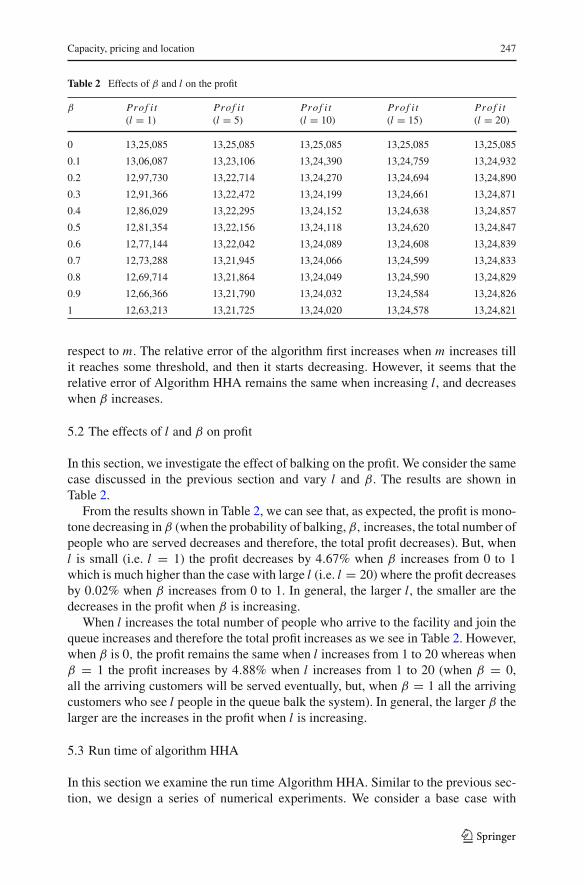
5.2 The effects of l and β on profit
In this section, we investigate the effect of balking on the profit. We consider the samecase discussed in the previous section and vary l and β. The results are shown inTable 2.
From the results shown in Table 2, we can see that, as expected, the profit is mono-tone decreasing in β (when the probability of balking, β, increases, the total number ofpeople who are served decreases and therefore, the total profit decreases). But, whenl is small (i.e. l = 1) the profit decreases by 4.67% when β increases from 0 to 1which is much higher than the case with large l (i.e. l = 20) where the profit decreasesby 0.02% when β increases from 0 to 1. In general, the larger l, the smaller are thedecreases in the profit when β is increasing.
When l increases the total number of people who arrive to the facility and join thequeue increases and therefore the total profit increases as we see in Table 2. However,when β is 0, the profit remains the same when l increases from 1 to 20 whereas whenβ = 1 the profit increases by 4.88% when l increases from 1 to 20 (when β = 0,all the arriving customers will be served eventually, but, when β = 1 all the arrivingcustomers who see l people in the queue balk the system). In general, the larger β thelarger are the increases in the profit when l is increasing.
5.3 Run time of algorithm HHA
In this section we examine the run time Algorithm HHA. Similar to the previous sec-tion, we design a series of numerical experiments. We consider a base case with
123

248 H. Abouee-Mehrizi et al.
Table 3 The effects of different parameters on time (seconds)
n T ime n T ime m T ime m T ime l T ime l T ime B T ime B T ime
10 0.03 50 15.74 1 0.72 12 3.31 1 2.59 15 2.68 0 5.19 0.5 5.23
0.03 7.30 0.62 3.90 4.06 6.46 2.54 2.61
0.06 3.34 0.72 2.45 3.34 4.54 3.49 3.42
0.02 10.41 0.52 7.40 2.39 2.50 6.61 6.35
0.03 5.13 0.56 3.85 3.51 7.00 2.14 2.12
15 0.31 75 27.97 2 0.97 15 3.96 2 2.73 20 2.76 0.1 5.21 0.6 5.23
0.31 14.34 0.92 7.57 4.04 7.04 2.54 2.57
0.30 17.72 1.33 6.54 4.24 4.66 3.43 3.42
0.39 18.19 0.58 6.58 2.32 2.40 6.33 6.35
0.16 24.59 0.97 2.65 3.73 7.49 2.11 2.14
20 0.70 100 46.61 5 2.28 20 15.68 5 2.71 25 2.73 0.2 5.24 0.8 5.23
0.53 113.79 2.26 6.57 4.28 8.46 2.54 2.89
0.89 26.33 2.03 3.73 4.21 4.77 3.39 3.42
0.55 21.29 0.75 2.84 2.28 2.39 6.32 6.32
0.55 44.90 0.92 8.55 5.27 7.49 2.12 2.14
30 1.40 150 90.81 7 2.53 25 10.39 7 2.62 30 2.96 0.3 5.24 0.9 5.24
0.91 148.45 2.09 13.14 4.73 9.39 2.54 2.61
0.47 123.53 29.73 14.17 4.34 4.84 3.40 3.42
1.70 116.33 1.64 6.66 2.25 2.39 6.35 6.33
1.06 238.35 4.48 5.54 5.32 9.38 2.12 2.17
40 4.04 200 242.01 10 2.84 30 17.29 10 2.67 40 3.26 0.4 5.23 1 5.21
2.87 357.54 4.06 9.75 5.45 11.61 2.54 2.53
2.17 223.47 2.84 24.24 4.43 4.93 3.42 3.42
2.37 290.08 1.65 14.90 2.39 2.54 6.36 6.57
1.67 457.38 2.32 11.30 5.35 9.91 2.15 2.12
n = 50, m = 10, l = 10, β = 0.5 and αi are chosen randomly with condi-tion that αmax < 10αmin. We choose the rest of the parameters randomly, wi ∼U [0.5, 10] , di j ∼ U [0.5, 500] , c ∼ U [1, 6] , c j
μ ∼ U [0.05, 2] , c0μ ∼ U [10, 25] .
We then vary one parameter at a time. We present the results in Table 3. (The times aregiven in seconds.) Table 3 shows that when the number of nodes (n) or facilities (m)increases, the CPU time for running the heuristic obviously increases; but, even with200 nodes the running time is reasonable. The CPU time remains almost the samewhen l and β change.
6 Summary and suggestions for future research
We presented the problem of making concurrent decisions on location, service capac-ity and price for multiple facilities on a network providing a single type of service.Demand of each node follows a Poisson process and service times at each facilityare assumed to be exponentially distributed. We developed a heuristic to obtain the
123
Capacity, pricing and location 249
optimal capacity and the ’optimal’ price at each facility as well as the locations ofthe facilities. We showed that balking which has been ignored in the literature affectsthe profit and decisions of the system. When the balking rate of the system is relativelyhigh and the arriving customers to that system are impatient (leave the system even ifthe number of people in the queue is low) the rate of losing the profit could be veryhigh. But, if the customers are patient, this rate is relatively low.
This problem can be extended in several ways: (1) One potential extension is torelax the uniform pricing assumption and obtain the optimal price at each facility. Inthis case the customer decision to choose a facility should depend not only on theproximity to the facility but also on the price charged by the facility. (2) A potentialinteresting problem is to assume that the facilities are managed by different firms.Then, the competition between facilities should be considered. (3) Another directionis to consider the possibility that customers observing the queue length may renegeafter joining the queue at a facility. (4) A related problem is to study the problem whencustomers may renege after joining the queue even though they cannot see the numberof people in front of them in the line.
Appendix
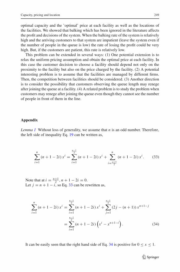
Lemma 1 Without loss of generality, we assume that n is an odd number. Therefore,the left side of inequality Eq. 19 can be written as,
n∑
i=1
(n + 1 − 2i) xi =n−1
2∑
i=1
(n + 1 − 2i) xi +n∑
i= n+32
(n + 1 − 2i) xi . (33)
Note that at i = n+12 , n + 1 − 2i = 0.
Let j = n + 1 − i , so Eq. 33 can be rewritten as,
n∑
i=1
(n + 1 − 2i) xi =n−1
2∑
i=1
(n + 1 − 2i) xi +n−1
2∑
j=1
(2 j − (n + 1)) xn+1− j
=n−1
2∑
i=1
(n + 1 − 2i)(
xi − xn+1−i)
. (34)
It can be easily seen that the right hand side of Eq. 34 is positive for 0 ≤ x ≤ 1.
123

250 H. Abouee-Mehrizi et al.
Lemma 2 Observe that f (x) is positive. To prove that f (x) is increasing in x , thederivative of f (x) with respect to x is determined and it is shown to be positive forany 0 ≤ x ≤ 1.
d f (x)
dx=
(n + 1) xn(
xn−1 + 2xn−2 + 3xn−3 + · · · + (n − 1)x + na)
(xn + xn−1 + · · · + x + a
)2
+xn+1
((n − 1)xn−2 + 2(n − 2)xn−3 + 3(n − 3)xn−4 + · · · + 2(n − 2)x + (n − 1)
)
(xn + xn−1 + · · · + x + a
)2
−2xn+1
(xn−1 + 2xn−2 + 3xn−3 + · · · + (n − 1)x + na
) (nxn−1 + (n − 1)xn−2 + · · · + 2x + 1
)
(xn + xn−1 + · · · + x + a
)3
(35)
d f (x)dx contains three terms of which the first and second ones are positive, but the third
is negative. We show that the summation of the first and the third terms is positiveand therefore the derivative of f (x) with respect to x is positive. Let g(x) denotes thesummation of the first and the third terms in the above equation.
g(x) =(n + 1) xn
(xn−1 + 2xn−2 + 3xn−3 + · · · + (n − 1)x + na
)
(xn + xn−1 + · · · + x + a
)2
−2xn+1
(xn−1 + 2xn−2 + 3xn−3 + · · · + (n − 1)x + na
) (nxn−1 + (n − 1)xn−2 + · · · + 2x + 1
)
(xn + xn−1 + · · · + x + a
)3
(36)
We can rewrite g(x) as a product of the two terms, g1(x) and g2(x),
g(x) = xn(xn−1 + 2xn−2 + 3xn−3 + · · · + (n − 1)x + na
)(xn + xn−1 + · · · + x + a
)2
((n + 1) − 2
(nxn + (n − 1)xn−1 + · · · + 2x2 + x
)(xn + xn−1 + · · · + x + a
))
.
Since the first term, g1(x), is positive for 0 ≤ x ≤ 1, we have to show that thesecond term g2(x) is also positive. We can rewrite g2(x) as,
g2(x) = (n + 1) − 2∑n
i=1 i xi
a + ∑ni=1 xi
> (n + 1) − 2∑n
i=1 i xi∑n
i=1 xi
By Lemma 1, we see that g2(x) is also positive. Therefore, d f (x)dx is positive and
f (x) is increasing in x for 0 ≤ x ≤ 1.
123

Capacity, pricing and location 251
Lemma 3 Without loss of generality, we assume that n is an odd number. Therefore,the left side of inequality Eq. 25 can be separated as,
nn∑
i=0
yi − 2n∑
i=1
iyi = n +n∑
i=1
(n − 2i) yi
= n +n−1
2∑
i=1
(n − 2i) yi +n∑
i= n+12
(n − 2i) yi . (37)
Denoting j = n − i , Eq. 37 can be rewritten as,
n +n∑
i=1
(n − 2i) yi =⎛
⎜⎝n +n−1
2∑
i=1
(n − 2i) yi
⎞
⎟⎠ +n−1
2∑
j=1
(2 j − n) yn− j
=n−1
2∑
i=1
(n − 2i)(
yi − yn−i)
.
It is clear that the term inside the summation is always positive for 0 ≤ y ≤ 1.Therefore the inequality Eq. 25 always holds.
Lemma 4
∂U (y, a)
∂a=
yn(n + 1)(yn + yn−1 + · · · + y + a
) − 2yn(yn + 2yn−1 + · · · + ny + (n + 1)a
)(yn + yn−1 + · · · + y + a
)3
= yn
(∑ni=1 yi + a
)3
(−(n + 1)a +
n∑
i=1
(2i − (n + 1)) yi
)
Based on Lemma 1, we have∑n
i=1 (2i − (n + 1)) yi ≤ 0. Therefore, ∂U (y,a)∂a ≤ 0
and U (y, a) is decreasing in a.
∂U (y, a)
∂y= nyn−1
(yn + 2yn−1 + · · · + ny + (n + 1)a
)(yn + yn−1 + · · · + y + a
)2
+ yn(nyn−1 + 2(n − 1)yn−2 + · · · + n
)(yn + yn−1 + · · · + y + a
)2
−2yn(yn + 2yn−1 + · · · + ny + (n + 1)a
) (nyn−1 + (n − 1)yn−2 + · · · + 1
)(yn + yn−1 + · · · + y + a
)3 .
123
252 H. Abouee-Mehrizi et al.
Similar to the proof of Lemma 2, we can see that ∂U (y,a)∂y ≥ 0 and U (y, a) is
increasing in y. The only difference is that in this case we have to use Lemma 3instead of Lemma 1.
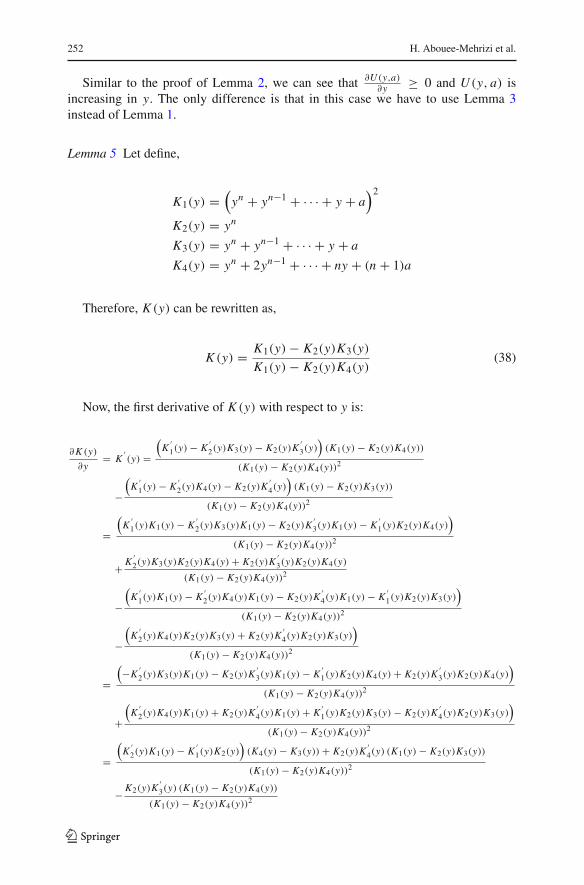
Lemma 5 Let define,
K1(y) =(
yn + yn−1 + · · · + y + a)2
K2(y) = yn
K3(y) = yn + yn−1 + · · · + y + a
K4(y) = yn + 2yn−1 + · · · + ny + (n + 1)a
Therefore, K (y) can be rewritten as,
K (y) = K1(y) − K2(y)K3(y)
K1(y) − K2(y)K4(y)(38)
Now, the first derivative of K (y) with respect to y is:
∂K (y)
∂y= K
′(y) =
(K
′1(y) − K
′2(y)K3(y) − K2(y)K
′3(y)
)(K1(y) − K2(y)K4(y))
(K1(y) − K2(y)K4(y))2
−(
K′1(y) − K
′2(y)K4(y) − K2(y)K
′4(y)
)(K1(y) − K2(y)K3(y))
(K1(y) − K2(y)K4(y))2
=(
K′1(y)K1(y) − K
′2(y)K3(y)K1(y) − K2(y)K
′3(y)K1(y) − K
′1(y)K2(y)K4(y)
)
(K1(y) − K2(y)K4(y))2
+ K′2(y)K3(y)K2(y)K4(y) + K2(y)K
′3(y)K2(y)K4(y)
(K1(y) − K2(y)K4(y))2
−(
K′1(y)K1(y) − K
′2(y)K4(y)K1(y) − K2(y)K
′4(y)K1(y) − K
′1(y)K2(y)K3(y)
)
(K1(y) − K2(y)K4(y))2
−(
K′2(y)K4(y)K2(y)K3(y) + K2(y)K
′4(y)K2(y)K3(y)
)
(K1(y) − K2(y)K4(y))2
=(−K
′2(y)K3(y)K1(y) − K2(y)K
′3(y)K1(y) − K
′1(y)K2(y)K4(y) + K2(y)K
′3(y)K2(y)K4(y)
)
(K1(y) − K2(y)K4(y))2
+(
K′2(y)K4(y)K1(y) + K2(y)K
′4(y)K1(y) + K
′1(y)K2(y)K3(y) − K2(y)K
′4(y)K2(y)K3(y)
)
(K1(y) − K2(y)K4(y))2
=(
K′2(y)K1(y) − K
′1(y)K2(y)
)(K4(y) − K3(y)) + K2(y)K
′4(y) (K1(y) − K2(y)K3(y))
(K1(y) − K2(y)K4(y))2
− K2(y)K′3(y) (K1(y) − K2(y)K4(y))
(K1(y) − K2(y)K4(y))2
123
Capacity, pricing and location 253
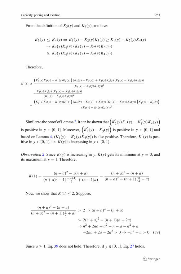
From the definition of K3(y) and K4(y), we have:
K3(y) ≤ K4(y) ⇒ K1(y) − K2(y)K3(y) ≥ K1(y) − K2(y)K4(y)
⇒ K2(y)K′4(y) (K1(y) − K2(y)K3(y))
≥ K2(y)K′4(y) (K1(y) − K2(y)K4(y))
Therefore,
K′(y) ≥
(K
′2(y)K1(y) − K
′1(y)K2(y)
)(K4(y) − K3(y)) + K2(y)K
′4(y) (K1(y) − K2(y)K4(y))
(K1(y) − K2(y)K4(y))2
− K2(y)K′3(y) (K1(y) − K2(y)K4(y))
(K1(y) − K2(y)K4(y))2
=(
K′2(y)K1(y) − K
′1(y)K2(y)
)(K4(y) − K3(y)) + K2(y) (K1(y) − K2(y)K4(y))
(K
′4(y) − K
′3(y)
)
(K1(y) − K2(y)K4(y))2
Similar to the proof of Lemma 2, it can be shown that(
K′2(y)K1(y) − K
′1(y)K2(y)
)
is positive in y ∈ [0, 1]. Moreover,(
K′4(y) − K
′3(y)
)is positive in y ∈ [0, 1] and
based on Lemma 4, (K1(y) − K2(y)K4(y)) is also positive. Therefore, K′(y) is pos-
itive in y ∈ [0, 1], i.e. K (y) is increasing in y ∈ [0, 1].
Observation 2 Since K (y) is increasing in y, K (y) gets its minimum at y = 0, andits maximum at y = 1. Therefore,
K (1) = (n + a)2 − 1(n + a)
(n + a)2 − 1(n(n+1)
2 + (n + 1)a)= (n + a)2 − (n + a)
(n + a)2 − (n + 1)( n2 + a)
Now, we show that K (1) ≤ 2. Suppose,
(n + a)2 − (n + a)
(n + a)2 − (n + 1)( n2 + a)
> 2 ⇒ (n + a)2 − (n + a)
> 2(n + a)2 − (n + 1)(n + 2a)
⇒ n2 + 2na + a2 − n − a − n2 + n
−2na + 2a − 2a2 > 0 ⇒ −a2 + a > 0. (39)
Since a ≥ 1, Eq. 39 does not hold. Therefore, if y ∈ [0, 1], Eq. 27 holds.
123
254 H. Abouee-Mehrizi et al.
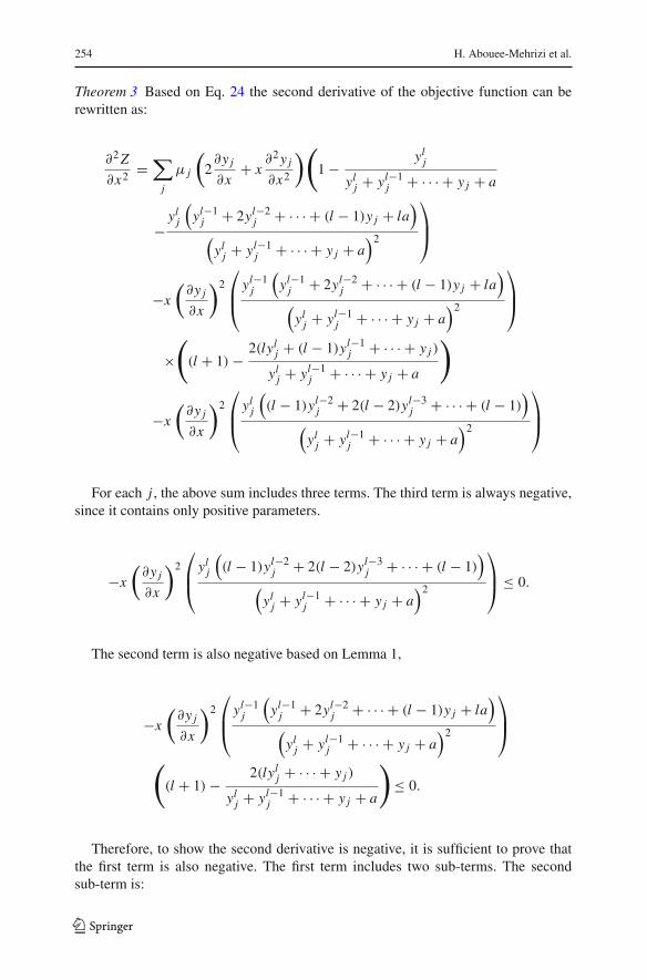
Theorem 3 Based on Eq. 24 the second derivative of the objective function can berewritten as:
∂2 Z
∂x2 =∑
j
μ j
(2∂y j
∂x+ x
∂2 y j
∂x2
) (1 − yl
j
ylj + yl−1
j + · · · + y j + a
−yl
j
(yl−1
j + 2yl−2j + · · · + (l − 1)y j + la
)
(yl
j + yl−1j + · · · + y j + a
)2
⎞
⎟⎠
−x
(∂y j
∂x
)2
⎛
⎜⎝yl−1
j
(yl−1
j + 2yl−2j + · · · + (l − 1)y j + la
)
(yl
j + yl−1j + · · · + y j + a
)2
⎞
⎟⎠
×(
(l + 1) − 2(lylj + (l − 1)yl−1
j + · · · + y j )
ylj + yl−1
j + · · · + y j + a
)
−x
(∂y j
∂x
)2
⎛
⎜⎝yl
j
((l − 1)yl−2
j + 2(l − 2)yl−3j + · · · + (l − 1)
)
(yl
j + yl−1j + · · · + y j + a
)2
⎞
⎟⎠
For each j , the above sum includes three terms. The third term is always negative,since it contains only positive parameters.
−x
(∂y j
∂x
)2
⎛
⎜⎝yl
j
((l − 1)yl−2
j + 2(l − 2)yl−3j + · · · + (l − 1)
)
(yl
j + yl−1j + · · · + y j + a
)2
⎞
⎟⎠ ≤ 0.
The second term is also negative based on Lemma 1,
−x
(∂y j
∂x
)2
⎛
⎜⎝yl−1
j
(yl−1
j + 2yl−2j + · · · + (l − 1)y j + la
)
(yl
j + yl−1j + · · · + y j + a
)2
⎞
⎟⎠
((l + 1) − 2(lyl
j + · · · + y j )
ylj + yl−1
j + · · · + y j + a
)≤ 0.
Therefore, to show the second derivative is negative, it is sufficient to prove thatthe first term is also negative. The first term includes two sub-terms. The secondsub-term is:
123

Capacity, pricing and location 255
1 − ylj
ylj + yl−1
j + · · · + y j + a−
ylj
(yl−1
j + 2yl−2j + · · · + (l − 1)y j + la
)
(yl
j + yl−1j + · · · + y j + a
)2
= 1 −yl
j
(yl
j + 2yl−1j + · · · + ly j + (l + 1)a
)
(yl
j + yl−1j + · · · + y j + a
)2 (40)
Based on Observation 1, the second sub-term is always in interval[
l2(l+1)
, 1],
which means that it is positive. Now consider the first sub-term. The second derivativeof the objective function is negative, i.e. the objective function is concave in price if∂2 y∂x2 ≤ 2
x
(− ∂y
∂x
). But,
∂2 y j
∂x2 = 1
μ j
n∑
k=1
(αk)2 wk prk j
eαk ce−αk x ≤ αmax
μ j
n∑
k=1
αkwk prk j
eαk ce−αk x = αmax
(−∂y j
∂x
).
Therefore, the objective function is concave for αmax ≤ 2x or x ≤ 2
αmax.
References
Aboolian R, Berman O, Drezner Z (2008) Location-allocation of service units on a congested network. IIETrans 40:112
Aboolian R, Berman O, Krass D (2008) Optimizing pricing and location decisions for competitive servicefacilities charging uniform price. J Oper Res Soc 59:1506–1519
Berman O, Drezner Z (2006) Location of congested capacitated facilities with distance sensitive demand.IIE Trans 38:213–221
Berman O, Kaplan E (1987) Facility location and capacity planning with delay-Dependent demand. Int JProd Res 25:1773–1780
Berman O, Krass D, Wang J (2006) Locating service facilities to reduce Lost demand. IIE Trans 38:933–946Berman O, Tong D, Krass D (2010a) Pricing, location and capacity planning with elastic demand and
congestion. Working paper. University of TorontoBerman O, Tong D, Krass D (2010b) Pricing, location and capacity planning with equilibrium driven
demand and congestion working paper. University of TorontoDafermos S (1980) Traffic equilibrium and variational inequalities. Trans Sci 14:42–54Marianov V, Serra D (1998) Probabilistic maximal covering location-allocation for congested system. J
Regional Sci 38:401–424Marianov V, Rios M (2000) A probabilistic quality of service Constraint for a location model of switches
in ATM communications networks. Annals Oper Res 96:237–246Marianov V, Rios M, Icaza MJ (2008) Facility location for market capture when users rank facilities by
shorter travel and waiting times. Euro J Oper Res 191:32–44Wang Q, Batta R, Rump CM (2002) Algorithms for a facility location problem with stochastic customer
demand and immobile servers. In: Berman O, Krass D (eds) Recent developments in the theory andapplications of location models part II, Kluwer Academic Publishers, vol 111, pp 17–34
Zhang Y, Berman O, Verter V (2009) Incorporating congestion in healthcare facility network design. EuroJ Oper Res 198:922–935
123