A Multi-Armed Bandit-based Approachto Mobile Network Provider Selection

Thomas Sandholm and Sayandev MukherjeeNext-Gen Systems, CableLabs

ABSTRACTWe argue for giving users the ability to “lease” band-width temporarily from any mobile network operator.We propose, prototype, and evaluate a spectrum mar-ket for mobile network access, where multiple networkoperators offer blocks of bandwidth at specified pricesfor short-term leases to users, with autonomous agentson user devices making purchase decisions by trading offprice, performance, and budget constraints.

We begin by showing that the problem of providerselection can be formulated as a so-called Bandit prob-lem. For the case where providers change prices syn-chronously, we approach the problem through contex-tual multi-armed bandits and Reinforcement Learningmethods like Q-learning either applied directly to thebandit maximization problem or indirectly to approxi-mate the Gittins indices that are known to yield the opti-mal provider selection policy. We developed a simulationsuite based on the open-source PyLTEs Python library.For a simulated scenario corresponding to a practicaluse case, our agent shows a 20− 41% QoE improvementover random provider selection under various demand,price and mobility conditions. Finally, we show that theproblem of provider selection for a given user agent inthe general spectrum market with asynchronously chang-ing prices can be mathematically modeled as a so-calleddual-speed restless bandit problem.

We implemented a prototype spectrum market anddeployed it on a testbed, using a blockchain to implementthe ledger where bandwidth purchase transactions arerecorded. User agents switch between provider networksby enabling the corresponding pre-downloaded eSIM pro-file on the devices on which these agents live. The real-lifeperformance under different pricing, demand, competingagent and training scenarios are experimentally evalu-ated on the testbed, using commercially available phonesand standard LTE networks. The experiments showed

Permission to make digital or hard copies of part or all of thiswork for personal or classroom use is granted without fee providedthat copies are not made or distributed for profit or commercialadvantage and that copies bear this notice and the full citation onthe first page. Copyrights for third-party components of this workmust be honored. For all other uses, contact the owner/author(s).© 2020 Copyright held by the owner/author(s).

that we can learn both user behavior and network perfor-mance efficiently, and recorded 25− 74% improvementsin QoE under various competing agent scenarios.

1 INTRODUCTION1.1 The operator landscape today:

MNOs and MVNOsToday mobile network provisioning and operation withbandwidth guarantees requires 1) a license to operateon a dedicated band frequency range, 2) permission toinstall radio transceivers in strategic locations and 3)infrastructure to connect the transceivers to a core net-work backhaul. Each of these requirements can be usedto differentiate a service, but at the same time also servesas a roadblock for providing new services. The end-resultis inefficient (both in terms of utilization, performanceand cost) use of network resources, such as RF spectrumacross different locations and time periods. The mostcommon way to address these issues today is throughpeering and roaming agreements between primary oper-ators or spectrum license holders, a.k.a. Mobile NetworkOperator (MNOs), and secondary providers, networkresource lessees, a.k.a Mobile Virtual Network Operators(MVNOs). Traditionally, these arrangements were set upto improve coverage of a service. More recently, a newtype of MVNO has emerged that allows operation onmultiple MNOs’ networks in a given location to improveperformance as well as coverage, e.g. GoogleFi.

From an end-user perspective these new MVNOs oper-ate similarly to services offered from a traditional MNOor MVNO. Contracts follow the traditional monthly oryearly agreements, and the user controls neither the net-work used at any given time nor the set of networksthat can be selected from at any given time and loca-tion. More importantly, an aggregator-MVNO’s (suchas GoogleFi’s) decision as to which network is best at aparticular time and place is based on an aggregate utilityover all its served users, and does not take the budgetor willingness-to-pay preferences of any individual userinto account given a task at hand.

1.2 eSIMs and the promise of agencyto end-users

With the introduction of eSIMs, end-users can pickand choose from a large number of competing network

arX

iv:2

012.

0475

5v2

[cs

.NI]

7 F

eb 2

021

providers in any given location without having to physi-cally visit a store or wait for a physical SIM card to beshipped. Providers of eSIMs typically offer shorter con-tracts with limited data volumes. Modern phones allowboth a physical and eSIM to be installed side-by-side,and any number of eSIM profiles may be installed on thesame device, albeit currently only a single one can be ac-tive at any given time. This setup is ideal for travelers orfor devices that just need very limited connectivity overa short period of time. An eSIM profile may also be usedto top off primary plans and avoid hitting bandwidththrottling thresholds.

Currently, end-users have to manually switch betweenSIMs and eSIMs to activate, although different profilescan be designated for phone calls and messaging anddata for instance.

1.3 The provider selection problemOne could argue that simply switching to the providerwith the best signal at any given time is sufficient, butapart from switching cost it could also be suboptimalbecause estimating future signal strength in a complexmobile network is non-trivial and the most recent sig-nal measured is not necessarily the best predictor [13].Mobility also plays an important role as the Qualityof Service (QoS) offered depends heavily on location,and therefore machine learning models have been de-ployed to improve performance in mobile networks bypredicting the best base stations to serve a user givena mobility pattern [38]. Different applications may havedifferent networking needs, complicating the selectionprocess further, and motivating work such as Radio Ac-cess Technology (RAT) selection based on price and ca-pacity [22]. Finally, the user may also impose constraintson the budget available for bandwidth purchases, bothin the near-term (daily or weekly) and the longer-term(monthly).

1.4 A learning agent approach toprovider selection

In this work we focus on data usage and allowing anagent on the device to determine which network provider(e.g. eSIM) to use at any given time and location tooptimize both bandwidth delivered and cost incurred.Because the agent is deployed on the device, it has accessto the device location and the task being performed (i.e.the bandwidth demand of the current app) in additionto the traditional network signal strength measures usedto pick a provider. Furthermore, since our agent is localthis privacy sensitive data never has to leave the device,

and can be highly personalized to the behavior of theuser over a long period of time.

Instead of relying on QoS guarantees offered by serviceproviders and outlined in fine-print in obscure legal con-tracts, the agent learns the Quality of Experience (QoE),here defined as bandwidth per unit price with potentialupper and lower bounds, for each provider under differ-ent demand conditions by exploration. The explorationitself follows a learning approach to construct an optimalswitching policy between providers given a certain state,activity and budget of the user. We evaluate our solutionboth via simulation and with commercial smart phoneson an experimental testbed.

1.5 MDPs, Bandit problems, andReinforcement Learning

We will show in Sec. 5.2 that the problem of how the useragent learns the best tradeoff between the explorationof different provider selection policies versus exploitingprovider selections that have worked well in the pastmay be posed as a so-called Bandit problem [17]. Banditproblems are a widely-studied class of Markov DecisionProcess (MDP) problems. If the dynamics of the inter-actions between the agent and the environment (thenetworks and other user agents), as represented by vari-ous probability distributions, are fully known, then theprovider selection problem corresponds to a Bandit prob-lem that can be solved exactly. However, this is seldomthe case. A different discipline for attacking MDP prob-lems when the probability distributions are unknown,called Reinforcement Learning (RL) [30], can be appliedto obtain solutions to these Bandit problems [9], often us-ing an algorithm called Q-learning [30, Sec. 6.5]. We willdiscuss and illustrate these approaches to the providerselection problem for a practically useful scenario inSec. 7.

1.6 Outline of the paperIn Sec. 2 we provide a survey of related approaches in theliterature, compiled across multiple fields, and compareand contrast the approach in the present work againstthat of other authors. Sec. 3 describes an experimentalstudy that clearly illustrates the benefits of providerselection, assuming of course that such provider selectionis supported by a spectrum market in short-term leasesfor access bandwidth sold by various network operators.

In Sec. 4 we describe an abstract version of such aspectrum market in a way that lets us mathematicallyformulate the provider selection problem. In Sec. 5 weshow that this problem formulation is an example of a

2

Bandit problem. In Sec. 6, we provide a brief review ofapproaches to solve the Multi-Armed Bandit problem.

In Sec. 7, we theoretically formulate the version of theMulti-Armed Bandit problem wherein the agent selectsbetween multiple fixed-price plans where the assignedbandwidth to a user is dependent on the number of otherusers who select the same provider (not disclosed to theuser). Sec. 8 describes a simulation setup to evaluate thealgorithms proposed in Sec. 7.

In Sec. 9, we delve into the details of the design and im-plementation of the spectrum market that we previouslydefined abstractly in Sec. 4.2. This spectrum market isdeployed on a testbed, on which we then performed ex-periments to evaluate the performance of the algorithmsproposed in Sec. 7, and compare them against the sim-ulation results we obtained in Sec. 8. Sec. 10 describesthe experimental setup and discusses the experimentalresults.

We describe the mathematical model for the generalprovider selection problem in the general spectrum mar-ket in Sec. 11. Finally, we summarize our findings andconclusions in Sec. 12.

2 RELATED WORKOptimal service provider selection has been investigatedin several domains, such as Cloud computing [5, 37],telecommunications [12, 32], wireless infrastructure ser-vice providers [25, 34], HetNets [2, 31] and WLANs [7,26]. There is also a large body of work on provider-focused centralized optimization of performance of usersconnected to one or many base stations using cognitiveradio technology [19–21, 39].

Cloud computing. In [5, 37] the authors address theproblem of selecting an optimal Cloud infrastructureprovider to run services on using Q-learning techniques.In [37], the authors define an RL reward function wherethey consider the profit from offering the service aswell as the idle time of virtual machines. They considerwhether to purchase reserved instances or on-demandinstances with different pricing schemes with the goal ofauto-scaling based on a stochastic load setting. Althoughtheir high-level RL mechanism is similar to ours, our workdiffers in multiple aspects beyond the application domain.We focus on throughput optimization, we assume a sunkcost for a time expiring capacity purchase and considernot only the workload but the QoS offered as well to bestochastic.

Telecommunications. The problem of selecting the besttelecom service provider for VOIP service is investigated

in [12]. They take QoS, availability and price into ac-count using a decision-tree model designed to predictclasses of service levels most appropriate for users giventheir requirements. The method is a dynamic rule-basedsolution and hence relies on finding good delineatingfeatures, and having a large supervised training dataset. In contrast, our approach can learn over time, andadjust more easily to non-stationary behavior. Our ap-proach does require training, but not supervised or man-ual classification of samples. In [32] a wide range ofgame-theoretical approaches to mobile network providerselection are surveyed, with the conclusion that compu-tational complexity may hamper its adoption in practice.Moreover, claiming Pareto optimality may be difficultin an non-cooperative environment where the pricingmechanism is not centrally controlled.

Wireless infrastructure service providers. Similar to ourwork, [34] also considers mobile customer wireless serviceselection, albeit focusing on Wireless Internet ServiceProviders (WISPs) as opposed to eSIM providers. Theirprimary focus is on power allocation as opposed to band-width optimization. Moreover, they rely on global stateto be communicated about each user and provider to finda global optimum (Nash Equilibrium). In contrast, ourRL algorithm only needs local information and learnswhich providers to pick from experienced QoS. The au-thors in [34] propose a learning automata model thatseeks to model switching probabilities instead of pre-scribing switch or stay actions, as in our approach. Areputation-based trust service and new security protocolswere proposed to solve the problem of WISP selectionin [25]. Adding a new trusted component to the net-work is, however, a steep hurdle to adoption. On theother hand, a poorly performing provider in our scenariowould get less likely to be picked in the future due todeteriorating consumer-perceived rewards fed into thereward function in our approach.

HetNets. A wireless service provider may decide toserve an area by offering an LTE macro cell and a mixof individual smaller contained LTE pico cell base sta-tions and Wi-Fi access points (APs), in what is typicallyreferred to as a Heterogeneous Network or HetNet, forshort. Each mobile station can then pick which basestation (BS) as well as which technology to use based onbandwidth requirements, capacity available, and SINR.The problem of picking the best AP or BS for a user inves-tigated in [2] is similar to our problem of network serviceprovider selection, although [2] generally assumes thatmore information is available about competing users thatcan be used in centralized decisions. The authors of [2]propose a genetic algorithm to solve a multi objective

3

optimization problem and show that it does significantlybetter than methods simply based on maximizing theSINR. Our solution, on the other hand, is fully decen-tralized and applies an exploration-exploitation processto determine which provider offers the best QoS overtime. In [31] the authors propose a Q-learning algorithmto allow users to select optimal small cells to connect towithout the need of a central controller. Their utility orreward function does not, however, take local conditionsinto account, such as the requirements of the currentlyrunning application. Furthermore, they don’t considerprice and thus not QoE, assume a single provider, usea Q-learning instead of bandit algorithm (we will showbelow that the latter outperforms the former).

WLANs. In a Wireless Local Area Network (WLAN)context the problem can be defined as a mobile stationselecting the best AP that is in signal range based onpast experience. In [7] a multi-layer feed-forward neuralnetwork model is proposed to learn to predict the bestprovider for an STA given various WLAN parameterssuch as signal to noise ratio, failure probability, beacondelay, and detected interfering stations. In contrast toour approach, the neural network in [7] is trained viasupervised learning model, relying on a large set of la-beled training data. Moreover, it does not take cost intoaccount and assumes all APs provide the same servicegiven the detected signal inputs. In [26] an approachto user association is proposed that learns the optimaluser-to-AP mapping based on observed workloads. Itdiffers from the approach presented in the present workin that it relies on a central controller.

Cognitive Radio Networks. In addition to service providerselection, there has also been a lot of research into cogni-tive network operation and self-configuring APs or BSsto solve resource allocation problems centrally. Manyof these algorithms are based on RL and Q-learningtechniques, e.g. [19, 20, 39]. RL and related Multi-armedbandwidth techniques have also been deployed to do linkscheduling, determining whether to be silent or transmitin a time slot, across a distributed set of independenttransmitters [16, 21].

Dynamic channel selection. The general mathematicalformulation of the dynamic channel selection problemas a Markov Decision Process yields a Restless Multi-armed Bandit Problem (RMBP). Unfortunately, thereis no closed-form solution to this problem aside fromspecial cases [10, 18]. Q-learning techniques have beenproposed in theory [4] and implemented via deep learn-ing models [29, 36], but the resulting model complexity,both in computation and storage requirements, is too

large to be suitable for deployment as a user agent ona mobile device. The closest approach to ours is in [36],but in contrast to their choice of a very simple rewardfunction and a sophisticated deep-learning approxima-tion to compute the action-value function, we use amore sophisticated reward function but a relatively sim-ple action-value function that can be implemented as atable.

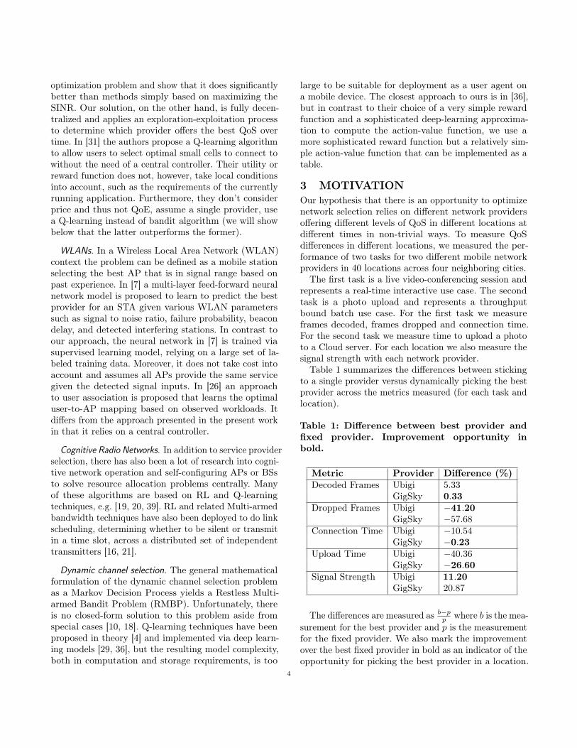
3 MOTIVATIONOur hypothesis that there is an opportunity to optimizenetwork selection relies on different network providersoffering different levels of QoS in different locations atdifferent times in non-trivial ways. To measure QoSdifferences in different locations, we measured the per-formance of two tasks for two different mobile networkproviders in 40 locations across four neighboring cities.

The first task is a live video-conferencing session andrepresents a real-time interactive use case. The secondtask is a photo upload and represents a throughputbound batch use case. For the first task we measureframes decoded, frames dropped and connection time.For the second task we measure time to upload a phototo a Cloud server. For each location we also measure thesignal strength with each network provider.

Table 1 summarizes the differences between stickingto a single provider versus dynamically picking the bestprovider across the metrics measured (for each task andlocation).

Table 1: Difference between best provider andfixed provider. Improvement opportunity inbold.

Metric Provider Difference (%)Decoded Frames Ubigi 5.33

GigSky 0.33Dropped Frames Ubigi −41.20

GigSky −57.68Connection Time Ubigi −10.54

GigSky −0.23Upload Time Ubigi −40.36

GigSky −26.60Signal Strength Ubigi 11.20

GigSky 20.87

The differences are measured as 𝑏−𝑝𝑝 where 𝑏 is the mea-

surement for the best provider and 𝑝 is the measurementfor the fixed provider. We also mark the improvementover the best fixed provider in bold as an indicator of theopportunity for picking the best provider in a location.

4

We note that the Dropped Frames, 41+%, from the video-conference task and the Upload Time, 26+%, metric fromthe photo upload task show the greatest opportunitiesfor improvement. The signal strength opportunity is alsosignificant (11+%).

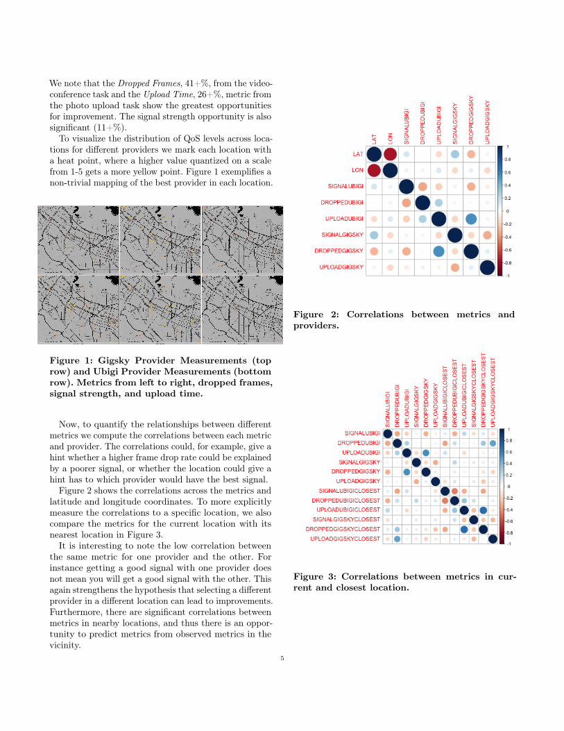
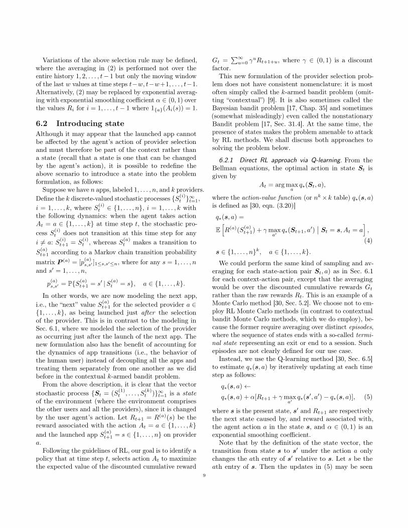
To visualize the distribution of QoS levels across loca-tions for different providers we mark each location witha heat point, where a higher value quantized on a scalefrom 1-5 gets a more yellow point. Figure 1 exemplifies anon-trivial mapping of the best provider in each location.

Figure 1: Gigsky Provider Measurements (toprow) and Ubigi Provider Measurements (bottomrow). Metrics from left to right, dropped frames,signal strength, and upload time.

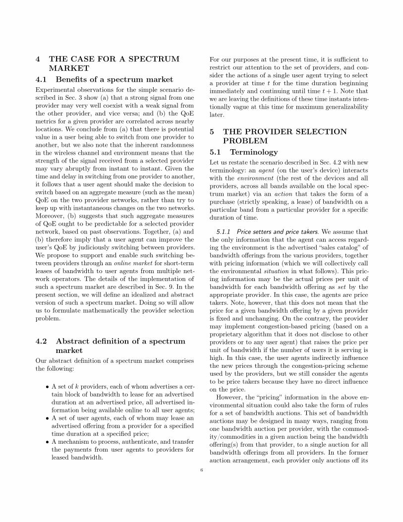
Now, to quantify the relationships between differentmetrics we compute the correlations between each metricand provider. The correlations could, for example, give ahint whether a higher frame drop rate could be explainedby a poorer signal, or whether the location could give ahint has to which provider would have the best signal.

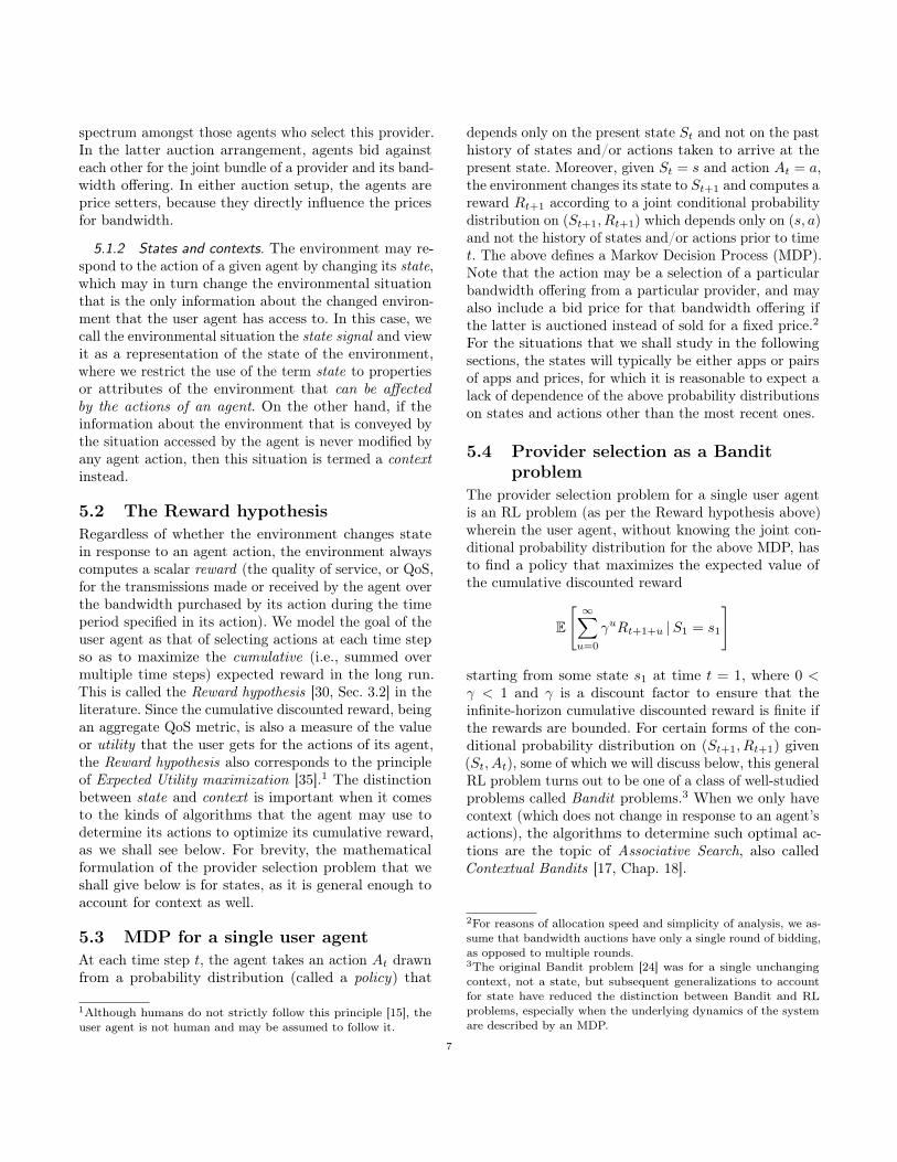
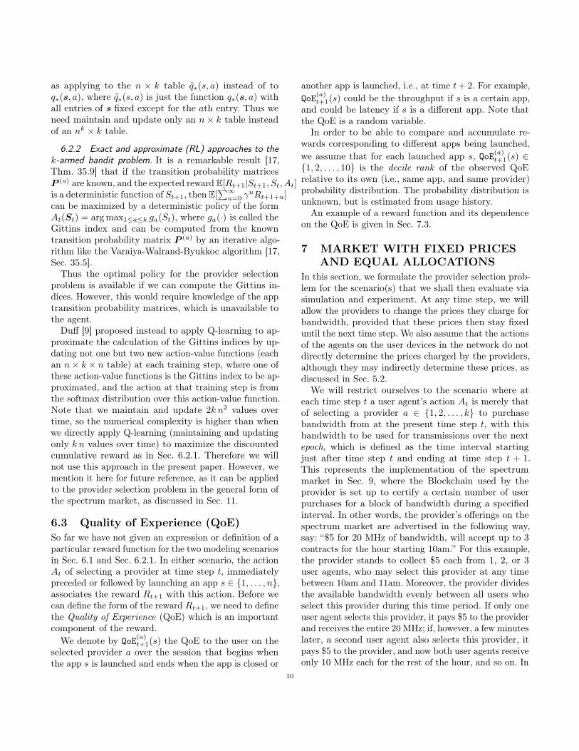
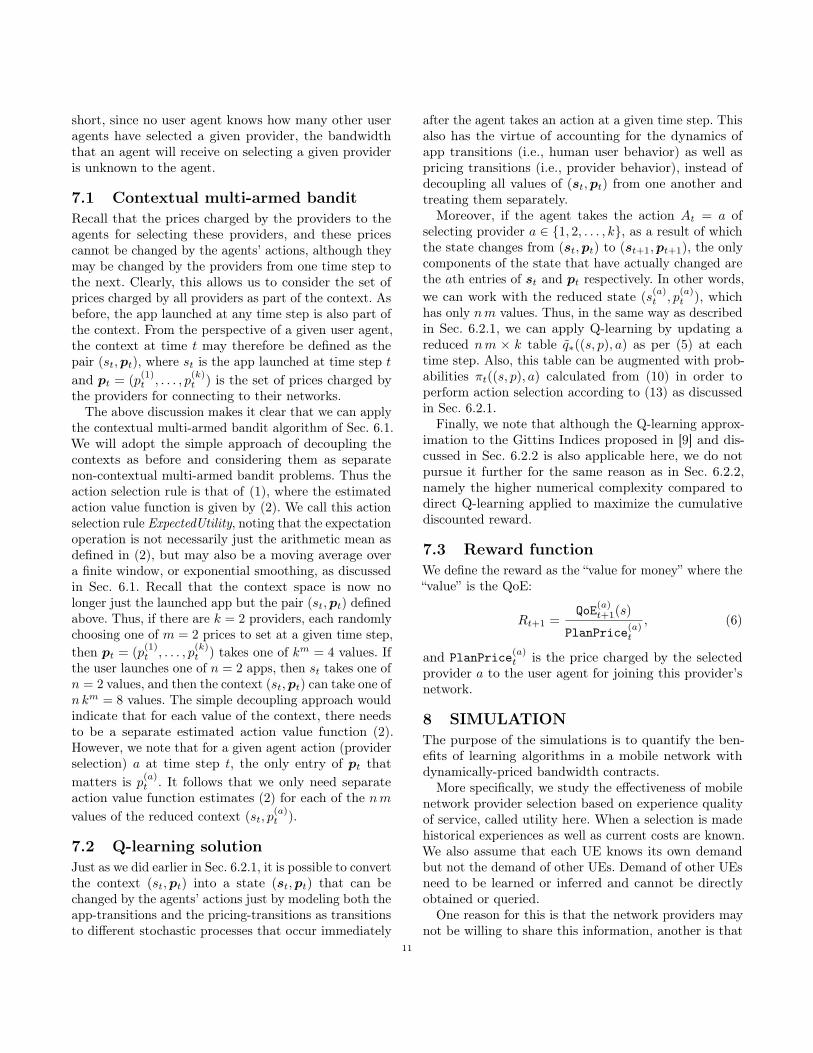
Figure 2 shows the correlations across the metrics andlatitude and longitude coordinates. To more explicitlymeasure the correlations to a specific location, we alsocompare the metrics for the current location with itsnearest location in Figure 3.

It is interesting to note the low correlation betweenthe same metric for one provider and the other. Forinstance getting a good signal with one provider doesnot mean you will get a good signal with the other. Thisagain strengthens the hypothesis that selecting a differentprovider in a different location can lead to improvements.Furthermore, there are significant correlations betweenmetrics in nearby locations, and thus there is an oppor-tunity to predict metrics from observed metrics in thevicinity.

Figure 2: Correlations between metrics andproviders.

Figure 3: Correlations between metrics in cur-rent and closest location.

5

4 THE CASE FOR A SPECTRUMMARKET

4.1 Benefits of a spectrum marketExperimental observations for the simple scenario de-scribed in Sec. 3 show (a) that a strong signal from oneprovider may very well coexist with a weak signal fromthe other provider, and vice versa; and (b) the QoEmetrics for a given provider are correlated across nearbylocations. We conclude from (a) that there is potentialvalue in a user being able to switch from one provider toanother, but we also note that the inherent randomnessin the wireless channel and environment means that thestrength of the signal received from a selected providermay vary abruptly from instant to instant. Given thetime and delay in switching from one provider to another,it follows that a user agent should make the decision toswitch based on an aggregate measure (such as the mean)QoE on the two provider networks, rather than try tokeep up with instantaneous changes on the two networks.Moreover, (b) suggests that such aggregate measuresof QoE ought to be predictable for a selected providernetwork, based on past observations. Together, (a) and(b) therefore imply that a user agent can improve theuser’s QoE by judiciously switching between providers.We propose to support and enable such switching be-tween providers through an online market for short-termleases of bandwidth to user agents from multiple net-work operators. The details of the implementation ofsuch a spectrum market are described in Sec. 9. In thepresent section, we will define an idealized and abstractversion of such a spectrum market. Doing so will allowus to formulate mathematically the provider selectionproblem.

4.2 Abstract definition of a spectrummarket

Our abstract definition of a spectrum market comprisesthe following:

∙ A set of 𝑘 providers, each of whom advertises a cer-tain block of bandwidth to lease for an advertisedduration at an advertised price, all advertised in-formation being available online to all user agents;∙ A set of user agents, each of whom may lease an

advertised offering from a provider for a specifiedtime duration at a specified price;∙ A mechanism to process, authenticate, and transfer

the payments from user agents to providers forleased bandwidth.

For our purposes at the present time, it is sufficient torestrict our attention to the set of providers, and con-sider the actions of a single user agent trying to selecta provider at time 𝑡 for the time duration beginningimmediately and continuing until time 𝑡+ 1. Note thatwe are leaving the definitions of these time instants inten-tionally vague at this time for maximum generalizabilitylater.

5 THE PROVIDER SELECTIONPROBLEM

5.1 TerminologyLet us restate the scenario described in Sec. 4.2 with newterminology: an agent (on the user’s device) interactswith the environment (the rest of the devices and allproviders, across all bands available on the local spec-trum market) via an action that takes the form of apurchase (strictly speaking, a lease) of bandwidth on aparticular band from a particular provider for a specificduration of time.

5.1.1 Price setters and price takers. We assume thatthe only information that the agent can access regard-ing the environment is the advertised “sales catalog” ofbandwidth offerings from the various providers, togetherwith pricing information (which we will collectively callthe environmental situation in what follows). This pric-ing information may be the actual prices per unit ofbandwidth for each bandwidth offering as set by theappropriate provider. In this case, the agents are pricetakers. Note, however, that this does not mean that theprice for a given bandwidth offering by a given provideris fixed and unchanging. On the contrary, the providermay implement congestion-based pricing (based on aproprietary algorithm that it does not disclose to otherproviders or to any user agent) that raises the price perunit of bandwidth if the number of users it is serving ishigh. In this case, the user agents indirectly influencethe new prices through the congestion-pricing schemeused by the providers, but we still consider the agentsto be price takers because they have no direct influenceon the price.

However, the “pricing” information in the above en-vironmental situation could also take the form of rulesfor a set of bandwidth auctions. This set of bandwidthauctions may be designed in many ways, ranging fromone bandwidth auction per provider, with the commod-ity/commodities in a given auction being the bandwidthoffering(s) from that provider, to a single auction for allbandwidth offerings from all providers. In the formerauction arrangement, each provider only auctions off its

6

spectrum amongst those agents who select this provider.In the latter auction arrangement, agents bid againsteach other for the joint bundle of a provider and its band-width offering. In either auction setup, the agents areprice setters, because they directly influence the pricesfor bandwidth.

5.1.2 States and contexts. The environment may re-spond to the action of a given agent by changing its state,which may in turn change the environmental situationthat is the only information about the changed environ-ment that the user agent has access to. In this case, wecall the environmental situation the state signal and viewit as a representation of the state of the environment,where we restrict the use of the term state to propertiesor attributes of the environment that can be affectedby the actions of an agent. On the other hand, if theinformation about the environment that is conveyed bythe situation accessed by the agent is never modified byany agent action, then this situation is termed a contextinstead.

5.2 The Reward hypothesisRegardless of whether the environment changes statein response to an agent action, the environment alwayscomputes a scalar reward (the quality of service, or QoS,for the transmissions made or received by the agent overthe bandwidth purchased by its action during the timeperiod specified in its action). We model the goal of theuser agent as that of selecting actions at each time stepso as to maximize the cumulative (i.e., summed overmultiple time steps) expected reward in the long run.This is called the Reward hypothesis [30, Sec. 3.2] in theliterature. Since the cumulative discounted reward, beingan aggregate QoS metric, is also a measure of the valueor utility that the user gets for the actions of its agent,the Reward hypothesis also corresponds to the principleof Expected Utility maximization [35].1 The distinctionbetween state and context is important when it comesto the kinds of algorithms that the agent may use todetermine its actions to optimize its cumulative reward,as we shall see below. For brevity, the mathematicalformulation of the provider selection problem that weshall give below is for states, as it is general enough toaccount for context as well.

5.3 MDP for a single user agentAt each time step 𝑡, the agent takes an action 𝐴𝑡 drawnfrom a probability distribution (called a policy) that

1Although humans do not strictly follow this principle [15], theuser agent is not human and may be assumed to follow it.

depends only on the present state 𝑆𝑡 and not on the pasthistory of states and/or actions taken to arrive at thepresent state. Moreover, given 𝑆𝑡 = 𝑠 and action 𝐴𝑡 = 𝑎,the environment changes its state to 𝑆𝑡+1 and computes areward 𝑅𝑡+1 according to a joint conditional probabilitydistribution on (𝑆𝑡+1, 𝑅𝑡+1) which depends only on (𝑠, 𝑎)and not the history of states and/or actions prior to time𝑡. The above defines a Markov Decision Process (MDP).Note that the action may be a selection of a particularbandwidth offering from a particular provider, and mayalso include a bid price for that bandwidth offering ifthe latter is auctioned instead of sold for a fixed price.2For the situations that we shall study in the followingsections, the states will typically be either apps or pairsof apps and prices, for which it is reasonable to expect alack of dependence of the above probability distributionson states and actions other than the most recent ones.

5.4 Provider selection as a Banditproblem

The provider selection problem for a single user agentis an RL problem (as per the Reward hypothesis above)wherein the user agent, without knowing the joint con-ditional probability distribution for the above MDP, hasto find a policy that maximizes the expected value ofthe cumulative discounted reward

E

[︃ ∞∑︁𝑢=0

𝛾𝑢𝑅𝑡+1+𝑢 |𝑆1 = 𝑠1

]︃

starting from some state 𝑠1 at time 𝑡 = 1, where 0 <𝛾 < 1 and 𝛾 is a discount factor to ensure that theinfinite-horizon cumulative discounted reward is finite ifthe rewards are bounded. For certain forms of the con-ditional probability distribution on (𝑆𝑡+1, 𝑅𝑡+1) given(𝑆𝑡, 𝐴𝑡), some of which we will discuss below, this generalRL problem turns out to be one of a class of well-studiedproblems called Bandit problems.3 When we only havecontext (which does not change in response to an agent’sactions), the algorithms to determine such optimal ac-tions are the topic of Associative Search, also calledContextual Bandits [17, Chap. 18].

2For reasons of allocation speed and simplicity of analysis, we as-sume that bandwidth auctions have only a single round of bidding,as opposed to multiple rounds.3The original Bandit problem [24] was for a single unchangingcontext, not a state, but subsequent generalizations to accountfor state have reduced the distinction between Bandit and RLproblems, especially when the underlying dynamics of the systemare described by an MDP.

7

5.5 A learning approachRecall that the agent has access to just the informa-tion in the state or context regarding the environment,and it receives a reward for each action it takes. TheReward hypothesis suggests that the way for the agentto maximize its cumulative reward is to learn from itsinteractions with the environment the actions to takewhen in a given state or context in order to maximizenot necessarily the immediate reward but the long-termcumulative reward. Note, in particular, the flexibilityand robustness of such a learning approach comparedto a rule-based approach with a predefined rule or setof rules, which will always take the same action whenfaced with the same situation, and may not know howto react in response to a situation that is not covered bythe rule.

In the next section, we present a brief review of ap-proaches to solve the multi-armed bandit problem.

6 REVIEW OF MULTI-ARMEDBANDIT PROBLEMS

6.1 Contextual 𝑘-armed banditWe simplify the provider selection problem descriptionby stipulating that as soon as the human user launchesan app (for brevity, making a call will also be consid-ered “launching an app” in what follows), the user agentinstantaneously selects one of, say, 𝑘 SIMs or eSIMs,and enables the selected SIM/eSIM if it was not enabledalready4.

The only action that the user agent takes is to selectthe SIM/eSIM (i.e., provider) to enable next. The context(not changeable by the agent’s action) is the app thatwas launched by the human user. The reward that theagent receives for its action is the QoE corresponding tothe context (i.e., app launched on the selected provider).Note that owing to randomness on the channel betweenthe device and the base stations serving it, the rewardis a random variable.

In short, the agent is faced repeatedly with a choice of𝑘 different actions (each corresponding to the selectionof a different network provider) at each time step. Eachtime step corresponds to a specific context (the applaunched by the human user). Note that the time stepsdo not need to be uniformly spaced. Following the action,the agent receives a reward drawn from a probabilitydistribution that depends on the context5. If we view thechoice of the 𝑘 different actions as that of “pulling one4Actually, the experimentally observed time between enabling aSIM/eSIM and being able to use it can be a few seconds (seeSec. 9.1), but we will ignore this in our modeling.5A reward definition will be introduced in Sec. 7.3.

of 𝑘 levers,” then the above is precisely the descriptionof a contextual 𝑘-armed bandit. A survey of contextualmulti-armed bandits may be found in [40].

The easiest way to approach a contextual 𝑘-armedbandit with, say, 𝑛 values of the context (each corre-sponding to a different app launched by the user) is tosimply apply a (non-contextual) 𝑘-armed bandit sep-arately to each of the 𝑛 contexts. In other words, weignore all relationships between the different contextsand completely decouple the bandit problems betweenthe different contexts. For the present scenario, this isequivalent to saying that we find, separately, the actionselection rule to maximize the cumulative reward overall time steps when each particular app was launched.Thus, in the following analysis, we will discuss only theaction selection rule for the (non-contextual) 𝑘-armedbandit problem corresponding to a specific app.

We start with some notation. Fix a specific app 𝑠 ∈{1, . . . , 𝑛}, and assume this context is unchanged inwhat follows. Let the time steps be numbered 1, 2, . . . .Let the action taken by the agent at time 𝑡 (i.e., thelabel of the selected provider) in context 𝑠 be denoted𝐴𝑡(𝑠) ∈ {1, . . . , 𝑘}. Then the simplest action selectionrule is [30, Sec. 2.2]:

𝐴𝑡(𝑠) = argmax𝑎

𝑄𝑡(𝑠, 𝑎), (1)

where for each 𝑎 ∈ {1, . . . , 𝑘} and 𝑡 = 1, 2, . . . , theestimated action value function 𝑄𝑡(𝑠, 𝑎) is defined bythe arithmetic average of the rewards for action 𝑎 ∈{1, . . . , 𝑘} upto and including time 𝑡− 1:

𝑄𝑡(𝑠, 𝑎) =

{︃∑︀𝑡−1𝑖=1 𝑅𝑖1{𝑎}(𝐴𝑖(𝑠))

𝑁𝑡−1(𝑠,𝑎), 𝑁𝑡−1(𝑠, 𝑎) > 0,

0, 𝑁𝑡−1(𝑠, 𝑎) = 0,(2)

where for any 𝑡 = 1, 2, . . . , 𝑅𝑡 = 𝑅(𝐴𝑡(𝑠))(𝑠) is the rewardfor taking action 𝐴𝑡(𝑠) at time step 𝑡 in context 𝑠,

𝑁𝑡−1(𝑠, 𝑎) =

{︃0, 𝑡 = 1,∑︀𝑡−1

𝑖=1 1{𝑎}(𝐴𝑖(𝑠)), 𝑡 = 2, 3, . . . ,(3)

is the number of times action 𝑎 was selected by the agentupto and including time 𝑡− 1 when the context is 𝑠, andfor any set 𝒮, the indicator function 1𝒮(·) is defined by

1𝒮(𝑥) =

{︃1, if 𝑥 ∈ 𝒮,0, otherwise.

If the maximizing argument in (1) is not unique then𝐴𝑡(𝑠) is chosen from amongst the maximizing argumentsat random. In fact, to encourage exploration versus mereexploitation, we may select the action according to (1)(breaking ties randomly as described) with probability1 − 𝜖 for some small 𝜖, say, while selecting a randomaction for 𝐴𝑡(𝑠) with probability 𝜖 [30, Sec. 2.4].

8

Variations of the above selection rule may be defined,where the averaging in (2) is performed not over theentire history 1, 2, . . . , 𝑡− 1 but only the moving windowof the last 𝑤 values at time steps 𝑡−𝑤, 𝑡−𝑤+1, . . . , 𝑡−1.Alternatively, (2) may be replaced by exponential averag-ing with exponential smoothing coefficient 𝛼 ∈ (0, 1) overthe values 𝑅𝑖 for 𝑖 = 1, . . . , 𝑡− 1 where 1{𝑎}(𝐴𝑖(𝑠)) = 1.

6.2 Introducing stateAlthough it may appear that the launched app cannotbe affected by the agent’s action of provider selectionand must therefore be part of the context rather thana state (recall that a state is one that can be changedby the agent’s action), it is possible to redefine theabove scenario to introduce a state into the problemformulation, as follows:

Suppose we have 𝑛 apps, labeled 1, . . . , 𝑛, and 𝑘 providers.Define the 𝑘 discrete-valued stochastic processes {𝑆(𝑖)

𝑡 }∞𝑡=1,𝑖 = 1, . . . , 𝑘, where 𝑆

(𝑖)𝑡 ∈ {1, . . . , 𝑛}, 𝑖 = 1, . . . , 𝑘 with

the following dynamics: when the agent takes action𝐴𝑡 = 𝑎 ∈ {1, . . . , 𝑘} at time step 𝑡, the stochastic pro-cess 𝑆

(𝑖)𝑡 does not transition at this time step for any

𝑖 ̸= 𝑎: 𝑆(𝑖)𝑡+1 = 𝑆

(𝑖)𝑡 , whereas 𝑆

(𝑎)𝑡 makes a transition to

𝑆(𝑎)𝑡+1 according to a Markov chain transition probability

matrix 𝑃 (𝑎) = [𝑝(𝑎)𝑠,𝑠′ ]1≤𝑠,𝑠′≤𝑛, where for any 𝑠 = 1, . . . , 𝑛

and 𝑠′ = 1, . . . , 𝑛,

𝑝(𝑎)𝑠,𝑠′ = P{𝑆(𝑎)

𝑡+1 = 𝑠′ |𝑆(𝑎)𝑡 = 𝑠}, 𝑎 ∈ {1, . . . , 𝑘}.

In other words, we are now modeling the next app,i.e., the “next” value 𝑆

(𝑎)𝑡+1 for the selected provider 𝑎 ∈

{1, . . . , 𝑘}, as being launched just after the selectionof the provider. This is in contrast to the modeling inSec. 6.1, where we modeled the selection of the provideras occurring just after the launch of the next app. Thenew formulation also has the benefit of accounting forthe dynamics of app transitions (i.e., the behavior ofthe human user) instead of decoupling all the apps andtreating them separately from one another as we didbefore in the contextual 𝑘-armed bandit problem.

From the above description, it is clear that the vectorstochastic process {𝑆𝑡 = (𝑆

(1)𝑡 , . . . , 𝑆

(𝑘)𝑡 )}∞𝑡=1 is a state

of the environment (where the environment comprisesthe other users and all the providers), since it is changedby the user agent’s action. Let 𝑅𝑡+1 = 𝑅(𝑎)(𝑠) be thereward associated with the action 𝐴𝑡 = 𝑎 ∈ {1, . . . , 𝑘}and the launched app 𝑆

(𝑎)𝑡+1 = 𝑠 ∈ {1, . . . , 𝑛} on provider

𝑎.Following the guidelines of RL, our goal is to identify a

policy that at time step 𝑡, selects action 𝐴𝑡 to maximizethe expected value of the discounted cumulative reward

𝐺𝑡 =∑︀∞

𝑢=0 𝛾𝑢𝑅𝑡+1+𝑢, where 𝛾 ∈ (0, 1) is a discount

factor.This new formulation of the provider selection prob-

lem does not have consistent nomenclature: it is mostoften simply called the 𝑘-armed bandit problem (omit-ting “contextual”) [9]. It is also sometimes called theBayesian bandit problem [17, Chap. 35] and sometimes(somewhat misleadingly) even called the nonstationaryBandit problem [17, Sec. 31.4]. At the same time, thepresence of states makes the problem amenable to attackby RL methods. We shall discuss both approaches tosolving the problem below.

6.2.1 Direct RL approach via Q-learning. From theBellman equations, the optimal action in state 𝑆𝑡 isgiven by

𝐴𝑡 = argmax𝑎

𝑞*(𝑆𝑡, 𝑎),

where the action-value function (or 𝑛𝑘×𝑘 table) 𝑞*(𝑠, 𝑎)is defined as [30, eqn. (3.20)]

𝑞*(𝑠, 𝑎) =

E[︁𝑅(𝑎)(𝑆

(𝑎)𝑡+1) + 𝛾max

𝑎′𝑞*(𝑆𝑡+1, 𝑎

′)⃒⃒𝑆𝑡 = 𝑠, 𝐴𝑡 = 𝑎

]︁,

(4)

𝑠 ∈ {1, . . . , 𝑛}𝑘, 𝑎 ∈ {1, . . . , 𝑘}.

We could perform the same kind of sampling and av-eraging for each state-action pair 𝑆𝑡, 𝑎) as in Sec. 6.1for each context-action pair, except that the averagingwould be over the discounted cumulative rewards 𝐺𝑡

rather than the raw rewards 𝑅𝑡. This is an example of aMonte Carlo method [30, Sec. 5.2]. We choose not to em-ploy RL Monte Carlo methods (in contrast to contextualbandit Monte Carlo methods, which we do employ), be-cause the former require averaging over distinct episodes,where the sequence of states ends with a so-called termi-nal state representing an exit or end to a session. Suchepisodes are not clearly defined for our use case.

Instead, we use the Q-learning method [30, Sec. 6.5]to estimate 𝑞*(𝑠, 𝑎) by iteratively updating at each timestep as follows:

𝑞*(𝑠, 𝑎)←𝑞*(𝑠, 𝑎) + 𝛼[𝑅𝑡+1 + 𝛾max

𝑎′𝑞*(𝑠

′, 𝑎′)− 𝑞*(𝑠, 𝑎)], (5)

where 𝑠 is the present state, 𝑠′ and 𝑅𝑡+1 are respectivelythe next state caused by, and reward associated with,the agent action 𝑎 in the state 𝑠, and 𝛼 ∈ (0, 1) is anexponential smoothing coefficient.

Note that by the definition of the state vector, thetransition from state 𝑠 to 𝑠′ under the action 𝑎 onlychanges the 𝑎th entry of 𝑠′ relative to 𝑠. Let 𝑠 be the𝑎th entry of 𝑠. Then the updates in (5) may be seen

9

as applying to the 𝑛 × 𝑘 table 𝑞*(𝑠, 𝑎) instead of to𝑞*(𝑠, 𝑎), where 𝑞*(𝑠, 𝑎) is just the function 𝑞*(𝑠, 𝑎) withall entries of 𝑠 fixed except for the 𝑎th entry. Thus weneed maintain and update only an 𝑛× 𝑘 table insteadof an 𝑛𝑘 × 𝑘 table.

6.2.2 Exact and approximate (RL) approaches to the𝑘-armed bandit problem. It is a remarkable result [17,Thm. 35.9] that if the transition probability matrices𝑃 (𝑎) are known, and the expected reward E[𝑅𝑡+1|𝑆𝑡+1, 𝑆𝑡, 𝐴𝑡]is a deterministic function of 𝑆𝑡+1, then E[

∑︀∞𝑢=0 𝛾

𝑢𝑅𝑡+1+𝑢]can be maximized by a deterministic policy of the form𝐴𝑡(𝑆𝑡) = argmax1≤𝑎≤𝑘 𝑔𝑎(𝑆𝑡), where 𝑔𝑎(·) is called theGittins index and can be computed from the knowntransition probability matrix 𝑃 (𝑎) by an iterative algo-rithm like the Varaiya-Walrand-Byukkoc algorithm [17,Sec. 35.5].

Thus the optimal policy for the provider selectionproblem is available if we can compute the Gittins in-dices. However, this would require knowledge of the apptransition probability matrices, which is unavailable tothe agent.

Duff [9] proposed instead to apply Q-learning to ap-proximate the calculation of the Gittins indices by up-dating not one but two new action-value functions (eachan 𝑛× 𝑘 × 𝑛 table) at each training step, where one ofthese action-value functions is the Gittins index to be ap-proximated, and the action at that training step is fromthe softmax distribution over this action-value function.Note that we maintain and update 2𝑘 𝑛2 values overtime, so the numerical complexity is higher than whenwe directly apply Q-learning (maintaining and updatingonly 𝑘 𝑛 values over time) to maximize the discountedcumulative reward as in Sec. 6.2.1. Therefore we willnot use this approach in the present paper. However, wemention it here for future reference, as it can be appliedto the provider selection problem in the general form ofthe spectrum market, as discussed in Sec. 11.

6.3 Quality of Experience (QoE)So far we have not given an expression or definition of aparticular reward function for the two modeling scenariosin Sec. 6.1 and Sec. 6.2.1. In either scenario, the action𝐴𝑡 of selecting a provider at time step 𝑡, immediatelypreceded or followed by launching an app 𝑠 ∈ {1, . . . , 𝑛},associates the reward 𝑅𝑡+1 with this action. Before wecan define the form of the reward 𝑅𝑡+1, we need to definethe Quality of Experience (QoE) which is an importantcomponent of the reward.

We denote by QoE(𝑎)𝑡+1(𝑠) the QoE to the user on the

selected provider 𝑎 over the session that begins whenthe app 𝑠 is launched and ends when the app is closed or

another app is launched, i.e., at time 𝑡+ 2. For example,QoE

(𝑎)𝑡+1(𝑠) could be the throughput if 𝑠 is a certain app,

and could be latency if 𝑠 is a different app. Note thatthe QoE is a random variable.

In order to be able to compare and accumulate re-wards corresponding to different apps being launched,we assume that for each launched app 𝑠, QoE(𝑎)𝑡+1(𝑠) ∈{1, 2, . . . , 10} is the decile rank of the observed QoErelative to its own (i.e., same app, and same provider)probability distribution. The probability distribution isunknown, but is estimated from usage history.

An example of a reward function and its dependenceon the QoE is given in Sec. 7.3.

7 MARKET WITH FIXED PRICESAND EQUAL ALLOCATIONS

In this section, we formulate the provider selection prob-lem for the scenario(s) that we shall then evaluate viasimulation and experiment. At any time step, we willallow the providers to change the prices they charge forbandwidth, provided that these prices then stay fixeduntil the next time step. We also assume that the actionsof the agents on the user devices in the network do notdirectly determine the prices charged by the providers,although they may indirectly determine these prices, asdiscussed in Sec. 5.2.

We will restrict ourselves to the scenario where ateach time step 𝑡 a user agent’s action 𝐴𝑡 is merely thatof selecting a provider 𝑎 ∈ {1, 2, . . . , 𝑘} to purchasebandwidth from at the present time step 𝑡, with thisbandwidth to be used for transmissions over the nextepoch, which is defined as the time interval startingjust after time step 𝑡 and ending at time step 𝑡 + 1.This represents the implementation of the spectrummarket in Sec. 9, where the Blockchain used by theprovider is set up to certify a certain number of userpurchases for a block of bandwidth during a specifiedinterval. In other words, the provider’s offerings on thespectrum market are advertised in the following way,say: “$5 for 20 MHz of bandwidth, will accept up to 3contracts for the hour starting 10am.” For this example,the provider stands to collect $5 each from 1, 2, or 3user agents, who may select this provider at any timebetween 10am and 11am. Moreover, the provider dividesthe available bandwidth evenly between all users whoselect this provider during this time period. If only oneuser agent selects this provider, it pays $5 to the providerand receives the entire 20 MHz; if, however, a few minuteslater, a second user agent also selects this provider, itpays $5 to the provider, and now both user agents receiveonly 10 MHz each for the rest of the hour, and so on. In

10

short, since no user agent knows how many other useragents have selected a given provider, the bandwidththat an agent will receive on selecting a given provideris unknown to the agent.

7.1 Contextual multi-armed banditRecall that the prices charged by the providers to theagents for selecting these providers, and these pricescannot be changed by the agents’ actions, although theymay be changed by the providers from one time step tothe next. Clearly, this allows us to consider the set ofprices charged by all providers as part of the context. Asbefore, the app launched at any time step is also part ofthe context. From the perspective of a given user agent,the context at time 𝑡 may therefore be defined as thepair (𝑠𝑡,𝑝𝑡), where 𝑠𝑡 is the app launched at time step 𝑡

and 𝑝𝑡 = (𝑝(1)𝑡 , . . . , 𝑝

(𝑘)𝑡 ) is the set of prices charged by

the providers for connecting to their networks.The above discussion makes it clear that we can apply

the contextual multi-armed bandit algorithm of Sec. 6.1.We will adopt the simple approach of decoupling thecontexts as before and considering them as separatenon-contextual multi-armed bandit problems. Thus theaction selection rule is that of (1), where the estimatedaction value function is given by (2). We call this actionselection rule ExpectedUtility, noting that the expectationoperation is not necessarily just the arithmetic mean asdefined in (2), but may also be a moving average overa finite window, or exponential smoothing, as discussedin Sec. 6.1. Recall that the context space is now nolonger just the launched app but the pair (𝑠𝑡,𝑝𝑡) definedabove. Thus, if there are 𝑘 = 2 providers, each randomlychoosing one of 𝑚 = 2 prices to set at a given time step,then 𝑝𝑡 = (𝑝

(1)𝑡 , . . . , 𝑝

(𝑘)𝑡 ) takes one of 𝑘𝑚 = 4 values. If

the user launches one of 𝑛 = 2 apps, then 𝑠𝑡 takes one of𝑛 = 2 values, and then the context (𝑠𝑡,𝑝𝑡) can take one of𝑛𝑘𝑚 = 8 values. The simple decoupling approach wouldindicate that for each value of the context, there needsto be a separate estimated action value function (2).However, we note that for a given agent action (providerselection) 𝑎 at time step 𝑡, the only entry of 𝑝𝑡 thatmatters is 𝑝

(𝑎)𝑡 . It follows that we only need separate

action value function estimates (2) for each of the 𝑛𝑚

values of the reduced context (𝑠𝑡, 𝑝(𝑎)𝑡 ).

7.2 Q-learning solutionJust as we did earlier in Sec. 6.2.1, it is possible to convertthe context (𝑠𝑡,𝑝𝑡) into a state (𝑠𝑡,𝑝𝑡) that can bechanged by the agents’ actions just by modeling both theapp-transitions and the pricing-transitions as transitionsto different stochastic processes that occur immediately

after the agent takes an action at a given time step. Thisalso has the virtue of accounting for the dynamics ofapp transitions (i.e., human user behavior) as well aspricing transitions (i.e., provider behavior), instead ofdecoupling all values of (𝑠𝑡,𝑝𝑡) from one another andtreating them separately.

Moreover, if the agent takes the action 𝐴𝑡 = 𝑎 ofselecting provider 𝑎 ∈ {1, 2, . . . , 𝑘}, as a result of whichthe state changes from (𝑠𝑡,𝑝𝑡) to (𝑠𝑡+1,𝑝𝑡+1), the onlycomponents of the state that have actually changed arethe 𝑎th entries of 𝑠𝑡 and 𝑝𝑡 respectively. In other words,we can work with the reduced state (𝑠

(𝑎)𝑡 , 𝑝

(𝑎)𝑡 ), which

has only 𝑛𝑚 values. Thus, in the same way as describedin Sec. 6.2.1, we can apply Q-learning by updating areduced 𝑛𝑚 × 𝑘 table 𝑞*((𝑠, 𝑝), 𝑎) as per (5) at eachtime step. Also, this table can be augmented with prob-abilities 𝜋𝑡((𝑠, 𝑝), 𝑎) calculated from (10) in order toperform action selection according to (13) as discussedin Sec. 6.2.1.

Finally, we note that although the Q-learning approx-imation to the Gittins Indices proposed in [9] and dis-cussed in Sec. 6.2.2 is also applicable here, we do notpursue it further for the same reason as in Sec. 6.2.2,namely the higher numerical complexity compared todirect Q-learning applied to maximize the cumulativediscounted reward.

7.3 Reward functionWe define the reward as the “value for money” where the“value” is the QoE:

𝑅𝑡+1 =QoE

(𝑎)𝑡+1(𝑠)

PlanPrice(𝑎)𝑡

, (6)

and PlanPrice(𝑎)𝑡 is the price charged by the selected

provider 𝑎 to the user agent for joining this provider’snetwork.

8 SIMULATIONThe purpose of the simulations is to quantify the ben-efits of learning algorithms in a mobile network withdynamically-priced bandwidth contracts.

More specifically, we study the effectiveness of mobilenetwork provider selection based on experience qualityof service, called utility here. When a selection is madehistorical experiences as well as current costs are known.We also assume that each UE knows its own demandbut not the demand of other UEs. Demand of other UEsneed to be learned or inferred and cannot be directlyobtained or queried.

One reason for this is that the network providers maynot be willing to share this information, another is that

11

it depends very much on the demand and preferences ofa UE how it impacts other UEs.

The simulator computes the effective bandwidth andQoE for the UE using basic utility functions and SINRestimates based on positions of UEs, Base Stations andresource contention when multiple UEs connected to thesame Base Station contend for spectrum resources.

Since the delivered performance is computed, it ismore deterministic than with a real-world scenario wheremeasurements may have non-negligible variance, so wealso complement the simulations with experiment withreal phones and networks in Sec. 10.

There are two types of UEs in the experiment: Back-ground UEs that are simply placed in the simulationgrid to inject contention, also referred to simply as UEs,and UEs that are allowed to make network selectiondecisions dynamically, and that we capture performancefrom, referred to as Device under Test (DUT).

We also simulate the complex problem of competingDUTS, or competing agents. It is easy to imagine algo-rithms where each agent makes the same decision andthus causes oscillation or lockstep behavior and loadimbalance. We also hypothesize that varying demandacross agents can be exploited to put them on differentoptimal providers and thereby yield a higher aggregateutility or QoE. This scenario also makes it clear that notonly does a DUT not know the future demand of otherDUTs, but it does not even know which provider theother DUTs will pick, and thereby potentially causingcontention impacting the DUT QoE.

8.1 SetupWe implemented a discrete even simulator based on thePyLTEs framework [27]. PyLTEs was extended to adddynamic bandwidth pricing, UE resource contention,DUT network selection and competition, stochastic appdemand, Base station position offsets across networks, astraight-path mobility model, and utility evaluation andrecording.

Two competing networks are configured where one hasa higher number of background UEs causing the maxi-mum throughput delivered to be lower. The maximumthroughput depends on the distance between the basestation and the UE as well as the number of other UEsusing the same base station.

The network base stations are positioned with an offsetand the DUTs start in the center and then move in astraight path away from the center at a random angle.

Recall the discussion in Sec. 5.2 that the expectedcumulative reward may be seen as a kind of utility fora given user agent. Our evaluation metric is aggregate

utility, a.k.a. social welfare across all DUTs. Utility, be-ing the expected cumulative reward, is computed basedon the maximum throughput delivered and the demandof the currently running app on the DUT. Apps runwith a transition probability to use the same app inthe next step or switch to a new app. Each app hasan associated utility function to compute the reward. Abatch app simply computes the reward as the maximumthroughput over price, and an interactive app sets a min-imum throughput threshold that needs to be deliveredto receive the full reward and caps the reward at thatlevel. If that throughput is not met a lower bar rewardslightly above 0 is delivered. For simplicity we specifythat both app types are equally likely at any given time.Since both rewards are based on throughputs, we willfor simplicity work with the throughput-to-price ratiosthemselves instead of converting them to their decileranks as defined in Sec. 6.3.

The intuition is that a network selector that wants tooptimize utility (i.e., expected cumulative reward) couldselect a lower cost, lower throughput network if the priceis right.

Below we run simulations to investigate: optimal his-tory length to estimate app utility, various combinationsof fixed price and location, and competing DUTs.

The fixed location configuration ensures that the twonetworks always deliver a fixed max throughput through-out the simulation. The fixed price configuration simi-larly ensures that the networks do not change their priceswithin a run.

In the competing agent setup, multiple DUTs get topick their preferred network in each step without knowingthe decisions of other DUTs. DUTs train or calibrate atdifferent times in this case to avoid lockstep behavior.

Each simulation is run in 200 steps (using the straight-walk mobility model described above). For each run oriteration we compute the social welfare for each bench-mark. The costs and apps and positions are replayed forall benchmarks. We then iterate over the same proce-dure generating new app, cost and position traces 100times and compute statistics with each iteration as anindependent sample.

We set up 36 base stations per network in a gridwith radius 1440 meters in a hexagonal layout with onenetwork offset in both x and y coordinates from the other.In the fixed location case we set a step walk length to 1meter ensuring that the signal from the networks doesnot change significantly to change the max throughputdelivered from each network during the run. For thevariable location setting the walk size is set to 20 metersfor each step, which results in the networks deliveringdifferent throughput over time.

12

A summary of the general configuration parametersused across all simulations are shown in Table 2. Fixedlocation is achieved by setting walk length to 1, fixedpricing is enforced by setting max cost equal to min cost,and finally competing agents are achieved by settingDUTs to 3.

Note, app demand is individually and independentlysampled on each DUT (in the competing agent case).

8.2 Provider selection policiesevaluated via simulation

We evaluated the following provider selection policies:(1) ExpectedUtility : As discussed in Sec. 7.1, this is the

contextual 𝑘-armed (𝑘 = 2) bandit optimal policygiven by (1) with 𝑛 = 2 contexts (apps), where thefunction being maximized is given by (2).

(2) History : Same as ExpectedUtility, except that wedefine not 𝑛 contexts (one per app) but only asingle context. In other words, this is the original(non-contextual) 𝑘-armed bandit of [24].

(3) RL: Recall that we have 𝑛 = 2 apps and 𝑘 = 2providers in the simulation. Although each providercan set one of 𝑚 = 2 prices in the simulation, wesimplify the state space for the Q-learning RL so-lution by using the smaller 𝑛× 𝑘 (app, provider)action-value table of Sec. 6.2.1 instead of the 𝑛𝑚×𝑘 ((app, price), provider) table of Sec. 7.2. Specifi-cally, we select the provider at time 𝑡 according to𝐴𝑡 = argmax𝑎∈{1,...,𝑘} 𝑞*(𝑆

(𝑎)𝑡 , 𝑎), where for any

𝑠 ∈ {1, 2} and 𝑎 ∈ {1, 2},

𝑞*(𝑠, 𝑎)←𝑞*(𝑠, 𝑎) + 𝛼[𝑅𝑡+1 + 𝛾max

𝑎′𝑞*(𝑠

′, 𝑎′)− 𝑞*(𝑠, 𝑎)], (7)

where 𝛼 = 0.2 and 𝛾 = 0.7.(4) LowestPrice: This is a baseline policy for compari-

son purposes, where at each time step we simplyselect the provider charging the lower price of thetwo providers.

(5) Random: This is another baseline policy that isevaluated purely to serve as a comparison againstHistory, ExpectedUtility, and RL. Here, one of thetwo providers is selected by tossing a fair coin ateach time step, independently from one step to thenext.

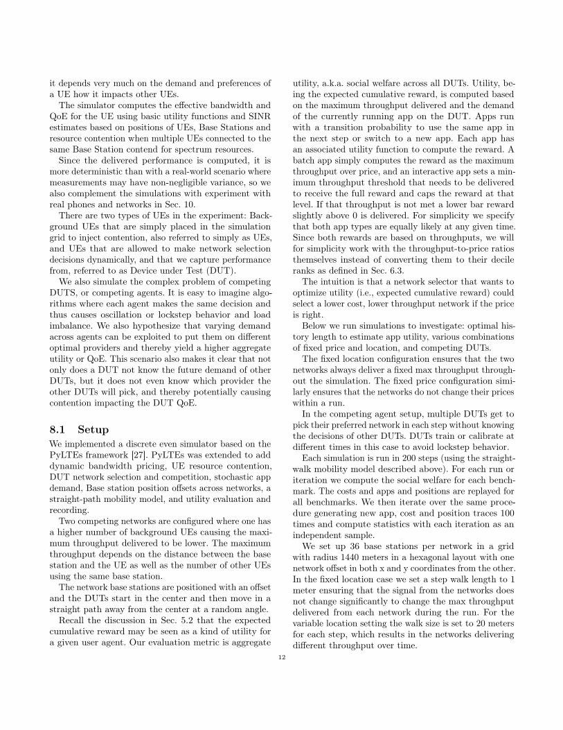
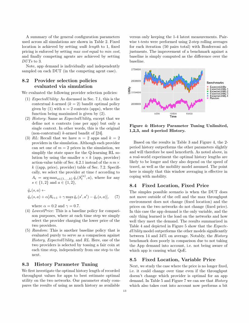
8.3 History Parameter TuningWe first investigate the optimal history length of recordedthroughput values for apps to best estimate optimalutility on the two networks. Our parameter study com-pares the results of using as much history as available

versus only keeping the 1-4 latest measurements. Pair-wise t-tests were performed using 2-step rolling averagesfor each iteration (50 pairs total) with Bonferroni ad-justments. The improvement of a benchmark against abaseline is simply computed as the difference over thebaseline.

Figure 4: History Parameter Tuning Unlimited,1,2,3, and 4-period History.

Based on the results in Table 3 and Figure 4, the 2-period history outperforms the other parameters slightlyand will therefore be used henceforth. As noted above, ina real-world experiment the optimal history lengths arelikely to be longer and they also depend on the speed oftravel, as well as the mobility model assumed. The pointhere is simply that this window averaging is effective incoping with mobility.

8.4 Fixed Location, Fixed PriceThe simples possible scenario is when the DUT doesnot move outside of the cell and the max throughputenvironment does not change (fixed location) and theprices on the two networks do not change (fixed price).In this case the app demand is the only variable, and theonly thing learned is the load on the networks and howwell they meet the demand. The results summarized inTable 4 and depicted in Figure 5 show that the Expecte-dUtility model outperforms the other models significantlybetween 14 and 34% on average. Notably, the Historybenchmark does poorly in comparison due to not takingthe App demand into account, i.e. not being aware ofwhich app is causing what QoE.

8.5 Fixed Location, Variable PriceNext, we study the case where the price is no longer fixed,i.e. it could change over time even if the throughputdoesn’t change which provider is optimal for an appdemand. In Table 5 and Figure 7 we can see that Historywhich also takes cost into account now performs a bit

13

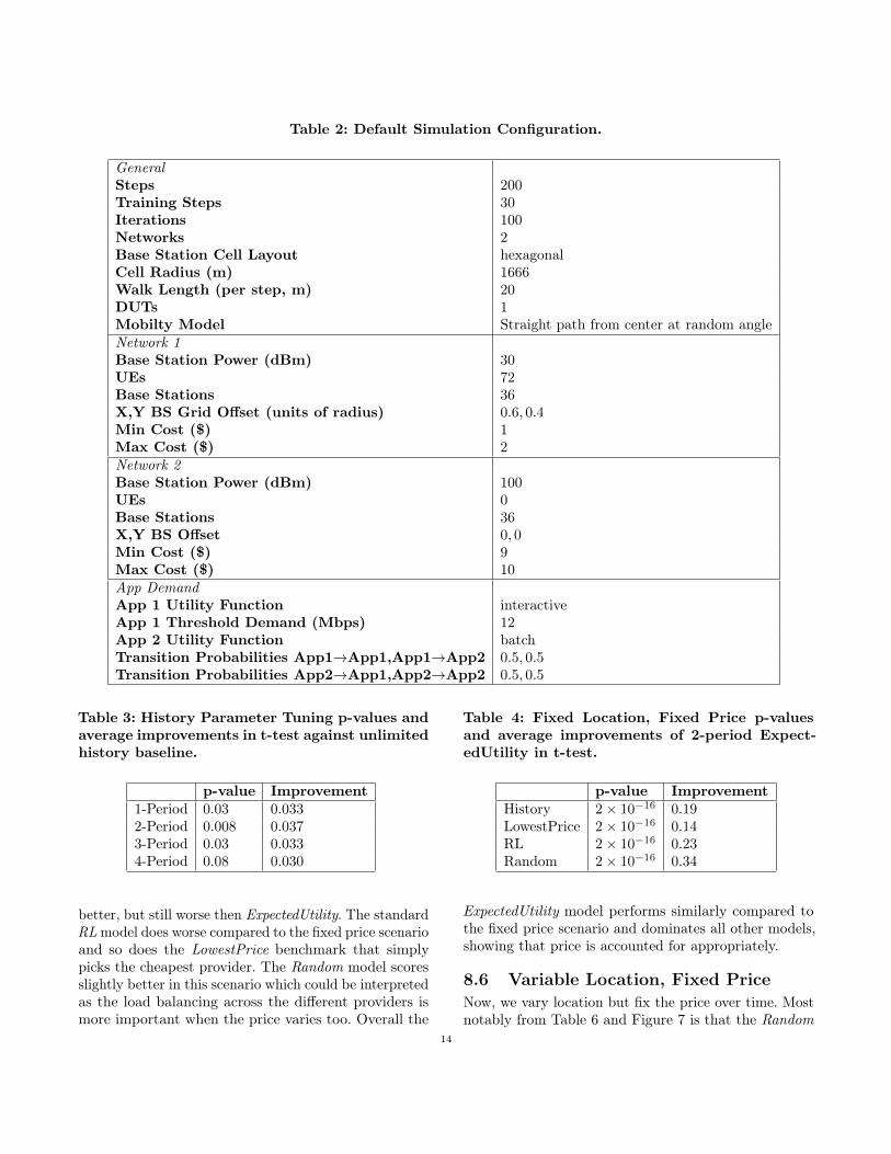
Table 2: Default Simulation Configuration.

GeneralSteps 200Training Steps 30Iterations 100Networks 2Base Station Cell Layout hexagonalCell Radius (m) 1666Walk Length (per step, m) 20DUTs 1Mobilty Model Straight path from center at random angleNetwork 1Base Station Power (dBm) 30UEs 72Base Stations 36X,Y BS Grid Offset (units of radius) 0.6, 0.4Min Cost ($) 1Max Cost ($) 2Network 2Base Station Power (dBm) 100UEs 0Base Stations 36X,Y BS Offset 0, 0Min Cost ($) 9Max Cost ($) 10App DemandApp 1 Utility Function interactiveApp 1 Threshold Demand (Mbps) 12App 2 Utility Function batchTransition Probabilities App1→App1,App1→App2 0.5, 0.5Transition Probabilities App2→App1,App2→App2 0.5, 0.5

Table 3: History Parameter Tuning p-values andaverage improvements in t-test against unlimitedhistory baseline.

p-value Improvement1-Period 0.03 0.0332-Period 0.008 0.0373-Period 0.03 0.0334-Period 0.08 0.030

better, but still worse then ExpectedUtility. The standardRL model does worse compared to the fixed price scenarioand so does the LowestPrice benchmark that simplypicks the cheapest provider. The Random model scoresslightly better in this scenario which could be interpretedas the load balancing across the different providers ismore important when the price varies too. Overall the

Table 4: Fixed Location, Fixed Price p-valuesand average improvements of 2-period Expect-edUtility in t-test.

p-value ImprovementHistory 2× 10−16 0.19LowestPrice 2× 10−16 0.14RL 2× 10−16 0.23Random 2× 10−16 0.34

ExpectedUtility model performs similarly compared tothe fixed price scenario and dominates all other models,showing that price is accounted for appropriately.

8.6 Variable Location, Fixed PriceNow, we vary location but fix the price over time. Mostnotably from Table 6 and Figure 7 is that the Random

14

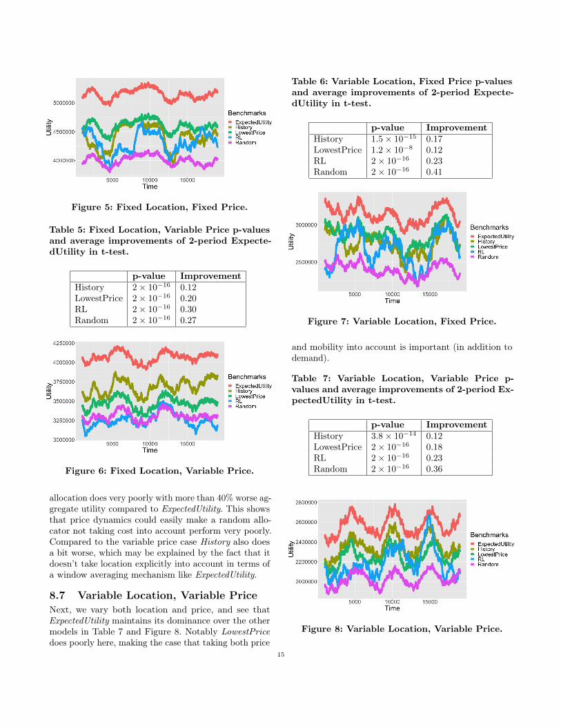
Figure 5: Fixed Location, Fixed Price.

Table 5: Fixed Location, Variable Price p-valuesand average improvements of 2-period Expecte-dUtility in t-test.

p-value ImprovementHistory 2× 10−16 0.12LowestPrice 2× 10−16 0.20RL 2× 10−16 0.30Random 2× 10−16 0.27

Figure 6: Fixed Location, Variable Price.

allocation does very poorly with more than 40% worse ag-gregate utility compared to ExpectedUtility. This showsthat price dynamics could easily make a random allo-cator not taking cost into account perform very poorly.Compared to the variable price case History also doesa bit worse, which may be explained by the fact that itdoesn’t take location explicitly into account in terms ofa window averaging mechanism like ExpectedUtility.

8.7 Variable Location, Variable PriceNext, we vary both location and price, and see thatExpectedUtility maintains its dominance over the othermodels in Table 7 and Figure 8. Notably LowestPricedoes poorly here, making the case that taking both price

Table 6: Variable Location, Fixed Price p-valuesand average improvements of 2-period Expecte-dUtility in t-test.

p-value ImprovementHistory 1.5× 10−15 0.17LowestPrice 1.2× 10−8 0.12RL 2× 10−16 0.23Random 2× 10−16 0.41

Figure 7: Variable Location, Fixed Price.

and mobility into account is important (in addition todemand).

Table 7: Variable Location, Variable Price p-values and average improvements of 2-period Ex-pectedUtility in t-test.

p-value ImprovementHistory 3.8× 10−14 0.12LowestPrice 2× 10−16 0.18RL 2× 10−16 0.23Random 2× 10−16 0.36

Figure 8: Variable Location, Variable Price.

15

8.8 Competing AgentsFinally, we vary both price, location and demand andalso introduce two more competing DUTs, running thesame provider selection algorithms, but with indepen-dent demands. Surprisingly, from Table 8 and Figure 9the standard RL does comparatively better although stillworse than ExpectedUtility. The fact that the Expecte-dUtility improvement over Random drops from about 40to 20% could be explained by the fact that the decisionsother DUTs are making could mislead the agent intothinking a network is worse than it is. It is still promisingthat the ExpectedUtility method does best even in thisscenario.

Table 8: 3 Competing Agents, p-values and av-erage improvements of 2-period ExpectedUtilityin t-test.

p-value ImprovementHistory 5.9× 10−7 0.13LowestPrice 6.1× 10−13 0.19RL 0.0024 0.085Random 1.6× 10−13 0.20

Figure 9: 3 Competing DUTs.

8.9 Summary of simulation resultsWe observe that in each of the simulated scenarios, theMonte Carlo algorithm for contextual multi-armed ban-dits, which we call ExpectedUtility, performs better thanthe direct Q-learning algorithm applied to maximize theexpected cumulative discounted reward, which we havecalled RL above. Given the relative lack of sophistica-tion of the Monte Carlo algorithm (1) compared to theRL Q-learning algorithm (7), these results may be sur-prising. However, they are explainable given that thesimulated scenarios are exactly contextual multi-armedbandit problems, and the Monte Carlo algorithm is,

in spite of its simplicity, a state-of-the-art solution tosuch problems [30, p. 43], performing as well or betterthan many other algorithms including deep Q-learning(DQN) [23, Tab. 1]. On the other hand, Q-learning isknown to be hard to train with low training sampleefficiency [33] and has been bettered in performance byother contextual multi-armed bandit methods in theliterature [8].

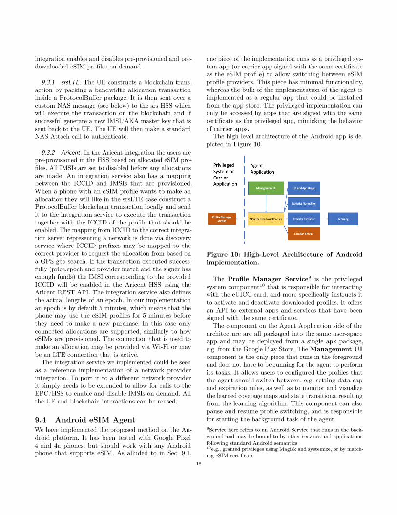
9 IMPLEMENTATION NOTESIn this section we go into some more details on how theproposed system has been implemented. as a prelude toour experiments. The current implementation relies oneSIM functionality and hence we start off with a quickprimer on eSIM.

9.1 eSIMEmbedded Subscriber Identity Module (eSIM) or Em-bedded Universal Integrated Circuit Card (eUICC) is aprogrammable chip embedded in a device that allows itto connect to different mobile networks without a phys-ical SIM card. The eSIM specifications are developedby the GSM Association (GSMA) and define the proto-cols and components required to remotely provision asoftware-based SIM card profile as part of subscribingto a mobile network service [3].

An eSIM profile is typically downloaded from a Sub-scription Manager - Data Preparation+ (SM-DP+) servercertified by the GSMA using a QR-code containing anactivation code. The download process maps the identityof the device to a subscription provided by a mobilenetwork operator. After the profile has been downloadedit may be activated, at which point the eSIM authenti-cates with and connects to a network with a matchingpublic land mobile network (PLMN) identifier withinreach, potentially after roaming to a supported provider.Typically only a single eSIM profile may be active at anygiven time, but any number of profiles may be down-loaded and be in an inactive state on the device. Afterthe eSIM is activated it behaves in the exact same way asa physical SIM card, until it is deactivated by switchingto another profile or by deleting it from the device.

The time it takes to switch depends on the provider,and can be substantial if roaming is involved. The over-head beyond the authentication process (e.g. LTE At-tach) is, however, negligible.

The eSIM profile contains a hash of the mobile networkprovider certificate that allows mobile apps developed bythat same provider to manage the eSIM profile in whatis known as a carrier app. Providers have no access to

16

profiles they did not provision (i.e. they cannot downloador switch to profiles they do not own).

Hence, to switch between profiles those profiles thoseprofiles could either be provided by an SMDP+ serveryou control or by the same provider that provisions theprofiles though the SMDP+ server.

As an alternative to controlling a certified SMDP+server, an app may also be promoted to a privilegedsystem app, e.g. by the mobile OS or an OEM, to allow itto switch between multiple profiles. This is the approachwe have taken in the implementation presented here.

The core piece of our implementation is the marketwhere bandwidth contracts are sold and purchased, dis-cussed next.

9.2 Blockchain MarketThe key part of the system that allows autonomouspurchasing of bandwidth contracts is a blockchain digi-tal market where providers can set prices and UEs canpurchase allocations. The blockchain is implementedas ledger where bandwidth purchase transactions arerecorded using smart contract processing. We used theopen source Sawtooth Hyperledger6 implementation toimplement a custom transaction processor to verify pur-chases, atomically execute bandwidth allocations andoffers, and record account balances. A transaction pro-cessor takes a signed payload and then verifies it againstthe current state of the blockchain before adding a ver-ified transaction to the ledger. We then allow the UEpurchasing a contract to send proof of purchase to anetwork provider to get access, either by directly get-ting access to AKA parameters or in the eSIM case bysimply enabling the pre-downloaded eSIM profile in theHSS. All services are implemented as REST endpointsoffering a JSON API. We also implemented an exchangethat allows for payment gateways to either withdrawor deposit real currency out of or into the bandwidthledger. Each UE and each provider will have a uniqueaccount in the blockchain that in the UE case needs tobe initiated with funds to start executing transactions.

The allocation and verification can also be done in asingle step where the UE will prepare and sign a purchaserequest transaction and send that directly to the providerwho will forward it to and execute it on the blockchain,before verifying the transaction and giving the UE access.This allows the UE to make allocations without beingconnected to or having direct access to the blockchainservices.

The payloads are encoded as Protocol Buffer bytestreamsusing a standard Sawtooth format that allows for batches

6https://www.hyperledger.org/use/sawtooth

of transactions to be encoded and forwarded by thirdparties. The inner part of the payload is specific to thetransaction processor that we defined. It can be encodedas json or as a simple comma separated string. Our cus-tom payload as an action element that defines the intentof the transaction. It can be allocate, offer, deposit, orwithdraw. Each of these payloads will also have a signerthat requests the action and a target provider that theaction is targeted at. The deposit and withdraw actionscan only be performed by trusted exchanges to fund orexchange blockchain currency to and from other curren-cies. A UE would typically issue the allocate actions witha target provider that matches an offer on the blockchain.The blockchain records that are atomically written asa result of executed actions provide a cryptographicallyverified input payload and a state resulting from exe-cuting that payload. The state in this case provides themost up-to-date record of the balance of the target ac-count, allocations remaining in an epoch (virtual time).This state together with the input payload that causedit to be recorded are available for anyone to verify thathas access to the blockchain, i.e. the network bandwidthproviders and payment gateway changes.

The payload is defined in Table 16. Note that not allpayload elements are used or required by all actions. Theledger transaction record is defined in Table 18, and thebasic processing rules for different actions are defined inTable 17.

9.3 LTE EPC IntegrationTo allow a network provider to sell bandwidth on ourblockchain market they need to interact with the ledgerto enable or provision users on demand and to updatepricing and bands of offers. Different prices may be set ondifferent frequency bands and for different band width.Each offer configuration has one price. The provider canalso specify how many allocations within an offer can besold within an epoch.

Users may purchase allocations independently of theprovider and the provider would then validate proof ofa transaction to grant the user an allocation and accessto the network.

We have built two Proof of Concept integrations, andwith the EPC/HSS of srsLTE7, and one one with theAricent EPC/HSS8. The srsLTE integration allows bothconnected and disconnected allocations over a customLTE protocol described below, and it provisions IM-SIs and AKA keys on demand. The Aricent EPC/HSS

7https://github.com/srsLTE/srsLTE8https://northamerica.altran.com/software/lte-evolved-packet-core

17

integration enables and disables pre-provisioned and pre-downloaded eSIM profiles on demand.

9.3.1 srsLTE. The UE constructs a blockchain trans-action by packing a bandwidth allocation transactioninside a ProtocolBuffer package. It is then sent over acustom NAS message (see below) to the srs HSS whichwill execute the transaction on the blockchain and ifsuccessful generate a new IMSI/AKA master key that issent back to the UE. The UE will then make a standardNAS Attach call to authenticate.

9.3.2 Aricent. In the Aricent integration the users arepre-provisioned in the HSS based on allocated eSIM pro-files. All IMSIs are set to disabled before any allocationsare made. An integration service also has a mappingbetween the ICCID and IMSIs that are provisioned.When a phone with an eSIM profile wants to make anallocation they will like in the srsLTE case construct aProtocolBuffer blockchain transaction locally and sendit to the integration service to execute the transactiontogether with the ICCID of the profile that should beenabled. The mapping from ICCID to the correct integra-tion server representing a network is done via discoveryservice where ICCID prefixes may be mapped to thecorrect provider to request the allocation from based ona GPS geo-search. If the transaction executed success-fully (price,epoch and provider match and the signer hasenough funds) the IMSI corresponding to the providedICCID will be enabled in the Aricent HSS using theAricent REST API. The integration service also definesthe actual lengths of an epoch. In our implementationan epoch is by default 5 minutes, which means that thephone may use the eSIM profiles for 5 minutes beforethey need to make a new purchase. In this case onlyconnected allocations are supported, similarly to howeSIMs are provisioned. The connection that is used tomake an allocation may be provided via Wi-Fi or maybe an LTE connection that is active.

The integration service we implemented could be seenas a reference implementation of a network providerintegration. To port it to a different network providerit simply needs to be extended to allow for calls to theEPC/HSS to enable and disable IMSIs on demand. Allthe UE and blockchain interactions can be reused.

9.4 Android eSIM AgentWe have implemented the proposed method on the An-droid platform. It has been tested with Google Pixel4 and 4a phones, but should work with any Androidphone that supports eSIM. As alluded to in Sec. 9.1,

one piece of the implementation runs as a privileged sys-tem app (or carrier app signed with the same certificateas the eSIM profile) to allow switching between eSIMprofile providers. This piece has minimal functionality,whereas the bulk of the implementation of the agent isimplemented as a regular app that could be installedfrom the app store. The privileged implementation canonly be accessed by apps that are signed with the samecertificate as the privileged app, mimicking the behaviorof carrier apps.

The high-level architecture of the Android app is de-picted in Figure 10.

Figure 10: High-Level Architecture of Androidimplementation.

The Profile Manager Service9 is the privilegedsystem component10 that is responsible for interactingwith the eUICC card, and more specifically instructs itto activate and deactivate downloaded profiles. It offersan API to external apps and services that have beensigned with the same certificate.

The component on the Agent Application side of thearchitecture are all packaged into the same user-spaceapp and may be deployed from a single apk package,e.g. from the Google Play Store. The Management UIcomponent is the only piece that runs in the foregroundand does not have to be running for the agent to performits tasks. It allows users to configured the profiles thatthe agent should switch between, e.g. setting data capand expiration rules, as well as to monitor and visualizethe learned coverage maps and state transitions, resultingfrom the learning algorithm. This component can alsopause and resume profile switching, and is responsiblefor starting the background task of the agent.9Service here refers to an Android Service that runs in the back-ground and may be bound to by other services and applicationsfollowing standard Android semantics10e.g., granted privileges using Magisk and systemize, or by match-ing eSIM certificate

18

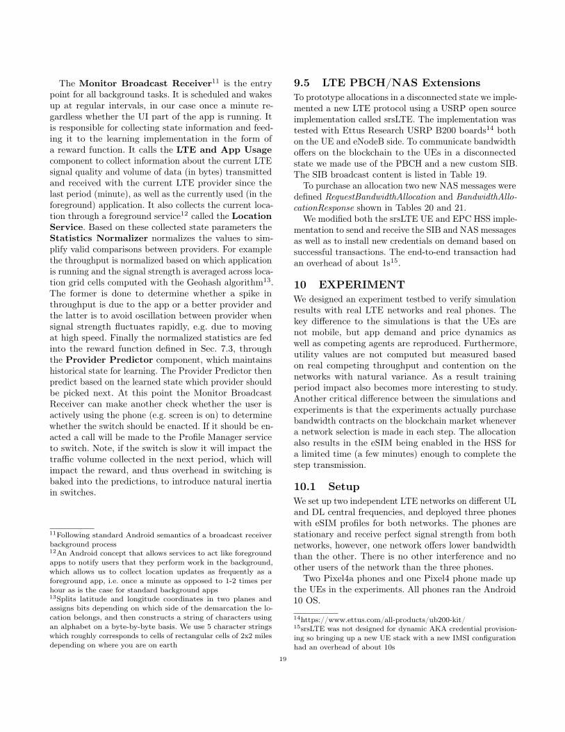
The Monitor Broadcast Receiver11 is the entrypoint for all background tasks. It is scheduled and wakesup at regular intervals, in our case once a minute re-gardless whether the UI part of the app is running. Itis responsible for collecting state information and feed-ing it to the learning implementation in the form ofa reward function. It calls the LTE and App Usagecomponent to collect information about the current LTEsignal quality and volume of data (in bytes) transmittedand received with the current LTE provider since thelast period (minute), as well as the currently used (in theforeground) application. It also collects the current loca-tion through a foreground service12 called the LocationService. Based on these collected state parameters theStatistics Normalizer normalizes the values to sim-plify valid comparisons between providers. For examplethe throughput is normalized based on which applicationis running and the signal strength is averaged across loca-tion grid cells computed with the Geohash algorithm13.The former is done to determine whether a spike inthroughput is due to the app or a better provider andthe latter is to avoid oscillation between provider whensignal strength fluctuates rapidly, e.g. due to movingat high speed. Finally the normalized statistics are fedinto the reward function defined in Sec. 7.3, throughthe Provider Predictor component, which maintainshistorical state for learning. The Provider Predictor thenpredict based on the learned state which provider shouldbe picked next. At this point the Monitor BroadcastReceiver can make another check whether the user isactively using the phone (e.g. screen is on) to determinewhether the switch should be enacted. If it should be en-acted a call will be made to the Profile Manager serviceto switch. Note, if the switch is slow it will impact thetraffic volume collected in the next period, which willimpact the reward, and thus overhead in switching isbaked into the predictions, to introduce natural inertiain switches.

11Following standard Android semantics of a broadcast receiverbackground process12An Android concept that allows services to act like foregroundapps to notify users that they perform work in the background,which allows us to collect location updates as frequently as aforeground app, i.e. once a minute as opposed to 1-2 times perhour as is the case for standard background apps13Splits latitude and longitude coordinates in two planes andassigns bits depending on which side of the demarcation the lo-cation belongs, and then constructs a string of characters usingan alphabet on a byte-by-byte basis. We use 5 character stringswhich roughly corresponds to cells of rectangular cells of 2x2 milesdepending on where you are on earth

9.5 LTE PBCH/NAS ExtensionsTo prototype allocations in a disconnected state we imple-mented a new LTE protocol using a USRP open sourceimplementation called srsLTE. The implementation wastested with Ettus Research USRP B200 boards14 bothon the UE and eNodeB side. To communicate bandwidthoffers on the blockchain to the UEs in a disconnectedstate we made use of the PBCH and a new custom SIB.The SIB broadcast content is listed in Table 19.

To purchase an allocation two new NAS messages weredefined RequestBandwidthAllocation and BandwidthAllo-cationResponse shown in Tables 20 and 21.

We modified both the srsLTE UE and EPC HSS imple-mentation to send and receive the SIB and NAS messagesas well as to install new credentials on demand based onsuccessful transactions. The end-to-end transaction hadan overhead of about 1s15.

10 EXPERIMENTWe designed an experiment testbed to verify simulationresults with real LTE networks and real phones. Thekey difference to the simulations is that the UEs arenot mobile, but app demand and price dynamics aswell as competing agents are reproduced. Furthermore,utility values are not computed but measured basedon real competing throughput and contention on thenetworks with natural variance. As a result trainingperiod impact also becomes more interesting to study.Another critical difference between the simulations andexperiments is that the experiments actually purchasebandwidth contracts on the blockchain market whenevera network selection is made in each step. The allocationalso results in the eSIM being enabled in the HSS fora limited time (a few minutes) enough to complete thestep transmission.

10.1 SetupWe set up two independent LTE networks on different ULand DL central frequencies, and deployed three phoneswith eSIM profiles for both networks. The phones arestationary and receive perfect signal strength from bothnetworks, however, one network offers lower bandwidththan the other. There is no other interference and noother users of the network than the three phones.

Two Pixel4a phones and one Pixel4 phone made upthe UEs in the experiments. All phones ran the Android10 OS.

14https://www.ettus.com/all-products/ub200-kit/15srsLTE was not designed for dynamic AKA credential provision-ing so bringing up a new UE stack with a new IMSI configurationhad an overhead of about 10s

19

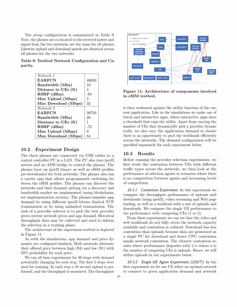
The setup configuration is summarized in Table 9.Note, the phones are co-located to the received power andsignal from the two networks are the same for all phones.Likewise upload and download speeds are identical acrossall phones for the two networks.

Table 9: Testbed Network Configuration and Ca-pacity.

Network 1EARFCN 40620Bandwidth (Mhz) 10Distance to UEs (ft) 4RSRP (dBm) -85Max Upload (Mbps) 2Max Download (Mbps) 32Network 2EARFCN 39750Bandwidth (Mhz) 20Distance to UEs (ft) 1RSRP (dBm) -72Max Upload (Mbps) 9Max Download (Mbps) 84

10.2 Experiment DesignThe three phones are connected via USB cables to acentral controller PC in a LAN. The PC also runs iperf3servers and an ADB bridge to control the phones. Thephones have an iperf3 binary as well as eSIM profilespre-downloaded for both networks. The phones also runa carrier app that allows programmatic switching be-tween the eSIM profiles. The phones can discover thenetworks and their dynamic pricing via a discovery andbandwidth market we implemented (using blockchains,see implementation section). The phones simulate appdemand by using different iperf3 bitrate limited TCPtransmission or by using unlimited transmission. Thetask of a provider selector is to pick the best providergiven current network prices and app demand. Historicalthroughput data may be collected and used to informthe selection in a training phase.

The architecture of the experiment testbed is depictedin Figure 11.

As with the simulations, app demand and price dy-namics are configured similarly. Both networks alternatetheir offered price between high ($4) and low ($1) with50% probability for each price.

We ran all base experiments for 30 steps with demandpotentially changing for each step. The first 5 steps wereused for training. In each step a 10 second upload is per-formed, and the throughput is measured. The throughput

Figure 11: Architecture of components involvedin eSIM testbed.

is then evaluated against the utility function of the cur-rent application. Like in the simulations we make use ofbatch and interactive apps, where interactive apps havea threshold that caps the utility. Apart from varying thenumber of UEs that dynamically pick a provider dynam-ically, we also vary the application demand to ensurethere is an opportunity to pack the workloads efficientlyacross the networks. The demand configuration will bespecified separately for each experiment below.

10.3 ResultsBefore running the provider selection experiments, wefirst study the contention between UEs with differenttraffic types across the networks, we then look at theperformance of selection agents in scenarios where thereis no competition between agents and increasing levelsof competition.

10.3.1 Contention Experiment. In this experiment wecompare the throughput performance of uploads anddownloads (using iperf3), video streaming and Web pageloading, as well as a workload with a mix of uploads anddownloads. We compare the single UE performance tothe performance with competing UEs (1 or 2).

From these experiments we can see that the video andweb workloads do not fully stress the network capacityavailable and contention is reduced. Download has lesscontention than uploads because data are generated ona single PC for download and hence CPU contentionmasks network contention. The clearest contention re-sults where performance degrades with 1/𝑛 where 𝑛 isthe number of competing UEs is uploads. Hence, we willutilize uploads in our experiments below.

10.3.2 Single UE Agent Experiment (1DUT). In thefirst experiment we let one UE select an optimal networkto connect to given application demand and network

20

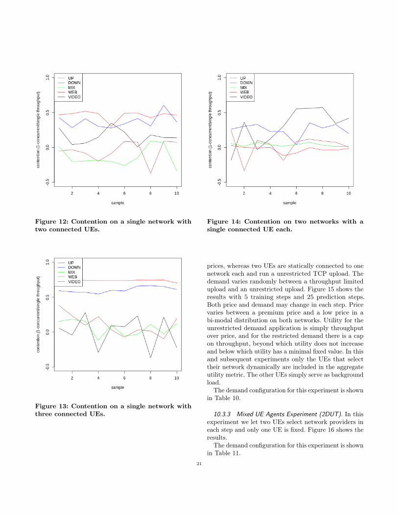
Figure 12: Contention on a single network withtwo connected UEs.

Figure 13: Contention on a single network withthree connected UEs.

Figure 14: Contention on two networks with asingle connected UE each.

prices, whereas two UEs are statically connected to onenetwork each and run a unrestricted TCP upload. Thedemand varies randomly between a throughput limitedupload and an unrestricted upload. Figure 15 shows theresults with 5 training steps and 25 prediction steps.Both price and demand may change in each step. Pricevaries between a premium price and a low price in abi-modal distribution on both networks. Utility for theunrestricted demand application is simply throughputover price, and for the restricted demand there is a capon throughput, beyond which utility does not increaseand below which utility has a minimal fixed value. In thisand subsequent experiments only the UEs that selecttheir network dynamically are included in the aggregateutility metric. The other UEs simply serve as backgroundload.

The demand configuration for this experiment is shownin Table 10.

10.3.3 Mixed UE Agents Experiment (2DUT). In thisexperiment we let two UEs select network providers ineach step and only one UE is fixed. Figure 16 shows theresults.

The demand configuration for this experiment is shownin Table 11.

21

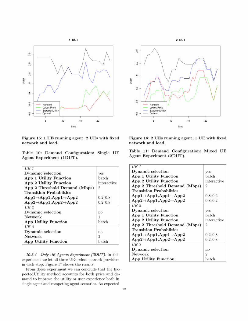
Figure 15: 1 UE running agent, 2 UEs with fixednetwork and load.

Table 10: Demand Configuration: Single UEAgent Experiment (1DUT).

UE 1Dynamic selection yesApp 1 Utility Function batchApp 2 Utility Function interactiveApp 2 Threshold Demand (Mbps) 2Transition ProbabiltiesApp1→App1,App1→App2 0.2, 0.8App2→App1,App2→App2 0.2, 0.8UE 2Dynamic selection noNetwork 1App Utility Function batchUE 3Dynamic selection noNetwork 2App Utility Function batch

10.3.4 Only UE Agents Experiment (3DUT). In thisexperiment we let all three UEs select network providersin each step. Figure 17 shows the results.

From these experiment we can conclude that the Ex-pectedUtility method accounts for both price and de-mand to improve the utility or user experience both insingle agent and competing agent scenarios. As expected

Figure 16: 2 UEs running agent, 1 UE with fixednetwork and load.

Table 11: Demand Configuration: Mixed UEAgent Experiment (2DUT).

UE 1Dynamic selection yesApp 1 Utility Function batchApp 2 Utility Function interactiveApp 2 Threshold Demand (Mbps) 2Transition ProbabiltiesApp1→App1,App1→App2 0.8, 0.2App2→App1,App2→App2 0.8, 0.2UE 2Dynamic selection yesApp 1 Utility Function batchApp 2 Utility Function interactiveApp 2 Threshold Demand (Mbps) 2Transition ProbabiltiesApp1→App1,App1→App2 0.2, 0.8App2→App1,App2→App2 0.2, 0.8UE 3Dynamic selection noNetwork 2App Utility Function batch

22

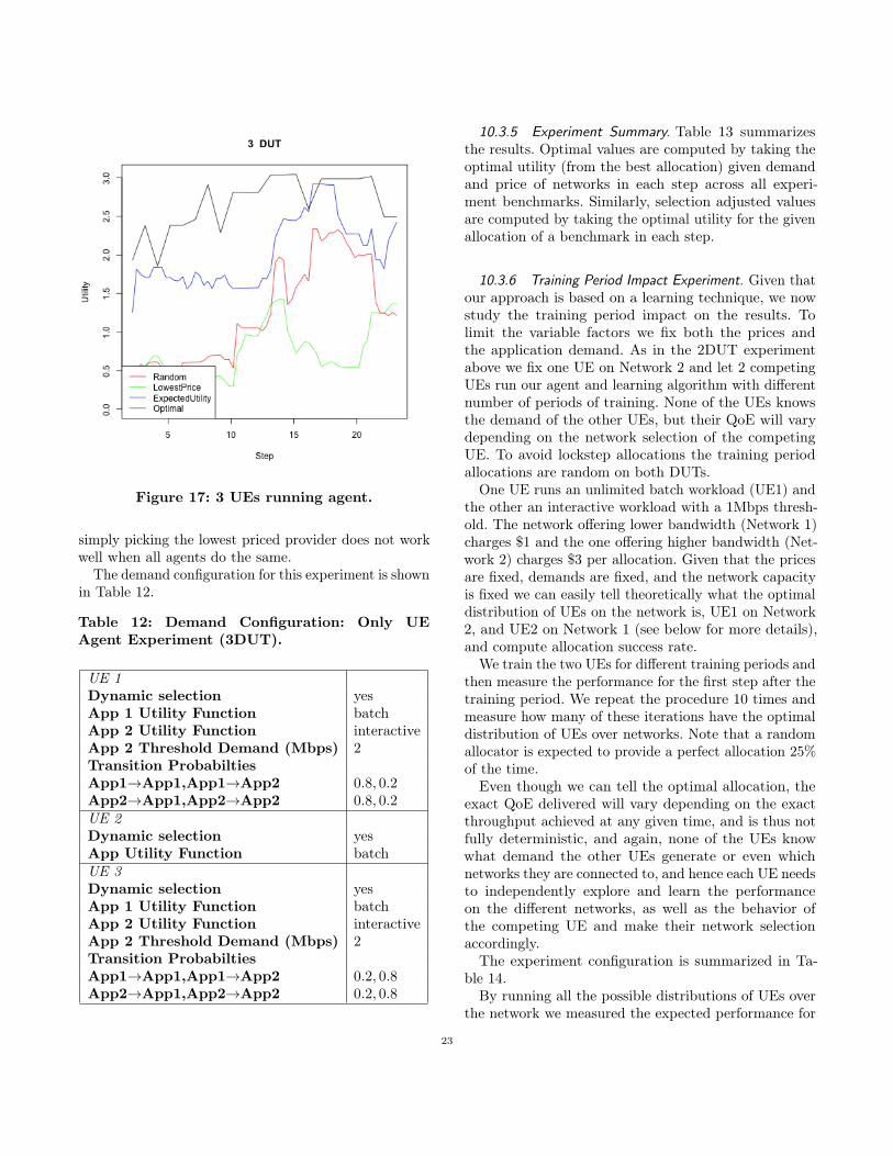
Figure 17: 3 UEs running agent.

simply picking the lowest priced provider does not workwell when all agents do the same.

The demand configuration for this experiment is shownin Table 12.

Table 12: Demand Configuration: Only UEAgent Experiment (3DUT).

UE 1Dynamic selection yesApp 1 Utility Function batchApp 2 Utility Function interactiveApp 2 Threshold Demand (Mbps) 2Transition ProbabiltiesApp1→App1,App1→App2 0.8, 0.2App2→App1,App2→App2 0.8, 0.2UE 2Dynamic selection yesApp Utility Function batchUE 3Dynamic selection yesApp 1 Utility Function batchApp 2 Utility Function interactiveApp 2 Threshold Demand (Mbps) 2Transition ProbabiltiesApp1→App1,App1→App2 0.2, 0.8App2→App1,App2→App2 0.2, 0.8

10.3.5 Experiment Summary. Table 13 summarizesthe results. Optimal values are computed by taking theoptimal utility (from the best allocation) given demandand price of networks in each step across all experi-ment benchmarks. Similarly, selection adjusted valuesare computed by taking the optimal utility for the givenallocation of a benchmark in each step.

10.3.6 Training Period Impact Experiment. Given thatour approach is based on a learning technique, we nowstudy the training period impact on the results. Tolimit the variable factors we fix both the prices andthe application demand. As in the 2DUT experimentabove we fix one UE on Network 2 and let 2 competingUEs run our agent and learning algorithm with differentnumber of periods of training. None of the UEs knowsthe demand of the other UEs, but their QoE will varydepending on the network selection of the competingUE. To avoid lockstep allocations the training periodallocations are random on both DUTs.

One UE runs an unlimited batch workload (UE1) andthe other an interactive workload with a 1Mbps thresh-old. The network offering lower bandwidth (Network 1)charges $1 and the one offering higher bandwidth (Net-work 2) charges $3 per allocation. Given that the pricesare fixed, demands are fixed, and the network capacityis fixed we can easily tell theoretically what the optimaldistribution of UEs on the network is, UE1 on Network2, and UE2 on Network 1 (see below for more details),and compute allocation success rate.

We train the two UEs for different training periods andthen measure the performance for the first step after thetraining period. We repeat the procedure 10 times andmeasure how many of these iterations have the optimaldistribution of UEs over networks. Note that a randomallocator is expected to provide a perfect allocation 25%of the time.

Even though we can tell the optimal allocation, theexact QoE delivered will vary depending on the exactthroughput achieved at any given time, and is thus notfully deterministic, and again, none of the UEs knowwhat demand the other UEs generate or even whichnetworks they are connected to, and hence each UE needsto independently explore and learn the performanceon the different networks, as well as the behavior ofthe competing UE and make their network selectionaccordingly.

The experiment configuration is summarized in Ta-ble 14.

By running all the possible distributions of UEs overthe network we measured the expected performance for

23

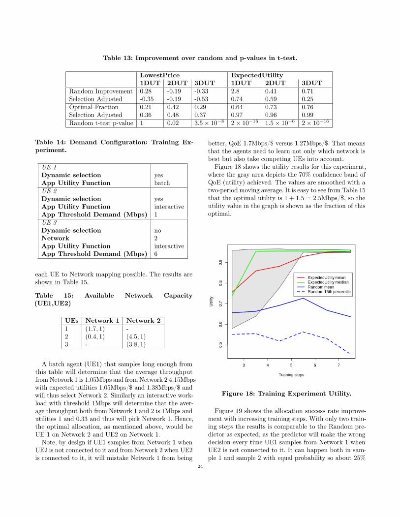
Table 13: Improvement over random and p-values in t-test.

LowestPrice ExpectedUtility1DUT 2DUT 3DUT 1DUT 2DUT 3DUT

Random Improvement 0.28 -0.19 -0.33 2.8 0.41 0.71Selection Adjusted -0.35 -0.19 -0.53 0.74 0.59 0.25Optimal Fraction 0.21 0.42 0.29 0.64 0.73 0.76Selection Adjusted 0.36 0.48 0.37 0.97 0.96 0.99Random t-test p-value 1 0.02 3.5× 10−8 2× 10−16 1.5× 10−6 2× 10−16

Table 14: Demand Configuration: Training Ex-periment.

UE 1Dynamic selection yesApp Utility Function batchUE 2Dynamic selection yesApp Utility Function interactiveApp Threshold Demand (Mbps) 1UE 3Dynamic selection noNetwork 2App Utility Function interactiveApp Threshold Demand (Mbps) 6

each UE to Network mapping possible. The results areshown in Table 15.

Table 15: Available Network Capacity(UE1,UE2)

UEs Network 1 Network 21 (1.7, 1) -2 (0.4, 1) (4.5, 1)3 - (3.8, 1)

A batch agent (UE1) that samples long enough fromthis table will determine that the average throughputfrom Network 1 is 1.05Mbps and from Network 2 4.15Mbpswith expected utilities 1.05Mbps/$ and 1.38Mbps/$ andwill thus select Network 2. Similarly an interactive work-load with threshold 1Mbps will determine that the aver-age throughput both from Network 1 and 2 is 1Mbps andutilities 1 and 0.33 and thus will pick Network 1. Hence,the optimal allocation, as mentioned above, would beUE 1 on Network 2 and UE2 on Network 1.

Note, by design if UE1 samples from Network 1 whenUE2 is not connected to it and from Network 2 when UE2is connected to it, it will mistake Network 1 from being

better, QoE 1.7Mbps/$ versus 1.27Mbps/$. That meansthat the agents need to learn not only which network isbest but also take competing UEs into account.

Figure 18 shows the utility results for this experiment,where the gray area depicts the 70% confidence band ofQoE (utility) achieved. The values are smoothed with atwo-period moving average. It is easy to see from Table 15that the optimal utility is 1 + 1.5 = 2.5Mbps/$, so theutility value in the graph is shown as the fraction of thisoptimal.

Figure 18: Training Experiment Utility.

Figure 19 shows the allocation success rate improve-ment with increasing training steps. With only two train-ing steps the results is comparable to the Random pre-dictor as expected, as the predictor will make the wrongdecision every time UE1 samples from Network 1 whenUE2 is not connected to it. It can happen both in sam-ple 1 and sample 2 with equal probability so about 25%

24

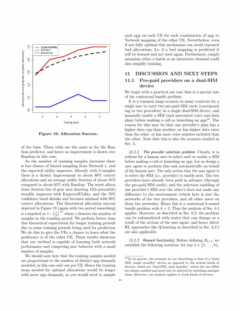
Figure 19: Allocation Success.

of the time. These odds are the same as for the Ran-dom predictor, and hence no improvement is shown overRandom in this case.

As the number of training samples increases thereis less chance of biased sampling from Network 1, andthe expected utility improves. Already with 3 samplesthere is a drastic improvement to about 80% correctallocations and an average utility fraction of about 85%compared to about 65% with Random. The worst alloca-tions (bottom line of gray area denoting 15th percentile)steadily improves with ExpectedUtility, and the 70%confidence band shrinks and becomes minimal with 90%correct allocations. The theoretical allocation successdepicted in Figure 19 (again with two period smoothing)is computed as 1−

(︀12

)︀.5𝑠 where 𝑠 denotes the number ofsamples in the training period. We perform better thanthis theoretical expectation for longer training periodsdue to some training periods being used for prediction.We do this to give the UEs a chance to learn what thepreference is of the other UE. These results showcasethat our method is capable of learning both networkperformance and competing user behavior with a smallnumber of samples.

We should note here that the training samples neededare proportional to the number of distinct app demandsmodeled, in this case only one per UE. Hence the trainingsteps needed for optimal allocations would be longerwith more app demands, as you would need to sample

each app on each UE for each combination of app toNetwork mapping of the other UE. Nevertheless, evenif not fully optimal this mechanism can avoid repeatedbad allocations. I.e. if a bad mapping is predicted itwill be learned and not used again. Furthermore, simplyassuming either a batch or an interactive demand couldalso simplify training.

11 DISCUSSION AND NEXT STEPS11.1 Pre-paid providers on a dual-SIM

deviceWe begin with a practical use case that is a special caseof the contextual bandit problem.

It is a common usage scenario in many countries for asingle user to carry two pre-paid SIM cards (correspond-ing to two providers) in a single dual-SIM device, andmanually enable a SIM (and associated voice and dataplan) before making a call or launching an app16. Thereason for this may be that one provider’s plan has ahigher data cap than another, or has higher data ratesthan the other, or has more voice minutes included thanthe other. Note that this is also the scenario studied inSec. 3.

11.1.1 The provider selection problem. Clearly, it istedious for a human user to select and/or enable a SIMbefore making a call or launching an app. Let us design auser agent to perform this task automatically on behalfof the human user. The only action that the user agent isto select the SIM (i.e., provider) to enable next. The twoproviders have already been paid in advance (throughthe pre-paid SIM cards), and the selection/enabling ofone provider’s SIM over the other’s does not make anydifference to the environment (which here is just thenetworks of the two providers, and all other users onthose two networks). Hence this is a contextual 𝑘-armedbandit problem with 𝑘 = 2. Thus the analysis of Sec. 6.1applies. Moreover, as described in Sec. 6.2, the problemcan be reformulated with states that can change as aresult of the actions of the user agent, and hence directRL approaches like Q-learning as described in Sec. 6.2.1are also applicable.

11.1.2 Reward function(s). Before defining 𝑅𝑡+1, weestablish the following notation: for any 𝑎 ∈ {1, . . . , 𝑘},

16To be precise, the scenario we are describing is that of a “dual-SIM, single standby” device as opposed to the newest kinds ofdevices, which are “dual-SIM, dual standby,” where the two SIMsare always enabled and need only be selected by switching amongstthem. However, our analysis applies to both kinds of devices.

25

(1) TotalDataUsed(𝑎)𝑡 are the cumulative data usage

on the prepaid plans (as a fraction of their respec-tive data caps); note that TotalDataUsed

(𝑎)𝑡 =∑︀𝑡

𝑡′=1 DataUsed(𝑎)𝑡′ , where DataUsed(𝑎)𝑡′ are the data

usage in time step 𝑡′ on the prepaid plans, as afraction of their respective data caps;

(2) LifeRemaining(𝑎)𝑡 are the remaining life on the

prepaid plans (in units of time steps);(3) PlanPrice

(𝑎)𝑡 are the costs of the prepaid plans

(per time step).

We now define 𝑅𝑡+1 as follows:

𝑅𝑡+1 =QoE

(𝑎)𝑡+1(𝑠)

PlanPrice(𝑎)𝑡

(︃1− TotalDataUsed

(𝑎)𝑡

LifeRemaining(𝑎)𝑡

)︃𝛽

(8)

for some chosen 𝛽 ≥ 0, where we explicitly show thedependence of QoE(𝑎)𝑡+1 on the selected provider 𝑎 andthe application 𝑠 launched by the user, and 𝛽 ∈ {1, 0}depending on whether or not we want to incentivize theuse of a provider when its prepaid plan is close to expirywhile its data cap has not been reached.

Alternatively, we may see the existence of the datacaps as turning the original contextual 2-armed ban-dit problem into a Contextual Bandit with Knapsackproblem [28, Chap. 10] defined as follows: at each step𝑡, the action 𝑎 results in the learning algorithm re-ceiving feedback comprising both a reward 𝑅𝑡+1 =

QoE(𝑎)𝑡+1(𝑠)/PlanPrice

(𝑎)𝑡 and a (data) consumption vec-

tor (DataUsed(1)𝑡 , DataUsed(2)𝑡 ) with DataUsed

(𝑖)𝑡 = 0 for

𝑖 ̸= 𝑎, and the goal is to maximize the (undiscounted) to-tal reward

∑︀𝑇−1𝑡=1 𝑅𝑡+1 subject to the budget constraints∑︀𝑇

𝑡=1 DataUsed(𝑎)𝑡 ≤ 1, 𝑎 = 1, 2, where 𝑇 is the total

number of time steps in the lifetime of the plans. Thereexist efficient algorithms to solve this convex bandit withknapsack problem that are optimal in a certain sense [1],but they are more computationally intensive than forthe contextual bandit problem.

11.2 Extensions to the 𝑘-armed banditWe now discuss some extensions and modifications to thebasic contextual 𝑘-armed bandit previously discussed inSecs. 6.1 and 7.1, and to the RL approach described inSec. 6.2.2. Although we have not evaluated these methodsvia simulation or experiment, they are well-known inthe literature and are the most promising approaches tostudy next.

11.2.1 Contextual UCB bandit. The upper confidencebound (UCB) modification to the contextual 𝑘-armed

bandit of sec. 6.1 changes the right hand side of (1):

𝐴𝑡(𝑠) = argmax𝑎

[︃𝑄𝑡(𝑠, 𝑎) + 𝑐

√︃ln 𝑡

𝑁𝑡−1(𝑠, 𝑎)

]︃, (9)

where 𝑐 > 0 is a fixed constant [30, Sec. 2.7].

11.2.2 Expanding the context space. Unlike a humanuser, a user agent residing on the user’s device can utilizeany attribute or measurement of the network that isavailable on the device. The obvious candidates to beused by the agent in choosing an action are the SINRsat the device from the 𝑘 providers at time 𝑡, which wedenote SINR

(𝑖)𝑡 , 𝑖 = 1, . . . , 𝑘, as these SINRs are not only

measured by the device but also strongly influence theQoE of most, if not all, apps. Note, however, that we canonly attempt to predict the QoE at time step 𝑡+1 basedon the SINR measurements at time step 𝑡. Moreover, theinherent randomness of wireless channels means that theaction 𝐴𝑡 = 𝑎 of selecting provider 𝑎 does not changethe distribution of the SINR SINR

(𝑎)𝑡+1, so the SINRs are

part of the context but cannot be part of the state.Let us return to the (non-contextual) 𝑘-armed bandit

problem that, as before, is obtained by treating eachcontext (i.e., launched app) completely separately anddecoupled from the other contexts. Fix the app to be 𝑠 ∈{1, 2, . . . , 𝑛}. This time, however, we shall incorporatethe SINRs. We would expect a larger SINR at time step𝑡 from provider 𝑎 to yield a preference on the part of theagent (as it would for a human user) to select the action𝐴𝑡(𝑠) = 𝑎. The so-called Gradient Bandit algorithmexpresses this preference through the soft-max functionyielding the probability distribution over actions givenby [30, Sec. 2.8]

P{𝐴𝑡(𝑠) = 𝑎} = exp(𝐻(SINR(𝑎)𝑡 (𝑠)))∑︀𝑘

𝑖=1 exp(𝐻(SINR(𝑖)𝑡 (𝑠)))

= 𝜋𝑡(𝑠, 𝑎), say,

(10)where 𝐻(·) is some selected function. This soft-max hasa heuristic physical interpretation for wireless channelsin the sense that if noise and interference is constantand fades on the link between the nearest base stationsof the different providers and the user device are inde-pendent and Rayleigh distributed, then the SINRs fromthe different providers at the user device are indepen-dent and Exponentially distributed. If 𝐻(SINR

(𝑖)𝑡 (𝑠)),

𝑖 = 1, . . . , 𝑘 represent the SINR values in dB, then theabove soft-max function 𝜋𝑡(𝑠, 𝑎) is also the probabilitythat SINR(𝑎)𝑡 (𝑠) = max1≤𝑖≤𝑘 SINR

(𝑖)𝑡 (𝑠).

The action 𝐴𝑡(𝑠) at time 𝑡 may be simply drawn fromthe distribution 𝜋𝑡(𝑠, 𝑎) or selected as argmax𝑎 𝜋𝑡(𝑠, 𝑎)or selected as argmax𝑎 𝜋𝑡(𝑠, 𝑎) with probability 1−𝜖 and

26

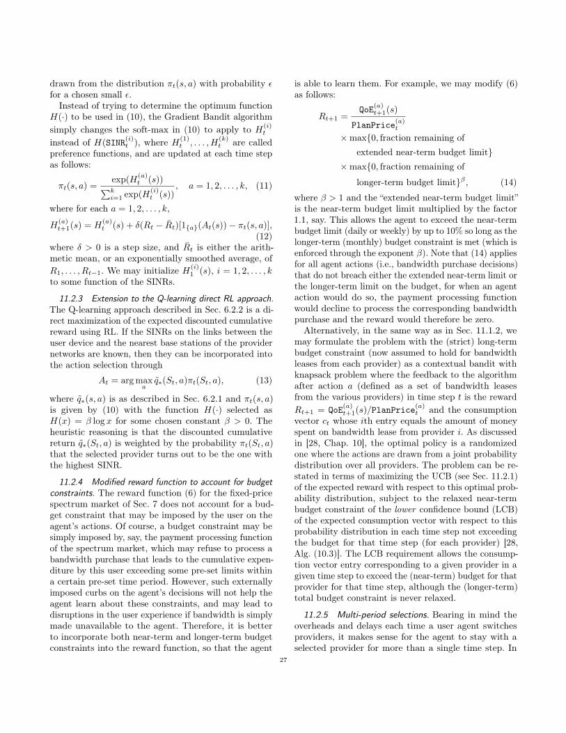
drawn from the distribution 𝜋𝑡(𝑠, 𝑎) with probability 𝜖for a chosen small 𝜖.

Instead of trying to determine the optimum function𝐻(·) to be used in (10), the Gradient Bandit algorithmsimply changes the soft-max in (10) to apply to 𝐻

(𝑖)𝑡

instead of 𝐻(SINR(𝑖)𝑡 ), where 𝐻

(1)𝑡 , . . . ,𝐻

(𝑘)𝑡 are called

preference functions, and are updated at each time stepas follows:

𝜋𝑡(𝑠, 𝑎) =exp(𝐻

(𝑎)𝑡 (𝑠))∑︀𝑘

𝑖=1 exp(𝐻(𝑖)𝑡 (𝑠))

, 𝑎 = 1, 2, . . . , 𝑘, (11)

where for each 𝑎 = 1, 2, . . . , 𝑘,

𝐻(𝑎)𝑡+1(𝑠) = 𝐻

(𝑎)𝑡 (𝑠) + 𝛿(𝑅𝑡 − �̄�𝑡)[1{𝑎}(𝐴𝑡(𝑠))− 𝜋𝑡(𝑠, 𝑎)],

(12)where 𝛿 > 0 is a step size, and �̄�𝑡 is either the arith-metic mean, or an exponentially smoothed average, of𝑅1, . . . , 𝑅𝑡−1. We may initialize 𝐻

(𝑖)1 (𝑠), 𝑖 = 1, 2, . . . , 𝑘

to some function of the SINRs.

11.2.3 Extension to the Q-learning direct RL approach.The Q-learning approach described in Sec. 6.2.2 is a di-rect maximization of the expected discounted cumulativereward using RL. If the SINRs on the links between theuser device and the nearest base stations of the providernetworks are known, then they can be incorporated intothe action selection through

𝐴𝑡 = argmax𝑎

𝑞*(𝑆𝑡, 𝑎)𝜋𝑡(𝑆𝑡, 𝑎), (13)

where 𝑞*(𝑠, 𝑎) is as described in Sec. 6.2.1 and 𝜋𝑡(𝑠, 𝑎)is given by (10) with the function 𝐻(·) selected as𝐻(𝑥) = 𝛽 log 𝑥 for some chosen constant 𝛽 > 0. Theheuristic reasoning is that the discounted cumulativereturn 𝑞*(𝑆𝑡, 𝑎) is weighted by the probability 𝜋𝑡(𝑆𝑡, 𝑎)that the selected provider turns out to be the one withthe highest SINR.

11.2.4 Modified reward function to account for budgetconstraints. The reward function (6) for the fixed-pricespectrum market of Sec. 7 does not account for a bud-get constraint that may be imposed by the user on theagent’s actions. Of course, a budget constraint may besimply imposed by, say, the payment processing functionof the spectrum market, which may refuse to process abandwidth purchase that leads to the cumulative expen-diture by this user exceeding some pre-set limits withina certain pre-set time period. However, such externallyimposed curbs on the agent’s decisions will not help theagent learn about these constraints, and may lead todisruptions in the user experience if bandwidth is simplymade unavailable to the agent. Therefore, it is betterto incorporate both near-term and longer-term budgetconstraints into the reward function, so that the agent

is able to learn them. For example, we may modify (6)as follows:

𝑅𝑡+1 =QoE

(𝑎)𝑡+1(𝑠)

PlanPrice(𝑎)𝑡

×max{0, fraction remaining ofextended near-term budget limit}

×max{0, fraction remaining of

longer-term budget limit}𝛽 , (14)

where 𝛽 > 1 and the “extended near-term budget limit”is the near-term budget limit multiplied by the factor1.1, say. This allows the agent to exceed the near-termbudget limit (daily or weekly) by up to 10% so long as thelonger-term (monthly) budget constraint is met (which isenforced through the exponent 𝛽). Note that (14) appliesfor all agent actions (i.e., bandwidth purchase decisions)that do not breach either the extended near-term limit orthe longer-term limit on the budget, for when an agentaction would do so, the payment processing functionwould decline to process the corresponding bandwidthpurchase and the reward would therefore be zero.

Alternatively, in the same way as in Sec. 11.1.2, wemay formulate the problem with the (strict) long-termbudget constraint (now assumed to hold for bandwidthleases from each provider) as a contextual bandit withknapsack problem where the feedback to the algorithmafter action 𝑎 (defined as a set of bandwidth leasesfrom the various providers) in time step 𝑡 is the reward𝑅𝑡+1 = QoE

(𝑎)𝑡+1(𝑠)/PlanPrice

(𝑎)𝑡 and the consumption

vector 𝑐𝑡 whose 𝑖th entry equals the amount of moneyspent on bandwidth lease from provider 𝑖. As discussedin [28, Chap. 10], the optimal policy is a randomizedone where the actions are drawn from a joint probabilitydistribution over all providers. The problem can be re-stated in terms of maximizing the UCB (see Sec. 11.2.1)of the expected reward with respect to this optimal prob-ability distribution, subject to the relaxed near-termbudget constraint of the lower confidence bound (LCB)of the expected consumption vector with respect to thisprobability distribution in each time step not exceedingthe budget for that time step (for each provider) [28,Alg. (10.3)]. The LCB requirement allows the consump-tion vector entry corresponding to a given provider in agiven time step to exceed the (near-term) budget for thatprovider for that time step, although the (longer-term)total budget constraint is never relaxed.

11.2.5 Multi-period selections. Bearing in mind theoverheads and delays each time a user agent switchesproviders, it makes sense for the agent to stay with aselected provider for more than a single time step. In

27

this case, the reward function should be the aggregatereward over the individual time steps (with a term toaccount for the overhead cost of switching), and theaction now has to include the selected number of timesteps in addition to the selection of the provider.

11.3 General provider selectionproblem as a Restless Bandit

Recall that in Sec. 6.2, we assumed that the state transi-tions on the Markov chains 𝑆(𝑖)

𝑡 for all provider networks𝑖 ∈ {1, . . . , 𝑘} other than the selected provider 𝑎 at time𝑡 were paused and only the selected provider’s Markovchain 𝑆

(𝑎)𝑡 made a transition to 𝑆

(𝑎)𝑡+1. This assumption

is true for the scenario in Sec. 6.2 because the states arejust the apps launched by the human user of the deviceon which the user agent resides. It even holds for thescenario studied in Sec. 7.2 because we assume that allproviders hold their prices fixed between two consecutivetime steps.

However, if the providers update their prices asyn-chronously, which may happen if the providers dynam-ically update their prices in response to user agent ac-tivity, for example, then we need to relax the restrictionthat only the selected provider’s Markov chain makes atransition and the other Markov chains do not. The cor-responding formulation of the provider selection problemas one of maximizing the expected cumulative discountedreward is called the Restless bandit problem. The restlessbandit has been previously studied in communicationsin the context of dynamic channel selection [10, 18, 36].

The design and implementation of a user agent forthe restless bandit is an open research topic. Under cer-tain assumptions, the optimal actions for the restlessmulti-armed bandit problem are obtained from a set ofWhittle indices that are similar to the Gittins indicesfor the (non-restless) multi-armed bandit. For a systemwhere each provider’s state takes only two values, theWhittle indices can be obtained in closed form as shownin [18, Thm. 2]. For richer state spaces, Whittle indicesmay not even exist, and even if they do, finding them isan open question. As with Duff’s [9] use of Q-learningto compute Gittins indices, attempts have been madeto apply Q-learning to compute Whittle indices [4]. Forlarge state spaces, Q-learning is realized via deep learn-ing models [29, 36]. However, these deep learning models,because of their higher computational and storage needs,are unsuited for implementation as user agents on mobiledevices. Significant work remains to be done on design-ing lightweight user agents for the restless multi-armedbandit.

We note in passing that the restless bandit formulationis even applicable to aggregator service providers likeGoogleFi if the reward for an individual user is replacedby the total reward to all users served by the aggregator.This formulation also makes clear the fact that the aggre-gator cannot consider the value of its actions (providernetwork selection) for any individual user it serves.

11.4 The Dual-Speed Restless Banditproblem

We can model the transition probability matrix in therestless bandit as taking one value when the provider ispopular (i.e., selected by more than a minimum numberof user agents), and a different value when the provider isunpopular. This corresponds to a situation where thereare more frequent price changes for a popular provider(selected by many user agents) than an unpopular one se-lected by few user agents [14]. The corresponding Banditproblem is called a Dual-Speed Restless Bandit prob-lem17.

In fact, we observe that so long as the set of pricescharged by the providers is finite, the dual-speed rest-less bandit problem can describe the general providerselection problem in a spectrum market for bandwidth.Instead of user agents selecting providers, they actuallyselect a provider’s offering, which is represented by ablock of bandwidth on a certain frequency band on aspecific provider’s mobile network.

As in Sec. 7.2, the entry of the state vector corre-sponding to the launched app on the selected provider’soffering changes, while the corresponding entry in allother providers’ offerings does not. However, unlike inSec. 7.2, the entries of the state vector correspondingto the prices of all offerings by all providers (whetherselected by the user agent or not) also have a state tran-sition. Unlike the definition in Sec. 6.2, the probabilitytransition matrix for these price-state transitions, how-ever, can take not one but two values, 𝑃pop and 𝑃unp

corresponding to “popular” and “unpopular” providers’offerings respectively, where popularity is defined as be-ing selected by more than a certain threshold numberof user agents, say. As in Sec. 6.2.2, we assume that allpopular offerings have the same price transition proba-bility matrix 𝑃pop, and all unpopular offerings have the

17We assume that the popularity or unpopularity of each provider,as measured say, by the number of user agents selecting thatprovider’s bandwidth offerings exceeding a pre-set threshold, andas represented by a binary state variable, is published and availableto all user agents. Otherwise, the problem becomes one with apartially-observable state, which is considerably more complicated.Results for a two-armed bandit with partially observed states havebeen derived in [11].

28

same price transition probability matrix 𝑃unp. Supposethere are 𝑛 possible prices, labeled {𝑝1, . . . , 𝑝𝑛}. A band-width offering priced at 𝑝𝑖 that drops from the popularto the unpopular category slows down the rate of itsprice changes by an amount 𝜖𝑖 < 1, 𝑖 = 1, . . . , 𝑛:

𝑃unp = I𝑛×𝑛 − diag(𝜖) + diag(𝜖)𝑃pop,

where 𝜖 = [𝜖1, . . . , 𝜖𝑛].Like the restless bandit, the dual-speed restless 𝑘-

armed bandit problem can also be solved using Whittleindices, but the interesting consequence of the dual-speed formulation is that these indices can be computedvia the Bertsimas–Niño-Mora algorithm [6, 14]. Theimplementation and evaluation of this approach for auser agent on a mobile device is left for future study.

12 CONCLUSIONSWe show that the provider selection problem is naturallyformulated as as a restless multi-armed bandit problem.For a practically relevant and useful scenario, we showthat the applicable bandit problem reduces to a con-textual multi-armed bandit. We demonstrate via bothsimulation and experiment that a simple Monte Carloalgorithm for the contextual multi-armed bandit per-forms well in several scenarios, and also outperforms adirect Reinforcement Learning (Q-learning) approach tomaximize the expected cumulative discounted reward.

We have also demonstrated, on a testbed with com-mercial UEs, the feasibility and benefits of a spectrumbandwidth market allowing UE agents to self-organizeonto the providers offering the best QoE, based on anend-user’s budget, demand and location at any giventime, using standard eSIM technology.

Finally, we note that all these advantages come with-out compromising the privacy of the user and withoutcentral coordination beyond exchange of digital band-width contracts. Furthermore, mobile network operatorsdo not need to share any information about their existingusers to participate in the market.

REFERENCES[1] Shipra Agrawal, Nikhil R. Devanur, and Lihong Li. An efficient

algorithm for contextual bandits with knapsacks, and anextension to concave objectives. In Vitaly Feldman, AlexanderRakhlin, and Ohad Shamir, editors, 29th Annual Conferenceon Learning Theory, volume 49 of Proceedings of MachineLearning Research, pages 4–18, Columbia University, NewYork, New York, USA, 23–26 Jun 2016. PMLR.

[2] Mariame Amine, Abdellaziz Walid, Abdellatif Kobbane, andJalel Ben-Othman. New user association scheme based onmulti-objective optimization for 5g ultra-dense multi-rat het-nets. In 2018 IEEE International Conference on Communi-cations (ICC), pages 1–6. IEEE, 2018.

[3] GSM Association et al. Official document SGP. 22—RSPtechnical specification. RSP Technical Specification, Version,1:1–125.

[4] Konstantin Avrachenkov and Vivek S. Borkar. Whittle indexbased Q-learning for restless bandits with average reward.arXiv preprint arXiv:2004.14427, 2020.

[5] Enda Barrett, Enda Howley, and Jim Duggan. Applyingreinforcement learning towards automating resource alloca-tion and application scalability in the cloud. Concurrencyand Computation: Practice and Experience, 25(12):1656–1674,2013.

[6] Dimitris Bertsimas and José Niño-Mora. Conservation laws,extended polymatroids, and multiarmed bandit problems; apolyhedral approach to indexable systems. Mathematics ofOperations Research, 21(2):257–306, 1996.

[7] Biljana Bojovic, Nicola Baldo, Jaume Nin-Guerrero, and PaoloDini. A supervised learning approach to cognitive accesspoint selection. In 2011 IEEE GLOBECOM Workshops (GCWkshps), pages 1100–1105. IEEE, 2011.

[8] Loris Cannelli, Giuseppe Nuti, Marzio Sala, and Oleg Szehr.Hedging using reinforcement learning: Contextual 𝑘-armedbandit versus 𝑞-learning. arXiv preprint arXiv:2007.01623,2020.

[9] Michael O. Duff. Q-learning for bandit problems. In Proceed-ings of the Twelfth International Conference on InternationalConference on Machine Learning, ICML’95, page 209–217,San Francisco, CA, USA, 1995. Morgan Kaufmann PublishersInc.

[10] Santiago Duran and Ina Maria Verloop. Asymptotic optimalcontrol of markov-modulated restless bandits. Proc. ACMMeas. Anal. Comput. Syst., 2(1), April 2018.

[11] Roland Fryer and Philipp Harms. Two-armed restless banditswith imperfect information: Stochastic control and indexa-bility. Mathematics of Operations Research, 43(2):399–427,2018.

[12] Imane Haddar, Brahim Raouyane, and Mostafa Bellafkih. Su-pervised machine learning for service providers’ classificationusing multiple criteria in a network architecture environment.In Proceedings of the 12th International Conference on Intel-ligent Systems: Theories and Applications, pages 1–7, 2018.

[13] J Dinal Herath, Anand Seetharam, and Arti Ramesh. A deeplearning model for wireless channel quality prediction. In ICC2019-2019 IEEE International Conference on Communica-tions (ICC), pages 1–6. IEEE, 2019.

[14] Bernardo A. Huberman and Fang Wu. The economics of atten-tion: Maximizing user value in information-rich environments.Advances in Complex Systems, 11(4):487–496, 2008.

[15] Daniel Kahneman and Amos Tversky. Prospect theory: Ananalysis of decision under risk. Enonometrica, 47(2):263–291,1979.

[16] Sunjung Kang and Changhee Joo. Low-complexity learning fordynamic spectrum access in multi-user multi-channel networks.In IEEE INFOCOM 2018-IEEE Conference on ComputerCommunications, pages 1367–1375. IEEE, 2018.

[17] Tor Lattimore and Czaba Szepesvári. Bandit Algorithms.Cambridge University Press, 2020.

[18] Keqin Liu and Qing Zhao. Indexability of restless banditproblems and optimality of whittle index for dynamic multi-channel access. IEEE Transactions on Information Theory,56(11):5547–5567, 2010.

29

[19] Faris B Mismar, Jinseok Choi, and Brian L Evans. A frame-work for automated cellular network tuning with reinforce-ment learning. IEEE Transactions on Communications,67(10):7152–7167, 2019.

[20] Somayeh Mosleh, Yao Ma, Jacob D Rezac, and Jason BCoder. Dynamic spectrum access with reinforcement learningfor unlicensed access in 5G and beyond. In IEEE VTC Spring,2020.

[21] Navid Naderializadeh, Jaroslaw Sydir, Meryem Simsek, HoseinNikopour, and Shilpa Talwar. When multiple agents learn toschedule: A distributed radio resource management framework.arXiv preprint arXiv:1906.08792, 2019.

[22] Virgilios Passas, Vasileios Miliotis, Nikos Makris, and ThanasisKorakis. Dynamic RAT selection and pricing for efficienttraffic allocation in 5G hetnets. In ICC 2019-2019 IEEEInternational Conference on Communications (ICC), pages1–6. IEEE, 2019.

[23] Carlos Riquelme, George Tucker, and Jasper Snoek. Deepbayesian bandits showdown: An empirical comparison ofbayesian deep networks for thompson sampling. In Inter-national Conference on Learning Representations, 2018.

[24] Herbert Robbins. Some aspects of the sequential design ofexperiments. Bulletin of the American Mathematical Society,58(5):527–535, 1952.

[25] Naouel Ben Salem, Jean-Pierre Hubaux, and Markus Jakobs-son. Reputation-based Wi-Fi deployment. ACM SIGMOBILEMobile Computing and Communications Review, 9(3):69–81,2005.

[26] Thomas Sandholm and Bernardo A Huberman. A learningapproach to Wi-Fi access. arXiv preprint arXiv:1811.09946,2018.

[27] Mariusz Słabicki and Krzysztof Grochla. The automaticconfiguration of transmit power in lte networks based onthroughput estimation. In 2014 IEEE 33rd InternationalPerformance Computing and Communications Conference(IPCCC), pages 1–2. IEEE, 2014.

[28] Aleksandrs Slivkins. Introduction to multi-armed bandits.Foundations and Trends® in Machine Learning, 12(1-2):1–286, 2019.

[29] Anonymous submission to ICLR 2021. NeurWIN: NeuralWhittle Index Network for restless bandits via Deep RL.https://openreview.net/forum?id=QpT9Q_NNfQL, 2020.

[30] Richard S. Sutton and Andrew G. Barto. ReinforcementLearning: An Introduction. The MIT Press, second edition,2018.

[31] Xu Tan, Xi Luan, Yuxin Cheng, Aimin Liu, and Jianjun Wu.Cell selection in two-tier femtocell networks using Q-learningalgorithm. In 16th International Conference on AdvancedCommunication Technology, pages 1031–1035. IEEE, 2014.

[32] Ramona Trestian, Olga Ormond, and Gabriel-Miro Muntean.Game theory-based network selection: Solutions and chal-lenges. IEEE Communications surveys & tutorials, 14(4):1212–1231, 2012.

[33] John N. Tsitsiklis and Benjamin Van Roy. Analysis oftemporal-difference learning with function approximation. InProceedings of the 9th International Conference on NeuralInformation Processing Systems, NIPS’96, page 1075–1081,Cambridge, MA, USA, 1996. MIT Press.

[34] Panagiotis Vamvakas, Eirini Eleni Tsiropoulou, and SymeonPapavassiliou. Dynamic provider selection & power resourcemanagement in competitive wireless communication markets.Mobile Networks and Applications, 23(1):86–99, 2018.

[35] John von Neumann and Oskar Morgenstern. Theory of Gamesand Economic Behavior. Princeton University Press, 1944.

[36] S. Wang, H. Liu, P. H. Gomes, and B. Krishnamachari. Deepreinforcement learning for dynamic multichannel access inwireless networks. IEEE Transactions on Cognitive Commu-nications and Networking, 4(2):257–265, 2018.

[37] Yi Wei, Daniel Kudenko, Shijun Liu, Li Pan, Lei Wu, andXiangxu Meng. A reinforcement learning based auto-scalingapproach for SaaS providers in dynamic cloud environment.Mathematical Problems in Engineering, 2019, 2019.

[38] Dilranjan S Wickramasuriya, Calvin A Perumalla, KemalDavaslioglu, and Richard D Gitlin. Base station predictionand proactive mobility management in virtual cells usingrecurrent neural networks. In 2017 IEEE 18th Wireless andMicrowave Technology Conference (WAMICON), pages 1–6.IEEE, 2017.

[39] Hailu Zhang, Minghui Min, Liang Xiao, Sicong Liu, PengCheng, and Mugen Peng. Reinforcement learning-based in-terference control for ultra-dense small cells. In 2018 IEEEGlobal Communications Conference (GLOBECOM), pages1–6. IEEE, 2018.

[40] Li Zhou. A survey on contextual multi-armed bandits. arXivpreprint arXiv:1508.03326, 2016.

A APPENDIXA.1 Implementation Details

Table 16: Blockchain Transaction Payload.

provider Public key of target of action.action Allocate,offer,withdraw, or deposit.from_frequency Lower inclusive bound of

frequency in khz being served.to_frequency Upper inclusive bound of

frequency in khz being served.bandwidth Band width within frequency

band in khz being served.epoch Monotonically increasing

integer defining thetime period theallocation is valid.

price Number of tokens required topurchase one allocation.

max_allocations Max number of allocationsthat can be purchased withthe specified bandwidth inthe specified range.

30

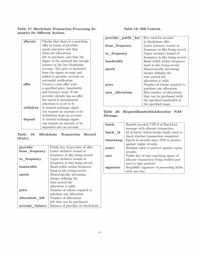
Table 17: Blockchain Transaction Processing Se-mantics for different Actions.

allocate Checks that there is a matchingoffer in terms of provider,epoch and price and thatthere are allocationsleft to purchase, and that thesigner of the payload has enoughbalance in his/her blockchainaccount. The price is deductedfrom the signer account andadded to provider account onsuccessful verification.

offer Creates a new offer witha specified price, bandwidthand freuency band. If theprovider already has an offerthe epoch is incremented,otherwise it is set to 0.

withdraw A trusted exchange signercan request an amount to bewithdrawn from an account.

deposit A trusted exchange signercan request an amount to bedeposited into an account.

Table 18: Blockchain Transaction Record(State).

provider Public key of provider of offer.from_frequency Lower inclusive bound of

frequency in khz being served.to_frequency Upper inclusive bound of

frequency in khz being served.bandwidth Band width within frequency

band in khz being served.epoch Monotonically increasing

integer defining thetime period theallocation is valid.

price Number of tokens required topurchase one allocation.

allocations_left Number of allocationsleft that can be purchased.

account_balance Balance of provider on blockchain.

Table 19: SIB Content.

provider_public_key Key used for accountin blockchain offer.

from_frequency Lower inclusive bound offrequency in khz being served.

to_frequency Upper inclusive bound offrequency in khz being served.

bandwidth Band width within frequencyband in khz being served.

epoch Monotonically increasinginteger defining thetime period theallocation is valid.

price Number of tokens required topurchase one allocation.

max_allocations Max number of allocationsthat can be purchased withthe specified bandwidth inthe specified range.

Table 20: RequestBandwidthAllocation NASMessage.

batch Base64 encoded UTF-8 of BatchListmessage with allocate transaction.

batch_id Id of batch (batch header hash) used tocheck whether transaction completed.

timestamp Epoch in seconds since 1970 to protectagainst replay attacks.

nonce Random value to protect against replayattacks.

user Public key of user matching signer ofallocate transaction being verified andused to sign payload.

signature Secp256k1 signature of preceeding fieldswith user key.

31

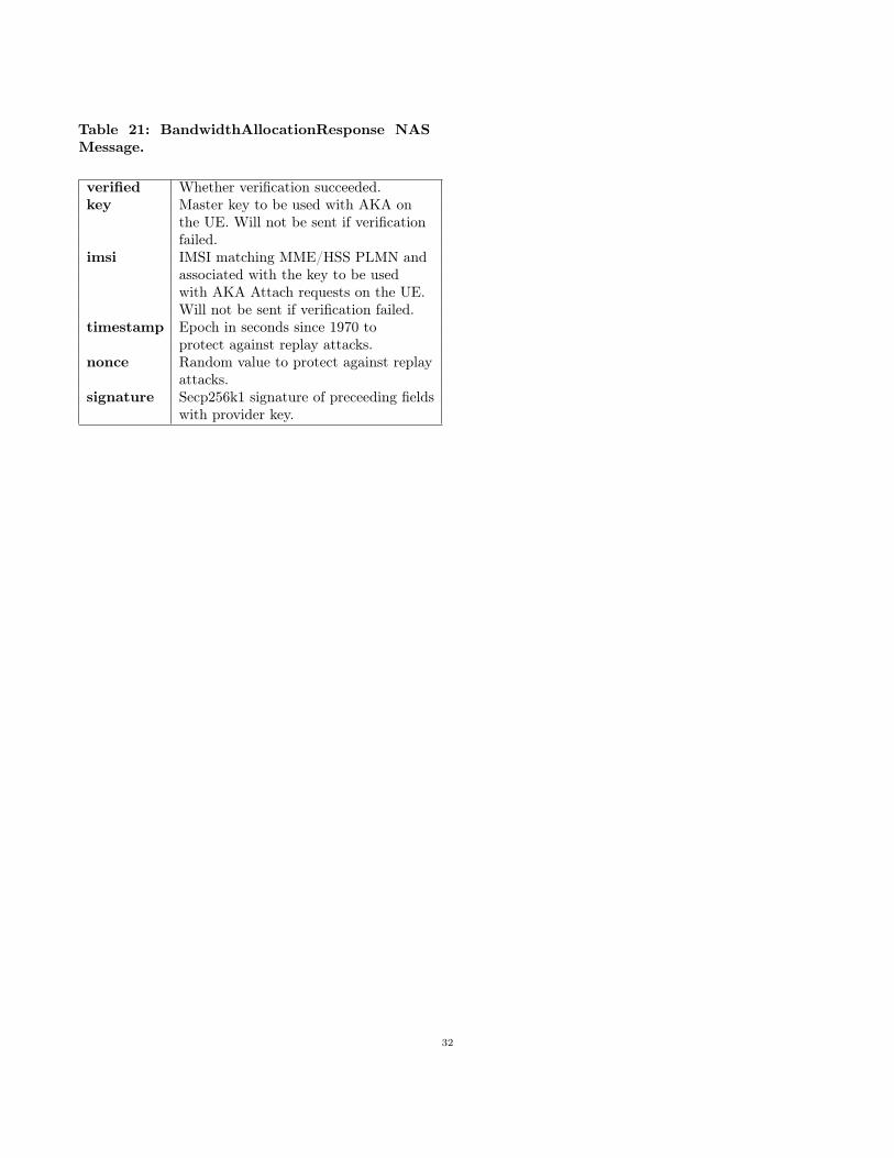
Table 21: BandwidthAllocationResponse NASMessage.

verified Whether verification succeeded.key Master key to be used with AKA on

the UE. Will not be sent if verificationfailed.

imsi IMSI matching MME/HSS PLMN andassociated with the key to be usedwith AKA Attach requests on the UE.Will not be sent if verification failed.

timestamp Epoch in seconds since 1970 toprotect against replay attacks.

nonce Random value to protect against replayattacks.

signature Secp256k1 signature of preceeding fieldswith provider key.

32