Performance Analysis of Mobile Ad HocNetwork Routing Protocols Using ns-3

Simulations

Xinyang Rui

Submitted to the graduate degree program in Electrical Engineering &Computer Science and the Graduate Faculty of the University of Kansas

School of Engineering in partial fulfillment ofthe requirements for the degree of Master of Science

Thesis Committee:

Prof. James P.G. Sterbenz: Chairperson

Prof. Gary Minden

Prof. Bo Luo

Date Defended

c© 2019 Xinyang Rui

The Thesis Committee for Xinyang Rui certifies

that this is the approved version of the following thesis:

Performance Analysis of Mobile Ad Hoc Network Routing Protocols

Using ns-3 Simulations

Committee:

Prof. James P.G. Sterbenz: Chairperson

Prof. Gary Minden

Prof. Bo Luo

Date Approved

i

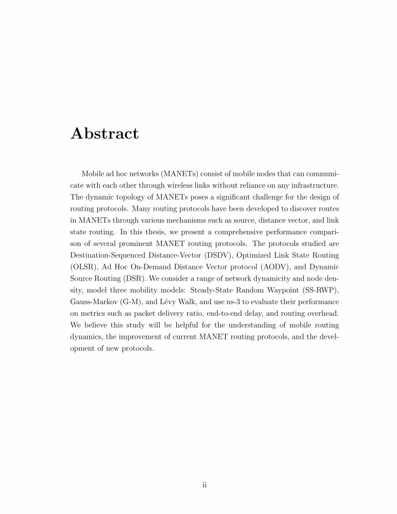
Abstract

Mobile ad hoc networks (MANETs) consist of mobile nodes that can communi-

cate with each other through wireless links without reliance on any infrastructure.

The dynamic topology of MANETs poses a significant challenge for the design of

routing protocols. Many routing protocols have been developed to discover routes

in MANETs through various mechanisms such as source, distance vector, and link

state routing. In this thesis, we present a comprehensive performance compari-

son of several prominent MANET routing protocols. The protocols studied are

Destination-Sequenced Distance-Vector (DSDV), Optimized Link State Routing

(OLSR), Ad Hoc On-Demand Distance Vector protocol (AODV), and Dynamic

Source Routing (DSR). We consider a range of network dynamicity and node den-

sity, model three mobility models: Steady-State Random Waypoint (SS-RWP),

Gauss-Markov (G-M), and Levy Walk, and use ns-3 to evaluate their performance

on metrics such as packet delivery ratio, end-to-end delay, and routing overhead.

We believe this study will be helpful for the understanding of mobile routing

dynamics, the improvement of current MANET routing protocols, and the devel-

opment of new protocols.

ii

I would like to dedicate this work to my parents for their unconditional and

continuous support for me to chase higher achievements as a graduate student

and researcher.

iii

Acknowledgements

I would like to thank my comittee members, especially Dr. James Sterbenz

for his instructions, patience, and continuous support. I would also like to thank

PhD students Amir Modarresi and Truc Anh N. Nguyen in the ResiliNets group

for their vital help with the ns-3 simulations, and previous member of the group

Yufei Cheng for the advice he offered and his studies on MANET routing protocols

which laid the foundation for my research. Lastly, I would like to thank fellow

Master’s student Sai Sandeep Bhooshi for the collaboration and the work he has

completed for MANET routing simulations.

iv

Contents

Acceptance Page i

Abstract ii

1 Introduction and Motivation 1

1.1 Contributions . . . . . . . . . . . . . . . . . . . . . . . . . . . . . 2

1.2 Problem Statement . . . . . . . . . . . . . . . . . . . . . . . . . . 3

1.3 Organization . . . . . . . . . . . . . . . . . . . . . . . . . . . . . 5

2 Background and Related Work 6

2.1 MANET Routing Protocols . . . . . . . . . . . . . . . . . . . . . 7

2.1.1 Topology-Based Routing Protocols . . . . . . . . . . . . . 7

2.1.2 Position-Based Routing Protocols . . . . . . . . . . . . . . 13

2.2 Mobility Models . . . . . . . . . . . . . . . . . . . . . . . . . . . . 13

2.2.1 Steady-State Random Waypoint . . . . . . . . . . . . . . . 14

2.2.2 Gauss-Markov . . . . . . . . . . . . . . . . . . . . . . . . . 16

2.2.3 Levy Walk . . . . . . . . . . . . . . . . . . . . . . . . . . . 16

2.3 Related work . . . . . . . . . . . . . . . . . . . . . . . . . . . . . 17

3 Simulation Methodology 19

3.1 Simulation Parameters . . . . . . . . . . . . . . . . . . . . . . . . 19

3.1.1 Network Dynamicity . . . . . . . . . . . . . . . . . . . . . 20

3.1.2 Node Density . . . . . . . . . . . . . . . . . . . . . . . . . 25

3.2 Data-Collection Methods . . . . . . . . . . . . . . . . . . . . . . . 25

3.2.1 Implementation of MANET Routing Protocols . . . . . . . 26

3.2.2 Data-Collection Methods . . . . . . . . . . . . . . . . . . . 30

v

4 Simulation Analysis 33

4.1 Varying Network Dynamicity . . . . . . . . . . . . . . . . . . . . 35

4.1.1 PDR Performance . . . . . . . . . . . . . . . . . . . . . . . 35

4.1.2 Routing Overhead Performance . . . . . . . . . . . . . . . 39

4.1.3 End-to-End Delay Performance . . . . . . . . . . . . . . . 48

4.2 Varying Node Density . . . . . . . . . . . . . . . . . . . . . . . . 54

4.2.1 PDR Performance . . . . . . . . . . . . . . . . . . . . . . . 54

4.2.2 Routing Overhead Performance . . . . . . . . . . . . . . . 56

4.2.3 End-to-End Delay Performance . . . . . . . . . . . . . . . 57

4.3 Performance Summary . . . . . . . . . . . . . . . . . . . . . . . . 59

5 Conclusions and Future Work 63

5.1 Conclusions . . . . . . . . . . . . . . . . . . . . . . . . . . . . . . 63

5.2 Future Work . . . . . . . . . . . . . . . . . . . . . . . . . . . . . . 63

References 66

vi

List of Figures

3.1 PDR varying α-value in G-M . . . . . . . . . . . . . . . . . . . . 23

3.2 Overhead varying α-value in G-M . . . . . . . . . . . . . . . . . . 23

3.3 Delay varying α-value in G-M . . . . . . . . . . . . . . . . . . . . 23

3.4 PDR varying TimeStep value in G-M . . . . . . . . . . . . . . . . 24

3.5 Overhead varying TimeStep value in G-M . . . . . . . . . . . . . . 24

3.6 Delay varying TimeStep value in G-M . . . . . . . . . . . . . . . . 24

3.7 Delay varying pause time in SS-RWP [1] . . . . . . . . . . . . . . 29

3.8 PDR varying pause time in SS-RWP [1] . . . . . . . . . . . . . . . 29

4.1 PDR varying dynamicity – SS-RWP, low density . . . . . . . . . . 37

4.2 PDR varying dynamicity – SS-RWP, med. density . . . . . . . . . 37

4.3 PDR varying dynamicity – SS-RWP, high density . . . . . . . . . 37

4.4 PDR varying dynamicity – G-M, low density . . . . . . . . . . . . 40

4.5 PDR varying dynamicity – G-M, med. density . . . . . . . . . . . 40

4.6 PDR varying dynamicity – G-M, high density . . . . . . . . . . . 40

4.7 PDR varying dynamicity – Levy, low density [1] . . . . . . . . . . 41

4.8 PDR varying dynamicity – Levy, med. density [1] . . . . . . . . . 41

4.9 PDR varying dynamicity – Levy, high density [1] . . . . . . . . . 41

4.10 Overhead varying dynamicity – SS-RWP, low density . . . . . . . 42

4.11 Overhead varying dynamicity – SS-RWP, med. density . . . . . . 42

4.12 Overhead varying dynamicity – SS-RWP, high density . . . . . . . 42

4.13 Overhead varying dynamicity – G-M, low density . . . . . . . . . 45

4.14 Overhead varying dynamicity – G-M, med. density . . . . . . . . 45

4.15 Overhead varying dynamicity – G-M, high density . . . . . . . . . 45

4.16 Overhead varying dynamicity – Levy, low density [1] . . . . . . . 47

4.17 Overhead varying dynamicity – Levy, med. density [1] . . . . . . . 47

vii

4.18 Overhead varying dynamicity – Levy, high density [1] . . . . . . . 47

4.19 Overhead fraction – SS-RWP, low density . . . . . . . . . . . . . . 49

4.20 Overhead fraction – SS-RWP, med. density . . . . . . . . . . . . . 49

4.21 Overhead fraction – SS-RWP, high density . . . . . . . . . . . . . 49

4.22 Delay varying dynamicity – SS-RWP, low density . . . . . . . . . 50

4.23 Delay varying dynamicity – SS-RWP, med. density . . . . . . . . 50

4.24 Delay varying dynamicity – SS-RWP, high density . . . . . . . . . 50

4.25 Delay varying dynamicity – G-M, low density . . . . . . . . . . . 52

4.26 Delay varying dynamicity – G-M, med. density . . . . . . . . . . . 52

4.27 Delay varying dynamicity – G-M, high density . . . . . . . . . . . 52

4.28 Delay varying dynamicity – Levy, low density [1] . . . . . . . . . . 53

4.29 Delay varying dynamicity – Levy, med. density [1] . . . . . . . . . 53

4.30 Delay varying dynamicity – Levy, high density [1] . . . . . . . . . 53

4.31 PDR varying density – SS-RWP, low dynamicity . . . . . . . . . . 55

4.32 PDR varying density – SS-RWP, med. dynamicity . . . . . . . . . 55

4.33 PDR varying density – SS-RWP, high dynamicity . . . . . . . . . 55

4.34 Overhead varying density – SS-RWP, low dynamicity . . . . . . . 58

4.35 Overhead varying density – SS-RWP, med. dynamicity . . . . . . 58

4.36 Overhead varying density – SS-RWP, high dynamicity . . . . . . . 58

4.37 Delay varying density – SS-RWP, low dynamicity . . . . . . . . . 60

4.38 Delay varying density – SS-RWP, med. dynamicity . . . . . . . . 60

4.39 Delay varying density – SS-RWP, high dynamicity . . . . . . . . . 60

viii

List of Tables

3.1 Parameters of SS-RWP in ns-3 . . . . . . . . . . . . . . . . . . . . 21

3.2 Simulation setup for testing G-M parameters . . . . . . . . . . . . 21

3.3 Simulation setup of the buffering test experiment . . . . . . . . . 27

4.1 Parameters for different scenarios varying dynamicity . . . . . . . 34

4.2 Parameters for different scenarios varying density . . . . . . . . . 34

4.3 Simulation parameters . . . . . . . . . . . . . . . . . . . . . . . . 34

4.4 Parameters of the network . . . . . . . . . . . . . . . . . . . . . . 35

4.5 DSR parameters . . . . . . . . . . . . . . . . . . . . . . . . . . . . 44

4.6 Performance summary of protocol abilities . . . . . . . . . . . . . 62

ix

Chapter 1

Introduction and Motivation

Mobile ad hoc networks (MANETs) are self-organizing networks that con-

sist of mobile nodes communicating with each other through necessary multi-hop

wireless links without the need for supporting infrastructure such as base sta-

tions. Being infrastructure-free is an important feature of MANETs, which leads

to potential applications in remote environments, disaster area recovery, and bat-

tlefields. In MANETs, each node acts not only as a host but also a router. Node

mobility leads to the constantly changing topology and link states of MANETs.

These characteristics pose a critical challenge for routing protocol design. Con-

ventional routing algorithms do not perform well in MANETs as they assume a

stable topology. Over the years, several routing protocols have been developed for

MANETs. Based on the update mechanisms they can be categorized to proactive

and reactive protocols. Algorithms such as source routing, link-state routing, and

distance vector have been adopted into MANET routing protocols. More detailed

introduction to the protocols is provided in Chapter 2.

The performance of MANET routing protocols on metrics such as average

end-to-end delay, routing overhead, and packet delivery ratio (PDR) is affected by

1

both the design of the protocols and the network scenarios. As a result, analyzing

the performance of the protocols in various scenarios, and finding the relationship

between the results and the mechanisms of the protocols, is important to achieving

deeper understanding of mobile routing dynamics. Assumptions can be made by

reviewing the nature of the protocols. For example, it is expected that reactive

protocols have more latency than proactive protocols in highly dynamic scenarios

as there is higher delay involved to allow the route discovery process. However,

such assumptions can only be validated efficiently through simulation studies.

Many factors such as node mobility, traffic pattern, propagation model, chan-

nel characteristics, and MAC effects have a significant impact on the performance

of routing protocols. Moreover, the interplay of these factors is rather complex [2].

In this thesis, we focus on two important factors that are network dynamicity and

node density. In simulation studies, network dynamicity is influenced by choice

of mobility models and parameter settings in each model, while node density is

directly related to the total number of nodes in the network, simulation area, and

transmission range of the mobile nodes. A variety of network scenarios in this

study are created by varying some of these parameters to provide comprehensive-

ness in our performance analysis of MANET routing protocols. We hope that

this thesis can provide more insights into mobile routing dynamics, and help the

development of new protocols as well as the improvement of existing protocols.

1.1 Contributions

The main contributions of this thesis are:

• Compare and analyze performance of prominent MANET routing protocols

with respect to network dynamicity and node density.

2

• Analyze impact of mobility models on MANET routing protocol perfor-

mance.

1.2 Problem Statement

Evaluating the performance of MANET routing protocols is a challenging task

due to the inherent complexity of MANETs and the random nature of node mo-

bility and traffic [3]. Network simulation is the predominant evaluation approach

for MANET routing studies [4]. One of the reasons behind the popularity of

simulations studies on MANETs is the difficulty of creating repeatable scenarios

involving tens or hundreds of mobile nodes [5]. Additionally, few of the promi-

nent MANET routing protocols have seen significant actual implementation. On

the other hand, there have been successful and detailed implementations of mul-

tiple MANET routing protocols and mobility models on a variety of simulation

platforms that provide a powerful tool for MANET simulation studies. The ns-3

simulator is our choice of simulation platform in this thesis to analyze MANET

routing performance. The four protocols studied have all been implemented in

ns-3. Both DSR and DSDV have been implemented by researchers from the Re-

siliNets research group with extensive documentation providing implementation

details such as header formats, control packet formats, and default values of the

parameters. However, to our best knowledge,the AODV and OLSR models lack

such comprehensive documentation. More importantly, some significant imple-

mentation details may heavily impact the simulation results. For example, it is

unclear from the implementation whether OLSR maintains a send buffer or not.

Buffering can affect the variation of end-to-end delay as has been pointed out by

previous studies. The buffering behaviors of the four protocols are tested, and the

3

results will be discussed in Chapter 4.

We analyze and compare the performance of prominent MANET routing pro-

tocols through ns-3 simulations. Even though simulation is a powerful tool for

studying MANET protocols, there are challenges to achieve insightful and cred-

ible results. Simulation studies should be completed in a valid experiment, with

sources of randomness such as seeds generated with random number generator

(RNG) being used [6]. Previous studies on MANET routing performance using

simulation tools have problems such as the lack of repeatability and comprehen-

siveness. In addition to the design and mechanisms, protocol performance is

influenced by the underlying settings. As a result, repeatability of the simulation

studies is very important for the results to be readily understood and validated by

fellow researchers, and requires detailed documentation. Unfortunately, the lack

of detailed documentation is a widespread problem in research on MANETs [7].

To guarantee repeatibilty for this study, we provide complete documentation on

parameter settings in protocol implementation, mobility models, and all proto-

col layers in our ns-3 simulations. The lack of comprehensiveness is explained in

detail in Section 2. We attempt comprehensiveness by using different mobility

models and creating a wide range of conditions in the simulations. Moreover,

we expect to achieve a more detailed understanding of MANET routing protocol

performance by carefully investigating the parameter settings of the protocols in

the simulation tools while reflecting on the design of the algorithms. To the best

of our knowledge, this is the first study of MANET routing that covers a variety

of of both protocols and mobility models.

4

1.3 Organization

The rest of this thesis is organized as follows. Chapter 2 presents the back-

ground of this study and an overview of related work. The protocols and mobility

models used in our ns-3 simulations are introduced. In Chapter 3, we explain our

choices of simulation parameters and introduce our data-collection method. Simu-

lation results and analysis of MANET routing performance with different network

dynamicity and node density are presented in Chapter 4. Chapter 5 presents the

conclusion and the potential future work following this study.

5

Chapter 2

Background and Related Work

Routing in MANETs is non-trivial because of the infrastructure-free nature

and the highly-dynamic topologies of mobile wireless networks. Many protocols

have been proposed over the years that can be classified based on their mechanisms

of exchanging routing information among mobile nodes. There have already been

many performance analysis and comparison studies on MANET routing protocols.

Although we have observed problems such as the lack of comprehensiveness and

repeatability in many of them, they provide helpful insights and guidance for our

research.

In this chapter, we present an overview of MANET routing protocols in differ-

ent categories. The basic mechanisms in different stages of routing including route

discovery and route maintenance in each protocol are introduced. In addition, we

present an introduction to the mobility models used in our simulation studies. A

discussion of previous studies on MANET routing performance analysis is also

provided.

6

2.1 MANET Routing Protocols

Over the years there has been significant research on routing protocol design

for MANETs. The protocols proposed can be classified into topology-based and

position-based routing protocols.

2.1.1 Topology-Based Routing Protocols

Topology-based routing protocols perform packet forwarding using the infor-

mation of links in the network [8]. They can be classified into proactive (or

table-driven), reactive (or on-demand), and hybrid protocols based on their up-

date mechanisms This classification is used in this section to introduce MANET

routing protocols. In some previous studies, the protocols are also categorized

into hello protocols and flooding protocols while analyzing their performance [9].

2.1.1.1 Proactive Routing Protocols

Proactive routing protocols calculate paths between node pairs with routing

information kept in forwarding tables. There is little communication setup la-

tency in this kind of protocol since paths are computed regardless of the need

of data transmission. However, the overhead of maintaining routes that may

not be needed is high, especially when routing information needs to keep up

with the changing topology. Examples of proactive routing protocols include

DSDV (Destination-Sequenced Distance-Vector protocol) [10] and OLSR (Opti-

mized Link State Routing protocol) [11].

DSDV is one of the first MANET routing protocols [12] [13]. It is a hop-by-hop

proactive routing protocol that uses the Bellman-Ford algorithm to calculate paths

based on the metric of hop counts. Each node maintains a table with entries for

7

all nodes in the network and is required to broadcast routing updates periodically

to propagate changes. Periodic updates contain the entire routing table of each

node, and a node may further propagate triggered updates if changes in the routing

table are invoked by periodic updates. Routing tables contain the information of

routes to every possible destination, which includes the next hop to the path and

the number of hops to each destination. The next hop on the shortest path is

determined by comparing the distances received for each destination. DSDV uses

sequence numbers as a mechanism to determine most recent route updates and

to prevent routing loops that the Bellman-Ford algorithm may produce. Each

node in the network advertises a monotonically increasing even sequence number

for itself, and the sequence number is incremented each time a periodic update is

made by a node.

DSDV is similar to wired distance vector protocols such as the Routing In-

formation Proctol (RIP) [14]. One of the disadvantages of DSDV is that it has

high routing overhead when the size of the ad hoc network is large as it involves

frequent network-wide essages. In addition, a path may have stale routing infor-

mation before route updates propagation in the network, which may cause packets

to be forwarded along the wrong path.

OLSR is a proactive protocol that belongs to the second generation of MANET

routing protocols. It uses the link-state algorithm for path calculation. Paths to all

destinations in the network are calculated and maintained before a data packet

is sent from a source node. Nodes use Hello messages for neighbor discovery.

Topology control (TC) messages are used to discover and broadcast link-state

information throughout the network periodically [13]. Multipoint relays (MPRs)

is an important concept in this protocol [15]. For a given node, all other nodes in

8

the network can be divided into a neighbor set, a two-hop neighbor set, an MPR

set, and an MPR selector set. The MPR set is a subset of neighbors of the selected

node that can reach all two-hop neighbors. Link state advertisements (LSA) are

only flooded to MPR set to reduce overhead. MPR selection is important in OLSR

because a smaller MPR set leads to lower overhead. OLSR has lower overhead

than other proactive algorithms because of MPR flooding optimization that will

be introduced further in Chapter4, and is scalable to large networks because it

introduces a kind of hierarchy to the network. It does, however, maintains routes

that are not needed.

2.1.1.2 Reactive Routing Protocols

Proactive protocols borrow mechanisms such as periodic updates from con-

ventional routing algorithms, which lead to certain problems including increased

routing overhead. As a result, a novel approach of routing in MANETs was pro-

posed in which mobile nodes use request packets to discover routes when they

are ready to communicate with others [16]. This is the main idea behind reac-

tive routing protocols in which paths are computed only when needed. When

routing request packets are generated at a relatively low rate, this type of pro-

tocol provides lower overall overhead. However, reactive protocols require higher

communication-setup latency as communication is delayed by the time it takes to

discover routes unless there is a cached route between the specific pair of nodes.

The AODV (Ad Hoc On-Demand Distance Vector) protocol [17] and DSR (Dy-

namic Source Routing) protocol [18] [19] are prominent examples of on-demand

protocols in MANETs.

AODV is a reactive successor to DSDV. As is explained by its reactive nature,

9

routes are discovered only when needed in AODV. There are four types of messages

in this protocol: route request (RREQ), route reply (RREP), route error (RERR),

and route reply ACK (RREP-ACK). The route discovery process is initiated when

the source node has no routing information about the destination node [20], which

means that either the destination was previously unknown to the source, or the

previous valid route has expired. Additionally, if the previous valid route has been

marked as invalid by a RERR message, a new route needs to be discovered.

AODV uses flooding as its route discovery mechanism. The source node floods

RREQ messages in the network using the broadcast IP address. AODV adopts

the concept of sequence number from DSDV. Sequence numbers are used at each

destination node to determine the freshness of routing information and to prevent

routing loops [21]. Route table entries are used to store routing information,

such as sequence numbers in AODV. When an RREQ message is received by an

intermediate node that possesses a route entry to the desired destination, the

destination sequence number in the route entry is compared to the one in the

RREQ. An RREP message is created and forwarded back to the source node when

the destination sequence number of the route entry is equal to or greater than the

one specified in RREQ. Otherwise, the RREQ is rebroadcasted by the intermediate

node. In addition, a reverse-route entry for the source node is created by each

node receiving the RREQ in the route table [22]. Periodic Hello messages are used

in AODV to detect broken links. Failure to receive a certain number of consecutive

Hello messages is an indication of link breakage between neighbors [12] [23]. Link-

layer acknowledgments can be used as an alternative for link failure detection.

It costs far less latency, which has been observed in our ns-3 simulation results.

AODV provides RERR messages for notifying nodes of link breakages. RERR

10

packets in AODV are intended to inform all sources sending data packets using

the failed link [21]. A RERR message includes a list of destinations that have

become unreachable due to the broken link [22]. However, RERR was not used

in AODV route maintenance when the protocol was first introduced. Instead,

when a link failure happened, the node upstream of the broken link propagated

an unsolicited RREP with a fresh sequence number and infinite hop count to all the

upstream nodes that had recently forwarded packets to a destination using that

link [12,20]. AODV has a relatively simple algorithm, and it maintains paths only

when needed. However, its performance suffers significantly from high mobility

and episodic connectivity. Flooding RREQ control messages causes high overhead

in large networks. Periodic Hello messages also lead to unnecessary bandwidth

consumption.

The DSR protocol allows nodes to dynamically discover a source route across

multiple network hops to any destination in the ad hoc network [19]. The use

of source routing is a distinguishing feature of DSR, which simplifies routing at

intermediate nodes by placing all responsibility for route selection at the source

node [24], and allows the source to know the complete hop-by-hop route to the

destination in DSR [21]. The control message types in DSR are the same as the

ones in AODV. In DSR, a route cache is used to store routes that are already

discovered. The first step of route discovery is to broadcast RREQ to the whole

network. Any node that receives an RREQ messages will examine their route

cache to find out if there is existing routing information for computing the route

to the destination. If no useful routing information is found, the RREQ packet

will be sent further on after having the address of the current node added to the

hop sequence stored in the RREQ packet header, whose length is proportional to

11

the number of hops. An RREP is generated when the RREQ packet reaches the

destination or an intermediate node with routes to the destination cached. Routes

are cached when RREP messages are received by source nodes. Route caching can

significantly reduce flooding of control messages in the network, but mobility and

episodic connectivity have a significant impact on DSR. Another disadvantage is

that the header length grows with network size, which leads to higher overhead

in every packet in a large network.

2.1.1.3 Hybrid Protocols

Hybrid routing protocols combine the advantages of both reactive and proac-

tive protocols with the potential to provide better scalability than pure reactive

or proactive protocols. This is because of their attempt to minimize the num-

ber of rebroadcasting nodes by defining a structure allowing nodes to collaborate,

which helps to maintain routing information much longer [25]. Zone Routing Pro-

tocol (ZRP) [26] is a prominent hybrid routing protocol which has a zone based

structure and reduces overhead for intra-zone nodes. ZRP aims to address the

problems of proactive and reactive routing protocols by combining the best prop-

erties of both approaches [27]. It has a structure with a routing zone for each

node in the network, which has a radius d expressed in hop count. ZRP consists

of three components: the proactive IntrA-Zone Routing Protocol (IARP), the re-

active IntEr Zone Routing Protocol (IERP), and Bordercast Resolution Protocol

(BRP) [28]. IARP is a family of limited-depth, proactive link-state routing pro-

tocols, which maintains routing information for nodes that are within the routing

zone of the node. Correspondingly, IERP is a family of reactive routing proto-

cols that offer enhanced route discovery and route maintenance services based

12

on local connectivity monitored by IARP [27]. The zone radius has a significant

impact on the performance of ZRP for given node density. This is because ZRP

reduces latency and overhead for RREQ for intra-zone nodes, but in the meantime

it causes more traffic and higher overhead for maintaining the view of the zones.

Zone overlap also contributes to the higher overhead in ZRP. There has not been

an implementation in ns-3 releases yet.

2.1.2 Position-Based Routing Protocols

Position-based routing algorithms eliminate some of the limitations of topology-

based routing by using additional location information [8]. In contrast to topology-

based routing methods, they make decisions based on the geographical coordinates

of the nodes [4], which are determined using GPS or other positioning services.

Position-based routing protocols thus do not require traditional route establish-

ment or maintenance. Nodes storing routing tables and routing information up-

date messages are also not needed [8]. As a result, they may be more efficient

than topology-based routing protocols in highly dynamic scenarios.

The ns-3 implementations of position-based routing protocols including Location-

Aided Routing (LAR) [29] and Simple Forwarding over Trajectory (SiFT) have

been developed by the ResiliNets research group. The comparative study with

other MANET routing protocols will be completed in future work. This thesis

focuses on prominent topology-based routing protocols.

2.2 Mobility Models

MANETs are often studied through simulation as is shown by previous studies.

While trace-driven mobility patterns that are observed in real-life systems pro-

13

vide accurate information, MANETs are not easily modeled if traces are not yet

created [30]. Therefore, the performance of routing protocols is heavily dependent

on the mobility model used in the simulation that governs node movements [31].

Most previous studies on MANET routing use only one mobility model. In this

thesis, several mobility models are used to create a variety of network scenarios.

The mobility models introduced in this section are Steady-State Random Way-

point (SS-RWP), Gauss-Markov (G-M), and Levy Walk. The Random Waypoint

(RWP) model is most commonly used in MANET simulation studies. On the

other hand, Levy Walk captures the statistical features of human mobility and

was recently implemented in ns-3 by the ResiliNets research group. We hope that

by using various mobility models, we can get better insight into the relationship

between MANET routing protocol performance and node mobility.

2.2.1 Steady-State Random Waypoint

The steady-state initialization is a method to improve the accuracy of RWP

simulations, which leads to the creation of SS-RWP. The RWP model is a relatively

simple and memoryless model that is more realistic in many scenarios than other

models such as random walk. It is the most common mobility model used in ad

hoc network simulations [31]. A node uniformly chooses a point in the area as

the destination position of its next movement and moves towards this position

at a velocity randomly chosen from an interval that is predefined by the model.

After reaching each destination, a new speed is chosen from the interval, and

a new destination point is uniformly chosen from the area. The node pauses

its movement for a specific amount of time that is the given pause time before

starting to move to its next destination. Note that the selection of speed and

14

destinations are independent of each other, and is independent of the choices of

previous movements as well.

In the implementation of RWP in both ns-2 and ns-3, the mobility model

begins with all nodes paused at their initial positions. The problem of this kind of

implementation is that it takes some time for the mobility model to converge. As

the routing performance metrics are heavily influenced by the distribution of speed

and location [31], the convergence stage of the mobility model may lead to the

simulation results not accurately reflecting the long-term values. This is the reason

why some of the previous studies [12] had a considerable warm-up time that takes

up 20 percent of the total simulation time before the actual transmission of data

packets. The SS-RWP model is a modification of the RWP model that eliminates

the convergence stage so that the movements of the nodes are converged to the

steady-state distribution from the start of the simulation. Some of the nodes start

in a paused state while other nodes start in a moving state, chosen based on a

probability distribution. Therefore we use the SS-RWP model in stead of RWP

in this thesis.

The wide acceptance of the RWP model and its variants are a result of its

simplicity of implementation and analysis [32]. However, because of its simplicity,

the RWP mobility model may not provide adequate accuracy in modeling realistic

movements. One of the limitations is that the average node movement speed will

drop over time. It also has been noticed by previous studies that the stationary

distribution of the location of a node is more concentrated around the center of the

area in which the nodes move [31]. In addition, some extreme mobility behaviors

such sharp turns frequently happen because of the memoryless feature.

15

2.2.2 Gauss-Markov

In the Gauss-Markov (G-M) mobility model, nodes have memory from their

previous movements. The parameter α determines how much memory there is,

and a time step dictates how frequently node velocity and direction are updated.

G-M is more suitable to be used to model realistic movements with fewer sharp

and abrupt turns. In this model, each node is assigned with the initial speed and

direction, as well as the average speed and direction. A new set of speed sn and

direction dn is calculated for each node after one time step [33]:

sn = αsn−1 + (1 − α)s+√

(1 − α2)sxn−1 (2.1)

dn = αdn−1 + (1 − α)d+√

(1 − α2)dxn−1 (2.2)

where s and d are the mean speed and direction parameters, and Gaussian

variables sxn−1 and dxn−1 give randomness to the new velocity and direction pa-

rameters [34].

2.2.3 Levy Walk

The RWP model and the G-M model are simple enough to be theoretically

tractable and emulated in network simulators in a scalable manner. However, the

accuracy of these models has not been validated by any empirical evidence [35].

Some of the tendencies of human mobility are not captured by these two models.

The Levy Walk mobility model was introduced to emulate the statistical features

and evaluate the impact of the tendencies of human mobility on routing protocol

performance. Analysis in previous studies shows that there is a similarity between

16

the statistical features of human mobility and Levy walks [35]. In addition, flights

and pauses can be best characterized by heavy-tailed distributions, which are not

produced by commonly used mobility models such as RWP and G-M.

2.3 Related work

The novel challenges and requirements of routing in MANET started to draw

attention from researchers in late 1990s. A guideline for routing performance eval-

uation studies was proposed regarding important aspects that should be consid-

ered [36]. There have been many studies that analyze and compare MANET rout-

ing protocol performance using simulation. One of the early studies of MANET

routing protocol performance comparison was done by Broch, et al. [12], whose

purpose was to evaluate the ability of various protocols to react to network topol-

ogy changes while successfully delivering data packets. The protocols evaluated

in this study were AODV, DSDV, DSR, Temporally-Ordered Routing Algorithm

(TORA) [37], and the RWP mobility model was used to simulate the movement

of 50 wireless nodes in a flat space. Performance metrics such as packet delivery

ratio and routing overhead were summarized and analyzed using ns-2 simulations.

Several researchers later completed similar studies on MANET routing proto-

col performance evaluation. Some of them focused on analyzing and comparing

on-demand protocol performance. Performance comparison of AODV and DSR

was performed by Perkins, et al. [21] and provided detailed analysis of the results.

On-demand Multipath Distance Vector protocol (AOMDV) [38] was later added

in MANET routing studies as well [39]. While these studies only focused on one

category of MANET routing protocols, they evaluated the performance of the

protocols on various metrics. Some studies later were carried out in similar sim-

17

ulation scenarios with DSDV, DSR, and AODV while evaluating performance on

various metrics [40] [41]. Location-based protocols were later included in perfor-

mance analysis studies with the performance of AODV, DSR, TORA, and LAR

being compared using the QualNet [42] and ns-2 simulators [43]. In addition,

performance comparison of MANET routing protocols is beneficial for selecting

a proper protocol in real-life scenarios. Some studies performed scenario-based

MANET simulations. Network sizes and parameter settings in mobility models

are set to simulate real-life scenarios, such as disaster area recovery and archaeo-

logical sites [44] [45]. With the completion of implementation of DSDV and DSR

in ns-3, comparison studies on MANET routing protocols using this newer simu-

lation platform emerged in recent years, analyzing the performance of prominent

protocols [46] [47]. Unfortunately, however, many of these studies provide very

limited analysis of the simulation results. Simulation analysis of multiple protocols

has been implemented in these studies, but many failed to cover all the prominent

protocols, and some important performance metrics have been overlooked. An-

other noticeable problem is the lack of comprehensiveness in the mobility models

used in these studies, with RWP commonly used, and only a few using G-M highly

dynamic scenarios. Pause time is widely used in these studies as the only param-

eter to be varied to create more dynamic topologies. Therefore, a comprehensive

performance comparison of MANET routing protocols on a sufficient number of

performance metrics with different mobility models to simulate the movement of

nodes needed. Previous studies have used ns-2 and GloMosim as the simulation

tools. In this thesis, simulation is carried out using the advanced ns-3 platform.

18

Chapter 3

Simulation Methodology

In this chapter, we present the simulation setup and data-collection methods

for our MANET routing protocol simulations in ns-3. In Section 3.1, we explain

our choices of parameter values for the simulations. We investigate the imple-

mentation of each mobility model used in the simulations and explain how the

parameters in each model affect node movement. Then we explain how we create

different network scenarios by changing the values of the parameters. In Sec-

tion 3.2, the detailed data-collection methods for calculating packet delivery ratio

(PDR), average end-to-end delay, and routing overhead are introduced. A brief

introduction to ns-3 is also presented in this section. In addition, routing protocol

send buffer settings heavily affect routing performance. We carry out simulation

experiments to test the effect of buffering behaviors of each protocol.

3.1 Simulation Parameters

In the implementation of SS-RWP (Steady-State Random Waypoint), G-M

(Gauss-Markov), and Levy Walk mobility models in ns-3, there are several pa-

19

rameters that are configurable to change node movement in simulations. In this

section we explain our choices of mobility model parameters that we vary to

evaluate routing protocol performance. Additionally, a brief introduction to the

implementations of mobility models in ns-3 is presented in each subsection.

3.1.1 Network Dynamicity

The frequently changing topologies of MANETs pose a significant challenge

for routing protocol design. Protocol performance can be heavily affected by

network dynamicity. Node mobility affects the average number of connected paths

and average link durations, which in turn affect the performance of the routing

protocols [48] [49]. As a result, one important part of this study is to investigate

how the dynamicity of networks affects routing performance. Creating proper

scenarios by varying the parameters in each mobility model in the simulations is

very important.

3.1.1.1 Steady-State Radom Waypoint

In the implementation of the SS-RWP model in ns-3, parameters including

simulation area, pause time, and node speed are configurable. Most previous

studies using RWP or SS-RWP only vary pause time to change node mobility,

and use the same range of varying pause times [21] [12] [50]. In this thesis, we

vary both pause time and node velocity (v) to create network scenarios with

different dynamicity to make them distinctive. Node velocity is defined as a

uniform random variable in SS-RWP. Some of the parameters in the SS-RWP

implementation in ns-3 are listed in Table 3.1. Previous studies set the interval

as from almost zero (0.01) to the given node speed [4]. If we use this range when

20

tuning node velocity, the expected value would only be half of the given velocity

in each scenario. Instead, we set the interval of node velocity to be [v − 1, v + 1],

where v is the given velocity.

Table 3.1. Parameters of SS-RWP in ns-3Parameter Description

MinSpeed Minimum speed value [m/s]MaxSpeed Maximum speed value [m/s]MinPause Minimum pause time value [s]MaxPause Maximum pause time value [s]

In many previous studies, 20 m/s, which is comparable to traffic speeds inside

a city [21], is set as the maximum node velocity in simulations. We vary node

velocity from human walking speed (1.5 m/s) to high-speed railway speed (100

m/s) to create a wider range of network scenarios. The case of highly mobile

airborne networks is beyond the scope of our work, and has have been studied

along with the proposal of a 3-D G-M mobility model [33] [34].

3.1.1.2 Gauss-Markov

Table 3.2. Simulation setup for testing G-M parametersParameter Value

Area 1500 × 300 [m2]Simulation time 200 [s]Number of nodes 50Link layer 802.11b DSSS rate 11 [Mb/s]Packet size 64 [Byte]Packets per second 4Maximum node velocity 20 [m/s]Transmission Range 250 [m]Traffic model Constant bit rate (CBR)

There are many parameters in the G-M model that affect network dynamicity,

and the relationship among those parameters is rather complex [34] [51]. Setting

21

α between 0 and 1 allows for varying degrees of randomness and memory [34].

There is less randomness and more predictability in the node paths as α increases

[51]. TimeStep is another important parameter that affects node mobility in G-

M, a new movement is set up after each TimeStep. Although both parameters

have a significant impact on the linearity and randomness of node movement, our

simulation studies show that varying α or the TimeStep will not result in a trend

in the performance metric values. Simulation parameters are listed in Table 3.2

below.

Simulation results are presented in Figures 3.1, 3.2, 3.3, 3.4, 3.5, and 3.6. The

results show that the parameters α and TimeStep mainly affects the trajectory

shapes rather than network dynamicity. As this study focuses on the performance

of MANET routing protocols in network scenarios with different dynamicity, we

will only vary the velocity in the G-M model for our simulations.

3.1.1.3 Levy Walk

The Levy Walk mobility model was first implemented in ns-3 by the ResiliNets

research group [52]. In the initial implementation, there is only one parameter v

that is configurable, which does not facilitate our study on routing performance

as it is very difficult to predict the differences in the scenarios created by varying

v. As α and its impact on node mobility in Levy Walk is well-studied [35], it is

added to the implementation as a second reconfigurable parameter. Varying α

affects the diffusivity of the network, which leads to changes in the distributions

of route hop-counts and path durations. Hop-counts and path duration have a

significant impact on MANET routing protocol performances.

22

PD

R

α-value

AODV0.0

0.2

0.4

0.6

0.8

1.0

0.0 0.2 0.4 0.6 0.8 1.0

Figure 3.1. PDR varying α-value in G-M

routing o

verh

ead [kb/s

]

α-value

AODV0

50

100

150

200

250

300

0.0 0.2 0.4 0.6 0.8 1.0

Figure 3.2. Overhead varying α-value in G-M

avera

ge e

nd-t

o-e

nd d

ela

y [s]

α-value

AODV0.00

0.05

0.10

0.15

0.20

0.0 0.2 0.4 0.6 0.8 1.0

Figure 3.3. Delay varying α-value in G-M

23

PD

R

time step [s]

AODV0.0

0.2

0.4

0.6

0.8

1.0

0 10 20 30 40 50

Figure 3.4. PDR varying TimeStep value in G-M

routing o

verh

ead [kb/s

]

time step [s]

AODV0

50

100

150

200

250

300

0 10 20 30 40 50

Figure 3.5. Overhead varying TimeStep value in G-M

avera

ge e

nd-t

o-e

nd d

ela

y [s]

time step [s]

AODV0.00

0.05

0.10

0.15

0.20

0 10 20 30 40 50

Figure 3.6. Delay varying TimeStep value in G-M

24

3.1.2 Node Density

Node density is affected by three parameters of the network including the

total number of nodes, area, and transmission range. In a very sparse network,

the number of possible connections between any node pair is very limited [48].

We use the degree of connectivity to measure node density in this thesis. The

calculation of the degree of connectivity d is :

d =Nπr2

A(3.1)

where N is the total number of nodes in the area, r is the transmission range

of the nodes, and A is the simulation area. From this calculation, we can see

that varying any one of transmission range, area, and the number of nodes, can

achieve the same effect in varying node density of the network. We choose to vary

transmission range in our MANET routing simulations as there have been studies

focusing on optimum transmission radius [22] [53].

3.2 Data-Collection Methods

In this thesis, three important performance metrics of routing protocols are

evaluated:

• Packet delivery ratio (PDR) – The ratio of the total number of data

packets received by destinations to those sent by sources.

• Average end-to-end delay of data packets – The average time it takes

for a data packet to be transmitted from the application at the source to

the application at the destination node.

25

• Routing overhead – The total number of overhead bytes generated by

routing protocols to transfer routing information. The total overhead is

averaged over time.

PDR and average end-to-end delay are the most important for best-effort traf-

fic. Average end-to-end delay in our simulation studies consists of transmission

delay, queuing delay, retransmission delay, and propagation delay. Extra bytes

generated by routing protocols consume network resources. In this section we

present a brief introduction to the ns-3 simulator and the implementation of

MANET routing protocols on this platform. Our data-collection method in ns-3

simulations for calculating the performance metrics listed above is also presented.

3.2.1 Implementation of MANET Routing Protocols

We use ns-3 [54] as the simulation tool in this study. It is an open-source

discrete-event network simulator for research on Internet systems. It is a replace-

ment for ns-2, which has been widely used in previous MANET routing studies.

The ns-3 project aims to develop an open, preferred simulation environment for

networking research [54], and relies on C++ for the implementation of the simula-

tion models. The problems caused by the combination of oTcl and C++ in ns-2 is

eliminated in ns-3 as oTcl is no longer used to control the simulations [55]. Addi-

tionally, there are many other improvements in ns-3 compared to its predecessor,

including modular extensibility, mixed wired and wireless models, and arbitrary

mix of link types and routing algorithms [4].

In the early releases of ns-3 the implementation of MANET routing protocols

only included AODV and OLSR. The implementations of DSDV and DSR were

developed by the ResiliNets group along with detailed documentation [13] [50].

26

They defined the modules and configurable parameters of both protocols and

explained how the protocols function in the ns-3 documentation [56].

We have made the following changes to some of the default parameters in the

implementation of MANET routing protocols in ns-3 to make the comparison fair

across protocols. For AODV, we change the RreqRetries value, which defines the

maximum number of retransmissions of RREQ to discover a route [56], from 2 to

16 to be the same as the default value in DSR. In addition, DeletePeriod is the

upper bound on the time for which an upstream node can have a neighbor as an

active next hop while this neighbor has invalidated the route to the destination.

We change its value from 15 to 300 to match the RouteCacheTimeout in DSR.

Buffering is a very important setting for MANET routing protocol implemen-

tations. AODV, DSDV, and DSR all have specifically implemented send buffers,

whereas the OLSR model does not provide any information about its buffering.

Buffering or queueing time and the length of the buffer (queue) are configurable

in AODV, DSDV, and DSR. A simulation experiment is carried out to test the

effectiveness of buffering mechanisms in the protocols. The values of parameters

in this experiment are listed in Table 3.3.

Table 3.3. Simulation setup of the buffering test experimentParameter Value

Area 1200 × 1200 [m2]Simulation time 200 [s]Link layer 802.11b DSSS rate 11 [Mb/s]Packet size 64 [Byte]Packets per second 1Source node position (0,0)Destination node velocity 20 [m/s]Transmission Range 1000 [m]Traffic model Constant bit rate(CBR)

The two nodes in this scenario are implemented with different mobility mod-

27

els. The source is set static using ns3::ConstantPositionMobilityModel and allocated

with a position at the center of the area using ns3::ListPositionAllocator, transmit-

ting to the destination node from this position. The destination node is imple-

mented with the G-M mobiltiy model, with trajectory is set as a straight line at

the angle of 180 degrees by changing the MeanDirection. The node will bounce

back when it hits the bounds of the area. Based on the simulation parameters,

the destination node will go out of the transmission range of the source node at

time 50 seconds and will come back in range at time 70 seconds. ASCII tracing

is enabled for reviewing the packets transmitted and received at each node after

the simulation.

We observe the following pattern from the trace files from each protocol. Both

AODV and DSR stop transmitting data packets after a failed transmission. They

both start the route discovery process after the destination node comes back within

transmission range of the source node, which transmits a burst of data packets

within a short interval that is less than one second. These are the data packets

buffered when route error was detected. However, neither DSDV nor OLSR show

this kind of pattern in their respective trace files. Data packets are transmitted

one per second even within the time that the destination is out of reach of the

source node. The results of packet delivery ratio show that these packets are

simply dropped. Both AODV and DSR have a buffer as is documented in their

ns-3 source code, but we observe that OLSR does not have a send buffer, which is

consistent with the fact that the mechanism is not mentioned in the RFC [11] nor

the implementation source code in ns-3. DSDV send buffers only functions when

there is no route available in the routing table and, therefore, we are not able to

see its effect in this experiment.

28

dela

y [m

s]

pause time [s]

DSDV

DSR

AODV

OLSR

AODV buff

DSR buff

0

5

10

15

20

25

30

35

40

45

0 100 200 300 400 500 600 700 800 900

Figure 3.7. Delay varying pause time in SS-RWP [1]

PD

R

pause time [s]

AODV

DSR

OLSR

DSDV

AODV buff

DSR buff0.0

0.2

0.4

0.6

0.8

1.0

0 100 200 300 400 500 600 700 800 900

Figure 3.8. PDR varying pause time in SS-RWP [1]

29

The effect of send buffers on routing performance can be seen in Figures 3.7

and 3.8. Figure 3.7 reveals that send buffers cause significant variations in average

end-to-end delay, especially for reactive protocols. This is because when the send

buffer is on, the time for a data packet to get delivered can be delayed considerably

because of link breakages, as is indicated by the results of our buffering test

experiment. In high mobility scenarios, send buffers provide improvement in PDR

as we can see from Figure 3.8. This is also consistent with the result of the

buffering test experiment. The variations in the delay results makes it hard to

study the impact of other factors on protocol delay performance. Additionally,

fairer comparison among all the protocols is certainly beneficial for this study.

Therefore, for the simulation studies on the impact of network dynamicity, we

disable send buffers of AODV, DSR, and DSDV. We do, however, keep the send

buffer in DSDV when studying the impact of node density to understand its effect,

which will be further explained in Chatper 4.

3.2.2 Data-Collection Methods

The two factors needed for calculating PDR are the number of data pack-

ets transmitted by the source nodes and the number received by the destination

nodes. We obtain both factors using the ns-3 tracing system. The tracing archi-

tecture is one of the main distinct features of ns-3 compared to ns-2, which uses a

callback-based design that decouples trace sources from trace sinks. In this way,

customization of the tracing or data output is enabled [57]. An introduction to

the mechanism of the tracing system is provided in the ns-3 manual [58]. Trace

sources in ns-3 provide access to interesting underlying data that are indications of

events that happen during simulations. Trace sinks are the entities that consume

30

trace information, and a trace source can be connected to multiple trace sinks

through an ns-3 Callback.

As we use the ns3::OnOffApplication to generate traffic from the source nodes,

the ns3::OnOffApplication/Tx trace source [59] is used to retrieve the total number

of transmitted data packets by all the traffic sources. The variable onOffTx is

implemented in a callback function, which is invoked by the trace source whenever

a new data packet is created and sent by the application so that the value of the

variable is increased by one. The total number of data packets transmitted by

traffic sources are stored in this variable at the end of the simulation. Similarly,

we connect the trace source ns3::PacketSink/Rx to another callback function that

has the variable sinkRx to record the total number of data packets received by

destination nodes, invoked whenever a data packet is received by the sink. PDR

is calculated at the end of the simulation by dividing the value of onOffTx by

sinkRx.

We calculate the average end-to-end delay in a similar method but with the

help of the ns3::DelayJitterEstimation class in ns-3. The member function Pre-

pareTx is implemented in the same callback function as onOffTx and is connected

to the OnOffApplication/Tx trace source. This member function is invoked once

on each data packet and records the transmission within the packet by storing

it as a ns3::Tag [56]. The transmission time is used to calculate the end-to-end

delay upon packet reception. The RecordRx member function of the DelayJitter-

Estimation class is implemented in the same callback as sinkRx and is connected

to the trace source PacketSink/Rx, invoked when a data packet is received at the

destination to update the delay. The GetLastDelay member function can return

the updated delay after the RecordRx gets called, which is added and recorded by

31

the variable delay. Average end-to-end delay is calculated by dividing delay by

sinkRx at the end of each simulation run. This calculation also reveals that the

performance metrics are not completely independent as, for instance, lower PDR

means that average end-to-end delay is calculated with fewer samples [21].

MANET routing protocols use different port numbers for transferring routing

information, including 654 for AODV, 269 for DSDV, and 698 used by OLSR.

We use this feature to record the control packet overhead for these three pro-

tocols in our simulations. A callback function is connected to the trace source

Ipv4L3Protocol/Tx so that it is invoked when an IPv4 packet is sent to the outgo-

ing interface. This includes both data packets and control packets of the routing

protocols. The GetDestinationPort function in the callback function examines the

destination port number in the UDP header of the packet. By checking the des-

tination port number, the callback function can determine whether the packet

being sent is a control packet. The size of a control packet is added to the vari-

able recording the total routing overhead.

The DSR header resides between IP header and UDP header in both data and

control packets, consisting of two parts: DSR fixed-size header and DSR options

header [50]. The message id in the DSR fixed-size header indicates the type of

message this DSR header is carrying: a control packet is indicated by message id

of 1 while a data packet has an id of 2. If the packet is a data packet, we only

add the size of the DSR header to the total routing overhead, whereas the full size

of control packets is added. In this thesis, the total routing overhead and control

packet overhead of DSR are both presented in the simulation results.

32

Chapter 4

Simulation Analysis

In this section, we present our ns-3 simulation results and performance analy-

sis of routing protocols including AODV, DSDV, DSR, and OLSR. The mobility

models used in the simulations are SS-RWP (Steady-State Randm Waypoint),

G-M (Gauss Markov), and Levy Walk. Our simulations focus on two important

aspects of MANETs, network dynamicity and node density. They both have a

heavy impact on the performance of routing protocols. In order to ensure com-

prehensiveness of scenarios covered in this analysis study, we create low, medium,

and high network density cases to perform simulations varying network dynamic-

ity. Network scenarios with low, medium, and high network dynamicity cases are

created accordingly for simulations varying node density. The parameter values

for low, medium, and high dynamicity and density cases are shown in Tables 4.1

and 4.2. Parameters used in our simulation studies are presented in Table 4.3.

We choose 64 bytes as the packet size in our simulations, and each source node

transmits 4 packets per second. This combination leads to fairly low traffic that

does not invoke network saturation. Simulation studies on saturated cases are left

for future work. The simulation area is set as rectangular instead of square to have

33

Table 4.1. Parameters for different scenarios varying dynamicity

Dynamicity Pause time Velocity Real-life speed

Low 300 [s] 1.5 [m/s] 5.4 [km/h], human walkingMedium 75 [s] 40 [m/s] 144 [km/h], high-speed cars

High 0 [s] 100 [m/s] 360 [km/h], high-speed railway

Table 4.2. Parameters for different scenarios varying density

Density Transmission range Degree of Connectivity

Low 120 [m] 5Medium 170 [m] 10

High 250 [m] 22

Table 4.3. Simulation parameters

Parameter Value

ns-3 version ns-3.27Link layer 802.11b DSSS 11Mb/sRTS/CTS enabled? noPacket fragmentation? noPropagation loss model rangeRouting protocol AODV, DSDV, DSR, OLSRTransport layer protocol UDPApplication type ns3::OnOffApplicationMobility model SS-RWP, G-M, Levy WalkNumber of simulation runs 10Total number of nodes 50Number of flows 10Simulation time 900 [s]Warmup time 50 [s]Simulation area 1500 × 300 [m2]Data packets per second 4Data packet payload size 64 byteNode velocity 1.5, 5, 10, 20, 40, 60, 80, 100 [s]Transmission range 93, 131, 161, 207, 268, 317 [m]Degree of connectivity 3, 6, 9, 15, 25, 35

34

a diversity of both long and short routes in terms of hop counts [4]. Parameters

of the network are needed for performance analysis of routing protocols, and are

presented in Table 4.4.

Table 4.4. Parameters of the network

Parameter Discription

N Total number of nodesd Degree of connectivityh Average route hop countsp Number of data packets per second from one source nodes Number of source nodes

4.1 Varying Network Dynamicity

Widely varying mobility characteristics are expected to have a significant im-

pact on the performance of routing protocols [49]. In this section, we analyze

the performance of MANET routing protocols with varying network dynamicity.

The mobility models used are SS-RWP, G-M, and Levy Walk. Low, medium, and

high network density cases are created and used to make network scenarios more

diverse.

4.1.1 PDR Performance

Figures 4.1, 4.2, and 4.3 show the PDR performance of routing protocols in

low, medium, and high node density cases as the network dynamicity increases

using SS-RWP. The three reasons packet drops occur in MANETs are: 1) full

interface queues caused by congestion, 2) packets being forwarded along a path

that no longer exists due to topology changes, and 3) lack of established routes

35

due to low connectivity. In our simulation settings, the interface queue of each

node is 100 packets long. Given the low traffic rate in the network, interface

queues being full is very unlikely to happen. The other two reasons then become

the main causes for packet drops. In the low density case, limited network con-

nectivity significantly reduces the chance of paths being established, resulting in

poor PDR performance of all four protocols. The protocols perform similarly as

low connectivity is the dominating factor in low density scenarios. In the medium

density case, AODV performs a lot better than the other three protocols in terms

of PDR. This performance superiority is observed in most of our simulation re-

sults. The reason is that AODV benefits from its on-demand nature and frequent

reinitialization of route discovery process to adapt to fast topology changes. Since

we removed the send buffer for both on-demand protocols, data packets rely on

paths that are already established, which are stored in table entries and route

cache for AODV and DSR respectively. PDR performance of DSR suffers from

stale route cache in dynamic scenarios, whereas routing table entries in AODV

are only valid for a much shorter time. The value of ActiveRouteTimeout, which

is the period of time during which the route is valid [60], is only 3 seconds by

default. This allows the route table entry to be fresh for most of the time during

the simulations. Frequent topology changes increase the chance of a cached route

being no longer valid in DSR. PDR performance of the protocols is similar in

the highly dense case with OLSR performing significantly worse in more dynamic

scenarios. In the highly dynamic scenario with no pause time and a node velocity

of 100m/s, AODV and DSR outperform DSDV and DSR due to their reactive

nature that helps adapt to rapid topology changes. Simulation results using the

G-M mobility model, which are presented in Figurse 4.4, 4.5, and 4.6, show very

36

PD

R

network dynamicity

AODV

DSR

OLSR

DSDV

0.0

0.2

0.4

0.6

0.8

1.0

0.0 10.0 20.0 30.0 40.0 50.0 60.0 70.0 80.0 90.0 100.0

Figure 4.1. PDR varying dynamicity – SS-RWP, low density

PD

R

network dynamicity

AODV

DSR

OLSR

DSDV

0.0

0.2

0.4

0.6

0.8

1.0

0.0 10.0 20.0 30.0 40.0 50.0 60.0 70.0 80.0 90.0 100.0

Figure 4.2. PDR varying dynamicity – SS-RWP, med. density

PD

R

network dynamicity

AODV

DSR

DSDV

OLSR

0.0

0.2

0.4

0.6

0.8

1.0

0.0 10.0 20.0 30.0 40.0 50.0 60.0 70.0 80.0 90.0 100.0

Figure 4.3. PDR varying dynamicity – SS-RWP, high density

37

similar trends and relative performance.

From the results we can see that PDR decreases for all the protocols with in-

creasing network dynamicity, which implies that packet drops are happening more

frequently. High network dynamicity causes link breakage to happen at a higher

frequency, which then leads to shorter path durations. Path duration is modeled

as the longest time interval during which all the links along a path exist [2]. Higher

network dynamicity reults in lower average path duration in the network [61]. Low

path duration increases the chance of data packets being transmitted along paths

that are no longer existing and getting dropped eventually. The simulation results

indicate that frequent updates that can keep up with topology changes in highly

dynamic scenarios are important to achieving reasonable PDR performance.

The simulation results using the Levy Walk mobility model shown in Fig-

ures 4.7, 4.8, and 4.9 show consistency with our analysis above. In the Levy Walk

simulations, we investigate how PDR performance changes when varying the value

of the α variable in the mobility model. Larger values of α lead to higher aver-

age path duration in the network [35], which causes lower network dynamicity.

Results in this study show that PDR decreases with decreasing α value, which

is consistent with our analysis of the results using other mobility models and re-

sults in previous studies. However, relative PDR performance of the protocols

is different from the results using other mobility models. AODV does not show

superior performance in the Levy Walk scenarios. We have not yet achieved an

explanation for this result, and it will be studied further in future work.

38

4.1.2 Routing Overhead Performance

Figures 4.10, 4.11, and 4.10 show the routing overhead performance of the pro-

tocols as the network dynamicity increases under SS-RWP. The simulation results

with G-M are shown in Figures 4.13, 4.14, and 4.15. We present both total routing

overhead and control packet overhead of DSR. The main components of routing

overhead are different for each protocol. In DSDV, routing overhead consists

of periodic updates and triggered updates. Nodes advertise their entire routing

tables in periodic updates, which are broadcasted after each periodic update in-

terval. Triggered updates are small updates in-between the periodic updates, and

are sent out whenever a node receives a DSDV packet that caused a change in its

routing table [62]. Flooding of RREQ is the main component of routing overhead

in AODV, and could contribute to 90% of total overhead in terms of the number

of routing packets generated [21]. For DSR, both the source route header and the

control packets (RREQ, RREP, and RRER) contribute to routing overhead. From

the results, we can see that the routing overhead performance of DSR is largely

dominated by source headers. The control packet overhead is much smaller com-

pared to the overhead of AODV, which shows the effectiveness of route cache

in reducing flooding of route requests. However our results reveal that the total

overhead of DSR is larger in most of the scenarios compared to other protocols.

Source route header overhead was not studied in most previous research. Previous

research also argue that it is unclear whether reduction of overhead is significant

for real world operations when considering the comparison of the source route

overhead to control packet overhead, as transmitting a packet is more costly in

terms of power consumption and network utilization [12]. However, we believe

that source route header overhead is an important part of the total routing over-

39

PD

R

velocity [m/s]

AODV

DSR

OLSR

DSDV

0.0

0.2

0.4

0.6

0.8

1.0

0.0 20.0 40.0 60.0 80.0 100.0

Figure 4.4. PDR varying dynamicity – G-M, low density

PD

R

velocity [m/s]

AODV

DSR

OLSR

DSDV

0.0

0.2

0.4

0.6

0.8

1.0

0.0 20.0 40.0 60.0 80.0 100.0

Figure 4.5. PDR varying dynamicity – G-M, med. density

PD

R

velocity [m/s]

AODV

DSR

OLSR

DSDV

0.0

0.2

0.4

0.6

0.8

1.0

0 10 20 30 40 50 60 70 80 90 100

Figure 4.6. PDR varying dynamicity – G-M, high density

40

PD

R

α-value

AODV

DSR

OLSR

DSDV

0.0

0.2

0.4

0.6

0.8

1.0

0.000.501.001.502.00

Figure 4.7. PDR varying dynamicity – Levy, low density [1]

PD

R

α-value

AODV

DSR

OLSR

DSDV

0.0

0.1

0.2

0.3

0.4

0.5

0.6

0.7

0.8

0.9

1.0

0.000.501.001.502.00

Figure 4.8. PDR varying dynamicity – Levy, med. density [1]

PD

R

α-value

AODV

DSR

OLSR

DSDV

0.0

0.1

0.2

0.3

0.4

0.5

0.6

0.7

0.8

0.9

1.0

0.000.501.001.502.00

Figure 4.9. PDR varying dynamicity – Levy, high density [1]

41

routing o

verh

ead [kb/s

]

network dynamicity

DSR total overheadDSDVAODVOLSR

DSR control packet overhead

0

50

100

150

200

250

300

0.0 10.0 20.0 30.0 40.0 50.0 60.0 70.0 80.0 90.0 100.0

Figure 4.10. Overhead varying dynamicity – SS-RWP, low density

routing o

verh

ead [kb/s

]

network dynamicity

DSR total overheadDSDVAODVOLSR

DSR control packet overhead

0

50

100

150

200

250

300

0.0 10.0 20.0 30.0 40.0 50.0 60.0 70.0 80.0 90.0 100.0

Figure 4.11. Overhead varying dynamicity – SS-RWP, med. density

routing o

verh

ead [kb/s

]

network dynamicity

DSR total overheadDSDVAODVOLSR

DSR control packet overhead

0

50

100

150

200

250

300

0.0 10.0 20.0 30.0 40.0 50.0 60.0 70.0 80.0 90.0 100.0

Figure 4.12. Overhead varying dynamicity – SS-RWP, high density

42

head as it consumes energy and bandwidth, which are both valuable resources in

MANETs.

All protocols generate fairly low overhead in the low density case because of

the limited connectivity of the network. DSDV and OLSR deliver fairly stable

overhead performance with varying dynamicity of the network as the overhead

mostly consists of periodic updates. There is a small increase in DSDV routing

overhead with higher node mobility. because rapid topology changes lead to nodes

sending more trigger updates. In the presence of high mobility, link failures can

happen very frequently, which trigger new route discoveries in AODV since there

is at most one route per destination in its routing table [21]. OLSR delivers better

performance in terms of routing overhead due to the optimization schemes in the

design of the protocol [63]. First, the flooding of topology control (TC) packets is

limited to MPR nodes. This mechanism is referred to as MPR flooding. A node

retransmits a broadcast packet only when it receives its first copy from a node

for which it is a MPR. Our results in all scenarios show the effectiveness of these

methods. Simulation results reveal that these mechanisms are very effective in

reducing routing overhead caused by broadcasting control packets.

Routing overhead in DSR consists of both control packets and source route

headers, and the latter is the dominating component. Source route header over-

head is affected by route hop counts, as well as how many hops a data packet can

be forwarded before getting dropped or eventually delivered during transmission.

Here we propose a simple model to help analyzing this type of overhead in DSR.

The parameters needed are listed in Table 4.5.

Previous studies suggest in dynamic cases, the deviation in the distribution of

route hop counts is small [35], so here we assume uniform route hop count in the

43

Table 4.5. DSR parametersParameter Discription

Rs source route header overheadθi % data packets dropped after i hopsθ0 % data packets dropped due to no route being availablel length of one address in DSR source route headerDr packet delivery ratio

network. Then the total overhead of source route header can be formulated as:

Rs = sphl(θ1 + 2θ2 + · · · + hDr) (4.1)

θ0 + θ1 + θ2 + · · · +Dr = 1 (4.2)

where s is the number of source nodes, p is the number of data packets trans-

mitted per second by one source node, h is the average route hop counts from

Table 4.4, and l and its description is listed in Table 4.5. We can see that the DSR

source route header overhead is heavily dominated by route hop counts because

of the h2 factor in the formulation. DSR total overhead increases with network

dynamicity in low node density cases as is shown in Figures 4.10 and 4.13. This is

because low node density leads to poor connectivity, which significantly reduces

the chances of routes being established and makes θ0 the most influential factor

in the above equations. A certain level of node mobility increases the ability of

setting up routes in the low connectivity cases between sources and destinations,

and reduces θ0 with the source route header overhead then increases accordingly.

However, further increase of network dynamicity causes DSR total overhead to

go down because high mobility causes more packets to be dropped after a small

number of hops.

44

routing o

verh

ead [kb/s

]

velocity [m/s]

DSR total overheadDSDVAODVOLSR

DSR control packet overhead

0

50

100

150

200

250

300

0.0 20.0 40.0 60.0 80.0 100.0

Figure 4.13. Overhead varying dynamicity – G-M, low density

Routing o

verh

ead [kb/s

]

velocity [m/s]

DSR total overheadDSDVAODVOLSR

DSR control packet overhead

0

50

100

150

200

250

300

0.0 20.0 40.0 60.0 80.0 100.0

Figure 4.14. Overhead varying dynamicity – G-M, med. density

routing o

verh

ead [kb/s

]

velocity [m/s]

AODVDSR total overhead

DSDVOLSR

DSR control packet overhead

0

50

100

150

200

250

300

0 20 40 60 80 100

Figure 4.15. Overhead varying dynamicity – G-M, high density

45

Routing overhead performance using G-M in low, medium, and high density

scenarios are shown in Figures 4.13, 4.14, and 4.15. Routing overhead of AODV,

DSDV, and DSR show an interesting trend that is first increasing then decreasing

with increasing dynamicity. We believe that this performance trend is related

to the node distribution in the G-M model. However, unlike previous studies

on RWP that focus on node distribution, there has been very little research on

G-M that focus on this. Further studies on G-M in future work should find an

explanation for this performance trend.

Simulation results of routing overhead performance using Levy Walk in low,

medium, and high density scenarios are shown in Figures 4.16, 4.17, and 4.18.

Decreasing α value in Levy Walk makes the nodes less spread out in the network,

which can be shown by the distribution of route hop counts and route life time [35].

A higher α value indicates a greater chance of establishing routes with more hops

and longer path duration. This explains why DSR total overhead is decreasing

with smaller α values as there are fewer paths with higher hop counts, which

leads to smaller h in Equation 4.1 that has a positive h2 factor. Large α makes

nodes more spread out in the network, and limits the knowledge of each node

on the network topology, which proactive protocols can benefit from to optimize

broadcasting and reduce the number of transmissions [64]. Thus DSDV and OLSR

generate more routing overhead in scenarios with larger α.

Energy is a limited and valuable resource in many the scenarios that MANETs

can be deployed. For example, power consumption is very important for mobile

battery-powered devices. In our research, energy consumption is not directly stud-

ied as a performance metric. However, routing overhead performance can show

some insight into energy consumption as transmitting overhead bytes consumes

46

routing o

verh

ead [kb/s

]

α-value

DSR total overheadDSDVOLSRAODV

DSR control packet overhead

0

50

100

150

200

250

300

0.000.501.001.502.00

Figure 4.16. Overhead varying dynamicity – Levy, low density [1]

routing o

verh

ead [kb/s

]

α-value

DSR total overheadDSDVOLSRAODV

DSR control packet overhead

0

50

100

150

200

250

300

0.000.501.001.502.00

Figure 4.17. Overhead varying dynamicity – Levy, med. density [1]

routing o

verh

ead [kb/s

]

α-value

DSR total overheadDSDVAODVOLSR

DSR control packet overhead

0

50

100

150

200

250

300

0.000.501.001.502.00

Figure 4.18. Overhead varying dynamicity – Levy, high density [1]

47

energy of mobile nodes in the network. In addition to the overhead results an-

alyzed above, we also show routing overhead fraction O of total traffic in the

network using SS-RWP. The calculation is:

O =R

R +D(4.3)

where R is the routing overhead traffic and D is the data packet traffic. From

Figures 4.21, 4.20, and 4.19 we can see that in highly dynamic scenarios, routing

overhead contributes to approximately 80% of the total traffic in the network for

DSR, AODV, and DSDV. Moreover, routing overhead of DSR is greater than

80% of the traffic in most scenarios. Our results suggest that there needs to

be further optimization to reduce routing overhead and energy consumption in

MANET routing protocols. These results show the effectiveness of MPR flooding

in OLSR in reducing routing overhead.

4.1.3 End-to-End Delay Performance

Average end-to-end delay performance in low, medium, and high density cases

under the SS-RWP model are presented in Figures 4.22, 4.23, and 4.24. In addition

to transmission delay, the main components of end-to-end delay are route-setup

latency, retransimission delay, queuing delay, and propagation delay. As we use the

ns3::ConstantSpeedPropagationDelayModel in the simulations, propagation delay

is very small because the default value of speed is the speed of light in vacuum

space [65]. There is no route-setup latency as we have disabled the send buffers.

Queuing delay is an influential component in congested scenarios. Congestion has

heavy impacts on delay of DSR and AODV while AODV has a good mechanism to

mitigate the impact of congestion as nodes only reply to the first received RREQ

48

routing o

verh

ead fra

ction

network dynamicity

DSR

DSDV

AODV

OLSR0.0

0.2

0.4

0.6

0.8

1.0

0.0 20.0 40.0 60.0 80.0 100.0

Figure 4.19. Overhead fraction – SS-RWP, low density

routing o

verh

ead fra

ction

network dynamicity

DSR

DSDV

AODV

OLSR0.0

0.2

0.4

0.6

0.8

1.0

0.0 20.0 40.0 60.0 80.0 100.0

Figure 4.20. Overhead fraction – SS-RWP, med. density

routing o

verh

ead fra

ction

network dynamicity

DSR

DSDV

AODV

OLSR0.0

0.2

0.4

0.6

0.8

1.0

0.0 20.0 40.0 60.0 80.0 100.0

Figure 4.21. Overhead fraction – SS-RWP, high density

49

avera

ge e

nd-t

o-e

nd d

ela

y [s]

network dynamicity

DSR

DSDV

OLSR

AODV

0.00

0.05

0.10

0.15

0.20

0.0 10.0 20.0 30.0 40.0 50.0 60.0 70.0 80.0 90.0 100.0

Figure 4.22. Delay varying dynamicity – SS-RWP, low density

avera

ge e

nd-t

o-e

nd d

ela

y [s]

network dynamicity

DSR

DSDV

OLSR

AODV

0.00

0.05

0.10

0.15

0.20

0.0 10.0 20.0 30.0 40.0 50.0 60.0 70.0 80.0 90.0 100.0

Figure 4.23. Delay varying dynamicity – SS-RWP, med. density

avera

ge e

nd-t

o-e

nd d

ela

y [s]

network dynamicity

DSR

DSDV

OLSR

AODV

0.00

0.02

0.04

0.06

0.08

0.10

0.12

0.14

0.0 10.0 20.0 30.0 40.0 50.0 60.0 70.0 80.0 90.0 100.0

Figure 4.24. Delay varying dynamicity – SS-RWP, high density

50

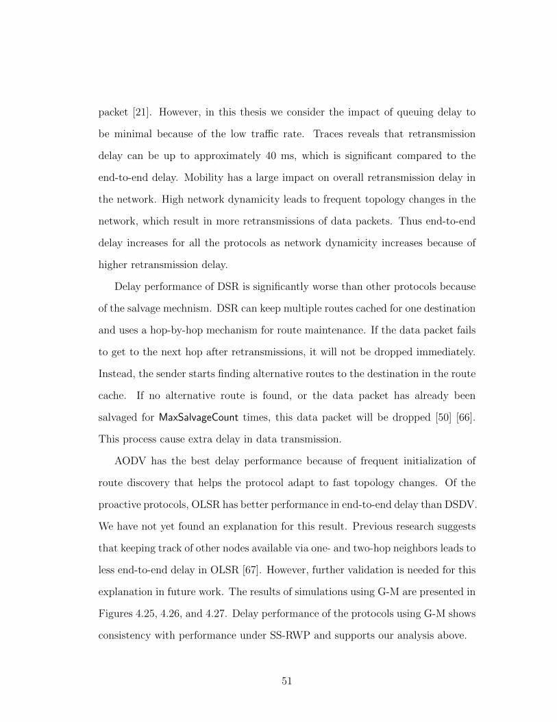
packet [21]. However, in this thesis we consider the impact of queuing delay to

be minimal because of the low traffic rate. Traces reveals that retransmission

delay can be up to approximately 40 ms, which is significant compared to the

end-to-end delay. Mobility has a large impact on overall retransmission delay in

the network. High network dynamicity leads to frequent topology changes in the

network, which result in more retransmissions of data packets. Thus end-to-end

delay increases for all the protocols as network dynamicity increases because of

higher retransmission delay.

Delay performance of DSR is significantly worse than other protocols because

of the salvage mechnism. DSR can keep multiple routes cached for one destination

and uses a hop-by-hop mechanism for route maintenance. If the data packet fails

to get to the next hop after retransmissions, it will not be dropped immediately.

Instead, the sender starts finding alternative routes to the destination in the route

cache. If no alternative route is found, or the data packet has already been

salvaged for MaxSalvageCount times, this data packet will be dropped [50] [66].

This process cause extra delay in data transmission.

AODV has the best delay performance because of frequent initialization of

route discovery that helps the protocol adapt to fast topology changes. Of the

proactive protocols, OLSR has better performance in end-to-end delay than DSDV.

We have not yet found an explanation for this result. Previous research suggests

that keeping track of other nodes available via one- and two-hop neighbors leads to

less end-to-end delay in OLSR [67]. However, further validation is needed for this

explanation in future work. The results of simulations using G-M are presented in

Figures 4.25, 4.26, and 4.27. Delay performance of the protocols using G-M shows

consistency with performance under SS-RWP and supports our analysis above.

51

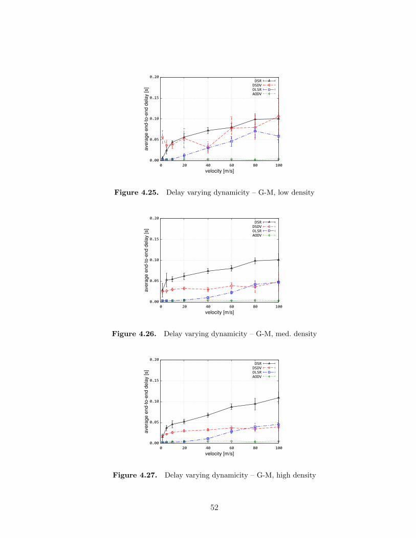
avera

ge e

nd-t

o-e

nd d

ela

y [s]

velocity [m/s]

DSR

DSDV

OLSR

AODV

0.00

0.05

0.10

0.15

0.20

0 20 40 60 80 100

Figure 4.25. Delay varying dynamicity – G-M, low density

avera

ge e

nd-t

o-e

nd d

ela

y [s]

velocity [m/s]

DSR

DSDV

OLSR

AODV

0.00

0.05

0.10

0.15

0.20

0 20 40 60 80 100

Figure 4.26. Delay varying dynamicity – G-M, med. density

avera

ge e

nd-t

o-e

nd d

ela

y [s]

velocity [m/s]

DSR

DSDV

OLSR

AODV

0.00

0.05

0.10

0.15

0.20

0 20 40 60 80 100

Figure 4.27. Delay varying dynamicity – G-M, high density

52

avera

ge e

nd-t

o-e

nd d

ela

y [s]

α-value

DSDV

DSR

AODV

OLSR

0.00

0.05

0.10

0.15

0.20

0.000.501.001.502.00

Figure 4.28. Delay varying dynamicity – Levy, low density [1]

avera

ge e

nd-t

o-e

nd d

ela

y [s]

α-value

DSR

DSDV

AODV

OLSR

0.00

0.05

0.10

0.15

0.20

0.000.501.001.502.00

Figure 4.29. Delay varying dynamicity – Levy, med. density [1]

avera

ge e

nd-t

o-e

nd d

ela

y [s]

α-value

DSR

DSDV

AODV

OLSR

0.00

0.05

0.10

0.15

0.20

0.000.501.001.502.00

Figure 4.30. Delay varying dynamicity – Levy, high density [1]

53

Figure 4.28, 4.29, and 4.30 show delay performance of protocols under the

Levy Walk model. Delay performance does not show a clear trend in the low

and medium density scenarios. Data packets experience only small delay and one

retransmission could significantly increase end-to-end delay. However, in the high

density scenarios, delay increases as α value increases due to longer path durations

that result in fewer retransmissions and salvaging processes.

4.2 Varying Node Density

Node density is the other important factor in MANETs that affects routing

performance. The immediate impact of node density is affecting the chance of

establishing paths. We vary transmission range in this thesis to vary node density.

4.2.1 PDR Performance

PDR performance of routing protocols in low, medium, and high network

dynamicity scenarios is shown in Figures 4.31, 4.32, and 4.33. From the results

we can see that PDR increases as degree of connectivity increases. This is because

higher node density increases the chance of paths being established and leads to

longer path duration. The protocols achieve reasonable PDR performance in high

density scenarios even with high network dynamicity as high degree of connectivity

can mitigate the impact of node mobility on PDR. AODV still shows superior

performance, particularly in the medium and high dynamicity scenarios due to

its ability to adapt to rapid topology changes. Proactive protocols perform worse

as they rely on periodic updates. PDR performance of all four protocols shows

consistency with our observations in the previous section. The send buffer of

DSDV can only provide very minimal PDR performance improvement.

54

PD

R

degree of connectivity

AODV

OLSR

DSDV buff

DSDV

DSR0.0

0.2

0.4

0.6

0.8

1.0

0 5 10 15 20 25 30 35 40

Figure 4.31. PDR varying density – SS-RWP, low dynamicity

PD

R

degree of connectivity

AODV

DSR

DSDV buff

DSDV

OLSR0.0

0.2

0.4

0.6

0.8

1.0

0 5 10 15 20 25 30 35 40

Figure 4.32. PDR varying density – SS-RWP, med. dynamicity

PD

R

degree of connectivity

AODV

DSR

DSDV buff

DSDV

OLSR0.0

0.2

0.4

0.6

0.8

1.0

0 5 10 15 20 25 30 35 40

Figure 4.33. PDR varying density – SS-RWP, high dynamicity

55

4.2.2 Routing Overhead Performance

Routing overhead of the protocols in low, medium, and high network dynam-

icity scenarios is shown in Figures 4.34, 4.35, and 4.36. The overhead of AODV

increases with degree of connectivity in low and medium dynamicity scenarios.

As mentioned in the previous section, routing overhead generated by AODV is

dominated by RREQ flooding. Assuming each traffic source generates a RREQ

packets per unit time on average, routing overhead generated by AODV can be

modeled by:

as(d− 1)N (4.4)

where s is the number of source nodes, N is total number of nodes, and d is

the degree of connectivity in Table 4.4. We assume a to be fairly stable when

varying the degree of connectivity in the low and medium dynamicity scenarios.

We can make this assumption because when node mobility is low, increasing node

density will not have the effect of mitigating the impact of network dynamicity

on the frequency of topology changes. AODV routing overhead then has a linear

relationship with degree of connectivity based on this assumption. The routing

overhead of OLSR and DSDV do not show this linear relationship as both pro-

tocols can limit unnecessary retransmissions during broadcast of updates. OLSR

routing overhead is lower due to the MPR flooding optimization, as described in

Section 4.1.

In high dynamicity scenarios, we can not make the assumption that a is a

constant. Let b denote the number of link breakages per unit time during the

simulations. The relationships among factors a, b, and d can help explain overhead

performance of AODV. a has a positive correlation with b in all scenarios. In low

56

connectivity scenarios (d ≤ 9), link breakages occur at a very high rate because of

high dynamicity. So a is large because of a high value of b, which leads to AODV

overhead increasing rapidly with d. However, increasing d will limit the number

of link breakages, thus b has a negative correlation with d. When the network has

reasonable connectivity (d > 9), the negative correlation between b and d starts

to become the dominant factor and causes a to decrease with increasing d, with

overhead then decreases.

DSR routing overhead can be divided into two parts based on the degree of

connectivity in the medium and low dynamicity scenarios. In the first part (d ≤ 9),

a higher degree of connectivity leads to more routes being set up, which leads to

more source route header overhead. Routing overhead increases with degree of

connectivity primarily because of the large increase in the source route overhead.

In the second part (d > 9), the network has reasonable connectivity, which can

also be shown by the PDR performance results shown in Figures 4.31 and 4.32.

In these scenarios, the source route overhead is fairly stable. On the other hand,

the control packet overhead slightly decreases as the cache hit ratio increases with

better connectivity of the network, which leads to the decreasing total overhead.

4.2.3 End-to-End Delay Performance

End-to-end delay in low, medium, and high network dynamicity scenarios vary-

ing network density is shown in Figures 4.37, 4.38, and 4.39. DSDV with send

buffers enabled has significantly higher delay in the extremely low density scenar-

ios. This is because the send buffer allows a certain number of data packets to

be queued when there is no route available. The send buffer of DSDV does not

provide good performance improvement, and its negative effect is significant in

57

routing o

verh

ead [kb/s

]

degree of connectivity

DSR total overhead

DSDV

DSDV buff

AODV

OLSR

0

50

100

150

200

250

300

0 5 10 15 20 25 30 35 40

Figure 4.34. Overhead varying density – SS-RWP, low dynamicity

routing o

verh

ead [kb/s

]

degree of connectivity

DSR total overhead

DSDV

DSDV buff

AODV

OLSR

0

50

100

150

200

250

300

0 5 10 15 20 25 30 35 40

Figure 4.35. Overhead varying density – SS-RWP, med. dynamicity

routing o

verh

ead [kb/s

]

degree of connectivity

AODV

DSR total overhead

DSDV

DSDV buff

OLSR

0

50

100

150

200

250

300

0 5 10 15 20 25 30 35 40

Figure 4.36. Overhead varying density – SS-RWP, high dynamicity

58

low connectivity scenarios. Further optimization is needed for buffering mecha-

nisms in DSDV. In the low and medium dynamicity scenarios, delay of DSR first

increases, and then decreases as d increases. This is because in low density scenar-

ios the salvaging process is happening significantly less frequently due to the lack

of established paths. Then when the network has reasonable connectivity, the lack

of established paths is no longer the dominant factor. Increasing network density

reduces link breakages and leads to lower delay as the number of retransmissions

and the number of salvaging processes are decreasing. Both OLSR and AODV

achieve very desirable delay performance, which is consistent with the results in

Section 4.1. The delay of AODV shows a slight increase when node density is

increasing. Further study of AODV delay performance in future work should find

an explanation to this performance trend.

4.3 Performance Summary

To summarize our analysis of routing protocol performance, we focus on the

protocols’ ability to adapt to rapid topology changes, and scalability to larger and

denser networks. Additionally, our analysis reveals the fundamental performance

tradeoff between adaptation to rapid topology changes and routing overhead. Im-

proving the ability to adapt to topology changes can lead to higher routing over-

head when designing and optimizing protocols.

AODV delivers good performance throughout our simulation studies. It has

better PDR performance than all other protocols in dynamic scenarios because

of the ability to adapt to topology changes. This ability comes from its frequent

initialization of route discovery, which also leads to desirable delay performance

in all scenarios. However, the problem with AODV comes from frequent flood-

59

avera

ge e

nd-t

o-e

nd d

ela

y [s]

degree of connectivity

DSR

DSDV buff

DSDV

OLSR

AODV

0.00

0.05

0.10

0.15

0.20

0.25

0 5 10 15 20 25 30 35 40

Figure 4.37. Delay varying density – SS-RWP, low dynamicity

avera

ge e

nd-t

o-e

nd d

ela

y [s]

degree of connectivity

DSR

DSDV buff

DSDV

OLSR

AODV

0.00

0.05

0.10

0.15

0.20

0.25

0 5 10 15 20 25 30 35 40

Figure 4.38. Delay varying density – SS-RWP, med. dynamicity

avera

ge e

nd-t

o-e

nd d

ela

y [s]

degree of connectivity

DSR

DSDV buff

DSDV

OLSR

AODV

0.00

0.05

0.10

0.15

0.20

0.25

0 5 10 15 20 25 30 35 40

Figure 4.39. Delay varying density – SS-RWP, high dynamicity

60

ing of RREQ packets, which results in linearly increasing routing overhead with

increasing degree of connectivity. This significantly limits AODV scalability to

denser and larger networks. It also causes AODV to generate high overhead in

extremely dynamic scenarios in which many extra route discovery processes are

triggered. Even so, AODV appears to be the best choice in most of the scenarios.

For DSR, the distinctive features are the aggressive use of route cache and the use

of source routing. However, the performance of DSR suffers from both features

in many of the scenarios. Aggressive use of cache causes stale routes, which hurts

DSR performance on PDR and delay. Even though route caching effectively helps

reduce flooding of control packets, injecting source route header in data packets

results in high total overhead and will cause extra processing burden in real im-

plementations. Apparently, further optimization of DSR is needed based on our

results and ananlysis. Firstly, the impact of the salvage mechanism needs to be

examined in future works. The salvaging limit should be chosen appropriately in

different scenarios to improve delay performance. Secondly, better route caching

strategies can be proposed in future work to achieve better overall performance.

DSDV, as expected, does not adapt well to frequent topology changes as it

is a proactive protocol relying on periodic updates. On the other hand, DSDV

does show reasonable scalability in high density scenarios. However, DSDV has

higher delay and the overall performance does not stand out in any of the scenar-

ios. OLSR, which is also a proactive protocol, delivers better delay and overhead

performance than DSDV in most cases. OLSR optimization schemes are very ef-

fective in limiting routing overhead, making it a good choice for low and medium

dynamicity scenarios. Reducing the intervals between periodic updates in proac-

tive protocols can improve their PDR performance, but at the cost of higher rout-

61

ing overhead, which shows the performance tradeoff in protocol design. Table 4.6

summarizes our discussion on the ability to adapt to rapid topology changes and

scalability to denser and larger networks of the protocols.

Table 4.6. Performance summary of protocol abilities

Protocol Adapting to topology changes Scalability

AODV Good FairOLSR Fair GoodDSDV Fair FairDSR Poor Fair

It should be noted that the above performance evaluation is made under the

default parameter settings with only a few changes. Parameters such as route-

cache timeout, periodic-update interval, active-route timeout, and salvaging limit,

are expected to have some impact on performance of routing protocols. Carefully

setting the parameters to proper values based on network cases is very helpful to

achieve better performance in real-life scenarios.

62

Chapter 5

Conclusions and Future Work

5.1 Conclusions

In this thesis, we analyzed the performance of prominent MANET routing

protocols (DSDV, AODV, DSR, and OLSR) using ns-3 simulations. Routing

protocol performance was evaluated for three mobility models (SS-RWP, G-M,

and Levy Walk). Both network dynamicity and node density of MANETs have a

significant impact on routing performance.

According to our results and analysis, AODV is the best choice in most of the

scenarios. OLSR performs better than its fellow proactive-protocol DSDV in most

scenarios. DSR performance could suffer from the use of route cache and source

routing.

5.2 Future Work

Given the scope of this thesis and our observations from the simulation results,

more can be achieved in future work. We present our thoughts on the future

63

outlook of simulation-based MANET routing studies in this section.

Future work can aim to provide more comprehensiveness. First, more perfor-

mance metrics can be evaluated in future studies on MANET routing protocols,

especially underlying metrics that provide more insight into node movement and

routing performance. For example, route life time and route hop counts studied

in [35] are good indicators of the dynamics of mobile wireless networks. In addi-

tion, presenting the distributions of metrics should be considered in performance

evaluation. In this thesis, we use connected data points with confidence interval

(CI) estimates in our presentation of the results. CI is a range of likely values for

a parameter [68]. For performance metrics such as PDR and routing overhead,

this is a simple, sufficient, and straightforward way to present results. But for

end-to-end delay, route life time, and route hop counts, presenting the distribu-

tion reveals more statistical characteristics and could provide more insights on

MANET routing performance. Second, more protocols can be included in the

comparison studies. These protocols include hybrid protocols such as ZRP, and

location-based protocols such as DREAM (Distance Routing Effect Algorithm

for Mobility), GPSR (Greedy Perimeter Stateless Routing), SiFT, and LAR. In

addition, more mobility models can be used, especially group mobility models

such as the Reference Point Group Mobility (RPGM) model [30]. Lastly, more

network scenarios should be created to evaluate routing performance in future

studies. Congestion is not considered in this thesis with the network being far

from saturated in our simulations because we first want to understand routing

performance and dynamics isolated from the effects of congestion and collisions.

However, congestion can have a significant impact on routing performance, and

saturated scenarios should be implemented in future work. In addition, MANET

64

routing protocols are generally designed based on the assumption that all partici-

pating nodes are fully cooperative [69]. Most simulation studies are carried out in

scenarios based on this assumption as well. However, a node may be misbehaving

by agreeing to forward packets and then failing to do so, because it is overloaded,

selfish, malicious, or broken [70]. Studying the impact of misbehaving nodes and

mitigation approaches is a good topic for future work and will be helpful especially

for actual implementation of MANET routing protocols.

There have been previous studies on MANET routing protocols that try to

establish detailed mathematical models to reveal the relationship among routing

performance metrics, node mobility, and parameters of the mobile networks [2], [3].

These models provide helpful insights and are good examples of exploiting math-

ematics to evaluate routing performance. However, validation of their models is

only done on a limited number of scenarios. Developing comprehensive mathemat-

ical models would be helpful for in-depth research on MANET routing protocols.

Future studies of MANET routing can also focus on the implementation of pro-

tocols in ns-3. Current ns-3 releases only have proactive and reactive protocols

implemented for MANET routing. This can be extended by adding implementa-

tions of hybrid protocols such as ZRP. In addition, implementations of AODV and

OLSR lack detailed documentation. Studies on their implementations can ana-

lyze and test the parameters and justify the default values. Research on protocol

implementation will be helpful for research on new protocol development.

65

References

[1] Sai Sandeep Bhooshi. MANET routing protocol simulations using different

mobility models. Master’s thesis, The University of Kansas, USA, 2018.

[2] Narayanan Sadagopan, Fan Bai, Bhaskar Krishnamachari, and Ahmed

Helmy. PATHs: analysis of path duration statistics and their impact on

reactive manet routing protocols. In Proceedings of the 4th ACM interna-

tional symposium on Mobile ad hoc networking & computing, pages 245–256.

ACM, 2003.

[3] Robin Groenevelt, Philippe Nain, and Ger Koole. Message delay in MANET.

In ACM SIGMETRICS Performance Evaluation Review, volume 33, pages

412–413. ACM, 2005.

[4] Yufei Cheng. Performance analysis of transactional traffic in mobile ad-hoc

networks. Master’s thesis, The University of Kansas, USA, 2014.

[5] Elizabeth M Royer and Charles E Perkins. An implementation study of

the AODV routing protocol. In Wireless Communications and Networking

Confernce, 2000. WCNC. 2000 IEEE, volume 3, pages 1003–1008. IEEE,

2000.

66

[6] Krzysztof Pawlikowski, H-DJ Jeong, and J-SR Lee. On credibility of simu-

lation studies of telecommunication networks. IEEE Communications mag-

azine, 40(1):132–139, 2002.

[7] Todd R Andel and Alec Yasinsac. On the credibility of MANET simulations.

Computer, 39(7):48–54, 2006.

[8] Martin Mauve, Jorg Widmer, and Hannes Hartenstein. A survey on position-

based routing in mobile ad hoc networks. IEEE network, 15(6):30–39, 2001.

[9] Philippe Jacquet and Laurent Viennot. Overhead in mobile ad-hoc network

protocols. PhD thesis, INRIA, 2000.

[10] Charles E Perkins and Pravin Bhagwat. Highly dynamic destination-

sequenced distance-vector routing (DSDV) for mobile computers. In ACM

SIGCOMM computer communication review, volume 24, pages 234–244.

ACM, 1994.

[11] T. Clausen and P. Jacquet. Optimized Link State Routing Protocol (OLSR).

RFC 3626 (Experimental), October 2003.

[12] Josh Broch, David A Maltz, David B Johnson, Yih-Chun Hu, and Jorjeta

Jetcheva. A performance comparison of multi-hop wireless ad hoc network

routing protocols. In Proceedings of the 4th annual ACM/IEEE international

conference on Mobile computing and networking, pages 85–97. ACM, 1998.

[13] Hemanth Narra, Yufei Cheng, Egemen K Cetinkaya, Justin P Rohrer, and

James PG Sterbenz. Destination-sequenced distance vector (DSDV) routing

protocol implementation in ns-3. In Proceedings of the 4th International

ICST Conference on Simulation Tools and Techniques, pages 439–446. ICST

67

(Institute for Computer Sciences, Social-Informatics and Telecommunications

Engineering), 2011.

[14] C. Hedrick. Routing Information Protocol. RFC 1058, June 1988.

[15] Ying Ge, T. Kunz, and L. Lamont. Quality of service routing in ad-hoc net-

works using OLSR. In Proc. 36th Annual Hawaii Int. Conf. System Sciences,

pages 9 pp.–, January 2003.

[16] David B Johnson. Routing in ad hoc networks of mobile hosts. In Mo-

bile Computing Systems and Applications, 1994. Proceedings., Workshop on,

pages 158–163. IEEE, 1994.

[17] C. Perkins, E. Belding-Royer, and S. Das. Ad hoc On-Demand Distance

Vector (AODV) Routing. RFC 3561 (Experimental), July 2003.

[18] D. Johnson, Y. Hu, and D. Maltz. The Dynamic Source Routing Protocol

(DSR) for Mobile Ad Hoc Networks for IPv4. RFC 4728 (Experimental),

February 2007.

[19] David B Johnson, David A Maltz, Josh Broch, et al. DSR: The dynamic

source routing protocol for multi-hop wireless ad hoc networks. Ad hoc net-

working, 5:139–172, 2001.

[20] Charles Perkins, Elizabeth Belding-Royer, and Samir Das. Ad hoc on-demand

distance vector (AODV) routing. Technical report, 2003.

[21] Charles E Perkins, Elizabeth M Royer, Samir R Das, and Mahesh K Ma-

rina. Performance comparison of two on-demand routing protocols for ad

hoc networks. IEEE Personal communications, 8(1):16–28, 2001.

68

[22] Elizabeth M Royer, P Michael Melliar-Smith, and Louise E Moser. An analy-

sis of the optimum node density for ad hoc mobile networks. In Communica-

tions, 2001. ICC 2001. IEEE International Conference on, volume 3, pages

857–861. IEEE, 2001.

[23] Ian D Chakeres and Elizabeth M Belding-Royer. AODV routing protocol

implementation design. In Distributed Computing Systems Workshops, 2004.

Proceedings. 24th International Conference on, pages 698–703. IEEE, 2004.

[24] Carl A Sunshine. Source routing in computer networks. ACM SIGCOMM

Computer Communication Review, 7(1):29–33, 1977.

[25] Mehran Abolhasan, Tadeusz Wysocki, and Eryk Dutkiewicz. A review of

routing protocols for mobile ad hoc networks. Ad hoc networks, 2(1):1–22,

2004.

[26] Z Haas. The zone routing protocol (ZRP) for ad hoc networks. IETF Internet

Draft, draft-ietf-manet-zone-zrp-01. txt, 1998.

[27] Nicklas Beijar. Zone routing protocol (ZRP). Networking Laboratory, Helsinki

University of Technology, Finland, 9:1–12, 2002.

[28] Kavita Pandey and Abhishek Swaroop. A comprehensive performance analy-

sis of proactive, reactive and hybrid manets routing protocols. arXiv preprint

arXiv:1112.5703, 2011.

[29] Young-Bae Ko and Nitin H Vaidya. Location-aided routing (LAR) in mobile

ad hoc networks. Wireless networks, 6(4):307–321, 2000.

69

[30] Tracy Camp, Jeff Boleng, and Vanessa Davies. A survey of mobility models

for ad hoc network research. Wireless communications and mobile computing,

2(5):483–502, 2002.

[31] William Navidi, Tracy Camp, and Nick Bauer. Improving the accuracy of

random waypoint simulations through steady-state initialization. In Proceed-

ings of the 15th International Conference on Modeling and Simulation, pages

319–326, 2004.

[32] Fan Bai and Ahmed Helmy. A survey of mobility models. Wireless Adhoc

Networks. University of Southern California, USA, 206:147, 2004.

[33] Dan Broyles, Abdul Jabbar, James PG Sterbenz, et al. Design and analysis of

a 3–D Gauss-Markov mobility model for highly-dynamic airborne networks.

In Proceedings of the International Telemetering Conference (ITC),(San

Diego, CA), 2010.

[34] Justin P Rohrer, Egemen K Cetinkaya, Hemanth Narra, Dan Broyles, Kevin

Peters, and James PG Sterbenz. AeroRP performance in highly-dynamic

airborne networks using 3D Gauss-Markov mobility model. In MILITARY

COMMUNICATIONS CONFERENCE, 2011-MILCOM 2011, pages 834–

841. IEEE, 2011.

[35] Injong Rhee, Minsu Shin, Seongik Hong, Kyunghan Lee, Seong Joon Kim,

and Song Chong. On the Levy-Walk nature of human mobility. IEEE/ACM

transactions on networking (TON), 19(3):630–643, 2011.

70

[36] S. Corson and J. Macker. Mobile Ad hoc Networking (MANET): Routing

Protocol Performance Issues and Evaluation Considerations. RFC 2501, Jan-

uary 1999.

[37] V Park and S Corson. Temporally-ordered routing algorithm (TORA) version

1. IETF Internet Draft, draft-ietf-manet-tora-spec-00.txt, 1997.

[38] Mahesh K Marina and Samir R Das. On-demand multipath distance vector

routing in ad hoc networks. In Network Protocols, 2001. Ninth International

Conference on, pages 14–23. IEEE, 2001.

[39] Manveen Singh Chadha and Rambir Joon. Simulation and comparison of

AODV, DSR and AOMDV routing protocols in manets. Applied Soft Com-

puting, 2012.

[40] P Manickam, T Guru Baskar, M Girija, and Dr D Manimegalai. Performance

comparisons of routing protocols in mobile ad hoc networks. arXiv preprint

arXiv:1103.0658, 2011.

[41] Mandeep Kaur Gulati and Krishan Kumar. Performance comparison of mo-

bile ad hoc network routing protocols. International Journal of Computer

Networks & Communications, 6(2):127, 2014.

[42] QualNet Homepage. https://web.scalable-networks.com/

qualnet-network-simulator-software, January 2008.

[43] Ioannis Broustis, Gentian Jakllari, Thomas Repantis, and Mart Molle.

A comprehensive comparison of routing protocols for large-scale wireless

MANETs. In SECON, volume 6, pages 951–956. Citeseer, 2006.

71

[44] Per Johansson, Tony Larsson, Nicklas Hedman, Bartosz Mielczarek, and

Mikael Degermark. Scenario-based performance analysis of routing protocols

for mobile ad-hoc networks. In Proceedings of the 5th annual ACM/IEEE in-

ternational conference on Mobile computing and networking, pages 195–206.

ACM, 1999.

[45] Chrisy Samara, Eirini Karapistoli, and Anastasios A Economides. Perfor-

mance comparison of MANET routing protocols based on real-life scenarios.

In Ultra Modern Telecommunications and Control Systems and Workshops

(ICUMT), 2012 4th International Congress on, pages 870–877. IEEE, 2012.

[46] Rakesh Kumar Jha and Pooja Kharga. A comparative performance analysis

of routing protocols in MANET using NS3 simulator. International Journal

of Computer Network and Information Security, 7(4):62–68, 2015.

[47] Yefa Mai, Yuxia Bai, Nan Wang, et al. Performance comparison and evalu-

ation of the routing protocols for MANETs using NS3. 2017.

[48] Bhavyesh Divecha, Ajith Abraham, Crina Grosan, and Sugata Sanyal. Im-

pact of node mobility on MANET routing protocols models. JDIM, 5(1):19–

23, 2007.

[49] Fan Bai, Narayanan Sadagopan, and Ahmed Helmy. IMPORTANT: A frame-

work to systematically analyze the impact of mobility on performance of rout-

ing protocols for adhoc networks. In INFOCOM 2003. Twenty-second annual

joint conference of the IEEE computer and communications. IEEE societies,

volume 2, pages 825–835. IEEE, 2003.

72

[50] Yufei Cheng, Egemen K Cetinkaya, and James PG Sterbenz. Dynamic source

routing (DSR) protocol implementation in ns-3. In Proceedings of the 5th In-

ternational ICST Conference on Simulation Tools and Techniques, pages 367–

374. ICST (Institute for Computer Sciences, Social-Informatics and Telecom-

munications Engineering), 2012.

[51] Mohammed Alenazi, Cenk Sahin, and James P Sterbenz. Design improve-

ment and implementation of 3d Gauss-Markov mobility model. Technical

report, AIR FORCE TEST CENTER EDWARDS AFB CA, 2013.

[52] Ashwini Balachandra. Implementation of truncated Levy Walk mobility

model in ns-3. Master’s thesis, The University of Kansas, USA, 2017.

[53] Leonard Kleinrock and John Silvester. Optimum transmission radii for packet

radio networks or why six is a magic number. In Proceedings of the IEEE

national telecommunications conference, volume 4, pages 1–4, 1978.

[54] The ns-3 Homepage. http://www.nsnam.org, January 2011.

[55] Elias Weingartner, Hendrik Vom Lehn, and Klaus Wehrle. A performance

comparison of recent network simulators. In Communications, 2009. ICC’09.

IEEE International Conference on, pages 1–5. IEEE, 2009.

[56] The ns-3 Network Simulator Doxygen Documentation. http://www.nsnam.

org/doxygen, July 2012.

[57] Thomas R Henderson, Mathieu Lacage, George F Riley, Craig Dowell, and

Joseph Kopena. Network simulations with the ns-3 simulator. SIGCOMM

demonstration, 14(14):527, 2008.

73

[58] The ns-3 Manual. https://www.nsnam.org/docs/manual/html/index.

html, July 2010.

[59] The list of all trace sources. https://www.nsnam.org/docs/release/3.19/

doxygen/group___trace_source_list.html, July 2014.

[60] ns3::aodv::RoutingProtocol Class Reference. https://www.nsnam.org/

doxygen/classns3_1_1aodv_1_1_routing_protocol.html, December

2018.

[61] Fan Bai, Narayanan Sadagopan, Bhaskar Krishnamachari, and Ahmed

Helmy. Modeling path duration distributions in MANETs and their impact

on reactive routing protocols. IEEE Journal on Selected Areas in Communi-

cations, 22(7):1357–1373, 2004.

[62] ns-3: DSDV Routing. https://www.nsnam.org/docs/models/html/dsdv.

html, January 2011.

[63] Philippe Jacquet, Anis Laouiti, Pascale Minet, and Laurent Viennot. Per-

formance analysis of OLSR multipoint relay flooding in two ad hoc wireless

network models. PhD thesis, INRIA, 2001.

[64] Laurent Viennot, Philippe Jacquet, and Thomas Heide Clausen. Analyzing

control traffic overhead versus mobility and data traffic activity in mobile

ad-hoc network protocols. Wireless Networks, 10(4):447–455, 2004.

[65] ns3::ConstantSpeedPropagationDelayModel Class Reference. https://

www.nsnam.org/doxygen/classns3_1_1_constant_speed_propagation_

delay_model.html, December 2018.

74

[66] ns3::dsr::DsrRouting Class Reference. https://www.nsnam.org/doxygen/

classns3_1_1dsr_1_1_dsr_routing.html, January 2011.

[67] Ashish Shrestha and Firat Tekiner. Investigation of MANET routing proto-

cols for mobility and scalability.

[68] Shinichi Nakagawa and Innes C Cuthill. Effect size, confidence interval and

statistical significance: a practical guide for biologists. Biological reviews,

82(4):591–605, 2007.

[69] Kejun Liu, Jing Deng, Pramod K Varshney, and Kashyap Balakrishnan. An

acknowledgment-based approach for the detection of routing misbehavior in

MANETs. IEEE transactions on mobile computing, 6(5):536–550, 2007.

[70] Sergio Marti, Thomas J Giuli, Kevin Lai, and Mary Baker. Mitigating routing

misbehavior in mobile ad hoc networks. In Proceedings of the 6th annual

international conference on Mobile computing and networking, pages 255–

265. ACM, 2000.

75