Available online at www.sciencedirect.com

www.elsevier.com/locate/solener

ScienceDirect

Solar Energy 118 (2015) 41–58

Predictive model for assessing and optimizing solar stillperformance using artificial neural network under

hyper arid environment

Ahmed F. Mashaly a,⇑, A.A. Alazba a,b, A.M. Al-Awaadh b, Mohamed A. Mattar b,c

a Alamoudi Chair for Water Researches, King Saud University, P.O. Box 2460, Riyadh 11451, Saudi Arabiab Agricultural Engineering Department, College of Food and Agriculture Sciences, King Saud University, P.O. Box 2460, Riyadh 11451, Saudi Arabia

c Agricultural Engineering Research Institute (AEnRI), Agricultural Research Center, P.O. Box 256, Giza, Egypt

Received 27 September 2014; received in revised form 13 January 2015; accepted 8 May 2015

Communicated by: Associate Editor G.N. Tiwari

Abstract

A mathematical model to forecast the solar still performance under hyper arid conditions was developed using artificial neural net-work technique. The developed model expressed by different forms, water productivity (MD), operational recovery ratio (ORR) andthermal efficiency (gth) requires ten input parameters. The input parameters included Julian day, ambient air temperature, relative humid-ity, wind speed, solar radiation, ultra violet index, temperature of the feed and brine water, and total dissolved solids of feed and brinewater. The developed ANN model was trained, tested and validated based on measured data. The results showed that the coefficient ofdetermination ranged from 0.991 to 0.99 and 0.94 to 0.98 for MD, ORR and gth during training and testing process, respectively. Theaverage values of root mean-square error for all water were 0.04 L/m2/h, 2.60% and 3.41% for MD, ORR and gth respectively. Findingsrevealed that the model was effective and accurate in predicting solar still performance with insignificant errors.� 2015 Elsevier Ltd. All rights reserved.

Keywords: Artificial neural network; Solar still; Solar desalination; Water recovery; Modeling

1. Introduction

Global water consumption is anticipated to increase byaround 55% by 2050, primarily owing to growing demandsfrom industry, electricity generation and municipal con-sumption. In light of this, more than 40% of the world pop-ulation is anticipated to live under water stress by 2050.Moreover, still 768 million people have no access to pota-ble water (WWAP, 2014), although that there are morethan 16,000 desalination plants operating over the world

http://dx.doi.org/10.1016/j.solener.2015.05.013

0038-092X/� 2015 Elsevier Ltd. All rights reserved.

⇑ Corresponding author. Tel.: +966 14673737; fax: +966 14673739.E-mail addresses: amashaly@ksu.edu.sa, mashaly.ahmed@gmail.com

(A.F. Mashaly).

with the total capacity reported at 66.4 million m3/day,and it is anticipated to increase to 100 million m3/day by2015 (GWI/IDA, 2013). However, these mentioned indica-tors raise concern over current practices of water resourcesustainability because desalination industry still dependmainly on fossil energy and with decline for 80% of worldoilfields by 2030 (Hook et al., 2009). Alternative may needto be adopted to ensure steady water supplies, especially inthe future following sustainable manner. Add to that,Kalogirou (2005) found that the production of 1000 m3/day of desalinated water need 10,000 tons (toe) of oil peryear. Accordingly, utilization of solar energy could beone of the promising renewable energy in desalinating

42 A.F. Mashaly et al. / Solar Energy 118 (2015) 41–58

water particularly in arid areas where oil is consumed dra-matically to operate desalination plants (Kalogirou, 2013).Therefore, the use of solar still in arid areas at small orlarge scale could help in desalinating necessary needs ofwater either by purifying seawater, groundwater or recy-cling of wastewater (Kabeel and Almagar, 2013). Theongoing efforts in this endeavor revealed that a solar stilluse evaporation and condensation process which in naturegenerate rainfall (Ahsan et al., 2010) and such device lim-ited by the high capital cost required to be applied on asmall scale. However, to optimize and enhance this config-uration to be used widely with possible low cost, this mayrequire further modeling processes to forecast optimal per-formance and identify critical parameters related to stillperformance to lower its costs. Based on the foregoing,there is a need to develop a predictive model that wouldbe able to accurately estimate the performance. Khadir(2005), Tripathy and Kumar (2009) stated that classicalmodeling techniques are complex and a need long timefor computing as well as occasionally are inaccurate to pre-dict still performance effectively. Additionally, Santos et al.(2012) stated that amount of labor and equipment neededto achieve classical heat and mass transfer modeling forsolar still performance oftentimes requires resources exceedthe capability of many rural communities. Therefore, liter-ature provides insufficient information on this aspect todevelop novel models that could simplify the performanceof still and optimize operational conditions (Dunkle, 1961;Mowla and Karimi, 1995; Tiwari and Tiwari, 2006; Devand Tiwari, 2009). An artificial neural network (ANN)could be considered as a possible alternative to classicalmodels in modeling thermal solar energy systems by incor-porating meteorological data to precisely predict still per-formance (Kalogirou et al., 1999). Multiple uses ofANNs for a wide range of fields for modeling and predic-tion in energy engineering systems were reviewed by(Kalogirou 2001; Yang et al., 2003; Sozen et al., 2005;Mellita and Kalogirou, 2008; Kalogirou, 2006) and foundthat the results were effective and accurate. Moreover, insolar energy field, many researchers studied some applica-tions of ANNs, for example, Kalogirou et al. (1998) usedthe ANN for modeling the heat-up response of a solarsteam generating plant. Santos et al. (2012) determinedthe effectiveness of modeling solar still distillate productionusing ANNs and local weather data. They used only inso-lation, ambient temperature, distillate volume, wind speed,wind direction and cloud cover as inputs. The ANNmethod was also used by Sozen et al. (2008) in order todetermine the efficiency of flat plate solar thermal collectorswhere the input data were the collector temperature, date,time, solar radiation, declination angle, azimuth angle andtilt angle. Porrazzo et al. (2013) used an ANN model foranalyzing a solar powered membrane distillation systemperformance under several operating conditions, specifi-cally distillate production versus feed flow rate, solar radi-ation and cold feed temperature. Farkas and Geczy-Vıg(2003) developed ANN models for three different types of

solar thermal collectors to predict the outlet temperatureof the solar collectors based on solar radiation, ambienttemperature and inlet temperature. Also, Lecoeuche andLalot (2005) showed an application of ANNs to forecastthe in-situ daily performance of solar air collectors wherethe output of the ANN is the outlet temperature of the col-lector, and inputs to the network are the solar radiationand the thermal heat loss coefficients. Hamdan et al.(2013) used three ANN models (Feed forward, Elman,and Nonlinear Autoregressive Exogenous (NARX) net-works) to find the performance of triple solar still operatingunder Jordanian climate. They utilized nine input variablesnamely time, hourly variation of cover glass temperature,water temperature in the upper basin, water temperaturein the middle basin, water temperature in the lower basinof the triple basin still, distillate volume, ambient tempera-ture, plate temperature and hourly solar intensity as inputsto the network. They found that the achieved findings pre-sented that feed forward model had the best ability todetermine the required performance, on the other handNARX and Elman network had the lowest ability to deter-mine it. However, still there is a need for a comprehensivemodel to develop inputs and outputs for optimization ofstill performance by incorporating operational and meteo-rological parameters. For this reason, this study aims toexamine the effectiveness of the solar still by modeling itsperformance with different types of water (seawater,groundwater and agricultural drainage water). Previousstudies, for example, Santos et al. (2012) and Hamdanet al. (2013) indicated that there is a gap in this area onthe development of inputs and outputs. All the main mete-orological and operational data that may affect the desali-nation process and in particular the processes ofevaporation and condensation were not included.Furthermore, the contribution of each component in themodeling process was not specified. So, this study willinvestigate development of an ANN model to predict theperformance of solar still experimentally and theoreticallythrough developed ANN model. Additionally, evaluatethe performance of the developed ANN model in termsof certain statistical performance criteria in forecastingsolar still performance and study the effectiveness of inputvariables on ANN model performance.

2. ANN theory

Artificial neural networks (ANNs) are information pro-cessing systems that are non-algorithmic, non-digital, andintensive parallel. By studying previously recorded data,they learn the relationship between the input and outputvariables (Caudill and Butler, 1993). ANNs consist of alarge number of neurons (processing elements), which arearranged in different layers in the network: an input layer,an output layer and one or more hidden layers (Kumar andSingh, 2008). The neuron in the network essentiallyreceives input signals, processes them then sends an outputsignal (Haykin, 1994). Every neuron is connected with no

A.F. Mashaly et al. / Solar Energy 118 (2015) 41–58 43

less than one other neuron and every connection is repre-sented by a real number called a weight. Iteratively, theweights are adjusted so as to the network attempts to pro-duce the desired output (Safa et al., 2009). Demuth andBeale (2004) stated that each artificial neuron is a unitarycomputational processor, which has a summing junctionoperator (

P) and a transfer (activation) function f(z).

The connections that between inputs, neurons and outputsconsist of weights (w) and biases (bÞ, are considered param-eters of the neural network. The weights and bias are sum-marized by the summing junction operator of a singleneuron (i) into a net input zj known as argument. Thetransfer function of a single neuron converts the net argu-ment zj into the scalar output where wij is the connectionweight, xi is the input variable, i and j are the integerindexes and bj is the bias of the single artificial neuron(i). Rather than being programmed, neural networks learnto solve a problem. Learning is done through training.Training is the procedure by which the networks learn,and so learning is the final result. So as to design, trainand develop an ANN model, commercial neural networksoftware of QNET 2000 (Vesta Services, 2000) was used.The Multi-layer perception (MLP) network is the mostpopular type of feed-forward networks that learn fromexamples. The architecture of the proposed MLP artificialneural network is shown in Fig. 1. The ANN used in thisstudy was a standard feed-forward back-propagation neu-ral network with three layers: an input layer, one hiddenlayer and an output layer. As shown in Fig. 1, by connec-tion strengths named weights, every layer was connected

Fig. 1. Architecture of the proposed ANN.

together. Input vectors and the corresponding target vec-tors were used to train a network till it can approximatea function which associates input vectors with specific out-put vectors. Ten variables were used as input parametersfor the input neurons of the input layer. These variableswere Julian day (J), ambient air temperature (To, �C), rel-ative humidity (RH, %), wind speed (U, km/h), solar radi-ation (Rs, W/m2), ultra violet index (UVI), temperature offeed water (TF,�C), temperature of brine water (TB,�C)total dissolved solids of feed water (TDSF, PPT), total dis-solved solids of brine water (TDSB, PPT). The output layerconsisted of the three neurons related to the distillatedwater productivity (MD, L/m2/h), operational recoveryratio (ORR, %) and thermal efficiency (gth, %). The numberof neurons in the hidden layer was determined through thetrial and error method. The optimal architecture was deter-mined through varying the number of hidden nodes from 2to 20, and the best architecture was selected. The trainingprocess of the ANN model was stopped when the level oferror is acceptable. This whole process is called the trainingof the ANN.

Two transfer functions were used to obtain the opti-mized status. The transfer functions adopted for the neu-rons as following:

Sigmoid function: (1)

f ðzÞ ¼ 1

1þ expð�zÞ ð1Þ

Hyperbolic tangent function:

f ðzÞ ¼ 1� expð�2zÞ1þ expð�2zÞ ð2Þ

The output of the network can be formulated by thefollowing:

Y ¼ f ðzkÞ ð3Þ

where:

zk ¼Xn

j¼1

wkj � f ðzjÞ þ bk ð4Þ

Moreover,

zj ¼X10

i¼1

wjixi þ bj ð5Þ

where zj and zk are the weighted sum of the inputs and out-put, respectively, xi is the incoming signal from the ith neu-ron (at the input layer), wji and wki are the weights on theconnection directed from neuron j to neuron i and neuronk to neuron j, respectively (at the hidden layer) and bj andbk are the biases of neuron j and k, respectively. TheComparison was conducted between the two functions toselect the best based on some statistical parameters. Thebasic steps for designing neural network model are datacollecting, preprocessing data, building network, trainingnetwork, testing network and validation of network.Before training process, a certain preprocessing steps on

44 A.F. Mashaly et al. / Solar Energy 118 (2015) 41–58

the data were performed to make more efficient training.The entire data set (316 data points) was randomized.They were divided as follows: 221 (70%) of this data wasused for training, 63 (20%) was used for testing and 32(10%) was used for validation. Furthermore, the validationdata were divided as follows: 16 data points for sea water,10 data points for ground water and 6 data points for agri-cultural drainage water. The sigmoid and hyperbolic tan-gent transfer functions of neuron activation in the hiddenlayers were selected (Vesta Services, 2000). Also beforethe training, the input and output values are normalizedto be in a range between 0.15 and 0.85, after that the dataare ready for the training process and are simulated to getthe prediction results. This normalization accelerates thetraining process and improves the network’s generalizationcapabilities. By using the following equation, the normal-ization of the data is performed:

�X ¼ xi � xmin

xmax � xmin

� ð0:85� 0:15Þ þ 0:15 ð6Þ

where X : the normalized data, xi: the input data beforenormalized, xmax: the maximum value of the input/outputvector and xmin: the minimum value of the input/outputvector.

The last step in neural network activity is thede-normalization of output.

Table 1 lists the summary descriptive statistics for theinputs used for training, testing and validation the devel-oped ANN models and the corresponding descriptivestatistics for the outputs. The table give some of statisticalparameters including mean, standard deviation, minimum,maximum, kurtosis, and skewness for all parameters in dif-ferent process. Generally, mean is the average value, stan-dard deviation gives a measure of spread or variability ofthe data values, kurtosis indicates to the degree of flatnessor peakedness in the region about the mode of a frequencycurve and skewness refers to the symmetry in the distribu-tion of the data. As an instance, the average value of Towas above 30 �C for both training and testing processes.The maximum value of RH with the training process wasgreater than that with testing process. The average valuesof the U, RS, UVI and the operational parameters(TDSF, TDSB, TF and TB) were so close to a large extentin both processes. Moreover, curves for J and Rs are mod-erately skewed .Curves of RH and U are leptokurtic as kur-tosis is more than 3. Additionally the curves with MD,ORR and gth are in both processes platykurtic.Additionally, in validation process the skewness is between�½ and +½, so the curves of all parameters are symmetricexcept RH, U, Rs. Moreover, the curve of U is leptokurtic.

The performance evaluation methodology of networkarchitecture includes obtaining the minimum statisticalmeasures of error between measured and correlated values.The agreement between observed and correlated values wasquantified with four statistical measures namely, coefficientof determination (R2), root mean-square error (RMSE),overall index of model performance (OI) and coefficient

of residual mass (CRM). These parameters were calculatedto check the performance of the developed model. Thesestatistical performance evaluation criteria are expressedas follows:

R2 ¼ 1�Pn

i¼1ðxp;i � xo;iÞ2Pni¼1ðxo;i � xoÞ2

ð7Þ

RMSE ¼

ffiffiffiffiffiffiffiffiffiffiffiffiffiffiffiffiffiffiffiffiffiffiffiffiffiffiffiffiffiffiffiffiffiPni¼1ðxp;i � xo;iÞ2

n

sð8Þ

OI ¼ 1

21� RMSE

xmax � xmin

� �þ 1�

Pni¼1 xo;i � xp;i

� �2Pni¼1 xo;i � xoð Þ2

! !

ð9Þ

CRM ¼Pn

i¼1xp;i �Pn

i¼1xo;i

� �Pni¼1xo;i

ð10Þ

where xo,i = observed value; xp,i = correlated value;n = number of observations; xmax = maximum observedvalue; xmin = minimum observed value; and �xo = averagedobserved values.

R2 was used to measure the linear correlation betweenthe measured and the correlated values. The optimal corre-lation coefficient is achieved when its value is equal tounity. RMSE has been used by different authors to com-pare correlated and measured parameters (Arbat et al.,2008). The RMSE values show how much the predictionsunder- or over-estimate the measurements. RMSE wasused as the error function which measures the network per-formance. Legates and McCabe (1999) mentioned thatRMSE has the advantage of expressing the error in thesame units as the variable, so, providing more informationabout the efficiency of the model. The lower the RMSE, thegreater the accuracy of prediction. The OI parameter wasused to verify the performance of mathematical models.An OI value of one for a model denotes a perfect fitbetween the measured and correlated values (Alazbaet al., 2012). The CRM parameter to show the differencebetween measured and correlated values relative to themeasured data. The CRM is a measure of the model ten-dency to overestimate or underestimate the measured data.A zero value points out a perfect fit, while positive and neg-ative values indicate an under-and over prediction by themodel, respectively (Alazba et al., 2012). The best ANNmodel was selected on basis of the smallest RMSE andCRM and highest R2 and OI values.

3. Experimental procedure

The experimental set-up of the solar still station wasconducted at the Agricultural Research and ExperimentStation (Educational farm), Department of AgriculturalEngineering, King Saud University, Riyadh, SaudiArabia (24�44010.9000N, 46�37013.7700E) during the periodof February–November 2013, where the weather datawas obtained from a local weather station (Davis – USA)

Table 1Descriptive statistics for the inputs and targets used in training, testing and validation the developed ANN model.

Statistics J To (�C) RH (%) U (km/h) Rs (W/m2) UVI TF (�C) TB (�C) TDSF (PPT) TDSB (PPT) MD L/m2/h ORR (%) gth (%)

Training

Mean 146.75 31.88 15.97 2.14 644.83 3.76 40.10 50.63 53.82 67.78 0.55 36.16 52.57Std. Dev. 86.88 6.64 12.17 2.62 175.99 1.68 5.81 6.88 38.91 42.95 0.23 16.62 14.58Kurtosis �1.18 �1.08 4.87 4.73 0.22 �0.67 �0.37 0.59 �1.05 �1.39 �0.86 �0.80 �0.30Skewness 0.56 0.08 2.02 2.12 �0.85 �0.17 �0.02 0.16 0.37 0.04 �0.43 �0.01 �0.28Minimum 54.00 16.87 2.14 0.00 75.10 0.00 22.10 31.29 4.71 7.30 0.05 2.07 15.84Maximum 305.00 43.57 70.00 12.33 920.69 7.39 51.26 68.69 130.00 132.80 0.92 75.11 82.16

Testing

Mean 146.19 32.04 16.17 1.98 625.20 3.52 40.27 50.31 56.42 68.01 0.53 34.39 50.83Std. Dev. 86.65 7.18 12.36 2.71 178.37 1.71 6.18 6.60 41.24 44.87 0.23 16.95 14.50Kurtosis �1.14 �1.25 3.82 6.19 �0.59 �0.75 �0.82 0.48 �1.32 �1.49 �1.07 �0.71 �0.44Skewness 0.60 �0.03 1.81 2.40 �0.59 0.02 �0.04 �0.10 0.21 �0.01 �0.22 0.19 �0.33Minimum 54.00 18.97 3.00 0.00 228.48 0.41 28.17 33.84 4.75 7.59 0.07 4.43 16.42Maximum 305.00 43.75 61.38 12.65 897.43 7.15 50.71 66.51 130.00 132.60 0.88 72.99 78.40

Validation

Mean 152.69 32.04 17.36 1.73 656.52 3.96 40.34 50.86 57.89 70.28 0.57 36.87 52.14Std. Dev. 91.22 7.11 13.91 2.37 179.16 1.77 6.19 8.10 40.34 45.28 0.24 17.86 15.27Kurtosis �1.37 �1.06 4.74 7.63 �0.09 �0.75 0.08 1.30 �1.16 �1.50 �0.71 �0.95 �0.11Skewness 0.50 �0.05 1.99 2.59 �0.80 �0.20 �0.38 �0.19 0.18 �0.12 �0.44 0.05 �0.66Minimum 54.00 17.69 4.10 0.00 215.12 0.50 24.61 27.59 4.80 6.71 0.06 5.84 17.44Maximum 305.00 43.18 66.95 11.15 908.67 7.42 50.62 67.96 129.30 129.80 0.97 74.22 78.82

A.F

.M

ash

aly

eta

l./So

lar

En

ergy

11

8(

20

15

)4

1–

58

45

3m

Drippers/Nozzles

(a) 2m Not to Scale (b)

(c)

Evaporation

Brine Water Outlet

Distilled Water Outlet

CondensationFeed Pipe/ Water inlet

Transparent plastic cover

Plastic sheet

Air natural circulation

Aluminum mesh

absorberblack mat

Thin aluminum plate

Fig. 2. Solar still panel: (a) front section, (b) picture of the panel, and (c) cross sectional view of the solar still panel.

46 A.F. Mashaly et al. / Solar Energy 118 (2015) 41–58

located close by the experimental site (24�44012.1500N, 46�37014.9700E). The design and configuration of the solar stillis presented in Fig. 2. A solar still system used in the exper-iments consists of one stage of C6000 panel (F cubed, 2011)with dimension of 6 m2. The solar still manufactured as a

panel using modern cost effective materials, such as coatedpolycarbonate plastic and was supplied by F cubed -Australia (2011). The panel heats a film of water flowingover the absorbance mat of the panel. The panel is at afixed 29 degree angle facing the south direction at 180

A.F. Mashaly et al. / Solar Energy 118 (2015) 41–58 47

degrees. The basic construction materials are galvanizedsteel legs, aluminum frame and polycarbonate covers.The transparent polycarbonate was coated from inside ofthe special coating material to prevent fogging (F cubed,2011). The water was fed to the panel using a centrifugalpump (model: PKm 60, 0.5 HP, Pedrollo, Italy) with a con-stant flow rate was (10.74 L/h). Eight drippers/nozzles dripthe feed causing a film flowing over the absorbent mat.Under the absorbent mat there was an aluminum screenwhich helps to distribute the dropped water over the absor-bent mat. Beneath the aluminum screen, there is a platemade also from aluminum. The reason for choosing alu-minum material, because it is considered a hydrophilicand that assists the even distribution of the sprayed water.The water flows through and over the absorbent mat, asthe solar energy absorbed and partially collected insidethe panel, water is heated and hot air is naturally circulatedwithin the panel. The hot air flows in the upper part towardthe top, and then reverses the direction in the back or thepanel toward the bottom. By this circulation the humidair touches the cold surfaces of the transparent polycarbon-ate cover and the bottom polycarbonate layer, thus watercondensate and flows down the panel and collected as dis-tilled stream. Three feed water sources were used as inputsto the solar desalination system (seawater, groundwaterand agricultural drainage water). Raw seawater wasobtained from the Gulf, Dammam, East of Saudi Arabiain February 2013. The initial concentration of the total dis-solved solids, pH, density and electrical conductivity of theraw seawater were 41.4 PPT, 8.02, 1.04 g cm�3, and

Fig. 3. Simple sketch for the

66.34 mS cm�1 respectively. While raw ground water whichwas reject of ground water treatment plant was obtainedfrom Bouwaib station, East of Riyadh, capital of SaudiArabia in May 2013. The initial concentration of the totaldissolved solids, pH, density and electrical conductivity ofground water were 7.45 PPT, 8.1, 1.01 g cm�3, and11.93 mS cm�1 respectively. Finally raw agricultural drai-nage water was obtained from Al-Oyun city, Al-Ahsa,East of Saudi Arabia in October 2013. The initial concen-tration of the total dissolved solids, pH, density and electri-cal conductivity of the raw agricultural drainage waterwere 4.71 PPT, 8.1, 1.001 g cm�3, and 7.54 mS cm�1

respectively. The three types of water were fed separatelyto the panel using pump mentioned above. The residencetime for the water to pass through the panel takes the panelabout 20 min. Consequently, samples of feed water, dis-tilled water and brine water were sampled each 20 min.The flow rate of feed water, distilled water and brine waterwere measured each 20 min. Furthermore, the tempera-tures at the geometric center of the feed water inlet, brinewater outlet and distilled water outlet were continuouslymeasured. Simple sketch for the experiment setup is shownin Fig. 3. The temperatures of the feed water, brine waterand distilled water (TD) were measured by using thermo-couples (T-type, UK). Temperatures data for feed, brineand distilled water were recorded on a data logger (model:177-T4, Testo, Inc., UK) at 1 min intervals. The amount offeed water was measured by calibrated digital flow meterwas mounted on the feed water line (model: micro-flo,Blue–White, USA). The amounts of brine water and

solar desalination system.

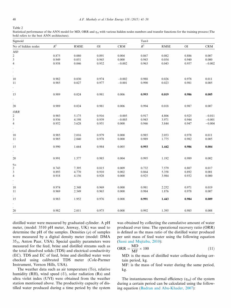
Table 2Statistical performance of the ANN model for MD, ORR and gth with various hidden nodes numbers and transfer functions for the training process (Thebold refers to the best ANN architecture).

Sigmoid Tanh

No of hidden nodes R2 RMSE OI CRM R2 RMSE OI CRM

MD

2 0.875 0.080 0.891 0.004 0.867 0.082 0.886 0.0073 0.949 0.051 0.945 0.000 0.943 0.054 0.940 0.0004 0.958 0.046 0.952 �0.002 0.963 0.043 0.957 �0.002...10 0.982 0.030 0.974 �0.002 0.988 0.026 0.978 0.01111 0.985 0.027 0.977 �0.001 0.990 0.023 0.981 0.005..15 0.989 0.024 0.981 0.006 0.993 0.019 0.986 0.005

.

.20 0.989 0.024 0.981 0.006 0.994 0.018 0.987 0.007

ORR

2 0.903 5.175 0.916 �0.005 0.917 4.806 0.925 �0.0113 0.936 4.198 0.939 �0.003 0.943 3.971 0.944 �0.0014 0.952 3.628 0.951 0.000 0.946 3.844 0.947 �0.004..10 0.985 2.016 0.979 0.000 0.985 2.053 0.978 0.01111 0.985 2.040 0.978 0.000 0.989 1.775 0.982 0.005.15 0.990 1.664 0.984 0.005 0.993 1.442 0.986 0.004

.

.20 0.991 1.577 0.985 0.004 0.995 1.192 0.989 0.002

gth

2 0.743 7.395 0.815 0.009 0.732 7.579 0.807 0.0173 0.893 4.770 0.910 0.002 0.864 5.358 0.892 0.0014 0.918 4.156 0.928 0.000 0.925 3.984 0.932 0.000..10 0.974 2.348 0.969 0.000 0.981 2.252 0.971 0.01911 0.969 2.549 0.965 0.000 0.984 1.876 0.978 0.007.15 0.983 1.952 0.976 0.008 0.991 1.443 0.984 0.009

.

.20 0.982 2.011 0.975 0.008 0.992 1.395 0.985 0.008

48 A.F. Mashaly et al. / Solar Energy 118 (2015) 41–58

distilled water were measured by graduated cylinder. A pHmeter, (model: 3510 pH meter, Jenway, UK) was used todetermine the pH of the samples. Densities (q) of sampleswere measured by a digital density meter (model: DMA35N, Anton Paar, USA). Special quality parameters weremeasured for the feed, brine and distilled streams such asthe total dissolved solids (TDS) and electrical conductivity(EC). TDS and EC of feed, brine and distilled water werechecked using calibrated TDS meter (Cole-ParmerInstrument, Vernon Hills, USA).

The weather data such as air temperature (To), relativehumidity (RH), wind speed (U), solar radiation (Rs) andultra violet index (UVI) were obtained from the weatherstation mentioned above. The productivity capacity of dis-tilled water produced during a time period by the system

was obtained by collecting the cumulative amount of waterproduced over time. The operational recovery ratio (ORR)is defined as the mass ratio of the distilled water producedper unit mass of feed water using the following equation(Sassi and Mujtaba, 2010):

ORR ¼MD

MF� 100 ð11Þ

MD: is the mass of distilled water collected during cer-tain period, kg.MF: is the mass of feed water during the same period,kg.

The instantaneous thermal efficiency (gth) of the systemduring a certain period can be calculated using the follow-ing equation (Badran and Abu-Khader, 2007):

A.F. Mashaly et al. / Solar Energy 118 (2015) 41–58 49

gth ¼_MD� L

RS � A� 100 ð12Þ

where _MD is the mass flow rate of distilled water collectedduring this period, kg/s.

L: Latent heat of vaporization = 2275 kJ/kg.Rs: Solar radiation on tilted surface, kW/m2.A: Area of solar still, m2.

4. Results and discussion

Overall system performance was as follows: for the threetypes of water, the average MD was 0.51 L/m2/h whichequal to about 5 L/m2/day this is consistent with whatwas found by Kabeel et al. (2012), while the average ORRand gth were 34% and 51% respectively. Furthermore, theaverage of final recovery ratio for the three types of waterwas 86%. The following steps are to develop the modelbased on the data obtained from the experiments.

4.1. Selection of optimal ANN architecture

The statistical performance of the ANN model for MD,ORR and gth with various hidden neuron numbers andtransfer functions for the training process is presented inTable 2. Initially with 2 neurons and sigmoid transfer func-tion in the hidden layer, statistical parameter values were asfollows 0.875, 0.080 L/m2/h, 0.891 and 0.0038 for R2,RMSE, OI and CRM respectively. By using hyperbolictangent transfer function, statistical parameters valueswere improved somewhat where it were 0.867,0.082 L/m2/h, 0.886 and 0.0072 for R2, RMSE, OI andCRM respectively. It was found that increasing the numberof neurons in the hidden layer, the values of statisticalparameters previously mentioned is improved, which

Table 3Connection weights and biases for developed neural network model.

#H.Na (W)j,ib

J To RH U Rs

1 3.006 0.161 0.094 1.361 �1.4022 0.160 �0.340 0.337 0.004 1.4403 �0.811 �0.658 �1.410 �0.229 �3.3574 �4.391 0.070 �1.141 2.157 1.1965 0.233 �0.915 �0.741 �0.517 �3.1116 �0.283 �1.683 0.699 �2.326 2.4817 �3.891 4.438 0.707 1.400 2.6298 1.490 0.492 0.582 1.151 �0.7619 �4.995 �1.770 1.325 �0.596 �5.398

10 �3.714 �1.682 3.320 �2.570 0.82011 1.442 0.313 �0.805 0.498 �0.36212 �0.017 0.737 1.655 �1.091 2.38013 0.890 4.312 �1.992 0.056 1.21714 �1.714 2.186 �5.431 �2.967 2.00815 �0.455 �0.235 �1.076 0.016 �1.284

a No. of Hidden neurons.b Connection weights between input and hidden layer.c Hidden biases.

reflects on the performance. This is illustrated by that whenthe number of neurons was 10, it found that the statisticalparameter values were 0.982, 0.030 L/m2/h, 0.974 and�0.0019 for R2, RMSE, OI and CRM respectively with sig-moid transfer function and were 0.988, 0.026 L/m2/h, 0.978and 0.0113 for R2, RMSE, OI and CRM respectively withhyperbolic tangent transfer function. With arrival the num-ber of neurons to 15, it was obtained the best results(bolded in Table 2) and that was with the hyperbolic tan-gent transfer function where the statistical parameter val-ues were 0.993, 0.019 L/m2/h, 0.986 and 0.0049 for R2,RMSE, OI and CRM respectively. With increasing thenumber after that to 20, it is noted that the values becomealmost constant in both functions. The same selectionmethod and approach was followed with both of ORRand gth. It was found that the best results were achievedwith hyperbolic tangent transfer function when the numberof neurons was 15, where the statistical parameter valueswere 0.993, 1.442%, 0.986 and 0.0043 for R2, RMSE, OIand CRM respectively with ORR and 0.991, 1.443%,0.984 and 0.0087 for R2, RMSE, OI and CRM respectivelywith gth, respectively. To summarize the above, the ANNmodel with 15 neurons in the hidden layer was selectedwith hyperbolic tangent transfer function where the resultsrevealed that this architecture made the most accurate pre-dictions for the solar desalination performance parameters.The trained values of connecting weights and biases for thedeveloped ANN (10–15–3) model are given in Table 3. Thedeveloped ANN model could be employed with any pro-gramming language such as Visual Basic or spreadsheetprogram (i.e. Microsoft Excel) for the prediction of solarstill performance (MD, ORR and gth). Mathematical for-mulations derived from the developed ANN model are dis-played from Eqs. 13–23. The de-normalizing of the outputs(MD, ORR and gth) can be written as follows:

bjc

UVI TF TB TDSF TDSB

�0.585 �3.399 6.744 �6.576 3.011 �0.1850.406 �0.031 0.093 �1.453 1.090 �1.7000.271 1.925 1.073 3.607 2.354 �3.067�3.975 �1.319 �1.787 5.195 2.992 �0.074

0.719 0.631 0.539 �2.550 2.337 �0.030�1.237 �6.572 2.782 �1.856 2.188 0.039�1.000 �5.468 2.980 �1.654 �0.533 1.963

0.954 �0.576 �1.054 �1.213 �0.002 �1.0490.472 3.484 �0.053 1.744 4.753 �1.8691.580 �1.071 1.517 �3.123 0.863 �0.594�3.196 0.107 �1.515 �1.703 1.825 0.539�3.508 �2.034 1.675 �1.521 0.688 �1.406

1.532 �2.408 �1.441 �2.254 �1.259 �3.178�1.407 �0.049 1.990 �0.044 2.453 �0.677

0.585 0.900 �1.239 1.005 �0.464 0.956

0.0

0.2

0.4

0.6

0.8

1.0

Cor

rela

ted

MD

, L/m

2 /hr

Observed MD, L/m2/hr

1:1

0

20

40

60

80

54 54 54 55 55 61 61 61 62 62 80 80 112

112

112

113

151

151

152

152

152

153

153

252

252

263

278

278

281

281

284

305

OR

R,

%

Number of day

Observed ORR Correlated ORR

0.0

0.2

0.4

0.6

0.8

1.0

54 54 54 55 55 61 61 61 62 62 80 80 112

112

112

113

151

151

152

152

152

153

153

252

252

263

278

278

281

281

284

305

MD

, L

/m2 /

hr

Number of day

Observed MD Correlated MD

0

20

40

60

80

Cor

rela

ted

OR

R, %

Observed ORR, %

1:1

0

20

40

60

80

100

0.0 0.2 0.4 0.6 0.8 1.0

0 20 40 60 80

0 20 40 60 80 100

Cor

rela

ted

η th,

%

Observed ηth, %

1:1

0

20

40

60

80

100

54 54 54 55 55 61 61 61 62 62 80 80 112

112

112

113

151

151

152

152

152

153

153

252

252

263

278

278

281

281

284

305

η th

, %

Number of day

Observed ηth Correlated ηth

Fig. 4. Comparison of observed MD, ORR and gth values with corresponding optimal ANN values during training process.

50 A.F. Mashaly et al. / Solar Energy 118 (2015) 41–58

MD ¼ MD� 0:15

ð0:85� 0:15Þ � ðMDmax �MDminÞ þMDmin ð13Þ

ORR ¼ ORR� 0:15

ð0:85� 0:15Þ � ðORRmax �ORRminÞ

þORRmin ð14Þ

gth ¼gth � 0:15

ð0:85� 0:15Þ � gthmax� gthmin

� �þ gthmin

ð15Þ

where the maximum and minimum values for MD, ORRand gth are tabulated in Table 1.

Also the normalized outputs can be computed asfollows:

MD ¼ 1� expð�2Z1Þ1þ expð�2Z1Þ

ð16Þ

ORR ¼ 1� expð�2Z2Þ1þ expð�2Z2Þ

ð17Þ

gth ¼1� expð�2Z3Þ1þ expð�2Z3Þ

ð18Þ

The sum of hidden signals can be calculated as follows:

Z1 ¼ ð1:213� F 1Þ þ ð1:166� F 2Þ � ð1:478� F 3Þþ ð0:862� F 4Þ � ð2:567� F 5Þ � ð3:276� F 6Þ� ð1:768� F 7Þ þ ð0:873� F 8Þ þ 0:873� F 9Þþ ð2:431� F 10Þ � ð1:091� F 11Þ þ ð0:068

� F 12Þ þ ð1:361� F 13Þ þ ð0:460� F 14Þþ ð0:154� F 15Þ þ 0:088 ð19Þ

A.F. Mashaly et al. / Solar Energy 118 (2015) 41–58 51

Z2 ¼ ð0:533� F 1Þ � ð0:223� F 2Þ � ð0:979� F 3Þþ ð0:281� F 4Þ � ð1:149� F 5Þ þ ð0:284� F 6Þ� ð1:275� F 7Þ þ ð0:191� F 8Þ þ ð0:671� F 9Þþ ð0:367� F 10Þ � ð0:764� F 11Þ � ð3:618� F 12Þþ ð3:406� F 13Þ þ ð0:251� F 14Þ� ð1:308� F 15Þ þ 1:334 ð20Þ

Z3 ¼ ð1:834� F 1Þ � ð1:255� F 2Þ � ð2:336� F 3Þþ ð1:389� F 4Þ þ ð1:512� F 5Þ � ð4:191� F 6Þ� ð2:698� F 7Þ þ ð1:743� F 8Þ þ ð1:256� F 9Þþ ð3:279� F 10Þ � ð2:010� F 11Þ � ð0:066

� F 12Þ þ ð0:823� F 13Þ þ ð0:569� F 14Þþ ð0:258� F 15Þ þ 0:634 ð21Þ

where the hyperbolic tangent transfer function ðF jÞ usedfor this model is calculated as follows:

F j ¼1� expð�2ZjÞ1þ expð�2ZjÞ

ð22Þ

where Zj the sum of input signals is computed by:

-50

-40

-30

-20

-10

0

10

20

30

40

50

0.0 0.1 0.2 0.3 0.4 0.5 0.6 0.7 0.8 0.9 1.0

Rel

ativ

e E

rror

, %

CorrelatedMD, L/m2/hr

-50

-40

-30

-20

-10

0

10

20

30

40

50

0 10 20 30 40

Rel

ativ

e E

rror

, %

Correlat

Fig. 5. Relative errors with MD, OR

Zj ¼ ðW j;1 � JÞ þ ðW j;2 � T OÞ þ ðW j;3 �RHÞþ ðW j;4 � UÞ þ ðW j;5 �RsÞ þ ðW j;6 �UVIÞþ ðW j;7 � T F Þ þ ðW j;8 � T BÞ þ ðW j;9 � TDSF Þþ ðW j;10 � TDSBÞ þ bj ð23Þ

where the connection weight values (W)j,i and hiddenbiases values bj, are listed in Table 3 for back propagation

algorithm (BPA) with 15 neurons. Zj is the product of theinput parameters with their weights. As stated before, thesubscript i and j symbolizes number of input and hiddenneuron, respectively.

4.2. ANN performance

4.2.1. Training process

As mentioned above, the best results of ANN model arerelated to 10–15–3 architecture that for MD predictionproduce R2 = 0.9934, RMSE = 0.019 L/m2/h, OI = 0.986and CRM = 0.0049 with training data, for ORR predictionproduce R2 = 0.9925, RMSE = 1.442%, OI = 0.986 andCRM = 0.0043 with training data and for gth predictionproduce R2 = 0.9911, RMSE = 1.443%, OI = 0.984 andCRM = 0.0087 with training data. It was noted that the

-50

-40

-30

-20

-10

0

10

20

30

40

50

0 10 20 30 40 50 60 70 80

Rel

ativ

e E

rror

, %

Correlated ORR, %

50 60 70 80 90ed ηth ,%

R and gth for training process.

0

20

40

60

80

54 54 55 55 55 61 61 62 62 62 80 80 112

112

113

113

151

151

151

152

152

152

153

252

252

263

278

278

281

281

284

305

OR

R, %

Number of day

Observed ORR Correlated ORR

0

20

40

60

80

Cor

rela

ted

OR

R, %

Observed ORR, %

1:1

0.0

0.2

0.4

0.6

0.8

1.0

Cor

rela

ted

MD

, L/m

2 /hr

Observed MD, L/m2/hr

1:1

0

20

40

60

80

100

0 20 40 60 80

0.0 0.2 0.4 0.6 0.8 1.0

0 20 40 60 80 100

Cor

rela

ted

η th

,%

Observed ηth, %

1:1

0.0

0.2

0.4

0.6

0.8

1.054 54 55 55 55 61 61 62 62 62 80 80 112

112

113

113

151

151

151

152

152

152

153

252

252

263

278

278

281

281

284

305

MD

, L/m

2 /hr

Number of day

Observed MD Correlated MD

0

20

40

60

80

100

54 54 55 55 55 61 61 62 62 62 80 80 112

112

113

113

151

151

151

152

152

152

153

252

252

263

278

278

281

281

284

305

η th,

%

Number of day

Observed ηth Correlated ηth

Fig. 6. Comparison of observed MD, ORR and gth values with corresponding optimal ANN values during testing process.

Table 4Statistical performance of developed ANN model for MD, ORR and gth

during the testing process.

Statistical parameter MD (L/m2/h) ORR (%) gth (%)

R2 0.97 0.98 0.94RMSE 0.04 2.36 3.67OI 0.96 0.97 0.94CRM 0.01 0.01 0.001

52 A.F. Mashaly et al. / Solar Energy 118 (2015) 41–58

R2 was above 0.99 for all and RMSE values were little andthis expression for the accuracy of the model. The sameresults almost were obtained by Hamdan et al. (2013)

during estimation of the performance of solar still underJordanian climate. Moreover, OI values were above 0.95for whole parameters and this is very close to one.Furthermore, CRM parameter showed an under correlatedwith MD, ORR and gth but it was a small and very close tozero. Fig. 4 describes the relationship between correlatedand observed values of MD, ORR and gth using the bestselected ANN model. It is clear from that figure that thecorrelated values by using the developed ANN model arein an excellent agreement with the observed values ofMD, ORR and gth. Fig. 5 shows the relative errors duringthe training process for the MD, ORR and gth, which themajority ranges approximately from �10 to +10%. This

A.F. Mashaly et al. / Solar Energy 118 (2015) 41–58 53

range is considered acceptable as well. The low relativeerrors support the use of developed ANN model. On theother hand, there are about 4.2%, 5% and 1.4% of the cor-related values falls outside this range for MD, ORR and gth

respectively. Nevertheless, these ratios are relatively smalland do not affect the applicability of the model in the pre-diction process.

4.2.2. Testing process

Fig. 6 shows the relationship between correlated andobserved values of MD, ORR and gth using the bestselected ANN model. The figure clearly shows that theMD, ORR and gth values correlated by using the developedANN Model are in good agreement with the observed val-ues. The points around the 1:1 line are all very close to it.Obviously, the developed ANN model obtained gave agood fit, where the average value of R2 was 96.3% for all,

0.0

0.2

0.4

0.6

0.8

1.0

54 54 55 55 61 61 62 62 62 80 80 80 112 112 113

MD

, L/m

2 /h

r

Observed MD Correlated MD

0

20

40

60

80

54 54 55 55 61 61 62 62 62 80 80 80 112 112 113 1

OR

R, %

Number of day

Observed ORR Correlated ORR

0

20

40

60

80

100

54 54 55 55 61 61 62 62 62 80 80 80 112 112 113 1

η th

, %

Number of day

Observed ηth Predicted ηth

0.0

0.2

0.4

0.6

0.8

1.0

151 151 151 151 152 153 252 252 263 2

MD

, L/m

2 /hr

Number of day

Observed MD Predicted MD

Fig. 7. Comparison of observed MD, ORR and gth values with correspo

and was highest in the case of ORR by 98%. As shownin the same figure, the observed data are similar a verylarge extent of the correlated data. For further understand-ing and analysis for process performance, the statisticalperformance of developed ANN models during the testingprocess is listed in Table 4. The results of the statisticalparameters R2, RMSE, OI and CRM are considerednumerical indicators used to evaluate the agreementbetween correlated and observed solar still performancevalues. Statistical parameters of the developed ANN modelfor MD, ORR and gth during the testing process were tab-ulated in Table 4 as stated before. It can be realized that thevalues of R2 are in a good range which indicate to a goodagreement between the correlated and observed values.From RMSE values, it can be recognized the high accuracyof prediction resulting from the developed ANN model.Additionally, RMSE was slightly high with gth and was

0

20

40

60

80

0 20 40 60 80

Cor

rela

ted

OR

R, %

Observed ORR, %

1:1

0.0

0.2

0.4

0.6

0.8

1.0

0.0 0.2 0.4 0.6 0.8 1.0

Cor

rela

ted

MD

, L/m

2 /hr

Observed MD, L/m2/hr

1:1

0

20

40

60

80

100

0 20 40 60 80 100

Cor

rela

ted

η th

, %

Observed ηth, %

1:1

113

13

13

63

nding optimal ANN values during validation process for sea water.

54 A.F. Mashaly et al. / Solar Energy 118 (2015) 41–58

least with MD. Based on the results of Table 4, it can alsobe seen that the overall OI average was 0.957 for all param-eters which is considered high value and close to one, aswell as this refers to the accuracy of the model. CRM val-ues for MD, ORR and gth were above zero which showsover estimation in predicting MD, ORR and gth. CRM val-ues are very close to zero, indicating the accuracy of themodel. The percentage of relative error is in an acceptableprediction range nearly in the vicinity of ±10%. Generally,the magnitude of errors and statistical parameters statedherein was about in the same value and order as found ear-lier by Santos et al. (2012) during modeling solar still pro-duction using local weather data.

0.0

0.2

0.4

0.6

0.8

1.0

151 151 151 151 152 153 252 252 263 26

MD

, L/m

2 /hr

Number of day

Observed MD Correlated MD

0

20

40

60

80

151 151 151 151 152 153 252 252 263 26

OR

R, %

Number of day

Observed ORR Correlated ORR

0

20

40

60

80

151 151 151 151 152 153 252 252 263

η th

, %

Number of day

Observed ηth Correlated ηth

Fig. 8. Comparison of observed MD, ORR and gth values with correspon

4.2.3. Validation process

In order to validate the developed ANN model, theobserved data were validated with correlated data fromthe developed ANN model to predict MD, ORR and gth.Figs. 7–9 show the relationship between number of day(Julian day) vs. observed and correlated values.Additionally, the graph of 45� (1:1) for correlated andobserved data of MD, ORR and gth for seawater, groundwater and agricultural drainage water, respectively also isshown in the same figures. Fig. 7 shows the comparisonbetween the observed and correlated MD, ORR and gth

during the validation process for sea water. It can be seenthat, in general, there is good agreement between the

30.0

0.2

0.4

0.6

0.8

1.0

0.0 0.2 0.4 0.6 0.8 1.0

Cor

rela

ted

MD

, L/m

2 /hr

Observed MD, L/m2/hr

1:1

30

20

40

60

80

0 20 40 60 80

Cor

rela

ted

OR

R, %

Observed ORR, %

1:1

0

20

40

60

80

0 20 40 60 80

Cor

rela

ted

η th

, %

Observed ηth, %

1:1

263

ding optimal ANN values during validation process for ground water.

A.F. Mashaly et al. / Solar Energy 118 (2015) 41–58 55

observed and correlated values. The R2 for all parametersis above 0.90, in addition to the RMSE values are smallas indicated in Table 5 which refers to the high accuracyof the model. The average value of OI is 0.92 which almostnear one. On the other hand, the CRM almost near zeroand all the parameter values are negative which indicatean under prediction but very small. As mentioned before,Fig. 8 depicts the relationship between correlated andobserved values of MD, ORR and gth using the bestselected ANN model during the validation process forground water. The figure clearly shows that the MD,ORR and gth values correlated by using the developedANN model are in a good agreement with the observedvalues. From Table 5, it can be see that the average valueof R2 for all parameters with the ground water was above

0

20

40

60

80

OR

R, %

Number of day

Observed ORR Correlated ORR

0.0

0.2

0.4

0.6

0.8

1.0

MD

, L/m

2/h

r

Number of day

Observed MD Correlated MD

0

20

40

60

80

100

278 278 281 284 305 3

278 278 281 284 305 30

278 278 281 284 305 30

η th

, %

Number of day

Observed ηth Correlated ηth

Fig. 9. Comparison of observed MD, ORR and gth values with correspondingwater.

0.97 and was the maximum with MD and ORR. RMSEwas 0.03L/m2/h, 2.64% and 2.9% for MD, ORR and gth

respectively. The RMSE shows the efficiency of the devel-oped network in the prediction process. It is clear fromthese values that they are relatively small, meaning a smalldeviation in the correlated value of the observed value. TheOI and the CRM are illustrated as well. The average valueof OI equals 0.96 which is close to one, this indicates thatthe developed model is good in terms of prediction.While the average value of CRM equals �0.005 which isvery small and very close to zero. In total, statisticalparameters emphasize that the developed model is goodfor prediction. Fig. 9 shows the relationship between corre-lated and observed values of MD, ORR and gth using thebest selected ANN model during the validation process

0.0

0.2

0.4

0.6

0.8

1.0

Cor

rela

ted

MD

, L/m

2 /hr

Observed MD, L/m2/hr

1:1

0

20

40

60

80

Cor

rela

ted

OR

R ,

%

Observed ORR, %

1:1

0

20

40

60

80

100

0.0 0.2 0.4 0.6 0.8 1.0

0 20 40 60 80

0 20 40 60 80 100

Cor

rela

ted

η th

, %

Observed ηth, %

1:1

05

5

5

optimal ANN values during validation process for agricultural drainage

Table 5Statistical performance of developed ANN model for MD, ORR and gth

with water type during the validation process.

Statistical parameter MD (L/m2/h) ORR (%) gth (%)

Sea water

R2 0.93 0.93 0.91RMSE 0.06 3.71 5.55OI 0.93 0.93 0.90CRM �0.02 �0.01 �0.02

Ground water

R2 0.99 0.98 0.95RMSE 0.03 2.64 2.90OI 0.98 0.96 0.94CRM �0.01 0.004 �0.008

Agric. drainage water

R2 0.995 0.99 0.97RMSE 0.02 1.44 1.79OI 0.98 0.98 0.94CRM �0.02 �0.01 �0.02

56 A.F. Mashaly et al. / Solar Energy 118 (2015) 41–58

for agricultural drainage water. The figure obviously showsthat the MD, ORR and gth values correlated by using thedeveloped ANN Model are in a good agreement with theobserved values. This good agreement is clearly reflectedthrough the values of the statistical parameters displayedin Table 5. The R2 between the observed values and thecorrelated values of the developed ANN model of solar stillperformance as an average was 0.985 which indicate to agood agreement and accurate prediction. In the light ofRMSE values shown in the table mentioned above, thereis a slight deviation in the correlated value of the real valueof all solar still performance parameters. OI values areclose from one, which indicated that the efficiency of thedeveloped model for prediction of MD, ORR and gth.Moreover, there are a slightly under estimation in forecast-ing MD, ORR and gth which equals to �0.02, �0.01 and�0.02 respectively according to CRM values. Based onthe above, it is finished that the model is good and effectivein the prediction of the three solar still parameters perfor-mance. Overall, the results obtained from the developedmodel with agricultural drainage water are the best results,and this is very clear through the values and meanings ofstatistical parameters. Observed values and ANN corre-lated values were approximately not significantly different,which corroborates the results of Benli (2013) who found

0

5

10

15

20

J To RH U Rs

Con

trib

utio

n R

atio

, %

Input V

MD ORR

Fig. 10. Contribution ratio for different input parameters

no significant difference between experimental and ANNcorrelated values during determination of thermal perfor-mance calculation of two different types solar collectorswith the use of artificial neural networks as well as Caneret al. (2011) during the investigation on thermal perfor-mance calculation of two type solar collectors using artifi-cial neural network. The results of this study show thatANN provides a powerful tool that can be used to forecastthe performance during solar water desalination.

4.3. Contribution ratio for different input variables

The contribution ratio was calculated, which describesthe ratio of the contribution of each input variable in themodeling process. Also, it illustrates how the change ineach input variable changes the output forecast.Furthermore, it is commonly used to select the input vari-ables in problems with numerous inputs. The contributionratio of the ten input variables of the three outputs wascomputed using the developed ANN model and resultsare represented in Fig. 10 for MD, ORR and gth. From thisfigure, it can be realized and known the importance of eachof the ten input parameters. The input parameter with thelargest contribution in the developed ANN model for MDforecasting is the TF which contributes about 16.56%. Alsothe input parameter with the largest contribution in thedeveloped ANN model for ORR forecasting is UVI whichcontributes about 18.19%. Moreover, the input parameterwith the largest contribution in the developed ANN modelfor gth forecasting is TF which contributes about 15.74%.On the other hand, the input parameter with the smallestcontribution is U with all parameters which contributeapproximately 2.76%, 2.04%, and 3.14% for MD, ORRand gth respectively. TO and RH contributes with an aver-age of nearly 8.8 �C and 8.8% respectively with all perfor-mance parameters. Additionally, the contribution ratio ofRs was almost equal with the three outputs. Moreover,the contribution ratios of TF and TDSF are greater thanthat with TB and TDSB. In the light of contribution ratioresults shown in Fig. 10, in general it is clear that variablessuch as UVI, Rs, TF and TDSF were the highest. This islogical, because of these parameters are responsible forincreasing the rate of evaporation, which leads to theimpact on productivity and efficiency.

UVI TF TB TDSF TDSBariables

ηth

of the developed ANN model for MD, ORR and gth.

A.F. Mashaly et al. / Solar Energy 118 (2015) 41–58 57

5. Conclusion

Back propagation artificial neural network model wasdeveloped for the prediction of the solar still performanceparameters. The suitability and effectiveness of artificialneural network (ANN) considering several weather andoperational parameters have been evaluated for solar stillperformance prediction. A total of ten variables was usedas the input parameters. Five input variables were relatedto the weather conditions, namely air temperature (To),relative humidity (RH), wind speed (U), solar radiation(Rs) and ultra violet index (UVI), four variables wererelated to the system operational conditions, namely tem-perature of feed water, temperature of brine, total dis-solved solids of feed water (TDSF) and total dissolvedsolids of brine (TDSB), and the last variable was numberof day (i.e. Julian day (J)). There were three neurons inthe output layer with distillate water productivity (MD),operational recovery ratio (ORR) and thermal efficiencyas the output. According to error analysis results, the opti-mal architecture of the developed ANN model was 10–15–3 with hyperbolic tangent (Tan h) transfer function for aprediction productivity capacity of solar still (MD), opera-tional recovery ratio (ORR) and thermal efficiency (gth)during the training process. In testing and validation pro-cesses with statistical criteria revealed that the developedANN model can produce very high efficiency results, justi-fying its suitability and effectiveness in solar desalinationprediction. Based on these results it is concluded that thedeveloped ANN model was accurate in predicting the solarstill performance parameters. The major advantage ofANN model is simple and can readily utilize and imple-mented with any programming language or spreadsheetfor prediction solar desalination performance. By theANN model, the influence of each input variable on theoutputs, represented as a contribution ratio, was known.TF is the input parameter with the largest contributionratio in the ANN model for MD and gth prediction.While UVI is with the largest contribution ratio in ORRprediction. Moreover, the study proved that ANN is anapplicable and effective tool that can predict solar still per-formance without the need to conduct more experiments,leading to saving time, effort and financial expenses.

Acknowledgement

The project was financially supported by King SaudUniversity, Vice Deanship of Research Chairs.

References

Ahsan, A., Islam, K.M.S., Fukuhara, T., Ghazali, A.H., 2010.Experimental study on evaporation, condensation and production ofa new tubular solar still. Desalination 260, 172–179.

Alazba, A.A., Mattar, M.A., ElNesr, M.N., Amin, M.T., 2012. Fieldassessment of friction head loss and friction correction factorequations. J. Irrig. Drain. E-ASCE 138 (2), 166–176.

Arbat, G., Puig-Bargues, J., Barragan, J., Bonany, J., Ramirez deCartagena, F., 2008. Monitoring soil water status for micro-irrigationmanagement versus modeling approach. Biosyst. Eng. 100 (2), 286–296.

Badran, O.O., Abu-Khader, M.M., 2007. Evaluating thermal performanceof a single slope solar still. Heat Mass Transfer. 43, 985–995.

Benli, H., 2013. Determination of thermal performance calculation of twodifferent types solar air collectors with the use of artificial neuralnetworks. Int. J. Heat Mass Transf. 60, 1–7.

Caner, M., Gedik, E., Kecebas, A., 2011. Investigation on thermalperformance calculation of two type solar air collectors using artificialneural network. Expert Syst. Appl. 38 (3), 1668–1674.

Caudill, M., Butler, C., 1993. Understanding Neural Networks: ComputerExplorations, vol. 1 of Basic Networks. The MIT Press, Cambridge,Mass, USA.

Demuth, H., Beale, M., 2004. Neural Network Toolbox: for Use withMATLAB (Version 4.0), The MathWorks Inc.

Dev, R., Tiwari, G., 2009. Characteristic equation of a passive solar still.Desalination 245, 246–265.

Dunkle, R.V., 1961. Solar water distillation, the roof type still and amultiple effect diffusion still. In: Proceedings of InternationalDevelopments in Heat Transfer Conference, ASME, University ofColorado, pp. 895–902.

F cubed. Ltd., 2011. Carocell Solar Panel. Australia, http://www.fcubed.com.au.

Farkas, I., Geczy-Vıg, P., 2003. Neural network modelling of flat-platesolar collectors. Comput. Electron. Agr. 40, 87–102.

Global Water Intelligence (GWI/IDA DesalData), 2013. Market Profileand Desalination Markets, 2009–2012 yearbooks and GWI availableat http://www.desaldata.com/.

Hamdan, M.A., Haj Khalil, R.A., Abdelhafez, E.A.M., 2013. Comparisonof Neural Network Models in the Estimation of the Performance ofSolar Still Under Jordanian Climate. J. Clean Energy Technol. 1 (3),238–242.

Haykin, S., 1994. Neural Networks: a Comprehensive Foundation.Macmillan, New York, p. 842.

Hook, M., Hirsch, R., Aleklett, K., 2009. Giant oil field decline rates andtheir influence on world oil production. Energy Policy 37, 2262–2272.

Kabeel, A., Almagar, A.M., 2013. Seawater greenhouse in desalinationand economics. In: Proceedings of 17th International WaterTechnology Conference, IWTC17 Istanbul.

Kabeel, A., Hamed, M.H., Omara, Z., 2012. Augmentation of the basintype solar still using photovoltaic powered turbulence system. Desalin.Water Treat. 48, 182–190.

Kalogirou, S.A., Neocleous, C., Schizas, C., 1998. Artificial neuralnetworks for modelling the starting-up of a solar steam generator.Appl. Energy 60 (2), 89–100.

Kalogirou, S.A., 2001. Artificial neural networks in renewable energysystems applications: a review. Renew. Sust. Energy Rev. 5, 373–401.

Kalogirou, S.A., 2006. Prediction of flat-plate collector performanceparameters using artificial neural networks. Sol. Energy 80, 248–259.

Kalogirou, S.A., 2005. Seawater desalination using renewable energysources. Prog. Energy Combust. 31, 242–281.

Kalogirou, S.A., 2013. Solar Energy Engineering: Processes and Systems.Academic Press.

Kalogirou, S.A., Panteliou, S., Dentsoras, A., 1999. Artificial neuralnetworks used for the performance prediction of a thermosiphon solarwater heater. Renew. Energy 18, 87–99.

Khadir, M., 2005. Aspects of artificial neural networks as a modelling toolfor industrial processes. Int. Arab J. Inf. Technol. 2 (4), 334–339.

Kumar, A.J.P., Singh, D.K.J., 2008. Artificial neural network-based wearloss prediction for a390 aluminum alloy. J. Theory Appl. Inf. Technol.4 (10), 961–964.

Lecoeuche, S., Lalot, S., 2005. Prediction of the daily performance of solarcollectors. Int. Commun. Heat Mass. 32, 603–611.

Legates, D.R., McCabe, J., 1999. Evaluating the use of goodness-of fit”measures in hydrologic and hydroclimatic model validation. WaterResour. Res. 35 (1), 233–241.

58 A.F. Mashaly et al. / Solar Energy 118 (2015) 41–58

Mellita, A., Kalogirou, S.A., 2008. Artificial intelligence techniques forphotovoltaic applications: a review. Prog. Energy Combust. 34, 574–632.

Mowla, D., Karimi, G., 1995. Mathematical modelling of solar stills inIran. Sol. Energy 55, 389–393.

Porrazzo, R., Cipollina, A., Galluzzo, M., Micale, G., 2013. A neuralnetwork-based optimizing control system for a seawater-desalinationsolar-powered membrane distillation unit. Comput. Chem. Eng. 54,79–96.

Safa, M., Samarasinghe, S., Mohsen, M., 2009. Modelling fuel consump-tion in wheat production using neural networks. In: Proceedings of18th World IMACS/MODSIM Congress, Cairns, Australia, pp. 775–781.

Santos, N.I., Said, A.M., James, D.E., Venkatesh, N.H., 2012. Modelingsolar still production using local weather data and artificial neuralnetworks. Renew. Energy 40, 71–79.

Sassi, K.M., Mujtaba, I.M., 2010. Simulation and optimization of fullscale reverse osmosis desalination plant. Comput. Aid. Chem. Eng. 28,895–900.

Sozen, A., Arcaklıoglu, E., Ozkaymak, M., 2005. Turkey’s net energyconsumption. Appl. Energy 81, 209–221.

Sozen, A., Menlik, T., Unvar, S., 2008. Determination of efficiency of flat-plate solar collectors using neural network approach. Expert Syst.Appl. 35 (4), 1533–1539.

Tiwari, A.K., Tiwari, G., 2006. Effect of water depths on heat and masstransfer in a passive solar still: in summer climatic condition.Desalination 195, 78–94.

Tripathy, P.P., Kumar, S., 2009. Neural network approach for foodtemperature prediction during solar drying. Int. J. Thermal Sci. 48,1452–1459.

Vesta Services Inc., 2000. Manual of Qnet2000 Shareware, Vesta Services,Inc., Illinois.

WWAP (United Nations World Water Assessment Programme), 2014.The United Nations World Water Development Report 2014: Waterand Energy. Paris, UNESCO.

Yang, I.H., Yeo, M.S., Kim, K.W., 2003. Application of artificial neuralnetwork to predict the optimal start time for heating system inbuilding. Energy Convers. Manage. 44, 2791–2809.