Optimization Strategies for Two-Mode Partitioning

DOI: 10.1007/s00357- 0

Optimization Strategies for Two-Mode Partitioning

Joost van Rosmalen

Erasmus University Rotterdam

Patrick J. F. Groenen

Erasmus University Rotterdam

Javier Trejos

Universidad de Costa Rica

William Castillo

Universidad de Costa Rica

Abstract: Two-mode partitioning is a relatively new form of clustering that clustersboth rows and columns of a data matrix. In this paper, we consider deterministic two-mode partitioning methods in which a criterion similar to k-means is optimized. Avariety of optimization methods have been proposed for this type of problem. How-ever, it is still unclear which method should be used, as various methods may lead tonon-global optima. This paper reviews and compares several optimization methodsfor two-mode partitioning. Several known methods are discussed, and a new fuzzysteps method is introduced. The fuzzy steps method is based on the fuzzy c-means al-gorithm of Bezdek (1981) and the fuzzy steps approach of Heiser and Groenen (1997)and Groenen and Jajuga (2001). The performances of all methods are compared in alarge simulation study. In our simulations, a two-mode k-means optimization methodmost often gives the best results. Finally, an empirical data set is used to give a prac-tical example of two-mode partitioning.

Keywords: Two-mode partitioning; Optimization methods; Meta-heuristics.

We would like to thank two anonymous referees whose comments have improved thequality of this paper. We are also grateful to Peter Verhoef for providing the data set used inthis paper.

Authors’ Addresses: Joost van Rosmalen and Patrick Groenen, Econometric Institute,Erasmus University Rotterdam, P.O. Box 1738, 3000 DR Rotterdam, The Netherlands,e-mail: [email protected]; Javier Trejos and William Castillo, CIMPA, Escuela deMatematica, Universidad de Costa Rica, San Jose, Costa Rica.

-009 9 31-2Journal of Classification 26:155-181 (2009)

Published online 28 May 2009

J. van Rosmalen, P. J. F. Groenen, J. Trejos, and W. Castillo

1. Introduction

Clustering can be seen as one of the cornerstones of classification.Consider a typical two-way two-mode data set of respondents by variables.Often, clustering algorithms are applied to just one mode of the data matrix,which can be done in a hierarchical or non-hierarchical way. Among thenon-hierarchical methods, k-means clustering (Hartigan 1975) is one of themost popular methods and has the advantage of a loss function being opti-mized. For an overview of clustering methodology for one-mode data, seeMirkin (2005).

A relatively new form of clustering is two-mode clustering. In two-mode clustering, both rows and columns of a two-mode data matrix are as-signed to clusters. Each row of a two-mode data matrix is assigned to oneor more row clusters, and each column to one or more column clusters. El-ements of the data matrix that are in the same row cluster and in the samecolumn cluster should be close. DeSarbo (1982) described such a two-modeclustering method, called the GENNCLUS model. A technique that is re-lated to two-mode clustering is blockmodeling, which is often used in so-cial network analysis (see, for example, Noma and Smith 1985; Doreian,Batagelj, and Ferligoj 2005) and can be used for both one-mode and two-mode data matrices (Doreian, Batagelj, and Ferligoj 2004). Blockmodelingattempts to partition network actors into clusters, so that a block structurecan be identified in a data matrix in which the rows and columns have beenreordered in a specific way; the elements within each block should typicallyhave similar values. An extensive overview of two-mode clustering methodscan be found in Van Mechelen, Bock, and De Boeck (2004).

In this article, we focus on two-mode partitioning, that is, partitioningthe sets of rows and columns so that each row and each column is assignedto exactly one cluster. To do so, we use a least-squares criterion that mod-els the elements of the data matrix belonging to the same row and columncluster by their average. Other optimization criteria and methods that do notoptimize a criterion can also be used to partition the rows and columns ofa data matrix. However, in the remainder of this paper, we focus on deter-ministic two-mode partitioning using a least-squares criterion and refer tothis method simply as two-mode partitioning. Several optimization meth-ods for finding good two-mode partitions based on this criterion are knownfrom the literature. However, these methods are not guaranteed to find theglobal optimum and often get stuck in local minima. Therefore, we study thelocal minimum problem of two-mode partitioning for several optimizationmethods and determine which method tends to give the best local minimumamong these methods. In addition, a new optimization method for two-modepartitioning is introduced, based on the fuzzy c-means algorithm of Bezdek

156


(1981). Using a simulation study, we identify the methods that perform wellunder most circumstances, within a reasonable computational effort.

The remainder of this article is organized as follows. In the next sec-tion, we introduce the notation and give an overview of the optimizationproblem, including two hill climbing algorithms. Section 3 describes theimplementation of two meta-heuristics for two-mode partitioning. Section4 introduces the fuzzy steps two-mode partitioning method. In Section 5, wecompare the performances of the methods using a simulation study. Section6 uses an empirical data set to compare the methods and to give a practi-cal example of two-mode clustering. Finally, we draw conclusions and giverecommendations for further research.

2. Overview of Optimization Problem

To define the two-mode partitioning problem, consider the followingnotation:

Xn×m = (xij)n×m Two-mode data matrix of n rows and mcolumns.

Pn×K = (pik)n×K Cluster membership matrix of the rows with Kthe number of row clusters, pik = 1 if row ibelongs to row cluster k, and pik = 0 otherwise.

Qm×L = (qjl)m×L Cluster membership matrix of the columns withL the number of column clusters, qjl = 1 if col-umn j belongs to column cluster l, and qjl = 0otherwise.

VK×L = (vkl)K×L Matrix with cluster centers for row cluster k andcolumn cluster l.

En×m = (eij)n×m Matrix with errors from cluster centers.

Usually, the rows of X correspond to objects, and the columns of X refer tovariables. The elements of X can be associations, confusions, fluctuations,etc., between row and column objects. Applying two-mode partitioning onlymakes sense if the data matrix is matrix-conditional, that is, its values can becompared among each other. Therefore, if one of the modes refers to vari-ables, these variables must be comparable, standardized, or measured on thesame scale. In the remainder of this paper, we assume that the data satisfythis condition.

Two-mode partitioning assigns each element of X to a row clusterand a column cluster. If L equals m, each column can be placed in a clusterby itself, so that two-mode partitioning reduces to one-mode k-means clus-tering, and the same is true if K equals n. The matrix V can be interpretedas the combined cluster means. The cluster memberships are given by the

157


matrices P and Q. Together, the three matrices P, Q, and V approximatethe information in X by PVQ′. To make this approximation as close to Xas possible, we use the additive model

X = PVQ′ + E, (1)

where E is the error of the model. Equation (1) can be seen as a special caseof the additive box model proposed by Mirkin, Arabie, and Hubert (1995);the additive box model does not partition the rows and columns, but allowsfor overlapping clusters.

Two-mode partitioning searches for the optimal partition P, Q andcluster centers V that minimize the sums of squares of E. This objectiveamounts to minimizing the squared Euclidean distance of the data points totheir respective clusters centers in V. Therefore, the criterion to be mini-mized can be expressed as

f(P,Q,V) = ‖X − PVQ′‖2 =K∑

k=1

L∑l=1

n∑i=1

m∑j=1

pikqjl(xij − vkl)2. (2)

Using the Euclidean metric is not mandatory; other metrics have been usedas well, especially in one-mode clustering (see, for example, Bock 1974).However, in this study, we restrict ourselves to the Euclidean metric.

The optimal cluster membership matrices must satisfy the followingconstraints.

1. The cluster memberships of each row and column object must sum toone, so that

∑Kk=1 pik = 1 and

∑Ll=1 qjl = 1.

2. All cluster membership values must be either zero or one, so that pik ∈{0, 1} and qjl ∈ {0, 1} .

3. None of the row or column clusters is empty, that is∑n

i=1 pik > 0 and∑mj=1 qjl > 0.

The first two constraints together require that each row of P and Q containsexactly one element with the value 1. Hence, each row and column objectis assigned to exactly one cluster. These two constraints are necessary andsufficient for the second equality in (2) to hold. A partition that is optimalaccording to (2) typically does not have empty clusters, and, in principle,the third constraint is not required during the estimation. However, somealgorithms may lead to a partition with empty clusters. Therefore, we adaptthese algorithms to correct for potential empty clusters or prevent them fromhappening.

No known polynomial time algorithm is guaranteed to find the globalminimum of f(P,Q,V) in every instance. Even for relatively small n and

158


m (say, n = 20 and m = 20), the number of possible partitions can be-come extremely large, and a complete enumeration of the possible solutionsis almost always computationally infeasible. However, if two of the threematrices P, Q, and V are known, the optimal value of the third matrix canbe computed easily. If both P and Q are known, the optimal cluster centersV can be computed as

vkl =

∑ni=1

∑mj=1 pikqjlxij∑n

i=1

∑mj=1 pikqjl

, (3)

which is the average of the elements of X belonging to row cluster k andcolumn cluster l. If V and either P or Q are known, the problem of mini-mizing f(P,Q,V) becomes a linear program that has a closed-form solu-tion. When V and Q are known, the optimal value of P can be computed asfollows. Let cik =

∑mj=1

∑Ll=1 qjl(xij − vkl)2. Then,

pik ={

1 if cik = min1≤r≤K cir,0 otherwise.

(4)

When P and V are known, the optimal matrix Q can be computed in asimilar fashion.

Several methods for finding an optimal two-mode partition, based onthe minimization of (2), have been proposed in the literature. Two of thesemethods are discussed in the remainder of this section. Both methods are hillclimbing algorithms and are guaranteed to find a local optimum (which mayor may not be the global optimum). Three additional optimization methodsfor two-mode partitioning are discussed in the next two sections.

2.1 Alternating Exchanges Algorithm

The alternating exchanges algorithm was proposed by Gaul andSchader (1996). This algorithm tries to improve an initial partition by mak-ing a transfer of either a row or a column object and immediately recalculat-ing V. Our implementation of the alternating exchanges algorithm performsthe following steps:

1. Choose initial P and Q, and calculate V according to (3).2. Repeat the following until there is no improvement of f(P,Q,V) in

either step.

(a) For each i and k, transfer row object i to row class k and re-calculate V according to (3). Accept the transfer if it has im-proved f(P,Q,V), otherwise return to the old P and V.

(b) For each j and l, transfer column object j to column class l andre-calculate V according to (3). Accept the transfer if it has im-proved f(P,Q,V), otherwise return to the old Q and V.

159


The alternating exchanges algorithm always converges to a local minimum,as the value of f(P,Q,V) decreases in every iteration, the algorithm isdefined on a finite set, and f(P,Q,V) is bounded from below by 0.

2.2 Two-Mode k-Means Algorithm

The k-means algorithm (Hartigan 1975) is one of the simplest andfastest ways to obtain a good partition, which accounts for its popularity inone-mode clustering. This algorithm can easily be extended to handle two-mode partitioning (see Baier, Gaul, and Schader 1997; Vichi 2001). Theso-called two-mode k-means algorithm aims to improve an initial partitionusing (3) and (4) and comprises the following steps.

1. Choose initial P and Q.2. Repeat the following, until there is no improvement of f(P,Q,V) in

any step.

(a) Update V according to (3).

(b) Let cik =∑m

j=1

∑Ll=1 qjl(xij − vkl)2. Then update P according

to

pik ={

1 if cik = min1≤r≤K cir ,0 otherwise.

(5)

(c) Update V according to (3).

(d) Let djl =∑n

i=1

∑Kk=1 pij(xij − vkl)2. Then update Q according

to

qjl ={

1 if djl = min1≤r≤L djr,0 otherwise.

(6)

The two-mode k-means algorithm always converges to a local mini-mum, as the value of the criterion f(P,Q,V) cannot increase in any step.However, one or more clusters may become empty after Step 2b or 2d. Thissituation is immediately corrected by transferring the row or column objectwith the highest value of

∑Kk=1 pikcik or

∑Ll=1 qjldjl to the empty cluster.

3. Meta-Heuristics

The algorithms discussed in the previous section contain no provi-sions to avoid finding non-global optima. As no known polynomial timealgorithm is capable of finding the global optimum in every instance, wealso use optimization methods that are based on meta-heuristics. Thesemeta-heuristics aim to increase the likelihood of finding the global optimum,though this cannot be guaranteed. Here, we discuss two optimization meth-ods for two-mode partitioning that are applications of the meta-heuristicssimulated annealing and tabu search. For the other three optimization meth-ods in this paper (the two algorithms discussed in the previous section and

160


the fuzzy steps method that is proposed in the next section), the likelihoodof finding a non-global optimum is reduced by performing multiple randomstarts. That is, these algorithms are performed several times with startingvalues that are chosen randomly every time an algorithm is run; the bestresult of all runs is retained as the final solution.

Other optimization methods have also been used for two-mode parti-tioning. Hansohm (2001) used a genetic algorithm, but found that its perfor-mance in two-mode partitioning is not as good as it is in one-mode k-meansclustering. Gaul and Schader (1996) implemented a penalty algorithm, butfound that it does not compare favorably with the alternating exchanges al-gorithm.

3.1 Simulated Annealing

Simulated annealing (see, for example, Van Laarhoven and Aarts1987) is a meta-heuristic that simulates the slow cooling of a physical sys-tem. Trejos and Castillo (2000) first used simulated annealing for two-modepartitioning. Their implementation of simulated annealing performs a lo-cal search that is based on the central idea of the alternating exchanges al-gorithm. To avoid getting stuck in local minima, transitions that increasef(P,Q,V) are also accepted with a positive probability.

Here, we use the implementation of Trejos and Castillo (2000), ex-cept for the values of certain parameters. These parameters are the coolingrate γ < 1, the number of iterations R in which the temperature remainsconstant, the initial value of the temperature T , and the maximum numberof iterations without accepted transitions, which is denoted by tmax. Thisimplementation comprises the following steps.

1. Choose initial P and Q and calculate V according to (3).2. Choose the parameters R, γ, and an initial value of T .3. Repeat the following until there is no change in P and Q for the last

tmax values of T .(a) Do the following R times:

i. Choose one of the two modes with equal probability.ii. Choose one of the objects of this mode with uniform proba-

bility and transfer it to another randomly chosen cluster.iii. Update V according to (3) and calculate Δf as the change

in f(P, Q,V) achieved by the transfer and the subsequentupdating of V.

iv. Always accept the transfer if Δf < 0, otherwise accept itwith probability exp(−Δf/T ).

(b) Set T = γT .

161


The partition with the lowest value of f(P,Q,V) found during estimationis retained as the final solution.

3.2 Tabu Search

The tabu search meta-heuristic (see, for example, Glover 1986) alsoperforms a local search, but tries to avoid local optima by maintaining a tabulist. The tabu list is a list of solutions that are temporarily not accepted. Weuse the following implementation of tabu search for two-mode partitioning,which is based on the alternating exchanges algorithm. See Castillo andTrejos (2002) for a more detailed description of this implementation.

Define Z(P,Q) = minV f(P,Q,V). The algorithm performs thefollowing steps.

1. Start with an initial partition (P,Q) and an empty tabu list. Set(P,Q)opt = (P,Q).

2. Choose the number of iterations S and a maximum length of the tabulist.

3. Perform the following steps S times.

(a) Generate a neighborhood of partitions N , consisting of the parti-tions that can be constructed by transferring one row or columnobject from (P,Q) to another cluster.

(b) Choose the partition (P,Q)cand as the partition in N with thelowest value of Z(P,Q) that is not on the tabu list.

(c) Set (P,Q) = (P,Q)cand. If Z((P,Q)cand) < Z((P,Q)opt),then (P,Q)opt = (P,Q)cand.

(d) Add (P,Q) to the tabu list. Remove the oldest item from the tabulist, if the list exceeds its maximum length.

The final solution of the algorithm is given by (P,Q)opt.

4. Fuzzy Two-Mode Clustering

Fuzzy methods relax the requirement that an object belongs to a singlecluster, so that the cluster membership can be distributed over the clusters.For one-mode clustering, the best known method is fuzzy c-means (Bezdek1981); for adaptations of this method see Tsao, Bezdek, and Pal (1994) andGroenen and Jajuga (2001). These methods try to make the optimizationtask easier by allowing for cluster membership values between 0 and 1. Inthis section, we extend one-mode fuzzy optimization methods to the two-mode case. First, we introduce a fuzzy two-mode clustering criterion. Wethen discuss an algorithm for finding an optimal fuzzy partition, based on

162


Bezdek (1981). Finally, we describe the fuzzy steps method, which reducesthe fuzziness of the solution in steps until a crisp partition (that is, a partitionin which all cluster membership values are either 0 or 1) is found.

Simply relaxing the constraint that the cluster membership values in(2) must be 0 or 1 by allowing for values between 0 and 1 does not guar-antee an optimal partition that is fuzzy. A crisp partition will still minimizef(P,Q,V) in that case, though a fuzzy partition might be equally good.Fuzzy optimal partitions can be obtained if the criterion f(P,Q,V) is al-tered by raising the cluster membership values to a power s, with s ≥ 1.Thus, the fuzzy two-mode clustering criterion is defined as

fs(P,Q,V) =K∑

k=1

L∑l=1

n∑i=1

m∑j=1

psikq

sjl(xij − vkl)2, (7)

subject to the constraints

K∑k=1

pik = 1,L∑

l=1

qjl = 1, pik ≥ 0, qjl ≥ 0,n∑

i=1

pik > 0, andm∑

j=1

qjl > 0.

(8)This criterion yields fuzzy optimal partitions and the fuzziness parameter sdetermines how fuzzy the optimal partition is. For s = 1, the fuzzy criterioncoincides with the crisp criterion.

4.1 The Two-Mode Fuzzy c-Means Algorithm

The algorithm for the optimization of fs(P,Q,V) is based on itera-tively updating each set of parameters while keeping the other two sets fixed.Given optimal Q and V, the optimal P can be found using the Lagrangemethod for each row i of P. The Lagrangian is given by

Li(P,Q,V, λ) =K∑

k=1

psik

L∑l=1

m∑j=1

qsjl(xij − vkl)2 − λ

(K∑

k=1

pik − 1

). (9)

Defining cik =∑L

l=1

∑mj=1 qs

jl(xij − vkl)2 and taking partial derivatives ofLi gives

∂Li

∂pik= sps−1

ik cik − λ and∂Li

∂λ=

K∑k=1

pik − 1. (10)

Setting these derivatives to zero and solving for pik yields

pik =c1/(1−s)ik∑K

k=1 c1/(1−s)ik

. (11)

163


However, (11) does not apply if any cik in row i is zero. In that case, anypartition with pik = 0 whenever cik > 0 and

∑Kk=1 pik = 1 is optimal.

Finding the optimal Q given P and V can be done in a similar fashion.When s is large enough, the optimal values of the cluster memberships be-come pik ≈ 1/K and qjl ≈ 1/L, which can easily be derived from (11). Inpractice, the cluster membership values approach these values quite rapidlyfor reasonably large s. For s = 3, the cluster membership values often differonly slightly and for s > 10, they are usually equal to each other within thenumerical accuracy of current computers. As s approaches 1 from above,1/(1 − s) approaches minus infinity, and the fuzzy optimization formula(11) becomes its crisp counterpart (4). In that case, the optimal partitionbased on (7) also approaches the optimal crisp partition. Therefore, highervalues of s correspond to fuzzier optimal partitions, and s close to 1 to crisppartitions. The optimal V can be obtained by setting the partial derivativesof (7) with respect to vkl to zero and solving for vkl, which yields

vkl =

∑ni=1

∑mj=1 ps

ikqsjlxij∑n

i=1

∑mj=1 ps

ikqsjl

. (12)

For a given value of s, the two-mode fuzzy c-means algorithm com-prises the following steps.

1. Choose initial P and Q, which can be either crisp or fuzzy, and calcu-late V according to (12).

2. Repeat the following, until the decrease in fs(P,Q,V) is small.

(a) Calculate cik =∑L

l=1

∑mj=1 qs

jl(xij − vkl)2 and update P as

pik = c1/(1−s)ik /

∑Kk=1 c

1/(1−s)ik .

(b) Calculate djl =∑K

k=1

∑ni=1 ps

ik(xij − vkl)2 and update Q as

qik = d1/(1−s)jl /

∑Kk=1 d

1/(1−s)jl .

(c) Update V according to (12).

This algorithm lowers the value of fs(P,Q,V) in each iteration, until con-vergence has been achieved. Therefore, the algorithm always converges toa saddle point or a local minimum, which may or may not be a global mini-mum.

4.2 Fuzzy Steps

The two-mode fuzzy c-means algorithm generally converges to a fuzzypartition. To ensure that our fuzzy optimization method converges to a crisppartition, we use the idea of fuzzy steps, which was proposed by Heiser andGroenen (1997). Our fuzzy steps method for two-mode partitioning starts

164


with an initial value of s that is greater than 1. This method uses the two-mode fuzzy c-means algorithm to minimize fs(P,Q,V) for a given valueof s and gradually lowers s to avoid local minima and obtain a good crisppartition. Our fuzzy steps method performs the following steps.

1. Choose an initial value of s, a fuzzy step size γ < 1, and a thresholdvalue smin.

2. Choose initial P0 and Q0 and calculate V0 according to (12). Theinitial P0 and Q0 can be either crisp or fuzzy.

3. Repeat the following while s > smin.

(a) Perform the two-mode fuzzy c-means algorithm starting with P0,Q0, and V0. The results are in P1, Q1, and V1.

(b) Set s = 1+γ(s−1) and set P0 = P1, Q0 = Q1, and V0 = V1.4. Apply the two-mode k-means algorithm starting from P0, Q0, and V0.

The formula in Step 3b for decreasing s gives an exponential decayof (s − 1). The value of smin should generally be set to a value slightlyhigher than 1, for example, 1.001. The two-mode k-means algorithm isperformed at the end of the fuzzy steps method to ensure that a crisp solutionis found. Although the two-mode k-means algorithm was defined for crisppartitions in Section 2.2, it can also be used in combination with fuzzy initialpartitions.

The fuzzy steps optimization method may sometimes get stuck in asaddle point, if two or more row or column clusters become equal. In thatcase, these clusters and their corresponding cluster membership values willremain equal for any value of s. Preliminary tests with this method suggestthat it often reaches a saddle point, if the starting value of s is too high.Therefore, one should not set the starting value of s too high, for example,s ≤ 1.2.

5. Simulation Study

To compare the performances of the optimization methods describedin the previous sections, we conduct a simulation study. With this simu-lation study, we also aim to determine which methods perform well undermost circumstances and how well the optimization methods can retrieve aclustering structure. First, we describe the setup of the simulation study andhow the results are represented. We then give the results of the simulationstudy and interpret them.

5.1 Setup of the Simulation Study

We generate the data matrix X in each problem instance by simulat-ing P, Q, V, and E, and then using (1) to construct X. Generating simu-

165


lated data this way comes natural and has the advantage that some clusteringstructure exists in the data. Also, the P, Q, and V used in generating X cangive a useful upper bound on the optimal value of f(P,Q,V).

A large number of factors can be varied in a simulation study fortwo-mode clustering, such as the values of n, m, K, and L, the size andthe distribution of the errors, the numbers of elements in the clusters, andthe locations of the cluster centers. As a full-factorial design with severallevels for each of these factors would require a prohibitively large numberof simulations, we limit the number of factors and the number of levels foreach factor. The simulation study is set up using a four-factor design andis loosely based on the approach of Milligan (1980). The first factor is thesize of the data matrix X. The numbers of rows and columns are given byn = m = 60, n = 150 and m = 30, and n = m = 120 for the threelevels of this factor. The second factor is the numbers of clusters; the threelevels of this factor are K = L = 3, K = L = 5, and K = L = 7.The third factor is the size of the error perturbations. All elements of Eare independently normally distributed with mean 0 and standard deviationequal to 0.5, 1, or 2 for the three levels of this factor. The final factor isthe distribution of the objects over the clusters. For the first level of thisfactor, all objects are divided over the clusters with equal probability. Forthe second and third levels, one cluster contains exactly 10% and 60% ofthe objects, respectively. The remaining objects are then divided over theremaining clusters with uniform probability. Constructing one cluster with10% of the objects represents a small deviation from a uniform distribution,whereas a cluster with 60% constitutes a large deviation. The size of thisdeviation also depends on the numbers of clusters.

Empty clusters are not allowed in the generated data sets. If a simu-lated data set contains an empty cluster, this data set is discarded and anotherdata set is simulated. The locations of the cluster centers vkl are chosen byrandomly assigning the numbers Φ( i

K×L+1), i = 1, . . . ,K × L to the el-ements of V, where Φ(.) is the inverse standard normal cumulative distri-bution function. As a result, the elements of V appear standard normallydistributed, and a fixed minimum distance between the cluster centers is en-sured.

We show the effects of some of these choices in Figures 1 through3. These figures give a visual representation of a simulated data matrixfor various levels of the factors. In these figures, the rows and columnsare ordered according to their cluster. The elements of the data matrix arerepresented by different shades of gray. The bars at the right-hand side showwhat values the shades of gray represent. Figure 1 represents a data set forwhich the levels of the factors ensure that the original clusters can easily berecognized. In Figure 2, the original clusters are more difficult to recognize,

166


1 10 20 30 40 50 601

10

20

30

40

50

60

−2

−1

0

1

2

Figure 1: Graphical representation of simulated data set with sizes n = m = 60, K = L =3, error standard deviation 0.5, and a uniform distribution of the objects over the clusters.

1 10 20 30 40 50 601

10

20

30

40

50

60

−4

−3

−2

−1

0

1

2

3

4

Figure 2: Graphical representation of simulated data set with sizes n = m = 60, K = L =5, error standard deviation 1, and 10% of the objects in one cluster.

1 20 40 60 80 100 1201

20

40

60

80

100

120

−8

−6

−4

−2

0

2

4

6

Figure 3: Graphical representation of simulated data set with sizes n = m = 120, K = L =7, error standard deviation 2, and 60% of the objects in one cluster.

and in Figure 3, this is almost impossible. The optimal partition shouldgenerally be easier to find if the number of clusters is low, the error standarddeviation is small, and the objects are evenly divided over the clusters.

167


The four factors in the simulation design give a total of 34 = 81possible combinations. To avoid drawing spurious conclusions based on asingle data set, we simulate 50 data sets for each combination, and all fivemethods are performed for each data set.

All optimization methods require an initial choice for P and Q. Forthe alternating exchanges and two-mode k-means methods, P and Q arechosen randomly by assigning each row and column to a cluster with uni-form probability. However, some methods may perform better if the initialpartitions are relatively good. Therefore, the initial partitions of the simu-lated annealing, tabu search, and fuzzy steps methods are chosen by apply-ing the two-mode k-means algorithm to a random partition.

The optimization methods also require choosing additional parame-ters. For the optimization methods that use multiple random starts (that is,the alternating exchanges, two-mode k-means, and fuzzy steps methods), thenumbers of random starts have been set so that the total computation timeof these methods is approximately equal. This is also true for the numbersof iterations R and S that are respectively used in the simulated annealingand tabu search methods. We also wish to ensure a good balance betweenthe performance and the computation time of the simulated annealing andtabu search methods for varying problem sizes. Therefore, the parameters Rand S are chosen as a function of the size of the neighborhood used in thesetwo methods, which equals n(K − 1) + m(L− 1); as a result, the computa-tion time should increase modestly with the size of the problem. The initialtemperature in the simulated annealing method is chosen in such a way thatthe initial acceptance rate for the transfer of a row or a column to anothercluster is at least 85%. As a result, the transfers of rows and columns shouldoccur almost randomly in the initial iterations of this method. The coolingrate γ in this method should be chosen slightly lower than 1. We stop thesimulated annealing method if there are no changes for tmax = 10 valuesof the temperature parameter, as further improvements are unlikely to oc-cur in that case. Preliminary experimentation with the tabu search methodshows that increasing the tabu list length typically has a positive effect onthe performance of this method. We set the length of the tabu list to onethird of the number of iterations S, as increasing the tabu list length anyfurther would increase computation time without meaningfully improvingthe performance. In the fuzzy steps method, the fuzzy step size γ is set toa value somewhat lower than 1. The threshold value of s (that is, the pa-rameter smin) is set to 1.001, as experimentation shows that the solution isalmost always close to a crisp partition at that value of s. The initial valueof s was optimized on a separate set of data sets, which were simulatedin the same way as the data sets in the simulation study. Initial values ofs = 1.025, 1.05, . . . , 1.2 were tested, and an optimal recovery was achievedwith s = 1.05.

168


The parameters of the optimization methods are thus chosen as fol-lows:

• Alternating exchanges: The alternating exchanges algorithm is run 30times for every simulated data set.

• Two-mode k-means: The two-mode k-means algorithm is run 500times for every simulated data set.

• Simulated annealing: Initial temperature T = 1, γ = 0.95, tmax = 10,and R = 1/4(n(K − 1) + m(L − 1)).

• Tabu search: We perform S = 3(n(K − 1) + m(L − 1))1/2 itera-tions, and the length of the tabu list is 1/3S.

• Fuzzy steps: The initial value of s is 1.05, the fuzzy step size γ is 0.85,and the threshold value smin is 1.001. The fuzzy steps method is run20 times for every simulated data set.

The values of the parameters that are a function of the neighborhood sizen(K − 1) + m(L − 1) are rounded to integer values.

We use three criteria to evaluate the results of the simulation study.The first criterion is the variance accounted for (VAF) criterion, which iscomparable to the R2-measure used in regression analysis. The VAF crite-rion is defined as

VAF = 1 −∑K

k=1

∑Ll=1

∑ni=1

∑mj=1 pikqjl(xij − vkl)2∑n

i=1

∑mj=1(xij − x)2

, (13)

where x = 1/(nm)∑n

i=1

∑mj=1 xij . The optimal value of VAF ranges from

0 to 1, and maximizing VAF corresponds to minimizing f(P,Q,V).Second, we report the average adjusted Rand index (ARI), which was

introduced by Hubert and Arabie (1985). This metric shows how well thepartitions found by the optimization methods approximate the original parti-tion. The ARI is invariant with respect to the ordering of the clusters, whichis arbitrary in two-mode partitioning. The ARI is based on the original Randindex, which is defined as the fraction of the pairs of elements on which thetwo partitions agree. For two random partitions, the expected value of theRand index depends on the parameters of the clustering problem. To ensurea constant expectation, the ARI is a linear function of the Rand index, sothat its expectation for randomly chosen partitions is 0, and its maximumvalue is 1. The ARI is defined as

ARI =

∑Ri=1

∑Rj=1

(aij

2

)−∑Ri=1

(ai.

2

)∑Rj=1

(a.j

2

)/(a2

)[∑R

i=1

(ai.

2

)+∑R

j=1

(a.j

2

)]/2 −∑R

i=1

(ai.

2

)∑Rj=1

(a.j

2

)/(a2

) , (14)

where aij is the number of elements of X that simultaneously belong tocluster i of the original partition and cluster j of the retrieved partition, R

169


is the total number of clusters, ai. =∑R

j=1 aij , a.j =∑R

i=1 aij , and a =∑Ri=1

∑Rj=1 aij = nm. Here we consider a pair of elements to be in the

same cluster only if they belong to same row cluster and to the same columncluster, so that R = K × L.

The final criterion is the average CPU time, which is of practical in-terest. In this study, the CPU time is also used as a control variable, as theparameters of the optimization methods have been chosen in such a way,that the average computation time is approximately equal for all methods.To provide a fair comparison, we made sure that the optimization meth-ods were programmed in an efficient way. Efficient updating formulas forcomputing the change in f(P,Q,V) when transferring an object from onecluster to another are given in Castillo and Trejos (2002). These updatingformulas were used for the alternating exchanges, simulated annealing, andtabu search methods. For the two-mode k-means algorithm, an efficient im-plementation is given by Rocci and Vichi (2008). All computer programsare written in the matrix programming language MATLAB 7.2 and are ex-ecuted on a Pentium IV 2.8 GHz computer. These programs are availablefrom the authors upon request.

Dolan and More (2002) discuss a convenient tool, called performanceprofiles, for graphically representing the distribution of the results of a sim-ulation study. Performance profiles are especially useful for determiningwhich optimization methods perform reasonably well in almost every in-stance. They can be constructed as follows. First, one has to identify aperformance measure. We use the VAF criterion for this and define VAF(p,s)

as the VAF achieved by method s in problem instance p. We include thepartition used to generate the data as one of the methods in the performanceprofiles. Then, the performance ratio ρ(p,s) is defined as

ρ(p,s) =maxs VAF(p,s)

VAF(p,s). (15)

Finally, the cumulative distribution function of the performance ratio can becomputed as

Ψ(s)(τ) =150

50∑p=1

I(ρ(p,s) ≤ τ), (16)

where I() denotes the indicator function. By drawing Ψ(s)(τ) in one fig-ure for all optimization methods, their performances can be compared quiteeasily.

170


5.2 Simulation Results

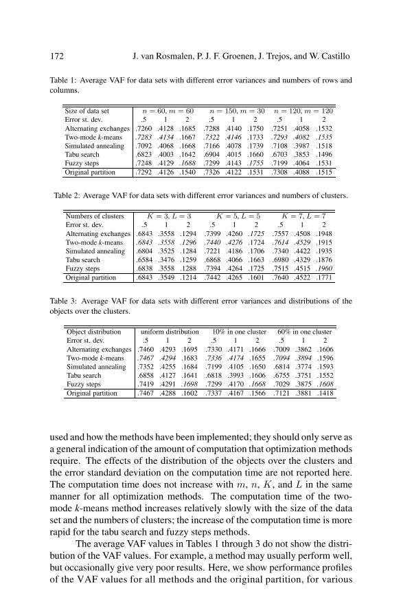
We now present the results of the simulation study. Tables 1 through3 show the average VAF values of all optimization methods and the originalpartitions for various combinations of the factors. Tables 1, 2, and 3 respec-tively show the effects of the size of the data set, the numbers of clusters,and the distribution of the objects over the clusters. As the error standard de-viation strongly affects the magnitude of the VAF values, we do not reportaverage VAF values over data sets with different error standard deviations;the effects of the error standard deviation are shown within each of thesethree tables. The results of the best performing optimization method areshown in italics, for each column in these tables.

Based on the VAF values, the two-mode k-means method appears toperform relatively well. This method always has the best average perfor-mance if the error standard deviation is 0.5 or 1. In addition, the partitionfound by this method is almost always as least as good as the original par-tition. For data sets with an error standard deviation of 2, the best perfor-mance is most often achieved by the fuzzy steps method, though the alternat-ing exchanges and the two-mode k-means methods also perform well. Thesimulated annealing method and especially the tabu search method do notperform as well as the other optimization methods in the simulation study.

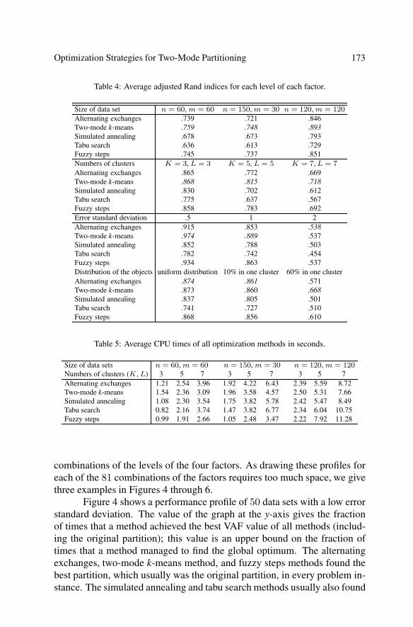
Table 4 gives the average values of the adjusted Rand Index, for eachlevel of each factor, averaged over the levels of the three other factors; thebest results are shown in italics. The two-mode k-means method again hasthe best average performance. This method almost always exactly retrievesthe original partition for data sets with a small error standard deviation anda uniform distribution of the rows and columns over the clusters. The bestperforming optimization method usually has an average ARI above 90%or even 99% if the characteristics of the simulated data sets are favorable.However, this value rapidly decreases, when the problem instances becomeharder. The original partitions are especially hard to retrieve if the errorstandard deviation is 2 or if 60% of the objects are located in one cluster.The ARI never becomes negative or close to 0 for any optimization method,indicating that at least some structure can always be found in the data set.Another important conclusion is that the differences in the average adjustedRand indices between the methods can be large. The difference in ARI cansometimes be as large as 20%, when the corresponding difference in VAFis just a few percentage points. Therefore, the choice of the optimizationmethod can be quite important, if one wants to find the ‘true’ clustering.

Finally, we give the average CPU times in seconds used by the meth-ods in Table 5, for each size of the data set and each number of clusters.Note that the average CPU times strongly depend on the type of computer

171


Table 1: Average VAF for data sets with different error variances and numbers of rows andcolumns.

Size of data set n = 60, m = 60 n = 150, m = 30 n = 120, m = 120Error st. dev. .5 1 2 .5 1 2 .5 1 2Alternating exchanges .7260 .4128 .1685 .7288 .4140 .1750 .7251 .4058 .1532Two-mode k-means .7283 .4134 .1667 .7322 .4146 .1733 .7293 .4082 .1535Simulated annealing .7092 .4068 .1668 .7166 .4078 .1739 .7108 .3987 .1518Tabu search .6823 .4003 .1642 .6904 .4015 .1660 .6703 .3853 .1496Fuzzy steps .7248 .4129 .1688 .7299 .4143 .1755 .7199 .4064 .1531Original partition .7292 .4126 .1540 .7326 .4122 .1531 .7308 .4088 .1515

Table 2: Average VAF for data sets with different error variances and numbers of clusters.

Numbers of clusters K = 3, L = 3 K = 5, L = 5 K = 7, L = 7Error st. dev. .5 1 2 .5 1 2 .5 1 2Alternating exchanges .6843 .3558 .1294 .7399 .4260 .1725 .7557 .4508 .1948Two-mode k-means .6843 .3558 .1296 .7440 .4276 .1724 .7614 .4529 .1915Simulated annealing .6804 .3525 .1284 .7221 .4186 .1706 .7340 .4422 .1935Tabu search .6584 .3476 .1259 .6868 .4066 .1663 .6980 .4329 .1876Fuzzy steps .6838 .3558 .1288 .7394 .4264 .1725 .7515 .4515 .1960Original partition .6843 .3549 .1214 .7442 .4265 .1601 .7640 .4522 .1771

Table 3: Average VAF for data sets with different error variances and distributions of theobjects over the clusters.

Object distribution uniform distribution 10% in one cluster 60% in one clusterError st. dev. .5 1 2 .5 1 2 .5 1 2Alternating exchanges .7460 .4293 .1695 .7330 .4171 .1666 .7009 .3862 .1606Two-mode k-means .7467 .4294 .1683 .7336 .4174 .1655 .7094 .3894 .1596Simulated annealing .7352 .4255 .1684 .7199 .4105 .1650 .6814 .3774 .1593Tabu search .6858 .4127 .1641 .6818 .3993 .1606 .6755 .3751 .1552Fuzzy steps .7419 .4291 .1698 .7299 .4170 .1668 .7029 .3875 .1608Original partition .7467 .4288 .1602 .7337 .4167 .1566 .7121 .3881 .1418

used and how the methods have been implemented; they should only serve asa general indication of the amount of computation that optimization methodsrequire. The effects of the distribution of the objects over the clusters andthe error standard deviation on the computation time are not reported here.The computation time does not increase with m, n, K, and L in the samemanner for all optimization methods. The computation time of the two-mode k-means method increases relatively slowly with the size of the dataset and the numbers of clusters; the increase of the computation time is morerapid for the tabu search and fuzzy steps methods.

The average VAF values in Tables 1 through 3 do not show the distri-bution of the VAF values. For example, a method may usually perform well,but occasionally give very poor results. Here, we show performance profilesof the VAF values for all methods and the original partition, for various

172


Table 4: Average adjusted Rand indices for each level of each factor.

Size of data set n = 60, m = 60 n = 150, m = 30 n = 120, m = 120Alternating exchanges .739 .721 .846Two-mode k-means .759 .748 .893Simulated annealing .678 .673 .793Tabu search .636 .613 .729Fuzzy steps .745 .737 .851Numbers of clusters K = 3, L = 3 K = 5, L = 5 K = 7, L = 7Alternating exchanges .865 .772 .669Two-mode k-means .868 .815 .718Simulated annealing .830 .702 .612Tabu search .775 .637 .567Fuzzy steps .858 .783 .692Error standard deviation .5 1 2Alternating exchanges .915 .853 .538Two-mode k-means .974 .889 .537Simulated annealing .852 .788 .503Tabu search .782 .742 .454Fuzzy steps .934 .863 .537Distribution of the objects uniform distribution 10% in one cluster 60% in one clusterAlternating exchanges .874 .861 .571Two-mode k-means .873 .860 .668Simulated annealing .837 .805 .501Tabu search .741 .727 .510Fuzzy steps .868 .856 .610

Table 5: Average CPU times of all optimization methods in seconds.

Size of data sets n = 60, m = 60 n = 150, m = 30 n = 120, m = 120Numbers of clusters (K , L) 3 5 7 3 5 7 3 5 7Alternating exchanges 1.21 2.54 3.96 1.92 4.22 6.43 2.39 5.59 8.72Two-mode k-means 1.54 2.36 3.09 1.96 3.58 4.57 2.50 5.31 7.66Simulated annealing 1.08 2.30 3.54 1.75 3.82 5.78 2.42 5.47 8.49Tabu search 0.82 2.16 3.74 1.47 3.82 6.77 2.34 6.04 10.75Fuzzy steps 0.99 1.91 2.66 1.05 2.48 3.47 2.22 7.92 11.28

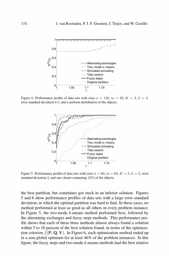
combinations of the levels of the four factors. As drawing these profiles foreach of the 81 combinations of the factors requires too much space, we givethree examples in Figures 4 through 6.

Figure 4 shows a performance profile of 50 data sets with a low errorstandard deviation. The value of the graph at the y-axis gives the fractionof times that a method achieved the best VAF value of all methods (includ-ing the original partition); this value is an upper bound on the fraction oftimes that a method managed to find the global optimum. The alternatingexchanges, two-mode k-means method, and fuzzy steps methods found thebest partition, which usually was the original partition, in every problem in-stance. The simulated annealing and tabu search methods usually also found

173


1 1.05 1.1 1.150

0.2

0.4

0.6

0.8

1

τ

Ψ(s

) (τ)

Alternating exchangesTwo−mode k−meansSimulated annealingTabu searchFuzzy stepsOriginal partition

Figure 4: Performance profile of data sets with sizes n = 150, m = 30, K = 3, L = 3,error standard deviation 0.5, and a uniform distribution of the objects.

1 1.05 1.1 1.150

0.2

0.4

0.6

0.8

1

τ

Ψ(s

) (τ)


Figure 5: Performance profile of data sets with sizes n = 60, m = 60, K = 5, L = 5, errorstandard deviation 2, and one cluster containing 10% of the objects.

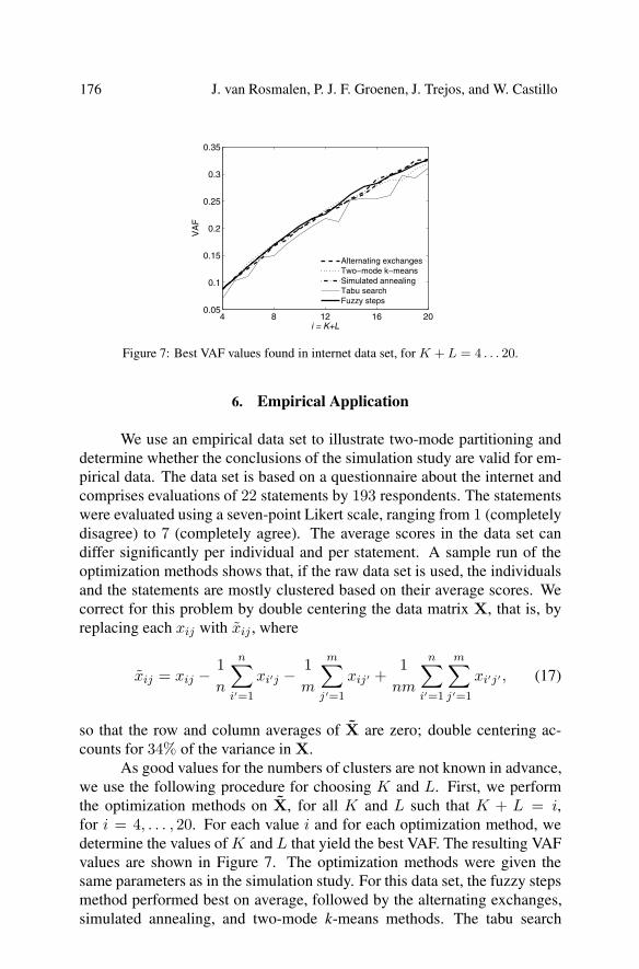
the best partition, but sometimes got stuck in an inferior solution. Figures5 and 6 show performance profiles of data sets with a large error standarddeviation, in which the optimal partition was hard to find. In these cases, nomethod performed at least as good as all others in every problem instance.In Figure 5, the two-mode k-means method performed best, followed bythe alternating exchanges and fuzzy steps methods. This performance pro-file shows that each of these three methods almost always found a solutionwithin 5 to 10 percent of the best solution found, in terms of the optimiza-tion criterion f(P,Q,V). In Figure 6, each optimization method ended upin a non-global optimum for at least 46% of the problem instances. In thisfigure, the fuzzy steps and two-mode k-means methods had the best relative

174


1 1.02 1.04 1.06 1.080

0.2

0.4

0.6

0.8

1

τ

Ψ(s

) (τ)


Figure 6: Performance profile of data sets with sizes n = 120, m = 120, K = 7, L = 7,error standard deviation 2, and one cluster containing 60% of the objects.

performances, followed by the alternating exchanges method. These threemethods seldom find a solution that is more than 5 percent worse than thebest solution found. The two implementations of meta-heuristics (simulatedannealing and tabu search) do not perform as well as the other methods, butcan usually find partitions that are better than the original partition.

As all optimization methods do not find a global optimum for a largenumber of problem instances represented in Figure 6, their performancesmay be considered unsatisfactory. If finding the global optimum is required,one may consider increasing the numbers of random starts in the optimiza-tion methods. To test the effectiveness of increasing the number of randomstarts, we applied the two-mode k-means and fuzzy steps methods to datasets similar to the ones used for Figure 6 with 50,000 and 2,000 randomstarts, respectively. The results show that increasing the numbers of ran-dom starts in this way (by a factor of 100) improves the performances ofthe methods only slightly; the average VAF values for the methods with in-creased numbers of random starts were approximately 0.2 percentage pointshigher than for the methods with the original numbers of random starts.However, even with these large numbers of random starts, no optimizationmethod performed as well as all others for a majority of the data sets. Theseresults show that all optimization methods have great difficulty in finding theglobal optimum in conditions such as represented in Figure 6. This problemis much less severe for smaller data sets and data sets with lower numbersof clusters and lower error standard deviations. As strongly increasing thenumber of random starts tends to improve the VAF value only slightly, wefind it unlikely that the solution found by the optimization methods are muchworse than the global optimum, in terms of the VAF criterion.

175


4 8 12 16 200.05

0.1

0.15

0.2

0.25

0.3

0.35

i = K+L

VA

F

Alternating exchangesTwo−mode k−meansSimulated annealingTabu searchFuzzy steps

Figure 7: Best VAF values found in internet data set, for K + L = 4 . . . 20.

6. Empirical Application

We use an empirical data set to illustrate two-mode partitioning anddetermine whether the conclusions of the simulation study are valid for em-pirical data. The data set is based on a questionnaire about the internet andcomprises evaluations of 22 statements by 193 respondents. The statementswere evaluated using a seven-point Likert scale, ranging from 1 (completelydisagree) to 7 (completely agree). The average scores in the data set candiffer significantly per individual and per statement. A sample run of theoptimization methods shows that, if the raw data set is used, the individualsand the statements are mostly clustered based on their average scores. Wecorrect for this problem by double centering the data matrix X, that is, byreplacing each xij with xij , where

xij = xij − 1n

n∑i′=1

xi′j − 1m

m∑j′=1

xij′ +1

nm

n∑i′=1

m∑j′=1

xi′j′ , (17)

so that the row and column averages of X are zero; double centering ac-counts for 34% of the variance in X.

As good values for the numbers of clusters are not known in advance,we use the following procedure for choosing K and L. First, we performthe optimization methods on X, for all K and L such that K + L = i,for i = 4, . . . , 20. For each value i and for each optimization method, wedetermine the values of K and L that yield the best VAF. The resulting VAFvalues are shown in Figure 7. The optimization methods were given thesame parameters as in the simulation study. For this data set, the fuzzy stepsmethod performed best on average, followed by the alternating exchanges,simulated annealing, and two-mode k-means methods. The tabu search

176


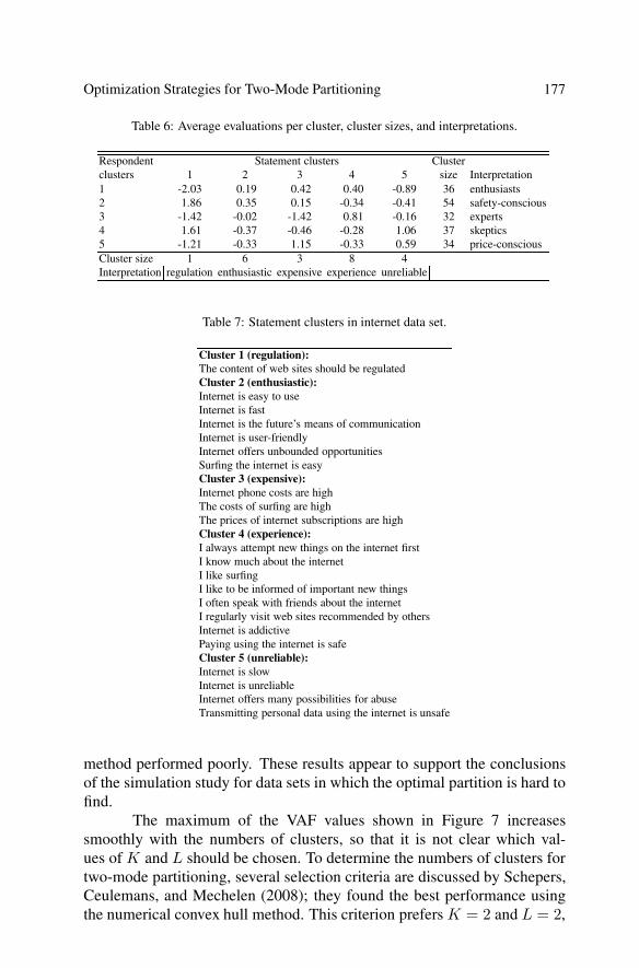
Table 6: Average evaluations per cluster, cluster sizes, and interpretations.

Respondent Statement clusters Clusterclusters 1 2 3 4 5 size Interpretation1 -2.03 0.19 0.42 0.40 -0.89 36 enthusiasts2 1.86 0.35 0.15 -0.34 -0.41 54 safety-conscious3 -1.42 -0.02 -1.42 0.81 -0.16 32 experts4 1.61 -0.37 -0.46 -0.28 1.06 37 skeptics5 -1.21 -0.33 1.15 -0.33 0.59 34 price-consciousCluster size 1 6 3 8 4Interpretation regulation enthusiastic expensive experience unreliable

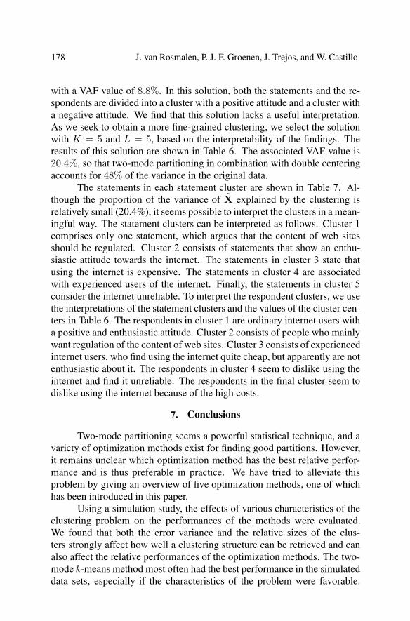
Table 7: Statement clusters in internet data set.

Cluster 1 (regulation):The content of web sites should be regulatedCluster 2 (enthusiastic):Internet is easy to useInternet is fastInternet is the future’s means of communicationInternet is user-friendlyInternet offers unbounded opportunitiesSurfing the internet is easyCluster 3 (expensive):Internet phone costs are highThe costs of surfing are highThe prices of internet subscriptions are highCluster 4 (experience):I always attempt new things on the internet firstI know much about the internetI like surfingI like to be informed of important new thingsI often speak with friends about the internetI regularly visit web sites recommended by othersInternet is addictivePaying using the internet is safeCluster 5 (unreliable):Internet is slowInternet is unreliableInternet offers many possibilities for abuseTransmitting personal data using the internet is unsafe

method performed poorly. These results appear to support the conclusionsof the simulation study for data sets in which the optimal partition is hard tofind.

The maximum of the VAF values shown in Figure 7 increasessmoothly with the numbers of clusters, so that it is not clear which val-ues of K and L should be chosen. To determine the numbers of clusters fortwo-mode partitioning, several selection criteria are discussed by Schepers,Ceulemans, and Mechelen (2008); they found the best performance usingthe numerical convex hull method. This criterion prefers K = 2 and L = 2,

177


with a VAF value of 8.8%. In this solution, both the statements and the re-spondents are divided into a cluster with a positive attitude and a cluster witha negative attitude. We find that this solution lacks a useful interpretation.As we seek to obtain a more fine-grained clustering, we select the solutionwith K = 5 and L = 5, based on the interpretability of the findings. Theresults of this solution are shown in Table 6. The associated VAF value is20.4%, so that two-mode partitioning in combination with double centeringaccounts for 48% of the variance in the original data.

The statements in each statement cluster are shown in Table 7. Al-though the proportion of the variance of X explained by the clustering isrelatively small (20.4%), it seems possible to interpret the clusters in a mean-ingful way. The statement clusters can be interpreted as follows. Cluster 1comprises only one statement, which argues that the content of web sitesshould be regulated. Cluster 2 consists of statements that show an enthu-siastic attitude towards the internet. The statements in cluster 3 state thatusing the internet is expensive. The statements in cluster 4 are associatedwith experienced users of the internet. Finally, the statements in cluster 5consider the internet unreliable. To interpret the respondent clusters, we usethe interpretations of the statement clusters and the values of the cluster cen-ters in Table 6. The respondents in cluster 1 are ordinary internet users witha positive and enthusiastic attitude. Cluster 2 consists of people who mainlywant regulation of the content of web sites. Cluster 3 consists of experiencedinternet users, who find using the internet quite cheap, but apparently are notenthusiastic about it. The respondents in cluster 4 seem to dislike using theinternet and find it unreliable. The respondents in the final cluster seem todislike using the internet because of the high costs.

7. Conclusions

Two-mode partitioning seems a powerful statistical technique, and avariety of optimization methods exist for finding good partitions. However,it remains unclear which optimization method has the best relative perfor-mance and is thus preferable in practice. We have tried to alleviate thisproblem by giving an overview of five optimization methods, one of whichhas been introduced in this paper.

Using a simulation study, the effects of various characteristics of theclustering problem on the performances of the methods were evaluated.We found that both the error variance and the relative sizes of the clus-ters strongly affect how well a clustering structure can be retrieved and canalso affect the relative performances of the optimization methods. The two-mode k-means method most often had the best performance in the simulateddata sets, especially if the characteristics of the problem were favorable.

178


When the optimal partition was hard to find, the alternating exchanges andfuzzy steps methods often performed best. The simulated annealing methodalso performed fairly well, but not as good as the three methods mentionedabove. The performance of the tabu search method generally is inferior.

In sum, the best average performance is obtained using the two-modek-means method, followed by the alternating exchanges and fuzzy stepsmethods. Which of these three methods gives the best performance dependson characteristics of the clustering problem. The performance profiles showthat no optimization method can find the global optimum in a majority ofthe cases for every type of simulated data set. However, the alternating ex-changes, two-mode k-means, and fuzzy steps methods almost always give asolution within 10% of the best solution found, in terms of the optimizationcriterion. As the two-mode k-means method requires relatively little CPUtime and is easy to implement, we believe it is the best choice for data setssimilar to the ones in this study. Note that performing a fairly large number(preferably more than 100) of random starts is necessary to ensure a goodperformance for this method. If finding a globally optimal partition is im-portant, and computation time is not really an issue, the number of randomstarts should be set much higher. However, for data sets in which the optimalpartition is hard to find, even a very large number of random starts may notensure that the global optimum is found.

The results of the methods for the empirical data set are similar to theresults of the simulation study. This data set also gives a useful exampleof the potential applications of two-mode partitioning. We believe that theclustering found in this data set is meaningful and provides relevant insight.

There are a few limitations associated with this study. First, we canonly evaluate the relative performances of the methods for situations similarto our simulation study. It is possible that the relative performances of themethods are different for data sets with different characteristics. However,we have tried to make the simulated data sets similar to data sets that aretypically found in practice. Therefore, the results should be reasonably sim-ilar for many empirical data sets. Second, the results of such a comparisonof optimization methods depend on the values of certain parameters of themethods and the way these methods have been implemented. Here, we havetried to choose the parameters of the optimization methods in a sensible waythat gives good performance. In addition, we have tried to make our com-puter programs as fast as possible. To do so, the efficient updating formulasthat were given by Castillo and Trejos (2002) and Rocci and Vichi (2008)turn out to be quite important.

Some avenues for further research exist. For example, we cannotexclude the possibility that some optimization methods can be improved bychoosing their parameters differently or implementing them in a different

179


way. Besides further theoretical research, we believe that further practicalexperience with two-mode partitioning is also required. Practice can showthe real merits and drawbacks of using two-mode partitioning.

References

BAIER, D., GAUL, W., and SCHADER, M. (1997), “Two-Mode Overlapping Clusteringwith Applications in Simultaneous Benefit Segmentation and Market Structuring,” inClassification and Knowledge Organization, eds. R. Klar and O. Opitz, Heidelberg:Springer, pp. 557-566.

BEZDEK, J. C. (1981), Pattern Recognition with Fuzzy Objective Function Algorithms, NewYork: Plenum Press.

BOCK, H. H. (1974), Automatische Klassifikation, Gottingen: Vandenhoeck & Ruprecht.CASTILLO, W. and TREJOS, J. (2002), “Two-Mode Partitioning: Review of Methods and

Application of Tabu Search,” in Classification, Clustering and Data Analysis, eds.K. Jajuga, A. Sololowksi, and H. Bock, Berlin: Springer, pp. 43-51.

DESARBO, W. S. (1982), “GENNCLUS: New Models for General Nonhierarchical Cluster-ing Analysis,” Psychometrika, 47 (4), 449-475.

DOLAN, E. D. and MORE, J. J. (2002), “Benchmarking Optimization Software with Perfor-mance Profiles,” Mathematical Programming, 91, 201-213.

DOREIAN, P., BATAGELJ, V., and FERLIGOJ, A. (2004), “Generalized Blockmodeling ofTwo-Mode Network Data,” Social Networks, 26, 29-53.

DOREIAN, P., BATAGELJ, V., and FERLIGOJ, A. (2005), Generalized Blockmodeling,Cambridge University Press.

GAUL, W. and SCHADER, M. (1996), “A New Algorithm for Two-Mode Clustering,” inData Analysis and Information Systems, eds. H. Bock and W. Polasek, Heidelberg:Springer, pp. 15-23.

GLOVER, F. (1986), “Future Paths for Integer Programming and Links to Artificial Intelli-gence,” Computers and Operations Research, 13, 533-549.

GROENEN, P. J. F., and JAJUGA, K. (2001), “Fuzzy Clustering with Squared MinkowskiDistances,” Fuzzy Sets and Systems, 120, 227-237.

HANSOHM, J. (2001), “Two-Mode Clustering with Genetic Algorithms,” in Classification,Automation, and New Media, Berlin: Springer, pp. 87-93.

HARTIGAN, J. A. (1975), Clustering Algorithms, New York: John Wiley and Sons.HEISER, W. J. and GROENEN, J. (1997), “Cluster Differences Scaling with a Within-

Clusters Loss Component and a Fuzzy Successive Approximation Strategy to AvoidLocal Minima,” Psychometrika, 62(1), 63-83.

HUBERT, L. and ARABIE, P. (1985), “Comparing Partitions,” Journal of Classification, 2,193-218.

MILLIGAN, G. W. (1980), “An Examination of the Effect of Six Types of Error Perturbationon Fifteen Clustering Algorithms,” Psychometrika, 45(3), 325-342.

MIRKIN, B. (2005), Clustering for Data Mining: A Data Recovery Approach, Boca RatonFL: Chapman & Hall.

MIRKIN, B., ARABIE, P., and HUBERT, L. J. (1995), “Additive Two-Mode Clustering: TheError-Variance Approach Revisited,” Journal of Classification, 12, 243-263.

NOMA, E. and SMITH, D. R. (1985), “Benchmark for the Blocking of Sociometric Data,”Psychological Bulletin, 97(3), 583-591.

180


ROCCI, R. and VICHI, M. (2008), “Two-Mode Multi-Partitioning,” Computational Statistics& Data Analysis, 52, 1984-2003.

SCHEPERS, J., CEULEMANS, E., and VAN MECHELEN, I. (2008), “Selecting amongMulti-Mode Partitioning Models of Different Complexities: A Comparison of FourModel Selection Criteria,” Journal of Classification, 25, 67-85.

TREJOS, J. and CASTILLO, W. (2000), “Simulated Annealing Optimization for Two-ModePartitioning,” in Classification and Information at the Turn of the Millenium, eds.W. Gaul and R. Decker, Heidelberg: Springer, pp. 135-142.

TSAO, E. C. K., BEZDEK, J. C., and PAL, N. R. (1994), “Fuzzy Kohonen Clustering Net-works,” Pattern Recognition, 27(5), 757-764.

VAN LAARHOVEN, P. J. M. and AARTS, E. H. L. (1987), Simulated Annealing: Theoryand Applications, Eindhoven: Kluwer Academic Publishers.

VAN MECHELEN, I., BOCK, H. H., and DE BOECK, P. (2004), “Two-Mode ClusteringMethods: A Structured Overview,” Statistical Methods in Medical Research, 13, 363-394.

VICHI, M. (2001), “Double k-Means Clustering for Simultaneous Classification of Objectsand Variables,” in Advances in Classification and Data Analysis. Studies in Classifi-cation, Data Analysis, and Knowledge Organization, eds, S. Borra, R. Rocchi, andM. Schader, Heidelberg: Springer, pp. 43-52.

181

Optimization Strategies for Two-Mode Partitioning

Documents

Transcript of Optimization Strategies for Two-Mode Partitioning