Graph Partitioning for HighPerformance Scienti�c SimulationsKirk Schloegel, George Karypis, and Vipin KumarArmy HPC Research CenterDept. of Computer Science and Engineering,University of MinnesotaMinneapolis, MinnesotaTo be included in CRPC Parallel Computing HandbookJ. Dongarra, I. Foster, G. Fox, K. Kennedy, and A. White, editors.Morgan Kaufmann, 2000.

Early DraftEarly DraftLimited Copies DistributedReproduction requires explicit permissionCopyright 1999, by the authors, all rights reserved

Contents0.1 Introduction . . . . . . . . . . . . . . . . . . . . . . . . . . . . . . . . . . . . . . . . . . . . . . 20.2 Modeling Mesh-based Computations as Graphs . . . . . . . . . . . . . . . . . . . . . . . . . . 30.3 Static Graph Partitioning Techniques . . . . . . . . . . . . . . . . . . . . . . . . . . . . . . . . 40.3.1 Geometric Techniques . . . . . . . . . . . . . . . . . . . . . . . . . . . . . . . . . . . . 50.3.2 Combinatorial Techniques . . . . . . . . . . . . . . . . . . . . . . . . . . . . . . . . . . 80.3.3 Spectral Methods . . . . . . . . . . . . . . . . . . . . . . . . . . . . . . . . . . . . . . . 120.3.4 Multilevel Schemes . . . . . . . . . . . . . . . . . . . . . . . . . . . . . . . . . . . . . . 140.3.5 Combined Schemes . . . . . . . . . . . . . . . . . . . . . . . . . . . . . . . . . . . . . . 160.3.6 Qualitative Comparison of Graph Partitioning Schemes . . . . . . . . . . . . . . . . . 160.4 Load Balancing of Adaptive Computations . . . . . . . . . . . . . . . . . . . . . . . . . . . . 180.4.1 Scratch-Remap Repartitioners . . . . . . . . . . . . . . . . . . . . . . . . . . . . . . . 210.4.2 Di�usion-based Repartitioners . . . . . . . . . . . . . . . . . . . . . . . . . . . . . . . 220.5 Parallel Graph Partitioning . . . . . . . . . . . . . . . . . . . . . . . . . . . . . . . . . . . . . 240.6 Multi-constraint, Multi-objective Graph Partitioning . . . . . . . . . . . . . . . . . . . . . . . 250.6.1 A Generalized Formulation for Graph Partitioning . . . . . . . . . . . . . . . . . . . . 290.7 Conclusions . . . . . . . . . . . . . . . . . . . . . . . . . . . . . . . . . . . . . . . . . . . . . . 33

1

CONTENTS 2

Figure 1: A partitioned 2D irregular mesh of an airfoil. The shading of a mesh element indicates the processor to which itis mapped.0.1 IntroductionAlgorithms that �nd good partitionings of unstructured and irregular graphs are critical for the e�cientexecution of scienti�c simulations on high performance parallel computers. In these simulations, computationis performed iteratively on each element (and/or node) of a physical two- or three-dimensional mesh andthen information is exchanged between adjacent mesh elements. For example, computation is performedon each triangle of the two-dimensional irregular mesh shown in Figure 1. Then information is exchangedfor every face between adjacent triangles. The e�cient execution of such simulations on parallel machinesrequires a mapping of the computational mesh onto the processors such that each processor gets roughly anequal number of mesh elements and that the amount of inter-processor communication required to performthe information exchange between adjacent elements is minimized. Such a mapping is commonly found bysolving a graph partitioning problem. For example, a graph partitioning algorithm was used to decomposethe mesh in Figure 1. Here, the mesh elements have been shaded to indicate the processor to which theyhave been mapped.In many scienti�c simulations, the structure of the computation evolves from time-step to time-step. Theserequire an initial decomposition of the mesh prior to the start of the simulation (as described above), andalso periodic load balancing to be performed during the course of the simulation. Other classes of simulations(i. e., multi-phase simulations) consist of a number of computational phases separated by synchronizationsteps. These require that each of the phases be individually load balanced. Still other scienti�c simulationsmodel multiple physical phenomenon (i. e., multi-physics simulations) or employ multiple meshes simultane-ously (i. e., multi-mesh simulations). These impose additional requirements that the partitioning algorithmmust take into account. Traditional graph partitioning algorithms are not adequate to ensure the e�cientexecution of these classes of simulations on high performance parallel computers. Instead, generalized graphpartitioning algorithms have been developed for such simulations.This chapter presents an overview of graph partitioning algorithms used for scienti�c simulations on highperformance parallel computers. Recent developments in graph partitioning for adaptive and dynamic sim-ulations, as well as partitioning algorithms for sophisticated simulations such as multi-phase, multi-physics,and multi-mesh computations are also discussed. Speci�cally, Section 0.2 presents the graph partitioningformulation to model the problem of mapping computational meshes onto processors. Section 0.3 describesnumerous static graph partitioning algorithms. Section 0.4 discusses the adaptive graph partitioning prob-lem and describes a number of repartitioning schemes. Section 0.5 discusses the issues involved with theparallelization of static and adaptive graph partitioning schemes. Section 0.6 describes a number of impor-tant application areas for which the traditional graph partitioning problem is inadequate. This section also

CONTENTS 3(a) (b) (c)Figure 2: A 2D irregular mesh (a) and corresponding graphs (b) and (c). The graph in (b) models the connectivity betweenthe mesh nodes. The graph in (c) (the dual of (b)) models the adjacency of the mesh elements.describes generalizations of the graph partitioning problem that are able to meet the requirements of theseas well as algorithms for computing partitionings based on these formulations. Finally, Section 0.7 presentsconcluding remarks, discusses areas of future research, and charts the functionality of a number of publicallyavailable graph partitioning software packages.0.2 Modeling Mesh-based Computations as GraphsIn order to compute a mapping of a mesh onto a set of processors via graph partitioning, it is �rst necessaryto construct the graph that models the structure of the computation. In general, computation of a scienti�csimulation can be performed on the mesh nodes, the mesh elements, or both of these. If the computationis mainly performed on the mesh nodes then this graph is straightforward to construct. A vertex existsfor each mesh node, and an edge exists on the graph for each edge between the nodes. (We refer to thisas the node graph.) However, if the computation is performed on the mesh elements then the graph issuch that each mesh element is modeled by a vertex, and an edge exists between two vertices whenever thecorresponding elements share an edge (in two-dimensions) or a face (in three-dimensions). This is the dualof the node graph. Figure 2 illustrates a 2D example. Figure 2(a) shows a �nite-element mesh. Figure 2(b)shows the corresponding node graph. Figure 2(c) shows the dual graph that models the adjacencies of themesh elements. Partitioning the vertices of these graphs into k disjoint subdomains provides a mapping ofeither the mesh nodes or the mesh elements onto k processors. If the partitioning is computed such thateach subdomain has the same number of vertices, then each processor will have an equal amount of workduring parallel processing. The total volume of communications incurred during this parallel processing canbe estimated by counting the number of edges that connect vertices in di�erent subdomains. Therefore, apartitioning should be computed that minimizes this metric (which is referred to as the edge-cut).The objective of the graph partitioning problem is to compute just such a partitioning (i. e., one that balancesthe subdomains and minimizes the edge-cut). Formally, the graph partitioning problem is as follows. Givena weighted, undirected graph G = (V;E) for which each vertex and edge has an associated weight, the k-waygraph partitioning problem is to split the vertices of V into k disjoint subsets (or subdomains) such thateach subdomain has roughly an equal amount of vertex weight (referred to as the balance constraint), whileminimizing the sum of the weights of the edges whose incident vertices belong to di�erent subdomains (i. e.,the edge-cut).In some cases, it is bene�cial to compute partitionings such that each subdomain has a speci�ed amount ofvertex weight. An example is performing a scienti�c simulation on a cluster of heterogenous workstations.Here, the subdomain weights should be speci�ed in such a way as to provide more work to the faster machinesand less work to the slower machines. Subdomain weights can be speci�ed by using a vector of size k inwhich each element of the vector indicates the fraction of the total vertex weight that the correspondingsubdomain should contain. In this case, the graph partitioning problem is to compute a partitioning thatsplits the vertices into k disjoint subdomains such that each subdomain has the speci�ed fraction of totalvertex weight and such that the edge-cut is minimized.It is important to note that the edge-cut metric is only an approximation of the total communicationsvolume incurred by parallel processing [32]. It is not a precise model of this quantity. Consider the example

CONTENTS 41

2

4

3

5

7 8

6

10

9

11

12

B

A

C

Figure 3: A partitioned graph with an edge-cut of seven. Here, nine communications are incurred during parallel processing.in Figure 3. Here, three subdomains, A, B, and C are shown. The edge-cut of the (three-way) partitioningis seven. During parallel computation, the processor corresponding to subdomain A will need to send thedata for vertices 1 and 3 to the processor corresponding to subdomain B, and the data for vertex 4 to theprocessor corresponding to subdomain C. Similarly, B needs to send the data for 5 and 7 to A and the datafor 7 and 8 to C. Finally, C needs to send the data for 9 to B and the data for 10 to A. This equals nineunits of data to be sent, while the edge-cut is seven. The reason that edge-cut and total communicationvolume are not the same is because the edge-cut counts every edge cut, while data is required to be sentonly one time if two or more edges of a single vertex are cut by the same subdomain (as is the case, forexample, between vertex 3 and subdomain B in Figure 3). It should also be noted that total communicationvolume alone cannot accurately predict inter-processor communication overhead. A more precise measure isthe maximum time required by any of the processors to perform communication (because computation andcommunication occur in alternating phases). This depends upon a number of factors, including the amountof data to be sent out of any one processor, as well as the number of processors with which a processormust communicate. In particular, on message-passing architectures, minimizing the maximum number ofmessage startups that any one processor must perform can sometimes be more important than minimizingthe communications volume [34]. Nevertheless, there still tends to be a strong correlation between edge-cutsand inter-processor communication costs for graphs of uniform degree (i. e., graphs in which most verticeshave about the same number of edges). This is a typical characteristic of graphs derived from scienti�csimulations. For this reason, the traditional min-cut partitioning problem is a reasonable approximation tothe problem of minimizing the inter-processor communications that underly many scienti�c simulations.Computing a k-way Partitioning via Recursive Bisection Graphs are frequently partitioned into ksubdomains by recursively computing two-way partitionings (i. e., bisections) of the graph [6]. This methodrequires the computation of k�1 bisections. If k is not a power of two, then for each bisection, the appropriatesubdomain weights need to be speci�ed in order to ensure that the resulting k-way partitioning is balanced.It is known that for a large class of graphs derived from scienti�c simulations, recursive bisection algorithmsare able to compute k-way partitionings that are within a constant factor of the optimal solution [84].Furthermore, if the balance constraint is su�ciently relaxed, then recursive bisection methods can be usedto compute k-way partitionings that are within log p of the optimal for all graphs [84]. Since the directcomputation of a good k-way partitioning is harder in general than the computation of a good bisection(although both problems are NP-complete), recursive bisection has become a widely used technique.0.3 Static Graph Partitioning TechniquesThe graph partitioning problem is known to be NP-complete. Therefore, in general it is not possible to com-pute optimal partitionings for graphs of interesting size in a reasonable amount of time. This fact, combined

CONTENTS 5(a) (b)Figure 4: Two mesh bisections normal to the coordinate axes. In (a) the mesh is bisected normal to the x-axis. In (b) themesh is bisected normal to the y-axis. The subdomain boundary in (a) is smaller than that in (b).

(a) (b)Figure 5: An eight-way partitioning of a mesh computed by a CND scheme. First, the solid bisection was computed. Thenthe dashed bisections were computed for each of the subdomains. Finally, the dashed-and-dotted bisections were computed.The centers-of-mass of the mesh elements are shown in (a). The mesh elements are shaded in (b) to indicated their subdomains.with the importance of the problem, has led to the development of several heuristic approaches [1, 2, 5, 6, 9,13, 16, 20, 21, 22, 24, 25, 26, 27, 29, 30, 36, 37, 44, 48, 54, 58, 60, 61, 66, 68, 73, 74, 76, 83, 94, 104]. These canbe classi�ed as either geometric [6, 22, 30, 58, 61, 66, 68, 76], combinatorial [1, 2, 20, 21, 24, 27, 54], spectral[36, 37, 73, 74, 83], combinatorial optimization techniques [5, 26, 104], or multilevel methods [9, 13, 16, 25, 29,44, 48, 60, 94]. In this section, we discuss several of these classes and describe the important schemes fromthem.0.3.1 Geometric TechniquesGeometric techniques [6, 22, 30, 58, 61, 66, 68, 76] compute partitionings based solely on the coordinate in-formation of the mesh nodes, and not on the connectivity of the mesh elements. Since these techniques donot consider the connectivity between the mesh elements, there is no concept of edge-cut here. Instead, inorder to minimize the inter-processor communications incurred due to parallel processing, geometric schemesare usually designed to minimize a related metric such as the number of mesh elements that are adjacentto non-local elements (i. e., the size of the subdomain boundary). Usually, these techniques partition themesh elements directly, and not the graphs that model the structures of the computations. Because of thisdistinction, they are often referred to as mesh partitioning schemes.Geometric techniques are applicable only if coordinate information exists for the mesh nodes. However,this is usually true for meshes used in scienti�c simulations. Even if the mesh is not embedded in a k-dimensional space, there are techniques that are able to automatically compute node coordinates based onthe connectivity of the mesh elements [28]. Typically, geometric partitioners are extremely fast. However,they tend to compute partitionings of lower quality than schemes that take the connectivity of the meshelements into account. For this reason, multiple trials are usually performed with the best partitioning ofthese being selected.Coordinate Nested Dissection Coordinate Nested Dissection (CND) (also referred to as RecursiveCoordinate Bisection) is a recursive bisection scheme that attempts to minimize the boundary between thesubdomains (and therefore, the inter-processor communications) by splitting the mesh in half normal toits longest dimension. Figure 4 illustrates how this works. Figure 4(a) gives a mesh bisected normal tothe x-axis. Figure 4(b) gives the same mesh bisected normal to the y-axis. The subdomain boundary in

CONTENTS 6

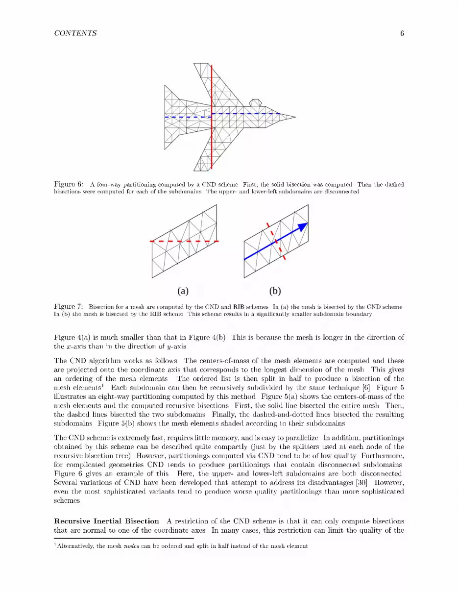
Figure 6: A four-way partitioning computed by a CND scheme. First, the solid bisection was computed. Then the dashedbisections were computed for each of the subdomains. The upper- and lower-left subdomains are disconnected.(b)(a)Figure 7: Bisection for a mesh are computed by the CND and RIB schemes. In (a) the mesh is bisected by the CND scheme.In (b) the mesh is bisected by the RIB scheme. This scheme results in a signi�cantly smaller subdomain boundary.Figure 4(a) is much smaller than that in Figure 4(b). This is because the mesh is longer in the direction ofthe x-axis than in the direction of y-axis.The CND algorithm works as follows. The centers-of-mass of the mesh elements are computed and theseare projected onto the coordinate axis that corresponds to the longest dimension of the mesh. This givesan ordering of the mesh elements. The ordered list is then split in half to produce a bisection of themesh elements1. Each subdomain can then be recursively subdivided by the same technique [6]. Figure 5illustrates an eight-way partitioning computed by this method. Figure 5(a) shows the centers-of-mass of themesh elements and the computed recursive bisections. First, the solid line bisected the entire mesh. Then,the dashed lines bisected the two subdomains. Finally, the dashed-and-dotted lines bisected the resultingsubdomains. Figure 5(b) shows the mesh elements shaded according to their subdomains.The CND scheme is extremely fast, requires little memory, and is easy to parallelize. In addition, partitioningsobtained by this scheme can be described quite compactly (just by the splitters used at each node of therecursive bisection tree). However, partitionings computed via CND tend to be of low quality. Furthermore,for complicated geometries CND tends to produce partitionings that contain disconnected subdomains.Figure 6 gives an example of this. Here, the upper- and lower-left subdomains are both disconnected.Several variations of CND have been developed that attempt to address its disadvantages [30]. However,even the most sophisticated variants tend to produce worse quality partitionings than more sophisticatedschemes.Recursive Inertial Bisection A restriction of the CND scheme is that it can only compute bisectionsthat are normal to one of the coordinate axes. In many cases, this restriction can limit the quality of the1Alternatively, the mesh nodes can be ordered and split in half instead of the mesh element.

CONTENTS 7

Figure 8: A Peano-Hilbert space-�lling curve is used to order the mesh elements. The eight-way partitioning that is producedby this ordering is shown.partitioning. Figure 7 gives an example. The mesh in Figure 7(a) is bisected normal to the longest dimensionof the mesh. However, the subdomain boundary is still quiet long. This is because the mesh is orientedat an angle to the coordinate axes. Taking this angle into account when orienting the bisection can resultin a smaller subdomain boundary. One way to do so is to treat the mesh elements as point masses and tocompute the principal inertial axis of the mass distribution. If the mesh is convex, then this axis will alignwith the overall orientation of the mesh. A bisection line that is orthogonal to this will often result in asmall subdomain boundary, as the mesh will tend to be thinnest in this direction [72].The Recursive Inertial Bisection (or RIB) algorithm improves upon the CND scheme by making use of thisidea as follows. The inertial axis of the mesh is computed and an ordering of the elements is produced byprojecting their centers-of-mass onto this axis. The ordered list is then split in half to produce a bisection.The scheme can be applied recursively to produce a k-way partitioning [61]. As an example, the bisectionof the mesh in Figure 7(b) is computed using the RIB algorithm. The solid arrow indicates the inertial axisof the mesh. The dashed line is the bisection. Here, the subdomain boundary is much smaller than thatproduced by the CND scheme in Figure 7(a).Space-�lling Curve Techniques The CND and RIB algorithms essentially �nd orderings of the meshelements and then split the ordered list in half to produce a bisection. In these schemes, orderings arecomputed by projecting the elements onto either the coordinate or inertial axes. A disadvantage of thesetechniques is that orderings are computed based only on a single dimension. A scheme that does so withrespect to more than one dimension can potentially result in orderings that produce better partitionings.One way of doing this is to order the mesh elements according to the positions of their centers-of-mass alonga space-�lling curve [64, 66, 68, 101] (or a related self-avoiding walk [31]). Space-�lling curves are continuouscurves that completely �ll up higher dimensional spaces such as squares or cubes. A number of such curves(eg., Peano-Hilbert curves [38]) have been de�ned that �ll up space in a locality-preserving way. Theseproduce orderings of the mesh elements with the desired characteristic that the elements that are near toeach other in space are likely to be ordered near to each other as well. After the ordering is computed,the ordered list of mesh elements is split into k parts resulting in k subdomains. Figure 8 illustrates aspace-�lling curve method for computing an eight-way partitioning of a quad-tree mesh.Space-�lling curve partitioners are fast and generally produce partitionings of somewhat better quality thaneither the CND or RIB schemes. They tend to work particularly well for classes of simulations in which thedependencies between the computational nodes are governed by their spatial proximity to one another as inn-body computations using hierarchical methods [101].Sphere-cutting Approach Miller, Teng, Thurston, and Vavasis [58] proposed a new class of graphs,called overlap graphs, that contains all well-shaped meshes as well as all planar graphs, and proved that

CONTENTS 8

(c)(a) (b)Figure 9: The nodes of a �nite-element mesh (a). A 3-ply neighborhood systems for the nodes (b). The (1, 3)-overlap graphfor the mesh (c).these graphs have O(n(d�1)=d) vertex separators2. In doing so, they extended results by Lipton and Tarjan[56] and others [59]. Meshes are considered well-shaped if the angles and/or aspect ratios of their elementsare bounded within some values. Most of the meshes that are used in scienti�c simulations are well-shapedaccording to this de�nition.Miller et al., used the concept of a neighborhood system to de�ne an overlap graph. A k-ply neighborhoodsystem is a set of n spheres in a d-dimensional space such that no point in space is encircled by more thank of the spheres. An (�, k)-overlap graph consists of a vertex for each sphere, and an edge between twovertices if the corresponding spheres intersect when the smaller of them is expanded by a factor of �. Figure 9illustrates these concepts. Figure 9(a) shows a set of points in a 2-dimensional space. Figure 9(b) shows a3-ply neighborhood system for these points. Figure 9(c) shows the (1, 3)-overlap graph constructed fromthis neighborhood system.Gilbert, Miller, and Teng [22] describe an implementation of a geometric bisection scheme based on theseresults. This scheme projects each vertex of a d-dimensional (�, k)-overlap graph onto the unit d+1-dimensional sphere that encircles it. A random great circle of the sphere has a high probability of splittingthe vertices into three sets A, B, and C, such that no edge joins A and B, A and B each have at most d+1d+2vertices, and C has only O(�k1=dn(d�1)=d) vertices [58]. Therefore, by selecting a few great circles at randomand picking the best separator from these, the algorithm can compute a vertex separator of guaranteedquality (in asymptotic terms) with high probability.While the sphere-cutting scheme is unique among those described in this chapter by providing guaranteeson the quality of the computed bisection for well-shaped meshes, it is not guaranteed to compute perfectlybalanced bisections. It is proven in [58] that the larger subdomain will contain no more than d+1d+2 of the totalnumber of vertices. However, experiments cited in [22] on a small number of test graphs indicate that inthree dimensions, splits as bad as 2 : 1 are rare, and that most are within 20%. The authors of [22] suggesta modi�cation of the scheme that will result in balanced bisections by shifting the separating plane normalto its orientation.0.3.2 Combinatorial TechniquesWhen computing a partitioning, geometric techniques attempt to group together vertices that are spatiallynear to each other regardless of whether or not these vertices are highly connected. Combinatorial parti-2A vertex separator is a set of vertices that, if removed, splits the graph into two roughly equal-sized subgraphs, such that noedge connects the two subgraphs. That is, instead of partitioning the graph between the vertices (and so cutting edges), thegraph is partitioned along the vertices. For this formulation, the sum weight of the separator vertices should be minimized.

CONTENTS 93

4

5

5

6

7

6

7

7

64

32

1

2

3

4

55

56

0

1

4

55

4

66

5

edge-cut: 3 edge-cut: 8

Figure 10: A graph partitioned by the LND algorithm. The vertex in the extreme bottom-right was selected and labelledzero. Then, the vertices were labeled in a breadth-�rst manner according to how far they are from the zero vertex. After halfof the vertices had been labeled, a bisection (solid line) was constructed such that the labeled vertices are in one subdomainand the unlabeled vertices are in another subdomain. This �gure also shows a higher-quality bisection (dashed line) for thesame graph.tioners, on the other hand, attempt to group together highly connected vertices regardless of whether or notthese are near to each other in space. That is, combinatorial partitioning schemes compute a partitioningbased only on the adjacency information of the graph, and not on the coordinates of the vertices. For thisreason, the partitionings produced typically have lower edge-cuts and are less likely to contain disconnectedsubdomains compared to those produced by geometric schemes. However, combinatorial techniques tend tobe slower than geometric partitioning techniques and are not as amenable to parallelization.Levelized Nested Dissection A partitioning will have a low edge-cut if adjacent vertices are usually inthe same subdomain. The Levelized Nested Dissection (LND) algorithm attempts to put connected verticestogether by starting with a subdomain that contains only a single vertex, and then incrementally growingthis subdomain by adding adjacent vertices [21].More precisely, the LND algorithm works as follows. An initial vertex is selected and assigned the numberzero. Then all of the vertices that are adjacent to the selected vertex are assigned the number one. Next,all of the vertices that are not assigned a number and are adjacent to any vertex that has been assigneda number are assigned that number plus one. This process continues until half of the vertices have beenassigned a number. At this point the algorithm terminates. The vertices that have been assigned numbersare in one subdomain, and the vertices that have not been assigned numbers are in the other subdomain.Figure 10 illustrates the LND algorithm. It shows the numbering starting with the extreme lower-rightvertex. Here, the solid line shows a bisection with an edge-cut of eight computed by the LND algorithm.This scheme tends to perform better when the initial seed is a pseudo-peripheral vertex (i.e., one of thepairs of vertices that are approximately the greatest distance from each other in the graph) as in Figure 10.Such a vertex can be found by a process that is similar to the LND algorithm. A random vertex is initiallyselected to start the numbering of vertices. Here, all of the vertices are numbered. The vertex (or one of thevertices) with the highest number is likely to be in a corner of the graph. This vertex can be used eitheras an input to �nd another corner vertex (at the other end of the graph) or as the seed vertex for the LNDscheme.The LND algorithm ensures that at least one of the computed subdomains is connected (as long as theinput graph is fully connected), and tends to produce partitionings of comparable or better quality thangeometric schemes. However, even with a good seed vertex, the LND algorithm can sometimes produce poorquality partitionings. For example, the graph in Figure 10 contains a natural bisector shown by the dashedline. However, the LND algorithm was unable to �nd this bisection. For this reason, multiple trials of theLND algorithm are often performed, and the best partitioning from these is selected. Several variations andimprovements of levelized nested dissection schemes are studied in [1, 12, 24, 78].

CONTENTS 10

(a) (b)Figure 11: A bisection of a graph re�ned by the KL algorithm. The two shaded vertices will be swapped by the KL algorithmin order to improve the quality of the bisection (a). The resulting bisection is shown in (b).Kernighan-Lin / Fiduccia-Mattheyses Algorithm (KL/FM) Closely related to the graph partition-ing problem is that of partition re�nement. Given a graph with a sub-optimal partitioning, the problem isto improve the partition quality while maintaining the balance constraint. Essentially, this di�ers from thegraph partitioning problem only in that it requires an initial partitioning of the graph. Indeed, a re�nementscheme can be used as a partitioning scheme simply by using a random partitioning as its input.Given a bisection of a graph that separates the vertices into sets A and B, a powerful means of re�ning thebisection is to �nd two equal-sized subsets, X and Y , from A and B respectively, such that swapping X toB and Y to A yields the greatest possible reduction in the edge-cut. This swapping can then be performeda number of times until no further improvement is possible [54]. However, the problem of �nding optimalsets X and Y is intractable itself (just like the graph partitioning problem). For this reason, Kernighanand Lin [54] developed a greedy method of �nding and swapping near-optimal sets X and Y (referred to asKernighan-Lin or KL re�nement).The KL algorithm consists of a small number of passes through the vertices. During each pass, the algorithmrepeatedly �nds a pair of vertices, one from each of the subdomains, and swaps their subdomains. The pairsare selected so as to give the maximum improvement in the quality of the bisection (even if this improvementis negative). Once a pair of vertices has been moved, neither are considered for movement in the rest of thepass. When all of the vertices have been moved, the pass ends. At this point, the state of the bisectionat which the minimum edge-cut was achieved is restored. (That is, all vertices that were moved after thispoint are moved back to their original subdomains.) Another pass of the algorithm can then be performedby using the resulting bisection as the input. The KL algorithm usually takes a small number of such passesto converge. Each pass of the KL algorithm takes O(jV j2). Figure 11 illustrates a single swap made by theKL algorithm. In Figure 11(a), the two dark grey vertices are selected to switch subdomains. Figure 11(b)shows the bisection after this swap is made.Fiduccia and Mattheyses present a modi�cation of the KL algorithm [20] (called Fiduccia-Mattheyses orFM re�nement) that improves its run time without signi�cantly decreasing its e�ectiveness (at least withrespect to graphs arising in scienti�c computing applications). Essentially, this scheme di�ers from the KLalgorithm in that it moves only a single vertex at a time between subdomains instead of swapping pairs ofvertices. The FM algorithm makes use of two priority queues (one for each subdomain) to determine theorder in which vertices are examined and moved. As in KL, the FM algorithm consists of a number of passesthrough the vertices. Prior to each pass, the gain of every vertex is computed (i. e., the amount by whichthe edge-cut will decrease if the vertex changes subdomains). Then it is placed into the priority queue thatcorresponds with its current subdomain and ordered according to its gain. During a pass, the vertices atthe top of each of the two priority queues are examined. If the top vertex in only one of the priority queuesis able to switch subdomains while still maintaining the balance constraint, then that vertex is moved tothe other subdomain. If the top vertices of both of the priority queues can be moved while maintaining thebalance, then the vertex that has the highest gain among these is moved. Ties are broken by selecting thevertex that will most improve the balance. When a vertex is moved, it is removed from the priority queue

CONTENTS 11

(c) (d)edge-cut: 8edge-cut: 7

-1

-1

-1

-2

-2-2

-2

-2

-2

-2

-2

-3

-3

-3-3

-4

+1

-3

0

-2-2

-2

-2

-2

-2

-2

-3

-3

-3-3

-4

+1

-3

0

+1

-3

+1

0

(a) (b)edge-cut: 6edge-cut: 6

-1

-1

-1

-1

-1

-2

-2-2

-2

-2

-2

-2

-2

-2

-3

-3

-3-3

-4

+1

-1

+1

Figure 12: A bisection of a graph re�ned by a KL/FM algorithm. The white vertices indicate those selected to be moved.In (a) the partitioning is in a local minima. In (b) the algorithm explores moves that increase the edge-cut. In (c) and (d) theedge-cut is increased, but now there are edge-cut reducing moves to be made.and the gains of its adjacent vertices are updated. (Therefore, these vertices may change their positions inthe priority queue.) The pass ends when neither priority queue has a vertex that can be moved. At thispoint, the highest quality bisection that was found during the pass is restored. With the use of appropriatedata-structures, the complexity of each pass of the FM algorithm is O(jEj).KL/FM-type algorithms are able to escape from some types of local minima because they explore movesthat temporarily increase the edge-cut. Figure 12 illustrates this process. Figure 12(a) shows a bisection of agraph with an edge-cut of six. Here, the weights of the vertices and edges are one. There are twenty verticesin the graph. Therefore, a perfectly balanced bisection will have subdomain weights of ten. However, inthis case we allow the subdomains to be up to 10% imbalanced. Therefore, subdomains of weight eleven areacceptable3. Figure 12(b) shows the gain of each vertex. Since all of the gains are negative, moving anyvertex will result in the edge-cut increasing. Therefore, the bisection is in a local minima. However, thealgorithm will still select one of the vertices with the highest gain and move it. The white vertex is selected.Figure 12(c) shows the new bisection as well as the updated vertex gains. There are now two positive gainvertices. However, neither of these can be moved at this time. The black vertex has just moved, and so it isineligible to move again until the end of the pass. The other vertex with +1 gain is unable to move as thiswill violate the balance constraint. Instead, one of the highest negative-gain vertices (shown in white) fromthe left subdomain is selected. Figure 12(d) shows the results of this move. Now there are two positive gainvertices that are able to move and two that are ineligible to move. The white vertex is selected. Figure 13shows the results of continued re�nement. By Figure 13(d), the bisection has reached another minima withan edge-cut of two. The re�nement algorithm has succeeded in climbing out of the original local minimaand reducing the edge-cut from six to two.While KL/FM schemes have the ability to escape from certain types of local minima, this ability is stilllimited. For this reason, the quality of the �nal bisection obtained by KL/FM schemes is highly dependenton the quality of the input bisection. Several techniques have been developed that try to improve thesealgorithms by allowing the movement of larger sets of vertices together (i.e., more than just a single vertexor vertex pair) [2, 16, 27]. These schemes have been shown to be able to improve the e�ectiveness of KL/FMre�nement at the cost of increased complexity of the algorithm. KL/FM-type re�nement algorithms tend3It is common for KL/FM-type algorithms to tolerate a slight amount of imbalance in the partitioning in an attempt to minimizethe edge-cut.

CONTENTS 12

edge-cut: 4 edge-cut: 2(c) (d)

-2

-2

-2

-2

-2

-3

-3-3

-4

-3

-1

-5

-1

+2

-3

-2-4

-3

-3

edge-cut: 6edge-cut: 7(a) (b)

-2

-2

-2

-2

-2

-2

-3

-3-3

-4

+1

-3

0

-1

-5

-5

-1

+2

-2

-2

-2

-2

-2

-3

-3-3

-4

-3

-1

-5

-1

+2

-1

-1

-3

-2-4

-2

-2

-2

-2

-2

-3

-3-3

-4

-3

-5

-3

-2-4

-3

-3

-2

-3

+1

0

+2

-2 -2

-3

Figure 13: The KL/FM algorithm from Figure 12 is continued here. Edge-cut reducing moves are shown from (a) through(d). By (d), the re�nement algorithm has reached a local minima.1 2

34

5 6

1 2

34

5 6

GL = A - D

6

5

4

3

2

1

1 2 3

6

5

4

3

2

1

1 2 3 4 5 6

1

2

3

4

5

6

1 2 3 5 64

1

1

1

1

1

1

1

1

1

1 1

1

1

1

2

2

3

3

2

2 -2

-2

-3

-3

-2

-2

1

1

1

1 1

1

1

1 1

1

11

11

4 5 6

A DInput Graph Partitioned GraphFigure 14: A graph along with its adjacency matrix A, degree matrix D, and Laplacian LG. The Fiedler vector of LGassociates a value with each vertex. The vertices are then sorted according to this value. A bisection is obtained by splittingthe sorted list in half.to be more e�ective when the average degree of the graph is large [9]. Furthermore, they perform muchbetter when the balance constraints are relaxed. When perfect balance is desired, these schemes are quiteconstrained as to the re�nement moves that can be made at any one time. As the imbalance toleranceincreases, they are allowed greater freedom in making vertex moves, and so, can lead to higher-qualitybisections.0.3.3 Spectral MethodsAnother method of solving the bisection problem is to formulate it as the optimization of a discrete quadraticfunction. However, even with this new formulation, the problem is still intractable. For this reason, a class ofgraph partitioning methods, called spectralmethods, relax this discrete optimization problem by transformingit into a continuous one. The minimization of the relaxed problem is then solved by computing the secondeigenvector of the discrete Laplacian of the graph.More precisely, spectral methods work as follows. Given a graph G, its discrete Laplacian matrix LG isde�ned as (LG)qr = 8<: 1; if q 6= r, q and r are neighbors,�deg(q); if q = r,0; otherwise.

CONTENTS 13

G 4

G 3

G 2

G 1

G 0

G 3

G 2

G 1

G 0

Coa

rsen

ing

Phas

eU

ncoarsening and Refinem

ent Phase

Initial Partitioning PhaseFigure 15: The three phases of the multilevel graph partitioning paradigm. During the coarsening phase, the size of thegraph is successively decreased. During the initial partitioning phase, a bisection is computed, During the uncoarsening andre�nement phase, the bisection is successively re�ned as it is projected to the larger graphs. G0 is the input graph, which isthe �nest graph. Gi+1 is the next level coarser graph of Gi. G4 is the coarsest graph.LG is equal to A�D, where A is the adjacency matrix of the graph and D is a diagonal matrix in which D[i; i]is equal to the degree of vertex i. The discrete Laplacian LG is a negative semide�nite matrix. Furthermore,its largest eigenvalue is zero and the corresponding eigenvector consists of all ones. Assuming that the graphis connected, the magnitude of the second largest eigenvalue gives a measure of the connectivity of the graph.The eigenvector corresponding to this eigenvalue (referred to as the Fiedler vector), when associated withthe vertices of the graph, gives a measure of the distance (based on connectivity) between the vertices. Oncethis measure of distance is computed for each vertex, these can be sorted by this value, and the ordered listcan be split into two parts to produce a bisection [36, 73, 74]. A k-way partitioning can be computed byrecursive bisection. Figure 14 illustrates the spectral bisection technique. It shows a graph along with itsadjacency matrix A, degree matrix D, Laplacian LG, and the resulting bisected graph.While the recursive spectral bisection algorithm typically produces higher quality partitionings than geo-metric schemes, calculating the Fiedler vector is computationally intensive. This process dominates the runtime of the scheme and results in overall times that are several orders of magnitude higher than geometrictechniques. For this reason, great attention has been focused on speeding up the algorithm. First, theimprovement of methods, such as the Lanczos algorithm [65], for approximating eigenvectors has made thecomputation of eigenvectors practical. Multilevel methods have also been employed to speed up the com-putation of eigenvectors [4]4. Finally, spectral partitioning schemes that use multiple eigenvectors in orderto divide the computation into four and eight parts at each step of the recursive decomposition have beeninvestigated [36]. Since the computation of the additional eigenvectors is relatively inexpensive, this schemehas a smaller net cost, while producing partitionings of comparable or better quality, compared to bisectingthe graph at each recursive step.

CONTENTS 14

1

13

8 6

5

6

[2]

[2]

[2]

[2]

[2]

edge weight: 30

[2]

[2]

[2][2]

[2]

5

4

1 51

3

5

edge weight: 37

edge weight: 21

edge weight: 37

21

12

1

3

23

2

1

1

1

3

4

1

2

12

1

3

23

2

1

1

3

3

4

1

1

1 1

1

44

1

13

(a)

Random Matching Heavy-edge Matching

(b)Figure 16: A random matching of a graph along with the coarsened graph (a). The same graph is matched (and coarsened)with the heavy-edge heuristic in (b). The heavy-edge matching minimizes the exposed edge weight.0.3.4 Multilevel SchemesRecently, a new class of partitioning algorithms has been developed [9, 13, 25, 29, 37, 44, 48, 60, 95] thatis based on the multilevel paradigm. This paradigm consists of three phases: graph coarsening, initialpartitioning, and multilevel re�nement. In the graph coarsening phase, a series of graphs is constructedby collapsing together selected vertices of the input graph in order to form a related coarser graph. Thisnewly constructed graph then acts as the input graph for another round of graph coarsening, and so on,until a su�ciently small graph is obtained. Computation of the initial bisection is performed on the coarsest(and hence smallest) of these graphs, and so is very fast. Finally, partition re�nement is performed on eachlevel graph, from the coarsest to the �nest (i.e., original graph) using a KL/FM-type algorithm. Figure 15illustrates the multilevel paradigm.A commonly used method for graph coarsening is to collapse together the pairs of vertices that form amatching. A matching of the graph is a set of edges, no two of which are incident on the same vertex. Forexample, Figure 16(a) shows a random matching along with the coarsened graph that results from collapsingtogether vertices incident on every matched edge. Figure 16(b) shows a heavy-edge matching that tends toselect edges with higher weights [44].The multilevel paradigm works well for two reasons. First, a good coarsening scheme can hide a large numberof edges on the coarsest graph. Figure 16 illustrates this point. The original graphs in Figures 16(a) and (b)4Note that multilevel eigensolver methods are not the same as the multilevel graph partitioning techniques discussed in Sec-tion 0.3.4.

CONTENTS 15After Coarsening

1 1

3

3

1 1

3

3101010

10

10

101010

10

10

101010

10

10

101010

10

10

Figure 17: A partitioning in a local minima for a graph and its coarsened variant. The graph to the right has been coarsened.Now it is possible to escape from the local minima with edge-cut reducing moves.have total edge weights of 37. After coarsening is performed on each, their total edge weights are reduced.Figures 16(a) and (b) show two possible coarsening heuristics, random and heavy-edge. In both cases, thetotal weight of the visible edges in the coarsened graph is less than that on the original graph. Note thatby reducing the exposed edge weight, the task of computing a good quality partitioning becomes easier. Forexample, a worst case partitioning (i.e., one that cuts every edge) of the coarsest graph will be of higherquality than the worst case partitioning of the original graph. Also, a random bisection of the coarsest graphwill tend to be better than a random bisection of the original graph.The second reason that the multilevel paradigm works well is that incremental re�nement schemes such asKL/FM become much more powerful in the multilevel context. Here, the movement of a single vertex acrossthe subdomain boundary in one of the coarse graphs is equivalent to the movement of a large number ofhighly connected vertices in the original graph, but is much faster. The ability of a re�nement algorithm tomove groups of highly connected vertices allows the algorithm to escape from some types of local minima.Figure 17 illustrates this phenomenon. The uncoarsened graph on the left hand side of Figure 17 is in alocal minima. However, the coarsened graph on the right side is not. Edge-cut reducing moves can be madehere that will result in the left side graph escaping from its local minima. As discussed in Section 0.3.2,modi�cations of KL/FM schemes have been developed that attempt to move sets of vertices in this way [2,16, 27]. However, computing these sets is computationally intensive. Multilevel schemes obtain much of thesame bene�ts quickly.Multilevel Recursive Bisection The multilevel paradigm was independently developed by Bui and Jones[9] in the context of computing �ll reducing matrix re-orderings, by Hendrickson and Leland [37] in thecontext of �nite-element mesh partitioning, and by Hauck and Borriello [29] (called Optimized KLFM) andby Cong and Smith [13] for hypergraph partitioning5. Karypis and Kumar extensively studied this paradigmin [44] by evaluating a variety of coarsening, initial partitioning, and re�nement schemes in the context ofgraphs from many di�erent application domains. Their evaluation showed that the overall paradigm is quiterobust and consistently outperformed the spectral partitioning method in terms of both speed and qualityof partitioning. They further showed that the choice of initial partitioning method used for the coarsestgraph does not have much impact on the overall solution quality. That is, even if the initial partitioningof the coarsest graph is poor, the use of a local re�nement scheme in the multilevel context results in highquality partitionings in most cases. The evaluation also showed that the use of the heavy-edge matchingheuristic in the coarsening phase is very e�ective in hiding edges in the coarsest graph. (Figure 16 gives anexample of this. The random matching in Figure 16(a) results in a total exposed edge weight of 30, whilethe heavy-edge matching in Figure 16(b) results in a total exposed edge weight of only 21.) As a result,5A hypergraph is a generalization of a graph in which edges can connect not just two, but an arbitrary number of vertices.

CONTENTS 16the initial partitioning of the coarsest graph, when obtained using the heavy-edge heuristic, is typically verygood, and is often not too di�erent from the �nal partitioning that is obtained after multilevel re�nement.This allows the use of greatly simpli�ed (and fast) variants of KL/FM schemes during the uncoarseningphase. These simpli�ed schemes signi�cantly speed up re�nement without compromising the quality of the�nal partitioning. Furthermore, these simpli�ed variants are much more amenable to parallelization than theoriginal KL/FM heuristic that is inheritly serial. Preliminary theoretical work that explains the e�ectivenessof the multilevel paradigm has been done in [43].Multilevel recursive bisection partitioning algorithms are available in several public domain libraries, suchas Chaco [35], MeTiS [46], and SCOTCH [67], and are used extensively for graph partitioning in a variety ofdomains. Additional variations of the heavy-edge heuristic are presented in [50] in the context of hypergraphpartitioning. These variations are implemented in the hMeTiS [45] library for partitioning hypergraphs.Multilevel k-way Partitioning Karypis and Kumar [48] present a scheme for re�ning a k-way parti-tioning that is a generalization of simpli�ed variants of the KL/FM bisection re�nement algorithm. Usingthis k-way re�nement scheme, Karypis and Kumar present a k-way multilevel partitioning algorithm in [48],whose run time is linear in the number of edges (i.e., O(jEj)), whereas the run time of the multilevel recur-sive bisection scheme is O(jEj log k). Experiments on a large number of graphs arising in various domainsincluding �nite-element methods, linear programming, VLSI, and transportation show that this scheme pro-duces partitionings that are of comparable or better quality than those produced by multilevel recursivebisection, and requires substantially less time. For example, partitionings of graphs containing millions ofvertices can be computed in only a few minutes on a typical workstation. For many of these graphs, theprocess of graph partitioning takes less time than the time to read the graph from disk into memory. Com-pared with multilevel spectral bisection [37, 73, 74], multilevel k-way partitioning is usually two orders ofmagnitude faster, and produces partitionings with generally smaller edge-cuts. The run times of multilevelk-way partitioning algorithms are usually comparable to the run times of small numbers (2-4) of runs ofgeometric recursive bisection algorithms [22, 30, 58, 61, 76] but tend to produce higher quality partitioningsfor a variety of graphs, including those originating in scienti�c simulation applications.Multilevel k-way graph partitioning algorithms are available in the JOSTLE [92], MeTiS [46], and PARTY[75] software packages.0.3.5 Combined SchemesAll of the graph partitioning techniques discussed in this section have advantages and disadvantages of theirown. Combining di�erent types of schemes intelligently can maximize the advantages without su�ering allof the disadvantages. In this section, we brie y describe a few such combinations.KL/FM-type algorithms are often used to improve the quality of partitionings that are computed by othermethods. For example, an initial partitioning can be computed by a fast geometric method, and thenthe relatively low quality partitioning can be re�ned by a KL/FM algorithm. Multilevel schemes use thistechnique, as well, by performing KL/FM re�nement on each coarsened version of the graph after an initialpartitioning is computed (by either LND [44], spectral [37], or other methods [25]).As another example, spectral methods can be used to compute coordinate information for vertices [28].These coordinates can then be used by a geometric scheme to partition the graph [83].0.3.6 Qualitative Comparison of Graph Partitioning SchemesThe large number of graph partitioning schemes reviewed in this section di�er widely in the edge-cut qualityproduced, run time, degree of parallelism, and applicability to certain kinds of graphs. Often, it is not clearas to which scheme is better under what scenarios. In this section, we categorize these properties for somegraph partitioning algorithms that are commonly used in scienti�c simulation applications. This task isquite di�cult, as it is not possible to precisely model the properties of the graph partitioning algorithms.

CONTENTS 171

1

1

1

50

10

1

1

1

1

1

10

50

1

1

Multilevel Spectral Bisection

Multilevel Partitioning

Kernighan-Lin

Needs

Coo

rdina

tes

Numbe

r of T

rials

no

no

no

no

no

no

no

no

yes

yes

yes

yes

yes

yes

yes

10 yes

yes50

Degre

e of

Par

alleli

sm

Quality

Loca

l View

Global

View

Run T

ime

Mulitlevel Spectral Bisection-KL

Coordinate Nested Dissection

Levelized Nested Dissection

Geometric Sphere-cutting

Geometric Sphere-cutting-KL

Recursive Inertial Bisection

Recursive Inertial Bisection-KL

Recursive Spectral Bisection

Figure 18: Graph partitioning schemes rated with respect to quality, run time, degree of parallelism and related character-istics.Furthermore, for most of the schemes, su�cient data on the edge-cut quality and run time for a commonpool of benchmark graphs is not available. The relative comparison of di�erent schemes draws upon theexperimental results in [22, 30, 36, 44]. We try to make reasonable assumptions whenever enough data is notavailable. For the sake of simplicity, we have chosen to represent each property in terms of a small discretescale. In absence of extensive data, it is not possible to do much better than this in any case.Figure 18 compares three variations of spectral partitioners [4, 37, 73, 74], a multilevel algorithm [48], an LNDalgorithm [21], a Kernighan-Lin algorithm (with random initial partitionings) [54], a CND algorithm [30],two variations of the RIB algorithm [35, 61], and two variations of the geometric sphere-cutting algorithm[22, 58].For each graph partitioning algorithm, Figure 18 shows a number of characteristics. The �rst column showsthe number of trials that are performed for each partitioning algorithm. For example, for the KL algorithm,di�erent trials can be performed each starting with a di�erent random partitioning of the graph. Each trialis a di�erent run of the partitioning algorithm, and the best of these is selected. As we can see from thistable, some algorithms require only a single trial either because multiple trials will give the same partitioningor a single trial gives very good results (as in the case of multilevel graph partitioning). However, for someschemes (eg., KL and geometric partitioning), di�erent trials yield signi�cantly di�erent edge-cuts. Hence,these schemes usually require multiple trials in order to produce good quality partitionings. For multipletrials, we only show the case of 10 and 50 trials, as often the quality saturates beyond 50 trials or the run timebecomes too large. The second column shows whether the partitioning algorithm requires coordinates for thevertices of the graph. Some algorithms such as CND and RIB are applicable only if coordinate informationis available. Others (eg., combinatorial schemes) only require the set of vertices and edges connecting them.

CONTENTS 18The third column of Figure 18 shows the relative quality of the partitionings produced by the various schemes.Each additional circle corresponds to roughly 10% improvement in the edge-cut. The edge-cut quality forCND serves as the base, and it is shown with one circle. Schemes with two circles for quality should �ndpartitionings that are roughly 10% better than CND. This column shows that the quality of the partitioningsproduced by the multilevel graph partitioning algorithm and the multilevel spectral bisection with KL isvery good. The quality of geometric partitioning with KL re�nement is also equally good when 50 or moretrials are performed. The quality of the other schemes is worse than the above three by various degrees.Note that for both KL partitioning and geometric partitioning, the quality improves as the number of trialsincreases.The reason for the di�erences in the quality of the various schemes can be understood if we consider the degreeof quality as a sum of two quantities that we refer to as local view and global view. A graph partitioningalgorithm has a local view of the graph if it is able to do localized re�nement. According to this de�nition, allthe graph partitioning algorithms that perform KL/FM-type re�nement possess this local view, whereas theothers do not. Global view refers to the extent that the graph partitioning algorithm takes into account thestructure of the graph. For instance, spectral bisection algorithms take into account only global informationof the graph by minimizing the edge-cut in the continuous approximation of the discrete problem. On theother hand, schemes such as a single trial of the KL algorithm does not utilize information about the overallstructure of the graph, since it starts from a random bisection. For schemes that require multiple randomtrials, the degree of the global view increases as the number of trials increases. The global view of multilevelgraph partitioning is among the highest. This is because multilevel graph partitioning captures global graphstructure at two di�erent levels. First, it captures global structure through the process of coarsening, andsecond, it captures global structure during initial graph partitioning by performing multiple trials.The sixth column of Figure 18 shows the relative time required by di�erent graph partitioning schemes.CND, RIB, and geometric sphere-cutting (with a single trial) require relatively small amounts of time. Weshow the run time of these schemes by one square. Each additional square corresponds to roughly a factorof 10 increase in the run time. As we can see, spectral graph partitioning schemes require several orders ofmagnitude more time than the faster schemes. However, the quality of the partitionings produced by thefaster schemes is relatively poor. The quality of these schemes can be improved by increasing the number oftrials and/or by using the KL/FM re�nement, both of which increase the run time of the partitioner. On theother hand, multilevel graph partitioning requires a moderate amount of time and produces partitionings ofvery high quality.The degree of parallelizability of di�erent schemes di�ers signi�cantly and is depicted by a number of trianglesin the seventh column of Figure 18. One triangle means that the scheme is largely sequential, two trianglesmeans that the scheme can exploit a moderate amount of parallelism, and three triangles means that thescheme can be parallelized quite e�ectively. Schemes that require multiple trials are inherently parallel, asdi�erent trials can be done on di�erent (groups of) processors. In contrast, a single trial of KL is verydi�cult to parallelize, and appears inherently serial in nature [23]. Multilevel schemes that utilize relaxedvariations of KL/FM re�nement and the spectral bisection scheme are moderately parallel in nature.0.4 Load Balancing of Adaptive ComputationsFor large-scale scienti�c simulations, the computational requirements of techniques relying on globally re�nedmeshes become very high, especially as the complexity and size of the problems increase. By locally re�ningand de-re�ning the mesh either to capture ow-�eld phenomena of interest [7] or to account for variations inerrors [66], adaptive methods make standard computational methods more cost e�ective. One such exampleis numerical simulations for improving the design of helicopter blades [7]. (See Figure 19.) Here, the �nite-element mesh must be extremely �ne around both the helicopter blade and in the vicinity of the soundvortex that is created by the blade in order to accurately capture ow-�eld phenomena of interest. It shouldbe coarser in other regions of the mesh for maximum e�ciency. As the simulation progresses, neither theblade nor the sound vortex remain stationary. Therefore, the new regions of the mesh that these enter needto be re�ned, while those regions that are no longer of key interest should be de-re�ned. These dynamic

CONTENTS 19

Figure 19: A helicopter blade rotating through a mesh. As the blade spins, the mesh is adapted by re�ning it in the regionsthat the blade has entered and de-re�ning it in the regions that are no longer of interest. (Figure provided by Rupak Biswas,NASA Ames Research Center.)adjustments to the mesh result in some processors having signi�cantly more (or less) work than othersand thus cause load imbalance. Similar issues also exist for problems in which the amount of computationassociated with each mesh element changes over time [18]. For example, in particles-in-cells methods thatadvect particles through a mesh, large temporal and spatial variations in particle density can introducesubstantial load imbalance.In both of these types of applications, it is necessary to dynamically load balance the computations asthe simulation progresses. This dynamic load balancing can be achieved by using a graph partitioningalgorithm. In the case of adaptive �nite-element methods, the graph either corresponds to the mesh obtainedafter adaptation or else corresponds to the original mesh with the vertex weights adjusted to re ect errorestimates [66]. In the case of particles-in-cells, the graph corresponds to the original mesh with the vertexweights adjusted to re ect the particle density. We will refer to this problem as adaptive graph partitioningto di�erentiate it from the static graph partitioning problem that arises when the computations remain �xed.Adaptive graph partitioning shares most of the requirements and characteristics of static graph partitioningbut also adds an additional objective. That is, the amount of data that needs to be redistributed amongthe processors in order to balance the computation should be minimized. In order to accurately measurethis cost, we need to consider not only the weight of a vertex, but also its size [62]. Vertex weight is thecomputational cost of the work represented by the vertex, while size re ects its redistribution cost. Thus,the repartitioner should attempt to balance the partitioning with respect to vertex weight while minimizingvertex migration with respect to vertex size. Depending on the representation and storage policy of the data,size and weight may not necessarily be equal [62].Oliker and Biswas studied various metrics for measuring data redistribution costs in [62]. They presented themetrics TotalV andMaxV. TotalV is de�ned as the sum of the sizes of vertices that change subdomainsas the result of repartitioning. TotalV re ects the overall volume of communications needed to balance thepartitioning. MaxV is de�ned as the maximum of the sums of the sizes of those vertices that migrate intoor out of any one subdomain as a result of repartitioning. MaxV re ects the maximum time needed by anyone processor to send or receive data. Results in [62] show that measuring the MaxV can sometimes be abetter indicator of data redistribution overhead than measuring the TotalV. However, many repartitioningschemes [62, 79, 80, 98] attempt to minimize TotalV instead of MaxV. This is because of the followingreasons: (i) TotalV can be minimized during re�nement by the use of relatively simple heuristics; mini-mizing MaxV tends to be more di�cult. (ii) The MaxV is lower bounded by the amount of vertex weightthat needs to be moved out of the most overweight subdomain (or into the most underweight subdomain).For many problems, this lower bound can dominate the MaxV and so no improvement is possible. (iii)Minimizing TotalV often tends to do a fairly good job of minimizing MaxV.

CONTENTS 20

(c) (d)edge-cut: 14edge-cut: 16

TotalV: 2MaxV: 2 MaxV: 2

TotalV: 4

(a) (b)edge-cut: 12 edge-cut: 12

TotalV: 13MaxV: 6

23

1

4

1

4

3

2

4

3

2

1

2

1

43

1

Figure 20: Various repartitioning schemes. An example of an imbalanced partitioning (a). This partitioning is balanced bypartitioning the graph from scratch (b), cut-and-pasted repartitioning (c), and di�usive repartitioning (d).Repartitioning Approaches A repartitioning of a graph can be computed by simply partitioning thenew graph from scratch. However, since no concern is given for the existing partitioning, it is unlikely thatmost vertices will be assigned to their original subdomains with this method. Therefore, this approach willtend to require much more data redistribution than is necessary in order to balance the load.An alternate strategy is to attempt to perturb the input partitioning just enough so as to balance it.This can be accomplished trivially by the following cut-and-paste repartitioning method: Excess verticesin overweight subdomains are simply swapped into one or more underweight subdomains (regardless ofwhether these subdomains are adjacent) in order to balance the partitioning. However, while this methodwill optimally minimize data redistribution, it can result in signi�cantly higher edge-cuts compared withmore sophisticated approaches and will typically result in disconnected subdomains. For these reasons, it isusually not considered as a viable repartitioning scheme for most applications. A better approach is to usea di�usion-based repartitioning scheme. These schemes attempt to minimize the data redistribution costswhile signi�cantly decreasing the possibility that subdomains become disconnected.Figure 20 illustrates these methods for a graph whose vertices and edges have weights of one. The shadingof a vertex indicates the original subdomain to which it belongs. In Figure 20(a), the original partitioning isimbalanced because subdomain 3 has a weight of six, while the average subdomain weight is only four. Theedge-cut of the original partitioning is 12. In Figure 20(b), the original partitioning is ignored and the graphis partitioned from scratch. This partitioning also has an edge-cut of 12. However, 13 out of 20 verticesare required to change subdomains. That is, TotalV is 13. MaxV is 6. In Figure 20(c), cut-and-pasterepartitioning was used. Here, only two vertices are required to change subdomains and MaxV is also two.The edge-cut of this partitioning is 16, and subdomain 1 is now disconnected. Figure 20(d) gives a di�usiverepartitioning that presents a compromise between those in Figure 20(b) and (c). Here, TotalV is four,MaxV is two, and the edge-cut is 14.

CONTENTS 212

2

New Partition

Old

Par

titio

n

Remapping

1

1

11

2

4

13

1

1

MaxV: 3TotalV: 6edge-cut: 12

(c)(b)(a)

21

3

4

4

3

2

2 3 4

2

3

4

4

2

3

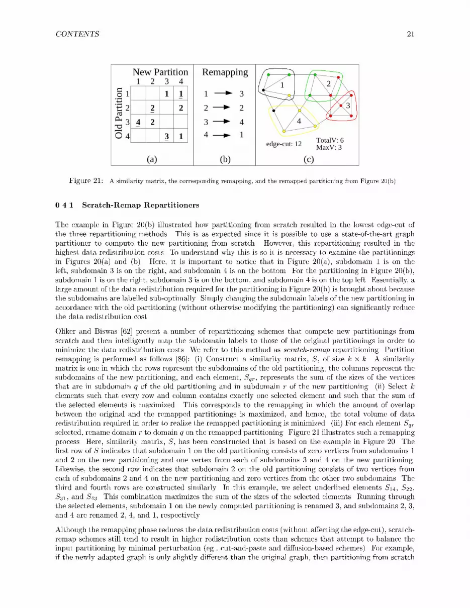
Figure 21: A similarity matrix, the corresponding remapping, and the remapped partitioning from Figure 20(b).0.4.1 Scratch-Remap RepartitionersThe example in Figure 20(b) illustrated how partitioning from scratch resulted in the lowest edge-cut ofthe three repartitioning methods. This is as expected since it is possible to use a state-of-the-art graphpartitioner to compute the new partitioning from scratch. However, this repartitioning resulted in thehighest data redistribution costs. To understand why this is so it is necessary to examine the partitioningsin Figures 20(a) and (b). Here, it is important to notice that in Figure 20(a), subdomain 1 is on theleft, subdomain 3 is on the right, and subdomain 4 is on the bottom. For the partitioning in Figure 20(b),subdomain 1 is on the right, subdomain 3 is on the bottom, and subdomain 4 is on the top left. Essentially, alarge amount of the data redistribution required for the partitioning in Figure 20(b) is brought about becausethe subdomains are labelled sub-optimally. Simply changing the subdomain labels of the new partitioning inaccordance with the old partitioning (without otherwise modifying the partitioning) can signi�cantly reducethe data redistribution cost.Oliker and Biswas [62] present a number of repartitioning schemes that compute new partitionings fromscratch and then intelligently map the subdomain labels to those of the original partitionings in order tominimize the data redistribution costs. We refer to this method as scratch-remap repartitioning. Partitionremapping is performed as follows [86]: (i) Construct a similarity matrix, S, of size k � k. A similaritymatrix is one in which the rows represent the subdomains of the old partitioning, the columns represent thesubdomains of the new partitioning, and each element, Sqr, represents the sum of the sizes of the verticesthat are in subdomain q of the old partitioning and in subdomain r of the new partitioning. (ii) Select kelements such that every row and column contains exactly one selected element and such that the sum ofthe selected elements is maximized. This corresponds to the remapping in which the amount of overlapbetween the original and the remapped partitionings is maximized, and hence, the total volume of dataredistribution required in order to realize the remapped partitioning is minimized. (iii) For each element Sqrselected, rename domain r to domain q on the remapped partitioning. Figure 21 illustrates such a remappingprocess. Here, similarity matrix, S, has been constructed that is based on the example in Figure 20. The�rst row of S indicates that subdomain 1 on the old partitioning consists of zero vertices from subdomains 1and 2 on the new partitioning and one vertex from each of subdomains 3 and 4 on the new partitioning.Likewise, the second row indicates that subdomain 2 on the old partitioning consists of two vertices fromeach of subdomains 2 and 4 on the new partitioning and zero vertices from the other two subdomains. Thethird and fourth rows are constructed similarly. In this example, we select underlined elements S14, S22,S31, and S43. This combination maximizes the sum of the sizes of the selected elements. Running throughthe selected elements, subdomain 1 on the newly computed partitioning is renamed 3, and subdomains 2, 3,and 4 are renamed 2, 4, and 1, respectively.Although the remapping phase reduces the data redistribution costs (without a�ecting the edge-cut), scratch-remap schemes still tend to result in higher redistribution costs than schemes that attempt to balance theinput partitioning by minimal perturbation (eg., cut-and-paste and di�usion-based schemes). For example,if the newly adapted graph is only slightly di�erent than the original graph, then partitioning from scratch

CONTENTS 22

(a) (b) (c)Figure 22: An imbalanced partitioning and two repartitioning techniques. The partitioning in (a) is imbalanced. It isbalanced by an incremental method in (b) and by a scratch-remap method in (c).could produce a new partitioning that is still substantially di�erent from the original, and thus requiresmany vertices to be moved even after the remapping phase. On such a graph, the imbalance could easilybe corrected by moving only a small number of vertices. Figure 22 illustrates an example of this. Thepartitioning in Figure 22(a) is slightly imbalanced as the upper-right subdomain has �ve vertices, while theaverage subdomain weight is four. In Figure 22(b), the partitioning is balanced by moving only a singlevertex from the upper-right subdomain to the lower-right subdomain. Therefore both TotalV and MaxVare one. Figure 22(c) shows a new partitioning that has been computed from scratch and then optimallyremapped to the partitioning in Figure 22(a). Despite this optimal remapping, repartitioning has a TotalVof seven and a MaxV of two. All three of the partitionings have similar edge-cuts.The reason that the scratch-remap scheme does so poorly here with respect to data redistribution is becausethe information that is provided by the original partitioning is not utilized until the �nal remapping process.At this point, it is too late to avoid high data redistribution costs even if we compute an optimal remapping.Essentially, the problem in our example is that the partitioning in Figure 22(a) is shaped like a `+', whilethe partitioning in Figure 22(c) forms an `x'. Both of these are of equal quality and so a static partitioningalgorithm could easily compute either of these. However, we would like the partitioning algorithm usedin a scratch-remap repartitioner to drive the computation of the partitioning towards that of the originalpartitioning whenever possible without a�ecting the quality. A scratch-remap algorithm can potentially dothis if it is able to extract and use the information implicit in the original partitioning during the computationof the new partitioning. An algorithm called Locally-Matched Multilevel Scratch-Remap (or simply LMSR)that tries to accomplish this is presented in [80]. LMSR decreases the amount of data redistribution requiredto balance the graph compared to current scratch-remap schemes, particularly for slightly imbalanced graphs[80].0.4.2 Di�usion-based RepartitionersDi�usive load balancing schemes attempt to minimize the di�erence between the original partitioning andthe �nal repartitioning by making incremental changes in the partitioning to restore balance. Subdomainsthat are overweight in the original partitioning export vertices to adjacent subdomains. These, in turn, mayfurther export vertices to their neighbors in an e�ort to reach global balance. By limiting the movement ofvertices to neighboring subdomains, these schemes attempt to minimize the edge-cut and maintain connectedsubdomains. As an example, the repartitioning in Figure 20(d) is obtained by a di�usive process. In thiscase, subdomain 3 migrates a vertex to each of subdomains 2 and 4. This, in turn, causes the recipientsubdomains to become overweight. They then each migrate a vertex to subdomain 1.Any di�usion-based repartitioning scheme needs to address two questions: (i) How much work should betransferred between processors? and (ii) Which tasks should be transferred? The answer to the �rst questiontells us how to balance the partitioning, while the answer to the second tells us how to minimize the edge-cut

CONTENTS 23as we do this. A lot of work has focused on answering the �rst question in the context of balancing unrelatedtasks that are unevenly distributed among processors [8, 14, 15, 39, 40, 41, 103, 105]. These take the machinearchitecture, but do not take the interdependencies of the tasks into consideration when computing theamount of work to transfer between processors. More recently, in the context of adaptive computationalsimulations, work has focused not only on how much, but also which tasks to transfer [18, 63, 64, 66, 69, 79,80, 85, 90, 91, 97, 98]. In the rest of this section, we focus on these schemes.Schemes for determining how much work to transfer between processors can be grouped into two categories.We refer to di�usion schemes in which the exchange of work among the processors is based only upontheir respective work loads (and not upon the loads of distant processors) [79] as local di�usion algorithms.In other schemes [18, 63, 64, 66, 69, 79, 80, 85, 90, 91, 97, 98], global views of the processor loads are used tobalance the partitioning. We call these global di�usion schemes. Most global di�usion schemes either performdi�usion in a recursive bisection manner [18, 85, 91], utilize space-�lling curves [64, 66, 69], or else compute ow solutions [63, 79, 80, 97, 98] that prescribe the amount of work to be moved between pairs of processors.Recursive bisection di�usion schemes [18, 85, 91] split the subdomains into two groups, and then attempt tobalance these groups. Next, both of the (balanced) groups are split in two and the algorithm recurses onthese subgroups.Adaptive space-�lling curve partitioners [64, 66, 69] can compute repartitionings by maintaining the originalordering of the mesh elements. Here, the weights associated with the ordered mesh elements are changedto re ect the structural changes in the computation. All that is required to compute a repartitioning is torecompute the k-way splitting of the ordered list with respect to the new weights.Flow solutions are usually computed in order to optimize some objective. Ou and Ranka [63] present aglobal di�usion scheme that optimally minimizes the one-norm of the ow using linear programming. Huand Blake [41] present a method that optimally minimizes the two-norm of the ow. They prove that sucha ow solution can be obtained by solving the linear equation (�L)� = b, where b is the vector containingthe load of each subdomain minus the average subdomain load, L is the Laplacian matrix (as de�nedin Section 0.3.3) of the graph that models the subdomain connectivity (i. e., the subdomain connectivitygraph), and �, the ow solution, is a vector with k elements. An amount of vertex weight equal to �q � �rneeds to be moved from subdomain q to subdomain r for every r that is adjacent to q in order to balancethe partitioning. Figure 23 illustrates the di�erence between one- and two-norm minimization of the owsolution. This �gure shows the subdomain connectivity graph for a nine-way partitioning along with thetwo di�erent ow solutions. Here, the two dark subdomains are overweight by ten, while the two whitesubdomains are underweight by ten. The weight of the rest of the subdomains equals the average subdomainweight. The ow solution in Figure 23(a) minimizes the one-norm of the data movement [63]. The owsolution in Figure 23(b) minimizes the two-norm of the data movement [41]. The one-norm minimizationsolution sends most of the ow through a few links, while the two-norm minimization solutions more evenlydistributes the ow through the links, but results in greater total ow.The ow solution indicates how much vertex weight needs to be transfered between each pair of adjacentsubdomains. The second problem is to determine exactly which vertices to move so as to minimize theedge-cut of the resulting partitioning. One possibility is to repeatedly transfer layers of vertices along thesubdomain boundary until the desired amount of vertex weight has been transferred [63, 91]. A more precisescheme is to move one vertex at a time across the subdomain boundary, each time selecting the vertex thatwill result in the smallest edge-cut [97]. This scheme, like the KL/FM algorithm, utilizes only a local viewof the graph, and thus, can make (globally) poor selections. This problem can be corrected if the transferof vertices is performed in a multilevel context [79, 98]. Such schemes, called multilevel di�usion algorithms,perform graph coarsening, and then begin di�usion on the coarsest graph. During the uncoarsening phase,vertices are moved to achieve (or maintain) load balance, while also trying to improve the edge-cut. Bybeginning di�usion on the coarsest graph, these algorithms are able to move large chunks of highly connectedvertices in a single step. Thus, the bulk of the work required to balance the partitioning is done quickly.Furthermore, by moving highly connected vertices together, high-quality edge-cuts can often be maintained.Experimental results show that multilevel di�usion can compute partitionings of higher quality than schemesthat perform di�usion only on the original graph [79, 98] and is often faster.

CONTENTS 24

(a)one-norm: 40two-norm: 400

10

10

10

10

(b)one-norm: 51.4two-norm: 245.6

5.7

5.7

5.7

5.7

4.3

4.34.3

4.3

1.4 1.4

1.4

2.9

2.9

1.4

Figure 23: Two di�erent ow solutions for the subdomain graph of an imbalanced partitioning. The one-norm of the datamigration is minimized in (a). The two-norm of the data migration is minimized in (b).For partitioned graphs that are highly imbalanced in localized areas, di�usion-based schemes require verticesto propagate over longer distances. For this class of problems, it is bene�cial to determine not only howmuch and which vertices to move, but also when vertices should move [15]. A di�usion algorithm, calledWavefront Di�usion that determines the best time to migrate vertices is presented in [80]. In WavefrontDi�usion, the ow of vertices moves in a wavefront starting from the most overweight subdomains. Thismethod guarantees that all subdomains will contain the largest possible selection of vertices when it istheir turn to export vertices. Thus, subdomains are able to select those vertices for migration that willbest minimize edge-cut and data redistribution costs. Wavefront Di�usion obtains signi�cantly lower dataredistribution costs while maintaining similar or better edge-cut results compared to di�usion schemes thatdo not determine the best time to migrate vertices, especially for partitionings that are highly imbalancedin localized areas [80].Tradeo� Between Edge-cut and Data Redistribution Costs Often, the objective of minimizingthe data redistribution cost is at odds with the objective of minimizing the edge-cut. For applications inwhich the mesh is frequently adapted or the amount of state associated with each element is relatively high,minimizing the data redistribution cost is preferred over minimizing the edge-cut. For applications in whichrepartitioning occurs infrequently, the key objective of a repartitioning scheme is going to be in obtainingthe minimal edge-cut.While a number of coarsening and re�nement heuristics have been developed [79, 93] that can control thetradeo� between these two objectives, many adaptive partitioners naturally minimize one in preference to theother. For example, compared against each other, the LMSR and Wavefront Di�usion algorithms present aclear tradeo� between edge-cut and data redistribution costs [80]. That is, the Wavefront Di�usion algorithmtends to minimize the amount of data redistribution required to realize the balanced repartitioning, whilethe LMSR algorithm tends to minimize the edge-cut of the repartitioning.0.5 Parallel Graph PartitioningThe ability to perform partitioning in parallel is important for many reasons. The amount of memory onserial computers is often not enough to allow the partitioning of graphs corresponding to large problems thatcan now be solved on massively parallel computers and workstation clusters. A parallel graph partitioningalgorithm can take advantage of the signi�cantly higher amount of memory available in parallel computersto partition very large graphs. Also, as heterogenous systems of parallel machines are integrated into singlesystem of systems (eg., the NASA Information Power Grid [42]), the role of graph partitioning will change.Here, the exact number of processors and/or the architectural characteristics of the hardware assignedto a computation will not be known until immediately before the computation is permitted to execute.

CONTENTS 25Parallel graph partitioning is crucial for e�ciency in such an environment. In the context of adaptive graphpartitioning, the graph is already distributed among processors, but needs to be repartitioned due to thedynamic nature of the underlying computation. In such cases, having to bring the graph to one processorfor repartitioning can create a serious bottleneck that could adversely impact the scalability of the overallapplication.Work in parallel graph partitioning [3, 23, 30, 49, 51, 77, 94] has been focused on geometric [30, 77], spectral[3], and multilevel partitioning schemes [49, 51, 94]. Geometric graph partitioning algorithms tend to be quiteeasy to parallelize. Typically, these require a parallel sorting algorithm. Spectral and multilevel partitionersare more di�cult to parallelize. Their parallel asymptotic run times are the same as that of performing aparallel matrix-vector multiplication on a randomly partitioned matrix [51]. This is because the input graphis not well-distributed across the processors. If the graph is �rst partitioned and then distributed across theprocessors accordingly, the parallel asymptotic run times of spectral and multilevel partitioners drop to thatof performing a parallel matrix-vector multiplication on a well-partitioned matrix. Essentially, performingthese partitioning schemes e�ciently in parallel requires a good partitioning of the input graph [51, 94]. Ofcourse, we cannot expect the input graph to already be partitioned in the case of static graph partitioning,since this is exactly what we are trying to do. However, for the adaptive graph partitioning problem, wecan expect the input partitioning to be of high quality (that is, have a low edge-cut, even though it willbe imbalanced). For this reason, parallel adaptive graph partitioners [80, 98] tend to run signi�cantly fasterthan static partitioners.Since the run times of most parallel geometric partitioning schemes are not a�ected by the initial distributionof the graph, they can essentially be used to compute a partitioning for the partitioning algorithm. That is,a rough partitioning of the input graph can be computed by a fast geometric approach. This partitioningcan be used to redistribute the graph prior to performing parallel multilevel (or spectral) partitioning [52].Use of this \boot-strapping" approach signi�cantly increases the parallel e�ciency of the more accuratepartitioning scheme by providing it with data locality.Parallel multilevel algorithms for graph partitioning are available in the ParMeTiS [52] and JOSTLE [92]libraries.0.6 Multi-constraint, Multi-objective Graph PartitioningIn recent years, with advances in the state-of-the-art of scienti�c simulation, sophisticated classes of com-putations such as multi-phase, multi-physics, and multi-mesh simulations have become commonplace. Formany of these, the traditional graph partitioning formulation is not adequate to ensure their e�cient execu-tion on high performance parallel computers. Instead, new graph partitioning formulations and algorithmsare required to meet the needs of these. In this section, we describe some important classes of scienti�c simu-lations that require more generalized formulations of the graph partitioning problem in order to ensure theire�ciency on high performance machines, we discuss these requirements, and we describe new, generalizedformulations of the graph partitioning problem as well as algorithms for solving these problem.Multi-physics Simulations In multi-physics simulations, a variety of materials and/or processes aresimulated together. The result is a class of problems in which the computation as well as the memory re-quirements are not uniform across the mesh. Existing partitioning schemes can be used to divide the meshamong the processors such that either the amount of computation or the amount of memory required isbalanced across the processors. However, they cannot be used to compute a partitioning that simultane-ously balances both of these quantities. Our inability to do so can either lead to signi�cant computationalimbalances, limiting e�ciency, or signi�cant memory imbalances, limiting the size of problems that can besolved using parallel computers. Figure 24 illustrates this problem. It shows a graph in which the amountof computation and memory associated with a vertex can be di�erent throughout the graph, and gives threepossible partitionings of it. The partitioning in Figure 24(b) balances the computation among the subdo-mains, but creates a serious imbalance for memory requirements. The partitioning in Figure 24(c) balancesthe memory requirement, while leaving the computation imbalanced. The partitioning in Figure 24(d), that

CONTENTS 26

(a) (b) (c) (d)edge-cut: 4computation: 18 and 18memory: 20 and 44

edge-cut: 4

memory: 32 and 32

edge-cut: 6computation: 18 and 18memory: 32 and 32

computation: 24 and 12computationmemoryFigure 24: An example of a computation with non-uniform memory requirements. Each vertex in the graph is split intotwo amounts. The size of the lightly-shaded portion represents the amount of computation associated with the vertex, whilethe size of the dark portion represents the amount of memory associated with the vertex. The bisection in (b) balances thecomputation. The bisection in (c) balances the memory, but only the bisection in (d) balances both of these.

Figure 25: A particle-in-cell computation. Here, both the mesh nodes and the particles must be balanced across thesubdomains.balances both of these, is the desired solution. In general, multi-physics simulations require the partitioningto satisfy not just one, but a multiple number of balance constraints. (In this case, the partitioning mustbalance two constraints, computation and memory).Multi-phase Simulations Multi-phase simulations consist ofm distinct computational phases, each sepa-rated by an explicit synchronization step. In general, the amount of computation performed for each elementof the mesh is di�erent for di�erent phases. The existence of the synchronization steps between the phasesrequires that each phase be individually load balanced. That is, it is not su�cient to simply sum up therelative times required for each phase and to compute a decomposition based on this sum. Doing so maylead to some processors having too much work during one phase of the computation (and so, these may stillbe working after other processors are idle), and not enough work during other phases (and so these maybe idle while other processors are still working). Instead, it is critical that every processor have an equalamount of work from all of the phases of the computation. A traditional partitioning scheme can be usedto balance the load across the processors for a single phase of the computation. However, the load may beseriously imbalanced for the other phases. Another method is to use m distinct partitionings, each of whichbalances the load of a single phase only. This method requires that costly data redistribution be performedafter each phase in order to realize the partitioning corresponding to the next phase. A better method is

CONTENTS 27

Figure 26: An internal combustion engine simulation is an example application whose computation is performed in multiplephases. Each shade represents elements active during a di�erent phase. (Figure provided by Analysis and Design ApplicationCompany Limited.)to compute a single partitioning that simultaneously balances the work performed in each of the phases. Inthis case, no redistribution of the data is necessary, and all of the phases are well balanced.Figure 25 shows an example. The graph in Figure 25 represents a simulation of particles moving througha mesh. This computation is composed of two phases. The �rst phase is a mesh-based computation. Thesecond phase is a particle-based computation. In order to load-balance such a computation, each processormust have a roughly equal amount of both the mesh computation and the particle computation. One suchbisection is shown that splits both the mesh elements and the particles in half.Figure 26 shows another example. This is the mesh associated with the numerical simulation of the portsand the combustion chamber of an internal combustion engine. In this particular problem, the overallcomputation is performed in six phases. (Each corresponding to a di�erent shade in the �gure.) In orderto solve such a multi-phase computation e�ciently on a parallel machine, every processor should containan equal number of mesh elements of each di�erent shade. Figure 27 shows two subdomains of an 8-waypartitioning of the mesh in Figure 26. This partitioning balances all six phases while also minimizing theinter-processor communications. (Note that not all of the shades are visible in Figures 26 and 27.)Multi-mesh Computations An important class of emerging numerical methods are multi-mesh compu-tations. Multiple meshes arise in several settings that use grids to discretize partial di�erential equations.For example, some operations are innately more e�cient on structured grids, such as radiation transportsweeps or FFTs. However, complex geometries are better �tted with unstructured meshes. In some simula-tions, both kinds of grids may be used throughout the computation. Similarly, various codes that solve formultiple physical quantities may use separate grids to solve the appropriate equations for each variable. Forexample, consider a simulation of the welding of a joint between two parts, a process in which the parts arepressed together and thermally annealed [70]. One grid could be used for the solution of the stress-strainrelations that mediate the mechanical deformation of the parts. A second grid could be used to solve theheat equation for thermal conduction in the system. Since the regions of high strain may be distinct fromthose with high thermal gradients, each grid can be individually tailored to accurately represent the relevantphysics.Now consider the implementation of such a multi-physics example on a distributed-memory parallel machine.A typical time-step consists of computing a solution on the �rst mesh, interpolating the result to the secondmesh, computing a solution on the second mesh, interpolating it back to the �rst mesh, and so on. One way ofperforming this type of computation in parallel is to partition the meshes separately so that every processorhas a portion of each mesh. This approach will balance the computations and minimize the communicationsduring each of the solution phases. However, because the di�erent meshes are partitioned independently,

CONTENTS 28

Figure 27: Two subdomains of an 8-way partitioning computed by the multi-constraint graph partitioner implemented inMeTiS 4.0 are shown. Note, that all of the subdomains have an equal number of elements of each shade (although they are notall visible). (Figure provided by Analysis and Design Application Company Limited.)there is no assurance that an individual processor will own portions of the meshes that spatially overlap.Therefore, the amount of communication performed during the interpolation and transfer of the solutiondata can be quite high, even if an e�cient approach is used to manage this communication [70]. Ideally,we would like to partition the di�erent meshes such that each processor performs an equal amount of workfor every mesh, and at the same time, the amount of inter-processor communications required during thecomputations of the solutions, as well as that required during the interpolation and transfer of the solutions,is minimized.Domain Decomposition-based Preconditioners The two keys to the e�cient solution of systems ofsparse linear equations via iterative methods are (i) the ability to perform the matrix-vector multiplicatione�ciently in parallel, and (ii) minimizing the number of iterations required for the method to converge. Thematrix-vector multiplication is typically implemented by �rst reordering the sparse matrix such that thenumber of non-zero elements that are o� of the block diagonal is minimized and then utilizing a striped par-titioning of the matrix and the vector. Here, an interprocessor communication is required for every non-zeroelement o� of the block-diagonal. A high-quality partitioning of the graph corresponding to the sparse matrixprovides a re-ordering such that the number of interprocessor communications is minimized. Minimizing thenumber of iterations required for the solution to converge can be done by the use of various preconditioners.A number of preconditioning schemes have been developed that construct a preconditioner of each block ofthe block diagonal separately, and then combine these to use as a preconditioner for the entire matrix. (eg.,block diagonal preconditioners and local ILU preconditioners). Essentially, these preconditioners ignore theintra-subdomain interactions that are represented by the non-zero elements o� of the block diagonal.Since the matrix re-ordering is commonly obtained by a graph partitioner, this ensures that the number ofnon-zeros that are ignored in the preconditioner is relatively small. Therefore, the matrix-vector multiplica-tions will be computed e�ciently. However, this ordering is not computed to try and minimize the magnitudeof these ignored non-zeros. Therefore, it could be the case that while the number of non-zero elements issmall, the sum of the ignored non-zeros is quite large. The consequence of this is that the preconditioner maynot be as e�ective as it could be if the sum of the ignored elements was minimized [55]. That is, the numberof iterations for the method to converge may not be minimized. The magnitude of the ignored elements couldbe minimized directly by a partitioning that is computed using the magnitude of the elements as the edgeweights of the graph. However, such an approach will not minimize the communication overhead incurred bythe matrix-vector multiplication. This is because such an ordering computed in this way would not minimizethe number of the ignored elements. Ideally, we would like to obtain an ordering that minimizes both the

CONTENTS 292

1

1

11

25

2

1

3

5

10

3

12

12

22

1

3

2

1

51

1

1

55

5

1

2

3

10

3

12

2

1

1

2

2

1

3

2

1

51

1

55

5

10

3

12

2

2

1

1

5

2

1

3

5

3

12

12

21

2

101

2

2

1

2

1

3

1

2

1

1

5

55

5

10

3

2

2

1

5

2

5

3

12

2

2

1

1

3

2

1

1

2

31

2

2

1

1

12

2

3

10

1

1

1

1

12

edge-cut: 12magnitude: 66

(a) (b)edge-cut: 23magnitude: 36

edge-cut: 15magnitude: 45

(c)Figure 28: Three di�erent partitionings for the graph that corresponds to a sparse symmetric matrix. The partitioning in (a)minimizes the edge-cut. The partitioning in (b) minimizes the magnitude of the ignored non-zero elements o� of the diagonal.The partitioning in (c) minimizes both of these simultaneously.1

1

3

3

1

1

5

2

2

10

10

1

1

12

12

1

12

12

10

12

1

3 2

5

5

1 2

3

3

5

1

2

2

5 2

2

1

2

52

2

1

1

1

1

2

5 3

15

22

2

5

1

3

1

1

1

5

1

1

10

2

2

3

3

2

2

2

5

11

5

1

3 --

--

--

--

--

--

--

--

--

--

--

--

--

--

--

--

--

--

--

--

12

1

2

2

--

--

--

--

--

--

--

--

--

--

--

--

--

--

--

--

--

--

--

-- 1

1

3

3

5

5

1

1

3

3

12

12

1

15

5

2

2

3

3

1

1

1

1

1

1

5

5

1

1

10

10

2

2

5

5

1

1

2

2

2

2

5

5

2

2

1

1

2

2

2

2

12

12

10

10

1

1

3

3

1

1

1

1

1

1

2

2

2

2

5

5

12

12 3

3

5

5

1

1

1

1

3

3

3

3

12

12

1

1

2

2

5

5 2

2

3

3 1

1

1

1

5

5

1

1

2

2

10

10

5

5

2

2

2

2

1

1

2

2

1

1

12

12

10

10

1

1

12

12

1

1

1

1

3

3

5

5

3

3

2

2

1

1 5

5

2

2

2

2 2

2

1

1

--

--

--

--

--

--

--

--

--

--

--

--

--

--

--

--

--

--

--

--

(a) (b) (c)Figure 29: Three orderings for a sparse matrix that correspond to the partitionings given in Figure 28.number of intra-domain interactions (reducing the communication overhead) and the numerical magnitudeof these interactions (potentially leading to a better preconditioner).Figures 28 and 29 illustrate an example of this problem. Figure 28(a) shows a partitioning of a graphthat minimizes the edge-cut. Figure 29(a) shows the corresponding matrix ordered with respect to thispartitioning. Here, there are only a small number of ignored non-zero entries o� of the diagonal. However,their magnitudes are high compared to the other elements. Figure 28(b) shows a partitioning of a graphthat minimizes the magnitude of the ignored entries and Figure 29(b) shows the matrix ordered accordingly.Here, there are quite a bit more ignored entries compared to the ordering shown in Figure 29(a). However,the magnitudes of these entries are small. Figures 28(c) and 29(c) show the partitioning that attempt tominimize both the number and the magnitude of the ignored entries as well as the corresponding matrix.0.6.1 A Generalized Formulation for Graph PartitioningThe common characteristic of these problems is that they all require the computation of partitionings thatsatisfy an arbitrary number of balance constraints and/or an arbitrary number of optimization objectives.Traditional graph partitioning techniques have been designed to balance only a single constraint (i.e., thevertex weight) and to minimize only a single objective (i.e., the edge-cut). An extension of the graph

CONTENTS 30

(1,0,0)

(1,0,0)

(1,0,0)

(1,0,0)

(1,0,0)

(0,0,1)

(0,0,1)

(0,0,1)

(0,0,1)

(0,1,0)

(0,1,0)

(0,1,0)

(0,1,0)

(0,1,0)

(0,1,0)(0,1,0)

(1, 0)(1, 0)

(1, 0)

(1, 0)

(1, 0)

(1, 0)

(1, 0)

(1, 0)(1, 0)

(0, 1)

(0, 1)

(0, 1)

(0, 1)

(1, 0)

(1, 0)

(0, 1)

(0, 1)

(0, 1)

(0, 1) (0,1,0)

(1,0,0)

(0,0,1)

(1, 0)

(1, 0)

(1,0,0)

(0,1,0)

(0,0,1)

(a) (b)Figure 30: An example of two overlapping meshes (light circles and dark squares) along with dashed interpolation edges (a)and the corresponding multi-constraint multi-objective formulation (b).partitioning formulation that can model these problems is to assign a weight vector of size m to each vertexand a weight vector of size l to each edge. The problem then becomes that of �nding a partitioning thatminimizes the edge-cuts with respect to all l weights, subject to the constraints that each of the m weightsis balanced across the subdomains. This multi-constraint, multi-objective graph partitioning problem is ableto e�ectively model all of the problems described above.For example, the problem of balancing computation and memory can be modeled by associating a vectorof size two with each vertex (i.e., a two-constraint problem), where the elements of the vector represent thecomputation and memory requirements associated with the vertex. Similarly, the problem of computing anordering for a system of sparse linear systems that is preconditioned by a block-diagonal method can bemodeled by assigning a vector of size two to each edge (i.e., a two-objective problem), where the elements ofthe vector represent the number of non-zero entries (all ones in this case) and the magnitude of these entries.Computing decompositions for multi-mesh computations is a multi-constraint, multi-objective problem. Fig-ure 30 illustrates an example for a simple case with two meshes. Figure 30(a) shows a pair of overlappinggraphs (one with light, circular vertices and dotted edges and the other with dark, square vertices and solidedges). Additionally, dashed lines are included that show the interactions required in order to facilitate theinterpolation and transfer process. Figure 30(b) shows the graph that models this problem. Here, the twographs (and additional edges) from Figure 30(a) are combined. Every square vertex is given a weight of (1,0) and every circular vertex is given a weight of (0, 1). Solid edges are weighted (1, 0, 0). Dotted edges areweighted (0, 1, 0). Dashed edges are weighted (0, 0, 1). (Note, that not all of the vertices and edges arelabeled here.) Figure 31 gives a four-way partitioning of this graph. Here, both types of vertices are balancedand their edge-cuts are minimized. At the same time, minimizing the number of dashed edges cut has helpedto ensure that regions from the two graphs that spatially overlap tend to be in the same subdomain. Thisminimizes the communications incurred by the interpolation and transfer process.Multi-constraint Graph PartitioningTheoretical work relating to multi-constraint graph partitioning includes the Ham-sandwich Theorem and itsgeneralization [87]. This theorem states that a single plane can divide three bounded and connected regionsequally in half in a three-dimensional space. If two of the regions are interpreted as slices of bread and oneas a slice of ham, then the conclusion is that a single stroke of a knife can evenly divide the sandwich in twoso that all three slices are cut exactly in half. Also, Djidjev and Gilbert [19] proved that if a vertex separator

CONTENTS 31

solid edge-cut: 10 dotted edge-cut: 12 dashed edge-cut: 12

1

1

3

2

4

Figure 31: The partitioned meshes from Figure 30.theorem holds for a class of graphs (for example, Lipton and Tarjan's planar separator theorem [56]), thenthe theorem also holds for graphs in which the vertices have an arbitrary number of distinct weights.Multi-constraint graph partitioning algorithms have recently been developed by a number of researchers [47,71, 82, 100, 102]. These vary in their generality and complexity. A method is presented in [100] that utilizesa slight modi�cation of a traditional graph partitioner as a black box in order to compute partitioningsfor multi-phase computations. This method partitions disjoint subsets of vertices sequentially. Vertices aregrouped together depending on the �rst phase of the multi-phase computation in which they are active.After a set of vertices is partitioned, their subdomains are locked. Subsequent partitioning of other sets ofvertices are in uenced by the locked vertices. In this way, free vertices that are highly connected to lockedvertices are likely to be assigned to the same subdomains as their neighbors. This scheme is su�cient forpartitioning the multi-phase mesh shown in Figure 26.A more complex and more general algorithm is presented in [47]. This is a multilevel scheme that extendsthe coarsening and re�nement phases to handle multiple balance constraints. A key component of thisalgorithm is the initial partitioning algorithm. Here, a partitioning needs to be computed that balancesmultiple constraints. The authors present a lemma that proves that a set of two-weight objects can bepartitioned into two disjoint subsets such that the di�erence between either of the weights of the two sets isbounded by twice the maximum weight of any object. They further show that this bound can be generalizedto m weights. However in this case, maintaining the weight bound depends on the presence of su�cientlymany objects with certain weight characteristics (an assumption that usually holds for medium- to large-sizegraphs). The lemma leads to an algorithm for computing such a bisection. This scheme is su�cient fora wide range of multi-phase, multi-physics, and multi-mesh simulations (including the example shown inFigure 26).A parallel formulation of the multi-constraint partitioner [47] is described in [82]. Experimental results showthat this formulation can e�ciently compute partitionings of similar quality to the serial algorithm andscales to very large graphs. For example, the parallel multi-constraint graph partitioner is able to computea three-constraint 128-way partitioning of a 7 million vertex graph in about 7 seconds on 128 processors ofa Cray T3E.Multi-objective Graph PartitioningFor any single-objective optimization problem (such as the traditional graph partitioning problem), anoptimal solution exists in the feasible solution space. In multi-objective optimization, there is no single

CONTENTS 32

2nd

obje

ctiv

e1st objectiveFigure 32: A number of solution points for a two-objective optimization problem. The lightly-shaded points are Paretooptimal.

pareto frontier

pareto-optimal points

optimally minimal values

2nd

obje

ctiv

e

1st objective

..

.

Figure 33: The Pareto frontier for a two-objective optimization problem. The optimally minimal values of each objectiveare also shown.overall optimal solution, although there is an optimal solution for each one of the objectives. Consider theset of solution points for the two-objective optimization problem shown in Figure 32. The optimally minimalvalues for the two objectives are shown by the dashed lines. In this set, two unique points have the (same)optimal value for the �rst objective. However, their values for the second objective di�er from each other.Clearly, we would prefer the lightly-shaded point over the black point, as this one is equal with respect tothe �rst objective and has a better (i. e., smaller) value for the second objective. In fact, in this set ofsolution points, we can quickly determine that most of the points are not of interest. The solutions thatare of interest are those that are not dominated by any other solution, regardless of whether or not theyhave optimal values for any of the objectives. These are called the Pareto-optimal points. A solution isPareto-optimal if there is no feasible solution for which one can improve the value of any objective withoutworsening the value of at least one other objective [57]. In Figure 32, the lightly-shaded points (and onlythese points) are Pareto-optimal. The set of all of Pareto-optimal points is called the Pareto frontier [57].(See Figure 33.) In general, multi-objective optimization problems have many Pareto-optimal solutions.One of the implications of multiple Pareto-optimal solutions is that the de�nition of the desired solutionbecomes ambiguous. Every multi-objective optimization scheme requires that some method be used in orderto disambiguate the de�nition of a desired solution. In the context of multi-objective graph partitioning, theuser should specify the area along the Pareto frontier in which they are interested, and by doing so, controlthe tradeo�s among the objectives.The key challenge in solving the multi-objective partitioning problem is to allow the user to control the

CONTENTS 33tradeo�s among the di�erent objectives. This is particularly di�cult when the objectives are dissimilar innature, as such objectives cannot readily be combined. A new method of reformulating the multi-objectivegraph partitioning problem so that it can be solved using a traditional (i. e., single-objective) partitioneris presented in [81]. This method provides the user with a �ne-tuned control of the tradeo�s among theobjectives, results in predictable partitionings, and is able to handle dissimilar objectives. Speci�cally, thealgorithm computes a multi-objective partitioning based on a user-speci�ed preference vector. This vectordescribes how the tradeo�s among the objectives should be enforced. For example, if there are two objectivesand the user supplies a preference vector of (1, 1), then the algorithm will allow one objective to move awayfrom its optimal value by some amount only if the other objective moves towards its optimal value by morethan that amount. For the case of three objectives with a preference vector of (6, 2, 1), the algorithm willmake a re�nement move only if 6x > �(2y + z) where x is the gain with respect to the �rst objective, y isthe gain with respect to the second objective, and z is the gain with respect to the third objective.A number of multi-constraint and multi-objective graph partitioning algorithms as well as some of theirparallel formulations have been implemented in the MeTiS [46] and ParMeTiS [52] libraries. Serial andparallel multi-phase partitioning algorithms [100] are implemented in the JOSTLE [92] library.0.7 ConclusionsThe state-of-the-art in graph partitioning for high performance scienti�c simulations has improved dra-matically over the past decade. Improvements in the speed, accuracy, generality, and scalability of graphpartitioners have led to signi�cant milestones. For example, extremely large graphs (over 0.5 billion vertices)have been partitioned on machines consisting of thousands of processors [53]. However, despite impressiveachievements, there is still work to be done in the �eld. In this section, we discuss some of the limitationsof current graph partitioning problem formulations (many of which were highlighted by Hendrickson andKolda [34]), as well as areas of future work. We end this chapter by charting the functionality of some ofthe publically available graph partitioning software packages.Limitations of the Graph Partitioning Problem Formulation As discussed in Section 0.1, the edge-cut metric is not a precise model of the inter-processor communication costs incurred by parallel processing.Nor is it even a precise model of the total communications volume [32]. While the min-cut formulationhas proved e�ective for the well-shaped meshes that are common to scienti�c simulations, alternative for-mulations are still needed that can be used in more general cases. As an example of recent work in thisarea, Catalyurek and Aykanat [10] have developed a hypergraph partitioning formulation that preciselymodels total communication volume. Experimental results comparing the hypergraph partitioning modelto the traditional graph partitioning model show that for graphs of non-uniform degree, using the hyper-graph model can signi�cantly decrease the inter-processor communication costs compared to using the graphmodel. However, for graphs of uniform degree, the hypergraph model provides only a modest improvementand requires more run time compared to state-of-the-art graph partitioners [10]. While the hypergraphpartitioning formulation allows us to precisely minimize communications volume, it does not allow us tominimize other important components of inter-processor communication cost such as the message startuptime or the time required for the processor with the most communication (i. e., minimize the maximumprocessor communication time). Developing new formulations and algorithms that do so is an open area ofresearch in the �eld.Other Application Modeling Limitations In addition to being imprecise, the traditional partitioningformulation is inadequate for many important classes of scienti�c simulation. For example, the standardgraph partitioning formulation can e�ectively model only square, symmetric sparse matrices. However, gen-eral rectangular and unsymmetric matrices are required for solving linear systems, least squares problems,and linear programs [33]. Bipartite graph partitioning [33] and multi-constraint graph partitioning [47, 82]can be e�ective for these types of applications. Also, minimizing the edge-cut of a partitioning does notensure the numerical scalability of iterative methods. Numerical scalability means that as the number of pro-cessors increases, the convergence rate of the iterative solver remains constant. Vanderstraeten, Keunings,

CONTENTS 34and Farhat [89] have shown that the numerical scalability of a class of iterative solvers can be maintained ifpartitionings are computed such that their subdomains have low average aspect ratios. The traditional parti-tioning formulation does not optimize subdomain aspect ratios. Walshaw, Cross, Diekmann, and Schlimbackdeveloped graph partitioning schemes that attempt to minimize the average aspect ratio of the subdomains[96]. Experimental results show that these schemes are able to compute partitionings with signi�cantlybetter subdomain aspect ratios than traditional partitioners. However, they often result in worse edge-cuts.While these results are promising, it is desirable for a partitioning to minimize both of these objectives (i. e.,edge-cut and aspect ratio) simultaneously. Recent work in multi-objective graph partitioning [81] may alsobe relevant here to control the tradeo� between these two objectives.Architecture Modeling Limitations When traditional graph partitioners are used for mapping compu-tations onto parallel machines, there is an assumption that the target architecture is at and homogeneous[17, 34]. While it is true that many current architectures display similar computing powers, bandwidths,and latencies regardless of the processors involved, heterogenous and hierarchical architectures are becomingincreasingly commonplace. For example, consider the problem of decomposing a mesh for parallel process-ing on an architecture that consists of a cluster of heterogenous workstations connected by a high-speed,high-latency network to a distributed memory multiprocessor in which each node consists of a four-processorshared memory machine. Here, both the computational and communicational speeds depend on the speci�cprocessors involved. Standard graph partitioners do not take such considerations into account when com-puting a partitioning. Partitioning for heterogenous and hierarchical architectures is especially important inmeta-computing environments [42]. In such an environment, it may be impossible to predict the type (ortypes) of machines or even the exact number of processors that a simulation will be executed on until imme-diately prior to execution. In this case, both computational speeds and communication costs can uctuatewidely even between repeated executions of the same simulation. Alternative (eg., hierarchical and other[11, 88, 99]) partitioning methods are starting to be applied to such problems, but more work still needs tobe done.Functionality of Available Graph Partitioning Packages Many of the graph partitioning schemesdescribed in this chapter have been implemented in publically available software packages. Figure 34 chartsthe functionality of some the more widely used packages. These are Chaco [35], JOSTLE [92], MeTiS [46],ParMeTiS [52], PARTY [75], SCOTCH [67], and S-HARP [85].AcknowledgmentsThe authors would like to thank Rupak Biswas, Bruce Hendrickson, Abani Patra, Horst Simon, and ChrisWalshaw for their insightful comments on earlier drafts of this chapter.This work was supported by NSF CCR-9423082, by Army Research O�ce contracts DA/DAAG55-98-1-0441and DA/DAAH04-95-1-0244, by Army High Performance Computing Research Center cooperative agreementnumber DAAH04-95-2-0003/contract number DAAH04-95-C-0008, the content of which does not necessarilyre ect the position or the policy of the government, and no o�cial endorsement should be inferred. Accessto computing facilities was provided by AHPCRC, Minnesota Supercomputer Institute.

CONTENTS 35Cha

co

Jostl

eM

etis

ParMeti

s

PARTY

SCOTCH

S-HARP

Geometric Schemes

Coordinate Nested DissectionRecursive Inertial Bisection

Spectral Methods

Recursive Spectral BisectionMultilevel Spectral Bisection

Combinatorial Schemes

Levelized Nest DissectionKL/FM

Multilevel Schemes

Multilevel Recursive BisectionMultilevel k-way Partitioning

Parallel Graph Partitioners

Dynamic Repartitioners

Parallel Static PartitioningParallel Dynamic Partitioning

Other Formulations

Space-filling Curve Methods

Multi-constraint Graph PartitioningMulti-objective Graph Partitioning

Diffusive RepartitioningScratch-Remap Repartitioning

Multilevel Fill-reducing Ordering

Figure 34: A chart illustrating the functionality of a number of publically available software packages.

Bibliography[1] C. Ashcraft and J. Liu. A partition improvement algorithm for generalized nested dissection. Technical Report BCSTECH-94-020, York University, North York, Ontario, Canada, 1994.[2] C. Ashcraft and J. Liu. Using domain decomposition to �nd graph bisectors. Technical report, York University, NorthYork, Ontario, Canada, 1995.[3] S. Barnard. PMRSB: Parallel multilevel recursive spectral bisection. In Proc. Supercomputing '95, 1995.[4] S. Barnard and H. Simon. A fast multilevel implementation of recursive spectral bisection for partitioning unstructuredproblems. In Proc. 6th SIAM Conf. Parallel Processing for Scienti�c Computing, pages 711{718, 1993.[5] E. Barnes, A. Vannelli, and J. Walker. A new heuristic for partitioning the nodes of a graph. SIAM Journal on DiscreteMathematics, 1:299{305, 1988.[6] M. Berger and S. Bokhari. Partitioning strategy for nonuniform problems on multiprocessors. IEEE Transactions onComputers, C-36(5):570{580, 1987.[7] R. Biswas and R. C. Strawn. A new procedure for dynamic adaption of three-dimensional unstructured grids. AppliedNumerical Mathematics, 13:437{452, 1994.[8] J. Boillat. Load balancing and poisson equation in a graph. Concurrency: Practice and Experience, 2:289{313, 1990.[9] T. Bui and C. Jones. A heuristic for reducing �ll in sparse matrix factorization. In 6th SIAM Conf. Parallel Processingfor Scienti�c Computing, pages 445{452, 1993.[10] U. Catalyurek and C. Aykanat. Hypergraph-partitioning based decomposition for parallel sparse-matrix vector multipli-cation. IEEE Transactions on Parallel and Distributed Systems, 10(7):673{693, 1999.[11] J. Chen and V. Taylor. ParaPART: Parallel mesh partitioning tool for distributed systems. In Proc. IRREGULAR'99,1999.[12] Y. Chung and S. Ranka. Mapping �nite element graphs on hypercubes. Journal of Supercomputing, 6:257{282, 1992.[13] J. Cong and M. Smith. A parallel bottom-up clustering algorithm with applications to circuit partitioning in vlsi design.In Proc. ACM/IEEE Design Automation Conference, pages 755{760, 1993.[14] G. Cybenko. Dynamic load balancing for distributed memory multiprocessors. Journal of Parallel and DistributedComputing, 7(2):279{301, 1989.[15] R. Diekmann, A. Frommer, and B. Monien. E�cient schemes for nearest neighbor load balancing. Parallel Computing,25:789{812, 1999.[16] R. Diekmann, B. Monien, and R. Preis. Using helpful sets to improve graph bisections. In D. Hsu, A. Rosenberg, andD. Sotteau, editors, Interconnection Networks and Mapping and Scheduling Parallel Computations, volume 21, pages57{73. AMS Publications, DIMACS Volume Series, 1995.[17] R. Diekmann, B. Monien, and R. Preis. Load balancing strategies for distributed memory machines. Parallel andDistributed Processing for Computational Mechanics: Systems and Tools, 1998.[18] P. Diniz, S. Plimpton, B. Hendrickson, and R Leland. Parallel algorithms for dynamically partitioning unstructured grids.Proc. 7th SIAM Conf. Parallel Proc., pages 615{620, 1995.[19] H. Djidjev and J. Gilbert. Separators in graphs with negative and multiple vertex weights. Technical report, Dept. ofComputer Science, Rice University, 1994.[20] C. Fiduccia and R. Mattheyses. A linear time heuristic for improving network partitions. In In Proc. 19th IEEE DesignAutomation Conference, pages 175{181, 1982.[21] A. George and J. Liu. Computer Solution of Large Sparse Positive De�nite Systems. Prentice-Hall, Englewood Cli�s,NJ, 1981.[22] J. Gilbert, G. Miller, and S. Teng. Geometric mesh partitioning: Implementation and experiments. In Proceedings ofInternational Parallel Processing Symposium, 1995.[23] J. Gilbert and E. Zmijewski. A parallel graph partitioning algorithm for a message-passing multiprocessor. InternationalJournal of Parallel Programming, pages 498{513, 1987.36

BIBLIOGRAPHY 37[24] T. Goehring and Y. Saad. Heuristic algorithms for automatic graph partitioning. Technical Report UMSI-94-29, Universityof Minnesota Supercomputing Institute, 1994.[25] A. Gupta. Fast and e�ective algorithms for graph partitioning and sparse matrix reordering. IBM Journal of Researchand Development, 41(1/2):171{183, 1996.[26] W. Hager and Y. Krylyuk. Graph partitioning and continuous quadratic programming. SIAM Journal on DiscreteMathematics, To appear, 1999.[27] W. Hager, S. Park, and T. Davis. Block exchange in graph partitioning. In P. Pardalos, editor, Approximation andComplexity in Numerical Optimization: Continuous and Discrete Problems. Kluwer Academic Publishers, 1999.[28] K. Hall. An r-dimensional quadratic placement algorithm. Management Science, 17(3):219{229, 1970.[29] S. Hauck and G. Borriello. An evaluation of bipartitioning technique. In Proc. Chapel Hill Conference on AdvancedResearch in VLSI, 1995.[30] M. Heath and P. Raghavan. A Cartesian parallel nested dissection algorithm. SIAM Journal of Matrix Analysis andApplications, 16(1):235{253, 1995.[31] G. Heber, R. Biswas, and G. Gao. Self-avoiding walks over adaptive unstructured grids. Concurrency: Practice andExperience, to appear 2000.[32] B. Hendrickson. Graph partitioning and parallel solvers: Has the emperor no clothes? In Proc. Irregular'98, pages218{225, 1998.[33] B. Hendrickson and T. Kolda. Partitioning rectangular and structurally nonsymmetric sparse matrices for parallelprocessing. SIAM J. Sci. Comput. (to appear), 1999.[34] B. Hendrickson and T. Kolda. Graph partitioning models for parallel computing. Parallel Computing (to appear), 2000.[35] B. Hendrickson and R. Leland. The chaco user's guide, version 2.0. Technical Report SAND94-2692, Sandia NationalLaboratories, 1994.[36] B. Hendrickson and R. Leland. An improved spectral graph partitioning algorithm for mapping parallel computations.SIAM J. Sci. Comput., 16(2):452{469, 1995.[37] B. Hendrickson and R. Leland. A multilevel algorithm for partitioning graphs. Proceedings Supercomputing '95, 1995.[38] D. Hilbert. Uber die stetige abbildung einer linie auf ein achenstuck. Math Annalen, 38, 1891.[39] G. Horton. A multi-level di�usion method for dynamic load balancing. Parallel Computing, 9:209{218, 1993.[40] Y. Hu and R. Blake. An improved di�usion algorithm for dynamic load balancing. Parallel Computing, 25:417{444, 1999.[41] Y. Hu, R. Blake, and D. Emerson. An optimal migration algorithm for dynamic load balancing. Concurrency: Practiceand Experience, 10:467{483, 1998.[42] W. Johnston, D. Gannon, and B. Nitzberg. Grids as production computing environments: The engineering aspectsof nasa's information power grid. In Proc. Eighth IEEE International Symposium on High Performance DistributedComputing, 1999.[43] G. Karypis and V. Kumar. Analysis of multilevel graph partitioning. In Proceedings of Supercomputing '95, 1995.[44] G. Karypis and V. Kumar. A fast and high quality multilevel scheme for partitioning irregular graphs. SIAM Journalon Scienti�c Computing, 20(1):359{392, 1998.[45] G. Karypis and V. Kumar. hMeTiS 1.5: A hypergraph partitioning package. Technical report, Dept. of Computer Scienceand Engineering, Univ. of Minnesota, 1998.[46] G. Karypis and V. Kumar. MeTiS 4.0: Unstructured graph partitioning and sparse matrix ordering system. Technicalreport, Dept. of Computer Science and Engineering, Univ. of Minnesota, 1998.[47] G. Karypis and V. Kumar. Multilevel algorithms for multi-constraint graph partitioning. In Proceedings of Supercomputing'98, 1998.[48] G. Karypis and V. Kumar. Multilevel k-way partitioning scheme for irregular graphs. Journal of Parallel and DistributedComputing, 48(1), 1998.[49] G. Karypis and V. Kumar. A parallel algorithm for multilevel graph partitioning and sparse matrix ordering. Journal ofParallel and Distributed Computing, 48(1), 1998.[50] G. Karypis and V. Kumar. Multilevel k-way hypergraph partitioning. In Proceedings of the Design and AutomationConference, 1999.[51] G. Karypis and V. Kumar. Parallel multilevel k-way partitioning scheme for irregular graphs. Siam Review, 41(2):278{300,1999.[52] G. Karypis, K. Schloegel, and V. Kumar. ParMeTiS: Parallel graph partitioning and sparse matrix ordering library.Technical report, Dept. of Computer Science and Engineering, Univ. of Minnesota, 1997.[53] J. Keasler. Partitioning challenges in ale3d, 1999. Talk presented at the Workshop on Graph Partitioning and Applications:Current and Future Directions, AHPCRC, MN.[54] B. Kernighan and S. Lin. An e�cient heuristic procedure for partitioning graphs. The Bell System Technical Journal,49(2):291{307, 1970.

BIBLIOGRAPHY 38[55] D. Keyes, 1998. Personal communications.[56] R. Lipton and R. Tarjan. A separator theorem for planar graphs. SIAM Journal on Applied Mathematics, 36:177{189,1979.[57] M. Makowski. Methodology and a modular tool for multiple criteria analysis of lp models. Technical Report WP-94-102,IIASA, 1994.[58] G. Miller, S. Teng, W. Thurston, and S. Vavasis. Automatic mesh partitioning. In A. George, John R. Gilbert, andJ. Liu, editors, Sparse Matrix Computations: Graph Theory Issues and Algorithms. IMA Volumes in Mathematics andits Applications. Springer-Verlag, 1993.[59] G. Miller and S. Vavasis. Density graphs and separators. In Second Annual ACM-SIAM Symposium on DiscreteAlgorithms, pages 331{336, 1991.[60] B. Monien, R. Preis, and R. Diekmann. Quality matching and local improvement for multilevel graph-partitioning.Technical report, University of Paderborn, 1999.[61] B. Nour-Omid, A. Raefsky, and G. Lyzenga. Solving �nite element equations on concurrent computers. In A. K. Noor,editor, American Soc. Mech. Eng, pages 291{307, 1986.[62] L. Oliker and R. Biswas. PLUM: Parallel load balancing for adaptive unstructured meshes. Journal of Parallel andDistributed Computing, 52(2):150{177, 1998.[63] C. Ou and S. Ranka. Parallel incremental graph partitioning using linear programming. Proceedings Supercomputing '94,pages 458{467, 1994.[64] C. Ou, S. Ranka, and G. Fox. Fast and parallel mapping algorithms for irregular and adaptive problems. Journal ofSupercomputing, 10:119{140, 1996.[65] B. Parlett, H. Simon, and L. Stringer. On estimating the largest eigenvalue with the lanczos algorithm. Mathematics ofComputation, 38(137):153{165, 1982.[66] A. Patra and D. Kim. E�cient mesh partitioning for adaptive hp �nite element methods. In International Conferenceon Domain Decomposition Methods, 1998.[67] F. Pellegrini and J. Roman. SCOTCH: A software package for static mapping by dual recursive bipartitioning of processand architecture graphs. HPCN-Europe, Springer LNCS 1067, pages 493{498, 1996.[68] J. Pilkington and S. Baden. Partitioning with space�lling curves. Technical Report CS94-349, Dept. of Computer Scienceand Engineering, Univ. of California, 1994.[69] J. Pilkington and S. Baden. Dynamic partitioning of non-uniform structured workloads with space�lling curves. Technicalreport, Dept. of Computer Science and Engineering, Univ. of California, 1995.[70] S. Plimpton, B. Hendrickson, and J. Stewart. A parallel rendezvous algorithm for interpolation between multiple grids.In Proc. Supercomputing '99, 1999.[71] A. Poe and Q. Stout. Load balancing 2-phased geometrically based problems. In Proc. 9th SIAM Conf. Parallel Processingfor Scienti�c Computing, 1999.[72] A. Pothen. Graph partitioning algorithms with applications to scienti�c computing. In D. Keyes, A. Sameh, andV. Venkatakrishnan, editors, Parallel Numerical Algorithms. Kluwer Academic Press, 1996.[73] A. Pothen, H. Simon, and K. Liou. Partitioning sparse matrices with eigenvectors of graphs. SIAM Journal of MatrixAnalysis and Applications, 11(3):430{452, 1990.[74] A. Pothen, H. Simon, L. Wang, and S. Barnard. Towards a fast implementation of spectral nested dissection. InSupercomputing '92 Proceedings, pages 42{51, 1992.[75] R. Preis and R. Diekmann. PARTY - a software library for graph partitioning. Technical report, University of Paderborn,1997.[76] P. Raghavan. Line and plane separators. Technical Report UIUCDCS-R-93-1794, Department of Computer Science,University of Illinois, Urbana, IL 61801, February 1993.[77] P. Raghavan. Parallel ordering using edge contraction. Technical Report CS-95-293, Department of Computer Science,University of Tennessee, 1995.[78] P. Sadayappan and F. Ercal. Mapping of �nite element graphs onto processor meshes. IEEE Transactions on Computers,C-36:1408{1424, 1987.[79] K. Schloegel, G. Karypis, and V. Kumar. Multilevel di�usion schemes for repartitioning of adaptive meshes. Journal ofParallel and Distributed Computing, 47(2):109{124, 1997.[80] K. Schloegel, G. Karypis, and V. Kumar. Wavefront di�usion and LMSR: Algorithms for dynamic repartitioning ofadaptive meshes. Technical Report TR 98-034, Dept. of Computer Science and Engineering, Univ. of Minnesota, 1998.[81] K. Schloegel, G. Karypis, and V. Kumar. A new algorithm for multi-objective graph partitioning. In Proc. EuroPar '99,pages 322{331, 1999.[82] K. Schloegel, G. Karypis, and V. Kumar. Parallel multilevel algorithms for multi-constraint graph partitioning. TechnicalReport TR 99-031, Dept. of Computer Science and Engineering, Univ. of Minnesota, 1999.[83] H. Simon, A. Sohn, and R. Biswas. HARP: A fast spectral partitioner. In Ninth ACM Symposium on Parallel Algorithmsand Architectures, pages 43{52, 1997.

BIBLIOGRAPHY 39[84] H. Simon and S. Teng. How good is recursive bisection? SIAM J. Scienti�c Computing, 18(5):1463{1445, 1997.[85] A. Sohn. S-HARP: A parallel dynamic spectral partitioner. Technical report, Dept. of Computer and Information Science,New Jersey Institute of Technology, 1997.[86] A. Sohn and H. Simon. JOVE: A dynamic load balancing framework for adaptive computations on an SP-2 distributed-memory multiprocessor. Technical Report 94-60, Dept. of Computer and Information Science, New Jersey Institute ofTechnology, 1994.[87] A. Stone and J. Tukey. Generalized \sandwich" theorems. In The Collected Works of John W. Tukey. Wadsworth, Inc.,1990.[88] J. Teresco, M. Beall, J. Flaherty, and M. Shephard. Hierarchical partition model for adaptive �nite element computation.Technical report, Dept. of Computer Science, Rensselaer Polytechnic Institute, 1998.[89] D. Vanderstraeten, R. Keunings, and C. Farhat. Beyond conventional mesh partitioning algorithms and minimum edgecut criterion: Impact on realistic applications. SIAM: Parallel Processing for Scienti�c Computing, pages 611{614, 1995.[90] R. VanDriessche and D. Roose. Dynamic load balancing of iteratively re�ned grids by an enhanced spectral bisectionalgorithm. Technical report, Dept. of Computer Science, K. U. Leuven, 1995.[91] A. Vidwans, Y. Kallinderis, and V. Venkatakrishnan. Parallel dynamic load-balancing algorithm for three-dimensionaladaptive unstructured grids. AIAA Journal, 32:497{505, 1994.[92] C. Walshaw. Parallel JOSTLE userguide. Technical Report Userguide Version 1.2.9, University of Greenwich, London,UK, 1998.[93] C. Walshaw and M. Cross. Load-balancing for parallel adaptive unstructured meshes. In M. Cross et al., editor, Proc.Numerical Grid Generation in Computational Field Simulations, pages 781{790. ISGG, Mississippi, 1998.[94] C. Walshaw and M. Cross. Parallel optimisation algorithms for multilevel mesh partitioning. Technical Report 99/IM/44,University of Greenwich, London, UK, 1999.[95] C. Walshaw and M. Cross. Mesh partitioning: a multilevel balancing and re�nement algorithm. SIAM J. Sci. Comput.,(to appear).[96] C. Walshaw, M. Cross, R. Diekmann, and F. Schlimback. Multilevel mesh partitioning for optimising domain shape.Technical Report 98/IM/38, School of Computing and Mathematical Sciences, University of Greenwich, London, UK,1998.[97] C. Walshaw, M. Cross, and M. Everett. Dynamic mesh partitioning: A uni�ed optimisation and load-balancing algorithm.Technical Report 95/IM/06, Centre for Numerical Modelling and Process Analysis, University of Greenwich, London,UK, 1995.[98] C. Walshaw, M. Cross, and M. Everett. Parallel dynamic graph partitioning for adaptive unstructured meshes. Journalof Parallel and Distributed Computing, 47(2):102{108, 1997.[99] C. Walshaw, M. Cross, M. Everett, S. Johnson, and K. McManus. Partitioning & mapping of unstructured meshes toparallel machine topologies. In A. Ferreira and J. Rolim, editors, Proc. Irregular '95: Parallel Algorithms for IrregularlyStructured Problems, volume 980 of LNCS, pages 121{126. Springer, 1995.[100] C. Walshaw, M. Cross, and K. McManus. Multiphase mesh partitioning. Technical Report 99/IM/51, University ofGreenwich, London, UK, 1999.[101] M. Warren and J. Salmon. A parallel hashed oct-tree n-body algorithm. Proceedings of Supercomputing '93, pages 12{21,1993.[102] J. Watts, M. Rie�el, and S. Taylor. A load balancing technique for multi-phase computations. Proc. of High PerformanceComputing `97, pages 15{20, 1997.[103] J. Watts and S. Taylor. A practical approach to dynamic load balancing. IEEE Transactions on Parallel and DistributedSystems, (to appear).[104] H. Wolkowicz and Q. Zhao. Semide�nite programming relaxations for the graph partitioning problem. Technical ReportCORR Report 96-17, Department of Combinatorics, University of Waterloo, 1996.[105] C. Xu and F. Lau. The generalized dimension exchange method for load balancing in k-ary ncubes and variants. Journalof Parallel and Distributed Computing, 24:72{85, 1995.