Energy Partitioning in Polyatomic Chemical Reactions: Quantum State Resolved Studies of Highly Exothermic Atom

Abstraction Reactions from Molecules in the Gas Phase and at the Gas-Liquid Interface

by

Alexander M. Zolot

B.A., Colorado College, 2001

A thesis submitted to the

Faculty of the Graduate School of the

University of Colorado in partial fulfillment

of the requirements for the degree of

Doctor of Philosophy

Chemical Physics

2009

This thesis entitled:

Energy Partitioning in Polyatomic Chemical Reactions:

Quantum State Resolved Studies of Highly Exothermic Atom Abstraction Reactions from

Molecules in the Gas Phase and at the Gas-Liquid Interface

Written by Alexander M. Zolot

has been approved for the Chemical Physics program by

___________________________

David J. Nesbitt

___________________________

J. Mathias Weber

Date: ______________

The final copy of this thesis has been examined by both the signatories, and we find that both the content and the form meet acceptable presentation standards of scholarly work in the

above mentioned discipline.

iii

Zolot, Alexander M. (Ph.D. Chemical Physics)

Energy Partitioning in Polyatomic Chemical Reactions:

Quantum State Resolved Studies of Highly Exothermic Atom Abstraction Reactions from

Molecules in the Gas Phase and at the Gas-Liquid Interface

Thesis directed by Professor David J. Nesbitt

This thesis recounts a series of experiments that interrogate the dynamics of

elementary chemical reactions using quantum state resolved measurements of gas-phase

products. The gas-phase reactions F + HCl → HF + Cl and F + H2O → HF + OH are studied

using crossed supersonic jets under single collision conditions. Infrared (IR) laser absorption

probes HF product with near shot-noise limited sensitivity and high resolution, capable of

resolving rovibrational states and Doppler lineshapes. Both reactions yield inverted

vibrational populations. For the HCl reaction, strongly bimodal rotational distributions are

observed, suggesting microscopic branching of the reaction mechanism. Alternatively, such

structure may result from a quantum-resonance mediated reaction similar to those found in

the well-characterized F + HD system. For the H2O reaction, a small, but significant,

branching into v = 2 is particularly remarkable because this manifold is accessible only via

the additional center of mass collision energy in the crossed jets. Rotationally hyperthermal

HF is also observed. Ab initio calculations of the transition state geometry suggest

mechanisms for both rotational and vibrational excitation.

Exothermic chemical reaction dynamics at the gas-liquid interface have been

investigated by colliding a supersonic jet of F atoms with liquid squalane (C30H62), a low

vapor pressure hydrocarbon compatible with the high vacuum environment. IR spectroscopy

provides absolute HF(v,J) product densities and Doppler resolved velocity component

distributions perpendicular to the surface normal. Compared to analogous gas-phase F +

hydrocarbon reactions, the liquid surface is a more effective “heat sink,” yet vibrationally

iv

excited populations reveal incomplete thermal accommodation with the surface. Non-

Boltzmann J-state populations and hot Doppler lineshapes that broaden with HF excitation

indicate two competing scattering mechanisms: i) a direct reactive scattering channel,

whereby newly formed molecules leave the surface without equilibrating, and ii) a partially

accommodated fraction that shares vibrational, rotational, and translational energy with the

liquid surface before returning to the gas phase.

Finally, a velocity map ion imaging apparatus has been implemented to investigate

reaction dynamics in crossed molecular beams. Resonantly enhanced multiphoton ionization

(REMPI) results in rotational, vibrational, and electronic state selectivity. Velocity map

imaging measurements provide differential cross sections and information about the internal

energy distribution of the undetected collision partner.

For my wife, Sabina, and my mom, Laurel. I have been inspired by your hard work, and I am

eternally grateful for your boundless love, support, and patience.

vi

Acknowledgements

A process as long and arduous as obtaining Ph.D. is impossible to complete without

the help of an army of people who help along the way. This is my feeble attempt to recognize

all those people explicitly, but I will no doubt leave many out, and to them I apologize.

I am particularly indebted to my advisor, David Nesbitt, whose depth of

understanding and laser sharp intellect have made my graduate education a challenging and

rewarding process. I have also had the opportunity to learn from visiting JILA fellow and

Johns Hopkins Professor Paul Dagdigian, who gave the ion imaging experiment a shot in the

arm and also seemed to finish another gas-liquid scattering model at home every night.

Thanks to the Nesbitt group members, past and present, for being there in a variety of

ways. My lab partner, Danny Bell, who helped clean out a diffusion pump on multiple

occasions, and helped me (or let me help him) build the ion imaging apparatus v.2.0. I’ve

worked particularly closely with Brad Perkins, “the source” of all practical liquid scattering

knowledge, Mike Ziemkiewicz, whose science and non-science insights have taught me

much, and Mike Deskevich, whose tips on Unix scripting revolutionized my computer world.

I’ve also enjoyed learning with and from Nesbitt group members Tom Baker, Julie Fiore,

Melanie Roberts, Erin Sharp, Rob Roscioli, Larry Fiegland, Mike Wojcik, Oliver Monti,

Christian Pluetzer, Jose Hodak, Richard Walters, Chandra Savage, Erin Whitney, Feng Dong,

Vasiliy Fomenko, Thomas Haeber, and Warren Harper.

Outside the Nesbitt group, I have benefited greatly from the assistance of Mathias

Weber, Anne McCoy, and Carl Lineberger. A special thanks for the technical advice at

cookie time with JILA comrades Lenny Sheps, Elisa Miller, Django Andrews, Jeff Rathbone,

and numerous other members of the Lineberger, Weber, and Ye groups. Nothing in my lab

would work without the constant input from the JILA mechanical, electronic, and computer

staff; a big thanks to Blaine Horner, Hans Green, Tom Foote, Tracy Buxkemper, Terry

vii

Brown, James Fung-A-Fat, Paul Beckingham, Peter Ruprecht, and many others, whom I have

not pestered as persistently as these poor souls.

Also, to my wonderful family, for their support and patience, and for providing

much-needed distractions, thanks: Matt, Liza, Rachel, Isaac, Alayna, Gabe, Heidi, Mom,

Jeanette, Lloyd, Doug, Sharon, Josh and Zach. I continued to be inspired by the memory of

my Father, Herbert Zolot, who taught me to love learning.

I especially need to thank my beautiful wife Sabina, the only public relations /

development expert who knows what it means to fill a Dewar. My love for you is boundless.

viii

Contents

Chapter I Introduction ............................................................................................................................1

References for Chapter I ....................................................................................................................10

Chapter II Experiment..........................................................................................................................18

2.1 Introduction..................................................................................................................................18

2.2 Infrared Laser Spectrometer.........................................................................................................19

2.3 Crossed Jet Apparatus ..................................................................................................................43

2.4 Data Analysis and Experimental Modeling..................................................................................51

References for Chapter II ...................................................................................................................64

Chapter III Reaction dynamics of F + HCl → HF(v,J) + Cl: experimental measurements and quasi-classical trajectory calculations ..............................................................................................................67

3.1 Introduction..................................................................................................................................67

3.2 Experiment ...................................................................................................................................72

3.3 Results..........................................................................................................................................83

3.4 Analysis........................................................................................................................................91

3.5 Discussion ....................................................................................................................................93

3.6 Summary and Conclusion ............................................................................................................99

References for Chapter III................................................................................................................101

Chapter IV F + H2O → HF(v,J) + OH: HF(v,J) nascent product state distributions formed in crossed molecular jets .......................................................................................................................................108

4.1 Introduction................................................................................................................................108

4.2 Experiment .................................................................................................................................112

4.3 Results and Analysis ..................................................................................................................117

4.4 Discussion ..................................................................................................................................122

4.5 Conclusions ................................................................................................................................130

References for Chapter IV................................................................................................................131

ix

Chapter V Reactive scattering dynamics at the gas-liquid interface: Studies of F + squalane (C30H62) (liquid) via high-resolution infrared absorption of product HF(v,J).....................................................134

5.1 Introduction................................................................................................................................134

5.2 Static Liquid Experiment ...........................................................................................................139

5.3 Continuously Refreshed Surface Experiment ............................................................................145

5.4 Comparing Results .....................................................................................................................152

5.5 Analysis of Results.....................................................................................................................156

5.6 Discussion ..................................................................................................................................169

5.7 Conclusions ................................................................................................................................174

References for Chapter V.................................................................................................................176

Bibliography.........................................................................................................................................179

Appendices...........................................................................................................................................192

Appendix A: F Center Laser Realignment .......................................................................................192

Appendix B: Ion Imaging Apparatus ...............................................................................................200

Appendix C: F + HCl Quasi-classical Trajectory Simulations.........................................................211

Appendix D: Surprisal Analysis of HF State Distributions Produced By F + H2O..........................219

Appendix E: Estimated State Resolved Branching Ratios ...............................................................222

References for Appendices A–E ......................................................................................................232

x

TABLES

3.1: HF densities and branching ratios following F + HCl → HF(v,J) + Cl 86

4.1: HF densities following F + H2O → HF(v,J) + OH 120

4.2: HF product branching ratios following F + H2O → HF(v,J) + OH 120

5.1: Summary of bond strengths in squalane and approximate reaction energies 137 for hydrogen abstraction by fluorine atoms

5.2: Normalized HF densities produced by reaction of F at the gas-squalane 153 interface

5.3: Energy partitioning following reaction of F with various hydrocarbons 173

A.1: Velocity map ion imaging electrode geometry 204

A.2: HF state resolved residence times following F + HCl → HF(v,J) + Cl 224

A.3: HF state resolved residence times following F + H2O → HF(v,J) + OH 227

xi

FIGURES

2.1: Optical elements of the infrared spectrometer 21

2.2: The F center laser 24

2.3: FCL tracer beam positioning on intracavity iris 26

2.4: The laser wavelength meter 28

2.5: The scanning Fabry-Perot interferometer 30

2.6: Illustration of the elliptical laser spot positions on the Herriot cell mirrors 37

2.7: Gaussian optics predictions for the IR spot size in the Herriot cell 39

2.8: The laser frequency servo loop 42

2.9: Illustration of the reaction vessel 44

2.10: Drawing of the radical jet source 47

2.11: Boltzmann plot of the HF background in the F atom source 49

2.12: Network of accessible infrared HF transitions 53

2.13: Illustration of the Monte Carlo simulation volume 58

2.14: Relative detection sensitivity to HF in the jet intersection region 61

3.1: Reaction coordinate for reaction F(2P) + HCl → HF(v,J) + Cl(2P) 70

3.2: Illustration of the experimental apparatus 73

3.3: Sample HF infrared absorption data following the reaction 77 F + HCl → HF + Cl

3.4: Observed HF Doppler distributions 79

3.5: Ratios of HF(J) density at various total gas density 82

3.6: HF density distribution following the reaction F + HCl → HF + Cl 85

3.7: HF vibrational branching and comparison to previous studies of F + HCl 87

3.8: HF rotational distributions in v = 2 and v = 1 and comparison to earlier 90 studies

3.9: QCT calculations of HF state distribution 95

xii

3.10: Comparison of HF(v = 2,J) following the reactions F + HCl and F + HD 98

4.1: Reaction coordinate for the reaction F + H2O → HF + OH 110

4.2: Schematic of the F + H2O crossed jet apparatus 113

4.3: H2O jet curve of growth 113

4.4: Sample Doppler measurements following reaction F + H2O → HF + OH 115

4.5: HF v = 1 integral absorbance measurements as a function of gas density 118

4.6: Observed and fitted HF infrared stick spectra 118

4.7: HF density distribution following the reaction F + H2O → HF + OH 121

4.8: Comparison of HF vibrational branching in the present and previous studies 123

4.9: Boltzmann analysis of HF rotational populations 128

5.1: Illustration of squalane and possible gas-liquid interface encounters 137

5.2: Energy level diagram for HF and exoergicity for reaction with squalane 138

5.3: Schematic of the static liquid apparatus 140

5.4: Transient HF infrared absorption measurement following reaction at 140 a static squalane interface

5.5: Representative HF Doppler measurements following reaction of F at a 142 liquid squalane surface

5.6: Jet density dependence of the observed HF absorption intensities and 144 Doppler measurements

5.7: HF density distribution following reaction at the squalane interface 146

5.8: Schematic of the refreshed liquid apparatus 147

5.9: Transient HF infrared absorption measurement following reaction at 149 a refreshed squalane interface

5.10: Sample 3D profile of HF absorption versus frequency and time 149

5.11: Sample HF Doppler measurements following reactive scattering a 151 liquid squalane surface

5.12: Stick spectrum of HF reactively formed at the squalane interface 151

xiii

5.13: Comparison of HF densities observed following reaction at a static and 154 refreshed squalane surface with various acquisition time delays

5.14: HF transient absorption profiles from various vibrational manifolds 155

5.15: Vibrational distribution of HF product at various delay times 157

5.16: HF vibrational branching comparison following F + hydrocarbon reactions in 160 the gas phase and at the gas-liquid interface

5.17: Boltzmann plots of the HF rotational state distributions 161

5.18: Fit HF Doppler profiles 165

5.19: Trends in HF Doppler fits 167

5.20: Comparison of energy partitioning following F + hydrocarbon reaction 171 in the gas phase and at the liquid interface

A.1: Essential elements of the FCL laser cavity 194

A.2: Schematic of the ion imaging apparatus 201

A.3: Simulated ion trajectories and equipotential lines in the velocity map 204 ion imaging apparatus

A.4: Background ion spectrum of the HCl jet 210

A.5: Scaling of energy conservation versus QCT step size 212

A.6: Scaling computer time versus QCT step size 212

A.7: F + HCl reaction cross section from QCT calculations 214

A.8: HF state distribution for full QCT trajectories 214

A.9: HF state distributions for trajectories started in the transition state region 216

A.10: HF state distributions for QCT studies of the exit well 218

A.11: Surprisal analysis of HF vibrational partitioning 220

A.12: Surprisal plots of the vHF = 1 rotational distribution 221

A.13: Trends in the calculated HF residence times from Monte Carlo simulation 223

A.14: HF state resolved flux following the reaction F + HCl → HF + Cl 225

A.15: HF flux distribution following F + H2O → HF + OH 228

xiv

A.16: Normalized HF densities and inferred fluxes following F + squalane reaction 230

1

________________

Chapter I Introduction

________________

The field of chemical reaction dynamics, as distinct from kinetics, originated with the

advent of quantum mechanics in the 1920’s. This revolution in physics established the laws

governing the motion of electrons and atoms, enabling the building blocks of matter to be

understood for the first time and theoretical chemistry to become a topic for exploration from first

principles. The first steps toward comprehending elementary chemical reactions were taken by

London,1 who developed the idea of an electronically adiabatic potential energy surface (PES) for

the simplest chemical reaction, H + H2. Eyring, Polanyi, and Sato made further refinements,2,3

leading to methods for constructing semi-empirical surfaces.4 Significant computational hurdles

prevented calculation of PESs from ab initio considerations until electronic computers made

large-scale numerical calculations possible. At this early juncture, the only experimental

measurements available for comparison were reaction rates, which shed little insight into the

fundamental reaction process because of their highly thermally averaged nature.

Experimental methods capable of probing the nature of elementary reaction events began

to be explored in the second half of the twentieth century. Taylor and Datz5 initiated the use of

crossed beams in their landmark study of the reaction K + HBr → KBr + H, and advances in this

technique lead to the so-called “alkali era” of reaction dynamics.6 By the late 1960’s, highly

sophisticated angular scattering experiments arose, notably in Lee and Herschbach’s “universal

detection” crossed beam apparatus, which detected products with a rotatable electron-impact

mass spectrometer.7 Around the same time, product state distributions began to be probed,

notably by Polanyi using chemiluminescence spectroscopy8 and chemical laser studies by

Pimentel and others.9,10

2

This experimental revolution was soon joined by a new era in theoretical studies, during

which the first semi-empirical, and then purely ab initio, PESs were developed with the help of

electronic computers in the 1970’s. However, the tools needed to accurately predict the details of

any arbitrary chemical reaction remain out of reach to this day. The fundamental difficulty in

theoretical chemistry is obtaining sufficiently accurate solutions to many body problems in

quantum mechanics, which are not analytically solvable. In contrast, two body problems are

readily solved, as revealed by the analytical solutions to the hydrogen atom and harmonic

oscillator, to name two chemically relevant examples. However, approximate numerical methods

of solving many body problems arose by the 1930’s, such as Hartree’s treatment of atoms larger

than hydrogen via the self consistent field method.11,12

Numerical solutions to the Schrödinger equation for reactive chemical systems awaited

the development of electronic computers. These large systems are significantly more

computationally demanding for many following reasons. First, the cost of ab initio calculations

scales very quickly with the number of atoms and electrons in the system being modeled, such

that high computational speed is absolutely crucial to obtain results. Secondly, meaningful results

on chemically relevant systems require calculations accurate to less than about 1 kcal/mol,

necessitating high-level theoretical methods13-15 and better and more sophisticated electronic basis

sets.16 Such accuracy is particularly remarkable, as it represents only a small portion of the total

system energy, which is 5–15 eV for loosely held electrons (i.e., 13.6 eV for a free H atom) to

several thousand eV for core electrons in third row elements (almost 4,000 eV for a Cl 1s

electron). Thirdly, accurate, and thus expensive, methods must be repeated at a large number of

atomic coordinates to span the 3N-6 dimensions describing a system with N atoms and construct

the multidimensional PES. Fourthly, after a PES has been constructed, modeling the dynamical

motion of the atoms adds computational expense, particularly when light hydrogen atoms

necessitate sophisticated quantum wave packet methods.17-19 Finally, single-surface methods fail

3

due to non- Born-Oppenheimer dynamics, requiring calculations of multiple electronic surfaces,

the coupling elements between them, and multisurface dynamical methods.

Despite these challenges, advances in computer technology over the past two decades

have enabled high-level ab initio PESs in 3N-6 dimensions with chemical accuracy to be

produced for a handful of benchmark three-atom systems, including H + H2,20 O + H2,21 F +

H2,22,23 Cl + H2,24 and F + HCl25 reactions. This milestone achievement has already produced

remarkable agreement with experiment, but significant challenges remain. In particular, as more

advanced calculations are performed, one hopes to find the minimum level of sophistication

needed to yield accurate predictions, necessitating close collaboration between experiment and

theory. Additionally, because of the increasing computer costs associated with larger chemical

systems, approximate theoretical methods will be needed for reactions with more atoms than the

current state of the art, which can handle N = 4 atom systems in nearly full dimensionality.26-28 In

the foreseeable future, the vast majority of chemical reactions will not be accessible from first

principles considerations. Such theoretical hurdles strongly motivate the continued experimental

study of chemical reaction dynamics to provide detailed information on a large number of

chemical reactions with which to rigorously test approximate and limited dimensional theoretical

studies of larger systems.

Experimental studies of chemical reaction dynamics aim to measure as many observables

as possible, to compare to detailed theoretical results. Using a quasi-classical description of the

reaction event, the fundamental results may be expressed as an opacity function O(b,E,N), which

is the probability of reaction occurring with impact parameter b, collision energy E, and the set of

reactant quantum states denoted by the vector N. Kinetic rate constants hide many of these details

by averaging over the thermal distribution of b, E, and N, to provide the rate constant k, which

depends only on temperature. Ideally, dynamical studies specify as many reactant parameters as

possible, while measuring properties of the product, such as the product states N’, and angular

deflection Ω, defined with respect to the reactants’ relative velocity. Since b cannot usually be

4

experimentally controlled, it is generally integrated over to provide the ideal experimental result:

state-to-state differential cross section, σ(E,N,N’,Ω). Thus, a perfect experiment would utilize

reactants with known E and N, and measure the product state distribution P(N’) and differential

cross section dσ/dΩ into each solid angle Ω,. Such detailed measurements would reveal general

features of the reaction dynamics and enable various theoretical methods to be critically

evaluated.

Practical applications for understanding chemical reactivity from first principles abound.

The physical insight gained from such studies may guide thinking about the nature of chemical

processes, assisting in the emerging field of coherent control, which aims to manipulate chemical

reactions using precisely constructed laser fields.29 In spite of the apparent simplicity of

elementary reactions, they have practical consequences in a number of regimes, including

atmospheric chemistry, combustion processes, the design and use of chemical lasers, and the

chemistry of the interstellar medium.30-37

Whether the goal is to increase understanding of fundamental physics that governs

chemistry, or applying this to atomic level engineering, the field of chemical reaction dynamics

depends critically on close interaction between theory and experiment. Thus, the study of

chemical reaction dynamics has evolved into a highly complex field. Specialized experiments

depend upon high-level theory for interpretation, and leading edge theoretical techniques use

experimental results to vindicate novel methods.

Over the past few decades, the tools of experimental chemical reaction dynamics have

progressed significantly. Skimmed supersonic beams provide cold, localized reactants with

narrow velocity distributions, while pseudo-random chopping of such jets facilitates

measurements of product speed distributions. For “universal” detection, products are ionized by

electron impact, and such detectors have also utilized spectroscopic ionization techniques to

provide state selectivity.38 Concurrent developments in laser technology have enabled novel

5

methods of state resolved characterization of products, including laser induced fluorescence

(LIF),39 coherent anti-stokes Raman spectroscopy (CARS),40 Rydberg time of flight detection of

H atoms,41 and resonantly enhanced multiphoton ionization (REMPI). REMPI detection has

recently blossomed in conjunction with velocity map ion imaging (VMII) methods,42-49 which

enable sensitive velocity measurements to be made in conjunction with spectroscopically

selective ionization. Each of these techniques presents unique advantages and problems with

respect to sensitivity, resolution, and applicability to a given molecular system.

In the Nesbitt group, we have developed high-resolution, high-sensitivity direct detection

of infrared (IR) laser absorption as a method for probing chemical reaction dynamics. IR

measurements result in unambiguous chemical assignments and rovibrational quantum-state

resolution. High-resolution measurements provide Doppler measurements of the product

translational distributions projected onto the laser axis. High-sensitivity detection enables studies

under low-density conditions, which preserve the nascent distributions formed in the reactive

collision. Additionally, since all molecules other than homonuclear diatomics exhibit transition

intensity in the IR, this detection method can, in principle, be used to detect almost any molecular

species. Indeed, recent advances in high-power, high-resolution lasers, such as continuous wave

optical parametric oscillators and quantum cascade sources, may lead to broader adoption of IR

absorption techniques. Ch. II includes a detailed description of the ultra-high sensitivity IR

spectrometer used for these dynamical studies.

Additional work has gone into constructing a VMII apparatus, as described in detail in

Appendix B. This new capability builds on remarkable developments over past decade, which

have enabled vastly improved velocity resolution.50,51 Now, detailed velocity measurements can

be made quickly, without a bulky and expensive rotatable detection apparatus. REMPI

spectroscopy produces state selective generation of ions. Coupling this ion generation technique

with VMII methods enables the parent ion’s velocity vector to be measured, coming tantalizingly

close to the perfect state resolved differential scattering cross section mentioned above.

6

Both IR spectroscopy and VMII techniques may be used to probe chemical reactions at a

highly detailed level. To fully appreciate the contributions made with these techniques, an

understanding of the past half-century of reaction dynamics and the current state of the art is

needed. Three-atom systems provide some of the most rigorous tests to theory currently available,

since existing methods enable the PES to be developed in full 3N-6 = 3 dimensionality.25,52,53

Reactions such as H + H2,54-57 O + H2,21,58-60 F + H2,17,61-71 and Cl + H2,24,72-75 have received

particular attention because having only a single “heavy” (i.e. nonhydrogenic) atom makes then

particularly approachable to high-level theoretical methods. More complicated three-atom

systems have also been treated with high-level theory, such as the reaction of F with HCl, which

is the subject of Ch. III.25

As one particularly well-studied example, the strongly exothermic reaction F + H2 and its

isotopic variants have proven to be an intensely productive focus of investigation from both

theoretical and experimental perspectives. Extensive crossed-beam studies have revealed details

of reactive scattering, including the differential and integral cross section as a function of

collision energy,66 as well as complete HF rovibrational quantum state distributions.70 On the

theoretical side, full-dimensional ab initio surfaces have been generated with global accuracy

approaching a few tenths of a kcal/mol.22,23 For three-atom system, rigorous quantum dynamical

calculations of the reaction on one or more electronic surfaces are computationally accessible.19

Indeed, the first definitive examples of elusive transition state resonance dynamics were

identified experimentally in the isotopic variant reaction F + HD → HF + D68,76 and then

confirmed in the F + H2 reaction.77 Calculation of non-adiabatic interactions between multiple

spin-orbit surfaces has also become feasible, and such benchmark calculations on the F(2P3/2,

2P1/2) + H2 system have demonstrated the importance of including non-adiabatic processes.19,78

These theoretical achievements are remarkable for the nearly quantitative agreement with

experiment that has been obtained, and for demonstrating the importance of both i) nonadiabatic

dynamics on multiple surfaces and ii) quantum resonances in the reaction dynamics using

7

wavepacket methods. Indeed, the ability to generate a PES from first principles and obtain results

from numerically exact dynamical calculations that can be rigorously tested against experiment

represents an important milestone achievement by the chemical physics community.

Advances in computational speed also enable existing methods to be tested on more

complex systems. One such step is hydrogen exchange between two “heavy” atoms such as the

reaction F + HCl → HF + Cl, which has been studied using the IR spectroscopy to probe the

reaction dynamics, discussed in detail in Ch. III. While roughly analogous to the well-

characterized F + H2 reaction, this system poses significant challenges because it contains nearly

three times as many electrons, which increase the cost of calculating the PES. Also, this system

has low lying spin-orbit excited electronic states in both the entrance and exit channels, which

necessitate high-level dynamically weighted multireference techniques to simulate.25

Although three-atom reaction systems continue to provide key challenges, entirely new

phenomena arise in four-atom and larger systems, such as mode-specific chemistry79-91 and

energy transfer into “spectator” degrees of freedom.92,93 However, as system size increases, so

does the number of open channels, necessitating considerably more detailed experimental

observations to characterize adequately the reaction channel and correlated product state

distributions. Furthermore, theoretical studies become significantly more challenging as

additional degrees of freedom dramatically increase the computational cost of i) exploring 3N-6

molecular dimensions when generating the PES, and ii) dynamically simulating atomic motion on

one or more electronic surfaces.

In spite of these challenges, the dynamics of polyatomic (i.e. N ≥ 4) reactions have begun

to be computationally feasible. In particular, remarkable advances have been made in developing

an accurate ab initio PES and performing exact quantum reactive scattering calculations for the

benchmark four-atom reaction system H + H2O ↔ H2 + OH.26-28,92 The rate of recent progress in

this dynamically rich reaction suggests that full-dimensional ab initio studies of four-atom

8

systems with more than one heavy (i.e., non-hydrogenic) atom will be feasible in the near future.

Recent work by Bowman and coworkers94 on the F + CH4 system has demonstrated that chemical

reactions with N > 4 are also beginning to be accessible, and accurate simulation of increasingly

large systems is becoming attainable.

Of course, there are alternative methods to simulating chemical reactions that do not

necessitate the exploration of the full PES. For instance, direct dynamics techniques enable

classical trajectory simulations to be performed in arbitrary dimensions by calculating the PES

energy and its derivatives “on the fly,” at the nuclear coordinates traversed by a given

trajectory.95-98 However, computational costs in large systems restrict such calculations to

relatively low levels of ab initio treatment. Furthermore, this method relies intrinsically on

classical dynamics, making inherently quantum phenomena, such as zero point energy99 and

reactions promoted by tunneling through barriers,68 difficult to model.

The current intractability of full dimensional studies for all but the simplest four-atom

system emphasizes the need for further experimental efforts at the state-to-state level. Such work

provides a crucial opportunity for benchmark testing of approximate theoretical methods against

detailed experimental measurements and stimulates the development of progressively more

rigorous multidimensional quantum computational techniques. Indeed, polyatomic reaction

dynamics remain an active area of investigation. Notable examples include rotationally resolved

studies of F + NH3, F + CH4,100,101 and F + C2H6102 performed by the Nesbitt group, and VMII

studies of F + CH4,45-48 and Cl reacting with oxygenated44 or halogenated43 hydrocarbons.

Theoretical investigations of F + CH4 have been published, and this reaction is emerging as the

benchmark atom plus penta-atom system.94,103 Indeed, this six-atom system appears to be a

fruitful testing ground for reduced dimensional studies, in part due to the large body of

experimental measurements. Alternatively, the detailed experimental studies of F + H2O

presented in Ch. IV provide stimulus for comparison to more tractable lower dimensional

systems, as reduced dimensional methods continue to be developed.

9

Moving further from the realm of full dimensionality and exact ab initio methods, the

reaction of F atoms at the surface of a saturated liquid hydrocarbon (squalane, C30H62) is

presented in Ch. V. Although bulk liquids may never be studied in full dimensions using ab initio

treatments, methods for simulating self assembled monolayer surfaces (SAM) and bulk liquids

using molecular mechanics (MM) methods have been developed by Hase and coworkers.104-107

The MM technique enables hundreds of large molecules to be simulated by fitting interatomic

forces to analytical two-body expressions. Meanwhile, Schatz and coworkers108,109 have studied

the scattering of open shell species with quantum mechanical (QM)110 algorithms capable of

describing reactive events, as an extension of the MM approach. This computational method has

recently been extended to the study of bulk liquid interfaces, providing direct theoretical

comparison to liquid scattering results.108,109

The development of theoretical tools capable of modeling such large chemical systems

represents a significant step toward the goal of understanding all chemistry from first principles.

Although simple three- and four-atom gas-phase reactions remain the only systems for which the

full dimensional PES can be computed, the lessons learned on these systems are already

providing insight into reactions at the interface of macroscopic systems. Nevertheless, these early

models are likely to miss key elements of the true reaction dynamics, necessitating continued

dialogue between experiment and theory to develop appropriate physical insight and theoretical

tools that can accurately predict chemistry at the atomic level in a wide range of circumstances.

10

References for Chapter I

1 F. London, Z. Elektrochem. Angew. Phys. Chem. 35, 552 (1929).

2 S. Sato, J. Chem. Phys. 23, 2465 (1955).

3 H. Eyring and M. Polanyi, Z. Phys. Chem. B-Chem. Elem. Aufbau. Mater. 12, 279 (1931).

4 S. Sato, J. Chem. Phys. 23, 592 (1955).

5 E. H. Taylor and S. Datz, J. Chem. Phys. 23, 1711 (1955).

6 K. R. Wilson, G. H. Kwei, D. R. Herschbach, J. A. Norris, J. H. Birely, and R. R. Herm, J. Chem. Phys. 41, 1154 (1964).

7 Y. T. Lee, J. D. McDonald, P. R. Lebreton, and D. R. Herschbach, Rev. Sci. Instrum. 40, 1402 (1969).

8 J. C. Polanyi and D. C. Tardy, J. Chem. Phys. 51, 5717 (1969).

9 J. H. Parker and G. C. Pimentel, J. Chem. Phys. 51, 91 (1969).

10 K. L. Kompa and G. C. Pimentel, J. Chem. Phys. 47, 857 (1967).

11 D. R. Hartree, Proc. Camb. Philol. Soc. 24, 111 (1928).

12 D. R. Hartree, Proc. Camb. Philol. Soc. 24, 89 (1928).

13 H. J. Werner and P. J. Knowles, J. Chem. Phys. 89, 5803 (1988).

14 R. J. Bartlett and G. D. Purvis, Phys. Scr. 21, 255 (1980).

15 S. R. Langhoff and E. R. Davidson, Int. J. Quantum Chem. 8, 61 (1974).

16 T. H. Dunning, J. Chem. Phys. 90, 1007 (1989).

11

17 S. C. Althorpe, Chem. Phys. Lett. 370, 443 (2003).

18 S. C. Althorpe and D. C. Clary, Annu. Rev. Phys. Chem. 54, 493 (2003).

19 F. Lique, M. H. Alexander, G. L. Li, H. J. Werner, S. A. Nizkorodov, W. W. Harper, and D. J. Nesbitt, J. Chem. Phys. 128, (2008).

20 Y. S. M. Wu, A. Kuppermann, and J. B. Anderson, Phys. Chem. Chem. Phys. 1, 929 (1999).

21 S. Rogers, D. S. Wang, A. Kuppermann, and S. Walch, J. Phys. Chem. A 104, 2308 (2000).

22 K. Stark and H. J. Werner, J. Chem. Phys. 104, 6515 (1996).

23 C. X. Xu, D. Q. Xie, and D. H. Zhang, Chin. J. Chem. Phys. 19, 96 (2006).

24 N. Balucani, D. Skouteris, G. Capozza, E. Segoloni, P. Casavecchia, M. H. Alexander, G. Capecchi, and H. J. Werner, Phys. Chem. Chem. Phys. 6, 5007 (2004).

25 M. P. Deskevich, M. Y. Hayes, K. Takahashi, R. T. Skodje, and D. J. Nesbitt, J. Chem. Phys. 124, 224303 (2006).

26 D. H. Zhang and J. Z. H. Zhang, J. Chem. Phys. 99, 5615 (1993).

27 D. H. Zhang, J. Chem. Phys. 125, 133102 (2006).

28 R. P. A. Bettens, M. A. Collins, M. J. T. Jordan, and D. H. Zhang, J. Chem. Phys. 112, 10162 (2000).

29 E. B. W. Lerch, X. C. Dai, S. Gilb, E. A. Torres, and S. R. Leone, J. Chem. Phys. 124, (2006).

30 R. A. Sultanov and N. Balakrishnan, Astrophys. J. 629, 305 (2005).

31 S. Javoy, V. Naudet, S. Abid, and C. E. Paillard, Exp. Therm. Fluid Sci. 27, 371 (2003).

12

32 D. Gerlich, E. Herbst, and E. Roueff, Planet Space Sci. 50, 1275 (2002).

33 O. D. Krogh, D. K. Stone, and G. C. Pimentel, J. Chem. Phys. 66, 368 (1977).

34 M. J. Berry, J. Chem. Phys. 59, 6229 (1973).

35 C. Zhu, R. Krems, A. Dalgarno, and N. Balakrishnan, Astrophys. J. 577, 795 (2002).

36 D. A. Neufeld, J. Zmuidzinas, P. Schilke, and T. G. Phillips, Astrophys. J. 488, L141 (1997).

37 R. von Glasow and P. J. Crutzen, in Treatise on Geochemistry, edited by R. F. Keeling, H. D. Holland, and K. K. Turekian (Elsevier Pergamon, Amsterdam, 2003), Vol. 4, pp. 347.

38 P. Casavecchia, Rep. Prog. Phys. 63, 355 (2000).

39 H. W. Cruse, P. J. Dagdigian, and R. N. Zare, Faraday Discuss. 55, 277 (1973).

40 P. M. Aker, G. J. Germann, and J. J. Valentini, J. Chem. Phys. 96, 2756 (1992).

41 X. M. Yang and D. H. Zhang, Accounts Chem. Res. 41, 981 (2008).

42 J. K. Pearce, B. Retail, S. J. Greaves, R. A. Rose, and A. J. Orr-Ewing, J. Phys. Chem. A 111, 13296 (2007).

43 R. L. Toomes, A. J. van den Brom, T. N. Kitsopoulos, C. Murray, and A. J. Orr-Ewing, J. Phys. Chem. A 108, 7909 (2004).

44 C. Murray, A. J. Orr-Ewing, R. L. Toomes, and T. N. Kitsopoulos, J. Chem. Phys. 120, 2230 (2004).

45 K. P. Liu, Phys. Chem. Chem. Phys. 9, 17 (2007).

46 J. J. M. Lin, J. G. Zhou, W. C. Shiu, and K. P. Liu, Chin. J. Chem. Phys. 17, 346 (2004).

47 J. G. Zhou, J. J. Lin, and K. P. Liu, J. Chem. Phys. 121, 813 (2004).

13

48 W. Shiu, J. J. Lin, K. P. Liu, M. Wu, and D. H. Parker, J. Chem. Phys. 120, 117 (2004).

49 J. G. Zhou, J. J. Lin, W. C. Shiu, S. C. Pu, and K. P. Liu, J. Chem. Phys. 119, 2538 (2003).

50 D. W. Chandler and P. L. Houston, J. Chem. Phys. 87, 1445 (1987).

51 A. Eppink and D. H. Parker, Rev. Sci. Instrum. 68, 3477 (1997).

52 G. Capecehi and H. J. Werner, Phys. Chem. Chem. Phys. 6, 4975 (2004).

53 J. F. Castillo, B. Hartke, H. J. Werner, F. J. Aoiz, L. Banares, and B. Martinez-Haya, J. Chem. Phys. 109, 7224 (1998).

54 D. G. Truhlar and Kupperma.A, J. Chem. Phys. 56, 2232 (1972).

55 R. D. Levine and S. F. Wu, Chem. Phys. Lett. 11, 557 (1971).

56 S. C. Althorpe, F. Fernandez-Alonso, B. D. Bean, J. D. Ayers, A. E. Pomerantz, R. N. Zare, and E. Wrede, Nature 416, 67 (2002).

57 R. E. Continetti, B. A. Balko, and Y. T. Lee, J. Chem. Phys. 93, 5719 (1990).

58 P. F. Weck and N. Balakrishnan, J. Chem. Phys. 123, 144308 (2005).

59 D. J. Garton, T. K. Minton, B. Maiti, D. Troya, and G. C. Schatz, J. Chem. Phys. 118, 1585 (2003).

60 D. J. Garton, A. L. Brunsvold, T. K. Minton, D. Troya, B. Maiti, and G. C. Schatz, J. Phys. Chem. A 110, 1327 (2006).

61 M. H. Alexander, D. E. Manolopoulos, and H. J. Werner, J. Chem. Phys. 113, 11084 (2000).

62 M. Baer, M. Faubel, B. Martinez-Haya, L. Y. Rusin, U. Tappe, and J. P. Toennies, J. Chem. Phys. 108, 9694 (1998).

14

63 M. Faubel, B. Martinez-Haya, L. Y. Rusin, U. Tappe, J. P. Toennies, F. J. Aoiz, and L. Banares, J. Phys. Chem. A 102, 8695 (1998).

64 D. M. Neumark, A. M. Wodtke, G. N. Robinson, C. C. Hayden, and Y. T. Lee, J. Chem. Phys. 82, 3045 (1985).

65 L. Y. Rusin and J. P. Toennies, Phys. Chem. Chem. Phys. 2, 501 (2000).

66 F. Dong, S. H. Lee, and K. Liu, J. Chem. Phys. 113, 3633 (2000).

67 Y. T. Lee, Science 236, 793 (1987).

68 R. T. Skodje, D. Skouteris, D. E. Manolopoulos, S. H. Lee, F. Dong, and K. Liu, J. Chem. Phys. 112, 4536 (2000).

69 W. B. Chapman, B. W. Blackmon, and D. J. Nesbitt, J. Chem. Phys. 107, 8193 (1997).

70 W. B. Chapman, B. W. Blackmon, S. Nizkorodov, and D. J. Nesbitt, J. Chem. Phys. 109, 9306 (1998).

71 W. W. Harper, S. A. Nizkorodov, and D. J. Nesbitt, J. Chem. Phys. 116, 5622 (2002).

72 B. F. Parsons and D. W. Chandler, J. Chem. Phys. 122, 174306 (2005).

73 M. H. Alexander, G. Capecchi, and H. J. Werner, Faraday Discuss. 127, 59 (2004).

74 F. Dong, S. H. Lee, and K. Liu, J. Chem. Phys. 115, 1197 (2001).

75 D. Skouteris, H. J. Werner, F. J. Aoiz, L. Banares, J. F. Castillo, M. Menendez, N. Balucani, L. Cartechini, and P. Casavecchia, J. Chem. Phys. 114, 10662 (2001).

76 R. T. Skodje, D. Skouteris, D. E. Manolopoulos, S. H. Lee, F. Dong, and K. P. Liu, Phys. Rev. Lett. 85, 1206 (2000).

77 M. H. Qiu, Z. F. Ren, L. Che, D. X. Dai, S. A. Harich, X. Y. Wang, X. M. Yang, C. X. Xu, D. Q. Xie, M. Gustafsson, R. T. Skodje, Z. G. Sun, and D. H. Zhang, Science 311, 1440 (2006).

15

78 Y. R. Tzeng and M. H. Alexander, J. Chem. Phys. 121, 5183 (2004).

79 R. B. Metz, J. D. Thoemke, J. M. Pfeiffer, and F. F. Crim, J. Chem. Phys. 99, 1744 (1993).

80 M. Brouard, I. Burak, S. Marinakis, L. R. Lago, P. Tampkins, and C. Vallance, J. Chem. Phys. 121, 10426 (2004).

81 A. Sinha, M. C. Hsiao, and F. F. Crim, J. Chem. Phys. 92, 6333 (1990).

82 A. Sinha, M. C. Hsiao, and F. F. Crim, J. Chem. Phys. 94, 4928 (1991).

83 S. Yan, Y. T. Wu, and K. P. Liu, Phys. Chem. Chem. Phys. 9, 250 (2007).

84 J. B. Liu, B. Van Devener, and S. L. Anderson, J. Chem. Phys. 119, 200 (2003).

85 J. R. Fair, D. Schaefer, R. Kosloff, and D. J. Nesbitt, J. Chem. Phys. 116, 1406 (2002).

86 B. R. Strazisar, C. Lin, and H. F. Davis, Science 290, 958 (2000).

87 C. Kreher, J. L. Rinnenthal, and K. H. Gericke, J. Chem. Phys. 108, 3154 (1998).

88 K. Kudla and G. C. Schatz, Chem. Phys. 175, 71 (1993).

89 M. J. Bronikowski, W. R. Simpson, B. Girard, and R. N. Zare, J. Chem. Phys. 95, 8647 (1991).

90 J. M. Pfeiffer, R. B. Metz, J. D. Thoemke, E. Woods, and F. F. Crim, J. Chem. Phys. 104, 4490 (1996).

91 J. D. Thoemke, J. M. Pfeiffer, R. B. Metz, and F. F. Crim, J. Phys. Chem. 99, 13748 (1995).

92 D. H. Zhang, M. H. Yang, and S. Y. Lee, Phys. Rev. Lett. 89, 283203 (2002).

93 M. C. Hsiao, A. Sinha, and F. F. Crim, J. Phys. Chem. 95, 8263 (1991).

16

94 G. Czako, B. C. Shepler, J. B. Braams, and J. M. Bowman, J. Phys. Chem. A(in press) (2009).

95 K. Bolton, W. L. Hase, and G. H. Peslherbe, in Modern Methods for Multidimensional Dynamics Computations in Chemistry, edited by D. L. Thompson (World Scientific, River Edge, NJ, 1998), pp. 143.

96 W. Chen, W. L. Hase, and H. B. Schlegel, Chem. Phys. Lett. 228, 436 (1994).

97 S. Rudic, C. Murray, J. N. Harvey, and A. J. Orr-Ewing, J. Chem. Phys. 120, 186 (2004).

98 E. Uggerud and T. Helgaker, J. Am. Chem. Soc. 114, 4265 (1992).

99 G. H. Peslherbe and W. L. Hase, J. Chem. Phys. 100, 1179 (1994).

100 W. W. Harper, S. A. Nizkorodov, and D. J. Nesbitt, J. Chem. Phys. 113, 3670 (2000).

101 W. W. Harper, S. A. Nizkorodov, and D. J. Nesbitt, Chem. Phys. Lett. 335, 381 (2001).

102 E. S. Whitney, A. M. Zolot, A. B. McCoy, J. S. Francisco, and D. J. Nesbitt, J. Chem. Phys. 122, 124310 (2005).

103 D. Troya, J. Chem. Phys. 123, 214305 (2005).

104 S. A. Vazquez, J. R. Morris, A. Rahaman, O. A. Mazyar, G. Vayner, S. V. Addepalli, W. L. Hase, and E. Martinez-Nunez, J. Phys. Chem. A 111, 12785 (2007).

105 T. Y. Yan and W. L. Hase, Phys. Chem. Chem. Phys. 2, 901 (2000).

106 T. Y. Yan, W. L. Hase, and J. R. Barker, Chem. Phys. Lett. 329, 84 (2000).

107 T. Y. Yan, N. Isa, K. D. Gibson, S. J. Sibener, and W. L. Hase, J. Phys. Chem. A 107, 10600 (2003).

108 D. Kim and G. C. Schatz, J. Phys. Chem. A 111, 5019 (2007).

109 B. K. Radak, S. Yockel, D. Kim, and G. C. Schatz, J. Phys. Chem. A (in press) (2009).

17

110 G. Li, S. B. M. Bosio, and W. L. Hase, J. Mol. Struct. 556, 43 (2000).

18

________________

Chapter II Experiment

________________

2.1 Introduction

In the late 1960’s, experimental advances in molecular jets, vacuum apparatus, and

molecular detection via ionization and spectroscopy made measurements of molecular scattering

dynamics possible, revolutionizing the field of chemical physics. Rapid growth in chemical

reaction dynamics lead the Nobel Prize committee, in 1986, to honor Polanyi, Herschbach and

Lee “for their contributions concerning the dynamics of chemical elementary processes.”1 On the

experimental front, these luminaries instigated the study of chemical reaction dynamics using two

complimentary techniques. Polanyi’s infrared chemiluminescence method revealed internal state

distributions of molecules immediately following chemical reaction.2 Meanwhile, Herschbach

and Lee obtained detailed angular scattering measurements using a crossed jet apparatus coupled

with a rotatable mass analyzer.3

In the decades following these landmark achievements, the study of chemical reaction

dynamics has progressed into a mature field, and extensive efforts have focused on revealing the

details of molecular scattering with increasing resolution and sensitivity. Many techniques have

been developed to measure one or more characteristics of the nascent products, though the “Holy

Grail” of state-correlated differential cross sections remains elusive. However, recent

developments in molecular beam and laser detection methods have come tantalizingly close to

this ideal, with quantum-state resolution and highly detailed velocity distribution measurements.

Two such methods have been utilized in my Ph.D. research, and will be described in this chapter.

Consider a bimolecular reaction of the form,

A + B → C + D, (2.1)

19

with known collision energy and quantum states of A and B. The quantum state resolved velocity

measurements of one fragment (C) enable the internal excitation of the unseen fragment (D) to be

inferred from conservation of energy. One method capable of such state resolved velocity

measurements is high-resolution IR laser spectroscopy, due to its inherent rovibrational

selectivity, and the potential for Doppler resolution. Another method is velocity map ion imaging

(VMII), which is considered in more detail in Appendix B. Briefly, VMII provides detailed

measurements of ions’ velocity vector distributions, while state selectivity results from resonantly

enhanced multiphoton ionization (REMPI).

2.2 Infrared Laser Spectrometer

Infrared detection of nascent product molecules provides several unique capabilities. In

addition to spectroscopic quantum-state resolution, IR absorption exhibits very narrow (≈ 1 MHz)

homogeneous linewidths under low-density conditions, typically limited by residence time

broadening in the continuous wave (CW) laser field. Thus, heterogeneous (Doppler) structure can

elucidate product velocity distributions. Additionally, since most molecules are IR active, this

technique can potentially be applied to detect almost any chemical species. Indeed, few other

optical techniques can detect the HF molecule, the focus of the following work, because of the

lack of a suitable fluorescent electronic state for LIF and particularly high energy electronic

states, which complicate ionization spectroscopy.4 Thus, IR detection provides a means of

expanding the number of chemical species whose dynamics can be measured beyond those with

suitable multiphoton transitions.

Key to the IR absorption method is the narrow bandwidth (Δν ≈ 3 MHz) tunable light

source. The F center laser, also commonly called the FCL or color center laser, used in the

present work has been discussed elsewhere.5,6 A detailed description of the Burleigh FCL-20 and

20

detailed realignment procedures comprises Appendix A. In practice, any narrow linewidth,

continuous wave, tunable IR laser could be used to construct such a spectrometer. This section

describes the IR source, the electro-optical diagnostic tools, and the components used to obtain

absorption sensitivity near the fundamental “shot-noise” limit for counting photons.

The optical elements of the apparatus are illustrated in Fig. 2.1 and consist of the tunable

IR source, a polarization stabilized HeNe reference laser (also used as a visible “tracer” beam), a

wavelength measurement device (λ meter), scanning Fabry-Perot cavity, a reference gas

absorption cell, the Herriot multipass cell, a pair of InSb detectors for high sensitivity differential

absorption detection, and a number of other power-monitoring and noise-reducing optical

elements. The following sections describe the electro-optical control of the laser frequency and

intensity.

A. The F Center Laser:

The fundamental functioning of the FCL closely parallels that of a common CW dye

laser. A short wavelength pump source, in this case the 647 nm light from a krypton ion laser,

generates a population inversion which fluoresces at longer wavelength, i.e., the infrared. The

gain medium is a salt crystal with Farbe center defects, commonly called color centers or F

centers, which are lattice positions missing a monovalent anion, occupied instead by a single

electron. The pumped transition is “vertical,” i.e., an electronic excitation that occurs while

nearby atoms remain in their ground state equilibrium positions. Following excitation, the atoms

rapidly relax to a new equilibrium position for the excited state. IR fluorescence and stimulated

emission occur via another vertical transition at large Stokes shift, forming a four state laser. The

phonon broadening in the crystal results in a broad, homogeneous fluorescence and therefore a

large tuning range for a narrow pump frequency.

21

Figure 2.1 Optical elements of the infrared spectrometer. A 647 nm krypton ion laser optically pumps the F center laser through an electro-optical modulator (EOM). A polarization-stabilized helium neon laser (HeNe) overlaps with the IR laser beam. The infrared diagnostics include a wavelength (λ) meter, an absorption gas cell, a chopped-beam photovoltaic power meter, and scanning Fabry-Perot Interferometer (FPI). Optical feedback from the latter can be isolated with a Faraday Isolator (FI). Low density HF product is detected with increased path length in a Herriot multipass cell. Paired InSb detectors detect differential changes in probe power with sensitivity near the shot noise limit.

22

Despite this apparent simplicity, color center lasers are notorious for their fickle gain

medium conditions. The salt crystals (primarily KCl or RbCl) are highly hygroscopic, such that

prolonged exposure to moist air is likely to damage their surface polish. Additionally, crystal

coloring occurs by exposing the crystals to a gas of alkali metal, resulting in the needed non-

stoichiometric metal cation/chloride ratio and making the crystal reactive to adsorbed water.

Thus, surface roughening results in reaction with water and the formation of OH-, which absorbs

in the IR and seriously degrades crystal performance.

Moisture problems are further complicated by crystal temperature and light constraints.

The laser transition utilizes type II F centers, Cl- vacancies with a neighboring Li atom dopant,

which minimize the excited color centers’ non-radiative rate. However, the F center–Li

association is only one of many that may form, and it is somewhat less strongly bound than

aggregates of two or more F centers, whose formation leads to the degradation of laser

performance. Additionally, electronically excited F centers migrate more readily through the

crystal, so aggregate F center formation must be prevented by never exposing the crystal to light

when the crystal is warmer than -20 °C, below which temperature the migration of excited type II

centers becomes adequately slow.

The combined constraints of cold and non-condensing conditions necessitate high

vacuum as part of the laser apparatus. The crystals are mounted on a cold finger in a vacuum

Dewar, such that they cryogenically cooled while being optically pumped. The crystal chamber

has a built-in sorption pump and is also attached to an ion pump, such that a sufficiently

outgassed chamber has a pressure of about 0.5–2×10-10 Torr. Moving crystals in and out of the

crystal chamber raises the largest hazard. The crystal chamber may only be vented to atmosphere

after completely warming it to room temperature, a process that must be done with a

cryogenically trapped mechanical pump to remove the sorption-pumped CO2 and H2O as the

warming proceeds. The warmed crystals can only be handled in a darkened room with red

23

safelight illumination, preferably with less than 50% relative humidity. Following removal,

crystals must be immediately transferred to a hermetically sealed container, surrounded by

desiccant, and placed in a freezer for storage. Likewise, reinstalling the crystals involves thawing

them before exposure to air and following the other precautions outlined in the Burleigh manual

when preparing the crystal chamber for the gain media.

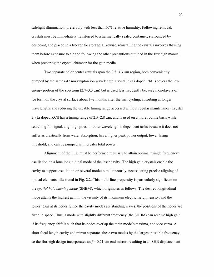
Two separate color center crystals span the 2.5–3.3 μm region, both conveniently

pumped by the same 647 nm krypton ion wavelength. Crystal 3 (Li doped RbCl) covers the low

energy portion of the spectrum (2.7–3.3 μm) but is used less frequently because monolayers of

ice form on the crystal surface about 1–2 months after thermal cycling, absorbing at longer

wavelengths and reducing the useable tuning range accessed without regular maintenance. Crystal

2, (Li doped KCl) has a tuning range of 2.5–2.8 μm, and is used on a more routine basis while

searching for signal, aligning optics, or other wavelength independent tasks because it does not

suffer as drastically from water absorption, has a higher peak power output, lower lasing

threshold, and can be pumped with greater total power.

Alignment of the FCL must be performed regularly to attain optimal “single frequency”

oscillation on a lone longitudinal mode of the laser cavity. The high gain crystals enable the

cavity to support oscillation on several modes simultaneously, necessitating precise aligning of

optical elements, illustrated in Fig. 2.2. This multi-line propensity is particularly significant on

the spatial hole burning mode (SHBM), which originates as follows. The desired longitudinal

mode attains the highest gain in the vicinity of its maximum electric field intensity, and the

lowest gain at its nodes. Since the cavity modes are standing waves, the positions of the nodes are

fixed in space. Thus, a mode with slightly different frequency (the SHBM) can receive high gain

if its frequency shift is such that its nodes overlap the main mode’s maxima, and vice versa. A

short focal length cavity end mirror separates these two modes by the largest possible frequency,

so the Burleigh design incorporates an f = 0.71 cm end mirror, resulting in an SHB displacement

24

Figure 2.2 The F center laser (FCL), consisting of two independent vacuum regions. The crystal chamber is always under vacuum when the crystal is present and cooled with liquid nitrogen. The laser will operate without evacuating the tuning arm, though operation will be impeded in the vicinity of water lines.

Kr+ Pump Laser Turning Mirror

Folding Mirror

CavityEndMirror

DichroicBeamSplitter

Grating Output Coupler

Output CouplingMirror

CornerReflector

Crystal Chamber

Tuning Arm Chamber

GalvonometerPlates

IntracavityEtalon

25

of 0.18 cm-1. For single-mode operation, a tunable “intracavity etalon” with a free spectral range

(FSR) of 0.6 cm-1 is placed in the tuning arm. This FSR is about three times the frequency

displacement of the SHBM, so it highly attenuates that component of the laser oscillation. To

obtain single mode operation, the cavity end mirror must be carefully adjusted, helping eliminate

the SHBM, and the intracavity iris should be partially closed, to selectively add the loss on

transverse cavity modes other than the desired TEM0,0 mode. Both of these adjustments are made

along with the pump beam (via the input steering mirror) and grating vertical tilt to optimize the

single mode laser power.

Particular difficulties may be encountered when scanning the laser continuously near the

extreme red end of the RbCl crystal bandwidth, below about 3200 cm-1. It was empirically found

that mode-hopping instabilities in this region mimic those observed when the intracavity etalon

has been tilted in its mount, away from optimal alignment. Specifically, the Burleigh manual

describes tilting the intracavity etalon such that the remnant of the 647 nm beam in the tuning arm

(used as a tracer) is reflected from the first etalon surface and positioned on the left edge of the

tuning arm iris. This positioning, as viewed from within the tuning arm, is illustrated as point A in

Fig. 2.3. For scanning the FCL below 3200 cm-1, this rotation should be exaggerated by rotating

the etalon further counterclockwise, placing the tracer reflection further to the left on the iris

mount, point B in Fig. 2.3.

B. Infrared Diagnostics

Two diagnostic devices are used to monitor the IR frequency. The first is a traveling

Michaelson interferometer, or λ meter, based on the design of Hall and Lee,7 which enables

absolute frequency calibration to within about 0.0005 cm-1. A home-built Fabry-Perot

Interferometer (FPI) provides an additional relative frequency calibration and real-time frequency

26

Figure 2.3 Position of the tracer beam reflected from the FCL etalon onto the intracavity iris, as viewed from the tuning arm. Location A indicates the recommended position according to the Burleigh manual, and location B is the position found to facilitate continuous tuning at the extreme red tuning range of the FCL.

27

stability measurement via piezoelectric scanning of its free spectral range. The details of these

devices are described next.

The λ meter works by counting interference fringes from the unknown (IR) and a

reference (polarization stabilized HeNe) lasers. Functionally, the IR laser and tracer HeNe are

directed onto a beam splitter and the two resulting laser beams reflect from a moving corner cube

cart, as illustrated in Fig. 2.4. The cart continuously translates on an air bearing, using solenoid

“cart kickers” to counteract friction and maintain its back and forth motion without any user

influence. The two beams recombine on the beam splitter and interfere on two photovoltaic

devices, one for the IR and one for the visible beam.

The interference measurements relate to frequency as follows. A laser beam at frequency

ν picks up a Doppler shift Δν after reflecting off the corner cube with speed vcart, according to,

Δν = ν vcart/c, (2.2)

where c is the speed of light. Because they reflect off the same cart, one laser channel picks up a

blue shift of ν + Δν, while the other is red shifted to ν - Δν. These beams recombine on the beam

splitter and interfere on a photodetector, producing a beat note (νb) at the difference between

these two frequencies, i.e. 2Δν. An equally valid analysis of this measurement is that when the

cart moves by λ/4 (λ = c/ν is the laser wavelength) then the difference in path length between the

two interferometer arms changes by λ/2, and the interference cycles 180°, i.e. from constructive

to destructive interference. This cycle occurs every time the cart moves this distance, such that

the photodetector signal oscillates at νb = 2vcart /λ = 2ν vcart/c, which is the same frequency

predicted under the Doppler picture, above.

The need to know vcart is removed by simultaneously measuring fringes generated by the

unknown IR laser (νIR) and a reference laser beam (νref) on separate detectors. The tracer HeNe

beam provides a convenient reference, with precision better than the 1.5 GHz gain bandwidth8 of

28

Figure 2.4 Schematic of the laser wavelength meter. A 50% beam splitter divides the incoming beam, containing both λref (HeNe) and λIR (IR), in two. Each beam reflects from a traveling cart, recombines, and lands on two separate photodetectors. Interference fringes are detected and turned into square waves in the phase locked loop / discriminator / frequency multiplier. The resulting square wave is counted on the commercial waveform counter.

29

an unstabilized HeNe. Eq. 2.2 holds for the relation of each beat frequency and the corresponding

laser frequency, such that the ratio of two such equations can be used to find

νIR = νrefνb_IR/νb_ref, (2.3)

where νb_IR and νb_ref are the measured beat frequencies of the IR and reference channels,

respectively.

The λ meter signal analysis electronics also appear in Fig. 2.4. The signal from each

photodiode is AC coupled and sent though a discriminator, turning the interference waveform

into a TTL pulse train. This square wave is used as the input to a phase lock loop, which servos to

the input frequency, providing a square wave with frequency F = Xνb, where X is a knob-

selectable frequency multiplier from 1–100. The output of the phase lock loop goes to a Hewlett

Packard “universal counter,” which counts the input square waves, and takes the ratio of the two

channels’ values. This value is multiplied by a calibration constant of 1579.807, corresponding to

the frequency of the reference laser in cm-1, divided by XIR/Xref = 10 for the relative discriminator

multiplier constants, such that the counter displays the IR frequency in cm-1. A typical cart speed

of 7 cm/s and phase locked loop multiplication factors of 100 and 10 result in 2.8 and 1.1 million

cycles for the IR and reference channels, respectively, in typical integration time of 0.5 s. Thus,

the fractional frequency uncertainty is less than a part in a million, and the IR frequency can be

measured with a precision of about 0.0005 cm-1. The accuracy of this measurement varies across

the FCL spectrum, but always suffices to locate 0.011 cm-1 Doppler broadened IR transitions.

This absolute wavelength measurement readily enables manual tuning of the FCL to any

desired HF transition, and the second frequency measurement device, a scanning Fabry-Perot

interferometer (FPI) schematically represented in Fig. 2.5, provides precise (1–2 MHz) relative

frequency calibration over short continuous scans. The confocal optical arrangement provides a

“bowtie” optical path, and a free spectral range (FSR, in cm-1) given by

FSR = 1/(4L), (2.4)

30

Figure 2.5 Schematic illustration of the scanning Fabry-Perot interferometer. A HV saw tooth wave, applied to the PZT on one end-mirror, results in a series of transmission fringes, which are monitored on a photodiode. The time delay between the beginning of the saw tooth wave and the arrival of the first transmission fringe is recorded on a time to amplitude converter, producing another saw tooth wave that can be used to calibrate the relative laser frequency.

31

where L is the distance between the cavity end mirrors. An L of 50 cm results in FSR of 0.005

cm-1. The exact value of FSR can be calibrated to better than 1×10-5 cm-1 by monitoring the FPI

output over short scans to get a good estimate of the FSR based on the λ meter reading. Following

small scans, the FCL can be tuned in progressively larger steps, which enable this calibration to

be extended over a very large frequency range and thereby increase the number of significant

digits in the calibration.

For typical diagnostic use, the FPI cavity modulates with a ≈ 500 V saw tooth wave,

applied to the cylindrical piezoelectric transducer (PZT) holding one of the cavity’s optical

elements. This voltage results in a mirror translation of about 2.5 μm, sufficient to make the FPI

resonant with the IR frequency 2–3 times. The scanning cavity has a finesse of approximately 20,

which is often sufficient to diagnose if the FCL is oscillating at one, or more than one, frequency

at a time. However, the 0.005 cm-1 FPI FSR roughly corresponds to twice the FCL longitudinal

mode spacing of about 0.01 cm-1, so lasing on adjacent modes can be hard to identify using only

the FPI. Fortunately, such multi-mode oscillation can also be identified by the modulation of the

fringe envelope on the λ meter, caused by interference between laser modes. Thus, single

frequency oscillation can be ascertained using the output of these two devices.

After recording short, continuous laser scans (0.3–10 GHz) the scanning FPI is used to

calibrate the frequency axis as follows. As the laser frequency changes, a time to amplitude

converter (TAC) measures the time from the start of the PZT translation to when the first fringe

exceeds a certain threshold voltage on the photodiode, as illustrated in Fig. 2.5. With increasing

laser frequency, the fringes are delayed and the TAC output increases. Thus, the rising edge of

the saw tooth wave corresponds to an IR fringe moving with respect to the PZT driver pulse,

followed by a very rapid falling edge as the next etalon fringe is detected. Advantages of this

method are that laser instabilities (particularly “hopping” between longitudinal modes, as occurs

with a poorly aligned FCL) are readily detected as discontinuities in the sloping side of the saw

32

tooth wave, and the abrupt “falling” edges of the TAC output provide markers for calibrating the

Doppler scan with the < 1×10-5 cm-1 precision of the FPI FSR measurement.

C. Intensity Stabilization and High Sensitivity Detection

In order to measure nascent HF product distributions with sufficiently low density to

maintain single collision conditions, absorption sensitivity close to the fundamental shot noise

limit, i.e., the limit determined by the counting of discrete photons, must be attained. In practice,

reaching this limit involves i) stabilizing the broad-band laser intensity fluctuations, ii)

subtracting the remaining technical noise from the “signal” detector using a paired “reference”

detector, and iii) carefully aligning optics such that non-common mode noise sources (such as

clipping of the beam in the Herriot cell) are below the shot noise level in the detection bandwidth.

This subsection describes how these three goals are attained.

The first bit of noise reduction results from stabilizing the laser output intensity.

Instabilities in both the krypton ion pump laser and the FCL both contribute to the IR root mean

square (RMS) noise of about 4% of the DC value without active stabilization. A commercially

available “laser noise eater” [ConOptics electro-optic modulator (EOM)], positioned as illustrated

in Fig. 2.1, reduces fluctuations on the 647 nm pump beam, reducing noise at acoustic

frequencies (about 10 kHz and slower) to be unobservable, with most of the remaining (≈ 0.2%

RMS) noise at 50 kHz and higher frequencies. However, since the EOM stabilizes the visible

laser light passing through it, 2-3% RMS noise remains on the IR light. Thus, a custom electronic

device, built by Terry Brown in the JILA electronics shop, has been inserted into the EOM servo

loop, which allows the feedback signal to be toggled between the 647 nm intensity and the FCL

IR power, as measured on the reference InSb detector. This servo operates synchronously with a

number of other electro-optical loops, as described in more detail in Sect. 2.2(D). The complexity

of the feedback loop necessitates a highly sophisticated circuit, containing proportional, integral,

33

differential (or PID) filtering. Adjustable frequency response for the feedback filters enables

noise cancellation in the maximum possible bandwidth and finely adjustable servo gain, to

maximize noise cancellation while maintaining servo loop stability. With this stabilization

implemented, acoustic noise on the IR laser is unobservably small and approximately 0.3% noise

remains, presumably caused by the servo loop because of its high frequency (100–500 kHz)

approaching the ≈ 500 kHz EOM frequency response.

To obtain absorption sensitivity close to the shot noise limit, the remaining laser noise is

subtracted from real “signal” fluctuations using a matched pair of low noise, liquid nitrogen

cooled, InSb detectors. Small (0.25 mm2) detectors result in fast (≈ 1 MHz) bandwidth, and very

quiet detector electronics result in a 0.9 pA/√Hz noise floor. This contribution is dwarfed by shot

noise on the detector’s photocurrent (ISN), given by

WPCSN BeII 2= (2.5)

where e is the fundamental electron charge, IPC is the total photocurrent, and BW is the bandwidth

of the measurement. For an IR power of 50 μW at 2.8 μm, IPC = 100 μA, and ISN/√BW = 5.9

pA/√Hz. Thus, the shot noise swamps technical noise by a factor of more than six. After

subtraction of the common mode noise between the two detectors, the ultimate detection

sensitivity is √2 times larger than IPC/ISN, about 7.6×10-8 Abs/√Hz.

The preceding argument suggests that increasing IR laser intensity I(ν) by a factor X

should increase the signal to noise by √X. In practice, increasing laser intensity leads to saturation

of the optical transition. Such saturation is quantified9,10 by relating the number density (N1 and

N2) in lower state 1 to upper state 2, via

N2g1/N1g2 = S/(1 + S). (2.6)

Here, gx is the degeneracy of state x, and the saturation parameter S is the ratio of the excitation

rate to the relaxation rate when subjected to intensity I(ν). In the collision-free, transit time

broadened conditions in the crossed jets, this ratio becomes

34

S = I(ν)S0/(Δν)2, (2.7)

where S0 = 4.5×10-7 cm2Hz11 is the HF integral cross section and Δν is the transit time limited

homogeneous linewidth. For an HF velocity of approximately 1000 m/s, and a beam diameter of

1 mm, Δν = 1 MHz. Setting S = 1 provides the characteristic saturating intensity Isat(ν),

Isat(ν) = Δν2/S0 = 2.2×1016 photons/cm2s = 1.8 mW/mm2. (2.8)

The probe beam is typically < 100 μW power in a 1 mm2 beam, such that laser intensity remains

more than a factor of ten below saturation. Significantly, the saturation parameter calculated via

Eq. 2.7 is independent of tightness of the laser focus under these transit time broadened

conditions, because I(ν) scales inversely with the square of the laser beam diameter, and so does

(Δν)2. Thus, all measurements are in a non-saturating regime and directly correlate to absolute HF

densities in the laser path, as used to estimate absolute reaction cross sections in Sect. 2.3.

Next, common mode laser noise is removed from the measured IR signal by comparison

of the laser intensity on the reference and signal InSb detectors. Approximately 40% of the power

is diverted onto the reference detector, to measure the IR power and fluctuations. The remaining

60% passes through the Herriot cell, about half of which makes it onto the signal detector. A

custom built “laser noise subtractor” scales the reference detector response to the DC level of the

signal detector and subtracts common mode noise. The output of this device is amplified 10-fold,

such that the IR shot noise swamps the electronic noise of subsequent electronic devices.

Experimentally realizable sensitivities of about twice the shot noise limit have been

obtained, resulting in absorbance noise of AS = 3×10-5 Abs in a 5 kHz bandwidth. The ultimate

HF detection limit comes from Beer’s law considerations of HF density and maximizing

absorption path length through the Herriot cell. With practically realizable configurations of 16

passes through 5 cm of absorbing HF (l = 80 cm), and σ = 1.4×10-15 cm2, (based on an integral

line strength of 1.5×10-17 cm/# and a 0.011 cm-1 Doppler width) Beer’s law produces a detection

limit (ρmin) of

35

ρmin = AN /σl, (2.9)

and a detection threshold of 4×108 HF/cm3 per quantum state.

Additional sensitivity enhancement results from the redundant information obtained

scanning the high-resolution laser in ≈ 3 MHz steps through a ≈ 300–900 MHz HF Doppler

profile. At each frequency, an independent measurement of absorption is obtained to construct the

Doppler profile, discussed in detail in Sect. 2.3(C). This scanning redundancy produces a large

number of independent data points [N > 100–150 under a typical Doppler full width half

maximum (FWHM)], providing a √N ≈ 10- to 12-fold gain in sensitivity. This effect is

conclusively demonstrated in Ch. III and IV, where F atoms reacting with either HCl or H2O

result in signal intensities on par with this limiting noise. Nevertheless, robust results have been

obtained via this Doppler averaging, as discussed in more detail in Ch. III. Statistics are further

improved by a regimen of signal averaging, during which each IR transition is probed repeatedly

over the course of the experiment. The 2.5–3.3 μm tunability of the IR source also enables many

HF(v,J) states to be probed on both the P (ΔJ = -1) and R (ΔJ = + 1) branch transitions, further

increasing the degree of data oversampling.

Finally, obtaining shot noise limited sensitivity also depends upon careful alignment of

the IR laser. Several optical components are likely to attribute to absorbance noise. The HeNe

tracer beam can weakly couple onto an InSb detector, but can be eliminated by placing an IR-

transmitting germanium filter in the beam path. Also, transmission problems can occur when

retroreflected IR beams overlap with incident ones and create standing waves along the beam

path, which effectively become low finesse etalons. Such interference is readily identified by the

sinusoidal noise pattern obtained when tapping on optical components that form one end of the

etalon. Such optics are most likely detector windows and nearby fast-focusing lenses, because of

their close proximity and weak sensitivity to lens alignment. This type of noise can be eliminated

using irises and careful rotation of components to prevent back reflection.

36

Another likely culprit for laser noise is the FPI, which also readily produces optical

feedback into the laser as it scans to modulate its transmission. However, this feedback is readily

identified because it oscillates with the FPI PZT translation, is synchronous with the HV driver,

and mimics the shape of the cavity transmission curve. Spatially filtering the FPI from the laser

by closing an alignment aperture and/or by using a Faraday isolator (FI in Fig. 2.1) effectively

eliminates this effect.

Partial clipping on the edge of the InSb detectors is another likely source of alignment

noise. The fast InSb detectors are small (0.5 mm square), necessitating short (5 cm) focal length

lenses to tightly focus the IR beam. The focus must be carefully centered on the detectors with a

translation stage, such that small lens displacements or beam steering does not change the

measured intensity. Remaining sources of loss along the laser path can cause intensity noise, as

small motions result in differential changes between the detected reference and signal levels.

However, stable optical mounts suppress such motion, which also tends to be in 100 Hz and

lower “acoustic” frequencies that are far removed from the faster signal bandwidth.

Finally, the Herriot cell12 is the most sensitive optical element to align for two reasons.

First, the long distance (60 cm) between the Herriot cell mirrors amplifies any mirror motion,

such that clipping noise readily becomes detectible. Secondly, the spherical mirrors enable laser

divergence to be manipulated, but an understanding the laser propogation is needed to utilize this

effect to prevent clipping on the laser beam on the edges of the mirrors. Specifically, the Herriot

cell consists of two spherical mirrors with 30 cm radius of curvature, positioned in a nearly

concentric fashion, i.e., they share an axis, but are somewhat less than d = 60 cm away from each

other. The laser beam produces an elliptical pattern on the Herriot cell mirrors, as illustrated in

Fig. 2.6. Careful choice of input spot position readily eliminates clipping on the entering beam,

focused into the Herriot cell via a 50 cm lens. However, subsequent spots reflecting from the

mirror increase in size, as the concave mirrors alter the beam divergence. Gaussian optics

37

Figure 2.6 Illustration of the elliptical laser spot positions on the Herriot cell mirrors. The beam divergence changes following each reflection from the curved optics. For optimal mirror spacing, the output beam is highly collimated to prevent clipping as it passes by the mirror and travels to the signal detector.

38

considerations13 reveal how laser spot size (ω, the 1/e electric field radius) changes as it passes

through the Herriot cell, as shown in Fig. 2.7. In this figure, the spot size is plotted as a function

of laser propagation distance. Reflections off the curved optics are readily identified as local

maxima in beam size, i.e., where the diverging beam becomes converging. The spot sizes on the

mirrors increase and then decrease for mirror spacing d less than twice the mirrors’ radius of

curvature. For the 16 pass cell modeled in Fig. 2.7, the spacing in panel b) leads to the most

collimated output spot, and therefore the least clipped beam. In practice, this alignment can be

attained by measuring the outgoing laser’s spot size with a translatable iris near the chamber

output while “walking” the mirror spacing to minimize this beam diameter.

The importance of laser collimation and alignment cannot be overemphasized, since light

fluctuations of ten parts per million will quickly dominate the detection noise. Indeed, an

attempted variation of the Herriot cell failed for this exact reason. Specifically, a triangular

multipass configuration was implemented in which the laser beam traveled from one curved

mirror to the other, off a flat mirror, and then returned to the first curved mirror. Thus, the jets

could be positioned such that the laser passed in only one direction through the intersection

region, parallel to the plane of the two jets’ axes. This arrangement was designed to produce

asymmetric Doppler shifts capable of distinguishing between forward and backward scattering of

the HF product. However, tilting of the curved mirrors into the triangular configuration

effectively changed the radius of curvature for one axis relative to the other, producing

astigmatism. Thus, the mirror spacing needed to collimate the output spot, as illustrated in Fig.

2.7 was different for the horizontal versus vertical beam dimensions and the outgoing spot

diverged on at least one axis, producing elliptical spots with different confocal beam parameters

on two perpendicular axes. In principle, this effect could be corrected using an astigmatic optic

(e.g., a cylindrical lens) in the triangular beam path. However, this additional complication to the

39

Figure 2.7 Gaussian optics predictions for the IR spot size in the Herriot cell. Mirror reflections are located at the circles, where local maxima of beam diameter occur. Minima are approximately at the squares, the locations of beam waists. After exiting the Herriot cell, the laser beam can only propagate to its waist and then continue to diverge. For the top panel, the mirrors are too close and the maximally collimated beam occurs prior to the outgoing pass. For the bottom panel, they are too far apart and the outgoing pass also diverges rapidly The middle panel, with mirror spacing d = 59.35 cm, produces a well-collimated output beam.

d=59.35 cm

spot

siz

e (c

m)

0.0

0.2

0.4

0.6

0.8

1.0

1.2

d=58.5 cm

0.0

0.2

0.4

0.6

0.8

1.0

1.2

d=59.6 cm

propagation distance (cm)0 200 400 600 800 1000

0.0

0.2

0.4

0.6

0.8

1.0

1.2

mirror reflections

OutputBeam

Herriot cell exit

40

vacuum alignment was not attempted, and all of the reported results utilize a traditional Herriot

cell.

D. Continuous and Automated Frequency Scanning

A pair of Brewster windows, mounted on a galvanometer (or galvo for short) as drawn in

Fig. 2.2, enables continuous tuning of the FCL, while maintaining single mode operation.

Functionally, these calcium fluoride windows displace the laser path by a small amount and

change the cavity’s free spectral range without changing the output path of the laser. Applying a

current to the galvo tilts the plates in opposite directions, refractively displacing the laser beam

and tuning the free spectral range of the cavity. To vary the IR frequency continuously, the

intracavity etalon must track the moving longitudinal mode as the galvo plates scan. Thus, both

the galvo and etalon PZT stacks must be calibrated for frequency tuned per volt applied. The ratio

of these values determines the relative feed forward voltage applied to these devices to

continuously scan the FCL frequency.

The single mode FCL output is monitored on the scanning FPI cavity to calibrate the feed

forward calibration as follows. With the etalon unplugged and therefore static, scanning the galvo

plates continuously changes the laser frequency until an adjacent longitudinal mode of the cavity

experiences lower loss through the etalon and the IR frequency “hops” to oscillate on this mode

instead. A plot of galvo monitor voltage versus the number of hops reveals the displacement of

the original longitudinal mode in units of cavity FSR = 0.01 cm-1, resulting in a feed forward

value of 7.23 V/cm-1. Although FSR is technically changing with the galvo scan, it only does so

in proportion to the number of observed hops out of the cavity mode number that is oscillating (n

≈ 350,000), such that it can be treated as constant.

A similar process is used to calibrate the etalon PZT feed forward with the galvo plates

stationary, except that in this case the laser frequency remains constant until the etalon

transmission shifts enough to transfer lasing to the adjacent longitudinal mode. Measuring these

41

transitions as a function of etalon feed forward provides a similar calibration curve, and a value of

–6.98 V/cm-1, as measured on the PZT HV driver output monitor. Unfortunately, the etalon PZT

responds nonlinearly to applied voltage over its 0–1000 V range, so this calibration is best

performed at about 500 V to obtain a median value of the tuning response.

To compensate for laser frequency drift and nonlinearities in the galvo and etalon feed

forward calibration, an servo loop prevents hopping between longitudinal modes as the cavity

scans. This servo loop, illustrated in Fig. 2.8, functions by continuously “dithering” the etalon

PZTs by applying a sinusoidal modulation voltage at frequency ω ≈ 2 kHz on top of the DC

voltage applied to maintain the proper intracavity etalon mode spacing. Thus, the etalon mirrors

oscillate at ω, but with low enough amplitude to avoid mode hops, resulting in a slight

modulation of the output IR intensity as the etalon transmission moves relative to the longitudinal

mode on which the cavity is oscillating. If the etalon is perfectly centered on the longitudinal

mode, the modulation frequency will be at 2ω, while any average frequency mismatch results in

some intensity modulation at the dither frequency, ω. Thus, synchronous detection of the error

signal at ω provides feedback to the etalon servo.

The feedback signal comes from one of two places. If the krypton ion pump laser

intensity is constant, then the reference InSb detects the IR modulation directly, as illustrated by

the short dashed line in Fig. 2.8. Alternatively, under data acquisition conditions, the FCL power

is actively constrained to be constant by the laser intensity servo described in Sect. 2.2(C). In this

case, the EOM transmits higher pump laser power to maintain the same IR power as the etalon

dithers. Thus, the EOM error signal contains the dither feedback information at frequency ω, and

the FCL servo loop is completed according to the long dashed line in Fig. 2.8.

42

Figure 2.8 Schematic for the laser frequency servo loop. The FCL servo dithers the intracavity etalon voltage and monitors the error signal at the applied frequency. In the first servo mode (short dashed line), the IR intensity varies and is directly monitored. However, when the IR laser intensity servo is used, the EOM modulates the pump laser power changes to maintain constant IR power. In this mode, the error signal from the laser intensity servo (long dashed line) contains the information about the etalon dither.

43

2.3 Crossed Jet Apparatus

For the gas-phase reaction dynamics studies, reactants enter the ≈ 100 L diffusion-

pumped vacuum chamber via two supersonic molecular jets. The jet axes are oriented at 90°

angles and intersect 2.5–5.0 cm downstream from their orifices, as illustrated in Fig. 2.9. One jet

emanates from a custom-built Proch-Trickl14 valve, which uses a PZT disc actuator to generate

200–500 μs gas pulses. This valve delivers about 8×1013 molecules/cm3 to the jet intersection

region at typical backing pressures of 200 Torr for a 500 μm pinhole orifice. The radical source,

described in detail below, uses a HV plasma (50–500 μs duration) to dissociate F2 into reactive F

atoms during an approximately 2 ms gas pulse. This valve has an approximately 0.03 by 0.3 cm

orifice and typically operates with a stagnation pressure of 70 Torr, resulting in an additional

1.0×1014 #/cm3 in the probe region. With the valves pulsing at 10.1 Hz, the average pressure in

the chamber rises to ≈ 1.0×10-4 Torr, corresponding to a mean free path of λ ≈ 50 cm between

molecular collisions, i.e., considerably greater than the distance to the chamber walls.

Low-density conditions ensure that the probability for secondary molecular collisions is

on the order of 1 % prior to leaving the ≈ 0.5 cm detection volume. Most collisions are with

helium and other rare carrier gas atoms which have small cross sections for rovibrationally

inelastic scattering;15 hence, this represents an upper limit for redistribution of the HF(v,J)

population. Nevertheless, possible inelastic relaxation is a concern that has been explicitly tested

for each system, as discussed in subsequent chapters. In general, such single collision conditions

are readily satisfied, as only 0.04% of the approximately 1×1012 #/cm3 F atoms present in the

probe region need to react and form HF in a given (v,J) state to exceed the detection threshold

computed in Sect. 2.2(C). Thus, the IR detection technique has enabled the study of reaction

dynamics of systems with rate constants up to about ten times lower than the gas kinetic rate (i.e.,

cross sections of about 1 Å2). The cross section for do-able experiments will scale with the

44

Figure 2.9 Illustration of the reaction vessel. Unskimmed molecular jets intersect at a 90° angle, centered on the IR multipass cell, whose axis is perpendicular to the plane defined by the central axes of the jets.

45

reactant densities, the absorption path length probed by the IR laser, and the RMS absorbance

noise, while scaling inversely with the IR line strength and the number of populated product

quantum states. Since the HF IR transition is a particularly strong one, and the present densities

have been pushed close to the limits of single collision conditions, probable areas for

improvement include lower noise (i.e., faster) data acquisition techniques, different probe

geometries (such as cavity ring down), and different jet sources, such as crossed slit jets or higher

efficiency radical sources.

In addition to providing a convenient source for directed, low density molecules, the

supersonic jets also cool the reactants, with rotational temperatures of ≈ 30 K observed for the

hydrides considered here, and colder distributions likely for species with smaller rotational

constants. Jets also provide a means to vary translational energy via choice of carrier gas. These

effects narrow the number of states and make kinetic energy dependent studies possible. The jets

can be characterized a number of ways. First, the measured velocities closely match the predicted

terminal velocities anticipated by fluid dynamics,16 indicating efficient cooling of the expansion

gases. Additionally, direct IR observations of HCl and the naturally present H218O isotopologue

(whose low atmospheric concentration makes it easy to probe in low rotational states) also

confirm efficient cooling.

A major new capability has also been developed for studying the nature of chemical

reaction events at the vacuum interface of bulk liquid surfaces. These gas-liquid scattering

experiments utilize the same F atom source as the crossed jet studies, but otherwise introduce a

number of novel features. The use of bulk liquids in vacuum raises a number of interesting points.

First, low vapor pressure (≈ 10-7 Torr) liquids are used to prevent loss of reactant and maintain

long mean free paths. Secondly, the probability of a molecule incident upon the liquid colliding

with the surface is essentially unity, and reaction probabilities are similarly high. However,

checks against jet shocks at the surface and other nonlinear effects are also necessary. Finally,

46

issues of surface cleanliness in vacuum must be confronted by continuously refreshing the

surface. These issues and further experimental details of the gas-liquid scattering studies can be

found along with the experimental results in Ch. V.

A. Radical Source:

The F atom source is a standard solenoid fuel injector modified to generate radicals in an

electrical discharge at the throat of the supersonic expansion, as shown in Fig. 2.10. The F atoms

are produced as follows. The solenoid pulses 50–100 Torr of a 10% F2 / 90% rare gas excimer

pre-mix into a small (≈ 0.025 mL) volume defined by a slotted hole in a 0.5 mm inert

(polychlorotrifluoroethylene) disk insulator, sandwiched between two metal electrodes. A

miniature slit (300 μm × 0.3 cm) in the downstream electrode forms the limiting orifice, from

which the gas expands past two slit-jet expansion-defining “jaws” and into the chamber. This

source utilizes a slit expansion geometry because it prolongs the time between routine cleaning

and sanding of the electrodes, presumably because the elongated orifice provides more electrode

surface area for a given nozzle area, such that plasma wear is diluted over more electrode

material. At the peak of the 2 ms gas pulse, a 500 μs HV pulse (≈ -1 kV) is applied to the lower

electrode, striking an electrical discharge through the gas mixture to the grounded upper electrode

on the valve body. Measuring HF densities produced in crossed jet studies of F + H2, with known

reaction cross section,17 enables F densities of approximately 2.6×1012 atoms/cm3 to be inferred.

Such densities correlate to ≈ 2×1016 F atoms/cm3 at the limiting orifice, or ≈ 10% of the F2

dissociating into F atoms in the plasma. These measurements have also been used to estimate the

reaction cross section for several systems, as discussed in detail in the next subsection.

Very recently, a similar plasma source has been designed for use with a Proch-Trickl

pulsed valve, based on a design borrowed from the Ye group at JILA. For this valve, a pinhole

source replaces the slit, and either ceramic or plastic insulators may be used. Based on the advice

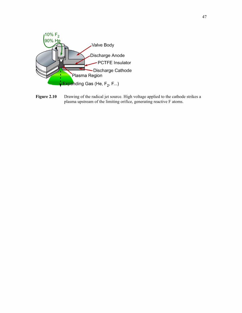
47

Figure 2.10 Drawing of the radical jet source. High voltage applied to the cathode strikes a plasma upstream of the limiting orifice, generating reactive F atoms.

48

of the Ye group, the electrodes were finely polished using a series of progressively finer sand

paper grits, a fine paste polish, and then electro polishing, to remove surface roughness and

extend the stable lifetime of the electrodes between servicing. This valve has been briefly used in

the ion imaging apparatus described in Appendix B, and radical Cl production efficiency is

comparable to that found for F atoms, above.

Because of the harsh environment in the radical atom source, the high voltage electrode

surfaces physically and chemically degrade, leading to unstable plasma current and F atom

production efficiency. Erratic performance generally arises after about a week of regular

operation, but sanding and polishing the electrodes restores stability. This wear results in drift of

the F atom density on an inverse day time scale, necessitating normalization of the data set with

respect to F atom density. Thus, a strong reference transition is observed every 2–3 hours during

data acquisition, such that the entire data set can be normalized and data collected over many

weeks meaningfully compared and signal averaged.

The high sensitivity to HF product density also necessitates compensation for trace

amounts of background HF contamination. This background originates from the F source,

presumably via pre-reaction with impurities in the gas mixture at part per million concentrations.

Fortunately, efficient cooling in the supersonic jet (even with the discharge on) confines all such

background to HF v = 0, with a rotational temperature of ≈ 60 K, as shown in Fig. 2.11. This

background is explicitly measured by re-scanning each transition originating in HF(v = 0) without

the second jet, such that the differential increase in integrated absorption can be attributed to the

HF reactive product channel. This procedure works well but often generates significant

uncertainties for the lowest [HF(v = 0,J < 6)] states arising from subtraction of weak and nearly

equivalent populations. Nevertheless, the plasma source and IR technique enable the HF

populations to be observed, and provide direct measurement of population in the ground

vibrational state, inaccessible via IR chemiluminescence methods.2,18-29

49

Figure 2.11 Boltzmann plot of the HF background produced in the F atom plasma source. The density of HF background is much smaller than that reactively produced in the crossed jets. Supersonic cooling confines the background to low J in the v = 0 manifold, as indicated by the ≈ 60 K fit to the rotational distribution.

v=0

Erot/kB (K)0 50 100 150

ln[ P

(J)/g

(J) ]

0

1

2

3

56K

50

B. Data acquisition

HF produced via reaction at the intersection of the pulsed jets results in a transient change

in the intensity of the IR probe when the frequency lies within the Doppler profile of a populated

HF(v,J) transition. A transient recorder (or, in a recent upgrade, a computer digital acquisition

board) digitizes this transient absorption waveform, and it is analyzed in real time. Specifically,

the absorption pulse is numerically averaged under a 100–500 μs window, coinciding with the

peak absorption signal and resulting in a 2–10 kHz detection bandwidth. Additional time gates,

preceding and/or following the signal gate by several hundred microseconds, are also averaged in

order to correct for pulse-to-pulse changes in the absorption baseline and eliminate slow noise

fluctuations. The net absorption is plotted as a function of laser frequency to construct Doppler

profiles such as those presented in Fig. 3.3, 4.4, 5.5, and 5.10.

A digital to analog converter provides a voltage ramp used to automate the laser tuning as

described in Sect. 2.2(D). Typically, the laser tunes about 3 MHz between jet pulses, and the

process is repeated ≈ 1000 times over a 3 GHz window, sufficient to resolve the entire Doppler

profile. However, it is also necessary to calibrate the frequency axis during the scan. For this

purpose, the TAC output is also recorded, providing a measure of the FPI output at each laser

step, as described in Sect. 2.2(B) and depicted in the top panel of Fig. 2.5. The TAC saw tooth

wave contains sharp falling edges, spaced by the FSR of the FPI, such that a simple edge finding

routine can be used to calibrate the frequency axis with the precision of the scanning etalon.

Additional DC data are acquired, including the signal InSb detector DC level, used to convert

measured waveforms into absorbance units, and the transmission of a reference gas cell, which

provides absolute frequency calibration.

When acquiring data, the Doppler profiles are typically scanned at least three times in

succession. This redundancy improves the statistical uncertainty of the measurements and also

helps reveal systematic changes (e.g., poor plasma reproducibility in the F atom source), which

51

can be missed during long average scans. Some degree of redundancy is warranted, as Doppler

measurements require only about one hundred seconds of acquisition time, and a similar amount

of time goes into manually tuning the laser and preparing it when transitioning between spectral

lines. Repeat measurements also statistically decrease uncertainties, an important effect for low

signal experiments.

2.4 Data Analysis and Experimental Modeling

A. Spectral Analysis

Sample Doppler measurements are presented in each chapter for the reaction being

studied. Figs. 3.3 and 5.5 illustrate the types of signal to noise and spectral features obtained for

the various studies. Because chemical reaction readily produces vibrationally excited HF product,

the measured absorption profiles, A(ν), contain structure according to the density of HF absorbing

from the lower state j and emitting from the upper state i at each Doppler detuning ν−ν0

according to the Beer-Lambert law, expressed as

Aij (ν-ν0) = ∫dx ∫dν’ [σi→j(ν-ν’)κi(x,ν’-ν0)- σi←j(ν-ν’)κj(x,ν’-ν0)]. (2.10)

Here κi/j(x,ν’-ν0) is the spectral density (i.e., molecules/cm3/cm-1) of absorbers in states i or j, at a

position x along the absorption path with Doppler shifted center frequency ν’-ν0. σj←i(ν-ν’) and

σj→i(ν-ν’) are the homogeneously broadened absorption/emission cross sections between states i

and j centered on ν’. Since the homogeneous lineshape is much narrower than the inhomogeneous

Doppler profile, it can be approximated as a delta function such that integrating over ν’ yields

Aji(ν-ν0) = Si→j ∫dx κi(x,ν-ν0) - Si←j ∫dx κj(x,ν-ν0). (2.11)

Thus, the net absorption at ν−ν0 is related to the difference in HF column-integrated spectral

density ∫dx κi/j(x,ν-ν0), weighted by the appropriate line strengths (Si↔j).

52

To simplify the discussion of the quantum-state distributions, measured Doppler profiles

are numerically integrated, and more detailed analysis of the absorption lineshapes is postponed

until Sect. 2.4(C). Integrating Eq. 2.11 with respect to ν relates the integral absorbance to the total

HF column-integrated density ∫dx ρi/j(x) = ∫dx ∫dν κi/j(x,ν-ν0)

∫A(ν-ν0) dν = Si→j ∫dx ρi(x) - Si←j ∫dx ρj(x). (2.12)

Eq. 2.12 permits the difference in column-integrated densities (CIDs) for the lower and upper

probe states to be extracted using the absorption line strengths (Si↔j), well known from the

analysis of Arunan, Setser and Ogilvie.11

For the excited vibrational populations observed following reactive scattering, significant

HF density often forms in both upper, j, and lower, i, states, resulting in a competition between

stimulated emission and absorption signals. Such non-equilibrium conditions are readily

anticipated following chemical reaction, and form the basis of chemical lasers.30 The presence of

two unknown CIDs in Eq. 2.12 leads to correlation between upper and lower state populations in

a least-squares fit to the spectral data. However, observation of lines originating from the highest

energetically accessible (vmax) manifold effectively breaks this correlation, since the population in

the (vmax + 1) upper state can be set to zero. Furthermore, the tunability of the IR laser permits

observation of both P and R branch transitions out of many HF(v,J) lower states, increasing the

number of measurements probing each state.

The network of accessible HF transitions in Fig. 2.12 illustrates the redundancy of the IR

spectral measurements. This presentation emphasizes that more than one transition is measured

for a large number of HF(v,J) states, and that the population in a given state is linked to that in

every other. Fitting the entire spectrum simultaneously produces the set of HF(v,J) CIDs from the

measured spectrum without any ad hoc assumptions. States whose energy exceeds the available

energy can also be probed, and the absence of measurable population justifies fixing the density

in these states to zero in the least squares fit. However, since the HF density in each manifold

53

Figure 2.12 The network of accessible HF transitions in the 2.5–3.3 μm tuning range of the IR laser. A large number of J states in the v = 0–3 manifolds are accessible, many of them via both P and R branch transitions.

54

depends upon measurements in every higher populated manifold, illustrated in Fig. 2.12, the

fitted uncertainties tend to increase in lower vibrational manifolds. This trend has been observed

in every data set presented here. Nevertheless, robust measurements of HF density have generally

been obtained down to the ground vibrational manifold.

B. Density-to-flux Transformation and Monte Carlo Simulation of the Crossed Molecular

Jets

The measured IR spectrum yields HF state resolved column-integrated densities via least

squares fitting of the spectrum described in the previous section. However, under crossed jet

conditions the flux of product molecules, not the density, is directly proportional to the state

resolved reaction cross section. Obtaining product fluxes requires consideration of the well-

known density-to-flux transformation,31-33 i.e. correctly taking into account the velocity-dependent

detection sensitivity intrinsic in any density-based measurement technique, such as IR

spectroscopy.

The single-collision conditions and excited Doppler measurements, discussed in more

detail in Sect. 2.4(D), emphasize the need for the density-to-flux transformation. Essentially, if

HF product is observed under single collision conditions it cannot be considered translationally

equilibrated, and by simple energy conservation, lower energy product states can be expected to

have higher recoil energies and spend less time in the detection volume. Conversely, translational

equilibration necessarily entails post-reaction collisions, which may also cause inelastic

redistribution of energy. Benchmark chemiluminescence studies2,18-22,24-27,29,34-38 were performed

under such translationally equilibrated conditions, further emphasizing the present interest in

revisiting these reactions under lower density.

The relationship between reaction cross section and product density can be found via

considerations based on those of Sonnenfroh and Liu.31 Fundamentally, the probability PF of an F

55

atom reacting following a displacement dl in the center of mass frame in the vicinity of a point r,

with density ρHX(r) of reactant HX is given by the Beer’s law-type expression,

PF = σjρHX(r)dl, (2.13)

where σj is the total reaction cross section for forming HF in state j, treated as a constant for the

current discussion. Shifting to the laboratory frame requires the substitution dl = (vrel/vF)dx,

where vrel = dl/dt is the relative velocity in the center of mass frame, and vF = dx/dt is the

laboratory-frame F velocity, defined to be along the x axis. Thus, PF becomes

PF = σjρHX(r)(vrel/vF)dx. (2.14)

Thus, the rate of F loss RF(r) (in #/cm3/s) at r is given by -PF times the density of F at r, ρF(r),

divided by the time spent at r, dt = dx/vF. The rate of formation of HF is RHF = -RF, such that

RHF(r) = PFρF(r)vF/dx = σjρF(r)ρHX(r)vrel, (2.15)

Note that the ρF(r) and ρHX(r) terms appear symmetrically in this expression, as they must, since it

also could have been derived from identical considerations of the HX jet.

The local HF density ρHF(r) results from the HF formation rate at r and the flux of HF

passing through r, due to reaction elsewhere. Mathematically, the density ρHF and the laboratory-

frame velocity vHF are related via the continuity equation of fluid dynamics,

dρHF(r)/dt = RHF(r) - ∇⋅ρHF(r)v. (2.16)

Integrating Eq. 2.16 over a finite volume V, ∫∫∫V dV, emphasizes the physical interpretation that the

rate of change of HF molecules in V [∫∫∫V dV dρHF(r)/dt] must be equal to the rate at which they

are formed [∫∫∫V dV RHF(r)] minus the net flux leaving V through its bounding surface A. This last

term is made explicit by substituting ∫∫∫V ∇⋅ρHF(r)vHF = ∫∫Ac ρHF(r)vHF⋅dA, where ∫∫Ac denotes

integral over a closed area A bounding V, according to Gauss’ divergence theorem.

When ρHF(r) is probed for a short time after the reaction begins in the crossed jets, the

explicit time dependence of ρHF(r) must be taken into account according to Eq. 2.16 in a detailed

model of the experimental conditions. For the present experiment, the steady state limit is valid,

56

since the approximately 10–50 μs HF travel time from anywhere in the reaction region the probe

laser is much smaller than i) the > 200 μs signal gate for averaging IR absorption data and ii) the

even longer ( > 0.5 ms) pulsed jet durations. Thus, time-dependent models can be avoided and

setting the left hand side of Eq. 2.16 to zero results in

∫∫∫V RHF(r)dV = ∫∫Ac ρHF(r)vHF⋅dA, (2.17)

which states that the HF flux away from r must be equal to the rate of HF production at r for

steady state conditions. Integrating over a sufficiently small region around r, the velocity vector

points normal to dA at all points. Denoting the small volume ΔV and surface area ΔA, dividing by

ΔA, and substituting in for RHF(r) using Eq. 2.15, one finds an expression for the localized flux

per unit area Φ,

Φ(r) = σjρFρHXvrelΔV/ΔA = ρ(r)vHF. (2.18)

Here, the explicit r dependence of ρF, ρHX, and vrel has been dropped because ΔV is assumed to be

small enough that they are nearly constant.

Eq. 2.18 is too simple to accurately represent the conditions in the crossed jet apparatus,

where a distribution of fluxes exist at each position, due to the generation of HF at every other

position, and with a velocity distribution depending upon the HF point of origin and location of

the flux in question. However, the total flux is a superposition of various flux components

(labeled with subscript i), each of which still obey

Φi = ρivi. (2.19)

The total flux, ΦTot = ΣiΦi, is still directly proportional to the state resolved cross section σj, in the

limit that any changes in collision energy are small and do not result in dramatically different

reaction cross section for portions of Φi originating from regions with significantly different mean

collision energies. The relationship between ΦTot and ρTot = Σiρi can be found by dividing both

sides of Eq. 2.19 by vi and summing over i,

ρTot = ΣiΦi/vi. (2.20)

57

Dividing this expression by ΦTot, one finds that the right hand side is ⟨1/v⟩ the flux-weighted

expectation value of the inverse speed, which rigorously connects ΦTot to ρTot according to,

ρj_Tot/⟨1/v⟩j = Φj_Tot. (2.21)

For fixed probe geometry ⟨1/v⟩ is also directly proportional to ⟨τ⟩, which is used as the density to

flux conversion factor in Ch. III and IV, and Appendix E, since the flux is subsequently

normalized to provide the relative magnetude of σj for various j. This substitution is also

intuitively appealing because ⟨τ⟩ weighting reveals an enhanced detection probability for

molecules in states that recoil such that they spend more time in the probe region.

In principle, the sum represented in Eq. 2.20 could be converted to an integral and

evaluated for the explicit experimental conditions. In practice, such integration is cumbersome

and is replaced by numerical Monte Carlo (MC) simulation instead. Specifically, the simulation

models the explicit HF formation and absorption events for each of the crossed jet systems in

order to directly approximate this sum. The details of the MC routine are as follows and are

illustrated in Fig. 2.13. The program randomly samples “reaction locations” r within the cubic

simulation volume with side 2d, where d is the distance from the jet orifices to the probe axis.

The product center of mass (COM) recoil direction is also randomly sampled within user-chosen

i) differential scattering constraints and ii) change in kinetic energy corresponding to formation of

a given product state. The reactant velocities are also randomly sampled from within the known

speed distribution, while constraining the velocity vector to be parallel to the line connecting r to

the corresponding reactants’ nozzle orifice.

Thus, the MC routine simulates the distribution of speeds, densities, collision angles, and

scattering angles present under the experimental conditions. The inputs to the model are as

follows: i) probe and jet geometries, ii) and product masses, iii) reaction exothermicity, iv) jet

58

Figure 2.13 Illustration of the Monte Carlo computational volume used to simulate the F + HCl reaction conditions. The jet sources define two edges of the cubic volume, located d = 4.5 cm from their intersection point. The Herriot cell probe volume, shaded red, is centered at this point and simulated by a 0.5 cm diameter cylinder, perpendicular to the plane of the jets. The contours are the detection probability for HF formed with ΔEtrans = 0.0 kcal/mol, also presented in Fig. 2.14.

59

angular and speed distributions [measured experimentally via high-resolution Dopplerimetry on

IR chromophores doped in the incident beams in a separate experiment], and v) the adiabatic,

zero-point corrected transition-state barrier heights obtained from high-level ab initio

calculations,39,40 below which the reaction can not proceed classically. These parameters and a

random sampling of the recoil dynamics enable the laboratory-frame trajectory of the HF product

to be computed. If a randomly generated trajectory intersects the detection volume V (a cylinder

with 0.5 cm radius, whose long axis is perpendicular to the plane of the jets), then such scattering

trajectories contribute to the detected signal. The relative importance of the detected trajectory is

found by histogramming the results according to the right hand side of Eq. 2.18, i.e., the product

flux, numerically proportional to the product of ρF(r), ρHX(r), and vrel. The histogrammed results

provide information on the distribution of HF residence times in the probe region, the spatial

distribution of detected reactions, the Doppler projection of the HF product, and the collision

energies. Sampling a million MC trajectories produces good convergence, and the process is

repeated for various differential scattering limits. A separate calculation is performed for each

value of recoil translational energy change, ΔEtrans, based on specific HF(v,J) states and assumed

coproduct (X radical from HX reacant) internal energy.

In general, the MC results are relatively insensitive to the assumed differential cross

section largely because spatial averaging within the unskimmed jets blurs the details of the recoil

dynamics. Nevertheless, different angular scattering limits are considered for each reaction

system, as discussed in more detail in Appendix E. The density-to-flux transformation results in a

modest increase in product branching into low-energy HF(v,J) states, when compared to the raw

HF column-integrated densities. This effect arises from the higher average laboratory-frame

velocities resulting for HF formed in lower internally excited states. Indeed, this physical picture

predicts that the computed ⟨τ⟩ values should scale inversely with the recoil speed, i.e., with the

60

average energy available to products to the negative one-half power, ⟨Eavail⟩-1/2, as observed for

sufficiently large Eavail, regardless of assumed differential cross section, as shown in Fig. A.13(b).

Of course, the exact values of the calculated ⟨τ⟩ values are dependent on the chosen

detection volume shown in Fig. 2.13. However, only the ratios of the HF residence times

influence the final results, since the normalized HF populations are ultimately reported.

Additionally, small changes in the shape or position of the probe volume are unlikely to perturb

the ratios of the ⟨τ⟩ values. This conclusion is expected because an average time was used as a

conveniently calculated value, versus the true ⟨1/v⟩ scaling factor derived from Eq. 2.20.

In addition to providing ⟨τ⟩ values, the MC model provides a number of other insights

into the experimental conditions. Specifically, the collision energy distribution is obtained from

the computation, and found to be somewhat higher than expected for the jets intersecting at 90°.

This increase results from the spatial distribution of detected products presented in Fig. 2.14,

which reveals that “head on” collisions, i.e., those occurring closer to the line connecting the two

jets, are somewhat likely to be detected, increasing the mean collision energy. This figure reveals

that in every recoil energy regime, the highest sensitivity is for products formed near the detection

volume, and collisions downstream with respect to the laboratory-frame center-of-mass velocity

have negligible detection probability. However, products formed closer to the valve orifices have

a reasonable probability of passing through the detection volume because the laboratory-frame

velocity of the collision partners points that direction. The top left panel in Fig. 2.14 reveals that

particularly endothermic processes that absorb kinetic energy (ΔEtrans < 0) preferentially sample

the region connecting the two jets. This effect occurs because this region corresponds to the

highest energy “head-on” collisions, and excessively energetic collisions are not likely elsewhere.

Thus, the Monte Carlo results match simple expectations based on and product flow.

61

Figure 2.14 The relative detection sensitivity to HF formed following the reaction F + HCl, integrated with respect to the coordinate perpendicular to the plane of the jets. Representative results are shown for varying amounts of energy released into kinetic energy (ΔEtrans) by the reaction event. The distance from the HCl and F sources are the horizontal and vertical axes, respectively, as illustrated in Fig. 2.13. Contours are linearly spaced from 10% to 90% detection probability. The red circle denotes the location of the detection region.

ΔEKIN = -7 kcal/mol ΔEKIN = -3 kcal/mol

ΔEKIN = 0 kcal/mol ΔEKIN = 11 kcal/mol

Distance from HCl source

Dis

tanc

e fro

m F

sou

rce

2 cm

ΔEtrans = -7 kcal/mol ΔEtrans = -3 kcal/mol

ΔEtrans = 0 kcal/mol ΔEtrans = 11 kcal/mol

ΔEKIN = -7 kcal/mol ΔEKIN = -3 kcal/mol

ΔEKIN = 0 kcal/mol ΔEKIN = 11 kcal/mol

Distance from HCl source

Dis

tanc

e fro

m F

sou

rce

2 cm

ΔEKIN = -7 kcal/mol ΔEKIN = -3 kcal/mol

ΔEKIN = 0 kcal/mol ΔEKIN = 11 kcal/mol

ΔEKIN = -7 kcal/mol ΔEKIN = -3 kcal/mol

ΔEKIN = 0 kcal/mol ΔEKIN = 11 kcal/mol

Distance from HCl source

Dis

tanc

e fro

m F

sou

rce

2 cm

ΔEtrans = -7 kcal/mol ΔEtrans = -3 kcal/mol

ΔEtrans = 0 kcal/mol ΔEtrans = 11 kcal/mol

62

Additionally, the MC model predicts detailed HF Doppler distributions for a given

angular scattering distribution. However, the signal to noise ratio obtained in the F + H2O and F +

HCl reactions described in Ch. III and IV is too low to enable detailed comparison to the

predictions. Geometric averaging of laboratory-frame COM and relative velocities under

unskimmed jet conditions tends to blur detailed information about HF product recoil in the COM

frame. Nevertheless, observed Doppler widths do directly report on the average energy released

into translational energy following the reactive event, as discussed in more detail Sect. 2.4(D).

C. Reactive Cross Section Estimates

The IR absorption technique also enables absolute measurement of HF density, from

which the reaction cross section σ can be estimated. Specifically, Eqs. 2.18 and 2.20 reveal that σ

scales with ρHF and inversely with ρF, ρHX, vrel, and ⟨τ⟩. Since ρHF varies with the discharge

conditions, it must be calibrated against a system with known reaction cross section. For the

present studies, F + H2 serves as a convenient reference, well characterized by Dong’s17 measured

cross section of σrxn(F + H2) = 3.0 Å2 and Chapman’s41 HF quantum-state distribution at 2.3

kcal/mol collision energy. Since the total density of HF has been measured previously, it is only

necessary to measure a single quantum state, j, and relate the fractional population fj in that state

to the total density via ρHF = ρHF,j/fj.

Thus, the relative cross sections for two reactions (denoted 1 and 2) can be expressed

according to parameters known experimentally or via MC simulation

2

222

111

1

2

1

HF

relHX

relHX

HF vv ρ

τρτρ

ρσσ

≈ . (2.22)

The values obtained in this way are somewhat approximate, since they depend critically upon the

modeling of the reaction conditions that produce the average ⟨τ⟩ values, as discussed in section

63

2.4(B). Nevertheless, cross sections calculated in this way for F + HCl and F + H2O agree with

the approximate values obtained from temperature-dependent rate constant measurements.42,43

D. Doppler Analysis

Doppler measurements obtained from the IR spectrometer can be considered

“orthogonal” information about the reaction dynamics when compared to the quantum-state

distributions. The observed Doppler profiles directly reveal laboratory-frame HF velocities,

projected along the probe axis, following the reaction event. However, as mentioned in the

previous section, the detailed information about the angular scattering dynamics of the F + H2O

and F + HCl systems is difficult to obtain with the signal to noise resulting from these relatively

low cross section reactions. Given the signal to noise shown in the sample Doppler measurements

in Fig. 3.3, and 4.4, we have been unable to disentangle velocity distributions for upper and lower

states (according to Eq. 2.11) from the experimental noise. Instead, we have fit a number of

selected states, whose upper state population have been found to be negligible, to a simple

Gaussian lineshape according to

A(ν) = A0 exp(-4ln(2)[(ν−ν0)/Δν] 2), (2.23)

where A(ν) is the measured Doppler profile, and the fitted parameters are the overall amplitude

A0, the line center ν0, and the Gaussian FWHM Δν. The Δν values are presented in the following

chapters, and measured values exceed the room temperature HF Doppler width (Δνthermal = 330

MHz) and vary explicitly as a function of HF(v,J) rovibrational state. These observations strongly

indicate that HF distributions remain translationally excited following the reactive encounter,

direct evidence for single collision conditions at the jet intersection region. Additional Doppler

analysis was possible for the large signals obtained following reaction at the gas-liquid interface.

More precise modeling was performed in this case, as described in detail in Ch. V.

64

References for Chapter II

1 From, pp. http://nobelprize.org/nobel_prizes/chemistry/laureates/1986/.

2 J. C. Polanyi and D. C. Tardy, J. Chem. Phys. 51, 5717 (1969).

3 Y. T. Lee, J. D. McDonald, P. R. Lebreton, and D. R. Herschbach, Rev. Sci. Instrum. 40, 1402 (1969).

4 L. M. Tashiro, W. Ubachs, and R. N. Zare, J. Mol. Spectrosc. 138, 89 (1989).

5 W. Gellermann, J. Phys. Chem. Solids 52, 249 (1991).

6 J. V. V. Kasper, C. R. Pollock, R. F. Curl, and F. K. Tittel, Appl. Optics 21, 236 (1982).

7 J. L. Hall and S. A. Lee, Appl. Phys. Lett. 29, 367 (1976).

8 T. M. Niebauer, J. E. Faller, H. M. Godwin, J. L. Hall, and R. L. Barger, Appl. Optics 27, 1285 (1988).

9 J. T. Verdeyen, Laser Electronics, 3rd ed. (Prentice Hall, Upper Saddle River, NJ, 1995).

10 W. Demtroder, Laser Spectroscopy. (Springer, Berlin, 1996).

11 E. Arunan, D. W. Setser, and J. F. Ogilvie, J. Chem. Phys. 97, 1734 (1992).

12 D. Herriot, H. Kogelnik, and R. Kompfner, Appl. Optics 3, 523 (1964).

13 A. Yariv, Quantum electronics, 3rd ed. (Wiley, New York, 1989).

14 D. Proch and T. Trickl, Rev. Sci. Instrum. 60, 713 (1989).

15 W. B. Chapman, M. J. Weida, and D. J. Nesbitt, J. Chem. Phys. 106, 2248 (1997).

16 D. R. Miller, in Atomic and molecular beam methods, edited by G. Scoles (Oxford University Press, New York, 1988), pp. 14.

65

17 F. Dong, S. H. Lee, and K. Liu, J. Chem. Phys. 113, 3633 (2000).

18 D. Brandt and J. C. Polanyi, Chem. Phys. 35, 23 (1978).

19 D. Brandt and J. C. Polanyi, Chem. Phys. 45, 65 (1980).

20 A. M. G. Ding, L. J. Kirsch, D. S. Perry, J. C. Polanyi, and J. L. Schreiber, Faraday Discuss. 55, 252 (1973).

21 L. J. Kirsch and J. C. Polanyi, J. Chem. Phys. 57, 4498 (1972).

22 J. C. Polanyi and K. B. Woodall, J. Chem. Phys. 57, 1574 (1972).

23 P. Beadle, M. R. Dunn, N. B. H. Jonathan, J. P. Liddy, and J. C. Naylor, J. Chem. Soc., Faraday Trans. II 74, 2170 (1978).

24 P. Beadle, M. R. Dunn, N. B. H. Jonathan, J. P. Liddy, J. C. Naylor, and S. Okuda, J. Chem. Soc., Faraday Trans. II 74, 2158 (1978).

25 D. Bogan and D. W. Setser, in Fluorine-containing free radicals: kinetics and dynamics of reactions: based on a symposium sponsored by the Division of Physical Chemistry at the 169th meeting of the American Chemical Society, Philadelphia, Pennsylvania, April 7-11, 1975, edited by J. W. Root (American Chemical Society, Washington, 1978), pp. 237.

26 D. J. Bogan and D. W. Setser, J. Chem. Phys. 64, 586 (1976).

27 N. Jonathan, Melliars.Cm, D. Timlin, and D. H. Slater, Appl. Optics 10, 1821 (1971).

28 N. Jonathan, Melliar-Smith Cm, S. Okuda, D. H. Slater, and D. Timlin, Mol. Phys. 22, 561 (1971).

29 K. Tamagake, D. W. Setser, and J. P. Sung, J. Chem. Phys. 73, 2203 (1980).

30 K. L. Kompa and G. C. Pimentel, J. Chem. Phys. 47, 857 (1967).

31 D. M. Sonnenfroh and K. P. Liu, Chem. Phys. Lett. 176, 183 (1991).

66

32 H. W. Cruse, P. J. Dagdigian, and R. N. Zare, Faraday Discuss. 55, 277 (1973).

33 C. Naulin, M. Costes, A. Benseddik, and G. Dorthe, Laser Chem. 8, 283 (1988).

34 J. C. Polanyi, Accounts Chem. Res. 5, 161 (1972).

35 M. A. Wickramaaratchi, D. W. Setser, H. Hildebrandt, B. Korbitzer, and H. Heydtmann, Chem. Phys. 94, 109 (1985).

36 W. H. Duewer and D. W. Setser, J. Chem. Phys. 58, 2310 (1973).

37 H. W. Chang, D. W. Setser, M. J. Perona, and R. L. Johnson, Chem. Phys. Lett. 9, 587 (1971).

38 J. P. Sung and D. W. Setser, Chem. Phys. Lett. 48, 413 (1977).

39 M. P. Deskevich, D. J. Nesbitt, and H. J. Werner, J. Chem. Phys. 120, 7281 (2004).

40 M. P. Deskevich, M. Y. Hayes, K. Takahashi, R. T. Skodje, and D. J. Nesbitt, J. Chem. Phys. 124, 224303 (2006).

41 W. B. Chapman, B. W. Blackmon, S. Nizkorodov, and D. J. Nesbitt, J. Chem. Phys. 109, 9306 (1998).

42 E. Wurzberg and P. L. Houston, J. Chem. Phys. 72, 5915 (1980).

43 P. S. Stevens, W. H. Brune, and J. G. Anderson, J. Phys. Chem. 93, 4068 (1989).

67

________________

Chapter III Reaction dynamics of F + HCl → HF(v,J) + Cl: experimental measurements

and quasi-classical trajectory calculations

________________

3.1 Introduction

Elementary chemical reactions play a pivotal role in the foundations of chemical reaction

dynamics.1,2 Three-atom hydrogen exchange reactions in the form X + HY → HX + Y have been

particularly important because of the theoretical tractability of developing potential energy

surfaces (PES) in full 3N-6 = 3 dimensionality.3-5 Intense effort has been focused toward reactions

such as O + H2,6-9 Cl + H2,10-14 H + H2,15-18 and F + H2,19-28 due to the accessibility of high-level

theoretical methods to systems with only a single “heavy” (i.e. nonhydrogenic) atom. In spite of

the apparent simplicity of such systems, the dynamics of these three-atom reactions have proven

to be extremely rich, with important roles in fields such as atmospheric, combustion, chemical

laser, and interstellar chemistry.29-35

As one particularly well-studied example, the strongly exothermic reaction F + H2 and its

isotopic variants has proven to be an intensely productive focus of investigation from both

theoretical and experimental perspectives.19-28

Extensive crossed-beam studies have revealed details of reactive scattering, including the

differential and integral cross section as a function of collision energy,22 as well as complete HF

rovibrational quantum state distributions.36 On the theoretical side, a full-dimensional ab initio

potential energy surface (PES) has been generated4,37 with global accuracy approaching a few

tenths of a kcal/mol. For such a three-atom system, rigorous quantum reaction dynamics on one

or more electronic surfaces are computationally accessible.38 Indeed, the first definitive examples

of elusive transition state resonance dynamics were identified experimentally in the isotopic

68

variant reaction F + HD → HF + D27 and then confirmed in the F + H2 reaction.39 Calculation of

non-adiabatic interactions between multiple spin-orbit surfaces has also become recently feasible,

with such benchmark calculations performed on the F(2P3/2, 2P1/2) + H2 system.40 These theoretical

achievements are remarkable for their nearly quantitative agreement with experiment. Indeed, the

ability to generate a PES from first principles and obtain results from numerically exact dynamics

calculations that can be rigorously tested against experiment represents an important milestone

achievement by the chemical physics community.

Advances in computational speed also enable existing methods to be tested on more

complex systems. One such step is hydrogen exchange between two “heavy” atoms such as the

reaction F + HCl → HF + Cl, which forms the subject of this chapter. Although the Cl atom’s

added electrons (when compared to F + H2) significantly increases the cost of ab initio

calculations, the F + HCl reaction offers a number of desirable features. First, it involves the two

lightest halogen atoms, each of which have already been studied through their respective

reactions with molecular hydrogen.10-14,20-23,25,26 Secondly, open shell halogen reactants and

products necessarily result in multiple, low-lying spin orbit surfaces and the possibility of non-

adiabatic dynamics. These surfaces can be explored in all 3N-6 reaction dimensions using

multireference ab initio techniques at achievable computational cost. Thirdly, from a purely

energetic perspective, the reaction can be viewed as a “substitution” for the spectator H atom in

the F + H2 system. Indeed, the nearly equal reaction exothermicity for these reactions [F + HCl

→ HF + Cl ΔH0 = -33.059(14) kcal/mol,41,42 F + H2 → HF + Cl ΔH0 = -32.001(14) kcal/mol43]

provides an interesting opportunity for probing mass related changes in reaction dynamics

without significantly different energetics. Finally, dynamical studies of such surfaces can help

elucidate both classical and quantum dynamical contributions along the progression F + H2, F +

HD, and F + HCl, a perspective which proves particularly useful in light of the large body of

work on heavy-light-heavy (HLH) mass combinations in chemical reactions.44 Indeed, based on

69

the understanding of F + HD, such HLH systems may be expected to exhibit quantum transition

state resonance dynamics, roughly corresponding to rapid “chattering” motion of the light atom

between the two heavy atoms.28,45,46 The convergence of theoretical and experimental techniques

capable of identifying such phenomena15,16,18,28,39,45-47 further motivates renewed studies of the F +

HCl system.

Further clarification of this broad analogy between F + H2 and F + HCl reaction systems

necessitates detailed comparison of their theoretical PES. Two F + HCl surfaces have been

recently reported, hereafter referred to as the SHHG PES48, and the DHSN PES.5 Both surfaces

exhibit strongly bent transition-state geometries with an F−H−Cl angle of 131.2° and 123.1° for

the SHHG and DHSN surfaces, respectively. This reaction geometry is surprisingly close to the

≈119° F–H–H angle found using multireference calculations on F + H2.4,37 There is general

agreement between experiment and theory about the low F + H2 classical barrier height (≈ 2

kcal/mol). In contrast, single reference variational methods used to generate the SHHG PES

revealed a classical barrier of 4.01 kcal/mol. This value was empirically scaled to 1.12 kcal/mol

on the SHHG surface, in light of the ≈ 1 kcal/mol activation energies inferred from temperature

dependent kinetic studies.49-51 However, the larger value is in much better agreement with that

found on the more recent DHSN surface (3.75 kcal/mol), developed using high level

multireference ab initio methods. By way of support, the present study requires high speed,

helium carrier gases in crossed molecular jets, with the HF product not detectable under lower

collision energy conditions. This qualitative observation lends credence to the appreciable

barriers predicted by theoretical treatment.

Other differences between F + HCl and F + H2 are readily evident, such as the ≈ 1–2

kcal/mol F–HCl and HF–Cl van der Waals wells visible in Fig. 3.1. These wells have been

experimentally characterized via spectroscopy in argon-matrices52 and helium nanodroplets,53

70

Figure 3.1 Reaction coordinate for the reaction F(2P) + HCl → HF(v,J) + Cl(2P), on the ground 1A’ and excited surfaces, reported in Ref. 5. The dashed line represents the total energy available in the center of mass frame, with the collision energy distribution shown in inset.

71

and via molecular beam-scattering studies.54 A new exit-well PES has recently been reported and

bound states of the Cl–HF complex characterized on this surface.55,56 Such strong attraction

between the HX permanent dipole moment and the polarizability/quadrupole of the

corresponding halogen atom create significant interaction that are not present on the F + H2

surface. Several studies have provided a theoretical framework for characterizing van der Waals

potentials in such open-shelled systems.57-59 However, the influence of these wells on highly

exothermic reactive dynamics has yet to be determined, further motivating the present work.

Previous studies of F + HCl → HF + Cl reveal a number of noteworthy features that

suggest rich dynamic processes underlie this three-atom reaction. Temperature-dependent kinetic

studies by Houston and coworkers have revealed strongly non-Arrhenius behavior, which was

interpreted as evidence of microscopic branching through direct versus complex-mediated

reaction mechanisms.49,50 Pioneering studies by Beadle, Polanyi, Setser and others60-65 exploited

fast flow arrested-relaxation conditions to measure highly inverted HF vibrational branching

ratios consistent with early barrier dynamics.66 The influence of collisions in these studies on HF

state distribution was carefully monitored and not found to perturb vibrational populations;

however, the measured rotational populations were significantly bimodal and thought to be

partially relaxed.60,61,67 As a result, the Boltzmann-looking low J state populations were attributed

to rotational thermalization prior to IR detection and hence neglected, with only the higher J

states considered truly nascent.

As will be described more fully herein, the present direct absorption experimental results

offer an alternative and intriguing analysis. Specifically, our results reveal a bimodal formation

pathway into both low J and high J states, even under reaction conditions with approximately a

1000-fold reduction in relaxation probability (i.e., residence time × density) when compared to

arrested relaxation studies.60,63,68-70 The observation of bimodal HF rotational distributions in

HF(v = 1, 2) therefore resurrects the possibility of microscopic branching, as first proposed to

explain non-Arrhenius kinetics. Interestingly, no indication of either microscopic branching or

72

bimodal HF rotational distributions has been found in previous theoretical studies of F + HCl,

including QCT calculations on a LEPS surface,71 and QCT66 and wave-packet72 studies on the

SHHG PES. Along with interest in both i) HLH resonance mediated and ii) nonadiabatic hopping

dynamics in chemical reactions, this has provided additional incentive for recent work5 in

developing and fitting a new high level ab initio potential for F + HCl, along with the

corresponding nonadiabatic matrix elements coupling these surfaces.73 It is our hope that the

availability of such benchmark surfaces will further facilitate theoretical investigations necessary

for unraveling the reaction dynamics in this fundamental, albeit dynamically rich, bond-breaking

and bond-making event.

3.2 Experiment

A crossed molecular-beam apparatus has been used to resolve the nascent product state

distributions in the reaction F + HCl → HF + Cl under rigorous single collision conditions. An

illustration of the crossed-jet–direct-infrared-absorption apparatus appears in Fig. 3.2 (a). The

experimental details have been described in detail previously.74-76 Here we present a brief

overview of the experiment, emphasizing the specific apparatus modifications and operating

conditions used in the present work.

Reactants are introduced into a 100 L diffusion-pumped vacuum chamber via two

supersonic molecular jets. The jet expansion axes are oriented at 90° to each other and the laser

probe axis. The F atom source is a standard solenoid fuel injector modified to generate radicals in

an electrical discharge at the throat of the supersonic expansion, as illustrated in Fig. 3.2 (b). The

F atoms are produced as follows. A pulsed solenoid valve releases 65 Torr (133.3 Pa/Torr) of a

10% F2 / 90% He gas mixture into a small (≈ 0.025 mL) volume defined by a slotted hole in a 0.5

mm inert (polychlorotrifluoroethylene) disk insulator sandwiched

73

Figure 3.2 (a) Diagram of the crossed molecular jet apparatus used to study the reaction F(2P) + HCl → HF(v,J) + Cl(2P). HF product is detected via absorption of infrared laser light multipassed orthogonal to the plane containing the jet axes. Low jet densities enable the reaction to be studied under rigorously single collision conditions. See text for details. (b) Schematic of the modified solenoid valve, which generates F(2P) radicals in a plasma discharge between the limiting orifice and the valve body.

74

between two flat nickel electrodes. A miniature slit (300 μm×0.3 cm) in the downstream

electrode forms the limiting orifice from which the gas expands past two slit-jet expansion-

defining “jaws” and into the chamber. At the peak of the 2 ms gas pulse, a 500 μs HV pulse (≈ -1

kV) is applied to the lower electrode, striking an electrical discharge through the gas mixture to

the grounded upper electrode on the valve body. A resulting radical density of approximately

2.6×1012 F atoms/cm3 in the probe region has been measured against other H abstraction systems

with known reaction cross sections (e.g., F + H2). Such densities correlate to ≈ 2×1016 F

atoms/cm3 at the limiting orifice, or ≈ 10% of the F2 dissociating into F atoms in the plasma. The

relative HF density produced in the reaction F + H2 can also be used to crudely estimate the

reaction cross section (at Ecom ≈ 4.3(1.3) kcal/mol) for F + HCl. Based on Dong’s22 measured

cross sections [σrxn(F + H2) = 3.0 Å2] at the F + H2 collision energy of 2.3 kcal/mol and the

quantum-state distribution reported by Chapman74, the relative density in HF(v = 3,J = 3) and the

F + HCl branching ratios reported herein is consistent with a total F + HCl reaction cross section

of σrxn(F + HCl) ≈ 0.2–0.5 Å2 at our experimental collision energy. This value is slightly smaller

than, but in reasonable agreement with, the ≈ 1 Å2 value from temperature-dependent rate

constant measurements.49

The second jet is a 1:1 mixture of HCl:He emanating from a custom-built Proch-Trickl77

valve, which uses a PZT disc actuator to generate 500 μs pulses. 200 Torr of the gas mixture

expands from a 500 μm pinhole to yield ≈ 4×1013 HCl molecules/cm3 at the jet intersection

region. The unskimmed jets intersect at a 90° angle, 4.5 cm downstream from each of the nozzle

orifices. With the valves pulsing at 10.1 Hz, the average pressure in the chamber rises to

≈ 1.0×10-4 Torr. This pressure corresponds to a mean free path of λ ≈ 50 cm between molecular

collisions, i.e., considerably greater than the distance to the chamber walls and well outside the 1

cm laser probe region.

75

To increase signal size, both jet expansions employ helium carrier gases, which results in

jet velocities of 1.3×105 cm/s (10% F2/He) and 9.2×104 cm/s (50% HCl/He), as directly measured

by translating a small hearing aid microphone along each expansion axis. The measured velocities

closely match the predicted terminal velocities anticipated by fluid dynamics,78 indicating

efficient cooling of the expansion gases. High collision energies are also necessary to surmount

the anticipated ≈ 4 kcal/mol barrier to reaction.5,48,79 Computational modeling of the experimental

conditions yields the collision energy distribution [P(Ecom)], inset in Fig. 3.1. The average

collision energy is 4.3(1.3) kcal/mol, such that most F + HCl collisions are expected to exceed the

barrier. Modeling of the experimental conditions, discussed in more detail in Sect. 3.4, takes into

account the velocity and angular distributions of gas in the supersonic expansions, as measured

experimentally via high-resolution Dopplerimetry on IR chromophores doped in the incident

beams in a separate experiment. Such measurements reveal translational velocity distributions

with widths corresponding to a temperature of 30–50 K, caused by incomplete jet cooling and

velocity slip relative to He carrier gas. Nevertheless, the reactant speed distribution makes a

relatively small contribution to the width of the experimental collision energy distribution when

compared to the wide range of lab-frame collision geometries available at the intersection of the

unskimmed jets, which is primarily responsible for the broad collision energy distribution.

Product HF is detected via direct laser absorption on the Δv = + 1 fundamental (v = 1←0)

and successive rovibrational “hot” bands (v = 2←1, v = 3←2, v = 4←3) in the near infrared. The

tunable IR source is a single mode (Δν ≈ 3 MHz) continuous wave (CW) F-center laser (FCL)

outfitted for continuous scanning by the addition of tunable galvo plates and a servo-loop-

controlled intracavity etalon. The product HF is probed with < 50 μW infrared power, kept

intentionally low to eliminate nonlinear effects due to optical saturation. Thus, high-sensitivity IR

intensity changes can be attributed to the interaction with HF product in a linear regime, such that

measurements can be directly correlated to absolute HF densities in the laser path length. The

76

absolute IR laser wavelength is measured with a traveling Michaelson interferometer80 referenced

to a polarization stabilized HeNe laser. This calibration is accurate to ≈ 15 MHz, more than

sufficient to locate individual HF rovibrational transitions. The relative frequencies during each

Doppler resolved scan are measured to much higher (1–2 MHz) precision via transmission fringes

from a scanning Fabry-Perot cavity.81

A sample Doppler measurement for the HF product absorbing on the transition HF(v’ =

4, J’ = 4) ← HF(v” = 3, J” = 3) is shown in Fig. 3.3(a). Typical HF(v,J) signal strengths

correspond to densities of about 5×107 HF molecules/cm3/quantum state in the intersection

region, which approaches the current detection sensitivity for the direct absorption technique.

Indeed, these absorption signals are comparable to the fundamental peak-to-peak noise limit of

≈ 2×107 HF molecules/cm3/state [double-dashed lines in Fig. 3.3(a)] created by the IR “photon

counting” shot-noise.

A number of experimental improvements are therefore vital to attaining sensitivities

approaching the shot-noise floor. First, the signal is increased via long absorption path length by

multipassing the IR light through the reaction chamber 16 times using a modified Herriot cell.82,83

Second, IR intensity fluctuations are minimized and removed from signal with the use of several

custom electronic devices. Specifically, the CW IR intensity fluctuations are reduced via electro

optical modulation and servo feedback control of the FCL’s pump laser intensity. Remaining

intensity noise is eliminated by electronic subtraction of common-mode noise observed on two

liquid nitrogen-cooled InSb detectors. The resulting “difference signal” is obtained with sufficient

sensitivity to reveal small (≈ 1 part in 105) intensity fluctuations on the signal detector caused by

the transient absorption of HF(v,J) product. On typical transitions, such methods yield a signal to

noise ratio (S/N) of ≈ 2:1 under conditions used in the current study.

77

Figure 3.3 Sample infrared absorption data on the line HF(v’ = 4, J’ = 4) ← HF(v” = 3, J” = 3). (a) Absorption as a function of laser frequency. Open circles: raw data at 3 MHz frequency resolution. Dashed lines: theoretical peak-to-peak quantum shot-noise limit. Solid line: Savitzky-Golay (55 point, 4th order) smoothed data. Dotted line: Gaussian fit of the raw data, with indicated FWHM width of 630 MHz. (b) Integral of the raw data as a function of frequency, yielding the column-integrated absorbance for the transition.

vHF=3,JHF=3

ν−ν0 (MHz)-1000 -500 0 500 1000

Inte

grat

ed A

bsor

banc

e (k

Hz)

0

5

10

15

20

a)

b)

Δν = 630 MHzA

bsor

banc

e (1

0-5)

-5

0

5

10

IntegralSignal

78

Additional sensitivity enhancement is obtained by scanning the high resolution laser in

≈ 3 MHz steps through a ≈ 400–900 MHz HF Doppler profile. At each frequency, we obtain an

independent measure of absorption by digitally recording the signal wave form and numerically

integrating over 330 μs. The step size, approximately equal to the laser bandwidth, results in a

large number of independent data points [N > 100 under a typical Doppler full width half

maximum (FWHM)], providing a √N ≈ 10- to 12- fold gain in sensitivity. The solid line in Fig.

3.3(a) presents the raw data smoothed by a 55-point, 4th-order Savitzky-Golay algorithm,84 which

better represents the uncertainty of the measurement. Indeed, profiles for significantly populated

states can even be least-squares fitted to a simple Gaussian lineshape. Such a fit to the

unsmoothed data is shown as the dotted curve in Fig. 3.3(a). The Doppler width from this least-

squares fit yields approximate information on HF recoil velocities in the lab frame, which are

clearly hotter than room temperature (Δνthermal = 330 MHz) and indeed vary explicitly as a

function of HF(v,J) rovibrational state.

By way of example, the inferred Doppler widths are plotted in Fig. 3.4 for several

transitions originating in the v = 2 and v = 3 manifold. The plot abscissa is the enthalpy released

in the reaction (-ΔH0) minus the internal energy of the HF product formed (EHF internal(v,J)), i.e., the

translational energy release upon reaction (ΔEtrans(v,J)). These widths are ≥ 2-fold broader than that

expected for room temperature HF, shown in Fig. 3.4 as a dashed line. Indeed, the observed

Doppler widths increase systematically with ΔEtrans(v,J), as expected from conservation of energy.

Such excess translational Doppler excitation in the laboratory frame is consistent with exothermic

energy release into the HF(v,J) products and represents additional confirmation of nascent, single

collision conditions.

79

Figure 3.4 Observed HF Doppler width (FWHM) distributions projected along the laser axis as a function translational energy released [ΔEtrans

(v,J) = -ΔH0 - EHF internal(v,J)]. The

solid curve represents expected values based on a Monte Carlo simulation of the experimental conditions. The horizontal dashed line is a 300 K HF Doppler distribution.

ΔEtrans(v,J) (kcal/mol)

-2 0 2 4 6 8

Δν/ν

0 /10

5

0.0

0.2

0.4

0.6

0.8

1.0

1.2

Δν/ν0 (300 K)

80

Nascent column-integrated HF(v,J) product densities (reported in Sect. 3.3) are obtained

from the total area under the various Doppler profiles. A representative analysis is presented in

Fig. 3.3(b), where the integral of the raw data is plotted as a function of laser frequency. The

smoothness of the plot underscores that the integral absorption values also benefit from a √N

improvement over N independent Doppler-resolved absorption measurements. Statistics of the

integral absorption measurements are further improved by a regimen of signal averaging during

which each IR transition is probed in at least three independent sets of triplicate scans (i.e., nine

times) during the course of the experiment. The 2.3–3.3 μm tunability of the IR source also

enables many HF(v,J) states to be probed on both the P (ΔJ = -1) and R (ΔJ = + 1) branch

transitions, further increasing the degree of oversampling of the data set. Data are also collected

on a strong reference transition [i.e., HF(v’ = 4, J’ = 4) ← HF(v” = 3, J” = 3)] every 2–3 hours

during data acquisition. By normalizing the entire data set to concurrent reference line

observations, day-to-day fluctuations in the electrical discharge and F atom densities are

eliminated from the analysis, so data acquired over multiple weeks can be meaningful compared.

Background HF(v = 0, J) in the ground vibrational state is present at trace levels, due to

pre-reaction with impurities in the fluorine source at the parts per million level. Fortunately,

efficient cooling in the supersonic jet confines all such background to HF v = 0, low J levels. To

take this into account, each transition out of the HF(v = 0,J) manifold is scanned with and without

the HCl reactant jet; the differential increase in integrated absorption is attributed to the HF

reactive product channel. This procedure works well but generates significant uncertainties for

the lowest (HF(v = 0, J < 6)) states arising from subtraction of weak and nearly equivalent

populations. Nevertheless, the present results provide first direct measurement of population in

the ground vibrational state, which had been inaccessible via previous IR chemiluminescence

methods.60-65

81

As noted previously, the experiment is conducted under rigorous single-collision

conditions, obtained from low reactant pulsed flow densities, but at the expense of product signal

strength. Based on our experimental conditions described above and an estimated49 reaction cross

section for F + HCl scattering of ≈ 1 Å2, fewer than 1% of the F atoms suffer a reactive collision

while transiting the secondary HCl jet. Of these 1% reactive events, the probability for elastic

and/or inelastic collisions prior to IR detection is predicted to be down by an order of magnitude.

Most collisions are with helium carrier gas, which is known to have small cross sections for

rovibrationally inelastic scattering;36 hence, this represents an upper limit for redistribution of the

HF(v,J) population. By way of explicit verification, nascent HF(v,J) has been monitored on

several rovibrational transitions as a function of backing pressure in the HCl jet. The resulting

rotational distributions are summarized as a density ratio between two J states in the v = 3 and v =

2 manifolds, as shown in Fig. 3.5. The observed ratio is much larger than the value for a room

temperature rotational distribution (dashed lines, Fig. 3.5), which furthermore remains constant

within experimental uncertainty over more than a fourfold increase in gas density. This

measurement represents explicit verification of the nascent character of the quantum-state

populations. The lack of rotational redistribution is also consistent with the Doppler translational

excitation plotted in Fig. 3.4, further validating that the quantum state distributions can be

attributed to a single reactive collisional event.

82

Figure 3.5 HF(v,J) density ratios observed in two rotational states versus the HCl density in the intersection region. (a) HF(v = 3) density ratio for J = 7 versus J = 3. (b) HF(v = 2) density ratio for J = 8 and J = 2. Dashed line is the ratio of densities at Trot = 300 K. The solid line indicates the average ratio, with no systematic shift toward thermalization as HCl density increases. Representative error bars are shown at the ρHCl value used for full HF quantum-state distribution measurements.

[HCl] (1014 /cm3)0.0 0.5 1.0 1.5

[HF J

=8]/[

HF J

=2]

0.0

0.5

1.0

[HF J

=7]/[

HF J

=3]

0.0

0.5

1.0

0.03

(300K)

vHF=3a)

0.01

vHF=2b)

(300K)

83

3.3 Results

The data set consists of a series of high-resolution HF absorption Doppler profiles,

recorded on each HF line within the tuning range (2.5–3.3 μm) of the FCL. Mathematically, the

absorbance is related to differences in absolute HF densities by the Beer-Lambert law, i.e.

Aji (ν - ν0) = ∫dx ∫dν’ [σj→i(ν-ν’)κj(x,ν’-ν0) - σj←i(ν-ν’)κi(x,ν’-ν0)], (3.1)

where κi/j(x,ν’-ν0) is the spectral density (i.e., molecules/cm3/cm-1) of absorbers in states i or j, at

a position x along the absorption path with Doppler shifted center frequency ν’-ν0. σj←i(ν-ν’) and

σj→i(ν-ν’) are the homogeneous absorption/emission lineshapes between states i and j, centered

around ν’. Since the homogeneous lineshape is much narrower than the inhomogeneous Doppler

profile, the integral over ν’ can be readily performed to yield

Aji(ν-ν0) = Sj→i ∫dx κj(x,ν-ν0) - Sj←i ∫dx κi(x,ν-ν0), (3.2)

whereby the net absorption at a given Doppler detuning, ν−ν0, is related to the difference in HF

column-integrated spectral density between states i and j at ν−ν0, weighted by the appropriate

line strength Si↔j. We integrate over the absorption profile to obtain,

∫A(ν-ν0) dν = Sj→i ∫dx ρj(x) - Sj←i ∫dx ρi(x), (3.3)

which, based on well-known absorption line strengths (Si↔j)85, permits the difference in column-

integrated densities for the lower and upper probe states to be extracted.

For the highly inverted vibrational populations observed in F + HCl reactive scattering,

significant HF density is often formed in both j and i, resulting in competition between stimulated

emission and absorption signals. By Eq. 3.3, this leads to correlation between upper and lower

state densities in a least-squares fit to the data. However, the correlation is effectively broken by

transitions out of the highest energetically accessible v = 3 manifold, for which there is zero

population in the upper state. Furthermore, the tunability of the IR laser permits observation of

both P and R branch transitions out of many HF(v,J) lower states, adding further redundancy to

84

the data set. By employing a network of such expressions as Eq. 3.3, the full spectrum of

integrated intensities has been fitted using linear least-squares analysis. The results of the fit

provide experimental values and uncertainties for the quantum state resolved HF(v,J) column-

integrated densities, as displayed in Fig. 3.6 and presented in Table 3.1.

The nascent population densities shown in Fig. 3.6 (discussed further in Sect. 3.4.)

immediately raise several interesting points. First, HF product is observed in a wide variety of

states, from low J states in the v = 0 manifold to v = 3 states with high rotational excitation. The

measured uncertainty increases uniformly from the highest vibrational manifold to the ground

state because of the coupling of the observed absorption/emission lines in the least-squares fit to

the observed spectrum. Thus, the number of observations that influence any given state grows

with the number of upper state densities that also must be known, up to the highest energy,

unpopulated, state in a series of transitions that are related according to Eq. 3.3. Nevertheless,

even densities in the lower vibrational manifolds are determined with repeatedly low

uncertainties.

The data reveal a strong propensity for vibrational population inversion. The maximum

HF densities are observed in the HF(v = 2) manifold, a somewhat smaller fraction in HF(v = 1),

and a yet smaller, but still significant, population in HF(v = 3). This trend is consistent with

Polanyi rules for strongly exothermic reactions with early barriers, which predict the formation of

the nascent HF population predominantly in high vibrational levels. In fact, the F + HCl reaction

is one of many systems studied by Polanyi and contemporaries60-65 via IR chemiluminescence

under arrested-relaxation conditions. The present study’s vibrational branching and that reported

in various chemiluminescence studies are compared in Fig. 3.7. The present HF densities are in

excellent agreement with the various arrested-relaxation studies. We note for later discussion,

however, that this level of agreement does not extend to rotational distributions in each HF(v)

manifold.

85

Figure 3.6 Column-integrated density distribution of nascent HF product formed from the reaction F + HCl. Values are obtained by least-squares fitting of the observed HF IR spectrum to a network of transitions, as discussed in the text. Vertical dashed line a reflects the reaction exothermicity (near v = 3, J = 3); b includes the 4.3 kcal/mol collision energy (near v = 3, J = 9).

v=1

JHF

0 5 10 15

HF

Col

umn

Inte

grat

ed D

ensi

ty (1

010 #

/cm

2 )

0

2

4

v=3

0

2

v=2

0

2

4

a b

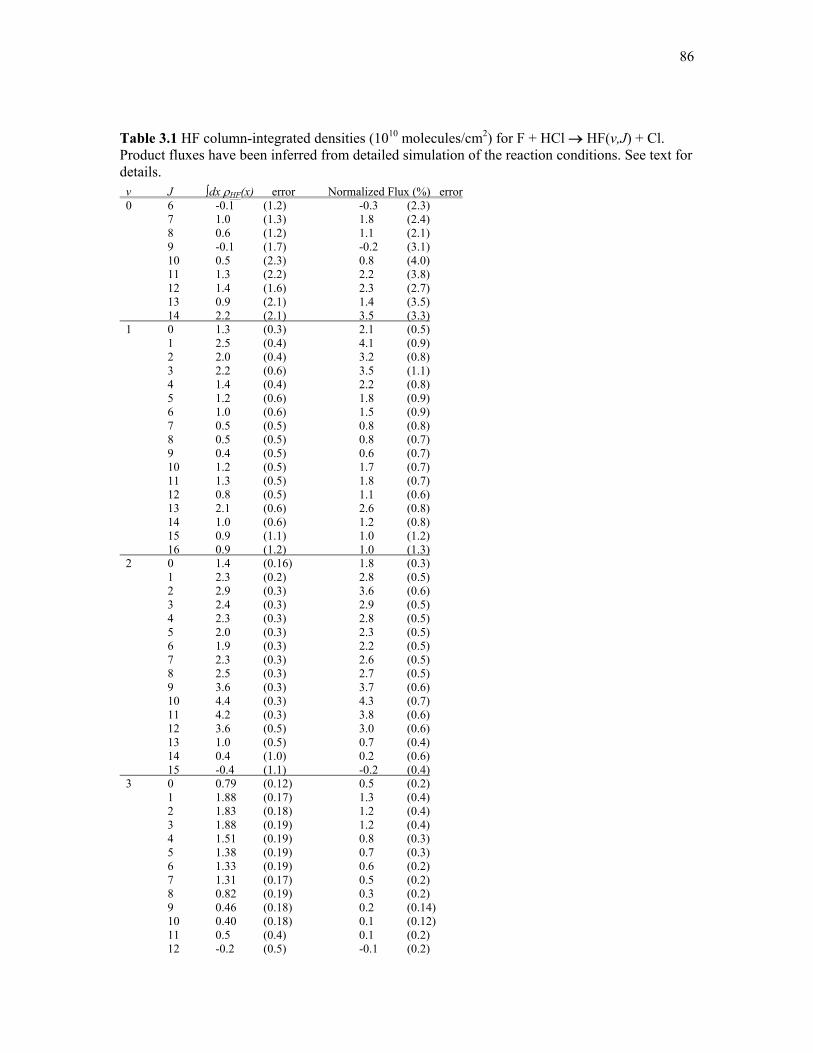
86

Table 3.1 HF column-integrated densities (1010 molecules/cm2) for F + HCl → HF(v,J) + Cl. Product fluxes have been inferred from detailed simulation of the reaction conditions. See text for details. v J ∫dx ρHF(x) error Normalized Flux (%) error 0 6 -0.1 (1.2) -0.3 (2.3) 7 1.0 (1.3) 1.8 (2.4) 8 0.6 (1.2) 1.1 (2.1) 9 -0.1 (1.7) -0.2 (3.1) 10 0.5 (2.3) 0.8 (4.0) 11 1.3 (2.2) 2.2 (3.8) 12 1.4 (1.6) 2.3 (2.7) 13 0.9 (2.1) 1.4 (3.5) 14 2.2 (2.1) 3.5 (3.3) 1 0 1.3 (0.3) 2.1 (0.5) 1 2.5 (0.4) 4.1 (0.9) 2 2.0 (0.4) 3.2 (0.8) 3 2.2 (0.6) 3.5 (1.1) 4 1.4 (0.4) 2.2 (0.8) 5 1.2 (0.6) 1.8 (0.9) 6 1.0 (0.6) 1.5 (0.9) 7 0.5 (0.5) 0.8 (0.8) 8 0.5 (0.5) 0.8 (0.7) 9 0.4 (0.5) 0.6 (0.7) 10 1.2 (0.5) 1.7 (0.7) 11 1.3 (0.5) 1.8 (0.7) 12 0.8 (0.5) 1.1 (0.6) 13 2.1 (0.6) 2.6 (0.8) 14 1.0 (0.6) 1.2 (0.8) 15 0.9 (1.1) 1.0 (1.2) 16 0.9 (1.2) 1.0 (1.3) 2 0 1.4 (0.16) 1.8 (0.3) 1 2.3 (0.2) 2.8 (0.5) 2 2.9 (0.3) 3.6 (0.6) 3 2.4 (0.3) 2.9 (0.5) 4 2.3 (0.3) 2.8 (0.5) 5 2.0 (0.3) 2.3 (0.5) 6 1.9 (0.3) 2.2 (0.5) 7 2.3 (0.3) 2.6 (0.5) 8 2.5 (0.3) 2.7 (0.5) 9 3.6 (0.3) 3.7 (0.6) 10 4.4 (0.3) 4.3 (0.7) 11 4.2 (0.3) 3.8 (0.6) 12 3.6 (0.5) 3.0 (0.6) 13 1.0 (0.5) 0.7 (0.4) 14 0.4 (1.0) 0.2 (0.6) 15 -0.4 (1.1) -0.2 (0.4) 3 0 0.79 (0.12) 0.5 (0.2) 1 1.88 (0.17) 1.3 (0.4) 2 1.83 (0.18) 1.2 (0.4) 3 1.88 (0.19) 1.2 (0.4) 4 1.51 (0.19) 0.8 (0.3) 5 1.38 (0.19) 0.7 (0.3) 6 1.33 (0.19) 0.6 (0.2) 7 1.31 (0.17) 0.5 (0.2) 8 0.82 (0.19) 0.3 (0.2) 9 0.46 (0.18) 0.2 (0.14) 10 0.40 (0.18) 0.1 (0.12) 11 0.5 (0.4) 0.1 (0.2) 12 -0.2 (0.5) -0.1 (0.2)

87

Figure 3.7 Vibrational HF product branching from F + HCl → HF(v) + Cl. The results of arrested-relaxation studies from Ref. 60,62,65 are as indicated. Population in v = 0 is directly observed for the first time; previous values are based on information theory predictions. Data are normalized to HF(v = 1–3) summed populations, enabling meaningful comparison of measurements with and without HF(v = 0) information.

vHF

0 1 2 3

Frac

tiona

l Pop

ulat

ion

0.0

0.2

0.4

0.6

0.8this work (density)Beadle et al.Ding et al.Tamagake et al.this work (flux)

88

Interestingly, direct absorption methods provide a first indication of finite nascent

population in the HF(v = 0, J) manifold, which does not emit in the near IR and thus had been

invisible to early chemiluminescence studies. Any rotational structure within the small v = 0

signals is masked by the scatter between points because of the conjunction of low signal levels,

subtraction of trace HF background, and uncertainty propagation with decreasing v. However, the

HF v = 0 densities comprise 9.5(67)% of the total HF density observed, with the total population

clearly exceeding this value due to exclusion of J ≤ 5 background. Interestingly, the observed v =

0 density is consistent with the 7–9% surprisal predictions reported by several of the

chemiluminescence studies60,65. This qualitative agreement between information theory and direct

measurements of ground state HF confirms a dynamical propensity for a sizeable population in

low energy states following reaction of F with HCl.

On the other hand, significant HF density is clearly also produced in high-energy

rovibrational states. The dashed lines in Fig. 3.6 indicate the energetic limits for HF quantum

states accessible via the 33 kcal/mol reaction exothermicity [≈ EHF(v = 3, J = 3)] and those with

the addition of the 4.3 kcal/mol average center-of-mass collision energy [≈ EHF(v = 3, J = 9)]. For

HF produced in states exceeding the lower limit, the center of mass recoil energy of the products

is actually less than that of the reactant collision energy. Thus, the F + HCl reactive encounter

favors excitation of the nascent HF molecule to such an extent that some fraction of the products

are formed with all of the reaction energy plus some of the reactant translational energy

sequestered in the HF internal energy. Indeed, finite density is observed above the upper energetic

threshold, only dropping off to zero above v = 3, J = 11. Populating these highest states requires

an additional 1.9 kcal/mol of collision energy, most likely arising from the significant width (σ =

1.3 kcal/mol, see inset of Fig. 3.1) in the crossed jet distributions. In principle, there may be an

additional energy contribution from reaction of spin orbit excited (2P1/2) versus ground state (2P3/2)

F atoms (Espin orbit = 1.1 kcal/mole) formed in a nearly statistical (2:4) ratio in the discharge

89

source. Evidence for such nonadiabatic reaction dynamics has been demonstrated in previous

quantum state resolved F + H2 and F + HD collision studies,76,86 where Ecom had negligible

uncertainties with respect to spin orbit excitation energy. However, the high transition state

barrier and collision energies necessary for the present study preclude any definitive implication

of nonadiabatic dynamics.

A high degree of HF rotational excitation in lower vibrational manifolds is also evident

from the state distributions in Fig. 3.6. Of considerable dynamic interest is the highly

nonmonotonic structure apparent in the rotational distributions. This structure is particularly

evident in the v = 2 manifold, which demonstrates a clear peaking at both low (J ≈ 2) and high (J

≈ 10) states. A qualitatively similar pattern of low (J ≈ 1–3) and high (J ≈ 11–13) state peaking is

also evident in the HF(v = 1) populations, though there appears to be additional structure in that

manifold. Raw data from early arrested-relaxation studies60,61 also indicate HF formation in low J

levels of v = 2 and v = 1. However, these low-J population components were previously ascribed

to rotational relaxation as a result of non-single-collision conditions and removed from the

analysis.60,61,67

The current results suggest grounds for reinterpretation. Data for the v = 1 and v = 2

manifolds are replotted in Fig. 3.8 along with the raw and “corrected” results from arrested-

relaxation studies.60,62 The crossed-jet studies, performed under much lower-density single-

collision conditions (see discussion in Sect. 3.1), clearly indicate the presence of a significant

bifurcation into both low and high J states. In principle, discrepancies between these studies could

arise from differences in thermal (Ecom ≈ kT = 0.6 kcal/mol) versus crossed supersonic jet (Ecom =

4.3 kcal/mol) collision energies. However, a much more likely interpretation is that the early

studies were in fact less rotationally relaxed than originally suspected, with partial rotational

relaxation simply adding to the true fraction of nascent product formed in low rotational states.

90

Figure 3.8 Rotational distributions for HF products in (a) v = 2 and (b) v = 1 manifolds, obtained from arrested relaxation (solid, dotted lines)60,62 and the present crossed jet experiments (circles with error bars). Distributions reported from previous studies have been modified for presumed rotational relaxation, as illustrated by raw (dashed line) and corrected (solid line) results of Ref. 60.

HF (v=2,J)Fr

actio

nal P

opul

atio

n

0.00

0.05

0.10

0.15a)

HF (v=1,J)

JHF

0 5 10 150.00

0.05

0.10

0.15b)

91

It is also conceivable that the rotational distributions reported in arrested-relaxation studies of F +

HBr and F + HI60,65,87 may also suffer from overcompensation for rotational relaxation and may

warrant study under lower density conditions.

It is apparent from Fig. 3.6 that the HF(v = 1,2; J) product distributions can not be

adequately described by any simple statistical model. Indeed, these populations are remarkable

for both the wide number of J states populated and the significant bifurcation of the population

into low-versus-high rotational states in HF(v = 1) and HF(v = 2). By comparison, the reaction of

F with H2,74 CH4,75 or C2H6,88 each with comparable ≈ 30 kcal/mol exothermicities, produces

similar degree of vibrational inversion but with a much more modest amount of HF rotation.

Specifically, the rotational distributions peak at Jmax ≈ 2 for F + CH4 and F + C2H6, and at Jmax ≈ 6

for F + H2. In each case, the population decays monotonically for J > Jmax. The current results are

qualitatively different, with a relatively flat rotational distribution in HF(v = 3) extending out to J

≈ 5–6. The HF(v = 1) and HF(v = 2) manifolds are even broader, with local maxima occurring

around J = 10. One intriguing interpretation of these double maxima may be microscopic

branching in the reaction dynamics. For example, if reaction occurs through two dynamical

pathways, one producing HF in low rotational states and the other with a propensity for rotational

excitation, a bimodal distribution such as seen in Fig. 3.6 could arise naturally. One precedent for

such bimodal and extensive rotational structure is the quantum transition-state resonance-

mediated reactions of F + HD, which will be discussed further in the following section.

3.4 Analysis

The results in Fig. 3.6 show nascent column-integrated densities for HF(v,J) produced

from the F + HCl reaction, as directly measured from the IR spectrum at the intersection of the

reactant jets. However, it is the state resolved fluxes that represent the experimental quantity of

interest; this requires consideration of the well-known89-91 density-to-flux transformation, i.e.

92

correctly taking into account the velocity-dependent detection sensitivity intrinsic in any density

based measurement technique. Modeling the effect of recoil energy on detection sensitivity

requires a detailed Monte Carlo (MC) simulation of the collision and absorption events based on

the explicit experimental geometry. Such a simulation has been described previously,92 is briefly

summarized here, and more completely detailed in Sect. 2.4(B) and Appendix E. The procedure

statistically calculates the relative signal contribution for a particular HF(v,J) quantum state

detected in some differential volume (dV) and Doppler detuning (dν) with respect to the probe

laser axis. This absorption signal arises from HF formation at another volume (dV’) in the jet

intersection region, with recoil energy and angular direction consistent with incident reactant

velocities, reaction energetics and conservation of linear momentum for limiting forms of the

differential cross section. The statistical averaging uses MC routines that simulate the distribution

of reactant speeds, densities, collision angles, and scattering angles present under the

experimental conditions. The inputs to the model are as follows: i) probe and jet geometries, ii)

known reactant and product masses, iii) reaction exothermicity, iv) reactant jet angular

distributions and speeds, and v) the adiabatic, zero-point corrected transition-state barrier height

(3.75 kcal/mol) obtained from high-level ab initio calculations,5,48,79 below which the reaction can

not proceed classically.

The key function of the MC simulation is to predict the probability distribution of

velocities for HF detected in state (v,J) as a function of HF–Cl recoil energy. These distributions,

projected onto to the IR probe axis, also can be used to predict Doppler widths plotted as the

dashed line in Fig. 3.4. The agreement between predicted and measured Doppler widths serves as

an independent measure of model reliability, and increases confidence in the quantity of interest

from the MC simulation. The density-to-flux transformation is obtained from

Φ(v,J) = ∫dx ρHF(v,J)(x) /⟨τ⟩(v,J), (3.4)

93

where Φ(v,J) is the state resolved flux per unit area (in HF molecules/cm2/s), ∫dx ρHF(ν,J)(x) is the

column-integrated density plotted in Fig. 3.6 and tabulated in Table 3.1, and ⟨τ⟩(v,J) is the average

time HF(v,J) spends in the probe laser volume. Due to spatial averaging within the unskimmed

jets, the MC results are relatively insensitive to the assumed differential cross section, which is

taken simply as isotropic. By way of support, MC simulations for extreme limits of i) sideways

and ii) forward/backward scattering yield ratios of density-to-flux transformation factors and

quantum state resolved populations that differ less than experimental uncertainties for a given

vibrational manifold. The state resolved flux values calculated via Eq. 3.4 have been normalized

to yield branching ratios into a given HF(v,J) state, as also summarized in Table 3.1. The density-

to-flux transformation results in a modest increase in product branching into low-energy HF(v,J)

states, yielding essentially identical trends for distributions of rotational HF column-integrated

densities discussed in Sect. 3.3. Net vibrational populations can be obtained by summing over

rotational states for a given vibrational state, as shown by the flux and density branching ratios

illustrated in Fig. 3.7. This comparison generally provides very good agreement with previous

studies, supporting expectations that chemiluminescence conditions were indeed sufficient to

completely arrest vibrational ineleastic collisions.

3.5 Discussion

Recent theoretical studies have reported the vibrational branching of HF product,

resulting in populations in [v = 0, 1, 2, 3] of [0.03, 0.31, 0.68, 0.01] on Kornweitz’s LEPS

surface71 and [0.01, 0.12, 0.72, 0.16] on the SHHG PES.66 Each of these studies consistently

overestimates the population in the highest (v = 2,3) manifolds compared to experimental

measurements, a trend continued by Hayes’ study73 on the new DHSN surface [0.001, 0.03, 0.43,

0.54]. Of particular importance, these calculations all reveal little or no population in the v = 0

manifold and a relatively insignificant fraction of v = 1 population. Such consistent over-

94

prediction of HF vibrational excitation with respect to experiment may signal the need to address

remaining deficiencies in these QCT calculations, arising from either i) pure quantum effects such

as transition state resonances, ii) non-adiabatic surface hopping dynamics, or iii) deficiencies in

the previous ground state ab initio surfaces.

In light of the discrepancies in vibrational branching, it is not surprising that theoretical

studies of the F + HCl reaction also fail to reproduce the highly structured rotational distributions

reported herein. Sayos’ QCT calculations66 found HF product almost exclusively in high J (J =

10–16) v = 2. As discussed in the introduction, Sayos’ SHHG PES and the more recent DHSN

PES both contain highly bent transition states. Such bent reaction geometry is likely to

significantly torque on the nascent HF diatom and constrain motion across the transition state.73

The inability to explain lower-energy rotational populations has prompted us to further explore

the DHSN surface via QCT, as described below.

To help interpret the observed trends in HF product state distributions and address

remaining discrepancies with theory, a series of QCT calculations have been performed on the

DHSN surface using a fourth-order Runge-Kutta integration method.84 Using a time step of 5

atomic units = 0.12 fs, energy is conserved to better than 0.03 and 0.0002 kcal/mol for reactive

and non-reactive events, respectively, with typical trajectories of 1–2 ps duration. The surface has

been explored using trajectories starting in the entrance channel with an initial F–HCl distance of

≈10 Å, collision energies of 4–10 kcal/mol, initial HCl angular momenta of J = 0–5, and impact

parameters of 0–4 Å. Representative calculations resulting from 50,000 trajectories starting in the

F + HCl channel at Ecom = 7 kcal/mol and JHCl = 2 are plotted in Fig. 3.9. The choice of collision

energy enhances reaction probability; however, the qualitative aspects of the HF product

quantum-state distributions for reactive events prove relatively insensitive to collision conditions.

Specifically, product HF is found exclusively in the v = 3 and v = 2 manifolds, with highest-

energy rotational states primarily correlating with v = 2, as anticipated from conservation of

95

Figure 3.9 QCT results on the DHSN potential energy surface. Rovibrational distributions in v = 1, v = 2, and v = 3 are shown for trajectory calculations beginning far in the entrance channel (circles), and for trajectories beginning in the van der Waals well (triangles).

vHF=3

JHF

0 5 10 150.00

0.05

0.10

vHF=2

Frac

tiona

l Pop

ulat

ion

0.00

0.05

0.10

vHF=1

0.00

0.05

96

energy. The results are qualitatively similar to those reported by Sayos et al.,48 who also found

only rotationally excited HF in v = 2. The results of Sayos et al. are less vibrationally excited than

the present DHSN calculations, but are performed on the SHHG PES, which has an empirically

lowered barrier that enabled study at lower collision energies. Nevertheless, trajectories on both

surfaces predict high vibrational excitation and, more specifically, only high rotational excitation

in v = 2.

As a further test of these trends, a second set of trajectories has been performed, starting

simply in the transition state (TS) region of the DHSN surface with total energy 0.2 kcal/mol

above the classical barrier. Although these TS calculations have not been chosen to accurately

reflect a distribution of reactive trajectories, they do reproduce the same propensity for i)

exclusive population in the v = 2 and (to a lesser extent) v = 3 manifolds, and ii) peaking of high J

state rotational excitation in v = 2. Thus, the DHSN surface clearly confirms results from earlier

surfaces, in which only the high-J HF(v = 2) and lower J HF(v = 3) products are predicted via

classical trajectory methods.

We have also used QCT methods to briefly explore the possible influence of the deep van

der Waals well in the HF + Cl exit channel. These trajectories are motivated by the wealth of

vibrational predissociation studies of van der Waals complexes, as well as the possibility of long

lived resonance states that explore portions of the exit well not extensively visited by classical

reaction path. Exit-well trajectories are started in the vicinity of the HF–Cl van der Waals

minimum, in an initial distribution of HF rovibrational states obtained from full trajectory

calculations shown in Fig. 3.9 and with zero kinetic energy in the HF–Cl coordinate. In essence,

these conditions mimic what might be expected if nascent reactive products were to become

trapped in the HF–Cl van der Waals well following reaction. The trajectories with non-rotating

but vibrationally excited HF were found to be nondissociative on the time scales explored; this

corresponds roughly to vibrational predissociation, which is known to be exquisitely sensitive to

the hard inner wall of the PES and poorly modeled by QCT.93 However, the dissociation

97

probability of the HF–Cl complex does rise rapidly with increasing HF internal rotation, in effect,

rotationally predissociating to yield HF with reduced internal energy. The results of such

trajectories are shown in Fig. 3.9, where the product HF fragments retain most of their vibrational

energy while being “cooled” into lower angular momentum states. Thus, the Van der Waals exit

well may play a significant role in the formation of the low-J HF observed experimentally and

may even contribute to HF population in lower vibrational manifolds. Indeed, previous studies of

exit-channel dynamics by Orr-Ewing and coworkers in reactive trajectories found that

rotationally cold products with strong dipole moments can torque on recoiling fragments and

thereby rotationally “heat up” in the exit channel.94 It would seem equally dynamically plausible

in the F + HCl system for highly rotationally excited HF to be “cooled” by angular forces in the

van der Waals exit channel, which would be an interesting direction for further theoretical

exploration.

As a final comment, we note that the broad bimodal rotational distributions observed in

the F + HCl system are not entirely novel. In fact, the resonance-mediated reaction F + HD

produces a similarly broad, highly structured distribution of rotational states in HF(v = 2), as

measured at Ecom = 0.6 kcal/mol by Harper et al.,76 and predicted by the quantum dynamical

calculations of Skodje et al.27 To facilitate comparison, the F + HD results for HF(v = 2, J) are

reproduced in Fig. 3.10 along with the distribution of HF(v = 2,J) fluxes from the present F + HCl

work. The distributions from each reaction share a number of qualitative features, including

highly nonstatistical populations, broad nearly constant intensities at low J and a sudden drop off

to zero population at high J. The calculations of Skodje et al. interpret the F + HD distribution as

the result of a transition state resonance due to H atom vibrational motion across the barrier, as

first observed in elegant differentially resolved scattering measurements by Liu and coworkers.

The qualitative similarity between rotational distributions in these two HLH systems therefore

suggest the presence of transition state resonance dynamics also playing an important role in

98

Figure 3.10 HF(v = 2,J) rotational distributions from F + HCl (circles), in comparison with the F + HD reaction (triangles) from Ref. 76. The broad and structured populations from F + HD are dominated by a reactive transition state resonance at ≈ 0.5 kcal/mol.

vHF=2

0.00

0.05

0.10

F+HCl (current experiment)Ecom = 4.3(1.3) kcal/mol

vHF=2

JHF

0 5 10 15

Frac

tiona

l Pop

ulat

ion

0.00

0.05

0.10

F+HD (Harper)Ecom = 0.6(2) kcal/mol

99

F + HCl reactive scattering. At the very least, this is an intriguing result worthy of further

experimental and theoretical attention. From an experimental perspective, we have constructed a

velocity map ion imaging apparatus, which should permit reactive studies of F + HCl by probing

the Cl(2P1/2,2P3/2) product with energy and angular scattering resolution. From a theoretical

perspective, this has motivated our development of a full set of high-level multireference (MRCI

+ Q), spin-orbit corrected potentials along with non-adiabatic terms coupling each of the surfaces.

It is our hope that such efforts will help further elucidate the dynamical richness clearly still

present in such a classic yet deceptively “simple” atom + diatomic reaction.

3.6 Summary and Conclusion

The reaction F + HCl → HF + Cl has been observed under rigorous single-collision

conditions for the first time, based on high resolution direct absorption IR laser spectroscopy on

the HF(v,J) product. The increased sensitivity of the direct absorption method permits operation

under much lower reactant densities, resulting in many orders of magnitude reduction in time

window for collisions of the nascent product. The absence of collisional relaxation is validated by

studies as a function of reactant backing pressure, as well as high resolution of Doppler profiles

of translationally “hot” product species. The HF vibrational distributions are in excellent

agreement with results reported in early arrested-relaxation IR emission studies. The IR laser

absorption technique also permits branching into the HF(v = 0) manifold to be observed directly

for the first time. The HF rotational distribution reveals significant structure, with strongly

bimodal populations evident in both the v = 2 and v = 1 manifolds. The presence of both low and

high J nascent rotational structure under single collision conditions is qualitatively similar to raw

data from early IR emission studies, for which the low J component was inferred to be due to

“unarrested” rotational relaxation processes. The current studies offer indications that some

100

fraction of this low J component may have been truly nascent, which might warrant reanalysis of

similar IR emission data from other X + HY systems.

This novel bifurcation in J state distributions highlights the possible presence of

microscopic branching in the reaction, which might signal the presence of more complex

dynamics due to quantum effects and/or non-adiabatic coupling between electronic surfaces. By

way of example, the bimodal rotational distributions observed in F + HCl are qualitatively quite

similar to what is seen in the F + HD system, for which the presence of a FH(v = 3)–D quantum

transition state scattering resonance has been confirmed by both experiment and theory. In

analogy to the work of Orr-Ewing on more nearly thermoneutral systems, we propose a possible

alternate mechanism for microscopic branching between low J and high J rotational distributions

that involves partial internal HF rotor relaxation in the outgoing exit-channel due to the HF–Cl

van der Waals well. High-level multireference potentials will soon be available to permit full 3D

quantum reactive scattering on multiple non-adiabatic surfaces, and thereby stimulate more

rigorous comparison between theory and experiment and promote understanding of the

underlying reaction dynamics.

101

References for Chapter III

1 G. B. Moore and I. W. M. Smith, J. Phys. Chem. 100, 12848 (1996).

2 P. J. Kuntz, E. M. Nemeth, J. C. Polanyi, S. D. Rosner, and C. E. Young, J. Chem. Phys. 44, 1168 (1966).

3 G. Capecehi and H. J. Werner, Phys. Chem. Chem. Phys. 6, 4975 (2004).

4 J. F. Castillo, B. Hartke, H. J. Werner, F. J. Aoiz, L. Banares, and B. Martinez-Haya, J. Chem. Phys. 109, 7224 (1998).

5 M. P. Deskevich, M. Y. Hayes, K. Takahashi, R. T. Skodje, and D. J. Nesbitt, J. Chem. Phys. 124, 224303 (2006).

6 P. F. Weck and N. Balakrishnan, J. Chem. Phys. 123, 144308 (2005).

7 S. Rogers, D. S. Wang, A. Kuppermann, and S. Walch, J. Phys. Chem. A 104, 2308 (2000).

8 D. J. Garton, A. L. Brunsvold, T. K. Minton, D. Troya, B. Maiti, and G. C. Schatz, J. Phys. Chem. A 110, 1327 (2006).

9 D. J. Garton, T. K. Minton, B. Maiti, D. Troya, and G. C. Schatz, J. Chem. Phys. 118, 1585 (2003).

10 B. F. Parsons and D. W. Chandler, J. Chem. Phys. 122, 174306 (2005).

11 M. H. Alexander, G. Capecchi, and H. J. Werner, Faraday Discuss. 127, 59 (2004).

12 F. Dong, S. H. Lee, and K. Liu, J. Chem. Phys. 115, 1197 (2001).

13 D. Skouteris, H. J. Werner, F. J. Aoiz, L. Banares, J. F. Castillo, M. Menendez, N. Balucani, L. Cartechini, and P. Casavecchia, J. Chem. Phys. 114, 10662 (2001).

14 N. Balucani, D. Skouteris, G. Capozza, E. Segoloni, P. Casavecchia, M. H. Alexander, G. Capecchi, and H. J. Werner, Phys. Chem. Chem. Phys. 6, 5007 (2004).

102

15 D. G. Truhlar and Kupperma.A, J. Chem. Phys. 56, 2232 (1972).

16 R. D. Levine and S. F. Wu, Chem. Phys. Lett. 11, 557 (1971).

17 R. E. Continetti, B. A. Balko, and Y. T. Lee, J. Chem. Phys. 93, 5719 (1990).

18 S. C. Althorpe, F. Fernandez-Alonso, B. D. Bean, J. D. Ayers, A. E. Pomerantz, R. N. Zare, and E. Wrede, Nature 416, 67 (2002).

19 M. H. Alexander, D. E. Manolopoulos, and H. J. Werner, J. Chem. Phys. 113, 11084 (2000).

20 S. C. Althorpe, Chem. Phys. Lett. 370, 443 (2003).

21 M. Baer, M. Faubel, B. Martinez-Haya, L. Y. Rusin, U. Tappe, and J. P. Toennies, J. Chem. Phys. 108, 9694 (1998).

22 F. Dong, S. H. Lee, and K. Liu, J. Chem. Phys. 113, 3633 (2000).

23 M. Faubel, B. Martinez-Haya, L. Y. Rusin, U. Tappe, J. P. Toennies, F. J. Aoiz, and L. Banares, J. Phys. Chem. A 102, 8695 (1998).

24 Y. T. Lee, Science 236, 793 (1987).

25 D. M. Neumark, A. M. Wodtke, G. N. Robinson, C. C. Hayden, and Y. T. Lee, J. Chem. Phys. 82, 3045 (1985).

26 L. Y. Rusin and J. P. Toennies, Phys. Chem. Chem. Phys. 2, 501 (2000).

27 R. T. Skodje, D. Skouteris, D. E. Manolopoulos, S. H. Lee, F. Dong, and K. Liu, J. Chem. Phys. 112, 4536 (2000).

28 R. T. Skodje, D. Skouteris, D. E. Manolopoulos, S. H. Lee, F. Dong, and K. P. Liu, Phys. Rev. Lett. 85, 1206 (2000).

29 R. A. Sultanov and N. Balakrishnan, Astrophys. J. 629, 305 (2005).

103

30 S. Javoy, V. Naudet, S. Abid, and C. E. Paillard, Exp. Therm. Fluid Sci. 27, 371 (2003).

31 D. Gerlich, E. Herbst, and E. Roueff, Planet Space Sci. 50, 1275 (2002).

32 O. D. Krogh, D. K. Stone, and G. C. Pimentel, J. Chem. Phys. 66, 368 (1977).

33 M. J. Berry, J. Chem. Phys. 59, 6229 (1973).

34 C. Zhu, R. Krems, A. Dalgarno, and N. Balakrishnan, Astrophys. J. 577, 795 (2002).

35 D. A. Neufeld, J. Zmuidzinas, P. Schilke, and T. G. Phillips, Astrophys. J. 488, L141 (1997).

36 W. B. Chapman, B. W. Blackmon, and D. J. Nesbitt, J. Chem. Phys. 107, 8193 (1997).

37 C. X. Xu, D. Q. Xie, and D. H. Zhang, Chin. J. Chem. Phys. 19, 96 (2006).

38 S. C. Althorpe and D. C. Clary, Annu. Rev. Phys. Chem. 54, 493 (2003).

39 M. H. Qiu, Z. F. Ren, L. Che, D. X. Dai, S. A. Harich, X. Y. Wang, X. M. Yang, C. X. Xu, D. Q. Xie, M. Gustafsson, R. T. Skodje, Z. G. Sun, and D. H. Zhang, Science 311, 1440 (2006).

40 Y. R. Tzeng and M. H. Alexander, J. Chem. Phys. 121, 5183 (2004).

41 J. D. D. Martin and J. W. Hepburn, J. Chem. Phys. 109, 8139 (1998).

42 W. T. Zemke, W. C. Stwalley, J. A. Coxon, and P. G. Hajigeorgiou, Chem. Phys. Lett. 177, 412 (1991).

43 B. P. Stoicheff, Can. J. Phys. 79, 165 (2001).

44 R. T. Skodje, Annu. Rev. Phys. Chem. 44, 145 (1993).

45 W. Jakubetz, D. Sokolovski, J. N. L. Connor, and G. C. Schatz, J. Chem. Phys. 97, 6451 (1992).

104

46 I. M. Waller, T. N. Kitsopoulos, and D. M. Neumark, J. Phys. Chem. 94, 2240 (1990).

47 F. Fernandez-Alonso and R. N. Zare, Annu. Rev. Phys. Chem. 53, 67 (2002).

48 R. Sayos, J. Hernando, J. Hijazo, and M. Gonzalez, Phys. Chem. Chem. Phys. 1, 947 (1999).

49 E. Wurzberg and P. L. Houston, J. Chem. Phys. 72, 5915 (1980).

50 C. M. Moore, I. W. M. Smith, and D. W. A. Stewart, Int. J. Chem. Kinet. 26, 813 (1994).

51 I. W. M. Smith and D. J. Wrigley, Chem. Phys. Lett. 70, 481 (1980).

52 B. S. Ault, J. Chem. Phys. 68, 4012 (1978).

53 J. M. Merritt, J. Kupper, and R. E. Miller, Phys. Chem. Chem. Phys. 7, 67 (2005).

54 V. Aquilanti, D. Cappelletti, F. Pirani, L. Y. Rusin, M. B. Sevryuk, and J. P. Toennies, J. Phys. Chem. 95, 8248 (1991).

55 A. V. Fishchuk, G. C. Groenenboom, and A. van der Avoird, J. Phys. Chem. A 110, 5280 (2006).

56 A. V. Fishchuk, P. E. S. Wormer, and A. van der Avoird, J. Phys. Chem. A 110, 5273 (2006).

57 J. Klos, M. M. Szczesniak, and G. Chalasinski, Int. Rev. Phys. Chem. 23, 541 (2004).

58 M. L. Dubernet and J. M. Hutson, J. Phys. Chem. 98, 5844 (1994).

59 M. Meuwly and J. M. Hutson, J. Chem. Phys. 119, 8873 (2003).

60 P. Beadle, M. R. Dunn, N. B. H. Jonathan, J. P. Liddy, and J. C. Naylor, J. Chem. Soc., Faraday Trans. II 74, 2170 (1978).

61 D. Bogan and D. W. Setser, in Fluorine-containing free radicals: kinetics and dynamics of reactions: based on a symposium sponsored by the Division of Physical Chemistry at

105

the 169th meeting of the American Chemical Society, Philadelphia, Pennsylvania, April 7-11, 1975, edited by J. W. Root (American Chemical Society, Washington, 1978), pp. 237.

62 A. M. G. Ding, L. J. Kirsch, D. S. Perry, J. C. Polanyi, and J. L. Schreiber, Faraday Discuss. 55, 252 (1973).

63 N. Jonathan, Melliar-Smith Cm, S. Okuda, D. H. Slater, and D. Timlin, Mol. Phys. 22, 561 (1971).

64 J. P. Sung and D. W. Setser, Chem. Phys. Lett. 48, 413 (1977).

65 K. Tamagake, D. W. Setser, and J. P. Sung, J. Chem. Phys. 73, 2203 (1980).

66 R. Sayos, J. Hernando, R. Francia, and M. Gonzalez, Phys. Chem. Chem. Phys. 2, 523 (2000).

67 D. S. Perry, Private Communication (2006).

68 D. Brandt and J. C. Polanyi, Chem. Phys. 35, 23 (1978).

69 L. J. Kirsch and J. C. Polanyi, J. Chem. Phys. 57, 4498 (1972).

70 J. C. Polanyi and K. B. Woodall, J. Chem. Phys. 57, 1574 (1972).

71 H. Kornweitz and A. Persky, J. Phys. Chem. A 108, 140 (2004).

72 B. Y. Tang, B. H. Yang, K. L. Han, R. Q. Zhang, and J. Z. H. Zhang, J. Chem. Phys. 113, 10105 (2000).

73 M. Y. Hayes, M. P. Deskevich, D. J. Nesbitt, K. Takahashi, and R. T. Skodje, J. Phys. Chem. A 110, 436 (2006).

74 W. B. Chapman, B. W. Blackmon, S. Nizkorodov, and D. J. Nesbitt, J. Chem. Phys. 109, 9306 (1998).

75 W. W. Harper, S. A. Nizkorodov, and D. J. Nesbitt, J. Chem. Phys. 113, 3670 (2000).

106

76 W. W. Harper, S. A. Nizkorodov, and D. J. Nesbitt, J. Chem. Phys. 116, 5622 (2002).

77 D. Proch and T. Trickl, Rev. Sci. Instrum. 60, 713 (1989).

78 D. R. Miller, in Atomic and molecular beam methods, edited by G. Scoles (Oxford University Press, New York, 1988), pp. 14.

79 I. Last and M. Baer, J. Chem. Phys. 80, 3246 (1984).

80 J. L. Hall and S. A. Lee, Appl. Phys. Lett. 29, 367 (1976).

81 A. S. Pine, J. Opt. Soc. Am. 66, 97 (1976).

82 D. Herriot, H. Kogelnik, and R. Kompfner, Appl. Optics 3, 523 (1964).

83 D. Kaur, A. M. Desouza, J. Wanna, S. A. Hammad, L. Mercorelli, and D. S. Perry, Appl. Optics 29, 119 (1990).

84 W. H. Press, S. A. Teukolsky, W. T. Vetterling, and B. P. Flannery, Numerical recipes in C: the art of scientific computing, 2 ed. (Cambridge University Press, New York, 1992).

85 E. Arunan, D. W. Setser, and J. F. Ogilvie, J. Chem. Phys. 97, 1734 (1992).

86 S. A. Nizkorodov, W. W. Harper, W. B. Chapman, B. W. Blackmon, and D. J. Nesbitt, J. Chem. Phys. 111, 8404 (1999).

87 D. Brandt and J. C. Polanyi, Chem. Phys. 45, 65 (1980).

88 E. S. Whitney, A. M. Zolot, A. B. McCoy, J. S. Francisco, and D. J. Nesbitt, J. Chem. Phys. 122, 124310 (2005).

89 H. W. Cruse, P. J. Dagdigian, and R. N. Zare, Faraday Discuss. 55, 277 (1973).

90 C. Naulin, M. Costes, A. Benseddik, and G. Dorthe, Laser Chem. 8, 283 (1988).

91 D. M. Sonnenfroh and K. P. Liu, Chem. Phys. Lett. 176, 183 (1991).

107

92 W. W. Harper, S. A. Nizkorodov, and D. J. Nesbitt, Chem. Phys. Lett. 335, 381 (2001).

93 E. Tannenbaum, K. J. Higgins, W. Klemperer, B. Segev, and E. J. Heller, J. Phys. Chem. B 106, 8100 (2002).

94 S. Rudic, C. Murray, J. N. Harvey, and A. J. Orr-Ewing, J. Chem. Phys. 120, 186 (2004).

108

________________

Chapter IV F + H2O → HF(v,J) + OH: HF(v,J) nascent product state distributions formed

in crossed molecular jets

________________

4.1 Introduction

As demonstrated in the previous chapter, significant progress has been made in

understanding gas-phase reaction dynamics in three-atom systems. However, significant hurdles

remain for larger systems because additional degrees of freedom dramatically increase the

computational cost of characterizing the PES and performing quantum dynamical calculations on

such surfaces in full dimensionality. Yet, even with the relatively modest increase from three to

four atoms, entirely new phenomena become feasible, such as mode-specific chemistry1-13 and

energy transfer into “spectator” degrees of freedom.14,15 Additionally, increasing system size and

number of open channels necessitate considerably more detailed experimental observations to

characterize adequately the product distributions at the quantum state-to-state level.

Recent work has demonstrated that the study of polyatomic (i.e. N ≥ 4) reaction dynamics

is on the horizon of computational feasibility. In particular, remarkable advances have been made

in developing an accurate ab initio PES and performing exact quantum reactive scattering

calculations for the benchmark four-atom reaction system H + H2O ↔ H2 + OH.16-18 Recent

progress in this dynamically rich reaction suggests that full-dimensional ab initio studies of four-

atom systems with more than one heavy (i.e., non-hydrogen) atom will be feasible in the near

future, and chemical systems with N > 4 are likely to become the outstanding computational

challenge in 3N-6 dimensions.

Direct dynamics methods present one interesting alternative to completely exploring

dynamics on a high-dimensional PES. This technique enables classical trajectory simulations to

109

be performed in arbitrary dimensions by calculating the PES energy and its derivatives “on the

fly,” at the nuclear coordinates traversed by a given trajectory.19-22 However, computational costs

in systems of high dimensionality restrict such calculations to relatively low levels of ab initio

treatment. Furthermore, this method relies intrinsically on classical dynamics, making inherently

quantum phenomena, such as zero point energy23 and reactions promoted by tunneling through

barriers,24 difficult to model. The current intractability of full dimensional studies for all but the

simplest four-atom system emphasizes the need for further experimental efforts at the state-to-

state level. Such work provides a crucial opportunity for benchmark testing of approximate

theoretical methods against detailed experimental measurements and stimulates the development

of progressively more rigorous multidimensional quantum computational techniques.

The F + H2O → HF + OH reaction represents an ideal candidate for detailed comparison

between experiment and novel theoretical techniques. In addition to fundamental interest in 4-

atom bond-making and bond-breaking, this reaction plays an important role in Earth’s

atmosphere, where it is primarily responsible for scavenging F atoms introduced into the

troposphere by photolysis of partially fluorinated compounds.25 In astronomy this reaction may be

important in determining the fate of F atoms in the interstellar medium.26 The dynamics of this

atom + triatom abstraction process are dominated by a relatively low transition state barrier (ΔE ≈

5 kcal/mol27) and yet a moderately high exothermicity (ΔH0 = -17.61(2) kcal/mol28,29).

Interestingly, these values are quite close to those found in the current state-of-the-art 4-atom

reaction system, H2 + OH, which features a similarly exothermic (ΔH0 = -14.4 kcal/mol28,30)

reaction path and low barrier (ΔE ≈ 6 kcal/mol)16 for formation of H2O product.

As shown in Fig. 4.1, many rovibrational quantum states of HF and OH products are

energetically accessible from reaction of F with H2O. From an experimental perspective, quantum

state resolved spectroscopic techniques have been developed that are capable of sensitively

probing reactive scattering and energy flow into both diatomic species.31-33 Alternatively, high-

110

Figure 4.1 Reaction coordinate for F + H2O → HF + OH on the two lowest adiabatic potential energy surfaces, from calculation in Ref. 27. Both surfaces asymptotically correlate to F(2P3/2) reactant, but result in ground OH(2P3/2) (solid line) and spin-orbit excited OH(2P1/2) (short dashes) in the product channel. The inset plot is the calculated experimental collision energy distribution, whose average value, Ecom = 5.4(1.3) kcal/mol above the reactant energy, is plotted as the long dashed line. Various vibrational levels of HF and OH products are shown as dotted lines.

Reaction Coordinate

Ener

gy (k

cal/m

ol)

0

10

20

30

40

P(Ecom)

(1,0)(0,1)

(0,0)

(0,2)

(2,0)(1,1)

(vHF,vOH)

⟨Ecom⟩

(3,0)

111

level theoretical treatment may hope to attain chemically accurate ab initio results, while still

using acceptably small basis sets to describe the second row atoms in this system. Recent

multireference configuration interaction studies of the F + H2O PES revealed that reaction on the

two lowest electronic PESs occurs over barriers of ΔE ≈ 5 kcal/mol and 25 kcal/mol, which

correlate adiabatically with the formation of ground (2Π3/2) and spin orbit excited (2Π1/2) product

OH.27 Although these two surfaces exhibit quite different adiabatic barriers to reaction, they can

cross via multidimensional “seams” of conical intersections, including nuclear configurations

close to the reactive transition state.

The importance of such non-adiabatic reaction considerations is emphasized by recent

crossed jet studies of F + H2O and F + D2O performed in our group.33,34 Though laser induced

fluorescence (LIF) measurements revealed that only OD(v = 0,N) is produced, with an average

rotational energy of Erot ≈ 1 kcal/mol, the reaction produces ground (2Π3/2) and spin-orbit excited

(2Π1/2) OD products in roughly a 2:1 ratio. This result is surprising since spin-orbit excited radical

adiabatically correlates to reaction on the first excited electronic surface, whose ≈ 25 kcal/mol

barrier exceeds the collision energy by five-fold. Thus, multiple theoretical surfaces and non-

adiabatic dynamical treatments will clearly be necessary to account for the apparent “surface

hopping” dynamics leading to OH(2Π1/2). The importance of such non-adiabatic dynamics

underlying this relatively simple four-atom reaction further motivates quantum-state resolved

studies of the HF(v,J) cofragment.

Both kinetic and dynamic studies of F + H2O have been performed previously.

Temperature dependent rates of the F + H2O/D2O reactions were reviewed by Stevens et al.,35

inferring a tunneling mechanism and a ΔE ≈ 4 kcal/mol estimate for the transition state barrier

height, in close agreement with the ΔE ≈ 5 kcal/mol value from ab initio theory.27 In a series of

pioneering dynamical studies, Setser and coworkers obtained rotationally resolved IR

chemiluminescence spectra of HF in the v = 1 manifold and inferred cold OH vibrations.36-38

112

Recent photodetachment studies of the anionic cluster FH2O- have also shed insight upon the title

reaction. Partial overlap between the FH2O- anion geometry and the F + H2O transition state

allows the reactive region of the PES to be accessed directly, resulting in a low energy tail

attributed to formation of product HF + OH.39 Direct dynamics simulations of the

photodetachment process found substantial branching into the product channel, yielding

rovibrationally excited HF products and vibrationally cold OH with modest amounts of rotational

excitation.40 These studies stimulate further study of this fundamental four-atom reaction under

crossed beam conditions to resolve completely the energy partitioning in the HF fragment.

The following sections of this chapter describe the complete HF(v,J) product state

distribution following the reaction F + H2O → HF + OH, measured using the high-sensitivity

laser spectrometer and crossed jet apparatus described in detail in Ch. I. Crossed supersonic jets

enable the reaction to be studied with ≈ 1000-fold reduction in gas density compared to

chemiluminescence studies. Furthermore, reverse seeding in a He diluent permits the supersonic

jet reactants to more easily surmount the barrier by increasing the collision energy. Sensitive IR

laser absorption methods provide i) complete rovibrational state resolution, ii) high resolution

Dopplerimetry measurements along the probe axis, and iii) the first experimental measure of total

product branching into each of the v = 0, 1 and 2 vibrational manifolds.

4.2 Experiment

Detailed descriptions of the crossed jet experimental apparatus appear in Ch. II. The

specific conditions used in the present study are described here and illustrated in Fig. 4.2. The

H2O jet contains ≈ 30 Torr H2O, produced by bubbling He through liquid water heated to 30 °C at

a total pressure of 200 Torr. The remainder of the gas line, including the pulsed valve, is heated to

60 °C to prevent condensation. Fig. 4.3 displays IR measurements of H218O concentration, present

113

Figure 4.2 Schematic of the crossed jet apparatus, containing pulsed molecular jets of F and H2O intersecting at 90° in a vacuum chamber. Product HF(v,J) is probed by quantum state resolved, high resolution IR laser absorption using a multipass cell oriented perpendicular to the plane defined by the jets axes.

Figure 4.3 Measured spectral intensity of a isotopically substituted H218O line present in

nature abundance in the reactant water jet. The jet’s stagnation pressure is constant at 200 Torr with helium carrier gas. Partial pressure of water is varied by changing the liquid temperature.

H2O Partial Pressure (Torr)0 20 40 60 80 100

H218

O ∫A

dν

(kH

z)

0

100

200

300

400

500 ObservedExpected

114

in natural isotopic abundance. These measurements match the expected linear curve of growth as

H2O partial pressure increases up to the 30 Torr value used, confirming the absence of significant

H2O clustering in the reactant jet.

Given its high sensitivity, the IR probe detects trace HF gas produced in the radical

source by impurities in the 10% F2 90% He mixture passed through the high voltage plasma jet

source. Detailed characterization of this background was presented in Ch. 2.3(B). The measured

HF density corresponds to 1.0 ppm generated in the plasma source. Placing a liquid nitrogen cold

trap in the F2 gas line reduces this background approximately two-fold while leaving the reactive

scattering intensity unchanged. Background corrections are made by measuring the HF spectrum

in the presence and absence of H2O reactant, and correcting the reactively scattered results for the

background HF densities. This correction is most important in the v = 0 manifold at low J, as

demonstrated by the ≈ 60 K HF background temperature shown in Fig. 2.11. As a result,

background HF can be confidently eliminated from the reactive product distributions, although

product signals in the very lowest HF(v = 0, J ≤ 4) rotational states are not measured reliably and

thus not reported. However, HF branching into these states is not expected to be dynamically

favored and does not change any of the conclusions drawn from the present results.

Doppler-resolved absorption measurements, such as those presented in Fig. 4.4(a,b), are

recorded for all HF(v” ≤ 2) IR transitions41 within 2.5–3.3 μm, for a total of about 500

observations of 42 lines. Fitting the lineshapes, such as that in Fig. 4.4(b), to a simple Gaussian

profile reveals translationally excited profiles (full width at half maximum [FWHM] of 880 MHz)

following the reaction, corresponding to HF recoil speeds of ≈ 2.20 km/s. This value exceeds the

1.25 km/s FWHM of the F + H2O center of mass (COM) velocity distribution. For states

originating in the v = 2 manifold [Fig. 4.4(a)], less energy is available for product translation, and

the observed Doppler widths decrease accordingly. However, the observed Doppler widths

115

Figure 4.4 Sample Doppler-resolved absorption measurements originating from (a) HF (v = 3←2; J = 1←0) and (b) HF (v = 2←1; J = 2←1) transitions, with total integrated intensities with respect to laser detuning in (aa) and (bb) and indicated by solid arrows. Solid lines in the left hand plots are least squares fits to Gaussian lineshapes, with Δν (FWHM) well in excess of the 300 MHz room temperature HF linewidth [dashed line in (b)]. Doppler profiles have been smoothed with Savitzky-Golay methods (4th order 25 point) relative to the high resolution measurements; fits and integrals have been obtained from the raw data.

b)

ν−ν0 (MHz)-1000 0 1000

Abs

(10-5

)

0

5

10 bb)

-1000 0 1000

∫Abs

dν

(kH

z)

0

30

60

90

a)

-5

0

5aa)

0

10

20

Δν=880MHz

Δν=610MHz

Δν300K=330MHz

v=3←2J=1←0

v=2←1J=2←1

∫Abs dν

116

strongly indicate that the nascent HF remains translationally excited following the reactive

encounter, providing evidence for single collision conditions at the reactant jet intersection

region.

Reaction cross sections and experimental conditions for the present study result in HF

densities of < 2×109 #/cm3 per quantum state, requiring highly sensitive measurements of HF

transient absorption. As shown by the raw data in Fig. 4.4(a,b), the IR absorption at these low

densities is on the order of the fundamental photon shot noise limit of ≈ 1×10-5 absorbance in the

experimental 4.0 kHz bandwidth. Even at nearly shot-noise limited sensitivity, signals profit from

integrating each Doppler profile to improve the signal to noise as described in Ch. III. This

treatment reduces uncertainty by the square root of the 200–300 measurements under the Doppler

FWHM, as reflected in the ≈ 5 kHz integral absorbance uncertainty in Fig. 4.4(aa,bb), and results

in a detection sensitivity of ≈ 1×10-8 HF/cm3.

Since absolute HF densities are obtained from the IR absorption technique, the total

reaction cross section of σ ≈ 0.8(0.5) Å2 for F + H2O at 5.4(1.3) kcal/mol collision energy has

been obtained by calibrating the F atom density against F + H2 as described in Ch. 2.4(C). This

result agrees with measured thermal rate constant, which is approximately ten times lower than

the molecular collision rate35 and suggests that the collision energy does not efficiently couple

into the reaction coordinate according to an intermediate- rather than early-barrier scenario. Ab

initio calculations support this conclusion, with the breaking O–H bond extended to r†(O–HA) =

1.031 Å at the transition state, significantly longer than the 0.958 Å bond length in H2O, and the

non-reactive O–H bond only mildly stretched to r†(O–HB) = 0.971 Å.27,42 This comparison

suggests that vibrational excitation of OH stretching modes in water may selectively increase the

reaction probability, an interesting area for future exploration.

As customary with the present experimental apparatus, nascent HF state distributions

have been directly confirmed experimentally. Absorption measurements originating in the HF(v =

117

1) manifold have been observed over a tenfold change in the collision rate, obtained by

simultaneously varying the distance dvalve from both jet sources to the intersection region on the

laser probe axis (see Fig. 4.2). Integral absorbances are scaled by their transition strengths to

produce a quantity roughly proportional to the HF rotational populations. These values have been

normalized and plotted in Fig. 4.5, from which HF rotations are found to be significantly excited

following the reaction event, since all three data sets appear significantly hotter than the 300 K

line in Fig. 4.4(b). This excitation remains unperturbed under the density conditions probed,

except perhaps at the highest collision densities explored (dvalve = 2.5 cm), which appears slightly

colder than the lower density measurements. Thus, the remainder of this study, including the

sample data in Fig. 4.4, has been carried out at the middle density conditions (dvalve = 3.5 cm, with

densities of ≈ 5×1014 #/cm3 in the probe region), yielding sufficient signal for reasonable

measurement uncertainties and maintaining rotationally unrelaxed conditions.

4.3 Results and Analysis

The observed HF spectral features are highly structured, as shown in the stick spectrum

of measured integral intensities in Fig. 4.6. Specifically, both absorption and stimulated emission

result from the nascent HF state distribution. Indeed, most of the nascent HF population is formed

in the v = 1 manifold, resulting in net emission signals in the fundamental (v = 1←0) band and

absorption on the v = 2←1 and v = 3←2 “hot bands”. No HF absorption signals are observable in

the v = 4←3 band, as expected based on the energy levels presented in Fig. 4.1.

The least squares analysis, described in detail in Ch. 2.4(A), has been performed using

the known HF(v,J) transition line strengths43 to obtain the nascent HF state resolved densities. All

500 observed HF line intensities are included in the fit, which matches experiment within

uncertainty, as shown in Fig. 4.6. The resulting HF densities for the 42 states whose population

118

Figure 4.5 Normalized HF v = 1 integral absorbance measurements, scaled to the transition linestrength [S0(v,J)] at three different source geometries. Both F and H2O jet nozzle distances (dvalve) are varied relative to the laser probe axis to change the reactant density in the intersection region. The dashed line represents a room temperature rotational distribution, noticeably colder than the measured data. Measurements confirm negligible rotational redistribution of HF population with increasing gas density. Conditions used for all reported data in this study correspond to dvalve = 3.5 cm.

Figure 4.6 A portion of the a) observed and b) fitted IR stick spectra for HF(v,J) formed by the F + H2O reaction. Transition intensities are found by locally integrating each Doppler-resolved measurement, as plotted in Fig. 4.4(aa) and (bb). Absorption features have positive amplitude, while negative absorption intensities result from stimulated emission on transitions originating from the vHF = 0 manifold due to inverted vibrational populations in vHF = 1.

JHF(v=1)0 1 2 3 4 5 6

Nor

mal

ized

∫Abs

dν/

S0(v

,J)

0.00

0.05

0.10

0.15

0.20

0.25

dvalve=4.5 dvalve=3.5 dvalve=2.5

300K

a) Observed

∫Abs

dν

(Abs

×kH

z)

-50

0

50

vHF=1←0 P

vHF=3←2 RvHF=2←1 P

b) Fit

IR Frequency (cm-1)3650 3700 3750

-50

0

50

7 6 53 2 1

0 1 2 3

119

has been measured in the current experiment are presented in Table 4.1.

Also presented in Table 4.2 and plotted in Fig. 4.7 are the HF rovibrational branching

ratios, PHF(v,J), obtained by consideration of the density-to-flux transformation,40 described in

Ch. 2.4(B) and discussed in more detail in Appendix E. This transformation is necessary since

laser absorption methods measure the HF density, whereas branching ratios are proportional to

the state resolved product flux leaving the reaction volume. Based on detailed Monte Carlo (MC)

modeling of the experimental apparatus,34,35 the expected residence time ⟨τ⟩(v,J) an HF molecule in

state (v,J) spends in the detection volume can be predicted. This set of ⟨τ⟩(v,J)values represents

proportionality constants for converting column-integrated HF density (#/cm2) to flux (#/s/cm2),

which are then normalized to yield branching ratios. The MC model also provides a detailed

picture for the distribution of collision energies in the crossed jet apparatus, presented in the inset

of Fig. 4.1.

120

Table 4.1 HF column-integrated densities [∫dx ρHF(x)] observed following the reaction F + H2O → HF(v,J) + OH, in units of 109 HF/cm2. Uncertainties in parenthesis are one standard deviation from the least squares fit.

J v = 0 v = 1 v = 2 0 -- 64 (4) 21 (2) 1 -- 109 (5) 16 (3) 2 -- 112 (5) 13 (3) 3 -- 105 (7) 7 (3) 4 -- 78 (7) 0 (3) 5 3 (14) 51 (6) 0 (3) 6 7 (13) 38 (6) 0 (3) 7 28 (12) 23 (7) --8 15 (12) 22 (7) --9 21 (12) 7 (5) --10 6 (11) 0 (4) --11 8 (10) 9 (5) --12 4 (10) 3 (4) --13 4 (9) 7 (4) --14 22 (9) 6 (4) --15 10 (8) 0 (4) --16 3 (9) -- --17 8 (7) -- --18 -3 (7) -- --

Table 4.2 HF state resolved flux (normalized to 100 %) following the reaction F + H2O → HF(v,J) + OH. Uncertainties in parenthesis are one standard deviation from the least squares fit.

J v = 0 v = 1 v = 2 0 -- 7.9 (4) 2.5 (2) 1 -- 13.5 (5) 2.0 (3) 2 -- 13.9 (6) 1.6 (4) 3 -- 13.0 (8) 0.9 (3) 4 -- 9.7 (8) 0.0 (3) 5 0.4 (15) 6.3 (6) 0.0 (3) 6 0.9 (14) 4.6 (6) 0.0 (4) 7 3.5 (13) 2.8 (7) -- 8 1.8 (13) 2.8 (7) --9 2.6 (13) 0.8 (5) --10 0.8 (12) 0.0 (5) --11 1.0 (11) 1.1 (5) --12 0.5 (11) 0.4 (5) --13 0.5 (10) 0.9 (5) --14 2.8 (10) 0.7 (5) --15 1.2 (9) 0.0 (4) --16 0.4 (10) -- --17 0.9 (8) -- -- 18 -0.4 (8) -- --

121

Figure 4.7 Observed nascent HF(v,J) populations produced by the F + H2O reaction. Vertical lines represent the energetic limit based on the reaction energy (dotted) and the reaction energy plus the experimental collision energy (dashed). Long dashed line in (b) represents a scaled HF(v = 1) distribution from the arrested relaxation study in Ref. 28.

122

4.4 Discussion

The HF product distribution, summarized in Fig. 4.8, reveals significant rovibrational

excitation of the nascent HF fragment following the reaction F + H2O. The most populated

manifold is v = 1, and significant rotational excitation is observed in the v = 0 and v = 1

populations. The general trends in the observed population distribution are discussed in this

section.

Summing over the rotational levels produces HF vibrational branching ratios into v = [0,

1, 2] of [0.21(6), 0.75(2), 0.046(6)]. Predominant formation in the highest thermochemically

accessible vibrational manifold, HF(v = 1), is in agreement with Polanyi rules48,49 for exoergic

reactions with early barriers, i.e. reactions characterized by reactant-like geometries (large F–H

distance) at the transition state. The high proportion of vibrationally excited HF confirms the

spectator nature of the OH fragment, which acts as an insignificant heat sink when compared to

the highly excited HF. The present results are also in good agreement with the [0.24, 0.76, 0.00]

vibrational branching estimates of Wickramaaratchi et al.,38 who used a surprisal analysis of the F

+ D2O reaction to infer the v = 0 population for F + H2O. The agreement between predicted and

observed branching ratios reflects favorably on the use of information theoretic treatments to

predict qualitatively vibrational partitioning into the nascent HF bond.

Interestingly, the present experimental conditions result in about 5% of the observed HF

population being formed in v = 2, which represents the first experimental observation of HF

product in this manifold. Earlier reactive studies36-38 at thermal collision energies (kT ≈ 0.6

kcal/mol) found no detectable v = 2 product, consistent with total available energy constraints.

However, recent estimates place the barrier for reaction at 4–5 kcal/mol,27,35 so any reactions seen

previously must have occurred either i) due to the “tail” of the thermal collision energy

distribution or ii) via quantum tunneling through the barrier. If tunneling were the dominant

123

Figure 4.8 The vibrational branching for HF product found via: i) information theory estimates in the arrested relaxation experiments in Ref. 38 (solid bars), ii) measured in the present study (unfilled bars), and iii) calculated using direct dynamics from the F–H2O anion geometry in Ref. 40 (striped bars). The energy in excess of the F + H2O reactant asymptote due to experimental collision energy or initial theoretical geometry is indicated in parenthesis.

vHF

0 1 2

Frac

tiona

l Pop

ulat

ion

0.0

0.2

0.4

0.6

0.8 ArrestedRelaxation(300K)PresentStudy(5.4 kcal/mol)Direct Dynamics(11.3 kcal/mol)

124

channel under thermal conditions, then the v = 2 manifold would not have been energetically

inaccessible. Alternatively, thermal reactions may be dominated by improbably energetic

collisions, in which case branching into the HF(v = 2, J) manifold may have been present below

the previous detection sensitivity.

In the present study, the higher crossed jet collision energies guarantee a high probability

of exceeding the classical barrier. Since the energetic threshold for formation of HF(v = 2)

exceeds the reaction enthalpy by ΔE ≈ 4.5 kcal/mol, the extra energy needed to create v = 2

population in the present study arises from the reactant’s Ecom ≈ 5.4(1.3) kcal/mol COM collision

energy. Such efficient coupling of reactant translational energy into product internal degrees of

freedom has been observed previously in the reaction of F + HCl → HF + Cl,46 another system

characterized by a moderately large (E† ≈ 4 kcal/mol) and early barrier. A simple physical picture

for the coupling of reactant translational energy into product internal energy is based on the

shifting nature of the reaction coordinate, which enables the barrier to be accessed via reactant

translation and closely resembles H–F vibration after the saddle point. Thus, the energy used to

overcome the barrier can readily couple into product internal energy, in accordance with early

barrier expectations.48,49

Supporting theoretical evidence for significant formation into HF(v = 2) population at

these higher energies has previously been reported via direct dynamics studies by Ishikawa et

al.40 These trajectory simulations were started near the FH2O- ion complex minimum-energy

geometry (found to be near the transition state region) in order to simulate dynamics following

electron photodetachment from the negative ion complex. Starting geometries were found to be

11.3 kcal/mol above the reactant asymptote, corresponding to an additional 5–6 kcal/mol more

incident collision energy than available in the present experimental study. As expected, these

higher energies lead to a larger proportion of HF forming in the (v = 2) manifold, reported as HF

[v = 0, 1, 2] branching ratios of [0.23, 0.54, 0.23].

125

Trends for HF(v) branching in the three vibrationally resolved studies of the F + H2O

reaction are summarized in Fig. 4.8. With increasing energy with respect to the transition state

(due to either Ecom or photodetachment starting geometry), the HF(v = 2) fractional population

grows, primarily at the expense of HF(v = 1). This trend is easily rationalized by the near

thermoneutral energetics for HF (v = 2) formation; small increases in the total energy enable the

channel to open, with population efficiently coupled into this manifold by early barrier dynamics.

As mentioned previously, total vibrational branching ratios in the F + D2O and F + H2O

arrested relaxation studies could only be inferred from surprisal analysis of the data, which

permitted the IR non-emitting DF(v = 0) and HF(v = 0) populations to be estimated indirectly.

Indeed, we have performed a similar statistical analysis (as described in Ref. 50,51) on the three

different vibrationally resolved data sets (the present study, direct dynamical calculations,40 and

the F + D2O chemiluminescence study38). The results yield linear plots with essentially identical

slopes, consistent with vibrational ratios matching a simple one-parameter surprisal model at each

of the various total energies. A more detailed description of these information theory analyses is

presented in Appendix D.

The degree of rovibrational excitation of the HF product measured in the present

experiment provides some information on the corresponding quantum states populated in the OH

cofragment. For example, based on the energy level diagram in Fig. 4.1, HF (v = 2) population

can only be accessed for the corresponding OH in its ground vibrational state. Similarly,

formation of both OH(v = 1) and HF(v = 1) is just barely energetically allowed, which would

leave insufficient energy for the high rotational excitation noted in HF(v = 1). Additionally, such

a channel would also be inconsistent with the broad Doppler lineshapes observed in the HF (v =

1) manifold, which reveal a significant fraction of the remaining reaction exothermicity flowing

into product translational recoil. Thus, a conservative upper limit of the 21(5)% product

branching into OH (v = 1) can be attributed to co-formation of HF (v = 0). This estimate greatly

exceeds the < 1% OD (v = 1):OH(v = 0) vibrational populations observed in F + D2O/H2O via

126

LIF.33,34 Such results match Frank-Condon considerations of the ab initio transition state

geometry for F–H2O, where the non-reactive OH bond length of 0.971 Å closely matches the

0.970 Å bond length of the OH radical product,27 such that the unbroken OH bond is anticipated

to be a spectator to the reaction.

The HF rotational distributions presented in Fig. 4.7 reveal several features of dynamical

interest. First of all, in comparison with the hot vibrational branching into HF vibrational states,

the rotational populations are relatively cool but still quite energetically excited. Indeed, of the 23

kcal/mol energy available, 41% or ⟨Evib⟩ ≈ 9.5(0.3) kcal/mol is deposited in HF vibration, while

the average rotational excitation is only ⟨Erot⟩ ≈ 2.1(0.4) kcal/mol. Secondly, appreciable

population is observed in rovibrational states higher than the 17.61(2) kcal/mol exothermicity,

due to efficient funneling of the incident collision energy (Ecom ≈ 5 kcal/mol) into internal energy

of the products. Specifically, the thermochemical limit can only populate HF in the v = 1

manifold up to J = 10, above which finite population is observed up to the total energy limit

above J = 14. Indeed, such collision-energy assisted, endoergic reactions are responsible for all

population found in the HF(v = 2) manifold, as discussed above. The v = 2 rotational populations

are quite cold and decrease rapidly with increasing J, up to J = 4, which is inaccessible at the

average collision energy employed. Conversely, the observed HF (v = 0, J) rotational states are

quite hyperthermal, with progressions extending up to the energetic limit at HF(v = 0,J = 17).

These trends match simple energetic expectations for populating higher rotationally excited states

in lower vibrational manifolds (and vice versa).

Interestingly, the current HF(v = 1, J) rotational distribution is remarkably similar to,

though slightly colder than, what was observed previously using IR chemilluminescence,37

reproduced as the long dashed lines in Fig. 4.7. The main difference between the two distributions

is that the crossed jet population decreases rapidly above J ≈ 5, resulting in a lower average

rotational energy of 1.3(0.2) kcal/mol versus > 1.6 kcal/mol for the previous study, whose

127

population is not reported above J = 10. This similarity seems to vindicate earlier studies.

However, the level of agreement is also surprising, since these arrested relaxation measurements

were performed at rather different thermal (Ecom ≈ 0.6 kcal/mol) versus crossed jet [Ecom ≈

5.4(1.3) kcal/mol] collision energies, and with an approximately 1000-fold increase in gas density

and secondary collision probability. Thus, the quite similar, yet slightly cooler, HF(v = 1)

rotational distributions may simply be the dynamical signature of the threshold HF(v = 2) channel

opening up energetically in the crossed beam and not observed via arrested relaxation methods.

More theoretical work will clearly be useful to help confirm or refute such a possible mechanism.

The nascent HF(v = 1,2) rotational distributions are found to be significantly non-thermal,

as revealed by the Boltzmann plots in Fig. 4.9. On one hand, the HF(v = 2) rotational distribution

shown in Fig. 4.9(a) appears quite cold, with most of the populated states falling on a 150 K slope

preceding a sudden increase for the J = 0 state. Cold rotations in HF(v = 2) are to be anticipated

because accessing this manifold requires translationally endoergic reactive collisions and the

additional energy needed to populate high J states is not available. On the other hand, the strongly

non-thermal HF(v = 1) rotational distribution contains significantly hotter components, as shown

in the Boltzmann plot in Fig. 4.9(b). The curvature of this plot is qualitatively reproduced by a

two-temperature fit to the data, corresponding to components with 180 K at low J and ≈ 1200 K

at high J.

Similar rotational distributions, characterized by a near-thermal component at low J and

hyperthermal decaying populations at high J, have previously been observed in polyatomic

scattering dynamics.21,47,52-54 In the present study, 33% of the HF population is found in states

with more than 400 cm-1 rotational energy, due to the slowly decaying distribution in HF(v = 1)

and the broad HF(v = 0) distribution peaked near J = 7–9. Indeed, HF rotation contains dynamical

signatures that are not readily anticipated from statistical considerations, as shown by the

nonlinear surprisal plots presented in Appendix D.

128

Figure 4.9 Boltzmann analysis of the HF product rotational populations in a) the vHF = 2 and b) vHF = 1 manifolds. Dashed lines represent thermal distributions, as labeled. Significant curvature in the observed distributions motivates fitting to the sum of two such thermal distributions, the total fit indicated by the solid line.

b) vHF=1

Erot /cm-10 1000 2000 3000 4000

-9

-6

-3

180K

a) vHF=2

0 100 200

ln[ P

(JH

F) /

(2J H

F+1)

]

-8

-7

-6

-5

-4

2.3K

1200K150K

129

The structured rotational distributions may indicate multiple dynamical constraints, as

opposed to a single constraint that might lead to a linear surprisal plot. Alternatively, the

curvature in Fig. 4.9(b) may be caused by dynamical branching in the reaction mechanism, for

example, between ground (2Π3/2) and excited (2Π1/2) states of the OH product. Both of these

electronic states have been observed via LIF studies of the OH and OD products following the

reactions F + D2O/H2O, and it is conceivable that branching between electronic channels might

also correlate with hotter and cooler rotational distributions of the HF coproduct. However, future

work will clearly be necessary to further elucidate possible non-adiabatic dynamics on the HF

fragment’s energy distribution.

Nonetheless, several physically motivated models anticipate highly rotationally excited

HF. We consider two mechanisms, differing by when, during the course of reaction, the HF bond

receives the torque necessary to create J > 9 states with more than 5 kcal/mol rotational energy.

One possible answer is that the torque occurs near the transition state. Highly bent transition state

geometries, such as the 103° F–H–O bond in the present reaction system,56 offer one efficient

mechanism for coupling reaction exothermicity into rotation of the nascent diatomic bond.49 An

alternative interpretation arises from the large dipole moments of both OH and HF fragments,

which result in strong dipolar forces between diatoms in the ≈ 5.5 kcal/mol product channel well.

Previous direct dynamical studies21 have found sufficient dipole-dipole interaction in polyatomic

exit channel dynamics to excite significantly product rotations well past the transition state region

of the PES. Distinguishing between these two mechanisms would be an interesting avenue for

future theoretical study and a clear step toward fundamental understanding of four-atom

polyatomic reaction dynamics.

130

4.5 Conclusions

The F + H2O → HF(v,J) + OH reaction has been studied by probing the nascent HF

rovibrational distribution under single-collision crossed molecular jet conditions using IR laser

spectroscopy. The results are summarized and discussed in light of recent ab initio

characterization of the reaction path and transition state geometry. This study represents the first

directly measured HF vibrational populations for this reaction, which are found to be highly

inverted, consistent with a large F–H distance comparable to “early barrier” transition state

geometry. These results generally agree with previous predictions, with branching into the

threshold HF(v = 2) manifold highly sensitive to the total system energy. HF rotational energy

increases monotonically as vibrational quanta decrease. The HF(v = 2,J) rotational distributions

prove to be quite cold, reflecting endothermic formation of v = 2 made possible by additional

incident kinetic energy in the crossed beam. The HF(v = 1,J) state distributions also exhibit

hyperthermal rotational structure that extends out to the energetic limit. Two possible

mechanisms, one due to energy release away from a strongly bent F–H2O transition state

geometry and the other induced by strong dipole-dipole interactions in the product well, are

proposed to explain the propensity toward high J.

131

References for Chapter IV

1 R. B. Metz, J. D. Thoemke, J. M. Pfeiffer, and F. F. Crim, J. Chem. Phys. 99, 1744 (1993).

2 M. Brouard, I. Burak, S. Marinakis, L. R. Lago, P. Tampkins, and C. Vallance, J. Chem. Phys. 121, 10426 (2004).

3 A. Sinha, M. C. Hsiao, and F. F. Crim, J. Chem. Phys. 92, 6333 (1990).

4 A. Sinha, M. C. Hsiao, and F. F. Crim, J. Chem. Phys. 94, 4928 (1991).

5 S. Yan, Y. T. Wu, and K. P. Liu, Phys. Chem. Chem. Phys. 9, 250 (2007).

6 J. B. Liu, B. Van Devener, and S. L. Anderson, J. Chem. Phys. 119, 200 (2003).

7 J. R. Fair, D. Schaefer, R. Kosloff, and D. J. Nesbitt, J. Chem. Phys. 116, 1406 (2002).

8 B. R. Strazisar, C. Lin, and H. F. Davis, Science 290, 958 (2000).

9 C. Kreher, J. L. Rinnenthal, and K. H. Gericke, J. Chem. Phys. 108, 3154 (1998).

10 K. Kudla and G. C. Schatz, Chem. Phys. 175, 71 (1993).

11 M. J. Bronikowski, W. R. Simpson, B. Girard, and R. N. Zare, J. Chem. Phys. 95, 8647 (1991).

12 J. M. Pfeiffer, R. B. Metz, J. D. Thoemke, E. Woods, and F. F. Crim, J. Chem. Phys. 104, 4490 (1996).

13 J. D. Thoemke, J. M. Pfeiffer, R. B. Metz, and F. F. Crim, J. Phys. Chem. 99, 13748 (1995).

14 M. C. Hsiao, A. Sinha, and F. F. Crim, J. Phys. Chem. 95, 8263 (1991).

15 D. H. Zhang, M. H. Yang, and S. Y. Lee, Phys. Rev. Lett. 89, 283203 (2002).

16 R. P. A. Bettens, M. A. Collins, M. J. T. Jordan, and D. H. Zhang, J. Chem. Phys. 112, 10162 (2000).

17 D. H. Zhang, J. Chem. Phys. 125, 133102 (2006).

18 D. H. Zhang and J. Z. H. Zhang, J. Chem. Phys. 99, 5615 (1993).

19 K. Bolton, W. L. Hase, and G. H. Peslherbe, in Modern Methods for Multidimensional Dynamics Computations in Chemistry, edited by D. L. Thompson (World Scientific, River Edge, NJ, 1998), pp. 143.

20 W. Chen, W. L. Hase, and H. B. Schlegel, Chem. Phys. Lett. 228, 436 (1994).

21 S. Rudic, C. Murray, J. N. Harvey, and A. J. Orr-Ewing, J. Chem. Phys. 120, 186 (2004).

132

22 E. Uggerud and T. Helgaker, J. Am. Chem. Soc. 114, 4265 (1992).

23 G. H. Peslherbe and W. L. Hase, J. Chem. Phys. 100, 1179 (1994).

24 R. T. Skodje, D. Skouteris, D. E. Manolopoulos, S. H. Lee, F. Dong, and K. P. Liu, Phys. Rev. Lett. 85, 1206 (2000).

25 R. von Glasow and P. J. Crutzen, in Treatise on Geochemistry, edited by R. F. Keeling, H. D. Holland, and K. K. Turekian (Elsevier Pergamon, Amsterdam, 2003), Vol. 4, pp. 347.

26 D. A. Neufeld, J. Zmuidzinas, P. Schilke, and T. G. Phillips, Astrophys. J. 488, L141 (1997).

27 M. P. Deskevich, D. J. Nesbitt, and H. J. Werner, J. Chem. Phys. 120, 7281 (2004).

28 S. A. Harich, D. W. H. Hwang, X. F. Yang, J. J. Lin, X. M. Yang, and R. N. Dixon, J. Chem. Phys. 113, 10073 (2000).

29 W. T. Zemke, W. C. Stwalley, J. A. Coxon, and P. G. Hajigeorgiou, Chem. Phys. Lett. 177, 412 (1991).

30 B. P. Stoicheff, Can. J. Phys. 79, 165 (2001).

31 A. Schiffman, W. B. Chapman, and D. J. Nesbitt, J. Phys. Chem. 100, 3402 (1996).

32 W. B. Chapman, B. W. Blackmon, S. Nizkorodov, and D. J. Nesbitt, J. Chem. Phys. 109, 9306 (1998).

33 M. Ziemkiewicz, M. Wojcik, and D. J. Nesbitt, J. Chem. Phys. 123, 224307 (2005).

34 M. Ziemkiewicz and D. J. Nesbitt, manuscript in preparation.

35 P. S. Stevens, W. H. Brune, and J. G. Anderson, J. Phys. Chem. 93, 4068 (1989).

36 H. W. Chang, D. W. Setser, M. J. Perona, and R. L. Johnson, Chem. Phys. Lett. 9, 587 (1971).

37 W. H. Duewer and D. W. Setser, J. Chem. Phys. 58, 2310 (1973).

38 M. A. Wickramaaratchi, D. W. Setser, H. Hildebrandt, B. Korbitzer, and H. Heydtmann, Chem. Phys. 94, 109 (1985).

39 X. Yang, X. B. Wang, and L. S. Wang, J. Chem. Phys. 115, 2889 (2001).

40 Y. Ishikawa, T. Nakajima, T. Yanai, and K. Hirao, Chem. Phys. Lett. 363, 458 (2002).

41 R. B. Leblanc, J. B. White, and P. F. Bernath, J. Mol. Spectrosc. 164, 574 (1994).

42 G. Herzberg, Infrared and Raman Spectra of Polyatomic Molecules. (D. Van Nostrand Company, New York, 1945).

133

43 E. Arunan, D. W. Setser, and J. F. Ogilvie, J. Chem. Phys. 97, 1734 (1992).

44 D. M. Sonnenfroh and K. P. Liu, Chem. Phys. Lett. 176, 183 (1991).

45 H. W. Cruse, P. J. Dagdigian, and R. N. Zare, Faraday Discuss. 55, 277 (1973).

46 A. M. Zolot and D. J. Nesbitt, J. Chem. Phys. 127, 114319 (2007).

47 W. W. Harper, S. A. Nizkorodov, and D. J. Nesbitt, J. Chem. Phys. 113, 3670 (2000).

48 J. C. Polanyi and W. H. Wong, J. Chem. Phys. 51, 1439 (1969).

49 J. C. Polanyi, Accounts Of Chemical Research 5, 161 (1972).

50 R. D. Levine and R. B. Bernstein, Molecular Reaction Dynamics and Chemical Reactivity. (Oxford University Press, New York, 1987).

51 J. T. Muckerman, J. Phys. Chem. 93, 179 (1989).

52 D. Troya, J. Chem. Phys. 123, 214305 (2005).

53 J. F. Castillo, F. J. Aoiz, L. Banares, E. Martinez-Nunez, A. Fernandez-Ramos, and S. Vazquez, J. Phys. Chem. A 109, 8459 (2005).

54 E. S. Whitney, A. M. Zolot, A. B. McCoy, J. S. Francisco, and D. J. Nesbitt, J. Chem. Phys. 122, 124310 (2005).

55 J. J. Valentini, J. Phys. Chem. A 106, 5745 (2002).

56 M. P. Deskevich, M. Y. Hayes, K. Takahashi, R. T. Skodje, and D. J. Nesbitt, J. Chem. Phys. 124, 224303 (2006).

134

________________

Chapter V Reactive scattering dynamics at the gas-liquid interface: Studies of F +

squalane (C30H62) (liquid) via high-resolution infrared absorption of product

HF(v,J)

________________

5.1 Introduction

Many practical chemical processes depend upon interactions at the gas-liquid interface,

including distillation, gas chromatography, biological respiration, and atmospheric chemistry on

aerosols and in bulk liquids. Despite such broad implications, relatively little is known about

elementary processes at the gas-liquid interface. In contrast, a much deeper level of understanding

has been established for gas-phase collision dynamics, where fundamental processes can be

studied in isolation and compared to high-level theoretical models. Molecular dynamics at the

surface of crystalline solids have also been probed in detail, largely motivated by interest in

processes such as heterogeneous catalysis and corrosion. Dynamics in both gas phase and at gas-

solid interfaces have proven more accessible due to their inherent compatibility with vacuum and

relative theoretical accessibility via computational methods. Despite these additional challenges,

there remains a keen motivation for study of comparable inelastic and reaction dynamics at the

gas-liquid interface.

Fenn and coworkers1 were the first to study the dynamics of gases scattering from liquid

surfaces using low vapor pressure liquids for molecular beam scattering studies. Nathanson and

coworkers have spearheaded the next generation of liquid scattering dynamics via flight-time

measurements of scattered species with mass spectroscopic detection.2-6 Minton and coworkers

used similar methods to investigate reactive and inelastic scattering of Cl and O atoms from

liquid hydrocarbon surfaces.7-10 The first quantum-state resolved studies were performed by

135

McCaffery and coworkers, who detected I2 scattered from various liquids by laser induced

fluorescence (LIF).11-14 McKendrick and coworkers have also utilized LIF to study reactions of O

atoms with liquid hydrocarbon surfaces.15-22 Our group has developed the use of high resolution

IR absorption methods to probe inelastic scattering of CO2 from a series of perfluorinated,

hydrocarbon and hydrogen bonded liquids.23-28 In this chapter, similar methods have been applied

to reactive scattering dynamics, using a modification of the crossed jet apparatus that was the

focus of the previous two chapters.

From these efforts, a general picture for scattering dynamics at the gas-liquid interface

has begun to emerge. The observations fit broadly into one of two mechanisms: trapping

desorption (TD), characterized by Boltzmann velocity and rotational state distributions matching

the liquid temperature, and impulsive/direct reactive scattering (DRS), in which recoiling

molecules retain a large fraction of their incident rotational and translational energy.

Significantly, molecular vibrations are largely decoupled from the surface temperature in either

TD or DRS scattering channels, indicating poor equilibration and suggesting an upper limit for

surface interaction on the 10–100 ps time scale for intermolecular vibrational energy transfer.

In comparison to inelastic scattering, reactions at the gas-liquid interface have only

recently begun to be characterized. Minton and coworkers used mass spectrometry to study the

reactions of Cl, O, and O2 with liquid squalane at 5–125 kcal/mol collision energies.7-10

McKendrick and coworkers found modest vibrational excitation of OH formed by reaction of O

atoms with various hydrocarbons,15-22 and the v = 1 rotational temperature was found to be colder

than that for v = 0, particularly when the fast moving products were selectively probed.22 Excited

vibrational population was found to increase with surface temperature19 and depend on the

particular liquid reactant,18 trends ascribed to changes in the surface structure that influences

secondary collisions with the liquid following reaction. Thus, both vibrational and rotational

excitation strongly depends upon the degree to which product-surface interactions lead to energy

transfer into the surface.

136

Previous studies of nearly thermoneutral full7-10,15-20,22,29 or half30-33 reactions at the gas-

liquid interface have exploited either high incident translational energy or photolysis energy,

respectively, and revealed that product molecules generally retained some fraction of the initial

excitation. By way of contrast, the present study of H atom abstraction by F atoms at the liquid

squalane surface is conducted at approximately thermal collision energies, though the reaction is

highly exothermic. Fig. 5.1 schematically represents possible mechanisms for producing gas-

phase HF following reaction at the gas-liquid interface. The important features are that incident or

adsorbed F atoms (a, c in Fig. 5.1) may react and immediately eject product HF (b, c), or they

may suffer one or more collisions with the surface (d, e) before desorbing (f). Competition

between such direct or multiple encounters directly impacts the translational and internal energy

of the recoiling products, as can be characterized spectroscopically using Doppler resolved

infrared absorption spectroscopy.

The multitude of reactive sites in the liquid reactant complicates discussion of the

reaction energetics, as summarized in Fig. 5.2 and Table 5.1. For H atom abstraction from any of

the three types of C–H bonds present (primary, secondary or tertiary) HF product may be formed

anywhere from v = 0–3, with correspondingly higher rotational levels accessible for the lower

vibrational manifolds. The energetic threshold for HF(v = 4) formation exceeds the reaction

exothermicity even for the most weakly bound tertiary C–H site, though these products become

accessible with an additional 2.3 kcal/mol excitation. Based on the corresponding gas-phase

dynamics (i.e., “Polanyi rules”36), one would anticipate DRS to couple energy most efficiently

into the newly formed HF bond. In the TD mechanism, HF may remain trapped on the surface

long enough to accommodate thermally with the bulk prior to desorption, in which case the

nascent reaction dynamics may be obscured. The present study reveals an energetic partitioning

between the DRS and TD extremes, interpreted with respect to the time-scale for desorption

following reactions at the gas-liquid interface.

137

Figure 5.1 a) Possible reactive encounters between reactant F atoms and a liquid hydrocarbon interface. Incident F atoms (a) may react immediately upon contact (b), or after absorbing at the interface (c). HF product may recoil directly into the gas phase (b,c), or may remain trapped (d,e) before desorbing (f). b) The chemical structure of squalane, a saturated hydrocarbon with a 24-carbon backbone and six symmetrically placed methyl side groups.

Table 5.1 Bond strengths and exothermicities for hydrogen abstraction by fluorine atoms for various C–H bonds. The average F + squalane exothermicity has been estimated by weighting according to the number of C–H bonds (NH) and functional groups (NCHx) in squalane. Uncertainties in parenthesis are one standard deviation. CH bond order D0 (kcal/mol) ΔHrxn (kcal/mol)a NH NCHx Primary 99.6(4)b -35.7(4) 24 8 Secondary 96.9(3)b -38.4(3) 32 16 Tertiary 95.0(4)b -40.3(4) 6 6 Squalanec 97.7 -37.5 Squalaned 97.3 -38.1

a D0(HF) = 135.27(1) kcal/mol from Ref. 34 b Based on Ref. 35 c D0 as average for equal probability abstraction of all H atoms d D0 as average for equal probability abstraction from all CHx groups

b)

a)

b)

a)

138

Figure 5.2 Energy level diagram for HF, along with the exoergicity for reaction of F atoms with different types of saturated hydrocarbon functional groups. Heterogeneous bond energies for the various C–H bonds result in approximately 5 kcal/mol uncertainty in the energy released following reaction of F with squalane. The 37–42 kcal/mol reaction energy is sufficient to access HF states with energy well above the v = 3, J = 0 level.

E (k

cal/m

ol)

0

10

20

30

40

vHF=0

vHF=1

vHF=2

vHF=3

vHF=4

CH3

CH2

CH

139

5.2 Static Liquid Experiment

The study employs the same high sensitivity IR laser spectrometer used in the previous

two chapters and in other state resolved studies of gas-phase collision dynamics in crossed

molecular jets.37-42 As a first attempt to probe the interactions at the gas-liquid interface, a

minimal alteration configuration was implemented by placing stagnant pool of liquid squalane

(commercially purchased) under the F atom plasma jet source, as illustrated in Fig. 5.3.

At room temperature the vapor pressure of liquid squalane is ≈ 10-7 Torr, i.e., negligible

compared to the ≈ 8×10-7 Torr base pressure of the vacuum chamber. However, the chamber must

be evacuated slowly (over the course of about one hour) from atmospheric pressure, in order to

prevent rapid outgassing and consequent “bumping” of the liquid reactant. The F atom source is

identical to that previously employed in crossed molecular jet studies, and described in detail in

Ch. 2.3(A). During the experiment, the F atom source operates at 10 Hz, and the average chamber

pressure rises to ≈ 1.0×10-4 Torr. This low pressure prevents shocking in the supersonic

expansion. The nascent nature of HF recoiling from the surface has also been directly verified, as

discussed in more detail below.

A sample transient absorption waveform is shown in Fig. 5.4, recorded with an FCL

frequency of approximately 3693.682 cm-1, line center of the v = 3←2,J = 2←1 HF transition.

The rising edge of the absorption occurs approximately 250 μs from the start of the F discharge

(dotted line in Fig. 5.4), in excellent agreement with time of flight predictions based on the 14.5

cm nozzle-to-liquid path length and 5.73 × 104 cm/s supersonic expansion velocity. The inset of

Fig. 5.4 emphasizes that the observed HF(v,J) signal duration is a convolution of the plasma

current pulse duration (td) and the source-to-surface flight time spread due to the F atom velocity

distribution. For short discharge pulses ( < 250 μs), the peak HF absorption signal grows linearly

with td. For longer discharge pulses ( > 250 μs), the peak signals remain constant with a width of

140

Figure 5.3 Schematic of the static liquid apparatus. A pulsed jet F atom source directs reactant at a shallow Pyrex container of squalane. The infrared laser multipass detects HF product 0.7 cm above the liquid surface with high resolution and ultra high sensitivity via direct absorption measurements.

Figure 5.4 Representative transient IR absorption measurement of HF v = 3←2, J = 2←1, formed by reactive scattering of fluorine atoms from liquid squalane at 0.7(3) kcal/mol collision energy. The solid line is the measured absorption (left axis), and the dotted line is the plasma current in the F atom source (right axis), with duration td = 115 μs. Inset plots show the signal waveform as a function of td. The shaded region denotes the time domain of digital signal averaging used to construct HF absorption measurements.

time (ms)0.0 0.5 1.0 1.5 2.0

% A

bsor

banc

e

0.00

0.05

0.10

I dis

char

ge (A

mp)

0.00

0.05

0.10

0.15

0.20

td=115μs

90μs

170μs

350μs

141

approximately td. The limiting signal duration is readily anticipated from the 200(50) m/s FWHM

of the F atom velocity distribution, measured separately using IR Doppler measurements of the F

atom jet oriented nearly parallel the IR laser axis and doped with HF. A discharge width of td =

115 μs is utilized for the remainder of this study, corresponding to ≈ 70% of the maximum

signal.

For the stagnant liquid surface study, the data is acquired in an identical fashion as in the

gas-phase studies. Specifically, a transient recorder captures the time-dependent absorption and

transfers it to a personal computer for analysis as described in Sect. 2.3(B). The signal under a

200 μs window centered on the peak HF signal, indicated by the shaded region in Fig. 5.4, is

numerically averaged, and only this value is recorded as a function of laser frequency to construct

the signal absorption profiles. Two such Doppler measurements, originating from different J

states in the v = 2 manifold, are presented in Fig. 5.5.

Single-collision conditions at the gas-liquid interface are necessary for the determination

of the nascent HF product state distribution. Placement of the nozzle orifice (≈ 0.01 cm2) a large

distance (14.5 cm) from the liquid ensures that the gas density is low at the surface. Under these

conditions, secondary radical-radical interactions at the liquid surface are negligible due to an F

atom coverage of approximately 0.001 monolayers per pulse. For these preliminary studies,

reacted liquid molecules must diffusively mix into the bulk, a likely process on the macroscopic

time scales for surface coverage. This concern is further allayed by the second-generation

experiment, described in the following section, which employs an actively refreshed surface, for

which similar results have been obtained, as discussed in Sect. 5.4. The experimental conditions

are such that gas-phase interactions subsequent to reaction at the surface are also highly

improbable, since the total gas density at the liquid surface is approximately 1.5×1013 #/cm3, and

the mean free path (≈ 10 cm) exceeds the 0.7 cm surface-probe distance by more than an order of

magnitude.

142

Figure 5.5 Representative HF Doppler measurements following reaction of F at a liquid squalane surface. Both lines are recorded on R-branch transitions originating from the v” = 2 manifold, with J” as indicated. Solid lines denote raw absorption measurements, and dotted lines are fits to Gaussian lineshape functions.

Abs

orpt

ion

0.000

0.002

0.004J=2

ν−ν0 (MHz)-800 -600 -400 -200 0 200 400 600 80

Abs

orpt

ion

0.0000

0.0004

0.0008J=6

143

To establish nascent conditions unambiguously, the absorption profiles for transitions out

of two rotational states shown in Fig. 5.5, the R-branch lines from J” = 2 and 6 in v” = 2, have

been recorded at a series of nozzle-surface distances dv, shown in Fig. 5.3. Since gas density

varies with 1/dv2, this quantity is used as the x-axis in Fig. 5.6. To quantify the HF translational

energy, the measured profiles are fitted to a Gaussian function according to Eq. 2.20. The fitted

widths Δν are scaled to the transition frequency ν, yielding a quantity directly proportional to the

velocity distribution’s full width at half maximum (FWHM). This value remains constant over a

ten-fold variation in the gas density, as shown in Fig. 5.6(a). Moreover, Δν/ν exceeds the value

expected at the 300 K surface temperature, and the J = 6 state exhibits more translational

excitation than J = 2. This trend for increasing translational energy release with increasing

internal excitation is measured throughout and is discussed in more detail with the Doppler

analysis presented in Sect. 5.5(B), where this correlation is further discussed. The density

independence of these high-resolution Doppler widths confirms that the observed HF

distributions are determined solely by nascent dynamics of the gas-surface reactive interaction

and not by secondary gas-phase collisions.

The measured HF absorbance intensities corroborate this conclusion. As seen in Fig.

5.6(b), the integral signals grow linearly with 1/dv2, as expected for signals linear in the F atom

density. In particular, the maximally populated rotational state at 300 K is J = 2, and the signal

from this state reveals no upward curvature with increasing density, which would be anticipated if

thermal relaxation were significant. Furthermore, the relative intensity ratio of 0.23(3) between

HF(v = 2, J = 6) and HF(v = 2 , J = 2) is significantly greater than the 0.07 value expected for a

300 K rotational distribution [dashed line in Fig. 5.6(b)], and the “hot” J = 6 density shows no

evidence of decreasing with increasing gas density. The robust insensitivity of both translational

and rotational energy distributions to the experimental conditions indicates that the measured HF

state distributions can be confidently attributed to dynamics at the liquid surface. To be safe,

144

Figure 5.6 Jet density dependence of the observed HF absorption measurements, varied by changing the distance from the F source to the squalane surface, dv. The total gas density scales with 1/dv

2, which is plotted along the abscissa. (a) Observed Doppler widths from Gaussian fits of the HF lines v = 3←2, J = 3←2 (circles) and v = 3←2, J = 7←6 (triangles). The FWHM of a 300 K distribution is plotted as a dashed line for comparison. The solid arrow indicates the density used for the remainder of this study. (b) HF integral absorption intensities for the same observations as in Fig. 5.5. Measured intensities scale linearly with gas density. The dashed line is the expected J” = 6 intensity relative to the measured J” = 2 slope for a 300 K rotational distribution. Error bars are representative of typical uncertainties.

(a)

Δν/ν

x 10

6

0

1

2

3

4

v=3 2 J=3 2v=3 2 J=7 6300K

(b)

1/dv2 (cm-2)

0.00 0.01 0.02 0.03

∫ Abs

(ν)d

ν (M

Hz)

0

2

4

6

8v=3 2 J=3 2v=3 2 J=7 6300K J=6 expectation

145

however, the most conservative (i.e. lowest density) conditions are used for the remainder of the

study, corresponding to dv = 14.5 cm, marked by arrow in Fig. 5.6(a), ≈ 1.5×1013 #/cm3.

Nascent HF rovibrational quantum state distributions have been determined from Doppler

profile measurements on all laser-accessible R and P branch rovibrational transitions connecting

the v + 1 ← v manifolds for v = 0,1,2,3. These measurements include a total of ≈ 300 Doppler

scans, typically repeated at least three times for each line. Data are normalized to the HF(v =

3←2, J = 1←2) reference line to account for slowly drifting F atom production efficiency. As in

previous studies, numerically integrating the Doppler profiles provides net absorption intensities

for each spectral line, and the observed spectrum is fitted to obtain the HF(v,J) state resolved

column densities. These nascent densities have been normalized and are displayed as populations

in Fig. 5.7. Populations exhibit a simple rise and decay with increasing J state. However, closer

inspection reveals a highly non-thermal HF distribution in J. More detailed analysis is delayed

until Sect. 5.5, after the refreshed liquid surface experiment is described.

5.3 Continuously Refreshed Surface Experiment

Following the studies described in the previous section, a more sophisticated liquid

surface has been implemented, as illustrated in Fig. 5.8. This renewed surface is based on the

innovations of Fenn and co-workers1,43 and the design has been taken from Perkins et al.23 To

continuously refresh the liquid interface, a 15 cm diameter glass disk rotates at 0.3 Hz through a

copper reservoir containing 200 mL of commercially purchased squalane. The motion of the

wheel viscously drags a layer of squalane from the reservoir, and a steel razor blade, mounted 0.5

mm from the glass disc surface, generates a uniform film of liquid while mechanically mixing the

liquid at the surface. The IR probe passes ≈ 0.7 cm above the liquid 16 times via the Herriot

multipass cell.44

146

Figure 5.7 Normalized HF(v,J) density distributions, measured following reactive scattering of F atoms from a static liquid hydrocarbon surface.

v=2

Nor

mal

ized

Den

sity

0.00

0.03

0.06

v=3

-0.0

v=1

0.00

0.03

0.06

v=0

J0 2 4 6 8 10 12 14

0.00

0.03

0.06

147

Figure 5.8 Schematic of the refreshed liquid apparatus. A rotating glass wheel is continuously recoated with liquid squalane as it passes through a trough of ≈ 100 mL liquid. The F source and IR detection are otherwise comparable to that depicted in Fig. 5.3.

148

Similar low-density conditions as used with the stagnant liquid studies ensure nascent HF

populations scattering from the surface. Secondary radical-radical interactions at the liquid

surface can be neglected due to the F atom coverage of approximately 0.001 monolayers per

pulse. At the 0.3 Hz rotation rate of the wheel, the surface is exposed to < 2% of a monolayer of F

prior to being mechanically mixed with the bulk in the liquid reservoir. Thus, the present results

can be definitively attributed to the reactive scattering of isolated F atoms from squalane at the

gas-liquid interface.

Sample absorption traces for detection of HF(v = 2,J = 1) product are presented in Fig.

5.9, along with the discharge current used for F atom generation. The 270 μs delay from the start

of the discharge pulse to the rise of the HF absorption closely matches the expected 260(40) μs

flight time for F atoms in a 573(85) m/s argon jet and the 15.0(1) cm valve-surface distance. The

inset of Fig. 5.9 presents the time profiles for various td, comparable to those presented in Fig.

5.4. For the remainder of the present study, a discharge width of td = 200 μs is utilized, reflecting

a compromise between signal intensity (≈ 70% of the long discharge maximum) and time

resolution.

The fundamental experimental measurement consists of a series of IR absorption

waveforms, such as those in the inset of Fig. 5.9, as a function of probe laser frequency. A fast

digital acquisition card records the transient absorption waveform with a 500 kHz bandwidth,

while the FCL tunes in 3 MHz steps through a ≈ 3 GHz window approximately centered on a

given HF IR transition. Thus, raw data results in “three dimensional” measurement of absorption,

as a function of laser frequency and time. 3D absorption profiles, such as the one presented in the

false color intensity plot in Fig. 5.10, have been recorded for every HF transition probed, enabling

reanalysis of various time windows to test for dynamical signatures as a function of time. For the

majority of this study, the analysis has been performed on a 200 μs window located at the rising

edge of the signal waveform, as shown in the shaded region of Fig. 5.9. However, alternative time

149

Figure 5.9 Transient IR absorption measurement of HF v = 3←2,J = 2←1, following reaction of fluorine atoms at the refreshed liquid surface. The solid line is the measured absorption (left axis), and the dashed line is the plasma current in the F atom source (right axis), with duration td = 200 ms. Inset plots show the signal waveform as a function of td. The shaded region denotes the time domain of digital signal averaging used to construct HF absorption measurements.

Figure 5.10 Sample 3D profile of the transition v = 3←2, J = 3←2 Infrared absorption is represented in false color, as a function of laser frequency (x axis) and time (y axis). Vertical line-outs result in waveforms such as those in Fig. 5.9, and time-domain averages produce Doppler profiles as in Fig. 5.1

time (μs)0 1000 2000 3000

Abs

orba

nce

0.0000

0.0005

0.0010

0.0015

0.0020 40μs120μs210μs280μs400μs

td=200μs

I dis

ch (A

)

0.00

0.05

0.10

0.15

0.20

1

00 0.6 1.2 1.8

Δν (GHz)

t (m

s) 1

00 0.6 1.2 1.8

Δν (GHz)

t (m

s)

150

windows were also considered and will be discussed in more detail in Sect. 5.4.

Representative Doppler measurements are presented in Fig. 5.11, from which certain

features of the gas-liquid scattering experiment are immediately apparent. Many observed lines

exhibit large intensities, with peak absorptions (Fig. 5.9) approaching 0.5%, or ≈ 1010 HF/cm3 per

quantum state. The rovibrational populations are broadly distributed in the v = 0–3 manifolds,

with significant inversion in HF vibration. Since IR absorption directly measures population

differences between upper and lower probed states, the HF lines can display either net absorption

or gain, depending on whether absorption from the lower state or stimulated emission from the

upper state is stronger. This competition is clearly illustrated in Fig. 5.11 by net emission signals

observed for transitions involving the v" = 0 lower level, as considered in more detail in Sect. 5.5.

Nevertheless, the raw data illustrate that even with near-thermal collision energies, HF product

does not remain trapped on the surface long enough to accommodate completely to the surface

temperature, and a significant fraction of the reaction exothermicity remains in the recoiling gas-

phase product.

Approximately 400 HF absorption profiles, such those shown in Fig. 5.11, have been

observed, originating from all energetically accessible HF quantum states having transitions

within the 2.5–3.3 μm tuning range of the FCL. In total, 87 transitions out of 59 quantum states

have been probed, spanning v = 0–4 and J between 0 and 15. Integrating the Doppler

measurements produces the “stick spectrum” of line intensities presented in Fig. 5.12(a). From

the procedure detailed in Sect. 2.4(A), this spectrum is least squares fitted to obtain the HF(v,J)

densities. The measured and fitted spectra agree within the 10 kHz experimental uncertainty of

the measured intensities as shown in Fig. 5.12. The raw densities are presented in Table 5.2.

These results are quite robust, as demonstrated in Fig. 5.13 and discussed next.

151

Figure 5.11 Sample Doppler resolved HF absorption measurements following reactive scattering from the liquid squalane surface.

Figure 5.12 Stick spectrum of the measured (a) and fitted (b) HF spectral intensities following reaction of F at a liquid squalane surface. Shading indicates lower vibrational state as follows: blue (v” = 3), green (v” = 2), red (v” = 1), and black (v” = 0). Absorption features are plotted with positive amplitude, whereas net emission, created by population inversion on certain transitions, yields negative absorption.

a) Measured

-0.3

0.0

0.3

0.6

b) Fit

ν (cm-1)3000 3250 3500 3750 4000

∫Abs

(ν) d

ν (M

Hz)

-0.3

0.0

0.3

0.6

J"= 0 1 2 3 4

2 GHz

0.2% Abs

v"=0v"=1

v"=2

v"=3

152

5.4 Comparing Results

Three sets of normalized data for F + squalane are presented in Fig. 5.13. The dots with

error bars are the “best set” data, i.e., the data acquired following scattering from the refreshed

liquid surface, during the 200 μs rising edge of the transient absorption waveform, as described in

detail in Sect. 5.3. The dashed line represents a reanalysis of the same raw data, where the time-

averaging gate has been moved 100 μs later, to the peak of the transient absorption signal. This

timing matches that used in the static liquid surface experiment, detailed in Sect. 5.2, the results

of which are replotted as dotted lines.

Overall, remarkable agreement exists among the data in Fig. 5.13. Nearly identical results

are obtained in both time windows, emphasizing that the observations are insensitive to this

experimental choice for short time delays following the interaction of the F atom pulse with the

liquid surface. Thus, the early portion of the time profiles likely can be attributed to the gas-liquid

reaction dynamics, whose temporal signatures are blurred over the > 100 μs F atom arrival time,

as shown in the insets of Fig. 5.9 and 5.4. The results obtained using the static liquid surface

agree remarkably well with those from the refreshed surface. The only significant difference is

the measured population in HF(v = 0, J = 2), the most populated state at room temperature. The

origin of this discrepancy remains unclear, but the otherwise broad agreement between these

studies justifies the early study’s publication45 and confirms that the static surface reveals similar

dynamics as observed in the more rigorous study.

The falling edge of the absorption signal has also been analyzed to investigate the

surprisingly slowly decay of signal evident in Figs. 5.4 and 5.9. Significant absorption is

observed from various HF states for more than 1 ms after the rising edge, as shown in the sample

time profiles in Fig. 5.14. In order to better understand the nature of these delayed signals, the

data has also been analyzed using time gates located 250–3500 μs after the F atom plasma pulse,

as marked in Fig. 5.14. The resulting HF rotational state distributions are 300 K within

153

Table 5.2 HF column-integrated densities [∫dx ρHF(x)] observed following the formation of HF(v,J) by reaction of F at the squalane surface. Values have been normalized to 100%. Uncertainties in parenthesis are one standard deviation from the least squares fit, in units of the least significant digit reported.

J v = 0 v = 1 v = 2 v = 3 0 2.17 (18) 2.48 (6) 2.26 (4) 0.25 (2) 1 5.19 (51) 6.57 (11) 5.69 (7) 0.74 (5) 2 7.79 (42) 7.32 (15) 7.51 (8) 0.98 (6) 3 4.47 (40) 6.22 (15) 6.59 (10) 0.91 (6) 4 2.60 (30) 4.17 (16) 4.69 (9) 0.72 (6) 5 1.19 (36) 2.28 (16) 3.42 (9) 0.31 (7) 6 0.45 (34) 1.36 (18) 2.10 (10) 0.15 (6) 7 0.14 (29) 0.93 (15) 1.44 (10) 0.05 (7) 8 0.11 (31) 0.68 (14) 1.17 (11) 0.05 (6) 9 0.25 (30) 0.64 (15) 0.88 (11) -0.02 (5) 10 0.10 (24) 0.58 (15) 0.64 (10) -0.03 (7) 11 0.11 (29) 0.41 (14) 0.40 (11) -0.05 (15) 12 -0.11 (22) 0.33 (15) 0.28 (17) -0.03 (18) 13 0.32 (20) 0.07 (20) 14 0.03 (24) 0.05 (35)

ΣJ 24.46 (120) 34.33 (61) 37.17 (54) 4.04 (30)

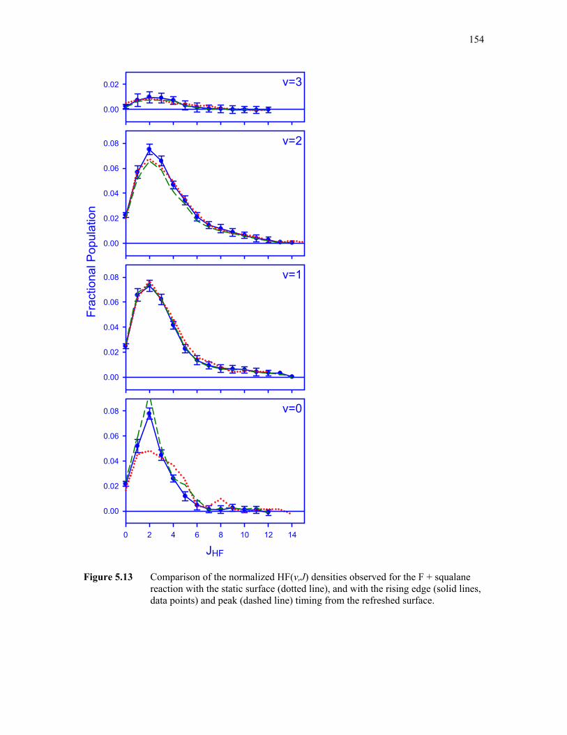
154

Figure 5.13 Comparison of the normalized HF(v,J) densities observed for the F + squalane reaction with the static surface (dotted line), and with the rising edge (solid lines, data points) and peak (dashed line) timing from the refreshed surface.

v=0

JHF

0 2 4 6 8 10 12 14

0.00

0.02

0.04

0.06

0.08

v=1

0.00

0.02

0.04

0.06

0.08

v=2

Frac

tiona

l Pop

ulat

ion

0.00

0.02

0.04

0.06

0.08

v=3

0.00

0.02

155

Figure 5.14 Sample time domain profiles for the indicated transitions originating from v” = 0–3. Pairs of vertical lines frame the timing domains used for temporal averaging. The first pair of solid lines and the adjacent pair of dotted lines frame the two time domains whose rovibrational state distributions are compared in Fig. 5.13.

v=2 1, J=3 2

0.0000

0.0005

v=3 2, J=3 2

Abs

orba

nce

0.0000

0.0005

0.0010

0.0015

0.0020

v=4 3, J=3 2

0.0000

0.0005

v=1 0, J=1 2

time (μs)0 1000 2000 3000 4000

0.0000

0.0005

156

uncertainty, while the shifting vibrational distributions are shown in Fig. 5.15. These data reveal a

systematic shift toward a room-temperature HF internal state distribution with increasing time.

Although these observations could, in principle, be caused by equilibration of HF product trapped

on from the surface, the required sub-kilohertz thermalization rate is inconsistent with 10–100 ps

vibrational relaxation times anticipated at the surface.46-49 On the other hand, this slow decay does

match that expected for product molecules reaching the edge of the vacuum chamber, relaxing

upon contact with the room temperature surface, and returning to the probe region. This

thermalization emphasizes the need to position the signal gate only 200 μs after the F atom pulse,

insuring insufficient time for the thermally recoiling HF to return to the probe region following

secondary collisions.

5.5 Analysis of Results

The high-resolution IR absorption measurements, such as those shown in Fig. 5.11,

contain two independent pieces of information about each HF quantum state: the total (state

resolved) transition intensity and detailed Doppler lineshape. Intensity information has been

integrated and fitted to obtain the state resolved populations presented in Table 5.2 and Fig. 5.13.

Additional information on the HF velocities, projected onto the probe axis, can also be obtained

via fitting of the observed lineshape. These two methods of analysis will be considered separately

in this section.

157

Figure 5.15 Vibrational distribution of HF product at three representative delay times, marked in Fig. 5.14. Populations are in good agreement between the first two gating windows, also compared in Fig. 5.13. After more than 1 ms delay, the apparent vibrational cooling appears to accelerate, as HF molecules relaxing at the sides of the vacuum apparatus have time to return to the probe region.

log10[time after discharge (s)]-4.0 -3.5 -3.0 -2.5 -2.0

Frac

tiona

l Pop

ulat

ion

0.0

0.2

0.4

0.6

0.8

1.0

v=0v=1v=2v=3

158

A. HF(v,J) state distribution

The “best set” HF rovibrational state distribution, defined in Sect. 5.4, for F + squalane

has been obtained from the spectrum in Fig. 5.12(a), according the procedure in Ch. 2.4(A). The

results appear in Table 5.2 and Fig. 5.13. In the least squares fit, the HF density in all unprobed

states (generally with J > 15) and those in v = 4 is set to zero. Monotonically decaying intensities

versus J in each band in Fig. 5.12 and the unobservable signals originating from v = 4 justify this

approximation. As a result, the higher state populations are less correlated and determined with

greater accuracy than those in lower vibrational manifolds, as can be seen by close inspection of

derived densities, shown in Fig. 5.13. Nevertheless, even for the v = 0 manifold, the peak

column-integrated rotational populations are determined to better than 5–10%, with precision

improving to 1–2% for the higher vibrational manifolds.

We previously noted that that the v = 4 manifold, at 42.4 kcal/mol above the ground

state, may be energetically accessible to F reacting with a tertiary C–H bond, within the certainty

of the bond strength and possible thermal activation. However, direct measurements of transitions

originating from the v = 4 manifold do not yield signals in excess of the ≤ 3×10-5 absorbance

noise limit, corresponding to less than 0.01% of the total HF population in any rotational state in

this manifold. Since detailed modeling of the liquid surface indicates that tertiary CH bonds are

accessible to impinging reactants,21,50,51 the lack of HF population in the v = 4 manifold can be

attributed to surface dynamics that do not favor extreme vibrational excitation, as also manifest in

the relatively small branching into v = 3.

The average state resolved density of HF above the liquid surface can be obtained by

scaling the column-integrated densities in Table 5.2 by the quantity N×x, where N = 16 is the

number of passes the probe laser makes through the Herriot cell and x =13(1) cm is the absorption

path length of HF above the liquid surface. The most populated states have a density of

approximately 1.2×1010 HF #/cm3 per quantum state, and the total HF density is approximately

159

1.5(2)×1011 HF #/cm3. Interestingly, this number is in excellent agreement with the estimated

1.5(3)×1011 #/cm3 F atom density impinging on the liquid surface, calibrated against the known F

+ H2 rate constant,42,52 as described in more detail in Ch. 2.4(C). This calibration utilizes a

number of experimentally determined values, such that propagation of uncertainty results in the

20% fractional uncertainty in the predicted F atom density. However, within these error bars, it is

clear that nearly all F atoms impinging on the surface react and return to the gas phase on the 200

μs time scale of the supersonic jet pulse. This analysis highlights a unique strength of high-

resolution direct absorption methods, whereby absolute absorbances can be used to accurately

infer absolute column-integrated densities of transient species.

Several interesting trends emerge from the HF state distributions following reaction with

the liquid squalane interface, plotted in Fig. 5.13. Summation over rotational states (Fig. 5.16)

reveals a rather broad distribution of vibrational state populations, with 25–35% of the total

population residing in each manifold between v = 0–2, and significantly less population entering

the v = 3 manifold. Also presented in Fig. 5.16 is the HF vibrational branching following gas-

phase reaction with ethane (gas), which has similar H–C bond strength. The gas-phase reaction

yields significantly more branching into v = 3, at the expense of v = 0–1.

The HF rotational state distributions for the reaction of F atoms with liquid squalane (see

Fig. 5.13) appear nearly Boltzmann in nature, with maximum rotational population in each

vibrational manifold occurring at J = 2, the maximum for a 300 K distribution. However, closer

inspection reveals excess population formed in highly rotationally excited states, starkly evident

in the v = 2 and v = 1 manifolds. Boltzmann plots of degeneracy-scaled populations versus

rotational energy are presented in Fig. 5.17. These curves strongly deviate from the straight lines

characteristic of a purely thermal distribution. Indeed, the observed rotational distributions show a

significant kink at intermediate J values between two approximately linear regions. This

observation has prompted analysis of these rovibrational manifolds by a “two-temperature”

160

Figure 5.16 HF vibrational state distributions following the reaction of F atoms with hydrocarbons in the gas phase, and at the gas-liquid hydrocarbon surface, as indicated.

vHF0 1 2 3

Frac

tiona

l Pop

ulat

ion

0.0

0.1

0.2

0.3

0.4

F+squalane (liquid)F+ethane (gas)

161

Figure 5.17 Boltzmann plots of the HF rotational state distributions in the v = 1 and v = 2 manifolds, as indicated. Measured populations are data points with error bars. The solid line is the result of the two-temperature fit, with the constituent high and low temperature thermal distributions plotted as the dashed and dotted lines, respectively.

vHF=1

Erot (cm-1)0 1000 2000 3000

ln(ρ

/(2J H

F+1)

)

20

22

24

26

305(7)K

2400(500)K

vHF=2

0 1000 2000 3000 400018

20

22

24

26

338(17)K

1600(400)K

162

model, also used extensively in the study of inelastic scattering of CO2 from liquid surfaces.23-26

The two-temperature model describes the rotational populations as the sum of two

thermal distributions:

ρv(J)/g(J) = A{(α/T1) exp(-E(J)/kT1) + [(1- α)/T2] exp(-E(J)/kT2)} , (5.1)

where ρv(J) is the density of HF(v,J), g(J) is the degeneracy, and E(J) is the rotational energy of

state J, α is the branching ratio between the two distributions, and A is an overall scaling factor.

The present F + squalane reactive scattering data exhibit much more dramatic and obvious

curvature than similar Boltzmann rotational state plots for gases inelastically scattered from

liquids.23-26 Of particular dynamical interest, the low temperature components in both HF(v = 1)

and HF(v = 2) manifolds match the 300 K surface temperature (Ts), nearly within one standard

deviation of the fit. In contrast, the curvature in the plots for v = 3 and v = 0 is much less

dramatic, justifying fits to a simpler one-temperature Boltzmann distribution to reveal qualitative

rotational energy trends. Such fits result in least squares values of 400(24) K and 315(30) K for v

= 3 and 0, respectively.

Although there is no a priori reason to expect the dynamically determined rotational state

distributions to approximate thermal distributions, this analysis does reveal qualitative features of

the distribution that are likely to prove robust to detailed dynamical modeling. Specifically, lower

vibrational manifolds, which may be strongly populated via longer lived trapping desorption (TD)

dynamics at the gas-liquid interface, are characterized by rotational temperatures close to the

surface temperature, Ts = 300 K. On the other hand, high vibrational excitation is correlated with

hyperthermal rotations. This behavior is exactly opposite to trends observed in the gas phase,38,41

where lower vibrational levels are generally accompanied by increasing rotational energy.

The v = 3 and v = 0 rotational state distributions readily conform to this picture. The v =

3 rotational "temperature" of about 400 K exceeds Ts, as expected because strongly

accommodating TD interactions only serve to depopulate this high-energy manifold. Although

163

partial rotational relaxation is likely, the fully equilibrated molecules are simply missing from this

distribution because they have also vibrationally relaxed. In contrast, the v = 0 population does

not exhibit any significant hyperthermal rotational component. This observation is consistent with

HF(v = 0) being formed almost exclusively via strongly trapped interactions, and the 0.24(1)

fractional vibrational branching into this manifold represents a clear upper limit for the HF

population component that spends an appreciable time on the surface as compared with the time

for vibrational energy transfer to the surface.

However, the v = 0 population represents only a relatively small fraction of the total

population. Most of the nascent HF escapes with v > 0, and a significant amount does so while

maintaining a nonthermal distribution of rotational energy. The simplest interpretation is that

surface interactions can occur with varying degrees of accommodation, and higher energy states

are selectively populated via processes that eject HF directly into the gas phase prior to complete

thermalization.

The intermediate vibrational levels (v = 1–2) appear to have both thermally

accommodated and rotationally hot signatures in their rotational distributions, motivating the two-

temperature fit in Fig. 5.17. The TD fraction (α), defined in Eq. 5.1, comprises 0.78(2) and

0.69(4) of the v = 1 and v = 2 populations, respectively. A simple picture for the dynamics based

on the rotational state analysis is that 70–80% of the HF product in the vibrationally excited (v =

1, 2) levels desorb after rotationally equilibrating with the liquid surface. However, these

molecules have not interacted with the bulk 300 K squalane long enough to lose their high

vibrational excitation, motivating their assignment to the DRS channel. Of course, this picture is

likely to be an oversimplification of the true dynamics, as gas-phase reactions, analogous to the

DRS component, have not been found to match the 2000 K Boltzmann distribution found for the

high-temperature component of the rotational state distributions. Nevertheless, the v = 1 and v =

2 populations appear to have both rotationally excited components, created by the DRS channel,

and 300 K components, from TD. More evidence for HF product-state-dependent residence times

164

on the liquid surface can be found from the observed absorption lineshapes, which we discuss

next.

B. Doppler lineshape analysis

The measured Doppler lineshapes directly reveal the HF velocity distribution, projected

along the laser axis, i.e., parallel to the liquid surface. Sample Doppler profiles are presented in

Fig. 5.18 and fits have been obtained using the method described in this section.

Modeling of Doppler lineshapes is straightforward for transitions terminating in an

unpopulated upper state, such as those originating in the v = 3 manifold and v = 2 with J > 7. In

this case, only the velocity distribution in the lower state must be considered in the Doppler

analysis. Such transitions have been fitted to a simple Gaussian lineshape:

A(ν) = A0 exp(-4ln(2)[(ν−ν0)/Δν]2) , (5.2)

where Δν is the FWHM of the transition, A0 is the peak absorbance, and ν0 is the line center

frequency. The choice of this functional form is arbitrary yet empirically justified by the robust

agreement between the fitted to the observed measurements, such as that shown in the top trace in

Fig. 5.18. Fits to Gaussian lineshapes are physically motivated by anticipated quasi-thermal

Doppler measurements, and Boltzmann-like velocity distributions observed following inelastic

scattering from liquid surfaces.23-26

For lower manifolds, emission from the upper state necessitates consideration of the

velocity distributions of both the upper and lower levels simultaneously. Specifically, lineshapes

can be expressed as a sum of two Gaussian components:

A(ν) = Al exp(-4ln(2)[(ν − ν0)/Δνl]2) - Au exp(-4ln(2)[(ν − ν0)/Δνu]2) . (5.3)

The subscripts l and u indicate components used to describe the lower and upper state

distributions, respectively. Correlations between Al and Au, and between Δνl and Δνu make a five-

165

Figure 5.18 Representative Doppler resolved absorption data (solid lines) and fits (dotted lines) for several HF J” = 2, ΔJ = + 1 transitions. Vibrational manifolds are as indicated. Absorption originating from the v” = 3 manifold is well represented by a single Gaussian fit, as no measurable population has been observed in the v” = 4 manifold. Doppler modeling of the v” = 1–2 levels includes contributions from absorbing molecules in the lower state (long dashes) and emission from the upper state (short dashes).

ν−ν0 (MHz)-600 -400 -200 0 200 400 600

Abso

rptio

n

0.001 Abs

v"=3

v"=2

v"=1

166

parameter least squares fit of individual Doppler profiles using Eq. 5.3 intractable. However, the

correlation between the peak absorbances can be broken by using the column-integrated state

densities shown in Fig. 5.13 to fix the ratio REA between the integrated emission and absorption

components of the Doppler profiles, given by

REA = Sov’J’→v”J” ∫dx∫dν ρv’J’(ν,x) / So

v’J’←v”J”∫dx∫dν ρv”J”(ν,x). (5.4)

Integration over the absorption and emission profiles in Eq. 5.3 relates the peak absorbances via

Au = Al REAΔνl/Δνu. The correlation between Δνl and Δνu can be broken by simultaneously fitting

the Doppler profiles of transitions in which a given level is both the upper and lower level, e.g.

the v + 2, J” ← v + 1, J’ and v + 1, J’ ← v, J lines, whose frequencies are denoted ν0’ and ν0 ,

respectively. In this case, Δνl of the former can be related to Δνu of the latter by scaling to the

absolute frequencies via Δνl = Δνu’(ν0/ν0

’).

These relationships are used in several ways. In the simplest approach, the Doppler fits

using Eq. 5.2 are carried out for transitions out of the highest energy states, which only have an

absorption component. The Δν parameters obtained from these fits are then used to fix Δνu in Eq.

5.3 to obtain fits of transitions out of the next lower vibrational manifold, and the process is

repeated for progressively lower levels. Uncertainties in the fitted Doppler widths are obtained by

a propagation of errors analysis. Alternatively, Eq. 5.3 and 5.4 are employed to fit simultaneously

sets of paired transitions. Similar widths are obtained within the derived uncertainties from both

procedures.

The Gaussian nature of the Doppler lineshapes suggests converting the fitted widths Δν

to translational temperatures Ttrans. Specifically, Ttrans for a Maxwell-Boltzmann distribution is

related to the Doppler FWHM Δν and center frequency ν via

Ttrans = (cΔν/ν)2(mHF/8k ln2), (5.5)

where mHF, c, and k are the mass of the HF molecule, speed of light, and Boltzmann’s constant,

respectively. The results of the Doppler analysis are presented in Fig. 5.19, which shows

167

Figure 5.19 Results from the least squares fit to the measured absorption lineshapes originating from the v = 3 (circles), v = 2 (triangles) and v = 1 (squares) manifolds. Observed Gaussian linewidths have been converted to translational temperatures via Eq. 5.5. HF translational energy increases with increasing rovibrational energy. Such translational dynamics indicate strongly state-dependent surface residence times.

JHF

0 2 4 6 8 10 12

T trans

(K)

0

300

600

900

1200vHF=3vHF=2vHF=1300K

168

that the product HF translational degree of freedom is hotter than or equal to the 300 K surface

temperature. Overall, the Doppler widths increase with rovibrational excitation, revealing a

positive correlation between average translational energy and internal HF energy. This

observation is most evident in the propensity for hotter translational temperatures as J increases

within a given vibrational manifold. The translational temperature also increases with the product

vibrational excitation, although this effect is less pronounced than the dependence upon the

rotation state.

Doppler widths for the v = 0 manifold are not presented in Fig. 5.19 because they cannot

be fitted reliably using the procedure detailed above. Careful inspection of the v” = 0 Doppler

measurements in Fig. 5.11 reveals less structure is this manifold than in the v” = 1,2 manifolds.

Specifically, the Doppler structure appears approximately Gaussian, because the Δν values in

HF(v = 0,J < 6) correspond to 300 K, i.e., nearly identical to those for the upper states, HF(v = 1,

J < 5). These similar Doppler widths result in strong parameter correlation through Eq. 5.3,

which prevents reliable least squares fitting of the v” = 0 manifold. Nevertheless, thermally

equilibrated HF(v = 0,J) Doppler profiles would be completely consistent the established trend

for more accommodation with the surface as internal energy decreases.

The strong positive correlation between increasing HF Doppler widths and increasing

internal HF rovibrational energy contrasts rather dramatically with that observed in previous

studies of H atom abstraction in the gas phase, where energy sequestered into product internal

energy necessarily reduces the amount available for recoil.38 This effect was most convincingly

demonstrated in studies of F + ethane, where the Doppler measurements of HF(v,J) translational

energy proved to be linearly correlated with Eavail = Etot - EHF(v,J) and therefore yielded a negative

correlation with HF internal energy. Stated most simply, this trend results from energy

conservation and insufficient time during the collisional event for energy flow into the isolated

ethyl cofragment.

169

By way of contrast, the gas-liquid interface offers a quite different scenario for H atom

extraction reaction dynamics. In particular, new correlations arise from quantum-state dependent

residence times on the liquid surface. For example, translational energy is likely to be dissipated

into the bulk liquid within one or two collisional interactions after the reaction event. Therefore,

translationally hot HF might be expected to correlate with molecules that escape from the surface

almost immediately following reaction (i.e., the DRS channel) and therefore retain a maximal

amount of energy released during reaction.

Similarly, molecules that have lost translational energy from the reaction event through

multiple collisions with the surface (i.e., the TD channel) may be linked with additional loss of

internal energy as well. In particular, since rotations are expected to equilibrate with the surface

almost as rapidly as translations, this consideration suggests a simple mechanism for a positive

correlation between rotational and translational energies. Because of the large size of its quanta,

vibrational energy transfer to the surface may be expected to occur much more slowly, explaining

the much weaker trend in translational energies with respect to final vibrational state. From this

perspective, the key difference between gas-phase (e.g. F + ethane) and gas-liquid (e.g. F +

squalane) reaction dynamics is the presence of many additional channels for subsequent energy

transfer after the primary reaction event. As one simple physical picture, the liquid surface offers

a larger cross section for subsequent inelastic interactions with the nascent product and thus

substantially restricts its ability to behave like a spectator.

5.6 Discussion

Following reaction of F atoms at the liquid squalane surface, HF desorbs into the gas

phase with varying amounts of energy in vibrational, rotational, and translational degrees of

freedom. High HF internal energy, particularly rotation, is strongly correlated with hot

translational distributions. This observation suggests that reaction occurs via competing

170

dynamical pathways, by which product escapes with a large fraction of the reaction energy, the

DRS channel, or partially accommodates with the room temperature surface via TD.

It is interesting to compare the present results with those reported by McKendrick and

coworkers for H abstraction by O from squalane and other liquid hydrocarbon interfaces.15-20,22

Such comparison is necessarily general because these two reactions are quite different.

Specifically, O atoms react with a significantly higher (5–10 kcal/mol) barrier,29 and the

exothermicity is much less (≈ 5 kcal/mol). In addition to a single abstraction event, forming OH

as probed my McKendrick and coworkers,15,16,18-20,22,29,53 subsequent reaction events can lead to

H2O product.7,9 Nevertheless, both HF and OH products are vibrationally excited following

reaction at the liquid surface, although they retain less vibrational energy than observed from

analogous gas-phase reactions. This result is consistent with the inefficient vibrational

accommodation following inelastic scattering of CO223-26 and I2

11-14 from liquid interfaces. The

OH and HF rotational distributions both closely match the surface temperature, but the fastest

moving OH(v = 1) products mimic the sub-thermal distributions expected from gas-phase

dynamics.15 Similarly, in the present study the hottest Doppler widths are observed for high HF

rotational levels; in this case hot rotations occur with rapidly recoiling molecules attributed to the

DRS mechanism. Recent theoretical simulations of O + squalane reaction have found similar

trends for increasing rotation and translational energy, though the much larger ( > 100 kcal/mol)

incident energies in these studies complicates more detailed comparison.51

Further insight into energy transfer into the liquid can be gained by comparing the results

of F + hydrocarbon reactions at the liquid interface and in the gas phase. We focus on the F +

ethane reaction system for this comparison because it has very similar energetics and has already

been studied using high-resolution IR methods. However, similar conclusions would be expected

for other F + hydrocarbon systems.41,54 Fig. 5.20 presents detailed energetic branching analysis, in

171

Figure 5.20 Energy partitioning following various F + hydrocarbon reactions in the gas phase and at the liquid interface. Expectation values for energy deposited in the indicated modes are evaluated according to Eq. 5.6. R denotes energy assumed to be sequestered in the unseen hydrocarbon radical.

0

5

10

15

20

25E

(kca

l/mol

)

F+squalane (liquid)F+ethane (gas)

HFvib

HFrot

HFtrans

R

172

which average values ⟨Ei⟩ of vibrational, rotational, or translational energy are presented. Here,

⟨Ei⟩ is computed as

⟨Ei⟩ = Σv,J P(v,J) Ei(v,J) , (5.6)

where P(v,J) is the HF state distribution, and Ei(v,J) is the energy (i = vibration, rotation, or

translation), and Etrans is taken as 2kTtrans(v,J), the energy of an effusive source at temperature

Ttrans, as derived in the present study via Doppler data in Fig. 5.18. The most dramatic change in

energy partitioning originates from the larger HF(v = 0,1) population formed via reaction at

liquid interface, primarily at the expense of HF(v = 3). The energy partitioning analysis presented

in Table 5.3 emphasizes this result. Approximately 60% of the available energy deposited in the

HF vibrational coordinate for various gas-phase reactions, versus < 40% for F atom abstraction at

the liquid squalane interface.

The presentation in Fig. 5.20 reveals that every HF mode retains less energy after

reaction at the liquid interface than in the gas phase, resulting in larger energy branching into the

unseen hydrocarbon, denoted R. In general, gas-phase halogen-alkane reactions result in modest

(4–12%) energy transfer to internal modes of the hydrocarbon radical product, which acts mostly

as a spectator to the reaction.38,55 By comparison, the HF product recoils from the liquid surface

after partial equilibration, during which the extent of relaxation in rotational, vibrational, and

translational degrees of freedom relax according to the propensity for energy transfer based on the

size of the energy quantum, i.e., larger quanta relax more slowly than smaller quanta. This trend

results in the average HF translational energy of 1.47(3) kcal/mol being only 25% higher than the

300 K value of 1.18 kcal/mol. Rotations are also nearly equilibrated, with 1.04(8) kcal/mol

average energy, nearly 75% larger than kT, as expected for a linear rotor at 300 K. With respect to

surface residence time, the observation of rotationally and translationally excited HF clearly

indicates fractional branching of HF into a channel that remains in contact with the

173

Table 5.3 Fractional energy partitioning (X) of reaction energy following reaction of fluorine with liquid squalane and several gas-phase hydrocarbons. Uncertainties in parenthesis are one standard deviation.

Reactant XHFvib XHFrot XHftrans Xcofragment squalanea 37(3) 2.8(3) 4.1(3) 56(8) ethaneb 56(6) 3.9(4) 16(2) 23(2) methanec 60.6(7) 4.4(6) neopentaned 64 toluened 55 benzened 63

a Uncertainty dominated by the heterogeneous C–H bond strength in squalane b From Ref. 38 c From Ref. 41 d From Ref. 54

174

surface for less than the sub-picosecond relaxation timescales for these modes. Finally,

vibrational excitation remains extremely hot, with 13.3(2) kcal/mol average energy, and only

partial relaxation occurs because of moderately slow (tens of ps) relaxation time on the liquid

surface. Indeed, theoretical studies indicate that vibrational relaxation times are extended by a

factor of only two to four by the partial caging present at the interface,46-49 so even the TD

channel is likely to be characterized by a ≈ 100 ps surface residence time.

Very recent computations of F + squalane by the Schatz group50 have reproduced many

of the general features of the experimental results, such as hotter rotational distributions in lower

vibrational manifolds. At an even higher level of detail, this work has found that excited rotations

are more likely to remain excited following scattering events that spend a relatively small time

below the so-called Gibbs surface. Indeed, the predicted vibrational distributions strongly agree

with measurements, though the theoretical rotational distributions are much more structured and

less Boltzmann-like than those presented here. These differences may arise from the very high F

atom translational energies (0.5, 1.0 eV) used in these studies, or the need for more accurate PES

calculations to reliably predict rotational distributions. Nevertheless, the results of these landmark

computational studies seem to confirm the present interpretation of the experimental results, and

present the opportunity to begin developing more detailed physical pictures for gas-liquid

scattering processes.

5.7 Conclusions

The reaction of fluorine atoms at the gas-liquid interface of squalane reveals a wide

variety of surface energy exchange with recoiling HF products. Highly inverted vibrational

populations indicate that a significant amount of the reaction energy remains sequestered in the

diatomic fragment as it recoils from the surface, although significant branching into the ground

vibrational manifold is also observed. In contrast, rotational and translational excitation of HF

175

product is moderate. At low J, population distributions closely resemble the 300 K surface

temperature, though a slowly decaying tail in the rotational population results from hyperthermal

populations. The observed rotational state populations are well described by either a thermal

distribution or the sum of two such distributions, depending on the vibrational manifold. The v =

3 manifold is characterized by a hot (400 K) distribution, while the v = 0 rotational state

distribution closely resembles a thermal distribution at the surface temperature, and intermediate

(v = 1–2) levels have rotational state distribution components characterized by thermalized (300

K) and very hot (2000 K) temperatures. Doppler measurements reveal that the HF translational

energy matches the liquid surface temperature for moderately excited states, whereas recoil

energy increases with HF internal energy. These results indicate microscopic branching of HF

interactions with the surface following the reactive event, with high energy components resulting

from brief “direct reactive scattering” interaction with the liquid surface, contrasted with “trapped

desorption” events during which the product may become translationally, rotationally, and even

vibrationally accommodated with the surface. The contribution from each of these components

varies with the resulting HF quantum state and is most readily deduced from the translational

energy measurements. These observations match expectations for partial equilibration at the

surface following an initial reaction event analogous to gas-phase F + hydrocarbon reactions.

Results are also consistent with previous studies in which bifurcated dynamic pathways and

relaxation rates were determined by energy gap expectations. Recent theoretical studies reproduce

the general features observed experimentally, and increase confidence in the present

interpretation.

176

References for Chapter V

1 S. L. Lednovich and J. B. Fenn, Aiche J. 23, 454 (1977).

2 G. M. Nathanson, P. Davidovits, D. R. Worsnop, and C. E. Kolb, J. Phys. Chem. 100, 13007 (1996).

3 M. E. Saecker and G. M. Nathanson, J. Chem. Phys. 100, 3999 (1994).

4 M. E. Saecker and G. M. Nathanson, J. Chem. Phys. 99, 7056 (1993).

5 M. E. Saecker, S. T. Govoni, D. V. Kowalski, M. E. King, and G. M. Nathanson, Science 252, 1421 (1991).

6 G. M. Nathanson, Annu. Rev. Phys. Chem. 55, 231 (2004).

7 J. M. Zhang, D. J. Garton, and T. K. Minton, J. Chem. Phys. 117, 6239 (2002).

8 D. J. Garton, T. K. Minton, M. Alagia, N. Balucani, P. Casavecchia, and G. G. Volpi, J. Chem. Phys. 112, 5975 (2000).

9 D. J. Garton, T. K. Minton, M. Alagia, N. Balucani, P. Casavecchia, and G. G. Volpi, Faraday Discuss.387 (1997).

10 J. M. Zhang, H. P. Upadhyaya, A. L. Brunsvold, and T. K. Minton, J. Phys. Chem. B 110, 12500 (2006).

11 A. J. Kenyon, A. J. McCaffery, C. M. Quintella, and M. D. Zidan, Faraday Discuss. 96, 245 (1993).

12 C. M. Quintella, A. J. McCaffery, and M. D. Zidan, Chem. Phys. Lett. 214, 563 (1993).

13 A. J. Kenyon, A. J. McCaffery, C. M. Quintella, and M. D. Zidan, J. Chem. Soc.-Faraday Trans. 89, 3877 (1993).

14 A. J. Kenyon, A. J. McCaffery, C. M. Quintella, and M. D. Zidan, Chem. Phys. Lett. 190, 55 (1992).

15 S. P. K. Kohler, M. Allan, H. Kelso, D. A. Henderson, and K. G. McKendrick, J. Chem. Phys. 122, 24712 (2005).

16 H. Kelso, S. P. K. Kohler, D. A. Henderson, and K. G. McKendrick, J. Chem. Phys. 119, 9985 (2003).

17 F. Ausfelder, H. Kelso, and K. G. McKendrick, Phys. Chem. Chem. Phys. 4, 473 (2002).

18 M. Allan, P. A. J. Bagot, R. E. Westacott, M. L. Costen, and K. G. McKendrick, J. Phys. Chem. C 112, 1524 (2008).

177

19 M. Allan, P. A. J. Bagot, M. L. Costen, and K. G. McKendrick, J. Phys. Chem. C 111, 14833 (2007).

20 M. Allan, P. A. J. Bagot, S. P. K. Kohler, S. K. Reed, R. E. Westacott, M. L. Costen, and K. G. McKendrick, Phys. Scr. 76, C42 (2007).

21 S. P. K. Kohler, S. K. Reed, R. E. Westacott, and K. G. McKendrick, J. Phys. Chem. B 110, 11717 (2006).

22 S. P. K. Kohler, M. Allan, M. L. Costen, and K. G. McKendrick, J. Phys. Chem. B 110, 2771 (2006).

23 B. G. Perkins, T. Haber, and D. J. Nesbitt, J. Phys. Chem. B 109, 16396 (2005).

24 B. G. Perkins and D. J. Nesbitt, J. Phys. Chem. B 110, 17126 (2006).

25 B. G. Perkins and D. J. Nesbitt, J. Phys. Chem. A 111, 7420 (2007).

26 B. G. Perkins and D. J. Nesbitt, J. Phys. Chem. B 112, 507 (2008).

27 B. G. Perkins and D. J. Nesbitt, Proc. Natl. Acad. Sci. U. S. A. 105, 12684 (2008).

28 B. G. Perkins and D. J. Nesbitt, J. Phys. Chem. A 112, 9324 (2008).

29 F. Ausfelder and K. G. McKendrick, Prog. React. Kinet. Mech. 25, 299 (2000).

30 A. Furlan, Chem. Phys. Lett. 309, 157 (1999).

31 A. Furlan, J. Phys. Chem. B 103, 1550 (1999).

32 A. Furlan and G. E. Hall, J. Chem. Phys. 109, 10390 (1998).

33 A. Furlan, Chem. Phys. Lett. 275, 239 (1997).

34 W. T. Zemke, W. C. Stwalley, J. A. Coxon, and P. G. Hajigeorgiou, Chem. Phys. Lett. 177, 412 (1991).

35 S. J. Blanksby and G. B. Ellison, Accounts Chem. Res. 36, 255 (2003).

36 J. C. Polanyi and W. H. Wong, J. Chem. Phys. 51, 1439 (1969).

37 A. M. Zolot and D. J. Nesbitt, J. Chem. Phys. 127, 114319 (2007).

38 E. S. Whitney, A. M. Zolot, A. B. McCoy, J. S. Francisco, and D. J. Nesbitt, J. Chem. Phys. 122, 124310 (2005).

39 S. A. Nizkorodov, W. W. Harper, W. B. Chapman, B. W. Blackmon, and D. J. Nesbitt, J. Chem. Phys. 111, 8404 (1999).

40 W. W. Harper, S. A. Nizkorodov, and D. J. Nesbitt, J. Chem. Phys. 116, 5622 (2002).

41 W. W. Harper, S. A. Nizkorodov, and D. J. Nesbitt, J. Chem. Phys. 113, 3670 (2000).

178

42 W. B. Chapman, B. W. Blackmon, S. Nizkorodov, and D. J. Nesbitt, J. Chem. Phys. 109, 9306 (1998).

43 M. P. Sinha and J. B. Fenn, presented at the Proceedings of the 5th International Symposium on Molecular Beams, France, 1975 (unpublished).

44 D. Kaur, A. M. Desouza, J. Wanna, S. A. Hammad, L. Mercorelli, and D. S. Perry, Appl. Optics 29, 119 (1990).

45 A. M. Zolot, W. W. Harper, B. G. Perkins, P. J. Dagdigian, and D. J. Nesbitt, J. Chem. Phys. 125, (2006).

46 I. Benjamin, J. Phys. Chem. B 110, 9375 (2006).

47 I. Chorny, J. Vieceli, and I. Benjamin, J. Phys. Chem. B 107, 229 (2003).

48 J. Vieceli, I. Chorny, and I. Benjamin, Chem. Phys. Lett. 364, 446 (2002).

49 J. Vieceli, I. Chorny, and I. Benjamin, J. Chem. Phys. 117, 4532 (2002).

50 B. K. Radak, S. Yockel, D. Kim, and G. C. Schatz, J. Phys. Chem. A (in press) (2009).

51 D. Kim and G. C. Schatz, J. Phys. Chem. A 111, 5019 (2007).

52 F. Dong, S. H. Lee, and K. Liu, J. Chem. Phys. 113, 3633 (2000).

53 F. Ausfelder, H. Kelso, and K. G. McKendrick, Phys. Chem. Chem. Phys. 4, 473 (2002).

54 D. J. Bogan and D. W. Setser, J. Chem. Phys. 64, 586 (1976).

55 S. Rudic, C. Murray, J. N. Harvey, and A. J. Orr-Ewing, J. Chem. Phys. 120, 186 (2004).

179

________________

Bibliography

________________

P. M. Aker, G. J. Germann, and J. J. Valentini, J. Chem. Phys. 96, 2756 (1992).

M. Alagia, N. Balucani, P. Casavecchia, D. Stranges, G. G. Volpi, D. C. Clary, A. Kliesch, and H. J. Werner, Chem. Phys. 207, 389 (1996).

M. H. Alexander, G. Capecchi, and H. J. Werner, Faraday Discuss. 127, 59 (2004).

M. H. Alexander, D. E. Manolopoulos, and H. J. Werner, J. Chem. Phys. 113, 11084 (2000).

W. A. Alexander, B. S. Day, H. J. Moore, T. R. Lee, J. R. Morris, and D. Troya, J. Chem. Phys. 128, (2008).

M. Allan, P. A. J. Bagot, M. L. Costen, and K. G. McKendrick, J. Phys. Chem. C 111, 14833 (2007).

M. Allan, P. A. J. Bagot, S. P. K. Kohler, S. K. Reed, R. E. Westacott, M. L. Costen, and K. G. McKendrick, Phys. Scr. 76, C42 (2007).

M. Allan, P. A. J. Bagot, R. E. Westacott, M. L. Costen, and K. G. McKendrick, J. Phys. Chem. C 112, 1524 (2008).

S. C. Althorpe, Chem. Phys. Lett. 370, 443 (2003).

S. C. Althorpe and D. C. Clary, Annu. Rev. Phys. Chem. 54, 493 (2003).

S. C. Althorpe, F. Fernandez-Alonso, B. D. Bean, J. D. Ayers, A. E. Pomerantz, R. N. Zare, and E. Wrede, Nature 416, 67 (2002).

F. J. Aoiz, L. Banares, and V. J. Herrero, Int. Rev. Phys. Chem. 24, 119 (2005).

F. J. Aoiz, L. Banares, B. MartinezHaya, J. F. Castillo, D. E. Manolopoulos, K. Stark, and H. J. Werner, J. Phys. Chem. A 101, 6403 (1997).

V. Aquilanti, D. Cappelletti, F. Pirani, L. Y. Rusin, M. B. Sevryuk, and J. P. Toennies, J. Phys. Chem. 95, 8248 (1991).

E. Arunan, D. W. Setser, and J. F. Ogilvie, J. Chem. Phys. 97, 1734 (1992).

B. S. Ault, J. Chem. Phys. 68, 4012 (1978).

F. Ausfelder, H. Kelso, and K. G. McKendrick, Phys. Chem. Chem. Phys. 4, 473 (2002).

F. Ausfelder and K. G. McKendrick, Prog. React. Kinet. Mech. 25, 299 (2000).

180

J. D. Ayers, A. E. Pomerantz, F. Fernandez-Alonso, F. Ausfelder, B. D. Bean, and R. N. Zare, J. Chem. Phys. 119, 4662 (2003).

M. Baer, M. Faubel, B. Martinez-Haya, L. Y. Rusin, U. Tappe, and J. P. Toennies, J. Chem. Phys. 108, 9694 (1998).

N. Balucani, G. Capozza, F. Leonori, E. Segoloni, and P. Casavecchia, Int. Rev. Phys. Chem. 25, 109 (2006).

N. Balucani, D. Skouteris, G. Capozza, E. Segoloni, P. Casavecchia, M. H. Alexander, G. Capecchi, and H. J. Werner, Phys. Chem. Chem. Phys. 6, 5007 (2004).

V. J. Barclay, B. A. Collings, J. C. Polanyi, and J. H. Wang, J. Phys. Chem. 95, 2921 (1991).

R. J. Bartlett and G. D. Purvis, Phys. Scr. 21, 255 (1980).

P. Beadle, M. R. Dunn, N. B. H. Jonathan, J. P. Liddy, and J. C. Naylor, J. Chem. Soc., Faraday Trans. II 74, 2170 (1978).

P. Beadle, M. R. Dunn, N. B. H. Jonathan, J. P. Liddy, J. C. Naylor, and S. Okuda, J. Chem. Soc., Faraday Trans. II 74, 2158 (1978).

I. Benjamin, J. Phys. Chem. B 110, 9375 (2006).

I. Benjamin, M. Wilson, and A. Pohorille, J. Chem. Phys. 100, 6500 (1994).

M. J. Berry, J. Chem. Phys. 59, 6229 (1973).

R. P. A. Bettens, M. A. Collins, M. J. T. Jordan, and D. H. Zhang, J. Chem. Phys. 112, 10162 (2000).

S. J. Blanksby and G. B. Ellison, Accounts Chem. Res. 36, 255 (2003).

D. Bogan and D. W. Setser, in Fluorine-containing free radicals: kinetics and dynamics of reactions: based on a symposium sponsored by the Division of Physical Chemistry at the 169th meeting of the American Chemical Society, Philadelphia, Pennsylvania, April 7-11, 1975, edited by J. W. Root (American Chemical Society, Washington, 1978), pp. 237.

D. J. Bogan and D. W. Setser, J. Chem. Phys. 64, 586 (1976).

K. Bolton, W. L. Hase, and G. H. Peslherbe, in Modern Methods for Multidimensional Dynamics Computations in Chemistry, edited by D. L. Thompson (World Scientific, River Edge, NJ, 1998), pp. 143.

S. B. M. Bosio and W. L. Hase, J. Chem. Phys. 107, 9677 (1997).

S. E. Bradforth, D. W. Arnold, R. B. Metz, A. Weaver, and D. M. Neumark, J. Phys. Chem. 95, 8066 (1991).

D. Brandt and J. C. Polanyi, Chem. Phys. 35, 23 (1978).

D. Brandt and J. C. Polanyi, Chem. Phys. 45, 65 (1980).

181

M. J. Bronikowski, W. R. Simpson, B. Girard, and R. N. Zare, J. Chem. Phys. 95, 8647 (1991).

M. Brouard, I. Burak, S. Marinakis, L. R. Lago, P. Tampkins, and C. Vallance, J. Chem. Phys. 121, 10426 (2004).

R. A. Brownsword, C. Kappel, P. Schmiechen, H. P. Upadhyaya, and H. R. Volpp, Chem. Phys. Lett. 289, 241 (1998).

G. Capecehi and H. J. Werner, Phys. Chem. Chem. Phys. 6, 4975 (2004).

P. Casavecchia, Rep. Prog. Phys. 63, 355 (2000).

J. F. Castillo, F. J. Aoiz, L. Banares, E. Martinez-Nunez, A. Fernandez-Ramos, and S. Vazquez, J. Phys. Chem. A 109, 8459 (2005).

J. F. Castillo, B. Hartke, H. J. Werner, F. J. Aoiz, L. Banares, and B. Martinez-Haya, J. Chem. Phys. 109, 7224 (1998).

D. W. Chandler and P. L. Houston, J. Chem. Phys. 87, 1445 (1987).

H. W. Chang, D. W. Setser, M. J. Perona, and R. L. Johnson, Chem. Phys. Lett. 9, 587 (1971).

S. D. Chao and R. T. Skodje, J. Chem. Phys. 119, 1462 (2003).

W. B. Chapman, B. W. Blackmon, and D. J. Nesbitt, J. Chem. Phys. 107, 8193 (1997).

W. B. Chapman, B. W. Blackmon, S. Nizkorodov, and D. J. Nesbitt, J. Chem. Phys. 109, 9306 (1998).

W. B. Chapman, M. J. Weida, and D. J. Nesbitt, J. Chem. Phys. 106, 2248 (1997).

W. Chen, W. L. Hase, and H. B. Schlegel, Chem. Phys. Lett. 228, 436 (1994).

I. Chorny, J. Vieceli, and I. Benjamin, J. Phys. Chem. B 107, 229 (2003).

R. E. Continetti, B. A. Balko, and Y. T. Lee, J. Chem. Phys. 93, 5719 (1990).

H. W. Cruse, P. J. Dagdigian, and R. N. Zare, Faraday Discuss. 55, 277 (1973).

G. Czako, B. C. Shepler, J. B. Braams, and J. M. Bowman, J. Phys. Chem. A(in press) (2009).

S. Davis, D. T. Anderson, G. Duxbury, and D. J. Nesbitt, J. Chem. Phys. 107, 5661 (1997).

B. S. Day, J. R. Morris, W. A. Alexander, and D. Troya, J. Phys. Chem. A 110, 1319 (2006).

W. Demtroder, Laser Spectroscopy. (Springer, Berlin, 1996).

M. P. Deskevich, M. Y. Hayes, K. Takahashi, R. T. Skodje, and D. J. Nesbitt, J. Chem. Phys. 124, 224303 (2006).

M. P. Deskevich, D. J. Nesbitt, and H. J. Werner, J. Chem. Phys. 120, 7281 (2004).

182

A. M. G. Ding, L. J. Kirsch, D. S. Perry, J. C. Polanyi, and J. L. Schreiber, Faraday Discuss. 55, 252 (1973).

F. Dong, S. H. Lee, and K. Liu, J. Chem. Phys. 113, 3633 (2000).

F. Dong, S. H. Lee, and K. Liu, J. Chem. Phys. 115, 1197 (2001).

V. Dribinski, A. Ossadtchi, V. A. Mandelshtam, and H. Reisler, Rev. Sci. Instrum. 73, 2634 (2002).

M. L. Dubernet and J. M. Hutson, J. Phys. Chem. 98, 5844 (1994).

W. H. Duewer and D. W. Setser, J. Chem. Phys. 58, 2310 (1973).

T. H. Dunning, J. Chem. Phys. 90, 1007 (1989).

A. Eppink and D. H. Parker, Rev. Sci. Instrum. 68, 3477 (1997).

H. Eyring, J. Am. Chem. Soc. 54, 170 (1932).

H. Eyring and M. Polanyi, Z. Phys. Chem. B-Chem. Elem. Aufbau. Mater. 12, 279 (1931).

J. R. Fair, D. Schaefer, R. Kosloff, and D. J. Nesbitt, J. Chem. Phys. 116, 1406 (2002).

M. Faubel, B. Martinez-Haya, L. Y. Rusin, U. Tappe, J. P. Toennies, F. J. Aoiz, and L. Banares, J. Phys. Chem. A 102, 8695 (1998).

F. Fernandez-Alonso and R. N. Zare, Annu. Rev. Phys. Chem. 53, 67 (2002).

A. V. Fishchuk, G. C. Groenenboom, and A. van der Avoird, J. Phys. Chem. A 110, 5280 (2006).

A. V. Fishchuk, P. E. S. Wormer, and A. van der Avoird, J. Phys. Chem. A 110, 5273 (2006).

A. A. Fokin and P. R. Schreiner, Chem. Rev. 102, 1551 (2002).

From, pp. http://nobelprize.org/nobel_prizes/chemistry/laureates/1986/.

A. Furlan, Chem. Phys. Lett. 275, 239 (1997).

A. Furlan, Chem. Phys. Lett. 309, 157 (1999).

A. Furlan, J. Phys. Chem. B 103, 1550 (1999).

A. Furlan and G. E. Hall, J. Chem. Phys. 109, 10390 (1998).

D. J. Garton, A. L. Brunsvold, T. K. Minton, D. Troya, B. Maiti, and G. C. Schatz, J. Phys. Chem. A 110, 1327 (2006).

D. J. Garton, T. K. Minton, M. Alagia, N. Balucani, P. Casavecchia, and G. G. Volpi, Faraday Discuss.387 (1997).

183

D. J. Garton, T. K. Minton, M. Alagia, N. Balucani, P. Casavecchia, and G. G. Volpi, J. Chem. Phys. 112, 5975 (2000).

D. J. Garton, T. K. Minton, M. Alagia, N. Balucani, P. Casavecchia, and G. G. Volpi, J. Chem. Phys. 114, 5958 (2001).

D. J. Garton, T. K. Minton, B. Maiti, D. Troya, and G. C. Schatz, J. Chem. Phys. 118, 1585 (2003).

W. Gellermann, J. Phys. Chem. Solids 52, 249 (1991).

D. Gerlich, E. Herbst, and E. Roueff, Planet Space Sci. 50, 1275 (2002).

S. Ghosal and S. Mahapatra, J. Phys. Chem. A 109, 1530 (2005).

J. L. Hall and S. A. Lee, Appl. Phys. Lett. 29, 367 (1976).

S. A. Harich, D. W. H. Hwang, X. F. Yang, J. J. Lin, X. M. Yang, and R. N. Dixon, J. Chem. Phys. 113, 10073 (2000).

W. W. Harper, S. A. Nizkorodov, and D. J. Nesbitt, J. Chem. Phys. 113, 3670 (2000).

W. W. Harper, S. A. Nizkorodov, and D. J. Nesbitt, Chem. Phys. Lett. 335, 381 (2001).

W. W. Harper, S. A. Nizkorodov, and D. J. Nesbitt, J. Chem. Phys. 116, 5622 (2002).

J. G. Harris, J. Phys. Chem. 96, 5077 (1992).

D. R. Hartree, Proc. Camb. Philol. Soc. 24, 111 (1928).

D. R. Hartree, Proc. Camb. Philol. Soc. 24, 89 (1928).

M. Y. Hayes, M. P. Deskevich, D. J. Nesbitt, K. Takahashi, and R. T. Skodje, J. Phys. Chem. A 110, 436 (2006).

D. Herriot, H. Kogelnik, and R. Kompfner, Appl. Optics 3, 523 (1964).

G. Herzberg, Infrared and Raman Spectra of Polyatomic Molecules. (D. Van Nostrand Company, New York, 1945).

R. C. Hilborn, Am. J. Phys. 50, 982 (1982).

M. C. Hsiao, A. Sinha, and F. F. Crim, J. Phys. Chem. 95, 8263 (1991).

N. Isa, K. D. Gibson, T. Yan, W. Hase, and S. J. Sibener, J. Chem. Phys. 120, 2417 (2004).

Y. Ishikawa, T. Nakajima, T. Yanai, and K. Hirao, Chem. Phys. Lett. 363, 458 (2002).

W. Jakubetz, D. Sokolovski, J. N. L. Connor, and G. C. Schatz, J. Chem. Phys. 97, 6451 (1992).

S. Javoy, V. Naudet, S. Abid, and C. E. Paillard, Exp. Therm. Fluid Sci. 27, 371 (2003).

184

N. Jonathan, Melliars.Cm, D. Timlin, and D. H. Slater, Appl. Optics 10, 1821 (1971).

N. Jonathan, Melliar-Smith Cm, S. Okuda, D. H. Slater, and D. Timlin, Mol. Phys. 22, 561 (1971).

J. V. V. Kasper, C. R. Pollock, R. F. Curl, and F. K. Tittel, Appl. Optics 21, 236 (1982).

D. Kaur, A. M. Desouza, J. Wanna, S. A. Hammad, L. Mercorelli, and D. S. Perry, Appl. Optics 29, 119 (1990).

H. Kelso, S. P. K. Kohler, D. A. Henderson, and K. G. McKendrick, J. Chem. Phys. 119, 9985 (2003).

A. J. Kenyon, A. J. McCaffery, C. M. Quintella, and M. D. Zidan, Chem. Phys. Lett. 190, 55 (1992).

A. J. Kenyon, A. J. McCaffery, C. M. Quintella, and M. D. Zidan, Faraday Discuss. 96, 245 (1993).

A. J. Kenyon, A. J. McCaffery, C. M. Quintella, and M. D. Zidan, J. Chem. Soc.-Faraday Trans. 89, 3877 (1993).

D. Kim and G. C. Schatz, J. Phys. Chem. A 111, 5019 (2007).

L. J. Kirsch and J. C. Polanyi, J. Chem. Phys. 57, 4498 (1972).

J. Klos, M. M. Szczesniak, and G. Chalasinski, Int. Rev. Phys. Chem. 23, 541 (2004).

W. Koechner, (Springer, Berlin, 1999), pp. 232.

S. P. K. Kohler, M. Allan, M. L. Costen, and K. G. McKendrick, J. Phys. Chem. B 110, 2771 (2006).

S. P. K. Kohler, M. Allan, H. Kelso, D. A. Henderson, and K. G. McKendrick, J. Chem. Phys. 122, 24712 (2005).

S. P. K. Kohler, S. K. Reed, R. E. Westacott, and K. G. McKendrick, J. Phys. Chem. B 110, 11717 (2006).

K. L. Kompa and G. C. Pimentel, J. Chem. Phys. 47, 857 (1967).

H. Kornweitz and A. Persky, J. Phys. Chem. A 108, 140 (2004).

C. Kreher, J. L. Rinnenthal, and K. H. Gericke, J. Chem. Phys. 108, 3154 (1998).

O. D. Krogh, D. K. Stone, and G. C. Pimentel, J. Chem. Phys. 66, 368 (1977).

K. Kudla and G. C. Schatz, Chem. Phys. 175, 71 (1993).

P. J. Kuntz, E. M. Nemeth, J. C. Polanyi, S. D. Rosner, and C. E. Young, J. Chem. Phys. 44, 1168 (1966).

185

S. R. Langhoff and E. R. Davidson, Int. J. Quantum Chem. 8, 61 (1974).

I. Last and M. Baer, J. Chem. Phys. 80, 3246 (1984).

R. B. Leblanc, J. B. White, and P. F. Bernath, J. Mol. Spectrosc. 164, 574 (1994).

S. L. Lednovich and J. B. Fenn, Aiche J. 23, 454 (1977).

Y. T. Lee, Science 236, 793 (1987).

Y. T. Lee, J. D. McDonald, P. R. Lebreton, and D. R. Herschbach, Rev. Sci. Instrum. 40, 1402 (1969).

E. B. W. Lerch, X. C. Dai, S. Gilb, E. A. Torres, and S. R. Leone, J. Chem. Phys. 124, (2006).

R. D. Levine and R. B. Bernstein, Molecular Reaction Dynamics and Chemical Reactivity. (Oxford University Press, New York, 1987).

R. D. Levine and S. F. Wu, Chem. Phys. Lett. 11, 557 (1971).

G. Li, S. B. M. Bosio, and W. L. Hase, J. Mol. Struct. 556, 43 (2000).

G. S. Li and W. L. Hase, J. Am. Chem. Soc. 121, 7124 (1999).

J. J. Lin, J. G. Zhou, W. C. Shiu, and K. P. Liu, Rev. Sci. Instrum. 74, 2495 (2003).

J. J. M. Lin, J. G. Zhou, W. C. Shiu, and K. P. Liu, Chin. J. Chem. Phys. 17, 346 (2004).

F. Lique, M. H. Alexander, G. L. Li, H. J. Werner, S. A. Nizkorodov, W. W. Harper, and D. J. Nesbitt, J. Chem. Phys. 128, (2008).

J. B. Liu, B. Van Devener, and S. L. Anderson, J. Chem. Phys. 119, 200 (2003).

K. P. Liu, Phys. Chem. Chem. Phys. 9, 17 (2007).

F. London, Z. Elektrochem. Angew. Phys. Chem. 35, 552 (1929).

D. E. Manolopoulos and M. H. Alexander, Phys. Chem. Chem. Phys. 6, 4984 (2004).

U. Manthe, G. Capecchi, and H. J. Werner, Phys. Chem. Chem. Phys. 6, 5026 (2004).

M. M. Maricq and J. J. Szente, J. Phys. Chem. 98, 2078 (1994).

J. D. D. Martin and J. W. Hepburn, J. Chem. Phys. 109, 8139 (1998).

E. Martinez-Nunez, A. Rahaman, and W. L. Hase, J. Phys. Chem. C 111, 354 (2007).

J. M. Merritt, J. Kupper, and R. E. Miller, Phys. Chem. Chem. Phys. 7, 67 (2005).

R. B. Metz, J. D. Thoemke, J. M. Pfeiffer, and F. F. Crim, J. Chem. Phys. 99, 1744 (1993).

M. Meuwly and J. M. Hutson, J. Chem. Phys. 119, 8873 (2003).

186

D. R. Miller, in Atomic and molecular beam methods, edited by G. Scoles (Oxford University Press, New York, 1988), pp. 14.

L. F. Mollenauer, Rev. Sci. Instrum. 49, 809 (1978).

C. M. Moore, I. W. M. Smith, and D. W. A. Stewart, Int. J. Chem. Kinet. 26, 813 (1994).

G. B. Moore and I. W. M. Smith, J. Phys. Chem. 100, 12848 (1996).

J. R. Morris, P. Behr, M. D. Antman, B. R. Ringeisen, J. Splan, and G. M. Nathanson, J. Phys. Chem. A 104, 6738 (2000).

J. T. Muckerman, J. Phys. Chem. 93, 179 (1989).

C. Murray, A. J. Orr-Ewing, R. L. Toomes, and T. N. Kitsopoulos, J. Chem. Phys. 120, 2230 (2004).

G. M. Nathanson, Annu. Rev. Phys. Chem. 55, 231 (2004).

G. M. Nathanson, P. Davidovits, D. R. Worsnop, and C. E. Kolb, J. Phys. Chem. 100, 13007 (1996).

C. Naulin, M. Costes, A. Benseddik, and G. Dorthe, Laser Chem. 8, 283 (1988).

D. A. Neufeld, J. Zmuidzinas, P. Schilke, and T. G. Phillips, Astrophys. J. 488, L141 (1997).

D. M. Neumark, A. M. Wodtke, G. N. Robinson, C. C. Hayden, and Y. T. Lee, J. Chem. Phys. 82, 3045 (1985).

S. A. Nizkorodov, W. W. Harper, W. B. Chapman, B. W. Blackmon, and D. J. Nesbitt, J. Chem. Phys. 111, 8404 (1999).

J. H. Parker and G. C. Pimentel, J. Chem. Phys. 51, 91 (1969).

B. F. Parsons and D. W. Chandler, J. Chem. Phys. 122, 174306 (2005).

B. F. Parsons, K. E. Strecker, and D. W. Chandler, Eur. Phys. J. D 38, 15 (2006).

J. K. Pearce, B. Retail, S. J. Greaves, R. A. Rose, and A. J. Orr-Ewing, J. Phys. Chem. A 111, 13296 (2007).

B. G. Perkins, T. Haber, and D. J. Nesbitt, J. Phys. Chem. B 109, 16396 (2005).

B. G. Perkins and D. J. Nesbitt, J. Phys. Chem. B 110, 17126 (2006).

B. G. Perkins and D. J. Nesbitt, J. Phys. Chem. A 111, 7420 (2007).

B. G. Perkins and D. J. Nesbitt, J. Phys. Chem. B 112, 507 (2008).

B. G. Perkins and D. J. Nesbitt, Proc. Natl. Acad. Sci. U. S. A. 105, 12684 (2008).

B. G. Perkins and D. J. Nesbitt, J. Phys. Chem. A 112, 9324 (2008).

187

D. S. Perry, Private Communication (2006).

G. H. Peslherbe and W. L. Hase, J. Chem. Phys. 100, 1179 (1994).

J. M. Pfeiffer, R. B. Metz, J. D. Thoemke, E. Woods, and F. F. Crim, J. Chem. Phys. 104, 4490 (1996).

A. S. Pine, J. Opt. Soc. Am. 66, 97 (1976).

J. C. Polanyi, Accounts Chem. Res. 5, 161 (1972).

J. C. Polanyi and D. C. Tardy, J. Chem. Phys. 51, 5717 (1969).

J. C. Polanyi and W. H. Wong, J. Chem. Phys. 51, 1439 (1969).

J. C. Polanyi and K. B. Woodall, J. Chem. Phys. 57, 1574 (1972).

W. H. Press, S. A. Teukolsky, W. T. Vetterling, and B. P. Flannery, Numerical recipes in C: the art of scientific computing, 2 ed. (Cambridge University Press, New York, 1992).

D. Proch and T. Trickl, Rev. Sci. Instrum. 60, 713 (1989).

M. H. Qiu, Z. F. Ren, L. Che, D. X. Dai, S. A. Harich, X. Y. Wang, X. M. Yang, C. X. Xu, D. Q. Xie, M. Gustafsson, R. T. Skodje, Z. G. Sun, and D. H. Zhang, Science 311, 1440 (2006).

G. Quemener and N. Balakrishnan, J. Chem. Phys. 128, (2008).

C. M. Quintella, A. J. McCaffery, and M. D. Zidan, Chem. Phys. Lett. 214, 563 (1993).

B. K. Radak, S. Yockel, D. Kim, and G. C. Schatz, J. Phys. Chem. A (in press) (2009).

B. Retail, J. K. Pearce, C. Murray, and A. J. Orr-Ewing, J. Chem. Phys. 122, (2005).

S. Rogers, D. S. Wang, A. Kuppermann, and S. Walch, J. Phys. Chem. A 104, 2308 (2000).

S. Rudic, C. Murray, J. N. Harvey, and A. J. Orr-Ewing, J. Chem. Phys. 120, 186 (2004).

L. Y. Rusin and J. P. Toennies, Phys. Chem. Chem. Phys. 2, 501 (2000).

M. E. Saecker, S. T. Govoni, D. V. Kowalski, M. E. King, and G. M. Nathanson, Science 252, 1421 (1991).

M. E. Saecker and G. M. Nathanson, J. Chem. Phys. 99, 7056 (1993).

M. E. Saecker and G. M. Nathanson, J. Chem. Phys. 100, 3999 (1994).

S. Sato, J. Chem. Phys. 23, 2465 (1955).

S. Sato, J. Chem. Phys. 23, 592 (1955).

R. Sayos, J. Hernando, R. Francia, and M. Gonzalez, Phys. Chem. Chem. Phys. 2, 523 (2000).

188

R. Sayos, J. Hernando, J. Hijazo, and M. Gonzalez, Phys. Chem. Chem. Phys. 1, 947 (1999).

A. Schiffman, W. B. Chapman, and D. J. Nesbitt, J. Phys. Chem. 100, 3402 (1996).

B. Scott Day, J. R. Morris, and D. Troya, J. Chem. Phys. 122, (2005).

W. Shiu, J. J. Lin, K. P. Liu, M. Wu, and D. H. Parker, J. Chem. Phys. 120, 117 (2004).

A. Simoes and K. Gavroglu, Stud. Hist. Philos. Mod. Phys. 31B, 511 (2000).

A. Sinha, M. C. Hsiao, and F. F. Crim, J. Chem. Phys. 92, 6333 (1990).

A. Sinha, M. C. Hsiao, and F. F. Crim, J. Chem. Phys. 94, 4928 (1991).

M. P. Sinha and J. B. Fenn, presented at the Proceedings of the 5th International Symposium on Molecular Beams, France, 1975 (unpublished).

R. T. Skodje, Annu. Rev. Phys. Chem. 44, 145 (1993).

R. T. Skodje, D. Skouteris, D. E. Manolopoulos, S. H. Lee, F. Dong, and K. Liu, J. Chem. Phys. 112, 4536 (2000).

R. T. Skodje, D. Skouteris, D. E. Manolopoulos, S. H. Lee, F. Dong, and K. P. Liu, Phys. Rev. Lett. 85, 1206 (2000).

D. Skouteris, H. J. Werner, F. J. Aoiz, L. Banares, J. F. Castillo, M. Menendez, N. Balucani, L. Cartechini, and P. Casavecchia, J. Chem. Phys. 114, 10662 (2001).

J. J. Sloan, D. G. Watson, J. M. Williamson, and J. S. Wright, J. Chem. Phys. 75, 1190 (1981).

I. W. M. Smith and D. J. Wrigley, Chem. Phys. Lett. 70, 481 (1980).

D. M. Sonnenfroh and K. P. Liu, Chem. Phys. Lett. 176, 183 (1991).

K. Stark and H. J. Werner, J. Chem. Phys. 104, 6515 (1996).

P. S. Stevens, W. H. Brune, and J. G. Anderson, J. Phys. Chem. 93, 4068 (1989).

B. P. Stoicheff, Can. J. Phys. 79, 165 (2001).

B. R. Strazisar, C. Lin, and H. F. Davis, Science 290, 958 (2000).

R. A. Sultanov and N. Balakrishnan, Astrophys. J. 629, 305 (2005).

Z. G. Sun, S. Y. Lee, and D. H. Zhang, Chin. J. Chem. Phys. 20, 365 (2007).

J. P. Sung and D. W. Setser, Chem. Phys. Lett. 48, 413 (1977).

K. Tamagake, D. W. Setser, and J. P. Sung, J. Chem. Phys. 73, 2203 (1980).

B. Y. Tang, B. H. Yang, K. L. Han, R. Q. Zhang, and J. Z. H. Zhang, J. Chem. Phys. 113, 10105 (2000).

189

E. Tannenbaum, K. J. Higgins, W. Klemperer, B. Segev, and E. J. Heller, J. Phys. Chem. B 106, 8100 (2002).

L. M. Tashiro, W. Ubachs, and R. N. Zare, J. Mol. Spectrosc. 138, 89 (1989).

E. H. Taylor and S. Datz, J. Chem. Phys. 23, 1711 (1955).

J. D. Thoemke, J. M. Pfeiffer, R. B. Metz, and F. F. Crim, J. Phys. Chem. 99, 13748 (1995).

R. L. Toomes and T. N. Kitsopoulos, Phys. Chem. Chem. Phys. 5, 2481 (2003).

R. L. Toomes, A. J. van den Brom, T. N. Kitsopoulos, C. Murray, and A. J. Orr-Ewing, J. Phys. Chem. A 108, 7909 (2004).

D. Townsend, M. P. Minitti, and A. G. Suits, Rev. Sci. Instrum. 74, 2530 (2003).

D. Troya, J. Chem. Phys. 123, 214305 (2005).

D. Troya and G. C. Schatz, J. Chem. Phys. 120, 7696 (2004).

D. Troya and G. C. Schatz, Int. Rev. Phys. Chem. 23, 341 (2004).

D. G. Truhlar and Kupperma.A, J. Chem. Phys. 56, 2232 (1972).

Y. R. Tzeng and M. H. Alexander, J. Chem. Phys. 121, 5183 (2004).

E. Uggerud and T. Helgaker, J. Am. Chem. Soc. 114, 4265 (1992).

J. J. Valentini, J. Phys. Chem. A 106, 5745 (2002).

S. A. Vazquez, J. R. Morris, A. Rahaman, O. A. Mazyar, G. Vayner, S. V. Addepalli, W. L. Hase, and E. Martinez-Nunez, J. Phys. Chem. A 111, 12785 (2007).

J. T. Verdeyen, Laser Electronics, 3rd ed. (Prentice Hall, Upper Saddle River, NJ, 1995).

J. Vieceli, I. Chorny, and I. Benjamin, J. Chem. Phys. 115, 4819 (2001).

J. Vieceli, I. Chorny, and I. Benjamin, Chem. Phys. Lett. 364, 446 (2002).

J. Vieceli, I. Chorny, and I. Benjamin, J. Chem. Phys. 117, 4532 (2002).

R. von Glasow and P. J. Crutzen, in Treatise on Geochemistry, edited by R. F. Keeling, H. D. Holland, and K. K. Turekian (Elsevier Pergamon, Amsterdam, 2003), Vol. 4, pp. 347.

I. M. Waller, T. N. Kitsopoulos, and D. M. Neumark, J. Phys. Chem. 94, 2240 (1990).

P. F. Weck and N. Balakrishnan, J. Chem. Phys. 123, 144308 (2005).

H. J. Werner and P. J. Knowles, J. Chem. Phys. 89, 5803 (1988).

E. S. Whitney, A. M. Zolot, A. B. McCoy, J. S. Francisco, and D. J. Nesbitt, J. Chem. Phys. 122, 124310 (2005).

190

C. D. Wick, J. I. Siepmann, and M. R. Schure, Anal. Chem. 74, 3518 (2002).

M. A. Wickramaaratchi, D. W. Setser, H. Hildebrandt, B. Korbitzer, and H. Heydtmann, Chem. Phys. 94, 109 (1985).

K. R. Wilson, G. H. Kwei, D. R. Herschbach, J. A. Norris, J. H. Birely, and R. R. Herm, J. Chem. Phys. 41, 1154 (1964).

N. Winter and I. Benjamin, J. Chem. Phys. 121, 2253 (2004).

S. H. Wu, P. Dupre, and T. A. Miller, Phys. Chem. Chem. Phys. 8, 1682 (2006).

Y. S. M. Wu, A. Kuppermann, and J. B. Anderson, Phys. Chem. Chem. Phys. 1, 929 (1999).

E. Wurzberg, A. J. Grimley, and P. L. Houston, Chem. Phys. Lett. 57, 373 (1978).

E. Wurzberg and P. L. Houston, J. Chem. Phys. 72, 5915 (1980).

C. X. Xu, D. Q. Xie, and D. H. Zhang, Chin. J. Chem. Phys. 19, 96 (2006).

S. Yan, Y. T. Wu, and K. P. Liu, Phys. Chem. Chem. Phys. 9, 250 (2007).

T. Y. Yan and W. L. Hase, Phys. Chem. Chem. Phys. 2, 901 (2000).

T. Y. Yan and W. L. Hase, J. Phys. Chem. B 106, 8029 (2002).

T. Y. Yan, W. L. Hase, and J. R. Barker, Chem. Phys. Lett. 329, 84 (2000).

T. Y. Yan, W. L. Hase, and J. C. Tully, J. Chem. Phys. 120, 1031 (2004).

T. Y. Yan, N. Isa, K. D. Gibson, S. J. Sibener, and W. L. Hase, J. Phys. Chem. A 107, 10600 (2003).

M. H. Yang, D. H. Zhang, M. A. Collins, and S. Y. Lee, J. Chem. Phys. 115, 174 (2001).

X. Yang, X. B. Wang, and L. S. Wang, J. Chem. Phys. 115, 2889 (2001).

X. M. Yang and D. H. Zhang, Accounts Chem. Res. 41, 981 (2008).

R. N. Zare and Dagdigia.Pj, Science 185, 739 (1974).

W. T. Zemke, W. C. Stwalley, J. A. Coxon, and P. G. Hajigeorgiou, Chem. Phys. Lett. 177, 412 (1991).

D. H. Zhang, J. Chem. Phys. 125, 133102 (2006).

D. H. Zhang, M. H. Yang, and S. Y. Lee, Phys. Rev. Lett. 89, 283203 (2002).

D. H. Zhang and J. Z. H. Zhang, J. Chem. Phys. 99, 5615 (1993).

J. M. Zhang, D. J. Garton, and T. K. Minton, J. Chem. Phys. 117, 6239 (2002).

191

J. M. Zhang, H. P. Upadhyaya, A. L. Brunsvold, and T. K. Minton, J. Phys. Chem. B 110, 12500 (2006).

J. G. Zhou, J. J. Lin, and K. P. Liu, J. Chem. Phys. 121, 813 (2004).

J. G. Zhou, J. J. Lin, W. C. Shiu, S. C. Pu, and K. P. Liu, J. Chem. Phys. 119, 2538 (2003).

C. Zhu, R. Krems, A. Dalgarno, and N. Balakrishnan, Astrophys. J. 577, 795 (2002).

M. Ziemkiewicz and D. J. Nesbitt, manuscript in preparation.

M. Ziemkiewicz, M. Wojcik, and D. J. Nesbitt, J. Chem. Phys. 123, 224307 (2005).

A. Zolot, M., P. Dagdigian, J., and D. Nesbitt, J., J. Chem. Phys. 129, 194705 (2008).

A. Zolot, M. and D. Nesbitt, J., J. Chem. Phys. 129, 184305 (2008).

A. M. Zolot, W. W. Harper, B. G. Perkins, P. J. Dagdigian, and D. J. Nesbitt, J. Chem. Phys. 125, (2006).

A. M. Zolot and D. J. Nesbitt, J. Chem. Phys. 127, 114319 (2007).

192

________________

Appendices

________________

Appendix A: F Center Laser Realignment

The FCL used in the present work was manufactured by Burleigh Instruments as part of

their commercial color center laser line developed in the early 1980s. The FCL was discontinued

in 1996 and Burleigh was subsequently purchased by EXFO, who does not support any Burleigh

electro optics products. This situation strongly compromises the ability to service and maintain

the FCL, and suggests that more robust modern technology, such as quantum cascade lasers, CW

optical parametric oscillators, and difference frequency generation, will be more suitable for this

type of apparatus in the future. Particular complications with using discontinued equipment arose

after an unfortunate series of events necessitated the complete factory alignment of the FCL.

Based on these experiences, I strongly advise FCL users to always fill the Dewar by hand, and

NEVER use an automated filling mechanism, which is prone to fail and freeze the exterior of the

crystal chamber, creating vacuum leaks. After such an o-ring freezing and vacuum failure, critical

alignment of mirrors mounted on the base plate was lost. Specifically, the mounting of the cavity

end mirror using a single set screw on a post has been found to be a critical design flaw of the

current version of the FCL, and accidental perturbation of this and other optical elements

necessitated the extensive efforts described below.

Although Burleigh Instruments no longer exists, a company founded by former Burleigh

engineers, Bristol Instruments, does provide expert assistance on many of their former employer’s

devices. Unfortunately, they do not have any expertise in the FCL field. However, through

contacts at Bristol instruments, I was able to talk to the retired Burleigh engineer who was

primarily responsible for the FCL assembly and alignment, and with his help I was able to

recreate the FCL factory adjustments. This alignment used to be performed at the Burleigh

193

factory with specially machined alignment jigs that no longer exist, meaning a number of the

factory alignments had to be recreated. The details of this process follow in this appendix, to

assist other workers who may want to resurrect a Burleigh FCL.

To aid the current discussion, Fig. A.1 provides a sketch of the FCL’s optical elements.

In regular operation, the krypton ion pump laser is guided into the cavity through input irises (IIa,

and IIb), reflects off the input steering mirror (ISM), enters the crystal vacuum chamber through a

vacuum window, and is reflected from a dichroic beam splitter (DBS). The folding mirror (FM)

focuses the pump beam onto the gain medium, mounted at Brewster’s angle. Finally, the pump

beam retroreflects from the cavity end mirror (CEM), which is mounted on a gear-driven

translation stage to enable adjustments while under vacuum. The IR laser cavity follows the pump

laser path between the CEM and FM, but the DBS efficiently transmits the IR light. The beam

then passes through a Brewster window forming the vacuum seal into the tuning arm, and through

the center of the cavity iris (CI), located close to the tuning arm input. An approximately 30 cm

gap between the CI and the output coupling grating provides space for additional cavity elements,

i.e., the galvo plates and thick etalon. Two interchangeable gratings provide coarse frequency

selection and are blazed to couple either 10% (the B grating) or 1.5% (the A grating ) of the light

out of the chamber in zeroth order with high retroreflection in first order. The gratings are

mounted on a right angle corner mount with a high reflector, such that tilting the grating tunes the

cavity wavelength without displacing the output laser beam. A final output-coupling mirror

(OCM) steers the beam out of the cavity and through the final window, which forms the tuning

arm vacuum seal.

The only benchmark for the alignment that was left unperturbed was the CI, though even

this position could be recreated, if necessary, by carefully positioning it 3.4 cm above the laser

base plate and centering it on the tuning arm axis. To assist alignment, an output iris (OI) was

added in front of and centered on the output window. The OI and CI define the laser oscillation

194

Figure A.1 Essential elements of the FCL laser cavity. Abbreviations for optical elements are as follows. Input Iris (IIa and IIb), Dichroic Beam Splitter (DBS), Folding Mirror (FM), Cavity End Mirror (CEM), Cavity Iris (CI), Output Coupling Mirror (OCM), Output Iris (OI).

195

path, along with the OCM and grating. However, the position of the OCM is not critical, since it

is after the output coupler, so this element is coarsely positioned in the middle of its adjustment

range and bolted firmly in place for the remainder of the alignment. Similarly, the horizontal tilt

of the grating is not critical, as it simply determines the frequency of the laser oscillation.

However, the vertical adjust on the grating should be selected such that the grating does not

produce a dramatic vertical tilt in the beam height. It must therefore be readjusted as the

alignment proceeds and beam path is optimized, as described next.

To perform the alignment, the round trip oscillator path is defined by directing a HeNe

beam into the laser output. Two steering mirrors define this beam path, which must be centered

on the CI and OI. Next, the grating vertical tilt must be optimized. By turning the grating

horizontal tilt (via the sine bar drive), one grating reflection can be directed approximately

backwards along the incoming HeNe path. Adjusting the grating vertical tilt enables this beam to

be perfectly retroreflected into the incoming beam, but displaces the alignment onto the CI. Thus,

the CI, OI, and grating retroreflection adjustments must be iterated until the beam is centered on

both irises and retroreflected along the HeNe input. Adequate positioning of the irises and OCM

can be checked, as it results in the tracer beam being level in the tuning arm and parallel to the

long edge of the laser base plate.

Next, the crystal chamber optics are coarsely positioned. To attain the needed

displacement from going through an Brewster window, the vacuum coupling between the crystal

chamber and tuning arm must be unbolted from the chamber housing and attached to the tuning

arm bellows, such that it occupies the position it would with the crystal chamber in place. After

bolting the DBS and FM onto the base plate, correct angular positioning may be verified using a

plumb bob measurement device or similar contraption to measure the HeNe path relative to some

reference point. Such measurements can be used to verify that the DBS is at Brewster’s angle

relative to the alignment beam (56.3°), and the FM bends the beam by 18.4° toward the CEM, the

angle at which the FM astigmatism compensates for the astigmatism induced by focusing the

196

laser light on the crystal at Brewster’s angle.1 Next, the CEM translation stage may be attached,

and its tilt coarsely adjusted. The tilt of the stage can be observed by affixing a card to the stage

and observing any apparent “walk” of the HeNe spot on the card as the stage translates. Properly

angling the stage minimizes such walk, as achieved by loosening the bolts attaching the stage to

the base plate and gently moving the stage in its slotted boltholes.

To replicate the beam displacement by the gain medium, a 2.0 mm thick quartz (or

similar material with index of refraction of ≈ 1.5, close to that of KCl and RbCl) dummy crystal

should be placed in the crystal cassette holder. Positioning the crystal cassette mount is the most

problematic procedure without the Burleigh alignment jigs, due to translational and angular

freedom provided in bolting it to the base plate. Acceptable positioning can be found by

expanding the HeNe tracer in a telescope and finding the location of its focus after reflecting from

the 3 cm focal length FM. This position defines the location of the beam waist between the two

curved mirrors, which should be the center of the F center crystal. Angular positioning of the

cassette holder requires reflecting an additional HeNe beam from the lower right side of the

crystal (as drawn in Fig. A.1) and measuring the angle of the dummy crystal’s face in order to

verify that it is close to 56.3° from the tracer beam, i.e., Brewster’s angle at 3 μm in the salt

crystals. The angular adjustment needs to only be close to Brewster’s angle, since the reflection is

a slowly increasing function and actually varies a bit between the different F center crystals and

operating wavelengths.

After the crystal cassette position is approximately correct, the CEM translation stage to

gain medium distance must be optimized, such that the middle of the CEM translation stage

motion corresponds to a CEM – crystal distance of ½ the CEM focal length (f = 7.1 mm).

Burleigh did this adjustment using an alignment jig, equipped with a special crystal marked with

a “cross-hair”, which could be illuminated and re-imaged on itself from the CEM. I recreated this

crystal by gluing a thin piece of paper, etched with a cross-hair, between two 1 mm microscope

197

slides, cut to match the desired crystal dimensions. The cross-hair crystal is best illuminated from

behind, as achieved by removing the FM in a reproducible manner, i.e., by screwing it out of its

mount and counting how many turns are needed for it to be released. Then, the inverted image of

the cross hair can be focused on itself by careful CEM positioning. At this point the worm screw,

which enables CEM translation while in vacuum, should be adjusted such that the focusing

position approximately corresponds to the center of the translation range.

After replacing the FM and quartz dummy crystal, the unexpanded HeNe alignment beam

can be retroreflected along its incoming path by carefully positioning the CEM. A card with a

small hole centered on the incoming beam can be placed in the tuning arm to facilitate this

adjustment. However, the CEM mount consists of a post with a setscrew to hold it in place, so it

is difficult to get the alignment perfect using only the CEM. For small angular displacements, the

FM mount angular adjust knobs can be used without significantly perturbing the earlier

alignments. Once adequate alignment has been obtained, the CEM should be translated on its

stage and any walking of the retroreflected beam observed. For the greatest sensitivity to walk,

observe the beam reflected off the DBS and toward the pump laser. Beam translation indicates

that the CEM translation is not perfectly parallel the alignment beam because perfect

retroreflection has only been attained for one CEM position. Changing the CEM stage angle can

largely eliminate horizontal motion, but small horizontal walk and vertical displacements may be

corrected by changing the FM angular adjust knobs and compensating with the CEM position.

The process of retroreflecting the beam and checking for walk must be repeated until perfect.

Once the CEM and FM have been positioned, the cavity has been aligned and the pump

laser beam path must be defined. The alignment beam’s reflection off the DBS can be centered on

IIa and IIb by adjusting the DBS and ISM. The ISM is readily adjusted to center the beam on IIa.

At this point, the beam should be close to centered on IIb. Viewing the closer iris is difficult and

best done by peering into the bulky ISM mount and looking at the inner surface of IIb in the

reflection off the ISM. Horizontal DBS adjustment is performed by slightly loosening the bolts

198

attaching its mount to the base plate and using a screwdriver to pry this mount and angle it.

Vertically adjust the DBS by firmly placing a finger on the top of the optic, which is only held by

its base, and gently pressing it forward or back. After iterating the DBS and ISM adjustments and

perfecting the iris alignment, a weak krypton ion pump beam can be used to check the cavity

alignment. Center the pump beam on the input irises and verify that the remnant of the pump

beam that exits the FCL output follows the incoming alignment beam. Note the retroreflected

pump beam may not be perfectly aligned with its incoming path, which may require slight

adjustments to the ISM to obtain. This slight fudging of the beam path is necessary because the

close (14 cm) spacing of the input irises is not sufficient to perfectly define the incoming beam

path. However, translation of the CEM should not produce significant walk of the reflected beam,

compared to the change in the beam divergence. Additionally, motion of the CEM should be

sufficient to change the retroreflected beam from somewhat diverging (at the closest crystal

distance), to collimated, to diverging again as the CEM is translated.

Following these adjustments, the cavity is ready to receive the crystal, and lasing

attempted. However, one more adjustment may be needed – perfecting the FM to crystal spacing,

which centers the waist of the stable cavity in the gain medium. Unfortunately, this can only be

optimized via the long process of inserting the crystal, pumping down and cooling the chamber,

testing the laser performance, then warming up the Dewar, removing the crystal, translating the

FM in its threaded mount, re-perfecting the alignment (all of the preceding paragraphs in this

subsection), and going through the whole process again. I found that the laser output

characteristics (particularly threshold) changes with as little as 1/8th of a turn of the FM in its

mount. It is critical to follow the proper crystal handling procedures described in Sect. 2.2(A),

particularly not exposing the warm crystal to white light and never letting the cold crystal

condense moist air. If properly aligned and using a good KCl crystal, with the 10% output

coupler, the FCL should have a threshold of about 0.5 W 647 nm pump power and output more

than 10 mW at 2.0 W pump power. (Note: it is important to be aware of possible “rollover” when

199

pumping the laser at high power, during which the gain medium heats to the point where its

output power fails to increase as expected, or even decreases with higher pump power. The

rollover power for the KCl crystal occurs above 2.0 W and above 1.0 W for the RbCl crystal.)

Other characteristics of a well-aligned, functional cavity are the beam waist (ω0 = 0.63 mm 1/e

electric field radius) and divergence (z0 = 48 cm) on the output grating, as inferred from

measurements further downstream. In fact, using a fresh crystal, multi-mode powers of more than

20 mW may be obtained with pump power of 2.0 W of 647 nm light. The methods and equipment

for making more color center crystals are described by Mollenauer.2 The difficulties in handling

and producing the gain media are the primary handicap with this IR source. Although this

realignment has been an unfortunate diversion from my graduate studies, it has been a valuable

learning experience as I have become fearless with respect to aligning complex optical systems.

200

Appendix B: Ion Imaging Apparatus

A great deal of effort has gone into the design and construction of a new experimental

apparatus for studying reactive scattering dynamics. Specifically, a velocity mapped ion imaging

(VMII) apparatus, based on the experimental innovations of Houston,3 Parker,4 Suits,5

Kitsopolous,6 Liu,7 and others, has been designed to enable crossed molecular jet studies to be

performed. The implementation of this new experimental technique was motivated by the unique

results obtained in the F + HCl reactive scattering dynamics, described in detail in Ch. III. The

VMII technique’s strength lies in measuring the angular distribution of products and the state of

spectroscopically ionizable species, such as Cl atoms. The details of this experimental apparatus

are presented in this section.

The key features of the experimental apparatus are schematically presented in Fig. A.2.

The frequency doubled output of an yttrium aluminum garnet (YAG) laser pumps a dye laser,

which is frequency tripled to provide tunable UV pulses with about 10 ns duration. A prism filter

separates the tripled light, at about 235 nm, from the lower harmonics. About 1 mJ of light at this

wavelength, focused via a 50 cm calcium fluoride lens, passes into the vacuum chamber. The

resulting intense UV field enables resonantly enhanced multiphoton ionization (REMPI) of

atomic and molecular species. The main advantage of REMPI is that ionization of chemical

species occurs state selectively, when the UV photon energy is one half of an electronically

excited state of the neutral. These excited states are readily ionized, so the two-photon transition

limits the detection process, which scales with the square of the laser intensity. In contrast,

analogous non-resonant multi photon ionization would not be state selective, and signal scales

with intensity to the third power.

Once the ions have been created, they accelerate toward a position sensitive detector, in

this case a microchannel plate (MCP) with phosphorescent output. Chandler and Houston

pioneered this ion imaging technique.3 Eppink and Parker4 introduced the velocity map

201

Figure A.2 Schematic of the ion imaging apparatus. Skimmed molecular beams intersect in a differentially pumped vacuum chamber at a 90° angle. Resonantly enhanced multiphoton ionization (REMPI) detection of collision products is achieved via intense tunable UV laser pulses, generated from third harmonic generation (THG) of a yttrium aluminum garnet (YAG) pumped dye laser. Ions are detected on a spatially sensitive microchannel plate (MCP) detector with phosphorescent optical output coupling. Accelerating electrode geometries produce velocity map ion imaging conditions, such that the location at which ions are detected on the MCP directly correlate to the product’s velocity projection in the plane of the detector. A charge coupled device (CCD) yields spatially resolved detection, and a PMT provides time domain measurements. HV pulsing of the MCP enables precise time of flight selection of ions, and a TTL pulse delay generator synchronizes the experimental timing and data acquisition.

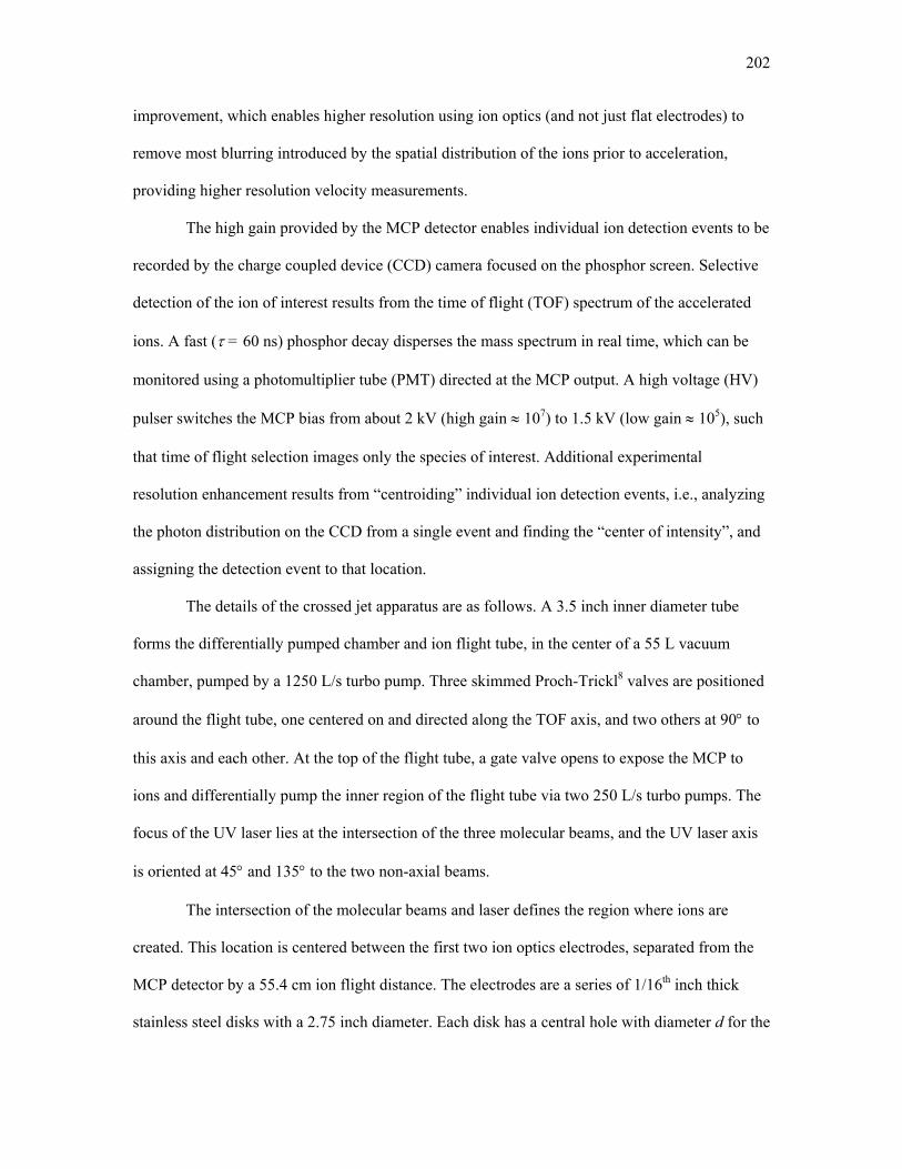
202

improvement, which enables higher resolution using ion optics (and not just flat electrodes) to

remove most blurring introduced by the spatial distribution of the ions prior to acceleration,

providing higher resolution velocity measurements.

The high gain provided by the MCP detector enables individual ion detection events to be

recorded by the charge coupled device (CCD) camera focused on the phosphor screen. Selective

detection of the ion of interest results from the time of flight (TOF) spectrum of the accelerated

ions. A fast (τ = 60 ns) phosphor decay disperses the mass spectrum in real time, which can be

monitored using a photomultiplier tube (PMT) directed at the MCP output. A high voltage (HV)

pulser switches the MCP bias from about 2 kV (high gain ≈ 107) to 1.5 kV (low gain ≈ 105), such

that time of flight selection images only the species of interest. Additional experimental

resolution enhancement results from “centroiding” individual ion detection events, i.e., analyzing

the photon distribution on the CCD from a single event and finding the “center of intensity”, and

assigning the detection event to that location.

The details of the crossed jet apparatus are as follows. A 3.5 inch inner diameter tube

forms the differentially pumped chamber and ion flight tube, in the center of a 55 L vacuum

chamber, pumped by a 1250 L/s turbo pump. Three skimmed Proch-Trickl8 valves are positioned

around the flight tube, one centered on and directed along the TOF axis, and two others at 90° to

this axis and each other. At the top of the flight tube, a gate valve opens to expose the MCP to

ions and differentially pump the inner region of the flight tube via two 250 L/s turbo pumps. The

focus of the UV laser lies at the intersection of the three molecular beams, and the UV laser axis

is oriented at 45° and 135° to the two non-axial beams.

The intersection of the molecular beams and laser defines the region where ions are

created. This location is centered between the first two ion optics electrodes, separated from the

MCP detector by a 55.4 cm ion flight distance. The electrodes are a series of 1/16th inch thick

stainless steel disks with a 2.75 inch diameter. Each disk has a central hole with diameter d for the

203

passage of ions and bending of electric field lines to create the ion lenses. Table A.1 summarizes

the spacing between the electrodes, and the electrode disk hole diameters. The VMII and TOF

conditions have been modeled using the Simion electrostatic modeling package (version 7.0), the

results of which are summarized in Fig. A.3. Velocity mapping conditions are demonstrated in

Fig. A.3(a), where the trajectories of several 1 eV Cl + ions are presented. The ions begin at three

locations along the laser axis, and with initial velocities oriented in 45° increments away from the

TOF axis. Varying the ratio of voltages between the repeller plate and first ion lens changes the

lens’ focal distance. Thus, ions created at different locations, but with the same initial velocity

component parallel the detector plane are detected at the same position on the MCP. Distances in

the image plane are directly proportional to this same velocity component, giving rise to the term

“velocity mapping.” The insensitivity to spatial origin when measuring velocities is what is meant

by VMII conditions.

An intuitive picture of the ion lens behavior can be gained by considering the surfaces

defined by the curved potential lines illustrated in Fig. A.3(b). Since the electrostatic forces bend

the ion velocities toward the surface normal, i.e., toward the field gradient, equipotential surfaces

play a role analogous to interfaces between regions with different indices of refraction in ray

optics – they bend diverging rays and enable the possibility of focusing optics.

Elementary electrodynamical considerations can be used to anticipate scaling of the

VMII conditions with respect to ion mass. Specifically, the local trajectory taken by an ion with a

given velocity vector can be described by the radius of curvature (rn) caused by the velocity

component normal to the local force (vn), according to

rn = vn2/a, (A.1)

where a is the acceleration caused by the applied force. In this case, the acceleration is simply

q|E|/m, where q is the ion’s charge, |E| is the magnitude of the electric field, and m is the ion

204

Table A.1 Geometry of the ion optics electrodes used in the ion imaging device. Electrode H (mm)a d (mm)b Repellerc 0.0 0 , 2.0 , 4.0 Lens 1 13.4 12.0 Lens 2 31.8 24.0 Lens 3 60.2 30.0

a Height of electrode above the bottom, repeller plate. b Diameter of the central aperture in each lens. c Repeller plate also acts as collimator for the on-axis molecular beam, necessitating several interchangeable electrodes to match beam dimensions.

Figure A.3 a) Simulated ion trajectories illustrating the velocity map ion imaging technique in the experimentally used, cylindrically symmetric flight tube geometry. As shown in the inset magnifications, 1 eV Cl + ions with initial velocities progressively angled by 45° in the plane of the trajectory diagram. Initial ion positions are displaced by 1 mm from each other perpendicular to the flight tube. The velocity mapping conditions illustrated result in ions landing on the detector at nearly the same location if they have the same velocity projection, regardless of the start location. b) Equipotential lines between the accelerating electrodes. Curved field lines in the vicinity of the central holes in the electrodes bend the trajectories and act as ion lenses.

a)

b)

205

mass. Thus, the local radius of curvature becomes

rn = mvn2/ q|E|. (A.2)

The numerator in this equation is proportional to the ion’s kinetic energy, T, and otherwise only

depends upon the direction of the initial velocity vector in the constant E filed. Thus, ions formed

at the same position and with parallel velocity vectors will follow the same three-dimensional

path through the electric field if they also have the same kinetic energy. Note that this result is

completely general, and applies to ions in electrostatic fields. The additional advantage of VMII

is that, to a very good approximation, the end point of the trajectories is also independent of

position in the vicinity of the region the ion lenses are mapping onto the detector plane. Thus,

ions with mass m and velocity components (vx, vy, vz) striking a given detector position all have

the same √(mvx2 + mvy

2), where the z-axis is the direction perpendicular to the detector axis.

Under most conditions only a single mass is selected and so this conditions produces a map of the

ions’ velocities projected onto the xy plane.

Careful inspection of Fig. A.3(a) reveals that VMII cannot distinguish between velocities

with the same vector component in the plane of the detector, but different absolute velocities.

Traditionally, this problem was resolved by studying systems with an axis of cylindrical

symmetry parallel to plane of the detector, such that the two dimensional information recorded in

x, z directions could be converted to cylindrical polar coordinates (r, z) via the inverse Abel

transformation or similar mathematical methods.9 The two non-axial molecular beams in Fig. A.2

produce a relative velocity vector in the plane of the jets, satisfying such a condition. However,

new VMII experimental techniques have made such symmetry considerations and data

transformation unnecessary. By turning on the MCP HV pulse for a very short time period (≈ 10

ns) compared to the spread of ion velocities perpendicular to the detector (≈ 200–400 ns) one can

select the ion velocities along the TOF axis. Such “slicing” of the velocity map was first

implemented by the Suits and Kitsopoulos groups.5,6 For optimal slicing resolution, it is therefore

206

useful to maximize the spread of the ions along the TOF axis, which can be practically expanded

to several hundred nanoseconds by lowering the electric field strength between the repeller and

first ion lens. Thus, 5–10% of the ion cloud can be sliced, avoiding the need for inverse Abel

transformation. Changing the lens voltage necessarily alters the ion focusing conditions, requiring

the use of a second lens to restore VMII conditions. For this reason, the current design was built

with a second variable electrode (lens 2) in addition to the final, grounded one (lens 3).

Following the construction of such a complicated device as the VMII apparatus, each

component was carefully characterized. In particular, many of the components shown in Fig. A.2

detect individual particles, such as photons on the PMT and CCD camera, and ion, electron, or

photon events on the MCP. These devices are characterized by measuring the gain G (or

calibration on the CCD analog to digital conversion) to verify proper functioning. Such

calibration is performed by measuring two independent quantities that are related to G, i) the

device output and ii) the noise on the output. Mathematically, the device output signal S when N

events are detected is given by

S = GN. (2.23)

Under the same shot noise limited conditions, repeat measurements of S result in a standard

deviation σS according to

σS = G√N. (2.24)

Thus, when both signal and noise are measured under shot noise limited conditions, a plot of σS2

versus S will yield a linear plot with a slope of G. Such calibrations result in the following. The

Lavision FlowMaster 3S CCD camera has a calibration of 2.15 photoelectrons (e-) per analog to

digital unit (ADU), very close to the factory specified 2 e-/ADU. Similarly, the Burle PS33189

MCP detector with 2.0 kV bias and 5.0 kV phosphor potential exhibits 29 ADU/event when

calibrated with the CCD camera. The MCP gain increases with the applied bias according to an

exponential curve with 120 V characteristic voltage. Finally, the electron tubes 9924QB PMT

207

gain was also calibrated, and fitted to the form G = Ae-V/V’ with A = 4500, and characteristic

voltage V’ = 143 V.

The ultimate velocity resolution of the VMII experiment may be limited by several

different factors. The translational temperature of the jet determines the spread of the unionized

species velocities parallel the jet direction, and for a helium carrier gas with a v/Δv ≈ 3, the

limiting resolution is about 300 m/s. However, perpendicular to the jet axis, the skimmer

geometry determines the velocity resolution, and for the on-axis valve, velocity spreads as small

as 10 m/s may be obtained. This value is sufficiently low that the recoil kinematics of the

ionization event also become significant. For Cl atoms ionized by three photons at 235 nm, the

electron recoils from the Cl with 2.8 eV excess energy, imparting a kick of 16 m/s to the Cl + ion.

In the limit that the electron recoils isotropically, this recoil produces an effective blurring of the

Cl atom’s initial velocity.

The REMPI spectral resolution has also been measured in two ways. Firstly, a jet of Cl or

HCl is introduced to the chamber, and the laser is scanned through a transition. The measured

≈ 0.5 cm-1 linewidth exceeds the 0.04 cm-1 expected from Doppler broadening and the 0.1 cm-1

laser linewidth. This measurement is confirmed by imaging Cl2 photolysis with the doubled 353

nm dye laser light. This process produces Cl atoms with 1660 m/s laboratory-frame velocities,

and resulting in atoms with a maximum 0.47 cm-1 Doppler shift. At line center, the edges of the

image have about ½ the center’s intensity, again revealing a homogeneous width of about 0.5

cm-1. These measurements indicate that power broadening dominates, and the time a Cl atom

spends in the upper state is about 60 ps before a third photon ionizes it. This observation makes

sense, as the REMPI process is limited by the two-photon transition, and the final ionization step

strongly saturated.

The detection efficiency has also been calibrated by measuring the number of ions

generated with a known gas density in the ionization region. Bleeding gas into the source

208

chamber produces a constant density of molecules in the ionization region, and the absolute

density can be measured directly on ion gauges in the source chamber and the detector chamber.

However, neither of these gauges directly measures the pressure in the ionization region of the

flight tube, which can only be inferred via conductance measurements of the intervening vacuum

components. Such measurements are performed by measuring the throughput between the source

and differentially pumped vacuum regions via ion gauge readings as a function of gas bleed.

Removing a single element (e.g., the ion lens stack) changes the conductance between the two

measured regions and provides a relative measure of that element’s conductance. Absolute

conductance values can be obtained via a region with known throughput, for example the

specified pumping speed of the detection region’s turbo pumps. Conductances measured this way

agree to within a factor of three to the infinitely thin “effusive source” expectation. More

importantly, the relative conductance provides an accurate measure of the pressure drop between

regions, and the ionization region has been calibrated to have 6% of the gas density produced by

the bleed in the source chamber, which is measured directly. Thus, the absolute density of

molecules in the ionization region can be known.

Next, the volume in which the UV laser ionizes 100% of the REMPI active species, i.e.,

the effective ionization volume can be inferred and calculated. Estimates of this volume can be

made from first principles considerations. For a Gaussian laser beam with 2.5 mm 1/e electric

field radius (ω), a 45 cm focal length lens (measured at 235 nm) produces a waist with ω0 = 24

μm. If the laser saturates the two-photon transition at the beam waist, the effective ionization

region can be calculated as 5.4×10-7 cm3, or about 20% of the focal volume, 2πω02z0, where z0 is

the confocal beam parameter. This estimate anticipates about 14 ions being produced per pulse

with an HCl density of 2.5×107 #/cm3 of HCl(J = 0) in the ionization region, very close to the 10–

20 ions observed with about 1.3 mJ pulse energy.

209

After completing construction and calibration of the VMII apparatus, we attempted to

study the reaction F + HCl via velocity map imaging the product Cl atoms. Unfortunately,

unanticipated background from the photo fragmentation/ionization process,

HCl + 3hν → Cl + + H, (A.3)

which occurs resonantly with the Cl transitions, swamps the signal. Indeed, a jet of 10% HCl in

He should produce about ten Cl + ions per shot under favorable reaction and detection conditions.

However, these ten ions are outnumbered by the 30–1200 ions per shot produced from the

process in Eq. 2.25, as shown in background the spectrum presented in Fig. A.4. Consequently,

any measured reaction dynamics would be masked by background at least three times higher than

the anticipated signal. Subtracting the background with only the HCl jet present from the

reactively produced “signal” with both reactants was attempted, but did not reveal any

meaningful structure within uncertainty. Thus, this project has been sidelined while seeking

methods to surmount this hurdle. Despite such difficulties, VMII presents a powerful new

technique for the study of state resolved reaction dynamics, and one on which we anticipate

fruitful results in the areas of photolysis and collision dynamics in the near future.

210

Figure A.4 Background ion spectrum of the 10% HCl jet in He, resulting in ions with mass to charge ratio equal to 35. Measurements have been made at frequencies corresponding to resonant ionization of ground state Cl (solid lines) and spin orbit excited Cl* (2P1/2) (dashed lines).

ν (cm-1)41800 42000 42200 42400 42600 42800

Ions

/Pul

se a

t m/q

= 3

5

0

200

400

600

800

1000Cl linesCl* lines

211

Appendix C: F + HCl Quasi-classical Trajectory Simulations

We have performed a QCT study of the reaction F + HCl → HF + Cl using the DHSN

surface and a fourth-order Runge-Kutta integration method.10 Varying the time step for numerical

integration produces a very rapid change in the energy conservation, found to scale with

approximately the 5th power of the step size, as shown in Fig. A.5. Yet, the computational cost

scales inversely with the step size, as shown in Fig. A.6, such that the choice of integration

parameters is a compromise between accuracy and computer cost. Reasonable accuracy is readily

obtained by choosing a time step of 5 atomic units = 0.12 fs, which conserves energy to better

than 0.03 and 0.0002 kcal/mol for reactive and non-reactive events, respectively, for typical 1–2

ps trajectories which require about 10 seconds of CPU time. Such fast calculations enable many

thousand trajectories to be run for various starting conditions in order to obtain reasonable

statistics.

Trajectories were started in the entrance channel with an initial distance of ≈ 10 Å

between the F atom and the HCl center of mass, and stopped when the F–Cl distance again

exceeded 10 Å. At this distance, the potential energy between the reactants/products is less than

0.001 kcal/mol and completely negligible. 4–10 kcal/mol collision energies were utilized in order

to simulate experimental conditions. Impact parameters of 0–4 Å were explored, though the

probability for reaction approached zero above 2 Å. The HCl reactant’s zero point energy was

explicitly included by beginning the trajectory with the H–Cl distance stretched to the zero point

level’s outer classical turning point. In order to randomly sample the phase of the HCl vibration

during the collision, the F–HCl distance was varied by 1 Å. The relative orientation of the

products was also randomly sampled.

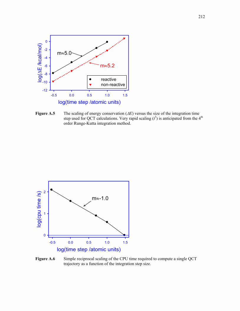
212

Figure A.5 The scaling of energy conservation (ΔE) versus the size of the integration time step used for QCT calculations. Very rapid scaling (t5) is anticipated from the 4th order Runge-Kutta integration method.

Figure A.6 Simple reciprocal scaling of the CPU time required to compute a single QCT trajectory as a function of the integration step size.

log(time step /atomic units)-0.5 0.0 0.5 1.0 1.5

log(

cpu

time

/s)

0

1

2

m≈-1.0

m≈5.2

log(time step /atomic units)-0.5 0.0 0.5 1.0 1.5

log(

Δ E /k

cal/m

ol)

-12

-10

-8

-6

-4

-2

0

reactivenon-reactive

m≈5.0

213

The calculated of reaction cross sections σ shown in Fig. A.7 are 2–3 orders of

magnitude smaller than anticipated from experiment at all collision energies studied. Modest

increases in reaction probability are obtained for higher collision energies and for rotationally

excited HCl, as noted by Hayes and Sun.11,12 Significantly, the reaction cross section remains

negligible at the experimental collision energy, which is above the classical barrier to reaction.

The low probability for reaction is discussed in more detail, below.

Following each reactive trajectory, the HF product is calculated using quasi-classical

approximation. The results of many such calculations are histogrammed and representative results

from 50,000 trajectories starting in the F + HCl channel at Ecom = 7 kcal/mol and JHCl = 2 are

plotted in Fig. A.8. Although collision energy and HCl rotation enhance reaction probability, the

qualitative aspects of the HF product quantum-state distributions for reactive events prove

relatively insensitive to collision conditions. Specifically, for all initial conditions studied,

product HF forms exclusively in the v = 3 and v = 2 manifolds, with high energy rotational states

primarily correlating with v = 2, as anticipated from conservation of energy. The results are

qualitatively similar to those reported by Sayos et al.,13 who also found only rotationally excited

HF in v = 2. Sayos et al.’s results are less vibrationally excited than the present DHSN

calculations, but were performed on the SHHG PES, which has an empirically lowered barrier

that enabled study at lower collision energies. Nevertheless, trajectories on both surfaces predict

high vibrational excitation and, more specifically, only high rotational excitation in v = 2. Thus,

full trajectory QCT methods do not qualitatively reproduce the observed HF state distributions.

Very recent wave packet calculations on the DHSN surface have been performed at substantially

lower energy than used in the present study, also resulting in branching primarily into high J in v

= 2.14 Thus, the DHSN surface reproduces the propensity for high J HF(v = 2) and lower J HF(v =

3) products first observed on older surfaces.

214

Figure A.7 Theoretical F + HCl reaction cross section from QCT calculations on the DHSN surface for reaction with HCl in the rotational states indicated. Reaction events are not observed until the center of mass collision energy well exceeds the 4 kcal/mol barrier. Modest rotational enhancement is evident, though computed cross sections remain nearly 1000 times smaller than experimentally determined.

Figure A.8 HF product state distribution for QCT scattering calculations on the DHSN potential energy surface. Initial conditions are Ecom = 7 kcal/mol, JHCl = 2. These results were obtained following 50,000 scattering trajectories.

Ecom (kcal/mol)0 2 4 6 8 10

σ rxn

(Å2 )

0.000

0.001

0.002

JHCl=1JHCl=2JHCl=5

v=3

0.00

0.05

0.10

v=2

J0 2 4 6 8 10 12 14 16

Frac

tiona

l Pop

ulat

ion

0.00

0.05

0.10

215

In order to test the validity of the full collision calculations, a second set of trajectories

has been performed, starting simply in the transition state (TS) region of the DHSN surface with

total energy 0.2 kcal/mol above the classical barrier. Although these TS calculations have not

been chosen to reflect accurately a distribution of reactive trajectories, they should represent the

type of distributions obtained for reactive trajectories that surmount the classical barrier. As

shown in Fig. A.9, trajectories starting near the transition state and proceeding to the HF + Cl

channel exhibit similar features as the full trajectory results, i.e., population forms exclusively in

highly vibrationally excited states (v = 2 in this case), and high J state rotational excitation is

favored. Thus, the full trajectory results are indicative of the qualitative features of general

trajectories traversing the transition state.

We have also used QCT methods to explore briefly the possible influence of deep van der

Waals well in the HF + Cl exit channel. These trajectories are motivated by the wealth of

vibrational predissociation studies of van der Waals complexes, as well as the possibility of long-

lived resonance states that explore portions of the exit well not extensively visited by classical

reaction path. Exit-well trajectories are started in the vicinity of the HF–Cl van der Waals

minimum, in an initial distribution of HF rovibrational states obtained from full trajectory

calculations shown in Fig. A.8 and with zero kinetic energy in the HF–Cl coordinate. The starting

position is chosen to be within 0.5 kcal/mol of the bottom of the van der Waals minimum, and the

total energy varies by this amount. In essence, these conditions mimic what might be expected if

nascent reactive products were to become trapped in the HF–Cl van der Waals well following

reaction. The trajectories with non-rotating but vibrationally excited HF were nondissociative on

the time scales explored; roughly corresponding to vibrational predissociation, which is known to

be exquisitely sensitive to the hard inner wall of the PES and poorly modeled by QCT.15

However, the dissociation probability of the HF–Cl complex does rise rapidly with HF rotation,

in effect rotationally predissociating to yield HF with reduced internal energy. The results shown

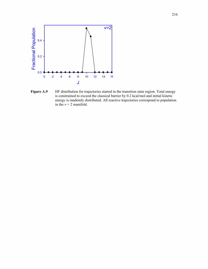
216

Figure A.9 HF distribution for trajectories started in the transition state region. Total energy is constrained to exceed the classical barrier by 0.2 kcal/mol and initial kinetic energy is randomly distributed. All reactive trajectories correspond to population in the v = 2 manifold.

v=2

J0 2 4 6 8 10 12 14 16

Frac

tiona

l Pop

ulat

ion

0.0

0.2

0.4

217

in Fig. A.10 reveal that product HF fragments retain most of their vibrational energy while being

“cooled” into lower angular momentum states. Such relaxation suggests the Van der Waals exit

well may play a significant role in the formation of the low J HF observed experimentally and

may even contribute to HF population in lower vibrational manifolds. Indeed, previous studies of

exit-channel dynamics by Orr-Ewing and coworkers in reactive trajectories found that

rotationally cold products with strong dipole moments can torque on recoiling fragments and

thereby rotationally “heat up” in the exit channel.16 It would seem equally dynamically plausible

in the F + HCl system for highly rotationally excited HF to be “cooled” by angular forces in the

van der Waals exit channel, which would be an interesting direction for further theoretical

exploration.

218

Figure A.10 Quantum state distribution obtained by starting trajectories in the HF–Cl van der Waals well. Initial HF rovibrational energy distribution is that plotted in A.8, and initial HF–Cl kinetic energy is fixed at zero.

v=1

J0 2 4 6 8 10 12 14 16

0.00

0.05

0.10

v=2

Frac

tiona

l Pop

ulat

ion

0.00

0.05

0.10

v=3

0.00

0.05

0.10

219

Appendix D: Surprisal Analysis of HF State Distributions Produced By F + H2O

The surprisal analysis works as follows. The “prior” distribution Pprior is defined as the

one with maximum entropy, the case where all states (described by the rotational, vibrational, and

translational states of the products) that are energetically accessible are equally likely to be

populated. Thus, the prior distribution is related to the degeneracy g(N) of each level N,

according to

Pprior(N) = g(N)/ΣNg(N), (A.4)

for N such that the energy of state N is less than the total energy. From information theory, the

surprisal17,18 I(N) is generated by comparing the calculated Pprior (N) to the observed distribution,

Pobs(N), via

I(N) = -ln[Pobs(N)/ Pprior(N)]. (A.5)

A linear plot of I(N) versus a quantity fN indicates a “constraint” on the quantity fN over the course

of reaction. Likely constraints are energy E(N) or the HF angular momentum JHF. The nearly

collinear surprisal plot in Fig. A.11 reveals that vibrational branching matches a simple one-

parameter surprisal model that is nearly the same at all studied energies.

Unlike the vibrational populations, statistical analysis fails to even qualitatively describe

the measured rotational distributions. Surprisal analyses of the v = 1 rotational distributions are

presented in Fig. A.12, using JHF and E(N) as fN, defined in the discussion of Eq. A.5. These plots

are constructed by summing over the unseen parameters in the state indicator N, such as the OH

rovibrational quanta. Neither of the plots in Fig. A.12 is linear over the entire range of HF

rotational states probed, and recently proposed modified surprisal analyses21 result in similarly

non-linear trends. Thus, simple statistical considerations are not sufficient to explain the observed

rotational distributions, even if they do match the vibrational trends in Fig. A.11 reasonably well.

Since no physical mechanism has been proposed to predict the slope of such surprisal plots from

first principles, even in when observed trends exhibit linear surprisals, they shed little insight.

220

Figure A.11 Surprisal analysis of HF vibrational partitioning observed in the present F + H2O study, inferred from comparison to F + D2O chemiluminescence in Ref. 19, and computed in the theoretical study in Ref. 20.

E(v) / ETotal

0.0 0.2 0.4 0.6 0.8 1.0

Vib

ratio

nal S

urpr

isal

-4

-3

-2

-1

0

1IR chemiluminescencepresent studydirect dynamics

221

Figure A.12 Surprisal plots of the vHF = 1 rotational distribution, plotted as a function of (a) fractional energy deposited in the HF product, and (b) HF angular momentum quantum number , JHF.

a)

E(v,J) / Etot

0.5 0.6 0.7 0.8 0.9

-ln(P

obs/P

prio

r)

-3

-2

-1

0

1

b)

JHF

0 2 4 6 8 10 12

-ln(P

obs/P

prio

r)

-3

-2

-1

0

1

222

Appendix E: Estimated State Resolved Branching Ratios

The precise HF branching ratios are obtained following the density-to-flux conversion,

and performed via Monte Carlo modeling of the crossed jet conditions, as described in detail in

Chapter 2.4(B) This model produces the average residence time, ⟨τ⟩, for product HF in each (v,J)

state, which varies with the assumed differential scattering distribution. The calculated ⟨τ⟩ values

for HF formed in the reaction F + HCl are presented in Fig. A.13(a) and Table A.2 for several

differential scattering cross section limits. Defining θ as the angle between the F and HF

velocities in the center of mass frame, the limiting cases considered here are defined as follows:

isotropic (-1 ≤ cos(θ) ≤ 1), forward (0.33 ≤ cos(θ) ≤ 1), side (-0.33 ≤ cos(θ) ≤ 0.33), and

backward (-1 ≤ cos(θ) ≤ -0.33). Although ⟨τ⟩ varies by a factor of 0.57–1.7, depending on the

unknown differential scattering limit, angular measurements on similar reactions have not found

this quantity to vary rapidly between adjacent product rotational states.22 Essentially, the reactions

tend to proceed through one or more mechanisms that do not turn on and off abruptly between

product states, such that the entire HF population distribution may be obtained using one

universal differential cross section assumption.

The density-to-flux analysis has been performed for each of the angular scattering limits

presented in Table A.2, resulting in the normalized fluxes in Fig. A.14. This presentation reveals

that the uncertainty in the branching ratio introduced by the assumed differential cross section is

smaller than the experimental uncertainty in the measured HF densities, at least to the extent that

the differential cross section (dσ/dΩ) does not vary with HF state. This insensitivity largely arises

from the similar shape of the curves in Fig. A.13 and is explained by substantial blurring of the

angular resolution of the experiment caused by spatial averaging within the unskimmed jets.

Therefore the exact choice of scattering limit is arbitrary, and for the analysis that follows, the

isotropic limit has been used, as presented in Fig. A.14 and Table 3.1.

223

Figure A.13 a) Calculated HF residence times from Monte Carlo simulation of the F + HCl crossed jet experiment. Computed values are shown for four limiting cases of differential scattering cross section, as discussed in the text. b) Log-log plot of the same data. For sufficiently high recoil energy, ⟨τ⟩ scales with available energy (Eavail) to the -½ power, i.e., with the inverse of the recoil speed.

⟨Eavail⟩ (kcal/mol)0 10 20 30

⟨τ⟩ (

μ s)

0

20

40

60 IsotropicBackwardSideForward

a) m=-1/2

ln( ⟨Eavail⟩ /kcal/mol )-2 -1 0 1 2 3

ln(⟨

τ⟩ /s

)

-13

-12

-11

-10

IsotropicBackwardSideForward

b)

224

Table A.2 HF(v,J) state resolved residence times in the probe region following the reaction F + HCl → HF + Cl, as calculated via Monte Carlo simulation of the crossed jet conditions. The crossed jet conditions are as described in Ch. III. Average residence times are presented for the isotropic differential cross section limit⟨τi⟩. Ratio of residence times to this value are also provided for the other three differential scattering limits, backward scattering ⟨τb⟩, side scattering ⟨τs⟩, and forward scattering ⟨τf⟩, as defined in the text. v J ⟨τi⟩(μs) ⟨τb⟩/⟨τi⟩ ⟨τs⟩/⟨τi⟩ ⟨τf⟩/⟨τi⟩ V J ⟨τi⟩ (μs) ⟨τb⟩/⟨τi⟩ ⟨τs⟩/⟨τi⟩ ⟨τf⟩/⟨τi⟩ 0 0 5.89 0.57 1.57 0.59 2 0 9.12 0.59 1.59 0.59 1 5.91 0.57 1.56 0.59 1 9.16 0.58 1.58 0.59 2 5.90 0.57 1.57 0.60 2 9.25 0.58 1.57 0.59 3 5.93 0.57 1.56 0.59 3 9.36 0.58 1.58 0.59 4 5.93 0.57 1.58 0.60 4 9.49 0.58 1.58 0.59 5 6.01 0.57 1.58 0.59 5 9.58 0.59 1.61 0.59 6 6.01 0.58 1.58 0.60 6 9.90 0.59 1.58 0.59 7 6.17 0.57 1.57 0.59 7 10.13 0.59 1.60 0.59 8 6.21 0.57 1.58 0.59 8 10.52 0.59 1.60 0.59 9 6.33 0.57 1.57 0.60 9 11.10 0.59 1.58 0.58 10 6.45 0.57 1.57 0.60 10 11.63 0.60 1.60 0.58 11 6.59 0.57 1.57 0.59 11 12.54 0.60 1.60 0.58 12 6.73 0.57 1.57 0.59 12 13.80 0.61 1.58 0.57 13 6.85 0.58 1.59 0.60 13 15.56 0.62 1.60 0.56 14 7.14 0.57 1.57 0.59 14 19.31 0.63 1.60 0.52

1 0 7.00 0.57 1.58 0.59 15 28.48 0.59 1.66 0.46 1 7.00 0.57 1.58 0.60 3 0 16.85 0.62 1.60 0.55 2 7.01 0.57 1.59 0.59 1 16.93 0.63 1.60 0.55 3 7.10 0.57 1.57 0.60 2 17.60 0.63 1.61 0.54 4 7.16 0.58 1.59 0.59 3 18.32 0.64 1.62 0.54 5 7.29 0.57 1.57 0.59 4 20.23 0.63 1.60 0.52 6 7.33 0.58 1.58 0.59 5 22.50 0.64 1.62 0.50 7 7.44 0.58 1.58 0.59 6 26.64 0.62 1.73 0.48 8 7.94 0.55 1.51 0.57 7 31.90 0.63 1.65 0.47 9 7.81 0.58 1.57 0.59 8 32.21 0.59 1.68 0.58 10 7.94 0.58 1.59 0.60 9 30.78 0.65 1.56 0.73 11 8.20 0.58 1.60 0.59 10 36.48 0.54 1.37 0.73 12 8.55 0.58 1.59 0.59 11 43.18 0.53 1.21 0.75 13 8.94 0.58 1.58 0.59 12 45.55 0.57 1.26 0.83 14 9.36 0.58 1.58 0.59 15 9.91 0.59 1.59 0.59 16 10.62 0.59 1.61 0.59

225

Figure A.14 Calculated HF state resolved flux following the reaction F + HCl → HF + Cl for four limiting cases of reactive differential cross section. All data have been normalized such that they sum to 1. The agreement shown here reveals the high confidence in the present results, limited by the unknown state-dependent differential cross sections.

v=0

J0 2 4 6 8 10 12 14 16

0.00

0.03

0.06IsotropicBackwardSide Forward

v=1

Nor

mal

ized

Flu

x

0.00

0.03

v=2

0.00

0.03

v=3

0.00

0.03

226

It is important to note that the structured rotational distributions in Fig. 3.6 cannot be

ascribed to varying detection sensitivity. With the present scaling, the local maxima at low and

high J in the v = 1 and v = 2 manifolds have comparable magnitudes. Thus, even if the dynamical

processes leading to these features are correlated with radically different differential cross

sections, the detection sensitivity changes by at most a factor of about 2.7 between the largest and

lowest ⟨τ⟩ values presented in Fig. A.13. Thus, for the most extreme case, any portion of the

results in Fig. A.14 cannot change by more than three-fold, which is insufficient to mask the

relevant bimodal structure. Additionally, if such extreme differential scattering structure were

present, it would further support bifurcated dynamics in the F + HCl reaction event.

Similar Monte Carlo modeling of the F + H2O experiment provides the ⟨τ⟩ values for

each HF(v,J) state for that system. In order to model the F + H2O reaction kinematics, the recoil

energy, and thus the HF and OH internal states, must be specified. Although the OH state

distribution is not explicitly measured in the current experiment, it has been found to be a small

heat sink (with respect to the total energy),23,24 consistent with the spectator bond approximation.

Indeed, varying the energy deposited in the OH fragment between zero and 1 kcal/mol (the

average rotational energy observed in the OH product in Ref. 23) changes the density-to-flux

results by a completely negligible amount.

The resulting residence times are presented in Table A.3, for limiting cases of the

differential cross section (dσ/dΩ). Since dσ/dΩ as a function of HF state is unknown, it is not

possible to perform the transformation with 100% certainty. However, in the limit that all product

states are formed with similar angular scattering dependence – consistent with the monotonic

distribution of product states and measurements of dσ/dΩ on other reactive systems – the choice

of dσ/dΩ does not significantly alter the results. This insensitivity is exploited in Fig. A.15,

which presents the normalized flux for each limiting case of dσ/dΩ. In v = 0 and v = 1, each of

227

Table A.3 HF(v,J) state resolved residence times (μs) in the probe region following the reaction F + H2O → HF + OH, as calculated via Monte Carlo simulation of the crossed jet conditions. The crossed jet conditions are as described in Ch. IV. Data are organized as in Table A.2. v J ⟨τi⟩(μs) ⟨τb⟩/⟨τi⟩ ⟨τs⟩/⟨τi⟩ ⟨τf⟩/⟨τi⟩ v J ⟨τi⟩ (μs) ⟨τb⟩/⟨τi⟩ ⟨τs⟩/⟨τi⟩ ⟨τf⟩/⟨τi⟩ 0 0 8.86 0.53 3.03 0.36 1 0 13.45 0.49 3.35 0.35 1 8.87 0.54 3.02 0.36 1 13.53 0.49 3.38 0.35 2 8.93 0.53 3.03 0.36 2 13.81 0.49 3.38 0.35 3 9.02 0.53 3.04 0.36 3 14.08 0.48 3.43 0.34 4 9.08 0.53 3.05 0.36 4 14.59 0.47 3.49 0.34 5 9.29 0.53 3.04 0.36 5 15.26 0.47 3.56 0.34 6 9.44 0.53 3.05 0.36 6 16.42 0.45 3.72 0.33 7 9.63 0.53 3.06 0.36 7 18.03 0.43 3.90 0.33 8 9.90 0.53 3.08 0.36 8 19.94 0.41 4.29 0.30 9 10.25 0.52 3.09 0.36 9 23.18 0.37 4.48 0.30 10 10.64 0.52 3.13 0.36 10 24.82 0.37 4.70 0.30 11 11.21 0.51 3.17 0.36 11 26.02 0.39 4.38 0.31 12 11.83 0.51 3.22 0.36 12 25.17 0.43 3.81 0.36 13 12.75 0.50 3.30 0.35 13 22.04 0.53 3.02 0.46 14 14.23 0.48 3.42 0.35 14 25.60 0.54 2.72 0.49 15 16.31 0.45 3.71 0.33 15 29.34 0.61 2.51 0.56 16 20.56 0.40 4.28 0.30 2 0 22.20 0.56 2.71 0.48 17 26.04 0.35 4.61 0.30 1 23.56 0.54 2.79 0.48 18 25.60 0.41 4.08 0.33 2 22.93 0.59 2.71 0.47 3 23.27 0.58 2.62 0.51 4 25.10 0.58 2.55 0.52 5 25.37 0.62 2.48 0.73 6 28.20 0.63 2.36 0.59 7 31.83 0.64 2.17 0.67

228

Figure A.15 Observed nascent HF(v,J) populations produced by the F + H2O reaction, obtained from the measured densities via the density-to-flux transformation. Data points, and dotted, solid, and dashed lines indicate the results from various assumed differential cross section scattering limits used in the density-to-flux conversion, as defined in the text.

v=1

Nor

mal

ized

Flu

x

0.00

0.03

0.06

0.09

0.12

0.15

v=2

0.00

0.03

v=0

J0 2 4 6 8 10 12 14 16 18

0.00

0.03

0.06

IsotropicBackwardSide Forward

229

these limiting cases results in rovibrational population distributions that agree well within the

reported experimental error bars, and the v = 2 populations are only slightly shifted by the chosen

angular scattering limit. The F + H2O results are particularly insensitive to changes in dσ/dΩ

because of i) the large amount of spatial averaging in the unskimmed jet geometry, ii) the

relatively small reaction exoergicity, compared to reactions such as F + HCl,25 or F + CH4,26 and

iii) the narrow distribution of HF states populated, primarily v = 1, J < 5. Thus, for the bulk of

Ch. IV, the results obtained assuming isotropic differential scattering have been discussed, as

presented in Table 4.2.

In the gas-phase studies in Ch. III and IV, Monte Carlo simulations of the recoil

dynamics enabled the density-to-flux transformation to be performed and state resolved branching

ratios to be estimated. In Ch. V, the reaction at the gas-liquid interface may have similar state-

dependent sensitivities. However, complications arise at the liquid interface because the dynamics

of the highly exothermic reaction event and subsequent interactions at the liquid interface

completely determines the state-dependent HF velocities in the laboratory frame. Thus, any

prediction of recoil velocities necessitates detailed dynamical commutation of the gas-liquid

scattering event. However, the Doppler measurements do provide direct experimental information

about the HF recoil velocities. As discussed in more detail in the next Chapter 5.5, the HF

velocities are quite close to thermal, and only change slowly with quantum state. Although

Doppler measurements in the current experimental arrangement only reveal velocities parallel the

liquid surface, a physically motivated cos(θ) angular distribution of HF velocities escaping the

surface can be used to infer residence times in the probe volume and compute the state resolved

HF flux. Fig. A.16 presents the normalized flux values, along with the normalized column-

integrated densities from Table 5.2. This presentation reveals that the fluxes and densities agree

nearly quantitatively in the present study. Thus, any flux correction results in only a slight

increase of the fractional branching into v = 3 and v = 2, at the expense of the slowly moving

230

Figure A.16 Normalized HF densities and inferred fluxes following reactive scattering of F from a liquid squalane surface.

v=0

JHF

0 2 4 6 8 10 12 14

0.00

0.02

0.04

0.06

0.08

v=1

0.00

0.02

0.04

0.06

0.08

v=2

Frac

tiona

l Pop

ulat

ion

0.00

0.02

0.04

0.06

0.08

Normalized DensityNormalized Flux

v=3

0.00

0.02

231

(nearly translationally equilibrated) molecules in v = 0 and v = 1. Since the effect of such

weighting does not change the populations within the experimental uncertainty, we have focused

our attention on interpreting the measured densities. This approximation is complicated by recent

theoretical work by Schatz and coworkers,27 revealing a propensity for recoiling HF to be directed

along the surface normal. However, the high F atom translational energy used in this theoretical

study (0.5, 1.0 eV) makes direct comparison to the present study difficult.

232

References for Appendices A–E

1 W. Koechner, (Springer, Berlin, 1999), pp. 232.

2 L. F. Mollenauer, Rev. Sci. Instrum. 49, 809 (1978).

3 D. W. Chandler and P. L. Houston, J. Chem. Phys. 87, 1445 (1987).

4 A. Eppink and D. H. Parker, Rev. Sci. Instrum. 68, 3477 (1997).

5 D. Townsend, M. P. Minitti, and A. G. Suits, Rev. Sci. Instrum. 74, 2530 (2003).

6 R. L. Toomes and T. N. Kitsopoulos, Phys. Chem. Chem. Phys. 5, 2481 (2003).

7 J. J. Lin, J. G. Zhou, W. C. Shiu, and K. P. Liu, Rev. Sci. Instrum. 74, 2495 (2003).

8 D. Proch and T. Trickl, Rev. Sci. Instrum. 60, 713 (1989).

9 V. Dribinski, A. Ossadtchi, V. A. Mandelshtam, and H. Reisler, Rev. Sci. Instrum. 73, 2634 (2002).

10 W. H. Press, S. A. Teukolsky, W. T. Vetterling, and B. P. Flannery, Numerical recipes in C: the art of scientific computing, 2 ed. (Cambridge University Press, New York, 1992).

11 M. Y. Hayes, M. P. Deskevich, D. J. Nesbitt, K. Takahashi, and R. T. Skodje, J. Phys. Chem. A 110, 436 (2006).

12 Z. G. Sun, S. Y. Lee, and D. H. Zhang, Chin. J. Chem. Phys. 20, 365 (2007).

13 R. Sayos, J. Hernando, R. Francia, and M. Gonzalez, Phys. Chem. Chem. Phys. 2, 523 (2000).

14 G. Quemener and N. Balakrishnan, J. Chem. Phys. 128, (2008).

15 E. Tannenbaum, K. J. Higgins, W. Klemperer, B. Segev, and E. J. Heller, J. Phys. Chem. B 106, 8100 (2002).

16 S. Rudic, C. Murray, J. N. Harvey, and A. J. Orr-Ewing, J. Chem. Phys. 120, 186 (2004).

17 R. D. Levine and R. B. Bernstein, Molecular Reaction Dynamics and Chemical Reactivity. (Oxford University Press, New York, 1987).

18 J. T. Muckerman, J. Phys. Chem. 93, 179 (1989).

19 M. A. Wickramaaratchi, D. W. Setser, H. Hildebrandt, B. Korbitzer, and H. Heydtmann, Chem. Phys. 94, 109 (1985).

20 Y. Ishikawa, T. Nakajima, T. Yanai, and K. Hirao, Chem. Phys. Lett. 363, 458 (2002).

21 J. J. Valentini, J. Phys. Chem. A 106, 5745 (2002).

233

22 X. M. Yang and D. H. Zhang, Accounts Chem. Res. 41, 981 (2008).

23 M. Ziemkiewicz and D. J. Nesbitt, manuscript in preparation.

24 M. Ziemkiewicz, M. Wojcik, and D. J. Nesbitt, J. Chem. Phys. 123, 224307 (2005).

25 A. M. Zolot and D. J. Nesbitt, J. Chem. Phys. 127, 114319 (2007).

26 W. W. Harper, S. A. Nizkorodov, and D. J. Nesbitt, J. Chem. Phys. 113, 3670 (2000).

27 B. K. Radak, S. Yockel, D. Kim, and G. C. Schatz, J. Phys. Chem. A (in press) (2009).