IEEE TRANSACTIONS ON SYSTEMS, MAN, AND CYBERNETICS—PART A: SYSTEMS AND HUMANS, VOL. 37, NO. 5, SEPTEMBER 2007 655

Hardware/Software Partitioning UsingBayesian Belief Networks

John T. Olson, Jerzy W. Rozenblit, Claudio Talarico, and Witold Jacak

Abstract—In heterogeneous system design, partitioning of thefunctional specifications into hardware (HW) and software (SW)components is an important procedure. Often, an HW platform ischosen, and the SW is mapped onto the existing partial solution, orthe actual partitioning is performed in an ad hoc manner. The par-titioning approach presented here is novel in that it uses Bayesianbelief networks (BBNs) to categorize functional components intoHW and SW classifications. The BBN’s ability to propagate evi-dence permits the effects of a classification decision that is madeabout one function to be felt throughout the entire network. Inaddition, because BBNs have a belief of hypotheses as their core,a quantitative measurement as to the correctness of a partitioningdecision is achieved. A methodology for automatically generatingthe qualitative structural portion of BBN and the quantitative linkmatrices is given. A case study of a programmable thermostat isdeveloped to illustrate the BBN approach. The outcomes of thepartitioning process are discussed and placed in a larger designcontext, which is called model-based codesign.

Index Terms—Hardware/software partitioning, heterogenoussystem design, model-based codesign.

I. INTRODUCTION

IN THIS, we present a new approach to the hardware(HW)/software (SW) partitioning problem [4]–[6], [8], [21],

[24] that uses Bayesian belief networks (BBNs) for functionalcomponent classification into HW and SW. Design of heteroge-neous systems entails choosing which functional componentsshould be implemented in HW and which should be imple-mented in SW. Typically, an HW platform is chosen, and theSW is written to make the HW meet the specified requirements.The problem with this approach, however, is that, during systemintegration, interface and incompatibility problems may arisevery late in the design cycle. HW/SW partitioning is used topush the implementation decisions into the early design phases,so that the decision of whether to use HW or SW is not made inisolation for each functional component.

In our previous work, we have established a systematic ap-proach to the design of heterogeneous systems. Called model-based codesign [5], [24], this approach uses simulatable system

Manuscript received April 26, 2002; revised June 3, 2005. This work wasrecommended by Associate Editor K. C. Chang.

J. T. Olson is with IBM Inc., Armonk, NY 10504 USA.J. W. Rozenblit is with the Department of Electrical and Computer En-

gineering, University of Arizona, Tucson, AZ 85721 USA (e-mail: jr@ece.arizona.edu).

C. Talarico is with the Department of Electrical Engineering, EasternWashington University, Cheney, WA 99044 USA.

W. Jacak is with the Department of Software Engineering, Upper AustriaUniversity of Applied Science, 4232 Hagenberg, Austria.

Color versions of one or more of the figures in this paper are available onlineat http://ieeexplore.ieee.org.

Digital Object Identifier 10.1109/TSMCA.2007.902623

descriptions as the basis for the generation of design descrip-tions from which the real system is built. Simulation is usedas a primary means of verifying functional requirements of thedesign. Thus, in parallel to the simulation, classifications of thesystem model components into HW or SW must be made.

The partitioning approach presented here uses the BBNconcept [3], [14], [20], [28]. The reasons for using the BBNframework are the following: 1) its ability to represent thecausal nature of a functional description (e.g., a function Acalling another function B is a causal influence from A to B)and 2) the ability to distribute local evidence (simulation resultsthat drive a particular functional component toward an HW orSW realization) throughout the entire network and thus makethe effects of a local partitioning decision affect partitioningdecisions throughout the entire model. This, in conjunctionwith the benefit of having probabilistic measurements as to thedegree of belief in classification decisions, makes the use ofBBNs appropriate.

In the ensuing sections, we first provide the motivation forthis new type of partitioning methodology and describe theproblem formally. We describe the principles of BBNs and thenaddress the existing body of HW/SW partitioning work. Then,we present our formal methodology, followed by an illustrativedesign example.

II. MOTIVATION

Extensive research has been conducted in the area ofHW/SW partitioning. There are three main partitioning ap-proaches: 1) methods in which the partitioning is driven towarda preexisting HW platform; 2) flexible methods that use nofixed preexisting HW platform; and 3) methods that are basedon traditional very large scale integration (VLSI) partitioningtechniques.

In the methods that drive partitioning onto a preexisting HWplatform, the configuration usually consists of a single micro-processor that runs the SW component and an application-specific integrated circuit (ASIC) to implement the HW portion.The work presented in [7], [9], [12], [16], [17], [31], [32], and[34] is among the most notable in this area of HW/SW partition-ing. The major limitation to this body of work is the inability toutilize a different HW configuration, particularly, in the caseswhere the design and fabrication of an ASIC is not feasible be-cause of the cost. Therefore, the need for HW/SW partitioningsystems that are flexible with regard to the type and number ofcomponents comprising the HW platform is warranted.

Several works have attempted to address the problem ofpartitioning onto a flexible HW/SW platform. Among themare [2], [10], [13], [15], [23], [25], [29], [30], and [33] that

1083-4427/$25.00 © 2007 IEEE

656 IEEE TRANSACTIONS ON SYSTEMS, MAN, AND CYBERNETICS—PART A: SYSTEMS AND HUMANS, VOL. 37, NO. 5, SEPTEMBER 2007

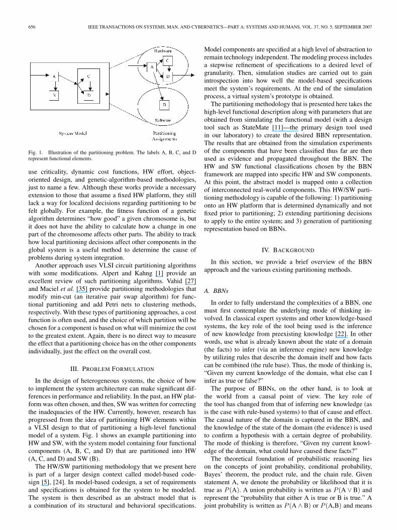
Fig. 1. Illustration of the partitioning problem. The labels A, B, C, and Drepresent functional elements.

use criticality, dynamic cost functions, HW effort, object-oriented design, and genetic-algorithm-based methodologies,just to name a few. Although these works provide a necessaryextension to those that assume a fixed HW platform, they stilllack a way for localized decisions regarding partitioning to befelt globally. For example, the fitness function of a geneticalgorithm determines “how good” a given chromosome is, butit does not have the ability to calculate how a change in onepart of the chromosome affects other parts. The ability to trackhow local partitioning decisions affect other components in theglobal system is a useful method to determine the cause ofproblems during system integration.

Another approach uses VLSI circuit partitioning algorithmswith some modifications. Alpert and Kahng [1] provide anexcellent review of such partitioning algorithms. Vahid [27]and Maciel et al. [35] provide partitioning methodologies thatmodify min-cut (an iterative pair swap algorithm) for func-tional partitioning and add Petri nets to clustering methods,respectively. With these types of partitioning approaches, a costfunction is often used, and the choice of which partition will bechosen for a component is based on what will minimize the costto the greatest extent. Again, there is no direct way to measurethe effect that a partitioning choice has on the other componentsindividually, just the effect on the overall cost.

III. PROBLEM FORMULATION

In the design of heterogeneous systems, the choice of howto implement the system architecture can make significant dif-ferences in performance and reliability. In the past, an HW plat-form was often chosen, and then, SW was written for correctingthe inadequacies of the HW. Currently, however, research hasprogressed from the idea of partitioning HW elements withina VLSI design to that of partitioning a high-level functionalmodel of a system. Fig. 1 shows an example partitioning intoHW and SW, with the system model containing four functionalcomponents (A, B, C, and D) that are partitioned into HW(A, C, and D) and SW (B).

The HW/SW partitioning methodology that we present hereis part of a larger design context called model-based code-sign [5], [24]. In model-based codesign, a set of requirementsand specifications is obtained for the system to be modeled.The system is then described as an abstract model that isa combination of its structural and behavioral specifications.

Model components are specified at a high level of abstraction toremain technology independent. The modeling process includesa stepwise refinement of specifications to a desired level ofgranularity. Then, simulation studies are carried out to gainintrospection into how well the model-based specificationsmeet the system’s requirements. At the end of the simulationprocess, a virtual system’s prototype is obtained.

The partitioning methodology that is presented here takes thehigh-level functional description along with parameters that areobtained from simulating the functional model (with a designtool such as StateMate [11]—the primary design tool usedin our laboratory) to create the desired BBN representation.The results that are obtained from the simulation experimentsof the components that have been classified thus far are thenused as evidence and propagated throughout the BBN. TheHW and SW functional classifications chosen by the BBNframework are mapped into specific HW and SW components.At this point, the abstract model is mapped onto a collectionof interconnected real-world components. This HW/SW parti-tioning methodology is capable of the following: 1) partitioningonto an HW platform that is determined dynamically and notfixed prior to partitioning; 2) extending partitioning decisionsto apply to the entire system; and 3) generation of partitioningrepresentation based on BBNs.

IV. BACKGROUND

In this section, we provide a brief overview of the BBNapproach and the various existing partitioning methods.

A. BBNs

In order to fully understand the complexities of a BBN, onemust first contemplate the underlying mode of thinking in-volved. In classical expert systems and other knowledge-basedsystems, the key role of the tool being used is the inferenceof new knowledge from preexisting knowledge [22]. In otherwords, use what is already known about the state of a domain(the facts) to infer (via an inference engine) new knowledgeby utilizing rules that describe the domain itself and how factscan be combined (the rule base). Thus, the mode of thinking is,“Given my current knowledge of the domain, what else can Iinfer as true or false?”

The purpose of BBNs, on the other hand, is to look atthe world from a causal point of view. The key role ofthe tool has changed from that of inferring new knowledge (asis the case with rule-based systems) to that of cause and effect.The causal nature of the domain is captured in the BBN, andthe knowledge of the state of the domain (the evidence) is usedto confirm a hypothesis with a certain degree of probability.The mode of thinking is therefore, “Given my current knowl-edge of the domain, what could have caused these facts?”

The theoretical foundation of probabilistic reasoning lieson the concepts of joint probability, conditional probability,Bayes’ theorem, the product rule, and the chain rule. Givenstatement A, we denote the probability or likelihood that it istrue as P (A). A union probability is written as P (A ∨ B) andrepresent the “probability that either A is true or B is true.” Ajoint probability is written as P (A ∧ B) or P (A,B) and means

OLSON et al.: HARDWARE/SOFTWARE PARTITIONING USING BAYESIAN BELIEF NETWORKS 657

the “probability that both A and B are true.” The relationshipbetween A ∧ B and A ∨ B is given by the following rule:

P (A ∨ B) = P (A) + P (B)− P (A ∧ B)

and it is illustrated graphically by the following diagram.

The notation P (B|A) is known as conditional probability,and it states the probability of B, given that we already knowabout A. P (B|A) is defined by the following rule:

P (B|A) =P (B ∧ A)P (A)

.

Of course, this rule cannot be used in cases where P (A) = 0.Due to the commutativity of ∧, we can also write

P (B ∧ A) = P (A ∧ B) = P (B|A) · P (A) = P (A|B) · P (B).

When written in this form, the former expression is calledthe multiplication rule. Bayes’ theorem is a direct consequenceof the multiplication rule and provides the mean to calculatethe probability that a certain proposition is true, given that wealready know related information. The theorem is stated asfollows:

P (B|A) =P (A|B) · P (B)

P (A).

P (B) is called the prior probability of B, and P (B|A), asidefrom being called the conditional probability, is also knownas the posterior probability of B. In general, joint statements(beliefs) can be calculated by using the definition of conditionalprobability and recursively applying Bayes’ theorem. The re-sulting expression is known as the chain rule and is stated asfollows:

P (E1, E2, . . . , En−1, En)= P (En|E1, E2, . . . , En−1) · P (E1, E2, . . . , En−1)= P (En|E1, E2, . . . , En−1) · P (En−1|E1, E2, . . . , En−2)·, . . . , ·P (E3|E2, E1) · P (E2|E1) · P (E1).

BBN simply represents an efficient way of storing a jointprobability distribution. Formally, a BBN is defined as a di-rected acyclic graph (DAG), representing the causal nature ofa problem domain [3], [14], [20], [28]. A BBN is composed oftwo parts: 1) the graphical representation showing the causalrelationship between nodes (the qualitative part) and 2) thelink matrices (also known as conditional probability tables) thatare associated with each edge of the DAG and the equationsthat govern the propagation of evidence (the quantitative part).Together, these two parts provide a system that is capable of

Fig. 2. Simple BBN showing that A has a causal influence over B and C.

Fig. 3. Definition for the entries in a link matrix.

translating evidence pertaining to measured results into theprobability that a given hypothesis is true.

In the qualitative portion of a BBN, a directed edge fromany node A to another node B (denoted A→ B) represents thecausal influence of A over B. Each node within a BBN repre-sents a statistical random variable, which may comprise severalhypotheses. Therefore, evidence related to the likelihood of Bcan be converted into the probability that a hypothesis in A isthe cause of B. The true power of the qualitative portion ofa BBN lies in the graphical nature in which it is represented.Someone with little experience in the area of probabilisticreasoning can easily understand the causal relationships amongthe nodes. In Fig. 2, it is easy to see that node A has a causalinfluence over nodes B and C.

The quantitative portion of a BBN uses the qualitative part bydetermining in which direction evidence and causal messagestravel throughout the network when distributing probabilisticevidence within a BBN. Evidence is a probabilistic measurepertaining to the degree of belief for all hypotheses withina given node (random variable) in the BBN. Two types ofmessages are used: 1) Evidence messages carry the effectsof newly introduced evidence. 2) Causal messages carry theeffects of causal influences. Evidence messages travel againstthe direction of the arc in the form of λ messages. The causalmessages travel in the direction of the arc in the form of πmessages. The combination of these two types of messages,along with the prior probabilities and link matrices, is usedto determine the beliefs that are associated with each node ofthe graph. The prior probabilities give the hypothetical beliefsfor each node before any evidences have been introduced(usually set to equal probability). The link matrices representconditional probabilities of choosing a hypothesis given that thevalues of the hypotheses of a node acting as a causal influenceare already known. Using Fig. 2, given that we know somethingabout node A, the link matrices would translate that knowledgeinto information that can be used by node B or C. For thelink between A and B, the link matrix shown in Fig. 3 givesthe conditional probabilities that comprise the entries of thematrix. For example, the entry in position (1,1) represents theprobability that element B should be implemented in HW, giventhat A is implemented in HW.

All of the messages that interact with the link matrices andthe directions in which they flow are shown in Fig. 4.

658 IEEE TRANSACTIONS ON SYSTEMS, MAN, AND CYBERNETICS—PART A: SYSTEMS AND HUMANS, VOL. 37, NO. 5, SEPTEMBER 2007

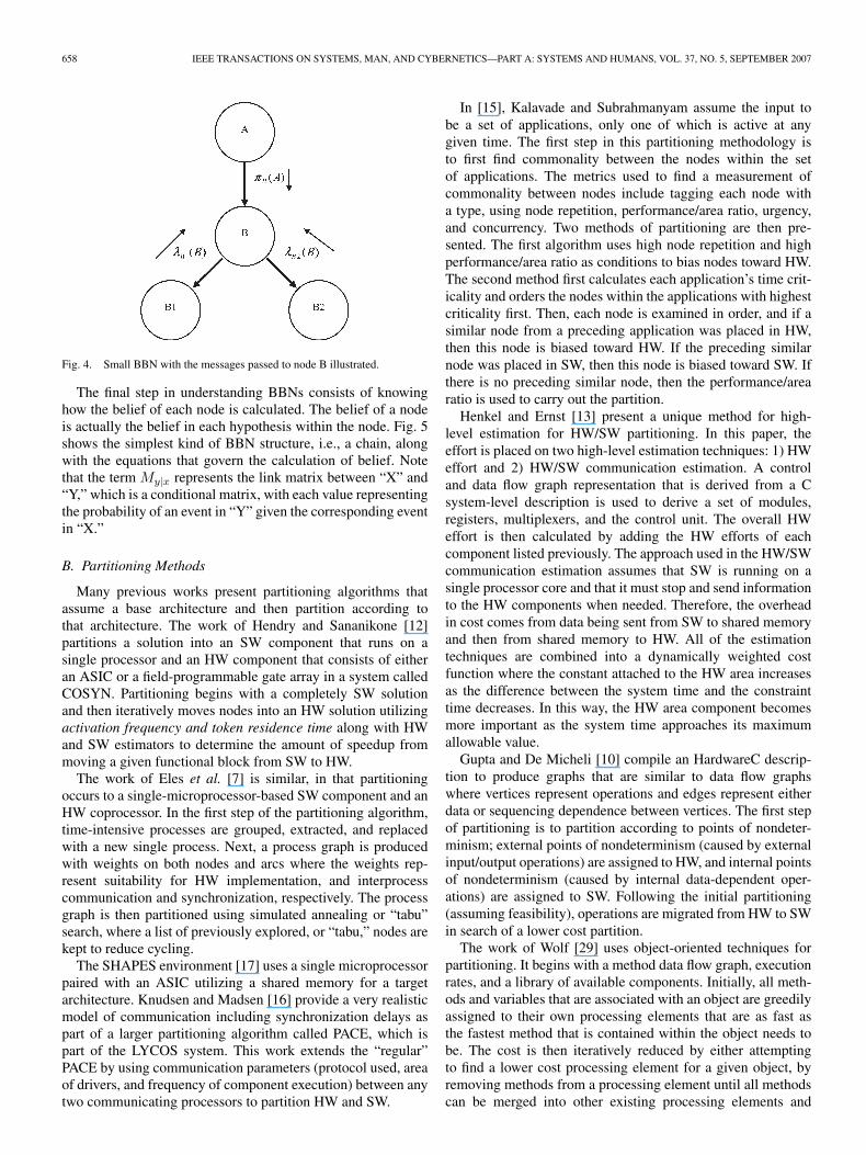
Fig. 4. Small BBN with the messages passed to node B illustrated.

The final step in understanding BBNs consists of knowinghow the belief of each node is calculated. The belief of a nodeis actually the belief in each hypothesis within the node. Fig. 5shows the simplest kind of BBN structure, i.e., a chain, alongwith the equations that govern the calculation of belief. Notethat the term My|x represents the link matrix between “X” and“Y,” which is a conditional matrix, with each value representingthe probability of an event in “Y” given the corresponding eventin “X.”

B. Partitioning Methods

Many previous works present partitioning algorithms thatassume a base architecture and then partition according tothat architecture. The work of Hendry and Sananikone [12]partitions a solution into an SW component that runs on asingle processor and an HW component that consists of eitheran ASIC or a field-programmable gate array in a system calledCOSYN. Partitioning begins with a completely SW solutionand then iteratively moves nodes into an HW solution utilizingactivation frequency and token residence time along with HWand SW estimators to determine the amount of speedup frommoving a given functional block from SW to HW.

The work of Eles et al. [7] is similar, in that partitioningoccurs to a single-microprocessor-based SW component and anHW coprocessor. In the first step of the partitioning algorithm,time-intensive processes are grouped, extracted, and replacedwith a new single process. Next, a process graph is producedwith weights on both nodes and arcs where the weights rep-resent suitability for HW implementation, and interprocesscommunication and synchronization, respectively. The processgraph is then partitioned using simulated annealing or “tabu”search, where a list of previously explored, or “tabu,” nodes arekept to reduce cycling.

The SHAPES environment [17] uses a single microprocessorpaired with an ASIC utilizing a shared memory for a targetarchitecture. Knudsen and Madsen [16] provide a very realisticmodel of communication including synchronization delays aspart of a larger partitioning algorithm called PACE, which ispart of the LYCOS system. This work extends the “regular”PACE by using communication parameters (protocol used, areaof drivers, and frequency of component execution) between anytwo communicating processors to partition HW and SW.

In [15], Kalavade and Subrahmanyam assume the input tobe a set of applications, only one of which is active at anygiven time. The first step in this partitioning methodology isto first find commonality between the nodes within the setof applications. The metrics used to find a measurement ofcommonality between nodes include tagging each node witha type, using node repetition, performance/area ratio, urgency,and concurrency. Two methods of partitioning are then pre-sented. The first algorithm uses high node repetition and highperformance/area ratio as conditions to bias nodes toward HW.The second method first calculates each application’s time crit-icality and orders the nodes within the applications with highestcriticality first. Then, each node is examined in order, and if asimilar node from a preceding application was placed in HW,then this node is biased toward HW. If the preceding similarnode was placed in SW, then this node is biased toward SW. Ifthere is no preceding similar node, then the performance/arearatio is used to carry out the partition.

Henkel and Ernst [13] present a unique method for high-level estimation for HW/SW partitioning. In this paper, theeffort is placed on two high-level estimation techniques: 1) HWeffort and 2) HW/SW communication estimation. A controland data flow graph representation that is derived from a Csystem-level description is used to derive a set of modules,registers, multiplexers, and the control unit. The overall HWeffort is then calculated by adding the HW efforts of eachcomponent listed previously. The approach used in the HW/SWcommunication estimation assumes that SW is running on asingle processor core and that it must stop and send informationto the HW components when needed. Therefore, the overheadin cost comes from data being sent from SW to shared memoryand then from shared memory to HW. All of the estimationtechniques are combined into a dynamically weighted costfunction where the constant attached to the HW area increasesas the difference between the system time and the constrainttime decreases. In this way, the HW area component becomesmore important as the system time approaches its maximumallowable value.

Gupta and De Micheli [10] compile an HardwareC descrip-tion to produce graphs that are similar to data flow graphswhere vertices represent operations and edges represent eitherdata or sequencing dependence between vertices. The first stepof partitioning is to partition according to points of nondeter-minism; external points of nondeterminism (caused by externalinput/output operations) are assigned to HW, and internal pointsof nondeterminism (caused by internal data-dependent oper-ations) are assigned to SW. Following the initial partitioning(assuming feasibility), operations are migrated from HW to SWin search of a lower cost partition.

The work of Wolf [29] uses object-oriented techniques forpartitioning. It begins with a method data flow graph, executionrates, and a library of available components. Initially, all meth-ods and variables that are associated with an object are greedilyassigned to their own processing elements that are as fast asthe fastest method that is contained within the object needs tobe. The cost is then iteratively reduced by either attemptingto find a lower cost processing element for a given object, byremoving methods from a processing element until all methodscan be merged into other existing processing elements and

OLSON et al.: HARDWARE/SOFTWARE PARTITIONING USING BAYESIAN BELIEF NETWORKS 659

Fig. 5. Actual calculations that must be made to determine the belief of X.

thus removing the need for it, or by moving methods to betterbalance the system load. The next step is to find the cheapestcommunication channel for each data path between processingelements. Finally, communication channels are allocated, anddevices are allocated.

Alpert and Kahng [1] provide an excellent review of themajor classes of partitioning algorithms for VLSI circuit de-sign, but these techniques also apply to any system in whichcomponents are grouped and whose intergroup communicationmust be kept to a minimum. Among these classes of partitioningalgorithms are the following: 1) move-based approaches suchas greedy and iterative exchange algorithms; 2) geometricapproaches such as vector partitioning; 3) combinatorial ap-proaches such as max-flow min-cut; and 4) clustering-basedapproaches [1].

V. BBN-BASED PARTITIONING METHODOLOGY

As we have stated in Section I, the HW/SW partitioningmethodology presented here is part of a larger design contextthat is known as model-based codesign [21], [24].

In traditional HW and SW design, decisions regarding par-titioning the HW and SW occur at the beginning of the designprocess. SW and HW components are designed separately andare later integrated. The difficulty with this type of design sce-nario is that there are often compatibility and timing problemsthat are encountered during integration and testing. It has beenshown that, the earlier design problems are found, the lower theoverall cost is to fix them [6].

In model-based codesign, however, the system to be designedis modeled at a high level of abstraction, and partitioning ispushed until as late as possible (as shown in Fig. 6). Becauseof this, there are fewer integration problems, and the waysin which HW and SW interact in the final solution are betterknown. By knowing SW/HW interactions, the design space canbe better optimized in terms of HW area, which in turn helpswith space-constrained embedded systems.

The HW/SW partitioning methodology presented here takesan executable functional model (including design characteris-tics of the functional components) and produces a partitionedmodel, as shown in Fig. 7.

There are four basic steps of the partitioning methodology:1) generation of the BBN; 2) transformation of the results fromsimulation of the current state of the model into evidence;3) propagation of the evidence throughout the BBN (as de-scribed in [20]); and 4) classification of each functional com-ponent into HW or SW, if possible. The decision whether toclassify a functional component into HW or SW can be madebased on the degree of belief for each assignment, as given in

Fig. 6. HW/SW codesign methodology.

the belief probabilities that are associated with each node ofthe BBN.

In the first step of the methodology, i.e., generation of theBBN representation, a functional model is simulated to de-termine values for the complexity, bandwidth, and frequencyof execution for each functional component. The hierarchicalstructure of the functional model is mapped into a “flat” BBNstructure. The values for complexity, bandwidth, and frequencyare combined to construct the probability matrix that is associ-ated with each causal link.

Once the representative BBN has been constructed, evidencethat is output from the simulation of the model is propagatedthroughout the network. Given a specific implementation ofa component (HW or SW), we use simulation to estimatethe performance indexes of interest (e.g., response time andthroughput) of the component. The information collected istransformed into evidence by comparing the estimated perfor-mances. Let us say that the performance of interest is responsetime, and the response time estimated through simulation isRTsw for the SW implementation and RThw for the HW im-plementation; then, the evidence for the given component iscomputed as follows:

λ =[

RThw/(RTsw + RThw)RTsw/(RTsw + RThw)

].

660 IEEE TRANSACTIONS ON SYSTEMS, MAN, AND CYBERNETICS—PART A: SYSTEMS AND HUMANS, VOL. 37, NO. 5, SEPTEMBER 2007

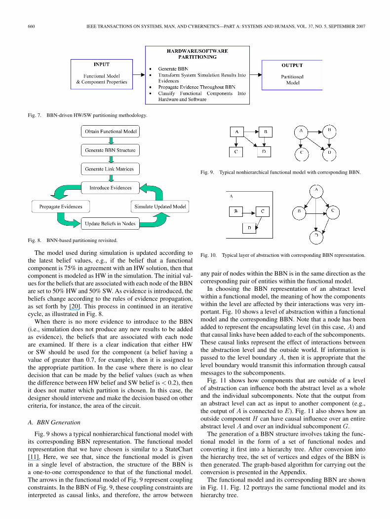
Fig. 7. BBN-driven HW/SW partitioning methodology.

Fig. 8. BNN-based partitioning revisited.

The model used during simulation is updated according tothe latest belief values, e.g., if the belief that a functionalcomponent is 75% in agreement with an HW solution, then thatcomponent is modeled as HW in the simulation. The initial val-ues for the beliefs that are associated with each node of the BBNare set to 50% HW and 50% SW. As evidence is introduced, thebeliefs change according to the rules of evidence propagation,as set forth by [20]. This process in continued in an iterativecycle, as illustrated in Fig. 8.

When there is no more evidence to introduce to the BBN(i.e., simulation does not produce any new results to be addedas evidence), the beliefs that are associated with each nodeare examined. If there is a clear indication that either HWor SW should be used for the component (a belief having avalue of greater than 0.7, for example), then it is assigned tothe appropriate partition. In the case where there is no cleardecision that can be made by the belief values (such as whenthe difference between HW belief and SW belief is < 0.2), thenit does not matter which partition is chosen. In this case, thedesigner should intervene and make the decision based on othercriteria, for instance, the area of the circuit.

A. BBN Generation

Fig. 9 shows a typical nonhierarchical functional model withits corresponding BBN representation. The functional modelrepresentation that we have chosen is similar to a StateChart[11]. Here, we see that, since the functional model is givenin a single level of abstraction, the structure of the BBN isa one-to-one correspondence to that of the functional model.The arrows in the functional model of Fig. 9 represent couplingconstraints. In the BBN of Fig. 9, these coupling constraints areinterpreted as causal links, and therefore, the arrow between

Fig. 9. Typical nonhierarchical functional model with corresponding BBN.

Fig. 10. Typical layer of abstraction with corresponding BBN representation.

any pair of nodes within the BBN is in the same direction as thecorresponding pair of entities within the functional model.

In choosing the BBN representation of an abstract levelwithin a functional model, the meaning of how the componentswithin the level are affected by their interactions was very im-portant. Fig. 10 shows a level of abstraction within a functionalmodel and the corresponding BBN. Note that a node has beenadded to represent the encapsulating level (in this case, A) andthat causal links have been added to each of the subcomponents.These causal links represent the effect of interactions betweenthe abstraction level and the outside world. If information ispassed to the level boundary A, then it is appropriate that thelevel boundary would transmit this information through causalmessages to the subcomponents.

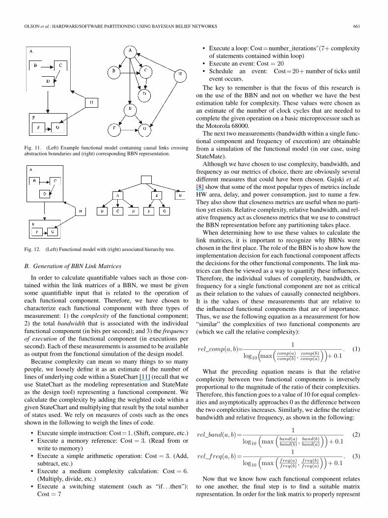
Fig. 11 shows how components that are outside of a levelof abstraction can influence both the abstract level as a wholeand the individual subcomponents. Note that the output froman abstract level can act as input to another component (e.g.,the output of A is connected to E). Fig. 11 also shows how anoutside component H can have causal influence over an entireabstract level A and over an individual subcomponent G.

The generation of a BBN structure involves taking the func-tional model in the form of a set of functional nodes andconverting it first into a hierarchy tree. After conversion intothe hierarchy tree, the set of vertices and edges of the BBN isthen generated. The graph-based algorithm for carrying out theconversion is presented in the Appendix.

The functional model and its corresponding BBN are shownin Fig. 11. Fig. 12 portrays the same functional model and itshierarchy tree.

OLSON et al.: HARDWARE/SOFTWARE PARTITIONING USING BAYESIAN BELIEF NETWORKS 661

Fig. 11. (Left) Example functional model containing causal links crossingabstraction boundaries and (right) corresponding BBN representation.

Fig. 12. (Left) Functional model with (right) associated hierarchy tree.

B. Generation of BBN Link Matrices

In order to calculate quantifiable values such as those con-tained within the link matrices of a BBN, we must be givensome quantifiable input that is related to the operation ofeach functional component. Therefore, we have chosen tocharacterize each functional component with three types ofmeasurement: 1) the complexity of the functional component;2) the total bandwidth that is associated with the individualfunctional component (in bits per second); and 3) the frequencyof execution of the functional component (in executions persecond). Each of these measurements is assumed to be availableas output from the functional simulation of the design model.

Because complexity can mean so many things to so manypeople, we loosely define it as an estimate of the number oflines of underlying code within a StateChart [11] (recall that weuse StateChart as the modeling representation and StateMateas the design tool) representing a functional component. Wecalculate the complexity by adding the weighted code within agiven StateChart and multiplying that result by the total numberof states used. We rely on measures of costs such as the onesshown in the following to weigh the lines of code.

• Execute simple instruction: Cost=1. (Shift, compare, etc.)• Execute a memory reference: Cost = 3. (Read from or

write to memory)• Execute a simple arithmetic operation: Cost = 3. (Add,

subtract, etc.)• Execute a medium complexity calculation: Cost = 6.

(Multiply, divide, etc.)• Execute a switching statement (such as “if. . .then”):

Cost = 7

• Execute a loop: Cost=number_iterations∗(7+ complexityof statements contained within loop)

• Execute an event: Cost = 20• Schedule an event: Cost=20+ number of ticks until

event occurs.The key to remember is that the focus of this research is

on the use of the BBN and not on whether we have the bestestimation table for complexity. These values were chosen asan estimate of the number of clock cycles that are needed tocomplete the given operation on a basic microprocessor such asthe Motorola 68000.

The next two measurements (bandwidth within a single func-tional component and frequency of execution) are obtainablefrom a simulation of the functional model (in our case, usingStateMate).

Although we have chosen to use complexity, bandwidth, andfrequency as our metrics of choice, there are obviously severaldifferent measures that could have been chosen. Gajski et al.[8] show that some of the most popular types of metrics includeHW area, delay, and power consumption, just to name a few.They also show that closeness metrics are useful when no parti-tion yet exists. Relative complexity, relative bandwidth, and rel-ative frequency act as closeness metrics that we use to constructthe BBN representation before any partitioning takes place.

When determining how to use these values to calculate thelink matrices, it is important to recognize why BBNs werechosen in the first place. The role of the BBN is to show how theimplementation decision for each functional component affectsthe decisions for the other functional components. The link ma-trices can then be viewed as a way to quantify these influences.Therefore, the individual values of complexity, bandwidth, orfrequency for a single functional component are not as criticalas their relation to the values of causally connected neighbors.It is the values of these measurements that are relative tothe influenced functional components that are of importance.Thus, we use the following equation as a measurement for how“similar” the complexities of two functional components are(which we call the relative complexity):

rel_comp(a, b)=1

log10

(max

(comp(a)comp(b) ,

comp(b)comp(a)

))+ 0.1

. (1)

What the preceding equation means is that the relativecomplexity between two functional components is inverselyproportional to the magnitude of the ratio of their complexities.Therefore, this function goes to a value of 10 for equal complex-ities and asymptotically approaches 0 as the difference betweenthe two complexities increases. Similarly, we define the relativebandwidth and relative frequency, as shown in the following:

rel_band(a, b)=1

log10

(max

(band(a)band(b) ,

band(b)band(a)

))+ 0.1

(2)

rel_freq(a, b)=1

log10

(max

(freq(a)freq(b) ,

freq(b)freq(a)

))+ 0.1

. (3)

Now that we know how each functional component relatesto one another, the final step is to find a suitable matrixrepresentation. In order for the link matrix to properly represent

662 IEEE TRANSACTIONS ON SYSTEMS, MAN, AND CYBERNETICS—PART A: SYSTEMS AND HUMANS, VOL. 37, NO. 5, SEPTEMBER 2007

Fig. 13. Functional model for programmable thermostat.

beliefs, it must be guaranteed that the summation of eachcolumn in the matrix equals 1. To that purpose, the link matrixis constructed as follows:

Mb|a =α

Nα

[rel_comp(a, b) 1

rel_comp(a,b)1

rel_comp(a,b) rel_comp(a, b)

]

+β

Nβ

[rel_band(a, b) 1

rel_band(a,b)1

rel_band(a,b) rel_band(a, b)

]

+γ

Nγ

[rel_freq(a, b) 1

rel_freq(a,b)1

rel_freq(a,b) rel_freq(a, b)

](4)

where Nα, Nβ , and Nγ are normalization factors, while the co-efficients α, β, and γ provide system designers the chance toexpress that one or more of the three measurements are morecritical than the other(s). The normalization factors aregiven by

Nα = (α+ β + γ)·(rel_comp(a, b) +

1rel_comp(a, b)

)

Nβ = (α+ β + γ)·(rel_band(a, b) +

1rel_band(a, b)

)

Nγ = (α+ β + γ)·(rel_freq(a, b)+

1rel_freq(a, b)

). (5)

VI. PARTITIONING EXAMPLE

In this section, we present a programmable thermostat designexample. Fig. 13 shows the functional model used in thisexample. Fig. 14 gives a block representation of the functionalmodel that will make the generation of the structural portion ofthe BBN easier to follow.

Fig. 15(a) shows the two levels of abstraction of the func-tional model that include five components: one that contains nosubcomponents (L) and four components that act as abstractionmodules. All links between the five top-level components areshown in Fig. 15(b), and since this is the iteration of thealgorithm corresponding to the first level of abstraction, thereare no links between different levels of abstraction.

Fig. 14. Block representation of the functional model.

Fig. 15. Hierarchical elements from (a) functional model and (b) correspond-ing hierarchy tree.

The second iteration of the BBN structural generation algo-rithm brings about many new nodes corresponding to the sub-components of “A,” “D,” “F,” and “I.” Fig. 16 shows the systemmodel at the first two levels of abstraction and the matching

OLSON et al.: HARDWARE/SOFTWARE PARTITIONING USING BAYESIAN BELIEF NETWORKS 663

Fig. 16. After the second iteration of the algorithm, both levels of the (left) functional model with the (right) corresponding BBN.

Fig. 17. Reduced functional model for programmable thermostat.

BBN. Note that links have been added for both the internodeconnections between nodes of the same abstraction level andthe links from the abstract parent nodes to the subordinate nodesrepresenting their subcomponents. Since this functional modelonly contains two levels of abstraction, the algorithm stops atthis point.

For the generation of the link matrices and the introductionof evidences, we have chosen to use a reduced functional modelshown in Fig. 17. This will allow the reader to better understandthe effects of evidence propagation.

The final result of the BBN structural generation algorithmfor the reduced node model is shown in Fig. 18.

In order to find the complexity, bandwidth, and frequencymeasures of each functional component, a StateMate designrepresentation was created and simulated. To demonstratehow the measures were calculated, consider the Control-Temperature functional component. First, we calculate thecomplexity. We have taken the embedded code in the Control-Temperature StateChart and placed the associated complexityvalues for each line next to the line in Fig. 19 (this codeis generated by StateMate). From adding the numbers inFig. 19 and multiplying by the number of states (four statesin the StateChart representation), we obtain a complexity valueof 6368.

To calculate the bandwidth of Control-Temperature, we takeall data and control lines coming into and exiting the StateChart,multiply each by the size of the data in bits, and multiply each

Fig. 18. BBN representation of reduced functional model.

by the number of times that data pass through the particular dataor control line per second to obtain a value with units of bits persecond. When making these calculations, we assume that allintegers are 32 bits long and that events are coded as integers.One important note to make is that since Control-Temperatureexecutes about once every second, and since it drives theexecution of all of the other components, all of the control linesare used once per second. In our design models, there are eightcontrol lines connected to Control-Temperature, each with anevent occurring about once a second for a total of 256 bits/s.The total bandwidth associated with Control-Temperature is768 bits/s, as calculated from the StateMate model.

To determine the frequency of execution, we find the fastestexecuting portion of the StateChart associated with the func-tional model. For Control-Temperature, this corresponds tothe time that it takes to take in and transmit a program, i.e.,fives times a second. All of the values just calculated aregiven in Fig. 20, along with the values for the other functionalcomponents.

For this example, we have chosen the following weights:α = 3, β = 1, and γ = 3 (these are the designer’s preferences).We obtain the set of link matrices shown in Fig. 21.

In the formulation of these matrices, the emphasis (designer’spreference) was placed on complexity and frequency. This canbe seen particularly well in the link matrix on the link from“Control-Temperature” to “Get-Current-Temp,” where theprobability that “Get-Current-Temp” should be implemented inthe same way as “Control-Temperature” is only 34%.

To continue, we now have a BBN that has been created forthe thermostat design example. We use a BBN calculation toolto perform the propagation of evidence and update of beliefs

664 IEEE TRANSACTIONS ON SYSTEMS, MAN, AND CYBERNETICS—PART A: SYSTEMS AND HUMANS, VOL. 37, NO. 5, SEPTEMBER 2007

Fig. 19. Embedded code for Control-Temp StateChart with associated complexity values.

Fig. 20. Table of complexity, bandwidth, and frequency of execution forfunctional components in programmable thermostat example.

called Hugin Lite, which is a shareware version of the HuginSystem by Hugin Expert A/S. Initially, all beliefs are equal, butlet us say that we introduce evidence to “Get-Current-Temp”that it is 83% likely that it should be implemented in HW.Fig. 22 illustrates how this evidence affects the entire BBN.

Because of the vast differences in the link matrix values be-tween the “Get-Current-Temp” and “Control-Temp” functionalcomponents, the introduction of this evidence actually drives“Control-Temp” toward an SW implementation. Next, we in-troduce evidence that “Program-Interaction” has a 65% chance

that it should be implemented in SW, and the result is shownin Fig. 23.

Here, we see that, although “Program-Interaction” has beendriven toward an SW implementation, “Time-Keeping” hasbeen driven slightly toward HW. This difference can be directlyattributed to the discrepancies between the two functional com-ponents, as illustrated in Fig. 21, where the link matrix showsthat any influence from “Program-Interaction” drives “Time-Keeping” in the opposite direction by a 0.52/0.48 ratio.

The process of propagating evidences throughout the BBNcontinues until no new data can be introduced. At this point, adecision is made as to whether each function should be imple-mented in HW or SW. This decision is based on the amount ofbelief that is associated with each type of implementation (i.e.,if the belief is greater than some threshold, e.g., 75%, then thattype of implementation will be chosen). The classification of afunction into HW or SW is reflected in the system model, andthe process continues until all functions can be classified intoeither HW or SW.

VII. SUMMARY

In this paper, we have introduced a new methodology for HWand SW partitioning. We have shown how BBNs can be used to

OLSON et al.: HARDWARE/SOFTWARE PARTITIONING USING BAYESIAN BELIEF NETWORKS 665

Fig. 21. BBN for programmable thermostat after the generation of the link matrices.

Fig. 22. Beliefs associated with each functional component after the introduc-tion of the first piece of evidence.

propagate evidence regarding the classification of functions intoHW or SW realizations. This propagation permits the effectsof a classification decision that is made about one functionto be felt throughout the entire network. In addition, becauseBBNs have a belief of hypotheses as their core, we know howwell a given classification fits into either HW or SW. Knowingthat a function with, for instance, 75% HW belief should beimplemented 75% of the time in HW allows the user to have ameasure of the appropriateness of their solution.

This paper also introduced a methodology for the generationof both the qualitative and quantitative portions of a BBNin the HW/SW partitioning domain. The generation of thestructure of the BBN exploits the ability to use abstract complexmodels in the representation of the functional components. Thegeneration of the associated link matrices uses quantifiableaspects of the individual functional components to determinerelative properties between components that are connected bycausal links.

The limitations of our work are given as follows: 1) theaccuracy and convergence of the method are bounded by theprecision and execution time of the simulations that are run todetermine the relative properties of the various components, and

Fig. 23. Beliefs for the functional components after the introduction of asecond piece of evidence.

thus, the fidelity of partitioning decisions is dependent on thevalidity of the simulation models; 2) the generation of the BBNrepresentation may not be trivial to manage by design engineerswho are not familiar with the tenets of belief networks; and3) other metrics for link matrix generation should be explored.

Future work should include testing other metrics and com-binations of other metrics for the link matrix generation. Wewould also like the ability to incorporate the BBN partitioningmethodology into an integrated computer-aided design systemfor HW/SW codesign.

APPENDIX

This appendix illustrates the algorithm for generating theBBN. The following definitions will be of use in the presen-tation of the algorithm that follows:(BBN) a directed acyclic graph G consisting of a set of vertices

V [G] and a set of edges E[G], where E[G] is defined asE[G] ⊆ V [G]× V [G];

(Functional model) a hierarchical system representation con-sisting of an array FM of functional nodes, where each

666 IEEE TRANSACTIONS ON SYSTEMS, MAN, AND CYBERNETICS—PART A: SYSTEMS AND HUMANS, VOL. 37, NO. 5, SEPTEMBER 2007

member can be accessed by an integer between 1 and thenumber of elements in the array;

(Functional node) a node within a functional model consistingof the following elements:

— name: a string that must be unique with respect to allother nodes in the same functional model.

— level: an integer that represents the level of abstrac-tion at which the current functional node sits. Thisnumber ranges from 1 to n, where n is the total num-ber of layers of abstraction in the functional model,and the highest level of abstraction has a level of 1.

— children: an array of names, where each entry rep-resents a functional node that is influenced by thegiven functional node identified by name, where eachmember can be accessed by an integer between 1 andnum_children. The children of a functional node canbe only the children on the same or higher level ofabstraction.

— num_children: an integer giving the number of entriesin the children array.

— abs_children: an array of names of the functionalnodes that are contained in the abstraction level be-low the current functional node, where each mem-ber can be accessed by an integer between 1 andnum_abs_children.

— num_abs_children: an integer giving the number ofentries in the abs_children array.

(Hierarchy tree) a general tree T consisting of a set of verticesV [T ] and a set of edges E[T ], where E[T ] is defined asE[T ] ⊆ V [T ]× V [T ]. The root vertex represents level 0,with the name equal to the string (“root”), and is onlymeant as an anchor for the functional nodes of the func-tional model.

The algorithm that is responsible for generating the set ofvertices V and the set of directed edges E for the BBN graphG is shown here.

BBN-GENERATE(FM)V[G]← ∅; //The set of vertices for the BBN is

initialized to empty

E[G]← ∅; //The set of directed edges for the BBN

is initialized to empty

V[T]← ∅; //The set of vertices for the hierarchy

tree is initialized

// to emptyE[T]← ∅; //The set of directed edges for the

hierarchy tree is

// initialized to empty// Find the deepest level of abstractiondeepest_level← 0;for i← 1 to length[FM] do

if (FM[i].level > deepest_level) thendeepest_level← FM[i].level;

// Create the root vertex and add it to hierarchytree T

V[T]← V[T] ∪ CREATE− VERTEX(root);// For each functional node of level 1 add a vertex vand a directed

// edge e = (v, root) between vertex and the root of

the hierarchy tree T

for i← 1 to length[FM] do

if (FM[i].level == 1) then

begin

v← FM[i].name;V[T]← V[T] ∪ CREATE− VERTEX(v);E[T]← E[T] ∪ CREATE− EDGE(root, v);

end if;// Traverse the functional model FM, level by level,until all children

// of all nodes have been added to V[T] and theassociated edges to E[T].

i← 1;while (i < deepest_level) // Try all levels but

deepest

begin

for j← 1 to length[FM; //step through FM

if (fm[j].level == i) then

begin

u← fm[j].name;for k← 1 to fm[j].num_abs_children dobegin

v← fm[j].abs_children[k];V[T]← V[T] ∪ CREATE− VERTEX(v);E[T]← E[T] ∪ CREATE− EDGE(u, v);

end for;end if;

i← i + 1;end while;// At this point the hierarchy tree has beenconstructed.// Copy the vertices and edges for the hierarchytree to the set of

// vertices and edges for the BBNV[G]← V[T];E[G]← E[T];// Remove the root node and the associated edgesfrom the BBN graph

V[G]← V[G]− root;for i← 1 to length(FM) do

if (FM[x].level == 1) then

v← FM[i].name;E← E− (root, v);

// Now, the edges not associated with hierarchy areadded by

// stepping through the functional model, until allinfluence related

// edges have been addedfor i← 1 to length(FM) do

begin//Step through FM

u← fm[i].name;for j← 1 to fm[i].num_children dobegin//Step through children

v← fm[i].children[j];E[G]← E[G] ∪ CREATE− EDGE(u, v); //Add edge

end for;end for;return (V[G], E[G]);

OLSON et al.: HARDWARE/SOFTWARE PARTITIONING USING BAYESIAN BELIEF NETWORKS 667

REFERENCES

[1] C. J. Alpert and A. B. Kahng, “Recent directions in netlist partitioning:A survey,” Integr. VLSI J., vol. 19, no. 1/2, pp. 1–81, Aug. 1995.

[2] V. Catania, M. Malgeri, and M. Russo, “Applying fuzzy logic to codesignpartitioning,” IEEE Micro, vol. 17, no. 3, pp. 62–70, May/Jun. 1997.

[3] E. Charniak, “Bayesian networks without tears,” AI Mag., vol. 12, no. 4,pp. 50–63, Winter 1991.

[4] M. Chiodo, P. Giusto, A. Jurecska, H. C. Hsieh, A. Sangiovanni-Vincentelli, and L. Lavagno, “Hardware-software codesign of embeddedsystems,” IEEE Micro, vol. 14, no. 4, pp. 26–36, Aug. 1994.

[5] S. J. Cunning, T. C. Ewing, J. T. Olson, J. W. Rozenblit, and S. Schulz,“Towards an integrated, model-based codesign environment,” in Proc.IEEE Conf. and Workshop ECBS, 1999, pp. 136–143.

[6] G. De Micheli and R. K. Gupta, “Hardware/software co-design,” Proc.IEEE, vol. 85, no. 3, pp. 349–365, Mar. 1997.

[7] P. Eles, Z. Peng, K. Kuchcinski, and A. Doboli, “Hardware/softwarepartitioning with iterative improvement heuristics,” in Proc. 9th Int. Symp.Syst. Synthesis, 1996, pp. 71–76.

[8] D. Gajski, S. Narayan, F. Vahid, and J. Gong, Specification and Design ofEmbedded Systems. Englewood Cliffs, NJ: Prentice-Hall, 1994.

[9] J. Grode, P. V. Knudsen, and J. Madsen, “Hardware resource allocationfor hardware/software partitioning in the LYCOS system,” in Proc. DATE,1998, pp. 22–27.

[10] R. K. Gupta and G. De Micheli, “System-level synthesis using re-programmable components,” in Proc. Eur. Conf. Des. Autom., 1992,pp. 2–7.

[11] D. Harel, “STATEMATE: A working environment for the developmentof complex reactive systems,” IEEE Trans. Softw. Eng., vol. 16, no. 4,pp. 403–414, Apr. 1990.

[12] D. C. Hendry and D. S. Sananikone, “Hardware/software partitioning ofembedded systems with multiple hardware processes,” Proc. Inst. Electr.Eng.—Computers Digital Techniques, vol. 144, no. 5, pp. 285–294,Sep. 1997.

[13] J. Henkel and R. Ernst, “High-level estimation techniques for usage inhardware/software co-design,” in Proc. ASP-DAC, 1998, pp. 353–360.

[14] F. V. Jensen, An Introduction to Bayesian Networks. London, U.K.: UCLPress, 1998.

[15] A. Kalavade and P. A. Subrahmanyam, “Hardware/software partitioningfor multifunction systems,” IEEE Trans. Comput.-Aided Design Integr.Circuits Syst., vol. 17, no. 9, pp. 819–837, Sep. 1998.

[16] P. V. Knudsen and J. Madsen, “Integrating communication protocol selec-tion with partitioning in hardware/software codesign,” in Proc. 11th Int.Symp. Syst. Synthesis, 1998, pp. 111–116.

[17] M. L. Lopez, C. A. Iglesias, and J. C. Lopez, “A knowledge-based systemfor hardware-software partitioning,” in Proc. DATE, 1998, pp. 914–915.

[18] M. P. Barros and W. Rosenstiel, “A Petri net based approach for perform-ing the initial allocation in hardware/software codesign,” in Proc. IEEEInt. Conf. Syst., Man, Cybern., Oct. 1998, vol. 1, pp. 505–510.

[19] J. T. Olson and J. W. Rozenblit, “Framework for hardware/software parti-tioning utilizing Bayesian belief networks,” in Proc. IEEE Int. Conf. Syst.,Man, Cybern., Oct. 1998, vol. 4, pp. 3983–3988.

[20] J. Pearl, Probabilistic Reasoning in Intelligent Systems: Networks ofPlausible Inference. San Mateo, CA: Morgan Kaufmann, 1988.

[21] J. W. Rozenblit and K. Buchenrieder, Eds., Codesign: Computer-AidedSoftware/Hardware Engineering. Piscataway, NJ: IEEE Press, 1994.

[22] J. S. Russell and P. Norvig, Artificial Intelligence: A Modern Approach.Upper Saddle River, NJ: Prentice-Hall, 1995.

[23] D. Saha, R. S. Mitra, and A. Basu, “Hardware software partitioning usinggenetic algorithm,” in Proc. 10th Int. Conf. VLSI Des., 1997, pp. 155–160.

[24] S. Schulz, J. W. Rozenblit, M. Mrva, and K. Buchenrieder, “Model-basedcodesign: The framework and its application,” Computer, vol. 3, no. 8,pp. 60–67, Aug. 1998.

[25] V. Srinivasan, S. Radhakrishnan, and R. Vemuri, “Hardware softwarepartitioning with integrated hardware design space exploration,” in Proc.DATE, 1998, pp. 28–35.

[26] D. E. Thomas, J. K. Adams, and H. Schmit, “A model and methodologyfor hardware-software codesign,” IEEE Des. Test Comput., vol. 10, no. 3,pp. 6–15, Sep. 1993.

[27] F. Vahid, “Modifying min-cut for hardware and software functional parti-tioning,” in Proc. 5th Int. Workshop CODES/CASHE, 1997, pp. 43–48.

[28] L. C. Van der Gaag, “Bayesian belief networks: Odds and ends,” Comput.J., vol. 39, no. 2, pp. 97–113, 1996.

[29] W. Wolf, “Object-oriented cosynthesis of distributed embedded systems,”ACM Trans. Des. Autom. Electron. Syst., vol. 1, no. 3, pp. 301–331,Jul. 1996.

[30] G. Stitt, R. Lysecky, and F. Vahid, “Dynamic hardware/software partition-ing: A first approach,” in Proc. IEEE DAC, 2003, pp. 250–255.

[31] G. N. Khan and M. Jin, “A new graph structure for hardware-softwarepartitioning of heterogeneous systems,” in Proc. IEEE Can. Conf. Electr.and Comput. Eng., 2004, pp. 229–232.

[32] R. Lysecky and F. Vahid, “A configurable logic architecture for dynamichardware/software partitioning,” in Proc. DATE, 2004, pp. 480–485.

[33] P. Waldeck and N. Bergmann, “Dynamic hardware-software partitioningon reconfigurable system-on-chip,” in Proc. IEEE Syst.-on-Chip RealTime Appl., 2003, pp. 102–105.

[34] P. Arato, S. Juhasz, Z. A. Mann, A. Orban, and D. Papp, “Hardware–Software partitioning in embedded system design,” in Proc. IEEE Symp.Intell. Signal Process., 2003, pp. 197–202.

[35] F. C. Filho, P. Maciel, and E. Barros, “A Petri net approach for hardware/software partitioning,” in Proc. Symp. Integr. Circuits and Syst. Des.,2001, pp. 72–77.

John T. Olson received the Ph.D. degree in electricaland computer engineering from the University ofArizona, Tucson, in 2000.

Since then, he has been with IBM Inc., Armonk,NY. He is currently the Lead Software Engineer forIBM’s Centralized Virtual Tape Products. He hasfiled several patents in the areas of automated errorrecovery, configurable error generation, and errornotification in computer systems.

Jerzy W. Rozenblit received the Ph.D. and M.S.degrees in computer science from Wayne State Uni-versity, Detroit, MI, and the M.Sc. degree in com-puter engineering from the Technical University ofWroclaw, Wroclaw, Poland.

He is currently a Professor and the Head of theDepartment of Electrical and Computer Engineering,University of Arizona, Tucson. He was a FulbrightSenior Scholar and a Visiting Professor at the Insti-tute of Systems Science, Johannes Kepler University,Linz, Austria, and a Fulbright Senior Specialist at

the Cracow University of Technology, Cracow, Poland. He has held visitingprofessorship appointments at the Technical University of Munich, Munich,Germany; Central Research Laboratories of Siemens AG; and Infineon Tech-nologies AG, Munich. Among many sponsors, his research in design hasbeen supported by the National Science Foundation, the U.S. Army, SiemensAG, and NASA. His research and teaching interests include complex systemsdesign and simulation modeling. He serves as an Associate Editor of the ACMTransactions on Modeling and Computer Simulation, an Area Editor of theTransactions of the Society of Modeling and Simulation International, and anExecutive Board Member of the IEEE Technical Committee on Engineering ofComputer-Based Systems.

668 IEEE TRANSACTIONS ON SYSTEMS, MAN, AND CYBERNETICS—PART A: SYSTEMS AND HUMANS, VOL. 37, NO. 5, SEPTEMBER 2007

Claudio Talarico received the M.S. degree fromUniversitá degli Studi di Genova, Genova, Italy, andthe Ph.D. degree from the University of Hawaii atManoa, Honolulu, both in electrical engineering.

He is currently an Assistant Professor of electri-cal engineering in the Department of Electrical En-gineering, Eastern Washington University, Cheney.Before joining Eastern Washington University, heheld various management and technical positions inthe area of digital integrated systems design at In-fineon Technologies, Sophia Antipolis, France; Ikos

Systems, Cupertino, CA (now part of Mentor Graphics); and Marconi Telecom-munication, Genova. His research interests include design methodologies forintegrated circuits and systems with emphasis on system-level design; em-bedded computing systems; hardware–software codesign; low-power design;system specification languages; and early design assessment, analysis, andrefinement of complex systems on chips.

Witold Jacak received the M.S.E. degree in elec-tronics and the Ph.D. degree in control and sys-tem engineering from the Technical University ofWroclaw, Wroclaw, Poland, in 1973 and 1978, re-spectively, and the Habilitation degree in intelligentmultiagent systems from the Technical University ofWarsaw, Warsaw, Poland, in 1992.

He was with the Institute of Technical Cybernet-ics, Technical University of Wroclaw, as a ProfessorAssistant from 1977 to 1989 and as a Professor from1989 to 1995. From 1991 to 1998, he was a Guest

Professor at the University of Linz, Linz, Austria. Since 1994, he has beenthe Head of the Information Technology Faculty, Department of SoftwareEngineering, Upper Austria University of Applied Science, Hagenberg. Hisresearch interests include artificial and computational and distributed intelli-gence, multiagent autonomous systems, cognitive modeling and simulation,and knowledge engineering.

Dr. Jacak is a member of editorial boards and a Council Member of severalnational and international committees.