Optimization of Heat Spreader

A thesis presented to

the faculty of

the Russ College of Engineering and Technology of Ohio University

In partial fulfillment

of the requirements for the degree

Master of Science

Rahat M. Taposh

June 2012

© 2012 Rahat M. Taposh. All Rights Reserved.

2

This thesis titled

Optimization of Heat Spreader

by

RAHAT M. TAPOSH

has been approved for

the Department of Mechanical Engineering

and the Russ College of Engineering and Technology by

Khairul Alam

Moss Professor of Mechanical Engineering

Dennis Irwin

Dean, Russ College of Engineering and Technology

3

ABSTRACT

TAPOSH, RAHAT M., M.S., June 2012, Mechanical Engineering

Optimization of Heat Spreader

Director of Thesis: Khairul Alam

One of the important components of a heat sink is the heat spreader which

improves the heat dissipation from the chip into the environment. The improvement due

to the spreading of the heat flux over a wider area is partially counteracted by the

spreading resistance, i.e., resistance due to the longer path taken by the heat flux. Several

studies have been carried out to determine the spreading resistance; which includes

cylindrical as well as cartesian co-ordinate system.

The heat spreader tends to be the most significant mass in the heat sink. Therefore

selection of the heat spreader dimension deserves serious consideration; this is

particularly true in high heat flux situations. The focus of this is to examine the optimum

dimension of heat spreader as a function of the thermal and geometric parameters of the

heat sink problem.

Approved: _____________________________________________________________

Khairul Alam

Moss Professor of Mechanical Engineering

4

ACKNOWLEDGMENTS

I would like to express my deepest gratitude to my academic advisor, Professor

Khairul Alam for his continuous flow of support and outstanding guidance during my

Master of Science in Mechanical Engineering program. I am very grateful to him for

giving me the opportunity to work on such a cutting edge research.

I would like to thank Dr. Xiaoping Shen, Dr. Hajrudin Pasic, and Dr. Daniel

Gulino for valuable guidance and critical comment being my thesis committee members.

I am extremely grateful to my family members for their lifelong support and

encouragement in pursuing my higher education. I am especially thankful to my mother

and aunt for supporting and helping me during various stages of my life.

5

TABLE OF CONTENTS

Page

Abstract ........................................................................................................................... 3

Acknowledgments ........................................................................................................... 4

List of Tables................................................................................................................... 6

List of Figures ................................................................................................................. 7

Nomenclature ................................................................................................................ 11

Chapter 1: Introduction .................................................................................................. 13

Chapter 2: Background .................................................................................................. 18

Chapter 3: Modeling and Analysis ................................................................................. 34

Chapter 4: Heat Spreader for High Heat Flux System .................................................... 56

Chapter 5: Conclusions and Summary ........................................................................... 67

References ..................................................................................................................... 70

6

LIST OF TABLES

Page Table 1 Comparative Results and Validation……………………………………55 Table 2 Optimum Thickness and Total Resistance of Heat Spreader……….......64

7

LIST OF FIGURES

Page Figure 2.1 Different configurations of extended surface (a) pin fin (Source:

“Heat Sink” n.d.) (b) straight fin (Source: “Heat Sink” n.d.) (c) flared fin (Source: “Heat Sink” n.d.) (d) metal foam between heat spreaders (Source: “Open Cell-Foam” n.d.). .......................................... 18

Figure 2.2 Contribution of different resistances, when heat flows from source

to environment through a heat sink ........................................................ 22 Figure 2.3 Variations of total resistance as a function of the spreader thickness

in non dimensional form; and the ratio of the source length to the length of the heat spreader (ℓ/ ) for ℎ/ =10 ......................................... 23

Figure 2.4 Variations of total resistance as a function of the spreader thickness

in non dimensional form; and the ratio of the source length to the length of the heat spreader (ℓ/ ) for ℎ/ =20 ......................................... 27

Figure 2.5 Schematic diagram of thermal system having square heat source of

length 2ℓ, square heat spreader of length 2L, thickness t and a heat flux q applied on the top of heat spreader (Source: Feng & Xu, 2004) ................................................................................................... 30

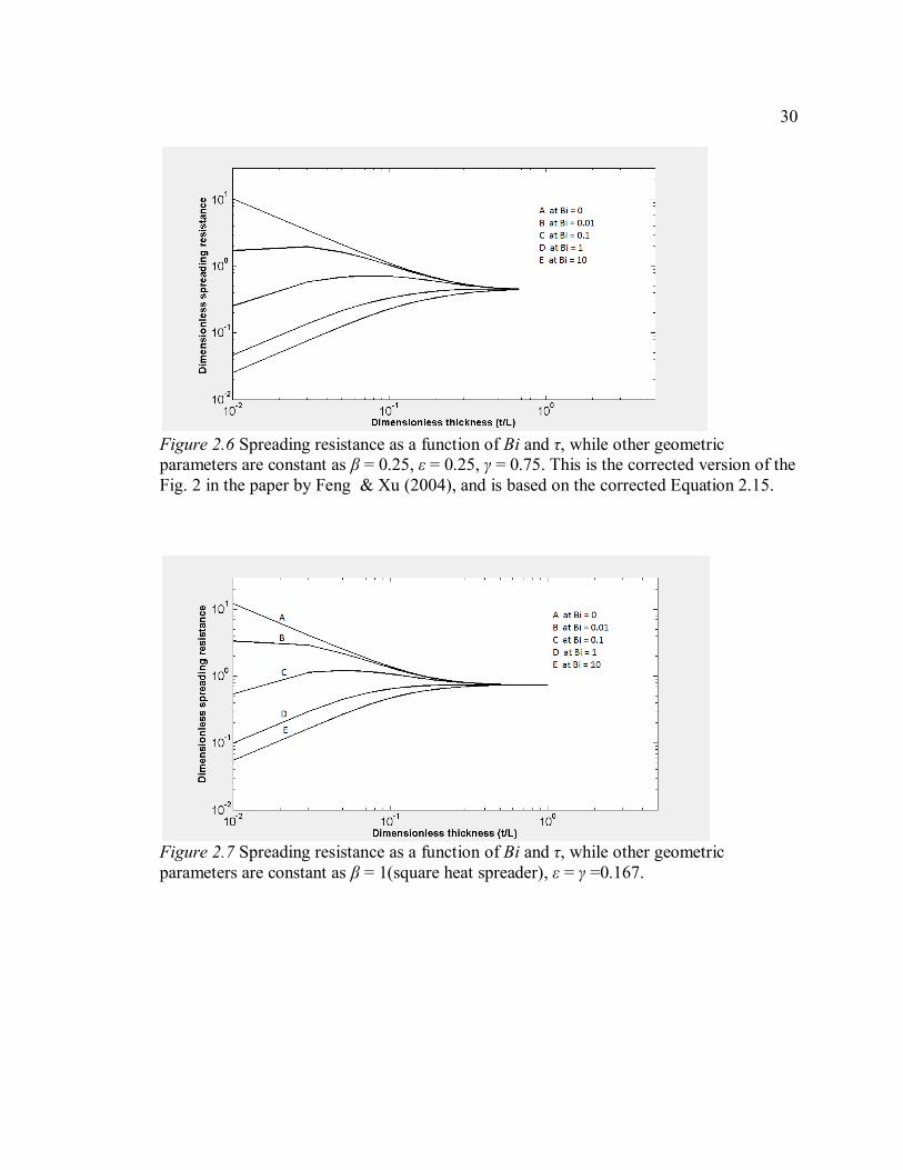
Figure 2.6 Spreading resistance as a function of Bi and τ, while other

geometric parameters are constant as β = 0.25, ε = 0.25, γ = 0.75. This is the corrected version of the Fig. 2 in the paper by Feng & Xu (2004), and is based on the corrected Equation 2.15 ........................ 30

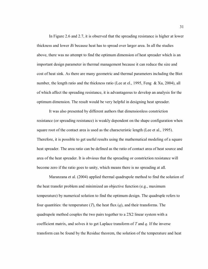
Figure 2.7 Spreading resistance as a function of Bi and τ, while other

geometric parameters are constant as β = 1(square heat spreader), ε = γ =0.167 ............................................................................................. 30

Figure 3.1 Minimum total resistance with respect to ℎ and at higher

values of the parameters ........................................................................ 38 Figure 3.2 Minimum total resistance with respect to ℎ and length ratio,

at lower values of the parameters .......................................................... 39 Figure 3.3 Contours of minimum total resistance (K/W) at of

ℎ and .......................................................................................... 40

8 Figure 3.4 Contours of minimum total resistance (K/W) at of

ℎ ....................................................................................................... 40 Figure 3.5 Contribution of conductive resistance, at minimum .................... 41 Figure 3.6 Contour plot for conductive resistance (K/W), with respect to

ℎ and at minimum total resistance, ....................................... 42 Figure 3.7 Contour plot for convective resistance (K/W), with respect to

ℎ and at minimum total resistance, ....................................... 43 Figure 3.8(a) Contour plot for spreading resistance, with respect to low ℎ

and at minimum total resistance, .............................................. 45 Figure 3.8(b) Contour plot for spreading resistance (K/W), with respect to ℎ

and at minimum total resistance, ............................................... 45 Figure 3.9 Contour plot for spreading resistance (K/W), at higher values of

ℎ ....................................................................................................... 46 Figure 3.10 Different foams offering the effective heat transfer coefficient

against power generated by the heater. Effective heat transfer coefficient provided by graphite foam found to be highest to date. (Source: “S-Bond Technologies” n.d.) .................................................. 47

Figure 3.11 Dimensionless optimum thickness, with respect to ℎ and

at minimum total resistance, , where each side (2 ) of square source is 20 mm long .................................................................... 48

Figure 3.12 Contour plot for dimensionless optimum thickness, with

respect to ℎ and at minimum total resistance, ....................... 49 Figure 3.13 Contour plot for dimensionless optimum thickness, at low ℎ

and , where each side ( ) of square heat source is 20 mm long ...... 50 Figure 3.14 Contour plot for dimensionless parameter, ℎ at low ℎ and

, where each side ( ) of square heat source is 20 mm long............. 52 Figure 3.15 Contour plot for dimensionless parameter, ℎ with respect to

ℎ and , where each side ( ) of square heat source is 30 mm long ...................................................................................................... 52

9 Figure 3.16 Contour plot for dimensionless parameter, ℎ with respect to ℎ

and , where each side ( ) of square heat source is 20 mm long (Source: Maranzana et al.,2004). ........................................................... 53

Figure 4.1 Total resistance of a heat spreader of different thermal

conductivities as a function of its thickness when convective heat transfer coefficient = 250 W/m2K and heat source is 5x5 mm2 .............. 57

Figure 4.2 Total resistance of a heat spreader of different thermal

conductivities as a function of its thickness when convective heat transfer coefficient = 5,000 W/m2K and heat source is 5x5 mm2 ........... 58

Figure 4.3 Total resistance of a heat spreader of different thermal

conductivities as a function of its thickness when convective heat transfer coefficient = 10,000 W/m2K and heat source is 5x5 mm2 ......... 59

Figure 4.4 Total resistance of a heat spreader of different thermal conductivities

as a function of its thickness when convective heat transfer coefficient = 20,000 W/m2K and heat source is 5x5 mm2........................................ 59

Figure 4.5 Total resistance of a heat spreader of different thermal conductivities

as a function of its thickness when convective heat transfer coefficient = 30,000 W/m2K and heat source is 5x5 mm2........................................ 60

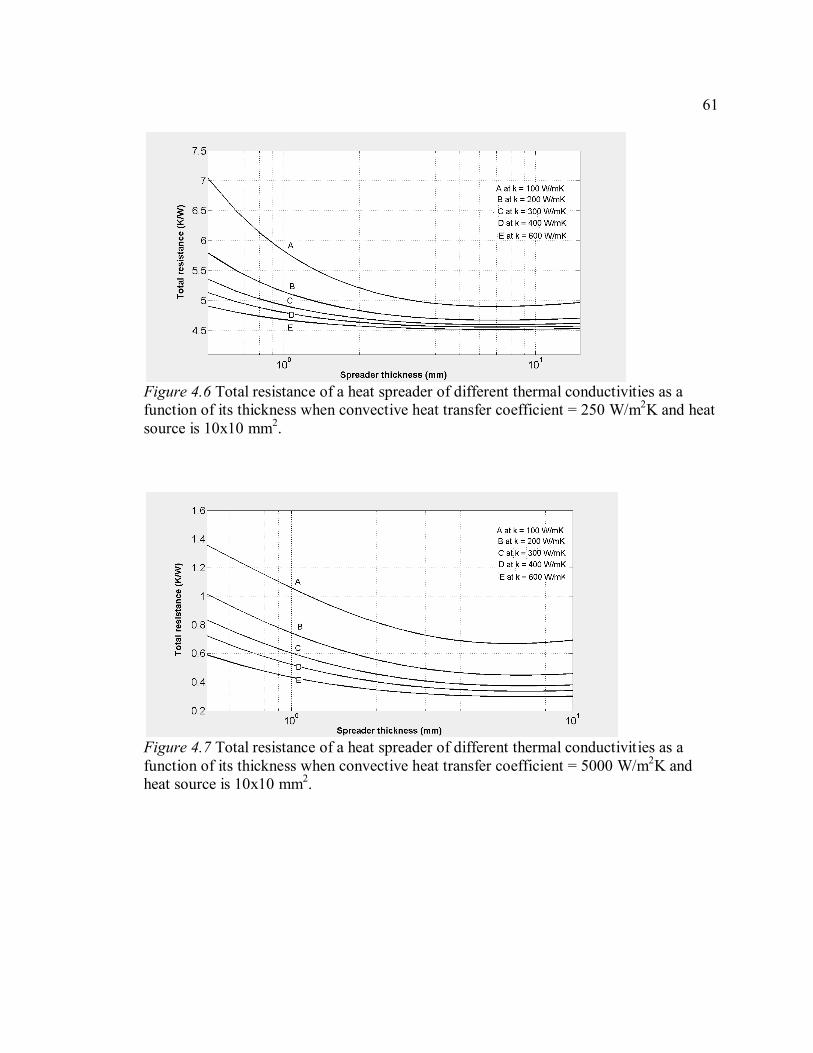
Figure 4.6 Total resistance of a heat spreader of different thermal conductivities

as a function of its thickness when convective heat transfer coefficient = 250 W/m2K and heat source is 10x10 mm2 ........................................ 61

Figure 4.7 Total resistance of a heat spreader of different thermal conductivities

as a function of its thickness when convective heat transfer coefficient = 5000 W/m2K and heat source is 10x10 mm2....................................... 61

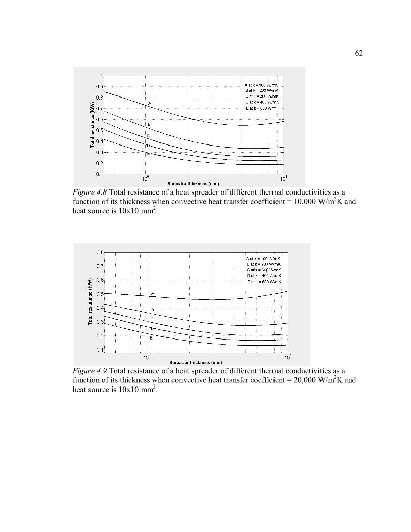
Figure 4.8 Total resistance of a heat spreader of different thermal conductivities

as a function of its thickness when convective heat transfer coefficient = 10,000 W/m2K and heat source is 10x10 mm2 .................................... 62

Figure 4.9 Total resistance of a heat spreader of different thermal conductivities

as a function of its thickness when convective heat transfer coefficient = 20,000 W/m2K and heat source is 10x10 mm2 .................................... 62

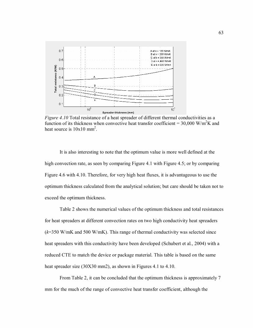
Figure 4.10 Total resistance of a heat spreader of different thermal conductivities

as a function of its thickness when convective heat transfer coefficient = 30,000 W/m2K and heat source is 10x10 mm2 .................................... 63

10 Figure 4.11 Total resistance for 350 W/mK conductivity material plotted as a

function of the heat transfer coefficient ................................................. 65 Figure 4.12 Total resistance for two different conductivities of heat spreader as

a function of the heat transfer coefficient............................................... 66

11

NOMENCLATURE

Ab heat spreader surface area exposed to the convective medium, m2

As heat source area, m2

Amn Fourier coefficients of T*

a heat source radius for for circular heat source, m

Bi Biot number, ℎ

b plate radius for cylindrical heat spreader, m

Cmn Fourier coefficients of Ψs

a length dimension given by equation (2.7), m

h heat transfer coefficient, W / m K

Jn Bessel function of order n

k thermal conductivity, W / m K

L half length of the spreader, m

Q total heat produced by the heat source, W

q heat flux of the heat source, W / m2

Rf convective thermal resistance, K / W

Rm material thermal resistance, K / W

Rs spreading thermal resistance, K / W

Rs,max maximum spreading thermal resistance, K / W

Rt total thermal resistance, K / W

r dimensionless plate thickness for cylindrical heat spreader,

12 T excess temperature relative to environment, K

Tmax maximum excess temperature on heat spreader, K

dimensionless excess temperature, ℎ

t thickness of the heat spreader, m

W width of rectangular heat spreader, m

w width of rectangular heat source, m

dimensionless coordinate in x direction,

dimensionless coordinate in y direction,

dimensionless coordinate in z direction,

Greek and other symbols

ratio of width to length of rectangular heat spreader,

dimensionless contact width,

dimensionless contact length,

eigenvalues used in equation (2.8)

dimensionless contact radius for cylindrical heat spreader, =

dimensionless thickness of the heat spreader,

dimensionless optimum thickness defined by equation (2.25)

a parameter defined by equation (2.9)

Ψs dimensionless spreading thermal resistance defined by equation (2.15)

dimensionless spreading thermal resistance defined by equation (2.14)

Ψs,max dimensionless maximum spreading thermal resistance

half length of the heat source, m

13

CHAPTER 1: INTRODUCTION

Since the inception of integrated electronic circuits, safe and efficient operation

depends on circuit temperature, which should be within an acceptable limit. The limit can

be maintained by dissipation of heat to the environment. The continuous evolution of

electronic technology has the growing tendency of large scale circuit integration into a

single chip, and higher density of chips on a single printed circuit board. As a result,

thermal management of electronic chips has become an important issue in circuit

reliabilities and performance. The International Technology Roadmap for

Semiconductors (ITRS) announced the high performance processor to have maximum

power of 365W in 2006 and predicted it to be 512W by 2011 while the junction

temperature to decrease from 100˚C, present value, to 90˚C by 2011 (ITRS, 2005 as cited

in Guenin, 2006). Bar-Cohen, Wang & Rahim ( 2007) indicated that the heat flux

dissipation will go up to 150 W/cm2 and perhaps 1kW/cm2 in a few years, which

emphasizes the need for designing high heat flux heat sinks for electronic cooling.

Any heat sink consists of two parts; a flat part or heat spreader and some extended

surface providing large surface area to enable high heat flux. Heat spreader, as a part of

heat sink, enables the heat flow from the source to extended surfaces. There are

numerous studies on extended surfaces but very few detailed publications on how heat

spreader can be optimized (Maranzana, Perry, Maillet, & Rael, 2004).

The use of extended surfaces is also limited by the total surface area that can be

accommodated in a given volume. The effective heat transfer coefficient, defined as the

14 heat transfer coefficient based on the base cross sectional area of the heat spreader to

incorporate the total convective heat transfer from the heat sink, is proportional to the

available heat transfer surface area. However, the geometry of typical electronic

enclosures havevery limited volume for extended surfaces. The use of foams as

replacement of extended surface has a potential positive impact in cooling technology.

Conductive foam have been developed with void spaces that are open and interconnected

with each other which gives significant amount of surface area for convection heat

transfer and therefore, has potential for energy transfer and electronic cooling (Straatman

et al., 2007). The foams can be made of aluminum, copper or carbon. For example,

Graphitic foam has very high surface area to volume ratio which can be as high as 5,000-

50,000 m2/m3. It also has very good material conductivity in the range of 800-1900 W/m

K (Straatman et al., 2007). Lee et al. (1993) showed that 1 cm2 chip producing 100 W of

heat could be cooled by metal foam heat sink with air as working fluid and a small fan to

drive the air. Therefore, the use of foam as extended surface has excellent potential for

thermal management.

In this analysis, a comprehensive design of high heat flux heat sink will be

presented on the basis of the heat flow from source to environment through a heat sink.

When heat flows from source to cooling fluid that carries away the heat to cool down the

electronic components, three types of resistance are experienced; conductive, convective

and spreading resistances. Thus the total resistance is the sum of all those three thermal

resistances. The conductive and spreading resistances are associated with heat spreader

and convective resistance is associated with extended surface rejecting heat by

15 convection to the coolant. There is also a thermal interface resistance which is common

to any heat sink and generally independent of heat sink design parameters. Our analysis

would be limited to conductive, convective and spreading resistances for finding the

optimum dimension of heat sink.

Conductive and convective resistances are the inverse of the thermal conductivity

and convective heat transfer coefficient, each divided by the associated area

perpendicular to the heat flow direction. By spreading resistance, we mean the resistance

due to the heat flow when there is a change in cross sectional area of the flow path. It is

also called constriction resistance. This spreading resistance depends on distribution of

the heat flow lines and dimensions of the heat spreader. It is the spreading resistance

which plays a significant role in designing the dimensions of heat spreader (Kennedy,

1960; Lee et al. 1995; Maranzana et al., 2004). In these analyses, the authors have

discussed and developed mathematical modeling of spreading resistance and the results

give heat spreader dimensions in non dimensional form with respect to thermal properties

of the material of spreader and convective flow.

The above studies describe the parameters of the modeling upon which the

spreading resistance is dependent and how the dimensionless parameters (for example,

Biot number, non dimensional length and non dimensional thickness), are related to each

other and what the dependence of the spreading resistance on these parameters is. But, in

case of thermal management, finding the optimum dimension of heat spreader has been

addressed rarely. Feng and Xu (2004) discussed the approach in their analysis.

16 Maranzana et al. (2004) used a different approach (thermal quadrupole method) for

optimization of the heat sink.

Feng & Xu (2004) and Maranzana et al. (2004) noted that the optimum dimension

can be found by minimizing the total resistance offered to the heat spreader when heat

flows from top surface of heat spreader to the convective medium. When we have the

total resistance to be minimum we will be able to get maximum amount of heat transfer

for a specific maximum temperature. Generally, the maximum allowable temperature of

the heat producing chip and the total heat produced by it are specified. The heat spreader

is designed on the basis of two specifications; convective resistance and the spreader

dimensions. There are many choices for the combination of these two parameters.

However, there exists a dimensionless thickness of the heat spreader where the total

resistance is found to be minimum (Feng & Xu, 2004) for a given cross section.

Finding the optimum thickness along with cross sectional area is one of the

objectives of our analysis. Other than the work by Maranzana et al. (2004), there does not

appear to be a published optimization study of the heat spreader. In this study the

following tasks are proposed

Selection of material parameters for designing a high heat flux heat spreader:

The parameters include the convective heat transfer coefficient h and thermal

conductivity k. Recent advances in thermal heat sinks have led to the

development of foam based heat sinks which can produce very high

convective heat transfer coefficients. Novel, high conductivity composites

17

based on copper, diamond and graphite have good potential for use as heat

spreaders

Determining the dimensions of a square spreader i.e. length, L and thickness, t

based on selected ranges of the convective coefficient of cooling fluid, h and

conductivity of heat sink material, k on the basis of the optimization.

Develop a set of design plots to select a heat spreader design to meet the

temperature constraints for the heat source.

Investigate the design of heat spreader for high heat fluxes.

In chapter 2, the description of the heat spreader dimension and the role played by

the resistances in designing the heat spreader will be presented in detail. Previous works

and their limitations will be described. The technique to finding the optimum dimensions

will also be developed.

In chapter 3, the results of optimization will be discussed in graphical form and

compared with previous studies. The design of the heat spreader will be discussed and the

result will be summarized.

The design consideration of heat spreader for high heat flux system will be

described in chapter 4. In addition, the criteria for which no heat spreader is needed will

be discussed.

18

CHAPTER 2: BACKGROUND

Heat sink is a thermal component used to transfer heat from heat source to cooling

fluid so that an acceptable temperature can be maintained for the safe functioning. Heat

sink plays a very important role in thermal management of electronic cooling technology.

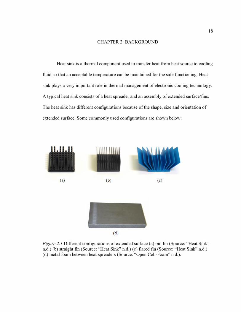
A typical heat sink consists of a heat spreader and an assembly of extended surface/fins.

The heat sink has different configurations because of the shape, size and orientation of

extended surface. Some commonly used configurations are shown below:

Figure 2.1 Different configurations of extended surface (a) pin fin (Source: “Heat Sink” n.d.) (b) straight fin (Source: “Heat Sink” n.d.) (c) flared fin (Source: “Heat Sink” n.d.) (d) metal foam between heat spreaders (Source: “Open Cell-Foam” n.d.).

19

The most common material for heat sink is aluminium. However, pure aluminium

is not suitable for machining. In practice, aluminium alloys 6061 and 6063 are commonly

used. Copper is also used in heat sinks. For high temperature application (upto 1000˚C

and heat removal capability of 20MW/m2), copper matrix reinforced with ceramic or

intermetallic particles or fibers of thermal conductivity 300 W/mK is currently being

developed (“New material for extreme environment”, n.d.). Highly conductive materials

(diamond, highly graphitized carbon fibers, carbon nanotubes with theoretical thermal

conductivity of 800-6000 W/mK) embedded in metallic matrix are also being developed

for high heat flux applications (“New material for extreme environment”, n.d.). These

materials can be used for both heat spreader and extended surface. However, foams

(carbon foam, aluminum foam etc) have good potential for use as extended surface for

thermal management.

When heat sinks are attached to the electronic chip, there is always a gap at the

interface of chip and heat sink. This gap is filled with air and creates a thermal resistance

known as thermal contact resistance. In order to reduce this resistance, thermal interface

material or TIM is used to fill in the gaps. There are different types of TIM based on

contact pressure between parts, interface gap between mating components etc. Most

commonly used materials are thermal grease, epoxy, polimide, graphite or aluminium

tape, silicon coated fabrics etc. Though they improve the contact or remove the gap, they

also have thermal resistance. Currently available TIM has the resistance values from 0.2-

1.5 m2K/W (“Thermal interface material”, n.d.). In this analysis, heat spreader optimum

20 dimension would be determined and the effect of high convective rates will be

investigated.

Many studies have been carried out to determine the spreading resistance of a heat

spreader similar to the investigation presented herein. Some of these studies are based on

cylindrical coordinate system (Kennedy, 1960; Lee, Au, Song, & Kevin, 1995). In any

coordinate system; cylindrical or rectangular, spreading resistance is calculated on the

basis of Biot number and non-dimensional geometric parameters.

Biot number is the non-dimensional convective heat transfer coefficient which

governs the heat transfer from solids to fluid. Biot number can be defined in many ways

depending on what length is used to non-dimensionalize the ℎ ratio. The length can be

the thickness, length, width of the spreader or the heat source. In this study, the Biot

number (written as Bi) is defined with respect to the thickness of the spreader as:

ℎ

Where h is the effective heat transfer coefficient at the heat spreader surface, t is

the thickness of the heat spreader, and k is the thermal conductivity. Biot number is the

ratio of thermal resistances offered by the solid material and the fluid medium. Very low

Biot number indicates very little amount of heat transfer to the environment because of

high convective resistance, whereas very high Biot number indicates large temperature

gradient inside the solid because of high conductive resistance.

To get the optimized dimension of a heat spreader the total resistance, Rt, will be

minimized. This total thermal resistance is the sum of three resistances,

21

Where Tmax is the maximum temperature at the heat source, and Q is the total heat

transferred through the heat sink. The terms on the right hand side of the above equation,

are the conductive, convective and spreading resistances, respectively.

These resistances will be described in the following chapters. The conductive and

convective resistances are well known in heat transfer literature, and are given by:

ℎ

The total heat transferred Q is related to the heat flux (q) and the source area (As)

as:

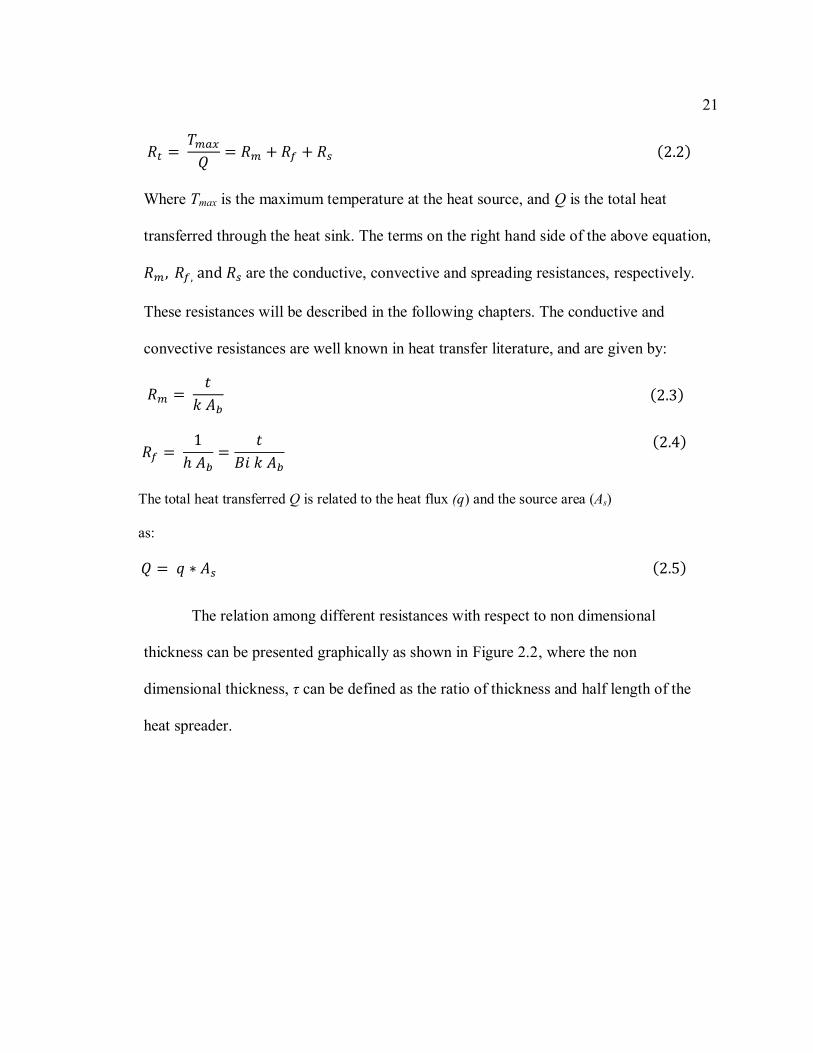
The relation among different resistances with respect to non dimensional

thickness can be presented graphically as shown in Figure 2.2, where the non

dimensional thickness, τ can be defined as the ratio of thickness and half length of the

heat spreader.

22

Figure 2.2 Contribution of different resistances, when heat flows from source to environment through a heat sink.

From Figure 2.2, it can be shown that for any value of ℎ and , total

resistance, due to spreading resistance, decreases with the increase of non dimensional

thickness and has a minimum point. This is the optimum point after which there is no

variation in Rt or Rs and here, we have optimum thickness.

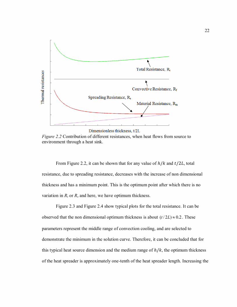
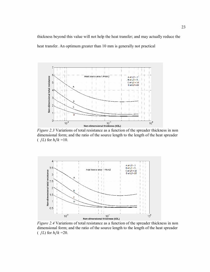
Figure 2.3 and Figure 2.4 show typical plots for the total resistance. It can be

observed that the non dimensional optimum thickness is about 2.0)2/( Lt . These

parameters represent the middle range of convection cooling, and are selected to

demonstrate the minimum in the solution curve. Therefore, it can be concluded that for

this typical heat source dimension and the medium range of ℎ , the optimum thickness

of the heat spreader is approximately one-tenth of the heat spreader length. Increasing the

23 thickness beyond this value will not help the heat transfer; and may actually reduce the

heat transfer. An optimum greater than 10 mm is generally not practical

Figure 2.3 Variations of total resistance as a function of the spreader thickness in non dimensional form; and the ratio of the source length to the length of the heat spreader ( ) for ℎ =10.

Figure 2.4 Variations of total resistance as a function of the spreader thickness in non dimensional form; and the ratio of the source length to the length of the heat spreader ( ) for ℎ =20.

24

The plots are invariant if the ratio of ℎ is the same. So, ℎ is an important

dimensional parameter for the design of the system. The total resistance decreases with

the increase of heat source length. At lower values of heat source length, sharp minimum

points could be found. At higher values, the approximate value near the minimum values

is for minimum resistance, because the plots are flat and there are no well defined

minima.

The first analysis of spreading resistance of heat spreader developed by Kennedy

(1960) was an analytical solution for axi-symmetric problems with a uniform heat flux

source on a short cylindrical spreader for different cases of adiabatic and isothermal

boundary conditions. This axisymmetric model has been widely used for more than three

decades in electronic cooling applications. The author did not separately introduce the

material, convective and conductive resistances; rather, the total resistance was referred

to as the spreading resistance and was expressed as

Where,

Song et al. (1994) and Lee et al. (1995) presented an extension of Kennedy’s

model for imposing general boundary conditions from iso-flux to isothermal at the

bottom surface of heat source depending on Biot number, non-dimensional thickness and

non-dimensional contact radius. These parameters are more appropriate to the cooling

systems. The dimensionless contact radius is the ratio of heat source radius to heat

25 spreader radius for cylindrical heat source and spreader. They also introduced a closed

form solution for non dimensional spreading resistance in terms of Bessel functions. The

dimensionless spreading/constriction resistance was derived as follows:

Where,

ℎ

ℎ

When the non-dimensional thickness, goes beyond 0.6, the spreading resistance

becomes independent of both dimensionless thickness and dimensionless contact length

(Song et al., 1994, Lee et al., 1995).

Lasance (2010) carried out a comparative analysis of five approaches for

calculating total thermal resistances and optimum thickness for square heat spreader. He

discussed what methods would be more appropriate and efficient based on the ratio of

convective heat transfer coefficient to material thermal conductivity and degree of

complexity of the model. In one of the approaches, optimum thicknesses were plotted

based on minimizing the total thermal resistance for different effective heat transfer co-

efficient and thermal conductivity, which is very close to the present work. A more

conclusive discussion will be presented in chapter 4, which will further validate the

present analysis.

In practice, most heat sinks tend to have rectangular or square cross section. Feng

& Xu (2004) and Maranzana et al. (2004) developed the mathematical model for

26 rectangular heat spreader. It has been shown by Lasance (2010) that the optimization

results for a square geometry are matched quite well by using an equivalent circular cross

section, and this is expected to be true for many different cross sections. Therefore, a

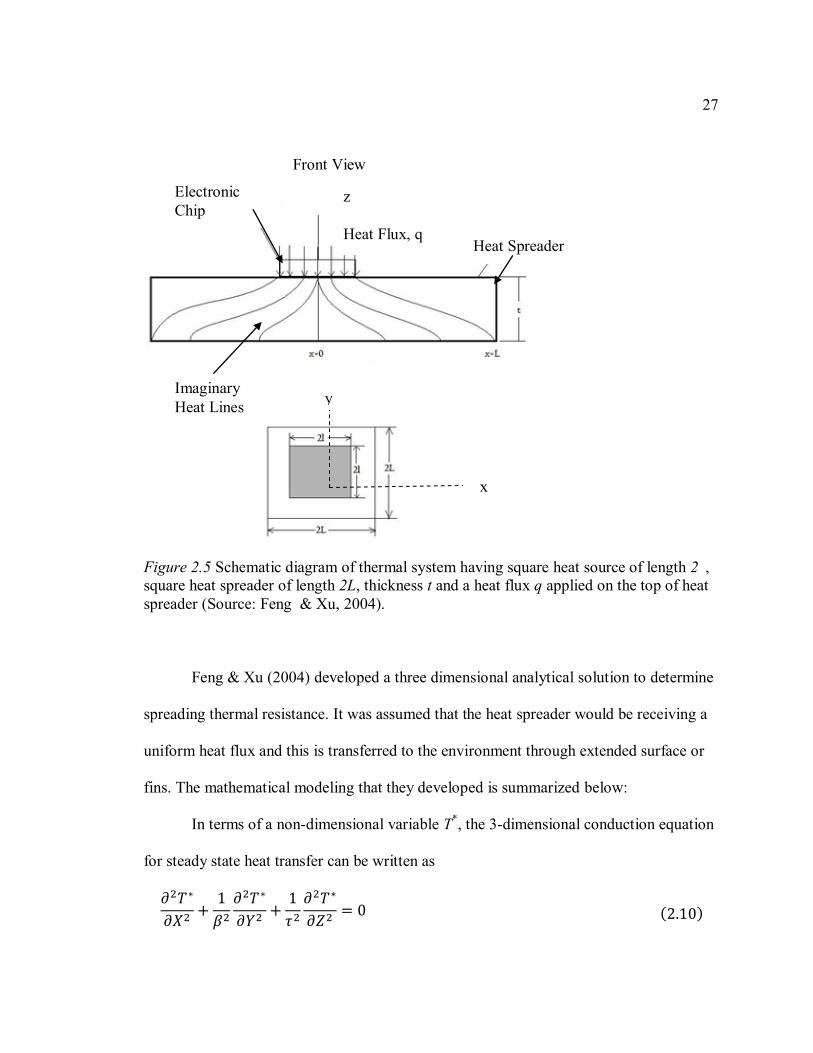
square geometry is analyzed in this study. Figure 2.5 illustrates the heat spreading in a

square heat source and spreader and will be used in the present analysis. The parameters

that will be used to describe the geometry of Figure 2.5 are , L and t

27

Figure 2.5 Schematic diagram of thermal system having square heat source of length 2 , square heat spreader of length 2L, thickness t and a heat flux q applied on the top of heat spreader (Source: Feng & Xu, 2004).

Feng & Xu (2004) developed a three dimensional analytical solution to determine

spreading thermal resistance. It was assumed that the heat spreader would be receiving a

uniform heat flux and this is transferred to the environment through extended surface or

fins. The mathematical modeling that they developed is summarized below:

In terms of a non-dimensional variable T*, the 3-dimensional conduction equation

for steady state heat transfer can be written as

Electronic Chip

Front View

Heat Flux, q Heat Spreader

z

x

y Imaginary Heat Lines

28 And the boundary conditions are

Where,

ℎ

All the results were found in terms of series solutions so that closed form

equations can be obtained for the non dimensional spreading resistance. The

dimensionless closed form solution for spreading resistance can be defined as

Feng & Xu (2004) wrote the dimensionless spreading resistance to be

But according to the present study, the corrected form for dimensionless spreading

resistance was found to be:

29 Where,

Cm0, C0n, Cmn are functions of ε,γ, Bi, τ, β in the solution by Feng & Xu (2004) and can be

expressed as:

Feng & Xu (2004) also found that as the dimensionless thickness increases

beyond 0.7, the spreading resistance is no longer dependent on Biot number and

dimensionless thickness as shown in Figure 2.6 below. This was also observed by (Lee et

al., 1995). The figure shows that spreading is a localized phenomenon near the heat

source; as a result, it is no affected by the changes i.e. changes due to Bi number far away

from the heat source.

30

Figure 2.6 Spreading resistance as a function of Bi and τ, while other geometric parameters are constant as β = 0.25, ε = 0.25, γ = 0.75. This is the corrected version of the Fig. 2 in the paper by Feng & Xu (2004), and is based on the corrected Equation 2.15.

Figure 2.7 Spreading resistance as a function of Bi and τ, while other geometric parameters are constant as β = 1(square heat spreader), ε = γ =0.167.

Dimensionless thickness,

Spre

adin

g re

sist

ance

(K/W

)

31

In Figure 2.6 and 2.7, it is observed that the spreading resistance is higher at lower

thickness and lower Bi because heat has to spread over larger area. In all the studies

above, there was no attempt to find the optimum dimension of heat spreader which is an

important design parameter in thermal management because it can reduce the size and

cost of heat sink. As there are many geometric and thermal parameters including the Biot

number, the length ratio and the thickness ratio (Lee at el., 1995, Feng & Xu, 2004), all

of which affect the spreading resistance, it is advantageous to develop an analysis for the

optimum dimension. The result would be very helpful in designing heat spreader.

It was also presented by different authors that dimensionless constriction

resistance (or spreading resistance) is weakly dependent on the shape configuration when

square root of the contact area is used as the characteristic length (Lee et al., 1995).

Therefore, it is possible to get useful results using the mathematical modeling of a square

heat spreader. The area ratio can be defined as the ratio of contact area of heat source and

area of the heat spreader. It is obvious that the spreading or constriction resistance will

become zero if the ratio goes to unity, which means there is no spreading at all.

Maranzana et al. (2004) applied thermal quadrupole method to find the solution of

the heat transfer problem and minimized an objective function (e.g., maximum

temperature) by numerical solution to find the optimum design. The quadruple refers to

four quantities: the temperature (T), the heat flux (q), and their transforms. The

quadrupole method couples the two pairs together to a 2X2 linear system with a

coefficient matrix, and solves it to get Laplace transform of T and q. If the inverse

transform can be found by the Residue theorem, the solution of the temperature and heat

32 flux can be obtained analytically. In practice, these integrals are generally computed

numerically by some existing software to get the solution in the time domain (Maillet et

al., 2000).

Maranzana et al. (2004) did the analysis for two cases of objective function; non

dimensional average temperature and non dimensional maximum temperature. The non

dimensional objective function based on maximum temperature can be defined by

ℎ

And optimization was done with respect to Bi and can be represented as

ℎ

where,

ℎ

But the analysis by Maranzana et al. (2004) gives double value of ℎ for

each when is fixed. They rejected one of these double values by assuming that

heat transfer becomes locally one dimensional at higher values at higher heat fluxes.

Therefore this limit is to be rejected since no heat spreader is needed for one dimensional

case.

In the present study, the optimization is based on the mathematical solution that

was developed by Feng & Xu (2004). To limit the error from summing up the infinite

Fourier series, a sufficient number of terms are used in calculating the values. To simplify

the analysis, the heat spreader geometry will be assumed to have a square cross section.

33 This approximation does not affect the usefulness of the result, since many heat spreaders

have square or nearly square cross section and the results are not very sensitive to the

ratio of width to length ratio (β). Therefore in the following analysis and results, the

length ratios are selected such that ε = γ and β=1.

As mentioned in chapter 1, it is the total resistance instead of spreading resistance

which must be minimized to get optimum dimension of heat spreader. In the present

work, the objective function to be minimized is the total resistance. It is similar to the

objective function used by Maranzana et al. (2004). The objective function to be used in

this study is:

ℎ

If we take the total thermal power to be fixed, then minimizing the total resistance

is equal to the minimization of maximum temperature; the objective function used by

Maranzana et al. (2004). When minimization is done with respect to τ, we get

ℎ

This leads an optimum value of the non-dimensional optimum thickness

ℎ

The optimum thickness for a wide range of ℎ value will be determined. This is

how we can choose any for a specific optimum thickness according to the possible

values of the ℎ ratio.

34

CHAPTER 3: MODELING AND ANALYSIS

3.1 Mathematical Modeling

According to Feng & Xu (2004), on the basis of geometric modeling of Figure

2.2, the total resistance is the sum of three resistances as was presented by equation 2.2 in

chapter 2 and again, for our convenience, is written as follow:

The maximum temperature is expected to occur at the center of the projected

heating area or on the top surface of the heat spreader. As shown in Figure 2.2, the

maximum temperature occurs at

x = y = 0 and z = t, or in dimensionless form,

ℎ

So,

Where,

is the dimensionless maximum temperature at the top center of the heat

spreader

And can be defined as

35

The coefficients of the above series are:

These resistances Rm, Rf, Rs depend on effective heat transfer coefficient h,

thermal conductivity k, Biot number and geometric parameter ε, τ through the equations

3.1 and 3.2. As we are minimizing the total resistances, our variable should be some

functions of these thermal and geometric parameters. Therefore, the variables that will be

used for optimization can be expressed into two groups

1. Variables based on thermal properties of material and convective heat transfer

such as h, k and ℎ

36

2. Variables based on geometric properties of heat spreader such as , .

The range of ℎ is specifically depends on possible values of effective heat

transfer coefficient, where k is a material property. The thermal conductivity has a range

of 200-400 W/mk. However, h can be very high for it is dependent on extended surface

(such as fins) area and fluid flow. Very high surface area to volume ratio is available in

foam as already mentioned in chapter 2. As a result, the value of effective heat transfer

coefficient of foam, for example graphite foams, can be as high as 20,000 (“S-Bond

Technologies”, n.d.). The other variables, such as and τ determine the dimensions

and the size of the heat sink.

The algorithm is as follows:

We will vary for a wide range, for example from 1.5 to 10 and ℎ from 1 to

250, with the increments of 0.05 and 1 respectively, keeping and k constant i.e.

we are finding the optimum dimension for a specific heat source area and heat

sink of specific thermal conductivity.

For each combination of of and ℎ combination, we obtain wide range

(about 600 data points) of values which will be used in equation 3.1and 3.2 to

get the total resistance.

From these 600 values of the minimum value of and corresponding τ would

be found by a search algorithm. In this algorithm, the position of τ is searched

until the first minimum value of the total resistance is found.

The minimum value of total resistance also determines the optimum

dimensionless thickness, .

37

Using MATLAB we can then also find values of , ,, at the optimum

point.

For different ranges of ℎ and and corresponding desired output ( ,

,, and τ ), the results will then be used to make a set of plots in the following

sections. These plots can be used to design the heat spreader.

3.2 Resistances and Their Significance in Designing Heat Spreader

Different resistance plots were produced by solving the equations described in the

last paragraph. The equations were solved numerically using Matlab. Though the plots

are good enough for physical interpretation of the heat flow through heat spreader, the

use of a numerical solution of the optimization is recommended to design heat spreader

for higher accuracy. The following symbols have already been used in the previous

chapters, but for the convenience their definitions are stated again;

is minimum total resistance

is contribution of convective resistance

is contribution of spreading resistance

is contribution of conductive or material resistance

ℎ is ratio of effective heat transfer coefficient and conductivity

is ratio of spreader length and source length

Ab is heat spreader area exposed to the convection medium

38

It should be noted that the following plots are drawn on the basis of k =400

W/mK in the rest of this chapter. The plots are also drawn with =20 mm, unless stated

otherwise.

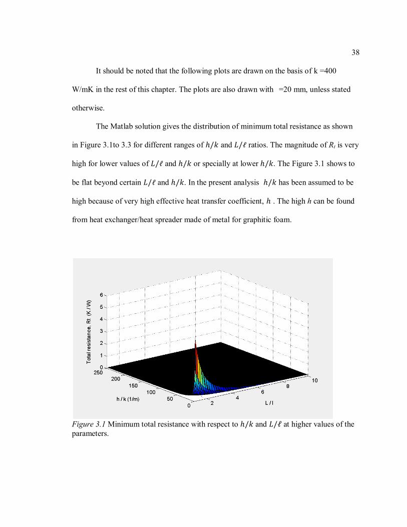
The Matlab solution gives the distribution of minimum total resistance as shown

in Figure 3.1to 3.3 for different ranges of ℎ and ratios. The magnitude of Rt is very

high for lower values of and ℎ or specially at lower ℎ . The Figure 3.1 shows to

be flat beyond certain and ℎ . In the present analysis ℎ has been assumed to be

high because of very high effective heat transfer coefficient, ℎ . The high h can be found

from heat exchanger/heat spreader made of metal for graphitic foam.

Figure 3.1 Minimum total resistance with respect to ℎ and at higher values of the parameters.

39

Figure 3.2 Minimum total resistance with respect to ℎ and length ratio, at lower values of the parameters.

Figure 3.3 and 3.4 shows that the effective heat transfer and length of spreader are

inversely related with each other with respect to the same minimum total resistance. In

other words, either effective heat transfer or length of the spreader should be increased to

maintain the same total resistance. The plots further illustrate the interdependence

between the geometry, the material property and the convection rates. Also, the change in

the values of contours changes significantly from higher to lower values of these

parameters and to get the minimum resistance requires either the increase of the heat

spreader dimension or higher values of effective heat transfer coefficient.

40

Figure 3.3 Contours of minimum total resistance (K/W) at lower range of ℎ and .

Figure 3.4 Contours of minimum total resistance (K/W) at higher values of ℎ .

41

Next the plots of conductive, convective and spreading resistances would be

described separately to get the comprehensive idea of how they contribute to the

minimum total resistance. It should also be kept in mind that the plots of different

resistances that would be presented here are computed from minimum total resistance i.e.

they are all computed after the optimization of heat spreader dimension.

The contribution of conductive resistance is shown in Figure 3.5 and 3.6. At lower

values of length ratio, between 1~1.5, the conductive resistance increases. It can be due to

the higher rate of change of optimum thickness with respect to length ratio, since

conductive resistance is dependent on thickness and length of the heat spreader.

Figure 3.5 Contribution of conductive resistance, at minimum .

42

Figure 3.6 shows the contour of conductive resistance. It shows that the

conductive resistance decreases when the length ratio goes beyond 1.5. It is shown

from the figure that the contours have almost same slope after the length ratio of 1.5,

which predicts the linear relation between ℎ and for a specific value of contour

plot.

Figure 3.6 Contour plot for conductive resistance (K/W), with respect to ℎ and at minimum total resistance, .

The plot also shows that the highest value of conductive resistance is about twice

the lowest value, which implies that the variation of conductive resistance over the range

of parameters is not significant. It also implies that the conductive resistance is not highly

dependent on ℎ and .

43

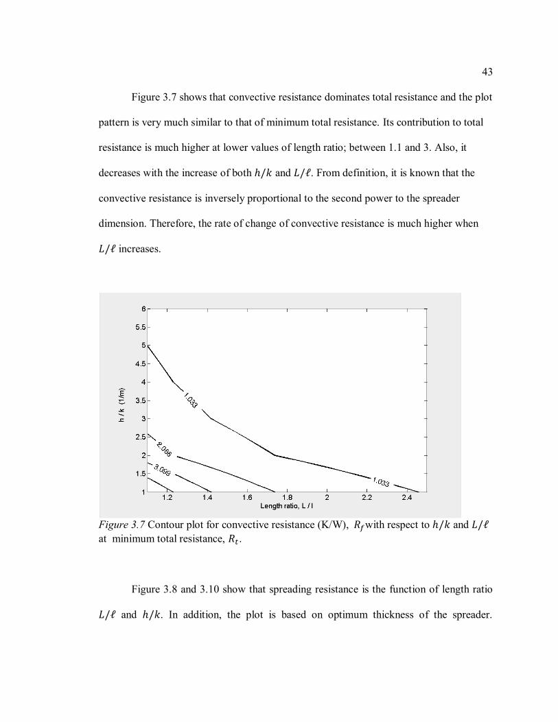
Figure 3.7 shows that convective resistance dominates total resistance and the plot

pattern is very much similar to that of minimum total resistance. Its contribution to total

resistance is much higher at lower values of length ratio; between 1.1 and 3. Also, it

decreases with the increase of both ℎ and . From definition, it is known that the

convective resistance is inversely proportional to the second power to the spreader

dimension. Therefore, the rate of change of convective resistance is much higher when

increases.

Figure 3.7 Contour plot for convective resistance (K/W), with respect to ℎ and at minimum total resistance, .

Figure 3.8 and 3.10 show that spreading resistance is the function of length ratio

and ℎ . In addition, the plot is based on optimum thickness of the spreader.

44 Therefore, the plot implicitly shows the relation of all the variables required to define

spreading resistance.

Figure 3.8(a) Contour plot for spreading resistance, with respect to low ℎ and at minimum total resistance,

45

Figure 3.8(b) Contour plot for spreading resistance (K/W), with respect to ℎ and at minimum total resistance,

Figure 3.8 to 3.9 focus on the spreading resistance at different ranges of the heat

spreader length and convection rates. It is well observed from Figure 3.8 that the

spreading resistance increases with the increase of . But, for a specific , spreading

resistance is constant with the increase of ℎ . This is true at lower values of ℎ , when

effective heat transfer coefficient is not large enough to make significant changes in the

heat flow lines. It is also shown from the figure that the spreading resistance increases at

higher rate when length ratio is in the range of 1.5~2. The figures also show that the

highest value of spreading resistance is about 3 times the lowest value. It is also shown

from the figure that though the variation of spreading resistance over the range of

parameters is large, the magnitude of the values is low.

46

Figure 3.9 Contour plot for spreading resistance (K/W), at higher values of ℎ

The following conclusion can be summarized from the above discussion;

At higher values of ℎ and , the total resistance is low, because in this region

convective resistance Rf and conductive resistance Rm are low as both of them are

inversely proportional to and Rf is inversely proportional to h.

At higher values of , the total resistance is higher because of higher Rs. As

increases, heat flow lines have to spread out more resulting higher

At lower ℎ and lower , both Rf and Rm are very high because they are

inversely proportional to L2 (~Ab). Rf is also inversely proportional to h, which

leads to very high .

In most of the plots, the upper limit for ℎ was 50. In making heat spreader Cu

and Al are generally used, which has thermal conductivity of about 400 W/mK and 200

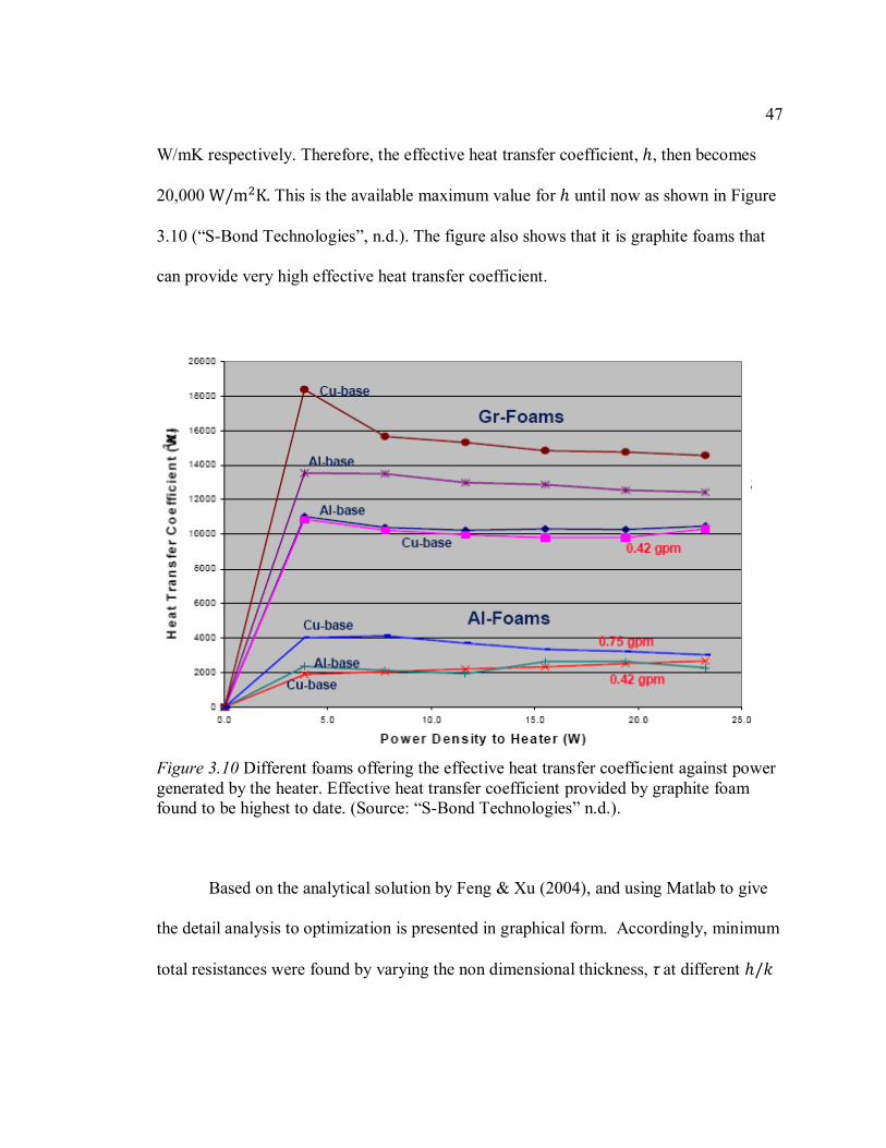
47 W/mK respectively. Therefore, the effective heat transfer coefficient, ℎ, then becomes

20,000 This is the available maximum value for ℎ until now as shown in Figure

3.10 (“S-Bond Technologies”, n.d.). The figure also shows that it is graphite foams that

can provide very high effective heat transfer coefficient.

Figure 3.10 Different foams offering the effective heat transfer coefficient against power generated by the heater. Effective heat transfer coefficient provided by graphite foam found to be highest to date. (Source: “S-Bond Technologies” n.d.).

Based on the analytical solution by Feng & Xu (2004), and using Matlab to give

the detail analysis to optimization is presented in graphical form. Accordingly, minimum

total resistances were found by varying the non dimensional thickness, τ at different ℎ

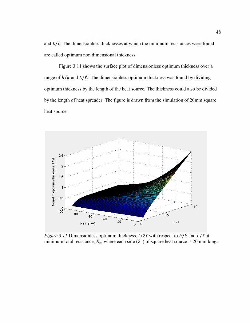
48 and . The dimensionless thicknesses at which the minimum resistances were found

are called optimum non dimensional thickness.

Figure 3.11 shows the surface plot of dimensionless optimum thickness over a

range of ℎ and . The dimensionless optimum thickness was found by dividing

optimum thickness by the length of the heat source. The thickness could also be divided

by the length of heat spreader. The figure is drawn from the simulation of 20mm square

heat source.

Figure 3.11 Dimensionless optimum thickness, with respect to ℎ and at minimum total resistance, , where each side ( ) of square heat source is 20 mm long.

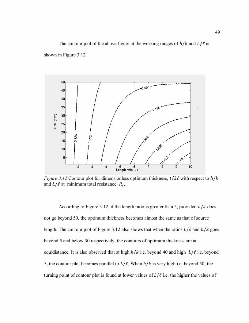
49

The contour plot of the above figure at the working ranges of ℎ and is

shown in Figure 3.12.

Figure 3.12 Contour plot for dimensionless optimum thickness, with respect to ℎ and at minimum total resistance, .

According to Figure 3.12, if the length ratio is greater than 5, provided ℎ does

not go beyond 50, the optimum thickness becomes almost the same as that of source

length. The contour plot of Figure 3.12 also shows that when the ratios and ℎ goes

beyond 5 and below 30 respectively, the contours of optimum thickness are at

equidistance. It is also observed that at high ℎ i.e. beyond 40 and high i.e. beyond

5, the contour plot becomes parallel to . When ℎ is very high i.e. beyond 50, the

turning point of contour plot is found at lower values of i.e. the higher the values of

50 ℎ , the lower the values of at where the turning point starts. This can also be

observed from Figure 3.11.

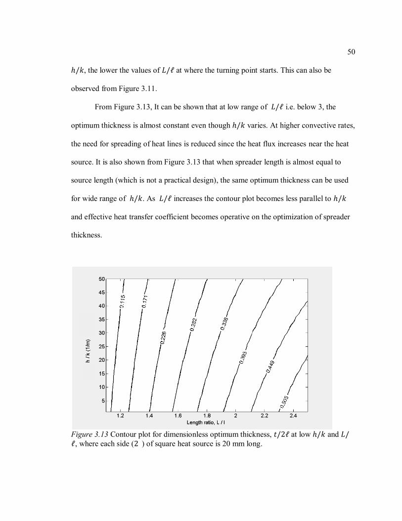
From Figure 3.13, It can be shown that at low range of i.e. below 3, the

optimum thickness is almost constant even though ℎ varies. At higher convective rates,

the need for spreading of heat lines is reduced since the heat flux increases near the heat

source. It is also shown from Figure 3.13 that when spreader length is almost equal to

source length (which is not a practical design), the same optimum thickness can be used

for wide range of ℎ . As increases the contour plot becomes less parallel to ℎ

and effective heat transfer coefficient becomes operative on the optimization of spreader

thickness.

Figure 3.13 Contour plot for dimensionless optimum thickness, at low ℎ and , where each side ( ) of square heat source is 20 mm long.

51

From Figure 3.1 to 3.13, the variables used were and ℎ . These variables

were selected based on available thermal and geometric properties of heat spreader and

heat source. Among them and are non-dimensional and ℎ is dimensional.

Although the usage of dimensional variable ℎ helps comprehend the design decision

quickly, it does not make the analysis absolutely non-dimensional.

Maranzana et al. (2004) have already introduced the above idea and presented the

plots accordingly in their paper. The plots used three Biot numbers which have already

been described in chapter 2. In the present work, the same plot has been produced based

on current numerical solution. In addition, by producing the same plot the validation of

the present work can be established and compared with that Maranzana’s work.

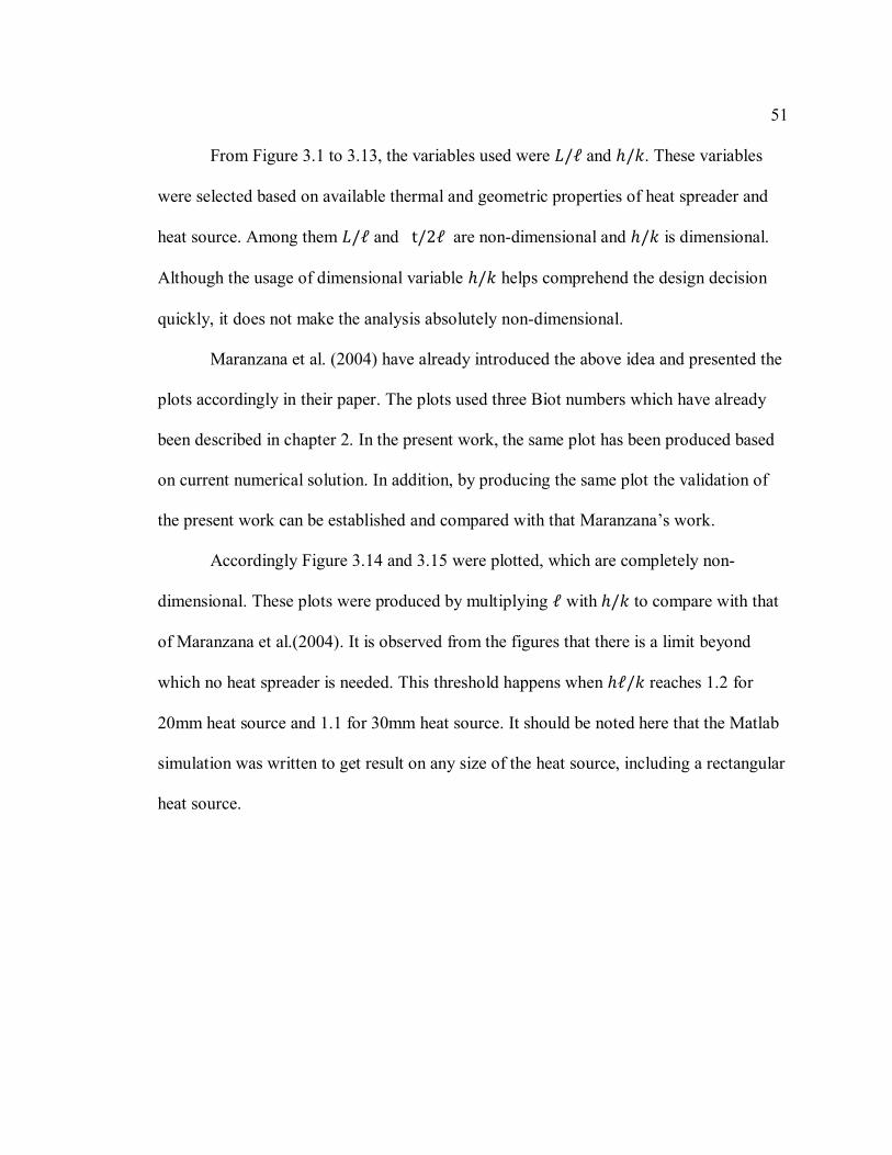
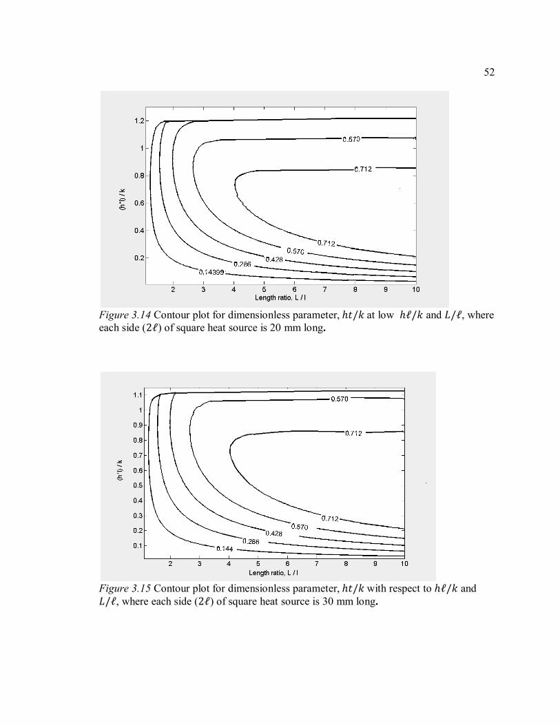
Accordingly Figure 3.14 and 3.15 were plotted, which are completely non-

dimensional. These plots were produced by multiplying with ℎ to compare with that

of Maranzana et al.(2004). It is observed from the figures that there is a limit beyond

which no heat spreader is needed. This threshold happens when ℎ reaches 1.2 for

20mm heat source and 1.1 for 30mm heat source. It should be noted here that the Matlab

simulation was written to get result on any size of the heat source, including a rectangular

heat source.

52

Figure 3.14 Contour plot for dimensionless parameter, ℎ at low ℎ and , where each side ( ) of square heat source is 20 mm long.

Figure 3.15 Contour plot for dimensionless parameter, ℎ with respect to ℎ and , where each side ( ) of square heat source is 30 mm long.

53

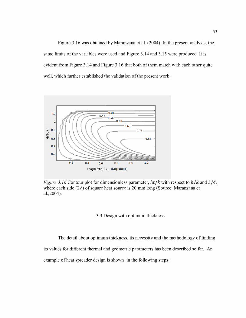
Figure 3.16 was obtained by Maranzana et al. (2004). In the present analysis, the

same limits of the variables were used and Figure 3.14 and 3.15 were produced. It is

evident from Figure 3.14 and Figure 3.16 that both of them match with each other quite

well, which further established the validation of the present work.

Figure 3.16 Contour plot for dimensionless parameter, ℎ with respect to ℎ and , where each side ( ) of square heat source is 20 mm long (Source: Maranzana et al.,2004).

3.3 Design with optimum thickness

The detail about optimum thickness, its necessity and the methodology of finding

its values for different thermal and geometric parameters has been described so far. An

example of heat spreader design is shown in the following steps :

54

Determine Rt (= Tmax / Q), where Q is constant power produced by heat source

and Tmax is the maximum temperature allowed for safe functioning of the heat

producing component.

Suitable combination of ℎ and are chosen from contour plot of Rt. For

example, Figure 3.3, Figure 3.4 can be used for a heat source of length 20 mm.

From contour plot of τ or from analytical solution, the optimum thickness is

determined by using ℎ and pair found in the previous step

For example, if a square heater of 20 mm length produces 1000 W and the

allowable maximum temperature is 100˚C, then according to the first step, Rt = 100/1000

or 0.1 ˚C/W.

From data or graph of minimum total resistance, we can choose the value of ℎ

and respectively to be 35 and 1.8 (other combinations can also be selected along

constant Rt contour lines).

From the contour plot of non-dimensional optimum thickness, the following

optimum thickness can be computed,

= 0.3054 or optimum thickness t = 0.3054*2*10 mm = 6 mm

L = 1.8*10 mm = 18 mm or length of spreader, 2L= 36 mm.

Therefore, a possible design for 20mm square heat source is:

Side length of spreader 36 mm,

Thickness 6 mm,

Thermal conductivity of spreader is 400 W/mK

Effective heat transfer coefficient is 14000 W/m2K

55

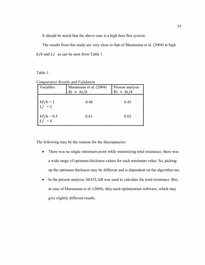
It should be noted that the above case is a high heat flux system.

The results from this study are very close to that of Maranzana et al. (2004) at high

ℎ and as can be seen from Table 1.

Table 1.

Comparative Results and Validation Variables Maranzana et al. (2004)

ℎ Present analysis ℎ

ℎ = 1 = 2

0.40 0.45

ℎ = 0.5 = 4

0.61 0.62

The following may be the reasons for the discrepancies:

There was no single minimum point while minimizing total resistance; there was

a wide range of optimum thickness values for each minimum value. So, picking

up the optimum thickness may be different and is dependent on the algorithm too.

In the present analysis, MATLAB was used to calculate the total resistance. But,

in case of Maranzana et al. (2004), they used optimization software, which may

give slightly different results.

56

CHAPTER 4: HEAT SPREADER FOR HIGH HEAT FLUX SYSTEM

The objective of the present work was to present analytical approach and

numerical solution for the design considerations of heat spreader in high heat flux

systems. In doing so, the total resistance was minimized to get the optimum dimension of

heat spreader by taking into considerations all the design parameters. From chapter 1 to 3

the analytical method and numerical solution in graphical format have been presented in

non-dimensional form. In this chapter the optimum dimensions for high heat flux system

will be investigated.

It was observed in Figures 2.3 and 2.4 that the total resistance approaches the

minimum value as the thickness value increases to about 2.0)2/( Lt in the range of h/k

ratio of 10 to 20. In practice, the thickness of heat spreaders tends to be different than

optimum because of considerations of weight, space, and cost-effectiveness. Lasance

(2010) has discussed the difference between two cases of h=250 W/m2K and h=10,000

W/m2K, He concludes that the thickness of the heat spreader is not critical at high

thermal conductivity values, a typical value for optimum thickness is about 2 mm, and

thicker is generally better for heat dissipation.

Using the analytical solution of Equation (2.10), several plots have been drawn in

dimensional form to examine the influence of spreader thickness and effective heat

transfer coefficient total resistance on the total resistance. Figures 4.1 to 4.5 illustrate a

particular example discussed by Lasance (2010), which has a heat source of 5mmX5mm

and a heat spreader of 30mmX30mm. Figure 4.1 shows that for high conductivity (300

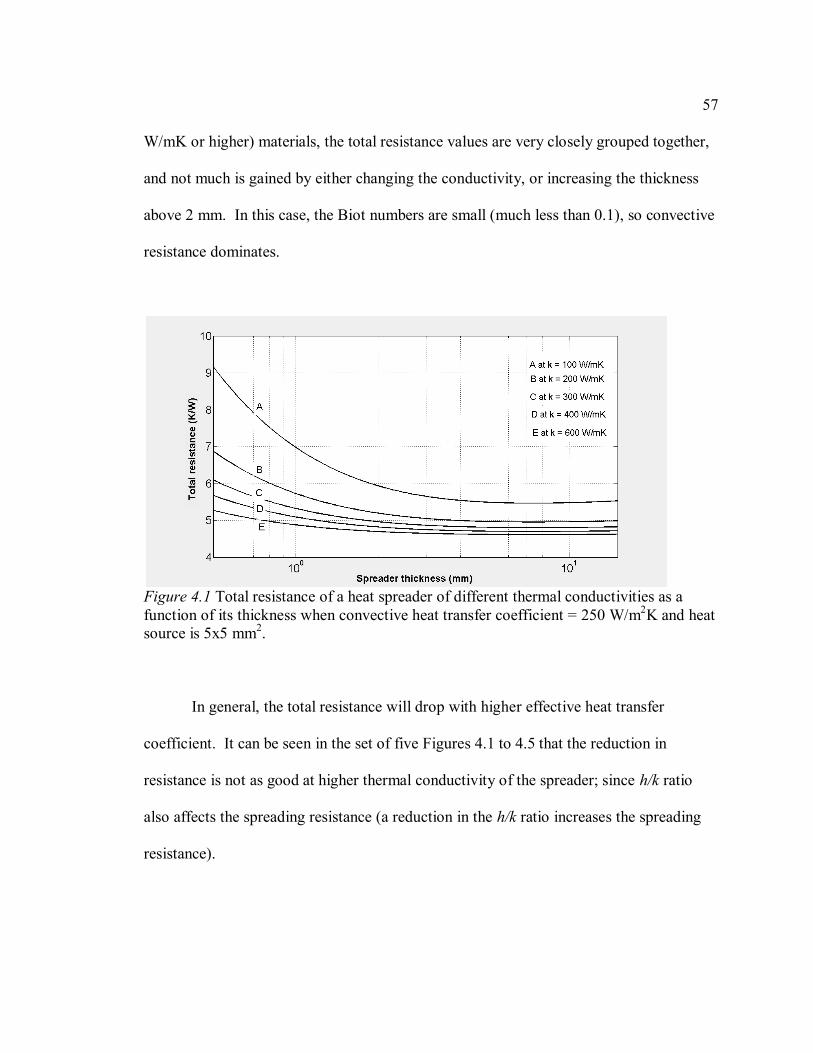
57 W/mK or higher) materials, the total resistance values are very closely grouped together,

and not much is gained by either changing the conductivity, or increasing the thickness

above 2 mm. In this case, the Biot numbers are small (much less than 0.1), so convective

resistance dominates.

Figure 4.1 Total resistance of a heat spreader of different thermal conductivities as a function of its thickness when convective heat transfer coefficient = 250 W/m2K and heat source is 5x5 mm2.

In general, the total resistance will drop with higher effective heat transfer

coefficient. It can be seen in the set of five Figures 4.1 to 4.5 that the reduction in

resistance is not as good at higher thermal conductivity of the spreader; since h/k ratio

also affects the spreading resistance (a reduction in the h/k ratio increases the spreading

resistance).

58

Figure 4.2 Total resistance of a heat spreader of different thermal conductivities as a function of its thickness when convective heat transfer coefficient = 5,000 W/m2K and heat source is 5x5 mm2.

The total resistance can be reduced by increasing the heat spreader area, or by

increasing the thermal conductivity of the spreader. However, beyond a certain value,

increase in the heat spreader area provides negligible reduction to the total resistance (as

shown in Figure 3.9) because the additional surface does not participate significantly in

heat transfer. Increase in the thermal conductivity is also not very effective in reducing

the total resistance beyond a certain value, as seen in the set of Figures of 4.1 to 4.5 for a

wide range of heat transfer coefficients, unless the h/k ratios are very high.

59

Figure 4.3 Total resistance of a heat spreader of different thermal conductivities as a function of its thickness when convective heat transfer coefficient = 10,000 W/m2K and heat source is 5x5 mm2.

Figure 4.4 Total resistance of a heat spreader of different thermal conductivities as a function of its thickness when convective heat transfer coefficient = 20,000 W/m2K and heat source is 5x5 mm2.

60

Figure 4.5 Total resistance of a heat spreader of different thermal conductivities as a function of its thickness when convective heat transfer coefficient = 30,000 W/m2K and heat source is 5x5 mm2.

For the same size of the heat spreader cross sectional area, it is expected that the

resistance will be lower if the heat source is bigger, because it requires less spreading of

the heat flux lines, and also reduces heat flux for the same heat transfer. This can be seen

in Figures 4.6 to 4.10, where the plots of total resistance have been repeated for the same

range of heat transfer coefficients, heat spreader size, and thermal conductivity values,

but with a 10X10 mm2 heat source.

61

Figure 4.6 Total resistance of a heat spreader of different thermal conductivities as a function of its thickness when convective heat transfer coefficient = 250 W/m2K and heat source is 10x10 mm2.

Figure 4.7 Total resistance of a heat spreader of different thermal conductivities as a function of its thickness when convective heat transfer coefficient = 5000 W/m2K and heat source is 10x10 mm2.

62

Figure 4.8 Total resistance of a heat spreader of different thermal conductivities as a function of its thickness when convective heat transfer coefficient = 10,000 W/m2K and heat source is 10x10 mm2.

Figure 4.9 Total resistance of a heat spreader of different thermal conductivities as a function of its thickness when convective heat transfer coefficient = 20,000 W/m2K and heat source is 10x10 mm2.

63

Figure 4.10 Total resistance of a heat spreader of different thermal conductivities as a function of its thickness when convective heat transfer coefficient = 30,000 W/m2K and heat source is 10x10 mm2.

It is also interesting to note that the optimum value is more well defined at the

high convection rate, as seen by comparing Figure 4.1 with Figure 4.5; or by comparing

Figure 4.6 with 4.10. Therefore, for very high heat fluxes, it is advantageous to use the

optimum thickness calculated from the analytical solution; but care should be taken not to

exceed the optimum thickness.

Table 2 shows the numerical values of the optimum thickness and total resistances

for heat spreaders at different convection rates on two high conductivity heat spreaders

(k=350 W/mK and 500 W/mK). This range of thermal conductivity was selected since

heat spreaders with this conductivity have been developed (Schubert et al., 2004) with a

reduced CTE to match the device or package material. This table is based on the same

heat spreader size (30X30 mm2), as shown in Figures 4.1 to 4.10.

From Table 2, it can be concluded that the optimum thickness is approximately 7

mm for the much of the range of convective heat transfer coefficient, although the

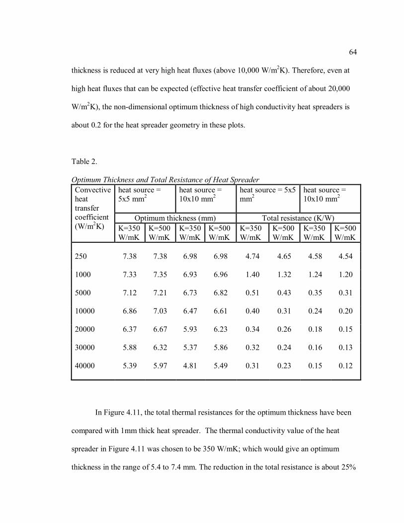
64 thickness is reduced at very high heat fluxes (above 10,000 W/m2K). Therefore, even at

high heat fluxes that can be expected (effective heat transfer coefficient of about 20,000

W/m2K), the non-dimensional optimum thickness of high conductivity heat spreaders is

about 0.2 for the heat spreader geometry in these plots.

Table 2.

Optimum Thickness and Total Resistance of Heat Spreader Convective heat transfer coefficient (W/m2K)

heat source = 5x5 mm2

heat source = 10x10 mm2

heat source = 5x5 mm2

heat source = 10x10 mm2

Optimum thickness (mm) Total resistance (K/W) K=350 W/mK

K=500 W/mK

K=350 W/mK

K=500 W/mK

K=350 W/mK

K=500 W/mK

K=350 W/mK

K=500 W/mK

250 7.38 7.38 6.98 6.98 4.74 4.65 4.58 4.54

1000 7.33 7.35 6.93 6.96 1.40 1.32 1.24 1.20

5000 7.12 7.21 6.73 6.82 0.51 0.43 0.35 0.31

10000 6.86 7.03 6.47 6.61 0.40 0.31 0.24 0.20

20000 6.37 6.67 5.93 6.23 0.34 0.26 0.18 0.15

30000 5.88 6.32 5.37 5.86 0.32 0.24 0.16 0.13

40000 5.39 5.97 4.81 5.49 0.31 0.23 0.15 0.12

In Figure 4.11, the total thermal resistances for the optimum thickness have been

compared with 1mm thick heat spreader. The thermal conductivity value of the heat

spreader in Figure 4.11 was chosen to be 350 W/mK; which would give an optimum

thickness in the range of 5.4 to 7.4 mm. The reduction in the total resistance is about 25%

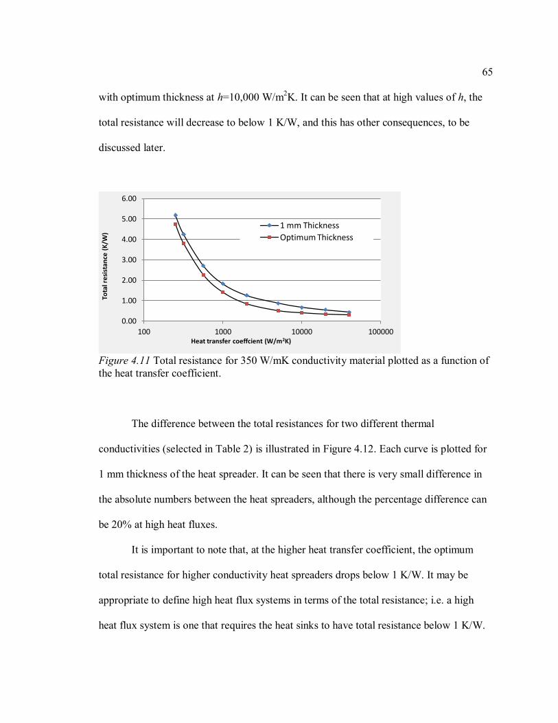
65 with optimum thickness at h=10,000 W/m2K. It can be seen that at high values of h, the

total resistance will decrease to below 1 K/W, and this has other consequences, to be

discussed later.

Figure 4.11 Total resistance for 350 W/mK conductivity material plotted as a function of the heat transfer coefficient.

The difference between the total resistances for two different thermal

conductivities (selected in Table 2) is illustrated in Figure 4.12. Each curve is plotted for

1 mm thickness of the heat spreader. It can be seen that there is very small difference in

the absolute numbers between the heat spreaders, although the percentage difference can

be 20% at high heat fluxes.

It is important to note that, at the higher heat transfer coefficient, the optimum

total resistance for higher conductivity heat spreaders drops below 1 K/W. It may be

appropriate to define high heat flux systems in terms of the total resistance; i.e. a high

heat flux system is one that requires the heat sinks to have total resistance below 1 K/W.

0.00

1.00

2.00

3.00

4.00

5.00

6.00

100 1000 10000 100000

Tota

l re

sist

ance

(K

/W)

Heat transfer coeffcient (W/m2K)

1 mm Thickness

Optimum Thickness

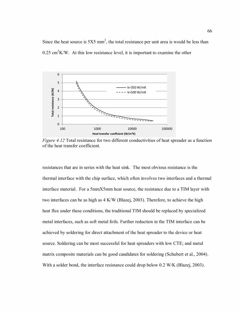
66 Since the heat source is 5X5 mm2, the total resistance per unit area is would be less than

0.25 cm2K/W. At this low resistance level, it is important to examine the other

Figure 4.12 Total resistance for two different conductivities of heat spreader as a function of the heat transfer coefficient. resistances that are in series with the heat sink. The most obvious resistance is the

thermal interface with the chip surface, which often involves two interfaces and a thermal

interface material. For a 5mmX5mm heat source, the resistance due to a TIM layer with

two interfaces can be as high as 4 K/W (Blazej, 2003). Therefore, to achieve the high

heat flux under these conditions, the traditional TIM should be replaced by specialized

metal interfaces, such as soft metal foils. Further reduction in the TIM interface can be

achieved by soldering for direct attachment of the heat spreader to the device or heat

source. Soldering can be most successful for heat spreaders with low CTE; and metal

matrix composite materials can be good candidates for soldering (Schubert et al., 2004).

With a solder bond, the interface resistance could drop below 0.2 W/K (Blazej, 2003).

0

1

2

3

4

5

6

100 1000 10000 100000

Tota

l re

sist

ance

(K

/W)

Heat transfer coeffcient (W/m2K)

k=350 W/mK

k=500 W/mK

67

CHAPTER 5: CONCLUSIONS AND SUMMARY

Several mathematical approaches for the determination of the thermal resistance

of heat spreaders have been discussed in chapter 1 and 2. An appropriate model for a

square heat spreader was applied to find a numerical solution for optimum dimensions of

a heat spreader. The optimized heat spreader was then studied in Chapter 3 for a wide

range of heat transfer coefficients, thermal conductivity and non-dimensional length

scales and resistances. The optimum thickness of the heat spreader was determined and

the contributions of different resistances to the total thermal resistance have been

illustrated in chapter 3. The behavior of conducive, convective and spreading resistance

in different ranges of geometric and thermal parameters was discussed in graphical

format. It was observed that the non-dimensional optimum thickness is approximately 0.2

for typical range of ℎ and . However, in typical non-critical applications, it is

common to use a heat spreader that is thinner than the optimum because the resistance

curve does not have a sharp minimum.

Finally, an algorithm was outlined for determination of the optimum heat spreader

for a heat sink. The optimized solution was compared with a numerical solution obtained

by other investigators using the quadrupole method. The two solutions were quite close in

value; and the differences were probably due to the fact that the minimum resistance

curve does not have a sharp minimum.

In chapter 4, the optimum thicknesses of heat spreader for high heat flux of two

different sizes was studied over a wide range of heat transfer coefficients and the non-

68 dimensional results were converted to proper units and compared in plots. It was

observed that the non-dimensional optimum thickness is still approximately 0.2 for wide

range of ℎ and . However, with the combination of high transfer coefficients and

high thermal conductivity, the optimum thickness starts to drop slightly when the h/k

ratio exceeds 50. These results are valid for typical heat source and heat spreader sizes.

It was observed that the performance of the heat sink does not improve greatly in

terms of total thermal resistance beyond the thermal conductivity of 350 W/mK. In

addition to this, it was also observed that the optimum value of the thickness does not

change significantly when the heat transfer coefficient is in the range of 1000 to 20000

W/mK. At lower values of the convection heat transfer coefficient (below 10,000

W/mK), the optimum thickness is not well defined. At higher convection rates, the total

resistance does show a better defined optimum. Therefore, in systems that require high

flux, it is advisable to design the heat spreader close to the optimum values, but not to

exceed the optimum thickness.

With the combination of high conductivity materials, and high convective heat

flux, the total resistance can become comparable or less than the resistance due to a TIM

layer between the heat source and the heat spreader. In such cases, the heat spreader

should be directly attached to the chip or heat source by using a soldering method so that

the interface resistance is reduced.

The present work is based on single heat source, with a square heat spreader. With

the growth of complex thermal management system, future work should include multiple

heat sources with heat spreaders of more complex shapes. In such cases, new analytical

69 formulation or modification of present work may be needed. In addition, experimental

work should also be done to verify the results of the present study.

70

REFERENCES

Blazej, D. (2003, November). Thermal Interface Materials. ElectronicsCooling.

Retrieved December 20, 2011 from: http://www.electronics-

cooling.com/2003/11/thermal-interface-materials/

Bar-Cohen, A., Wang, P., & Rahim, E. ( 2007). Thermal Management of High Heat Flux

Nanoelectronic Chips. Microgravity Science and Technology, Vol. XIX – 3/4, 48-

52.

Feng, T.Q., & Xu, J.L. (2004). An analytical solution of thermal resistance of cubic heat

spreaders for electronic cooling. Applied Thermal Engineering , 24 (2-3), 323-

337.

Gallego, N.C., & Klett, J.W. (2003). Carbon Foams for Thermal Management. Carbon,

41, 1461-1466.

Guenin, B. M. (2006, August). Packaging challenges for high heat flux devices.

ElectronicsCooling. Retrieved May 2, 2011 from: http://www.electronics-

cooling.com/2006/08/packaging-challenges-for-high-heat-flux-devices

Heat Sink. (n.d.). Retrieved April 29, 2012 from: http://en.wikipedia.org/wiki/Heat_sink

Kennedy, D. (1960). Spreading resistance in cylindrical semiconductor devices. Journal

of Applied Physics , 31 (8), 1490-1497.

Lasance, C.J.M. (2010). How to Estimate Heat Spreading Effects in Practice. Journal of

Electronic Packaging, 132, 031004-1.

71 Lee, S., Au, V., Song, S., & Kevin, P.M. (1995). Constriction/ Spreading resistance

model for electronics packaging. Proccedings of ASME/JSME Thermal

Engineering Conference, (pp. 199-206).

Lee, Y.C., Zhang, W., Xie, H., & Mahajan, R.L. (1993). Cooling of a FCHIP package

with 100 W, 1 cm2 Chip. Proccedings of ASME International Electronic

Packaging Conference, (pp. 419-423). New York.

Maillet, D., André, S., Batsale, J.C., Degiovanni, A., & Moyne, C. (2000). Thermal

Quadrupoles: Solving the Heat Equation through Integral Transforms.

Chichester: Willey.

Maranzana, G., Perry, I., Maillet, D., & Rael, S. (2004). Design optimization of spreader

heat sink for power electronics. International Journal of Thermal Sciences , 43

(1), 21-29.

New material for extreme environment. (n.d.). Retrieved May 2, 2011, from

http://www.extremat.org/heat-sink-materials?Edition=en

Open Cell-Foam. (n.d.). Retrieved April 29, 2012 from

http://www.ultramet.com/refractoryopencells_thermalmanagement.html

S-Bond Technologies. (n.d). Retrieved April 29, 2012 from http://www.s-

bond.com/cms/files/App_Bull_Graphite_Foam_ID51677.pdf

Straatman, A.G., Gallego, N.C., Yu, Q., Betchen, L., & Thompson, B.E. (2007). Forced

convection heat transfer and hydraulic losses in graphite foam. Journal of Heat

Transfer , 129 (9), 1237-1245.

72 Schubert, T., Trindade, B., Weibgarber, T., & Kieback, B. (2004). Interfacial design of

Cu-based composites prepared by powder metallurgy for heat sink application.

Materials Sci. Engg. A, 475, 39-44.

Thermal interface material. (n.d.). Retrieved May 2, 2011, from Holland Shielding

System BV: http://www.hollandshielding.com/?p=Nieuws&id=217&Lang=2

!!!!!!!!!!!!!!!!!!!!!!!!!!!!!!!!!!!!!!!

!!

Thesis and Dissertation Services