Optimization in microgrid design and energy management

Scholars' Mine Scholars' Mine

Doctoral Dissertations Student Theses and Dissertations

Fall 2014

Optimization in microgrid design and energy management Optimization in microgrid design and energy management

Tu Anh Nguyen

Follow this and additional works at: https://scholarsmine.mst.edu/doctoral_dissertations

Part of the Electrical and Computer Engineering Commons

Department: Electrical and Computer Engineering Department: Electrical and Computer Engineering

Recommended Citation Recommended Citation Nguyen, Tu Anh, "Optimization in microgrid design and energy management" (2014). Doctoral Dissertations. 2351. https://scholarsmine.mst.edu/doctoral_dissertations/2351

This thesis is brought to you by Scholars' Mine, a service of the Missouri S&T Library and Learning Resources. This work is protected by U. S. Copyright Law. Unauthorized use including reproduction for redistribution requires the permission of the copyright holder. For more information, please contact [email protected].

https://library.mst.edu/

https://library.mst.edu/

https://scholarsmine.mst.edu/

https://scholarsmine.mst.edu/doctoral_dissertations

https://scholarsmine.mst.edu/student-tds

https://scholarsmine.mst.edu/doctoral_dissertations?utm_source=scholarsmine.mst.edu%2Fdoctoral_dissertations%2F2351&utm_medium=PDF&utm_campaign=PDFCoverPages

http://network.bepress.com/hgg/discipline/266?utm_source=scholarsmine.mst.edu%2Fdoctoral_dissertations%2F2351&utm_medium=PDF&utm_campaign=PDFCoverPages

https://scholarsmine.mst.edu/doctoral_dissertations/2351?utm_source=scholarsmine.mst.edu%2Fdoctoral_dissertations%2F2351&utm_medium=PDF&utm_campaign=PDFCoverPages

mailto:[email protected]

OPTIMIZATION IN MICROGRID DESIGN AND ENERGY MANAGEMENT

by

TU ANH NGUYEN

A DISSERTATION

Presented to the Faculty of the Graduate School of the

MISSOURI UNIVERSITY OF SCIENCE AND TECHNOLOGY

in Partial Fulfillment of the Requirements for the Degree

DOCTOR OF PHILOSOPHY

in

ELECTRICAL ENGINEERING

2014

Approved by

Dr. Mariesa L. Crow, AdvisorDr. Jonathan KimballDr. Mehdi FerdowsiDr. Pourya Shamsi

Dr. Curt Elmore

c© 2014

Tu Anh Nguyen

All Rights Reserved

iii

PUBLICATION DISSERTATION OPTION

This dissertation has been prepared in publication format. Section 1.0, pages 1-3,

has been added to supply background information for the remainder of the dissertation.

Paper 1, pages 4-30, is entitled “Performance Characterization for Photovoltaic-Vanadium

Redox Battery Microgrid Systems”, and is prepared in the style used by the Institute of

Electrical and Electronics Engineers (IEEE) Transactions on Sustainable Energy as pub-

lished on March 21, 2014. Paper 2, pages 31-53, is entitled “Optimal Sizing of a Vanadium

Redox Battery System for Microgrid Systems”, and is prepared in the style used by the

IEEE Transactions on Sustainable Energy as submitted on August 29, 2014. Paper 3, pages

54-77, is entitled “Stochastic Optimization of Renewable-based Microgrid Operation Incor-

porating Battery Operation Cost”, and is prepared in the style used by IEEE Transactions

on Sustainable Energy and will be submitted in December 2014.

iv

ABSTRACT

The dissertation is composed of three papers, which cover microgrid systems per-

formance characterization, optimal sizing for energy storage system and stochastic opti-

mization of microgrid operation. In the first paper, a complete Photovoltaic-Vanadium

Redox Battery (VRB) microgrid is characterized holistically. The analysis is based on a

prototype system installation deployed at Fort Leonard Wood, Missouri, USA. In the sec-

ond paper, the optimal sizing of power and energy ratings for a VRB system in isolated

and grid-connected microgrids is proposed. An analytical method is developed to solve

the problem based on a per-day cost model in which the operating cost is obtained from

optimal scheduling. The charge, discharge efficiencies, and operating characteristics of

the VRB are considered in the problem. In the third paper, a novel battery operation cost

model is proposed accounting for charge/discharge efficiencies as well as life cycles of the

batteries. A probabilistic constrained approach is proposed to incorporate the uncertainties

of renewable sources and load demands in microgrids into the UC and ED problems.

v

ACKNOWLEDGMENT

I would like to express my deep gratitude to my advisor Dr. Mariesa L. Crow for

her guidance, her caring and continuous support during my PhD program. I would like to

sincerely thank Dr. Curt Elmore for his leadership and obtaining the grants to finance this

research. I would also like to thank the other members of my committee, Dr. Jonathan

Kimball, Dr. Mehdi Ferdowsi, and Dr. Pourya Shamsi for their guidance, time, and years

of hard work at the Missouri University of Science and Technology.

Special thanks go out to my office mates .Maigha, Xin Qiu, Darshit Shah, Meng

Fanjun and many others for their support and entertainment over my time at Missouri Uni-

versity of Science and Technology. I want to thank all members of my research group

consisting of Jerry Tichenor, Joe Guggenberger, Thoshitha Gamage for their key support

during the development of this project.

Finally, I would like to thank my Mom, Dad, family and friends for their constant

support and encouragement during this process. Without them, none of this would be

possible.

vi

TABLE OF CONTENTS

Page

PUBLICATION DISSERTATION OPTION . . . . . . . . . . . . . . . . . . . . . . . . . . . . . . . . . . . . . . . . . . . . . . iii

ABSTRACT . . . . . . . . . . . . . . . . . . . . . . . . . . . . . . . . . . . . . . . . . . . . . . . . . . . . . . . . . . . . . . . . . . . . . . . . . . . . . . . . iv

ACKNOWLEDGMENT . . . . . . . . . . . . . . . . . . . . . . . . . . . . . . . . . . . . . . . . . . . . . . . . . . . . . . . . . . . . . . . . . . . v

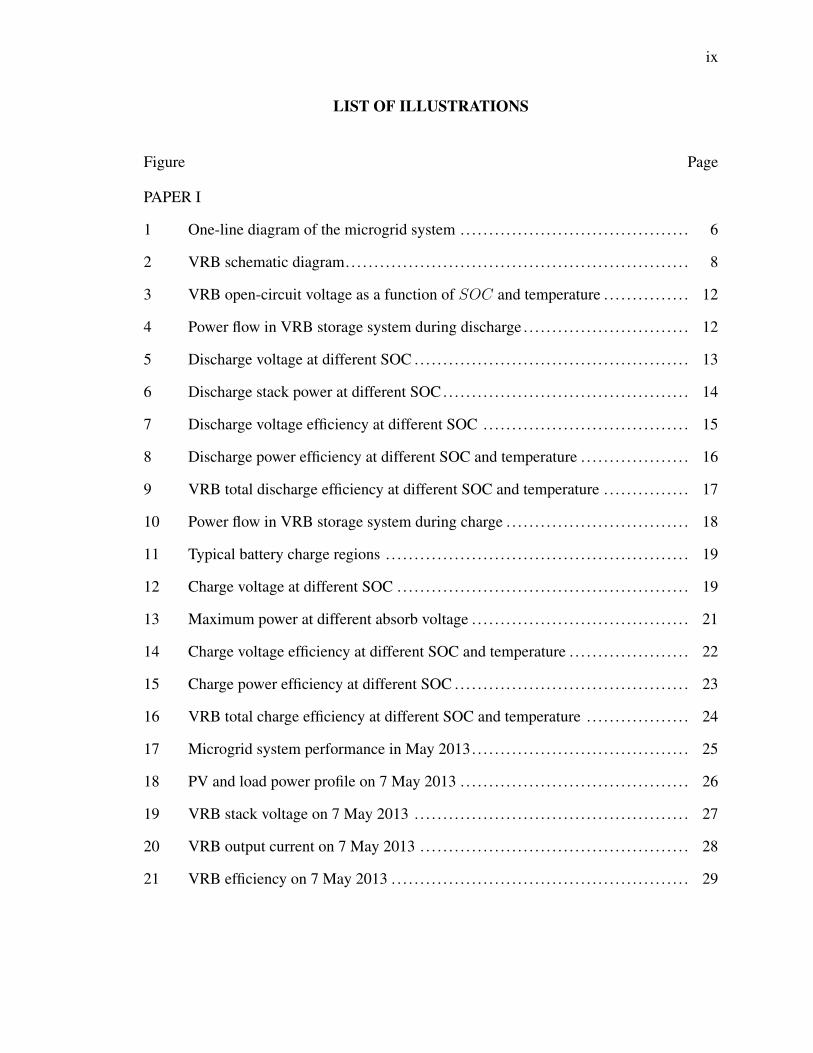
LIST OF ILLUSTRATIONS. . . . . . . . . . . . . . . . . . . . . . . . . . . . . . . . . . . . . . . . . . . . . . . . . . . . . . . . . . . . . . . ix

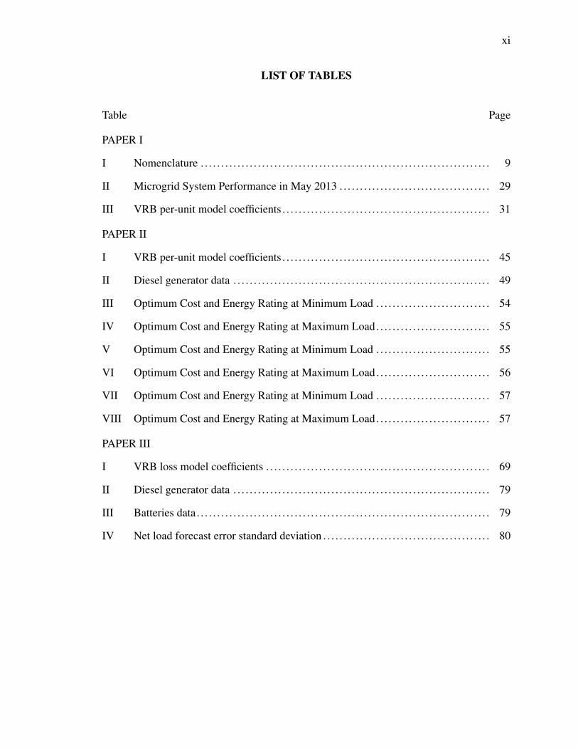
LIST OF TABLES. . . . . . . . . . . . . . . . . . . . . . . . . . . . . . . . . . . . . . . . . . . . . . . . . . . . . . . . . . . . . . . . . . . . . . . . . . xi

SECTION

1. INTRODUCTION . . . . . . . . . . . . . . . . . . . . . . . . . . . . . . . . . . . . . . . . . . . . . . . . . . . . . . . . . . . . . . 1

PAPER

I. PERFORMANCE CHARACTERIZATION FOR PHOTOVOLTATIC-VANADIUMREDOX BATTERY MICROGRID . . . . . . . . . . . . . . . . . . . . . . . . . . . . . . . . . . . . . . . . . . . . . . . . . . . . . . . . 4

Abstract . . . . . . . . . . . . . . . . . . . . . . . . . . . . . . . . . . . . . . . . . . . . . . . . . . . . . . . . . . . . . . . . . . . . . . . . . . . . . . . 4

I. INTRODUCTION . . . . . . . . . . . . . . . . . . . . . . . . . . . . . . . . . . . . . . . . . . . . . . . . . . . . . . . . . . . . . . . . . 4

II. MICROGRID SYSTEM DESCRIPTION . . . . . . . . . . . . . . . . . . . . . . . . . . . . . . . . . . . . . . . 6

III. VANADIUM REDOX BATTERIES PERFORMANCE CHARACTERI-ZATION. . . . . . . . . . . . . . . . . . . . . . . . . . . . . . . . . . . . . . . . . . . . . . . . . . . . . . . . . . . . . . . . . . . . . . . . . 7

A. VRB State of Charge and Open-circuit Voltage . . . . . . . . . . . . . . . . . . . . . . . . . . . 9

B. VRB Discharge Performance . . . . . . . . . . . . . . . . . . . . . . . . . . . . . . . . . . . . . . . . . . . . . . . 11

C. VRB Charge Performance . . . . . . . . . . . . . . . . . . . . . . . . . . . . . . . . . . . . . . . . . . . . . . . . . . 18

D. VRB Heating Ventilation and Air Conditioning (HVAC). . . . . . . . . . . . . . . . . 24

IV. MICROGRID SYSTEM PERFORMANCE. . . . . . . . . . . . . . . . . . . . . . . . . . . . . . . . . . . . 25

V. VRB GENERALIZED PER-UNIT MODEL. . . . . . . . . . . . . . . . . . . . . . . . . . . . . . . . . . . . 29

A. Per-unit Model . . . . . . . . . . . . . . . . . . . . . . . . . . . . . . . . . . . . . . . . . . . . . . . . . . . . . . . . . . . . . . 30

B. Validity Domain of the Model . . . . . . . . . . . . . . . . . . . . . . . . . . . . . . . . . . . . . . . . . . . . . . 31

VI. CONCLUSIONS AND FUTURE WORK . . . . . . . . . . . . . . . . . . . . . . . . . . . . . . . . . . . . . 31

vii

Acknowledgments . . . . . . . . . . . . . . . . . . . . . . . . . . . . . . . . . . . . . . . . . . . . . . . . . . . . . . . . . . . . . . . . . . . 32

References . . . . . . . . . . . . . . . . . . . . . . . . . . . . . . . . . . . . . . . . . . . . . . . . . . . . . . . . . . . . . . . . . . . . . . . . . . . . 32

II. OPTIMAL SIZING OF A VANADIDUM REDOX BATTERY SYSTEM FORMICROGRID SYSTEMS. . . . . . . . . . . . . . . . . . . . . . . . . . . . . . . . . . . . . . . . . . . . . . . . . . . . . . . . . . . . . . . . . . 34

Abstract . . . . . . . . . . . . . . . . . . . . . . . . . . . . . . . . . . . . . . . . . . . . . . . . . . . . . . . . . . . . . . . . . . . . . . . . . . . . . . . 34

I. INTRODUCTION . . . . . . . . . . . . . . . . . . . . . . . . . . . . . . . . . . . . . . . . . . . . . . . . . . . . . . . . . . . . . . . . . 35

II. FORMULATION OF THE OPTIMAL SIZING PROBLEM FOR VRB MI-CROGRIDS . . . . . . . . . . . . . . . . . . . . . . . . . . . . . . . . . . . . . . . . . . . . . . . . . . . . . . . . . . . . . . . . . . . . . 36

A. Problem Definition. . . . . . . . . . . . . . . . . . . . . . . . . . . . . . . . . . . . . . . . . . . . . . . . . . . . . . . . . . 36

B. Per-day Cost Model . . . . . . . . . . . . . . . . . . . . . . . . . . . . . . . . . . . . . . . . . . . . . . . . . . . . . . . . . 38

C. Problem Formulation . . . . . . . . . . . . . . . . . . . . . . . . . . . . . . . . . . . . . . . . . . . . . . . . . . . . . . . 40

III. MICROGRID COMPONENT CHARACTERIZATION . . . . . . . . . . . . . . . . . . . . . . 41

A. PV Array . . . . . . . . . . . . . . . . . . . . . . . . . . . . . . . . . . . . . . . . . . . . . . . . . . . . . . . . . . . . . . . . . . . . 41

B. Diesel Generator . . . . . . . . . . . . . . . . . . . . . . . . . . . . . . . . . . . . . . . . . . . . . . . . . . . . . . . . . . . . 42

C. VRB . . . . . . . . . . . . . . . . . . . . . . . . . . . . . . . . . . . . . . . . . . . . . . . . . . . . . . . . . . . . . . . . . . . . . . . . . 43

IV. ANALYTICAL APPROACH. . . . . . . . . . . . . . . . . . . . . . . . . . . . . . . . . . . . . . . . . . . . . . . . . . . . 44

A. Domain Definition . . . . . . . . . . . . . . . . . . . . . . . . . . . . . . . . . . . . . . . . . . . . . . . . . . . . . . . . . . 45

B. The Optimization Algorithm . . . . . . . . . . . . . . . . . . . . . . . . . . . . . . . . . . . . . . . . . . . . . . . 47

V. CASE STUDIES RESULTS. . . . . . . . . . . . . . . . . . . . . . . . . . . . . . . . . . . . . . . . . . . . . . . . . . . . . . 48

A. Case Study I - Isolated Microgrid . . . . . . . . . . . . . . . . . . . . . . . . . . . . . . . . . . . . . . . . . . 51

B. Case Study II - Grid-connected Microgrid. . . . . . . . . . . . . . . . . . . . . . . . . . . . . . . . . 55

VI. CONCLUSIONS . . . . . . . . . . . . . . . . . . . . . . . . . . . . . . . . . . . . . . . . . . . . . . . . . . . . . . . . . . . . . . . . 57

References . . . . . . . . . . . . . . . . . . . . . . . . . . . . . . . . . . . . . . . . . . . . . . . . . . . . . . . . . . . . . . . . . . . . . . . . . . . . 58

III. STOCHASTIC OPTIMIZATION OF RENEWABLE-BASED MICROGRID OP-ERATION INCORPORATING BATTERY OPERATION COST . . . . . . . . . . . . . . . . . . . . . . . 60

Abstract . . . . . . . . . . . . . . . . . . . . . . . . . . . . . . . . . . . . . . . . . . . . . . . . . . . . . . . . . . . . . . . . . . . . . . . . . . . . . . . 60

I. INTRODUCTION . . . . . . . . . . . . . . . . . . . . . . . . . . . . . . . . . . . . . . . . . . . . . . . . . . . . . . . . . . . . . . . . . 61

viii

II. BATTERY OPERATION COST MODEL . . . . . . . . . . . . . . . . . . . . . . . . . . . . . . . . . . . . . . 64

A. kWhf Price for Battery. . . . . . . . . . . . . . . . . . . . . . . . . . . . . . . . . . . . . . . . . . . . . . . . . . . . . 65

B. kWhf Consumption for Battery . . . . . . . . . . . . . . . . . . . . . . . . . . . . . . . . . . . . . . . . . . . 66

III. STOCHASTIC UNIT COMMITMENT FOR MICROGRIDS. . . . . . . . . . . . . . . . 70

A. Problem Formulation . . . . . . . . . . . . . . . . . . . . . . . . . . . . . . . . . . . . . . . . . . . . . . . . . . . . . . . 70

B. Uncertainties in Forecasting Error of Load Demands and RenewableSources . . . . . . . . . . . . . . . . . . . . . . . . . . . . . . . . . . . . . . . . . . . . . . . . . . . . . . . . . . . . . . . . . . 73

C. Stochastic Dynamic Programming . . . . . . . . . . . . . . . . . . . . . . . . . . . . . . . . . . . . . . . . . 75

IV. A CASE STUDY AND RESULTS. . . . . . . . . . . . . . . . . . . . . . . . . . . . . . . . . . . . . . . . . . . . . . 78

V. CONCLUSIONS . . . . . . . . . . . . . . . . . . . . . . . . . . . . . . . . . . . . . . . . . . . . . . . . . . . . . . . . . . . . . . . . . . 83

References . . . . . . . . . . . . . . . . . . . . . . . . . . . . . . . . . . . . . . . . . . . . . . . . . . . . . . . . . . . . . . . . . . . . . . . . . . . . 83

SECTION

2. CONCLUSIONS . . . . . . . . . . . . . . . . . . . . . . . . . . . . . . . . . . . . . . . . . . . . . . . . . . . . . . . . . . . . . . . 88

VITA . . . . . . . . . . . . . . . . . . . . . . . . . . . . . . . . . . . . . . . . . . . . . . . . . . . . . . . . . . . . . . . . . . . . . . . . . . . . . . . . . . 90

ix

LIST OF ILLUSTRATIONS

Figure Page

PAPER I

1 One-line diagram of the microgrid system . . . . . . . . . . . . . . . . . . . . . . . . . . . . . . . . . . . . . . . . 6

2 VRB schematic diagram. . . . . . . . . . . . . . . . . . . . . . . . . . . . . . . . . . . . . . . . . . . . . . . . . . . . . . . . . . . . 8

3 VRB open-circuit voltage as a function of SOC and temperature . . . . . . . . . . . . . . . 12

4 Power flow in VRB storage system during discharge . . . . . . . . . . . . . . . . . . . . . . . . . . . . . 12

5 Discharge voltage at different SOC . . . . . . . . . . . . . . . . . . . . . . . . . . . . . . . . . . . . . . . . . . . . . . . . 13

6 Discharge stack power at different SOC . . . . . . . . . . . . . . . . . . . . . . . . . . . . . . . . . . . . . . . . . . . 14

7 Discharge voltage efficiency at different SOC . . . . . . . . . . . . . . . . . . . . . . . . . . . . . . . . . . . . 15

8 Discharge power efficiency at different SOC and temperature . . . . . . . . . . . . . . . . . . . 16

9 VRB total discharge efficiency at different SOC and temperature . . . . . . . . . . . . . . . 17

10 Power flow in VRB storage system during charge . . . . . . . . . . . . . . . . . . . . . . . . . . . . . . . . 18

11 Typical battery charge regions . . . . . . . . . . . . . . . . . . . . . . . . . . . . . . . . . . . . . . . . . . . . . . . . . . . . . 19

12 Charge voltage at different SOC . . . . . . . . . . . . . . . . . . . . . . . . . . . . . . . . . . . . . . . . . . . . . . . . . . . 19

13 Maximum power at different absorb voltage . . . . . . . . . . . . . . . . . . . . . . . . . . . . . . . . . . . . . . 21

14 Charge voltage efficiency at different SOC and temperature . . . . . . . . . . . . . . . . . . . . . 22

15 Charge power efficiency at different SOC . . . . . . . . . . . . . . . . . . . . . . . . . . . . . . . . . . . . . . . . . 23

16 VRB total charge efficiency at different SOC and temperature . . . . . . . . . . . . . . . . . . 24

17 Microgrid system performance in May 2013. . . . . . . . . . . . . . . . . . . . . . . . . . . . . . . . . . . . . . 25

18 PV and load power profile on 7 May 2013 . . . . . . . . . . . . . . . . . . . . . . . . . . . . . . . . . . . . . . . . 26

19 VRB stack voltage on 7 May 2013 . . . . . . . . . . . . . . . . . . . . . . . . . . . . . . . . . . . . . . . . . . . . . . . . 27

20 VRB output current on 7 May 2013 . . . . . . . . . . . . . . . . . . . . . . . . . . . . . . . . . . . . . . . . . . . . . . . 28

21 VRB efficiency on 7 May 2013 . . . . . . . . . . . . . . . . . . . . . . . . . . . . . . . . . . . . . . . . . . . . . . . . . . . . 29

x

PAPER II

1 Total capital cost per day for a 10kW-scale system . . . . . . . . . . . . . . . . . . . . . . . . . . . . . . . 39

2 VRB charge and discharge efficiencies . . . . . . . . . . . . . . . . . . . . . . . . . . . . . . . . . . . . . . . . . . . . 43

3 VRB optimal size search flow chart . . . . . . . . . . . . . . . . . . . . . . . . . . . . . . . . . . . . . . . . . . . . . . . 46

4 PV-Diesel Microgrid Oneline Diagram . . . . . . . . . . . . . . . . . . . . . . . . . . . . . . . . . . . . . . . . . . . . 48

5 PV output power data. . . . . . . . . . . . . . . . . . . . . . . . . . . . . . . . . . . . . . . . . . . . . . . . . . . . . . . . . . . . . . . 49

6 Dispatch on one day of June 2013 at minimum load and P ratedV RB = 5 kW and

EratedV RB = 65 kWh . . . . . . . . . . . . . . . . . . . . . . . . . . . . . . . . . . . . . . . . . . . . . . . . . . . . . . . . . . . . . . . . . . . 50

7 Costs for operation in June 2013 at minimum and maximum load for a powerrating P rated

vrb of 5 kW and 10 kW . . . . . . . . . . . . . . . . . . . . . . . . . . . . . . . . . . . . . . . . . . . . . . . . . . 51

8 Dispatch on one day of June 2013 at maximum load and P ratedV RB = 5 kW and

EratedV RB = 65 kWh . . . . . . . . . . . . . . . . . . . . . . . . . . . . . . . . . . . . . . . . . . . . . . . . . . . . . . . . . . . . . . . . . . . 52

9 Costs for operation in September 2013 at minimum and maximum load for apower rating P rated

vrb of 5 kW and 10 kW. . . . . . . . . . . . . . . . . . . . . . . . . . . . . . . . . . . . . . . . . . . 53

10 Dispatch on one day of September 2013 at minimum load and P ratedV RB = 5 kW

and EratedV RB = 65 kWh . . . . . . . . . . . . . . . . . . . . . . . . . . . . . . . . . . . . . . . . . . . . . . . . . . . . . . . . . . . . . . . 54

11 Dispatch on one day of September 2013 at maximum load and P ratedV RB = 5 kW

and EratedV RB = 65 kWh . . . . . . . . . . . . . . . . . . . . . . . . . . . . . . . . . . . . . . . . . . . . . . . . . . . . . . . . . . . . . . . 56

PAPER III

1 State space for DP algorithm . . . . . . . . . . . . . . . . . . . . . . . . . . . . . . . . . . . . . . . . . . . . . . . . . . . . . . . 77

2 Forward DP algorithm . . . . . . . . . . . . . . . . . . . . . . . . . . . . . . . . . . . . . . . . . . . . . . . . . . . . . . . . . . . . . . 78

3 A typical microgrid . . . . . . . . . . . . . . . . . . . . . . . . . . . . . . . . . . . . . . . . . . . . . . . . . . . . . . . . . . . . . . . . . 80

4 Load and renewable power forecast . . . . . . . . . . . . . . . . . . . . . . . . . . . . . . . . . . . . . . . . . . . . . . . 81

5 Deterministic UC solution. . . . . . . . . . . . . . . . . . . . . . . . . . . . . . . . . . . . . . . . . . . . . . . . . . . . . . . . . . 81

6 Stochastic UC solution . . . . . . . . . . . . . . . . . . . . . . . . . . . . . . . . . . . . . . . . . . . . . . . . . . . . . . . . . . . . . 82

xi

LIST OF TABLES

Table Page

PAPER I

I Nomenclature . . . . . . . . . . . . . . . . . . . . . . . . . . . . . . . . . . . . . . . . . . . . . . . . . . . . . . . . . . . . . . . . . . . . . . . 9

II Microgrid System Performance in May 2013 . . . . . . . . . . . . . . . . . . . . . . . . . . . . . . . . . . . . . 29

III VRB per-unit model coefficients . . . . . . . . . . . . . . . . . . . . . . . . . . . . . . . . . . . . . . . . . . . . . . . . . . . 31

PAPER II

I VRB per-unit model coefficients . . . . . . . . . . . . . . . . . . . . . . . . . . . . . . . . . . . . . . . . . . . . . . . . . . . 45

II Diesel generator data . . . . . . . . . . . . . . . . . . . . . . . . . . . . . . . . . . . . . . . . . . . . . . . . . . . . . . . . . . . . . . . 49

III Optimum Cost and Energy Rating at Minimum Load . . . . . . . . . . . . . . . . . . . . . . . . . . . . 54

IV Optimum Cost and Energy Rating at Maximum Load. . . . . . . . . . . . . . . . . . . . . . . . . . . . 55

V Optimum Cost and Energy Rating at Minimum Load . . . . . . . . . . . . . . . . . . . . . . . . . . . . 55

VI Optimum Cost and Energy Rating at Maximum Load. . . . . . . . . . . . . . . . . . . . . . . . . . . . 56

VII Optimum Cost and Energy Rating at Minimum Load . . . . . . . . . . . . . . . . . . . . . . . . . . . . 57

VIII Optimum Cost and Energy Rating at Maximum Load. . . . . . . . . . . . . . . . . . . . . . . . . . . . 57

PAPER III

I VRB loss model coefficients . . . . . . . . . . . . . . . . . . . . . . . . . . . . . . . . . . . . . . . . . . . . . . . . . . . . . . . 69

II Diesel generator data . . . . . . . . . . . . . . . . . . . . . . . . . . . . . . . . . . . . . . . . . . . . . . . . . . . . . . . . . . . . . . . 79

III Batteries data. . . . . . . . . . . . . . . . . . . . . . . . . . . . . . . . . . . . . . . . . . . . . . . . . . . . . . . . . . . . . . . . . . . . . . . . 79

IV Net load forecast error standard deviation . . . . . . . . . . . . . . . . . . . . . . . . . . . . . . . . . . . . . . . . . 80

1. INTRODUCTION

During the past decades, the electric power industry has been reshaping in response to

the rising concerns about global climate change and fast increasing fossil fuel prices. This

trend has brought forth the concept of ”Microgrid” which can be understood as a cluster

of distributed energy resources, energy storage and local loads, managed by an intelligent

energy management system (EMS). The microgrids exhibit many advantages over the tra-

ditional distribution systems such as energy losses reduction due to the proximity between

DGs and loads, reliability improvement with the ability to work in islanded mode during

system faults, transmission and distribution lines relief via efficient energy management

to reduce energy import from the grid. For a more efficient, reliable and environmentally

friendly energy production, it is critical to increase the integration of renewable energy

resources (RE) in microgrids. Beside the advantages, the high integration of renewable

energy also creates challenges to microgrids’ design and operations.

Renewable power sources are typically highly variable depending on weather condi-

tions, thereby necessitating the use of highly-efficient and rapid response energy storage

systems (ESS) to store the surplus renewable energy and re-dispatch that energy when

needed. Although many promising technologies are introduced to the consumer market,

there’s lack of information in the field to support them. Furthermore, most commercial

chargers have been designed for lead acid batteries and when used with other energy stor-

age technologies may adversely affect the round trip efficiency of the system. Therefore,

there is still a gap that needs to be filled for characterizing the efficiencies and operating

characteristics of new energy storage technologies.

Among the latest ESS technologies on the market, Vanadium Redox Battery (VRB)

has shown lots of attractive features over the traditional battery storage: quick response,

high efficiency, long life cycle, low self-discharge and easily estimated state of charge.

2

By proper control and scheduling of the VRB system, the microgrid operating costs can

be significantly reduced. However, the initial capital and maintenance costs for the VRB

are still relatively high in comparison to other energy storage systems (such as lead acid

batteries). Therefore it is imperative to size and operate the VRB such that the reduction in

operating costs can justify the increase in the capital investment.

As similar to the main grid operation, microgrid operation can be determined by unit

commitment (UC) and economy dispatch (ED). The UC is performed from one day to one

week ahead providing the start-up and shut-down schedule for each generation and storage

unit which can minimize the operation cost of the microgrid. After UC is taken place, ED

is performed from few minutes to one hour in advance to economically allocate the demand

to the running units considering all unit and system constraints. Although the optimization

of operation for the conventional power systems have been well studied in the literature, the

proposed methods cannot be applied directly to microgrids with high integration of RE and

ES devices. Specifically, due to the stochastic nature of the renewable resources such as

solar and wind, the actual renewable power generation can be far different from the forecast

values incurring extra operation cost for committing costly reserve units or penalty cost for

curtailing the demands. In addition, to better utilize the renewable energy in the microgrid

it is necessary to charge/discharge and coordinate the energy storage units in an efficient

and economical way.

To address the above problems, three journal papers have been proposed in this dis-

sertation:

In the first paper, a complete Photovoltaic-Vanadium Redox Battery (VRB) micro-

grid is characterized holistically. The analysis is based on a prototype system installation

deployed at Fort Leonard Wood, Missouri, USA. Specifically, the characterization of the

PV-VRB microgrid performance under different loading and weather conditions; the devel-

opment of a two-stage charging strategy for the VRB, and a quantification of the component

efficiencies and their relationships.

3

In the second paper, the optimal sizing of power and energy ratings for a VRB system

in isolated and grid-connected microgrids is proposed. An analytical method is developed

to solve the problem based on a per-day cost model in which the operating cost is obtained

from optimal scheduling. The charge, discharge efficiencies, and operating characteristics

of the VRB are considered in the problem. Case studies are performed under different

conditions of load and solar insolation.

In the third paper, a novel battery operation cost model is proposed accounting for

charge/discharge efficiencies as well as life cycles of the batteries. The model allows to

treat a battery as an equivalent fossil fuel generator in the Unit Commitment (UC) and

Economy Dispatch (ED). A probabilistic constrained approach is proposed to incorporate

the uncertainties of renewable sources and load demands in microgrids into the UC and ED

problems. The UC is solved using stochastic dynamic programming.

I. PERFORMANCE CHARACTERIZATION FORPHOTOVOLTATIC-VANADIUM REDOX BATTERY MICROGRID

Tu A. Nguyen, Xin Qiu, Joe D. Guggenberger∗, M. L. Crow, IEEE Fellow, and A. C.

Elmore∗

Department of Electrical and Computer Engineering

∗Department of Geological Engineering

Missouri University of Science and Technology, Rolla, MO 65401

Abstract

The integration of photovoltatics (PV) and vanadium redox batteries (VRB) in mi-

crogrid systems has proven to be a valuable, environmentally-friendly solution for reducing

the dependency on conventional fossil fuel and decreasing emissions. The integrated mi-

crogrid system must be characterized to develop appropriate charging strategies specifically

for VRBs, sizing microgrid systems to meet a given load, or comparing the VRB to other

energy storage technologies in different applications. This paper provides a performance

characterization analysis in a PV-VRB microgrid system for military installations under

different conditions of load and weather. This microgrid system is currently deployed at

the Fort Leonard Wood army base in Missouri, USA.

Index Terms

Microgrid, renewable energy, energy storage, vanadium redox battery, efficiency

characterization

I. INTRODUCTION

Microgrids with integrated renewable resources are emerging as a solution for re-

ducing the dependency on conventional fossil fuel and reducing emissions in distribution

systems. The variability of renewable power sources requires quick response and highly

4

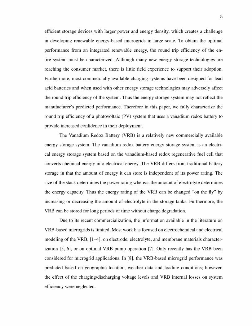
efficient storage devices with larger power and energy density, which creates a challenge

in developing renewable energy-based microgrids in large scale. To obtain the optimal

performance from an integrated renewable energy, the round trip efficiency of the en-

tire system must be characterized. Although many new energy storage technologies are

reaching the consumer market, there is little field experience to support their adoption.

Furthermore, most commercially available charging systems have been designed for lead

acid batteries and when used with other energy storage technologies may adversely affect

the round trip efficiency of the system. Thus the energy storage system may not reflect the

manufacturer’s predicted performance. Therefore in this paper, we fully characterize the

round trip efficiency of a photovoltaic (PV) system that uses a vanadium redox battery to

provide increased confidence in their deployment.

The Vanadium Redox Battery (VRB) is a relatively new commercially available

energy storage system. The vanadium redox battery energy storage system is an electri-

cal energy storage system based on the vanadium-based redox regenerative fuel cell that

converts chemical energy into electrical energy. The VRB differs from traditional battery

storage in that the amount of energy it can store is independent of its power rating. The

size of the stack determines the power rating whereas the amount of electrolyte determines

the energy capacity. Thus the energy rating of the VRB can be changed “on the fly” by

increasing or decreasing the amount of electrolyte in the storage tanks. Furthermore, the

VRB can be stored for long periods of time without charge degradation.

Due to its recent commercialization, the information available in the literature on

VRB-based microgrids is limited. Most work has focused on electrochemical and electrical

modeling of the VRB, [1–4], on electrode, electrolyte, and membrane materials character-

ization [5, 6], or on optimal VRB pump operation [7]. Only recently has the VRB been

considered for microgrid applications. In [8], the VRB-based microgrid performance was

predicted based on geographic location, weather data and loading conditions; however,

the effect of the charging/discharging voltage levels and VRB internal losses on system

efficiency were neglected.

5

In this paper, a complete PV-VRB microgrid is characterized holistically. The anal-

ysis is based on a prototype system installation deployed at Fort Leonard Wood, Missouri,

USA. Specifically, the following contributions are made in this paper:

• the characterization of the PV-VRB microgrid performance under different loading

and weather conditions,

• the development of a two-stage charging strategy for the VRB, and

• a quantification of the component efficiencies and their relationships.

II. MICROGRID SYSTEM DESCRIPTION

The microgrid system had been constructed to serve a standalone 5 kW (maximum)

AC load in a single building. As shown in Fig. 1, the electrical system is designed with a

48 VDC bus and a 120 VAC split-phase bus. The PV arrays and VRB are connected to the

DC bus whereas the utility grid and load circuits are connected to the AC bus through a

transfer switch. The inverter links the two buses to power the load on the AC side by using

renewable energy from the DC side. A PLC-controlled transfer switch is used to connect

the load to the grid when the renewable energy is not available and the energy storage is

depleted.

1.2

Solar Array 2

IV

2.2

MPPTI

1.3

Solar Array 3

IV

2.3

MPPTI

1.1

Solar Array 1

IV

2.1

MPPTI

SOLAR PANELS 48V DC BUS

V

CB

CB

CB

CB

CB

I

3

VRB

3SOC

ENERGY STORAGE

6

I

4

DC/AC LOAD

7

VacVac

INVERTER SUBPANEL

120V/240V AC SPLIT PHASE

BUS

CB

DC Current Measurement

AC Current Measurement

DC Voltage Measurement

AC Voltage Measurement

VRB State of Charge

Component Number

I

V

Vac

3SOCIac

LEGEND

Fig. 1: One-line diagram of the microgrid system

6

The PV array is constructed from 54 280 W solar panels (model Suntech STP280-

24/Vd) for a composite rating of 15 kW. The system is electrically divided into three 5 kW

PV arrays which are south facing and tilted at a fixed angle of 38 to match the latitude

of Fort Leonard Wood. Each of the arrays is connected to the DC bus through an Outback

FlexMax 80 MPPT/charge controller to track the PV maximum power point.

A 38-cell Prudent Energy VRB rated 5 kW/20 kWh is used for energy storage. The

capacity range of the VRB is specified as 20kWh at a SOC of 73% and 0kWh at a SOC

of 20%. It can be charged to a maximum voltage of 56.5 V and discharged to a minimum

voltage of 42 V. The VRB energy storage system is self-contained in an enclosure and

includes the electrolyte tanks, cell stacks, pumps, and controllers. The enclosure temper-

ature is regulated between 10 C and 30 C via an external heating, ventilation, and air

conditioning (HVAC) system.

The system is instrumented to measure environmental data including solar insola-

tion and temperature as well as the voltage and current parameters necessary for monitor-

ing, controlling its operation and characterizing its performance. Operational data was are

recorded using Campbell Scientific Model CR3000 and CR1000 dataloggers which sample

every 5s and average the values every 1min.

III. VANADIUM REDOX BATTERIES PERFORMANCE CHARACTERIZATION

A vanadium redox battery (shown in Fig. 2) is a flow-type battery that stores chem-

ical energy and generates electricity by reduction-oxidation (redox) reactions between dif-

ferent ionic forms of vanadium in the electrolytes [4]. The batteries are comprised of two

closed electrolyte circuits. In each circuit, the electrolyte is stored in a separate tank and

circulated via pumps through the cell stacks where the electrochemical reactions (1)-(2)

occur [9]. Table I contains a list of all nomenclature used in this section.

7

MonitorMonitor

Battery Controller

Inverter

Pump Pump

Cell Stack

Reference Cell Stack

Heat Exchanger Heat Exchanger

Negative Electrolyte

Tank

Positive Electrolyte

Tank+

_

Fig. 2: VRB schematic diagram

V O+2 + 2H+ + e−

dcV O2+ +H2O (1)

V 2+ dcV 3+ + e− (2)

The catholyte contains V O2+ and V O+2 ions and the anolyte contains V 3+ and

V 2+ ions suffused in a H2SO4 solution. During discharge, V 2+ is oxidized to V 3+ in the

negative half-cell producing electrons and protons. Protons diffuse through the membrane

while the electrons transfer through the electrical external circuit to the positive half-cell

where V O+2 is reduced to V O2+. The redox process occurs in reverse during the charge

cycle.

8

TABLE I: Nomenclature

Nc Number of cells in VRB stackCx Concentration of the species x in the electrolyte (mol/l)Vstack VRB stack voltage at terminals (V)Voc VRB open-circuit voltage (V)Eo VRB standard potential (V)Vloss VRB internal voltage loss∆Go Gibbs free enthalpy at standard condition (kJ/mol)∆Hr

o Reaction enthalpy at standard condition (-155.6 kJ/mol)∆Sr

o Reaction entropy at standard condition (-121.7 J/mol K)F Faraday constant (96485.3365 s A/mol)R Universal gas constant (8.3144621 J/mol K)T Electrolyte temperature (K)Ten VRB enclossure temperature (C)Tamb Ambient temperature (C)Istack VRB stack acurrent (A)Pload VRB load power (kW)Pcharge VRB charge power (kW)Pstack VRB load power at terminal (kW)Ppump VRB pump power (kW)PAC Air conditioner power (kW)ηv VRB efficiency with internal voltage lossηp VRB efficiency with parasitic loss

ηV RBd VRB total discharge efficiencyηV RBc VRB total charge efficiency

A. VRB State of Charge and Open-Circuit Voltage

The VRB charge and discharge operations depend on the state of charge, the load,

and the power produced by the PV array. The VRB’s state of charge is defined by the ratio

of the concentration of unoxidized vanadium (V 2+) to the total concentration of vanadium

(CV ). This is also the same as the ratio of vanadium oxide (CV O+2

) to the total concentration

(3):

SOC =CV 2+

CV

=CV O+

2

CV

(3)

The total concentration of vanadium is the sum of the vanadium ions which is the

9

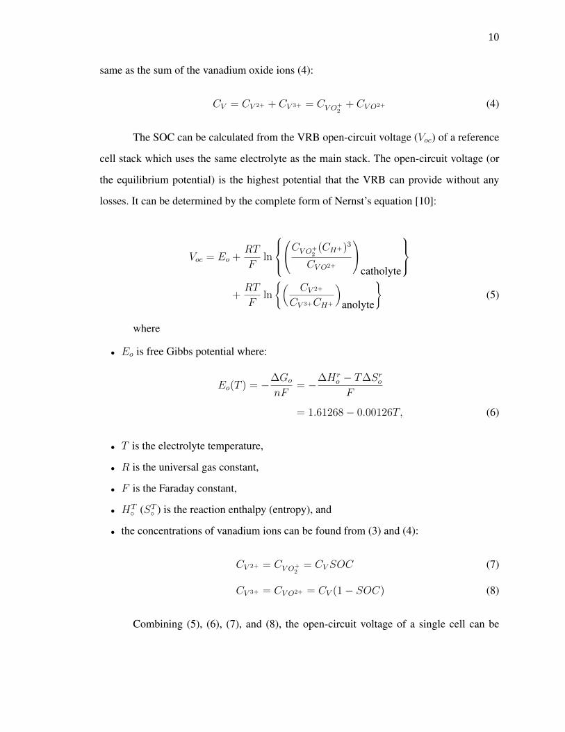
same as the sum of the vanadium oxide ions (4):

CV = CV 2+ + CV 3+ = CV O+2

+ CV O2+ (4)

The SOC can be calculated from the VRB open-circuit voltage (Voc) of a reference

cell stack which uses the same electrolyte as the main stack. The open-circuit voltage (or

the equilibrium potential) is the highest potential that the VRB can provide without any

losses. It can be determined by the complete form of Nernst’s equation [10]:

Voc = Eo +RT

Fln

CV O+

2(CH+)3

CV O2+

catholyte

+RT

Fln

(CV 2+

CV 3+CH+

)

anolyte

(5)

where

• Eo is free Gibbs potential where:

Eo(T ) = −∆Go

nF= −∆Hr

o − T∆Sro

F

= 1.61268− 0.00126T, (6)

• T is the electrolyte temperature,

• R is the universal gas constant,

• F is the Faraday constant,

• HT (ST

) is the reaction enthalpy (entropy), and

• the concentrations of vanadium ions can be found from (3) and (4):

CV 2+ = CV O+2

= CV SOC (7)

CV 3+ = CV O2+ = CV (1− SOC) (8)

Combining (5), (6), (7), and (8), the open-circuit voltage of a single cell can be

10

expressed as a function of SOC and temperature:

Voc = 1.61268− 0.00126T + 1.72× 10−4T ln(

SOC

1− SOC)

+ 1.72× 10−4T ln (f(SOC)) (9)

where f(SOC) is an emperically determined function of state of charge. The manufacturer

data sheet provides a SOC versus Voc at 25C. By fitting a curve through the manufacturer’s

data, f(SOC) can be found with a fitness (R2) of 0.999:

f(SOC) = −154.2SOC3 + 264.7SOC2 − 95.4SOC + 30.7 (10)

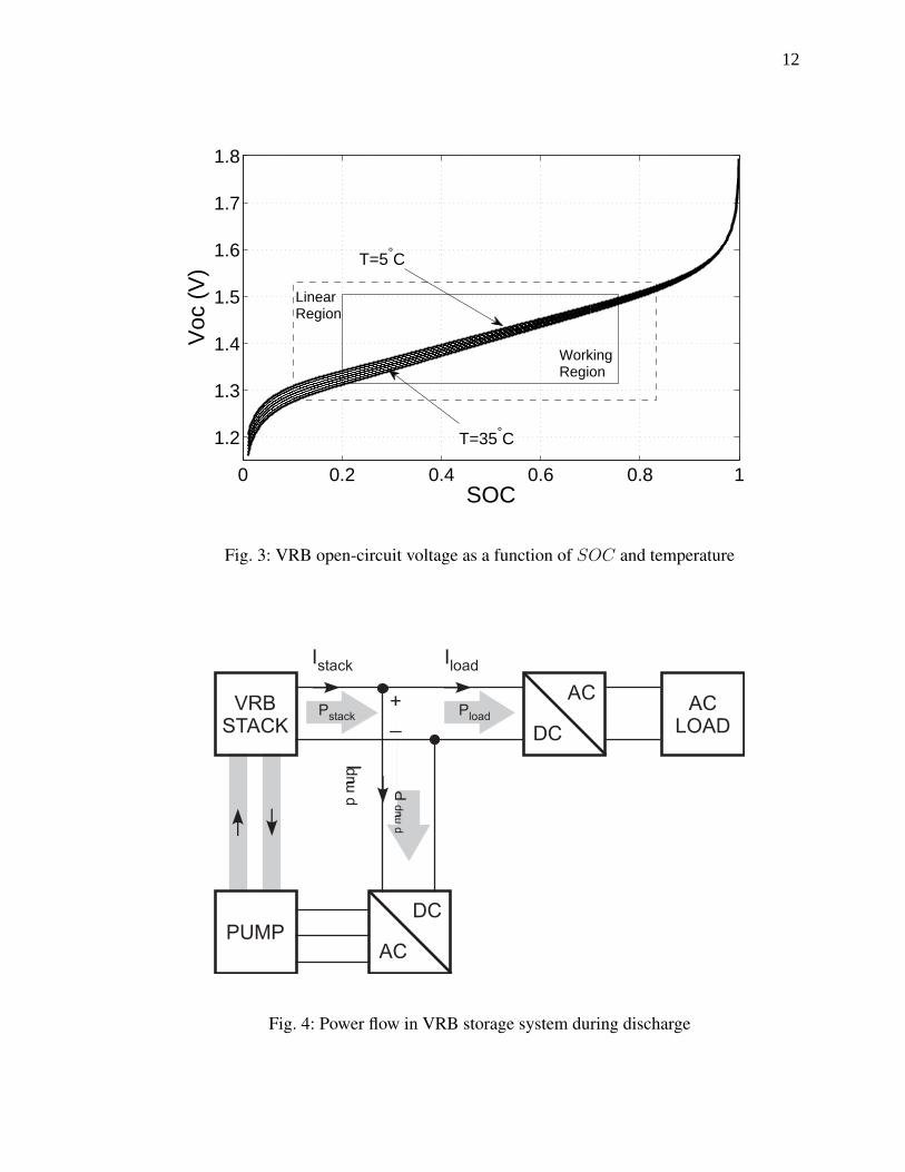
Fig. 3 shows a series of traces calculated at different temperatures of the single-cell

open-circuit voltage as a function of SOC using the function in (10). The upper curve is

measured at temperature of 5C and each lower trace is for an increase of 5C to the bottom

trace which is for T = 35C. In the area between SOC = 0.1 and SOC = 0.83, Voc and

SOC can be linearly correlated, therefore the single-cell Voc(T, SOC) in linear region can

be characterized as:

Voc(T, SOC) =T

1000(SOC − 1.1755) + 1.6123 (11)

Since the working region of the VRB lies within the linear region (as a function of temper-

ature), this relationship will be used when calculating the system efficiency.

B. VRB Discharge Performance

During discharge, the VRB supplies power to the load and to its own pumps as

shown in Fig. 4. To characterize the discharge performance of the VRB, the stack voltage,

the internal voltage losses and the parasitic losses are correlated to the stack current, the

load power, and the SOC and temperature.

1) VRB stack voltage and internal voltage loss: The VRB cell stack is composed of

38 cells in series. Due to the internal voltage losses, the VRB stack voltage is lower at higher

discharge current. The stack voltage is approximately proportional to the stack current at

11

0 0.2 0.4 0.6 0.8 1

1.2

1.3

1.4

1.5

1.6

1.7

1.8

SOC

Voc

(V

)

T=5°C

T=35°C

WorkingRegion

LinearRegion

Fig. 3: VRB open-circuit voltage as a function of SOC and temperature

Pp

um

p

PloadPstackVRB

STACK

PUMP

AC LOAD

AC

DC

DC

AC

Istack Iload

Ipu

mp

+_

Fig. 4: Power flow in VRB storage system during discharge

12

0 10 20 30 40 5045

46

47

48

49

50

51

52

53

Istack (A)

Vst

ack

(V)

SOC = 0.7

SOC = 0.35

x Measured data points__ Calculated curves at specific SOC

Fig. 5: Discharge voltage at different SOC

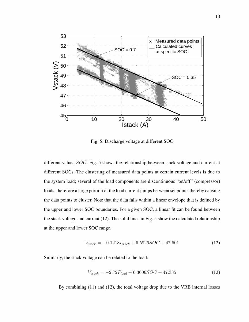
different values SOC. Fig. 5 shows the relationship between stack voltage and current at

different SOCs. The clustering of measured data points at certain current levels is due to

the system load; several of the load components are discontinuous “on/off” (compressor)

loads, therefore a large portion of the load current jumps between set points thereby causing

the data points to cluster. Note that the data falls within a linear envelope that is defined by

the upper and lower SOC boundaries. For a given SOC, a linear fit can be found between

the stack voltage and current (12). The solid lines in Fig. 5 show the calculated relationship

at the upper and lower SOC range.

Vstack = −0.1218Istack + 6.5926SOC + 47.601 (12)

Similarly, the stack voltage can be related to the load:

Vstack = −2.72Pload + 6.3606SOC + 47.335 (13)

By combining (11) and (12), the total voltage drop due to the VRB internal losses

13

0 0.5 1 1.5 20

0.5

1

1.5

2

2.5

Pload (kW)

Pst

ack

(kW

)

SOC = 0.7

SOC=0.5x Measured data points__ Calculated curves at specific SOC

Fig. 6: Discharge stack power at different SOC

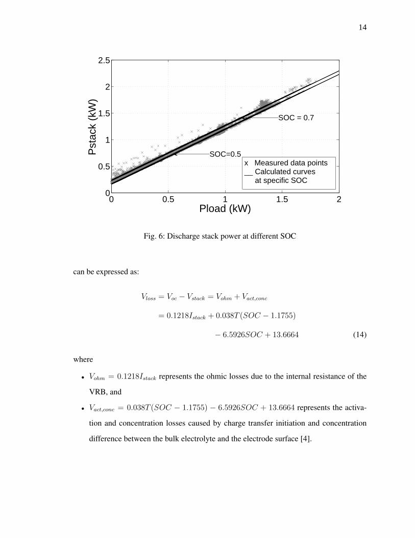
can be expressed as:

Vloss = Voc − Vstack = Vohm + Vact,conc

= 0.1218Istack + 0.038T (SOC − 1.1755)

− 6.5926SOC + 13.6664 (14)

where

• Vohm = 0.1218Istack represents the ohmic losses due to the internal resistance of the

VRB, and

• Vact,conc = 0.038T (SOC − 1.1755) − 6.5926SOC + 13.6664 represents the activa-

tion and concentration losses caused by charge transfer initiation and concentration

difference between the bulk electrolyte and the electrode surface [4].

14

0 0.5 1 1.5 20.82

0.84

0.86

0.88

0.9

0.92

0.94

0.96

Pload (kW)

Vol

tage

Effi

cien

cy

SOC=0.7, T=25°C

SOC=0.35, T=25°C x Measured data points__ Calculated curves at specific SOC

Fig. 7: Discharge voltage efficiency at different SOC

2) VRB parasitic losses: As shown in Fig. 6, the stack power is approximately

linear to the load power at a given SOC:

Pstack = 1.0334Pload + 1.727SOC2 − 1.737SOC + 0.596 (15)

The parasitic loss is the power required to run the pumps and the controller of the VRB. It

is calculated as the difference between the stack power and the load power:

Ppump = Pstack − Pload

≈ 0.0334Pload + 1.727SOC(SOC − 1) + 0.596 (16)

Note that at a specific load, the parasitic power is a quadratic function of SOC and its

minimum occurs when the SOC is approximately 0.5.

15

0 0.5 1 1.5 2 2.50

0.2

0.4

0.6

0.8

1

Pload (kW)

Out

put P

ower

Effi

cien

cy

SOC=0.5

SOC=0.7


Fig. 8: Discharge power efficiency at different SOC and temperature

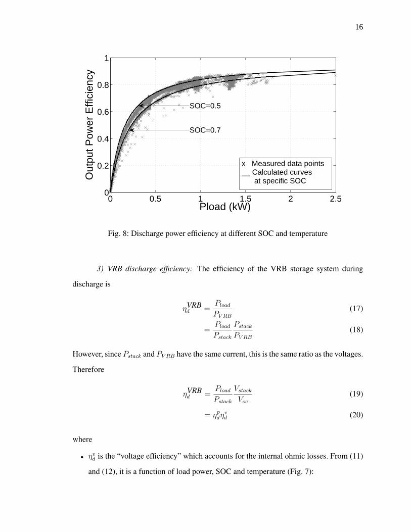
3) VRB discharge efficiency: The efficiency of the VRB storage system during

discharge is

ηVRBd =

Pload

PV RB

(17)

=Pload

Pstack

Pstack

PV RB

(18)

However, since Pstack and PV RB have the same current, this is the same ratio as the voltages.

Therefore

ηVRBd =

Pload

Pstack

VstackVoc

(19)

= ηpdηvd (20)

where

• ηvd is the “voltage efficiency” which accounts for the internal ohmic losses. From (11)

and (12), it is a function of load power, SOC and temperature (Fig. 7):

16

0 0.5 1 1.5 2 2.50

0.2

0.4

0.6

0.8

Pload (kW)

Tot

al D

isch

arge

Effi

cien

cySOC=0.5, T=25°C

SOC=0.35, T=25°C

SOC=0.7, T=25°C


Fig. 9: VRB total discharge efficiency at different SOC and temperature

ηvd =VstackVoc

=−2.72Pload + 6.3606SOC + 47.335

0.038T (SOC − 1.1755) + 61.2674(21)

• ηpd is the output power efficiency which accounts for the parasitic losses. From (15), it

is characterized as a function of load power and SOC (Fig. 8):

ηpd =Pload

Pstack

=Pload

1.0334Pload + 1.727SOC(SOC − 1) + 0.596(22)

The combined efficiencies are shown in Fig. 9. Note that the total discharge effi-

ciency is maximum when the SOC is 0.5 with a maximum discharge efficiency of 78%.

The VRB is most efficient under heavy load and is dominated by the parasitic losses as

opposed to the ohmic losses. This is due to the pumps having to circulate the electrolyte

even during low discharge currents.

17

4) Inverter efficiency: During discharge, the VRB supplies power to the AC load

through an inverter. From measured operation, the linear correlation between the input and

the output power of the inverter was fit resulting in (23) with R2 = 0.988.

P acload = 0.991P dc

load − 0.0574 (23)

The inverter efficency is therefore characterized:

ηINV = 0.991− 0.0574

P dcload

= 0.991− 0.0574

1.0091P acload + 0.0579

(24)

C. VRB Charge Performance

Fig. 10: Power flow in VRB storage system during charge

In the microgrid system, the power from the PV arrays is used to charge the VRB

storage system. When PV power is available, but not high enough to run the VRB pumps,

the VRB cannot start to charge, therefore the charging current is zero. The parasitic power

is around 500W to maintain the minimum flow rate of the electrolyte. When the available

PV power is higher than the parasitic power, the VRB will start to charge. Commercially

available battery chargers operate by charging in one of several modes to avoid overcharg-

ing the battery. Furthermore, many charge controllers for PV-battery systems also include a

18

DC voltage

DC current

Bulk Absorb Float

Charging Begins

Fig. 11: Typical battery charge regions

0 10 20 30 40 5049

50

51

52

53

54

55

Istack (A)

Vst

ack

(V)


SOC=0.35

SOC=0.7

Fig. 12: Charge voltage at different SOC

maximum power point tracker (MPPT) to extract the maximum power from the PV panels.

These regions are shown in Fig. 11 and summarized:

• Bulk: when the VRB stack voltage is lower than the absorb voltage, the MPPT/charge

controller tracks the maximum PV power and charges the VRB with the maximum

19

current. The absorb voltage level can be set by the user at different levels from 55V to

56.5V .

• Absorb: when the VRB stack voltage reaches the absorb voltage set point, the MPPT/charge

controller regulates the stack voltage and charges the VRB at a constant voltage.

1) VRB bulk stage: During the bulk stage, the larger current the current produced

by the PV, the faster the VRB is charged. Fig. 12 shows that the stack voltage in bulk

stage is approximately linear to the stack current. The (Vstack, Istack) and (Vstack, Pcharge)

correlations are given by:

Vstack = (0.166SOC + 0.054)Istack + 7.27SOC + 47.85 (25)

Vstack = (1.895SOC + 1.552)Pcharge + 6.82SOC + 46.79 (26)

Combining (11) and (25), the internal voltage loss is characterized as a function

of the stack current and SOC in (27). In this case, the internal resistance is linear to the

SOC due to the ionic effect which opposes the flow of charges in the electrolyte and the

membrane [4].

Vloss = Vstack − Voc

Vloss = (0.166SOC + 0.054)Istack + 7.27SOC

− 0.038T (SOC − 1.1755)− 13.42

(27)

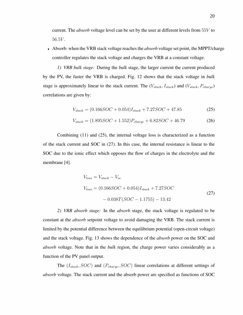
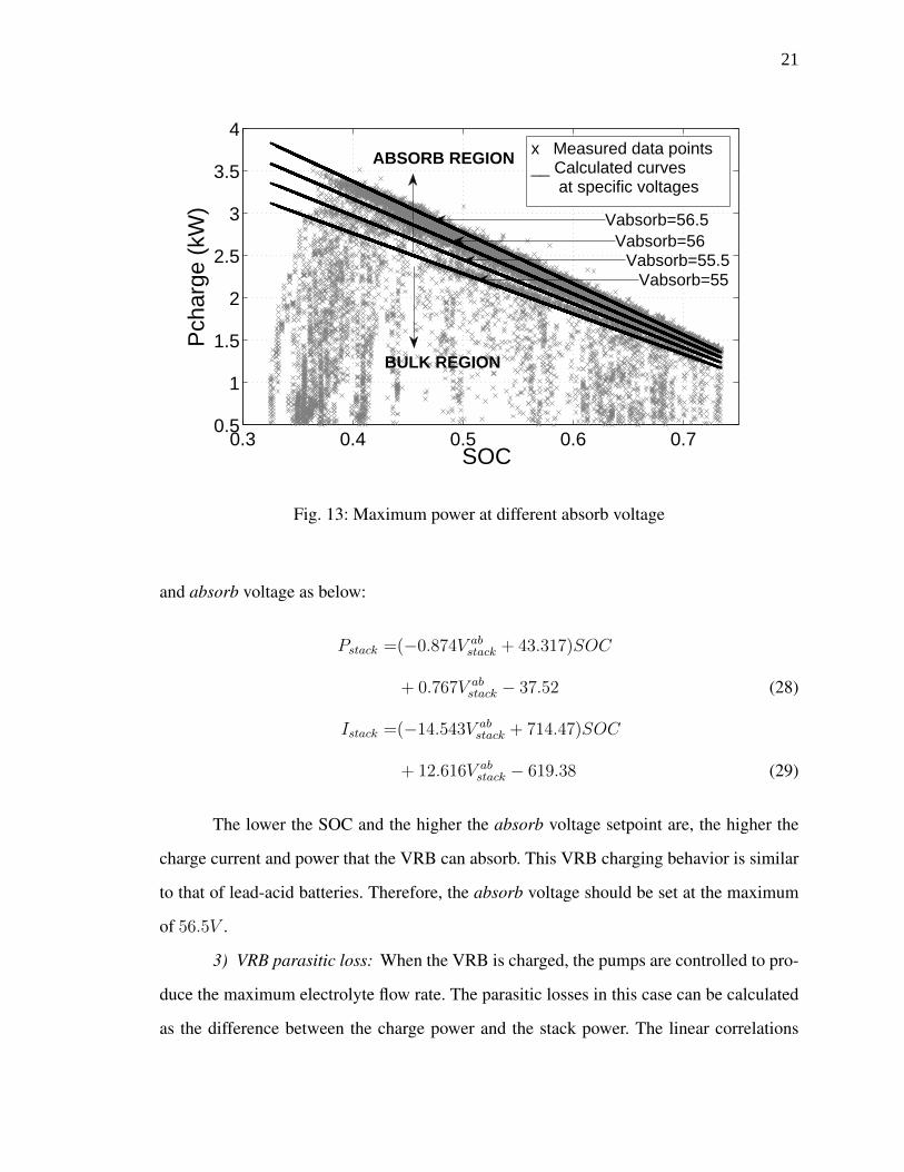
2) VRB absorb stage: In the absorb stage, the stack voltage is regulated to be

constant at the absorb setpoint voltage to avoid damaging the VRB. The stack current is

limited by the potential difference between the equilibrium potential (open-circuit voltage)

and the stack voltage. Fig. 13 shows the dependence of the absorb power on the SOC and

absorb voltage. Note that in the bulk region, the charge power varies considerably as a

function of the PV panel output.

The (Istack, SOC) and (Pcharge, SOC) linear correlations at different settings of

absorb voltage. The stack current and the absorb power are specified as functions of SOC

20

0.3 0.4 0.5 0.6 0.70.5

1

1.5

2

2.5

3

3.5

4

SOC

Pch

arge

(kW

)

x Measured data points__ Calculated curves at specific voltages

ABSORB REGION

BULK REGION

Vabsorb=56.5Vabsorb=56

Vabsorb=55.5Vabsorb=55

Fig. 13: Maximum power at different absorb voltage

and absorb voltage as below:

Pstack =(−0.874V abstack + 43.317)SOC

+ 0.767V abstack − 37.52 (28)

Istack =(−14.543V abstack + 714.47)SOC

+ 12.616V abstack − 619.38 (29)

The lower the SOC and the higher the absorb voltage setpoint are, the higher the

charge current and power that the VRB can absorb. This VRB charging behavior is similar

to that of lead-acid batteries. Therefore, the absorb voltage should be set at the maximum

of 56.5V .

3) VRB parasitic loss: When the VRB is charged, the pumps are controlled to pro-

duce the maximum electrolyte flow rate. The parasitic losses in this case can be calculated

as the difference between the charge power and the stack power. The linear correlations

21

0.5 1 1.5 2 2.5 3 3.5 40.91

0.92

0.93

0.94

0.95

0.96

0.97

0.98

0.99

1

Pload (kW)

Vol

tage

Effi

cien

cy


SOC=0.7, T=25°C

SOC=0.35, T=25°C

Fig. 14: Charge voltage efficiency at different SOC and temperature

between Pstack and Pcharge at different SOC are characterized as:

Pstack = (−0.128SOC + 1.05)Pcharge + 0.19SOC − 0.59 (30)

Ppump = Pcharge − Pstack

≈ (0.128SOC − 0.05)Pcharge − 0.19SOC + 0.59 (31)

4) VRB charge efficiency: Similar to the discharge efficiency, the charge efficiency

of the VRB storage system is calculated based on the voltage efficiency and the input power

efficiency:

ηV RBc = ηvcη

pc (32)

in which

22

0 1 2 3 40

0.2

0.4

0.6

0.8

1

Pcharge (kW)

Inpu

t Pow

er E

ffici

ency

SOC=0.35

SOC=0.7x Measured data points__ Calculated curves at specific SOC

Fig. 15: Charge power efficiency at different SOC

• the voltage efficiency ηvc can be found based on (11) and (26)

ηvc =VocVstack

=0.038T (SOC − 1.1755) + 61.2674

(1.895SOC + 1.552)Pcharge + 6.82SOC + 46.79(33)

• the input power efficiency ηpc can be specified from (30)

ηpc =Pstack

Pcharge

=(−0.128SOC + 1.05)Pcharge + 0.19SOC − 0.59

Pcharge

(34)

As shown in Fig. 16, the maximum charge efficiency is around 80%. When the

available PV power is less than 500W, the charge efficiency is zero due to the VRB parasitic

loss.

23

0 1 2 3 40

0.2

0.4

0.6

0.8

Pcharge (kW)

Tot

al C

harg

e E

ffici

ency


SOC=0.7, T=25°C

SOC=0.35, T=25°C

Fig. 16: VRB total charge efficiency at different SOC and temperature

5) MPPT charger efficiency: The MPPT chargers are used to track the maximum

PV power and charge the VRB. The MPPT input and output power are correlated in (35):

P outMPPT = 0.989P in

MPPT − 0.124 (35)

The MPPT efficiency is specified as:

ηMPPT =P outMPPT

P inMPPT

= 0.989− 0.124

1.0111P outMPPT + 0.1253

(36)

D. VRB Heating Ventilation and Air Conditioning (HVAC)

Enviromental controls are required for the VRB storage system to operate properly.

Freezing temperatures can hinder electrolyte flow, whereas high temperatures can damage

the VRB membrane and cause overheating of the electrical equipment. In this system, VRB

enclosure temperature is regulated between 10C and 30C by a built-in HVAC system that

includes a cooling-heating air conditioner and ventilation fans. The temperature control

scheme is:

24

• Heating is ON when the enclosure temperature is lower than 10C.

• Fans are ON when the enclosure temperature is between 25C and 30C.

• Cooling is ON when the enclosure temperature is greater than 30C.

The fans’ load is a constant 300W . The air conditioner load had been characterized in [8]

as:

PAC = (0.00313)|Ten(Tamb − Ten)|+ 0.4125 (37)

where Ten is the VRB enclosure temperature and Tamb is the external ambient temperature.

Fig. 17: Microgrid system performance in May 2013

IV. MICROGRID SYSTEM PERFORMANCE

The microgrid system is designed to operate in either a grid or renewable mode.

• Renewable mode: the load is powered by the VRB and by available PV power. This

mode occurs when VRB is serving the load and the SOC > 0.35, or when there is

sufficient PV power and the VRB is charging and SOC > 0.55. The system switches

from this mode to grid mode when the VRB is discharging and the SOC falls below

0.35.

• Grid mode: the load is powered by the utility grid and the VRB is charged by available

PV power. The system remains operating in this mode until the VRB SOC reaches

0.65.

25

0 2 4 6 8 10 12 14 16 18 20 220

5

10

15

Time of Day

Pow

er (

kW)

PpvPmppt,outPinv,outPgrid

GridMode

Renewable Mode

PPV

Renewable Mode

Pinv P

grid

PMPPT

Pinv

Fig. 18: PV and load power profile on 7 May 2013

The system operating characteristics and efficiencies can be predicted based on

SOC, charge power and load power as presented in Section III. A case study has been

performed based on field data taken in May 2013. During this period, the system is serving a

2 kW (peak) load. The inputs of the prediction model are daily load power profile, available

PV power profile and the initial SOC. At each time step (1 min), the system operating

characteristics, the losses in the system, transfer switch status, and SOC are updated. The

measured performance for the month of May 2013 is shown in Fig. 17. The upper trace is

the power from the charge controller, the lower trace is the power from the VRB (negative

indicates charging), and the middle black trace is the load power. A typical day is shown in

the inset to provide greater detail.

The actual cumulative data and predicted data of a typical day in May (7 May)

have been plotted in Figs. 18-21. Note that this was a sunny day with intermittent cloud

cover. The effect of the compressor load can be clearly seen in the various powers. From

the results, whole-day period can be analyzed in three main periods as indicated in Fig. 18:

26

00 02 04 06 08 10 12 14 16 18 20 22 2444

46

48

50

52

54

56

58

Time of Day

VR

B S

tack

vol

tage

(V

)

MeasuredPredicted

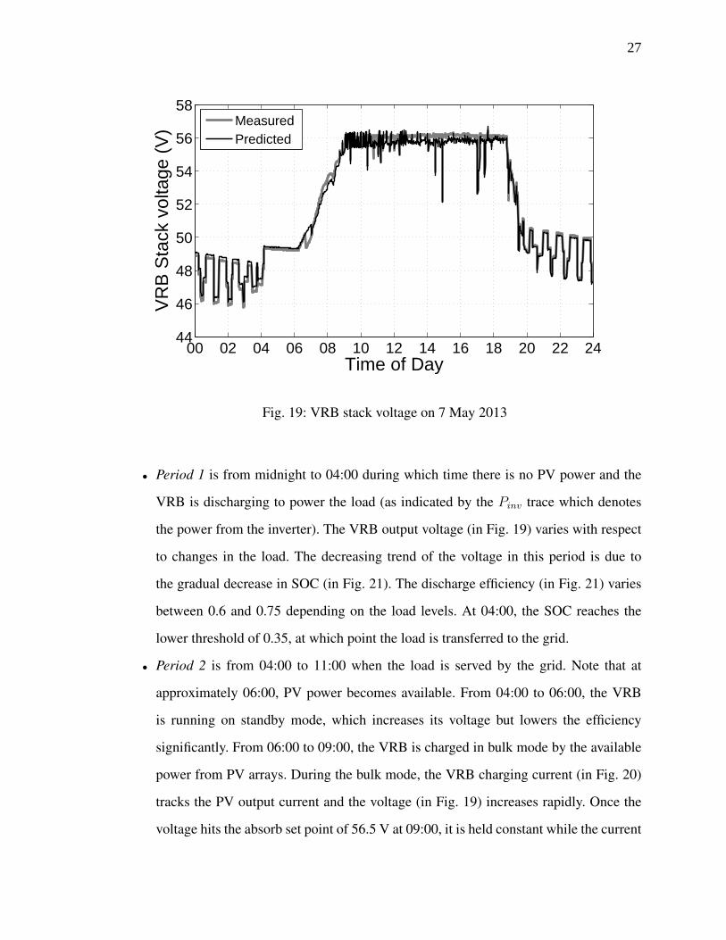
Fig. 19: VRB stack voltage on 7 May 2013

• Period 1 is from midnight to 04:00 during which time there is no PV power and the

VRB is discharging to power the load (as indicated by the Pinv trace which denotes

the power from the inverter). The VRB output voltage (in Fig. 19) varies with respect

to changes in the load. The decreasing trend of the voltage in this period is due to

the gradual decrease in SOC (in Fig. 21). The discharge efficiency (in Fig. 21) varies

between 0.6 and 0.75 depending on the load levels. At 04:00, the SOC reaches the

lower threshold of 0.35, at which point the load is transferred to the grid.

• Period 2 is from 04:00 to 11:00 when the load is served by the grid. Note that at

approximately 06:00, PV power becomes available. From 04:00 to 06:00, the VRB

is running on standby mode, which increases its voltage but lowers the efficiency

significantly. From 06:00 to 09:00, the VRB is charged in bulk mode by the available

power from PV arrays. During the bulk mode, the VRB charging current (in Fig. 20)

tracks the PV output current and the voltage (in Fig. 19) increases rapidly. Once the

voltage hits the absorb set point of 56.5 V at 09:00, it is held constant while the current

27

00 02 04 06 08 10 12 14 16 18 20 22 24−60

−40

−20

0

20

40

60

Time of Day

VR

B O

utpu

t Cur

rent

(A

)

MeasuredPredicted

DISCHARGE DISCHARGE

BULK

CHARGE

ABSORB

Fig. 20: VRB output current on 7 May 2013

slowly decreases

• Period 3 is from 11:00 to 12:00 when the load is served by the renewable system

again. From 11:00 to 19:00, the PV power is sufficient to simultaneously charge the

VRB and serve the load. During this period, the charging efficiency is at its maximum

because the VRB is charged at its maximum rate. After 19:00, the VRBs SOC is high

enough to discharge when there is no PV power.

The actual and predicted system performance of May 2013 are given in Tab. II.

In Tab. II, the renewable system efficiency is the ratio between the renewable part of

load energy and the PV energy taken by the system. Note from Fig. 18 that far more power

is available from the PV system than is being utilized and that the PV utilization factor is

42% which indicates that the PV system is too large for the load and storage system. The

system efficiency can be improved by serving a larger load, because at higher load the VRB

is more efficient and also more direct PV power can be used. The time in Grid mode could

also be reduced with a larger storage system.

28

00 02 04 06 08 10 12 14 16 18 20 22 240

0.2

0.4

0.6

0.8

1

Time of Day

VR

B E

ffici

ency

MeasuredPredicted

SOC

Fig. 21: VRB efficiency on 7 May 2013

V. VRB GENERALIZED PER-UNIT MODEL

VRB systems in practice are highly scalable due to the fact that high-power and

high-capacity VRB systems are normally built by integrating a number of small standard-

ized VRB modules of which power and capacity are determined by the number of cells

TABLE II: Microgrid System Performance in May 2013

Actual (kWh) Predicted (kWh)Available PV energy 1857 −

PV energy taken by the system 787 805Energy consumed by the load 493 −Energy provided by the grid 145 143

VRB internal loss 43 45VRB parasitic loss 198 202

HVAC loss 58 70PV utilization factor 42% 43%

Renewable system efficiency 51.65% 50.55%

29

and the size of electrolyte tanks. Therefore, VRB system models should also be scalable.

Therefore, the results in Section IV are generalized by converting the models from absolute

to per-unit values.

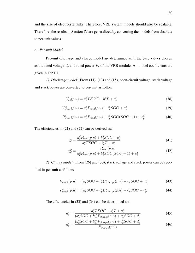
A. Per-unit Model

Per-unit discharge and charge model are determined with the base values chosen

as the rated voltage Vr and rated power Pr of the VRB module. All model coefficients are

given in Tab.III

1) Discharge model: From (11), (13) and (15), open-circuit voltage, stack voltage

and stack power are converted to per-unit as follow:

Voc(p.u) = aovTSOC + bovT + cov (38)

V dstack(p.u) = advPload(p.u) + bdvSOC + cdv (39)

P dstack(p.u) = adpPload(p.u) + bdpSOC(SOC − 1) + cdp (40)

The efficiencies in (21) and (22) can be derived as:

ηvd =advPload(p.u) + bdvSOC + cdv

aovTSOC + bovT + cov(41)

ηpd =Pload(p.u)

adpPload(p.u) + bdpSOC(SOC − 1) + cdp(42)

2) Charge model: From (26) and (30), stack voltage and stack power can be spec-

ified in per-unit as follow:

V cstack(p.u) = (acvSOC + bcv)Pcharge(p.u) + ccvSOC + dcv (43)

P cstack(p.u) = (acpSOC + bcp)Pcharge(p.u) + ccpSOC + dcp (44)

The efficiencies in (33) and (34) can be determined as:

ηvc =aovTSOC + bovT + cov

(acvSOC + bcv)Pcharge(p.u) + ccvSOC + dcv(45)

ηpc =(acpSOC + bcp)Pcharge(p.u) + ccpSOC + dcp

Pcharge(p.u)(46)

30

TABLE III: VRB per-unit model coefficients

aik bik cik dik

(i, k) = (o, v) 0.001Nc

Vr

−1.1755Nc

Vr

1.6123Nc

Vr−

(i, k) = (d, v) −2.72Pr

Vr

6.3606Vr

47.335Vr

−

(i, k) = (d, p) 1.0334 1.127Pr

0.596Pr

−

(i, k) = (c, v) 1.895Pr

Vr

1.552Pr

Vr

6.82Vr

46.79Vr

(i, k) = (c, p) −0.128 1.05 0.19Pr

−0.59Pr

B. Validity Domain of the Model

The experimental data presented in this paper were sampled every 5 s and averaged

over a 1-min window, therefore the developed VRB model is valid when considering loads

and changes in solar insolation that change in this time frame. Fast transients in load and

switching operations may possibly lead to changes in efficiency due to heating or other

effects that would not be captured in this model. For example, the effects of a load spike

or isolated cloud cover may not be captured if these phenomena do not last longer than 5

s. Furthermore, this model has not been validated in extreme temperature ranges. Although

the effect of the HVAC system was modeled, there may be additional aspects to consider

during extremely hot or cold weather.

The models are valid regardless of whether the system is gridconnected or islanded.

During islanded operation, the load would not be served during VRB stand-by mode and

the efficiency of the system would be impacted. For an analysis of how the model may

perform at different latitudes, the interested reader is referred to an earlier analysis that

addresses some of these issues [8]

VI. CONCLUSIONS AND FUTURE WORK

In this paper, a PV-VRB microgrid system performance has been characterized.

The system operating characteristics, losses, and efficiencies are quantified and formulated

31

based on measured data. The VRB discharge and charge efficiencies are found to be non-

linear with the load/charge power. Based on the system characterization, a scalable model

has been built to accurately predict the system behavior and performance. A case study

has been performed for May 2013. The storage size is shown to be too small to utilize the

available PV power. Future work in this area will include optimizing the size of the PV-

VRB system to maximize the PV utilization and also in control strategies to maximize the

efficiency of the system.

Acknowledgments

The authors gratefully acknowledge the financial support of the Army Corps of

Engineers under contract W9132T-12-C-0016.

References

[1] J. Chahwan, C. Abbey, and G. Joos, “VRB modelling for the study of output terminal

voltages, internal losses and performance,” in Electrical Power Conference, 2007.

EPC 2007. IEEE Canada, Oct. 2007, pp. 387 –392.

[2] T. Nguyen, X. Qiu, T. Gamage, M. L. Crow, B. McMillin, and A. C. Elmore,

“Microgrid application with computer models and power management integrated

using PSCAD/EMTDC,” Proc. North Amer. Power Symp., 2011.

[3] L. Barote, C. Marinescu, and M. Georgescu, “VRB modeling for storage in stand-

alone wind energy systems,” in PowerTech, 2009 IEEE Bucharest, July 2009.

[4] C. Blanc and A. Rufer, “Multiphysics and energetic modeling of a vanadium redox

flow battery,” in IEEE 2008 International Conference on Sustainable Energy Tech-

nologies, Nov. 2008, pp. 696 –701.

[5] M. Vijayakumar, L. Li, Z. Nie, Z. Yang, and J. Z. Hu, “Structure and stability of hexa-

aqua v(iii) cations in vanadium redox flow battery electrolytes,” Physical Chemistry

Chemical Physics, vol. 14, 2010.

[6] M. Vijayakumar, L. Li, G. Graff, J. Liu, H. Zhang, Z. Yang, and J. Z. Hu, “Towards

understanding the poor thermal stability of v5+ electrolyte solution in vanadium redox

flow batteries,” Journal of Power Sources, vol. 196, no. 7, pp. 3669 – 3672, 2011.

32

[7] X. Ma, H. Zhang, C. Sun, Y. Zou, and T. Zhang, “An optimal strategy of electrolyte

flow rate for vanadium redox flow battery,” Journal of Power Sources, vol. 203, pp.

153 – 158, 2012.

[8] J. Guggenberger, A. C. Elmore, J. Tichenor, and M. L. Crow, “Performance prediction

of a vanadium redox battery for use in portable, scalable microgrids,” IEEE Transac-

tions on Smart Grid, vol. 3, no. 4, 2012.

[9] M. Li and T. Hikihara, “A coupled dynamical model of redox flow battery based on

chemical reaction, fluid flow, and electrical circuit,” IEICE Transactions, vol. 91-A,

no. 7, pp. 1741–1747, 2008.

[10] K. Knehr and E. Kumbur, “Open circuit voltage of vanadium redox flow batteries:

Discrepancy between models and experiments,” Electrochemistry Communications,

vol. 13, no. 4, pp. 342 – 345, 2011.

33

II. OPTIMAL SIZING OF A VANADIDUM REDOX BATTERY SYSTEM FORMICROGRID SYSTEMS

Tu A. Nguyen, M. L. Crow, IEEE Fellow, and A. C. Elmore∗


∗Department of Geological Engineering


Abstract

The vanadium redox battery (VRB) has proven to be a reliable and highly-

efficient energy storage system for microgrid applications. However, one challenge in

designing a migrogrid system is specifying the size of the energy storage system. This

selection is made more complex due to the independent power and energy ratings inherent

in VRB systems. Sizing a VRB for both required power output and energy storage

capacity requires an in-depth analysis to produce both optimal scheduling capabilities

and minimum capital costs. This paper presents an analytical method to determine the

optimal ratings of VRB energy storage based on an optimal scheduling analysis and

cost-benefit analysis for microgrid applications. A dynamic programming algorithm is

used to solve the optimal scheduling problem considering the efficiency and operating

characteristics of the VRBs. The proposed method has been applied to determine the

optimal VRB power and energy ratings for both isolated and grid-connected microgrids

which contain PV arrays and fossil-fuel-based generation. We first consider the case in

which a grid-tie is not available and diesel generation is the backup source of power.

The method is then extended to consider the case in which a utility grid tie is available.

Index Terms

Microgrids, renewable energy, energy storage, vanadium redox battery, optimal

scheduling, optimal sizing

34

I. INTRODUCTION

The integration of renewable energy resources in microgrids has been increasing

in the recent decades. Higher penetration of renewable energy is an environmentally-

friendly solution for improving the reliability and decreasing costs of microgrid systems.

Renewable power sources are typically highly variable depending on weather conditions,

thereby necessitating the use of highly-efficient and rapid response energy storage systems

(ESS) to store the surplus renewable energy and re-dispatch that energy when needed.

One of the most recent ESS technologies commercially available is the vanadium redox

battery (VRB). The VRB exhibits many advantages over many traditional battery storage

systems; the VRB has independent power and energy ratings, quick charge and discharge

response, high efficiency, long life cycle, low self-discharge, and an easily estimated state

of charge. By proper control and scheduling of the VRB system, the microgrid operating

costs can be significantly reduced. However, the initial capital and maintenance costs for

the VRB are still relatively high in comparison to other energy storage systems (such as

lead acid batteries) [1]. Therefore it is imperative to size and operate the VRB such that

the reduction in operating costs can justify the increase in the capital investment. In this

paper, the operating cost can be characterized as a function of VRB ratings (both power

and energy) to better quantify the cost-benefit analyses.

Although a number of studies have been conducted on the ESS sizing problem

for microgrids, most work has focused on lead-acid or Li-on batteries [2–5]. In [6],

the relationship between the ESS capacity and daily operating cost is found by solving

the unit commitment problem for the microgrid. In [1], the problem is similarly solved

with additional reliability constraints. The cost analysis to determine the optimal size of a

compressed-air storage system for large scale wind farms was introduced in [7]. The cost

sensitivity of varying ESS sizes and technologies for wind-diesel systems was analyzed

in [8]. However, in these previous analyses, the ESS charge and discharge efficiencies

were often neglected or considered as constants, furthermore the charging limit of the

batteries under different conditions of the state of charge (SOC) and charging voltage

35

was not considered. We extend these earlier works to include these oversights.

As opposed to other ESS, the VRB’s charge/discharge efficiencies can be char-

acterized as explicit non-linear functions of charge/discharge power and the SOC [9].

Furthermore, the VRB’s power and energy ratings are independently scalable, which

allows better flexibility in sizing the VRB for microgrid systems. Therefore, this paper

focuses on the optimal sizing of power and energy ratings for a VRB system in isolated

and grid-connected microgrids. An analytical method is developed to solve the problem

based on a per-day cost model in which the operating cost is obtained from optimal

scheduling. The charge, discharge efficiencies, and operating characteristics of the VRB

are considered in the problem. Case studies are performed under different conditions of

load and solar insolation.

II. FORMULATION OF THE OPTIMAL SIZING PROBLEM FOR VRB MICRO-GRIDS

A. Problem Definition

In this paper, the optimal size of the VRB is defined as the independent power

and the energy ratings required to minimize the total cost per day. The cost per day is

determined by:

TC = TCPD +OC − TB (1)

where TCPD is the total capital cost amortized per day for the VRB, OC is the total

operating cost of the system in that day, and TB is the total benefit achieved by selling

the extra renewable energy to the grid. If isolated microgrids are considered, then TB is

zero.

The following data are given as inputs to the formulation:

• Maximum and minimum load power,

• Power rating of the PV arrays and the diesel generators,

• Historical hourly insolation profile for the site,

36

• Buying and selling prices of the utility’s electricity.

The system constraints are:

• R1: The primary system load will always be met. This ensures that the high priority

(primary) loads of the system are always served. The primary loads have been

identified prior to microgrid deployment.

• R2: Sufficient energy capacity will always be held in reserve to meet essential load

demand if fuel becomes unavailable. This constraint ensures that if the fuel supply

is compromised (through disaster, inclement weather, etc.), there is enough energy

reserve to serve the primary load for a pre-specified length of time (typically between

1 hour and 36 hours).

• R3: The VRB is not charged (or discharged) beyond the maximum (or minimum)

recommended efficiency and/or operational SOC limits. To achieve optimal per-

formance, the VRB is not allowed to operate if its efficiency drops below a pre-

determined threshold.

• R4: The charging rate is limited by the absorb power. The charging rate of the

VRB is limited by electrochemical processes which depend on both the VRB SOC

and the voltage. This constraint ensures that the charging rate conforms to physical

limitations.

• R5: The VRB is charged only by the PV array. One of the primary objectives of

a microgrid is to minimize the amount of fossil fuel used, therefore the VRB may

only be charged via renewable resources and not by the diesel generator or the utility

grid tie.

• R6: The diesel generator is not operated at light load. The diesel generators are

most efficient when heavily loaded, therefore it is preferred to run fewer generators

at higher output.

• R7: Once a generator is started (or shut down) it remains online (or offline) a

minimum time before changing its status. This constraint minimizes “chopping”

(discontinuous operation) around breakpoints.

37

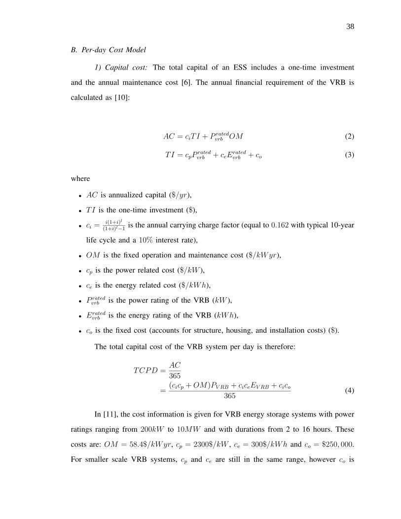
B. Per-day Cost Model

1) Capital cost: The total capital of an ESS includes a one-time investment

and the annual maintenance cost [6]. The annual financial requirement of the VRB is

calculated as [10]:

AC = ciTI + P ratedvrb OM (2)

TI = cpPratedvrb + ceE

ratedvrb + co (3)

where

• AC is annualized capital ($/yr),

• TI is the one-time investment ($),

• ci =i(1+i)l

(1+i)l−1is the annual carrying charge factor (equal to 0.162 with typical 10-year

life cycle and a 10% interest rate),

• OM is the fixed operation and maintenance cost ($/kWyr),

• cp is the power related cost ($/kW ),

• ce is the energy related cost ($/kWh),

• P ratedvrb is the power rating of the VRB (kW ),

• Eratedvrb is the energy rating of the VRB (kWh),

• co is the fixed cost (accounts for structure, housing, and installation costs) ($).

The total capital cost of the VRB system per day is therefore:

TCPD =AC

365

=(cicp +OM)PV RB + ciceEV RB + cico

365(4)

In [11], the cost information is given for VRB energy storage systems with power

ratings ranging from 200kW to 10MW and with durations from 2 to 16 hours. These

costs are: OM = 58.4$/kWyr, cp = 2300$/kW , ce = 300$/kWh and co = $250, 000.

For smaller scale VRB systems, cp and ce are still in the same range, however co is

38

smaller due to the smaller structure, housing, and installation costs. In this paper, co is

estimated to be $25, 000 for a 10kW -scale system (Fig. 1).

0 10 20 30 40 50 6015

20

25

30

Evrb

(kWh)

TC

PD

($)

Pvrb

=10 kW

Pvrb

=5 kW

Fig. 1: Total capital cost per day for a 10kW-scale system

2) Operating cost: For an isolated PV-diesel microgrid, the operating cost is the

daily fuel cost of the diesel generators. For a grid-connected microgrid, the operating

cost is the sum of the diesel fuel costs and the cost of the grid electricity. The expected

operating cost can be determined:

• For an isolated microgrid:

OC =N∑k=1

[m∑i=1

CdgiHdgi(Pdgi,k)T

](5)

• For a grid-connected microgrid:

OC =N∑k=1

[m∑i=1

CdgiHdgi(Pdgi,k)T + Cbuy,kPgrid,kT

](6)

where

• N is the number of time periods in a one day cycle,

• T is duration of each time period,

• m is the number of diesel generators,

• Hdgi(gal/h), which is a function of Pdgi,k, is the fuel consumption of diesel generator

i,

• Cdgi($/gal) is the fuel price for diesel generator i,

39

• Cbuy,k($/kWh) is the electricity buying price in time period k,

• Pdgi,k is the dispatched power for diesel generator i in time period k, and

• Pgrid,k is the power supplied by the grid in time period k.

3) Benefit: For a grid-connected microgrid, the unused renewable power can be

sold to the grid as a benefit. The total benefit per day is then:

• For an isolated microgrid:

TB = 0 (7)

• For a grid-connected microgrid:

TB =N∑k=1

Csell,kPext,kT (8)

in which

• Csell,k($/kWh) is the electricity selling price in time period k, and

• Pextra,k is the power sold to the grid in time period k.

C. Problem Formulation

From equations (4) and (6), the objective function is:

min(TC) = min(TCPD +OC − TB) (9)

where the constraints are expressed as:

R1:m∑i=1

Pdgi,k + Pvrb,k = Pload,k − PPV,k

R2: SOCvrb,kEvrb ≥ Eresv

R3: SOCminvrb ≤ SOCvrb,k ≤ SOCmax

vrb

R4: Pvrb,k ≤ Pab,k(SOCvrb,k, Vab,k)

R5: Pvrb,k ≥ 0 if Pdg,k > 0

R6: Pmindgi ≤ Pdgi,k ≤ Pmax

dgi

R7:

T updgi,k ≥ T up,mindgi if generator i is online

T dwdgi,k ≥ T dw,mindgi if generator i is offline

40

in which

• Pload,k is the demand in period k,

• PPV,k is power output of PV arrays in period k,

• Pvrb,k is the dispatched power for VRB in period k, where Pvrb,k ≥ 0 if the VRB is

discharging and Pvrb,k < 0 if the VRB is charging,

• SOCvrb,k is the state of charge of VRB in period k,

• Evrb is the capacity rating of the VRB,

• Eresv is the energy reserve requirement for storage,

• SOCminvrb and SOCmax

vrb are the highest and lowest allowable state of charge respec-

tively,

• Pab,k and Vab,k are the absorb power and absorb voltage of the VRB in period k

respectively,

• Pmindgi and Pmin

dgi are the power output limits of diesel generator i, and

• Tup/dwdgi,k is the up/down time of diesel generator i until period k, where T up/dw,mindgi is

the minimum up/down time for diesel generator i.

III. MICROGRID COMPONENT CHARACTERIZATION

To operate the system at greatest efficiency, each of the system components must

be characterized with respect to their power and energy consumption versus efficiencies.

These characteristics will be integrated into the objective function (9) and constraints

R1-R7.

A. PV Array

Assuming that maximum power point tracking is used, the output power of the

PV array can be calculated:

PPV = Pmax,STCIs + 0.001(Tc − 25)Kp (10)

where

41

• Pmax,STC (in kW ) is the maximum power at the standard operating condition (1kW/m2,

25oC),

• Is (in kW/m2) is the solar insolation,

• Tc (in oC) is the panel temperature,

• Kp (in W/oC) is the sensitivity of the output power to temperature.

The panel temperature can be found from the ambient temperature by:

Tc =NOCT − 25

0.8Is + Ta (11)

where NOCT is the normal operating cell temperature measured at 0.8kW/m2 and 20oC.

All of the coefficients and parameters can be obtained from manufacturers’ data

or by experimental characterization.

B. Diesel Generator

The fuel consumption of a diesel generator can be characterized as a linear

function of output power [12]:

Hdg(Pdg) = BdgPrateddg + AdgPdg (12)

where Hdg is the fuel consumption in gal/hr, P rateddg and Pdg are the rated power and

output power of the diesel generator in kW respectively, and Adg and Bdg are the

coefficients of the consumption curve in gal/kWh.

The efficiency ηdg in % of diesel generator output is calculated based on the fuel

consumption function [13]:

ηdg =100Pdg

HdgLHVgas(13)

where LHVgas is the lower heating value of the fuel in kWh/gal, which for diesel fuel

is LHVdg = 43.75 kWh/gal.

42

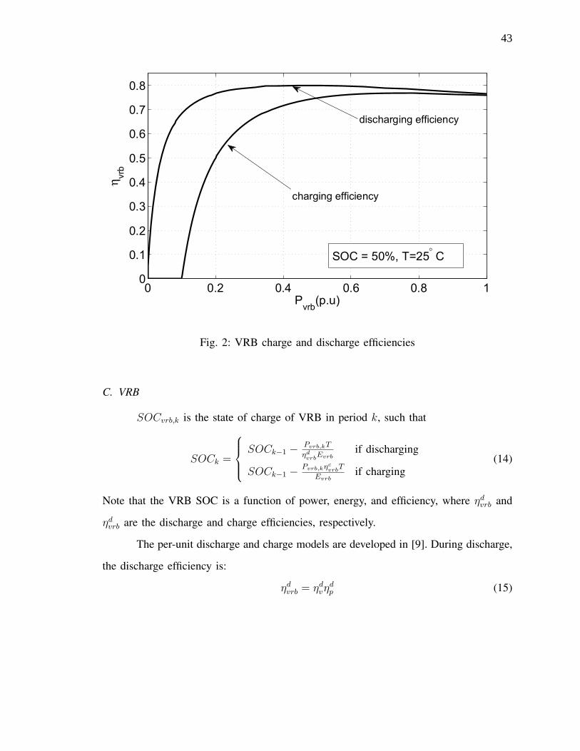
Fig. 2: VRB charge and discharge efficiencies

C. VRB

SOCvrb,k is the state of charge of VRB in period k, such that

SOCk =

SOCk−1 − Pvrb,kT

ηdvrb

Evrbif discharging

SOCk−1 −Pvrb,kη

cvrbT

Evrbif charging

(14)

Note that the VRB SOC is a function of power, energy, and efficiency, where ηdvrb and

ηdvrb are the discharge and charge efficiencies, respectively.

The per-unit discharge and charge models are developed in [9]. During discharge,

the discharge efficiency is:

ηdvrb = ηdvηdp (15)

43

where

ηdv =advPvrb(p.u.) + bdvSOC + cdvaovTeSOC + bovTe + cov

(16)

ηdp =Pvrb(p.u.)

adpPvrb(p.u.) + bdpSOC(SOC − 1) + cdp(17)

and ηv and ηdp are respectively the voltage and stack efficiencies and Te is the electrolyte

temperature in Ko.

During charge, the VRB efficiency is:

ηcvrb = ηcvηcp (18)

where

ηcv =aovTeSOC + bovTe + cov

(acvSOC + bcv)Pvrb(p.u.) + ccvSOC + dcv(19)

ηcp =(acpSOC + bcp)Pvrb(p.u.) + ccpSOC + dcp

Pvrb(p.u.)(20)

The absorb power is the maximum power that the VRB can absorb during charging

when the voltage is regulated to be constant. It is characterized as a function of absorb

voltage and the SOC:

Pab(p.u.) = (aabVab(p.u.) + bab)SOC + cabVab(p.u.) + dab (21)

All model coefficients are given in Table I and the charge and discharge efficien-

cies as a function of power are shown in Fig. 2.

IV. ANALYTICAL APPROACH

In eq. (4), the total cost per day (TCPD) of the VRB has been characterized as

an explicit function of power (P ratedvrb ) and energy (Erated

vrb ) ratings. At specific values of

P ratedvrb and Erated

vrb , the TCPD is constant and independent of the operating cost and the

total benefit of the microgrid. Therefore, the process of minimizing TC becomes the

minimization of (OC − TB) by finding an optimum dispatch pattern for the generators,

44

TABLE I: VRB per-unit model coefficients

(i, k) aik bik cik dik

(o, v) 0.07917 −0.00244 1.27640 −

(d, v) −0.28333 0.13251 0.98614 −

(d, p) 1.0334 0.34540 0.1192 −

(c, v) 0.19739 0.16167 0.14208 0.97479

(c, p) −0.128 1.05 0.038 0.118

(a, b) −8.3904 8.6634 7.3632 −7.504

the grid-tie, and the VRB as a function of PV power output. However, assuming constant

power and energy ratings provides only a local optimal solution. To obtain the global

solution for the optimization, the optimization should be performed over the whole

domain of P ratedvrb and Erated

vrb . The existence of a solution for an optimal VRB size is

guaranteed in this problem due to the fact that the TCPD is linearly increasing whereas

the operating cost is decreasing when P ratedvrb and Erated

vrb are increasing, resulting in a

convex optimization surface.

Fig. 3 shows a flowchart of the algorithm to search for optimal size of the VRB.

The algorithm contains the following main steps:

A. Domain Definition

As previously mentioned, P ratedvrb and Erated

vrb are independent, which means the

search domain is a multi-multidimensional space. To narrow the search space, upper and

lower limits of P ratedvrb and Erated

vrb are defined:P rated,minvrb ≤ P rated

vrb ≤ P rated,maxvrb

Erated,minvrb ≤ Erated

vrb ≤ Erated,maxvrb

Due to the constraint that requires the energy storage to serve a critical load during

45

End

≥

≥

Solve min(OC-TB) and find the total cost per day: TC=TCPD+OC-TB

Set up parameters and initial values

=

Start

=

≤

≤

Define domain:

≤

≤ ;

=

+ ∆

=

+ ∆E

YES

YES

NO

NO

Fig. 3: VRB optimal size search flow chart

a minimum period of time when the fuel is not available, Erated,minvrb is defined as the

minimum required reserve. P rated,minvrb is chosen as the maximum of the priority loads.

In this problem, it is assumed that renewable power is available to charge the VRB only

if the PV power is greater than the load power. Therefore, P rated,maxvrb and Erated,max

vrb can

be specified:

46

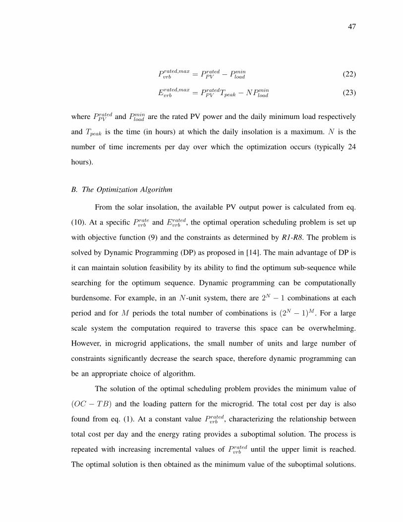
P rated,maxvrb = P rated

PV − Pminload (22)

Erated,maxvrb = P rated

PV Tpeak −NPminload (23)

where P ratedPV and Pmin

load are the rated PV power and the daily minimum load respectively

and Tpeak is the time (in hours) at which the daily insolation is a maximum. N is the

number of time increments per day over which the optimization occurs (typically 24

hours).

B. The Optimization Algorithm

From the solar insolation, the available PV output power is calculated from eq.

(10). At a specific P ratevrb and Erated

vrb , the optimal operation scheduling problem is set up

with objective function (9) and the constraints as determined by R1-R8. The problem is

solved by Dynamic Programming (DP) as proposed in [14]. The main advantage of DP is

it can maintain solution feasibility by its ability to find the optimum sub-sequence while

searching for the optimum sequence. Dynamic programming can be computationally

burdensome. For example, in an N -unit system, there are 2N − 1 combinations at each

period and for M periods the total number of combinations is (2N − 1)M . For a large

scale system the computation required to traverse this space can be overwhelming.

However, in microgrid applications, the small number of units and large number of

constraints significantly decrease the search space, therefore dynamic programming can

be an appropriate choice of algorithm.

The solution of the optimal scheduling problem provides the minimum value of

(OC − TB) and the loading pattern for the microgrid. The total cost per day is also

found from eq. (1). At a constant value P ratedvrb , characterizing the relationship between

total cost per day and the energy rating provides a suboptimal solution. The process is

repeated with increasing incremental values of P ratedvrb until the upper limit is reached.

The optimal solution is then obtained as the minimum value of the suboptimal solutions.

47

1.2

Solar Array 2

IV

2.2

MPPTI

1.3

Solar Array 3

IV

2.3

MPPTI

1.1

Solar Array 1

IV

2.1

MPPTI

SOLAR PANELS 48V DC BUS

V

CB

CB

CB

CB

CB

I

3

VRB

3SOC

ENERGY STORAGE

6

I

4

DC/AC LOAD

7

VacVac

INVERTER SUBPANEL

120V/240V AC SPLIT PHASE

BUS

CB

DC Current Measurement

AC Current Measurement

DC Voltage Measurement

AC Voltage Measurement

VRB State of Charge

Component Number

I

V

Vac

3SOCIac

LEGEND

DG

Fig. 4: PV-Diesel Microgrid Oneline Diagram

V. CASE STUDIES RESULTS

The case studies are performed to illustrate the optimization method. These cases

are based on an actual microgrid system located at the Fort Leonard Wood US Army

base in Missouri, USA (Fig. 4), which can be either isolated or grid-connected. The AC

load ranges between 2-5 kW. The PV arrays are rated 15 kW. Hourly data of the solar

insolation and ambient temperature at the site were collected from December 2012 to

September 2013. The diesel generator (DG) maximum output is 8 kW. The initial state

and fuel consumption of the DG are given in Table II. Fuel usage at forward operating

military bases will vary with size, location, and mission. By the time fuel reaches in-

theater staging, it can cost 10 or more times the domestic price [15]. Similarly, fuel costs

in extreme rural areas experience significant inflation due to transportation costs. For

example, delivering fuel to rural areas of Alaska is complicated and expensive, since fuel

must typically be delivered by either barge or plane [16]. Electricity price will also vary

48

0 3 6 9 12 15 18 21 240

2

4

6

8

10

12

14

Time of Day (hr)

Pow

er (

kW)

Dec 12Mar 13Sep 13Jun 13

Fig. 5: PV output power data

widely with locations. The electricity in the remote areas can cost double or more the

price in urban cities due to the high cost of transmission and generation. For example, the

average electricity price for residential customers in Hawaii in June 2014 is ¢38.66/kWh

[17]. Therefore, to better approximate the deployed performance of the microgrid, a diesel

fuel cost of $40/gal, electricity price of ¢40/kWh and buy back price of ¢20/kWh were

used in this study.

TABLE II: Diesel generator data

Adg Bdg Initial state0.065 gal/kWh 0.0215 gal/kWh 2 hr

T up,mindg T dw,mindg Fuel cost1 hr 1 hr $40/gal

49

0 3 6 9 12 15 18 21 24−5

0

5

10

Pow

er (k

W)

Time of day (hr)

0 3 6 9 12 15 18 21 24

P

load

Ppv

Pdg

Pvrb

Fig. 6: Dispatch on one day of June 2013 at minimum load and P ratedV RB = 5 kW and

EratedV RB = 65 kWh

The energy storage is required to have a reserve of 2 kWh, which is sufficient to

run the minimum critical load for 1 hour. The VRB may discharge to a SOC of 20%.

The VRB is assumed to be initialized at the minimum 20% SOC at the beginning of the

day (12am). The VRB rating range considered is

5kW ≤ P ratedvrb ≤ 10kW

10kWh ≤ Eratedvrb ≤ 100kWh

The optimization is solved using PV data from four days in December 2012,

March 2013, June 2013, and September 2013 (Fig. 5) which represent typical scenarios

of solar insolation ranging from a low in December 2012 to a high in September 2013.

From the given weather data, the PV power output is calculated from eq. (10) for both

50

0 10 20 30 40 50 60 70 80 90 100

250

300

0 10 20 30 40 50 60 70 80 90 1000

100

200

200

Prated = 10 kW, Max Load


Prated = 5 kW, Min Load


EVRB (kWh)

Ma

x L

oa

d T

C (

$)

Min

Lo

ad

TC

($

)

Minimum Cost

Fig. 7: Costs for operation in June 2013 at minimum and maximum load for a power

rating P ratedvrb of 5 kW and 10 kW

the minimum and maximum system loads. The optimization process illustrated in Fig. 3

is used to find the optimal size of the VRB for both maximum load and minimum load

scenarios for both isolated and grid-connected cases.

A. Case Study I - Isolated Microgrid

In this case study, the microgrid is isolated and the load must be met through

the combination of PV, diesel generation, and VRB energy storage. The optimization

process yields a series of operating scenarios that have associated costs. As an example

of these, the costs for the minimum and maximum load cases for June 2013 are shown

in Fig. 7 for both power ratings. Note that the cost axis for minimum load is on the right

side of the figure and the maximum load cost is on the left axis. There is not a single

combination of power and energy ratings that provides a consistent minimum, but there

51

0 3 6 9 12 15 18 21 24−5

0

5

10

Pow

er (k

W)

Time of day (hr)

0

Pload

Ppv

Pdg

Pvrb

Fig. 8: Dispatch on one day of June 2013 at maximum load and P ratedV RB = 5 kW and

EratedV RB = 65 kWh

is definitely commonality between the traces. Note that the minimum cost occurs at a 65

kWh VRB rating except in the 5kW VRB minimum load case, in which the minimum

occurs at 60 kWh rating. However, the minimum costs between the 65 kWh and 60 kWh

ratings are very close.

Figures 6 and 8 show the operating profiles of the (5 kW, 65 kWh) rated VRB for

June 2013 under minimum and maximum loads respectively. In the minimum load case,

the diesel generator never engages which is why the operating costs are much smaller

than for the maximum load case. In the maximum load case the diesel generator runs

at night, but note that it ramps down as the sunlight increases. Also note that when the

diesel hits the minimum limit (35% loading) at just before 09:00 it is disengaged and the

VRB picks up the load in correspondence with Constraint R6. The VRB also picks up

52

0 10 20 30 40 50 60 70 80 90 100240

260

280

300

320

0 10 20 30 40 50 60 70 80 90 1000

50

100

150

200





Minimum Cost

EVRB (kWh)

Ma

x L

oa

d T

C (

$)

Min

Lo

ad

TC

($

)

Fig. 9: Costs for operation in September 2013 at minimum and maximum load for a

power rating P ratedvrb of 5 kW and 10 kW

the load at 16:00 hours to keep the diesel generator off during light load. Also note that

the diesel generator is off for the majority of the sunlight hours during which the solar

array can simultaneously serve the load and charge the VRB according to Constraint R5.

According to Constraint R3, the VRB is always charged or discharged when its efficiency

is high (see Fig. 2).

This process is repeated for the remaining three operating profiles of December

2012, March 2013, and September 2013. For example, similar results for September

2013 are shown in Figures 9 – 11. In this month, the optimum energy rating shows more

variation than in June, but there is still consistency.

The minimum cost and energy rating across all months and power ratings for

minimum loading is given in Table III. Similarly, the minimum cost and energy rating

53

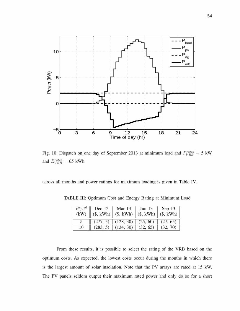
0 3 6 9 12 15 18 21 24−5

0

5

10Po

wer

(kW

)

Time of day (hr)

0 3 6 9 12 15 18 21 24

P

load

Ppv

Pdg

Pvrb

Fig. 10: Dispatch on one day of September 2013 at minimum load and P ratedV RB = 5 kW

and EratedV RB = 65 kWh

across all months and power ratings for maximum loading is given in Table IV.

TABLE III: Optimum Cost and Energy Rating at Minimum Load

P ratedvrb Dec 12 Mar 13 Jun 13 Sep 13

(kW) ($, kWh) ($, kWh) ($, kWh) ($, kWh)

5 (277, 5) (128, 30) (25, 60) (27, 65)10 (283, 5) (134, 30) (32, 65) (32, 70)

From these results, it is possible to select the rating of the VRB based on the

optimum costs. As expected, the lowest costs occur during the months in which there

is the largest amount of solar insolation. Note that the PV arrays are rated at 15 kW.

The PV panels seldom output their maximum rated power and only do so for a short

54

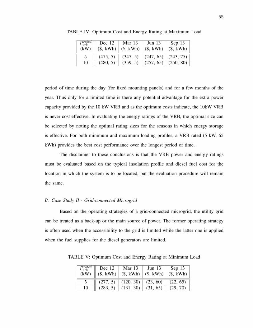
TABLE IV: Optimum Cost and Energy Rating at Maximum Load


(kW) ($, kWh) ($, kWh) ($, kWh) ($, kWh)

5 (475, 5) (347, 5) (247, 65) (243, 75)10 (480, 5) (359, 5) (257, 65) (250, 80)

period of time during the day (for fixed mounting panels) and for a few months of the

year. Thus only for a limited time is there any potential advantage for the extra power

capacity provided by the 10 kW VRB and as the optimum costs indicate, the 10kW VRB

is never cost effective. In evaluating the energy ratings of the VRB, the optimal size can

be selected by noting the optimal rating sizes for the seasons in which energy storage

is effective. For both minimum and maximum loading profiles, a VRB rated (5 kW, 65

kWh) provides the best cost performance over the longest period of time.

The disclaimer to these conclusions is that the VRB power and energy ratings

must be evaluated based on the typical insolation profile and diesel fuel cost for the

location in which the system is to be located, but the evaluation procedure will remain

the same.

B. Case Study II - Grid-connected Microgrid

Based on the operating strategies of a grid-connected microgrid, the utility grid

can be treated as a back-up or the main source of power. The former operating strategy

is often used when the accessibility to the grid is limited while the latter one is applied

when the fuel supplies for the diesel generators are limited.

TABLE V: Optimum Cost and Energy Rating at Minimum Load


(kW) ($, kWh) ($, kWh) ($, kWh) ($, kWh)

5 (277, 5) (120, 30) (23, 60) (22, 65)10 (283, 5) (131, 30) (31, 65) (29, 70)

55

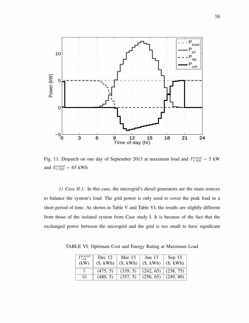
0 3 6 9 12 15 18 21 24−5

0

5

10Po

wer

(kW

)

Time of day (hr)

0 3 6 9 12 15 18 21 24

P

load

Ppv

Pdg

Pvrb

Fig. 11: Dispatch on one day of September 2013 at maximum load and P ratedV RB = 5 kW

and EratedV RB = 65 kWh

1) Case II.1: In this case, the microgrid’s diesel generators are the main sources

to balance the system’s load. The grid power is only used to cover the peak load in a

short period of time. As shown in Table V and Table VI, the results are slightly different

from those of the isolated system from Case study I. It is because of the fact that the

exchanged power between the microgrid and the grid is too small to have significant

TABLE VI: Optimum Cost and Energy Rating at Maximum Load


(kW) ($, kWh) ($, kWh) ($, kWh) ($, kWh)

5 (475, 5) (339, 5) (242, 65) (238, 75)10 (480, 5) (357, 5) (256, 65) (249, 80)

56

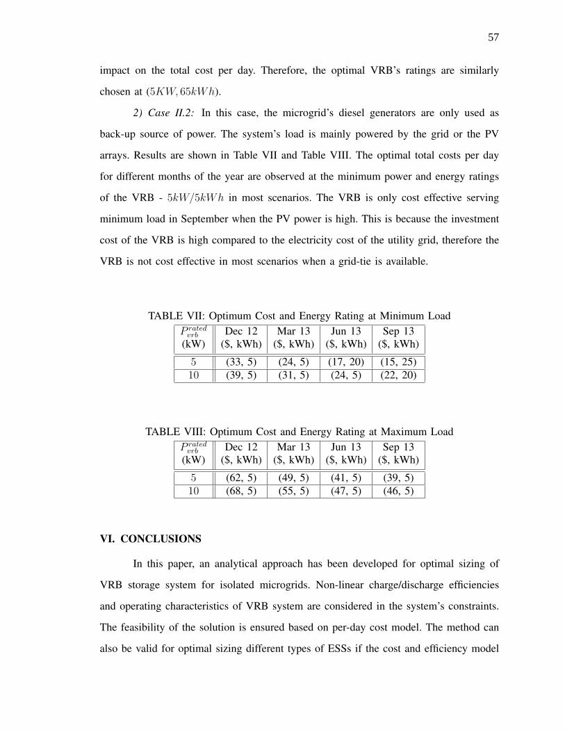
impact on the total cost per day. Therefore, the optimal VRB’s ratings are similarly

chosen at (5KW, 65kWh).

2) Case II.2: In this case, the microgrid’s diesel generators are only used as

back-up source of power. The system’s load is mainly powered by the grid or the PV

arrays. Results are shown in Table VII and Table VIII. The optimal total costs per day

for different months of the year are observed at the minimum power and energy ratings

of the VRB - 5kW/5kWh in most scenarios. The VRB is only cost effective serving

minimum load in September when the PV power is high. This is because the investment

cost of the VRB is high compared to the electricity cost of the utility grid, therefore the

VRB is not cost effective in most scenarios when a grid-tie is available.

TABLE VII: Optimum Cost and Energy Rating at Minimum LoadP ratedvrb Dec 12 Mar 13 Jun 13 Sep 13

(kW) ($, kWh) ($, kWh) ($, kWh) ($, kWh)

5 (33, 5) (24, 5) (17, 20) (15, 25)10 (39, 5) (31, 5) (24, 5) (22, 20)

TABLE VIII: Optimum Cost and Energy Rating at Maximum LoadP ratedvrb Dec 12 Mar 13 Jun 13 Sep 13

(kW) ($, kWh) ($, kWh) ($, kWh) ($, kWh)

5 (62, 5) (49, 5) (41, 5) (39, 5)10 (68, 5) (55, 5) (47, 5) (46, 5)

VI. CONCLUSIONS

In this paper, an analytical approach has been developed for optimal sizing of

VRB storage system for isolated microgrids. Non-linear charge/discharge efficiencies

and operating characteristics of VRB system are considered in the system’s constraints.

The feasibility of the solution is ensured based on per-day cost model. The method can

also be valid for optimal sizing different types of ESSs if the cost and efficiency model

57

are known. Case studies have been performed to find optimal VRB power and energy

ratings for both isolated and grid-connected microgrids considering different scenarios

of load and insolation. The results show the optimal solution occurs when the operating

cost benefit by increasing VRB capacity can justify the increment in investment capital.

References

[1] S. Bahramirad, W. Reder, and A. Khodaei, “Reliability-constrained optimal sizing

of energy storage system in a microgrid,” Smart Grid, IEEE Transactions on, vol. 3,

no. 4, pp. 2056–2062, 2012.

[2] B. Borowy and Z. Salameh, “Methodology for optimally sizing the combination of

a battery bank and pv array in a wind/pv hybrid system,” Energy Conversion, IEEE

Transactions on, vol. 11, no. 2, pp. 367–375, 1996.

[3] M. Elhadidy and S. Shaahid, “Optimal sizing of battery storage for hybrid

(wind+diesel) power systems,” Renewable Energy, vol. 18, no. 1, pp. 77 – 86,

1999.

[4] P. Arun, R. Banerjee, and S. Bandyopadhyay, “Optimum sizing of battery-integrated

diesel generator for remote electrification through design-space approach,” Energy,

vol. 33, no. 7, pp. 1155 – 1168, 2008.

[5] M. R. Aghamohammadi and H. Abdolahinia, “A new approach for optimal sizing of

battery energy storage system for primary frequency control of islanded microgrid,”

International Journal of Electrical Power & Energy Systems, vol. 54, no. 0, pp. 325

– 333, 2014.

[6] S. Chen, H. Gooi, and M. Q. Wang, “Sizing of energy storage for microgrids,”

Smart Grid, IEEE Transactions on, vol. 3, no. 1, pp. 142–151, 2012.

[7] H. T. Le and T. Q. Nguyen, “Sizing energy storage systems for wind power firming:

An analytical approach and a cost-benefit analysis,” in Power and Energy Society

General Meeting - Conversion and Delivery of Electrical Energy in the 21st Century,

2008 IEEE, 2008, pp. 1–8.

58

[8] M. Ross, R. Hidalgo, C. Abbey, and G. Joos, “Analysis of energy storage sizing

and technologies,” in Electric Power and Energy Conference (EPEC), 2010 IEEE,

2010, pp. 1–6.

[9] T. Nguyen, X. Qiu, J. D. Guggenberger, M. L. Crow, and A. C. Elmore, “Perfor-

mance characterization for photovoltaic-vanadium redox battery microgrid systems,”

IEEE Transactions on Sustainable Energy, 2013, Revised and Resubmitted.

[10] S. M. Schoenung and W. V. Hassenzahl, “Long- vs. short-term energy storage

technologies analysis - a life-cycle cost study,” Sandia National Laboratories,

Albuquerque SAND2003-2783, Tech. Rep., 2003.

[11] EPRI, “Vanadium redox flow batteries, an in-depth analysis,” EPRI, Tech. Rep.,

2007.

[12] O. Skarstein and K. Ulhen, “Design considerations with respect to long-term diesel

saving in wind/diesel plants,” Wind Engineering, vol. 13(2), pp. 72–87, 1989.

[13] L. Rodolfo Dufo and A. Jose L. Bernal, “Multi-objective design of pv-wind-diesel-

hydrogen-battery systems,” Renewable Energy, vol. 33, no. 12, pp. 2559 – 2572,

2008.

[14] T. Nguyen and M. Crow, “Optimization in energy and power management for

renewable-diesel microgrids using dynamic programming algorithm,” in Cyber Tech-

nology in Automation, Control, and Intelligent Systems, 2012 IEEE International

Conference on, 2012, pp. 11–16.

[15] Strategic Environmental Research and Development Program (SERDP), “Sustain-

able Forward Operating Bases,” August 2010.

[16] “Rural Fuel Pricing in Alaska,” [Online]. Available:

http://www.law.state.ak.us/pdf/civil/ 021810RuralFuelPricinginAlaska.pdf.

[17] “Electric Power Monthly,”,2014, [Online]. Available:

http://www.eia.gov/electricity/monthly/pdf/epm.pdf.

59

III. STOCHASTIC OPTIMIZATION OF RENEWABLE-BASED MICROGRIDOPERATION INCORPORATING BATTERY OPERATION COST

Tu A. Nguyen, M. L. Crow, IEEE Fellow



Abstract

Integration of renewable energy resources in microgrids has been increasing in the

recent decades in response to the concerns of climate change and rising fuel prices. Due

to the randomness in the renewable resources such as solar and wind, the actual renewable

power generation can deviate from the forecast values incurring extra operation cost for

committing costly reserve units or penalty cost for shedding the loads. In addition, it is

often desired to charge/discharge and coordinate the energy storage units in an efficient

and economical way. To address these problems, a novel battery operation cost model

is proposed in this paper which allows to consider a battery as an equivalent fuel-run

generator. A probabilistic constrained approach is used to incorporate the uncertainties

of renewable sources and load demands into the unit commitment (UC) and economic

dispatch (ED) problems. The UC is solved using stochastic dynamic programming. The

result of stochastic UC is presented in comparison with the deterministic UC in a case

study of a typical microgrid.

Index Terms

Microgrids, renewable energy, energy storage, vanadium redox battery, optimal

scheduling, unit commitment, economic dispatch

60

I. INTRODUCTION

During the past decades, the electric power industry has been reshaping in re-

sponse to the rising concerns about global climate change and fast increasing fossil fuel

prices. For a more efficient, reliable and environmentally friendly energy production, it

is critical to increase the deployment of distributed generation (DG), especially from

renewable energy resources (RE), as well as distributed energy storage (DS). This trend

has brought forth the concept of ”Microgrid” which can be understood as a cluster of

distributed energy resources, energy storage and local loads, managed by an intelligent

energy management system (EMS)[1]. The advantages of microgrids over the traditional

distribution systems exhibit in many aspects: energy losses reduction due to the proximity

between DGs and loads, reliability improvement with the ability to work in islanded

mode during system faults, transmission and distribution lines relief via efficient energy

management to reduce energy import from the grid[2].

As similar to the main grid operation, microgrid operation can be determined by

unit commitment (UC) and economy dispatch (ED). The UC is performed from one day

to one week ahead providing the start-up and shut-down schedule for each generation

and storage unit which can minimize the operation cost of the microgrid. After UC is

taken place, ED is performed from few minutes to one hour in advance to economically

allocate the demand to the running units considering all unit and system constraints[3].

Although the optimization of operation for the conventional power systems have

been well studied in the literature, the proposed methods cannot be applied directly to

microgrids with high integration of RE and ES devices. Specifically, due to the stochastic

nature of the renewable resources such as solar and wind, the actual renewable power

generation can be far different from the forecast values incurring extra operation cost for

committing costly reserve units or penalty cost for curtailing the demands. In addition,

to better utilize the renewable energy in the microgrid it is necessary to charge/discharge

and coordinate the energy storage units in an efficient and economical way. To address

these problems, the stochastic model of renewable energy and load demands as well as

61

the working characteristics and operational cost of the ES devices should be incorporated

into the UC and ED problems.

In the specialized literature, studies related to stochastic optimization for renewable-

based microgrids operation have been conducted. In [4], microgrid day-ahead scheduling

is addressed as a two-stage stochastic problem in which the first stage identifies the

optimal dispatch for the distributed units while the second stage considers the variability

and uncertainty of photovoltaic (PV) and wind energy generation. The outputs of PV

and wind generation units are considered in different scenarios generated by Monte

Carlo simulation. The optimization of unit commitment, which is a mixed non-linear

programming problem, is solved by iteration method using CPLEX. The probabilistic UC

in [5] is similarly formulated as a two-stage stochastic programming problem in order

to incorperate the uncertainty in load and PV forecast. Forecast errors are modelled by

normal distribution. Two-stage stochastic programming is also used in [6],[7].

Scenario-based stochastic programming for microgrid operation is proposed in

[8],[9],[10]. The scenarios of PV, wind generations and load demands are respectively

generated by Roulette Wheel Mechanism (RWM), Lattice Monte Carlo Simulations

(LMCS) and Latin hypercube sampling (LHS). The repeated and low-probability sce-

narios are then removed in [8],[9] while in [10] K-means clustering algorithm is used to

reduce the number of scenarios. The stochastic optimization of UC is solved by Adaptive

Modified Firefly Algorithm in [8] and by TeachingLearning-Based Optimization (TLBO)

algorithm in [9].

In [11], the economic dispatch problem optimizes fuel as well as green-house

gas emission cost. Expected values and cumulative probability functions (CDF) of PV

and wind power outputs based on Beta and Weibull distributions, respectively. The CDF

of total required reserve is obtained by the convolution CDF of PV and wind power.

The multi-objective optimization is solved using genetic algorithm. The ED in [12] is

similarly addressed and solved by Particle Swarm Optimization (PSO). In [13], microgrid

ED is formulated by wait-and-see approach. Cost optimization of the stochastic ED is

62

solved by an improved PSO; means and standard deviations of optimal solutions are

are determined by two-point estimate method. In [14], a discrete probabilistic model is

proposed considering the intermittency of renewable power sources through the estimation

of the probability density function (PDF) of the generator output powers. A model for

ED and demand-side management is developed for in a power system with multiple wind

farms in [15]. The loss of load probability (LOLP) is considered as a constraint in ED

to improve the reliability of the system.

As observed in the literature, the majority of existing studies is based on Scenario-

based stochastic programming [4]-[9]. This approach is based on replication of de-

terministic models across scenarios which generated by MCS in most of the works.

The computational burden in this approach increases exponentially to the number of

investigated scenarios thereby increasing significantly computational cost [2]. Scenario

reduction using different techniques, as seen in the previous studies, might ease the

problem; however, it can neglect the low-probability but high-impact scenarios. Therefore,

we propose a probabilistic constrained approach to incorporate the uncertainties into the

UC and ED for microgrids. In this approach, the perfect holding of power balance is

relaxed by introducing a probabilistic constraint which contains renewable powers and

load demands as random variables. The constraint is enforced with high probability while

the penalty for constraint violation is applied in the cost function. The advantage of this

method over the scenario based method is that all possibilities of load demands and

renewable generations are covered without considering a large number of scenarios. In

this paper, stochastic dynamic programming is used to solve the UC.

Regarding to energy storage management in microgrids, most of the previous

studies [4]-[15] assumed the energy storage as a single battery with constant efficiency

and zero operational cost. For this assumption, the ED tends to dispatch as much power as

possible to charge/discharge the battery regardless of its performance and state of health

(SOH). In practice, multiple ES technologies, which are different in terms of cycling life

time, efficiencies and working characteristics, may co-exist in a microgrid. Therefore,

63

it is necessary to optimally dispatch power to multiple storage units considering their

life time, efficiencies and working characteristics. In [16][17], efficiencies of different

storage technologies are characterized as functions of charge/discharge power. In [16],

an objective is defined to optimize the total charge/discharge efficiencies of ES devices;

however, the problem is simplified by priority list method. In this paper, we propose

a novel battery operation cost model which allows to consider a battery as an equiva-

lent fossil fuel generator in the UC and ED. The model accounts for charge/discharge

efficiencies, life time and capacity degradation of the batteries.

Specifically, the following contributions are made in this paper:

• A novel battery operation cost model is propose accounting for charge/discharge

efficiencies as well as cycling life time of the batteries. The model allows to treat a

battery as an equivalent fossil fuel generator in the UC and ED.

• A probabilistic constrained approach is proposed to incorporate the uncertainties of

renewable sources and load demands in microgrids into the UC and ED problems.

The UC is solved using stochastic dynamic programming.

II. BATTERY OPERATION COST MODEL

For a small-scale fossil fuel generator in microgrids, the operation cost is typically

the fuel cost which is fuel price times fuel consumption. The cost can be characterized

as a function of its output power as following [3, 10]:

Fgen(Pgen) = cgen.Hgen(Pgen)($/h) (1)

= cgen[agP2gen + bgPgen + cg]($/h)

where cgen($/gal) is fuel price, Hgen(Pgen)(gal/h) is fuel consumption and Pgen(kW )

is output power of generator i.

Different from a generator, a battery such as lead-acid or lithium-ion consumes

no fuel to run. This is a challenge to evaluate the operation cost of a battery. However,

64

in terms of energy conversion process, a battery and a generator are analogous. In a

generator, energy is stored in fuel form and generated in electricity form via combustion

process. Similarly, in a battery, electricity is charged and discharged via electrochemical

process. In general, charging a battery is analogous to refilling fuel for a generator; thus,

the input electricity (kWh) can be considered as the ”fuel” for the battery. We call

it kWhf to emphasize the analogy. Therefore, the operation cost of a battery can be

determined in the same form as (1) by deriving kWhf price and kWhf consumption

of the battery. In this paper, lead-acid, lithium-ion and vanadium redox battery are

investigated.

A. kWhf Price for Battery

For a generator, the price of fossil fuel cgen($/gal) is composed of two components

as follow:

cgen = cfuelgen + cavaigen ($/gal) (2)

in which cfuelgen represents the cost for fuel and cavaigen represents availability cost .

The availability cost includes fuel transportation cost and other service costs such as cost

for on-site storage facility. Depending on the location of the generator, cgen can be much

larger than cfuelgen due to transportation and other service cost. For example, delivering

fuel to rural areas of Alaska is complicated and expensive, since fuel must typically be

delivered by either barge or plane [18].

Similarly, kWhf price for a battery can be determined as:

cbat = ckWhf

bat + cavaibat ($/kWhf ) (3)

where ckWhf

bat is the price of energy used to charge the battery and cavaibat represents

the availability cost of battery capacity. In a microgrid, if renewable energy is used to

charge the battery, ckWhf

bat can be zero; therefore, cavaibat is the main portion of the price.

cavaibat can be defined as the cost to have 1kWh storage capacity available:

65

cavaibat =ReplacementCost

CΣ

($/kWhf ) (4)

where CΣ is the total lifetime cycling capacity of a battery. By convention, an

electrochemical battery such as lead acid and lithium-ion is often considered to be at

the end of its life (EOL) when it has degraded to 80% of its rated energy capacity [19].

Assuming that a battery will be discharged to its rated depth of discharge (DOD) every

cycle, the average capacity degradation rate is 0.2LrCr(kWh/cycle) in which Cr(kWh) is

the battery rated capacity and Lr(cycle) is the rated life time.

Different from a lead acid or a lithium-ion battery, a vanadium redox battery

(VRB) has no capacity degradation from repeated deep discharge and recharge. Cycle

life of a VRB mainly depends on the life expectancy of its Proton Exchange Membrane

(PEM) and its pumps. A VRB can last over 10000 cycles until its membrane degradation

or pumps failure.

Therefore, total lifetime usable capacity of a battery can be estimated as follow:

• Lead acid and lithium-ion battery:

CΣ = CrDODr[Lr −0.2

Lr

(1 + 2 + ...+ Lr)](kWh) (5)

= CrDODr(0.9Lr − 0.1)(kWh) (6)

• Vanadium redox battery:

CΣ = CrDODrLr(kWh) (7)

B. kWhf Consumption for Battery

kWhf consumption of a battery during discharge is defined as the energy usage

(kWhf ) for supplying a load during a unit time:

Hbat = PΣbat = P d

bat + P ldbat(kWhf/h) (8)

66

in which P dbat(kW ) is the battery output power, P ld

bat(kW ) is the power loss during

discharge.

kWhf consumption of a battery during charge is defined as the energy loss

(kWhf ) for charging the battery during a unit time:

Lbat = P lcbat(kWhf/h) (9)

in which P cbat(kW ) is the battery charge power, P lc

bat(kW ) is the power loss during charge.

Depending on battery type, Hbat and Lbat can be characterized as functions of

P dbat and P c

bat, respectively. In this section, Hbat and Lbat are characterized for lead-acid,

lithium-ion and vanadium redox battery.

1) Lead acid and lithium-ion battery: The power loss of lead-acid and li-ion

battery is mainly caused by the heat loss during charge or discharge. The heat is generated

by ohmic resistances of the electrodes and electrolytes, and also by polarization effects

[20]. The power loss is proportional to the voltage drop (polarization)caused by the

current:

Pjoule = ∆V × I(kW ) (10)

For lead-acid and lithium-ion battery, the voltage drop can be determined based

on the empirical method proposed in [21]:

• During discharge:

∆V = (R +K

SOC)I +

Qr.K(1− SOC)

SOC(11)

• During charge:

∆V = (R +K

0.9− SOC )I +Qr.K(1− SOC)

SOC(12)

where R(Ω) is the internal ohmic resistance, K is a constant which can be

calculated from manufacturer’s data, Qr(Ah) is the rated capacity of the battery.

67

From (11),(12), kWhf consumption during charge and discharge for lead acid

and lithium-ion battery can be determined as follow:


P ldbat = 10−3[(R +

K

SOC)I2 +

Qr.K(1− SOC)

SOCI] (13)

≈ 103(R + KSOC

)

V 2r

(P dbat)

2 +103Cr.K(1− SOC)

SOC.V 2r

P dbat

Hbat = P dbat + P ld

bat(kWhf/h)

• During charge:

P lcbat = (R +

K

1.1− SOC )I2 +Qr.K(1− SOC)

SOCI (14)

≈103(R + K

1.1−SOC)

V 2r

(P cbat)

2 +103Cr.K(1− SOC)

SOC.V 2r

P cbat

Lbat = P lcbat(kWhf/h)

with SOC is the state of charge, Vr is the rated voltage of battery.

2) Vanadium redox battery: The power loss of a vanadium redox battery during

charge and discharge includes two components: power for pumping the electrolytes and

stack loss power due to internal resistance and electrochemical process. Based on the

empirical proposed in [17], open circuit voltage, stack voltage can be characterized as

functions of SOC and charge/discharge power:

• Open circuit voltage:

Voc = aovSOC + bov(V ) (15)


Idstack = adiPdbat + bdiSOC + cdi (A) (16)

68

• During charge:

Icstack = (aciSOC + bci)Pcbat + cciSOC + dci(A) (17)

All model coefficients are given in Table I where Vr(V ) and Ir(A) are the rated

voltage and rated current of the VRB.

TABLE I: VRB loss model coefficients

(i, k) aik bik cik dik

(o, v) 0.2414Vr 0.9925Vr − −

(d, i) 1.0719Vr×10−3 0.0183Ir 0.0210Ir −

(c, i) −0.3093Vr×10−3

1.0397Vr×10−3 0.0604Ir −0.122Ir

From (16),(17), kWhf consumption during charge and discharge for VRB can be

determined as follow:


Hbat = 10−3IdstackVoc(kWhf/h)

= 10−3(aovSOC + bov)[adiP

dbat + (bdiSOC + cdi )] (18)

• During charge:

Lbat = P cbat − 10−3IcstackVoc(kWhf/h)

= [1− 10−3(aovSOC + bov)(aciSOC + bci)]P

cbat

− 10−3(aovSOC + bov)(cciSOC + dci) (19)

69

III. STOCHASTIC UNIT COMMITMENT FOR MICROGRIDS

A. Problem Formulation

In this paper, the stochastic unit commitment is formulated to minimize the

expected operation cost of a microgrid over a time horizon N . The objective function is

as follow:

minC =N∑

k=1

(Fk + Sk) (20)

Fk = EFg,k + F d

b,k + F cb,k + Fm,k

(21)

in which,

Fg,k =

n1∑

i=1

sgi,kFgi(Pgi,k)T =

n1∑

i=1

sgi,kcgiHgi(Pgi,k)T (22)

F db,k =

n2∑

i=1

sdbi,kFdbi(P

dbi,k)T =

n2∑

i=1

sdbi,kcbiHdbi(P

dbi,k)T (23)

F cb,k =

n2∑

i=1

scbi,kFcbi(P

cbi,k)T =

n2∑

i=1

scbi,kcbiLcbi(P

cbi,k)T (24)

Fm,k = Fm(Pm,k)T (25)

(26)

where

• N is the time horizon, T (hr) is the time step;

• Fk is the total expected operation cost in period k; Sk is the total transition cost

which accounts for the start-up and shut-down cost of the generators in period k .

• n1 and n2 are the number of generators and batteries, respectively;

• gi and bi denote generator i and battery i, respectively;

• Fg,k, Fdb,k, F

cb,k($) are respectively the total operation cost during period k of the

generators, the discharging batteries and the charging batteries; Fm,k is the cost due

to power mismatch;

• sgi,k, sdbi,k, scbi,k are respectively the binary status during period k of the generator i

70

and battery i; AND(sdbi,k, scbi,k) = 0 due to the fact that a battery could not charge

and discharge at the same time.

• cgi($/gal) is the fuel price for generator i; cbi($/kWhf ) is the kWhf price for

battery i;

• Hgi(gal/h) is the fuel consumption of generator i; Hbi(kWhf/h) and Lbi(kWhf/h)

are respectively the kWhf consumptions during discharging and charging of battery

i;

• Pgi,k, Pdbi,k, P

cbi,k(kW ) are respectively the dispatched power during period k to gen-

erator i, discharging battery i and charging battery i; Pm,k is the power mismatch

during period k.

To better define the problem, the following conventions are introduced:

• Charging power P cbi,k is considered as negative generation.

• Renewable sources (PV and Wind turbines generators) are not dispatchable and

considered as a negative load. The net load at period k is defined as:

Pnet,k =∑

Pload,k −∑

PPV,k −∑

PW,k

Since Pload,k, PPV,k, PW,k are random, Pnet,k is considered as a random variable.

• The batteries are charged only when Pnet,k < 0.

• The power mismatch Pm,k during period k is the difference between total generation

and the net load defined as follow:

– If Pnet,k ≥ 0

Pm,k = Pgen,k − Pnet

Pgen,k =

n1∑

i=1

sgi,kPgi,k +

n2∑

i=1

sdbi,kPdbi,k (27)

with Pgen,k > 0 is the total generation.

71

– If Pnet,k < 0

Pm,k = Pchg,k − Pnet

Pchg,k =

n2∑

i=1

scbi,kPcbi,k (28)

with Pchg,k < 0 is the total charge.

• The microgrid is grid connected. The electricity price and buy back price are con-

sidered as deterministic.

The constraints of the problem are defined based on the energy management strategies and

physical limits of the devices in the microgrid. The following constraints are considered:

• R1- The power mismatch is greater than zero with a predefined probability.

• R2- One battery should not be discharged to charge another battery; Generators

should not be used to charge the batteries.

• R3- Each storage device cannot be charged (or discharged) beyond the maximum

(or minimum) SOC.

• R4- The charge (or discharge) rate for each storage device should not exceed the

maximum (or minimum) rates.

• R5- Each generator should not be low loading when online.

• R6- Once a generator is brought online, it should remain online for a minimum set

time; when a generator is powered off, it should remain off a minimum time before

it can be restarted.

The above constraints are formulated as follow:

R1 :

P(Pm,k ≥ 0 ∩ Pnet,k > 0) = αkP(Pnet,k > 0)

P(Pm,k ≥ 0 ∩ Pnet,k < 0) = βkP(Pnet,k < 0)

with αk, βk ∈ [0, 1]

R2 :

AND(sdbi,k, scbj,k) = 0 ∀i, j

AND(sgi,k, scbj,k) = 0) ∀i, j

72

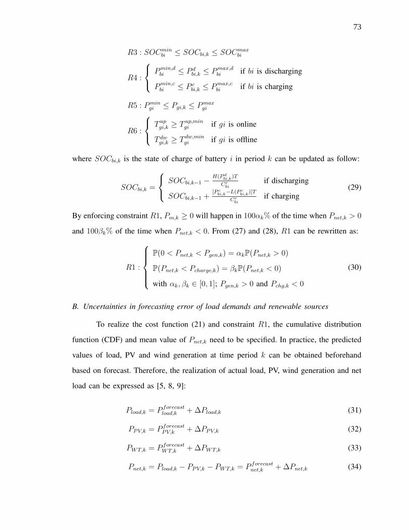
R3 : SOCminbi ≤ SOCbi,k ≤ SOCmax

bi

R4 :

Pmin,dbi ≤ P d

bi,k ≤ Pmax,dbi if bi is discharging

Pmin,cbi ≤ P c

bi,k ≤ Pmax,cbi if bi is charging

R5 : Pmingi ≤ Pgi,k ≤ Pmax

gi

R6 :

T upgi,k ≥ T up,min

gi if gi is online

T dwgi,k ≥ T dw,min

gi if gi is offline

where SOCbi,k is the state of charge of battery i in period k can be updated as follow:

SOCbi,k =

SOCbi,k−1 −H(P d

bi,k)T

Crbi

if discharging

SOCbi,k−1 +[P c

bi,k−L(P cbi,k)]T

Crbi

if charging(29)

By enforcing constraint R1, Pm,k ≥ 0 will happen in 100αk% of the time when Pnet,k > 0

and 100βk% of the time when Pnet,k < 0. From (27) and (28), R1 can be rewritten as:

R1 :

P(0 < Pnet,k < Pgen,k) = αkP(Pnet,k > 0)

P(Pnet,k < Pcharge,k) = βkP(Pnet,k < 0)

with αk, βk ∈ [0, 1]; Pgen,k > 0 and Pchg,k < 0

(30)

B. Uncertainties in forecasting error of load demands and renewable sources

To realize the cost function (21) and constraint R1, the cumulative distribution

function (CDF) and mean value of Pnet,k need to be specified. In practice, the predicted

values of load, PV and wind generation at time period k can be obtained beforehand

based on forecast. Therefore, the realization of actual load, PV, wind generation and net

load can be expressed as [5, 8, 9]:

Pload,k = P forecastload,k + ∆Pload,k (31)

PPV,k = P forecastPV,k + ∆PPV,k (32)

PWT,k = P forecastWT,k + ∆PWT,k (33)

Pnet,k = Pload,k − PPV,k − PWT,k = P forecastnet,k + ∆Pnet,k (34)

73

where ∆Pload,∆PPV ,∆PWT are the forecasting errors which mainly depend on the

forecasting methods and forecasting horizon. To model the uncertainties of load and

renewable source forecast, ∆Pload,∆PPV ,∆PWT are considered as random variables.

Although wind power forecast error can be more precisely described with Weibull,

Cauchy [22] or mixed Normal-Laplace distribution [23], it can be approximated with

a zero mean Normal distribution [24]. Furthermore, the net load error ∆Pnet,k, which

is the sum of all errors, can be approximated with zero mean Normal distribution [24]

due to the fact that the load demands and PV generation forecast errors are very close

to Normal distribution [5, 8, 9, 24]. The standard deviation of ∆Pnet,k can be calculated

as follow:

σnet,k =√σ2

∆Pload+ σ2

∆PPV+ σ2

∆PWT(35)

As a result, the following expected values and probabilities can be calculated:

1) E(Pnet,k) = P forecastnet,k (36)

2) E(Pm,k|Pnet,k > 0) = Pgen,k − P forecastnet,k (37)

3) E(Pm,k|Pnet,k < 0) = Pchg,k − P forecastnet,k (38)

4) P(Pnet,k < 0) = Φ

(−P forecastnet,k

σnet,k

)= pk (39)

5) P(Pnet,k > 0) = 1− pk (40)

6) P(0 < Pnet,k < Pgen,k) = Φ

(Pgen,k − P forecast

net,k

σnet,k

)− pk (41)

7) P(Pnet,k < Pchg,k) = Φ

(Pcharge,k − P forecast

net,k

σnet,k

)(42)

where Φ is the CDF of Standard Normal distribution N(0, 1).

74

Therefore constraint R1 can be realized as:

R1 :

Pgen,k = P forecastnet,k + σnet,kΦ−1 [αk(1− pk) + pk]

if Pnet,k > 0

Pchg,k = P forecastnet,k + σnet,kΦ−1 [βkpk]

if Pnet,k < 0

The system will generate (or charge) more or less power by choosing different

values of αk and βk. Choosing larger αk will increase the generation while choosing

larger β will reduce the charging power. Therefore, depending on energy management

policies, αk and βk can be flexibly selected. For example, if βk = 0.5, 50% chance that

the excess power from the renewable energy will be exported to the grid. The expected

operation cost in (21) can be expressed as:

Fk = (1− pk)(Fg,k + F db,k + E Fm,k|Pnet,k > 0)

+ pk(F cb,k + E Fm,k|Pnet,k < 0) (43)

in which

E Fm,k|Pnet,k > 0 = −cex,k|Pgen,k − P forecastnet,k |αk

+ cim,k|Pgen,k − P forecastnet,k |(1− αk) (44)

E Fm,k|Pnet,k < 0 = −cex,k|Pchg,k − P forecastnet,k |βk

+ cim,k|Pchg,k − P forecastnet,k |(1− βk) (45)

with cex,k, cim,k are the prices of the electricity which are exported to or imported from

the grid.

C. Stochastic Dynamic Programming

This UC problem can be categorized as a sequential decision-making problem for

which Dynamic Programming (DP) is well known. Dynamic programming (DP) is the

method to find the shortest route to the destination by breaking it down to a sequence of

75

steps overtime; at each step it finds the possible optimum sequences (routes) based on

the possible optimum subsequences in the previous steps and finally find the optimum

sequence at last step. The main advantage of DP is it can maintain solution feasibility by

its ability to find the optimum sub-sequence while searching for the optimum sequence.

Dynamic programming can be computationally burdensome. For example, in an N -unit

system, there are 2N−1 combinations at each period and for M periods the total number

of combinations is (2N − 1)M [3]. For a large scale system the computation required to

traverse this space can be overwhelming. However, in microgrid applications, the small

number of units and large number of constraints significantly decrease the search space,

therefore dynamic programming can be an appropriate choice of algorithm[17, 25].

Due to the uncertainties associated with the stochastic problem, the cost at each

stage is generally a random variable [26]. Therefore, in the stochastic DP technique, the

problem is formulated to minimize the expected cost. For applying DP, the states space

at stage k is defined as follow:

Lk =L1k...L

jk...L

mkk

(46)

Ljk =

sjg1,k, ..., s

jgn1,k, s

d,jb1,k, ..., s

d,jbn2,k, s

c,jb1,k...s

c,jbn2,k

(47)

where Lk is the set of feasible states in stage k; mk is the number of states of Lk;

sjxi,k is the binary status of unit xi which can be a generator, a discharging battery or a

charging battery. Ljk is a valid state if it satisfies constraints R2,R3, R6 and the following

conditions:

Pmingen,k ≤ P forecast

net,k + σnet,kΦ−1 [αk(1− pk) + pk] ≤ Pmaxgen,k

if sc,jbi,k = 0 ∀iPmincharge,k ≤ P forecast

net,k + σnet,kΦ−1 [βkpk] ≤ Pmaxcharge,k

otherwise

76

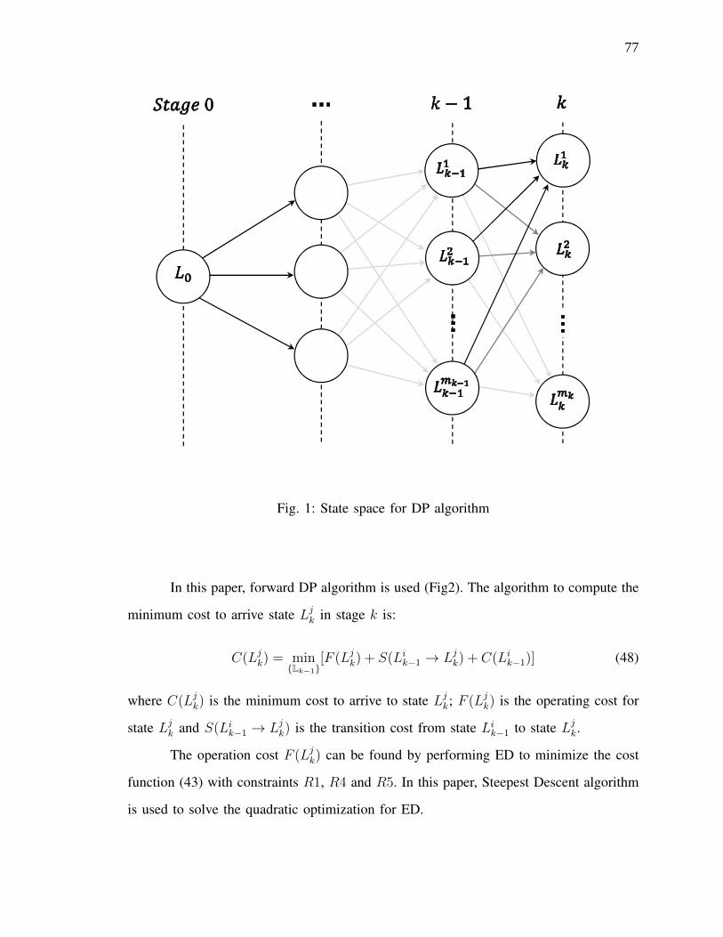
Fig. 1: State space for DP algorithm

In this paper, forward DP algorithm is used (Fig2). The algorithm to compute the

minimum cost to arrive state Ljk in stage k is:

C(Ljk) = min

Lk−1[F (Lj

k) + S(Lik−1 → Lj

k) + C(Lik−1)] (48)

where C(Ljk) is the minimum cost to arrive to state Lj

k; F (Ljk) is the operating cost for

state Ljk and S(Li

k−1 → Ljk) is the transition cost from state Li

k−1 to state Ljk.

The operation cost F (Ljk) can be found by performing ED to minimize the cost

function (43) with constraints R1, R4 and R5. In this paper, Steepest Descent algorithm

is used to solve the quadratic optimization for ED.

77

Fig. 2: Forward DP algorithm

IV. A CASE STUDY AND RESULTS

In this paper, a case study is developed to test the proposed approach. Fig. 3 shows

a typical microgrid which connected to the low voltage side of a distribution transformer

78

to power the residential loads. The microgrid includes a 50kW diesel generator, 2 ×20kW wind turbines, 50kW PV array, a 10kW/40kWh Vanadium Redox battery and an

12kW/30kWh AGM battery bank. The total load is 50kW at peak. The cost for AGM

battery is estimated at $8000. The replacement cost for the VRB is estimated at $20000

(20% of the investment cost [27]).

The data of generator and batteries, extracted from manufacturers’ data [28–30],

and their initial states are given in Table.II and Table.III. Day-ahead forecast values of

total load demands, PV and wind generations are given in Fig. 4 based on per-unit data

from [31, 32]. The standard deviations for load, PV and wind power forecast errors are

respectively 3.12%, 12.5% and 13.58% [33, 34]. αk and βk are chosen at 0.9 and 0.1

respectively.

TABLE II: Diesel generator dataadg bdg cdg Start-up cgen

3.10−4 gal/hkW 2 0.052gal/h

kW0.8gal/h $1 $4/gal

T up,mindg T dw,min

dg Pmindg Pmax

dg Ini. state2hr 2hr 5kW 50kW 1hr

TABLE III: Batteries data

Lr DODr Cr VrV RB 10000cl 50% 40kWh 60VAGM 1000cl 50% 30kWh 60V

SOCmin SOCmax Ini. SOC kWhf priceV RB 0.3 0.8 0.5 0.1$/kWhfAGM 0.5 1 0.5 0.59$/kWhf

The standard deviations of the net load forecast error at each hour are calculated

from (35) and given in Table.IV. The results for deterministic UC is shown in Fig.

5. By incorporating the operation cost functions of the batteries, ED tends to dispatch

79

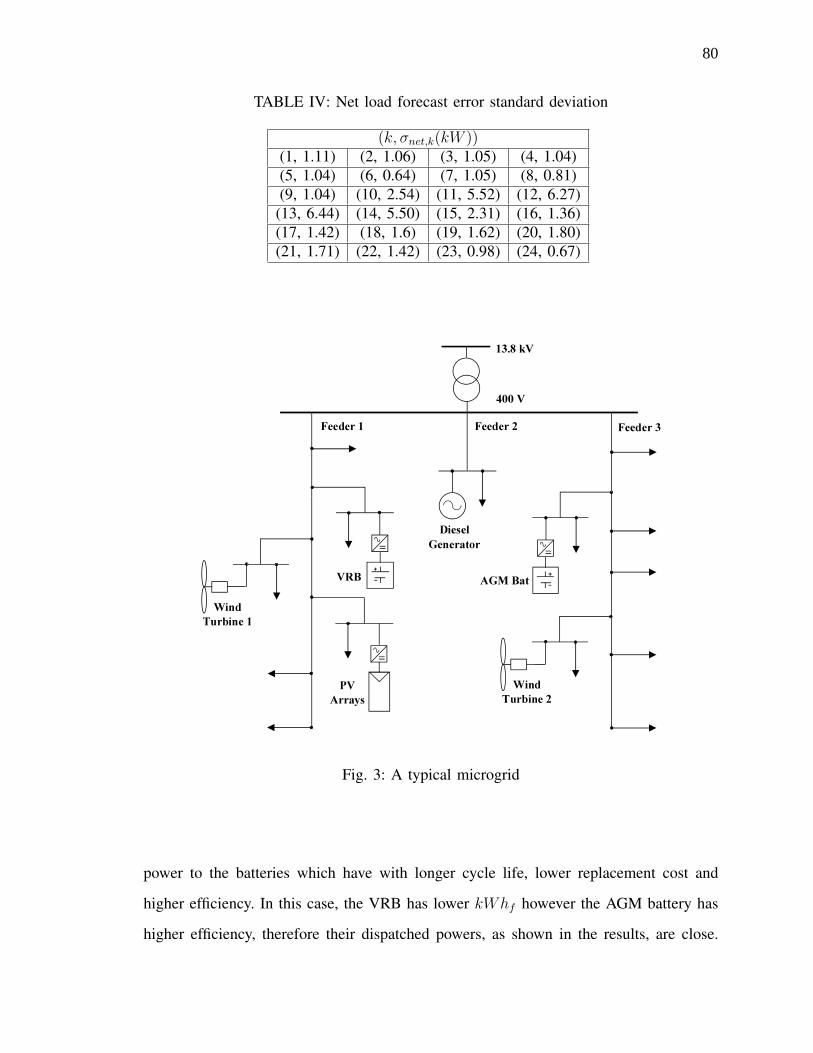
TABLE IV: Net load forecast error standard deviation

(k, σnet,k(kW ))(1, 1.11) (2, 1.06) (3, 1.05) (4, 1.04)(5, 1.04) (6, 0.64) (7, 1.05) (8, 0.81)(9, 1.04) (10, 2.54) (11, 5.52) (12, 6.27)

(13, 6.44) (14, 5.50) (15, 2.31) (16, 1.36)(17, 1.42) (18, 1.6) (19, 1.62) (20, 1.80)(21, 1.71) (22, 1.42) (23, 0.98) (24, 0.67)

Fig. 3: A typical microgrid

power to the batteries which have with longer cycle life, lower replacement cost and

higher efficiency. In this case, the VRB has lower kWhf however the AGM battery has

higher efficiency, therefore their dispatched powers, as shown in the results, are close.

80

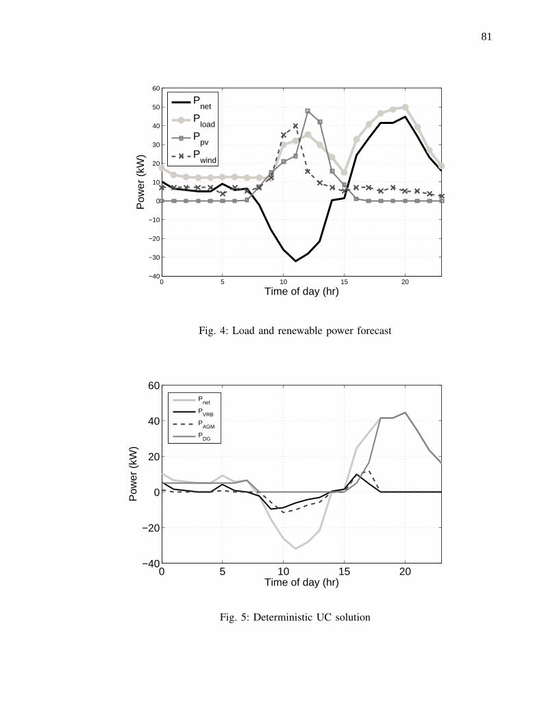
0 5 10 15 20−40

−30

−20

−10

0

10

20

30

40

50

60

Time of day (hr)

Pow

er (

kW)

Pnet

Pload

Ppv

Pwind

Fig. 4: Load and renewable power forecast

0 5 10 15 20−40

−20

0

20

40

60

Time of day (hr)

Pow

er (

kW)

Pnet

PVRB

PAGM

PDG

Fig. 5: Deterministic UC solution

81

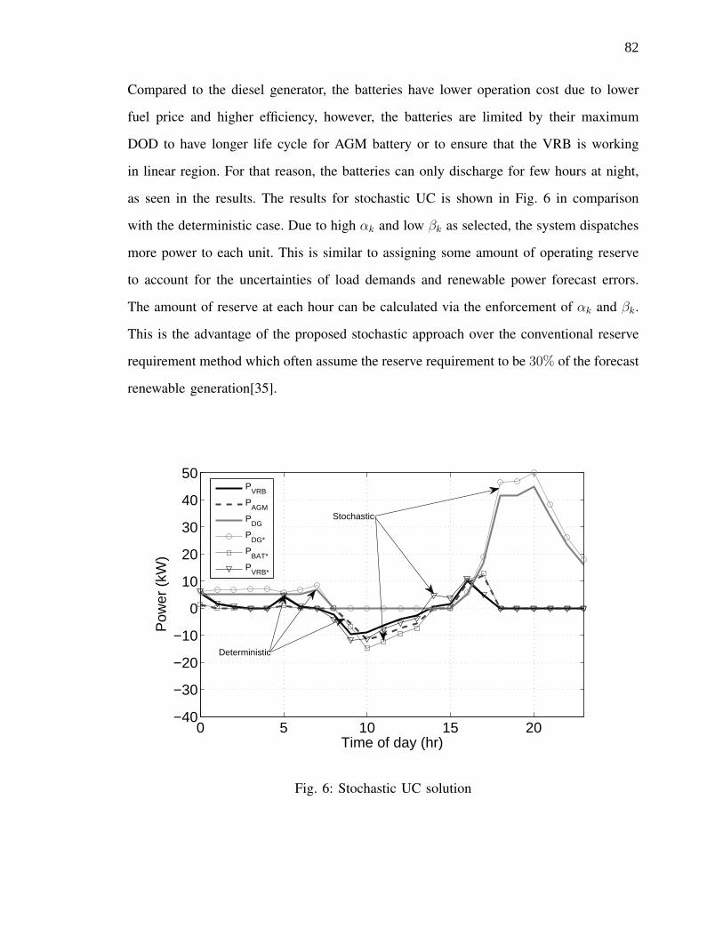
Compared to the diesel generator, the batteries have lower operation cost due to lower

fuel price and higher efficiency, however, the batteries are limited by their maximum

DOD to have longer life cycle for AGM battery or to ensure that the VRB is working

in linear region. For that reason, the batteries can only discharge for few hours at night,

as seen in the results. The results for stochastic UC is shown in Fig. 6 in comparison

with the deterministic case. Due to high αk and low βk as selected, the system dispatches

more power to each unit. This is similar to assigning some amount of operating reserve

to account for the uncertainties of load demands and renewable power forecast errors.

The amount of reserve at each hour can be calculated via the enforcement of αk and βk.

This is the advantage of the proposed stochastic approach over the conventional reserve

requirement method which often assume the reserve requirement to be 30% of the forecast

renewable generation[35].

0 5 10 15 20−40

−30

−20

−10

0

10

20

30

40

50

Time of day (hr)

Pow

er (

kW)

PVRB

PAGM

PDG

PDG*

PBAT*

PVRB*

Deterministic

Stochastic

Fig. 6: Stochastic UC solution

82

V. CONCLUSIONS

In this paper, a novel battery operation cost model has been proposed. The

model considers cycle life and charge/discharge efficiencies of the batteries. The model

makes economic dispatch for multiple batteries possible in the microgrid system without

introducing additional objective functions to maximize their efficiencies and their cycle

lives. In addition, a probabilistic constrained approach has been proposed to consider the

uncertainties in load and renewable power forecast errors. Stochastic dynamic program-

ming is applied in this method to find the optimal day-ahead scheduling for a typical

microgrid with a diesel generator, PV arrays, wind turbines, VRB and AGM batteries.

Results show the proposed approach can maintain the system optimal operation with a

high probability without investigating a vast number of scenarios. Future work in this area

will include the consideration of electricity market price uncertainty into the stochastic

UC and ED in which αk and βk need to be optimally selected to maximize the microgrid’s

profit.

References

[1] N. Hatziargyriou, Ed., Microgrids: Architectures and Control. Wiley, 2014.

[2] H. Liang and W. Zhuang, “Stochastic modeling and optimization in a microgrid: A

survey,” Energies, vol. 7, no. 4, pp. 2027–2050, 2014.

[3] B. F. W. Allen J. Wood, Power Generation, Operation, and Control. John Wiley

& Sons INC., 1996, vol. 2nd.

[4] W. Su, J. Wang, and J. Roh, “Stochastic energy scheduling in microgrids with

intermittent renewable energy resources,” Smart Grid, IEEE Transactions on, vol. 5,

no. 4, pp. 1876–1883, July 2014.

[5] X. Peng and P. Jirutitijaroen, “A probabilistic unit commitment problem with pho-

tovoltaic generation system,” in TENCON 2009 - 2009 IEEE Region 10 Conference,

Jan 2009, pp. 1–6.

83

[6] M. Lubin, C. G. Petra, M. Anitescu, and V. Zavala, “Scalable stochastic optimization

of complex energy systems,” in High Performance Computing, Networking, Storage

and Analysis (SC), 2011 International Conference for. IEEE, 2011, pp. 1–10.

[7] G. Martinez, N. Gatsis, and G. B. Giannakis, “Stochastic programming for energy

planning in microgrids with renewables,” in Computational Advances in Multi-

Sensor Adaptive Processing (CAMSAP), 2013 IEEE 5th International Workshop

on. IEEE, 2013, pp. 472–475.

[8] S. Mohammadi, S. Soleymani, and B. Mozafari, “Scenario-based stochastic opera-

tion management of microgrid including wind, photovoltaic, micro-turbine, fuel cell

and energy storage devices,” International Journal of Electrical Power & Energy

Systems, vol. 54, no. 0, pp. 525 – 535, 2014.

[9] T. Niknam, R. Azizipanah-Abarghooee, and M. R. Narimani, “An efficient scenario-

based stochastic programming framework for multi-objective optimal micro-grid

operation,” Applied Energy, vol. 99, no. 0, pp. 455 – 470, 2012.

[10] M. Mazidi, A. Zakariazadeh, S. Jadid, and P. Siano, “Integrated scheduling of

renewable generation and demand response programs in a microgrid,” Energy

Conversion and Management, vol. 86, no. 0, pp. 1118 – 1127, 2014.

[11] H. Bilil, G. Aniba, and M. Maaroufi, “Probabilistic economic emission dispatch

optimization of multi-sources power system,” Energy Procedia, vol. 50, no. 0, pp.

789 – 796, 2014.

[12] A. A. ElDesouky, “Security and stochastic economic dispatch of power system

including wind and solar resources with environmental consideration,” International

Journal of Renewable Energy Research-IJRER, vol. 3, no. 4, 2013.

[13] Y. Tan, Y. Cao, C. Li, Y. Li, L. Yu, Z. Zhang, and S. Tang, “Microgrid stochastic

economic load dispatch based on two-point estimate method and improved particle

swarm optimization,” International Transactions on Electrical Energy Systems,

2014.

[14] J. M. Lujano-Rojas, G. J. Osorio, and J. P. Catalao, “A probabilistic approach to

84

solve economic dispatch problem in systems with intermittent power sources,” in

T&D Conference and Exposition, 2014 IEEE PES, 2014, pp. 1–5.

[15] Y. Zhang, N. Gatsis, and G. B. Giannakis, “Risk-constrained energy management

with multiple wind farms,” in Innovative Smart Grid Technologies (ISGT), 2013

IEEE PES. IEEE, 2013, pp. 1–6.

[16] T. Nguyen and M. Crow, “Optimization in energy and power management for

renewable-diesel microgrids using dynamic programming algorithm,” in Cyber

Technology in Automation, Control, and Intelligent Systems (CYBER), 2012 IEEE

International Conference on, 2012, pp. 11–16.

[17] T. Nguyen, X. Qiu, J. Guggenberger II, M. Crow, and A. Elmore, “Performance

characterization for photovoltaic-vanadium redox battery microgrid systems,” IEEE

Transactions on Sustainable Energy, vol. 5, no. 4, pp. 1379–1388, 2014.

[18] Rural fuel pricing in alaska. [Online]. Available: http://www.law.state.ak.us/pdf/

civil/021810RuralFuelPricinginAlaska.pdf

[19] T. Markel, K. Smith, and A. Pesaran, “Improving petroleum displacement potential

of phevs using enhanced charging scenarios,” EVS-24 NREL/CP-540-45730, 2009.

[20] H. A. Kiehne, Battery technology handbook. CRC Press, 2003, vol. 60.

[21] O. Tremblay and L.-A. Dessaint, “Experimental validation of a battery dynamic

model for ev applications,” World Electric Vehicle Journal, vol. 3, no. 1, pp. 1–10,

2009.

[22] B. Hodge and M. Milligan, “Wind power forecasting error distributions over multiple

timescales,” in Power and Energy Society General Meeting, 2011 IEEE. IEEE,

2011, pp. 1–8.

[23] J. Wu, B. Zhang, H. Li, Z. Li, Y. Chen, and X. Miao, “Statistical distribution for wind

power forecast error and its application to determine optimal size of energy storage

system,” International Journal of Electrical Power & Energy Systems, vol. 55, pp.

100–107, 2014.

[24] R. Doherty and M. O’Malley, “A new approach to quantify reserve demand in

85

systems with significant installed wind capacity,” IEEE Transactions on Power

Systems, vol. 20, no. 2, pp. 587–595, 2005.

[25] L. M. Costa and G. Kariniotakis, “A stochastic dynamic programming model for

optimal use of local energy resources in a market environment,” in Power Tech,

2007 IEEE Lausanne. IEEE, 2007, pp. 449–454.

[26] D. P. Bertsekas, Dynamic programming: deterministic and stochastic models, D. P.

Bertsekas, Ed. Prince-Hall, 1987.

[27] G. Kear, A. A. Shah, and F. C. Walsh, “Development of the all-vanadium redox flow

battery for energy storage: a review of technological, financial and policy aspects,”

International Journal of Energy Research, vol. 36, no. 11, pp. 1105–1120, 2012.

[28] MQ Power. [Online]. Available: http://www.powertechengines.com/

MQP-DataSheets/MQP050IZ Rev 0.pdf

[29] Prudent Energy. [Online]. Available: http://www.pdenergy.com/pdfs/Prudent

Energy Product Brochure 2011.pdf

[30] Sunxtender. [Online]. Available: http://www.sunxtender.com/solarbattery.php?id=11

[31] D. Hung, N. Mithulananthan, and K. Lee, “Determining PV penetration for

distribution systems with time-varying load models,” IEEE Transactions on Power

Systems, to be published, early Access.

[32] A. A. Moghaddam, A. Seifi, and T. Niknam, “Multi-operation management of

a typical micro-grids using particle swarm optimization: A comparative study,”

Renewable and Sustainable Energy Reviews, vol. 16, no. 2, pp. 1268–1281, 2012.

[33] N. Lu, R. Diao, R. Hafen, N. Samaan, and Y. Makarov, “A comparison of forecast

error generators for modeling wind and load uncertainty,” in Power and Energy

Society General Meeting (PES), 2013 IEEE, 2013, pp. 1–5.

[34] F. Kreikebaum, R. Moghe, A. Prasai, and D. Divan, “Evaluating the application of

energy storage and day-ahead solar forecasting to firm the output of a photovoltaic

plant,” in Energy Conversion Congress and Exposition (ECCE), 2011 IEEE, 2011,

pp. 3556–3561.

86

[35] A. Zakariazadeh and S. Jadid, “Energy and reserve scheduling of microgrid

using multi-objective optimization,” in Electricity Distribution (CIRED 2013), 22nd

International Conference and Exhibition on, 2013, pp. 1–4.

87

88

2. CONCLUSIONS

In this dissertation, three papers have been proposed solve three problems including:

microgrid systems performance characterization, optimal sizing for energy storage system

and stochastic optimization of microgrid operation. In the first paper, a PV-VRB microgrid

system performance has been characterized. The system operating characteristics, losses,

and efficiencies are quantified and formulated based on measured data. The VRB dis-

charge and charge efficiencies are found to be nonlinear with the load/charge power. Based

on the system characterization, a scalable model has been built to accurately predict the

system behavior and performance. A case study has been performed for May 2013. In

second paper, an analytical approach has been developed for optimal sizing of VRB stor-

age system for isolated microgrids. Non-linear charge/discharge efficiencies and operating

characteristics of VRB system are considered in the system’s constraints. The feasibility

of the solution is ensured based on per-day cost model. The method can also be valid for

optimal sizing different types of ESSs if the cost and efficiency model are known. Case

studies have been performed to find optimal VRB power and energy ratings for both iso-

lated and grid-connected microgrids considering different scenarios of load and insolation.

The results show the optimal solution occurs when the operating cost benefit by increas-

ing VRB capacity can justify the increment in investment capital. In the third paper, a

novel battery operation cost model has been proposed. The model considers cycle life

and charge/discharge efficiencies of the batteries. The model makes economic dispatch for

multiple batteries possible in the microgrid system without introducing additional objective

functions to maximize their efficiencies and their cycle lives. In addition, a probabilistic

constrained approach has been proposed to consider the uncertainties in load and renew-

able power forecast errors. Stochastic dynamic programming is applied in this method to

find the optimal day-ahead scheduling for a typical microgrid with a diesel generator, PV

arrays, wind turbines, VRB and AGM batteries. Results show the proposed approach can

89

maintain the system optimal operation with a high probability without investigating a vast

number of scenarios. Future work in this area will include the consideration of electricity

market price uncertainty into the stochastic UC and ED in which αk and βk need to be

optimally selected to maximize the microgrid’s profit.

90

VITA

Tu Anh Nguyen obtained his B.S. in Electrical Engineering from Hanoi University

of Technology (currently Hanoi University of Science and Technology) in July 2007. He

received his Ph.D. in Electrical Engineering from Missouri University of Science and Tech-

nology in December 2014.

Tu Nguyen was employed as a graduate research assistant at the Missouri University

of Science and Technology under Dr. Mariesa L. Crow from 2009 to 2014. During this

time, he was part of a team that designed and built three working renewable-energy micro-

grids, as well as completed research which led to this dissertation. From 2008 to 2009, Tu

Nguyen worked as an Power Transformer Test Engineer at ABB Ltd. Vietnam.

Tu Nguyen is a member of The Institute of Electrical and Electronics Engineers

(IEEE) and IEEE Power and Energy Society (PES).

Optimization in microgrid design and energy management

Documents

Transcript of Optimization in microgrid design and energy management