120

3. OPTIMIZATION OF JOINT WATER AND ENERGY USES OF THE SYRDARYA BASIN

3.1. Operating Models to Manage Water and Energy Systems of the Basin. Model Assessment in Regard to Optimization of Use of Water and Energy Resources

3.1.1. Basic Principles of River Flow Control The modern water use complex of the Syrdarya basin must provide rational use of all water resources in the basin consisting of many hydro-technical constructions on the Syrdarya and its tributaries which transport water, transform flow in reservoirs, supply water to water users, generate power, all the while registering and controlling the quantity and the quality of the used water. The main water-consumer in the Syrdarya basin is irrigated agriculture. The municipal and industrial sector, the housekeeping sector, fishery, and pastures are other water-consumers. A main water-user is hydro-power generation; that is why the basin is characterized as complex and has a repeated (secondary use) character of water use, along with extremely limited and uneven distribution of water resources through the territory of the basin and in time. The first document for regulation and distribution of the limited water resources of the basin was “The Conclusion of the Expert Sub-commission of the State Expert Commission of State Planning of the USSR on the Amplified Scheme of Complex Use and Protection of Water Resources of the Basin of the Syrdarya River” dated April 12, 1982. This document determined that the inflow to Chardara reservoir should be 12 km3 during normal years, with a decrease to 10 km3 during dry years (90%). The above amounts of inflow were to be achieved by means of the flows from the reservoirs located upstream. Water resources of the Syrdarya basin, except for the guaranteed inflow to Chardara reservoir and for non-returnable losses, were to be distributed by the Ministry of Water of the USSR among the other zones according to the limits shown in Table 3.1.1.1.

Table 3.1.1.1. USSR Ministry of Water distribution limits for the Syrdarya Basin.

Republic Limit (km3/year) Share (%) Kazakhstan 2.16 7.2 Kyrgyz Republic 2.95 9.8 Tajkistan 2.92 9.7 Uzbekistan 22.04 73.3 Total 30.07 100

During this period, water withdrawal from the main river beds of the Naryn and Syrdarya rivers upstream from Chardara reservoir was equal to: 1.11 km3/year for Kazakhstan, 0.39

121

km3/year for Kyrgyz Republic, including 0.23 km3/year for Toktogul reservoir, 1.78 km3/year for Tajkistan, and 10.51 km3/year for Uzbekistan. Withdrawal of water downstream from Chardara reservoir for Kazakhstan was equal to 8.15 km3/year. The guaranteed inflow to Chardara reservoir, and the above water distribution were the major priorities for regulation of flow after fulfilling irrigation water demand in the basin. The power generation use of the water resources was planned within the limits of irrigation water regulation. Imbalances in electricity demand, inevitable when using irrigation regimes of reservoir operation, were compensated by the EPP CA. These principles remained till the collapse of the USSR in 1991. The common fact for the newly independent four republics of the basin is that currently both power generation and irrigation demands cannot be fully satisfied by normal river flow. Complex regulation of the flow is necessary, both in seasonal and multiyear time frames. None of the possible regimes of regulation can simultaneously satisfy the demands of all four republics, so there is a need for compromise and an agreed system of compensation for damages and opportunity costs. The main principles of regulation of flow in the Syrdarya basin include the following: • Reservoir operation on small rivers is isolated for each of the other rivers; • Charvak and Andijan reservoir releases are established considering the use of return water

from irrigated lands; and • the three mainstream reservoirs (Toktogul, Kairakum, and Chardara) comprise the cascade of

reservoirs which pass water through different parts of the basin and provide the main regulation of flow within the system. This means that, first of all, water demand is satisfied by side inflow, while the Kairakum reservoir increases water provision in the midstream region, but if there is a lack of water, it is covered by compensating releases from Toktogul reservoir.

Some recommendations for improving the functioning of the system and for regulation of flow in the Syrdarya basin are:

1. Conditions for eliminating releases to Arnasai depression inlcude: • Limit inflow to Chardara reservoir during the non-vegetation period to no more than 11

km3; and • Provide releases from Chardara reservoir during the non-vegetation period in excess of 7-

8 km3; and • Empty Chardara reservoir during the vegetation period to the dead volume.

2. Achievement of these conditions is possible only if the other reservoirs of the Naryn-Syrdarya cascade function according to the following important parameters:

2.1. Toktogul reservoir: • Limit non-vegetation releases to the range of 3-5.5 km3; • The summer release from Toktogul reservoir must not be less than 6.5 km3 during

normal flow years, not less than 7.5 km3 during low water years, and 3-4 km3 during high-water years.

122

2.2. Kairakum and Chardara reservoirs: • Increase the October and November releases from Kairakum reservoir to at least 800

m3/s, emptying the reservoir to its dead volume (890 mln.m3); • October and November releases from Chardara reservoir should be greater than 550-

600 m3/s, with a slight decrease in the second half of November (down to 400-450 m3/s), and staying within this range until the middle of March; after that, releases from Chardara reservoir can be increased up to 700 m3/s (depending on the temperature of the air, and the ice conditions downstream). This will allow release of 7-8 km3 of water from Chardara reservoir during the non-vegetation period, depending on winter climate conditions.

3. Maintaining the non-vegetation period release regime of Chardara reservoir described in Article 2.2 will allow an increase in the inflow to the Aral Sea and the pre-Aral Region up to 4-5 km3 during the non-vegetation period.

4. The operating regime of the Naryn-Syrdarya cascade of reservoirs described above must be supported by corresponding compensatory supplies of heat and power resources to the Republics of Kyrgyzstan and Tajikistan form the Republics of Uzbekistan and Kazakhstan. Obligatory punctual fulfillment of these deliveries will allow optimal regulation and rational use of the transboundary water resources of the Syrdarya basin.

3.1.2. Hydro-economic and Hydro-energy Calculations The results of the traditional water balance calculations for the Syrdarya basin rivers are presented below for the vegetation period (April – September) and non-vegetation period (October – March). These calculations were carried out by the SIC ICWC for two possible variants of operation of Toktogul reservoir: (1) “power generation”, and (2) “irrigation.” The inflow of water to Toktogul, Andijan, and Charvak reservoirs was assumed to be 9.3 + 2.9 + 5.1 = 17.3 km3, and the side inflow was equal to 12.2 km3, based on the normal conditions; the total is 29.5 km3. The initial amount of water in the reservoirs corresponded to the actual data for April 1, 2000: Toktogul – 9.5 km3, Andijan – 1.4 km3, Charvak – 1.1 km3, Kairakum – 3.4 km3, Chardara – 5.4 km3, total = 20.8 km3. The required withdrawal of water from the Naryn and Syrdarya Rivers for irrigation was based on the limits in the amount of 18.5 km3. With the withdrawal of water from the Karadarya River – 3.3 km3, and Chirchik River – 4.9 km3, the total demand for water is estimated as 18.5 + 3.3 + 4.9 = 20.8 km3. The losses in the river beds and reservoirs were based on the minimum estimates without taking into account flooding of the delta downstream from Kazalinsk. Vegetation period: Under the “power generation” scenario, the release of water from Toktogul reservoir is 3.5 km3, based on the power demand of Kyrgyzstan; the resulting amount of water in the reservoir at the end of the vegetation period is 9.5 + (9.3 – 3.5) = 15.3 km3. Under the “irrigation” scenario, the release of water from Toktogul reservoir based is 6.5 km3, based on the irrigation demand of Uzbekistan and Kazakhstan; the resulting amount of water in the reservoir at the end of the vegetation period is 9.5 + (9.3 – 6.5) = 12.3 km3.

123

The calculations show, that in case of the first option lack of water is expected for irrigation during the vegetation period in the amount of 3 km3, including 2.2 km3 before Chardara reservoir. The lack will be zero only if the vegetation period release from Toktogul is not less than 6.5 km3. The estimated power generation during the vegetation period by the cascade of Naryn HPPs in the first case is 3.1 bln.kWh (assuming 1.13 m3/kWh), which corresponds to the domestic electricity demand of Kyrgyzstan from the cascade. In the second case, power generation by the cascade is equal to 5.3 bln.kWh., and the surplus is estimated as 2.2 bln.kWh. – this is the electricity exported to Uzbekistan and Kazakhstan under the condition of return of equal an amount of power and fuel to Kyrgyzstan during the non-vegetation period.

Table 3.1.2.1. Water Balance of the Syrdarya Basin Under Two Scenarios: Power Generation and

Irrigation.

Items of the balance Power

Scenario Irrigation Scenario

1. Water resources of the basin, km3 29.5 29.5 2. Total consumption of water in the reservoirs, km3 0.0 3.0 Total inflow (1 + 2) 29.5 32.5 3. Required withdrawal of water from the rivers, km3 26.7 26.7 4. River bed losses, km3 3.0 3.0 5. Inflow to Aral Sea, km3 2.8 2.8 Total outflow ( 3 + 4 + 5 ), km3 32.5 32.5 BALANCE (outflow - inflow), (-) Lack, km3 -3.0 0.0

Non-vegetation period: Let us consider the possible regimes of operation of Toktogul reservoir during the non-vegetation period (October – March) for the case of the inflow of water to the hydro-station through Naryn in the amount of 3.4 km3 (analog – non-vegetation period of 1999-2000), based on the options selected above. Under the power generation scenario, the amount of water in Toktogul reservoir at the beginning of the non-vegetation period (October, 2000) would be 15.3 km3. The release of water from Toktogul reservoir is based on the domestic electricity demand of Kyrgyzstan, generating 6.6 bln.kWh of electricity. In this case, the estimated release downstream from Toktogul reservoir is equal to 7.3 km3. At the end of the non-vegetation period (March 31) the amount of water in Toktogul reservoir will be 15.3 + (3.4 – 7.3) = 11.4 km3. Inflow to the Aral Sea will be 5.9 km3. Under the irrigation scenario, the amount of water in Toktogul water reservoir at the beginning of the non-vegetation period (October) would be 12.3 km3. The release of water from Toktogul reservoir is planned in the amount of 4.8 km3, which provides electricity generation of 4.4 bln.kWh. The lack of power is 2.2 bln.kWh. Compensation to Kyrgyzstan for the non-generated electricity would be required from Uzbekistan and Kazakhstan. In this case, at the end of the non-vegetation period (March) the amount of water in Toktogul reservoir would be 12.3 + (3.4 – 4.8) = 10.9 km3, which is 0.5 km3 less than in the first option. Inflow to the Aral Sea would be 3.4 km3, which is 2.5 km3 less than in the first option. UDC Energia carries out water-analysis calculations taking into account the provisions of the Agreements between the Governments of Kyrgyzstan, Uzbekistan, Kazakhstan, and Tajkistan, and the conditions of provision of the contractual and agreed upon balance of flow of power between the countries of Central Asia. The following tables (Tables 3.1.2.1 - 7) represent:

124

• Power generation by the HPPs of the EPP CA by month in 1998 (Table 3.1.2.1) • Increase in power generation by HPPs of EPP CA by month in 1999 (Table 3.1.2.2); • Flows in the Naryn, Syrdarya, Chirchik, Vakhsh Rivers in 1999 (Table 3.1.2.3); • Actual regime of operation of the main reservoirs and HPPs in 2000 (Table 3.1.2.4); • Actual regime of operation of Kairakum and Chardara reservoirs in 1999 (Table 3.1.2.5); • Power balance of Barki Tochik with the actual regime of operation of Nurek reservoir during

non-vegetation and vegetation periods in 1999 (Table 3.1.2.6); • Power balance of Kyrgyzenergo with the actual regime of operation of Toktogul reservoir

during non-vegetation and vegetation periods in 1999 (Table 3.1.2.7).

125

Table 3.1.2.1 Power Generation by HPPs of the EPP CA by Month in 1998 (mln.kWh)

Name January February March April May June July August September October November December Year

Ministry of Power of the Republic of Uzbekistan

399.8 297.3 373.5 332.8 556.8 641.8 719.1 672.4 363.7 345.6 304.5 318.6 5325.9

GAHK “Barki Tochik”

1408.0 1130.8 931.8 804.2 1432.5 1431.3 1482.2 1516.7 1386.5 1200.3 1291.0 1410.7 15426.0

JSC “Kyrgyzenergo”

1444.2 1169.3 1242.8 937.1 636.7 647.1 1078.6 1007.5 508.4 750.1 1249.7 1465.9 12137.4

APC and JSC TATEK

113.7 96.6 106.7 159.6 194.5 209.7 207.0 208.2 174.3 112.9 101.8 114.7 1799.4

GETK “Kuvvat”

- - 0.7 0.8 0.4 0.6 0.7 0.2 - - 0.1 0.5 4.0

Republic of Kazakhstan Chardara HPP

39.7 33.5 48.9 58.5 42.3 43.2 35.0 34.5 19.6 24.8 34.5 39.8 454.3

Republic of Uzbekistan Andijan HPP

27.6 2.2

75.3 11.9

90.8 47.8

76.4 44.5

158.1 109.4

179.8 108.0

191.6 110.5

149.5 84.5

96.0 57.9

87.1 48.4

54.9 27.6

70.3 0.2

1257.4 652.9

Tuyamuyun HPP

25.4 63.4 43.0 31.9 48.7 71.8 81.1 65.0 38.1 38.7 27.3 70.1 614.5

Total EPP CA 3433.0 2802.8 2795.2 2369.4 3021.3 3153.5 3714.2 3589.0 2548.5 2520.8 3036.5 3420.5 36404.7

126

Table 3.1.2.2 Increase in Power Generation by HPPs of EPP CA in 1999 (%)

Name Jan Feb Mar Apr May Jun Jul Aug Sep Oct Nov Dec Year

Ministry of Power of the Republic of Uzbekistan

38.5 9.3 -19.7 -27.4 -23.8 -22.0 -10.4 6.4 -2.4 -8.9 -8.6 -29.7 -11.4

GAHK “Barki Tochik”

6.8 6.2 16.7 -10.7 13.7 14.3 7.7 15.9 14.3 3.5 11.5 5.8 9.0

JSC “Kyrgyzenergo”

13.8 14.6 30.6 75.0 29.4 38.2 43.4 21.3 -16.3 -6.2 33.7 14.7 22.1

APC and JSC TATEK

22.6 26.4 37.3 83.9 68.0 54.3 0.7 -14.0 -6.3 -21.9 -28.0 -2.0 10.9

GETK “Kuvvat” - - 16.7 33.3 -42.9 -25.0 -12.5 -66.7 - - - 66.7 -9.1

Republic of Kazakhstan Chardara HPP

29.7 24.5 13.2 15.8 -25.3 -24.5 -33.7 -36.2 -50.4 -32.4 -15.0 -2.4 -14.2

Republic of Uzbekistan Andijan HPP

133.9 65.9 2.1 12.2 12.0 32.1 5.8 -20.6 -31.8 -15.1 -41.3 16.2 -0.1

Total for EPP CA 14.0 11.9 15.2 12.8 8.0 9.7 10.2 10.2 -0.4 -3.9 12.2 14.6 8.6

127

Table 3.1.2.3 Water Level in the Rivers Naryn, Syrdarya, Chirchik, Vakhsh in 1999

(data presented by Hydro-Meteorology Center of the Republic of Uzbekistan)

Name Items I II III IV V VI VI VIII IX X XI XII Ave. Veg.

Period

Ave. Year

Naryn River (inflow to Toktogul reservoir) Actual inflow m3\s 142 184 204 251 753 975 1160 775 479 302 247 213 732 473

% of normal 95 125 130 90 123 103 140 136 152 135 127 133 123 123

% of provision 61 7 3 59 17 43 19 11 7 7 5 5 17 13

Chirchik River (inflow to Charvak reservoir) Actual inflow m3\s 70 72 81 169 441 491 462 262 153 107 95 84 330 207

% of normal 111 119 101 80 108 90 112 113 115 111 112 117 102 104

% of provision 14 10 38 61 35 61 27 26 21 16 17 13 40 40

Vakhsh River (inflow to Nurek reservoir) Actual inflow

(calculated data) m3\s 170 150 230 480 1082 1160 1607 1465 821 365 289 234 1103 671

% of normal 96 90 117 117 141 99 104 110 122 108 116 114 112 111

% of provision

Syrdarya River (Ak-Dzhar alignment) Actual inflow m3\s 899 830 725 663 458 376 428 387 313 478 920 478 438 580

% of normal 227 202 174 130 63 44 64 82 98 120 199 108 74 115

% of provision 4 10 10 19 75 83 77 53 38 27 2 33 75 30

128

Table 3.1.2.4. Actual Regime of Operation of the Main Water Reservoirs and HPPs in 2000 (January –

April)

Name Items January February March April NARYN RIVER

Toktogul reservoir Inflow m3/s 181 179 191 283 Idle release mln.m3 485 449 512 733 Release through HPP m3/s 673 676 553 331 mln.m3 1803 1694 1481 858 Water level m 875.91 870.48 866.09 865.51

SYRDARYA RIVER Kairakum reservoir Inflow m3/s 947 932 585 424 Idle release mln.m3 2536 2335 1567 1099 Release through HPP m3/s 1171 1186 851 627 mln.m3 3136 2972 2279 1625 Water level m 347.40 347.34 347.12 346.53 Chardara reservoir Inflow m3/s 1147 1032 589 491 Idle release mln.m3 3072 2586 1578 1273 Release through HPP m3/s 360 387 342 601 mln.m3 964 970 916 1558 Water level m 251.30 251.51 252.18 251.93

CHIRCHIK RIVER Charvak reservoir Inflow m3/s 72 68 80 197 Idle release mln.m3 193 170 214 511 Release through HPP m3/s 107 131 160 146 mln.m3 287 328 429 378 Water level m 165.37 858.99 848.91 853.38

VAKHSH RIVER Nurek reservoir Inflow m3/s 165 102 214 482 Idle release mln.m3 442 256 573 1249 Release through HPP m3/s 607 559 289 393 mln.m3 1626 1401 774 1019 Water level m 872.46 857.11 854.18 857.56

129

Table 3.1.2.5 Operation of Kairakum and Chardara Reservoirs in 1999

Name I II III I q. IV V VI II q. VII VIII IX III q. X XI XII IVq. Vegetation Year 1. TOKTOGUL RESERVOIR

Release m3\s 634 574 552 587 428 222 246 299 420 408 197 342 298 540 611 483 5.07 км3 13.47 км3

2. KAIRAKUM RESERVOIR Inflow Ak-Dzhar HP m3\s

899 831 770 833 664 460 376 500 428 385 313 375 479 920 1042 814 6.93 км3 19.88 км3

Side inflow (+) Uchkurgan –Kairakum

m3/sec +265 +257 +218 +246 +236 +238 +130 +201 +8 -23 +116 +33 +181 +380 +431 +331 +117 6.41 км3

Release m3\s 896 920 899 905 744 552 504 600 619 575 235 476 502 743 851 699 8.51 км3 21.11 км3

Volume mln.m3 Beg. Period 2466 3021 3217 2466 3105 3493 3389 3105 2987 2434 1862 2987 2014 2038 2454 2014 3105 2466 End period 3021 3217 3105 3105 3493 3389 2987 2987 2434 1862 2014 2014 2038 2454 3433 3433 2014 3433 Level (m) Beg. period 345.47 346.70 347.10 345.47 346.87 347.66 347.45 346.87 346.63 345.39 343.95 346.63 344.34 344.40 345.44 344.34 346.87 345.47 End period 346.70 347.10 346.87 346.87 347.66 347.45 346.63 346.63 345.39 343.95 344.34 344.34 344.40 345.44 347.54 347.54 344.34 347.54

3. CHARDARA RESERVOIR Inflow m3/sec 1001 1020 1018 1013 730 447 262 480 210 179 186 192 399 923 1046 789 5.31 км3 19.46

км3 Side inflow (+) Kairakum-Chardara

m3/sec +105 +100 +119 +108 -14 -105 -242 -120 -409 -396 -49 -284 -103 +180 +195 +90 -202 1.6 км3

Release (m3/sec)

400 т.395 х.5

425 т.362 х.63

738 т.454 х.284

521 т.404 х.117

650 т.566 х.83

675 т.426 х.250

688 т.459 х.230

671 т.484 х.188

650 т.473 х.177

600 т.472 х.129

300 517 т.415 х.102

335 494 т.481 х.13

375 401 9.39 км3 16.7 км3

Volume mln.m3 Beg. Period 4113 4517 5002 4113 5081 5265 4705 5081 3557 2373 1090 3557 771 800 1859 771 5081 4113 End period 4517 5002 5081 5081 5265 4705 3557 3557 2373 1090 771 771 800 1859 3634 3634 771 3634 Level (m) Beg. period 250.50 251.06 251.73 250.50 251.84 252.25 251.32 251.84 249.67 247.58 244.38 249.67 243.24 243.35 246.46 243.24 251.84 250.50 End period 251.06 251.73 251.84 251.84 252.25 251.32 249.67 249.67 247.58 244.38 243.24 243.24 243.35 246.46 249.80 249.80 243.24 249.80

130

Table 3.1.2.6 Balance of power for Barki Tochik in 1999

I quarer.

Fact 1999

April Fact May Fact June Fact II quarter

Fact July Fact August Fact

September Fact

III quarter

Fact

October Fact

November Fact

December Fact

IV quarter

Fact 1999 Fact Notes

1.1. Consumption 3932 1101.0 1303.3 1330.7 3735 1344.4 1356.4 1219.0 3919.8 1239.3 1329.6 1452.5 4021.4 15608.2 in % to 1998 5.2 8.4 10.8 4.0 6.6 5.0 10.5 8.8 4.1 6.1 6.4 1.2. Power Generation 3657.9 867.3 1432.5 1431.3 3731.1 1482.2 1516.7 1386.5 4385.4 1239.1 1330.8 1451.7 4021.6 15796 Including TPP 187.3 63.1 0 0 63.1 0 0 0 0 38.8 39.8 41.0 119.6 370.0 HPP 3470.6 804.2 1432.5 1431.3 3668 1482.2 1516.7 1386.5 4385.4 1200.3 1291.0 1410.7 3902.0 15426.0 Cascade of Vakhsh HPPs 3118.3 698.5 1345.4 1345.5 3389.4 1422.5 1417.3 1337.2 4177.1 1130.2 1180.2 1288.1 3598.3 14283.1

Nurek HPP 2359.5 523.0 1033.9 1043.8 2600.7 1058.0 1105.2 1025.3 3188.5 886.2 919.9 998.1 2804.2 10952.9 Baipazin HPP 551.4 118.0 219.3 216.1 553.4 236.0 243.2 214.3 693.5 171.0 187.6 209.9 568.5 2366.8 Main HPP 207.4 57.5 92.2 85.5 235.2 99.0 98.5 97.6 295.1 73.0 72.7 80.1 225.8 963.5 Other HPP 96.2 31.5 31.2 32.4 95.1 29.5 24.4 27.6 81.5 23.1 43.1 39.5 105.7 378.5 Kairakum HPP 256.1 74.2 55.9 53.5 183.6 59.7 45.4 21.7 126.8 47.0 67.7 83.1 197.8 764.3

1.3. Outcome of power 129.2 100.7 229.9 137.8 160.3 167.5 465.6 0.8 1.2 - 2.0 697.5

Incl. to Uzbekistan 115.1 74.5 189.6 111.2 132.3 123.5 367.1 - 1.2 - 1.2 557.9 to Kyrgyzstan 14.1 26.2 40.3 26.6 28.0 42.6 97.1 - - - - 137.4 to Kazakhstan - - - - - - - 1.4 1.4 0.8 - - 0.8 2.2 1.4. Power received 274.1 233.7 233.7 - 1.0 - 0.8 1.8 509.6 Incl. from Uzbekistan 211.2 147.7 147.7 - 1.0 - 0.8 1.8 360.7 from Kyrgyzstan 62.9 86.0 86.0 - - - - - 148.9

2. REGIME OF NUREK RESERVOIR 2.1. Inflow-std m3\s 180 412 768 1170 783 1550 1330 671 1184 339 250 206 265 603 19,0 км3 2.2. Inflow-fact m3\s 183 480 1082 1160 907 1607 1465 821 1298 365 289 234 296 671 21,2 км3 2.3. Outflow-fact m3\s 549 401 726 728 618 1038 1099 813 983 529 575 618 574 681 21,5 км3 2.4. Volume of water mln.m3 204 956 1119 2279 1538 979 20 2537

Empty volume mln.m3 2816 445 761 1033 2239 239

2.5. Beg. of the period Level, m 889.77 853.52 856.48 869.54 853.52 883.38 900.76 910.21 883.38 910.41 906.10 898.58 910.41 889.77 Volume, mln.m3. 8541 5725 5929 6885 5725 8004 9542 10521 8004 10541 10096 9335 10541 8541 2.6. End of the period Level, m 853.52 856.48 869.54 883.38 883.38 900.76 910.21 910.41 910.41 906.10 898.58 886.93 886.93 886.93 Volume, mln.m3. 5725 5929 6885 8004 8004 9542 10521 10541 10541 10096 9335 8302 8302 8302

131

Table 3.1.2.7 Power Balance of Kyrgyzenergo for 1999.

Name of the item 1999 I q. Fact

Apr. Fact

May Fact

June Fact

II q. Fact

July Fact

Aug. Fact

Sept. Fact

III q. Fact

Oct. Fact

Nov. Fact

Dec. Fact

IV q. Fact

1999 Fact

1. Power Balance of Kyrgyzenergo in 1999 (mln.kWt.h.) 1.1. Cosumption 4232.6 881.1 608.7 515.9 2005.7 528.7 528.3 508.9 1565.9 696.7 1195.5 1521.8 3414.0 11218.2

% of 1998 4.2 16.7 -6.7 -4.3 3.1 -3.3 -0.5 -4.7 -2.9 -6.1 15.4 4.9 5.7 3.4

1.2. Power generation 4367.8 998.8 664.4 662.2 2325.4 1092.8 1021.0 536.2 2650.0 803.6 1356.3 1616.2 3776.1 13119.3

Incl.: TPP 511.5 61.7 27.7 15.1 104.5 14.2 13.5 27.8 55.5 53.5 106.6 150.3 310.4 981.9

HPP 3856.3 937.1 636.7 647.1 2220.9 1078.6 1007.5 508.4 2594.5 750.1 1249.7 1465.9 3465.7 12137.4

Of which HPP of North.Kyr. 51.2 12.4 21.9 22.1 56.4 28.5 18.8 25.9 73.2 21.2 16.1 13.6 50.9 231.7

Cascade of Naryn HPPs 3805.1 924.7 614.8 625.0 2164.5 1050.1 988.7 482.5 2521.3 728.9 1233.6 1452.3 3414.8 11905.7

Toktogul HPP 1635.9 371.4 198.1 225.6 795.1 422.8 425.3 199.0 1047.1 315.4 554.3 643.6 1513.3 4991.4

Kurpsai HPP 1105.3 266.0 186.9 175.7 628.6 288.8 269.8 133.3 691.9 199.1 333.7 393.9 926.7 3352.5

Tashkumyr HPP 577.1 82.2 122.5 119.2 323.9 183.5 160.1 82.7 426.3 116.4 188.6 218.3 523.3 1850.6

Shamaldysai HPP 187.6 56.0 46.0 47.7 149.7 70.3 60.6 31.5 162.4 41.0 61.1 83.0 185.1 684.8

Uchkurgan HPP 299.2 149.1 61.3 56.8 267.2 84.7 72.9 36.0 193.6 57.0 95.9 113.5 266.4 1026.4

1.3. Export of power 135.2 117.7 69.8 172.5 360.0 590.7 520.6 69.9 1181.3 155.9 160.8 95.9 412.6 2089.0

Incl. to Kazakhstan 70.6 31.7 48.9 24.9 105.5 178.2 133.5 69.9 381.6 155.9 160.6 95.9 412.4 970.1

to Uzbekistan 1.7 - 20.9 147.6 168.5 412.5 387.1 - 799.7 - 0.2 - 0.2 970.1

to Tajikistan 62.9 86.0 - - 86.0 - - - - - - - - 148.9

1.4. Import of power - 0 14.1 26.2 40.3 26.6 25.0 42.6 97.1 49.0 - 1.5 50.5 187.9

Incl. from Uzbekistan - - - - - - - - - - - 1.5 1.5 1.5

from Turkmenistan - - - - - - - - - 49.0 - 49.0 49.0

From Tajikistan in Suluktu - - 14.1 26.2 40.3 26.6 25.0 42.6 97.1 - - - - 137.4

2. Actual regime of operation of Toktogul reservoir 2.1. Inflow-std (m3/s) 151 280 610 950 613 827 568 318 571 225 195 161 194 382

2.2. Inflow-fact (m3/s) 176 253 770 905 643 1090 721 429 747 320 263 210 264 458

2.3. Outflow-fact (m3/s) 587 428 222 246 299 420 408 197 342 298 540 611 483 428

2.4. Inflow volume (mln.m3) 1458 1708 2709 1787 838 602 3227 52 990

Outflow volume (mln.m3) 3208 457 718 1072 1738

2.5. Beg. of period

Level. (m) 877.31 863.00 860.83 867.63 863.00 875.18 882.63 885.96 875.18 888.30 888.50 885.71 888.30 877.31

Volume (mln.m3) 13544 10336 9879 11337 10336 13045 14832 15670 13045 16272 16324 15606 16272 13544

2.6. End of period

Level. (m) 863.00 860.83 867.63 875.18 875.18 882.63 885.96 888.30 888.30 888.50 885.71 881.42 881.42 881.42

Volume (mln.m3) 10336 9879 11337 13045 13045 14832 15670 16272 16272 16324 15606 14534 14534 14534

NPG GMO Level (m) 900.00 837.00

Volume (mln.m3) 19500 5422

132

3.1.3. Models to Manage Water and Energy Complexes 3.1.3.1. BVO Syrdarya In water management, as in most branches of economic activities, forecasting is an important instrument to plan operations of any engineered system, and to set and estimate the operation modes and future results. Forecasting also shows the path of the activity to attain the optimal system management. This is also true in Syrdarya transboundary water management. The water balance method is the basis for the Naryn-Syrdarya cascade operation mode. BVO Syrdarya has gained good experience in forecasting calculations, including recent changes in the Syrdarya water complex operations. The calculations are based on the non-vegetation (October - March) and vegetation (April - September) periods of a water year. The estimated interval is a month or ten days. The interests of multiple water users are closely related in the Syrdarya basin, and to optimize the satisfaction of the users’ water demands and needs together with the ecological sustainability of the basin water systems is crucial. The Aral Sea and the pre-Aral zone conditions, desiccation and desertification of which during the last four decades have become one of the chief problems of Central Asia and an ecological disaster for the planet, must also be taken into consideration. It is also critical to consider the Syrdarya water resources as having been exhausted with a resulting water deficit in the region; hence, a thrifty and careful attitude to water is the foundation stone of activities of all the water management agencies and systems of the region. Finally, the core of the BVO Syrdarya water forecast calculations is to define a ratio between available water resources and the need for them; this allows solving two very important problems: 1. Justification of water requirements while finding an optimal option for satisfying the

interests of water users and consumers. This requires an hierarchical principle for the basin water participants taking into account the interests of each participant, and the demand priorities. It is universally recognized that, needs for potable water and municipal water have first priority, then comes irrigated farming and other customers. Demand margins exist for all water users to prevent serious and irreplaceable harm.

2. Estimation of size of available water resources based on Central Asian hydrometeorological

services forecasts. Here there are many difficulties including forecast reliability and warranty. Forecasting methods are still far from being perfect, and low accuracy of the results is related to the general recent economic decline, poor supply of hydrometeorological services, small number of observation stations being poorly equipped, and breakdown in links between the associated agencies of the countries of the region, including the ones out of the Aral Sea basin borders, irregular information services (impossibility to receive or buy information from countries contiguous to the oceans and Poles, were weather is, in fact, formed). These are general problems of the former Soviet Union, and in the process of overcoming the recent economic decline, cementing economic, technical and cultural ties with Central Asian and other countries the mentioned difficulties may be overcome.

133

After the received information has been collected and analyzed the two articles mentioned above may be compared in the water balance forecast equation, and three possible development variants may be expected:

1. Equality of water demands and available water resources, no comments are required for this; 2. Water demands exceed the amount of available water resources, in other words, there is a

water deficit, and the next step is to plan water uses. As a result, the deficit requires a correction of the water delivery to users, and decreased water resources are directly dependent on water availability. Only one requirement is strictly observed, that is equality of all countries/water users, in other words the correction amounts are proportionate to water withdrawal limits.

3. Water resource availability exceeds demands, i.e. an excess water distribution problem. The BVO Syrdarya forecasts the operation of the Naryn–Syrdarya cascade and presents these estimations to the ICWC for approval at their quarterly meetings. This approved operation plan then becomes the law for all basin water managers and a guide to action. The estimations are based on two periods of the year – vegetation and non-vegetation. First of all, initial conditions are established for the calculations. The most important of these are:

• Reservoir storage for the cascade at the beginning of the estimation period; • Water demand (required diversions) for each estimated river site, which are a sum of water

amount assigned for each country/water user within this site, and then, the indices are aggregated to the basin level;

• Forecasted water supply consisting of natural inflows to the upstream reservoirs of the cascade, i.e., Toktogul, Andijan and Charvak reservoirs, and lateral inflows to the Syrdarya, Chirchik and Karadarya Rivers;

• Toktogul operation mode, usually set at the meeting of the representatives of the water, fuel and energy agencies of the Syrdarya basin countries (often held in Bishkek, Kyrgyzstan at the end of August). At this meeting, departmental interests are “mated,” and gas, coal and other resource compensations and electricity transfers are determined to ensure water storage during the fall and winter and increased releases in the vegetation period. As a result, taking into account fuel deliveries and electricity transfers, the meeting recommends a Toktogul operation mode for vegetation and non-vegetation periods. Intergovernmental agreements (between the Kyrgyz Republic on one side and the Republics of Uzbekistan and Kazakhstan on the other side) are developed based on these factors;

• The mode of the two other upstream reservoirs of the cascade is agreed upon along the way with managers or agencies concerned. For Charvak reservoir this agency is the Uzbek Ministry of Energy, and Tashremvod under the Uzbek Ministry of Agriculture and Water Management, and for Andijan Reservoir this is the Uzbek Ministry of Agriculture and Water Management. Before and after the completion of forecast calculations the operation regime of these reservoirs is agreed upon with the indicated agencies; and

• Annual intergovernmental agreements between Tajikistan and Uzbekistan establish the Kairakum operation mode in the vegetation period, water amounts by the beginning of summer, amounts and time for mutually transferred electricity between the energy systems of Tajikistan and Uzbekistan.

134

The forecast of the Naryn-Syrdarya Cascade operation applies for the entire water year, but it undergoes refining before the vegetation period begins, because the hydrometeorological services make forecasts of water resources individually for the vegetation and non-vegetation periods. The forecast of the cascade operation mode is defined more exactly for each month (if necessary, usually in the middle of the vegetation period) and each ten-day period. In addition, at the end of each month the actual situation is recorded and then compared with the approved plan. Between the ICWC meetings the members are informed of the current situation. The decision has been made that BVO Syrdarya is entitled to adjust allowed amounts of water diversion and operation modes of reservoir cascades, if the specified changes are within 10 % of total water diversion. If changes exceed 10 %, decisions on adjustment must be agreed upon by the ICWC members at the nearest meeting. The opportunities to optimize current methods of planning and managing water resources of the Syrdarya Basin include: • Annual Planning of the Basin’s Operation. The purpose of this task is to define an optimal

(or most rational) mode of reservoir operation and to allocate water among the basin countries and their planning zones as aggregate users. These aggregate users, if the established environmental requirements are met, will satisfy the demands of all water users within their zone to the extent possible. In terms of optimization criteria, the task may be formulated as one of minimizing total damage (in economic terms) from water undersupply to irrigation and energy uses with regard to compensatory costs to achieve targeted margins of water use, social and associated effects;

• Adjusting the Operation Mode of Reservoirs and Allocating Water between Water

Users within a Year. An optimal solution for this task, compared to the previous task, is found based on the current hydrological and meteorological situation, its forecast, actual water diversions, and compensatory actions performed. In terms of optimization criteria, the task may be formulated as one of minimizing deviations from targeted modes and allowed amounts of water diversion. Then, water undersupply (deficit) should be allocated proportionally in every area of the basin and for every water user; and

• Seeking an Optimal Strategy for the International Water and Energy Consortium

activities. This may serve as a peculiar optimization model, which may help in developing the mechanism of the Consortium activities. To ensure successful work of the Consortium, schedules for irrigation and hydropower water demands must be set, and allowed amounts of fuel and energy resources allocated to each country must be fixed. It is essential to find an operation mode for the reservoirs that would be compatible with the schedule of compensatory actions and allocation of fuel resources. In terms of optimization criteria, the task may be formulated as one of satisfying water and energy demands under minimum costs and maximum benefits to the Consortium.

3.1.3.2. UDC Energia

135

One of the major tasks of UDC Energia is the operational planning of the water and energy modes for the Electric Power Pool of Central Asia (EPP CA) for the forthcoming day. Major functions of this operational planning task are: • Optimize the TPP and HPP joint operation modes within the EPP CA equivalent electricity

scheme with consumption nodes and transmission lines presented thereon; and • Introduce these electricity modes into the admissible area by taking into account some

technological and mode constraints. The software complex OPTIMUM developed by UDC Energia copes with this task. This complex carries out hourly calculations of optimal modes for the forthcoming day by minimizing either total fuel consumption or total fuel costs of the EPP CA. For calculation purposes the complex takes into account constraints on: • Power balance of the EPP CA; • Available capacities of power stations; and • Direct and reverse line and sectional power transfers. For cases of capacity deficit, the complex calculates nodal regulation measures with further proportional distribution among energy nodes. As a calculation method, the complex applies the simplex method of linear programming. UDC Energia developed the complex using the C language for operation on PCs in the MS-DOS environment. To date, major shortcomings of the complex are: • Lack of the possibility to take into account daily integral constraints on:

- Balanced power flows in energy systems; - Power generation by stations; and - Consumption of energy carriers by power stations.

• Irrational identification and allocation of regulation measures for the EPP CA; and • Mismatch of the objective function to the conditions under which modes are planned. Attempts by UDC Energia to modernize the OPTIMUM complex to remove the specified shortcomings failed. The opportunity to implement a new algorithm by the simplex method vanished practically at once, because the simplex tableau is very large and computer memory was insufficient. An attempt to apply a gradient method to implement the new algorithm faced problems of great dimensions of the task and large times for calculations. Under these circumstances, the appearance of the GAMS technology and specifically the GAMS compiler served as a stimulus for UDC Energia to continue studies on development and implementation of a new algorithm to optimize the complex of operational planning of the EPP CA modes.

136

3.2. GAMS as an Instrument for Building Complex High-Level Optimization Models

3.2.1. Mathematical Basis of GAMS

With the development of algorithms and computers in 1950s and 1960s, significant progress was achieved in solving large mathematical problems. One of the effective instruments for solving such problems is the General Algebraic Modeling System (GAMS). GAMS was designed as a means of providing a high level language for compact representation of large complex mathematical optimization models. GAMS allows the modeler to make changes in complex models quickly and simply. GAMS also allows the description of complicated relationships by simple equations and operators and it allows the creation of a model, the result of which does not depend on the chosen method of solution. GAMS operates in the DOS environment, and works with files saved in text format. Each model created according to the GAMS technology consists of: • An initial data block; • An equations block; and • An output block. GAMS is able to solve linear and non-linear systems of algebraic equations and inequalities, which describe problems from different fields of science, economics and engineering. Within the boundaries of the USAID/EPIC program, the general GAMS User Manual was translated into the Russian language1, and a GAMS Tutorial for Beginners2 was developed. The tasks represented and described in the Tutorial served as the basis for the creation of the models reported below: electricity network model; electricity transit model; water management model with salinity factor; and water-energy model. Of course, the problems presented in the Tutorial could not be implemented in real life due to their extreme simplicity, however, the actual implemented models, which take into account many additional factors, were based on those simple examples.

The mathematical basis for GAMS and its implementation to solve problems of water and energy management are presented in the above referenced reports, which are not included in this final report, but represent the results of work of the USAID/EPIC program equally with all other materials. These reports can be obtained from the authors or USAID.

3.2.2. Test Examples of Using GAMS System in Optimization Models

1 Brooke, A., D. Kendrick, A. Meeraus, and R. Raman, “GAMS Language Guide (Russian Version),” Translated by:

O. Tikhonova, A. Savitsky, and D. McKinney, USAID Environmental Policies and Institutions for Central Asia (EPIC) Program Report No. 99 – 12-W, Almaty, Kazakhstan, August 1999.

2 Savitsky, A., and D. McKinney, “GAMS Tutorials for Beginners,” USAID Environmental Policies and Institutions for Central Asia (EPIC) Program Report No. 99 – 13-W, Almaty, Kazakhstan, June 1999 (in English and Russian).

137

The examples of this section are taken from the GAMS Tutorial for Beginners.

3.2.2.1. Example 1. Production, distribution, and consumption of power This example considers the problem of balanced production, distribution, and consumption of electric power in a simple network. Consider an arbitrary electrical network, in which one group of nodes includes the objects which generate electricity, and the other group which includes the objects which consume electric power. The generated electricity can be transferred to the consumers through the network. Figure 3.2.2.1 represents the network, in which the consumers and producers of electric power are located at nodes, and the following data are known: • Generation at node a5 = 100; • Consumption at node a4 = 80; • Consumption at node a8 = 30; • Consumption by junction a2 = 10; • Transmission from node a8 to node a6 = 100; and • Transmission from node a2 to node a3 = 50. Determine the following: • Power transfer through all nodes in the network; and • Power generation at node a1. Along with this, it is known, that power generation in this node

is less than 900.

This problem is a simple analogy of the problem of allocation of power generation and distribution among the nodes of a given network. The real world sense of the problem becomes clear, if we assume, that node a1 belongs to the set “uzb” representing the Republic of Uzbekistan, while node a5 belongs to the other set “kir” representing the Kyrgyz Republic. In addition to that, there is a constraint on the transit of power through the network connections.

Let us consider what rules should be enforced in the model:

1) The sum of power flows through any non-generating or non-consuming node m must equal zero (the direction of the power flow is indicated by + or -)

∑∈

=Nn

mnI 0),(

where N represents the set of nodes that are connected to node m.

2) The power flow coming from one node m to a second node n does not change by the linear

relationship. But, for the first (from) node m it has the negative sense (-), while for the second (to) node n it has the positive sense (+)

),(),( mnInmI −=

138

3) The power flow transferred through a generating node n increases by the amount of the generated power

)(),(),( nEknInmI =+

4) The power flow transferred through a consuming node n decreases by the amount of the

consumed power:

)(),(),( nRknInmI −=− where

I(m,n) – power flow from node m to node n; E(n) – power generated by node n; R(n) – power consumed by node n; m,n,k – belong to the set of nodes of the network.

U1Uzb R2

A3

U5Kir

A6

R4

R8R7

Figure 3.2.2.1. Network for electricity examples. Based on conditions (1)-(4) above, it can be shown that the amount of generated power is equal to the amount of consumed power in the network. The mathematical model of this problem includes the following: VARIABLES assign the names of variables:

e(m) - generated power; r(m) - consumed power;

139

iii(m,m1) - transferred power; obj - objective function, not used in these calculations, but must appear in

model. EQUATION assign the names of equations: coni(m,m1) - equation for power flow from one node m to a second node m1; conu0(m) - equation for a non-generating or non-consuming (power transit) node m; conue(m) - equation for a generating node m; conur(m) - equation for a consuming node m; ben - equation, not used in these calculations, but must appear in model.

Here, the constraints (1) – (4) presented above are written:

coni(m,m1).. iii(m,m1) =E= -iii(m1,m); conu0(m)$(m0(m)).. sum(m1$(M_and_M1(m,m1)),iii(m,m1)) =E= 0; conue(m)$(me(m)).. sum(m1$(M_and_M1(m,m1)),iii(m,m1)) =E= e(m); conur(m)$(mr(m)).. sum(m1$(M_and_M1(m,m1)),iii(m,m1)) =E= -r(m); ben.. obj =E= 1;

where

$(m0(m)) - applies ONLY to power transit nodes defined in the set m0; $(me(m)) - applies ONLY to power generation nodes defined in the set me; $(mr(m)) - applies ONLY to power consumption nodes defined in the set

mr; $(M_and_M1(m,m1)) - applies ONLY in case of relationships between the nodes m and

m1 defined in the set M_and_M1; This example served as the basis for the development of the model of water-energy market designed by Kyrgyzenergo (see “Optimization of the Syrdarya Water and Energy Uses under Current Conditions,” A. Zyryanov and E. Antipova, Vol. 2, Section 2.1). 3.2.2.2. Example 2. Current and voltage in a direct current network In this example, the problem is to determine the unknown variables in a direct current network with an arbitrary configuration consisting of current sources and resistance. Kirkoff’s and Ohm’s laws are used in the model:

• Kirkoff’s law: the sum of currents in each of the nodes is equal to zero. • Ohm’s law: the decrease in voltage across a resistor is proportional to the

resistance multiplied by the current. VARIABLES

e(m) - set of current sources; r(m) - set of resistances; uuu(m,m1) - matrix of voltages between the points m and m1;

140

iii(m,m1) - matrix of currents on the direction from m to m1; obj - objective function, not used in these calculations, but must appear in

model.

EQUATION coni(m,m1) - equation for calculation of current; conu(m,m1) - equation for calculation of voltage; ii(m) - Kirkoff’s law; uu_0(m1,m,m2) – Ohm’s law for a node with branches; uu_e(m1,m,m2) – Ohm’s law for a node including a current source; uu_r(m1,m,m2) – Ohm’s law for a node including a resistor; sor - the name of the equation for solving of this model.

ii(m).. sum(m1$m_and_m1(m,m1),iii(m,m1)) =E= 0; coni(m,m1).. iii(m,m1) =E= -iii(m1,m) ; conu(m,m1).. uuu(m,m1) =E= uuu(m1,m) ; uu_0(m1,m,m2)$m0(m).. 0 =E= (uuu(m,m1)-uuu(m,m2))$m1_m_m2(m1,m,m2); uu_e(m1,m,m2)$(me(m)$(m1_m_m2(m1,m,m2)$( ord(m1) gt ord(m2)))).. uuu(m,m1)-uuu(m,m2) =E= e(m); uu_r(m1,m,m2)$(mr(m)$m1_m_m2(m1,m,m2)).. uuu(m,m1)-uuu(m,m2) =E= -r(m)*iii(m,m1); sor.. obj =E=1; This example served as the basis for the development of the models on power networks (see Section 3.3.3; Appendix 2; and “Optimization of Electric Mode of Energy Systems Operation,” S. Zaitseva, Sh. Khisoriev, and A. Savitsky, Vol. 2, Section 3.2). 3.2.2.3. Example 3. Optimal management of a river system. Figure 3.2.2.2 represents a simple river system, which includes water sources, reservoirs, consumers, and an estuary. It is necessary to redistribute the available water resources in such a way, that consumer demand for water is optimally satisfied (according to an optimum criterion). The problem is based on graph theory whereby conservative transport of water is carried out through a directed graph. At the nodes (depending on their character) water resources change according to certain rules. For each type of node, the inflow (Win) and outflow (Wout) are calculated. Win is calculated as the sum of Wout of all releases from all nodes connected by an arc to the node under calculation, and possible withdrawal of water to consumers is deducted at nodes under calculation.

141

Supply 1 Supply

Post 1

Post 2 Post 3

Post 4

Post 6

Post 5

Post 7

Post 8

Post 9

Post 10

Out 1

Lake 1 Lake 2

Intake 1

Intake 2

Figure 3.2.2.2. River network for water resources management example. OBJECTIVE FUNCTION

∑∑n m mnreq

mnIntake),(

),(min

POSITIVE VARIABLES intake(n,m) - withdrawal of water for consumer n in time period m; in_flow(n,m) - inflow to node n in time period m; ou_flow(n,m) - release from node n in time period m; vol(n,m) - volume of water reservoir n in time period m; supp(n,m) - supply of water from source n in time period m; req(n,m) - demand for water by consumer n in time period m r(n) - return flow coefficient from consumer n. VARIABLES obj - name of the criterion variable. EQUATION ou_flow_no(n,m) - for simple nodes; ou_flow_ns(n,m) - for sources of water;

142

ou_flow_nr(n,m) - for consumers of water; ou_flow_nl(n,m) - for reservoirs; ou_flow_nn(n,m) - for simple nodes; ben - for the objective function. Equation for simple nodes and not the first period of time

ou_flow_no(n,m)$(nn(n)$(NOT mm(m))).. ou_flow(n,m) =E= in_flow(n,m); Equation for sources and not the first period of time

ou_flow_ns(n,m)$(ns(n)$(NOT mm(m))).. ou_flow(n,m) =E= supp(n,m); Equation for consumers and not the first period of time

ou_flow_nr(n,m)$(nr(n)$(NOT mm(m))).. ou_flow(n,m) =E= r(n)*intake(n,m); Equation for reservoirs and not the first period of time ou_flow_nl(n,m)$(nl(n)$(NOT mm(m))).. ou_flow(n,m) =E= -vol(n,m)+vol(n,m-1)+in_flow(n,m); Equation for total inflow to a node and not the first period of time; ou_flow_nn(n,m)$(NOT mm(m)).. in_flow(n,m) =E= sum(n1$(n_from_n(n,n1)),ou_flow(n1,m)) -sum(n1$(n_to_nr(n,n1)),intake(n1,m )); Equation for the criterion function

ben.. obj =E= sum(m,sum(n$nr(n),(intake(n,m)/(req(n,m))))); Lower limit of withdrawal of water

intake.LO(n,m) = 0.0; Upper limit of withdrawal of water

intake.UP(n,m) = req(N,m); where

nn(n) - set of simple nodes; mm(m) - initial time period; ns(n) - set of supply nodes; nr(n) - set of consumer nodes; and nl(n) - set of reservoir nodes.

143

This example served as the basis for the development of models of optimal management of water resources in river systems (see Section 3.3.2; Appendix 1; and “Optimization of the Syrdarya Water and Energy Uses under Current Conditions: Kazakhstan Part,” N. Kipshakbaev and A. Tasybaev, Vol. 2, Section 1.1) .

3.3. Basic Provisions and Principles of Optimization of the Syrdarya Basin Water and Energy Uses

3.3.1. Basic Outline Regarding Complex Management and Optimization of Syrdarya Water and Energy uses

3.3.1.1 Introduction

The specialists from the water and energy organizations of the four countries of the

Syrdarya basin (Republic of Kazakhstan, Kyrgyz Republic, Republic of Tajikistan, and Republic of Uzbekistan), as well as the specialists from three regional organizations (UDC Energia, BVO Syrdarya, and SIC ICWC) participated in the creation of the model of optimal regulation of water and energy resources described in this report. Each of the organizations brought its own sub-problems to the mathematical models, providing the general basic models created by the regional organizations with their features. The specialists from the national groups worked closely with the specialists from the regional groups, and their opinions and suggestions continuously corrected the work of the main designers of the models. The structure of the developed models can be seen in Figures 3.3.1.1 – 3. In the figures:

• Solid bold lines indicate the models not related to any specific external program complexes

or internal departmental data bases. Such models are available for wide distribution and use; • Dotted bold lines indicate the models related to and functioning within the boundaries of

existing program complexes of the organizations-designers. However, the methodology itself, the approach, and the model can be used and adjusted for the program complexes of other organizations;

• Solid thin lines indicate the problems solved with the help of the models; and • Solid lines indicate the relationships between the sub-models and the general models, while

the dotted lines show that the models belong to the base component (it shows that the work was carried out within the boundaries of one of the components of the general models).

144

1 1 a

1 b

1 c

1 d

1 e

1 f

Basic water resources management model of

Syrdarya River (BVO Syrdarya)

Water quality (salinity) model of Syrdarya River

(Kazakh SIC ICWC)

Water and energy model of Naryn-Syrdarya Cascade (Kyrgyzenergo)

Water and energy model of Chardara reservoir

(KEGOC)

Water management model of Chu and Talas Rivers

(Kyrgyz Min. of Ag. And Water, Kazakh SIC ICWC)

Water management model of Karadarya River and Uzbek reservoirs

(Uzbek Min. of Ag. And Water)

Water and energy model of Kairakum reservoir

(TajikNIIGMI)

Figure 3.3.1.1. “River” model component.

145

2

2 a 2 b

ES CA Model “OPTIMUM”

(UDC Energia) Simplified power scheme of CA

Test calculations

Tajik energy system model

(Barki Tojik, KEGOC)

Uzbek energy system model

(Uzbek Min. of Energy)

Test calculations Tajik energy system Uzbek energy system

Figure 3.3.1.2. “Energy” model component.

3

Planning Zone model (SIC ICWC)

Figure 3.3.1.3. “Planning zone” model component.

Below, all models and sub-models are numbered, and are referred to as “models” with the number shown in Figures 3.3.1.1 - 3.

3.3.1.2 Water component models

Model 1 is a mathematical model for the calculation of the optimal use of water

resources in general river basins, created by the regional organization BVO Syrdarya. The theoretical basis of the model is described in Section 3.3.2 and the Users Manual for the model is presented in Appendix 1 of this report. This model is the basis for models 1a and 1b described below in the text (Model 1a, see “Optimization of the Syrdarya Water and Energy Uses under Current Conditions: Kazakhstan Part,” N. Kipshakbaev and A. Tasybaev, Vol. 2, Section 1.1;

146

Model 1 b, see “Optimization of the Syrdarya Water and Energy Uses under Current Conditions,” A. Zyryanov and E. Antipova, Vol. 2, Section 2.1). In general, the purpose of this model is to find the optimal use of water resources in a river basin. In particular, the model corresponds completely to the purposes and problems facing the organization-designer – BVO Syrdarya – to find the optimal regime of regulation of water reservoirs and hydro-technical constructions within the boundaries of the established water use limits, taking account of technical abilities, and according to existing international agreements.

Model 1, a package of user-level programs, has a very good user interface, and is ready for wide distribution and use. The manual on how to use the package of application programs is presented in Appendix 1 of this report. This model, besides its use for current operational regulation of water resources in a river basin, is an instrument for obtaining information when developing international agreements on mutual use of transboundary water resources. In contradistinction to existing programs, this new program complex provides solutions many times faster, and the obtained solutions are optimal (the best) for the objective and constraints defined by the user, but may not be immediately acceptable.

Model 1 creates output files conforming to the agreed upon forms for presenting information to the ICWC. The resulting output forms from model 1 do not need further adjustment or correction, thus increasing the speed and accuracy with which the BVO Syrdarya specialists can provide the ICWC with information necessary for operational and seasonal water resources planning, as well as the preparation of international agreements. The model has been used by the BVO Syrdarya to prepare operational plans for the basin reservoirs for the 2000 vegetation period.

The model can be adapted easily for other river and irrigation systems. The specialists from the Kyrgyz Ministry of Agriculture and Water Management and the Kazakh affiliate of SIC of ICWC used model 1 as the base to construct a new model (model 1d) to calculate the optimal operation regime for water resources facilities in the Chu-Talas transboundary river system shared by Kazakhstan and Kyrgyzstan (see “Use of BVO Syr Darya Model, with Eastern and Central Chu Taken as an Example,” A. Artyukhin, Vol. 2, Section 2.2). Also, model 1 was the base for the calculation of the optimal regulation of Chardara water reservoir (model 1c) by the specialists from KEGOC (see “Status of Water and Energy Complex. Kazakhstan Part of the Syr Darya Basin,” V. Borisovsky, Vol. 2, Section 1.2), in which the energy component was given special attention.

Model 1 was developed and easily adapted for the internal databases of the Ministry of Agriculture and Water Management of the Republic of Uzbekistan. The specialists from the national group of the Republic of Uzbekistan, with the help of this model, carried out real production calculations for planning of the work of Andijan reservoir on the Karadarya river for the 2000 vegetation period (model 1e). In addition to that, they adapted and connected this model to the Ministry’s internal database on water reservoirs of Uzbekistan and carried out a set of production tests to determine the optimal operation regimes of water reservoirs in Uzbekistan. The universality of the model is also demonstrated by the fact that the modeled reservoirs do not have to belong to the Syrdarya basin (see “Results of BVO Syr Darya Model Application in the Uzbek Ministry of Agriculture and Water Management,” Sh. Kuchkarov and Kh. Gaparov, Vol. 2, Section 4.1).

The abilities of the model created by BVO Syrdarya were not enough to solve the specific problems facing Kyrgyzenergo. The specialists from BVO Syrdarya together with the specialists from Kyrgyzenergo developed an additional block, which allows, along with the

147

optimal regulation of the water resources, the determination of the loading regime of the Naryn HPPs cascade, as well as the required flows of power between the countries of the Syrdarya basin. This block is presented in the scheme as model 1b.

Model 1b can work only within the boundaries of the model of the BVO Syrdarya. This close relationship provides the correlation between the water and energy factors. The purpose of this model is to minimize the energy consumption for power generation by thermal- and hydro-power plants within the capabilities of these plants. Along with that, the international agreements on mutual exchange of power and provision of the agreed upon releases of water from the Uchkurgan HPP of the Naryn HPP cascade are taken into account. The output forms of the model are close to the accounting forms presented by Kyrgyzenergo to the governmental bodies, with the only difference being that there is no list of the supplied energy sources by their types (the percentage shares of gas, fuel oil, and coal are not determined).

The theoretical basis of the model created by Kyrgyz specialists is presented in the report of regional organizations, because of the close relationship between model 1 and model 1b (see Appendix 1; see also “Optimization of the Syrdarya Water and Energy Uses under Current Conditions,” A. Zyryanov and E. Antipova, Vol. 2, Section 2.1).

The members of Coordination Group from the Republic of Kazakhstan (Kazakh Affiliate of SIC of ICWC) presented a task to the Technical Group of accounting for salinity when calculating the optimal use of water resources in the Syrdarya basin. Together with the BVO Syrdarya, they developed this model (model 1a) which is an additional block for the BVO Syrdarya model. To carry out the first calculations of salinity as an element of regulation of the water regime of the Syrdarya river, Kazakh specialists had to gather and generalize observations of salinity on the Syrdarya River for a period of more than 10 years. Model 1a is a block with which calculations that are not contradictory to each other, but are mutually related, can be carried out by the two organizations – BVO Syrdarya and Kazakh SIC ICWC. Model 1a has a user interface and this sub-model is a package of programs ready for wide use. The theory of the model is presented in the report of the regional organizations due to close relationships between model 1 and model 1a (see also “Optimization of the Syrdarya Water and Energy Uses under Current Conditions: Kazakhstan Part,” N. Kipshakbaev and A. Tasybaev, Vol. 2, Section 1.1).

From the scientific point of view, it can be mentioned, that, in practice, salinity is considered only as a consequence of regulation, but in this model it serves, for the first time in Syrdarya basin water resources planning, as an element of regulation which affects the general decisions of basin facility operation. That is due to the contributions of the specialists of the Kazakh branch of SIC ICWC. This scientific success is mentioned in the final protocol of the Coordination Group.

Model 1f created by the Tajik representatives of water organizations is devoted to the search of optimal regimes of operation of Kairakum reservoir. The materials on the work are presented in the report on the activities of the national groups (see “Optimization of the Syr Darya Water and Energy Uses under Current Conditions,” G. Petrov and S. Navruzov, Vol. 2, Section 3.1).

3.3.1.3 Energy component models

Model 2 was created by specialists from UDC Energia. This model allows calculation

and determination of the optimal regimes of operation of thermal- and hydro-power plants taking account of the technical capabilities of power networks of the EPP CA. The model accounts for

148

the requirements of the operation of hydro-power plants by BVO Syrdarya, as well as the international agreements on providing balanced flows of power between the countries of Central Asia. The theoretical basis of the model is presented in Section 3.3.3 of this report. The model operates as a separate module in the GAMS language environment or in the environment actually existing at UDC Energia, the complex OPTIMUM. The OPTIMUM prepares the data for model 2, directly creates and launches model 2, and, after obtaining the results, saves them in the database of the complex. Then, by means of the modified complex OPTIMUM, the following activities are carried out:

• Creation, displaying, and printing of all results forms; • Creation and transfer of data to the power systems; and • Transfer of data to UDC Energia.

The manual for the modified complex OPTIMUM which includes model 2 is presented

in Appendix 2 of this report (more details appears in the Russian language version of this report). The high degree of relationship between model 2 and the program complex OPTIMUM can be explained first of all by the willingness of UDC Energia to use the developed interface of the complex OPTIMUMon the one hand, and, on the other hand, to widen the functional abilities of the complex itself.

The various water resources models, e.g., models 1, 1a, and 1b, can be checked by hand, and it is possible to obtain solutions close to the optimum of the older calculation methodologies, however, in the case of the energy planning models, e;g, model 2, it is possible to calculate the optimal regime of operation of the EPP CA only by means of software program complex. That is why, the specialists of UDC Energia, in the process of developing the model, continuously compared the obtained results with the results of the calculations by the industrial software program complexes MUSTANG and RASTR, and the original complex OPTIMUM. Examples of the comparative calculations are presented in Appendix 2 of this report.

In order to provide a high reliability and timeliness of obtaining results, as well as taking advantage of the long experience of UDC Energia in optimizing the water and energy regimes of the EPP CA, model 2 uses a linear model of the electricity regime. This is present in the optimization block in the form of linear coefficients of plant capacity distribution through the electricity network using an equivalent scheme of the EPP CA. For the calculation of these coefficients the model of the complex OPTIMUM was used. The mathematical form of the accepted energy model and the grounds for its use are described in Section 3.3.3 of this report.

The specialists from KEGOC JSC (Kazakhstan) and Barki Tojik (Tajikistan) developed model 2a, which includes the tasks of model 2, but allows a more complete calculation of the electricity system regime. The mathematical form of model 2a is presented in the report on the activities of the national groups for modeling (see “Optimization of Electric Mode of Energy Systems Operation,” S. Zaitseva, Sh. Khisoriev, and A. Savitsky, Vol. 2, Section 3.2). The purpose of model 2a coincides with the purpose of model 2, and this is to determine the optimal loading of thermal power plants on the one hand, as well as to fulfill the technological limits and international agreements on balanced power transfers, the quantity of water flowing through the turbines of HPPs under the requirements of BVO Syrdarya, and the minimization of capacity losses, on the other hand.

Due to the difficulties related to checking the exactness of the obtained results, the sub-model was checked on test examples of UDC Energia, the power system of Uzbekistan, and the

149

power system of Tajikistan. Checking of the obtained calculations was carried out through the use of the existing program complexes MUSTANG and RASTR.

A complex of service and support programs was created for model 2a, which make the model very comfortable for practical use. The sub-model is universal enough, and can be distributed to and used by different organizations and departments. Model 2a is a program complex which can work independently from any other computer systems and is a user-level program product. The manual on how to use this program complex can be found in the report on the work of the national groups (see “Optimization of Electric Mode of Energy Systems Operation,” S. Zaitseva, Sh. Khisoriev, and A. Savitsky, Vol. 2, Section 3.2).

Model 2a optimizes the generation and consumption of power together with the calculation of the optimal regime of operation of the power systems. The models related to optimal regulation of water resources are described in the world literature, however, the description of a complex models of this type is very rare. The new scientific features of this model are mentioned in the final protocol of the meeting of the Coordination Group.

The purposes of and tasks facing model 2b, created by the specialists from the Ministry of Energy of the Republic of Uzbekistan, are very close to those of model 2a. As with models 2 and 2a, model 2b was cross-tested for exactness of the calculations. Model 2b is included in the functioning complex in the Uzbek Energy Ministry. The place and the role of this model in this complex is described and presented in the materials of the technical group from Uzbekistan, and is included in the report on the activities of the national groups (“Optimization of the Syr Darya Water and Energy Uses under Current Conditions,” A. Praigel, Vol. 2, Section 4.2).

3.3.1.4 Planning zone component model

Model 3 is devoted to the “Planning Zone”, and is developed by SIC ICWC. The

theoretical description of model 3 is included in Section 3.3.4 of this report. The work has not yet progressed to the same state of completion as the “River” and “Energy” components due to the complicated nature of the problem and the model itself. However, the description of the model and preliminary results of calculations are described below and in Appendix 3. 3.3.1.5 Summary

The models described above have been distributed among the participants of the

Technical Group not only as executable modules, but also as the source files. Therefore, all possibilities are created for further distribution of corrections and additions to the models at any level, in any part, and at any degree.

3.3.2. “River” Component (BVO Syrdarya)

3.3.2.1. Background

Weakening of the relationships between the economic subjects and republics of the USSR, which began after 1985 and increased after the creation of sovereign countries in the region in 1991, decreasing development of the economy, decreasing production, and shortening

150

of the activities of resource generating branches forced the countries of the Syrdarya basin to change the operation of the hydro-facilities located within their territories in order to satisfy their own demands. These processes especially affected the functioning of Toktogul reservoir, leading to significant deviations from the designed regime of operation of the whole Naryn-Syrdarya cascade of reservoirs, resulting in deficits of water for agricultural irrigation in the region during the vegetation periods, significant amounts of non-productive losses of water resources during the non-vegetation periods, bringing large damages to the economy and infrastructure of the Central Asian countries. If the tendencies of the last years remain the same, emptying of Toktogul water reservoir is possible, leading the hydro-power sector of the Kyrgyz Republic into a critical condition, as well as agricultural irrigation of the whole region. Generally, the ways out of this situation are known, but their realization is difficult due to inter-departmental and international controversies, different approaches of the members of the water and energy sectors of the Syrdarya basin to the development of market relationships since the joining of the Central Asian countries to the world market system, as well as to the lack of a common pricing policy for the natural resources, and the impossibility to quickly overcome the inertia of the old methods of management and control.

Thus, it was necessary to improve the strategy of water management under the current political and economic situation in Central Asia. For this, a new model of optimal regulation of transboundary water resources was needed which can help to increase the effectiveness of the rational use of water in the Syrdarya basin. The purpose of this work, therefore, was to create an improved model, operation of which in the process of regulation of water resources of the Syrdarya River would allow satisfaction of the current needs of the main water users in the basin, under the existing natural, political, and economic conditions, while supporting environmental sustainability of the natural systems of the basin, including the Aral Sea and the pre-Aral Region (the delta of Syrdarya River).

Since the BVO Syrdarya, the international executive body of the ICWC, implements the regulation of transboundary water resources of the Syrdarya basin, it is the main user of the developed model. In addition to that, the users of the resulting information from the model are the water management bodies included in the structure of ICWC, UDC Energia, and the energy departments of the Central Asian countries as well as other departments and organizations interested in the use of the model due to their specific activities.

The work was carried out by the personnel of the BVO Syrdarya (Khamidov, M.Kh., Leshanskiy, A.I., Zheleznova, E.M.), according to the technical Terms of Reference developed by the Coordination Group along with the help of other specialists and the assistance of the USAID/EPIC Program staff, which provided sponsorship and technical support to the executors.

The basic requirements of the mathematical model for optimal regulation of transboundary water resources of the Syrdarya basin under the current conditions can be formulated as follows:

1. On the basis of the standard technical indices, and taking into account the current natural and

economic conditions, the model, when used, should reflect, provide, and account for the following:

• Water balance at the borders of the calculation sites and at the international borders

for the planning period;

151

• The needs of the countries in the basin for water, and the abilities to satisfy them during the planning period or season (non-vegetation, vegetation), and within the set calculation units of time (month, decade);

• The projected operation regime of the Naryn-Syrdarya cascade of water reservoirs according to the technical requirements and rules of its operations, maintaining Toktogul reservoir as the main multiyear flow regulator in the Syrdarya basin, with filling of Kairakum and Chardara reservoirs by the beginning of the vegetation period, and with provision for all reservoirs of the Naryn-Syrdarya cascade to fulfill their functions;

• The possible amount of flow to the Aral Sea and pre-Aral Region, approved by the ICWC for the water year and for the season;

• The amounts of sanitary releases for parts of the Syrdarya river and its main tributaries for certain periods of time, first of all – for the vegetation period;

• Not allowing non-productive losses of water; and • The ability to make corrections – during the modeling of water resources regulation

processes, and taking into account changes in the initial conditions – the amounts of withdrawal of water, the operation regime of the Naryn-Syrdarya cascade of reservoirs, and other indices of functioning of the water using sector of the Syrdarya basin.

2. Taking into account the fact, that BVO Syrdarya is the main user of the model, which should,

therefore, first of all help to solve the problems of that organization, at the current stage of work the model considers as additional issues the issues of regulation of the water quality, the use of power resources in the region, and the issues of optimization of the development of agricultural production, with the regulation of the use of water and soil resources within the so-called planning zones. That is, they were developed within the boundaries of other technical orders within the same time, and the possibility of adding special blocks to the main models is provided. Along with this, the possibilities of joint and mutual use of the model for solving the listed problems, when necessary, are provided.

3. One of the indices of the results – average monthly releases from the water reservoirs of the

Naryn-Syrdarya cascade – is used by the UDC Energia for seasonal planning and correction of water and power balances, and power regimes of the EPP CA.

When formulating the purposes of optimization, it was taken into account, that optimal

regulation can be achieved in case of fulfillment of the following conditions:

1. Rational use of water resources of the basin is ensured by means of supplying national water users during the water year (and during the periods – vegetation, non-vegetation, month, and decade) with water according to the limits of withdrawal approved by ICWC.

2. Keeping environmental sustainability of the water systems of the basin, including the Aral

Sea and the pre-Aral region, by means of providing regular inflow to all major canals of the region in the established amounts of sanitary and environmental releases, as well as providing amounts of water to the Aral Sea and Region approved by ICWC.

152

Such limits on optimization should be fulfilled on the basis of the decisions of directive bodies, using the information and recommendations of the interested parties. In order to fulfill the above tasks, the Mathematical model of the river system (including the issues of regulation of the quality of water, hydro-power, and electricity market) was created. The specialists from regional and national organizations participated in creation of this model.

3.3.2.2. The structure of the model and additional blocks (salt and energy) The mathematical model consists of the main block, which provides the search for

optimal regulation of water resources in a given river system (adjusted and tested for the Syrdarya and Chu Rivers). This block is connected to a block of accounting and regulation of the water quality (salinity) in the river system (adjusted and tested for the Syrdarya River). The energy balance block (adjusted and tested for the Syrdarya River in the Kyrgyz Republic) is an additional block. The mathematical model, as a package of application programs, exists in two options:

1st option – optimal regulation of water resources taking account of salinity. The salinity factor is an agent of regulation, and affects the operation regimes of the reservoirs equally with the water users, for which the regulation of water resources is carried out. The salinity block was developed and tested by the specialists from Kazakhstan. 2nd option – optimal regulation of water resources taking account of power generation by HPPs and TPPs. The energy sub-block was developed by Kyrgyz specialists, and can be added to the basic model instead of the salinity sub-block.

The water and salinity blocks are so inter-related, that in order to save space, these blocks are described together in the theoretical part. However, it is important to understand that the salinity block is added upon the request of the user, and a GAMS model is created in this case which differs from the basic water model. The power block is described separately, but it is necessary to understand that it is an additional block to the model of optimal regulation of water resources, same as the salinity block, added according to the request of the user.

Description of the connections (arcs) between the junctions (nodes) in the model. In order to solve the problem, a river system is formally separated into two groups of

mathematical objects:

1. those objects in which variables describing quantity and quality of water change in accordance with physical laws for actual physical objects. These mathematical objects are called “nodes”.

2. those objects that transfer numerical characteristics of water quality and quantity between groups of mathematical objects of the first type (nodes). These mathematical objects are called “arcs”.

153

The water transfer variable usually includes codes of the conveying (from node) and receiving (to node) nodes to which they are connected, which results in unproductive utilization of computer memory. The EPIC Program staff developed an approach in which the water transfer variable was associated with arcs rather than nodes. In turn, these arcs have a description of connections isolated from the main calculation process. This description dissected conveying and receiving nodes.

Equations of the mathematical model of optimal regime of regulation of water resources with the account for their quality (salinity factor).

Time Steps and Indexes

A certain sequence of, potentially unequal, time intervals or steps are used in the model. In order to show that a variable is time-dependent we use the symbol t. Each node (see below) in the model has an index distinguishing it from other nodes in a group of nodes of the same type. For instance, in a group of five reservoirs (ordered in some sequence) the third reservoir may be Charvak. We are thus able to identify all specific objects – nodes that are components of single-type groups. The total of all groups of nodes equals the total of nodes describing the river system. In the algorithmic version of the model, each node has a nonrecurrent index. For example for reservoirs, it is the group of indices V1, V2, …Vn, and for water sources – I1, I2, …In. In order not to complicate the description, we use the same index j to identify a node in each node type. A node type is specified before each block of equations. The presence of the symbol j says that this variable is calculated for each node in a set of nodes of a given type. In addition, we use the index d for each arc. There is a relationship between indices of nodes and indices of arcs best elucidated in the next section.

Arcs For each arc in the river system network we define a paired connection: “node – arc” as the arc’s beginning, and “arc – node” as the arc’s end. Only Wd,t, and Sd,t, the time-dependent variables defining water flow and salt transport along the arc are peculiar to each arc. If a given node is present in the connection “node – arc”, then the flow of water and salt identified with this connection in the formulas below has the symbolic representation Wout,j,t and Sout,j,t respectively. If a given node is present in the connection “arc – node”, then the flow of water and salt identified with this connection in the formulas below has the symbolic representation Win,j,t and Sin,j,t respectively. However, in both cases the value of these flows are identified only with the arc Wd,t and Sd,t. These flows are variables depending only on the two indexes d and t. Win j’,t = Wout j’’,t if these variables belong to one arc, where j’ and j’’ are different indexes of nodes. If the j’’-d d-j’ connection exists, this means that

tjintdtjout WWW ,,,,, ′′′ == ; idem for the salt transport variable. Thus, to describe water and salt flows we need only (# of arcs)*(# of time steps)*2 => variables

154

instead of usual for this category of problem:

(# of nodes)*(# of nodes)*(# of time intervals)*2 => variables.

Nodes In this section we describe the equations which are used for the calculations in the model for each group of nodes. Simple Nodes, Nodes of HydroStations, Distributing Nodes, and Control Nodes For each node j of this type and for each time period t, we have Water tjq

intjin

outtjout WWW ,,,,,, +∑=∑ (3.3.2-1)

Salt

tjout

intjin

intjin

tjout WW

SS ,,

,,

,,

,, *

∑

∑

= (3.3.2-2)

where

Wout,j,t = water outflow from a node (mln.m3) Win,j,t = water inflow to a node (mln.m3) Sout,j,t = salt outflow from a node (thous.tons) Sin,j,t = salt inflow to a node (thous.tons) Wq,j,t = virtual source or consumer located in each simple node of the network

(mln.m3). Control nodes are a specific subgroup of simple nodes for which information must be reported in separate accounting forms. There is nothing else distinguishing these nodes from the main group of nodes. In addition to that, the connection “reservoir node – control node” identifies a curve, which when water is flowing through it, power generation occurs, and the equation which is responsible for the calculation of power generation by the HPP is activated. Equations 3.3.2-3, 4, 5, and 6 apply to nodes related to water consumers and the river mouth. For each node j of this type and for each time t, we have

155

Water

∑

∑

=

intjreq

intjin

tj W

WA

,,

,,

, provided tjreqin

tjin WW ,,,, <∑ (3.3.2-3)

∑=

intjinjtjout WRW ,,,, * provided 10 ≤≤ jR (3.3.2-4)

Salt jstjouttjout MWS ,,,,, *= (3.3.2-5)

tjout

intjin

intjin

tjin WW

SS ,,

,,

,,

,, *

∑

∑

= (3.3.2-6)

where Aj,t = degree of demand satisfaction of the consumer at node j and time t

(dimensionless) Wreq,j,t = water demand of the consumer at node j and time t (mln.m3) Rj = return flow ratio for node j (dimensionless) Ms,j,t = mineralization of return water from consumer j and time t (g/L) Sin,j,t = salt flowing with water from the river and irrigation system to the planning

zone at node j and time t (thous.tons) The variables Win,j,t and Sin,j,t are input variables and Wout,j,t, and Sout,j,t are output variables of the planning zone model (see Section 3.3.4) when the models are used jointly. In this description the variable Ms,j,t is determinate, and it automatically transfers its determinacy to the Sout,j,t variable. In this version of the model the Wout,j,t variable from a planning zone is determined through an empirical coefficient which approximates the impact of the planning zone on the return flow formation and salinity. The coefficient Rj was identified by the based on retrospective data. When the models of the river system and the planning zone are used jointly, the formulas to determine Sout,j,t and Wout,j,t should be deleted from the river model and the planning zone model should assume these functions. The node in which variables Sout,j,t and Wout,j,t show themselves through the connection “node – arc” “arc – node” acts as an indeterminate source. Unlike a determinate source, no special symbol distinguishes this type of source in the network. The mathematical model will “guess” its existence through the existence of connections “node_1 – arc” “arc – node_2”, where node_1 belongs to the subgroup of flow users, and node_2 belongs to any other group, except determinate flow sources. When the return ratio Rj,t is equal to zero for node_1, the flow

156

along this connection is calculated, but it is obvious that the resulting solution will not differ from the solution when this connection “node – arc” “arc – node” is not present. Determinate Water Source Nodes Equations 3.3.2-7 and 8 apply to determinate water source nodes. Water

∑+=user

tjouttjstjout WWW ,,,,,, (3.3.2-7)

Salt

∑+=user

tjouttjutjstjstjout WMWMS ,,,,,,,,,, ** (3.3.2-8)

where Ws,j,t = known hydrograph of flow from the source j (mln.m3) Ms,j,t = mineralization of water in the source j (g/L) Wout,j,t = return flow (mln.m3) user = subset of water users connected with the given flow source Mu,j,t = mineralization of return waters from the user u (g/L). This variable should

come from the Planning Zone model. Equations 3.3.2-7 and 8 apply to each source node and to each time. To include a node of this type in the river system there must be only one outgoing arc and the incoming arcs can come only from nodes identified as users. Reservoirs Equations 3.3.2-9 through 29 apply to reservoir nodes. Water

2/,2/,,,,,,1,, * dttjdttjruser

tjoutuser

tjintjtj eAWWVV −−− −∑−∑=− (3.3.2-9)

( ) ( ) jbtjjtjotjr VaVFA ,,,, *== (3.3.2-10)

[ ]tjntjbtjptjertj HHWKKP ,,,,,,,,, *** −= (3.3.2-11) ( ) o

dtjjtjltjb HVKVFH j +== ,,,, *)( (3.3.2-12)

157

( ) jtjoutjtjoutjtjn CWBWAH ++= ,,2

,,,, ** (3.3.2-13) ( ) ( ) jotjntjbjotjntjbjotje CHHBHHAK ,,,,,,

2,,,,,,, ** +−+−= (3.3.2-14)

tjxtjptjout WWW ,,,,,, += (3.3.2-15) To calculate the state of a reservoir, the system of equations 9 - 15 is supplemented by the initial condition regarding the state of the reservoir ojtj VV ,, = (3.3.2-16) where Vj,t = volume of water in the reservoir j at time t (mln.m3) Vj,t-1 = volume of water in the reservoir j at time t-1 (mln.m3) Ar j,t-dt/2 = Average area of the reservoir water surface for time steps t and t-1 (km2) ej, t-dt/2 = Average evaporation for time steps t and t-1 (m/time step) Ar j, t = Area of the reservoir water surface for time step t (km2) Fo(Vj,t) = Water surface elevation and storage volume relationship for reservoir j

(dimensionless) Pj,t = Power generated by an HPP at reservoir j at time t (thous.kWh) Kr = Proportionality coefficient relating the potential energy of water (N/m) to

electrical energy expressed in thousands of kWh, given by the expression: N = ρ * 9.81 * H * Q where N = electrical power (watts); ρ = density of water (1000 kg/m3); H =

head (m); Q = flow (m3/s) Kе,j,t = Efficiency of turbines, approximately equal to 0.85 (dimensionless) Hb,j,t = Upstream water level (m) Hn,j,t = Downstream water level (m) Wp,j,t = Water flow through turbines for time step t (mln.m3) F1(Vj,t) = Relationship between the upstream water level and the reservoir storage

volume (dimensionless) aj, bj, kj, dj = Empirical coefficients of power functions (exponents of a power are

dimensionless; dimensions of cofactors are calculated through Sedov’s pi theorem)

Aj, Bj, Cj, = Empirical coefficients of quadratic functions (dimensions are calculated Aoj, Boj, Coj through Sedov’s pi theorem) Wx,j,t = Transit flow through the water outlet (mln.m3) Vj,o = Initial storage of the reservoir j (mln.m3) Coefficients included in the power functions that relate the reservoir volume, surface area, and water level are interrelated based on the mathematical identity

158

)()()(

bb

b HSHdHdW = (3.3.2-17)

The algorithm to identify coefficients is realized in the mathematical model and includes the following actions: Using the method of least squares we identify coefficients in an exponential relationship based on an assigned relationship between the water level Hb and the reservoir water volume W(Hb): R

obb HHgHW )(*)( −= (3.3.2-18) Then, using the equation (3.3.2-17) we can obtain 1)(**)( −−= R

obb HHRgHS (3.3.2-19) Then, using equations (3.3.2-18) and (3.3.2-19) we obtain

RR

bRR

b HWgRHS1

112

)]([**)(−

−−

= (3.3.2-20) Define a symbolic representation for the group

112

* −−

= RR

gRa (3.3.2-21) and for the group

R

Rb 1−= (3.3.2-22)

After that, the origin of the second equation in the system (3.3.2-10) becomes clear. The index j shows that these calculations should be performed for all reservoirs of the river network under consideration. ( ) jb

tjjtjr VaA ,,, *= (3.3.2-23) Considering equation (3.3.2-18) and the function of the relationship between W(Hb) and Hb, we can derive the formula of the relationship between Hb and W(Hb), where W(Hb) will be the argument

( ) oR

bb HHWgHR

+= 1*1

(3.3.2-24)

159

Define a symbolic representation for the group

R

gK j1

= (3.3.2-25) and for the group

R

d j1= (3.3.2-26)

After that, the origin of the equation in the system (3.3.2-12) becomes clear. Coefficients included in the quadratic functions and serving to calculate efficiency and downstream levels are regression coefficients identified by using retrospective data. As the practice shows, these coefficients are known for most reservoirs. In case the data on these coefficients are not available, we recommend:

Aj = 0, Bj = 0, and Сj = Ho Aoj = 0, Boj = 0, and Соj = 0.85

Salt ∑−∑=− −

outtjout

intjintjvtjv SSSS ,,,,1,,,, (3.3.2-27)

tj

tjouttjvtjout V

WSS

,

,,,,,,

*= (3.3.2-28)

ojojstjv VMS ,,,,, *= (3.3.2-29)

where Sv = Salt content in the reservoir at the time t (thous.tons) Sv-1 = Salt content in the reservoir at the time t-1 (thous.tons) Ms,j,o = Average weighted mineralization in reservoir j at initial time (g/L) Nodes With Channel Losses For each node j with channel losses and for each time t Water tjjtj

intjintjout eLBWW ,,,,,, **−∑= (3.3.2-30)

160

∑=in

tjinjtj WMB ,,, * (3.3.2-31)

Check the condition Mj * Lj * ejt < 1 or it is recommended to apply the more precise formula

)**exp(* ,,,,, tjjj

intjintjout eLMWW −∑=

Salt ∑=

intjintjout SS ,,,, (3.3.2-32)

where Bj,t = Average width of the river on the calculated reach (km) Lj = Length of the calculated river reach (km) Mj = Empirical coefficient (km/mln.m3) ej,t = Evaporation for time step t (m/time step) Nodes With Lag Time Water jtjintjinjtjinjtjintjout NWWNWNWW ,21,,,,,11,,,1,,,, *)(*)1(* −− −++−= (3.3.2-33)

provided 11*,

,1 <=TU

LN

jo

jj (3.3.2-34)

Salt tjaddjtjinjtjintjout SNSNSS ,,,11,,,1,,,, *)1(* ++−= − (3.3.2-35)

0*)(

,*)(*

,21,,,,

,21,,,,,,,,

>−

−−=

−

−

jtjintjin

jtjintjintjsptjadd

NWWif

NWWMS (3.3.2-36)

0*)(

,*)(*

,21,,,,

,21,,,,,,

,,,,

<−

−=

−

−

jtjintjin

jtjintjintjin

tjintjadd

NWWif

NWWWS

S (3.3.2-37)

1,,,,,, −−= tjsptjsptjadd VVS (3.3.2-38)

161

jtjintjintjptjp NWWVV ,21,,,,1,,,, *)( −− −−=− (3.3.2-39) tjsptjsp MV ,,,, = (3.3.2-40) ojpojsptjsp VMV ,,,,,, *= as calculation starts (3.3.2-41) ojptjp VV ,,,, = as calculation starts (3.3.2-42) where N1j, N2j = Empirical coefficients (dimensionless) Lj = Length of a calculated river reach (m) Uoj = Average water velocity (m/s) Tj = Number of seconds in a time step (dimensionless) Sadd,j,t = Salt inflow to the floodplain or salt return to the river (salt flow between the river

channel and the floodplain, thous.tons) VSp,j,t = Salt content in the floodplain for a given time step (thous.tons) Vp,j,t = Water storage in the floodplain at a given time (mln.m3) Msp,j,t = Water mineralization in the floodplain (g/L) Vp,j,o = Water volume in the floodplain at the initial time (mln.m3) Msp,j,o = Water mineralization in the floodplain at the initial time (g/L) Note that if N1j > 1, this node should be replaced by two nodes sequentially located on the river channel. The N2j coefficient should be calculated based on retrospective water balances. If there are no data or an opportunity to calculate it, it should be set equal to zero. Then, it is no longer necessary to calculate the salt balance on the river floodplain reaches and in Equation 3.3.2-33, Sadd,j,t = 0, provided that the other equations of the system (3.3.2-34 – 41) are ignored.

Objective Function

=F ∑

∑ ∏

u

t j tjreq

tjin

U

WW

c,,

,,

1

*

∑

∑ ∑∑

+

p

p ttjreq

ttjin

P

WWz

c,,,,1

2

*

G+ (3.3.2-43)

(1) (2) (3) water consumers deltas & depressions technological components where F = Objective function (dimensionless)

162

z1 = 1 or –1 and indicating the desirability (+1) or undesirability (-1) of water flowing to a given delta or depression allowing distinction of objects such as Arnasai depression. (dimensionless)

c1,c2 = Weight coefficients; we recommend the predominance of the first coefficient over the second for irrigation-related problems (dimensionless)

ΣP = Number of depressions and river mouths ΣU = Number of water users (dimensionless) G = Group of technological components u,p,t = These letters on a sum show that summation takes place for nodes, users, and

river mouths, and in a respective time

Constraints This model enables calculation of the following variables for each time step: Wout,j,t = Water outflow from some object on the river Win,j,t = Water inflow to some object on the river Sin,j,t = Salt outflow from some object on the river Sout,j,t = Salt inflow to some object on the river Vj,t = Water volume in any reservoir on the river SV,j,t = Salt amount in any reservoir on the river Pj,t = Power generation of any hydroelectric power station on the river Sadd,j,t = Salt flow to floodplains on the river VSp,j,t = Salt content in floodplains on the river Vp,j,t = Water volume in floodplains on the river For each variable, node, and time step, three types of constraints can be defined:

• lower bound; • upper bound; and • fixed value

If one of the three bounds is assigned to some variable for some time step, a solution will be obtained in which this condition is strictly fulfilled. The process of entering constraints in the model is automated and uncomplicated using the model interface. However, attention must be paid to the correct entry of constraints (their compatibility), using them only where they is a sine qua non. At present, the ecological factor is considered by assigning a sanitary release on individual reaches of the river network through the lower bound on water flows in the reaches. The issue of including water quality in the objective function needs detailed refinement in designing this component of the objective function. However, the model provides the user with sufficient data to form this component. Now, management of water quality is achieved by entering constraints on water salinity in a section in the model. Technological Components for Securing Stable Solutions

163

Despite the fact that technological components have no pronounced physical sense in the model, their use in the objective function greatly simplifies and accelerates the calculation. These should be used with priorities (c1, and c2) many orders of magnitude less than the priorities of major management tasks. Ignoring the technological components may sometimes lead to solutions that are optimal, but absolutely unacceptable in practice. Small priorities for these components will not greatly affect a solution, which will be close to optimal.

=G ( )

∑ ∑

∑∑ − −

i t

i ttiouttiout

ti

WWc

**

21,,,,

3 (solution stability)

endttv

itiupti

v

VVc

=∑

∑

+,,,

4 * (water storage at end of time step)

∑

∑

∑

+

h

v tjTtj

h

PP

c g ,,,

5 * if tjTt

tj PP ,,, <∑ (meeting energy demands)

( )

∑∑

∑∑

+

ti

j ttjq

ti

Wc

**

2,,

6 (constraint incompatibility)

(3.3.2-44) where PT,j,t = Hydropower demand (thous.kWh) Vup,j,t = Maximum available volume of the reservoir (mln.m3) tend = Index of last time step (dimensionless) Σi = Number of nodes in the river network (dimensionless) Σt = Number of time steps (dimensionless) Σh = Number of HPPs (dimensionless) Σv = Number of reservoirs (dimensionless) c3-c6 = Weight coefficients (dimensionless and very small compared to c1, c2 i,v,vg,t = These indices show that summation takes place for nodes, reservoirs, reservoirs

with HPPs, and in respective time Solution Stability This component is present only in especially high-water years or when calculating river reaches where there are considerable unused water volumes. Available “extra” water should be delivered to the river mouth (delta). However, it is not considered important when the delta gets

164

it, but its quality is important. Therefore, sometimes (especially if upper and lower constraints are not preset) an irregular water release along the river channel occurs. That is an undesirable mode of operation. Water Storage at End of Time Step Sometimes it is necessary to solve problems related to water storage for the next vegetation period. In this case a fixed value for storage at the end of a period of time can be assigned, and an incompatible solution may be found. Certainly, after several calculation experiments the maximum water storage may be defined which can be reserved for the next period. It is simpler, however, to assign a priority to this technological component and let the model determine the bound for the maximum water storage in reservoirs with only a single calculation experiment. Meeting Energy Demands At present, this is one of the most unrefined parts of the model and comparing the interests of energy and irrigation has not been fully investigated at this stage. This component, as well as some comparison of power generation demands, may be completely deleted from the objective function without any detriment to the solution, but not to the time of identifying this solution. The problem is that power generation is a variable subject to optimization. Therefore, if there isn’t any starting basis for seeking power generation by HPPs (i.e., given demands), then the GAMS compiler will start searching throughout the entire range of possible values of power generation from zero to infinity. This takes time, thereby prolonging the solution process tens of times. This leads to the inclusion of this component in the program. Constraint Incompatibility The objective function has one more component (priority C6 < 0), which equals the sum of squares of all virtual volumes of water flowing or consumed in the system for the calculation period. We take this component with a negative sign. The role of this component is as follows: under a correctly determined and technically available solution, it will equal zero, and virtual flow volumes do not appear in the solution. However, if constraints and requirements of the solution exclude the possibility of some solution, then instead of an emergency stop while solving a problem, the user will obtain a solution, in which virtual users would consume water surpluses, and a virtual flow would make up the deficit. In any case, you can easily find the reach for which mutually excluding requirements exist and the settlement of these situations take a small amount of time. Having assessed technological components in the objective function, one may notice that they all are subordinate to a single task – to accelerate the calculation process at the expense of minimum deviation from the classical optimum. The user can obtain the classical mathematical optimum by assigning zero to all priorities. To obtain such a solution, however, may take 10-20 times more time.

165

Constraints on the Number of Incoming and Outgoing Arcs for Nodes of Each Type Simple Nodes, Measurement Station Nodes, Distribution/Hydroengineering Complexes, Controls--There are no constraints on the number of incoming and outgoing arcs. Flow Users--There are no constraints on the number of incoming arcs. There can only be outgoing arc. River Deltas--There are no constraints on the number of incoming arcs. Outgoing arcs are only from flow users. Determinate Water Sources--There are no incoming arcs. There is one outgoing arc. Reservoirs--There are no constraints on the number of incoming and outgoing arcs. Nodes Registering Channel Losses--There are no constraints on the number of incoming arcs. There can be only one outgoing arc. Nodes Registering Lag Time--One incoming arc, and one outgoing arc. Calculation is carried out for all but the first time step. For the first time step, this node acts as a simple node. Subblock With Hydro and Thermal Power Stations, Energy Consumption, and Transmission

This model consists of two blocks, water and energy, and it is aimed at solving the following two problems:

1. Provide for a country’s use of its own energy system with minimum costs; and 2. Provide irrigation releases to users and to the river delta during the vegetation period.

The model includes water and energy aspects. The water part is based completely on the model of the BVO Syrdarya described in the previous section. A block describing generation, transmission, and consumption of electricity is joined to the equations of the water balance in the river described in the previous section. When this block is connected to the base model, the objective function undergoes substantial changes. The energy part is a transportation problem that includes securing a balance between generation and consumption of electricity with regard to economic factors, and defining electricity power transfers from the EPP CA. For these calculations the cost of the generated power is considered to be an economic indicator. The subblock uses the following mathematical objects:

1. A set of HPPs owned by an individual Republic and which are a subset of the HPPs of the base model;

2. A set of TPPs owned by an individual Republic, at which it is possible to manage power generation (calculated stations);

3. A set of TPPs owned by an individual Republic, at which it is impossible to manage power generation (noncalculated stations);

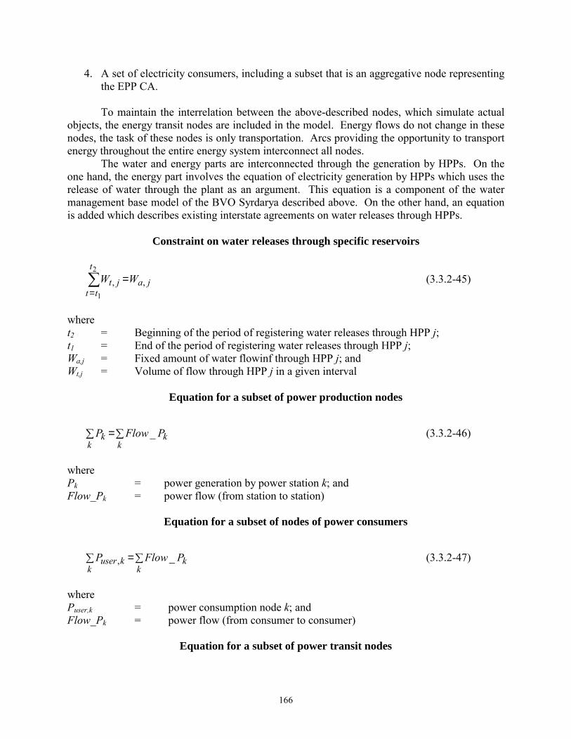
166

4. A set of electricity consumers, including a subset that is an aggregative node representing the EPP CA.

To maintain the interrelation between the above-described nodes, which simulate actual objects, the energy transit nodes are included in the model. Energy flows do not change in these nodes, the task of these nodes is only transportation. Arcs providing the opportunity to transport energy throughout the entire energy system interconnect all nodes. The water and energy parts are interconnected through the generation by HPPs. On the one hand, the energy part involves the equation of electricity generation by HPPs which uses the release of water through the plant as an argument. This equation is a component of the water management base model of the BVO Syrdarya described above. On the other hand, an equation is added which describes existing interstate agreements on water releases through HPPs.

Constraint on water releases through specific reservoirs

ja

t

ttjt WW ,,

2

1

=∑=

(3.3.2-45)

where t2 = Beginning of the period of registering water releases through HPP j; t1 = End of the period of registering water releases through HPP j; Wa,j = Fixed amount of water flowinf through HPP j; and Wt,j = Volume of flow through HPP j in a given interval

Equation for a subset of power production nodes

∑=∑k

kk

k PFlowP _ (3.3.2-46)

where Pk = power generation by power station k; and Flow_Pk = power flow (from station to station)

Equation for a subset of nodes of power consumers

∑=∑k

kk

kuser PFlowP _, (3.3.2-47)

where Puser,k = power consumption node k; and Flow_Pk = power flow (from consumer to consumer)

Equation for a subset of power transit nodes

167

0_ =∑k

kPFlow (3.3.2-48)

Objective Function

( ) ∑ ∑++∑ −=

kodcctrkk

uudemandu PccPccPPcF ***** 98

2,7 (3.3.2-49)

where Pu = Power consumption by consumers in an individual Republic u Pdemand,u = Power demands of consumers in an individual Republic u Pk = Power generation by all power stations in a Republic including thermal

stations Podc = Power flow to the EPP CA ∑ ⋅u

)( = Symbolic representation of summing a set of power consumers

∑ ⋅k

)( = Symbolic representation of summing a set of power producers

c7,c8,c9 = Weight coefficients of components of the objective function. c9 is considerably greater than c7 and c8. c8 is greater than c7. When c7=1, c8=10, c9=100, good solutions are obtained.

ck = Cost of power generation by a specific power station ctr = Cost of transmitting or receiving power from the EPP CA To provide for required minimum utilization of TPPs during the heating season, constraints are entered on electric power generation. These constraints may be changed depending upon the availability of coal and gas. In addition, other tasks and constraints affect the calculation of the water and energy balance. These include:

− Constraints on the volume of water discharged from a reservoir (annual, vegetation period, or any other period);

− Rates for electricity related to transfers in the EPP CA; and − Task on transfers, etc.

If there are no constraints, this model finds an optimal solution; if the whole complex of constraints is assigned, it maintains the water and energy balance. Both operation modes of the complex are of interest for the organizations that carry out long-term management of the water and energy complex. Based on this model, three calculations were made of different variants for the water and energy mode of the Naryn Cascade of HPPs and the power pool of the Kyrgyz Republic. In all variants considered, the model found an optimal solution with regard to the imposed constraints. Embedded in the model are the costs of generating power at stations and the tariff for “export or import” of electricity, equal to 1.3 tyin/kWh for HPPs, 94 tyin/kWh for TPPs, and a tariff of 100 tyin/kWh for import/export, respectively. For all options, the following constraints were used:

168

• Maximum and minimum monthly electric power generation by TPPs with regard to the required mode of heating loads;

• Conveyance capacity of HPPs of the Naryn Cascade of HPPs; and • Maximum and minimum levels of reservoirs of the Naryn Cascade of HPPs.

For more complete description of the results of using this model, see “Optimization of the Syrdarya Water and Energy Uses under Current Conditions,” A. Zyryanov and E. Antipova, Vol. 2, Section 2.1. The procedure of connecting this block to the base model and opportunities of the interface of this complex are described in the software guide (see below).

Summary

The mathematical description of the water management model was presented above:

• The basic model for the determination of the optimal operation regimes of hydro-technical facilities in the basin of a river (adjusted and tested in the basins of the Syrdarya and Chu Rivers) with the aim of providing consumers with water resources.

• The water quality (salinity factor) block can be added to this model, which transforms the basic model into a program for determining the optimal regulation of the water-salt regime in the basin of any river (adjusted and tested in the Syrdarya basin).

• The energy block can be added to this basic model, which transforms it into a program for determining the optimal regulation of the water-energy regime of the flow in the basin of any river (adjusted and tested in the basin of the Naryn River). The models, consisting of the blocks, created according to the national interests of the

Republics, are being used by specialists from the national and regional organizations of the Central Asian Republics.

3.3.3. “Energy” Component (UDC Energia) 3.3.3.1. Problem statement and general requirements to the model In accordance with the intergovernmental agreements between the Central Asia (CA) countries on the joint and complementary use of water and energy resources of the Naryn-Syrdarya cascade of reservoirs the UDC Energia and the BVO Syrdarya are charged with direct management and monitoring of water release operations as appropriate to provide the agreed water, fuel and power system conditions. These duties are an integral part of the general task of planning and management of water and power system operation within the EPP CA that UDC Energia is carrying out as its daily operation. One of the major planning tasks is operational planning of the EPP CA water and power system operation for the forthcoming twenty-four hours. The water releases of the HPPs determined by the BVO Syrdarya based on the annual planning of water and energy resources of the Naryn-Syrdarya cascade are used as input data for this task.

169

The major functions of the operational planning task are:

• Optimization of the joint TPP and HPP operation using the equivalent electric power network of the EPP CA with all available consumption centers and electric power lines; and

• Set electric power operation conditions in the allowable range through consideration of numerous operation and technology constraints.

The output documents of the operational planning task are used as guides for action of the EPP CA dispatcher of UDC Energia as well as for dispatchers of the EPP CA in their every-day and twenty-four hour management of the EPP CA water and electric power conditions. The program complex "OPTIMUM" used by the UDC Energia in its many-years of practice for this task is now obsolete. This program is absolutely inadequate for the up-to-date requirements in functional, algorithmic and technical respects. Recognizing the importance of the solution of this task in overcoming general problems of water and energy system planning in the CA region, the Coordination Group entrusted UDC Energia with responsibility to elaborate a model of operational planning of the EPP CA water and electric power operation conditions ("Energy" component) and to integrate it with the existing UDC Energia software complex "OPTIMUM." The "Energy" component is one of three interrelated components of the general model of planning and management of water and energy resources of the Naryn-Syrdarya cascade. Two other components of this general model are the "River" component (BVO Syrdarya) and the "Planning Zone" component (SIC ICWC). The support of UDC Energia and BVO Syrdarya from this complex of models contributes to the improvement of planning and management of water and energy resources of the Naryn-Syrdarya cascade system up to an advanced quality level in conformity with up-to-date requirements. The main requirements to the "Energy" component are as follows: • The model should minimize the costs to the EPP CA when buying power from its producers

(principal TPPs and HPPs of the EPP CA) for considered periods; • Payment period should be twenty-four hours; • EPP CA hourly electric power operation for the period should be optimized; • Optimization should be performed taking into account all major hourly and integral

operational and technological constraints for the twenty-four hour period; • The model should consider as a constraint the output of the "River" component (BVO

Syrdarya) with regard to the water discharge of the Naryn-Syrdarya cascade; • The optimization part of the model should be based on GAMS technology; • The model should provide the means of obtaining highly reliable final results; • The model design should be support operation in market economy conditions to the

maximum extent possible; • The model should be tested under conditions and real networks and reference data; and • The model should be integrated into the complex "OPTIMUM" aimed at its further use in the

EPP CA operational planning of water and power operation conditions. The work was carried out by the personnel of the UDC Energia (Ametov, I.D; Rojnov, E.; and Mikhnevich, M.), according to the technical Terms of Reference developed by the

170

Coordination Group along with the help of other specialists and the assistance of the USAID/EPIC Program staff, which provided sponsorship and technical support to the executors. 3.3.3.2. Input and output model data The model input data is divided into regulatory standards and reference documents (RSD) and operational data (OD). The RSD consists of general quantitative data on the model and information concerning: • power generating systems (PS) of the EPP CA; • power generating units (PU) of the PSs; • reference power plants of the EPP CA; • off-reference power plants in the PUs of the PS; • PUs of the electric model; • lines of the electric model; • line sections of the electric model; • inter-system power transfers; and • PU consumption diversity rates by PUs of the electric model. The comprehensive RSD list is given in Appendix 2.1. Once this RSD is computed, then it is updated as required. The OD is designed to perform immediate operational calculations. The OD is computed for every 24 hours and it is divided into external and internal information. The external OD includes data received from the PS and the BVO Syrdarya. The data communicated by the PS covers such data as prognostic hourly values of power consumption and loads for off-reference TPPs and HPPs by the PS power units. The data communication by the PS is performed at this stage with a telecommunication system. The BVO Syrdarya communicates to the UDC Energia recommended average values of HPP water discharges in the Naryn-Syrdarya cascade for one month, decade (10 days) and 24 hours. These data are the output of the water optimization model of the Naryn-Syrdarya cascade ("River" component). Currently the above mentioned data is communicated to the UDC Energia by mail or by telephone. The internal OD is computed immediately in the UDC Energia. It includes the following: • Hourly data on:

- Constraints on available effective power capacity of the EPP CA reference power plants; - Constraints on forward and back transfers of effective power for supervised lines and line

sections; and - States (ON/OFF) of lines in the EPP CA electric power model;

• 24-hourly data on:

- Constraints on PS effective power transfer balance; - Constraints on water discharge/fuel consumption for supervised power plants; and - Constraints on power output for supervised power plants.

171

The model output includes: • Supervisory task records for the UDC Energia dispatcher; • Supervisory task records for the PS; and • Results files for communication with technological tasks and information display systems

within the UDC Energia. The supervisory task records of the UDC Energia dispatcher are displayed in the form of documents with resulting hourly data on: • EPP CA including summary hourly values of:

- consumption; - loads; - available power; - available power reserves; and - regulatory operations

• PSs including summary hourly values of:

- consumption; - loads; - available power; - available power reserves; - regulatory operations - active power transfer balances - inter-system active power transfers and active power transfers by individual lines; and - loads by individual HPP

• Stations including the following values:

- hourly loads; - hourly reserves of available power; - summary 24-hourly power outputs; and - HPP 24-hours average water discharge

• Active power transfers for supervised lines and line sections displayed by hourly values. The supervisory tasks for the PSs are computed in the form of text files and communicated to the PSs by telecommunication system. Also, the data communicated to the PSs includes summary 24-hourly values of the above mentioned parameters. The input and output PS data is presented in unified data layouts making possible their effective computing and processing in the PSs and UDC Energia. The structures of data layouts received from and communicated to the PSs are presented as illustrative examples in the Appendix 2.2. As stated above, the model interactions with technological tasks and data display systems of the UDC Energia are kept going through computed files with resulting data of the model. The technological tasks using the model results are as follows: • Supervisory records; • Reports

172

The data display systems of the UDC Energia using model results data are as follow: • Technological information display system (TIDS); • Display group control system (DGCS); • Graphic parameter display system (GPDS) The resulting data for the "Energy" component is considered in the above mentioned systems as the plan targets. The TIDS and DGCS systems operate in real time enabling the display of planned targets at the same rate as telemetric information and with information of the supervisory records. Moreover the GPDS system graphically displays all three parameter categories, i.e. plan targets, telemetric parameters and supervisory records. All three systems operate within the UDC Energia local area networks. The complete diagram of information interactions of the model "Energy" and the complex "OPTIMUM" is given below in Figure 3.3.3.1. 3.3.3.3. Mathematical formulation of the “Energy” component The “Energy” component model is intended to optimize water and electric power conditions of the EPP CA with regard to the hourly and 24-hour integrated technological and operating condition constraints. This model includes the following:

• Model of electric power conditions; and • Optimization model

The optimization model consists of an objective function and a large set of technological and operating condition constraints. The constraints are subdivided into hourly and integrated ones.

Model of electric power conditions The model of electric power conditions is included in the "Energy" component to determine, based on the EPP CA electric power model, the linearized factors of nodal power allocation and their application in identifying constraints in the optimization model. The model of electric power conditions is based on the following assumptions:

• Active resistances in the electric network components are equal to zero; • Reactive power flows in the network are not considered in the model; and • Linearity of electric power conditions against reactive power that is equivalent to the

constancy of nodal power allocation values.

173

Data transmission on WPP 24-hours water discharge (telephone, mail)

Communication channels

Communication channels

UDC local networks

EP

UDC Energia Model "Energy"

Complex "OPTIMUM"

Communications from the EPP for the forthcoming twenty-four hours: - forecasted hourly power generating unit consumption ; - hourly loads of unvalued WPP; - hourly loads of unvalued HPP; (Robcom telecommunication system, model-108

STANDARDS AND NORMS OF THE "OPTIMUM" COMPLEX: - EPP structure components and characteristics; - Structure components and characteristics of the PG power generating

units (PU); - Structure components and characteristics of the UPG power plant

models; - Data by units of structural model; - Data by lines of structural

model; - Consumption diversity rates by power model units; - Data on the HVL sections and inter-system energy transfers;

Operational information on the complex "OPTIMUM" computed by the UDC for forthcoming 24 hours:

- restraints and power costs for reference plants; - power transfer restrains per lines and line sections; - data on line commutations in reference circuit; - restraints in WPP 24-hours water discharge/power output; - restraints in EPP 24-hours power transfer balance

EP EP

Supervisory task transmission to the EPP in hourly values of: - EPP summary load; - EPP summary available power capacity; - adjustment operations; - EPP power capacity reserves; - WPP inter-system power transfers; WPP loads and

water discharges; (Robcom telecommunication system, model-108, 109, 110)

Computation and transmission of planned values to the UDC technological tasks: - supervisory records; - report

Computation and transmission of planned values to the UDC dialogue display systems: - TIDS; - DGCS; - GPDS;

Computation and printing of supervisory task records to the UDC dispatcher for forthcoming 24 hours

EP …….

…...

BVO Syrdarya ("River"Component)

Figure 3.3.3.1. Diagram of information interfaces of the "Energy" component. The allowance and necessity of these assumptions are determined by the following:

• Early comparative estimations of error rates in determining active power flow allocations in lines between a complete electric power model (with representation of line resistances and node powers) and a simplified electric power model (with regard to the above mentioned assumptions);

174

• The fact that the electric power model will be applied to a simplified, equivalent EPP CA electric power network in which prognostic values of consumption and loads of off-reference power plants of larger power units and power systems will be used as input parameters; and

• The need to obtain, within a limited time, guaranteed results of calculations of hourly values of linearized factors of nodal power allocations independently from the input conditions of hourly estimations of steady-state electric power conditions.

The above mentioned assumptions enable the determination of the factors of nodal power allocations via parameters of electric network components by the following generalized equation:

q

qijqji

jiT

jiTqji A

XAXAXK

C ,,

,,

,,,

***

−= (3.3.3-1)

where

qjiC , = power allocation factor for node q on arc i –j

0

1 * KYYA −= (3.3.3-2)

Y-1 = inverse matrix of node conductances of the equivalent EPP CA electric power network;

YK0 = column vector of reference node couplings;

j

ijiT U

UK =,, (3.3.3-3)

KТij = transformation factor for the transformer on arc i –j; Ui, Uj = voltages of the nodes i and j; XTij = reactance of transformer arc i –j; Xiq, Xjq = reactance of arcs i –q and j –q;

Considering the adopted assumption of linearity of electric power conditions relative to the active power, the active power transfers by any network component of the model may be determined in the optimization model by the following equation:

∑=

qq

qijij PCP * (3.3.3-4)

where

ijP = active power transfer on branch i –j;

175

qijC = power allocation factor of node q on branch i –j; and

qP = active power of node q.

Objective function The objective function of the optimization model is represented by set of 4 minimized components:

• The sum of 24-hourly costs to buy power from the reference EPP CA power plants

∑ ∑=

24

1*min

t q

tq

tq PCost (3.3.3-5)

where:

tqCost = power selling cost of plant q in hour t; and

tqP = power generated at plant q in hour t.

• The sum of 24-hourly costs to buy additional power from the reference EPP CA power plants

due to deviations in the minimum generation capacity (Рq,min) of the power plants

∑ ∑ ∆=

24

1min,*min

t q

tq

tq PCost (3.3.3-6)

where t

qP min,∆ = deviation of the minimum available power Рq,min in plant q in hour

t;

• The sum of 24-hourly costs to buy additional power from the reference EPP CA power plants due to deviations in the maximum generation capacity (Рq,max) for the power plants

∑ ∑ ∆=

24

1max,*min

t q

tq

tq PCost (3.3.3-7)

where t

qP max,∆ = deviation of the maximum available power Рq,max in plant q in hour t;

• The sum of 24-hourly damages from shortages of power supplied to consumers due to

deviations in consumption by the nodes (power units)

176

∑ ∑ ∆=

24

1*min

t n

tnq DY (3.3.3-8)

where

Уn = cost caused by shortage of the 1st MWh of power supply on unit n; t

nD∆ = deviation in power consumption of unit n in hour t.

Hourly Constraints

The constraints considered in the optimization of each hour of the reference 24 hour period are as follows:

• Constraints on power generation from reference power plants max,min, qqq PPP ≤≤ (3.3.3-9) • Constraints on the deviation of Pq,max

max,max,max, *0 q

tq

tq PPRP ≤∆≤ (3.3.3-10)

where t

qPR max, = available additional regulatory range of Рq,mах for plant q;

• Constraints on the deviation of Pq,min min,min,min, *0 q

tq

tq PPRP ≤∆≤ (3.3.3-11)

where t

qPR min, = available additional regulatory range of Рq,min for plant q;

• Constraints on the scale of regulatory operations in the power unit t

ntn

tn DDRD *0 ≤∆≤ (3.3.3-12)

where t

nDR = available additional regulatory range at unit n;

tnD = predetermined consumption in unit n.

• Constraints on active power transfers in the lines ( ) max,min,max,min, ** ijn

n

nij

qqqq

qijij PDCPPPCP ≤∑+∑ −+≤ (3.3.3-13)

177

• Constraints on active power transfers for sections of the lines:

( ) maxsec,min,max,minsec, ** PDCPPPCP nn

nij

m qqqq

qij ≤∑+∑∑ −+≤ (3.3.3-14)

where m = set of power lines i-j entering the section n

• Constraints on the active power balance of the EPP CA ( ) ∑−∑=∑ −+

nn

kkfix

qqqq DPPPP ,min,max, (3.3.3-15)

where kfixP , = sum of fixed values of demand, loads of off-reference power

plants, external power transfers and fixed loads of the reference power plants in the power unit k.

Integral Constraints

• Constraints on active power transfer balance of power system s for 24 hours

( )100

*min,min,

ccss

KCCC ≤− (3.3.3-16)

where min,sC = predetermined value of power transfer balance for the power system

s for 24 hours; Kc = power transfer balance factor (% of min,sC ) that is common for all

PS;

( )∑

∑−∑ −+−=

∈ ∈=sq sn

tn

t

tq

tq

tq

tsfixs DPPPPC

24

1min,max,, (3.3.3-17)

= design value of power transfer balance for power system ‘s’; t

sfixP , = sum of predetermined values of power consumption, loads at hour

't' for off-reference power plants, of external power transfers and fixed loads for reference power plants of the power system ‘s’;

( )t

qtq

tq PPP min,max, −+ = sum of loads of power plants of the PS at hour t;

178

∑∈ sn

tnD = value of decrease in power consumption of the power unit n

entering in the power system s at hour t.

• Constraints on the sum of power consumption for 24 hours in plant q

( )

100*min,

min,qq

qqKQ

QQ ≤− (3.3.3-18)

where Qq,min = predetermined 24 hour value of power consumption at the plant q;

Kq = power carrier consumption factor (% of Qq,min) that is common for

all plants;

( ) qt

tq

tq

tqs RPPPQ *

24

1min,max,∑ −+=

= (3.3.3-19)

Rq = specific power consumption in power plant q • Constraints on the sum of power output for 24-hours from plant q

( )

100*min,

min,wq

qqKW

WW ≤− (3.3.3-20)

where Wq,min = predetermined 24 hour value of power output at the plant q; Kw = power output factor (% of Wq,min) that is common for all plants;

( )∑ −+==

24

1min,max,

t

tq

tq

tqq PPPW (3.3.3-21)

The independent variables extending the range of available power in the plants ( t

qP min,∆ , tqP max,∆ ) and the decrease in power consumption of the power units ( t

nD∆ ) were

added to the model in the implementation and testing stage. These variables are automatic input instruments of the EPP CA power conditions into the allowable field when inconsistent constraints are detected. The need for and expediency of these additional variables was determined by the following considerations. Constraint incompatibility, as a rule, is due to the impossibility of inputting electric power conditions within allowable limits by means of given set of independent variables. The allowable limits are determined by the given constraints. The independent variables, as a rule, are the power capacities of the plants.

179

It is practically impossible to determine the existence of inconsistent constraints at the stage of data preparation processing for further calculations. There may be a few causes for this. The major ones are that a large number of parameters must be controlled and they are dependent on the design of the electric power conditions. Therefore the task of detecting inconsistent constraints and searching for ways of inputting power conditions into allowable limits should be loaded immediately in the optimization algorithm. One of possible way to get around this problem may to extend the allowable limits when inconsistent constraints are detected. This can be achieved both through extending the regulatory range of principal independent variables and by introducing extra independent variables. These considerations were the basis for modifications to the “Energy” model during its development. Indeed, in case of constraint incompatibility it is possible to try to extend the range of available power capacities of power plants by both decreasing the minimum limit of available power (Pq,min) and increasing the maximum limit of available power (Pq,max). Such changes aren't contrary to the technology of the electric power system operation. Thus, the decrease in Pq,min may be achieved through switching off part of the power units or power generators in the plant. Or, the increase in Pq,max may be achieved through switching on extra units or generators in the plant. The advantage of providing extra operational range in the plants is evident from consideration of power conditions. Thus, the need to decrease Pq,min in an individual plant or in a few plants may result from the plant being locking-out by network factors or it may be caused by a decrease in total EPP CA power consumption down to the sum of Pq,min of all plants in the network. While the required increase in Pq,max may result both from a general shortage of EPP CA generating capacity in whole or from a power shortage in an individual unit or power supply region because of constraints in the power lines. It is quite evident that the process of extending available power limits in the power plants should be regulated. This problem may be solved by enabling consumers to determine for each plant an appropriate extent of extra regulatory range in which to decrease Pq,min or increase Pq,max. Perhaps, the most convenient way to achieve this is through the assignment of the factors

tqPR min, or t

qPR max, for each plant. An extra regulatory range could be determined for each

plant with these factors as a power share of Pq,min or Pq,max of the plants, respectively. In a special case the assignment of t

qPR min, or tqPR max, equal to zero may prohibit extending the

regulatory range in the plants. A third regulatory parameter of the model is the power consumption of the power units. In practice when the power generation is insufficient in the EPP CA or in a separate power region due to constraints in the lines, then a partial load switching off in the power units is applied as a means of balancing in planning and implementation of the EPP CA power conditions. This approach is applied in the “Energy” model by decreasing the regulatory range and the power consumption in power consumption units. The scale of the regulatory range, similar to the case of power plants, is determined by the share factor t

nDR and power consumption of the power unit. It is quite evident that all three extra mechanisms of allowable limit extension should be used only if necessary and their scale should be minimum or equal to zero when the power conditions are totally balanced and incompatible constraints are missing.

180

The minimization of power selling costs for the plants and damage caused by shortage of power supply in the power consumption units are used as conditions for allocating extra power increments to power plants and decreasing power consumption in the power units. 3.3.3.4. Model elaboration and tests UDC Energia over many years has carried out the operational planning of water and power operating conditions of the EPP CA using the software complex "OPTIMUM" which was designed by UDC specialists. The need of UDC Energia to develop new planning software is grounded in the fact that the existing software complex doesn't meet current requirements with regard both to functional and algorithmic aspects. The disadvantages of OPTIMUM are caused by limited capacities of its computation unit as regards its applied optimization method (simplex method) and its implementation program. However, this complex in itself is a very huge program product which has been developed and worked through over many years of operation and provides the following services: • Automatic operational data gathering from all over the power system; • Input and correction of operational information; • Control and processing of all input information; • Maintenance of a complex data base; • Computation, display and printing of a large number of output forms; • Automatic computation and transmission of results within the power system; and • Transmission of results to the unified information display system in real time operation and

to other applied tasks operating in the UDC. The OPTIMUM superstructure (input, output, and data processing routines, etc.) accounts for 75% of the program compared to the computation unit. Taking into account the limited resources available to build a new model, the sophisticated design of the model itself, the need for thorough tests of the new model based both on controlled examples and on real data, it was deemed expedient to replace the existing OPTIMUM computation unit with one constructed on the base of the model described above using GAMS technology. In this way the design and implementation of each model version consisted of the following activities: • Elaboration and computation of the model and its adjustment on simple schemes; • Elaboration within OPTIMUM of interface modules for the GAMS model based on the

complex data base and its auxiliary units; • Up-dating input modules related to reference data and output forms; and • Testing and up-dating the new model on the real operation scheme and real data base. The model elaboration was carried-out by stages with successive implementation of two versions of the model:

• First version, being more simplified, provided planning of the EPP CA operation for 24 hours by optimizing the EPP CA power conditions for each hour separately with no consideration of integral 24-hourly constraints.

181

• Second version, being more sophisticated and comprehensive in structure, provided optimization of the EPP CA hourly power conditions on the condition of hourly optimization to minimize the EPP CA 24-hourly costs of buying power from the TPPs and HPPs, including integral (24-hour) constraints on power consumption by power plants, in power generation by power plants and in active power transfers of the power systems.

Both versions were quite self-supporting with regard to their implementation and industrial operation. They were successively tested: first on the simplest electrical power scheme, then on the real equivalent EPP CA scheme used by the UDC Energia in operational planning of the EPP CA power conditions. At first stage, each model version was computed by hand, then it was thoroughly tested in detail on the simplest example and up-dated to obtain positive computation results. At the next stage, each model version was introduced into OPTIMUM and put into operation and transmission of results. Then, the tests of the modified OPTIMUM complex on the real electric power scheme and on the real data were carried out. More detailed description of the process of elaboration and tests of the model "Energy" is given in Appendix 2.3. 3.3.3.5. General appraisal of achieved results The work reported here resulted in the following achievements:

• The model for the complex task of operational planning of the EPP CA water and power operation and meeting all current requirements of operation standards of the EPP CA power planning task was created using the GAMS technology and successfully tested on the control examples;

• In the process of elaboration and testing, the model was modified with respect to the initial concept providing extension of the model to include implementation of power conditions regulation within the allowed limits;

• The complex of operational planning of the EPP CA water and power conditions (OPTIMUM) operated by the UDC Energia was modified to include in its structure the elaborated GAMS model "Energy"; and

• The first experimental design computations on the modified complex "OPTIMUM" basing on the real scheme and data were carried out.

3.3.3.6. Unresolved matters and problems The initial Terms of Reference for the “Energy” component called for the development of a seasonal planning model of the EPP CA water and power conditions based on the complex of operational planning. Due to several circumstances the model of seasonal planning has not yet been completed. The elaboration of the “Energy” model in the GAMS language and the associated modernization of the OPTIMUM complex required considerable labor input. In the process of modernizing OPTIMUM substantial time was taken to solve the problem of limited PC memory and the GAMS model – OPTIMUM joint execution. The result has been a modified version of OPTIMUM enabling the first experimental design computations to be carried out on the control

182

and real electric power schemes. The results obtained with the modified OPTIMUM complex were absolutely identical to the results achieved with an independent GAMS model. This fact may be considered as evidence of the correctness of the GAMS-model as well as the modified OPTIMUM complex. A number of experimental computations were carried out on the real scheme of the EPP CA. For the most part these experiments obtained completely correct solutions. A part of results require further analysis and consideration. Certain time is required to complete all tests of the modified OPTIMUM complex, analysis of the obtained results and, perhaps, certain improvements to the algorithm and complex as a whole. In the process of working with the "Energy" component there appeared some additional items needing further improvement, such as:

• Simulation of electric power conditions; • Modification of the objective function; • Input of a number of additional technological constraints.

3.3.3.7. Conclusions and proposals The works described here are aimed at elaborating the "Energy" component of the general model of planning and management of water and energy resources of the Naryn-Syrdarya cascade, and, using it as a basis, modifying the OPTIMUM complex of operational planning of the EPP CA water and power conditions, confirmed the possibility and expediency of using GAMS technology for solving such types of complex optimization tasks. Further possibilities of GAMS application exist in elaborating the following models and program complexes required by the UDC Energia: • Models of the HPP systems on the rivers Syrdarya and Amudarya for the purposes of

operational and seasonal planning of the EPP CA water and power conditions. These models will enable carrying out operational and agreed adjustments of water discharges of the HPPs determined by the BVOs Syrdarya and Amudarya.

• Operational adjustment and further optimization of the EPP CA water and power conditions based on telemetry data and estimated states. This will enable the dispatcher and the computation team of the UDC Energia to:

- Perform real time calculations for the EPP CA electric power conditions with minimum

deviations from the estimated power conditions for every moment; - Carry out alternative calculations based on the current water and power conditions of the

EPP CA:

� Switching on or off plant equipment (HPPs and TPPs); � Switching on or off power lines; � Increasing or decreasing power consumption related with implementation of contracts

on power supply; and � Changing conditions of power outputs and power carrier consumption in plants.

183

• Optimization of the EPP CA electric power conditions with respect to active power losses, which will enable the UDC Energia to:

- Carry out calculations aimed at minimizing active power losses within the EPP CA; - Determine optimum values of transformation ratios for transformers of the main system

substations; - Determine optimum loads of available sources of reactive power in the EPP CA; and - Elaborate proposals on the implementation of extra sources of reactive power in the EPP

CA. With respect to the perspective of future work, the UDC Energia considers it expedient and necessary to develop industrial versions of the program of operational and seasonal planning of the EPP CA water and power conditions as well as the three above mentioned programs. The programs should be designed to operate in the Windows environment and be oriented to: • Use up-to-date data base management systems (DBMS) to create a unified database for these

programs and access facilities (Explorer, SQL-server); • Use advanced information technologies (Web-technology, etc.) to arrange information

interactions of the programs with the power systems, BVO Syrdarya and other external organizations;

• Application of an advanced user's interface for the information input, correction and display; • Extensive use of graphical facilities for output information display; • Access system data from the information display systems and technological tasks of the UDC

Energia.

3.3.4. “Planning Zone” Component (SIC ICWC) 3.3.4.1. Introduction Within the WARMIS database developed through the EU TACIS WARMAP Program, the territory of the Aral Sea basin is divided into 44 units called "Planning Zones". The Syrdarya basin is divided into 20 Planning Zones. A Planning Zone is a hydrological unit within a hydrographic basin with united integrity of water supply systems and geomorphological structure of irrigation networks (irrigation and drainage systems). A planning zone is located within the limits of a region, but a region may be divided into several planning zones. A planning zone may consist of one or several administrative regions. All the territory of a planning zone has common hydrological conditions of water resources formation and economic factors to perform agricultural activity. The water resources formed within the planning zone are called local ones, while the water resources received by the planning zone from the transboundary sources are called transboundary ones. Planning zones are considered participants of the water and power complex through using water and power resources form a response in the form of the volume and quality of and in the form of benefits or damages resulting from limited water supply and, perhaps, power resources. It is necessary to emphasize that the notion of damage of the planning zone means not simply a

184

product shortage expressed in some equivalent (economic or financial prices) but a summary value of benefit losses both immediately in the planning zone and in the associate branches related with farm products processing of the considered planning zone. Interior losses of the planning zone result from addition together of losses caused by shortage of obtained volume of farm products within available lands and losses caused by deterioration of the land reclamation state of sown areas resulting in increased soil salinity. This interpretation of damage in the "Planning Zone" component is determined by the fact that this model is a component of the Basin Model and National Models whose response forms objective functions at higher hierarchic levels. Therefore for correct estimation of the consequences of one or another strategy of re-distribution of water resources at States or River Basins levels it is necessary to account for all damage components. Undoubtedly, the volume of farm products of the planning zone depends on many other factors playing no less important roles but not related immediately with water resources. In the planning zones the volumes of industrial, municipal and farm water supply with regard to the irrigated farming on average constitute up to 10%. Also, in the future, for some separate planning zones having in their structure developed industries and densely populated regions (e.g., Chirchik, Fergana, and Andijan) these types of water consumption may acquire a competitive importance compared with irrigated farming. Nevertheless at the first stage it is assumed that these types of water consumption are completely satisfied and the damage of these economy branches occurs only as a result of shortages of raw materials from the irrigated farming. Note that all economic figures of the planning zone strictly correspond to the State to which the planning zone belongs, i.e., the comparison of the planning zones by their economic figures may be performed only at the interior State level. Besides the exterior response to the changes of environmental conditions, the planning zone, as with any system owning its interior resources, is seeking the best, in some sense, re-distribution of water resources within itself. At present a lot of diverse, and optimal in one or another aspect, ways of water resource re-distribution within the planning zones have been proposed, beginning from the best execution of applications and finishing with maximum crop yield in a long-term perspective. The criterion of water resources re-distribution and management within the planning zone adopted by this work is based on the investigations of real water resources distribution now implemented in Central Asian countries. For any planning zone, this criterion seeks to find a way out of water resource deficit conditions with minimum economic losses. 3.3.4.2. Functioning of the Planning Zone From the point of view of the water and energy complex the planning zone is a concentrated object consuming some quantity of electric power and transboundary water resources with further re-distribution in space and time and with quality modifications. In this work the planning zone management is performed via the quantity and quality of transboundary water resources and, at the same time, accounting of quantities of local water resources. The result of the water resources consumption is expressed in some volume of farm and industrial products and on that base the damage in the planning zone is determined. The interior structure of the planning zone with respect to farming consists of: irrigation zones (systems of main channels, inter-farming, intra-farming and irrigation channels), diversion channel systems

185

(collector-drainage networks) and sown areas under a corresponding set of crops. In its turn each sown area is characterized by a set of physical and chemical features representing soil conditions at the current moment. Modifications of the water resources volumes and quality immediately affect the volume of farm production through the water volumes and indirectly through deterioration of soil conditions at the expense of soil salinity alterations. Therefore the model should apply to both process components related to modifications of water resources. Thus, the planning zone is an open system with concentrated parameters with input of the given hydrograph and quality of transboundary water resources supply, and output of the hydrograph, collector-drainage flow mineralization, and potential damage resulting from the limited water and energy resources. The interior structure of the planning zone is a set of objects representing processes of water and salt re-distribution within the farming areas and processes decreasing farm production yields as a result of alterations in soil mineralization and lack of water resources. In its turn each object of the planning zone is characterized by a set of variables and functions representing its spatial and technological properties. To describe functioning of the planning zone, consider the following set of objects:

• Irrigation zone – a complex of irrigation systems supplying water to a single area of crop cultivation. The planning zone may have several irrigation zones, part of which uses local water resources and other parts which use transboundary ones. The irrigation zones may be supplied with water by gravity flows or power-depended methods (pumping-plants systems, ground water, etc.). The irrigation zone is characterized by the following parameters: maximum flow-carrying capacity, efficiency, electricity consumption per unit of water resources, land areas under control (gross and net) and unit cost of supplied water resources.

• Drainage system – a system maintaining the required balance of salts and ground water

level within the irrigation areas and draining water excess into the collector-drainage network. The drainage systems are characterized by the following parameters: drainage module, drainage areas and areas of collector-drainage flow formation, volumes of electricity consumption per unit of collector-drainage flows.

• Farm crop - crop cultivated within the planning zone. It is characterized by the following

parameters: area under this crop, specific value of productivity per area unit and cost of this crop. Moreover, each crop is characterized by four functions: evapotranspiration, specific volume of water resources required to produce this crop within the planning zone, stress functions representing the decrease in cropping power resulting from water resources deficit and degree of soil salinity.

• Irrigation area - surface of the planning zone used for cultivated crops. It is a sum of net

values of the objects of the "Irrigation zone". It is differentiated by depth of ground water (conforming to the WARMIS database six occurrence levels are adopted: 0-1 m, 1-1.5 m, 1.5-2 m, 2-3 m, 3-5 m, > 5 m). Each level is characterized by three parameters: total irrigation area, average soil void ratio, average soil infiltration rate, and a function that indicates the distribution of areas by their degree of salinity. Moreover for the surface of the planning zone a drainage function is constructed representing the attribution of

186

diverse objects’ drainage to the irrigation areas on the basis of the thickness of the aeration zone layer.

• Ground waters - underground water resources involved in the water-salt exchange with

the aeration zone of the irrigation areas. It is characterized by the following parameters: ground water table depth, mineralization and an inflow-outflow function from the horizons of deep underground waters.

• Air environment - is considered only with regard to the sources (precipitation) and water

resources outflow (evaporation, evapotranspiration).

3.3.4.2. Equations of the planning zone component The objects of the planning zone are related between themselves based on the law of conservation of mass (of water and salt) and agricultural product losses are defined through the stress coefficients computed based on water deficiency and salt excess. The following set of variables is entered for formal description of physical and technological processes: T = discrete time, t∈ {T0, T0+∆t, T0+2∆t,…, T0+k∆t,...,};

)(tℑ =

)()(

tstw

= vector of water resource,

w(t) = average amount of water (m3) for a time interval ∆t, s(t) = mineralization of the water (kg/m3).

Water Resources Water resources of the Planning Zone are formed from three entries: surface inflow from local water sources, precipitation and surface inflow from transboundary water sources. The first two components are erratic, they are assigned as hydrographs and form the vector ℑ ,lc(t):

ℑ ,lc(t) = ℑ L(t) × η* + ℑ E(t) (3.3.4-1)

where η* = a reduced efficiency factor of the irrigation systems. (η* =ηtr×ηlc×ηvc×ηpr); ℑ L(t) = resources incoming from local sources; ℑ E(t) = resources formed by precipitation (wE = qE(t) × FN; sE=0) qE(t) = normal precipitation per unit of area; and FN = irrigated area (net). Water volumes are calculated through water supply rates, they are differentiated by Planning Zones and include leaching volumes. We will designate by {ℜ } a variety of crops grown on the areas {Fr} of the Planning Zone and having {wr

ℜ (t)} as a specific water supply.

187

We imply correspondence between {ℜ } and {Fr}. The leaching rate for each crop is {ℑ rN(t)}.

We define ℑ rℜ as:

Wr

ℜ = wrℜ × Fr; sj

ℜ =sjℜ (3.3.4-2)

and form the vector

ℑ rF(t) = ℑ r

ℜ (t) + ℑ rN(t); r∈ {ℜ } (3.3.4-3)

The vector ℑ r

F(t) represents the total water required for raising crops on the area Fr. This volume is covered by two entries: local water resources and transboundary water resources, i.e.:

ℑ rF(t) = ℑ r

F,lc(t)+ ℑ rF,tr(t), or ℑ r

F,tr(t) =ℑ rF(t) - ℑ r

F,lc(t) (3.3.4-4)

Water from local sources is, as a rule, rigidly associated with specific crops and lands, and, hence, is out of control, but it is impossible not to take stock of it as the link between crop capacity and water supply values is nonlinear. Equation (4) defines water for each crop, and the amount that should be supplied from transboundary sources. Total water required for the basin from the Planning Zone ℑ 0,tr+(t), accounting for losses in irrigation systems, will be expressed by the formula:

*

)()( }{

,

,0η

∑ ℑ=ℑ ℜ∈+ r

trFt

trt

t , t∈ {time} (3.3.4-5)

where {time} = any time interval. As a rule, transboundary resources are delivered to the Planning Zone from different sources that have different mineralization. We designate this variety by {inpT}, the resultant vector of transboundary water resources is

∑ ℑ=ℑ∈

+

}{

, )()(inpTi

trFi

tr tt , t∈ {time} (3.3.4-6)

Management of water supply to the Planning Zone lies in formation of the vector ℑ tr+(t) equal to vector ℑ 0,tr+(t) and the disagreement between them is the unbinding management, which, depending on the symbol, brings either a crop water deficit or waste water discharges from the irrigated fields. We will designate disagreement between the ℑ tr+(t) and ℑ 0,tr+(t) vectors as

δℑ +(t) =ℑ 0,tr+(t) -ℑ tr+(t) (3.3.4-7) In the future, the vector δℑ +(t) will play the role of a management variable. If under the terms of water fluctuation all crops are equally subject to an associated impact, we will receive expressions to estimate water “infringements” for crops

188

δwr(t)=ς (t)× wr

F(t) (3.3.4-8)

where

)()()()(

twtwtwt lctr +

=+δς (3.3.4-9)

Water and Salt Balance in the Aeration Zone

In these methods the aeration zone means the entire soil layer from its free surface to the ground water level. A planning zone, as we specified above, is ranked into six zones according to the depth of ground water occurrence. For each zone, its own equations of water and salt balance are formulated. In addition, we consider each zone as an entity with a full list of the crops grown in the planning zone. That is the total number of equations for each type of balance will equal 6 × {R} , where {} is the number of elements in the set {R}. To avoid complicating equations with indexes of crop types and the depth of ground water occurrence, consider a unit surface element (1 ha), on which one crop r is grown, and which the depth of ground water occurrence H ranks. Direct the z-axis downward, so that Z = 0 coincides with the earth surface. Then, the depth of the aeration zone layer will equal Z(t). The following equality applies

dtdz

dttdZ gr

−=)( , t∈ ∆t (3.3.4-8)

Considering movement along the z-axis, write equations of water and salt flows. For water flow we obtain

0)()( =+∂

∂+∂∂ Eu

mzv

tθθθ ; v=k/m (3.3.4-9)

where: θ = volumetric soil moisture, equal to the ratio of the water volume to the total soil volume (0 ≤ θ ≤ m), m = porosity, v = true speed of water flow in pores, uE(t ) = evaporation rate and evapotranspiration from a length unit, k = coefficient of soil filtration. For salt flow we obtain

0=∂∂+

∂∂

zq

tS s

; )(zsDsqs ∂∂−= νθ (3.3.4-10)

where: qs = salt flow, S = total amount of salt, s = concentration of dissolved salt, D = coefficient of diffusion. Boundary conditions include

189

at the soil surface r

rF

twt )(),0( =νθ ; s(0,t)=sr(t) (3.3.4-11)

at the water table 0),( =∂

∂z

tZs ; θ(Z,t)=m (3.3.4-12)

The equation of ground water level fluctuation is as follows

[ ])()(1 0infhh

grdrprgr

ttqzqqqqmdt

dz −+−++= (3.3.4-13)

where: zgr = ground water level, qinf , qpr = infiltration flows from canals and irrigated fields, q0 = water from deep aquifers, qdr = drainage outflow, qh = additional water from elevated ground water levels in higher irrigated areas; this water is lagged by the time interval th. Before making assumptions to close the system (3.3.4-9) – (3.3.4-13), we introduce a grid along the z-axis and perform the usual averaging of θ and S within the interval ∆z. Now we may integrate equations (3.3.4-9) and (3.3.4-10) with respect to z, and as a result we obtain, for the interval (z,z+∆z)

0)( =∆×+−+∆∂∂

∆+ zum

ffzt

Ezzz

θθ (3.3.4-14)

where: fz+∆z , fz = speed at the boundaries of the interval, and the value ∆z × uE = UE is the rate of evaporation and evapotranspiration. In the absence of plants, it is taken based on S. F. Averyanov’s experimental formula; if plants are available, it is taken based on the numerical constants determined for various plants at various times experimentally, i.e.

UE = u0(1-z/zK), ∀ 0 ≤ z ≤ zK; UE = 0, ∀ z>zK (3.3.4-15)

where: u0(t) = rate of evaporation from water surface, zK = critical depth. For equation (3.3.4-10) by analogy with (3.3.4-14) we have

0=−+∆∂∂

∆+sz

szz qqz

tS (3.3.4-16)

The right bound of the last interval on the grid along the z-axis coincides with the ground water level, therefore

qpr=fz+∆z (3.3.4-17)

We take infiltration outflow from canals according to the formula

190

qinf=(1-η* )×(wT+wL+wE)/FN (3.3.4-18)

We calculate drainage flow from the actual value plus the increment resulting from the elevated ground water level

qdr=q0dr × (1+∆zgr/Hdr) (3.3.4-19)

Further calculations are based on the principle of quasi-steady flow condition for each interval ∆t. These intervals are used in calculating how main variables change inside each layer.

Amounts of Crops Deviations in amounts of grown crops are expressed through coefficients of the stress resulting from water shortage and excess soil salinity. Water shortage is proportionally allocated between crops and it does not depend on the depth to ground water, therefore stress coefficients are equal to

[ ]∑=∈ }_{

)(,vegtt

rrr twtfWstress δ (3.3.4-20)

Because of water shortage, actual yields will be

yWr =yr

0×(1- stressWr) (3.3.4-21)

The degree of soil salinity depends on zones with different ground water levels. In accordance with the SANIIRI procedure, soil salinity is calculated as the average salinity for the growing period of a crop. Determining the degree of soil salinity through its weighted average for irrigated areas for each level, we obtain its initial value for the water and salt balance problem

h

areasshshs

h F

FSS

∑

= ∈ }_{,,

0 (3.3.4-22)

After we have solved the water and salt balance problem, we obtain the matrix Sr,h(t) instead of only the weighted average of soil salinity. On the basis of this matrix we calculate first

[ ]evgr

bvgr

vegtthr

hrtt

tSttS

−

∑ ∆= −∈∗ }{

,

,

)()( (3.3.4-23)

191

where: trbvg , tr

evg = beginning and end of crop r growing period. Then for each level of ground water occurrence we calculate

stressSr,h=fs(r,S*r,h), ∀ r∈ {R}, h∈ {1,2,. . .,6} (3.3.4-24)

Using stress coefficients we calculate amounts of crops in accordance with their areas at the level under consideration. As an initial amount, we adopt the value obtained from Equation (3.3.4-21). After that, we calculate the total production in the planning zone by summing on all levels (in terms of crops)

r

Hhhrhr

Wrr F

stressSFyy

∑ −= ∈ }{

),, 1( (3.3.4-25)

The amount of the produce under-produced equals ∆Yr = Fr×(yr

0 – yr). Cost appraisal of the damage with regard to inter-industry relations is calculated by the formula

ℵ = ∑[ αr + ∑(βr,p ∆Yr )] ∆Yr (3.3.4-26) r∈ {R} p∈ {P}

where: αr = direct cost of the produce under-produced; βr,p = inter-industry damages occurring because of the shortage of the r crop in the p industry. 3.3.4.3. Joining the Planning Zone and River components The planning zone model describes modifications of the planning zone conditions for a given set of farm crops with diverse levels of water consumption, salt concentrations, ground water occurrence, diverse soil salinity degrees and technical conditions of the irrigation and drainage systems. These factors form vectors of the input and output resources through which the "River" component interacts with the "Planning zone" component. In the River component the Planning zone is considered as a point to which certain properties are attributed concerning consumption and transformation of water resources resulting in some value determined as a potentially possible national income obtained for a twelve month period. Designate by "J" the number of the node under which the planning zone is entered in the River model and designate by {J+} the set of nodes from which water is supplied to planning zone J, and designate by {J-} the set of nodes where water is supplied to the River by planning zone J. For the River component there are only transboundary resources, thus, every flow of water at the level of the River component is a transboundary one. In the River component the nodes are the following objects: reservoirs, river sections, planning zones. The arcs are facilities supplying water from one node to another. Therefore, the interactions between the components River and Planning Zone are through a set of corresponding arcs. Each arc (j,J), j∈ {J+} in the River component receives the vector ℑ j,J, j∈ {J+} and each arc (J,j), j∈ {J-} in the Planning Zone component receives the vector ℑ J,j, j∈ {J-}. The resulting vector of input water resources supplied to the

192

Planning Zone component is determined as a weighted average. This transformation is common for both components. Moreover, the damage caused in the planning zone by the resulting hydrograph of the transboundary water resources is transferred from the Planning Zone component to the River component. When a more detailed analysis is carried out, then a lost volume for each farm crop may be transferred to the River component. 3.3.4.4. Description of the Algorithm and Reference Data The description of the algorithm and reference data are provided in Appendix 3.

193

3. OPTIMIZATION OF JOINT WATER AND ENERGY USES OF THE SYRDARYA BASIN......................................................................................................................................... 120

3.1. Operating Models to Manage Water and Energy Systems of the Basin. Model Assessment in Regard to Optimization of Use of Water and Energy Resources 120

3.1.1. Basic Principles of River Flow Control ................................................................... 120 3.1.2. Hydro-economic and Hydro-energy Calculations.................................................... 122 3.1.3. Models to Manage Water and Energy Complexes................................................... 132

3.2. GAMS as an Instrument for Building Complex High-Level Optimization Models136 3.2.1. Mathematical Basis of GAMS ................................................................................. 136 3.2.2. Test Examples of Using GAMS System in Optimization Models........................... 136

3.3. Basic Provisions and Principles of Optimization of the Syrdarya Basin Water and Energy Uses................................................................................................................ 143

3.3.1. Basic Outline Regarding Complex Management and Optimization of Syrdarya Water and Energy uses ............................................................................................ 143

3.3.2. “River” Component (BVO Syrdarya) ...................................................................... 149 3.3.3. “Energy” Component (UDC Energia)...................................................................... 168 3.3.4. “Planning Zone” Component (SIC ICWC).............................................................. 183