REZA BIHAMTA

Optimisation of the Hydroforming Process of Geometrically Complex Aluminium Tubes Taking Account of Preceding

Forming Processes

Thèse présentée à la Faculté des études supérieures et postdoctorales de l'Université Laval

dans le cadre du programme de doctorat en génie civil pour l'obtention du grade de Philosophiae doctor (Ph.D.)

DEPARTEMENT DE GENIE CIVIL ET DE GENIE DES EAUX FACULTÉ DES SCIENCES ET GÉNIE

UNIVERSITÉ LAVAL QUÉBEC

2011

RezaBihamta, 2011

11

Résumé

Les réglementations gouvernementales concernant l'économie de carburant et la réduction

des gaz à effet de serre forcent les industries de transport et les fabricants à modifier la

façon dont les pièces sont conçues et fabriquées. Le problème de la réduction du poids est

mis à l'avant-plan et on croit fortement que l'utilisation étendue des alliages d'aluminium et

le développement de designs innovants font partie de la solution pour remplir les mandats.

En même temps, la faible formabilité de l'aluminium pose un vrai défi aux fournisseurs de

pièces de véhicules chaque fois qu'ils sont confrontés à fabriquer des composants à

géométrie complexe avec des procédés de mise en forme conventionnels. En conséquence,

d'autres procédés plus avancés sont explorés, comme l'hydroformage qui offre de tels

avantages comparés aux procédés d'usage courant. Cette technologie semble être le

catalyseur qui permettra aux métaux difficilement formables d'être utilisés sur une échelle

beaucoup plus large

Dans la présente thèse, une étude approfondie a été effectuée sur l'hydroformage des tubes

d'aluminium ainsi que les procédés connexes.

Dans les études numériques, une stratégie d'optimisation issue de l'application du logiciel

Ls-Opt et des codes sources développés dans MATLAB a été présentée. Elle rend possible

l'optimisation de l'étirage à paroi variable, du pliage et de l'hydroformage des tubes soit

d'une façon regroupée ou seule.

Dans la partie expérimentale du projet, dans le prototype de banc d'étirage, la distribution

d'épaisseur désirée sur le tube initial a été mise en application. Une nouvelle méthode de

conception de moule d'hydroformage à géométrie complexe est aussi présentée et

appliquée expérimentalement avec succès. Enfin, les résultats de l'optimisation globale ont

été appliqués et validés expérimentalement et une correspondance acceptable a été

observée. Les résultats de ce projet se révèlent fortement utiles pour les industries de

transport terrestre et de l'aérospatiale pour produire des produits tubulaires plus facilement

et avec moins d'essais et erreurs.

Ill

Mots clés: AA6061, aluminium, CAO/CAM/ IAO, étirage des tubes, hydroformage des

tubes, méthode des éléments finis, mise en forme des métaux, optimisation, pliage des

tubes.

IV

Abstract

Government regulations for fuel economy and greenhouse gas emissions reduction are

forcing transport industries and manufacturers to modify the way parts are designed and

built. The problem of weight reduction has come to the fore and it is strongly believed that

the extensive use of aluminium alloys and innovative designs are part of the solution to

meet the mandates. At the same time, the low formability of aluminium is creating a real

challenge to automotive parts suppliers when trying to manufacture geometrically complex

components with conventional forming processes. As a result, more advanced forming

processes, such as hydroforming, are being explored. Hydroforming offers advantages

compared to conventional forming processes. This technology appears to be the enabler

that will allow difficult to form metals to be used on a much wider scale.

In the following dissertation, a comprehensive study was performed on the aluminium tube

hydroforming and preceding processes.

In the numerical studies an optimisation loop by the application of Ls-Opt software and

developed codes in MATLAB was presented. This will make possible optimizing the

processes like variable thickness tube drawing, bending, and tube hydroforming, all

together or solely.

In the experimental part of the project, the desired thickness distribution of the initial tube

was applied in the prototype tube drawing machine. Additionally, a new method for the

design of geometrically complex hydroforming dies was presented and applied successfully

in the experiments. Finally, global optimisation results were applied in the experiment and

acceptable agreement was observed. The results of this project seem to be considerably

useful for transportation and aerospace industries to produce their tubular products more

easily and with less trial and error.

Key words: AA6061, Aluminium, CAD/CAM/CAE, Finite element method, Metal

forming, Optimisation, Tube bending, Tube drawing, Tube hydroforming.

Acknowledgments

I thank all my family members for their supports and encouragement during all stages of

my studies through the end of my Ph.D. I also acknowledge the special role of my mother

in all successes I have in my life. Unfortunately she is no longer among us, but I believe her

spirit is happy from this success too.

I thank Prof. Mario Fafard, Prof. Michel Guillot, Dr. Ahmed Rahem, Dr. Guillaume

D'Amours, and Dr. Quang-Hien Bui for their contributions and help in all aspects of this

thesis. I also thank Mr. Jean-François Béland and Mr. Guillaume Filion for their

consultations in numerical steps of the thesis and Mrs Sakineh Orangi and Mr. Arash

Taheri for their supports and help during my frequent journeys to Quebec City for this

project. Also, the collaboration and help of all of employees of NRC-Aluminium

Technologies Centre in Saguenay (Chicoutimi) is highly appreciated.

I also thank Natural Science and Engineering Research Council, Alfiniti, Aluminerie

Alouette, Cycles Devinci, CROI, NRC-ATC, Aluminium Research Centre-REGAL, and

CQRDA for their financial contributions to this thesis.

Lastly, I would like to highlight the role and character of Prof. Mario Fafard as a key factor

in success and co-ordination of this project. I Also give a special thanks to Prof. Michel

Guillot, a person from whom I learned not only science and technology, but also patience,

politeness, and persistence.

VI

To

My mother and my sister whom I lost while completing this thesis, and to my father and my brother for their encouragement to continue the thesis.

vu

Table of Contents

Résumé ii Abstract iv Acknowledgments v Table of content vii List of Tables xi List of Figures xii

Chapter 1 Introduction 1 1.1. General background 1 1.2. Research needs 3

1.1.1. Variable thickness tube drawing 3 1.2.2. Recovery heat treatment 3 1.2.3. Tube bending 3 1.2.4. Tube hydroforming 4 1.2.5. Global optimisation loop 5

1.3. Contents 5 References 6 Chapter 2 Literature Review 7

2.1. Cold tube drawing process 7 2.1.1. Introduction 7

2.2. Various classifications of the tube drawing process 8 2.1.3. Tube drawing in the literature 11 2.2. Intermediate heat treatment 18 2.2.1. Introduction 18 2.2.2. 6000-Series Aluminium 19 2.2.3. Heat treatment to recover ductility 21

2.3. Rotary-draw tube bending 23 2.3.1. Introduction 23 2.3.2. Hydrobending 23 2.3.3. Rotary-Draw Bending 24 2.3.4. Tube bending in literature 27

2.4. Tube hydroforming 31 2.4.1. Introduction 31 2.4.2. Advantages of THF 31 2.4.3. Process options 33 2.4.4. Application of THF in automotive parts 37 2.4.5. Application of FEM in THF 38 2.4.6. Pre-forming of tubes for the hydroforming process 39 2.4.7. Lubricants for hydroforming applications 40 2.4.8. Tube hydroforming (THF) in literature 41

2.5. Conclusion and Summary 45 References 47

vin

Chapter 3 A new method for production of variable thickness aluminium tubes: numerical and experimental studies 51

3.1. Introduction 52 3.2. Design modifications and experiments 56

3.2.1. Design modifications 56 3.2.2. Details of experiments 57

3.3. FE modeling and optimisation 59 3.3.1. Base FE model details 60 3.3.2. Optimisation procedure 61

3.4. Results and discussion 65 3.4.1. Base FE model results 65 3.4.2. Optimisation results 68

3.5. Conclusion 76 Acknowledgements 76

References 77 Appendix 3.A 79 Appendix 3.B 80 Appendix 3.C 82

Chapter 4 Application of a new procedure for the optimisation of variable thickness drawing of aluminium tubes 85

4.1. Introduction 86 4.2. Numerical modeling 88

4.2.1. Base FE Model 89 4.2.2. Optimisation procedure 91

4.3. Experiments 93 4.4. Results and discussion 97

4.4.1. Base FE model validation 97 4.4.2. Optimisation results 98 4.4.3. Experimental results 100 4.4.4. Comparison between two types of mandrel design 102

4.5. Conclusion 104 Acknowledgements 105 References 105 Appendix 4.A (LFOPC optimisation method) 107 Appendix 4.B 108

Chapter 5 Numerical study on the new design concept of hydroforming dies for complex tubes 109

5.1. Introduction 110 5.2. Design of new die I l l

5.2.1. Geometric specifications of part 111 5.2.2. Geometry of initial tube 116

5.3. Finite element model details 117 5.3.1 Material properties 117 5.3.2. Die geometry and meshing 118

IX

5.3.3. Boundary conditions and contact condition 119 5.4. Experiments 120 5.5. Results and discussion 122

5.5.1. Thickness reduction percentages 122 5.5.2. Distribution of thickness 124 5.5.3. State of equivalent strains 126 5.5.4. Preforming by die closing 128 5.5.5.Thickness reduction distribution in the circumferential direction 131 5.5.6.Another advantage of the three parts die: More facility in the

bending step 133 5.6. Conclusion 134

Acknowledgements 135 References 135

Chapter 6 Global optimisation of the production of complex aluminium tubes by the hydroforming process 138

6.1. Introduction 139 6.2. Cold forming processes prior to hydroforming 141

6.2.1. Variable thickness tube drawing 141 6.2.2. Heat Treatment 143 6.2.3. Tube bending 146 6.2.4. Tube hydroforming (THF) process 151

6.3. Global optimisation 153 6.3.1. Optimisation procedure 153 6.3.2. Optimisation variables 153 6.3.3. Objectives and constraints 154 6.3.4. Sampling methods 155

6.4. Experiments 156 6.4.1. Variable thickness tube drawing 156 6.4.2. Annealing heat treatment 156 6.4.3. Tube bending 156 6.4.4. Tube hydroforming 157

6.5. Results and discussion 158 6.5.1. Variable thickness tube drawing 158 6.5.2. Tube bending 160 6.5.3. Tube hydroforming (THF) 161

6.6. Conclusion 173 Acknowledgements 173 References 174

Chapter 7 Conclusion and Recommendation 176 7.1. Conclusion 176 7.2. Future work and recommendations 177

Appendices 179 Appendix A) Thickness Applier Code (TAC) 180 Appendix B) Geometry Updating Code (GUC) 193 Appendix C) Shape Variable Manager (SVM) and post-processor 194 Appendix D) Pre-processing command file 199 Appendix E) File management in global optimisation of THF process 201

XI

List of Tables

Table 2.1 : Chemical Composition (wt %) of the Al. 6063 and 6061 20

Table 3.1: Comparison of base FE model and primary experiment 65 Table 3.2: Upper and lower limits for the optimisation variables 68 Table 3.3: The three error indicators for the minimum and maximum thickness models.. .69 Table 3.4: The average values for various responses in the 10 iterations or 10x16 simulation points 73

Table 4.1 : Summary of design variables and their range of variation 93 Table 4.2: Validation of base FE model by primary experiment 97 Table 4.3: Summary of performance of optimum and non-optimum die in the experiments 101

Table 5.1: Specification of various sections of part 114 Table 5.2: The initial and corresponding final thicknesses of tube in various zones 117

Table 6.1: Specifications of samples in Figs. 6.3 and 6.4 145 Table 6.2: Optimisation variables with their domains and starts values 154 Table 6.3: An example of correlation matrix between optimisation variables and responses 169

Table A1 : Shell element card and required fields 181 Table A2: Other options of the shell element to be completed by the program 181 Table El: Required translations (TR) and rotations (Rot) to position the tube after application of variation of thickness to the first bending step 201 Table E2: Required translations (TR) and rotations (Rot) to position the tube after the first bending in the second bending step 201 Table E3: Required translations (TR) and rotations (Rot) to position the tube after the second bending in the THF step 201

Xll

List of Figures

Fig. 1.1: The small Kappa Architecture features 2 Fig. 1.2: Automotive exhaust components 2

Fig. 2.1: Schematic view of two-step tube drawing 1) Tube 2) Die 1 (Sinker) 3) Locator 4) Die2 5) Die3 6) Space between dies 7) Mandrel 8 Fig. 2.2: a) Tube drawing without a mandrel, 1: Drawing die, 2: workpiece b) Drawing over a stationary mandrel. 1: Drawing ring, 2: workpiece, 3: mandrel, 4: plug c) Drawing over a floating plug, 1: Drawing ring, 2: workpiece, 3: floating plug d) Drawing over a moving mandrel, 1 Drawing ring, 2 workpiece, 3 moving mandrel 10 Fig. 2.3: The dieless tube drawing technology 14 Fig. 2.4: Deformed tube by residual stress after slitting 17 Fig. 2.5: Various available structures for aluminium from cold deformation to grain growth 19 Fig. 2.6: Hydrobending in a press by a die 23 Fig. 2.7: Schematics of rotary-draw bending 24 Fig. 2.8: Bending steps in rotary-draw bending 25 Fig.2.9: Schematics of free bending method 27 Fig. 2.10: Sketch of push assistant devices in RDB of thin-walled tube 29 Fig. 2.11: Five different boosting methods for applying the pushing load 30 Fig. 2.12: Schematics of the THF process 31 Fig. 2.13: Length per length in the conventionally produced part with respect to the hydroformed part 32 Fig. 2.14: Concept of HPH process a) Before application of pressure (die open) b) Before application of pressure (die closed) c) Pressure applied (die closed) d) Maximum pressure

34 Fig. 2.15: Reduction of thickness in the HPH process 35 Fig.2.16: Concept of LPH process a) Before application of pressure (die open) b) Before application of pressure (die closing) c) 1st stage Pressure (die closing) d) 2n pressure stage (die closed) 36 Fig. 2.17: State of tube thickness in the LPH process 37 Fig. 2.18: Hydroformed frame for Ford F-150 pick-up truck 38 Fig. 2.19: All-aluminium cars, employing the space frame with numerous hydroformed components, (a) Audi A2, and(b) Audi A8 38 Fig. 2.20: Different forming stages (a) Tube blank (b) useful wrinkles in pre-forming stage (c) pre-formed part (d) finally formed part 45

Fig. 3.1: Various methods of tube drawing a) sinking b) fixed mandrel c) float mandrel d) moving mandrel method 55 Fig. 3.2: Concept of variable thickness tube drawing a) sinking step b) reducing wall thickness step with a position controlled -mandrel (for illustration purpose angles of the die and mandrel were drawn with exaggeration) 57 Fig. 3.3: Tube drawing tools a) conical mandrel b) die 58 Fig. 3.4: Self closing mechanism for pulling tube through die and mandrel 59 Fig. 3.5: Lubrication mechanism for (1) die and (2) mandrel 59 Fig. 3.6: An overall view of developed FE model 60

xm

Fig. 3.7: True stress-strain curve for the AA6063-O tube 60 Fig. 3.8: Flow chart for optimisation process 63 Fig. 3.9: Mandrel displacement curve in primary and full experiments 66 Fig. 3.10: Tube displacement curve in primary and full experiments 66 Fig. 3.11: State of residual stress in the drawn tube in various directions a) thickness (X) direction, b) axial direction (Y), c) hoop direction (Z) and d) von-Mises 68 Fig. 3.12: Meta-modeling accuracy for the minimum thickness model (last iteration) 69 Fig. 3.13: Meta-modeling accuracy for the maximum thickness model (last iteration) 70 Fig. 3.14: Optimisation history for a) minimum thickness and b) maximum thickness during the optimisation process (In this figure the results of the first simulation in each iteration were presented) 71 Fig. 3.15: 3D scatter plot for two optimisation objectives with respect to first design variable i.e. initial thickness (tho) 72 Fig. 3.16: 3D scatter plot for two optimisation objectives with respect to first design variable i.e. outer diameter (OD) 72 Fig. 3.17: Distribution of thickness in axial direction with initial tube dimension of OD: 53.98 mm and th0: 2.40 mm 74 Fig. 3.18: Correlation bars for the optimisation objectives i.e. maximum and minimum thickness and drawing force 75 Fig. 3.19: Variation of maximum and minimum thickness with respect to tube initial outer diameter (experimental results) 75

Fig. 4.1 : Tube drawing process 87 Fig. 4.2: Schematic of the variable thickness tube drawing process (For illustration purpose the mandrel angle is drawn with exaggeration) 88 Fig. 4.3: An overall view of the developed FE model 89 Fig. 4.4: True Stress-Strain curve for tube material (AA 6063-O) 90 Fig. 4.5: Flow chart for optimisation process 94 Fig. 4.6: a) Variable thickness tube drawing machine b) self closing jaw of pulling axis c) lubrication system for the die and mandrel 95 Fig. 4.7: Methodology for measurement of tube thickness after drawing 96 Fig. 4.8: Examples of tube drawing tools a) conical mandrel b) die 96 Fig. 4.9: Mandrel and tube displacement curve for the primary experiment (normalized time=0.61) and full experiment (normalized time=l) 97 Fig. 4.10: 3D scatter plot of drawing force with respect to die angle and die fillet 99 Fig. 4.11: 3D scatter plot of drawing force with respect to die fillet and mandrel angle 99 Fig. 4.12: 3D scatter plot of maximum thickness with respect to die angle and die fillet radius 100 Fig. 4.13: Geometry of optimized tools a) Die b) Mandrel 101 Fig. 4.14: Variation of tube drawing force in optimum and non-optimum tools with respect to tube initial outer diameter in the experiments 102 Fig. 4.15: Stepped mandrel 103

XIV

Fig. 4.16: State of residual stress in a) axial direction b) hoop direction c) von-Mises stress and d) equivalent plastic strain in the tube produced by the stepped mandrel 103 Fig. 4.17: State of residual stress in a) axial direction b) hoop direction c) Von-mises and d) equivalent plastic strain in the tube produced by the conic mandrel (conic angle=3°) 104 Fig 4.B1: a) Geometries of die and mandrel in the initial state b) Geometries of die and mandrel after change in the geometric parameters (conflict of tube with die) c) axial motion of the tube for adjusting and removing the conflict 108

Fig. 5.1: a) The case study of this paper with eight different sections 112 Fig. 5.1: b) Schematic view of eight sections of case study with variable thickness and various sections (For illustration purpose, the sections are drawn with larger scale) 113 Fig. 5.2: Schematic of THF die with symmetric parting line and initial tube diameter of 40.2mm 115 Fig. 5.3: Schematic of THF die with un-symmetric parting line (three parts) and initial tube diameter of 50.8mm 1 ) fixed die 2) upper die 3) rear die 115 Fig. 5.4: Schematic view of three-part die and hydroforming machine 1) upper die 2) rear cylinder 3) rear die 4) left feeding cylinder 5) fixed die 6) right feeding cylinder 116 Fig. 5.5: Initial thickness distribution of tube and correspondent place of each section in final part 118 Fig. 5.6: True Stress- Strain curve for the AA 6061-O material 118 Fig. 5.7: a) Axial feeding curve b) hydroforming pressure 119 Fig. 5.8: Three-parts dies after installation in Interlaken hydroforming press 121 Fig. 5.9: Left and right pusher with rectangular sections 121 Fig. 5.10: Thickness reduction percentage in the part produced using two halves die in the time=1.2sec 122 Fig. 5.11: For three-part die: a) Thickness reduction percentages after closing the die and before start of hydroforming b) thickness reduction percentage contour in the part after end of hydroforming process 123 Fig. 5.12: Thickness reduction percentage in the tube with overall thickness of 2.74 mm with the two-half die 124 Fig. 5.13: Thickness distribution in the produced part with two-half die at time=1.2sec (before completion of hydroforming) 125 Fig. 5.14: Thickness distribution in the produced part with three-part die at the end of hydroforming step (Time=2 sec.) 125 Fig. 5.15: Effective plastic strain after die closing for the three-part die 126 Fig. 5.16: Effective plastic strain at the end of hydroforming step for the three-part die...127 Fig. 5.17: Effective plastic strain at the end of hydroforming step for the two-half die (Time=1.2 Sec.) 127 Fig. 5.18: Form of tube after end of closing step and end of hydroforming step 130 Fig. 5.19: a) tube after preforming by die closing b) after hydroforming 130 Fig. 5.20: Distribution of thickness in the circumferential direction in four different sections i) section Aii) section C iii) section E iv) section G from FE results 132 Fig. 5.21: Sections of tube after hydro forming 133

XV

Fig. 5.22: Two differently prebent tubes that were successfully hydroformed in the three-part hydroforming die 133 Fig. 5.23: Effective plastic strain in the part with just two bent regions 134

Fig. 6.1 : Tubular automobile parts produced by the THF method A) Roof headers, B) Instrument Panel Support, C) Radiator Supports, D) Engine Cradles E) Roof rails, F) Frame Rails 139 Fig.6.2: Application of various thicknesses to the initial tube by the developed preprocessor 143 Fig. 6.3: Stress-Strain curves for the tubes in the original condition (O) and only one-step drawn to outer diameter of 2.25 inches and various thicknesses (details are presented in table 1) 144 Fig. 6.4: Stress-Strain curves for the tubes drawn 2 steps from 2.50 inches to 2.25 inches and from 2.25 inches to 2.00 inches with various thicknesses (details are presented in table 6.1) 144 Fig. 6.5: The applied annealing heat treatment cycle 145 Fig. 6.6: Applied material property to the tubes after extrapolation by Holloman's power law (<T = fc",n=0.263,k=211.48) 146 Fig. 6.7: Schematics of rotary-draw bending 147 Fig. 6.8: Modeling of the first step, rotary-draw bending a) before performance of bending b) after bending c) distribution of tube thickness at the end of process 149 Fig. 6.9: Modeling of the second step, rotary-draw bending a) before performance of bending b) after bending c) distribution of tube thickness at the end of process

150 Fig. 6.10: Initial state of tube with the three-part THF die 151 Fig. 6.11: Application of different mesh densities in the various zones of the tube 152 Fig. 6.12: Surpassing of die parts by the tube because of inappropriate mesh density and numerical parameters selection 152 Fig. 6.13: Application of optimisation objectives a) all regions of part (thickness reduction objective) b) critical node to guarantee die filling c) two ends of tube to minimize the thickness increase 155 Fig. 6.14: Thickness measurement in the bent tube by the ultrasonic method 157 Fig. 6.15: Three-part THF die installed in HF-1000 hydroforming press 158 Fig. 6.16: Thickness distribution in the tube after two-step drawing 159 Fig. 6.17: Modified thickness distribution in the tube for two-step drawing 160 Fig. 6.18: Thickness variation percentage in the tube after two-step bending 161 Fig. 6.19: Sealing by the local deformation of tube ends 162 Fig. 6.20: Design of pusher for the local deformation method sealing A) guiding zone B) indentation zone C) sealing surface 163 Fig. 6.21: Deformation of tube because of local deformation sealing forces a) experimentally b) numerically 163 Fig. 6.22: Sealing by both O-ring and local deformation methods 164

XVI

Fig. 6.23: Hydroforming from preceding processes up to end a) initial tube with variable thickness b) after two-step bending c) preformed tube by closing of die parts d) hydroformed part 165 Fig. 6.24: Total forces on the pushers during the experiments 166 Fig. 6.25 : Total forces on the pushers from THF process FE model 166 Fig. 6.26: 3D scatter plot of three responses of optimisation (Blue points are simulation points of the first iteration and the red points are the result of the second iteration) 168 Fig. 6.27: Hydroforming pressure vs. right and left pushers displacements 169 Fig. 6.28: Accuracy model for the thickness reduction% response (RMS err: 0.0295 (0.21%), Sqrt PRESS: 0.0793 (0.59%), R-sq=0.99) 170 Fig. 6.29: Accuracy model for the thickness increase% response (RMS err: 0.0917 (0.182%), Sqrt PRESS: 0.245 (0.486%), R-sq=l) 171 Fig. 6.30: Accuracy model for the die filling response (RMS err: 0.00189 (0.00616%), Sqrt PRESS: 0.00493 (0.016%), R-sq=0.999) 171 Fig. 6.31: Accuracy model for the final shell thickness response (RMS err: 3E-5 (0.00255%), Sqrt PRESS: 9E-5 (0.0068%), R-sq=l) 172 Fig. 6.32: Contours of effective plastic strain at the end of THF process 172

Fig. Al: a) Shaded view of a tube after application of thickness variation b) position of and thickness value for each element 180 Fig.Cl: An example of an unacceptable shape of tube (green) in some simulations 194

Chapter 1

Introduction

1.1. General background

Tubular parts have a very important role in transportation applications like cars,

motorcycles and bicycles. The demand for fuel efficiency and reduction of greenhouse gas

emission make reduction of weight in transportation industries a high priority for designers.

European-C02 emission performance standards for light commercial vehicles set the short-

term target of reaching an average CO2 emission level of 175 g/km by 2017 compared to an

average emission level of approximately 185 g/km in 2009 [European C02 Emission

Performance Standards for Light Commercial Vehicles ].

The majority of tubular parts have complex geometries (Fig. 1.1 and Fig. 1.2) and one of the

usual methods for their production is the tube hydroforming (THF) process. In this cold

forming process, finding the appropriate production parameters, i.e. the load evolution of

internal pressure and axial feeding, is fairly difficult and time consuming because of the

required number of experimental and/or numerical iterations to produce a final part without

faults like wrinkling, bursting and unfilled zones. It seems that the existence of a third

parameter, such as variation of thickness in the initial tube prior to THF, can sometimes

help to solve some problems like bursting appearing in the THF process. On the other hand,

in the original design of most tubular parts, the thickness of tubes is considered constant

along the axial direction. However, in real loading conditions of these parts, all regions of

the part do not experience the same load and in the regions with lower stress, larger

thickness is considered as overdesign and will increase the overall weight of the

component.

Fig. 1.1: The small Kappa Architecture features [http://solsticegxpowners.com, visited

August 2011].

Fig. 1.2: Automotive exhaust components [http://www.muraropresse.com, visited August

2011].

In this thesis, a general approach for the production of tubes with complex geometry is

developed. Initial investigations showed that four principal processes are usually required

for production of tubes with complex geometries: tube drawing with or without variable

thickness, tube bending, hydroforming; and finally recovery heat treatment. Depending on

the final geometry of the tubes, various combinations of these processes are required. To

obtain workpieces without any problems like bursting and wrinkling at the end of

hydroforming, it is necessary to optimize all the processes involved in the production of

parts from tube drawing to THF.

1.2. Research needs

1.2.1. Variable thickness tube drawing

As mentioned above, for tubular parts, it is not really necessary to have constant thickness

along the axial direction. On the other hand, with increasing the local thickness of tubes in

the regions with high chance of bursting, finding the appropriate loading path for the

hydroforming step would be easier.

At the start of this project, a complete investigation of the methodology for the production

of variable thickness tubes by the drawing method was performed. The investigation

included optimisation of tooling geometry and initial tube geometry using the finite

element model, and performance of extensive experiments to define formability limits of

the studied alloy i.e. AA6061-O. The optimisation method used to optimize the geometry

and initial tube geometry is an automatic method and will be explained in detail in the next

chapters.

1.2.2. Recovery heat treatment

After cold tube drawing in two steps, the ductility of tubes will be reduced and there is high

risk of breaking the tubes in the next cold forming steps like bending and hydroforming.

Therefore, recovery heat treatment to recover all of the tube's ductility to the initial state is

performed at a temperature around 404 °C for 2 hours, then controlled cooling down to

260° C, then air cooling.

1.2.3. Tube bending

The bending process that was considered in this thesis is rotary-draw tube bending which is

used in the majority of the hydroforming shops for tubes with some bends in their

geometries. Having bending in the production chain of complex tubes may change the

results in the hydroforming step from two viewpoints:

1) Change in tube thickness in the bent region: in the outer surface of a bent region, tubes

will experience reduction in wall thickness because of tensile stresses. The reduction in the

thickness of these regions can increase the probability of bursting and/or wrinkling during

the hydroforming step.

2) Residual stress: after the bending process, if there is no stress relieving step, there will be

residual stresses in some tube's regions. The zones with tensile residual stresses are prone

to failure during the hydroforming step.

Because of limitations in the final geometry of the tube, there are some restraints in the

applicable modification to the bending process, and it is not straightforward to play with the

geometric parameters of this process. However, because of the above reasons i.e. change in

the thickness of tube and residual stresses, the bending process should be simulated and

included in the optimisation loop of the hydroforming process.

1.2.4. Tube hydroforming

Usually complex geometry tubes have lots of variation in their cross sections and need a

considerably high percentage of deformation to completely fill the hydroforming die. To

obtain minimum possible inflation load in the tube, it is always preferable to have an initial

tube shape as near as possible to the final shape. On the other hand, if the tube's diameter is

larger than the distance between two halves of the hydroforming die, the tube will be

crushed before starting the hydroforming pressure application. To improve capability of the

THF process, a new method of designing THF dies was presented for the first time. Based

on the analyses performed, most of the parts that cannot be produced by the cold

hydroforming method, now can be produced by this method. This modification, which will

be explained in the next chapters, uses a three-part die instead of two, and thus, tubes with

larger initial diameters prior to THF can be used. Because of the special design of the THF

die, preforming of the part is performed while the die is closing, considerably reducing

production time and increasing successful part production possibility significantly.

After preparation of the hydroforming process finite element model, this model with the

preceding process like tube bending and tube drawing will be included in a global

optimisation loop to optimize the hydroforming process including the preceding process to

produce parts without problems.

1.2.5. Global optimisation loop

The developed optimisation process is able to optimize the hydroforming including

preceding forming steps, by automatically changing the defined variables based on the

selected design of experiment (DOE) method. In the case study of this project, the selected

variables were initial tube thickness, hydroforming pressure and axial feeding. The

optimisation algorithm, included the bending step simulation in the global optimisation, and

the simulation results were copied from one step to the other automatically to include the

effect of bending steps in the final results in the hydroforming step.

1.3. Contents

Including the present chapter, this thesis consists of seven chapters including four chapters

based on papers accepted or submitted to journals.

The second chapter includes a literature review about the processes dealt with i.e. tube

drawing, heat treatment, rotary draw bending and tube hydroforming. The literature review,

attempts to present the most up-to-date researches about these processes.

The third chapter presents a new method for the production of variable-thickness tubes by

the drawing method. This chapter, which was published in the journal of Material

Processing and Technology, evaluates the effect of various parameters on the minimum and

maximum possible thickness in the variable-thickness tube drawing method.

The fourth chapter is a submitted paper that presents the experimental and numerical results

on the optimisation of tool geometry in the variable thickness tube drawing method.

The fifth chapter presents a new concept for the design of hydroforming dies. This method,

to be registered as an invention in North America, makes production of complex geometry

parts by the hydroforming method possible, while it was virtually impossible by the classic

THF method.

The sixth chapter presents the methodology of the global optimisation of the tube

hydroforming process, taking into account the preceding processes. The developed

methodology is adjustable for adding or removing some other processes too.

The last (seventh) chapter contains conclusion and recommendations for future work.

In Appendices A-E, some details of the developed optimisation procedure and codes are

presented.

References

[1] European CO2 Emission Performance Standards for Light Commercial Vehicles, The international council on clean transportation, Policy update number 11, March 3, 2011. [2] http://solsticegxpowners.com, visited August 2011. [3] http://www.muraropresse.com, visited August 2011

Chapter 2

Literature Review

2.1. Cold tube drawing process

2.1.1. Introduction

In general, hot forming processes produce low-strength materials and uneven dimensional

accuracy for the final product. If high quality products are required, cold processing should

follow the preliminary hot forming process. In axi-symmetric components, such as wire

(rod) and seamless tubes, this is achieved by the cold drawing of the hot-finished product

through a die (or a series of dies). This treatment imparts good mechanical properties and

effectively regulates dimensional tolerances.

In the tube drawing process, the specimen is inserted in the die and gripped by a device that

can pull it forward on a mechanical or hydraulic bench and reduces the diameter and/or its

wall thickness. Depending on the amount of deformation and area reduction sometimes

drawing in more than one die i.e. multi-dies drawing is necessary. A schematic view of

two-step tube drawing is presented in Fig. 2.1.

rzâ zzz2zzèèzzzzzzzzzzzzzzzzz ZZZZ

A \ \ \ \ \ W S S S ^ \ ^ \ S ^ S N N N N N S g S ^

Fig. 2.1: Schematic view of two-step tube drawing 1) Tube 2) Die 1 (Sinker) 3) Locator 4) Die2 5) Die3

6)Space between dies 7) Mandrel [Neves, 2005].

2.2. Various classifications of the tube drawing process

The main operational tube drawing processes are:

1. Sinking

2. Fixed plug

3. Floating plug

4. Moving mandrel

5. Ultrasonic vibration

These processes are illustrated schematically in Figs. 2.2a to 2.2a". In the sinking operation,

the tube is drawn without any internal support of the mandrel. Therefore the change in the

wall thickness can not be controlled. As the bending and unbending that the tube wall

experiences while passing through the die, there is a maximum limit for the diameter

reduction in this method. This process is generally used only as a preliminary operation

(Fig.2.2a).

The usually-adopted method is tube drawing over a cylindrical plug. Either a stationary or a

floating tool can be used. In the former case, the tool is positioned in the die throat and is

held there by a rigid plug bar. The tube, of a bore slightly larger than the plug diameter, is

pulled over the plug and the plug bar. Initially the tube is sunk onto the plug and is then

drawn. Both the diameter and the wall thickness of the tube are reduced in a controlled

manner (Fig. 2.2b).

For the drawing of long, small diameter and thin-walled tubes, a floating plug is used. An

initially hot-processed or cold-annealed tube is inserted into a die that contains, in one side,

an unsupported conical free plug. The tube is drawn over the plug and is then coiled on a

drum for ease of storage and transportation. In the other alternative of the operation, a

conical plug that is free to float is prevented from moving in one direction by a bar (Fig.

2.2c).

The older method of drawing (moving mandrel method) over a long mandrel that supports

the tube hole is now seldom used, mainly because the tube drawn in this way attaches

tightly to the mandrel. As a result, to remove the tube after drawing, the tube and mandrel

may have to be reeled in a cross-rolling reeler that expands the tube and frees it from the

mandrel. The reeling operation can impart helical markings to the tube's outer surface,

consequently makes it necessary to do another drawing operation, and is also likely to

affect the uniformity of dimensions along the entire length of the tube. In some cases,

where highly polished and dimensionally accurate, but relatively short tubing is needed,

moving mandrel drawing can be used if withdrawal of the tool is possible without reeling

(Fig. 2.2d).

In the ultrasonic vibratory systems, used either in the wire or tube drawing, the die is

vibrated at an appropriate frequency to increase the efficiency of the process by affecting

the rate of feed of lubricant and the mechanics of the drawing. Also, in various research it

was ascertained that application of ultrasonic movement to plug causes reduction in the

drawing forces [Hayashi et al., 2003, Murakawa and Jin, 2001]. The described techniques

above are equally applicable to the manufacturing of ferrous and non-ferrous tubes.

10

a)

b)

c)

d)

Fig. 2.2: a) Tube drawing without a mandrel, 1 : Drawing die, 2: workpiece b) Drawing over

a stationary mandrel. 1: Drawing ring, 2: workpiece, 3: mandrel, 4: plug c) Drawing over a

floating plug, 1: Drawing ring, 2: workpiece, 3: floating plug d) Drawing over a moving

mandrel, 1 Drawing ring, 2 workpiece, 3 moving mandrel [Tschaetsch 2006].

11

The development of the floating-plug technique, with advantages like savings in tool

material, better carrying the lubricant, and saving space when coil drawing in some cases,

has overtaken the use of the fixed-plug operation method.

2.1.3. Tube drawing in the literature

The tube drawing and similar processes like wire drawing have been the subject of various

papers since 1962. During this period, various aspects of this process were evaluated

analytically (energy, slab, and upper bound methods) and numerically for various materials.

Some of the published documents on tube drawing are presented in chronological order.

In 1963, Duncan et al. presented a general method for physically calibrating tube drawing

dies to study tube ironing and tube sinking, and tested them experimentally and

theoretically. Their developed model provides an accurate basis for optimisation of drawing

dies on the base of stress in the drawing dies. In 1970, Bratt and Adami analysed influence

of initial anisotropy on the reduction of thin-walled tubes by the upper and lower methods.

They also predicted maximum reduction ratios for a given material.

In 1971, Pierlin and Jermanok published a book on the drawing processes, and presented a

slab method analysis for the cylindrical mandrel drawing of tubes.

A slip-line field approach was adopted by Collins and Williams in 1985. They attempted to

construct the axisymmetric analogue of Hill's well-known bar-drawing solution. Finally,

they developed a nonlinear optimisation routine to find the correct pressure distribution on

the die with acceptable accuracy.

Urbanski et al. in 1992 used the matrix method for simulation of mandrel drawing. Their

method is based on an extremum principle, which states that for a plastically deforming

body with volume V under traction F and velocity v prescribed on the surfaces Sd and Sm,

with an incompressibility condition introduced, using penalty functions with penalty

constants K and Kb, the actual solution minimizes the following functional:

12

i(v) = \ a p ( s ) ï d V - \ ( F . v ) d S d - \ ( F . v ) d S m + y s* s„

K \ ( è r + è z +èe)2dV +Kb[ \(Cd)2dSd + \ (C m ) 2 dSJ (2.1

S„

where in the above equation:

I(v) : Functional of the total power of deformation

a : Yield stress

s, s : Effective strain and strain rate

F : Friction force vector

v : Vector of velocity

Sm : Mandrel-material contact surface

K : Penalty constant for incompressibility

Kb : Penalty constant for the boundary condition

V : Volume of the deformation zone

Cd : Penalty function referring the die-material contact surface

Cm : Penalty function referring the mandrel-material contact surface

Additional conditions are introduced regarding the free surface velocity and volume

constancy of the plastic region. Based on their model, they can predict amount of strain and

also friction coefficient in the die and mandrel.

Kamezis and Farrugia in 1998, studied one and two-step tube drawing and compared them

from various aspects like residual stress, drawing force, temperature and amount of

mechanical working induced in the tube per pass. They also compared the reaction force on

the mandrel and drawing force with experimental data, and found good agreement between

them. Another interesting result obtained was comparison of tubes obtained by one and

two-pass drawing operations. The tubes produced by single-pass drawing have significantly

lower amount of residual stress compared with two-pass operations for the same schedules

13

using the same die profiles and drawing speeds. Single-pass schedules however require

higher drawing forces.

The procedure Kamezis and Farrugia used to optimize the drawing process was based on

the calculation of workability parameters (Cpr0cess), implemented with a FORTRAN user

subroutine in ABAQUS software. CproCess is defined as the amount of work that the

maximum tensile stress crT carried out through the applied equivalent strain in a metal-

working process [Dieter 1984, Semiatin et al. 1985 and Cockcroft 1967] i.e.: ê f _ (2.2

Cprocess = J ° T d e

0

where ëtota, is the total yield strain at the end of the process. According to the Cockcroft and

Latham the magnitude of Cpr0cess can not exceed a maximum Cmax defined from the tensile

strain-stress curve to failure. Therefore, the optimisation of the tube drawing is based on the

calculation of CproCess- By comparing Cpr0Cess and Cmax, the risk of material failure during

processing is assessed: those single-pass schedules which exhibit Cpr0cess less than Cmax can

be safely adopted. Problems arise, however, in deciding the proper magnitude of Cmax.

Tensile, upsetting compression, and torsion tests provide quite different values [Dieter

1984]. At the same time, elongation is not usually as accurate as reduction of cross-

sectional area at failure. Material anisotropy can also be a problem. These issues have to be

addressed when establishing a rigorous optimisation process. The approach they followed

in their study was to determine Cmax from the tensile stress-strain curves for normalised

hollow tube materials. In order to estimate the variation of Cpr0Cess during processing, the

above equation was converted to an appropriate discrete expression that can be calculated

by the FE code:

Cpmcess = H " CJT - ^ d t = f j " <jT edt = £ a T èAt (2-3

where è is the equivalent strain rate calculated from the individual principal strain-rate

components and At is the variable time increment used in the FE analysis.

Wang et al. in 1999 presented a theoretical study on the deformation velocity field and

drawing force during the dieless drawing of tubes by means of the power equilibrium

14

method. Dieless drawing is a newly developed flexible metal forming technique without

dies that is performed only according to the property that yield strength of metal varies with

deformation temperature. The precision and shape of the product are controlled by the

drawing speed and the speed of movement of the heating-cooling apparatus. Dieless

drawing is a technology that has many advantages, such as high precision, high efficiency,

low consumption of energy and more flexibility. It can be used to form some materials, i.e.

those that have high strength and high frictional resistance and low plasticity at room

temperature, which can not be formed using conventional forming technologies. Variable

section tubular parts, such as conical and wavelike, which are difficult to be formed using

conventional metal forming technology, can be formed easily using this technology. In Fig.

2.3 schematic view of this process is presented.

The obtained results by the power equilibrium for the drawing force have acceptable

agreement with the experiments.

heating coal oogjjggogj

Fig. 2.3: The dieless tube drawing technology [Wang et al. 1999].

In 2005, Luis et al. presented a comparison among finite element and analytical methods to

study the wire drawing process. Their investigations showed that FE and upper methods

provide more accurate results since they consider all of the energies involved in the

process. Another result they obtained was the inaccuracy of the slab method in the cold

wire drawing. This seems reasonable because in the cold drawing process the internal

15

energies play an important role. Lastly, the result of the homogeneous deformation (lower

bound) approach was considered completely inaccurate.

In 2007, Kim et al. used the ductile fracture criterion and FE method to avoid fracture and

to obtain successfully formed parts. Especially two types of mandrel, straight and stepped,

were proposed and those were compared in view of forming failure. Consequently it is

known that the stepped mandrel is more effective to disperse stress concentration compared

to the conventional straight type of mandrel; It can transmit drawing forces to the

deforming tube without any failure.

In 2008, Kuboki et al. evaluated the effect of presence of plugs in the amount of residual

stress in the drawn tubes. Their research showed that there is a minimum geometric

reduction of 6%, which is effective for levelling the residual stress. Also, in order to

evaluate the intensity of the residual stress, an index, which is the integration of the

absolute value of axial residual stress, is introduced as equation 2.4.

2 ^ | "" r\o~ \dr I n d e x = *'. ' ' ' (2-4

nirl-rl) where rout is the outer radius and r;n is the inner radius of the drawn tube.

This paper also presented a simple and easy to implement method to evaluate

experimentally produced residual stress in the final part. After drawing, the tail portion of a

drawn tube was slit into eight pieces with a length of 120 mm, every 45° in the hoop

direction as shown in Fig. 2.4(a). With larger residual stress more opening in the tube's end

is expected. When the plug is not employed, the tube tail opens wider as shown in Fig.

2.4(b), i.e. the intensity of the residual stress is larger. On the other hand, when the plug is

employed to add the geometric reduction in thickness Rt of 7.3%, the tube tail does not open

(Fig. 2.4(c)), in other words, the intensity of the residual stress is quite small.

In order to evaluate the intensity of the residual stress quantitatively in the experiments, the

displacement S at the tube-tail end was measured as shown in Fig. 2.4(a) and (b). In the

analysis, the displacement S was calculated from the curvature c, determined by the

16

equations 2.5 and 2.6. using x-y coordinate in Fig. 2.4(d) based on simple theory of

strength of materials.

\o~zydA -rj\cTzdA c = - ^

(2.5

E(I-2n\ydA+r] 2 A)

jydA (2.6 rj = A

A

where in the above equations

CT : axial residual stress, A: area, rj : position of neutral plane in y direction, E: Young's

modulus, /: second moment of area about x axis.

Béland et al. (2011) optimized the cold drawing of AA6063 aluminium to reduce the

production steps from two to one. In this study, they developed a finite element model for

the tube drawing process. They also developed a program in MATLAB to automatically

change the geometric parameters of the tools. Finally based on the geometry corresponding

to minimum drawing force , they reduced the production steps for their case studies form

two steps to one. However, in this study, the design variable selection procedure did not

take into account the possible effects of changing of two or three geometric parameters at

the same time on the output i.e. drawing force.

Bui et al. (2011) presented a new formability criterion for drawn tubes. In this method, a

tube was drawn through a die and a conic mandrel, while changing the position of the

mandrel. Therefore, the thickness of the tube was reduced and reached a limit that is called

drawing limit for that specific alloy. Investigation in this research proved that in the tube

drawing process, depending on some parameters like material alloy and heat treatment type,

in the point of rupture the axial stress is constant. This idea was confirmed by experiments

for AA6063-O, AA6063-T4, and AA6061-O alloys.

17

Slit width = 0.9mm y h 1 Length = 120mm

•Ôrl-& O 'B i $ > co

Position of slit Shape of tube tip after slitting

(a) Schematic illustration of slits

(b) Without plug (initial thickness f0 = 4mm)

(c) With plug (initial thickness t0 = 4.75mm, target thickness G =4.0mm, geometric reduction in thickness /R, =15.8% )

1 A neutral plane

« X

- >

(d) Definition of coordinates for curvature calculation

Fig. 2.4: Deformed tube by residual stress after slitting [Kuboki 2008].

Xu et al. (2011) studied the effect of plug design on the accuracy of rectangular shape tubes

after the drawing process. In their studies, they proposed a change in the design of the

drawing mandrel, and evaluated it numerically and experimentally. The change applied a

relief zone in the straight part of the mandrel and consequently increased the tube's surface

finish at the end of the process.

18

2.2. Intermediate heat treatment

2.2.1. Introduction

Cold drawing, like other cold deformations, causes significant modification in the

microstructure and mechanical properties (such as yield stress, ultimate strength, and

elongation) of the aluminium alloy by the strain hardening phenomena. Cold working of

the aluminium upon drawing decreases tube ductility and as-drawn tubes are more prone to

fracture during the bending process. In cold deformation, energy is stored in the material

mainly in the form of dislocation during deformation. As presented in Fig. 2.5, grains get

flatter and deform in the flow direction. The result is that when stress is applied to the

wrought aluminium, sliding of the planes of atoms is impeded by the faults created, and

more energy is needed to deform the metal after it has been worked. Yield stress and

ultimate strength increase while ductility is reduced. This energy is released in three main

processes, those of recovery, recrystallization, and grain coarsening.

The process of recrystallization of plastically deformed metals and alloys is of central

importance in the processing of metallic alloys for two main reasons.

The first reason is to soften and restore the ductility of material hardened by low

temperature deformation (that occurring below about 50% of the absolute melting

temperature). The second is to control the grain structure of the final product. In metals

such as iron, titanium, and cobalt that undergo a phase change on cooling, the grain

structure is readily modified by control of the phase transformation. For all other metallic

alloys, especially those based on copper, nickel, and aluminium, recrystallization after

deformation is the only method for producing a completely new grain structure with a

modified grain size [Jiang et al. 2007].

The dislocation structures introduced by deformation make them thermodynamically

unstable, so that on holding at high temperature after deformation further structural changes

occur by the process of static recovery and static recrystallization.

19

Annealing from cold work Recrystallization

Grain growth

Original Cold Annealed Start of Partial Complete Partial Complete structure worked after cold recrys- recrys- recry»- grain grain

structure working tallization tallization tallization growth growth 5052-H18

The temperature is raised uniformly

Fig. 2.5: Various available structures for aluminium from cold deformation to grain growth

[Beaulieu 2003].

2.2.2. 6000-Series Aluminium

The tube material in this thesis is AA6061. The principal alloying elements in 6000-series

alloys are magnesium and silicon that in combination, form precipitation of Mg2Si. These

precipitates obtained in the heat treatment of foundry and wrought alloys increase the

mechanical properties of aluminium. The alloys of this series are the most suited to

structural applications, since they lend themselves readily to the production of extrusions.

They provide an acceptable tensile strength, a high resistance to corrosion, and formability

that is ideal for extruding. In addition, they can be welded and anodized. Usually alloys of

the 6000-series are produced in the T4 temper and then attain the T6 temper by artificial

aging.

20

The alloy which is by far the most widely used in structures and the most readily available

is AA6061-T4. In practice, AA6061-T6, or its close relatives, offers the best combination

of strength, weldability, and corrosion resistance at an affordable price. Among the many

uses seen today for AA6061 are recreational vehicles, truck bodies, street lighting

standards, rivets and gas cylinders. It is also used extensively in marine applications.

AA6005-T5 has strength equal to that of alloy AA6061-T6 when not welded, but costs

somewhat less. However, when welded, the resistance of AA6005-T6 is only 85% of that

ofAA6061-T6.

In architectural applications, AA6063 has been the alloy of choice for many years. It is also

used in construction in the same manner as AA6061, because it is more easily extruded and

hence cheaper, but it does not have the same strength. AA6066 possesses greater strength

than does AA6061 but is less resistant to corrosion and is more difficult to extrude. Alloy

6070 is approximately 25% stronger than AA6061, but is more difficult to extrude and

costs a little more. AA6105-T5 has qualities that are in general somewhat superior to those

of AA6061-T6. AA6351 is also of recognized merit, as, in the T5 temper, it is equal in

strength to alloy AA6061-T6, and in the T6 temper it is slightly superior in strength.

Furthermore, this alloy offers greater corrosion resistance and fracture toughness [Beaulieu

2003]. In Table 2.1 the chemical composition of aluminium AA6063 and AA6061 is

presented; as expected for the 6000-series the main elements in this group are Mg and Si.

Table 2.1: Chemical Composition (wt %) of the Al. 6063 and 6061 [MatWeb.com].

Alloy Si Fe Cu Mn Mg Zn Cr Ti Al

AA6063 0.20-

0.60

<=0.35 <=0.10 <=0.10 0.45-

0.90

<=0.10 <=0.10 <=0.10 <=97.5

AA6061 0.40-

0.80

<=0.7 0.15-

0.40

<=0.15 0.80-

1.20

<=0.25 0.040-

0.0350

<=0.150 95.8-

98.6

21

2.2.3. Heat treatment to recover ductility

High temperature heating (350-420°C) followed by slow cooling (10°C/hour) eliminates

the strained microstructure obtained after a cold working process (rolling, drawing etc.),

and promotes the formation of partially or totally new grain structure. This treatment

decreases yield and ultimate strength, and increases ductility.

Medium temperature heating («250 °C) allows the diffusion of dislocations, reducing

dislocation density in the metal while keeping the original structure. The recovery favors an

equilibrium state, and is prompted by a rise of temperature because it is based on solid

diffusion [Bourget 2007].

Before, and even during the recrystallization of a cold-worked metal, the driving force for

the migration of the high-angle boundaries is dismissing continuously due to recovery. In

general, recovery and recrystallization processes overlap chronologically in the same

sample. In other words, as the lattice defect distribution in the same sample is

heterogeneous, a given micro-region (more deformed) goes through the recrystallization

process, some other neighboring micro-region (less deformed), goes through the recovery

process. This means that the regions that are not swept by the migration of the high angle

boundaries show a decrease in dislocation density due to recovery. The decrease in the

stored energy in these non-recrystallized regions can also occur through dislocation

rearrangements.

There are some factors that influence the competition between recovery and

recrystallization. They are SFE (Stacking Fault Energy), strain, annealing temperature,

heating-up speed, deformation temperature, and applied stress. In the following paragraphs,

each factor will be briefly analyzed.

Higher strains increase the quantity of recrystallization nuclei as well as the driving force

for recrystallization. On the other hand, smaller deformations hinder recrystallization,

leaving room for recovery to occur. Furthermore, these factors can be analyzed in the

22

following manner: the number of nuclei formed in highly strained materials migrates to

smaller distances and with higher speed in order to complete recrystallization. The opposite

occurs for materials with moderate strain while the reaction fronts have to migrate larger

distances with lower speed, the occurrence of recovery decreases the driving force for

recrystallization.

The lower the annealing temperature, the higher will be the participation of recovery in the

global softening process; the explanation of this is that the recovery mechanism has in

general smaller activation energies than those associated with the recrystallization

mechanisms. If both processes are thermally activated and compete between themselves,

lower temperature favors the lower activation energy, i.e. recovery.

Recovery occurs through various temperatures starting at 0.27/ (Tf is the absolute metal

melting temperature). On the other hand, recrystallization generally occurs in the range of

0.3 to 0.6 Tf' Therefore, when a metal is slowly heated, the residence time at lower

temperature is greater, where exclusively recovery prevails. Consequently, the driving force

for recrystallization will diminish due to the decrease in the quantity of lattice defects and

to their rearrangement, hence delaying recrystallization.

Most of the time, the majority of the energy accumulated due to straining is eliminated

through the recrystallization process. Recrystallization is defined as being associated with

removal of defects through the migration of high angle grain boundaries. Both generation

and migration of high angle boundaries are thermally activated processes. The generation

of new high angle boundaries can occur by migration of small angle boundaries, also

known as sub-boundaries, or by the coalescence or rotation of subgrains [Padilha and Plaut

2003].

23

2.3. Rotary-draw tube bending

2.3.1. Introduction

For most hydroformed components it is necessary to have at least one bending step before

they can be fit into the hydroforming die. During the bending operation, the tube material is

subjected to excessive compressive and tensile stresses in the inner and outer surfaces of

tube respectively. For the minimum recommended bend radius, i.e. two times the tube

diameter, the material thinning on the outer surface will be around 20%, and if the bend

radius is equal to tube diameter it will increase to 33%.

For THF applications, two main methods of tube bending are hydrobending and rotary-

draw bending.

2.3.2. Hydrobending

This method is only suitable for certain component geometries where the bends are

primarily in a single plane. The bends are primarily created in the hydroforming die by the

action of the dies closing as shown in Fig. 2.6; this method should be implemented

whenever possible as it can cause considerable reduction in the time and cost of production,

and also in the initial investment to produce parts.

L—' Tool Open ! Tool Closed *—'

Hydroformed part

Fig. 2.6: Hydrobending in a press by a die [Singh 2003].

24

2.3.3. Rotary-Draw Bending

2.3.3.1. General description

This method is the most popular, cost-effective method to bend thin-walled tubes outside of

hydroforming dies. The machine can be computer-controlled (CNC) or manual. An

example of a rotary-draw bending machine is shown in Fig. 2.7.

Clamp die bend die

Pressure die

Fig. 2.7: Schematics of rotary-draw bending

rhttp://www.copper.org/applications/cuni/app syscomp.html visited 25 April, 2011].

Fig. 2.8 shows a typical series of the bending steps in rotary-draw bending. After loading

the tube, the sequence of operations is:

a. Rotate tube to orientate the weld seam (if any) to the desired position and move tube

into position for the first bend.

b. The clamp die closes to grip the tube between the clamp and bend die insert. The

material inside the tube advances into position. The bend and clamp dies rotate and

draw the tube around the bend with the same pushing assistance from the pressure

die. The mandrel is withdrawn backward.

c. The tube is moved forward and rotated into position for the second bend.

d. The machine actions listed in step b are repeated for second bend.

e. The tube is moved forward into position for the third bend.

f. The machine actions listed in Step b are repeated for the third bend.

25

g. The tube is moved forward into position for the fourth bend.

h. The machine actions listed in Step b are repeated for the fourth bend.

i. Once the final bend is formed, the bend blank is removed from the machine.

/ f =

> Clamp length 2 x tube diameter

3 4

5 6

1 g-è h. i

1 2 Bent blank geometry r

Fig. 2.8: Bending steps in rotary-draw bending [Singh 2003].

2.3.3.2. Design guidelines for rotary-draw bending

Some important product design guidelines for draw bending to keep in mind are as follows:

Clamping length

As described in step b, during bending some part of the tube is clamped and then pulled

through the bend. This clamping action should generate sufficient force to avoid slipping of

the tube in the clamps and/or marking the tube surface. The minimum recommended

clamping length should be approximately two times the tube outer diameter. In the case that

the shorter length is used, the clamp-die and bend-die clamping surfaces will require

serrations, knurling, or abrasive coatings to increase the gripping force. However, these

surfaces will generally need regular maintenance during production and can be the source

of unacceptable marking on the tube's surface.

26

Distance between bends

The requirement for clamping length to be equal to two times tube OD also means that the

straight-line distance between bends must also be at least two times OD. If the distance

between the bends is less than that, contoured clamp dies and bend dies will be required.

Multiple-bend radii

Components with multiple bends should be designed with the same bend radius for all the

bends. If this is not possible, then a multi-stacked bending machine will be required.

Bend radius

The minimum centerline bend radius should be at least two times the tube OD. A 2D bend

radius will generally produce 20% thinning and 20% thickening of the material in the

outside and inside of the bend radius respectively. For high-strength material with reduced

elongation, the bend radius will have to be increased accordingly.

Need for a mandrel

For certain tube diameter and thickness ratios, the materials and wiper die are not

necessary. Without the mandrel, the tube section becomes an oval shape with considerable

reduction in section circumference. For hydroforming applications, if the tube with an oval

section can fit inside the hydroforming die then tubes bent without a mandrel can be used.

Expansion effects

Even when bending with a mandrel inside the tube the section circumference in the bend

area can be reduced by up to 6% [Liu 2001]. The amount of expansion is controlled by the

specified bending-tool mandrel diameter. For the bends that are away from the component

ends, the hydroformed section should be designed to take into account the additional

expansion that must be achieved in these areas [Singh 2003].

27

2.3.4. Tube bending in literature

During the last decade, there are some publications on the bending of tubes in general and

specially for hydroforming purposes. Here some of them are presented briefly.

Li et al. (2009) investigated deformation behaviour of thin-walled tube bending with large

diameter and small bending radius. In this research, with respect to three parameters i.e.

wrinkling, wall thinning, and cross section deformation, the deformation behaviour of thin-

walled tube NC bending with large diameter D/t (50.0-87.0) and small bending radius

Rd/D (1.0-2.0) were investigated via a series of 3D-FE models by ABAQUS solver. Their

results proved that wrinkling tendency increases with smaller Rd/D and larger D/t.

Gao and Strano (2004), by a finite element model, analysed the bending and hydroforming

processes. In their analysis, they changed process variables such as the friction coefficient,

the tube material, and the pre-bent tube radius. It was found that a lower friction coefficient

can reduce thinning in the pre-bending process, and that a large pre-bending radius is

beneficial to both pre-bending and subsequent hydroforming. Also with modification in the

pre-bending step radius it is possible to change the state of thinning in the hydroforming

step.

Gantner et al. (2005) presented a new method (free bending) for bending of tubes for

hydroforming applications. In this method, by application of controlled movement in the

three different directions i.e. X, Y and Z, tubes can be bent in any direction (Fig. 2.9).

Lubrication block

Fig.2.9: Schematics of free bending method [Gantner et al. 2005].

28

As mentioned in Gantner et al. (2005), the advantages of this method can be summarised as

follows:

• Fast bending speed up to 350 mm/s.

• Almost arbitrary bending angles can be realised (bends over 180° together with spiral

forms).

• Freely definable multi radius bending also with very different radii.

• Bends can flow together in a transition-less way.

• Different radii without tool change.

• No re-clamping necessary.

• Limited wall thickness reduction in the outer bend due to the axial pushing force.

However, this method has some disadvantages as follows:

• At present, the minimum bending radius is limited to 2.5 times the outer tube diameter

(2.0 if a mandrel is used).

• Free-Bending technique reacts very sensitively to variations in material properties, so

adjustment to the bending parameters may be required.

• Adjustment of tube movement in 3 directions with respect to required final geometry for

some geometries needs some iterations [Gantner et al. 2005].

Lee et al. (2005) evaluated numerically the state of deformation of oval tubes in the rotary-

draw bending process for hydroforming applications. Their results ascertained that in spite

of the relatively low thinning ratio compared with oval tubes, circular cross-sectional tubes

used in automotive hydroforming applications often collapse or hoop-buckle if a mandrel is

not used during the bending operation. In such cases, higher internal pressure during the

hydroforming can not deform the tube to fill the final die cavity completely. However,

proper selection of oval tubes for a given bending condition helps to improve the shape of

the bent tube because hoop-buckling or wrinkling on the bend can be avoided even though

a mandrel is not employed. Also, bending of oval tubes rather than circular ones reduces

both wall thinning (5-10%) and strain (7-20%) on the outside of the bend when compared

to circular tubes bent with the aid of a mandrel. It is observed that an oval tube tends to be

easily hoop-buckled or excessively flattened (1) as it approaches a circular cross section,

(2) as the bend radius becomes smaller, and (3) as the wall thickness becomes thinner. The

29

maximum side-bulge on the bend decreases as the wall thickness and the bend radius

increase and the aspect ratio decreases [Lee et al. (2005)].

Yang et al. (2001) simulated two bending steps before hydroforming of an automotive part.

Their results confirmed the effect of clearance between the tube and wiper die. They

declared that when the clearance is larger than 0.6 mm the tube is prone to wrinkling. It was

also confirmed that the smaller the bend radius, the larger will be the section distortion.

Li et al. (2010) evaluated deformation behaviour of A1-5052O and lCrl8Ni9Ti in rotary-

draw bending under push assistant loading conditions. Based on this study, smaller bending

radius/tube diameter is possible with application of appropriate pushing during the bending

and the amount of thinning in the tube will be decreased as well (Fig. 2.10).

Their results also confirmed the role of appropriate boosting (Fig. 2.11) in the quality of the

bent tube. The suitable boosting method is direct boosting of the tube at the trailing end of

tube (Fig.2.11 section 5). Forward moving Vp p ^ ^ e

Boos v. rA

aster Mandrel / / / s

/ / / / / / / / / / / / / V / / W '/AW/////, \ T T J T T J T T 1 T

< * * * * * * * * J - J * > ; / * > > > / > > >

Wiper die Trailing end of tube

ending regions

Flexible balls

Tube

Clamp die

Bend die grip section

Fig. 2.10: Sketch of push assistant devices in rotary-draw bending of thin-walled tube [Li et

al. (2010)].

30

" " " " »

/ . ' . ' / r ) / y / * /

< r r r , , / j , j T j

(D (2) ' j r J j f f f s

(3) (4) U I U . I T 7 W

J J J J J V j f t j

(5)

5 boosting methods

Fig. 2.11: Five different boosting methods for applying the pushing load [Li et al. (2010)].

He et al. (2009) numerically studied the important parameters in the wrinkling of NC

bending of aluminium alloy thin-walled tubes (AATT) with large diameters under multi-die

constraints. In that research, all of the concentration was on the evaluation of important

parameters in the wrinkling of the large diameter thin walled aluminium tubes. With

increasing size factor (D/t) of tubes, the chance of wrinkling increases considerably.

With increases in the diameter of AATT, effects of clearances and friction parameters on

the wrinkling are more significant. It is worth mentioning that the smaller the friction

between the bending dies and the tubes, the larger the wrinkling possibility, but the larger

the friction between the mandrels and the tubes, the smaller the wrinkling possibility.

Heng and He (2011) reported similar results about the effect of clearance in the success of

bending process. Based on numerical and experimental studies, they concluded that with a

smaller clearance of tube-wiper die, the wrinkling can be limited efficiently, while the wall

thinning degree and cross-section deformation degree increase. Also, the clearance between

tube and pressure die determines the clearance of the tube-wiper die, therefore the

wrinkling possibility rises with larger clearance on this interface.

31

2.4. Tube hydroforming

2.4.1. Introduction

Tube hydroforming (THF) is one of the most important processes and in some cases the

exclusive method for the production of complex tubes. The principle of the THF process is

quite simple. The process starts with a circular tube, with or without some pre-forming

processes like bending, and then the deformed tube is placed in a die with the desired

cavity. During the hydroforming process, actuators help in sealing the tube and applying

axial feeding while the tube inflates by the augmented internal pressure (Fig. 2.12). The

fluid to apply internal pressure is usually water with anticorrosion additives, and in some

cases hot gas to increase formability of special materials like aluminium.

.Pipe

Forming tool

^J^A<A^ A/A/ /A

Fig. 2.12: Schematics of the THF process [www.designlight.se].

2.4.2. Advantages of THF

In comparison with conventional methods this method has the following advantages:

1) Weight reduction: Because of elimination of some extra joining processes like welding,

the final weight of the parts is lower than the parts produced by other methods. For the

closed sections, the tube is also more mass efficient than the equivalent stamped assembly.

32

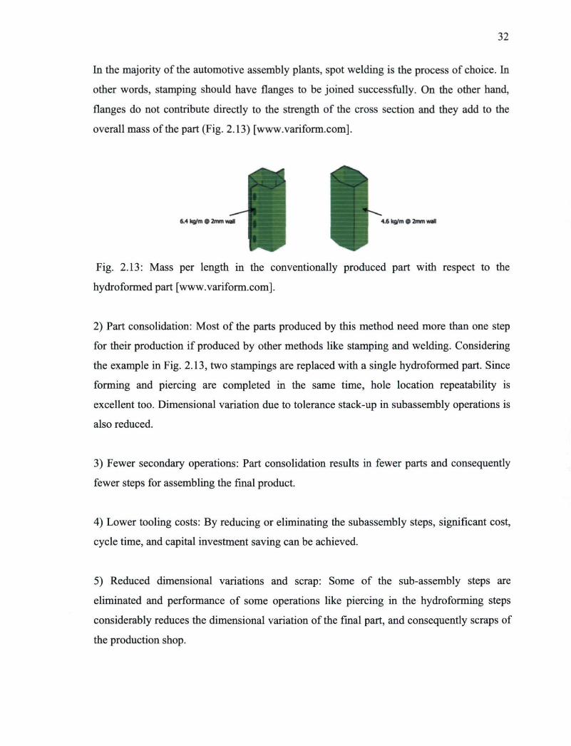
In the majority of the automotive assembly plants, spot welding is the process of choice. In

other words, stamping should have flanges to be joined successfully. On the other hand,

flanges do not contribute directly to the strength of the cross section and they add to the

overall mass of the part (Fig. 2.13) [www.variform.com].

6.4 kg/m 9 2mm wal 4.6 kg/m @ 2mm wall

Fig. 2.13: Mass per length in the conventionally produced part with respect to the

hydroformed part [www.variform.com].

2) Part consolidation: Most of the parts produced by this method need more than one step

for their production if produced by other methods like stamping and welding. Considering

the example in Fig. 2.13, two stampings are replaced with a single hydroformed part. Since

forming and piercing are completed in the same time, hole location repeatability is

excellent too. Dimensional variation due to tolerance stack-up in subassembly operations is

also reduced.

3) Fewer secondary operations: Part consolidation results in fewer parts and consequently

fewer steps for assembling the final product.

4) Lower tooling costs: By reducing or eliminating the subassembly steps, significant cost,

cycle time, and capital investment saving can be achieved.

5) Reduced dimensional variations and scrap: Some of the sub-assembly steps are

eliminated and performance of some operations like piercing in the hydroforming steps

considerably reduces the dimensional variation of the final part, and consequently scraps of

the production shop.

33

6) Reduced reliance on skilled labour: Hydroforming can minimize the need for expensive

and hard to find skilled labour. Many complex shapes are unable to be performed on

traditional systems and must be hand reworked to achieve tight tolerances. This process can

take time and may result in excess scrap. (Ahmetoglu and Altan (2000), Xu et al. (2009)).

2.4.3. Process options

From the view point of the level of pressure used in the production step, THF processes can

be classified into two general categories: High Pressure Hydroforming (HPH) and Low

Pressure Hydroforming (LPH).

In the HPH process, to avoid pinching, the perimeter of the initial tube is smaller than the

final product. As shown in the Figs. 2.14 a-d, the process starts with a round tube (Fig.2.14

a), and then continues with completely closing the die before filling it with water

(Fig.2.14b), then with application of pressure (Fig. 2.14c). Pressure is applied in a way that

causes the material to stretch into previously unfilled areas of the die cavity. Usually one of

the results is undesired ripples in the tube wall roughly perpendicular to the tube centerline

as shown in (Fig. 2.14b and 2.14c). In the last step, the maximum pressure will be applied

to completely fill the corners (Fig. 2.14d). In the HPH, the second more significant

characteristic is the difference between the tube and die cavity peripheries. As a result, the

cross sectional corners are unfilled when the die is closed.

The key characteristic of the HPH process is uneven wall thickness, often in the pattern

shown in Fig. 2.14d and Fig. 2.15. Both show internal pressure stretches the material into

the comer, creating tensile stresses in the tube wall. The wall thins because of progression

of forming from Fig.2.14b) to (Fig.2.14c) and (Fig.2.14d); more of the tube wall contacts

the die cavity surface. Pressure needed to stretch the material is high enough to make it

stick to the die surface, and stretching occurs in a decreasing portion of material, which

concentrates wall thinning.

Strategies to reduce wall thinning are applied and give promising results. Examples of these

strategies are end feeding, lubrication, annealing and high n-value material. End feed is

34

only effective within 500 mm from the tube end. The other three options increase piece

cost.

a)

b)

c)

Fig. 2.14: Concept of HPH process a) Before application of pressure (die open) b) Before

application of pressure (die closed) c) Pressure applied (die closed) d) Maximum pressure

(die closed) [http://www.excellatechnologies.com].

35

HPH

Fig. 2.15: Reduction of thickness in the HPH process

[http://www.excellatechnologies.com].

In the LPH method, at any cross section, initial tube periphery is essentially equal to the die

cavity. Pinching is avoided by forming the tube filled with low pressure water as the die

closes on it. As seen in Fig. 2.16, the die halves contact the round tube in Fig. 2.16a. The

normally round starting shape is forced toward the intended shape as the die closes in Fig.

2.16b. The tube is filled with water in Fig. 2.16c and low pressure is applied while the die

continues to close.

What distinguishes this process is the equality of the periphery or circumference of the

starting tube with the desired periphery of the finished part. Coupling this with low pressure

water to keep the tube wall in contact with the die cavity wall (but still able to slide)

effectively harnesses the large mechanical force caused by the closing press and die. This

force resolves into compressive components that act parallel to the tube wall as shown in

Fig. 2.17. The water resists unwanted deformation inward (i.e. crushing or ripples in the

metal), and the die outward, which facilitates a controlled reshaping of the cross-section

throughout the length of the part.

36

This combination of hydraulic and mechanical forces used during the cycle facilitates

complex part forming. Using low pressure water when the die is closing allows material to

slide on the cavity surface and get pushed into place using the power of the press.

As the die closes, forming is almost complete. Pressure is increased to a higher level

(usually <60 MPa) to produce the final form of the part as shown in Fig.2.16d). Holes are

punched at this stage since the backing force provided by the water is greatest and

decreases chance of deformation because of the punches forces

[http://www.excellatechnologies.com].

a)

b)

c)

Fig.2.16: Concept of LPH process a) Before application of pressure (die open) b) Before

application of pressure (die closing) c) 1st stage Pressure (die closing) d) 2nd pressure stage

(die closed) [http://www.excellatechnologies.com].

37

H»F

Fig. 2.17: State of tube thickness

[http://www.excellatechnologies.com].

in the LPH process

2.4.4. Application of THF in automotive parts

Various parts for automotive, appliance, and plumbing are produced by THF technology as

listed below:

1) Exhaust system parts; usually made of stainless steel for obtaining required structural,

thermal, and corrosion properties.

2) Exhaust parts, engine tubes, catalytic converters, pressure tubes, tail pipes, connectors,

and manifolds.

3) Chassis parts; common material is low to medium carbon steels and aluminium for

structural and cost related reasons.

4) Frame rails, engine sub-frames (cradles), roof rails and bows, instrument panels, rear

axle frames, and radiator frames (Fig. 2.18 and Fig. 2.19).

5) Engine and power train components: suspension cross members, hollow camshafts, drive

shafts, and gear shafts.

6) Body and safety parts: windshield headers, pillars, space frame components, seat frames,

and shock absorber housings [Koc and Taylan 2001].

38

Fig. 2.18: Hydroformed frame for Ford F-150 pick-up truck [Korkolis 2009a].

b) a)

Fig. 2.19: All-aluminium cars, employing the space frame with numerous hydroformed

components, (a) Audi A2, and (b) Audi A8 [Korkolis 2009a].

2.4.5. Application of FEM in THF

The Finite Element Method (FEM) is a well-established feature for metal forming

technology. The objective of FEM is to replace costly and elaborate experimental testing by

fast, low-cost computer simulations.

Any practical implementation of preliminary considerations must take into account the

special features of hydroforming as follows:

39

1) Consideration of partial strain hardening on pre-formed tubes. 2) Correlation between

process parameters: motions and forces of the horizontal cylinders, variation of internal

pressure in time, motion of additional die components such as hole punches and counter-

pressure punches, closing movement of the die.

3) Functional coordination of process parameters: internal pressure, different additional die

elements such as hole punches and counter-pressure punches and axial cylinders. 4)

Springback 5) Failure criteria like buckling and bursting 6) Material behaviour like

anisotropy and flow curve, and 7) Description of the contact (friction) conditions [Koc and

Altan (2001) and Metal Forming Handbook/Schuler (c) Springer-Verlag Berlin Heidelberg

(1998)].

Application of current commercial finite element analysis (FEA) software, such as LS-

DYNA, PAM-STAMP, ABAQUS, MARC, AUTOFORM, DEFORM, etc., for stamping

and forging processes into THF was performed and presented successful results [Koc and

Altan 1998, 1999 and Singh 1999]. Consequent and seamless simulation of bending,

preforming, and hydroforming, and sometimes annealing, results in accurate predictions in

terms of the formability and thinning of the desired part, as well as pointing out necessary

changes in tool design. In order to shorten the development time and efforts for the THF

process, supplemental codes and techniques are being developed. Adaptive simulation

technique, for instance, iterates between appropriate internal pressure and axial feeding

inputs to ensure a part without any fractures and wrinkles [Altan et al.1999 and Doege et

al. 1998]. In the literature review section details of some of the performed works is

presented. As regards the development of an optimisation algorithm that automatically

changes the parameters of the THF process i.e. internal pressure, axial feeding and

parameters of the preceding processes like parameters in the variable thickness tube

drawing, at the best knowledge of the author, there is not any special research in the

literature.

2.4.6. Pre-forming of tubes for the hydroforming process

Many THF operations require pre-formed tubes in order to fit the tube into the

hydroforming die cavity and to reach the desired shape at the end of the process.

40

Preforming of tubes usually includes bending and crushing operations. However in this

project, however the preforming operations include two-step variable thickness tube

drawing, and two-step tube bending. Details of each process were explained separately in

the previous chapters. Furthermore, annealing seems to be necessary after two-step drawing

to recover the tube's ductility for the next cold working steps.

In order to take into account the effects of pre-forming, and to design parts, tooling, and

process parameters properly, investigation of bending and crushing of tubes seems to be

necessary. In literature, research in this area have been dated to very recent years and in a

limited manner, only including the tube bending effects [Dohmann and Hartl 1996]. These

investigations are mainly experimental [Longhouse 1997] or based on FEA [Koc and Altan

1999 and Hurton 1997] of complex shaped parts. Thinning and thickening of the tubes,

particularly during bending operations, may greatly affect the success of the hydroforming

process as thinned sections may not be able to withstand internal pressure during

expansion, and consequently burst, whereas excessive thickening may lead to wrinkles on

the bent tube, and these may require high pressure for straightening.

In order to analyze the entire THF process, it is necessary to carry the results of all

preforming steps like bending, tube drawing and crushing analyses into the hydroforming

stage. Use of FEA is so far the only way of achieving this. Appropriately selected FEA

software would carry the strain history gained during pre-forming directly into the

hydroforming stage just as in actual forming of complex parts [Koc and Altan 2001].

However, this thesis is among the few works that take into account history of prior pre­

forming steps.

2.4.7. Lubricants for hydroforming applications

As is the case in other cold forming operations, lubricants are among the most important

factors in the hydroforming process, as they minimize friction at locations with relative

motion between die and workpiece.

41

Many components can be manufactured in the required shape only through the use of

appropriate lubricants. Lubricants permit obtaining more even wall thickness variation,

simplify the forming of tubular branches, reduce partial stretching processes, and improve

forming in areas that do not allow any material flow by axial feed.

A number of different lubricants can be considered for use in hydroforming. Depending on

their composition, these can be assigned to the following groups:

1) Solid lubricants, generally on a graphite or M0S2 basis 2) Polymer dispersion based

lubricants 3) Waxes, oils, and 4) Emulsions.

Lubricant is generally applied by means of spraying or immersion. Except in the case of

oils, the applied coating must generally have dried and hardened prior to the forming

process. Special attention must be paid to ensure an even coating thickness. The optimum

thickness of the lubricant layer must be determined by trial and error [Metal Forming

Handbook / Schuler (c) Springer-Verlag Berlin Heidelberg 1998].

2.4.8. Tube hydroforming (THF) in literature

2.4.8.1. Loading path in the literature

In literature there are many numerical and experimental studies about the tube

hydroforming process. Most of these studies focused on finding appropriate loading path,

mostly in geometrically not very complex forms like T-shape, Y-shape, rectangular and

trapezoid sections.

Xu et al. (2009a) presented a paper to find optimum loading paths for trapezoid-sectional

dies. In that study, they used finite element (FE) method for exploring effects of loading

paths, die angles, and friction coefficients on the quality of the final part. They also used an

analytical method for verification of their results.

Cheng et al. (2009) studied the distribution of thickness in a Y-shaped tube by the FE and

experimental methods. In their studies, the part experienced maximum 83.5% thickening

42

and 33% minning which does not seems to be an acceptable distribution of thickness for a

part.

Xu et al. (2009b) mathematically studied thickness distribution along the cross-section of a

square-sectional hydroformed part. They also evaluated the effect of friction coefficient,

strain hardening exponent, and the anisotropy coefficient on the thickness distribution.

The variation of thickness which they observed in a square cross section, was from 2.65mm

(11.6%) to 2.16 mm (28%), while their initial tube thickness was 3 mm.

Abedrabbo et al. (2009) presented an optimisation process linked with a FE model for

optimizing high strength steel tubes. The optimisation software they used was HEEDS

coupled with Ls-Dyna software for maximizing the formability in the fairly simple

rectangular tubes. However, in their optimisation process the variable parameters were only

internal pressure and axial feeding.

2.4.8.2. Materials properties in the literature

On the material related side, Koç et al. (2001b) presented experimental and analytical

approaches to characterizing materials for the THF process. In their studies they used three

methods (on-line, off-line, and a mix of the two) for measurement of changes in the

geometry of a bulged tube. The on-line measurement method showed more precise results

for the material characterization.

Korkolis and Kyriakides (2009b) evaluated the effect of loading path on the failure of the

inflated aluminium tubes. They loaded A1-6260-T4 tubes along orthogonal paths to failure

and compared the results with the tubes loaded in the radial direction. They demonstrated

that stresses like strains are path dependent if the pre-strains are significant.

Hashemi et al. (2009) applied a stress-based forming limit diagram to obtain optimum

loading path in THF. Their methodology was based on the well-known Marciniak and

43

Kuczynski model [Marciniak and Kuczynski 1967]. They compared their numerical studies

with the present experiments in the literature.

Korkolis et al. (2010) evaluated constitutive modeling and rupture prediction criteria for the

A1-6061-T6 alloy based on the experimental and numerical results by the biaxial loading in

the hydroforming machine. Their investigations proved that for this specific alloy and heat

treatment Yld2000-2D shows the best agreement with the experiments.

Koç et al. (2011) performed an experimental study on the comparative assessment of

hydraulic bulge test analysis methods. Hydraulic bulge testing of sheet materials has been

known to provide flow stress properties at higher strain levels compared to commonly used

tensile tests. The result of this study confirmed that the best combination to predict flow

stress curves was the combination of Kruglov's method for thickness and Panknin's

method for bulge radius calculation at room and elevated temperatures.

Song et al. (2010) evaluated the effect of flow stress characteristics of tubular material on

forming limit in the THF process. In this study, it was confirmed that the forming limit

diagram derived from the free bulge test can play a more important role in the evaluation of

formability for the THF processes than the diagram derived from sheet specimens' results.

Also, in order to find the reasonable forming limit curve for the THF process, all of the

aspects in the analytical forming limit curves and the results from the free bulge test should

be considered. The practical valuable forming limit stress diagram from the free bulge test

has been determined using the reasonable forming limit curve from the actual test results.

Williams et al. (2010) evaluated influence of forming effects on the axial crush response of

hydroformed aluminium tubes. They evaluated impact response of AA5754 aluminium

alloy in the hydroformed and non-hydroformed tubes experimentally and numerically by

Ls-Dyna explicit solver. In that research the hydroformed tubes showed larger energy

absorption than the non-hydroformed tubes. It was also shown that the energy absorption

characteristics of tubes with the same mass could vary greatly by adjusting the tube's

geometry and the amount of work hardening experienced by the tube during hydroforming.

44

Nikhare et al. (2009) compared high and low pressure hydroforming of TRIP steel by the

FE method. They confirmed that die closing force and internal force is much less for the

low-pressure THF process. On the other hand, thickness and stress distributions are more

uniform in low-pressure hydroforming. High pressure hydroforming is more sensitive to

friction coefficient than the low pressure process.

2.4.8.3. THF die design in the literature

There is also some research on design of dies and the role of preforming before THF the

process.

Koç (2004) evaluated the effect of die crushing and pre-bending on the thickness

distribution and formability of complex tubes. However, in his study, a separate die for the

preforming (crushing) stage was used.

Kang et al. (2005) studied tube size effect on hydroforming formability. Their results

showed that the diameter of the initial tube is one of the crucial factors in hydroformability.

Trana (2002) showed that the preforming process can be performed by the hydroforming

die closing, saving considerable time and production cost.

Kim et al. (2003) studied the THF process for production of automobile lower arms. The

pre-bending and preforming (stamping) processes were used before the hydroforming

operation. In their studies, only the geometric changes in the pre-bending and preform steps

were included without considering residual stresses and work hardening in the part due to

prior steps.

Hwang and Altan (2003) combined the crushing processes with preforming in a rectangular

die. However, in all of the prior studies only two half dies were used.

45

Lang et al. (2009) investigated the preforming effect during multiple stages of aluminum

alloy tube hydroforming by using useful wrinkles. By FE and experimental studies they

evaluated the effect of the presence of wrinkles that were usually considered to be harmful

during the THF process. The presence of useful wrinkles in the preform step considerably

facilitated the production of faultless parts in the final step, i.e. THF step. Fig. 2.20 shows

the various forming steps with useful wrinkles in them.

Fig. 2.20: Different forming stages (a) Tube blank (b) useful wrinkles in pre-forming stage

(c) pre-formed part (d) finally formed part [Lang et al. (2009)].

2.5. Conclusion and Summary

The THF process and the required preceding processes like tube drawing, recovery heat

treatment and tube bending were reviewed and the state of the arts was highlighted.

46

Various methods of tube drawing like sinking, fixed mandrel, moving mandrel, dieless and

variable-thickness tube drawing were presented. New developments in this field, like

formability criteria and tools optimisation publications, were also presented.

Regarding heat treatment, the different mechanisms for recovery of ductility of aluminium

after cold deformation in different temperature levels were depicted. Also, some detailed

information about the studied alloys in this project i.e. AA6063 and AA6061 were

presented.

Various methods to bend tubes for the THF application were presented and compared. The

required guidelines for the design of bending dies and publications on this subject were also

summarised.

In the comprehensive literature review about the THF process, some studies about

application of FE in THF, process options, and its applications in the production of

automotive parts were presented. Some other studies like finding appropriate loading path,

preforming of tubes before THF, and die design for THF were also evaluated.

Based on this literature review, there is lack of publications about optimisation the THF

process taking into account all of the preceding processes. The role of preceding processes

like tube drawing, heat treatment and bending is as important, as the role of loading path in

the THF process.

47

References

[I] Abedrabboa N., Worswicka M., Mayer R., Riemsdijk I.V., 2009 "Optimization methods for the tube hydroforming process applied to advanced high-strength steels with experimental verification, Journal of Materials Processing Technology (209) pp: 110-123. [2] Ahmetoglu M., Altan T., 2000 "Tube hydroforming: state-of-the-art and future trends" Journal of Material Processing Technology (98) pp: 25-33. [3] Altan T., Koc M., Aueulan Y., Tibari K., 1999 "Formability and design issues in tube hydroforming", Proceedings of the International Conference on Hydroforming, Stuttgart, Germany. [4] Beaulieu D., 2003 "Aluminum Structures Design", PRAL, Chapter 2. [5] Béland J.-F., Fafard M., Rahem A., D'Amours G, Côté T., 2011 "Optimization on the Cold Drawing Process of 6063 Aluminium Tubes", Appl. Math. Modelling, doi: 10.1016/j.apm.2011.04.025. [6] Bratt J. F., Adami L., 1970 "On the Drawing Process of Thin-Walled Tubes of Anisotropic Material", Journal of The Frankiiu Institute, Vol. 200, NO. 4. [7] Bui Q.H., Bihamta R., Guillot M., D'Amours G, Rahem A., Fafard M., 2011, "Investigation of the formability limit of aluminium tubes drawn with variable wall thickness" Journal of Materials Processing Technology, (211) pp: 402-414. [8] Cheng D.M., Teng B.G., Guo B., Yuan S.J., 2009 "Thickness distribution of a hydroformed Y-shape tube", Materials Science and Engineering A, (499) pp:36-39. [9] Cockcroft M.G., 1967 "Ductility", ASM, Metals Park, OH, pp: 199-225. [10] Collins I.F. and Williams B.K., 1985 "Slipline fields for axisymmetric tube drawing", International Journal of Mechanical Science, (27) pp: 225-233. [II] Dieter G.E., 1984 "Workability Testing Techniques", ASM, Metals Park, OH. [12] Doege E., Keesters R., Rogers C , 1998 "Determination of optimized control parameters for internal high pressure forming processes with FEM", Sheet Metal pp: 119-128. [13] Dohmann F., Hartl C, 1996 "Hydrofoming -a method to manufacture light-weight parts", Journal of Materials Processing and Technology, (60) pp: 669-676. [14] Duncan J.P., Kenny B., Moore G.G., 1963 "Stress analysis and calibration of tube drawing dies" International Journal of Mechanical Sciences (5) pp: 371-384. [15] Gantner P., Bauer H., Harrison D.K., De Silva A.K.M., 2005 "Free-Bending-A new bending technique in the hydroforming process chain" Journal of Materials Processing Technology (167) pp: 302-308. [16] Gao L., Strano M. 2004 "FEM analysis of tube pre-bending and hydroforming" Journal of Materials Processing Technology (151) pp: 294-297. [17] Hashemi R., Assempour A., Masoumi K. E., 2009 "Implementation of the forming limit stress diagram to obtain suitable load path in tube hydroforming considering M-K model", Materials and Design (30) pp: 3545-3553. [18] Hayashi M., Jin M., Thipprakmas S., Murakawa M., Hung J.C, Tsai Y.-C, Hung C. H., 2003, Simulation of ultrasonic-vibration drawing using the finite element method (FEM)", Journal of Materials Processing Technology (140) pp: 30-35. [19] He Y., Jing Y., Mei Z., Heng L., Yongle K., 2009 "3D numerical study on wrinkling characteristics in NC bending of aluminum alloy thin-walled tubes with large diameters under multi-die constraints", Computational Materials Science (45) pp: 1052-1067.

48

[20] Heng L., He Y., 2011 "A Study on multi-defect constrained bendability of thin-walled tube NC bending under different clearance" Chinese Journal of Aeronautics (24) pp:102-112. [21] Hurton F., 1997 "Using forming simulation in development of complex hydroformed shapes", Proceedings of the Second International Conference on Innovations in Hydroforming Technology, Columbus, OH. [22] Hwang Y.-M., Altan T., 2003 "Finite element analysis of tube hydroforming processes in a rectangular die", Finite Elements in Analysis and Design (39), pp: 1071-1082. [23] Jiang W.G., Wang GC, Lu S.Q., Li J.W., 2007 "Prediction of microstructure evolution of Al-l%Mg alloy during hot deforming and used sequential heat treatment", Journal of Material Processing Technology (182) pp: 274-280. [24] Kang S.J., Kim H. K, Kang B. S., 2005 "Tube size effect on hydroforming formability", Journal of Materials Processing Technology (160) pp: 24-33. [25] Karnezis P., Farrugia D.C.J., 1998, "Study of cold tube drawing by finite-element modelling", Journal of Materials Processing Technology, (80-81) pp:690-694. [26] Kim J., Lei L.-P., Kang B.-S., 2003 "Preform design in hydroforming of automobile lower arm by FEM", Journal of Materials Processing Technology (138) pp: 58-62. [27] Kim S.W., Kwon Y.N., Lee Y.S., Lee J.H., 2007 "Design of mandrel in tube drawing process for automotive steering input shaft" Journal of Materials Processing Technology (187) pp: 182-186. [28] Koç M., Altan T., 1998 "Development of guidelines for part, process and tooling design in the tube hydroforming (THF) process classification of the THF parts and analytical models for prediction of process parameters", Report No. ERC/NSM-98-R-34, The Ohio State University, Columbus, OH. [29] Koç M., Altan T., 1999 "Application of 2D FEA for the THF process case studies and guidelines for axisymmetric parts", Report No. ERC/NSM-99-R-19, The Ohio State University, Columbus, OH. [30] Koç M., Altan T., 2001a "An overall review of the tube hydroforming (THF) technology", Journal of Materials Processing Technology, (108), pp: 384-393. [31] Koç M., Aue-u-lan Y., Altan T., 2001b "On the characteristics of tubular materials for hydroforming-experimentation and analysis", International Journal of Machine Tools & Manufacture (41) pp: 761-772. [32] Koç M., 2004 "Advances in Tube Hydroforming - An Enabling Technology for Low-Mass Vehicle Manufacturing-Material, Lubrication, Loading, Simulation Issues, and Alternatives", Tsinghua Science and Technology, (9) pp: 527-545. [33] Koç M., Billur E., Necati Cora Ô., 2011 "An experimental study on the comparative assessment of hydraulic bulge test analysis methods", Materials and Design (32) pp: 272-281. [34] Korkolis I., 2009 "Formability and hydroforming of anisotropic aluminum tubes", PhD dissertation, The University of Texas at Austin. [35] Korkolis Y.P., Kyriakides S., 2009b "Path-dependent failure of inflated aluminium tubes", International Journal of Plasticity, (25) 2059-2080. [36] Korkolis Y.P., Kyriakides S., Giagmouris T., Lee L.H., 2010 "Constitutive Modelling and Rupture Predictions of A1-6061-T6 Tubes under Biaxial Loading Paths" Journal of Applied Mechanics ASME (77) 064501 (5pages) dor.10.1115/1.4001940.

49

[37] Kuboki T., K. Nishida, Sakaki T., Murata M., 2008 "Effect of plug on levelling of residual stress in tube drawing", Journal of Materials Processing Technology, Volume 204, pp: 162-168. [38] Langa L., Li H., Yuanb S., Danckertc J., Nielsenc K.B., 2009 "Investigation into the pre-forming's effect during multi-stages of tube hydroforming of aluminum alloy tube by using useful wrinkles", Journal of Materials Processing Technology (209), pp:2553-2563. [39] Lee H., Van Tyne C.J., Field D., 2005 "Finite element bending analysis of oval tubes using rotary draw bender for hydroforming applications" Journal of Materials Processing Technology (168) pp: 327-335. [40] Li H., Yang H., Yan J., Zhan M., 2009 "Numerical study on deformation behaviors of thin-walled tube NC bending with large diameter and small bending radius", Computational Materials Science (45) pp: 921-934. [41] Li H , Yang H., Zhan M., Kou Y.L., 2010 "Deformation behaviours of thin-walled tube in rotary draw bending under push assistant loading conditions", Journal of Materials Processing Technology (210) pp: 143-158. [42] Liu J., 2001 "Tube hydroforming process development with aid of computer simulation", technical paper 2001-01-1134. Warrendale, PA: Society of Automotive Engineers (SAE). [43] Longhouse B., 1997 "An introduction to recognizing potential applications and product design", Proceedings of the Second Annual Automotive Tube Conference, TPA International, Detroit, MI, pp: 137-171. [44] Luis C.J., Leon J, Luri R., 2005 "Comparison between finite element method and analytical methods for studying wire drawing processes", Journal of Material Processing Technology (164-165), pp: 1218-1225. [45] Marciniak Z, Kuczynski K., 1967 "Limit strains in the process of stretch-forming sheet metal" International Journal of Mechanical Science, pp: 609-620. [46] Murakawa M. and Jin M., 2001 "The utility of radially and axially ultrasonically vibrated dies in the wire drawing process", Journal of Material Processing Technology, No: 113, pp: 81-86. [47] Neves .F. O., Button .S. T., Caminaga C, and Gentile F. C , 2005 "Numerical and Experimental Analysis of Tube Drawing With Fixed Plug", J. of the Braz. Soc. of Mech. Sci. & Eng., (XXVII). [48] Nikhare C, Weiss M., Hodgson P.D., 2009 "FEA comparison of high and low pressure tube hydroforming of TRIP steel" Computational Materials Science (47) pp:146-152. [49] Padilha A.F, Plaut R.L, 2003 "Work hardening, Recovery, Recrystallization, and Grain Growth", Handbook of Aluminum (2), pp: 193-220. [50] Pierlin LL. and Jermanok M.Z., 1971 "Theory of Drawing", Mietallurgia, Moscow. [51] Semiatin S.L., Lahoti G.D., Jonas J.J., 1985, "ASM Metals Handbook", vol. 8, ASM, Metals Park, OH, pp: 154-184. [52] Singh H., 1999 "Simulation of hydroforming process", Proceedings of the Automotive Tube Conference, Detroit, ML [53] Singh H., 2003 "Fundamentals of Hydroforming", Society of Manufacturing Engineers, USA, pp: 19-27. [54] Tschaetsch H., 2006 "Metal Forming Practices", Springer Berlin Heidelberg; pp: 105-106.

50

[55] Song W.-J., ChanHeo S., WanKu T., Kim J., KangB.-S., 2010 "Evaluation of effect of flow stress characteristics of tubular material on forming limit in tube hydroforming process", International Journal of Machine Tools & Manufacture (50) pp: 753-764. [56] Trana K, 2002 "Finite element simulation of the tube hydroforming process- bending, preforming and hydroforming", Journal of Materials Processing Technology (127) pp: 401-408. [57] Urbanski S., Packo M., Stahlberg U., Keife H., 1992 "Cylindrical mandrel drawing of tubes: A matrix method simulation compared with experiment", Journal of Materials Processing Technology (32) pp: 531-543. [58] Wang Z.T., Luan G.F., Bai G.R., 1999 "Study of the deformation velocity field and drawing force during the dieless drawing of tube", Journal of Materials Processing Technology (94) pp: 73-77. [59] Williams B.W., Worswick M.J., D'Amours G, Rahem A., Mayer R., 2010 "Influence of forming effects on the axial crush response of hydroformed aluminum alloy tubes", International Journal of Impact Engineering (37) pp: 1008-1020. [60] Xu X., Zhang W., Li S., Lin Z., 2009a "Study of tube hydroforming in a trapezoid-sectional die" Thin-Walled Structures, (47) pp: 1397-1403. [61] Xu X., Li S., Zhang W., Lin Z., 2009b "Analysis of thickness distribution of square-sectional hydroformed parts", Journal of Materials Processing Technology (209) pp: 158-164. [62] Xu W., Wang K, Wang P., Zhou J., 2011 "A newly developed plug in the drawing process for achieving the high accuracy of aluminum rectangular tube" International Journal of Advanced Manufacturing Technology, DOI 10.1007/sOO 170-011-3292-8.

Chapter 3

A new method for production of variable-thickness aluminium tubes: numerical and experimental studies1

Abstract

Tube drawing is one of the most-used techniques to produce tubes in various sizes. In this

method, a tube passes through the die and mandrel to produce constant wall thickness tube.

In some applications like the transportation industry, design necessities cause requirement

for these kinds of tubes. Furthermore, some manufacturing processes like tube

hydroforming dictates having a tube with variable thickness. In this study, with a

modification made to the classic tube drawing process, the sinking and fixed-mandrel tube

drawing methods were mixed together to produce tubes with variable thickness in the axial

direction. An optimisation method, namely the leapfrog optimizer for constrained

minimization, was coupled with a finite element model to study design specifications i.e.

effect of initial tube geometry on this new process. The results (tube drawing force, the

minimum and maximum final thickness of tube) were compared with experiments

performed in the designed and manufactured machine and acceptable agreement was

observed.

Keywords: Tube drawing, Metal forming, Optimisation, Variable thickness tube,

Aluminium alloys.

Published paper in Journal of Materials Processing Technology

52

3.1. Introduction

Tube drawing is one of the complementary processes following the tube extrusion method

to have more precise dimensions with better surface finish. This process can be classified in

four categories as follows:

Sinking: in this method, there is no mandrel inside the tube and most of the deformation

happens in the hoop direction. Depending on the process parameter selection (for example

drawing velocity, die profile), there is both the possibility of increasing or decreasing tube

thickness while decreasing its outer diameter (Fig. 3.1a).

Tube drawing with fixed-mandrel: In this method there is a mandrel inside the tube which

is fixed with a long rod and produces more precise dimensions inside the tube and less

strain non-homogeneity (Fig. 3.1b).

Tube drawing with a float mandrel: The overall performance of this method is similar to

fixed-mandrel method except the technique to position mandrel (Fig. 3.1c).

Tube drawing with moving mandrel: In this method the mandrel moves with the tube while

drawing. The extraction of the mandrel after drawing is one of the major problems in this

method which in some cases causes scratching of the tube's outer surface (Fig. 3.1d).

The tube drawing process and similar processes like wire drawing have been the subject of

various studies since 1963. During this period, various aspects of this process were

evaluated analytically (energy, slab, and upper bound methods) and numerically for various

materials.

Duncan et al. (1963) presented a paper in which a general method of physically calibrating

tube drawing dies used for studies of tube ironing and, under certain restrictions, tube

sinking, was outlined and tested both experimentally and theoretically on a special die.

Bratt and Adami (1970), using the upper and lower methods, analyzed the influence of

53

initial anisotropy on the reduction of thin-walled tubes, and for a given material predicted

maximum reduction ratios. Pierlin and Jermanok (1971) have published a book on drawing

processes, in which for the cylindrical mandrel drawing of tubes a slab method analysis is

presented.

A slip-line field approach has been adopted by Collins and Williams (1985). They

attempted to construct the axisymmetric analogue of Hill's well-known bar-drawing

solution. Karnezis and Farrugia (1998) studied one and two-step tube drawing and

compared them from various aspects like residual stress, drawing forces, temperatures, and

amount of mechanical working induced in the tube per pass. Wang et al. (1999) presented

theoretical studies of deformation velocity field and drawing force during the dieless

drawing of tube by means of the power equilibrium method.

Luis et al. (2005) presented a comparison between finite element (FE) and analytical

methods to study the wire drawing process. Their investigations showed that FE and upper

methods provide an accurate result since they consider all of the energies involved in the

processes.

Kim et al. (2007) used the ductile fracture criterion and FE method to avoid fracture and

obtaining successfully formed parts. Especially two types of mandrel, straight and stepped,

were proposed and compared in view of forming failure.

Kuboki et al. (2008) evaluated the effect of presence of plugs in the amount of residual

stress in the drawn tubes. Their research showed that there is a minimum bare geometric

reduction of 6%, which is effective to level the residual stress.

Danckert and Endelt (2009) studied the effect of the length and shape of the bearing zone

in the tube drawing process. Based on the analyses which were done with Ls-Dyna finite

element software, they proposed a new design for plugs which need less force for drawing.

54

Béland (2009) optimized the geometry of the die and mandrel in the drawing of constant

thickness tubes using the finite element method. Based on the numerical and experimental

studies he made on AA6063-T4 aluminium, the production process of a tube was reduced

from two steps to just one with considerable savings in production time and tube cost.

Recently, several studies have been undertaken in order to produce the variable thickness

aluminium tubes for transportation purposes. Initial estimates by Guillot et al. (2010)

showed that applying variable thickness tubes in car structures, around 25% reduction in

the weight of structures is expected. This weight reduction in the structure of a car, and

consequently in the overall weight of a car, can reduce fuel consumption, and accordingly

will be more economical and environmentally friendly. In other applications, like bicycle

industry, to achieve minimum possible weight the frame tubes will be chosen with variable

thickness.

Bihamta et al. (2010) investigated the state of residual stress in variable thickness tubes,

and suggested doing stress relieving heat-treatment depending on the loading direction.

Guillot et al. (2010) presented some experiments with different aluminium alloys and

various mandrel geometries. Bui et al. (2010) developed an analytical method to define

forming criterion for variable thickness tube drawing.

Prior publications all concentrated on progressive reduction of tube wall thickness without

considering possible increases in the tube thickness. The novelty of this study was the

modification made to this process, in a way that the sinking and fixed-mandrel methods

were combined together to produce a variable thickness tube in the axial direction. With

this modification, both augmentation in the tube's thickness (in the sinking sub-step) and

decrease (in the wall thickness reduction sub-step) can be experienced in one drawing step.

For a better investigation of the idea, a FE model of the process was developed to simulate

this new process. In addition, this proposed FE model was used together with an

optimisation procedure to determine the optimum tube geometry in having maximum and

minimum possible thicknesses. In this paper, some primary tube drawing tests were also

performed on AA6063-O tubes to evaluate the accuracy of the developed base FE model

55

and to identify the model parameters like friction coefficients between die-tube and

mandrel-tube pairs. Other sets of tube drawing tests were also conducted until tube failure

to validate the optimisation results.

g S ^ S S

a)

• dfcjwinft ^

b)

d)

Fig. 3.1: Various methods of tube drawing a) sinking b) fixed mandrel c) float mandrel d)

moving mandrel method.

56

3.2. Design modifications and experiments

3.2.1. Design modifications

To produce variations of thickness in tubes both in axial and/or radial directions there are

some other methods like radial forging (Bihamta et al. 2007a) and indentation forging

(swage autofrettage) (Bihamta et al. 2007b) which have some limitations in producing thin-

wall tubes, and their equipment especially for radial forging, is more expensive than for the

tube drawing method.

As explained before, to obtain tubes with increased wall thickness, the tube sinking process

is required. To reduce the tube wall thickness in the drawing process, it was necessary to

change the distance between the die and the mandrel during this process, and to use a

conical mandrel which is not straight like older methods shown in Fig. 3.1. It was therefore

necessary to supply a movement system to the conical mandrel to enable it to change its

axial position with a pre-defined curve. In this paper, this method will be called the

position-controlled mandrel method. Fig. 3.2 explains the concept of this idea. If an

increase in tube wall thickness is desired (tube sinking), the mandrel will move backward in

a way there will not be any contact between mandrel and tube (Fig. 3.2a). In the regions

where a reduction in tube thickness is desired the mandrel will move forward and will

reduce thickness of tube in that region (Fig. 3.2b). It can be seen that in the moving-

mandrel method (Fig. 3.1d), the mandrel moves together with the tube during the drawing

process. On the other hand, in the position-controlled-mandrel method proposed in this

paper, the mandrel can be moved independently from the tube using a special displacement

control system. One of the most important aspects which should be considered in the

mandrel design is to have minimum possible mandrel angle or else a small inaccuracy in

the mandrel motion (in the axial direction) will cause a considerable change in the final

thickness of the tube.

57

/ / ; ; ; / ; r7-7-7

a)

(ày/// 1 / / / / / / / / / / / / ™ QkMHBB k.

f

/ / / / / / /

b)

Fig. 3.2: Concept of variable thickness tube drawing a) sinking step b) reducing wall

thickness step with a position controlled -mandrel (for illustration purpose angles of the die

and mandrel were drawn with exaggeration).

3.2.2. Details of experiments

As explained before, it was necessary to give an axial motion to the conic mandrel (Fig.

3.3a) to change the minimum distance between die (Fig. 3.3b) and mandrel during the

drawing process. The current tube drawing machines are generally not equipped with this

capability. Therefore, to verify the idea of variable-thickness tubes, a machine was

fabricated at Laval University. In this machine, it was necessary to change design of the

classic drawing machines. In the modification made to this kind of machine, a control

system to change the position of the mandrel was designed. In this control system the

points of any desired curve (linear, quadratic ...) can be implemented as a displacement

curve for the mandrel and consequently variation of thickness to the tube. In this machine,

the drawing (pulling) axis has capacity of 335 kN and 2.1 m stroke and the mandrel axis

can implement 135 kN with 1.5 m stroke. The mechanism to grip tube was a self closing

mecanism at the end of the pulling axis (Fig. 3.4). To detect the exact position of mandrel

and tube, magnetic and optical encoders were attached to the hydraulic cylinders.

58

For all the tests, Magnus CAL 70-2 drawing oil was used as a lubricant. As shown in Fig.

3.5, two different lubrication systems were designed for the die and mandrel. Die

lubrication jets inject oil to the contact surface of the die and tube. But for the mandrel

lubrication, a pipe was inserted from the other end of the tube to provide lubricant between

the mandrel and tube (Guillot et al. 2010).

039 34

1

CM CO

R36 n CM

I gr I

1 1 1. -

rO

1 '

—■»-

1

04

— f

939 - m

a)

0158.75-0.10

b) Fig. 3.3: Tube drawing tools a) conical mandrel b) die

59

Fig. 3.4: Self-closing mechanism to pull tube through die and mandrel.

Fig. 3.5: Lubrication mechanism for (1) die and (2) mandrel.

3.3. FE modeling and optimisation

The axi-symmetric nature of geometries and loading allows usage of axi-symmetric

modeling in this analysis. The initial evaluations confirmed that there was not a

considerable change between the results of 3D and axi-symmetric models. In this study, Ls-

Dyna was used as a FE solver. Fig. 3.6 presents an overall view of the developed FE model.

60

Fig. 3.6: An overall view of developed FE model.

3.3.1. Base FE model details

3.3.1.1. Material properties

AA6063-O (O means full annealed alloy) was the material used in both numerical and

experimental studies. Piecewise linear plasticity (material model # 24 in the Ls-Dyna

software) was chosen as a material model for the tube. Fig. 3.7 presents the stress-strain

curve of this material obtained from tensile tests and extrapolated up to higher strains based

on the power law ( a = AsB + C ) (Hossford 2005).

140-

120

100

1 -1 M co

40

20 -

i 140-

120

100

1 -1 M co

40

20 -

140-

120

100

1 -1 M co

40

20 -

1 1

140-

120

100

1 -1 M co

40

20 -

/ "i ~ AA 6063-0 1 I

140-

120

100

1 -1 M co

40

20 -

/ 1 1 1 1 1 [

140-

120

100

1 -1 M co

40

20 -

J 1

0 0.1 D.2 0.3 0.4 0.5 0.6

True Strain (mm/mm)

Fig. 3.7: True stress-strain curve for the AA6063-O tube

61

3.3.1.2. Contact and boundary conditions

A surface to surface contact model was defined for tube-die and tube-mandrel pairs. The

friction coefficient was chosen as 0.07 and 0.13 respectively, based on the calibration of

forces from experimental measurement and the FE model. The reason for having different

coefficients for the die and mandrel will be explained in the FE model validation section.

3.3.2. Optimization procedure

3.3.2.1. Design of experiments (DOE)

DOE is the selection procedure to find the points in the design space that should be

analyzed. Many different types are available like factorial, Koshal, composite, .D-optimal,

and Latin Hypercube designs. In this study, the D-optimal method was selected as a DOE

method. For more details about specifications of this method, interested readers can refer to

Stander et al. (2009) and Myers and Montgomery (2002). To signify the role of D-optimal

in reducing number of required experiments, the number of required experiment points for

full factorial (all possible points) and D-Optimal methods are presented in appendix A.

3.3.2.2. LFOPC optimisation method

The optimisation algorithm used to solve the approximate sub-problem is the leapfrog

optimizer for constrained minimization (LFOPC) method. It is a gradient method that

generates a dynamic trajectory path, from any given starting point, towards a local

optimum. This method differs conceptually from other gradient methods, such as sequential

quadratic programming (SQP), in that no explicit line searches are performed.

The LFOPC algorithm uses a penalty function formulation to incorporate constraints into

the optimisation problem. This implies that when constraints are violated (active), the

violation is magnified and added to an augmented objective function, which is solved by

the gradient-based dynamic leapfrog method (LFOP). The algorithm uses three phases. In

62

Phase 0, the active constraints are introduced as mild penalties through the pre-

multiplication of a moderate penalty parameter value. This allows for the solution of the

penalty function formulation where the violation of the (active) constraints are

premultiplied by the penalty value and added to the objective function in the minimization

process. After the solution of Phase 0 through the leapfrog dynamic trajectory method,

some violations of the constraints are inevitable because of the moderate penalty. In the

subsequent Phase 1, the penalty parameter is increased to more strictly penalize violations

of the remaining active constraints. Finally, and only if the number of active constraints

exceed the number of design variables, a compromised solution is found to the optimisation

problem in Phase 2. Otherwise, the solution terminates having reached convergence in

Phase 1 (Stander et al. 2009).

3.3.2.3. Optimisation flowchart

As illustrated in Fig. 3.8, in step 1, optimisation starts by developing a base FE model in the

preprocessing software of Ls-Dyna solver which is called Ls-Prepost. In constructing a

base FE model, it is necessary to define design variables as parameters using

*PARAMETER_EXPRESSION card in Ls-Dyna.

In step 2, the optimisation options like sampling method (D-optimal), optimisation

algorithm (LFOPC algorithm), design variables and their variation domain, constraints,

responses, and objectives will be defined.

One of the most important points in the optimisation loop is updating the geometries based

on the values assigned by the optimisation algorithm. For this step (step 3), a program was

developed in MATLAB to automatically update geometries or, in other words, mesh of the

die, mandrel, and tube. In this study, the geometric parameters of the tube will be

investigated, and geometric optimisation of the die and mandrel will be presented in

another paper. More details about this program are presented in appendix B.

S

Changing Design Variables Values

(Ls-Opt)

No

63

Initial Model Preparation

(Ls-Prepost)

T Defining Design Variables

(Ls-Opt)

Shape updates and FE Model adjustments (MATLAB code)

X Simulating updated Model (s)

(Ls-Dyna) X

Post Processing Results

and Extracting Responses

.Convergence Criterion met?,

I Yes

Optimized Design (s)

Fig. 3.8: Flow chart for optimisation process

Step 4 in the flow chart is solution of prepared model by Ls-Dyna solver. The optimisation

step consists of various iterations to reach the optimum design, and each iteration has

various simulation points (here 16 simulations). The represented response surface will be

composed based on the result of all simulated points.

Step 5 is post-processing of simulated points and extracting required responses which will

be explained in the next section. Based on the simulation results, if convergence is reached

in the objective function and/or design variable the optimisation will be finished, otherwise

it will return to the beginning of the chart to assign new values for the design variables. The

convergence criterion in this optimisation was having less than 2% change in the values of

the design variable or in objective function values.

64

3.3.2.4. Objectives, design variables, and user-defined responses

Design variables in this study were initial wall thickness and outer tube diameter. Based on

the initial experiments, it was found that to have larger thickness in a sinked zone (the zone

in which there is not any contact between mandrel and tube), the tube should have a larger

outer diameter and greater thickness. On the other hand, to minimize the thickness in the

region where smaller thickness is required, smaller initial outer diameter and thickness

were preferred. Therefore, the optimisation objective falls into finding optimum conditions

where the thickness in the tube's upper region of tube is maximum and in the lower zone is

minimum.

As explained before, tube thicknesses in the maximum and minimum regions are the focus

of this paper. Unfortunately, optimisation software is not usually able to extract responses

like minimum or maximum thickness of tube directly from simulation results. Therefore,

two user defined responses for extraction of minimum and maximum thickness were

developed by another MATLAB code. This program reads the dynain file of Ls-Dyna,

calculates the minimum and maximum thickness, and writes the measured values from a

dynain file of a solved Ls-Dyna problem to a file which will be read as a response of

thickness. To implement the forming limit criterion proposed in (Bui et al. 2010) it was also

necessary to calculate the ratio of maximum drawing force over minimum area of tube after

the finishing process to be as an average axial stress of tube. Based on the developed

criterion, this amount should be less than 150MPa for the AA6063-O alloy (Bui et al.

2010). Again to check this response, the MATLAB program reads the rcforc and dynain

files to calculate the tube's maximum force and minimum section area at the end of the

process. As an optimisation constraint, the maximum average tube stress will be

constrained to be less than 150 MPa. Equation 1-4 explain this mathematically.

Anin

Fmax : Maximum drawing force (2)

AmiB : Minimum section area of tube after drawing (3)

âax ia l<l50MPa(4)

65

3.4. Results and discussion

3.4.1. Base FE model results

3.4.1.1. Calibration of base FE model

To accurately calibrate the developed base FE model, a primary experiment with the

following tube geometry was performed: tube initial thickness (2.40 mm), tube initial outer

diameter (53.98 mm), tube final thickness (1.97 mm), and tube final outer diameter (47.3

mm). It should be mentioned that the primary experiment which was used for the

calibration purpose was not the full experiment where the tube was subjected to failure. The

primary experiment stopped at a tube thickness of 1.97 mm. However, the full experiment

was stopped at a tube thickness of 1.63 mm (failure point). The mandrel and tube motion

curves in the primary and full experiments were presented in Figs. 3.9 and 3.10. In Table

3.1, the reaction forces on the die, mandrel, and drawing forces were presented from FE

and primary experiments. The friction coefficients between die, mandrel, and tube were

0.07 and 0.13 respectively. The reasons for assigning different friction coefficients to the

die and mandrel were the weak lubrication of the mandrel in the designed machine, and

also different surface finishes of die and mandrel. In this system, the lubricant is injected by

entering a pipe from the other side of the tube; when there is a small distance between die

and mandrel, this pipe can not deliver enough lubricant between mandrel and tube (Fig.

3.8). Based on the performed comparison, it seems that the developed FE model has

enough accuracy to be used in the optimisation of the process.

Table 3.1: Comparison of base FE model and primary experiment.

Reaction force on the die (kN)

Reaction force on the mandrel (kN)

Tube drawing Force (kN)

FE 22.16 3.25 25.41 Experiment 23.35 3.43 26.78

eo

10

Full experiment Normalized time=l ^^w

Primary experiment Normalized time=0.61

0.2 0.4 0.6 0.8 Normalized time (Sec./Sec.)

Fig. 3.9: Mandrel displacement curve in primary and full experiments.

66

T20O

1000

|

Full experiment tu

Normalized time=l

Primary experiment Normalized time=0.61

0.2 0.4 0.6 0.8 Normalized time (Sec. Sec.)

Fig. 3.10: Tube displacement curve in primary and full experiments.

67

3.4.1.2. State of residual stresses in the produced tube

It was necessary to investigate the state of residual stress in the produced tubes by this

method. The level of residual stresses affects fatigue life of the mechanical components

under dynamic loading. Further, if a part has unrelieved residual stress its precision can not

be controlled, as noted by Kuboki et al. (2008). Depending on the loading direction and

residual stress direction, (compression/tension) the state of residual stresses can be useful or

harmful for components. In Fig. 3.11 the state of residual stress in three different directions

i.e. thickness (x), axial (y), hoop (z) directions and effective von-Mises stress are presented.

As was expected, the state of residual stress in the thickness direction (X) is negligible

because both the right and left hand side of the tube are free surfaces and can not have

stress in the normal (thickness direction), on the other hand, the tube's low thickness does

not keep much residual stress (Fig. 3.1 la).

Distribution of residual stress in the axial direction (Y) is positive (tensile), which is a

negative point for the part if it is going to undergo axial tensile loading; it seems necessary

to do a stress relieving heat treatment operation before its application (Fig. 3.1 lb).

In the hoop direction (Z), the inside of the tube has compressive residual stress (-86.9

MPa), and the outside has maximum 52.0 MPa tensile residual stress. This kind of residual

stress distribution in hoop direction seems to be useful for applications where there is

tensile hoop loading like high pressure fluid inside the tube (Fig. 3.1 lc).

In Fig. 3.1 ld, the distribution of von-Mises effective residual stress is presented. It is clear

that the residual stress in the tube's exterior surface is higher than in the interior surface.

Based on the maximum (123.6 MPa) and minimum (64.3 MPa) values of residual stress,

there is a considerable difference in the level of residual stress in the tube, which dictates

special attention in design and stress analysis of parts produced by this method.

68

Fling* Level» L L L

1.702*400 ^f*1

Fringe Levels

1400e+O2 M F l

F ring* Level»

6.188*401 MPa F ring* Level*

1.236*402 * » •

1.171*40oJ fft unt*a J 3.810*401 J 1.176*402 J

6400*41 J I 1 160eX)2 I 2421rK)1 J 1 1.117*402j I 1.091*41 _ 1441*402 1432**01 1468*402

t j 1 4317*41. I £ «426*41 . I « -1483*400. I J -2.0Ut*<X>_ 1 * -2 645**00.

•> 9.208*401 "§ H 8010*401

6411*401 _

S 613e*01 .

* 4 415e+01 .

„ 4468*400.

1 (5 -1.746*401. 1 ° 4.134*401

4*23*401 .

1 « 4*12*401.

9 984e->01_

P 9 392e*01.

o 8799r>01

8J06»401.

« 5 _ 7413*401.

-3.076e+OO 3.217*401. -7.301 «401. 7420*401.

-3 607e»00_ 2 018e*01_ 4.689*401. 6427*401. -3 607e»00_ 2 018e*01_

Contour* of X-»tre»s 1 max ipt. valu* 1 min- -3.60679. at eleml 6081 I max-1 70168, at eleml 4345

Contour* of Y-stres» max Ipt velue min-20.182, at eleml 4330 max-140.014, at eleml 1388

1 Contours of Z-*tr*ss 1 max Ipt valu* 1 min--86 8948, at eleml 5026 1 max-51 9839, at eleml 1324

Contours of Effective Stress (v-m) max Ipt valu* min-64 2714. at eleml 4343 max-123 569, at eleml 1387

11 - I L x <b» L_x w I

Y

L-X (d)

Fig. 3.11: State of residual stress in the drawn tube in various directions a) thickness (X)

direction, b) axial direction (Y), c) hoop direction (Z) and d) von-Mises.

3.4.2. Optimisation results

As mentioned before, the tube's outer diameter and initial thickness were selected as

optimisation variables. Table 3.2 summarizes the initial, maximum, and minimum values of

the variables.

Table 3.2: Upper and lower limits for the optimisation variables.

Initial value Maximum Minimum

Outer diameter 53.98 mm

(2.125")

69.85 mm

(2.75")

53.98 mm

(2.125")

Tube initial thickness 2.4 mm 2.8 mm 2.2 mm

3.4.2.1. Meta-model accuracy evaluation

The first point which should be checked in each meta-model based optimisation problem is

its accuracy, or in other words the error values. To evaluate model accuracy three error

indicators i.e. root mean square error (RMS), square root (Press) and R parameters were

69

calculated and are presented in Table 3.3 for the minimum and maximum thickness models

for the last iteration. In other iterations the level of error is approximately the same.

Descriptions of these parameters are presented in appendix C.

Table 3.3: The three error indicators for the minimum and maximum thickness models.

Minimum thickness model Maximum thickness model

RMS Error 0.005(0.27%) 0.001 (0.02%)

Square root

(Press)

0.012 (0.68%) 0.001(0.54%)

R2 0.912 0.999

In Figs. 3.12 and 3.13 the predicted responses versus computed responses were plotted.

Ideally they should have exactly the same values but because of fitting errors, there is

always a difference between them. However, the difference is clearly acceptable, and the

meta-model seems to work well in optimisation of variable thickness tube drawing.

M<UM**P,««WKy

r\ Hull — a t . t — i m t » SgnPKH OUIISISM. S* l iu

/ ■ /

/ a

/ a 1 y

/■■ ■ » / / a

■ /

in ui in i» in Lie

Fig. 3.12: Meta-modeling accuracy for the minimum thickness model (last iteration).

70

Oatat «MSt. IMIH7«IUrv S«.*tSS IMUÎ4HBV « K I M

/ /

Fig. 3.13: Meta-modeling accuracy for the maximum thickness model (last iteration).

Fig. 3.14 presents the variation of optimisation objectives i.e. minimum and maximum

thickness in the first simulation of all iterations. As mentioned earlier, each iteration

includes 16 design points, and based on the results of all simulated points, the next design

points were selected. It is clear that these two objectives are in opposition i.e. the

improvement of one would cause deterioration of the other. The convergence criteria for

the optimisation were having less than 2% change in both design points and objectives. As

can be seen in Figs. 3.14a and 3.14b, the difference in the objectives and designs are less

than 2%. Therefore the optimisation loop stopped after 9 iterations.

Fig. 3.14 only presents the optimisation history for the first simulation points but it is

possible that the best optimisation point could be in the other simulation points. Therefore

scatter plots of all simulation points were presented in Figs. 3.15 and 3.16. Based on the

scatter plots the optimum point is the point with the following tube geometry initial

thickness (thO): 2.53 mm and outer diameter (OD): 54.0 mm and optimized results of

minimum thickness: 1.71 mm and maximum thickness: 2.66 mm.

71

I o I E

1

Number of Iteration a)

14-

2 >

r '

— ' •

2.1-

2-\ ■

> , i ■

^ ^ " ^ * ~ « 4 i i i ■

^ ^ " ^ * ~ « 4 i i i

^ , " F Y 4 6

Number of Iteration

b)

Fig. 3.14: Optimisation history for a) minimum thickness and b) maximum thickness

during the optimisation process ( This figure presents the results of the first simulation in

each iteration)

72

*•** Initial thickness (mm) & &

Fig. 3.15: 3D scatter plot for two optimisation objectives with respect to first design

variable i.e. initial thickness (tho).

Outer diameter (rmi) > " *

Fig. 3.16: 3D scatter plot for two optimisation objectives with respect to first design

variable i.e. outer diameter (OD).

For easier investigation of various responses and their variation during the optimisation, the

averages of each response in each iteration are presented in Table 3.4.

73

Table 3.4: The average values for various responses in the 10 iterations or 10x16

simulation points.

I f (D r *

5" 3

O o 3 3

- i 3-O 3 3

Thickness

(mm

)

Thickness

(mm

)

Reaction

Force (kN)

Reaction

Force (kN)

Draw

ing

Force (kN)

stress

(MPa)

1 56.1 2.40 2.55 2.22 18.7 1.6 20.3 63.4 2 58.7 2.42 2.59 2.05 25.5 2.8 28.3 99.2 3 60.7 2.44 2.63 1.91 29.8 3.33 33.1 126 4 58.9 2.45 2.63 1.84 28.9 3.53 32.4 128 5 57.7 2.46 2.63 1.79 28.5 3.70 32.2 131 6 56.5 2.48 2.64 1.75 27.9 3.82 31.7 133 7 55.3 2.50 2.65 1.73 27.4 3.93 31.3 133 8 55.2 2.52 2.66 1.75 27.5 3.95 31.4 132 9 54.7 2.53 2.68 1.75 27.3 4.02 31.3 131 10 54.4 2.55 2.69 1.74 27.4 4.09 31.3 132

3.4.2.2. Comparison of optimized results with experiments

As noted in the previous section, the optimized dimensions for the tube outer diameter

(OD) and initial thickness (tho) are 54.0 mm and 2.53 mm respectively. During experiments

it was not possible to have a tube with initial dimensions exactly equal to the above

mentioned dimensions. The closest tube dimension available was a tube with OD=53.98

mm and th0=2.40 mm. Fig. 3.17 shows the thickness evolution of the studied tube during

the drawing process and the maximum and minimum thicknesses. The maximum and

minimum thicknesses obtained by the experiments are 2.50 mm and 1.63 mm respectively,

which seems to be in acceptable agreement with the numerical results.

74

2.6 2.5 2.4 2.3 2.2 2.1

2 1.9 1.8 1.7 1.6 1.5

1 J 1 1 — ^ ^ C L — — i J 1 i i

1 i 1 T i 1 r - ^ ^ i | r r

i J i J. i i J i i y_ i

0 100 200 300 400 500 600 700 800 900 1000 1100

Distance from Tube Head (mm)

Fig. 3.17: Distribution of thickness in axial direction with initial tube dimension of OD:

53.98 mm and th0: 2.40 mm.

3.4.2.3. Correlation bars for the various optimisation parameters and responses

Fig. 3.18 presents the correlation between tube initial geometry and minimum thickness,

maximum thickness and drawing force. It is clear from this figure that the most important

parameter in having maximum thickness is initial thicknesses, and then outer diameter.

Minimum achievable thickness strongly depends on the tube initial outer diameter and to

some extent on initial thickness. For the drawing force, outer diameter has a more

important effect than tube initial thickness.

To support the correlation bars, some results from performed experiments on tubes with

different outer diameters (OD=53.98, 63.49 and 69.85 mm) are presented in Fig. 3.19. As is

clear, the minimum thickness depends more strongly on the outer diameter variation than

the maximum thickness does. Repeating this experiment with various tube initial

thicknesses was not possible because all the available tubes for experiments had constant

wall thickness i.e. 2.40 mm.

75

s 4* ee

s 4* ee

D Drawing force ■ Minimum thickness ■ Maximum thickness

<> c je u .C

• £

D Drawing force ■ Minimum thickness ■ Maximum thickness

<> c je u .C

• £

<> c je u .C

• £

O O

** • E ■ •o •

** • E ■ •o •

"— O

1 "— 0.1 0.2 0.3 0.4 0.5 0.6

Coefficient of correlation 0.7 0.8 0.9

Fig. 3.18: Correlation bars for the optimisation objectives i.e. maximum and minimum

thickness and drawing force.

2.7

2.5 Ê" J . 2.3 M in « 5 2.1 u

8 19 3

1.7

1.5 50

•Maximum thickness ■Minimum thickness

55 60 65 Outer diameter (mm)

70 75

Fig. 3.19: Variation of maximum and minimum thickness with respect to tube initial outer

diameter (experimental results).

76

3.5. Conclusion

A modification to the tube drawing process, the sinking and position controlled -mandrel

tube drawing methods mixed together, was presented to enable increase and decrease in the

thickness of tubes in one-pass drawing, as well as allowing having any desired variation of

thickness in the axial direction of tube. Because of the novelty of this process, it was

necessary to develop a numerical model to investigate various aspects of this process like

reaction forces on the die and mandrel, and their distribution, as well as the state of residual

stress in various regions and directions. A subsequently validated base FE model was

applied in an optimisation loop to investigate the maximum and minimum possible

thickness which can be obtained with the variation of tube initial geometry i.e. outer

diameter and initial thickness. This numerical study also showed very good agreement with

the performed experiments. In conclusion, the following results can be summarized:

1) Reaction force between die and tube has the maximum portion of total drawing force.

2) The state of residual stress in the axial direction seems not to be appropriate for the part

if it is going to undergo axial loading, but it seems to be useful if it is going to experience

internal tensile hoop loading.

3) In maximizing tube thickness, tube initial thickness has the most important effect but for

the minimization of thickness the tube initial outer diameter plays more significant role.

4) In increasing tube drawing force, tube outer diameter has more considerable effect than

initial thickness.

Acknowledgements

The authors thank the Natural Sciences and Engineering Research Council of Canada,

National Research Council Canada-Aluminium Technology Centre, Alfiniti, Aluminerie

Alouette, C.R.O.I and Cycles Devinci for the financial support of this research. A part of

the research presented in this paper was financed by the Fonds Québécois de la Recherche

sur la Nature et les Technologies (FQRNT) by the intermediary of the Aluminium Research

Centre - REGAL. The authors want to express special thanks to Mr. J-F Béland researcher

at the Aluminium Technology Centre for his help and suggestions during optimisation

process development.

77

References

[I] Béland J.F., 2009 "Optimization of cold tube drawing of aluminium 6063-T4 with finite element method", M.Sc. thesis, Laval University, Quebec, Canada (In French). [2] Bihamta R., D'Amours G, Rahem A., Guillot M., Fafard M., 2010 "Numerical studies on the production of variable thickness aluminium tubes for transportation purposes", SAE2010 World Congress, Detroit, USA. [3] Bihamta R., Ameli A., Movahhedy M.R., Mashreghi A.R., 2007a "A comparative study on the radial and indentation forging of tubes", International Journal of Forming Processes (10), pp: 179-194. [4] Bihamta R, Movahhedy M.R., Mashreghi A.R., 2007b "A numerical study of swage autofrettage of thick walled tubes", Materials and Design (28), pp: 804-815. [5] Bratt J. F., Adami L., 1970 "On the Drawing Process of Thin- Walled Tubes of Anisotropic Material", Journal of The Frankiiu Institute (200), NO. 4. [6] Bui Q. H., Bihamta R., Guillot M., D'Amours G., Rahem A., Fafard M., 2011 "Investigation of the formability limit of aluminium tubes drawn with variable wall thickness", Journal of Materials Processing Technology (211) pp: 402-414. [7] Collins I. F. and Williams B.K., 1985 "Slipline fields for axisymmetric tube drawing", International Journal of Mechanical sciences (27), pp: 225-233. [8] Danckert J. and Endlet B., 2009 "Ls-Dyna used to analyze the drawing of precision tubes", 7th Europeian Ls-Dyna conference. [9] Duncan J.P, Kenny B., Moore G.G., 1963 "Stress analysis and calibration of tube drawing dies", International Journal of Mechanical sciences(5), pp: 371-384. [10] Guillot M., Girard S., D'Amours G., Rahem A., Fafard M., 2010 "Experimental exploration of the aluminum tube drawing process for producing variable wall thickness components used in light structural applications", SAE 2010 World Congress, Detroit, USA. [II] Hosford W. F., 2005 "Mechanical Behavior of Materials", Cambridge University Press. [12] Karnezis P. E and Farrugia, D. C. J., 1998 "Study of cold tube drawing by finite-element modeling", Journal of Material Processing Technology (80-81) pp: 690-694. [13] Kim S.W., Kwon Y.N., Lee Y.S., Lee J.H., 2007 "Design of mandrel in tube drawing process for automotive steering input shaft", Journal of Materials Processing Technology (187)pp:182-186. [14] Kuboki T., K. Nishida, Sakaki T., Murata M., 2008 "Effect of plug on leveling of residual stress in tube drawing", Journal of Materials Processing Technology (204) pp: 162-168. [15] Luis C.J., Leon J, Luri R., 2005 "Comparison between finite element method and analytical methods for studying wire drawing processes", Journal of Material Processing Technology (164-165) pp: 1218-1225. [16] Myers R.H., Montgomery D.C, 2002 "Response Surface Methodology", Second edition, John Wiley & Sons, New York. [17] Pierlin I.L. and Jermanok M.Z., 1971 "Theory of Drawing", Mietallurgia, Moscow. [18] Wang Z.T., Luan G.F., Bai G.R., 1999 "Study of the deformation velocity field and drawing force during the dieless drawing of tube", Journal of Materials Processing Technology (94) pp:73-77.

78

[19] Stander N., Roux W., Goel T., Eggleston T., Craig K., 2009 "A design optimization and probabilistic analysis tool for the engineering analyst", LS-OPT® User's Manual, Livermore Software Technology Corporation.

79

Appendix 3.A)

Comparison of number of experimental points in D-Optimal and full factorial methods

(Stander et al. 2009).

Quadratic

Number of Linear Approximation Approximation Number of

D-

Variables n D-Optimal Factorial Optimal Factorial

1 4 2 5 3

2 5 4 10 9

3 7 8 16 27

4 8 16 23 81

5 10 32 32 243

6 11 64 43 729

7 13 128 55 2187

8 14 256 68 6561

9 16 512 83 19683

10 17 1024 100 59049

80

Appendix 3.B

In this appendix some more details about the developed MATLAB program are presented.

This MATLAB program was included in the optimisation loop to work as a preprocessor

for updating geometric features like tube geometry in the optimisation loop automatically.

In the following chart, the step-by-step general algorithm of this program is explained.

81

Reading XPOENT file which is produced for each design point by Ls-Opt

Getting desired geometric parameters like die and mandrel angles, die fillet, tube initial geometries like outer diameter and initial thickness

based on the decision of optimization loop

Creating die and mandrel geometries and their meshes

Based on the tube geometry defining start point for the tube. This point should not be in conflict with the die and mandrel geometries. If because of larger outer diameter of tube it has coincidence with for example die geometry, it will be moved axially to be sure that it does not have any

coincidence with others

Creating tube geometry and its mesh

Based on the changes which happen in the node and element numbers, updating FE model features like boundary conditions, and detecting the

new interior points which used to be controlled by the ♦TERMINATION NODE command

Creating updated FE model i.e. new .k files to be used in the optimization loop

82

Appendix 3.C

In this section the used equations for error measures are summarized:

Mean Square Error (MSE) and Root Mean Square Error (RMS):

P _ 2

MSE - £ ( y . - y t ) I P (C.1 i

RMS = ylMSE (C.2

p _ 2 p

R2=-± r (C.3 and R = M r (C.4

j>,-j» Xu-7)2i>,-y) Where

P: denotes the number of data points, which here is 16 for each iteration.

y j : is the observed response value (target value), yt is the model's prediction of response.

In this study, responses were maximum thickness, minimum thickness, axial stress, reaction

force on the die and mandrel, and finally the total drawing force.

y' is the mean value of y , y' is the mean value of y,

PRESS residual

Before presenting a definition of PRESS residual it is necessary to give an introduction to

define the matrix X which will be used in its definition.

Consider a response variable y dependent upon a number of variables JC. The exact

functional relationship between these quantities can be written as:

y = rj(x) (C.5

83

The exact functional relationship can be approximated (e.g. polynomial approximation) as

n(x)*f (x) (C.6

The approximating function/is assumed to be a summation of basis functions:

/(x) = £«M(x) (C.7 i=i

Where L is the number of basis functions $used to approximate the model.

The constants a = [al,a2,...,aL]Thave to be determined in order to minimize the sum of the

square error:

t 4 { [y (x p ) - f (x p ) f } = f j{[y(xp)-zla l<t> l^P)f} (C8 P = \ p=\ /=i

P is the number of experimental points and y is the exact functional response at the

experimental points x i. The solution to the unknown coefficients is:

a = (XTX)~xXTy (C.9

Where X is the matrix

X = [ X J = [^(xu)] (CIO

The prediction sum of square residual (PRESS) uses each possible subset of P-l responses

as a regression data set, and the remaining response in turn is used to form a prediction set.

PRESS can be computed from a single regression analysis of all P points.

p — 2

y t - y t -PRESS = Y A —) (Cll tf \ -h /

84

Where P: denotes the number of data points, which here is 16 for each iteration.

y j : is the observed response value (target value), y, is the model's prediction of response.

hu are the diagonal terms of

H = X(XTX)~ lXT (C.12

H is the "hat" matrix, the matrix that maps the observed responses to the fitted responses,

i.e. ~y = Hy (C.13

The press residual can also be written in its square root form too

p - 2

SPRESS = Z (— ) (C ! 4

Chapter 4

Application of a new procedure for the optimisation of variable thickness drawing of aluminium tubes1

Abstract

The application of aluminium tubes especially with variation of thickness, in the structures

of various transportation devices like cars and bicycles makes it a point of interest for

various designers. In this paper, the variable thickness tube drawing process was studied

with the newly developed procedure to evaluate the effect of tools geometries on the

maximum possible tube deformation. The procedure applies the desired variation in the

design variables (die angle, mandrel angle, and die fillet radius) and the required

adjustments and changes in the geometries with the aid of an in-house code automatically.

Based on the optimized results, a die and a mandrel were built to verify numerical results in

variable thickness tube drawing. The numerical results were compared with the

experiments in the prototype machine, and acceptable agreements were observed.

Keywords: Optimisation, Finite Element Method, Metal Forming, Tool Design, Tube

Drawing, AA6063.

1 Submitted paper to CIRP Journal of Manufacturing Science and Technology

86

4.1. Introduction

The application of the finite element method for optimizing mechanical systems is very

popular in the industrial and academic environments. Most of the time, numerical studies

were limited to only the manual change of some parameters to investigate their effects on

the problem output. However, this kind of application of the FE method seems time

consuming and always needs user interaction to prepare new models with new parameters.

In this study, an automatic procedure for the optimisation of metal forming processes by the

FE method is presented and applied to the optimisation of tools for the variable thickness

tube drawing method.

The tube hydroforming process (THF) has a very important role in the production of

complex tubes, especially for transportation applications. In most of these devices, the

constant axial thickness is not only unnecessary, it is considered to be overdesigned, and

causes increased overall weight of the structures. To reduce tube thickness in both axial

and/or radial directions, various methods such as radial and indentation forging can be

used. However, as was explained in detail in Bihamta et al. (2007a; 2007b), the main

restrictions with these methods are the high equipment costs and the limitation of these

methods to thick wall tubes.

The drawing process studied in this paper is a modification of the conventional tube

drawing method enabling it to produce variable thickness tubes. In conventional tube

drawing processes with a fixed mandrel (Fig. 4.1), the mandrel is positioned by a long rod,

and its position is not changed during the process. Conversely, in the modification which

was made to this process, the position of the mandrel during the process will be changed.

Therefore, the distance between the die and mandrel will be changed and will give a

variation of thickness to the tube in the axial direction. Various types of tube drawing

processes have been studied since 1962. During this period, different aspects of this process

were evaluated analytically (energy, slab and upper bound methods) and numerically for

various materials. Some of the studies which deal with tooling in tube drawing are

presented below.

87

Kim et al. (2007) used the ductile fracture criterion and finite element (FE) method to avoid

fracture and to obtain successfully formed parts. Specifically, two different types of

mandrel were proposed and compared from the viewpoint of forming failure. Kuboki and et

al. (2008) evaluated the effect of the presence of plugs in the amount of residual stress in

drawn tubes. Their research showed that there is a minimum bare geometric reduction of

6%, which is effective to level the residual stress. Danckert and Endelt (2009) studied the

effect of the length and shape of the bearing zone in the tube drawing process. Based on the

finite element analyses they proposed a new design for plugs that need less force for

drawing.

Fig. 4.1 : Tube drawing process.

Béland (2009) optimized the geometry of the die and mandrel in the drawing of constant

thickness tubes using the finite element method. Based on the numerical and experimental

studies made on AA6063-T4 aluminium tubes, the production process of a tube was

reduced from two steps to just one with considerable savings in production time and cost.

In the previously mentioned publications, the tube drawing process was studied only for

constant wall thickness tubes without any attention paid to the variation of thickness along

the tube axis. They also did not use an automatic numerical procedure, nor any application

of optimisation algorithm and design of experiment (DOE) methods for selection of points.

In this paper, the tube drawing process for the production of variable thickness tubes,

recently introduced by Guillot et al. (2010), Bihamta et al. (2010a,b), Bihamta et al. 2011

and Bui et al. (2011), was studied to determine optimum geometry for the die and mandrel.

As Fig. 4.2 clearly shows, the main difference between the variable thickness and constant

thickness tube drawing methods is having a conic, and in some cases stepped mandrel

88

instead of a straight one. The other difference is the axial motion of the mandrel during the

drawing operation, which gives a variation of thickness to the tube in the axial direction.

From a numerical point of view, in this study, D-optimal, the design of experiments (DOE)

method, and the leapfrog optimizer for constrained minimization (LFOPC) optimisation

method were used for point selection and for the optimisation process respectively. As will

be explained in detail in the next section and appendix A, the developed algorithm changes

the design variables (in this case geometric features of die and mandrel) automatically. The

algorithm developed in-house also performs geometric inspections and result extraction

automatically.

Thickness Diminution

I [ Z Z Z Z Z Z Z Z

Thickness Augmentation

Fig. 4.2: Schematic of the variable thickness tube drawing process (For illustration

purposes the mandrel angle is drawn with exaggeration).

Finally, some experiments to validate numerical results were developed in a prototype

machine that was designed and fabricated at Aluminium Research Centre-REGAL/Laval

University.

4.2. Numerical modeling

To optimize this process, it was necessary to develop an initial FE model, and to include

this model in an appropriate optimisation loop. In the first step, this model was explained,

and then applied parameters for optimisation were depicted.

89

4.2.1. Base FE Model

The axisymmetric nature of geometry and loading allows this process to be modeled

axisymmerrically by the FE method. Likewise, a 3D model was tested and it produced

almost the same results. Fig. 4.3 presents an overall view of this model.

The geometries of die, mandrel, and tube were defined and meshed by codes developed in-

house. During the optimisation process the geometries are updated by the developed codes

depending on the selected values for the design variables, i.e. die and mandrel angles and

die fillet radius. The other necessary FE definitions, such as boundary conditions, tube

displacement curves, and material properties, are done once before starting the optimisation

process. The mandrel displacement curve was updated automatically by the developed

code, because depending on the various mandrel angles, their displacements were different

to achieve the same thickness reduction.

Fig. 4.3: An overall view of the developed FE model.

4.2.1.1. Material properties

AA6063-O was the material used in both numerical and experimental studies. Piecewise

linear plasticity was chosen as a material model. Fig. 4.4 presents the true stress-strain

curve of this material obtained from tension tests and extrapolated up to higher strains

based on the Holloman hardening law (Hosford 2005).

0.1 0.2 0.3

True Strain 0.4

90

140 -,

120

100 -

140 -,

120

100 -

140 -,

120

100 -

• - on

HI g 60-

8 4 0 -

20

0 -

AA 6063-0 \ { • - on

HI g 60-

8 4 0 -

20

0 -

AA 6063-0 \ { • - on

HI g 60-

8 4 0 -

20

0 -

• - on

HI g 60-

8 4 0 -

20

0 -

• - on

HI g 60-

8 4 0 -

20

0 -

I i i 1 i 0.5 0.6

Fig. 4.4) True Stress-Strain curve for tube material (AA 6063-O).

4.2.1.2 Boundary conditions and contact condition

As in the real process, the mandrel was left constraint-free in the axial direction but was

constrained in the radial direction. In addition, for variational movement of the mandrel in

the axial direction, a curve was defined to the prescribed motion of the mandrel. As

mentioned before, based on the mandrel angle, the axial motion was updated by the in-

house code to have the same minimum thickness at the end. The success of the process in

experiments depends significantly on the appropriate design of this curve. In other words,

the distribution of thickness along the tube axial direction, the distribution of minimum

thickness along the tube axis, and the rate of deformation are implemented by this curve.

The die was constrained in all directions as a rigid part, and a displacement was prescribed

at one end of the tube for the tube motion. The surface to surface contact type was chosen

as a contact formulation between the die-tube and the mandrel-tube. The friction

coefficients between the die-tube and the mandrel-tube were chosen as 0.07 and 0.13

respectively, which was based on the calibration of forces from an experimental

measurement and the FE model. The reason for different coefficients for the die and

mandrel interfaces was because of different lubrication systems for the die and mandrel

with different lubrication efficiencies.

91

4.2.2. Optimisation procedure

4.2.2.1. Design of experiments (DOE)

DOE is the selection procedure to find the points in the design space that should be

analyzed. Many different types are available, such as factorial, Koshal, composite, D-

optimal and Latin Hypercube designs. In this study, the D-optimal method was selected as

DOE method. For more details about the specifications of this method, interested readers

can refer to Stander et al. (2009) and Myers and Montgomery (2002).

4.2.2.2. LFOPC optimisation method

The optimisation algorithm used to solve the approximate sub-problem is the leapfrog

optimizer for constrained minimization (LFOPC) method. More explanation of this method

is available in appendix A.

4.2.2.3. Optimisation flowchart

The developed optimisation flowchart is shown in Fig. 4.5. In step 1, optimisation starts by

developing a base FE model. In this model, all of the design variables were defined as

parameters. In step 2, the optimisation options, such as sampling method (D-optimal),

optimisation algorithm (LFOPC algorithm), design variables and their variation domain,

constraints, responses, and objectives are defined. One of the most important stages in the

optimisation loop is updating the geometries based on the values assigned by the

optimisation algorithm. For the third step, an in-house code was developed to automatically

update geometries or, in other words, the mesh of the die, mandrel, and tube. More details

about the algorithm of this code are presented in Appendix B. Step 4 of the flow chart is the

solution of the prepared FE model. The optimisation step consists of various iterations to

reach the optimum design, and each iteration has various simulation points. In step 5, the

deformed tube geometry is checked by a developed code to ensure that its geometry is

acceptable. Step 6 is the post-processing of simulated points, and extracting required

92

responses, which will be explained in the next section. Based on the simulation results, if

the convergence in the objective function and/or design variables is reached, the

optimisation process will be finished; otherwise, it will return to the beginning of the chart

to assign new values to the design variables. The convergence criterion in this optimisation

was to have less than 2% change in the design variables or objective function values.

4.2.2.4. Design variables and optimisation objective

In this optimisation study, the design variables, (the variables which will be changed to

reach the optimum point), are die angle, die fillet radius, and mandrel angle. As Fig. 4.5

(step 3) clearly shows, all changes in the geometries of tools were performed automatically

by a developed code included in the optimisation loop. In table 4.1, a summary of the

design variables and their ranges are presented; the ranges are also based on the feasibility

performance also. For instance, if the assigned mandrel angle was less than 1°, there was a

possibility to surpass the maximum possible stroke for the mandrel cylinder in the machine.

On the other hand, it was not preferable to have an angle larger than 6°, because with larger

mandrel angles a small inaccuracy in cylinder movement will cause considerable change in

tube thickness. Furthermore, if the die angle is very large, the die will be very weak against

the forming forces.

The objectives of this optimisation study were to verify the effect of the tools' geometries

(die and mandrel) on the drawing force in the progressive thickness reduction, and

consequently on the minimum possible thickness that can be obtained. The constraint

applied to the problem was to limit the axial stress in the tube to be less than the yield stress

of the drawn tube, which is around 150 MPa for this material with heat treatment

conditions as ascertained in Bui et al. (2011). This criterion is easy to implement and also

showed acceptable results in other studies, such as Béland (2009).

93

Table 4.1: Summary of design variables and their range of variation.

Min. Max.

Die Angle (°) 8.0 15.5

Die Fillet (mm) 2.5 19.5

Mandrel Angle (°) 1.0 6.0

To apply this objective, a predefined minimum thickness (in this case 1.9 mm) was defined;

it was then attempted to reach this minimum thickness with the minimum possible drawing

force. Based on initial observations in the experiments and numerical studies, it was

guaranteed that, in the defined domains for the tool parameters, the tube will not rupture at

this minimum thickness. In all numerical studies of this paper, Ls-Dyna and Ls-Opt were

used as FE solver and optimisation engine respectively. In-house codes were written in

MATLAB.

4.3. Experiments

Experiments were performed in the prototype tube drawing machine. The drawing (pulling)

axis has a capacity of 335kN and 2.1 m stroke; the mandrel axis can implement 135 kN of

force with 1.5 m stroke. The mechanism to grip the tube was a self-locking mechanism at

the end of the pulling axis. To detect the exact position of the mandrel and tube gripper,

magnetic and optical encoders were attached to the cylinders. The lubricant utilized for all

the tests was Magnus CAL 70-2 drawing oil. All of the tests were performed at a drawing

speed of 6 mm/s. Fig. 4.6 shows an overall view of the machine with a self-closing

mechanism and lubrication system. For more details on the technical specifications of this

machine, interested readers can see Girad (2010).

94

Changing Design Variables Values

Initial model preparation

Defining Design Variables (optimization software)

Shape updates and FE model adjustments

Simulating updated Model (s)

Checking deformed shape of tube

Post Processing Results and Extracting Responses

No

Fig. 4.5: Flow chart for optimisation process

95

'i '

11 • \

1* V ■ ~

a)

b) c)

Fig. 4.6: a) Variable thickness tube drawing machine b) self closing jaw of pulling axis

c) lubrication system for the die and mandrel.

To have a better measurement of axial tube thickness during the experiments, the tubes

were cut by into two halves the mechanical saw. The thickness of the tubes was measured

in various areas with a Starrett special micrometer for tube thickness measurement with an

accuracy of ± 0.01/ww (Fig. 4.7).

96

Fig. 4.7: Methodology for measurement of tube thickness after drawing.

In the first set of experiments, the first set of dies and mandrels was fabricated simply to

test the designed machine. This was not necessarily optimal to obtain the minimum

possible tube thickness. Fig. 4.8 presents details of this set of tooling. As presented in the

results section, the optimized tools performed better in the experiments.

<p39 34

R36

J ^v

1 s CO

|l '

—to» 0 4 939 ■ - ^ —

0158.75-Qio

a)

Fig. 4.8: Examples of tube drawing tools a) conical mandrel b) die.

97

4.4. Results and discussion

4.4.1. Base FE model validation

It is necessary to calibrate the base finite element model before applying it in the

optimisation loop in all optimisation studies. For this purpose, the reaction forces on the die

and mandrel from the FE model were calibrated with the forces recorded from the tube

drawing machine, and presented in table 4.2. As shown, the maximum difference in the

forces from FE and experiments are 1.19 kN, 0.18 kN and 1.37 kN for the die, mandrel, and

drawing forces respectively. The specifications of the experiment which was used for

calibration purposes are as follows: tube initial thickness (2.40 mm), tube initial outer

diameter (53.98 mm), tube final thickness (1.97 mm), and tube final outer diameter (47.3

mm). The mandrel and tube motion curves in the primary (tube drawing before rupture) and

full experiments (progressive drawing up to rupture) are presented in Fig. 4.9.

Table 4.2: Reaction forces from FE model and primary experiment.

Reaction force on the die (kN)

Reaction force on the mandrel (kN)

Tube drawing Force (kN)

FE 22.16 3.25 25.41 Experiment 23.35 3.43 26.78

1200

Fig. 4.9: Mandrel and tube displacement curve for the primary experiment (normalized

time=0.61) and full experiment (normalized timeA).

98

4.4.2. Optimisation results

4.4.2.1. Optimum die and mandrel geometry

As mentioned earlier, this paper focuses on the geometry with which the minimum

thickness can be obtained; it is expected that this design corresponds to the point where the

drawing force is minimum. As noted in prior studies about shape optimisation in metal

forming, such as Kleinermann and Ponthot (2003), there is not necessarily just one solution

as an optimum point, but there is always a cluster of solutions where the objective function

is minimum or maximum in these points. As can be seen in Figs. 4.10 and 4.11, based on

the various combinations of die and mandrel geometry, it is possible that a minimum

drawing force, and consequently the minimum thickness occurs in more than one

combination. For this study, as shown by the circles in Figs. 4.10 and 4.11, it was better to

consider the following final combination: die angle (12°), die fillet radius (10 mm), and

mandrel angle (1°). As demonstrated, in other combinations the die angle is larger, which

corresponds to more machining time and weaker die. For the mandrel, the smaller mandrel

angle is preferred because in larger mandrel angles, a small inaccuracy in axial motion will

cause larger variation in final tube thickness.

This optimisation problem finished at the 4th iteration, and each iteration included 24

simulation points. Comparing Figs. 4.10 and 4.11 with Fig. 4.12, the number of points is

not the same because in Figs. 4.10 and 4.11 the range of drawing force was limited to 40

kN for better distinction of forces.

99

4E+4

3.8E+4

3.6E+4

o 3.4E+4

É? 3.2E+4

3E+4

2.8E+4

A5 X

5 ^ e ï ^ an9te(deg.)

Fig. 4.10: 3D scatter plot of drawing force with respect to die angle and die fillet.

3.8E+4

2.8E+4

Mandrel 6 *„>* an9le(deg.)

Fig. 4.11: 3D scatter plot of drawing force with respect to die fillet and mandrel angle.

100

4.4.2.2. Effect of tools' geometry on the maximum tube thickness

As mentioned by Bihamta et al. (2011), in this process it is possible to have an increase in

the tube's thickness if there is not any contact between the tube and mandrel. Fig. 4.12

shows that die geometry plays a fairly important role in the augmentation of the tube's

maximum thickness. For instance, two different combinations of die geometry (with

constant tube geometry) can have a maximum thickness from 2.37 mm to 2.50 mm.

10 Die

12 u an9le (deg.)

W*Ù

Fig. 4.12: 3D scatter plot of maximum thickness with respect to die angle and die fillet

radius.

4.4.3. Experimental results

A new set of dies and mandrels based on the optimum values was fabricated; their

geometry is presented in Fig. 4.13. We can clearly see that the main changes in this design

with respect to the initial design are the die fillet radius, die angle, and mandrel angle.

101

In table 4.3, the performance of optimized tools (die and mandrel) and initial die are

summarized. All experiments in this table were performed two times and the results given

are the average values. As shown, in optimum tooling, the minimum thickness in the tubes

with an outer diameter of 53.98, 63.50, and 69.85 mm was decreased by an additional 26%,

16%, and 7%, respectively. Also, as presented in Fig. 4.14, the tube drawing force of the

optimum tool was considerably lower. The lower tube drawing force also results in lower

wear of tooling in the long run.

©

185

b)

25.40

Fig. 4.13: Geometry of optimized tools a) Die b) Mandrel.

Table 4.3: Summary of performance of optimum and non-optimum die in the experiments.

Optimum

Non-Optimum

■ « - > j m m * Qi O

53 £ S S

i i "3D

t* | - j 0

fi en S "->

OJ

S g fi <

S fi S .5 -S

C . m

Q o JE a a ■a e .M

S — Xi £ S >-

O H Q Q X S < S H H Q

1 53.98 2.4 12 10 1 1.22 29.7

2 63.50 2.4 12 10 1 1.63 37.4

3 69.85 2.4 12 10 1 1.88 41.3

4 53.98 2.4 10 18 5.1 1.65 35.2

5 63.50 2.4 10 18 5.1 1.94 40.5

6 69.85 2.4 10 18 5.1 2.03 43.8

102

45

43

2 41 JH • * — ■ *

o 39 k .

o LL

37 O) c a 35 « k .

n E 33 3 E 31 X

29

27

25

-♦— Optimum Tool -O— Non-Optimum Tool

1 - ^ ^ ■ ^ " r _ j y ^ ^ ^

1 - ^ ^ ■ ^ " r

- y ^

i 1

2.1 2.2 2.3 2.4 2.5 2.6

Tube Initial Outer Diameter (Inches)

2.7 2.8

Fig. 4.14: Variation of tube drawing force in optimum and non-optimum tools with respect

to tube initial outer diameter in the experiments.

4.4.4. Comparison between two types of mandrel design

In this study, a numerical study was also performed on the stepped mandrel (Fig. 4.15)

which was previously studied experimentally in Guillot et al. (2010). A comparison

between Figs. 4.16 and 4.17 ascertains that the state of stress in the tubes produced by the

conic mandrel is more homogeneous and uniform than the tubes produced by the stepped

mandrel. Therefore, tubes produced with this kind of mandrel should be used with more

caution. However, as noted by Guillot et al. (2010), the surface roughness of these tubes is

better than those made with conic mandrels.

103

Fig. 4.15: Stepped mandrel.

0)

3

O

a)

\

Fiinge Levels

7.787*«01

b.526e*01

3.265e*01

1.003e.01

1.258e*01

-3.519e»01

5.780e»01

4UM1e*01

1.030e.02

1.256e«02

1.483e*02

o O)

3 O

b)

\

Fringe I evels

1.313e*02

1.060e*02

8.063e*01

!>.529e*01

2.996e>01

4X22* «00

2.071e*01

4.605e«01

7.139«*01

9.672e«01

1-221e>02

13

■o

3

o

«0

Ï Fringe Levels

1.445» «02

1.300e«02

1.156e-02

1.012**02

8.672e-01

7.228e»01

5.784e*01

4.340e»01

2.897e*01

1.453e*01

9.0O9e4)2

TrT

3

■a

3 o

d)

ringe Levels

6.794e4)1

6.3C2e-01

5.810»4)1

5.318e4>1

4.826e4)1

4.334e4)1

3.842eJ)1

3.350*01

2.858*4)1

2.366*411

1.874 e 4)1

J

Fig. 4.16: State of residual stress in a) axial direction b) hoop direction c) von-Mises stress

and d) equivalent plastic strain in the tube produced by the stepped mandrel.

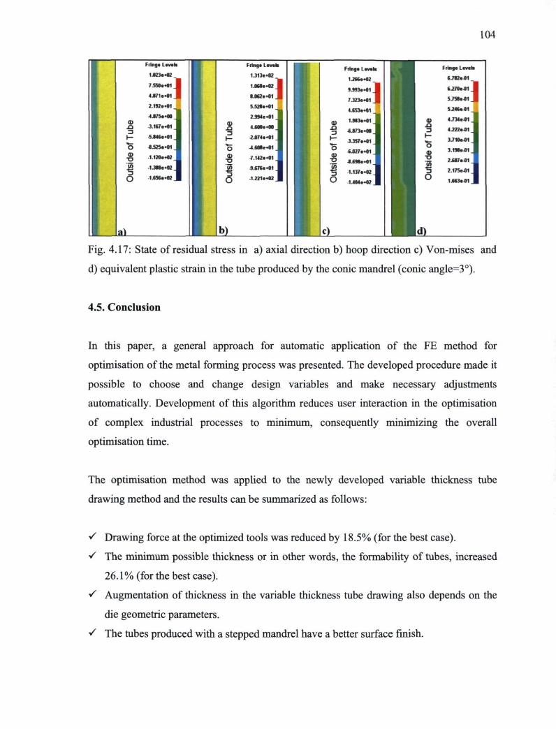
104

3

o

Fringe L * v * l *

1.0? 3 . ^ 2

I M O f O ,

4 J 7 1 * * * 1

2 192e-01

4.8 /5 . .00

J.1«7***1

5846e-01

8.525**01

1 120e*02

-1.3*8e02

1656. .0?

]

al_

1 a; 3

■ o

Fringe L * v * l *

1.313e.02

1.060e-02

8.062e<01

5.528e.01

2.994e-01

4.600e-00

2.074e«01

-l.608e.01

7.142**01

9.676e.01

1 2?1e«02

b)_

Fringe I evels

i jce**«2_

SJW.H1 J 7J23**41 J 4.653e.01

a) 1.983**01

4J73**M_

r - 3.35/..01

CJ 0)

-a 1

4J»7**«1 _ CJ 0)

-a 1

-8.698e.01

CJ 0)

-a 1 1.137**02 _

U 1.404**02

«L

OJ

3

O 0) -a io

O

Fringe I eveh

«.7*7*411

( 2 7 0 * 4 1

5 7 4 8 . 0 1

5 2 4 4 * 4 1

4.734*41

4 2 2 2 * 4 1

3.710.«1

3.194*41

2.687*4)1

2.175*41

1443*41

]

ld)_ Fig. 4.17: State of residual stress in a) axial direction b) hoop direction c) Von-mises and

d) equivalent plastic strain in the tube produced by the conic mandrel (conic angle=3°).

4.5. Conclusion

In this paper, a general approach for automatic application of the FE method for

optimisation of the metal forming process was presented. The developed procedure made it

possible to choose and change design variables and make necessary adjustments

automatically. Development of this algorithm reduces user interaction in the optimisation

of complex industrial processes to minimum, consequently minimizing the overall

optimisation time.

The optimisation method was applied to the newly developed variable thickness tube

drawing method and the results can be summarized as follows:

S Drawing force at the optimized tools was reduced by 18.5% (for the best case).

S The minimum possible thickness or in other words, the formability of tubes, increased

26.1% (for the best case).

S Augmentation of thickness in the variable thickness tube drawing also depends on the

die geometric parameters.

■S The tubes produced with a stepped mandrel have a better surface finish.

105

S The state of the residual stress in the stepped-mandrel tubes has more non-homogeneity,

which seems to be a negative point for these tubes.

Acknowledgements

The authors thank the Natural Sciences and Engineering Research Council of Canada,

National Research Council Canada-Aluminium Technology Centre, Alfiniti, Aluminerie

Alouette, C.R.O.I and Cycles Devinci for their financial support of this research. A part of

the research presented in this paper was financed by the Fonds Québécois de la Recherche

sur la Nature et les Technologies (FQRNT) by the intermediary of the Aluminium Research

Centre - REGAL. The authors want to express special thanks to Mr. J-F Béland, researcher

at the Aluminium Technology Centre, for his help and suggestions during the optimisation

process development, and Mr. Alain Deschenes, from Laval University, for his technical

support in experiments.

References

[1] Béland J.F., 2009, "Optimization of cold tube drawing of aluminium 6063-T4 with finite element method", M.Sc. thesis, Laval University, Quebec, Canada (In French). [2] Bihamta R., Ameli A., Movahhedy M.R., Mashreghi A.R., 2007a "A comparative study on the radial and indentation forging of tubes", International Journal of Forming Processes, (10) pp: 179-194. [3] Bihamta R., Movahhedy M.R., Mashreghi A.R, 2007b "A numerical study of swage autofrettage of thick walled tubes", Materials and Design, (28) pp: 804-815. [4] Bihamta R., D'Amours G, Rahem A., Guillot M., Fafard M., 2010a "Numerical studies on the production of variable thickness aluminium tubes for transportation purposes", SAE2010 World Congress, Detroit, USA. [5] Bihamta, R., D'Amours, G., Bui, Q. H., Rahem, A., Guillot, M., Fafard, M., 2010b "Optimization on the production of variable thickness aluminum tubes", Proceedings of the ASME 2010 International Manufacturing Science and Engineering Conference MSEC2010, October 12-15, Erie, Pennsylvania, USA. [6] Bihamta R., Bui Q. H., Guillot M., D'Amours G., Rahem A., Fafard M., 2011 "A new method for production of variable thickness aluminium tubes: numerical and experimental studies", Journal of Materials Processing Technology (211) pp: 578-589. [7] Bui Q. H., Bihamta R., Guillot M., D'Amours G., Rahem A., Fafard M., 2011 "Investigation of the formability limit of aluminium tubes drawn with variable wall thickness", Journal of Materials Processing Technology (211) pp: 402-414.

106

[8] Danckert J. and Endlet B., 2009 "Ls-Dyna used to analyze the drawing of precision tubes", 7th European Ls-Dyna conference. [9] Girad S., 2010 "Development of techniques for drawing of tubes with variable thickness", M.Sc. thesis, Laval University, Quebec, Canada (In French). [10] Guillot M., Fafard M., Girard S., D'Amours G., Rahem A. 2010 "Experimental exploration of the aluminum tube drawing process for producing variable wall thickness components used in light structural applications", SAE 2010 World Congress, Detroit, USA. [11] Hosford W. F., 2005 "Mechanical Behavior of Materials", Cambridge University Press. [12] Kim S.W., Kwon Y.N., Lee Y.S., Lee J.H., 2007 "Design of mandrel in tube drawing process for automotive steering input shaft", Journal of Materials Processing Technology (187) pp: 182-186. [13] Kleinermann J-P, Ponthot J-P, 2003 "Parametric identification and shape /process optimization in metal forming simulation". Journal of Materials Processing Technology (139) pp: 521-526. [14] Kuboki T., K. Nishida, Sakaki T., Murata M., 2008 "Effect of plug on leveling of residual stress in tube drawing", Journal of Materials Processing Technology, (204), pp: 162-168. [15] Myers R.H., Montgomery D.C, 2002 "Response Surface Methodology", Second edition, John Wiley & Sons, New York. [16] Stander N., Roux W., Goel T., Eggleston T., Craig K, 2009 "A design optimization and probabilistic analysis tool for the engineering analyst", LS-OPT® User's Manual, Livermore Software Technology Corporation.

107

Appendix 4.A (LFOPC optimisation method)

The LFOPC optimisation method is a gradient method that generates a dynamic trajectory

path, from any given starting point, towards a local optimum. This method differs

conceptually from other gradient methods, such as sequential quadratic programming

(SQP), as no explicit line searches are performed.

The LFOPC algorithm uses a penalty function formulation to incorporate constraints into

the optimisation problem. This implies that when constraints are violated (active), the

violation is magnified and added to an augmented objective function, which is solved by

the gradient-based dynamic leapfrog method (LFOP). The algorithm uses three phases. In

Phase 0, the active constraints are introduced as mild penalties through the pre-

multiplication of a moderate penalty parameter value. This allows for the solution of the

penalty function formulation where the violation of the (active) constraints are pre-

multiplied by the penalty value and added to the objective function in the minimization

process. After the solution of Phase 0 through the leapfrog dynamic trajectory method,

some violations of the constraints are inevitable because of the moderate penalty. In the

subsequent Phase 1, the penalty parameter is increased to more strictly penalize violations

of the remaining active constraints. Finally, and only if the number of active constraints

exceeds the number of design variables, a compromised solution is found to the

optimisation problem in Phase 2. Otherwise, the solution terminates having reached

convergence in Phase 1 (Stander et al. 2009).

108

Appendix 4.B

In this appendix, the algorithm of the in-house code is explained in detail. This code was

included in the optimisation loop to work as a preprocessor to automatically update

geometric features like die and mandrel geometries in the optimisation loop.

Ua) Lib) c)

Fig 4.B1: a) Geometries of die and mandrel in the initial state b) Geometries of die and

mandrel after change in the geometric parameters (conflict of tube with die) c) axial motion

of the tube for adjusting and removing the conflict.

Chapter 5

Numerical and experimental studies on the new design concept of hydroforming dies for complex tubes1

Abstract

Recently, the tube hydroforming (THF) process has found a remarkable role in the

production of tubular parts especially for the transportation industry. In prior research, there

were only two parameters, i.e. hydroforming pressure and axial feeding, to play with to

obtain a part without any problems like bursting and wrinkling. However, for parts with

complex geometries it is sometimes impossible to produce them by changing only these

two variables.

In this paper a new concept to design THF dies is presented and verified by numerical and

experimental studies. By application of this concept, dies will have three parts instead of

two, and consequently the tube will be preformed by the die closing before the start of the

hydroforming step. The numerical verifications confirmed that without this modification,

the production of most of the workpieces with complex geometries is difficult, if not

impossible. The numerical results showed good agreement with the performed experiments.

1 Paper to be submitted to Journal of Computational Materials Science

110

Keyword: Tube hydroforming (THF), Aluminium tubes, Die Design, Metal Forming, Thin

Walled Tubes.

5.1. Introduction

Tube hydroforming (THF) is one of the important metal forming processes and in some

cases the exclusive method for the production of complex tubes. In comparison with

conventional methods (i.e. stamping and welding) this method has the following

advantages: a) Part consolidation b) weight reduction c) improved structural strength and

stiffness d) lower tooling costs e) fewer secondary operations f) reduced dimensional

variation and g) reduced scrap [Ahmetoglu and Altan (2000) and Xu et al. (2009)] h) lower

spring-back.

In the literature, there are various studies about the tube hydroforming process; most of

them concentrated on finding the appropriate loading path, mostly in geometrically not very

complex tubes like T-shape [Kashanizadeh and Mosavi (2006), Fann and Hsiao (2003) and

Lin and Kwan (2004)], Y-shape [Ingarao et al.(2009) and Cheng et al. (2009)], rectangular

[Xu et al. (2009), Hwang and Altan (2003), Hama et al. (2006) and Yuan et al. (2006)], and

trapezoid sections [Xu et al.(2009)]. Other aspects of this process that were studied up to

now are appropriate characterization of material property for the THF process [Koç et

al.(2001)], and forming criterion to apply in the numerical studies [Hashemi et al. (2009)].

Nikhare et al. (2009) made a modification to the production of rectangular section tubes

from circular ones. With this modification they were able to produce the same final product

with lower pressure and more uniform thickness distribution. Elyasi et al. (2009) presented

a mechanism for improving die corner filling in a new THF die.

There is also some research on the design of dies and the role of preforming before THF,

which is the main objective of this paper. Koç (2004) evaluated the effect of die crushing

and pre-bending on the thickness distribution and formability of complex tubes. However, a

separate die for the preform (crushing) stage was used. Kang et al. (2005) studied tube size

I l l

effect on hydroforming formability. Their results showed that the diameter of the initial

tube is one of the crucial factors in hydroformablity. Trana (2002) showed that the

preforming process can be performed by the hydroforming die closing. Kim et al. (2003)

studied the hydroforming process for the production of automobile lower arms. The

prebending and preforming (stamping) processes were used before the hydroforming

operation. In their studies, only the geometric changes in the prebending and preform steps

were included, without considering residual stresses and work hardening in the part due to

prior steps. Hwang and Altan (2003) combined the crushing processes with performing in a

rectangular die. However, in all of the prior studies only two-half dies were used.

In this paper, a new modification to the design of THF dies is presented to produce a part

with different cross sections. In this modification, instead of using two half dies, a three-

part die is used. This modification facilitates performance of the process with a larger initial

tube diameter which in Kang et al. (2005) showed more formability. Furthermore, other

advantages of this modification are using lower pressure, lower axial feeding, having less

difficulty in using pre-bent tubes, and having less chance of parting line marks on the final

part. For a better comparison, the hydroforming process using the newly design and

conventionally designed die are modeled by the Ls-Dyna finite element software;

parameters like thickness distribution, thickness reduction percentage, and plastic strain are

compared. The new modification showed considerable improvement in the successful

performance of THF dies.

5.2. Design of new die

5.2.1. Geometric specifications of part

The considered part in this research is schematically shown in Fig. 5.1. This part is

composed of eight different sections with various thicknesses in each region. The variation

of thickness in this part is in a way that some regions have very low thickness (1.2 mm or

1.4 mm) while others are thicker, for instance 2.4 mm. Applying this kind of thickness

variation by the hydroforming method alone is impossible. Therefore, the initial tube

112

should be chosen with variable thickness. The methodology for production of such tubes is

outside the scope of this paper; it was explained in detail in previous publications [Bihamta

et al. (2010a), Bihamta et al. (2010b), Guillot et al. (2010), Bihamta et al. (2011), and Bui

et al. (2010)]. As can be seen in Fig. 5.1, the maximum and minimum diameters of

circumscribed circles are 45.0 mm and 40.2 mm respectively. Based on Table 5.1, the first

design idea that comes to mind is taking an initial tube diameter of 40.2 mm, and taking

parting line of the die symmetrically from the center of the part, as in Fig. 5.2. Based on

this design, the maximum hoop strain happens in section 8 with an average value of 42%.

This value was calculated from the deviation of the tube's final perimeter from its initial

perimeter. This amount of deformation seems very high, and it is expected to require a lot

of pressure and axial feeding for complete filling, as shown in finite element modeling of

this design. On the other hand, as ascertained in some prior publications like Nikhare et al.

(2009), the THF process with low pressure has more thickness uniformity than the process

with high pressure and axial feeding.

Fig. 5.1a) The case study of this paper with eight different sections.

113

Fig. 5.1: b) Schematic view of eight sections of case study with variable thickness and

various sections (For illustration purpose, the sections are drawn with larger scale).

The second design idea is using a tube with larger diameter, for instance 50.8 mm (2

inches), to have less deformation. But application of this tube size is not possible with a

symmetric die parting line, and would cause pinching of the tube during the closing step.

To avoid this problem, instead of having symmetric parting in a die with only two halves,

the die is designed with an unsymmetrical parting line in three parts, as shown in Fig. 5.3.

114

Part 1 in Fig. 5.3 is the fixed part which is attached to the hydroforming press, part 2 is

referred to as the upper die. which is attached to the upper side of the hydroforming die,

and part 3 is the rear die, which is moved by one of the feeding cylinders of the

hydroforming press. The Interlaken hydroforming press of CNRC-NRC, Aluminium

Technology Centre, that this die was designed for has four feeding cylinders. Therefore two

of them are assigned for axial feeding, and a third one for movement of the rear die. Fig.

5.3 shows the parting line passing through the end of the part fillets. Fig. 5.4 presents a

schematic view of the three-part die assembly in the hydroforming press.

Table 5.1: Specifications of various sections of part.

Section 1

Initial

diameter

(mm)

45

Section

thickness

(mm)

2.4

Tube

Initial

perimeter

(mm)

141.3675

Section

final

perimeter

(mm)

183.542

Perimeter

ratio

(mm/mm)

1.298

Section 2 45 2.4 141.3675 183.542 1.298

Section 3 45 1.4 141.3675 183.542 1.298

Section 4 45 1.4 141.3675 177.337 1.254

Section 5 45 1.2 141.3675 177.337 1.254

Section 6 40.4 1.2 126.9166 165.83 1.307

Section 7 40.2 1.9 126.2883 165.83 1.313

Section 8 43.2 1.9 135.7128 192.975 1.422

115

Fig. 5.2: Schematic of THF die with symmetric parting line and initial tube diameter of

40.2 mm.

Fig. 5.3: Schematic of THF die with un-symmetric parting line (three parts) and initial tube

diameter of 50.8 mm 1) fixed die 2) upper die 3) rear die.

116

Fig. 5.4: Schematic view of three-part die and hydroforming machine 1) upper die 2) rear

cylinder 3) rear die 4) left feeding cylinder 5) fixed die 6) right feeding cylinder.

5.2.2. Geometry of initial tube

As explained before, producing parts with controlled variation of thickness in the axial

direction with the THF method is impossible. Therefore, in this numerical study, various

thicknesses were assigned to the different regions of the initial tube that are presented with

more details in Table 5.2. The values of this table are obtained from some finite element

iterations.

As shown in Table 5.2 and Fig. 5.5, the assigned thicknesses have larger values than the

thickness in the final part. This is because of reduction of thickness during the

hydroforming step especially in the middle regions that can not have enough feeding from

the axial motion of the cylinders. To have constant outer diameter in the initial tube, the

initial shell was designed with different outer diameter in a way that after applying various

shell thicknesses, the outer tube diameter in all regions became 50.8 mm (2 inches). The

eight lines in Fig. 5.5, show the approximate transition of each section of the final part in

the initial tube.

117

Table 5.2: The initial and correspondent final thicknesses of tube in various zones.

Region Initial Thickness

(mm)

Correspondent final

thickness (mm)

A 2.74 2.4

B 2.17 1.4

C 1.59 1.4

D 1.48 1.2

E 1.37 1.2

F 1.86 1.9

G 2.23 1.9

5.3. Finite element model details

5.3.1 Material properties

The tube material in this study was AA6061-O. As-extruded tubes were drawn to obtain a

better surface finish and to reach appropriate dimensional tolerances, then fully annealed.

The stress-strain curve of this material was obtained with a uniaxial tensile test and

extrapolated by the Holloman power law ( a = ksn , n=0.263, k=211.48), Swift

( a = k(£ + £0)" k=235.83MPa, n=0.32867), and Voce ( a = a0[l-exp(-Ae)]

cr0 =129.25MPa, A = 23.623) methods. Since the Holloman model had better agreement

with the experimental results (see Fig. 5.6), this data was implemented in the finite element

model.

118

1 .2 3 4

5

Fringe Levels

2.740e+00

2.603e+00 1

2.466e*00 _ |

3 4

5

Fringe Levels

2.740e+00

2.603e+00 1

2.466e*00 _ | A A TB

3 4

5

Fringe Levels

2.740e+00

2.603e+00 1

2.466e*00 _ |

/ D 6 / 7

2.329e*00

2.192e*00 .

E ^ 8 2.055e+00 _

1.918e+00 Time- 0 Contours of Shell Thickness min-1.37, at elem# 169743 / F 1.781e+00_ Time- 0 Contours of Shell Thickness min-1.37, at elem# 169743 / F

] 1.644e*00 max-2.74, at elem* 51801 G G 1.507e*00 .

1.370e+00

Fig. 5.5: Initial thickness distribution of tube and correspondent place of each section in

final part.

250 -

200

150 -

I 10° H

50

1 r i i

Swif) \

j Hollomon j Swif)

\ * -^r^^z *

Voce

Uniaxial Test Result Hollomon Voce Swift

— J Uniaxial Test f. Results

' i

Uniaxial Test Result Hollomon Voce Swift

— J Uniaxial Test f. Results

' i 1 |

i

Uniaxial Test Result Hollomon Voce Swift

— J Uniaxial Test f. Results

' i 1 |

i i i 0 1 0.2 0.3 0.4

True Strain (m/m) 0.5 06

Fig. 5.6: True Stress-Strain curve for the AA 6061-O material.

5.3.2. Die geometry and meshing

In order to design the die geometry, Pro-Engineer software was used before the surface of

the die was entered into the Hypermesh software to be meshed. The element size for the

tube and dies were approximately 1.5 mm and 2.5 mm respectively. The shell element with

four nodes was used because of its capability to have variable thicknesses in each node.

119

5.3.3. Boundary conditions and contact condition

The fixed die was constrained in all directions. The rear and upper dies were left constraint-

free in the moving direction, but they were completely constrained in other directions. To

apply axial feeding to the tube, two rows of nodes at a distance of 35 mm from the two

ends of the tube were selected, and two different displacements were applied to represent

the axial motion of right and left pushers. The distance 35 mm is the length of the guiding

zone in the pushers, and there is no variation of thickness in this length.

The surface to surface contact formulation was chosen to define contact conditions between

tube and dies. The friction coefficient between them was selected as 0.05 as reported in

[Williams et al. 2010]. Figs. 5.7a and 5.7b show pressure and displacement curves for this

part. The pressure and feeding up to time=l sec. is zero because the first second is the

closing step. Fig. 5.7shows that at time 1.05 sec, when the pressure is zero, the axial

feeding curves have values around 2.2 mm; these values are applied to be sure that there is

enough sealing in the tube before application of pressure starts.

ç ■o 4)

U.

1 X

<

45

40

35

30

25

20

15

10

5

0

! : I •O— Right Feeding i i

{ \ \ [ \ l . - .y / j^^C" .

: : Ï ! i i i

Closing Step • 4 : : 1 ; ».

^Hydtofonpmg $tep 4 W '• ! 1 ! »

o i i i i y ■ î -f — f î

1 12 1.4 1.6 1.8 Normalized Time (Sec.)

a)

120

Normalized Time (Sec)

b) Fig. 5.7: a) Axial feeding curve b) hydroforming pressure.

5.4. Experiments

After completion of the numerical studies, a die was built and installed in the hydroforming

press (Fig. 5.8). Outer tube surfaces were lubricated with Hydrodraw 625 lubricant. The

liquid that was used in the press for application of pressure was water with NOVACOOL

9034/5 added to avoid corrosion of the press. For sealing, O-ring and local deformation

methods are used at the same time. The details of this type of sealing are presented in

Bihamta etal. 2012.

As geometries of the sections 1 and 8 (Fig. 5.1b) are closer to rectangular forms than

circular ones, it was necessary to make the pushers sections rectangular. Alternatively, a

long transition section between the two sections could be considered, but this would

increase the overall length of the die. The drawback of rectangular-section pushers is that

they have more difficulty in sealing during the hydroforming process. In Fig. 5.9 photos of

rectangular pushers are presented.

121

1 ' M ' \ ! m

-—

1 . - ^ =

i* c g

Fig. 5.8: Three part dies after installation in Interlaken hydroforming press.

Left Right

Fig. 5.9: Left and right pusher with rectangular sections.

122

5.5. Results and discussion

5.5.1. Thickness reduction percentages

As mentioned earlier, the main objective of this paper is to investigate the effect of

appropriate die design (three or two-part dies) on the feasibility of producing complex

tubeswith the THF method. Figs. 5.10 and 5.11 show thickness reduction percentages for

the tubes that were deformed by the two-half die with smaller initial tube diameter and the

three-part die with larger initial tube diameter, with the same pressure and axial feeding,

respectively.

For the die with two halves and consequently smaller diameter, the verification of thickness

reduction in the region with the minimum thickness, i.e. section E, showed 59% thickness

reduction just up to time=1.2 seconds; at this point the simulation stopped because this

thickness is much smaller than the desired thickness for this section. The region with the

59% thickness reduction seems to be the most susceptible zone for bursting of the tube

during hydroforming since it is located after the tube bent region; even increasing the axial

feed can not help to solve the thickness reduction problem in this zone.

Time» 1.2047 roin--0.49663, al atom* 56721 max-59.0924, a t ' t tm* 135099

Fringe Level» 6.9MrH>1 5611er01 5.313e*01 6 015e*O1 4717e+01 4.420e*O1 4.122e*01 3.824e*01 3.526e*01 3.228e*01 2.930e-K)1 2.632>*01 2.334e<01 2.036e*O1 1.738e*01 1440e-K)1 1.142*401 (.4431400 5.463er00 2.484e*O0 -4.966e.01

Fig. 5.10: Thickness reduction percentages in the part produced using two-half die at

time=1.2sec.

123

i.S22e4M

3«2»e-4>2.

1.744**O0

-L33?m*m

T r * - I m m - 11 J H * . * r «tern* 149157 nw-Q.Ct2222, * f elema 17393*

-1.713eM»

-5.307e*«

■ u n n i .

4.*71e*4»

a)

T V i » - 2 mm--59,591f, J t i t e m * 181922 m * x - 1 2 ^ 0 * 1 , ; t eterrw 124S46

1.fi07e*00

■ 1.993«.0O

■5.593«-00

-9.193e*O0

1279e*01

-1639e.01

-2 .36»^ tM

-2.719e*01

-3.079e»O1

3*39e*01

3799e*01

-4i59e*oi

-4519e-01

-4.879e.01

-5239e*01

-S.599e*01

b)

Fig. 5.11: For three-part die: a) Thickness reduction percentages after closing the die and

before the start of hydroforming b) thickness reduction percentage contour in the part after

the end of the hydroforming process.

On the other hand, for the three-part die, after the closing step and complete filling of the

die, the maximum thickness reductions are 0.6% and 12% respectively. The minus sign in

the thickness reduction is indicating augmentation of thickness. As shown in Figs. 5.11a

and 5.1 lb, there is a thickness augmentation of 11% and 59% at the end of the closing and

hydroforming steps, respectively. However, the 59% increase in thickness is a local value

around the nodes of application of displacement; the real maximum value seems to be

124

around 20%. This value was considered safe enough as in prior studies such as Filion

(2011) the higher values for the same die and tube material did not cause any problem.

When comparing the two- and three-part dies, the question arose if with different thickness

distributions in the tube it possible to have a successful hydroforming step using a two-half

die? To evaluate this option, initial tube thickness in all regions was assigned to be more

than the corresponding value in the tube for the three-part die. In this attempt, the overall

tube thickness was considered to be 2.74 mm (the maximum thickness in the tube for the

three-part die). Even with this over-assignment of thickness, the amount of thickness

reduction is considerable, with a maximum value of 39% (Fig. 5.12). However, it should be

noticed that this part is far different from the tube with variable thickness.

T i m t - 2 min-302454, at elem# 45201 max-39.074, at elenv* 41106

Fringe Levels

3.907e*01

3.214e*01

2.521 e*01

1.828e«01

1.135e+01

4.414e*00

2.518e»00

9.450erOO

-1.638e*01

2.331 er01

-3.025e+01

Fig. 5.12: Thickness reduction percentages in the tube with overall thickness of 2.74 mm

with the two-half die.

5.5.2. Distribution of thickness

In Figs. 5.13 and 5.14 distributions of thickness in the produced parts by the two-half die

(up to time=1.2sec.) and three-part die are presented. The part produced by the two-half die

has a thickness in some regions reaching 0.45 mm, which is far from the minimum

acceptable thickness of the part. On the other hand, the part produced by the three-part die

has the minimum thickness of 1.2 mm corresponding to the minimum desired thickness in

the final part. As mentioned above, the maximum thickness increase of 4.1 mm is only for

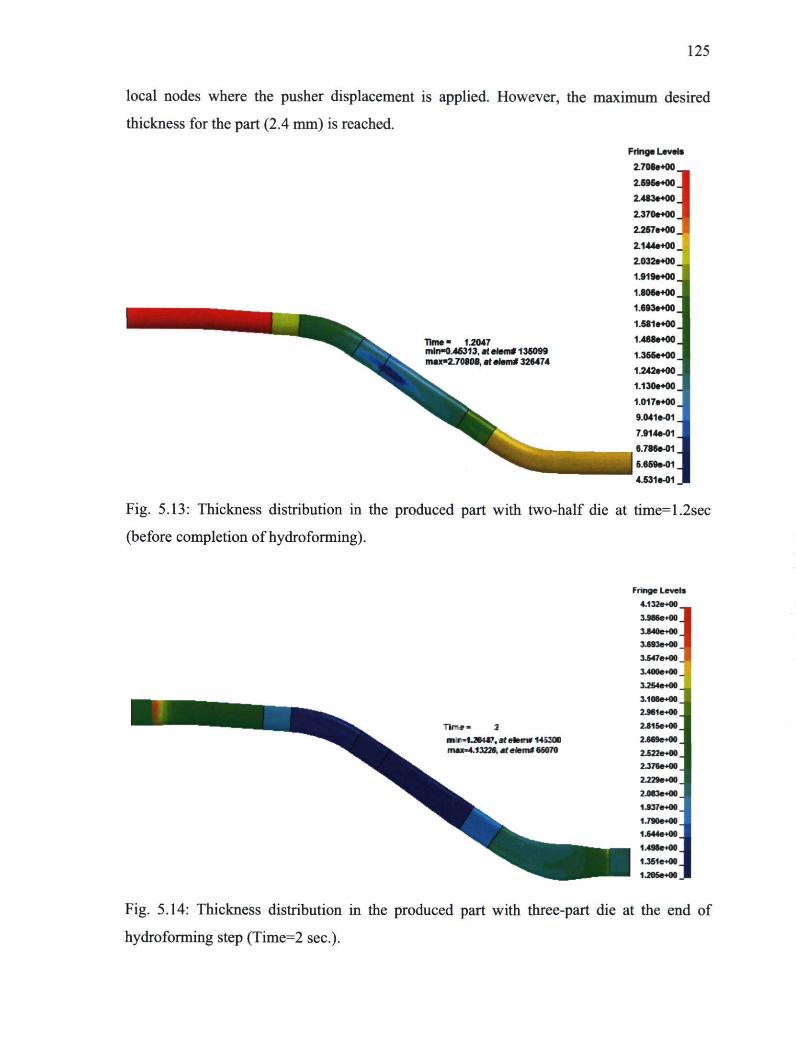
125

local nodes where the pusher displacement is applied. However, the maximum desired

thickness for the part (2.4 mm) is reached.

Time - f .2047 min-0.46313. at etem* 135099 max-2.70808, at «tern* 326474

Fig. 5.13: Thickness distribution in the produced part with two-half die at time=1.2sec

(before completion of hydroforming).

m r =1.20447, a ( e l e n » 1+S30C maxM.«22S , a t e t e m * 65070

Fringe Levels

4.132e*00

3.986e*00

3.840e*00

3.693e*O0

3.547e<00

3.4O0e*O0

3.254er00

3.108e*O0

2.961e*O0

2.815e*O0

2.669e»O0

2 522e*00

2.376e*O0

2.229e*00

2.083e»O0

1.937e»O0

1790e»00

1.644e»O0

1.498e*00

1.351eKK>

1.2O5e-O0

.

Fig. 5.14: Thickness distribution in the produced part with three-part die at the end of

hydroforming step (Time=2 sec).

126

5.5.3. State of equivalent strains

Figs. 5.15 and 5.16 show equivalent plastic strain in the tube after the closing and

hydroforming steps. The average equivalent strain at the end of the closing step is around

4%, which is less than the maximum strain for this material in the uniaxial test. However,

there are some regions like the corners close to the die parting line with locally higher

values (18%).

In the hydroforming step some regions have higher amounts of plastic strain, but in general

the average value for the hydroforming step is 20%. Regarding the three-dimensional

nature of the loading in the hydroforming step and values of thickness reduction, these

amounts of strain seem to be safe to perform the THF process successfully.

Fig. 5.15: Effective plastic strain after die closing for the three-part die.

127

Fringe Levels

3.820*-01 3.629e-01 3.439e-01 3.248*01 3.057e-01 2.867e-01 2.676e-01 2.485*4)1 2.29 5e 4)1 2.104*-01 1.913e01 1.723e-01 1.532*01 1.342*01 1.151e-01 9.602e-02 7.696*-02 5.789*4)2 3.88 3e-02 1.976*4)2 7.000* 4M

Fig. 5.16: Effective plastic strain at the end of hydroforming step for the three-part die.

Fig. 5.17: Effective plastic strain at the end of hydroforming step for the two-half die

(Time=1.2 Sec).

128

For the die with two halves, distribution of the plastic strain was shown in Fig. 5.17. It can

be seen that the maximum amount of strain is around 88%, which does not seem safe

enough in the hydroforming step.

5.5.4. Preforming by die closing

To illustrate the role of deformation by the die closing step, Fig. 5.18 compares geometry

of a tube at the end of the closing step (Time=l Second) with its geometry at the end of the

hydroforming step. It is clear from this figure that the tube geometry is very close to its

final geometry, especially in sections E, F, and G which have more complex shapes.

Deformation of tube after closing die

Section A (Time=l Sec.)

Deformation of tube after Hydroforming

Section A (Time=2 Sec.)

Section B (Time=l Sec.) Section B (Time=2 Sec.)

129

Section C (Time=l Sec.) Section C (Time=2 Sec.)

Section D (Time=l Sec.) Section D (Time=2 Sec.)

Section E (Time=l Sec.) Section E (Time=2 Sec.)

130

Section F (Time=l Sec.) Section F (Time=2 Sec.)

Section G (Time=l Sec.)

Section G (Time=2 Sec.)

Fig. 5.18: Form of tube after end of closing step and end of hydroforming step.

Fig. 5.19 shows tube geometry after preforming and hydroforming steps. As expected, after

die closing the tuba has a geometry very close to the final part.

Fig. 5.19: a) tube after preforming by die closing b) after hydroforming.

131

5.5.5. Thickness reduction distribution in the circumferential direction

In Figs. 5.20i through 5.20iv, thickness distributions in the circumferential direction for the

three-part die from experiments and FE results are presented. For the experimental curves,

the tubes were cut from the sections shown in Fig. 5.1b to measure their thickness in the

circumferential direction (Fig. 5.21). It is clear that the values in the numerical studies are

lower than in the experiments. As discussed in detail in [Bihamta et al. 2012], in the

preceding bending steps the tube experiences a 4% reduction and 7% thickness increase

which was not taken into account in the FE model in this paper. Furthermore, non-

homogeneous lubrication in the experiments can be an additional reason for local tube

thinning. However, if the average thickness reduction and increase (in the preceding

processes) is added to the values from FE, it will be in good agreement with experimental

results. It is worth mentioning that when comparing experimental and numerical results for

section E, which is not located in the bent zone, the difference between averages of

thickness reduction is only 0.4%; this confirms the effect of the preceding bending step in

the difference between results. The presented results are for a representative section, but

there is always a possibility of mild variation along a section. Also, as ascertained in

D'Amours et al. (2007), the prediction of thickness and its reduction by the shell elements

is not as precise as by solid elements; this can be one of the sources for the difference

between FE and experiments.

♦ Experiment " ■

_Average_Experimental

—*—FE —»—Average J E

0.2 03 0A 0 5 0.6 0.7 0.8

Normalized Circumference (mm/mm)

0.9 Section A

i)

132

25

20

» 15 * S 5 10

I5 I

0.1 OJ OJ 04 0.5 0.6 0.7 Normalized Circumference (mm/mm)

0.8 03 Section C

ii)

0.3 0.4 0.5 0.6 0.7 No im a l i i c d Circumference fin m/mm)

G Section E

iii)

— — Av«nge_Expehm*ntaJ é FE ■ Avwage FE

— — Av«nge_Expehm*ntaJ é FE ■ Avwage FE

— I — i f "

— I — * \ • i f "

—

„ \ _

* \ • i f " —

* /

0.1 0.2 0.3 0.4 0.5 0.6 0.7 0.8 0.9 '

Normalized Circumference (mnVmm) Section G

iv)

Fig. 5.20: Distribution of thickness and average thickness reduction from experiments and

FE in the circumferential direction in four different sections i) section A ii) section C iii)

section E iv) section G (Start point of measurement is shown in each section).

133

Fig. 5.21: Sections of tube after hydroforming.

5.5.6. Another advantage of the three-part die: More facility in the pre-bending step

The majority of parts produced with the THF method require a pre-bending operation

before hydroforming. A major problem in the hydroforming of parts with two-half dies is

positioning of the bent tube in the hydroforming die: a small change in the bending radius

or angle makes it difficult to position the tube in the die, and can even causes pinching of

tube during die closing in some cases. On the other hand, when using three-part dies, even a

1-inch change in one of the radii and with the removal of another slight bend in one end of

tube, acceptable results were obtained. This would be almost impossible using two-half

dies. Therefore, to make the bending step economical (fewer bending dies), two equal

bending radii were chosen (R=10 inches), and the small bent region with a radius of 23

inches was eliminated (Fig. 5.22).

Fig. 5.22: Two differently prebent tubes that were successfully hydroformed in the three-

part hydroforming die.

134

Fig. 5.23 presents the effective plastic strain in a hydroformed part with just two bent

regions. Comparing this Figure with Fig. 5.15 shows approximately the same level of strain

for both tubes.

Fig. 5.23: Effective plastic strain in the part with just two bent regions.

5.6. Conclusion

The idea of using a three-part die instead of one with two-halves for producing complex

tubes by the THF method was presented. A comparison with the traditional (two-half)

method yielded the following results:

1. The idea of using a three-part die enables using larger initial tube diameters that

consequently increases the chance of successful hydroforming with less chance of

bursting during the hydroforming step.

2. In some complex parts, it is absolutely impossible to produce the part with a two-half die

as some complex geometries can not be extracted from the die after hydroforming. The

three-part die makes extraction easier.

3. By application of three parts in the THF dies, an automatic preform of the tube

geometry can be performed to make its geometry closer to the geometry of the final

part.

135

4. Excellent agreement between loading path obtained from numerical and experimental

results was observed. However, to better predict thickness reduction percentages, some

improvements can be applied to the FE model.

5. Using three-part dies facilitates some preceding steps like bending.

Acknowledgements

The authors thank the Natural Sciences and Engineering Research Council of Canada,

National Research Council Canada-Aluminium Technology Centre, Alfiniti, Aluminerie

Alouette, C.R.O.I and Cycles Devinci for their financial and technical support of this

research. A part of the presented research in this paper was financed by the Fonds

Québécois de la Recherche sur la Nature et les Technologies (FQRNT) by the intermediary

of the Aluminium Research Centre-REGAL.

References

[1] Ahmetoglu M., Altan T., 2005 "Tube hydroforming: state-of-the-art and future trends" Journal of Material Processing Technology (98) pp: 25-33. [2] Bihamta, R, D'Amours, G., Bui, Q. H., Rahem, A., Guillot, M., Fafard, M.,2010a " Optimization on the production of variable thickness aluminum tubes", Proceedings of the ASME 2010 International Manufacturing Science and Engineering Conference MSEC 2010a, Erie, Pennsylvania, USA. [3] Bihamta R, D'Amours, G, Rahem, A., Guillot, M., Fafard, M.,2010b "Numerical studies on the production of variable thickness aluminium tubes for transportation purposes", SAE 2010 World Congress, Detroit, MI, USA. [4] Bihamta R, Bui Q. H., Guillot M., D'Amours G, Rahem A., Fafard M., 2011 "A new method for production of variable thickness aluminium tubes: numerical and experimental studies", Journal of Materials Processing Technology (211) pp: 578-589. [5] Bihamta R, D'Amours G, Bui Q-H, Guillot G, Rahem A., Fafard M.,2012 "Global optimization on the production of complex aluminium tubes by the hydroforming process", to be submitted in 2012. [6] Bui Q. H., Bihamta R, Guillot M., D'Amours G, Rahem A., Fafard M., 2011 "Investigation of the formability limit of aluminium tubes drawn with variable wall thickness", Journal of Materials Processing Technology (211) pp: 402-414. [7] Cheng D.M., Teng B.G., Guo B., Yuan S.J., 2009 "Thickness distribution of a hydroformed Y-shape tube", Materials Science and Engineering A, (499) pp: 36-39. [8] D'Amours G, Rahem A., Williams D., Worswick M., and Mayer R, 2007 "Crashworthiness of aluminium tubes; Parti: hydroforming at different corner-fill radii and end feeding levels", materials processing and Design: Modeling, Simulation and applications conference NUMIFORM 2007.

136

[9] Elyasi M., Bakhshi-Jooybari M., Gorji A., 2009 "Mechanism of improvement of die comer filling in a new hydroforming die for stepped tubes", Materials and Design (30) pp: 3824-3830. [10] Fann K. J., Hsiao P.Y., 2003 "Optimization of loading conditions for tube hydroforming ", Journal of Materials Processing Technology (140) pp: 520-524. [11] Filion G., 2011 "Virtual and experimental fabrication of complex geometry aluminium tubes by hydroforming method" MSc. Thesis, Laval University (In French). [12] Guillot M., Fafard, M., Girard, S., Rahem, A., D'Amour, G.,2010 "Experimental study of the aluminum tube drawing process with variable wall thickness", SAE 2010 World Congress, Detroit, MI, USA. [13] Hama T., Ohkubo T., Kurisu K., Fujimoto H., Takuda H., 2006 "Formability of tube hydroforming under various loading paths", Journal of Materials Processing Technology, (177) pp: 676-679. [14] Hashemi R., Assempour A., Mansoumi K. E., 2009 "Implementation of the forming limit stress diagram to obtain suitable load path in tube hydroforming considering M-K model", Materials and Design (30) pp: 3545-3553. [15] Hwang Y.-M., Altan T., 2003 "Finite element analysis of tube hydroforming processes in a rectangular die", Finite Elements in Analysis and Design (39) pp:1071-1082. [16] Ingarao G., Di Lorenzo R, Micari F., 2009 "Internal pressure and counterpunch action design in Y-shaped tube hydroforming processes: A multi-objective optimization approach", Computers and Structures (87) pp: 591-602. [17] Jeong Kim, Li-Ping Lei, Beom-Soo Kang., 2003 "Preform design in hydroforming of automobile lower arm by FEM", Journal of Materials Processing Technology (138) pp: 58-62. [18] Kang S. J., Kim H. K., Kang B. S., 2005 "Tube size effect on hydroforming formability", Journal of Materials Processing Technology (160) pp:24-33. [19] Kashani Zadeh H., Mosavi Mashhadi M., 2006 "Finite element simulation and experiment in tube hydroforming of unequal T shapes", Journal of Materials Processing Technology (177) pp: 684-687. [20] Koç M., Aue-u-lan Y., Altan T., 2001 "On the characteristics of tubular materials for hydroforming-experimentation and analysis", International Journal of Machine Tools & Manufacture (41) pp: 761-772. [21] Koç M., 2004 "Advances in Tube Hydroforming: An Enabling Technology for Low-Mass Vehicle Manufacturing Material, Lubrication, Loading", Simulation Issues, and Alternatives Tsinghua Science and Technology (9) pp:527-545. [22] Lin F. C, Kwan C. T., 2004 "Application of abductive network and FEM to predict an acceptable product on T-shape tube hydroforming process", Computers & Structures (82) pp: 1189-1200. [23] Nikhare C, Weiss M., Hodgson P.D., 2009 "FEA comparison of high and low pressure tube hydroforming of TRIP steel", Computational Materials Science (47) pp:146-152. [24] Trana K, 2002 "Finite element simulation of the tube hydroforming process- bending, preforming and hydroforming", Journal of Materials Processing Technology (127) pp:401-408. [25] Williams B.W., Worswick M.J., D'Amours G., Rahem A. and Mayer R, 2010 "Influence of forming effects on the axial crush response of hydroformed aluminum alloy tubes", International Journal of Impact Engineering (37), pp: 1008-1020.

137

[26] Xu X., Li S., Zhang W., Lin Z., 2009 "Analysis of thickness distribution of square-sectional hydroformed parts", Journal of Materials Processing Technology (209) pp:158-164. [27] Yuan S.J., Han C, Wang X.S., 2006 "Hydroforming of automotive structural

components with rectangular-sections" International Journal of Machine Tools and Manufacture (46) (2006) pp: 1201-1206.

Chapter 6

Global optimisation of the production of complex aluminium tubes by the hydroforming process1

Abstract

With the recent development of analysis software products, designers and engineers are

able to design more complex parts to obtain better performance in the final products. In this

study, the tube hydroforming process, including preceding processes, i.e. variable thickness

tube drawing and two-step bending, are globally optimized to obtain parts without any

problems like bursting or un-filled zones at the end of the forming processes. Unlike most

previous studies which searched for an optimum hydroforming process by changing two

hydroforming parameters, i.e. axial load feeding and internal pressure, in this study, the

distribution of initial tube wall thickness and the variation of thickness due to bending steps

will be taken into account in a global optimisation algorithm. The developed algorithm is a

general-purpose algorithm that can encompass different processes and change various

parameters in each process to be able to reach the global objective. The case study used was

a part that needs two-step variable thickness tube drawing, and two bending stepsbefore

hydroforming. To verify the numerical results in each forming stage and at the end of all

forming processes, extensive experiments were performed, and acceptable agreements were

observed.

1 Paper to be submitted to Journal of Materials and Design

139

Keywords: Tube Hydroforming, Tube Bending, Variable Thickness Tube Drawing,

AA6061, Aluminium.

6.1. Introduction

Aluminium tubes, mostly produced by the tube hydroforming (THF) process, play an

important role in transportation industries such as automotive and bicycle production. As

shown in Fig. 6.1, in fabricating almost all THF parts, it is necessary to use some other

preliminary processes like tube drawing, annealing heat treatment, tube bending, and

preforming before the final THF process. The wider application of aluminium tubes by

industry is hindered because of the reduced ductility and more complex material behavior

of aluminium in comparison with steels [Korkolis (2009)].

Fig. 6.1 : Tubular automobile parts produced by the THF method.

A) Roof headers, B) Instrument Panel Support, C) Radiator Supports, D) Engine Cradles E)

Roof rails, F) Frame Rails [ http://www.vari-form.com].

Various aspects of the THF process have been studied. Xu et al. (2009) presented a paper to

find the optimum loading path for a trapezoid-sectional die. Cheng et al. (2009) studied

distribution of thickness in a Y-shape tube by the finite element (FE) and experimental

methods. Xu et al. (2009) mathematically studied thickness distribution along the cross-

140

section of a square-sectional hydroformed part. Koç et al. (2001) presented experimental

and analytical approaches to characterize materials for the THF process. Korkolis and

Kyriakides (2009) evaluated the effect of loading path on the failure of inflated aluminium

tubes. Hashemi et al. (2009) applied a stress-based forming limit diagram to obtain

optimum loading paths in THF. Song et al. (2010) evaluated the effect of flow stress

characteristics of tubular material on forming limit in the THF process. Kang et al. (2005)

studied tube size effect on hydroforming formability. The publications above are examples

of research performed in this field. However, on the subject of this paper, which is studying

the THF process including the preceding processes, there is only little research. For

instance, Koç (2004) evaluated effect of die crushing and pre-bending on the thickness

distribution and formability of complex tubes. Trana (2002) showed that the preforming

process can be performed by the hydroforming die closing, saving considerable time and

production cost. Hwang and Altan (2003) studied the crushing processes in combination

with performance in a rectangular die. None of the above mentioned studies, however,

included the initial tube thickness as an optimisation variable. There is also no specialized

optimisation algorithm, nor an automatic method to manage the optimisation procedure.

Abedrabbo et al. (2009) presented an optimisation process linked with a FE model to

optimize the high-strength steel tube hydroforming process. In that study, despite having an

optimisation algorithm for modification of the hydroforming parameters, they only took

into account the THF process without preceding processes.

In this paper, in the first step, a code was developed to assign various thicknesses to the

initial tube wall. This shell with various thicknesses is considered as the tube issued from

one- or two-step variable wall thickness tube drawing. It is worth mentioning that because

of the annealing heat treatment after tube drawing, it is assumed that all material properties

return to the initial state and there are not any residual stresses induced by the drawing.

After assignment of thickness to the shell tube, the FE model is transferred automatically to

the bending steps, and afterward the bent tube is transferred to the hydroforming step.

Depending on the defined objectives and constraints, the optimisation loop will return to

the initial step to change tube thickness and/or some parameters in the hydroforming step to

141

reach the objective. All of the changes in the parameters of the preceding processes and

hydroforming step are performed automatically without any user interaction.

In the next sections, the processes and their FE models that are involved in the production

of the case study part are explained. The experimental section explains the geometric

features of the part and the experimental rig.

6.2. Cold forming processes prior to hydroforming

In general, for most THF processes, some preform processes are necessary. Without them,

the tube cannot be positioned in the THF die appropriately. Furthermore, the quality of the

preceding operations has a direct effect on the quality of final workpiece. In the following

sections, the important cold forming processes prior to THF are studied numerically and

experimentally.

6.2.1. Variable thickness tube drawing

6.2.1.1. Production of variable thickness tubes

The variable thickness tube drawing process is a new enhancement applied to the classic

tube drawing method to produce tubes with variable thickness along the tube's length

and/or in the radial direction. As explained in more detail in prior publications [Bihamta et

al. (2011), Bui et al. (2011a), Bui et al.(2011b), Bihamta et al. (2010), and Guillot et al.

(2010)], in this method, the desired variation of wall thickness can be induced through the

application of axial displacement of the conic mandrel. However, in this process some

parameters like material heat treatment, its alloying elements, and tool geometry, limit the

minimum attainable thickness in one step; if smaller than that is required, it should be

performed in more than one step. On the other hand, if two or more tube drawing steps are

necessary, the synchronization between two passes is a crucial factor. If the location of

thickness reduction in the second step is not in the appropriate zone, there is a possibility of

tube fracture. There are two solutions to avoid this problem.

142

The first solution consists of applying a very accurate non-destructive measurement

mechanism, such as a laser, to accurately measure the thickness along the tube axis and

implement very precise axial displacement to the tube in the next steps. The

implementation of the first solution requires very precise and expensive equipment.

Another alternative is the application of mild transition between zones with variable wall

thicknesses. This mild transition can guarantee that if there is inaccuracy in the second

pass, the tube will not experience any rupture.

In the zones that are more prone to bursting in the hydroforming step, augmentation of

thickness in the initial tube can eliminate the chance of bursting, and the final thickness in

the tube can be controlled. On the other hand, if a zone in the part undergoes lower loads

than other regions when in service, the thickness of this region can be reduced to diminish

overall weight of part.

Details of the numerical and experimental studies on this process are outside the scope of

this paper; interested readers can see [Bihamta et al. (2011), Bui et al. (2011a), Bui et al.

(201 lb), Bihamta et al. (2010), and Guillot et al. (2010)].

6.2.1.2. Tube thickness as an optimisation variable in the THF process

In this study, it was possible to use solid elements or shell elements to include initial tube

thickness in the global THF process optimisation. If solid 3D elements are to be used in the

tube bending and THF steps, four-node 2D elements can be used inn the tube-bending step.

Due to the axi-symmetric geometry of the tube drawing process, the results can then be

rotated and converted to complete a 3D tube. In comparison with shell elements, this kind

of element has more precision in prediction of thickness variation in the THF process

[D'Amours et al. (2007)], but utilizing them seems to be computationally very expensive.

On the other hand, application of shell elements for the simulation of THF and tube

bending processes seems to be more efficient computationally, and provides acceptable

results.

143

Since it is common to do annealing heat treatment after one- or two-step tube drawing, the

material property in the drawn tube (after heat treatment) is considered to be the same as

the initial material. Therefore, the inclusion of the tube drawing processes in the global

optimisation loop seems to be unnecessary, and will increase the computation time.

Consequently, the parameter that was included from the tube drawing process is variation

of thickness in the tube.

For implementation of thickness in the initial tube, a code was developed and included as a

part of the preprocessor in the optimisation loop to update values of thickness in the

optimisation loop based on the optimisation iterations. This code reads coordinates of

various elements and applies the different thicknesses upon request of the optimisation

engine. An example of output of this code is presented in Fig. 6.2.

1 F ring» Laval* 2.740*+«l

umim jjtmm imium 2.192e*00 UNHt f unam 1.7B1e*C0

1.844*^)0.

IMIaiM. 1.370a*«_

Fig.6.2: Application of various thicknesses to the initial tube by the developed

preprocessor.

6.2.2. Heat Treatment

Because of cold deformation in the tube drawing process, the ductility of tubes is reduced,

increasing the risk of fracture in the rest of the production cycle, i.e. tube bending and THF.

Figs. 6.3 and 6.4 show that for tubes drawn in one and two steps the ductility of tubes is

reduced considerably with increasing thickness reduction; this dictates the necessity for an

annealing heat treatment. The level of yield stress also increased considerably with

increased deformation.

144

180

[ 160 -

.

120 :

— 100 £ i- 80 m M

S 60

40

20

120 :

— 100 £ i- 80 m M

S 60

40

20

£ . i . . . m*?. 120 :

— 100 £ i- 80 m M

S 60

40

20

£ m*?. 120 :

— 100 £ i- 80 m M

S 60

40

20

m*?. 120 :

— 100 £ i- 80 m M

S 60

40

20

m*?. 120 :

— 100 £ i- 80 m M

S 60

40

20

120 :

— 100 £ i- 80 m M

S 60

40

20

....L

120 :

— 100 £ i- 80 m M

S 60

40

20

i :::::! ....L

120 :

— 100 £ i- 80 m M

S 60

40

20

i :::::!

120 :

— 100 £ i- 80 m M

S 60

40

20

i :::::!

120 :

— 100 £ i- 80 m M

S 60

40

20

i :::::!

120 :

— 100 £ i- 80 m M

S 60

40

20

i :::::!

120 :

— 100 £ i- 80 m M

S 60

40

20

i :::::!

120 :

— 100 £ i- 80 m M

S 60

40

20

^ 4

r ; 3::

r t l=

120 :

— 100 £ i- 80 m M

S 60

40

20

^ 4

r ; 3::

r t l= O Condition:

120 :

— 100 £ i- 80 m M

S 60

40

20

^ 4

r ; 3::

r t l= O Condition:

120 :

— 100 £ i- 80 m M

S 60

40

20

^ 4

r ; 3::

r t l= O Condition:

120 :

— 100 £ i- 80 m M

S 60

40

20 r ; 3::

r t l= O Condition:

120 :

— 100 £ i- 80 m M

S 60

40

20 r ; 3::

r t l=

120 :

— 100 £ i- 80 m M

S 60

40

20 r ; 3::

r V

120 :

— 100 £ i- 80 m M

S 60

40

20 r ; 3::

r V

120 :

— 100 £ i- 80 m M

S 60

40

20 r ; V

120 :

— 100 £ i- 80 m M

S 60

40

20

120 :

— 100 £ i- 80 m M

S 60

40

20

0 0 2 4 6 8 10 12 14 16 18 20 22 24 26 28 30

Strain (mm/mm)

Fig. 6.3: Stress-Strain curves for the tubes in the original condition (O) and only one-step

drawn to outer diameter of 2.25 inches and various thicknesses (details are presented in

table 6.1).

180

160 -■

140

—120 £ Sioo M M m K SJ m

60 -

* i i i i i i i i t ■ i ■ i i i i i

; ; ; j ; ; ; j ; ; ; ; ; ;

180

160 -■

140

—120 £ Sioo M M m K SJ m

60 -

■ i* i " T " i " r *^J^A^ i ■ i i i i i i

■ i I I I I ■ I I I I I I I I I I I I I

180

160 -■

140

—120 £ Sioo M M m K SJ m

60 -

\ } ^ ^ * i i i i ^ J i i i i i i i i i i i i i

--:--

180

160 -■

140

—120 £ Sioo M M m K SJ m

60 -

vr-H-H".--:--.--

i \ » ■ ^ * * — * - •

1 11 1 1 1 1 ^ k I I I I ^ ^ ^ I «

l l 1 1 1 1 1 l l 1 1 1 1 1 1 \ 1 I

--:--

180

160 -■

140

—120 £ Sioo M M m K SJ m

60 -

ft l l 1 1 1 Jt l l l l l

180

160 -■

140

—120 £ Sioo M M m K SJ m

60 -

t i l 1 • • 1 \ l 11 l l 1 1 1 1 1 \ l 1 1 1 1 1 \ 1 1 l l 1 1 1 1 1 \ 1 1 1 1 1 \

180

160 -■

140

—120 £ Sioo M M m K SJ m

60 - i i i i i i i • ' "Iv ' ' ' \ i 1 i \ i i i • i ^ i \

1 i « i i i i i »•. ^

20 »\N7i i !o\! i i 5 \ 20

■ i \L iV • • • * • ■ * * • » ■ • i i \ i X i I I I I I I I I I

■ < i i >. i i i i i i ■ ■ ■ ■ i i i i \ I I I I I I I I I

0 2 4 6 t 10 12 Strain (mm/mm)

Fig. 6.4: Stress-Strain curves for the tubes drawn two steps from 2.50 inches to 2.25 inches

and from 2.25 inches to 2.00 inches with various thicknesses (details are presented in table

6.1).

145

Table 6.1: Specifications of samples in Figs 6.3 and 6.4.

Initial Outer OD after Final

Diameter (OD) Drawing Thickness Total Number of Sample # (Inches) (Inches) (mm) Drawing steps

1 2

3

4

5

6

7

8

2.5

2.5

2.5

2.5

2.25

2.25

2.25

2.25

2.25

2.25

2.25

2.25

2.00

2.00

2.00

2.00

2.59

2.33

2.00

1.91

2.66

2.21

1.58

1.47

1

1

1

1

2

2

2

2

450

400

350

O 300 e 5 250

• 200 E

£ 150

100

50

; : : ; iiii

• ■*-»•■ -j-J-j-i-i- R rrrf' -HA iiii • ■*-»•■ -j-J-j-i-i- R rrrf' -HA

j î j j

• ■*-»•■

s»i j î j j

• ■*-»•■

: : : c

j î j j

• ■*-»•■

: : : c

i i i ! : : : : i i i !

Ill: ! T^S

Ill: ! ■ ! ll Di: j j

A

- i - .

Ill: ! ■ ! ll Di: j j

L i . - i - .

Ill: ! ■ ! ll Di: j j

I I i ; i : : : : : \

0 1 2 3 4 5 6 7 8 9 10 11 Heat Treatment Time (Hr.)

Fig. 6.5: The applied annealing heat treatment cycle.

In Fig. 6.5, the annealing heat treatment cycle applied to the tubes after two-step drawing is

presented. In zone A of Fig. 6.5, the temperature of the tubes increased from room

temperature to 405°C as fast as possible. After reaching the maximum temperature

146

(405 °C), the tubes are kept there during two hours (zone B), followed by controlled cooling

at the 28°C/hour rate down to 260°C (zone C), and subsequently cooled at the ambient

temperature (zone D).

The material properties used in the FE analysis for the tubes after annealing heat treatment

is presented in Fig. 6.6. Hollomon's equation is used for extrapolation of stresses up to

larger stresses.

oc\r\ ZUU

180

160 -

140

î 120 ^ 100 £ £ 80^

60

40

20 -n

! ! ! ' '

7

ZUU

180

160 -

140

î 120 ^ 100 £ £ 80^

60

40

20 -n

i i ^ ! i i i

7

ZUU

180

160 -

140

î 120 ^ 100 £ £ 80^

60

40

20 -n

! ! ! ! ! | | i i

7

ZUU

180

160 -

140

î 120 ^ 100 £ £ 80^

60

40

20 -n

1 i i

7

ZUU

180

160 -

140

î 120 ^ 100 £ £ 80^

60

40

20 -n

— i - ^ T - i—

r i T r

AA

A:>

i

i

i i

J L

1

1

n r I - 4 - I - - I

n i r r

— i - i — i —

-\ r r 4 1_

1

1

1 1

i r

4 L

1 1

1 1

i i

4 1_

i i

7

ZUU

180

160 -

140

î 120 ^ 100 £ £ 80^

60

40

20 -n

i i

4 i.

1 1

i i i

i X

L

T r

i i

1 L

1 l

T r

i i 1 — i _ j — i —

— i — t - t - - i — 4 i_

T r 1

1

l 1

1

T

1 1

1 1

"1 T

— i _ j — i

— i - i — i — --

7 0 0.1 0.2 0.3 0.4 0.5 0.6 0 Strain (mm/mm)

7

Fig. 6.6: Applied material property to the tubes after extrapolation by Holloman's power

law (cr = ke", n=0.263, k=211.48).

6.2.3. Tube bending

6.2.3.1. Rotary-draw tube bending

There are various types of bending processes that can be applied as a preceding process in

the THF production cycle. In this project the rotary-draw bending method was selected. As

147

shown in Fig. 6.7, the tube is located between clamp die and bend die, and by the rotation

of the bend die, the tube takes the form of the bending die.

Clamp die ^ ^

Pressure

Fig. 6.7: Schematics of rotary-draw bending

[http : //www. copper. org/applications/cuni/appsy scomp .html].

There are some considerations, like the minimum clamping length, multi radii tubes,

distance between bends, and minimum bend radius, that should be considered for tube

bending specially for tubes to be used in the THF process. Tubes that were not bent

precisely will experience pinching in the die closing step, and will burst during the

hydroforming step. However as described in detail in [Bihamta (2011)], the special design

of the THF die in this case permits small variations in the geometry of bent tubes. It is

worth mentioning that if minor flattening and/or wrinkling occurs in the tube bending step,

it can be corrected in the hydroforming step. However some wrinkles are difficult to

correct, and there is a risk of bursting in the deep wrinkles during the THF process.

Therefore, flattening and wrinkling should be avoided as much as possible in the bending

step.

Regardless of all the advantages with variable thickness tubes, this kind of tube cannot be

bent by methods that use a mandrel inside the tube, because the variation of thickness

inside the tube hinders entrance of the mandrel into the tubes.

148

6.2.3.2. Numerical modeling of rotary-draw bending

As explained before, to evaluate and optimize the THF process, it is necessary to include

preceding forming processes like tube bending in the optimisation loop; otherwise, the

optimisation process will neglect some effects like thickness variation in the bending zone

and/or flattening and/or wrinkling by the tube bending zone.

In the numerical modeling of the bending process, the tube wall thickness, with variation of

thickness along it, is transferred to the bending step. In the FE model, the geometry of the

bend die, pressure die, and clamp die were modeled using the shell elements (Fig. 6.8).

For the case of this paper, it was necessary to do bending in two steps; therefore the results

of the first tube bending stage were transferred to the second bending step. Like

experiments in the laboratory, the same dies were used to bend the tube in the next step.

Also, to locate the tube from the first bending step to the second step, it is necessary to do

some rotations and translations of the mesh; these values are included in the finite element

model of the second bending step to enable its automatic performance during the

optimisation process. Interested readers are referred to details in appendix E from [Bihamta

(2011)]. Fig. 6.9 presents the results of tube bending in the second bending step.

149

Fig. 6.8: Modeling of the first step, rotary-draw bending a) before performance of bending

b) after bending c) distribution of tube thickness at the end of process.

150

c)

Fig. 6.9: Modeling of the second step, rotary-draw bending a) before performance of

bending b) after bending c) distribution of tube thickness at the end of process.

151

6.2.4. Tube hydroforming (THF) process

Tube hydroforming (THF) is one of the most important processes and in some cases the

exclusive method for the production of complex shaped tubes. In this process, a tube is

located in the die and sealed by one of the sealing methods that will be explained in the

experimental section. Then by the application of an appropriate loading path, i.e. axial load

feeding and hydroforming pressure, it will take the geometry of the die. The liquid in this

process is always water with some anticorrosion additives; for some low déformable

materials like special aluminium alloys, hot gas is used.

After assignment of the thickness distribution to the tube prior to bending, and the bending

stage in two steps, the geometry of the tube is transferred to the final forming step (THF).

As shown in Fig. 6.10, the tube has a maximum thickness reduction of 5% and thickness

increase of 7.9% after two bending steps. Neglecting these thickness variations from prior

steps can lead to an unsuccessful loading path for the THF process, especially in the

regions that experienced thickness reduction.

WWimj0 LtV*JW

y<M5*«O0_

J . 0 M * * M

3 437.KIO

1.792»*M

1 1 4 » « « * » _

1 ■7JM»«1_

2-t21e*W>_

■ M M r t l . M I M I .

Fig. 6.10: Initial state of tube with the three-part THF die.

In this study, the geometry of die and tube were designed and meshed in Pro/Engineer and

HyperMesh software respectively. Because of the complex geometry of the THF die, for

152

better establishment of contact between die parts and tube, different mesh densities are

applied to the various parts of the tube in such a way that in the region with more complex

geometry and more tube deformation, finer mesh (1.5x1.5 mm) is used, and in other

regions coarser meshes i.e. 3x3 mm are assigned (Fig. 6.11). If some numerical parameters,

like the mesh density, minimum time step of implicit solver, and contact type are not

selected appropriately, some numerical problems, such as the tube surpassing the die

surface, which lead to ineffective results will happen. In Fig. 6.12 an example of this kind

of numerical problem, is presented. MBJI Ltvtft

3 x3mm

Fig. 6.11 : Application of different mesh densities in the various zones of the tube.

Fig. 6.12: Surpassing of die parts by the tube because of inappropriate mesh density and

numerical parameters selection.

The surface-to-surface contact formulation is used to define the contact between die parts

and tube with a friction coefficient of 0.05 as confirmed in [Williams et al. (2010)].

153

6.3. Global Optimisation

6.3.1. Optimisation procedure

The main objective of this study is to present a methodology for optimizing the THF

process while taking into account the preceding process. The developed optimisation

procedure is able to take into account the preceding process models and automatically copy

the results to the next step and to continue to the next optimisation loop. However,

depending on user preference, some processes can be excluded from the global

optimisation to save computational time.

In the global optimisation of this study, Ls-opt software was used as the base optimisation

engine, and the required preprocessing and post processing operations were performed

automatically by the developed codes. Readers interested in more details on optimisation

codes can refer to appendices A-E in [Bihamta (2011)].

6.3.2. Optimisation variables

The optimisation procedure of non-linear processes like hydroforming or tube bending with

a huge number of elements (-2.2 million elements for tube and dies in the hydroforming

step) is time consuming. In this study, for the bending (first and second) and hydroforming

steps using four CPUs, it takes approximately two, six, and eleven hours respectively.

Therefore, appropriate selection of optimisation variables are an important decision and the

variables that seem to have less effect should be excluded. In the case of global

optimisation of the THF process, three variables, i.e. hydroforming pressure, axial feeding,

and tube initial thickness, are the optimisation variables. In table 6.2, domain of change of

these variables with starting variables are summarized. For axial feeding only one variable

(di), for hydroforming pressure two variables (pi and P2), and for initial thickness one

variable (thn) is defined.

154

Table 6.2: Optimisation variables with their ranges and starts values.

Variable Start value Minimum Maximum

di (mm) 26 24 34

Pi (MPa) 50 47.5 55

p2(MPa) 56 55 60

tho (mm) 1.6 1.35 1.65

tho is the thickness of the central region of the tube. Variation of thickness in this zone is

less concerned by the THF parameters (pressure and axial feeding). Therefore, by the third

variable (thickness variation), the final thickness in this part will be controlled. It is worth

mentioning that in other studies it might be interesting to have the thickness of more zones

or even location of thickness change as optimisation variables.

6.3.3. Objectives and constraints

For this optimisation process, three direct and one indirect objective were defined. The

direct objectives were minimization of thickness reduction in all regions of the part,

complete die filling, and minimization of thickness increase in two ends of tube. The

indirect objective was to have the final thickness in the central region of the part in the

acceptable range (1.2-1.3 mm). This is called an indirect objective because it is applied as

constraint in the optimisation procedure. The other constraint was p2-pi>0; guaranteeing

that the pressure curve is always increasing.

After assignment of the displacement (di) by the optimisation engine, it will be used

directly for the right-hand side in the preprocessing code, and for the left-hand side it will

be summed with 6 (as the initial investigation proved that for the left-hand side larger feed

is required). However, two separate displacements can be defined as optimisation variables

too.

For the thickness reduction, all elements were selected to verify their thickness reduction

percentages at the end of hydroforming. For die filling verification the displacement of a

155

critical node in the radial direction is maximized. Finally, for the thickness increase

minimization, only the elements in the ends of tubes were selected (Fig. 6.13).

As the values for the thickness increase in FE solver, they are reported as negative values;

the responses of this parameter before being used in the minimization function are

multiplied by -1 to be able to use only the minimization function to three objectives.

Fig. 6.13: Application of optimisation objectives a) all regions of part (thickness reduction

objective) b) critical node to guarantee die filling c) two ends of tube to minimize the

thickness increase.

6.3.4. Sampling methods

In the optimisation process to reduce the number of simulation points, a polynomial

metamodel with linear order is selected. Also, for the point selection method, the D-optimal

method is selected. This method was used in previous studies like [Bihamta et al. (2011)]

and [Bihamta et al. (2010)], and showed acceptable results. For the optimisation algorithm,

the leapfrog method is selected. Interested readers can refer to [Stander et al. (2009) and

Myers and Montgomery (2002)].

156

6.4. Experiments

For production of the selected part in this paper, four different processes are required. In

this section the summary of the experiments are presented.

6.4.1. Variable thickness tube drawing

As explained earlier, the initial tube for the part selected for this paper, and for a majority

of complex THF parts, should have variation of thickness. The experiments for the

production of the variable thickness tube were performed in the prototype machine that was

fabricated at the Aluminium Research Centre-REGAL at Laval University. Interested

readers can refer to prior publications on this subject like [Bihamta et al. (2011), Bui et al.

(2011a), Bui et al. (2011b), Bihamta et al. (2010), and Guillot et al. (2010)] for more

details.

6.4.2. Annealing heat treatment

The required heat treatment for the tubes in this paper was performed in a TPS-(Blue M

series) oven in the NRC-Aluminium Technology Centre. One of the important features of

this oven is its capability for controlled cooling, which made application of heat treatment

cycles like Fig. 6.5 possible.

6.4.3. Tube bending

The bending operation in this paper was performed by Alutech Ttrg Co. In Fig. 6.14 a

photo of a tube after two-step bending is shown. As shown in this photo, the non­

destructive test (NDT) method, i.e. ultrasonic method, is used for measurement of thickness

variation after bending the tube. The advantage of this method with respect to the other

measurement methods, like measurement by the micrometer, is that in this method it is not

necessary to cut the tube to measure its thickness; however, its precision is less than the

measurement by micrometer.

157

Fig. 6.14: Thickness measurement in the bent tube by the ultrasonic method.

6.4.4. Tube hydroforming

The hydroforming experiments for this paper were performed in an Interlaken HF-1000

press at the NRC-Aluminium Technology Centre. The maximum applicable force by this

press in the axial direction and in the feeding cylinder directions are 8.89 MN and 667 kN

respectively. This press also has the capability of applying axial feeding by four different

cylinders in which two of them are used to apply the axial feeding, and the third one for

movement of the rear part of the die. Fig. 6.15 presents a photo of the THF die and required

accessories.

The liquid utilized for application of pressure inside the tube was water; to avoid corrosion

in the press, NOVACOOL 9034/5 was added. To lubricate the tubes, Hydrodraw 625 was

sprayed on the tube outer surface, and after some minutes it dried in the ambient

temperature. It is worth pointing out that during hydroforming, the surface of the dies

should be sprayed with water to activate the lubricant on the tube surface.

158

Fig. 6.15: Three-part THF die installed in HF-1000 hydroforming press.

6.5. Results and discussion

6.5.1. Variable thickness tube drawing

In prior publications [Bihamta et al. (2011), Bui et al. (2011a), Bui et al.(2011b), Bihamta

et al. (2010), and Guillot et al. (2010)], the majority of the results like state of residual

stresses, validation of FE model, optimisation on the initial tube, and tool geometry were

presented; in this paper only the experimental results that were not published anywhere else

are going to be discussed.

Fig. 6.16 presents the experimental result of the two-step tube drawing; the minimum

thickness at the end of the second step is 1.48 mm. In other experiments, the smaller value,

i.e. 1.43 mm, for the minimum thickness was also obtained. However, because of

159

considerable eccentricity (0.1 mm - 0.15 mm) in the initial tubes, it was preferred to

increase the minimum thickness to fairly larger values (1.60 mm) to avoid rupture in the

tubes with eccentricity.

In Fig. 6.16 the transitions between different thicknesses are fairly sharp, and if appropriate

synchronization is not performed in the second step, there is chance of tube rupture,

therefore the transition profile was modified to avoid this problem. Fig. 6.17 presents the

modified thickness distribution. Because of volume constancy, the tube's total length

decreased after the slight increase in middle region thickness.

E E

2.8 2.6 2.4 2.2

!? 1.8 01 J3 1.6

1.4 1.2

j J J J J : J ! 1

:::|:::i:::l:::i:::i:::i:::;:::::::±::: ^ p - • - Step ::::: -c^step

1 v - i - f - — r -^ p - • - Step ::::: -c^step 2 ::::::::":::

— -----

— 4J :::;:::::::: ....

i — i — i ' — 5Q::::

\ : : : : : : 0 * * l :::/::::::: :::::::: \ — —]—- — H — -

:::::::: \ — —]—- — i — i — — H — -

:::::::: ---j—j— ::±:::::: :::J-::::::Z:::

A ■—!•—t—■—f— h . . .1 . . .

I A — i —

::::::::::: ::::::: ------ ...t.4— •-4-4-4-4.--L A -,-.-- .

200 400 600 800 1000 Distance from Tube Head (mm)

1200

Fig. 6.16: Thickness distribution in the tube after two-step drawing.

160

2.8

2.6

2.4

2.2

£. 2

r-

.Q 3 r-

1.4

1.2

■ - « - S t e ■ - « - S t e p i • -O-Ste • -O-Ste D2 — • -O-Ste

...J....U-

........ ........

....... ;:::i:::j::::[:::i::: ....:.... 4444- ::::j::::|:::p

200 400 600 800 Distance from Tube Head (mm)

1000 1200

Fig. 6.17: Modified thickness distribution in the tube for two-step drawing.

The thickness measurement of the tubes after the drawing process was performed using a

micrometer after cutting the tubes into two halves.

6.5.2. Tube bending

Thickness variation, especially its reduction in the bent regions, is the most important effect

of the tube bending process that can affect results in the tube hydroforming step. Fig. 6.18

presents the thickness reduction prediction by the FE method, after two-step tube bending.

The thickness reduction and increase in the outer and inner surfaces of the tube are 4.3%

and 5.3% respectively. For validation of numerical results, the thickness of tubes was

measured by the ultrasonic method and the average decrease and increase were 3.4% and

7.6% respectively. It seems that the difference between experiments and numerical results

has origins such as error in thickness measurement, matching the correspondent points in

the zone where there is transition of thickness, and also weakness of the shell element in

thickness variation prediction.

2.370e~00

1.41lei00 °211e-01 4314e 4M -ISXt-Sl SMtrn** -»-*7*«-»1 1.4»7*r»t

-1.M7e.00

161

1

348««r0« 3,M««*O0

^34««<«a.

Fig. 6.18: Thickness variation percentages in the tube after two-step bending.

6.5.3. Tube hydroforming (THF)

6.5.3.1. Tube sealing

One of the most important factors that can completely influence the success of the THF

process is appropriate sealing of the tube before and during the process. Without

appropriate sealing, application of higher pressures is not possible. There are four main

methods to seal the tubes for THF applications.

The local deformation method, by appropriate pusher design, it indents in the thickness of

the tube and locally deforms it and seals the tube during the THF process (Fig. 6.19). As

shown in Fig. 6.20, each pusher has three different zones: the first zone is to guide the

pusher inside the tube, and is called the guiding zone (zone A); the second zone is to indent

in the thickness of the tube (zone B); and the third zone (zone C) is the surface which

performs sealing during the THF process.

Compared to other sealing methods like sealing with O-rings, this method is cheaper and

faster, especially in mass production. In this study, however, this method in its original

state was not successful because while using the local deformation method the tube started

to deform from the thinnest part of tube (zone with the minimum thickness of 1.60 mm in

162

the middle). In other words, the force for local deformation of the tube ends was larger than

the force for deformation of the zone in the middle of the tube, causing the tube to deform

in the middle zone, makingthe hydroforming process impossible (Fig. 6.21a). As seen in

Fig. 6.21b, numerical modeling with the application of the same axial displacement (4 mm)

showed the same deformation in the tube middle. It is worth noting that in the initial

numerical studies, it was found that only 2.5 mm axial displacement would be enough to

have an appropriate seal for hydroforming (without any problem in the middle of tube), but

in the experiments (because of inaccuracies in the tube ends due to imperfect cutting), this

value increased to 4 mm and caused this problem.

Fig. 6.19: Sealing by the local deformation of tube ends [Filion 2011].

The second sealing method uses O-rings. Compared to the first method, this method is

slower, and it is necessary to change the O-rings frequently. This method may also not seal

completely under higher hydroforming pressures. However, in cases where tube thickness

is not large enough, or when there is thickness variation in the tube and the local

deformation method is not applicable, this method could be a good alternative.

163

B A Fig. 6.20: Design of pusher for the local deformation method sealing A) guiding zone B)

indentation zone C) sealing surface.

Fig. 6.21: Deformation of tube because of local deformation sealing forces a)

experimentally b) numerically.

A third method is sealing by combining welding and the local deformation methods.

Instead of deformation of the tube end by the pusher, one intermediate part will be

machined to be sure that it fits the pusher, then it will be welded to the tube end. By

application of this method it is guaranteed that problems like Fig. 6.21 will not happen, and

the quality of sealing is better. However, this method requires extra operations like welding

and machining, and is also slower than other sealing methods.

164

Lastly, the fourth method consists of developing a customized sealing method. This

method, by application of a modified pusher design, takes advantage of both local

deformation and O-ring sealing methods. Two rows of slots are designed for the O-rings,

and the end of the pusher will perform the local deformation (Fig. 6.22). Two rows of O-

rings will seal the tube under lower pressures, and the pusher displacement while there is

pressure inside the tube can indent inside the tube without deforming it as in Fig. 6.21.

Fig. 6.22: Sealing by both O-ring and local deformation methods.

6.5.3.2. Experimental and numerical results

6.5.3.2.1. Three-part die closing sequence

The first step in the successful hydroforming of the THF dies with three parts is finding the

appropriate closing sequence. Depending on the geometry of the workpiece, it may be

necessary to close the rear and top dies with different closing speeds with respect to each

other to avoid possible tube pinching due to die closing. However, with the numerical

iterations, it was found that, for this case study, closing two dies with the same speed is the

best closing cycle. In Fig. 6.23c, the preformed tube due to die closing is shown.

165

Fig. 6.23: Hydroforming from preceding processes up to end a) initial tube with variable

thickness b) after two-step bending c) preformed tube by closing of die parts d)

hydroformed part.

6.5.3.2.2. Validation of THF process FE model

One of the appropriate methods for validation of the THF process numerical model is

comparison of reaction forces on the pushers from experiments and finite element results.

In Figs. 6.24 and 6.25 the resultant force on the right and left pushers are presented. As is

clear, the maximum forces on the right pusher in the experiments and FE model are 145.3

kN and 153.6 kN respectively, and for the left pusher theses values are 168.8 kN and 160.4

kN. Obviously there is a good agreement between maximum forces predicted from FE and

experiments. However, there are clearly some valleys in the experiment forces, these

reductions in forces are from the nature of application of the force by the hydraulic pusher

system. When the hydraulic system wants to apply the force, there is a delay (some

fractions of seconds) between hydraulic valve opening and application of pusher force. This

delay causes a reduction in forces and consequently some valleys in the experimental

166

forces. On the other hand, there is a lag between the start of the forces in the experiments

and FE; this lag results from the extra time that is spent sealing the tubes in the

experiments. The real experiments for this tube took 176 seconds.

o

a "5 ** o

200 180 160 140 120 100 80 60 40 20

0

■Right pusher (Exp.) ■ Left Pusher (Exp.)

AA -

0 0.1 0.2 0.3 0.4 0.5 0.6 0.7 0.8 0.9 1 Normalized time (Sec/Sec.)

Fig. 6.24: Total forces on the pushers during the experiments.

u

d> .c (fl 3 Q. n

180 160 140 120 100 80 60

Z 40 20

, f * l L^^m-—-»

* t f r I Right pusher (FE)

- - - - Left pusher (FE)

* t f r I Right pusher (FE)

- - - - Left pusher (FE) " ' È " ' È

* * ^ ^ ■% 1 .

*m^ Mil \'til\l

V * ^ A-I - J * «.IV k ^ 11 >.••/'.

I I I I I I I I

0.1 0.2 0.3 0.4 0.5 0.6 0.7 Normalized time (Sec/Sec.)

0.8 0.9

Fig. 6.25: Total forces on the pushers from THF process FE model.

167

6.5.3.2.3. Global optimisation results

It seems that the easiest and most efficient method to verify the optimisation result is to plot

all simulation results in 3D scatter plots. With this kind of plot, it is possible to observe

three responses at different simulation points in the same graph. Fig. 6.26 presents a scatter

plot for three responses, i.e. thickness reduction%, thickness increase%, and final shell

thickness. In this study, the optimisation reached convergence at the end of the second

iteration with a total number of 16 simulation points. However, the convergence of an

optimisation problem depends on the convergence criterion defined for it. In this study, if

the variation of the design variable and responses between iterations is less that 1%, it is

assumed that convergence is reached. In Fig. 6.26, the point that is distinguished by the

circle is the optimum point. The design variables corresponding to this point are (di=30.8

mm, pi=47.5 MPa, p2= 56.8 MPa, and tho=1.35 mm); correspondingly the thickness

reduction, thickness increase, and final shell thickness are 12.8%, 59.6%, and 1.29 mm

respectively. To validate the result of the global optimisation, the hydroformed tube was cut

from the different sections and thickness variation in various directions was measured; very

good agreement between them was observed. The details of the measurements and

thickness variation were presented in [Bihamta et al. 2012].

Fig. 6.27 presents the loading path from the result of the optimisation results that was

applied in the experiments. As is clear in this figure, because of different deformation in the

right and left hand sides of the tube, the total amount of axial feeding for these two sides is

not the same. After application of this loading path, the part was produced successfully

without any problems like bursting or unfilling (Fig. 6.23d).

15.5

S? c

14.5

OT

o

z 13.5

168

S r » * ' . * < ! * '

i r i

Fig. 6.26: 3D scatter plot of three responses of optimisation (Blue points are simulation

points of the first iteration and the red points are the result of the second iteration).

An important output of the global optimisation loop is a correlation matrix between design

variables and responses. The correlation matrix gives an idea of the importance of the

variables in changing responses. In table 6.3 an example of the correlation matrix in one of

the iterations is presented; for thickness reduction% response, the most important

parameters are axial feeding and the second step pressure (p2) respectively. Likewise, for

die filling, the most important parameter is axial feeding. On the other hand, for final

thickness the most important parameter is tube initial thickness. This confirms that if a

special thickness in a particular region of the part is required, the hydroforming parameters

cannot guarantee specific thickness without changing tube initial thickness. The numbers in

table 6.3 can vary from an iteration to another slightly. However the trend of correlations is

always the same.

169

60

«• 50 Q. S 2 40 M (fl O i 30 -c E £ 20 2

f * 10

0 c (

r- " T " 1

1

1

~ T _

_ -L _

T

_L

- 1

-

_

"" ' " -— r —,

~ 1

_ 1

r

L

--

—1 - T ' T " — " ™1

L

1 1 1 1 1 1 1 1

4 L

1 1 1 1 1 1

- T ~ T ^ " I " T " — r ' - r i — r - — -

~ T -

_ 1 _

T

l

" " H — r — i

_

r - . - .

' 1

1

—* 1 60

«• 50 Q. S 2 40 M (fl O i 30 -c E £ 20 2

f * 10

0 c (

r- " T " 1

1

1

~ T _

_ -L _

T

_L

- 1

-

_

"" ' " -— r —,

~ 1

_ 1

r

L

--

—1 — " ™1

L

1 1 1 1 1 1 1 1

4 L

1 1 1 1 1 1

— -

~ T -

_ 1 _

T

l

" " H

_

r - . - .

' 1

1

—* 1 60

«• 50 Q. S 2 40 M (fl O i 30 -c E £ 20 2

f * 10

0 c (

r- " T " 1

1

1

~ T _

_ -L _

T

_L

- 1

-

_

"" ' " -— r —,

~ 1

_ 1

r

L

--

—1

1 1

— " ™1

L

1 1 1 1 1 1 1 1

4 L

1 1 1 1 1 1

1

f-\ ~ r -*Ç

y i - L _i_ _

i r i "

4 L 1

_

— -

~ T -

_ 1 _

T

l

_ -- _

r - . - .

' 1

1

—* 1 60

«• 50 Q. S 2 40 M (fl O i 30 -c E £ 20 2

f * 10

0 c (

r- " T " 1

1

1

~ T _

_ -L _

T

_L

- 1

-

_

"" ' " -— r —,

~ 1

_ 1

r

L

--

—1

1 RightPusher - o -Le f t Pusher

_ i—i ~ r ~* f-\ ~ r -*Ç

y i - L _i_ _

i r i "

4 L 1

_

— -

~ T -

_ 1 _

T

l

_ -- _

r - . - .

' 1

1

—* 1 60

«• 50 Q. S 2 40 M (fl O i 30 -c E £ 20 2

f * 10

0 c (

r- " T " 1

1

1

~ T _

_ -L _

T

_L

- 1

-

_

"" ' " -— r —,

~ 1

_ 1

r

L

--

—1

1

1

_ i . _

r

_ 1

L

_ -L _ 1 1 1 1 1

J. 1_

_ J.

~ T

1

i

- *-***£- L -y*

i i r

i i i i i J.

f-\ ~ r -*Ç

y i - L _i_ _

i r i "

4 L 1

_

— -

~ T -

_ 1 _

T

l

_ -- _

r - . - .

' 1

1

—* 1 60

«• 50 Q. S 2 40 M (fl O i 30 -c E £ 20 2

f * 10

0 c ( ) 5 10 15 20 25 30 35 40

Axial Feeding (mm)

Fig. 6.27: Hydroforming pressure vs. right and left pushers displacements.

Table 6.3: An example of correlation matrix between optimisation variables and responses.

H cr n K S

O 3' r i

H

rt 63 09

cr s Eft

= c» M

rt E r * - B Ùà s sr rs e o r r -

era O

PC S

rt rO 09

S S rt rt 0 s

I " r ce ^

Axial displacement -0.92 0.99 0.04 1

pressure 1 -0.05 0.02 0.1 0.05

pressure 2 0.16 0.01 0.02 0.09

Initial thickness 0.2 0.05 1 -0.04

An important factor that should be verified in each numerical study based on metamodel

studies is accuracy of the predicted responses vs. computed responses. As presented in

Figs. 6.28, 6.29, 6.30, and 6.31, there is acceptable error between computed and predicted

170

responses. Three error indicators, i.e. RMS error, Sqrt PRESS, and R-sq are used. Readers

interested in definitions of theses indicators can see appendix C of [Bihamta et al. (2011)].

Figs. 6.28, 6.29, 6.30, and 6.31 are the accuracy curves for the last iteration; similar curves

are available for the prior iterations.

I

a.

1

12.0 IK" 12.0

13 13.5 14 Computed Response Value

14.5 15

2 a

L i

Fig. 6.28: Accuracy model for the thickness reduction% response (RMS err: 0.0295

(0.21%), Sqrt PRESS: 0.0793 (0.59%), R-sq=0.99).

171

> I

60-

45 50 55 60

o j

Computed Composite Value

Fig. 6.29: Accuracy model for the thickness increase% response (RMS err: 0.0917

(0.182%), Sqrt PRESS: 0.245 (0.486%), R-sq=l).

! -fl > ■ \*i c o a. p v

CC ■a

T3

a 0.

30 6—

V s

I

30.5 30.6 30.6 30.6 30.6 Computed Response Value

30.7 30.7

1 I

■-1

Fig. 6.30: Accuracy model for the die filling response (RMS err: 0.00189 (0.00616%), Sqrt

PRESS: 0.00493 (0.016%), R-sq=0.999).

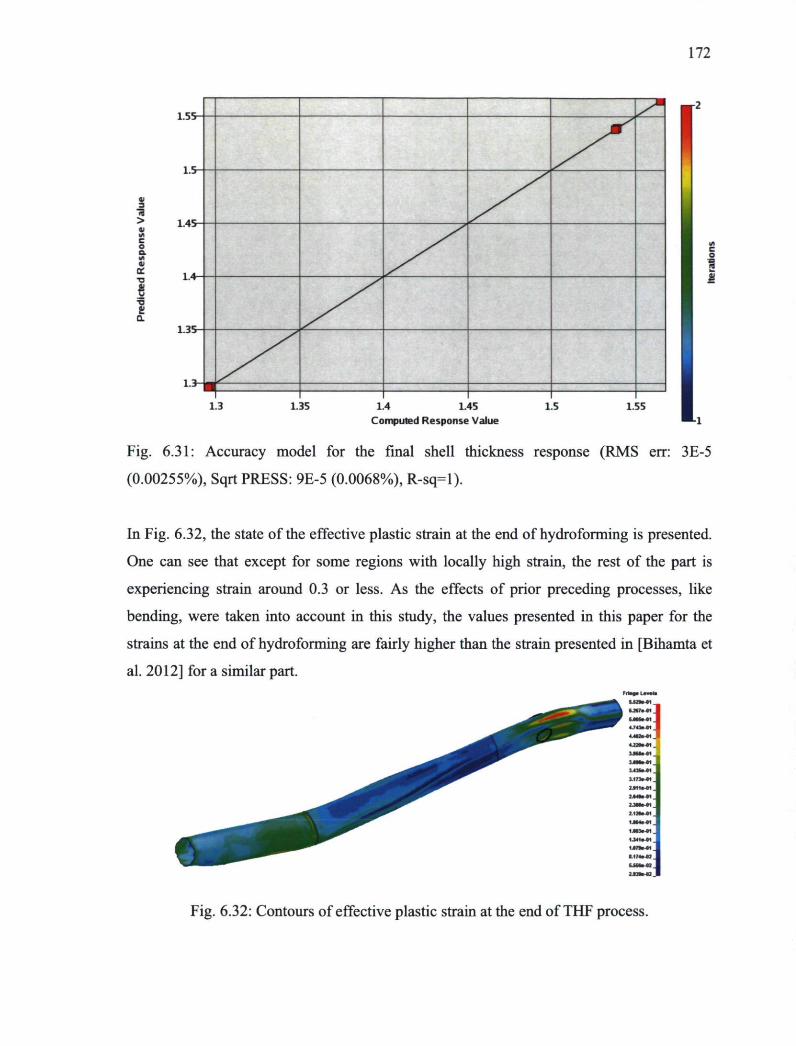
172

>

1.3-1.3-

1.3 1.35 1.4 1.45 Computed Response Value

1.5 1.55

c o

I I

Fig. 6.31: Accuracy model for the final shell thickness response (RMS err: 3E-5

(0.00255%), Sqrt PRESS: 9E-5 (0.0068%), R-sq=l).

In Fig. 6.32, the state of the effective plastic strain at the end of hydroforming is presented.

One can see that except for some regions with locally high strain, the rest of the part is

experiencing strain around 0.3 or less. As the effects of prior preceding processes, like

bending, were taken into account in this study, the values presented in this paper for the

strains at the end of hydroforming are fairly higher than the strain presented in [Bihamta et

al. 2012] for a similar part.

Fig. 6.32: Contours of effective plastic strain at the end of THF process.

173

6.6. Conclusion

In this study, some numerical and experimental studies were performed on the THF process

taking into account the effects of preceding processes. The preceding processes that were

studied besides THF were variable thickness tube drawing, annealing heat treatment, and

bending. The important results of this paper can be summarized as follows:

a) In variable thickness tube drawing, the synchronization between two-step drawing is an

important parameter and can lead to tube failure if it is not performed well.

b) In the case that precise synchronization between two steps of variable thickness tube

drawing is not possible, the best alternative is to replace sharp transition of thickness

with mild ones to reduce the risk of rupture due to inaccurate synchronization.

c) Rotary-draw tube bending can lead to considerable variation in the thickness of tubes;

ignorance of this fact can lead to unsuccessful hydroforming.

d) Geometrically complex tubes have some bent regions. These zones cannot get enough

material by the axial displacement of the pushers, therefore the third parameter, i.e.

initial tube thickness, can play a role in successful hydroforming of these parts.

e) The customized sealing method that was presented for the first time in this paper takes

advantages of both local deformation and O-ring methods for sealing of tubes.

f) In the dies with three parts, the cycle of approaching of dies is a very important factor

in appropriate preforming of the tube.

g) The loading path from numerical optimisation showed excellent agreement with the

experiments in the final hydroforming.

Acknowledgements

The authors thank the Natural Sciences and Engineering Research Council of Canada,

National Research Council Canada-Aluminium Technology Centre, Alfiniti, Aluminerie

Alouette, C.R.O.I and Cycles Devinci for their financial and technical support of this

research. A part of the presented research in this paper was financed by the Fonds

Québécois de la Recherche sur la Nature et les Technologies (FQRNT) by the intermediary

of the Aluminium Research Centre-REGAL.

174

References

[I] Abedrabboa N., Worswicka M., Mayer R., Riemsdijk I.V., 2009 "Optimization methods for the tube hydroforming process applied to advanced high-strength steels with experimental verification, Journal of Materials Processing Technology (209) pp: 110-123. [2] Bihamta R., Bui Q. H, Guillot M., D'Amours G, Rahem A., Fafard M., 2011 "A new method for production of variable thickness aluminium tubes: numerical and experimental studies", Journal of Materials Processing Technology (211) pp: 578-589. [3] Bihamta R., D'Amours G., Bui H., Rahem A., Guillot M., Fafard M., 2010 "Optimization on the Production of Aluminium Variable Thickness Tube Drawing Process", ASME2010, Erie, Pennsylvania, USA. [4] Bihamta R., D'Amours G., Rahem A., Guillot M., Fafard M., 2010 "Numerical studies on the production of variable thickness aluminium tubes for transportation purposes", SAE 2010 world congress, Detroit, MI, USA. [5] Bihamta R., D'Amours G., Bui Q-H., Rahem A., Fafard M. 2011 "Numerical study on the new design concept of hydroforming dies for the complex tubes" to be submitted to computational materials science. [6] Bihamta R., 2011 "Optimization of hydroforming process of geometrically complex aluminium tubes taking account of preceding forming processes" PhD dissertation, Laval University, Quebec city, Canada. [7] Bui Q. H., Bihamta R., Guillot M., D'Amours G, Rahem A., Fafard M., 2011 "Investigation of the formability limit of aluminium tubes drawn with variable wall thickness", Journal of Materials Processing Technology, Volume (211) pp: 402-414. [8] Bui Q. H., Bihamta R., Guillot M., Rahem A., Fafard M., 2011 "Effect of cross section reduction on the mechanical properties of variable thickness drawing of aluminium tubes" Journal of Manufacturing Science and Engineering, Vol. 133(5), Under press. [9] Cheng D.M., Teng B.G., Guo B., Yuan S.J., 2009 "Thickness distribution of a hydroformed Y-shape tube", Materials Science and Engineering A, (499) pp: 36-39. [10] Filion G. 2011 "Virtual and experimental fabrication of complex geometry aluminium tubes by hydroforming method" MSc. Thesis, Laval University, 2011 (In French). [II] Hashemi R., Assempour A., Masoumi K. E., 2009 "Implementation of the forming limit stress diagram to obtain suitable load path in tube hydroforming considering M-K model", Materials and Design (30) pp:3545-3553. [12] D'Amours G., Rahem A., Williams D., Worswick M., Mayer R., 2007 "Crashworthiness of aluminium tubes; Parti: hydroforming at different corner-fill radii and end feeding levels", materials processing and Design: Modeling, Simulation and applications conference NUMIFORM 2007. [13] Guillot M., Fafard, M., Girard, S., Rahem, A., D'Amours G., 2010 "Experimental Exploration of the Aluminum Tube Drawing Process for Producing Variable Wall Thickness Components used in Light Structural Applications", SAE 2010 world congress, Detroit, MI, USA. [14] Hwang Y.-M., Altan T. 2003, "Finite element analysis of tube hydroforming processes in a rectangular die", Finite Elements in Analysis and Design (39), pp: 1071-1082. [15] http://www.vari-form.com. [ 16] http://www.copper.org/applications/cuni/app_syscomp.html

175

[17] Kang S.J., Kim H. K., Kang B. S., 2005 "Tube size effect on hydroforming formability", Journal of Materials Processing Technology (160) pp: 24-33. [18] Koç M., Altan T., 2001 "An overall review of the tube hydroforming (THF) technology", Journal of Materials Processing Technology, (108), pp: 384-393. [19] Koç M., 2004 "Advances in Tube Hydroforming- An Enabling Technology for Low-Mass Vehicle Manufacturing-Material, Lubrication, Loading, Simulation Issues, and Alternatives", Tsinghua Science and Technology, (9) pp: 527-545. [20] Korkolis I., 2009 "Formability and hydroforming of anisotropic aluminum tubes", PhD dissertation, The University of Texas at Austin. [21] Korkolis Y.P., Kyriakides S., 2009 "Path-dependent failure of inflated aluminium tubes", International Journal of Plasticity, (25) 2059-2080. [22] Myers R.H., Montgomery D.C, 2002 "Response Surface Methodology". Second edition, John Wiley & Sons, New York. [23] Song W.-J., ChanHeo S., WanKu T., Kim J., Kang B.-S., 2010 "Evaluation of effect of flow stress characteristics of tubular material on forming limit in tube hydroforming process", International Journal of Machine Tools & Manufacture (50) pp: 753-764. [24] Stander N , Roux W., Goel T., Eggleston T., Craig K, 2009 "A design optimization and probabilistic analysis tool for the engineering analyst" LS-OPT® User's Manual, Livermore Software Technology Corporation. [25] Trana K, 2002 "Finite element simulation of the tube hydroforming process- bending, preforming and hydroforming", Journal of Materials Processing Technology (127) pp: 401-408. [26] Williams B.W., Worswick M.J., D'Amours G., Rahem A., Mayer R., 2010 "Influence of forming effects on the axial crush response of hydroformed aluminum alloy tubes", International Journal of Impact Engineering (37) pp: 1008-1020. [27] Xu X., Zhang W., Li S., Lin Z., 2009 "Study of tube hydroforming in a trapezoid-sectional die" Thin-Walled Structures, (47) pp: 1397-1403. [28] Xu X., Li S., Zhang W., Lin Z., 2009 "Analysis of thickness distribution of square-sectional hydroformed parts", Journal of Materials Processing Technology (209) pp:158-164.

Chapter 7

Conclusion and Recommendations

7.1. Conclusion

The main objective of this project was to develop numerical and experimental methods

required for the production of geometrically complex tubes for the transportation industry.

Because of the geometric complexity of these parts, it is usually required to use methods

like tube hydroforming for their production. As there are various parameters to be changed

to reach an optimum process, manual optimisation of the process without a special

algorithm to change the variables seems difficult.

In this thesis, the variable thickness tube drawing process as a necessary preceding process

for tube hydroforming was studied to optimize the geometry of initial tubes to produce the

required minimum and maximum thickness for the project case study (see chapter 3). The

geometries of die and mandrel were optimized to produce the minimum possible thickness

in this process (see chapter 4). It was found that the present die design in tube

hydroforming is not efficient for most complex geometry parts. Therefore, a new concept

for the design of the hydroforming dies was presented and verified by experiments (see

chapter 5). Finally, in the developed optimisation loop, the hydroforming process and

177

preceding processes like tube bending and tube drawing were optimized, and the results

showed excellent agreement with the experiments (see chapter 6). The general conclusions

can be drawn as follows:

7.1.1. Variable thickness tube drawing

Variable thickness tube drawing is an essential element in the production of light-weight

complex workpieces; considerable weight reduction can be achieved by their application.

However, as explained in detail in the dissertation text, this type of tube has some

limitations that hinder their applications.

7.1.2. Tube bending process

The tube bending process is one of the crucial preceding processes in a production cycle of

complex tubes in which successful hydroforming without an appropriate bending is

impossible. The outer radius of the bent region always exhibits considerable thickness

reduction, the ignorance of which can lead to misleading results at the end of the

hydroforming process.

7.1.3. Tube hydroforming

A successful hydroforming without considering the effect of preceding processes is not

possible. Also, for the majority of complex geometry tubes, the proposed design concept in

this thesis is essential.

7.2. Future work and recommendations

The following points show possible future development from this dissertation:

1. Due to the widespread application of rectangular tubes in the structures of vehicles,

the development of variable thickness tube technology to rectangular section tubes

seems necessary.

178

2. Development of variable thickness tubes in the circumferential direction can be

helpful to compensate for the thickness reduction in the bending operation.

3. Development of precise material models to predict material properties after

recovery heat treatments while taking into account tube deformation historyand heat

treatment condition.

4. Development of an automatic method to design THF dies. This method can start

from the final geometry of the tube and result in the complete design of the THF

die.

5. Implementation of more variables like thickness of more regions, or location of

thickness change, in the optimisation process to obtain lighter parts.

6. Development of a global optimisation method that takes into account the design and

manufacturing of parts together.

Appendices

180

Appendix A) Thickness Applier Code (TAC)

Thickness Applier Code (TAC) was developed in MATLAB to apply variation of wall

thickness along the tube. Based on the assigned thickness by the optimisation loop, in

various regions of the shell tube, different thicknesses are applied. This program is applied

as a user definedpre-processor in the optimisation procedure.

The code algorithm reads the assigned thickness from Xpoint file of Ls-Opt optimisation

software and based on the location of element and its nodes, determines the value of the

thickness for each node. In the case that element is located in the zone with constant

thickness (for example zone 1 in Fig. Al), all nodes of those elements have the same

thickness value or else each element will have different thickness value like in the transient

zone 2 in Fig. Al.

After calculating the appropriate thickness of each node, TAC completes the shell elements

card in the order presented in table Al. Note that the format required by the finite element

software, such as space between each number, must be respected.

a)

1 7 I 1 X W .

171 Je .«0

1.I44M4».

1.C7*^«0.

b)

Fig. Al: a) Shaded view of a tube after application of thickness variation b) position of and

thickness value for each element.

181

Table Al: Shell element card and required fields [1]

Cardl 1 2 3 4 5 6 7 8 9

In table Al the definition of variables are as follows:

EID: Element ID (should be unique) PID: part ID. Nl: Nodal point 1 N2: Nodal point 2 N3: Nodal point 3 N4: Nodal point 4 N5-8: Mid side nodes for eight node shell (in the TAC code this field left blank)

Table A2: Other options of the shell element to be completed by the program Card 1 2 3 4 5 6 7 8 9

10

Variable EID PID Nl N2 N3 N4 N5 N6 N7 N8

Type I I I I I I I I I I

Default noue none none none none none 0 0 0 0

Remarks 3 3 3 3

10

Variable THIC1 THIC2 THIC3 THIC4 BETA or MOD

Type F F F F F

Default 0. 0. 0. 0. 0.

Remarks 1 2

THIC1: Shell thickness at Node 1 THIC2: Shell thickness at Node 2 THIC3: Shell thickness at Node 3 THIC4: Shell thickness at Node 4

BETA: Orthotropic material base offset angle (should not be changed) MCID: Material coordinate system ID (should not be changed).

182

Text of TAC program %This program is written based on the part which meshed in the Hypermesh %and in the case of other softwares you should make attention to do Inecessary adjustments. %The purpose of this program is to creat variation of thickness in the shell elements %Reza BIHAMTA, PhD student, Laval University

%When using this program be carfull that your numbering for the nodes and %elements will start from 1 and nodes has just 3 column for the 3x y and z % coordinates clc clear all format long Entryl='XPoint.k'; fidl=fopen(Entryl, 'r ' ) ; Var=fscanf (fidl, '°ôf %f %f %f %f %f %f %f %f',[9,inf]); fclose(fidl);

Entry='tube_shell.k'; % Exit='tube_shell_th.k'; fid=fopen(Entry, 'r'); for i=l:5

rien=fgetl(fid); end Nodes2=fscanf(fid, *%i %f %f %f', [4,inf]); Nodes=Nodes2' ; rien=fgetl(fid);

Elements=fscanf(fid,'%i %i %i %i %i %i',[6,inf]); rien=fgetl(fid); fclose(fid);

Ll=196.76; %Length of places with 2.74mm thickness L2=85; %Length of places from 2.74mm to 1.59mm thickness L3=132.99; %Length of places with 1.59mm thickness L4=60; %Length of places with 1.59mm to 1.37 thickness L5=180; %Length of places with 1.37 thickness L6=90; %Length of places with 1.37mm to 2.23 thickness L7=270.95; %Length of places with 2.23 thickness

thl_l=Var(1);%2.7 4; %Thickness of first region of tube thl_2=Var(1);%2.74; %Thickness in the end of first region if it is same as thl it means that there is not any variation in this region dthl=thl_2-thl_l; th2_l=Var(1);%2.74 ; %thickness of the second region of tube th2_2=Var(2);%1.59; dth2=th2_2-th2_l; th3_l=Var(2);%1.59 th3_2=Var(2);%1.59 dth3=th3 2-th3 1;

183

th4_l=Var(2) ;%1.59 th4_2=Var(3) ;%1.37 dth4=th4_2-th4_l; th5_l=Var(3);%1.37 th5_2=Var(3) ;%1.37 dth5=th5_2-th5_l; th6_l=Var(3);%1.37 th6_2=Var(4) ;%2.23 dth6=th6_2-th6_l; th7_l=Var(4);%2.23 th7_2=Var(4) ;%2.23 dth7=th3_2-th3_l; A=sort(Nodes(:,3), 'descend'); % AL=length(A); %yl=max(A)-Ll; yl=max(Nodes(:,3))-Ll; AS=yl*ones(length(A) , 1); % clc WA=zeros(length(A),1); for i=l:(length(A))

Z(i)=Nodes(i,3)-AS(i); %% I am checking the difference between the Y of various points to find the point where the diference is zero or a small number

if -2<Z (i) && 2>Z (i)

WA(i)=Z(i); if Z (i)==0

S=0; KK=i;

else KK=0 ;

end end

end D=max(WA); E=min(WA); S=0; if sign(E)~=0

S=E;

end

if S~=0 for k=l:length(A)

Z(k)=Nodes(k,3)-AS(k) ; end

end

for k=l:length(A) Z(k)=Nodes(k,3)-AS(k) ;

end ZXl=min(abs(Z));

184

for k=l:length(A)

if ZXl==min(abs(Z(k) ) ) KK=k;

end end Q=fix(100*Nodes(KK,3)); Nodes_100=fix(100*Nodes); R=zeros(AL,1);

for j=l:AL

if Nodes_100(j,3)==Q R(j,D=j;

end end for L=1:AL

if R(L)==max(R) UU=L;

end end SLOPl=dthl/((Nodes(UU,3)-max(Nodes(:, 3) ) ) ) ; ES=length(Elements) ; ELTR=Elements' ; th=zeros(length(Nodes),1); for i=l:ES

if Nodes(ELTR(i,3),3)>=Nodes(KK,3) th(ELTR(i,3))=thl_l+SLOPl*(Nodes(ELTR(i,3),3)-Nodes(KK,3));

end if Nodes(ELTR(i,4) , 3)>=Nodes(KK, 3)

th(ELTR(i,4))=thl_l+SLOPl*(Nodes(ELTR(i,4),3)-Nodes(KK, 3));

end if Nodes(ELTR(i,5),3)>=Nodes(KK, 3)

th(ELTR(i,5))=thl_l+SLOPl*(Nodes(ELTR(i, 5) , 3)-Nodes(KK, 3)) ; end if Nodes(ELTR(i, 6) , 3)>=Nodes(KK, 3)

th(ELTR(i,6))=thl_l+SLOPl*(Nodes(ELTR(i,6),3)-Nodes(KK, 3)); end

end

9- * * * * * * * * * * * * * * * * * * * * * * * * * * * * * * * * * * * * * * Q. * * * * * * * * * * * * * * * * * * * * * * * * * * * * * * * * * * * * * * o y2=max(Nodes(:,3))-(L2+L1); AS2=y2*ones(length(A) ,1) ; WA2=zeros(length(A) , 1) ; for i=l:(length(A))

Z(i)=Nodes(i,3)-AS2(i); % I am checking the difference between the Y of various points to find the point where the diference is zero or a small number

% D(i)=A(i)-Z(i); if -2<Z(i) && 2>Z(i)

% if

185

%disp('test2'); WA2(i)=Z(i); if Z(i)==0

S=0; KK2=i;

else KK2=0;

end

end end D=max(WA2) ; E=min(WA2) ; if sign(E)~=0 'I Don't forget maybe some generalization will be necessary!

S=E; end %if S~=0 for k=l: length(A)

Z (k)=Nodes(k,3)-AS2(k);

end ZX=min(abs (Z)); for k=l:length(A)

if ZX==min(abs(Z(k))) KK2=k;

end end

Q=fix(100*Nodes(KK2,3)); Nodes_100=fix(100*Nodes) ; R=zeros(AL,1); for j=l:AL

if Nodes_100(j,3)==Q R(j.D=j;

end end for L=1:AL

if R(L)==max(R) UU2=L;

end end

SLOP2=dth2/((Nodes(UU2,3)-Nodes(KK,3))); ES=length(Elements) ; ELTR=Elements ' ; for i=l:ES

if Nodes(ELTR(i,3),3)>=Nodes(KK2,3) && Nodes(ELTR(i,3),3)<Nodes(KK,3) th(ELTR(i,3))=thl_2+SLOP2*(Nodes(ELTR(i,3) , 3)-Nodes(KK, 3)) ;

end if Nodes(ELTR(i,4),3)>=Nodes(KK2,3) && Nodes(ELTR(i,4),3)<Nodes(KK,3)

th(ELTR(i,4))=thl_2+SLOP2*(Nodes(ELTR(i,4),3)-Nodes(KK,3)); %-Nodes(KK,3));

%disp('test2_3')

186

end if Nodes (ELTR (i, 5) , 3) >=Nodes (KK2, 3) && Nodes (ELTR (i, 5) , 3) <Nodes (KK, 3)

th(ELTR(i,5))=thl_2+SLOP2*(Nodes(ELTR(i,5),3)-Nodes(KK,3)); %-Nodes(KK,3));

end if Nodes(ELTR(i,6),3)>=Nodes(KK2,3) && Nodes(ELTR(i,6),3)<Nodes(KK,3)

th(ELTR(i,6))=thl_2+SLOP2*(Nodes(ELTR(i,6) , 3)-Nodes(KK,3)); %-Nodes(KK,3));

end end 'V * * * * * * * * * * * * * * * * * * * * * * * * * * * * * * * * * * * * * * * * * * * * * * * * * * * * * * * * * * * * * * * * * * * * * * * * o ** û k *

y3=max(Nodes(:,3))-(L3+L2+L1) ; AS3=y3*ones(length(A) ,1); WA3=zeros(length (A), 1 ) ; for i=l:(length(A))

Z(i)=Nodes(i,3)-AS3(i); % I am checking the difference between the Y of various points to find the point where the diference is zero or a small number

end

ZX3=min(abs(Z)); for k=l:length(A)

if ZX3==min(abs(Z(k))) KK3=k;

end end

D=max(WA3); E=min(WA3);

Q=fix(100*Nodes(KK3,3)); Nodes_100=fix(100*Nodes); R=zeros(AL,1); for j=l:AL

if Nodes_100(j,3)==Q R(j,l)=j;

end end for L=1:AL

if R(L)==max(R) UU3=L;

end end

SLOP3=dth3/((Nodes(UU3, 3)-Nodes(KK2, 3))) ; ES=length(Elements) ; ELTR=Elements' ; for i=l:ES

if Nodes(ELTR(i,3),3)>=Nodes(KK3,3) && Nodes(ELTR(i,3),3)<Nodes(KK2,3)

th(ELTR(i,3))=th3 1+SL0P3*(Nodes(ELTR(i,3),3)-Nodes(KK2,3));

187

end if Nodes(ELTR(i,4),3)>=Nodes(KK3,3) &&

Nodes(ELTR(i, 4),3)<Nodes(KK2,3) th(ELTR(i,4))=th3_l+SLOP3*(Nodes(ELTR(i,4),3)-Nodes(KK2,3));

end if Nodes(ELTR(i,5),3)>=Nodes(KK3,3) &&

Nodes(ELTR(i,5),3)<Nodes(KK2,3) th(ELTR(i,5))=th3_l+SLOP3*(Nodes(ELTR(i,5),3)-Nodes(KK2,3));

end if Nodes(ELTR(i,6),3)>=Nodes(KK3, 3) &&

Nodes(ELTR(i,6),3)<Nodes(KK2, 3) th(ELTR(i,6))=th3_l+SLOP3*(Nodes(ELTR(i,6),3)-Nodes(KK2,3));

end end

y4=max(Nodes(:,3))-(L4+L3+L2+L1) ; AS4=y4*ones(length(A),1); WA4=zeros(length(A),1); for i=l:(length(A))

Z(i)=Nodes(i,3)-AS4(i); % I am checking the difference between the Y of various points to find the point where the diference is zero or a small number

% D(i)=A(i)-Z(i) ; end

ZX4=min(abs(Z)); for k=l:length(A)

if ZX4==min(abs(Z(k))) KK4=k;

end end

D=max(WA4); E=min(WA4);

Q=fix(100*Nodes(KK4,3)); Nodes_100=fix(100*Nodes); R=zeros(AL,1); for j=l:AL

if Nodes_100(j,3)==Q R(j,D=j;

end end for L=1:AL

if R(L)==max(R) UU4=L;

end end

SLOP4=dth4/((Nodes(UU4,3)-Nodes(KK3,3)));

188

ES=length(Elements) ; ELTR=Elements' ; for i=l:ES

if Nodes(ELTR(i, 3),3)>=Nodes(KK4,3) && Nodes(ELTR(i,3),3)<Nodes(KK3,3)

th(ELTR(i,3))=th4_l+SLOP4*(Nodes(ELTR(i,3),3)-Nodes(KK3,3)); % disp('test3');

end if Nodes(ELTR(i, 4),3)>=Nodes(KK4,3) &&

Nodes(ELTR(i,4),3)<Nodes(KK3,3) th(ELTR(i,4))=th4_l+SLOP4*(Nodes(ELTR(i,4),3)-Nodes(KK3,3));

end if Nodes(ELTR(i,5) ,3)>=Nodes(KK4,3) &&

Nodes(ELTR(i,5) ,3)<Nodes(KK3,3) th(ELTR(i,5))=th4_l + SLOP4*(Nodes(ELTR(i,5),3)-Nodes(KK3, 3));

end if Nodes(ELTR(i,6),3)>=Nodes(KK4,3) &&

Nodes(ELTR(i,6),3)<Nodes(KK3,3) th(ELTR(i,6))=th4_l+SLOP4*(Nodes(ELTR(i,6) ,3)-Nodes(KK3, 3)) ;

end end

y5=max(Nodes(:,3))-(L5+L4+L3+L2+L1); AS5=y5*ones(length(A) , 1) ; WA5=zeros(length(A),1); for i=l:(length(A))

Z (i)=Nodes(i,3)-AS5(i); % I am checking the difference between the Y of various points to find the point where the diference is zero or a small number end

ZX5=min(abs (Z)); for k=l:length(A)

if ZX5==min(abs(Z(k))) KK5=k;

end end

D=max(WA5); E=min(WA5);

Q=fix(100*Nodes(KK5,3)); Nodes_100=fix(100*Nodes); R=zeros(AL,1); for j=l:AL

if Nodes_100(j,3)==Q R(jfl)-j;

end end for L=1:AL

if R(L)==max(R) UU5=L;

189

end end

SLOP5=dth5/((Nodes(UU5,3)-Nodes(KK4,3))); ES=length(Elements); ELTR=Elements'; for i=l:ES

if Nodes(ELTR(i,3),3)>=Nodes(KK5,3) && Nodes(ELTR(i,3),3)<Nodes(KK4,3)

th(ELTR(i,3))=th5_l+SLOP5*(Nodes(ELTR(i,3),3)-Nodes(KK4,3));

end if Nodes(ELTR(i,4),3)>=Nodes(KK5,3) &&

Nodes(ELTR(i,4),3)<Nodes(KK4,3) th(ELTR(i,4))=th5_l+SLOP5*(Nodes(ELTR(i,4),3)-Nodes(KK4,3));

end if Nodes(ELTR(i,5),3)>=Nodes(KK5,3) &&

Nodes(ELTR(i,5),3)<Nodes(KK4,3) th(ELTR(i,5))=th5_l+SLOP5*(Nodes(ELTR(i,5),3)-Nodes(KK4,3));

end if Nodes(ELTR(i,6),3)>=Nodes(KK5,3) &&

Nodes(ELTR(i,6),3)<Nodes(KK4,3) th(ELTR(i,6))=th5_l+SLOP5*(Nodes(ELTR(i,6),3)-Nodes(KK4, 3));

end end

y6=max(Nodes(:,3))-(L6+L5+L4+L3+L2+L1) ; AS6=y6*ones(length(A) , 1) ; WA6=zeros(length(A),1); for i=l:(length(A))

Z(i)=Nodes(i,3)-AS6(i); % I am checking the difference between the Y of various points to find the point where the diference is zero or a small number end

ZX6=min(abs (Z)); for k=l:length(A)

if ZX6==min(abs(Z(k))) KK6=k;

end end

D=max(WA6); E=min(WA6);

Q=fix(100*Nodes(KK6,3)) ; Nodes_100=fix(100*Nodes); R=zeros(AL,1); for j=l:AL

if Nodes_100(j,3)==Q R(j,D=j;

190

end end for L=1:AL

if R(L)==max(R) UU6=L;

end end

SLOP6=dth6/((Nodes(UU6,3)-Nodes(KK5,3))); ES=length(Elements); ELTR=Elements'; for i=l:ES

if Nodes(ELTR(i,3),3)>=Nodes(KK6,3) && Nodes(ELTR(i,3),3)<Nodes(KK5,3)

th(ELTR(i,3))=th6_l+SLOP6*(Nodes(ELTR(i,3),3)-Nodes(KK5,3)); end if Nodes(ELTR(i,4),3)>=Nodes(KK6,3) &&

Nodes(ELTR(i,4),3)<Nodes(KK5,3) th(ELTR(i,4))=th6_l+SLOP6*(Nodes(ELTR(i,4),3)-Nodes(KK5,3));

end if Nodes(ELTR(i,5),3)>=Nodes(KK6,3) &&

Nodes(ELTR(i,5),3)<Nodes(KK5,3) th(ELTR(i,5))=th6_l+SLOP6*(Nodes(ELTR(i,5),3)-Nodes(KK5,3));

end if Nodes(ELTR(i,6),3)>=Nodes(KK6,3) &&

Nodes(ELTR(i,6),3)<Nodes(KK5,3) th(ELTR(i,6))=th6_l+SLOP6*(Nodes(ELTR(i,6),3)-Nodes(KK5,3));

end end

O

y7=max(Nodes(:,3))-(L7+L6+L5+L4+L3+L2+L1); AS7=y7*ones(length(A),1); WA7=zeros(length(A),1); for i=l:(length(A))

Z(i)=Nodes(i,3)-AS7(i); % I am checking the difference between the Y of various points to find the point where the diference is zero or a small number end

ZX7=min(abs(Z)); for k=l:length(A)

if ZX7==min(abs(Z(k))) KK7=k;

end end

D=max(WA7); E=min(WA7);

Q=fix(100*Nodes(KK7,3)); Nodes_100=fix(100*Nodes); R=zeros(AL,1); for j=l:AL

if Nodes 100(j,3)==Q

191

R(j.D=j; end

end for L=1:AL

if R(L)==max(R) UU7=L;

end end

SLOP7=dth7/((Nodes(UU7, 3)-Nodes(KK6,3))); ES=length(Elements); ELTR=Elements'; for i=l:ES

if Nodes(ELTR(i,3),3)>=Nodes(KK7,3) && Nodes(ELTR(i,3),3)<Nodes(KK6,3)

th(ELTR(i,3))=th7_l+SLOP7*(Nodes(ELTR(i, 3),3)-Nodes(KK6,3)); end i f N o d e s ( E L T R ( i , 4 ) , 3 ) > = N o d e s ( K K 7 , 3 ) &&

N o d e s ( E L T R ( i , 4 ) , 3 ) < N o d e s ( K K 6 , 3 ) t h ( E L T R ( i , 4 ) ) = t h 7 _ l + S L O P 7 * ( N o d e s ( E L T R ( i , 4 ) , 3 ) - N o d e s ( K K 6 , 3 ) ) ;

e n d i f N o d e s ( E L T R ( i , 5 ) , 3 ) > = N o d e s ( K K 7 , 3 ) &&

N o d e s ( E L T R ( i , 5 ) , 3 ) < N o d e s ( K K 6 , 3 ) t h ( E L T R ( i , 5 ) ) = t h 7 _ l + S L O P 7 * ( N o d e s ( E L T R ( i , 5 ) , 3 ) - N o d e s ( K K 6 , 3 ) ) ;

e n d if Nodes(ELTR(i,6),3)>=Nodes(KK7,3) &&

Nodes(ELTR(i,6),3)<Nodes(KK6,3) th(ELTR(i,6))=th7_l+SLOP7*(Nodes(ELTR(i, 6) ,3)-Nodes(KK6,3)) ;

end end

o

fid=fopen(Exit,'w'); fprintf(fid,'%s\n','^KEYWORD'); fprintf(fid,'%s\n','*NODE');

for i = 1 : length(Nodes)

fprintf(fid, '%8i',Nodes (i,1)); fprintf(fid,'%16.7g',Nodes(i,2)); fprintf(fid,'%16.7g',Nodes(i,3)); fprintf(fid,'%16.7g\n',Nodes(i,4));

end fprintf(fid,'%s\n','*ELEMENT_SHELL_THICKNESS'); for i=l: length(Elements)

fprintf(fid, '%8i',ELTR (i,1)); fprintf(fid,'%8i',1);

for j=3:6 fprintf(fid,'%8i',ELTR(i,j));

end for j=7:10

fprintf(fid,'%8i',0) ;

192

end fprintf(fid, '\n',''); for j=3:6

fprintf(fid,'%16.3E',th(ELTR(i,j))); end

fprintf(fid,'\n','');

end

fprintf(fid,'%s','*END'); fclose(fid);

193

Appendix B Geometry Updating Code (GUC)

When studying tube drawing, to optimize geometries of the die, mandrel, and tube, it is

necessary to have a code to update their geometries based on the optimisation loop

decision. The geometric parameters that are changed by the program are die angle, die fillet

radius, and mandrel angle, and in the case of optimizing the tube geometry, tube initial

outer diameter and wall thickness.

Like TAC, GUC reads the optimisation variables from an XPoint file, then starts from a

reference point and generates the new meshes based on the new geometric variables. This

program also updates the following items:

1) Updating mandrel boundary conditions: when the mandrel angle changes, the amount

of axial movement should be updated in the mandrel boundary conditions to have

constant final thickness in the tube. Based on the new mandrel and die angles, the new

displacement is calculated and applied in the mandrel boundary conditions.

2) Re-positioning the tube: when the tube outer diameter changes, its position should be

modified to avoid geometrical conflict with the die.

3) Updating tube boundary conditions: when geometry or equivalently tube meshes change,

the applied boundary conditions for tube motion should be updated based on the new node

IDs. The program detects these changes and creates modified .k file(s).

194

Appendix C Shape Variable Manager (SVM) and post-processor codes

A frequent problem when using commercial optimisation software is using the results from

a simulation that the solver announces as a normally terminated job but in reality the shape

of the deformed part is not acceptable; the result of such a simulation should not be used in

composing response surfaces. Fig. CI shows one example of a solution where Ls-Dyna

solver announced a "Normal termination" but the result is not acceptable at all. To solve

this problem, the geometry of the drawn tube before response extraction is checked with a

MATLAB code, and if it is acceptable a number, for example 1, is assigned to a dummy

response; otherwise, the output file of this response is excluded from being used by the

optimisation engine.

Fig.Cl) An example of an unacceptable tube shape (green) in some simulations.

Besides the codes that are necessary to control pre-processing of the optimisation

processes, it is necessary to have some post-processor codes to verify the results of the

simulation and part shape. These codes also calculate some parameters like minimum and

maximum thicknesses, and average stress in a special section by determining the area of an

appropriate section and correspondent force. As in the optimisation program, it is possible

to call only one program as optimisation pre-processor and only one as post processor, thus

all the necessary programs for extracting the required results like maximum and minimum

thicknesses, area calculation in a specific zone, and finally calculation of average stress, are

merged in the following program.

195

It is worth mentioning that depending on the optimisation parameters and objectives,

sometimes calculation of all parameters is not necessary; they are presented here only to

give an idea of how to access to result files by user defined codes and make the necessary

calculations.

SVM code (ia MATLAB)

clc clear all format long Entry_file = 'dynain'; Entry_file2 = 'refore' %Exit_file = 'Outputl' Exit_file2 = 'Output2' Exit_file3 = 'Output3', E x i t _ f i l e 4 = ' O u t p u t 4 \ E x i t _ f i l e 5 = *Ou tpu t5 ' E x i t _ f i l e 6 = ' O u t p u t 6 \ E x i t _ f i l e 7 = ' 0 u t p u t 7 \ %Exit_file8 = 'TERMINATION_CARDS.k';

fid=fopen(Entry_file, 'r ' ) ; % This line opens the dynain file content

if fid == -1 % if for any reason like error in the simulation it is not %available if will return -1 and optimization engine will get error signal

!echo ' E r r o r t e r m i n a t i o n ' exit

end

for j=l:2 garbage=fgetl(fid); % Ususally two first line of the dynain files are

some ^comments and they are not required end

Boundary_nodes = fscanf(fid,'%i %i %i %i %i %i %i %i',[8,inf]);

garbage=fgetl(fid); % elimination of text in the middle of file

NODES = fscanf(fid,'%i %f %f %f %i %i',[6,inf]); % reading Nodes points

NODES = NODES';

junk=fgetl(fid);

p=0; for i=l:length(NODES)

A= NODES(:,2); end

for i=l:length(NODES)

196

if A(i)<=19.67 % by checking this coordinate if there is an inclination in % %the deformed tube like Fig.CI,

P=l; end

end

L=length(NODES); pl=NODES(l,l)+20; p2=pl+0.75*length(NODES); Dx=NODES (20,2)-NODES(20+0.75*length(NODES),2);

for i=l:L/4 dx=NODES(i,2)-NODES(0.75*L+i,2);

AB(i,l)=dx; end f=0; for i=25:L/4

f=f+l; AR_Nodes(f)=NODES(0.75*L+i,1 AR(f)=NODES(0.75*L+i,2);

end

A=min(AB); % calculation of minimum thickness of tube after deformation

%***********Paragraph for calculation of average stress******************

%In the following paragraph I am going to calculate the section area of %tube in the region with minimum area, for i=l:L/4

if A==AB(i) sss=i;

end end

Odl=2*NODES(sss,2); % THESE ARE THE DIAMETER OF TUBE IN THE REGION OF MINIMUM %THICKNESS Od2=2*NODES(0.75*L+sss,2);

fid=fopen(Exit_file2,'w'); %for the maximum thickness check

fprintf(fid,'%f',Dx); fclose(fid);

fid=fopen(Exit_file3, 'w') ;

fprintf(fid,'%f',A); fclose(fid);

9, *************** Extraction of reaction forces***********

% The reaction forces from deformation are calculated,

fid=fopen(Entry_file2, 'r') ;

197

for j=l:8 garbage=fgetl(fid);

end i=0; L=l; while (1)

i=i+l;

TEST1= fscanf(fid, '%s',3); if length (TEST1)==0

break; end Time(i)= fscanf(fid,'%f',1); junk2= fscanf(fid,'%s',3);

FORCEY(i)= fscanf(fid,'%f',1); TEST2= fscanf(fid,'%s',4);

end fclose(fid);

FORCEY=FORCEY'; Time=Time'; q=3;

k=lj for i=l: length(FORCEY)/4

%j=j+4; FORCE_Slave_l(k)=-2*pi*F0RCEY(j) ; F0RCE_Slave_4(k)=-2*pi*F0RCEY(q) ; k=k+l; j=j+4; q=q+4;

end

k=l; for i=l: length(Time)/4

%j=j+4; Time2(k)=Time(j); k=k+l; j=j+4;

end Time2=Time2'; FORCE_Slave_l=FORCE_Slave_l'; FORCE_Slave_4=FORCE_Slave_4'; DWG_Force=F0RCE_Slave_4+F0RCE_Slave_l;

4here I am calculating the total

tube drawing force av_area=0.25*pi*(Odl~2-Od2

A2);%Area of tube in the minimum thickness

region Sig_Axial_Avrage=DWG_Force/av_area; ■* the avrage axial stresswhic will be compared with axial stress from experiments

198

Sig_Ax_Max=max(Sig_Axial_Avrage); RCl=max(FORCE_Slave_l); RC4=max(FORCE_Slave_4); DWG F Max=max(DWG Force);

fid=fopen(Exit_file4,'w'); Ifor the Reaction of interface 1 (I multiplied it to %%%%%%%%%%%%%%%%%%%%%%%%%%%%2*pi too) fprintf (fid, ' %f \RC1) ; fclose(fid);

fid=fopen(Exit_file5,'w'); %for the Reaction of interface 4 (I multiplied it to 2*pi too) fprintf(fid,'%f',RC4); fclose(fid);

fid=fopen(Exit_file6,'w'); multiplied it to 2*pi too) fprintf(fid,'%f',DWG_F_Max); fclose(fid);

%for the total drawing force (I

fid=fopen(Exit_file7,'w'); multiplied it to 2*pi too) fprintf(fid,'%f',Sig_Ax_Max); fclose(fid);

sfor the total drawing force (I

exit % The exit command at the end of program is used to be sure that the %%%program will be terminated at the end and the licence no longer be occupied.

199

Appendix D Pre-processing command file

Automatic optimisation procedures make it necessary to link some programming software

(here MATLAB) with the optimisation programs to update the required geometries and/or

extract some results from simulation after each simulation point. Therefore it is necessary

to copy the programmed text inside the folder of each simulation point. Here are some

examples of command lines for this purpose.

A) cp /home/rbihamta/Etirage /Ml.m . B) cp /home/rbihamta/Etirage /yn . C) matlab -nodisplay -r Ml <yn

In line A, the optimisation program copies the Ml file (pre-processor file in MATLAB) to

the each simulation point folder. By putting the "." at the end of the line the destination

point will be exactly the folder of the simulation point.

In line B a file with the name yn containing the letter "y" is copied to the same folder as the

MATLAB file, because in the performance of the MATLAB program there is a warning

message that needs response of y (y: stands for yes) to proceed with running the program.

In the destination program, MATLAB will be run (without being displayed) to construct

the simulation file (in the case where the solver is Ls-Dyna, theses files will be .k files).

Post-processing command file

The post-processor file is supposed to be run immediately after the end of simulation

points, therefore its command can be written in the next lines after the solver running

command (here Ls-Dyna), or in a separate command file for the post processor. In this

example it is written in the same command file as follows:

A) /opt/LSTC/lsdyna i=DynaOpt.inp ncpu=l memory=400m B) cp/home/..../Dynain_Check.m . C) matlab -nodisplay -r Dynain_Check

In line A Ls-Dyna solver will run the simulation points that were already constructed by the

pre-processor codes by using 1 CPU and 400 MB memory. Then it will copy the

200

DynainCheck file to the folder that result of the simulation exists; finally it will perform

the DynainCheck program to check the result of simulations in the Dynain file of the Ls-

Dyna solver.

201

Appendix E File management in global optimisation of THF process

Multi-process optimisation studies include more than one process for optimisation like tube

bending, tube drawing, and tube hydroforming. The management of results between

various steps is an important task which should be programmed to enable the optimisation

loop to be performed automatically. In the tables El to E3, the required

translations/rotations to position the initial tube after application of variation of thickness to

the first bending step, the second bending step, and finally the tube hydroforming step are

presented.

Table El: Required translations (TR) and rotations (Rot) to position the tube after application of variation of thickness to the first bending step.

TR(Y) -50 TR(X) 0 TR(Z) 0

Rot (X) 0 Rot (Y) 0 Rot (Z) 0

Table E2: Required translations (TR) and rotations (Rot) to position the tube after the first bending in the second bending step.

Rot* (Y) 180° TR(Y) -392.94 TR(Z) 0 TR(X) 0 Rot (X) 0 Rot(Z) 0

*Origin of Rotation: 0,1223.95,0

Table E3: Required translations (TR) and rotations (Rot) to position the tube after the second bending in the THF step.

Rot (X) -90° Rot (Y) 90° Rot (Z) 180° TR(X) 440 TR(Y) 15.35 TR(Z) 6.5

202

Finding appropriate rotations and/or translations between processes is the first stage in

multi-step optimisations; the next is how to implement these parameters in the finite

element software automatically. To apply the transformations in Ls-Dyna software, the

following commands should be used:

*DEFINE_TRANSFORM: by this command, the appropriate rotation and/or translations

should be defined, then in the *Include command should be called.

*INCLUDE_TRANSFORM: in this command, the name of the file and transformation to

be used in inclusion of dynain file (result file of Ls-Dyna) in the next optimisation step

should be entered.

References 1) Ls-Dyna Keyword User Manual Volume 1 version 971 may 2007 pp: 14.44.