Optimal Unemployment Insurance andEmployment History

Hugo A. HopenhaynUniversidad Torcuato Di Tella and University of Rochester

Juan Pablo Nicolini∗, †

Universidad Torcuato Di Tella

September 29, 2005

Abstract

This paper considers the optimal design of unemployment insur-ance contracts in an environemnt in which workers experience mul-tiple unemployment spells. The environment is suited to study theoptimality of employment history related restrictions typically foundin existing unemployment insurance programs. We show that whenthe principal cannot distinguish quits from layoffs, optimality calls forcontracts with employment history contingent transfers. In particular,we show that the employment tax an employed worker pays decreasesand the unemployment benefit he is entitled to in case of unemploy-ment increases with job duration in the optimal contract. We showthat these properties hold both when workers have incentives to quitform good jobs and when they have incentives to take bad jobs.

Keywords: Unemployment insurance, optimal contract. JEL: I3, J2, J6.

∗Corresponding author. Miñones 2159, Capital Federal, (C1428ATG), Argentina.email: juanpa@utdt.edu.

†We thank Fernando Alvarez, Hal Cole, Narayana Kocherlacota, Victor Rios-Rull,two anonymous referees and seminar participants at CEMFI and Federal Resrve Bank ofMinneapolis for suggestions. All remaining erros are ours.

1

1 Introduction

Current unemployment insurance (UI) programs restrict coverage based onthe employment record of unemployed workers. For instance, in the UnitedStates, a minimum of six months of employment is needed to qualify for bene-fits, and coverage ratios increase with the length of previous jobs. In addition,some of these restrictions have a significant impact on equilibrium outcomes.Indeed, there is evidence that in Canada1, coincidental with the minimumrequirement number of periods - 12 months - to qualify for unemploymentbenefits, job termination rates double. The optimality properties of theseparameters of UI systems have been neglected in theoretical work on optimaldesign, which has focused on the simplified case of a single unemploymentspell2.This paper extends previous theoretical research, by considering theproblem of optimal unemployment insurance design in a model of multipleunemployment spells.We model unemployment insurance design as a repeated moral hazard

problem. In our model, the search effort of unemployed workers cannot beperfectly monitored by the enforcement agency. As a consequence, the insur-ance mechanism must trade-off incentives for job search with unemploymentduration risk. The unemployment insurance program specifies contingenttransfers from the enforcement agency to the worker as a function of currentand past employment/unemployment records. The optimal program is theone that minimizes the budget for a given ex-ante expected utility for theworker.As a first exploration, in Section 2, we assume that termination rates

are exogenous. We show that previous results for the case of a single unem-ployment spell have their analogues in our multiple spells case: transfers tounemployed workers decrease with the length of their unemployment spell,and reemployment taxes also increase with the length of the previous spells.Furthermore, these transfer schedules also decrease with previous unemploy-ment spells. The intuition for these results is simple. Since agents are riskaverse and value consumption smoothing, optimal incentives are provided byusing permanent and not temporary reductions in consumption. Hence, thelonger a worker is unemployed, the lower is his permanent consumption level.

1See Christofides and McKenna (1996) and Baker and Rea (1998).2See Baily (1978), Shavel and Weiss (1979) and Hopenhayn and Nicolini (1997). Ex-

ceptions that study on-the-job moral hazard problems are Wang and Williamson (1996),(2002) and Zhao (2000).

2

As job termination is exogenous, workers are insured completely againstjob loss. This property has two interesting implications. First, the opti-mal contract does not condition the transfers on the length of previous em-ployment spells, so this environment does not provide a rationale to theemployment history restrictions that motivates our analysis. Second, if anunemployed worker becomes employed and loses immediately this job, hisreplacement ratio is increased. This suggests the possibility of a loopholein the optimal contract, that can lead to opportunistic behavior. Indeed,anecdotal evidence in countries with generous unemployment insurance pro-grams, suggests that, as job termination is a way to upgrade benefits, the UIprogram may induce inefficient quits. Obviously, this opportunistic behaviorcan only arise if the principal cannot distinguish quits from layoffs.In the remaining section, the paper studies the design problem when quits

and layoffs cannot be perfectly monitored. We explore two ways in whichopportunistic workers may take advantage of the UI contract in this modifiedscenario.First, we consider the case where the disutility of working and the generos-

ity of unemployment insurance induce voluntary quits from socially efficientjobs. If the "no quit " constraint is not taken into account in the UI design,workers will look for jobs and once unemployed quit just to upgrade theirbenefits. When this constraint binds, it is optimal to condition the transferson the agent’s employment history. In particular we show that the tax work-ers pay while employed decreases with tenure while unemployment benefitsrise. These properties hold for the entire length of the employment spell.Second, we consider the case of job heterogeneity, where an added problem

arises: unemployed workers may take bad jobs -that they would never acceptin the absence of an unemployment insurance program- with the purpose ofsoon after quitting and requalifying for higher unemployment benefits. Ifthe quality of jobs accepted by workers cannot be perfectly monitored, suchbehavior can arise introducing an added adverse selection problem. Theoptimal unemployment insurance design in the presence of such adverse se-lection problem shares most of the qualitative properties of the contract inthe previous case, since employment taxes decrease and future unemploy-ment entitlements rise with employment tenure. Yet there is one qualitativedifference between the two cases: while in the first scenario the monotonic-ity properties hold for the entire employment spell, in the latter case theyhold only for a finite period of time. From there on, both the employmenttax and the future entitlement become constant. The explanation for this

3

results is quite intuitive. The opportunistic strategy of taking a bad joband soon quitting to upgrade benefits is more costly the longer the workerremains in that job. As a consequence, the adverse selection constraint isrelaxed with job tenure and ceases to bind after a finite number of periods.As this constraint is relaxed, workers with longer tenure can be providedbetter insurance against job loss.The main contribution of the paper is to consider incentives and UI de-

sign in the presence of repeated unemployment spells. Three recent papers,Wang and Williamson (1996) and (2002) and Zhao (2000)) also derive anoptimal contract that exhibits employment dependence. These papers dif-fer from ours, in that they introduce a moral hazard problem for employedworkers3. Even though the incentive problem we study - opportunistic quits- is of very different nature, their results are closely related to our first sce-nario, when the no quit constraint binds. The work of Wang and Williamsonaccounts for general equilibrium effects- and allows for private savings. How-ever, given the complexity of their environment only simulation results areprovided. While our environment abstracts from some of those features, weprovide very general qualitative properties of the optimal contract. The pa-per by Zhao (which is contemporaneous to our paper) also provides a generalcharacterization in a simple environment with unobservable job effort.The paper proceeds as follows. In section 2, we describe the model with

repeated unemployment spells in an environment where quits and layoffs canbe distinguished by the principal. We relax this assumption in section 3and study the optimal design when both, moral hazard and adverse selectionincentive problems are present.

2 The Model

We model the unemployment insurance problem as a standard repeatedmoral hazard problem. Moral hazard arises as the principal (enforcementagency) cannot monitor an unemployed worker’s search effort. The prefer-ences of the agent are given by

E∞Xt=0

βt [u (ct)− at] (1)

3Wang and Williamson assume that on-the-job effort affects the probability to keep thejob, while in Zhao it also affects the probability distribution of output.

4

were ct and at are consumption and search effort at time t, β < 1 is thediscount factor, common to the principal and agent, andE is the expectationsoperator. The function u is strictly increasing, strictly concave and unboudedabove. For convenience, we assume that the effort level can take only twovalues, 0 or 1. If effort is zero, the probability of finding a job is also zero,while if it is one, the probability of finding a job is some strictly positivenumber smaller than one called p4.We also assume that all jobs are identical,offering a constant wage w over time and terminating at a constant andexogenous rate λ.We follow the literature in repeated moral hazard and assume that the

principal can directly control the consumption of the agent or, equivalently,monitor its wealth.5 An unemployment insurance contract specifies, for eachperiod, a net transfer to the agent and, if the agent is unemployed, a rec-ommended action as a function of the realized history. Associated to eachcontract is an expected discounted utility to the agent V and a cost to theprincipal C, measured by the expected discounted value of net transfers tothe agent. These values assume that the agent responds to the contract ratio-nally maximizing (1) by choosing the search effort. Given a level of lifetimeutility for the agent at time zero, the optimal contract minimizes the cost ofgranting that utility to the agent in an incentive compatible way.Incentive problems arise when the principal is interested in implementing

positive search effort. In the following analysis we restrict to this case. Thecost of implementing positive search effort increases with the promised utilityto the agent. As a consequence, for sufficiently high initial utility levels,implementing high effort may not be optimal. In the appendix we solve thegeneral problem and characterize the set of utilities such that the high effortis indeed optimal. The analysis in this section corresponds to utility levelswithin this set.6

4In Hopenhayn and Nicolini (1997) and in a preliminary version of this paper, weallowed for a continuum of effort levels. It significantly complicates the analysis withoutproviding additional insights.

5According to Engen and Gruber (1995), the median 25-64 year old worker has grossfinancial assets equivalent to less than 3 weeks of income, and the average unemploymentspell for those becoming unemployed is approimately 13.1 weeks. Gruber (1997) showsconsumption falls by more than 20% for workers that enter unemployment with no claimsto insurance.

6In the appendix we also show that for higher utility levels the solution is either trivialbecause there is no incentive problem or it is a lottery between the trivial solution andthe one we solve for in this section.

5

2.1 Recursive contract

Consider first the situation of an unemployed worker. In each period, thecontract specifies current consumption c and effort a, together with contin-uation values, contingent on the employment status of the agent at the endof the period. Let V e correspond to next period entitlement if the workerfinds a job at the end of the current period, and V u the corresponding ex-pected discounted utility if he does not find a job. Since V is the expecteddiscounted utility offered by the contract to the worker at the beginning ofthe current period, and we assumed a = 1, then

V = u (c)− 1 + β (pV e + (1− p)V u) . (2)

Given that search effort is not observed by the principal, the contractmust satisfy the following incentive compatibility constraint:

βp (V e − V u) ≥ 1. (3)

Let C (V ) denote the minimal budget necessary to provide a lifetime ex-pected utility V to an unemployed worker andW (V ) the corresponding bud-get (possibly negative) for an employed worker. Then, the optimal problemwhen the worker is employed is given by

W (V ) = minc,V e,V u

c− w + β[(1− λ)W (V e) + λC (V u)] (4)

subject to : u (c) + β ((1− λ)V e + λV u) = V (5)

With probability λ employment terminates and the worker is granted contin-uation utility V u at a cost to the principal C (V u); with probability (1− λ)employment continues, and the worker is granted continuation utility V e ata cost to the principal W (V e) . The optimal choice of c, V e and V u minimizethe cost of granting the value V to the employed worker.Consider now the dynamic programming equation when the worker is

unemployed:

C(V ) = minc,V e,V u

c+ β (pW (V e) + (1− p)C (V u)) (6)

subject to : u (c)− 1 + β (pV e + (1− p)V u) = V (7)

and : βp (V e − V u) ≥ 1 (8)

6

In the current period, the unemployed worker receives a transfer c. Withprobability p the worker finds a job at the end of the period and is grantedcontinuation utility V e at a cost to the principal W (V e); with probability(1− p) , the worker remains unemployed and is granted continuation utilityV u at a cost to the principal C (V u) . The optimal choices of c, V e and V u

minimize the cost of granting this initial value V to the unemployed workersubject to the incentive compatibility constraint.

2.2 Characterization of the solution

It is straightforward to verify that both functions C(V ) and W (V ) are in-creasing and strictly convex, as the corresponding return functions are linear,and the function u in the constraints is strictly concave7. Consequently, thesefunctions are almost everywhere differentiable.>From the first order and envelope conditions of the problem when the

agent is employed, we obtain:

W 0 (V ) =1

u0 (ce)=W 0 (V e) = C 0 (V u) . (9)

By the strict convexity of W, it follows that V = V e so promised util-ity remains constant while employed. This has two important implications.Firstly, consumption of an employed worker is constant. If ce < w, the workerwill be taxed, otherwise he will get a subsidy. Second, and more importantly,the utility when the worker loses his job, V u, is also independent of the lengthof the employment spell. Hence there is no employment dependence in theoptimal unemployment insurance plan. This follows quite naturally from thefact that employment termination is exogenous. As there is no on-the-jobmoral hazard, the worker is completely insured against this shock.

Let us consider now the problem of the principal when the agent is un-employed. If we let δ be the multipliers of the incentive constraint, the firstorder and envelope conditions of this problem are

7A standard proof consists of replacing the control variable c by its utility index u =u (c) , which is a monotone transformation. With this transformation, all above constraintsare linear. Since the inverse function c (u) is convex, it follows that the return functionfor the principal is convex. Convexity of the value functions follows immediately fromstandard dynamic programming arguments.

7

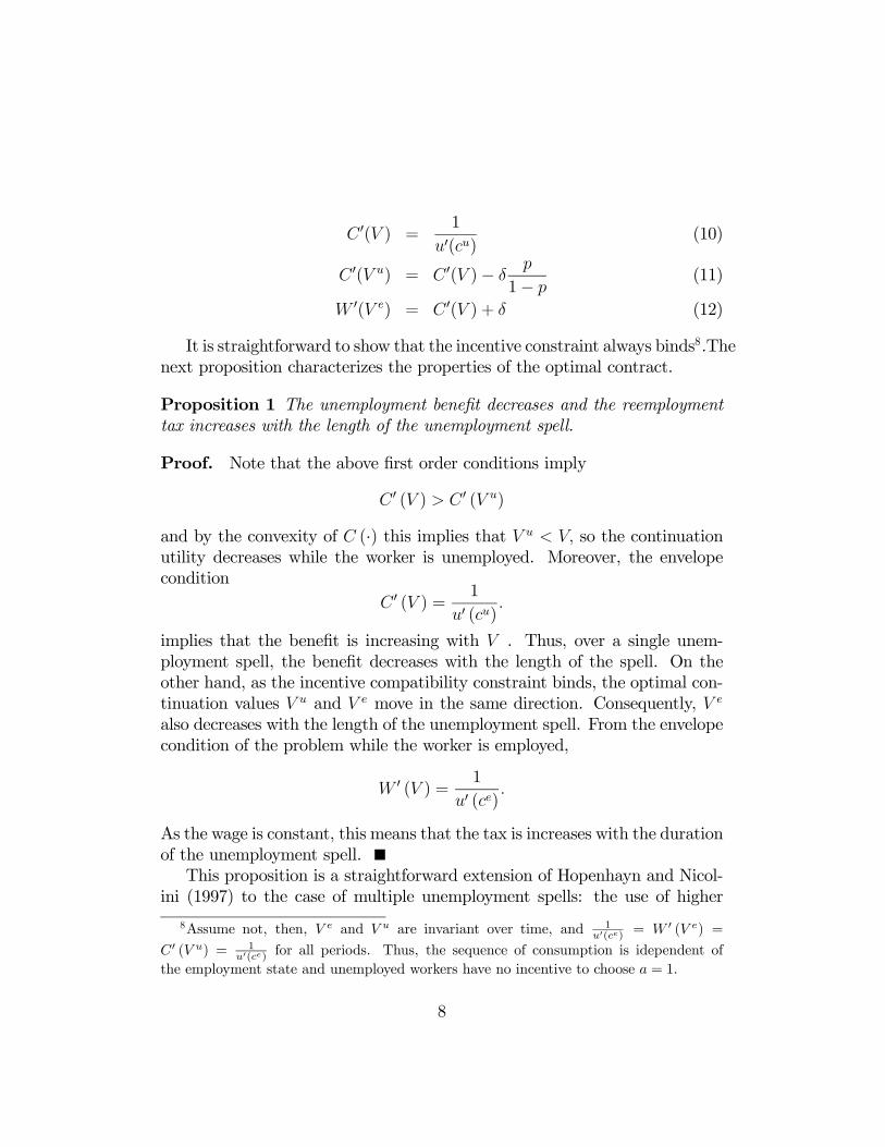
C 0(V ) =1

u0(cu)(10)

C 0(V u) = C 0(V )− δp

1− p(11)

W 0(V e) = C 0(V ) + δ (12)

It is straightforward to show that the incentive constraint always binds8.Thenext proposition characterizes the properties of the optimal contract.

Proposition 1 The unemployment benefit decreases and the reemploymenttax increases with the length of the unemployment spell.

Proof. Note that the above first order conditions imply

C 0 (V ) > C 0 (V u)

and by the convexity of C (·) this implies that V u < V, so the continuationutility decreases while the worker is unemployed. Moreover, the envelopecondition

C 0 (V ) =1

u0 (cu).

implies that the benefit is increasing with V . Thus, over a single unem-ployment spell, the benefit decreases with the length of the spell. On theother hand, as the incentive compatibility constraint binds, the optimal con-tinuation values V u and V e move in the same direction. Consequently, V e

also decreases with the length of the unemployment spell. From the envelopecondition of the problem while the worker is employed,

W 0 (V ) =1

u0 (ce).

As the wage is constant, this means that the tax is increases with the durationof the unemployment spell.This proposition is a straightforward extension of Hopenhayn and Nicol-

ini (1997) to the case of multiple unemployment spells: the use of higher

8Assume not, then, V e and V u are invariant over time, and 1u0(ce) = W 0 (V e) =

C0 (V u) = 1u0(ce) for all periods. Thus, the sequence of consumption is idependent of

the employment state and unemployed workers have no incentive to choose a = 1.

8

reemployment taxes as part of the incentive structure follows from the effi-ciency of permanent income punishments when workers have a preference forconsumption smoothing.

Corollary 1 All net future contingent transfers increase with the value ofV.

Proof. This follows immediately from the last proposition.The Corollary indicates the persistent effect of rewards and punishments.

In particular, it implies that the replacement ratio and the reemploymenttax both depend in a non-trivial way on all previous unemployment spellsand on their duration. It should be noted that there is no simple statisticto compare different unemployment/employment histories. If two workers aand b experience the same number of unemployment spells but each spell islonger for worker a, this worker will face higher taxes or lower replacementratios. But aside from this very strong ordering of unemployment histories,little else can be said. For example, take two workers a and b that startemployed with identical V (and thus the same consumption). Now suppose bremains employed for the next two periods while a loses the job after the firstperiod and is reemployed after one period of unemployment. From equations(9-12) it follows that the final continuation utility of a will exceed that of b,so its consumption will be higher (tax will be lower). 9 This occurs, loosely,because while there is a reward for finding a job there is no punishmentfor losing it. (this can lead to opportunistic quits, as discussed in the nextsection). In particular, this implies that the total cumulative periods ofunemployment or subsidies received in the past is not a sufficient statistic.In providing incentives for search effort, the optimal contract generates

a loophole, which could be exploited by workers to upgrade their unemploy-ment benefits. In what follows, we discuss this issue.

2.3 A loophole in the optimal contract

The empirical literature on job duration provides some evidence that hazardrates for job termination tend to rise sharply at the time workers becomeeligible for unemployment insurance, suggesting the existence of opportunis-

9This fine point was indicated by a referee

9

tic quits10. In this section we identify a loophole in the optimal insuranceprogram derived above that leaves room for such opportunistic behavior.

Proposition 2 Consider an unemployed worker with promised future utilityequal to V. If the worker finds a job and is fired the following period, theoptimal contract will offer him a utility level V u > V.

Proof. Letting V e denote the promised utility when the worker finds thejob, from the above first order conditions for the problems defining C andW , it follows that

C 0(V ) < W 0(V e) = C 0(V u).

By the convexity of the function C, it follows that V u > V.

This Proposition has two critical implications. Consider a worker thatis unemployed. To provide incentives for searching, the worker must bebetter off getting a job than remaining unemployed. Thus, an immediateimplication of the incentive constraint is that V e > V u. However, this doesnot imply that once employed, the worker is better off keeping the job ratherthan losing it. In particular, since V u > V u it could be the case that V u > V e.This would give rise to opportunistic quit behavior. Moreover, getting a job,no matter how short-lived it is, upgrades unemployment benefits. This couldgive incentives for workers to fake employment, e.g. taking a bad job andthen quitting, just to upgrade their unemployment insurance benefits. Ineither case, workers could abuse the UI system only if the principal is notable to monitor perfectly the causes of job termination. We analyze thesecases in the following section.

3 Quits and Layoffs

In this section we assume that the principal cannot distinguish quits fromlayoffs. This is important, since UI is designed to protect workers againstexogenous shocks. As quits may be considered, at least to some extent, en-dogenous, only fired workers should qualify for benefits. To cope with this

10For instance, in Canada job termination rates double at the 12 month period, which isthe minimum period for eligibility (see Christofides and McKenna (1996) and Baker andRea (1998)).

10

problem, many unemployment insurance programs require involuntary sep-arations to re-qualify for benefits. Admittedly, however, this distinction be-tween involuntary and voluntary separations is hard to establish in practice,leaving room for opportunistic behavior. It is therefore natural to extend themodel and study the optimal contract when the principal cannot distinguishquits form layoffs.Two possible forms of opportunistic behavior may arise. First, if faced

with very generous unemployment insurance, workers may quit their jobs tocollect benefits and avoid the disutility of working. This case is considered insubsection 3.1. Secondly, when job offers are heterogeneous and the principalcannot monitor the quality of jobs, workers may take bad jobs and soonquit from them just to upgrade their unemployment benefits. This case isconsidered in subsection 3.2. As we show below, when any of these twocases occurs, it is optimal to condition benefits on employment duration.In particular, we show that in order to prevent either form of opportunisticbehavior, replacement ratios rise with employment duration and the tax paidby an employed worker decreases with tenure.

3.1 Quitting from good jobs

So far we have assumed that effort at work does not affect the utility of anemployed worker. For the analysis in the previous sections, this is just anormalization with no effect on any qualitative results. However, when quitsand layoffs cannot be distinguished, workers could decide to quit opportunis-tically. As the following Proposition shows, the contract derived above is notimmune to such behavior.

Proposition 3 Suppose e ≥ 0 is the disutility of effort for an employedworker. Let V e and V u denote the utility value in the optimal contract, fora currently employed worker with initial utility V e,who remains employed orloses the job, respectively.

1. If e = 0, then V e > V u.

2. If e > 1p, then V u > V e

Proof. See appendix

This proposition implies that when the disutility of effort at work is suf-ficiently high, workers that find a job would certainly prefer quitting it after

11

one period11 and restarting benefits at a higher level rather than continuingemployed. To prevent this behavior, the optimal contract must guaranteethat for an employed worker

V e ≥ V u, (13)

where V e corresponds to the utility of keeping the job and V u the utility oflosing it.Adding this constraint, to the optimization problem defined by equation

(4) and the promise-keeping constraint (5), we obtain a program that isalmost identical to the one considered for an unemployed worker: if binding,the incentives needed to deter job quits are quite similar in nature to thoseneeded to induce job search. Not surprisingly, the first order conditions forthe two problems are almost identical. Consequently, if the no-quit constraint(13) binds,

C 0 (V u) < W 0 (V ) < W 0 (V e) (14)

and if it does not bind

C 0 (V u) =W 0 (V ) =W 0 (V e) . (15)

Together with the envelope conditions, the first equation implies that con-sumption falls when the worker loses the job (incomplete replacement) andit rises if the worker remains employed.Let {V e

t } and {V ut } denote the optimal continuation utilities derived from

this program for a worker that starts employment at t = 0 with an enti-tlement of utility V e

0 . The following Proposition shows that if the no-quitconstraint binds in any period, then it must bind in all. It then follows fromthe above argument that the utility given by these two sequences is strictlyincreasing in t, the employment tenure. In particular, this implies that taxeswhile employed decrease with tenure and replacement ratios after becomingunemployed increase with the length of the previous employment spell.

Proposition 4 Suppose there exists an elapsed duration time t such thatthe constraint V e

t ≥ V ut binds. Then this constraint binds during all the

employment spell. When this happens, the sequences V et and V u

t are strictlyincreasing.11The sufficient condition e > 1/p is far from necessary. Also note that no matter how

large e is, the incentive constraint of the unemployed problem ensures that workers thatfind a job are better off taking that job.

12

Proof. See appendix.

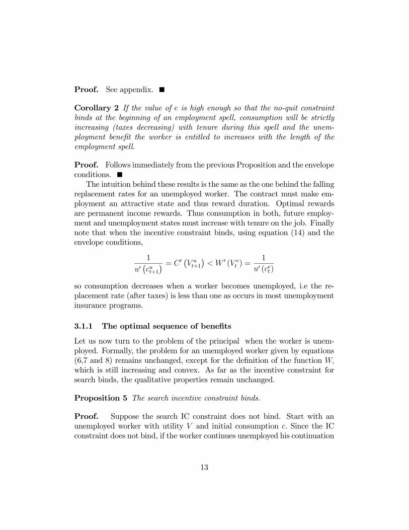
Corollary 2 If the value of e is high enough so that the no-quit constraintbinds at the beginning of an employment spell, consumption will be strictlyincreasing (taxes decreasing) with tenure during this spell and the unem-ployment benefit the worker is entitled to increases with the length of theemployment spell.

Proof. Follows immediately from the previous Proposition and the envelopeconditions.The intuition behind these results is the same as the one behind the falling

replacement rates for an unemployed worker. The contract must make em-ployment an attractive state and thus reward duration. Optimal rewardsare permanent income rewards. Thus consumption in both, future employ-ment and unemployment states must increase with tenure on the job. Finallynote that when the incentive constraint binds, using equation (14) and theenvelope conditions,

1

u0¡cut+1

¢ = C 0 ¡V ut+1

¢< W 0 (V e

t ) =1

u0 (cet)

so consumption decreases when a worker becomes unemployed, i.e the re-placement rate (after taxes) is less than one as occurs in most unemploymentinsurance programs.

3.1.1 The optimal sequence of benefits

Let us now turn to the problem of the principal when the worker is unem-ployed. Formally, the problem for an unemployed worker given by equations(6,7 and 8) remains unchanged, except for the definition of the function W,which is still increasing and convex. As far as the incentive constraint forsearch binds, the qualitative properties remain unchanged.

Proposition 5 The search incentive constraint binds.

Proof. Suppose the search IC constraint does not bind. Start with anunemployed worker with utility V and initial consumption c. Since the ICconstraint does not bind, if the worker continues unemployed his continuation

13

utility and consumption will remain unchanged so V ≥ u (c)+βV. In contrast,the value of getting a job is:

Ve = u(c)− e+ βVu

< u (c)− e+ βV

< V

where consumption in the first period does not change by the contradictionhypothesis and the second line follow from the no quit constraint. But thisimmediately violates the search IC constraint.As a consequence, with the exception of the employment dependence

properties indicated above, all other qualitative characteristics of the unem-ployment insurance program ( i.e. that benefits decrease and taxes increasewith the length of the current and previous unemployment spells) remainunchanged.

3.2 Accepting bad jobs

In this section we explore another potential source of incentive problems,namely, the possibility that workers may take bad matches and then quit fromthem, just to upgrade their unemployment benefits, exploiting the loopholeindicated in section 2.3. In order to evaluate this possibility, we extend themodel allowing for heterogenous job matches, the quality of which cannot beperfectly monitored by the principal. In contrast to current unemploymentinsurance generosity, which will typically lead workers to be excessively picky,future generosity may indeed have the opposite effect.12

A bad job offer, is here defined as one that is inefficient for an unem-ployed worker to take, and that in the absence of unemployment insurancethe worker would never accept. The presence of such job opportunities intro-duces new constraints into the unemployment insurance design problem. Inwhat follows, we characterize the unemployment insurance contract subjectto these additional constraints, showing how employment dependence arisesas an optimal response to prevent workers from exploiting these opportuni-ties.Bad jobs are socially inefficient because they provides a lower flow of

utility. These jobs pay the same wage w as the good jobs, but generate

12Mortensen (1977) considers this latter effect in a search model with multiple spells.

14

disutility d per period. A natural alternative would be to define the bad jobas one with a lower wage w0. In absence of unemployment insurance, the twoproblems are identical, letting d = u(w)− u (w0) . However, this is not truefor an unemployment insurance program that involves transfers during theemployment state, since the marginal valuation of such transfers will differdepending on the wage received. Our separability assumption avoids thiscomplication, and thus simplifies considerably the analysis13. In addition,for the analysis that follows, it is key that the principal cannot observe thequality of the job. We therefore find more natural to assume heterogeneityin utility which is unobservable. Given a search effort equal to one, bad jobsarise with positive probability and have constant termination rate λb ∈ (0, 1),which may be different from λ, the termination rate of the good jobs. As inthe previous section we assume that quits and layoffs cannot be distinguishedby the principal, for otherwise workers would never choose to take the badjob and the adverse selection constraint would never bind.The bad job provides a costly way to send a signal of employment that

the principal cannot distinguish from the signal corresponding to a goodjob. These alternative jobs are socially useless, in the sense that no workerwould take them in the absence of unemployment insurance. However, anunemployment insurance contract with no employment dependence like theone considered before, may increase the private value of these jobs. We alsoassume, as it is standard in the search literature, that while employed, theworker cannot look for another job.Instantaneous utility derived from the bad job is

u(w)− d

where d is such thatd > α[u(w)− (u(0)− 1)]. (16)

This inequality is imposed to make sure that in the absence of insurance,the worker is better off searching for the good job than taking the bad one.Indeed, if we let V s denote the value that an unemployed worker has -in theabsence of any insurance- if it is optimal to search, it is easy to check that:

(1− β)V s = α(u(0)− 1) + (1− α)u(w), (17)13We conjecture that similar properties of the optimal unemployment insurance program

would emerge without this separablity assumption. However, either strong conditions mustbe imposed in preferences to ensure that the problem is convex or randomizations mightbe optimal. We thank the comments of a referee that helped us to clarify this issue.

15

where

α =1− β (1− λ)

1− β (1− (λ+ p)).

Equation (17) expresses the flow value of this unemployed worker as a weightedsum of the utility flow when unemployed (u (0)− 1) and the utility flow whenemployed (u (w)) , where the weights α and 1− α are derived from the ratesof exit from unemployment p and from employment λ, together with thediscount factor.On the other hand, the value of taking the bad job and quitting after one

period Vb is given by:Vb = u (w)− d+ βVs.

The worker will not take the bad job, if and only if Vb ≤ Vs, i.e

u(w)− d < (1− β)Vs

which after substituting for Vs gives condition (16).

3.2.1 The self-selection constraint

Consider a given unemployment insurance contract, specifying net transfersto the worker τ t as a function of the state (employed, unemployed) andthe employment history h. Suppose this history is such that the worker isunemployed at time zero. Let V indicate the value that the contract gives tothe worker at this node. As in the previous section, let V u denote the valueif the worker remains unemployed, V e the value if the worker gets a job andc the current consumption (equal to the current period transfer τ). Thecontinuation contract for a worker that finds the job can be described by thetwo sequences: {ct}∞t=0 , {V u

t }∞t=1which denote, respectively, the consumptionin the first, second, third, etc. periods of employment and the continuationvalues if the job is terminated in the first, second, third, etc. periods ofemployment. Taking into account the constant probability of termination λ,it follows that

V e =∞Xt=0

βt(1− λ)t£u(ct) + βλV u

t+1

¤. (18)

In turn, the value of taking the bad job and quitting after T periods is givenby:

QT =TXt=0

βt (1− λb)t [u(ct)− d] + (1− λb)

T βT+1V uT+1.

16

In order for the worker not to take this alternative, it must be the case thatfor all T ≥ 0, V u ≥ QT , i.e.

V u ≥TXt=0

βt (1− λb)t [u(ct)− d] + (1− λb)

T βT+1V uT+1, (19)

for all T = 0, 1, ...Notice that for a given value entitlement V e, these constraints restrict

the particular paths©ct, V

ut+1

ªthan can be used to support that value. The

optimal choice of this path determines the nature of employment dependencein the unemployment insurance contract. This problem is analyzed in thefollowing section.

3.2.2 Employment dependence: the optimal choice of©ct, V

ut+1

ªThe optimal path

©ct, V

ut+1

ªis the solution to the following problem:

W (V e, V u) = minct,V u

t+1

∞Xt=0

βt(1− λ)t£ct − w + βλC(V u

t+1)¤

(20)

subject to (18) and (19).Before solving the problem, we must make sure that the choice set is well

defined. Note that 18 imposes a lower bound on the sequence of controls,while 19 imposes upper bounds. Lemma 5 in the appendix establishes thatthis set is nonempty.We now characterize the solution for the optimal path. Letting γ and

µt be the Lagrange multipliers of constraints 18 and 19 respectively andθ = (1− λb) / (1− λ) the first order conditions14 for the optimal (20) are:

1

u0(ct)= γ − θt

∞Xj=t

µj (21)

and

C 0(V ut+1) = γ − θt

λbλ

∞Xj=t

µj − θt(1− λb)

λµt (22)

14The argument to prove that the value function is convex is the same as before, sincethe added constraint is linear in utilities.

17

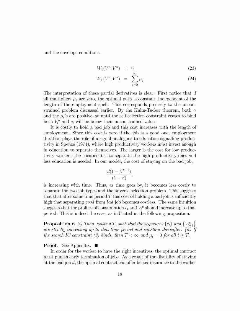
and the envelope conditions

W1(Ve, V u) = γ (23)

W2 (Ve, V u) =

∞Xj=0

µj (24)

The interpretation of these partial derivatives is clear. First notice that ifall multipliers µt are zero, the optimal path is constant, independent of thelength of the employment spell. This corresponds precisely to the uncon-strained problem discussed earlier. By the Kuhn-Tucker theorem, both γand the µt’s are positive, so until the self-selection constraint ceases to bindboth V u

t and ct will be below their unconstrained values.It is costly to hold a bad job and this cost increases with the length of

employment. Since this cost is zero if the job is a good one, employmentduration plays the role of a signal analogous to education signalling produc-tivity in Spence (1974), where high productivity workers must invest enoughin education to separate themselves. The larger is the cost for low produc-tivity workers, the cheaper it is to separate the high productivity ones andless education is needed. In our model, the cost of staying on the bad job,

d(1− βT+1)

(1− β),

is increasing with time. Thus, as time goes by, it becomes less costly toseparate the two job types and the adverse selection problem. This suggeststhat that after some time period T this cost of holding a bad job is sufficientlyhigh that separating good from bad job becomes costless. The same intuitionsuggests that the profiles of consumption ct and V u

t should increase up to thatperiod. This is indeed the case, as indicated in the following proposition.

Proposition 6 (i) There exists a T, such that the sequences {ct} and©V ut+1

ªare strictly increasing up to that time period and constant thereafter. (ii) Ifthe search IC constraint (3) binds, then T <∞ and µt = 0 for all t ≥ T.

Proof. See Appendix.In order for the worker to have the right incentives, the optimal contract

must punish early termination of jobs. As a result of the disutility of stayingat the bad job d, the optimal contract can offer better insurance to the worker

18

the longer he has been employed. Thus, the tax is a decreasing function ofjob length and the benefit received in case of unemployment is an increasingfunction. Eventually, for long enough duration, the incentive problems disap-pear and both the tax and future promised utility in case of unemploymentbecome constant over time while employment lasts. Interestingly, the proofshows that the optimal sequence of benefits is independent of λb on a setthat includes λb ∈ [λ, 1] .Replacement rates. Using (21) and (22) it follows that

C 0(V ut+1)−

1

u0(cet)= −θtλb

λ

∞Xj=t

µj − θt(1− λb)

λµt + θt

∞Xj=t

µj

=θt

λ

"(λ− λb)

∞Xj=t

µj − (1− λb)µt

#.

For λb ≥ λ, the terms in bracket is strictly negative until the self-selectionconstraint stops binding. By the envelope theorem C 0 ¡V u

t+1

¢= 1/u0 (cut ) this

implies that cut < cet so consumption falls when becoming unemployed. Thisresults extends to the case λ ≥ λb since as shown in the Appendix (Lemma9) the optimal policy in that case is identical to the one obtained for λ = λb.So as in the case of opportunistic quits, the (after tax) replacement rates areless than one.Note that there is no adverse incentive problem if T = 0, which would

occur if the flow disutility d is large relative to the upgrade in UI benefits.In the working paper version we show that, provided a continuity conditionholds, there is a nonempty set of parameters for which T > 0 and acceptingbad jobs is not optimal for the planner. The argument relies on shrinkingthe time period -and appropriately rescaling probabilities- in such a way thatit becomes essentially costless for the agent to take the bad job and quit aninstant after15.

3.2.3 The optimal sequence of benefits

Let us now turn to the problem of the principal when the worker is unem-ployed. The only change needed to the first order conditions given in section

15We thank the comment of one referee that made us think about this issue.

19

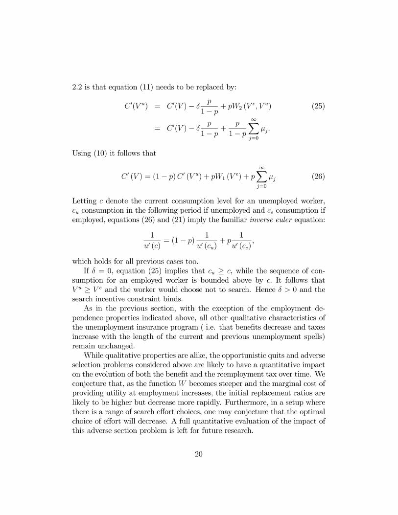
2.2 is that equation (11) needs to be replaced by:

C 0(V u) = C 0(V )− δp

1− p+ pW2 (V

e, V u) (25)

= C 0(V )− δp

1− p+

p

1− p

∞Xj=0

µj.

Using (10) it follows that

C 0 (V ) = (1− p)C 0 (V u) + pW1 (Ve) + p

∞Xj=0

µj (26)

Letting c denote the current consumption level for an unemployed worker,cu consumption in the following period if unemployed and ce consumption ifemployed, equations (26) and (21) imply the familiar inverse euler equation:

1

u0 (c)= (1− p)

1

u0 (cu)+ p

1

u0 (ce),

which holds for all previous cases too.If δ = 0, equation (25) implies that cu ≥ c, while the sequence of con-

sumption for an employed worker is bounded above by c. It follows thatV u ≥ V e and the worker would choose not to search. Hence δ > 0 and thesearch incentive constraint binds.As in the previous section, with the exception of the employment de-

pendence properties indicated above, all other qualitative characteristics ofthe unemployment insurance program ( i.e. that benefits decrease and taxesincrease with the length of the current and previous unemployment spells)remain unchanged.While qualitative properties are alike, the opportunistic quits and adverse

selection problems considered above are likely to have a quantitative impacton the evolution of both the benefit and the reemployment tax over time. Weconjecture that, as the function W becomes steeper and the marginal cost ofproviding utility at employment increases, the initial replacement ratios arelikely to be higher but decrease more rapidly. Furthermore, in a setup wherethere is a range of search effort choices, one may conjecture that the optimalchoice of effort will decrease. A full quantitative evaluation of the impact ofthis adverse section problem is left for future research.

20

4 Final Remarks

In this paper we derive an optimal unemployment insurance program as thesolution to a repeated principal agent problem. This paper extends previ-ous work allowing for multiple employment/unemployment spells. We showthat replacement rates decrease as a function of current and previous un-employment spells. The taxes paid by employed workers are also increasingin all previous unemployment spells. When job termination is exogenous,the history of current and previous employment duration has no effect onreplacement rates or taxes.In practice, most unemployment insurance schemes condition replacement

ratios on the duration of previous employment spells. This paper provides atheoretical foundation for such practice. When quits and layoffs cannot beperfectly distinguished by the enforcing agency, the above optimal contractcan lead to opportunistic quit behavior. Moreover, workers may also havean incentive to accept bad matches and soon quit from them, simply toupgrade their unemployment insurance benefits. Preventing such behaviorimposes further constraints into the design of the insurance contract. Oncethese additional constraints are introduced, the optimal program calls forincomplete replacement ratios, which increase with the length of previousunemployment spells and taxes that decrease with tenure on the job.Incentives are provided to make the employment state more attractive.

Hence, the worker’s expected future utility decreases with the length of un-employment spells and increases with the length of employment spells. Thisexplains the duration dependence of unemployment benefits and taxes. More-over, a change of state from unemployment to employment is rewarded andfrom employment to unemployment penalized, accounting for the incompletereplacement rate policy. The additional sources of opportunistic quit behav-ior examined in this paper increase the cost of providing search incentivesfor unemployed workers. We conjecture that this is likely to result in higherinitial replacement ratios for the unemployed but a steeper decline with thelength of unemployment.

21

A Proofs

A.1 Convexity of the optimal program when e ∈ {0, 1}The optimal contract problem when the worker is unemployed has a discretechoice variable - the effort level. The general problem, as we will show, isnot convex, so the unconstrained optimum may involve the use of lotteries.Let

C0 (V ) = minc,V u

c+ βC (V u)

subject to : u (c) + βV u = V

and

C1 (V ) = minc,V u,V e

c+ β {pW (V e) + (1− p)C (V u)} (27)

subject to : u (c)− 1 + β {pV e + (1− p)V u} = V

p (V e − V u) ≥ 1

C (V ) = minq,V0,V1

(1− q)C0 (V0) + qC1 (V1) (28)

subject to : (1− q)V0 + qV1 = V

where C0 and C1 are the cost of recommending the low and high effort leveltoday respectively, while C is the cost of a lottery between the high effortlevel an the low effort level with the corresponding promised utilities. Weshow in the next proposition that the problem so defined is convex, so nofurther randomizations can improve upon the optimal solution.

Lemma 1 The functions C0, C1 and C are convex.

Proof. If C is convex, it is immediate to verify that the problem definedby equation (27) defines convex functions C0 and C1. We now show that ifthese two functions are convex, then equation (28) defines a convex functionC. Let (q, V0, V1) be solutions for V and q0, V 0

0 , V01 be solutions for V

0. Let

V λ = λV + (1− λ)V 0,

22

and for this starting value take as choice variables

qλ = λq + (1− λ) q0,

V λ0 =

λ (1− q)V0 + (1− λ) (1− q0)V 00

1− qλ

V λ1 =

λqV1 + (1− λ) q0V 01

qλ

Simple algebra shows that this is a feasible solution for V λ. Therefore, bydefinition

C(V λ) ≤ ¡1− qλ¢C0¡V λ0

¢+ qλC1

¡V λ1

¢Convexity of C0 and C1 imply that

C0¡V λ0

¢ ≤ λ (1− q)C0 (V0) + (1− λ)(1− q0)C0 (V 00)

(1− qλ)

and

C1¡V λ1

¢ ≤ λqC1 (V1) + (1− λ)q0C1 (V 01)

qλ

It therefore follows that¡1− qλ

¢C0¡V λ0

¢+ qλC1

¡V λ1

¢ ≤ λC (V ) + (1− λ)C (V 0) ,

which completes the proof.We do now show that the derivative of the C1 function is larger than

the derivative of the C0 function, such that they display the single crossingproperty.

Lemma 2 For any V, C 00(V ) < C 0

1(V ).

Proof. >From the first order and envelope conditions of the C0 and C1problem we obtain

C 00(V ) =

1

u0(c0)= C 0(V u

0 ) (29)

u(c0) + βV u0 = V (30)

C 01(V ) =

1

u0(c1)> C 0(V u

1 ) (31)

u(c1) + βV u1 = V (32)

23

Now, assume that c0 < c1. The result follows from the concavity of u. Now,assume that c0 ≥ c1. Then, 30 and 32 and the convexity of C imply that

C 0(V u0 ) ≤ C 0(V u

1 )

The result follows from 29 and 31.We can now characterize the function C(V ). First, if either C0(V ) or

C1(V ) is below the other for all the domain, then C(V ) coincides with thatcurve. If they cross, by the single crossing property, they cross only once. Aswe already showed, C1(V ) has a larger slope, so C1(V ) will intersect C0(V )from below. Therefore, as it can be seen from the first order condition, theC(V ) function will coincide with C1 for low values of V, will be linear forintermediate values of V, which means that randomizations are optimal, andwill coincide with C0 for high values of V. The analysis of the text is relevantfor low values of V.

A.2 Proof of Proposition 3

Consider an employed worker. Let Vu denote the utility of quitting. Underthe optimal contract described in section 2.2, this is is the utility obtainedby quitting any period. Consider the strategy: "stay this period but quitthe next". The utility obtained equals:

u (ce)− e+ βVu.

In turn, the strategy of quitting immediately gives utility:

Vu = u (cu) + βhpV e + (1− p)Vu

iwhich, as once the worker is unemployed the incentive constraint binds, canbe written as

Vu = u (cu) + βVu

Under the above optimal contract, ce = cu, so the net gain of delaying oneperiod the quit decision is:

−e+ β³Vu − Vu

´.

24

If e = 0, then noting that Vu ≥ Vu (with strict inequality if reemploymentis desired) it follows that the agent has no loss (strict gain) by delaying thequitting decision. Applying this principle recursively, the worker is better offby not quitting.To prove part 2, suppose by way of contradiction that e > 1/p but the

value of employment Ve ≥ Vu. Let Ve denote the utility that an unemployedworker with initial value Vu gets if he finds a job. We first show that Ve ≥ Vu.Let ce be the first period consumption of this employed worker. As provedin section 2.2 consumption rises if an unemployed worker gets a job, so ce ≥cu = ce. Since consumption is monotonic in value, this implies that Ve ≥ Vewhich by the contradiction assumptions is no less than Vu. The incentiveconstraint for the unemployed worker implies that β

³Ve − Vu

´= 1/p which

together with the previous result implies that β³Vu − Vu

´≤ 1/p < e, so the

strategy of quitting immediately dominates the strategy of waiting one moreperiod. Applying this result recursively, prover that Ve < Vu.

A.3 Proof of Proposition 4

First note that if this constraint does not bind at time T , then from equation(15) it follows that V e

T = V eT+1 and by iterative application V e

t = V eT for all

t ≥ T. Moreover, as V et remains constant so does V

ut and thus V

et ≥ V u

t forall t ≥ T and the constraint does not bind for any future period. Next weshow that if the constraint binds in some period T then it must bind in allsubsequent periods. The combination of these two results proves the firstpart of the proposition. Suppose, by way of contradiction, that (13) bindsat t, i.e. V u

t+1 = V et+1, but it does not bind at t+1. Using equations (14) and

(15) it follows that:

C 0 ¡V ut+1

¢< W 0 (V e

t ) < W 0 ¡V et+1

¢and

C 0 ¡V ut+2

¢=W 0 ¡V e

t+1

¢=W 0 ¡V e

t+2

¢By strict convexity of functions C and W, and since V u

t+1 = V et+1 it follows

thatV ut+2 > V u

t+1 = V et+1 = V e

t+2,

which violates the no-quit constraint.That V e

t (and thus V ut ) strictly increases when the no-quit constraint

binds, follows immediately from equation (14).

25

A.4 Proofs for Section 3.2

The proofs in this section follow from a series of intermediate Lemmas. Thebasic outline is as follows. Two cases are distinguished: λb ≤ λ and λb ≥ λ. Akey result that we establish for the first case is that the constrained optimalsolution is the same for all λb in that range, so we reduce the problem toproving all results for λb = λ. For the case λb > λ, the optimal program isnot independent of λb so a separate proof is given.

Lemma 3 Let QT denote the value of taking the bad job at time zero andquitting at the end of period T . Then QT+1 − QT has the same sign asu (cT+1)− d+ βV u

T+2 − V uT+1.

Proof. Follows immediately by noting that:

QT+1 =T+1Xt=0

βt (1− λb)t ¡u (ct)− d+ βλbV

ut+1

¢+ βT+2 (1− λb)

T+1 V uT+2

= QT − βT+1 (1− λb)T+1 V u

T+1 + βT+1 (1− λb)T+1 ¡u (cT+1)− d+ βV u

T+2

¢= QT + βT+1 (1− λb)

T+1 ¡u (cT+1)− d+ βV uT+2 − V u

T+1

¢.

Lemma 4 Take any λb > 0. Consider a feasible plan©ct, V

ut+1

ªsuch that

the self selection constraint (19) binds until period T ≤ ∞ and does not bindthereafter. Then that plan satisfies the self selection constraint for all otherλb.

Proof. The proof is by induction. First consider time T = 0,

u (c0)− d+ βV u1 = Vu

is the value of quitting for sure after one period and it is independent of λb,so it is obviously satisfied. Suppose the constraint holds for some T0 < T, sothe value QT0 of quitting at the end of period T0 equals Vu. By Lemma 3, thesign of QT0+1 −QT0 is independent of λb, and since by assumption it is zerofor the given λb, it must be zero for all. Finally, we need to show that theconstraint is satisfied for T0 > T. Again, we show this by induction. PeriodT + 1 is the first period for which µt = 0. Hence from that point on ct = c

26

and V ut+1 = V are constant. Since by assumption QT = Vu > QT+1 it follows

that:u (cT+1)− d+ βV u

T+2 < V uT+1

or equivalently,u (c)− d+ βV < V u

T+1. (33)

But this implies that QT+1−QT < 0 for all λb, so the self-selection constraintis slack for T +1. Finally, note that since V ≥ V u

T+1, it follows from equation(33) that

u (c)− d+ βV < V,

so Qt > Qt+1 for all t ≥ T + 1.The following Lemma uses the previous result to establish the existence

of a feasible plan.

Lemma 5 For all V u and V e = V u+ 1pβthere exist paths

©ct, V

ut+1

ªsatisfying

constraints (3), (18) and (19). Moreover, the paths can be chosen so thatconstraint (3) binds.

Proof. Pick any sequence {ct, V ut } such that constraint (19) is satisfied

with equality for all T. By lemma 4 the constraint is satisfied for all λb. Inparticular, for λb = λ the worker is indifferent between quitting or not anyperiod. It follows that

V u =∞Xt=0

βt(1− λ)t£u(ct)− d+ βλV u

t+1

¤. (34)

Let Ve denote the value of taking a good job that is associated to this path.Subtracting (34) from (18), it follows that:

Ve − V u =d

1− β (1− λ).

Using equation (16) it follows that

Ve − V u >u (w)− (u(0)− 1)1− β (1− (λ+ p))

. (35)

To evaluate the right hand side of this equation, note that for search to be atall valuable, it must be the case that (1− β)V s > u (0) , where the second

27

term is the value of never searching. In conjunction with equation (17) thisimplies that

(u (w)− u (0)) >α

(1− α)=1− β (1− λ)

βp

which together with (35) implies that Ve − V u > 1βp. This path satisfies the

incentive constraint. Moreover, it follows that by decreasing some compo-nents of the sequence an alternative path that satisfies constraint (19) andgives a value Ve − V u = 1

βpcan be found.

The remainder of this section proves that the optimal plan has strictlyincreasing sequences

©ct, V

ut+1

ªup to some T and constant thereafter. The

following two lemmas give intermediate results that are used in some of theproofs.

Lemma 6 V ut+2 − V u

t+1 has the same sign as λb (λb − λ)P∞

j=t+1 µj + (1 −λ)µt − (1− λb)

2 µt+1.

Proof. >From equation (22) it follows that

C 0 ¡V ut+2

¢−C 0 ¡V ut+1

¢= θt

λbλ

∞Xj=t

µj+θt (1− λb)

λµt−θt+1

λbλ

∞Xj=t+1

µj−θt+1(1− λb)

λµt+1

having the same sign as λb (1− θ)P∞

j=t+1 µj + µt − θ (1− λb)µt+1 which inturn has the same sign as λb (λb − λ)

P∞j=t+1 µj + (1− λ)µt − (1− λb)

2 µt+1.The claim follows from the convexity of C.

Lemma 7 Assume λb ≥ λ. Suppose V ut ≥ V u

t+1 and Qt = Vu. Then V ut+2 <

V ut+1 and µt+1 > 0.

Proof. If Qt = Vu, the incentive constraints imply that Qt−1 ≤ Vu = Qt,and Qt = Vu ≥ Qt+1. These inequalities and Lemma 3 imply that

u (ct)− d+ βV ut+1 ≥ V u

t ≥ V ut+1 ≥ u (ct+1)− d+ βV u

t+2 > u (ct)− d+ βV ut+2,

(where ct+1 > ct follows from (21) and θ ≤ 1) so V ut+1 > V u

t+2. Finally note thatby Lemma 6 it follows that if µt+1 = 0 and since λb ≥ λ then V u

t+2−V ut+1 ≥ 0

contradicting the previous inequality.

28

Lemma 8 In the optimal plan for λb ≥ λ, the sequences©ct, V

ut+1

ªare non-

decreasing. Moreover, whenever µt+s > 0, for some s ≥ 0, then ct+1 > ct,and V u

t+1 > V ut . In addition, if µt+s = 0 for all s ≥ 0, then ct+s = ct and

V ut+1+s = V u

t+1 for all s ≥ 0.

Proof. The results for {ct} follow immediately from (21) and θ ≤ 1. Toshow the results regarding V u

t , consider first the case µt > 0 and supposetowards a contradiction that V u

t ≥ V ut+1. Applying repeatedly Lemma 7,

V ut+s > V u

t+s+1 and µt+s > 0 for all s. But sinceP

µs < ∞ and θ ≤ 1,C 0 (V u

t ) → γ and so eventually it must increase. Now suppose instead thatµt = 0. By the first order conditions (22) and since θ ≤ 1 it follows thatV ut+1 ≥ V u

t and that Vut+1 = V u

t only when µt+s = 0 for all s ≥ 0.The following Lemma proves that the optimal plan for λb ≤ λ is the same

as that for λb = λ. Applying Lemma 8, it follows that the paths©ct, V

ut+1

ªare nondecreasing for all λb.

Lemma 9 The optimal plan for λb ≤ λ is the same as that for λb = λ.

Proof. We first show that in the optimal plan for λb = λ the self-selectionconstraint binds every period until some T ≤ ∞ and ceases to bind thereafter.From Lemma 8, it follows that V u

t+1 ≥ V ut . By Lemma 6 and using λb = λ,

V ut+1 − V u

t has the same sign as (1− λ)µt−1 − (1− λb)2 µt which implies

that whenever µt > 0, µt−1 must also be strictly positive. This implies thatthe plan for λb = λ satisfies the assumptions of Lemma 4, so this plan isfeasible for all λb. To show that indeed it is optimal for λb < λ we constructmultipliers {µt}Tt=0 that support this solution. Let θ = (1− λb) / (1− λ) anddefine

µt =1

θt+1

õt − (1− θ)

Xj≥t

µj

!.

Using the first order conditions

1

u0(ct)= γ − θt

∞Xj=t

µj

C 0(V ut+1) = γ − θt

λbλ

∞Xj=t

µj − θt(1− λb)

λµt

29

by repeated substitution it follows that

1

u0 (ct)= γ −

∞Xj=t

µj

C 0(V ut+1) = γ −

∞Xj=t

µj − θt(1− λ)

λµt.

The multipliers are positive and support the same allocation. This completesthe proof.Lemmas 8 and 9 prove part (i) of Proposition 6. The next Lemma is used

to prove part (ii).

Lemma 10 Take a plan©ct, V

ut+1

ªthat satisfies the self selection constraints

for some λb. Let Qt (λb) be the associated value of taking the bad job at time

zero and quitting at the end of period t. Then if Qt (λb) = V u, then Qt

³λb´≤

V u for λb ≥ λb.

Proof. For all t ≤ T define

Ut (λb) = u (ct)− d+ βλbVut+1 + β (1− λb)Ut+1 (λb)

where UT+1 (λb) = V uT+1. This is the value -t periods after entry- of staying

in the bad job and quitting for sure at T +1.We first prove inductively that

QT (λb)−Qt (λb) = βt+1 (1− λb)t+1 ¡Ut+1 (λb)− V u

t+1

¢.

To simplify notation, we omit the argument λb from Q and U functions. Fort = T − 1,

QT −QT−1 = βT (1− λb)T ¡u (cT )− d+ βλbV

uT+1

¢+βT+1 (1− λb)

T+1 V uT+1 − βT (1− λb)

T V uT

= βT (1− λb)T ©£u (cT )− d+ βλbV

uT+1

¤+ β (1− λb)V

uT+1 − V u

T

ª= βT (1− λb)

T (UT (λb)− V uT ).

30

To complete the induction, supposeQT−Qt+1 = βt+2 (1− λb)t+2 ¡Ut+2 − V u

t+2

¢.Then

QT −Qt = QT −Qt+1 +Qt+1 −Qt

= βt+2 (1− λb)t+2 ¡Ut+2 − V u

t+2

¢+ βt+1 (1− λ)t+1

¡u (ct+1)− d+ βλbV

ut+2

¢+βt+2 (1− λb)

t+2 V ut+2 − βt+1 (1− λb)

t+1 V ut+1

= βt+1 (1− λb)t+1 £u (ct+1)− d+ βλbV

ut+2 + β (1− λb)Ut+2 − V u

t+1

¤= βt+1 (1− λb)

t+1 ¡Ut+1 − V ut+1

¢.

An important implication of this result is that when QT (λb) = V u, thenQT (λb) ≥ Qt (λb) for all t, so Ut+1 (λb) ≥ V u

t+1. Moreover, we now show thatwhen QT (λb) = V u, Ut (λb ) is nonincreasing in λb for all t. The proof isagain by induction. For t = T +1 it is obviously satisfied, since UT+1 = V u

T+1

is independent of λb. Now suppose it holds for t+ 1. Then

Ut (λb) = u (ct)− d+ βλbVut+1 + β (1− λb)Ut+1 (λb)

and∂Ut

∂λb= β(V u

t+1 − Ut+1 (λb)) + β (1− λb)∂Ut+1

∂λb.

But as discussed above the first term is nonpositive and by the inductionhypothesis so is the second term.We are now ready to complete the proof. Fix λb and suppose that the

self-selection constraint binds for some T, i.e. QT (λb) = V u. In particular,this implies that QT (λb)−Q0 (λb) = β (U1 (λb)− V u

1 ) is decreasing in λb. ButQ0 (λb) = u (c0)−d+βV u

1 is independent of λb and thus QT (λb) is decreasingin λb.We are now ready to prove part (ii) of Proposition 6 Take λb ≥ λ. In

every period T where the self-selection constraint binds, QT (λb) = V u, so bythe previous lemma it follows that QT (λ) ≥ QT (λb) ≥ V u. Note that

V u ≤ QT (λ) =TXt=0

βt (1− λ)t©u (ct)− d+ βλV u

t+1

ª+ βT+1 (1− λ)T V u

T+1

=−d³1− [β (1− λ)]T+1

´(1− β (1− λ))

+TXt=0

βt (1− λ)t©u (ct) + βλV u

t+1

ª+ βT+1 (1− λ)T V u

T+1

≤−d³1− [β (1− λ)]T+1

´(1− β (1− λ))

+ V e

31

This implies that

V e − V u ≥d³1− [β (1− λ)]T+1

´(1− β (1− λ))

Now, assume towards a contradiction that for any T ∈ R, ∃ s > 0, 3µT+s > 0. Then,

V e − V u ≥ d

(1− β (1− λ)).

But as in the proof of lemma 5, this in turn implies that Ve − V u > 1βp.

As a consequence, the incentive compatibility constraint does not hold withequality, and Ve can be reduced lowering total cost. This proves part (ii) ofProposition 6 for λb ≥ λ. But by Lemma 9 the optimal plan for λb < λ isexactly the same as the one for λb = λ. This completes the proof.

32

References

[1] Anderson, P. and B, Meyer. ”Unemployment insurance in the UnitedStates: layoff incentives and cross subsidies”, Journal of Labor Eco-nomics, 1993.

[2] Baily, M. ”Some Aspects of Optimal Unemployment Insurance ” Journalof Public Economics, Vol. 10, 379-402, 1978.

[3] Baker, M. and S. Rea. ”Employment spells and unemployment insuranceeligibility requirements”, The Review of Economics and Statistics, 80-94, 1998.

[4] Christofides, L. and C. McKenna. ”Unemployment insurance and jobduration in Canada”, Journal of Labor Economics, 286-313, 1996.

[5] Engen, Eric and J. Gruber, ”Unemployment Insurance and Precaution-ary Savings,” Journalof Monetary Economics, 47(3), June 2001, 545-579.

[6] Green, D. and C. Riddell. ”The economic effects of unemployment in-surance in Canada: An empirical analysis of UI disentitlement”. Journalof Labor Economics, 1993.

[7] Gruber, J. ”The Consumption Smoothing Benefits of UnemploymentInsurance, ” American Economic Review, vol. 87 no. 1, March 1997.

[8] Hopenhayn, H. and J.P. Nicolini. ”Optimal Unemployment Insurance”,Journal of Political Economy, Vol 105, 412-438, 1997.

[9] Hopenhayn, H. and J.P. Nicolini. ”Employemnt rated UnemploymentInsurance”, Working Paper, Universidad Di Tella, 2002.

[10] Mortensen, D. ”Unemployment Insurance and Job Search Decisions. ”Industrial and Labor Relations Review, Vol. 4, July 1977.

[11] Phelan, C. and R. Townsend. ”Computing multi-period information con-strained optima.” Review of Economic Studies, 1991.

[12] Shavell, S. and L. Weiss. ”The optimal payment of unemployment in-surance benefits over time.” Journal of Political Economy, 1979.

33

[13] Spear, E. and Srivastava, S., ”On Repeated Moral Hazard With Dis-counting”, Review of Economic Studies, 54, 599-617.

[14] Wang, C. and S. Williamson. ”Unemployment Insurance with MoralHazard in a Dynamic Economy”, Carnegie-Rochester Conference Seriesin Public Policy, 44, 1-41, 1996.

[15] Wang, C. and S. Williamson. ”Moral Hazard, Optimal UnemploymentInsurance and Experience Rating”, Journal of Monetary Economics ,Vol. 49, pp. 1337-1371, 2002.

[16] Zhao, R. "The Optimal UI Contract: Why a Replacement Ratio?"mimeo, University of Chicago. 2000.

34