INSTITUT NATIONAL DE LA STATISTIQUE ET DES ETUDES ECONOMIQUES Série des Documents de Travail du CREST

(Centre de Recherche en Economie et Statistique)

n° 2009-01

Optimal Income Taxation with Endogenous Participation

and Search Unemployment*

E. LEHMANN1 A. PARMENTIER2

B. VAN DER LINDEN3 Les documents de travail ne reflètent pas la position de l'INSEE et n'engagent que leurs auteurs. Working papers do not reflect the position of INSEE but only the views of the authors. *We thank for their comments participants at seminars at the Université Catholique de Louvain, CREST, Malaga, EPEE-Evry, Gains-Le Mans, CES-Paris 1, ERMES-Paris 2, the IZA-SOLE 2008 Transatlantic meeting, the 7th Journées Louis-André Gérard-Varet, the HetLab conference at the University of Konstanz, The Economics of Labor Income taxation workshop at IZA, Thema- Cergy Pontoise, AFSE 2008, EALE 2008 and T2M 2009, with a particular mention to Daron Acemoglu, Pierre Cahuc, Helmuth Cremer, Bruno Decreuse, Laurence Jacquet, Guy Laroque, Cecila Garcia-Peñalosa and Fabien Postel-Vinay. Mathias Hungerbühler was particularly helpful in providing suggestions and comments at various stages. Any errors are ours. This research has been funded by the Belgian Program on Interuniversity Poles of Attraction (P6/07 Economic Policy and Finance in the Global Economy: Equilibrium Analysis and Social Evaluation) initiated by the Belgian State, Prime Minister’s Office, Science Policy Programming. Simulations programs are available at http://www.crest.fr/ckfinder/userfiles/files/Pageperso/elehmann/LPVsimulations.zip 1 CREST-INSEE, IZA, IDEP and Université Catholique de Louvain. Address : CREST-INSEE, Timbre J360, 15 Boulevard Gabriel Péri, 92245 Malakoff Cédex, France. Mail : etienne.lehmann@ensae.fr 2 EPEE-TEPP-Université d’Evry Val d’Essonne and Université Catholique de Louvain. Address : EPEE-TEPP, 4 Boulevard François Mitterrand, 91025 Evry Cédex, France. Mail : alexis.parmentier@univ-evry.fr 3 IRES–Département d’économie, Université Catholique de Louvain, FNRS, ERMES-Université Paris 2 and IZA. Address : IRES, Place Montesquieu 3, B1348, Louvain-la-Neuve, Belgium. Mail : bruno.vanderlinden@uclouvain.be

Abstract

We characterize optimal redistributive taxation when individuals are heterogeneous in their skillsand their values of non-market activities. Search-matching frictions on the labor markets createunemployment. Wages, labor demand and participation are endogenous. The government onlyobserves wage levels. Under a Maximin objective, if the elasticity of participation decreasesalong the distribution of skills at the optimum, the average tax rate is increasing, marginaltax rates are positive everywhere, while wages, unemployment rates and participation rates aredistorted downwards compared to their laissez-faire values. Under a general utilitarian objec-tive, numerical simulations suggest that the downward distortions of wages and unemploymentremain. However, the optimal policy then induces upward distortions of participation.

Keywords: Non-linear taxation; redistribution; adverse selection; random participation;unemployment; labor market frictions.

RésuméNous caractérisons la politique redistributive optimale dans une économie où les individus

diffèrent par leurs compétences et la valeur qu’ils attachent à la non participation. Des frictionsde recherche sur le marché du travail engendrent du chômage. Les salaires, la demande detravail et les décisions de participation sont endogènes. Le gouvernement n’observe que lesniveaux de salaires. Lorsque le gouvernement a un objectif Maximin, lorsque l’élasticité de laparticipation à l’optimum décroit le long de la distribution des productivités, nous montronsque les taux moyens de taxation sont croissants, que les taux marginaux sont positifs partout,et que les salaires les taux de chômage et les taux de participations sont distordus vers le basen comparaison avec leur valeurs de laissez faire. Lorsque l’objectif du gouvernement est plusgénéral, des simulations numériques suggèrent que les salaires et les taux de chômages restentdistordus vers le bas. Néanmoins, les distorsions de participation peuvent s’inverser pour lestravailleurs les moins qualifiés.

Mots ClefsTaxation non linéaire, redistribution, sélection adverse, participation aléatoire,frictions sur le marché du travail.

JEL codes: H21; H23; J64

I Introduction

In the literature on optimal redistributive taxation initiated by Mirrlees (1971), non-employment,

if any, is synonymous with non-participation. The importance of participation decisions is not

debatable. However, according to Mirrlees (1999), “another desire is to have a model in which

unemployment [in our words, “non-employment”] can arise and persist for reasons other than a

preference for leisure”. Along this view, it is important to recognize that some people remain

jobless despite they do search for a job at the market wage. To account for this fact, one should

depart from the assumption of walrasian labor markets. Our contribution is to characterize the

optimal redistribution policy in a framework where wages, employment, (involuntary) unemploy-

ment and (voluntary) non participation are endogenously affected by taxation on labor income.

We argue that the optimal redistributive taxation distorts wages and unemployment downwards.

However, participation should not necessarily be distorted downwards since negative marginal

tax rates can be optimal for the low skilled workers.

As it is standard in the optimal tax literature, we assume that the government is only able

to condition taxation on wages. Our economy is made of a continuum of skill-specific labor

markets. On each of them, we introduce matching frictions à la Mortensen and Pissarides

(1999). This setting is particularly attractive because both labor supply (along the participa-

tion/extensive margin) and labor demand determine the equilibrium levels of employment. In

our model, taxes are distorsive via the participation margin and the wage-cum-labor demand

margin. Concerning participation, we assume that whatever their skill level, individuals differ

in their value of remaining out of the labor force.1 A higher level of taxes reduces the skill-

specific value of participation, thereby inducing some individuals to leave the labor force. Labor

demand is affected by taxation through wage formation. In various wage-setting models, the

equilibrium gross wage maximizes an objective that is increasing in the after-tax (net) wage and

decreasing in the pre-tax (gross) wage. For instance, a higher pre-tax wage reduces the labor

demand in a monopoly union model while it reduces firms’ profit in Nash bargaining models.

Since an increase in tax progressivity renders a higher pre-tax wage less attractive to workers,

a lower pre-tax wage is substituted for a lower after-tax wage.2 This wage moderation effect of

tax progressivity stimulates labor demand and reduces unemployment. In order to be as general

as possible, we deal with wage-formation in a reduced form way that is consistent with those

properties.1Because of this additional unobserved heterogeneity, the government has to solve an adverse selection problem

with « random participation » à la Rochet and Stole (2002).2 It is worth noting that this mechanism also holds in the textbook competitive labor supply framework. There,

the after-tax wage equals consumption and a higher pre-tax wage is obtained thanks to more effort. Hence,solving the consumption/leisure tradeoff amounts to maximize an objective that is increasing in the net wage anddecreasing in the gross wage. For simplicity, we ignore labor supply responses along the intensive margin in ourmodel.

1

As it is standard in the optimal taxation literature, we stick to the welfarist view accord-

ing to which the government’s objective depends on utility levels. Moreover, in order to focus

sharply on redistributive issues, we assume that the economy without taxes (laissez faire) is

efficient (in the Benthamite sense). We first show that when the government has a Maximin

(Rawlsian) objective and the elasticities of participation are decreasing along the skill distri-

bution, optimal marginal tax rates are positive everywhere and optimal average tax rates are

increasing. The reason is that a more progressive tax schedule increases the level of tax at

the top of the skill distribution where participation decisions are less elastic and decreases the

level of tax where participation reacts more strongly to the tax pressure. Since redistribution

lowers participants’ expected surplus, the participation rate is lower at the optimum than at the

laissez faire. However, a more progressive tax schedule distorts wages and unemployment rates

downwards.

The paper also suggests that the downward distortions of wages and unemployment rates

are still optimal under a general utilitarian criterion. Unemployment has now two additional

effects on social welfare (associated with the wage-cum-labor demand margin). First, since

income net of taxes and transfers has to be higher in employment than in non-employment (to

induce participation), unemployment per se causes a loss in social welfare. Second, because some

participants to the labor market are eventually unemployed, enhancing participation increases

earnings inequalities, which has a detrimental effect on social welfare. However, it can no longer

be proved that optimal marginal tax rates are positive. Pushing down wages to stimulate labor

demand has a negative impact on welfare, in particular at the low end of the skill distribution.

This gives a rationale for providing a higher transfer to low-skilled workers than to the non-

employed (which we henceforth define as an EITC). Thus, upward distortions of the low skilled

individuals’ participation rates can be optimal.

To illustrate how our optimal tax formulas could be used for applied purposes, we calibrate

our model on the US economy. In the Maximin case, it turns out that the optimal tax profile is

well approximated by an assistance benefit tapered away at a high and nearly constant rate. If

the government maximizes a Bergson-Samuelson social welfare function, the optimal tax profile

is different with hump-shaped marginal tax rates. Moreover, an EITC is optimal.

A number of studies are related to our work. In the optimal taxation literature that follows

Mirrlees (1971), the intensive margin (i.e. work effort) is the only source of deadweight losses.

In this competitive labor market model, tax progressivity induces a downward distortion of work

effort and thus of pre-tax wages. In our non-competitive model, tax progressivity reduces pre-tax

wages and increases labor demand. Thus, the equity-efficiency trade-off in our non walrasian

labor market framework is dramatically different from the one appearing in the Mirrleesian

literature. Both mechanisms can account for the empirical fact that gross incomes decrease with

2

marginal tax rates (Feldstein, 1995, Gruber and Saez, 2002). Whether this wage moderating

effect of tax progressivity is due to a labor supply response along the intensive margin or to

a non competitive wage formation remains an open empirical question. However, we believe

that the mechanism on which our model is based might be crucial. On the one hand, Blundell

and MacCurdy (1999) and Meghir and Phillips (2008) conclude that the labor supply responses

along the intensive margin are empirically very small. On the other hand, Manning (1993)

finds a significantly negative effect of tax progressivity on the UK unemployment rate (see also

Sørensen 1997 and Røed and Strøm 2002).

There is now growing evidence that the extensive margin (i.e. participation decisions) mat-

ters a lot. Diamond (1980) and Choné and Laroque (2005) have studied optimal income taxation

when individuals’ decisions are limited to a dichotomic choice about whether to work or not.

The optimum trades off the equity gain of a higher level of tax against the efficiency loss of a

lower level of participation. However, gross incomes are not distorted in these models because

of a competitive labor market and exogenous productivity levels. Saez (2002) has proposed

a model of optimal taxation where both extensive and intensive margins of the labor supply

are present. He shows that the optimal tax schedule heavily depends on the comparison be-

tween the elasticities of participation decisions with respect to tax levels and of earnings with

respect to marginal tax rates. Our model emphasizes that the monotonicity of the elasticities

of participation is also important.

Some papers have made a distinction between unemployment and non-participation. Boad-

way et alii (2003) study redistribution when unemployment is endogenous and generated by

matching frictions or efficiency wages. The government’s information set is different from ours

because they assume that it observes productivities and can distinguish among the various types

of non-employed. Boone and Bovenberg (2004) depart from the standard model of nonlinear

income taxation à la Mirrlees (1971) by adding a job-search margin that is the single deter-

minant of the unemployment risk. As in our model, the government cannot verify job search.

However, in their model, the cost of participation is homogeneous in the population and the

unemployment risk does not depend on wages nor on taxation. In Boone and Bovenberg (2006),

the framework is similar but since the government observes employed workers’ skill, taxation

is skill-specific. Their focus is on the respective roles of the assistance benefit and of in-work

benefits in redistributing income while ours is on redistributive taxation when the government

observes only wages.

Closely related to the current paper, Hungerbühler et alii (2006), henceforth HLPV, proposes

an optimal income tax model with unobservable worker’s ability and where unemployment is

endogenous due to matching frictions. The main difference concerns the costs of participation.

In HLPV, they are introduced in a minimalist way since they take a unique value whatever the

3

skill level. Consequently, every agent above (below) an endogenous threshold of skill participates

(does not participate). The elasticity of participation is thus infinite at the threshold and zero

above. To take care of participation decisions in a much more general and realistic way, we let

the opportunity cost of participation vary within and between skill levels. This has important

consequences. First, labor demand distortions at the bottom of the skill distribution are radically

different. In HLPV, the highest distortions along the wage-cum-labor demand margin appear for

the least skilled participating agents. In our model, these distortions are lower for the least skilled

since the tax schedule now trades off the benefit of distorting the labor demand upwards and

the induced reduction in participation to the labor market. In particular, labor demand is not

distorted at the bottom under a Maximin objective. Second, while most of the other results of

HLPV can be retrieved under a Maximin criterion, this is no longer true under the general social

welfare function. In particular, HLPV shows that marginal tax rates are positive everywhere

while our more general treatment of participation decisions is compatible with negative marginal

rates and EITC for the low skilled.

The paper is organized as follows. The model and fiscal incidence are presented in the next

section. Section III characterizes the Maximin optimum. Section IV presents the optimality

conditions under the general utilitarian criterion. Section ?? explains how we calibrate the model

and presents numerical simulations of optimal tax schedules. Finally, Section VI concludes.

II The model

As usual in the optimal non linear tax literature that follows Mirrlees (1971), we consider a

static framework where the government is averse to inequality. For simplicity we assume risk-

neutral agents with homogeneous tastes. In our model, the sources of differences in earnings are

threefold. First, individuals are endowed with different levels of productivity (or skill) denoted

by a. The distribution of skills admits a continuous density function f (.) on a support [a0, a1],

with 0 < a0 < a1 ≤ +∞. The size of the population is normalized to 1. Second, whatever theirskill, some people choose to stay out of the labor force while some others do participate to the

labor market. To account for this fact, we assume that individuals of a given skill differ in their

individual-specific gain χ of remaining out of the labor force. We call χ the value of non-market

activities. Third, among those who participate to the labor market, some fail to be recruited

and become unemployed. This “involuntary” unemployment is due to matching frictions à la

Mortensen and Pissarides (1999) and Pissarides (2000). A worker of skill a produces a units

of output if and only if she is employed in a type a job, otherwise her production is nil. This

assumption of perfect-segmentation is made for tractability and seems more realistic than the

polar one of a unique labor market for all skill levels. The timing of events is the following:

4

1. The government commits to an untaxed assistance benefit b and a tax function T (.) that

only depends on the (gross) wage w.

2. For each skill level a, firms choose the number of job vacancies they open. Creating a

vacancy of type a costs κ (a). Individuals of type (a,χ) decide whether they participate

to the labor market of type a.

3. On each labor market, the matching process determines the number of filled jobs. An

individual of type (a,χ) who chooses to participate renounces χ.3 All participants of skill a

are alike during the matching process. We henceforth call these individuals participants of

type a for short. Each employed worker supplies an exogenous amount of labor normalized

to 1. So, earnings and (gross) wages are equal among workers of the same skill level.

4. Each worker of skill a produces a units of goods, receives a wage w = wa and pays taxes.

Taxes finance the assistance benefit b and an exogenous amount of public expenditures

E ≥ 0. Agents consume.

We assume that the government does neither observe individuals’ types (a,χ) nor the job-

search and matching processes.4 It only observes workers’ gross wages wa and is unable to

distinguish among the non-employed individuals those who have searched for a job but failed

to find one (the unemployed) from the non participants. Moreover, as our model is static, the

government is unable to infer the type of a jobless individual from her past earnings. Therefore,

the government is constrained to give the same level of assistance benefit b to all non-employed

individuals, whatever their type (a,χ) or their participation decisions. An individual of type

(a,χ) can decide to remain out of the labor force, in which case her utility equals b+χ. Otherwise,

she finds a job with an endogenous probability `a and gets a net-of-tax wage wa−T (wa) or shebecomes unemployed with probability 1− `a and gets the assistance benefit b.5

II.1 Participation decisions

To participate, an individual of type (a,χ) should expect an income, `a (wa − T (wa))+(1− `a) b,higher than in case of non participation, b+ χ. Let

Σadef≡ `a (wa − T (wa)− b)

3According to Krueger and Mueller (2008), Time use surveys “suggest that the unemployed spend consider-ably more time searching for a new job than do individuals who are classified as employed or out of the laborforce. [...These] results [can be interpreted] as evidence that the conventional labor force categories representmeaningfully different states and behavior patterns” (p.13).

4The government is therefore unable to infer the skill of workers from the screening of job applicants made byfirms. So, the tax schedule cannot be skill-specific. Moreover, we do not consider the possibility that redistributioncould also be based on observable characteristics related to skills (see Akerlof, 1978).

5Our model can easily be extended to include a skill-specific fixed cost of working.

5

denote the expected surplus of a participant of type a. Let G (a, .) be the cumulative distribution

of the value of non-market activities, conditional on the skill level, that is

G (a,Σ)def≡ Pr [χ ≤ Σ |a ]

Then, the participation rate among individuals of skill a equals G (a,Σa) and hence the number

of participants of type a equals Ua = G (a,Σa) f (a). We denote the continuous conditional

density of the value of non-market activities by g (a,Σ). This density is supposed positive on an

interval whose lower bound is 0. Note that the characteristics a and χ can be independent or

not. We define

πadef≡ Σa · g (a,Σa)

G (a,Σa)(1)

the elasticity of the participation rate with respect to Σ, at Σ = Σa. This elasticity is in general

both endogenous and skill-dependent. Note that πa also equals the elasticity of the participation

rate of agents of skill a with respect to wa−T (wa)− b when `a is fixed. The empirical literaturetypically estimates the latter elasticity.

II.2 Labor demand

On the labor market of skill a, creating a vacancy costs κ (a) > 0. This cost includes the

investment in equipment and the screening of applicants. Only a fraction of vacancies finds a

suitable worker to recruit. Following the matching literature (Mortensen and Pissarides 1999,

Pissarides 2000 and Rogerson et alii 2005), we assume that the number of filled positions is a

function H (a, Va, Ua) of the numbers Va of vacancies and Ua of job-seekers. Contrary to HLPV,

we do not limit the analysis to constant-returns-to-scale Cobb-Douglas matching functions but

impose the following less restrictive assumptions:

Assumption 1 The matching function H (a, ., .) on the labor market of skill a is twice-continuously

differentiable on [a0, a1]×R2+, is increasing in both Ua and Va, exhibits constant returns to scalein (Ua, Va), verifies H (a, Va, 0) = H (a, 0, Ua) = 0, and H (a, Va, Ua) < min (Va, Ua).

Define tightness θa as the ratio Va/Ua. The probability that a vacancy is filled equals

q (a, θa)def≡ H (a, 1, 1/θa) = H (a, Va, Ua) /Va. Due to search-matching externalities, the job-

filling probability decreases with the number of vacancies and increases with the number of job-

seekers. Because of constant returns to scale, only tightness matters and q (a, θa) is a decreasing

function of θa. Symmetrically, the probability that a job-seeker finds a job is an increasing

function of tightness θaq (a, θa) = H (a, θa, 1) = H (a, Va, Ua) /Ua.6 Firms and individuals being

atomistic, they take tightness θa as given.6The functions q (a, θa) and θaq (a, θa) are defined from [a0, a1]×R∗+ to (0, 1).

6

When a firm creates a vacancy of type a, it fills it with probability q (a, θa). Then, its profit

at stage 4 equals a−wa. Therefore, its expected profit at stage 2 equals q (a, θa) (a− wa)−κ (a).Firms create vacancies until the free-entry condition q (a, θa) (a−wa) = κ (a) is met. This pins

down the value of tightness θa and in turn the probability of finding a job through

L (a,wa)def≡ q−1

µa,

κ (a)

a− wa

¶· κ (a)

a− wa(2)

where q−1 (a, .) denotes the inverse function of θ 7→ q (a, θ), holding a constant.

In equilibrium, one has `a = L (a,wa) and

Σa = L (a,wa) (wa − T (wa)− b) (3)

From the assumptions made on the matching function, L (., .) is twice-continuously differen-

tiable and admits values within (0, 1). As the wage increases, firms get lower profit on each filled

vacancy, fewer vacancies are created and tightness decreases. This explains why ∂L/∂wa < 0.

Moreover, due to the constant-returns-to-scale assumption, the probability of being employed

depends only on skill and wage levels and not on the number of participants. If for a given wage,

there are twice more participants, the free-entry condition leads to twice more vacancies, so the

level of employment is twice higher and the employment probability is unaffected. This property

is in accordance with the empirical evidence that the size of the labor force has no lasting effect

on group-specific unemployment rates. Finally, because labor markets are perfectly segmented

by skill, the probability that a participant of type a finds a job depends only on the wage level wa

and not on wages in other segments of the labor market. The following Lemma, which is proved

in Appendix A, implies that the labor demand function L (., .) can be taken as a structural

primitive without loss of generality. The rest of the paper therefore uses this function.

Lemma 1 Let L (a,wa) be a twice-continously differentiable labor demand function such that

• ∂L/∂wa < 0 and,

• for each a, there exists wa such that L (a,wa) > 0 if and only if wa < wa.

Then, there exists a unique matching technology H (a, ., .) and a vacancy cost function

κ (a) that generates L (., .) through (2). Moreover, H (., ., .) verifies Assumption 1.

II.3 The wage setting

We focus on redistribution and consider a setting such that the role of taxation is only to

redistribute income (as in Mirrlees) and not to restore efficiency.7 For this purpose, we consider7Boone and Bovenberg (2002) studies how nonlinear taxation can restore efficiency when the Hosios condition

is not fulfilled. Hungerbühler and Lehmann (2009) extends HLPV by relaxing the Hosios assumption.

7

a wage-setting mechanism that maximizes the sum of utility levels in the absence of taxes and

benefits. To obtain this property, the matching literature typically assumes that wages are

the outcome of Nash bargaining and that the workers’ bargaining power equals the elasticity

of the matching function with respect to unemployment (see Hosios 1990). This assumption

is only meaningful if the elasticity of the matching function is constant and exogenous. With

a Cobb-Douglas matching function H (a, Ua, Va) = A (Ua)γ (Va)

1−γ , Equation (2) implies that

L (a,w) = A1/γ ((a− w) /κ (a))((1−γ)/γ). Then, Nash bargaining under the Hosios conditionleads to a wage level that solves (see HLPV):8

wa = argmaxw

L (a,w) · (w − T (w)− b) (4)

When the matching function is not of the Cobb-Douglas form, we assume that (4) still holds.

So, Σa = maxw

L (a,w) · (w − T (w)− b) and the equilibrium wage maximizes the skill-specific

participation rates given the tax/benefit system.

Different wage-setting mechanisms can provide microfoundations for (4). The Competitive

Search Equilibrium introduced by Moen (1997) and Shimer (1996) leads to this property. An-

other possibility is to assume that a skill-specific utilitarian monopoly union selects the wage

wa after individuals’ participation decisions but before firms’ decisions about vacancy creation

(see Mortensen and Pissarides, 1999).

II.4 The equilibrium

The objective in (4) multiplies the employment probability by the difference between the net

incomes in employment and in unemployment. We call this latter difference the ex-post surplus

and denote it xdef≡ w−T (w)−b. It subtracts an “employment tax”, T (w)+b, from the earnings

w.

For a given function w 7→ T (w) + b, the equilibrium allocation is recursively defined. The

wage-setting equations (4) determine wages wa and in turn xa = wa − T (wa) − b. The labordemand functions (2) determine the skill-specific employment probability `a = L (a,wa) and

unemployment rates 1− L (a,wa). Then, from (3), expected surpluses equal Σa = `axa, so the

participation rates are given byG (a,Σa) and the employment rates equal L (a,wa)G (a,Σa). For

each additional worker of type a, the government collects taxes T (wa) and saves the assistance

benefit b. Since E ≥ 0 is the exogenous amount of public expenditures, the government’s budgetconstraint defines the level of b:

b =

a1Za0

(T (wa) + b) · L (a,wa) ·G (a,Σa) · f (a) da−E (5)

8 If different wage levels solve (4), then we make the tie-breaking assumption that the wage level preferred bythe government will be selected. See also the discussion in Mirrlees (1971, footnotes 2 and 3 pages 177). Moreover,we do not consider the case where there does not exist any solution w for which w − T (w)− b > 0.

8

II.5 The laissez faire

The laissez faire is defined as the economy without tax and benefit. According to (4), the

equilibrium level of wage maximizes L (a,w) ·w. To ensure that program (4) is well-behaved at

the laissez faire, we assume that for any (a,w),

∂2 logL

∂w · ∂ logw (a,w) < 0 (6)

We henceforth denote wLFa the wage at the laissez faire. To guarantee the reasonable property

that wLFa increases with the level of skill, we further assume that for any (a,w):

∂2 logL

∂a∂w(a,w) > 0 (7)

As a matter of illustration, when the matching function is CESH (a, U, V ) = (U−ρ + V −ρ)−1ρ

with ρ > 0,9 then, Equation (2) implies that the labor demand function is:

L (a,w) =

"1−

µa− wκ (a)

¶−ρ# 1ρIt can be checked that condition (6) is always verified and that condition (7) holds true if

the vacancy cost increases less than proportionally or decreases with the skill level a (so that

a κ (a) /κ (a) ≤ 1).10 These conditions are standard in the matching literature (see Pissarides,2000).

Appendix B verifies that, when the exogenous amount of public expenditures E is nil, the

laissez-faire economy maximizes the Benthamite objective, which equals the sum of utility levels.

Because of our wage-setting mechanism (4), wages at the laissez faire maximize “efficiency” (i.e.

maximize the Benthamite criterion). Note that participation decisions are then also efficient.

II.6 Fiscal incidence

We now reintroduce the tax/benefit system and explain how tax reforms affect the equilibrium.

In our setting, the influence of the tax and benefit system comes through the profile of the

relationship between the ex-post surplus x = w − T (w) − b and earnings w. Because of themultiplicative form of (4), what actually matters is how log x varies with logw. When T (.) is

differentiable, the first-order condition11 of Program (4) writes:

−∂ logL∂ logw

(a,wa) = η (wa) (8)

9The positive value of ρ ensures that H (a,U, 0) = H (a, 0, V ) = 0 and H (a,U, V ) < min (V,U).10 In addition, one has then ∂L/∂a > 0.11The solution to (4), if any, necessarily lies in (−∞, a− κ (a)). Since L (a, a− κ (a)) = 0, w = a−κ (a) does not

solve (4). From a theoretical viewpoint, the wage can be negative whenever T (.) is negative enough to keep someagents of type a participating to the labor market (i.e. w − T (w) > b). Hence the solution to (4) is necessarilyinterior. In the rest of the paper, we focus on positive wage levels. Since ∂ logL/∂w < 0, η (w) has to be positive.As the expected surplus is positive, so is w−T (w)− b. Hence, the marginal tax rate T 0 (w) has to be lower than1.

9

where

η (w)def≡ 1− T 0 (w)1− T (w)+b

w

=∂ log (w − T (w)− b)

∂ logw(9)

When the wage increases by one percent, the term ∂ logL/∂ logw measures the relative

decrease in the employment probability, while η (w) measures the relative increase in the ex-

post surplus. In equilibrium, Equation (8) requires that these two relative changes sum to

zero. Notice that in our setting the profile of η(w) gathers all the information about the profile

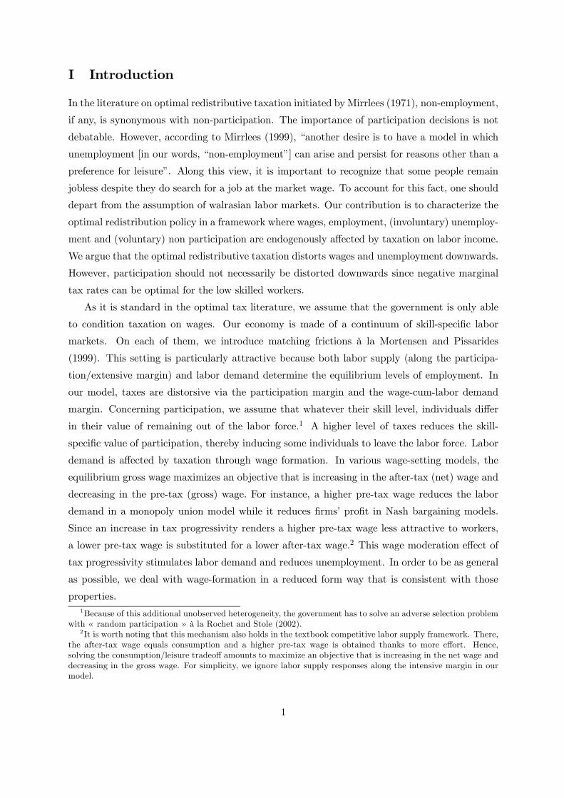
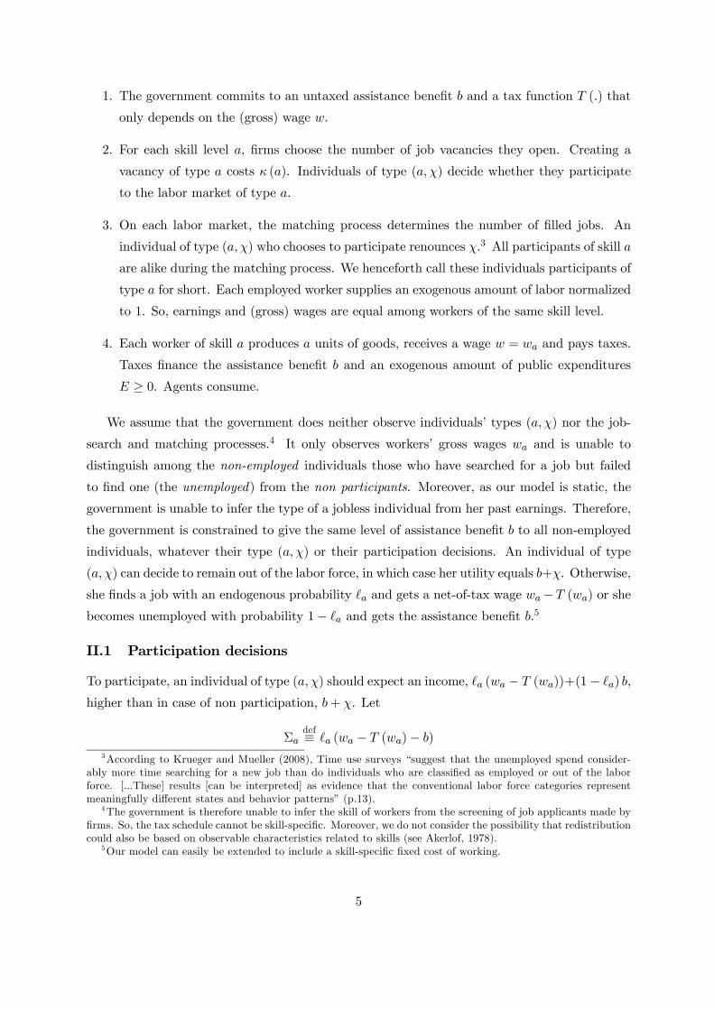
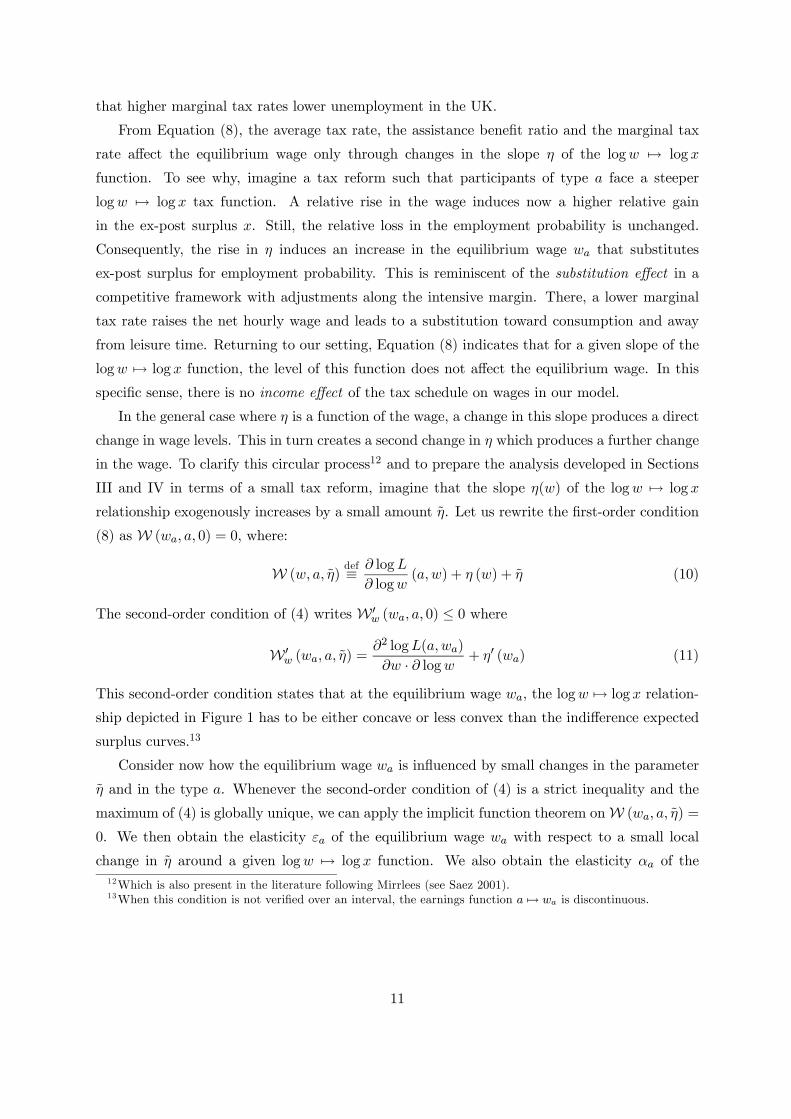
of the tax/benefit system needed to fix the equilibrium wage. Figure 1 displays indifference

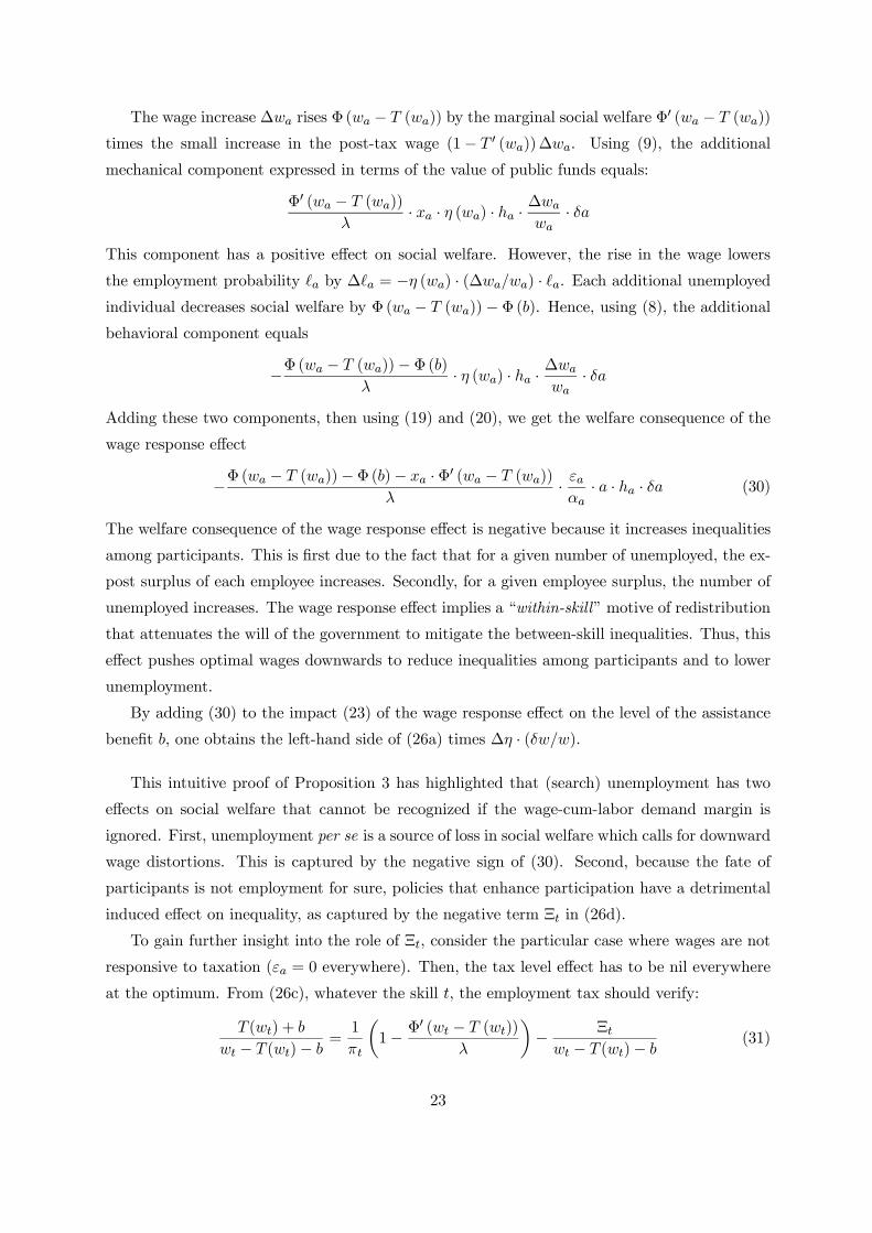
expected surplus curves. The equation of these indifference curves can be written as log x =

constant− logL(a,w). From (2) and (6), these curves are increasing and convex. The solution

to Program (4) then consists in choosing the highest indifference curve taking the relationship

between log x and logw into account. In case of differentiability, this amounts to choosing the

highest indifference curve tangent to the logw 7→ log x = log (w − T (w)− b) schedule. Thefirst-order condition (8) combined with (9) expresses this tangency condition.

log(w)

log(x)

log(wa)

log(xa) η(wa)

log(w–T(w)–b)

log(L(a,w)) + log(x) = constant

Figure 1: The choice of the wage for a type a match.

For comparative static purposes, consider for a while the average tax rate T (wa) /wa, the

assistance benefit ratio b/wa and the marginal tax rate T 0 (wa) as parameters. So, η(wa) is

provisionally a parameter, too. Under Condition (6), Equations (8) and (9) imply that the

equilibrium wage wa (thereby the unemployment rate 1−L (a,wa)) increases with the average taxrate and the assistance benefit ratio and decreases with the marginal tax rate. These properties

are standard in the equilibrium unemployment literature. They hold under monopoly unions

(Hersoug 1984), right-to-manage bargaining (Lockwood and Manning 1993), efficiency wages

with continuous effort (Pisauro 1991) or matching models with Nash bargaining (Pissarides

1998). Sørensen (1997) and Røed and Strøm (2002) provide some empirical evidence in favor

of the wage-moderating effect of higher marginal tax rates. In addition, Manning (1993) finds

10

that higher marginal tax rates lower unemployment in the UK.

From Equation (8), the average tax rate, the assistance benefit ratio and the marginal tax

rate affect the equilibrium wage only through changes in the slope η of the logw 7→ log x

function. To see why, imagine a tax reform such that participants of type a face a steeper

logw 7→ log x tax function. A relative rise in the wage induces now a higher relative gain

in the ex-post surplus x. Still, the relative loss in the employment probability is unchanged.

Consequently, the rise in η induces an increase in the equilibrium wage wa that substitutes

ex-post surplus for employment probability. This is reminiscent of the substitution effect in a

competitive framework with adjustments along the intensive margin. There, a lower marginal

tax rate raises the net hourly wage and leads to a substitution toward consumption and away

from leisure time. Returning to our setting, Equation (8) indicates that for a given slope of the

logw 7→ log x function, the level of this function does not affect the equilibrium wage. In this

specific sense, there is no income effect of the tax schedule on wages in our model.

In the general case where η is a function of the wage, a change in this slope produces a direct

change in wage levels. This in turn creates a second change in η which produces a further change

in the wage. To clarify this circular process12 and to prepare the analysis developed in Sections

III and IV in terms of a small tax reform, imagine that the slope η(w) of the logw 7→ log x

relationship exogenously increases by a small amount η. Let us rewrite the first-order condition

(8) as W (wa, a, 0) = 0, where:

W (w, a, η)def≡ ∂ logL

∂ logw(a,w) + η (w) + η (10)

The second-order condition of (4) writes W 0w (wa, a, 0) ≤ 0 where

W 0w (wa, a, η) =

∂2 logL(a,wa)

∂w · ∂ logw + η0 (wa) (11)

This second-order condition states that at the equilibrium wage wa, the logw 7→ log x relation-

ship depicted in Figure 1 has to be either concave or less convex than the indifference expected

surplus curves.13

Consider now how the equilibrium wage wa is influenced by small changes in the parameter

η and in the type a. Whenever the second-order condition of (4) is a strict inequality and the

maximum of (4) is globally unique, we can apply the implicit function theorem onW (wa, a, η) =

0. We then obtain the elasticity εa of the equilibrium wage wa with respect to a small local

change in η around a given logw 7→ log x function. We also obtain the elasticity αa of the12Which is also present in the literature following Mirrlees (see Saez 2001).13When this condition is not verified over an interval, the earnings function a 7→ wa is discontinuous.

11

equilibrium wage wa with respect to the skill level a along the same logw 7→ log x function:

εadef≡ η (wa)

wa· ∂wa∂η

= − η (wa)

wa · W 0w (wa, a, 0)

> 0 (12a)

αadef≡ a

wa

∂wa∂a

= − a

wa · W 0w (wa, a, 0)

· ∂2 logL

∂a∂w(a,wa) > 0 (12b)

These elasticities are in general endogenous and in particular they depend on the curvature term

η0 (wa) in W 0w. This is because a change in wage ∆wa, that is either caused by a change in η or

in a, induces a change in η (wa) that equals η0 (wa)∆wa and a further change in the wage. This

is at the origin of a circular process captured by the term η0 (wa) in W 0w. However, as will be

clear in Sections III and IV, only the ratio εa/αa enters the optimality conditions and this ratio

does not depend on η0 (wa) but only on a and wa. The positive signs of εa and αa follow from

the strict second-order condition W 0w< 0 and from (7).

In addition to its effect on wage and unemployment through η (.), taxation also influences

participation decisions. To isolate this effect, consider a tax reform that rises log (w − T (w)− b)by a constant amount for all w so that η (w) is kept unchanged. Such a tax reform does neither

change the wage level, nor the employment probability. However, the employment tax T (wa)+b

is reduced and hence the surplus Σa an agent of type a can expect from participation increases.

Therefore, such a reform increases the participation rate G (a,Σa), thereby the employment rate

L (a,wa) ·G (a,Σa). The magnitude of this behavioral response is captured by the elasticity πadefined in (1). In sum, the income effect affects the participation margin and not the wage-cum-

labor demand margin.

II.7 Government’s objective and incentive constraints

The government cares about inequalities measured in terms of the net income that accrues to

agents according to their status on the labor market. Section III is devoted to the Maximin

(Rawlsian) objective. There, the government values only the utility of the least well-off. Un-

employed individuals are the least well-off because they get b, which is always lower than the

workers’ and non participants’ utility levels, which are respectively equal to w−T (w) and b+χ.

Section IV considers the following general Bergson-Samuelson social welfare function:a1Za0

⎧⎨⎩[L (a,wa)Φ (wa − T (wa)) + (1− L (a,wa))Φ (b)]G (a,Σa) ++∞ZΣa

Φ (b+ χ) g (a,χ) dχ

⎫⎬⎭ f (a) da(13)

where Φ0 (.) > 0 > Φ00 (.). The “pure” (Benthamite) utilitarian case sums the utility levels of

all individuals and corresponds to the case where Φ (.) is linear. The stronger the concavity of

Φ (.), the more averse to inequality is the government.

The government does not observe the productivity of each job but only the wage negotiated

by each worker-firm pair. So, it aims at maximizing its objective subject to the budget constraint

12

(5) and the choices made by the agents. Since a worker-firm pair maximizes an objective

L (a,w) (w − T (w)− b) that is increasing in the ex-post surplus x = w−T (w)−b and decreasingin gross wages, the government’s self-selection problem can be viewed as one where worker-firms

pairs of skill a are agents with an objective L (a,w) x. Therefore, according to the taxation

principle (Hammond 1979, Rochet 1985 and Guesnerie 1995), the set of allocations induced by

a tax/benefit system {T (.) , b} through the wage-setting equations (4) corresponds to the set ofincentive-compatible allocations

¡b, {wa, xa,Σa}a∈[a0,a1]

¢that verify:

∀¡a, a0

¢∈ [a0, a1]2 Σa ≡ L (a,wa) xa ≥ L (a,wa0) xa0 (14)

This condition expresses that a firm-worker pair of type a chooses the bundle (wa, xa) rather

than any other bundle (wa0 , xa0) designed for firm-worker pairs of another type a0. From (7),

the strict single-crossing condition holds. Hence, (14) is equivalent to the envelope condition

associated to (4)

Σa = Σa ·∂ logL

∂a(a,wa) (15)

and the monotonicity requirement that the wage wa is a nondecreasing function of the skill level

a. Following Mirrlees (1971), it is much more convenient to solve the government’s problem in

terms of allocations.14 Contrary to HLPV, and in the spirit of Saez (2001), we will express the

optimality conditions in terms of behavioral elasticities that can be easily interpreted for applied

purposes.

III The Maximin case

Let ha = L (a,wa) G (a,Σa) f (a) denote the (endogenous) mass of workers of skill a. We obtain

(see Appendix C):

Proposition 1 For any skill level a ∈ [a0, a1], the maximin-optimal tax schedule verifies:1− η (wa)

η (wa)· εaαa· wa · a · ha = Za and Za0 = 0 (16a)

Za =

a1Za

[xt − πt (T (wt) + b)]ht · dt, (16b)

where T (wt) + b = wt − xt and since η (w) = ∂ log (w − T (w)− b) /∂ logw, xt verifies:

∀t, u log xt = log xu +

wtZwu

η(w) d logw

14We assume the existence of an optimal allocation a 7→ (wa, xa) that is continuous, differentiable and increasing.Existence and continuity are usual regularity assumptions (see e.g. Mirrlees 1971, 1976 or Guesnerie and Laffont1984). The monotonicity assumption means that we rule out bunching. We verify in the simulations thatthe monotonicity requirement is verified along the optimum. The differentiability assumption is made only forconvenience. It implies that the tax schedule T (.) is almost everywhere differentiable in the wage.

13

In Proposition 1, the elasticities πa of the participation rate, εa of the wage with respect to

η and αa of the wage with respect to the skill level a are respectively given by (1), (12a) and

(12b) along the optimal allocation. Moreover, wa is determined by the wage-setting condition

(8).

III.1 Intuitive proof of Proposition 1

The resolution in terms of incentive-compatible allocations enables a rigorous derivation. How-

ever, this method does not provide much economic intuition. So, we propose here an intuitive

proof in the spirit of Saez (2001). Recall that in our model, it is much more convenient to think

of the tax schedule as a function that associates the log of the ex-post surplus to the log of the

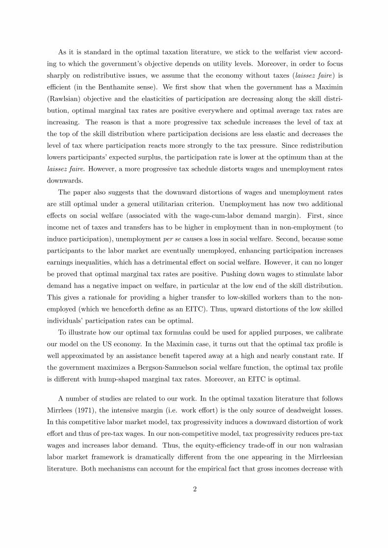
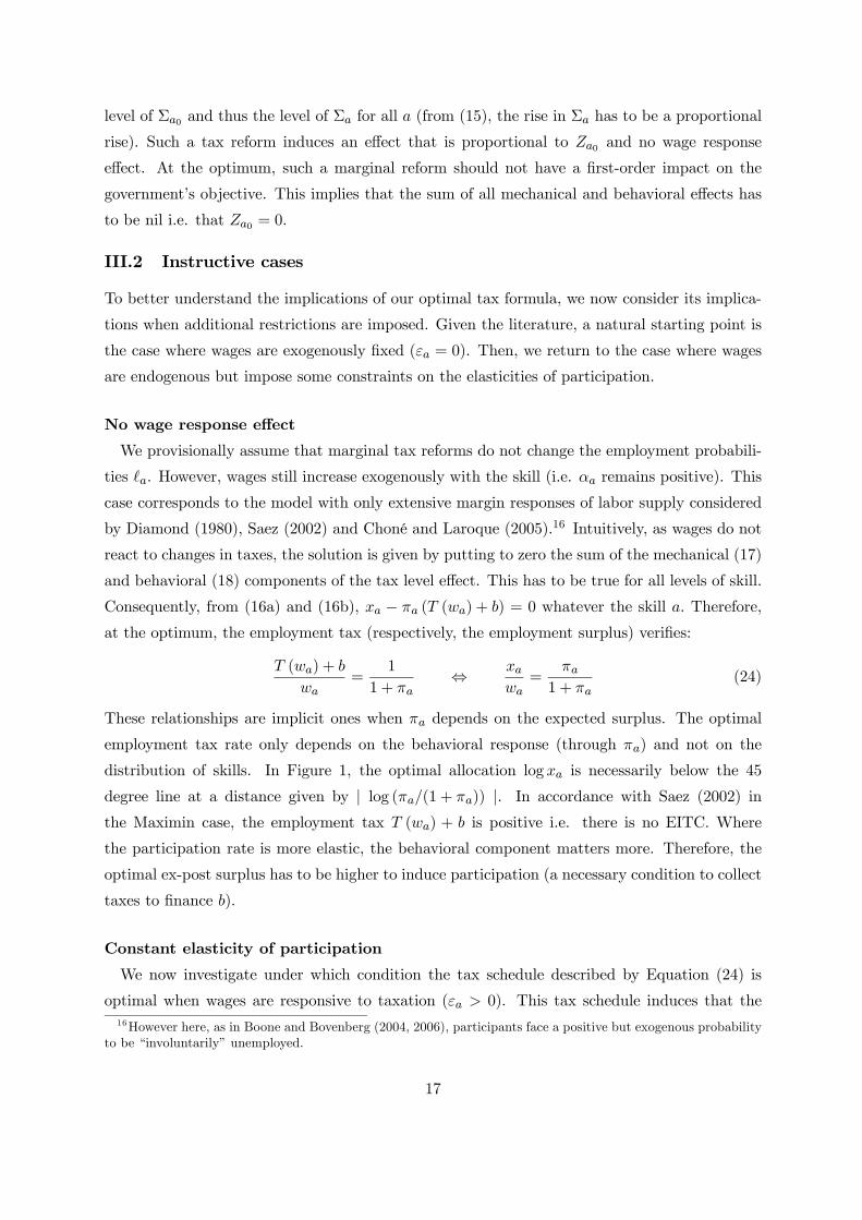
wage. We consider the effect of the following small tax reform around the optimum depicted

in Figure 2. The slope η(w) of logw 7→ log x is marginally increased by η = ∆η for wages

in the small interval [wa − δw,wa].15 We take ∆η sufficiently small compared to δw, so that

bunching or gaps in the wage distribution around wa− δw or wa induced by the tax reform can

be neglected. This reform has two effects on the government’s objective (5). There is first a tax

level effect that concerns individuals of skill t above a. Those of them who are employed thus

receive a wage wt above wa. Second, there is a wage response effect. It takes place for those

whose wages lie in the [wa − δw,wa] interval.

log(w)

log(x) = log(w–T(w)– b)

log(wa-δw) log(wa)

Δη > 0

Tax level effect, due toΔxt/xt = Δη × (δw/w)

δlog(w) = δw/w

Wage response effect, due to Δwa/wa = εa × (Δη/η) > 0

Before reform scheduleAfter reform schedule

Figure 2: The tax reform

15The reasoning below will be entirely developed in terms of this local change in η. For the reader interestedby the implementation of such a reform, the small local increase ∆η would be the result of a small decline in themarginal tax rate, the level of the average employment tax being kept locally constant. Above wa, the inducedreduction in the employment tax should be compensated for by an appropriate reduction of the marginal tax rateto keep η unchanged.

14

Wage response effect Tax Level effectDue to: ∆wa/wa = εa (∆η/η) ∆xt/xt = ∆η (δw/w)

Mechanical Component T (wa) increases by T (wt) decreases byT 0 (wa) ∆wa ∆T (wt) = −∆xt

Behavioral component Labor demand is reduced by Participation rates increase by:∆`a/`a = −η (wa) (∆wa/wa) ∆Gt/Gt = πt (∆xt/xt)

Table 1: Summary of the different components of the effects of the tax reform

The tax level effect

Consider skill levels t above a. Since η (.) is unchanged around wt, the equilibrium wage wt is

unaffected by the tax reform, and so is the employment probability L (t, wt). From (9), the tax

reform increases the ex-post surplus xt = wt − T (wt)− b by∆xtxt

= ∆η · δww

(see Figure 2). The consequence of this rise of (the log of) the ex-post surplus can be decomposed

into a mechanical component and a behavioral component through a change in the participation

decisions (see Table 1).

The rise in xt corresponds to a reduction in the employment tax level T (wt) + b such that

∆ (T (wt) + b) = −xt · ∆η · (δw/w). Since there are ht workers of type t, the mechanical

component of the tax level effect at skill level t equals:

−xt · ht ·∆η ·δw

w(17)

Consider now the participation decisions of individuals of skill t above a. From (3), since

their employment probability is unchanged, their expected surplus increases by the same relative

amount ∆Σt/Σt = ∆η · (δw/w) as their ex-post surplus xt. According to (1) the number ofemployed individuals of type t thus increases by πt ·ht ·∆η ·(δw/w). For each of these additionalemployed individuals, the government receives T (wt) + b additional employment taxes. Hence,

the behavioral component of the tax level effect at skill level t equals:

πt · (T (wt) + b) · ht ·∆η ·δw

w(18)

From (16b), the sum of the mechanical and behavioral components over all skill levels t

above a gives the tax level effect. It equals −Za ·∆η · (δw/w).

The wage response effect

This effect concerns individuals whose skill level is such that their wage in case of employ-

ment lies in the interval [wa − δw,wa]. Let [a− δa, a] be the corresponding interval of the skill

distribution. From (12b), one has

δa =a

αa· δww

(19)

15

Therefore, the number of agents concerned by this effect is (a/αa) f (a) (δw/w).

Due to the small tax reform, those employed face a more increasing logw 7→ log x tax

schedule. The tax reform thus induces a wage increase ∆wa that substitutes ex-post surplus for

employment probability. From (12a), one has

∆wawa

=εa

η (wa)·∆η (20)

Since the equilibrium wage maximizes participants’ ex-post surplus Σa, the tax reform has only

a second-order effect on Σa and thereby on the participation rate of these individuals. The wage

response effect can be decomposed into a mechanical component and a behavioral component

through a change in the labor demand decisions (see Table 1).

The wage increase ∆wa changes the employment tax paid by T 0 (wa) ·∆wa. From (9), one

gets 1− T 0 (wa) = xa · η(wa)/wa, so

∆ (T (wa) + b) = T0 (wa) ·∆wa = [(1− η (wa))wa + η (wa) (T (wa) + b)]

∆wawa

(21)

Multiplying the last term by the number of employed individuals ha gives the mechanical com-

ponent of the wage response effect.

The wage increase ∆wa also induces a reduction in the employment probability L (a,wa).

Given (8), the fraction of employed among participants is decreased by:

∆L (a,wa) = −η (wa)∆wawa

L (a,wa) (22)

When an additional participant of type a finds a job, the government levies additional taxes

T (wa) and saves b. Multiplying the employment tax T (wa) + b by ∆`a times the number of

participants G (a,Σa) f (a) δa gives the behavioral component of the wage response effect. The

sum of these two components equals

∆ [(T (wa) + b) · L (a,wa)] ·G (a,Σa) · f (a) · δa = (1− η (wa))wa · ha ·∆wawa

· δa

Given (19), (20) and the last expression, the total wage response effect on the interval

[wa − δw,wa] equals1− η (wa)

η (wa)· εaαa· a · wa · ha ·∆η ·

δw

w(23)

The wage response effect can be either positive or negative. From Subsection II.5, recall that

the laissez-faire value of the wage is efficient. If η (wa) < 1, (resp. η (wa) > 1) the wage is below

(above) its laissez-faire value, hence it is inefficiently low (high). Adding the wage response and

the tax level effects gives (16a) in Proposition 1.

To obtain Za0 = 0 in (16a), consider a tax reform that rises log (w − T (w)− b) by a constantamount for all w, so that η (w) is kept unchanged. This reform is implemented by increasing the

16

level of Σa0 and thus the level of Σa for all a (from (15), the rise in Σa has to be a proportional

rise). Such a tax reform induces an effect that is proportional to Za0 and no wage response

effect. At the optimum, such a marginal reform should not have a first-order impact on the

government’s objective. This implies that the sum of all mechanical and behavioral effects has

to be nil i.e. that Za0 = 0.

III.2 Instructive cases

To better understand the implications of our optimal tax formula, we now consider its implica-

tions when additional restrictions are imposed. Given the literature, a natural starting point is

the case where wages are exogenously fixed (εa = 0). Then, we return to the case where wages

are endogenous but impose some constraints on the elasticities of participation.

No wage response effect

We provisionally assume that marginal tax reforms do not change the employment probabili-

ties `a. However, wages still increase exogenously with the skill (i.e. αa remains positive). This

case corresponds to the model with only extensive margin responses of labor supply considered

by Diamond (1980), Saez (2002) and Choné and Laroque (2005).16 Intuitively, as wages do not

react to changes in taxes, the solution is given by putting to zero the sum of the mechanical (17)

and behavioral (18) components of the tax level effect. This has to be true for all levels of skill.

Consequently, from (16a) and (16b), xa − πa (T (wa) + b) = 0 whatever the skill a. Therefore,

at the optimum, the employment tax (respectively, the employment surplus) verifies:

T (wa) + b

wa=

1

1 + πa⇔ xa

wa=

πa1 + πa

(24)

These relationships are implicit ones when πa depends on the expected surplus. The optimal

employment tax rate only depends on the behavioral response (through πa) and not on the

distribution of skills. In Figure 1, the optimal allocation log xa is necessarily below the 45

degree line at a distance given by | log (πa/(1 + πa)) |. In accordance with Saez (2002) in

the Maximin case, the employment tax T (wa) + b is positive i.e. there is no EITC. Where

the participation rate is more elastic, the behavioral component matters more. Therefore, the

optimal ex-post surplus has to be higher to induce participation (a necessary condition to collect

taxes to finance b).

Constant elasticity of participation

We now investigate under which condition the tax schedule described by Equation (24) is

optimal when wages are responsive to taxation (εa > 0). This tax schedule induces that the16However here, as in Boone and Bovenberg (2004, 2006), participants face a positive but exogenous probability

to be “involuntarily” unemployed.

17

aggregate tax level effect Za equals 0 everywhere along the skill distribution (See Equation 16b).

Therefore, the wage response effect has to be nil everywhere. So, according to (16a), the slope

η of the logw 7→ log x function has to equal 1 everywhere. Therefore, from (9), the ratio xa/wa

has to be constant. This is consistent with (24) only when the elasticity of participation πa is

the same for all skill levels at the optimum.

Reciprocally, assume that the elasticity of participation is constant and consider the tax

policy defined by an employment tax T (w) + b that equals w/ (1 + π) for all wage levels w. In

this case, the mechanical (17) and behavioral (18) components of the tax level effect sum to 0

at each skill level. Moreover, from (9), this policy induces η (w) to be constant and equal to 1,

so wages are not distorted and the wage response effect is nil everywhere. Therefore, this policy

satisfies the conditions in Proposition 1.

Decreasing elasticity of participation

We think that the assumption of a constant elasticity of participation is not plausible. This

judgment is based on empirical evidence that suggests a decreasing profile with a (see the

empirical evidence in Juhn et alii, 1991, Immervoll et alii, 2007 and Meghir and Phillips, 2008).

Of course, the profile of πa at the optimum can be different from the one observed in the current

economy. Still, the two following examples suggest that the slopes of πa in the current economy

and at the optimum might have the same signs.

The first example specifies

G (a,Σ) = A (a) · Σπa with A (a) > 0 and πa > 0 (25)

Then, provided that Σa ≤ (A (a))−1/πa , the participation rates remain within (0, 1) and the

elasticity of participation is exogenous and equals πa.

The second example is based on the following three assumptions. Firstly, the value of non

market activities χ is distributed indepentently of the skill level a. Thus, G (., .) does not depend

on a. Secondly, the distribution of χ is such that Σ 7→ Σg (Σ) /G (Σ) is a decreasing function.This is for instance the case if χ follows the exponentional distribution G (Σ) = 1− exp (−σ1Σ)or the Pareto distribution G (Σ) = 1 − σ0Σ

−σ1 , both with σ0 > 0 and σ1 > 0. Thirdly, for

a given wage level, the employment probability increases in the skill level (See Footnote 10).

Then, since Σa > 0 from (15), πa = Σag (Σa) /G (Σa) is decreasing in the skill level a in the

current economy and at the optimum.

When the elasticity of participation is decreasing in the skill level along the optimum, we

find:

Proposition 2 If everywhere along the Maximin optimum one has πa < 0, then

18

i) wa < wLFa and L (a,wa) > L¡a,wLFa

¢for all a in (a0, a1), while wa0 = wLFa0 , L (a0, wa0) =

L¡a0, w

LFa0

¢, wa1 = w

LFa1 and L (a1, wa1) = L

¡a,wLFa1

¢.

ii) Compared to the laissez faire, the participation rates are distorted downwards.

iii) The average tax rate T (w) /w is an increasing function of the wage and the marginal tax

rates T 0 (w) are positive everywhere. The in-work benefit (if any) at the bottom-end of the

distribution is lower than the assistance benefit −T (wa0) < b.

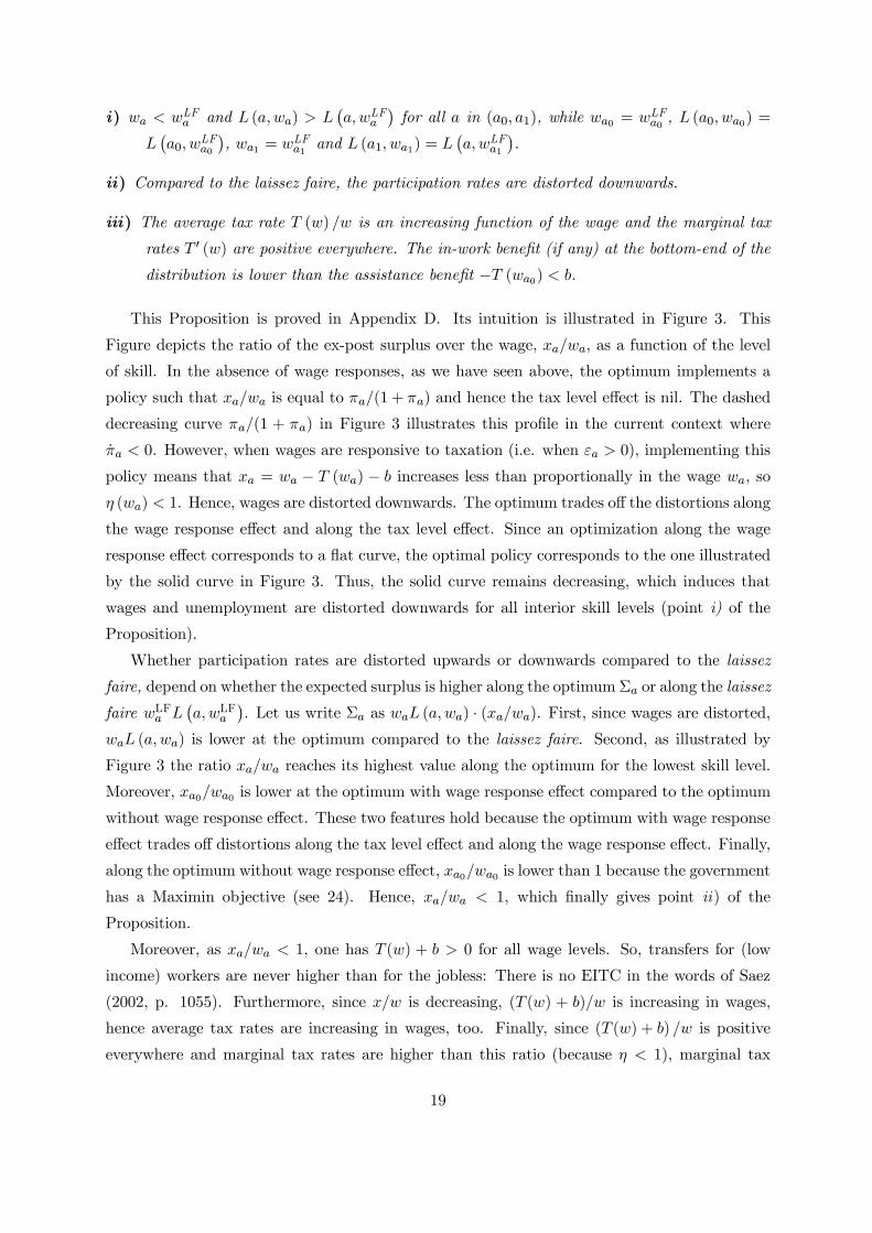
This Proposition is proved in Appendix D. Its intuition is illustrated in Figure 3. This

Figure depicts the ratio of the ex-post surplus over the wage, xa/wa, as a function of the level

of skill. In the absence of wage responses, as we have seen above, the optimum implements a

policy such that xa/wa is equal to πa/(1 + πa) and hence the tax level effect is nil. The dashed

decreasing curve πa/(1 + πa) in Figure 3 illustrates this profile in the current context where

πa < 0. However, when wages are responsive to taxation (i.e. when εa > 0), implementing this

policy means that xa = wa − T (wa) − b increases less than proportionally in the wage wa, soη (wa) < 1. Hence, wages are distorted downwards. The optimum trades off the distortions along

the wage response effect and along the tax level effect. Since an optimization along the wage

response effect corresponds to a flat curve, the optimal policy corresponds to the one illustrated

by the solid curve in Figure 3. Thus, the solid curve remains decreasing, which induces that

wages and unemployment are distorted downwards for all interior skill levels (point i) of the

Proposition).

Whether participation rates are distorted upwards or downwards compared to the laissez

faire, depend on whether the expected surplus is higher along the optimum Σa or along the laissez

faire wLFa L¡a,wLFa

¢. Let us write Σa as waL (a,wa) · (xa/wa). First, since wages are distorted,

waL (a,wa) is lower at the optimum compared to the laissez faire. Second, as illustrated by

Figure 3 the ratio xa/wa reaches its highest value along the optimum for the lowest skill level.

Moreover, xa0/wa0 is lower at the optimum with wage response effect compared to the optimum

without wage response effect. These two features hold because the optimum with wage response

effect trades off distortions along the tax level effect and along the wage response effect. Finally,

along the optimum without wage response effect, xa0/wa0 is lower than 1 because the government

has a Maximin objective (see 24). Hence, xa/wa < 1, which finally gives point ii) of the

Proposition.

Moreover, as xa/wa < 1, one has T (w) + b > 0 for all wage levels. So, transfers for (low

income) workers are never higher than for the jobless: There is no EITC in the words of Saez

(2002, p. 1055). Furthermore, since x/w is decreasing, (T (w) + b)/w is increasing in wages,

hence average tax rates are increasing in wages, too. Finally, since (T (w) + b) /w is positive

everywhere and marginal tax rates are higher than this ratio (because η < 1), marginal tax

19

rates are positive everywhere, including at the boundaries of the skill distribution (Point iii) of

the Proposition).

a

xa/wa

πa/(1+πa)

Optimum

Figure 3: Intuition of Proposition 2

Most of the properties put forward in Proposition 2 are in line with HLPV. There, the value

χ of non market activities is identical for all types. Therefore, a unique threshold level of skill

separates nonparticipants from participants. The elasticity of participation is thus infinite at

the threshold and then nil for all participating types, which is a very specific decreasing a 7→ πa

relationship. In this sense, under a Maximin criterion, the results of HPLV are generalized.

However, an exception concerns the distorsion of the labor demand of the low skilled agents.

Our transversality condition Za0 = 0 implies that the lowest level of expected surplus Σa0is optimized. Our model is thus characterized by a no-distorsion at the bottom of the skill

distribution property (provided that there is no bunching, a case that never occurs in our

numerical experiments). Since η (wa0) = 1, the wage-cum-labor demand margin is not distorted

for the lowest participating skill. This result is in contrast with HLPV. There, the government

can not optimize along the surplus of the lowest participating skill level because of binding

participation constraints. Thus, the governement distorts the labor demand margin at the

bottom of the participating skill level distribution.

Moreover, Proposition 2 is in contrast to the literature initiated by Mirrlees (1971). In this

framework, optimal marginal tax rates are positive whenever the government values redistrib-

ution (see e.g. the discussion in Choné and Laroque 2007). Therefore, labor supply, thereby

the volume of labor used, are distorted downwards while in our case the volume of labor among

participants is distorted upwards. However, Point ii) reduces this contrast. In our model, par-

ticipation is distorted downwards. Consequently, the net effect on aggregate employment is

ambiguous.

Finally, the property according to which employment tax rates are always positive is also

obtained in the models of Saez (2002) and Choné and Laroque (2005) where participation

20

margins are central. Saez (2002) however emphasizes that this result only holds under a Maximin

criterion. With a more general objective, he finds that the optimal income tax schedule is

typically characterized by a negative employment tax at the bottom provided that labor supply

responses along the extensive margin are high enough compared to responses along the intensive

margin.

IV The general utilitarian case

Under the general social objective (13), Appendix E shows that the optimum verifies (recall that

`a = L (a,wa) and ha = `a G (a,Σa) f (a)):

Proposition 3 For any skill level a ∈ [a0, a1], the optimal tax schedule verifies:µ1− η (wa)

η (wa)· wa −

Φ (wa − T (wa))−Φ (b)− xa · Φ0 (wa − T (wa))λ

¶· εaαa· a · ha = Za (26a)

Za0 = 0 (26b)

where Za =

a1Za

½µ1− Φ

0 (wt − T (wt))λ

¶xt − πt [T (wt) + b+ Ξt]

¾ht · dt (26c)

and Ξt =`t ·Φ (wt − T (wt)) + (1− `t)Φ (b)− Φ (b+Σt)

λ · `t, (26d)

in which the positive Lagrange multiplier associated to the budget constraint (5), λ, verifies

λ =

a1Za0

⎧⎨⎩`aG (.)Φ0 (wa − T (wa)) + (1− `a)G (.)Φ0 (b) ++∞ZΣa

Φ0 (b+ χ) g (a,χ) dχ

⎫⎬⎭ f (a) da(27)

We now explain how to extend the intuitive proof of Section III. Equation (27) defines the

marginal social value of public funds, λ. It is obtained by a unit increase in E financed by

a unit decrease in b holding w 7→ w − T (w) − b constant. Next, we consider again the smalltax reform depicted in Figure 2. This tax reform has a tax level effect and a wage response

effect, each of them being decomposed into mechanical and behavioral components (see Table

1). In the Maximin case, these components only capture the impact on the least well-off (i.e.

on additional tax receipts to finance the assistance benefit b). Now, the government also values

how the utility levels of all other economic agents are affected by the tax reform. To make the

formula comparable, we divide these additional impacts by λ, so as to express them in terms of

the value of public funds. For each component, we now examine how the various components

are changed.

21

Tax level effect

The rise in the ex-post surplus xt increases the social welfare of the corresponding workers

by Φ0 (wt − T (wt)) /λ. Adding this welfare gain to the loss in tax receipts, the mechanicalcomponent of the tax level effect at skill level t equals

−µ1− Φ

0 (wt − T (wt))λ

¶· xt · ht ·∆η ·

δw

w(28)

instead of (17). The integral of relation (28) over the skill distribution above a corresponds to the

“between-skill” motive of redistribution. Since λ averages marginal social welfare over the whole

population and Φ is concave, the term in parentheses is positive for most workers. This means

that the rise in xt is in general detrimental to the government’s objective. This might however

not be true for workers with sufficiently low earnings. In this case, the government would increase

the ex-post surplus with respect to the laissez faire for these workers. In opposition to the case

where the government has a Maximin objective, this would imply a rise in the participation rate

of the less skilled workers.

As far as the behavioral component is concerned, consider individuals of type t who are

induced to participate by the tax reform. Their expected utility levels only change by a second-

order amount. However, this change in participation decisions increases inequalities because

participants’ income is different whether they get a job or not. The inequality-averse govern-

ment values this by (`t · Φ (wt − T (wt)) + (1− `t)Φ (b)−Φ (b+Σt)) /λ, which equals `t ·Ξt (byDefinition (26d)) and is negative. So, the behavioral component of the tax level effect at skill

level t equals

πt {T (wt) + b+ Ξt} · ht ·∆η ·δw

w(29)

instead of (18). From (26c), the sum of the mechanical and behavioral components over all skill

levels t above a equals −∆η · (δw/w) · Za. It is hard to draw clear conclusions about the valueof Za. Still, two opposite effects are specific to the general utilitarian case. Compared to the

Maximin, raising the ex-post surplus for skills above a is now less detrimental for the social

welfare in terms of the mechanical component but the welfare gain of additional participants is

less important because of the negative induced impact of increased inequalities on social welfare

(the negative Ξt term).

Wage response effect

In addition to its impact on b through the tax receipts (described in (21) and (22)), the wage

response effect has also a direct influence on social welfare through a change in the expected

social welfare of participants of type a, `aΦ (wa − T (wa)) + (1− `a)Φ (b). Holding b constant,a mechanical and a behavioral component should again be distinguished.

22

The wage increase ∆wa rises Φ (wa − T (wa)) by the marginal social welfare Φ0 (wa − T (wa))times the small increase in the post-tax wage (1− T 0 (wa))∆wa. Using (9), the additional

mechanical component expressed in terms of the value of public funds equals:

Φ0 (wa − T (wa))λ

· xa · η (wa) · ha ·∆wawa

· δa

This component has a positive effect on social welfare. However, the rise in the wage lowers

the employment probability `a by ∆`a = −η (wa) · (∆wa/wa) · `a. Each additional unemployedindividual decreases social welfare by Φ (wa − T (wa))− Φ (b). Hence, using (8), the additionalbehavioral component equals

−Φ (wa − T (wa))− Φ (b)λ

· η (wa) · ha ·∆wawa

· δa

Adding these two components, then using (19) and (20), we get the welfare consequence of the

wage response effect

−Φ (wa − T (wa))− Φ (b)− xa · Φ0 (wa − T (wa))

λ· εaαa· a · ha · δa (30)

The welfare consequence of the wage response effect is negative because it increases inequalities

among participants. This is first due to the fact that for a given number of unemployed, the ex-

post surplus of each employee increases. Secondly, for a given employee surplus, the number of

unemployed increases. The wage response effect implies a “within-skill” motive of redistribution

that attenuates the will of the government to mitigate the between-skill inequalities. Thus, this

effect pushes optimal wages downwards to reduce inequalities among participants and to lower

unemployment.

By adding (30) to the impact (23) of the wage response effect on the level of the assistance

benefit b, one obtains the left-hand side of (26a) times ∆η · (δw/w).

This intuitive proof of Proposition 3 has highlighted that (search) unemployment has two

effects on social welfare that cannot be recognized if the wage-cum-labor demand margin is

ignored. First, unemployment per se is a source of loss in social welfare which calls for downward

wage distortions. This is captured by the negative sign of (30). Second, because the fate of

participants is not employment for sure, policies that enhance participation have a detrimental

induced effect on inequality, as captured by the negative term Ξt in (26d).

To gain further insight into the role of Ξt, consider the particular case where wages are not

responsive to taxation (εa = 0 everywhere). Then, the tax level effect has to be nil everywhere

at the optimum. From (26c), whatever the skill t, the employment tax should verify:

T (wt) + b

wt − T (wt)− b=1

πt

µ1− Φ

0 (wt − T (wt))λ

¶− Ξtwt − T (wt)− b

(31)

23

If Ξt was zero, Formula (31) would be identical to Expression (4) in Saez (2002). Then, if the

welfare of low skilled workers is highly valued by the government, i.e. if their ability and thus

wage is sufficiently low (i.e. such that Φ0 (wt − T (wt)) /λ > 1), the employment tax T (wt) + bshould be negative, meaning that transfers for low income workers, −T (wt), are higher thanfor the jobless. Now because of unemployment, inequalities between the agents induced to

participate by this policy are increased (since Ξt is negative). This reduces the willingness of

the government to redistribute to low income workers.

When wages are responsive to taxation, the only analytical result in the general utilitarian

case concerns wage distortions at both extremes of the skill distribution. There, as in the

Maximin case, the tax level effect is nil. Nevertheless, there is a reason to choose an inefficient

wage level. This is because unemployment reduces social welfare. To mitigate this effect, it is

worth distorting wages downwards at both extremes of the skill distribution.

Concerning the robustness of Proposition 2 obtained under a Maximin objective, we cannot

say whether nor when the two new terms in (28) and (29) change the sign of the tax level

effect. We can nevertheless make the following conjectures in line with this proposition. As far

as point i) is concerned, the government has now an additional incentive to reduce wages and

stimulate labor demand since the welfare impact of the wage response effect (30) is negative.

However, pushing wages downwards obviously reduces social welfare, and the more so as one

moves towards the low-end of the wage distribution. Therefore, compensating transfers for low-

skilled workers are expected. Numerical simulations are needed to throw some light on these

conjectures.

Before presenting the simulations, it is worth considering an alternative specification to the

government’s objective (13). First, this allows to better understand the role of government’s

aversion towards inequality among participants of the same skill level. Appendix ?? shows that

when the government is only concerned by redistribution between (a,χ) groups but not between

the unemployed and the employed of the type, the term Ξt in (29) and the term given by (30)

disappear from the optimal tax formula. The optimal tax schedule now verifies (16a) and

Za =

a1Za

½µ1− Φ

0 (wt − T (wt))λ

¶xt − πt [T (wt) + b]

¾ht · dt (32a)

λ =

a1Za0

⎧⎨⎩G (.)Φ0 (`a (wa − T (wa)) + (1− `a) b) ++∞ZΣa

Φ0 (b+ χ) g (a,χ) dχ

⎫⎬⎭ f (a) da (32b)

instead of Equations (26a)-(27). Therefore, only the mechanical component of the tax level effect

is changed with respect to our Maximin case (relation (28) replaces relation (17)). As already

mentioned, this component implies a reduction of the “between skill motive of redistribution”

compared to the Maximin case. Thus, the extent of redistribution and the distortions along the

24

wage-cum-labor demand margin are reduced compared to the Maximin case.

Second, this alternative social welfare criterion, also used in HLPV, allows to emphasize a

difference with respect to this paper. When εa = 0, since the term Ξt is equal to 0, one retrieves

again Expression (4) of Saez (2002). Thus, the employment tax might also be negative for the

lowest skill level agents. Heterogenous costs of participation might thus remove the property of

positive marginal tax rates found by HLPV. Thus, the difference in the results with HLPV are

not due to the objective function but to our more general treatment of the cost of participation.

V Simulations

To illustrate how our optimal tax formulae could be used for applied purposes, this section

proposes a calibration of our model based on the US economy. This enables us to compute

optimal income tax schedules that provide some numerical feel of the policy implications of our

analysis. As the underlying model remains stylized in several dimensions the following simulation

results should only be considered as illustrative.

V.1 Calibration

To avoid the complexity of interrelated participation decisions within families, we only consider

single adults in the US.17 In addition to the function Φ(.) for the Bergson-Samuelson criterion,

the structural primitives of the model are the density function of skills f(a), the cumulated

density function of non-market activities G(a,χ) and the labor demand function L (., .) (or the

matching function H(a, V, U) and vacancies costs κ(a) as explained in Section II.2). In order to

control the behavioral responses, we do not calibrate the parameters of the matching function

nor the a 7→ κ(a) function but specify the labor demand function. We take

logL (a,w) = B (a)− ε³ w

c · a´ 1

ε

Under this specification, the first-order condition (8) for the wage-setting program implies:

wa = c · a · (η (wa))ε (33)

Hence, along a tax schedule where logw 7→ log (w − T (w)− b) is linear, the behavioral elastici-ties εa and αa are exogenous.

Next, we roughly approximate the tax system that is applied to single adults without children

by a linear function T (w) = τ ·w+τ0 with τ = 25% and τ0 = −3000. The selection of a value ofb for the current economy determines whether η (w) is lower or larger than 1, and, consequently,

whether wages (and thus unemployment) are distorted upwards or downwards. As a benchmark17These are “primary individuals”, i.e. persons without children living alone or in households with adults who

are not their relatives. They are older than 16 and younger than 66.

25

and to be consistent with our theoretical analysis where taxes are used only to redistribute

income, we assume that wages are efficient in the current economy, so we take b = −τ0 = 3000.Since η is then constant, the elasticity αa of the wage with respect to the skill equals 1 in

the current economy (see 12b), as it would be the case in a perfectly competitive economy.

Moreover ε equals the elasticity of the wage with respect to η in the current economy (12a).

This elasticity also equals the compensated elasticity of wage with respect to 1−T 0.18 FollowingGruber and Saez (2002), estimates of the latter elasticity would lie between 0.2 and 0.4. We

take a conservative value ε = 0.1 in the benchmark calibration and conduct a sensitivity analysis

where ε = 0.2. We set c to 2/3, so that in the current economy, total wage income represents two

third of the total production. Finally, we use (33) and the distribution of weekly earnings of the

Current Population Survey of May 2007 to approximate a distribution of skills among employed

workers. Reexpressing variables in annual terms, the range of skills is [$3, 900; $218, 400].19 Using

a quadratic Kernel with a bandwidth of $63, 800 we get an approximation of L (a)G (a,Σa) f (a)

in the current economy which is depicted by the lowest curve in Figure 4.

To be able to infer relevant properties of the a 7→ πa relationship from observed elasticities, we

adopt the simplest specification of the cumulative distribution of non-market activities, namely

(25). So, the elasticity of participation varies exogenously with the level of skill. Because, to our

knowledge, the empirical literature does not provide any information about the concavity of the

function a 7→ πa, we assume the following simple declining profile πa = (πa0 − πa1)³a1−aa1−a0

´3+

πa1 . We set the elasticity at the bottom, πa0 , to 0.4 and the elasticity at the top, πa1 , to 0.2 in

the benchmark calibration and conduct sensitivity analysis. These elasticities are in line with

the evidence summarized by Immervoll et alii (2007) and Meghir and Phillips (2008).

We adjust the scale parameters B (a) of the labor demand function and A (a) of (25) to

generate some realistic properties of skill-specific unemployment and participation rates along

our approximation of the current economy. The profile of unemployment (resp. participation)

rates in the current economy is calibrated by a decreasing (increasing) function of a:20

1− `a = 0.035 +µa1 − aa1 − a0

¶40.045 and Ga = 0.31

Ã1−

µa1 − aa1 − a0

¶6!+ 0.58

In our approximation of the current economy, the mean unemployment rate is 5.1%, the mean

participation rate equals 80.3% and the mean elasticity of the participation rate equals 0.29.

Figure 4 depicts the calibrated skill distribution f (a),21 the distribution of skill among partici-

pants in the current economy Gaf (a) and the distribution of skills among employed individuals18For any compensated change in marginal tax rates, one has ∆η = ∆(1−T 0)

1−T 01−T 0

1−(T+b)/w =∆(1−T 0)1−T 0 · η.

19The data are collected for wage and salary workers. We ignore weekly earnings below 50$, which correspondsto the lowest 1.2% of the earnings distribution.20By approximating a by the educational attainment, our unemployment and participation rates for the whole

population, for a0 and a1 are in line with the CPS data in June 2007.21f(a) is deducted from the above approximation of `aGaf(a).and the calibrations of functions `a and Ga.

26

`aGaf (a). We compute the level of exogenous public expenditures E from the government’s bud-

0,E+00

1,E-06

2,E-06

3,E-06

4,E-06

5,E-06

6,E-06

7,E-06

8,E-06

9,E-06

1,E-05

0 50 000 100 000 150 000 200 000a

f (a )

G a f (a )

l a G a f (a )

Figure 4: Densities f (a), Gaf (a) and `aGaf (a) in the current economy.

get constraint (5). This leads to an amount E = $5, 636 per capita. In the Bergson-Samuelson

utilitarian case, we take Φ(y) = (y+E)1−σ/(1−σ), with σ = 0.2 in the benchmark. The exoge-nous public expenditures finances a public good that generates social utility that is considered

as a perfect substitute to private consumption under this specification.

V.2 The results in the benchmark

-20%

0%

20%

40%

60%

80%

0 20 000 40 000 60 000 80 000 100 000 120 000 140 000

w

Marginal Tax rates

Berson Samuelson optimum without wage response

Maximin Optimum

Bergson-Samuelson Optimum

Figure 5: Marginal Tax Rates under the benchmark calibration

Marginal tax rates are drawn in Figure 5. Under the Maximin, redistribution takes the

form of a Negative Income Tax (NIT) in the following sense: An assistance benefit close to

$14, 198 is taxed away at a high, and in this case nearly constant, marginal tax rate close to

80%. This figure appears to be very high. However, this result is close to Saez (2001) and is

due to the extreme aversion to inequality of a maximin government. With the more general

27

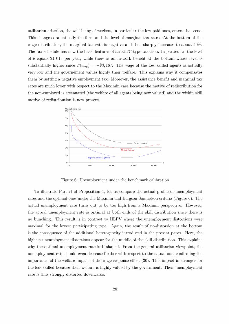
utilitarian criterion, the well-being of workers, in particular the low-paid ones, enters the scene.

This changes dramatically the form and the level of marginal tax rates. At the bottom of the

wage distribution, the marginal tax rate is negative and then sharply increases to about 40%.

The tax schedule has now the basic features of an EITC-type taxation. In particular, the level

of b equals $1, 015 per year, while there is an in-work benefit at the bottom whose level is

substantially higher since T (wa0) = −$3, 167. The wage of the low skilled agents is actually

very low and the governement values highly their welfare. This explains why it compensates

them by setting a negative employment tax. Moreover, the assistance benefit and marginal tax

rates are much lower with respect to the Maximin case because the motive of redistribution for

the non-employed is attenuated (the welfare of all agents being now valued) and the within skill

motive of redistribution is now present.

1%

2%

3%

4%

5%

6%

7%

8%

0 50 000 100 000 150 000 200 000a

Unemployment rate

Current economy

Maximin Optimum

Bergson-Samuelson Optimum

Figure 6: Unemployment under the benchmark calibration

To illustrate Part i) of Proposition 1, let us compare the actual profile of unemployment

rates and the optimal ones under the Maximin and Bergson-Samuelson criteria (Figure 6). The

actual unemployment rate turns out to be too high from a Maximin perspective. However,

the actual unemployment rate is optimal at both ends of the skill distribution since there is

no bunching. This result is in contrast to HLPV where the unemployment distortions were

maximal for the lowest participating type. Again, the result of no-distorsion at the bottom

is the consequence of the additional heterogeneity introduced in the present paper. Here, the

highest unemployment distortions appear for the middle of the skill distribution. This explains

why the optimal unemployment rate is U-shaped. From the general utilitarian viewpoint, the

unemployment rate should even decrease further with respect to the actual one, confirming the

importance of the welfare impact of the wage response effect (30). This impact in stronger for

the less skilled because their welfare is highly valued by the government. Their unemployment

rate is thus strongly distorted downwards.

28

40%

45%

50%

55%

60%

65%

70%

75%

80%

85%

90%

0 50 000 100 000 150 000 200 000

a

Participation rate

Current economy

Maximin Optimum

Bergson-Samuelson Optimum

Figure 7: Participation rates under the benchmark calibration.

As an illustration of Part ii) of Proposition 1, Figure 7 shows that a Maximin government

would accept a sharp decline in participation rates. In order to finance an important assistance

benefit, the government has to set high tax levels that decrease the ex-post surplus. Under the

more general utilitarian objective, optimal participation rates are higher for low skilled workers

and lower for high skilled workers. In order to reduce the unemployment rates of the low skilled,

the governement distorts highly their wages downwards. However, it compensates them by fixing

a negative employment tax. Their expected surplus is thus increased, thereby pushing up their

participation rates. Since unemployment rates are lower and participation rates are higher at

the bottom of the skill distribution, the tax-schedule is designed to boost low-skill employment.

V.3 Sensitivity analysis

Figure 5 depicts the optimal tax schedule if the reaction of wages to taxation is ignored (ε = 0).

Compared to our benchmark where ε = 0.1, the optimal profile is notably different. In particular,

the marginal tax rates are lower at the low-end of the wage distribution and higher for more

skilled agents since, by assumption, they do not have any effect on wages and unemployment .

So, this figure illustrates that taking into account or ignoring the wage-cum-labor demand margin

has substantial quantitative implications. Still, the assistance benefit and the tax reimbursement

at the bottom are close to those in the benchmark (so that the property T (wa0) + b < 0 still

holds).

If the sensitivity of wages to taxation is raised from ε = 0.1 towards ε = 0.2, the wage

response effects are reinforced. The Maximin optimum therefore implements a tax schedule

where the function w 7→ x (w) /w vary less (i.e. the solid curve of Figure 3 becomes flatter)

so as to prevent too important distortions along the wage-cum-labor demand margin. The tax

schedule becomes closer to a linear one, marginal tax rates vary less. The simulations displayed

29

in Figure 8 show that this also happens along the Bergson-Samuelson optimum.

-20%

0%

20%

40%

60%

80%

0 20 000 40 000 60 000 80 000 100 000 120 000 140 000w

Marginal Tax rates

Maximin Optimum Higher Epsilon

Bergson-Samuelson Optimum

Maximin Optimum

Bergson-Samuelson Optimum Higher Epsilon

Figure 8: Dotted curves: ε equals 0.2 instead of 0.1 (solid curves).

The other sensitivity analyses we conduct concern the calibration of the elasticity of partic-

ipation πa. First, we decrease by a constant amount of 0.05 all the shape of a 7→ πa. In the

Maximin case without wage response, Equation (24) implies that the government would choose

higher tax levels as participation responds less, so the dashed curve in Figure 3 is shifted down-

wards. Consequently, in the presence of wage response, the solid curve shifts downwards too.

Hence the Maximin optimum implements higher levels of (T (w) + b) /w and therefore higher

marginal tax rates. Figure 9 quantifies this mechanism. Once again, The Bergson-Samuelson

optimum is affected in a similar way compared to the Maximin optimum.

-20%

0%

20%

40%

60%

80%

0 20 000 40 000 60 000 80 000 100 000 120 000 140 000w

Marginal Tax Rates

Maximin Optimum Lower Pi

Bergson-Samuelson Optimum

Maximin Optimum

Bergson-Samuelson Optimum Lower Pi

Figure 9: Dashed curves: (πa0 ,πa1) equals (0.35; 0.15) instead of (0.4; 0.2) (solid curves)

Last, we change the elasticities of participation so that the relationship a 7→ πa is steeper

while keeping the average elasticity in the current economy almost constant. For that purpose,

we take (πa0 ,πa1) = (0.48; 0.13) instead of (0.4; 0.2). To understand the rise in marginal tax

30

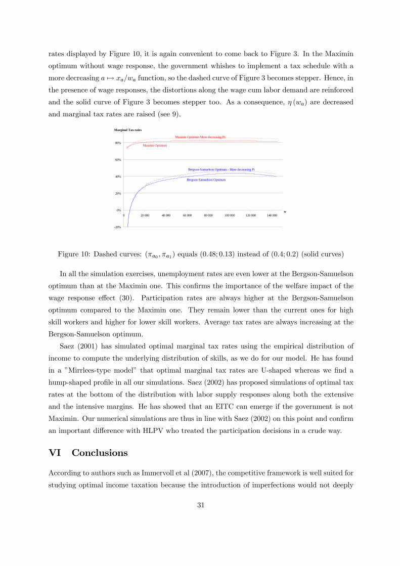
rates displayed by Figure 10, it is again convenient to come back to Figure 3. In the Maximin

optimum without wage response, the government whishes to implement a tax schedule with a

more decreasing a 7→ xa/wa function, so the dashed curve of Figure 3 becomes stepper. Hence, in

the presence of wage responses, the distortions along the wage cum labor demand are reinforced

and the solid curve of Figure 3 becomes stepper too. As a consequence, η (wa) are decreased

and marginal tax rates are raised (see 9).

-20%

0%

20%

40%

60%

80%

0 20 000 40 000 60 000 80 000 100 000 120 000 140 000w

Marginal Tax rates

Maximin Optimum More decreasing Pi

Bergson-Samuelson Optimum

Maximin Optimum

Bergson-Samuelson Optimum - More decreasing Pi

Figure 10: Dashed curves: (πa0 ,πa1) equals (0.48; 0.13) instead of (0.4; 0.2) (solid curves)

In all the simulation exercises, unemployment rates are even lower at the Bergson-Samuelson

optimum than at the Maximin one. This confirms the importance of the welfare impact of the

wage response effect (30). Participation rates are always higher at the Bergson-Samuelson

optimum compared to the Maximin one. They remain lower than the current ones for high

skill workers and higher for lower skill workers. Average tax rates are always increasing at the

Bergson-Samuelson optimum.

Saez (2001) has simulated optimal marginal tax rates using the empirical distribution of

income to compute the underlying distribution of skills, as we do for our model. He has found

in a ”Mirrlees-type model” that optimal marginal tax rates are U-shaped whereas we find a

hump-shaped profile in all our simulations. Saez (2002) has proposed simulations of optimal tax

rates at the bottom of the distribution with labor supply responses along both the extensive

and the intensive margins. He has showed that an EITC can emerge if the government is not

Maximin. Our numerical simulations are thus in line with Saez (2002) on this point and confirm

an important difference with HLPV who treated the participation decisions in a crude way.

VI Conclusions

According to authors such as Immervoll et al (2007), the competitive framework is well suited for

studying optimal income taxation because the introduction of imperfections would not deeply

31

modify the equity-efficiency trade-off. By modelling jointly participation decisions, wage forma-

tion and labor demand in a frictional economy, we show on the contrary that this trade off is

deeply modified. In the Maximin case, a set of clear-cut analytical properties are shown if the

elasticity of participation decreases with the level of skill. Then at the optimum, the average tax

rate is increasing, marginal tax rates are positive everywhere, while wages, unemployment rates

and participation rates are distorted downwards compared to their laissez-faire values. These

precise recommendations contrast with the small number of analytical properties derived in the

literature following Mirrlees (1971).

When the government has a general utilitarian social welfare function, the equity-efficiency

trade-off is more deeply affected by the wage-cum-labor demand margin. To induce participation,

the net income of workers should be higher than the one of the non-employed. This creates an

inequality that matters from a utilitarian perspective. Taxation should then promote wage

moderation to reduce the detrimental effect of unemployment on social welfare. Moreover, the

role of taxation on participation is more complex because some participants will not find a job.

Therefore, stimulating participation through lower tax levels raises inequalities. Our numerical

exercise shows that optimal unemployment rates are substantially distorted downwards and that

an EITC can be optimal.

Finally, our paper contributes to the literature of self-selection models with random partic-

ipation. The seminal paper of Rochet and Stole (2002) is developped in a context of nonlinear

pricing. Our paper proposes a new method for signing the distorsions in a different framework.

This method considers in a first step the tax function that minimizes distortions along the ex-

tensive margin by removing wage responses. In a second step, we show that the ”full” optimum

with wage responses is the result of a tradeoff between this tax function and a linear function

for which wages and unemployment are not distorted.

The present model could be extended in different directions. First, a dynamic model would

enable to introduce earning-related unemployment insurance. Hence, one can expect that a

“dynamic optimal taxation” version (à la Golosov et alii 2003) of our model would deliver

interesting insights about the optimal combination of unemployment insurance and taxation

to redistribute income. Second, we abstract from any response of the labor supply along the

intensive margin. Although we are confident that responses along the extensive margin are much

more important, enriching our framework to include hours of work, in-work effort or educational

effort belongs to our research agenda. Finally, in the real world, labor supply decisions are

typically taken at the household level, not at the individual one.

32

Appendices

A Proof of Lemma 1

From the free-entry condition, tightness on the labor market is positive if and only if a − w >κ (a). Hence, one must have κ (a) = a − wa. Let ξ = κ (a) / (a− wa), so that wa = a −(κ (a) /ξ). As wa increases from −∞ to wa, ξ increases from 0 to 1. Then, (2) can be rewritten

L³a, a− κ(a)

ξ

´= ξ · q−1 (a, ξ) and so one must have

q−1 (a, ξ) =L³a, a− κ(a)

ξ

´ξ

for each ξ in (0, 1]. For each a, since L³a, a− κ(a)

ξ

´is bounded, one has lim

ξ 7→0q−1 (a, ξ) = +∞.

Hence, q−1 (a, .) defines a decreasing function from [0, 1] onto [0,+∞]. Inverting the last func-tion, one retrieves q (a, θ) defined over [a0, a1] × R+ onto [0, 1]. Then, the matching functionH (a, V, U) ≡ V · q (a, V/U) is well defined over [a0, a1] × R2+ and exhibits constant returns toscales. Since q (., .) is bounded above by 1, one obtains that H (a, 0, U) = H (a, V, 0) = 0 and

H (a, V, U) < V . Moreover, since the elasticity in ξ of L³a, a− κ(a)

ξ

´is negative, the elasticity

with respect to ξ of q−1 is lower than −1. Consequently, the elasticity of q with respect to θmust lie in between −1 and 0. Therefore H (a, ., .) is increasing in both arguments. To finallyshow that H (a, V, U) < U , let us define θ = V/U and w by (a− w) q (a, θ) = κ (a). Then, onehas that H (a, V, U) /U = θq (a, θ) = L (a,w) < 1.

B Benthamite efficiency of the laissez-faire allocation

Let U be the Benthamite objective. Consider an equilibrium allocation. There are G (a,Σa) f (a)participants of type a whose net income is wa − T (wa) if they are employed and b otherwise,while non participants obtain b+ χ. So, the Benthamite objective writes:

U =

a1Za0

⎧⎨⎩(L(a,wa)(wa − T (.)) + (1− L(a,wa))b) ·G (a,Σa) ++∞ZΣa

(b+ χ) · g (a,χ) · dχ

⎫⎬⎭ f (a) · da=

a1Za0

⎧⎨⎩(Σa + b) ·G (a,Σa) ++∞ZΣa

(b+ χ) · g (a,χ) · dχ

⎫⎬⎭ f (a) · dawhere the second equality uses (3). Given the government’s budget constraint (5), this objectivecan be rewritten when E = 0 as:

U =a1Za0

⎧⎨⎩L (a,wa) · wa ·G (a,Σa) ++∞ZΣa

χ · g (a,χ) · dχ

⎫⎬⎭ f (a) · daThe Benthamite objective aggregates average earnings plus the value of non-market activities

over the whole population, no matter how they are distributed. In this sense, the Benthamitecriterion is an extreme case.

For each a and w, the function Σ 7→ L (a,w) · w · G (a,Σ) +R +∞Σ δ · g (a, δ) · dδ reaches a

unique maximum for Σ = L (a,w) ·w. Therefore, when we compare any allocation a 7→ (wa,Σa)

33

to the laissez-faire one, we get:

ULF =a1Za0

⎧⎪⎨⎪⎩L ¡a,wLFa ¢ · wLFa ·G¡a,ΣLFa

¢+

+∞ZΣLFa

χ · g (a,χ) · dχ

⎫⎪⎬⎪⎭ f (a) · da≥

a1Za0

⎧⎨⎩L ¡a,wLFa ¢ · wLFa ·G (a,Σa) ++∞ZΣa

χ · g (a,χ) · dχ

⎫⎬⎭ f (a) · da≥

a1Za0

⎧⎨⎩L (a,wa) ·wa ·G (a,Σa) ++∞ZΣa

χ · g (a,χ) · dχ

⎫⎬⎭ f (a) · da = UThe first inequality holds because ΣLFa = L

¡a,wLFa

¢· wLFa at the laissez faire, according to (3).

The second inequality holds because wLFa maximizes w 7→ L (a,w) · w.

C Proof of Proposition 1

From (3), one gets that (T (wa) + b)L (a,wa) equals L (a,wa) ·wa−Σa, so the budget constraint(5) can be rewritten as

b =

a1Za0

[L (a,wa) · wa − Σa] ·G (a,Σa) · f (a) · da−E

Let σa = logΣa. We use optimal control by considering σa as the state variable and wa as thecontrol.

maxwa,σa

a1Za0

[L (a,wa) · wa − expσa] ·G (a, expσa) · f (a) da

s.t : σa =∂ logL

∂a(a,wa)

Let qa be the multiplier associated to the equations of motion of σa and let Za = −qa. TheHamiltonian writes

H (w,σ, q, a) def≡ [L (a,w) · w − expσ] ·G (a, expσ) · f (a) + q · ∂ logL∂a

(a,w)

Since we assume that a maximum exists where wa is a continuous function of a (see footnote14), there exists a continuously differentiable function a 7→ qa, such that the following first-ordercondition are verified:

0 =∂H∂w

=∂ (L (a,w) · w)

∂w(a,wa) ·G (a,Σa) · f (a) + qa ·

∂2 logL

∂a∂w(a,wa) (35a)

−qa =∂H∂σ

= − {G (a,Σa)− [L (a,wa) ·wa − Σa] · g (a,Σa)} · Σa · f (a) (35b)

together with the transversality conditions qa0 = qa1 = μa0 = μa1 = 0. Using qa1 = 0, Za = −qa,one has Za =

R a1a qt · dt. Hence, (35b) with (1) gives (16b). The transversality condition qa0 = 0

gives Za0 = 0 in (16a). From (8), one has

∂ (L (a,w) · w)∂w

(a,wa) = (1− η (wa)) · L (a,wa) · wa (36)

34

From (12a) and (12b) one obtains

∂2 logL

∂a∂w(a,wa) =

αaεa· η (wa)

a(37)

Introducing these two last expressions into (35b) gives the first equality in (16a).

D Proof of Proposition 2

We first show that Z is positive on (a0, a1). From (16b), one has

Za =

µπa

1 + πa− xawa

¶(1 + πa) · wa · ha (38)

Assume by contradiction that Z is negative at some point. Since a 7→ Za is continuous,there exists an interval where Z remains negative. Given that Za0 = Za1 = 0, this implies theexistence of an interval [a, a] such that Za = Za = 0 and such that Za ≤ 0 for all a ∈ [a, a].

• Since Za = 0 and Za is negative in the neighborhood on the right of a, one has Za ≤ 0.Given (38) this implies that:

πa1 + πa

≤ xawa

• Since Za ≤ 0, one has from (16a) that η (wa) ≥ 1 for all a ∈ [a, a]. Given (9), this impliesthat xa/wa is nondecreasing, so

xawa≤ xawa

• Since Za = 0 and Za is negative in the neighborhood on the left of a, one has Za ≥ 0.Given (38) this implies that

xawa≤ πa1 + πa

These three inequalities leads to πa ≥ πa, so one must have a = a since a→ πa is decreasing.Hence, Za is nonnegative on (a0, a1) and can only be nil pointwise.

Next, assume by contradiction that there exists a2 ∈ (a0, a1) such that Za2 = 0. Since Za iseverywhere nonnegative, a2 is an interior minimum of Za, so Za2 = 0, and from (38)

πa21 + πa2

=xa2wa2

However since Za2 = 0, one has η (wa2) = 1 from (16a). Hence, from (9) and the differentiabilityof a 7→ wa, xa/wa admits a derivative with respect to a that is nil. Since Za can only be nilpointwise within (a0, a1), there exists a real a3 in the neighborhood of a2 such that a3 > a2and Za3 > 0. According to the mean value theorem, there exists a4 ∈ (a2, a3) such thatZa4 = (Za3 − Za2) / (a3 − a2) > 0. From (38), one obtains

πa41 + πa4

>xa4wa4

Since a4 is in the neighborhood of a2 and a 7→ xa/wa has a zero derivative at a2, thenone has (xa4/wa4) ' (xa2/wa2) at a first-order approximation. However, (πa4/ (1 + πa4)) '

35

(πa2/ (1 + πa2)) +³πa2/ (1 + πa2)

2´(a4 − a2) at a first-order approximation. Hence, since since

πa2 < 0, one must haveπa4

1 + πa4<

πa21 + πa2

=xa2wa2

' xa4wa4

which leads to the contradiction. Therefore, Za is positive everywhere within (a0, a1).From (16a), one has η (wa) < 1 for any a ∈ (a0, a1), which has different implications.

i) For any a ∈ (a0, a1), one has ∂ logL/∂w (a,wa) > −1 from (8). Moreover, at the Laissezfaire, ∂ logL/∂w

¡a,wLFa

¢= −1 from (8) and (9). Hence, from (6) wa < wLFa which means

that optimal wages are distorted downwards. Furthermore, since ∂L/∂w (a, .) < 0, onehas 1 − L (a,wa) < 1 − L

¡a,wLFa

¢and unemployment rates are distorted downwards.

Finally, Za0 = Za1 = 0 induces wa0 = wLFa0 , L (a0, wa0) = L¡a0, w

LFa0

¢, wa1 = wLFa1 and

L (a1, wa1) = L¡a1, w

LFa1

¢.

ii) Since η (wa) < 1, xa/wa is nonincreasing in a, so it is maximized at a0. Since Za0 = 0 andZa > 0 on (a0, a1), one must have Za0 ≥ 0. Therefore, xa0/wa0 ≤ πa0/ (1 + πa0) < 1.Hence for all a, xa < wa and participation rates are distorted downwards.

iii) x < w for all w implies that the employment tax rate (T (w) + b) /w is always positive.Moreover, it is nondecreasing since η (w) < 1. So, the average tax rate T (w) /w is increas-ing in wage w. Finally (9) and η (w) ≤ 1 induces T 0 (w) ≥ (T (w) + b) /w, so marginal taxrate are positive everywhere.

E Proof of Proposition 3

The proof of Proposition 3 extends the one of Proposition 1 in Appendix C. Let λ be themultiplier associated to the budget constraint. From (3), wa − T (wa) = (Σa/L (a,wa)) + b, sothe Hamiltonian becomes:

H (w,σ, q, a, b,λ) def≡∙L (a,w)Φ

µexpσ

L (a,w)+ b

¶+ (1− L (a,w)Φ (b))

¸G (a, expσ) · f (a)

+

+∞Zexpσ

Φ (b+ χ) g (a,χ) f (a) dχ+ λ [L (a,w) · w − expσ] ·G (a, expσ) · f (a) + q · ∂ logL∂a

(a,w)

The first-order conditions now becomes, where we define Za = −qa/λ

0 =1

λ

∂H∂w

=

⎡⎣∂L (a,w)∂w

(a,wa) ·Φ³

ΣaL(a,wa)

+ b´− Φ (b)− Σa

L(a,wa)Φ0³

ΣaL(a,wa)

+ b´

λ

+∂ (L (a,w) · w)

∂w(a,wa)

¸·G (a,Σa) · f (a)− Za ·

∂2 logL

∂a∂w(a,wa)

Za =1

λ

∂H∂σ

=

⎧⎨⎩Φ0³

ΣaL(a,wa)

+ b´

λ−G (a,Σa) + [L (a,wa) · wa −Σa] · g (a,Σa)

L (a,wa)Φ³

ΣaL(a,wa)

+ b´+ (1− L (a,wa))Φ (b)−Φ (b+Σa)

λ· g (a,Σa)

⎫⎬⎭ · Σa · f (a)These two conditions with the transversality conditions Za0 = Za1 = 0, (36) and (37) give (26a)to (26d). Finally, the condition with respect to b is exactly (27).

36

F Optimal allocation under an alternative objective

When the government is concerned by redistribution between skill groups but not between theunemployed and the employed of each skill group, its objective writes

a1Za0

{Φ [L (a,wa) (wa − T (wa)) + (1− L (a,wa)) b]G (a,Σa) (40)

+

+∞ZΣa

Φ (b+ χ) g (a,χ) dχ

⎫⎬⎭ f (a) daThen, the Hamiltonian becomes:

H (w,σ, q, a, b,λ) def≡ [Φ (expσ + b)]G (a, expσ) · f (a)

+

+∞Zexpσ

Φ (b+ χ) g (a,χ) f (a) dχ+ λ [L (a,w) · w − expσ] ·G (a, expσ) · f (a) + q · ∂ logL∂a

(a,w)

The first-order conditions now becomes, where we define Za = −qa/λ

0 =1

λ

∂H∂w

=∂ (L (a,w) ·w)

∂w(a,wa) ·G (a,Σa) · f (a)− Za ·

∂2 logL

∂a∂w(a,wa)

Za =1

λ

∂H∂σ

=

⎧⎨⎩Φ0³

ΣaL(a,wa)

+ b´

λ−G (a,Σa) + [L (a,wa) · wa − Σa] · g (a,Σa)

⎫⎬⎭ · Σa · f (a)These two conditions with the transversality conditions Za0 = Za1 = 0, (36) and (37) give (16a),and (32a). Finally, the condition with respect to b is exactly (32b).

References

[1] Akerlof, G, 1978, The Economics of Tagging as Applied to the Optimal Income Tax, WelfarePrograms, and Manpower Training, American Economic Review, 68, 8-19.

[2] Blundell, R. and T. MaCurdy, 1999, Labor Supply: A Review of alternative approaches, inO. Ashenfelter and D. Card (eds), Handbook of Labor Economics, North-Holland.

[3] Boadway, R., K. Cuff and N. Marceau, 2003, Redistribution and employment policies withendogenous unemployment Journal of Public Economics, 87, 2407-2430.

[4] Boone, J. and L. Bovenberg, 2002, Optimal Labour Taxation and Search, Journal of PublicEconomics, 85, 53-97.

[5] Boone, J. and L. Bovenberg, 2004, The Optimal Taxation of Unskilled Labor with JobSearch and Social Assistance, Journal of Public Economics, 88, 2227-2258.

[6] Boone, J. and L. Bovenberg, 2006, The Optimal Welfare and In-work benefits with searchunemployment and observable abilities, Journal of Economic Theory, 126, 165-193.

[7] Choné, P. and G. Laroque, 2005, Optimal Incentives for Labor force participation, Journalof Public Economics, 89, 395-425.

37

[8] Choné, P. and G. Laroque, 2007, Negative marginal tax rates and heterogeneity, mimeoCREST.

[9] Diamond, P., 1980, Income Taxation with fixed hours of work, Journal of Public Economics,13, 101-110.

[10] Feldstein, M., 1996, The Effect of Marginal Tax Rates on Taxable Income: A Panel Studyof the 1986 Tax Reform Act, Journal of Political Economy, 103, 551-72.

[11] Golosov, M., N. Kocherlakota and A. Tsyvinski, 2003, Optimal Indirect and Capital Tax-ation, Review of Economic Studies, 70, 569-547.

[12] Gruber, J. and E. Saez, 2002, The elasticity of taxable income: evidence and implications,Journal of Public Economics, 84, 1-32.

[13] Guesnerie, R., 1995, A Contribution to the Pure Theory of Taxation, Cambridge UniversityPress.

[14] Guesnerie, R. and Laffont, J-J, 1984, A complete solution to a class of principal-agent prob-lems with an application to the control of a self-managed firm, Journal of Public Economics,25, 329-369.

[15] Hammond, P., 1979, Straightforward Individual Incentive Compatibility in LargeEconomies, Review of Economic Studies, 46, 263-282.

[16] Hersoug, T., 1984, Union Wage Responses to Tax Changes, Oxford Economic Papers, 36,37-51.

[17] Hosios, A.,1990, On the Efficiency of Matching and Related Models of Search and Unem-ployment, Review of Economic Studies, 57, 279-298.

[18] Hungerbühler, M., E. Lehmann, 2009, On the Optimality of a MinimumWage: New Insightsfrom Optimal Tax Theory, Journal of Public Economics, 93, 464-481.

[19] Hungerbühler, M., E. Lehmann, A. Parmentier and B. Van der Linden, 2006, OptimalRedistributive Taxation in a Search Equilibrium Model, Review of Economic Studies, 73,743-767.

[20] Immervoll, H., Kleven, H., Kreiner, C. T. and Saez, E., 2007, Welfare reforms in Europeancountries: a Microsimulation analysis, Economic Journal, 117, 1-44.

[21] Juhn, C., Murphy K. M.,Topel R. H., Yellen J. L. and Baily M. N., 1991, Why has the Nat-ural Rate of Unemployment Increased over Time?, Brookings Papers on Economic Activity,1991, 75-142.

[22] Krueger, A.B. and A. Mueller, 2008, The Lot of the Unemployed: Time Use Perspective,IZA discussion paper 3490.

[23] Lockwood B. and Manning A., 1993, Wage Setting and the Tax System: Theory andevidences for the United Kingdom, Journal of Public Economics, 52, 1-29.

[24] Manning, A., 1993, Wage Bargaining and the Phillips Curve: The Identification and Spec-ification of Aggregate Wage Equations, Economic Journal, 103, 98-118.

[25] Meghir C. and D. Phillips, 2008, Labour Supply and Taxes, IZA discussion paper 3405.

[26] Mirrlees, J., 1971, An Exploration in the Theory of Optimum Income Taxation, Review ofEconomic Studies, 38(2), 175-208.

38

[27] Mirrlees, J., 1976, Optimal Tax Theory: A Synthesis, Journal of Public Economics, 6(3),327-358.

[28] Mirrlees, J., 1999, Optimal marginal tax rates at low incomes, mimeo, Faculty of Economics,Cambridge, England.

[29] Moen, E., 1997, Competitive Search Equilibrium, Journal of Political Economy, 105(2),385-411.

[30] Mortensen, D. and Pissarides, C., 1999, New developments in models of search in theLabor Market, in O. Ashenfelter and D. Card (eds.), Handbook of Labor Economics, vol 3B, North-Holland, Amsterdam.

[31] Pisauro, G., 1991, The effect of taxes on labour in efficiency wage models, Journal of PublicEconomics, 46(3), 329-345.

[32] Pissarides, C. A., 1998, The impact of employment tax cuts on unemployment and wages:the role of unemployment benefits and tax structure, European Economic Review, 42, 155-183.

[33] Pissarides, C. A., 2000, Equilibrium Unemployment Theory, Second Edition, MIT Press,Cambridge, USA.

[34] Rochet, J-C, 1985, The taxation principle and multi-time Hamilton-Jacobi equations, Jour-nal of Mathematical Economics, 14, 113-128.

[35] Rochet, J-C and L. Stole, 2002, NonLinear Pricing with Random Participation, Review ofEconomic Studies, 69, 277-311.

[36] Røed, K., S. Strøm, 2002, Progressive Taxes and the Labour Market: Is the TradeoffBetween Equality and Efficiency Inevitable? , Journal of Economic Surveys, 16, 77-110.

[37] Rogerson, R., R. Shimer and R. Wright, 2005, Search-Theoretic Models of the Labor Mar-ket: A Survey, Journal of Economic Literature, 43, 959-988.

[38] Saez, E, 2001, Using Elasticities to Derive Optimal Income Tax Rates, Review of EconomicsStudies, 68, 205-229.

[39] Saez, E., 2002, Optimal Income Transfer Programs:Intensive Versus Extensive Labor SupplyResponses, Quarterly Journal of Economics, 117, 1039-1073.

[40] Shimer, R., 1996, Contracts in frictional labor markets, MIT mimeo.

[41] Sørensen, P. B., 1997, Public finance solutions to the European unemployment problem?,Economic Policy, 25, 223-264.

39