Optimal Fiscal Policy in an Economy Facing Sociopolitical Instability
Upload
khangminh22Category
view
3download
0
OPTIMAL ECONOMIC GROWTH AND ENERGY POLICY
by
Esteban Hnyilicza
B.S., Univ. Nac. de Ing., Lima, Peru (1967)
S.M.,, Massachusetts Institute of Technology (1969)
SUBMITTED IN PARTIAL FULFILLMENT OF THE
REQUIREMENTS FOR THE DEGREE OF
DOCTOR OF PHILOSOPHY
at the
MASSACHUSETTS INSTITUTE OF TECHNOLOGY
September 1976
Signature ofDepartmentAugust 31,
Author. . . . . . . . .. ..of Electrical Engineering and1976
Computer S ience,
Certified by.....*...................g.................................Thesis Co-Supervisor
Certified by..............7...............................Thesis Co-Supervisor
Accepted by..Chairman, Departmental
I7
6 e on Graduate? StudentsARCHIVES
J-~~4%157 77

-2-
OPTIMAL ECONOMIC GROWTH AND ENERGY POLICY
by
Esteban Hnyilicza
ABSTRACT
This study is concerned with the long-term interactions between theenergy markets and the aggregate determinants of economic growth. Theframework of analysis is provided by a macroeconomic energy model. Thestructure of the model is formulated drawing upon the neo-classicaltheories of producer and consumer behavior, th, theory of general equil-ibrium and the theory of economic growth. There are two vectors of pro-duction corresponding to energy products and non-energy products, re-spectively. The output of the energy sector is disaggregated as betweenconsumption and intermediate goods; the output of the non-energy sectoris disaggregated as between consumption, intermediate, and investmentgoods. Technological constraints on the production processes are em-bodied in two cost possibility frontiers that yield the value of grossoutput for given factor input prices and given levels and configurationof output. Structural specification of the cost frontiers correspondsto the transcendental logarithmic functional form incorporating constantreturns to scale. Technical change is assumed to be described in termsof exponential indices of factor augmentation; the property of Hicks-neutrality is therefore susceptible of being tested empirically bystatistical tests of suitable parametric restrictions. Sectoral supplyand demand functions are obtained using results from the theory of de-rived factor demand and product supply for technologies with multipleoutputs--necessary assumptions are the existence of competitive marketsand the presence of cost-minimizing behavior. The technological flowcoefficients between 3ectors explicitly incorporate price-dependent sub-stitution possibilities; however, because of the presence of sectoralsupply functions, the consumption-investment split is not determinedentirely on the demand side as in conventional input-output analysis,but rather takes place within a simultaneous process of market equili-bration that generates a complete set of market-clearing prices andquantities. The derived demand for imports is obtained directly fromthe assumptions of cost-minimizing behavior. Household behavior ismodeled based on the assumption of utility-maximizinq behavior. Inter-temporal and intra-temporal allocation models yield demand functions forfull consumption for three commodity groups and leisure, respectively.The model is completed with equations accounting for capital accumula-tions in the production and household sectors, and by accountingidentities and balance equations.

-3-
The model was estimated using yearly time-series data correspondingto the U.S. postwar period. Historical simulation of the complete modelsuggests that it provides a satisfactory explanation of historical growthpatterns.
The problem of optimal growth was formulated as an optimal controlproblem involving the maximization of welfare subject to the behavioraland technological constraints embodied in the macroeconomic model. Theset of available policy instruments were taken to include tax rates oncapital income and capital property, investment tax credits, tax rateson energy consumption goods and on investment goods. The performanceindex for the optimal control problem was defined in terms of the pre-sent value of a discounted stream of utilities accruing to householdsfrom the consumption of energy goods, non-energy goods, capital servicesand leisure. The parameters of this welfare function are inferred fromthe estimated demand functions for the household sector, so that the wel-fare measure is consistent with the preferences of consumers as revealedin the historical data.
The resulting optimal control problem involves a nonlinear system,nonlinear performance index and implicit state equations. The solutionof the nonlinear optimal control problem with implicit state equationsnecessitated the development of new computational algorithms that arebased on existing algorithms of the differential dynamic programming andMin-H types. This set of algorithms have been implemented in OPCON, ageneral purpose computer code designed for the solution of nonlinearoptimal control problems in discrete-time with implicit state transitionmappings.
Finally, the results of the optimal control experiments are dis-cussed in terms of their implications for the structure of optimalgrowth paths and in terms of the relative welfare gains accruing underalternative policies.
Thesis Co-Supervisor: Dale W. JorgensonTitle: Professor of Economics (Harvard University)
Thesis Co-Supervisor: Fred C. SchweppeTitle: Professor of Electrical Engineering (M.I.T.)
-4-
ACKNOWLEDGMENTS
"Tradition requires that I absolve my critics fromresponsibility for all errors. Although I deeplyrespect tradition as a matter of principle, I seeno reason to absolve them. If I have committedblunders, one or another of those learned men andwomen should have noticed; if they did not, thenlet them share the disgrace. As for my interpre-tation and bias, the usual disclaimer is unnecessarysince no one in his right mind is likely to holdthem responsible for either."
- Eugene D. Genovese
I should first like to thank the members of my disseration committee.To Professor Dale W. Jorgenson, who served as co-supervisor on thisthesis, I am deeply grateful for his encouragement and guidance; I havebeen privileged to benefit from his advice since the early stages of thiswork. My intellectual debt to him will be obvious from these pages toanyone familiar with his work. I am indebted to Professor Fred C.Schweppe not only for his willingness to serve as thesis co-supervisor,but also for his help and support throughout several years during mygraduate education. His friendship and generosity during various crucialstages of my graduate career will not easily be forgotten. ProfessorRobert S. Pindyck helped guide this study throughout the early stageswith his often ruthless--and, in retrospect, accurate--criticisms thatserved to steer this work away from unproductive directions. He alsoprovided the encouragement and the support for the development of theoptimal control algorithm. Not least, but last, Dr. Martin Baughmanwas an inestimable source of encouragement during the initial phases ofthis study and besides supplying the resources fcr the conduct of theresearch, he helped shape the nature and thrust of its subject matter.
David 0. Wood supported this effort throughout, and the quality ofthe final product is measurably greater in both form and substance dueto his suggestions about both its conceptual and empirical aspects.
I am grateful to E.R. Berndt, R. Boyce, R.E. Hall, J.A. Hausman,E.A. Hudson, and E. Kuh for helpful discussions.
Nancy C. Perkins contributed to this work in more ways than canhere be listed and shared the burden of this effort in full. I amgrateful to her in terms that are best left unsaid.
Jamie Factor, Peter Heron and Cheryl Williams deserve my thanks forhaving, through their typing skills, succeeded where others had failed.

-5-
The computational work reported herein was carried out at theM.I.T. Information Processing Center, the National Bureau of EconomicResearch, and the Cambridge Scientific Center of the InternationalBusiness Machines Corporation through the MIT/IBM Joint Study Agreement.
This research was supported by the National Science Foundation undergrants #GI-39150 and #GS-41519, the Massachusetts Institute of TechnologyEnergy Laboratory, and the Energy Research and Development Administrationthrough grant No. E(49-18) 2295.

TABLE OF CONTENTS
ABSTRACT . . . .
ACKNOWLEDGMENTS .
TABLE OF CONTENTS
LIST OF TABLES
LIST OF FIGURES
CHAPTER I: INTRODUCTION . . . . . .
1.1 Purpose and Methodology
1.2 Growth, Welfare and Fiscal
1.3 Overview......... .o
References to Chapter I . .
Pol icy
CHAPTER II: A LONG-TERM MACROECONTHEORETICAL FOUNDATIONS
2.1 Introduction ......
2.2 Overview of the Model
OMIC ENERG
2.2.1 Production Structure
2.2.2 Household Behavior .
2.2.3 Capital Accumulation .
2.3 The Structure of Production .
2.3.1 Background.......
2.3.2 Description of Technology
2.3.3 Derived Factor Demand and ProductSupply.. .. .........
2.3.4 Technological Change........
2
4
6
10
15
19
20
23
30
34
Y MODEL:36
37
40
43
45
46
1.7
47
53
63
65
-7-
TABLE OF CONTENTS (Continued)
2.4 The Structure of Consumer Behavior . . . . . . . . . 72
2.4.1 Background . . . . . . . . . . . . . . . . . 72
2.4.2 Utility, Functional Separability andAggregation.. ............... 76
2.4.3 Hierarchical Decomposition of UtilityMaximization . . . . . . . . . . . . . . . . 88
2.4.4 The Inter-Temporal Allocation Model . . . . . 91
2.4.5 The Intra-Temporal Allocation Model ... ... 95
2.5 Capital Accumulation . . . . . . . . . . . . . . . . 97
2.6 Income-Expenditure Identities . . . . . . . . . . . 102
2.7 Balance Equations . . . . . . . . . . . . . . . . . 113
2.8 Summary . . . . . . . . . . . . . . . . . . . . . . 117
References to Chapter II . . . . . . . . . . . . . . . . 121
CHAPTER III: ECONOMETRIC SPECIFICATION AND EMPIRICALVALIDATION . . . . . . . . . . . . . . . . . . . . . . . 127
3.1 Estimation of the Model of Producer Behavior . . . . 128
3.1.1 Data Sources and Preparation. . . . . . . . . 129
3.1.2 Econometric Specification: Cost andRevenue . . . . . . . . . . . . . . . . . . . 143
3.1.3 Parameter Estimation and HypothesisTesting . . . . . . . . . . . . . . . . . . . 160
3.1.4 Concavity Tests of Cost Frontiers . . . . . . 182
3.1.5 Substitutability and Complementarityin the U.S. Energy and Non-EnergyProduction Sectore. . . . . . . . . . . . . . 193
3.1.6 Technological Change: Factor AugmentationBiases . . . . . . . . . . . . . . . . . . . 205

-8-
TABLE OF CONTENTS (Continued)
3.2 Estimation of the Model of ConsumerBehavior - - - a - - 0 - a In- a- 4. . . . . .
3.2.1
3.2.2
3.2.3
3.2.4
Data Sources and Preparation......
Estimation of the Inter-Temporal Model
Estimation of the Intra-Temporal Model
The Structure of Consumer PreferencesSubstitution Possibilities......
. . . . 219
. . . . 220
. . . . 225
. . . . 230
and
3.3 Summary . &. 0. . . 0. . . 0. 4P .40 .0 .
References to Chapter III. ........ .......
CHAPTER IV: SIMULATION: ENERGY MARKETS AND ECONOMICPERFORMANCE . . . . . . . . 0. a. 0. *. a. . . . . . .
4.1 Introduction . . . . *.0. . . . . *. 0 . .
4.2 The Complete Model: Equations and Variables.
4.3 Historical Simulation: 1948-1971... ......
4.4 Tax Policy in a Model of General Equilibrium
4.5 Government Debt, Government Expenditures andFiscal Policy... ............
4.6 Summary....... . ...........
References to Chapter IV .
. 235
. 240
. . . 242
. 244
. 245
. .. 246
. .. 261
. .. 308
.. . 0. 329
.. . a. 341
.. . a. 343
CHAPTER V: OPTIMAL GROWTH POLICIES AND ENERGY RESOURCES
5.1 Introduction
5.2 The Theory of Optimal Economic Growth......
5.3 An Intertemporal Measure of Aggregate SocialWelfare. . . ......... . ..........
5.4 Finite Planning Horizon and IntergenerationalEquity
344
345
348
351
356

-9-
TABLE OF CONTENTS (Continued)
5.5 The Optimal Growth Problem: Formulation andoiIutioni iA
5.6 Welfare Ga
5.7 Summary .
iyurith!ms ... . ..I.I. . e & . .
ins from Optimal Tax Policies . .
. . .4 . . . . . . . .1 .0 .0 .0 .4 . .0 .0
References to Chapter V . . . . . . . .
APPENDIX A: STATE-SPACE FORM OF MACROECONOMICMODEL . . . . . 0.0.0.a. . . . . . .
A.1 Introduction . . . .P .0.0 .a .0 .0 .& .0
A.2 Implicit State Equations . . . . .
A.3 State Variables..............
A.4 Output Variables . .. 4. a.6.. .
A.5 Exongenous
A.6 Parameters.. ...........
APPENDIX B: OPCON -- A GENERAL PURPOSE COMPUTERSOLUTION OF NONLINEAR TIME-VARYING OPTIMALPROBLEMS ............. .. . .........
B. Introduction .. *.... ag...
B.2 Program Highlights
B.3 Algorithms.. ... ..........
B.4 Implicit State Equations, Algebraic C
ENERGY
.C.DE FORTH
CODE FOR THECONTROL
onstraints
8.5. Summary..........
362
365
370
385
388
389
391
399
400
402
404
409
410
414
416
422
423
.& .0 .a .0 .0

- 10 -
LIST OF TABLES
3-1: Input price indices, U.S. energy sector,1947-1971....................a ..... . . . .0. .a.......135
3-2: Input price indices, U.S. non-energy sector,
1947-1971..................0 .. ..0 .... . . .0.0. .0.......136
3-3: Input quantity indices, U.S. energy sector,
1947-1971.... . . ............. . .. ...........137
3-4: Input quantity indices, U.S. non-energy sector,1974-1971. . ................ . . .......... 138
3-5: Output price and quantity indices, U.S. energy
sector, 1947-1971. . .... .... ...........139
3-6: Output price and quantity indices, U.S. non-energy
1947-1971.. . . . . .. .............. .............140
3-7: Input cost shares, U.S. energy sector, 1947-1971..........144
3-8: Output revenue shares, U.S. energy sector, 1947-1971.. ... 145
3-9: Input cost shares. U.S. non-energy sector, 1947-1971......146
3-10: Output revenue shares, U.S. non-energy sector, 1947-1971 . 147
3-11: Multivariate share estimating system for the translog
cost frontier, U.S. energy sector..........a.0 . ........148
3-12: Multivariate share estimating system for the translogcost frontier, U.S. non-energy sector a....... .. ... ....... 159
3-13: Parameter estimates of the translog cost frontier, U.S.
energy sector....... . ............
3-14: Parameter estimates of the translog cost frontier, U.S.non-energy sector.................. . ...........
. . 162-5
166-71

- 11 -
3-15: Likelihood ratio tests on the structure of technology,
U.S. energy sector .. . . . .. .. .
3-16: Likelihood ratio tests on the structure of technology,
U.S. non-energy sector . . . . . . .D.0.0.0.0.0.0.0.0.0
3-17: Estimates of the eigenvalues of the Hessian matrices
of the translog cost frontier: U.S. energy sector
3-18 Estimates of the eigenvalues of Hessian matrices of
the trcanslog cost frontier: U.S. non-energy sector . . . . 188
3-19: Parameter estimates of the translog cost frontier
with concavity restrictions, U.S. non-energy sector . . 189-90
3-20: Factor demand elasticities, U.S. energy sector....-....196
3-21: Factor demand elasticities, U.S. non-energy sector . . . . 197
3-22: Allen-Uzawa partial elasticities of substitution,
U.S. energy sector .......... t... . . . .. ........ 198
3-23: Allen-Uzawa partial elasticities of substitution,
U.S. non-energy sector..a.. ..... .a..a.*...a..*....199
3-24: Elasticities of factor demands with respect to
output intensities, U.S. energy sector..........4.D..a . 203
3-25: Elasticities of factor demands with respect to
output intensities, U.S. non-energy sector............204
3-26: Annual rates of total cost diminution, U.S. enery.
and non-energy sectors, 1948-1971. ... . .. ....... 206
3-27: Parameter estimates of the translog cost frontier
under alternative hypotheses on technological change,
U.S. non-energy sector.............. .............. 210-11
3-28: Parameter estimates of the translog cost frontier
under alternative hypotheses on technological
change, U.S. non-energy sector. . .. ........ 212-14
. . 180
181
. . . . 187

- 12 -
3-29: Price and quantity components, full consumption per
capita, 1947-1971 . -. . . . . . *. . D. 0. a. a. . . . . .
3-30: Price indices of consumption by U.S. households,1947-1971 . . . . . . . . . . .#.0.0.0.*.0.0.0.*.w.0.a.a.a
3-31: Consumption quantity indices per capita, U.S. households,
1947-1971 . . . .6 .a .a .0 .a .0 .0 .0 .a . .V .I . . . . . . . . .
3-32: Parameter estimates of inter-temporal translog utility
function ........................ .. .........
3-33: Multivariate estimating system of expenditure shares,
intra-temporal model of consumer behavior .. .
3-34: Parameter estimates of intra-temporal direct translog
utility function.......4.... . . . . . ....
3-35: Likelihood ratio tests of groupwise separability
hypotheses on the structure of consumer preferences
3-36: Price and income elasticities of commodity groups,
intra-temporal model of consumer behavior
4-1: Simulation 1: surcharge of 8% on the tax rate on
energy consumption goods . . ..o.0 . .0.*..a..&....
4-2: Simulation 2: surcharge of 2% on the tax rate on
labor income...................... . . . . .......
4-3: Simulation 3: surcharge of 8% on the tax rate on
investment goods. . ...... ...M.0.0. .*.a..a.&..a.
4-4: Simulation 4: reduction of 1% in the tax rate on
capital property, U.S. energy sector ....... . .
4-5: Simulation 5: reduction of 1% in the tax rate on
capital property, U.S. non-energy sector.......
4-6: Average percentage changes in endogenous variables,
1948-1971, simulations 1 through 5 . . . .1.0.a.0.a
. . . 233-4
. . . . 227
239
. . . . 311
313
316
.. . I. 318
. . . . 320
. . . 322-4
222
223
224
226
232

- 13 -
4-7: Effect of 1% reduction in capital property tax oncapital service price under partial and general
equilibrium . . . . . . . . . . . . . . . . . . . . . . 326
4-8: Dynamic elasticities of demands for factors of
production with respect to TPE under partialand general equilibrium . . . . . . . . . . . . . . . . 327
4-9: Average percentage changes in endogenous variables,1948-1971, simulations lA through 5A . . . . . . . . . 332-4
4-10: Average percentage change in endogenous variables
1948-1971, simulations lB through 5B . . . . . . . . . 335-7
4-11: Percentage change in selected variables in responseto 1% reduction in TPE under alternative fiscal
packages.-...... . . . . . . . . . . . . . . . . 338
5-1: Optimal and historical rates for TCE, effectivetax rate on energy consumption, 1948-1971 . . . . . . . 372
5-2: Optimal and historical tax rates for TI, effectivetax rate on investment goods, 1948-1971 . . . . . . . . 373
5-3: Optimal and historical rates for TI, effective taxrate on labor income, 1948-1971 . . . . . . . . . . . . 374
5-4: Optimal and historical rates for ITCE, investmenttax credit, U.S. energy sector, 1948-1971........ . 375
5-5: Optimal and historical rates, for ITCN, investmenttax credit, U.S. non-energy sector, 1948-1971 . . . . . 376
5-6: Optimal and historical rates for TKE, effectivetax rate on capital property, U.S. energy sec-tor, 1948-1971 . . . . . . . . . . . . . . . . . . . . . 377
5-7: Optimal and historical rates for TKN, effectivetax rate on capital property, U.S. non-energysector, 1948-1971 . . . . . . . . . . . . . . . . . . . 378
5-8: Welfare gains from optimal tax policies underalternative strategies. ... ............ 379
5-9: Optimal paths of energy consumption per capitaunder alternative strategies, 1948-1971 . . . . . . . . 380

- 14 -
5-10: Optimal paths of non-energy consumption percapita under alternative strategies, 1948-1971.. .... 381
5-11: Optimal paths of capital services to householdsunder alternative strategies, 1948-1971... ... .... 382
5-12: Optimal paths of leisure per capita under al-ternative strategies, 1948-1971 .. ........... 383
5-13: Optimal paths of full consumption per capitaunder alternative strategies, 1948-1971.......... .. 384

- 15 -
LIST OF FIGURES
2-1: Long-term Macroeconomic Energy Model . . . . . . . ..
4-1: EC - Energy consumption products supplied by U.S.
energy sector, historical vs simulated, 1948-1971 .
4-2: EM - Energy intermediate products supplied by U.S.
energy sector, historical vs simulated, 1948-1971 .
4-3: PEC - Price index, energy consumption products sup-
plied by U.S. energy sector, historical vs simulated,
1948-1971 . . . . . . . . . . . . . . . . . . . . . .
4-4: PEM - Price index, energy intermediate products
supplied by U.S. energy sector, historical vs simu-
lated, 1948-1971.. . . . . . . . . ... . . . . . . . .
4-5: EMN - Energy intermediate products purchased by U.S.
non-energy sector, historical vs simulated, 1948-1971
4-6: EME - Energy intermediate products purchased by U.S.
energy sector, historical vs simulated, 1948-1971 . .
4-7: RE - Competitive imports of energy products, histori-
cal vs simulated, 1948-1971 . . . . . . . . . . . . .
4-8: LE - Labor services purchased by U.S. energy sector,
historical vs simulated, 1948-1971 . . . . . . . . ..
4-9: KE - Capital services supplied to U.S. energy sector,
historical vs simulated, 1948-1971 . . . . . . . . ..
4-10: PKE - Price of capital services, U.S. energy sector,
historical vs simulated, 1948-1971 . . . . . . . . . .
4-11: CE - Energy consumption products purchased by U.S.
households, historical vs simulated, 1948-1971 . .
4-12: PCE - Price index, energy consumption products pur-
chased by U.S. households, historical vs simulated,
1948-1971 . . . . . . . . . . . . . . . . . . . . . ..
118
262
263
264
266
266
267
268
269
270
271
272
. . . 273

- 16 -
4-13: ME - Nominal rate of return, U.S. energy sector,
historical vs simulated, 1948-1971. . . . . . . . . . . . . 274
4-14: INE - Gross investment, U.S. energy sector, historical
vs simulated, 1948-1971 . . . . . . . . . . . . . . . . . . 275
4-15: KSE - Capital stock, U.S. energy sector, historical vsvs simulated, 1948-1971 . . . . . . . . . . . . . . . . . . 276
4-16: NC - Non-energy consumption products supplied by U.S.non-energy sector, historical vs simulated, 1948-1971 . . . 277
4-17: NM - Non-energy intermediate products supplied by U.S.non-energy sector, historical vs simulated, 1948-1971 . . . 278
4-18: NI - Investment goods supplied by U.S. non-energy
sector, historical vs simulated, 1948-1971 . . . . . . . . 279
4-19: PNC - Price index, non-energy consumption goods
supplied by U.S. non-energy sector, historical
vs simulated, 1948-1971 . . . . . . . . . . . . ... . . . 280
4-20: PNI - Price index, investment goods supplied by U.S.non-energy, sector, historical vs simulated, 1948-1971. . . 281
4-21: NMN - Non-energy intermediate products purchased by
U.S. non-energy sector, historical vs simulated,
1948-1971...-.-.. . . . . . . . . . . . . . . . . . . . . 282
4-22: NME - Non-energy intermediate products purchased by
U.S. energy sector, historical vs simulated, 1948-1971. . . 283
4-23: RN - Competitive imports of non-energy products,
historical vs simulated, 1948-1971. . . . . . . . . . . . . 284
4-24: LN - Labor services purchased by U.S. non-energy
sector, historical vs simulated, 1948-1971. . . . . . . . . 285
4-25: KN - Capital services applied to U.S. non-energy
sector, historical vs simulated, 1948-1971. . . . . . . . . 286

- 17 -
4-26: PKN - Price of capital services, U.S. non-energy sector,
historical vs simuleted, 1948-1971. . . . . . . . . . . . . . 287
4-27: MN - Nominal rate of return, U.S. non-energy sector,
historical vs simulated, 1948-1971. . . . . . . . . . . . . . 288
4-28: INN - Gross investment, U.S. non-energy sector, histori-
cal vs simulated, 1948-1971 . . . . . ...... . . . . . . 289
4-29: KSN - Capital stock, U.S. non-energy sector, historical
vs simulated, 1948-1971 . . . . . . . . . . . . . . . . . . . 290
4-30: CN - Non-energy consumption goods purchased by U.S.
households, historical vs simulated, 1948-1971. . . . . . . . 291
4-31: PCN - Price index, non-energy consumption goods pur-
chased by U.S. households, historical vs simulated,
19481971..-..........-.-.-..-.-.-.-.-.-.-....292
4-32: IMIN - Direct imports of investment goods, historical
vs simulated, 1948-1971 . . . . . . . . . . . . ... . . . . 293
4-33: PL - Price index, supply of labor services, historical
vs simulated, 1948-1971 . . . . . . . . . . . ..... . . . . 294
4-34: L - Supply of labor by U.S. households, historical vs
simulated, 1948-1971. . . . . . . . . . . . . . . . . . . . . 295
4-35: I - Gross private domestic investment, historical vs
simulated, 1948-1971. . . . . . . . . . . . . . . . . . . . . 296
4-36: PIN - Price index, gross private domestic investment,
historical vs simulated, 1948-1971. . . . . . . . . . . . . . 297
4-37: F- Full consumption, U.S. households, historical vs
simulated 1948-1971 . . . . . . . . . . . . . . . . . . . . . 298
4-38: MW - Nominal rate of return on wealth, historical vs
simulated 1948-1971 . . . . . . . . . . . . . . . . . . . . 299

- 18 -
4-39: CK - Capital services supplied to U.S. households,
historical vs simulated, 1948-1971..........
4-40: PCK - Price of capital services, U.S. household
sector, historical vs simulated, 1948-1971..........
4-41: ICD - Gross investment in consumer diirables by U.S.
households, historical vs simulated, 1948-1971 - -
4-42: IRS - Gross investment in residential structures by
U.S. households, historical vs simulated, 1948-1971
4-43: KCD - Capital stock of consumer durables, U.S.
household sector, historical vs simulated, 1948-1971
4-44: KRS - Capital stock of residential structures, U.S.household sector, historical vs simulated, 1948-1971
4-45: S - Gross private domestic saving, historical vs
simulated, 1948-1971.. . .... .-.-.-.. . .... ..
4-46: W - Private domestic wealth, historical vs simulated,
1948-1971.,.. .... . .... s...e..........
300
301
302
. . . . 303
304
305
306
307

- 19 -
CHAPTER I
INTRODUCTION
1.1 Purpose and Methodology
1.2 Growth, Welfare and Fiscal Policy
1.3 Overview
- 20 -
CHAPTER I
INTRODUCTION
"...within whatever technological assumptionsinstinct and observation lead one to make, itis possible to pose and to answer what I haveclaimed to be the central question of capitaltheory. What is the payoff to society from anextra bit of saving transformed efficientlyinto capital formation?"
- Robert M. Solow
1.1 Purpose and Methodology
This is a study about energy and economic growth. Its primary aim
is to identify the causal links and the behavioral interdependencies
among governmental policy, aggregate economic activity and patterns of
energy utilization. It attempts to develop quantitative relationships
between the flow of energy resources and the structural determinants of
growth, and to assess the impact of alternative outcomes of these proce-
sses from the standpoint of overall social welfare.
Within these rough boundaries, many specific questions suggest them-
selves. What are the interrelations between an economy's productive capa-
city, the demand for energy and the forces behind productivity growth?
What does the rate of capital accumulation required to sustain an effi-
cient growth path imply with regard to the consumption of energy resources?
How effective is fiscal policy in promoting efficient functioning of energy
markets while guiding the economy towards such a growth path? To develop a
framework of inquiry that will make it possible for such questions to be

- 21 -
meaningfully addressed is the chief goal of this work.
These questions are not entirely new and they are certainly not simple.
Indeed, they differ little in substance from the central issues that have
shaped the theory of economic growth throughout the past several decades.
In contrast to the established tradition in that field, however, the object
of our study is a concrete economy evolving over a definite historical
period. As such, it is rich in empirical content. In addition, the per-
spective adopted in this work differs in one more respect from that of
most earlier researchers in long-term macrodynamics. This distinguishing
aspect consists of the explicit recognition of the crucial role of energy
resources in the economic activities of production, consumption and in-
vestment and, a fortiori, in the growth process itself.
The analytical framework that serves as the focal point of our study
is provided by a long-term macroeconometric energy model of the U.S. econo-
my. The methodological basis of the model rests upon the neoclassical theo-
ries of producer and consumer behavior, the theory of economic growth and
the theory of general equilibrium. The synthesis of a model that has its
roots in these diverse fields and that, in addition, was designed to be
susceptible of empirical validation, has been achieved not without a certain
degree of compromise. The model focuses on the connections between energy
flows and intertemporal choices between present and future consumption;
it does not explicitly address those aspects of intertemporal behavior that
are intrinsically due to the exhaustible nature of the energy resource base.
Although it is directly tied to historical data, the macroeconomic model must

- 22 -
be termed pre-institutional in nature and its policy implications must be
evaluated in this light. Finally, the model is highly aggregative. This
property, of course, guarantees an analysis unencumbered by the burdens
of high dimensionality and is, in any event, intrinsic to an undertaking
such as we have described. Even Mrs. Robinson -- not an apologist of neo-
classicism by any account -- concedes that "a model which took account of
all the variegation of reality would be of no more use than a map at a
scale of one to one."1
In order to establish the characterization of optimal growth trajectories
for our macroeconometric model, we construct an aggregate index of social
welfare defined in terms of a discounted stream of utilities accruing to
households. Both the rate of pure time preference, as well as the para-
meters of the intra-period utility function are inferred from estimated
consumer demand functions and, consequently, our measure of welfare is
consistent with the preferences of consumers as revealed in the histori-
cal data. Our optimal control studies, therefore, provide a unifying
synthesis of the descriptive and normative aspects of growth.
The study of interactions between growth and government policy -- and,
inescapably, of the role of energy resources -- within a framework such
as we have described, has both theoretical and empirical interest. But --
we must ask -- can we demonstrate that the subject of economic growth
carries with it some measure of direct immediacy for the prescription
of public policy?
1Robinson [lI, p. 33
- 23 -
1.2 Growth,-Welfare and Fiscal Policy
The nature and extent of governmental control over economic growth
has been the subject of prolonged controversies among economic policy-
makers. The debate has entailed both positive and normative aspects.
There is the question, on the one hand, of whether in a capitalistic
economy the sovereignty of the consumer prevails to the extent that it is
he alone, and not the government, who can and does in fact decide the
rate of investment and hence the rate of growth. Another matter in dispute,
related but distinct, is whether the government ought to intervene at all
in the process of choosing between present and future consumption, and,
if so, in what direction and by how much. Even if it were established
that the government can control the split between consumption and invest-
ment, it is argued, it need not follow that the government should in fact
decide the consumption-investment mix.
The prospect of a strict laissez-faire attitude toward growth has been
viewed at times with some apprehension by its opponents. James Tobin has
asked:2
"Can we as a nation, by political decision and govern-mental action, increase our rate of growth? Or must therate of growth be regarded fatalistically, the result ofuncoordinated decisions and habits of millions of consum-ers, businessmen and governments, uncontrollable in ourkind of society except by exhortation and prayer?"
It seems safe to suggest that the government is not in fact condemned
to a policy of perennial passivity toward growth. "The belief in the
inability of the government to influence investment in a capitalistic
economy" -- it has been argued by Phelps [3 ] -- "flies in the face of
2Tobin [2 ], pp. 10-11

- 24 -
modern as well as classical economic theory." Paul Samuelson was prepared
to go even further: 3
"With proper fiscal and monetary policies, our economycan have full employment and whatever rate of capitalformation and growth it wants."
Whether this pronouncement is overly optimistic will remain a matter of
debate. Nonetheless, the weight of the evidence suggests that the dis-
cretionary powers of government to influence the rate of growth extend
beyond the specific controls over research, tangible capital expenditures
and education. Full employment can be achieved by a combination of low
taxes (budgetary deficit) and high interest rates or high taxes (budgetary
surplus) and low interest rates, as Phelphs [ 4] puts it:
"If the government chooses high taxes and low interestrates, consumption expenditures by the heavily taxedhouseholds will be small while the low interest rateswill stimulate large investment expenditures and henceproduce a high rate of growth."
If we accept that the growth rate is susceptible of being controlled at
least to a certain degree, the extent to which the government should exer-
cise this power is still not immediately obvious. Does it at least follow
that this power should be exercised at all? In other words, is there a
need for a growth policy?
This question can be rephrased in yet another way: are freely function-
ing markets efficient in making intertemporal allocations?
The advocates of a laissez-faire posture predicated upon the prevalence
of consumer sovereignty would reply that indeed they are. But as Phelps
has pointed out, "The fundamental error of this proposition, viewed from
Samuelson [ 5 3, pp. 229-234.
l

- 25 -
the standpoint of contemporary fiscal and monetary theory, arises from its
neglect of the role played by government taxation."4 Indeed, critics of
such a passive approach to economic growth would contend that "the market
solution in principle cannot provide any reliable indication of consumer
preferences, since the government may have biased the solution one way or
the other." 5 They would further point out that "the market solution can
never be relied upon to express consumers' true preferences for growth
because the market solution is contaminated by the way in which the govern-
ment elects to use its fiscal and monetary controls."6
But if freely operating markets fail to insure a growth path in accord
with consumer preferences solely because of the distortions introduced by
the government's own policies, would it not be possible to design these
policies with the specific intent of neutralizing such distortions and
restoring the full virtues of the market solution? Wouldn't the necessity
for an active growth policy therefore disappear for reasons not unlike
those put forth by the supporters of the proposition of consumer sovereignty?
It is precisely this category of questions that has been investigated by
Phelps [ 3 ] under what he termed the principle of fiscal neutrality:
"We shall say that tax policy is neutral if it pro-duces the same allocation of resources (among con-sumption goods, among people, and between aggregateconsumption and investment) as would be produced ifthere was no government treasury, hence no taxes andgovernment debt, but only a government agency to con-script resources for use in the production of pitlicgoods and an agency to redistribute wealth so as toachieve the desired distribution of lifetime income."
4Phelps [ 4], p. 75.
5Phelps [3], p, 13.
6Ibid., p. 13

- 26 -
The practical difficulties with such a strategy of fiscal neutrality are
obvious. But if it were implementable, would it inevitably lead to a
Pareto-optimal growth path in the sense of an efficient intertemporal
allocation of resources?
Such a result would indeed hold -- as Phelps points out in his own
analysis -- "if a competitive equilibrium is attained; if there is com-
plete information about future as well as current prices and also perfect
information about current and future supplies of public goods; if pro-
ducers have complete information about the future as well as the current
technology; if there are no externalities in production; if consumers
know their tastes and their preferences are unchanging over time; if there
are no externalities in consumption other than the public goods whose
production we take as given. "7 That is to say, this set of arguments --
which are familiar examples of market failure in a static context -- are
also valid objections against a laissez-faire approach to the problems of
intertemporal choice and apply, by extension, to a strategy of fiscal
neutrality towards growth. Let us examine them in some detail.
The objection relating to the myopic perception of consumer prefer-
ences was advanced by Pigou.8
"Generally speaking, everybody prefers presentpleasures or satisfactions to future pleasures orsatisfactions of equal magnitude, even when thelatter are perfectly certain to occur...This impliesonly that our telescopic faculty is defective, andthat we, therefore, see future pleasures, as itwere, on a diminished scale.... [People] distributetheir resources between the present, the near
7Phel ps [4], pp. 81-82.
8Pigou [6 1, pp. 24-25.

- 27 -
future and the remote future on the basis of awholly irrational preference."
Pigou's argument implies that there is no feasible consumption pro-
gram which the individual would not at some point in his lifetime prefer
to exchange for some other feasible consumption program. If indeed this
claim is correct -- and it is not obvious that it is empirically
testable -- then it would follow that there is no Pareto optimum because
there is no set of consistent preferences. The implications of this pro-
position would clearly extend beyond the rebuttal of the market process
as an efficient allocation mechanism.
The absence of comprehensive future markets is a serious objection
to the extent that it prevents both consumers and producers from accurately
forecasting the course of future prices. As Graaff points out:9
"Let us abstract from such familiar difficulties asexternal effects in production, the dependence ofproduction functions upon the distribution of wealth,or the presence of monopoly. Let us assume, that isto say, conditions cnmpletey1 favorable to the satis-factory working of the price mechanism. The amountof saving any one household undertakes (out of a givenincome, and at a given interest rate) will depend uponthe goods and services it expects those savings to beable to purchase in future years -- upon the expectedlevel of prices. If it holds a part of its savings inthe form of bonds, expected interest rates will enterthe picture; if in the form of money, the general levelof prices; if in the form of durable commodities,relative prices.
Uncertainty arising from imperfect forecasting of future prices is also
present in production decisions: 10
9Graaff [7], p. 103.
10Ibid., p. 104.

- 28 -
"No individual entrepreneur can estimate, on the basisof [current] market data alone, the productivity ofinvestment until the investment plans of other entre-preneurs are determined... We have here somethinganalogous to external effects in production -- butagain something quite different from true externaleffects, since it works through the price system andhas nothing to do with the interrelation of produc-tion functions in a technological sense."
The point here is that the profitability of investments cannot be
known until entrepreneurs know future prices, and these future prices can-
not be known until they know what other entrepreneurs will invest.
Koopmans has referred to this phenomenon as secondary uncertainty:
"In a rough and intuitive judgment the secondaryuncertainty arising from lack of communication, thatis from one decision maker having no way of findingout what the concurrent decisions and plans made byothers (or merely of knowing suitable aggregatemeasures of such decisions or plans), is quantita-tively at least as important as the primary uncer-tainty arising from random acts of nature andunpredictable changes in consumer preferences."
Another condition that may cause departures from an efficient growth
path is the presence of monopolistic or oligopolistic market structures.
The major consequence of this from the standpoint of the growth process
is that firms will not invest up to the point where the rate of return on
investment is equal to the rate of return available to savers.
Finally, it is frequently argued that a laissez-faire doctrine of
growth will not lead to efficient intertemporal allocations because of the
divergence between social and individual levels of risk (Solow [8 1,
Tobin [9 1), because of external returns to investment in R&D and exter-
nalities arising from learning effects in tangible capital investment
(Arrow [10], Solow [8 1) and because of intertemporal externalities in
1Koopmans [11], pp. 162-163.

- 29 -
consumption arising from interpersonal jointness of preferences (Sen [121,
Marglin [13]).
The above set of arguments against strictly passive or else neutral
strategies toward growth, it has been suggested, demonstrate the failure
of market processes in guaranteeing a Pareto-optimal growth path and
point to the necessity of an active growth policy. Indeed, when taken as
a whole, they constitute a strong case in favor of a departure from fiscal
neutrality. They do not provide, of course, any insight on what guide-
lines ought to be followed in designing a growth strategy.
Analytical studies of such normative questions are scarce, primarily
because models of economic growth have traditionally been cast in an
abstract framework, focusing on questions far removed from the prescrip-
tion of public policy.* Typically, growth theorizing has been concerned
with the expansion rates required to fulfill certain long-term equilibrium
conditions -- as in the study of Golden Rule steady-state paths (Phelps
[14], Swan [15]). In traditional neoclassical models, moreovEr, growth
rates are entirely determined by population growth; fiscal policy might
conceivably be used to promote capital formation, but this results only
in a changed capital-labor ratio and exerts no impact upon the long-term
growth path. In recent years, fiscal policy parameters have been in-
cluded in neoclassical growth models by some authors (e.g. Cornwall [16],
Sato [17] and [18]), but they have been concerned for the most part with
distributional issues or with the speed of adjustment, rather than with
the properties of the growth path itself.
*For comprehensive surveys of mathematical models of economic growth, thereader is referred to Hahn and Matthews [19] and Britto [20].

- 30 -
The most promising framework for the analysis of fiscal policy and
its impact on growth -- a framework, we might add, upon which the present
study builds -- is the one developed by Jorgenson [21] and his students
(Christensen [22], Hudson [23]). The work of Jorgenson in the econo-
metrics of economic growth has succeeded in linking neoclassical growth
theory with empirically-based methodologies of model-building and with
the realities of fiscal policy and its implications for the problem of
intertemporal choice.
1.3 Overview
The structure of our macroeconomic energy model is presented in
Chapter II. Our modeling approach reflects the fact that changes in
technologies in the energy sector or introduction of policy initiatives
which affect equilibrium in the energy markets will have consequences for
other sectors of the economy and will therefore affect the overall level
and composition of economic growth. Attention is focused on the proper-
ties and configuration of alternative paths of potential output rather
than on questions related to the levels of capacity utilization or
employment, as in short-term stabilization models. A full set of market-
clearing prices and quantities is computed within a simultaneous process
of market equilibration. This property makes it possible to establish
a link between the macroeconomic relationships in the model and economic
quantities susceptible of interpretation from the standpoint of micro-
economic analysis. Indeed, although the model is aggregative, the intro-
duction of a higher degree of sectoral detail would entail no new
conceptual difficulties.
-
- 31 -
Chapter III is devoted to the estimation of the behavioral equations
in our macroeconomic model and presents the results of statistical tests
of alternative hypotheses on the structure of technology and the structure
of consumer preferences. The hypothesis of separability between inputs
and outputs in the characterization of technology is decisively rejected.
Price elasticities of demand for factors of production, as well as
Allen-Uzawa partial elasticities of substitution and transformation are
computed and the implied patterns of substitutability and complementarity
are examined. Statistical tests of various hypotheses concerning the
configuration of technological change are reported; the commonly adopted
hypothesis of Hicks neutrality is rejected and our results suggest the
presence of energy-using biases in the structure of technical progress
over the period 1948-1971. The remaining sections deal with the estima-
tion of the model of consumer behavior. From the estimated parameters
for the inter-temporal allocation model, we derive the implied values for
the rate of social discount. Estimated values of the discount rate range
between 2.02% and 7.98%, depending on the underlying assumptions about
the structure of inter-temporal preferences. Finally, several hypotheses
about the structure of intra-temporal consumer preferences are investi-
gated, including groupwise separability among the various commodity groups.
In Chapter IV we present the final form of our macroeconometric
energy model, including the full list of equations and variables. The
results of historical simulation of the model throughout the period
1948-1971 are reported. In terms of the accuracy of these ex-post fore-
casts, the performance of the model is judged satisfactory. We then
perform a set of simulations corresponding to the effects of changes in
selected tax variables. An analysis of these simulation results highlights

- 32 -
the strongly interrelated nature of the variables in our general equi-
librium model. A comparison of these results with studies of similar tax
measures based on partial equilibrium suggests the conclusion that a
partial equilibrium analysis leads to an overprediction of the effects of
the tax changes because it neglects the stabilizing forces arising from
the feedback interrelationships among variables. Finally, we perform a
set of tax policy experiments under two alternative assumptions about
government financing: budget-balancing and deficit-financing fiscal
packages. Detailed analysis of tax measures aimed at stimulating invest-
ment expenditures show that the impact on actual investment levels
crucially depends on the configuration of the entire budgetary scheme.
In Chapter V, we develop a framework of analysis that makes it pos-
sible to compute optimal growth paths under alternative strategies,
within the context of our macroeconomic energy model. We discuss the
specification of a measure of economic welfare which is consistent with
the behavioral assumption underlying our model and with the preferences
of consumers as revealed in the historical data. The resulting infinite-
horizon problem is reduced to a finite-horizon problem by constructing a
valuation of terminal capital stock that is commensurate with the under-
lying social welfare function. Given the objective function and the
behavioral and technological constraints embodied in our macroeconomic
model, the problem of optimal growth is formulated as a nonlinear optimal
control problem with implicit state equations. The numerical solution of
this optimal control problem demands the development of new computational
algorithms that are generalizations of existing algorithms in the theory
of optimal control. These algorithms are incorporated into OPCON, a

- 33 -
general purpose software package for the solution of nonlinear optimal
control problems with nonlinear objective functions. Finally, we present
the results of a set of numerical optimization experiments that yield
insight into the structure of optimal growth paths and the relative
welfare gains accruing under alternative policies.

- 34 -
REFERENCES TO CHAPTER I
[1] Robinson, J., "A Model of Accumulation," in Essays in the Theory ofEconomic Growth, Macmillan, London, 1962.
[2] Tobin, J., "Growth through Taxation," The New Republic, July 25,1960.
[3] Phelps, E. S., Fiscal neutrality toward economic growth, McGraw-Hill, New York, 1965.
[4] Phelps, E. S., "Government 'Neutralism' and 'Activism' in GrowthDecisions," in The Goal of Economic Growth, E. S. Phelps (ed.),Norton & Co., New York, 1969.
[5] Samuelson, P. A., "The New Look in Tax and Fiscal Policy," FederalTax Policy for Economic Growth and Stability, Subcommittee on TaxPolicy, Joint Committee on the Economic Report, 84th Cong., 1955.
[6] Pigou, A. C., The Economics of Welfare, 4th ed., Macmillan & Co.,London, 1932.
[7] Graaff, J. de V., Theoretical Welfare Economics, Cambridge Univer-sity Press, London, 1957.
[8] Solow, R. M., Capital Theory and the Rate of Return, North Holland,Amsterdam, 1963.
[9] Tobin, J., "Economic Growth as an Objective of Government Policy,"American Economic Review Papers and Proceedings, vol. 54, May, 1964.
[10] Arrow, K. J., "The Economic Implications of Learning by Doing,"Review of Economic Studies, vol. 29, June, 1962.
[11] Koopmans, T. C. , Three Essays on the State of Economic Science,McGraw-Hill, New York, 1957.
[12] Sen, A. K., "On Optimizing the Rate of Saving," Economic Journal,vol. 71, September, 1961.
[13] Marglin, S. A., "The Social Rate of Discount and the Optimal Rateof Investment," Quarterly Journal of Economics, vol. 17,February, 1973.

- 35 -
[14] Phelps, E. S., "The Golden Rule of Accumulation," American EconomicReview, vol. LV, September, 1965.
[15] Swan, T. W., "Growth Models of Golden Ages and Production Functions,"in Economic Development with Special Reference to East Asia,K. E. Berrill, (ed.), Macmillan, London, 1963.
[16] Cornwall, J., "Three Paths to Full Employment Growth," QuarterlyReview of Economics, February 1963.
[17] Sato, R., "Fiscal Policy in a Neo-Classical Growth Model," Reviewof Economic Studies, February 1963.
[18] Sato, R., "Taxation and Neo-Classical Growth," Public Finance,No. 3, 1967.
[19] Hahn, F. H., and Matthews, R. C. 0., "The Theory of EconomicGrowth: a Survey," Economic Journal, December 1964.
[20] Britto, R., "Some Recent Developments in the Theory of EconomicGrowth: An Interpretation," Journal of Economic Literature, 1974.
[21] Jorgenson, D. W., Econometrics of Economic Growth, Handout for theFisher-Schulz Lecture, presented at the 3rd World Congress of theEconometric Society, Toronto, Canada, August 1975.
[22] Christensen, L. R., Saving and the Rate of Return, Social SystemsResearch Institute, SFM 6805, The University of Wisconsin, 1968.
[23] Hudson, E. A., Optimal Growth Policies, Ph.D. Thesis, Dept. ofEconomics, Harvard University, September 1973.

- 36 -
CHAPTER II
A LONG-TERM MACROECONOMIC ENERGY MODEL: THEORETICAL FOUNDATIONS
2.1 Introduction
2.2 Overview of the Model
2.2.1 Production Structure
2.2.2 Household Behavior
2.2.3 Capital Accumulation
2.3 The Structure of Production
2.3.1 Background
2.3.2 Description of Technology
2.3.3 Derived Factor Demand and Product Supply
2.3.4 Technological Change
2.4 The Structure of Consumer Behavior
2.4.1 Background
2.4.2 Utility, Functional Separability and Aggregation
2.4.3 Hierarchical Decomposition of Utility Maximization
2.4.4 The Inter-Temporal Allocation Model
2.4.5 The Intra-Temporal Allocation Model
2.5 Capital Accumulation
2.6 Income-Expenditure Identities
2.7 Balance Equations
2.8 Summary

- 37 -
CHAPTER II
A LONG-TERM MACROECONOMIC ENERGY MODEL: THEORETICAL -FOUNDATIONS
"Theories are nets: only he who casts will catch."
- Novalis
2.1 Introduction
In this chapter we discuss the theoretical foundations of a
policy-oriented macroeconometric energy model designed to capture the
long-run dynamic interactions between the U.S. energy sector and the
aggregate determinants of economic growth.
Our primary objective in the development of our macroeconomic
model has been the formulation of an integrated and consistent frame-
work of analysis that would relate the market mechanisms for energy
products, non-energy products, and primary factors of production to
the fundamental process underlying the determination of economic
growth: the link between current capital formation and future pro-
ductive capacity.
This objective has demanded a new approach to macroeconomic
energy modeling. The reasons that have determined this necessity are
several.
In the first place, traditional approaches to macroeconometric
model-building are all based to some extent on dynamic versions of
the Keynesian multiplier and do not provide a suitable framework for
the analysis of interactions between the economy and the energy sec-

- 38 -
tor. As Paul Samuelson has observed:*
"The usual macroeconomic model is not built insuch a way that one can fit into it changingassumptions about a micrceconomic availability ofsomething like oil, or energy generally. NeitherKeynes nor Irving Fisher gave us ways of handlingan event of this type. Yet the forecaster mustsomehow adjust his system and his thinking toallow for this new limitation on supply. What ishe to do?"
Secondly, models of economic growth with their inescapable
emphasis on determinants of long-run supply, have seldom been devel-
oped through the stages of econometric implementation. In sharp con-
trast to their short-term quarterly counterparts, long-term growth
models have mostly remained in the theoretical literature, rarely
undergoing the test of empirical validation. Perhaps the scarcity of
econometrically implemented long-term models can be explained in part
by the overriding concern with short-term forecasts throughout the
last two decades and in part by the fact that the causal mechanisms
behind the processes of capital accumulation and technological inno-
vation -- both central to any theory of growth -- are not completely
understood. In any event, empirical studies of economic growth, such
as those of Kendrick L 2], Denison [ 3] and Jorgenson and Griliches
f 4], have usually focused on the explanation of specific properties
of long-run economic behavior, such as variations in the levels of
productivity.
The third and final reason that has dictated the necessity for a
new modeling framework lies in the fact that in those few instances
where econometric models incorporate some form of supply constraints,
*Samuelson [1].

- 39 -
the treatment of intermediate inputs is absent or else present only
in rudimentary form. Indeed, the majority of studies that investi-
gate the interactions between the energy sector and the overall econ-
omy have typically centered on isolated quantitative features as in
the analysis of energy-GNP ratios by Schurr et al. [5 ], Darmstadter
et al. [6 ], Netschert [7 ] and the more rigorous study by Berndt and
Wood [8 ].
Recent disruptions in the domestic and international energy mar-
kets have highlighted the necessity of long-term planning in a sphere
of economic activity as critically dependent on a depletable resource
base as is the energy sector. It has come to be generally recognized
that the formulation of a judicious energy policy for the long-term
requires the explicit consideration of supply and resource constraints
that fall outside the traditional Keynesian framework. The short-
comings of conventional modeling approaches discussed above have come
to command substantial attention in the recent past.
As a result, interest in the development of macroeconomic models
suitable for the evaluation of long-range energy policy has increased.
Foremost among these research efforts is the path-breaking work of
Jorgenson [9 1 and Hudson and Jorgenson [10]. In these studies, pro-
jections from a one-sector growth model are fed into an inter-industry
model that establishes the connection between intermediate demands
and final demands as in conventional input-output analysis. The
growth model, implemented by Hudson [11], was based on the formulation
of Christensen [12], [13], and Jorgenson [14]. It constituted one of

- 40 -
the first theoretically robust long-run models to be empirically
validated. The inter-industry model possesses a significant innovative
feature: the technological flow coefficients are endogenously
determined as a function of relative prices. Such a treatment of
technological coefficients can be found in the literature on neoclas-
sical multisector models (Morishima [15]), but the formulation of Jor-
genson and his co-workers is unique in that it constitutes the first
consistent empirical implementation of such a system of derived
demand functions.
In developing the macroeconomic energy model described in this
chapter, we have taken several features of the Hudson-Jorgenson model
as a point of departure. For example, we have maintained the neo-
classiral assumption of equality between savings and investment,
rather than allowing for disequilibrium as in the growth models of
the Keynes-Wicksell type (Fischer [16]). There are, however, signi-
ficant differences between our model and that of Hudson-Jorgenson.
The growth model in Hudson and Jorgenson [10] does not include an
energy sector and the inter-industry model is entirely static. The
fundamental novelty of our approach to macroeconomic energy modeling
lies in the complete integration of the sectoral capital accumulation
dynamics and the sectoral production structure into the growth process
itself.
2.2 Overview of the Model
The underlying theoretical basis for our macroeconomic energy
model is the neoclassical theory of general equilibrium. There are

- 41 -
three basic constituents of the general equilibrium problem:
(i) Producer Behavior. Given some specification of techno-
logically feasible combinations of inputs and outputs,
producers attempt to acquire factor services and produce
goods in such a 'ay as to maximize their flow of profit.
(ii) Consumer Behavior. Given some representation of consumer
preferences, households attempt to offer factor services
and purchase goods in such a way as to attain a maximum
level of utility flow.
(iii) Market Adjustment Process. Given the demand and supply
functions resulting from the characterization of producer
and consumer behavior, market forces determine an adjust-
ment process toward a set of prices for goods and factor
services that clear all goods and factor markets.
Our macroeconomic model has been formulated within this basic
structure, incorporating fully endogenous treatment of the production
and household sectors. The role of each individual decision unit in
the overall system can be established in a straighforward way. House-
holds acting as price takers develop decisions attempting to arrive
at preferred positions subject to expenditure constraints and given
price data; producers acting as price takers develop decisions attemp-
ting to achieve maximum profit subject to technological constraints
and given price data. Analysis of these decisions yields results
describing the manner in which individual decisions are affected by
changes in price data taken as given. Processes of market adjustment

- 42 -
then alter prices until all the foregoing decisions are mutually con-
sistent and markets clear.
The other two major components of the model are the government
and foreign sectors. The government sector has its revenue generated
by the tax structure and the tax bases but its expenditure is largely
exogenous. Demand for imports is generated as part of the system of
derived factor demands in the production sector but the rest of the
foreign trade sector is exogenous to the model.
The structure of production in our model incorporates two pro-
duction sectors corresponding to energy and non-energy products,
respectively. The model includes five markets for products, two mar-
kets for capital services and one market for labor services. The
products are supplied by the energy and non-energy sectors and used
by all sectors; factors are supplied by the household sector and used
by the two production sectors. The rate of capital accumulation and
the rate of increase of wealth are also determined within the model
and, together with the rate of technological progress, establish the
dynamic evolution of the system. Identities that relate the income
and expenditure flows across the various product categories and ba-
lance equations that summarize the conditions for market equilibrium
complete the structure of the model.
The formulation of our model falls within the tradition of gen-
eral equilibrium models because we assume that the supply and demand
schedules for each good and service determine all prices and quanti-
ties transacted within a simultaneous process of market equilibration.

- 43 -
Our formulation is neoclassical because we postulate that the beha-
vioral characteristics of the basic decision units can be described
in terms of maximizing behavior in the presence of appropriate con-
straints.
Having selected this general framework, we now must make specific
assumptions about the levels of aggregation in the various markets and
across the various product categories, we must select concrete mech-
anisms for the embodiment of our behavioral assumptions and we must
choose specific functional forms leading to relationships between
variables suitable for empirical implementation. This we proceed to
do in the remainder of this chapter.
First, we present brief overviews of the sub-models corresponding
to the structure of production, household behavior and capital accumu-
lation.
2.2.1 Production Structure
The characterization of technology in macroeconomic modeling has
traditionally been approached in terms of an aggregate production
function specifying the level of value-added output attainable from a
given combination of primary factor inputs. More often than not,
intermediate inputs have been entirely neglected or, alternatively,
have been accorded superficial treatment in an input-output frame-
work embodying the assumption of a Leontief technology of fixed pro-
portions. In-models of economic growth, a value-added specification
of technology has tended to facilitate focusing on the fundamental
questions concerning the allocation of output as between consumption

- 44 -
and investment. Our approach to the description of technology in the
context of our macroeconomic energy model consists of explicitly incor-
porating intermediate inputs in the production processes while at the
same time maintaining the specification of supply constraints on the
consumption-investment split from the output side.
Our production model consists of two sectors producing energy pro-
ducts and non-energy products, respectively. Both the energy and non-
energy sectors have five inputs: capital services, labor services,
energy products, non-energy products and imports. The output of the
energy sector consists of energy consumption goods and energy inter-
mediate goods as joint products. The output of the non-energy sector
consists of non-energy consumption goods, non-energy intermediate
goods and investment goods produced as joint products.
Our specification of the structure of production can be contras-
ted with that of the conventional two-sector model in which each sec-
tor produces a single homogeneous output and the consumption-invest-
ment split is determined entirely on the demand side.
More specifically, we describe the technological constraints on
the production possibilities of the two sectors in terms of two cost
possibility frontiers incorporating the assumption of constant returns
to scale. Using results from the duality theory of production, we
are able to specify derived factor demand functions for each of the
five inputs of the two sectors; correspondingly, we specify derived
product supply functions for each output of the two sectors. In the
specification of the cost frontiers, explicit account is taken of

- 45 -
shifts in production possibilities across time brought about by tech-
nical chaiiye; the resulting parameters that characterize this time
variation can be interpreted as exponential indices of factor augmen-
tation.
2.2.2 Household Behavior
Our model for the household sector is based on a characterization
of consumer preferences in terms of utility maximization. Consumers
are assumed to make their spending-saving and work-leisure decisions
as if to maximize the sum of present and discounted future utilities
subject to a suitable budget constraint. Under the assumption of
inter-temporal separability of preferences, we derive a consistent
system of demand functions for leisure, energy products, non-energy
products and capital services. Following the system of accounts
developed by Christensen and Jorgenson [17], we take purchases of
consumer durables to be part of investment expenditures and we
include an annual service value which is imputed to these consumer
durables as part of consumption expenditures. The demand function
for leisure, when taken jointly with the total time endowment of the
household sector yields a supply function for labor services.
Our overall consumption model is decomposed into two stages:
(a) The inter-temporal allocation model specified in terms of
an inter-temporal utility function with time-varying preferences.
This inter-temporal model resolves the allocation of full consumption
between the present and the future, where full consumption is defined
as an aggregate index composed of leisure and an arbitrary commodity

- 46 -
bundle. The inter-temporal utility function explicitly depends on the
subjective rate of social discount. The associated budget constraint
depends on non-human wealth at the end of the previous period plus
potential human wealth, which consists of potential time resources
evaluated at the expected after-tax wage rate and of expected transfer
payments discounted to the present. Under suitable assumptions on the
expected rates of growth of the wage rate, total time resources and
the level of transfer payments, it is possible to derive an explicit
expression for the present value of the total resources of the house-
hold sector. A readily estimable demand function for full consumption
is obtained.
(b) The intra-temporal allocation model which specifies beha-
vioral relations for the allocation of full consumption within a given
period among leisure, energy products, non-energy products and capi-
tal services. The appropriate budget constraint is given by the
value of full consumption for the period under consideration. The
assumption of utility- maximizing behavior leads to the derivation of
a readily estimable set of relationships for the relative expenditure
shares of leisure and the three commodity groups.
2.2.3 Capital Accumulation
Capital services are supplied to the production processes of the
energy and non-energy sectors by their respective capital stocks com-
posed of producer durables, non-residential structures, inventories
and land. Capital goods are assumed to be malleable, i.e. the ex-post

- 47 -
substitution possibilities between capital and other factors are
assumed to be equal to the ex-ante substitution possibilities. The
stock of capital is assumed to be non-transferable between sectors.
The dynamics of capital accumulation in each sector is governed by
the sectoral rates of replacement and by investment demand for expan-
sion. The level of capital services are related to the sectoral capi-
tal stocks by the efficiency of capital in each sector. The sum of
gross investment across sectors must equal total investment expendi-
tures by the private domestic s ;uor. The price of capital services
in each sector is derived from the equality between the asset price
and the discounted value of its services; the service price of capital
turns out to be related to the price of the capital asset group in
that sector, the sectoral depreciation rate, the sectoral rate of re-
turn, the tax rate on capital income and the tax rate on capital pro-
perty.
2.3 The Structure of Production
Our objective in this section is to develop a complete specifi-
cation of the technological constraints on the production possibili-
ties of the energy and non-energy sectors in our macroeconomic model.
2.3.1 Background
Most existing macroeconomic models treat technology in a rudimen-
tary way. Demand for factors of production is typically tied to an
underlying aggregate production function relating capital and labor

- 48 -
inputs to output measured in terms of value-added. In some short-
term models even the derived demand for capital is absent and the
level of output depends on labor input alone. Prices are determined
endogenously for many categories of goods but their interdependence
is not specified by an explicit model of technology.
Our point of departure in the characterization of producer behavior
is the modern theory of cost and production. Our goal is to arrive
at a specification that will capture the full range of interdependen-
cies between prices, technology and relative factor and product inten-
sities. To this end, it will be necessary to choose a specific con-
ceptual structure for producer behavior that can be embodied in
empirically relevant functional forms.
The modern theory of cost and production admits at least two
entirely equivalent specifications of producer behavior for techno-
logies with multiple inputs and multiple outputs. In terms of quan-
tities, a complete model of production includes the production possi-
bility frontier and the necessary conditions for producer equilibrium.
Under the assumptions of competitive markets and constant returns to
scale, this model implies the existence of a cost possibility frontier
defining the set of product intensities and factor prices consistent
with a certain value of total output and of a corresponding price
possibility frontier defining the set of prices consistent with zero
profits. Both the cost and price possibility frontiers when taken
jointly with the conditions determining product and factor intensities
are dual to the production possibility frontier and the conditions

- 49 -
for producer equilibrium.
It is this duality between prices and quantities that we will
exploit in formulating the behavioral relationships for derived fac-
tor demands and derived product supplies in our model of production.
This concept of duality is a natural extension of the familiar dual-
ity between cost and production functions in microeconomic analysis.
The use of the concept of duality in the economic analysis of
production originated with the work of Hotelling* on optimal taxation
rules in 1932. Hotelling proposed the notion of a "price potential"
function to characterize producer behavior and used it as a basis to
develop a detailed system of interrelated supply and demand functions.
Similar ideas can be found in the work of Hicks [18] and, in the con-
text of consumer behavior, the study of Roy 19] on expenditure sys-
tems. The ideas of Hotelling were formalized by Shepard in 1953 in
his pioneering work on cost and production.** Shepard's lemma asserts
that, for a given state of technology, the gradient of the dual func-
tion is equal to the supply and demand correspondences. This consti-
tutes the cornerstone of the modern theories of derived factor demand
and product supply and has had a profound influence in econometric
studies of producer behavior. Shepard also proved the fundamental
result in duality theory concerning the recoverability of the produc-
tion possibilities set starting from the cost function corresponding
to the underlying technoloy. It is this theorem, later extended by
Uzawa [20 ] and others, that justifies the use of the cost function
in the characterization of producer behavior.
*Hotelling [21].
**Shepard [22].

- 50 -
In an independent path of inquiry, Samuelson in 1962 introduced
a function dual to the macroeconomic production function in the neo-
classical theory of growth and termed it the factor-price frontier.
Referred to also as the surrogate production function, it defines the
set of values of the wage rate and the rate of interest consistent
with a certain level of technology. The factor-price frontier has
been discussed in the context of capital theory by Bruno [23] and
Burmeister and Kuga [24].
rIn recent years, the above set of results has been generalized to
the case of technologies exhibiting multiple inputs and multiple out-
puts. McFadden [25] has extended the duality properties of the cost
and production frontiers to the case of several outputs. The price
possibility frontier or profit function which is a generalization of
the factor-price frontier to the case of several outputs has received
attention by several workers: Diewert [26] has established necessary
and sufficient conditions on transformation and profit functions for
duality to hold; Lau [27] has investigated the relationships between
separability and non-jointness assumptions in transformation and pro-
fit functions, respectively; Christensen, Jorgenson and Lau [28] have
conducted extensive empirical tests of symmetry and group-wise and
commodity-wise additivity for profit functions corresponding to aggre-
gate U.S. data. Hall [291 has studied The properties of the cost
possibility frontier -- which he refers to as the joint cost function
-- and has investigated the implications of non-jointness and func-
tional separability.

- 51 -
Empirical implementation of the conceptual structure afforded by
duality for technologies with several inputs lagged substantially
behind the theoretical developments. The primary reason for this was
the absence of suitable functional forms. Direct generalizations of
functional forms used extensively in the two-factor case -- e.g. the
Cobb-Douglas (Cobb and Douglas 130]) and the CES (Arrow, Chenery,
Minhas, and Solow [311) -- imposed severe restrictions in the multiple-
factor case as was notee by Uzawa [32] and McFadden 133]. For exam-
ple, the Cobb-Douglas form requires that the elasticities of substi-
tution between any pairs of inputs be unity. The CES, in the multiple
input case, requires that the elasticities of substitution between
all input pairs be constant and equal. Various generalizations of the
CES have been suggested; for example the two-level CES form introduced
by Sato [34] and Uzawa [32], impose the restrictions that the Allen
partial elasticities of substitution between all factors from different
input groups be equal, or be equal to unity, respectively.
As a result of these highly restrictive conditions, interest fo-
cused on specifying functional forms that placed no a priori restric-
tions on substitution possibilities between factors. This interest
culminated in the development of two very flexible functional forms.
Diewert [35] proposed a form that he termed the Generalized Leontief
Production Function. This function is a quadratic form in the quan-
tities of inputs elevated to the power one-half. It reduces to the
Leontief fixed input ratios production function as a special case.
Christensen, Jorgenson and Lau [281, [361 proposed the Transcendental

- 52 -
Logarithmic -- or translog -- functional form. This form is linear-
quadratic in the logarithms of inputs. It reduces to the multiple-
input Cobb-Douglas form as a special case. For any point in input
space there exists a member of the translog family that can attain
an arbitrary set of elasticities of substitution. Separability and
aggregation properties can be imposed on the translog form as empiri-
cally testable parametric restrictions.
This flexibility of the translog form has already led to a num-
ber of applications to the econometric analysis of production. Berndt
and Christensen [37] investigated separability and aggregation proper-
ties between structures and equipment as components of capital inputs
in U.S. manufacturing. Woodland [38] studied substitution possibili-
ties between structures, equipment and labor for selected industries
in Canadian manufacturing. Humphrey and Moroney [39] used translog
cost and production functions to study substitution possibilities
between natural resource inputs and primary factor inputs for U.S.
manufacturing. Berndt and Wood [40] investigated substitution pat-
terns between energy, materials and primary factor inputs in U.S.
manufacturing. On the basis of tests of separability between primary
factors and other inputs, they concluded that a value-added specifi-
cation of technology was not supported by the data. Toews [41] studied
substitution patterns among inputs and rates of technological progress
for twelve U.S. manufacturing industries.
This latter set of studies constitute attempts to model producer
behavior taking explicit account of intermediate inputs and of the

- 53 -
interactions between prices and technology. Nonetheless, they fall
short of establishing the link between the individual producing sectors
and aggregate economic activity.
The inter-industry model of Hudson-Jorgenson 110] is another
important example of the application of the translog functional form.
The result is an elegant empirical implementation of the neoclassical
multisector model of production. Several earlier attempts to intro-
duce price-dependence in the technological coefficients of an input-
output structure -- see, for example, Theil and Tilanus [42] and
Johansen [43] -- had been predominantly based on an ad-hoc character-
ization of substitution possibilities. The computation of equilibrium
prices is carried out in the Hudson-Jorgenson inter-industry model by
invoking the Non-Substitution theorem -- Samuelson [44] -- and thus
decoupling the production structure from the product demand side.
The resulting computational savings are attained not without some
cost: Hudson-Jorgenson must assume non-jointness in production and
in addition must assume transferability of capital stock across sec-
tors, both conditions being necessary for Non-Substitution to hold.
2.3.2 Description of Technolqgy
The technological constraints on the production possibilities of
the energy and non-energy seotors are assumed to be described by the
transformation functions
TE E(x;Y) =

- 54 -
and
TNCxN;YN) = 0
where xEs XN and yE 1N are input and output vectors, respectively.
We assume that TE and TN are defined and continuous for all non-
negative inputs and outputs and that the input requirement sets are
closed and strictly convex. It follows -- McFadden f 1, Diewert [ I
-- that there exist cost functions VECYE;wE) and VN(YN;WN) differen-
tiable in the input price vectors wE and wN and defined by
VE(YE'WE) = min {<wE)xE> : T E E)=0}XE
and
VN(YN;WN) = min {<wN'xN> : TN(xNN)=O}YE
For given input price vectors and a certain configuration of out-
put, the quantities VE=VE(YE;wE) and VN= N(YNiwN) represent the mini-
mum cost of production achievable subject to the respective techno-
logical constraints in the energy and non-energy sectors. We refer
to the functions VE and VN .s the cost possibility frontiers for the
energy and non-energy sectors respectively. We now state the fol-
lowing
Theorem (Diewert [ 1, p. 489)
The cost frontiers VE and VN satisfy the following conditions:
(i) VE and VN are positive real valued functions, defined
and finite for all finite positive output vectors and
positive input price vectors.

- 55 -
Cii) VE and VN are nondecreasing left continuous functions in
output for all positive input price vectors.
Ciii) VE and VN are nondecreasing functions in tfie input price
vectors.
Civ) VE and VN are linear homogeneous in input prices for all
positive values of output.
Cv) VE and VN are concave functions in input prices for all
positive values of output.
The above conditions are sufficient to guarantee the duality
properties of the cost frontiers: i.e. they can be used to infer
properties of the underlying technology and indeed, to reconstruct
the original production possibility sets from which they were ori-
ginally derived.
We now define the appropriate set of iariables intervening in
the two cost frontiers. For the energy sector, we define the input
price vector as
WE(PKE5PLEPEME 'NME'PRE)
where
PKE - implicit deflator, purchases of capital services by the
energy sector
PLE - implicit deflator, purchases of labor services by the
energy sector
PEME - implicit deflator, intermediate energy products purchased
by the energy sector

- 56 -
PNME - implicit deflator, intermediate non-energy products pur-
chased by the energy sector
PRE - implicit deflator, competitive energy imports
We define the output vector as YE = (ECEM), where
EC
EM
- supply of energy consumption products
- supply of energy intermediate products
For the non-energy sector we define, analogously, the input price vec-
tor as
wN = PKN'PLN'PEMN'PNMN'PRN)
where
PKN - implicit deflator, purchases of
non-energy sector
PLN - implicit deflator, purchases of
non-energy sector
PEMN - implicit deflator, intermediate
by the non-energy sector
PNMN
PRN
capital services by the
labor services by the
energy products purchased
- implicit deflator, intermediate non-energy products pur-
chased by the non-energy sector
- implicit deflator, competitive non-energy products
The output vector is defined as yN = (NC,NM,NI), where
NC
NM
- supply of non-energy consumption products
- supply of non-energy intermediate products

- 57 -
NI - supply of investment goods
To account for shifts in the production possibilities sets due to tech-
nological change, we adopt a factor augmentation model, described in
detail in section 2.3.4, which establishes an explicit time dependence
of the cost frontiers. It follows that the two cost possibility fron-
tiers can be written as:
VE= VE(ECEMPKE'PLESPEMEsPNME'PREst)
VN= N (NC,NM,NI 1pKN'PLN'PEMN'PNMN'PRN~t)
The specification described above has several advantages from the
standpoint of our overall model. Using results from the duality theory
of production, we are able to obtain readily estimable expressions for
the input cost shares and output expenditure shares. Moreover, the
explicit incorporation of competitive imports within the overall in-
put structure allows us to obtain import demand equations using the
theory of derived factor demand. A satisfactory treatment of demand
for imports is important for our objective of studying long-term policy
implications of energy requirements. Our approach is less restric-
tive than the more conventional treatment of imports as either final
goods that enter the utility function of consumers or as intermediate
goods which are separable from primary factors in the productive pro-
cess. Our derivation of import demands as cost-minimizing input
requirement levels is analogous to the approach followed by Burgess
[45] in studying aggregate import demands in the context of a value-

- 58 -
added specification of technology.
More importantly for the study of the growth process, the speci-
fication of the production structure given by the two cost frontiers
above, enables us to resolve the allocation of output as between con-
sumption and investment without resorting to an aggregate value-added
production function. This is accomplished by disaggregating the out-
put of each sector among consumption, intermediate and -- for the non-
energy sector -- investment goods. In a conventional two-sector model,
the configuration of demands would entirely determine the allocation
of output. Such a specification would provide no way of explaining
changes in the relative prices of various categories of final demand.
From the standpoint of policy instruments, in addition, our specifi-
cation affords greater flexibility in allowing separate consideration
of tax rates for each category of final demand in both sectors.
In selecting a specific functional form for the two cost possi-
bility frontiers, a major consideration was to adopt a form that
would admit arbitrary elasticities of substitution and transformation
between pairs of inputs and outputs. We have selected the transcen-
dental logarithmic form introduced by Christensen, Jorgenson and Lau
[28] which meets the above requirements. If VE and VN, as before,
denote the value of gross output of the energy and non-energy sectors,
the translog specification of the cost frontiers results in the expres-
sions
ln VE = fE(EC,EM) +gE PKE'PLE9EME9NME'PREt)
+ hE(EC,EM,PKE'PLE'PEME'PNME'PRE~t)

- 59 -
in VN = fNCNC,NM,NI) + YN(PKN'PLN'PEMN'PNMN'PRNst)
+ h N(NC,NM,NI 'PKN'PLN'PEMN'PNMN'PRN't)
where fE' 9E hE' N' 9N and hN are linear-quadratic in the logarithms
of arguments.
Rather than imposing separability between inputs and outputs --
i.e. assuming hE = hN = 0 -- as a maintained hypothesis, we will regard
it as a hypothesis to be tested. Although the majority of econometric
studies of production have enforced input-output separability a priori,
we must state that a strong argument against enforced separability can
be made on theoretical grounds for models with more than one produc-
tive sector. It has been demonstrated by Hall [29] that if a technol-
ogy is separable it can be only trivially non-joint: i.e. there exists
effectively a single sector of production. This result is analogous
to that obtained by Morishima and Murata [46] who proved that the
Non-Substitution theorem does not hold for a multi-sector technology
with non-transferable capital stock. To show the essential equivalence
of both results note that the Non-Substitution property states that
the choice of technique is independent of the configuration of final
demands: i.e. there is a unique set of equilibrium prices regardless
of the composition of output. It can be easily seen that input-output
separability implies that the marginal rates of substitution between
pairs of factor inputs are independent of the configuration of output:
i.e. non-substitution holds and therefore capital stock must be trans-
ferable between sectors. In summary, enforced separability between

- 60 -
inputs and outputs in a multi-sector technology is an assumption that
raises legitimate theoretical questions.
With the inclusion of explicit time-dependence to account for
technological change in the manner described in Section 2.3.4, the
translog cost frontier for the energy sector takes the form
in V = E + m E E n EIn V a Z aE iIn y.1 + s inwi=l j=i
+ 1/2
n+ 1/2 S
i=1
m n+
m E+ ES Sit
j =1
m ES . lnylny
n E E EE yi..n w in w.j=1 1 3
E E E n E Ep in y in w + sEyit n w 't
in yF t + 1/2 ytt2t
with m=2 and n=5.
Similarly, for the non-energy sector, the translog cost frontier
is of the form:
in VN= N + m
m+ 1/2 S
n+ 1/2 5
i =1
czj in y + 2 lnW
m N N NE 6..ii n y.ln y.j=i 13 1
n T N w N wNn j in wI n Nj=l -'j 1 3
(2.1)

- 61
m n+ z z
i=1I j=i
m N+ E itj=1
N n NpN in
" N NS Yt ln w. t
in y N t + 1/2 y!Nt'21 t
with m=3 and n=5.
To meet the first duality requirement of Theorem 2.1, the cost
frontiers must satisfy
C E EVE (YE;WE) > 0
VN (NWN > 0 (2.3)
for yE > 0, WE > 0, yN > 0, wN > 0.
To meet the second duality requirement we must have
E E m E Ealn VE/ainY = a + S 6. in y
n E E E+ E p.. ln w.+ 6it t > 0j=1 3 3 i
and
aa E N m N Naln V / n y.= .+ .z 6..1 In y
+n i n 0N+Nw. + 6
ci=1 3 itt>0 (2.4)
Efor i=1,2,...m and WE - WN > 0 and must approach infinity as y,
(2.2)

- 62 -
NyN go to infinity.
To meet the third duality requirement, we must have
al V/lnwE E + E Eal E/ n . 6 +E Y.. In W.
M E E E+ E 0 in y + EYi t >0j=l 3
and
N N + N lnamn VN/ln w = + 2 n win
m N N N+ p.in y + yit t > 0j=l
(2.5)
for i=l,2,...,n and YE> 0, yN> 0.
To meet the fourth duality requirement, that of linear homogeneity
in input prices, the following restrictions must hold:
E =S. =1 E yE = , i=l,2,...,
j=l
Ep.. = Os, i=l1,2,. .,
n NS S. = 1i=l1
n NIy. = 0, i1,2,...,n
j=1 3
n
mE
j=l
and

- 63 -
m NS p.. = 0, i=1,2,...,n (2.6)
j=l '
Finally the concavity of the cost frontiers requires the Hessian
matrices of second.order derivatives with respect to input prices to
be negative semi-definite; i.e. we must have
z HE < 0
and
z HN z < 0 (2.7)V
for z > 0 and HE E a2E ; HN - 2 aVN
V 3Vaapjapj
apjap
2.3.3 Derived Factor Demand and Product Supply
The specification of the behavioral relationships for derived
factor demands and product supplies in our model of production is
based on the following:
Duality Lemma (Shepard-Uzawa-McFadden-Diewert)
If the cost frontiers VE and VN satisfy the conditions 2.2 through
2.7 above, then the cost-minimizing input requirement for each factor
is equal to the derived factor demand obtained from the cost frontier;
i.e.:

- 64 -
E =aVE .(2.8)r= 1,...,5
and
N aVN (2.9)
awg
Furthermore, the partial derivatives of the cost frontiers with
respect to output levels yield the marginal costs and are equal to the
corresponding prices of output; i.e.:
E VEP 1=--Tj=1, 2
3y.
3
P =-- j = 1, 2, 3 (2.11)3y.
Applying the duality lemma to the translog cost frontiers, it
follows that logarithmic differentiation of the frontiers with respect
to factor prices yields expressions for the input cost shares. Analog-
ously, logarithmic differentiation of the cost frontiers with respect
to output quantities yields expressions for the revenue shares. The
following sets of cost and revenue shares are obtained for the energy
sector:
ME aln VE E m E E n E EMi E = i + S p..ln y.+ S y.. ln w.+ yt*aln w. j=l13 = 3 3 i

- 65 -
E alnVE E+ E n E E EFj = - = + Y.. in i'l 11 ln W + jtan yj j= 13 '
j -1,...,m (2.12)
Similarly for the non-energy sector, we have
N 3ln V Nal = N ~ I +
m N N nE pjln y + Z
In N Nyj In w + Yi t 't
i = 1,...,
nlflVN N mF :+ &?lny.+
a l ln y. = ji i1N
pi.. In wN+ S6N,1 it
j = ,
2.3.4 Technological Change
In this section we present the theoretical basis for the specifi-
cation of our model of technological change. First, we briefly re-
view some earlier studies on technical change and productivity trends.
(a) Background
The theoretical formalization of the notion of technical change
in the context of growth theory can be traced back to the work of
Hicks [471 and Harrod [48]. Hicks and Harrod approached the question
of technical progress as an index number problem and were concerned
(2.13)

- 66 -
with the problem of quantifying the effects of shifts in the produc-
tion frontiers in a way appropriate for the measurement of producti-
vity changes.
Empirical investigation of the sources of productivity growth did
not rest on a firm conceptual basis until the pioneering work of
Solow [49]. The results obtained by Solow appeared to confirm earlier
observations by Abramowitz [50] to the effect that only a small por-
tion of increases in measured output could be explained by correspon-
ding changes in productive inputs. Solow based his studies on a neo-
classical production function with two primary factor inputs and he
assumed that technical change could be characterized by a single index
taken to be equal to the index of total- factor productivity.
It followed from Solow's definition that the index of technologi-
cal change accounted not only for the consequences of innovations in
technological know-how, but in addition, it incorporated the effects
of quality improvements in physical inputs, non-constant returns to
scale, external economies, measurement and aggregation biases and
other influences. A large portion of the empirical literature on
productivity trends during the past decade and a half has been aimed
at adjusting the data and the specification of the models so as to
correct for these biases and obtain a measure of "true" technolog:cal
change. Several researchers have reported that a more careful speci-
fication of the input structure and of the measurement of factor in-
tensities tends to produce a lower measure of the rate of technologi-
cal change. Nevertheless, certain indeterminacies remain unresolved

- 67 -
and the only undisputed conclusion appears to be that the alternative
estimates of total factor productivity are "highly sensitive to the
choice of conventions for measuring real factor inputs."*
It should be emphasized that none of the empirically relevant
theories of technological change that have been put forth at the
macroeconomic level can be regarded as truly endogenous. The decom-
position of variations in total factor productivity into shifts
occurring in the direction of the various particular inputs, as in the
models of the factor-augmentation type, is an important first step
but it predominantly addresses the question of the consequences
rather than the causes of technological change. Kennedy's induced
innovation hypothesis based on the innovation possibility frontier
[51], Solow's factor embodiment model [52] and Arrow's learning-by-
doing hypothesis [53] all represent useful contributions in the direc-
tion of developing an endogenous theory but have not been found to be
fully satisfactory. A truly endogenous theory of technological change
will have to integrate aspects pertaining to the effects of relative
prices and interest rates on the rate and timing of technical change,
as in the work of Lucas [54] and Nordhaus [55], the marginal social pro-
duct and the extent of externcl economies resulting from research and
development expenditures, as in the studies of Griliches [56] and
Nordhaus [57], the speed and timing of the diffusion of new technolo-
gies, as treated by Salter [58] and Mansfield [59] and the effects of
inter-industry structure as a source of external economies resulting
in increased productivity, as in the studies of Massell [60] and
Denison.[61].
*Christensen and Jorgenson [62].

- 68 -
The vast majority of empirical studies of technical change have
been carried out in the context of a value-added specification of
technology and under the assumption of Hicks neutrality. The excep-
tions are Binswanger [631 who formulated a multi-factor model suitable
for testing share-augmenting biases using a translog cost function
and U.S. agricultural data, Toews [41] who studies rates of technolo-
gical change in twelve U.S. manufacturing industries that utilize
natural resource inputs, and Berndt and Wood [64], who formulated a
factor-augmentation model for the U.S. manufacturing sector.
The specification of our model of technological change will be
such as to enable us to identify biases in the rates of factor augmen-
tation and to regard the property of Hicks neutrality as a hypothesis
to be tested rather than as a maintained hypothesis. Our formulation
is based on the model developed by Berndt and Jorgenson [65].
(b) Factor Augmentation, Factor Price Diminution and the TraCost Frontier
From the standpoint of the production function, factor augmenta-
tion models have been formulated under the assumption that technical
change occurs at a constant exponential rate; i.e.
* txi* =it e Pi(2.14)
where
= services of input i at time t measured in augmented units.

- 69 -
x = services of input i at time t measured in natural units
pi = constant exponential rate of augmentation for input i
t = time measured with respect to a fixed reference point
From the standpoint of the dual cost function, the appropriate
characterization of this model of technical change is in terms of fac-
tor price diminution. The corresponding specification for factor
price diminishing technical change is
* xgt= e i = 1,...,n (2.15)
where Wit and wit are the prices associated with xt and xit, respec-
tively, and X is the constant rate of price diminution for input i.
We note that since equality must be preserved between the value
of total input and the value of total output, it must be true that
* *w x. = w x i = l,...,n (2.16)
i.e. the value of an input must be independent of the measure of fac-
tor augmentation. For this to hold, it is necessary that Xg = -pi,
i.e., the rate of price diminution is the negative of the rate of
factor augmentation.
We can now proceed to reinterpret the expressions for the trans-
log cost frontiers of Eqs. (2.1) and (2.2) which are given in terms
of prices corresponding to inputs measured in natural units. The
time dependence in both cost frontiers can be thought of as having

- 70 -
originated from a model formulated in terms of prices subject to a
constant rate of diminution as in Eq. (2.15), i.e.
( M* * * * *VE (ECEMiPKE9PLE9PEME9pNME'pREJ
= VE (ECEMPKESPLE9PEME'PNME9PRE't) (2.17)
VN (NCNMNI,PKNSPLN'PEMN9PNMN9PRN)
= VNCNCNM,NI2PKN9PLN2PEMN0PNMN'PRN,t) (2.18)
Assuming a model of factor price diminishing technical change of
the form
E
PiE PiE e
NPiN = iNe
i = K,L,E,N,R
i = K,L,E,N,R (2.19)
we obtain the following relationships between the exponential rates
of price diminution and the parameters associated with the time vari-
able in Eqs. (2.1) and (2.2)
EX K EL E E E ETKt = KK XK + YKL ~L -KE ~E + TKN XN + YKR ~R
and
and

- 71 -
fLt YLK + LLL + YLE E + T LN
XEK K + EL L +E E
YEE XE
FXv
E
E+ YLR XR
E+ ER XE
~"NK K + ThL
RK + RL
XL + TNE
LX + RE
E EE+ TMN XN
XE + T Nx E
SPCL E + PCEL
+ pML L +
XE + PeN * E
E~ME XE XI4 N
E+ pcg XR
E+ PMR XR
NXNiKt 'KKN + LX+ KE XE + KN
x N + LL~ LKN x N+XL+Y'fLE TLN AN
N+ TKR XR
N+ LR XR
Et ~EK K + XEL L+ E E + EN
xN + YNLtj ,K
N t ~~ RKYht
L + ThE N + N
N N RL + R N+ sthLxL + -ThE dXE + RN 4
ET YEt
t
E'fRt
E+ YNR XR
EXR+ RR
E = PCKCt
E K EP MK XK
and
(2.20)
N
NN YER
NTht + YNR
N+ YRR XR

- 72 -
N N N N N NCt PCKXK+ PCL AL + PCE XE + PCN XN + PCR AR
N N N N N A.SMt PMKK+PML+XL MEE +N IN + PR R
2.4 The Structure of Consumer Behavior
This section describes the theoretical background and the func-
tional specification of the behavioral relationships embodying the
structure of consumer preferences, which constitute the basis for our
model of the household sector.
2.4.1 Background
Our point of departure for the specification of a model for the
household sector is the characterization of consumer behavior in terms
of satisfaction maximization given prices, preferences and resources.
The first step in our approach is the development of a framework in
which consumer preferences are assumed to be embodied in a differenti-
able cardinal utility function. Next, we decompose the overall maxi-
mization problem into a multi-level structure focusing on the inter-
temporal and intra-temporal preference structures of consumers. The
inter-temporal model establishes the allocation of wealth as between
the current period and all future periods. The rate of return on wealth
provides the link between forward and future prices so that the inter-
temporal allocation function can be viewed as providing the basis for
a theory of saving for the household sector. The intra-temporal model

70
leads to a set of demand functions for energy, non-energy, capital
services and leisure that characterize the expenditure and working
patterns of households given the total level of expenditures in the
current period. We complete the specification of our mode1 - the
household sector by expressing the resulting behavioral relationships
in terms of functional forms suitable for empirical implementation.
Our selection of the neoclassical theory of consumer behavior
as the basis for our model is at variance with traditional practice
in macroeconomic modeling, which has tended to rely or ad-hoc speci-
fications of consumer demand functions rather than on the utility
maximization hypothesis so prevalent in microeconomic analysis.
Moreover, empirical studies of consumer behavior in the past have
assumed either that households maximize a static utility function in
each period without reference to other time periods -- as in demand
studies of specific commodities -- or else that inter-temporal allo-
cation can be expressed in terms of a utility finction having single
commodity aggregates as arguments -- as in the studies referred to
as the modern theories of consumption.
The choice of a cardinal utility function as the basis for our
model was a consequence of several considerations. On theoretical
grounds, utility maximization can be shown to be consistent with the
leading theories of consumer behavior: e.g. the theory of revealed
preference (Samuelson [66]), the life-cycle hypothesis (Modigliani
and Ando [67]) and the permanent income hypothesis (Friedman [68]).
The Keynesian expenditure function (Keynes [69]), the Cambridge savings

- 74 -
hypothesis (Robinson [70]) and the Pigou effect (Pigou [71]) can also
be derived as special cases from the postulate of utility-maximizing
behavior. Furthermore, a binary choice relation can be shown to imply
behavior patterns derivable from an underlying utility function
(Debreu [72], Houthakker [73]).
On empirical grounds, the approach we have selected leads to an
empirically estimable set of demand functions. Finally, a cardinal
utility function has the additional advantage of permitting, under
appropriate conditions, the inter-temporal aggregation of utility.
This property will be especially useful when we use the utility func-
tion of the household sector as the basis for the specification of
the welfare functional in the optimal growth studies of Chapter 5.
The nature of the inter-temporal allocation problem resulting
from the multi-level decomposition of utility maximization is entirely
analogous to that considered by Koopmans [74] in his studies of pre-
ference structures defined on infinite consumption programs arising
in the context of the theory of optimal economic growth. Koopmans
introduced the terms immediate utility and prospective utility to
refer to the preference structure associated with choices between
consumption in the present and consumption in the entire future.
The methodological basis for our hierarchical decomposition into
inter-temporal and intra-temporal components is rooted in a series of
results on functional structure and consumer budgeting that has evolved
during the past three decades. The conceptual framework can be traced
back to the work of Leontief [75] and Sono [76] on functional struc-
ture and to the subsequent studies on functional separability by

- 75 -
Strotz [77], [781 and Gorman [79] in the context of consumer budgeting.
These studies on separability and the analysis of the restrictions on
the system of demand functions that they imply, have been subsequently
extended by Goldman and Uzawa [80], Green [81] and Blackorby, Lady,
Nissen and Russell [82]. The notion of strong recursiveness was intro-
duced by Lady and Nissen [83] in order to extend the treatment of
separability to the case of asymmetric structures induced by the time
ordering of the arguments of the utility function. This succession
of studies have culminated in a set of results that have important
implications for both the question of hierarchical consistency -- i.e.
whether the two-level decomposition will yield the same allocation
patterns as the original global maximization -- and for the question
of inter-temporal consistency -- i.e. whether the structure of inter-
temporal preferences is such that it can be inferred from ex-post
observations of consumer behavior. The study of functional structure
also has important implications for the issue of inter-period aggrega-
tion of utility, as studied by Koopmans [74] and Morishima [75].
Several of these various sets of results will be reviewed in sub-section
2.4.2.
The specification of functional forms for our model of the house-
hold sector is based on the trascendental logarithmic utility functions
introduced by Christensen, Jorgenson and Lau [85]. The translog func-
tion has been employed in empirical studies of consumer behavior by
Jorgenson and Lau [86], Jorgenson [9 1, [871 and Christensen and Manser
[88].

- 76 -
2.4.2 Utility2 Functional Separabili-y and Aggregation
In this section we review several results from the theory of
consumer behavior that will be required in establishing necessary and
sufficient conditions for the validity of our multi-level characteri-
zation of consumer preferences described in 2.4.3. First we review
the implications of separability restrictions in terms of the existence
of theoretically consistent price and quantity indices. We then exa-
mine the implications of functional structure on the hierarchical con-
sistency and the inter-temporal consistency of the overall allocation
problem. Finally we present some results on inter-period aggregation
of utility that are generalizations of earlier results obtained by
Koopmans [74] and Morishima [841.
The underlying motivation for the examination of these questions
stems from our assumption that decisions faced by households can be
stated in terms of selecting a consumption program
Xt xtx2t ... 1, X1t+1 ' x2t+1 , ... ] (2.22)
so as to maximize a cardinal utility U(Xt) subject to the constraint
00 n
i .11Pit+T Xit+C = Mt (2.23)
where Mt is the present value of total resources of the household sec-
tor and pit+ are expected forward prices.
Before proceeding with our review of functional structure and
consumer budgeting, we require some preliminary notions.

- 77 -
Let Z = {z: z = (z1 , z2, .. ), z IlR+}
and r Z. Let U: r +.lR+ be a continuous, non-decreasing, strictly
quasi-concave utility function mapping r into the non-negative real
line.
Definition 2.1
Let A = {l, 2, ... } denote the index set of variables in U and
let {As, Ac} be a partition of A. The group of variables AS is said
to be separable from the k-th variable Ak in U if and only if for any
set Z of values of the variables in As, the correspondence
B (Z3, -c) = {zs es: U(zs c - U(Zc, Zc)
is independent of Zks the value of the k-th variable.
If U is differentiable, the definition implies that the marginal
rates of substitution
au/az .
i= au/az .
be independent of Zk for all i, j E As. If U is twice differentiable,
this is equivalent to the condition that
3M..
azk
for all i, i s AS'
Let A be partitioned into a set of disjoint sectors

- 78 -
11 = {A1, A2, '..
The following definitions will be useful in the sequel.
Definition 2.2
Consumer preferences are said to be weakly separable with respect
to a partition I if every sector Ai c I is separable from the variables
in all the other sectors.
Definition 2.3
Consumer preferences are said to be strongly separable with res-
pect to a partition II if any proper subset of 11 is separable from its
complement.
These properties of the structure of consumer preferences can be
shown to imply specific restrictions on the forms of the utility func-
tions that embody these preferences.
Theorem 2.2 (Leontief-Goldman-Uzawa)
Consumer preferences are weakly separable if and only if there
exist continuous functions F, f5, f2 , ... such that
U(z1, z2 , ... ) = F(f(z1 ), f2 (s 2 )' ... )
Theorem 2.3 (Goldman-Uzawa)
Consumer preferences are strongly separable if and only if there
exist continuous functions F, f, f2 , ... such that

- 79 -
U(z9, z2, ... ) = F(f1(z1) + f 2 (z 2 ) +
Definition 2.4
If in theorems 2.2 and 2.3 the category satisfaction functions
fi, f2 , ... are homothetic, then the utility function is said to be
weakly homothetically separable and strongly homothetically separable,
respecti vely.
Definition 2.5
Consider a utility function U(Z) = U(z1 , z2, ... ) with index set
A = fig 2, ... } and let IT = {A1 , A2 , ... } be a partition of A.
Consumer preferences are said to have the property of strong
additive price aggregation with respect to the partition H if there
exist price and quantity indices
p =f (pz ,j=1, 2, ... , ni) (2.24)
and
z = g1 (z , j=l, 2, ... n ) (2.25)
such that
n-
P1 iz z = s =p xxj=l i ,j 2, ... 1
for all i = 19 2....
an

- 80 -
Theorem 2.4 (Blackorby-Lady-Nissen-Russeli)
A necessary and sufficient condition for consumer preferences to
have the property of strong additive price aggregation with respect
to a partition II is that they be weakly homothetically separable with
respect to H.
Definition 2.6
Consider a utility maximization problem defined by the utility
function U(Z) = U(z1 , z2, ... ) and the budget constraint
z.=Mi 1
Let A = 0, 2, ... } be the index set of U and IT = {A, A2, '...
a partition of A. Assume that U is weakly separable with respect to
A. A decomposition of this maximization problem with respect to H
is a pair (Pl, P2) of maximization problems defined by
Pl - Maximize U(zx , 2
subject to
7 z = M
where P = f and zx =g as in Eqs. (2.24) and (2.25)
P2 - Maximize ux (zX , z , ... zn )
subject to
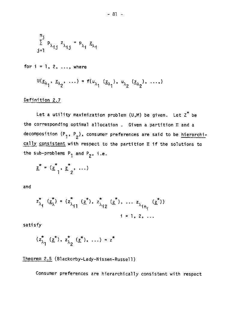
- 81 -
nj
X j.. zx = pj=1 3 13l
for i = 1, 2, ... , where
U(Z , L , ... ) = f(uX (I X), U 2 (LX)2
Definition 2.7
Let a utility maximization problem (U,M) be given. Let Z* be
the corresponding optimal allocation . Given a partition I and a
decomposition (P, P2), consumer preferences are said to be hierarchi-
cally consistent with respect to the partition fl if the solutions to
the sub-problems P1 and P2 ' i.e.
* * *
2= (Lz ,z2 , ... )S2
and
Z () = (z (z*), z (z) .. z (z*))1
i il -i2>i n.
i = 1, 2, ...
satisfy
(z (z*), Z (z*), ... ) =z1 2
Theorem 2.5 (Blackorby-Lady-Nissen-Russell)
Consumer preferences are hierarchically consistent with respect

- 82 -
to a partition IT if and only if they are weakly homothetically separ-
able with respect to IT.
The preceeding set of results have focused on the multi-level
structure of consumer preferences and the associated conditions for
consistent aggregation. In the remainder of this section we will
discuss conditions regarding the inter-temporal structure of consumer
preferences.
Assume given a utility function of the form
U = U(xlt, X2 t, '''Xl nts xlt+l' X2t+l' '..' Xnt+l -
x1 t+-C1' x2t+-c' ''- nt+-d
and let U be weakly separable with respect to the ordered partition
A = {At, At+l' ... 'At+, induced by the time index -c, i.e. A =
{lt+T, 2t+t, ... , nt+T}. We rewrite U as
U = U(xt' xt+1, .. 4' Xt+T ... )
A consumption program X is an infinite sequence of consumption
vectors: X = fxt, xt+ .'' xt+, .... }. A consumption segment X12
is a sub-program starting at time T and ending at time T2l ''i.e.
2 T1 = . t+.',Xt+Tz+1' 't+T 112 1 2-
The consumption segments X0 and X 1iwill be denoted by X andT2 COT2
X respectively; thus X = X0 .

- 83 -
The utility function of order T., u is the restriction of U to
the subset generated by the segments X , i.e.
u1 = u1 (xt)
u2 = u2 (xt xt+1 )
U r= U T (xt' t+19 *so$''xt+- 1
Similarly, the utility function of co-order T, uTis the restric-
tion of U to the subset generated by the segments XT, i.e.
uT = uT (xt+T' xt+T+l, .. )
Given the ordered partition 1T = {At, At+1 , ... } the continuation
of AT is the subset H1T = {At+T, At+T+1l ... }; the segment corresponding
to this continuation is, of course XT.
Definition 2.8
Given a utility function U and an ordered partition II = {At
At. ... , consumer preferences are paid to be strongly recursive
with respect to U if and only if each continuation IT. T = 1, 2, ..
is separable from the variables in the preceding sectors At, At+1 '
.. , Itt+--l'
The condition of strong recursiveness is less restrictive than
that of strong separability and was proposed by Lady and Nissen [83]
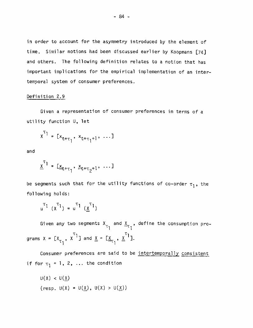
- 84 -
in order to account for the asymmetry introduced by the element of
time. Similar notions had been discussed earlier by Koopmans [741
and others. The following definition relates to a notion that has
important implications for the empirical implementation of an inter-
temporal system of consumer preferences.
Definition 2.9
Given a representation of consumer preferences in terms of a
utility function U., let
x - [xt+T , Xt+Trl3+19
and
- -~t+T3 'At+T2l ..x T1 2
be segments such that for the utility functions of co-order T, the
following holds:
u l(X )U 1 (x)
Given any two segments X and X , define the consumption pro-
TTT
grams X = [XTx x, 1and X_= [xX , XT.
Consumer preferences are said to be intertemporally consistent
if for T1 = 1, 2, ... the condition
U(X) < U(X)
(resp. U(X) = U(X), U(X) > U(x))

- 85 -
holds if and only if
u (X ) < u (X4)
(resp. u1 (X,1 ) = u1 (X ), uT (X ) > UT 1(X1 1 1 1 1 1 1
Theorem 2.6 (Blackorby-Nissen-Primont-Russell)
A necessary and sufficient condition for consumer preferences to
be inter-temporally consistent is that they be strongly recursivo with
respect to the partition induced by the time ordering.
Definition 2.10
Given a representation of consumer preferences in terms of a
utility function U, let
X = [xt' xt+19 .'.'2 t+T
and
_= [At' t+1' 1' ' At+.."
be segments such that for the utility functions of order T1 the fol-
lowing holds:
UT (X )=uT (X )
Given any two segments X and X( , define the consumption pro-
grams

- 86 -
X = EX ,X 1]and X= [4.9 XT
Consumer preferences are said to be stationary if for T1=1,2,...,
the condition
U(X) < U(X)
holds if and only if
uTi (XT, )c<u 1 (X 1)
The following theorem on inter-period aggregation of utility is
slightly less restrictive than earlier results obtained by Koopmans
and Morishima and gives sufficient conditions for a representation of
an intertemporal structure of consumer preferences that will be espe-
cially usefully in the study of optimal growth paths in Chapter 5.
Theorem 2.7
Given a representation of consumer preferences in terms of a
utility function U, there exist functions uT (xt+T) such that
U(X) = 1 (x > 0T0 u (t+T
whenever consumer preferences are strongly recursive and stationary.
Proof.- From Theorem 2.6 it follows that consumer preferences are
intertemporally consistent. The proof then follows that of Koopmans
[74] and Morishima [84] with strong recursiveness substituting for
strong separability.

- 87 -
The conditions of the following theorem are still less restric-
tive in terms of functional structure and the additional requirement
on price variations is often satisfied by expected forward prices.
Theorem 2.8
If an inter-temporal utility function U = U(xt t+l,' ''''
xt+.r,...) is stationary, weakly separable and forward prices (pt+'
pt+2' '''-9 t+, ... ) are always proportional then there exist func-
tions 4:(xt+r) such that
U(X) = C (xt+1n)> 0
Proof: -
The assumption that forward prices change proportionally implies
by using the Leontief-Hicks composite-good theorem (Wold [89]) that
all future goods can be regarded as a single good for -c> 0, i.e. we
can write
U(X) = U(xt' fiX)
By s4milar arguments we can express f'1(Xl) as
fJ X ) = f 1(xt+ 1, xt+ 2 ''..) = fjxt+i f2(X2)
Repeating the argument, we can construct a sequence f., i=1,2,...
such that
fi = fi (xt+i' i+l(X i=l,2,..

- 88 -
It follows from Lady and Nissen [83] that U is strongly recursive.
The proof is complete by invoking Theorem 2.7
2.4.3 Hierarchical Decomposition of Utility Maximization
The point of departure for our model of the household sector is
the assumption that the decisions faced by consumers in period t can
be characterized in terms of the maximization of the utility function
U = U(xt xt+1. ... xt+, ... ) (2.26)
where
Xt= (CEt/Pt CNt/Pt CKt/Pt Ut /Pt)
and
CE - Energy consumption goods purchased by households
CN - Non-energy consumption goods purchased by households
CK - Capital services supplied to households
LJ - Leisure time of the household sector
P - Population
subject to the budget constraint:
Mt(t+T CE + t+T OCN + t+T[ K + t+TrLMt = St+T CtO CEt++ pCN t+T + p CK Kt+T + p L t+)
(2.27)
where St+ is the discount factor for the household sector at time t
in the future, and

- 89 -
PCE - Implicit deflator, energy consumption goods purchased by
households
PCN - Implicit deflator, n'n-energy consumption goods purchased
by households
PCK - Implicit deflator, capital services supplied to households
PL - Implicit deflator, supply of labor services
We observe that the leisure time available to households is evalu-
ated at the opportunity cost of time resources, taken to be equal to
the after-tax wage rate PL'
The above specification can be justified either by regarding the
household sector as an economic entity by itself or by interpreting
the arguments of the utility function as variables that have been
aggregated over all households and then expressed in per capita terms.
The choice of an infinite planning horizon is a result of viewing the
household sector as an entity which lives perpetually although the
composition of its membership constantly changes.
We assume that consumer preferences are stationary and that they
are weakly homothetically separable with respect to the partition Ii
induced by the time index. If follows from Theorem 2.4 that consumer
preferences have the property of strong additive price aggregation:
i.e. there exist price and quantity indices
= t C N tpF =t PCE'PCtN' PCK' PL
Ft = 9t (CEt, CNt, CKt, LJt)
f
(2.28)

- 90 -
such that
U = U(Ftt/P Ft+1/Pt+i . Ft+C /t+ (2.29)
and
pt+T t = B = p+ tCE + pt+CN t T + pt+ tCK + pt+TF t+T t+ +CE t+ T CN t+T CK t+ + L t+T
(2.30)
The indices p and Ft are referred to as the price and quantity
indices of full consumption in period t, respectively.
From Theorem 2.5 it follows that a hierarchical decomposition of
the utility maximization problem given by Eqs. 2.26 and 2.27 is hier-
archically consistent. We therefore define the following utility
maximization problems:
Inter-temporal Allocation Problem
Find a full consumption path
Ft = (Ft3 Ft+1 , ., Ft+' .. )
that maximizes U = U(Ft/Pt, Ft+ 1/Pt+1s ... , Ft+/Pt+,s ... ) subject
to:
CO
I St+ + Ft+T =Mt (2.31)T=a
Intr-Temfppral Allocation Problem
Find a consumption vector
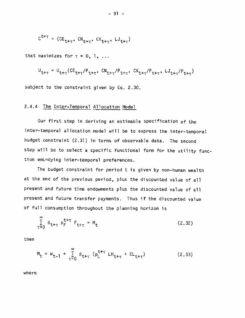
- 91 -
Ct+T - (CE t+T, CNt+T, CKt+C, LJt+T)
that maximizes for T = 0, 1, ...
U t+T= Ut+T(CEt+T/Pt+T, CN t+T'Pt+T, CKt+T/Pt+T, LJt+T/Pt+)
subject to the constraint given by Eq. 2.30.
2.4.4 The Inter-Temporal Allocation Model
Our first step in deriving an estimable specification of the
inter-temporal allocation model will be to express the inter-temporal
budget constraint (2.31) in terms of observable data. The second
step will be to select a specific functional form for the utility func-
tion emLodying inter-temporal preferences.
The budget constraint for period t is given by non-human wealth
at the end of the previous period, plus the discounted value of all
present and future time endowments plus the discounted value of all
present and future transfer payments. Thus if the discounted value
of full consumption throughout the planning horizon is
_ tt+T +T F =M (2.32)T=0t F t+T t
then
0=
Mt =W l + 1 5St+ r(p+, LH t+- + EL t+) (2.33)-L-'r0
where

- 92 -
at = (1/l+MW)
St+T = (/+y)T t T = 1, 2, ... (2.34)
and
W - Private national wealth
PL - Implicit deflator, supply of labor services
LH - Total time endowment of the household sector
EL - Government transfer payments to households
MW - Nominal rate of return, private national wealth
In order to express the budget constraint in terms of variables
in the current period, we must make assumptions about the expected
future prices, expected future time endowments and expected future
transfer payments. In particular, we assume:
(a) Future prices are the same as present prices:
t+T tPCE = PCE
t+T _tPCN = PCN
t+T=_ tPCK =CK
p+= T = 1, 2, ... (2.35)
(b) Future time endowments grow geometrically:
LHt+[ = (1 +-n)T LHt = 1, 2, ... (2.36)
(c) Future transfer payments grow geometrically at the same

- 93 -
constant rate :
ELt+T = (1 +-n) ELt z =1, 2, ... (2.37)
Using these assumptions, together with the expression for
future discount rates given by Eq. (2.34) we can rewrite the budget
constraint (2.33) as follows:
Mt = (1 + MW) Wt- 1 + V[pL LHt + ELt] (2.38)
where
P = ( 1) (1+n)TI+Y(2.39)= T0 y-rI
Because of the assumption about constant future prices given by
2.35, it follows that all forward prices change in direct proportion
to the future discount rates. The conditions of Theorem 2.8 are there-
fore satisfied and we can write
CO
U(Ft) 0 ( uT)u(Fpt+ /t+) (2.40)
where 6 is the rate of pure time preference; i.e. the subjective rate
of social discount.
We will assume that inter-temporal preferences can be adequately
approximated by a neutral transcendental logarithmic utility function.
Following the convention adopted by Christensen, Jorgenson and Lau []
for direct utility functions, we approximate the negative of the loga-
rithm of the utility function as follows:

- 94 -
ln (F +F-. nU(Ft)= _ (0 V)[aoln Ft+ + 00 (n t+T2T=O t+T t+T
+ 1n Ft+T t] (2.41)Pt+T
The translog approximation must satisfy the monotonicity and quasi-
convexity restrictions imposed by the theory of demand. Maximization
of utility subject to the budget constraint leads to the following
identity by applying the first-order conditions for stationarity to
the Lagrangian:
31n U p Ft oo nln U FtI Ft U (2.42)t t t =9 t+,
Applying this relationship to the translog utility function given in
(2.41), we obtain the following allocation equation:
PFFt ,F a + 00 ln(Ft/Pt) + tMFt - lF 7t t tOt (2.43)Mt am + MO ln(Ft/Pt) + mt . t (.3
where
aM T al+6 =~ (I.) cm (2. 44)
T0
and
6 0 _ t(2.46)
-=

- 95 -
Finally, substituting the expression for Mt from (2.38) into (2.44),
we obtain
F + S 00 ln(Ft/Pt) + %t ' tPFFt " 0M + SMO ln(Ft/Pt) + SMt - t- + t-+ pL t+ t
(2.47)This form of the inter-temporal allocation function gives the value
of wealth allocated to consumption in the current period as a func-
tion of observable quantities and of parameters to be estimated.
2.4.5 The Intra-Temporal Allocation Model
The intra-temporal allocation model is aimed at explaining the
decisions made by consumers in the current period t concerning their
expenditure levels for energy products CE, non-energy CN, capital
services CK and leisure LJ, given the level of total current expendi-
tures Bt = pFtF and the prices of the three commodity groups and labor.
We assume that the intra-period utility function
Ut = Ut(CEt/Pt CNt/Pt CKt/Pt LJt/Pt) (2.48)
is a function of per capita levels of consumption and leisure and can
be approximated by a direct transcendental logarithmic utility function
with time-varying preferences. Specifically we express the negative
of the logarithm of the intra-period utility function as:
C C C C 4 C-lnUt = a + aE ln CEt/Pt + a ln CNtt + K in CKt/Pt
+ Ut/PnLJ/t P+ IEE(ln CEt/PX12 + C ln CEt/Pt In CNtt
+ ... + C t 2](2.49)

- 96:
Applying the necessary conditions for stationarity to Eq. (2.49) sub--
ject to the budget constraint
t t t t tPCE CEt + pCN CNt +pCK CKt + pL Lt = Bt = PFFt (2.50)
we obtain the following expressions for the expenditure shares of each
commodity group and leisure:
t CEPCE t
B t
tPCNCN t
B t
pL t _CK tB t
p tLJ __tB t
C 4aE + ]
i=i
C n x C +Ei t Et
(2.51)c 4
cc + 6C n x* + '
C i0 C: + n xt + .t
_ tM 1=1 in
am + in xt + st t
c 4 c 1 caK + . Kiz n xt+ Nt ' t
4a +jI E. in xi + t(m +~ N t tt
aC in x + Jti =1
Cct +
4 Cztlii =1
(2.52)
(2.53)
(2.54)
ln xi+ ct
where xi refer to the per capita values of the three commodity groups
and leisure, i.e.
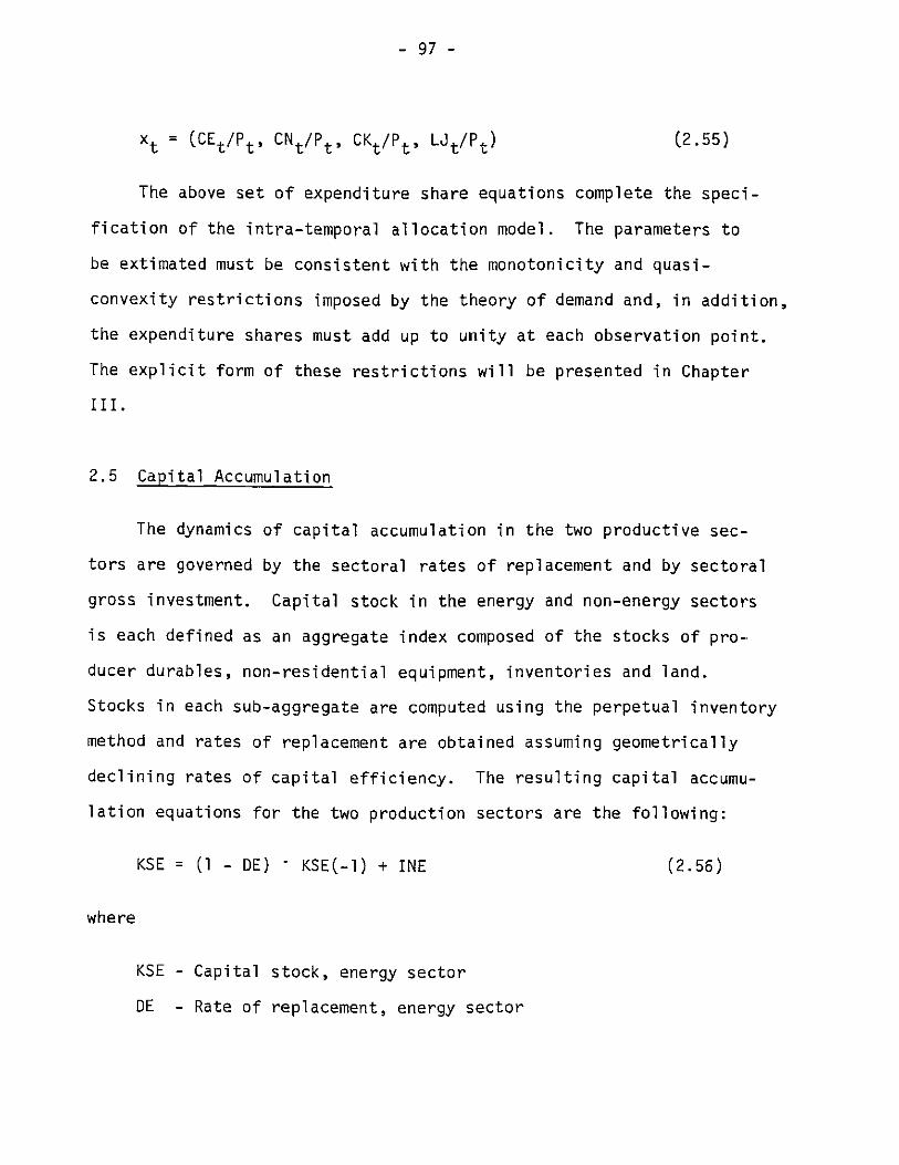
- 97 -
xt = (CEt/Pts CNt/Pt, CKt/Pt, LJt/Pt) (2.55)
The above set of expenditure share equations complete the speci-
fication of the intra-temporal allocation model. The parameters to
be extimated must be consistent with the monotonicity and quasi-
convexity restrictions imposed by the theory of demand and, in addition,
the expenditure shares must add up to unity at each observation point.
The explicit form of these restrictions will be presented in Chapter
III.
2.5 Capital Accumulation
The dynamics of capital accumulation in the two productive sec-
tors are governed by the sectoral rates of replacement and by sectoral
gross investment. Capital stock in the energy and non-energy sectors
is each defined as an aggregate index composed of the stocks of pro-
ducer durables, non-residential equipment, inventories and land.
Stocks in each sub-aggregate are computed using the perpetual inventory
method and rates of replacement are obtained assuming geometrically
declining rates of capital efficiency. The resulting capital accumu-
lation equations for the two production sectors are the following:
KSE = (1 - DE) - KSE(-l) + INE (2.56)
where
KSE - Capital stock, energy sector
DE - Rate of replacement, energy sector

- 98 -
INE - Gross investment, energy sector
and
KSN = (1 - DN) ' KSN(-l) + INN (2.57)
where
KSN - Capital stock, non-energy sector
DN - Rate of replacement, non-energy sector
INN - Gross investment, non-energy sector
The equations of capital accumulation for the household sector
are analogous. For the stock of consumer durables, we have
KCD = (1 - DCD) ' KCD(-l) + ICD (2.58)
where
KCD - Stock of consumer durables, household sector
DCD - Rate of replacement, consumer durables
ICD - Gross investment in consumer durables
with an analogous equation for residential structures:
KRS = (1 - DRS) ' KRS(-l) + IRS (2.59)
where
KRS - Capital stock, residential structures
DRS - Rate of replacement, residential structures
IRS - Gross investment in residential structures
The model of capital stocks and flows is completed by the fol-
lowing relationships which determine the levels of capital services

- 99 -
supplied by the capital stocks held by the production and household
sectors and relate the sectoral gross investment levels to the level
of total purchases of investment goods by the private domestic sec-
tor:
KE = QKE ' KSE(-l)
KN = QKN - KSN(-1)
CK = QKS 0 KRS(-l) + QKD KCD(-I)
INE = ZINE - I
INN = ZINN - I
IRS = ZRS 0I
ICD = ZCD I
(2.60)
(2.61)
(2.62)
(2.63)
(2.64)
(2.65)
(2.66)
where
KE - Capital services, energy sector
QKE - Quality of capital, energy sector
KN - Capital services, non-energy sector
QKN - Capital services, non-energy sector
ZINN - Scaling variable, gross investment in
to total investment
ZINE - Scaling variable, gross investment in
total investment
ZRS - Scaling variable, gross investment in
tures to total investment
ZCD - Scaling variable, gross investment in
to total investment
IT - Gross private domestic investment
non-energy sector
energy sector to
residential struc-
consumer durables

- 100 -
sector
In order to complete the characterization of capital inputs, we
must select a method for the imputation of the rental value of owner-
utilized assets. Our point of departure is the identity that relates
the price of an asset to the discounted value of its services. The
value of capital service input is equal to the value of property com-
pensation in the absence of taxes. Also, in the absence of tax policies,
the price of capital services of an asset group is equal to the oppor-
tunity cost of the asset group plus its depreciation. In order to
incorporate the effect of taxes, we employ the formulation developed
by Christensen and Jorgenson [ ]. Specifically, for tangible fixed
assets held by the energy sector, the price of capital services is:
1 - TKE'PVDE - ITCE
PKE = (1/QKE)[ -TE[ME'p(-l) + DE'p - CAG]
+ TPE'p1 (2.67)
where
TKE - Effective tax rate on capital income, energy sector
TPE - Effective tax rate on capital property, energy sector
PVDE - Present value of depreciation deductions for tax purposes
per dollar of investment, energy sector
ITCE - Effective investment tax credit, energy sector
ME - Rate of return on fixed tangible assets, energy sector
DE - Rate of replacement, energy sector
CAG - Effective rate of capital gains per dollar of fixed assets
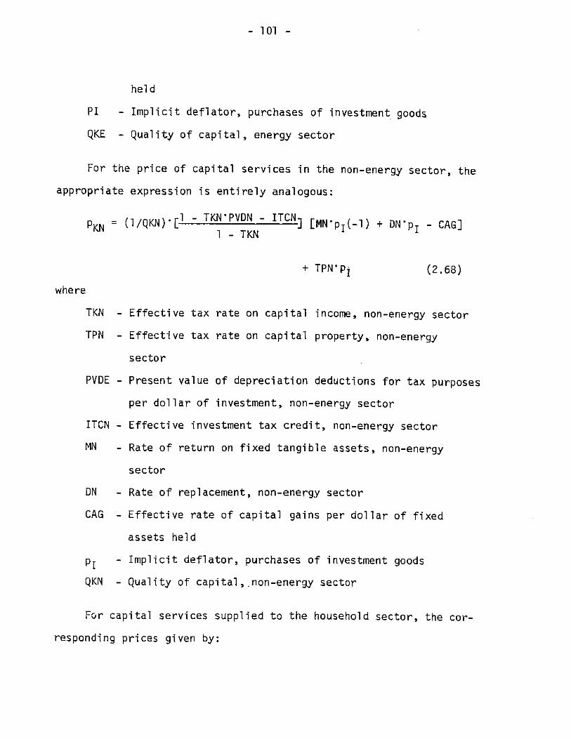
- 101 -
held
PI - Implicit deflator, purchases of investment goods
QKE - Quality of capital, energy sector
For the price of capital services in the non-energy sector, the
appropriate expression is entirely analogous:
pKN= (1/QKN)'[ 1 - TKN'PVDN - ITCNj [MN'p(-l) + DN'p1 - CAG]1 - TKN
+ TPN'Pi (2.68)
where
TKN - Effective tax rate on capital income, non-energy sector
TPN - Effective tax rate on capital property, non-energy
sector
PVDE - Present value of depreciation deductions for tax purposes
per dollar of investment, non-energy sector
ITCN - Effective investment tax credit, non-energy sector
MN - Rate of return on fixed tangible assets, non-energy
sector
DN - Rate of replacement, non-energy sector
CAG - Effective rate of capital gains per dollar of fixed
assets held
pI - Implicit deflator, purchases of investment goods
QKN - Quality of capital,.non-energy sector
For capital services supplied to the household sector, the cor-
responding prices given by:

- 102 -
pCK = (1/QCK) [MC'p(-i) + DC'p1 - CAG] + TPC'pI (2.69)
where
TPC - Effective tax rate on capital property, household sector
MC - Rate of return, fixed tangible assets, household sector
DC Rate of replacement, household sector
CAG - Effective rate of capital gains per dollar of fixed assets
held
QCK - Quality of capital, household sector
2.6 Income-Expenditure Identities
In order to complete the specification of the model, we must
introduce accounting relationships that stipulate the equality between
revenues and outlays for each sector and each product category.
For each of the two producing sectors, the value of output must
equal the value of input:
PEC EC + PEM EM = PKE KE + PLE LE + PNME NME + PEME EME + PRE RE
(2.70)
where
PEC - Implicit deflator, supply of energy consumption products
EC - Supply of energy consumption products
PEM - Implicit deflator, supply of energy intermediate products
EM - Supply of energy intermediate products
PKE - Implicit deflator, capital services, energy sector

- 103 -
KE - Capital services, energy sector
PLE - Implicit deflator, labor services purchased by the energy
sector
LE - Labor services purchased by the energy sector
PNME - Implicit deflator, non-energy intermediate products pur-
chased by the energy sector
NME - Non-energy intermediate products purchased by the energy
sector
PEME - Implicit deflator, energy intermediate products purchased
by the energy sector
EME - Energy intermediate products purchased by the energy sec-
tor
PRE - Implicit deflator, competitive imports of energy products
RE - Competitive imports of energy products
A similar identity holds for the non-energy sector:
PNC NC + PNM NM + PNI NI = pKN KN + PLN LN + PEMN EMN + PNMN NMN
+ PRN RN (2.71)
where
PNC - Implicit deflator, supply of non-energy consumption pro-
ducts
NC - Supply of non-energy consumption products
PNM - Implicit deflator, supply of non-energy intermediate pro-
ducts
NM - Supply of non-energy intermediate products

- 104 -
PNI - Implicit deflator, supply of investment goods
NI - Supply of investment goods
PKN - Implicit deflator, capital services, non-energy sector
KN - Capital services, non-energy sector
PLN - Implicit deflator, purchases of labor services by the non-
energy sector
LN - Labor services purchased by the non-energy sector
PEMN - Implicit deflator, energy intermediate products purchased
by the non-energy sector
EMN - Energy intermediate products purchased by the non-energy
sector
PNMN - Implicit deflator, non-energy intermediate products pur-
chased by the non-energy sector
NMN - Non-energy intermediate products purchased by the non-
energy sector
PRN - Implicit deflator, competitive imports of non-energy pro-
ducts
RN - Competitive imports of non-energy products
The value of energy consumption goods purchased by the final users
must equal the gross revenue on sales of energy consumption goods by
the energy sector:
(1 + TCE) PEC EC = pCE CE + pSTE STE + pGE GE + PEXE EXE (2.72)
where
PEC - Implicit deflator, supply of energy consumption goods

- 105 -
TCE - Effective tax rate, energy consumption goods
EC - Supply of energy consumption goods
PCE - Implicit deflator, energy consumption goods purchased by
households
CE - Energy consumption goods purchased by households
PSTE - Implicit deflator, energy consumption goods delivered to
business inventories
STE - Energy consumption goods delivered to business inventories
GE - Implicit deflator, government purchases of energy consump-
tion goods
GE - Government purchases of energy consumption goods
PEXE - Implicit deflator, gross exports of energy consumption
goods
EXE - Gross exports of energy consumption goods
Similarly for non-energy consumption goods there must be equality
between revenues and expenditures:
(1 + TCN) PNC NC = PCND CND + PSTN STN + PGN GN + PEXN EXN
(2.73)
where
PNC - Implicit deflator, supply of non-energy consumption products
NC - Supply of non-energy consumption products
TCN - Effective tax rate, non-energy consumption products
PCND - Implicit deflator, non-energy domestic consumption products
purchased by households

- 106 -
CND - Non-energy domestic consumption products purchased by households
PSTN - Implicit deflator, non-energy products delivered to business
inventories
STN - Non-energy consumption products delivered to business
inventories
PGN - Implicit deflator, government purchases of non-energy con-
sumption products
GN - Government purchases of non-energy consumption products
PEXN - Implicit deflator, gross exports of non-energy consumption
products
EXN - Gross exports of non-energy consumption products
PCIM - Implicit deflator, imports of non-energy consumption goods
CIM - Imports of non-energy consumption goods
The revenues received by the suppliers of investment goods, plus
the corresponding sales taxes, must equal the total outlays on invest-
ment goods by the private, government and foreign sectors:
(1 + TI) pNI NI + pIMI1 MI + pSTE STE + PSTN STN = p, I + PGI GI
+ PEXI EXI
where (2.74)
PNI - Implicit deflator, supply of investment goods
NI - Supply of investment goods
p1 - Implicit deflator, gross private domestic investment

- 107 -
I - Gross private domestic investment
pG1 - Implicit deflator, purchases of investment goods by the
government sector
GI - Purchases of investment goods by the government sector
TI - Effective tax rate, purchases of investment goods
PIMI - Implicit deflator, imports of investment goods
IMI - Imports of investment goods
PSTE - Implicit deflator, inventory investment of energy products
STE - Inventory investment of energy products
PSTN - Implicit deflator, inventory investment of non-energy pro-
duct
STN - Inventory investment of non-energy products
PEXI - Implicit deflator, gross exports of investment goods
EXI - Gross exports of investment goods
The income-expenditure identities must also hold for intermediate
products:
PEM EM = PEMN EMN + PEME EME (2.75)
where
PEM - Implicit deflator, supply of energy intermediate products
EM - Supply of energy intermediate products
PEMN - Implicit deflator, energy intermediate products purchased
by the non-energy sector
EMN - Energy intermediate products purchased by the non-energy
sector

- 108 -
PEME - Implicit deflator, energy intermediate products purchased
by the energy sector
EME - Energy intermediate products purchased by the energy sec-
tor
and
PNM NM = PNME NME + PNMN NMN C2.76)
where
PNM - Implicit deflator, supply of non-energy intermediate pro-
ducts
NM - Supply of non-energy intermediate products
PNME - Implicit deflator, non-energy intermediate products pur-
chased by the energy sector
NME - Non-energy intermediate products purchased by the energy
sector
PNMN - Implicit deflator, non-energy intermediate products pur-
chased by the non-energy sector
NMN - Non-energy intermediate products purchased by the non-
energy sector
The total value of saving by the private domestic sector plus
the government and foreign saving in the U.S. must equal the value of
gross private domestic investment:
S = pI I + pQ (G - G(-l)) + PR (R - R(-l)) (2.77)
where

- 109 -
S - Gross private domestic saving
pI - Implicit deflator, gross private domestic investment
I - Gross private domestic investment
G - Net claims on government by private domestic sector
PG - Implicit deflator, net claims on government by private domes-
tic sector
R - Net claims on rest of the world by private domestic sector
PR - Implicit deflator, net claims on rest of the world by pri-
vate domestic sector
The total value of wealth is the value of fixed tangible assets
plus the value of net claims on the government and foreign sectors:
W = p1 (KSE+ KSN+ KRS + KCD) ZW + p G + PR R (2.78)
where
pI - Implicit deflator, gross private domestic investment
KSE - Capital stock, energy sector
KSN - Capital stock, non-energy sector
KRS - Capital stock, residential structures
KCD - Capital stock, consumer durables
ZW - Aggregation variable, capital stock to wealth
PG - Implicit deflator, net claims on government sector
G - Net claims on government sector
PR - Implicit deflator, net claims on foreign sector
R - Net claim on foreign sector
i - Private domestic wealth
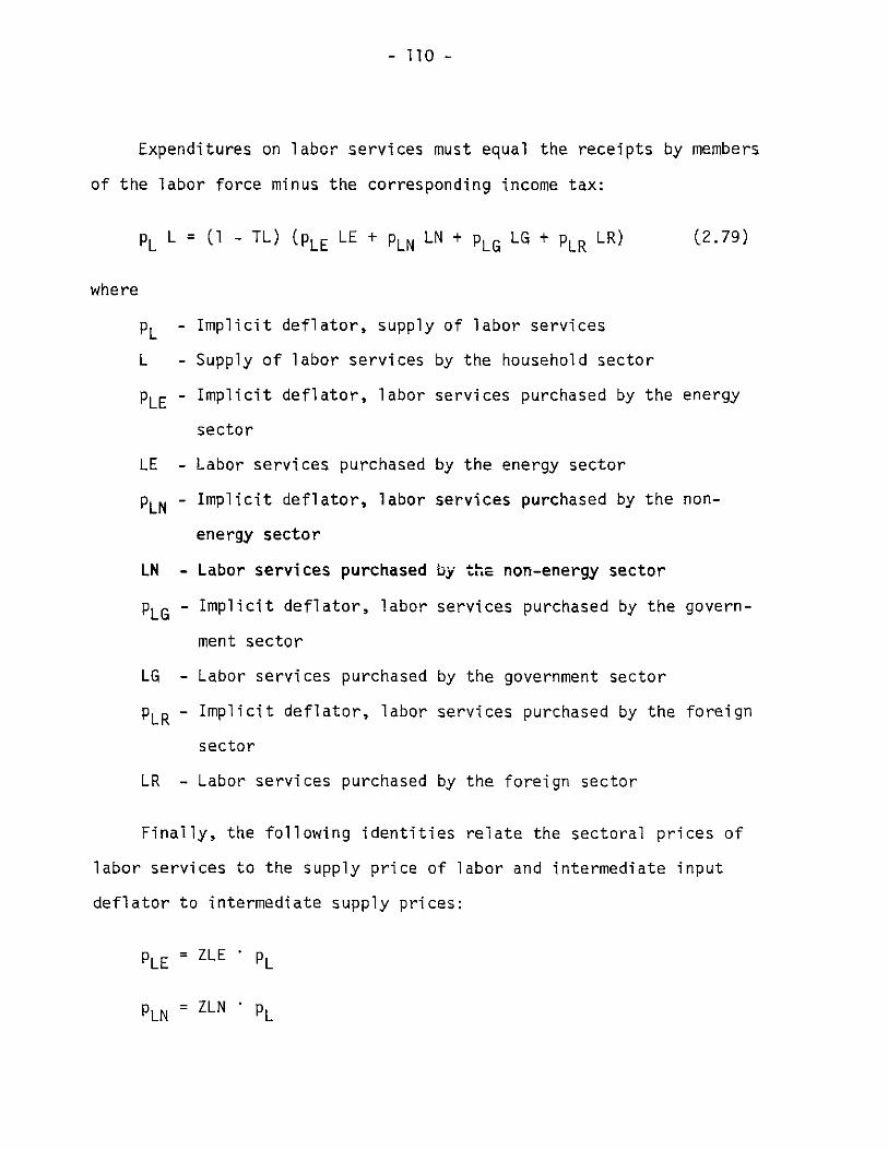
- 110 -
Expenditures on labor services must equal the receipts by members
of the labor force minus the corresponding income tax:
PL L = (1 - TL) (PLE LE + PLN LN + PLG LG + PLR LR) (2.79)
where
- Implicit deflator, supply of labor services
L - Supply of labor services
PLE - Implicit deflator, labor
sector
LE - Labor services purchased
PLN - Implicit deflator, labor
energy sector
LN - Labor services purchased
PLG - Implicit deflator, labor
ment sector
LG - Labor services purchased
PLR - Implicit deflator, labor
sector
LR - Labor services purchased
by the household sector
services purchased by the energy
by the energy sector
services purchased by the non-
by the non-energy sector
services purchased by the govern-
by the government sector
services purchased by the foreign
by the foreign sector
Finally, the following identities relate the sectoral prices of
labor services to the supply price of labor and intermediate input
deflator to intermediate supply prices:
PLE = ZLE PL
PLN = ZLN K*PL

- 111 -
PEMN = ZNE*PEM
PNME = ZEN ' PNM (2.80)
where
PL - Implicit deflator, supply of labor services
PLE - Implicit deflator, labor services purchased by the energy
sector
PLN - Implicit deflator, labor services purchased by the non-
energy sector
ZLE - Scaling variable, price of labor services to price of labor
service purchased by the energy sector
ZLN -- Scaling variable, price of labor services to price of
labor service purchased by the non-energy sector
PEMN - Implicit deflator, intermediate energy products purchased
by the non-energy sector
PNME - Implicit deflator, intermediate non-energy products pur-
chased by the energy sector
ZNE - Scaling variable, price of energy intermediate goods to
price of energy purchased by the non-energy sector
ZEN - Scaling variable, price of non-energy intermediate goods
to price of non-energy goods purchased by the energy sec-
tor
PEM - Implicit deflator, energy intermediate products
PNM - Implicit deflator, non-energy intermediate products

- 112 -
The following identity relates to the nominal rate of return
on wealth to the sectoral rates of return:
MW-[KSE(-l) + KSN(-l) + KCD(-l) + KRS(-l)]
= ZRN-[ME-KSE(-l) + MN-KSN(-1)] (2.81)
where
MW - Nominal
KSE - Capital
KSN - Capital
KCD - Capital
KRS - Capital
ZRN - Scaling
rate of
ME - Nominal
sector
MN - Nominal
rate of return on wealth
stock, energy sector
stock, non-energy sector
stock, consumer durables
stock, residential structures
variable, sectoral rates of return to nominal
return on wealth
rate of return on fixed tangible assets, energy
rate of return on fixed tangiblc assets, non-
energy sector
Finally, the quantity index of full consumption for the house-
hold sector is defined as an aggregate of the quantity indices for
leisure, non-energy goods, energy goods and capital services purchased
by households:
F = 0.8225 LJ + 1.0786 CK + 0.9349 CN + 2.4956 CE + 0.8559* (2.82)
*This linear aggregation equation is an approximation to the Divisiaaggregate index obtained by regressing the Divisia index for Fagainst the four quantity components. For this OLS regression,
R2 = 1.00.

- 113 -
where
F - Full consumption, household sector
CK - Capital services supplied to households
CN - Non-energy consumption goods purchased by households
CE - Energy consumption goods purchased by households
LJ - Leisure time available to households
2.7 Balance Equations
As a result of the process of market equilibration, equality
between quantities supplied and quantities demanded must hold for each
product category in the model.
The supply of energy consumption goods must equal the amounts
used by households, government, the foreign sector, and business
inventories:
EC = CE + STE + GE + EXE (2.83)
where
EC - Energy consumption products supplied by the energy sector
CE - Energy consumption products purchased by households
STE - Energy consumption products delivered to business inventories
GE - Energy consumption products purchased by the government
EXE - Exports of energy consumption products
Non-energy consumption products supplied by the domestic and
foreign sectors must be used up by households, business inventories,
and the government and foreign sectors:
NC + CIM = CN + STN + GN + EXN (2.84)

- sI 1 4 -
where
NC - Non-energy consumption products supplied by the non-energy
sector
CIM - Imports of non-energy consumption goods
CN - Non-energy consumption goods purchased by households
STN - Non-energy consumption goods delivered to business
inventories
GN Non-energy consumption goods purchased by the government
sector
EXN - Exports of non-energy consumption goods
Investment goods supplied by the domestic non-energy sector, plus
imported investment goods and inventory investment in the two produc-
tion sectors must equal gross private domestic investment plus invest-
ment goods purchased by the government and foreign sectors. Gross
private domestic investment is itself composed of gross investment in
the production and household sectors:
NI + STE + STN = I + GNI + E'I (2.85)
IMI + I = INE + INN + ICD + IRS (2.86)
where
NI - Supply of investment goods by the non-energy sector
IMI - Imports of investment goods
STE - Energy consumption goods delivered to business inventories
STN - Non-energy consumption goods delivered to business inven-
tories

- 115 -
I - Gross private domestic investment
GNI - Investment goods purchased by the government sector
EXI - Exports of investment goods
INE - Gross investment, energy sector
INN - Gross investment, non-energy sector
ICD - Gross investment, consumer durables
IRS - Gross investment, residential structures
Clearing of the intermediate goods markets implies the following
equalities between supply and demand:
NM = NME + NMN (2.87)
EM = EME + EMN (2.88)
where
NM - Supply of non-energy intermediate products
NME - Non-energy intermediate products purchased by the energy
sector
NMN - Non-energy intermediate products purchased by the non-energy
sector
EM - Supply of energy intermediate products
EME - Energy intermediate products purchased by the energy sector
EMN - Energy intermediate products purchased by the non-energy
sector
The supply of labor must be used up exactly by the two production
sector, by the government sector and the foreign sector and by the
fraction of workers that remain unemployed:

- 116 -
L = LE + LN + LG + LR + LU (2.89)
where
L - Supply of labor by the household sector
LE - Labor services purchased by the energy sector
LN - Labor services purchased by the non-energy sector
LG - Labor services purchased by the government sector
LR - Labor services purchased by the foreign sector
LU - Unemployed labor
The total time resources of the household sector must be exhausted
between leisure and labor:
LH = LJ + L (2.90)
where
LH - Time endowment of the household sector
LJ - Leisure time of the household sector
L - Supply of labor by the household sector
Total purchases of non-energy consumption goods by households equal
the quantities of domestic and imported goods purchased:
CN = CND + CIM (2.91)
where
CN - Non-energy consumption goods purchased by households
CND - Domestic non-energy consumption goods purchased by households
CIM - Imported non-energy consumption goods purchased by households

- 117 -
2.8 Summary
This chapter has described the behavioral assumptions which underlie
the specification of the individual equations in our macro-economic
energy model. The next chapter addresses the econometric questions
surrounding the empirical implementation of the model.
Our long-term macroeconomic model has three major components: the
sub-model of producer behavior, the sub-model of consumer behavior and
the sub-model of investment and capital accumulation. The key interac-
tions between these three sectors are diagrammatically represented in
Fig. 2-1.
The two production sub-sectors lead to derived demand relationships
for the following factor inputs:
Energy Sector
- Capital Services (KE)
- Labor Services (LE)
- Energy Intermediate
Products (EME)
- Non-Energy Intermediate
Products (NME)
- Imports (RE)
Non-Energy Sector
- Capital Services (KN)
- Labor Services (LN)
- Energy Intermediate
Products (EMN)
- Non-Energy Intermediate
Products (NMN)
- Imports (RN)
Correspondingly, the behavioral assumptions underlying our
production sub-model yield derived supply relationships for the
following products:

PRICE OFINVESTNRENT1-
GOVERNMEN1 SECTOR--- ---- - GOVERNMENT DEMANI
TAX REVENUES, - FOR CONSUMPTION G(TRANSFER PAYMENTS, INVESTMENT GOODS APURCHASES OF GOODS LABOR SERVICESAND SERVICES
FOREIGN SECTOR
NET DEMAND FORCONSUMPTION GOODS,INVESTMENT GOODSAND
HOUSEHOLDPRICE OF DEMAND FORCAPITAL CAPITALSERVICES SERVICES
HOUSEHOLDDEMAND FORNON-ENERGY
PRODUCTS
WEALTH, FROMPREVIOUS PERIOD
HOUSEHOLD
TIME RESOURCES SECIOR
--F-[POPULA TION i
POPULATION A A HOUSEHOLDDEMAND FOR
ENERGYPRODUCTS
INCOME DMN OTRANSFER LEISURRECEIPlS
SUPPLY OFLABOR
SERVICESI
LFFECTIVE TAXLABOR RATE ON LABOR
- -- C---INCO I ME
TAX REVENUESFROM LABOR
INCOME
INVETMENTh G[ODSINVESTMENT GOODSDEA
DODS, MARKET - tNERGY S " ----
kND -----
PRICES AND QUANTITIES: INVESTMENTINVESTMENT GOODS DEMAND
NON-ENERGYSECTOR EXPANSION PRICE OF COST OF EXPANSION
L INVESTMENT - CAPITAL - CAPITAL INVESTMENT ---.DEMANDS--S NON-ENERGY' DA
NON-ENERGY NON-ENERGY SECTOR ENERGENERGSECTOR SECTOR SECTOR
REPLACEMENT L CAPITAL REPLACEMENTINVESTMENT RATE OF SERVICES INVESTMENT
_- ----- DEMAND REPLACEMENT TAX RATE DEMANDT RNON-ENERGY NON-ENERGY NON-ENERGY ENERGY
SECTOR SECTOR SECTOR SECTOR
L CAPITAL STOCK..FROM PREVIOUS F- PERIOD _
NON-ENERGYSECTOR L
CAPITALEFFICIENCYF
SUPPLY OF I NON-ENERGYINVESTMENT SECTOR
GOODS _
LSUPPLY OFCAPITAL
CHANGES IN SERVICESINVENTORIES NON-ENERGY
SECTOR
L - NON-ENERGYCONSUMPTION GOODS INTERMEDIATE ENERC
MARKET NON-ENERGY GOODS MARKET
PRICE OF SUPPLY OFNON-ENERGY PRICES AND QUANTITIES: SUPPLY PRICES AND QUANTITIES: PRODUCTCONSUMPTION NON-ENERGY NON-ENERGY PRODUCTION
GOODS CONSUMPTION GOODS CONSUMPTION NON-ENERGYSECTOR INTERMEDIATE GOODS SECTO
PRICE OFENERGY - ENERGY CONSUMPTION
CONSUMPTION GOODS MARKETGOODS
PRICES AND QUANTITIES:ENERGY CONSUMPTION SUPPLY OF
GOODS ENERGYCONSUMPTION
GOODS
CHANGES ININVENTORIES
- LABOR SERVICES
DEMAND FORLABOR SERVICES
LABOR MARKET NON-ENERGYSECTOR
EMPLOYMENT LEVEL,PRICE OF LABOR
SERVICES DEMAND FOR __LABOR SERVICESENERGY SECTOR TAX REVENUES
I
LAG
PRICE OF COST OFCAPITAL - - CAPITALSERVICES ENERGYENI Y SECTORSECfOR
AL EFFECTIVECAPITAL
RATE OF SERVICESEPLACEMENT TAX RATE
ENERGY ENERGYSECTOR SECTOR
CAPITAL STOCKROM PREVIOUS
PERIOD
ENERGYSECTOR
CAPITALEFFICIENCY
ENERGYSECTOR
SUPPLY OFCAPITALSERVICESENERGY]SECTOR
i Y
TION
)R
Fig. 2-1: Long-Term Macroeconomic Energy Model
FROM LAPiITAL .INCOME
2
-4

- 119 -
Energy Sector Non-Energy Sector
- Energy Consumption - Non-Energy Consumption
Products (EC) Products (NC)
- Energy Intermediate - Non-Energy Intermediate
Products (EM) Products (NM)
- Investment Goods (NI)
The sub-model of consumer behavior determines the demands of house-
holds for energy consumption goods (CE), non-energy consumption goods
(CN), capital services (CK) and leisure (LJ). The demand for leisure
yields a supply schedule for labor services when considered jointly
with the total time endowment of the household sector. The third com-
ponent of the model serves to determine the demand for investment, the
sectoral rates of return and, through the accumulation and capital
efficiency relationships, the supply of capital services. In addition
to the market-clearing conditions for the various product categories,
the production and household sectors are linked through the sectoral
rates of return which are determinants of capital service prices and,
through the nominal rate of return on wealth, of the budget constraint
of the household sector.
The model attempts to characterize the interrelations between
levels of energy utilization and overall economic performance. Since
it is primarily a long-term growth model, it focuses attention on the
properties of alternative paths of potential output rather than on ques-
tions related to the levels of capacity utilization and employment.
The model draws upon the body of neoclassical theory: i.e. representa-

- 120 -
tions of the decisions of individual economic agents are derived from
postulated assumptions of constrained maximizing behavior. A full set
of market-clearing prices and quantities are computed within a simul-
taneous process of market equilibration: i.e. it follows the tradition
of general equilibrium models. This property makes it possible to
establish a link between the macroeconomic relationships in the model
and economic magnitudes susceptible of interpretation from the vantage
point of microeconomic analysis. Indeed, although the model is
aggregative, the introduction of a higher degree of sectoral detail
would entail no new conceptual difficulties.
- 121 -
REFERENCES TO CHAPTER II
[1] Samuelson, P. A., "The Year Ahead: Economic Outlook," The Times,London, December 31, 1974.
[2] Kendrick, J. W., Productivity Trends in the U.S., Princeton,Princeton University Press, 1961.
[3] Denison, E. F., The Sources of Economic Growth in the U.S. and theAlternatives Before Us, Supplementary Paper No. 13, New York,Committee for Economic Development, 1962.
[4] Jorgenson, D. W. and Griliches, Z., "The Explanation of ProductivityChange," Review of Economic Studies, Vol. 34, July 1967.
[5] Schurr, S. H. et al., Energy in the American Economy, 1850-1955:An Economic Analysis of its History and Prospects, The JohnsHopkins Press, Baltimore, 1960.
[6] Darmstadter et al., Energy in the World Economy, Resources for theFuture, Inc., The Johns Hopkins Press, Baltimore, 1971.
[7] Netschert, B., "Fuels for the Electric Utility Industry, 1971-1985,"National Economic Research Associates, Inc., Washington, D.C.,1972.
[8] Berndt, E. R. and Wood, D. 0., "An Economic Interpretation of theEnergy-GNP Ratio," in Energy: Demand, Conservation and Institu-tional Problems, M.I.T. Press, Cambridge, Massachusetts, 1974.
[9] Jorgenson, D. W., Energy Resources and Economic Growth, Cambridge,Ballinger, 1975 (forthcoming).
[10] Hudson, E. A. and Jorgenson, D. W., "U.S. Energy Policy andEconomic Growth, 1975-2000, The Bell Journal of Economics andManagement Science, Vol. 5, No. 2, Autumn 1974.
[11] Hudson, E. A., Optimal Growth Policies, Ph.D. Thesis, Dept. ofEconomics, Harvard University, September 1973.
[12] Christensen, L. R., Saving and the Rate of Return, Social SystemsResearch Institute, SFM 6805, The University of Wisconsin, 1968.

- 122 -
[13] Christensen, L. R., "Tax Policy and Investment Expenditures in aModel of General Equilibrium," Proceedings of the 82nd AnnualMeeting of the American Economic Association, American EconomicReview, May, 1970.
[14] Jorgenson, D. W., Long-Term Impact of U.S. Tax Policy, unpublished,September 1972.
[15] Morishima, M., Equilibrium, Stability and Growth, Clarendon Press,Oxford, 1964.
[16] Fischer, S., "Keynes-Wicksell and Neoclassical Models of Money andGrowth," American Economic Review, December 1972.
[17] Christensen, L. R., and Jorgenson, D. W., "U.S. Real Product andReal Factor Input," 1929-1967, Review of Income and Wealth,Series 16, March 1970.
[18] Hicks, J. R., Yalue and Capital, Clarendon Press, Oxford, 1946.
[19] Roy, R., De l'Utilit6: Contribution a la Theorie des Choix, Hermann,Paris, 1943.
[20] Uzawa, H., "Duality Principles in the Theory of Cost and Produc-tion," International Economic Review, 5, 1964.
[21] Hotelling, H., "Edgeworth's Taxation Paradox and the Nature ofDemand and Supply Functions," The Journal of Political Economy,40, 1932.
[22] Shepard, R. W., Cost and Production Functions, Princeton UniversityPress, 1953.
[23] Bruno, M., "Fundamental Duality Relations in the Pure Theory ofCapital and Growth," The Review of Economic Studies, 36, January1969.
[24] Burmeister, E., and Kuga, K., "The Factor-Price Frontier, Dualityand Joint Production," The Review of Economic Studies, 37, January,1970.
[25] McFadden, D. L., "Cost, Revenue and Profit Functions," in AnEconometric Approach to Production Theory.
[26] Diewert, W. E., "An Application of the Shepard Duality Theorem:A Generalized Leontief Production Function," Journal of PoliticalEconomy, May/June 1971.
[27] Lau, L. J., "Profit Functions of Technologies with Multiple Inputsand Outputs," The Review of Economics and Statistics, Vol. 54,No. 3, August 1972.

- 123 -
[28] Christensen, L., Jorgenson, D. W., and Lau, L, R., "TranscendentalLogarithmic Production Frontiers," The Review of Economics andStatistics, February, 1973.
[29] Hall, R. E., "The Specification of Technologies with Several Kindsof Outputs," The Journal of Political Economy, Vol. 81, No. 4, 1973.
[30] Cobb, C., and Douglas, P. H., "A Theory of Production," AmericanEconomic Review, Supplement to Vol. 18, 1928.
[31] Arrow, K. J., Chenery, B. S., Minhas, B. S., and Solow, R. M.,"Capital-Labor Substitution and Economic Efficiency," The Review ofEconomics and Statistics, August, 1961.
[32] Uzawa, H., "Production Functions with Constant Elasticities ofSubstitution," The Review of Economic Studies, 29, October 1962.
[33] McFadden, D. L., "Further Results on C.E.S. Production Functions,"The Review of Economic Studies, 30, June 1963.
[34] Sato, K., "Two-Level Constant-Elasticity-of-Substitution ProductionFunction," The Review of Economic Studies, 34, April 1967.
[35] Diewert, W. E., "Functional Forms for Profit and TransformationFunctions," Journal of Economic Theory,
[36] Christensen, L. R., Jorgenson, D. W., and Lau, L. J., "ConjugateDuality and the Transcendental Logarithmic Production Function,"Econometrica, 39, July 1971 (abstract).
[37] Berndt, E. R. and Christensen, L. R., "The Translog Function andthe Substitution of Equipment, Structures and Labor in U.S. Manu-facturing 1929-68," Journal of Econometrics, Vol. 1, No. 1,March 1973.
[38] Woodland, A. D., "Substitution of Structure, Equipment, and Laborin Canadian Production," International Economic Review, February1975.
[39] Humphrey, D. B., and Moroney, J. M., "Substitution among Capital,Labor and Natural Resource Products in American Manufacturing,"Journal of Political Economy, Vol. 83, No. 1, February 1975.
[40] Berndt, E. R. and Wood, D. 0., "Technology, Prices and the DerivedDemand for Energy," Review of Economics and Statistics, August1975.
[41] Toews, A. L., "Input Substitution and Technological Change in U.S.Manufacturing Industries using Natural Resource Products," Ph.D.Thesis, Dept. of Economics, Tulane University, May 1975.

- 124 -
[42] Theil, H. and Tilanus, C. B., "The Demand for Production Factorsand the Price Sensitivity of Input-Output Predictions,"International Economic Review, Vol. 5, No. 3, September 1964.
[43] Johansen, L., "Substitution vs. Fixed Production Coefficients inthe Theory of Economic Growth: A Synthesis," Econometrica, Vol. 27,April 1959.
[44] Samuelson, P. A., "Abstract of a Theorem Concerning Substitutabilityin Open Leontief Models," in T. C. Koopmans (ed.), ActivityAnalysis of Production and Alloration, Wiley, New York, 1951.
[45] Burgess, D. F., "A Cost Minimization Approach to Import DemandEquations," Review of Economics and Statistics, July 1974.
[46] Morishima, M., and Murata, Y., "An Input-Output System InvolvingNon-transferable Goods," Econometrica, Vol. 36, No. 1, January1968.
[47] Hicks, J. R., The Theory of Wages, Macmillan, London, 1932.
[48] Harrod, R. F., Towards a Dynamic Economics, Macmillan, London, 1948.
[49] Solow, R. M., "Technical Change and the Aggregate ProductionFunction," Review of Economics and Statistics, August 1957.
[50] Abramowitz, M., "Resource and Output Trends in the U.S. Since1870," American Economic Review, 1956.
[51] Kennedy, C., "Induced Bias in Innovation and the Theory of Distri-bution," Economic Journal, September 1964.
[52] Solow, R. M., "Investment and Technical Progress," in K. Arrow,S. Karlin and P. Suppes (eds.), Mathematical Methods in the SocialSciences, Stanford University Press, Stanford, 1960.
[53] Arrow, K. J., "The Economic Implications of Learning by Doing,"Review of Economic Studies, June 1962.
[54] Lucas, R., "Tests of a Capital-Theoretic Model of TechnologicalChange," Review of Economic Studies, June 1963.
[55] Nordhaus, W., Invention, growth and welfare: a theoretical treat-ment of technological change, M.I.T. Press, Cambridge, 1969.
[56] Griliches, Z., "Research Expenditures, Education, and the AggregateAgricultural Production Function," American Economic Review,December 1964.
[57] Nordhaus, W., "An Economic Theory of Technological Change,"American Economic Review, May 1969.

- 125 -
[58] Salter, W., Productivity and Technical Change, Cambridge UniversityPress, London, 1960.
[59] Mansfield, E., The economics of technological change, W. W. Norton& Co., New York, 1968.
[60] Massell, B., "A Disaggregated View of Technological Change,"Journal of Political Economy, December 1961.
[61] Denison, E. F., Whyrowth rates differ: Postwar experience in ninewestern countries, The Brookings Institution, Washington, 1967.
[62] Christensen, L. R. and Jorgenson, D. W., "The Measurement of U.S.Real Capital Input, 1929-1967," Review of Income and Wealth, 15,December 1969.
[63] Binswanger, H. D., "The Measurement of Technical Change Biases withMany Factors of Production," American Economic Review, December1974.
[64] Berndt, E. R. and Wood, D. 0., "Technological Change, Tax Policyand the Derived Demand for Energy," M.I.T. Energy LaboratoryReport MIT-EL-75-019, (mimeographed draft), 1975.
[65] Berndt, E. R. and Jorgenson, D. W., "Characterizing the Structureof Technology," in D. W. Jorgenson, E. R. Berndt and E. A. Hudson,Energy Resources and U.S. Economic Growth, unpublished manuscript,1975.
[66] Samuelson, P. A., Foundation of Economic Analysis, Harvard Univer-sity Press, Cambridge, 1947.
[67] Modigliani, F. and Ando, A., "The 'Life Cycle' Hypothesis ofSaving," American Economic Review, March 1963.
[68] Friedman, M., A Theory of the Consumptionunction, PrincetonUniversity Press, Princeton, 1957.
[69] Keynes, J. M., The General Theor of Employent, Interest and MoneMacmillan, London, 1936.
[70] Robinson, J., The Accumulation of Capital, Macmillan, London, 1956.
[71] Pigou, A. C., Employment and Equilibrium, Macmillan, London, 1941.
[72] Debrew, G., Theory of Value, Wiley, New York, 1959.
[73] Houthakker, H. S., "Revealed Preference and the Utility Function,"Economica, May 1950.
[74] Koopmans, T. C., "Stationary Ordinal Utility and Impatience,"Econometrica, 28, 1960.

- 126 -
[75] Leontief, W., "Introduction to the Internal Structure of FunctionalRelationships," Econometrica, 1947.
[76] Sono, M., "The Effect of Price Changes on the Demand and Supply ofSeparable Goods," International Economic Review, 1961.
[77] Strotz, R. H., "The Empirical Implications of a Utility Tree,"Econometrica, April 1957,
[78] Strotz, R. H., "The Utility Tree -- A Correction and FurtherAppraisal," Econometrica, July 1959.
[79] Gorman, W. M., "Separable Utility and Aggregation," Econometrica,July 1959.
[80] Goldman, S. M. and Uzawa, H., "A Note on Separability in DemandAnalysis," Econometrica, July 1964.
[81] Green, H. A. J., Aggregation in Economic Analysis: An IntroductorySurvey, Princeton University Press, Princeton, 1964.
[82] Blachorky, C., Lady, G., Nisson, D., and Russell, R., "HomotheticSeparability and Consumer Budgeting," Econometrica, May 1970.
[83] Lady, G. M. and Nissen, D. H., "Functional Structure in DemandAnalysis," Econometric Society Winter Meetings, Washington, D.C.,1958.
[84] Morishima, M., Theory of Economic Growth, Clarendon Press, Oxford,1969.
[85] Christensen, L., Jorgenson, D. W., and Lau, I. J., "TranscendentalLogarithmic Utility Functions," American Economic Review, July 1975.
[86] Jorgenson, D. W. and Lau, L. J., "The Structure of ConsumerPreferences," Annals of Economic and Social Measurement, Vol. 4,No. 1, 1975.
[87] Jorgenson, D. W., "Consumer Demand for En gy," Harvard Instituteof Economic Research, Harvard University, Discussion Paper No. 386,November 1974.
[88] Christensen, L., and Manser, M., "The Translog Utility Function andthe Substitution of Meats in U.S. Consumption, 1946-1968," Officeof Prices and Living Conditions, U.S. Bureau of Labor Statistics,1962.
[89] Wold, H., Demand Analysis, Wiley, New York, 1953.

~ 127 -
CHAPTER III
ECONOMETRIC SPECIFICATION AND EMPIRICAL VALIDATION
3.1 Estimation of the Model of Producer Behavior
3.1.1 Data Sources and Preparation
3.1.2 Econometric Specification: Cost and Revenue Shares
3.1.3 Parameter Estimation and Hypothesis Testing
3.1.4 Concavity Tests of the Cost Frontiers
3.1.5 Substitutability and Complementarity in the U.S.
Energy and Non-Energy Production Sectors
3.1.6 Technological Change: Factor Augmentation Biases
3.2 Estimation of the Model of Consumer Behavior
3.2.1 Data Sources and Preparation
3.2.2 Estimation of the Inter-Temporal Model
3.2.3 Estimation of the Intra-Temporal Model
3.2.4 The Structure of Consumer Preferences and Substitution
Possibilities
3.3 Summary

- 128 -
CHAPTER III
ECONOMETRIC SPECIFICATION AND EMPIRICAL VALIDATION
"I have no data yet. It is a capital mistaketo theorize before one has data. Insensibly,one begins to twist facts to suit theoriesinstead of theories to suit facts."
- Sir Arthur Conan Doyle
The present chapter is devoted to the econometric specification of
the behavioral relationships in the production and household sectors of
our macroeconomic energy model and to a presentation of our empirical
results. Specifically, we discuss the estimation of the various sets of
simultaneous equation systems corresponding to the various model compo-
nents and we discuss the implications of the resulting parameter estimates
in terms of substitution possibilities among factors of production and
among commodity groups, respectively. In addition, we present the results
of a series of statistical tests of various behavioral hypotheses about
the structure of production and the structure of consumer preferences.
3.1 Estimation of the Model of Producer Behavior
In this section we present the empirical results for our model of pro-
ducer behavior. We first describe the sources and preparation of data for
the energy and non-energy sectors. The stochastic specification of the
model of production in terms of cost and revenue shares is then discussed
and the resulting parameter estimates are presented together with the re-
sults of statistical tests on various separability hypotheses about the

- 129 -
structure of the underlying technology. Tests for the presence of autocor-
related disturbances in the estimating share equations are implemented by
making use of the autoregressive transformation for singular equation sys-
tems introduced by Berndt and Savin [ 1]. Tests for the concavity of the
estimated cost frontiers are developed by means of a reparametrization pro-
cedure based on the Cholesky factorization of the Hessian matrices of the
cost frontiers evaluated at the point of approximation. The implications
of our empirical results in terms of the substitution possibilities among
factors of production are evaluated by computing the Allen-Uzawa partial
elasticities of substitution.and transformation. The section is concluded
by presenting the results of tests for the presence of biases in the rates
of technological change in both the energy and non-energy sectors.
3.1.1 Data Sources and Preparation
In order to provide the appropriate data base required for the empirical
implementation of our model of producer behavior, we have constructed time
series data corresponding to price and quantity components of factor inputs
and the various output categories in the energy and non-energy sectors of the
U.S. private domestic economy for the years 1947 through 1971.
The energy sector is defined to consist of all industries contained within
the following categories:
El : Coal Mining
E2 : Crude petroleum and Natural Gas production
E3 : Petroleum refining and related industries
E4 : Electric Utilities
E5 : Gas Utilities

- 130 -
The non-energy sector is defined to be composed of all industries classified
within the following categories:
Ni : Agriculture, Non-fuel Mining and Residential Construction
N2 : Manufacturing, excluding petroleum refining
N3 : Transportation
N4 : Communications, Trade and Services
An extensive system of accounts measuring inter-industry transactions
of goods and services from 25 producing sectors to 10 consuming sectors
and 5 categories of final demand was developed by Faucett Associates for
the Ford Foundation Energy Policy Project and is described in Faucett
[ 2]. This set of accounts includes inter-industry flow tables in both
constant and current dollars that are based on data from the annual Bureau
of Mines Minerals Yearbook, the Census of Mineral Industries (1954, 1958,
1963 and 1967), the Census of Manufacturers (1947, 1954, 1963 and 1967),
the U.S. Department of Commerce Input-Output Tables (1947, 1948, 1963),
Annual Surveys of Manufacturers and other secondary sources. We construct
annual price and quantity indices for energy intermediate inputs, non-energy
intermediate inputs and imports in both the energy and non-energy sectors
based on this set of accounts.
Based on the tables developed by Faucett, we construct annual quantity
indices of energy inputs into both the energy and non-energy sectors as
Divisia quantity indices of coal, crude petroleum, refined petroleum pro-
ducts, natural gas and electricity purchased by industries in the two res-
pective production sectors. We then compute the value of energy purchases

- 131 -
as the sum of current dollar purchases of these five energy types. Finally
we define the price index of energy intermediate inputs into each sector
implicitly as the ratio of the current dollar value to the constant dollar
value of energy purchases.
Annual quantity indices of non-energy intermediate inputs into the two
production sectors are constructed from the Faucett inter-industry tables
as Divisia quantity indices of non-energy intermediate good purchases from
agriculture, non-fuel mining and construction; manufacturing excluding pe-
troleum products; transportation and communications, trade and services.
We then compute the value of total non-energy intermediate good purchases
as the sum of current dollar purchases of all these non-energy intermediate
goods. Finally, we define the price indices implicitly as the current dol-
lar value divided by the constant dollar value of non-energy purchases.
Constant and current dollar series of imports to the energy sector are
constructed by Divisia aggregation of er-ergy product imports into the five
energy categories composing the energy sector. Similarly, indices of non-
energy imports to the non-energy sector are constructed by Divisia aggrega-
tion of imported non-energy products into the four categories which compose
the non-energy sector. The corresponding price indices are defined implicit-
ly as before.
Our next step in the development of the data base was the construction
of time series for the price and quantity components of capital service
inputs into the energy and non-energy sectors. Imputation of a rental or
service price for the use of a capital asset is the major problem in the
separation of capital service flows into price and quantity components.
The relationship between the value of an asset and the discounted value of
- 132 -
its services served as a basis for our imputation. Annual price and quan-
tity indices for capital services inputs were developed for the five
energy sectors El through ES and the four non-energy sectors Ni through
N4. The methodology followed in the development of these time series close-
ly paralled that of Christensen and Jorgenson [3 ]. The starting point
was the development of capital stock and service price data for each of
the four asset groups in each sector: producer durables, non-residential
structures, inventories and land. Capital service price indices for each
asset group were constructed following established procedures that incor-
porate the effects of the effective tax rate on capital income, the effec-
tive tax rate on capital property, the rate of return on fixed assets,
the rate of replacement, the present value of depreciation allowances, the
rate of capital gains and, where applicable, the investment tax credit.
The quantity of capital services in each of the five energy sectors and
four non-energy sectors were obtained by Divisia aggregation of the flows
of the four asset groups. The sector capital service price was computed im-
plicitly from the constant dollar Divisia index and the current dollar va-
lue figure. Finally, the data corresponding-to the five energy sectors and
the four non-energy sectors were aggregated to yield the price and quantity
indices of capital service inputs into our energy sector and our non-energy
sector, respectively.
Annual data on price and quantity indices of labor service inputs to the
four non-energy sectors N1 through N4 and the five energy sectors El through
E5 were developed using four categories of data as the point of departure:
number of employed persons, hours worked per week, weeks worked per year and

- 133 -
wages earned per hour. These original time series data were obtained from
publications of the U.S. Bureau of the Census, Department of Commerce and
the Bureau of Labor Statistics, Department of Labor. The detailed steps fo-
llowed in arriving at the appropriate aggregate compensation measures are
described in Gollop [ 4]. After adjusting for the earnings imputed to un-
compensated family workers included in [ 4], Divisia indices were computed
for the quantity of labor inputs into the energy sector by aggregation of
El through E5 and to the non-energy sector by aggregation over Nl through N4.
Price indices for labor inputs to the energy and non-energy sector were com-
puted implicitly in terms of the current and constant dollar values of labor
inputs.
Annual quantity and price indices for the various output categories of the
energy and non-energy sectors were developed in several steps. First, it was
necessary to modify the original matrices reported in Faucett [ 2] which in-
cluded expenditures on consumer durables in the category of personal consump-
tion expenditures. Since we choose to follow the system of accounts developed
by Christensen and Jorgenson [ 5 1, expenditures on consumer durables were
treated as an investment flow component of gross private domestic investment.
Service flows imputed to the stock of consumer durables were allocated to
personal consumption expenditures. Next, we allocated total purchases of the
government and foreign sectors as between consumption and investment in pro-
portion to the aggregate quantities purchased of consumption and investment
goods by each sector respectively -- the latter figures taken from the na-
tional accounts developed by Christensen and Jorgenson [ 5 ]. By Divisia aggre-
gation, we then computed the quantity indices for energy consumption goods,
non-energy consumption goods and investment goods. The quantity indices for

- 134 -
energy intermediate products and non-energy intermediate products were com-
puted by Divisia aggregation of the corresponding flow components of the
inter-industry matrices reported in Faucett [ 2]. Finally, price indices
were defined as implicit deflators in each case, in terms of the correspon-
ding constant dollar and current dollar figures.
The price indices for inputs to the energy sector are tabulated in Table
3-1. We note that the greatest rate of growth over the period 1947-1971 oc-
curred for the price of labor inputs:
PKE LE PEME NME PRE
Average growthrate p.a. 1.8% 5.2% 1.3% 2.1% 1.0%
1947-1971
From Table 3-2 which shows the price deflators for the inputs to the
non-energy sector we also note that the prices of capital service inputs,
energy and non-energy intermediate inputs and those of imports rose less
rapidly over 1947-1971 than the price of labor inputs:
PKN LN EMN NME PRN
Average growthrate p.a. 2.1% 5.2% 0.03% 1.9% 1.0%1947-1971
Quantity indices for inputs to the energy sector are shown in Table
3-3. We observe that the rate of growth of imported inputs in real terms
was greater than that of any other input over the period 1947-1971 and
that both capital service inputs and intermediate energy inputs grew an
approximate total of 300% over the same period:

TABLE 3-1: INPUT PRICE INDICES, U.S. ENERGY SECTOR, 1947-1971
PKEYear
19471948194919501951
19521953195419551956
19571958195919601961
19621963196419651966
19671968196919701971
0.83191.11100.90280.96571.0536
0.99051.02741.06091.12551 .1506
1.07291'.00001.05171.09841.1095
1.13021.16161.19581.23701.2613
1.32751.33091.27661.31721.3560
PLE
0.57440.64240.64120.70600.7284
0.75580.76780.84010.88580.9270
0.97851.00001.04721.03491.0810
1.10941.15731.21621.25961.3323
1.39801.48661.64181.78281.8763
PEME
0.65990.82250.79830.78820.8148
0.83740.86690.90970.94220.9551
0.98661.00000.99731.02321.0391
1.04191.02961.03341.02761.0281
1.02711.03911.07211.11871.2222
PNME
0. 70300.78590.80630.80090.8480
0.87940.90140.91350.96741.0055
0.97141.00000.95391.03161.0413
1.04890.99651.07361.10191.1259
1.18551.18621.43651.44791.3836
PRE
0.82670.87990.83470.91781.1523
1.10871.04321.06541.05201.0686
1.07671.00000.97950.98810.9674
0.93710.93820.96140.97071.0025
1.00361.00971.03931.12291.1826
c-n

Table 3-2: INPUT PRICE INDICES, U.S. NON-ENERGY SECTOR, 1947-1971
PKNYear
19471948194919501951
19521953195419551956
19571958195919601961
19621963196419651966
19671968196919701971
0.85800.93780.84370.98531.0473
0.99150.99140.98481.06601.0219
1.01611.00001.10531.09521.0790
1.11251.12271. 16911.23231.2568
1.22981.28161.28601.25291.3723
PLN
0.56080.60170.62230.66530.6854
0.71700.74690.81000.86110.9013
0.95611.00001.03441.08271.1084
1.12971.16341.22241.25691.3375
1.39501.49341.60061.75231.8500
PEMN
0.79280.93860.85530.86530.9026
0.92470.99630.93031.02201.0757
0.98271.00000.98851.01750.9630
0.94450. 89890.93380.97920.9179
0.90280.91600.92670.89651.0588
PNMN
0.74500.79960.79510.82580.8926
0.89190.89220.90480.93990.9730
0.97811 .00000.97681.01441.0207
1 .02671.00521.03731 .05851 .0966
1.10861.11611. 23871.23731.2197
PRN
0.81970.88840.83990.91351 .1498
1.10731.04241.06441.05021. 0670
1.07581.00000.97960.98800.9676
0.93780.93860.96160.97151.0037
1.00451.01061.04011. 12331. 1833
'

TABLE 3-3: INPUT QUANTITY INDICES*, U.S. ENERGY SECTOR, 1947-1971
KYear
19471948194919501951
19521953195419551956
19571958195919601961
19621963196419651966
19671968196919701971
6.46126.94047.71668.19268.6207
9.25319.7535
10.263210. 790511. 4435
12.133112.794113.124413.441713.7392
14.047914.295314.394614.792015.1650
15.605316.305216.994018.034518. 7289
L
8.20267.44777.73316.55578.4364
8.51118.87797.77547. 70298.1605
8.33638.15298.13118.72268.4796
8.46528.45018.33978.43748.5215
8.53768.67058.41098.01198.0831
NE
10.707011.903011.461012.162013.4400
13.636014.681014.718015. 331016. 3510
17.536017.097018.081018.522018.9510
19.924021.172021.774022.506024.1870
25.538027.111028.506030.243030. 2760
* in billions of 1958 dollars
R
7.67806.36706.54808.05607.5350
7.78908.02807.57508. 28108.8120
10.790010.615011.986011.906012.7310
13.630014.539014.150014.624015.4090
15.914015.970015.047016.435018. 7950
0.60200.76500.84501.01300.9760
1.09301.27701.16201. 39301 s5390
1.79501.72501. 85001.70101.7240
2.01102.15802.16502.24002.6990
2.69503.32703.61603.79204. 4890

TABLE 3-4: INPUT QUANTITY INDICES*, U.S, NON-ENERGY SECTOR, 1974-1971
KYear
19471948194919501951
19521953195419551956
19571958195919601961
19621963196419651966
19671968196919701971
104.9730108.6850115.0760117.0610123.8960
130.4890133.1760136.4900140.5550148.0720
155.7800164.2590164.8680170.5230175.6190
181.1270187.8110194.7020201.3720212.2320
223.1810231.5520240.7360250.7020253.5850
L
215.7920222.4120261'. 5350206.9810242.7530
255.5010262.9550235.9120239.8900246.1040
244.9430233.6240241.8710241.7170245.5460
262.5630270.0390273.7480284.7230300.0270
311.5110320.5870326.8890316.7650321.3020
E
10. 86009.9420
10.731011.694012.2960
12.206013.429013.075012.792013.5280
'15.478015.347016.595017.362018.8410
20.517022.120022.652023.014026.1780
28.416029.824031.931036.341033.9200
* in billions of 1958 dollars
N
285.6260252.8320264.5500292.5370302.1160
312.7570335.8660322.8400345.9120358.2400
363.8270348.6040380.2990387.0690390.5460
413.5250433.7720456.2790492.2100509.5040
526.1270560.5570562.8890544.8480576.4650
R
7.90908.78908.20009.51509.5210
9.834010.59209.7350
11.028011.9110
11.972012.540014.823014.354014.0060
15.919016.570017.623020.334024.1680
26.110031.170034.275035.648037.0820
__j
wD
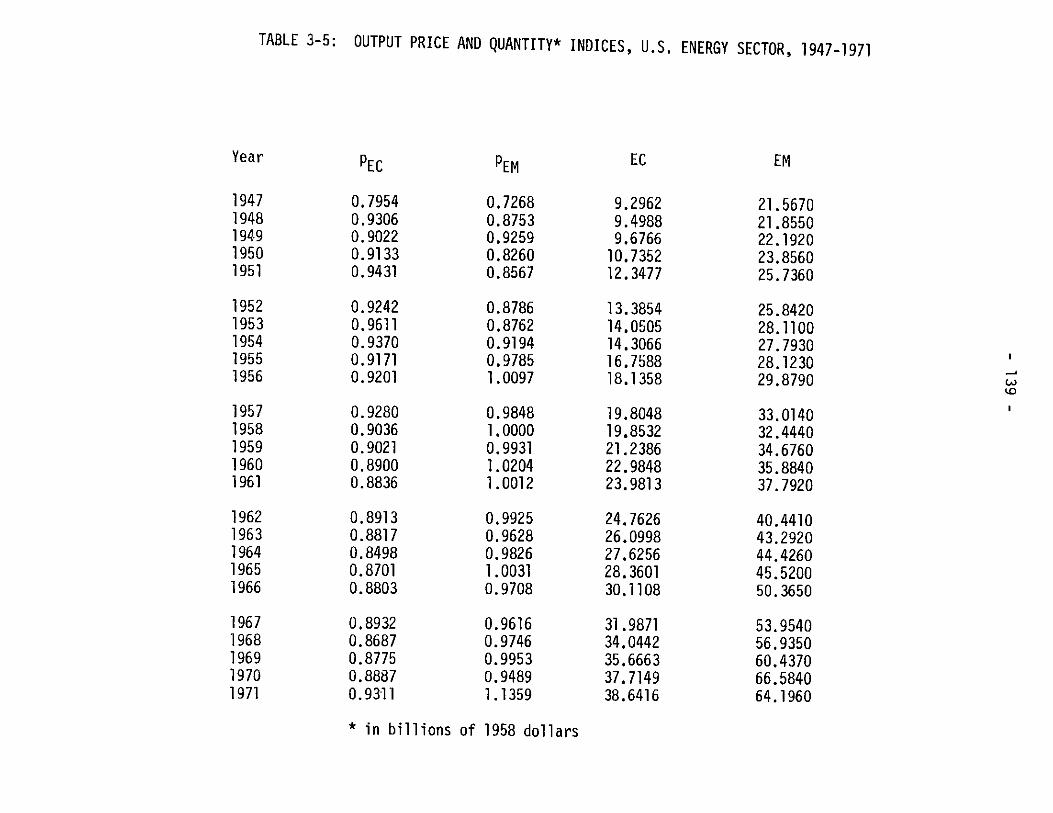
OUTPUT PRICE AND QUANTITY* INDICES, U.S. ENERGY SECTOR, 1947-1971
pECYear
19471948194919501951
19521953195419551956
19571958195919601961
19621963196419651966
19671968196919701971
0. 79540.93060.90220.91330.9431
0.92420.96110.93700.91710.9201
0.92800.90360.90210.89000.8836
0.89130.88170.84980.87010.8803
0.89320.86870.87750.88870.9311
PEM
0.72680.87530.92590.82600.8567
0.87860.87620.91940.97851.0097
0.98481.00000.99311.02041.0012
0.99250.96280.98261.00310.9708
0.96160.97460.99530.94891.1359
EC
9.29629.49889.676610.735212.3477
13.385414.050514. 306616.758818.1358
19.804819.853221.238622.984823.9813
24.762626.099827.625628.360130.1108
31.987134.044235.666337.714938.6416
* in billions of 1958 dollars
EM
21.567021.855022.192023.856025.7360
25.842028.110027. 793028.123029.8790
33.014032.444034.676035.884037.7920
40.441043.292044.426045.520050.3650
53.954056.935060.437066.584064.1960
I~
TABLE 3-5:
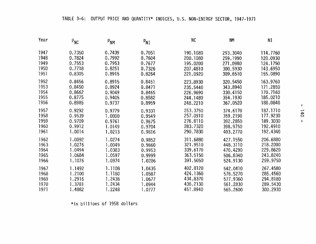
OUTPUT PRICE AND QUANTITY* INDICES, U.S. NON-ENERGY SECTOR, 1947-1971
Year pNC PNM PNI NC NM NI
1947 0.7350 0.7439 0.7051 190.1080 293.3040 114.77601948 0.7824 0.7992 0.7604 200.1080 259.1990 120.09301949 0.7553 0.7953 0.7677 195.0200 271.0980 124.17501950 0.7718 0.8251 0.7326 207.4810 300.5930 143.69501951 0.8305 0.8915 0.8264 221.0920 309.6510 155.0890
1952 0.8456 0.8915 0.8451 223.8930 320.5450 163.97601953 0.8450 0.8924 0.8471 235.5440 343.8940 171.28501954 0.8662 0.9049 0.8465 226.9690 330.4150 170.71601955 0.8775 0.9405 0.8582 244.1480 354.1930 185.02101956 0.8985 0.9737 0.8959 248.2210 367.0520 188.0840
1957 0.9292 0.9779 0.9331 253.3750 374.6170 187.17101958 0.9539 1.0000 0.9549 257.0910 359.2190 177.9230 o1959 0.9709 0.9761 0.9675 276.8110 392.2850 189.30301960 0.9912 1.0149 0.9704 283.7320 398.9750 192.49101961 1.0014 1.0213 0.9816 290.7830 403.2770 192.4340
1962 1.0092 1.0274 0.9852 311.6880 427.1550 206.68801963 1.0276 1.0049 0.9860 321.9510 448.3110 218.20001964 1.0494 1.0383 0.9953 339.6170 470.4290 229.86201965 1.0684 1.0597 0.9999 363.5150 506.8340 243.82401966 1.1076 1.0974 1.0206 391.5050 524.9130 259.9750
1967 1.1492 1.1108 1.0435 402.8120 542.0410 267.45801968 1.2100 1.1180 1.0587 424.1360 576.5270 285.45601969 1.2916 1.2438 1.0677 434.8370 577.9360 294.81801970 1.3781 1.2434 1.0944 436.2130 561.2830 289.54301971 1.4882 1.2248 1.0777 451.8940 565.2600 300.2930
*in billions of 1958 dollars
TABLE 3-6:
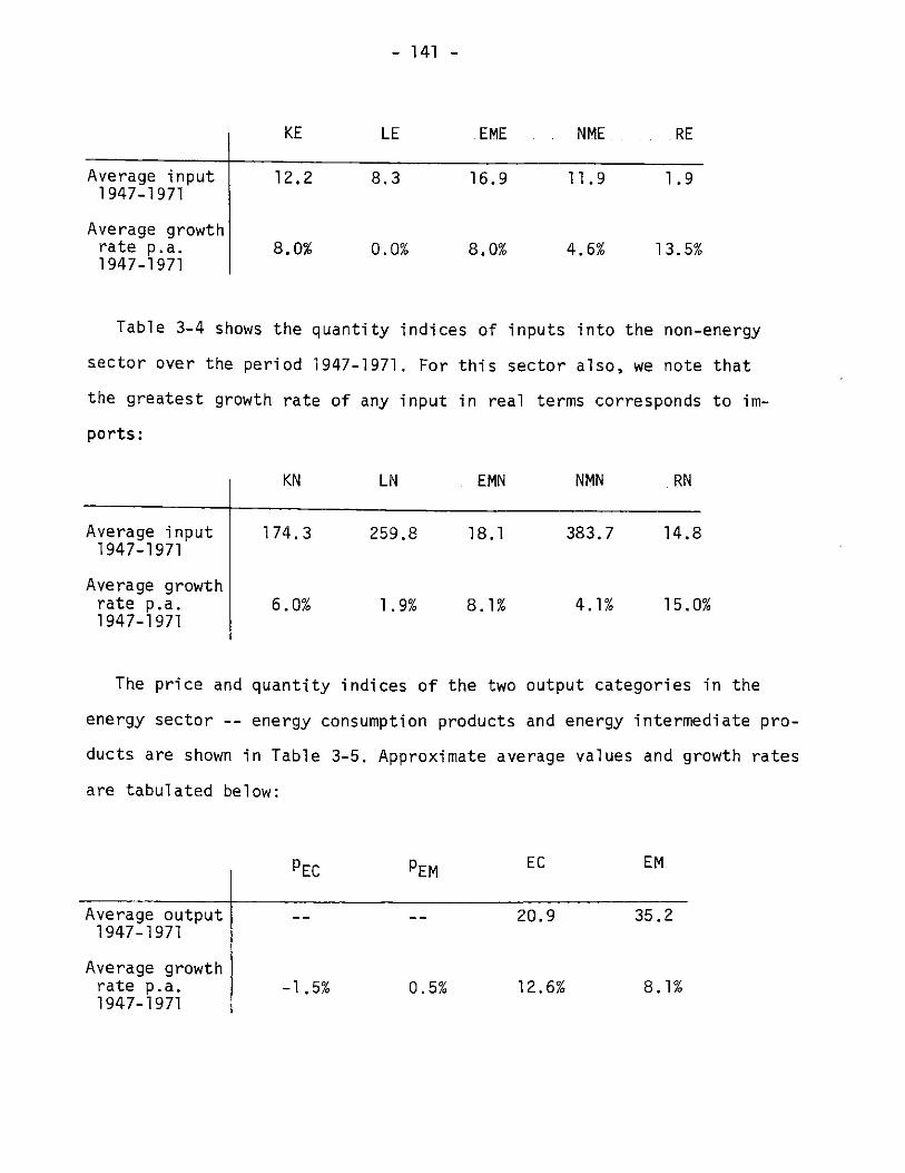
- 141 -
KE LE EME NME. RE
Average input 12.2 8.3 16.9 11.9 1.91947-1971
Average growthrate p.a. 8.0% 0.0% 8.0% 4.6% 13.5%1947-1971
Table 3-4 shows the quantity indices of inputs into the non-energy
sector over the period 1947-1971. For this sector also, we note that
the greatest growth rate of any input in real terms corresponds to im-
ports:
KN LN EMN NMN RN
Average input 174.3 259.8 18.1 383.7 14.81947-1971
Average growthrate p.a. 6.0% 1.9% 8.1% 4.1% 15.0%1947-1971
The price and quantity indices of the two output categories in the
energy sector -- energy consumption products and energy intermediate pro-
ducts are shown in Table 3-5. Approximate average values and growth rates
are tabulated below:
PEC PEM EC EM
Average output -- -- 20.9 35.21947-1971
Average growthrate p.a. -1.5% 0.5% 12.6% 8.1%1947-1971

- 142 -
Annual price and quantity indices for the three product categories of
the non-energy sector -- non-energy consumption goods, non-energy inter-
mediate goods and investment goods -- are tabulated in Table 3-6. The fo-
llowing are approximate average values and growth rates:
pNC PNM PNI NC NM NI
Average output -- -- -- 284.7 398.9 190.11947-1971
Average growthrate p.a. 3.8% 2.6% 2.1% 5.5% 3.6% 6.4%1947-1971
We tabulate below some representative figures corresponding to the ra-
tios in real terms between various inputs to the energy sector and the
output quantity index defined as the Divisia aggregate of inputs and de-
noted by YE:
KE/YE LE/YE KE/LE EME/YE
1947 0.22 0.28 0.80 0.33
1958 0.21 0.16 1.40 0.31
1971 0.19 0.08 3.20 0.29
Representative values of capital-output, labor-output,capital-labor and energy-output ratios for the U.S.energy sector for 1947, 1958 and 1971
We observe that the capital-output ratios and the energy-output ra-
tios have shown slight declines over the period 1947-1971 and that the
labor-output ratio has decreased very significantly over the same period.
The corresponding values for the non-energy sector are tabulated below
where the output quantity index YN was constructed as the Divisia accrecate
of the input quantity indices:

- 143 -
KN/YN LN/YN KN/LN EMN/YN
1947 0.21 0.38 0.55 0.0161958 0.19 0.28 0.65 0.0181971 0.19 0.25 0.76 0.024
Representative values of capital-output, labor-output,capital-labor and energy-output ratios for the U.S. non-energy sector for 1947, 1958 and 1971
It can be observed that the values of the capital-output and
labor-output ratios have declined slightly whereas the energy-output
ratio shows a small increase over the period 1947-1971. We also
note that the capital-labor ratio in the energy sector has been con-
sistently larger than that of the non-energy sector, and further,
that the difference in these two ratios has markedly increased over the
period considered.
3.1.2 Econometric Specification: Cost and Revenue Shares
The econometric specification of our model of production is based
on the systems of cost and revenue share equations for the energy and
non-energy sectors described in section 2.3.3. We recall that these
two sets of share equations were derived from the translog cost fron-
tiers under the assumptions of perfectly competitive product and fac-
tor markets.
In the energy sector there are five input equations, each corres=
ponding to the cost shares MK, ME, ME. ME, and MR and two output
equations corresponding to the revenue shares FC and FM. The systems

Table 3-7: INPUT COST SHARES, U.S. ENERGY SECTOR, 1947-1971
Total
Input Cost*
23.046827.970527.059329.507933.6932
35.077438.132638.967742.889346.8539
50.889150.384053.595756.705759.0256
Year
19471948194919501951
19521953195419551956
19571958195919601961
19621963196419651966
19671968196919701971
K
0.2331990.2756790.2574620.2681150.269576
0.2612710.2627810.2794270.2831660.281020
0.2557920.2539320.2575410.2603610.258243
0.2552260.2566640.2564160.2601240.253676
0.2574990.2551140.2372610.2456690.233249
L
0.2044310.1710460.1832370.1568570.182384
0.1833790.1787580.1676350.1590880.161462
0.1602900.1618150.1588730.1591910.155289
0.1509600.1511550.1510920.1510900.150569
0.1483540.1515280.1510230.1477220.139294
Cost Shares
E
0.3065730.3503130.3381210.3248660.325018
0.3255310.3337560.3435910.3367940.333309
0.3397500.3393340.3364480.3342120.333618
0.3337010.3369430.3351890.3287880.329786
0.3260310.3311710.3342280.3164790.339858
* in billions of current dollars
62.207864.695467.130170.340675.4023
80.452785.064991.438396.6951
108.8790
N
0.2342030.1788960.1951140.2186550.189643
0.1952720.1897710.1775770.1867840.189108
0.2059660.2106820.2133280.2165960.224594
0.2298180.2239430.2262990.2290880.230086
0.2344980.2226960.2363890.2460950.238841
R
0.0215940.0240650.0260660.0315080.033379
0.0345470.0349350.0317700.0341680.035100
0.0379780.0342370.0338100.0296400.028256
0.0302940.0310060.0310060.0309120.035884
0.0336190.0394910.0411000.0440360.048758
4:4:

OUTPUT REVENUE SHARES, U.S. ENERGY SECTOR, 1947-1971
Year
19471948194919501951
19521953195419551956
19571958195919601961
19621963196419651966
19671968196919701971
80.452785.064991.438396.6951
108.8790
* in billions of current dollars
TotalOutput Revenue*
23. 046827.970527.059329.507933.6932
35.077438.132638.967742.889346.8539
50.889150.384053.595756.705759.0256
62.207864.695467.130170.340675.4023
EC
0. 3208210.3160160.3226430.332250.345612
0.3526720.3541320.3440260.3583670.356137
0.3611430.3560650.3574730.3607380.358998
0.3547880.3557070.3497250.350830.351546
0.355120.3476580.3422880.346610.33044
EM
0.6801510. 6839340.677310. 6677850.654413
0.6473020.645880.6557380.6416110.643893
0.6388650.6439340.642520.6457470.641007
0.645210.6442860.6502850.6491620.648461
0.64490.6523230.6578390.6534110.669715
.4C,,
Tabl e 3-8:
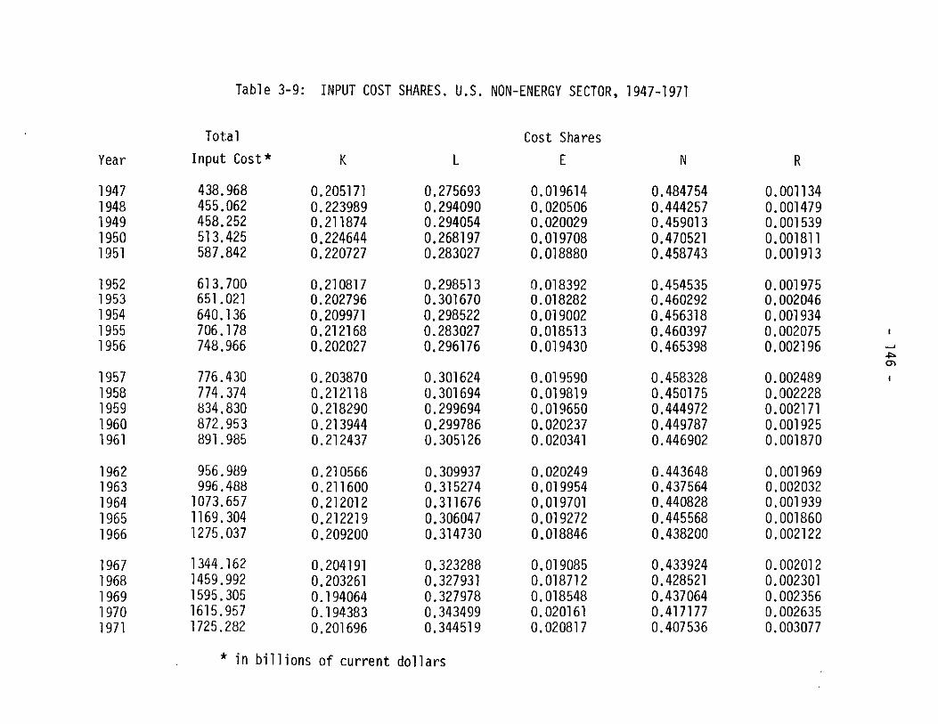
INPUT COST SHARES. U.S. NON-ENERGY SECTOR, 1947-1971
Total
Input Cost*
438.968455.062458.252513.425587.842
Year
19471948194919501951
19521953195419551956
19571958195919601961
19621963196419651966
19671968196919701971
K
0.2051710.2239890.2118740.2246440.220727
0.2108170.2027960.2099710.2121680.202027
0.2038700.2121180.2182900.2139440.212437
0.2105660.2116000.2120120.2122190.209200
0.2041910.2032610.1940640.1943830.201696
L
0.2756930.2940900.2940540.2681970.283027
0.2985130.3016700.2985220.2830270.296176
0.3016240.3016940.2996940.2997860.305126
0.3099370.3152740.3116760.3060470.314730
0.3232880.3279310.3279780.3434990.344519
Cost Shares
E
0.0196140.0205060.0200290.0197080.018880
0.0183920.0182820.0190020.0185130.019430
0.0195900.0198190.0196500.0202370.020341
0.0202490.0199540.0197010.0192720.018846
0.0190850.0187120.0185480.0201610.020817
* in billions of current dollars
613.700651.021640.136706.178748.966
776.430774.374834.830872.953891.985
956.989996.488
1073.6571169.3041275.037
1344.1621459.9921595.3051615.9571725.282
N
0.4847540.4442570.4590130.4705210.458743
0.4545350.4602920.4563180.4603970.465398
0.4583280.4501750.4449720.4497870.446902
0.4436480.4375640.4408280.4455680.438200
0.4339240.4285210.4370640.4171770.407536
R
0.0011340.0014790.0015390.0018110.001913
0.0019750.0020460.0019340.0020750.002196
0.0024890.0022280.0021710.0019250.001870
0.0019690.0020320.0019390.0018600.002122
0.0020120.0023010.0023560.0026350.003077
W-I
CF)
Table 3-9:

OUTPUT REVENUE SHARES, U.S. NON-ENERGY SECTOR, 1947-1971
TotalYear Output Revenue* NC NM NI
1947 438.968 0.318587 0.49705 0.1843631948 455.062 0.344064 0.455253 0.2006831949 458.252 0.321431 0.470534 0.2080341950 513.425 0.311874 0.483087 0.2050391951 587.842 0.312353 0.469613 0.218034
1952 613.700 0.308478 0.465696 0.2258261953 651.021 0.305717 0.471407 0.2228751954 640.136 0.307108 0.467128 0.2257641955 706.178 0.303389 0.471741 0.224871956 748.966 0.297785 0.477228 0.224987
1957 776.430 0.303228 0.471827 0.2249441958 774.374 0.316698 0.463883 0.2194191959 834.830 0.32193 0.458668 0.2194021960 872.953 0.322165 0.463856 0.2139791961 891.985 0.326457 0.461764 0.211778
1962 956.989 0.328613 0.458587 0.21281963 996.488 0.331987 0.452103 0.215911964 1073.657 0.331936 0.454977 0.2130861965 1169.304 0.33214 0.459348 0.2085111966 1275.037 0.340091 0.451807 0.208102
1967 1344.162 0.3444 0.447959 0.2076411968 1459.992 0.351506 0.441496 0.2069971969 1595.305 0.352055 0.450613 0.1973311970 1615.957 0.371994 0.431903 0.1961041971 1725.282 0.389808 0.422608 0.187584
* in billions of current dollars
Table 3-10:

EMK
Table 3-11: MULTIVARIATE SHARE ESTIMATING SYSTEM FOR THE TRANSLOG COST FRONTIER, U,S. ENERGY SECTOR
E
EK
E
EL
EcEc
E
EME
EMN
FEFc
ESt
EYKK
E" KL
EYKE
ESKN
EpCK
EYKt
+
EYKL
EYLL
EYLE
EYLN
EPLC
EYLt
EYKE
EYLE
EYEE
EYEN
EPCE
EYEt
E' KN
EYLN
EYEN
EYNN
EPCN
EyNt
E'CK
EICL
EPCE
EPCN
E6CC
EPct
EYKt
EYLt
EYEt
EYNt
EIct
EYtt
1(PKE/PRE)
in(PLE'PRE)
Ei EM/PRE)
In E1n(pNM/PRE)
in(EC/EC)
t
EEK
EEL
EE
EN
E
E
-I
4Pb00~
- 149 -
of cost and revenue shares are coupled since we do not impose input-
output separability a priori. The values of the cost and revenue shares
for the energy sector are tabulated in Tables 3-7 and 3-8 for the
period 1947-1971.
In the non-energy sector there are also five input equations asso-
ciated with the cost shares MK, ML, MN, M , Mand three output equa-
tions associated with the revenue shares FN, FN, and FN The values
of the cost and revenue shares for the non-energy sector for the years
1947-1971 are tabulated in Tables 3-9 and 3-10.
The Energy Sector
The specific form of the seven share equations for the energy pro-
duction sector was given in Eqs. 2-12 in Chapter II. Because of the
cross-terms involving input prices in the revenue shares and output
quantities in the cost shares, both systems must be estimated simul-
taneously. The unconstrained system of seven shares involves 63
unknown parameters.
Assuming a well-behaved technology leading to cost frontiers with
continuous first-order derivatives, it follows that the Hessian mat-
rices are symmetric and therefore the following symmetry constraints
must hold:
E EP ij Pj i =K L, E, NR C, M (3.1)
E E i K, L, E, N, R j = K, L, E, N, R (3.2)iK L Ei
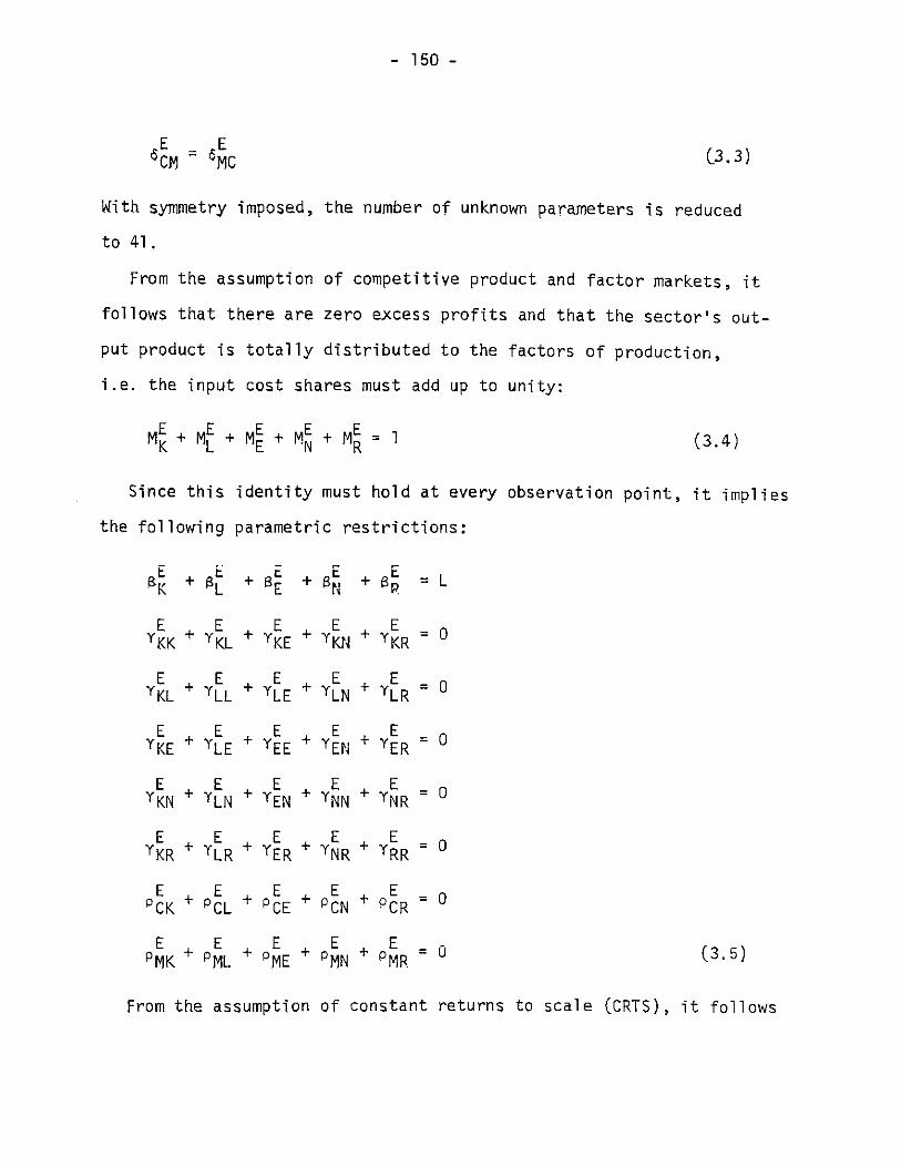
- 150 -
E E C3. 3)6CM MC
With symmetry imposed, the number of unknown parameters is reduced
to 41.
From the assumption of competitive product and factor markets, it
follows that there are zero excess profits and that the sector's out-
put product is totally distributed to the factors of production,
i.e. the input cost shares must add up to unity:
ME + M + ME + ME + ME ] =(3.4)MK + L +E + N+R
Since this identity must hold at every observation point, it implies
the following parametric restrictions:
EK + a t + a t + 4 t + a m = L
E E E E EYKK + YIK + yKE + K + KR = 0
E + E + YE + E 0YKL + yL + TLE + LN + TLR = 0
E E E + E +YE 0TKE + YLE + YEE + TEN + yER = 0
E E + E +YE + E 0YKN + YLN + TEN + TNN + TNR = 0
E E E + E + E 0YKR + YLR + yER + TNR + TRR = 0
E E E + E +PE 0PCK PCL + 20E + CN + 9CR 0
E E E E EPMK + PML + PME + PMN + PMR = 0 (3.5)
From the assumption of constant returns to scale (CRTS), it follows

- 151 -
that the output revenue shares must add up to unity:
E EFC + FM 1 C3.6)
This identity must also hold at every observation point and it
implies the following parametric restrictions:
E Eac +a m
E EPCK + PMK =0
E EPCL + PML =0
E EPCE + PME 0
E EPCN + pMN = 0
E EPCR + PMR = 0
CC 6MC =0
E EECM + 6MM 0 (3.7)
With these additional constraints imposed, the total number of
parameters remaining to be determined is reduced to 25.
Because of the identities (3.4) and (3.6), the system of cost and
revenue shares is doubly over-identified and in order to avoid singu-
larity of the covariance matrix it is necessary to drop one input
share equation and one output share equation from the complete system.
We arbitrarily drop the cost share equation corresponding to ME and
the revenue share corresponding to FM. The method of estimation will

- 152 -
later be ckQsen so that the resulting parameter estijmates are inva-
riant with respect to the equations deleted.
In examining the resulting set of share equations, we observe that
the parameters corresponding to the time variable, i.e. E ETKt' 'It2E E E
YEt' YNt' oCt, are not identifiable. We must adjoin to the existing
set of estimating share equations an equation that reflects the nature
of the time variation of the cost frontier.
The total time variation of the cost frontier of the energy sector
can be decomposed as follows:
._VE aVE __E3E
SVE at a~+ aIn EC (in EC) + EM(ln EM) + a In pKE n KE
EV . aVE+ aVEn P (In pLE) + aVEn p (ln PEME)a EIni RLE E(
+ a (piME(n PNME) + a nPRE n RE) (3.8)
The last seven terms in the right hand side of this equation repre-
sent the contributions to the total time variation attributable to
shifts in the various input prices and in the configuration of output.
The first term of the right hand side -- the partial derivative of
VE with respect to time -- can be interpreted as the rate of techno-
logical change, i.e. as shifts in the cost frontier due to structural
changes unexplained by shifts in the endogenous input and output com-
ponents.
An expression for the rate of technological change can be obtained

- 153 -
by formally taking the partial derivatiye of te cost frontier --
Eq. (2.1) -- with respect to time:
_E E E E E E=t [t T+YKt in p Lt in pLE XEt in pEME + yNt in pNME
+ Rt ln +RE in EC + Et ln EM + ytt't] (3.9)Mt PEM ttt t (a
This expression can serve as the additional estimating equation
sought for, provided we can construct an appropriate time-series for
the dependent variable. Denoting the rate of cost diminution attri-
butable to technological change by StE we obtain from Eq. (3.8) the
following expression:
E aV E 1 ' a E. aVE avE. aVE__S t V - E~r.E.C EC - riEM -7pyKE PKE~ap LE LE
aVE . aV . 9V E
~apEME PEME -3 pNME 9NME 3 PRE PRE (3.10)
Making use of the fact that VE is of the translog form this becomes
SE VE PECEC EC PEMEM EM KEKE PKE PLELE PLE
t VE VE EC VE EM VE KE VE LE
PEMEEME PEME PNMENME PNME PRERE .PRE- __ _ _ _- __ _ _ ___ - RE ( . 1VE PEME VE NME VE -RE
Since the relevant data are available at discrete points in time,
we must approximate the terms in the right-!hand side of Eq. 3.11 by
appropriate index numbers defined in terms of observable magnitudes.
We approximate the rates of growth by the period to period charges

- 154 -
in logarithms, i.e.:
E i t ti-3.12In VE- ln VE 3.12)
VEEE
and we approximate the weighted rates of growth by the same quantity
times the arithmetic average of the relative shares in the two periods:
M = i M + Mt1j][ln pt -in p t~] (3.13)
i = KE, LE, EME, NME, RE
Yi 1 t til t t-1F.- = [F + F ][n y - in p.] (3.14)
i = 1,2; y1 = EC; Y2 = EM
These index numbers were suggested as discrete approximations to
Divisia index numbers by Tornquist [27]. With these approximations,
the rate of total cost diminution due to technological change can be
expressed in terms of observable quantities as follows:
VtE ~t tl (Mt- Mt-l lnt 1 -S -in E V nVtE - M + M ]l -in p~]
2 t tt-i- [F. + Fhj]fln yI - in yJ~3
j=1 J J0
(3.15)
After having deleted the share equations associated with ME andR
FM to insure non-singularity of the estimating system, there remained
five share equations. We now adjoin equation 3.9 to the system, where
the time-series corresponding to the dependent variable is computed

- 155 -
according to equation 3.15 above. The final set of equations to.be
estimated comprises six share equations and 27 unknown parameters.
The complete set of estimating equations is shown in Table 3.11
where all the parametric restrictions implied by the symmetry condi-
tions and CRTS have been incorporated. It has been assumed that depar-
tures from the set of factor demands implied by cost-minimizing
behavior are attributable to random errors and can be adequately
Erepresented by the vector of stochastic disturbances s.
The Non-Energy Sector
The production model for the non-energy sector comprises the three
revenue share equations corresponding to non-energy consumption goods,
non-energy intermediate goods, and investment goods and the five cost
share equations corresponding to each of the five factor inputs.
This system of eight coupled share equations involves 80 unknown para-
meters in its unconstrained form -- see Eqs. 2-13.
The symmetry constraints on the translog cost frontier for the non-
energy sector imply the following parametric restrictions:
N NP P i = K, L, E, N, R j = C, M, I (3.16)
N = y i = K, L, E, N, R j = K, L, E, N, R (3.17)
6 N I = C, M, I j = C, M, I (3.18)&ij ij
With symmetry imposed, the number of parameters to be determined
is reduced to 52.

- 156 -
As before, the assumption of perfectly competitive markets and of
constant returns to scale imply that the input cost shares and the
output revenue shares must add up to unity:
mN + MN + mN +mN +mNMK ML ME + MN + MR 1
FN + N + FN 1Fc Fm FI
(3.19)
(3.20)
Since the identity given by Eq. 3.19 must hold at every observation
point, the following restrictions on the parameters of the cost fron-
tiers hold:
aN + aN + aNK+ L + E
N + YN + NTKK TKL ThE
N N NTKL + LL + LE
N + N + NYKE + LE + EE
YKN + YLN + YEN
NN NYKR + LR + TER
N N NPCK + PCL + PCE
N + PN NPMK +ML +PME
N + N NPIK + L + -PIE
+ 5N + =N 1
+TyLN TLyR =-0
N N+ yEN + ER 0
+ N +N 0
+TNR + TRR -
+ N + -+R 0
ECN + ER-
+ N N+ IN + MR 0+ PN N 0
~IN P IR
Similarly the constraint on the revenue shares given by Eq. 3.20
(3.21)

- 157 -
must hold at every obseryation point and this leads tQ the following
parametric restrictions:
N + N N
N N=N + N + N QPCK +MK PIK =
N N NPCL+ ML + IL
N + N NPCE +ML + IL
N N NPCN + PMN + PIN =
N+ N N 0PCR + MR + PIR =
6N + 6N + 6N 0Gcc SMC 61C=
N + + = 0
iN + NI + SN =0&i II (.22
With these additional restrictions imposed, the total number of
parameters to be determined is reduced to 34.
The restrictions implied by identities 3.19 and 3.20 determine that
the full system of eight share equations is doubly singular: we must
therefore delete one input share and one output share from the esti-
mating system in order to insure non-singularity of the covariance
matrix. We arbitrarily choose to delete the cost share equation
associated with MN and the revenue share equation corresponding toRNF .
(3.22)

- 158 -
For the parameters associated with the time variable to be iden-
tifiable, it is necessary to adjoin to the set of six share equations
an equation reflecting the time variation of the cost frontier VN'
In exact analogy with the derivation described above for the energy
sector, we formally take the partial derivative of VN -- given in
equation (2.2) -- with respect to time, obtaining the expression:
aVN N N N N N9t~ t + YKt Kn p +Lt ln PLN + TEt in PEMN + YNt PNMN
+ Yt in pRN + CIn NC + 6Mt ln NM + 6Nt ln NI +
+ tt t](3.23)~tt . I
As before, the partial derivative of VN with respect to time
represents the rate of cost diminution attributable to technological
change -- we denote it by S . An expression for S in terms of the
rates of change of input prices and output quantities can be obtained by
totally differentiating VN with respect to time and taking the translog
functional form into consideration:
N VN PNCNC NC PNMNM NM PNINI NI PKNP$' PKNS t 1 NU V K V NM ~V NT ~V pN N N N N PKN
PLNLN PLN PEMNEMN PEMN PNMNNMN PNMN pRNRN PRNVN PLN VN PEMN VN NMN VN PRN
(3.24)
Again we approximate the rates of change in the right-hand side of

MN N N N N N N N NK OK YKK KL yKE KN CK "MK YKtIn KNPRN
N N N N N N N N NML SL KL LL LE LN PCL ML YLtPLNPRN
MN N N N N N N N N NE SE KE TLE YEE YEN PCE ME EtpEM/PRN
N N N N N N N N N N+MN N + KN LN YEN NN PCN MN TNt ln(NM/PRN) +
FN N N N N N N N NC ac CK PCL PCE PCN 6CC 6MC Pct ln(NC/NI)
N N N N N N N N NFM aM MK ML ME MN 6MC 6MM PMt l n(NM/NI)
N N N N N N N N Nst t YKt YLt YEt YNt Pct Pmt Ytt t
Table 3-12: MULTIVARIATE SHARE ESTIMATING SYSTEM FOR THE TRANSLOG COST FRONTIER, U,S, NON-ENERGY SECTOR
E N
NN
N
NE
NEN
N
E:t

- 160 -
(3.24) by discrete Divisia index numbers so that a time-series for
S can be generated in terms of observable quantities:St
N - In V ~ - [Mt + M-~][ln pt -In p ]t N N Til i i 1
> [Ft + Ft~l[ln yt - in ytl]j=1 j3
(3.25)
The final set of estimating equations for the non-energy produc-
tion sector includes four input cost shares and two output shares --
i.e. the original eight equations minus the two equations deleted to
avoid singularity -- and Eq. (3.23) representing the rate of change
of cost diminution attributable to technological change. The values
of the dependent variable for the latter equation are computed as
shown in Eq. (3.25). The final number of parameters to be determined
in the seven estimating equations is 36.
In Table 3.12 we show the final estimating system for the translog
cost frontier of the non-energy production sector, incorporating all
the parametric restrictions implied by the symmetry constraints and
CRTS. Again we postulate that the vector of stochastic disturbances
E represents departures from cost minimizing behavior due to random
errors.
3.1.3 Parameter Estimation and Hypothesis Testing
We have fitted the parameters of the translog cost frontiers for

- 161 -
both the energy and non-energy production sectors employing the sto-
chastic specifications outlined above. We employ an iterative ver-
sion of the three-stage least-squares estimator proposed by Zellner
and Theil [6]. This I3SLS estimator is consistent and asymptoti-
cally equivalent to the maximum likelihood estimator (Malinvaud [7])
although in finite samples it provides parameter estimates that can
differ from the full information maximum likelihood estimates (Dhrymes
[8 ]). Berndt [9 ] has shown that the I3SLS estimator preserves the
invariance property of the Iterative Zellner Efficient Estimator
brought forth in the studies of Pollak and Wales [10] and the work
of Barten [11] on maximum likelihood estimators. This property is
important for our purposes since it implies that the I3SLS parameter
estimates obtained by dropping one equation from the estimating system
are invariant to the equation ommitted.
We have estimated the parameters in the two production models
under alternative sets of restrictions on the structure of the under-
lying technology. We present empirical results of statistical tests
conducted on the validity of the alternative hypotheses. Alternative
specifications on the structure of the stochastic disturbances are
also hypothesized and tested.
The parameter estimates for the energy and non-energy production
sectors are shown in Tables 3-13 and 3-14, respectively. Estimates
were obtained for observations during the period 1948-1971 under six
different assumptions on the structure of the production models.
The estimation and testing of hypotheses were conducted in the fol-

PARAMETER ESTIMATES OF THE TRANSLOG COST FRONTIER, U.S. ENERGY SECTOR*
_____ I _________________
Symmetry,Input/OutputSeparability
Symmetry,I/0 Separability
Berndt-SavinAutoreg. Transf.
F I + t0.25079
(210.7720)
0.0853(10.2730)
-0.0093(-1.4059)
-0.0146(-2.8378)
-0.0423(-4.8424)
-0.0005(-2.4551)
0.1609(166.0870)
0.2495(42.3290)
0.1390(7.9235)
-0.1345(-2.3422)
-0.0039(-0.3525)
-0.0808(-5.4326)
0.0003(0.2959)
0.1637(42.8270)
Symmetry,{K,L},{E,N}Separabili ty
0.2700(92.6381)
0.0338(5.5812)
-0.0342(-5.5435)
0.0218(4.9267)
-0.0005(-2.4-80)
0.1532(50.3595)
Symmetry,{K,..,N)},{E}Separabili ty
0.2679(100.3210)
0.0792(10.9070)
-0.0134(-2.1896)
-0.0619(-10.0568)
0.0268(6.4822)
-0.0006(-3.3994)
0.1538(56.8704)
I _______ I _________ J___________ I __________ __________
Symmetry,I/0 Separability
{K ,L},{E ,N}Separability
0.2564(245.2830)
0.03953(6.0597)
-0.0257(-3.6445)
-0.0006(-1.8997)
0.1635(161.7640)
* asymptotic t-ratios in parentheses
Symmetry
EK
E^KK
EKL
EYKE
EYKN
E'CK
EYKt
EL
0.2753(95.7547)
0.0791(11.7280)
-0.0086(-1.3712)
-0.0284(-4.9355)
-0.0338(-4.1480)
0.0410(8.6288)
-0.0012(-5.4644)
0.1495(42.3136)
I.
Table 3-13:

Table 3-13 (cont.): PARAMETER ESTIMATES OF THE TRANSLOG COST FRONTIER, U.S. ENERGY SECTOR
Symmetry, er ySymmetry, Symmetry, Symmetry,Symmetry,I/0 Separability tKrL},{E5N} {K LlN}s{E} I/0 Separability
Symmetry Input/Output Berndt-Savin Separability Separability {K,L}{EN}Separability Autoreg. Transf. Separability
-0.1282(-8.2182)
0.0165(1.6942)
0.0615(6.5411)
-0.0199(-3.1514)
0.0026(5.1751)
0.3271(95.6482)
0.05949(6.05501)
0.0127(1.2808)
-0.1151(-8.41 89)
-0.0005(-0.0874)
0.0743(7.8413)
0.0017(4.5246)
0.3389(417.6250)
0.0440(6.9134)
0.0197(2.3785)
-0.0199(-2.5924)
-0.0191(-3.8540)
-0.0000(-0.3664)
0.3337(111-.1310)
0.0371(4.6902)
0.0304(3.2865)
-0.1173(-9.7123)
0.0735(8.0276)
-0.0124(-2.8622)
0.0020(6.2659)
0.3253(120.5730)
0.0610(25.9166)
____________________ J A a
-0.0279(-3.2435)
-0.0001(-0.3928)
0.3368(636.7290)
0.0302(4.8425)
0.0265(3.5038)
-A
EYLL
EYLE
EYLN
E'CL
EYLt
EE
EYEE
EYEN
-0.1229(-3.3086)
0.0319(1.3086)
0.0922(3.3914)
0.0020(1.8963)
0.3388(85.2590)
0.0272(1.5471)
-0.0042(-0.2533)
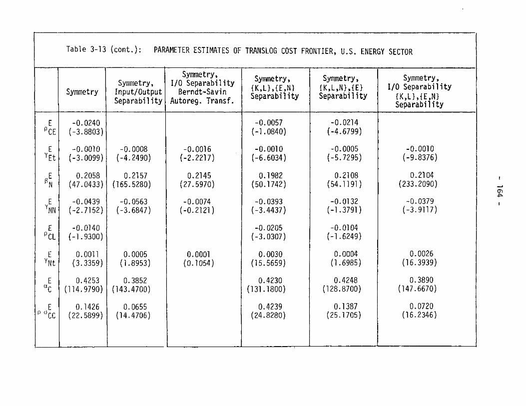
Table 3-13 (cont.): PARAMETER ESTIMATES OF TRANSLOG COST FRONTIER, U.S. ENERGY SECTOR
Symmetry, Symmetry, Symmetry, Symmetry,Symmetry, B/0 Separability KL{KEN}LK}L{N}s{E} 1/0 Separability
Symmetry Input/Output Berndt-Savin Separabil ity Separability IK,L },{E,N}Separability Autoreg. Transf. Separability
-0.0240(-3.8803)
-0.0010(-3.0099)
0.2058(47.0433)
-0.0439(-2.7152)
-0.0140(-1.9300)
0.0011(3.3359)
0.4253(114.9790)
0.1426(22.5899)
-0.0008(-4.2490)
0.2157(165.5280)
-0.0563(-3.6847)
0.0005(1.8953)
0.3852(143.4700)
0.0655(14.4706)
-0.0057(-1.0840)
-0.0010(-6.6034)
0.1982(50.1742)
-0.0393(-3.4437)
-0.0205(-3.0307)
0.0030(15.5659)
0.4230(131.1800)
0.4239(24.8280)
-0.0214(-4.6799)
-0.0005(-5.7295)
0.2108(54.1191)
-0.0132(-1.3791)
-0.0104(-1.6249)
0.0004(1.6985)
0.4248(128.8700)
0.1387(25.1705)
-0.0010(-9.8376)
0.2104(233.2090)
-0.0379(-3.9117)
0.0026(16.3939)
0.3890(147.6670)
0.0720(16.2346)
_____________________ L ___________________ I -' -
-I
E'CE
EYEt,
ENN
EYNN
E'CL
EYNt
E
[E
"G c
-0.0016(-2.2217)
0.2145(27.5970)
-0.0074(-0.2121)
0.0001(0.1054)
I
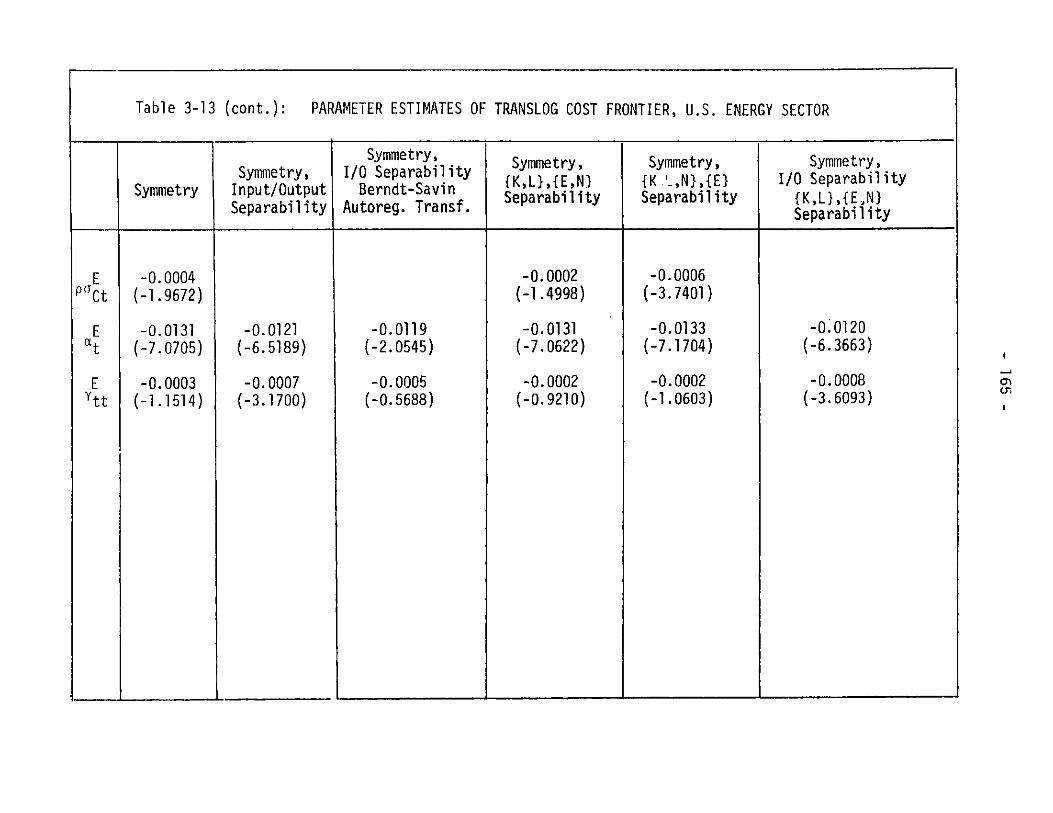
Table 3-13 (cont.): PARAMETER ESTIMATES OF TRANSLOG COST FRONTIER, U.S. ENERGY SECTOR
Symmetry, Symmetry, Symmetry, Symmetry,Symmetry., I/0 Separability {K,L},{E3,N} {K '.,N},{E1} I/0 Separability
Symmetry Input/Output Berndt-Savin Separability Separability K,L},{E ,N}Separability Autoreg. Transf. Separability
-0.0004(-1.9672)
-0.0131(-7.0705)
-0.0003(-1.1514)
-0.0121(-6.5189)
-0.0007(-3.1700)
-0.0119(-2.0545)
-0.0005(-0.5688)
-0.0002(-1.4998)
-0.0131(-7.0622)
-0.0002(-0.9210)
-0.0006(-3.7401)
-0.0133(-7.1704)
-0.0002(-1.0603)
-0.0120(-6.3663)
-0.0008(-3.6093)
EpaCt
Et
EYtt

Table 3-14: PARAMETER ESTIMATES OF THE TRANSLOG COST FRONTIER, U.S. NON-ENERGY SECTOR*
1Symmetry,. Symmetry, Symmetry, Symmetry,Symmetry, I/O Separabil ity {K,L },{E,NI {K,L ,N},{EI} I/O Separability
Symmetry Input/Output Berndt-Savin Sepaabili ty eparbili y {K/0 }ep ,N}Separability Autoreg. Transf. Separability Separability (KL},{EN}
_ _ _ __ ___-__ __S e p a r a b i l i t y
0.2211(69.7538)
0.0356(5.3629)
-0.0039(-0.5199)
-0.0067(-10.1069)
-0.0294(-6.5187)
0.0445(6.5187)
-0.0007(-3.0714)
0.3704(66.3491)
0.2064(253.7420)
0.0412(6.1688)
-0.0439(-7.2627)
-0.0047(-6.7681)
0.0126(10.7307)
0.0003(1.9069)
0.3101(286.8760)
J-1 _ __ _ 1 _ _ __ _ _
0.2189(11.2900)
0.0230(1.4535)
0.0120(0.6950)
-0.0040(-2.1729)
-0.0273(-1.7362)
-0. 0021(-1.3261)
0.2851(9.1273)
0.1950(106.8990)
0.0452(7.9154)
-0.0477(-9.7238)
0.0452(7.4409)
0.0006(4.1405)
0.2879(108.2880)
0.2102(71.3580)
0.0559(9.7707)
-0.0276(-4.1750)
-0.0261(-6.3232)
0.0479(7.7180)
-0.0000(-0.0153)
0.3771(69.6366)
0.2035(327.0520)
0.0717(16.7186)
-0.0621(-13.8353)
0.0009(6.5606)
0.3119(312.8410)
_-I- -.. IL
0)11'
*asymntotic t-ratios in
NK
NYKK
NYKL
NYKE
NYKN
NPCK
NYKt
N"L
parentheses

Table 3-14 (cont.): PARAMETER ESTIMATES OF TRANSLOG COST FRONTIER, U.S. NON-ENERGY SECTOR
Symmetry, er Symmetry, Symmetry, Symmetry,Symmetry, 1/0 Separability {KqL }q{E5N} {KL N} {E} 1/0 Separability
Symmetry Input/Output Berndt-Savin Separability Separability IK,L },EN}Separability Autoreg. Transf. Separability
0.1447(12.1069)
0.0059(5.5782)
-0.1591(-19.6263)
0.1381(17. 2173)
-0. 0021(-5.5843)
0.0186(28.0909)
0.0032(7.7510)
-0.0023(-2.3005)
0.0331(5.7593)
0.0045(6.3141)
0.0120(9. 0457)
-0.0000(-0.0524)
0.0202(224.492)
0.0029(6.8842)
0.0006(0.9917)
0.1110(3.1067)
0.0068(1.5169)
-0.1151(-3. 5925)
0.0010(0.3639)
0.0197(19.8970)
0.0091(5.3391)
-0.0058(-1.3283)
-0.0000(-0.0144)
0.0890(11.6551)
0. 0026(15.3624)
0.0173(46.8508)
0.0042(9.2318)
-0.0003(-0.5037)
0.1629(14.3524)
- -0.1550(-19. 2717)
0.1310(17.4340)
-0.0027(-7.3255)
0.0175(46.7985)
0.0041(12.3894)
_____________ J. ___________ A ___________
0.0649(13.3163)
-0. 0009(-5.9015)
0.0198(315.4430)
0.0039(8.5046)
0.0005(1.0456)
%-4
NYLL
NYLE
NYLN
NPCL
NYLt
NE
NYEE
NYEN
I

Table 3-14 (cont.): PARAMETER ESTIMATES OF THE TRANSLOG COST FRONTIER, U.S. NON-ENERGY SECTOR
Symmetry, Symmetry, Symmetry, Symmetry,Symmetry, I/0 Separability {K,L},{E,N} {K,L,N},{E} I/0 Separability
Symmetry Input/Output Berndt-Savin Separability Separability {K,L},{E,N}Separability Autoreg. Transf. Separability
0.0087(11.8729)
-0.0001(-3. 6996)
0.3630(75.0815)
0.2242(27.7487)
-0.2228(-46.4328)
0.0030(11.3049)
0.3513(89.7114)
0.3409(33.6529)
-0.0001(-7. 5613)
0.4452(413.2880)
-0.0261(-19.9183)
-0.0004(-9.8414)
0.2993(140.4330)
0.1026(23.5441)
-0.0004(-0.2548)
0.4626(27.6330)
0.1567(4.3533)
-0.0002(-0.1017)
0.0050(5.4212)
0.0000(1.3654)
0.4532(254.2680)
0.0633(28.7733)
-0.1800(-30.2946)
-0.0021(-43.1741)
0.3334(88.3876)
0.3142(31.4521)
0.0045(5.4631)
0.0000(1.6246)
0.3647(75.7555)
0.2158(27.2688)
-0.2171(-46.4444)
0.0028(10.9731)
0.3558(89.9587)
0.3243(33.9793)
_ _ _ _I__ _-_ L-_.__ _I_ _-. _ _ _ _I__ _I
-0.0000(-5.8148)
0.4463(426.8850)
-0.0041(-4.4040)
-0.0001(-7.3834)
0.2926(138.468)
M-aC)~
N'CE
NEt
NSN
NNN
N'CN
Ny Nt
NcC
N6CC

ENC
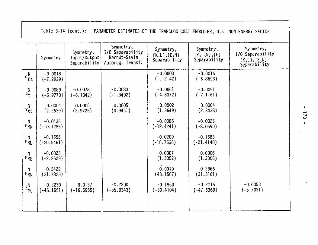
Table 3-14 (cont.): PARAMETER ESTIMATES OF THE TRANSLOG COST FRONTIER, U.S. NON-ENERGY SECTOR
Symmetry, Symmetry, Symmetry, Symmetry,Symmetry, I/0 Separability {KL},{E5N} {K,L,N},{E} I/0 Separability
Symmetry Input/Output Berndt-Savin Separability Separability {K,L},{EN}Separability Autoreg. Transf. Separability
-0.0018(-7. 2929)
-0.0089(-6.9770)
0.0004(2. 2639)
-0.0436(-10.1285)
-0.1655(-20.5461)
-0.0023(-2.2529)
0.2422(31.7825)
-0.2230(-46.1551)
-0.0078(-6.1042)
0.0006(3.9725)
-0.0137(-16.6955)
-0.0083(-1.8402)
0.0005(0.9451)
-0.2200(-35.9343)
-0.0003(-1.2142)
-0.0061(-4.8372)
0.0002(1.3649)
-0.0086(-12.4241)
-0.0209(-18.7536)
0.0007(1.3052)
0.0919(43.1507)
-0.1850(-33.4104)
-0.0016(-6.8693)
-0.0091(-7.1161)
0.0004(2. 3438)
-0.0325(-8.0590)
-0.1683(-21.4140)
0.0006(1.2306)
0.2366(31.3161)
-0.2215(-47.6369)
NCt
Nat
Nytt
NPMK
NSML
NPME
NSMN
N6MC
__ __ __ __ I_ _I__ __L_ _ -_ ___--__ __ __ _
-J
0
-0.0053(-5.7031)
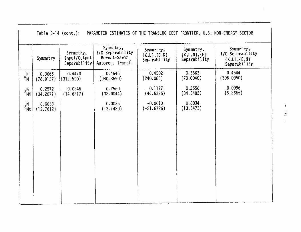
Table 3-14 (cont.): PARAMETER ESTIMATES OF THE TRANSLOG COST FRONTIER, U.S. NON-ENERGY SECTOR
Symmetry, Symmetry, Symmetry, Symmetry,Symmetry, I/0 Separability {K,LJ,{E,NI {K,L,N},{E} I/0 Separability
Symmetry Input/Output Berndt-Savin Separability Separability {KL},{EN}Separability Autoreg. Transf. Separability
0.4470(312.590)
0.0246(14.6217)
0.4646(980.8690)
0.2560(32.0044)
0.0035(13.1420)
0.4502(240.065)
0.1177(44.5325)
-0.0013(-21.6726)
0.3663(78.0040)
0.2556(34.5482)
0.0034(13.3473)
____________________________________ L I -
0.4544(306.0950)
0.0096(5.2665)
-J
N
N6MM
N6Mt
0.3666(76.9127)
0.2572(34.2071)
0.0033(12.7612)
I

- 172 -
lowing sequence: (i) symmetry -- taken as a maintained hypothesis,
(ii) input-output separability, (iii) autocorrelation in the stochastic
disturbances. (iv) separability between {K, LI and {E, NI, (v) separa-
bility between {EI and {K, L, NI, and (vi) composite separability
between inputs and outputs and between {K, L} and {E, NI.
Likelihood Ratio Tests
To implement the statistical tests on the validity of the above
hypotheses, we employ test statistics based on the likelihood ratic
X, where
max L
Max_ L (3.26)Max L
The likelihood ratio is the ratio of the maximum value of the
likelihood function for the production model Q without restriction
to the maximum value of the likelihood function for the modelQ0
subject to restriction. For normally dis'tributed disturbances, the
likelihood ratio is equal to the ratio of the determinant of the
restricted estimator of the variance-covariance matrix of the dis-
turbances to the determinant of the unrestricted estimator, each
raised to the power -(n/2).
Our test statistic for each set of restrictions is based on minus
twice the logarithm of the likelihood ratio, or:
-2 ln x = n(in [ .[ - in ISQI) (3.27)
where EQ is the restricted estimator of the variance-covariance
matrix and E is the unrestricted estimator. Under the null hypothesis

- 173 -
the likelihood ratio test statistic is asymptotically distributed as
chi-squared with a number of degrees of freedom n equal to the number
of restrictions to be tested. We employ the asymptotic distribution
of the likelihood ratio test statistic for tests of hypothesis.
Economic studies employing likelihood ratio test statistics in multi-
variate equation systems include Byron [12] and Woodland [13]. For
a comparison of the relative power of the Wald, likelihood ratio and
Lagrange multiplier test statistics, see Berndt and Savin [14].
Tests of Separability between Inputs and Outputs
A technology is said to be separable with respect to a partitioning
between inputs and outputs if the production possibility frontier
is groupwise additive between inputs and outputs. In terms of a cost
frontier C(y, w), a necessary and sufficient condition for separa-
bility is that it admit a representation of the form C(y, w) = F(y)-G(w)
-- see e.g., Hall [15]. For the translog specification of the cost fron-
tiers, separability implies that all the interaction terms must vanish
identically, i.e.:
E N 0 for all i, j (3.28)Ptj = Pu =
We implement tests for the null hypothesis of separability between
inputs and outputs in terms of the parametric restrictions given in
Eq. 3.28.
We assign a level of significance of 0.005 to this test. The
results for the energy production sector are as follows:

- 174 -
Degrees of freedom = 5
Critical value = 16.7496
Test Statistic = 50.338
For the non-energy production sector, the results of the test are:
Degrees of freedom = 10
Critical value = 25.1882
Test Statistic = 44.843
In both instances, the null hypothesis of separability between inputs
and outputs is rejected. This result conforms with the theoretical
arguments presented in Section 2.3.2 regarding the implications of
separability assumptions in multiple-output technologies. As was
pointed out by Hall [15], enforced separability eliminates an important
feature of multi-sector and more elaborate technologies -- the depen-
dence of output price ratios on factor prices. We note also that
using a value-added production function, Burgess [16] was unable to
reject the hypothesis of separability between inputs and outputs.
Tests of Autocorrelation in the Stochastic Disturbances
The assumption underlying the stochastic specification of the systems
of cost and revenue shares shown in Tables 3-11 and 3-12 is that the
stochastic disturbance vectors eN and eE are uncorrelated across
time. We have conducted a limited set of tests for the null hypo-
thesis of zero autocorrelation as against a first-order multivariate
autoregressive process. These tests were conducted only for the

- 175 -
input shares systems under the assumption of input-output separa-
bility. Thus, although the results of our tests reject the hypo-
thesis of no autocorrelation, it is likely that the results would be
less conclusive for the case without the separability assumption:
it seems plausible that for the tests we conducted, the presence
of autocorrelated disturbances can be explained at least in part by
the fact that the effects of the composition of output on the time-
variation of the input shares are neglected under the assumption of
separability.
We implemented our statistical tests for the presence of autocor-
related disturbances by making use of the multivariate autoregressive
transformation introduced by Berndt and Savin [ 1]. Berndt and Savin
showed that the adding-up constraint on the share equations imposes
restrictions on the parameters of the autoregressive process. When
these restrictions are not imposed, the specification of the model
is conditional on the equation deleted and the estimates are not
consistent.
If the original system of equations is of the form
pt = Hqt + vt
and it is assumed that the disturbance vector vt corresponds to a
first-order autoregressive process of the form
vt = Rvt-1 +E:t
where et is a zero-mean uncorrelated process, then consistent esti-
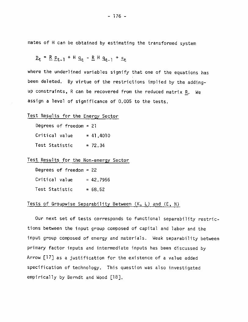
- 176 -
mates of H can be obtained by estimating the transformed system
ptffPt- + H Rt - _ H at-, + Et
where the underlined variables signify that one of the equations has
been deleted. By virtue of the restrictions implied by the adding-
up constraints, R can be recovered from the reduced matrix R. We
assign a level of significance of 0.005 to the tests.
Test Results for the Energy Sector
Degrees of freedom = 21
Critical value = 41.4010
Test Statistic = 72.34
Test Results for the Non-energy Sector
Degrees of freedom = 22
Critical value = 42.7956
Test Statistic = 68.52
Tests of Groupwise Separability Between {K, LI and fE, NI
Our next set of tests corresponds to functional separability restric-
tions between the input group composed of capital and labor and the
input group composed of energy and materials. Weak separability between
primary factor inputs and intermediate inputs has been discussed by
Arrow [17] as a justification for the existence of a value added
specification of technology. This question was also investigated
empirically by Berndt and Wood [18].

- 177 -
For our translog cost frontiers, inputs K and L will be weakly
separable from E, N if and only if
MK yLE -'L M KE = 0 i = E, N
and
i i Mi 1i .N(.9MK LN - L 'KN 0 i E, N (3.29)
One of the ways in which these conditions can be satisfied is if
the following equalities hold:
E E E EYKE LE KN LN = 0
N N N N 0(3.30)YKE -LE =KN =LN =
These conditions have been referred to as the linear separability
restrictions by Berndt and Wood [18] and correspond to the notion of
explicit groupwise separability used by Jorgenson [19] in the context
of consumer demand studies. We define the null hypothesis of group-
wise separability between {K, LI and {E, N} in terms of the equalities
3.30. We assign a level of significance of 0.005 to these tests.
Test Results for the Energy Sector
Degrees of freedom = 4
Critical value = 14.8602
Test Statistic = 33.36
Test Results for the Non-Energy Sector

- 178 -
Degrees of freedom = 4
Critical value = 14.8602
Test Statistic = 25.08
In both instances the separability hypothesis is rejected. This
result suggests that a value-added specification of technology may not
be suitable for an econometric model intended to study the effects
of energy use on aggregate exonomic performance.
Tests of Groupwise Separability between {E} and {K, L, N}
We next implement statistical tests of the hypothesis of group-
wise separability between the input group formed by capital, labor,
and non-energy and the input group composed of energy.
The restrictions that define the null hypothesis of separability
between {E} and {K, L, N} are:
E E EYKE LE EN = 0
KE LE N = 0 (3.31)
We assign a significance level of 0.005 to these tests.
Test Results for the Energy Sector
Degrees of freedom = 3
Critical value = 12.8386
Test Statistic = 13.534

- 179 -
Test Results for the Non-Energy Sector
Degrees of freedom = 3
Critical value = 12.8386
Test Statistic = 9.610
The results indicate that the null hypothesis can be rejected
for the energy sector but cannot be rejected for the non-energy sec-
tor at the chosen level of significance.
Tests of GroupwiseSeparability between {K, L} and {E, N} givenInput-Output Separabil ity
The final set of tests involves separability between the input
group composed of {K, L} and the input group composed of {E, N} given
separability between inputs and outputs.
Test Results for the Energy Sector
Degrees of freedom = 4
Critical value = 14.8602
Test Statistic = 22.344
Test Results for the Non-Energy Sector
Degrees of freedom = 4
Critical value = 14.8602
Test Statistic = 13.383
We notice that for the non-energy sector, a maintained hypo-

- 180 -
Table 3-15: LIKELIHOOD RATIO TESTS ON THE STRUCTURE
OF TECHNOLOGY, U.S. ENERGY SECTOR
Degrees of Critical TestFreedom Value Statistic
Separability betweenInputs and Outputs 5 16.74 50.33
No Autcorrelation inShare Equations 21 41.40 72.34
Groupwise Separabilitybetween {K,L} and {E,N} 4 14.86 33.36
Groupwise Separabilitybetween {K,L,N} and {E} 3 12.83 13.53
Input-Output Separ-ability and GroupwiseSeparability between{K,L} and {E,N} 4 14.86 22.34

- 181 -
Table 3-16: LIKELIHOOD RATIO TESTS ON THE STRUCTURE
OF TECHNOLOGY, U.S. NON-ENERGY SECTOR
Degrees of Critical TestFreedom Value Statistic
Separability betweenInputs and Outputs 10 25.18 44.84
No Autcorrelation inShare Equations 22 42.79 68.52
Groupwise Separabilitybetween {K,L} and {E,N} 4 14.86 25.08
Groupwise Separabilitybetween {K,L,N} and {E} 3 12.83 9.60
Input-Output Separ-ability and GroupwiseSeparability between{K,L} and {E,N} 4 14.86 13.83

- 182 -
thesis of input-output separability would lead to the acceptance of
separability between {K, LI and fE, NI whereas the latter was rejected
for the more complete specification discussed above.
3.1.4 Concavity Tests of the Cost Frontiers
The conditions that must be satisfied by a cost frontier for
it to be consistent with a well-behaved technology were described
in Section 2.3.2. The positivity conditions require that the input
demand functions and output supply functions be strictly positive.
These conditions will be satisfied if the fitted cost and revenue
shares are strictly positive. We have verified that the fitted shares
based on our I3SLS estimates satisfy the posiLivity conditions at
each annual observation for all of the alternative specifications
described in the previous section.
In order to verify the concavity of the cost frontiers with
respect to input prices, we must establish the negative semidefinite-
ness of the Hessian matrices of second-order partial derivatives with
respect to input prices.
The functional form of the translog approsimations to the cost
frontiers were given in Eqs. (2.1) and (2.2) in Chapter II. Denoting
the right-hand sides of these two equations by (PE and DN, respectively,
we have:
ln VE =E
and

- 183 -
ln VN N
so that
VE exp [(D El
(3.32)
(3.33-a)
and
VN = exp N (3.33-b)
Let [H k = E, N denote a representative element in the
i-th row and j-th column of the Hessian matrices HV and HN, respec-
tively.
Since by definition
V ii 9w.3 w. , k = E, N (3.34)
we obtain the following expression by differentiating Eqs. 3.33 twice:
[H k =exp k (l/w wv I(kl 1w 3 13
k kww+ (1w j.
k +[~.3
k +[s.1
nE
j=l
n k
i- y in wf +
kyij
m
i=1
ln w kw. +
mE
j=lk
Puiln yk + ykIn y i t ]
pi ln y + yit t] exp [4'k1
k = E, N (3.35)
The elements of the diagonal take the form

- 184 -
Hk] 1 k n k k[H ] = exp [k] (- )[ + z Y ln ww1=
m k k+ k+ S P iln y. +Yit ' t] + w Yjy exp LOk
j=1 k k m itk1
+ exp [k1 . 1 +k + y ln w + p. in y + Y t]2k] w jj 1 j1 i j i
k = E, N (3.36)
We wish to evaluate the Hessian matrices at the point of approxi-
mation of the translog frontiers which is determined by the base year
to; in our case t0 = 1958. In the base year, t = 0 by definition,
w = 1, i = 1, ... , n by construction of the price indices and
y = 1, j = 1, ... , m because we assume that the output quantity
indices have been normalized accordingly. It then follows from
Eqs. (3.35) and (3.36) that the elements of the Hessian matrices are
given by
[HE]I t=t0 _ E + aE E
[H]. t N + N N(3.37)Vi = y.. 1 3.
and
[H E t=tO = + ( -E
EHN t=t0 N N N
V ii = + Ng (N- 1) (3.38)y.. . (

- 185 -
In order for the Hessian matrices to be negative semi-definite
and thus insure the concavity of the cost frontiers, it is necessary
and sufficient that they have non-positive eigenvalues. To test
these conditions empirically, we must be able to evaluate the eigen-
values of the Hessian in terms of the estimated parameters of the
translog approximation.
To accomplish this, we observe that if the Hessian matrices
are negative semi-definite, then they admit a Cholesky factorization
of the form (Gantmacher [20]):
Hk= Lk DkLvk k=k
where Lksk =E,
Lk =xk
~LK
AEK
NK
xkRK
k = E, NIk
N is a unit lower triangular matrix:
0 0 0 11
EL
kNL
kRL
0
1
NE
kRE
0 0
0 0
I
kRN
0
1J
k = E, N
and Dk, k = E, N is a diagonal matrix with non-negative elements:
(3.39)
(3.40)

- 186 -
0 0 0 0
0 0 0
6k 0
0 0 0 k
0
0
00 0 0R
k=E, N
In order to express the concavity restrictions we reparametrize
the coefficients in the estimating share equations as follows:
k k k kTKK = K ~ K - 1)
k k xk k. kYKL K LK~K L
k k . k k. kYKE K XEK ~K SE
k k . k 2 k k (. kYLL K LK) + 6L - L -L
k = k *xk *k + 6k ( k k. kYLE K LK EK + L EL) - L L E
k k . xk 2 k . ,k 2 k k+ kYEE K EK) + 6 L EL ~E E ' 6 E
k k . 6 k k. kYKN NK K-K N
k k . * 6kk +k.k k kYLN LK NK K NL L~L N
*This reparametrization procedure is based on Lau [21].
6k
0
Dk = 0
0
(3.41)
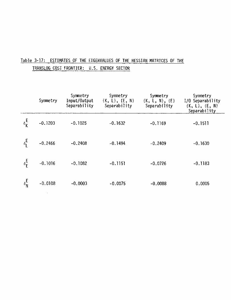
ESTIMATES OF THE EIGENVALUES OF THE HESSIAN MATRICES OF THE
TRANSLOGCOST FRONTIER: U.S. ENERGY SECTOR
SymmetrySymmetry Input/Output
Separability
Symmetry{K, LI, {E, N}Separability
Symmetry{K, L, N}, {E}Separability
SymmetryI/0 Separability{K, L}, {E, N}Separability
-0.1203
-0.2466
-0.1016
-0.1025
-0.2408
-0.1082
-0.1632
-0.1494
-0,1151
-0.1169
-0.2409
-0,0726
-0.1511
-0.1630
-0.1183
-0.018 -00003-0.0075 -0.0088 000
EK
E
0.0005
Table 3-17:
-0.0108 -0,0003

ESTIMATES OF THE EIGENVALUES OF HESSIAN MATRICES OF THE TRANSLOG
COST FRONTIER: U.S. NON-ENERGY SECTOR
SymmetrySymmetry Input/Output
Separability
Symmetry1K, L}, {E, N}Separability
Symmetry1K, L, N}, {E}Separability
SymmetryI/0 Separability1K, LI , E, N}Separability
-0.1290
-0.0400
-0.0141
-0.1226
-0.1775
-0.0162
-0.1199
-0.2109
-0.0147
-0.1050
-0.0349
-0.0134
-0.0899
-0.1495
-0.0151
0.0128 0.0215
SN
N
6N
W-a0000
Table 3-18: -
0.0146 -0.0035 -0.0028

- 189 -
TABLE 3-19: PARAMETER ESTIMATES OF THE
TRANSLOG COST FRONTIER WITH CONCAVITY
RESTRICTIONS, U.S. NON-ENERGY SECTOR*
0. 2007(70.0290)
0.0351
-0.0042
-0.0073
-0.0288
0.044451(6.5621)
-0.0007(-3.0339)
0.3705(97.2699)
0.145853
0.0054
-0.1598
0.1386(19. 2750)
I1I
NSK
NYKK
NKL
NKE
NKN
NCK
NKt
N
LLNYLL
NYLE
NYLN
N'PCL
NYLt
NE
NTEE
NYEN
NPCE
NYEt
NSN
NYNN
N'CN
NYNt
Na C
NCC
*asymptotic t-ratios in parentheses
-0.0022(-8.3031)
0.0182(27.6252)
0. 3200
-0.0016
0.0088(12.1511)
-0.0001(-3.1139)
0.3630(144.8070)
0.2246
-0. 2233(-54.2730)
0.0030(25.7553)
0.3515(92.7581)
0.3414(34.5058)
I I

- 190 -
Table 3-19 (cont.): PARAMETER ESTIMATES OF THE
TRANSLOG COST FRONTIER WITH CONCAVITY
RESTRICTIONS, U.S. NON-ENERGY SECTOR*
*asymptotic t-ratios in parentheses
N -0.0019Pct (-8.1107)
N -0.0089ct (-7.0167)
N 0.0004Ytt (2.2733)
N -0.0429PMK (-10.0269)
N -0.1660PML (-50.8858)
N -0.0017PME (-1.7243)
N 0.2429PMN (85.2872)
N -0.2236MC (-54.0977)
N 0.3667Nm (137.0210)
N 0.25736MM (80.0773)
N 0.00346Mt (26.6373)

- 191 -
k k.TEN = AEK NK
k + k .xk . k k k. kK NL EL L+XNE 6E-E N
kN k)2. 6k + (xNL)2. k k + (NE2). 6k +6k k. kTNN (NK) K (NL) L CNE) E N SN N
k = E, N (3.42)
The effect of this reparametrization is to replace the ten
k k k k k k k k k k kparameters yKK' TKL' KE' TLL' TLE' EE' TKN' TLN' EN' TNN'k = E, N
k k k k k k k k k kby the new parameters XLK' XEK' XEL' 2NK' XNL' XNE, 6K, 6L, 6E' 6N'
k = E, N.
The symmetry conditions together with the conditions defining the
remaining parameters imply:
1 Xk+ k + k + Xk 0+XLK+AEK + NK + RK 0
+ +L+xRk01+EL+XNL RL =
+ k kNE ARE
k1 + RN
k
In terms of the new parameters, necessary and sufficient conditions
for concavity are:
= 0
= 0
k = E,N (3.43)

- 192 -
k<0K -
k < 0L-
6k <0E
6k <0N
We have estimated the reparametrized systems of cost shares for
both the energy and non-energy sectors in order to verify the concavity
property.
As can be seen from Table 3-17, in the case of the energy sector,
all the eigenvalues of the Hessian matrices satisfy the non-positivity
conditions necessary to insure concavity. This holds under all five
alternative hypotheses on the structure of technology. Asymptotic t-
ratios for the four estimated eigenvalues with only symmetry restric-
tions imposed are -12.12, -17.88, -12.80, and -4.31, respectively.
The corresponding estimates of the eigenvalues for the non-energy
sector are shown in Table 3-18. We notice that the concavity conditions
are not satisfied except for the two cases that include the assumptions
of input-output separability. The statistical significance of these
violations is not negligible -- asymptotic t-ratios for the estimated
eigenvalues in the case of only symmetry imposed are -18.21, -4.03,
-17.43, and 4.52 -- so that we chose to re-estimate the translog cost
frontier under the restrictions implied by symmetry and with the
additional conditions for concavity imposed. In this case, we impose
the concavity restriction by setting 6N = 0 and re-estimating theN

- 193 -
remaining parameters. The resulting estimated parameters and implied
estimates are shown in Table 3-19. The values of the estimated eigen-
values for this constrained case were:
N N NN L E
-0.1290 -0.03996 -0.0143(-19.41) (-5.43) (-19.55)
3.1.5 Substitutability and Complementarity in the U.S. Energy and
Non-Energy Production Sectors
In this section we analyze our empirical results on the structure
of technology for the energy and non-energy sectors in terms of their
implications about the substitution possibilities between factors of
production and between categories of output. Given the estimated para-
meters of the translog cost frontier, we compute the price elasticities
of demand for factors of production and the Allen-Uzawa partial
elasticities of substitution and transformation. We also compute
elasticities of factor demands with respect to the composition of
output for both the energy and non-energy sectors.
For a technology described in terms of a cost frontier V = V(y,w)
with output y and input prices w, the partial elasticities of sub-
stitution between inputs i and j are given by the expression (Allen
[22], Uzawa [23]):
V V..
TV V

- 194 -
where V V = v..Va2=w.aw ' ij w w
and, by definition, a.. = a.. For the translog cost frontiers, the
Allen-Uzawa partial elasticities of substitution are given by:
k k k 2kGii =~ ii + (Mg) -i
(M k)2I
i = K, L, E, N, R
k = E, N
Y k + MkMkk -= ii i -j
1 J
i, i = K, L, N, E, R, i A j
k = E, N (3.45)
The price elasticity of demand for factors of production, ry
is defined as
=lnx.
3 alnw
where output quantities and all other input prices are fixed. The
Allen-Uzawa partial elasticities of substitution are related to the
price elasticities of demand for factors of production:
k k(kpij M a. (3.46)
k = E, N

- 195 -
k k k kTherefore, in general, n f vn even though ak 1 =
The price elasticities of demand for factors of production are
tabulated for selected years in tables 3-20 and 3-21 for the energy
and non-energy sectors. It is worthwhile to list representative
figures for the own-price elasticities and compare the corresponding
substitution possibilities for the two sectors:
Energy Sector: Own-Price Demand Elasticities
E E E E EKK LL EE T NN "RR
-0.43 -1.64 -0.48 -0.98 -0.75
Non-Energy Sector: Own-Price Demand Elasticities
N ,N N N NnKKLL nEE nNN RR
-0.62 -0.22 -0.82 -0.05 -0.07
In comparing the own-price elasticities between the two sectors,
we observe that the degree of price-responsiveness of demand for a
given factor is inversely related to the relative intensities of the
factor in the two corresponding sectors, which is a result
consistent with an economy operating in an efficient region. Thus,
we note that the demand elasticities for capital and energy inputs are
lower in the energy sector than in the non-energy sector. Conversely,
the elasticities of demand for labor and non-energy inputs are sub-
stantially higher in the energy sector.
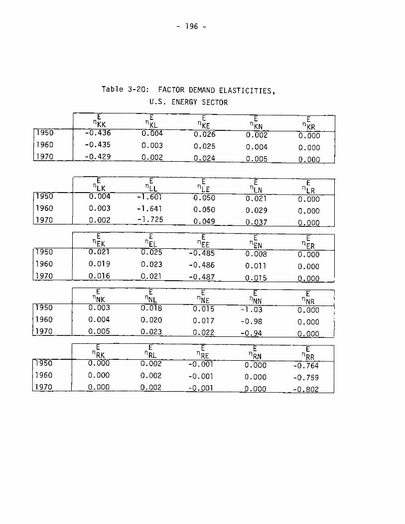
- 196 -
Table 3-20: FACTOR DEMAND ELASTICITIES,
U.S. ENERGY SECTOR
rI: L E
1950 -0.436 0.004 0.026 0.002 0.0001960 -0.435 0.003 0.025 0.004 0.0001970 -0.429 0.002 0.024 0.005 0.000
E E E E E"LK "LL "LE "LN TLR
1950 0.004 -1.601 0.050 0.021 0.0001960 0.003 -1.641 0.050 0.029 0.0001970 0.002 -1.725 0.049 0.037 0.000
E E E E E"EK ____ "EEKENEL
1950 0.021 0.025 0.485 0.008 0.000
1960 0.019 0.023 -0.486 0.011 0.0001970 0.016 0.021 -0.487 0.015 0.000
E E E E Er'NK nNL rN E NN UNR
1950 0.003 0.018 0.015 -1.03 0.0001960 0.004 0.020 0.017 -0.98 0.0001970 0.005 0.023 0.022 -0.94 0.000
E E E E E_ RK RL RE nRN rRR
1950 0.000 0.002 -0.001 0.000 -0.7641960 0.000 0.002 -0.001 0.000 -0.759
11970 __ 0.000 0.002 -0.001 0.000 -0.802
LT KL
EI<
EtT'KK
EKE
E

- 197 -
Table 3-21: FACTOR DEMAND ELASTICITIES,
U.S. NON-ENERGY SECTOR
NrKK
Nr KL
N-"hKE
NThKN
N"KR
1950 -0.621 0.021 0.000 0.061 0.000
1960 -0.623 0.027 0.000 0.062 0.000
1970 1-0.624 0.036 0 ,00 0.047 0.00 R
N N N N NS LK "LL "LE ILN LR
1950 0.021 -0.228 0.000 -0.020 0.000
1960 0.027 -0.220 0.000 -0.013 0.000
1970 0.036 -0.232 0.000 -0.009 0.000
N N N N N_EELEK EL TEE EN ER
1950 {0.000 0.000 -0.812 0.081 0.000
1960 0.000 - 0.000 -0.820 0.074 0.000
1970 0.000 0.000 -0.821 0.058 0.000
SN N N NNK _NL
T NNERNN UNR1950 0.033 -0.012 0.003 -0.054 0.000
1960 0.028 -0.009 0.003 -0.053 0.000
11970 0.023 -0.007 0.002 -0.046 0.000
N NN N_rP.K _RL RE RN "RR
950 0.001 0.001 0.000 -0.001 -0.094
1960 0.001 0.001 0.000 -0.001 -0.072
L1970 0.001 0.001 0.000 -0.001 -0.273

- 198 -
Table 3-22: ALLEN-UZAWA PARTIAL ELASTICITIES OF
SUBSTITUTION, U.S. ENERGY SECTOR
KK1950
1960
1970
-1.25
-1.28-1 .34
ESKL
0.0300.025
0.021
EUKE
0.048
0.044
0.036
EaKN
E~KR
0.013
0.0170.023
0.000
0.000n nnn
E E E E_LL LE LN LR
1950 -- 91 0.123 0.112 0.009
1960 -9.75 0.125 0.130 0.009
1970 -11208 09.125 0.163 0.014
E E EaEE a EN ER
1950_1 .-290.042 -0.002
1960 -1.28 0.049 -0.002
_1970 -1-.293o-.87 03 -0.003
E aE'N N NR
1950 -5.24 0.001
1960 -4.65 0.001
1970 -3 .87 0 .002
E1950 RR
90 -18.211960 -18.321 970 -15.58
It f% n ^

- 199 -
Table 3-23: ALLEN-UZAWA PARTIAL ELASTICITIES
OF SUBSTITUTION, U.S. NON-ENERGY SECTOR
1950 i-2.93 ~0.0/8 -0.0003 0.154 0.0001960 -3.10 0.090 -0.0003 0.142 0.000
1970 _-3.17 0.109 -0.0004 0.118 0.000
CNN N N_LL LE LN LR
1950 -0/.60 0.0007 -0.041 0.0011960 -0.749 0.0007 -0.029 0.0011970 -0.714 0.0007 -0.021 0.001
N N N1950_ aEE a EN aER1950 -43.71 0.171 0.0011960 -41.61 0.162 0.0011970 -41.40 0.137 0.002
N NaNN aNR1950 -0.107 -0.0011960 -0.107 -0.0011970 -0.099 -0.001
N_aRR
1950 -2.031960 -0.691970 -9.13
I Rl a I a * --- Ir-
aKKNKL
NKE
NrKN
Ncl"

- 200 -
The Allen-Uzawa partial elasticities of substitution were com-
puted for both the energy and non-energy sectors and are shown in
tables 3-22 and 3-23, respectively. Our empirical results based on
the translog specification indicate that the structure of technology
in the energy sector is characterized by a certain degree of sub-
stitutability between all pairs of factor inputs, with the exception
of energy and imports that exhibit slight complementarity (aER~ 0.002).
In particular, we note that capital and energy inputs are slightly
substitutable (aE~ 0.044).KEIn the non-energy sector, capital and energy inputs can be seen
to be slightly complementary (crNKE -0.0003). Complementarity is also
exhibited between labor and non-energy inputs arid between non-energy
inputs and imports.. All other pairs of factor inputs are substitutable.
The translog cost frontier estimated without the assumption of
separability between inputs and outputs permit the marginal rate of
transformation between various outputs to be affected by changes in the
composition of input. The elasticity of transformation between a pair
of outputs is defined as the negative of the percentage change in the
output mix divided by the percentage change in the ratio of output
prices. In terms of the parameters of the translog cost frontiers,
the elasticity of transformation between outputs i and j takes the form
k - - (F!i F )/(6aj (1 - F F )) (3.47)
k kwhere F, F. are the corresponding fitted values of the revenue shares.3
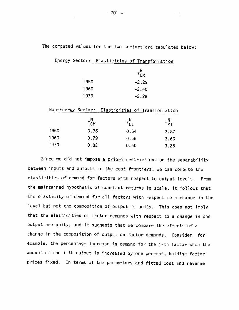
- 201 -
The computed values for the two sectors are tabulated below:
Energy Sector: Elasticities of Transformation
ETCM
1950 -2.29
1960 -2.40
1970 -2.28
Non-Energy Sector: Elasticities of Transformation
N N NCM TCI MI
1950 0.76 0.54 3.87
1960 0.79 0.56 3.601970 0.82 0.60 3.25
Since we did not impose a priori restrictions on the separability
between inputs and outputs in the cost frontiers, we can compute the
elasticities of demand for factors with respect to output levels. From
the maintained hypothesis of constant returns to scale, it follows that
the elasticity of demand for all factors with respect to a change in the
level but not the composition of output is unity. This does not imply
that the elasticities of factor demands with respect to a change in one
output are unity, and it suggests that we compare the effects of a
change in the composition of output on factor demands. Consider, for
example, the percentage increase in demand for the j-th factor when the
amount of the i-th output is increased by one percent, holding factor
prices fixed. In terms of the parameters and fitted cost and revenue
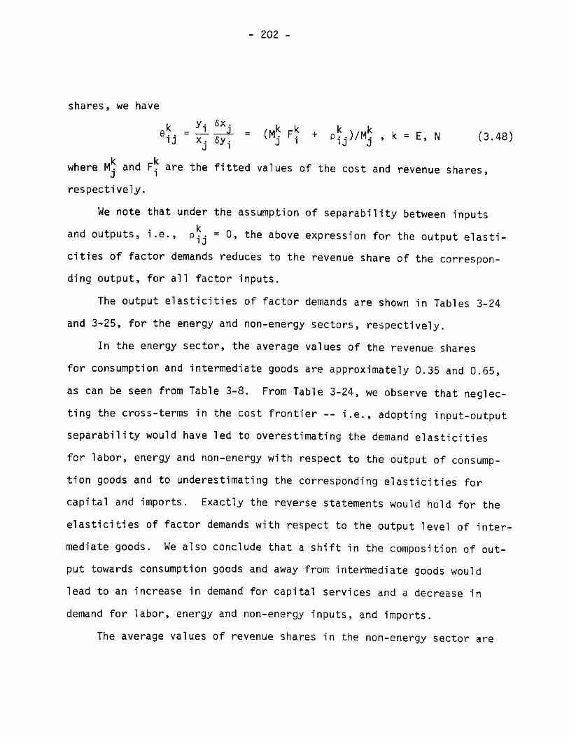
- 202 -
shares, we have
. =ifj = (M$ F + p)/M , k = E, N (3.48)
where M and F j are the fitted values of the cost and revenue shares,
respectively.
We note that under the assumption of separability between inputs
kand outputs, i.e., = 0, the above expression for the output elasti-
cities of factor demands reduces to the revenue share of the correspon-
ding output, for all factor inputs.
The output elasticities of factor demands are shown in Tables 3-24
and 3-25, for the energy and non-energy sectors, respectively.
In the energy sector, the average values of the revenue shares
for consumption and intermediate goods are approximately 0.35 and 0.65,
as can be seen from Table 3-8. From Table 3-24, we observe that neglec-
ting the cross-terms in the cost frontier -- i.e., adopting input-output
separability would have led to overestimating the demand elasticities
for labor, energy and non-energy with respect to the output of consump-
tion goods and to underestimating the corresponding elasticities for
capital and imports. Exactly the reverse statements would hold for the
elasticities of factor demands with respect to the output level of inter-
mediate goods. We also conclude that a shift in the composition of out-
put towards consumption goods and away from intermediate goods would
lead to an increase in demand for capital services and a decrease in
demand for labor, energy and non-energy inputs, and imports.
The average values of revenue shares in the non-energy sector are

- 203 -
TABLE 3-24 ELASTICITIES OF FACTOR DEMANDS
WITH RESPECT TO OUTPUT INTENSITIES, U.S. ENERGY SECTOR
ECK
E"CL
E0CE
E0CN
E0CR
1950 0.542 0.230 0.259 0.248 0.436
1960 0.577 0.251 0.286 0.282 0.464
1970 0.571 0.212 0.256 0.262 0.402
EaE E EMK 0ML 0ME MN MR
1950 0.457 0.769 0.740 0.751 0.564
1960 0.422 0.748 0.713 0.717 0.536
1970 0.428 0.787 0.743 0.737 0.592

- 204 -
TABLE 3-25 ELASTICITIES OF
OUTPUT INTENSITIES,
NCL
NKCK
FACTOR DEMANDS WITH RESPECT TO
U.S. NON-ENERGY SECTOR
NCE eNCN
NCR
1950 0.528 0.786 0.768 -0.191 2.81
1960 0.559 0.772 0.762 -0.187 2.54
1970 0.598 0.766 0.794 -0.192 2.08
eN 0NN 6 NNMK ML ME MN MR
1950 0.275 -0.109 0.473 1.00 -1.79
1960 0.254 -0.079 0.463 1.00 -1.53
1970 0.220 -0.060 0.433 1.01 -1.12
NeN8N NeNIK IL IE IN IR
1950 0.195 0.323 -0.242 0.191 -0.02
1960 0.185 0.307 -0.225 0.181 -0.01
1970 0.180 0.293 -0.227 0.174 -0.04

- 205 -
approximately 0.32 for consumption goods, 0.46 for intermediate goods,
and 0.22 for investment goods. An examination of Table 3-25 suggests
that a maintained hypothesis of input-output separability would lead to
erroneous estimates of the elasticities of factor demands with respect
to output. We conclude that a shift in the composition of output toward
consumption goods and away from intermediate goods would increase the
demands for capital, labor energy inputs, and imports, and decrease the
demand for non-energy inputs; similarly, a shift toward investment goods
and away from consumption goods would increase the demand for non-energy
inputs and decrease the demand for capital, labor, energy inputs, and
imports; finally, a shift towards intermediate goods and away from in-
vestment goods would increase the demand for capital and energy inputs
and decrease the demand for labor, non-energy inputs and imports.
3.1.6 Technological Change: Factor Augmentation Biases
Our analysis of technological change in the U.S. energy and non-
energy production sectors is based on the explanation of the rate of
total cost diminution defined as the negative of the growth rate of
total factor productivity. The rates of total cost diminution for each
of the two sectors are denoted by SE and SN, respectively, and are com-
puted by means of a discrete Divisia approximation as described in
section 3.1.2. The values of the rate of total cost diminution for the
energy and non-energy sectors are shown in Table 3-26 for the period
1948-1971. The average annual rates for this period were -0.0133 and
-0.0067, respectively; thus the average rate of increase of total

- 206 -
TABLE 3-26: ANNUAL RATES OF TOTAL COST DIMINUTION,
U.S. ENERGY AND NON-ENERGY SECTORS, 1948-1971
Year
1948
1949
1950
19511952
1953
1954
19551956
1957
1958
1959
1960
19611962
1963
1964
1965
19661967
1968
1969
1970
1971
Energy Sector
s E
0.0030
0.0042
-0.0272
-0.0234
0.0448
-0.0145
-0.0210
-0.0145
-0.0046
-0.0072
0.0067
-0.0137
-0.0290
-0.0245
-0.0128
-0.0212
-0.0335
0.0033
-0.0368
-0.0330
-0.0150
-0.0432
-0.0316
0.0659
Non-Energy SectorCN
-0.0259
0.0064
-0.05710.0224
0.0098
-0.0098
-0.0166
-0.0286
0.0113
0.0039
0.0043
-0.0239
-0.0040
0.0034
-0.0080
-0.0047
-0.0151
-0.0135-0.00610.0093
-0.0101
0.00290.0021
-0.0156

- 207 -
factor productivity in the energy sector was double the average rate
in the non-energy sector. The value of the augmentation rate for the
non-energy sector (0.67%) is close to estimates for U.S. manufacturing
obtained by Star [24] (0.59%), Gollop [4] (0.84%) and Berndt and Wood
[25] (0.60%).
The empirical results discussed in section 3.1.3 assumed a
parametrization of the structure of technology such that the effects
of technological change were embodied in the parameters
E NY ,3y i = K,L,E,N,Rit it
ESi = C,Mit
N6 i = C,I,Mit
These parameters can be interpreted as factor-share and output-share
augmentation indices. In particular since they appear in the share
equations as coefficients that multiply the time index, it follows
that yEtKt, or example, can be taken as the average yearly rate of
capital-share-augmenting technological change. We remark that the net
effect of technical change on a given factor share depends on the
technological substitution parameters as well as on the rates of factor
augmentation.
Summarized below are the estimated values and corresponding
t-statistics of the factor-share augmentation parameters from Tables
3-13 and 3-19.
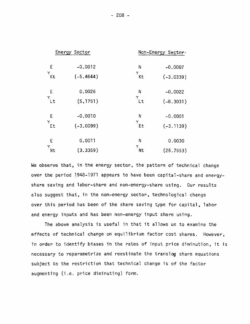
- 208 -
Energy Sector Non-Energy Sectorf
E -0.0012 N -0.0007y Y
Kt (-5.4644) Kt (-3.0339)
E 0.0026 N -0.0022
Lt (5.1751) Lt (-8.3031)
E -0.0010 N -0.0001Y YEt (-3.0099) Et (-3.1139)
E 0.0011 N 0.0030'C YNt (3.3359) Nt (25.7553)
We observe that, in the energy sector, the pattern of technical change
over the period 1948-1971 appears to have been capital-share and energy-
share saving and labor-share and non-energy-share using. Our results
also suggest that, in the non-energy sector, technological change
over this period has been of the share saving type for capital, labor
and energy inputs and has been non-energy input share using.
The above analysis is useful in that it allows us to examine the
effects of technical change on equilibrium factor cost shares. However,
in order to identify biases in the rates of input price diminution, it is
necessary to reparametrize and reestimate the translog share equations
subject to the restriction that technical change is of the factor
augmenting (i.e. price diminuting) form.

- 209 -
The estimating system incorporating this restriction is obtained
by substituting the expressions in Egs (2-20) and (2-21) into the
cost and revenue share equations; in addition, the estimating equations
corresponding to the rates of total cost diminution are replaced by:
E = ME XE + ME EK K MLXL+ ME E + M N +
and
N N N N+MN N + MN N + M N + MNRNSt K = KK+ LXL+MEE + MNXN+ R R
Equations
that
(3.49) are obtained by using Egs (2.20),
(3.49)
(2.21) and noting
= E E + E E + EK K + L LX E
= 5N N + N N + NK K + LXL E
E + E
N + N* ~E
E + $EN .
N + N
N XN
(3.50)
EYtt
E t E + E E E xE + E EKt K +YttL t L Et E YNtXN
E EYRt R
N = N XN + N N N xN + N N N xNtt T Kt K YLtXL + yEt E Y tXaN + YRt R
(3.51)
We remark that in the absence of equations (3.49) the condition of
CRTS would imply that one of the indices of input price diminution
would remain unidentified.
ME xE
ESt
NSt
and
E
X R
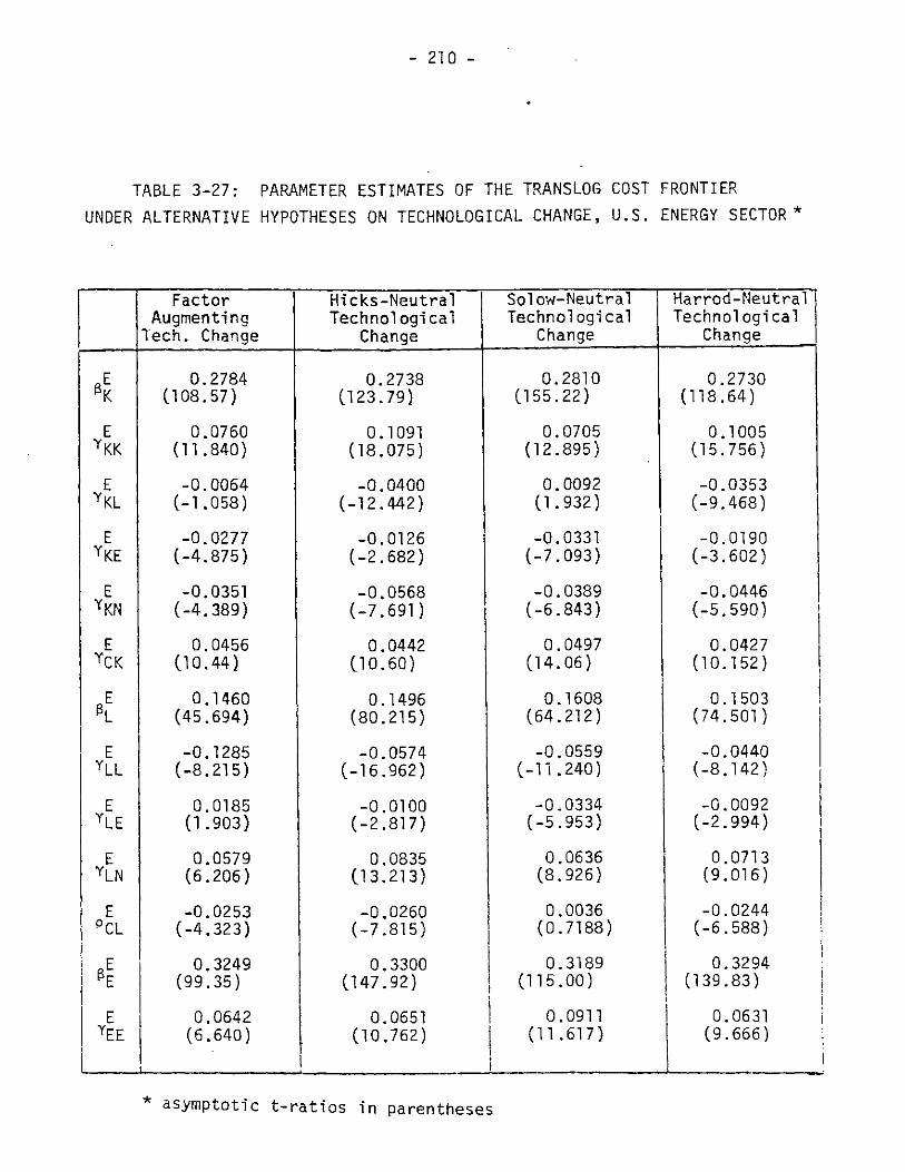
- 210 -
TABLE 3-27: PARAMETER ESTIMATES OF THE TRANSLOG COST FRONTIER
UNDER ALTERNATIVE HYPOTHESES ON TECHNOLOGICAL CHANGE, U.S. ENERGY SECTOR*
Factor Hicks-Neutral Solow-Neutral Harrod-NeutralAugmenting Technol ogi cal Technol ogi cal Technological
Tech. Change Change Change Change
EK
ET KK
ETKL
EYKE
EYKN
ETC K
ESL
ETLL
ET LE
ETLN
EPCL
EE
EEYEE
0.2738(123.79)
0.1091(18.075)
-0.0400(-12.442)
-0.0126(-2.682)
-0.0568(-7.691)
0.0442(10.60)
0.1496(80.215)
-0.0574(-16.962)
-0.0100(-2.817)
0.0835(13.213)
-0.0260(-7.815)
0.3300(147.92)
0.0651(10.762)
_____________ S J ___________________________________--
0.2810(155.22)
0.0705(12.895)
0.0092(1.932)
-0.0331(-7.093)
-0.0389(-6.843)
0.0497(14.06)
0.1608(64.212)
-0.0559(-11 .240)
-0.0334(-5.953)
0.0636(8.926)
0.0036(0.7188)
0.3189(115.00)
0.0911(11.617)
0.2730(118.64)
0.1005(15.756)
-0.0353(-9.468)
-0.0190(-3.602)
-0.0446(-5.590)
0.0427(10.152)
0.1503(74.501)
-0.0440(-8.142)
-0.0092(-2.994)
0.0713(9.016)
-0.0244(-6.588)
0.3294(139.83)
0.0631(9.666)
* asymptotic t-ratios in parentheses
0.2784(108.57)
0.0760(11.840)
-0.0064(-1.058)
-0.0277(-4.875)
-0.0351(-4.389)
0.0456(10.44)
0.1460(45.694)
-0.1285(-8.215)
0.0185(1.903)
0.0579(6.206)
-0.0253(-4.323)
0.3249(99.35)
0.0642(6.640)

- 211 -
TABLE 3-27 (Cont.): PARAMETER ESTIMATES OF THE TRANSLOG COST FRONTIER
UNDER ALTERNATIVE HYPOTHESES ON TECHNOLOGICAL CHANGE, U.S.
EEN
EPCE
ESN
EYNN
ECL
ESCc
EPCC
E*
E*
E*
-N
E
ENERGY SECTOR
Factor Hicks-Neutral Solow-Neutral Harrod-NeutralAugmenting Technological Technological TechnologicalTech. Change Change Change Change
0.0053(0.5607)
-0.0279(-4.721)
0.2094(52.2435)
-0.0311(-2.014)
-0.0254(-4.323)
0.4234(118,95)
0.1407(22.693)
0.0596(-5.924)
-0.0494(-6.606)
-0.0221(-4.007)
-0.0622(-3.8010)
0.0306(3.382)
-0.0002(-0.0248)
-0.0153(-3.605)
0.2095(54.101)
-0.0236(-1.476)
-0.0260(-7.815)
0.4117(134.93)
0.1199(21.626)
0.0
0.0
0.0
0.0
-0.0133(-7.386)
0.0111(1.327)
-0.0401(-7.342)
0.2041(55. 072)
-0.0401(-2.648)
0.0036(0.7188)
0.4257(124.88)
0.1466(23.888)
-0.0268(-8.156)
0.0075(0.837)
-0.0191(-4.296)
0.2089(48.812)
-0.0374(-2.260)
-0.0244(-6.588)
0.4132(134.34)
0.1251(22.363)
0.0082(1.980)
______________ b .4 .1 _______________________________________________ .4, _________________________________________
E E ~ E -K K R- E - E EXL XR XE XE E E ExxE
XE XR --- R

- 212 -
TABLE 3-28: PARAMETER ESTIMATES OF THE TRANSLOG COST FRONTIERUNDER ALTERNATIVE HYPOTHESES ON TECHNOLOGICAL CHANGE, U.S. NON-ENERGY SECTOR*
Factor Hicks-Neutral Solow-Neutral !Harrod-Neutral
Augmenting Technological Technological TechnologicalTech. Change Change Change Change
0.2170(85.337)
0.0270(4.513)
-0.0069(-1 .437)
-0.0063(-9.774)
-0.0236(-6.615)
0.0445(6.849)
0.3524(91.597)
0.1139(12.535)
0.0083(10.649)
-0.1391(-20.144)
0.1411(21.863)
0.0201(38.474)
0.0026(7.534)
0.1989(76.247)
0.0290(5.159)
-0.0268(-15.404)
-0.0083(-12.968)
0.0002(0.0578)
0.0403(8.184)
0.3190(336.19)
0.075-1(35.477)
0.0021(8.730)
-0.0665(-50.781)
0.0830(35.480)
0.0173)(43.703)
0.0037(9.963)
0.2206(74.972)
0.0332(8.936)
-0.0004(-0.1619)
-0.0091(-13.961)
-0.0281(-6.139)
0.0427(12.022)
0.3245(144.05)
0.0705(30.331)
-0.0040(-5.834)
-0.0845(-22 .184)
0.1131(32.921)
0.0140(21.905)
0.0050(11.033)
0.2058(83.969)
0.0502(8.826)
-0.0435(-11 .170)
-0.0069(-11.135)
-0.0064(-1.923)
0.0167(2.892)
0.3437(132.02)
0.1537(19.799)
0.0039(8.560)
-0.1381(-22.668)
0.1587(22.471)
0.0189(46.914)
0.0036(10.346)
* asymptotic in parentheses
NSK
NYKK
NYKL
NYKE
NTKN
NPCK
NSLL
NTLL
NLhE
yN i
LN
NCL
sNE
NEE
t-ratios
- T--I
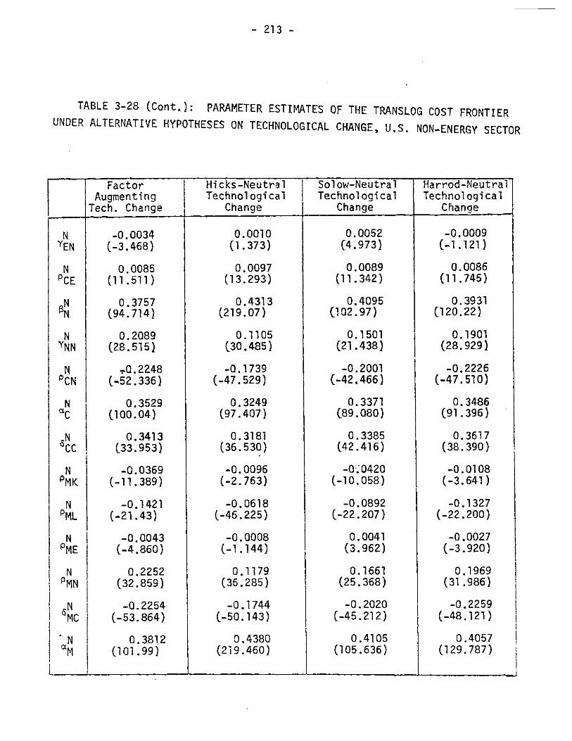
- 213 -
TABLE 3-28 (Cont.): PARAMETER ESTIMATES OF THE TRANSLOG COST FRONTIERUNDER ALTERNATIVE HYPOTHESES ON TECHNOLOGICAL CHANGE, U.S. NON-.ENERGY SECTOR
Factor Hicks-Neutral Solow-Neutral Harrod-NeutralAugmenting Technological Technological Technological
Tech. Change Change Change Change
-0.0034(-3.468)
0.0085(11.511)
0.3757(94.714)
0.2089(28.515)
?Q.2248(-52.336)
0.3529(100.04)
0.3413(33.953)
-0. 0369(-11.389)
-0.1421(-21.43)
-0.0043(-4.860)
0.2252(32.859)
-0.2254(-53.864)
0.3812(101.99)
0.0010(1.373)
0.0097(13.293)
0.4313(219.07)
0.1105(30.485)
-0.1739(-47.529)
0.3249(97.407)
0.3181(36.530)
-0. 0096(-2.763)
-0.0618(-46.225)
-0.0008(-1.144)
0.1179(36.285)
-0.1744(-50.143)
0.4380(219.460)
0.0052(4.973)
0.0089(11.342)
0.4095(102.97)
0.1501(21.438)
-0.2001(-42.466)
0.3371(89.080)
0.3385(42.416)
-0 '0420(-10.058)
-0.0892(-22.207)
0.0041(3.962)
0.1661(25.368).
-0.2020(-45.212)
0.4105(105.636)
-0.0009(-1.121)
0.0086(11.745)
0.3931(1 20. 22)
0.1901(28.929)
-0.2226(-47. 510)
0.3486(91.396)
0.3617(38.390)
-0.0108(-3.641)
-0.1327(-22.200)
-0.0027(-3.920)
0.1969(31.986)
-0.2259(-48.121)
0.4057(129.787)
NYEN
NPCE
NN
NYNN
NPCN
Nac
N3CC
NPMK
NPML
NPME
N9MN
N4MC
Nam

- 214 -
TABLE 3-28 (Cont.): PARAMETER ESTIMATES OF THE TRANSLOG COST FRONTIER
UNDER ALTERNATIVE HYPOTHESES ON TECHNOLOGICAL CHANGE, U.S. NON-ENERGY SECTOR
* AN
AN
N
N= AK
N= AL
N= E
NAR
N- R
- R
= N -xNN R
Factor Hicks-Neutral Solow-Neutral Harrod-NeutralAugmenting Technological Technological Technological
Tech. Change Change Change Change
N 0.2375 0.1281 0.1853 0.2000MM (35.672) (37.580) (28.38) (32.9611
N * -00372 0.0 -0.0252K (-7.695) (-12.33)
N * -0.0622 0.0 -0.01658. (-8.1990) (-24.487)
N * 0.0991 0.0(5.097)
-0.0312 0.0* (-6.613)
0.0329 -0.0067(6.371) C-5.386)

- 215 -
Parameter estimates of the translog cost frontiers under alternative
hypotheses on the structure of technological change are shown in Tables
3-27 and 3-28.
Statistical tests of the various hypotheses were implemented using
the likelihood ratio test. The results for the null hypothesis of factor
augmenting -- i.e. price diminuting -- technical change as against the
translog specification with symmetry alone imposed (at the 0.005 sig-
nificance level) were:
Enerqy Sector
Degrees of Freedom = 3
Critical Value = 12.383
Test Statistic = 0.842
Non-Energy Sector
Degrees of Freedom = 4
Critical Value = 14.860
Test Statistic = 1.970
The hypothesis that technological change has been of the factor
augmenting type over the period 1974-1971 is thus decisively accepted
for both sectors. The implied estimates of the exponential indices of
price diminution are summarized below:
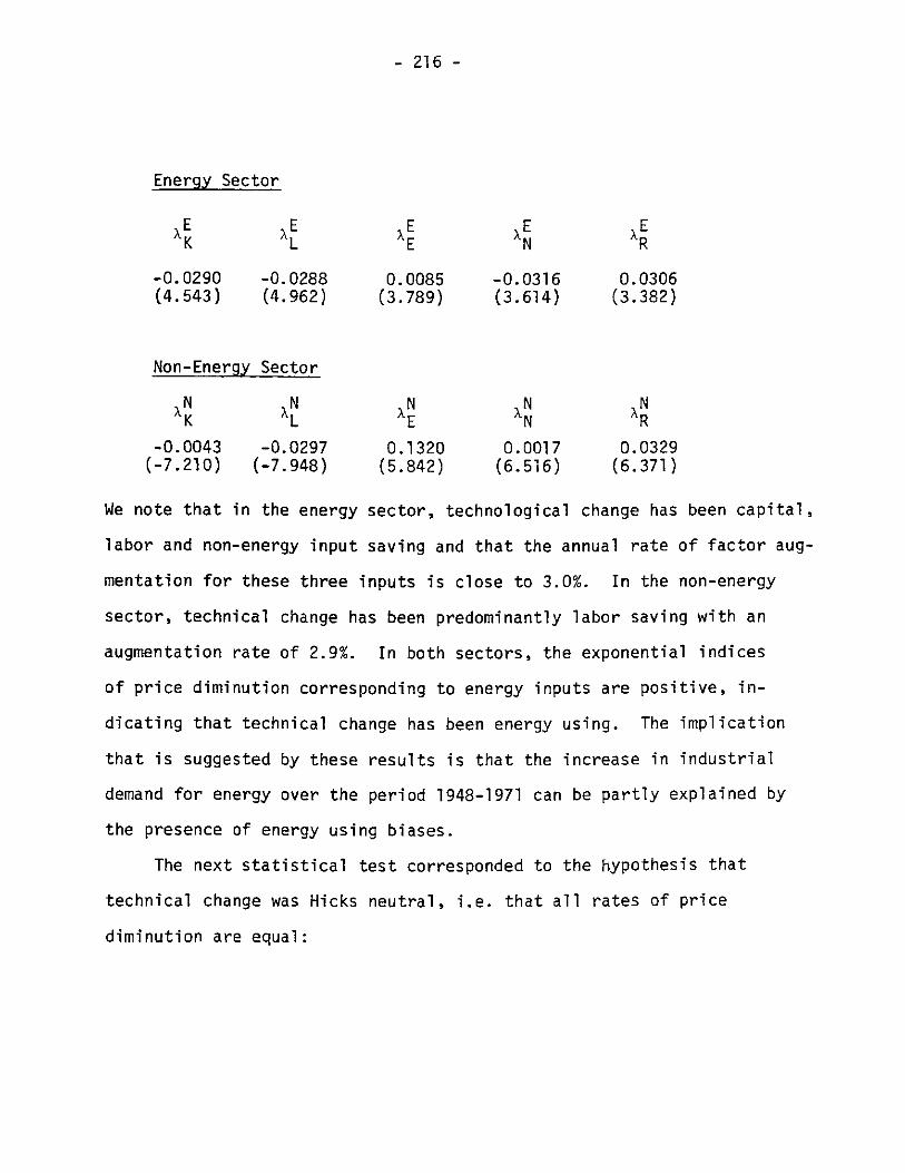
- 216 -
Energy Sector
E E E E EK L E N R
-0.0290 -0.0288 0.0085 -0.0316 0.0306(4.543) (4.962) (3.789) (3.614) (3.382)
Non-Energy Sector
N N N N NK L E N R
-0.0043 -0.0297 0.1320 0.0017 0.0329(-7.210) (-7.948) (5.842) (6.516) (6.371)
We note that in the energy sector, technological change has been capital,
labor and non-energy input saving and that the annual rate of factor aug-
mentation for these three inputs is close to 3.0%. In the non-energy
sector, technical change has been predominantly labor saving with an
augmentation rate of 2.9%. In both sectors, the exponential indices
of price diminution corresponding to energy inputs are positive, in-
dicating that technical change has been energy using. The implication
that is suggested by these results is that the increase in industrial
demand for energy over the period 1948-1971 can be partly explained by
the presence of energy using biases.
The next statistical test corresponded to the hypothesis that
technical change was Hicks neutral, i.e. that all rates of price
diminution are equal:

- 217 -
X E =XE = kE = >1EK L E N R
XN1 XN==X N==XN = XNK L E N R
Note that this implies that technical change is also neutral with
respect to factor shares. The results for the null hypothesis of
Hicks neutrality at the 0.005 significance level were:
Energy Sector
Degrees of Freedom = 4
Critical Value = 14.860
Test Statistic = 16.80
Non-Energy Sector
Degrees of Freedom = 4
Critical Value = 14.860
Test Statistic = 27.02
We thus reject the hypothesis of Hicks neutrality for both the
energy and non-energy sectors. The common rate of price diminution
was found to be -0.0133 (-7.348) for the energy sector and -0.0067
(-5.386) for the non-energy sector.
The final tests involve the hypotheses of Solow-neutral technical
change--i.e. that productivity growth is purely of the capital-
augmenting type--and of Harrod-neutral technical change--i.e. that
factor augmentation is null for all inputs except labor.
Tests for the null hypothesis of Solow neutrality as against factor
augmenting technical change were implemented by setting all exponential

- 218 -
E Nindices to 0 except XK and XK; the results at the 0.005 significance
level were:
Energy Sector
Degrees of Freedom
Critical Value
Test Statistic
Non-Energy Sector
Degrees of Freedom
Critical Value
Test Statistic
- 4
- 14.860
= 10.36
= 4
- 14.860
- 22.62
Thus the hypothesis of Solow-neutrality is rejected in the non-energy sector
whereas in the energy sector we are unable to reject it.
The results for the null hypothesis of Harrod-neutrality as against
factor augmenting technical change--implemented by setting all exponen-
E Ntial indices to 0 except X L and XL were:
EnergyjSector
Degrees of Freedom
Critical Value
Test Statistic
Non-Energy Sector
Degrees of Freedom
Critical Value
Test Statistic
- 4
= 14.860
= 22.22
- 4
= 14.860
- 17.60
We thus reject the hypothesis of Harrod-neutrality in technical change
in both the energy and non-energy sectors.

- 219 -
The above series of tests suggest the following set of conclusions.
First, to the extent that technological progress has occurred in the
U.S. energy and non-energy production sectors over the period of 1948-
1971, it has been introduced through the factors of production and not
through some independent force acting over time. Second, technical
change has been predominantly labor saving and energy using in the
non-energy sector and capital, labor and non-energy saving in the
energy sector. Third, our results do not support the hypothesis of
Hicks neutrality which is commonly adopted by empirical researchers.
We should point out that the technical change biases identified
with our model need not necessarily persist into the future and
therefore our results are of limited value from the standpoint of tech-
nology forecasting; for this purpose it would be necessary to have
a fully endogenous model of technical change with the characteristics
outlined in Section 2.3.4. Such a model based on an endogenous theory
would make it possible to better address questions such as the induced
innovation hypothesis or issues related to governmental energy policy
such as the enactment of investment tax credits applying only to
energy-conserving capital or the promotion of R & D funding policies
aimed at producing energy-saving biases in technological change.
3.2 Estimation of the Model of Consumer Behavior
In this section we present the empirical results for our model of con-
sumer behavior. We first discuss the sources of data and the preparation of

- 220 -
our set of accounts on personal consumption expenditures. Next we
describe the stochastic specification of the model of the household sector
in terms of the expenditure shares corresponding to the inter-temporal and
intra-temporal sub-models, respectively. After presenting the parameter
estimates for both sub-models, we examine their implications in terms of
the possibilities for substitution among commodity groups: and'in terms of
the validity of alternative separability hypotheses about the structure
of consumer preferences.
3.2.1 Data Sources and Preparation
The empirical implementation of our model of consumer behavior
required the construction of time series data corresponding to price
and quantity components of leisure and three commodity groups: energy
goods, non-energy goods and capital services; we constructed these time
series for the U.S. household sector for the period 1947-1971.
Price and quantity components of personal consumption expenditures
on energy were constructed as Divisia aggregates of consumption by house-
holds of refined petroleum products, electricity and natural gas. Con-
sumption of non-energy products was defined as an aggregate Divisia index
of consumption expenditures for the products of sectors Nl, N2, N3 and N4
defined in section 3.1.1 and of imported consumer goods; consumer durables
were not included in this category. Price and quantity components of capital
services consumed by households were constructed by aggregating over the
corresponding series of capital services from consumer durables and residential

- 221 -
structures. The quantity index for leisure was constructed taking as a basis
the total time endowment of the household sector and the supply of labor; the
price index for leisure was taken to be equal to the after-tax wage rate.
The price and quantity components of full consumption to be used
in the inter-temporal allocation model were constructed by Divisia
aggregation of the corresponding series for leisure and the three commo-
dity groups. The time series for full consumption are tabulated in
Table 3-29.
PF F/P
AverageValue -- 12.161947-1971
AverageGrowth Rate 6.9 1.1%p.a. 1947-1971
Price indices for the three commodity groups and leisure are
tabulated in Tables 3-30; quantity indices expressed in per capita
terms are shown in Table 3-31; both these sets of data are summarized
below:
L PCN CK CE
AverageGrowthRate p.a. 2.3% 2.4% 0.0%1947-1971
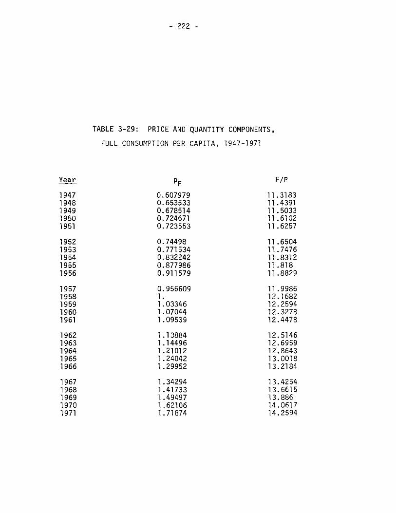
- 222 -
TABLE 3-29: PRICE AND QUANTITY COMPONENTS,
FULL CONSUMPTION PER CAPITA, 1947-1971
Year PF F/P
1947 0.607979 11.31831948 0.653533 11.43911949 0.678514 11.50331950 0.724671 11.61021951 0.723553 11.6257
1952 0.74498 11.65041953 0.771534 11.74761954 0.832242 11.83121955 0.877986 11.8181956 0.911579 11.8829
1957 0.956609 11.99861958 1. 12.16821959 1.03346 12.25941960 1.07044 12.32781961 1.09539 12.4478
1962 1.13884 12.51461963 1.14496 12.69591964 1.21012 12.86431965 1.24042 13.00181966 1.29952 13.2184
1967 1.34294 13.42541968 1.41733 13.66151969 1.49497 13.8861970 1.62106 14.06171971 1.71874 14.2594

TABLE 3-30; PRICE INDICES OF CONSUMPTION BY U,S. HOUSEHOLDS, 1947-1971
Year PL PCN CK CE
1947 0.524696 0.797251 0.8208 0.85551948 0.565074 0.843783 0.7895 1.00021949 0.596125 0,823441 0.6684 0.95661950 0.637924 0.835753 0,855 0.96291951 0.63175 0.886219 0.8421 0.9851
1952 0.650301 0.913857 0.8754 0.97741953 0.675668 0.918971 0.931 1.01451954 0.73855 0.925951 0.9374 1.99291955 0.783713 0.930959 1.0135 0.99561956 0.81852 0,943762 0.9884 1.0121
1957 0.863579 0.972002 0.9735 1.01461958 0.905656 1. 1. 1.1959 0.936416 1.01514 1,0874 1.0011960 0.972524 1.0351 1.12 0.98021961 0.998223 1.04148 1,1165 1.008
1962 1.04246 1.0468 1.1608 0.99671963 1.04598 1,06046 1.2029 0.98631964 1.11321 1,07407 1,2389 0.95111965 1.14325 1.0821 1.2734 0.97561966 1.20095 1.11547 1.323 0.976
1967 1,24413 1.15061 1.3054 0.98271968 1,31855 1.2002 1.311 0.96111969 1.39195 1.25513 1,4008 0.9691970 1,52284 1.31779 1.3619 0.97381971 1.61586 1.37869 1.474 1.0188

CONSUMPTION QUANTITY INDICES PER CAPITA, U.S. HOUSEHOLDS, 1947-1971
LJ/PYear
19471948194919501951
19521953195419551956
19571958195919601961
19621963196419651966
19671968196919701971
10.958110.063611.11811.189611.1645
11.136611.20211.279111.197911.2112
11.317211.48511.535611.578211.6884
11.720311.871211.982912.056512.2178
12.380112.562712.747612.895213.0592
CN/P
1.146461.147381.141971.157991.15804
1.180561.20181.20041.236251.26283
1.25433.26696
1.309661.320071.33049
1.363051.395241.446341.503651.54986
1.587411.637591.66741.683551.71973
CK/P
0.2401440.2563990.2730780.2892150.315513
0.3284290.3368440.3496250.3606740.38068
0.3916410.3999670.4015180.411870.419482
0.4238280.4342690.4479520.4646920.486437
0.5079060.5253560.5488980.5713760.585902
CE/P
0.0511350.0529980.0565860.0625090.067435
0.0722430.0755320.0774270.0840390.086516
0.0930950.0968110.9193310.1105630.112534
0.1157630.1189730.1257170.1285010.13588
0.1403980.1508820.1591140.1658630.169463
I)
N)
TABLE 3-31:

- 225 -
.1
AverageValue1947-1971
AverageGrowthRate p.a.1947-1971
LJ/P
11.69
1 .2%
CN/P
1.31
2.0%
CK/P
0.39
5.8%
CE/P
0.09
8.5%
3.2.2 Estimation of the Inter-Temporal Model
The estimating equation for the inter-temporal allocation sub-model
is obtained from Eg. 2.47 by defining the share of present full consumption
in current wealth
St (3.52)- pF F/ (1 + MW) Wt1
which leads to the share equation
a0 + 100 ln (Ft/Pt) + Sot . t
aM + In (Ft/Pt) + MT."
[1 +y(p. LHt + ELt)
(1 + MW) .- wt-l
FSt ~=

TABLE 3-32: PARAMETER ESTIMATES OF
INTER-TEMPORAL TRANSLOG UTILITY FUNCTION*
HomotheticSeparabi 1i ty
I I I
ExplicitHomotheticity
Neutrality Homogeneity NeutralHomogeneity
Neutral LinearLogarithmic
i i IIII lT.IILY
-0.0250(24.82)
0.0095(24.80)
-0.0001(-24.63)
0.3828(71.47)
-0.0019(49.23)
39.82(24.43)
-0.07425(-3.761)
0.0254(3.806)
0.3426(97.65)
12.746(3.574)
-0.0197(-26.22)
0.0073(43.67)
-0.000(-21.74)
0.3732(27.31)
50.72(0. 000)**
-0.0248(-43.45)
0.0092(57.18)
0.3716(60,19)
0.0004(49.23)
40934(0, 000)**
-0.0245(-176.41)
0.0091(66.26)
0,3732(0,000)**
40.34(24.58)
I. I . I -I I
*Asymptotic t-ratios in parentheses
**Singular likelihood function
00
4ot
1 Mo
13Mt
p
N)N)
-0.0724(-116.95)
13.09(110, 39)

- 227 -
Since this equation is homogeneous of degree zero in the parameters, we
adopt the normalization aM = -1, which leaves 6 parameters to be estimated,
The restrictions implied by the theory of demand are those of
monotonicity, i.e.
0S o C3.54)
and quasi-convexity which can be shown to imply the parametric restriction
00 -at0 -0(3.55)
In table 3-32 we present I3SLS estimates of the parameters of the
translog utility function under alternative hypotheses on the inter-
temporal structure of consumer preferences. The most general specification
incorporates a maintained hypothesis of homothetic separability, which was a
necessary assumption for the derivation of the inter-temporal allocation
model in Section 2.4.4. Next we assume that inter-temporal preferences
are explicitly homothetic which implies the parametric restriction
a00 = aMO = 0
The next three specifications incorporate both separately and jointly
the restrictions of neutrality, i.e., st = 0, and homogeneity, i.e.,
sot = 0.
Finally, we estimate the share equation under the assumption that the
utility function is neutral linear logarithmic. The results of likelihood
ratio tests of each of the five alternative hypotheses as against a homo-
thetically separable utility function are shown below for a significance
level of 0.005

- 228 -
Degrees Critical Testof Freedom Value Statistic
ExplicitHomotheticity 2 10.60 17.24
Neutrality 1 7.87 3.39
Homogeneity 2 10.60 4.12
Neutral 2 10.60 6.51Homogeneity
NeutralLinear 4 14.86 18.12LogarithmicUtility
We remark that the fitted values of the parameters of the translog
utility function satisfy the monotonicity and quasi-convexity restrictions
given by 3.54 and 3.55.
Given the estimated parameters for each of the above six specifications,
we can compute the implied estimates of the social discount rat3 6 by using
Eg. 2.44:
+6 a
from which we obtain
- 0
+ a0
We tabulate below the implied estimates of the social discount rate corre-

- 229 -
sponding to each of the alternative hypotheses on the intertemporal
structure of consumer preferences:
a Discount RateS
HomotheticSeparability -0.0250 2.66%
Explicit -0.742 7.98%Homotheti city
Neutrality -0.0197 2.02%
Homogeneity -0.0248 2.62%
Neutral -0.0245 2.57%Homogenei ty
NeutralLinear -0.0724 7.80%LogarithmicUtility
We remark that the above set estimates of the social rate of discount is
well within the range of values that might be derived from observable
magnitudes of market behavior, as well as values of the discount rate
that are commonly used in practice. The market rate of interest faced
by households wishing to borrow funds -- e.g. the mortgage rate -- is in

- 230 -
the neighborhood of 8.00%; the yield on long-term government securities
-- commonly used as the discount rate in cost-benefit analysis of water
resource projects -- is currently at 6-1/4%. The Department of the
Interior recommends the use of an 8% rate for internal purposes, while
the Office of Management and Budget specifies a 10% rate of discount for
projects to be included in budgetary requests. Dorfman [26], using a
constant-elasticity function defined on per capita aggregate consumption,
concludes that the social rate of discount is "no greater than 3%."
3.2.3 Estimation of the Intra-Temporal Model
The estimating system for the intra-temporal allocation model is
derived from the expenditure share equations for leisure, energy, non-
energy and capital services given in Equations 2.51-2.54 of Chapter 2.
Since the equations for the budget shares are homogeneous of degree
zero in the parameters, normalization of the parameters is required for
estimation. We adopt the normalization
aMC + C + N + KC + EC = - (3.56)
which leaves 28 parameters to be estimated in the unrestricted model.
The additional identities given by:
+ 3C + aC + SC- C+ JN JK JE = MJ
C + 5C + 5C + 5C CNJ NN NK NE = MN
c + 5C + 5C + 5C CKJ KN KK KE = MK
C C+ E + CEK + CE C5EJ + EN + EK + EE = ME

- 231 -
C + C + C + c Ct+ N + Kt + Et = SMt (3.57)
reduce the number of parameters to be estimated to 23.
Since the negative of the logarithm of the direct translog utility
function is twice differentiable in the logarithms of the quantities con-
sumed, it follows that the Hessian of the utility function is symmetric;
this condition implies the following set of restrictions on the
parameters:
C CaC = % Ci,j = J,N,K,E
i i j (3.58)
These symmetry restrictions further reduce the total number of parameters
to be estimated to 20.
The budget constraint implies that the sum of all expenditure
shares must be equal to unity, i.e.
MC + M + M + M C 1 (3.59)
where M C is the budget share of the i-th commodity group.
The stochastic specification for the estimating share system is
based on the assumption of additive disturbances that are serially un-
correlated. The estimating system for the intra-temporal allocation
model in terms of per capita quantities is shown in Table 3-33. Because
of the budget constraint (3.59), it follows that only three share equa-
tions are necessary to estimate the entire system, since the disturbances
across the four equations are constrained to add up to zero.
The resulting I3SLS estimates for the parameters of the direct
intra-temporal translog utility function with symmetry alone imposed are
shown in Table 3-34.

MULTIVARIATE ESTIMATING SYSTEM OF EXPENDITURE SHARES, INTRA-TEMPORAL MODEL
OF CONSUMER BEHAVIOR
a ln(LJ/P) + 3J Nln(CN/P) + Kln(CK/P) + scEln(CE/P) + 8ct
-1 + Mln(LJ/P) + 0MNln(CN/P) + 0MKln(CK/P) +SMEln(CE/P) + 0Mt-t
C i CMN+ M(K MC C
acN + JNlln(LJ/P) + ScNNln(CN/P) + 0Ncln(CK/P) + SNEln(CE/P) + SNt
-1 + Mln(LJ/P) + Mcln(CN/P) + Mln(CK/P) + "c'Mln(CE/P) + Mt t
aK + fKln(LJ/P) + CNKln(CN/P) + 0KK n(CK/P) + 3KElln(CE/P) + cat-l + + IBMKlf(K/)+ SElf(C/P
C
CMN
CMK C MNln(CN/P) c
~MTc ln(LJ/P) +
+ e3+t
+ E:NCt
N)CA)N)
+ K+t
Tabl e 3-33:
+C Mln(CK/P) + c S ln(CE/P) +

- 233 -
Table 3-34: PARAMETER ESTIMATES OF INTRA-TEMPORAL DIRECT TRANSLOG
UTILITY FUNCTION*
C
CsJJ
CJN
CSK
CSE
CSJT
CSMJ
CSMN
CSMK
SCSME
C5MT
CaN
CNN
- rII -T
Neutrality
-0.2458(-4.785)
-1.6498(-67.04)
-0.1152(-5.546)
0.0373(277.90)
-1.4062(-1812.82)
-0.0084(-22.708)
-1.7103(-311.44)
-0.2789(-18.637)
-0.0332(-46.722)
-1.7029(0.0)**
-0.0026(-7.110)
-0.3979(-8.025)
-0.0760(-10.752)
Homotheticity
-0.4200(-7.2921)
-0.9913(-19.512)
-0.0106(-0.4365)
0.0395(33.485)
-0.9226(-25.968)
-0.9489(-18.300)
-0.0291(-1.311)
0.0127(2.304)
-1.0632(-29.792)
-0.0002(-29.792)
-0.3140(-7.957)
0.0154(1.570)
Homogeneity
-0.3879(-75.44)
-0.1601(89.278)
0.0805(67.185)
0.0555(169.715)
0.0175(20.130)
-0.0854(-224.05)
-0.0959(-250.215)
-0.3719(-100.28)
-0.0179(0.0) **
*asymptotic t-ratios in parentheses.**singular likelihood function.
Symmetry
1 4
-0.4102(-4.625)
-0.1990(-5.762)
0.1389(4.990)
0.0417(3.681)
-0.0216(-1.237)
-0.0024(-2.780)
-0.3221(-4.051)
-0.1188(-4.708)

- 234 -
Table 3-34 (cont.): PARAMETER ESTIMATES OF INTRA-TEMPORAL DIRECT
UTILITY FUNCTION*
IrI1
Neutrality
-0.0374(-9.377)
-0.0897(0.0)**
-0.2070(0.0)**
0.0072(4.555)
-0.0416(0.0) **
Homotheti city
-0.0625(-62.43)
-0.0065(0.0) **
-0.0071(0.0)**
-0.1704(0.0) **
0.0028(2.573)
-0.0080(-10.370)
-0.0024(0.0) **
Homogeneity
-0.0257(-3.623)
-0.0508(3.416)
0.0008(1.030)
-0.2112(-9.815)
-0.0112(-2.035)
-0.0303(-7.640)
0.0016(0.0)**
**singular likelihood function.
CSNK
CSNE
C5NT
CaK
C5KK
C5KE
CKT
Symmetry
-0.0847(0.0) **
-0.2087(0.0) **
0.0052(0.0)**
-0.2689(0.0) **
0.0092(0.0) **
-0.0707(0.0)**
0.0006(0.0)**

- 235 -
3.2.4 The Structure of Consumer Preferences and Substitution
Possibilities
In this section we report on the results of statistical tests
designed to investigate alternative hypotheses about the structure of
consumer preferences in the U.S. household sector. The tests are con-
ducted under a maintained assumption of utility-maximizing behavior with
a functional specification derived from a direct translog utility func-
tion, as described in the previous section. We will also present numeri-
cal estimates of price and income elasticities which provide insight
into the possibilities for substitution among commodity groups.
We implement tests on the structure of consumer preferences by
using the likelihood ratio test applied to the corresponding parametric
restrictions on the translog utility.
We test for neutrality of consumer preferences by testing the para-
C C Cmetric restrictions 0t C ' 2CNt = 0' SKt = 0. The results of the test
for this hypothesis as against the alternative hypothesis of a translog
utility function with symmetry alone imposed are, at the 0.005 level of
significance:
Degrees of freedom = 3
Critical value = 12.38
Test statistic = 14.0
We test for homotheticity of consumer preferences by testing the para-
metric restrictions aC C=0 CNC= 0, K = 0, S0 E = 0. The results forSMJ 0 MN 0 MK -,ME =0
the test of homotheticity as against symmetry alone, at the 0.005 level
of significance, are:
Degrees of freedom = 4
Critical value = 14.86

- 236 -
Test statistic = 4.03
We test for homogeneity of consumer preferences by testing the parametric
restrictions M3 = '0, MN 0,0MK 'ME -0. The results for the
test of homogeneity as against the alternative hypothesis of a translog
utility function with symmetry alone imposed, at the 0.005 level of
significance are:
Degrees of freedom = 5
Critical value = 16.74
Test statistic = 22.03
The parameter estimates corresponding to the hypothesis of neutrality,
homotheticity and homogeneity are shown in Table 4-34. The results of
the above set of tests lead us to reject the hypothesis of neutrality and
homogeneity, while we are unable to reject the hypothesis of homotheticity.
We remark that the parametric restrictions adopted to implement the tests
correspond to explicit separability restrictions in the nomenclature
used by Jorgenson and Lau [191; according to their terminology the
above set of hypotheses correspond to an explicitly neutral, explicitly
homothetic and explicitly homogeneous direct translog utility function,
respectively.
The final set of structural hypotheses we wish to investigate cor-
respond to groupwise separability among commodity groups. We test for
groupwise separability between LJ and {CN,CK,CE} by testing the para-
C C Cmetric restrictions JN = 0' JK =0,' JE = 0. We test for groupwise
separability between CN and {UJ, CK, CE} by testing the parametric re-
strictions s = 0, ONK 0, = O' = 0. We test for groupwise separabilityJN NK NE

- 237 -
Table 3-35: LIKELIHOOD RATIO TESTS OF GROUPWISE SEPARABILITY
HYPOTHESES ON THE STRUCTURE OF CONSUMER PREFERENCES
*0.005 significance level
Groupwise Separability Degrees of Critical Testbetween Freedom Value* Statistic
LJ and {CN, CK, CE} 3 12.38 16.38
CN and {LJ, CK, CE} 3 12.38 14.42
CK and {LJ, CN, CEI 3 12.38 16.12
CE and {LJ, CN, CK} 3 12.38 4.64
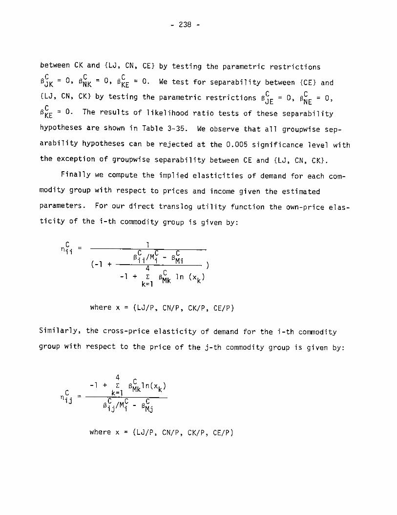
- 238 -
between CK and {LJ, CN, CE} by testing the parametric restrictions
C C -oSJK = NK KE = 0. We test for separability between {CE} and
{LJ, CN, CK} by testing the parametric restrictions 5E = 0, E = 0,C
SKE = 0. The results of likelihood ratio tests of these separability
hypotheses are shown in Table 3-35. We observe that all groupwise sep-
arability hypotheses can be rejected at the 0.005 significance level with
the exception of groupwise separability between CE and {LJ, CN, CK}.
Finally we compute the implied elasticities of demand for each com-
modity group with respect to prices and income given the estimated
parameters. For our direct translog utility function the own-price elas-
ticity of the i-th commodity group is given by:
C _CI
(-1+ Mi
-1 + z Mk ln (xk)k=1
where x = (LJ/P, CN/P, CK/P, CE/P)
Similarly, the cross-price elasticity of demand for the i-th commodity
group with respect to the price of the j-th commodity group is given by:
4-1 + E SMkln(xk)
C k=lU SK/MC -
13 i Mj
where x = (LJ/P, CN/P, CK/P, CE/P)

- 239 -
Table 3-36: PRICE AND INCOME ELASTICITIES OF COMMODITY GROUPS, INTRA-
TEMPORAL MODEL OF CONSUMER BEHAVIOR
Price Elasticities
C C CC"Jh"JN TJK JE
1950 -2.724 -0.380 -0.210 -0.098
1960 -1.177 -0.098 -0.051 -0.036
1970 -1.090 -0.057 -0.034 -0.026
C C CTNN NK "NE
1950 -18.130 1.980 0.165
1960 -1.432 0.640 0.198
1970 -1.243 0.329 0.160
C CTKK KE
1950 -0.529 1.960
1960 -0.833 0.232
1970 -0.893 0.121
CDEE
1950 -0.184
1960 -0.468
1970 -0.593
Income Elasticities
nJB "NB T KB DEB
1950 3.435 --- -3.213 -1.843
1960 1.362 0.692 0.012 0.074
1970 1.207 0.817 0.477 0.338

- 240 -
The income elasticity for the i-th commodity group is computed by using
the identity
C1iB ij
Income and price elasticities are tabulated in Table 3-36. We
observe slight substitutability between non-energy, capital and energy,
while leisure and the other three commodity groups exhibit slight com-
plementarity. We also note increasing income elasticities for CE, CN and
CK throughout the period 1948-1971 while the income elasticity of leisure
decreased during the same period. We summarize below typical values of
the own-price elasticities of demand throughout the period 1948-1971.
Own-Price Elasticities of Demand
C C C CTJ ET NN T KK "EE
-1.225 -1.534 -0.799 -0.421
3.3 Summary
This chapter has discussed the estimation of the behavioral equations
in our macroeconomic energy model and has presented the results of statis-
tical tests of alternative hypotheses on the structure of technology and
the structure of consumer preferences.
The translog specification of the cost frontiers appears to provide a
satisfactory characterization of technology for the U.S. energy and non-
energy sectors. The unrestricted estimates satisfy the concavity constraints
implied by the theory of cost and production; the single exception turns out
- 241 -
to be statistically insignificant. The hypothesis of separability between
inputs and outputs is decisively rejected for both the energy and non-
energy sectors. An important consequence of this result is that the elasti-
cities of factor demands with respect to output intensities are not equal
to the corresponding cost shares, as in the separable case. Price elastici-
ties of demand for factors of production, as well as Allen-Uzawa partial
elasticities of substitution are computed and the implied patterns of subs-
titutability and complementarity are examined for the two production sectors.
Statistical tests of various hypotheses concerning the structure of technolo-
gical change are reported; the commonly adopted hypothesis of Hicks neutrali-
ty is rejected and our results reveal the presence of energy-using biases in
technical progress occuring during the period 1948-1971.
The remaining sections deal with the estimation of the model of consumer
behavior. From the estimated parameters for the inter-temporal allocation
model, we derive the implied values for the rate of social discount. The
estimated values of the discount rate range between 2.02% and 7.98%, depen-
ding on the underlying assumptions about the structure of inter-temporal
preferences. Finally, several structural assumptions about the intra-tempo-
ral translog utility function are investigated, including groupwise separa-
bility among the various commodity groups.

- 242 -
REFERENCES TO CHAPTER III
[I] Berndt, E. R., and Savin, N. E., "Estimation and Hypothesis Testingin Singular Equation Systems with Autoregressive Disturbances,"Discussion Paper 74-02, Dept. of Economics, University of BritishColumbia, April 1974.
[2] Faucett, J., "Data Development for the I/0 Energy Model: FinalReport," Jack Faucett Associates, Chevy Chase, Md., May 1973.
[3] Christensen, L., and Jorgenson, D. W., "The Measurement of U.S.Real Capital Input, 1929-1967," Review of Income and Wealth, 15,December 1969.
[4] Gollop, F., "Modeling Technical Change and Market Imperfections:An Econometric Analysis of Manufacturing 1947-1971, Ph.D. Thesis,Dept. of Economics, Harvard University, July 1974.
[5] Christensen, L., and Jorgenson, D. W., "U.S. Real Product and RealFactor Input," 1929-1967, Review of Income and Wealth, Series 16,March 1970.
[6] Zellner, A. M., and H. Theil, "Three-Stage Least Squares: Simul-taneous Estimation of Simultaneous Equations," Econometrica, 30,January 1962.
[7] Malinvaud, E., Statistical Methods of Econometrics, Rand McNally& Co., Chicago, 1970.
[8] Dhrymes, P. J.. "Small Sample and Asymptotic Relations BetweenMaximum Likelihood and Three Stage Least Squares Estimators,"Discussion #109, Dept. of Economics, University of Pennsylvania,February 1971.
[9] Berndt, E. R., "The Economic Theory of Separability, Substitutionand Aggregation with an Application to U.S. Manufacturing 1929-1968," Ph.D. Thesis, Dept. of Economics, University of Wisconsin,1972.
[10] Pollak, R. A. and Wales, T. J., "Estimation of a Linear ExpenditureSystem," Econometrica, Vol. 37, No. 4, October 1969.
[11] Barten, A. P., "Maximum Likelihood Estimation of a Complete Systemof Demand Equations," European Economic Review, Fall 1969.
[12] Byron, L., "Empirical Tests of Hypothesis Using LikelihoodRatio Statistics," Discussion Paper No. 237, Univeristy ofToronto, 1972.

- 243 -
[13] Woodland, A.D., "Substitution of Structure, Equipment and Labor inCanadian Production," International Economic Review, February, 1975.
[14] Berndt, E.R. and Savin, E., "A Comparison of the Wald, LiklihoodRatio and Lagrange Multiplier Test Statistics," Discussion Paper No.137, University of British Columbia, Vancouver, 1975.
[15] Hall, R.E., "The Specification of Technologies with Several Kinds ofOutput," The Journal of Political Ecnonomy, Vol. 81, No. 4, 1973.
[16] Burgess, D.F., "A Cost Minimization Approach to Import Demand Equa-tions," Review of Economics and Statistics, July, 1974.
[17] Arrow, K.J., "The Measurement of Real Value Added," Technical ReportNo. 70, University Institute for Mathematical Studies in the SocialSciences, Stanford University, 1972.
[18] Berndt, E.R. and Wood, D.O., "Technology, Prices and the Derived De-mand for Energy," Review of Economics and Statistics, August, 1975.
[19] Jorgenson, D.W., "Consumer Demand for Energy," Harvard Institute ofEconomic Research, Harvard University, Discussion Paper No. 386,November, 1974.
[20] Gantmacher, A., The Theory of Matrices, Chelsea Publishing Co., NewYork, 1960.
[21] Lau, L., "Econometrics of Monotonicity, Convexity and Quasi-Convexity," Econometrica, 43, 1975.
[22] Allen, R.G.D., Mathematical Analysis for Economists, Macmillan,London, 1938.
[23] Uzawa, H., "Production Functions with Constant Elasticities of Sub-stitution," Review of Economic Studies, Vol. 29, October, 1962.
[24] Star, S., "Accounting for the Growth of Output," American EconomicReview, March, 1974.
[25] Berndt, E.R. and Wood, D.O., "Technological Change, Tax Policy, andthe Derived Demand for Energy," Energy Laboratory Report MIT-EL-75-019, (mimeographed draft), 1975.
[26] Dorfman, R., "An Estimate of the Social Rate of Discount," DiscussionPaper No. 442, Harvard Institute of Economic Research, HarvardUniversity, November, 1975.
[27] Tornquist, L., "The Bank of Finland's Consumption Price Index,"Bank of Finland Monthly Bulletin, No. 10, 1936.

- 244 -
CHAPTER IV
SIMULATION: ENERGY MARKETS AND ECONOMIC PERFORMANCE
4.1 Introduction
4.2 The Complete Model: Equations and Variables
4.3 Historical Simulation: 1948-1971
4.4 Tax Policy in a Model of General Equilibrium
4.5 Government Debt, Government Expenditures and Fiscal Policy
4.6 Summary

- 245 -
CHAPTER IV
SIMULATION: ENERGY MARKETS AND ECONOMIC PERFORMANCE
"The skeptic will say:
- It may well be true that this system ofequations is reasonable from a logicalstandpoint. But this does not prove thatit corresponds to nature.
You are right, dear skeptic. Experience alonecan decide on truth."
- Albert Einstein
4.1 Introduction
In this chapter we present the final form of our long-term macro-
economic energy model; we examine its dynamic behavior both in terms
of its ability to replicate historical growth patterns as well as from
the standpoint of its capabilities as a tool for policy analysis.
The previous chapter was devoted to the empirical validation of
individual components of the overall model. The results we obtained
were important because they suggested that the specification of our
behavioral equations was satisfactory in terms of conventional measures
of goodness of fit and in terms of the implied values of static measures
of price responsiveness such as demand elasticities. However, the
model is intended to be regarded as a whole, and it is not until we
investigate its dynamic performance in its final form that we can
evaluate whether it has successfully captured the links between the
forces of economic growth and the patterns of energy utilization.
In the next section, we present the complete model and we list the
- 246 -
full set of equations and describe the corresponding variabiCs. Section
4.3 is devoted to a presentation of historical simulations of the
complete model for the period 1948-1971. In section 4.4 we investigate
the impact of selected fiscal policy instruments on relative prices,
the levels of energy consumption and the configuration of national
output. Special emphasis is given to a discussion of the interconnected
nature of the endogenous variables of the model. We show that analyses
based on partial equilibrium representations which do not take account
of the simultaneous interdependence and feedback relationships among
variables, can lead to inaccurate inferences about the effects of given
tax policies on the performance of the energy markets. Indeed, not even
general equilibrium analysis necessarily guarantees an accurate evalua-
tion of the effects of a selected tax measure. As we demonstrate in
section 4.5, the manner in which a particular tax reduction or surcharge
reflects itself on the levels of government debt or government expendi-
tures can have a crucial impact on the ultimate effect of the tax
measure itself. It follows that the consequences of a change in the
rates of selected tax instruments cannot be correctly assessed unless
the change in the tax rate is accompanied by the specification of a
complete fiscal package.
Although the simulation experiments described in this chapter do not
constitute an attempt at conducting an exhaustive policy study, they yield
valuable insight into the potentialities of the model for such applications.
4.2 The Complete Model: Equations and Variables
The final form of the macroeconomic energy model is presented in

- 247 -
the following pages which provide a list of all the equations in the
model. The complete model includes 83 estimated coefficients and 127
variables, of which 59 are endogenous, 2 definitional and 66 exogenous.
Of the 61 equations in the model, 17 are behavioral equations, 2 are
definitional and 42 are identities, aggregation and balance equations.
In order to provide the reader with a guide for cross-referencing
between the list of equations in the following pages and the derivations
in Chapter 2, we give the following tabulation that refers each
individual equation to the corresponding form derived in Chapter 2:
1.-
2.-
3.-
4.-
5.-
6.-
7.-
8.-
9.-10.-
11.-
12.-
13.-
14.-
15.-
16.-
17.-
18.-19.-
20.-
*
*
(2.12)
(2.12)
(2.12)
(2.12)
(2.13)
(2.13)(2.13)
(2.13)
(2.70)
(2.71)(2.12)
(2.13)
(2.13)
(2.85)
(2.2)
(2.84)
(2.87)
(2.83)
21.-
22.-
23.-
24.-
25.-
26.-
27.-
28.-29.-
30.-
31 .0-
32.-33.-
34.-
35.-36.-
37.-
38.-39.-
40.-
(2.88)
(2.72)
(2.73)
(2.74)
(2.75)
(2.76)
(2.80)
(2.80)(2.89)
(2.79)
(2.67)
(2.68)(2.60)
(2.61)
(2.63)
(2.64)
(2.65)
(2.66)
(2.56)
(2.57)
41.-
42.-
43.-
44.-
45.-
46.-
47.-
48.-
49.-
50.-
51 . -
52.-
53.-
54.-
55.-
56.-
57.-
58.-59.-
60.-
61.-
(2.58)
(2.59)(2.86)
(2.78)
(2.47)**
**
**
(2.62)
(2.52)
(2.53)
(2.54)**
**
**
**
(2.91)
(2.81)
(2.82)(2.77)
(2.50)
* Definitional Equations** Equations relating total to per capita quantity indices
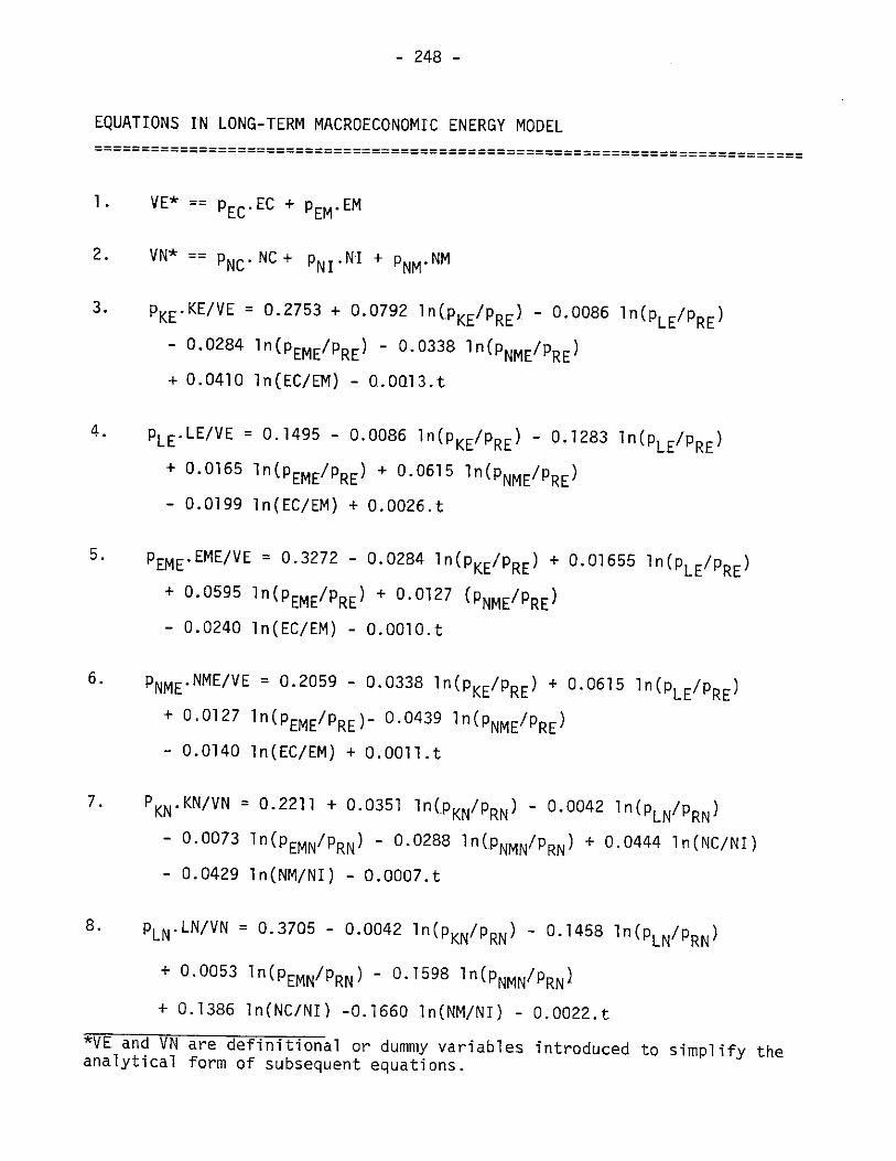
- 248 -
EQUATIONS IN LONG-TERM MACROECONOMIC ENERGY MODEL
1. VE* == PEC.EC + PEM.EM
2. VN* == PNC.NC + pNI.NI + pNM.NM
3. PKE.KE/VE = 0.2753 + 0.0792 in (PKE/PRE) - 0.0086 ln(PLE/PRE)
- 0.0284 ln(PEME/PRE) - 0.0338 ln(pNME/PRE)
+ 0.0410 ln(EC/EM) - Q.0013.t
4. PLE.LE/VE = 0.1495 - 0.0086 In(PKE/PRE) - 0.1283 In(pLE RE+ 0.0165 ln(PEME/PRE) + 0.0615 ln(PNME/PRE)
- 0.0199 ln(EC/EM) + 0.0026.t
5. PEME.EME/VE = 0.3272 - 0.0284 In(PKE/PRE) + 0.01655 ln(pLE/PRE)
+ 0.0595 ln(pEME/PRE) + 0.0127 (pNME1PRE)- 0.0240 ln(EC/EM) - 0.0010.t
6. PNME.NME/VE = 0.2059 - 0.0338 In(PKE/PRE) + 0.0615 ln(PLE/PRE)
+ 0.0127 In(PEME/PRE)- 0.0439 ln(PNME/PRE)
- 0.0140 In(EC/EM) + 0.00ll.t
7. PKN.KN/VN = 0.2211 + 0.0351 ln(pKN/PRN) - 0.0042 In(pLN/PRN
- 0.0073 In(PEMN/PRN) - 0.0288 ln(PNMN/PRN) + 0.0444 ln(NC/NI)
- 0.0429 ln(NM/NI) - 0.0007.t
8. PLN.LN/VN = 0.3705 - 0.0042 ln(PKN/PRN) - 0.1458 In(pLN/PRN)
+ 0.0053 In(PEMN/PRN) - 0.1598 ln(PNMN/PRN)
+ 0.1386 ln(NC/NI) -0.1660 ln(NM/NI) - 0.0022.t
*VE and VN are definitional or dummy variables introduced to simplify theanalytical form of subsequent equations.

- 249 -
EQUATIONS IN LONG-TERM MACROECONOMIC ENERGY MODEL (continued)
9. PEMN.EMN/VN = 0.0182 - 0.0073 ln(PKN/PRN) + 0.0054 ln(PLN/PRN)+ 0.0032 ln(pEMN/PRN) - 0.0023 In (PNMN/PRN)
+ 0.0088 ln(NC/NI) - 0.0017 ln(NM/NI) - 0.0001.t
10. PNMN.NMN/VN = 0.3631 - 0.0288 In(P /PRN) - 0.1599 ln(PLN/PRN)- 0.0023 ln(PEMN/PRN) + 0.2246 ln(PNMN/PRN)
- 0.2233 ln(NC/NI) + 0.2425 In(NM/NI) + 0.0030.t
I1- PEC.EC + pEM.EM = PKE.KE + PLE.LE + PEME.EME + pNME.NME + PRE.RE
12. pNC.NC + PNM.NM + PNI.NI = PKN.KN = PLN.LN + PEMN. EMN + PNMN.NMN + PRN.RN
13. PEC.EC/V = 0.4253 + 0.1426 ln(EC/EM) + 0.0410 In(pKE RE- 0.0199 ln(PLE/PRE) - 0.0240 ln(PEME/PRE)
- 0.0140 In (PNME/PRE) - 0.005.t
14. PNC.NC/VN = 0.3516 + 0.3415 ln(NC/NI) - 0.2236 ln(NM/NI)
+ 0.0444 1n(PKN/PRN) + 0.1386 1n(PLN/PRN)+ 0.0088 1n (PEMN/PRN) - 0.2233 ln(pNMN/PRN) - 0.0019.t
15. PNM.NM/VN = 0.3667 - 0.2236 ln(NC/NI) + 0.2574 ln(NM!NI)
- 0.0429 ln(PKN/PRN) - 0.1660 ln(PLN/PRN)
- 0.0018 In(PEMN/PRN) + 0.2425 ln(pNMN/PRN) + 0.0034.t
16. NI + STE + STN = I + GI + EXI
17. NI = exp[ .1 [ln(VN(-1)) - 0.3516 ln(NC(-1))0.2817

- 250 -
EQUATIONS IN LONG-TERM MACROECONOMIC ENERGY MODEL (continued)
- 0.3516 n(NC(-1)) - 0.3667 lnCNM (-1))
- 0.2211 ln(PKN(-l)) - 0.3705 lnCPLN(l))
- 0.0182 In(PEMN (-1
- 0.3631 n(pNMN (-1))]]
18. NC + CIM = CN + STN + GN + EXN
19. NM = NME + NMN
20. EC = CE + STE + GE + EXE
21. EM = EME + EMN
22. (1 + TCE).p' EC.EC =pCE.CE
+ pSTE.STE + PGE.GE + PEXE.EXE
23. (1 + TCN) .PNC.NC = P CND.CND + PSTN. STN
+ PGN.GN + PEN.EXN
24. (1 + TI).PNI.NI =
+ Pr-I + PI.GI
PIMI.IMI + PSTE.STE + PSTN.STN
+ PEXI.EXI
25. PEM. EM = PEME.EME + p EMN.EMN
26. PNM.NM = PNME.NME + PNMN.NMN
27. pEMN = ZNE. pEM
28. pNME = ZEN. PNM

- 251
EQUATIONS IN LONG-TERM MACROECONOMIC ENERGY MODEL (continued)
29. L = LE + LN + LG + LR + LR
30. PL.L = (1-TL) (PLE.LE + PLN.LN + pLG.LG + PLR.LR)
31. PE (1/KE).1-TKE/PVDE-ITCE31. pKE = (l/QKE) . ITKE
[ME.p1(-1) + DE.p1 - CAG] + TPE.p1
1-TKN-PVDN-ITCN32. PKN = (1/QKN).[ - 1TKN N [MN.p (-W ) + DN. - CAG +TPNp
33. KE = QKE.KSE(-1)
34. KN = QKN.KSN(-1)
35. INE = ZINE.I
36. INN = ZINN.I
37. ICD = ZICD.I
38. IRS = ZIRS.I
39. KSE = (1-DE).KSE(-1) + INE
40. KSN = (1-DN).KSN(-1) + INN
41. KCD = (1-DCD).KCD(-1) + ICD
42. KRS = (1-DRS).KRS(-1) + IRS
43. IMI + I1= INE + INN + ICD + IRS

- 252 -
EQUATIONS IN LONG-TERM MACROECONOMIC ENERGY MODEL (continued)
44. W = p 1(KSE + KSN + KRS + KCD).ZW + PG. G + pR. R
45. pF.F/P = [-0.0742 + 0.0254.t] .
[(1 +MW).HW(-1) + 12. 7 4 5 8 ( PL.HLH + EL)] / (-l + 0.343.t)
46. HLH = L/P
47. HW = W/P
48. HEL = EL/P
49. KC = QKS.KRS(-1) + QKD.KCD(-l)
50. PL.LJ/PF.F = -(-0.4102 - 0.1991.ln(HLJ) + 0.1389. ln(HCN)
+ 0.0417 ln(HCK) -0.0216 ln(HCE) -0.0024.t)
51. PCN.CN/PF.F = -(-0.3221 + 0.1389.ln(HLJ) - 0.1188. ln(HCN)
- 0.0257.ln(HCK) + 0.0508 1n(HCE) + 0.0008.t)
52. p CK.HCK/PF .F = -(-0.2113 + 0.0418 in(HLJ) - 0.0257. ln(HCN)
- 0.0113 ln(HCK) - 0.0303 ln(HCE) + 0.0017.t)
53. LJ = HLJ.P
54. CK = HCK.P
55. CE = HCE.P
56. CN = HCN.P
57. CND = CN-CIM

- 253 -
VARIABLES IN LONG-TERM MACROECONOMIC ENERGY MODEL (continued)
58. MW.(KSE(-1) + KSN(-1) + KCD(-1) + KRS(-1)
= ZRN. (ME. KSE(-1) + MN. KSN(-1))
59. F = 0.8225 LJ = 1.0787 CK + 0.9349 CN + 2.4957 CE + 0.8559
60. S = pI.I + PG(G-G(-l)) + PR(R-R(-.l))
61. PF = 1/F (PL LJ + PCN. CN + PCE. CE + pCK.CK)

- 254 -
VARIABLES IN LONG-TERM MACROECONOMIC ENERGY MODEL
-Quantities
*NMN - Non-energy intermediate products purchased by the non-energy
sector
*EMN - Energy intermediate products purchased by the non-energy
sector
*NME - Non-energy intermediate products purchased by the energy
sector
*EME - Energy intermediate products purchased by the energy sector
*RN - Competitive imports of energy products
*RE - Competitive imports of non-energy products
*CE - Energy consumption goods purchased by households
*CN - Non-energy consumption goods purchased by households
*KC - Capital services supplied to households by stock of consumer
durables and residential structures
*KE - Capital services supplied to the energy sector by its capital
stock
*KN - Capital services supplied to the non-energy sector by its
capital stock
*KSE - Capital stock of producer durables, non-residential structures,
inventories and land, energy sector
*KSN - Capital stock of producer durables, non-residential structures,
non-energy sector, inventories and land, non-energy sector
*LE - Labor services purchased by the energy sector
*LN - Labor services purchased by the non-energy sector
*EC - Energy consumption products supplied by the domestic energy
sector
*Asterisk denotes endogenous variable

- 255 -
VARIABLES IN LONG-TERM MACROECONOMIC ENERGY MODEL (continued)
*EM - Energy intermediate products supplied by the domestic energysector
*NC - Non-energy consumption products supplied by the domestic energysector
*NM - Non-energy intermediate products supplied by the domestic non-energy sector
*NI - Investment goods supplied by the domestic non-energy sector
*I - Gross private domestic investment
*INE - Gross investment in the energy sector
*INN - Gross investment in the non-energy sector
*IRS - Gross investment in residential structures
*ICD - Gross investment in consumer durables
*KRS - Capital stock, residential structures
*KCD - Capital stock, consumer durables
CIM - Direct imports of consumption goods by the private domesticsector
*CND - Total purchases of domestic non-energy consumption goods by theprivate domestic sector
STN - Non-energy consumption products delivered to business inventories
STE - Energy consumption products delivered to business inventories
GN - Government purchases of domestic non-energy consumption products
*IMIN - Direct imports of investment goods by the private domestic sector
GI - Government purchases of domestic investment goods
GE - Government purchases of energy consumption products
EXN - Gross exports of non-energy consumption products
EXI - Gross exports of investment goods
EXE - Gross exports of energy consumption products

- 256 -
VARIABLES IN LONG-TERM MACROECONOMIC ENERGY MODEL (continued)
R - Net claims on rest of world by the private domestic sector
G - Net claims on government by the private domestic sector
LH - Total availability of time resources to the household sector
EL - Transfer payments to the household sector
LU - Rate of unemployment
*L - Supply of labor services by the household sector
*LJ - Leisure time of the household sector
P - Total population
*HEL - Transfer payments, per capita
*HCE - Consumption expenditures by households on energy products, percapita
*HCN - Consumption expenditures by households on domestic non-energyproducts, per capita
*HCK - Consumption expenditures by households on capital services, percapita
*HLJ - Leisure available to households, per capita
LR - Labor services purchased by the foreign sector
LG - Labor services purchased by the government sector
*HLH - Total availability of time resources to households, per capita
*F - Full consumption, household sector
-Prices
PNMN - Implicit deflator, non-energy intermediate products purchasedby the non-energy sector
*PEMN - Implicit deflator, energy intermediate products purchased by
the non-energy sector
pNME - Implicit deflator, non-energy intermediate products purchasedby the energy sector

- 257 -
VARIABLES IN LONG-TERM MACROECONOMIC ENERGY MODEL (continued)
*pEME
PRE
pRN
*pCE
*pCN
*pCK
*PKE
*p KN
*p LN
*PEC
*PEM
*p NM
*pNI
*pI
*PCN D
- Implicit deflator, energy intermediate products purchased bythe energy sector
- Implicit deflator, competitive imports of energy products
- Implicit deflator, competitive imports of non-energy products
- Implicit deflator, energy consumption goods purchased byhouseholds
- Implicit deflator, non-energy consumption goods purchased byhouseholds
- Implicit deflator, capital services supplied to households byconsumer durables and residential structures
- Implicit deflator, capital services, energy sector
- Implicit deflator, capital services, non-energy sector
- Implicit deflator, labor services purchased by the energy sector
- Implicit deflator, labor services purchased by the non-energysector
- Implicit deflator, energy consumption products supplied by thedomestic energy sector
- Implicit deflator, energy intermediate products supplied bythe domestic energy sector
- Implicit deflator, non-energy consumption products suppliedby the domestic energy sector
Implicit deflator, non-energy intermediate products suppliedby the domestic non-energy sector
- Implicit deflator, investment goods supplied by the domesticnon-energy sector
- Implicit deflator, gross private domestic investment
- Implicit deflator, total purchases of domestic non-energyconsumption goods by the private domestic sector
- Implicit deflator non-energy consumption products delivered tobusiness inventories
PSTN

- 258 -
VARIABLES IN LONG-TERM MACROECONOMIC ENERGY MODEL (continued)
PSTE - Implicit deflator, energy consumption products delivered tobusiness inventories
PGN - Implicit deflator, government purchases of domestic non-energyconsumption products
PGI - Implicit deflator, government purchases of domestic investmentgoods
PGE - Implicit deflator, government purchases of energy consumptionproducts
P - Implicit deflator, net claims on government by the privatedomestic sector
P - Implicit deflator on rest of world by the private domesticsector
PEXN - Implicit deflator, gross exports of non-energy consumptionproducts
PEXI - Implicit deflator, gross exports of investment goods
pEXE - Implicit deflator, gross exports of energy consumption products
*P - Implicit deflator, supply of labor services
pLG - Implicit deflator, labor services purchased by the governmentsector
PLR - Implicit deflator, labor services purchased by the foreign sectc
P - Implicit deflator, full consumption by the household sectorr
-Financia
DN -
DE -
DRS -
DCD -
*MN -
*ME -
I Variables
Rate of replacement, capital stock, non-energy sector
Rate of replacement, capital stock, energy sector
Rate of replacement, capital stock, residential structures
Rate of replacement, capital stock, consumer durables
Nominal rate of return, fixed tangible assets, non-energy sector
Nominal rate of return, fixed tangible assets, energy sector
or

- 259 -
VARIABLES IN LONG-TERM MACROECONOMIC ENERGY MODEL (continued)
*MW - Nominal rate of return on wealth, household sector
*W - Private national wealth
*S - Gross private national saving
ITCE - Effective investment tax credit, energy sector
ITCN - Effective investment tax credit, non-energy sector
*HW - Private national wealth, per capita
PVDE - Present value of depreciation deductions for tax purposes perdollar of investment, non-energy sector
PVDN - Present value of depreciation deductions for tax purposes perdollar of investment, non-energy sector
CAG - Effective rate of capital gain per dollar of fixed assets held
-Tax Variables
TCE - Effective tax rate, energy consumption goods
TCN - Effective tax rate, non-energy consumption goods
TI - Effective tax rate, investment goods
TKE - Effective tax rate on capital income, energy sector
TKN - Effective tax rate on capital income, non-energy sector
TL - Effective tax rate, labor services
TPE - Effective tax rate on capital property, energy sector
TPN - Effective tax rate on capital property, non-energy sector
-Aggregation and Scaling Variables
ZNE - Price of intermediate energy products to price of intermediateenergy products purchased by the non-energy sector
ZEN - Price of intermediate non-energy products to price of interme-diate non-energy products purchased by the energy sector
ZW - Capital stock to wealth

- 260 -
VARIABLES IN LONG-TERM MACROECONOMIC ENERGY MODEL (continued)
QKN - Quality of capital, non-energy sector
QKE - Quality of capital, energy sector
QCK - Quality of capital, household sector gross
ZINE - Gross private domestic investment to gross investment in theenergy sector
ZINN - Gross private domestic investment to gross investment in thenon-energy sector
ZIRS - Gross private domestic investment to gross investment in res.structures
ZICD - Gross private domestic investment to gross investment in con-sumer durables
ZRN - Nominal rate of return, energy and non-energy sectors, tonominal rate of return on wealth
AL - Index of total cost diminution, non-energy sector, lagged oneperiod

- 261 -
4.3 Historical Simulation: 1948-1971
A fully dynamic simulation of the complete model was performed for
the period 1948-1971 with all exogenous variables set at their historical
values. The simulated time paths of key endogenous variables together
with the corresponding historical values are plotted in Figs. 4-1
through 4-46; error statistics including actual and percentage mean and
R.M.S. deviations are also tabulated for each variable.
This simulation provides a crucial test of the realism and validity
of the model. On the basis of the results exhibited in the following
pages, the ability of the model to capture the chief causal mechanisms
of aggregate economic performance must be judged highly satisfactory.
The simulated values of both price and quantity variables closely track
the corresponding historical time-paths. This result could not have been
predicted solely on the basis of goodness-of-fit of individual behavioral
equations since the simulation of the model entails the repeated
solution of a set of 61 simultaneous nonlinear equations with a high
degree of interdependence among contemporaneous variables.
The year 1952 and, to a smaller extent, 1953, shows above average
deviations of simulated vs. historical values for a few endogenous
variables -- e.g. EC, NM, NC, EM, PKN' PKE. The higher than usual errors
in these years can be largely explained by the fact that governmental
intervention during the Korean War created regulatory constraints that
signified a departure from a market economy upon which our model is
predicated. In addition, the expansionary pressures of the Korean War,
and the subsequent recession caused sharp fluctuations in the levels of

* HISTORICAL44*
1953 1958 1963
* in billions of 1958 dollars
HISTORICALMEAN 225.738 ERROR
STATISTICS ~
EC - ENERGY CONSUMPTION PRODUCTS SUPPLIED BY U.S. ENERGY SECTOR,HISTORICAL VS SIMULATED, 1948-1971
SHISTORICAL
o SIMULATED
-F
32
20
1948 1968
N)0Y)N)
1973
MEANRMS
ACTUAL
0.32380.9175
FIG. 4-1:
1.15354.6641

* HISTORICAL80*
1953
*in billions of 1958 dollars
HISTORICALMEAN
FIG.. 4-2:
38.889 ERRORSTATISTICS
MEANRMS
ACTUAL
0.63031.4066
1.48313.6174
EM. - ENERGY INTERMEDIATE PRODUCTS SUPPLIED BY U.S. ENERGY SECTOR,HISTORICAL VS SIMULATED, 1948-1971
SHISTORICAL
o SIMULATED
I-
60.
40.
20
1948 1958 1963 1968 1973

1953
HISTORICALMEAN
1958
0.9036 ERRORSTATISTICS
PEC - PRICE INDEX, ENERGY CONSUMPTION PRODUCTS SUPPLIED BYU.S. ENERGY SECTOR, HISTORICAL VS SIMULATED, 1948-1971
1.000
0.920
0.840
C
1948
* HISTORICAL
o SIMULATED
| I1963 1968
N)a)
1973
0.27322.8613
MEANRMS
ACTUAL
0.00250.0261
FIG. 4-3:
'
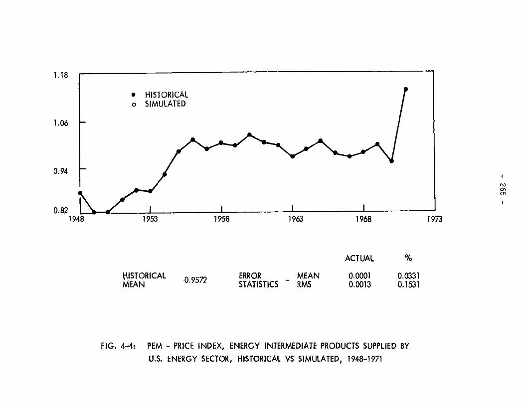
* HISTORICAL
o HISTORICALo SIMULATED
1953
lo
1973
%I
t,'ISTORICALMEAN
FIG. 4-4:
.0.9572 ERRORSTATISTICS
MEANRMS
0.00010.0013
0.03310.1531
PEM - PRICE INDEX, ENERGY INTERMEDIATE PRODUCTS SUPPLIED BY
U.S. ENERGY SECTOR, HISTORICAL VS SIMULATED, 1948-1971
1.18
1.06 -
0.94 F
0.821948 1958 1963 1968
ACTUAL
L-----A

1953 1958 1963 1968
*in billions of 1958 dollars
ACTUAL
HISTORICALMEAN
FIG. 4-5:
19-5095 ERROR MEANSTATISTICS RMS
M528950.7937
1.44684.8616
EMN - ENERGY INTERMEDIATE PRODUCTS PURCHASED BY U.S. NON-ENERGYSECTOR, HISTORICAL VS SIMULATED, 1948-1971
4.0*
e HISTORICALo SIMULATED
24.
8194
I~
N)1
197348

340*
* HISTORICALo SIMULATED
26.0
18.0
10.0
1948 1953 1958 1963 1968 1973
*fin billions of 1958 dollars
ACTUAL %
HISTORICAL 19.3799 ERROR MEAN 0.3487 1.5869MEAN STATISTICS RMS 0.7558 3.5352
FIG. 4-6 EME - ENERGY INTERMEDIATE PRODUCTS PURCHASED BY U.S. ENERGYSECTOR, HISTORICAL VS SIMULATED, 1948-1971

1953 1958 1963 1968
*in billions of 1958 dollars
ACTUAL
HISTORICALMEAN 2002.08 ERROR
STATISTICS
FIG. 4-7: RE - COMPETITIVE IMPORTS OF ENERGY PRODUCTS, HISTORICAL VSSIMULATED, 1948-1971
5000.0*.
3500.
2000.
500.
1948
* HISTORICAL
o SIMULATED
-I
N)CYiOD
1973
MEANRMS
43.47256.71
2.0919.075

1953
* HISTORICALo SIMULATED
1973
*in billions of 1958 dollars
HISTORICALMEAN 8206.28 ERROR
STATISTICS
LE - LABOR SERVICES PURCHASED BYHISTORICAL VS SIMULATED,
U.S. ENERGY SECTOR,1948-1971
9500. *
8500.
7500.
6500.
1948
I3a'j1.0
1958 1963 1968
MEANRMS
ACTUAL
101.242245.445
FIG. 4-8:
1.25453.1309
-1

20.0*
* HISTORICAL
* SIMULATED
15.0
10.0
5.0
1948 1953 1958 1963 1968 1973*in billions of 1958 dollars
ACTUAL %
HISTORICAL 12.7737 ERROR MEAN 0.0543 0.3078MEAN STATISTICS RMS 0.1497 0.9943
FIG. 4-9: KE - CAPITAL SERVICES SUPPLIED TO U.S. ENERGY SECTOR,HISTORICAL VS SIMULATED

1.38
1953
* HISTORICALo SIMULATED
1973
HISTORICALMEAN 1.1381 ERROR
STATISTICS
FIG. 4-10: PKE - PRICE OF CAPITAL SERVICES,HISTORICAL VS SIMULATED,
U.S. ENERGY SECTOR,1948-1971
Na
1.22
1.06
0.901948 1958 1963 1968
MEANRMS
ACTUAL
0.01520.0384
1.48373.6813
%

36.*
* HISTORICAL
26. o SIMULATED
16. -
6.1948 1953 1958 1963 1968 1973
*in billions of 1958 dollars
ACTUAL %
HISTORICAL 19.659 ERROR MEAN 0.3239 1.3248MEAN STATISTICS RMS 0.9175 5.4570
FIG. 4-11: CE - ENERGY CONSUMPTION PRODUCTS PURCHASED BY U.S. HOUSEHOLDS,HISTORICAL VS SIMULATED, 1948-1971
I)
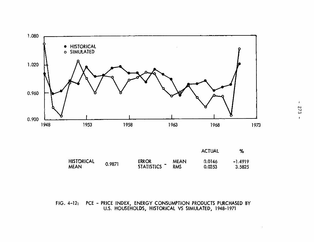
1953
HISTORICALMEAN
FIG. 4-12:
1958
.0.9871
1963
ERRORSTATISTICS
1968
MEANRMS
ACTUAL
0.01460.0353
1973
-1.49193.5825
PCE - PRICE INDEX, ENERGY CONSUMPTION PRODUCTS PURCHASED BYU.S. HOUSEHOLDS, HISTORICAL VS SIMULATED, 1948-1971
1.080
* HISTORICALo SIMULATED
1.020
0.960
0.9001948
I

0.230
0.150
0.070
0.0101963
* HISTORICALo SIMULATED
1973
HISTORICALMEAN 0. 0758 ERROR
STATISTICS
FIG. 4-13: ME - NOMINAL RATE OF RETURN,HISTORICAL VS SIMULATED,
U.S. ENERGY SECTOR,1948-1971
N)
4~.
1953 1958 1968
MEANRMS
ACTUAL
0.000040.0114
-1.457232.0939
1948

17.0*
* HISTORICAL
o*SIMULATED
12.0 ~
7.0
1948 1953 1958 1963 1968 1973
*in billions of 1958 dollars
ACTUAL %
HISTORICAL 9.4665 ERROR MEAN 0.0857 1.1492MEAN STATISTICS RMS 0.4641 5.0240
FIG. 4-14: INE - GROSS INVESTMENT, U.S. ENERGY SECTOR, HISTORICAL VSSIMULATED, 1948-1971
I)

150.*
* HISTORICALo SIMULATED
100.
50.1948 1953 1958 1963 1968 1973
*in billions of 1958 dollars
ACTUAL %
HISTORICAL 98.5034 ERROR MEAN 0.4633 0.3522MEAN STATISTICS RMS 1.1489 1.0177
FIG. 4-15: KSE - CAPITAL STOCK, U.S. ENERGY SECTOR, HISTORICAL VSSIMULATED, 1948-1971

475*
* HISTORICAL
o SIMULATED
375.
275.
175.
1948 1953 1958 1963 1968 1973
*in billions of 1958 dollars
ACTUAL %HISTORICAL 301.768 ERRCR MEAN 4.644 1.433MEAN STATISTICS - RMS 14.816 5.555
FIGI 4-16: NC - NON-ENERGY CONSUMPTION PRODUCTS SUPPLIED BY U.S.NON-ENERGY SECTOR, HISTORICAL VS SIMULATED,
1948-1973

550.
400.
250.
19
700. *
1973
HISTORICALMEAN
FIG. 4-17:
417.321ERRORSTATISTICS
MEANRMS
ACTUAL
9.356618.7478
2.27064.9894
NM - NON-ENERGY INTERMEDIATE PRODUCTS SUPPLIED BY U.S.NON-ENERGY SECTOR, HISTORICAL VS SIMULATED, 1948-1971
* HISTORICALo SIMULATED
1953
*in billions of 1958 dollars
N)
-a
48 1958 1963 1968
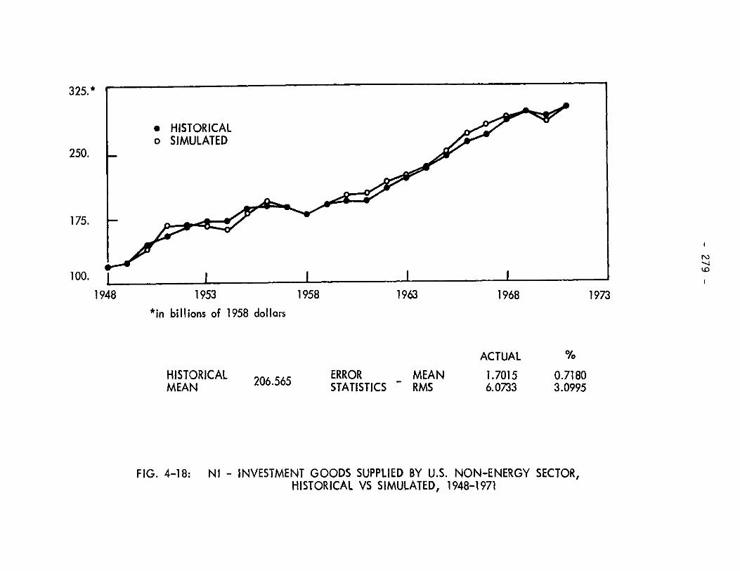
325.*
e HISTORICALo SIMULATED
250.
175.
100.
1948 1953 1958 1963 1968 1973*in billions of 1958 dollars
ACTUAL %
HISTORICAL 206.565 ERROR MEAN 1.7015 0.7180MEAN STATISTICS RMS 6.0733 3.0995
FIG. 4-18: NI - INVESTMENT GOODS SUPPLIED BY U.S. NON-ENERGY SECTOR,HISTORICAL VS SIMULATED, 1948-1971
I)

1.60
1953
* HISTORICALo SIMULATED
1973
HISTORICALMEAN
FIG. 4-19:
1.0040 ERRORSTATISTICS
MEANRMS
ACTUAL
0.00310.0277
0.34042.7446
PNC - PRICE INDEX, NON-ENERGY CONSUMPTION GOODS SUPPLIED BYU.S. NON-ENERGY SECTOR, HISTORICAL VS SIMULATED, 1948-1971
N)000
1.30
1.00
0.701948 1958 1963 1968

1.20
1948 1953
* HISTORICALo SIMULATED
I-I
1973
HISTORICALMEAN 0.9382 ERROR MEAN
STATISTICS RMS
FIGI 4-20: PNI - PRICE INDEX, INVESTMENT GOODS SUPPLIED BYSECTOR, HISTORICAL VS SIMULATED,
U.S. NON-ENERGY,1948-1971
00
1.04
0.88
0.72
1958 1963 1968
ACTUAL0.00540.0356
0.64283.7314

650. *
6 HISTORICALo SIMULATED
500.
350.
200.
1948 1953 1958 1963 1968 1973
*in billions of 1958 dollars
ACTUAL %HISTORICAL 405.590 ERROR MEAN 0.2142 2.3008MEAN STATISTICS - RMS 18.5498 5.0617
FIG. 4-21: NMN - NON-ENERGY INTERMEDIATE PRODUCTS PURCHASED BY U.S.NON-ENERGY SECTOR, HISTORICAL VS SIMULATED, 1948-1971
I2
N)

20.0*
* HISTORICALo SIMULATED
15.0
10.1
5.01948 1953 1956 1963 1968 1973
*in billions of 1958 dollars
ACTUAL %
HISTORICAL 11-73o5 ERROR MEAN 0.1424 1.4897MEAN STATISTICS RMS 0.5074 5.4669
FIG. 4-22: NME - NON-ENERGY INTERMEDIATE PRODUCTS PURCHASED BY U.S.ENERGY SECTOR, HISTORICAL VS SIMULATED, 1948-1971
N)IA

38.*
* HISTORICALo SIMULATED
28.
18. -
8.
1948 1953 1958 1963 1968 1973*in billions of 1958 dollars
ACTUAL %
HISTORICAL 17.3216 ERROR MEAN -0.2256 -1.3572MEAN STATISTICS RMS 1.6361 11.1383
FIG. 4-23: RN - COMPETITIVE IMPORTS OF NON-ENERGY PRODUCTS,HISTORICAL VS SIMULATED, 1948-1971

350.*
* HISTORICALo SIMULATED
300.
250.
200.
1948 1953 1958 1963 1968 1973
*in billions of 1958 dollars
ACTUAL %HISTORICAL ERROR MEAN 3.773 1.3299MEAN 263.537 STATISTICS RMS 9.914 3.8430
FIG. 4-24: LN - LABOR SERVICES PURCHASED BY U.S. NON-ENERGY SECTOR,HISTORICAL VS SIMULATED, 1948-1971
00Ln

'1953
*in billions of 1958 dollars
HfSTORICALMEAN
FIG. 4-25:
173.398 ERRORSTATISTICS
MEANRMS
ACTUAL
0.97781.9896
0.41140.8860
KN - CAPITAL SERVICES APPLIED TO U.S. NON-ENERGY SECTOR;HISTORICAL VS SIMULATED, 1948-1971
280.*
220.
160.
100.
1948
* HISTORICALo SIMULATED
-I
1958 .1963 1968 1973

1.42
1953 1958 1963
HISTORICALMEAN
FIG. 4-26:
1.1033 ERRORSTATISTICS
MEANRMS
ACTUAL0.02180.0780
2.00497.4127
PKN - PRICE OF CAPITAL SERVICES, U.S. NON-ENERGY SECTOR,HISTORICAL VS SIMULATED, 1948-1971
* HISTORICALo SIMULATED
I-
1.22
1.02
0.82
1948 1968 1973
Alb. =OEM
I

1953
HISTORICALMEAN
1958
0. 1753
1963
ERRORSTATISTICS
1968
MEANRMS
ACTUAL
0.00200.0133
MN - NOMINAL RATE OF RETURN, U.S. NON-ENERGY SECTOR,HISTORICAL VS SIMULATED, 1948-1971
0.35
0.25
0.15
0.05
1948
* HISTORICAL
o SIMULATED
-
N)0000
1973
1.73749.5464
FIG2 4-27:

___ __ ___ __ ___ __ ___ _In p
1953 1958 1963 1968
*in billions of 1958 dollars
HISTORICALMEAN
FIG. 4-28:
46.5922 ERRORSTATISTiCS
MEANRMS
ACTUAL0.64862.2769
1.14935.0240
INN - GROSS INVESTMENT, U.S. NON-ENERGY SECTOR,HISTORICAL VS SIMULATED, 1948-1971
70. *
* HISTORICAL
o SIMULATED
50.
30.
1948
N)OD
1973
4

1953
*in billions of 1958 dollars
HISTORICALMEAN
FIG. 4-29:
681.739 ERRORSTATISTICS
MEANRMS
ACTUAL
3.98457.5707
KSN - CAPITAL STOCK, U.S. NON-ENERGY SECTOR,HISTORICAL VS SIMULATED, 1948-1971
960.*
0 HISTORICAL
_ o SIMULATED800.
640.
480.
1948 1958 1963 1968 1973
0.46600.9255
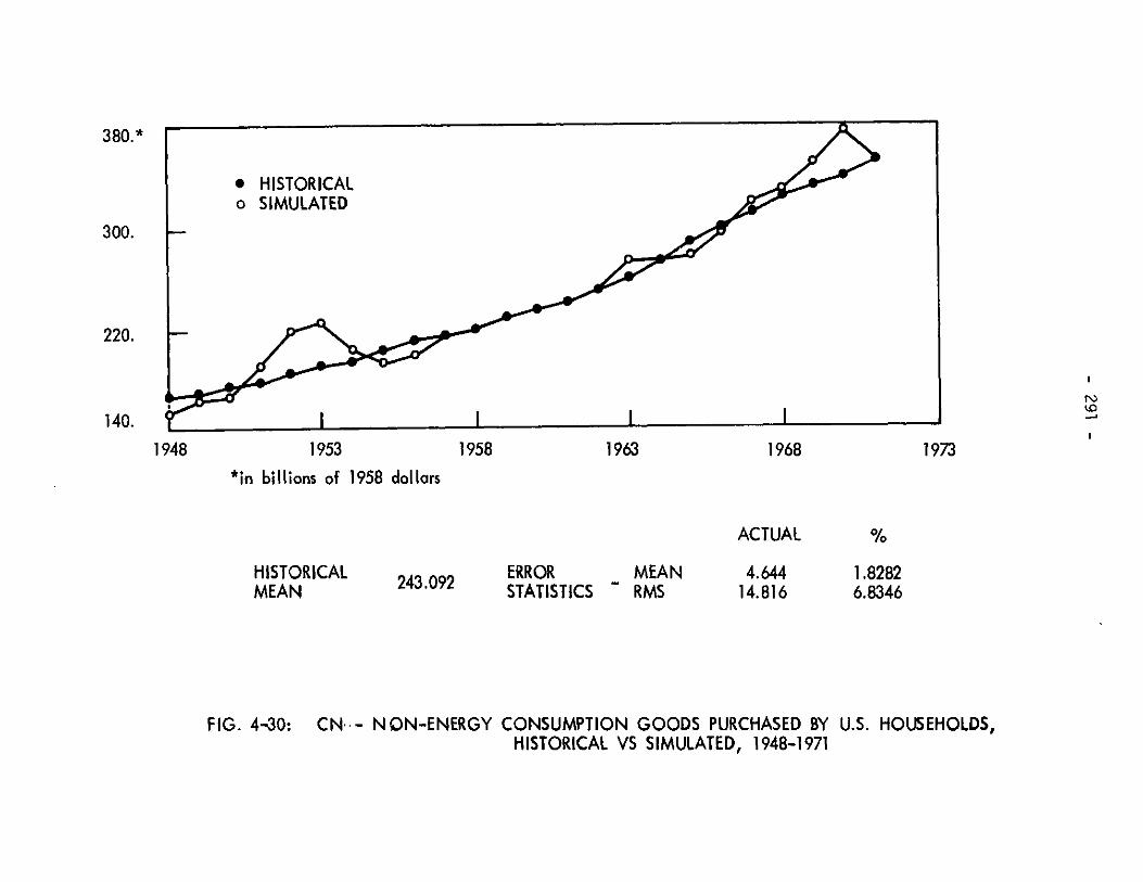
380.*
* HISTORICALo SIMULATED
300.
220.
140.
1948 1953 1958 1963 1968 1973
*in billions of 1958 dollars
ACTUAL %
HISTORICAL 243.092 ERROR MEAN 4.644 1.8282MEAN STATISTICS RMS 14.816 6.8346
FIG. 4-30: CN- - NON-ENERGY CONSUMPTION GOODS PURCHASED BY U.S. HOUSEHOLDS,HISTORICAL VS SIMULATED, 1948-1971
N
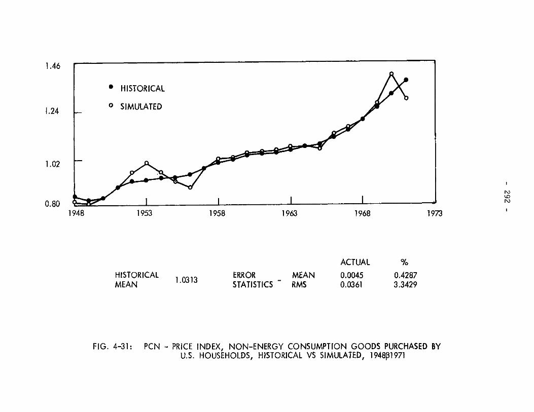
1953
HISTORICALMEAN
1958
1.0313 ERRORSTATISTICS
FIG. 4-31: PCN - PRICEU.S.
INDEX, NON-ENERGY CONSUMPTION GOODS PURCHASED BYHOUSEHOLDS, HISTORICAL VS SIMULATED, 1948P1971
1.46
1.24
1.02
0.80
* HISTORICAL
o SIMULATED
I~~
1948 1963 1968
N)
N)
1973
0.42873.3429
MEANRMS
ACTUAL
0.00450.0361
--- M

1953
*in billions of 1958 dollars
3600. *
1973
HISTORICALMEAN
FIG. 4-32:
1031.12 ERROR MEANSTATISTICS RMS
ACTUAL
18.536553.2711
1.13665.0309
IMIN - DIRECT IMPORTS OF INVESTMENT GOODS, HISTORICAL VS SIMULATED,1948-1971
HISTORICAL
o SIMULATED
Af-lb
I0
N)
2400.
1200.
0.1948 1958 1963 1968

1953
HISTORICALMEAN
1958
0.9755 ERRORSTATISTICS
FIG. 4-33: PL - PRICE INDEX, SUPPLY OF LABOR SERVICES,1948-1971
HISTORICAL VS SIMULATED,
1.70
1.30
0.90
0.50
* HISTORICAL
o SIMULATED
1948 1963 1968 1973
MEANRMS
ACTUAL
0.000060.0004
0.00380.0438

475.*
* HISTORICAL
o SIMULATED400.
325.
250.
1948 1953 1958 1963 1968 1973
*in billions of 1958 dollars
ACTUAL %HISTORICAL 344.752 ERROR MEAN 3.874 1.0656MEAN STATISTICS RMS 10.037 3.0956
FIG. 4-34: L - SUPPLY OF LABOR BY U.S. HOUSEHOLDS, HISTORICAL VS SIMULATED,1948-1971
N(D,

215*
* HISTORICAL
170. o SIMULATED
125.
80.1948 1953 1958 1963 1968 1973
*in billions of 1958 dollars
ACTUAL %
HISTORICAL 131.336 ERROR MEAN 1.7015 1.1493MEAN STATISTICS RMS 6.0733 5.0240
FIG. 4-35: 1 - GROSS PRIVATE DOMESTIC INVESTMENT, HISTORICAL VS SIMULATED,1948-1971
w

1.45
1953
* HISTORICAL
o SIMULATED
-O
1973
HISTORICALMEAN 0.9955 ERROR
STATISTICS
FIG. 4-36: PIN - PRICE INDEX, GROSS PRIVATEHISTORICAL VS SIMULATED,
DOMESTIC INVESTMENT,1948-1971
Ia
1.20
0.95
0.70
1948 1958 1963 1968
ACTUAL
MEAN~ RMS
0.00860.0573
0.89005.5306
-a -- -mm
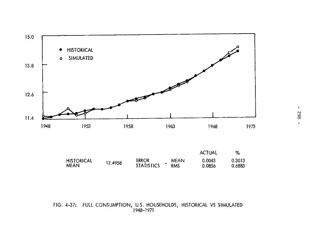
1953
HISTORICALMEAN
FIG. 4-37:
1958
12.4958
1963
ERRORSTATISTICS
1968
MEANRMS
ACTUAL
0.00430.0856
15.0
1973
0.30130.6883
FULL CONSUMPTION, U.S. HOUSEHOLDS, HISTORICAL VS SIMULATED1948-1971
* HISTORICAL
o SIMULATED
OD
13.8
12.6
11.4
1948

(1 V3AV. I%)V
0.090
0.050 . HISTORICAL
0 SIMULATED
0.010 A1948 1953 1958 1963 1968 1973
ACTUAL %
HISTORICAL ERROR MEAN 0.00002 1.6166MEAN STATISTICS RMS 0.0065 9.3070
FIG., 4-38: MW - NOMINAL RATE OF RETURN ON WEALTH, HISTORICAL VS SIMULATED1948-1971
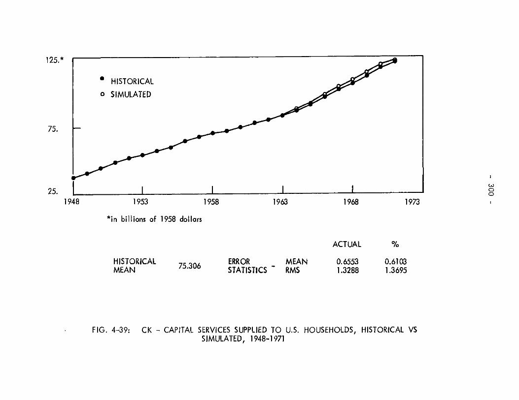
125.*
* HISTORICAL
o SIMULATED
75.
25.I I I1948 1953 1958 1963 1968 1973
*in billions of 1958 dollars
ACTUAL %
HISTORICAL 75.306 ERROR MEAN 0.6553 0.6103MEAN STATISTICS RMS 1.3288 1.3695
. FIG. 4-39: CK - CAPITAL SERVICES SUPPLIED TO U.S. HOUSEHOLDS, HISTORICAL VSSIMULATED, 1948-1971
CiJ00

1.80
1953
* HISTORICAL
o SIMULATED
1973
HISTORICALMEAN 1.0937 ERROR
STATISTICS
FIG. 4-40: PCK - PRICE OF CAPITAL SERVICES,HISTORICAL VS SIMULATED,
U.S. HOUSEHOLD SECTOR,1948-1971
(A)
C
1.40
1.00
0.601948 1958 1963 1968
ACTUALMEANRMS
0.02620.0859
2.53358.6416
Imm
%
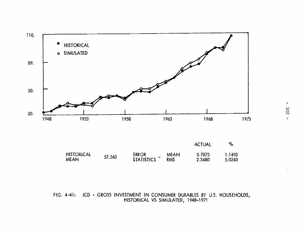
1953
HISTORICALMEAN
FIG. 4-41:
1958
52.563 ERRORSTATISTICS
1963 1968
MEANRMS
ACTUAL
0.70752.3480
110.
1973
1.14935.0240
ICD - GROSS INVESTMENT IN CONSUMER DURABLES BY U.S. HOUSEHOLDS,HISTORICAL VS SIMULATED, 1948-1971
* HISTORICAL
o SIMULATED
woCm)
89.
50.
20.1948

1953 1958 1963 1968
*in billions of 1958 dollars
ACTUAL
HISTORICALMEAN 23.7453 ERRCR
STATISTICS
FIG. 4-42: IRS - GROSS INVESTMENT IN RESIDENTIAL STRUCTURES BYHISTORICAL VS SIMULATED, 1948-1971
U.S. HOUSEHOLDS,
48. *
* [ISTORICALo SIMULATED
36.
24.
12.
1948
LA.
1973
MEANRMS
0.27821.0771
1.14925.0240
NUNN

380.*
* HISTORICALo SIMULATED
280.
180.
80.
1948 1953( 1958 1963 1968 1973*in billions of 1958 dollars
ACTUAL %HISTORICAL 207.815 ERROR MEAN 2.8636 0.9853MEAN STATISTICS RMS 5.5212 2.1736
FIG. 4-43; KCD - CAPITAL STOCK OF CONSUMER DURABLES, U.S. HOUSEHOLD SECTOR,HISTORICAL VS SIMULATED, 1948-1971
CtJ
0

1953
*in billions of 1958 dollars
460.*
1973
HISTORICALMEAN 320.711 ERROR
STATISTICS
FIG. 4-44: KRS - CAPITAL STOCK OF RESIDENTIAL STRUCTURES,HISTORICAL VS SIMULATED,
U.S. HOUSEHOLD SECT-OR,1948-1971
* HISTORICAL
o SIMULATED
-
320.
180. CC0
1948 1958 1963 1968
MEANRMS
ACTUAL
1.69373.3950
0.41270.8936

350.* -
* HISTORICAL
o SIMULATED250.
150.
50.1948 1953 1958 1963 1968 1973
*in billions of current dollars
ACTUAL %
HISTORICAL 142.943 ERROR MEAN 3.6169 2.0994MEAN STATISTICS RMS 9.5346 4.8479
FIG. 4-45: S - GROSS PRIVATE DOMESTIC SAVING, HISTORICAL VS SIMULATED,1948-1971
I'
w

4.4*
* HISTORICAL
o SIMULATED3.2
2.0
0.81948 1953 1956 1963 1968 1973
*in trillions of 1958 dollars
ACTUAL %
HISTORICAL 1.8466 ERROR MEAN 0.0294 1.1633MEAN STATISTICS RMS 0.1158 4.6000
W - PRIVATE DOMESTIC WEALTH, HISTORICAL VS SIMULATED, 1948-1971
(p.)
0
FIG.' 4-46:

- 308 -
capacity utilization which are not adequately reflected in the configura-
tion of the long-run equilibrium. It is reasonable to expect that
explicit incorporation of a disequilibrium representation of short-
term adjustment processes would result in a more accurate explanation of
the behavior of price and output levels during these two years.
The sectoral rates of return and the nominal rate of return on
wealth show somewhat high R.M.S. errors but3 on the.whole, track the his-
torical paths satisfactorily through the various peaks and troughs. The
quantity of competitive energy imports is significantly over-predicted
especially in the period 1960-1971. This can be attributed to the
implementation of the oil import quota that maintained historical energy
import levels below the values that would have prevailed in the absence
of such protectionary measures.
An examination of the simulation results shows that the model has
succeeded in closely replicating the actual time-paths of the endogenous
variable over an extended historical period spanning a fairly broad
range of conditions of the overall economy. We conclude that our beha-
vioral assumptions, our empirical specification and the final form of
the model constitute a satisfactory basis for analyzing long-term inter-
actions between energy and economic growth.
4.4 Tax Policy in a Model of General Equilibrium
Our aim in this and the following section is to investigate the
dynamic response of the model to changes in selected policy variables.
The simulation experiments described were designed with the intent of
exploring the capabilities of the model as a tool for policy analysis
by highlighting the degree and nature of interrelations among variables.

"Z
:Q
NC

- 310 -
The results we discuss should be evaluated in this light rather than as
an attempt to prescribe any specific set of policy actions.
First, we performed five different simulation runs, each reflecting
the model's response to a given change in the rate of a selected tax
variable. Each simulation is described in detail below and the results
are summarized in Tables 4-1 through 4-6. An examination of these
results provides valuable insight into the structure of the model. In
order to further illustrate the general equilibrium properties of the
model, we selected one particular tax measure -- a reduction in the
capital income tax rate -- and contrasted the results of the simulation
with the implications that would follow from a partial equilibrium
analysis of the same tax measure.
The five simulation runs were:
1. - Surcharge of 8% on the tax rate on energy consumption goods
2. - Surcharge of 2% in the tax rate on labor income
3. - Surcharge of 8% in the tax rate on investment goods
4. - Reduction of 1% in the tax rate on capital property, energy
sector
5. - Reduction of 1% in the tax rate on capital property, non-energy
sector.
Each of these surcharges and reductions were applied to the historical
tax rates uniformly throughout the period 1948-1971. We summarize the
results below:
Simulation 1 (8% surcharge on the tax rate on energy consumption goods):
The tax variable TCE enters the model in equation 22 from which it
is apparent that the tax on energy consumption goods serves as a wedge
between the producers' price PEC and the consumers' price PCE. From
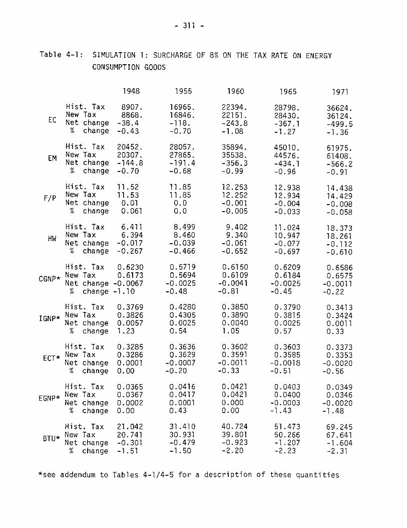
- 311
Table 4-1: SIMULATION 1: SURCHARGE OF 8% ON THE TAX RATE ON ENERGY
CONSUMPTION GOODS
1948 1955 1960 1965 1971
Hist. Tax 8907. 16965. 22394. 28798. 36624.New Tax 8868. 16846. 22151. 28430. 36124.
EC Net change -38.4 -118. -243.8 -367.1 -499.5% change -0.43 -0.70 -1.08 -1.27 -1.36
Hist. Tax 20452. 28057. 35894. 45010. 61975.EM New Tax 20307. 27865. 35538. 44576. 61408.
Net change -144.8 -191.4 -356.3 -434.1 -566.2% change -0.70 -0.68 -0.99 -0.96 -0.91
Hist. Tax 11.52 11.85 12.253 12.938 14.438F/P New Tax 11.53 11.85 12.252 12.934 14.429
Net change 0.01 0.0 -0.001 -0.004 -0.008% change 0.061 0.0 -0.005 -0.033 -0.058
Hist. Tax 6.411 8.499 9.402 11.024 18.373HW New Tax 6.394 8.460 9.340 10.947 18.261
Net change -0.017 -0.039 -0.061 -0.077 -0.112% change -0.267 -0.466 -0.652 -0.697 -0.610
Hist. Tax 0.6230 0.5719 0.6150 0.6209 0.6586
CGNP* New Tax 0.6173 0.5694 0.6109 0.6184 0.6575Net change -0.0067 -0.0025 -0.0041 -0.0025 -0.0011% change -1.10 -0.48 -0.81 -0.45 -0.22
Hist. Tax 0.3769 0.4280 0.3850 0.3790 0.3413
IGNP* New Tax 0.3826 0.4305 0.3890 0.3815 0.3424Net change 0.0057 0.0025 0.0040 0.0025 0.0011% change 1.23 0.54 1.05 0.57 0.33
Hist.aTax 0.3285 0.3636 0.3602 0.3603 0.3373
ECT* New Tax 0.3286 0.3629 0.3591 0.3585 0.3353Net change 0.0001 -0.0007 -0.0011 -0.0018 -0.0020% change 0.00 -0.20 -0.33 -0.51 -0.56
Hist. Tax 0.0365 0.0416 0.0421 0.0403 0.0349
EGNP* New Tax 0.0367 0.0417 0.0421 0.0400 0.0346Net change 0.0002 0.0001 0.000 -0.0003 -0.0020% change 0.00 0.43 0.00 -1.43 -1.48
Hist. Tax 21.042 31.410 40.724 51.473 69.245
BTU* New Tax 20.741 30.931 39.801 50.266 67.641Net change -0.301 -0.479 -0.923 -1.207 -1.604% change -1.51 -1.50 -2.20 -2.23 -2.31
*see addendum to Tables 4-1/4-5 for a description of these quantities

- 312 -
Table 4-1 we note that, as expected, the tax surcharge shifts the com-
position of output towards investment goods and away from consumption
goods although the shift is greatest at the beginning of the period and
becomes progressively smaller as the economy adjusts to the reduction in
energy demand. The output of the energy sector shows average percentage
reductions of -0.91% and -0.89% in consumption and intermediate goods,
respectively, with the reductions becoming progressively greater towards
the end of the period 1948-1971. However, the price of energy inter-
mediate goods is almost unchanged and the price of energy consumption
goods is reduced an average of -0.15% throughout the period; consequently,
the share of consumption goods in total energy produced decreases by up
to -0.56% in 1971. Total energy consumed measured in B.T.U.'s decreases
by approximately 2 percent throughout the period. Full consumption by
households decreases an average of -0.006%with a growing decline towards
the end of the period.
Dynamic elasticities with respect to TCE of:
1948 1955 1965 1971
EC -0.116 -0.192 -0.350 -0.376
EM -0.197 -0.189 -0.268 -0.255
KE 0.0 -0.070 -0.146 -0.195
KN 0.0 -0.043 -0.120 -0.169
pKE -0.259 -0.188 -01246 -0.183
pKN -0.287 -0.233 -0.209 -0.109
pCE 0.261 0.306 0.474 0.450
pEC -0.079 -0.032 -0.012 0.008
CE -0.144 -0.231 -0.396 -0.416
Simulation 2 (2% surcharge on the tax rate on labor income):
The immediate effect of a surcharge on the labor income tax is to

- 313 -
Table 4-2: SIMULATION 2: SURCHARGE OF 2% ON THE TAX RATE ON LABOR
INCOME
1948 1955 1960 1965 1971
Hist. Tax 8907. 16965. 22394. 28798. 36624.
EC New Tax 8863. 16890. 22289. 28680. 36472.Net change -44.2 -75.0 -105.7 -117.3 -152.0% change -0.49 -0.44 -0.47 -0.40 -0.41
Hist. Tax 20452. 28057. 35894. 45010. 61975.
EM New Tax 20478. 28082. 35934. 45047. 62049.Net change 26.32 24.86 40.31 37.21 74.37% change 0.12 0.08 0.11 0.08 0.12
Hist. Tax 11.523 11.850 12.253 12.938 14.438
F/P New Tax 11.520 11.849 12.251 12.937 14.437Net change -0.003 -0.001 -0.002 -0.001 -0.001% change -0.021 -0.009 -0.015 -0.009 -0.004
Hist. Tax 6.411 8.499 9.402 11.024 18.372New Tax 6.415 8.507 9.411 11.034 18.391
HW Net change 0.004 0.008 0.009 0.010 0.018% change 0.057 0.096 0.096 0.090 0.102
Hist. Tax 0.6230 0.5719 0.6150 0.6209 0.6586
CGNP* New Tax 0.6203 0.5707 0.6130 0.6197 0.6581Net change -0.0027 -0.0012 -0.0020 -0.0012 -0.0005
% change -0.43 -0.20 -0.32 -0.19 -0.075
Hist. Tax 0.3769 0.4280 0.3850 0.3790 0.3413
IGNP* New Tax 0.3796 0.4292 0.3869 0.3802 0.3418Net change 0.0027 0.0012 0.0019 0.0012 0.0005% change 0.71 0.28 0.49 0.31 0.14
Hist. Tax 0.3285 0.3636 0.3602 0.3603 0.3373
ECT* New Tax 0.3281 0.3628 0.3591 0.3589 0.3358Net change -0.0004 -0.0008 -0.0011 -0.0014 -0.0015% change -0.12 -0.24 -0.30 -0.38 -0.44
Hist. Tax 0.0365 0.0416 0.0421 0.0403 0.0349
EGNP* New Tax 0.0365 0.0416 0.0420 0.0400 0.0346Net change 0.00 0.00 -0.0001 -0.0003 -0.0003% change 0.0 0.0 -0.23 -0.74 -0.85
Hist. Tax 21.042 31.410 40.724 51.473 69.245
BTU* New Tax 20.875 31.136 40.201 50.388 68.349Net change -0.167 -0.274 -0.523 -1.085 -1.896% change -0.79 -0.87 -1.28 -2.10 -2.73
*see addendum to Tables 4-1/4-5 for a description of these quantities

- 314 -
decrease the supply price of labor services according to equation 30.
This affects the value of present full consumption as determined by the
inter-temporal allocation equation 45, and, in turn, the quantities de-
manded by households of energy goods CE, non-energy goods CN and capital
services CK. As can be seen from Tables 4-2 and 4-6, the effect of the
tax increase on the economy is mildly contractionary; of course, the
mechanisms that cause the reductions in aggregate demand are different,
as we have seen, to those that would be present in a stabilization model
with a detai-led representation of the short-run dynamics of the labor mar-
ket. There is a shift in the composition of national output towards in-
vestment and away from consumption, with the shift showing a declining
trend towards the end of the period. The level of energy consumed
throughout the period 1948-1971 measured in B.T.U.'s declines an average
of -1.3%.
Dynamic Elasticities with respect to TL of:
1948 1955 1965 1971
EC -0.064 -0.044 -0.041 -0.060
EM 0.248 0.221 0.204 0.208
KE 0.0 -0.045 -0.056 -0.075
KN 0.0 0.026 0.050 0.066
pKE 0.065 0.152 0.165 0.210
pKN -0.152 -0.100 -0.035 -0.045
pCE -0.130 -0.094 -0.065 -0.055
PEC -0.103 -0.075 -0.060 -0.050
CE 0.308 0.265 0.230 0.230
Simulation 3 (8% surcharge on the tax rate of investment goods):
The tax rate on investment goods enters the model in equation 24

- 315 -
directly affecting the demand price of investment, p1 . Tracing the pro-
pagation of a higher tax TI through the model, we observe that the in-
crease in P1 results in lower rates of return ME and MN and, therefore, in
a lower MW. This affects the budget constraint of households and thus,
the quantities demanded CE, CN and CK; in turn, of course, these changes
affect the equilibrium values of NI and pNI' among others, thus estab-
lishing a feedback into equation 24. In examining the results summarized
in Tables 4-3 and 4-6, we note that although gross investment decreases,
as expected, the value share of investment in GNP becomes greater as a
result of proportionally greater reductions in the demands CE and CN.
The output of the energy sector shows decreases in both consumption and
intermediate goods averaging -1.126% and -1.131%, respectively, with the
decline becoming gradually more pronounced throughout the period. Full
consumption declines initially but later increases in response to changes
in the relative prices of present vs. future consumption. Average reduc-
tions in B.T.U.'s consumed amount to -1.05% for the period 1948-1971.
Dynamic Elasticities with respect to TI of:
1948 1955 1965 1971
EC 0.032 0.033 0.031 0.032EM -0.008 -0.003 -0.004 -0.005KE 0.0 -0.005 -0.006 -0.008
KN 0.0 -0.003 -0.005 -0.007
PKE 0.008 0.023 0.025 0.030
PKN -0.019 -0.011 -0.005 -0.005
PCE -0.016 -0.013 -0.009 -0.007
pEC -0.013 -0.010 -0.008 -0.007CE 0.038 0.040 0.035 0.036

- 316 -
Table 4-3: SIMULATION 3: SURCHARGE OF 8% ON THE TAX RATE ON
INVESTMENT GOODS
1948 1955 1960 1965 1971
Hist. Tax 8907. 16965. 22394. 28798. 36624.
EC New Tax 8885. 16920. 22333. 28727. 36528.Net change -21.9 -44.7 -61.6 -70.6 -95.8% change -0.24 -0.26 -0.27 -0.24 -0.26
Hist. Tax 20452. 28057. 35894. 45010. 61975.
EM New Tax 20465. 28065. 35909. 45023. 61999.Net change 13.2 7.9 15.3 13.2 24.3% change 0.064 0.028 0.042 0.029 0.039
Hist. Tax 11.523 11.850 12.253 12.938 14.438
F/P New Tax 11.521 11.853 12.255 12.940 14.440Net change -0.001 0.002 0.001 0.002 0.002% change -0.011 0.021 0.014 0.015 0.017
Hist. Tax 6.411 8.499 8.402 11.024 18.372
HW New Tax 6.439 8.541 9.453 11.079 18.459Net change 0.027 0.042 0.051 0.054 0.087% change 0.435 0.496 0.543 0.498 0.473
Hist. Tax 0.6230 0.5719 0.6150 0.6209 0.6586
CGNP* New Tax 0.6199 0.5705 0.6127 0.6196 0.6580Net change -0.0031 -0.0014 -0.0023 -0.0013 -0.0006% change -0.51 -0.30 -0.39 -0.22 -0.12
Hist. Tax 0.3769 0.4280 0.3850 0.3790 0.3413
IGNP* New Tax 0.3800 0.4294 0.3872 0.3803 0.3419Net change 0.0031 0.0014 0.0022 0.0013 0.0006% change 0.79 0.33 0.58 0.29 0.18
Hist. Tax 0.3285 0.3636 0.3602 0.3603 0.3373
ECT* New Tax 0.3286 0.3631 0.3596 0.3593 0.3362Net change 0.0001 -0.0005 -0.0006 -0.0010 -0.0011% change 0.00 -0.14 -0.18 -0.31 -0.30
Hist. Tax 0.0365 0.0416 0.0421 0.0403 0.0349
EGNP* New Tax 0.0366 0.0416 0.0421 0.0401 0.0347Net change 0.0001 0.0000 0.0000 -0.0002 -0.0002% change 0.27 0.00 0.00 -0.46 -0.57
Hist. Tax 21.042 31.410 40.724 51.473 69.245
BTU* New Tax 20.876 31.139 40.205 50.794 68.339Net change -0.166 -0.271 -0.519 -0.679 -0.806
% change -0.85 -0.86 -1.20 -1.23 -1.17
*see addendum to Tables 4-1/4-5 for a description of these quantities

- 317
Simulation 4 (1% reduction in the tax rate on capital property, energy
sector):
The tax rate on capital property for the energy sector, TPE, enters
the model in equation 31. The reduction in TPE has the initial effect of
increasing the rate of return ME which in turn affects MW and thus the
budget equation for the household sector. Because of the interrelated
nature of the variables in our general equilibrium model, the demand
price of investment goods P1 which feeds back into equation 31, is also
modified in the simultaneous process of market equilibration. The out-
come of the interactions is such that it brings about a somewhat unex-
pected result: the reduction in TPE which might appear to apply strong
pressure in the direction of stimulating investment, in effect results in
only slightly higher values of gross investment. The implications of
this result will be explored in greater depth in Section 4-5. As can be
seen from Tables 4-4, the consumption of energy measures in B.T.U.'s de-
creases an average of -1.1% throughout the period 1948-1971.
Dynamic elasticities with respect to TPE of:
1948 1955 1965 1971
EC 0.005 0.005 0.004 0.004
EM -0.001 -0.001 -0.001 -0.001
KE 0.0 -0.001 -0.001 -0.001
KN 0.0 -0.001 -0.001 -0.001
PKE 0.001 0.003 0.003 0.004
PKN -0.003 -0.002 -0.001 -0.001
PCE -0.003 -0.002 -0.001 -0.001
PEC -0.002 -0.002 -0.001 -0.001CE 0.006 0.005 0.005 0.005

- 318
Table 4-4: SIMULATION 4: REDUCTION OF 1% IN THE TAX RATE ON CAPITAL
PROPERTY, U.S. ENERGY SECTOR
1948 1955 1960 1965 1971
Hist. Tax 8907. 16965. 22394. 28798. 36624.
EC New Tax 8885. 16927. 22341. 28738. 36546.Net change -22.4 -38.4 -53.8 -59.9 -78.0% change -0.25 -0.22 -0.24 -0.21 -0.21
Hist. Tax 20452. 28057. 35894. 45010. 61975.
EM New Tax 20464. 28068. 35913. 45028. 62010.Net change 12.4 11.5 19.12 17.8 35.6% change 0.06 0.04 0.05 0.04 0.05
Hist. Tax 11.523 11.850 12.253 12.938 14.438
F/P New Tax 11.522 11.850 12.252 12.938 14.438Net change -0.001 0.0 -0.001 0.0 0.0% change -0.007 0.0 -0.005 0.0 0.0
Hist. Tax 6.411 8.499 9.402 11.024 18.372
HW New Tax 6.413 8.503 9.406 11.029 18.381Net change 0.002 0.004 0.004 0.005 0.009% change 0.027 0.046 0.046 0.043 0.049
Hist. Tax 0.6230 0.5719 0.6150 0.6209 0.6586
CGNP* New Tax 0.6198 0.5705 0.6127 0.6195 0.6580Net change -0.0032 -0.0014 -0.0023 -0.0014 -0.0006% change -0.84 -0.24 -0.37 -0.22 -0.09
Hist. Tax 0.3769 0.4280 0.3850 0.3790 0.3413
IGNP* New Tax 0.3801 0.4294 0.3872 0.3804 0.3419Net change 0.0032 0.0014 0.0022 0.0014 0.0006% change 0.84 0.32 0.57 0.36 0.17
Hist. Tax 0.3285 0.3636 0.3602 0.3603 0.3373
ECT* New Tax 0.3286 0.3632 0.3596 0.3593 0.3362Net change 0.0001 -0.0004 -0.0006 -0.0010 -0.0011% change 0.03 -0.12 -0.18 -0.30 -0.33
Hist. Tax 0.0365 0.0416 0.0421 0.0403 0.0349
EGNP* New Tax 0.0366 0.0417 0.0421 0.0401 0.0347Net change 0.0001 0.0001 0.0000 -0.0002 -0.0002% change 0.27 0.24 0.00 -0.46 -0.57
Hist. Tax 21.042 31.410 40.724 51.473 69.245
BTU* New Tax 20.876 31.145 40.212 50.803 68.358Net change -0.166 -0.265 -0.512 -0.670 -0.887% change -0.78 -0.84 -1.25 -1.30 -1.28
*see addendum to Tables 4-1/4-5 for a description of these quantities

- 319 -
Simulation 5 (1% reduction in the tax rate on capital property, non-
energy sector):
The initial impact of the reduction in the tax variable TPN, through
equation 32, is to increase the rate of return of the non-energy sector,
MN; in turn, this causes MW to increase through equation 58. From that
point on, the repercussions of the tax change are qualitatively very sim-
ilar to those that followed the reduction in TPE, because the predominant
impact is subsumed in the change in MW. If there were sectoral invest-
ment demand functions that explicitly depended on the sectoral rates of
return, then the difference in the behavior of the model resulting from
changes in TPE and TPN, respectively, would be somewhat more pronounced.
Again we observe the somewhat unexpected effects on investment ex-
penditures of the private sector--this is discussed in 4-5 below. From
Table 4-5 we note a reduction of in the supply of energy consumption
products of -0.27% in 1948 which decreases to -0.24% by 1971. The de-
crease in total energy consumption measured in B.T.U.'s is similar to
that in Simulation 4 during the initial part of the period, but is sig-
nificantly larger, -2.73%, by 1971.
Dynamic elasticities with respect to TPN of:
1948 1955 1965 1971
EC 0.005 0.005 0.005 0.005
EM -0.001 -0.001 -0.001 -0.001
KE 0.0 -0.001 -0.001 -0.001
pKE 0.002 0.003 0.004 0.005
pKN -0.002 -0.002 -0.001 -0.001
PCE -0.002 -0.002 -0.001 -0.001
pEC -0.002 -0.002 -0.001 -0.001
CE 0.009 0.006 0.005 0.005

- 320 -
TABLE 4-5: SIMULATION 5: REDUCTION OF 1% IN THE TAX RATE ON CAPITALPROPERTY, U.S. NON-ENERGY SECTOR
1948 1955 1960 1965 1971
Hist. Tax 8907. 16965. 22394. 28798. 36624.EC New Tax 8882. 16923. 22336. 28731. 36534.
Net change -24.7 -41.8 -58.2 -66.2 -89.6% change -0.27 -0.24 -0.26 -0.23 -0.24
Hist. Tax 20452. 28057. 35894. 45010. 61975.EM New Tax 20461. 28067. 35911. 45025. 62003.
Net change 8.96 9.95 16.88 14.99 28.54% change 0.043 0.035 0.047 0.033 0.046
Hist. Tax 11.523 11.850 12.253 12.938 14.438F/P New Tax 11.524 11.851 12.254 12.939 14.439
Net change 0.001 0.001 0.001 0.001 0.001% change 0.013 0.011 0.004 0.007 0.011
Hist. Tax 6.411 8.499 9.402 11.024 18.372New Tax 6.413 8.503 9.405 11.028 18.380Net change 0.002 0.003 0.003 0.004 0.007% change 0.021 0.041 0.040 0.037 0.042
Hist. Tax 0.6230 0.5719 0.6150 0.6209 0.6586CGNP* New Tax 0.6203 0.5707 0.6130 0.6197 0.6581
Net change -0.0027 -0.0012 -0.0020 -0.0012 -0.0005% change -0.43 -0.20 -0.32 -0.19 -0.075
Hist. Tax 0.3769 0.4280 0.3850 0.3790 0.3413IGNP* New Tax 0.3796 0.4292 0.3869 0.3802 0.3418
Net change 0.0027 0.0012 0.0019 0.0012 0.0005% change 0.71 0.28 0.49 0.31 0.14
Hist. Tax 0.3285 0.3636 0.3602 0.3603 0.3373
ECT* New Tax 0.3281 0.3628 0.3591 0.3589 0.3358Net change -0.0004 -0.0008 -0.0011 -0.0014 -0.0015% change -0.12 -0.24 -0.30 -0.38 -0.44
Hist. Tax 0.0365 0.0416 0.0421 0.0403 0.0349EGNP* New Tax 0.0365 0.0416 0.0420 0.0400 0.0346
Net change 0.00 0.00 -0.0001 -0.0003 -0.0003% change 0.0 0.0 -0.23 -0.74 -0.85
Hist. Tax 21.042 31.410 40.724 51.473 69.245BTU* New Tax 20.875 31.136 40.201 50.388 68.349
Net change -0.167 -0.274 -0.523 -1.085 -1.896% change -0.79 -0.87 -1.28 -2.10 -2.73
*See addendum to Tables 4-1/4-5 for a description of these quantities
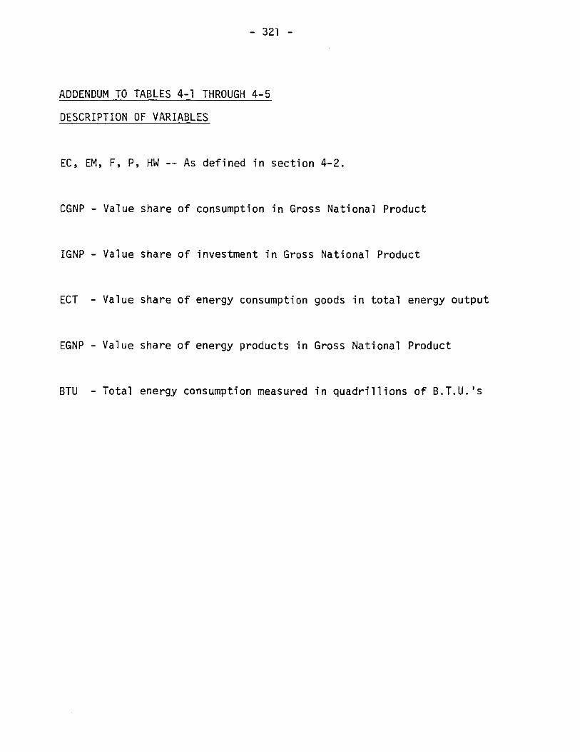
- 321 -
ADDENDUM TO TABLES 4-1 THROUGH 4-5
DESCRIPTION OF VARIABLES
EC, EM, F, P, HW -- As defined in section 4-2.
CGNP - Value share of consumption in Gross National Product
IGNP - Value share of investment in Gross National Product
ECT - Value share of energy consumption goods in total energy output
EGNP - Value share of energy products in Gross National Product
BTU - Total energy consumption measured in quadrillions of B.T.U.'s

- 322 -
Table 4-6: AVERAGE PERCENTAGE CHANGES IN ENDOGENOUS VARIABLES,1948-1971, SIMULATIONS I THROUGH 5
Average percentage change in selected endogenousvariables from historical simulation values 1948-1971
Simulation Simulation Simulation Simulation SimulationVariable 1 2 3 4 5
pKE -0.877 -0.296 -0.175 -0.151 -0.165
EM -0.897 0.156 0.060 0.074 0.065
PCN -0.451 0.179 0.086 0.088 0.087
pEMN -0.959 -0.001 -0.001 -0.001 -0.001
pKN -0.933 0.261 0.117 0.127 0.121
pEM -0.002 -0.001 -0.001 -0.001 -0.001
EC -0.909 -0.501 -0.290 -0.257 -0.279
PEC -0.155 0.188 0.097 0.094 0.096
RN -0.141 0.538 0.258 0.265 0.262
EMN -0.914 0.250 0.110 0.121 0.114
NMN -1.101 0.197 0.077 0.095 0.083
LN -0.947 0.299 0.135 0.146 0.139
KN -0.277 0.069 0.028 0.033 0.029
NM -1.093 0.194 0.076 0.093 0.082
NI -0.418 0.098 0.040 0.047 0.042
PNI -0.234 0.034 0.013 0.016 0.014
NC -0.978 0.301 0.135 0.147 0.140
PNC -0.352 0.144 0.069 0.071 0.070
RE -0.731 -0.277 -0.165 -0.141 -0.157
NME -0.819 0.082 0.022 0.038 0.028
EME -0.884 0.064 0.012 0.028 0.017

- 323 -
Table 4-6 (cont.): AVERAGE PERCENTAGE CHANGES IN ENDOGENOUS VARIABLES,1948-1971, SIMULATIONS 1 THROUGH 5
Average percentage change in selected endogenousvariables from historical simulation values 1948-1971
Simulation Simulation Simulation Simulation SimulationVariable 1 2 3 4 5
LE -0.907 0.090 0.025 0.041 0.031
KE -0.353 0.091 0.037 0.044 0.039
PCE 1.336 0.214 0.109 0.106 0.108
CE -1.045 -0.587 -0.336 -0.298 -0.324
CN -1.204 0.369 0.166 0.180 0.171
P, -0.364 0.054 0.608 0.025 0.022
I -0.661 0.156 0.064 0.076 0.067
L -0.751 0.236 0.106 0.115 0.109
PL 0.001 -0.424 -0.212 -0.212 -0.212
ME 0.736 -0.273 -0.575 -3.155 0.006
MN -0.707 0.254 -0.661 0.124 4.643
KSE -0.383 0.098 0.040 0.047 0.042
KSN -0.303 0.074 0.030 0.036 0.032
INE -0.661 0.157 0.064 0.076 0.067
INN -0.661 0.157 0.064 0.076 0.067
ICD -0.661 0.157 0.064 0.076 0.067
IMIN -0.661 0.157 0.064 0.076 0.067
IRS -0.661 0.157 0.064 0.076 0.067
S -0.967 0.199 0.639 0.096 0.085
LJ 0.199 -0.060 0.002 -0.026 -0.007
KCD -0.539 0.127 0.052 0.062 0.005

- 324 -
Table 4-6 (cont.): AVERAGE PERCENTAGE CHANGES IN ENDOGENOUS VARIABLES,1948-1971, SIMULATIONS 1 THROUGH 5
Average percentage change in selected endogenousvariables from historical simulation values 1948-1971
Simulation Simulation Simulation Simulation SimulationVariable 1 2 3 4 5
KRS -0.315 0.077 0.032 0.037 0.033
W -0.586 0.114 0.525 0.055 0.048
CK -0.370 0.089 0.036 0.043 0.038
pCK -1.873 -0.633 -0.379 -0.325 -0.362
MW -0.689 0.196 -0.722 0.814 4.402
F -0.006 -0.017 0.013 -0.006 0.006

- 325 -
Partial vs. General Equilibrium
The final experiment to be described in this section is aimed at
illustrating the limitations of partial equilibrium analysis in evaluating
the impact of a given tax measure. Suppose we wish to assess the effect
of a 1% reduction in the capital property tax rate for the energy sector
on the equilibrium values of the derived demands for factors of produc-
tion in the energy sector. A partial equilibrium model can be constructed
from the four equilibrium share equations 3, 4, 5 and 6 of our macro-
economic energy model. These four equations, by transposition of var-
iables, can be interpreted as derived demand functions: by regarding
prices as exogenous, one can compute the equilibrium values of the
demands for capital services, labor services, energy and non-energy in-
termediate inputs. The impact of the tax reduction could then be evalu-
ated by computing a new capital service price time series corresponding
to the reduced tax rate, substituting this new series into the four equa-
tion models, and computing the new set of equilibrium demands. Indeed,
we have conducted this experiment and report on its results below.
Table 4-7 shows time series for capital service prices corresponding
to historical values, the partial equilibrium effects of a 1% reduction
in TPE computed by using equation 31 directly, and the general equilibrium
effects of the same tax measure on PKE, taken directly from the results
of simulation 4 with the complete macroeconomic model. We note that the
values of pKE computed by direct substitution into equation 31 greatly
overestimate the effect of the tax reduction on the equilibrium values of
capital service prices. This is.due to the fact that the partial equilib-
rium analysis doesn't take into account the rise in the rate of return
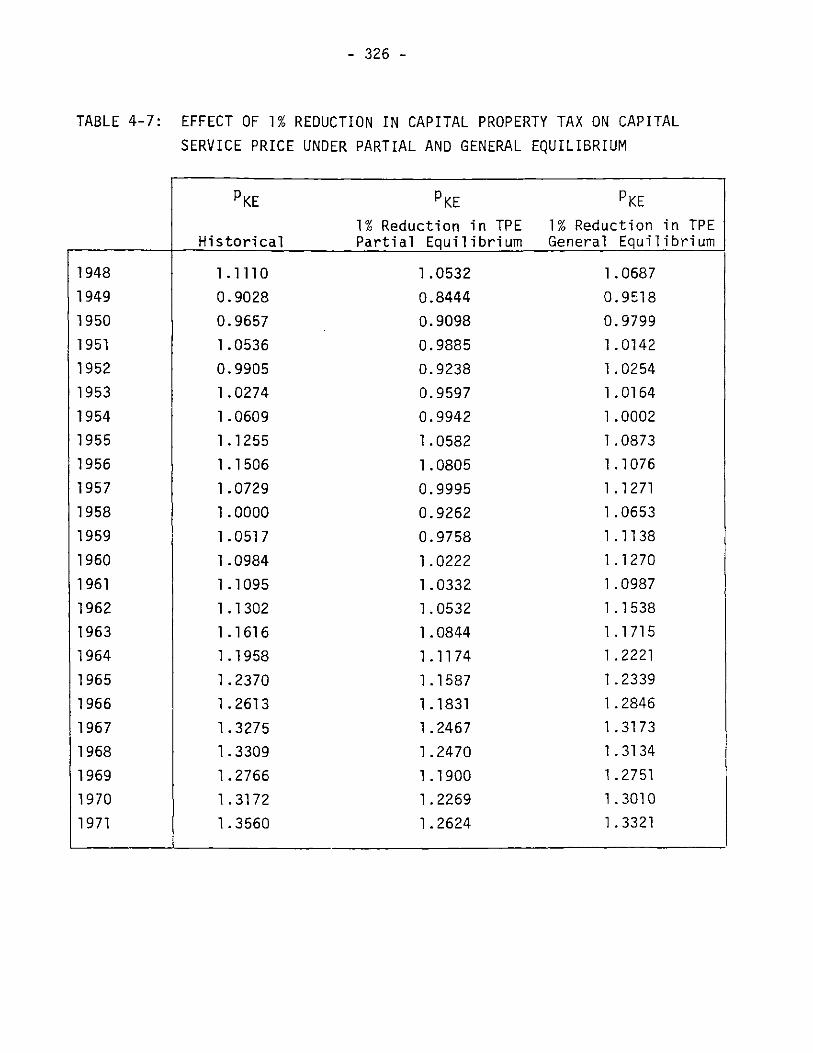
- 326 -
TABLE 4-7: EFFECT OF 1% REDUCTION IN CAPITAL PROPERTY TAX ON CAPITAL
SERVICE PRICE UNDER PARTIAL AND GENERAL EQUILIBRIUM
PKE
Historical
KE
1% Reduction in TPEPartial Equilibrium
1948
1949
1950
1951
1952
1953
1954
1955
19561957
1958
1959
1960
1961
1962
1963
1964
1965
1966
1967
1968
19691970
1971
1.11100.9028
0.9657
1.0536
0.99051.0274
1.0609
1.1255
1.1506
1.0729
1.0000
1.0517
1.0984
1.1095
1.1302
1.1616
1.1958
1.2370
1.2613
1.32751.3309
1.2766
1.31721.3560
PKE
1% Reduction in TPEGeneral Equilibrium
1.0532
0.8444
0.9098
0.98850.9238
0.9597
0.9942
1.0582
1.08050.9995
0.9262
0.9758
1.0222
1.03321.0532
1.0844
1.1174
1.1587
1.18311.2467
1.2470
1.19001.2269
1.2624
9.
1.0687
0. 9518
0.9799
1.0142
1.0254
1.0164
1.0002
1.08731.1076
1.1271
1.0653
1.11381.1270
1.0987
1.15381.17151.2221
1.2339
1.2846
1.31731.3134
1.2751
1.3010
1.3321

- 327 -
TABLE 4-8: DYNAMIC ELASTICITIES OF DEMANDS FOR FACTORS OF PRODUCTION
WITH RESPECT TO TPE, UNDER PARTIAL AND GENERAL EQUILIBRIUM
Dynamic elasticities of demands with respect to TPE
Partial Equilibrium General Equilibrium
1948 -0.0366 0.01952 -0.1743 -0.0001
1956 -0.0493 -0.0010
KE 1960 -0.1588 -0.0011
1964 -0.1436 -0.0012
1968 -0.0858 -0.0013
1971 -0.0836 -0.0015
1948 -0.0026 -0.0007
1952 -0.0116 -0.0005
1956 -0.0036 -0.0002
LE 1960 -0.0118 -0.00041964 -0.0115 -0.0003
1968 -0.0073 -0.0007
1971 -0.0074 -0.0006
1948 -0.0019 -0.0021
1952 -0.0026 -0.0071
1956 -0.0017 -0.0016
EME 1960 -0.0021 -0.00201964 -0.0018 -0.0016
1968 -0.0016 -0.00221971 -0.0014 -0.0018
1948 -0.0042 -0.0005
1952 -0.0051 -0.0034
1956 -0.0034 -0.0001
NME 1960 -0.0039 -0.00021964 -0.0033 -0.0001
1968 -0.0028 -0.0003
1971 -0.0022 -0.0004

- 328 -
for the energy sector, which acts as a stabilizing force through the
lagged value RE(-l) in equation 31.
Table 4-8 presents a tabulation of dynamic elasticities of demand
for factors of production in the energy sector, corresponding to both
partial and general equilibrium analyses. The column corresponding to
general equilibrium was constructed directly from the results of simula-
tion 4. The partial equilibrium results were computed using the partial
equilibrium sub-model described above. The difference between the two
sets of dynamic elasticities can be explained as follows: as discussed
above, the tax reduction augments the rate of return in the energy sector,
resulting in a smaller decrease in the equilibrium values of the capital
service price PKE. The nominal rate of return on wealth, however,
decreases as a result of lowered values of RN; this shows up in reduced
demand by households and, ultimately, in lower equilibrium levels for the
derived demands for factors of production. The net result is a change in
equilibrium factor inputs substantially lower than that computed under
partial equilibrium.
The somewhat unexpected results for the general equilibrium
case tend to support the conjectures of Christensen [ 1], Harberger [ 2]
and others that an analysis of investment incentives based on partial
equilibrium may be misleading. Our results suggest that the interactions
between rates of return, demand price of investment goods and capital
service prices are such that they produce stabilizing forces that tend to
offset the effects of the tax reduction. As we shall see in the next
section, this observation is not insensitive to the composition of the
entire fiscal package adopted by the government in implementing the tax
change. We conclude, nevertheless, that an analysis based on partial

- 329 -
equilibrium may tend to greatly overstate the effectiveness of tax poli-
cies to influence the equilibrium demands for factors of production and,
in some instances, to predict incorrectly not only the magnitude but
even the direction of this influence.
4.5 Government Debt, Government Expenditures and Fiscal Policy
The simulation experiments reported in the last section were con-
ducted with the levels of government expenditures and government debt
fixed exogenously at their historical values. In this section, the
extent to which the effectiveness of a given tax measure is influenced by
the configuration of the entire fiscal package adopted by the government
will be examined in greater detail.
It has long been recognized that the selection of a budget-balancing
fiscal package or, alternatively, deficit financing through the sale of
government debt to the household sector, can decisively alter the
effectiveness of a given tax measure. In the case of tax measures in-
tended to stimulate investment expenditures, this question has been
examined, for example, by Taubman and Wales [3 1. Because of the com-
plementarity between capital and energy revealed in the dynamic simula-
tions of our general equilibrium model, discrepancies in the effects of
such investment incentives in the face of different fiscal packages will
effect themselves in the levels of energy demanded for industrial pro-
duction.
In this section we evaluate the impact of alternative tax policies
under two alternative government financing schemes.

- 330 -
Fiscal Plan A: Deficit Financing
Under this strategy, it is assumed that a tax reduction or surcharge
is not accompanied by offsetting revenue or expenditure measures.
Rather, the foregone or added revenues result in changes in the govern-
ment deficit that are covered by the sale of government debt to the
household sector. We implement this financial strategy of the govern-
ment in the context of our macroeconomic energy model by introducing
government deficit DEF and government debt G as endogenous variables and
by adding the following two equations to our macroeconomic model:
62A. DEF = TKE-PKE-KE + TKN-PKN-KN
+ TCE-PEC-EC + TCN-pNCUNC
+ TISPNI-NI + TLSPL-L
+ TPE-p(-1-KSE(-l)
+ TPN-p1C-1)-KSN(-l)
+ TPH-p1(-l)-[KRS(-l) + KCD(-l)
- EPLGOLG + pGESGE + PGN-GN + PGI-GI + MG-PG(-l)-G(-l)]
where
TPH - Effective tax rate on capital property, household sector.
MG - Effective rate of return on government deb.
and
63A. PG-G = PG-G(-l) - DEF
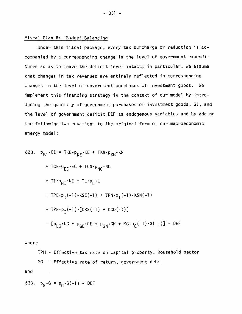
- 331 -
Fiscal Plan B: Budget Balancing
Under this fiscal package, every tax surcharge or reduction is ac-
companied by a corresponding change in the level of government expendi-
tures so as to leave the deficit level intact; in particular, we assume
that changes in tax revenues are entirely reflected in corresponding
changes in the level of government purchases of investment goods. We
implement this financing strategy in the context of our model by intro-
ducing the quantity of government purchases of investment goods, GI, and
the level of government deficit DEF as endogenous variables and by adding
the following two equations to the original form of our macroeconomic
energy model:
62B. PGI-GI = TKE-pKE-KE + TKNSpKN-KN
+ TCE-pECSEC + TCN-PNCSNC
+ TI-pNIONI + TL-pLL
+ TPE-p1(-l)-KSE(-l) + TPN-p1(-l)-KSN(-l)
+ TPH-p1(-l)-[KRS(-l) + KCD(-l)]
- [PLG-LG + PGE-GE + PGNOGN + MG-pG(-l)-G(-l)] - DEF
where
TPH - Effective tax rate on capital property, household sector
MG - Effective rate of return, government debt
and
63B. PG-G = PG-G(-l) - DEF

- 332 -
TABLE 4-9: AVERAGE PERCENTAGE CHANGES IN ENDOGENOUS VARIABLES,
1948-1971, SIMULATIONS IA THROUGH 5A
Average percentage change in selected endogenousvariables from historical simulation values 1948-1971
Simulation Simulation Simulation Simulation SimulationVariable IA 2A 3A 4A 5A
pKE
EM
pCN
P EMN
P KN
pEM
EC
p EC
RN
EMN
NMN
LN
KN
NM
NI
pNI
NC
PNC
RE
NME
-0.969
-0.937
-0.461
-0.004
-0.968
-0.003
-1.017
-0.147
-1.157
-0.945
-1.151
-0.976
-0.285
-1.143
-0.432
-0.245
-1.008
-0.360
-1.115
-0.863
-0.101
0.097
0.094
0.000
0.147
0.000
-0.197
0.089
0.274
0.140
0.123
0.163
0.038
-0.122
0.055
0.023
0.165
0.075
-0.102
0.062
* 0.021
0.003
0.002
0.000
0.005
0.000
0.021
-0.002
-0.001
0.001
0.005
0.001
-0.001
0.005
-0.001
0.001
0.001
0.000
0.012
0.005
0.042
-0.118
-0.099
-0.000
-0.164
-0.000
0.127
-0.822
-0.227
-0.154
-0.149
-0.175
-0.041
-0.147
-0.061
-0.029
-0.178
-0.078
0.055
-0.087
-0.385
-0.293
-0.140
-0.004
-0.308
-0.004
-0.392
-0.035
-0.324
-0.285
-0.368
-0.291
-0.075
-0.366
-0.121
-0.080
-0.302
-0.106
-0.287
-0.281

- 333 -
TABLE 4-9 (cont.): AVERAGE PERCENTAGE CHANGES IN ENDOGENOUS VARIABLES,
1948-1971, SIMULATIONS 1A THROUGH 5A
Average percentage change in selected endogenousvariables from historical simulation values 1948-1971
Simulation Simulation Simulation Simulation SimulationVariable IA 2A 3A 4A 5A
EME
LE
KE
pCE
CE
CN
PI
I
L
PL
ME
MN
KS E
KSN
INE
INN
ICD
IMIN
IRS
S
LJ
-0.932
-0.954
-0.363
1.345
-1.168
-1.242
-0.381
-0.683
-0.774
0.0014
-0.960
-0.728
-0.394
-0.312
-0.683
-0.683
-0.683
-0.683
-0.683
1.390
0.293
0.056
0.068
0.050
0.102
-0.230
0.202
0.035
0.089
0.129
-0.212
-0.098
0.136
0.054
0.041
0.089
0.089
0.089
0.089
0.089
-1.115
-0.078
0.006
0.005
-0.002
-0.002
0.023
0.002
0.569
-0.001
0.001
0.000
-1.371
-0.776
-0.002
-0.002
-0.001
-0.001
-0.001
-0.001
-0.001
-0.682
-0.016
-0.084
-0.095
-0.054
-0.095
0.150
-0.219
-0.045
-0.098
-0.138
0.212
4.712
-0.145
-0.058
-0.045
-0.098
-0.098
-0.098
-0.098
-0.098
2.491
0.134
-0.304
-0.306
-0.097
-0.048
-0.443
-0.373
-0.122
-0.192
-0.232
0.212
-0.079
4.291
-0.107
-0.083
-0.192
-0.192
-0.192
-0.192
-0.192
12.612
0.567I

- 334 -
TABLE 4-9 (cont.): AVERAGE PERCENTAGE CHANGES IN ENDOGENOUS VARIABLES,
1948-1971, SIMULATIONS 1A THROUGH 5A
Average percentage change in selected endogenousvariables from historical simulation values 1948-1971
Simulation Simulation Simulation Simulation SimulationVariable 1A 2A 3A 4A 5A
KCD -0.555 0.072 -0.002 -0.078 -0.152
KRS -0.324 0.043 -0.001 -0.047 -0.087
W 0.771 -0.636 -0.238 1.427 7.361
CK -0.381 0.058 -0.002 -0.054 -0.102
PCK -2.049 -0.232 0.026 0.128 -0.664
MW -0.715 0.110 -0.806 0.595 4.797
F 0.058 -0.041 -0.011 0.081 0.379

- 335 -
TABLE 4-10: AVERAGE PERCENTAGE CHANGE IN ENDOGENOUS VARIABLES
1948-1971, SIMULATIONS 1B THROUGH 5B
Average percentage change in selected endogenousvariables from historical simulation values 1948-1971
Simulation Simulation Simulation Simulation SimulationVariable 1B 2B 3B 4B 5B
pKE
EM
pCN
PEMN
P KN
pEM
EC
pEC
RN
EMN
NMN
LN
KN
NM
NI
KS E
KSN
INE
INN
ICD
IMIN
-1.821
-0.476
-0.866
0.003
-1.825
0.003
-0.084
-0.471
-1.182
-0.577
-0.908
-0.715
0.645
-0.890
0.271
0.900
0.702
1.499
1.499
1.499
1.499
I
-0.253
0.107
-0.223
0.003
-0.436
0.003
0.508
-0.190
-0.210
0.039
0.004
-0.018
0.326
0.009
0.227
0.457
0.356
0.787
0.787
0.787
0.787
0.465
-0.240
0.207
-0.003
0.450
-0.003
-0.461
0.163
0.000
-0.194
-0.125
-0.140
-0.481
-0.131
-0.366
-0.667
-0.524
-1.121
-1.121
-1.121
-1.121
-0.889
0.392
-0.534
0.007
-1.095
0.007
1.154
-0.432
-0.294
0.254
0.122
0.117
0.975
0.136
0.708
1.361
1.065
2.324
2.324
2.324
2.324
-0.421
0.182
-0.332
0.004
-0.657
0.004
0.749
-0.279
-0.280
0.085
0.025
0.000
0.517
0.033
0.365
0.724
0.565
1.242
1.242
1.242
1.242- - -I

- 336 -
TABLE 4-10 (cont.): AVERAGE PERCENTAGE CHANGE IN ENDOGENOUS VARIABLES,
1948-1971, SIMULATIONS 1B THROUGH 5B
Average percentage change in selected endogenousvariables from historical simulation values 1948-1971
Simulation Simulation Simulation Simulation SimulationVariable 1B 2B 3B 4B 5B
I RS
S
LJ
KCD
KRS
w
CK
PCK
MW
F
PNI
NC
PNC
RE
NME
EME
LE
KE
pCE
CE
CN
1.499
0.731
0.134
1.211
0.725
0.079
0.841
-1.549
-1.525
0.043
-0.413
-0.749
-0.677
0.139
-0.242
-0.375
-0.450
0.834
0.976
-0.102
-0.918
0.787
0.586
-0.003
0.625
0.369
0.205
0.429
0.356
-0.379
0.025
-0.079
-0.020
-0.176
0.440
0.194
0.174
0.145
0.421
-0.214
0.584
-0.023
-1.121
-0.339
0.067
-0.908
-0.541
0.127
-0.628
-0.227
-0.400
-0.003
0.085
-0.139
0.162
-0.475
-0.319
-0.286
-0.260
-0.617
0.182
-0.528
-0.173
i i
2.324
1.786
-0.039
1.862
1.102
0.665
1.280
0.627
-0.266
0.065
-0.209
0.112
-0.420
1.092
0.598
0.531
0.463
1.256
-0.484
1.324
0.142
1.242
0.935
-0.010
0.990
0.584
0.334
0.679
0.498
-0.481
0.038
-0.121
-0.004
-0.262
0.662
0.311
0.278
0.235
0.667
-0.314
0.861
-0.002

- 337 -
TABLE 4-10 (cont.): AVERAGE PERCENTAGE CHANGE IN ENDOGENOUS VARIABLES,
1948-1971, SIMULATIONS 1B THROUGH 5B
Average percentage change in selected endogenousvariables from historical simulation values, 1948-1971
Simulation Simulation Simulation Simulation SimulationVariable 1B 2B 3B 4B 5B
PIN -0.707 -0.162 0.768 -0.415 -0.245
1 1.499 0.787 -1.121 2.324 1.242
L -0.564 -0.013 -0.113 0.096 0.001
PL 0.002 0.160 0.000 0.213 0.212
ME -1.837 -0.152 -0.722 -0.275
MN -1.397 -0.345 -0.441 -0.860 -0.418

- 338 -
TABLE 4-11: PERCENTAGE CHANGE IN SELECTED VARIABLES IN RESPONSE TO1% REDUCTION IN TPE UNDER ALTERNATIVE FISCAL PACKAGES
HistoricalG and DEF*
Fiscal Plan ADeficit Financing*
Fiscal Plan B*Budget Balancing
1948 0.0 0.0 0.883I 1958 0.065 -0.084 2.265
1968 0.095 -0.173 4.251
1948 0.0 0.0 0.0
KE 1958 0.051 -0.059 1.207
1968 0.064 -0.100 2.386
1948 0.0 0.0 0.0
KN 1958 0.034 -0.040 0.847
1968 0.055 -0.085 2.037
1948 -0.070 0.061 0.060
pKE 1958 -0.172 0.090 -0.897
1968 -0.210 -0.033 -1.531
1948 0.146 -0.153 -0.154
pKN 1958 0.085 -0.110 -0.902
1968 0.075 -0.110 -2.076
1948 -0.251 0.244 0.244
EC 1958 -0.232 0.130 1.033
1968 -0.266 -0.083 2.237
1948 0.060 -0.066 -0.067
EM 1958 0.050 -0.083 0.385
1968 0.065 -0.146 0.878
1948 0.0 0.0 0.0
NI 1958 0.038 -0.048 0.617
1968 0.062 -0.117 1.533
*All figures represent percentage deviations fromvalues.
historical simulation

- 339 -
The impact of each of the two fiscal packages on the effectiveness
of selected tax measures will be assessed by replicating the set of 5
simulations described in section 4-4 under each of the two financing
schemes. That is, we simulate the effect of surcharges in the tax rates
on energy consumption goods, labor income, investment goods, and reduc-
tion in capital property taxes in the energy and non-energy sector; the
simulations were repeated for both Fiscal Plan A (lA through 5A) and
Fiscal Plan B (1B through 5B). Average percentage changes in selected
endogenous variables for simulations 1A through 5A are shown in Table 4-9
and the corresponding values for simulations lB through 5B are tabulated
in Table 4-10. Tables 4-9 and 4-10 are directly comparable to Table 4-6
and thus, it is possible to observe the respective consequences of the
deficit financing and budget balancing fiscal packages described above.
In what follows, we examine in some depth the implications of the two
alternative budgetary schemes for one specific policy measure: a 1% re-
duction in the tax rate on capital property for the U.S. energy sector.
We select this particular tax measure for detailed analysis both because
it serves to illuminate the contrasts between the two budgetary strategies
and also because it is representative of a variety of actual tax proposals
frequently discussed in the context of stimulating investment expenditures.
From Table 4-11 we can observe the effect of the 1% reduction in TPE
on key endogenous variables: gross private domestic investment, prices
and quantities of capital services, supply of energy consumption and in-
termediate goods, and supply of investment goods. The most striking fea-
*2B corresponds to 0.05% surcharge on TL; 5B corresponds to a 1% propor-tional reduction in TPN. All other tax charges are the same as for thecorresponding runs 1 through 5 in section 4-4.

- 340 -
ture of these results is the fact that the effect of the tax cut on in-
vestment and capital service levels is a slight increase under historical
deficit and debt, a slight decline under deficit financing and a sharp
increase under the budget-balancing fiscal plan. This seemingly con-
flicting outcome can be, in fact, explained by tracing the impact of the
tax change through the model's equations.
The dynamic response to the tax reduction when deficit and debt levels
are held at their historical values was already discussed in section 4.4.
Under fiscal plan A, the immediate effect of the reduction in TPE shows
up in equations 31 and 62A. The impact on Eq. 31 is the tendency for the
after-tax rate of return ME to rise; this causes an increase in the por-
tion of total wealth allocated to present consumption, through the inter-
temporal allocation equation 45. At the same time, the foregone revenues
have the effect of increasing the government deficit through equation 62A;
this increases the debt level according to equation 63A and reflects
itself in higher values of national saving and end-of-period wealth,
following equations 44 and 60. The corresponding increased demand for
leisure and energy consumption goods, when reflected by the feedback ef-
fects throughout the model, cause the level of investment to decline.
This result supports the conjecture made by Christensen [1 ] who used
a simplified conceptual model to argue that investment incentives imple-
mented in conjunction with a fiscal package based on deficit financing
would lead to just such a counterintuitive outcome.
The initial effect of the tax reduction in the case of Fiscal Plan B
is similar: through equation 31, the after-tax rate of return ME shows a
tendency to rise. But in this instance, the foregone revenues are reflec-
ted in a smaller amount of investment goods purchased by the government,
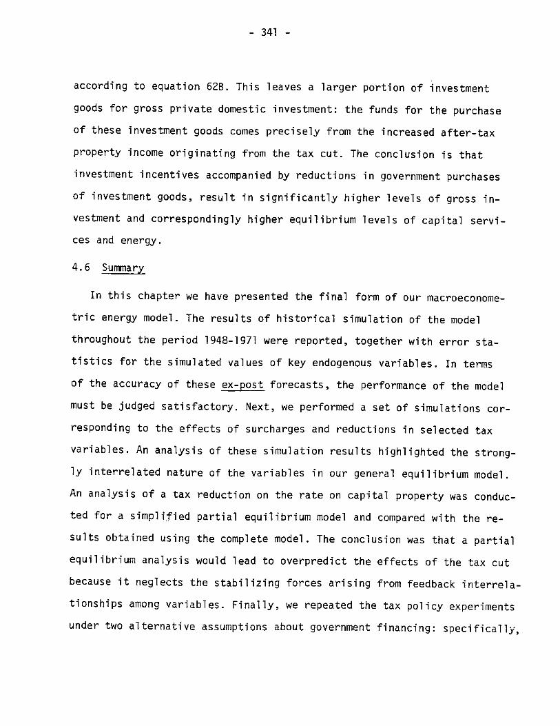
- 341 -
according to equation 62B. This leaves a larger portion of investment
goods for gross private domestic investment: the funds for the purchase
of these investment goods comes precisely from the increased after-tax
property income originating from the tax cut. The conclusion is that
investment incentives accompanied by reductions in government purchases
of investment goods, result in significantly higher levels of gross in-
vestment and correspondingly higher equilibrium levels of capital servi-
ces and energy.
4.6 Summary
In this chapter we have presented the final form of our macroeconome-
tric energy model. The results of historical simulation of the model
throughout the period 1948-1971 were reported, together with error sta-
tistics for the simulated values of key endogenous variables. In terms
of the accuracy of these ex-post forecasts, the performance of the model
must be judged satisfactory. Next, we performed a set of simulations cor-
responding to the effects of surcharges and reductions in selected tax
variables. An analysis of these simulation results highlighted the strong-
ly interrelated nature of the variables in our general equilibrium model.
An analysis of a tax reduction on the rate on capital property was conduc-
ted for a simplified partial equilibrium model and compared with the re-
sults obtained using the complete model. The conclusion was that a partial
equilibrium analysis would lead to overpredict the effects of the tax cut
because it neglects the stabilizing forces arising from feedback interrela-
tionships among variables. Finally, we repeated the tax policy experiments
under two alternative assumptions about government financing: specifically,

- 342 -
we examined the implications of budget-balancing and deficit-financing
fiscal packages. Detailed analysis of tax measures aimed at stimulating
investment expenditures show that the impact on actual investment levels
is critically dependent on the configuration of the entire budgetary
scheme.
- 343 -
REFERENCES TO CHAPTER IV
[1] Christensen, L., "Tax Policy and Investment Expenditures in a Modelof General Equilibrium," Proceedings of the 82nd Annual Meeting ofthe American Economic Association, American Economic Review,May 1970.
[2] Harberger, A. C., "The Quantitative Impact of Tax Policy onInvestment Expenditures," The Brookings Institution, Washington,D.C., 1971.
[3] Taubman, P., and Wales, T. J., "Impact of Investment Subsidiesin a Neoclassical Growth Model," Review of Economics and Statistics,August 1969.
- 344 -
CHAPTER V
OPTIMAL GROWTH POLICIES AND ENERGY RESOURCES
5.1 Introduction
5.2 The Theory of Optimal Economic Growth
5.3 An Intertemporal Measure of Aggregate Social Welfare
5.4 Finite Planning Horizon and Intergenerational Equity
5.5 The Optimal Growth Problem: Formulation and SolutionAl gorithm
5.6 Welfare Gains from Optimal Tax Policies
5.7 Summary
- 345 -
CHAPTER V
OPTIMAL GROWTH POLICIES AND ENERGY RESOURCES
Would you tell me, please, which way I oughtto go from here?
- That depends a good deal on where you want toget to, said the Cat.
- I don't much care where -- said Alice.
- Then it doesn't matter which way you go, saidthe Cat."
- Lewis Carroll
5.1 Introduction
This chapter discusses the design of optimal policies for energy and
economic growth. Our primary objective is to demonstrate that our macro-
economic model provides a suitable basis for optimization experiments
that can yield insight into the structure and configuration of optimal
fiscal plans, the relative degrees of controllability of alternative
tax instruments, and the welfare gains accruing from alternative growth
policies.
Our first goal is to arrive at a formulation that makes it possible
to take advantage of the conceptual and algorithmic framework afforded by
the theory of optimal control. To this end, we must construct a suitable
objective function. Given such an index of performance and a set of
available policy instruments, the problem of optimal growth can be posed
in terms of the maximization of welfare subject to the behavioral and
technological constraints embodied in our macroeconomic model.
The specification of a suitable measure of economic welfare is, of
course, at the heart of such an endeavor. We postulate a social welfare

- 346 -
function defined in terms of a discounted stream of utilities accruing
to households from a sequence of full consumption flows. The arguments
of this welfare measure -- i.e. the indices of full consumption -- are
defined as aggregates of consumption levels of energy, non-energy, capital
services and leisure, and are, therefore, directly tied to the variables
in our macroeconomic model.
Two important properties of this welfare function must be emphasized.
First, it constitutes a characterization of social preferences which is
consistent with the preferences of consumers as revealed in the histori-
cal data. This follows from the fact that we have chosen both the social
discount rate and the structure of inter-temporal preferences implicit
in the welfare function to conform with the estimated model of inter-
temporal allocation reported in Sec. 3.2.2. Second -- and this follows
from much the same fact -- our welfare measure constitutes an objective
function which is consistent with the behavioral assumptions underlying
the equations of our macroeconomic model. Both of these characteristics
of our welfare index are in contrast to the traditional practice in
applications of optimal control to economic policy-making in which the
objective function is chosen in an ad-hoc way, with the choice of target
variables and reference paths guided more by conventional wisdom than by
economic theory or empirical fact. Koopmans [ l has warned about the
shortcomings of this practice in the context of theoretical models of
optimal economic growth:
"Our aim is to argue against the complete separation ofthe ethical or political choice of an objective functionfrom the investigation of the set of technologicallyfeasible paths. Our main conclusion will be that sucha separation is not workable. Ignoring realities inadopting 'principles' may lead one to search for a non-existent optimum or to adopt an 'optimum' that is opento unanticipated objections."

- 347 -
We wish to point out that the formulation of optimal growth policies
within the context of a welfare functional such as we have described, is
susceptible of a descriptive, as well as a normative interpretation. In
the former sense, our optimal control framework for the characterization
of growth paths, can be viewed as an embodiment of the neoclassical para-
digm: the economic system operating in a decentralized fashion attains a
configuration of equilibrium magnitudes that results in the maximization
of consumers' satisfactions. If, on the other hand, one were to adopt a
normative interpretation, then the outcome of the optimization experi-
ments might be regarded as a prescription for governmental action.
The possibility of this dual interpretation suggests that a charac-
terization of growth paths in terms of an optimality criterion such as
we have described, does not necessarily presuppose a definitive resolu-
tion of the controversies between active and passive or neutral fiscal
policies discussed in Section 1.2. Indeed, in the descriptive interpre-
tation, the optimal growth policies are not inconsistent with the views
of Bauer [2 ] who -- according to Koopmans [11,
"favors that balance between the welfare of presentand future generations that is implied in the spon-taneous and individual savings decisions of the presentgeneration. A policy implementing this preferencewould merely seek to arrange for tax collection andother government actions affecting the economy in sucha way as to distort or amend the individual savingspreferences as little as possible."
This attitude, the reader will undoubtedly recognize, differs in small
measure from the concepts behind the principle of fiscal neutrality
studied by Phelps.
On the other hand, in the purely normative sense, the prescription
of optimal growth policies can be argued to support the view of Allais
[ 31, who proclaims that:

- 348 -
"the balancing of the interests of different generationsis an ethical or political problem, in which the com-petitive market solution has no valid claim to moralsuperiority over other solutions that depend for theirrealization on action by the state."
which is an argument for an active growth policy in the sense discussed
in Chapter I.
In the next section, we briefly review the key contributions to the
theory of optimal economic growth. In section 5.3, we derive the specific
form for our welfare functional which characterizes preferences over
infinite sequences of consumption programs. In 5.4, we recast the opti-
mal growth problem as a finite horizon problem by constructing a valua-
tion of the terminal capital stock that is consistent with the preferences
of subsequent generations. In 5.5 we present the precise formulation of
the optimal control problem and we discuss the computational algorithms
used to compute the numerical solutions. Finally, in section 5.6 we
present the results of the optimal control experiments and we discuss the
properties and implications of the resulting growth paths.
5.2 The Theory of Optimal Economic Growth
That the subject of optimal economic growth had its origins with the
study on optimal saving by Ramsey [ 4] is a proposition few would argue
against. Britto [ 5 1 in a recent survey paper on the theory of economic
growth, has stated that the "classic paper by the Cambridge philosopher
F. P. Ramsey...set up a framework that has remained unaltered until the
present day." Ramsey attempted to answer the question of how much a com-
munity should save by postulating a utility functional -- a social welfare
function -- additive in the utility of different generations and depending
on the level of consumption and negatively on the amount of work. (This
- 349 -
latter dependence can be reinterpreted as a positive dependence on
leisure). He posed the problem of finding the path of consumption that
would maximize the utility functional subject to simplified constraints
on technology and capital accumulation. Ramsey employed the techniques
of the calculus of variations to solve the resulting infinite-horizon
problem. An unusual feature of Ramsey's welfare function -- in the light
of present-day practice -- is that utilities accruing to future genera-
tions were not discounted. Indeed, Ramsey pointedly stated that:
"...it is assumed that we do not discount later enjoy-ments in comparison with earlier ones, a practice whichis ethically indefensible and arises merely from theweakness of the imagination."
From a mathematical standpoint this assumption forced Ramsey to
introduce a satiation level -- termed the bliss point -- to the utility
of consumption in order to insure convergence of the integral over [0,].
But the assumption of an effective discount rate of zero is most inter-
esting because it relates to a question that lies at the center of con-
troversies that concern both the proper role of government in growth as
well as the characterization of intertemporal preferences in optimal
growth models. Harrod [ 6], expressed himself no less forcefully on
this question:
"On the assumption...that a government is capable ofplanning what is best for its subjects, it will pay noattention to pure time preference, a polite expressionfor rapacity and the conquest of reason by passion."
On the opposite of this debate, arguments for a positive rate of
social discount have been put forth, among others, by Bdhm-Bawerk [7]:
"...we feel less concerned about future sensations of joyand sorrow simply because they do lie in the future. Con-sequently we accord to goods which are intended to servefuture ends a value which falls short of the true intensityof their future marginal utility."

- 350 -
and by Irving Fisher [8]:
"In such an ideal loan market, therefore, where everyindividual could freely borrow or lend, the rates ofpreference or impatience for present over future incomefor all the different individuals would become, at themargin, exactly equal to each other and to the rate ofinterest."
Either a positive discount rate or the utility satiation level --
Ramsey's bliss point -- serve the purpose of eliminating well-posedness
difficulties stemming from the infinite-horizon nature of the problem.
But other approaches have also been suggested. Von Weizsicker [9 I intro-
duced the so-called overtaking criterion according to which a feasible
consumption path Ct is said to overtake another feasible consumption path
C if there is some period in the future after which the utility yielded-t
by the former path is not less than that yielded by the latter. The
optimal path would be then the path that overtook all others. Hammond
and Mirlees [10] introduced the notion of an agreeable plan as one that
provides an arbitrarily close approximation to the optimum and which is
constructed by disregarding the infinite nature of the horizon in a well-
defined sense. Recently, Solow [11] has proposed the application of a
max-min criterion to the problem of optimal capital accumulation; this
max-min criterion, which also provides an alternative to the maximization
of discounted utilities, constitutes an extension of the egalitarian
principles espoused by Rawls [12] to the problem of intertemporal choice.
The final set of results concern the computation of optimal growth
paths for finite planning horizons in which constraints on the terminal
capital stock are specified; this leads to the family of results known as
the turnpike theorems (Cass [13], Samuelson [14]).
Probably the single most dominant feature of the majority of past
- 351 -
studies in optimal growth has been the absence of direct links to the
processes underlying concrete economies. Solow's remark about the
"stylized facts" in theoretical models of economic growth applies equally
well to optimal economic growth studies: "I don't think that models like
this lead directly to prescription for policy or even to detailed diag-
nosis. But neither are they a game. They are more like reconnaissance
exercises."*
In the remainder of this chapter, we shall apply the principles of
the theory of optimal economic growth to a relatively detailed macro-
econometric energy model which is tied to historical data. Our approach
is novel in that it will explore the feasibility of extending these same
conceptual principles within a framework that is not entirely lacking in
realism or empirical content.
5.3 An Intertemporal Measure of Aggregate Social Welfare
Our objective in this section is to construct an aggregate index of
social welfare that will serve as the basis for the specification of the
objective function in the optimal growth studies described in sections
5.5 and 5.6.
Our approach to the characterization of social preferences in the
context of our growth model is based on a direct generalization of the
theory of consumer behavior. We begin with a brief review of the sub-
model of the household sector described in Chapter 2.
Recall that our model of consumer behavior was formulated starting
from the assumption that households make their spending and working deci-
sions on the basis of utility maximization. Specifically, we postulated
the existence of a continuous, real-valued, positive, quasi-concave
*c P, p105.

- 352 -
utility function U(X), defined on the set of all feasible per capita
consumption programs given by
X = [xt' Xt+1' '..')xt+-'
where
xt= (CEt/Pt, CNt/Pt CKt/Pt tLJ/Pt)
and
CE - Energy consumption goods purchased by households
CN - Non-energy consumption goods purchased by households
CK - Capital services supplied to households
LJ - Leisure time of the household sector
We assumed that preferences were stationary and that they were weakly
homothetically separable with respect to the partition H induced by the
time ordering. It then followed from Theorem 2.4 that there existed
aggregate price and quantity indices pF and Ft such that an equivalentF t
utility maximization problem could be posed in terms of U(Ft), where
Ft = [F t/P Ft+1 /t+l, ..., Ft+/Pt+.'I
is termed the per capita full consumption program.
By assuming stationary expectations about forward prices, the condi-
tions for inter-temporal aggregation expressed in Theorem 2.8 were satis-
fied and, consequently, we were able to write
U(Ft 1 + (Ft+[/t+)(5.1)*
*Note that U is now defined on the set of Ft rather than Xt; we havemaintained the same notation for both utility functions since there islittle chance of confusion.

- 353 -
where 6 is the social discount rate.
Finally, using the translog approximation to the direct inter-
temporal utility function we had
T I-rF t r+F-ln U(Ft) _ I1 [a ln t+T + t ln t] (5.2)*
=O t+t t+r
The two expressions given by Eqs. (5.1) and (5.2) will be taken as
the basis for the specification of an index of social welfare to be used
in our optimal growth studies. Note that the utility index U is defined
on the set of full consumption programs Ft; each intra-period index of
full consumption Ft+1, is in turn a Divisia aggregate of CE, CN, CK and
LJ which are all endogenously determined within our macroeconomic model.
In effect, therefore, the welfare function is directly linked to the per
capita consumption levels of energy, non-energy, capital services and
leisure.
The utility index given by (5.1) introduces a partial order into the
space of feasible consumption programs Ft since to each element
Ft = [Ft/Pt, Ft+1/Pt+1 , ... , Ft+ /Pt+1''.'
it assigns a real number U(Ft). We emphasize that our ability to perform
the intertemporal aggregation of preferences implicit in (5.1) hinged on
the fulfillment of the following conditions:
(a) The selection of a cardinal utility index y for the charac-
terization of intra-period preferences.
(b) Stationarity of preferences (cf. definition 2.10).
*This approximation corresponds to a neutral, explicitly homothetictranslog utility function.
- 354 -
(c) Weak separability of preferences (cf. definition 2.2).
(d) Stationary expectations of forward prices.
These conditions are entirely analogous, though slightly less restrictive,
than those imposed by Koopmans [16] and Morishima [17] in their studies
on intertemporal aggregation of utilities.
Since our measure of welfare given by Eq. 5.1 is an aggregate index,
it is natural to ask how it relates to the utility functions of indi-
vidual consumers. There are, it turns out, three possible interpretations:
(i) All consumers are assumed to have identical utility functions,
equal to U(Ft).
(ii) The welfare index is first defined as an aggregate utility
function for the household sector as a whole, and then ex-
pressed in per capita terms.
(iii) The utility functions of individual consumers are different,
but are then aggregated and expressed in per capita terms.
In both the second and third of the above interpretations U(Ft) can
be viewed as representing the utility of the "average" consumer. Con-
ditions for the validity of utility aggregations from the standpoint of
welfare economics are discussed below.*
Our measure of welfare given by the utility index (5.1), admits of
both descriptive and normative interpretations. The descriptive interpre-
tation, as we have already suggested, follows from regarding the utility
function as an embodiment of the preferences of the household sector as
revealed in the historical data.
The alternative interpretation is to view U(Ft) as a social welfare
*For a detailed discussion of these conditions from the standpoint of thetheory of functional aggregation, see Green [18].

- 355 -
function in the sense of Samuelson [19] and Bergson [20]. In this con-
text, the relevance of Arrow's Impossibility theorem* to the specifica-
tion of welfare functions in optimizing models of economic planning has
been propounded by some. Julius Margolis has written:**
"Despite many efforts to circumvent [Arrow's] contribu-tion, the central theorem still holds. The typicalresponse of the applied economist to the Arrow theoremis to acknowledge its existence with a footnotereference and to proceed to try the impossible."
The most penetrating analysis of this controversy is that by Leif
Johansen [21]. Johansen emphasizes the distinction between Bergson's
and Arrow's notion of a welfare function. In the latter interpretation,
the welfare function is a function whose domain is an entire set of indi-
vidual preference orderings and whose range is a set of aggregate social
preferences measures: i.e. it is a mechanism for consistently synthe-
sizing a set of social preference measures, given the set of individual
orderings. It is this kind of mapping between sets of orderings whose
existence is precluded by Arrow's theorem. In the Bergsonian interpreta-
tion, on the other hand -- as Johansen points out -- a social welfare
function is taken to be a single aggregate measure of social preferences,
defined consistently with one particular configuration of individual
preferences. It is this single measure -- rather than the mechanism for
synthesizing a set of such measures as in Arrow's sense -- which is re-
quired for the purposes of characterizing the objective function in our
policy optimization studies.
We finally remark that in the context of measures of welfare defined
*Arrow [22].**Margolis, in Chase [23], p. 72.

- 356 -
in terms of per capita consumption levels, such as ours, there has been
some argument as to whether each component of intra-period utility should
be weighted by the population in that given year; Lerner [24] and
Koopmans [1 3 have argued in favor of this approach and Arrow and
Kurz [25] used it in their studies of optimal fiscal policy. Most
writers, however, have chosen to use unweighted utility indices.
5.4 Finite Planning Horizon and Intergenerational Equity
The problem of finding optimal growth policies given the specifica-
tion of the welfare function in the preceding section, can be posed as
that of finding time paths for the policy instruments that will maximize
U(Ft) subject to the dynamic constraints of the macroeconomic model.
An equivalent formulation* is to find policy variables so as to minimize
V(Ft) = -In U(Ft), where V is approximated by the translog form (5.2).
By defining the per capita level of full consumption HFt = Ft/Ptt we have:
CO
V(Ft) = -ln U(Ft ) = E(-1)t[aln HFt+ + ln HFt+-t] (5.3)=1+=
This form of an objective function involves an infinite planning
horizon, whereas for the purposes of computing numerical solutions to the
optimal growth problem, we obviously require a formulation in terms of a
finite horizon. Suppose that an optimal growth trajectory is to be com-
puted for the planning period [O,T]. If the objective function for this
planning problem is constructed by simply truncating (5.3), the result
would be an optimal trajectory that would sharply shift towards consump-
*This follows from the monotonicity of the logarithm function.

- 357 -
tion and totally neglect investment during the last years of the period.
This would be a reflection of the fact that the preferences of genera-
tions subsequent to the period [0,T] had been disregarded. There are two
alternative approaches that can be adopted to resolve this difficulty.
The first involves solving the optimal control problem over a period con-
siderably longer than [0,T] and then discarding all but the first T
periods of the solution. This method will eliminate the end-of-period
effects described above, but since it adds substantially to the computa-
tional burdens, it is unattractive for large-scale problems. The alter-
native approach, which we shall adopt, consists of defining a new welfare
measure by taking the truncation of (5.3) to [0,T] and adding to it a
value function reflecting the summarized impact of variables in [0,T] on
the outcome of the growth process for r > T. In particular, we attempt
to define such a value function as a terminal cost on the state variables
at period T, x(T). More precisely, we shall construct a value function
VK whose arguments are the components of capital stock at period T, i.e.:
VK = VK(KSN(T), KSE(T), KCD(T), KRS(T)) (5.4)
The levels of capital stock are selected as the arguments for the
terminal state value function because they reflect the levels of produc-
tive capacity and supply of capital services to households available to
generations after the terminal time T. The function VK can therefore be
interpreted as a measure of the welfare value of the bequest of capital
stock to future generations.
Our approach to the specification of a measure VK consists in deriving
a quantitative expression for the discounted value of utilities accruing

- 358 -
to generations after T from the stream of consumption flows HFt+T, T > T
consistent with a given bequest of capital stock at time T.
If we write
TCOV(Ft) =-lnU(Ft) = s PT(HFt+T) + s p (HFt+7 ) (5.5)
=O =T+l
then we can view VK as an approximation to the second term in Eq. (5.5)
i.e.,
TV(Ft) = s p (HFt+V) + VK(x(T)) (5.6)*
r=0
In order to compute the approximation VK, we make the following
assumptions:
(a) Consumer preferences are stationary.
(b) Full consumption per capita grows at a constant exponential
rate g for - > T.
(c) The ratios between the level of full consumption and the com-
ponents of capital stock remain constant for T > T.
To summarize, our aim is to develop a valuation of the components of
capital stock at time T commensurate with the underlying social welfare
function; our approach is to equate the value of the capital stock at
time T to the discounted sum or utilities of the consumption stream which
it is capable of sustaining for T > T.
From assumption (b), it follows that
HFT+- = (1 + g)T-HFT (5.7)
*Note that VK(x(T)) can be interpreted to be analogous to the "cost-to-go"
function of dynamic programming; Bellman [26].

- 359 -
Define XKSN' XKSE' xKCD' AKRS such that
HFT = =xKSN - KSN(T)
HFT = xKSE * KSE(T)
(5.8)HFT = xKCD " KCD(T)
HFT = xKRS - KRS(T)
From (5.7) and assumption (c) it then follows that
HFT+, = (+g)" XKSNO KSN(T)
HFT- = (1 + g)T - xKSE - KSE(T)
HFT+T = (1 + g)T - xKRS KRS(T)
(5.9)HFT+t = (1 + g)T - xKCD - KCD(T)
We will assume that VK is additively separable,* i.e.:
VK = VKSN(KSN(T)) + VKSE(KSE(T)) + VKCD(KCD(T)) + VKRS(KRS(T))
(5.10)
Each component of VK will be constructed by equating it to the
utility level of the consumption stream over (T+l, co) sustainable by the
given level of capital stock at T.
We therefore have:
VKSN(KSN(T)) = 7T(l (l)T [aolnHFt+, + s0tln HFt+.-t] (5.11)1=T+1
*It is not obvious whether much is to be gained by considering a moregeneral structure.

- 360 -
which can be rewritten as follows by using (5.9):
VN(KSN(T))= )T+=0 1KSN(KN(T))) ln[(ig) x[an[(+g)TXKSN-[=0
+ a t -ln[(l+g) xKSN KSN(T)] - t]
Expanding, we obtain
T+i
v KSN (KSN(T)) =()
+ nxKSN r 1+6)t=0
0tln(l+g) (,r=o
+ a0ln(KSN(T))
co
+ s0tln(l+g) t E (+)- + 0tlnT=O
+ s0tln(KSN(T)) t ( )t= 0
x KS Nccl T=01
(5.13)
Using the identities
t=0
= (1 - 1 ~ 1+66
(o) or = 1 ( 1 -)-U=0-
we obtain:
VKSN(KSN(T)) = (!) [(a + s0t)ln(l+g)
+ ( 0 + St) -KSN 6
+ (ao + t) ln(KSN(T)) S +
(5.12)
00
t=0 ( i ) t
and
62
-
6
(5.14)

- 361 -
The actual numerical values for the relevant parameters are:
a0 = -0.07425*
t = 0.0254*
g = 1.01**
XKSN = 1.60 X 10⁻⁵
XKSE = 10.2 X 10⁻⁵
>KCD = 3.79 X 10⁻⁵
XKRS = 3.33 X 10⁻⁵
6 = 0.0798
T = 23
Substituting the appropriate values into Eq. 5.14, we obtain:
VKSN(KSN(T)) = 9.624 - 0.8791n[KSN(T)] (5.15)
Going through the derivation for the other components of VK in analogous
fashion, we obtain:
VKSE(KSE(T)) = 8.000 - 0.8791n[KSE(T)]
VKRS(KRS(T)) = 9.041 - 0.8791n[KRS(T)]
VKCD(KCD(T)) = 8.866 - 0.8791n[KCD(T)] (5.16)
Finally we rewrite the constant terms in logarithmic form to obtain:
VKSN(KSN(T)) = -ln[KSN(T)/56622]
*These correspond to the explicitly homothetic translot inter-temporalutility function estimated in section 3.2.2.
**Full consumption per capita grew at an average annual rate of 1% overthe period 1948-1971.

- 362 -
VKSE(KSE(T)) = -ln[KSE(T)/8328]
VKCD(KCD(T)) = -ln[KCD(T)/23968]
VKRS(KRS(T)) = -ln[KRS(T)/29193]
This latter form of the components of V K makes it clear that they
can be reinterpreted as penalty functions that are approximations to the
following set of inequality constraints:
KSN(T) > 56622
KSE(T) > 8328
KCD(T) > 23968
KRS(T) > 29193
5.5 The Optimal Growth Problem: Formulation and Solution Algorithm
From the last section, it follows that the objective function for
our optimal growth problem is given by the following welfare index:
V(Ft) _ T _6_[a0nHFt+ + 0tln HFt+,t]'r=0
- ln[KSN(T)/56622] - ln[KSE(T)/8328]
- ln[KCD(T)/23968] - ln[KRS(T)/29193] (5.17)
with a0 = -0.07425, 0t = 0.0254, 6 = 0.0798, T = 23.
The next step in the formulation of the optimal growth problem in a
form suitable for the application of the techniques of optimal control
theory is the characterization of our macroeconomic energy model in
state-variable form. The detailed reformulation, which is presented in
Appendix A, results in a set of implicit state equations of the form:

- 363 -
_Q[x(k),x(k+l),y(k+l),w(k),u(k),k] = 0 (5.18)
where k is the time index, x is the state vector, y is the output
vector, w is the vector of exogenous variables and u is the vector of
control variables. The state-variable representation of our model in-
volves 12 state variables and 49 output variables so that Q is a system
of 61 simultaneous equations in the unknowns x(k+l) and y(k+l).
Given the objective function V(Ft) in (5.17) and the state-space
form of the macroeconomic model, (5.18), the optimal growth problem can
be stated as follows:
Optimal Growth Problem
Find time-paths for the policy variables, {u(k), k=1, ... , TI such
that the objective function
V(Ft)
given by (5.15) is minimized, subject to the dynamic constraints:
Q[x(k),x(k+l),y(k+l),w(k),u(k),k] = 0
This statement of the problem makes it clear that we are confronted with
a large-scale optimal control problem with nonlinear state equations and
a nonlinear objective function. The complexity of this problem is
further increased by the fact that the state-space representation of our
model is in implicit form. The implicit state equations arise, of
course, because of the simultaneous interdependence among contemporaneous
endogenous variables. All of the conceptual and algorithmic developments
of the modern theory of optimal control, on the other hand, assume the
existence of an explicit, fully recursive, state transition mapping of

- 364 -
the form*:
x(k+l) = f(x(k),u(k),w(k),k) (5.19)
Conventional applications of optimal control techniques to problems
of economic policy have assumed a representation of the form (5.19) --
e.g. Pindyck [27], Kendrick and Taylor [28]. Alternatively, in those in-
stances where the equations of the model could not be cast into an expli-
cit state equation form, this question has been bypassed by recasting the
dynamic optimization problem into a static problem and using the methods
of static optimization rather than optimal control (Fair [29], Athans,
Kuh, Pindyck [30]).
Our aim has been to preserve the dynamic decomposition properties of
optimal control theory while at the same time maintaining the underlying
realism of the economic model with its full range of interdependencies.
This objective has necessitated the development of new computational
algorithms. These algorithms have been incorporated into OPCON, a general
purpose software package for the solution of nonlinear optimal control
problems with nonlinear objective functions. The algorithms in OPCON are
generalizations of existing optimal control algorithms to the case of im-
plicit state equations.
One set of algorithms in OPCON belong to the family of differential
dynamic programming (DDP) methods introduced by Jacobson and Mayne [311.
The DDP algorithms are based on the application of the principle of
*It might be noted that the distinction between implicit and explicitstate equations is analogous -- and in some cases, identical -- to thedistinction between the structural and the reduced forms of an econo-metric model.

- 365 -
optimality (Bellman [26]) within a neighborhood of a nominal trajectory.
This leads to a successive approximation procedure involving first- and
second-order expansions of the value function. The Taylor series coeffi-
cients serve locally as "sufficient statistics" for the cost-to-go
function and consequently eliminate the "curse of dimensionality" usually
associated with dynamic programming. The cost of this feature is, of
course, that one no longer has a guarantee of a global, but only of a
local optimum.
The second family of algorithms implemented in OPCON is of the Min-H
type, studied by Kelley [32]. These algorithms also use a successive
approximation technique, but involve repeated minimizations of the
Hamiltonian function at every time stage. These methods can be derived
by a direct application of the discrete-time minimum principle
(Halkin [33]).
The necessity of modifying these algorithms for the case of implicit
systems arises from the fact that they all require the evaluation of the
Jacobian and Hessian matrices of the state transition mapping f and the
gradients of the Hamiltonian function. Our approach consisted in
utilizing the implicit function theorem in order to derive functional re-
lationships that relate the first- and second-order derivatives of f
to the corresponding derivatives of Q. For more details on the OPCON
computer program, the reader is referred to Appendix B.
5.6 Welfare Gains from Optimal Tax Policies
In this section we present computational results for a set of numeri-
cal experiments based on the optimal growth problem described above. The

- 366 -
main purpose of these optimization experiments is to investigate the
relative degrees of controllability afforded by the various tax instru-
ments and, in addition, to determine the relative welfare gains accruing
from alternative optimal growth paths.
The experiments were conducted over the period 1948 to 1971. This
means that in addition to conveying information on the aspects just men-
tioned, our results allow an evaluation of historical tax policy relative
to our aggregate measure of social welfare. Since our welfare index is,
by construction, consistent with the historical data and with the beha-
vioral assumptions underlying our macroeconomic model, a superficial
examination of our optimal growth problem might lead to the suggestion
that we are embarking upon a tautological exercise. That this is not so
follows from the observation that, although it is true that our welfare
function constitutes an embodiment of the preferences of consumers as
revealed in the historical data, the particular configuration of equi-
librium values throughout the period were attained given a specific set
of paths for the tax variables. What we are attempting to do is, in fact,
to lift this latter restriction and, while maintaining consumer prefer-
ences unchanged, to ask whether a different set of fiscal policy variables
might have resulted in the attainment of higher overall welfare. It
would be quite legitimate, in fact, to argue that our particular formula-
tion constitutes a search for a neutral fiscal policy in the sense of
Phelps [34]: indeed, given a represe:;tation of the intertemporal pref-
erences of consumers, we seek to determine those paths for the tax in-
struments leading to an outcome of the growth process that will best con-
form with these preferences. In this sense, the significance of our

- 367 -
optimal control exercises is that they provide the basis for a quanti-
tative appraisal of the extent to which historical tax policies have
deviated from a policy of fiscal neutrality.
We have computed seven different optimal growth paths, each corres-
ponding to a different set of controllable policy variables. We refer to
a given set of controllable policy variables as a strategy. The seven
strategies considered were defined by taking a single tax instrument to
be controllable in each case:
Strategy 1: Controllable
consumption goods.
Strategy 2: Controllable
ment goods.
Strategy 3: Controllable
income.
Strategy 4: Controllable
sector.
Strategy 5: Controllable
non-energy sector.
Strategy 6: Controllable
income, energy sector.
Strategy 7: Controllable
tax rates:
tax rates:
tax rates:
tax rates:
tax rates:
tax rates:
tax rates:
TCE, effective tax rate on energy
TI, effective tax rate on invest-
TL, effective tax rate on labor
ITCE, investment tax credit, energy
ITCN, investment tax credit,
TKE, effective tax rate on capital
TKN, effective tax rate on capital
income, non-energy sector.
The optimal paths for the policy instruments are tabulated against
the historical values in Tables 5-1 through 5-7. We observe that the
optimal tax rate for TCE is an average of 10% below the historical values

- 368 -
with the sharpest decline in the early part of the period. The optimal
rate for TI is approximately 14% above the historical rates, with the in-
crease concentrated in the early years and gradually declining towards
the end of the period. The optimal rate for TL is approximately 14%
below the historical rate. The optimal rates for ITCE and ITCN are
approximately 6% and 28% above the historical rates, respectively.
Finally, TKE and TKN have optimal values which are 0.1% and 1.0% below
their historical values, respectively.
In Table 5-8, we present values of the welfare index under histori-
cal tax rates and under optimal tax rates for each one of the seven stra-
tegies. V is the value of the objective function, used in the optimal
control computations. U = exp[-V] is the value of the underlying utility
index. J is a scaled utility index obtained by weighting U by the popu-
lation of the U.S. in 1948 expressed in thousands. We have also tabu-
lated the values of AJ = J -opt Jhist which give the welfare gains
accruing from the use of an optimal tax path as compared with the histori-
cal tax rates. We can regard the value of Ad for a given strategy as a
measure of the degree of controllability afforded by that particular
policy variable. Using this criterion of controllability, we observe
that the greatest degree of control is obtained with TCE and TI. We also
note from Table 5-8 that AV for TKE and ITCE are of the same order of
magnitude; the same holds for AV corresponding to TKN and ITCN. These
two results are as expected since the tax variables involved have their
effects through the price of capital services in the energy and non-
energy sectors, respectively.
The final set of tables, i.e. 5-9 through 5-13, present the optimal

- 369 -
paths for full consumption per capita, as well as the three commodity
groups and leisure, under strategies 1 through 5. We summarize below the
average direction of change of each optimal path relative to the histori-
cal values under each of the five strategies:
HCE HCN HCK HLJ HF
Strategy I(TCE) - + + - +
Strategy 2(TI) - - - + +
Strategy 3(TL) + - - + +
Strategy 4(ITCE) 0 0 0 0 +
Strategy 5(ITCN) - - - + +
The results of our optimal growth experiments lead us to the fol-
lowing set of conclusions:
1. Optimal growth paths show a tendency to have higher consumption
levels towards the initial part of the planning period at the expense
of consumption in the later years of the period.
2. The most effective tax instruments in terms of their effect on the
level of welfare are TCE and TI. This is not surprising since TCE
affects CE which is effectively an argument in the utility function
and TI also has direct effect on the relative prices of consumption
and investment.
3. Optimal paths of full consumption are higher than historical paths
under each of the seven strategies; however the shifts in the com-

- 370 -
position of full consumption -- i.e. the changes in leisure and the
three commodity groups -- are in general, in different directions
under alternative strategies.
4. The fact that the optimal for TCE is below the historical values and
TI is above its historical value suggests an overcapitalization of
the economy and a tendency towards a higher consumption-investment
ratio.
5. The changes in the various tax rates are sharpest in the early part
of the planning period and decline gradually toward the end. If we
view the growth turnpike as the utility-maximizing steady-state path,
then this result can be interpreted as being indicative of the fact
that the initial capital stock position of the economy is far from
the turnpike capital stock whereas the terminal capital stock posi-
tion is close to the turnpike capital stock.
We must emphasize that these observations are only suggestive of the
properties of optimal growth paths and that definitive conclusions must
await further investigation.
5.7 Summary
In this chapter, we have presented a framework of analysis that
enabled us to compute optimal growth policies within the context of our
macroeconomic energy model. We have discussed the specification of a
social welfare function which is consistent with the preferences of con-
sumers as revealed in the historical data; this index of aggregate
welfare was susceptible of both normative and descriptive interpretations.
The resulting infinite-horizon optimization problem was reduced to a
- 371 -
finite-horizon problem by constructing a valuation of the terminal capi-
tal stock that was commensurate with the underlying welfare measure.
Given the objective function and the behavioral and technological
constraints embodied in our macroeconomic model, the problem of optimal
growth can be formulated as a nonlinear optimal control problem, with
implicit state equations. The numerical solution of this optimal control
problem demanded the development of new solution algorithms that are
generalizations of existing algorithms in the theory of optimal control.
These algorithms have been incorporated into OPCON, a general purpose
software package for the solution of nonlinear optimal control problems
with nonlinear objective functions.
Finally, we present the results of a set of numerical optimization
experiments that yield insight into the structure of optimal growth paths
and the relative welfare gains accruing under alternative policies.

TCEHISTORICAL
1948
1949
1950
1951
1952
1953
1954
19551956
1957
1958
1959
19601961
1962
1963
1964
1965
1966
1967
1968
19691970
1971
Table 5-1: OPTIMAL AND HISTORICAL RATES FOR TCE, EFFECTIVE TAX RATE
ON ENERGY CONSUMPTION, 1948-1971
- 372 -
TCEOPTIMAL
0.08520
0.09069
0.088430.08095
0.09054
0.08599
0.089190.08413
0.08780
0.10130
0.10664
0.10993
0.127090.14485
0.12399
0.12489
0.12674
0.12993
0.12065
0.11430
0.12442
0.12384
0.12276
0.11865
0.00849
0.02680
0.03155
0.04235
0.05476
0.053740.06032
0.05926
0.07644
0.08232
0.08995
0.09453
0.11384
0.132950.11225
0.11497
0.11793
0.12196
0.113270.10773
0.118830.10765
0.11784
0.11864
I
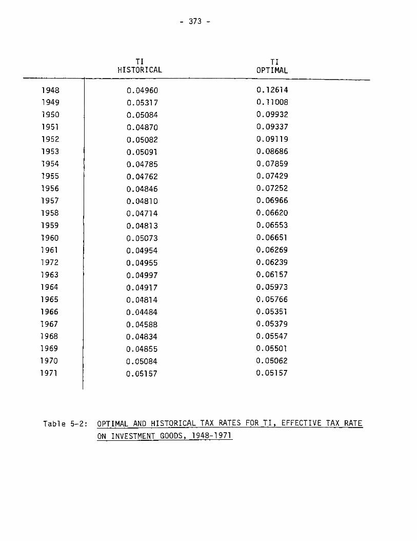
TIHISTORICAL
1948
1949
1950
1951
1952
1953
1954
1955
1956
1957
1958
1959
1960
1961
1972
1963
1964
1965
1966
1967
1968
1969
1970
1971
Table 5-2: OPTIMAL AND HISTORICAL TAX RATES FOR TI, EFFECTIVE TAX RATE
ON INVESTMENT GOODS, 1948-1971
- 373 -
0.04960
0.05317
0.05084
0.04870
0.05082
0.05091
0.04785
0.04762
0.04846
0.04810
0.04714
0.04813
0.05073
0.04954
0.04955
0.04997
0.04917
0.04814
0.04484
0.04588
0.04834
0.04855
0.05084
0.05157
TIOPTIMAL
0.12614
0.11008
0.09932
0.09337
0.09119
0.08686
0.07859
0.07429
0.07252
0.06966
0.06620
0.06553
0.06651
0.06269
0.06239
0.06157
0.05973
0.05766
0.05351
0.05379
0.05547
0.05501
0.05062
0.05157

- 374 -
TLHISTORICAL
TLOPTIMAL
1948
1949
1950
1951
1952
1953
1954
19551956
1957
1958
1959
1960
1961
1962
1963
1964
1965
1966
19671968
19691970
1971
0.081190.06825
0.06493
0.091630.10305
0.10104
0.08860
0.09044
0.09393
0.09545
0.09428
0.09484
0.09896
0.09805
0.10097
0.10179
0.09043
0.093510.09850
0.10184
0.11092
0.12099
0.11159
0.10282
Table 5-3: OPTIMAL AND HISTORICAL RATES FOR TL, EFFECTIVE TAX RATE
ON LABOR INCOME, 1948-1971
0.04971
0.03977
0.03130
0.073950.08518
0.08415
0.07035
0.07374
0.078720.08047
0.07837
0.07928
0.083830.08360
0.085270.088470.07692
0.08027
0.08410
0.08743
0.095880.09296
0.09491
0.10282
I
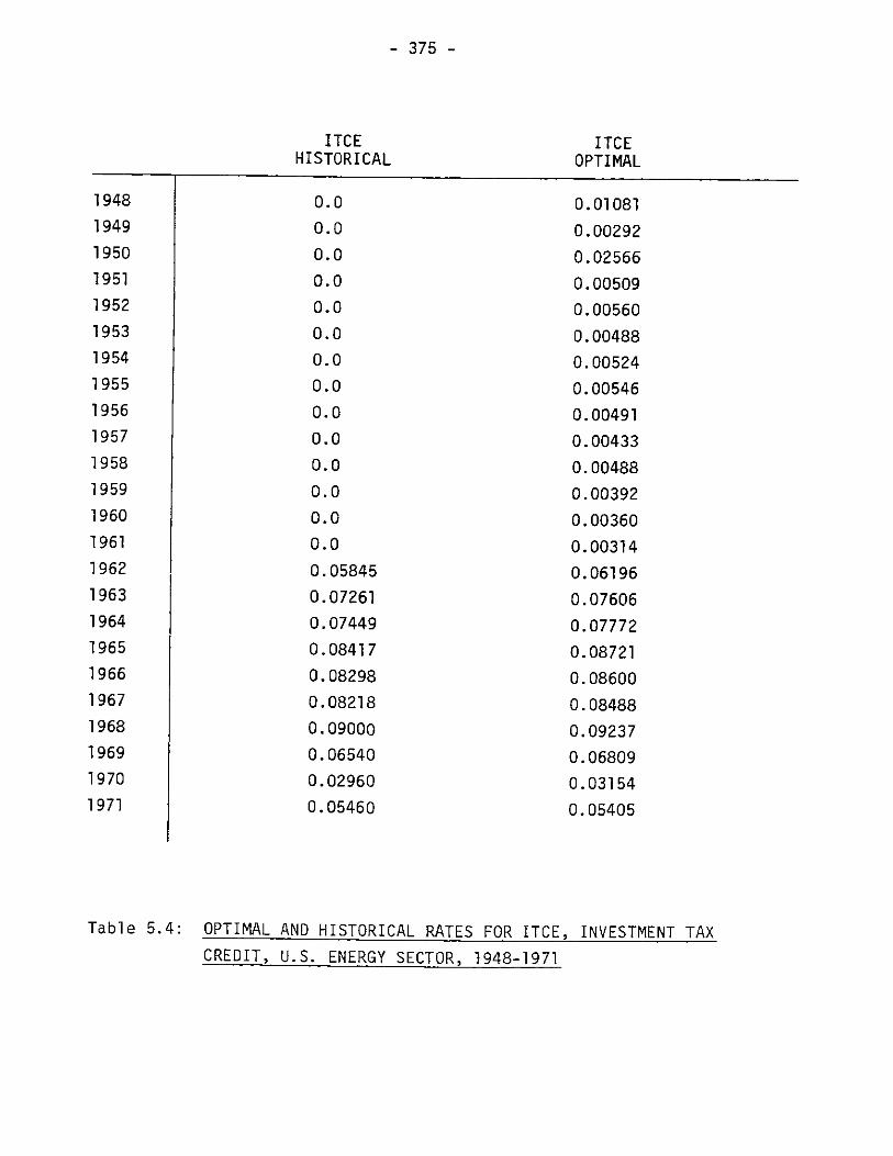
- 375 -
ITCE ITCEHISTORICAL OPTIMAL
1948 0.0 0.010811949 0.0 0.002921950 0.0 0.025661951 0.0 0.005091952 0.0 0.005601953 0.0 0.004881954 0.0 0.005241955 0.0 0.005461956 0.0 0.004911957 0.0 0.004331958 0.0 0.004881959 0.0 0.003921960 0.0 0.003601961 0.0 0.003141962 0.05845 0.061961963 0.07261 0.076061964 0.07449 0.077721965 0.08417 0.087211966 0.08298 0.086001967 0.08218 0.084881968 0.09000 0.092371969 0.06540 0.068091970 0.02960 0.031541971 0.05460 0.05405
Table 5.4: OPTIMAL AND HISTORICAL RATES FOR ITCE, INVESTMENT TAX
CREDIT, U.S. ENERGY SECTOR, 1948-1971

ITCNHISTORICAL
1948
1949
1950
1951
1952
1953
1954
1955
1956
1957
1958
1959
1960
1961
1962
1963
1964
1965
1966
1967
1968
1969
1970
1971
Table 5.5: OPTIMAL AND HISTORICAL RATES, FOR ITCN, INVESTMENT TAX
CREDIT, U.S. NON-ENERGY SECTOR, 1948-1971
- 376 -
0.0
0.0
0.0
0.0
0.0
0.0
0.0
0.0
0.0
0.0
0.0
0.0
0.0
0.0
0.34709
0.04311
0.04423
0.04998
0.04926
0.04879
0.05348
0.03887
0.01759
0.03210
ITCNOPTIMAL
0.08304
0.01956
0.19000
0.03128
0.03168
0.02143
0.03070
0.03241
0.03052
0.02669
0.02391
0.02360
0.02202
0.01930
0.46363
0.06379
0.06421
0.06927
0.06896
0.06674
0.06838
0.05637
0.03059
0.03209
I

- 377 -
TKEHISTORICAL
TKEOPTIMAL
1948
1949
1950
1951
1952
1953
1954
1955
1956
1957
1958
1959
1960
1961
1962
1963
1964
1965
1966
1967
1968
1969
1970
1971
0.3122
0.2656
0.2234
0.4168
0.2534
0.2679
0.2444
0.2558
0.3816
0.3757
0.2447
0.3670
0.3957
0.3904
0.3724
0.3792
0.3852
0.3784
0.3712
0.3592
0.4035
0.3964
0.3602
0.3600
Table 5-6: OPTIMAL AND HISTORICAL RATES FOR TKE, EFFECTIVE TAX RATE ON
CAPITAL PROPERTY, U.S. ENERGY SECTOR, 1948-1971
0.3080
0.2644
0.2147
0.4144
0.2513
0.2660
0.2429
0.2542
0.3799
0.3743
0.2432
0.3658
0.3946
0.3894
0.3714
0.3783
0.3844
0.3776
0.3705
0.3585
0.4029
0.3957
0.3597
0.3599
I

TKNHISTORICAL
1948
1949
1950
1951
1952
1953
1954
1955
1956
1957
1958
1959
1960
1961
1962
1963
1964
1965
1966
1967
1968
1969
1970
1971
Table 5-7: OPTIMAL AND HISTORICAL RATES FOR TKN, EFFECTIVE TAX RATE ON
CAPITAL PROPERTY, U.S. NON-ENERGY SECTOR, 1948-1971
- 378 -
I
TKNOPTIMAL
0.5098
0.3486
0.5109
0.5470
0.4873
0.5016
0.5059
0.5053
0.5008
0.4931
0.4956
0.5210
0.5194
0.5124
0.4887
0.4978
0.5056
0.4966
0.4873
0.4714
0.5296
0.5202
0.4728
0.4725
0.3721
0.3393
0.4303
0.5264
0.4688
0.4856
0.4917
0.4908
0.4876
0.4821
0.4814
0.5113
0.5103
0.5045
0.4840
0.4904
0.4984
0.4904
0.4809
0.4657
0.5224
0.5141
0.4684
0.4724

ControlvV *u* AVariable hist Opt hist opt hist opt
TCE -2.683789 -2.687329 14.64047 14.69238 2146746. 2154358. 7612.0
TI -2.683789 -2.685293 14.64047 14.66250 2146746. 2149971. 3231.0
TL -2.683789 -2.684070 14.64047 14.64458 2146746. 2147350, 604.0
TKE -2.683789 -2.683790 14.64047 14.64048 2146746. 2146748. 2.0
TKN -2.683789 -2.683935 14.64047 14.64259 2146746. 2147058. 312.0
ITCE -2.683789 -2.683792 14.64047 14.64052 2146746. 2146753. 7.0
ITCN -2.683789 -2.684194 14.64047 14.64640 2146746. 2147616. 870.0
* U =ln[-V] ** J = 146632. U AJ = Jopt ~-hist
Table 5-8: WELFARE GAINS FROM OPTIMAL TAX POLICIES UNDER ALTERNATIVE STRATEGIES
CA)

OPTIMAL PATHS OF ENERGY CONSUMPTION PER CAPITA UNDER ALTERNATIVE STRATEGIES, 1948-1971
HCEHISTORICALSIMULATION
0.048960.060070.06701
0.061500.065040.070180.080700.08528
0.091200.099520.101330.103720.10729
0.108880.119070.120270.127730.13075
0.139490.145780.149860.155740.172340.15972
HCEOPTIMAL
STRATEGY 1(TCE)
0.050630.061760.06898
0.062530.053130.056410.054970.05137
0.053020.063330.068340.073470.07793
0.080930.091710.099250.101810.10472
0.118570.129700.138290.153600.173070.15557
HCEOPTIMAL
STRATEGY 2(TI)
0.048980.059590.06668
0.061200.064840.069930.080340.08492
0.090880.099190.101020.103430.10703
0.108620.118830.120020.127480.13051
0.139250.145530.149610.155500.172070.15957
HCEOPTIMAL
STRATEGY 3(TL)
194819491950
19511952195319541955
19561957195819591960
19611962196319641965
196619671968196919701971
HCEOPTIMAL
STRATEGY 4(ITCE)
0.048960.060070.06701
0.061500.065040.070180.080700.08528
0.091200.099520.101320.103720.10729
0.108880.119070.120270.127730.13075
0.139490.145780.149850.155740.172340.15971
HCEOPTIMAL
STRATEGY 5(ITCN)(ITCN)I
0.048910.060060.06659
0.061490.065020.070160.080670.08524
0.091160.099490.101290.103690.10726
0.108850.117780.120240.127680.13069
0. 139430.145710.149790.155670.172280.159680.156
0.051660.062870.07049
0.063430.067610.072620.082910.08710
0.092870.101310.103250.105610.10913
0.110580.121140.121990.129470.13242
0.14150.147940.152150.161240.175370.15839
L46)
0
Table 5-9:

Table 5-10: OPTIMAL PATHS OF NON-ENERGY CONSUMPTION PER CAPITA UNDER ALTERNATIVE STRATEGIES, 1948-1971
HCNHISTORICALSIMULATION
HCNOPTIMAL
STRATEGY 1(TCE)
HCNOPTIMAL
STRATEGY 2(TI)
HCNOPTIMAL
STRATEGY 3(TL)
HCNOPTIMAL
STRATEGY 4(ITCE)
HCNOPTIMAL
STRATEGY 5(ITCN)
194819491950
19511952195319541955
19561957195819591960
19611962196319641965
196619671968196919701971
_____________________________________ L
1.04661.08751.0877
1.22251.36101.38361.24171.1607
1.17301.24511.25521.27941.2998
1.31711.35221.44011.41421.4214
1.49981.59971.63361.72341.82641.7088
1.13081.14911.1380
1.27672.08122.20982.84663.3248
3.55503.53403.59193.61263.7136
3.88263.96173.80134.27064.4442
4.52674.49654.60634.57964.90845.4549
1.04671.08351.0858
1.21781.35311.37631.23941.1596
1.17221.24421.25441.27861.2992
1.31641.35171.43931.41371.4209
1.49911.59891.63271.72261.82551.7083
1.01911.06291.0635
1.19851.31601.34201.22131.1489
1.16291.23291.24281.26691.2975
1.30581.33961.42631.40331.4112
1.48721.58431.61741.68961.80431.7079
1.04661.08751.0877
1.22251.36091.38361.24171.1608
1.17301.24511.25521.27941.2999
1.31711.35221.44011.41431.4214
1.49971.59961.63351.72341.82651.7088
1.04601.08741.0853
1.22231.36041.38321.24151.1606
1.17291.24501.25511.27931.2998
1.31701.35001.441.41411.4213
1.49961.59941.63331.72311.82631.7087
Tabl e 5-10: OPTIMAL PATHS OF NON-ENERGY CONSUMPTION PER CAPITA UNDER ALTERNATIVE STRATEGIES, 1948-1971

Table 5-11: OPTIMAL PATHS OF CAPITAL SERVICES TO HOUSEHOLDS PER CAPITA UNDER ALTERNATIVE
STRATEGIES, 1948-1971
HCKHISTORICALSIMULATION
194819491950
19511952195319541955
19561957195819591960
19611962196319641965
196619671968196919701971
HCKOPTIMAL
STRATEGY 1(TCE)
0.256390.273070.28934
0.313080.331190.340730.349780.35572
0.373880.387900.395490.395710.40605
0.416880.424850.437500.451740.46787
0.491010.514720.535570.557930.578050.58672
HCKOPTIMAL
STRATEGY 2(TI)
0.256390.273070.28993
0.314350.333140.343260.357420.36954
0.401120.432170.456990. 472500.50230
0.531270.557070.591120.627510.66538
0.717120.771950.825340.883120.938910.97544
HCKOPTIMAL
STRATEGY 3(TL)
0.256390.273070.28934
0.313050.331120.340600.349580.35546
0.373580.387560.395140.395350.40567
0.416490.424450.437070.451300.46741
0.490520.514200.535020.557350.577430.58609
HCKOPTIMAL
STRATEGY 4(ITCE)
0.256390.273070.28920
0.312750.330670.340010.348730.35435
0.372280.386210.393790.393990.40424
0.415000.422890.435420.449540.46552
0.488490.512040.532700.554790.574640.58290
HCKOPTIMAL
STRATEGY 5(ITCN)
0.256390.273070.28934
0.313090.331190.340730.349780.35572
0.373880.387890.395490.395710.40604
0.416880.424850.437490.451740.46787
0.491010.514720.535570.557930.578040.58672
0.256390.273070.28934
0.313080.331150.340680.349730.35566
0.373820.387840.395430.395650.40598
0.416810.424780.437420.451620.46774
0.490870.514580.535430.557770.577880.58655
wo00

OPTIMAL PATHS OF LEISURE PER CAPITA UNDER ALTERNATIVE STRATEGIES, 1948-1971
HLJHISTORICALSIMULATION
HLJOPTIMALSTRATEGY
(TCE)
HLJOPTIMALSTRATEGY 2(TI)
1
HLJOPTIMALSTRATEGY 3
(TL)
HLJOPTIMALSTRATEGY 4(ITCE)
HLJOPTIMALSTRATEGY 5
(ITCN)___________________________________i.
194819491950
19511952195319541955
19561957195819591960
19611962196319641965
196619671968196919701971
11.294311.211111.2993
11.411710.838110.903511.211111.3221
11. 326411. 307011.448711.437011.5212
11.775511.666411.724411.924212.0637
12.202712.330312.524012.691312.841513. 3164
11.128911.108611.2248
11.32649.74819.75189.10188.6321
8. 52918.66848.74938.77518.7898
8.92708.93438.18438.98428.9970
9.22449.52659.6639.983410.01619.9084
11.292111.285111.3432
11.466411.896411.959711.252211.3553
11. 388911.332611.470211.492411.5378
11.790911.678911.737111.935212.0738
12.211712.339212.532312.698912.848713.3180
coLA)
11.341411.249711.3329
11.448210.910210.965011.238111.3367
11.375211. 324011.466211.491111.5389
11.791211.683811.743711.938712.0770
12.219212.349912.544412.732912.867112.3180
11.294411.211111.2998
11.411710.838310.903511.211211.3221
11.362411.307011.448711.473011.5212
11.775511.666411.724411.924112.0637
12.202912.330412.524112.691312.841413.3164
11.303911.211511.3555
11.413510.841510.905911.213611.3250
11.365111.309211.405011.475011.5230
11.777011.763511.725611.926211.0657
12.205212.332812.525812.693912.842913.3166
i
Table 5-12:
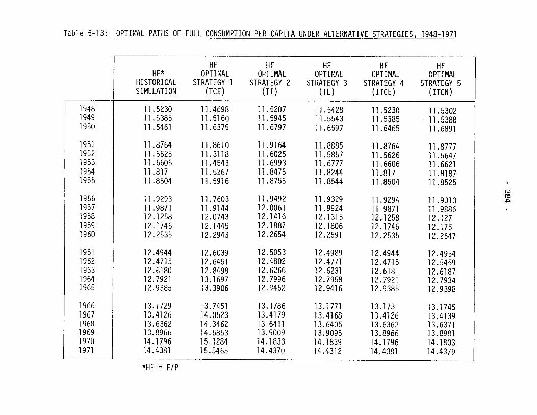
Table 5-13: OPTIMAL PATHS OF FULL CONSUMPTION PER CAPITA UNDER ALTERNATIVE STRATEGIES,
HF*HISTORICALSIMULATION
194819491950
19511952195319541955
19561957195819591960
19611962196319641965
196619671968196919701971
HFOPTIMAL
STRATEGY 1(TCE)
11.523011.538511.6461
11.876411.562511.660511.81711.8504
11.929311.987112.125812.174612.2535
12.494412.471512.618012.792112.9385
13.172913.412613.636213.896614.179614.4381
HFOPTIMAL
STRATEGY 2(TI)
11.469811.516011. 6375
11.861011.311811.454311. 526711.5916
11.760311.914412.074312.144512.2943
12.603912.645112.849813.169713.3906
13. 745114.052314.346214.685315.128415.5465
HFOPTIMAL
STRATEGY 3(TL)
11.520711.594511.6797
11.916411. 602511. 699311.847511.8755
11.949212.006112.141612.188712.2654
12.505312.480212.626612.799612.9452
13.178613.417913.641113.900914.183314.4370
HFOPTIMAL
STRATEGY 4(ITCE)
11.542811.554311.6597
11.888511.585711.677711. 824411.8544
11.932911.992412.131512.180612.2591
12.498912.477112.623112.795812.9416
13.177113.416813.640513.909514.183914.4312
HFOPTIMAL
STRATEGY 5(ITCN)
11.523011.538511.6465
11.876411.562611.660611.81711.8504
11.929411.987112.125812.174612.2535
12.494412.471512.61812.792112.9385
13.17313.412613.636213.896614.179614.4381
*HF = F/P
11.530211.538811.6891
11.877711.564711.662111.818711.8525
11.931311.988612.12712.17612.2547
12.495412.545912.618712.793412.9398
13.174513.413913.637113.898114.180314.4379
L41,OD3
1948-1971

- 385 -
REFERENCES TO CHAPTER V
[1] Koopmans, T. C., "On the Concept of Optimal Growth," EconometricApproach to Development Planning, Pontifical Academy of Sciences,Rome, 1965.
[2] Bauer, P. T., Economic Analysis and Policy in UnderdevelopedCountries, Duke University Press, 1957.
[3] Allais, M., Economie et Int6ret, Imprimerie Nationale, Paris,1947.
[4] Ramsey, F. P., "A Mathematical Theory of Savings," Economic Journal,38, December 1928.
[5] Britto, R., "Some Recent Developments in the Theory of EconomicGrowth: An Interpretation," Journal of Economic Literature, 1974.
[6] Harrod, R. F., Towards a Dynamic Economics, Macmillan, London,1948.
[7] Bbhm-Bawerk, E. von, Positive Theory of Capital, in Capital andInterest (1921), Translation 4th ed., Libertarian Press, 1959.
[8] Fisher, I., The Theory of Interest (1930), Kelley, New York, 1965.
[9] Weizssdcher, C. C. von, "Existence of Optimal Programs of Accumula-tion for an Infinite Time Horizon," Review of Economic Studies,April 1965.
[10] Hammond, P., and Mirlees, J. A., "Agreeable plans" in The Theoryof Economic Growth, Mirlees, J. A. and Stern, N., (eds.), Macmillan,London, 1973.
[11] Solow, R. M., "Intergenerational Equity and Exhaustible Resources,"The Review of Economic Studies, Symposium on the Economics ofExhaustible Resources, 1974.
[12] Rawls, J., A Theory of Justice, Harvard University Press, Cambridge,1971.
[13] Cass, D., "Optimum Growth in an Aggregative Model of CapitalAccumulation: A Turnpike Theorem," Econometrica, October 1966.

- 386 -
[14] Samuelson, P. A., "A Catenary Turnpike Involving Consumption and theGolden Rule," American Economic Review, June 1965.
[15] Solow, R. M.,' Growth Theory: An exposition, Oxford UniversityPress, New York/Oxford, 1970.
[16] Koopmans, T. C., "Stationary Ordinal Utility and Impatience,"Econometrica, 28, 1960.
[17] Morishima, M., Theory of Economic Growth, Clarendon Press, Oxford,1969.
[18] Green, H. A. J., Aggregation in Economic Analysis: An IntroductorySurvey, Princeton University Press, Princeton, 1964.
[19] Samuelson, P. A., Foundations of Economic Analysis, Harvard Univer-sity Press, Cambridge, 1947.
[20] Bergson, A., "On the Concept of Social Welfare," Quarterly Journalof Economics, 1954.
[21] Johansen, L., "An examination of the possible relevance ofK. Arrow's General Possibility Theorem for economic planning,"Economics of Planning, Vol. 9, 1969.
[22] Arrow, K. I., Social Choice and Individual Values, 2nd edition,Wiley, New York, 1966.
[23] Chase, S. B. Jr., Problems in Public Expenditure Analysis, TheBrookings Institution, Washington, D.C., 1968.
[24] Lerner, A. P., "Consumption-Loan Interest and Money," Journal ofPolitical Economy, October 1959.
[25] Arrow, K. J., and Kurz, M., Public Investment, The Rate of Return,and Optimal Fiscal Policy, Johns Hopkins Press,, Baltimore., 1970.
[26] Bellman, R. E., Dynamic Programming, Princeton University Press,Princeton, 1957.
[27] Pindyck, R. S., Optimal Planning for Economic Stabilization, North-Holland, Amsterdam/New York, 1973.
[28] Kendrick, D., and Taylor, L., "Numerical Solution of NonlinearPlanning Models," Econometrica, May 1970.
[29] Fair, R., "The Solution of Optimal Control Problems as MaximizationProblems," Annals of Social and Economic Measurement.
- 387 -
[30] Altans, M., Kuh, E., and Pindyck, R. S., "Optimal Control of aMacroeconomic Model Using Sequential Open-Loop Strategies," presentedat the 3rd World Congress of the Econometric Society, Toronto,Canada, August, 1975.
[31] Jacobson, D. H., and Mayne, D. Q., Differential Dynamic Programming,American Elsevier, 1970.
[32] Kelley, H. J., "Method of Gradients," in Optimization Techniques,A. Lietman, (ed.), Academic Press, New York, 1962.
[33] Halkin, H., "A maximum principle of the Pontryagian type forsystems described by nonlinear difference equations, SIAM Journalon Control, 4, No. 1, 1966.
[34] Phelps, E. S., Fiscal neutrality toward economic growth, McGraw-Hill, New York, 1965.

- 388 -
APPENDIX A: STATE-SPACE FORM OF MACROECONOMIC ENERGY MODEL
A.1 -- Introduction
A.2 -- Implicit State Equations
A.3 -- State Variables
A.4 -- Output Variables
A.5 -- Exogenous Variables
A.6 -- Parameters
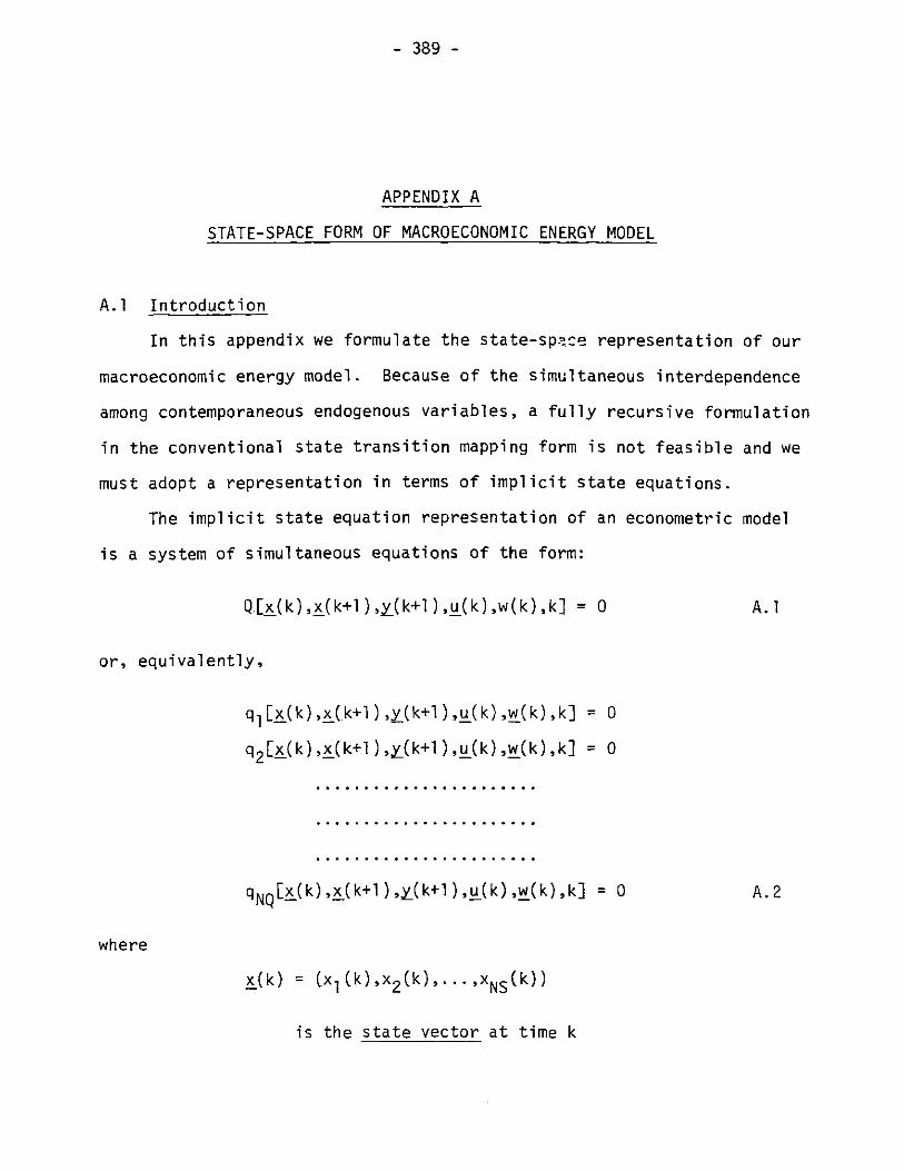
- 389 -
APPENDIX A
STATE-SPACE FORM OF MACROECONOMIC ENERGY MODEL
A.1 Introduction
In this appendix we formulate the state-space representation of our
macroeconomic energy model. Because of the simultaneous interdependence
among contemporaneous endogenous variables, a fully recursive formulation
in the conventional state transition mapping form is not feasible and we
must adopt a representation in terms of implicit state equations.
The implicit state equation representation of an econometric model
is a system of simultaneous equations of the form:
Q.[x(k),x(k+l),y(k+1),u(k),w(k),k] = 0 A.1
or, equivalently,
ql[x(k),x(k+l),y(k+l),u(k),w(k),k] = 0
q2[x(k),x(k+l),y(k+l),u(k),w(k),k] = 0
qNQ0[x(k),x_(k+ ),y(k+),u(k),w(k),k = 0A.2
where
x(k) = (x(k),x2 (k),...,xNS(k))
is the state vector at time k
1

- 390 -
x(k+l) = xl(k+Il),x2(k+1,...,xNS(k+l))
is the state vector at time k+I
y(k+l) = (yl(k+l),y2 (k+1),.. .,yNY (k_1))
is the output vector at time k+l
u(k) = (u1(k) ,u2jk),... ,uNC(k))
is the control vector at time k
w(k) = (w1(k),w(2),. ..2,wNW(k))
is the exogenous input vector at time k
The implicit state equation system A.1 should be viewed as a simul-
taneous equation system in the unknown vectors x(k+l) and y(k+l) with
the quantities x(k),u(k) and w(k) regarded as predetermined variables. It
follows that one must have dim Q = dim x+ dim y i.e. NQ = NS + NY.
In order to go from the standard econometric model form to the im-
plicit state equation form, it is sufficient to replace each unlagged
endogenous variable by an output variable y. and each lagged endogenous
variable by a state variable xi.
In the next section we list the implicit state equations for our
macroeconomic energy model. These state equations can be found to be in
precise correspondence with the 61 equations in standard econometric form
listed in Section 4.2.
In the remaining sections of this Appendix we list the definitions of
the state, output and exogenous variables in terms of the original
variables in the model.
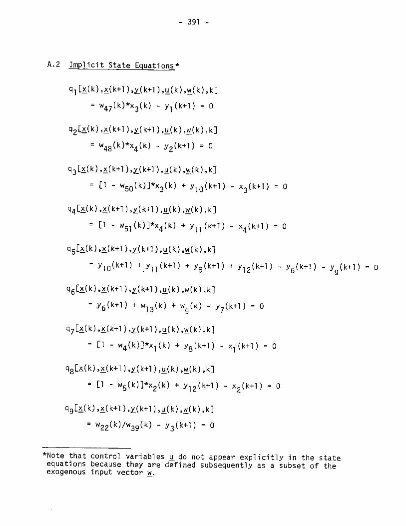
- 391 -
A.2 Implicit State Equations*
q1 [x(k) ,x(k+l) ,y(k+1) ,u(k) ,w(k) ,k]
= w4 7 (k)*x3 (k) - yl(k+l) = 0
q2[x(k)9,x(k+l)9,y(k+1),u(k),w(k),k]
= w48(k)*x4 (k) - y2(k+l) = 0
q3[x(k),x(k+1),y(k+l),u(k),w(k),k]
= [1 - w5 0 (k)]*x3(k) + yl0(k+l) - x3(k+l) = 0
q4j[x(k) , x(k+l) ,y(k+1 ) .u (k) ,w(k) ,k]
= [1 - w51 (k)]*x4 (k) + yul(k+l) - x4(k+l) = 0
q5[x_(k),x(k+1),y_(k+1),u(k),w(k) ,k]
= y10(k+l) +.y1 (k+l) + y8 (k+l) + y1 2(k+l) - y6(k+l) - y9(k+l) = 0
q 61x (k) ,x (k+1) ,y_(k+1) ,u_(k) ,w(k) ,k]
y6 (k+1) + w13(k) + w9(k) - y7 (k+1) = 0
q7[x(k),x(k+1),y(k+l),u(k),w(k).k]
- [1 - w4 (k)]*x1 (k) + y8 (k+l) - x(k+l) = 0
q8[x(k) ,x(k+1) ,y(k+l) ,u(k) ,w(k) ,k]
= [l - w5(k)]*x2 (k) + y12 (k+l) - x2(k+l) = 0
q9 [x(k),x(k+l) ,y(k+l),u(k),w(k),k]
= w2 2(k)/w3 9 (k) - y3 (k+1) = 0
*Note that control variables u do not appear explicitly in the stateequations because they are defined subsequently as a subset of theexogenous input vector w.

- 392 -
ql0[x_(k),x_(k+1),y_(k+l),u(k),w(k),k]
= w6 (k)/w3 9 (k) - y4 (k+1) = 0
q1 [x(k) ,x(k+1)g,y(k+1) ,u(k) ,w(k) ,kJ
= y13 (k+1)/w39 (k) - y5(k+1) = 0
ql2[x(k),x(k+1),y_(k+1),u_(k),w_(k),k]
- w69(k) + 0.35*ln[x6(k)] + 0.366*ln[x7(k)]+ 0.281705*ln[y7 (k+1)j
+ 0.2211*ln[x8(k)] + 0.370572*1n[w37(k-1)]
+ 0.18266*ln[xg(k)] + 0.363098*1n[w46(k-1)]
+ 0.026949*1n[w34 (k-1)] - ln[x5 (k)] = 0
q13[x(k),x(k+1) ,y(k+1),u(k),w(k),k]
= w64 (k)*y6 (k+1) - y1 0(k+1) = 0
q14 [x(k),x(k+1),y(k+1),u(k),w(k),kj
- w6 5(k)*y6 (k+1) - y1 (k+1) = 0
q15[x(k),x(k+1),y(k+1),u(k),w(k),k]
= w70 (k)*y6 (.k+1) - y8 (k+1) = 0
q16[x_(k),x_(k+ ),y(k+ ),u(k),w(k),k]
w 2(k)*y6(k+) - y2k)(k+1) = 0
q18 [x(k),x(k+1),y(k+H),u(k),w(k),k]
= W 72 (k)*[xl (k) + x2 (k)]I - Y13 (k+l) =0
qly[x(k),x(k+1),y(k+),u(k),w(k),k]
=y35(k+l)*y 34 (k+l)+ y3 2(k+1)*y3 1 (k+1) - y2 9 (k+l) = 0
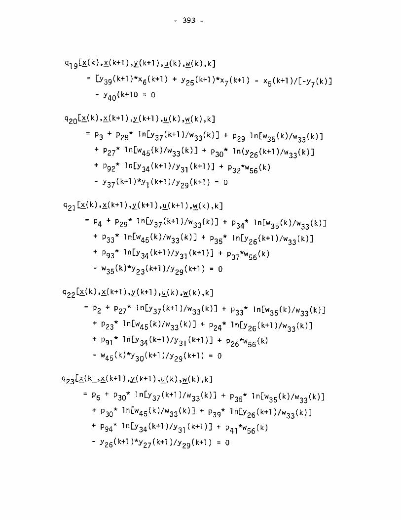
- 393 -
q19[x(k),x(k+1),y(k+1),u(k),w(k),k]
[y39 (k+1)*x6 (k+1) + y2 5 (k+1)*x7 (k+1) - x5(k+l)/[-y7(k)]
- y40 (k+10 = 0
q 20EX-(k),x_(k+l),y_(k+l),u(k),w(k),k]
P3 + p28* In[y37(k+1)1/w33(k)] + p29 ln[w35(k)/w33(k)]
+ 2* ln[w45(k)/w33(k)] + p30* ln(y26(k+1)/w33(k)]
+ p92* lnY34(k+1)/y31 (k+l)] + p32*w56(k)
- y37(k+f)*y1 (k+1)/y29(k+1) = 0
q21 [x(k),x(k+1),y(k+1),u(k+1),w(k),k]
P4 + p2 9* 1nEy 37 (k+1)/w33(k)] + p34* ln[w3 5(k)/w3 3(k)]
+ p33* In[w45(k)/w33(k)] + p35* InIY 26(k+1)/w33(k)]
+ p93* InEY34 (k+1)/y3 (k+1)] + p37*w56(k)
- w35 (k)*y2 3 (k+I1)/y2 9 (k+1) = 0
q22 [x_(k),x(k+1),y(k+1),u(k),w(k),k]
- P2 + P27* InEY 37(k+1)/w33 (k)] + p33* InwE 35(k)/w3 3(k)]
+ p23* ln[w45(k)/w33(k)] + p24* ln[Y 26 (k+1)/w33(k)]
+ p91* ln[y34 (k+1)/y31(k+i)] + p26*w56 (k)
- w45 (k)*y3 0 (k+1)/y29 (k+1) = 0
q 3x -(k_, x(k+l) ,y_(k+1) ,u_(k) ,w_(k) ,k]
= p6 + p30* 1nY37 (k+1)/w33(k)] + p35* ln[w35 (k)/w33(k)]+ p30* ln[w45(k)/w33(k)] + p39* In[y26(k+1)/w33(k)]
+ p94* In[y34(k+1)/y31(k+1)] + p41 *w56(k)
- y26 (k+1)*y2 7 (k+1)/y29 (k+l) = 0

- 394 -
q24[x(k),x(k+1),y(k+1),u(k),w(k),k]
= Pl4 + p70* lnlx 8(k+1)/w34(k)] + p71* 1n[w37(k)/w34(k)]
+ P69* ln[x9(k+1)/w34 (k)] + p72( ln[w46(k)/w34(k)]
+ P9 6* lnEx6(k+])/y7(k+1)] + p100* ln[x7(k+1)/y7(k+1)]
+ p74*w56(k) - x8(k+1)*y2 (k+1)/x5(k+1) = 0
q25[(k),x(k+1),y(k+1),u(k),w(k),k]
= p15 + p71* 1n[x8(k+1)/w34(k) * p76* ln[w37(k)/w34(k)]
+ p75* ln[x9(k+1)/w34(k)] * p7* ln[w46(k)/w34(k)]
+ p97* ln[x6(k+1)/y7(k+1)] + p101* ln[x 7(k+1)/y7(k+1)]
+ p79*w56(k) - w37 (k)*y24 (k+l)/x5(k+1) = 0
q 26 [x(k),x(k+1),y_(k+l),u_(k),w(k),k]
P12 + P69* ln[x8 (k+1)/w34 (k)] * p75* 1n[w37 (k)/w34(k)]
+ p62* ln[x9(k+f)/w34(k)] + p63* ln[w46(k)/w34(k)]
+ p95* lnEx6(k+1)/y7(k+1)] + p99* ln[x 7(k+1)/y7(k+1)]
+ p65*w56 (k) - x9(k+1)*y33 (k+1)/x5(k+1) = 0
q 27[x(k),x(k+l),y_(k+1),u(k),w(k),k]
=P7 + p72 * ln[x8(k+f)/w34 (k)] + p77* lnw37(k)/w34 (k)]
+ p63* In[x 9(k+1)/w34(k)] + p84* ln[w46(k)/w34 (k)]
+ p98* ln[x6(k+1)/y7(k+1)] + p102* In[x 7(k+f)/y7(k+1)
+ p86*w56 (k) - w4 6 (k)*y28 (k+1)/xx5(k+1) = 0
q28[x(k),x(k+1),y(k+1),u(k),w(k),k]
= p1 + P92* lnEY37 (k+1)/w33(k)] + p93 * ln[w35 (k)/w33(k)]
+ p * ln[w45 (k)/w33(k)] + P 94 In y26 (k+f)/w33(k)]
+ p21* lnEY34 (k+1)/y31 (k+1)] + p22*w56 (k)
- y35 (k+1)*y34 (k+1) /y29 (k+1) = 0

- 395 -
q29[x(k),x(k+1),y(k+l),u(k),w(k),k]
= p1 + p96* ln[x8(k+1)/w34(k)] + p97* ln[w37(k)/w34(k)]
+ p95* ln[x9(k+1)/w34(k)] + p98* ln(w46(k)/w34(k)]
+ p58* ln[x6(k+1)/y7(k+1)] + p80* ln[x7(k+1)/y7 (k+1)]
+ p6 0*w5 6 (k) - y3 9(k+1)*x6 (k+1)/x5 (k+1) = 0
q30[x_(k),x(k+l),y(k+1),u(k),w(k),k]
= p16 + p100* in[x 8(k+1)/w34(k)] + p101k ln[w37(k)/w34(k)]
+ p99* in[x9(k+1)/w34(k)] + p102* ln[w46(k)/w34(k)]
+ p80* ln[x6(k+1)/y7(k)] + p81* ln[x7(k+l)/y7(k+1)]
+ p82 w56(k) - y25(k+1)*x7(k+1)/x5 (k+1) = 0
q31 [x(k),x(k+1),y(k+1),u(k),w(k),k]
= ylg(k+1) + w53 (k) + w12(k) + w7(k) - x6(k+1) = 0
q 32[x_(k),x_(k+l),y_(k+l),u(k),w(k),k]
= y2 7 (k+l) + y28(k+1) - x7(k+1) = 0
q33 [x(k),x(k+1),y(k+1),u(k),w(k),k]
= y36 (k+1) + w52(k) + w11(k) + w8(k) - y34 (k+1) = 0
q34[x(k) ,x(k+1) ,y(k+1) ,u(k) ,w(k) ,k]
- y3 3(k+1) + y30(k+1) - y31(k+1) = 0
q 35[x (k),x_(k+l),y_(k+l),u_(k),w(k),k]
- [w4 1(k)*w5 2 (k) + w30(k)*w11 (k) + w2 7(k)*w8 (k)
- (1 + w54(k))*y35(k+1)*y34 (k+1)]/[-y36(k+1)] - y41(k+1) = 0

- 396 -
q36[x(k),x(k+1),y(k+l),u(k),w(k),kJ
= [w3 1(k)*w13(k) + w28(k)*wg(k)
- (1 + w55 (k))*y40(k+1)*y7 (k+1)]/[-y6 (k+1)] - x10(k+1) = 0
q37[x(k),x(k+1),y(k+1),u(k),w(k),k]
= w45 (x)*y3O(k+1) + xg(k+1)*y3 3 (k+1) - y3 2(k+1)*y3 1(k+1) = 0
q38[x(k) ,x(k+1) ,y(k+1) ,u(k) ,w(k) ,k]
= y26 (k+1)*y27 (k+1) + w4 6(k)*y28 (k+1) y25 (k+1)*x7 (k+1) = 0
q39[x(k),x(k+1),y(k+1),u(k),w(k),k]
= w66 (k)*y3 2 (k+1) - x9(k+1) = 0
q40[x(k) ,x(k+1) ,y(k+1) ,u(k) ,w(k) ,k]
= w6 3(k)*y2 5 (k+1) - y2 6 (k+l) = 0
q 41 [x(k),x(k-1),y_(k+1),u(k),w(k),k]
= y23 (k+l) + y24 (k+1) + w21 (k) + w23(k) + w24 (k) - y2 2(k+1) =0
q42[f(k),x(k+1),y(k+),u(k),w(k),k]
= [1 - w59(k)]*[w3 5 (k)*y23 (k+1) + w37(k)*y24 (k+1)
+ w3 6(k)*w2 1(k) + w38 (k)*w2 3 (k)] - y2 0 (k+1)*y 22 (k+1) = 0
q43[x(k),x(k+1),y(k+1)s,u(k),w(k),k]
= [(y37 (k+i)*w47 (k) - x10(k+i)*w6 1(k))*(1 - w57(k))/
(1 - w5 7 (k)*w43(k) - w19(k)) + w1(k) - w50(k)*xl0(k+l)]/
x10 (k) - y42 (k+1) = 0

- 397 -
q44[x(k),x(k+1),y_(k+1),u(k),w(k),k]
= [(x8 (k+1)*w48 (k) - xl(k+l)*w62(k))*(1 - w58(k))/
(1 - w58 (k)*w44 (k) - w20(k)) + w1(k) - W51 (k)*xOK+1)]/
x10(k) - y43 (k+1) = 0
q45[x(k) ,x(k+1) ,y(k+1),u(k),w(k),k]
- [1 + Y1 4(k+1)]*x 11(k)*[p10 4 + p90*w56(k)]*[{ +
(p*y20(k+1)*y3(k+1) + p19 *y4(k+1))/(1 + Y14(k+1))*xll(k)]/
[p103 + P52*w56 (k)] - y16(k+1) = 0
q46[x(k) ,x(k+1) ,y(k+1),u(k),w(k),k]
-[p8 + P45* ln(y21 (k+1)) + p47* ln(y1 7(k+1)) + p46*ln(y5 (k+l))
+ p4* In(y38(k+1)) + p48*w56(k) + y20(k+1)*y21 (k+1)/y16 (k+1)]
=0
q47 [x(k),x(k+l)q,y(k+1),u(k),w(k) ,k]
-[p10 + p47* ln(y21(k+1)) + p83* lny(k+1))
+ p68* ln(y5(k+1)) + p61* !n(Y38(k+1)) + p89*w56(k)
+ w25 (k)*y17 (k+1)/y16(k+1)] = 0
q48[x(k),x(k+1) ,y(k+1),u(k),w(k),k]
-[p9 + p46* ln(y21(k+1)) + p68* ln(y17(k+1)) + p50* ln(Y 5(k+1))
+ p49 In(Y38(k+1)) + p51*w56(k) + y15(k+1)*y5 (k+1)/y1 6(k+1)] = 0
q49[x(k),x(k+1),y(k+1),u(k),w(k),k]
= y38 (k+1)*w39 (k) - y3 6(k+1) = 0
q50[x(k) ,x(k+1) ,y(k+1) ,u(k+1) ,w(k+1) ,k]
= y1 7 (k+1)*w3 9 (k) - y18(k+1) = 0

- 398 -
q51 [x(k),x(k+1)s,y(k+1),u(k),w(k),k]
= y1 8 (k+1) - w2(k) - y1g(k+1) = 0
q 52 Ex(k),x(k+1),y_(k+l),u(k),w(k),kI
- w67(k)*[x3(k)*y42 (k+1) + x4(k)*y43(k+1)]/[x3(k) + x4(k)
+ x1(k) + x2(k)] - y14(k+1) = 0
q53[x(k),x(k+1),y(k+1),u(k),w(k),k]
= [y1 6(k+1) - y38 (k+1)*y41 (k+1) - y5 (k+1)*y15(k+1)
- y2 1(k+1)*y 2 0 (k+1)]/y17 (k+1) - w25(k+1) = 0
q54[x(k),x(k+1) ,y(k+1),u(k),w(k),k]
= [y37(k+1)*y(k+1) + w35(k)*y23(k+1) + w45 (k)*y3 0 (k+1)
+ y26 (k+1)*y2 7 (k+1) - y35 (k+1)*y34 (k+1) - Y32(k+1)*y31(k+1)]/
[-w33 (k)] - y44 (k+1) = 0
q55[x(k),x(k+1),y(k+1),u(k),w(k),k]
= [x8 (k+1)*y2(k+1) + w37(k)*y24 (k+1) + xg(k+1)*y33(k+1)
+ w4 6(k)*y2 8 (k+1) - y3 9(k+1)*x6 (k+1) - y2 5 (k+1)*x7 (k+1)
- y40(k+1)*x7 (k+1)*y7*k+1)]/[-w34 (k)] - y45(k+1) = 0
q56 [x(k),x(k+1),y_(k+1),u(k),w(k),k]
= [w4 2(k)*w53 (k) + w32 (k)*w12 (k) + w2 6(k)*w7(k)
- (1 + w60 (k))*y3 9 (k+1)*x6 (k+1)]/[-y19 (k+1)1 - y46 (k+1) = 0
q57[x(k),x(k+1),y(k+1),u(k),w(k),kJ
= x10(k+1)*[x3 (k+1) + x4(k+1) + x1(k+1) + x9(k+1)]*w68 (k)
+ w29 (k)*wl 0(k) + w4 0(k)*w49 (k) - Y47(k+l)

- 399 -
q58[Ex(k)s,x(k+1) ,y(k+1),u(k),w(k),k]
= y47 (k+1)/w39(k) - xl(k+1) = 0
q59 [x(k),x(k+1),yf k+1),u(k),w(k),k]
= y2 1 (k+1)*w3 9 (k) - y4 8(k+1) = 0
q60[x(k),x(k+l),y_(k+1),u(k),w(k) ,k]
x12(k+) - (0.822514*y 2 1 (k+1) + 1.07866*y 5 (k+1)
+ 0 .934 9O9*y 7(k+l) + 2.49568*y3 8 (k+1) + 0.855918 = 0
q61 [x(k),x(k+1),y(k+1),u(k),w(k),k]
Sx 15(k+1)*y6 (k+1) + w2 9 (k)*[wl1 (k) - wl(k-1)] + w40(k)*[w49(k)
- w4 9 (k-1)] - y49 (k+1) = 0
A.3 State Variables
x1 = KCD
x2 = KRS
x 3 = KSE
x 4 = KSN
x5 = VN
x 6 = NC
x 7 = NM
8 ~= KN
9 =EMN
x 10 ~ Pi
x 11 = HW
x12 = F

- 400 -
A.4 Output Variables
yl = KE
Y2 = KN
y 3 = HLH
Y4 = HEL
y 5 = HCK
y6 = I
Y7 = NI
Y8 = ICD
Y9 = IMIN
y10 = INE
Yl= INN
Y12 = IRS
yl 3= CK
Y14 = MW
Y15 = PCK
Y16 = VF*
yl 7 = HCND
Y18 = CND
Yi9 = CNQ
Y20 = PL
Y21 = HLJ
Y22 = L
Y23 = LE
Y24 = LN
*VF = PF-F

- 401 -
Y25
Y2 6 =
Y27 =
Y28=
y2 9 =
y3 0 =
Y3 1 =
32
y3 3 =
Y3 4 =
Y3 5 =
Y36 =
Y3 7 =
Y38 =
Y3 9 =
Y4 0 =
Y4 1 =
Y42 =
Y4 3 =
y4 4 =
y4 5 =
Y4 6
Y4 7 =
y4 8 =
Y4 9 =
PNM
9NME
NME
NMN
VE
EME
EM
SEM
EMN
EC
PEC
CE
PKE
HCE
PNC
PNI
PCE
ME
MN
RE
RN
PCN
w
LJ
s

- 402 -
A.5 Exogenous Variables
wI = CAPG
w2 = cIM
w3 = CK
w 4 = DCD
w5 = DRS
w 6 = EL
wy7 = EXN
w8 = EXE
wg9 = EXI
w 10= G
w ll= GEQ
wl12 = GNC
w 3 = GNI
w 14= DUMM*
wl15 = DUM2*
wl16 = DUM3*
w 17 = DUM4*
wl18 = DUM5*
* 9 = ITCE
w20 = ITCN
w 21= LG
w 22= LH
w23 = LR
dummy variables used internally in the OPCON model subroutine.*These are

- 403 -
w24 =LU
=25 CND
* =26 PEXC
W27 PEXE
=28 PEXI
*w29 PG
* =30 GE
w31 PGI
=32 PGNC
* =33 PRE
w34 -RN
W35 PLE
=36 PLG
=37 LN
*w38 PLR
w39 PR
W40 PSTE
*w41 -PSTN
w42 =VDN
=43 =XEE
* =44 XNN
w45 = QKE
w46 = QKN
w47 =R
w 48 =REPE
w 4 = REPN

- 404 -
w 50= STE
w51 = STN
W52= TEC
w53 = TI
w54 = t (TIME)
w 55= TKE
w 56= TKN
w 57= TL
w 58= TNC
w 59= TPE
w 60= TPN
w 61= ZEN
S 62 = ZINE
w63 = ZINN
w 64= ZNE
w 65= ZRN
w6 6 = ZW
w67 = ALAG
w68 = ZICD
w 69= ZIRS
w 70= QCK
A.6 Parameters
p1 = AEC
p2 = AEE

- 405 -
p3 = AEK
p4 = AEL
p5 = AEM
p6 = AEN
p7 = AER
p8 = AJ
p9 = AK
p 1 0 = AN
p1 1 = ANC
Pl2 = ANE
p 1 3 = ANI
p1 4 = ANK
p1 5 = ANL
p1 6 = ANM
P17 = ANN
p1 8 = ANR
p 1 9 = A
P2 0 = A2
P21 = BECC
P22 = BECT
P23 = BEEE
p2 4 = BEEN
P25 = BEER
p2 6 = BEET
P27 = BEKE
p2 8 = BEKK
P29 = BEKL

- 406 -
p3 0 = BEKN
p3 1 = BEKR
P32 = BEKT
p3 3 = BELE
p3 4 = BELL
p3 5 = BELN
p3 6 = BELR
p3 7 = BELT
p3 8 = BEMC
p3 9 = BENN
P40 = BENR
p4 1 = BENT
P42 = BERR
p4 3 = BERT
p4 4 = BJE
p4 5 = BJJ
p4 6 = BJK
p4 7 = BJN
p4 8 = BJT
p4 9 = BKE
p5 0 = BKK
p5 1 = BKT
p5 2 = BNCC
p5 3 = BNCM
p5 4 = BMJ
p5 5 = BMK
p5 6 = BMN
- 407 -
p5 7 = BMT
p5 8 = BNCC
p5 9 = BNCM
P60 = BNCT
P61 = BNE
P62 = BNEE
p6 3 = BNEN
P64 = BNER
P65 = BNET
P66 = BNIC
p6 7 = BNIM
P68 = BNK
P69 = BNKE
P70 = BNKK
P7l = BNKL
P72 = BNKN
p7 3 = BNKR
p7 4 = BNKT
p7 5 = BNLE
p7 6 = BNLL
p7 7 = BNLN
p7 8 = BNLR
p7 9 = BNLT
p8 0 = BNMC
P81 = BNMM
P82 = BNMT
p8 3 = BNN

- 408 -
p84 = BNNN
p85 = BNNR
p86 = BNNT
p87 = BNRR
p88 = BNRT
p89 = BNT
P90 = BO
p91 = CECE
p92 = CECK
p9 3 = CECL
p9 4 = CECN
p9 5 = CNCE
P96 = CNCK
p97 = CNCL
p9 8 = CNCN
p9 9 = CNME
p1 0 0 = CNMK
pi 01 = CNML
pl 02 = CNMN
p1 0 3 = GM
pl 04 = GO

- 409 -
APPENDIX B: OPCON -- _A GENERAL PURPOSE COMPUTER CODE FOR THE SOLUTION
OF NONLINEAR TIME-VARYING OPTIMAL CONTROL PROBLEMS
BA -- Introduction
B.2 -- Program Highlights
B.3 -- Algorithms
B.4 -- Implicit State Equations, Algebraic Constraints
B5 -- Summary

- 410 -
APPENDIX B
OPCON -- A GENERAL PURPOSE COMPUTER CODE FOR THE SOLUTION OF NONLINEAR
TIME-VARYING OPTIMAL CONTROL PROBLEMS
B.1 Introduction
This appendix presents a brief summary of the structure and capa-
bilities of OPCON, a computer code designed for the solution of nonlinear,
time-varying optimal control problems. Several features of the program
are specifically designed for use in connection with econometric models.
The code is entirely written in FORTRAN IV and its design is such that
it places minimum demands on the software operating environment. Because
of the use of object-time dimensioning, the size of the internal array
spaces and therefore the overall storage requirements are at the control
of the user. There are, therefore, no hard limits on the dimensionality
of the systems that can be handled.
A popular approach to the solution of large-scale optimal control
problems for econometric models has been the reformulation of the problem
as a static optimization problem which involves "stacking up" the time
sequence of control variables into one large vector. One of the arguments
often made in favor of this approach is that it bypasses the apparently
bewildering problem of computing implicit Hamiltonians in models for
which contemporaneous endogenous variables are mutually interdependent in
a simultaneous fashion. It turns out that this difficulty is more apparent
than real. The static optimization approach ignores the central principle
of optimal control theory: i.e., the decomposition of a dynamic problem

- 411 -
TABLE BI: SYNOPSIS OF OPCON
o Purpose:
o Method:
o Scope:
o Input:
Output:
To solve optimal control problems of nonlinear time-varying
systems in discrete-time with nonlinear cost functionals.
There are four optional solution methods:
(i) First-order differential dynamic programming, small
variations method
(ii) Second-order differential dynamic programming, small
variations method
(iii) Min-H first variation method
(iv) Differential dynamic programming, global variations
method*
There are no hard limits on the dimensionality of the systems
that can be handled by OPCON.
The user, in addition to providing a subroutine that specifies
the state equations and the cost functional, must specify an
initial guess for the optimal control path and must give the
value of the initial state vector. The user has to select
from the various optional features provided for a given
solution method.
After convergence, the program will print out the optimal
control path and the optimal state trajectory; if convergence
is not achieved within the prescribed number of iterations,
then the best current approximations to the optimal control
path and state trajectory will be printed. More detailed
printouts of individual iterations as well as plotting of
any system variables are included as optional features.

- 412 -
L .1- _________
Fig. Bl: Information flow between OPCON and user's sub-program
Command Program(user-supplied)
-- Number of words requiredfor all arrays
-- I/0 units
OPCONLoad Module
(pre-compiled)
Input Data File(user-supplied)
--Dimensions-- Parameter values-- Exogenous inputs-- Option indicators, etc.
MODELSubroutine
(user-supplied)
state equations
cost functional

- 413 -
into a sequence of static problems and, in addition, fails to provide the
conceptual insights derived from the state-space formulation -- e.g., the
information provided by the optimal co-state vectors and local feedback
matrices.
There are three optional solution methods in OPCON, all of which are
generalizations of well-known algorithms in optimal control theory to the
case of implicit state transition mappings and implicit Hamiltonians:
(a) First-order differential dynamic programming, small variationsmethod (DDPl)
(b) Second-order differential dynamic programming, small variationsmethod (DDP2)
(c) First-order Min-H method (MINHl)
The various solution algorithms differ as to their relative efficien-
cy, robustness and convergence properties. The versatility thus afforded
is imperative when dealing with nonlinear dynamic optimization problems.
OPCON incorporates special-purpose numerical differentiation subroutines
for the efficient computation of first- and second-order derivatives for
the case of implicit systems.
In order to use OPCON, the user must provide a subroutine in FORTRAN
that gives the model's equations and structure of the cost functional, he
must also write a command program consisting of two instructions that de-
fine the overall array space and the input and output devices to be used.
The model subroutine and the command program constitute the user sub-
program. The user sub-program is then compiled and linked with the pre-
compiled OPCON load module. In addition, the user must provide an input
data file that gives information on dimensionality of the variables,
exogenous inputs, selection of options, etc. The standard option in OPCON
is numerical computation of derivatives; if the user wishes to by-pass

- 4.14 -
this option and enter analytical derivatives, he must include them in
appropriate sub-routines as part of the user's sub-program.
B.2 Program Highlights
The following are some of the main provisions and optional features
of OPCON:
0 The program can handle systems with implicit state equations and
algebraic constraints. This provision is especially important for
applications involving econometric models, where it is often not
possible to recast even the simplest systems in explicit state
equation form.
o Special provisions are included for the treatment of block-
recursive systems; the user must specify the number and composi-
tion of the blocks.
o Each optional solution algorithm may be used individually or se-
quentially in a sequence specified by the user; in the case of
sequential use, the control variables for each succeeding optimi-
zation will be initialized to the values resulting from the
preceding run.
* In subroutine DDP1, step-size adjustment can be determined by any
one of three optional methods: if no direct search is desired,
then the step-size will be adjusted uniformly across time-sLages;
if it is desired to search for an optimum step-size at each time-
stage, the user can select between two linear search methods:
golden section search and quadratic interpolation.
* Subroutines DDP2 and DDPG include various optional features in

- 415 -
addition to the standard options associated with second-order dif-
ferential dynamic programming. For instance, the local feedback
gain matrices may be set equal to the identity matrix, or may be
recomputed only every k1 time-stages or every k2 iterations. In
addition, several provisions are included to correct for the cases
where the Hessian matrix is ill-conditioned or is indefinite and
fails to generate descent directions.
After convergence occurs in DDP2 or DDPG, there is the option of
printing out a sequence of matrices that correspond to a time-
varying linearization about the optimal trajectory; the option
includes printouts of the linearized system matrix A(t), the
linearized input matrix B(t), the Ricatti matrix corresponding to
the linearized system, K(t), the linearized gain matrix G(t) and
the linearized closed loop system matrix ACL(t).
o The derivatives required by the selected solution method can be
pre-computed analytically and entered into the program as part of
the user sub-program. Alternatively, the user has the option of
requesting that all required derivatives be computed internally
by appropriate numerical differentiation subroutines included as
part of OPCON.
o Standard output of the program includes a listing of all relevant
input data and parameters and the optimal control path and optimal
state trajectory after convergence; the user can suppress part of
this standard output if desired. In addition, the user can re-
quest more detailed printouts of the solution process, including
values of the current control paths and state trajectories at each
iteration. A plotting subroutine will plot graphs of any single

- 416 -
variable or pair of variables as a function of time.
0 Special provisions are included that allow for recursive simula-
tions and optimizations. These options facilitate the performance
of:
-- Sensitivity studies
-- Use of penalty function methods
-- Convexification of singular or ill-conditionedqproblems
B.3 - Algorithms
The two differential dynamic programming methods available in OPCON
(DDPl, DDP2) are generalizations of the first- and second-order algorithms
proposed by Jacobson and Mayne [Bl1; the development of these algorithms
is based on the application of the principle of optimality about a local
neighborhood of a nominal trajectory, using a Taylor series expansion of
the cost-to-go function. The MINHl algorithm is a straightforward gen-
eralization of Kelley's method [B2] and is most easily derived by a direct
application of the Minimum P-inciple. The four algorithms, when considered
jointly, span a fairly wide range in terms of their relative efficiency,
robustness and convergence properties. The first-order differential dy-
namic programming method with small variations (DDPl) is the least expen-
sive of the methods and, correspondingly, is the least attractive from the
standpoint of robustness and convergence properties; MlNHl and DDP2 are
approximately equal in robustness but DDP2 has better convergence proper-
ties and is more expensive. A short description of each method follows:
(a) DDP1 - First-order differential dynamic programming, small variations
The first-order small variations version of differential dynamic pro-
l
- 417 -
gramming is a successive approximation algorithm in which at every itera-
tion a new control sequence is constructed which minimizes a linearized
expansion of the value function about the current nominal trajectory. It
has a good deal of common structure with various gradient-type algorithms
and differs from them primarily in the way the step-size is controlled so
as to remain within the region of linearization.
The main steps in the algorithm are as follows:
Step 1.- Given an initial state vector x and an initial guess for
the control variables [h], compute the corresponding nominal trajectory
[x4].
Step 2.- Starting at the terminal time NT, compute the sequence of
first-order approximations to the value function [Vk(x)] about the
nominal trajectory. Compute the expected change in cost ao.
new
Step 3.- Compute a new control sequence [uk] as follows:
new old kuk = uk - e-Hu
where c is the step-size and H k is the gradient of the Hamiltonian withu
respect to u.
Step 4.- Using the updated control sequence, compute the corres-
ponding state trajectory and the new value of the cost function V; compare
the change in cost V - V with the expected change in cost a0 . If V - V
is negative and IV - Vf/a0 > c, accept the new trajectory. Otherwise,
reduce e and repeat Step 3.
Step 5.- Reset the current nominal control path and state trajectory,
reset the step-size and go to Step 2.

- 418 -
Stp 6.- Stop when I a0 IIn subroutine DDPi, the user is required to provide the following input
parameters:
EPSIL - Initial value for the step-size.
DELMIN - Lower bound on the ratio of actual to expected cost change
for acceptance of new trajectory (c in the above descrip-
tion). Typical value is 0.5.
ETA - Parameter to be used as a convergence criterion (').
ITRM - Maximum number of iterations to be performed.
IYRCHM - Maximum number of step-size reductions to be performed in
any one given iteration.
Step-size adjustment will be performed by one of three available
methods according to the value of the indicator ISERCH:
If ISERCH=0 Step size will be set equal to predetermined fixed
value uniformly across time stages
If ISERCH=1 A search for the optimum step-size will be performed by
the golden section search method (Murray [B3], p. 9)
If ISERCH=2 A search for the optimum step-size will be performed by
the quadratic interpolation method (Murray [B3], p. 9)
The two search methods provided, based on function comparison and
function approximation, respectively, can be used either separately or
jointly to synthesize virtually any arbitrary search method.
(b) DDP2 - Differential Dynamic Programming; Second-Order Small Variations
The successive approximations algorithm implemented in DDP2 can be
derived by formally applying the principle of optimality to a second-order
approximation of the value function about the current nominal trajectory.

- 419 -
Special conditions are applied to insure that at every iteration, the
updated control path and corresponding trajectory will not go outside the
region where the quadratic approximation is valid. In the case of linear
systems and quadratic criteria, the algorithm reduces to the solution of
the discrete-time Riccati equation and thus converges in one iteration.
Structurally, the algorithm bears resemblance to the second-variation
successive sweep method (McReynolds and Bryson [B4]) and other Newton-type
algorithms but is computationally more efficient and does not impose the
restriction of positive definiteness on the inverse Hessian H uu* The
major steps of the second-order differential dynamic programming algorithm
are the following:
Step 1.- Same as DDPl
Step 2.- Calculate the sequence of second-order approximations to
the value function backwards in time: [V (xk)] and
[Vx()] ; store the sequence of local gain matrices.
Step 3.- Compute a new control sequence using
new old
uk = uk + Es.-Pk + Qko(xk~)
where [Pk] and [Qk1 are sequences of local gain matrices
computed in Step 2.
Steps 4-6.- Same as DDPl
The set of parameters required from the user are the same as those
listed for DDPl. In addition, there exist the following provisions:
o The matrices Pk and Qk in Step 3 are computed in terms of the in-
verse of the extended Hessian matrix Ck. In the event that Ck is either
singular, ill-conditioned or indefinite, the basic method must be modified
in order to generate descent directions. OPCON includes the following

- 420 -
options to deal with this situation:
(i) Replace Ck by the identity matrix I for those time-stages for
which it is ill-conditioned or indefinite.
(ii) Substitute the inverse of Ck by the generalized Penrose
inverse (Wilkinson [B5]).
(iii) Use Greenstad's variant of Newton's method in order to improve
the direction of search when C k is indefinite. This can be
cc;tly since it involves an eigenvector analysis (Greenstadt
[B6]).
(iv) Modify Ck by using Murray's variation of the Marquardt-
Levenberg method. This involves the Cholesky factorization
of Ck suitably modified so as to insure numerical stability
even when it is not positive-definite (Murray [B3]).
Since these modifications of the basic method -- especially (iii)
and (iv) -- can become computationally costly, it is recommended that
they be used only in the event that the simple variation indicated in (i)
has been shown to be ineffective.
o If the user so specifies, the matrices Pk and Qk will only be re-
computed every k1 time-stages or every k2 iterations. This may result in
substantial computational savings and may not hinder the overall effect-
iveness of the algorithm especially when restricted to the early set of
iterations.
o After convergence occurs in DDP2, the user has the option of re-
questing printouts of the following time-varying matrices linearized
about the optimal trajectory:
- Linearized system matrices A(k)

- 421 -
- Linearized input matrices B(k)
- Riccatic matrix corresponding to the
linearized system K(k)
- Linearized gain matrix G(k)
- Linearized closed-loop system matrix ACL(k)
(c) MINHl - -First-Order Min-H Method
The first-order Min-H method is an iterative scheme wherein each suc-
cessive control sequence is selected after minimizing the Hamiltonian at
each stage with respect to the control inputs, where the Hamiltonian is
computed using a first-order expansion of the value function. The basic
steps are:
Step 1.- Same as DDP1
Step 2.- Same as DDPl
Step 3.- Find ur to minimize the Hamiltonian function
oldHk (k, uk' Pk
Step 4.- For X = 1, define the new control sequence
new old old
uk = uk - x(uk - u )Step 5.- If cost does not decrease, reduce < , 0 < < 1,
repeat Step 4.
Step 6.- Stop if no improvement for X <
The crucial step, of course, is the minimization of the Hamiltonian in
Step 3. Three options are available to perform this functional minimi-
zation:
- Newton (indirect)

- 422 -
- Davidon-Fletcher-Powell
- Gauss-Newton
B.4 - Implicit State Equations, Algebraic Constraints
A dynamical system in discrete time can be characterized by means of
the state equation
x(k+l) = f[x(k), u(k), w(k), k (1)
where x is the state vector, u is the control vector and w is a vector
of exogenous variables -- i.e., uncontrollable inputs.
If the state transition mapping f is given by an analytical expres-
sion, then the system is fully recursive and the state equations are said
to be of the explicit form. It may occur, on the other hand, that the dy-
namical behavior of the system is given by a set of equations of the form
O[x(k+l), x(k), u(k), w(k), k] = 0 (2)
and that an expression for x(k+l) in closed form cannot be obtained. In
this case, the state equations are said to be of the implicit type. If
the state representation of a dynamical system includes equations of both
forms (1) and (2), the state equations are said to be of the mixed type.
OPCON has provisions that allow it to handle systems of the explicit,
implicit or mixed types. All the required first and second-order deriva-
tives will be computed internally using special-purpose implicit differen-
tiation subroutines. If the numerical differentiation option is not
selected in the case of implicit systems, then the user will be required
to provide appropriate analytical derivatives of the implicit state equa-
tions 0 which will be used internally to compute the implicit derivatives
of the state transition mapping f.
It can be seen that the implicit state formulation is sufficiently

- 423 -
general to include any set of algebraic constraints involving state,
control or exogenous variables as a special case.
The ability to handle implicit state equations is crucial for appli-
cations involving econometric models. The implicit state equation cor-
responds to the structural form of an econometric model, whereas an ex-
plicit state equation can only be obtained if a reduced form of the model
exists. An analytical reduced form often does not exist for the simplest
kinds of models.
The solution of the implicit system of equations is performed by a
nonlinear algebraic equation solving subroutine based on Newton's method.
Frequently it occurs that econometric models can be partitioned into
blocks of equations such that an equation in any given block does not
depend on variables in any of the succeeding blocks. Considerable compu-
tational savings can be achieved by exploiting this block-recursive
structure. OPCON provides the user with the option of specifying a
block-recursive structure when entering the model equations; this struc-
ture is utilized internally by the program both to solve the state equa-
tions at each time period and to compute the numerical derivatives.
B.5 Summary
We have presented an overview of OPCON, a user-oriented, self-
contained computer code whose capabilities include:
- Solution of nonlinear, time-varying optimal control problems
with nonlinear cost functionals
- Simulation of nonlinear implicit systems
- Performance of sensitivity studies
- Computation of local optimal feedback matrices

- 424 -
References
[Bl] Jacobson, D. H. and Mayne, D. Q., Differential Dynamic Programming,American Elsevier, 1970.
[B2] Kelley, H. J., "Method of Gradients," Optimization Techniques, A.Lietman, (Ed.), Academic Press, N.Y., 1962.
[B3] Murray, W. , Numerical Methods for Unconstrained Optimization,Academic Press,19.
[B4] McReynolds, S. R. and A. E. Bryson, Proc. 6th Joint AutomaticControl Conference, Troy, New York, 1965, p. 551.
[B5] Wilkinson, J. H.,, "The algebraic eigenvalue problem," Oxford Uni-versity Press, 1965.
[B6] Greenstadt, J. L., "On the relative inefficiencies of gradientmethods," Maths. Comput. 21, p. 360-367, 1967.
Copyright © 2022 FDOKUMEN