Optimal Policy for Software Vulnerability Disclosure1

Ashish Arora, Rahul Telang, Hao Xu

H. John Heinz III School of Public Policy and ManagementCarnegie Mellon University, Pittsburgh PA 15213

Email: {ashish; rtelang; xhao}@andrew.cmu.edu

Abstract

Software vulnerabilities represent a serious threat to cyber security, most cyber-attacksexploit known vulnerabilities. Unfortunately, there is no agreed-upon policy for their dis-closure. Disclosure policy (which sets a protected period given to a vendor to release thepatch for the vulnerability) indirectly affects the speed and quality of the patch that a vendordevelops. Thus CERT/CC and similar bodies acting in the public interest can use disclosureto influence the behavior of vendors and reduce social cost. This paper develops a frame-work to analyze the optimal timing of disclosure. We formulate a model involving a socialplanner who sets the disclosure policy and a vendor who decides on the patch release. Weshow that the vendor typically release the patch less expeditiously than is socially optimal.The social planner optimally shrinks the protected period to push the vendor to deliver thepatch more quickly and sometimes the patch release time coincides with disclosure. Weextend the model to allow the proportion of users implementing patches to depend uponthe quality (chosen by the vendor) of the patch. We show that a longer protected perioddoes not always results in a better patch quality. Another extension allows for some fractionof users to use “work-arounds”. We show that the possibility of work-arounds can providethe social planner more leverage and hence the social planner shrinks the protected period.Interestingly, possibility of work-arounds can sometimes increase the social cost due to thenegative externalities imposed by the users who can use the work-arounds on the users whocan not.

Keyword: Economics of Cyber-Security, Software Vulnerability, Disclosure Policy, In-stant Disclosure, Patching, Patch Quality.

forthcoming: Management Science

1 The authors thank the participants at the Third workshop on Economics and Information Security (WEIS2004), Minneapolis, the Ninth INFORMS Conference on Information Systems and Technology (CIST) 2004,Denver, the ZEW Conference in Mannheim (2005) and seminar participants at Stanford University, for theirvaluable feedback. We also thank the DE, the AE, and two anonymous reviewers for many valuable suggestions,and Ed Barr for suggesting many improvements in the writing. This research was partially supported througha grant from Cylab, Carnegie Mellon University. Rahul Telang acknowledges the generous support of NationalScience Foundation through the CAREER award CNS - 0546009.

“First, the Nation needs a better-defined approach to the disclosure of vulnerabilities. Theissue is complex because exposing vulnerabilities both helps speed the development of solutionsand also creates opportunities for would be attackers.”

The National Strategy to Secure Cyberspace, (2003: p 33)

1 Introduction

Information security breaches pose a significant and increasing threat to national security and

economic well-being. In the Symantec Internet Security Threat Report (2003), companies re-

ported experiencing about 30 attacks per week. These attacks often exploit software defects or

vulnerabilities. The number of reported vulnerabilities has increased dramatically over time.

The same Symantec report documented 2,524 vulnerabilities discovered in 2002, affecting over

2000 distinct products, an 81.5 percent increase over 2001. The CERT/CC (Computer Emer-

gency Response Team/Coordination Center) received and cataloged 8,064 vulnerabilities in 2006

alone and reported more than 82,000 incidents involving various cyber-attacks. Although precise

estimates are not available, losses from cyber-attacks can be substantial. The CSI-FBI survey

estimates show that the loss per company was more than $500,000 in 2004, and more than

$200,000 in 2005 (CSI-FBI 2005). Software vendors, including Microsoft, have announced their

intention to reduce vulnerabilities in their products. Despite this, it is likely that vulnerabilities

will continue to be discovered in the foreseeable future.

1.1 Vulnerability Disclosure Policies

There is considerable debate about how software vulnerabilities should be disclosed. In one view,

discoverers should report vulnerabilities to vendors and wait until the vendor develops a patch.

However, since a vendor is unlikely to fully internalize all user-losses when a vulnerability is

exploited, some believe that often patches are excessively delayed. This belief fueled the creation

of full-disclosure mailing lists in late 90’s, such as “Bugtraq” where vulnerability information is

disclosed immediately and discussed openly. Proponents of instant disclosure claim it increases

public awareness, presses vendors to issue patches quickly, and improves the quality of software

over time. However, many believe that the disclosure of vulnerabilities, especially without a

patch, is dangerous for it leaves users defenseless against attackers. Richard Clarke, President

1

Bush’s former special advisor for cyberspace security, said: “It is irresponsible and ... extremely

damaging to release information before the patch is out.” (Clarke, 2002).

While Bugtraq tends to favor full and quick disclosure, organizations like CERT follow a

more cautious approach. After learning of a vulnerability, CERT contacts the vendor(s) and

provides a time window to patch the vulnerability; the de facto policy is to give vendors 45 days.

After that, the vulnerability is publicly disclosed. Other organizations have proposed their own

policies. For example, OIS, which represents a consortium of 11 software vendors, suggests a

30 day window.2 In addition, firms such as iDefense and 3Com/Tippingpoint buy vulnerability

information from users on behalf of their clients, an arrangement which may be socially harmful

absent appropriate vulnerability disclosure guidelines (Kannan and Telang, 2005).

1.2 Research Questions

A lack of consensus on the appropriate disclosure policy necessitates a conceptual framework to

analyze and guide disclosure policy.3 Thus, the goal of this paper is, (i) to develop a model of

the optimal policy for vulnerability disclosure, which provides actionable recommendations to

the policy maker, and (ii) to analyze how the optimal policy is conditioned by various factors.

In particular, we examine how long a vendor should be allowed to keep a vulnerability secret

(henceforth the “protected period”) to optimally balance the need to protect users while provid-

ing vendors with incentives to develop a patch expeditiously. Our model can be used to analyze

alternatives and to suggest improvements in policies of entities, such as CERT, acting on behalf

of society at large.

The optimal disclosure policy depends on the behavior of vendors, potential attackers, and

users. In this paper, a vendor is assumed to minimize costs, and hence its choice of when to

deliver the patch minimizes the sum of the cost of developing a patch and the portion of the

user losses it internalizes. Developing a patch early is costly. However, developing a patch

late is costly for the users because attackers can find the vulnerability on their own, and this

probability is increasing in time. Thus the vendor trades-off these costs. However, since the2 Organization for Internet Safety members include @stake, BindView, Caldera International (The

SCO Group), Foundstone, Guardent, ISS, Microsoft, NAI, Oracle, SGI, and Symantec. For details, seehttp://www.oisafty.org

3 See also the “Full Disclosure Debate Bibliography”, http://www.wildernesscoast.org/bib/disclosure-by-date.html(Accessed, August 24, 2005). See also Preston and Lofton (2002).

2

vendor does not internalize all customer losses, it has insufficient incentives to produce the

patch expeditiously. The social planner can potentially influence the vendor decision by credibly

threatening to disclose the vulnerability information after a protected period (thereby making

it available to attackers as well). Thus, the social planner chooses the protected period by

trading-off customer losses due to disclosure against the benefits of an earlier patch from the

vendor (which also reduces customer loss). One key result is that the vendor is more responsive

to disclosure if it internalizes more customer loss. However, even when the vendor internalizes a

small fraction of the customer loss, an optimal disclosure policy can generate significant social

benefits. More interestingly, the social planner can achieve the first best outcome even if the

vendor does not internalize customer loss fully.

While our set up is general, we make simplifying assumptions for tractability. However, we

show in Section 4.3 that our results are robust to various extensions. In extensions of the basic

model, we allow the users’ patching rate to vary with the quality of the patch and we allow the

vendor to choose the quality of the patch. We show that giving more time to the vendor does

not always result in a higher quality patch. In another extension, we allow some users (smart

users) to defend themselves by applying work-arounds instead of waiting for a patch, if informed

of the vulnerability. We show that the social planner can be more aggressive and disclose the

vulnerability early, even if the vendor internalizes very little of the customer loss. However, for

intermediate values of the proportion of smart users, the presence of smart users increases the

social loss.

In section 2, we review the relevant literature. We present the basic set up and assumptions

in section 3 and the vendor’s decision and the choice of the socially optimal protected period in

section 4. Section 4.4 analyzes the case where the speed with which users apply the patch is a

function of the quality of the patch. Section 5 extends the model to allow the users to implement

work-arounds, and section 6 summarizes and concludes.

2 Prior Literature

This paper contributes to the emerging literature on the economic and policy aspects of cyber

security, hitherto a near exclusive domain of computer scientists and technologists (Gordon

3

and Loeb, 2002). Typical empirical work in this domain has been devoted to trend analysis

of vulnerabilities. Arbaugh, Browne, McHugh and Fithen (2001) show that the number of

the cumulative incidences (C) follow specific trend over time (M). In particular, they estimate

C = α+β√

M . Arbaugh, Fithen and McHugh (2000) propose a life-cycle model of a vulnerability

and show that the number of attacks exhibit a bell shaped curve over time since the discovery

of the vulnerability. Arora, Nandkumar and Telang (2006) find that disclosing a vulnerability

leads to more attacks, and the number of attacks are higher if the patch is not available at the

time of disclosure. Arora, Krishnan, Telang and Yang (2005a) find that early disclosure prompts

vendors to release patches more quickly.

Some recent papers analyze economic issues related to vulnerability disclosure. Kannan and

Telang (2005) show that a market for software vulnerability would lower social welfare if buyers

choose to disclose the vulnerabilities they buy. August and Tunca (2005) analyze how unpatched

users exert externalities on patched users, and show that the presence of the externality affects

the vendors’ incentives to improve network security. We also explore such externalities by

allowing a fraction of users to implement work-arounds and impose the externalities on the users

that lack this ability. Arora, Caulkins and Telang (2005) develop an analytical model where the

possibility of patching a software product after it has been released creates incentives for the

vendors to rush to the market with buggier products, especially in larger markets. Cavusoglu

et al. (2005) present a model of risk sharing between the vendor and software users where the

risk arises due to vulnerabilities. These papers do not deal with the issue of disclosure directly.

Choi, Fershtman and Gandal (2005) present a model in which the vendor chooses to disclose

vulnerability information along with a patch when a vulnerability is discovered. They show that

the vendor may not disclose the vulnerability information even when it is socially optimal to

do so. They do not model the threat of disclosure. Png, Tang and Wang (2006) model a game

between users and attackers. They show that externalities cause users to underinvest in security

and suggest policy measures to remedy the problem. Nizovtsev and Thursby (2007) model the

incentives of benign users to disclose software vulnerabilities through an open public forum,

whereas in our model, a benign user only contacts CERT which then chooses the disclosure

window. Cavusoglu et al. (2004) also analyze the question of vulnerability disclosure. However,

their operationalization of social cost differs from ours. Thus, unlike in our model, they find

4

that vendors may release the patch before the socially optimal time.

3 Basic Set-up and Assumptions

There are four participants in our model – a social planner, a vendor, representative users

(customers of the vendor’s products) and attackers. Customers’ and attackers’ behavior is

exogenously fixed and we focus on the decisions of the social planner and the vendor. We model

a situation (see Figure 1) where a vulnerability is discovered by a benign discoverer (different

from the vendor or attackers) and is reported to a social planner (like CERT) at time ‘0’.4 The

social planner immediately informs the vendor and sets a protected period, T , after which it

commits to publicly disclose this information. The vendor makes a one-time decision on when

to release a patch.5 For simplicity, patch release time, τ , is assumed to be deterministic.

s s s s s0 x T τ tend

Figure 1: Timeline of Vulnerability

Users incur losses when attackers exploit the vulnerability in their systems. Attackers exploit

the vulnerability when they become aware of it and if the customers have not patched. The

disclosure policy is binary: either all information is disclosed or none is. To ensure that losses

are bounded, we treat the product life-cyle (or version life-cyle), tend as large but finite. Instant

disclosure means T = 0 while a secrecy policy implies T > tend, which essentially means that

the information is never disclosed (any action after tend is economically irrelevant in our model).

We assume, for now, that customers apply the patch as soon as it is released.

Attackers may discover the vulnerability at time x, where x is a random variable with a

p.d.f., f(x). Attackers exploit the vulnerability at time x or at time T , whichever is earlier.

Estimates suggest that about 60 percent of the documented vulnerabilities can be exploited

almost instantly, either because exploit tools are widely available or because no exploit tool is4Since our goal is to study the socially optimal protected period, we examine the case where the vulnerability

is reported to the social planner. If the vendor were to find the vulnerability, it would act as if the protectedperiod were infinite. If the attacker were to find the vulnerability, it would be as if the protected period were 0.

5This assumption makes sense if the vendor has to commit resources for patching for a period of time. However,implicitly it requires that the vendor releases a patch as soon as the patch is ready.

5

needed (Symantec, 2003). Allowing for a deterministic period of exploit-tool development is

straight-forward. A key assumption in our model, relaxed in section 5, is that users remain

unprotected until a patch is released.

Our model has two stages. In the first stage, the social planner chooses the optimal protected

period T ∗ and in the second stage, the vendor chooses a patch development time, τ∗, in response

to T . The social planner sets T taking into account the vendor’s response. Accordingly, we first

solve the second stage and then solve the first stage. Before we proceed, we list the notation in

Table 1 below and outline key assumptions.

τ patch release time set by the vendorT protected period set by the social plannerV (τ, T ) vendor expected cost functionS(τ(T ), T ) social planner cost functionq quality of the patchC(τ, q) vendor patch development cost when the quality of the patch is qζ(z) instantaneous loss for unpatched customers at time z after the patch releasel(y) cumulative pre-patch customer loss when exposed to attacks for duration yL(τ(T ), T ) expected pre-patch customer lossL(τ(T ), tend) expected post-patch customer lossL(τ(T ), T, tend) total (pre and post-patch) expected customer lossλ proportion of customer loss internalized by the vendorp(z, q) proportion of users who have applied the patch of quality q by the

elapsed time z since patch release.F (x) probability of attacker finding the vulnerability by time xτ s socially optimal patch release time (if the social planner could release patch)τ∞ patch release time by the vendor under secrecy policyT k kink point in vendor’s reaction function w.r.t to Tα proportion of smart users who can implement work-around if informed

by the social plannerw cost of work-aroundV w(τ, T ) vendor cost function when smart users implement work-aroundSw(τ(T ), T ) social planner cost function when smart users implement work-aroundτw vendor patching time when smart users implement work-around.Tw cut-off point such that for T ≤ Tw, vendor induces work-around and vice-versaα minimum proportion of smart users such that work-around is socially optimal

Table 1: Notation

6

3.1 Assumptions

Let l(y) be the cumulative customer loss when users are exposed to an unpatched vulnerability

for duration y. The longer users are exposed without a patch, the greater the losses suffered.6

Even though a given user, once attacked, might not suffer additional losses even as she remains

exposed, as the period of exposure increases, the number of users who are likely to be attacked

will increase. This is because the number of attackers aware of the vulnerability and in pos-

session of the attack scripts increases. As Arbaugh et al. (2000) note “intrusions increase once

the community discovers a vulnerability and the rate of intrusions accelerates as news of the

vulnerability spreads to a wider audience”. This suggests the following assumption.

A1: l(y) is increasing and strictly convex in y, tend ≥ y ≥ 0 and l(0) = 0.

Customer losses depends upon the gap between when the vulnerability is discovered by

attackers (or disclosed to them) and when the patch is released. If the patch is released before

disclosure, customers suffer a loss only if an attacker rediscovers the vulnerability prior to the

patch. From Figure 1, x is when an attacker finds the vulnerability and τ is when the patch is

released. Customers may be attacked between time x and τ , and do not suffer losses beyond

tend. Hence, cumulative customer loss is l(τ − x) (or l(tend − x) if τ > tend). If the patch is

released after T and the customers apply the patches instantly, there are two possibilities: First,

attackers could find the vulnerability on their own and exploit it for τ−x periods. Alternatively,

at time T , attackers learn about the vulnerability when it is disclosed and exploit it until the

patch is released at τ , for τ−T periods. The probability that attackers discover the vulnerability

on their own by time x is given by the cdf F (x). Thus, the expected pre-patch customer loss

L(τ, T ), which is a function of the protected period T and the patch release time τ , can be

written as,

L(τ, T ) =

τ∫0

l(τ − x)dF (x), when τ < T

T∫0

l(τ − x)dF (x) + (1− F (T ))l(τ − T ), when τ ≥ T(1)

The first part of (1) is the customer loss when a patch is released before the protected period

T but an attacker discovers the vulnerability at x < τ , exposing customers to attacks for the

duration τ − x. The second part is when the patch is released after disclosure, and attackers6Customer loss also depends on vulnerability and customer specific factors, which we ignore here.

7

either find it before T and attack for the duration τ − x or learn of the vulnerability at T when

it is publicly disclosed and attack for the duration τ − T .

The customer loss that the vendor internalizes is in the form of either a loss in reputation

or a loss in future sales or as customer support costs to which it is contractually obligated.

We represent the proportion of customer loss internalized by the vendor as λ and call it the

internalization factor. Although vendors in the United States do not face any liability for defects

in software products, λ may be interpreted as contractual liability. We assume that λ < 1.

We use subscripts to denote partial derivatives of functions with respect to their arguments,

except that we use l′(·) to denote the derivative of l(·). We use superscripts to denote particular

values of variables.

Even after the vendor releases the patch, customers may not apply the patch instantly,

and may continue to incur losses. Since a patch may disclose additional details about the

vulnerability, we allow the post-patch losses incurred (by un-patched customers) to differ from

those before the patch release. If z is the time elapsed since the patch was released, let p(z, q)

denote the proportion of customers that have applied that patch by time z, where q (q ≥ 0) is

the quality of the patch. Since higher quality patches are easier for the customers to download

and apply, we assume that

A2 : pq(z, q) > 0

The expected cumulative post-patch loss is L(tend−τ, q) =∫ tend−τ0 ζ(z)(1− p(z, q))dz, where

ζ(z) is the instantaneous post-patch loss for unpatched customers at time z. The total (pre and

post-patch) expected customer loss is given by L(τ, T, q), and can be written as -

L(τ, T, q) =

∫ τ

0l(τ − x)dF (x) +

∫ tend−τ

0ζ(z)(1− p(z, q))dz, when τ ≤ T

∫ T

0

l(τ − x)dF (x) + (1− F (T ))l(τ − T )︸ ︷︷ ︸

L(τ,T )

+∫ tend−τ

0

ζ(z)(1− p(z, q))dz

︸ ︷︷ ︸L(τ,q)

; when τ > T

(2)

Note that L(·) captures the post-patch losses and does not depend on T . Similarly, L(τ, T )

does not depend upon q. We will show in the next section that L(·) is convex. However, since we

8

require the total expected customer loss to be convex, a sufficient though not necessary condition

is that L(·) be convex. We assume -

A3: L(τ, q) is strictly convex in (τ, q)

Concretely, A3 requires that ζ′(tend−τ)

ζ(tend−τ)> p′(tend−τ,q)

1−p(tend−τ,q), i.e., the growth rate of instantaneous

losses for unpatched users is greater than the rate at which unpatched users decline. Convexity

of L(τ, q) also requires that pqq(z, q) < 0, or that the share of patched users increases at a

diminishing rate as quality increases.7

A4: (i) Cτ (τ, q) < 0, Cττ (τ, q) > 0, C(0, q) = ∞, and Cτ (0, q) = −∞. (ii) C(τ, q) is strictly

convex in (τ, q), Cq(τ, q) > 0, Cτq(τ, q) < 0

We assume that patch development cost C(τ, q) is decreasing and convex in τ . The more

resources the vendor allocates to develop a patch, shorter is the time taken to patch. However,

the benefits of delay are decreasing. We need C(0, q) = ∞, and Cτ (0, q) = −∞ for technical

convenience. The second part of A4 deals with the impact of quality on patch development

cost. It is likely that accelerating patch development and increasing the quality of the patch

draw upon scarce resources. Hence, we assume that the shorter is the time allocated for patch

development, the costlier is the patch quality and the marginal cost with respect to quality is

also higher.

Finally, we need the following condition for tractability

A5 : minτ

{C(τ) + λ

∫ τ

0l(τ − x)dF (x)

}+ λ

∫ tend−τ

0ζ(z)(1− p(z, q))dz < λ

∫ tend

0l(tend − x)dF (x)

The inequality ensures that, left to itself, the vendor would voluntarily develop a patch before

the end of the life-cycle, and moreover, this is socially desirable as well. The left hand side of the

inequality is the vendor loss if the vendor releases a patch. The right-hand side of the inequality

is the vendor loss when the vendor does not develop a patch. Essentially, we require tend to be

long, or λ to be large. Note that if post-patch losses are large, A5 may not hold.

The assumption is empirically sensible in that the vast majority of the vulnerabilities handled

by CERT are patched, which suggests that the relative to the typical time taken to patch, the

product life-cycles are long. However, tend would be small, if, for instance, a vulnerability is7There is one final restriction on p(z, q) and ζ(z) of the requirement that the relevant matrix of second order

derivatives be positive definite. There is no meaningful economic interpretation of this restriction.

9

discovered shortly before a new version of the product is scheduled to be released. In this case,

optimal disclosure policy is trivial – one should simply wait for the vulnerability to be addressed

in the new version.8 If the assumption were violated, then every interior solution for the vendor’s

problem on the optimal patch release time would have to be compared to the payoff from not

releasing the patch. We discuss this further in section 4.4, along with other extensions.

3.2 Vendor’s Objective Function

Given a commitment by the social planner to a protected period T , and customer patching rate

p(z, q), the vendor chooses a patch development time τ and the patch quality q to minimize

its costs. The social planner’s commitment is assumed to be credible because either this is a

repeated game (which we do not explicitly model) or the social planner is concerned about its

reputation, or both. The vendor’s expected cost function is

V (τ, q; T ) = C(τ, q) + λL(τ, T, q)

This cost function has two terms. The first term is the cost of patch development, C(τ, q) and

the second is the portion of expected user loss internalized by the vendor, λL(τ, T, q).

4 Model and Analysis

We are now ready to analyze, (i) the vendor’s decision to release the patch for a given protected

period, and (ii) the socially optimal protected period. We begin by analyzing the case where

customer apply the patches instantly (p(0, q) = 1) so that post-patch losses are zero (L(·) = 0)

and hence patch quality is exogenously set at some level q. We relax these assumption later in

section 4.4.

First, we outline the vendor’s decision and then we analyze the optimal disclosure policy and

how various factors condition the policy.8 If the vendor does not fix it in the new release, then it is as if the clock were restarted - i.e., tend is large.

10

4.1 Vendor’s Decision

The expected user loss is as given in equation (1) and the vendor’s objective function is 9

V (τ ; T ) = C(τ) + λL(τ, T ) (3)

From equation (1), L(τ, T ) is continuous everywhere, and is differentiable everywhere except

perhaps at τ = T . Lemma 1 shows that it is also convex in τ . Since C(τ) is also convex in

τ , that vendor cost function V (τ, T ) is strictly convex in τ as well. Lemma 1 shows that there

always exists a unique optimal τ∗ for a given T . (All proofs are in the online appendix)

Lemma 1. The expected customer loss function L(τ, T ) is strictly convex in patch development

time τ . For any given T, there exists a unique optimal patch development time τ∗.

However, an optimal τ∗ may be at a kink point because the vendor cost function is not

differentiable in τ at τ = T (unless l′(0) = 0). In the following, we analyze the possibility

of such a kink point and its properties.10 Figure 2 shows the two components of the vendor’s

objective function and highlights such a kink point.

co

st

T

C( )

L( ,T)

V( ,T)

Figure 2: Kink Point in Vendor Cost function

At any such kink point, the left hand side derivative of V w.r.t τ is V −τ (T )

∣∣∣τ=T

=(

Cτ (τ) +

9For notational clarity, we suppress q from the cost function C(·) and the loss function L(·) when q is not adecision variable

10We are grateful to a reviewer for alerting us to the existence and importance of the kink point.

11

λ∫ T

0l′(τ − x)dF (x)

). The right hand side derivative is given by

V +τ (T )

∣∣∣∣τ=T

= Cτ (T ) + λ

∫ T

0

l′(T − x)dF (x) + λ(1− F (T ))l

′(0).

Since l′(0) > 0, the right hand side derivative is bigger than the left hand side derivative. The

economic interpretation is that a kink will exist if attackers can exploit even a very small gap

between the disclosure and the patch. Empirical results in Arora, Nandkumar and Telang (2006)

show that typically the disclosure is followed by a spike in attacks, which subside following the

release of the patch, but only with some delay. This suggests that l′(0) > 0 is plausible and

perhaps even likely.

At a “kink” equilibrium τ∗ = T , the right hand side derivative must be non-negative and the

left hand side derivative must be negative. Define T k such that V +τ (T )

∣∣∣τ=T k

= 0. Note that the

second derivative of the right hand side w.r.t. T is equal to Cττ (T ) + λ∫ T

0l′′(T − x)dF (x) > 0.

Thus, the right hand side derivative is increasing in T . Since, V +τ (T )

∣∣∣τ=T k

= 0 for T < T k,

V +τ (T )

∣∣∣τ=T

< 0. Hence, for all T < T k, τ∗ 6= T .

Define the socially optimal patching time, τ s, i.e., the patch release time that minimizes the

unconstrained social cost (i.e., λ = 1) as:

τ s = arg minτ

{C(τ) +

∫ τ

0l(τ − x)dF (x)

}. (4)

Let τ∞ denote the optimal patch development time given secrecy policy (i.e., τ∞ = arg minτ

C(τ)+

λ∫ τ0 l(τ − x)dF (x)).

Lemma 2. T k, τ s and τ∞ exist.

The difference between T k and τ∞ (the time when the vendor will release the patch if left

alone) is due to the impact of disclosure. If even a vanishingly small delay in releasing the patch

(after disclosure) leads to a loss (so that l′(0) > 0), then T k < τ∞. Any increase in l

′(0) will

decrease T k and increase the gap between T k and τ∞. A vulnerability for which no exploit code

is needed, which can be remotely exploited, or where attackers have large numbers of “zombie”

computers under their control, are likely to be characterized by higher values of l′(0) and lower

values of T k. Correspondingly, T k plays an important role in our analysis because we show

12

below that even if λ < 1, the social planner may be able to achieve the first best outcome by

setting T ≥ T k. Thus the factors that affect T k have important implications for the disclosure

policy. To further characterize T k, we show below that T k decreases when the internalization

factor (λ) increases or the probability of attackers finding the vulnerability increases (a first

order stochastic dominant shift in F (x)).11

Lemma 3. (i) T k is decreasing in λ. (ii) If G(x) is a c.d.f. defined over the same domain as

F (x) such that G(x) ≥ F (x) then T k corresponding to G(x) is smaller than the T kcorresponding

to F (x).

Note that T k is the smallest protected period such that the vendor releases the patch within

the protected period. A higher λ and an increased probability of the vulnerability being dis-

covered by attackers imply higher marginal cost to the vendor of delaying the patch for a given

T .

We are now ready to define the optimal vendor behavior for a given T . Vendor’s best response

function is the implicit function of Vτ (τ, T ) = 0.

Theorem 1. For T ∈ [0, T k), the vendor patches after disclosure i.e., T < τ∗ < T k and the

slope of τ∗(T ) is strictly less than one. For T ∈ [T k, τ∞], the vendor patches at T i.e., τ∗ = T ,

and hence slope of τ∗(T ) is equal to one. For T ∈ [τ∞, tend], the vendor patches at τ∞, and

hence the slope of τ∗(T ) is equal to zero.

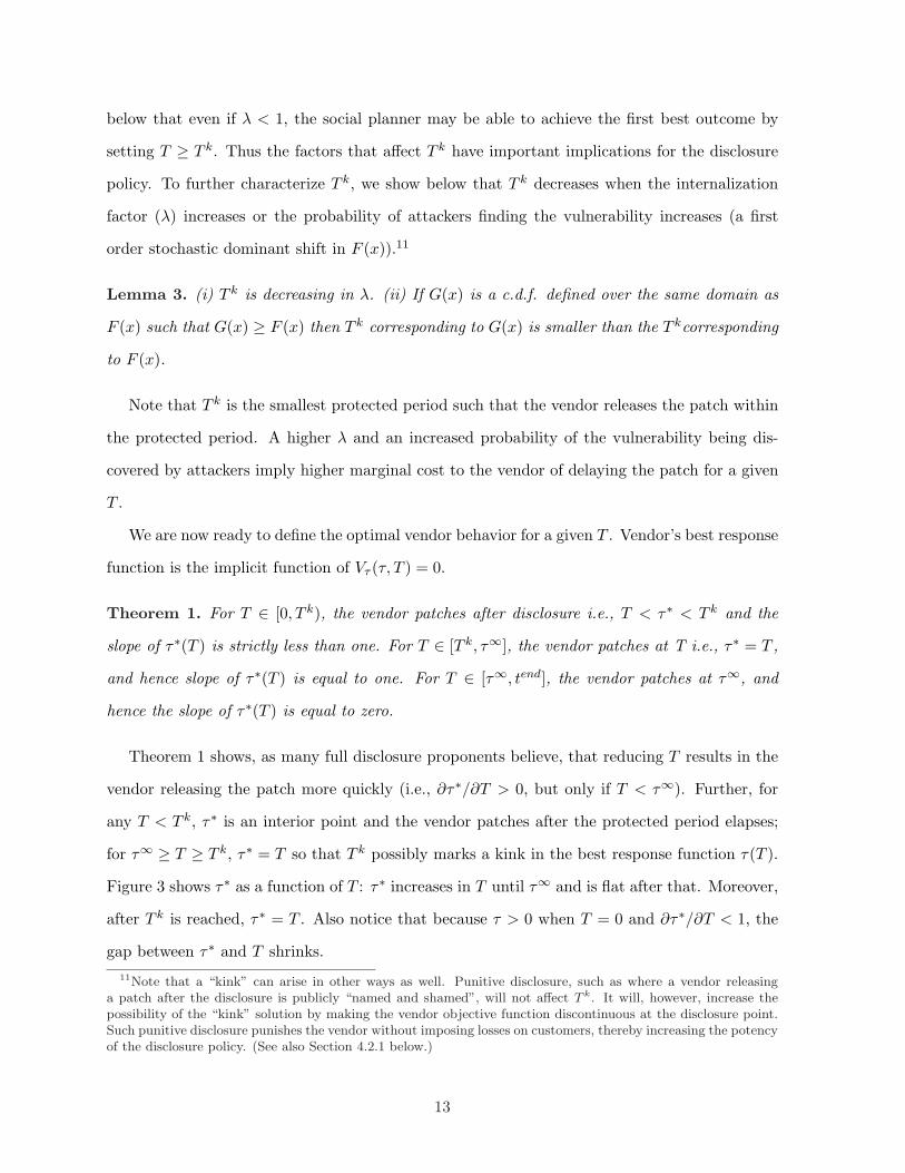
Theorem 1 shows, as many full disclosure proponents believe, that reducing T results in the

vendor releasing the patch more quickly (i.e., ∂τ∗/∂T > 0, but only if T < τ∞). Further, for

any T < T k, τ∗ is an interior point and the vendor patches after the protected period elapses;

for τ∞ ≥ T ≥ T k, τ∗ = T so that T k possibly marks a kink in the best response function τ(T ).

Figure 3 shows τ∗ as a function of T : τ∗ increases in T until τ∞ and is flat after that. Moreover,

after T k is reached, τ∗ = T . Also notice that because τ > 0 when T = 0 and ∂τ∗/∂T < 1, the

gap between τ∗ and T shrinks.11Note that a “kink” can arise in other ways as well. Punitive disclosure, such as where a vendor releasing

a patch after the disclosure is publicly “named and shamed”, will not affect T k. It will, however, increase thepossibility of the “kink” solution by making the vendor objective function discontinuous at the disclosure point.Such punitive disclosure punishes the vendor without imposing losses on customers, thereby increasing the potencyof the disclosure policy. (See also Section 4.2.1 below.)

13

-

6

¡¡

¡¡

................................

.............................

................................................

.......................

..........................

................................................¡

¡

T k τ∞ T

τ∗

Figure 3: Patch development time τ as function of Protected Period T

The lower is λ, the slower is the vendor to patch. However, this is only true when T < T k,

after which the vendor chooses to patch at T regardless of λ. (Recall from Lemma 3 that T k

itself is decreasing in λ.) This is formalized in Corollary 1.

Corollary 1. A higher internalization factor implies an earlier patch, ∂τ∗/∂λ < 0 for any

T < T k. When T ≥ T k, ∂τ∗/∂λ = 0.

4.2 The Social Planner’s Decision: Optimal Disclosure Policy

The social planner chooses optimal T ∗ to minimize total social cost, S(T ), taking into account

the vendor’s best response function τ(T ). The social cost is given by

S(T ) = C(τ(T )) + L(τ(T ), T ) (5)

Social cost differs from vendor cost in that the former includes the entire expected user loss,

whereas the latter includes only a fraction λ of the expected user loss. When the vendor inter-

nalizes only a portion of customer loss, i.e. λ ∈ (0, 1), the vendor’s incentives and the social

planner’s incentives are not aligned.

We can now derive the socially optimal policy. We assume that S(T ) admits only a single

minimum (see the online appendix for the sufficient condition for a unique T .) A variety of

functional forms, including the exponential and quadratic loss functions, yield a single minima.

Recall that τ s is the socially optimal time to deliver the patch, i.e., the time a vendor would

release the patch on its own if it internalized the entire customer loss. Since the vendor does

14

not internalize the entire customer loss, absent a threat of disclosure, the vendor delivers the

patch after τ s. Given a protected period T , the vendor will deliver the patch after T if T < T k,

and exactly at time T for T ≥ T k. Hence, as long as τ s ≥ T k, the social planner can choose

T = τ s and the vendor would patch exactly at τ s. However for τ s < T k, the socially optimal T ,

denoted by T ∗, lies between τ s and T k as shown in the next proposition and in Figure 4.

Theorem 2. When τ s < T k, the socially optimal protected period T ∗ is bounded within (τ s, T k)

i.e. τ s < T ∗ ≤ τ(T ∗) ≤ T k. When τ s ≥ T k, T ∗ = τ(T ∗) = τ s.

Clearly, whenever τ s ≥ T k, the social planner can achieve the socially best outcome even

though λ < 1. Thus, disclosure policy can be an effective and potent tool even though the social

planner can affect vendor behavior only indirectly.

-

6

.

.............................................

...........................................

........................................

.....................................

..................................

................................

.............................

..........................

........................

.....................

.....................

..................... .................... .................... .................... ..................... ..............................................

.........................

...........................

.............................

..............................¢¢¢¢

τ s T ∗ T k τ∞ T

S

Figure 4: Social Cost as Function of T

4.2.1 Factors Affecting the Optimal Disclosure Policy

An increase in λ will cause the vendor to release the patch earlier because the vendor internalizes

a larger fraction of customer losses. A higher λ also implies that the vendor is more sensitive to

disclosure. Hence, the social planner will optimally reduce T ∗. The optimal protected period,

T ∗, decreases with λ until λ reaches λ0 and is constant thereafter. The intuition is that T k is

decreasing in λ (from Lemma 3), so that for high enough λ, τ s ≥ T k holds. If τ s ≥ T k, the

social planner can choose T = τ s and the vendor would patch exactly at the socially optimal

time τ s. This is formalized in Theorem 3.

15

Theorem 3. There exists a λ0 ∈ (0, 1) such that for λ ≥ λ0, τ s ≥ T k, and τ∗ = T ∗ = τ s and

T ∗ is independent of λ. For λ < λ0, τ s < T k and the socially optimal protected period, T ∗, is

decreasing in λ.

When τ > T , there is a period when customers are exposed. The gap between T and τ

falls with λ , and τ becomes more responsive to T . In short, the social planner has greater

leverage with the vendor when λ is higher. This result is important; disclosure policy relies

upon the sensitivity of the vendor to customer losses. When the vendor is more sensitive to

customer losses (higher λ), the social planner has more leverage in forcing vendors to release the

patch on time. In this respect, our result is counter-intuitive: One expects greater alignment

between the firm’s objective function and social welfare to weaken the need for regulation, but

here the reverse is true, because a greater alignment between the two also increases the efficacy

of regulation. However, our numerical analysis (see Section 4.5) suggests that even for low λ,

suitably chosen disclosure can generate significant social benefits.

There are two ways to a higher λ. One is when customers are able to punish the vendor by

switching to a competing product. We conjecture that competition increases λ. Second, larger

users are more likely to contract with vendors about the patching support. Thus, vendors whose

market base consists of large users will have higher λ.

4.3 Robustness of the model

Though not analyzed here, the social planner plausibly has a spectrum of disclosure possibilities.

For instance, the social planner could issue a general warning that a particular product is

insecure, which could hurt the vendor without imposing large losses on users. In terms of

our model, one would add a term to the vendor’s cost, so the modified vendor cost is V (·) =

C(τ) + λL(τ, T ) + ψ(τ, T ) and the social cost is S(·) = C(τ) + L(τ, T ), where ψ(τ, T ) captures the

damage suffered by the vendor not due to the customer loss. We expect that ψ(τ, T ) = 0 for

τ ≤ T and is positive and increasing in τ − T . Including such a term will cause a discontinuity

in the cost function at τ = T , and cause cost function to be concave around τ = T , thereby

increasing the likelihood of the vendor patching at T . This modification can also be used to

analyze the case where the vendor suffers losses that are not included in the social cost function

16

(e.g., where the vendor loses some customers to other vendors by releasing the patch late).

It is also plausible that the post disclosure loss function differs from l(·). If we let m(τ − T )

represent the post disclosure losses, then as long as m(0) = 0, m(·) is convex, and V +τ (T )

∣∣∣τ=T

is monotonically increasing in T , our basic results should continue to hold.12 Disclosure by the

social planner may also increase λ by forcing the vendor to acknowledge responsibility. This is

as if the vendor’s (but not social) post-patch loss function were m(·) = σl(·), where σ > 1.

We have assumed through A5 that despite a finite product life-cycle, “not patching” is not

an optimal choice. The online appendix shows that if assumption A5 is violated, then there

exists a threshold, TNP (tend), such that T > TNP implies that the vendor does not patch. It

is intuitive that TNP increases with tend. Further, since the vendor does not internalize the

entire customer loss, there is a range of values of tend such that the social planner’s choice of the

protected period is constrained by the need to get the vendor to patch. The unconstrained choice

of the protected period would result in the vendor not releasing the patch. When the constraint

binds, the protected period is shorter than when the constraint does not bind. Finally, there is

a threshold value of tend (possibly zero) below which the social planner chooses secrecy and the

vendor does not develop a patch.

4.4 Customers do not Patch Instantly

Thus far we have assumed that all customers patch as soon as the patch is available (or

p(0, q) = 1). The .NET passport vulnerability is a good example. A fix on the server side

stops the invasion and customers need no patch (Infoworld, 2003). However, many vulnera-

bilities require that customers download and apply patches. Not all customers apply patches

immediately upon release (Rescorla 2003). Six months after the DDOS attacks that paralyzed

several high-profile Internet sites, more than 100,000 machines were still unpatched and vulner-

able (InternetNews.com, 2000).

Users may not patch their systems immediately because (i) it takes time to find out about

the patch, (ii) applying the patch may take time and may be difficult for unskilled users, (iii)

poor quality patches may themselves create new problems. For example, the initial Microsoft12If m(0) > 0 and m′′(·) < 0, the cost functions may be non-convex, implying that patching soon after disclosure

is sub-optimal, and thus we should see many cases of patching coinciding with disclosure.

17

patch for a vulnerability CVE-2001-0016 disabled many updates of service pack 2 of Windows

NT, making the patched system even more vulnerable to attacks (Beatie et. al. 2002). The

following statement clearly points to how the patch quality can affect the patch uptake:

“About 95 percent of exploits occur after bulletins and patches are put out....(T)he reason the

exploit is effective is because the patch uptake is too low. The reason the patch uptake is too low

is it’s too hard to patch, and the quality of the patch is not consistent enough that people can

feel safe patching right away.”, Microsoft chief security strategist Scott Charney.13

The speed with which customers apply patches depends on two factors: the time elapsed

since the patch is released (z) and the quality of the patch (q). Quality can be interpreted to

include those features as well that make it easier for users to download and install the patches.

4.4.1 Quality of Patch is Exogenous

We first consider the case when quality is exogenously fixed at some level q. The expected loss

function is of the form given in equation (2). Thus the vendor’s objective function is

V (τ, T ) = C(τ) + λL(τ, T ; q)

= C(τ) + λL(τ, T ) + λL(τ ; q)

One can show that Theorems 1-3 continue to hold.14

Since post-patch losses fall as the patch is delayed, τ∗, τ s, T k, and τ∞ are all larger than

when patches are installed instantaneously. The vendor therefore delays the patch. If dτdT is

(weakly) smaller for a given T in the presence of post-patch losses, then the social planner also

optimally allows more time (higher T ∗). Indeed, in the extreme case, where users never patch,

not developing a patch is both privately and socially optimal.

Theorem 4. When users do not patch instantly, (i) T k is higher, (ii) the vendor slows patch

development, and (iii) if dτdT in the presence of post-patch loss is no higher than dτ

dT in the absence

of post-patch loss, the social planner allows more time before disclosure.

The theorem formalizes the intuition that the vendor and the social planner are both less13 http://entmag.com/news/article.asp?EditorialsID=5833; (accessed September 1, 2006)14The proofs are analogous to those in the previous section and are omitted here. They are available from the

authors upon request.

18

aggressive in the presence of post-patch losses. Moreover, we are less likely to see cases where

the patch coincides with the disclosure, since T k moves to the right.

The rate of user implementation of patches can be low. In a case study of the OpenSSL

Remote Buffer Overflow vulnerability (exploited by the notorious slapper worm), Rescorla (2003)

reports that 60 percent of the investigated servers did not patch even after two weeks of the

release of the patch. Our results imply that in such cases, vendors should be given more time

to develop patches.

4.4.2 Quality of Patch is Endogenous

A common argument for giving vendors more time is that it facilitates the development of higher

quality patches. High quality patches are those that customers trust, are easier to download

and apply, and less likely to cause problems later. Simply put, a higher quality patch increases

the uptake of patches. When the vendor can choose both q and τ , the vendor’s cost function is:

V (τ, q) = C(τ, q) + λL(τ, T, q)

= C(τ, q) + λL(τ, T ) + λL(τ, q)

Consider the impact of increasing the protected period, T . An increase in T will lead to an

increase in τ . The impact of higher τ on q depends on the sign of Vτq(·). It is easy to see from

equation (2) that Lτq(·) = 0 and Lτq(·) > 0 so that Vτq(·) = Cτq(·)+λLτq(·) is of indeterminate

sign. If the development cost effect, Cτq(·), dominates, then Vτq(·) < 0, and the vendor will

increase q. However, if the post-patch loss effect, λLτq(·), dominates, then Vτq(·) > 0, and the

vendor will decrease q.

Theorem 5. When patch quality is endogenous, the optimal time for patch development τ∗ is

increasing in disclosure time T , i.e., dτ∗dT > 0. If Vτq(·) ≤ 0, patch quality is increasing in T,

( ∂q∂T ≥ 0) and if Vτq(·) > 0, patch quality is decreasing in T , ( ∂q

∂T ≤ 0) .

Theorem 5 appears counter-intuitive. It is commonly believed that providing more time to

vendors will improve the quality of the patch. However this view is only partially true. An

increase in τ (due to an increase in T ) has two opposing effects on the marginal benefit of

quality. On the one hand, the marginal cost of quality falls since Cq(·) falls with τ , but on the

19

other hand, increasing τ also reduces the marginal benefit of quality because a delayed patch

also reduces the marginal benefit of quality in mitigating post-patch loss. When the post-patch

loss effect dominates, increasing the protected period reduces the patch quality.

What happens to the optimal protected period when quality is set endogenously? In general,

the protected period can be higher or lower with endogenous quality. However, if the post-patch

loss effect dominates the patch development cost effect, then the optimal protected period is

lower when quality is endogenous. When the patching cost effect dominates, the impact on T is

ambiguous: reducing T hastens the patch but lowers its quality (see online appendix for proof).

4.5 Numerical Analysis

To gain more insight into the optimal disclosure policy, we performed numerical simulation, with

the following functional forms: C(τ) = 50000/τ0.75, l(y) = 25y2, F (x) uniform over [0, z] and

we let z vary from 200 to 300 days. We let λ vary from 0.1 to 0.9. Since the effectiveness of the

policy depends on the relative magnitudes of the customer loss and the patching cost, we repeat

the simulation with customer loss l(·) = 2500y2, keeping the rest same.

Given the paucity of information on the patching costs and the customer loss functions, we

chose parameter values that match observed patch release behavior. In a related empirical study

(Arora, Krishnan, Telang, and Yang 2005), we estimate that instant disclosure leads to a patch

in 31 days and secrecy leads to patch in about 61 days, on average. With the chosen forms,

for λ = 0.1, under instant disclosure, the patch release time τ varies from about 25 days (low

customer loss) to 5 days (high customer loss), and under secrecy, τ correspondingly varies from

58 days to 18 days. We calculate the optimal patch release times under instant disclosure, under

secrecy, and under the optimal protected period. To avoid clutter, we plot these values for only

z = 300; lower values of z make both the vendor and the social planner more aggressive.

In figure 5, λ is on the x-axis and time (in days) is on the y-axis. Note that the patch takes

the longest time under secrecy and the shortest under instant disclosure. As expected, the patch

release time falls with λ. Also the difference between the patch release time and the protected

period (the middle two lines) shrinks with λ. Beyond λ = 0.5, the difference between T and τ

is small. In short, when the vendor is responsive enough, disclosure is very effective in forcing

the vendor to release the patch in time. But even for small λ, the optimum disclosure policy is

20

0.1 0.2 0.3 0.4 0.5 0.6 0.7 0.8 0.910

15

20

25

30

35

40

45

50

55

60

Tim

e in d

ays

Low Customer Loss

under optimal policy

under secrecy policy

under instant disclosure

optimal T

(a) fig 5(a)

0.1 0.2 0.3 0.4 0.5 0.6 0.7 0.8 0.92

4

6

8

10

12

14

16

18

Tim

e in d

ays

High Customer Loss

under optimal policy

under secrecy policy

under instant disclosure

optimal T

(b) fig 5(b)

Figure 5: τ and T by λ

effective in reducing the vendor’s patch release time (from 60 to 48 days in figure 5(a) and from

17 to 12 days in figure 5(b)). When the customer loss is high (figure 5(b)), τ is lower as is the

protected period, T , and the difference between the two is smaller.

Turning to the social losses, we find that the instant disclosure performs poorly compared

with either the secrecy or the optimal policy, with social losses 300-400 percent greater under

the instant disclosure than under the optimal policy. Accordingly, in figures 6(a) and 6(b) we

only plot the percentage reduction in the social loss under the optimal policy compared to the

secrecy policy.

Note that the difference between z =200 and z =300 is small. For low values of λ, the

optimal policy generates benefits (social loss reductions) of about 25-30 percent in figure 6(a)

and about 40-45 percent for figure 6(b). To put this in perspective, if we take $1 billion as

a conservative lower bound for the losses arising from information security breaches due to

inappropriate disclosure, the implied savings from the optimal disclosure policy range from

$250 million to $450 million. More importantly, by offering a credible alternative to the instant

disclosure, CERT also potentially reduces some cases of instant disclosure, which are significantly

more costly.

In both figures, as λ increases, secrecy (no disclosure) becomes almost as effective as optimal

policy even though the gap between τ and T remains large. More interestingly, we showed earlier

21

0.1 0.2 0.3 0.4 0.5 0.6 0.7 0.8 0.9-5

0

5

10

15

20

25

30

% R

eduction in S

ocia

l Loss u

nder

optim

al polic

yLow Customer Loss

z=300

z=200

(a) fig 6(a)

0.1 0.2 0.3 0.4 0.5 0.6 0.7 0.8 0.90

5

10

15

20

25

30

35

40

45

50

% R

eduction in S

ocia

l Loss u

nder

optim

al polic

y

High Customer Loss

z=300

z=200

(b) fig 6(b)

Figure 6: percentage reduction in social loss under the optimal policy

that with higher λ, the protected period is short. However, even when λ is small and the social

planner can not be very aggressive, the social benefits of optimal policy are high. Thus policy

has bite in terms of reducing the social losses when λ is small even though the vendor is not as

responsive.

Note that the optimal policy matters more when the customer losses (relative to the patching

costs) are higher (figure 6(b) vs. figure 6(a)). Higher customer loss makes the vendor more

responsive but higher customer loss also raises the social loss. Since the vendor internalizes

only a fraction of the customer loss, the socially optimal policy relative to the secrecy policy

is more effective when the customer loss is higher. One interpretation of this result is in terms

of market size. An increase in the market size is equivalent to an increase in the customer loss

relative to the patch development cost, since the latter is roughly invariant to changes in market

size. Arora, Caulkins and Telang (2005) show that vendors patch more expeditiously in larger

markets. The numerical simulations reported here confirm that finding and also show that if

the vendor internalizes only a fraction of customer loss, the socially optimal policy relative to

the secrecy is more effective in larger markets.

We also experimented with skewed distributions for F (·). When F (·) is skewed to the right

(i.e. the hackers have a higher chance of finding vulnerability later) then gains from the optimal

22

policy are even higher. Left skewed distributions, on the other hand, produced lower gains.

Finally, for λ larger than 50 percent, the vendor’s response under the secrecy is very similar

to that under the optimal disclosure policy. As long as the vendor internalizes at least 50 percent

of the user loss, the vendor’s decision to release a patch on its own creates the additional social

costs of the order of only 5 percent. We also explored kink solutions and they lead to similar

predictions.

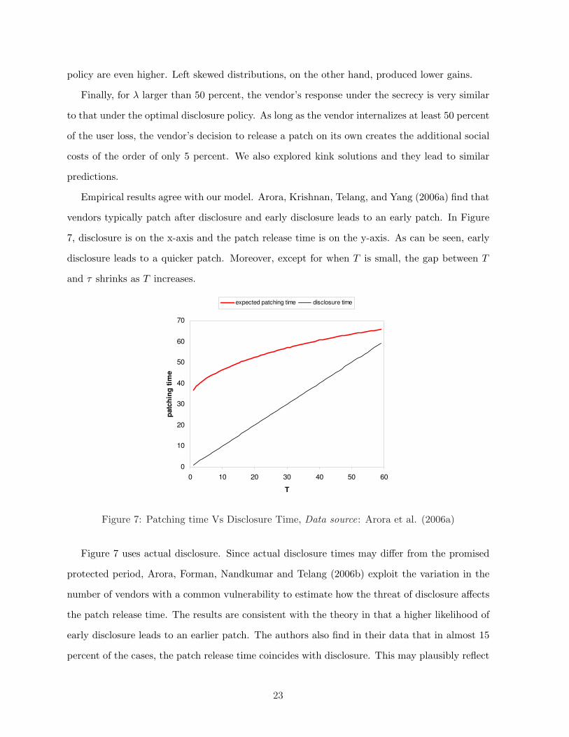
Empirical results agree with our model. Arora, Krishnan, Telang, and Yang (2006a) find that

vendors typically patch after disclosure and early disclosure leads to an early patch. In Figure

7, disclosure is on the x-axis and the patch release time is on the y-axis. As can be seen, early

disclosure leads to a quicker patch. Moreover, except for when T is small, the gap between T

and τ shrinks as T increases.

0

10

20

30

40

50

60

70

0 10 20 30 40 50 60

T

patc

hin

g t

ime

expected patching time disclosure time

Figure 7: Patching time Vs Disclosure Time, Data source: Arora et al. (2006a)

Figure 7 uses actual disclosure. Since actual disclosure times may differ from the promised

protected period, Arora, Forman, Nandkumar and Telang (2006b) exploit the variation in the

number of vendors with a common vulnerability to estimate how the threat of disclosure affects

the patch release time. The results are consistent with the theory in that a higher likelihood of

early disclosure leads to an earlier patch. The authors also find in their data that in almost 15

percent of the cases, the patch release time coincides with disclosure. This may plausibly reflect

23

un-modeled communication between CERT and the vendor. However, it is also predicted by our

model when T k < τ s. In terms of our model, it appears that λ > 0.5 corresponds to τ s > T k.

5 Customers can implement work-arounds

So far, we assumed that customers have no choice but to wait for the patch. However, sometimes

customers can implement work-arounds instead. Examples of work-arounds include shutting off

a port, changing the default settings, disabling a service, revising and recompiling a portion of

code.

Suppose α fraction of users (henceforth smart users) can implement a work-around at a

one time cost w, if informed of the vulnerability by the social planner.15A work-around will be

implemented only if the expected loss of waiting for a patch, l(τ − T ) is greater than w. Thus

the expected loss for users implementing work-arounds isT∫0

l(T − x)dF (x) + w. The remaining

(1−α) percent of users must wait for the patch and their expected loss is as before. For brevity,

we ignore kink solutions and post-patch losses, and patch quality. We also assume that all

customers are fully informed about τ and T . Since there is no uncertainty in the model and

customers are not being strategic, the vendor can credibly announce τ .

The possibility of work-arounds lowers the expected post disclosure loss for smart users, and

in turn, the vendor has an incentive to delay the patch, which hurts users who can not apply

work-arounds. However, the choice of the patch release time also affects customers’ choice of

work-around. In particular, if the vendor chooses τ such that l(τ − T ) < w then smart users

would not apply work-arounds and instead wait for the patch. In this case, the vendor loss

function is

V (τ, T ) = C(τ) + λ( T∫

0

l(τ − x)dF (x) + (1− F (T ))l(τ − T ))

s.t. l(τ − T ) < w

If, however, the vendor chooses a τ such that l(τ − T ) > w, then smart users can apply a15If smart users could apply work-around when the exploitation by the hackers start and not wait for the social

planner to inform, then the potency of disclosure reduces. The social planner has no incentive to use disclosureas a tool to encourage work-around.

24

work-around and the vendor loss function, denoted by V w(τ, T ) is

V w(τ, T ) = C(τ) + λα( T∫

0

l(T − x)dF (x) + w)

+ λ(1− α)( T∫

0

l(τ − x)dF (x) + (1− F (T ))l(τ − T ))

s.t. l(τ − T ) ≥ w (6)

Let τw = arg minτ{V w(τ ; T )} and similarly τ = arg min

τ{V (τ ; T )} denote the vendor’s optimal

choices of τ , conditional on allowing and not allowing the work-arounds respectively. If neither

constraint binds, the patch release time in the work-around case is equivalent to the patch release

time with no work-around but the internalization factor equal to λ · (1 − α). Thus for a given

T , τw = τ(λ · (1− α), T ). While the patch release time in the no work-around case is τ(λ, T ).

Define Tw as the protected period where the vendor is indifferent between inducing work-

arounds and not, so that V w(τw(Tw), Tw) = V (τ(Tw), Tw). The following theorem establishes the

conditions that Tw exists.16

Theorem 6. (i) For all w such that l(τ(λ · (1 − α)), 0) > w and C(τ∞) < λw, there exists a

0 < Tw < τ∞ such that the vendor induces work-arounds by smart users if T ∈ [0, Tw) and does

not induce work-arounds if T > Tw.

(ii) ∂T w

∂α > 0, and ∂T w

∂λ < 0.

By choosing a T smaller than Tw, the social planner can induce the vendor to choose a τ such

that the work-around is feasible: releasing the patch very quickly after disclosure (the only way

to head off a work-around) is costly. A T greater than Tw will, on the other hand, induce the

vendor to release the patch soon after disclosure and avoid a work-around. An increase in α, the

percent of smart users, will decrease V w(·), and therefore increase Tw. A more subtle reasoning

implies that increasing λ will decrease Tw. When the vendor is indifferent between inducing

work-arounds or not, the patch development cost is smaller in the work-around case, and hence,

the user-loss is greater. An increase in λ increases the weight of the user-loss component in the

vendor cost function, so that the point of indifference is at a smaller T . The second part of the

Theorem 6 formalizes this intuition.

The second part of Theorem 6 also points to the interaction between λ and α in conditioning16 For technical convenience, we assume that T w is unique. The assumption is satisfied by a variety of functional

forms for l(·), including the quadratic function.

25

Tw and, indirectly, also the protected period T . Thus, low λ and high α would lead to more

work-arounds for a fixed T . However, they also affect optimal T .

Let the social cost, with and without work-around, respectively be:

Sw(α) = C(τw(T ))+α

(T∫0

l(T − x)dF (x)+w

)+(1−α)

(T∫0

l(τw(T )− x)dF (x)+(1−F (T ))l(τw(T )−T ))

s.t. T < Tw(α).

S(α) = C(τ(T )) +T∫0

l(τ(T )− x)dF (x) + (1− F (T ))l(τ(T )− T )

s.t. T > Tw(α).

Recall that Tw is a T such that the vendor is indifferent between work-around and no work-

around (V w = V ). Since λ < 1, it is immediate that at Tw, Sw(·) > S(·). Thus if the social

planner finds it optimal to induce work-around, it will always set T ∗ < Tw.

If Sw(α) − S(α) is decreasing in α, then we can find a α such that Sw(α) = S(α).17 Any

α < α implies that the social planner will set a long enough protected period which does not

induce a work-around. Conversely, when the percentage of smart users is greater than α, the

social planner chooses a short protected period and discloses early, and the vendor delays the

patch.

Theorem 6 provides insights into the interplay between λ and α. In particular, we conjecture

that the social planner is more likely to prefer work-arounds and, hence, early disclosure when

proportion of smart users is high and when λ is low. We perform numerical simulations using

the same functional forms as before to analyze this (C = 50000/τ0.75 L = 25.(τ − T )2). We

fix z = 100 and w = 20, λ = 0.4.

In Figure 8, as λ falls, the minimum percentage of smart users required for early disclosure, α,

falls and, consequently, the disclosure policy is more aggressive. This relationship is conditioned

by the cost of the work-around, w. As w increases, the protected period is larger. Note when

λ is small, α is also small. Intuitively, for a small λ, the patch release time is longer and the

social planner will optimally disclose early enough to induce a work-around, even with a small

fraction of smart users.17 As long as Sw(α)−S(α) is decreasing in α and w < C(τs)+

R τs

0l(τs−x)dF (x), a unique α exists. Existence

follows upon noting that Sw(0)− S(0) > 0 and Sw(1)− S(1) < 0 and Sw(α)− S(α) is continuous in α. Further,S(α) weakly increases with α as well (the constraint T > T w becomes tighter). Thus, as long as Sw(α)− S(α) isdecreasing in α, α is unique.

26

0.1 0.2 0.3 0.4 0.5 0.6 0.7 0.8 0.90

0.1

0.2

0.3

0.4

0.5

0.6

0.7

0.8

0.9

1

w = 20

w = 40

work-around region

no work-around region

ˆ

Figure 8: Required proportion of smart users to induce work-around

To summarize, when at least some users can implement work-arounds at a reasonable cost,

disclosure acquires additional potency because it empowers these users. Clearly, the higher

the fraction of users able to implement work-arounds, the more important it is to empower

them via disclosure, and, thus shorter the protected period. Interestingly, when the vendor

internalizes only a small fraction of user-losses, the empowerment aspect of disclosure becomes

more significant: the social planner will choose quick disclosure even with a smaller fraction of

users able to implement work-arounds.

One might expect that the “option value” implicit in smart users would always be socially

beneficial. However, this intuition is incomplete because the vendor does not fully internalize

user losses. Smart users convey a negative externality upon other users because smart users’

presence leads the vendor to prefer the work-around option even when it is not socially desirable.

As a result, the social planner may be forced to choose a longer protected period to avoid a work-

around. This negative externality may even offset the beneficial effect leading to a net increase

in social cost.18 Indeed, for an intermediate range of α, where the vendor prefers to induce

work-arounds but the social costs are lower without work-arounds, the presence of smart users

raises total social cost.

Theorem 7. If Sw(α) − S(α) is decreasing in α then there exists a region between [ ˆα, α] such18 We are grateful to an anonymous reviewer for pointing us in this direction.

27

that the presence of smart users results in a higher social cost.

0 0.1 0.2 0.3 0.4 0.5 0.6 0.7 0.8 0.9 110

20

30

40

T

proportion of smart users

0 0.1 0.2 0.3 0.4 0.5 0.6 0.7 0.8 0.9 15000

5500

6000

6500

Socia

l C

ost

Tw

T *

work-around region No work-around region

Social cost

Figure 9: Social cost, T ∗ and Tw as a function of smart users

In Figure 9, we plot T and Tw on the left y-axis, and the social cost on the right y-axis. At

α = 0, the social cost is approximately 6000. For intermediate values of α, the social cost is

higher than 6000. In Figure 9, Tw = T ∗(α = 0) at α = 0.2. Beyond that, the social planner

strictly prefers no work-arounds but the only way to prevent work-arounds is by setting T ∗ = Tw.

Once α is reached, the social planner strictly prefers work-arounds (notice the jump in optimal

T ∗) and discloses early. Further increases in the fraction of smart users reduce social cost, and

at α > 0.78, the social cost drops below 6000.

The effect of market size follows the same intuition as in the previous section. A larger

market increases the marginal cost of customer loss relative to the patch development cost, and

hence decreases τ and T , and also reduces the gap between τ and T (see Figure 6). Thus, a

larger market reduces Tw, makes a work-around less likely, and increases α.

6 Conclusions

How and when vulnerabilities should be disclosed is an important policy issue. A sensible

disclosure policy must balance the need to protect users against attackers and the need to prod

vendors to develop patches expeditiously. We develop a model that outlines how the policy

28

maker can optimally influence vendor behavior to minimize social cost.

We find that as long as the vendor does not internalize the entire user loss, the vendor will

release the patch later than is socially optimal, unless threatened with disclosure. In some

cases, the policy maker can force the vendor to release the patch at the socially optimal time

while in other cases the optimal protected period is such that the vendor releases the patch

after disclosure, though still earlier than the vendor would otherwise have. The more responsive

the vendor is to user losses, the more aggressive the social planner can be by setting a shorter

protected period. In general, both an instant disclosure and a secrecy policy are sub-optimal,

though numerical simulations suggest that instant disclosure is particularly inefficient.

These results are robust to a partial implementation of the patch by users and to endogenous

variations in the quality of the patch. When users take time to apply patches, the protected

period should be longer. When the vendor also chooses patch quality (and higher quality patches

are applied faster), contrary to conventional wisdom, a longer protected period may even reduce

the quality of the patch and increase social cost.

When users can defend themselves via work-arounds, disclosure empowers users and increases

the potency of disclosure policy, leading to a shorter protected period. However, this also creates

a negative externality for users incapable of defending themselves. The vendor opts for work-

arounds too readily, leading the social planner to extend the protected period in some cases. As

a result, the social cost may actually rise as the proportion of users capable of implementing

work-arounds increases. This suggests that unless the defensive measures are within the reach

of a large enough number of users, encouraging their use may be counter-productive.

Our results are subject to a variety of qualifications. First, we leave for future research the

case where a vendor can respond to disclosure by accelerating the rate of patch development,

preferring to focus on the insights from a simpler static model. Thus, our model is best thought

of relating to the policy rather than a patch release decision support system. We conjecture that

allowing for such measures will lower the cost of disclosure, implying that the optimal protected

period would be shorter. Second, in our model, costs and benefits are known with certainty.

Thus it ignores the possibility that if the patch development cost is more expensive than expected

and the vendor is making a good faith effort to develop a patch, the protected period may be

optimally extended in a dynamic model with communication between the social planner and the

29

vendor. Third, we ignore the complications created when more than one vendor is affected by

a single vulnerability. This case is empirically relevant and is the subject of a companion piece

(Arora, Forman, Nandkumar and Telang 2006b), whose results suggest that the basic insights

developed here are robust. Finally, we ignore the possibility that early disclosure would force

vendors to provide secure software in the first place.

Despite these qualifications, our simple model is consistent with the observed evidence.

Specifically, it correctly predicts that typically vendors release a patch after the disclosure,

and that the gap between when the patch is released and the disclosure falls with the protected

period. Moreover, though we work with continuous and convex loss functions, a kink in the

vendor’s response to the protected period arises naturally, yielding the prediction that the patch

release time for some patches would coincide with disclosure.

Different assumptions may well lead to different conclusions about the optimal disclosure

policy, but our model can be tailored to reflect those differences without major changes to the

basic structure. In this sense, our model highlights the key areas where additional empirical

evidence is required, by bringing out the key implications of the assumptions we have made.

The contribution of this paper, therefore, lies not only in the specific results obtained but also in

the framework developed that allows for various generalizations and highlights the possibilities

and limits of social disclosure policy.

References

Arbaugh W.A., Fithen W. L., and McHugh J. (2000), “Windows of Vulnerability: A Case StudyAnalysis”, IEEE Computer.

Arbaugh W.A., Browne H., McHugh J., and Fithen W.L. (2001), “A Trend Analysis of Ex-ploitations”. IEEE Symposium on Security and Privacy. Oakland, California, USA.

Arora A., Caulkins J.P., and Telang R. (2005), “Research Note - Sell First, Fix Later: Impactof Patching on Software Quality,” Management Science, 52(3),465-471.

Arora A., Krishnan R., Telang R., and Yang Y. (2006a), “How Quickly do they Patch? AnEmpirical Analysis of Vendor Response to Disclosure Policies”, ICIS, Milwaukee 2006.

Arora A., Nandkumar A., and Telang, R. (2006), “Does Information Security Attack FrequencyIncrease With Vulnerability Disclosure? - An Empirical Analysis”, Information Systems Frontier8, 350-362.

30

Arora A., Forman C., Nandkumar A., and Telang R. (2006b) “Competitive and Strategic Effectsin the Timing of Patch Release” , WEIS 2006, Cambridge, England.

August T., and Tunca T. (2005), “Network Software Security and User Incentives,” ManagementScience, 52 (11), 1703-1720.

Beattie S., Arnold S., Cowan C., Wagle, P., and Wright, C. (2002), “Timing the Application ofSecurity Patches for Optimal Uptime”, Proc of LISA: 16th Systems Administration Conference

Cavusoglu H., Cavusoglu H., and Raghunathan S. (2004), “How Should We Disclose SoftwareVulnerabilities?”, 14th WITS, Washington D.C.

Cavusoglu H., Cavusoglu H., and Zhang J. (2005), “Security Patch Management: Share theBurden or Share the Damage?,”Working paper, Tulane University.

Choi J., Fershtman C., and Gandal N. (2005), “Internet Security, Vulnerability Disclosure andSoftware Provision”, WEIS 2005, Boston, MA June 2-3.

Clark R., (2002) http://www.blackhat.com/html/bh-usa-02/bh-usa-02-speakers.html#RichardClarke, (accessed July 19, 2006 ).

CSI-FBI (2005) “CSI/FBI Computer Crime and Security Survey”, 2006)

Gordon L.A., and Loeb M.P. (2002). “The Economics of Information Security Investment”.ACM Transactions on Information and System Security, 5.

Infoworld, 2003, www.infoworld.com/article/03/06/30/HNpass 1.html; www.internetnews.com/dev-news/article.php/2203651 respectively (accessed, 08/24/05)

Kannan K., and Telang R. (2005), “Market for Software Vulnerabilities? Think Again”, Man-agement Science, 51(5), 726-740.

NetworkMagazine.com (2000), “The Pros and Cons of Posting Vulnerabilities”. http://www.networkmagazine.com/article/NMG20001003S0001 (Accessed, 08/24/2005)

National Strategy to Secure Cyberspace (2003), http://www.whitehouse.gov/pcipb (Accessed,08/24/2005)

Nizovtsev D., and Thursby M., (2005), “To disclose or not? An analysis of software user behav-ior”, Information Economics and Policy, 19(1), 43-64.

Png Ivan, Tang C.Q., and Wang S.Y., (2006), “Information Security: User Precautions andHacker Targeting”, WEIS 2006, Cambridge, England.

Preston E., and Lofton J. (2002). ”Computer Security Publications: Information Economics,Shifting Liability and the First Amendment”, Whittier Law Review, 24, 71-142.

Rescorla E. (2003), “Security Holes... Who Cares?”, Proceedings of the 12th USENIX SecurityConference, August.

31

Symantec Inc (2003), “Symantec Internet Security Threat Report”. http://www.symantec.com

32

This page is intentionally blank. Proper e-companion title page, with INFORMS branding andexact metadata of the main paper, will be produced by the INFORMS office when the issue isbeing assembled.

33

Online Appendix

When A5 is violated and not-patching may be privately optimal

A5 could be violated if post patch losses are high, i.e., if users do not apply patches. In this case,disclosure policy is pointless. So, in what follows, we discuss the case where post patch lossesare zero, i.e., if p(z, q) = 1. If A5 is still violated, there are two possibilities. First, the vendorwill not patch even under instant disclosure i.e., min

τ≤tend

{C(τ) + λl(τ)

}≥ λl(tend). In this case,

there is no role for disclosure policy. If, on the other hand, minτ≤tend

{C(τ) + λl(τ)

}< λl(tend) the

role of disclosure policy exists.

The discussion here closely parallels the discussion of work-arounds. Define TNP such that thevendor is indifferent between patching or not patching. Formally, min

τ

{C(τ) + λ

( ∫ T NP

0 l(τ −x)dF (x)+(1−F (TNP ))l(τ−TNP )

)}= λ

( ∫ T NP

0 l(tend−x)dF (x)+(1−F (TNP ))l(tend−TNP ))

Note that as long as minτ

{C(τ) + λl(τ)

}< λl(tend) i.e., as long as it is privately optimal to

patch under instant-disclosure, TNP exists because the violation of A5 implies that the vendor’scost with patching is strictly greater than without patching at T = tend. Since the cost withand without patching is continuous in T , TNP exists. Further, the derivative of the cost withpatching with respect to T is −(1 − F (T ))l′(τ(T ) − T ) and that of the cost without patchingis −(1 − F (T ))l′(tend − T ). The second derivative is smaller (larger in absolute value) becausetend ≤ τ(T ). Thus, the cost without patching falls faster than the cost with patching as theprotected period increases. This implies that TNP is unique. It is immediate that T ≤ TNP

implies that the vendor will patch and T > TNP , the vendor will not patch. Finally, notethat λ

∫ T NP

0 l(tend − x)dF (x) + (1−F (TNP ))l(tend − TNP ) is increasing in tend, so that TNP isincreasing in tend.

It is also obvious that the social cost with patching is strictly less than the social cost withoutpatching at T = TNP .

S(TNP ) = minτ

{C(τ) +

∫ T NP

0 l(τ − x)dF (x) + (1− F (TNP ))l(τ − TNP )}

<

∫ T NP

0 l(tend − x)dF (x) + (1− F (TNP ))l(tend − TNP ) = SNP (TNP ; tend)

If the social planner wishes for the vendor not to patch, the optimal protected period is tend.

The social cost is∫ tend

0 l(tend − x)dF (x). If the social planner wishes for the vendor to patch, itchooses T ≤ TNP to minimize S(T ).

Define ˆt as the lifecycle length such that the (unconstrained) optimal protected period is justshort enough to induce patching i.e., arg min

T

{C(τ(T ))+

∫ T0 l(τ(T )−x)dF (x)+(1−F (T ))l(τ(T )−

T )}

= TNP (ˆt). Define t as such a tend that the social planner is indifferent between having the

vendor patch or not i.e., minT

{C(τ(T ))+

∫ T0 l(τ(T )−x)dF (x)+(1−F (T ))l(τ(T )−T ) s.t. T ≤

34

TNP (t)}

=∫ t0 l(t − x)dF (x). Then, for tend < t, the social planner simply maintains the vul-

nerability secret and the vendor does not patch. For ˆt ≥ tend ≥ t, the social planner prefers tohave the vendor develop a patch but is constrained by the need to induce patching and sets aprotected period T = TNP (tend). For tend > ˆt the social planner’s choice is unconstrained andcorresponds to the case analyzed in the text.

Proof of Lemma 1

Step (i) and (ii) show that L(τ, T ) is convex in τ for τ < T and for τ > T . Utilizing theseresults, we show in (iii) that it is convex everywhere.

(i) We first show that for any τ > T , Lττ > 0.

From equation (1),

Lτ = λ

( ∫ T

0

l′(τ − x)dF (x) + (1− F (T ))l

′(τ − T )

)

Lττ = λ

( ∫ T

0

l′′(τ − x)dF (x) + (1− F (T )l

′′(τ − T )

)

Since l(.) is strictly convex in τ , Lττ > 0, i.e. L(τ) is strictly convex in τ .

(ii) We show that for any τ < T , L(τ) is strictly convex in τ . From equation (1), Lτ =λ

∫ τ0 l

′(τ − x)dF (x). Hence, Lττ = λ

∫ τ0 l

′′(τ − x)dF (x) + l

′(0) > 0

(iii) We need to prove that, for any τ1 < τ2 and 0 < k < 1,

kL(τ1) + (1− k)L(τ2) > L(kτ1 + (1− k)τ2) (O1)

From (i) and (ii), when τ1 < τ2 ≤ T or T ≤ τ1 < τ2, (O1) holds. We only need to prove theinequality holds when τ1 ≤ T ≤ τ2.

Define k such that kτ1 + (1 − k)τ2 = T . When k ≤ k, kτ1 + (1 − k)τ2 = τ ≤ T . Let M(k) =L(τ)− kL(τ1)− (1− k)L(τ2). Convexity is equivalent to M(k) < 0.

We first show that M(k) < 0. Note that

∫ τ2

0

l(τ2 − x)dF (x) =∫ T

0

l(τ2 − x)dF (x) +∫ τ2

T

l(τ2 − x)dF (x)

≤∫ T

0

l(τ2 − x)dF (x) +∫ τ2

T

l(τ2 − T )dF (x)

≤∫ T

0

l(τ2 − x)dF (x) +∫ ∞

T

l(τ2 − T )dF (x)

≤∫ T

0

l(τ2 − x)dF (x) + (1− F (T ))l(τ2 − T ) = L(τ2)

35

Therefore, k.L(τ1) + (1− k)L(τ2) ≥ k∫ τ10 l(τ1 − x)dF (x) + (1− k)

∫ τ20 l(τ2 − x)dF (x)

The convexity of∫ τ0 l(τ − x)dF in τ implies that k

∫ τ10 l(τ1 − x)dF (x)+(1−k)

∫ τ20 l(τ2 − x)dF (x) >∫ τ

0 l(τ − x)dF (x)

At k = k, k∫ τ10 l(τ1 − x)dF (x) + (1− k)

∫ τ20 l(τ2 − x)dF (x) >

∫ T0 l(T − x)dF (x) = L(T ). Hence

kL(τ1) + (1− k)L(τ2) > L(T )

Recall M(k) = L(T )− k.L(τ1)− (1− k)L(τ2). Thus M(k) < 0

Note that dMdk = Lτ

∂τ∂k − L(τ1) + L(τ2) = (τ1 − τ2)Lτ (τ)− L(τ1) + L(τ2)

And d2Mdk2 = (τ1 − τ2)2Lττ (τ)

For all k 6= k, Lττ (τ) > 0. Therefore, d2Mdk2 > 0 when k 6= k. Also, M(0) = M(1)= 0 and

M(k) < 0. Furthermore, M(k) > 0 is not possible because it would require d2Mdk2 < 0 over some

interval. Hence we must have that M(k) < 0, ∀0 < k < 1. QED

Existence and uniqueness of τ∗

From equation (3), V (τ, T ) = C(τ) + λL(τ) is a continuous function defined over a compactdomain [0, tend], and must attain a minimum. By A4, Cτ (0) = −∞ so that developing the patchinstantaneously cannot be optimum, and by A5, the vendor voluntarily develops the patch beforetend, i.e., arg min

τ{C(τ) +

∫ T0 l(τ − x)dF (x)} < tend. Hence the minimum point must be in the

interior of the domain so that 0 < τ∗ < tend. By the strict convexity of V in τ , τ∗ must beunique. QED

Proof of Lemma 2

(i) A unique T k exists.

Recall that V +τ (T )

∣∣∣τ=T

=

(Cτ (τ) + λ

( ∫ T

0l′(τ − x)dF (x) + (1− F (T ))l′(0)

)) ∣∣∣∣τ=T

. To save on no-

tation, define φ(T ) = V +τ (T )

∣∣∣τ=T

. Then T k is unique if φ(T ) = 0 has a unique solution. By A4,

φ(0) < 0. By A5, arg minτ{C(τ) +

∫ T0 l(τ − x)dF (x)} < tend and convexity of V implies that

φ(tend) = Cτ (tend) + λ∫ tend

0 l′(tend − x)dF (x) > 0. By the Intermediate Value theorem, there

exists at least one T k such that φ(TK) = 0. We have already shown in the text that φ(T ) isincreasing in T , so that for any T < T k, φ(T ) < 0, and for any T > T k, φ(T ) > 0. Hence, T k

must be unique.

(ii) There exists a unique τ s.

The proof that Cτ (τ) +∫ τ0 l

′(τ − x)dF (x) = 0 has a unique solution is analogous to the proof

of uniqueness of τ∗ shown in Lemma 1 and hence not repeated here.

(iii) There exists a unique τ∞.

36

A continuous function on a compact domain attains a minimum. C(τ) + λτ∫0

l(τ − x)dF (x) is

continous in τ in the range [0, tend] . Therefore τ∞ exists. By A5 τ∞ < tend. By A4, τ∞ > 0.

Hence τ∞ is in the interior. C(τ)+λτ∫0

l(τ − x)dF (x) is strictly convex in τ in the range [0, tend].

Therefore τ∞ is unique. Moreover, τ∞ > T k because Cτ (T k)+T k∫0

l′(T k − x)dF (x) < φ(T k) = 0.

QED

Proof of Lemma 3

(i) Note that ∂T k

∂λ = − φλφT

. φT > 0 and φλ =T∫0

l′(T − x)dF (x) + (1 − F (T ))l

′(0) > 0. Thus

∂T k

∂λ < 0.

(ii) Define φ(T ) = V +τ (T )

∣∣∣τ=T

. We can rewrite φ(T ) after integrating by parts as φ(T ) = Cτ (T )+

λ.( ∫ T

0 l′′(T − x)F (x)dx + l

′(0)

). φ(T k) = 0 implicitly defines T k. Replacing F (x) by G(x)

would increase increase the second term, λ.( ∫ T

0 l′′(T − x)F (x)dx

), and leave the other two

unchanged. Since φ(T ) is increasing in T , it must be that T k corresponding to G(x) is smallerthan the T k corresponding to F (x). QED

Proof of Theorem 1

Theorem 1 has four major results. We prove them one by one.

(i). When T ∈ [0, T k), T < τ∗ < T k

Recall that φ(T ) is monotonically increasing in T , and φ(T k) = 0. Hence, for T ∈[0, T k),φ(T ) < φ(T k) = 0. If the vendor’s cost were minimized at τ = T , V −

τ (T ) < 0 and V +τ (T ) ≡

φ(T ) ≥ 0, which leads to a contradiction. Hence, τ∗ cannot be at T . Further, τ∗ < T also leadsto a contradiction because it implies that T does not constrain the vendor’s patching time i.e.,τ∗ = τ∞. In other words, τ∗ < T implies T > τ∞. Note that τ∞ > T k (by Lemma 2) whichimplies T > T k, which contradicts the condition that T ∈ [0, T k) .

(ii). For T ∈ [0, T k), 0 < ∂τ∗∂T < 1.

We have already shown that τ∗ is an interior point in this range, so that Vτ (τ∗) = 0. Differen-tiating both sides of the equation w.r.t T , we get Vττ

∂τ∗∂T + VτT = 0. Thus, ∂τ∗

∂T = −VτTVττ

.

Substituting we get, ∂τ∗∂T =

λ

(1−F (T )

)(l”(τ−T )

)

Cττ+λR T0 l”(τ−T )dF (x)+λ

“1−F (T )

”l”(τ−T )

. Since the numerator and

denominator are positive and the denominator is greater than the numerator, 0 < ∂τ∗∂T < 1.

(iii). For T ∈ [T k, τ∞), τ∗ = T and ∂τ∗∂T = 1

As in part (i) above, τ∗ < T is not possible for T < τ∞. For τ∗ > T ,

37

Vτ =(

Cτ (τ) + λ∫ T0 l

′(τ − x)dF (x) + λ(1− F (T ))l′(τ − T )

)> φ(T ) > φ(T k) = 0. Therefore

τ∗ > T is not possible either. Since a minimum always exists, it must be that τ∗ = T . Sincethis holds for all T ∈ [T k, τ∞), it follows that ∂τ∗

∂T = 1.

(iv) For T ∈ [τ∞, tend), τ∗ = τ∞.

The result is obvious upon noting that τ∗ ≤ τ∞. QED

Proof of Corollary 1

From Theorem 1, when T ≥ T k, the vendor always patches at T or at τ∞, whichever is smaller.Hence, a change in λ does not change τ∗. When T < T k, the vendor’s cost is minimized at aninterior point. Totally differentiating Vτ = 0 (the first order condition for an interior optimum)and re-arranging terms we get ∂τ∗

∂λ = −VτλVττ

. Note that the numerator Vτλ = Lτ > 0 anddenominator is always positive. Thus, it follows that ∂τ∗

∂λ < 0. QED

Proof for the Existence and Uniqueness of T ∗

(i) There exists an optimal disclosure time T ∗.

Increases in T beyond τ∞ leave social and private costs unchanged because the vendor willalways patch at τ∞. Thus we can restrict our attention to the range [0,τ∞]. S(T ) is continuouson the compact range and therefore must attain a minimum in this range. QED

(ii) If Cττ (τ)λ

l′(τ−T )

l′′ (τ−T )+ l

′(τ−T )

l′′ (τ−T )

T∫0

l′′(τ − x)dF (x) + λ(1− F (T ))l

′(τ − T ) < (1− λ)

T∫0

l′(τ − x)dF (x)

holds then T ∗ is unique.

Suppose T 1 marks the first local minimum for social cost. We show that for any T > T 1,dS(T )

dT > 0 implying that S(T ) does not have any stationary points after T 1. Hence T 1 must bethe only point where S(T ) reaches a minimum. Recall from the definition of S that

dSdT = Sτ .

dτdT + ST = (1− λ)

T∫

0

l′(τ − x)dF (x) + (1− F (T ))l

′(τ − T )

dτ

dT + (F (T )− 1)l′(τ − T )

and dτdT = λ(1−F (T ))l”(τ−T )

Cττ (τ)+λTR0

l”(τ−x)dF (x)+λ(1−F (T ))l”(τ−T )

. Thus, dSdT > 0 iff

λ(1−F (T ))l”(τ−T )

Cττ (τ)+λTR0

l”(τ−x)dF (x)+λ(1−F (T ))l”(τ−T )

> (1−F (T ))l′(τ−T )

(1−λ)

24TR

0

l′(τ−x)dF (x)+(1−F (T ))l

′(τ−T )

35. Simplifying it leads

to the required result. Note that S(T ) is not differentiable at T k. However, if the first minimumis at T k the condition applied to the right derivative of T k is sufficient to rule out an interiorminimum beyond T k.

Proof of Theorem 2

38

(i) When τ s ≥ T k, T ∗ = τ s

In this case it is obvious that setting T > τ s cannot be optimal because whenever T ≥ T k the

vendor will patch at T yielding a social cost equal to C(T ) +T∫0

l(T − x)dF (x). By definition,

this function is minimized at T = τ s. It only remains to check that any T < T k yields strictly

higher social cost. The social cost in this case is C(τ) +T∫0

l(τ − x)dF (x) + (1− F (T ))l(τ − T ).

Note thatT∫0

l(τ − x)dF (x) + (1 − F (T ))l(τ − T ) ≥T∫0

l(τ − x)dF (x) +tend∫T

l(τ − T )dF (x) >

T∫0

l(τ − x)dF (x) +tend∫T

l(τ − x)dF (x) >τ∫0

l(τ − x)dF (x). It follows that the social cost in this

case, C(τ) +T∫0

l(τ − x)dF (x) + (1 − F (T ))l(τ − T ) > C(τ) +τ∫0

l(τ − x)dF (x) > C(τ s) +

τs∫0

l(τ s − x)dF (x). Therefore, T < T k is not optimal. Hence, T ∗ = τ s is the only possibility.

ii) When τ s < T k, τ s < T ∗ ≤ τ(T ∗) ≤ T k.

When T ∈ [0, T k), Theorem 1 implies that T < τ(T ). In the next theorem, we show thatdT ∗dλ < 0. Since τ s is the optimal T ∗ when λ = 1, it must be that optimal T ∗ > τ s when λ < 1.

Next we show that T ∗ ≤ T k. The first derivative of S evaluated at T > T k is positive, as shownbelow.

dSdT = Sτ .

∂τ∗∂T +ST = Sτ+ST because ∂τ∗

∂T = 1 when T > T k. Sτ+ST = Cτ (T )+∫ T0 l

′(T − x)dF (x) >

Cτ (τ s) +∫ τs

0 l′(τ s − x)dF (x) = 0, because T > τ s and Cτ (T ) +

∫ T0 l

′(T − x)dF (x) is increasing

in T . Therefore, it must be that Sτ + ST > 0.

Hence τ s < T ∗ ≤ T k. As already proved, T < T k implies τ s < T ∗ ≤ τ(T ∗) ≤ T k. QED

Proof of Theorem 3

i) There exists a λ0 so that λ ≥ λ0 implies τ s ≥ T k and λ < λ0 implies τ s < T k.

We first show that T k is monotonically decreasing in λ . By definition, φ(T k) = V +τ

∣∣∣τ=T k

= 0.

Differentiating both sides w.r.t. λ, ∂φ∂T

dT k

dλ + ∂φ∂λ = 0. From the proof of Lemma 3, ∂φ

∂λ > 0. Also,∂φ∂T > 0, hence dT k

dλ < 0. From (4), τ s stays constant when λ changes.

When λ = 1, φ(T k) = Cτ (T k) +∫ T k

0 l′(T k − x)dF (x) + (1 − F (T k))l′(0) = 0. Recall that

Cτ (T )+∫ T0 l

′(T − x)dF (x) = 0 solves for τ s. Comparing the conditions, it is clear that T k < τ s.

When λ = 0, T k = ∞ > τ s . Thus, by the Intermediate Value Theorem, there exists a 0 ≤ λ0 ≤ 1such that T k(λ0) = τ s. Hence, when λ ≥ λ0, τ s ≥ T k(λ) and λ < λ0 implies τ s < T k(λ).

ii) For λ < λ0, τ s < T k. In this range, a higher internalization ratio, λ, implies a lower sociallyoptimal protected period, T ∗.

39

We want to prove that dT ∗dλ < 0. When τ s < T k, T ∗ is either an interior point or T ∗ = T k.

When T ∗ = T k then dT ∗dλ < 0. To see this, first note that dT k

dλ < 0 from (i) above. If T ∗ does notdecrease with λ then T ∗ > T k for some λ which is not possible.

If T ∗ is in the interior then satisfies first-order condition, i.e. dSdT = 0. For ease of notation, let

Q(T ) = dSdT = Sτ .

∂τ∗∂T + ST . So Q(T ∗) = 0. By the implicit function theorem, dT ∗

dλ = −dQdλdQdT

. The

denominator is simply d2SdT 2 which is positive for any interior minimum. Thus, we need to show

that dQdλ > 0.

dQ

dλ=

d2S

dTdλ= Sττ .

∂τ

∂λ.∂τ∗

∂T+ Sτ .

∂2τ

∂T∂λ+ SτT .

∂τ

∂λ

=∂τ

∂λ

(Sττ .

∂τ∗

∂T+ SτT

)+ Sτ .

∂2τ

∂T∂λ

Recall that Sτλ = 0 and Vτ = 0 at any interior minimum. Thus, we must have Cτ = −λ.Lτ .Therefore Sτ = (1− λ)Lτ > 0. From Corollary 1, we also know that ∂τ∗

∂λ < 0. In summary, it issufficient for the numerator to be positive if term in parenthesis above is negative and ∂2τ

∂T∂λ > 0.We show them respectively.

1. We first show that Sττ .∂τ∗∂T + SτT < 0.

Recall that ∂τ∗∂T = −VτT

Vττ= −λ.SτT

Vττ. Substituting this above

Sττ .∂τ∗

∂T+ SτT = −Sττ

λ.SτT

Vττ+ SτT

= S tauT

(1− λ

Sττ

Vττ

)

Note than SτT = −(1−F (T ))l”(τ−T ) < 0 and λ.Sττ

Vττ= λ. Cττ (τ)+L”(τ)

Cττ (τ)+λL”(τ)< 1 Thus, Sττ .∂τ∗

∂T +SτT <

0.

2. We show that ∂2τ∂T∂λ > 0.

∂τ∗∂T = −VτT

Vττ. Note that the numerator VτT = λ.SτT , hence its partial derivative w.r.t. λ is SτT .

The partial derivative of Vττ w.r.t. λ is Lττ . Thus, ∂2τ∂T∂λ = −SτT .Vττ−λ.SτT .Lττ

V 2ττ

= SτT .(λLττ−Vττ )V 2

ττ.

Moreover, Vττ = Cττ + λ.Lττ where Cττ > 0. Since SτT < 0, it must be that ∂2τ∂T∂λ > 0

Thus, dGdλ > 0 and hence dT ∗

dλ < 0. QED

Proof of Theorem 4

We want to show that when customers do not patch, then (i) T k moves to the right. (ii) Bothvendor and social planner become less aggressive. Recall that 0 < p(z) < 1.

(i) For readability, let T k be the solution of φ(T ) = V +τ (T )|τ=T in the presence of post-patch

40

losses. By definition of T k, we have

φ(T k) = Cτ (τ) + λ

( ∫ T

0

l′(τ − x)dF (x) + (1− F (T ))l

′(0)− ζ(tend − τ)(1− p(tend − τ))

)∣∣∣∣τ=T k

= 0

= Cτ (T k) + λ

( T k∫

0

l′(T k − x)dF (x) + (1− F (T k))l

′(0)− ζ(tend − T k)(1− p(tend − T k))

)= 0

(O2)

In the absence of post-patch loss, T k was defined as

V +τ

∣∣∣τ=T k

= Cτ (T k) + λ

( ∫ T k

0

l′(T k − x)dF (x) + (1− F (T k))l

′(0)

)= 0

Since (O2) is increasing T (by A3 and the convexity of C and l in τ), it must be that T k > T k.

(ii) Suppose τ∗ and T ∗ were the optimal patching time and protected period in the absence ofpost-patch loss. Fix T ∗ and consider the optimal τ∗ in the presence of post-patch loss. Thevendor solves:

Vτ = Cτ + λ

( ∫ T ∗

0l′(τ − x)dF (x) + (1− F (T ∗))l

′(τ − T ∗)− ζ(tend − τ)(1− p(tend − τ))

)= 0

It is immediate that optimal τ∗ > τ∗ for the same T ∗. We also know that social planner solves:

dS

dT

∣∣∣τ=τ∗,T=T ∗

= Sτ .∂τ

∂T+ ST = 0 (O3)

Now, consider what happens to the optimal protected period in the presence of post-patch loss.Consider

dS

dT

∣∣∣τ=τ∗,T=T ∗

= Sτ .∂τ

∂T+ ST (O4)

Sτ = Cτ (τ)(1 − 1λ), Sτ = Cτ (τ)(1 − 1

λ). Since, Cτ < Cτ , and (1 − 1λ) < 1, it must be that

Sτ < Sτ . Similarly ST |τ=τ = −(1 − F (T ))l′(τ − T ) < ST |τ=τ . Finally, we need that ∂τ

∂T < ∂τ∂T

which we assume. 19

In summary, all positive terms in (O4) are smaller than in (O3) and the negative term is larger.Therefore, dS

dT

∣∣∣τ=τ∗,T=T ∗

< 0. Since S is convex and has an interior optimum, the social planner

should set optimal T ∗ > T ∗. QED19It is hard to show ∂τ

∂T< ∂τ

∂Twithout additional functional form restrictions. However, from (O3), ∂τ

∂T=

−STSτ

= (1−F (T ))l′(τ−T )

Cτ (1− 1λ

). ∂τ

∂T= λ(1−F (T ))l”(τ−T )

Vτ τ. Thus all we need is Vτ τ

l”(τ−T )> Cτ (λ−1)

l′(τ−T )

for ∂τ∂T

< ∂τ∂T

. Intuitively,

it is easy to see that this holds. Particularly, consider the neighborhood of [T k, T k]. We know that ∂τ∂T

= 1 and∂τ∂T

< 1 in this region.

41

Proof of Theorem 5:

(i) When T < T k, vendor cost is minimized at an interior point.

We need to show that dτ∗dT > 0; and dq∗

dT ≥ 0 ⇔ Vqτ ≤ 0. Let H(τ, q) be the determinant of theHessian formed from V . Since V is convex, H(τ, q) > 0. By Cramer’s Rule, and upon notingthat VqT = 0 we get

dτ∗

dT= −VτT .Vqq

H(τ, q)

Note that VτT = −(1− F (T ))l′′(τ − T ) < 0. Since, Vqq > 0, we have dτ∗

dT > 0.

Similarly, we have that

dq∗

dT=

VτT .Vτq

H(τ, q)

Thus if Vτq ≤ 0 then dq∗dT is positive and negative otherwise.

(ii) When T ≥ T k, the vendor cost is minimized at the kink, i.e. τ∗ = T

Vq|τ=τ∗&q=q∗ = 0. Taking the total derivative w.r.t. q and noticing that VqT = 0, dq∗dT = −Vτq

Vqq,

it follows that dq∗dT ≥ 0 ⇔ Vτq ≤ 0. QED

Proof of the Statement: The optimal protected period is lower in case of endogenous

quality when post-patch loss dominates patch development cost

To prove this, we compare optimal T in when quality is exogenous and when it is endogenous.For the comparison to be worthwhile, we fix the quality in exogenous case to be the same as inendogenous case.

Let S(T ) be the social cost. Then in the case when quality is endogenous, the social cost is

S(T ) = C(τ∗(T ), q∗(T ), T ) + L(τ∗(T ), T ) + L(τ∗(T ), q∗(T ))

The socially optimal protected period, T ∗, is implicitly given by the first order condition

dS

dT=

[Cτ + Lτ + Lτ

] dτ

dT+

(Cq + Lq

) dq

dT+ LT = 0 (O5)

Consider dSdT evaluated at T = T ∗ when q be exogenously fixed at q∗. Since q is exogenous, the

derivative of S with respect to T is given by

dS

dT

∣∣∣T=T ∗, q is exogenous

=[Cτ + Lτ + Lτ

] dτ

dT+ LT (O6)

42

If dSdT

∣∣∣T=T ∗

given in (O6) is negative then optimal T when quality is exogenous must be largerthan T ∗ (because S has as an interior minima). Note that the patch release time τ is same inboth (O5) and (O6) but dτ

dT is different in the two equations. However, one can show that dτdT is

larger when quality is endogenous ( dτdT in (O5) is larger than dτ

dT in (O6)).20

From the vendor’s first order condition for q we know that Cq + Lq < 0. When the post-patch loss effect dominates, dq

dT < 0 (from Theorem 5). Recall that Sτ = Cτ + Lτ + Lτ > 0,so that the derivative of social cost with respect to the protected period T, evaluated at T ∗,dSdT

∣∣∣T=T ∗, q is exogenous

= [Cτ +Lτ + Lτ ] dτdT +LT is negative when quality is held fixed at q∗. If

T is unique, then it follows that the optimal protected period will be greater in the exogenousquality case if the post-patch loss effect dominates. Intuitively, if the post-patch loss effectdominates, then quality will increase as the protected period shrinks. Here, it makes sense toshrink the protected period because it encourages higher quality and quicker patching. However,the reverse is not true because when the patch development cost effect dominates, reducing T

does bring forth a quicker patch but of lower quality. QED

Proof of Theorem 6

(i) Recall that ignoring the constraints, for a given T , τw = τ(λ(1−α), T ) > τ = τ(λ, T ). Fix aw such that l(τw) > w. This ensures that at T = 0, the constraint will not bind if work-aroundis induced but may or may not bind in case of no work-around (i.e. l(τ) <> w). As T increases,the gap between τ (and τw) and T decreases. Eventually, at T , l(τ − T ) = w and for any T > T ,the constraint will not bind when a work-around is not induced. As T increases further, the gapbetween τw and T will shrink enough so that at T = ˆ

T , l(τw−T ) = w. For T >ˆT the constraint

will bind when vendor wants to induce work-around. Figure 10 explains the intuition.

-s s sT = 0 T

ˆT

︸ ︷︷ ︸constraint may bind when no-workarounds

︸ ︷︷ ︸constraint binds when work-around induced

Figure 10: Work-around regions with T

For α = 0, ˆT = T . Further, for any T , the patch release time required to induce users to

work-around must be weakly greater than the patch release time required to induce them notto work-around, it also follows that ˆ

T ≥ T . Recall that the unconstrained optimal patch releasetime in the work-around case is simply the τ chosen for an internalization factor equal to λ(1−α).As α increases, the patch release time chosen under work-around increases and thus ˆ

T increasesas well. By definition, T does not change with α.

We now prove that Tw exists. We first show that V w ≤ V for all T <ˆT .

20 When quality is exogenous, dτdT

= VτTVττ

. When quality is exogenous, dτdT

=VτT .Vqq

Vττ .Vqq−(Vτq)2. A little algebraic

manipulation yields the desired result.

43

Note that at α = 0, V w ≤ V for all T ≤ T . When α = 0, V w and V are identical except that V

is the (weakly) constrained value for T ≤ T . If l(τ(λ), T ) > w, the constraint binds for T < T

and V w < V . T ∈ [T ,ˆT ] (when both V and V w are unconstrained) V w = V . Since V does not

depend on α, if we show that V w decreases in α then it must be that V w < V for all T ∈ [0, ˆT ].

By the envelope theorem

dV w

dα= V w

α = λ.

( ∫ T

0

l(T − x)dF (x) + w −∫ T

0

l(τw − x)dF (x)− (1− F (T ))(τw − T ))

Since w < l(τw − T ) when T <ˆT ,

dV w

dα< λ.

( ∫ T

0

l(T − x)dF (x) + l(τw − T )−∫ T

0

l(τw − x)dF (x)− (1− F (T ))(τw − T ))

Since l in convex and l(0) = 0, it must be that

∫ T

0

l(τw − x)dF (x) =∫ T

0

l(τw − T + T − x)dF (x) >

∫ T

0

l(τw − T )dF (x) +∫ T

0

l(T − x)dF (x)

= l(τw − T )F (T ) +∫ T

0

l(T − x)dF (x)

Substituting in the expression of dV w

dα above and rearranging the terms, we have dV w

dα < 0.

Therefore V w < V for all T ∈ [0,ˆT ] for α > 0. The assumption that C(τ∞) < λw ensures

that V w > V for T = τ∞. To see this note that V w is decreasing in α. Further, at α = 1, thevendor will not patch so that, evaluated at T = τ∞, V w = λ

( ∫ τ∞0 l(τ∞ − x)dF (x) + w

), and

V = C(τ∞) + λ( ∫ τ∞

0 l(τ∞ − x)dF (x)), so that V − V w = C(τ∞) − λw. By continuity, there

is some Tw such that V w = V . It also follows that Tw ≥ ˆT . If, as assumed in the text, Tw is

unique, this implies that at Tw, V wT − VT > 0 because V w cuts V from below.

(ii) ∂T w

∂α = −V wα −Vα

V wT −VT

. The divisor has been shown to be positive in the neighborhood of Tw.Further, Vα = 0 and V w

α < 0 as shown earlier. This implies that ∂T w

∂α > 0.

Similarly, ∂T w

∂λ = − V wλ −Vλ

V wT −VT

, it is sufficient to show that Vλ−V wλ < 0, when evaluated at T = Tw.

(Vλ − V w

λ

)∣∣∣∣T=T w

=(V (τ, Tw)− C(τ)

)−

(V w(τw, Tw)− C(τw)

)

= C(τw)− C(τ) < 0

QED

Proof of Theorem 7

Proof: Define T ∗(α = 0) as the optimal protected period in the absence of smart users. Tw(α =0) < T ∗(α = 0) and Tw(α) is strictly increasing in α from Theorem 6. Therefore, there existsa ˆα such that Tw( ˆα) = T ∗(α = 0). However, at any such Tw, Sw > S. Since, by definition

44

of α, Sw(α) − S(α) = 0, there exists a region [ˆα, α] where social planner strictly prefers nowork-arounds. However, in this region Tw > T ∗(α = 0). Therefore, the social planner hasto set optimal T ∗ = Tw(α) to prevent work-arounds. However, an increase in T ∗ so thatT ∗ > T ∗(α = 0), but such that there are no work-arounds can only increase social cost. QED

45