† Department of Economic Studies, University of Dundee. ‡ Leverhulme Centre for Research on Globalisation and Economic Policy, University of Nottingham.

We thank Ben Ferret and the other participants at the GEP Conference on Trade and Labour Perspectives at the University of Nottingham, two anonymous referees and the Editor Jonathan Eaton for comments and suggestions. The usual disclaimer applies. The British Academy Research Grant (Ref SG-32914) is gratefully acknowledged.

Aggregate Scale Economies, Market Integration, and Optimal Welfare State Policy

Hassan Molana† and Catia Montagna†,‡

Revised: May 2005

Forthcoming: Journal of International Economics Abstract Using a two-sector-two-country model with aggregate scale economies and unionisation, we show that optimal welfare state policy entails positive levels of unemployment benefits under free-trade and capital mobility. In this setting, economic integration does not reduce the revenue raising capacity of governments and thus does not lead to a race-to-the-bottom in social standards. Instead, trade and capital flows interact with welfare state policies in increasing welfare even when each government acts independently (non-cooperatively) in determining its optimal welfare payment. Cooperation is shown to improve upon non-cooperative outcomes by raising both the generosity of the welfare state and aggregate welfare. Keywords: circular causation; international trade; capital mobility; optimal policy; welfare state JEL Classification: E6, F1, F4, H3, J5 Corresponding author: Catia Montagna, Department of Economic Studies, University of

Dundee, Dundee, DD1 4HN, UK; Tel: 0044-1382-344845; e-mail: c.montagna@dundee.ac.uk

1

1. INTRODUCTION Large-scale public provision of social insurance and progressive systems of redistributive

taxation are increasingly perceived as being incompatible with economic globalisation. Two

main arguments define the emerging conventional wisdom. First, in an environment

characterised by deep trade integration, the distortionary effects of welfare state policies and the

taxation necessary to finance them are thought to adversely affect a country’s economic

performance vis-à-vis its competitors.1 Second, the credible threat of exit of increasingly mobile

capital and firms allegedly leads to a shrinking of the tax base and to pressures to shift the burden

of taxation on to less mobile factors such as labour. As a result, globalisation purportedly

reduces governments’ ability to finance social policies by weakening their control over both the

volume and structure of tax revenue, thus entailing a danger of a ‘race-to-the-bottom’ in social

and labour standards as countries compete with each other to attract and/or retain industry.

In general, however, there does not seem to be compelling evidence that the increased

extent of goods and capital market integration during the last decades has contributed

systematically to the retrenchment of mature welfare states and/or to a substantial reduction of

overall tax burdens2, and some recent empirical studies find a positive relationship between

openness and the size of the welfare state (e.g., Rodrik, 1998). Nevertheless, the arguments at

the core of the conventional wisdom are not fundamentally disputed even by more complex

analyses of the relationship between globalisation and the welfare state such as, for example, the

‘compensation hypothesis’ (Garrett, 1998; Garrett and Mitchell, 1999; Rodrik, 1997, 1998).3

In this paper we contend that circumstances can exist in which welfare states and high

degrees of economic integration are perfectly compatible, and argue that the roots of these

circumstances lie in the imperfectly competitive nature of goods and factor markets. Our

1 This is the ‘distortionary argument’ for welfare state retrenchment in a global economy as developed, for

instance, in Alesina and Perotti (1997). 2 Although labour income taxes as a proportion of government revenue have grown faster than capital taxation

(which has tended to fall after the mid-1990s), overall tax burdens in advanced industrial economies have not significantly reduced. Moreover, despite wide cross-country diversity in spending levels, social expenditure in OECD countries (except Norway) has increased up until the mid-1990s; in the European Union, subsequent reforms have generally been limited to a restructuring of expenditure with modest declines in some areas and stability or even a slow growth in others (for evidence see: European Commission, 2002; Garrett and Mitchell, 2001; Bretschger and Hettich, 2002).

3 This hypothesis explains the continued expansion of the welfare state as a response to the rising demands for social insurance resulting from the increasing exposure to external risk and economic dislocations caused by growing international openness.

2

argument relies on the well-known principle that in a second-best world – which is, after all, at

the very core of the rationale behind the existence of the welfare state – economic policy can be

welfare improving. This principle has been addressed at both the microeconomic and

macroeconomic levels.

At the microeconomic level, within market structures which enable producers to set their

price above marginal cost, the level of provision of a differentiated good (determined by the

equilibrium number of firms resulting from free entry and exit) has been shown to be sub-

optimal. This is because the marginal utility of consumption will, in such equilibrium, exceed

the marginal cost of production. A social planner who maximises consumer surplus subject to

the zero profit condition can, in such circumstances, use distortion-free lump-sum transfers from

consumers to producers to subsidise a welfare-improving entry, hence raising the provision of

varieties.4

This type of policy effectiveness in the face of market imperfections has also emerged in

studies of sub-optimal general macroeconomic equilibrium. A seminal paper by Hart (1982)

shows that in the presence of imperfect competition in both goods and labour markets, the

equilibrium level of activity will be too low and there will be unemployment. In this context, a

simple balanced budget fiscal intervention will have desirable typical Keynesian effects.

Building on Hart’s work, a succession of studies − notably Blanchard and Kiyotaki (1987),

Mankiw (1988) and Startz (1989) − has strengthened the proposition that some exogenous

stimulation of demand, either through fiscal expansion or via income redistribution, can be

welfare improving when there are some market imperfections in the economy. In the case of

imperfectly competitive goods markets, while the marginal benefit of consumption exceeds the

marginal cost of production, individual consumers per se will not (due to a free riding incentive)

take any initiative to improve upon this sub-optimal situation by raising their expenditure

autonomously. This reluctance by private agents then gives a strong incentive for a

(redistributive or expansionary) fiscal intervention by the government.

The policy effectiveness channel in our analysis is, in spirit, similar to that outlined

above, but is also reinforced by the existence of aggregate economies of scale stemming from

4 See Dixit and Stiglitz (1977). Anderson et al. (1992) explain the origins of this result in Chamberlin’s work on

the trade off between production efficiency and benefits of diversity.

3

vertical linkages between sectors.5 We embed these features within a standard two-county model

with trade and capital mobility. Each country is characterised by: (i) vertical linkages between

two production sectors that are populated by endogenously determined masses of

monopolistically competitive firms; (ii) a unionised labour market; and (iii) a welfare state policy

in the form of unemployment benefits financed via proportional factor income taxation. The

intersectoral linkages give rise to aggregate scale economies, with productivity in the

downstream sector increasing in the mass of varieties produced in the upstream sector. In this

context, an expansionary welfare state policy contributes to the correction of the sub-optimal

production of intermediate varieties, thus leading to an increase in aggregate efficiency.

We obtain the optimal unemployment benefit rate for different degrees of economic

integration under non-cooperative and cooperative policy regimes. We find that the welfare state

complements, rather than conflicts with, globalisation forces in improving economic

performance and raising welfare.6 In particular, (i) the optimal policy entails a positive

unemployment benefit rate in all regimes; (ii) the optimal unemployment benefit rate (together

with employment and welfare) increases with economic integration; and (iii) the cooperative

solution entails higher unemployment benefits (and higher employment and welfare) than the

non-cooperative solutions. Thus, contrary to the conventional wisdom, the opening up to trade

and capital mobility and competition between governments do not lead to a race-to-the-bottom in

social policies and to the ultimate disappearance of the welfare state. The basic mechanism at

the core of these results can be explained as follows. The increase in the demand for final goods,

which is triggered by the immediate expansionary impact of the welfare policy, induces a

deepening of the division of labour in the intermediate sector. The latter leads to a rise in

aggregate efficiency, real income and welfare. The strength of this cumulative process is

positively related to the extent of vertical linkages between sectors. 7

The rest of the paper is organised as follows. Section 2 outlines the model and derives

the optimal policy under autarky. Section 3 extends the autarky results to the two-country case, 5 Inter-industry connections are an important source of external returns to scale in manufacturing − see Bartelsman,

et al. (1994) for evidence − and they have been extensively acknowledged by the theoretical literature, e.g. Ethier (1982), Matsuyama (1995) and Venables (1996).

6 These results go against those of Alesina and Perotti (1997), but are consistent with the positive empirical relationship between social spending and competitiveness found by De Grauwe and Polan (2003).

7 Alternative mechanisms are examined by van der Ploeg (2003) who shows that conditional unemployment benefits may spur job creation, and by Acemoglu and Shimer (2000) who find that unemployment insurance can improve allocative efficiency by enabling workers to pursue riskier and more productive options.

4

derives the Nash non-cooperative equilibrium solutions under free-trade without and with capital

mobility, and compares them to those obtained under full cooperation. Section 4 concludes the

paper.

2. THE MODEL: AUTARKY There are two monopolistically competitive sectors (x and y) in the economy, each supplying

horizontally differentiated goods with internal increasing returns to scale. Sector y produces only

a final consumption good, while the output of sector x is used both as an intermediate input in

sector y and as a final consumption good by consumers. The vertical linkages between the two

sectors give rise to aggregate scale economies. The deep division of labour and the complex

inter-industry linkages typical of industrial economies are known to result in high degrees of

specialisation and, to some extent, in some sector specificity of factors of production.8 We

therefore assume that labour is used directly only in sector x, while sector y employs it only

indirectly via the use of intermediate inputs.9 We also assume that the labour market is

unionised. Consistent with the observed tendency in European labour markets towards

segmentation in union coverage and decentralisation in collective bargaining (Boeri et al, 2001),

we assume that wages are set by decentralised (firm-level) monopoly unions. The government,

whose role in the economy is limited to income redistribution, is a provider of welfare protection

in the form of unemployment benefits financed via proportional factor income taxation. The real

unemployment benefits payment is chosen optimally by the government before the other agents

in the economy (consumers, unions and firms) optimise their objective functions taking the fiscal

policy instruments (tax and unemployment benefit rates) as given.10

2.1. Final consumers The preferences of the representative consumer are characterised by the utility function

1

(1 )1

c cX YU Vμ μ

ξμ μ

−⎛ ⎞ ⎛ ⎞

= + −⎜ ⎟ ⎜ ⎟−⎝ ⎠ ⎝ ⎠, (1)

8 Whilst technological advances in the early phases of industrialisation led to an increase in intersectoral labour

mobility, starting from the 1920s the growing complementarity between skills and technology generally led to an increase in sector specificity of labour (Hiscox, 2002).

9 Relaxing this assumption would not alter the qualitative nature of the results of the paper. 10 Given that, as we shall see, all agents in the economy are insignificantly small individually to interact

strategically, no strategic complication arises in terms of the sequence of the moves.

5

where 0<μ <1, Xc and Yc are the consumption of the goods produced by sectors x and y

respectively, and V~ is the utility of leisure. The individual is endowed with one unit of labour

and supplies it inelastically in the labour market; 1=ξ if the individual is employed and 0=ξ

otherwise. Following Blanchard and Giavazzi (2003), we assume that higher aggregate

unemployment “makes it more painful to be unemployed” and thus reduces the utility of leisure.

Hence, we let )(~ ufV = where u denotes the rate of unemployment in the economy, with

0)0( >f and 0f ′ < . Clearly, )1()0( ff − ought to be sufficiently large so as to yield a

plausible equilibrium solution for u within the positive unit interval. More specifically, we shall

use 1V eη= − , where 1 u= − is the aggregate employment rate and η is a positive parameter.

Optimisation of (1) subject to the budget constraint yields the demand functions

cx

MXP

μ= , (2)

(1 )cy

MYP

μ= − , (3)

where xP and yP are the prices of the two goods and M is nominal disposable income to be

defined later.

We assume that both differentiated goods are aggregated into CES baskets given by

11

x

ii N

X x di

σσσ

σ−−

∈

⎛ ⎞= ⎜ ⎟⎜ ⎟

⎝ ⎠∫ , (4)

11

y

jj N

Y y dj

δδδ

δ−−

∈

⎛ ⎞⎜ ⎟=⎜ ⎟⎝ ⎠

∫ , (5)

where xi (yi) is the quantity of a typical variety of the good, Nx (Ny) is the mass of available

varieties and σ >1 (δ >1) is the elasticity of substitution between varieties produced in sector x

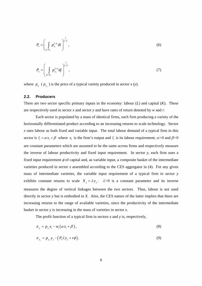
(y). The industry price indices dual to (4) and (5) are, respectively,

6

11

1i

x

x xi N

P p diσ

σ−

−

∈

⎛ ⎞= ⎜ ⎟⎜ ⎟

⎝ ⎠∫ , (6)

11

1j

y

y yj N

P p djδ

δ−

−

∈

⎛ ⎞⎜ ⎟=⎜ ⎟⎝ ⎠

∫ , (7)

where ixp (

jyp ) is the price of a typical variety produced in sector x (y).

2.2. Producers There are two sector specific primary inputs in the economy: labour (L) and capital (K). These

are respectively used in sector x and sector y and have rates of return denoted by w and r.

Each sector is populated by a mass of identical firms, each firm producing a variety of the

horizontally differentiated product according to an increasing returns to scale technology. Sector

x uses labour as both fixed and variable input. The total labour demand of a typical firm in this

sector is i il xα β= + where ix is the firm’s output and il is its labour requirement; α>0 and β>0

are constant parameters which are assumed to be the same across firms and respectively measure

the inverse of labour productivity and fixed input requirement. In sector y, each firm uses a

fixed input requirement φ of capital and, as variable input, a composite basket of the intermediate

varieties produced in sector x assembled according to the CES aggregator in (4). For any given

mass of intermediate varieties, the variable input requirement of a typical firm in sector y

exhibits constant returns to scale j jX yλ= . λ>0 is a constant parameter and its inverse

measures the degree of vertical linkages between the two sectors. Thus, labour is not used

directly in sector y but is embodied in X. Also, the CES nature of the latter implies that there are

increasing returns to the range of available varieties, since the productivity of the intermediate

basket in sector y is increasing in the mass of varieties in sector x.

The profit function of a typical firm in sectors x and y is, respectively,

( )i ix x i i ip x w xπ α β= − + , (8)

( )j jy y j x jp y P y rπ λ φ= − + . (9)

7

2.3. Factor markets The market for capital is perfectly competitive, with r adjusting to satisfy the resource constraint

yN Kφ = , (10)

where K is the economy’s endowment of capital.

The labour market is unionised. While wages are set by decentralised firm-level

monopoly unions, employment is determined by firms. Given the symmetry between firms, in

sector x there is a mass Nx of identical unions. Denoting by L the aggregate labour force, a

typical union i will have a mass of members il and will embrace the workers of, and set the

wage rate for, firm i in sector x. Unionisation implies that involuntary unemployment persists in

equilibrium and that each union will have some unemployed members11 – i.e., i il l< where il is

the union’s employed members. Each union maximises the expected real income of its typical

member subject to its labour demand. Hence, union i’s objective function is

(1 )i i i ii

i i

l t w l lU bl P l

− −= + , (11)

where

μμ −= 1yx PPP (12)

is the consumer price index, t is the labour income tax rate and b is the real lump-sum benefit

received by an unemployed worker. We assume that unemployment benefit payments are not

taxed, i.e., they are net transfers.

2.4. Government budget constraint and aggregate income The government, whose role in the economy is limited to income redistribution, is a provider of

welfare protection in the form of unemployment benefits financed via proportional factor income

taxation. Noting that x x

i ii N i N

l di L L l di∈ ∈

= ≥ =∫ ∫ , the government budget constraint is given by

( )x x

i i i ii N i N

Pb l l di t w l di q rK∈ ∈

− = +∫ ∫ . (13)

11 We follow the literature in assuming that unemployed workers from other unions cannot be employed in a given

union’s firm before the latter’s unemployed members are hired.

8

The right-hand-side of equation (13) is the total tax revenue extracted from the primary factors,

where q is the capital income tax rate, and the left-hand-side of the equation gives the total

unemployment benefit bill.

Aggregate income of consumers, M, is determined by the total disposable incomes of

primary factors and the transfers from the public to private sector

(1 ) ( ) (1 )x

i i i ii N

M t w l Pb l l di q rK∈

⎡ ⎤= − + − + −⎣ ⎦∫ . (14)

2.5. General Equilibrium Given the assumed preferences and technologies, the total expenditure on the varieties of the

good produced in sector x is given by x y xE M N P yμ λ= + , where the two terms on the right-

hand-side are the total expenditures by the country’s consumers and by firms in sector y,

respectively. The total expenditure on the varieties of the good produced in sector y is instead

given by (1 )yE Mμ= − . Using these, the demand functions for the variety facing a typical firm

in sectors x and y are, respectively

ixxi

x x

pExP P

σ−⎛ ⎞

= ⎜ ⎟⎜ ⎟⎝ ⎠

, (15)

jyyj

y y

pEy

P P

δ−⎛ ⎞⎜ ⎟=⎜ ⎟⎝ ⎠

. (16)

Firms in both sectors set their prices by maximising their profits − given by (8) and (9) − subject

to their demand − in (15) and (16) − and taking the total expenditures and input prices as given.

The first order condition for this maximisation can be used to obtain the firms’ optimal price

rules in sectors x and y respectively

1ix ip wασ

σ=

−, (17)

1jy xp Pλδ

δ=

−. (18)

9

For simplicity, we will use the normalisation ( )1 /α σ σ= − and replace (17) with ix ip w= . We

shall, however, keep (18) intact in order to examine the effect of a rise in the extent of vertical

integration captured by a reduction in λ.

The mass of firms in each sector is endogenously determined via free entry and exit and

the market clearing process. Hence, at the free-entry equilibrium, all firms in both sectors will

break even. Substituting (17) and (18) into (8) and (9) respectively and setting the resulting

equations equal to zero, we obtain the equilibrium output scale of a typical firm in sector x and y

ix βσ= , (19)

( )1j

x

ryP

φ δλ

− ⎛ ⎞= ⎜ ⎟

⎝ ⎠. (20)

Hence, in the symmetric equilibrium, while in sector x the optimal output scale of firms is

constant, in sector y the vertical linkages imply that it depends on the relative price of the two

inputs used in the sector. In particular, ceteris paribus, the equilibrium output scale in sector y

increases with the depth of the division of labour in sector x (i.e., it is increasing in xN through

its effect on xP ). Moreover, this effect is larger the larger is the degree of intersectoral linkages

(1/λ).

The wage rate paid by each firm in sector x is determined by the monopoly union

covering its workers. A typical union takes P, b and t as given and chooses its wage rate iw to

maximise its objective function in (11) subject to the firm’s labour demand (i.e., i il xα β= + ) as

well as (15) and (17). The wage setting equation resulting from this optimisation is

( ) 11 1

i

i

w bP

tε

=⎛ ⎞

− −⎜ ⎟⎝ ⎠

, (21)

where iε denotes the wage elasticity of labour demand facing the union and is an inverse

measure of unions’ monopoly power. It is straightforward to show that 1iε σ= − .

The optimal (real) wage set by the union is positively related to both labour income tax

rate and real unemployment benefit since: (i) a ceteris paribus increase in t reduces the after tax

10

wage; and (ii) a higher unemployment benefit rate b reduces the utility difference between being

employed and unemployed. The wage rate is also negatively related to ε since an increase in the

latter reduces the rent extracting ability of the union.

Given the assumed symmetry between firms in each sector, we drop the subscripts i and j

from the equations and, adopting good Y as numeraire, we set 1yP = .

For any given values of the policy instruments, t, q and b, a general equilibrium is

attained when all private agents optimise their objective functions and goods and capital markets

clear. In addition, since the general equilibrium also requires the government budget constraint

to hold, one of the policy instruments will have to be left to adjust in order to ensure that the tax

revenue equals the unemployment benefit bill. For simplicity, we shall assume in the rest of the

analysis that the government sets identical tax rates for the income of the two primary inputs and

let q=t. The solution of the model will therefore determine the endogenous variables − i.e. Nx,

Ny, x, y, px, py, Px, P, r, w, L, M, Ex, Ey − and the policy instrument that is left to vary to balance

the budget – i.e. either t or b.

2.6. Optimal unemployment benefit and the role of vertical linkages The government maximises aggregate welfare to determine the optimal unemployment benefit

rate b, allowing the tax rate t to adjust so as to balance its budget. The government’s objective

function is given by the aggregate indirect utility which can be obtained from (1), i.e.,

( )MU V L LP

= + − . (22)

where 1LLV e

η ⎛ ⎞⎜ ⎟⎝ ⎠= − . The function in (22) is maximised subject to the government budget

constraints and all other equations determining Nx, Ny, x, y, px, py, Px, P, r, w, L, M, Ex, Ey and t in

terms of b. This is equivalent to first solving the model and determining these variables in terms

of b and then substituting the resulting expressions in (22) to obtain the welfare function as

( )U b . Given the analytical complexity of the model, we resort to numerical simulations. Figure

1 below plots the aggregate welfare function and the function determining the aggregate

employment rate, ( )U b and / ( )L L b= , for two different values of the vertical linkages

parameter λ. As the figure suggests, aggregate employment is positively related to the real

11

unemployment benefit rate and the optimal policy entails a positive b. Recalling that λ is an

inverse measure of the degree of vertical linkages between sectors, it is also clear that the

optimal unemployment benefit rate and the associated level of aggregate employment and

welfare are higher the stronger the intersectoral linkages are.

The concavity of ( )U b reflects the trade-off that the government faces as a result of an

increase in unemployment benefit. This trade-off rests on the fact that, a rise in b leads to an

increases in aggregate employment and in real income. On the one hand, the higher income

generates an incentive to raise b. On the other hand, the higher employment reduces the utility of

leisure, hence making a lower unemployment benefit rate more desirable.

The fact that real income and employment are increasing in b may seem counterintuitive

and is at odds with the conventional wisdom. Central to this outcome is the existence of

complementarities – stemming from monopolistic competition and intersectoral linkages − which

result in a sub-optimal provision of intermediate varieties. The expansionary nature of the

welfare policy reduces the extent of this sub-optimality. To see the intuition behind this, let us

sketch the complex adjustment process that follows an exogenous change in b. For any given Nx

(the mass of firms in sector x), an increase in b will initially prompt unions to demand higher

nominal wages. This will have two main effects. First, as firms in sector x mark-up their prices,

the increase in wages is transferred into a higher price for each variety and thus leads to an

increase in Px – the price index in the industry. By triggering a substitution of Y for X by

consumers and a reduction in demand for intermediates by firms in sector y, this effect will lower

the demand for X – which, due to the vertical linkages, is however partially dampened by the

higher demand for Y by consumers. Second, the increase in the benefit rate and the subsequent

rise in the wage rate lead together to a higher aggregate nominal income that stimulates

consumers’ demand for both X and Y. Note that, via the vertical linkages in production, the

higher consumption of Y enhances the direct increase in the demand for X. It is straightforward

to show that the immediate impact of a rise in b (i.e., before the mass of firms, employment

levels and other prices adjust) is a net increase in the demand for good X that triggers new entry

of firms into sector x. The expansion of Nx reduces Px which, other things equal, stimulates both

final and intermediate demand for good X and thus leads to further entry into the sector.

12

Figure 1. Equilibrium in the Autarky Case (1) Optimal Unemployment Benefit and the Role of Vertical Integration

(1) Parameter values used in the numerical simulation are given in the note to Table A3 in the Appendix. A reduction in λ is equivalent to a rise in the productivity of X and hence to a higher degree of vertical integration.

(2) ( )U b is aggregate welfare, measured here by the aggregate indirect utility, evaluated at the general

equilibrium solution. The plot of U depicts per capita welfare (i.e. as ratio of L ) scaled by 0.1 to enable comparison with /L L= .

Unemployment Benefit, b

( ) ; 1U b λ = (2)

( ); 1b λ =

Welfare and Em

ployment R

ateW

elfare and Employm

ent Rate

( ); 0.95U b λ = (2)

( ); 0.95b λ =

Unemployment Benefit, b

13

A rise in unemployment benefit, therefore, ultimately generates a positive pecuniary

externality via an overall expansion of product variety in sector x which, by reducing Px, will

lead to: (i) a higher productivity of the intermediate goods that will reduce the cost of production

in sector y; (ii) a lower consumer price index that will foster the demand for final goods via a real

income effect; and (iii) a substitution of X for Y by consumers that will further stimulate the

demand for X. The combined effects of these forces will give rise to a cumulative process of

entry of new firms into the intermediate industry, higher aggregate efficiency12, employment and

real income. This virtuous circle clearly generates an incentive for the government to increase its

unemployment benefit. In doing so, however, it faces a trade-off in that the higher employment

reduces the aggregate utility of leisure.

It is straightforward to verify that the virtuous circle discussed above is stronger the

higher the extent of intersectoral linkages is, i.e., the stronger the aggregate returns to scale are.

In fact, the smaller the value of λ is, the greater the following will be: (i) the increase in the

demand for intermediates following the rise in final goods demand; (ii) the entry of new firms in

sector x; (iii) the ensuing aggregate productivity gains; and (iv) the increase in employment and

real income. Hence, as illustrated in Figure 1 above and in Table A3 in the Appendix, the

optimal unemployment benefit rate is higher and the tax rate on primary factors’ incomes is

lower (due to a higher tax base) at smaller values of λ. Note also that, despite the higher

employment, the overall size of the welfare state (i.e., the total unemployment benefit bill) is

larger at smaller values of λ, i.e., the increase in b dominates the fall in unemployment.

3. INTERNATIONAL OPENNESS The aim of this section is to shed light on the effects of international economic integration on the

optimal unemployment benefit policy described above. To this end, we extend the model to a

standard symmetric two-country setting. We assume that the two economies (Home and

Foreign, denoted by H and F respectively) are identical in every respect (tastes, technologies,

institutional features and factor endowments). Hence, the model developed in Section 2 applies

symmetrically to the foreign country – whose variables will be denoted with an asterisk

12 In De Grauwe and Polan (2003), social expenditure affects workers’ productivity by entering directly as an

argument in the production function of the private sector. Here, instead, the effects of government policy on aggregate efficiency emerges endogenously.

14

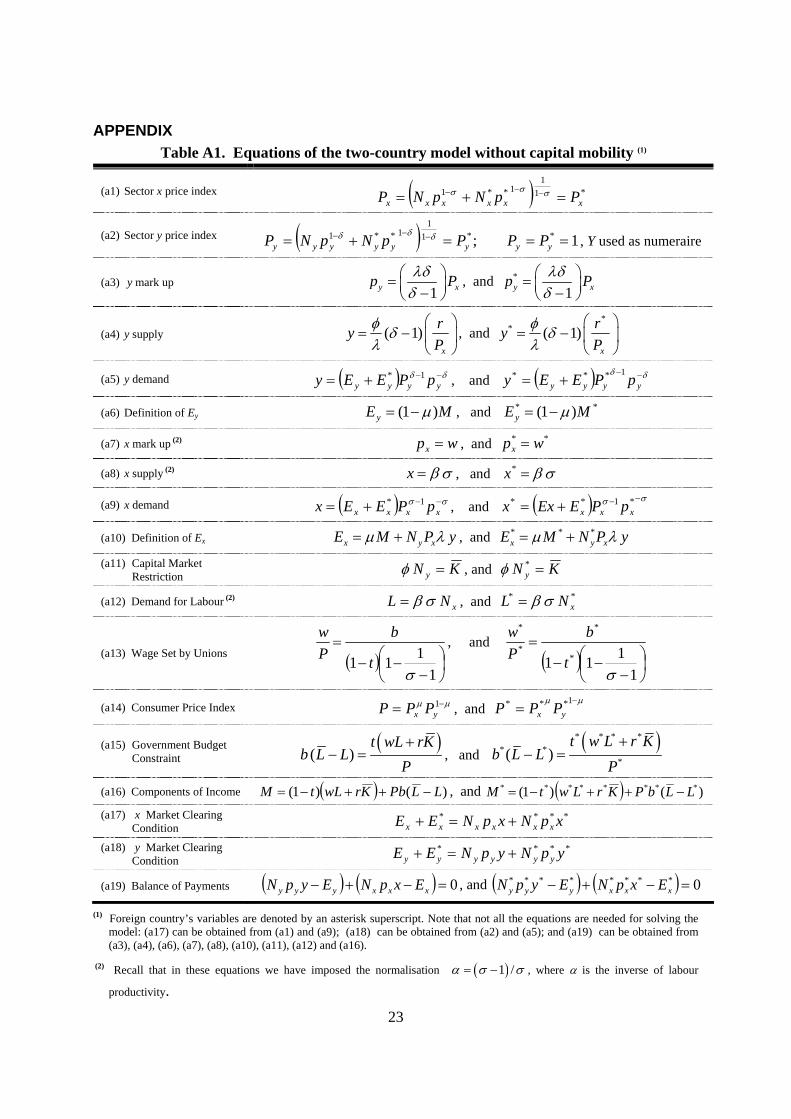
superscript. The equations for the two country model are given in Tables A1 and A2 in the

Appendix.

To start with, we shall focus on the effects of free-trade in goods and assume that both

primary factors of production are internationally immobile. Given the absence of trade barriers,

the CES aggregators and the price indices of the two differentiated goods will be defined over

the varieties produced in, and will be common to, both countries. It follows that a major

implication of free-trade is that the increasing returns to the range of available varieties of input

X are fully ‘international’, i.e., the external economies of scale that characterise the economy are

not country specific. Thus, productivity in sector y in both countries is increasing in ( )*x xN N+ ,

where *xN is the mass of varieties of good X produced in the foreign country.

3.1. Optimal non-cooperative policy under free-trade and no capital mobility We model the optimal non-cooperative policy as the outcome of a Nash game between

governments. Hence, each government chooses its unemployment benefit rate to maximise the

aggregate welfare of their residents given by (22), allowing the income tax rate to adjust to

balance its budget and taking the unemployment benefit rate set by the other government as

given. Clearly, as in the autarky case, the maximisation of (22) is carried out subject to the

governments’ budget constraints and all other equations determining the endogenous variables

for H and F in terms of b and *b .

The Nash equilibrium is depicted in Figure 2 below by the intersection of the two

governments’ reaction functions and consists of positive and – given that the two countries are

identical in every respect – symmetric unemployment benefit rates. The fact that the two

reaction functions are upward sloping reflects the positive spill-over effects that an increase in

unemployment benefit in one country has on the other country’s welfare. A unilateral increase in

unemployment benefit in one country leads to an increase in the mass of intermediate varieties

produced there and thus to a higher aggregate efficiency. However, given that – due to the free

tradability of the good – the returns to scale are fully international, the expansion in the

intermediate product range in one country generates a positive pecuniary externality for its

trading partner who will enjoy higher real income and whose government, as a result, will find it

optimal to raise its unemployment benefit rate too.

15

Figure 2. Non-Cooperative Nash Equilibrium in the Two-Country Case (1) Reaction Functions with Free-trade and No Capital Mobility

(1) Parameter values used in the numerical simulation are given in the note to Table A3 in the Appendix.

(2) The broken lines show the shift in the reaction functions as a result of an increase in the degree of vertical integration. See the relevant column in Table A3 in the Appendix for the effect of a rise in the extent of vertical integration captured by a reduction in λ.

As is clear from Table A3 in the Appendix, the Nash equilibrium unemployment benefit

rates are higher than in the autarkic regime. Furthermore, the tax rate is lower and employment,

real income, and aggregate welfare are higher. Hence, due to positive inter-country spillovers

that result from free-trade, a departure from autarky makes it optimal for governments to

increase the generosity and the real size of their welfare state, ( )b L L− , despite the lower tax

rates and the lower unemployment. Essentially, the positive efficiency effects of international

trade reinforce, and are reinforced by, the efficiency gains due to aggregate increasing returns

that are triggered by the policy.

45o

( )*, ; 1R b b λ =

( )* *, ; 1R b b λ =

(2)

(2)

Unem

ployment B

enefit in Country F, b

Unemployment Benefit in Country H, b

16

Again, as in the autarkic case, when intersectoral linkages are stronger, the Nash

equilibrium unemployment benefits are higher and, consistently, so are the level of employment

in sector x, aggregate real income, and welfare (see Table A3 for a numerical comparison). This

is because at lower values of λ, stronger aggregate scale economies imply that the expansionary

effects of welfare state expenditure generate larger efficiency gains which, under free-trade,

result in greater international pecuniary externalities.

3.2. Effects of capital mobility With capital mobility, the stock of capital available to a country can exceed or fall short of its

endowment K as capital can now flow in or out of the country. We use the source principle as

the tax rule, so that the income generated by an inflow of capital is taxed before it is repatriated.

We also assume that the capital flow between the two countries responds to differences in the net

of tax return on this factor. The modified equations of the model are given in Table A2 in the

Appendix.

A comparison of the Home country’s aggregate welfare function under no capital

mobility with that derived under capital mobility is illustrated in Figure 3 which plots, for a

given b*, the Home country’s welfare function against its unemployment benefit rate b. It is

clear that capital mobility leads to a shift in the Home welfare function such that, for any given

b*, a higher optimal value of b is obtained which also corresponds to a higher level of aggregate

welfare.

The basic intuition behind this result is that a unilateral increase in the generosity of

unemployment protection in the Home country results, through the virtuous circle outlined

above, in a lower tax rate. The latter leads to an incipient inflow of capital, thus generating a

unilateral incentive for the Home government to raise b beyond the case without capital mobility.

In the (b, b*) space, this implies an outward (upward) shift of the Home (Foreign) reaction

function. As a result, compared to the case without capital mobility, the Nash non-cooperative

solution under capital mobility entails higher (but identical, given the symmetry between

countries) unemployment benefit rates. Given the virtuous circle triggered by the policy, it is not

surprising that capital mobility also implies a higher level of employment and aggregate welfare

− as can be seen from the numerical comparisons provided in Table A3 in the Appendix. Again,

as in the previous cases, the virtuous circle of entry, higher efficiency and higher aggregate

17

employment and income triggered by the policy is more enhanced the stronger vertical linkages

and aggregate scale economies become.

Figure 3. Non-Cooperative Nash Equilibrium in the Two-Country Case (1) The shift in welfare function and optimal b due to capital mobility

(1) Parameter values used in the numerical simulation are given in the note to Table A3 in the Appendix. We have used *b =11. Note that the above graph is based on the K>0 case (i.e. capital flows from country F to country H). To enable comparison, U is scaled as in Figure 1 – see note (2) therein.

In sum, the welfare policy creates a positive externality even in the presence of capital

mobility. Note that although governments’ choice variables are not the capital tax rates, this can

be thought of as a ‘fiscal’ competition case (defined as non-cooperative policy setting by

independent governments), to the extent that each government’s policy (optimal choice of

unemployment benefits financed by adjusting the capital tax rates) influences the allocation of

mobile capital amongst different jurisdictions13. These results then clearly suggest that capital

mobility does not hinder the sustainability of welfare states and that a race-to-the-bottom in

13 This definition of tax competition is taken from Wilson and Wildasin (2004).

( )*,

Capital Mobility

U b b

( )*,

No Capital Mobility

U b b

Welfare in C

ountry H

Unemployment Benefit in Country H, b

18

social standards does not necessarily emerge as a result of the competition between countries for

internationally mobile factors of production14. In fact, whilst due to the symmetric nature of the

model the Nash equilibrium is characterised by the same inter-country distribution of the mobile

factor as before barriers to capital mobility were removed, both countries are in all respects

better off as a result of allowing for capital mobility in spite, and indeed because of, a higher

unemployment benefit entitlement15 (see Table A3 for a numerical comparison of the two cases).

3.3. The cooperative solution Finally, we analyse the cooperative equilibrium solution. The latter is obtained when the two

governments agree to set t=t* and b=b* at the outset and choose the latter to maximise their joint

welfare function subject to the relevant constraints determining the endogenous variables in

terms of b. Note that, given the symmetry between countries, the cooperative equilibrium is not

affected by capital mobility.

Figure 4. Cooperative Equilibrium in the Two-Country Case (1)

(1) Parameter values used in the numerical simulation are given in the note to Table A3 in the Appendix. To enable comparison, U is scaled as in Figure 1 – see note (2) therein.

14 Recall that the reduction in tax rates in this context results from an expansion of the tax base due to a rise in

employment and real returns to the factors and not from a desire to attract capital as in the tax competition case. 15 Note that, despite the higher b, the total unemployment benefit bill falls as a result of capital mobility. This is

due to the much higher level of employment compared to the non-capital mobility case.

( ) *( )U b U b+

Jointly Determined Unemployment Benefit, b

Joint Welfare

19

Figure 4 plots the joint welfare function against the common unemployment benefit rate.

It is clear from this figure and the numerical results provided in Table A3 in the Appendix that

the cooperative solution entails a higher optimal unemployment benefit rate than the Nash

equilibrium, both without and with capital mobility. The reason for this is that in the non-

cooperative regimes each government does not take account of the fact that a rise in its own

unemployment benefit rate will be matched by a rise in the other government’s rate. In other

words, in the non-cooperative case each government fails to internalise that the positive

externality of the policy implies that after a raise in b (b*) the optimal response for the

government of F (H) is to raise b* (b). Cooperation gets round this omission. It is worth noting

again that, as in all cases considered before, the optimal policy implies a higher b (and a higher

employment and welfare) the stronger the vertical linkages between sectors become.

The main results in Table A3 in the Appendix may be summarised as follows: A NT NK Cb b b b< < < ; A NT NK Ct t t t> > > ; A NT NK C< < < ; and A NT NK CU U U U< < < , where

the superscripts A, NT, NK, and C denote the solutions respectively obtained under autarkic,

Nash with free-trade only, Nash with free-trade and capital mobility, and full cooperation. These

results stem from the positive international spillover effects of the policy which imply that: (i) in

comparison to the autarkic regime, both the free-trade and the capital mobility regimes entail a

higher optimal unemployment benefit payment; and (ii) when deciding on their level of

unemployment benefit independently (or non-cooperatively), governments underestimate the

extent of the positive policy spillovers, thus setting them below the level that would be optimal

from a global welfare point of view.

4. CONCLUSIONS The conventional wisdom holds that economic globalisation, defined by free-trade and capital

mobility, reduces governments’ ability to effectively finance social policies and that a shrinking

tax base and competition for internationally mobile capital could in fact lead to a race-to-the-

bottom in social standards.

In this paper we develop a theoretical two-sector-two-country model with aggregate scale

economies and unionisation and find that (i) optimal welfare policy entails a positive level of

unemployment benefit provision which is higher the higher the degree of international economic

integration becomes (i.e., as we move from autarky to free-trade and to capital mobility) even

20

when each government acts independently (non-cooperatively) in determining its optimal

welfare payment; and (ii) optimal cooperative governments’ behaviour entails a higher level of

benefit entitlement and a higher aggregate welfare.

Hence, this model provides a clear example of circumstances in which welfare states and

increasing degrees of economic integration are perfectly compatible. Contrary to the

conventional wisdom, international trade and capital mobility need not lead to a reduction in the

revenue raising capacity of governments and to a race-to-the-bottom in social standards.

International openness can instead complement social insurance policies in increasing welfare,

thus facilitating the provision of a more generous welfare protection. Our analysis does not

counter the importance of institutional factors, as proposed by political scientists, in explaining

the compatibility between welfare states and economic openness16, but suggests that these factors

may not be necessary for reconciling the provision of social insurance with the pressures

stemming from economic openness.

At the core of our results lies the imperfectly competitive nature of markets and the well-

known principle that in a second-best world economic policy can be welfare improving. In the

labour market, unionisation implies that wages are positively related to unemployment benefit

and income tax rates. In the goods market, monopolistic competition leads to a suboptimal

production of varieties and to the emergence of pecuniary externalities stemming from the links

between upstream producers and their customers – i.e., the downstream industry and final

consumers. Effectively, government policy contributes to the extraction of the rents associated

with these pecuniary externalities, thus alleviating the sub-optimal provision of varieties in a

fashion that reinforces and is reinforced by the standard gains from international openness.

16 Political scientists argue that the extent to which economic (and political) pressures stemming from globalisation

are translated into welfare state retrenchment will typically depend on country-specific political and institutional factors and envisage conditions in which a retrenchment of welfare state may not result (e.g., Garrett, 1998; Swank, 2002).

21

References

Acemoglu, D. and R. Shimer (2000). “Productivity Gains from Unemployment Insurance”,

European Economic Review, 44, 1195-1224.

Alesina, A. and R. Perotti (1997). “The Welfare State and Competitiveness”, American

Economic Review, 87, 921-39.

Anderson, S.P., de Palma, A. and , J-F. Thisse (1992). Discrete Choice Theory of Product

Differentiation, MIT Press. Cambridge, Massachusetts.

Bartelsman, E.J., Caballero, R.J. and R.K. Lyons (1994). “Customer- and Supplier-Driven

Externalities”, American Economic Review, 84, 1075-1084.

Blanchard, O. and F. Giavazzi (2003), “Macroeconomic Effects of Regulation and Deregulation

in Goods and Labour Markets”, Quarterly Journal of Economics, 118, 879-907.

Blanchard,O. and N. Kiyotaki (1987). “Monopolistic Competition and the Effects of Aggregate

Demand”, American Economic Review, 77, 647-66.

Boeri T., A. Grugiavini, and L. Calmfors (2001). The Role of Unions in the Twenty-First

Century, (Eds.), Oxford University Press.

Bretschger, L. and Hettich, F. (2002). “Globalisation, Capital Mobility and Tax Competition:

Theory and Evidence for OECD Countries”, European Journal of Political Economy, 18,

695-716.

De Grauwe, P. and M. Polan (2003). “Globalisation and Social Spending”, CESifo Working

Paper No. 885.

Dixit, A.K. and J.E. Stiglitz (1977). “Monopolistic Competition and Optimum Product

Diversity”, American Economic Review, 67, 297-308.

Ethier, W.J. (1982). “National and International Returns to Scale in the Modern Theory of

International Trade”, American Economic Review, 72, 389-405.

European Commission (2002). Public Finances in EMU, European Economy – Report and

Studies, 3.

Garrett, G. (1998). Partisan Politics in the Global Economy, Cambridge University Press,

Cambridge.

Garrett, G. and D. Mitchell (1999). “Globalization and the Welfare State”, mimeo, Department of Political Science, Yale University.

Garrett, G. and D. Mitchell (2001). “Globalisation, Government Spending and Taxation in the

OECD”, European Journal of Political Research, 39, 145-177.

22

Hart, O.D. (1982). “A Model of Imperfect Competition with Keynesian Features”, Quarterly

Journal of Economics, 97, 109-138.

Hiscox, M.J. (2002). International Trade and Political Conflict: Commerce, Coalitions, and

Mobility, Princeton University Press.

Mankiw, N.G. (1988). “Imperfect competition and the Keynesian Cross”, Economics Letters, 26,

7-13.

Matsuyama, K. (1995). “Complementarities and Cumulative Processes in Models of

Monopolistic Competition”, Journal of Economic Literature, XXXIII, 701-729.

Ploeg, F. van der (2003). “Do Social Policies Harm Employment and Growth?”, CESifo

Working Paper No. 886.

Rodrik, D. (1997). Has Globalisation Gone too Far?, Institute for International Economics,

Wahsington, DC.

Rodrik, D. (1998). “Why Do More Open Economies Have Bigger Governments”, Journal of

Political Economy, 106, 997-1032.

Startz, R. (1989). “Monopolistic competition as a foundation for Keynesian macroeconomic

models”, Quarterly Journal of Economics, 104, 737-52.

Swank, D. (2002). Global Capital, Political Institutions, and Policy Change in Developed

Welfare States, Cambridge University Press, Cambridge.

Venables, A.J. (1996). “Equilibrium Location of Vertically Linked Industries”, International

Economic Review, 37, 341-59.

Wilson, J.D. and D.E. Wildasin (2004). “Capital Tax Competition: Bane or Boon”, Journal of

Public Economics, 88, 1065– 1091.

23

APPENDIX

Table A1. Equations of the two-country model without capital mobility (1)

(a1) Sector x price index ( ) *11

1**1xxxxxx PpNpNP =+= −−− σσσ

(a2) Sector y price index ( ) 1; **11

1**1 ===+= −−−yyyyyyyy PPPpNpNP δδδ , Y used as numeraire

(a3) y mark up 1y xp Pλδ

δ⎛ ⎞= ⎜ ⎟−⎝ ⎠

, and *

1y xp Pλδδ

⎛ ⎞= ⎜ ⎟−⎝ ⎠

(a4) y supply ( 1)x

ryP

φ δλ

⎛ ⎞= − ⎜ ⎟

⎝ ⎠, and

** ( 1)

x

ryP

φ δλ

⎛ ⎞= − ⎜ ⎟

⎝ ⎠

(a5) y demand ( ) δδ −−+= yyyy pPEEy 1* , and ( ) δδ −−+= yyyy pPEEy 1***

(a6) Definition of Ey MEy )1( μ−= , and ** )1( MEy μ−=

(a7) x mark up (2) wpx = , and ** wpx =

(a8) x supply (2) σβ=x , and σβ=*x

(a9) x demand ( ) σσ −−+= xxxx pPEEx 1* , and ( ) σσ −−+= *1**xxx pPEExx

(a10) Definition of Ex x y xE M N P yμ λ= + , and * * *x y xE M N P yμ λ= +

(a11) Capital Market Restriction KN y =φ , and KN y =*φ

(a12) Demand for Labour (2) xNL σβ= , and **xNL σβ=

(a13) Wage Set by Unions ( ) ⎟⎠⎞

⎜⎝⎛

−−−

=

1111

σt

bPw

, and ( ) ⎟

⎠⎞

⎜⎝⎛

−−−

=

1111 *

*

*

*

σt

bPw

(a14) Consumer Price Index μμ −= 1yx PPP , and

μμ −=

1***yx PPP

(a15) Government Budget Constraint

( )( )

t wL rKb L L

P+

− = , and ( )* * * *

* **( )

t w L r Kb L L

P+

− =

(a16) Components of Income ( ) )()1( LLPbKrwLtM −++−= , and ( ) )()1( ******** LLbPKrLwtM −++−= (a17) x Market Clearing

Condition **** xpNxpNEE xxxxxx +=+

(a18) y Market Clearing Condition

**** ypNypNEE yyyyyy +=+

(a19) Balance of Payments ( ) ( ) 0=−+− xxxyyy ExpNEypN , and ( ) ( ) 0******** =−+− xxxyyy ExpNEypN

(1) Foreign country’s variables are denoted by an asterisk superscript. Note that not all the equations are needed for solving the model: (a17) can be obtained from (a1) and (a9); (a18) can be obtained from (a2) and (a5); and (a19) can be obtained from (a3), (a4), (a6), (a7), (a8), (a10), (a11), (a12) and (a16).

(2) Recall that in these equations we have imposed the normalisation ( )1 /α σ σ= − , where α is the inverse of labour

productivity.

24

Table A2. Modifications to allow for capital mobility in the two-country model (1)

(11′) Capital Market Restriction KKN y +=φ , and KKN y −=*φ

(15′) Government Budget Constraint

( )( )( )

t wL r K Kb L L

P+ +

− = , and ( )* * * *

* **

( )( )

t w L r K Kb L L

P+ −

− =

(16′) Components of Income

( ) )()1( LLPbKrwLtM −++−= , and ( ))()1()()1(

***

*****

LLbPrKtKKrLwtM

−+−+

−+−=

(19′) Balance of Payments ( ) ( ) (1 ) 0y y Y x x xN p y E N p x E t rK− + − − − = , and ( ) ( ) 0)1(******** =−+−+− rKtExpNEypN xxxyyy

(1) Note that capital flow is denoted by K, with K>0 when the flow is from country F to country H. In the above, income equations are based on the convention that the Home country is the net importer of capital, i.e. K>0. When K<0, these are given by ( ) KrtLLPbKKrwLtM ** )1()()()1( −−−+++−= and ( ) )()1( ******** LLbPKrLwtM −++−= . In principle, the capital flow between country F and country H is determined by the relative net returns, e.g.

( )* *(1 ) (1 )K t r t rκ

= − − − , where K>0 when the flow is from F to H and (0, )κ ∈ ∞ determines the degree of substitution,

0κ → and κ → ∞ reflecting the extreme cases of zero and perfect substitution. However, given that in this model

,K K K⎡ ⎤∈ − +⎣ ⎦ , we have normalised the capital flow equation as ( ) ( )( ) ( )

* *

* *

1 1

1 1

t r t rKK t r t r

− − −=

− + − in order to remain consistent with

the capital market restriction. Clearly, K=0 when * *(1 ) (1 )t r t r− = − while the extreme cases of very large tax rate in F or H, i.e. */ 0t t → or * / 0t t → , leads to K K→ or K K→ − .

Table A3. Comparing Solutions for Different Symmetric Equilibria (1)

Autarky

Equilibrium

Two-Country Nash Non-cooperative

Equilibrium (no capital mobility)

Two-Country Nash Non-cooperative

Equilibrium (capital mobility)

Two-Country Cooperative Equilibrium

λ 1 0.95 1 0.95 1 0.95 1 0.95

Optimal b 10.6800 11.0900 12.9865 13.4855 12.9886 13.4875 13.0800 13.8100

t 0.1111 0.1099 0.1090 0.1077 0.1089 0.1076 0.1040 0.1027

/L L= 0.8562 0.8577 0.8588 0.8604 0.8590 0.8605 0.8652 0.8667

/w P 15.0186 15.5733 18.2187 18.8917 18.2193 18.8923 18.2456 18.9191

/r P 0.0968 0.1005 0.1178 0.1223 0.1178 0.1224 0.1188 0.1234

( / ) /M P L 13.826 14.363 16.824 17.478 16.827 17.481 16.974 17.631

( ) /b L L L− 1.536 1.578 1.834 1.883 1.832 1.881 1.763 1.810

/U L 24.082 24.588 27.027 27.647 27.027 27.648 27.038 27.651 (1) Parameter values used are 10 3 10.3, 5, 10, 6, 10 , 10 , 10K K L Kμ η δ σ β φ− − −= = = = = = = . Optimal b refers to the

welfare maximising value of benefit payment. These results are robust to plausible changes in parameter values. All analytical solutions and calibrations are done in Maple and the work files are available on request from the authors.