NBER WORKING PAPER SERIES

OPTIMAL INTEREST RATE POLICY IN A SMALL OPEN ECONOMY

Eric ParradoAndrés Velasco

Working Paper 8721http://www.nber.org/papers/w8721

NATIONAL BUREAU OF ECONOMIC RESEARCH1050 Massachusetts Avenue

Cambridge, MA 02138January 2002

We thank Andrés Escobar, Luis Oscar Herrera, Paolo Pesenti, Jaume Ventura, and seminar participants atthe Econometrics Society Meeting, the Lacea Winter Camp 2001 and NBER-IFM Spring Meetings 2001 forcomments. Velasco thanks the Center for International Development at Harvard for generous support. Theviews expressed herein are those of the authors and not necessarily those of the National Bureau of EconomicResearch or the IMF.

© 2002 by Eric Parrado and Andrés Velasco. All rights reserved. Short sections of text, not to exceed twoparagraphs, may be quoted without explicit permission provided that full credit, including © notice, is givento the source.

Optimal Interest Rate Policy in a Small Open EconomyEric Parrado and Andrés VelascoNBER Working Paper No. 8721January 2002JEL No. E52, F41

ABSTRACT

Using an optimizing model we derive the optimal monetary and exchange rate policy for a small

stochastic open economy with imperfect competition and short run price rigidity. The optimal monetary

policy has an exact closed-form solution and is obtained using the utility function of the representative

home agent as welfare criterion. The optimal policy depends on the source of stochastic disturbances

affecting the economy, much as in the literature pioneered by Poole (1970). Optimal monetary policy

reacts to domestic and foreign disturbances. If the intertemporal elasticity of substitution in consumption

is less than one, as is likely to be the case empirically, the optimal exchange rate policy implies a dirty

float: interest rate shocks from abroad are met partially by adjusting home interest rates, and partially by

allowing the exchange rate to move. This optimal pattern may help rationalize the observed fear of

floating.

Eric Parrado Andrés VelascoMonetary and Exchange Affairs Department Harvard UniversityInternational Monetary Fund Kennedy School of Government700 19th Street, N.W. 79 JFK StreetWashington, DC 20431 Littauer 106eparrado@imf.org Cambridge, MA 02138

and NBERandres_velasco@harvard.edu

1. Introduction

After the exchange rate crises of the last decade many small open economies,both rich and poor, have adopted ßexible exchange rates in combination withsome kind of monetary or interest rate rule. Exactly what such a rule shouldlook like, however, remains very much an open question. In closed economies,inßation-targeting or Taylor-type rules are common, even though the optimalityof such rules is yet to be established analytically. In the open economy, host ofadditional tricky issues turn up. Should monetary policy respond systematicallyto the nominal or real exchange rate? Equivalently, should the ßoat be completelyclean or not?In the prehistory of international macroeconomics (that is to say, in the 1970s),

the answer to most of these questions was clear. The alleged advantage of a ßexibleexchange rate was that it helped insulate the economy from foreign real shocks.Behind that protective shield, domestic monetary policy could get on with the taskof stabilizing the domestic economy. Put in the language of the 1970�s literature,ßoating gave monetary policy a measure of independence so set interest rates inorder to attain internal balance, while the real exchange rate did much (if not all)of the work in securing external balance. This is a well known implication of theMundell-Fleming model. It is also what most textbook treatments prescribe.But in recent years this conventional wisdom has become less conventional, and

(according to some) perhaps also less wise. To begin with, there is the empiricalobservations that many small countries do not ßoat the way theory suggests theyshould. For instance, in the recent Asian crisis several countries abandoned pegs tothe dollar but then tightened monetary policy in response to adverse shocks, bothinternal and external, and attempted to Þght the depreciation of their currencies.In 1997-98 most Latin American countries also used tight money and high interestrates to prop up their currencies.1 Gavin, Hausmann, Pagés-Serra, and Stein(1999) and Calvo and Reinhart (2000) have documented this pattern, in whatthey call the �fear of ßoating� puzzle.Theoretically, the beneÞts of exchange rate ßexibility for small open economies

have also become a subject of contention. One issue is whether high variability

1Things have changed more recently, with Chile and Colombia relaxing monetary policy andgoing for a ßexible exchange rate, with the resulting nominal and real depreciation. Note thephenomenon is not universal, however, even among small economies: during the Asian crisesAustralia and New Zealand allowed their currencies to depreciate sharply and weathered thestorm with little cost in terms of domestic output.

in the nominal and real exchange rate (which may also mean high variability inthe terms of trade) is harmful to exports or growth. Another is whether ßoatingreally provides the kind of monetary independence it is supposed to: high volatilityof the nominal and real exchange rate could conceivably cause endemically highdomestic interest rates. A related point has to do with the ability of changes innominal exchange rates to affect relative prices: pass-through may be so large andquick that a depreciation only buys you more inßation. And, even more damming,depreciation could even be contractionary because of negative wealth effects orbecause of its harmful impact on the balance sheets of domestic banks and Þrms.Faced with these important questions, in this paper we adopt a �back to

basics� approach. We take a state-of-the-art stochastic macroeconomic modelwith sticky prices, adapt it to focus on the behavior of a small open economy,and use it to characterize optimal monetary and exchange rate policies. Since ourmodel is built from microfoundations, we can use individual utility functions toevaluate the welfare consequences of policies, with the optimal policy being thatwhich delivers the highest expected utility to domestic residents. In this contextwe are able to assess how monetary policy should respond to different stochasticdisturbances affecting the economy, in an update of the classic literature pioneeredby Poole (1970).It turns out that the 1970s prescriptions are mostly replicated by this vintage

2001 model. In particular, we show that:

� Home interest rates always respond to domestic disturbances: procyclicallyin the case of productivity shocks and countercyclically in the case of govern-ment spending shocks. In doing so, it replicates the behavior of the economyunder ßexible prices, and attains the corresponding level of welfare.

� The optimal exchange rate regime is always one of ßoating, in that thenominal and real exchange rates move in response to shocks from abroad.The direction and size of the optimal responses in home interest rates dependon parameter values, and most crucially on the intertemporal elasticity ofsubstitution in consumption.

� In the empirically relevant case of a small intertemporal elasticity of sub-stitution in consumption, the optimal policy involves a dirty ßoat of theexchange rate, with the domestic interest rate partially mimicking changesin world interest rates. This optimal pattern may help rationalize the ob-served fear of ßoating in some economies.

2

� This dirty ßoat is optimal regardless of whether the foreign central bankfollows its optimal policy or any other arbitrary pattern of responses to itsown domestic shocks.

� The alternative policy of permanently Þxing the exchange rate provokes awelfare loss that is increasing in the variance of both foreign and domesticshocks. This is because Þxing imposes two kinds of costs on the domesticeconomy: the real exchange is no longer available to cushion shocks fromabroad, and the interest rate (now endogenous and targeted at maintainingthe peg) is no longer available to respond to domestic disturbances.

We carry out the analysis in a model of the �new open economy macroe-conomics� tradition brought to life by Obstfeld and Rogoff (1995, 1998). Theoptimizing, general equilibrium, sticky-price models of this literature lend them-selves admirably to the analysis of alternative monetary policy rules. Predictably,there has been a slew of such papers recently.2 Our model differs from much recentwork in the following three dimensions:

� It focuses on a small open economy, while most papers �with the importantexception of Galí and Monacelli (2000)� focus on a world economy composedof two countries of comparable size.

� Like Obstfeld and Rogoff (forthcoming) and Corsetti and Pesenti (2001a),but unlike much work in the literature, we obtain closed-form solutionswithout resorting to log-linear approximations, and we are able to solveexplicitly for the Þrst and second moments of the endogenous variables in themodel, so we can study the effects of uncertainty on equilibrium variables.Our expressions for welfare are also exact, and can be used quite simply tocalculate optimal policies and evaluate alternatives.

� We focus on optimal interest rate policies (so we can afford to be agnostic asto the source of money demand), while most papers have tried to characterizethe optimal behavior of the nominal quantity of money.

In order to make the analysis tractable and get closed-form solutions we as-sume, in line with the literature, some speciÞc functional forms. Moreover, we

2Aside from those mentioned in the text, a partial list ought to include Monacelli (2001),Parrado (2001), Benigno and Benigno (2000), Ghironi and Rebucci (2000), Obstfeld and Rogoff(2000), and Svensson (2000).

3

do not introduce credibility or Þnancial fragility considerations, which are surelykey in designing optimal monetary and exchange rate policies. We discuss theimportance of such omissions in the concluding section.Perhaps the closest predecessor of this paper is that by Galí and Monacelli

(2000), who also study interest rate policies in a small open economy. Yet theirframework is different: they work with Calvo staggered prices and are forced toresort to linear approximations to get solutions. Another closely related paper isby Henderson and Kim (1999), who compute exact utilities and optimal monetarypolicies, but for a closed economy.The paper is organized as follows. Section 2 contains a description of the

theoretical model that includes both domestic and foreign shocks. In section 3 weshow how to solve the basic model, while section 4 presents the details of the Þrm�sprice setting. Section 5 discusses the structure of monetary policy rules. Section6 presents a closed-form solution for the welfare function based on the utilityfunction of the representative agent. Section 7 presents the analysis of optimalmonetary policies in a benchmark case. Section 8 studies the implications ofalternative policy scenarios. The Þnal section suggests extensions and directionsfor future research.

2. The Basic Model

In this model, a home and a foreign economy make up the world. There is measuren of home agents, each of which has the monopoly in producing a single tradablegood. There is measure n∗ of foreign agents, each of which also produces a goodunder monopoly conditions. Thus, n and n∗ indicate both the population size andthe economic size of each country.

2.1. Individual preferences

Home agent i, who is both a consumer and a producer, has the following utilityfunction

U it = Et

( ∞Xs=t

(1 + δ)−(s−t)·(Cis)

1−ρ

1− ρ − �κs1 + v

(Y is )1+v

¸), (2.1)

where δ is the rate of time preference. The notation Et[xt+j ] represents the ex-pectation of variable xt+j conditional on information available at t.

4

The variable Y i is output produced by home agent i. We stick to the standardassumption that he has monopoly rights over this variety, so that he is the soleproducer of the variety in the world economy. This term captures the disutilitythe individual experiences from having to produce more output. The stochasticparameter �κ represents an inverse productivity shock.The aggregate real consumption index Ci for any agent i is given by

Cit =

¡CiH,t

¢α ¡CiF,t

¢1−ααα(1− α)1−α , (2.2)

where CH,t and CF,t are the quantities that home agents consume of domestic andforeign goods, respectively, while α indicates the share of home agents� consump-tion of their own good on total consumption.The two consumption subindexes are symmetric and are deÞned, as in Dixit

and Stiglitz (1977), by

CH,t =

"µ1

n

¶ 1θZ n

0

CiH,t (j)θ−1θ dj

# θθ−1

; CF,t =

"µ1

n∗

¶ 1θZ n∗

0

CiF,t (j)θ−1θ dj

# θθ−1

,

(2.3)where CiH,t (j) is the consumption of home variety j by home agent i at time t,and the same for foreign varieties.Analogously to Obstfeld and Rogoff (1998) and Corsetti and Pesenti (2001a),

the elasticity of substitution across goods produced within a country is θ > 1,while the elasticity of substitution between the bundles produced by the homeeconomy and the rest of the world is 1.Rest-of-the-world agents have identical preferences. Foreign values of the cor-

responding domestic variables will be denoted by an asterisk (∗) and may differfrom home variables. Preferences over consumption of goods are symmetric acrossregions, except that foreign residents have a share α∗ home goods in their con-sumption basket. The rate of time preference δ is the same across countries.

2.2. Prices and demand curve facing each monopolist

Home prices indexes for the two preceding consumption baskets, denoted by PH,tand PF,t are deÞned as

5

PH,t =

·1

n

Z n

0

PH,t(j)1−θdj

¸ 11−θ; PF,t =

·1

n∗

Z n∗

0

PF,t(j)1−θdj

¸ 11−θ, (2.4)

where the domestic currency price index for overall real consumption Ct is givenby

Pt = PαH,tP

1−αF,t . (2.5)

The law of one price holds across all individual goods since agents of the homeeconomy and the foreign economy have identical preferences, so that PH,t (j) =StP

∗H,t (j) , ∀j ∈ [0, n], where PH,t (j) and P ∗H,t (j) are the prices of home good j in

home and foreign economies, respectively, and St represents the nominal exchangerate. The same relationship obviously holds for foreign goods.The commodity demand functions resulting from cost minimization are:

CH,t(j) =1

n

·PH,t(j)

PH,t

¸−θCH,t; Ct(j) =

1

n∗

·PF,t(j)

PF,t

¸−θCF,t. (2.6)

Using the deÞnition of total consumption (equation (2.2)), one can derive thedemand functions for home and foreign goods as:

CH,t = α

·PH,tPt

¸−1Ct; CF,t = (1− α)

·PF,tPt

¸−1Ct. (2.7)

2.3. Asset markets and budget constraints

The typical home agent has access to an internationally tradable bond B∗ denom-inated in terms of the foreign good and to a domestic bond B denominated interms of home money, and held only by domestic residents. His budget constraint,written using the foreign good as the numeraire, is therefore

B∗ it −B∗ it−1 +Bit −Bit−1PF,t

= r∗t−1B∗ it−1 + it−1

Bit−1PF,t

+P iH,tPF,t

Y iH,t −PH,tPF,t

T it −PH,tPF,t

CiH,t − CiF,t, (2.8)

where T it are lump-sum taxes levied by the government. Notice that r∗t , the realinterest rate on the foreign bond, is the �own� rate of return on the foreign good,and it is the nominal return on the domestic bond. We will assume, without lossof generality, that in equilibrium the net supply of this domestic bond is zero.

6

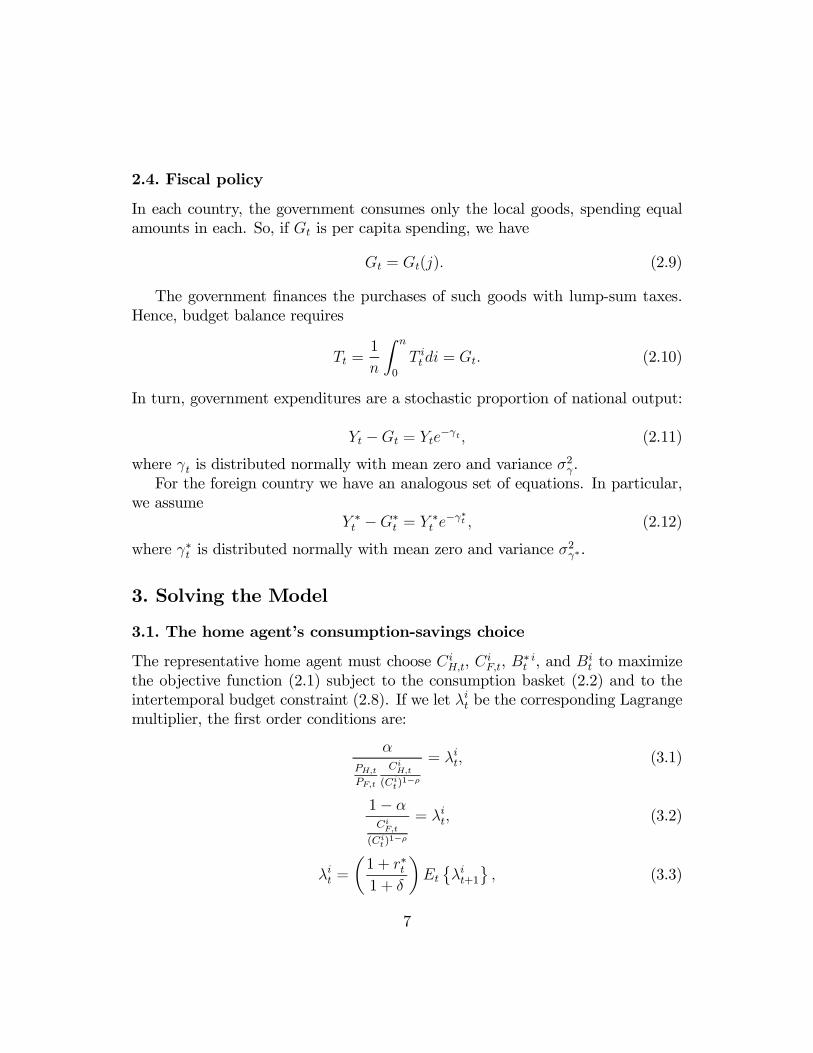
2.4. Fiscal policy

In each country, the government consumes only the local goods, spending equalamounts in each. So, if Gt is per capita spending, we have

Gt = Gt(j). (2.9)

The government Þnances the purchases of such goods with lump-sum taxes.Hence, budget balance requires

Tt =1

n

Z n

0

T it di = Gt. (2.10)

In turn, government expenditures are a stochastic proportion of national output:

Yt −Gt = Yte−γt, (2.11)

where γt is distributed normally with mean zero and variance σ2γ.

For the foreign country we have an analogous set of equations. In particular,we assume

Y ∗t −G∗t = Y ∗t e−γ∗t , (2.12)

where γ∗t is distributed normally with mean zero and variance σ2γ∗.

3. Solving the Model

3.1. The home agent�s consumption-savings choice

The representative home agent must choose CiH,t, CiF,t, B

∗ it , and B

it to maximize

the objective function (2.1) subject to the consumption basket (2.2) and to theintertemporal budget constraint (2.8). If we let λit be the corresponding Lagrangemultiplier, the Þrst order conditions are:

αPH,tPF,t

CiH,t(Cit)

1−ρ

= λit, (3.1)

1− αCiF,t

(Cit)1−ρ

= λit, (3.2)

λit =

µ1 + r∗t1 + δ

¶Et©λit+1

ª, (3.3)

7

λitPF,t

=

µ1 + it1 + δ

¶Et

½λit+1PF,t+1

¾. (3.4)

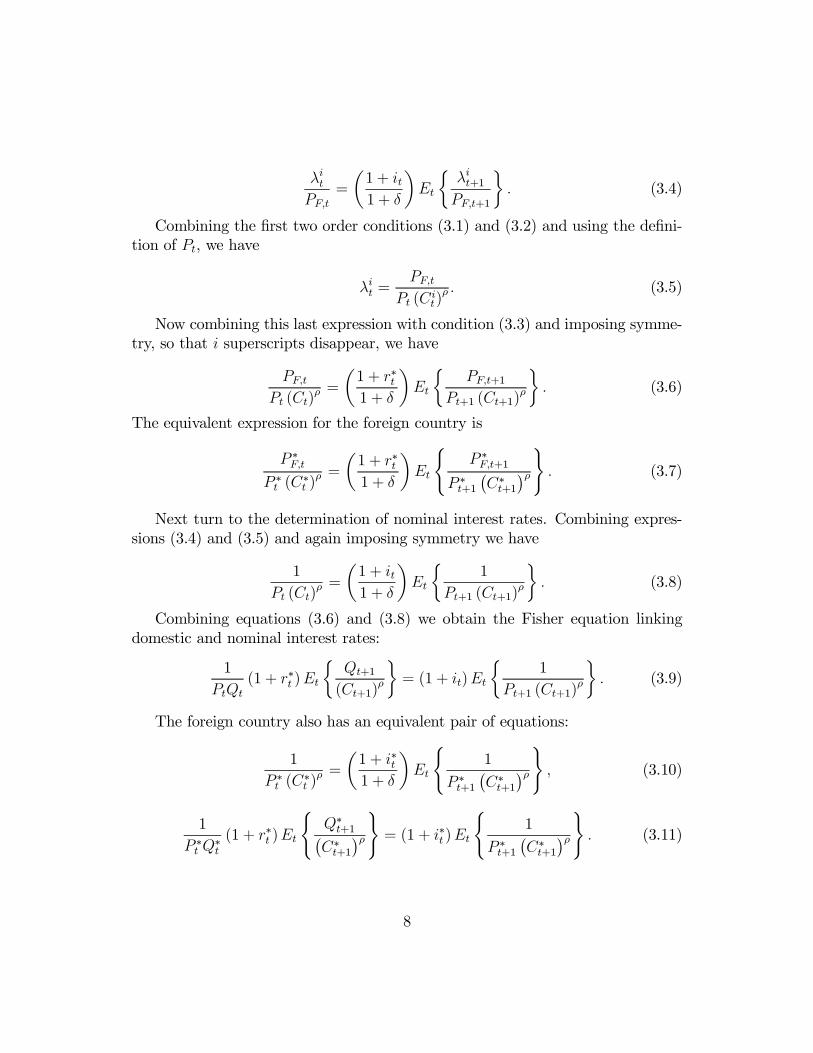
Combining the Þrst two order conditions (3.1) and (3.2) and using the deÞni-tion of Pt, we have

λit =PF,t

Pt (Cit)ρ . (3.5)

Now combining this last expression with condition (3.3) and imposing symme-try, so that i superscripts disappear, we have

PF,tPt (Ct)

ρ =

µ1 + r∗t1 + δ

¶Et

½PF,t+1

Pt+1 (Ct+1)ρ

¾. (3.6)

The equivalent expression for the foreign country is

P ∗F,tP ∗t (C∗t )

ρ =

µ1 + r∗t1 + δ

¶Et

(P ∗F,t+1

P ∗t+1¡C∗t+1

¢ρ). (3.7)

Next turn to the determination of nominal interest rates. Combining expres-sions (3.4) and (3.5) and again imposing symmetry we have

1

Pt (Ct)ρ =

µ1 + it1 + δ

¶Et

½1

Pt+1 (Ct+1)ρ

¾. (3.8)

Combining equations (3.6) and (3.8) we obtain the Fisher equation linkingdomestic and nominal interest rates:

1

PtQt(1 + r∗t )Et

½Qt+1(Ct+1)

ρ

¾= (1 + it)Et

½1

Pt+1 (Ct+1)ρ

¾. (3.9)

The foreign country also has an equivalent pair of equations:

1

P ∗t (C∗t )ρ =

µ1 + i∗t1 + δ

¶Et

(1

P ∗t+1¡C∗t+1

¢ρ), (3.10)

1

P ∗t Q∗t(1 + r∗t )Et

(Q∗t+1¡C∗t+1

¢ρ)= (1 + i∗t )Et

(1

P ∗t+1¡C∗t+1

¢ρ). (3.11)

8

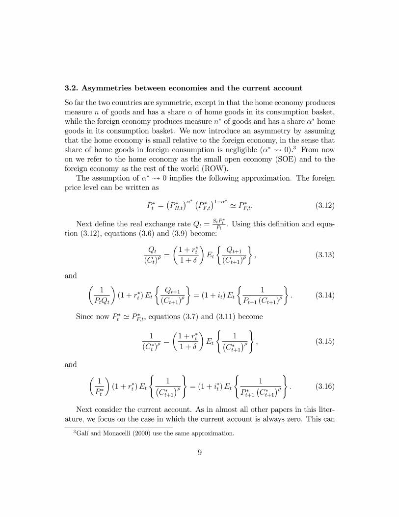
3.2. Asymmetries between economies and the current account

So far the two countries are symmetric, except in that the home economy producesmeasure n of goods and has a share α of home goods in its consumption basket,while the foreign economy produces measure n∗ of goods and has a share α∗ homegoods in its consumption basket. We now introduce an asymmetry by assumingthat the home economy is small relative to the foreign economy, in the sense thatshare of home goods in foreign consumption is negligible (α∗ Ã 0).3 From nowon we refer to the home economy as the small open economy (SOE) and to theforeign economy as the rest of the world (ROW).The assumption of α∗ Ã 0 implies the following approximation. The foreign

price level can be written as

P ∗t =¡P ∗H,t

¢α∗ ¡P ∗F,t

¢1−α∗ ' P ∗F,t. (3.12)

Next deÞne the real exchange rate Qt =StP ∗tPt. Using this deÞnition and equa-

tion (3.12), equations (3.6) and (3.9) become:

Qt(Ct)

ρ =

µ1 + r∗t1 + δ

¶Et

½Qt+1(Ct+1)

ρ

¾, (3.13)

and µ1

PtQt

¶(1 + r∗t )Et

½Qt+1(Ct+1)

ρ

¾= (1 + it)Et

½1

Pt+1 (Ct+1)ρ

¾. (3.14)

Since now P ∗t ' P ∗F,t, equations (3.7) and (3.11) become

1

(C∗t )ρ =

µ1 + r∗t1 + δ

¶Et

(1¡

C∗t+1¢ρ), (3.15)

and µ1

P ∗t

¶(1 + r∗t )Et

(1¡

C∗t+1¢ρ)= (1 + i∗t )Et

(1

P ∗t+1¡C∗t+1

¢ρ). (3.16)

Next consider the current account. As in almost all other papers in this liter-ature, we focus on the case in which the current account is always zero. This can

3Galí and Monacelli (2000) use the same approximation.

9

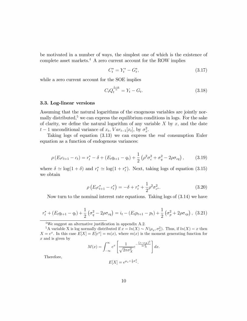
be motivated in a number of ways, the simplest one of which is the existence ofcomplete asset markets.4 A zero current account for the ROW implies

C∗t = Y∗t −G∗t , (3.17)

while a zero current account for the SOE implies

CtQ1−ααt = Yt −Gt. (3.18)

3.3. Log-linear versions

Assuming that the natural logarithms of the exogenous variables are jointly nor-mally distributed,5 we can express the equilibrium conditions in logs. For the sakeof clarity, we deÞne the natural logarithm of any variable X by x, and the datet− 1 unconditional variance of xt, V art−1[xt], by σ2x.Taking logs of equation (3.13) we can express the real consumption Euler

equation as a function of endogenous variances:

ρ (Etct+1 − ct) = r∗t − δ + (Etqt+1 − qt) +1

2

¡ρ2σ2c + σ

2q − 2ρσcq

¢, (3.19)

where δ ' log(1 + δ) and r∗t ' log(1 + r∗t ). Next, taking logs of equation (3.15)we obtain

ρ¡Etc

∗t+1 − c∗t

¢= −δ + r∗t +

1

2ρ2σ2c∗. (3.20)

Now turn to the nominal interest rate equations. Taking logs of (3.14) we have

r∗t +(Etqt+1 − qt) +1

2

¡σ2q − 2ρσcq

¢= it− (Etpt+1 − pt) + 1

2

¡σ2p + 2ρσcp

¢, (3.21)

4We suggest an alternative justiÞcation in appendix A.2.5A variable X is log normally distributed if x = ln(X) ∼ N(µx, σ2x). Thus, if ln(X) = x then

X = ex. In this case E[X] = E[ex] = m(x), where m(x) is the moment generating function forx and is given by

M(x) =

Z ∞

−∞ex

"1p2πσ2X

e− (x−µX)

2

2σ2X

#dx.

Therefore,E[X] = eµx+

12σ

2x .

10

where it ' log(1 + it). For the ROW the corresponding equation, obtained from(3.16), is

r∗t = i∗t −

¡Etp

∗t+1 − p∗t

¢+1

2

¡σ2p∗ + 2ρσc∗p∗

¢, (3.22)

where i∗t ' log(1 + i∗t ).

4. Price Setting

Turn now to the problem faced by monopolistic producers in each country, whomust set prices. We Þrst revisit the demand functions facing each set of producers,and then solve their respective problems.

4.1. Demand functions revisited

Above we had developed expressions for demand for each good in the home econ-omy. We now want to manipulate those expressions, plus the corresponding for-eign demand functions, in order to obtain world demand for each particular vari-ety. Appendix A.3 shows that total world demand for each home variety j can bewritten as:

Y dt (j) =

·Pt(j)

PH,t

¸−θ(Yt −Gt) +Gt. (4.1)

This means that, in symmetric equilibrium when PH,t(j) = PH,t, we have

Y dt (j) = Yt. (4.2)

DeÞning aggregate demand as

Y dt ≡1

n

Z n

0

Y dt (j)dj, (4.3)

we conclude Y dt = Yt, as it should be.

4.2. The price setters� problem

Home agents set prices for period t based on period t − 1 information and mustsatisfy all the demand at the quoted prices. It follows that the problem of home

11

agent i in period t− 1 is to choose its price, P iH,t, to maximize the expected valueof its objective function

Et−1

½µ1

1 + δ

¶·(Cit)

1−ρ

1− ρ − �κt1 + v

(Y it )1+v

¸¾. (4.4)

Maximization of equation (4.4) is subject to budget constraint (2.8) and de-mand function (4.1). The Þrst order necessary condition can be rearranged toread

Et−1©�κtY

1+vt

ª=θ − 1θEt−1

©(Ct)

1−ρª . (4.5)

For the ROW an analogous condition holds:

Et−1©�κ∗t (Y

∗t )1+vª = θ − 1

θEt−1

©(C∗t )

1−ρª . (4.6)

4.3. Log-linear versions

Taking logs of equation (4.5) we Þnd

Et−1yt+1 + v

2σ2y+

1

2 (1 + v)σ2κ =

1

1 + vlog

µθ − 1θ

¶+1− ρ1 + v

Et−1ct+(1− ρ)22 (1 + v)

σ2c ,

(4.7)where Et−1 log �κt = 0.Taking logs of (4.6) we have

Et−1y∗t+1 + v

2σ2y∗+

1

2 (1 + v)σ2κ∗ =

1

1 + vlog

µθ − 1θ

¶+1− ρ1 + v

Et−1c∗t+(1− ρ)22 (1 + v)

σ2c∗,

(4.8)where Et−1 log �κ∗t = 0.

5. Specifying Monetary Policy

The alert reader will have noticed that so far money demand has not entered themodel. We could avoid introducing money demand explicitly because we describemonetary policy entirely in terms of interest rules. This means that, whatever theshape or form of the money demand function, each central bank lets money supply

12

adjust endogenously so that a) the nominal interest rate is equal to the chosenrate and b) money demand is satisÞed. We now specify the monetary authorityreaction functions, which specify the setting of such chosen nominal interest ratesat home and abroad.

5.1. Policy rule of the SOE

The monetary authority of the small open economy designs an optimal monetarypolicy. Its policy function is

1 + it = (1 + i) (PH,t)ψp (eκt)ψκ (eκ∗t )ψκ∗ eψγγteψγ∗γ∗t , (5.1)

where the ψκ and ψγ are the coefficients associated with the domestic shocks whileψκ∗ and ψγ∗ are the coefficients associated with the foreign shocks. We introducethe term (PH,t)

ψp, where ψp > 0, following Woodford (1999), Henderson andKim (1999) and others, in order to ensure nominal uniqueness in the equilibriumsolution. The formulation implies that the monetary authority raises the nominalinterest rate if the log of the home price level is above a target, set to zero as anormalization. Notice also that this rule implies that the authorities� target rateof home inßation is zero.6 Appendix A.5 shows that under this rule the homeprice level is determinate �in fact, it is constant and equal to its log target of zero.This means, given the deÞnition of the overall price level pt, that we can set theterm Etpt+1 − pt =

¡1−αα

¢(Etqt+1 − qt) in what follows.

Taking logs the policy rule becomes

it = i+ ψppH,t + ψκκt + ψκ∗κ∗t + ψγγt + ψγ∗γ

∗t , (5.2)

where it ' log(1 + it), i ' log(1 + i), κt = log(eκt), and κ∗t = log(eκ∗t ).5.2. Policy rule of the ROW

The rest of the world also designs an optimal monetary policy. Its rule is givenby

1 + i∗t = (1 + i∗) (P ∗t )

ψ∗p∗ (eκ∗t )ψ∗κ∗ eψ∗γ∗γ∗t . (5.3)

As in the case of the small open economy, the term (P ∗t )ψ∗p∗ ensures that the

foreign price level P ∗t (which, recall, is both the foreign home price level and the

6A non zero rate of inßation could easily be introduced, but it adds nothing to our analysis.

13

foreign CPI) is both unique and constant. It follows that here the nominal interestrate i∗t+1 is equal to the ex ante foreign real interest rate r

∗t+1.

Taking logs the policy rule becomes

i∗t = i∗ + ψ∗p∗p

∗t + ψ

∗κ∗κ

∗t + ψ

∗γ∗γ

∗t , (5.4)

where i∗t ' log(1 + i∗t ) and i∗ ' log(1 + i∗).

6. A Closed-Form Solution

Appendix A.4 shows that both economies, home and rest-of-the-world, have a welldeÞned and unique steady state. In this section we study the behavior of theseeconomies out of long run equilibrium. It turns out that deviations from steadystate for all variables of interest can be obtained by means of a simple system oflinear equations. For computing that system we use the fact that, since all shocksare temporary, the expectation today of a variable�s level tomorrow is invariablythe steady state: Et−1xt = x for any variable x, where variables with no timesubscripts denote the steady state.Start with equation (3.19), which can be written

ct − c = −1ρ(r∗t − r∗) +

1

ρ(qt − q) , (6.1)

so that consumption is above its steady state level whenever the real interest ratesis below its steady state level, or the real exchange rate is above it. For the ROW,equation (3.20) yields

c∗t − c∗ = −1

ρ(r∗t − r∗) . (6.2)

Notice that combining (6.1) and (6.2) one obtains

ct − c = (c∗t − c∗) +1

ρ(qt − q) , (6.3)

Next, the balanced current account equation (3.18) gives aggregate demandfor the SOE as

ct − c = (yt − y)−µ1− αα

¶(qt − q)− γt, (6.4)

14

while the equivalent expression for the ROW yields

c∗t − c∗ = (y∗t − y∗)− γ∗t . (6.5)

The nominal interest rate equation for the SOE can be obtained by re-writing(3.21) in deviations from the steady state, and using the fact that pt − p =¡1−αα

¢(qt − q):

r∗t − r∗ = (it − i) + α−1 (qt − q) , (6.6)

while for the ROW this isr∗t − r∗ = i∗t − i∗. (6.7)

The resulting interest rate parity equation is then

it − i = i∗t − i∗ − α−1 (qt − q) , (6.8)

Finally, both policy rules can be written as7

it − i = ψκκt + ψ∗κ∗κ∗t + ψγγt + ψγ∗γ∗t , (6.9)

i∗t − i∗ = ψκ∗κ∗t + ψ∗γ∗γ∗t . (6.10)

This completes the description of the system. We have eight independent equa-tions and eight unknowns, so that the system is fully and uniquely determined.

7. Computing Optimal Policy

7.1. Calculating ex-ante utility

In this section we derive ex-ante utility to get a welfare measure in a closed form.The expected welfare function can be written as

Et−1

( ∞Xs=t

(1 + δ)−(s−t) U is

)=1 + δ

δEt−1U it , (7.1)

where Et−1U it = Et−1

½(Cit)

1−ρ

1−ρ − �κt1+v(Y it )

1+v

¾.

Using the condition of optimal price setting (4.5) we can write expected utilityas simply

7We have set the terms ψ∗pp∗t and ψppH,t equal to zero, since that is the value they take inequilibrium. See appendix A.5.

15

Et−1Ut =µ

1

1− ρ −1

1 + v

θ − 1θ

¶exp

·(1− ρ) c+ 1

2(1− ρ)2 σ2c

¸, (7.2)

where we have imposed symmetry and eliminated the i superscripts.For the ROW the analogous expression is

Et−1U∗t =µ

1

1− ρ −1

1 + v

θ − 1θ

¶exp

·(1− ρ) c∗ + 1

2(1− ρ)2 σ2c∗

¸. (7.3)

7.2. Optimal policy: the case of the ROW

We calculate optimal policy maximizing objective function (7.3) subject to theequilibrium conditions of the economy, given by equations (6.2), (6.5), (6.7), and(6.10).This is done in the following way. From expression (7.3) we see that if we can

compute the expected value and the variance of foreign consumption we have aclosed-form solution for foreign welfare. Maximizing the resulting expression withrespect to the optimal policy coefficients yields the optimal policy rule. Thattedious procedure is presented in appendix A.6. The solution is:

ψ∗κ∗ =ρ

ρ+ v, (7.4)

ψ∗γ∗ =ρ (1 + v)

ρ+ v.

This means that the foreign interest rate rule becomes

i∗t = i∗ + ψ∗p∗p

∗t +

ρ

ρ+ vκ∗t +

ρ (1 + v)

ρ+ vγ∗t , (7.5)

so that under the optimal policy steady state foreign consumption (and output)is

c∗ =1

ρ+ vlog

µθ − 1θ

¶,

and foreign utility is

16

U∗ =

µ1

1− ρ −1

1 + v

θ − 1θ

¶exp

½1− ρρ+ v

log

µθ − 1θ

¶¾(7.6)

exp

(1

2

µ1− ρρ+ v

¶2 £σ2κ∗ + (1 + v)

2 σ2γ∗¤).

What happens if ρ = 1? The policy coefficients that maximize foreign utilityare then

ψ∗κ∗ =1

1 + v, (7.7)

ψ∗γ∗ = 1,

so that under the optimal policy, foreign steady state consumption is

c∗ =1

1 + vlog

µθ − 1θ

¶, (7.8)

and foreign utility is

U∗ =1

1 + v

·log

µθ − 1θ

¶−µθ − 1θ

¶¸. (7.9)

7.3. Optimal policy: the case of the SOE

We calculate optimal policy maximizing objective function (7.2) subject to theequilibrium conditions of the economy, given by equations (6.1), (6.2), (6.4), (6.5),(6.6), (6.7), (6.9), and (6.10). The procedure is just as in the case of the ROW,and relies on the fact that, from expression (7.2), if we can compute the expectedvalue and the variance of home consumption we can have a closed-form solutionfor home welfare. Maximizing the resulting expression (see appendix A.7) oneobtains

17

ψκ =ρ

ρ [1 + v (1− α)] + αv , (7.10)

ψγ =ρ (1 + v)

ρ [1 + v (1− α)] + αv ,

ψκ∗ =v (ρ− 1) (1− α)

ρ [1 + v (1− α)] + αvψ∗κ∗,

ψγ∗ =v (ρ− 1) (1− α)

ρ [1 + v (1− α)] + αvψ∗γ∗.

This means that the domestic interest rate rule becomes

it = i+ ψppH,t +ρ

ρ [1 + v (1− α)] + αvκt ++ρ (1 + v)

ρ [1 + v (1− α)] + αvγt(7.11)

+v (ρ− 1) (1− α)

ρ [1 + v (1− α)] + αv¡ψ∗κ∗κ

∗t + ψ

∗γ∗γ

∗t

¢,

so that under the optimal policy steady state home consumption is

c =1

ρ+ vlog

µθ − 1θ

¶,

and home utility is

U opt =

µ1

1− ρ −1

1 + v

θ − 1θ

¶exp

½1− ρρ+ v

log

µθ − 1θ

¶¾(7.12)

exp

(1

2

·1− ρ

ρ [1 + v (1− α)] + αv¸2α2£σ2κ + (1 + v)

2 σ2γ¤)

exp

(1

2

·1− ρ

ρ [1 + v (1− α)] + αv¸2 ·(1 + v) (1− α)

ρ+ v

¸2ρ2£σ2κ∗ + (1 + v)

2 σ2γ∗¤).

If ρ = 1, the policy coefficients that maximize home utility are

18

ψκ =1

1 + v, (7.13)

ψγ = 1,

ψκ∗ = 0,

ψγ∗ = 0,

so that under the optimal policy, domestic steady state consumption is

c =1

1 + vlog

µθ − 1θ

¶, (7.14)

and domestic utility is

Uopt =1

1 + v

½log

θ − 1θ

− θ − 1θ

¾. (7.15)

7.4. Discussion and interpretation

Appendix A.8 computes the equilibrium of our two economies under ßexible prices.It turns out that the two optimal interest rate rules computed above cause theÞx-price economy to mimic the response of the ßex-price economy to real shocks.This means that utility levels are the same regardless of whether prices are stickyor not: a properly designed monetary policy manages to attain the economy�ssecond best.8

Both economies react to their domestic �productivity� disturbances: wheneverκ (or κ∗) is positive, the local central bank raises the local nominal interest ratein order to reduce demand for the home good and hence allow local producersto work less when doing so is particularly irksome. Notice that such monetarypolicies are procyclical : a fall in κ is a positive productivity shock that underßexible prices would elicit greater labor supply; under predetermined prices, themonetary authority instead engineers an expansionary monetary response thathas the same effect.9

Both economies also react to their �demand� disturbances: whenever govern-ment spending γ (or γ∗) is above its steady state level, the local central bank raises

8Not the Þrst best, of course, because the monopolistic distortion is still there, and there isnothing monetary policy can do about that.

9Obstfeld and Rogoff (forthcoming) make a similar point in the context of a model with two�large� countries.

19

its nominal interest rate to reduce demand for the local good. Such policies arecountercyclical : an increase in demand by the government is offset by a cut indemand by the local private sector.The small open economy also chooses to react to foreign shocks, but only

insofar as they are expressed via the foreign real (and nominal) interest rate.That is to say, ψκ∗ = 0 if ψ

∗κ∗ = 0, and ψγ∗ = 0 if ψ

∗γ∗ = 0. Moreover, the optimal

SOE policy involves a movement of home interest rates in tandem with foreignrates (ψκ∗ > 0 and ψγ∗ > 0) only if ρ, the inverse of the intertemporal elasticityof substitution, is larger than one. But if ρ < 1, home rates move in the oppositedirection as foreign rates (ψκ∗ < 0 and ψγ∗ < 0). There is no movement of homeinterest rates in response to foreign shocks only if ρ is exactly equal to one.An intuition for these results can be developed in the following way. Using

equation (6.1), (6.4), and (6.6), one can express demand for home output as

yt − y = γt −1 + (1− α) (ρ− 1)

ρ(it − i) + (1− α) (ρ− 1)

ρ(i∗t − i∗) . (7.16)

Hence, deviations of home output from its steady state level can be written ex-clusively as a function of the home and foreign interest rate disturbance and thelocal government demand shock. Notice that the foreign Þscal purchases shock γ∗tdoes not enter this expression: it matters for the determination of foreign output,but not of foreign consumption demand.10

The sign of the effect of foreign interest rates on domestic demand depends onwhether the intertemporal elasticity of substitution ρ is larger or smaller than one.This is because a fall in foreign interest rates has two effects on domestic aggregatedemand: it increases foreign consumption of all goods and it also appreciates thereal exchange rate (q tends to fall) switching demand away from domestic goods.One channel increases demand for home goods, and the other reduces it. If ρ > 1,as is likely to be the case empirically, a fall in foreign interest rates causes a fallin home demand, calling in turn for a cut in home interest rates to stabilize homedemand and output. With unitary elasticity of substitution between home andforeign goods and across time periods (ρ = 1), it turns out that the two effectscancel each other, so that shocks to the foreign interest rate have a null impacton foreign demand for home goods.What kind of an exchange rate regime does the optimal policy imply? If ρ

is exactly one, foreign interest rate shocks call for no reaction by domestic rates,

10Recall that each government consumes local goods only.

20

so the policy is a clean ßoat. In this case, since the foreign interest rate doesnot affect home demand, domestic monetary policy can be targeted at offsettingdomestic shocks only.If ρ < 1, home and foreign interest rates move in opposite directions, so given

arbitrage �as it appears in equation (6.8)� nominal and real exchange rate move agreat deal in response to foreign Þnancial shocks. This is a case of love of ßoating.Finally, if ρ > 1, local rates mimic, but only partially, the movement in foreign

rates. This follows from the fact that the term v(ρ−1)(1−α)ρ[1+v(1−α)]+αv in the bottom two

cells of (7.10), which is the ratio of the movement in domestic and foreign interestrates in response to foreign shocks, is smaller than one. In this case the optimalpolicy is dirty ßoat. This case, which is probably the empirically relevant one, canhelp rationalize the observed fear of ßoating mentioned in the introduction.These results can be summarized in the following way. Expressions (6.6) and

(6.7) can be rewritten to yield

qt − q = α [(i∗t − i∗)− (it − i)] , (7.17)

so that, when only foreign shocks occur,

qt − q = α (ψ∗κ∗ − ψκ∗)κ∗ + α¡ψ∗γ∗ − ψγ∗

¢γ∗, (7.18)

=

½α (v + ρ)

ρ [1 + v (1− α)] + αv¾¡ψ∗κ∗κ

∗ + ψ∗γ∗γ∗¢ ,

where the term in curly brackets is positive and decreasing in ρ. So the larger isρ, the smaller is the reaction of the nominal and real exchange rates to the foreignshocks.

8. Alternative Policy Scenarios

In this section we study alternative international scenarios in which domesticpolicy may have to be conducted, and one alternative domestic rule-of-thumbpolicy: a Þxed exchange rate.

8.1. No optimal policy abroad

So far we have assumed the ROW central bank follows an optimal policy. Whatif that is not the case? Does this mean that the home country coefficients are nolonger optimal?

21

We know the optimal foreign policy is given by (7.5). Consider now the fol-lowing variation on that policy:

i∗t = i∗ + ψ∗p∗p

∗t + φκ∗

ρ

ρ+ νκ∗t + φγ∗

ρ (1 + v)

ρ+ vγ∗t , (8.1)

where φκ∗ and φγ∗ are any two real numbers. Of course, if φκ∗ = φγ∗ = 1, thenthe foreign central bank is following optimal policies. Appendix A.9 shows that inthis case the optimal SOE monetary policy is unchanged. The difference betweensecond best and actual home welfare is (see same appendix for details):

U opt − Unopt =

µ1

1− ρ −1

1 + v

θ − 1θ

¶exp

½1− ρρ+ v

log

µθ − 1θ

¶¾(8.2)

exp

½1

2Φ£2φκ∗ (1− φκ∗)− ρ

¡1− φ2κ∗

¢− v (1− φκ∗)2¤σ2κ∗¾exp

½1

2Φh2φγ∗

¡1− φγ∗

¢− ρ ¡1− φ2γ∗¢− v ¡1− φγ∗¢2i (1 + v)2 σ2γ∗¾exp

(1

2

·ρ (1 + v) (1− α)

ρ [1 + v (1− α)] + αv¸2µ

1− ρρ+ v

¶2 £σ2κ∗ + (1 + v)

2 σ2γ∗¤)

− exp(1

2

·ρ (1 + v) (1− α)

ρ [1 + v (1− α)] + αv¸2µ

1− ρρ+ v

¶2 £φ2κ∗σ

2κ∗ + (1 + v)

2 φ2γ∗σ2γ∗¤),

where Φ = ρ(ρ−1)(1+v)(1−α)[ρ[1+v(1−α)]+αv](ρ+v)2 . Therefore, the loss in utility associated with non-

optimal foreign monetary policy is increasing in the variance of foreign shocks,and in the distance between the φ�s and their �optimal� level of one.What is going on here? Two things. The Þrst is that, without the optimal

policy in place, foreign output is more variable, and foreign producers protectthemselves against that variability (and the cost of possibly having to provide alot of labor services when it is irksome to do it), by setting higher prices. As aresult, steady foreign output drops. Given the fact that q = αρ

α+(1−α)ρ (y − y∗), thismeans that the steady state real exchange rate depreciates and the terms of tradeturn against the home country. This reduces SOE utility.The second key observation is that there is nothing that the home central bank

can do about this unwelcome development. Given that the ROW is large relativeto the SOE, homemonetary authorities cannot inßuence output variability abroad.And since foreign demand shocks do not affect home demand (once temporary

22

movements in the real exchange rate are accounted for), the SOE central bankshould not be trying to counteract those either.

8.2. A Þxed exchange rate

What are the welfare consequences of Þxing the exchange rate? Clearly, sincein this model a Þx is not the welfare-maximizing policy, utility must be lower.But how much lower? What does the difference depend on? These are importantquestions, since hard exchange rate pegs are alleged to have other virtues: theyare simple, credible, and may serve to promote economic and political integration.Those beneÞts could conceivable more than offset the macroeconomic costs, if thelatter are sufficiently low.Under a Þxed exchange rate, SOE monetary policy becomes endogenous, with

interest rates adjusting to keep the real exchange rate Qt equal to its steady statelevelQ. Appendix A.10 shows that in that case the difference between second-bestand actual levels of welfare is under Þxing:

U opt − UÞx =

µ1

1− ρ −1

1 + v

θ − 1θ

¶exp

½1− ρρ+ v

logµθ − 1θ

¶¾(8.3)

exp

½− (1− ρ) ∆

2

£σ2κ + (1 + v)

2 σ2γ¤¾

exp

½− (1− ρ) £(1 + v)2 − (1− ρ)2¤ ∆

2 (ρ+ v)2σ2κ∗

¾exp

(− (1− ρ) £(1 + v)2 − (1− ρ)2¤ ∆ (1 + v)2

2 (ρ+ v)2σ2γ∗

),

where ∆ = αρ[1+v(1−α)]+αv > 0. Thus, the loss in utility associated with Þxing is

increasing in the variance not only of foreign shocks, but also domestic shocks.This is because Þxing imposes two kinds of costs on the domestic economy: thereal exchange is no longer available to cushion shocks from abroad, and the interestrate (now endogenous and targeted at maintaining the peg) is no longer availableto respond to domestic disturbances.

23

9. Limitations and extensions

Rather than restating our conclusions, here we discuss their limitations and sug-gest directions for future research. The omission of all issues having to do withcredibility and Þnancial fragility is also important. Dealing with the former is,in principle, easy. Here we have focused on ex ante optimal monetary policies,and have therefore swept aside the issues that would arise if government couldreoptimize ex post (that is, after prices have been set). Because monopolisticcompetition here renders equilibrium output levels too low, a problem of timeinconsistency would occur, possibly leading to inefficiently large movements inthe nominal and real exchange rates. Such a �depreciation� bias under ßoatingcould be costly, rendering the policy inferior to other simple rules such as credibleÞxing. But notice: as Corsetti and Pesenti (2001a) and others have stressed, inmodels such as these a surprise devaluation also entails a surprise drop in theterms of trade. Therefore, myopic policy makers need not be subject to the sameinßation/devaluation bias that affects them in the closed economy, and hence timeinconsistency problems need not erase the welfare superiority of ßexible exchangerates.Regarding Þnancial fragility and imperfect Þnancial markets, one of us has

explored their importance for the design of monetary and exchange rate policiesin a small open economy. See Céspedes, Chang, and Velasco (2000 and 2001).In that work we discuss dollarized liabilities and endogenous risk premia arisingfrom costly state-veriÞcation, as in Bernanke and Gertler (1989). The bottomline of that work is that such Þnancial imperfections may be very important indetermining how severe and costly is the domestic adjustment to adverse externalshocks. But ßexible exchange rates, even in the presence of dollar liabilities, canhelp cushion the unwanted effects of such shocks.

24

A. Appendices

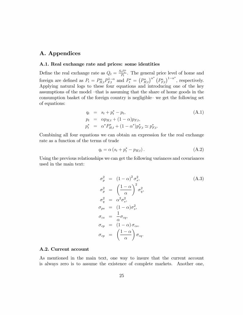
A.1. Real exchange rate and prices: some identities

DeÞne the real exchange rate as Qt =StP ∗tPt. The general price level of home and

foreign are deÞned as Pt = PαH,tP1−αF,t and P ∗t =

¡P ∗H,t

¢α∗ ¡P ∗F,t

¢1−α∗, respectively.

Applying natural logs to these four equations and introducing one of the keyassumptions of the model �that is assuming that the share of home goods in theconsumption basket of the foreign country is negligible� we get the following setof equations:

qt = st + p∗t − pt, (A.1)

pt = αpH,t + (1− α)pF,t,p∗t = α∗P ∗H,t + (1− α∗)p∗F,t ' p∗F,t.

Combining all four equations we can obtain an expression for the real exchangerate as a function of the terms of trade

qt = α (st + p∗t − pH,t) . (A.2)

Using the previous relationships we can get the following variances and covariancesused in the main text:

σ2p = (1− α)2 σ2s, (A.3)

σ2p =

µ1− αα

¶2σ2q ,

σ2q = α2σ2s,

σps = (1− α)σ2s,σcs =

1

ασcq,

σcp = (1− α)σcs,σcp =

µ1− αα

¶σcq.

A.2. Current account

As mentioned in the main text, one way to insure that the current accountis always zero is to assume the existence of complete markets. Another one,

25

sketched in what follows, relies on assuming an extreme asymmetry between thetwo economies.Recall that SOE is composed by individuals with measure n, who make also

n goods, while ROW is composed by individuals with measure n∗, who make n∗

goods. Clearing in each good market requires

nαPtCt + n∗α∗ (StP ∗t )C

∗t = nPH,t (Yt −Gt) , (A.4)

n (1− α)PtCt + n∗ (1− α∗) (StP ∗t )C∗t = n∗¡StP

∗F,t

¢(Y ∗t −G∗t ) , (A.5)

which can be rewritten as

n

n∗αPtCt + α

∗ (StP ∗t )C∗t =

n

n∗PH,t (Yt −Gt) , (A.6)

n

n∗(1− α)PtCt + (1− α∗) (StP ∗t )C∗t =

¡StP

∗F,t

¢(Y ∗t −G∗t ) . (A.7)

Now introduce two assumptions: i) α∗ ' 0 and ii) nn∗ ' 0. Using these

assumptions together with (A.6) we get

P ∗t C∗t = P

∗F,t (Y

∗t −G∗t ) . (A.8)

Therefore, the ROW current account is zero.Next, adding the two market clearing conditions and plugging (A.8) in this

relation we have an analogous condition for SOE

PtCt = PH,t (Yt −Gt) , (A.9)

so that naturally the home current account is also zero. Finally, using the deÞ-nitions of the real exchange rate and the domestic price level in this last resultyields equation (3.18) in the text.

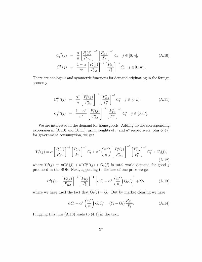
A.3. Demand functions

Plugging equation (2.7) into equation (2.6), it follows that the home demand forhome and foreign goods is given by

26

CHt (j) =α

n

·Pt(j)

PH,t

¸−θ ·PH,tPt

¸−1Ct j ∈ [0, n], (A.10)

CFt (j) =1− αn∗

·Pt(j)

PF,t

¸−θ ·PF,tPt

¸−1Ct j ∈ [0, n∗].

There are analogous and symmetric functions for demand originating in the foreigneconomy

CH∗t (j) =α∗

n

"P ∗t (j)P ∗H,t

#−θ ·P ∗H,tP ∗t

¸−1C∗t j ∈ [0, n], (A.11)

CF∗t (j) =1− α∗n∗

"P ∗t (j)P ∗F,t

#−θ ·P ∗F,tP ∗t

¸−1C∗t j ∈ [0, n∗].

We are interested in the demand for home goods. Adding up the correspondingexpression in (A.10) and (A.11), using weights of n and n∗ respectively, plus Gt(j)for government consumption, we get

Y dt (j) = α

·Pt(j)

PH,t

¸−θ ·PH,tPt

¸−1Ct + α

∗µn∗

n

¶"P ∗t (j)P ∗H,t

#−θ ·P ∗H,tP ∗t

¸−1C∗t +Gt(j),

(A.12)where Y dt (j) ≡ nCHt (j) + n

∗CH∗t (j) + Gt(j) is total world demand for good jproduced in the SOE. Next, appealing to the law of one price we get

Y dt (j) =

·Pt(j)

PH,t

¸−θ ·PH,tPt

¸−1 ·αCt + α

∗µn∗

n

¶QtC

∗t

¸+Gt, (A.13)

where we have used the fact that Gt(j) = Gt. But by market clearing we have

αCt + α∗µn∗

n

¶QtC

∗t = (Yt −Gt)

PH,tPt. (A.14)

Plugging this into (A.13) leads to (4.1) in the text.

27

A.4. Steady state

Let variables without time subscripts denote steady state values. In that state,equation (3.19) becomes

r∗ = δ − 12

¡ρ2σ2c + σ

2q − 2ρσcq

¢, (A.15)

where δ ' log(1 + δ) and r∗ ' log(1 + r∗), while equation (3.20) is

r∗ = δ − 12ρ2σ2c∗ . (A.16)

For the steady state to be well deÞned it therefore must be the case that

ρ2σ2c + σ2q − 2ρσcq = ρ2σ2c∗, (A.17)

which follows directly from equation (6.3).For nominal interest rates, the steadystate equations are

r∗ +1

2

¡σ2q − 2ρσcq

¢= i+

1

2

¡σ2p + 2ρσcp

¢, (A.18)

and

r∗ = i∗ +1

2

¡σ2p∗ + 2ρσc∗p∗

¢. (A.19)

With sticky prices in the foreign country, σ2p∗ = σc∗p∗ = 0, so that we have

i∗ = r∗ = δ − 12ρ2σ2c∗ . (A.20)

And since c∗t = y∗t − γ∗t , it follows that σ2c∗ = σ2y∗ + σ2γ∗, so we have

i∗ = r∗ = δ − 12ρ2¡σ2y∗ + σ

2γ∗¢. (A.21)

Plugging (A.20) in (A.18), the steady state domestic nominal interest rate mustbe

i = δ − 12ρ2σ2c∗ +

1

2

¡σ2q − 2ρσcq

¢− 12

¡σ2p + 2ρσcp

¢, (A.22)

or

28

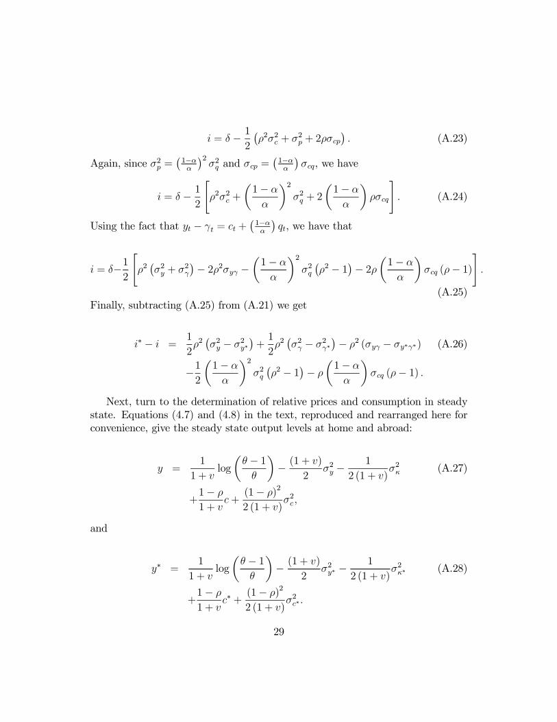
i = δ − 12

¡ρ2σ2c + σ

2p + 2ρσcp

¢. (A.23)

Again, since σ2p =¡1−αα

¢2σ2q and σcp =

¡1−αα

¢σcq, we have

i = δ − 12

"ρ2σ2c +

µ1− αα

¶2σ2q + 2

µ1− αα

¶ρσcq

#. (A.24)

Using the fact that yt − γt = ct +¡1−αα

¢qt, we have that

i = δ−12

"ρ2¡σ2y + σ

2γ

¢− 2ρ2σyγ − µ1− αα

¶2σ2q¡ρ2 − 1¢− 2ρµ1− α

α

¶σcq (ρ− 1)

#.

(A.25)Finally, subtracting (A.25) from (A.21) we get

i∗ − i =1

2ρ2¡σ2y − σ2y∗

¢+1

2ρ2¡σ2γ − σ2γ∗

¢− ρ2 (σyγ − σy∗γ∗) (A.26)

−12

µ1− αα

¶2σ2q¡ρ2 − 1¢− ρµ1− α

α

¶σcq (ρ− 1) .

Next, turn to the determination of relative prices and consumption in steadystate. Equations (4.7) and (4.8) in the text, reproduced and rearranged here forconvenience, give the steady state output levels at home and abroad:

y =1

1 + vlog

µθ − 1θ

¶− (1 + v)

2σ2y −

1

2 (1 + v)σ2κ (A.27)

+1− ρ1 + v

c+(1− ρ)22 (1 + v)

σ2c ,

and

y∗ =1

1 + vlog

µθ − 1θ

¶− (1 + v)

2σ2y∗ −

1

2 (1 + v)σ2κ∗ (A.28)

+1− ρ1 + v

c∗ +(1− ρ)22 (1 + v)

σ2c∗.

29

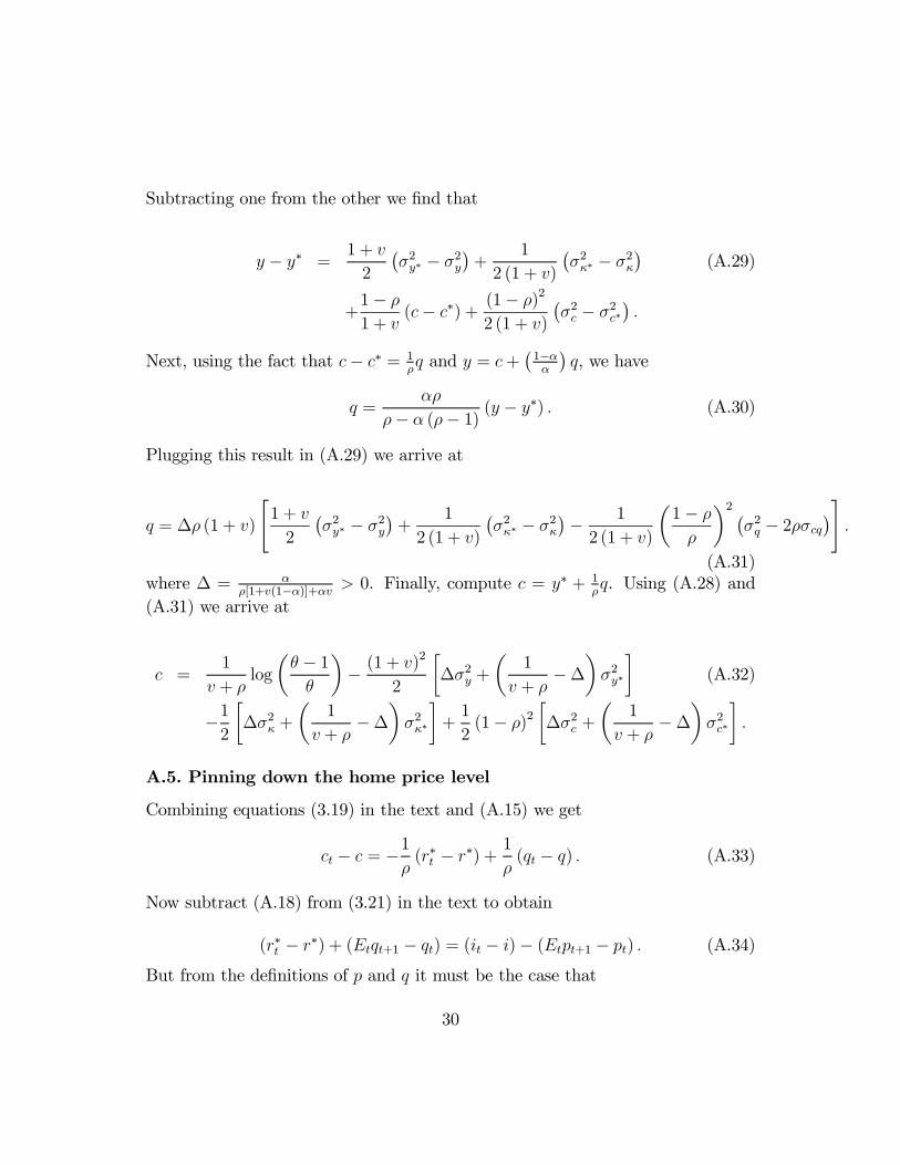
Subtracting one from the other we Þnd that

y − y∗ =1 + v

2

¡σ2y∗ − σ2y

¢+

1

2 (1 + v)

¡σ2κ∗ − σ2κ

¢(A.29)

+1− ρ1 + v

(c− c∗) + (1− ρ)22 (1 + v)

¡σ2c − σ2c∗

¢.

Next, using the fact that c− c∗ = 1ρq and y = c+

¡1−αα

¢q, we have

q =αρ

ρ− α (ρ− 1) (y − y∗) . (A.30)

Plugging this result in (A.29) we arrive at

q = ∆ρ (1 + v)

"1 + v

2

¡σ2y∗ − σ2y

¢+

1

2 (1 + v)

¡σ2κ∗ − σ2κ

¢− 1

2 (1 + v)

µ1− ρρ

¶2 ¡σ2q − 2ρσcq

¢#.

(A.31)where ∆ = α

ρ[1+v(1−α)]+αv > 0. Finally, compute c = y∗ + 1ρq. Using (A.28) and

(A.31) we arrive at

c =1

v + ρlog

µθ − 1θ

¶− (1 + v)

2

2

·∆σ2y +

µ1

v + ρ−∆

¶σ2y∗

¸(A.32)

−12

·∆σ2κ +

µ1

v + ρ−∆

¶σ2κ∗

¸+1

2(1− ρ)2

·∆σ2c +

µ1

v + ρ−∆

¶σ2c∗

¸.

A.5. Pinning down the home price level

Combining equations (3.19) in the text and (A.15) we get

ct − c = −1ρ(r∗t − r∗) +

1

ρ(qt − q) . (A.33)

Now subtract (A.18) from (3.21) in the text to obtain

(r∗t − r∗) + (Etqt+1 − qt) = (it − i)− (Etpt+1 − pt) . (A.34)

But from the deÞnitions of p and q it must be the case that

30

Etpt+1 − pt = (EtpH,t+1 − pH,t)−µ1− αα

¶(Etqt+1 − qt) . (A.35)

Combining these last two equations and recalling that Etqt+1 = q we have

(r∗t − r∗)−µ1

α

¶(qt − q) = (it − i)− {EtpH,t+1 − pH,t} . (A.36)

Next recall that the monetary policy rule is

it − i = ψκκt + ψ∗κ∗κ∗t + ψγγt + ψγ∗γ∗t + ψPpH,t.Using this plus (6.1) and (6.4) in (A.36) and rearranging we have

EtpH,t+1 = (1 + ψP ) pH,t + ψκκt + ψ∗κ∗κ

∗t +

¡ψγ − ρ

¢γt + ψγ∗γ

∗t (A.37)

+ρ (yt − y) + (1− ρ)µ1− αα

¶(qt − q) .

Solving this difference equation forward and ruling out bubbles we have

pH,t = Et

∞Xs=0

½ρ (yt+s − y) + (1− ρ)

µ1− αα

¶(qt+s − q)

¾¡1 + ψp

¢−s(A.38)

+Et

∞Xs=0

©ψκκt+s + ψ

∗κ∗κ

∗t+s +

¡ψγ − ρ

¢γt+s + ψγ∗γ

∗t+s

ª ¡1 + ψp

¢−s.

Taking expectations of this equation as of t−1, recalling that all shocks have zeromean and that therefore home output and the real exchange rate are expected tobe at its steady state value in all future periods, this expression becomes

Et−1pH,t = 0. (A.39)

Notice Þnally that since pH,t is pre-set as of t− 1, Et−1pH,t = pH,t = 0.Next we can calculate EtpH,t+1. Leading (A.38) by one period we have

pH,t+1 = Et+1

∞Xs=0

½ρ (yt+1+s − y) + (1− ρ)

µ1− αα

¶(qt+1+s − q)

¾¡1 + ψp

¢−s(A.40)

+Et+1

∞Xs=0

©ψκκt+1+s + ψ

∗κ∗κ

∗t+1+s +

¡ψγ − ρ

¢γt+1+s + ψγ∗γ

∗t+1+s

ª ¡1 + ψp

¢−s.

31

Taking expectations of this expression as of t we have EtpH,t+1 = 0. Weconclude that EtpH,t+1 − pH,t = 0 for all t. An analogous computation must becarried out to pin down the foreign price level.

A.6. Optimal policy in the ROW

Start by taking the logs of equation (4.6)

(1 + v) y∗+1

2(1 + v)2 σ2y∗+

1

2σ2κ∗+(1 + v)σκ∗,y∗ = log

θ − 1θ+(1− ρ) c∗+1

2(1− ρ)2 σ2c∗.(A.41)

Plugging the log version of equation (2.12) into the previous equation we canexpress expected consumption as a function of endogenous variances

c∗ = − 1

2 (ρ+ v)σ2κ∗ −

1

2

(1 + v)2

(ρ+ v)σ2γ∗ −

(1 + v)2

(ρ+ v)σc∗,γ∗ − (1 + v)

(ρ+ v)σκ∗,y∗(A.42)

+1

(ρ+ v)log

θ − 1θ

+1

2 (ρ+ v)

£(1− ρ)2 − (1 + v)2¤σ2c∗.

Combining the ROW policy rule (5.4) with equation (6.2) we get

c∗t − c∗ = −1

ρ

¡ψ∗κ∗κ

∗ + ψ∗γ∗γ∗t

¢. (A.43)

Using (A.43) we can compute all the endogenous variances in terms of exogenousvariances only:

σc∗,γ∗ = −1ρψ∗γ∗σ

2γ∗, (A.44)

σκ∗,y∗ = −1ρψ∗κ∗σ

2κ∗,

σ2c∗ =

µ1

ρψ∗κ∗

¶2σ2κ∗ +

µ1

ρψ∗γ∗

¶2σ2γ∗. (A.45)

Therefore, we can also compute expected consumption only in terms of exoge-nous variances

32

c∗ =1

ρ+ vlog

µθ − 1θ

¶(A.46)

− 1

2 (ρ+ v)

(1− 2 (1 + v) 1

ρψ∗κ∗ −

£(1− ρ)2 − (1 + v)2¤µ1

ρψ∗κ∗

¶2)σ2κ∗

− 1

2 (ρ+ v)

((1 + v)2 − 2 (1 + v)2 1

ρψ∗γ∗ −

£(1− ρ)2 − (1 + v)2¤µ1

ρψ∗γ∗

¶2)σ2γ∗.

Plugging both the variance of consumption (A.45) and the expected consump-tion (A.46) into expected utility (7.3), and then maximizing, we get the policycoefficients in (7.4) in the text.

A.7. Optimal policy in the SOE

Start by taking the logs of equation (4.5)

(1 + v) y+1

2(1 + v)2 σ2y+

1

2σ2κ+(1 + v) σκ,y = log

θ − 1θ

+(1− ρ) c+ 12(1− ρ)2 σ2c .

(A.47)Plugging the log version of equation (2.11) into the previous equation we can

express expected consumption as a function of endogenous variances:

c =ρ (1− α) (1 + v)

ρ (1 + v) + αv (1− ρ)c∗ (A.48)

−12∆ (1 + v)2

( ¡ρ1−α

α

¢2σ2c∗ + σ

2γ

−2hα+ρ(1−α)

α

i ¡ρ1−α

α

¢σc,c∗ + 2

hα+ρ(1−α)

α

iσc,γ − 2

¡ρ1−α

α

¢σc∗,γ

)

−12∆σ2κ − (1 + v)∆σκ,y +∆ log

θ − 1θ

+1

2∆

((1− ρ)2 − (1 + v)2

·α+ ρ (1− α)

α

¸2)σ2c .

Next, combining equations (6.1), (6.3), and (6.6) we have

ct − c = −αρ(it − i) + (1− α) (c∗t − c∗) , (A.49)

where c∗t − c∗ is given by equation (A.43). Therefore,

33

ct − c = −αρ(it − i)− 1− α

ρ(r∗t − r∗) . (A.50)

Finally, using both policy rules we get

ct − c = −αρ

¡ψκκ+ ψγγt

¢− [αψκ∗ + (1− α)ψ∗κ∗] κ∗ρ − £αψγ∗ + (1− α)ψ∗γ∗¤ γ∗tρ .(A.51)

Now we can compute all the endogenous variances in terms of exogenous vari-ances only:

σc,γ = −αρψγσ

2γ, (A.52)

σκ,y = −α+ ρ (1− α)ρ

ψκσ2κ,

σ2c∗ =

µ1

ρψ∗κ∗

¶2σ2κ∗ +

µ1

ρψ∗γ∗

¶2σ2γ∗,

σc,c∗ =

µ1

ρ

¶2ψ∗κ∗ [αψκ∗ + (1− α)ψ∗κ∗] σ2κ∗ +

µ1

ρ

¶2ψ∗γ∗

£αψγ∗ + (1− α)ψ∗γ∗

¤σ2γ∗,

σγ,c∗ = 0,

σ2c =

µα

ρψκ

¶2σ2κ + [αψκ∗ + (1− α)ψ∗κ∗]2

µ1

ρ

¶2σ2κ∗ (A.53)

+

µα

ρψγ

¶2σ2γ +

£αψγ∗ + (1− α)ψ∗γ∗

¤2µ1ρ

¶2σ2γ∗.

Therefore, we can also compute expected consumption only in terms of exoge-nous variances

34

c = ∆ρ (1− α) (1 + v)

α

"1ρ+v

log¡θ−1θ

¢− 12(ρ+v)

σ2κ∗ − 12(1+v)2

(ρ+v)σ2γ∗

+ (1+v)2

(ρ+v)1ρψ∗γ∗σ

2γ∗ +

(1+v)(ρ+v)

1ρψ∗κ∗σ

2κ∗

#(A.54)

+∆ρ (1− α) (1 + v)

α

(1

2 (ρ+ v)

£(1− ρ)2 − (1 + v)2¤ "µ1

ρψ∗κ∗

¶2σ2κ∗ +

µ1

ρψ∗γ∗

¶2σ2γ∗

#)

−12∆ (1 + v)2

µρ1− αα

¶2 "µ1

ρψ∗κ∗

¶2σ2κ∗ +

µ1

ρψ∗γ∗

¶2σ2γ∗

#− 12∆ (1 + v)2 σ2γ

+∆ (1 + v)2·α+ ρ (1− α)

α

¸µρ1− αα

¶ ³1ρ

´2ψ∗κ∗ [αψκ∗ + (1− α)ψ∗κ∗] σ2κ∗

+³1ρ

´2ψ∗γ∗

£αψγ∗ + (1− α)ψ∗γ∗

¤σ2γ∗

+v (1 + v)2

·α+ ρ (1− α)

α

¸α

ρψγσ

2γ −

1

2∆σ2κ + (1 + v)∆

·α+ ρ (1− α)

ρψκσ

2κ

¸+∆ log

θ − 1θ

+1

2∆

((1− ρ)2 − (1 + v)2

·α+ ρ (1− α)

α

¸2) ³αρψκ´2 σ2κ + ³αρψγ´2 σ2γ + [αψκ∗ + (1− α)ψ∗κ∗]2 ³1ρ´2 σ2κ∗

+£αψγ∗ + (1− α)ψ∗γ∗

¤2 ³1ρ

´2σ2γ∗

.Plugging both the variance of consumption (A.53) and the expected consump-

tion (A.54) into expected utility (7.2) and maximizing we get the policy coefficientsin (7.10) in the text.

A.8. The ßex-price solution

With ßexible prices, price-setting equations (4.5) and (4.6) must hold, but notjust in expectational form, so that we have

�κt (Yt)1+v =

θ − 1θ

(Ct)1−ρ , (A.55)

and

�κ∗t (Y∗t )1+v =

θ − 1θ

(C∗t )1−ρ . (A.56)

Taking logs we have

35

yt =1

1 + vlog

µθ − 1θ

¶+1− ρ1 + v

ct − 1

1 + vκt, (A.57)

y∗t =1

1 + vlog

µθ − 1θ

¶+1− ρ1 + v

c∗t −1

1 + vκ∗t . (A.58)

Using c∗t = y∗t − γ∗t we arrive at:

c∗t =1

ρ+ vlog

µθ − 1θ

¶− 1

ρ+ vκ∗t −

1 + v

v + ργ∗t . (A.59)

Next, using ct = c∗t +1ρqt and ct +

¡1−αα

¢qt = yt − γt we have

ct = ∆ log

µθ − 1θ

¶−∆κt + ρ∆ (1 + v)

µ1− αα

¶c∗t −∆ (1 + v) γt. (A.60)

Plugging (A.59) into (A.60) we get

ct =1

ρ+ vlog

µθ − 1θ

¶−∆κt −∆ (1 + v) γt (A.61)

+ρ∆ (1 + v)

µ1− αα

¶·− 1

ρ+ vκ∗t −

1 + v

ρ+ vγ∗t

¸,

so that

Et−1c∗t = c∗ =

1

ρ+ vlog

µθ − 1θ

¶, (A.62)

and

Et−1ct = c =1

ρ+ vlog

µθ − 1θ

¶. (A.63)

Subtracting (A.63) from (A.61) we obtain

ct − c = −∆κt −∆ (1 + v) γt (A.64)

−ρ (1 + v)µ1− αα

¶1

ρ+ v∆κ∗t − ρ (1 + v)

µ1− αα

¶1 + v

ρ+ v∆γ∗t ,

while subtracting (A.62) from (A.59) yields

c∗t − c∗ = −1

ρ+ vκ∗t −

1 + v

ρ+ vγ∗t . (A.65)

36

Using (A.64) and (A.65) we can compute the respective variances of home andforeign consumption

σ2c = ∆2σ2κ +∆2 (1 + v)2 σ2γ (A.66)

+ρ2µ1− αα

¶2µ1 + vρ+ v

¶2∆2£σ2κ∗ + (1 + v)

2 σ2γ∗¤,

σ2c∗ =

µ1

ρ+ v

¶2σ2κ∗ +

µ1 + v

ρ+ v

¶2σ2γ∗.

Do the optimal policies under sticky prices mimic the behavior of the ßexibleprice economy? Start with the easier case of the ROW. Taking logs of (7.5) weget the optimal policy rule

i∗t − i∗ =ρ

ρ+ vκ∗t +

ρ (1 + v)

ρ+ vγ∗t . (A.67)

Using this and (6.7) into equation (6.2) in the text we get (A.65) exactly. Hence,movements of consumption are the same as in under ßexible prices.Next, do the same for the SOE. The optimal policy (7.11) in logs turns out

to be:

it − i =ρ

ρ [1 + v (1− α)] + αvκt +ρ (1 + v)

ρ [1 + v (1− α)] + αvγt (A.68)

+v (ρ− 1) (1− α)

ρ [1 + v (1− α)] + αvρ

v + ρκ∗t +

v (ρ− 1) (1− α)ρ [1 + v (1− α)] + αv

ρ

v + ργ∗t .

Combining (A.64), (A.65), and (A.68) we have

ct − c = −αρ(it − i)− 1− α

ρ(i∗t − i∗) . (A.69)

Finally, plugging (6.6) in the text into this last expression we get

ct − c = − α

ρ [1 + v (1− α)] + αvκt −α

ρ [1 + v (1− α)] + αv (1 + v) γt (A.70)

− (1 + v) (1− α)ρ [1 + v (1− α)] + αv

ρ

v + ρκ∗t −

(1 + v) (1− α)ρ [1 + v (1− α)] + αv

ρ (1 + v)

v + ργ∗t .

We conclude that in the SOE, too, Þxed-price movements in consumption mimicthe movements in a ßex-price economy if the optimal interest rule is used.

37

What about utility? Expressions (7.2) and (7.3) for welfare still hold, regard-less of whether prices are Þxed or ßexible. Using (A.63) and (A.62) in those onecan check that utility under ßexible prices is the same as utility with Þxed prices(equations (7.6) and (7.12) in the main text) and the optimal policy rule.

A.9. No optimal policy abroad

Under the arbitrary policies, steady state foreign output (or consumption), earliergiven in (A.46), becomes

c∗ =1

ρ+ vlog

µθ − 1θ

¶(A.71)

− 1

2 (ρ+ v)

(1− 21 + v

ρφκ∗ −

£(1− ρ)2 − (1 + v)2¤µ1

ρφκ∗

¶2)σ2κ∗

− 1

2 (ρ+ v)

((1 + v)2

µ1− 21

ρφγ∗

¶− £(1− ρ)2 − (1 + v)2¤µ1

ρφγ∗

¶2)σ2γ∗.

Plugging this equation into equation (A.54) we obtain home steady state con-sumption, and then home utility as a function of both home and foreign policycoefficients. Thus, maximizing expected utility with respect to the home policycoefficients we get the same result described in equation (7.11) above. With thatpolicy, the utility level of the representative home is

Unopt =

µ1

1− ρ −1

1 + v

θ − 1θ

¶exp

½1− ρρ+ v

log

µθ − 1θ

¶¾(A.72)

exp

½1

2Φ£2φκ∗ (1− φκ∗)− ρ

¡1− φ2κ∗

¢− v (1− φκ∗)2¤σ2κ∗¾exp

½1

2Φh2φγ∗

¡1− φγ∗

¢− ρ ¡1− φ2γ∗¢− v ¡1− φγ∗¢2iσ2γ∗ (1 + v)2¾exp

(1

2

·α (1− ρ)

ρ [1 + v (1− α)] + αv¸2 £σ2κ + (1 + v)

2 σ2γ¤)

exp

(1

2

·ρ (1 + v) (1− α)

ρ [1 + v (1− α)] + αv¸2µ

1− ρρ+ v

¶2 £φ2κ∗σ

2κ∗ + (1 + v)

2 φ2γ∗σ2γ∗¤).

38

whereΦ = ρ(ρ−1)(1+v)(1−α)[ρ[1+v(1−α)]+αv](ρ+v)2 . Subtracting (A.72) from (7.15) one gets expression

(8.2) in the text.

A.10. A Þxed exchange rate

Combining equation (6.3) with equation (6.4) we get domestic goods market equi-librium as

yt − y − γt = ct − c = c∗t − c∗. (A.73)

In turn, temporary deviations in foreign consumption, as always, are given by

c∗t − c∗ = −1

ρ(r∗t − r∗) = −

1

ρ(i∗t − i∗) . (A.74)

If, for simplicity, we assume that the ROW central bank follows its optimalpolicy, (A.73) and (A.74) together yield

yt − y = γt −1

ρ+ vκ∗t −

1 + v

ρ+ vγ∗t , (A.75)

andct − c = − 1

ρ+ vκ∗t −

1 + v

ρ+ vγ∗t . (A.76)

Substituting these equations into (4.5) we obtain

(1 + v) y = logµθ − 1θ

¶+ (1− ρ) c− σ

2κ

2− (1 + v)

2

2σ2γ (A.77)

− 1

2 (ρ+ v)2£(1 + v)2 − (1− ρ)2¤σ2κ∗

− (1 + v)2

2 (ρ+ v)2£(1 + v)2 − (1− ρ)2¤σ2γ∗ .

Clearly, since the foreign central bank follows optimal policies, ROW steadystate income is c∗ = 1

ρ+vlog¡θ−1θ

¢. Using this and (A.77) in y = α+ρ(1−α)

αc −

ρ(1−α)αc∗ we obtain

39

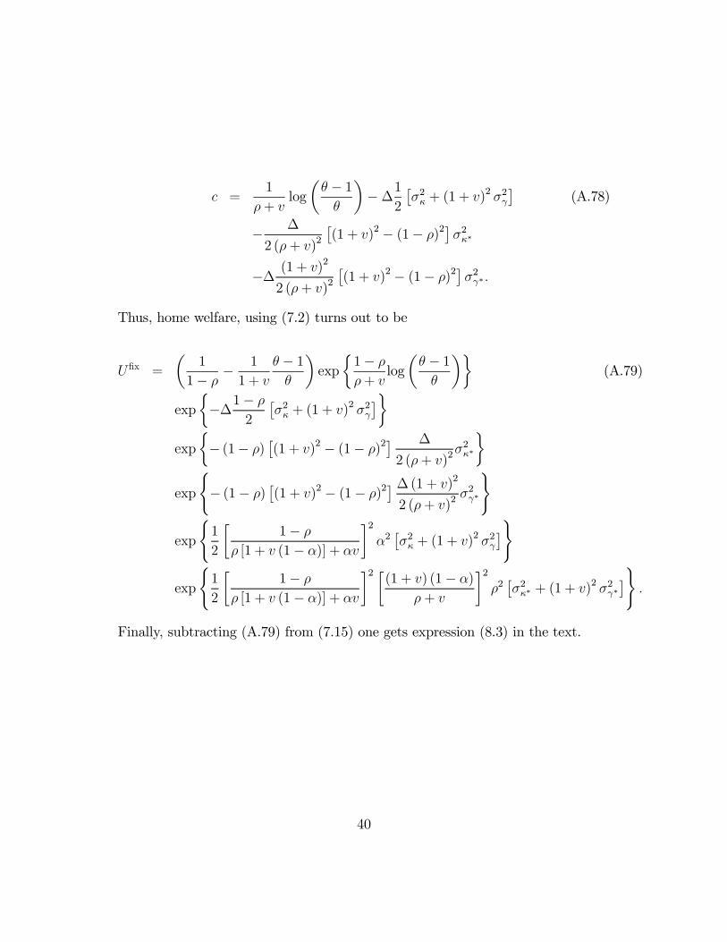
c =1

ρ+ vlog

µθ − 1θ

¶−∆1

2

£σ2κ + (1 + v)

2 σ2γ¤

(A.78)

− ∆

2 (ρ+ v)2£(1 + v)2 − (1− ρ)2¤σ2κ∗

−∆ (1 + v)2

2 (ρ+ v)2£(1 + v)2 − (1− ρ)2¤σ2γ∗.

Thus, home welfare, using (7.2) turns out to be

UÞx =

µ1

1− ρ −1

1 + v

θ − 1θ

¶exp

½1− ρρ+ v

logµθ − 1θ

¶¾(A.79)

exp

½−∆1− ρ

2

£σ2κ + (1 + v)

2 σ2γ¤¾

exp

½− (1− ρ) £(1 + v)2 − (1− ρ)2¤ ∆

2 (ρ+ v)2σ2κ∗

¾exp

(− (1− ρ) £(1 + v)2 − (1− ρ)2¤ ∆ (1 + v)2

2 (ρ+ v)2σ2γ∗

)

exp

(1

2

·1− ρ

ρ [1 + v (1− α)] + αv¸2α2£σ2κ + (1 + v)

2 σ2γ¤)

exp

(1

2

·1− ρ

ρ [1 + v (1− α)] + αv¸2 ·(1 + v) (1− α)

ρ+ v

¸2ρ2£σ2κ∗ + (1 + v)

2 σ2γ∗¤).

Finally, subtracting (A.79) from (7.15) one gets expression (8.3) in the text.

40

References

[1] Benigno, Gianluca, and Paolo Benigno (2000), �Price Stability as a NashEquilibrium in Monetary Open-Economy Models,� mimeo, New York Uni-versity.

[2] Bernanke, Ben, and Mark Gertler (1989), �Agency costs, Net worth, andBusiness Fluctuations,� American Economic Review, Vol. 79, No. 1, pp. 14-31.

[3] Calvo, Guillermo, and Carmen Reinhart (2000), �Fear of Floating,� mimeo,University of Maryland.

[4] Céspedes, Luis F., Roberto Chang, and Andrés Velasco (2000), �BalanceSheets and Exchange Rate Policy,� mimeo, Harvard University.

[5] Céspedes, Luis F., Roberto Chang, and Andrés Velasco (2001), �Dollariza-tion of Liabilities, Exchange Rates, and Credible Monetary Policies,� paperprepared for the NBER conference on Crisis Prevention, Islamorada, Florida,January 2001.

[6] Corsetti, Giancarlo, and Paolo Pesenti (2001a), �Welfare and MacroeconomicInterdependence,� The Quarterly Journal of Economics, Vol. 116, No. 2, pp.421-445.

[7] Corsetti, Giancarlo, and Paolo Pesenti (2001b), �International Dimensions ofOptimal Monetary Policy,� mimeo, FRB of New York.

[8] Dixit, Avinash, and Joseph Stiglitz (1977), �Monopolistic Competition andOptimum Product Diversity,� American Economic Review, Vol. 67, No. 3,pp. 297-308.

[9] Flood, Robert P. (1979) �Capital Mobility and the Choice of Exchange RateSystem,� International Economic Review, Vol. 20, No. 2, pp. 405-416.

[10] Galí, Jordi, and Tommaso Monacelli (2000), �Optimal Monetary Policy andExchange Rate Volatility in a Small Open Economy,� mimeo, Boston College.

[11] Gavin, Michael, Ricardo Hausmann, Carmen Pagés-Serra, and Ernesto Stein(1999), �Financial Turmoil and Choice of Exchange Rate Regime,� mimeo,IADB.

41

[12] Ghironi, Fabio, and Alessandro Rebucci (2000), �Monetary Rules for Emerg-ing Market Economies,� mimeo, FRB of New York.

[13] Henderson, Dale W., and Jinill Kim (1999), �Exact Utilities under Alterna-tive Monetary Rules in a Simple Macro Model with Optimizing agents,� inA. Razin, A. Rose, and P. Isard (eds.), International Finance and FinancialCrises: Essays in Honor of Robert P. Flood, Jr. Washington and Boston:IMF and Kluwer Academic Publishers.

[14] Lane, Phillip R. (2001), �The New Open Economy Macroeconomics: A Sur-vey,� Journal of International Economics, Vol. 54, No. 2, pp. 235-266.

[15] Monacelli, Tommaso (2001), �Relinquishing Monetary Independence,�mimeo, Boston College.

[16] Obstfeld, Maurice, and Kenneth Rogoff (1995), �Exchange Rate DynamicsRedux,� Journal of Political Economy, Vol. 103, No. 3, pp. 624-660.

[17] Obstfeld, Maurice, and Kenneth Rogoff (1996), Foundations of InternationalMacroeconomics, Cambridge: MIT Press.

[18] Obstfeld, Maurice, and Kenneth Rogoff (1998), �Risk and Exchange Rates,�NBER, WP #6694.

[19] Obstfeld, Maurice, and Kenneth Rogoff (2000), �New Directions for Stochas-tic Open Economy Models,� Journal of International Economics, Vol. 50,No. 1, pp. 117-153.

[20] Obstfeld, Maurice, and Kenneth Rogoff (2002), �Global Implications of Self-Oriented National Monetary Rules� forthcoming in The Quarterly Journalof Economics.

[21] Parrado, Eric (2001), �Inßation Targeting and Exchange Rate Rules in anOpen Economy,� mimeo, IMF.

[22] Poole, William (1970), �Optimal Choice of Monetary Policy Instruments in aSimple Stochastic Macro Model,� The Quarterly Journal of Economics, Vol.84, No.2, pp. 197-216.

[23] Rotemberg, Julio J., and Michael Woodford (1998), �An Optimization BasedEconometric Framework for the Evaluation of Monetary Policy,� in NBERMacroeconomics Annual 1997, Cambridge: MIT Press, pp. 297-346.

42

[24] Rotemberg, Julio J., and Michael Woodford (1999), �Interest-Rate Rules inan Estimated Sticky Price Model,� in J. Taylor (ed.), Monetary Policy Rules,Chicago: The University of Chicago Press, pp. 57-119.

[25] Svensson, Lars E.O. (2000), �Open Economy Inßation Targeting,� Journalof International Economics, Vol. 50, No. 1, pp. 155-183.

[26] Woodford, Michael (1999), �Interest and Prices,� Chapters 2 and 4.Manuscript, Princeton University.

43