ETH Library

Optimal control for electromagnetichaptic guidance systems

Conference Paper

Author(s):Langerak, Thomas; Zarate, Juan José ; Vechev, Velko; Lindlbauer, David; Panozzo, Daniele; Hilliges, Otmar

Publication date:2020-10

Permanent link:https://doi.org/10.3929/ethz-b-000454841

Rights / license:In Copyright - Non-Commercial Use Permitted

Originally published in:https://doi.org/10.1145/3379337.3415593

This page was generated automatically upon download from the ETH Zurich Research Collection.For more information, please consult the Terms of use.

Optimal Control forElectromagnetic Haptic Guidance Systems

Thomas Langerak1, Juan José Zárate1, Velko Vechev1, David Lindlbauer1,Daniele Panozzo2, Otmar Hilliges1

1 Department of Computer Science, ETH Zurich, Zurich, Switzerland2 Courant Institute of Mathematical Sciences, New York University, New York, USA

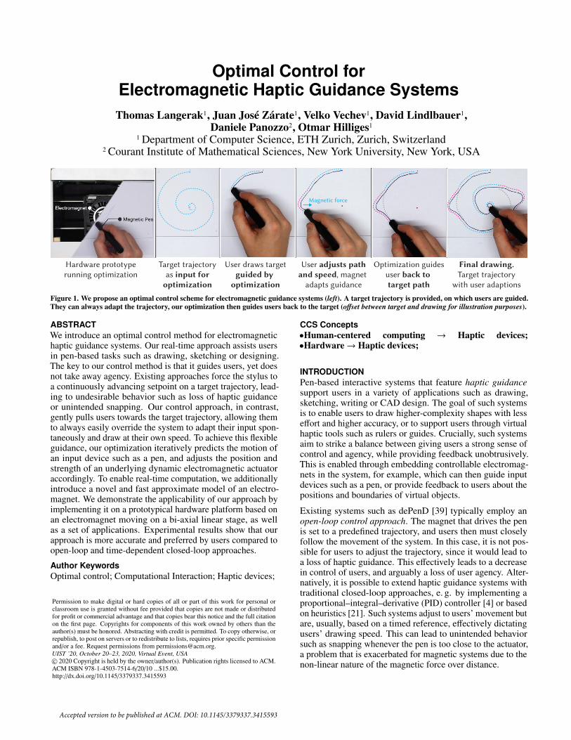
Hardware prototyperunning optimization

Target trajectoryas input for

optimization

User draws targetguided by

optimization

User adjusts pathand speed, magnet

adapts guidance

Optimization guidesuser back to target path

Final drawing.Target trajectory

with user adaptions

Magnetic force

Figure 1. We propose an optimal control scheme for electromagnetic guidance systems (left). A target trajectory is provided, on which users are guided.They can always adapt the trajectory, our optimization then guides users back to the target (offset between target and drawing for illustration purposes).

ABSTRACTWe introduce an optimal control method for electromagnetichaptic guidance systems. Our real-time approach assists usersin pen-based tasks such as drawing, sketching or designing.The key to our control method is that it guides users, yet doesnot take away agency. Existing approaches force the stylus toa continuously advancing setpoint on a target trajectory, lead-ing to undesirable behavior such as loss of haptic guidanceor unintended snapping. Our control approach, in contrast,gently pulls users towards the target trajectory, allowing themto always easily override the system to adapt their input spon-taneously and draw at their own speed. To achieve this flexibleguidance, our optimization iteratively predicts the motion ofan input device such as a pen, and adjusts the position andstrength of an underlying dynamic electromagnetic actuatoraccordingly. To enable real-time computation, we additionallyintroduce a novel and fast approximate model of an electro-magnet. We demonstrate the applicability of our approach byimplementing it on a prototypical hardware platform based onan electromagnet moving on a bi-axial linear stage, as wellas a set of applications. Experimental results show that ourapproach is more accurate and preferred by users compared toopen-loop and time-dependent closed-loop approaches.

Author KeywordsOptimal control; Computational Interaction; Haptic devices;

Permission to make digital or hard copies of all or part of this work for personal orclassroom use is granted without fee provided that copies are not made or distributedfor profit or commercial advantage and that copies bear this notice and the full citationon the first page. Copyrights for components of this work owned by others than theauthor(s) must be honored. Abstracting with credit is permitted. To copy otherwise, orrepublish, to post on servers or to redistribute to lists, requires prior specific permissionand/or a fee. Request permissions from permissions@acm.org.UIST ’20, October 20–23, 2020, Virtual Event, USA© 2020 Copyright is held by the owner/author(s). Publication rights licensed to ACM.ACM ISBN 978-1-4503-7514-6/20/10 ...$15.00.http://dx.doi.org/10.1145/3379337.3415593

CCS Concepts•Human-centered computing → Haptic devices;•Hardware→ Haptic devices;

INTRODUCTIONPen-based interactive systems that feature haptic guidancesupport users in a variety of applications such as drawing,sketching, writing or CAD design. The goal of such systemsis to enable users to draw higher-complexity shapes with lesseffort and higher accuracy, or to support users through virtualhaptic tools such as rulers or guides. Crucially, such systemsaim to strike a balance between giving users a strong sense ofcontrol and agency, while providing feedback unobtrusively.This is enabled through embedding controllable electromag-nets in the system, for example, which can then guide inputdevices such as a pen, or provide feedback to users about thepositions and boundaries of virtual objects.

Existing systems such as dePenD [39] typically employ anopen-loop control approach. The magnet that drives the penis set to a predefined trajectory, and users then must closelyfollow the movement of the system. In this case, it is not pos-sible for users to adjust the trajectory, since it would lead toa loss of haptic guidance. This effectively leads to a decreasein control of users, and arguably a loss of user agency. Alter-natively, it is possible to extend haptic guidance systems withtraditional closed-loop approaches, e. g. by implementing aproportional–integral–derivative (PID) controller [4] or basedon heuristics [21]. Such systems adjust to users’ movement butare, usually, based on a timed reference, effectively dictatingusers’ drawing speed. This can lead to unintended behaviorsuch as snapping whenever the pen is too close to the actuator,a problem that is exacerbated for magnetic systems due to thenon-linear nature of the magnetic force over distance.

Accepted version to be published at ACM. DOI: 10.1145/3379337.3415593

We propose a real-time closed-loop control approach that al-lows users to retain agency and control while being assisted byan electromagnetic haptic guidance system. Our approach en-ables users to draw at their desired speed and adjust their targettrajectory continuously. It then adapts and complies to suchmodifications while giving corrective feedback. Our algorithmthen positions and regulates a variable-strength electromagnetsuch that it provides dynamically adjustable in-plane magneticforces to the pen tip.

We contribute a novel optimization scheme forelectromagnetic-based haptic guidance system, i. e. modelsand control algorithm, that enables formalizing this problemin the established Model Predictive Contour Control (MPCC)framework [16], which has previously only been employedin context such as RC-racing [20] or drone cinematography[26]. We provide an accurate system model, parameters,and an appropriate cost function alongside a method tooptimize the model parameters given user inputs. Modelingthe non-linear interaction of an electromagnetic force fieldtypically makes use of the finite element method (FEM),which is not applicable for real-time scenarios. To overcomethis challenge, we additionally contribute a novel approximateyet accurate model of the electromagnetic force field that canbe evaluated analytically in real time.

Compared to simpler control schemes such as Model Predic-tive Control (MPC) [8] and many implementations of PIDcontrol, our approach does not require a timed reference andhence allows users to draw at their desired speed. Further-more, our optimization scheme allows for error-correctingforce feedback, gently pulling the user back to the desired tra-jectory rather than pushing or pulling the pen to a continuouslyadvancing setpoint on the trajectory. With our approach, thereference path can be updated at every timestep, thus allowingusers to continuously change their desired trajectories. Thisenables applying the algorithm to fully dynamic references, forexample virtual tools such as rulers or programmable frenchcurves.

To assess the proposed control algorithm, we developed aproof-of-concept hardware implementation (see Figure 2),leveraging an electromagnet that moves underneath the draw-ing surface or display on a bi-axial linear stage. The magnetprovides variable strength guidance onto the tip of a minimallyinstrumented pen or stylus via an electromagnet positioneddirectly below a drawing surface, guided by our proposed ap-proach. We demonstrate the feasibility of our approach with aset of applications, specifically drawing guidance on conven-tional paper for sketching and writing, and a digital sketchingapplication that features virtual haptic guides and rulers.

To evaluate our approach, we performed two experimentswith twelve participants each. We first compared free-handdrawing of shapes with varying complexity with and withoutour feedback system. Results showed that the haptic guidanceusing our approach improved the accuracy across shapes byup to 50% to 1.87 mm. We then compared our approach to ourimplementation of dePENd (open-loop) and a simple MPC-based closed-loop control scheme. Our approach showedsignificantly higher accuracy, and was preferred by users.

In summary, we contribute

• A novel MPCC-based optimization scheme for electromag-netic haptic guidance systems including models, parameters,cost function and control algorithm.• A novel real-time approximate model for electromagnets

that generalizes beyond our hardware implementation.• Evaluations showing the improved accuracy of our method.• A prototypical software and hardware implementation avail-

able as open source at https://ait.ethz.ch/projects/2020/magpen/.

Figure 2. We implement our proposed guidance system using a two-axis linear stage equipped with an electromagnet. All technical and userevaluations were completed using the Pressure Sensitive Tablet (right).We additionally developed an all-digital implementation using a multi-touch tablet with display (left).

RELATED WORK

Haptic guidanceProviding haptic guidance to users can provide benefitsfor learning [36] and short-term performance (cf. Abbinket al. [1]). Teranishi et al. [36] demonstrate that participantsshowed improved learning for handwriting skills when receiv-ing guidance through a 3-DOF Phantom Omni device. Mullinet al. [25] use a similar device as handwriting aid for rehabili-tation. Forsynth and MacLean [10] show that force cues arebeneficial in navigation tasks. The focus of these works is thatusers receive tight guidance (i. e. they are supposed to followthe system as closely as possible). Our work aims at providinga control strategy that allows users to deviate from predefinedtrajectories while still receiving guidance.

There exists a large range of devices and systems that aim atproviding guidance to users. Comp*Pass [27] uses pantograph-like devices to assist users in drawing, while I-Draw [9] is amotorized drawing assistant. Lin et al. [19] use a magnetmounted on a small robotic arm to retain the correspondencebetween the pen and a portable base. Digital rubbing employsa comparable system using a solenoid for tracing over digitalimages on real paper [14]. While users handle larger-scale mo-tions of the devices, they generally aim at having full controlover the resulting drawing. Users can take back this control,however these system do not provide a way to guide usersback to the target trajectory. Besides aforementioned systems,

several works aid users in the process of crafting and manu-facturing (cf. Zoran et al. [44]). Free-D [43] and D-Coil [29]assist users in sculpting of physical artefacts by guiding themon a predefined 3D shape. Shilkrot et al. [31] proposes anaugmented paint brush to assist users in painting. While userscan override these systems to deviate from the target shape,they have no mechanism that guides users back to the target.

Closest to our work in terms of hardware is dePENd by Ya-maoka et al. [39]. They move a permanent neodymium magneton a two-axis setup to control the metal tip of a ballpoint pen.The neodymium magnet “drags” the input pen around a prede-fined path, similar to a plotter. dePENd employs an open-loopstrategy to control the magnet, which means users cannot de-viate from the predefined path without risking to lose hapticguidance. We propose a mathematical model and optimalcontrol strategy that allows users to move at their own pacethrough a drawing, for example, and reacts in real-time to userinput by altering the position and strength of the magnet. Weshow that our approach provides better results than their open-loop approach, as well as existing closed-loop approaches.

Kianzad et al. [13] use a ballpoint drive to assist users insketching. They employ a proportional-derivative (PD) con-trol loop, which allows users to deviate from the target to acertain extend. We show in our experiments that our optimiza-tion scheme outperforms such existing closed-loop approaches.Muscle-Plotter [21] proposes active guidance for users basedon electrical muscle stimulation. Their control strategy isbased on heuristics for users to share control with the system.Our approach could be applied to their work if the electromag-netic force model is replaced by a model of the interactionbetween the muscle stimulation and the force users produce.

Magnetic ActuationProviding magnetically-driven haptic feedback on tabletopsis desirable as the force can be exerted through the surfacewithout affecting the display. A common approach is usingarrays of controllable electromagnets, combined with perma-nent magnets embedded in objects on the surface. McIntoshet al. [22] show how a permanent magnet attached to a fingercan be used for tracking and haptic feedback for mobile inter-actions. Fingerflux by Weiss et al. [37] provide near-surfacehaptic feedback before the finger touches the screen to guideusers to appropriate screen locations. Pangaro et al. [28] modelthe force-field of each electromagnet and combine these usingstandard aliasing techniques, allowing directed movement ofmultiple objects on the surface. Similarly, Yoshida et al. [40]use linear induction motors to control objects on a tabletop.Strasnick et al. [34] use electromagnets to control an objecton a mobile phone case. Suzuki et al. [35] combine these twoworks and use a grid of electromagnetic cores to move objectson a tabletop. While our optimization scheme could be appliedto such devices as well, smooth motion is problematic due tothe low resolution of the grid, and the interaction of forcesbetween multiple electromagnets. Furthermore, magnets aremodeled using a simplification of the magnetic pole model(known as Gilbert model), considering only attraction betweensingle point poles, leading to undesirable snapping behavior.

Online Path FollowingOptimal reference following given real world influences isstudied in depth in the control theory literature. Methods likeModel Predictive Control (MPC) [8] optimize the referencepath and the actuator inputs simultaneously based on the sys-tem state. MPC is widely applied in many robotics (e. g. tocontrol quadrocopters, Mueller et al. [24]) and graphics appli-cations (e. g. for human motion prediction, Da Silva et al. [6]).However, Aguiar et al. [2] show that the tracking error forfollowing timed-trajectories can be larger than if following ageometric path only.

To address this issue, Lam et al. propose Model Predictive Con-touring Control (MPCC) [17] to follow a time-free reference,optimizing system control inputs for time-optimal progress.MPCC has been successfully applied in industrial contouring[17], RC racing [20] and in drone cinematography [26]. Wealso pose our optimization problem in this well establishedframework. However, to the best of our knowledge, we are thefirst to apply it for haptic guidance systems where one has toconsider both a controllable (i. e. the electromagnetic force)and non-controllable (i. e. the user) system. We contributea formulation of the problem including models and controlalgorithms to enable employing MPCC in this context.

OPTIMAL CONTROL FOR EM HAPTIC GUIDANCEThe goal of our online optimal control scheme is to allowusers to maintain control and agency over the input device(e. g. pen, stylus), while experiencing dynamic guidance fromthe system. Importantly, it leverages time-free references andthus the dynamics are entirely driven by the pen position overtime, which is different from approaches such as MPC.

OverviewThe proposed optimization scheme allows us to adjust themagnet position and strength such that it gently pulls the pentip towards a desired stroke, while allowing users to draw attheir desired speed and without fully taking over control. Thealgorithm is generally hardware agnostic and works for de-vices with electromagnetic actuators underneath an interactionsurface. This can be implemented via bi-axial linear stage asin our prototype (see Figure 2) or via a matrix of electromag-nets which would lend itself better towards miniaturization.Furthermore, the algorithm requires a reference trajectory overthe optimization horizon. This can be defined a-priori, such asa known shape to be traced, or may be provided dynamically,e. g. the output of a predictive model (e. g. Aksan et al. [3]).

At each time step, we minimize a cost functional over a reced-ing time horizon to find optimized values for system states xand inputs u. As a high-level abstraction, the cost function

minimizex,u

∑Cforce(x,u)︸ ︷︷ ︸Eq. 3, 4 & 5

+Cpath(x,u)︸ ︷︷ ︸Eq. 6

+Cprogress(x,u)︸ ︷︷ ︸Eq. 7

, (1)

serves three main purposes: 1) ensuring that the user perceiveshaptic feedback of dynamically adjustable force (Cforce), 2)stays close to the desired path but does not rigidly prescribeit (Cpath), and 3) makes progress along it (Cprogress) but allowsthe user to vary drawing speed freely.

Setpoint

Open-Loop

PenElectromagnet Shortest Distance to Setpoint

Time-dependentclosed-loop (MPC)

Time-independentclosed-loop (OURS)

t=1…n

t=3

t=2

t=1

t=3

t=2

t=1

Figure 3. Overview of different control strategies on a target trajectory(green), with constant pen position. For open-loop, the position of theelectromagnet is identical to the constantly advancing setpoint, leadingto loss of haptic guidance. For MPC, although the pen is static, the guid-ance changes at every timestep since the setpoint advances. In our ap-proach, the setpoint is also based on the pen position, therefore remainsstationary in this case and guides the user towards the target trajectory.

CLOSED-LOOP CONTROLOur main contributions are models and a control strategy thatenables using the MPCC framework [17] for electromagnetichaptic guidance. MPCC is a closed-loop time-independentcontrol strategy that minimizes a cost function over a fixedreceding horizon. There are several advantages in using ourformulation over open-loop (as used in dePENd [39]) or time-dependent strategies (e. g. MPC). First, closed-loop controlallows to react to user-input, whereas open-loop control re-moves all user agency. Both MPC and MPCC are closed-loopcontrol strategies. However, MPC tracks a timed reference,requiring a fixed velocity by users. MPCC follows a time-free trajectory, which allows the user to progress at their ownspeed. Figure 3 illustrates the expected behavior for the differ-ent strategies, given that the user slows down or stops movingthe pen. The desired behavior here would be that the algorithmessentially “waits”, i. e. provides guidances towards a slowlyor no-longer advancing setpoint. In this situation, open-loopapproaches would lead to lost haptic guidance. Closed-looptime-dependent approaches would guide the pen towards aconstantly advancing setpoint (although users do no longermove), which can lead to problems such as the user beingguided backwards (e. g. timestep t = 3 is in front of t = 2).

Our method is designed to exert a force Fθ of desired strengthonto the pen to guide the user towards the target trajectory s.The path s of length L is parametrized by θ ∈ [0, L]. Note thatwe do not prescribe how fast users draw and hence for eachgiven pen position pp we first need to establish the closest po-sition on the path parameterized by s(θ). The vector betweenthe pen position and s(θ) is defined as rθ. We leverage a reced-ing horizon optimization strategy and the global reference canhence be adjusted or replaced entirely at every iteration. Thepath s is then a local fit to the global reference. Furthermore,

Table 1. Overview control parameters and values

Name Range / Value Description

pp R2 Position of penpm R2 Position of electromagnetFa R3 Electromagnetic force vectorα [0, 1] Electromagnetic intensitys θ ∈ [0, L] Target trajectory of length Lx [pm, pm, α, θ] System statesu [pm, α, θ] System inputs

we seek to find optimized values for the electromagnet inten-sity α and the in-plane electromagnet position pm. Solvingthe error functional given in Eq. (10) at each timestep yieldsoptimized values for system states x and inputs u.

As common in MPC(C), the system is initialized from mea-surements at t = 0. The system state is then propagated overthe horizon with the dynamics model f (x,u). The system statevector x contains variables that are controlled by the algorithm(magnet intensity and position, current path progress). Thefirst of the optimized inputs (u0) is then applied to the physicalsystem, transitioning the system state to x1, before iterativelyrepeating the process to allow for correcting modeling errors.

desired forcespring-likebehavior

currentactuation force

Figure 4. Illustration of actuation force Fa, desired force Fθ, and theforce cost-term C f associate with the difference between those two forces.

Haptics model: controlling the force of the electromagnetThe main goals of our approach is that users can move freely interms of position and speed, and that the actuator continuouslypulls them towards an advancing setpoint s(θ) on the targettrajectory s. At any time, the magnet exhibits an actuationforce Fa on the pen, given by our electromagnetic force model(see Implementation section). Therein lies the challenge, il-lustrated in Figure 4. The setpoint is continuously advancingbased on the movement of the pen to ensure progress. The ac-tuator needs to pull the pen towards the setpoint by exhibitingforce Fθ, but currently exhibits Fa. The two forces only alignif the pen is exactly at the setpoint, which is rarely the case. Toovercome this challenge, we propose modeling this interactionby a spring-like behavior that “pulls” Fa towards Fθ. In thisway, the magnet continuously guides the pen towards the set-point, and the force linearly increases with distance betweenthe pen and the target setpoint denoted as:

Fθ(rθ) = c F0 rθ erθ . (2)

Here erθ is a unit vector in the direction of rθ, c is a scalar thatregulates the stiffness of the spring (in our case c = 5/h), F0a scaling of the EM force (i. e. the force felt by users) andh the distance between dipoles in z (see Fig. 4). Althoughsimple, this formulation ensures that the haptic guidance isstrong under large deviation from the path while vanishing asthe user approaches the target path (rθ → 0). Note that Eq. 2 isa design choice. Different formulations can be used to achievedifferent user experiences. Furthermore, replacing our hard-ware prototype and force-model would allow for adaptation ofthe remainder of the method to different actuation principles.

The above haptics model serves as basis for our problem for-mulation of electromagnetic guidance in the MPCC frame-work. Using the vectors of the current actuation force Fa and

desired force Fθ, we formulate a quadratic cost term to pe-nalize the difference between desired force and actual forceas:

C f (pm,pp, α) = ‖ Fθ(rθ) − Fa(d) ‖2. (3)

where d is the in-plane vector between the magnet and the pen.Since the actuation force Fa declines rapidly with distance d,the gradient of C f goes to 0 for large values of d causing theoptimization to become unstable. To counterbalance this issuewe encourage the electromagnet to stay close to the pen:

Cd(pm,pp) = d2. (4)

Finally, we prioritize proximity between the magnet and thepen rather than increasing its force by penalizing excessiveuse of magnetic intensity α:

Cα(α) = α2. (5)

Controlling the position of the electromagnetWe continuously optimize the position of the electromagnetwith the goal of keeping the distance between the desired pathand the pen minimal. To give the user freedom in decidingtheir drawing speed we first need to find the reference points(θ) on the target trajectory s. Finding the closest point on thepath is an optimization problem itself and hence can not beused within our optimization. Similar to recent work in robottrajectory generation [26, 11], we decompose the distance tothe closest point into a contouring and lag error, as shown inFigure 5. rθ is the vector between the pen pp and a point s(θ)on the spline, and n as the normalized tangent vector to thespline at that point, which is defined as n =

∂s(θ)∂θ

. The vectorrθ can now be decomposed into a lag error and a contour error(Figure 5). The lag-error Cl is computed as the projection ofrθ. The contour-error Cc is the component of rθ orthogonal tothe normal:

Cl(pp, θ) = ‖〈rθ,n〉‖2,Cc(pp, θ) = ‖rθ − (〈rθ,n〉) n‖2.

(6)

Separating lag from contouring error allows us, for example,to differentiate how we penalize a deviation from the path (Cc),versus encouraging the user to progress (Cl). We furthermoreinclude cost terms to ensure that the magnet stays ahead of thepen (Cθ) and to encourage smooth progress (Cθ) computed as

Cθ(θ) = −θ,

Cθ(θ) = (θt − θt−1)2.(7)

Dynamics modelTo phrase electromagnetic haptic guidance in the MPCC frame-work, we contribute a a dynamics model f (x,u) describingthe system dynamics given its states x and inputs u.

x = f (x,u) with

x = [pm, pm, α, θ] ∈ R6 and u = [pm, α, θ] ∈ R4.(8)

The system state x consists of the position of the electromagnetpm ∈ R

2 and its velocity pm, the magnet intensity α and thecurrent path progress θ. The inputs to the system u consist of

Figure 5. Illustration of lag- and contouring error decomposition.

the in-plane electromagnet accelerations pm, and velocities αand θ for magnet intensity and the spline progress respectively.Note that we empirically found that magnet accelerations yieldsmoother motion than using velocities. The system model isgiven by the non-linear ordinary differential equations usingfirst and second derivatives as inputs:

pm = vm, α = vα and θ = vθ, (9)

where v(·) are the external inputs. The continuous dynamicsmodel x = f (x,u) is discretized using a standard forwardEuler approach: xt+1 = f (xt,ut) [12].

In our hardware implementation, we derive the sets of ad-missible states χ and inputs ζ empirically to conform to thephysical hardware constraints of the linear stage (e. g. max x,y-position) and EM specifications (e. g. max voltage). These areused in the constrained optimization problem solved in Eq. 11.The pen position is propagated via a standard linear Kalmanfilter [12]. While not an accurate user model, it works well inpractice since the states are recalculated at every timestep.

Term Description of cost Eq.

C f Decreases difference in magnetic force 3Cd Decreases distance between magnet and pen 4Cα Encourages close distance over large force 5Cl Decreases lag to path contour 6Cc Decreases distance to path contour 6Cθ Magnet stays ahead of pen 7Cθ Ensures smooth progress 7

Table 2. Summary of costs terms used in optimization.

OptimizationWe combine the cost terms (Table 2) to control the force andposition of the actuator to form the final stage cost:

Jk = w fC f (pm,k,pp,k, αk, θk)+wdCd(pm,k,pp,k) + wαCα(αk)+wlCl(pp,k, θk) + wcCc(pp,k, θk)+

wθCθ(θk) + wθCθ(θk), (10)

where the scalar weights wl,wc,wθ,wθ,w f ,wd,wα > 0 controlthe influence of the different cost terms. The values used inour experiments and applications can be found in the Imple-mentation section. The system states and inputs are computedby solving the N-step finite horizon constrained non-linearoptimization problem at time instance t.

The final objective therefore is:

minimizex,u,θ

N∑k=0

wk

(Jk + uT

k Ruk)

(11)

Subject to: xk+1 = f (xk,uk) (System Model)x0 = x(t) (Initial State)

θ0 = θ(t) (Initial Progress)

θk+1 = θk + θkdt (Progress along path)0 ≤ θk ≤ L (Path Length)xk ∈ χ (State Constraints)uk ∈ ζ (Input Constraints)

Here k indicates the horizon stage and the additional weight wkreduces over the horizon, so that the current timestep has moreimportance than later timesteps. R ∈ Snu

+ is a positive definitepenalty matrix avoiding excessive use of the control inputs.In our implementation we use a horizon length of N = 10.Experimentally we found that this is sufficient to yield robustsolutions to problem instances and longer horizons did notimprove results, yet linearly increases computation time. Thealgorithm is summarized in Appendix A Alg. 1.

IMPLEMENTATIONIn this section, we detail our electromagnetic force model usedin our optimal control scheme as well as the implementationof our hardware prototype.

Electromagnetic force modelOur approach requires a model of the interaction betweena variable-strength electromagnet (EM) and the permanentmagnet in the stylus that is sufficiently accurate and can beevaluated in real time. Accurately modeling the non-linearEM field of the electromagnet’s core is typically done throughfinite element analysis (FEA), which cannot be performed inreal time. Similarly, precomputing the volumetric map of theEM field Bm via FEA for all levels of electrical current is notcomputationally feasible. We therefore contribute a novel fastapproximate yet accurate electromagnetic model that providesa good balance between speed and accuracy to enable hapticguidance in applications such as writing or sketching.

In general, we aim at finding the actuation force on the pen Fp,which is given by integrating over the volume of the permanentmagnet in the pen:

Fp =

$∇

(Mp · Bm(·)

)dxdydz, (12)

where Mp is the magnetization of pen magnet and Bm(·) is theEM field evaluated at the pen position, which is too costly toevaluate in real time. Our model approximates this underlyingphysical phenomena, can be efficiently evaluated at everyiteration of our optimization procedure and provides a verygood fit to empirical data. In this section, we briefly discussthe most important aspects of our model, for a full derivationand analysis we refer readers to the Appendix B.

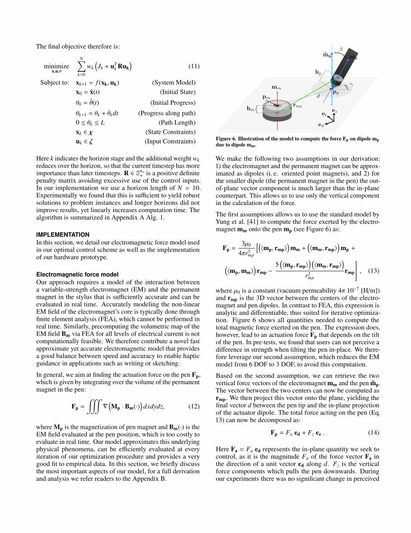
Figure 6. Illustration of the model to compute the force Fp on dipole mpdue to dipole mm.

We make the following two assumptions in our derivation:1) the electromagnet and the permanent magnet can be approx-imated as dipoles (i. e. oriented point magnets), and 2) forthe smaller dipole (the permanent magnet in the pen) the out-of-plane vector component is much larger than the in-planecounterpart. This allows us to use only the vertical componentin the calculation of the force.

The first assumptions allows us to use the standard model byYung et al. [41] to compute the force exerted by the electro-magnet mm onto the pen mp (see Figure 6) as:

Fp =3µ0

4πr5mp

[(〈mp, rmp〉

)mm +

(〈mm, rmp〉

)mp +

(〈mp,mm〉

)rmp −

5(〈mp, rmp〉

) (〈mm, rmp〉

)r2

mprmp

, (13)

where µ0 is a constant (vacuum permeability 4π 10−7 [H/m])and rmp is the 3D vector between the centers of the electro-magnet and pen dipoles. In contrast to FEA, this expression isanalytic and differentiable, thus suited for iterative optimiza-tion. Figure 6 shows all quantities needed to compute thetotal magnetic force exerted on the pen. The expression does,however, lead to an actuation force Fp that depends on the tiltof the pen. In pre-tests, we found that users can not perceive adifference in strength when tilting the pen in-place. We there-fore leverage our second assumption, which reduces the EMmodel from 6 DOF to 3 DOF, to avoid this computation.

Based on the second assumption, we can retrieve the twovertical force vectors of the electromagnet mm and the pen mp.The vector between the two centers can now be computed asrmp. We then project this vector onto the plane, yielding thefinal vector d between the pen tip and the in-plane projectionof the actuator dipole. The total force acting on the pen (Eq.13) can now be decomposed as:

Fp = Fa ed + Fz ez . (14)

Here Fa = Fa ed represents the in-plane quantity we seek tocontrol, as it is the magnitude Fa of the force vector Fa inthe direction of a unit vector ed along d. Fz is the verticalforce components which pulls the pen downwards. Duringour experiments there was no significant change in perceived

friction when comparing the drawings with and without elec-tromagnet (i. e. with or without Fz). For this reason we do notactively account for Fz in our optimization and only maintainthe in-plane force contribution (ed direction). The actuationforce as function of pen-magnet separation is obtained as:

Fa = α F0

d(4 − d2

h2

)h(1 + d2

h2

) 72

ed, (15)

where α ∈ [0, 1] is a dimensionless scalar to control the desiredstrength of the force that should be felt by users, h is the center-to-center distance between both magnets projected on to thez-axis (Figure 4) and F0 is a constant force parameter givenby the expression,

F0 =3 µ0 mp mm

4 π h4 . (16)

The actuation force Fa is zero if the two magnets are alignedwith one another (d = 0), it has a maximum Fmax

a = 0.9 F0 atd = 0.39h, and we can assume there is no more attraction fordistances d > 2h. Note that the second assumption (only usein-plane component) lead only to a small approximation errorCompared to an angle dependent formulation (see AppendixB.2), a tilt of up to β = 30◦ leads to a max error in ourmodel (Equation 30) equivalent to shifting the distance d by ±3 mm. This uncertainty in d is comparable with the in-planepositioning error (dispersion) of our hardware prototype. Anangle dependent formulation of our model (i. e. 6 DOF) can befound in Appendix B.2 for future use in cases where the penangle is tracked. This model remains valid for other hardwareimplementations involving a single moving electromagnet orcan be easily extended onto a grid of fix electromagnets.

Hardware prototypeWe have developed one possible hardware instance that uti-lizes our optimization scheme for an in-plane haptic guidancesystem (see Figure 2). Our system consists of 3 main compo-nents: 1) a moving platform that controls the 2D location ofthe electromagnetic actuator, 2) an input device such as a sty-lus, and 3) an output device such as a digital tablet or digitizerused in combination with a non-digital drawing surface.

Motion platformThe motion platform consists of a controllable electromagneton a bi-axial linear stage directly underneath the drawingplane. The linear stage has two orthogonal 12 mm lead screws,which are driven by two 24 V, 4.0 A NEMA23 high-torquestepper motors. We control the motors with a DQ542MAstepper driver and an Arduino UNO. As electromagnet, weuse an Intertec ITS-MS-5030-12VDC magnet (5 cm diameter,3 cm height, 12 V), controlled via pulse-width modulation.It can deliver up to 488 mN of lateral force at 11 W. Weused FEM analysis to select this magnet from a range ofcommercially available magnets [5]. It provides a balancebetween power consumption, size, and force, i. e. it delivers astrong perceivable force while having a small footprint relativeto our hardware.

To measure the positional dispersion of the motion platform,we moved the electromagnet at full strength (α = 1) to 300

random locations and then always back to the center of thedrawing surface. During theses trials, a user held the pen up-right and followed the magnet passively. By measuring thedifference in target and actual position, we found that our sys-tem yields 2.8 mm (± 0.8 mm) of point dispersion. We believethis is sufficient for most applications and our experiments.One of the factors that contribute to this dispersion is the van-ishing of the actuation force Fa as d → 0. This can lead to thepen motion stopping slightly before it reaches the target.

SoftwareOur software runs on a standard PC (Intel Core i7-4770 CPU4 cores at 3.40 GHz) in all our experiments. The solver isimplemented in FORCES Pro [7], which produces efficientC-code. The following weight values are used for our controlscheme (Equation 10):

wl wc wθ wθ w f wd wα wv wm

1.5 1.5 10. 0.1 10. 0.05 7. 1. 1.

Due to the steepness of the electromagnetic force Fp and thepotentially fast pen motion, runtime and latency are crucialperformance metrics. The optimization algorithm contributesto both, whereas latency is dominated by the hardware andI/O. The mean solve time for a problem instance is 7.4 ms (±3.0 ms). This can be expected to be mostly constant since wedo not manipulate the system state space and the only mea-sured input comes from the pen. The hardware and overall sys-tem latency adds to the solve time. We use a high-speed cam-era (1000 fps) to establish the motion (pen) to motion (magnet)latency. This yields an approximate latency of ~10 ms. Giventhe combined latency envelope of ~20 ms, we did not experi-ence any abrupt pen snapping in our experiments.

Input and Output DevicesOur primary input and output devices for our user experimentsconsist of a 3D printed ballpoint pen with a permanent ringmagnet mounted in the shaft (see Figure 2) and a piece of paper.The strokes are recorded by a Sensel Morph pressure sensitivetouch pad [23]. If the system cannot locate the pen (e. g. whenit is lifted) the last known position is used. We chose theSensel for its high spatial resolution (6502 DPI), high speed(500 Hz) and low latency (2 ms), according to specification,and since the sketching surface does not interfere with theinput recognition. Additionally, we developed an all digitalinput/output system with a multi-touch tablet + stylus. Weuse a Galaxy Tab A tablet with capacitive input and an off-the-shelf stylus with a permanent magnet placed near the tip.This magnet is slightly bigger (12 mm radius, 12 mm height)to compensate for the increase in tablet thickness.

EVALUATIONWe first evaluated if our optimization scheme is beneficial forusers in providing haptic guidance compared to a no-feedbackbaseline. In a second experiment, we compared our methodwith an open-loop and a closed-loop approach.

Experiment 1 - Haptic feedbackWe compared our MPCC formulation with a no-feedback base-line to gather insights on task performance and user perception.

Circle Line Spiral

Sinusoidal Dog Ellipse

Figure 7. Shapes of our user tests. The drawing surface only containedsparse visual references (shown in blue) and starting positions (orange).

Users were asked to draw several shapes (see Figure 7) andwe evaluated accuracy and subjective feedback.

Procedure and tasksWe recruited 12 participants from the local university, all with-out professional drawing experience. Users were given anintroduction to the system functionality and got to experiencethe system in a self-timed training phase. During the experi-ment we asked each participant to draw six basic shapes, eachwith and without haptic feedback. The presentation orderof shapes and interface condition was counterbalanced. Thedrawing surface (white piece of paper) only contained a start-ing point and, in the case of more complex shapes, limitedadditional visual guidance (see Figure 7). Furthermore, theparticipants were shown a scaled version during task execu-tion (scaled to prevent 1:1 copying). After the full experiment,users completed a questionnaire on their preference.

Quantitative ResultsWe compute the Hausdorff-like distance [30] between thedrawn path and the reference path as error metric. To makethe metric robust to drawing speed, we re-sample both pathsequidistantly. To ensure fairness we also compute the inversedistance (reference to drawn path). A Kolmogorov-Smirnovtest [15] indicated that the set of uni-directional distances isnot significantly different from the set of inverse distances.We therefore only report uni-directional distances. The quan-titative results for each target averaged over all participantsare summarized in Table 3. Our method on average resultedin a 66% (± 24.5%) lower error, i. e. it improve the averagepoint-to-path difference by 1.54 mm. A two-way ANOVA onthe mean error revealed a main effect for the feedback type(F=46.187, p<.001) and for the shapes (F=11.771, p < .001).Post-hoc analysis revealed that the line was statistically signif-icantly different from all other shapes. This indicates that ourmethod is beneficial for non-trivial shapes.

Qualitative ResultsA brief exit interview shows that users subjectively rate thesystem favorably, on a 5-point Likert scale (5 is best), interms of accuracy (4.33 ± 0.62), speed (4.00 ± 0.91), force(3.50 ± 0.86) and overall performance (4.50 ± 0.9). While weacknowledge that this might be in part due to novelty effects,we believe that the quantitative results indicate that our systemis beneficial for users in general. The ratings indicate thatparticipants generally see benefit in our approach and are notdisturbed or hindered when using our approach.

Table 3. Mean accuracy (mm). * indicates statistical significance (α.05).

With Without

Scenario Mean SD Mean SD Err %

Circle* 2.19 0.90 4.26 2.39 0.51Line 1.18 0.80 1.03 0.84 1.15Spiral* 2.55 0.75 4.38 1.64 0.58Sinus* 2.53 0.70 5.08 2.19 0.50Dog* 2.31 0.54 3.81 1.32 0.60Ellipse* 2.40 0.56 3.84 1.22 0.62

Experiment 2: Comparison of control strategiesIn this second experiment, we compared our time-free closed-loop optimization strategy to a simpler MPC variant and ourimplementation of dePENd [39], denoted as dePENd∗.

Procedure and tasksWe asked twelve new participants (students and staff from alocal university) to draw one complex shape (dog in Figure 7)in three different conditions: dePENd∗, time-dependent closedloop (MPC), and time-free closed loop (Ours), counterbal-anced using a latin square. The speed of the system in thetime-dependent cases was decided empirically based on pre-tests to work well at regular drawing speeds. After receivinginstructions and a brief training, participants completed thethree drawings. Participants were also encouraged to providecomments during the individual conditions.

Data collectionWe analyze three measures: 1) the mean distance from thepen to the path, 2) the mean distance from the pen positionprojected onto the path and the setpoint along the path, denotedas d(pen, s(θ)), and 3) the mean distance from the pen to theelectromagnet. By taking the mean of the error terms oversubjects we ensured equal numbers of datapoints, accountingfor differences in speed. Participants were instructed to drawat roughly constant speed. This was done to ensure fairness incomparing our approach with the open-loop approach, whichwould deteriorate if the variability of the drawing speed wereto high. Note that our approach does generally not require thisassumption.

Quantitative resultsTable 4 summarizes our quantitative findings. Not surprisingly,the distance from the electromagnet to the pen and d(pen, s(θ))for dePENd∗ is quite large. Since the force exerted on the penfalls-off quadratically with distance, participants often lost anyhaptic guidance early on, confirmed via user comments suchas “I don’t feel anything” (P3) and “Is the system on?” (P6).

A Kruskal-Wallis test revealed that our approach has the high-est accuracy compared to dePENd∗ and MPC (H(2)=20.76,p<.001). Furthermore, the setpoint s(θ) (H(2)=7.362, p<.05)

Table 4. Mean distances in mm for Experiment 2).|pen-path| d(pen, s(θ)) |pen-em|

dePENd∗ 4.1(±0.7) 38.0(±56.9) 38.2(±25.1)MPC 3.9(±1.3) 45.0(±50.8) 8.6(±1.6)Ours 2.0(±0.6) 6.2(±0.8) 4.6(±0.9)

0 0.2 0.4 0.6 0.8 1

0

100

200

300

400

500

DePENd*

MPC

OURS

Time

Dis

tanc

e (m

m)

Figure 8. Comparison of error (path distance pen-s(θ)) over time for asingle participant (P1). The inverse u-shape illustrates that the setpoints(θ) moves at a different speed than the user for dePENd∗ and MPC. Thedata is smoothed to increase readability.

and the electromagnet (H(2)=27.12, p <.001) are closest tothe pen using our approach. Thus our time-free formulationovercomes both problems of wrong setpoints (MPC) and arun-away electromagnet (dePENd∗). Figure 8 shows one typ-ical example of a user. Both the distance along the path andthe pen-magnet distance fluctuate strongly for dePENd∗ andMPC control strategies. Our approach yielded a continuouslylow error.

While MPC reduces the distance from the pen to the magnet,it does not optimize for the progress along the path and hencemay pull the pen into undesired directions. Furthermore, wesaw that MPC produced extreme corner cutting behavior tocatch up to the advancing setpoint. Both dePENd∗ and MPCalso produce results with high standard deviations. This islikely due to the absence of direct coupling between userfeedback and path progress, which makes it possible for theuser to lag behind the setpoint significantly (albeit at the costof reduced force feedback). In our approach, the path progressis adjusted to the user’s drawing speed, drastically reducingthe standard deviation and in consequence ensuring deliveryof force feedback throughout the drawn path.

Qualitative resultsFrom our observations we saw that s(θ) was either in frontor behind the user for MPC. This was also confirmed in ourinterview, where people especially commented on the MPCstrategy: “The system tries to push me in the wrong direction”(P2) and “It is counteracting me” (P11). In contrast with ourformulation the magnet remains always slightly ahead of thepen, resulting in users commenting on our approach as themost preferred condition. In the words of one subject this is:“since I still had control” (P9).

In summary, theses initial results indicate that our approachoutperforms existing open-loop and time-dependent closed-loop approaches. dePENd∗ causes numerous problems, in-cluding users not perceiving any haptic feedback. This isespecially troublesome in settings where autonomy is desired.In MPC the haptic feedback is perceived, but can be erroneous.This is especially evident when users do not conform to theexpected behavior. We plan to perform more in-depth experi-ments to investigate, for which applications our approach canbe especially beneficial, and for which levels of autonomy.

APPLICATIONSTo further demonstrate the potential of our approach we illus-trate possible usage-scenarios including calligraphy, outliningand inking. Finally, we combine the haptic feedback mech-anism with a simple digital drawing application to initiallyexplore the possibility of dynamic references.

CalligraphyFigure 9 illustrates writing of flourished characters, with onlyminimal visual guidance (single starting point). Our systemtakes the character as input, users can then draw at their desiredspeed. Although an offset from the reference path remains, thelines are smooth and the overall shape is close to the desiredcharacters.

Figure 9. Our approach can be used as a guidance system for calligraphy,where users either follow a target path very closely, or deviate if desired.

Outlining & inkingFigure 10 illustrates the effect of two core capabilities of theproposed approach. Here we first outline the proportions ofthe dragon head (gray guidance lines) and then use differentpens to ink-in the details. Note that the system provides hapticguidance but allows the user to draw the shape in differentstyles (e. g. the ears of the two upper dragons) and with vary-ing high-frequency detail, while maintaining similarity to thereference shape. This is a direct consequence of using time-free closed loop control approach. In this case, all four variantswere drawn without changes to the system or desired path.

Figure 10. Different variants of the same dragon, drawn with identicalsystem settings by a novice. Each pair of drawings used with differenttools. First a pencil for proportions and a fine-liner (top) or pencil (bot-tom) to ink-in details. Multi-stroke lines are achieved by approachingeach separate instance as a new drawing.

Virtual toolsUsing a digital tablet with capacitive display (Figure 11) weexplore integrating dynamically changing references. In asketching application, artist select different virtual tools, andposition and configure these anywhere. The canvas and thehaptic feedback system then pull the stylus towards thesevirtual guides. In Figure 11, the user has selected a tool thathelps them when drawing an ellipse that snaps to a previouspart of the drawing, both visually and in terms of haptics.

Figure 11. Virtual tools can be used to dynamically construct a refer-ence path combining haptic and visual feedback. Here a simple drawingapplication combines freeform sketching with different virtual rules andguides that can be felt by the user.

DISCUSSIONOur experiments indicate that the proposed approach indeedincreases accuracy in drawing tasks and that users perceive thesystem favorably. While our system increased users’ accuracyfor complex shapes, it did not yield any improvements for thestraight line. This may be explained by user feedback, thatthe maximum speed of the linear stage is a limiting factor inthe current implementation. In our interviews, some usersindicated that they had the feeling that their drawings withoutfeedback were more accurate once they experienced the hapticguidance. This hints at the possibility of short-term musclememory when using our haptic guidance approach. Long-termlearning is a very interesting area to explore for our approachand haptic guidance systems in general. We plan to conductsuch experiments in the future.

Our experiments currently focused on drawing and sketchingapplications. We believe that our control strategy will bebeneficial for a broad set of applications. We started exploringthe usage of our approach with a tablet and digital stylus.More experiments, however, are needed to find out at whichlevel of complexity our approach becomes the most beneficial.Allowing users to adjust their input on-demand is crucial formost applications, especially since systems most often do nothave complete knowledge of users’ target path. Our approachis a first step in the direction of balancing user input and systemcontrol for haptic guidance systems, and can be extended toother devices beyond electromagnetic systems if appropriateforce models are provided.

In terms of hardware, the speed of the employed linear stagewas a limiting factor, without which users would have beenable to complete drawings and general inputs faster. We planto implement advances in that direction in the future. This mayinclude faster and smaller form-factor linear stages or a matrixof stationary electromagnets. The former would require nochanges to our formulation, whereas the latter would requirechanges to the EM model and the dynamics model. An EMmatrix opens-up the path towards a thin form-factor designand is a particularly interesting research direction.

Once the hardware-induced speed limitation is overcome, ef-ficient closed-loop control approaches become an interestingdirection for future work, since faster pen motion would alsotighten the latency and accuracy budget. In the context ofsensing it would be interesting to incorporate a mechanismto reconstruct the tilt of the pen. This could be achieved forexample via an accelerometer built into the pen or via a grid ofhall-sensors underneath the surface. Information on the pen tiltcould then be combined with the angle dependent formulationof our EM model (see Appendix C). Furthermore, we believethere are many research opportunities in combining our ap-proach with ink beautification approaches (e. g. [33, 32, 38]).Particularly interesting would be to leverage fully predictivemodels for non-drawing applications (e. g. DeepWriting [3]).

We believe that it could be an interesting direction for futurework to combine our approach with different types of hap-tic feedback, either environment mounted or body-worn, anddifferent form factors such as spherical electromagnets [18,42]. Electromagnetic feedback in combination with spatialactuation maybe interesting in other settings. For example, amagnet mounted to a robotic arm could deliver contact-lessfeedback in VR scenarios. It would also be interesting to inves-tigate how to best exploit the system capabilities in the contextof motor memory and learning. All these scenarios make itnecessary that a system interactively reacts to user input. Ourapproach enables such applications, and can generalize to suchsystems that go beyond 2D haptic guidance systems.

CONCLUSIONWe have proposed a novel optimization scheme for electromag-netic haptic guidance systems based on the MPCC framework.Our approach balances user input and system control so thatusers can adjust their trajectory and speed on-demand. Itoptimizes the system states and its inputs over a receding hori-zon via solving a stochastic optimal control problem at eachtimestep. Our formulation has been designed to provide dy-namically adjustable forces and automatically adjusts magnetposition and strength. It can be evaluated analytically and ishence suitable for iterative, real-time optimization approaches.We implemented our approach on a prototypical hardwareplatform and showed experimentally that the feedback is wellreceive by users, and provides higher accuracy than open-loop and time-dependent closed-loop approaches. We believethat our approach provides a principled way towards hapticguidance where users retain agency while being unobtrusivelyassisted, and is applicable broadly in applications such as draw-ing, sketching, writing or guidance via virtual haptic tools.

ACKNOWLEDGEMENTSThis work was supported in partby grants from the Hasler Founda-tion (Switzerland), ERC (OPTINTStG-2016-717054), the ETH ZurichPostdoctoral Fellowship Programme(ETH/Cofund 18-1 FEL-39), NSFCAREER award 1652515, the NSF grants IIS-1320635, OAC-1835712, OIA-1937043, CHS-1908767, CHS-1901091, a giftfrom Adobe Research, a gift from nTopology, and a gift fromAdvanced Micro Devices, Inc.

REFERENCES[1] David A. Abbink, Mark Mulder, and Erwin R. Boer.

2012. Haptic shared control: smoothly shifting controlauthority? Cognition, Technology & Work 14, 1 (2012),19–28. DOI:http://dx.doi.org/10.1007/s10111-011-0192-5

[2] A. Pedro Aguiar, Joao P. Hespanha, and Petar V.Kokotovic. 2008. Performance limitations in referencetracking and path following for nonlinear systems.Automatica 44, 3 (2008), 598 – 610. DOI:http://dx.doi.org/10.1016/j.automatica.2007.06.030

[3] Emre Aksan, Fabrizio Pece, and Otmar Hilliges. 2018.DeepWriting: Making Digital Ink Editable via DeepGenerative Modeling. In Proceedings of the 2018 CHIConference on Human Factors in Computing Systems(CHI ’18). Association for Computing Machinery, NewYork, NY, USA, 1–14. DOI:http://dx.doi.org/10.1145/3173574.3173779

[4] Karl Johan Åström and Tore Hägglund. 1995. PIDcontrollers: theory, design, and tuning. Vol. 2.Instrument society of America Research Triangle Park,NC.

[5] COMSOL Multiphysics. COMSOL Multiphysics.(????). www.comsol.com.

[6] M. Da Silva, Y. Abe, and J. Popovic. 2008. Simulationof Human Motion Data using Short-HorizonModel-Predictive Control. Computer Graphics Forum27, 2 (2008), 371–380. DOI:http://dx.doi.org/10.1111/j.1467-8659.2008.01134.x

[7] Alexander Domahidi and Juan Jerez. 2014. FORCESProfessional. embotech GmbH (http://embotech.com/FORCES-Pro). (2014).

[8] T. Faulwasser, B. Kern, and R. Findeisen. 2009. Modelpredictive path-following for constrained nonlinearsystems. In Proceedings of the 48h IEEE Conference onDecision and Control (CDC). 8642–8647. DOI:http://dx.doi.org/10.1109/CDC.2009.5399744

[9] Piyum Fernando, Roshan Lalintha Peiris, and SurangaNanayakkara. 2014. I-Draw: Towards a FreehandDrawing Assistant. In Proceedings of the 26thAustralian Computer-Human Interaction Conference onDesigning Futures: The Future of Design (OzCHI ’14).Association for Computing Machinery, New York, NY,USA, 208–211. DOI:http://dx.doi.org/10.1145/2686612.2686644

[10] Benjamin A. C. Forsyth and Karon E. MacLean. 2006.Predictive Haptic Guidance: Intelligent User Assistancefor the Control of Dynamic Tasks. IEEE Transactions onVisualization and Computer Graphics 12, 1 (Jan. 2006),103–113. DOI:http://dx.doi.org/10.1109/TVCG.2006.11

[11] Christoph Gebhardt, Stefan Stevšic, and Otmar Hilliges.2018. Optimizing for Aesthetically Pleasing QuadrotorCamera Motion. ACM Trans. Graph. 37, 4, Article 90(July 2018), 11 pages. DOI:http://dx.doi.org/10.1145/3197517.3201390

[12] Bruce P Gibbs. 2011. Advanced Kalman filtering,least-squares and modeling: a practical handbook. JohnWiley & Sons.

[13] Soheil Kianzad, Yuxiang Huang, Robert Xiao, andKaron E. MacLean. 2020. Phasking on Paper: Accessinga Continuum of PHysically Assisted SKetchING. InProceedings of the 2020 CHI Conference on HumanFactors in Computing Systems (CHI ’20). Associationfor Computing Machinery, New York, NY, USA, 1–12.DOI:http://dx.doi.org/10.1145/3313831.3376134

[14] Hyunjung Kim, Seoktae Kim, Boram Lee, Jinhee Pak,Minjung Sohn, Geehyuk Lee, and Woohun Lee. 2008.Digital Rubbing: Playful and Intuitive InteractionTechnique for Transferring a Graphic Image onto Paperwith Pen-Based Computing. In CHI ’08 ExtendedAbstracts on Human Factors in Computing Systems(CHI EA ’08). Association for Computing Machinery,New York, NY, USA, 2337–2342. DOI:http://dx.doi.org/10.1145/1358628.1358680

[15] Andrey Kolmogorov. 1933. Sulla determinazioneempirica di una lgge di distribuzione. Inst. Ital. Attuari,Giorn. 4 (1933), 83–91.

[16] Denise Lam, Chris Manzie, and Malcolm Good. 2010.Model predictive contouring control. In Decision andControl (CDC), 2010 49th IEEE Conference on. IEEE,6137–6142. DOI:http://dx.doi.org/10.1109/CDC.2010.5717042

[17] Denise Lam, Chris Manzie, and Malcolm C Good. 2013.Model predictive contouring control for biaxial systems.IEEE Transactions on Control Systems Technology 21, 2(2013), 552–559. DOI:http://dx.doi.org/10.1109/TCST.2012.2186299

[18] Thomas Langerak, Juan Zarate, David Lindlbauer,Christian Holz, and Otmar Hilliges. 2020. Omni:Volumetric Sensing and Actuation of Passive MagneticTools for Dynamic Haptic Feedback. In Proceedings ofthe Annual Symposium on User Interface Software andTechnology (UIST ’20).

[19] Long-Fei Lin, Shan-Yuan Teng, Rong-Hao Liang, andBing-Yu Chen. 2016. Stylus Assistant: DesigningDynamic Constraints for Facilitating Stylus Inputs onPortable Displays. In SIGGRAPH ASIA 2016 EmergingTechnologies (SA ’16). Association for ComputingMachinery, New York, NY, USA, Article Article 14, 2pages. DOI:http://dx.doi.org/10.1145/2988240.2988255

[20] Alexander Liniger, Alexander Domahidi, and ManfredMorari. 2014. Optimization-based autonomous racing of1:43 scale RC cars. Optimal Control Applications andMethods (2014). DOI:http://dx.doi.org/10.1002/oca.2123

[21] Pedro Lopes, Doaa Yüksel, François Guimbretière, andPatrick Baudisch. 2016. Muscle-Plotter: An InteractiveSystem Based on Electrical Muscle Stimulation ThatProduces Spatial Output. In Proceedings of the 29th

Annual Symposium on User Interface Software andTechnology (UIST ’16). Association for ComputingMachinery, New York, NY, USA, 207–217. DOI:http://dx.doi.org/10.1145/2984511.2984530

[22] Jess McIntosh, Paul Strohmeier, Jarrod Knibbe,Sebastian Boring, and Kasper Hornbæk. 2019.Magnetips: Combining Fingertip Tracking and HapticFeedback for Around-Device Interaction. InProceedings of the 2019 CHI Conference on HumanFactors in Computing Systems (CHI ’19). Associationfor Computing Machinery, New York, NY, USA, 1–12.DOI:http://dx.doi.org/10.1145/3290605.3300638

[23] morph. 2017. Sensel Morph Official Site. (2017).https://sensel.com/pages/the-sensel-morph.

[24] M.W. Mueller and R. D’Andrea. 2013. A modelpredictive controller for quadrocopter state interception.In Proceedings of the European Control Conference(ECC), 2013. 1383–1389. DOI:http://dx.doi.org/10.23919/ECC.2013.6669415

[25] James Mullins, Christopher Mawson, and SaeidNahavandi. 2005. Haptic handwriting aid for trainingand rehabilitation. In Systems, Man and Cybernetics,2005 IEEE International Conference on, Vol. 3. IEEE,2690–2694. DOI:http://dx.doi.org/10.1109/ICSMC.2005.1571556

[26] Tobias Nägeli, Lukas Meier, Alexander Domahidi,Javier Alonso-Mora, and Otmar Hilliges. 2017.Real-time Planning for Automated Multi-View DroneCinematography. ACM Transactions on Graphics(Proceedings of ACM SIGGRAPH) (2017).

[27] Ken Nakagaki and Yasuaki Kakehi. 2014. Comp*Pass:A Compass-Based Drawing Interface. In CHI ’14Extended Abstracts on Human Factors in ComputingSystems (CHI EA ’14). Association for ComputingMachinery, New York, NY, USA, 447–450. DOI:http://dx.doi.org/10.1145/2559206.2574766

[28] Gian Pangaro, Dan Maynes-Aminzade, and HiroshiIshii. 2002. The Actuated Workbench:Computer-Controlled Actuation in Tabletop TangibleInterfaces. In Proceedings of the 15th Annual ACMSymposium on User Interface Software and Technology(UIST ’02). Association for Computing Machinery, NewYork, NY, USA, 181–190. DOI:http://dx.doi.org/10.1145/571985.572011

[29] Huaishu Peng, Amit Zoran, and François V.Guimbretière. 2015. D-Coil: A Hands-on Approach toDigital 3D Models Design. In Proceedings of the 33rdAnnual ACM Conference on Human Factors inComputing Systems (CHI ’15). Association forComputing Machinery, New York, NY, USA,1807–1815. DOI:http://dx.doi.org/10.1145/2702123.2702381

[30] R Tyrrell Rockafellar and Roger J-B Wets. 2009.Variational analysis. Vol. 317. Springer Science &Business Media.

[31] Roy Shilkrot, Pattie Maes, and Amit Zoran. 2014.Physical Rendering with a Digital Airbrush. In ACMSIGGRAPH 2014 Studio (SIGGRAPH ’14). Associationfor Computing Machinery, New York, NY, USA, ArticleArticle 40, 1 pages. DOI:http://dx.doi.org/10.1145/2619195.2656328

[32] Edgar Simo-Serra, Satoshi Iizuka, and Hiroshi Ishikawa.2018. Mastering Sketching: Adversarial Augmentationfor Structured Prediction. ACM Trans. Graph. 37, 1,Article 11 (Jan. 2018), 13 pages. DOI:http://dx.doi.org/10.1145/3132703

[33] Edgar Simo-Serra, Satoshi Iizuka, Kazuma Sasaki, andHiroshi Ishikawa. 2016. Learning to Simplify: FullyConvolutional Networks for Rough Sketch Cleanup.ACM Trans. Graph. 35, 4, Article 121 (July 2016), 11pages. DOI:http://dx.doi.org/10.1145/2897824.2925972

[34] Evan Strasnick, Jackie Yang, Kesler Tanner, Alex Olwal,and Sean Follmer. 2017. ShiftIO: Reconfigurable TactileElements for Dynamic Affordances and MobileInteraction. In Proceedings of the 2017 CHI Conferenceon Human Factors in Computing Systems (CHI ’17).Association for Computing Machinery, New York, NY,USA, 5075–5086. DOI:http://dx.doi.org/10.1145/3025453.3025988

[35] Ryo Suzuki, Jun Kato, Mark D. Gross, and Tom Yeh.2018. Reactile: Programming Swarm User Interfacesthrough Direct Physical Manipulation. In Proceedings ofthe 2018 CHI Conference on Human Factors inComputing Systems (CHI ’18). Association forComputing Machinery, New York, NY, USA, 1–13. DOI:http://dx.doi.org/10.1145/3173574.3173773

[36] Akiko Teranishi, Georgios Korres, Wanjoo Park, andMohamad Eid. 2018. Combining full and partial hapticguidance improves handwriting skills development.IEEE transactions on haptics 11, 4 (2018), 509–517.DOI:http://dx.doi.org/10.1109/TOH.2018.2851511

[37] Malte Weiss, Chat Wacharamanotham, Simon Voelker,and Jan Borchers. 2011. FingerFlux: Near-SurfaceHaptic Feedback on Tabletops. In Proceedings of the24th Annual ACM Symposium on User InterfaceSoftware and Technology (UIST ’11). Association forComputing Machinery, New York, NY, USA, 615–620.DOI:http://dx.doi.org/10.1145/2047196.2047277

[38] Jun Xing, Li-Yi Wei, Takaaki Shiratori, and Koji Yatani.2015. Autocomplete Hand-Drawn Animations. ACMTrans. Graph. 34, 6, Article 169 (Oct. 2015), 11 pages.DOI:http://dx.doi.org/10.1145/2816795.2818079

[39] Junichi Yamaoka and Yasuaki Kakehi. 2013. DePENd:Augmented Handwriting System Using Ferromagnetismof a Ballpoint Pen. In Proceedings of the 26th AnnualACM Symposium on User Interface Software andTechnology (UIST ’13). Association for ComputingMachinery, New York, NY, USA, 203–210. DOI:http://dx.doi.org/10.1145/2501988.2502017

[40] Shunsuke Yoshida, Haruo Noma, and Kenichi Hosaka.2006. Proactive desk II: Development of a newmulti-object haptic display using a linear inductionmotor. In Virtual Reality Conference, 2006. IEEE,269–272. DOI:http://dx.doi.org/10.1109/VR.2006.110

[41] Kar W Yung, Peter B Landecker, and Daniel D Villani.1998. An analytic solution for the force between twomagnetic dipoles. Physical Separation in Science andEngineering 9, 1 (1998), 39–52.

[42] Juan Zarate, Thomas Langerak, BernhardThomaszewski, and Otmar Hilliges. 2020. Contact-freeNonplanar Haptics with a Spherical Electromagnet. In2020 IEEE Haptics Symposium (HAPTICS). 698–704.

[43] Amit Zoran and Joseph A. Paradiso. 2013. FreeD: AFreehand Digital Sculpting Tool. In Proceedings of theSIGCHI Conference on Human Factors in ComputingSystems (CHI ’13). Association for ComputingMachinery, New York, NY, USA, 2613–2616. DOI:http://dx.doi.org/10.1145/2470654.2481361

[44] Amit Zoran, Roy Shilkrot, Pragun Goyal, Pattie Maes,and Joseph A Paradiso. 2014. The wise chisel: The riseof the smart handheld tool. IEEE Pervasive Computing13, 3 (2014), 48–57. DOI:http://dx.doi.org/10.1109/MPRV.2014.59

APPENDIXCONTROL ALGORITHM

Algorithm 1: Closed Loop Haptic Feedback Control.Function MPCC(x0,w,pp,parameters)

[Cl,Cc,Cθ,Cθ]←compute lag and contour error[C f ,Cd,Cα]←compute force errorJk ← sum(Cl,Cc,Cθ,Cθ,C f ,Cd,Cα)[x,u]←minimize(Jk)

return [x,u]

x0, w← initializewhile drawing not finished do

pp ←Measure pen positionpp,k ← KalmanFilter(pp)x0 ← update system states, from sensor dataparameters← update MPCC parameters[xt=1..n,ut=1...n]← MPCC(x0,w,p,params)x0 ← x1apply(u0)

end

DIPOLE-DIPOLE MODELIn this section we describe the derivation of the dipole-dipolemodel for the in-plane actuation force, as well as the case ofconsidering a pen tilt β of the pen. Please refer to the schematicFigure 6 for vector notations we use in this section.The coordinate system is given by,

ed =pm − pp

||pm − pp||(17)

ez = [0, 0, 1]T (18)et = ed × ez (19)

with ed the in-paper-plane distance from the pen contact pointto the electromagnet center projection, ez the vertical out-of-plane direction and et the orthogonal vector to the formertwo.

The dipole-dipole expression for the force acting on mp due tomm and separated by rmp is given by Eq. 13), repeated here:

Fp =3µ0

4πr5mp

[(〈mp, rmp〉

)mm +

(〈mm, rmp〉

)mp +

(〈mp,mm〉

)rmp −

5(〈mp, rmp〉

) (〈mm, rmp〉

)r2

mprmp

, (20)

The two dipoles and the vector distance between them can beexpressed in the proposed coordinate system as,

mm = α mm ez (21)mp = −(mp sin β cos γ) ed

+(mp sin β sin γ) et

+(mp cos β) ez (22)rmp = −(d + hp sin β cos γ) ed

+(hp sin β sin γ) et

+(h − (1 − cos β)hp) ez (23)

and the three scalar products of equation 20,

〈mm, rmp〉 = α mm[h − (1 − cos β)hp] (24)〈mp, rmp〉 = mp [− sin β cos γ(d + hp sin β cos γ)

+ sin β2 sin γ2hp +

cos β(h − hp(1 − cos β))] (25)〈mm,mp〉 = αmmmp cos β (26)

Position-aware dipole-dipole modelWe first derive the position-aware dipole-dipole model, beforecontinuing to the full position-aware and angle-aware model.We rewrite Eq. 20 with an equivalent pen dipole mp, obtainedby applying the small tilting angle approximation (cos β ' 1and sin β ' 0) to Eq. 22,

mp = mp ez , (27)

where the scalar magnetization is given by mp = BrV/µ0. Br isthe residual magnetization of the permanent magnet and V itsvolume and ez is the z-unit vector. This approximation removesthe requirement for tracking the pen tilt. More importantly itdrastically simplifies the force equation since both dipoles nowonly have a z component and thus the actuation only dependson the distance d between pen and magnet (not on β nor γ).This provides a simplified version of the 3D distance vector,

rmp = −d ed + h ez, (28)

where the vertical distance, h = hm + hp, is constant. Note thatthe in-plane distance d = ‖pp − pm‖ is one of the variables we

−2 −1.5 −1 −0.5 0 0.5 1 1.5 2

−1

−0.75

−0.5

−0.25

0

0.25

0.5

0.75

1

Figure 12. In-plane magnetic force as function of position. The hori-zontal displacement between curves (each denoting a different pen-tilt)is the approximation error induced by the upright pen (purple) assump-tion (angles defined in Figure 6).

Table 5. List of electromagnet model and hardware parameters

Name Value Description

µ0 4π 10−7 [H/m] Vacuum permeabilityBr 1.3 [T] Pen magnet type (NIB N42)V 0.66 [cm3] Pen magnet volumemp 0.683 [A m2] pen dipole (= BrV/µ0)mm 1.286 [A m2] electromagnet dipoleh 2.71 [cm] z-distance mm to mphp 1.40 [cm] height pen-tip to magnethm 1.31 [cm] z-distance from plane to mm.F0 0.488 [N] force factor in Eq. 30

seek to control, given the projections of the pen position (pm)and the electromagnet position (pp) onto the sketching plane.

The electromagnet dipole (mm) is mounted in a fixed uprightposition. Therefore it can be expressed via Eq. 21, withoutincurring any approximation error. The magnetization valueof the full-strength dipole mm, which approximates the elec-tromagnet, can be derived experimentally. For this purposewe scan the magnetic field generated by the electromagnet,setting α = 1 and using a hall sensor and adjust the parametersof EM field equation to give a good fit, as explained below insection Electromagnet dipole equivalent. Table 5 reports thevalues of mm, mp and h that were used in our experiments.

The total force acting on the pen (Eq. 20) can now be decom-posed into the in-plane and vertical force components:

Fp = Fa ed + Fz ez . (29)

Here Fa = Fa ed represents the quantity we seek to control.By substituting the results form Eq. 21, 27 and 28 into Eq. 20and maintaining only the in-plane contributions (ed direction),we obtain the expression for the actuation force as function ofpen-magnet separation:

Fa = α F0

d(4 − d2

h2

)h(1 + d2

h2

) 72

ed, (30)

where F0 is a constant force parameter given by the expression,

F0 =3 µ0 mp mm

4 π h4 . (31)

Fig. 12 illustrates how the dimensionless ratio within paren-theses in Eq. 30 governs the force strength as function ofdistance d = ‖rd‖. The actuation force Fa is zero if the twomagnets are aligned with one another (d = 0), it has a maxi-mum Fmax

a = 0.9F0 at d = 0.39h, and we can assume there isno more attraction for distances d > 2h. In Table 5 we reportthe value of F0 we obtained for our prototype.

Note that these simplifications lead only to a small approxima-tion error. Compared to an angle dependent formulation, a tiltof up to β = 30◦ leads to a max error in our model (Eq. 30)equivalent to shifting the distance d by ±3 [mm] (Figure 12).

Angle-aware dipole-dipole modelIn this section, we derive the complete EM model, using both,the pen position and its tilting angle as free variables. Wecontinue the deduction of Fp by substituting Eq. 21—26 intothe main expression Eq. 20. However, by following that pathwe wouldn’t necessarily attain information on how strong theactuation force depends on the tilting angles β and γ. Here wetake a different path. Based on the geometry of our system, weconsider the cases where the pen is tilted by only a small angle.We introduce this small-angle approximation by keeping onlythe first order terms in β,

sin β ≈ β (with β in radians) (32)cos β ≈ 1 (33)

As an indication of what this approximation means, for anangle β = 30◦, the difference between using sin β or cos β ortheir approximations forms (Eq. 32 and 33) is 5% and 15 %,respectively. Under the small-β approximation, the dipoles’vectors are,

mm = α mm ez (34)mp ' −mpβ cos γed + mpβ sin γet + mp ez (35)

and the distance between dipoles,

rmp ' −(d + hpβ cos γ) ed + hpβ sin γ et + h ez (36)

with the length of that distance, at first order on β,

rmp ' d2 + h2 + 2dhpβ cos γ (37)

In turn, the scalar products (Eq. 24—26) can be written as,

〈mm, rmp〉 ' α mmh (38)〈mp, rmp〉 ' mp [−β cos γd + h] (39)〈mm,mp〉 ' α mmmp (40)

We can now substitute these expressions into the main forceequation 20. As we do in previous section, we consider onlythe terms that contribute to the component ed of the force.

Keeping only these terms that contain β up to the first order,

F(d)p =

3µ0αmmmp

4πr5mp

−d +5dh2

r2mp− hβ cos γ − hpβ cos γ+

+5h2hpβ cos γ

r2mp

−5hd2β cos γ

r2mp

ed (41)

=3µ0αmmmp

4π(h2 + d2)5/2

[−d(d2 + h2) + 5dh2

(h2 + d2)+

β cos γ(−h − hp +

5(h2hp − hd2)(h2 + d2)

−5d2h2hp

(h2 + d2)2

)]ed

(42)

F(d)p = α F0

[f0(d) + β cos γ f1(d)

]ed (43)

where we define,

F0 =3 µ0 mp mem

4 π h4 . (44)

f0(d) =d(4 − d2

h2

)h(1 + d2

h2

) 72

(45)

f1(d) =1 +

hp

h(1 + d2

h2

) 52

+5( hp

h + d2

h2

)(1 + d2

h2

) 72

−5( hp

h

) (d2

h2

)(1 + d2

h2

) 92

(46)

Note that by considering the case β = 0 in Eq. 43, we recoverwhat we obtain for Fa as calculated in Eq. 30. That meansthat the equation for F(d)

p subsumes the cases of the pen beingtilted by a small angles, and it can be used in future EMactuated systems which may be able to track β and γ.

ELECTROMAGNET DIPOLE EQUIVALENTHere we describe the experimental validation of the dipolemodel for our electromagnet, that allows us to compute theforce that the electromagnet exerts onto the permanent magneton the pen. . The magnetic field generated by a dipole mm(electromagnet) at the position of dipole mp (pen) can bewritten as,

Bm(rmp,mm) =µ0

4π

3rmp(mm · rmp

)r5

mp−

mm

r3mp

(47)

where the vector rmp is the vector that goes from mm to mp(see Figure 6). The magnetic field Bm is well described in acylindrical system centered on the dipole and with the z-axisaligned on the direction of mm. Taking only the z componenton Eq. 47 and using the definitions of rmp (Eq. 28) and mm(Eq. 21) we arrive at,

Bm,z(d) =µ0αmm

4π

2h2 − d2(d2 + h2) 5 2

(48)

We measure the z-component of the magnetic field generatedby the electromagnet to compare it with the dipole predictionof Eq. 48. We use a hall sensor (Allegro A1324, sensitivity is 5mV/G) to measure the z-magnetic flux at a fix height hm, where

the magnet of the pen would be. Setting the electromagnet toα = 1 and moving it in a grid we attain multiple readings ofthe hall sensor for different electromagnet positions pm. Wepresent the obtained magnetic field plotted in Figure 13, top.

Due to symmetry over the z-axis we expect for Bm,z, we re-plot all points as a function of distance ds = ‖ps − pm‖, withps = (0, 0) the in-plane position of the hall sensor. In turn, Eq.48 can be expressed in the form,

Bm,z(ds) = C12C2

2 − d2s(

d2s + C2

2

)5/2 (49)

where we have defined two parameters used for the fitting,

C1 =µ0αmm

4π(50)

C2 = h (51)

The bottom plot of Figure 13 shows the measured data formagnetic flux Bm,z(ds) and the fitting to Eq. 49, from whichwe obtained C1 = −1.276 10−07 and C2 = 2.713 10−02. Byreplacing these values in equations 50 and 51, we observe thatour system can be described by the values mm = 1.286 [Am2] and h = 2.71 [cm]. We want to emphasize the excellentagreement in Figure 13 between the experimental values andthe proposed dipole model for the electromagnet. However,we should note that the experimental points show a flatteningof Bm,z(x) for values of x < 3 [mm], that translates into smallervalues of forces in that region, as Fa ∝ ∇Bm,z.

0 2 4 6 8 10

0

0.002

0.004

0.006

0.008

0.01

0.012

Data Fit

x (cm)

Bz,

m (

T)

Figure 13. 3D overview of all data points. The x,y axis are position andthe z-axis is B(z)

2