Optimal Constrained Investment in the Cramer-Lundberg model

OPTIMAL CONSTRAINED INVESTMENT IN THE

CRAMER-LUNDBERG MODEL

TATIANA BELKINA, CHRISTIAN HIPP, SHANGZHEN LUO, AND MICHAEL TAKSAR

Abstract. We consider an insurance company whose surplus is represented

by the classical Cramer-Lundberg process. The company can invest its surplusin a risk free asset and in a risky asset, governed by the Black-Scholes equation.

There is a constraint that the insurance company can only invest in the risky

asset at a limited leveraging level; more precisely, when purchasing, the ratioof the investment amount in the risky asset to the surplus level is no more than

a; and when shortselling, the proportion of the proceeds from the short-selling

to the surplus level is no more than b. The objective is to find an optimalinvestment policy that minimizes the probability of ruin. The minimal ruin

probability as a function of the initial surplus is characterized by a classical

solution to the corresponding Hamilton-Jacobi-Bellman (HJB) equation. Westudy the optimal control policy and its properties. The interrelation between

the parameters of the model plays a crucial role in the qualitative behavior ofthe optimal policy. E.g., for some ratios between a and b, quite unusual and at

first ostensibly counterintuitive policies may appear, like short-selling a stock

with a higher rate of return to earn lower interest, or borrowing at a higherrate to invest in a stock with lower rate of return. This is in sharp contrast

with the unrestricted case, first studied in Hipp and Plum (2000), or with the

case of no shortselling and no borrowing studied in Azcue and Muler (2009).

1. Introduction

Ruin minimization has become a classical criterion in optimization models and inrecent years it has been extensively studied, being of a natural interest to the policy-makers and supervisory authorities of the insurance companies. Browne [3] was oneof the first to consider the ruin minimization problem for a diffusion model; there itwas found that the optimal investment policy is to keep a constant amount of moneyin the risky asset. Taksar and Markussen in [16] studied a diffusion approximationmodel in which one controls proportional reinsurance; they obtained the minimalruin probability function and the optimal reinsurance policy in a closed form. In [14]Schmidli studied the ruin optimization problem for the classical Cramer-Lundberg

This research was supported by the Russian Fund of Basic Research, Grants RFBR 10-01-00767

and RFBR 11-01-00219.

This research was supported by a UNI summer fellowship.This research was supported by the Norwegian Research Council Forskerprosjekt ES445026

“Stochastic Dynamics of Financial Markets”.Key Words: Stochastic Control, Classical risk model, HJB Equation, Investment constraints,

Ruin Probability.

AMS 2010 Subject Classifications. Primary 93E20, 91B28, 91B30, Secondary 49J22, 60G99.Correspondence Email: [email protected], Postal Address: Department of Mathematics, University

of Northern Iowa, Cedar Falls, Iowa 50614-0506, USA.

1

arX

iv:1

112.

4007

v1 [

q-fi

n.PM

] 1

7 D

ec 2

011

2 TATIANA BELKINA, CHRISTIAN HIPP, SHANGZHEN LUO, AND MICHAEL TAKSAR

process, with the control of proportional reinsurance. In [15] a similar problem wasconsidered with investment and reinsurance control.

In this paper we study a ruin probability minimization problem in which thereare constraints on the investment possibilities. Namely, the insurance companyhas an opportunity to invest in a financial market that consists of a risk free assetand a risky asset, however, it can buy the risky asset up to the limit, which isa times the current surplus and it can shortsell the risky asset up to the limit ofno more than b times the current surplus. If a > 1, then borrowing to invest isallowed and the amount borrowed to buy the risky asset is no more than (a − 1)times the current surplus. The risky asset is governed by a geometric Brownianmotion, and the surplus is modeled by the classical compound Poisson risk process.The objective is to find the optimal investment policy which minimizes the ruinprobability. The model was first considered in Hipp and Plum [5], where therewere no constraints on the investment possibilities, that is the investment in therisky asset could be at any amount (positive or negative) irrespective of the surpluslevel. Further, Azcue and Muler [1], studied the same model with no shortsellingand no borrowing requirement.

It has been noticed, that in the case of no constraints on the investment (See[3], [5], [6] and [13]), the optimal investment strategy is highly leveraged whenthe surplus levels are small. There are several papers in which there are direct orindirect constraints imposed on the leveraging level. In [1] bounds on the leveraginglevel are the result of a no-shortselling-no-borrowing constraint. In [12] only alimited amount of borrowing is allowed and it is at a higher rate than the risk freelending/saving one.

In this paper we consider general constraints on borrowing and shortselling,which are formulated in proportions to the surplus; they can be higher or lowerthan those of no-shortselling-no-borrowing ones. Note that in many recent papers,e.g. [1], [5], and [14], the risk free interest rate r is assumed to be zero after inflationadjustment, and the rate of return of the risky asset µ is positive. It thus excludesthe case of µ < r. Here, we assume a positive interest rate r and we do not assumeany relationship between µ and r. In [5], the condition µ > r is implicit (therer = 0), and the optimal policy does not involve short-selling even though it isallowed. The same phenomenon is observed in diffusion approximation models aswell, e.g. [12] and [13].

The generality of constraints on investment brings a whole new dimension tothe possible qualitative behavior of the optimal policies. Some of those might lookcounterintuitive, at first. For example, depending on the relationship between a, band other parameters of the model, the optimal policy might involve shortsellingnot only when µ < r but also when µ > r. Moreover, the optimal policy mightconsist of switching from maximal borrowing to maximal shortselling then to max-imal borrowing again as the surplus level increases (see a detailed analysis of theexponential claim size distribution case at the end of this paper). This is a man-ifestation of a rather complex interplay between the potential profit and risk atdifferent levels of surplus. In short, at some surplus levels it is optimal for thecompany to leverage its risky or the risk free asset (purchase or short-sell) at themaximum levels (a or b); and to bet on stock’s volatility to increase the chances forthe surplus level to bounce back.

OPTIMAL CONSTRAINED INVESTMENT IN THE CRAMER-LUNDBERG MODEL 3

Our mathematical technique is based on operator theories applied for the solutionof the corresponding HJB equation (see [1], [5] and [14]). We first show existenceof a classical solution to the corresponding HJB equation. To this end we firstobserve that the minimizer in the HJB equation is constant, on one of the edgesof the admissible values for the proportion, as long as the wealth of the insurer issmall, x < ε, say. Then we define a special operator T in the space of continuousfunctions f(x) on compact intervals I = [ε,K] such that the HJB equation on Iis equivalent to f ′(x) = Tf(x). We prove that the operator T is Lipschitz andconclude that the equation f ′(x) = Tf(x) has a solution on I. Finally we showthat the solution, extended to (0,∞), is bounded and proportional to the minimalruin probability.

The rest of the paper is organized as follows. The optimization problem isformulated in Section 2. In Section 3, an operator is defined to show existence of aclassical solution to the HJB equation. A verification theorem is proved in Section4. In Section 5 we investigate the case with exponential claim size distributionand present several numerical examples. The last section is devoted to economicanalysis.

2. The Optimization Problem

We assume that without investment the surplus of the insurance company isgoverned by the Cramer-Lundberg process:

Xt = x+ ct−N(t)∑i=1

Yi,

where x is the initial surplus, c is the premium rate, N(t) is a Poisson process withintensity λ, the random variables Yi’s are positive i.i.d. representing the size of theclaims. Suppose that at the time t, the insurance company invests a fraction θt ofits surplus into a risky asset whose price follows a geometric Brownian motion

dSt = µStdt+ σStdBt.

Here µ is the stock return rate, σ is the volatility, and Bt is a standard Brownianmotion independent of N(t)t≥0 and Yi’s. Then the fraction (1 − θt) of the thesurplus is invested in the risk free asset whose price is governed by

dPt = rPtdt,

where r is the risk-free interest rate. If 0 ≤ θt ≤ 1, then the insurance companypurchases the risky asset at a cost of no more than its current surplus; if θt > 1,the insurance company borrows to invest in the risky asset; and if θt < 0, theinsurance company shortsells the risky asset to invest in the risk free asset. Letπ := θss≥0 stand for the control functional. Once π is chosen, the surplus processXπt is governed by the equation below

Xπt = x+

∫ t

0

[c+ r(1− θs)Xπs + µθsX

πs ]ds+ σ

∫ t

0

θsXπs dBs −

N(t)∑i=1

Yi, (2.1)

We assume all the random variables are defined on a complete probability space(Ω,F , P ). On this space we define the filtration Ftt≥0 generated by processesXtt≥0 and Btt≥0. A control policy (or just a control) π is said to be admissible


if θt is Ft-predictable and it satisfies θt ∈ U = [−b, a]. We denote by Π the set ofall admissible controls.

In this paper, we make the following assumptions: (i) the exogenous parametersa, b, c, r, µ, σ, are positive constants (b = 0 is not allowed); (ii) the claim distri-bution function F has a finite mean and it has a continuous density with support(0,∞).

The ruin time of the process Xπt under the investment strategy π is defined as

follows

τπ = inft ≥ 0 : Xπt < 0, (2.2)

and the survival probability as

δπ(x) = 1− P (τπ <∞). (2.3)

The maximal survival probability is defined as

δ(x) = supπ∈Π

δπ(x), (2.4)

which is a non-decreasing function of x. If we assume that δ is twice continuouslydifferentiable, then it solves the following Hamilton-Jacobi-Bellman equation:

supθ∈UL(θ)δ(x) = 0, x ≥ 0, (2.5)

where

L(θ)δ(x) =σ2x2θ2

2δ′′(x) + [c+ rx+ (µ− r)θx]δ′(x)−M(δ)(x),

M(δ)(x) = λ[δ(x)−∫ x

0

δ(x− s)dF (s)].

(2.6)

We note that M(δ)(x) is positive, given that δ is an increasing function on (0,∞).The minimum in the HJB equation is attained at some value θ∗(x) ∈ U and thismeans that

L(θ∗(x))δ(x) = 0, x ≥ 0,

while for all other values θ ∈ U and x ≥ 0

L(θ)δ(x) ≤ 0.

This implies that for x > 0

δ′′(x) = 2 infθ∈UM(δ)(x)− [c+ rx+ (µ− r)θx]δ′(x)/(σ2θ2x2). (2.7)

We have used this formula for numerical calculations when x is large enough.

3. Existence of a smooth solution to the HJB equation

For any twice continuously differentiable function W , let

αW (x) = − (µ− r)W ′(x)

σ2xW ′′(x), (3.1)


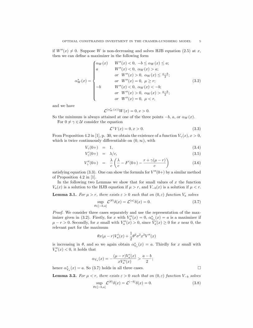
if W ′′(x) 6= 0. Suppose W is non-decreasing and solves HJB equation (2.5) at x,then we can define a maximizer in the following form

α∗W (x) =

αW (x) W ′′(x) < 0, −b ≤ αW (x) ≤ a;

a W ′′(x) < 0, αW (x) > a;

or W ′′(x) > 0, αW (x) ≤ a−b2 ;

or W ′′(x) = 0, µ ≥ r;−b W ′′(x) < 0, αW (x) < −b;

or W ′′(x) > 0, αW (x) > a−b2 ;

or W ′′(x) = 0, µ < r,

(3.2)

and we haveL(α∗W (x))W (x) = 0, x > 0.

So the minimum is always attained at one of the three points −b, a, or αW (x).For 0 6= γ ∈ U consider the equation

LγV (x) = 0, x > 0. (3.3)

From Proposition 4.2 in [1], p. 30, we obtain the existence of a function Vγ(x), x > 0,which is twice continuously differentiable on (0,∞), with

Vγ(0+) = 1, (3.4)

V ′γ(0+) = λ/c, (3.5)

V ′′γ (0+) =λ

c

(λ

c− F ′(0+)− r + γ(µ− r)

c

)(3.6)

satisfying equation (3.3). One can show the formula for V ′′(0+) by a similar methodof Proposition 4.2 in [1].

In the following two Lemmas we show that for small values of x the functionVa(x) is a solution to the HJB equation if µ > r, and V−b(x) is a solution if µ < r.

Lemma 3.1. For µ > r, there exists ε > 0 such that on (0, ε) function Va solves

supθ∈[−b,a]

L(θ)δ(x) = L(a)δ(x) = 0. (3.7)

Proof. We consider three cases separately and use the representation of the max-imizer given in (3.2). Firstly, for x with V ′′a (x) = 0, α∗Va(x) = a is a maximizer ifµ− r > 0. Secondly, for x small with V ′′a (x) > 0, since V ′a(x) ≥ 0 for x near 0, therelevant part for the maximum

θx(µ− r)V ′a(x) +1

2θ2σ2x2V ′′(x)

is increasing in θ, and so we again obtain α∗Va(x) = a. Thirdly for x small withV ′′a (x) < 0, it holds that

αVa(x) = − (µ− r)V ′a(x)

xV ′′a (x)>a− b

2;

hence α∗Va(x) = a. So (3.7) holds in all three cases.

Lemma 3.2. For µ < r, there exists ε > 0 such that on (0, ε) function V−b solves

supθ∈[−b,a]

L(θ)δ(x) = L(−b)δ(x) = 0. (3.8)


The results in lemmas 3.1 and 3.2 are intuitively appealing: at low surplus levels,when the stock return rate µ is higher than the interest rate r, the company investsin the stock at the maximum level a; on the other hand, when the interest rate ishigher, the company would invest in the risk-free asset at the maximum level of1 + b (all the surplus together with shortselling proceeds at the maximum level b).

For ε > 0 the function Vγ(x) with γ ∈ a,−b is now extended to the range[0,∞) as follows. To this end, fix ε < K < ∞, and a positive decreasing functionA(x) with A(x) < min(a, b) (to be chosen later). On the set C of functions w(x)which are continuous on [ε,K] consider the operator

Tw(x) = 2 infθ∈U,|θ|>A(x)

Mγ(W )(x)− [c+ rx+ θx(µ− r)]w(x)/(θ2σ2x2), (3.9)

where

Mγ(W )(x) = λ

(W (x)−

∫ ε

0

Vγ(y)f(x− y)dy −∫ x

ε

W (y)f(x− y)dy

),

W (x) = Vγ(ε) +

∫ x

ε

w(y)dy,

and f(x) is the common density of the claims.

Lemma 3.3. For w ∈ C the function Tw(x) is continuous on [ε,K]. Furthermore,the operator T is Lipschitz with respect to the supremum norm on C.

Proof. To prove continuity of Tw(x) we show that for fixed w ∈ C the functions

x→ Mγ(W )(x)− [c+ rx+ θx(µ− r)]w(x)/(θ2σ2x2), θ ∈ U , |θ| ≥ A(K)

are uniformly continuous on [ε,K]. This is true for the functions

x→ [c+ rx+ θx(µ− r)]w(x)

andx→ 1/(θ2σ2x2).

The representation

Mγ(W )(x) = λ

(W (x)−

∫ x

x−εVγ(x− y)f(y)dy −

∫ x−ε

0

W (x− y)f(y)dy

)shows that also Mγ(W )(x) is continuous on [ε,K]. Since the maximum of uniformlycontinuous functions is continuous, we have continuity of Tw(x).

Now we consider two continuous functions v(x), w(x) on [ε,K] and use the norm

||v(x)|| = sup|v(x)| : ε ≤ x ≤ K.Then the inequalities

|V (x)−W (x)| ≤∫ x

0

|v(y)− w(y)|dy ≤ K||v − w||,∣∣∣∣∫ x−ε

0

(V (x− y)−W (x− y))f(y)dy

∣∣∣∣ ≤ K2||v − w||,

|[c+ rx+ θx(µ− r)][v(x)− w(x)]| ≤ [c+ rK + (a+ b)K(µ+ r)|]|v − w||together with boundedness of 1/(θ2x2) imply that there exists a constant C suchthat for all v, w ∈ C we have

||Tv − Tw|| ≤ C||v − w||.


Using the standard Piccard-Lindelof argument we now obtain that for all K > εthere exists a continuously differentiable function w(x) satisfying

w′(x) = Tw(x), w(ε) = V ′γ(ε). (3.10)

With K → ∞ we obtain a similar function defined on [ε,∞). We further showw(x) > 0 on [0,∞). Define x0 = infx ≥ 0 : w(x) = 0. Suppose x0 < ∞, then itholds w(x0) = 0. Thus

w′(x0) = Tw(x0) = infθ∈U,|θ|>A(x0)

Mγ(W )(x0)/(θ2σ2x20) > 0,

which contradicts:

w′(x0) = limε→0+

w(x0)− w(x0 − ε)ε

≤ 0.

We then conclude w is never 0 and hence positive on [0,∞).Next we proceed to select an appropriate function A(x) such that an anti-

derivative of the solution w of equation (3.10) solves the HJB equation.For any W ∈ C1(0,∞) and W ′(x) > 0, write

φW (x) =2[M(W )(x)− (c+ rx)W ′(x)]

(µ− r)xW ′(x),

ψW (x) = − (µ− r)2[W ′(x)]2

2σ2[M(W )(x)− (c+ rx)W ′(x)].

(3.11)

One can check that ψW (x) = − (µ−r)W ′(x)σ2xφW (x) , and that φW (x) = αW (x) and ψW (x) =

W ′′(x) if W solves L(αW (x))W (x) = 0.

Lemma 3.4. (i) For µ > r, since Va solves (3.7), it holds φVa(x) ≥ a on (0, ε);(ii) for µ < r, since V−b solves (3.8), it holds φV−b(x) ≤ −b on (0, ε).

Its proof is given in Appendix 1.We denote by V (n) the solution of equation (3.10) with A(x) ≡ β/n where n is

a positive integer and β = mina, b.Now define

x∗n = infx : |φV (n)(x)| < β/n,and set x∗n =∞ if φV (n)(x) ≥ β/n for all x ∈ [0,∞). We have x∗n > 0 by Lemma 3.4,and

|φV (n)(x∗n)| = β/n, (3.12)

when x∗n < ∞, by continuity of φV (n) . Now we see V (n) is twice continuouslydifferentiable and solves HJB equation (2.5) on (0, x∗n); further notice that forx ∈ (0, x∗n) we have |α∗

V (n)(x)| > β/(n + 1) (it equals a, −b or |φV (n)(x)|). Thus,

V (n)(x) = V (n+1)(x) for x ∈ (0, x∗n), and x∗n ≤ x∗n+1 provided that both x∗n andx∗n+1 are finite.

Now we define

A(x) =

β 0 < x ≤ εβ/(n+ 1) x∗n < x ≤ x∗n+1

, (3.13)

and denote

x∗ = limn→∞

x∗n; (3.14)


for any x ∈ (0, x∗), write

V (x) = limn→∞

V (n)(x). (3.15)

We note it holds V (x) = V (n)(x) for x ∈ [0, x∗n]. From the previous discussions,we see that V is twice continuously differentiable and solves HJB equation (2.5) on(0, x∗). And it holds |φV (x)| > A(x) on (0, x∗). In the sequel, we write v = V ′;and we have v(x) > 0 on (0, x∗). Further V is bounded on (0, x∗). In fact, one canshow V (n)(∞) is bounded (as the verification theorem) and V (n)(x)/V (n)(∞) isthe maximal survival probability when investment control is restricted over regionUn := [−b,−β/n] ∪ [β/n, a]. We then see that V (n)(∞) decreases in n. This showsboundedness of V .

Now we proceed to show that x∗ is infinite. We state two lemmas without proof.The following lemma implies that a function that solves the HJB equation coincideswith the fixed point of operator (2.7).

Lemma 3.5. Suppose function u(x) satisfies

(i) u(x) = v(x) on (0, x0] and u(x) ∈ C1(x0, x0 + δ0) ∩ C[x0, x0 + δ0) wherex0 ≥ 0, δ0 > 0 and x0 + δ0 < x∗;

(ii) function U(x) solves HJB equation (2.5) on (x0, x0 + δ0), where U(x) =1 +

∫ x0u(s)ds.

Then u(x) = v(x) on (x0, x0 + δ0).

For any C1 function W , write

IW (x) = M(W )(x)− (c+ rx)W ′(x). (3.16)

We have the following Lemma (we refer to [15] for its proof):

Lemma 3.6. For x0 > 0 with IV (x0) > 0, there exists a twice continuously differ-entiable function Vα,x0 satisfying:

(i) it is of the form

Vα,x0(x) =

V (x) 0 ≤ x ≤ x0∫ xx0vα,x0(s)ds+ V (x0) x > x0

, (3.17)

where vα,x0∈ C1[x0,∞);

(ii) it solves

L(αδ(x))δ(x) = 0, (3.18)

on (x0,∞);(iii) Vα,x0

is concave on (x0,∞) and it holds IVα,x0 > 0 on (x0,∞).

Define sets

S1 = x : φV (x) < a,S2 = x : φV (x) > a.

(3.19)

Now we obtain:

Lemma 3.7. If x∗n <∞ for all n ≥ 1, then limn→∞

x∗n =∞.

Proof. Assuming limn→∞

x∗n = x∗ <∞, we prove Lemma 3.7 by contradiction.

For the case µ− r > 0, define x1 = infs : (s, x∗) ⊂ S1, where S1 is defined in(3.19); from Lemma 3.1 and Lemma 3.4, we have x1 > 0; now we show x1 < x∗

by contradiction. Suppose such x1 does not exist. Then there exists a sequence


x′n → x∗ such that limφV (x′n) ≥ a. Define yn = supx : x < x∗n, φV (x) > a/2,then lim yn = x∗. Further one can show V = Vα,yn on [yn, x

∗n] with φV (yn) = a/2

and φV (x∗n) = β/n. So there exits zn ∈ (yn, x∗n) such that

limn→∞

φ′V (zn) = −∞.

Notice

M(V )′(x) = λ[V ′(x)− f(x)−∫ x

0

V ′(x− y)f(y)dy].

There exists K > 0 such that M(V )′(x) > −K on (0, x∗) due to boundedness of fand V . Further notice

φ′V (x) =2

µ− rxM(V )′(x)V ′(x)−M(V )(x)(V ′(x) + xV ′′(x)) + cV ′2(x)

x2V ′2(x)(3.20)

thus

φ′V (zn) >2

µ− r(−znK −M(V )(zn))V ′(zn)− znM(V )(zn)V ′′(zn)

z2nV′2(zn)

=2

µ− r−znK −M(V )(zn)− znM(V )(zn)V ′′(zn)/V ′(zn)

z2nV′(zn)

,

(3.21)

which tends to −∞. From V ′′(zn) = V ′′α,yn(zn) < 0 and boundedness of M(V ),it must hold limV ′(zn) = 0 and then limV ′′(zn) = 0. Since V solves the HJBequation, it then holds limM(V )(zn) = 0. Contradiction!

Thus x1 exits such that 0 < x1 < x∗. It holds φV (x1) = a by continuity ofφV . Hence we can select x0 ∈ (x1, x

∗) such that 0 < φV (x0) < a; then we haveIV (x0) > 0 and from Lemma 3.6, there exists a function Vα,x0 which is concave andtwice continuously differentiable on (x0,∞), such that Vα,x0

(s) = V (s) on (0, x0],and it solves

L(αVα,x0(x))Vα,x0

(x) = 0,

on (x0,∞). Now define

x2 = supx : x ≥ x0; 0 < φVα,x0 (t) < a,∀ t ∈ [x0, x);noticing µ − r > 0, V ′′α,x0

(s) < 0, and IVα,x0 (s) > 0 (by Lemma 3.6), and thenφVα,x0 (s)>0, it holds

0 < αVα,x0 (s) = φVα,x0 (s) < a,

for s ∈ (x0, x2), we then have

supu∈[−b,a]

L(u)Vα,x0(s) = L(αVα,x0(s))Vα,x0(s) = 0,

which is the HJB equation (the maximizer of quadratic function L(u)Vα,x0(s) inu is the vertex αVα,x0 (s)). By Lemma 3.5, we conclude that Vα,x0

(s) = V (s) and

φV (s) = φVα,x0 (s) < a on (x0, x2 ∧x∗). If x2 ∈ (x0, x∗), by continuity of φVα,x0 and

definition of x2, we have φV (x2) = φVα,x0 (x2) = a, which contradicts to x2 ∈ S1.

If x2 ≥ x∗, we have φVα,x0 (x∗) 6= 0 since IVα,x0 (x∗) > 0 by Lemma 3.6, and itcontradicts to

φVα,x0 (x∗) = limn→∞

φVα,x0 (x∗n) = limn→∞

φV (x∗n) = limn→∞

φV (n)(x∗n) = 0.

This finishes the proof for the case µ− r > 0. The case µ− r < 0 can be shown ina similar way.

By Lemma 3.7 and the previous discussions, we have the following theorem:


Theorem 3.1. Function V (x) defined in (3.15), with the function A(x) constructedin (3.13), is a twice continuously differentiable solution to HJB equation (2.5)on (0,∞) with the initial values V (0+) = 1, V ′(0+) = λ/c, and V ′′γ (0+) =λc

(λc − F

′(0+)− r+γ(µ−r)c

).

In the following, we show some properties on the interplay between the optimalpolicies and parameters. These theorems are stated via four parameter cases. Wegive the proof of Theorem 3.3 in Appendix 2 and omit proofs the others which aresimilar.

Theorem 3.2. If µ > r and a ≥ b, then

(i) V solves HJB equation

supθ∈[−b,a]

L(θ)δ(x) = L(αδ(x))δ(x) = 0, (3.22)

on S1 and HJB equation (3.7) on S2;(ii) the associated maximizer in the HJB equation is given by

α∗V (x) =

αV (x) = φV (x) if φV (x) < a

a if φV (x) ≥ a, (3.23)

where it always holds φV (x) > 0.

For a 6= b, define sets:

Sa2 = x : a < φV (x) <2ab

b− a,

Sb2 = x : φV (x) >2ab

b− a.

(3.24)

Then we have:

Theorem 3.3. If µ > r and a < b, then

(i) V solves equation (3.22) on S1, equation (3.7) on Sa2 , and equation (3.8)on Sb2;

(ii) the associated maximizer in the HJB equation is given by

α∗V (x) =

αV (x) = φV (x) if φV (x) < a

a if a ≤ φV (x) ≤ 2abb−a

−b if φV (x) > 2abb−a

, (3.25)

where it always holds φV (x) > 0.

Define sets

S3 = x : φV (x) > −b,S4 = x : φV (x) < −b,

Sb4 = x : − 2ab

a− b< φV (x) < −b,

Sa4 = x : φV (x) < − 2ab

a− b.

(3.26)

We then obtain the following two theorems for the case µ < r:

Theorem 3.4. If µ < r and a ≤ b, then


(i) V solves the equation (3.22) on set S3, equation (3.8) on set S4;(ii) the associated maximizer in the HJB equation is given by

α∗V (x) =

αV (x) = φV (x) if φV (x) > −b−b if φV (x) ≤ −b

, (3.27)

where φV (x) < 0.

Theorem 3.5. If µ < r and a > b, then

(i) V solves the equation (3.22) on set S3, equation (3.7) on set Sa4 , and equa-tion (3.8) on Sb4;

(ii) the associated maximizer in the HJB equation is given by

α∗V (x) =

αV (x) = φV (x) if φV (x) > −b−b if − b ≥ φV (x) ≥ − 2ab

a−ba if φV (x) < − 2ab

a−b

, (3.28)

where φV (x) < 0.

Remark 3.1. By the verification Theorem 4.1, the function V (x) is bounded andproportional to the maximal survival function δ, in fact, δ(x) = V (x)/V (∞).

Remark 3.2. Noticing |α∗V (x)| > A(x), the optimal policy always involves invest-ment when µ 6= r.

Remark 3.3. In contrast to our case, when there are no constraints on the invest-ment as in [5], the optimal investment policy involves no shortselling of the riskyasset although it is allowed.

Remark 3.4. If µ = r, the optimal investment strategy α∗V equals 0, a or −b.

4. A Verification Theorem

In this section, we prove a verification result; that is, we show that the solutionV to the HJB equation is a multiple of the maximal survival probability function.The first lemma below shows that ruin is never caused by investment if investmentstrategies are constant at low surplus levels.

Lemma 4.1. For any non-negative integer n and an admissible control policy πsuch that when Xπ

t is small ut ≡ a if µ > r or ut ≡ −b if µ < r, it holds

P (τπ < τn+1|τπ > τn) = 0,

where τπ is defined in (2.2), and τ0 = 0, τ1, τ2,... are the times of claim arrivals.

Next we state an ergodicity result (Lemma 4.2) of the controlled surplus processand non-triviality (Lemma 4.3) of the optimization. For proofs of the lemmas werefer readers to [1] and [15].

Lemma 4.2. For any admissible control policy π, the surplus process Xπt either

diverges to infinity or drops below 0 with probability 1.

Lemma 4.3. There exists a control policy π (e.g., a suitable constant investmentstrategy), such that P (τπ =∞) > 0.

Now we prove the verification theorem:


Theorem 4.1. Suppose g is a positive, increasing, and twice continuously differen-tiable function on [0,∞); and it solves the HJB equation (2.5). Then g is boundedand the maximal survival probability function is given by δ(x) = g(x)/g(∞). More-over, the associated optimal investment strategy is π∗ = u∗(t)t≥0, where u∗(t) =α∗δ(X

∗t−), and X∗t is the surplus at time t under the control policy π∗.

Proof. For any ε > 0, we extend g to gε such that gε is increasing and twicecontinuously differentiable on (−∞,∞) with gε(x) = 0 on (−∞,−ε) and gε(x) =g(x) on [0,∞). For any admissible control π and positive constant M , define exittime

τπM = inft ≥ 0 : Xπt /∈ (0,M).

Write τ∗M = τπ∗

M to denote the first exit time from interval (0,M) of the surplusprocess under the optimal control policy π∗. By Ito’s Lemma (See [4]), we have

gε(Xt∧τ∗M ) =g(x) +

∫ t∧τ∗M

0

[c+ rX∗s + (µ− r)α∗g(X∗s )X∗s ]g′(X∗s )

+σ2

2[α∗g(X

∗s )]2(X∗s )2g′′(X∗s )ds+

∫ t∧τ∗M

0

σα∗g(X∗s )g′(X∗s )dWs

+∑

s≤t∧τ∗M ,X∗s<X∗s−

[gε(X∗s )− g(X∗s−)]

=g(x) +

∫ t∧τ∗M

0

L(α∗g(X∗s ))g(X∗s )ds+M(1)t +M

(2)t ,

(4.1)

where

M(1)t =

∫ t∧τ∗M

0

σα∗g(X∗s )g′(X∗s )dBs;

M(2)t =

∑s≤t∧τ∗M ,X∗s<X∗s−

[gε(X∗s )− g(X∗s−)]

+λ

∫ t∧τ∗M

0

[g(X∗s )− E(g(X∗s − Y ))]ds.

Since g solves the HJB equation, we have L(α∗g(X∗s ))g(X∗s ) = 0; further noticing that

α∗g(X∗s )g′(X∗s ) is bounded and M

(1)t , M

(2)t are both martingales, we take expecta-

tion on both sides of (4.1) and obtain

E[gε(Xt∧τ∗M )] = g(x). (4.2)

Similarly, for any admissible control π = utt≥0, noticing L(us)g(Xπs ) ≤ 0, it holds

E[gε(Xt∧τπM )] ≤ g(x). (4.3)

Letting t→∞ and then M →∞, by Fatou’s Lemma, we obtain

E[gε(Xτπ )] ≤ g(x). (4.4)

Further noticing by Lemma 4.2 that

E[gε(Xτπ )] ≥ g(∞)P (τπ =∞),

from Lemma 4.3, we must have that g(∞) is finite and that

P (τπ =∞) ≤ g(x)

g(∞). (4.5)


On the other hand, from (4.2), we have

g(x) = E[gε(X∗t∧τM )]

= E(g(X∗t∧τM )IX∗t∧τM

>0) + g(0)P (X∗t∧τM = 0)

+ E(gε(X∗t∧τM )I−ε<X∗

t∧τM<0)

≤ g(∞)P (X∗t∧τM > 0) + g(0)P (−ε < X∗t∧τM < 0),

where in the last inequality we used P (X∗t∧τM = 0) = 0 which holds by Lemma 4.1.Notice P (−ε < X∗t∧τM < 0) → 0 as ε → 0 since the claim distribution has acontinuous density. Letting t→∞ and then M →∞, we obtain

g(x) ≤ g(∞)P (τ∗ =∞);

from (4.5), we then have g(x)g(∞) = P (τ∗ = ∞), which is the maximal survival prob-

ability. The proof is completed.

5. Analysis of the Case of Exponential Claims and NumericalExamples

We will analyze a specific case in which the claim size Y has an exponentialdistribution with EY = m and the claims arrive with intensity λ. We give severalexamples. We note that in Example 1, the parameters satisfy

m[aµ+ (1− a)r − λ] + c < 0, (5.1)

which is equivalent to V ′′a (0+) > 0 (all the parameters will be specified later). Thisrelation will ensure some nontrivial investment policy, which switches from maximallong position to maximal shortselling and again to maximal long position when thesurplus increases. Before we introduce the examples we will state an auxiliary resultneeded for the analysis.

Lemma 5.1. Let F (x) = 1− e−x/m be the distribution function of an exponentialrandom variable with parameter 1/m. Then any bounded at 0 solutions to theintegro-differential equation of the second order

λ

∫ x

0

V (x− z) dF (z)− λV (x) + V ′(x)[µx+ c] +1

2σ2x2V ′′(x) = 0, (5.2)

with the initial conditionλV (0) = cV ′(0). (5.3)

is also a solution to the linear differential equation of the third order

x2V ′′′(x)+

[x2

m+ 2

(1 +

µ

σ2

)x+

2c

σ2

]V ′′(x)+2

[µx

mσ2+µ− λ+ c/m

σ2

]V ′(x) = 0.

(5.4)with the initial conditions (5.3) and (5.5) below

limx→+0

[cV ′′(x) + (µ− λ+ c/m)V ′(x)] = 0. (5.5)

Proof. The proof of this lemma was suggested to the authors by S.V. Kurochkin.Let g(x) denote the left hand side of (5.2). Then differentiating it, we see that theleft hand side of (5.4) is equal to g′(x) + g(x)/m. Therefore if V is a solution to(5.2) (that is g(u) ≡ 0) then it is also a solution to (5.4).

From a general theory of the ordinary differential equations with singularities(e.g., see [7], [17] ) and a more detailed analysis in [2] follows an existence of a


two parametric family of solutions to (5.4) bounded at 0 whose derivative is alsobounded at 0. Moreover each such bounded solution to (5.4) satisfies (5.5) (cf.(3.6)).

Suppose W (x) is any bounded at 0 solution to (5.4), which is subject to (5.5).The condition (5.5) implies that W ′′(0+) is bounded as well. Obviously for anyc1, c2, the function c1W (x) + c2 is a bounded solution to (5.4), satisfying (5.5).

Suppose V (x) is a bounded at 0 function which satisfies (5.2) and (5.3). LetV (0) = ζ, V ′(0) = ν. Take

W (x) = ν(W (x)−W (0))/W ′(0) + ζ.

Then W (x) obviously satisfies (5.4), (5.5). Substitute W into (5.2) instead of V ,and let g(x) denote the left hand side of (5.2). Then the left hand side of (5.4) isequal to g′(x) + g(x)/m. Thus g(x) = Ce−x/m for some constant C. Taking into

account that W ′(0) and W ′′(0) are bounded, we can substitute these expressions

into the left hand side of (5.2) and see that g(0) = −λW (0) + cW ′(0) = 0 due to

condition (5.3) and the fact that W (0) = V (0) and W ′(0) = V ′(0) by construction.

Therefore W satisfies (5.2) , (5.3).From [10] and [11] we know that there exists at most one solution V for an

integro-differential equation (5.2) with given V (0) and V ′(0) subject to (5.3). Thus

W (x) = V (x).

Lemma 5.2. Let F (z) = 1 − e−z/m be a distribution function of an exponentialrandom variable with mean m. Then the integro-differential equation (5.2) with theboundary condition (5.3) has a one-parametric family of solutions bounded at 0. Inthe neighborhood each solution of this family of 0 is represented by an asymptoticseries

V (x) = C0 +D1

[x+

∞∑k=2

Ckxk

], x→ 0, (5.6)

where C0 = V (0), D1 = λcC0 and

Ck = Dk/k, k = 2, 3, . . . , (5.7)

D2 = −(µ− λc

+1

m

), D3 = −D2[σ2 + 2µ− λ+ c/m] + µ/m

2c, (5.8)

Dk =− Dk−1[(k − 1)(k − 2)σ2/2 + (k − 1)µ− λ+ c/m]

c(k − 1)

+(1/m)Dk−2[(k − 3)σ2/2 + µ]

c(k − 1), k ≥ 4.

(5.9)

The asymptotic expansion means that the difference between the V (x) and the firstn terms in the right hand side of (5.6) is o(xn) when x→ 0.

The proof of this theorem can be obtained from Lemma 5.1, which reduces theintegro-differential equation (5.2) to an ordinary differential equation(5.4), and ageneral theory of the ordinary differential equations with pole-type singularities(see [17] Ch. 4 and [9]). The particular expression for the coefficients (5.7)-(5.9)has been found in [2].

In the numerical examples, we consider exponential claim size distribution withmean m = 1. Further, set σ = 0.1, λ = 0.09, and c = 0.02. The other parametersare given as follows via three examples.


Example 5.1. (µ > r and a < b) We choose µ = 0.02, a = 1, b = 20, r = 0.015.

Example 5.2. (µ < r and a > b) We choose µ = 0.02, a = 20, b = 1, r = 0.025.

Example 5.3. (µ < r and a < b) We choose µ = 0.01, a = 1, b = 20, r = 0.015.

Let V be the solution of the HJB equation (2.5) with V (0) = 1. From the pre-vious sections, we know that V (∞) is finite and the function V (x)/V (∞) coincideswith the maximal survival probability δ (2.4); and the optimal feedback controlfunction α∗V (x) is given by (3.2). If α∗V (x) = αV (x) then the function V satisfies

λ

∫ x

0

V (x− z) dF (z)− λV (x) + (c+ rx)V ′(x) =1

2

(µ− r)2(V ′(x))2

σ2V ′′(x); (5.10)

otherwise it satisfies (5.2) with

µ = aµ+ (1− a)r, σ = aσ, (5.11)

when α∗V (x) = a, and with

µ = −bµ+ (1 + b)r, σ = bσ, (5.12)

when α∗V (x) = −b.Numerical computations show that the optimal investment strategy is quite sur-

prising: there exists 0 < x1 < x2 < x3 <∞ such that

α∗V (x) =

a 0 ≤ x < x1

−b x1 ≤ x < x2

a x2 ≤ x ≤ x3

αV (x) x > x3.

(5.13)

In the following we show that such investment strategies typically occur when (5.1)holds and b is large.

From Lemma 3.1 we know that in the neighborhood of 0 the function V satisfies(3.1), that is (5.2) with µ given by (5.11); and α∗V (x) = a in this neighborhood. Inview of (5.1), the coefficient D2 in the asymptotic expansion (5.6) of the functionV at 0 is positive. Thus V ′′(x) ∼ D1D2 > 0, when x→ 0 and

αV (x) ∼ − (µ− r)σ2D2x

< 0. (5.14)

If one chooses instead of αV (x) its asymptotic approximation given by (5.14), then

we see that − (µ−r)σ2D2x

> a−b2 for x > x = 2 (µ−r)

σ21

D2(b−a) . If b is large enough then

x is small and the ratio of αV (x) and the right hand side of (5.14) is close to 1(note that for µ given by (5.11) the asymptotic expansion (5.6) does not dependon b) and αV (x) > a−b

2 . The choice of a or b in our example ensures that this isthe case, as numerical computations show. Therefore there exists x1 > 0 such thatαV (x) > a−b

2 for x > x1, while V ′′(x1) > 0 and αV (x) < a−b2 for x < x1. In view of

(3.2), the function V satisfies (5.2) with µ given by (5.12) in the right neighborhoodof x1 and it satisfies (5.2) with µ given by (5.11) for x < x1.

This shows that α∗V (x) = a for x < x1 and α∗V (x) = −b in the right neighborhoodof x1. Let us show that there exists x2 such that α∗V (x) = −b for x1 < x < x2,while α∗V (x) = a in the right neighborhood of x2. That is the point x1 is the firstpoint of the “extreme” switching from the maximal long position to the maximalshort position in the risky asset, while x2 is the point of the second “extreme”switching from the maximal short to the maximal long position. Since V ′′(x1) > 0


Figure 1. Example 1 - Maximal survival probability (The lowercurve is for the no-borrowing-no-shortselling case)

the function V is convex in the neighborhood of x1. On the other hand, if V ′′(x) ≥0 for all x > x1 then V ′(x) ≥ V ′(x1) > 0 for all x > x1 and V (x) → ∞ asx→∞. Contradiction! Therefore there exists a point x such that V ′′(x) = 0 whileV ′′(x) > 0 for x < x. Therefore, αV (x) → −∞ as x ↑ x and there exists x2 suchthat αV (x) > a−b

2 for x1 < x < x2 and αV (x) ≤ a−b2 in the right neighborhood of

x2.Suppose that α∗V (x) = a for all x > x2. Then the function V satisfies (5.2) with

µ and σ given by (5.11). From the general theory of the differential equations withsingularity at infinity (see [17] Chapter 4, or [7]) follows that for a solution V of(5.2) we have

V ′(x) = dx−2µ/σ2

[1 + o(1)],

and

V ′′(x) = d(−2µ/σ2)x−2µ/σ2−1[1 + o(1)],

when x→∞ for some positive d. (This precise formula on asymptotic approxima-tion for V ′ and V ′′ was proved in [2], using an approach developed in [9]. Also asimilar result was obtained in [8]). Thus for V being a solution to (5.2), it holds

αV (x)→ (µ− r)σ2

2µσ2, x→∞. (5.15)

Obviously the right hand side of (5.15) is positive and less than a. Really (µ−r)σ2

2µσ2 <

a is equivalent to 1a + r

(µ−r)a2 >12a which is obvious. Thus there exists x3 such that

α∗V (x) = a for x2 < x < x3 and α∗V (x) = αV (x) for x > x3. That is the switchingat the point x3 is from the maximal long position to a long position which is lessthan the maximal possible. The numerical computations are depicted in the graphs.(The authors would like to thank Yuri Gribov for providing numerical computationsfor the first two examples.)


Figure 2. Example 1 - Optimal investment proportion

Figure 3. Example 1 - Optimal investment proportion near zero surplus

6. Economic Interpretation

As we can see from Lemma 3.1 and Lemma 3.2 in the neighborhood of 0, whenthe surplus level is low, the optimal policy is always to take position which bringsthe highest rate of return. If µ > r then it is optimal to borrow and to take themaximal long position, if µ < r then the optimal policy requires to shortsell therisky asset and put into the risk-free asset the maximal allowable amount. In casea > b and µ > r the optimal policy would require no shortselling, maintaining atlow levels maximal long position and then purchasing risky asset at the level lessthan the maximum possible so as to reduce the volatility of the portfolio. Like wise


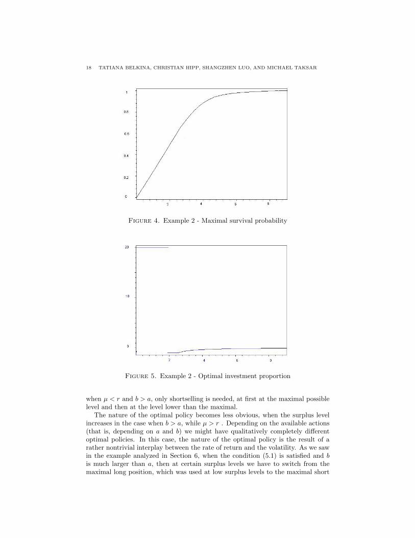
Figure 4. Example 2 - Maximal survival probability


when µ < r and b > a, only shortselling is needed, at first at the maximal possiblelevel and then at the level lower than the maximal.

The nature of the optimal policy becomes less obvious, when the surplus levelincreases in the case when b > a, while µ > r . Depending on the available actions(that is, depending on a and b) we might have qualitatively completely differentoptimal policies. In this case, the nature of the optimal policy is the result of arather nontrivial interplay between the rate of return and the volatility. As we sawin the example analyzed in Section 6, when the condition (5.1) is satisfied and bis much larger than a, then at certain surplus levels we have to switch from themaximal long position, which was used at low surplus levels to the maximal short


Figure 6. Example 3 - Maximal Survival Probability


position, now “gambling” on the effect of a largest possible volatility which mustincrease the surplus level with higher probability than otherwise would be the case.At first glance this policy might appear counterintuitive, if one takes into accountthat for such a policy the rate of return is the lowest possible. When the surpluslevel increases even more, it becomes again optimal to stick to the highest possiblerate of return; and with high surplus levels, it is optimal to have lower than themaximal possible rate of return, simultaneously having lower volatility. It is worthmentioning, that when b is not much larger than a a similar analysis show that


the effect of switching to the short position is not observed, and no shortselling isoptimal at any surplus levels; i.e., the set Sb2 defined in (3.24) could be empty then.

A similar phenomenon can be observed when µ < r and a > b. For certain valuesof the parameters, the optimal policy at low surplus levels would involve shortsellingthe risky asset so as to have the maximal rate of return for the resulting portfolio,while at higher surplus level we might observe a switch to the policy with thehighest volatility, that is to the one with maximal long position in the risky asseteven though that is the policy with the lowest return rate.

It is worth mentioning that none of those effects can be observed when we haveeither unconstrained case as in [5] or the no-borrowing-no-shortselling case of [1].In [5] the ability to have unlimited large leverage enables one to adhere only to thepolicies without shortselling, while in [1], the no-shortselling constraint does notallow to achieve sufficiently large volatility, of the portfolio, so as to reach higherlevels with higher probability while having a lower rate of return.

References

[1] Azcue, P. and Muler, M.: Optimal Investment Strategy to Minimize the Ruin Prob-

ability of an Insurance Company under Borrowing Constraints, Insurance Math.

Econom. 44(1) 26–34, (2009)[2] Belkina, T.A., Konyukhova N.B., Kurkina, A. O.: Optimal control of investments

in dynamical insurance models: II. Cramer-Lundberg model with exponential claim

size distribution (in Russian), Survey of the Industrial and Applied Mathematics 17,3–24 (2010).

[3] Browne, S.: Optimal investment policies for a firm with a random risk process:

exponential utility and minimizing the probability of ruin, Math. Ope. Res 20(4),937–958 (1995)

[4] Cont, R. and Tankov, P.: Financial modelling with jumps processes, Chapman &Hall/CRC, Boca Raton, (2004)

[5] Hipp, C. and Plum, M.: Optimal investment for insurers, Insurance Math. Econom.

27, 215–228 (2000)[6] Hipp, C. and Plum, M.: Optimal investment for investors with state dependent

income, and for insurers. Finance and Stochastics (3) 7, 299–321 (2003)

[7] Fedoryuk, M.V: Asymptotic analysis: Linear Ordinary Differential Equations.Springer, Berlin, 1993.

[8] Frolova, A., Kabanov, Y., and Pergamenshchikov S.: In the insurance business riskyinvestments are dangerous, Finance and Stochastics, 6, 227-235 (2002).

[9] Konyukhova, N.B.: Singular Cauchy problems for systems of ordinary differential

equations, U.S.S.R. Comput. Maths. Math. Phys. , 23, 72–82 (1983).

[10] Konyukhova, N.B.: Singular Cauchy problems for some systems of nonlinear func-tional differential equations. Differential Equations, 31, 1286-1293 (1995).

[11] Konyukhova, N.B.: Singular problems for systems of nonlinear functional differen-tial equations. Int. Scientific Journal Spectral and Evolution Problems, 20, 199–214

(2010)

[12] Luo, S.: Ruin minimization for insurers with borrowing constraints, North AmericanActuarial Journal, 12 (2), 143 – 174 (2008)

[13] Promislow, S.D. and Young, V.: Minimizing the probability of ruin when claims

follow Brownian motion with drift, North American Actuarial Journal 9(3), 109–128(2005)

[14] Schmidli, H.: Optimal proportional reinsurance policies in a dynamic setting, Scan.

Actuarial J. 1, 55–68 (2001)[15] Schmidli, H.: On minimizing the ruin probability by investment and reinsurance, The

Annals of Applied Probability 12(3), 890–907 (2002)

[16] Taksar, M. and Markussen, C.: Optimal dynamic reinsurance policies for large in-surance portfolios, Finance and Stochastics 7 97–121 (2003)


[17] Wasow, W: Asymptotic Expansion for Ordinary Differential Equations. Dover, New

York, 1987.

Appendix 1.We now show Lemmma 3.4 and write

ξγ,W (x) = − γ2(µ− r)xW ′(x)

2[M(W )(x)− (c+ rx+ (µ− r)γx)W ′(x)],

ηγ,W (x) =2[M(W )(x)− (c+ rx+ (µ− r)γx)W ′(x)]

σ2γ2x2,

(6.1)

for any function W with W ′ > 0. Note that ηγ,W (x) = − (µ−r)W ′(x)σ2xξγ,W (x) , and that

ξW (x) = αW (x) and ηγ,W (x) = W ′′(x) if W solves L(γ)W (x) = 0.We prove result (i) by contradiction. For convenience, note V = Va on (0, ε)

when µ > r. Suppose φV (x) < a for some x ∈ (0, ε). From L(a)V (x) = 0, we haveξa,V (x) = αV (x) and ηa,V (x) = V ′′(x). From φV (x) < a and µ− r > 0, we have

2[M(V )(x)− (c+ rx)V ′(x)] < a(µ− r)xV ′(x),

wherefrom it holds

2[M(V )(x)− (c+ rx+ (µ− r)ax)V ′(x)] < −a(µ− r)xV ′(x) < 0, (6.2)

and it implies V ′′(x) = ηa,V (x) < 0; further notice that V solves

supθ∈[−b,a]

L(θ)V (x) = L(a)V (x) = 0,

where a is the maximizer. Hence the vertex of the quadratic function L(θ)V (x) inθ must be to the right of a, i.e., it must hold αV (x) = ξa,V (x) ≥ a; with (6.2), weobtain

2a[M(V )(x)− (c+ rx+ (µ− r)ax)V ′(x)] ≥ −a2(µ− r)xV ′(x). (6.3)

Inequality (6.3) yields φV (x) ≥ a. Contradiction! Result (ii) can be proved in thesame manner.

To show Theorem 3.3. we need the following Lemma:

Lemma 6.1. For x0 ≥ 0 and γ ∈ a,−b, there exists function Vγ,x0satisfying the

following: Vγ,x0(x) = V (x) on [0, x0]; V ′γ,x0

(x0) = v(x0); and for x ∈ (x0,∞)

L(γ)Vγ,x0(x) = 0. (6.4)

Appendix 2.Now we prove Theorem 3.3. For any x ∈ S1, define x1 = infs : (s, x) ⊂

S1. From Lemma 3.4, we have x1 > 0. It holds φV (x1) = a by continuity.Select x0 ∈ (x1, x) such that A(x0) < φV (x0) < a. Then it holds IV (x0) > 0.From Lemma 3.6, there exists a function Vα,x0 concave and twice continuouslydifferentiable on (x0,∞) that solves

L(αVα,x0(x))Vα,x0

(x) = 0,

on (x0,∞). Now define

x2 = sups : s ≥ x0;A(t) < φVα,x0 (t) < a,∀ t ∈ [x0, s);


noticing V ′′α,x0(s) < 0 and

0 < αVα,x0 (s) = φVα,x0 (s) < a,

for s ∈ (x0, x2), we have

supθ∈[−b,a]

L(θ)Vα,x0(s) = L(αVα,x0

(s))Vα,x0(s) = 0,

i.e., Vα,x0solves the HJB equation. By Lemma 3.5, we conclude Vα,x0

(s) = V (s)and φV (s) = φVα,x0 (s) < a on (x0, x2). Since x2 is the supremum, if x2 ≤ x,

then we have φV (x2) = a which contradicts x2 ∈ S1. Thus it holds x2 > x andwe conclude that V equals Vα,x0

in a neighborhood of x and solves (3.22) withmaximizer α∗V = αV .

For any x ∈ Sa2 , we choose x0(< x) such that 2a < φV (s) < 2abb−a for all s on

[x0, x]; from Lemma 6.1, there exists Va,x0 such that Va,x0(s) = V (s) for s ∈ [0, x0]

and it solves L(a)Va,x0(s) = 0 on (x0,∞). Hence we have V ′′a,x0

(s) = ηa,Va,x0 (s) and

αVa,x0 (s) = ξa,Va,x0 (s) on (x0,∞). Now define

x2 = sups : s ≥ x0; 2a < φVa,x0 (t) <2ab

b− a,∀ t ∈ [x0, s);

it follows V ′′a,x0(s) = ηa,Va,x0 (s) > 0 and αVa,x0 (s) = ξa,Va,x0 (s) < a−b

2 . Thus Va,x0

solves HJB equation (3.7) on (x0, x2). By Lemma 3.5, we conclude Va,x0(s) = V (s)

and φVa,x0 (s) = φV (s) on (x0, x2); since x2 is the supremum, if x2 ≤ x, then

φV (x2) = 2a or φV (x2) = 2abb−a . This contradicts x2 ∈ Sa2 . Hence we have x < x2.

Thus V is equal to Va,x0and solves (3.7) with maximizer α∗V = a on (x0, x2) that

contains x.Similarly one can show for any x ∈ Sb2, in a neighborhood of x, V is equal to

V−b,x0 and solves (3.8) with maximizer α∗V = −b.Laboratory of Risk Theory, Central Economics and Mathematics Institute of the

Russian Academy of Sciences. , Moscow, Russia

Institute for Finance, Banking and Insurance, Karlsruhe Institute of Technology,

Karlsruhe, Germany

Department of Mathematics, University of Northern Iowa, Cedar Falls, IA, USA

50614

Department of Mathematics, University of Missouri, Columbia, MO, USA 60211

Optimal Constrained Investment in the Cramer-Lundberg model

Documents

Transcript of Optimal Constrained Investment in the Cramer-Lundberg model