Online fibre property measurements - DiVA Portal

DOCTORA L T H E S I S

EISLABDepartment of Computer Science and Electrical Engineering

Online Fibre Property Measurements

Foundations for a method based on ultrasound attenuation

Yvonne Aitomäki

ISSN: 1402-1544 ISBN 978-91-86233-54-9

Luleå University of Technology 2009

Yvonne A

itomäki O

nline Fibre Property Measurem

ents Foundations for a method based on ultrasound attenuation

ISSN: 1402-1544 ISBN 978-91-86233-XX-X Se i listan och fyll i siffror där kryssen är

Luleå University of Technology

Online Fibre Property Measurements:

Foundations for a method based on ultrasound attenuation

Yvonne Aitomäki

Online Fibre Property

MeasurementsFoundations for a method based on ultrasound

attenuation

Yvonne Aitomaki

EISLABDept. of Computer Science and Electrical Engineering

Lulea University of TechnologyLulea, Sweden

Supervisors:

Torbjorn Lofqvist, Jerker Delsing

Tryck: Universitetstryckeriet, Luleå

ISSN: 1402-1544 ISBN 978-91-86233-54-9

Luleå 2009

www.ltu.se

http://www.ltu.se

To Erik

Abstract

This thesis presents the foundations of a method for estimating fibre properties of pulp suitablefor online application in the pulp and paper industry.

In the pulp and paper industry, increased efficiency and greater paper quality control aretwo of the industry’s main objectives. It is proposed that online fibre property measurementsare a means of achieving progress in both of these objectives.

Optical based systems that provide valuable geometric data on the fibres and other pulpcharacteristics are commercially available. However, measurements of the elastic properties ofthe fibres are not feasible using these systems.

To fill this gap an ultrasound based system for measuring the elastic properties of thewood fibres in pulp is proposed. Ultrasound propagation through a medium depends on itselastic properties. Thus the attenuation of an ultrasonic wave propagating through pulp willbe affected by the elastic properties of the wood fibres. The method is based on solving theinverse problem where the output is known and the objective is to establish the inputs. Inthis case, attenuation is measured and a model of attenuation based on ultrasound scatteringis developed. A search algorithm is used for finding elastic properties that minimize the errorbetween the model and measured attenuation. The results of the search are estimates of theelastic properties of the fibres in suspension.

The results show resonance peaks in the attenuation in the frequency region tested. Thesepeaks are found in both the measured and modelled attenuation spectra. Further investigationof these resonances suggests that they are due to modes of vibration in the fibre. Theseresonances are shown to aid in the identification of the elastic properties.

The attenuation is found to depend heavily on the geometry of the fibres. Hence fibregeometry, which can be obtained from online optical fibre measurement system, provides thekey to extracting the elastic properties from the attenuation signal.

Studies are also carried out on the effect of viscosity on attenuation as well as the differencesin attenuation between hollow and solid synthetic fibres in suspensions. The measurementmethod is also applied to hardwood and softwood kraft pulps. The results of these studiesshow that using the model derived in the thesis and attenuation measurements, estimates ofthe elastic properties can be obtained. The elastic property estimates for synthetic fibres agreewell with values from other methods. These elastic property estimates for pulps agree well withprevious studies of individual fibre tests though further validation is required.

The conclusions, based on the work so far and under three realizable conditions, are that

the shear modulus and the transverse Young’s modulus of pulp fibres can be measured. Once

these conditions are met, a system based on this method can be implemented. By doing this

the industry would benefit from the increase in paper quality control and energy saving such

system could provide.

v

Contents

Part I xiii

Chapter 1 – Introduction 1

Chapter 2 – Fibres in Pulp 5

2.1 Fibres and the effects of processing . . . . . . . . . . . . . . . . . . . . . 5

2.2 Measurement methods of mechanical properties of fibres . . . . . . . . . 9

Chapter 3 – Ultrasound in Suspensions 11

3.1 Overview of acoustic waves . . . . . . . . . . . . . . . . . . . . . . . . . . 11

3.2 Attenuation Models of two phase suspensions . . . . . . . . . . . . . . . 16

Chapter 4 – Comparison to Spherical Scatters 27

Chapter 5 – Modes of Vibration 33

5.1 Effect of oblique incidence . . . . . . . . . . . . . . . . . . . . . . . . . . 36

5.2 Comparison between Attenuation and Modes of Vibration . . . . . . . . 37

5.3 Examining the major modes . . . . . . . . . . . . . . . . . . . . . . . . . 44

Chapter 6 – Parameter Estimation 49

6.1 Search Algorithm . . . . . . . . . . . . . . . . . . . . . . . . . . . . . . . 50

6.2 Parameter Sensitivity of the JED Model . . . . . . . . . . . . . . . . . . 51

Chapter 7 – Online Considerations 55

7.1 Measurements . . . . . . . . . . . . . . . . . . . . . . . . . . . . . . . . . 55

7.2 Model and Estimation Process . . . . . . . . . . . . . . . . . . . . . . . . 56

Chapter 8 – Summary of the Papers 59

8.1 Paper A - Estimating Suspended Fibre Material Properties by ModellingUltrasound Attenuation . . . . . . . . . . . . . . . . . . . . . . . . . . . 59

8.2 Paper B - Ultrasonic Measurements and Modelling of Attenuation andPhase Velocity in Pulp Suspensions . . . . . . . . . . . . . . . . . . . . . 60

8.3 Paper C - Inverse Estimation of Material Properties from Ultrasound At-tenuation in Fibre suspensions . . . . . . . . . . . . . . . . . . . . . . . . 60

8.4 Paper D - Sounding Out Paper Pulp: Ultrasound Spectroscopy of DiluteViscoelastic Fibre Suspensions . . . . . . . . . . . . . . . . . . . . . . . . 61

8.5 Paper E - Damping mechanisms of ultrasound scattering in suspension ofcylindrical particles: Numerical analysis . . . . . . . . . . . . . . . . . . 61

vii

viii

8.6 Paper F - Estimating material properties of solid and hollow fibres insuspension using ultrasonic attenuation . . . . . . . . . . . . . . . . . . . 62

8.7 Paper G -Comparison of softwood and hardwood pulp fibre elasticity usingultrasound . . . . . . . . . . . . . . . . . . . . . . . . . . . . . . . . . . 63

Chapter 9 – Conclusion 65

Chapter 10 – Further Work 6910.1 Further work . . . . . . . . . . . . . . . . . . . . . . . . . . . . . . . . . 69

Part II 79

Paper A 811 Introduction . . . . . . . . . . . . . . . . . . . . . . . . . . . . . . . . . . 842 Theory . . . . . . . . . . . . . . . . . . . . . . . . . . . . . . . . . . . . . 853 Experimental . . . . . . . . . . . . . . . . . . . . . . . . . . . . . . . . . 894 Results . . . . . . . . . . . . . . . . . . . . . . . . . . . . . . . . . . . . . 905 Conclusions . . . . . . . . . . . . . . . . . . . . . . . . . . . . . . . . . . 916 Further Work . . . . . . . . . . . . . . . . . . . . . . . . . . . . . . . . . 92A Appendix . . . . . . . . . . . . . . . . . . . . . . . . . . . . . . . . . . . 92

Paper B 951 Introduction . . . . . . . . . . . . . . . . . . . . . . . . . . . . . . . . . . 972 Phase Velocity . . . . . . . . . . . . . . . . . . . . . . . . . . . . . . . . . 983 Attenuation . . . . . . . . . . . . . . . . . . . . . . . . . . . . . . . . . . 1024 Conclusion . . . . . . . . . . . . . . . . . . . . . . . . . . . . . . . . . . . 1055 Further Work . . . . . . . . . . . . . . . . . . . . . . . . . . . . . . . . . 105

Paper C 1071 Introduction . . . . . . . . . . . . . . . . . . . . . . . . . . . . . . . . . . 1092 Theory . . . . . . . . . . . . . . . . . . . . . . . . . . . . . . . . . . . . . 1103 Results . . . . . . . . . . . . . . . . . . . . . . . . . . . . . . . . . . . . . 1114 Conclusion . . . . . . . . . . . . . . . . . . . . . . . . . . . . . . . . . . . 113

Paper D 1151 Introduction . . . . . . . . . . . . . . . . . . . . . . . . . . . . . . . . . . 1172 Theory . . . . . . . . . . . . . . . . . . . . . . . . . . . . . . . . . . . . . 1183 Experiment . . . . . . . . . . . . . . . . . . . . . . . . . . . . . . . . . . 1194 Results and Discussion . . . . . . . . . . . . . . . . . . . . . . . . . . . . 1225 Conclusion . . . . . . . . . . . . . . . . . . . . . . . . . . . . . . . . . . 1286 Acknowledgments . . . . . . . . . . . . . . . . . . . . . . . . . . . . . . . 128A Appendix . . . . . . . . . . . . . . . . . . . . . . . . . . . . . . . . . . . 129

Paper E 1311 Introduction . . . . . . . . . . . . . . . . . . . . . . . . . . . . . . . . . . 133

2 Theory . . . . . . . . . . . . . . . . . . . . . . . . . . . . . . . . . . . . . 1343 Method . . . . . . . . . . . . . . . . . . . . . . . . . . . . . . . . . . . . 1374 Results and Discussion . . . . . . . . . . . . . . . . . . . . . . . . . . . . 1385 Conclusion . . . . . . . . . . . . . . . . . . . . . . . . . . . . . . . . . . . 140A Appendix . . . . . . . . . . . . . . . . . . . . . . . . . . . . . . . . . . . 142

Paper F 1471 Introduction . . . . . . . . . . . . . . . . . . . . . . . . . . . . . . . . . . 1492 Theory . . . . . . . . . . . . . . . . . . . . . . . . . . . . . . . . . . . . . 1503 Experiment . . . . . . . . . . . . . . . . . . . . . . . . . . . . . . . . . . 1544 Estimation Process . . . . . . . . . . . . . . . . . . . . . . . . . . . . . . 1565 Results and Discussion . . . . . . . . . . . . . . . . . . . . . . . . . . . . 1576 Conclusion . . . . . . . . . . . . . . . . . . . . . . . . . . . . . . . . . . . 162

Paper G 1671 Introduction . . . . . . . . . . . . . . . . . . . . . . . . . . . . . . . . . . 1692 Method . . . . . . . . . . . . . . . . . . . . . . . . . . . . . . . . . . . . 1703 Results . . . . . . . . . . . . . . . . . . . . . . . . . . . . . . . . . . . . . 1734 Discussion . . . . . . . . . . . . . . . . . . . . . . . . . . . . . . . . . . . 1755 Conclusion . . . . . . . . . . . . . . . . . . . . . . . . . . . . . . . . . . . 177

Acknowledgements

I would like to thank my supervisor Torbjorn Lofqvist for his enthusiasm and ideas aswell as his advice and support. I would also like to thank Jerker Delsing for keepingme in mind of the main objectives and, more recently, for the constructive remarks thathave helped pull the thesis together. I would also like to thank Jan Niemi for being suchan excellent work colleague and coauthor. It has been great having someone to bounceideas off and I feel we’ve learnt a huge amount about acoustics, measurements and we’vealso found time to compare notes on parenting.

Thomas Brannstrom has been my mentor for the last year and has been a great sourceof wisdom and clever thinking for which I am most grateful. I would also like to thankJan van Deventer for listening to my rantings on cylinder modes and life in general - Iforgot to thank him in my licentiate so I am making sure I do it now. Thanks also go toJohan Carlson, who has found the time to read and re-read my recent articles and hasmade some valuable suggestions. Thanks also to Mikael Sjodahl and Niklas Brannstromfor commenting on my thesis.

I would also like to thank my friends and colleagues at the CSEE department formaking the department an enjoyable place to work. Not only that but there are so manyof you who have helped me that were I to list some, I would be leaving out others, soI have to thank you collectively and hope that will suffice. My thanks also go to thefantastic group of researchers, who made up the research school for women, for sharingyour experiences with me. Your support has increased my self-confidence.

Following convention, I would finally like to thank my family, but in all truth you areup there highest on my list of people to thank. Especially you, Erik. I couldn’t havemanaged without you. So, thank-you Emelie(7) for my lyckosten. Thank-you James(5)for telling me to break-a-leg when I go off to write this thesis. Thank-you Daisy(2)for making sure I get up in the morning and reminding me that work is only part oflife. Thank-you Astrid(12) for being so thoughtful and for helping Erik with the littleones. Thank-you Martin(15) for reminding me that it’s not easy being a teenager either.Thank-you mum for reading and correcting my English and for being ‘on my side’.

xi

Part I

Chapter 1

Introduction

Paper products are an essential part of our daily lives and the paper and pulp industry,which provide these products, is a cornerstone of World industry. In 2007, the Europeanpulp and paper industry employed 260 000 people, produced 100 million tonnes of paper,40 million tonnes of pulp and had a turnover of e80 billion. This accounted for 26% and23% of the World’s paper and pulp production, respectively [1]. It is a mature industrystriving to adapt to the new demands of customers and to take advantage of its accessto forest-based energy resources.

The energy consumption of the paper industry is high. In countries belonging to theConfederation of European Paper Industries (CEPI) this was 1.3 million TJ1 in 2006 [1].Increased efficiency is therefore an obvious means of reducing costs as not only does thisreduce the amount of energy, which has to be bought, but any energy by-products fromthe process can be sold. This is exemplified by the Sodra business strategy that statesthat energy is becoming an increasingly important element of operations [2].

One of the most energy intensive parts of the pulp manufacturing process is therefining of the pulp. In a typical plant this uses 1 GJ per tonne dry material [3]. Henceincreased efficiency in this part of the process can have a large economic impact.

Online fibre property measurement could improve energy efficiency and optimise pa-per quality, for example:

1. In the refiner by allowing the refining energy level to be set according to the par-ticular fibre properties or by reducing the percentage of fibres refined, if the fibresalready have suitable properties.

2. By reducing waste - early detection of faults associated with the fibre propertiescan allow the pulp to be reprocessed at an earlier stage in the paper manufacturing.

3. Paper quality could be optimised by improving fractionation of the pulp. The aimof fractionation is to separate the pulp according to its properties. With online

11 · 1018 Joules

1

2 Introduction

fibre property measurement the fractionation process can be improved. These im-provements would lead to the fibres, and hence the pulp, being better suited to theend product.

Optical fibre property measurements are currently available and their use in improvingpaper quality is shown by Hagedorn [4]. The flexibility of the fibres is an importantproperty since greater flexibility increases the strength of the paper. This flexibilitydepends on both geometry and Young’s modulus [5]. In optical systems such as the STFIFibermaster, (Lorentsen-Wettre, Sweden) [6], bendibility is used as a relative measure offlexibility. However, using this measure the influence of bendibility cannot be separatedfrom the geometry since they are interdependent variables [4]. The consequence of thisis that there is ambiguity as to whether it is the elastic properties of the fibre (such asYoung’s modulus) or the geometry that needs to be modified by the process.

Ultrasound measurements have the potential to measure the elastic properties of thefibres in suspension. This is because ultrasound propagation is a function of these elasticproperties. If an ultrasound method can measure elastic properties then a future papermanufacturing plant could have sensors based on this technology at crucial stages in theprocess. This would work alongside an online optical pulp analyser providing geometricfibre data. The result would be increased process efficiency, which results in reducedenergy usage, and greater paper quality control. Thus profit margins are increased.

In addition, if the optical and ultrasound sensors were combined with an online papermeasurement system, such as a laser ultrasonic web stiffness sensor [7], it would allow therelationship between pulp properties and paper quality to be more precisely established.

The objective of this thesis is to provide the first step towards an online method ofmeasuring the elastic properties of fibres. Hence, the following hypothesis is tested:

The measurement of the ultrasound attenuation can be used to estimate theelastic properties of wood fibres in pulp online.

This hypothesis can be broken down into three research questions,

1. Can elastic properties be estimated from ultrasound attenuation?

2. Can the method be applied to wood fibres in pulp?

3. Can the measurement method be used online?

Can elastic properties be estimated from ultrasound attenuation?

The method of estimating the elastic properties from ultrasound attenuation consists ofthree parts: a model, measurements and an algorithm for finding the parameters of themodel that minimizes the difference between the model output and the measurements.Since the method is to be applied to wood fibres in pulp, the model is based on theacoustic scattering of particles in suspension (Chapters 3 & 5). The measurements are ofultrasound attenuation. The algorithm searches through the range of elastic propertiesto find the values that minimize the difference between the modelled attenuation and the

3

measured attenuation. The outcome of the algorithm, being the estimates of the elasticproperties, gives the best-fit to measured attenuation (Chapter 6).

This question is central to the thesis and is addressed in all the papers as well as thechapters specified in the text.

Can the method be applied to wood fibres in pulp?

To apply this method to pulp a model is required, which captures only the wood fibreproperties that are important to attenuation. From this, the elastic properties of thefibres can be extracted.

Again this question is central to the thesis but is particularly addressed in the finalpaper, Paper G and Chapter 2.

Can the method be used online?

The ultimate aim is to have an online method. This will influence decisions about thecomplexity of the model chosen. Hence, the need to establish the simplest model thatwill allow estimates of the elastic fibre properties to be made. Consideration should alsobe made of the computational efficiency of such a method and the equipment required.

The thesis is made up of two parts: a summary of the work and a collection of papers. Thefirst part presents more detailed information on wood fibres in pulp and the backgroundphysics, followed by more detailed issues not covered in the scientific papers. The papersare then summarised before conclusions are drawn and further work is discussed. Thesecond part is a collection of seven papers.

Chapter 2

Fibres in Pulp

2.1 Fibres and the effects of processing

Paper in the broadest sense of the word dates back to the ancient Egyptians who used thepapyrus plant to make sheets on which to write. Our modern day paper making however,has its roots in China, possibly as early as 8 BC [8]. The basic steps are gathering theraw material, breaking it down to a pulp with the addition of water then forming it intoa sheet before drying it. Although these steps may not have changed, the process isnow high speed (up to 1,900 m/min [9]), high volume, and fully automated. The hugevariations in the processes and the type of wood or even the organic and non-organicmaterial used as input in the process reflect the differences required in the final products.The focus of this research is on the measurement of the properties of fibres used in themanufacture of paper products; more specifically wood fibre properties because wood isby far the most common source of fibres used in paper making.

Before discussing fibre property measurements and the effect the pulp process has ontheir properties it is worthwhile introducing some of the elements of the fibre that areimportant to its mechanical properties.

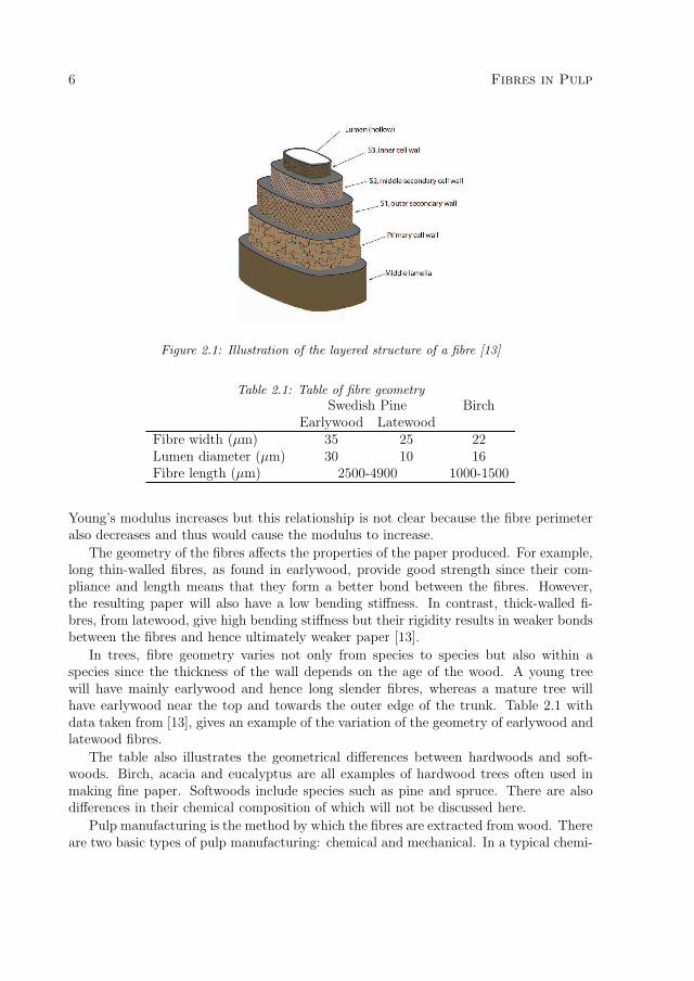
A wood fibre has a layered structure as shown in figure 2.1. The hollow in thecentre of the fibre is called the lumen and the outer edge of the fibre is the primary cellwall. In wood, the fibres are held together by the middle lamella which is also shown inthe diagram. The lines on the primary cell wall and secondary walls (s1, s2 and s3 inthe diagram) illustrate fibrils that are part of the cell walls. Fibrils or microfibrils aremade of cellulose molecules and their orientation, as indicated in the diagram, can varyconsiderably. The s2 layer has fibrils that are parallel and form a steep spiral about theaxis of the fibre. The microfibrillar angle (MFA) of this layer has been measured and hasbeen found to relate to the strength of individual fibres [10]. These results show that themore axially aligned the microfibrils (smaller MFA), the greater the strength of the fibres.On a larger scale, the MFA has been related to the Young’s modulus of wood where adecrease in MFA correlates to increased stiffness (higher modulus) [11]. Interpretingthe data on individual fibre measurements [12] shows that when MFA decreases, the

5

6 Fibres in Pulp

Figure 2.1: Illustration of the layered structure of a fibre [13]

Table 2.1: Table of fibre geometrySwedish Pine Birch

Earlywood LatewoodFibre width (μm) 35 25 22Lumen diameter (μm) 30 10 16Fibre length (μm) 2500-4900 1000-1500

Young’s modulus increases but this relationship is not clear because the fibre perimeteralso decreases and thus would cause the modulus to increase.

The geometry of the fibres affects the properties of the paper produced. For example,long thin-walled fibres, as found in earlywood, provide good strength since their com-pliance and length means that they form a better bond between the fibres. However,the resulting paper will also have a low bending stiffness. In contrast, thick-walled fi-bres, from latewood, give high bending stiffness but their rigidity results in weaker bondsbetween the fibres and hence ultimately weaker paper [13].

In trees, fibre geometry varies not only from species to species but also within aspecies since the thickness of the wall depends on the age of the wood. A young treewill have mainly earlywood and hence long slender fibres, whereas a mature tree willhave earlywood near the top and towards the outer edge of the trunk. Table 2.1 withdata taken from [13], gives an example of the variation of the geometry of earlywood andlatewood fibres.

The table also illustrates the geometrical differences between hardwoods and soft-woods. Birch, acacia and eucalyptus are all examples of hardwood trees often used inmaking fine paper. Softwoods include species such as pine and spruce. There are alsodifferences in their chemical composition of which will not be discussed here.

Pulp manufacturing is the method by which the fibres are extracted from wood. Thereare two basic types of pulp manufacturing: chemical and mechanical. In a typical chemi-

7

Wood

chipsDigester

(removes ligin)Refiner Screen Washing

To paper

machine

Figure 2.2: Simplified process diagram of a chemical pulp process (no bleach)

cal pulp manufacturing process, illustrated in figure 2.2, the wood is cooked in a solutionof chemicals. The lignin of the wood is made soluble (digested) and the fibres separateas whole fibres. These softened fibres are then fed at high pressure into a refiner (refiningprocess) where they are mechanically beaten. In a typical mechanical pulp manufacturingprocess, the wood fibres are exposed to heat and pressure (thermomechanical pulps [14])before being separated by grinding or milling. These pulps can then be refined to improvethe fibre properties for paper making. An overview of these different processes and thevariations that exist between them is provided by Wikstrom [15] and Karlsson [13].

From the brief description of pulp manufacturing, it is obvious that one of the fun-damental steps in making paper is the mechanical treatment of the fibres, typically inthe refiner. One of the objectives of this stage is to fibrillate the fibre. This is wherethe fibres are beaten to increase their flexibility and their ability to swell, before paperformation [16]. There is some evidence to show that this increased flexibility is indepen-dent of geometry and hence due to elasticity of the fibre wall [17]. Collapsing of the fibrestructure, so that the fibres have a ribbon geometry results in greater paper strength [13].The relationship between flexibility and collapsed fibres is expected since in theory,

F = 1/EI (2.1)

where F is the flexibility, E is the Young’s modulus and I is the second moment ofarea [12]. If the fibre collapses, then I decreases and consequently F increases. Fromthe equation it can been seen that the elastic modulus of the fibre is important in fibreflexibility directly. It could also have an indirect affect since from general studies of hollowcylinders [18], low E values lead to an increased tendency to collapse. Since collapsedfibres are more flexible it follows then low E will both directly and indirectly lead togreater fibre flexibility and hence stronger paper.

Refining also causes some of the microfibrils to be either released from the cell wallor bowed out. This increases the bonding of the fibres to each other, increases thestrength of the paper and its homogeneity [10]. The relationship between the frequencyof refining and the viscoelastic properties of water saturated lignin, which is relatedto the viscoelasticity of the fibres since they are composed on lignin, has also beeninvestigated [19]. Although it was found that refining frequencies would not soften thelignin, the study does provide some data on the viscoelasticity of saturated wood andhence to some degree fibres.

8 Fibres in Pulp

(a) (b)

20μm

(c)

20μm

(d)

Figure 2.3: Examples of refined fibres in pulp: 2.3(b) Softwood fibres from chemical pulp (mag-nification x75), 2.3(a) Cross section of fibre in softwood chemical pulp showing two collapsedfibres. 2.3(c) Hardwood chemical pulp (bleached), 2.3(d) Softwood chemical pulp

Figure 2.3 are photographs of refined pulp fibres. Figure 2.3(a) illustrates their vari-ability along the their length. Note also from the photograph and the dimensions givenin Table 2.1 that the length is much greater than the fibre diameter, which is the reasonfor the assumption of infinite length used in the model. Figure 2.3(c) and 2.3(d) are athigher magnification and show the cross sectional variation between a hardwood pulpand a softwood pulp, respectively.

The cross sectional view of a group of refined pulp fibres is shown in the figure 2.3(b).Two of the fibres can clearly be seen to have maintained their structure whereas the othertwo fibres have collapsed and lie together.

In the processing of fibres their material properties and their geometric properties arealtered in order to make a better quality paper product. It follows then that measuringand monitoring these properties can improve paper quality and this is exemplified in astudy done by Hagedorn [4].

9

2.2 Measurement methods of mechanical properties

of fibres

As customers, our demands on paper vary from the softness of tissue to the strengthand durability of cardboard, and from the porous nature of vacuum bags to non-porousmilk cartons. In addition are the demands made on the printing surfaces of most paperproducts. To match these demands on the final paper products, there is a wide rangeof pulp characteristics that require monitoring and measuring. The flexibility and theelastic properties of the fibres are two of these characteristics but, as discussed in section2.1, their influence on paper strength means they have an important role in paper quality.

The flexibility of fibres depends on the elasticity of the fibres and their geometry.Fractioning fibres using a mesh separates long or stiff fibres from shorter or flexible fibressince the long and/or stiff fibres do not pass as easily through the mesh as shorter and/ormore flexible fibres. Some assessment of fibre flexibility can therefore be made usingdifferent sizes of mesh. However, the problem of separating the length property from theflexibility property of the fibre remains.

The stiffness of individual fibres can be measured and through this Young’s modulusestablished. The first of the two main methods used is carried out by setting the fibrein a v-shaped notch on the tip of a thin capillary tube submersed in water. Water isthen allowed to flow through the capillary. This water flow is increased until the middlepart of the fibre reaches a preset mark [20]. The second method is to measure the extentto which a fibre has followed the contour of a wire set between the fibre and a glassplate, when a hydraulic pressure is applied. This process has been automated and isavailable [20].

The L&W STFI Fibermaster [6] gives an indication of the stiffness through a mea-surement quantity referred to as bendability. This is defined as the difference in formfactor when measured with high and normal flows in the measuring cell. The form factoris the ratio of the greatest extension of the fibre to the real length of the fibre in the sameprojected plane [21]. The use of flow and optical measurement results in the ability of thesystem to provide a measurement related to the elasticity of the fibre. One of the prob-lems with this method is that the fibre is projected onto a plane so that deflections outof plane cause distortions and hence are a source of inaccuracy. Another issue is that thecurrent measurement is a relative measurement of the flexibility of the fibres and not anabsolute one. An industrial study measuring the bendability and paper quality showed acorrelation between these two properties, however this correlation was explained as beingdue to the fact that the bendibility uses the shape factor, which is also correlated withpaper quality, and hence the two could not be separated [4].

In research investigation of fibre flexibility, individual fibres are tested [12, 22]. Onemethod was to test individual fibres by applying epoxy glue to each end of carefullyselected long, straight fibres [12]. The fibre was then mounted in a loading machineand the load was measured under cyclic displacement. From this and the geometricmeasurements, the Young’s modulus, and the flexiblity was calculated. This was donefor approximately 400 fibres and provides figures for comparison with other methods.

10

Measurements of other elastic properties such as shear modulus and intrinsic loss havenot been found for pulp fibres.

It can be seen from this overview of the current measurement methods that a rapidonline method for measuring the elastic properties of the fibres directly does not yetexist.

Chapter 3

Ultrasound in Suspensions

3.1 Overview of acoustic waves

Ultrasound is simply sound with higher frequencies than that the human ear can detect(>20kHz), hence theories on audible sound also apply to ultrasound. The mechanism bywhich a sound wave propagates through a medium depends on its material properties.Hence by measuring the velocity of the wave and its attenuation information can beobtained about these material properties. The term wave velocity will in this thesis andrefers to the phase velocity of the wave. As the wave propagates through a mediumit tends to diminish in amplitude. This is due the dissipation of energy as the waveadvances. This is quantified by the attenuation, α, and its relationship to the amplitude,So, at a point in space is

S ′ = Soe−αd, (3.1)

where S ′ is the wave amplitude after it has travelled a distance d in the medium. Hence

α =1

dln

(So

S ′

). (3.2)

Sound waves with different frequencies are absorbed, or attenuated, by differentamounts depending on the medium. Hence α is frequency dependent and the equationabove is valid for a particular frequency.

If the sound is a pulse then it will contain different frequencies and the shorter thepulse, the more frequencies it will contain. The advantage of measuring using a pulseis that the frequency response of the medium can be obtained in a single measurement.However, the transient effects are more complex to model and hence it is common tomodel the system as a steady state one.

3.1.1 Waves in fluids

In fluids, the classical explanation for attenuation is that it is due to viscosity, η, andthermal conduction. For non-metallic fluids, the attenuation due to thermal conduction

11

12 Ultrasound in Suspensions

is negligible compared to that due to viscosity [23]. Unfortunately for most commonliquids this does not account for all the attenuation mechanisms. In water, this excessattenuation is attributed to structural relaxation [24] and an additional viscous term, ηB

is used. For water, ηB is approximately three times that of the η. The relationship forthe attenuation, α, can be written in terms of the relaxation time τ [23] such that

α ≈ 1

2

ω2

cτ, (3.3)

where ω is the angular frequency and τ is

τ = (4

3η + ηB)/ρ1c

2. (3.4)

From this it can be seen that as the frequency increases, the attenuation becomesincreasingly significant, even in low viscous fluids such as water, as it is a function of ω2.

In a non-viscous fluid the wave velocity, cc, equals the thermodynamic speed of sound,c. This is defined as [23]

c =

√B

ρ, (3.5)

where B is the adiabatic bulk modulus and ρ1 is the density of the fluid [23]. c is aconstant in the wave equation which is derived from the linearised mass conservationand linearised conservation of momentum [25] such that

∇2p − 1

c2

∂2p

∂t2= 0 (3.6)

If the fluid is unbound and viscous, then the effect of the viscosity can be approximatedby the introduction of τ into the wave equation such that

cc ≈ c(1 +3

8ω2τ 2). (3.7)

Although cc has a term depending on ω2, τ 2 is very small for low viscosity fluids likewater and hence the dispersion, which is where waves of different frequencies travel atdifferent velocities, is small.

3.1.2 Waves in Solids

The wave motion in solids is more complex and it is described by Navier’s displacementequation, which is expressed for a isotropic, elastic medium as

(λ + 2G)∇∇ · ζ + G∇2ζ = ρ2∂2ζ

∂t2(3.8)

where ζ is the displacement vector and ρ is the density. λ and G are elastic moduli whereλ is Lame constant and G is the shear modulus. ∇2 is the three dimensional Laplace

13

cs

(a)

cc

(b)

Figure 3.1: Illustrations of a shear wave (3.1.2) and a pure compression wave 3.1.2 propagatingin a solid

operator [26]. This can be re-written to divide the motion into a dilation (compression)and rotation.

(λ + 2G)∇(∇ · ζ) + G∇× (∇× ζ) = ρ2∂2ζ

∂t2(3.9)

Thus in an unbound solid two types of waves can exist: a compressional wave and ashear wave (rotational) wave. The shear wave is a transverse wave, where the particlemotion is perpendicular to the direction of propagation (Figure 3.1.2) and hence is termeda rotational wave.

The velocity of a shear wave depends only on the shear modulus of the solid suchthat

cs =

√G

ρ2. (3.10)

In a compression wave, the particle motion and the wave direction are concurrent. Thesimplest case of a compression wave propagation in a solid is when it is along the axisof a narrow bar or rod of isotropic material, where surface of the rod is allowed to movefreely and the frequency is low (theoretically when the frequency is zero). The velocityof this wave will solely depend on the Young’s modulus such that [27]

co =

√E

ρ2. (3.11)

However, if the isotropic media is now extended, it can be thought of as if the surfacewere fixed. It therefore requires a greater stress to cause the same strain. It can be shownthat wave velocity of a compression wave is then dependent on the shear modulus, G aswell as the bulk elasticity of the material, K [28]. Its velocity becomes

cc =

√K + 4

3G

ρ2. (3.12)

For a volume of the material where the force, p, is applied uniformly on each side of ancubic element of the medium, K is defined as p = K/ρ2 [28]. A full derivation of these


wave velocities and how they relate to the stress and strain in a solid medium is givenin [28].

In solids, the intrinsic attenuation per wavelength can be approximated by the phasedifference between the stress and the strain, also referred to as the loss tangent, tan δ [29].Stress and strain are related by a general elastic modulus, M . The specific modulus orcombination of moduli will depend on the geometry, the type of loading, the specificmaterial etc. To model this phase difference, M is made complex such that

M = M ′ + iM ′′

and

tan δ =M ′′

M ′(3.13)

In terms of the attenuation, α, this becomes, if tan δ � 1

α = π tan δ (3.14)

This phase difference will cause dispersion and the effect can be calculated by usingthe complex elastic modulus in the calculation of the wave velocity. Hence cc can beexpressed as a complex wave speed, cc = cc

√1 − i tan δ

In a suspension, the wave travels from a fluid to either a solid or another fluid. Asthe wave hits the boundary of the two media, part of the wave is reflected and part ofthe wave is transmitted. In the simple case of a plane wave arriving at a boundary thatis perpendicular to the direction of the wave, calculating the ratio of the intensity of thetransmitted wave to the reflected wave is straightforward. This is done by considering theboundary condition at the interface and assuming the velocity and pressure to be contin-uous at this point. The result is that the amplitude of the wave being reflected dependson the difference in the characteristic impedances of the two media. The characteristicimpedance is the product of the density and the velocity of the wave. Since a plane waveand a flat boundary are considered, the only waves propagating are compression waves.The calculation is more elaborate if the wave progression is not perpendicular to theboundary and particularly if the interface is on a solid [30].

3.1.3 Thermoelastic Scattering

Associated with an ultrasonic pressure wave is a temperature field which is in phasewith the pressure wave and depends on the thermal properties of the medium. In asuspension, there are two media that normally have different thermal properties. Theresult is that the temperature field inside the suspended particle is different in amplitudeto that of the surrounding liquid away from the boundary. In order to maintain theequilibrium at the boundary, the temperature field in the boundary layer varies andcauses the boundary layer to expand and contract and hence become the source of asecondary wave (Figure 3.2). This is known as thermoelastic scattering. Considering theθ−r plane, of a cylindrical scatterer in a fluid media, this thermal elastic scatter appearsas a symmetric monopole wave emanating from the scatterer. This wave decays quickly

15

Pulsating

Boundary

layer

Scatterer

Figure 3.2: Diagram of an pulsating boundary layer, the source of a secondary sound wave.

and is not noticeable at a large distance from the scatterer. It does however dissipateenergy and in some cases, such as for an emulsion of sunflower oil and water, it can be thedominant effect in attenuation [31]. For fibres where the scatterer has a larger diameterand for higher frequency this effect is small [32].

3.1.4 Viscous boundary effects

In the previous section the attenuation and motion of an unbound fluid was discussed.The added effect of a boundary is apparent when a viscous fluid flows close to andparallel to the surface of a wall. In this case there exists a primary wave with motionat a distance from the wall, with only a component in the x direction parallel to thewall, ux. There also exists a secondary wave, u′, with motion in x that is a function ofz (direction perpendicular to boundary) and time t. In studying the absorption arisingfrom the shear at the boundary, the equation governing the flow is the rotation part ofthe Navier Stokes equation,

ρ∂u

∂t= η∇× (∇× u). (3.15)

The boundary conditions are that the velocity approaches the free stream velocity farfrom the boundary and the wall is fixed which means that the velocity is zero at thispoint such that u = (ux + u′). Hence equation 3.15 for the x direction is

∂u′

∂t=

η

ρ

∂2u′

∂z2. (3.16)

This is a diffusion equation, rather than a wave equation and hence no wave propagationis possible [33]. The solution for equation 3.15 that satisfies the boundary condition arethat the complex secondary wave u′ is [23]

u′ = −uxe−(1+i)z/δ (3.17)

δ =√

2η/ρ1ω (3.18)

The quantity δ is the viscous penetration depth or viscous skin depth. The final expres-sion for the secondary wave if ux = Uoe

i(ωt−kcx) is

u = Uoe−z/δei(ωt−kcx−z/δ) (3.19)


where kc is the wave number of the primary wave in the fluid.As can be clearly seen from this equation, this wave attenuates exponentially and

its effect is confined to the distance given by the viscous skin. This description is for amoving fluid but it is also valid for a when the fluid is motionless and the solid surfaceis moving.

At a large distance from the scatterer this wave is not noticeable, but as with thethermoelastic wave, it does dissipate energy at the boundary. The above expression isvalid if the wavelength is much greater than the skin depth, which for water is above theGHz region.

3.1.5 Summary

The attenuation of the sound or ultrasound wave reflects the nature of the medium thewave has passed through. Considering a sound wave travelling through a suspension ofsolid particles in a fluid, the attenuation of the sound wave will depend on the viscosityand the bulk viscosity of the fluid, the difference in the characteristic impedance betweenthe fluid and the solid i.e. differences in density and wave velocity in these two media,and the attenuation in the solid itself. This illustrates the possibility of being able toestimate a number of fluid and solid properties by measuring the attenuation of soundin a suspension of solid particles in a fluid. The additional attenuation of thermoelasticscattering could potentially provide the thermal properties of the media. The viscousboundary effects reinforce the effects of the viscosity and hence could potentially lead toa means of establishing the viscosity of the fluid [34].

3.2 Attenuation Models of two phase suspensions

3.2.1 Historical background

The propagation of sound in suspensions has been discussed for over hundred years.Rayleigh [35] calculated the attenuation of sound due to small spherical obstacles in anon-viscous atmosphere, when considering the effect of fog on sound. He showed thatthe attenuation depends on the number of scattering particles and the ratio of theirdiameter to the wavelength of the sound. Knudsen [36] used expressions by Sewell [37] inthe calculation of attenuation for spherical and cylindrical particles in a viscous fluid tomodel audible sound in fog and smoke. Incidentally, Sewell’s work confirmed the futilityof using suspended or stretched wires for absorbing sound in rooms. In 1953, Epsteinand Carhart [38] developed a model for the attenuation of sound by spherical particleswhere energy loss is due to the thermal and viscous losses in the boundary layer as wellas scattering from the particle itself.

This model was modified slightly by Allegra and Hawley [39] and the resultingEpstein-Carhart [38]/Allegra-Hawley [39] (ECAH) model has been the basis for investiga-tions on attenuation and velocity measurements in emulsions [31]. A summary of differentexperiments on suspensions based on acoustic scattering theories is given in [40], though

17

which specific model has been used in each case is not mentioned. In 1982, Habeger [32]derived a version of the ECAH model for cylindrical scatterers and tested this with exper-iments on suspensions of viscoelastic polymer fibres in water. The fibre properties thatwere known or could be measured, using alternative methods, were used in the modelwith no adjustments. The values of the loss tangent and Poisson’s ratio were set to fitthe experimental data.

As the concentration of the scatterers increases, models based on a linear relationshipbetween the attenuation of a single particle and the number particles start to becomeless appropriate [41]. Multiple scattering models [42] have been developed for sphericalparticles but these cannot be directly applied to other shapes.

Another type of model that has been applied to paper pulp is Biot’s model by Adams[43]. The Biots model treats the suspension as a solid permeated by tubes through whichthe fluid phase passses. This type of model is suitable for high concentrations where thefibres can be allow to interact with each other to form a structure. The results showedsome promising results but required four parameter to be estimated, two of which arethe compression and the shear wave velocities of the fibre material and the other two arestructural parameters of the suspension. Habeger [32] claims that more difficulties liein trying to assess the structural and material properties required in this model than inestablishing the material properties in a scattering model.

Habeger [32] used the results of work on synthetic fibres to explain qualitatively theeffect of the refining process on paper pulp using the results of ultrasound attenuationmeasurement and suggested more work was warranted [44].

The three research questions in the introduction were:

1. Can the measurement of ultrasound be used to estimate the elastic properties fromultrasound attenuation?

2. Can the method be applied to wood fibres in pulp? and

3. Can the method be used online?

Basing the model of attenuation on Habeger’s work provided a good basis for answer-ing the first question because his work showed that the model captures the behaviourof fibres in suspension. In addition, his results showed that it was possible, to obtainestimates for one of the material properties when the others are defined [32]. However,his model is complex as it involves thermoelastic scattering, viscous boundary effect aswell as the general wave propagation behaviour in the suspension. Hence to make themodel more amenable to use in solving the inverse problem, where material properties areestimated from measurement of attenuation, an analytical solution for the attenuationwas sought.

At first glance, it would seem that Habeger’s work in part answers the second questionin that he used the results of polymer fibres to interpret attenuation measurements of pulp[44]. However, the dependance of the attenuation on the geometric properties of the fibres,makes interpretation of these measurements without accurate size information, highlyspeculative. With the onset of optical measurements systems, accurate size information


on the wood fibres in pulp is available and hence basing a system on this model is morefeasible.

One of the implications of the third question is that a simple model is sought. Al-though Habeger’s model may be a good basis for the system, it is complex and hencesimpler version of it that captures the necessary behaviour of the fibres was sought.

3.2.2 Assumptions and Modification of the attenuation model

A number of assumption are used in the attenuation models in work covered by this thesis(JED1 models) and in the model derived by Habeger [32]. There is also a difference in thederivation between that of Habeger and that used in the JED models. In this section asummary of the different assumptions used in each model is presented. The difference inthe derivations is also summarised. The summary includes reference to the appropriateequations in the full derivation of the JED model is given in the next section (section3.2.3)

All the JED models assume:

• The scatterer is an infinitely long cylinder

• Thermal properties can be neglected.

• The suspension is dilute hence multiple scattering do not occur and there is inter-action between fibres.

• The effect of viscosity on the stress at a large distance from the scatterer can beapproximated by the addition of the attenuation of the fluid to the attenuation dueto fibre interaction. This is shown in equations 3.41-3.45 and equations 3.52 and3.53

In all the JED models there is a scaling factor that differs from that of Habeger’smodel but is similar to that used in the ECAH model. This is explained in more detailin and after equation 3.45.

JED v1

The initial version of the JED model is derived in detail in Paper A. The evanescentwaves in the fluid are neglected (equation 3.27). This modifies the stress in the fluid(equation 3.28). The boundary conditions are modified.

JED non-viscous

This is derived in Paper E. Viscosity, η1 is assumed to be negligible. Hence, as abovethe evanescent waves in the fluid are neglected (equation 3.27) and the stress in the fluidmodified (equation 3.28) by setting η1 = 0. The boundary conditions are modified.

1a Just Estimate of Damping

19

JED non-viscous distributed radii

As above but the attenuation allows for non-uniform radii.

JED viscous

This is also derived in Paper E. The evanescent waves in the fluid are included (equa-tion 3.27) and all the terms in the stress (equation 3.28) are included. The boundaryconditions are modified.

JED hollow distributed radii

This is derived in Paper F. The cylinder is hollow and the centre is assumed to be fluidfilled. Viscosity, η1 is assumed to be negligible. Hence, as above the evanescent wavesin the fluid are neglected (equation 3.27) and the stress in the fluid modified (equation3.28) by setting η1 = 0. The boundary conditions are modified. The attenuation allowsfor non-uniform radii as in the JED non-viscous distributed radii.

3.2.3 General description of the JED model

A similar model is used in all the works covered by this thesis, hence a description is givenhere. It is presented in detail so as to allow the differences to be clearly seen betweenthese JED models and the model developed by Habeger [32].

In the JED model, the energy loss of an ultrasound wave after it has interacted withan infinitely long, cylindrical scatterer is calculated. The basic geometry is show inFigure 3.3. The material of the scatterer is assumed to be viscoelastic and isotropic. Fora solid, it can be seen from equation 3.9, that the displacement can be separated intoa compressional part and a rotational part. These are expressed for the solid scatterer,where the time dependence is taken as e−iωt, so that ∂/∂t is replaced with −iω, such that

V2 = iωζ = iω(∇φ2 + ∇×A2). (3.20)

where φ2 and A2 are scalar and vector displacement potentials. In this, A2 is purelyrotational can be expressed as

∇ · A2 = 0. (3.21)

The wave numbers are related to these scalar or wave displacement potentials throughthe wave equations such that

∇2φ2 = − k22cφ2 (3.22)

∇×∇×A2 = k22sA2. (3.23)

The subscript 2 is used to indicate the terms related to the solid. Terms relating to thefluid have the subscript 1.


r

z

θ

R

Fluid

incident

plane wave

Solid cylinder

Figure 3.3: Diagram of an ultrasound plane wave being scattered off a cylindrical scatterer.

For the suspending fluid, similar expressions are used except the displacement poten-tials are replaced with velocity potentials. So,

V1 = −∇φ1 −∇× A1, (3.24)

where

∇ · A1 = 0. (3.25)

The wave numbers are related to these scalar or vector velocity potentials through thewave equations such that

∇2φ1 = − k21cφ1 (3.26)

∇×∇×A1 = k21sA1. (3.27)

In the above equations k2c = ω/(c2(1 − i tan δ2/2)) and k2s =√

iωρ2/μ2.The stress tensor can be expressed in terms of the wave potentials:

τ1ij = η1

[(k2

1s − 2k21c)φ1

]δij + 2η1εij (3.28)

τ2ij =[(ω2ρ2 − 2μ2k

22c)φ2

]δij + 2μ2εij (3.29)

Where the strain is

εij =1

2(Vi,j + Vj,i − 2Γl

ijVl) (3.30)

21

The fluid wave potential is divided into an incident part and a reflected part, φ1 =φ1o + φ1r. The incident plane wave potential, φ1o, is expressed in cylindrical coordinatesand it behaves according to the wave equations and hence is set to equal ei(k1ccr+k1csz−ωt)

[32]. Since the plane of the cylinder lies at an angle ψ to the incident wave, the wavenumbers are expressed in terms of their components along the cylindrical coordinate axes.

k1cc = k1c cos(ψ) (3.31)

k1cs = k1c sin(ψ). (3.32)

φ1o can then be expressed in terms of Bessels functions [45], such that

φ1o =

(J0(k1ccr) + 2

∞∑n=1

in cos(nθ)Jn(k1ccr)

)ei(k1csz−ωt). (3.33)

where Jn is a Bessel function of the first kind of order n.

Since the reflected wave potentials in the fluid are not bounded at the origin in thatthey do not span r = 0, they are expanded in terms of Bessel functions of the third kind,subsequently referred to as Hankel functions, H

(1)n , hence

φ1r =

(B01

H(1)0 (k1ccr) + 2

∞∑n=1

in cos(nθ)Bn1H(1)

n (k1ccr)

)ei(k1csz−ωt). (3.34)

where Bn1are the coefficients of expansion of the reflected wave potential, φ1r. Note that

any expansion coefficients which involves a wave number that is dependent ψ, will alsobe dependent ψ. Hence in the case Bn1

is dependent on ψ.

The combination of equations 3.33 and 3.34 gives an expression for φ1o expanded interms of Bessel and Hankel functions. To meet the boundary conditions for all valuesof z and t, the time and z dependence of the potentials must be the same as φ1o. Theequivalent expression for the compressional wave potential in the solid is then

φ2 =

(B02

J0(k2ccr) + 2

∞∑n=1

in cos(nθ)Bn2Jn(k2ccr)

)ei(k1csz−ωt) (3.35)

where, k2cc =√

k22c − k2

1cs and Bn2are the coefficients of expansion of φ2. Note that all

waves along the boundary surface in the z direction are equal (see Chapter 5). Hence,k2c sin ψ = k1cs

To meet the boundary conditions in cylindrical coordinates, the transverse potentialcan be expanded in terms of two independent scalar potentials [46] such that, M =∇× χk, N = ∇×∇× ξk and A = M + N. Where χ and ξ are solutions to the scalarHelmholtz equation so, ∇2χ = −k2

2sχ and ∇2ξ = −k22sξ [32].

This means that the transverse waves in solid can be expanded in terms of Bessel


functions such that

k22sξ2 =

(D02

J0(k2scr) + 2

∞∑n=1

in∂ cos(nθ)

∂θDn2

Jn(k2scr)


ik1csχ2 =

(E02

J0(k2scr) + 2∞∑

n=1

in cos(nθ)En2Jn(k2scr)


where, k2sc =√

k22s − k2

1cs and Dn2and En2

are the coefficients of expansion, ξ2 and χ2.For a viscous fluid, evanescent waves in the boundary layer exists and these are

expanded in terms of Hankel functions,

k21sξ1 =

(D01

H(1)0 (k1scr) + 2

∞∑n=1

in∂ cos(nθ)

∂θDn1

H(1)n (k1scr)


and

ik1csχ1 =

(E01

H(1)0 (k1scr) + 2

∞∑n=1

in cos(nθ)En1H(1)

n (k1scr)

)ei(k1csz−ωt). (3.39)

where k1sc = k1scos(ψ) and Dn1and En1 are the coefficients of expansion of the evanes-

cent wave potentials ξn1and χn1

, repectively. Again, all waves on the surface in the zdirection are equal hence k2s sin ψ = k1cs.

The boundary conditions are that the velocities and the stresses in all directions arecontinuous at the solid-fluid interface. So at r = R, where R is the radius of the cylinder,V1r = V2r, V1θ = V2θ, V1z = V2z, τ1rr = τ1rr, τ1rθ = τ2rθ and τ1rz = τ2rz.

The angular dependencies of the functions are orthogonal so the coefficients can bedetermined by applying the boundary condition to each order of expansion separately.The stresses and velocities (equation 3.28 and 3.29) are then expressed for a single nth

order of the series and the appropriate boundary condition used. This results is a seriesof equations that can be solved for the unknown expansion coefficients. Since only B1n isnecessary for the calculation of the attenuation, the system of equations can be expressedas a matrix and Cramer’s rule [47] used to solve for B1n. This was done in Papers E andF.

The second part relates the coefficients of expansion to the energy loss of the incidentwave as it interacts with a number of cylindrical scatterers. The average loss per unittime due to the viscous and thermal processes can be approximated by the product ofthe velocity and the stress integrated over the surface, S with its centre at the centre ofthe scatterer such that

U =1

2�

(∫S

V ∗

j τijdSi

), (3.40)

where U is the energy loss per unit time, V ∗

j is the conjugate of the velocity in the j axis,τij is the stress tensor and � indicates that only the real part is taken [38].

23

At a large distance from a cylindrical scatterer, the energy loss per unit time per unitlength, L, can be expressed as

limr→∞

L =r

2�

( ∫V ∗

r τrrdθ

), (3.41)

since the evanescent waves do not contribute. This can be simplified further by assumingthat the effects of viscosity of the water on the compression wave are negligible and hence

limr→∞

τrr = (iωρ1 − 2ηk21c)(φ1o + φ1r) − 2η(φ1o,rr + φ1r,rr) (3.42)

becomes

limr→∞

τrr ≈ iωρ1(φ1o + φ1r), (3.43)

where τrr is the stress in the radial direction is calculated using equation 3.42. Similarly

Vr ≈= −φ1o,r − φ1r,r. (3.44)

Using 3.43 and 3.44 in 3.41 and using the expanded series for the potentials gives

L = −ωρ1

∞∑n=0

εn�([Jn(kccr) + B1nH

1n(kccr)] × [J ′n(kccr)

∗ + B∗

1nH1′n (kccr)

∗]), (3.45)

where εn = 1 for n = 0, εn = 2 for n > 0. In the above equation εn is not squared, whichis similar to the approach used in Epstein and Carhart in their appendix [38]. This differsfrom Habeger’s equation 37 where ε is squared. The reason for not squaring this term isunclear in Epstein and Carhart derivation. However, using ε2 results in a poor match toexperimental results. Note that in Paper A this difference was mistakingly attributed toa factor of two missing when asymptotic values are inserted in the Bessel functions.

Continuing with the derivation from equation 3.45, asymptotic values are inserted inthe Bessel functions giving

L = −ωρ1

∞∑n=0

εn� (B1n + B1nB∗

1n) , (3.46)

This shows that the losses are simply a function of the amplitude of the reflected wave.To equation 3.46 the losses due to the scattering, Ls are added. Ls at a large distancefrom the scatterer is such that

Ls = ωρ1

∞∑n=0

� (εnB1nB∗

1n) . (3.47)

The total energy loss Lt is therefore

Lt = −ωρ1

∞∑n=0

� (εnB1n) . (3.48)

24

The average energy carried per unit time across a normal unit area by the compressionwave is

E =1

2k1cωρ1, (3.49)

where k1c is the wave number of the compression wave in the fluid [38]. Rememberingthat Bn is dependent on ψ, the attenuation due to a single scatterer for an angle ψ is

αψ =Lt

E=

−2

k1c

∞∑n=0

� (B1nεn) . (3.50)

This is multiplied by the number of particles per unit length, N where

N =fr

πR2(3.51)

and where fr is the volume fraction. The cylindrical scatterers lie at different orientationsto the oncoming wave, hence the average cosine of attenuation over the range of anglesfrom ψ = 0 to ψ = π

2is

α =−2fr

πR2k1c�

(∫ π

2

0

εnB1n cos(ψ)dψ

). (3.52)

To compensate, in some degree, for the assumption that viscosity effects are neglected(equation 3.46) the attenuation of the fluid is added in the calculated in equation (3.52).The expression for α is therefore,

α =−2fr

πR2k1c�

(∫ π

2

0

εnB1n cos(ψ)dψ

)+ αf , (3.53)

where αf is the attenuation due to the fluid.A similar approach is taken by Hipp et al. [41] for low attenuating systems. In their

approach they include a background attenuation term which is defined as

αbg = frα′ + (1 − fr)α

′′ (3.54)

where α′ intrinsic attenuation of the dispersed phase or scatterers and α′′ is the intrinsicattenuation of the dispersant, or surrounding fluid. In their derivation, this term is addedto the attenuation due to the interaction with the particles. For very dilute suspensions,fr � 1 hence αbg ≈ α′′ and hence adding this background term become the equivalentto equation 3.53.

In addition to being able to calculate the attenuation, the coefficients of expansionscan also be used to calculated for the wave potentials in the area surrounding a singlefibre. Figure 3.4 shows the effect of the fibre on the reflected wave potential field wherethe angle of incidence is 45◦.

25

−0.5 0 0.5−0.5

−0.4

−0.3

−0.2

−0.1

0

0.1

0.2

0.3

0.4

0.5

x−direction (mm)

y−di

rect

ion

(mm

)

Figure 3.4: Amplitude of the reflected wave potential surrounding a fibre scattering a plane,ultrasonic wave of 10MHz where ψ = 45◦. The fibre was nylon with c2 = 2530ms−1, ν = 0.431,tan δ=0.2 and R = 26μm

Chapter 4

Comparison to Spherical Scatters

The JED models are the cylindrical equivalence of the model of attenuation for sphericalparticles derived by Epstein and Carhart/ Allegra Hawley [38, 39]. It is therefore ofinterest to compare these models to show the similarities and the points at which theydeviate. This is of particular interest when considering the possible applications of thismodel to modelling attenuation in pulp since pulp is made up of both fibres and fines. Itis therefore possible that the fine proportion of the suspension could be modelled usingthe ECAH model if necessary.

The derivations of both models are very similar with the exception that, in the spher-ical case, the boundary conditions are expressed in terms of spherical coordinates andhence the wave potentials are expanded in terms of modified Bessel functions. In addi-tion, in spherical coordinates, there is only one transverse wave as opposed to two forthe cylindrical case [32, 46].

The derivation for the spherical model, as described by Epstein and Carhart [38], istaken up from the expression for the energy loss per unit time due to a single particle,W , where

W = −2πωρN

kc

∞∑n=0

(2n − 1)�(An + |An|2) (4.1)

and N is the number of particles, kc is the wave number of the compression wave inthe fluid, An are the coefficients associated with the reflected wave potential and n is aninteger. ω is the angular frequency and ρ is the density of the fluid.

The energy of the incident wave carried per unit time across a normal unit area isdefined as, [38],

E =1

2kcωρ (4.2)

Hence

αs = −4πN

k2c

∞∑n=0

(2n + 1)�(An + |An|2) (4.3)

27

28 Comparison to Spherical Scatters

For a unit volume, the number of spheres, N , is

N = fr3

4πR3, (4.4)

where fr is the volume fraction. Hence

αs = −fr3

R3k2c

∞∑n=0

(2n + 1)�(An + |An|2). (4.5)

Epstein and Carhart only considered the first two terms and neglected the |An|2 termsince it was the square of a small number. Hence their final expression was

αs = −fr3

R3k2c

�(A0 + 3A1). (4.6)

In Allegra Hawley [39] the attenuation is given as:

αs = −fr3

2R3k2c

∞∑n=0

(2n + 1)�(An). (4.7)

In their equation there is an additional factor of two in the denominator when comparedto that of Epstein and Carhart (equation 4.5). The reason for this is not clear from theAllegra Hawley’s article.

In a review of ultrasound techniques for characterizing colloidal dispersions [48], anexpression for the complex wave number, β, in a scattering medium is given for dilutesuspensions. This is based on the far field scattered or reflected wave potential, φ1(θ, r)for a single particle,

φ(θ, r) = φof(θ)eik1cr

r, (4.8)

where φo is the incident wave potential and k1c is the wave number of the fluid. f(θ)gives the scattering amplitude as a function of the angle with respect to the propagationaxis 1. f(θ) is defined as

f(θ) =1

ikc

∞∑n=0

(2n + 1)AnPn cos θ. (4.9)

The complex wave number can then be expressed as

(β

kc

)2

= 1 + 4πNf(0). (4.10)

1Note that for a spherical scatterer the incidence angle ψ, used for cylindrical particles, would haveno relevance

29

where f(0) is the forward scattering scattering amplitude. This is from a derivation forspherical particles by Foldy [49]. At low concentration, the assumption β

kc≈ 1 can be

made. Thus,

β = kc +4πN

2k2c

∞∑n=0

(2n + 1)�(An) − i4πN

2k2c

∞∑n=0

(2n + 1)�(An). (4.11)

The attenuation of the medium is the imaginary part of the above equation. Hence

αs = −4πN

2k2c

∞∑n=0

(2n + 1)�(An). (4.12)

Substituting for N ,

αs = − 3fr

2R3k2c

∞∑n=0

(2n + 1)�(An), (4.13)

which is the same expression as equation 4.7 derived by Allegra and Hawley [39] andsupports the addition of the factor of two.

The JED model gives expression for the attenuation of cylindrical particles in sus-pension such that,

αc =−2fr

πR2k1c

�(∫ π

2

0

εnB1n cos(ψ)dψ

). (4.14)

where the expansion of coefficient of the reflected wave potential is B1n.As can be seen by comparing the spherical and cylindrical attenuations, the expres-

sions are similar. However, without considering the differences in the expansion coef-ficients one sees that αs is inversely proportional to R3 and k2

c compared to αc whichis inversely proportional to R2 and kc. The R terms are simply a result of the volumeconcentration calculation and the effect of the assumption of infinitely long particles. Itmeans that for a given fr and R, there will be fewer spherical particles than cylindricalparticles attenuating the ultrasound signal. The kc terms show that as the frequencyincreases (kc = 2πf/c1c), this term will tend to lower αs more than αc.

Another difference is the influence of higher terms of the series expansion on the at-tenuation. In the spherical attenuation calculation, the terms in the series are multipliedby (2n + 1), hence greater weight is given to higher terms in the series that to the lowerterms in the series. In the cylindrical case the only difference is between the first termin the series and the other terms of the series is a factor of two. However, in both thecylindrical and the spherical attenuation these higher terms quickly become small. Hencethis should not make a significant impact on the attenuation.

A comparison of the model attenuation from a suspension of nylon particles in water,normalised with respect to concentration, between sphercial and cylindrical particles isshown in the figure 4.1. In this case, the cylindrical particles have been aligned so that

30 Comparison to Spherical Scatters

2 4 6 8 10 12 140

1

2

3

4

5

6

7

8

9

10

11 x 104

Frequency (MHz)

Nor

mal

ised

Atte

nuat

ion(

Np/

m)

Spherical modelCylindrical model

Figure 4.1: Plot of the modelled attenuation of spherical and cylindrical nylon particles in water.The angle of incidence and the loss tangent were set to zero. Neither the viscous properties ofthe water nor the thermal properties of either the particle material or the water are considered.The parameter values were R = 22μm, c2 = 1340ms−1, ρ2 = 1131 kgm−3, tan δ = 0, ν = 0.3,c1 = 1490ms−1 and ρ1 = 996 kgm−3.

the angle of incidence is zero. To allow a clearer comparison of the resonances betweenthe two types of particles, the intrinsic loss in the particle material in both cases wasremoved.

The figure shows that there exists a similar resonance pattern between the cylindricaland spherical attenuation resonance maxima though they are not exactly aligned exists.The difference is thought to be due to solution to Bessel functions and to those of themodified Bessel functions. Physically, it relates to the differences in the geometry. Theseresults, together with the results from Chapter 5 which show that the mode in a nyloncylinder at these frequencies can be approximated to modes excited when the angle ofincidence is zero, suggests that the resonances are from the same cause in both the cylin-drical case and the spherical case. A review article [50] discusses the different types ofwaves in spherical and cylindrical particles in general and describes the different wavesthat exist, for example quasi-Rayleigh waves (or rather leaky waves in this case sincethe scatterer is immersed in water), Franz waves for when the scatterer acts as an im-penetrable object and Stonely waves, for when it behaves as an elastic object as well aswhispering gallery waves. However, the latter were shown to exist where the wavelengthis much smaller than the radius [51], which is not the case here. It should be possibleusing the descriptions of these waves to show that the resonance features shown in thisexample are from the same type of wave. However, this is not studied further in thisthesis.

The addition of intrinsic loss in the particle material by increasing tan δ, has adamping effect on the resonance in both cases, as is shown in figure 4.2.

31

2 4 6 8 10 12 140

0.2

0.4

0.6

0.8

1

1.2

1.4

1.6

1.8

2

x 104

Frequency (MHz)

Nor

mal

ised

Atte

nuat

ion(

Np/

m)


Figure 4.2: Plot of the modelled attenuation of spherical and cylindrical nylon particles in water.Here the intrinsic loss of the particle material has been included. The only parameter that differsfrom Fig. 4.1 is tan δ = 0.2.

2 4 6 8 10 12 140

0.2

0.4

0.6

0.8

1

1.2

1.4

1.6

1.8

2

x 104

Frequency (MHz)

Nor

mal

ised

Atte

nuat

ion(

Np/

m)


Figure 4.3: Plot of the modelled attenuation of spherical and cylindrical nylon particles in water.The attenuation is the average of the attenuation with incident angles ranging from 0 to π

2 . Theparameter values are the same as those in Fig. 4.2.

The orientation of the cylindrical particle affects the attenuation hence a comparisonbetween randomly orientated particles and the spherical model is done and shown infigure 4.3. The effect of this is further damping of the resonances maxima of the cylin-drical particles and a shift in frequencies. The reason for the damping and the shift infrequencies is described in more detail in chapter 5.

In conclusion, the comparison between the spherical and the cylindrical models shows

32

that the relationship to the frequency differs as well as the relationship to the volumeconcentration. The resonance frequencies between a cylindrical scatterer and a sphericalscatterer have a similar shape, though to a lesser extent when the incident angle is varied.This suggests that the dominant resonance modes are the same type in both cases, forthis material in this frequency-radius region. Finally, the comparison also shows that anincrease in the intrinsic loss of the material has a damping effect on these resonances inboth cases.

Chapter 5

Modes of Vibration

When an object is struck, it will vibrate. These vibrations are a superposition of numer-ous waves of certain velocities and frequencies propagating in specific directions. Themodes of these vibrations are generally a function of the material properties and thegeometry of the object. If the object is surrounded by another medium, e.g. the object isimmersed in water, the frequencies and wave velocities of these modes are altered. Theenergy of the vibrations will be attenuated due to a number of processes e.g. internalfriction in the solid which is quantified by the loss tangent (Chapter 3).

When an object is forced to vibrate at a certain frequency, the energy absorbed bythe object depends on the frequencies of these modes of vibration. This is why the modesof vibration of particles in a suspension are important when studying the attenuation ofultrasound waves in suspensions of such particles.

Figure 5.1 is the attenuation calculated over a range of frequencies by the JED non-viscous model (Chapter 3) and shows a feature appearing to be resonance maximum. Theassumption is that particular frequencies of the incident wave will match the frequenciesof certain modes of vibration and this will affect the energy absorbed by the cylinder andhence the attenuation. By studying the modes of vibration of infinitely long cylinderssurrounded by a fluid, the reason for the extrema in the attenuation spectra (heretoreferred as attenuation) can be investigated. A greater understanding of these extremacould lead to a better understanding of the relationship between them and the materialproperties of the cylinders.

Modes of vibration even in simple geometries quickly become quite complex. Anexample of the simplest modes of vibration mentioned earlier in chapter 3, was thelongitudinal wave propagating along the z axis of a narrow, unconstrained rod. Andiagram of the geometry is given is Figure 5.2. This is the first mode of vibration of alongitudinal wave, L[0,1] (labelled 1 in figure 5.3). At low frequencies (shown in figure 5.3as low values of a/Λ) this wave has a velocity, co, which equals

√E/ρ2, where E is the

Young’s modulus and ρ2 is the density. As the frequency increases, the longitudinal wavestarts to exhibit the behaviour of a surface wave and the wave velocity will asymptoticallyapproach the velocity of a surface wave (cS in figure 5.3). As discussed by Kolsky [28],

33

34 Modes of Vibration

5 10 15 20 250

20

40

60

80

100

Frequency (MHz)

Atte

nuat

ion

(Npm

−1) p

er %

con

c

Figure 5.1: Attenuation calculated from the JED non-viscous model for a suspension of nylonfibres in water. The cylinder radius was 26μm and the material properties used are given inTable 5.1.

r

z

θ

R

Fluid

Solid cylinder

Figure 5.2: Diagram of the geometry of a rod.

35

Figure 5.3: The normalised phase velocity c/co of longitudinal waves as a function of normalisedfrequency, a/Λ, in cylindrical steel bars of radius a and Poisson ratio, in the diagram given theterm σ, where σ = 0.20. c0 =

√E/ρ as explained in the text, c1 and c2 in the diagram refer to

the compressional and the shear wave velocity in steel, repectively. cS is the wave velocity ofthe surface or Rayleigh waves [52].

Pochhammer derived the frequency equation for infinitely long cylinders where the wavepropagation is along the axis of the cylinder, z. These can be used to give expressions forlongitudinal or extensional waves, torsional waves and flexural waves [28]. These waveshave different modes of vibration, one of them being the L[0,1] discussed above. Thevelocities of the other modes of vibration of the longitudinal wave are shown in Figure5.3 labelled 2 and 3.

cS , discussed above, is the velocity of a surface wave or Rayleigh wave and is a wavewhich travels along the free surface of a half space. The particle motion is in the planeof the surface and from being large at the surface, falls off rapidly as the depth into themedium increases. Their use in the determination of elastic properties in the thin surfacelayer of different materials discussed by Every [53].

The figure shows that above the normalised frequency of 0.2, according to Kolskya second cylindrical mode appears on at the surface, L[0,2] labelled 2 in figure 5.3.Longitudinal waves are symmetrical in θ and hence are of the zeroth circumferentialmode. Other waves such as flexural waves, have higher orders. These higher ordercircumferential modes give rise to dipolar n = 1 and quadrupole n = 2 radiation patterns


k1c

ψ

(a)

k2cs

(b)

Figure 5.4: Diagram of the wave caused by an oblique angle between the incident plane waveand the z-axis of the cylinder.

in the medium surrounding the cylinders.

The aim in examining modes of vibration is to identify which mode of vibrationscan be identified from the attenuation and with that information go on to relate themodes to the elastic constants involved. The solutions for the natural frequencies arecomplicated when shear waves are considered. This is the case when the incident wavepropagates in the z-direction and when modes greater than n > 0 are considered. Thecomplexity is increased when the cylinder is surrounded by a fluid as the effect of thefluid on the cylinder surface alters the oundary conditions. These effects are inertial and,if the fluid is viscous, the viscous boundary effects discussed in Chapter 3 also have tobe considered. This means that the system is complex and analytical expressions for themodes of vibration are difficult to establish. A modern approach to calculating mode ofvibrations of fluid load cylinders is through finding numerical solutions of the equationsthat govern the motion and satisfy the boundary conditions [54].

5.1 Effect of oblique incidence

Before studying the modes further it is of interest to investigate the effects of an obliqueangle of incidence between the wave initiating the vibrations in the cylinder and the z-axis of the cylinder. A diagram of a cylinder surrounded by a fluid with an incident waveapproaching the cylinder at an oblique angle, ψ, is shown in figure 5.4(a). This causescompression at points along the cylinder surface with the distance between the pointsequalling the projected incident wavelength, λ1c sin ψ, where λ1c is the wavelength of thecompression wave in the fluid. In effect, there now exists a wave in the solid propagatingin z with a wave number, k2cs (figure 5.4(b)), such that k2cs = k1c sin ψ, where k1c is thewave number of the compression wave in the fluid.

37

Table 5.1: Material Properties

Material Property ValueNylon: density, ρ2 (kgm−3) 1140Nylon: Compression velocity,c2 (ms−1) 2531Nylon: Poisson’s ratio,ν, 0.433Water: density ρ1 (kgm−3) 1000Water: Compression velocity,c1 (ms−1) 1500

5.2 Comparison between Attenuation and Modes of

Vibration

The modes of vibration of an immersed cylinder can be obtained using commerciallyavailable software based on the numerical solutions mentioned earlier. In this sectiona comparison between these modes and a JED model of attenuation is presented. Thecomparison is done for the specific case of the nylon fibres in suspension using the materialproperties given in table 5.1 and a fibre radius of 26μm (as used in Paper D). Thefrequency range examined was 1-25 MHz. Since the JED non-viscous model has shownto adequately model nylon fibres in suspension (Paper D), this model is used in thecomparison. In the calculation of the modes, the surrounding fluid is assumed to benon-viscous and the fibre material is assumed to be isotropic. The parameters used inthe mode calculation were as for the JED non-viscous model.

The modes are calculated using the software, Disperse, developed by Lowe andPavlakovic at the Imperial College London, UK. The software is designed for analysingof the modes in wave guides and is based on their work in this area [54]. The model usedby Disperse for calculating the mode of cylindrical wave guides is based on the generalsolution for the propagation of waves in hollow cylinders [55, 56]. The modes are foundby obtaining a global matrix (GM) made up of the partial waves in a similar way to thematrix of the system of equations used in the JED models for calculating the reflectioncoefficients, Bn. However, the objective when establishing wave guides modes, is to findthe modal response of the GM and subsequently to find the guided waves that propa-gates along the axis of the cylinder. This is done by iteratively varying three parameters:frequency, wave number and attenuation until valid combinations of these three formguided waves [26]. The valid solutions are when the determinant of the GM is zero.

The exact details of the differences between the system of equations used in the JEDmodels and the GM have not been examined. However, the assumption used by Pal-vakovic and Lowe is that the wave propagates in z direction [26], which is not necessarilythe case in the JED model when the angle of incidence can be set to zero. For example,in Paper D normal incidence is used in the comparison between the JEDv1 model andthe model used by Flax and Neubauer [57].

The partial waves in the global matrix used by Palvakovic and Lowe each have twodirections, whereas in the JED models, only one direction of the partial waves is consid-


5 10 15 20 250

2000

4000

6000

8000

10000

Frequency (MHz)

Pha

se V

eloc

ity (z−a

xis)

(ms−

1 )

F( 1,1)

M( 2,2)

M (2,1)

M(1,1)

M( 3,1)

M( 1,2)

M(3,2)

M(2,2)

M( 3,3)

M( 2,3)

M( 0,1)

Figure 5.5: The GM solutions calculated for a nylon cylinder immersed in water with a radiusof 26μm with the material properties given in Table 5.1. The modes have been labelled with thefirst number indicating the circumferential mode. The second number is arbitrary. The wavewith the prefix F, can be identified as a flexural wave. Note that the software was unable to linkthe modes in the above cases and hence each point is a modal solution to the GM. Difficulties inlocating the modes of vibration meant that a search for minimum values was used as a startingpoint for the search the modes of vibration. These minimum values appear as extraneous pointsin the figure

.

ered. This suggests that one would find the system of equations used for calculating theattenuation to be a subset of the GM.

Figure 5.5 show the phase velocity, plotted again frequency, of the modes propagatingin the z direction and calculated from the GM. The angle of incidence required to excitea mode, when the incident wave is propagated in water, can be calculated from phasevelocity of the mode and the velocity of the wave in water.

The attenuation from the JED model is averaged over all angles of incidence. Itis also the sum of n terms associated with θ (circumferential terms). To compare thefeatures in the attenuation with the modes of vibration, the attenuation is calculatedfor one angle of incidence and for one of the series of the circumferential term. This isdone since otherwise attenuation from each of the different n terms and each angle aresuperimposed on one another and the individual features of the attenuation due to eachterm and angle are lost.

Figures 5.6 are plots of the zeroth circumferential modes and the attenuation for then = 0 circumferential terms for two different angles. The frequency at which a mode isexcited in shown in figure 5.6(a) as the frequency at which the mode line intersects the 30◦

line. The corresponding attenuation (ψ = 30◦, n = 0) is plotted in figure 5.6(c). At thefrequency of mode excitation, it can be seen that the attenuation drops and immediatelyincreases just after this point. Similar plots of the mode line and attenuation but with

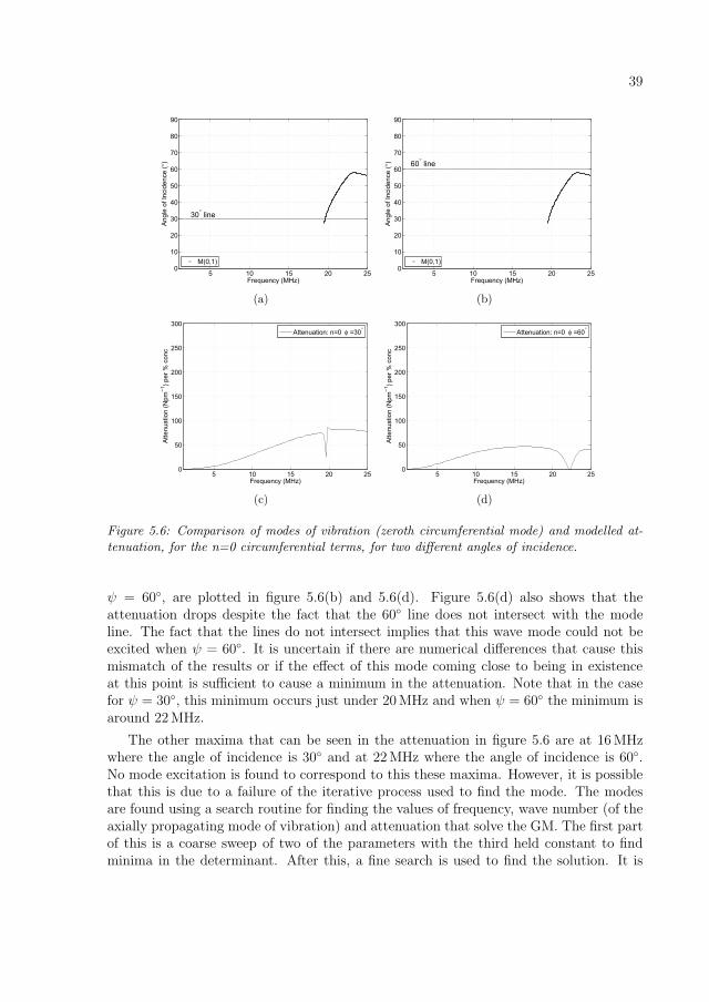
39

5 10 15 20 250

10

20

30

40

50

60

70

80

90

Frequency (MHz)

Ang

le o

f Inc

iden

ce (°

)

M(0,1)

30° line

(a)

5 10 15 20 250

10

20

30

40

50

60

70

80

90

Frequency (MHz)

Ang

le o

f Inc

iden

ce (°

)

M(0,1)

60° line

(b)

5 10 15 20 250

50

100

150

200

250

300

Frequency (MHz)

Atte

nuat

ion

(Npm

−1) p

er %

con

c

Attenuation: n=0 φ =30°

(c)

5 10 15 20 250

50

100

150

200

250

300

Frequency (MHz)

Atte

nuat

ion

(Npm

−1) p

er %

con

c


(d)

Figure 5.6: Comparison of modes of vibration (zeroth circumferential mode) and modelled at-tenuation, for the n=0 circumferential terms, for two different angles of incidence.

ψ = 60◦, are plotted in figure 5.6(b) and 5.6(d). Figure 5.6(d) also shows that theattenuation drops despite the fact that the 60◦ line does not intersect with the modeline. The fact that the lines do not intersect implies that this wave mode could not beexcited when ψ = 60◦. It is uncertain if there are numerical differences that cause thismismatch of the results or if the effect of this mode coming close to being in existenceat this point is sufficient to cause a minimum in the attenuation. Note that in the casefor ψ = 30◦, this minimum occurs just under 20 MHz and when ψ = 60◦ the minimum isaround 22 MHz.

The other maxima that can be seen in the attenuation in figure 5.6 are at 16 MHzwhere the angle of incidence is 30◦ and at 22 MHz where the angle of incidence is 60◦.No mode excitation is found to correspond to this these maxima. However, it is possiblethat this is due to a failure of the iterative process used to find the mode. The modesare found using a search routine for finding the values of frequency, wave number (of theaxially propagating mode of vibration) and attenuation that solve the GM. The first partof this is a coarse sweep of two of the parameters with the third held constant to findminima in the determinant. After this, a fine search is used to find the solution. It is


5 10 15 20 250

10

20

30

40

50

60

70

80

90

Frequency (MHz)

Ang

le o

f Inc

iden

ce (°

)

M(1,1)M(1,2)M(1,3)

30° line

(a)

5 10 15 20 250

10

20

30

40

50

60

70

80

90

Frequency (MHz)

Ang

le o

f Inc

iden

ce (°

)

M(1,1)M(1,2)M(1,3)

60° line

(b)

5 10 15 20 250

50

100

150

200

250

300

Frequency (MHz)

Atte

nuat

ion

(Npm

−1) p

er %

con

c


(c)

5 10 15 20 250

50

100

150

200

250

300

Frequency (MHz)

Atte

nuat

ion

(Npm

−1) p

er %

con

cAttenuation: n=1 φ =60°

(d)

Figure 5.7: Comparison of modes of vibration (first circumferential mode) and modelled atten-uation for the n=1 circumferential terms for two different angles of incidence.

possible that a coarse sweep was not done in the correct region to be able to locate thisroot. An alternative reason is that the software specifies that only modes propagationin the z are located [26]. It may, therefore, be possible that this maxima is caused by apurely circumferential mode and hence would not be detected by the software.

Similar plots are shown in figures 5.7 - 5.9 for n = 1 to n = 3. In all the figures wheren > 0, the attenuation has a maximum at the frequency where the mode is excited. Thesemaxima for n > 0 are caused by an increase in the radial displacement at the frequencyat which a mode or modes are excited. This increase is radial displacement, suggestedby Pavlakovic and Lowe [26], absorbs energy and hence the attenuation increases.

However at n = 0, there is a minimum in the attenuation. This is attributed to therebeing little radial displacement in this mode and hence little energy is leaked into thewater [26].

Figure 5.7 shows the comparison of the first circumferential modes and the attenuationfor the n = 1 circumferential terms. Figure 5.7(c) is a plot attenuation at ψ = 30◦

41

5 10 15 20 250

10

20

30

40

50

60

70

80

90

Frequency (MHz)

Ang

le o

f Inc

iden

ce (°

)

M(2,1)M(2,2)M(2,3)M(2,4)

30° line

(a)

5 10 15 20 250

10

20

30

40

50

60

70

80

90

Frequency (MHz)

Ang

le o

f Inc

iden

ce (°

)

M(2,1)M(2,2)M(2,3)M(2,4)

60° line

(b)

5 10 15 20 250

50

100

150

200

250

300

Frequency (MHz)

Atte

nuat

ion

(Npm

−1) p

er %

con

c


(c)

5 10 15 20 250

50

100

150

200

250

300

Frequency (MHz)

Atte

nuat

ion

(Npm

−1) p

er %

con

c


(d)

Figure 5.8: Comparison of modes of vibration (second circumferential mode) and modelledattenuation for the n=2 circumferential terms for two different angles.

(n=1). In figure 5.7(a) the intersect of the 30◦ line and the mode lines M[1,1] and M[1,3],are at the frequencies at which these modes are excited when ψ = 30◦. These modeexcitation correspond to obvious maxima occurring in the attenuation plotted in figure5.7(c). However the impact of the excitation of M[1,2] on the attenuation is difficult toassess when ψ = 30◦ as it crosses at the same point as M[1,1]. The match between thefrequencies at which maxima occur in the attenuation and frequencies at which modesare excited is similar in the case of ψ = 60◦ (shown in Figures 5.7(b) and 5.7(d)) exceptthat the frequencies at which the modes are excited is higher. At ψ = 60◦ there appearsto be little or no effect of the M[1,2] mode on the attenuation.

Figure 5.8 shows the plots for the second circumferential modes and the attenuationfor the n = 2 circumferential terms. As seen for both the incident angles plotted, thereis a good match between frequencies at which the modes are excited and the frequenciesat which maxima appear in the attenuation.

In figure 5.9 the comparison between the third circumferential modes and the attenu-


5 10 15 20 250

10

20

30

40

50

60

70

80

90

Frequency (MHz)

Ang

le o

f Inc

iden

ce (°

)

M(3,1)M(3,2)

30° line

(a)

5 10 15 20 250

10

20

30

40

50

60

70

80

90

Frequency (MHz)

Ang

le o

f Inc

iden

ce (°

)

M(3,1)M(3,2)

60° line

(b)

5 10 15 20 250

50

100

150

200

250

300

Frequency (MHz)

Atte

nuat

ion

(Npm

−1) p

er %

con

c


(c)

5 10 15 20 250

50

100

150

200

250

300

Frequency (MHz)

Atte

nuat

ion

(Npm

−1) p

er %

con

cAttenuation: n=3 φ =60°

(d)

Figure 5.9: Comparison of modes of vibration (third circumferential mode) and modelled atten-uation for the n = 3 circumferential terms for two different angles incidence.

ation for the n = 3 circumferential terms is shown. There is again a good match betweenthe mode excitation frequencies and the frequencies of the maxima in the attenuation.Note the maximum in the attenuation, when ψ = 60◦ for the mode M[3,1], is very smalland hence is marked with a circle.

The good match between the mode excitations and the extrema in the attenuationaids in the validation of the JED models. This comparison can also be used to identifythe modes causing the maxima in the experimentally derived attenuation. Examininga plot of the modelled attenuation for the nylon fibres in figure 5.10, the maxima aredifficult to distinguish as the loss tangent is large. A plot of the attenuation using a lowerloss tangent allows identification of the different modes as shown by the dashed line infigure 5.10.

As can be seen by comparing the maxima in Figure 5.10, with those in figures 5.7 -5.9, the dominant maxima are those from the lower frequency modes, M[1,1], M[2,1] andM[3,1]. Interestingly, the other maxima from the other modes are not distinct despite

43

5 10 15 20 250

50

100

150

200

250

300

Frequency (MHz)

Atte

nuat

ion

(Npm

−1) p

er %

con

c

tan δ=0.1tan δ=0.01

Figure 5.10: Modelled attenuation in a suspension of nylon fibres in water. The cylinder radiuswas 26μm and the material properties used are given in Table 5.1.

5 10 15 20 250

50

100

150

200

250

300

Frequency (MHz)

Atte

nuat

ion

(Npm

−1) p

er %

con

c 20°,n=150°,n=170°,n=1

(a)

5 10 15 20 250

50

100

150

200

250

300

Frequency (MHz)

Atte

nuat

ion

(Npm

−1) p

er %

con

c 20°,n=250°,n=270°,n=2

(b)

Figure 5.11: Plot of the attenuation of three different incidence angles. Figure 5.11(a) is theattenuation considering only n = 1 circumferential terms and figure 5.11(b) is the attenuationconsidering only n = 2 circumferential terms.

the fact that when examined individually the impact they have on the attenuation isconsiderable. The reason is because these latter modes show a stronger relationshipbetween the angle of incidence and the frequency than the M[1,1], M[2,1] and M[3,1]modes. The M[1,1], M[2,1] and M[3,1] also have a strong relationships to the frequencybut these appear at velocities below that for the fluid, c1. Because the lowest velocity thatcan be excited is c1 (1500 ms−1) these relationships are not apparent. For these higherfrequency modes, in general, a decrease in the wave velocity in the z direction (lower angleof incidence), increases the frequency at which the mode is excited (see figure 5.5). Sincethe attenuation is determined for randomly orientated fibres and hence is average of theattenuation of all angles of incidence, this shift in frequency with incident angle meansthat the effect of the excitation of these higher modes on the attenuation is effectivelydampened out. This is shown in figures 5.11(a) and 5.11(b).


(a) (b)

Figure 5.12: Diagram of the mode shape of M[2,1] at two different instants of the motion

The result is that in the total attenuation in a suspension of randomly orientatedfibres, the main source of the resonance features is due to the modes M[2,1] and M[1,1].The mode M[3,1] also appears to have an effect when the loss tangent is low, but as canbe seen in figure 5.10, when the loss tangent is higher, this is barely distinguishable.

5.3 Examining the major modes

Once the modes causing the maxima in the attenuation are identified, they can be ex-amined more closely to gain information on which elastic properties affect them. Thusthe elastic properties that can be expected to be determined from these attenuationmeasurements are identified.

Figure 5.12 shows the shape of the mode M[2,1] responsible for the first maximumseen in the attenuation at 9 MHz in figure 5.10. This mode would produce a quadrupoleradiation pattern in the r − θ plane. The mode also has very little deformation alongthe z-axis. In both the JED models and the GM calculation of the modes used in thiscomparion, the material is assumed to be isotropic. In general, fibre materials can bemore accurately described as transversely isotropic than isotropic, for example polyesterand nylon fibres. A transversely isotropic (T-isotropic) material [53] can be defined by 5elastic constants (as opposed to 2 in the isotropic case) and these are Err, Ezz, Grz,Grθ,and νzr (See Section 5.3.1). Assuming an isotropic material when the material is T-isotropic would definitely affect modes that have strain in both the r−θ plane and alongthe z axis. It is less certain that a mode with little or no z dependance would be affected,assuming that the motion is calculated based on the transverse properties. This impliesthat the mode illustrated in figure 5.12 is related to the transverse properties of thematerial rather than the longitudinal properties. Measurement of attenuation capturingthis mode would then give estimates for the transverse properties of the material.

45

r r’

(a)

r r’

(b)

Figure 5.13: Diagram of the mode shape of M[1,1] at two different instants of the motion

The next maximum in the attenuation, shown in figure 5.10, is at 11 MHz and iscaused by the mode M[1,1]. The resulting motion is a tilting movement about the liner, r′ as shown in figure 5.13. A view of the mode in the r, z plane is shown in figure 5.14.As can be seen this is a shearing motion in the r, z plane. Hence it would be expectedthat this mode would give estimates for the shear in the longitudinal direction, Grz.This supports the findings in Papers D and Papers F. However unless Grz ≈ Grθ, thebehaviour of this mode when the material is assumed to be isotropic instead of T-isotropiccould be affected. It would be of interest to investigate further the difference between themodes of a cylinder of T-isotropic material and those of a cylinder of isotropic material.This can be done by using the GM to calculate the modes of a cylinder of T-isotropicmaterial and of particularly interesting would be any changes to the M[1,1] mode.

The final mode that causes a maximum in the attenuation curve, though marginallywhen the loss tangent is high, is the M[3,1] mode. The behaviour of this mode is shownin figure 5.15. As can be seen from its shape, the greatest displacement is in the r, θplane. Hence it is expected that the main properties governing this motion would bethose in the transverse direction. As before, this suggests that inaccuracies due to theassumption of an isotropic material would not affect this mode significantly. This is,again, assuming that the motion is calculated based on the transverse properties.

There is an potential problem in estimating the elastic properties from these modesthat is highlighted from their investigation. This is that the modes M[2,1] and M[3,1] arelargely influenced by the transverse properties, Eθ,r, Gθ,r of the material and the M[1,1]is largely influenced by the longitudinal shear, Grz. If the fibre material is isotropic, theelastic property estimates will not be affected. If the material is T-isotropic but Grz ≈Gθ,r, again, there should be little problem in estimating elastic properties. However, ifthe material is T-isotropic, such that Grz �= Gθ,r, then, at best, the transverse Young’smodulus, Eθ,r and Grz can be estimated but the isotropic condition that −1 ≤ ν ≤ 0.5


(a) (b)

Figure 5.14: Diagram of the mode shape of M[1,1] at two different instants of the motion inthe r, z plane

(a) (b)

Figure 5.15: Diagram of the mode shape M[3,1] at two different instants

will not hold hence neither will the relationships between the other elastic constants.However, the consequences of this are likely to be more serious since the modes M[2,1]and M[3,1] depend on both Eθ,r and Gθ,r which would not be compatible with value forGrz estimated from the mode M[1,1]. A model based on T-isotropic material may haveto be used, if the accuracy of the isotropic model is inadequate.

Since the angle of incidence makes little difference to the frequencies at which themodes M[1,1], M[2,1] and M[3,1] are excited, it is possible to study these modes underthe condition that that the incident wave is perpendicular to the cylinder (ψ = 0). Thissimplifies the JED non-viscous model considerably to the models used by Faran [58] and

47

5 10 15 20 250

50

100

150

200

250

300

Frequency (MHz)

Atte

nuat

ion

(Npm

−1) p

er %

con

c φ = 0°

All angles

(a)

5 10 15 20 250

50

100

150

200

250

300

Frequency (MHz)

Atte

nuat

ion

(Npm

−1) p

er %

con

c φ = 0°

All angles

(b)

Figure 5.16: Comparison between the attenuation with a incidence angle of 0◦ and attenuationfrom randomly orientated fibres. Figure 5.16(a) is with a loss tangent of 0.2 and figure 5.16(b)is with no intrinsic loss in the fibres.

Flax et al. [59, 60] and use can be made of these authors interpretation of these modesof vibration. This was investigated to some extent in Paper C. The results of this papershowed that the resonance peaks in the back-scattering models [58–60] were at the samefrequencies as the peaks in the attenuation (ψ = 0). However, in the derivation of thesurface waves (Franz, Stoneley and Rayleigh waves) by Flax et al. [60] it was assumedthat the wavelength was much smaller that the diameter. No such assumption can bemade for fibre suspensions and hence it was concluded that it is difficult to establishwhich kind of waves cause the maxima in the attenuation. More work could be done inthis area.

However, although normal incidence models can be used to analysis the type of modesthat are excited, this does not mean the attenuation of randomly orientated fibres is theequivalent to attenuation of fibres lying normally to the incident wave. As can be seen infigure 5.16, although the first three maxima appear at approximately the same frequenciestheir effect on the amplitude of the attenuation at that frequency is different. Also, themodes at higher frequencies make a considerable difference to the level of attenuation athigher frequencies.

In conclusion, the wave modes that cause the maxima in the attenuation in a sus-pension of solid cylindrical scatterers have been identified. Their relation to materialproperties has been briefly investigated. This comparison also highlights a potentialproblem with the assumption of an isotropic material used in the JED models in theirapplication to T-isotropic fibres. The possibilities of a more thorough investigation on themodes of vibration could be done by comparing to previous studies on mode of vibrationsof cylinder with normal incidence excitation since the frequency of these modes causingthe maxima do not have a strong relationship to ψ. However, when fitting the modelledattenuation to the experimental attenuation, all modes must be considered and not justthe modes contributing to the maxima as there is a considerable difference between the

48

attenuation when ψ = 0 and the average attenuation of the all orientations.

5.3.1 Transversely Isotropic Material

In a material with cylindrical orthotropy, the relationship between the stress, τij , andthe strain εij in terms of compliance is⎧⎪⎪⎪⎪⎪⎪⎨

⎪⎪⎪⎪⎪⎪⎩

εrr

εθθ

εzz

εθz

εrz

εrθ

⎫⎪⎪⎪⎪⎪⎪⎬⎪⎪⎪⎪⎪⎪⎭

=

⎡⎢⎢⎢⎢⎢⎢⎣

S11 S12 S13 0 0 0S22 S23 0 0 0

S33 0 0 0S44 0 0

S55 0S66

⎤⎥⎥⎥⎥⎥⎥⎦

⎧⎪⎪⎪⎪⎪⎪⎨⎪⎪⎪⎪⎪⎪⎩

τrr

τθθ

τzz

τθz

τrz

τrθ

⎫⎪⎪⎪⎪⎪⎪⎬⎪⎪⎪⎪⎪⎪⎭

(5.1)

Where

S11 =1

Err

; S22 =1

Eθθ

; S33 =1

Ezz

;

S12 = S21 = − νθr

Eθθ= − νrθ

Err;

S13 = S31 = − νzr

Ezz= − νrz

Err;

S23 = S32 = − νzθ

Ezz= − νθz

Eθθ;

S44 =1

Gθz; S55 =

1

Grz; S66 =

1

Grθ;

and the compliance relation is describe by 9 independent elastic constants [61].A transversely isotropic materials is a special class of the orthotropic material which

have the same properties in one plane (r,θ) and different properties in the directionnormal to this plane (z). Hence

S11 =1

Err= S22 =

1

Eθθ;

So Err = Eθθ and νθr = νrθ

S44 =1

Gθz= S55 =

1

Grz;

So Gθz = Grz and

S11 − S12 = S66;1 + νθr

Err=

1

Grθ;

hence Err = (1 + νθr)Grθ so νθr does not need to be estimated. This leave Err, Ezz, Grz,Grθ and νzr

Chapter 6

Parameter Estimation

The earlier chapters have dealt with the modelling of attenuation in suspensions of cylin-drical scatterers. Assuming that the attenuation can be modelled, the next step is touse the model to solve the inverse problem. What is an inverse problem? The inverseproblem is where a model is used to establish the inputs to the system from a knownoutput.

There are some obvious issues with the inverse problem. To illustrate, the result of asum is 10 and is the result of 2 numbers added together thus model is established. Theproblem is that 5 and 5 and 3 and 7 are equally valid solutions. So unless a better modelis available, the solution will be non-unique. This is an example of an ill-posed problem.

A well-posed problem is one where a solution: exists, it is unique, and that thesolution depends continuously on the data. Even if a problem is well-posed, it is notnecessarily well-conditioned. A well-conditioned problem in non-mathematical terms, iswhen errors in the solution are related to errors of approximately the same magnitude inthe dependent variables [62]. An example of an ill-conditioned problem is if there werea small error in the attenuation, it would result in large errors in the estimation of theshear wave speed.

Parameter sensitivity is also an important aspect in solving the inverse problem. Thisis where changes in the parameters of the model or in the physical properties of the systemdo not result in changes in the output. For example, a change in the compression wavevelocity of the fibre does not result in changes in the attenuation.

The lack of sensitivity of the output to the parameter of interest classes the systemas an ill-posed problem as the solutions are non-unique and since there is more than onevalue that gives the same output.

The method of establishing values of the parameter is done by optimizing the fitbetween the modelled output and the measured output. This is generally done using asearch algorithm. This algorithm will have certain criteria that it should meet beforereturning a result. For example a change in the parameters, for which the values arebeing searched, causes a change in the output that is below a certain tolerance. Oncethese criteria are met, the results are returned. The results are a single value for each of

49

50 Parameter Estimation

the parameters. As there is only one value returned for each parameter, a single valueis returned for parameters that would theoretically give non-unique solutions. A smallerror in the attenuation or a different initial starting point would give a different valuefor the parameter. The result is that a small error in the attenuation gives large errors inthe parameter of interest and the problem can be seen as being ill-conditioned. Hence,the parameter sensitivity can be related to the degree of ill-conditioning.

The parameters estimated from the JED models were all properties of the suspension.In all cases, the properties of water were assumed to be known as was the density of thefibre material. The three main properties estimated were the compression wave velocity,c2c, Poisson’s ratio, ν, the loss tangent, tan δ. In Papers F & G, in addition to these threeproperties, the volume fraction was also estimated within narrow boundaries to allow forerrors in the measurement.

Establishing values for these properties is done by optimizing the fit between themodelled attenuation and the measured attenuation. This is done by minimizing thedifference between the modelled and the measured attenuation. The difference is quan-tified by a cost function, V . This cost function is defined to suit the problem. The costfunction used in all cases was

V =

N∑n=1

|αmn − αen|2 (6.1)

where αm, is the attenuation of the model at the nth frequency interval and αe is theattenuation calculated from experimental measurements at the nth frequency interval. Nis the maximum number of frequency intervals used. The frequency intervals used werea subsample of the measured signal. The subsample start value and end value was set bythe amplitude of the attenuation i.e. by the energy in the reflected signal. The subsamplerate was chosen so that the main features of αe were represented. This subsample ratewas lower than the sample rate of the signal because of the computational time takento calculate at higher rates. The points on the experimental attenuation curves shownin the papers where a comparison is done between the model and the experiments aremarked with the subsample intervals.

6.1 Search Algorithm

To minimise V , a search algorithm is used. The algorithm used was an interior trustregion and that can be subject to bounds on the parameters [63]. It is based on the trustregion method for unconstrained minimisation which can be expressed as

min{ψk(s)def

= gTk s +

1

2sT Bks : ||Dks|| ≤ Δk} (6.2)

Where gkdef

= ∇f(xk). Bk is the symmetric approximation to the Hessian matrix∇2f(xk). Dk is the scaling matrix and Δk is a positive scalar representing the trustregion size. The symbols || · || denote the 2-norm. More details are given in the article.

51

Table 6.1: Parameter values

Parameter Symbol Value

Frequency f 1-15 MHzRadius R 20 μmDensity ρ 1390 kgm−3

Loss tangent tan δ 0.3wave velocity (water) c1 1498 ms−1

Density ρ1 1093 kgm−3

Volume Fraction fr 0.13%.

Equation 6.2 is given to show the basis of the algorithm used. Neither the choice ofalgorithm nor the details of its function are dealt with in this thesis. However themethod of estimating material properties from attenuation measurements would benefitfrom further work.

6.2 Parameter Sensitivity of the JED Model

To asses the influence of a specific parameter (in this case a material property) has onthe JED modelled attenuation, this paramater is changed and the effect this has on theattenuation is calculated.

The influence of the shear and compression wave velocity in the solid (c2s and c2c

respectively) are investigated since it is from these values the elastic moduli can beobtained assuming the density, ρ2 is known.

The attenuation over a range of values for c2c and c2s for a range of frequencies wascalculated. The difference between these attenuation curves and the attenuation curveat a fixed value of c2c and c2s was calculated using equations 6.1 and 6.2. The fixed valueor reference point was c2c = 2000 ms−1 and c2s = 750 ms−1. The other parameters werekept constant and their values are given in Table 6.2.

Plotting V against the range of values of c2c and c2s shows the degree by which theattenuation changes with changes in c2c and c2s. Note that since the material is assumedto be isotropic and Poisson’s ratio, ν is set such that ν ≥ 0, this puts the limit on c2c asc2c >

√2c2s. The isotropic condition sets the upper bound on ν as ν ≤ 0.5. Contours of

the level of V over c2c and c2s are plotted in figure 6.1(a). The different colours representdifferent values of V . The values of c2c and c2s that correspond to areas of blue havelow V and hence there is little difference between the attenuation at the reference pointand the attenuation calculated using these values of c2c and c2s. The plot shows deeptroughs, where c2s is constant, but c2c varies. The presence of the three troughs, seenmore clearly in the surface version of the same plot (Fig. 6.1(b)), implies that the modelis sensitive to c2s in that it only gives three distinct values for c2s but it is less sensitiveto the value of c2c. This is because values of c2c, which vary along the base of the troughshown in figure 6.1(b), give approximately the same value of attenuation.

52 Parameter Estimation

c2 (ms−1)

c s (ms−

1 )

2000 4000 6000 8000 10000

1000

2000

3000

4000

5000

6000

7000

(a)

0

5000

10000 05000

10000

0

200

400

600

800

1000

cs (ms−1)c2 (ms−1)

V

(b)

Figure 6.1: Fig. 6.1(a) is a contour plot of V against c2c and c2s. Fig. 6.1(b) is a 3D surfaceof V against c2c and c2s. The crosses mark the convergence points of the search function.

02000

40006000

800010000

0.2

0.3

0.4

0.50

0.1

0.2

0.3

0.4

0.5

c2 (ms−1)c

s (ms−1)

tan

δ

Figure 6.2: Plot of the randomised starting point used to investigate the sensitivity and in papersD and E

Although these troughs exist, the lowest point is only at the fixed point which showsthat there is only one global minima. This means that it should be possible to correctlyidentify the material properties of c2c and c2s assuming the values of tan δ and ρ wereknown.

Since the existence of a global minima has been established for this case, the ability ofthe trust-region reflective Newton algorithm to locate the global minimum is then tested.This is done because being able to locate the global minimum from any starting pointmeans that the method of estimating the elastic properties will not be dependent on thestarting point. For the method to be robust, an algorithm that converges to the globalminimum is required.

The random starting points used in Papers E and F were used in this test and areplotted in figure 6.2. The resulting converging points of the algorithm are plotted ascrosses on figure 6.1(a). 17% of the starting points sucessfully converge on the reference

53

05000

10000

0

5000

100000

0.2

0.4

0.6

0.8

c2 (ms−1)cs (ms−1)ta

nδ

(a)

Figure 6.3: Points of convergence of the randomised starting points when tan δ is also optimisedby the trust-region reflective Newton algorithm.

point. The majority of the other starting points converge at or very close to the bound-aries of the parameters. A more sophisticated cost function which penalised values lyingclose to the boundary would prevent the initial values converging on the edges of theboundaries and increase the number of points converging on the reference value.

The above analysis assumes that ρ and tan δ are known. The likelihood of knowingthe density of the fibres material of the fibre in suspension is high since this can often beobtained by other measurements. However, knowing the loss tangent is unlikely if onedoes not know c2c or c2s. Hence the influence tan δ has on the sensitivity should also beconsidered.

If the algorithm is used to optimise tan δ as well as c2c or c2s the points converge asshown in figure 6.3(a). This is using the same randomised starting points as used above.

These convergence points match with local minima in V . This is illustrated for twocases: in figure 6.4(a) with tan δ = 0 and in figure 6.4(b) with tan δ = 0.03. The pointsmarked with a circle are the convergence points with a value of tan δ that equals thecontour plot. Hence it can be seen that the convergence points are where V is localminimum.

When tan δ is not fixed, it can be seen that there is a convergence point that isin the centre of the range of c2c and c2s. So, even penalising the values close to theboundaries would not remove this local minimum. However, at this convergence pointthe attenuation curve does not contain the resonance features as shown in figure 6.5. Itmay, therefore, be possible to modify the cost function such that if a resonance feature,i.e. a point of zero gradient, exists in the attenuation curve to which the comparison isbeing made, then it should also exist in the optimised curve, or at least weighted so thatvalues causing a resonance feature would have a lower cost function.

Studying the sensitivity plot, it can be seen that at c2s > 4000 the contours are flatter,showing the cost function does not vary in this region. This suggests that it would bedifficult to identify materials with properties in this region due to the low sensitivity ofthe cost function to c2c and c2s.

54

c2 (ms−1)

c s (ms−

1 )

2000 4000 6000 8000 10000

1000

2000

3000

4000

5000

6000

7000

(a)

c2 (ms−1)

c s (ms−

1 )

2000 4000 6000 8000 10000

1000

2000

3000

4000

5000

6000

7000

(b)

Figure 6.4: Two examples of plots of V over a range of values of c2c and c2s and a specificvalue of tan δ. In figure 6.4(a)), tan δ = 0. The point of convergence that also have tan δ = 0are marked with a circle. In figure 6.4(b)) tan δ = 0.03 hence the point marked with a circle isthat with tan δ = 0.03

0 5 10 150

5

10

15

20

25

Frequency (MHz)

Atte

nuat

ion

(Npm

−1)

Figure 6.5: Plot of the attenuation at the convergence point, c2c = 7100, c2s=2800. The solidline is the reference attenuation and the dashed line is the attenuation calculated using theaforementioned values of c2c and c2s.

In conclusion, the sensitivity study shows that the model is more sensitive to c2s

than c2c but that there is a global minimum, hence if the model accurately predicts theattenuation and there is low noise, it is possible for c2c, c2s and tan δ to be identified, ifthe solution lies at or near the reference point tested. A more sophisticated cost functionreduces the dependency of the method of estimating elastic properties on the startingpoint.

Chapter 7

Online Considerations

The objective is to make the measurement method an online system. The implications ofthis should then be considered. The following is a brief discussion of these considerations.

To be an online system the three parts of the measurement method should be consid-ered. These are the measurements of the attenuation, the model used and the estimationof the elastic properties from the model and measurement data.

7.1 Measurements

Affecting the measurements are the transducers, the working frequency range and anydisturbances to the signal that are not modelled.

The transducers used in the experiments were standard, commercially available ones.It should therefore not be a problem basing an online system on these transducers.

The frequencies used should be those which excite wave modes, to increase the accu-racy of the estimation process. However high frequencies are more difficult to implementin a measurement system as they attenuate more than lower frequencies and hence thedistance travelled by the pulse must be reduced in order that the signal to noise ratiois sufficiently high. The experimental results used a frequency range of 2-30 MHz and adistance travelled by the pulse of 20 mm. A system based on these dimensions would bedesirable.

The signal is potentially disturbed by a number of factors that should be investigated.These are

1. temperature

2. pressure

3. fines

4. air bubbles

5. additives (e.g. fillers)

6. dirt

55

56 Online Considerations

7.2 Model and Estimation Process

The model and the estimation process are treated together since it is their combinedeffect that has an impact on whether or not the system can be implemented as an onlineone.

In addition to the attenuation measurement, the model requires the cross-sectionalgeometry of the fibres. In the experiments carried out on pulp, these measurement wereobtained from the PulpEye pulp analyser system [64] and laboratory measurements ofthe fibre wall thickness. Online fibre wall thickness measurements are currently beingdeveloped [65]. Systems for obtaining this information should be available presently.

Speed of Computation

The objective for an online measurement system is that the results be available withinthe time taken for a control loop to be executed.

The current speed of computation varies from 40 minutes to several hours dependingon the starting values. This is running on a single 2.5 GHz processor and no work has yetbeen done on the speed of the computation of the elastic fibre property measurements.

The following are suggests for improving the speed of the computation and have notbeen tested.

Cost function 1

The minimisation of the error between the measured and modelled attenuation uses asearch algorithm. This searches the entire valid space, with different initial values. Oncethe first values have been established, these could be used as the starting point for thenext estimation. Hence greatly reducing the time taken for the estimation.

Cost function 2

Alternatively, the cost function can be modified using the suggestion in Chapter 6, whichwould reduce the dependancy on the initial values. This would reduce the number ofdifferent starting points required to locate the global minimum and hence reduce thesearch time. Once first results for a pulp are established they could then be used as thestart for the next iteration which again would reduce the search time.

Discrete values of the estimate

Given the discrepancies between the shapes of the fibres and the regular shapes usedin the model and the variation in the fibre properties, the accuracy of the method willnot very be high. Therefore it is unnecessary to search for slight changes in properties.This point has not been used in the estimation process and would be likely to contributesignificantly to the speed of the process.

57

Integration

The integration over all angles is done based on a gradient estimation procedure. Whilstthis increases the speed of the estimation in the current implementation, it is not con-ducive to making the code parallelised. Using trapezoidal numerical integration, althoughslower would allows the process to be more easily distributed over a number of processorsand hence the speed would be proportional to the number of processors.

Distributed radii

Calculation for the different radii is also a calculation that can be easily parallelised sinceone result is not dependent on the other. This is another part of the process where thespeed would be proportional to the number of processors used.

Programming language

The code is written in Matlab, Mathworks Inc. This is an excellent tool for evaluationdifferent methods and testing different algorithms. However, it is slow so once an algo-rithm for the search part of the estimation process has been evaluated and decided on,the code can be written in a lower level language, such as ‘C’.

A commercial optical pulp analyser takes typically 15 minutes from the time the pulpenter the system before the results are analysed. This means that the method for de-termining elastic properties has a maximum of 15 minutes before any loss of data willoccur.

Chapter 8

Summary of the Papers

This section give a summary of each paper included in the thesis. It includes a commentfor each paper on my personal contributions and the involvement of the other authors.Torbjorn Lofqvist has been my supervisor throughout and his was the original idea ofcharacterizing paper pulp using ultrasound.

8.1 Paper A - Estimating Suspended Fibre Mate-

rial Properties by Modelling Ultrasound Atten-

uation

Authors: Yvonne Aitomaki and Torbjorn LofqvistReproduced from: Proceedings of International Conference of Mathematical Modellingof Wave Phenomena 2005

SummaryThe JED model v1 (see Chapter 3) is described in detail. This is compared to the modelthat includes thermal and viscous shear effects in the fluid derived by Habeger [32].Experimentally derived attenuation for a suspension of nylon fibres cut from fishing linein water is compared to the predicted attenuation from the model. The nylon usedin the fishing line is a polyamide copolymer so the exact material properties of thefibre were difficult to establish since the type of the copolymer was not known. Theresults lay between those expected for nylon 66 and nylon 6. Resonance peaks in theattenuation were both predicted and found experimentally. The conclusion was that themodel appears to be sufficiently sensitive to material properties. Thus estimations ofthese properties from the attenuation may be possible.

Personal contributionWork was carried out by Aitomaki with consultation with Lofqvist. The paper waswritten by Aitomaki and Lofqvist.

59

60 Summary of the Papers

8.2 Paper B - Ultrasonic Measurements and Mod-

elling of Attenuation and Phase Velocity in Pulp

Suspensions

Authors: Jan Niemi, Yvonne Aitomaki and Torbjorn LofqvistReproduced from: Proceeding of IEEE Ultrasonic Symposium, Rotterdam, Holland 2005

SummaryThis paper introduces a method of performing phase unwrapping that minimises disconti-nuities in the phase shift. This is used to calculate the phase velocity in pulps of differentconsistency. The results show that dispersion is caused by fibres and correlates withmass fraction. Attenuation measurements of pulp are also made, with the aim of findingresonance peaks in the frequency response of the attenuation predicted by the model.Clear peaks are not found. This is thought to be due to the effect of the distributedradii of the pulp fibres. Estimations of the properties are made from these curves butcomparison with known values was not done. This is due to the difficulties in carryingout single fibre tests on saturated wood fibres.

Personal contributionThe experiments and the phase velocity work was carried out by Niemi and Lofqvist.The attenuation theory and calculations was carried out by Aitomaki. The paper waswritten by Niemi and Aitomaki and Lofqvist.

8.3 Paper C - Inverse Estimation of Material Prop-

erties from Ultrasound Attenuation in Fibre sus-

pensions

Authors: Yvonne Aitomaki and Torbjorn LofqvistReproduced from: Elsevier Ultrasonics, Volume 49, Issues 4-5, May 2009, Pages 432-437

SummaryIn this paper experiments on nylon 66 give evidence for the effect different fibre radiihave on the attenuation. This supports the JED model. An estimation process is im-plemented which estimates material properties that give the best fit between the modeland the measurement attenuation. The results show that the shear modulus is withinthe expected range based on previous studies. The Young’s Modulus is underestimatedeven when compared to transverse values for the material.

Personal contributionWork was carried out by Aitomaki with consultation with Lofqvist. The paper waswritten by Aitomaki with considerable comments and corrections provided Lofqvist andthe journal reviewer.

61

8.4 Paper D - Sounding Out Paper Pulp: Ultra-

sound Spectroscopy of Dilute Viscoelastic Fibre

Suspensions

Authors:Yvonne Aitomaki and Torbjorn LofqvistPresented at Acoustics and Ultrasonics in the Processing of Industrial Soft Solids Con-ference, held in Leeds, February 2005. The proceedings were sent but as yet have notbeen published.SummaryThe reason why the resonance peaks appear in the frequency response of the attenuationis explored in this paper. The influence of the shear wave velocity and the fibre radius onthe resonance of the first peaks is shown. Hence, experimentally determining the locationof the first resonance peak would help establish the value of the shear modulus. Thissupports the results in Paper D, which showed that the shear modulus was estimatedto within a previously established range. The reason that the first resonance peaks areassociated with shear waves is because shear wave velocity is lower than compression wavevelocity. The exact nature of the wave that causes this resonance is not yet established,since the proof that they are Rayleigh waves relies on asymptotic values for the Besselfunctions, which are only valid for ka � 1, where a is the radius and k the wave numberof the wave in the fluid. Since this is not the case with the fibre suspension used, theconclusion that the peaks in attenuation are also caused by Rayleigh waves cannot bedrawn.Personal contributionWork was carried out by Aitomaki with consultation with Lofqvist. The paper waswritten by Aitomaki. Feedback and comments were provided by Lofqvist.

8.5 Paper E - Damping mechanisms of ultrasound

scattering in suspension of cylindrical particles:

Numerical analysis

Authors: Yvonne Aitomaki, Jan Niemi and Torbjorn LofqvistTo be submitted to: Journal of the Acoustical Society of AmericaSummaryThe addition of viscosity to the ultrasound scattering models increase complexity. Thispaper investigates whether or not the addition of viscosity is necessary in a suspensionof cylindrical scatterers when their radii is of the order of the wavelength and is notclose to the viscous skin depth. The modelled attenuation of a scatterer surrounded bya viscous fluid is compared to that where the fluid is non viscous. The results showthat the intrinsic loss in the scatterer and the viscosity both have a damping effect onthe attenuation. Hence, with high intrinsic loss (tan δ ≥ 0.1), the effects of viscosity isnegligible. This holds if the frequency is not in the region where the viscous skin depth

62 Summary of the Papers

equals the radius.

The conclusion is that a simpler model where the fluid is assumed to be non-viscouscan be used to model attenuation in suspensions of fibres with tan δ ≥ 0.1.

Personal contributionThe original idea was that of Lofqvist. Work was carried out by Aitomaki with consulta-tion with Lofqvist. The paper was written by Aitomaki. Feedback and comments wereprovided by Lofqvist and Carlson, whose help is gratefully acknowledged.

8.6 Paper F - Estimating material properties of solid

and hollow fibres in suspension using ultrasonic

attenuation

Authors: Yvonne Aitomaki and Torbjorn LofqvistTo be submitted to: IEEE Transactions on Ultrasonics, Ferroelectrics, and FrequencyControl

SummaryThis study firstly investigates the difference in attenuation measurements between solidand hollow fibres in suspension. Secondly, it tests whether a solid model (JED nonviscous distributed radii) is sufficient for modelling hollow fibres or whether a hollowmodel (JED hollow distributed radii) should be used. The measured attenuation insuspensions of hollow and solid fibres of the same material, polyester, are compared. Acomparison is then done between the estimated material properties obtained from usingthese different models on the different measurements of attenuation. The results showthat the solid model gives good results with solid fibres in suspension and the hollowmodel gives reasonable results with the hollow fibres in suspension. Both of these resultscompare well with reference values for block polyester. However the solid model with thehollow fibres suspension gives poor estimates of elastic properties despite giving the bestmatch to the modelled attenuation and the measured attenuation.

On a more general scientific note, this paper highlights the point that a good fitbetween data and the model does not necessarily mean the model gives a correct inter-pretation of the behaviour of the system. It may simply mean there are sufficient degreesof freedom in the model to allow a good fit to be achieved.

Personal contributionWork was carried out by Aitomaki with consultation with Lofqvist. The paper waswritten by Aitomaki. Feedback and comments were provided by Lofqvist and Carlson,whose help is gratefully acknowledged.

63

8.7 Paper G -Comparison of softwood and hardwood

pulp fibre elasticity using ultrasound

Authors: Yvonne Aitomaki and Torbjorn LofqvistTo be submittedSummaryThis paper is a preliminary test of the model on fibres in pulp. A comparison is donebetween the estimated values for elastic moduli between softwood and hardwood fibresafter refining. The estimates are obtained from fitting attenuation measurements fromthese pulps to modelled attenuation. The model used is a layered cylinder model, wherethe surrounding fluid is assumed to be non-viscous and the distribution of the fibre radiiis also considered (JED hollow distributed radii). The measurements are made on pulpswith negligible fine content and at pressures of approximately 5 bars. This high pressurereduces the size of the air bubbles in the suspensions, that otherwise could significantlyattenuate the ultrasound. An optical measurement device is used to measure the fibregeometry with the exception fibre wall thickness. The wall thickness and the mass fractionwere both established by laboratory measurements of the pulp samples. The results showthat there is little difference between the estimates of the elastic moduli for the hardwoodand the softwood pulp fibres. The results for softwood are 1.6 GPa well to individual fibretest from other work.

The results show that either the due to the processing these fibres undergo, they bothhave similar values for their elastic moduli or that method is not sufficiently accurateto detect differences between hardwood and softwood fibres. Based on the assumptionthat the fibres are better described as transversely isotropic than isotropic, the resultsof previous studies and the work done in chapter 5, the estimated value for the Young’smodulus is likely to be that of the transverse plane (Eθ,r) of the fibres than of the axialdirection, Ez.Personal contributionThe original idea was that of Lofqvist and Aitomaki. The measurements were carriedout by Niemi and Aitomaki and Lofqvist. The estimates of the elastic properties wascarried out by Aitomaki. The method was written by Niemi and the rest of the paperwas written by Aitomaki. Feedback and comments were provided by Lofqvist.

Chapter 9

Conclusion

The hypothesis set out in the introduction was: The measurement of the ultrasoundattenuation can be used to estimate the elastic properties of wood fibres in pulp online.This was divided into three research question. These questions were investigated in thethesis and are answered as follows:

1. Can elastic properties be estimated from ultrasound attenuation?

Concluding the work done in Papers D and F, the method can give estimates forshear modulus and the transverse Young’s modulus of fibres. This is supported bythe investigation of the modes of vibration in Chapter 5. The aforementioned pa-pers also highlight the importance of the outer fibre radius (or radii) and the radius(radii) of the lumen on the attenuation. Consequently, this geometric informationis required in order to extract elastic properties from the ultrasonic signals. Opticalsystems such as PulpEye [64] can provide values for the outer fibre radii and meth-ods of obtaining the fibre wall thickness are currently being implemented [65]. Theradii of the lumen can be determined from these values. This provides sufficientgeometric detail to estimate the elastic properties of fibres.

2. Can the method be applied to wood fibres in pulp?

In the introduction it was stated that a model is required which captures onlythe wood fibre properties that are important to attenuation. Concluding the workin this thesis, the wood fibre can be assumed to be an infinitely long cylinder. Itcannot be assumed to be solid and hence a hollow model is required (Papers F & G).The material of the fibre does not necessarily need to be modelled as transverselyisotropic. The method can give good estimates from assuming the material to beisotropic (Papers D & F). In addition, the fluid in the model can be treated asnon-viscous, as wood fibres are viscoelastic [19] (Paper E).

The exact shape of the cross section of the fibres is assumed to not have an impor-tant impact on the attenuation. In addition, the dependency of attenuation on theelastic properties is assumed to have symmetric distribution about the average of

65

66 Conclusions

the elastic properties. Given these assumptions the conclusion can be drawn thatthe method can be applied to wood fibres in pulp (Paper G). Obviously, theseassumptions need to be verified. The further work section contains a discussion ofhow this can be done.

3. Can the measurement method be used online?

Using a simple model in the method, decreases the computation time taken to es-timate the elastic properties. Based on the work done, the simplest model thatcould be used would be the layered cylindrical model that treats distribution radiidistribution (JED distributed radii). Implementation of the suggestions for reduc-ing the computational time (Chapter 7) should allow the results to be available ina time comparative to that of the optical results from current pulp analysers. Thecomputational time is, however, dependent on the number of processors used.

The measurement system used in Paper G was attached to as a module in a PulpEyesystem. PulpEye is a pulp analyser and is available as an online version. Henceit should be straightforward to make the measuring system itself online. Makinga standalone system would, however, require more work. The addition of fineshas not been addressed in this thesis. The impact of fines on attenuation and thenecessity of including a model for such particles would need addressing in an onlineversion of a system based on this method.

From these answers it can be seen that all the evidence so far supports the hypothesisthat the measurement of the ultrasound attenuation can be used to estimate the elasticproperties of wood fibres in pulp online and hence continued testing is justified.

There are certain conditions that need to be fulfilled for the method to have ap-plication in the paper and pulp industry and it is these that should be tested. Theseconditions are:

1. The diameter distribution of the fibres is required as are estimates of the radii oflumen.

2. The elliptical cross-section of the fibres can be treated appropriately.

3. A suspension of fibres with different elastic properties can be treated appropriately.

With these conditions fulfilled the shear modulus and the transverse Young’s modulusof the pulp fibres can be measured. Thus a system with sensors based on this methodcan be implemented.

With such a system, process efficiency and paper quality could be improved through:

1. Improvement in the refining process based on fibre flexibility calculation obtainedfrom the geometry and the elastic properties.

2. Early detection of inappropriate fibre stiffness in the paper manufacturing process.

3. Improvement in pulp fractionation allowing pulp to be better suited to the endproduct.

67

These all contribute not only to economic gains for the paper industry but are ofbenefit to the wider community in terms of the reduced environmental impact that in-creased energy efficiency produces and the increase in availability of energy by-productsfrom this industry.

�� !� "�� !��#�� $% ��& ��'��$�� !�� (�� !��$(��)� �!�� $�� & � �!� #��# %��$�� !�� (�� *�� $� � �!�� #�� +,�� -.��$�� /0��#�� 1��%�� 2 -�� $�� $�� %�� !�� )�� $� �� *�� $�3

Chapter 10

Further Work

10.1 Further work

Modelling

For completeness, this method should be tested on isotropic fibres. This would providemore confidence in the results. Glass is one of the few fibres that is isotropic and isreadily available hence is the obvious choice in such a test. An initial test was attemptedwith chopped glass fibres with a diameter of 20 μm and a length of 12.7 mm. This provedunsuccessful, as the fibres could not be easily separated. Attempts to separate the fibresincluded baking in oven and boiling with sulphuric acid. Neither attempt was successful.With hindsight, experience and a little patience, this is not a difficult test and couldbe performed on longer, larger diameter glass fibres that could be cut to length in thelaboratory.

The assumption that the exact shape of the layered scatterer has little impact onthe attenuation requires validation before the method can be applied to wood pulp withconfidence. This can be investigated by examining the differences in attenuation betweenellipsoidal scatterers and regular cylindrical scatterers. However, ellipsoidal geometry isconsiderably more challenging. It could be tested using simulations to some extent bya comparison between the cylindrical model and the model developed by Hasheminejadand Sanaei [66]. However, this would require the assumption of zero or negligible shearas the theory only applies to fluid cylinders. The reason is that the equivalent function toBessel functions for ellipsoidal geometries are Mathieu functions as used by Harumi [67]in expressions for an elastic ribbon (the extreme case of an ellipse). However, thesefunctions are not orthogonal hence one cannot solve for each series of n as one can forthe Bessel functions, unless there are special conditions. The implications of this are thatif it were necessary to model fibres as ellipses, using Mathieu functions the model wouldbecome very large and complex. Alternatively, a model based on the T-matrix approachwould perhaps be more appropriate [68].

Perhaps an easier approach is to investigate experimentally ellipsoidal geometry by

69

70 Further Work

scaling the problem and using a much larger scatterer and low frequencies. This wouldallow the geometry of the scatterer to be more easily controlled. A comparison betweenthe modes of a cylinder and an ellipse could be done and the effects on the amplitudeof the scattered wave after averaging over the surface at a distance from the scattererand over different incident angles. This would in fact be a similar experiment to thatdone very early on by Faran in 1951 [58] on cylinders and spheres. The basis of theexperiment is that the attenuation is proportional to the reflection coefficient from asingle scatterer. It may also be possible to extrude elliptical fibres and test these directlyin suspension under the assumption that extruding to a different geometry has little effecton the material properties of the fibre.

The next assumption that should be investigated before the method can be applied towood pulp with confidence is that the dependency of attenuation on the elastic propertieshas symmetric distribution about the average of the elastic properties. This should besimple to test and can be done by simulation. The model can be used to simulate theattenuation from a mixture of fibres with different elastic properties. This attenuationcan then be compared to the attenuation from an average of the elastic properties. Ifthese two attenuations do not differ significantly, then the assumption is correct.

However, considering the modal behaviour of the attenuation this is unlikely andhence it may be necessary to modify the model to allocate different fractions of thesuspension to different elastic moduli. It is difficult to predict whether there is sufficientinformation in the attenuation signal to provide estimates for the elastic moduli of thedifferent fibres. The accuracy of the assumption that the dependency of attenuationon the elastic properties has symmetric distribution about the average of the elasticproperties will depend on the distribution of these properties. Hence it will depend onthe type of pulp that is being tested.

Comparison to other methods

Alternatively, other methods of measuring the transverse elastic properties of fibres andthe longitudinal shear modulus could be investigated. For example an atomic forcemicroscope (AFM) could be used to measure these properties but differences in scale andfrequency make the comparison of these results difficult. Another method is to builda composite of the fibres and from testing and modelling, derive the transverse fibreproperties. This would be of great value in validating the results for polymer fibres,in particular fibres that are not affected by their immersion in water such as polyester.However, the elastic properties of wood fibre when wet are known to differ from theirproperties when dry [22] so it would be difficult to validate the estimation from theultrasound method using this technique.

Error Analysis

A basic attempt to test the sensitivity of the estimations to noise in the attenuationmeasurement was carried out in Papers D, F & G by estimating the values from theexperimentally measured attenuation, αe ± 2σ where σ is the standard deviation of the

71

mean. A more thorough analysis of the stability of the model in general to noise inthe parameters could establish which parameters and to what degree, they influence theattenuation.

Fines

As mentioned in the conclusion, the fine content will also attenuate the ultrasound.The percentage of fines in the pulp will be the deciding factor in whether they have tobe taken into account or not. The attenuation due to fines can be predicted using ascattering model for spherical particles such as those discussed in Chapter 4. Furtherwork on how such a model could be included in the method would be necessary if it werefound that fines have a significant impact on the attenuation. However, previous studieshave shown that fine concentration in pulp does not have a large impact on ultrasoundattenuation [69].

72 Further Work

References

[1] A. Crevecoeur and E. Kilby, Key Statistics 2007. Confederation of European PaperIndustries, Brussels, 2007.

[2] Sodra, “Sodra annual report 2008,” Feb. 2008.

[3] W. Birk, Personal communication, Apr. 2009.

[4] A. Hagedorn, J. Orccotoma, P. Schueler, B. Snow, and J. Jarvinen, “Optimizingmachine efficiency through fibre quality management,” in 2006 TAPPI Papermaker’sConference. Technical Association of the Pulp and Paper Industry, 2006.

[5] A. Kaw, Mechanics of composite materials. Taylor & Francis, 2006.

[6] Lorentzen-Wettre, “L&W STFI Fibermaster.” [Online]. Available: http://www.lorentzen-wettre.com/bprod/prod.cfm?prodid=9100

[7] D. Krotz, “Laser ultrasonic sensor streamlines papermaking process,”http://www.lbl.gov/Science-Articles/Archive/EETD-papersensor-Ridgway.html,2006-04-04.

[8] (2006, 08) New evidence suggest longer paper making history in china. [Online].Available: http://news.xinhuanet.com/english/2006-08/08/content 4937457.htm

[9] S. Anttilainen, “Metso supplied sc paper machine line sets a newworld speed record at stora enso kvarnsveden,” 2007. [Online].Available: http://www.metsoautomation.com/News/newsdocuments.nsf/Web2NewsDoc/CAC7C79ED6B6E117C22572A00048448C?OpenDocument&ch=ChMetsoPaperWebEng&id=CAC7C79ED6B6E117C22572A00048448C&

[10] D. McIntosh, Handbook of Pulp and Paper Technology. Van Nostrand ReinholdCompany, 1970, ch. 1-5, pp. 37–46.

[11] J. Yang and R. Evans, “Prediction of moe of eucalypt wood from microfibril angleand density,” Holz als Roh- und Werkstoff, vol. 61, no. 6, pp. 449–452, 2003.

[12] J. Tchepel, J. Provan, A. Nishida, and C. Biggs, “A procedure for measuring theflexilibity of single wood-pulp fibres,” Mechanics of Composite Materials, vol. 42,no. 1, pp. 83–92, 2006.

73

http://www

http://www.lbl.gov/Science-Articles/Archive/EETD-papersensor-Ridgway.html

http://news.xinhuanet.com/english/2006-08/08/content

http://www.metsoautomation.com/News/newsdocuments.nsf

74 References

[13] H. Karlsson, Fibre Guide. Lorentzen & Wettre, Kista, Sweden, 2006.

[14] K. K. Pitea, “Valkommen till en rundvandring in kappa kraftliner pitea,” 2006.

[15] T. Wikstrom, “Flow and rheology of pulp suspensions at medium consistency,” PhDThesis, Chalmers University of Technology, 2002.

[16] P. Brodeur and J. Gerhardstein, “Overview of applications of ultrasonics in the pulpand paper industry,” in 1998 IEEE Ultrasonics Symposium, 1998, pp. 809–815.

[17] A. Heikkurinen and L. L., Mechanical pulping, ser. Papermaking Science and Tech-nology. Fapet Oy, 1999, no. 5, ch. The character and properties of mechanical pulp,pp. 395–413.

[18] E. Avallone, T. Baumeister, A. Sadegh, and L. Marks, Marks’ Standard Handbookfor Mechanical Engineers, 11st ed. McGraw-Hill Book Company, Inc, 2006, ch.Cylinders and Spheres, pp. 5:45–5:57.

[19] L. Salmen, “Viscoelastic properties of in situ lignin under water-saturated condi-tions,” Journal of material science, vol. 19, no. 9, pp. 3090–3096, Sept. 1984.

[20] J. Levlin and L. Soderhjelm, Pulp and Paper Testing. Fapet Oy, 1999.

[21] H. Karlsson and P. Fransson, “STFI FiberMaster fives the papermaker new muscles,”Sv. Papperstidning, vol. 10, no. 26, 1997.

[22] E. Ehrnrooth, “Softening and mechanical behaviour of single wood pulp fibres - theinfluence of matrix composition and chemical and physical characteristics,” PhDThesis, Department of Wood and Polymer Chemistry, University of Helsinki, 1982.

[23] L. Kinsler, A. Frey, A. Coppens, and J. Sanders, Fundamentals of Acoustics, 4th ed.John Wiley and Sons Inc., 2000.

[24] L. Hall, “The origin of ultrasonic absorption in water,” Phys. Rev., vol. 73, no. 7,pp. 775–781, Apr 1948.

[25] A. D. Pierce, Acoustics: An introduction to its physical principles and applications.American Institute of Physics, 1994, ch. The wave theory of sound, pp. 1–53.

[26] B. Palvakovic and M. Lowe, User’s Manual: Disperse- A system for generatingdispersion curves, 2nd ed., Imperial College London, London, UK, July 2003.

[27] L. Kinsler, A. Frey, A. Coppens, and J. Sanders, Fundamentals of Acoustics, 4th ed.John Wiley and Sons Inc., 2000, ch. Chapter3 Vibrations of bars, p. 218.

[28] Kolsky, Stress Waves in Solids. Dover, 1963.

[29] A. Bhatia, Ultrasonic Absorption. Dover, 1968, ch. 11, p. 272.

References 75

[30] W. M. Ewing, W. Jardetzky, and F. Press, Elastic Waves in Layered Media.McGraw-Hill Book Company, Inc, 1957, ch. Homogeneous and isotropic half space,pp. 24–73.

[31] D. McClements and M. Povey, “Scattering of ultrasound by emulsions,” Journal ofPhysics D: Applied Physics, vol. 22, pp. 38–47, 1989.

[32] C. Habeger, “The attenuation of ultrsound in dilute polymeric fiber suspensions,”Journal of Acoustical Society of America, vol. 72, pp. 870–878, sep 1982.

[33] M. Morse, P and K. Ingard, Theoretical Acoustics. Princetown University Press,1986, ch. 6, p. 401.

[34] N. Herrmann and D.J.McClements, “Influence of visco-inertial effect on the ultra-sonic properties of mondisperse silican suspensions,” Journal of the Acoustical Soci-ety of America, vol. 106, p. 1178, 1999.

[35] Rayleigh, The Theory of Sound. Macmillan, 1926.

[36] V. Knudsen, J. Wilson, and N. Anderson, “The attenuation of audible sound in fogand smoke,” The Journal fo the Acoustical Society of America, vol. 20, no. 6, pp.849–857, Nov 1948.

[37] C. J. T. Sewell, “The extinction of sound in a viscous atmosphere by small obstaclesof cylindrical and spherical form,” Philosophical Transactions of the Royal Societyof London. Series A, Containing Papers of a Mathematical or Physical Character,vol. 210, pp. 239–270, 1911. [Online]. Available: http://www.jstor.org/stable/90992

[38] P. Epstein and R. Carhart, “The absorption of sound in suspensions and emulsions.i. water fog in air,” The Journal of the Acoustical Society of America, vol. 25, no. 3,pp. 553–565, May 1953.

[39] J. Allegra and S. Hawley, “Attenation of sound in suspension and emulsions: Theoryand experiments,” The Journal of the Acoustical Society of America, vol. 51, no. 5,pp. 1545–1564, 2 1972.

[40] M. Povey, Ultrasonic Techniques for Fluid Characterization. Academic Press, 1997,ch. A.4, p. 179.

[41] A. K. Hipp, G. Storti, and M. Morbidelli, “Acoustic characterization of concentratedsuspensions and emulsions. 1. model analysis,” Langmuir, vol. 18, no. 2, pp.391–404, 2002. [Online]. Available: http://pubs.acs.org/doi/abs/10.1021/la015538c

[42] P. Lloyd and M. Berry, “Wave propagations through an assembly of spheres iv.relations between different multiple scattering theories,” Proc. Phys. Soc., vol. 91,pp. 678–688, 1967.

http://www.jstor.org/stable/90992

http://pubs.acs.org/doi/abs/10.1021/la015538c

76 References

[43] D. Adams, “Ultrasonic propagation in paper fibre suspensions,” in 3rd IFAC con-ference on instrumentation and automation in paper, 1776.

[44] C. Habeger and G. Baum, “Ultrasonic characterizations of fibre suspension,” TheInstitue of Paper Chemistry, Appleton, Wisconsin, IPC Technical Paper series 118,Nov 1981.


[46] P. Morse and H. Feshbach, Method of Theoretical Physics. McGraw-Hill BookCompany, Inc, 1953, vol. II, ch. 13.

[47] G. Strang, Linear Algebra and Its Applications. Brooks Cole, February 1988.

[48] R. Challis, M. Povey, M. Mather, and A. Holmes, “Ultrasound techniques for charac-terizing colliodal dispersions,” Reports in Progress in Physics, vol. 68, pp. 1541–1637,2005.

[49] L. L. Foldy, “The multiple scattering of waves. I. General theory of isotropic scatter-ing by randomly distributed scatterersisotropic scattering by randomly distributedscatterers,” Phys. Rev. (2), vol. 67, pp. 107–119, 1945.

[50] S. K. Numrich and H. Uberall, Physical Acoustics Vol. XXI. Academic Press, 1992,ch. Scattering of sound pulses and the ringing of target resonances, p. 235.

[51] J. Dickey, G. Frisk, and H. Uberall, “Whispering gallery wave modes on elasticcylinders,” Journal of the Acoustical Society of America, vol. 59, no. 6, pp. 1339–1346, June 1976.

[52] R. M. Davies, “A critical study of the hopkinson pressure bar,” PhilosophicalTransactions of the Royal Society of London. Series A, Mathematical andPhysical Sciences, vol. 240, no. 821, pp. 375–457, 1948. [Online]. Available:http://www.jstor.org/stable/91440

[53] Every, Dynamic methods for measuring the elastic properties of solids, ser. Handbookof elastic properties of solids, liquids and gases. Academic Press, 2001, vol. 1, ch.Introduction, p. 25.

[54] B. N. Pavlakovic and M. Lowe, “A general purpose apporach to calculating thelongitudinal and flexural modes of mulit-layered, embedded, transversely isotropiccylinders,” Review of Progress in Quantitative NDE, vol. 18, pp. 239–246, 1999.

[55] D. C. Gazis, “Three-dimensional investigation of the propagation of waves inhollow circular cylinders. i. analytical foundation,” The Journal of the AcousticalSociety of America, vol. 31, no. 5, pp. 568–573, 1959. [Online]. Available:http://link.aip.org/link/?JAS/31/568/1

http://www.jstor.org/stable/91440

http://link.aip.org/link/?JAS/31/568/1

References 77

[56] ——, “Three-dimensional investigation of the propagation of waves in hollowcircular cylinders. ii. numerical results,” The Journal of the AcousticalSociety of America, vol. 31, no. 5, pp. 573–578, 1959. [Online]. Available:http://link.aip.org/link/?JAS/31/573/1

[57] L. Flax and W. Neubauer, “Acoustic reflection from layered elastic absorptive cylin-ders,” Journal of the Acoustical Society of America, vol. 61, no. 2, pp. 307–312, Feb1977.

[58] J. Faran, “Sound scattering by solid cylinders and spheres,” Journal of the AcousticalSociety of America, vol. 23, no. 4, pp. 405–418, July 1951.

[59] L. Flax, L. Dragonette, and H. Uberall, “Theory of elastic resonance excitation bysound scattering,” Journal of the Acoustical Society of America, vol. 63, no. 3, pp.723–730, Mar 1978.

[60] G. Frisk, J. Dickey, and H. Uberall, “Surface wave modes on elastic cylinders,”Journal of the Acoustical Society of America, vol. 58, no. 5, pp. 996–1008, Nov 1975.

[61] P. Sinha, Composite materials and structures. The Department of AerospaceEngineering, Indian Institute of Technology, Kharagpur, 1995, ch. Macromechanicalbehaviour. [Online]. Available: http://www.ae.iitkgp.ernet.in/ebooks/index.html

[62] E. E. Kalu and A. Kaw, Numerical Methods with Applications. Kalu, E. E. andKaw, A., 2008.

[63] T. Coleman and Y. Li, “An interior trust region approach for nonlinear minimizationsubject to bounds,” SIAM Journal on Optimization, vol. 6, pp. 418–445, 1996.

[64] Eurocon, “Pulpeye pulp analyser.” [Online]. Available: http://www.pulpeye.com/

[65] O. Sundvall, Personal communication, Nov 2008.

[66] S. Hasheminejad and R. Sanaei, “Ultrasonic scattering by a fluid cylinder of ellipticcross section, including viscous effects,” Ultrasonics, Ferroelectrics and FrequencyControl, IEEE Transactions on, vol. 55, no. 2, pp. 391–404, February 2008.

[67] K. Harumi, “Scattering of plane waves by a rigid ribbon in a solid,” Journalof Applied Physics, vol. 32, no. 8, pp. 1488–1497, 1961. [Online]. Available:http://link.aip.org/link/?JAP/32/1488/1

[68] T. A. K. Pillai, V. V. Varadan, and V. K. Varadan, “Sound scattering by rigidand elastic infinite elliptical cylinders in water,” The Journal of the AcousticalSociety of America, vol. 72, no. 3, pp. 1032–1037, 1982. [Online]. Available:http://link.aip.org/link/?JAS/72/1032/1


http://www.ae.iitkgp.ernet.in/ebooks/index.html

http://www.pulpeye.com

http://link.aip.org/link/?JAP/32/1488/1


78 References

[69] M. Tormanen, J. Niemi, T. Lofqvist, and R. Myllyla, “Pulp consistency determinedby a combination of optical and acoustical measurement techniques,” MeasurementScience and Technology, vol. 17, no. 4, pp. 695–702, 2006. [Online]. Available:http://stacks.iop.org/0957-0233/17/695

http://stacks.iop.org/0957-0233/17/695

Part II

Paper A

Estimating Suspended Fibre

Material Properties by Modelling

Ultrasound Attenuation

Authors:

Yvonne Aitomaki and Torbjorn Lofqvist

Reformatted version of paper originally published in:

Proceedings of International Conference of Mathematical Modelling of Wave Phenomena2005

© Vaxjo University Press, Reprinted with permission

81

Estimating Suspended Fibre Material Properties by

modelling Ultrasound Attenuation


Abstract

An analytical model for use in the inverse problem of estimating material properties ofsuspended fibres from ultrasonic attenuation has been developed. The ultrasound at-tenuation is derived theoretically from the energy losses arising when a plane wave isscattered and absorbed off an infinitely long, isotropic, viscoelastic cylinder. By neglect-ing thermal considerations and assuming low viscosity in the suspending fluid, we canmake additional assumptions that provide us with a tractable set of equations that canbe solved analytically. The model can then be to used in inverse methods of estimatingmaterial properties. We verify the model with experimentally obtained values of attenu-ation for saturated Nylon fibres. The experimental results from Nylon fibres show localpeaks in the attenuation which are thought to be due to the resonant absorption at theeigenfrequencies of the fibres. The results of the experiments show that the model issufficiently sensitive to detect differences in different types of Nylon. Applications forsuspended fibre characterization can be found in the paper manufacturing industry.

List of Symbols

Unless otherwise indicated subscript 1 refers to the fluid medium and subscript 2 refers to the solidmedium.

A1,A2 transverse vector potentials M,N transverse vector potentialac R× kc M elastic modulusas R× ks R radius of the fibreacc R× kcc r , θ,

zcylindrical coordinates

asc R× ksc V velocityacs R× kcs α acoustic attenuationBn, Dn, Encoefficients of expansion α1 acoustic attenuation ın waterCp heat capacity in the fluid β thermal expansivityc velocity of sound tan δ2 loss tangent of the viscoelastic solidc complex speed of sound in the sound εij strainfr volume fraction of fibres η1 viscosity of the fluid

H(1)n nth order Hankel function of the first

kindΓl

ij Christoffel symbol

Jn nth order Bessel function of the firstkind

λ wavelength

K heat conductivity coefficient ω angular frequency

84 Paper A

k unit vector along the z-axis in cylin-drical

ρ density

co-ordinates λ2, μ2 Lame’s 1st and 2nd constantskc wave number of the compressional

waveυ2 Poisson’s ratio

ks wave number of the transverse wave ψ the angle between the incident wavekcc wave number of the compressional

waveand the longitudinal axis of the cylin-der

along the r-axis φc compressional wave scalar potentialkcs wave number component of the φo incident compressional wave

compressional wave along the z-axis scalar potentialksc wave numbers of the transverse wave φr reflected compressional wave

along the r-axis scalar potentialχ, ξ transverse wave scalar potentials

1 Introduction

Our research is aimed at the on-line estimation of the characteristics of pulp fibres sus-pended in water. An application is in the paper manufacturing industry where esti-mating fibre characteristics can potentially improve the quality control of the finishedpaper. The measurement method used is based on ultrasound as it is rapid, inexpensive,non-destructive and non-intrusive.

The focus of our investigation is on establishing the material properties of the sus-pended, fluid-saturated fibres from ultrasonic attenuation measurements. To do this weneed to solve the inverse problem of deriving these properties from the attenuation. Wetherefore require a model that relates attenuation to material properties and one that isanalytical since this is more amenable than numerical solutions for solving the inverseproblem. Habeger established a model related attenuation to material properties, wherethe equations are solved numerically [1]. We have developed an analytical solution basedon the same equations.

Habeger’s model is a cylindrical extension of the Epstein-Carhart [2]/Allegra-Hawley[3] model. In the calculation of attenuation, the set of equations are solved numericallyand are based on a number of different material properties. By neglecting thermal effectsand assuming low viscosity in the suspending fluid, we can make additional assumptionsthat provide us with a more tractable set of equations that can then be solved analytically.

In this paper we describe the simplified model used to relate the attenuation to thematerial properties of the fluid saturated fibres. We compare the analytical solution withthat obtained by a numerical solution of the non-simplified equation system [1], to verifythe validity of the additional assumptions that are made. We then verify the model withexperimentally obtained values of attenuation for saturated Nylon fibres. We go on todiscuss the results, draw conclusions and outline the next steps in our investigations.

Paper A 85

2 Theory

The attenuation is derived from calculating the energy losses arising when a plane waveis incident upon an infinitely long, straight cylinder. The cylinder material is assumedto be isotropic and viscoelastic. The energy losses taken into account are from the wavebeing partially reflected, partially transmitted at the solid/fluid interface and from thegeneration of damped, transverse waves in the solid medium at the boundary. The highlydamped thermal skin layer, that is generated by the acoustically induced pulsations ofthe solid is shown by [1] to have the greatest effect where the thermal wavelength is ofthe order of the radius. We, therefore, consider frequencies above this region and hencethe thermal effects are neglected in the derivation of attenuation. The advantage is thatthe thermal material properties of the fibre and fluid can then be neglected, reducingthe number of material properties in the solution and hence increasing the feasibility ofestimating the remaining material properties from attenuation measurements. A viscouswave in the fluid (as defined by [2]) is also generated but again this is highly dampedand is neglected in the final stages of the derivation.

Expressions for the wave potentials from the conservation of mass, energy and mo-mentum were derived by [2] and are expressed for the fluid as:

∇ ·A1 = 0 (1)

∇2φc1 = − k2c1

φc1 (2)

∇×∇×A1 = k2s1A1 (3)

V1 = − ∇φc1 + ∇× A1 (4)

where, kc1 = ω/c1 and ks1=

√iωρ1/η1.

In the solid, the displacement potentials are used instead of the velocity potentials.Hence,

∇ · A2 = 0 (5)

∇2φc2 = − k2c2

φc2 (6)

∇×∇× A2 = k2s2A2 (7)

V2 = iω (∇φc2 −∇× A2) (8)

where kc2 = ω/(c2(1 − i tan δ2/2)) and ks2=

√iωρ2/μ2. Further details of the definition

for the wave number in a viscoelastic solid and the complex shear modulus, μ2, aredescribed in the Appendix.

The stress tensor can be expressed in terms of the wave potentials:

τij1 = η1

[(k2

s1− 2k2

c1)φc1

]δij + 2η1εij (9)

τij2 =[(ω2ρ2 − 2μ2k

2c2)φc2

]δij + 2μ2εij (10)

86 Paper A

Where the strain is

εij =1

2(Vi,j + Vj,i − 2Γl

ijVl) (11)

The fluid wave potential is divided into an incident part and a reflected part, φc1 =φo1

+ φr1. The incident plane wave potential, φo1

, is expressed in cylindrical coordinatesand we let this equal ei(kcc1

r+kcs1z−ωt) as in [1].

Since the plane of the cylinder lies at an angle ψ to the incident wave, the wavenumbers are expressed in terms of their components along the cylindrical coordinateaxes.

kcc1 = kc1 cos(ψ) (12)

kcs1= kc1 sin(ψ) (13)

The inicident wave potential is expanded using Bessel functions of the first kind [4] as

φo1=

(J0(kcc1r) + 2

∞∑n=1

in cos nθJn(kcc1r)

)ei(kcs1

z−ωt) (14)

And the reflected wave potential in the fluid expanded using Hankel functions of the firstkind:

φr1=

(B01

H(1)0 (kcc1r) + 2

∞∑n=1

in cos nθBn1H(1)

n (kcc1r)

)ei(kcs1

z−ωt) (15)

The combination of the equations (14) and (15) give us an expression for φo1expanded

in terms of Bessel and Hankel functions. To meet the boundary conditions for all valuesof z and t, the time and z dependence of the potentials must be the same as φo1

. Theequivalent expression for the compressional wave potential in the solid is

φc2 =

(B02

J0(kcc2r) + 2∞∑

n=1

in cos nθBn2Jn(kcc2r)

)ei(kcs1

z−ωt) (16)

where, kcc2 =√

(k2c2 − k2

cs1).

To meet the boundary conditions in cylindrical coordinates, the transverse potentialcan be expanded in terms of two independent scalar potentials, see [5] such that, M =∇× χk, N = ∇×∇× ξk and A = M + N. Where χ and ξ are solutions to the scalarHelmholtz equation so, ∇2χ = −k2

s2χ and ∇2ξ = −k2

s2ξ. The energy dissipated by the

transverse waves in the fluid are however very small when the viscosity is low hence theseare neglected. Expanding the transverse waves in solid in terms of Bessel and Hankelfunctions we get

k2s2

ξ2 =

(D02

J0(ksc2r) + 2∞∑

n=1

in∂ cos nθ

∂θDn2

Jn(ksc2r)

)ei(kcs1

z−ωt) (17)

ikcs1χ2 =

(E02

J0(ksc2r) + 2

∞∑n=1

in cos nθEn2Jn(ksc2r)

)ei(kcs1

z−ωt) (18)

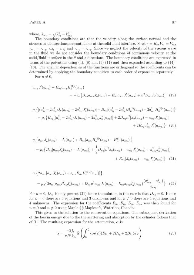
Paper A 87

where, ksc2 =√

k2s2− k2

cs2.

The boundary conditions are that the velocity along the surface normal and thestresses in all directions are continuous at the solid-fluid interface. So at r = R2, Vr1

= Vr2,

τrr1= τrr2

, τrθ1= τrθ2

and τrz1= τrz2

. Since we neglect the velocity of the viscous wavein the fluid we do not consider the boundary conditions of continuous velocity at thesolid/fluid interface in the θ and z directions. The boundary conditions are expressed interms of the potentials using (4), (8) and (9)-(11) and then expanded according to (14)-(18). The angular dependencies of the functions are orthogonal so the coefficients can bedetermined by applying the boundary condition to each order of expansion separately.

For n �= 0,

acc1J′(acc1) + Bn1

acc1H(1)′n (acc1)

= −iω[Bn2

acc2J′

n(acc2) − En2asc2J

′

n(asc2) + n2Dn2Jn(asc2)

](19)

η1

{[(a2

s1− 2a2

c1)Jn(acc1)− 2a2

cc1J ′′n(acc1)]+Bn1

[(a2s1− 2a2

c1)H(1)

n (acc1)− 2a2cc1

H(1)′′n (acc1)]

}= μ2

{Bn2

[(a2s2− 2a2

c2)Jn(acc2) − 2a2cc2J

′′

n(acc2)] + 2Dn2n2[Jn(asc2) − asc2J

′

n(asc2)]

+ 2En2a2

sc2J ′′n(asc2)

}(20)

η1

{acc1J

′

n(acc1) − Jn(acc1) + Bn1[acc1H

(1)′n (acc1) − H(1)

n (acc1)]}

= μ2

{Bn2

[acc2J′

n(acc2) − Jn(acc2)] +1

2Dn2

[n2Jn(asc2) − asc2J′

n(asc2) + a2sc2

J ′′n(asc2)]

+ En2[Jn(asc2) − asc2J

′

n(asc2)]}

(21)

η1

{2acs1

[acc1J′

n(acc1) + acc1Bn1H(1)′

n (acc1)]}

= μ2

{2acs1

acc2Bn2J ′n(acc2) + Dn2

n2acs1Jn(asc2) + En2

asc2J′

n(asc2)(a2

sc2− a2

cs1)

acs1

}(22)

For n = 0, Dn2is only present (21) hence the solution in this case is that Dn2

= 0. Hencefor n = 0 there are 3 equations and 3 unknowns and for n �= 0 there are 4 equations and4 unknowns. The expression for the coefficients Bn1

, Bn2, Dn2

, En2was then found for

n = 0 and n �= 0 using Maple ©,Maplesoft, Waterloo, Canada.This gives us the solution to the conservation equations. The subsequent derivation

of the loss in energy due to the the scattering and absorption by the cylinder follows thatof [1]. The resulting expression for the attenuation, α is:

α =−2fr

πR2kc1

�(∫ π

2

0

cos(ψ)(B01+ 2B11

+ 2B21)dψ

)(23)

88 Paper A

2 4 6 8 10 12 14 16 18 200

100

200

300

400

500

Frequency (MHz)

Atte

nuat

ion

(Np/

m)

Rayon NumericalRayon Analytical

Figure 1: test

2 4 6 8 10 12 14 16 18 200

20

40

60

80

100

120

Frequency (MHz)

Atte

nuat

ion

(Np/

m)

Polyester NumericalPolyester AnalyticalNylon NumericalNylon Analytical

Figure 2: Attenuation as a function of frequency for different fibres. The attenuation is ex-pressed in nepers per meter (Np/m),where neper (Np) is a dimensionless unit [6]. η1 =9.4 × 10−4 Nsm−2, ρ1 = 996 kgm−3, c1 = 1490ms−1, K1 = 0.59Wm−1K−1, Cp1

= 4.14 ×103 Jkg−1K−1, β2 = 2.36 × 10−4 K−1. The parameter values for the fibres are shown in ta-ble 2

Rayon Nylon PolyesterR (m) 13 ×10−6 30 ×10−6 13 ×10−6

tan δ2 0.125 0.2 0.1υ2 0.3 0.4 0.4ρ2(kgm−3) 1400 1140 1340c2(ms−1) 1090 1340 5860K2(Wm−1K−1) 0.15 0.36 0.038Cp2

(Jkg−1K−1) 1.5 ×103 1.42 ×103 1.02 ×103

β2(K−1) 36×10−5 6×10−5 1.7×10−5

Table 2: Parameter values of the different fibres used in the numerical and analytical models

Note that in the insertion of asymptotic values for the Bessel and Hankel function asr → ∞, Habeger’s [1] expression appears to be missing a factor of 2. The attenuation isthe sum to infinity of a series of Bn1

where n is an integer. However, when calculating theattenuation, the energy associated with the the higher order was assumed to be negligibleand the series was truncated at n = 2. The attenuation calculated does not take intoaccount the attenuation of the compressional wave through the water itself. This is,therefore, added to the attenuation of the fibres calculated above and is assumed to beα1 = 25 × 10−15f 2 taken from [6], where f is the frequency.

The effects of the additional assumptions that were made to derive the analyticalmodel can be assessed by comparing the attenuation predicted by the analytical solu-tion presented here and the numerical solution presented by [1]. These assumptions arethat the acoustic attenuation from thermal processes are negligible and that the viscouswave generated in the fluid is also negligible. The results of the differences between thepredicted attenuation are shown in figure 2 for three different types of polymer fibres:

Paper A 89

Rayon, Nylon and Polyester. In general the discrepancy in the results is proportional tothe attenuation. The two curves for each fibre have a similar shapes, with the excep-tion of Polyester at low frequencies. This exception is not further examined here. Theeffect the assumptions have depends on the frequency range and radius used as well asthe fluid properties and the thermal properties of the fibre. In the cases examined here,the discrepancies are not large, although the effect these errors have on the parameterestimation needs to be assessed when the model is used in solving the inverse problem.

We have, therefore, a simplified expression for α that can be used in solving theinverse problem. It is a function of the material properties of the saturated fibre and thesuspending fluid, the radius of the fibre and fibre volume fraction. The next step is thento verify the model with experimentally obtained values of attenuation from suspensionof fibre with known material properties and uniform radius.

3 Experimental

The experimental setup consists of a broadband transducer with a centre frequency of10 MHz (V311), manufactured by Panametrics, Waltham, MA, USA. A pulser/receiver5072PR from Panametrics was used to excite the transducer and amplify the receivedsignal. The signal was then digitized using a CompuScope 14100 oscilloscope card, byGage Applied Technologies Inc., Lachine, QC, Canada, with 14-bit resolution and asampling rate of 100 MHz. All data was stored in a computer for off-line analysis.The resulting time-domain waveforms were calculated using the average of 100 sampledwaveforms to reduce random noise. Before the averaging, the sampled waveforms arealigned to reduce timing jitter by using a method proposed by [7]. A digital thermometerF250, by Automatic Systems Laboratories LTD, England, monitored the temperatureboth in the suspension under test and in the room. The temperature was used to calculatethe speed of sound in the water [8]. The fibre suspension was carefully poured into themeasurement cell and then stirred until the majority of the air bubbles were removed.The measurement cell is described in detail in [9]. The attenuation of the sample wascalculated according to [10].

The fibre suspension was made of Nylon fishing line, (STROFT™ GTM) with a nom-inal diameter of 60μm,1 chopped to a length of approximately 4 mm. The Nylon was apolyamide copolymer tempered to improve its tensile strength. The fibres were weighedand mixed with water to a concentration of 0.5% by weight. They were then left in waterfor 3 days to stabilise the temperature and to allow the fibres to become fully saturated.To prevent the fibres from settling during the test the suspension was stirred gently. Aset of 30 runs were taken each with an average of 100 pulses.

1Permissbile diameter fluctuation ±1μm, Permissible norminal size deviation +38μm

90 Paper A

2 4 6 8 10 12 140

10

20

30

40

50

60

70

80

90

100

Frequency (MHz)

Atte

nuat

ion

(Np/

m)

Nylon 6Nylon 6,6Experimental Data

Figure 3: test

2 4 6 8 10 12 140

0.2

0.4

0.6

0.8

1

1.2

1.4

1.6

1.8

2

Frequency (MHz)

Nor

mal

ised

Atte

nuat

ion

+/− 2 STDAverage Normalised Attenuation

Figure 4: Attenuation as a function of frequency for a suspension of Nylon fibres in waterat 0.5% concentration. Modelled and experimental attenuation values. Parameters for thesaturated fibres are in shown in table 3. Right-hand figure is the Average of the Attenuationnormalised by the value of the attenuation at 5MHz to remove the variance directly proportionalto the attenuation.

4 Results

Figure 4 show the results from the 0.5% concentration of suspended Nylon fibres. As wecan see there is a large variation in the level of attenuation although the shape of thecurve is similar in all the measurement with local peaks in the attenuation at 4.8 MHzand at 7.7 MHz.

In the right-hand figure 4, the attenuation has been normalised by the value of theattenuation at 5MHz to remove the effect of variance directly proportional to the atten-uation. Attenuation proportional variance is thought to be due to the inherent inho-mogeneity of the suspension as the attenuation is proportional to the volume fraction.The fibres form flocs and through a combination of stirring and settling each time anultrasonic pulse is emitted it travels through a different arrangement of fibres resulting ina different volume concentration and hence a different attenuation. The remaining vari-ance, shown in the normalised attenuation graph increases with increasing attenuationand this is thought to be due to an decrease in the signal to noise ratio at the higherlevels of attenuation found at higher frequencies.

The modelled attenuation is plotted in figure 4 with two possible set of parameterswhich are listed in table 3. The material properties are however, difficult to establish.The density was taken from the manufacturer data sheet, and adjusted for 5% waterabsorption. The speed of sound in Nylon 6 was taken from Habeger [1], whereas forNylon 6,6 although the rod velocity was taken from his measurements in saturated fibres,Poisson’s ratio in Nylon 6,6 was taken as 0.39 [11]. This means the speed of sound inNylon 6,6 was calculated as 2345 ms−1. Poisson’s ratio for Nylon 6 was taken as the valuethat gave the best fit in Habeger [1] experiments. The exact value of the loss tangent was

Paper A 91

Nylon 6 Nylon 6,6R (μm) 46.8 ± 0.4 46.8 ± 0.4c2(ms−1) 1340 2345ρ2(kgm−3) 1131 1131υ2 0.3 0.39tan δ2 0.2 0.15

Table 3: Parameter values used for Nylon

adjusted to best fit the experimental data as it can vary from very low, 0.01, in lightlycrossed amorphous polymer to 3 depending on the molecular structure [12].

As the plots show, neither Nylon 6 or Nylon 6,6 fits the whole range. Nylon 6, gives agood fit for the low frequencies and Nylon 6,6 for the higher frequencies. The wide marginof error in the elastic constants and hence the speed of sound and the fact that the Nylonused was a polyamide copolymer, tempered to improve its tensile strength, could explainsome of the discrepancies between the model results and the experimental results. Otherexplanations are that the values of the material parameters are not constant across thefrequency range we are examining or that some of the fibres are not freely suspended butinteract with one another which results in unpredictable ultrasonic attenuation. Multiplescattering would also cause differences between predicted and experimental results.

The peaks are thought to correspond to the resonant absorption at the eigenfrequen-cies of the cylinder, possibly of the shear wave, as opposed to reflections of internal wavesfrom the ends of the fibres. This is because the peaks appear in both the experimentaland the modelled values of attenuation and the modelled values are based on cylindersof infinite length.

5 Conclusions

In conclusion, we have established an analytical model relating the attenuation of ul-trasound, in a suspension of fibres in a low viscosity fluid, to the material properties ofthe fibres. This model is amenable for use in solving the inverse problem of determiningmaterial properties of saturated fibres from measurements of attenuation. The results ofthe experiments indicate that the Nylon tested, a polyamide copolymer, has propertiesbetween that of Nylon 6 and Nylon 6,6. The material properties of saturated fibres aredifficult to assess and hence have large margin of error. The results suggests that themodel is sufficiently sensitive to material properties to detect differences in different typesof Nylon.

The additional assumptions made that allow the analytical solution to be derivedcauses some discrepancies in the calculation of attenuation. However, the large variationsin attenuation thought to be due to the inherent inhomogeneity, is likely to mask thesedifferences.

92 Paper A

6 Further Work

The elastic properties of the saturated Nylon fibres need to be investigated with analternative method to verify that they do indeed lie between that of Nylon 6 and Ny-lon 6,6. Investigations at different concentrations need to be carried out to test if theinhomogeneity of the attenuation is the cause of the attenuation proportional variation.

Further work needs to be done to establish the cause of the local peaks in the frequencyresponse of the attenuation. By testing other materials and different diameters of fibresthe accuracy of the model can be assessed further.

The next step is then to use this model in solving the inverse problem in suspensionsof greater complexity such as paper pulp where online data on the material propertiesof wood fibre in suspension is required. For this, a method for optimising the fittingof the modelled attenuation to the experimental values needs to be developed. Theeffects of non-uniform diameters and anisotropic nature of the pulp fibres also need tobe assessed.

A Appendix

Here, we have defined the elastic modulus involved in the vibratory motion as complex and equal to:

M2(ω) = M ′

2− iM ′′

2, where M2(ω) = λ2(ω) + 2μ2(ω) (A.24)

tan δ2 is then defined as the phase difference between the real and imaginary part of the elastic modulus:

tan δ2 = −M′′

2

M ′

2

(A.25)

Denoting the compressional speed of sound in the solid as complex where c2 = c′2− ic′′

2we get

c′22− c′′2

2=M ′

2

ρ2

, 2c′2c′′2

=M ′

2tan δ2ρ2

(A.26)

As tan δ2 is small at the limit tan δ → 0, which is the equivalent of assuming c′2� c′′

2we get,

c2 ≈ c′2

(1 − i

tan δ22

)(A.27)

With the additional assumption that k′c2� k′′c2

we get the same expression as derived by [13]. For easeof readability in the main text, the prime that distinguishes the real from the imaginary part has beendropped. So, in the main text, c2 = c′

2.

μ2 can be expression in terms of Poisson’s ratio, υ2 and the complex speed of sound using (A.24)and (A.27), if we assume that Poisson’s ratio is real at these frequencies.

μ2 =

(0.5 − υ2

1 − υ2

)c′2ρ2(1 − i tan δ2) (A.28)

Paper A 93

References





[5] P. Morse and H. Feshbach, Method of Theoretical Physics. McGraw-Hill BookCompany, Inc, 1953, vol. II, ch. 13.

[6] L. Kinsler, A. Frey, A. Coppens, and J. Sanders, Fundamentals of Acoustics, 4th ed.Wiley, 1999, ch. 8.

[7] A. Grennberg and M. Sandell, “Estimation of subsample time delay differences innarrowband ultrasonic echoes using the hilbert transform correlation,” IEEE Trans-actions on Ultrasonics, Ferroelectrics, and Frequency Control, vol. 41, no. 5, pp.588–595, 1994.

[8] N. Bilaniuk and G. S. K. Wong, “Speed of sound in pure water as a function oftemperature,” The Journal of the Acoustical Society of America, vol. 93, no. 4, pp.2306–2306, 1993.

[9] T. Lofqvist, “Ultrasonic wave attenuation and phase velocity in a paper-fibre sus-pension,” in Proc.IEEE Ultrasonics Symposium, vol. 1, Oct 1997, pp. 841–844.

[10] D. McClements and P. Fairley, “Frequency scanning ultrasonic pulse echo reflec-tometer,” Ultrasonics, vol. 30, pp. 403–405, 1992.

[11] L. Pedersen. (2002) Tables of acoustic properties of materials. [Online]. Available:http://www.ondacorp.com/tecref\ acoustictable.html

[12] J. Ferry, Viscoelastic Properties of Polymers, 3rd ed. John Wiley & Sons Inc, 1980,ch. 2, pp. 46–47.

[13] M. Povey, Ultrasonic Techniques for Fluid Characterization. Academic Press, 1997,ch. A.4, p. 179.

http://www.ondacorp.com/tecref\

http://www.ondacorp.com/tecref\

Paper B

Ultrasonic Measurements and

Modelling of Attenuation and

Phase Velocity in Pulp Suspensions

Authors:

Jan Niemi, Yvonne Aitomaki and Torbjorn Lofqvist


Proceedings of IEEE Ultrasonic Symposium, pp.775-779 (Rotterdam, Holland),2005

© 2005 IEEE, Reprinted with permission

95

Ultrasonic Measurements and Modelling of

Attenuation and Phase Velocity in Pulp Suspensions

Jan Niemi, Yvonne Aitomaki and Torbjorn Lofqvist

Abstract

In the manufacturing process of paper the mass fraction and material properties of thefibres in the pulp suspension are important for the quality of the finished product. Thisstudy presents two different methods of pulp characterisation. The first is based onphase velocity, which we use to investigate the composition of the pulp. Here a methodis presented where the optimal number of circular shifts within the sampling windowof the signal is determined which gives, in a weakly dispersive medium, a continuousphase spectrum and minimizes the likelihood of discontinuities within the bandwidth.Hence, the ambiguity in phase unwrapping is avoided. The results from phase velocitymeasurements show that the phase velocity weakly increases with increasing amount offines in the suspension. The dispersion is caused by the fibres and it correlates with fibremass fraction. The second method is based on attenuation and is used to characterisethe wood fibres. The results of the attenuation experiments show that it is possible toinversely calculate wood fibre properties by fitting the model to the experimental data,if the fibre diameter distribution is known. However, the accuracy of these calculation isdifficult to determined and more work in this area is required.

1 Introduction

In the manufacturing process of paper the mass fraction and material properties of thefibres in the pulp suspension are important for the quality of the finished product. Whenusing recycled paper, fibres with unknown and varying material properties enter theprocess. Therefore, there is an increasing demand for methods of on-line characterisationof the pulp suspension as well as the fibres in suspension.

This study presents two different methods of pulp characterisation. The first is basedon phase velocity, which we use to investigate the composition of the pulp. The secondis based on attenuation and is used to characterise the wood fibres.

In the first method, we investigate how the phase velocity changes with different massfractions of fibres and fines. To determine the phase velocity, a method is proposed basedon a method by [1], where the an echo is circularly shifted an optimal number of samples.

In the second method, to be able to characterise the wood fibres, we use an analyticalmodel which relates the material properties of saturated fibres to the attenuation. Wethen aim to solve the inverse problem of identifying which values result in the best fit ofthe model to the attenuation values calculated from experiments.

98 Paper B

Time

S1 S2

Stee

lre

flec

tor

Sam

ple

spac

eB

uff

er-

ro

dTr

ans-

du

cer

d

1

2

3

Figure 1: Lattice diagram of the pulse-echo measurement system used this study

2 Phase Velocity

2.1 Theory and experiments

When determining the phase velocity from pulse-echo measurements, one encounters theproblem of performing a correct phase unwrapping. The problem is well known andhas been addressed in earlier investigations, for instance [2]. The problem arises whenthe phase velocity is calculated from the phase spectra of a the Fourier transform ofeach of the two echoes. In this study, we propose a method, termed Minimum PhaseAngle (MPA), that determines an optimal number of circular shifts to the windowedsignal which results in a continuous phase spectrum and minimizes the likelihood ofdiscontinuities within the bandwidth. Therefore the ambiguity in the phase unwrappingis avoided. To experimentally test the method experiments were performed in pulpfibre suspensions, which are weakly dispersive. The experiments were carried out usingthe pulse-echo technique in a custom designed test cell. A schematical view of themeasurement cell used in this study is shown in Fig. 1.

The echoes from the interfaces depend on the initial pulse pressure amplitude p0(t)emitted from the transducer and the reflection and transmission coefficients of the differ-ent interfaces. For simplicity, we omit the reflection and transmission coefficients and theattenuation. With these assumptions, the echoes from the interfaces between the bufferrod/suspension and suspension/steel reflector are

P1(ω) = P0(ω)e−2j ω

c1d1 = P0(ω)e−jϕ1(ω) (1)

P2(ω) = P0(ω)e−2jω(

d1

c1+

d2

c2)= P0(ω)e−jϕ2(ω) (2)

where P1(ω) and P2(ω) are the Fourier transform of the echoes p1(t) and p2(t), re-spectively. d1 and d2 are the distance in respective medium. The factor 2 above comesfrom that the fact the pulse is travelling back and forth through the medium. c1 and c2

are the velocities in the buffer rod and pulp suspension, respectively. P0(ω) is the Fourier

Paper B 99

transform of the initial emitted pulse from the transducer. Note that echo p1(t) has anextra phase shift of π compared to p2(t).

2.2 The method of minimum phase angle

To reduce the ambiguity in the phase unwrapping the following method is proposed.

td2

td1

ts2

ts1

time

p1 p2

t=0

p0

Figure 2: The received signal with illustrations of the time delays and time shifts

The sampled signal is divided into two sampling windows with time delays td = nd/fs

shown in Fig. 2 where nd is the number of samples that the sampling window is delayedand fs is the sampling frequency. Within each sampling window the signal is circularlyshifted sample by sample. At each shift, a calculation of the phase angle is carried outas

PA =1

f2 − f1

f2∑m=f1

ϕ2m (3)

where ϕm is the phase spectrum within the frequency bandwidth of f1 < m < f2

of the shifted sample. Thereafter a sign shift of the echo is carried out, representinga phase shift of π, and again circularly shifted and calculated with the same method.The results are compared and the circularly shifted sample that gives a phase spectrumwithout discontinuities and minimum value of PA is then chosen. The outcome is thenthe optimal time shift of ts = ns/fs where ns is the number of samples the signal isshifted.

This results in two time delays, the time delay from the sampling window and timedelay from the circular shift within the window. This gives the phase spectrum for therespective echoes as

ϕ1(ω) = φ1(ω) + ω(td1 + ts1) (4)

ϕ2(ω) = φ2(ω) + ω(td2 + ts2) (5)

100 Paper B

where φ1 and φ2 are the respective phase spectra of the circularly shifted signal. td1

and td2 are the time delay for respective sampling window. ts1 and ts2 are the circularshift within respective sampling window. An illustration of how PA changes when echop1(t) is circularly shifted within the sampling window is shown in Fig. 3. In this example,the minimum of PA is found when p1(t) is shifted 100 samples to the left and inverted.Fig.2.3(c) shows the phase spectrum at the minimum of PA for p1(t) and −p1(t). Wecan see that the inverted signal has a phase spectrum with the minimum likelihood of adiscontinuity being present in the spectrum.

The phase velocity for a pulp suspension sample can be expressed using (1)-(2) and(4)-(5) as

c2(ω) =ω2d2

ω(t2 − t1) + θ(ω) − θd(ω) + mπ(6)

where t1 = td1 + ts1, t2 = td2 + ts2, θ(ω) = φ2(ω)−φ1(ω), θd(ω) is the phase difference dueto diffraction [3] and m is a correction term if a phase shift of π is added by the proposedmethod. In this study m = 0 if the proposed method inverts p1(t) to compensate for theextra phase shift that occurred, m = 1 if p1(t) and p2(t) are not inverted and m = −1 ifboth p1(t) and p2(t) are inverted.

2.3 Experiment

The experimental setup consists of a broadband transducer with a centre frequency of10 MHz (V311), manufactured by Panametrics, Waltham, MA, USA. A pulser/receiver5072PR from Panametrics was used to excite the transducer and amplify the received sig-nal. The signal was then digitized using a CompuScope 14100 oscilloscope card, by GageApplied Technologies Inc., Lachine, QC Canada, with 14-bit resolution and a samplingrate of 100 MHz. All data was stored in a computer for off-line analysis. The resultingtime-domain waveforms were calculated off-line using the average of 100 sampled wave-forms to reduce random noise. Before the averaging process, the sampled waveformsare aligned to reduce timing jitter by employing a method proposed by [4]. A digitalthermometer F250, by Automatic Systems Laboratories LTD, England, monitored thetemperature both in the suspension under test and in the room. The temperature inthe pulp suspensions under test was 20.0 ± 0.2◦C. The pulp suspensions was carefullypoured into the measurement cell and thereafter stirred slowly to remove air bubblesfrom the suspension. An illustration of the measurement cell is shown in Fig. 1 andis described in detail in [5]. To accurately determine the distance d2 in the cell, pure,distilled water was used as a reference since it has a well known relationship betweenspeed of sound and temperature, see [6]. Using the temperature of the calibration fluidand a cross-correlation technique to determine the time-of-flight for an ultrasonic pulse,the distance d2 was found to be 0.03010± 0.00004 m.

The pulp samples used in this study were produced from thermo-mechanical pulp(TMP). The TMP was fractionated by Bauer-McNett fractionator according to SCAN-standard 6:69 [7]. This process separated the pulp into two fractions; a fibre fraction

Paper B 101

0 50 100 150 200-1

-0.8

-0.6

-0.4

-0.2

0

0.2

0.4

0.6

0.8

1

sample

ampl

itude

[V]

p1

(t)

(a)

0 20 40 60 80 100 120 1400

1

2

3

4

5

6

7

8x 10

−5

sample shift

PA

−p1

(t)

p1

(t)

(b)

0 5 10 15 20−4

−3

−2

−1

0

1

2

3

4

Frequency [MHz]

Phas

e sp

ectr

um [r

ad]

−p1

(t) n=100

p1

(t) n=93

(c)

Figure 3: (a) shows echo p1(t). (b) shows the results of pa(m) from p1(t) and when p1(t) isinverted. (c) shows the phase spectrum of p1(t) and −p1(t) when the echoes are shifted 93 and100 samples respectively, i.e at respective minimum of pa

102 Paper B

0 2 4 6 8 10 121480

1481

1482

1483

1484

1485

1486

Frequency [MHz]

Phas

e Ve

loci

ty [m

/s]

fib 0.0% fin 0.25%fib 0.0% fin 0.50%fib 0.0% fin 0.75%fib 0.0% fin 1.0%

Figure 4: Phase velocity in pulp suspension containing fines and no fibres

and a fines fraction. The fibre fraction consists of fibres that passed the 48 wire mesh,resulting in fibre lengths that vary between 1-3 mm and diameter of 20-50 μm. The fineswere obtained by passing the pulp through the 200 wire mesh and then subsequentlyfiltered through 400 wire mesh. They have a length of 30-74 μm and a diameter of a fewμm. Both the fines and fibre size distributions were analyzed using a Kajaani Fiberlabinstrument, Metso Corporation, Finland. From these fractions, a set of samples weremade by mixing fibres and fines at predetermined ratios between 0-1.0% by mass.

2.4 Results

The results from the phase velocity measurement for suspensions containing only finesis shown in Fig.4. The figure shows that the velocity dispersion is small within thebandwidth of the ultrasonic pulse, 1.8-10 MHz, and that the phase velocity increaseswith increasing amount of fines in the suspension.The uncertainty in the measurement is±0.3 m/s based on ±2 standard deviations.

Fig. 5, shows measurements of phase velocity for samples where the mass faction offibres are the same as for fines. In this case, the velocity dispersion is noticeable and itis seen to correlate well with mass fraction, giving higher velocity dispersion with highermass fraction. As an example, the velocity for 1.0% mass fraction changes from thelowest below 4 MHz to be the highest above.

3 Attenuation

3.1 Theory

The model is based on calculating the energy loss in the scatter wave from an infinitelylong, viscoelastic, isotropic, cylindrical fibre. It is described in full in [8]. In [8], themodelled attenuation agrees well with experimental results of synthetic fibres such as

Paper B 103

0 2 4 6 8 10 121480

1481

1482

1483

1484

1485

1486

Frequency [MHz]

Phas

e Ve

loci

ty [m

/s]

fib 0.25% fin 0.0%fib 0.50% fin 0.0%fib 0.75% fin 0.0%fib 1.00% fin 0.0%

Figure 5: Phase velocity in pulp suspension containing fibres and no fines

nylon and shows localised extrema in the frequency response of attenuation. These peaksin frequency response of the attenuation are thought to be at the vibrational modes ofthe fibres. Although the locations of these peaks depend largely on the diameter of thesaturated fibres, they also depend on their material properties.

In nylon, the locations of the peaks are more repeatable and hence more reliable thanthe measurement of the attenuation itself which varies due to the inhomogeneous natureof the suspension. The repeatability of the frequency at which these peaks occur andthe fact that changes in diameter, Poisson’s Ratio, Young’s Modulus and the density ofthe fibre produce different effects on the shape of the modelled frequency response of theattenuation, means that the suspension can be better characterised if these extrema canbe located.

The aim is, therefore, to determine if localised extrema also exist in the frequencyresponse of the attenuation of wood fibres. This would allow us to solve the inverseproblem with less ambiguity than attempting to solve the inverse problem from a simplecurve.

The model shows the attenuation in the frequency range 1Mhz to 25 MHz to be verysensitive to fibre diameter. Using an average fibre diameter of 40 μm localised maxima inattenuation were predicted to be between 5 MHz to 10 MHz. However, the wood fibres inpaper pulp have different diameters hence the diameter distribution of the wood samplesis required to produce expected attenuation.

3.2 Experiment

The same measurement cell and paper pulp samples were used as in the phase velocityexperiments. As the diameter of wood fibres are smaller than nylon the peaks are ex-pected to appear at a higher frequency. Hence a 30 MHz transducer (Panametric V333)was used and the signal digitised by a CompuScope 102G oscilloscope card (Gage Ap-plied Technologies, Inc Lachine QC Canada) with a 10-bit resolution and a sample rate

104 Paper B

2 4 6 8 10 12 14 16 18 200

10

20

30

40

50

60

70

80

Frequency (MHz)

Atte

nuat

ion

(Np/

m)

Modelled resultsAverage Attenuation (Expt)2*Std of Mean

Figure 6: Comparison of the modelled attenuation to the measured attenuation for 0.5% concen-tration of wood fibres. Plot of the mean and 2x STD of the mean for 300 readings. The followingmaterial properties for saturated wood fibres were used in the model: density=1500 kg/m3, Pois-son ratio = 0.45, speed of sound= 1050 m/s and loss tangent=0.2. The properties of water wereassumed to be: density=996 kg/m3, speed of sound=1490 m/s, and viscosity=9.4 · 10−4Pa · s

of 2GHz. The distance the signal travelled was calculated using the method previouslydescribed. Since the initial echo from the buffer rod could not be easily identified, theattenuation in the sample was obtained using pure, distilled water as reference giving,

αs(f) = αw(f) +1

2d2

ln

( |Pw(f)||Ps(f)|

)(7)

where αs is the attenuation in the sample, d2 is the distance travelled by the signal,Ps(f) is the amplitude in the frequency domain of the second echo in the sample andPw(f) is the amplitude in the frequency domain of the second echo in water. αw(f) isthe attenuation of water [9] and is assumed to be

αw(f) = 25 · 10−15f 2 (8)

3.3 Results

Figure 6 is a comparison of the experimentally calculated average attenuation and themodelled attenuation. Good agreement has been obtained by adjusting the saturatedwood fibre properties. The maximum at 2.2 MHz in the experimental results is notreflected in the model results though a small maximum does exists at 2.4 MHz and aslightly large one at 3.2 MHz, corresponding to fibres with diameters of 60 μm and 40μmrespectively. This lack of agreement could be because the model is for a fibre that iscontinuous over its cross section. As wood fibres are hollow the vibrational modes, whichare believed to be causing the maxima, will not occur at the frequencies predicted by themodel. However, it may also be due differences between the distribution of the diametersin this particular sample and that used in the size analysis. The peak could also be an

Paper B 105

experimental artifact. The sensitivity of the modelled attenuation on the fibre diameter,means the distribution of the diameters is the dominant factor in determining the materialproperties of the suspended fibres. With unknown fibre diameter distributions, thereis a greater possibility of determining the diameters of the fibres if the local extremain the frequency response of the attenuation are clear. However, the superposition ofmaxima and minima of one wood fibre diameter with other fibres of a different diametersresults in a the smoothing of the signal, masking the effects of the individual fibres. Thefeaturelessness of the curve means that the calculation of the material properties fromthe experimental measured attenuation is ambiguous. Combinations of different valuescan give similar results.

4 Conclusion

In this study we have considered measurements of phase velocity and attenuation in pulpsuspensions. The proposed method to calculate phase velocity avoids the ambiguity withphase unwrapping if the medium is weakly dispersive. The result shows that the phasevelocity increases with increasing amount of fines in the suspension. The dispersion iscaused by the fibres and it correlates with fibre mass fraction.

The results of the attenuation experiments show that it is possible to inversely cal-culate wood fibre properties by fitting the model to the experimental data, if the fibrediameter distribution is known. However, the accuracy of these calculation is difficult todetermined and more work in this area is required.

5 Further Work

The proposed minimum phase angle, or MPA, method has to be tested in cases whenthe phase velocity is highly dispersive.

The peak in the experimental results of the frequency response of attenuation at2.2 MHz needs further investigation. Experiments on synthetic fibres are being carriedout to explore the effect of hollow compared to solid fibres. If these effects are significant,further development of the model is required to take this into account.

References

[1] P. He, “Experimental verification of models for determining dispersion from atten-uation,” IEEE Transactions on Ultrasonics, Ferroelectrics, and Frequency Control,vol. 46, no. 3, pp. 706–714, 1999.

[2] J. Tribolet, “A new phase unwrapping algorithm,” IEEE Transactions on Acoustics,Speech, and Signal Processing, vol. 25, no. 2, pp. 170–177, 1977.

106

[3] P. Rogers and A. Van Buren, “An exact expression for the lommel diffraction correc-tion integral,” Journal of the Acoustical Society of America, vol. 55, no. 4, pp. 724 –8, 1974.

[4] A. Grennberg and M. Sandell, “Estimation of subsample time delay differences innarrowband ultrasonic echoes using the hilbert transform correlation,” IEEE Trans-actions on Ultrasonics, Ferroelectrics, and Frequency Control, vol. 41, no. 5, pp.588–595, 1994.

[5] T. Lofqvist, “Ultrasonic wave attenuation and phase velocity in a paper-fibre suspen-sion,” in Proc.IEEE Ultrasonics Symposium, vol. 1, Oct 1997, pp. 841–844.

[6] N. Bilaniuk and G. S. K. Wong, “Speed of sound in pure water as a function oftemperature,” The Journal of the Acoustical Society of America, vol. 93, no. 4, pp.2306–2306, 1993.

[7] SCAN-M 6:69, Fibre fractionation of mechanical pulp in the McNett apparatus, Scan-dinavian Pulp, Paper and Board Testing Committee, Stockholm.

[8] Y. Aitomaki and T. Lofqvist, “Estimating suspended fibre material properties bymodelling ultrasound attenuation,” in Mathematical modeling of wave phenomena:2nd Conference on Mathematical Modeling of Wave Phenomena, B. Nilsson andL. Fishman, Eds., vol. 834:1. AIP, 2006, pp. 250–259.


,

Paper C

Sounding Out Paper Pulp:

Ultrasound Spectroscopy of Dilute

Viscoelastic Fibre Suspensions

Authors:


Presented at:

Proceedings from the Acoustics and ultrasonics in the processing of industrial soft solids

107

108 Paper C

Sounding out Paper Pulp: Ultrasound Spectroscopy

of Dilute Viscoelastic Fibre Suspensions


Abstract

A model of attenuation of ultrasound in fibre suspensions is compared to a modelof backscattering pressure from submersed cylinders subjected to a sound wave. Thisanalysis is carried out in the region where the wavelength is of the same order as that ofthe diameter of the fibre. In addition we assume the cylinder scatterer to have no intrinsicattenuation and the longitudinal axis of the scatterer is assumed to be perpendicular tothe direction of propagation of the incident wave. Peaks in the frequency response of boththe backscattering pressure, expressed in the form of a form function, and the attenuationare shown to correspond. Similarities between the models are discussed. Since the peaksin the form function are due to resonance of the cylinder, we infer that the peaks inthe attenuation are also due to resonance. The exact nature of the waves causing theresonance are still unclear however the first resonance peaks are related to the shearwave and hence the shear modulus of the material. The aim is to use the attenuationmodel for solving the inverse problem of calculating paper pulp material properties fromattenuation measurements. The implications of these findings for paper pulp propertyestimation is that the supporting fluid could, if possible, be matched to density of that ofpulp fibres and that the estimation of material properties should be improved by selectinga frequency range that in the region of the first resonance peaks.

1 Introduction

This study is part of a project aimed at the on-line characterisation of pulp fibres sus-pended in water, as used in the paper manufacturing industry. An analytical model wasdeveloped to relate ultrasound attenuation to the material properties of the fibre and thesupporting fluid. This model was presented in [1]. This has then been used this to solvethe inverse problem of estimating material properties from measurements of ultrasonicattenuation in dilute suspensions of viscoelastic fibres [2].

Experiments from these studies showed local peaks in the frequency response of theattenuation [1, 2]. The focus of the study is on the cause of these peaks. A large bodyof work exists on attenuation due to suspended spherical particles, as reviewed in [3].However, for cylindrical scatterers, much of the work has been based on backscatteringand in the regime where the ratio of the wavelength to the diameter of the scatterer issmall [4–9]. One of the theories arising from these works is the Resonance ScatteringTheory (RST) [5]. This study compares the backscattering from theory developed for a

110 Paper C

submersed cylinder [10] to a model of ultrasonic attenuation in a suspension of fibres ina fluid [1]. The theory developed by [10] is essentially the same as the nuclear scatteringtheory introduced in the derivation of the RST theory [5]. In this study we will use therewritten version of [10] found in [11] since this matches the propagation direction of thewave used in the attenuation model.

Once a comparison of the resonance peaks is made, the explanation for the peaks inthe backscattering is investigated to see if it is valid for the peaks found in the attenuation.

2 Theory

The attenuation is calculated from the simple cylinder scattering, (SCS), model [1]. Thederivation of this model follows Habeger [12] cylindrical extension of the Epstein andCarhart [13]/Allegra Hawley [14] model. The resulting expression for the attenuation, α,of a suspension of fibres in a fluid of low viscosity, such as water is

α =−2fr

πR2k�

(∫ π

2

0

(ε2nBn) cos(ψ)dψ

), (1)

where fr is the volume fraction; R is the radius of the fibre; k is the wave number ofthe wave in water; ψ is the angle of the fibre to the direction of the oncoming planeultrasound wave; εn = 1, if n = 0, otherwise εn = 2, and n is a positive integer. Bn arethe nth expansion coefficients of the wave potential of the reflected wave. The coefficients,Bn, are a function of the fluid properties: viscosity, density and speed of the compressionwave and the fibre properties: shear modulus, density, loss tangent and speed of boththe compression and the shear wave. The speed of the shear wave is a function of theshear modulus and the density and is related to the compression wave speed by Poisson’sratio.

For the purpose of the comparison between the attenuation and backscattering weassume that the axial plane of the fibres is perpendicular to the direction of propagationof the wave. Since we are focusing on the frequency at which the peaks occur we alsoassume that there is no intrinsic attenuation in the cylinder. This is done by setting theloss tangent to zero.

The expression for backscattering pressure from a cylinder at a large distance fromthe cylinder is

Ps ≈√

2a

2reikrf∞(π) (2)

where Ps is the scattering pressure; a is the size of the scatterer and in this case equalsR; r is the distance to the scatterer centre, k is the wave number of the wave in the fluidand f∞(π) is the form function [5, 10].

The form function can be expressed using a phase shift expression, where the phaseshift is that between the incident and reflected wave such that:

f∞(π) =2√πka

∞∑n=0

(−1)nεn sin(ηn)e−i(ηn+ 3π

4) (3)

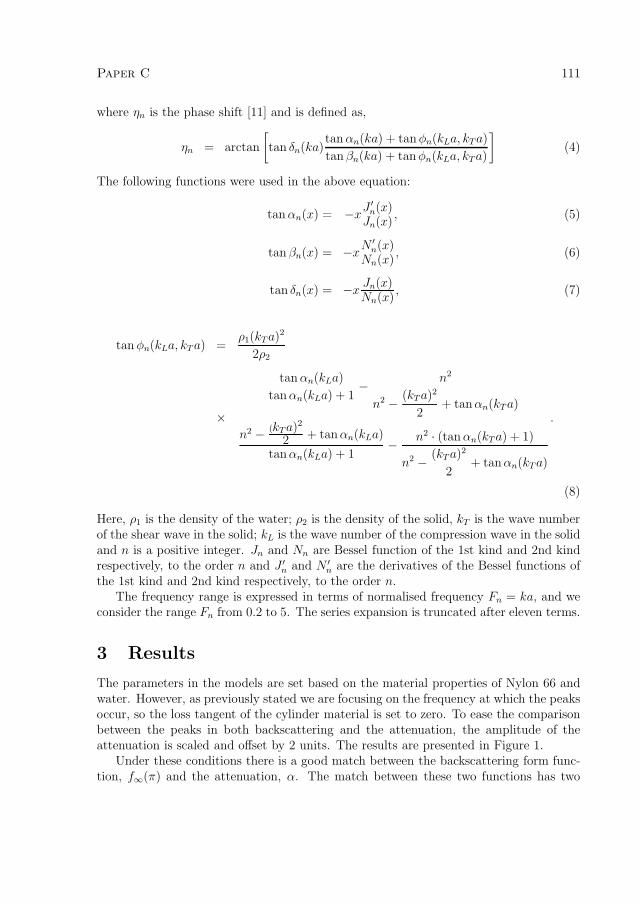
Paper C 111

where ηn is the phase shift [11] and is defined as,

ηn = arctan

[tan δn(ka)

tan αn(ka) + tan φn(kLa, kT a)

tan βn(ka) + tanφn(kLa, kTa)

](4)

The following functions were used in the above equation:

tan αn(x) = −xJ ′n(x)Jn(x)

, (5)

tan βn(x) = −xN ′

n(x)Nn(x)

, (6)

tan δn(x) = −xJn(x)Nn(x)

, (7)

tan φn(kLa, kT a) =ρ1(kT a)2

2ρ2

×

tan αn(kLa)

tanαn(kLa) + 1− n2

n2 − (kT a)2

2+ tanαn(kT a)

n2 − (kT a)2

2 + tanαn(kLa)

tanαn(kLa) + 1− n2 · (tan αn(kT a) + 1)

n2 − (kT a)2

2+ tanαn(kT a)

.

(8)

Here, ρ1 is the density of the water; ρ2 is the density of the solid, kT is the wave numberof the shear wave in the solid; kL is the wave number of the compression wave in the solidand n is a positive integer. Jn and Nn are Bessel function of the 1st kind and 2nd kindrespectively, to the order n and J ′n and N ′

n are the derivatives of the Bessel functions ofthe 1st kind and 2nd kind respectively, to the order n.

The frequency range is expressed in terms of normalised frequency Fn = ka, and weconsider the range Fn from 0.2 to 5. The series expansion is truncated after eleven terms.

3 Results

The parameters in the models are set based on the material properties of Nylon 66 andwater. However, as previously stated we are focusing on the frequency at which the peaksoccur, so the loss tangent of the cylinder material is set to zero. To ease the comparisonbetween the peaks in both backscattering and the attenuation, the amplitude of theattenuation is scaled and offset by 2 units. The results are presented in Figure 1.

Under these conditions there is a good match between the backscattering form func-tion, f∞(π) and the attenuation, α. The match between these two functions has two

112 Paper C

0 1 2 3 4 50

0.05

0.1

0.15

0.2

0.25

0.3

0.35

Frequency (Mhz)

Func

tion

Am

plitu

de α

f∞(π)

Figure 1: Plot of the acoustic attenuation, α, and the form function, f∞(π), against normalisedfrequency for nylon fibres suspended in water. To ease the comparison between the peaks in bothfunctions, the amplitude of the attenuation is scaled and offset by 2 units.

consequences. Firstly, the solution for the expansion coefficients used by Faran [10] canbe used in the calculation of attenuation -equation (2) -instead of the solution for theexpansion coefficient used in the attenuation. This results in a simpler solution as thatused by Faran [10] uses slip boundary conditions. We can then compare the amplitudes ofthe attenuation calculated using the two different solutions for the expansion coefficientsand hence the effects of the different boundary conditions. Work on this continues.

The second consequence of the match between the form function and the attenuationis that the resonance peaks in the form function have been well discussed, in both [10]and [6]. Faran [10] states that the normal modes of the cylinder are found when thenormal component of the stress and the tangential component of the shear stress at thesolid boundary are zero gives a condition which is identical to setting the denominatorof Equation (8) to zero. Using this condition the normal modes can be calculated fromEquation (8). Faran [10] also discusses that a shift in the resonance frequency of animmersed cylinder due to the reactive component of the acoustic impedance acting onthe scatterer by the surrounding fluid. Although in his study this shift was small asthe metal cylinders that were used had much greater densities than the surroundingfluid, in our case, where the density of nylon is close to that of water, the effect will beconsiderable. When calculating the normal mode for nylon, the first mode occurs at anormalised frequency of 1.4 (R = 44μm, 7.8 MHz), however, the effect of the surroundingfluid moves this peak to a normalised frequency of 1.0 (R = 44μm, 5.3 MHz). Thefrequency can be found by setting the denominator in equation 4 to zero. Also discussedis the fact that the since the speed of the shear waves is much lower than the speed ofthe compression wave. The first modes to appear are from the shear wave. Since then = 0 does not support shear waves, the frequency of this mode depends on the speedof the wave and hence occurs at a normalised frequency of 3.57 (R = 44 μm, 19.3 MHz).These calculations are for a cylinder with no loss.

Paper C 113

Resonances in backscattering are explained as being caused by creeping waves in thefluid and in the solid [6]. However, the assumption used in these explanations is thatthe normalised frequency is much greater than 1, which is not the case here. Hence theactual wave propagation modes in this region of normalised frequency are still not clear.

4 Conclusion

From the results so far it appears that the coefficient derived by Faran [10] for backscat-tering can be used to derive attenuation. From this model, the resonance modes of acylinder and a cylinder in water can be obtained. They confirm that the peaks in theattenuation curves are due to resonance. It appears as if the shear waves are causingfirst peaks in the ultrasound attenuation although the exact nature of these waves hasnot been established. These calculations have been done under the conditions of no loss.

The implication of these findings for the use of estimating material properties of paperpulp from ultrasound attenuation are that, if possible, the density of the surrounding fluidshould be as close as possible to that of the suspended fibre. This increases the phaseshift in the suspension and increases the dependency of the attenuation on the materialproperties of the fibre. The frequency range should also be set, if possible, so thatresonance peaks exists within the range. Since the frequencies of the peaks depend onthe material properties of the fibre, identifying these frequencies should aid in estimatingmaterial properties.

References


[2] Y. Aitomaki, “Towards a measurement of paper pulp quality: ultrasonic spec-troscopy of fibre suspensions,” Licentiate Thesis, Luleøa University of Technology,2005.


[4] H. Uberall, G. Gaunaurd, and J. Diarmuid Murphy, “Acoustic surface wave pulsesand the ringing of resonances,” Journal of the Acoustical Society of America, vol. 72,no. 3, pp. 1014–1017, Sept 1982.

[5] J. Diarmuid-Murphy, J. George, A. Nagl, and H. Uberall, “Isolation of the resonantcomponent in acoustic scattering from fluid-loaded elastic spherical shells,” Journalof the Acoustical Society of America, vol. 65, no. 2, pp. 368–373, Feb 1979.

114


[7] H. Uberall, L. Dragonette, and L. Flax, “Relation between the creeping waves andthe normal modes of vibration of a curved body,” Journal of the Acoustical Societyof America, vol. 61, no. 3, pp. 711–715, Mar 1977.


[9] G. Frisk, J. Dickey, and H. Uberall, “Surface wave modes on elastic cylinders,”Journal of the Acoustical Society of America, vol. 58, no. 5, pp. 996–1008, Nov 1975.

[10] J. Faran, “Sound scattering by solid cylinders and spheres,” Journal of the AcousticalSociety of America, vol. 23, no. 4, pp. 405–418, July 1951.

[11] J. Mathieu and P. Schweitzer, “Measurement of liquid density by ultrasoundbackscattering analysis,” Meausurement Science and Technology, vol. 15, pp. 869–876, 2004.




,

Paper D

Inverse Estimation of Material

Properties from Ultrasound

Attenuation in Fibre Suspensions

Authors:



Elsevier Ultrasonics, Volume 49, Issues 4-5, May 2009, Pages 432-437

© 2009 Elsevier, Reprinted with permission

115

Inverse Estimation of Material Properties from

Ultrasound Attenuation in Fibre Suspensions


Abstract

An investigation of a new method for measuring fibre material properties from ultrasonicattenuation in a dilute suspension of synthetic fibres of uniform geometry is presented.The method is based on inversely solving an ultrasound scattering and absorption modelof suspended fibres in water for the material properties of the fibres. Experimental re-sults were obtained from three suspensions of nylon 66 fibres each with different fibrediameters. A forward solution to the model with reference material values is comparedto experimental data to verify the model’s behaviour. Estimates of the shear and Young’smodulus, the compressional wave velocity, Poisson’s ratio and loss tangent from nylon66 fibres are compared to data available from other sources. Experimental data confirmsthat the model successfully predicts that the resonance features in the frequency responseof the attenuation are a function of diameter. Consistent estimated values for the com-pressional wave velocity and the Poisson’s ratio were found to be difficult to obtain butin combination gave values of shear modulus within previously reported values and withlow sensitivity to noise. Young’s modulus was underestimated by 54% but was consistentand had low sensitivity to noise. The underestimation is believed to be caused by theassumption of isotropic material used in the model. Additional tests on isotropic fibrewould confirm this. Further analysis of the model sensitivity and the reasons for theresonance features are required.

1 Introduction

The quality of paper pulp depends on a large number of factors and some of these arethe properties of the pulp fibre itself [1]. Measuring pulp fibre characteristics has there-fore the potential to provide paper manufacturers with increased control over their pulpproduction. The measurement method being investigated here is based on ultrasound, asit is rapid, inexpensive, non-destructive and non-intrusive. Consequently, such measure-ments could be done online. As an initial step on the way to online measurement of pulpfibre properties, the aim of this measurement method is to provide ultrasonic based mea-surements of the material properties of finite length, uniform fibres in suspension. Twoapproaches that can be used to model ultrasound propagation in fibre suspensions areto model it either as a solid porous media or as cylindrical scatters suspended in a fluid.The solid porous media approach has been applied to paper pulp using Biot’s model ofthe attenuation and velocity of ultrasound [2]. However, the structural and solid/fluid

117

118 Paper D

interaction parameters are many and difficult to establish. Using dilute solutions andhigher frequencies than the Biot model, scattering models can be considered. Epstein-Carhart/Allegra-Hawley [3, 4], (ECAH), model and the Harker and Temple model [5]have been developed for spherical-like particles in suspension. A review of these andother theories mainly based on spherical particles and their application to determiningparticle size distribution is found in [6]. Studies of cylindrical particles have concentratedon large scatterers, where the product of the wave number and the radius, kR, is largeand hence asymptotic assumptions can be made. In these studies, back-scattering ratherthan attenuation is considered [7, 8].

A scattering model for a suspension of fibres in water was developed by Habeger [9].This is a cylindrical extension of the ECAH model and relates the attenuation to theproperties of water, the properties of the fibre, and the fibre concentration. In the cal-culation of attenuation, the model equations are based on a number of different materialproperties and are solved numerically. Since the model is to be used to solve the in-verse problem, i.e. determining the material properties from attenuation measurements,a simpler, analytical version of this model was sought which would have less unknownparameters and would have a quicker and more stable solution. By neglecting thermaleffects and assuming low viscosity in the suspending fluid, a more tractable set of equa-tions is reached that can be solved analytically [10]. This simplified cylinder scattering(SCS) model is the basis for the measurement method described here.

Firstly we test the model’s forward, predictive accuracy and behaviour and secondly,its suitability for providing inverse solutions. In the predictive part we experimentallyverify the model’s response to changes in fibre diameter given reference data for the fibreproperties. In the inverse testing, we investigate whether the SCS model can be used toestimate material properties of fibres in suspension from the attenuation of ultrasoundacross a range of frequencies.

We start by describing the SCS model and the experimental procedure used to obtainthe frequency response of attenuation of a suspension of nylon fibres in water. Wediscuss the results from the predictive and inverse tests and draw conclusions about themeasurement methods as well make some suggestions for further work.

2 Theory

In the SCS model, the attenuation is calculated from the energy losses arising when aplane wave is incident upon an infinitely long, straight cylinder. The cylinder material isassumed to be isotropic and viscoelastic. The energy losses taken into account are fromthe wave being partially reflected, partially transmitted at the solid-fluid interface andfrom the generation of damped, transverse waves in the solid medium at the boundary.The highly damped thermal skin layer, that is generated by the acoustically inducedpulsations of the solid has been shown to have the greatest effect at frequencies wherethe thermal wavelength is of the order of the radius [9]. To simplified the model weneglect these thermal effects but to reduce the impact this has on the model’s accuracywe only consider frequencies above this thermally sensitive region. A viscous wave in the

Paper D 119

fluid (as defined by [3]) is also generated but due to the low viscosity, the energy lossdue to this wave is small and is also neglected. In the model the waves are expressedin terms of the wave potentials of the incident and reflected wave in the fluid and thecompressional and shear wave potentials in the fibre. The derivation is presented in [10]and the resulting equation for the attenuation α is

α =−2fr

πR2kc1

∞∑n=0

�(∫ π

2

0

εnBn cos(ψ)dψ

)(1)

where fr is the volume fraction; R is the radius of the fibre; kc1 is the wave number ofthe compressional wave in water; � denotes the real part of the expression, ψ is the angleof between the axial plane of the fibre and the direction of the oncoming ultrasoundwave; n is a positive real integer; εn = 1 if n = 0, otherwise εn = 2 and where Bn

is the nth expansion coefficient of the wave potential of the reflected wave. With theassumptions stated above, the solution for the coefficients Bn, comes from using theboundary condition of continuous velocity in the radial direction and continuous stressin radial, tangential and axial directions at the fluid-solid interface. The actual expressionfor Bn is solved analytically using Maple© (Maplesoft, Waterloo, Canada). The result isan expression for Bn as a function of the fluid properties: viscosity, ν1, density, ρ1 andvelocity of the compressional wave, c1 and the fibre properties: radius, R, density, ρ2,velocity of the compressional wave, c2, shear wave, cs2 and the loss tangent, tan δ. Tan δis the tangent of the angle by which the strain in a solid lags the stress causing it andis often taken as the elastic energy losses in solids [11]. Bn is also an explicit functionof the shear modulus, G. The model assumes the material to be isotropic hence theelastic properties are set by only two parameters, in this case the Poisson’s ratio, ν andc2. Details of the relationship between these two parameters and the properties: Young’smodulus, E, G and cs2, referred to later in the paper are given in the appendix.

As can be seen in equation 2, the attenuation is a function of the sum of Bn. In ourexperiments on nylon in water, the series was truncated at n =3, as higher terms did nothave any significant effect on the attenuation in the frequency range we are considering.

3 Experiment

The experiments were carried out using the pulse-echo technique. A diagram of the mea-surement cell used in this study is shown in figure. 1. Three fibre suspensions were madeup using different diameters of nylon 66 fibres (Swissflock, Emmenbrucke, Switzerland).The fibre dimensions are given in table 1. The fibres were weighed and mixed with dis-tilled water to a concentration of 0.5% by weight. The broadband transducer (V319,Panametrics, Waltham, MA, USA) used had a centre frequency of 15 MHz. The trans-ducer was excited and the received signal amplified by a pulser/receiver (Model 5073PR,Panametrics). The signal was then digitized using an oscilloscope card (CompuScope12400, Gage Applied Technologies Inc., Lachine, QC, Canada) with a 12-bit resolutionand a sampling rate of 400 MHz. All data were stored in a computer for off-line analysis.

120 Paper D

Table 1: Fibre dimensions

Diameter LengthDry Saturated

(10−6 m) (10−6 m) (10−3 m)14.8 14.9±1.5 1.243.6 45.9±7.2 1.549.6 51.9±2.0 1.5

Time

S1 S2

Stee

lre

flec

tor

Sam

ple

spac

eB

uff

er-

ro

dTr

ans-

du

cer

d

1

2

3

Figure 1: Diagram of the pulse-echo measurement system

The cell was calibrated using water, emptied and carefully filled with the fibre sus-pension. Each measurement set consisted of a sequence of 100 pulses and their echoes.Five sets were taken and the sample was stirred after each set. The cell was emptiedand rinsed with temperature-controlled water, before the cell was filled with the nextsample and the process repeated. Once all three samples were measured, the whole pro-cedure was repeated twice more but with the samples measured in a different order. Thisresulted in 1500 pulse echoes for each sample

A digital thermometer (Model F250, Automatic Systems Laboratories LTD, England)monitored the temperature in the sample under test. During the whole process thetemperature of the suspension varied from a minimum of 20.75±0.2 ◦C to a maximumof 21.47±0.2 ◦C. The temperature of the water during calibration was taken and used tocalculate the velocity of the wave in the water. The distance d in figure 1 is the distancebetween the buffer rod and steel reflector. This was found using this wave velocity and thetime-of-flight for an ultrasonic pulse to travel that distance. The latter was determinedfrom a cross-correlation technique.

A fast Fourier transform was applied to each echo. The echoes were then averaged

Paper D 121

and the attenuation calculated from

αE(f) =1

2dln

(S2A1

S1A2

)+ αw, (2)

where f is the frequency, S1 = S1(f) and S2 = S2(f) are the frequency dependentamplitudes of the first and second echoes in the sample, A1 = A1(f) and A2 = A2(f)are the frequency dependent amplitudes of the first and second echoes in water. αw isthe theoretical attenuation of water and equals 25 · 10−15f 2 [12]. The addition of theexpression

1

2dln

(A1

A2

)+ αw, (3)

in equation 2 serves to calibrate the sample signals with the signals from water to com-pensate for losses at the interfaces, transducer alignment and possible diffraction effects.The variance of the attenuation was calculated by first order approximations of the atten-uation which is described particularly for the pulse-echo model by [13] in their comparisonof parametric to non-parametric techniques for calculating ultrasound attenuation andphase velocity. Note that the noise in the signal from the distilled water sample is as-sumed to be insignificant as the signal in water has a high signal to noise ratio due to itslow attenuation.

Lack of homogeneity of the fibre suspension is reduced by taking a large number ofreadings. On average the mass fraction of the measured suspension is equal to that ofthe whole sample. The volume fraction, fr, used in the model, is calculated as,

fr =ρ1mf

ρ2 + (ρ1 − ρ2)mf

(4)

where mf is the mass fraction, ρ1 is the density of the water and ρ2 is the density of thefibre.

Method for Parameter Estimation

The second part of the study tested the inverse solution of the model. An iterative searchwas used to find the values of the material properties that minimises the differencebetween the model attenuation and the average measured attenuation, over a rangeof frequencies with a known fibre diameter. After initial trial runs with four materialproperties being estimated i.e. ρ2, c2, ν and tan δ, it was decided that the known value ofthe density should be used in the model. The density was fixed to improve the accuracyof the other three material properties and is a property that in general can be measuredusing alternative methods. Additionally, work done by [14] on fibres in pulp indicatesthat the density of fibre material does not vary significantly. Elastic properties such asthe G and E were calculated using the formula set out in the appendix, as mentionedearlier.

122 Paper D

Table 2: Limits used in the parameter estimation procedure.

Material Property Upper Value Lower Valuec2 500 ms−1 7000 ms−1

ν 0.2 0.5tan δ 0 1

2 4 6 8 10 12 140

20

40

60

80

100

120ν2=0.443

Frequency (MHz)

Atte

nuat

ion

(Np/

m)

(a)

2 4 6 8 10 12 140

20

40

60

80

100

120ν2=0.441

Frequency (MHz)

Atte

nuat

ion

(Np/

m)

(b)

Figure 2: Predicted and measured attenuation for the 52μm nylon 66 fibres. The experimentalattenuation is marked with crosses. The predicted attenuation is modelled in figure (a) withυ =0.443 and in figure (b) with υ = 0.410. The other material property values used in thecalculation were c2 = 2600 ms−1, tan δ = 0.03 (solid line)/tan δ = 0.2 (dotted line), ρ2 = 1140kgm−1. The dashed line includes thermal and viscous terms.

The algorithm used was a constrained non-linear least squares fit [15]. The constraintswere limits were set on the material properties (see table 2) so that the minimised costfunction would only be a result of realistic values of c2, ν and tan δ. The algorithm wasset initially to fit the average experimental attenuation curve. It was run a 100 timeswith randomised initial values for the material properties for each of the three differentfibre suspensions. The sensitivity of the algorithm to noise in the data was measured bysetting the algorithm to fit the average experimental attenuation curve plus then minustwo standard deviations and recording the effect on the material parameter estimations.

4 Results and Discussion

4.1 Parameter Estimation

The predicted attenuation was calculated for two different diameters of fibre suspensionsusing the values in table 1 over a frequency range matching that of the bandwidth ofthe transducer. This predicted and the average measured attenuation is plotted for thelarger fibre suspension in figures 4.2(a) and 4.2(b) and for the smaller fibre suspension in

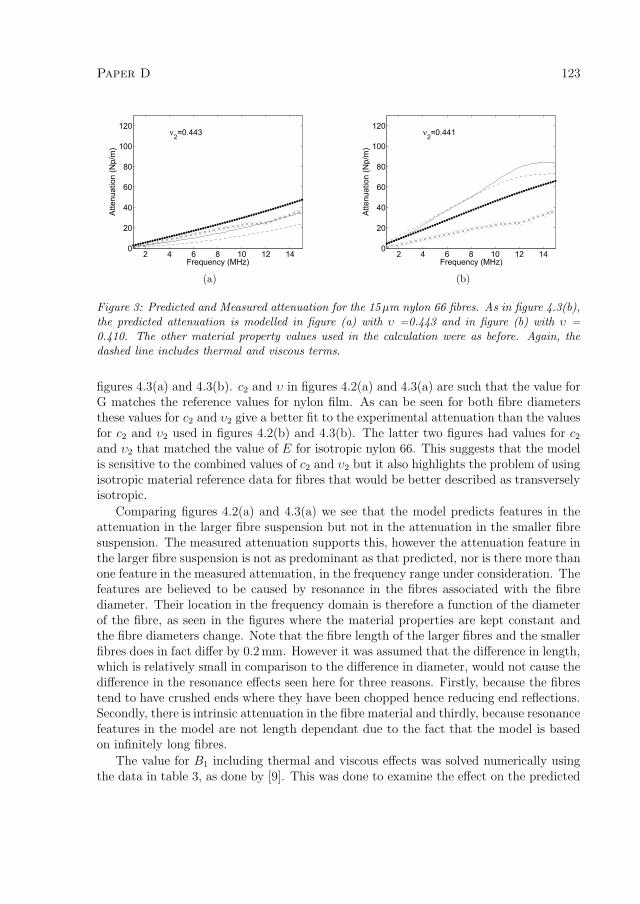
Paper D 123

2 4 6 8 10 12 140

20

40

60

80

100

120ν2=0.443

Frequency (MHz)

Atte

nuat

ion

(Np/

m)

(a)

2 4 6 8 10 12 140

20

40

60

80

100

120ν2=0.441

Frequency (MHz)

Atte

nuat

ion

(Np/

m)

(b)

Figure 3: Predicted and Measured attenuation for the 15μm nylon 66 fibres. As in figure 4.3(b),the predicted attenuation is modelled in figure (a) with υ =0.443 and in figure (b) with υ =0.410. The other material property values used in the calculation were as before. Again, thedashed line includes thermal and viscous terms.

figures 4.3(a) and 4.3(b). c2 and υ in figures 4.2(a) and 4.3(a) are such that the value forG matches the reference values for nylon film. As can be seen for both fibre diametersthese values for c2 and υ2 give a better fit to the experimental attenuation than the valuesfor c2 and υ2 used in figures 4.2(b) and 4.3(b). The latter two figures had values for c2

and υ2 that matched the value of E for isotropic nylon 66. This suggests that the modelis sensitive to the combined values of c2 and υ2 but it also highlights the problem of usingisotropic material reference data for fibres that would be better described as transverselyisotropic.

Comparing figures 4.2(a) and 4.3(a) we see that the model predicts features in theattenuation in the larger fibre suspension but not in the attenuation in the smaller fibresuspension. The measured attenuation supports this, however the attenuation feature inthe larger fibre suspension is not as predominant as that predicted, nor is there more thanone feature in the measured attenuation, in the frequency range under consideration. Thefeatures are believed to be caused by resonance in the fibres associated with the fibrediameter. Their location in the frequency domain is therefore a function of the diameterof the fibre, as seen in the figures where the material properties are kept constant andthe fibre diameters change. Note that the fibre length of the larger fibres and the smallerfibres does in fact differ by 0.2 mm. However it was assumed that the difference in length,which is relatively small in comparison to the difference in diameter, would not cause thedifference in the resonance effects seen here for three reasons. Firstly, because the fibrestend to have crushed ends where they have been chopped hence reducing end reflections.Secondly, there is intrinsic attenuation in the fibre material and thirdly, because resonancefeatures in the model are not length dependant due to the fact that the model is basedon infinitely long fibres.

The value for B1 including thermal and viscous effects was solved numerically usingthe data in table 3, as done by [9]. This was done to examine the effect on the predicted

124 Paper D

Table 3: Thermal properties for nylon 66 from [9]

Thermal Material Property ValueHeat capacity ( Jkg◦K) 1420Heat conductivity coefficient ( Wm−1K−1) 0.36Thermal expansivity ( μK−1) 60

attenuation of neglecting the thermal effects and shear in the fluid. These results areplotted in figures 2 and 3 with dashed lines. They show that including these effectsslightly dampens the resonance feature and in general lowers the predicted attenuationbut does not affect the location of the resonance feature in the larger fibre. Increasingtan δ also has a dampening effect as illustrated by the dotted lines in figure 2 and 3.Although with the increased tan δ the curves are closer to the shape of the measuredattenuation, it too does not affect the location of the resonance feature as illustrated bythe plots of the larger fibre.

Noise in the measured attenuation is expressed in terms of the standard deviation asa percentage of the attenuation. The maximum values in the chosen frequency region are0.2%, 3.4% and 3.9% for the 15 μm, 46 μm and 52 μm fibres, respectively. The maximumstandard deviation occurs at the higher frequencies where the signal-to-noise ratio issmaller.

The diameter values used in the predicted attenuation are from table 1. The diametermeasurements made of the water saturated fibres compared well to the diameters statedby the manufacturer plus the 8% volumetric swelling that is stated in [16] for watersaturated nylon 66.

4.2 Parameter Estimation

Estimates for the material properties were found from the best-fit solution to each ofthe average measured attenuation curve of the three different fibre suspensions. The100 random initial values gave rise to a number of clustered values for c2, υ2 and tan δ.The c2 and υ2 values were used to calculate E and G. Figure 4 is a plot of the resultingestimates for E, G and tan δ for the three different fibre diameter. The size of the markerin figure 4 represents the value of the cost function and the colour, the value of tan δ.

For the 52 μm diameter fibre suspensions, the cluster with the lowest cost functioncontained 45% of the best-fit solutions to the attenuation. For the 46 μm diameter fibresuspension the cluster contained 30% of the best-fit solutions. These best-fit resultsare plotted in figure 5. The material property values that gave these best-fit solutionsare presented in table 4 and show that the solutions with these low cost functions weremuch closer to the reference material properties values given in table 5 than the solutionswith higher cost functions. This positive results suggests that the model can be used insolving the inverse problem. The solutions that gave higher cost function were presumedto be caused by the optimisation algorithm falsely identifying local minima as the global

Paper D 125

0 1 2 3 4 50

1

2

3

4

5

6

7

8

9

10

G (GPa)

E (G

Pa)

52μm fibre46μm fibre15μm fibre

0.1

0.2

0.3

0.4

0.5

0.6

0.7

0.8

0.9

1

Figure 4: Scatter Plots of the estimated E and G with the value of tan δ represent by colour.The different symbol represent the different fibre suspension. The size of the symbol representsthe size of the cost function hence a small symbol represents a better fit.

Table 4: Estimated Values for nylon 66 material properties from the attenuation in the suspen-sions of the 3 different fibre diameters

Attenuation Measured c2 ν tan δ E GValue Diameter

10−6 m ms−1 GPa GPaAverage 2051 0.418 0.222 1.92 0.68Av. + 2SD 14.8 2072 0.420 0.225 1.94 0.68Av. - 2SD 2053 0.417 0.217 1.92 0.68Average 4404 0.488 0.325 1.53 0.51Av. + 2SD 45.9 6611 0.495 0.334 1.55 0.52Av. - 2SD 3456 0.480 0.320 1.47 0.49Average 2897 0.463 0.362 1.92 0.66Av. + 2SD 51.9 3835 0.481 0.419 1.82 0.68Av. - 2SD 2460 0.445 0.325 1.98 0.61

126 Paper D

Table 5: Table of reference values for nylon 66 material properties. Nylon sheet and blockdata is obtained from [17] and Goodfellows Cambridge Limited, England respectively, exceptwhere marked. Data from [17] shows that the effect of increasing the frequency on the elasticmoduli of nylon 66 is offset by the effect of the water saturation, hence elastic data obtainedunder dry, quasi-static conditions is comparable to that obtained under saturated, high frequencyconditions. Ez, Eθ,r, Gzand Gθ,r were derived from compliance data from [17] using a tensormatrix for transversely isotropic materials, such as [18].

Description ρ2 c2 ν tan δ Ez Eθ,r Gz Gθ,r

kgm−1 ms−1 GPa GPa GPa GPaSaturated, 1140 - - 0.10 3.6 2.3 0.74 0.36transverselyisotropic sheetsmeasured athigh frequencyDry, isotropic 1140 26001 0.410 0.032 3.3 3.3 1.171 1.171

block measuredquasi-statically1 calculated from the isotropic values of E and ν2 from [17] for dry, isotropic sheet measurements

minimum.The results of the fitting procedure to the attenuation in the 15μm fibre suspension

are more ambiguous. The size of the marker in figure 4 shows that best fit solutions tothe attenuation in this suspension had lower cost function values than the cost functionvalues from the fitting to the attenuation in the other two fibre suspensions. This meansthat there was a better fit between the model and the measurement data for a suspensionwith this diameter of fibre than in the suspension of the larger fibres. However, in the caseof the small fibre suspension the optimisation procedure converged to a large number ofdifferent points. The estimation from the lowest cost function results were E = 0.08 GPaand G = 0.02 GPa, which were over two orders of magnitude less than the referencevalues. This misidentification of the material parameters is thought to be because thereare no resonance features captured with this combination of frequency range and fibrediameter and hence a large number of different values for c2, υ2 and tan δ provide goodfit solutions to the model. In this case, this result indicates the model is not suitable forsolving the inverse solution when used with this optimisation procedure.

In the figure we can see a cluster of 26% of the values lying close to the values from theminimum cost function cluster of the other two fibres. These values had the second lowestvalue of the cost function and were the ones that they lay closest to the reference valuesof the E and G of all the solutions. Table 4 contains these values since we chose to usethem in evaluating the accuracy of the estimates of the material properties. The fibresare more accurately described as transversely isotropic than isotropic hence referencevalues from drawn nylon film [17] are included in the reference table values. The results

Paper D 127

2 4 6 8 10 12 140

10

20

30

40

50

60

70

80

90

100

Frequency (MHz)

Atte

nuat

ion

(Np/

m)

Φ 53 ExptΦ 53 FittedΦ 46 ExptΦ 46 FittedΦ 15 ExptΦ 15 Fitted

Figure 5: Best fit curves and measurements of the attenuation in the three different fibre sus-pensions. The values for the material properties from the best fit curves are given in table4

in table 4 show that estimated values for the shear modulus lie between the value forthe Gz and Gθ,r. The estimates from the three fibres give values close to each other.However, there are insufficient numbers of different diameters fibres to draw conclusionsabout the variation between the fibres. We define the sensitivity of the estimation ofeach parameter to noise in the data as the value estimated from the attenuation plus twostandard deviations. Using this definition we can see that the sensitivity of the shearmodulus to noise is low.

The estimated value for E is out of the range of values expected for the fibre. It variesbetween 14% and 36% lower than Eθ,r (54% lower than the isotropic value), however theestimates from the three different fibres are close to each other and have low sensitivityto noise. A probable reason for the low estimation is the assumption in the model of thefibre being isotropic because if Gθ,r is correct, even with a υ2 = 0.5 i.e. incompressiblematerial, the maximum value of E is 3G and hence it would only just be in the rangegiven in the table 5. These reference values are possible because of they assume thefibre to be transversely isotropic compared to the model that assumes the material to beisotropic.

The c2 and υ2 differ from one fibre to the next and from the reference values intable 5. They also are more sensitive to noise in the attenuation curves than the elasticmoduli. This implies that applying the modelling over this range of frequencies thereis not sufficient data to specify the individual value of c2 and υ2. However, as can beseen from the consistent values obtained for the elastic moduli, their combined valuesare consistent. It is possible that better estimation of c2 and υ2 would be obtained if agreater frequency range was captured.

128 Paper D

Comparison between the estimated values of tan δ in table 4 and its reference val-ues in table 5 shows that the estimated values are an order of magnitude larger thanexpected. Possible reasons for this are that the fibres are in a region of resonance andhence the damping effect is greater. Additionally, the larger estimated value for the losstangent may be compensating for thermal and fluid shear effects being neglected in themodel since neglecting thermal effects and fluid shear effects has a damping effect on theattenuation as previously discussed (see figure 2).

5 Conclusion

The aim of this measurement method was provide ultrasonic based measurements ofthe material properties of short, uniform fibres in suspension. The measurement methodgave reasonable and consistent results for the shear modulus with low sensitivity to noise.The Young’s modulus was lower than predicted but consistent and had low sensitivity tonoise. The reduced value is thought to be caused by the anisotropic nature of the fibres.

The results suggest that the the frequency range should include at least one resonancefeature for the optimisation method used here to unambiguously identify the best-fit tothe measured attenuation and give reasonable estimated values of the material parame-ters. This was despite a better match between the model and the experimental resultsexisting in the region without a resonance feature.

The difference between the predicted and the measured attenuation were not ex-plained by the noise, incorrect tangent delta values or the assumptions of negligiblethermal or viscous effects. Given this and the reasonable accuracy of the shear modulusit would seem that the errors come from the assumption of isotropic material. Addingcomplexity to the model by basing it on transversely isotropic material could improve fitof the model to the experiment data. However, increasing the complexity could introduceproblems in solving the inverse problem of estimating the material properties from themeasured attenuation. It may slow the estimation procedure and may results in overparameterisation of the model whereby noise would be modelled as well as introducinga larger potential number of solutions that would make identifying the correct solutionmore difficult.

Further work is needed on the sensitivity of the model to the different parametersalso further experiments on isotropic fibres would aid in explaining the reason for the lowvalue of Young’s modulus.

6 Acknowledgments

We wish to thank to Swissflock, Emmenbrucke, Switzerland for providing the fibres andRhodia, France for the nylon fibre properties. Thanks go also to Jan Niemi and JesperMartinsson for their support and for supplying part of the programming code.

Paper D 129

A Appendix

The relationships between the different elastic properties and the compressional wavevelocity are the standard relationships and for clarity are give here:

The shear modulus, G, is calculated from

G =(0.5 − υ)

(1 − υ)ρ2c

22. (A.5)

Young’s modulus, E, is calculated from

E =(1 + υ)(1 − 2υ)

(1 − υ)ρ2c

22. (A.6)

References

[1] J. Levlin and L. Soderhjelm, Pulp and Paper Testing. Fapet Oy, 1999.

[2] D. Adams, “Ultrasonic transmission through paper fiber suspensions,” Ph.D. disser-tation, University of London, 1975.



[5] A. Harker and J. Temple, “Velocity and attenuation of ultrsound in suspensions ofparticles in fluids,” Journal of Physics D: Applied Physics, vol. 21, pp. 1576–1588,1988.





130




[13] J. Martinsson, J. Carlson, and J. Niemi, “Model-based phase velocity and attenua-tion estimation in wideband ultrasonic measurement systems,” IEEE Transactionson Ultrasonics, Ferroelectrics and Frequency Control, vol. 54, no. 1, pp. 138–146,January 2007.



[16] A. Anton and B. Baird, Encyclopedia of polymer science and technology. Wiley-Interscience, 2003, vol. 3, ch. Polyamides, Fibers, pp. 584–617.

[17] W. Leugh, K. Ho, and C. Choy, “Mechanical relaxations and moduli of orientednylon 66 and nylon 6,” Journal of Polymer Science, vol. 22, pp. 1173–1191, 1984.

[18] J. Melo and D. Radford, “Determination of the elastic constants of a transverselyisotropic lamina using laminate coefficients of thermal expansion,” Journal of Com-posite Materials, vol. 36, pp. 1321–1329, 2002.

Paper E

Damping mechanisms of

ultrasound scattering in suspension

of cylindrical particles:

Numerical analysis

Authors:


To be submitted

to Journal of the Acoustical Society of America as a letter to the editor

131

132 Paper E

Damping mechanisms of ultrasound scattering in

suspension of cylindrical particles:

Numerical analysis


Abstract

The addition of viscosity to the ultrasound scattering models increase complexity. Inves-tigated is the necessity of the addition of viscosity in a suspension of cylindrical scatterersin two different frequency-radius regimes. The modelled attenuation of a scatterer sur-rounded by a viscous fluid is compared to that where the fluid is non-viscous. The resultsshow that the intrinsic loss in the scatterer and the viscosity both have a damping effecton the attenuation.

The conclusion is that a simpler model where the fluid is assumed to be non-viscouscan be used to model attenuation in suspensions of fibres with tan δ ≥ 0.1. This holds ifthe frequency is not in the region where the viscous skin depth equals the radius.

1 Introduction

Early studies on spherical scatterers have shown the importance of viscosity as a lossmechanism in the attenuation of ultrasound in suspensions [1, 2]. These studies giveexplicit expressions for the attenuation in suspension of spherical particles showing clearlyits dependance on the viscosity. These expressions are valid when the wavelength ismuch greater than the radius of the particle (long wavelength limit). The importanceof viscosity has been shown in a more recent experimental study where suspensions ofsmall solid spheres over a wide range of frequencies were investigated [3]. However, theaddition of viscosity adds considerable complexity to the system and in cases where moreelaborate geometry is modelled, the viscosity of the fluid is often neglected [4–7].

Ultrasound scattering models based on those discussed above, have been used tosolve the inverse problem of obtaining material properties of the scatterers [8,9]. Solvingthe inverse problem is optimised if only the parameters influencing the attenuation areincluded since including redundant parameters has a serious impact on the speed of theoptimisation. This is because, in general, the model becomes more complex if it hasa greater number of parameters. Also, the addition of any unknown parameter addsanother dimension to the search space and hence can have a large impact on the speedof optimisation.

If we are interested in obtaining the material properties of the scatterer, it would beof value to know the loss in accuracy of the attenuation when the fluid is assumed to

133

134 Paper E

be non-viscous. This would provide a basis for appropriate assumptions to be made. Ithas been shown that when scattering occurs in between two eigenfrequencies of vibrationof an elastic body, the scatterer appears as an impenetrable object [10]. Hence, if theinterest is in estimating material properties of the scatterer, then the wavelength regimechosen should be where eigenfrequencies of the scatterers exist. The eigenfrequencies arelikely to be where the wavelength is of the order of the radius of the scatterers. In thisstudy the influence of viscosity on attenuation where the wavelength is of the same orderas the radius is investigated.

One application of this type of model is for estimating the material properties ofwood fibres in suspension, such as found in paper pulp. With a view to this application,this paper focuses on cylindrical scatterers with a density close to that of water andwith diameters in the order of 10 microns. The aim is to establish if viscosity effectscan be neglected when modelling the attenuation of ultrasound in a dilute suspension ofsuch scatterers in water. The model is based on single particle scattering of ultrasoundoriginally derived for spherical particles [1, 2] and adapted for cylindrical scatterers [8].This is done by comparing the simulated results from the model using the conditionthat a non-viscous fluid surrounds the scatterers to the results from the model using thecondition that a viscous fluid surrounds the scatterers. A numerical comparison is chosenbecause the number of terms involved in analytical expressions are large, for example, oneof the terms is a result of the determinant of a 6 by 6 matrix. Two frequency-scattererradius regimes are investigated, one where the frequency range is chosen such that thewavelengths are in the order of the radius of the scatterer and the other where the viscousboundary layer is known to effect the attenuation [3]. The model is only valid for lowconcentrations [11] and hence the comparison are done with a suspension of scatterers of1% concentration by volume.

2 Theory

In a fluid medium, the total attenuation of an ultrasound plane wave in a known diluteconcentration of randomly orientated cylindrical scatterers can be calculated based on theattenuation of a single cylindrical scatterer [8]. This attenuation from a single scatterercan be calculated from the scattering of the wave from an oblique orientated cylinder(see Fig. 1) using the wave equations and associated boundary conditions. The resultingexpression by [8] for the attenuation of cylindrical scatterers is

α =−2fr

πR2kc1

∞∑n=0

�(∫ π

2

0

εnB1n cos(ψ)dψ

). (1)

where fr is the volume fraction; R is the radius of the scatterer; kc1 is the wave number ofthe compressional wave in water and is defined as kc1 = ω/c1 where c1 is the compressionwave velocity in the fluid and ω is the angular frequency; � denotes the real part of theexpression, ψ is the angle of incidence; n is a positive real integer and εn = 1 if n = 0,otherwise εn = 2 and B1n is the coefficient associated with the reflected compression wave

Paper E 135

r

z

θ

R

Fluid

incident

plane wave

Solid cylinder

Figure 1: Geometry used for formulating the attenuation from a infinitely long cylinder of radiusR.

potential in the fluid. Note that in this paper, the prime superscripts used by [8] havebeen replaced by a subscript 2 to represent the solid and a subscript 1 to represent thefluid terms.

The B1n coefficients are from the expansion of the of the reflect wave potential, φ1r,in Hankel functions (H1

n) such that

φ1r =

(B01

H(1)0 (k1ccr) + 2

∞∑n=1

in cos(nθ)Bn1H(1)

n (k1ccr)

)ei(k1csz−ωt). (2)

where kcc is the component of the wave number in the r direction such that kcc = kc cos(ψ)where ψ is the angle of incidence. These coefficients and the coefficient associated withother wave potentials (specified later) are calculated from the application of boundaryconditions to the expressions for stress and velocity in terms of wave potentials. Whenthese wave potentials are expanded in terms Hankel and Bessel function (Bessel func-tion for the wave potential in the solid since they bounded at r = 0) each boundarycondition becomes a series in cos(nθ). As these are orthogonal, each term in the solvedindependently of the others (see, for example, [12] for more details).

In the calculation of attenuation, the series in equation 1 was truncated after fourterms. This value was chosen as no significant differences in the attenuation are seenwhen a higher number of terms are included.

To test the effect of viscosity on attenuation, B1n was calculated under two differentconditions. Firstly assuming the fluid to be viscous and secondly assuming the fluid tobe non-viscous. The thermal effects are not considered.

136 Paper E

2.0.1 Viscous fluid condition

With a viscous fluid surrounding the scatterer, for n > 0 there are six unknown wavepotential coefficients and six boundary conditions. For n = 0, this reduces to fourunknowns and four boundary conditions. The unknown coefficients are B1n and thecoefficient associated with the two orthogonal viscous shear waves (evanescent waves) aswell as those associated with the wave potentials in the solid: the compressional waveand the two orthogonal shear waves. In a viscous fluid, the boundary conditions are thatthe velocities and stresses at the surface of the scatterer in the r, θ and z directions arecontinuous. B1n, can therefore be expressed as

B1n =Q

P, (3)

where

Q =

∣∣∣∣∣∣∣∣∣

b1 a12 . . . a16

b2 a21 . . . a26...

.... . .

...b6 a62 . . . a66

∣∣∣∣∣∣∣∣∣(4)

and

P =

∣∣∣∣∣∣∣∣∣

a11 a12 . . . a16

a21 a21 . . . a26...

.... . .

...a61 a62 . . . a66

∣∣∣∣∣∣∣∣∣. (5)

The elements in the matrices are functions of the properties of the fluid and the solidand are given in the appendix.

2.0.2 Inviscid fluid condition

When the surrounding fluid is non-viscous there are no evanescent waves appearing at thesurface of the scatterer. Therefore the number of unknown coefficients for n > 0, reducesto four as does the number of boundary conditions. For n = 0, this reduces further toonly three unknowns and three boundary conditions. The remaining coefficients are B1n

and the coefficients associated with the wave potentials in the solid. In a non-viscousfluid, the boundary conditions are that the velocities and stresses at the surface of thescatterer in the r are continuous and the stress in the θ and z directions is zero. Thesolution for B1n is then

B1n =a1ccJ

′

n(a1cc) − J(a1cc)L

−a1ccH1′n (a1cc) + H1′

n (a1cc)L(6)

where a1cc, such that a1cc = k1ccR (The prime denotes the first derivative of the Besseland Hankel functions.) and

L =R

S. (7)

Paper E 137

R and S are a subset of the matrices P and Q, respectively such that

R =

∣∣∣∣∣∣a44 a45 a46

a54 a55 a56

a64 a65 a66

∣∣∣∣∣∣ (8)

and

S =

∣∣∣∣∣∣a14 a15 a16

a54 a55 a56

a64 a65 a66

∣∣∣∣∣∣ . (9)

With the simplification of an non-viscous fluid, B1n is now equivalent to the reflectivewave coefficient used in backscattering [10] if the angle of incidence is zero.

In the subsequent calculation of attenuation from Bn as done by [8] which followsthe derivation used in spherical particles [1, 2], the subsequent effect of viscosity on thereflected wave at a large distance from the scatterer is considered to be negligible. Itis therefore also neglected here and the primary interest is the effect of viscosity on theenergy absorbed at the boundary of the scatterer. When the attenuation is calculatedfrom the viscous fluid condition it is termed αv and when it is calculated from the non-viscous fluid condition it is termed αnv.

3 Method

The attenuation was calculated for the two conditions using equation 1 over the frequencyrange 1 MHz to 25 MHz for a scatterer with a radius of 20 μm. This radius was usedsince we chose to test the hypothesis that the viscosity will not affect the attenuation insuspensions of scatterers of this radius or above. For comparison, a suspension of scat-terers with a radius approximately equal to the viscosity skin depth, δ, in the frequencyrange investigated was also tested. This is because it has been shown that viscosity is aprimary cause of attenuation when δ ≈ R [3]. δ was calculated as

δ =√

η1/(πρ1f) (10)

Where f is the frequency, η1 is the viscosity and ρ1 is the density, of the fluid [13]. Whenf = 3.3 MHz, then δ = 0.3 μm hence the scatterer radius of this second suspension wasset to 0.3 μm.

From the expression for B1n, we can see that the attenuation depends on both theproperties of the fluid and of the scatterer. To gain an understanding of the effects ofthis assumption for different wave velocities the attenuation was calculated for valuesof the compression wave velocity in the solid, c2, and Poisson’s ratio, v, ranging from1·103 ms−1 to 10·103 ms−1 and 0 to 0.5 respectively. The intrinsic loss in the scatterersalso effects B1n and is quantified by the loss tangent, tan δ [14]. Note that the term tan δused here is not related to the viscous skin depth δ. Two different values of tan δ, a highvalue of 0.1 and a low value of 0.01 and a fixed value for ρ2 of 1390 kgm−3 were used inthe calculations.

138 Paper E

24

68

10

0

0.2

0.4

0

5

10

15

20

c2 ⋅ 103 (ms−1)ν

E (N

pm−1

)

Figure 2: Plot of the error caused by excluding viscous effects for a range of values of c2 andν. Here R=20μm and tan δ =0.1

The difference in the attenuation under the two conditions is expressed in terms of acost function, V , where

V =1

N

N∑i=1

|αvi − αnvi|2 (11)

and the ith term is the value at an ith frequency and N is the number of points sampledin the frequency range. The units of V are Npm−1MHz−1.


Fig. 2 is a plot of V when R = 20 μm for a high tan δ over a range of values of c2 andv. As can be seen the difference between the two conditions is negligible. If the tan δ islower, as shown in Fig. 3, the difference increases slightly for certain values of c2 and v.The maximum difference is 12 Npm−1MHz−1 and occurs at c2 = 4 · 103 ms−1, v = 0.41.The attenuation curves under the two different conditions at this point are plotted inFig. 4. It shows that αv and αnv are aligned except for a resonance feature at 2.5 MHzwhich does not appear in αv because the viscosity damps this resonance. When tan δ ishigh, this peak is smaller because high values of tan δ also have a damping effect on theresonance.

As discussed in the method, as a comparison αnv and αv were calculated for R =0.3 μm, which is a condition where one would expect the viscosity to have a significanteffect. In this case V was calculated over the same range of c2 and v for a high andlow values of tan δ and is shown in Fig. 5 and Fig. 6. As expected αnv and αv differsignificantly over the whole range of c2 and v values.

In the flatter regions, such as at c2 = 6.5 · 103 ms−1, v = 0.27, the difference isbecause αv � αnv. This is shown in Fig.7 which is a plot of the attenuation underthe two conditions at this point. This figure is with the attenuations calculated using

Paper E 139

24

68

10

0

0.2

0.4

0

5

10

15

20

c2 ⋅ 103 (ms−1)ν

E (N

pm−1

)

Figure 3: Plot of the error caused by excluding viscous effects for a range of values of c2 andν. The values of R and tan δ are 20μm and 0.01, respectively.

5 10 15 20 250

50

100

150

200

250

300

350

400

Frequency (MHz)

Atte

nuat

ion

(Npm

−1)

Figure 4: Attenuation calculated using the non-viscous model, αnv, and the viscous model αv.Here, R = 20μm and tan δ = 0.01, c2 = 4 · 103 ms−1 and v = 0.41. The solid line is αv and thedashed line is αnv.

tan δ = 0.01 but a similar result was obtained when tan δ = 0.1.

The peaks in plots Fig. 5 and 6 are where αnv � αv, as was the case for the scattererwith the large radius. However, when the wavelength of the incident wave is much greaterthan R, the resonance peak in αnv is at a much higher frequency. In this case the peakis at 185 MHz although its effect is seen at lower frequencies. This is best illustrated byplotting αnv and αv up to a high frequency as shown in Fig. 8. Note that the higherfrequency range used in this plot is simply to illustrate the resonance feature.

140 Paper E

24

68

10

0

0.2

0.4

0

50

100

150

200

c2 ⋅ 103 (ms−1)ν

E (N

pm−1

)

Figure 5: Plot of the error caused by excluding viscous effects for a range of values of c2 andν. The values of R and tan δ are 0.3μm and 0.1, respectively.

24

68

10

0

0.2

0.4

0

50

100

150

200

c2 ⋅ 103 (ms−1)ν

E (N

pm−1

)

Figure 6: Plot of the error caused by excluding viscous effects for a range of values of c2 andν. The values of R and tan δ are 0.3μm and 0.01, respectively.

5 Conclusion

If the scatterer has a high intrinsic loss, the non-viscous assumption is valid where theradius of the scatterer is much greater than the viscous skin depth. With low intrinsicloss the two conditions differ slightly even when the scatterer radius is much larger thanthe viscous skin depth. This is thought to be due to the damping effect the viscosity hason the resonance of the scatterer.

As expected, in the region where the viscous skin depth is approximately that ofthe radius, the viscosity has a considerable effect. However, this is only due in partto the additional attenuating effect of viscosity in this region. With certain values ofcompressional wave velocity and Poisson’s ratio, the difference in the two conditions isstill due to the damping effect the viscosity has on the resonance of the scatterer.

These results suggest that there is a degree of interchangeability between the intrinsic

Paper E 141

5 10 15 20 250

50

100

150

200

250

300

350

400

Frequency (MHz)

Atte

nuat

ion

(Npm

−1)

Figure 7: Attenuation calculated using the non-viscous model, αnv, and the viscous model αv.Here, R = 20μm and a low tan δ with c2 = 6.5 · 103 ms−1 and v = 0.27. The solid line is αv

and the dashed line is αnv.

50 100 150 2000

1000

2000

3000

4000

5000

6000

7000

8000

Frequency (MHz)

Atte

nuat

ion

(Npm

−1)

Figure 8: Attenuation calculated using the non-viscous model, αnv, and the viscous model αv,for R = 0.3μm and a low tan δ where c2 and ν are 4·103 ms−1 and 0.41, respectively. The solidline is αv and the dashed line is αnv.

loss of the scatterer and viscosity since both parameters affect damping, when the radiusis not of the order of the viscous skin depth.

This could be used to advantage in solving the inverse problem of estimating thematerial properties from the attenuation of cylindrical scatters with low density, eitherby including viscosity and forgoing the estimation of intrinsic loss or excluding viscosityand allowing the estimate of intrinsic loss to be raised. Including viscosity but forgoingthe estimation of intrinsic loss could be especially useful if the scatterer is immersedin a well-defined, low viscous fluid like water where the intrinsic loss of the scatterer is

142 Paper E

not known and not of interest. In doing so the number of parameters that need to beestimated is reduced. Alternatively, excluding the viscosity and allowing the intrinsic lossto be raised could allow more complex cross sectional geometries to be modelled suchas elliptical shapes, layered cylinders or non-isotropic materials without the additionalcomplexity of including viscosity.

A Appendix

The elements of the matrix in equations 4 - 9 are expressed using the following terms andwhere terms with subscript 1 represent the fluid and terms with subscript 2 represent thesolid. ac = kcR and kc is the wave number of the compression wave, acc = kccR and kcc isthe component of the wave number in the r direction such that kcc = kc cos(ψ). acs = kcsRand kcs is the component of the wave number in the z direction such that kc = kc sin(ψ).Similarly, as = ksR and ks is the wave number of the shear wave, asc = kscR and ksc isthe component of the wave number in the r direction such that ksc = ks cos(ψ). Jn andH1

n are the Bessel functions and Hankel functions of the first order. The prime denotesthe first derivative and double prime denotes the second derivative on the Bessel andHankel functions. ρ2 is the density, μ2 is the shear modulus and tan δ is loss tangent orintrinsic loss, of the solid. η1 is the viscosity and ρ1 is the density of the fluid. The wavenumbers are defined as k1c = ω/c1 where c1 is the compression wave velocity in the fluid

and ω is the angular frequency, k1s = (iωρ1/η1)1

2 , k2c = ω/c2(1 + i tan δ) where c2 is the

compression wave velocity in the solid and k2s = ω(ρ2/μ2)1

2 . The elements in the matrixare

a11 = −a1ccH1′n (a1cc)

a12 = −iωn2Jn(a2sc)

a13 = −iω(−a2scJ′

n(a2sc))

a14 = −iωa2ccJ′

n(a2cc)

a15 = −n2H1n(a1sc)

a16 = a1scH1′n (a1sc)

b1 = a1ccJ′

n(a1cc)

a21 = −H1n(a1cc)

a22 = −iωa2scJ′

n(a2sc)

a23 = −iω(−Jn(a2sc))

a24 = −iωJn(a2cc)

a25 = −a1scH1′n (a1sc)

Paper E 143

a26 = H1n(a1sc)

b2 = Jn(a1cc)

a31 = −a21csH

1n(a1cc)

a32 = 0

a33 = −iωa22scJn(a2sc)

a34 = −iωa21csJn(a2cc)

a35 = 0

a36 = −a21scH

1n(a1sc)

b3 = a21csJn(a1cc)

a41 = −η1((a21s − 2a2

1c)H1n(a1cc) − 2a2

1ccH1′′n (a1cc))

a42 = 2μ2n2(Jn(a2sc) − a2scJ

′

n(a2sc))

a43 = 2μ2a22scJ

′′

n(a2sc)

a44 = (ω2ρ2R2 − 2μ2a

22c)Jn(a2cc) − 2μ2a

22ccJ

′′

n(a2cc)

a45 = −2η1n2(H1

n(a1sc) − a1scH1′n (a1sc))

a46 = −2η1a21scH

1′′n (a1sc)

b4 = η1((a21s − 2a2

1c)Jn(a1cc) − 2a21ccJ

′′

n(a1cc))

a51 = −η1(a1ccH1′n (a1cc) − H1

n(a1cc))

a52 = (1/2)μ2(n2Jn(a2sc) − a2scJ

′

n(a2sc) + a22scJ

′′

n(a2sc))

a53 = μ2(Jn(a2sc) − a2scJ′

n(a2sc))

a54 = μ2(a2ccJ′

n(a2cc) − Jn(a2cc))

a55 = −(1/2)η1(n2H1

n(a1sc) − a1scH1′n (a1sc) + a2

1scH1′′n (a1sc))

a56 = −η1(H1n(a1sc) − a1scH

1′n (a1sc))

b5 = η1(a1ccJ′


a61 = −2η1a1csa1ccH1′n (a1cc)

a62 = μ2n2a1csJn(a2sc)

a63 = μ2J′

n(a2sc)(a22sc − a2

1cs)a2sc/a1cs

a64 = 2μ2a2cca1csJ′

n(a2cc)

144 Paper E

a65 = −η1n2a1csH

1n(a1sc)

a66 = −η1H1′n (a1sc)(a

21sc − a2

1cs)a1sc/a1cs

b6 = 2η1a1csa1ccJ′

n(a1cc).

Acknowledgment

The authors would like to thank Johan Carlson for this suggestions and comments.

References



[3] N. Herrmann and D.J.McClements, “Influence of visco-inertial effect on the ultra-sonic properties of mondisperse silican suspensions,” Journal of the Acoustical Soci-ety of America, vol. 106, p. 1178, 1999.

[4] S. M. Hasheminejad and M. Rajabi, “Acoustic scattering characteristics of a thick-walled orthotropic cylindrical shell at oblique incidence,” Ultrasonics, vol. 47, pp.32–48, 2007.

[5] D. C. Gazis, “Three-dimensional investigation of the propagation of waves inhollow circular cylinders. i. analytical foundation,” The Journal of the AcousticalSociety of America, vol. 31, no. 5, pp. 568–573, 1959. [Online]. Available:http://link.aip.org/link/?JAS/31/568/1

[6] M. Venkatesan and P. Ponnusamy, “Wave propagation in a solid cylinderof arbitrary cross-section immersed in fluid,” The Journal of the AcousticalSociety of America, vol. 112, no. 3, pp. 936–942, 2002. [Online]. Available:http://link.aip.org/link/?JAS/112/936/1

[7] Y. Angel and C. Artistegui, “Analysis of sound propagation in a fluid through ascreen of scatterers,” Journal of the Acoustical Society of America, vol. 72, p. 118,2005.




Paper F 145

[9] Y. Aitomaki and T. Lofqvist, “Material property estimates from ultrasound attenu-ation in fibre suspensions,” Ultrasonics, vol. doi:10.1016/j.ultras.2008.11.005, 2009.




[13] L. Kinsler, A. Frey, A. Coppens, and J. Sanders, Fundamentals of Acoustics, 4th ed.Wiley, 1999, ch. 8.



Paper F

Estimating material properties of

solid and hollow fibres in

suspension using ultrasonic

attenuation

Authors:


To be submitted

IEEE Transactions on Ultrasonics, Ferroelectrics, and Frequency Control

147

148 Paper F

Estimating material properties of solid and hollow

fibres in suspension using ultrasonic attenuation


Abstract

The aim of this paper is to estimate the material properties of hollow fibres suspended ina fluid using the combination of ultrasound measurements and a simple, computationallyefficient analytical model. The industrial application of this method is to evaluate theproperties of wood fibres in paper pulp. The necessity of using a layered cylindricalmodel (LCM) as opposed to a solid cylindrical model (SCM) for modeling ultrasoundattenuation in a suspension of hollow fibres is evaluated. The two models are describedand used to solve the inverse problem of estimating material properties from attenuationmeasurements in dilute suspensions of solid and hollow polyester fibres. The results showthat the experimental attenuation of hollow fibres differs from that of solid fibres. Resultsfrom using a LCM in conjunction with hollow fibre suspension measurements are similarto that of using a SCM used in conjunction with solid fibre suspension measurements.These results compare well to block polyester values for E and G. However, using theSCM with the hollow fibre suspension did not produce realistic estimations for E and G.We conclude that the LCM gives reasonable estimations of hollow fibre properties andthe SCM is not sufficiently complex to model hollow fibres in this frequency-diameterregion.

1 Introduction

Estimating the material properties of hollow fibres suspended in a fluid using the com-bination of ultrasound measurements and a simple, computationally efficient analyticalmodel could potentially provide a means of evaluating the properties of wood fibres inpaper pulp online. Assuming it were possible, it would provide online feedback on thepulp processing, thereby allowing increased process control and potential efficiency im-provements.

An early attempt at interpreting attenuation measurement of wood fibres was doneby [1] and has been presented in a report based on his work done on polymer fibers [2].However attenuation is sensitive to the geometry of the suspended particles (hence itsuse in particle sizing [3]). Therefore interpreting attenuation measurements withoutgeometric data is unreliable. The onset of optical measurement of pulp which providegeometric information on the wood fibres, opens the possibility of using this data inultrasound scattering models to estimate their elastic properties.

149

150 Paper F

Estimating the material properties of the fibres from measurement of ultrasound at-tenuation requires a model, measurement data and an estimation process itself wherebest fit between the measurement data and the model results is calculated by adjustingthe material fibre properties. The method requires a model that gives unambiguous,accurate results. Models such as those derived by [4] could be used to calculate theattenuation in the fibres but the aim is also to use the simplest model possible to pro-vide the necessary material properties. A previous study on solid nylon fibres showedpromising results for the estimation of shear and to some extent Young’s modulus basedon a simple cylindrical scattering model [5,6]. However, since pulp fibres are hollow, thesuitability of this model for hollow fibres must be investigated.

A library of information has built up over the years on the acoustic behaviour ofcylindrical shells and a comparison of a number of theories was carried out by [7]. Thefocus of these works, for example [8], is modes of vibration of the cylindrical shell andis summarised by [9]. These modes have an impact on the amplitude of an acousticwaved scattered by a cylindrical shell and hence the attenuation of the acoustic wave.The relationship between modes of vibration and the amplitude of the scattered wavehas been studied extensively, for example by [10]. A typical model used as a basis forwork done by [11–14], is that of [15], which provides a model for the back-scatteringof ultrasound from a layered cylinder. This assumes the fluid medium surrounding thescatters to be non-viscous and since the fluid in pulp is water, which has a low viscosity,this taken as a reasonable assumption.

The following investigation uses a solid model (SCM) [6], attenuation measurementsfrom hollow and solid fibres in suspension and an estimation process to establish thefibre properties that give a best fit between the model and the measurements. Theresults are then compared to those from using a hollow model (LCM) , the hollow fibremeasurement data and the estimation process. The LCM is based on a layered cylindermodel [15]. Polyester fibres were chosen since they have a greater uniformity in bothgeometry and elastic properties than natural fibres. This allows the accuracy of theparameter estimation to be more easily investigated. Conclusions are drawn on theappropriate level of complexity of the model needed to obtain estimates for the elasticproperties of the fibres.

2 Theory

In a fluid medium, the total attenuation of an ultrasound plane wave in a suspension ofrandomly orientated fibres is calculated based on the attenuation of a single fibre [2] andis valid for low concentrations. This single fibre attenuation can be calculated from thescattering of this plane wave from an oblique orientated cylinder using the wave equationsand associated boundary conditions. This is done in the two models used here.

Paper F 151

r

z

θ

R

Fluid

incident

plane wave

Solid cylinder

Figure 1: Geometry used for formulating the attenuation from an infinitely long cylinder ofradius R.

2.1 Solid fibre model

The solid fibre is modelled using a SCM and is described in detail in [6]. Parametersrelating to the fluid surrounding the fibre are given the subscript 1 and those relatingto the solid are given the subscript 2. The fibre excitation is illustrated in Fig. 1. Theattenuation, α, of the suspension is expressed as

α =−2fr

πR2kc1

∞∑n=0

�(∫ π

2

0

εnBn cos(ψ)dψ

)(1)

where fr is the volume fraction; R is the radius of the fibre; kc1 is the wave number of thecompressional wave in water; � denotes the real part of the expression, ψ is the angle ofincidence; n is a positive real integer; εn = 1 if n = 0, otherwise εn = 2 and where Bn

is the nth expansion coefficient of the wave potential of the reflected wave. The solutionfor the coefficients Bn, come from using the boundary condition of continuous velocityin the radial direction and continuous stress in radial, tangential and axial directions atthe fluid-solid interface. The result is an expression for Bn as a function of the fluidproperties: viscosity, η1, density, ρ1, and velocity of the compressional wave, c1, and thefibre properties: radius, R, density, ρ2, velocity of the compressional wave, c2, shear wave,cs and the loss tangent, tan δ.

In low attenuating suspension, an additional background attenuation, αbg, should beadded to the attenuation calculated in equation (1) which is defined as

αbg = frα′ + (1 − fr)α

′′, (2)

where α′ is the intrinsic attenuation of the scatterers and α′′ is the intrinsic attenuationof the surrounding fluid [16]. For very dilute suspensions, fr � 1 hence αbg = α′′.

152 Paper F

Hence the expression for the attenuation becomes

α =−2fr

πR2kc1

∞∑n=0

�(∫ π

2

0

εnBn cos(ψ)dψ

)+ α′′. (3)

2.2 Hollow fibre model

As above, the parameters relating to the fluid surrounding the fibre are given the subscript1 and those relating to the solid are given the subscript 2. In addition, parameters relatingto the inner fluid are given the subscript 3. In this model we assume that the fluid isnon-viscous hence the plane wave can be expressed simply in terms of a scalar potential,φc1, which is made up of an incident and a reflective part, φc1 = φo1

+ φr1. The incident

part is then expanded as a series of Bessel functions of the first kind, Jn, and similarlythe reflective part is expanded as a series of first order Hankel functions, H

(1)n , such that,

in cylindrical coordinates,

φo1=

(∞∑

n=1

inεn cos(nθ)Jn(kcc1r)

)ei(kcs1

z−ωt) (4)

and

φr1=

(∞∑

n=1

inεn cos(nθ)Bn1H(1)

n (kcc1r)

)ei(kcs1

z−ωt). (5)

where the radial and axial components of the wave number of the compression wave inthe fluid are kcc1 = kc1 cos(ψ) and kcs1

= kc1 sin(ψ), respectively.

In the solid, the oblique angled plane wave induces both compression and shear waveswith wave numbers kc2 and ks2

, respectively. These waves are expressed in terms of scalarand vector potentials and expanded in Bessel function of the first and second kind, Yn

φc2 =

(∞∑

n=1

inεn cos(nθ) (Bn2Jn(kcc2r) + Cn2

Yn(kcc2r))

)ei(kcs1

z−ωt) (6)

where, kcc2 =√

k2c2− k2

cs1, and

k2s2

ξ2 =

(∞∑

n=1

inεn∂ cos(nθ)

∂θ(Dn2

Jn(ksc2r) + Fn2Yn(ksc2r))

)ei(kcs1

z−ωt) (7)

ikcs1χ2 =

(∞∑

n=1

inεn cos(nθ)(En2Jn(ksc2r) + Gn2

Yn(ksc2r))

)ei(kcs1

z−ωt) (8)

where, ksc2 =√

k2s2− k2

cs2, Bn2

, Cn2, Dn2

, Fn2, En2

and Gn2is the nth expansion

coefficient of the wave potentials.

Paper F 153

The inner fluid is assumed to be non-viscous and hence can be expressed in termsof a scalar potential. This is expanded as a series of Bessel functions as it contains theorigin, and

φo3=

(∞∑

n=1

inεn cos(nθ)Jn(kcc3r)

)ei(kcs1

z−ωt). (9)

In this case, the inner and outer fluids are the same hence kcc3 = kcc1.

The boundary conditions are that the radial velocity and the stresses are continuousat the surface when r = R and on the inner surface when r = N . Since the fluids areassumed to be non-viscous, the tangential and circumferential stresses are zero on thesesurfaces. Expressing the stresses and velocities in terms of these series expansions of thescalar and vector potentials we obtain the expression for Bn1

as

Bn1=

acc1J′

n(acc1) − J(acc1)L

−acc1H1′n (acc1) + H1

n(acc1)L(10)

where

L =Q

P(11)

and

Q =

∣∣∣∣∣∣∣∣∣∣∣∣∣∣

a21 a22 a23 a24 a25 a26 0a31 a32 a33 a34 a35 a36 0a41 a42 a43 a44 a45 a46 0a51 a52 a53 a54 a55 a56 a57

a61 a62 a63 a64 a65 a66 a67

a71 a72 a73 a74 a75 a76 0a81 a82 a83 a84 a85 a86 0

∣∣∣∣∣∣∣∣∣∣∣∣∣∣,

P =

∣∣∣∣∣∣∣∣∣∣∣∣∣∣

a11 a12 a13 a14 a15 a16 0a31 a32 a33 a34 a35 a36 0a41 a42 a43 a44 a45 a46 0a51 a52 a53 a54 a55 a56 a57

a61 a62 a63 a64 a65 a66 a67

a71 a72 a73 a74 a75 a76 0a81 a82 a83 a84 a85 a86 0

∣∣∣∣∣∣∣∣∣∣∣∣∣∣.

The matrix elements are functions of the properties of the fluid and the solid and aredefined in the appendix.

The attenuation is derived as in the solid model, hence we use equation (1) replacingthe expression for B1n with that of equation (10).

154 Paper F

Table 1: Table of fibre properties.Property Solid Fibre Hollow FibreOuter radius, R (μm) 40 ± 0.19 44 ± 0.18Inner radius, N (μm) - 18 ± 0.18Density ( kgm−3) 1390 1390Linear density (×106 kgm−1) 17 17Ez (GPa) 12 7.3

2.3 Suspensions with distributed radii

Since the attenuation is highly dependent on the size of the scatterer, the distributionof the radius is included in the model. Hence equation (12) for the attenuation in asuspension based on scatterers with a single valued radius, has to be modified. A similarapproach to that used for polydisperse suspension of spherical particles [17] is appliedhere to cylindrical particles. The distribution of the radii is described by a histogram ofX discrete bin sizes with a volume fraction of scatterers in each bin of frx. The averageradius in each bin, Rx, is calculated. The attenuation from the SCM (equation (12)) fora suspension of scatterers with distributed radii becomes

αscm =

X∑x=1

(−2frx

πRx2kc1

∞∑n=0

�(∫ π

2

0

εnBnx cos(ψ)dψ

))+ α′′. (12)

The LCM has both an inner radius N and an outer radius, R, that can vary inde-pendently hence an additional division is required. The distribution is now describedby a two dimensional histogram. The first dimension is a before with X bins and thesecond dimension is a histogram describing the distribution of the N in Y bins each witha volume fraction in each bin of frxy. Hence the attenuation from the LCM (equation(13)) with a suspension of scatterers with distributed radii becomes,

αlcm =

Y∑y=1

(X∑

x=1

(−2frxy

πR2xykc1

∞∑n=0

�(∫ π

2

0

εnBnxy cos(ψ)dψ

)))+ α′′. (13)

3 Experiment

Two samples were prepared, one with solid polyester fibres and the other with hollowpolyester fibres. The fibres were supplied by Wellman International Limited, Ireland,and the fibre material in both samples had a density of 1390 kgm−3 and a linear density,ρL, of 17·10−6 kgm−1. The radius of a sample of 30 fibres was measured using a lightmicroscope. The averages of the measurements are shown in Table 1. The inner diameterof the hollow fibre was calculated from R, ρ2 and ρL and is also given in the table. Theradii distribution was calculated from the measurements and is presented in Table 2.

The axial elasticity, Ez, of six hollow and ten solid fibres was measured using anInstron 4411 tensile testing machine. The load was measured by a 5N standard load cell

Paper F 155

Table 2: Table of radii distribution

Fibre Centre of Bin Average Fraction of total fibres(μm) (μm)

Solid, R19 17.9 0.3820 20.3 0.3622 23.1 0.26

Hollow, R17.9 18.9 0.2122 22.0 0.6025 24.0 0.19

Hollow, N8 8.1 0.399 9.2 0.3010 10.3 0.31

Reflector

Sample

Transducer

d

Figure 2: Diagram of the pulse-echo measurement system

and displacement was registered by an electronic unit of the tensile stage. During themeasurement, the data were transferred to a PC. The upper grip of the machine wasattached through a hinge and thus allowed to self-align. A loading rate of 10% of thefibre length per minute was used. Ez was then calculated from these measurements andthe fibre geometry.

A summary of the fibre properties is given in Table 1. The fibres mixed with pure,distilled water to a mass fraction of 0.17± 0.03%. The experiments were carried outusing a pulse-echo technique and a diagram of the setup is shown in Fig. 2. A broad-band transducer (V319, Panametrics, Waltham, MA, USA) with a centre frequency of10 MHz was used. The transducer was excited and the received signal amplified by apulser/receiver (Model 5073PR, Panametrics). The signal was then digitized using anoscilloscope card (CompuScope 12400, Gage Applied Technologies Inc., Lachine, QC,Canada) with a 12-bit resolution. The sampling rate was set at 200 MHz and all datawere stored in a computer for off-line analysis.

The cell was filled with pure, distilled water and a sequence of 300 pulses and echoes

156 Paper F

were recorded. The cell was then emptied and filled with a sample of the suspension ofsolid fibres. A sequence of 500 pulse-echoes were recorded. A sample of the suspension ofhollow fibres was then measured in the same way. The temperature of the suspensions andthe water varied from a minimum of 20.98±0.2 ◦C to a maximum of 21.33±0.2 ◦C duringthe course of the experiments. The time-of-flight between the pulse and the echo wasdetermined using cross-correlation [18] implemented in Matlab, MathWorks, USA. Thistime-of-flight and the speed of sound in water, determined from the water temperature,was used to estimate the distance the pulse travelled, i.e. twice the distance labelled din Fig. 2.

A fast Fourier transform was applied to each echo. Using the average of the wa-ter echoes as a reference the attenuation in the sample was calculated for a particularfrequency, f , as

αe =1

2dln

(A1

S1

)+ α′′, (14)

where S1 and A1 are the frequency dependent amplitudes of the echoes in the sampleand water respectively. α′′ is the theoretical attenuation of water and assumed to equal25 · 10−15f 2 [19].

The standard deviation of the average of the attenuation, σα was calculated by anerror propagation technique for ultrasound attenuation [20].

4 Estimation Process

Both models were used to solve the inverse problem of estimating the material parametersfrom αe over the frequency range 2 MHz - 15 MHz. An iterative search was used to findthe values of the material properties, c2, ν and tan δ that minimises the difference betweenthe model attenuation, αm and the average αe, over a range of frequencies. This differenceis defined as the cost function V and is such that

V =N∑

n=1

|αmn − αen|2 (15)

where αm, is the attenuation of the model at the nth frequency interval and αe is theattenuation calculated from experimental measurements at the nth frequency interval.N is the maximum number of frequency intervals used. The fluid parameters ρ1 andc1, were set to 996 kgm−1 and 1490 ms−1 respectively. The radii used are those in Table2. ρ2 was set to 1390 kgm−1 since this is the density of the material. However for thecalculation of fr, from the mass fraction, a density of 1115 kgm−1 was used which is thedensity of the hollow fibre structure. The shear wave velocity, cs, as well as the elasticproperties E and G were calculated from the estimated values of c2, ν and the known ρ2.

The algorithm used to calculate the cost function, V , was a constrained non-linearleast squares fit [21]. The constraints were limits set on the material properties (see Table

Paper F 157


Material Property Upper Value Lower Value

c2 500 ms−1 6000 ms−1

ν 0.2 0.5tan δ 0.1 0.5

3) so that the minimised cost function would only be a result of realistic values of c2, νand tan δ. The algorithm was run with 24 different initial values equally spaced over thesearch space. The estimation of the properties was done on the average of αe. To assessthe effect of noise on the results, the estimation process was also carried out on αe ± σα.

The sample rate used in the estimation process, Sp, is a compromise between theaccuracy and the speed of optimisation. This was set to use 1 in 4 of the experimentalpoints giving an effective sample rate of 50 MHz since this was sufficient to capture thedetails of the experimental curves.


The results of αe for the solid fibre suspension and the hollow fibre suspension are shownin Fig. 3. A resonance feature in αe in the solid fibre suspension can be seen clearly at12 MHz. Such a distinct feature is not seen in αe in the hollow fibre suspension thoughthe curve between 3-7 MHz is not as flat as that of αe in the solid fibre suspension.This suggests that there maybe some resonance effects in this frequency range in thehollow fibres. In the solid fibre suspension, σα was at a maximum at the two extremesof the frequency range where it was 0.21 Npm−1, though between these extremes, it was0.01 Npm−1. For the hollow fibres the figures were 0.17 Npm−1 at the extremes, otherwiseit was a maximum of 0.04 Npm−1.

The results of the parameter estimation from fitting αscm to αe in the solid fibresuspension are presented in terms of c2 and cs in Fig. 4. The figure shows a numberof clustered results where the size of the marker indicates the size of V ; a small valueof V is represented by a small marker. From these marker sizes it can be seen that thecluster at c2 = 1720 ms−1 , cs = 765 ms−1, gives the lowest value of V and hence the bestfit to the experimental results. The fact that there are clusters with larger sizes showsthat the algorithm is sensitive to the initial values of the optimisation in that it does notsuccessfully converge to the lowest value from all initial values.

The best fit curves associated with the cluster with the lowest V are plotted inFig. 5. The range of values for elastic moduli E and G from this cluster and fromoptimisation procedure using αe ± 2σα are given in Table 4. The range of values of theother parameters are also given in Table 4. It can be seen that the results correspondwell with block polyester but not with the measured Ez of the fibres of 12 GPa (seeTable 1). It is commonly accepted that nylon fibres can more accurately be describedas transversely isotropic than isotropic [22]. Also ultrasound frequency measurement of

158 Paper F

2 4 6 8 10 12 140

5

10

15

20

25

Frequency (MHz)

Atte

nuat

ion

(Np/

m)

Figure 3: Plot of αe in hollow fibre (dashed line) and solid fibre (solid line) suspensions (fibreconcentration: 0.013% by volume).

1000 2000 3000 4000 5000 60000

500

1000

1500

2000

2500

3000

c2 (ms−1)

c s (ms−

1 )

Figure 4: Plot of the estimated compressional wave velocity and shear wave velocity from opti-mising αscm to αe in the solid fibre suspension. The shade or colour of the markers representthe value of tan δ and the size of marker, the value of the cost function, V .

the elastic constants studies of drawn nylon film show that the Young’s modulus in thedrawn direction (corresponding to Ez) is greater than the other directions. Hence theabove results suggests that these values are from the cross sectional plane of the fibre(r, θ) rather than the axial direction (z). Support for this can be found from the study ofcircumferential modes when a cylinder is excited by oblique incidence [23]. However, thedifferences in material (the latter study used steel and water) makes direct comparisondifficult since in the steel case additional approximations can be made.

Fig. 6.6(a) shows the estimated values for c2 and cs from optimising the αscm to αe inthe hollow fibre suspension. Fig. 6.6(b) shows the estimated values for E and G. Note

Paper F 159

2 4 6 8 10 12 140

5

10

15

20

25

Frequency (MHz)

Atte

nuat

ion

(Np/

m)

Figure 5: Plot of the best-fit curves of the cluster with the lowest V . Results from optimisingαscm to αe in the solid fibre suspension. Experimental results are marked with crosses.

Table 4: Table of Estimated and Reference values for Polyester Properties

Polyester Method E G c2 cs ν tanδSample GPa GPa ms−1 ms−1

Solid fibre U.S+SCM 2.41-2.45 0.83-0.87 1700-1720 760-770 0.372-0.376 0.11-0.12

Hollow fibre U.S+LCM 1.66-1.69 0.57-0.59 2030-2060 630-620 0.447-0.450 0.10

Hollow fibre U.S+SCM 0.50-0.51 0.17 1250-1910 340 0.460-0.484 0.13-0.23

Block Reference1 2-4 0.7-1.5 1600-3100 700-1025 0.37-0.44 -

1 taken from Goodfellow Cambridge Limited, Cambridge, UK.

that the size of the marker is scaled by a factor of ten in comparison with Fig. 4, as thevalues for V were small. Unlike the solid fibre results there are no values around 2 GPa.There are two clusters with small V but both give very low estimates for E and G asshown in Table 4. The best fit curves from these clusters are shown in Fig. 7. As can beseen, the fit is remarkably good, however the values of the material properties for thesebest fit curves are 25% of the reference value of E and G and hence are not reasonable.

The results of the optimisation of αlcm to αe in the hollow fibre suspension are givenin Fig. 8. The cluster with the lowest value of V is at c2 = 2030 ms−1 , cs = 620 ms−1.The range of values for elastic moduli E and G from this cluster and from estimatingthe parameters using αe ± 2σα are given in Table 4. The range of values of the otherparameters are also given in Table 4.

The best fit curves associated with this cluster are plotted in Fig. 9. It can be seenthat unlike the solid fibre, αe of the hollow fibre suspension shows no distinct resonancefeatures. There is a slight feature centred around 5 MHz which also exists in the fittedcurve. However, the fitted curves also show small resonance features at 7 MHz whichdoes not appear in the experimental values. One possible explanation for this is that

160 Paper F

1000 2000 3000 4000 5000 60000

500

1000

1500

2000

2500

3000

c2 (ms−1)

cs (m

s−1)

(a)

0 5 10 15 20 250

2

4

6

8

10

E (GPa)

G (G

Pa)

(b)

Figure 6: Fig. 6.6(a) is a plot of the estimated compressional wave velocity and shear wavevelocity and Fig. 6.6(b) is a plot of the estimated Young’s modulus and shear modulus. Bothplots are the results of the parameter estimation procedure when αscm is fitted to αe in the hollowfibre suspension. The shade or colour of the markers represent the value of tan δ and the sizeof marker, the value of the cost function, V .

2 4 6 8 10 12 140

5

10

15

20

25

Frequency (MHz)

Atte

nuat

ion

(Np/

m)

Figure 7: Plot of the best-fit curves of the clusters with two lowest V . The results from theparameter estimation procedure when αscm is fitted to αe in the hollow fibre suspension. Exper-imental results are marked with crosses.

the fibres are not isotropic, hence the material properties are dependent on the angle ofincidence in a way that is not captured by the model since the model assumes the fibresto be isotropic. These anisotropy in the material properties could cause resonance acrossa broader range of frequencies.

Since the results of the estimation depend on Sp and to some extent on the choice oflimits chosen on the optimisation, some additional clarification of these subjects is givenhere.

Paper F 161

1000 2000 3000 4000 5000 60000

500

1000

1500

2000

2500

3000

c2 (ms−1)

cs (m

s−1)

Figure 8: Plot of the compressional wave velocity, c2 and shear wave velocity, cs from resultsof the parameter estimation procedure when αlcm is fitted to αe in the hollow fibre suspension.The shade or colour of the markers represent the value of tan δ and the size of marker, thevalue of the cost function, V .

2 4 6 8 10 12 140

5

10

15

20

25

Frequency (MHz)

Atte

nuat

ion

(Np/

m)

Figure 9: Plot of the best-fit curves of the remaining cluster of results from the parameterestimation procedure when the hollow model is used to model αe in the hollow fibre suspension.Experimental results are marked with crosses.

The boundary on the volume fraction was set as ±20%. This was to take into accountthe accuracy of the scales used for weighing the fibres which gives an error of ±17%. Anadditional few percent was added to allow for other losses in fibres such as fibres floatingon the surface. The lower boundary of the loss tangent was set at a fairly high value of 0.1.The reason this was chosen is that the layered model used has no damping mechanismsif the loss tangent is not set since the viscosity is not taken into account. This meansthat any resonance peaks tend to be very large. It is also possible, with the low Sp,

162 Paper F

that these peaks lie between two sample points and hence are not correctly rejected as apoor fit. Using a higher loss tangent removes these problems and gives more consistentoptimisation results. Values for the loss tangent at ultrasonic frequencies for polyesterare difficult to obtain, though other polymers such as nylon have values of 0.1 [24].

6 Conclusion

The hollow model when used in conjunction with the hollow fibre suspension measure-ments gave similar estimation of E and G to those from the solid model used in con-junction with the solid fibre suspension measurements. These compare well to values ofE and G for block polyester. However the estimated value for E from this method doesnot reflect the measured axial value of E.

The solid model when used in conjunction with a hollow fibre suspension does notgive reasonable estimates of the material properties of fibres, at least in this frequency-diameter region. Hence, despite giving a good fit to the experimental results the modelis not capturing the behaviour of the hollow fibres. We conclude, therefore, that in thisfrequency-diameter region, it is necessary to use the more complex hollow model whenestimating material properties such as the elastic modulii from suspensions of hollowfibres.

Paper F 163


n(a2cc)

a12 = −iωa2ccY′

n(a2cc)


a14 = −iωn2Yn(a2sc)

a15 = iωa2scJ′

n(a2sc)

a16 = iωa2scY′

n(a2sc)

a21 =(ω2ρ2R

2 − 2Ga22c)Jn(a2cc) − 2Ga2

2ccJ′′

n(a2cc)

iωρ1R2

a22 =(ω2ρ2R

2 − 2Ga22c)Yn(a2cc) − 2Ga2

2ccY′′

n (a2cc)

iωρ1R2

a23 = 2Gn2(Jn(a2sc) − a2scJ′

n(a2sc))/(iωρ1R2)

a24 = 2Gn2(Yn(a2sc) − a2scY′

n(a2sc))/(iωρ1R2)

a25 = 2Ga22scJ

′′

n(a2sc)/(iωρ1R2)

a26 = 2Ga22scY

′′

n (a2sc)/(iωρ1R2)

a31 = 2(a2ccJ′


a32 = 2(a2ccY′

n(a2cc) − Yn(a2cc))

a33 = n2Jn(a2sc) − a2scJ′

n(a2sc) + a22scJ

′′

n(a2sc)

a34 = n2Yn(a2sc) − a2scY′

n(a2sc) + a22scY

′′

n (a2sc)

a35 = 2(Jn(a2sc) − a2scJ′

n(a2sc))

a36 = 2(Yn(a2sc) − a2scY′

n(a2sc))

a41 = 2a2cca21csJ

′

n(a2cc)

a42 = 2a2cca21csY

′

n(a2cc)

a43 = n2a21csJn(a2sc)

a44 = n2a21csYn(a2sc)

a45 = a32scJ

′

n(a2sc) − a2scJ′

n(a2sc)a21cs

a46 = a32scY

′

n(a2sc) − a2scY′

n(a2sc)a21cs


n(a3cc)

164 Paper F

a52 = −iωa3ccY′

n(a3cc)


a54 = −iωn2Yn(a3sc)

a55 = iωa3scJ′

n(a3sc)

a56 = iωa3scY′

n(a3sc)

a57 = −a4ccJ′

n(a4cc)

a61 =(ω2ρ2N

2 − 2Ga3c2)Jn(a3cc) − 2Ga23ccJ

′′

n(a3cc)

iωρ1N2

a62 =(ω2ρ2N

2 − 2Ga3c2)Yn(a3cc) − 2Ga23ccY

′′

n (a3cc)

iωρ1N2

a63 = 2Gn2(Jn(a3sc) − a3scJ′

n(a3sc))/(iωρ1N2)

a64 = 2Gn2(Yn(a3sc) − a3scY′

n(a3sc))/(iωρ1N2)

a65 = 2Ga23scJ

′′

n(a3sc)/(iωρ1N2)

a66 = 2Ga23scY

′′

n (a3sc)/(iωρ1N2)

a67 = Jn(a4cc)

a71 = 2(a3ccJ′


a72 = 2(a3ccY′

n(a3cc) − Yn(a3cc))

a73 = n2Jn(a3sc) − a3scJ′

n(a3sc) + a23scJ

′′

n(a3sc)

a74 = n2Yn(a3sc) − a3scY′

n(a3sc) + a23scY

′′

n (a3sc)

a75 = 2(−a3scJ′

n(a3sc) + Jn(a3sc))

a76 = 2(−a3scY′

n(a3sc) + Yn(a3sc))

a81 = 2a3cca24csJ

′

n(a3cc)

a82 = 2a3cca24csY

′

n(a3cc)

a83 = n2a24csJn(a3sc)

a84 = n2a24csYn(a3sc)

a85 = a33scJ

′

n(a3sc) − a3scJ′

n(a3sc)a24cs

a86 = a33scY

′

n(a3sc) − a3scY′

n(a3sc)a24cs

Paper F 165

References

[1] C. Habeger and G. Baum, “Ultrasonic characterizations of fibre suspension,” TheInstitue of Paper Chemistry, Appleton, Wisconsin, IPC Technical Paper series 118,Nov 1981.



[4] S. M. Hasheminejad and M. Rajabi, “Acoustic scattering characteristics of a thick-walled orthotropic cylindrical shell at oblique incidence,” Ultrasonics, vol. 47, pp.32–48, 2007.


[6] ——, “Estimating suspended fibre material properties by modelling ultrasound at-tenuation,” in Mathematical modeling of wave phenomena: 2nd Conference on Math-ematical Modeling of Wave Phenomena, B. Nilsson and L. Fishman, Eds., vol. 834:1.AIP, 2006, pp. 250–259.

[7] A. Leissa, Vibrations of Shells. NASA, Washington, DC. Tech. Rep. NASA SP-288,1973.

[8] W. Flugge, Stresses in shells. Springer, 1973.

[9] R. Blevins, Formulas for natural frequency and mode shapes, 2nd ed. Van NostrandReinhold Company, 1979.

[10] S. K. Numrich and H. Uberall, Physical Acoustics Vol. XXI. Academic Press, 1992,ch. Scattering of sound pulses and the ringing of target resonances, p. 235.


[12] H. Uberall, L. Dragonette, and L. Flax, “Relation between the creeping waves andthe normal modes of vibration of a curved body,” Journal of the Acoustical Societyof America, vol. 61, no. 3, pp. 711–715, Mar 1977.

[13] J. Diarmuid-Murphy, J. George, A. Nagl, and H. Uberall, “Isolation of the resonantcomponent in acoustic scattering from fluid-loaded elastic spherical shells,” Journalof the Acoustical Society of America, vol. 65, no. 2, pp. 368–373, Feb 1979.

166

[14] H. Uberall, G. Gaunaurd, and J. Diarmuid Murphy, “Acoustic surface wave pulsesand the ringing of resonances,” Journal of the Acoustical Society of America, vol. 72,no. 3, pp. 1014–1017, Sept 1982.



[17] R. E. Challis, J. S. Tebbutt, and A. K. Holmes, “Equivalence between three scatter-ing formulations for ultrasonic wave propagation in particulate mixtures,” J. Phys.D: Appl. Phys., vol. 31, pp. 3481–3497, 1998.

[18] S. Orfanidis, Optimum Signal Processing. An Introduction, 2nd ed. Prentice-Hall,Englewood Cliffs, NJ,, 1996.


[20] J. Martinsson, J. Carlson, and J. Niemi, “Model-based phase velocity and attenua-tion estimation in wideband ultrasonic measurement systems,” IEEE Transactionson Ultrasonics, Ferroelectrics and Frequency Control, vol. 54, no. 1, pp. 138–146,January 2007.


[22] D. Hadley, P. R. Pinnock, and I. M. Ward, “Anisotropy in oriented fibres fromsynthetic polymers,” Journal of Materials Science, vol. 4, no. 2, pp. 152–165, 1969.

[23] Y. Fan, F. Honarvar, A. N. Sinclair, and M. R. Jafari, “Circumferential resonancemodes of solid elastic cylinders excited by obliquely incident acoustic waves,” TheJournal of the Acoustical Society of America, vol. 113, no. 1, pp. 102–113, 2003.[Online]. Available: http://dx.doi.org/10.1121/1.1525289

[24] J. Ferry, Viscoelastic Properties of Polymers, 3rd ed. John Wiley & Sons Inc, 1980,ch. 2, pp. 46–47.


http://dx.doi.org/10.1121/1.1525289

Paper G

Comparison of softwood and

hardwood pulp fibre elasticity using

ultrasound

Authors:

Yvonne Aitomaki, Jan Niemi and Torbjorn Lofqvist

To be submitted

167

168 Paper G

Comparison of softwood and hardwood pulp fibre

elasticity using ultrasound

Yvonne Aitomaki, Jan Niemi and Torbjorn Lofqvist

Abstract

A method based on ultrasound scattering for estimating the elastic properties of fibres insuspension is tested on pulp. Estimates of the elastic moduli are found by measuring andmodelling the attenuation of ultrasound in hardwood and softwood pulps. The methodgives an single unambiguous value for moduli of each fibre type. The results show thatthe refined hardwood and softwood fibres have the equal elastic properties after chemicaltreatment and refining. Further work on the method is required to validate these results.

1 Introduction

Fibre properties in pulp contribute significantly to the characteristics of the finish paperproduct. One of these properties is the flexibility of fibres which affects the strengthof the paper since greater flexibility improves bonding between the fibre [1]. It wouldtherefore be advantageous to measure the flexibility of fibres during the production. Theflexibility of a fibre is defined as function of both the elastic modulus of the structure andits cross sectional geometry, more specifically, its second moment of area [2]. Individualfibre tests [3] showed that the flexibility of fibres can be altered by the refining energy inthat it increases the second moment of area. Their results also showed a large differencebetween the elasticity of fibres at two different fraction levels. Fractioning fibres separatesfibres according to a combination of length and flexibility whereby short or flexible longfibre pass through a mesh [1]. In these individual fibre test, measurement of the twodifferent fractions showed that the flexibility of fibres is not only due to differences in thesecond moment of area but to their elasticity.

Some of the current methods of measuring fibre flexibility are from single fibres mea-surement in the laboratory [3, 4]. Measurements of the fibres flexibility can also beobtained from devices such as the SFTI Fibermaster (Lorentzen-Wettre, Sweden), bymeasuring the way a fibre is deformed by different rates of flow through the instrument.This is however, a relative measure of flexibility and it is difficult to separate the contri-bution of the geometry from the elastic properties of the fibres [5].

A potential method of measuring the elastic properties of fibre and hence their flex-ibility is to measure the elastic modulus by ultrasound. However, ultrasound scatteringhas a large dependence on the size of the scatterer which is why it has be used for parti-cle sizing in opaque mixtures [6]. Therefore an integral part of this method is its use inconjunction with optical measurement devices such as a PulpEye (Eurocon Analyzer AB,

170 Paper G

Sweden) or the STFI Fibermaster. The ultrasound method has been tested on hollowpolymer fibres and shows some promising results [7]. Since ultrasound is non-destructive,non-contact quick and inexpensive it lends itself to online material characterisation.

Although this model shows promising results for synthetic fibres it is less certainwhether it is suitable for testing wood fibres which are considerably less cylindrical inform than synthetic fibres. Wood fibre also have a more complex fibre wall structure thansynthetic fibres. This added complexity may cause additional anisotropic behaviour thatis not included in the model.

This study is therefore a preliminary investigation on whether ultrasound can beused to measure the elastic properties of fibres in pulp. A comparison is done betweensoftwood pulp and hardwood pulp. The method is based on solving the inverse problem.This is where measurements are taken and the problem is to establish the parametervalues that would produce such measurements. The method therefore has three parts:measuring ultrasound attenuation from fibres in suspension, modelling the attenuationand optimising the fit between the model and the measurements. The optimisation givesan estimate of the material properties that give the best fit to the measurements. Themethod requires knowledge of the geometric properties of the fibres.

2 Method

2.1 Experimental setup

The ultrasound was measured using a pulse-echo technique in the measurement cellillustrated in Fig. 1. The cell was inserted in as a module in PulpEye (Eurocon AnalyzerAB, Sweden) optical based pulp analyzer. The propagating ultrasonic signal travelsthrough the suspension, reflects back at a polished steel reflector and is then receivedby the transducer. The distance between the transducer and the reflector was 19.2 mm.The ultrasound was generated by a PVDF transducer from GE Sensing & InspectionTechnologies, PA, USA, with a center frequency of 25 MHz. The transducer was excitedand amplified by a dual pulser/receiver model DPR500 from JSR ultrasonics, NY, USA.The captured ultrasonic signal from the pulser/receiver was digitized by an oscilloscopecard (CompuScope 12400, from Gage Applied Technologies Inc., Canada), sampling at100 MHz with a 12-bit resolution. The data was store on a PC for later analysis.

Note that the measurement cell is a combined optical and ultrasonic measurementdevice but, for clarity, the optical section has not been shown since this was not used inthis study.

The softwood pulp was that used for kraftliner Brown and the hardwood pulp wasthat used for kraftliner white. Both of are were chemical pulps after the refining stageand were delivered from SCA Munksund, Sweden. The pulp was first fractioned usinga Britt Jar, with a mesh 50, to remove the fines contents in the pulp sample. Afterthe measurements a smaller sample of each pulp was used to determine the total massconsistency (method standard ISO 4119:1995 [8]). The fibre geometry was analyzed byPulpEye using a camera based method.

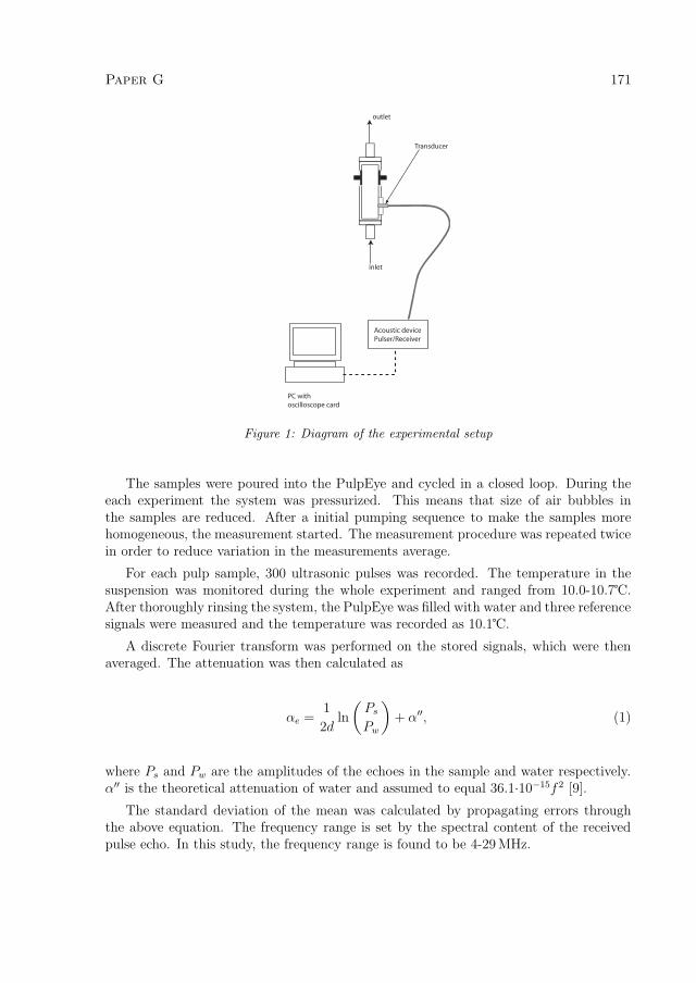
Paper G 171

Acoustic device Pulser/Receiver

Transducer

PC with oscilloscope card

inlet

outlet

Figure 1: Diagram of the experimental setup

The samples were poured into the PulpEye and cycled in a closed loop. During theeach experiment the system was pressurized. This means that size of air bubbles inthe samples are reduced. After a initial pumping sequence to make the samples morehomogeneous, the measurement started. The measurement procedure was repeated twicein order to reduce variation in the measurements average.

For each pulp sample, 300 ultrasonic pulses was recorded. The temperature in thesuspension was monitored during the whole experiment and ranged from 10.0-10.7℃.After thoroughly rinsing the system, the PulpEye was filled with water and three referencesignals were measured and the temperature was recorded as 10.1℃.

A discrete Fourier transform was performed on the stored signals, which were thenaveraged. The attenuation was then calculated as

αe =1

2dln

(Ps

Pw

)+ α′′, (1)

where Ps and Pw are the amplitudes of the echoes in the sample and water respectively.α′′ is the theoretical attenuation of water and assumed to equal 36.1·10−15f 2 [9].

The standard deviation of the mean was calculated by propagating errors throughthe above equation. The frequency range is set by the spectral content of the receivedpulse echo. In this study, the frequency range is found to be 4-29 MHz.

172 Paper G

2.2 Model and Optimisation

The second part of the method requires a model of the attenuation of ultrasound in asuspension of fibres. It is based on the attenuation, αm, of an ultrasound wave scatteredby a layered cylinder. The expression for αm is derived elsewhere [7] and is

αm =Y∑

y=1

(X∑

x=1

(−2frxy

πRxy2kc1

∞∑n=0

�(∫ π

2

0

εnBnxy cos(ψ)dψ

)))+ α′′. (2)

In this expression the distribution of the cross sectional geometry is described by a twodimensional histogram where the first dimension is of x intervals of the radial sizes Xand the second dimension is y intervals of the lumen sizes Y . The volume fraction ineach interval is given by frxy. Rx is the average radius of the fibres within the intervalX. kc1 is the wave number of the compression wave in the fluid. � denotes the realpart of the expression, ψ is the angle of incidence; n is a positive real integer; εn = 1if n = 0, otherwise εn = 2 and where Bnxy is the nth expansion coefficient of the wavepotential of the reflected wave for X, Y fibre size interval. The expression for Bnxy is afunction of the fibre properties and the properties of the water and is given in a previouspublication [7]. α′′ is the intrinsic attenuation of water. A layered cylinder is used since,as the afore mentioned study shows, a solid fibre model is not sufficiently complex tocapture the behaviour of the ultrasound.

The elastic moduli, Young’s modulus, E, and the shear modulus, G, are estimated bythe method. These are calculated from the properties estimated from the model whichare the compression wave velocity, c2, the shear wave velocity, cs, and the intrinsic loss,tan δ. The properties of water are assumed to be known and the values used in the modelare the compression wave velocity, c1 = 1496 ms1 and the density, ρ1 = 996 kgm−3. Thewater is assumed to be non-viscous which has be found to be a reasonable assumption ifthe solid is viscoelastic [7]. Studies have shown the fibre material to be viscoelastic [10].

The fibre diameters, φ were sorted into size grouping and the percentage in each groupwas calculated. The average diameter of each group was also calculated. These numbersare presented in Table 1 and were used in equation 2.

The average diameter of the softwood fibre was 29.8± 2.2 μm and the average wallthickness was 2.42 μm. This gives an average lumen size of 24.9 μm and makes up for84% of the fibre. In the calculation we assume that the lumen is this percentage in allthe fibres. For hardwood fibres, the assumption is that the lumen makes up 81% of thefibre. This is based on an average wall thickness of 1.80μm and an average diameter of18.55± 0.92 μm.

The dry mass fraction of the pulps were measured as 0.206% and 0.232% for thehardwood and the softwood samples, respectively. From the geometry of the fibres andtaking the density of the wood fibre material as 1500 kgm−3 [4], this gives a density for thehardwood fibre structure as 491 kgm−3 and for the softwood fibre structure as 442 kgm−3.These are typical values for pine. The volume fraction is therefore 0.34% and 0.41% forthe hardwood and the softwood pulps, respectively.

The algorithm used in the optimisation is a non-linear least square fit with boundarieson the parameters [11]. These boundaries used are given in Table 2. In addition the

Paper G 173

Table 1: Table of radii distribution

Fibre Upper limit of Bin Average Percentage of fibres(μm) (μm) %

Softwood, φ

≤ 16 14.8 5.622 20 19.428 26.2 30.434 31.9 22.8≤35 45.1 21.8

Hardwood, φ

10 9.5 2.216 14.9 37.918 19.4 45.622 25.4 11.625 33.7 2.7


Material Property Lower Value Upper Value

c2 500 ms−1 6000 ms−1

ν 0.2 0.5tan δ 0.1 0.5

volume fraction was allowed to vary down to 0.15% to allow for the fact that a proportionof the fibres are collapsed and therefore the number of fibres per unit volume is less. Theresults of the optimisation algorithm can depend on the initial values. This is becausethe algorithm is not always able to locate the best-fit between the measured attenuationand the modelled attenuation. To improve the chances of the best fit being located, 16different initial values for the parameters being estimated, were used. These were spacedevenly across the allowed search space.

3 Results

Figure 2 is a plot of the experimental measurements of the attenuation in the softwoodand the hardwood pulp. The standard deviation of the mean, σm, of the measurementswas a maximum of 1.2 Npm−1 for the softwood and the hardwood pulps. However,these maximum in σm were only at the highest frequencies, otherwise σm was less than0.3 Npm−1. The gradients for both pulps appear constant and do not appear to show anyof the resonance peaks that have been observed in experimental attenuation in syntheticfibre suspension [12,13]. However, if the attenuation was due solely to the wave travellingthrough the fibre material, without scattering or resonance, it would be proportional tothe quantity of the material and its intrinsic attenuation. Therefore it would be expectedthat the pulp with the higher volume fraction would have a large attenuation unless theintrinsic loss was significantly higher. The results show however that larger attenuation

174 Paper G

0 5 10 15 20 25 300

10

20

30

40

50

60

70

80

Frequency (MHz)

Atte

nuat

ion

(Np/

m)

Figure 2: Plot of αe in softwood fibre (solid line) and hardwood fibre (dashed line) pulps.

Table 3: Table of Estimated Values for Hardwood and Softwood Properties

Fibre Type E G c2 cs ν tan δGPa GPa ms−1 ms−1

Softwood fibres 1.56-1.60 0.52-0.53 6000 590-604 0.495 0.1-0.08Hardwood fibre 1.56-1.57 0.52-0.53 6000 590-592 0.495 0.05

is in the suspension with the slightly lower volume fraction. This indicates that eitherthere are significant differences in intrinsic attenuation properties of the material or thatthe attenuation is a result of a more complex interaction between the fibres and theultrasound. In the model, the attenuation is based on the latter.

In solving inverse problems, it is common to obtain ambiguous results. In our case,the fitting procedure did successfully identify one result that had a lower error differencebetween the measured and modelled attenuation. The solution with the lowest errorfor the softwood and the hardwood pulps are plotted in figures 7.3(a) and 7.3(b). Theestimates of the material properties of these best-fits are given in table 3 for both typesof pulp. As can be seen from 7.3(a), the fit to the attenuation in the softwood pulp isgood and the estimate values of the Young’s modulus match the values from a studyon individual fibre measurements [3]. The hardwood fibre estimates of all the propertiesare very close to that of the softwood fibres. The best fit curve captures the overalltrend of the measurement curve but there exists two resonance features in the modelledattenuation that are not seen in the experimental results.

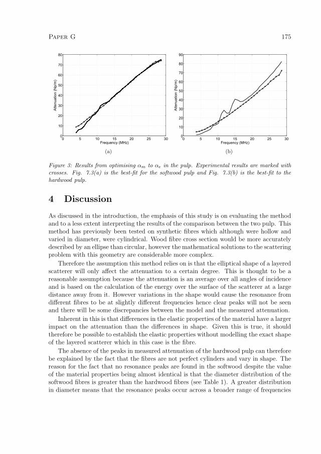
Paper G 175

0 5 10 15 20 25 300

10

20

30

40

50

60

70

80

Frequency (MHz)

Atte

nuat

ion

(Np/

m)

(a)

0 5 10 15 20 25 300

10

20

30

40

50

60

70

80

90

Frequency (MHz)

Atte

nuat

ion

(Np/

m)

(b)

Figure 3: Results from optimising αm to αe in the pulp. Experimental results are marked withcrosses. Fig. 7.3(a) is the best-fit for the softwood pulp and Fig. 7.3(b) is the best-fit to thehardwood pulp.

4 Discussion

As discussed in the introduction, the emphasis of this study is on evaluating the methodand to a less extent interpreting the results of the comparison between the two pulp. Thismethod has previously been tested on synthetic fibres which although were hollow andvaried in diameter, were cylindrical. Wood fibre cross section would be more accuratelydescribed by an ellipse than circular, however the mathematical solutions to the scatteringproblem with this geometry are considerable more complex.

Therefore the assumption this method relies on is that the elliptical shape of a layeredscatterer will only affect the attenuation to a certain degree. This is thought to be areasonable assumption because the attenuation is an average over all angles of incidenceand is based on the calculation of the energy over the surface of the scatterer at a largedistance away from it. However variations in the shape would cause the resonance fromdifferent fibres to be at slightly different frequencies hence clear peaks will not be seenand there will be some discrepancies between the model and the measured attenuation.

Inherent in this is that differences in the elastic properties of the material have a largerimpact on the attenuation than the differences in shape. Given this is true, it shouldtherefore be possible to establish the elastic properties without modelling the exact shapeof the layered scatterer which in this case is the fibre.

The absence of the peaks in measured attenuation of the hardwood pulp can thereforebe explained by the fact that the fibres are not perfect cylinders and vary in shape. Thereason for the fact that no resonance peaks are found in the softwood despite the valueof the material properties being almost identical is that the diameter distribution of thesoftwood fibres is greater than the hardwood fibres (see Table 1). A greater distributionin diameter means that the resonance peaks occur across a broader range of frequencies

176 Paper G

5 10 15 20 25 300

2

4

6

8

10

12

14

16

18

Frequency (MHz)

Atte

nuat

ion

(Npm

−1)

15μm20μm26μm32μm45μm

Figure 4: Plot of the attenuation due to the different diameter (given in table 1) that summed,give the best fit to the measured attenuation in the softwood fibre pulp (shown in Fig. 7.3(a))

and when these are summed together the result is that there is virtually no evidence ofthe resonance peaks are seen in the final curve. To illustrate this point Fig. 4 showsa plot of the attenuation from the different diameters that make up the total modelledattenuation in Fig. 7.3(a).

Examining the results it is seen that the estimated values for c2 for both the softwoodand the hardwood pulp were equal to the boundary value set for the optimisation pro-cess. Since this velocity is that of steel it is highly unlikely to be the true value of the c2.However, the estimated value for Young’s modulus is a typical value. The most likelysource of this error is due to the assumption in the model that the material is isotropicas opposed to transversely isotropic. It maybe possible to use a transversely isotropicmaterial but this introduces five independent elastic constants instead of two and hencecould introduce further ambiguities into the results of the optimisation. Hence, an alter-native option is to not limit the value of c2, allow it to be adjusted to compensate forthe error in assuming the material to be isotropic and only use the value of the Young’smodulus that is calculated from it.

The tan δ for the hardwood fibres was equal to the boundary value set for the optimi-sation process. This was also true of the volume fraction for hardwood fibres. So, withthe volume fraction at its minimum value and knowing that a low tangent delta valuelowers the attenuation at all points except for the resonance peaks, it would appear thatthe model is predicting the attenuation to be higher than the measurement value. Thiscould be an effect of a large number of collapsed fibres.

The estimated value for E of 1.6 GPa compares well with the upper range of individualfibre measurements [3], this, however, is unexpected. This is because others studies onpolymer fibres have previously shown that the estimated value is close to that of thetransverse Young’s modulus, Eθr and not the longitudinal direction, Ez. This supportedto some extent by studies on the modes of vibration in nylon cylinder in water [7] but

Paper G 177

the relationship of the modes of vibration to a specific modulus was not done. It couldbe that the wood material is now isotropic possibly due to the action of the refiningprocess. However, this is unlikely and if the material was isotropic then the reason forthe model giving very high values for c2 could not be true. We would suggest thereforethat the value estimated is Eθr and that Ez is typically much higher than this. The pulpused in the individual study was refined thermomechanical pulp of black spruce whereasthe pulps used here was refined kraft pulp. It is therefore expected that there wouldbe considerable differences in the elastic properties. This supports the suggestion thatthe value estimated using the ultrasound method is that of Eθr . The individual fibrestesting was also done at much lower frequencies which could also be a cause of differencein the measurements .

Not all the initial values converged on the lowest difference between the measuredattenuation and the modelled attenuation. Modification to the error difference calculationcould improve the number of values that converged to the best fit value so that theoptimisation would be less sensitive to the initial values. This would make it unnecessaryto have several initial values and hence the optimisation process would be more efficient.

A considerably improvement would be to included the measurement the wall thicknesswith respect to the fibre diameter for each fibre. This would allow account to be takenof the fact that the wall thickness can vary in proportion to the size of the fibre.

5 Conclusion

The method successfully identifies a single value for the shear modulus and the Young’smodulus. The results show that the hardwood fibres and softwood fibres which areprocessed for the use in Kraftliner have almost identical elastic properties. However,some further work is needed to establish the accuracy of the estimation.

Most importantly, it needs to be established if the elastic properties of the fibresare more important to the attenuation that the exact geometry of the fibre. This canbe done by investigating the effect of the ellipsoidal rather than cylindrical form of thefibres. This could be tested experimentally by scaling the system such that the dimensionof the scatterer is increased, and the frequency range decreased, to such a degree that thescatterer shape could be more easily controlled. If it is found that variation in the thescattering geometry has a large impact on the attenuation then the model would have tobe replaced with a model that has the more complex ellipsoidal geometry.

The effect of collapsed fibres on the attenuation should also be further investigated aswell as the possibilities of identifying mixtures of fibres with different elastic properties.

An improved test of this model would be to compare pulp before and after refiningor comparing sample from different pulp treatments.

References

[1] H. Karlsson, Fibre Guide. Lorentzen & Wettre, Kista, Sweden, 2006.

178 Paper G

[2] A. Kaw, Mechanics of composite materials. Taylor & Francis, 2006.

[3] J. Tchepel, J. Provan, A. Nishida, and C. Biggs, “A procedure for measuring theflexilibity of single wood-pulp fibres,” Mechanics of Composite Materials, vol. 42,no. 1, pp. 83–92, 2006.


[5] A. Hagedorn, J. Orccotoma, P. Schueler, B. Snow, and J. Jarvinen, “Optimizingmachine efficiency through fibre quality management,” in 2006 TAPPI Papermaker’sConference. Technical Association of the Pulp and Paper Industry, 2006.

[6] A. Dukhin and P. Goetz, Ultrasound for Characterizing Colloids: Particle Sizing,Zeta Potential, Rheology. Elsevier Science, 2002.

[7] Y. Aitomaki, “Online fibre property measurements: Foundations for a method basedon attenuaion,” Ph.D. dissertation, Lulea University of Technology, 2009.

[8] Pulps - Determination of stock concentration, International Organization for Stan-dards, 1995.

[9] F. Fisher and V. Simmons, “Sound absorption in sea water,” Journal of the Acous-tical Society of America, vol. 62, no. 3, pp. 558–564, Sept 77.

[10] L. Salmen, “Viscoelastic properties of in situ lignin under water-saturated condi-tions,” Journal of material science, vol. 19, no. 9, pp. 3090–3096, Sept. 1984.




Online fibre property measurements - DiVA Portal

Documents

Transcript of Online fibre property measurements - DiVA Portal